Embed Size (px)
Citation preview

Increasing Access to Youth Mental Health Services: A Cost-Benefit
Analysis of the PATH Program in the Fox Valley
By:
Andrew Behm Ann Drazkowski Samuel Matteson
Maria Serakos Cherie Wolter
Prepared for Mary Wisnet Community Development Program Officer
Health & Healing and Strengthening Families United Way Fox Cities
La Follette School of Public Affairs University of Wisconsin - Madison
1225 Observatory Dr. Madison, WI 53706

i
Table of Contents Executive Summary ............................................................................................................................ iii
Acknowledgements .............................................................................................................................. 1 Introduction ............................................................................................................................................ 2
Fox Valley PATH Program .................................................................................................................. 3
Program Costs and Benefits .............................................................................................................. 5 Costs .......................................................................................................................................................... 7 Short Term Benefits ....................................................................................................................................... 8 Reduction in School Staff Time Spent on Mental Health ................................................................................ 8 Avoided Juvenile Crime ................................................................................................................................................ 9 Avoided Costs Associated with Suicide ................................................................................................................. 9
Long-‐Term Benefits ..................................................................................................................................... 10 Increased Lifetime Income ....................................................................................................................................... 10 Avoided Costs of Adult Crimes ............................................................................................................................... 12
Unquantifiable Benefits ............................................................................................................................. 13
Analysis ................................................................................................................................................. 14 Effect of PATH on High School Graduation .......................................................................................... 14 Monte Carlo Simulation .............................................................................................................................. 15
Results ................................................................................................................................................... 17 Costs .................................................................................................................................................................. 19 Short-‐Term Benefits .................................................................................................................................... 21 Change in Time Spent to Address Truancy ....................................................................................................... 22 Change in Time Spent Disciplining Students .................................................................................................... 22 Guidance Counselor Time Freed for Other Activities ................................................................................... 23 Avoided Juvenile Crime ............................................................................................................................................. 24 Avoided Suicide ............................................................................................................................................................. 24
Long-‐Term Benefits ..................................................................................................................................... 25 Increased Lifetime Income ....................................................................................................................................... 25 Avoided Cost of Adult Crimes ................................................................................................................................. 26
Sensitivity Analysis ...................................................................................................................................... 26
Limitations ........................................................................................................................................... 29
Recommendations ............................................................................................................................. 30
Conclusion ............................................................................................................................................ 31 References ............................................................................................................................................ 33
Appendices ........................................................................................................................................... 37

ii
List of Appendices A. PATH Overview B. Profile of PATH Participants C. Graduation Effect Size Estimation and Calculation D. PATH Questionnaire School Responses E. United Way Fox Cities PATH Cost-Benefit Analysis School Questionnaire F. United Way Fox Cities Administrative Costs G. Avoided Administrative Costs Associated with Behavioral Problems H. Avoided Truancy Costs I. Avoided Administrative Costs Associated with Shift in Guidance Counselor Time J. Benefit of Avoided Juvenile Criminal Activity K. Benefit of Avoided Suicide L. Benefit of Increased Lifetime Earnings M. Benefit of Avoided Adult Criminal Activity N. Unquantifiable Benefits O. Expected High School Graduation Rate and Adjustment Factor P. Monte Carlo Equations and Estimates Q. Stata Simulation Code
Page iii
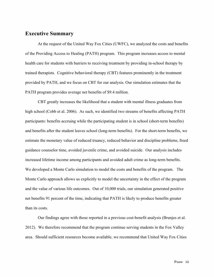
Executive Summary
At the request of the United Way Fox Cities (UWFC), we analyzed the costs and benefits
of the Providing Access to Healing (PATH) program. This program increases access to mental
health care for students with barriers to receiving treatment by providing in-school therapy by
trained therapists. Cognitive behavioral therapy (CBT) features prominently in the treatment
provided by PATH, and we focus on CBT for our analysis. Our simulation estimates that the
PATH program provides average net benefits of $9.4 million.
CBT greatly increases the likelihood that a student with mental illness graduates from
high school (Cobb et al. 2006). As such, we identified two streams of benefits affecting PATH
participants: benefits accruing while the participating student is in school (short-term benefits)
and benefits after the student leaves school (long-term benefits). For the short-term benefits, we
estimate the monetary value of reduced truancy, reduced behavior and discipline problems, freed
guidance counselor time, avoided juvenile crime, and avoided suicide. Our analysis includes
increased lifetime income among participants and avoided adult crime as long-term benefits.
We developed a Monte Carlo simulation to model the costs and benefits of the program. The
Monte Carlo approach allows us explicitly to model the uncertainty in the effect of the program
and the value of various life outcomes. Out of 10,000 trials, our simulation generated positive
net benefits 91 percent of the time, indicating that PATH is likely to produce benefits greater
than its costs.
Our findings agree with those reported in a previous cost-benefit analysis (Brunjes et al.
2012). We therefore recommend that the program continue serving students in the Fox Valley
area. Should sufficient resources become available, we recommend that United Way Fox Cities

Page iv
look for ways to expand into other schools in the area or increase the number of therapists or
staffing hours in schools currently participating in the program.

Page 1
Acknowledgements This analysis would have been impossible without the help and information we received
from several sources. We would like to thank the following people: Mary Wisnet, Community
Development Program Officer, United Way Fox Cities for contributing her knowledge, time, and
data to this analysis and organizing our site visit; Lois Mischler, therapist at Family Services, for
providing general background on PATH students and data on their diagnoses; Justin Heitl,
Assistant Principal at Appleton East for High School, for meeting with our team to explain issues
in youth mental health and describe the operation of PATH; Peter Kelly, President and CEO
United Way Fox Cities, for his leadership and dedication to the PATH program and his time to
discuss the future of the program with us; David Weimer, for his guidance, feedback, and the
opportunity to do this cost benefit analysis, and in particular the program for correlated draws
from normal distributions used in our Monte Carlo simulation; and the many other staff and
therapists working with the PATH program.

Page 2
Introduction The US Department of Health and Human Services describes childhood mental disorders
as “serious deviations from expected cognitive, social and emotional development” (CDC 2013
1). Although these disorders affect up to one in five children in the United States, only between
six and 20 percent of children with mental disorders or illnesses receive treatment (Kataoka et al.
2002; Costello et al. 2005). As few as 10 percent of children with disorders classified as serious
mental illness: major depressive disorders, post-traumatic stress disorders, eating disorders, and
bipolar disorders, receive treatment (Erickson 2012). Students without insurance or with
inadequate insurance are the most likely to have their mental health treatment needs unmet
(Kataoka et al. 2002). Early detection and assessment can prevent mental health problems from
compounding and causing a cycle of poor life outcomes (“New Freedom Commission Report”
2003). According to Vander Stoep et al. (2003), 47 percent of high school non-completion is
attributable to mental health disorders. Furthermore, the U.S. Department of Education (2001)
states that 50 percent of students with mental health disorders will drop out of high school
without treatment.
Without intervention, mental health disorders can affect a child's academic performance
and their ultimate educational attainment level via poor grades, behavior problems, detentions,
suspensions, and expulsions (Fergusson and Woodward 2002). If children are not appropriately
screened and treated early, childhood mental disorders can persist and potentially result in a
downward spiral of school failure, poor employment opportunities, and poverty in adulthood
(“New Freedom Commission Report” 2003). School-based programs like PATH increase access
to mental health services for children, allowing timely screenings and interventions that can
reduce these immediate and future negative outcomes.

Page 3
Fox Valley PATH Program
In 2006, United Way Fox Cities, the Community Foundation, and the Fox Valley
Chamber of Commerce sponsored the Fox Cities Leading Indicators for Excellence (LIFE) study
to provide an overview of issues affecting the Fox Valley community. Based on data collected
over five years through surveys and studies by UWFC and other groups, the LIFE study found
that approximately one in four tenth graders experienced a depressive episode and 13.8 percent
of tenth graders attempted suicide in the previous year. UWFC responded to these findings by
developing the Providing Access to Healing (PATH) program to facilitate in-school access to
mental health services for students in elementary, middle, and high school.
PATH began in 2008 as a pilot project in the Menasha Joint School District. Originally
targeting high school students, PATH later expanded to serve middle and elementary school
students. According to the Wisconsin Department of Public Instruction, 55.7 percent of students
in the Menasha Joint School District were eligible for free or reduced meals during the 2013-14
school year. This rate of free and reduced lunch is significantly higher than the state average of
43.3 percent. These students likely come from low-income families that may not have access to
health insurance or mental health services. United Way thus targeted both underinsured and
uninsured students, as well as students who may have had insurance but encountered barriers to
accessing treatment. For example, many could not attend daytime appointments because their
parents worked long hours or did not have access to a car, and mass transit in the Fox Cities area
is limited. When available, the use of mass transit to attend mental health appointments led to
longer school absences.
A follow-up LIFE study released in 2011 found that the prevalence of depression and
suicidal thoughts remained steady in the Fox Valley region. As a result, the program expanded

Page 4
to the Appleton, Kaukauna, Kimberly, and Little Chute school districts. In 2012, La Follette
students prepared a cost-benefit analysis based on data from the pilot program in the Menasha
Joint School District (Brunjes et al. 2012). Their analysis found that PATH produced net
benefits for students in the five school districts in excess of $7 million dollars, or nearly $50,000
per participating student. The program subsequently expanded to the Freedom, Hortonville,
Seymour, Shiocton, and Neenah school districts. See Appendix A for a detailed program
description of PATH and Figure 4 for a timeline of PATH’s development and implementation.
PATH currently operates at 23 school facilities in ten school districts, serving
predominantly high school and middle school students with a smaller presence in elementary
schools. Each school district allocates services among schools within the district out of a budget
of service hours determined by UWFC. UWFC is trying to address long-term sustainability by
reducing the dependency on grants and charitable donations. In place of charitable donations,
the program is increasing billing to third-party insurers by serving more students who are
covered by Medicaid or private insurance. Nonetheless, the vast majority of present funding for
the PATH program continues to come directly from the United Way Fox Cities and two grants
provided by the Community Foundation.
In the 2013-2014 school year, 183 students were enrolled in the PATH program across all
school levels. Of these students, 105 were females and 78 were males. All faced one or more
barriers to accessing mental health care such, as lack of insurance, a high insurance deductible,
inadequate transportation, parent work conflicts, or lack of parental support. PATH students
suffer from a variety of mental disorders, and the majority of program participants experience
multiple disorders. The most common mental disorders faced by PATH students are adjustment
disorders (affecting 41 percent), mood disorders, including depression, (33 percent), anxiety

Page 5
disorders (27 percent), and ADHD (15 percent). PATH participants also suffer from
oppositional defiant disorder (ODD), conduct disorders, and eating disorders. Other community
and school-based programs serve students who would otherwise participate in the PATH
program. These programs tend to serve students with more severe criminal backgrounds and
may be provided with mental health services through the juvenile justice system. See Appendix
B for a detailed profile of PATH participants.
Program Costs and Benefits
We reviewed the previous La Follette PATH cost benefit analysis (Brunjes et al. 2012)
and extensively reviewed the literature for estimates of the likely effects of cognitive behavioral
therapy (CBT), PATH’s main mode of treatment. We used a different approach than the
previous La Follette cost-benefit analysis. At the time of the previous analysis, there was little
background information or data on the students participating in the program. The previous La
Follette analysis therefore estimated the prevalence of various disorders among PATH
participants and estimated net benefits based on the effect of CBT on each disorder. However,
most students enrolled in the PATH program have comorbid mental health diagnoses.
Separately analyzing the effect on each disorder risks overestimating the benefits of the program
for students with multiple disorders. Instead, we analyze the impacts of PATH’s school-based
CBT intervention program on a generic mental disorder without differentiating by specific
diagnosis.
School-based mental health programs like PATH that use cognitive behavioral
interventions have been shown to reduce the likelihood of dropping out of high school and
increase the presence of additional positive behaviors (Cobb et al. 2006). Haveman and Wolfe
(1984) identify numerous private and public effects of graduation, including increased

Page 6
productivity and wages, reduced criminal activity, better health status, and increased enjoyment
of leisure. School-based mental health programs increase the propensity of youth to graduate
from high school. To capture many of these benefits associated with reducing the dropout rate in
our analysis, we use educational attainment as the driver of the long-term benefits of the PATH
program. The long-term expected benefits of PATH’s CBT intervention estimated in our
simulation result from more students graduating high school.
As discussed further in Appendix C, we expect half of PATH participants not to complete
high school in the absence of the program. We expect CBT to improve the behavior and
academic performance in the short-term. Helping a student graduate high school turns this
temporary improvement into a permanent effect that potentially improves the student’s entire life
course. We expect about one quarter of the participants to drop out despite the intervention, and
we expect half the participants to be on track to graduate anyway. Because the direct effect of
CBT on long-term earnings and adult crime are complicated by natural recovery and the decay of
the CBT effect over time, we use the high school graduation effect of CBT as the basis for
estimating all long term impacts of PATH. We do not expect the effect of CBT to persist over
many years, so we assume CBT does not directly affect adult outcomes in our
simulation. However, as long as the effect of CBT persists long enough to help students
graduate from high school, it can alter the students’ life trajectory. If a student with a mental
disorder drops out of high school, then we expect that the benefit of natural recovery to be
overshadowed by the loss incurred by failing to graduate.
Short-term benefits accrue during a PATH participant’s time in school. These benefits
include avoided school staff time addressing truancy, avoided school staff time addressing
student behavior and discipline problems, guidance counselor time freed for activities other than

Page 7
providing mental health care, avoided juvenile crime, and avoided suicide. In addition, a survey
of PATH school principals and counselors report several immediate benefits to the program,
such as increased emotional affect, improved academic performance, and reduced classroom
disruptions (see Appendices D and E). The PATH program incurs costs for therapist time,
UWFC overhead, and space in school buildings.
Costs
The United Way Fox Cities incurs costs to implement the PATH program. UWFC
provided information on these costs through a financial statement for the 2013-2014 school year
and a budget projection for the 2014-2015 school year. Starting with the pilot program in 2008
in the Menasha School District and up until the completion of the 2013 to 2014 school year,
UWFC has paid $55 directly to the mental health care provider for each student therapy
session. For the 2014-2015 school year, UWFC changed its reimbursement to fixed grants to the
three service providers based on the districts they serve. Because we prepared our analysis based
on the 2013-14 school year, the change in the reimbursement structure is not included. See
Appendix F for a detailed breakdown of costs incurred by the United Way Fox Cities.
We inflated the 2013-2014 costs to match the costs to the benefits we estimated, which
include benefits accruing to 31 students participating in the program in years other than 2013-
2014. We also increased costs to account for administrative overhead at UWFC, which did not
appear to be included in the cost in the financial statement provided.
Although school districts receive PATH services at no additional charge, the services
occur inside the school building. Therefore, schools must find space for PATH
sessions. Ideally, this space is dedicated to PATH full time, which allow the therapist to create a

Page 8
comfortable environment without needing to compete with other uses. Our simulation models
the cost of a dedicated room for PATH at each participating school.
Short Term Benefits
PATH yields several benefits while participating students are in school. These short-term
benefits affect school personnel, the community at large, and students themselves. We discuss
the short-term benefits of PATH included in our analysis below. Specifically, these are saved
school staff time, avoided costs of juvenile crime, and avoided suicides.
Reduction in School Staff Time Spent on Mental Health
PATH may reduce disruptive behavior and truancy by addressing the mental health needs
of participating students. Disruptive behavior causes a variety of negative outcomes, including
classroom disruption, suspensions, and expulsions. Disciplining students for these problems
requires time, which includes an opportunity cost for school administrators who forgo devoting
time and efforts to other purposes. Truancy potentially also incurs legal costs, as habitually
truant students are in violation of Wisconsin’s compulsory attendance law (WI State Statute
118.15). However, schools may divert habitually truant students to PATH or similar programs
rather than prosecuting them in court. Finally, in the absence of PATH guidance counselors
devote more time to students in need of mental health interventions, distracting them from other
duties.
CBT has been shown to reduce problematic behaviors (Liber et al. 2013), so school
administrators no longer have to devote as much time to addressing these problems. In our
analysis, we calculate the avoided guidance counselor time spent addressing mental illness, the
avoided school staff time spent on student discipline, and reduced school staff time spent on
truancy cases. We quantify the opportunity cost of guidance counselor time by considering both

Page 9
the salaries of school guidance counselors and the change in the amount of time devoted to
addressing disciplinary problems. To gather information about the time spent on each of the
aforementioned student behavioral issues, we surveyed administrators at each PATH school (see
Appendix D). For a detailed discussion of the reduced behavioral and disciplinary problems,
reduced truancy costs, and shift in guidance counselor time associated with PATH, see
Appendices G, H, and I, respectively.
Avoided Juvenile Crime CBT can reduce the number of crimes committed by participating students while they are
in school. We model the effect of CBT on juvenile crime as a reduction in the commission of
additional crimes by students with a prior contact with the law. The effect of CBT on students
without a prior contact with the law is unclear, and we did not estimate the value of this
effect. The benefit of avoided juvenile crime is the cost of juvenile crimes that would have been
committed in the absence of PATH. These costs are those incurred by the tri-county
(Outagamie, Winnebago, Calumet) juvenile justice system. We assume that juvenile crimes that
are avoided by CBT may not have been committed immediately. For students under the age of
15, we discount the cost of a juvenile crime from the current age of the student to age 15 because
we assume crimes are most likely to be committed at age 15. For students aged 15 to 19, we do
not discount the cost of juvenile crime because we assume these students are in their peak years
of crime commission. CBT can therefore avoid crimes in the same year in which the treatment is
applied. Appendix J details these estimates and the effect of CBT on juvenile crime.
Avoided Costs Associated with Suicide As a cognitive behavioral intervention, the PATH program helps prevent suicides by
reducing the symptoms of mental illnesses and improving the ability of students to cope with

Page 10
distress. Suicide levies large costs on families, friends of victims, and the community. These
costs are difficult to quantify, let alone monetize. This analysis quantifies the cost of suicide
using literature estimates of the value of a statistical life. The value of a statistical life is based
on observations of people’s market decisions that involve small increases or decreases of the risk
of death. We assume that the suicide reducing effect of CBT lasts for less than a year. We do not
discount the value of a statistical life because suicides that are avoided due to CBT will be
avoided within a year of treatment, and the effects of CBT after one year of treatment can
potentially fade out (Weisz 2006). See Appendix K for details on how we calculated the avoided
costs of suicide.
Long-Term Benefits
In providing CBT to youth with mental illness, PATH greatly increases the likelihood
that its participants graduate from high school (Cobb et al. 2006). By reaching this educational
milestone, PATH high school graduates give themselves and the community the opportunity to
experience a stream of benefits for their lifetime. Haveman and Wolfe (1984) identify a variety
of benefits accruing from high school graduation, including increased earnings and decreased
criminal activities. Our analysis focuses on these long-term benefits of high school
graduation. Haveman and Wolfe (1984) also cite a variety of additional private and public
benefits. Our analysis does not estimate the value of these benefits, but we acknowledge them in
our unquantified benefits below.
Increased Lifetime Income CBT improves a student’s chance of graduating from high school (Cobb et al. 2006),
which, in turn, increases his or her probability of earning additional income throughout his or her

Page 11
lifetime. We expect a workforce with higher educational attainment to be more productive,
benefitting workers, firms, and the community.
The Bureau of Labor Statistics (2014) estimates that median weekly earnings increase
and unemployment rates decline as individuals advance through their schooling. Workers with
less than a high school diploma earn a median $472 per week and have an 11.0 percent
unemployment rate, while those who end their education with a high school diploma earn $651
per week and are unemployed at a 7.5 percent rate. Workers with a bachelor’s degree earn a
median of $1,108 per week and have a 4.0 percent unemployment rate. High school graduates
also work longer than dropouts: graduates spend an average of 35 years in the workforce, as
compared to 30 years for dropouts (Skoog and Ciecka 2001). These earnings differentials add up
over the course of a lifetime: Cohen and Piquero (2008) estimate that the lifetime earnings of
high school graduates are between $420,000 and $630,000 higher than non-graduates in 2007
dollars, equivalent to approximately $480,000 to $720,000 in 2014 dollars.
We estimate the effect of PATH on total lifetime income. In estimating this effect we
consider the ultimate level of educational attainment of participants. Our simulation allows for a
variety of educational outcomes. Students can drop out, or they can graduate high school in four
or six years. After graduating on-time or late, students can complete some college or they can
graduate college with a bachelor’s degree or higher. We obtained median annual total income
figures from Current Population Survey data for Wisconsin adults in 2014 by educational
attainment (King et al. 2010). These figures account for all sources of income, including
earnings, unemployment compensation, and retirement income. We reduce these figures by 19
percent, as adults who experienced depression as an adolescent earn 19 percent less than they
would otherwise (Fletcher 2013).

Page 12
Because many of the earnings’ standard deviations were large, we developed triangular
distributions with a minimum and maximum value one standard deviation away from the median
for use in our simulation. From these numbers, we used zero as the minimum of the triangle
distribution when it was within one standard deviation of the median. Our distributions estimate
the present value of lifetime earnings at age 18, and we further discount these values from age 18
to the students’ actual ages. See Appendix L for a detailed discussion of our lifetime income
calculations and assumptions.
Avoided Costs of Adult Crimes In addition to the benefit of increased lifetime earnings, high school graduation reduces
adult crime. Higher educational attainment is associated with lower adult criminal activity, and
high school graduation is estimated to reduce the commission of adult crime by 10 to 20 percent
(Levin et al. 2007). Moreover, high school dropouts are more likely to be incarcerated. Dropouts
comprise less than 20 percent of the US population, yet they represent 37 percent of federal
prison inmates, 54 percent of state prison inmates, 38 percent of local jail inmates, and 33
percent of probationers (Levin et al. 2007). To the extent that CBT decreases the likelihood of
dropping out of high school, it reduces the commission of crimes as adults.
The benefit of avoided adult crime costs has been monetized in several cost-benefit
analyses (Cohen 1998; Cohen and Piquero 2008; Levin et al. 2007; Reynolds et al. 2011). We
use Levin et al.’s (2007) estimates for the avoided costs of adult criminal activity based on the
effect of high school graduation reducing the commission of high cost crimes, including murder,
rape/sexual assault, violent crime, property crime, and drugs offenses. Crimes impose
operational costs within the criminal justice system, lost earnings during incarceration (including
parole and probation), victim restitution and medical care, and government expenditures on

Page 13
crime prevention. Adjusted to 2014 dollars, the Levin et al. (2007) numbers estimate that high
school graduation avoids $38,054 worth of crimes after graduation for males and $10,458 for
females. Using these figures, we develop a distribution of the cost of crime for the Monte Carlo
simulation. Because Levin et al. (2007) estimate the effect of a high school graduation, we
discount the avoided cost of adult crime from age 18 to the students’ current ages. See Appendix
M for a detailed discussion of avoided adult crime calculations and assumptions.
Unquantifiable Benefits Graduating high school produces benefits beyond those included in our analysis. While
we attempt to cover the downstream benefits of PATH with the largest financial gains, several
impacts are small or difficult to value. Haveman and Wolfe (1984) discuss the numerous
channels through which schooling yields economic and social impacts. These include increased
enjoyment of leisure, better ability to further individual knowledge, increased nonmarket
productivity, better familial relationships and child development, better informed purchased
decisions, and increased charitable giving. However, the intangibility of these benefits places
them outside this analysis.
We did not value decreased classroom disruptions among PATH students, increased
future productivity (except as it is reflected in lifetime income), reduced for non-PATH mental
health treatment, increased quality of life years, and decreased legal costs due to habitual
truancy. Although we were unable to locate the effect of CBT on these outcomes in the
academic literature, they may have limited or lasting effects on PATH participants. See
Appendix N for a discussion of the literature surrounding the effects of CBT on these
unquantifiable outcomes.

Page 14
Analysis Our analysis of PATH is based on a Monte Carlo simulation using the statistical software
Stata. Short-term benefits of the program accrue while students are in school as described
above. Long-term benefits of the program result from increasing students’ chance of graduating
from high school. The following sections elaborate the Monte Carlo simulation of this
graduation effect and various short-term effects.
Effect of PATH on High School Graduation
Because the long-term benefits in our analysis depend on high school graduation, the
effect of CBT on high school graduation is of first importance. We draw on several sources to
estimate the number of non-graduations in the population of PATH-participating students in the
absence of the PATH program and the effect of CBT in avoiding these non-graduations. We
consider two groups of students living with mental illness: those participating in PATH, and
those with mental illness not participating in a program like PATH. Our approaches to estimating
status quo non-graduations and the effect of CBT are detailed below.
Long-term benefits of the PATH program focus on the benefits gained by students from
the increased likelihood that they graduate from high school. We construct two long-term
benefit estimates, one for increased lifetime earnings and the other for avoided costs of adult
crime associated with high school graduation. For the former, we use the six-year weighted
graduation rate of schools participating in PATH because we are interested in a single effect of
high school graduation on avoided costs. For the latter, we use weighted average four- and six-
year graduation rates for males and females. These weighted graduation rates are computed in
Appendix O, and make use of the four- and six-year high school graduation data from all of the
participating high schools weighted by their population shares.

Page 15
Monte Carlo Simulation Monte Carlo is a stochastic approach for assessing the impact of uncertain model
parameters on the distribution of outcomes of interest, such as net benefits. Instead of
calculating outcomes from the averages of uncertain parameters, the Monte Carlo simulation
randomly draws values from the assigned probability distributions. This allows the simulation to
address uncertainty in the likelihood of different outcomes and the correlation between
outcomes. Outcomes are correlated when the occurrence of one outcome increases the chance of
another outcome. For example, a student who has higher earnings as an adult is less likely to
commit a crime. Separately estimating an income outcome and a crime outcome would not take
into account the relationship between the two outcomes. The causal models that relate status quo
probabilities and treatment effects to outcomes of interest are of central importance in the Monte
Carlo simulation. We have described these causal models using mathematical equations in the
relevant appendices.
The Monte Carlo simulation randomly assigns outcomes to students out of specified
probability distributions of possible outcomes. The effect of CBT is also drawn from a statistical
distribution of possible effect sizes. By drawing 10,000 observations of the relevant variables,
we develop a distribution of net benefits that reflects our uncertainty about the effect of CBT and
the life processes that determine the outcomes in which we are interested. Rather than
simulating outcomes for each of the students actually participating in PATH, the Monte Carlo
simulation assigns outcomes to 30 representative gender-age combinations. Each gender-age
combination is scaled up by the number of PATH participants of that specific gender and age.
In addition to randomly assigning outcomes to students, the Monte Carlo simulation
randomly draws the money value of outcomes from probability distributions. For example, not

Page 16
every high school graduate has the same income. The Monte Carlo draws the present value of
lifetime income from probability distributions of lifetime income. Altogether, the Monte Carlo
simulation of representative gender-age combinations addresses the size of the effect of CBT,
which is not known with certainty, and the resulting life outcomes, which depend on random life
events that cannot be predicted.
Among the variables not known with certainty, some affect the estimate of net benefits so
much that we further explore the implications of their sensitivity. Assumptions about the
discount rate and the effect of CBT on the high school dropout rate have a large effect on net
benefits. Drawing from a probability distribution for these variables would widen the
distribution of net benefits without providing useful information. Instead, estimating net benefits
using a high, low, and most probable assumption of the uncertain parameter allows us to
explicitly see the effect of varying that uncertain parameter. See Appendix P for a summary of
the equations and estimates used in the Monte Carlo and Appendix Q for the Stata code.
When benefits or costs occur in the future, we scale the benefits and costs to account for
time discounting. Time discounting reflects time preference: people prefer good outcomes
sooner rather than later and prefer bad outcomes later rather than sooner. Time discounting also
reflects the return on capital: a present quantity of money can be invested and return a greater
quantity of money in the future. For an investment project, future benefits must be weighed, not
against present money costs, but against the future value that money could have returned in an
alternate investment. PATH is not a traditional infrastructure project, but PATH has a similar
pattern of present costs and future benefits. Each of the appendices dealing with program
benefits also addresses discounting.

Page 17
Results The Monte Carlo simulation estimates that the average present value of net benefits from
PATH are $9.4 million. There is significant uncertainty in the estimate of net benefits, and 91
percent of trials produce positive net benefits. Said another way, there is a 91 percent chance
that the program is a desirable investment. Because our largest benefits depend on educational
attainment, uncertainty in the relationship between educational attainment and income drives
uncertainty in net benefits. For example, college graduates often earn more than students that
only graduate high school, but not always.

Page 18
Table 1: PATH Benefits and Costs
Thousands of Dollars
Costs
Program Cost 338
Cost of Space in Schools 217
Total Costs 555
Average Short-Term Benefits
Time Spent on Truancy 18
Time Spent on Behavior 14
Guidance Counselor Time 71
Avoided Juvenile Crime 8
Avoided Suicide 48
Total Average Short-Term Benefits 159
Average Long-Term Benefits
Increased Lifetime Income 9,086
Avoided Adult Crime 694
Total Average Long-Term Benefits 9780
Average Net Benefits 9,384
Table 1 shows the average values for the various benefits of PATH. The effect of high
school graduation on income drives net benefits. The importance of changes in lifetime income
is discussed in more depth below.
The difficulty of measuring the effect of CBT and the uncertain nature of various life
outcomes distribute net benefits over a considerable range. Figure 1 visually describes the
distribution of estimated net benefits for PATH.

Page 19
Figure 1: Distribution of PATH Net Benefits
Figure 1 shows that we estimate large net benefits from PATH. The horizontal axis of
Figure 1 shows that many of the Monte Carlo trials estimate net benefits in the tens of millions of
dollars. Second, our estimate of net benefits has considerable uncertainty. About 9 percent of
simulation trials estimate negative net benefits.
Costs The cost of PATH consists of costs borne by the United Way and costs borne by
schools. Although private insurers, public insurers, and charitable organizations reimburse the
United Way for a portion of PATH costs, society still bears the cost of providing PATH
services. We value the resources used for PATH at its full value because we assume they could
be productively employed elsewhere in society if not used for PATH.
The cost of providing PATH services also includes the cost of the space that schools
donate for services. Our analysis assumes that schools make a room available throughout the

Page 20
school year. We assume that school space has an opportunity cost of $9 per hour based on the
hourly rate charged for school space by Monona Grove, Wisconsin. We recognize that the
opportunity cost of school space depends on the degree to which space in each school is
constrained. Therefore we reduce the cost of space by a space-scarcity factor drawn from a
distribution with an average of 70 percent.
Table 2: PATH Costs for the 2013-2014 School Year
Thousands of Dollars
Program Cost 338
Cost of Space in Schools 217
Total Costs 555
The United Way Fox Cities provided a financial statement for the 2013-2014 school year
showing expenditures in excess of $250,000 for therapy sessions and license fees. We estimated
PATH benefits for 183 participating students based on the intake form data provided by the
United Way. Out of these 183 students, 152 of them completed intake forms during the 2013-
2014 school years. The other 31 students completed intake forms either during an earlier or a
later school year. We assumed that the $250,000 spent during the 2013-2014 school year only
went to serve the 152 students completing intake forms that year. To account for students
completing intake forms in other years we increased PATH costs borne by the United Way by
20.4 percent.
We increased the PATH program cost by 12.6 percent compared to the UWFC financial
statement to account for administrative overhead at the United Way based on information from
UWFC’s website.

Page 21
The UWFC indicated that $440,000 is budgeted for PATH for the 2014-2015 school
year. The reason for the significant increase is unclear, but we assumed that it is not relevant for
our analysis. However, if these higher costs are driven by the need to serve any of the 183
students for which we estimate benefits, then leaving out these higher costs tends to inflate our
estimate of net benefits.
Short-Term Benefits We estimate that PATH produces short-term benefits of $64,000. These benefits accrue
before students graduate while they are still in school. These benefits accrue when PATH
reduces the time school staff spends addressing truancy, reduces the time school staff spends
disciplining students, makes guidance counselor time available for activities other than providing
mental health services, avoids student suicides, or avoids juvenile crimes.
Table 3: Short-Term Benefits of PATH
Thousands of Dollars
Time Spent on Truancy 18
Time Spent on Behavior 14
Guidance Counselor Time 71
Avoided Juvenile Crime 8
Avoided Suicide 48
Total 159
Table 3 summarizes the average estimate of benefits in each short-term category. These
benefits are small relative to PATH program costs and relative to the benefits generated by
inducing students to graduate that otherwise would drop out. As discussed below, the estimates
of short-term benefits are uncertain.

Page 22
Change in Time Spent to Address Truancy As shown in Table 3, we estimate that PATH saves schools $18,000 worth of time that
would otherwise be spent addressing truancy for PATH-participating students. This estimate is
based on schools’ reports of the change in staff time spent addressing truancy. See Appendix E
for details of the survey.
Of the 19 schools responding to the survey, seven reported that PATH changed the
amount of time school staff spent addressing truancy. We assume that we can extrapolate this
rate of 37 percent from schools responding to the survey to all 23 participating schools. That is,
the Monte Carlo model randomly simulates a 37 probability of a change in school staff time
spent addressing truancy. The schools reporting a change in time spent addressing truancy
reported an average of five hours saved. The change in hours reported by different schools
varied over a large range. For schools that experience a change in the time spent addressing
truancy, the Monte Carlo simulation randomly draws the change in hours from a normal
distribution based on the mean and standard deviation of the values reported by schools.
Truancy potentially has other, larger costs. Habitual truancy is technically a criminal
offense, and schools can bring habitually truant students to court. Truancy court involves
significant cost for the county court system, students, school staff, and the student’s family if it
attends. We did not include the possibility of avoiding these costs as a benefit because both the
effect of CBT on habitual truancy and the frequency of prosecutions for habitual truancy are
unclear.
Change in Time Spent Disciplining Students Table 3 above shows our estimate that PATH saves schools $14,000 worth of time that
would otherwise be spent addressing discipline for PATH-participating students. We arrived at

Page 23
this estimate from schools’ reports of the change in staff time spent addressing discipline. See
Appendix E for details of the survey.
Of the 19 schools responding to the survey, eleven reported that PATH changed the
amount of time school staff spent addressing discipline. We assume that we can extrapolate this
rate of 58 percent from schools responding to the survey to all 23 participating schools. The
schools reporting a change in time spent on discipline saved approximately 2.5 hours per month
on average. Schools reported values over a large range.
Guidance Counselor Time Freed for Other Activities As shown in Table 3 above, we estimate that PATH makes $71,000 worth of guidance
counselor time available for activities other than providing mental health services to PATH-
participating students. Our estimate is based on schools’ responses to the survey detailed in
Appendix E.
Thirteen of the 19 schools responding to the survey reported that PATH changed the
amount of time guidance counselors spent providing ad hoc mental health services to PATH
participants. We extrapolate the 68 percent rate to all 23 PATH-participating schools. On
average, these 13 schools reported that guidance counselors spent about 10 fewer hours
providing mental health care to PATH participants. Schools reported values over a large range.
Based on the survey results, we estimate that guidance counselor time does not change in
32 percent of trials. This accounts for the large number of observations at zero benefit. For
simulation trials in which guidance counselor time changes, guidance counselors occasionally
spend more time providing mental health care to PATH participants. This is because survey
responses to this question varied over a large range, and we assumed that the actual change in
guidance counselor time fit a normal distribution.

Page 24
Avoided Juvenile Crime Of the 183 students in PATH, 31 have had prior contact with the law. For these students,
we estimate that CBT avoids $8,000 worth of subsequent crimes on average.
CBT reduces the rate of recidivism for a period of time. Because the reduction in
recidivism does not apply to first-time offenders, we did not estimate a reduction in the
commission of crime by PATH-participants without prior contact with the law. The CBT effect
on recidivism decays over times, so we only modeled the commission or avoidance of one crime
for each participant. Modeling the commission of additional crimes would potentially increase
the benefit by increasing the number of crimes that PATH could prevent. However, modeling
more crimes would introduce added uncertainty from the decay over time of the reduction of
recidivism.
We estimated that an average juvenile crime costs society $2,100, and we drew
observations from a normal distribution centered at that value. This estimate only includes costs
incurred by the justice system. The estimate represents an average of crimes over a range of
severity, including low-probability but potentially very costly crimes.
Avoided Suicide CBT can potentially prevent suicides, and suicide is anecdotally a significant issue in the
Fox Cities. Based on Boardman et al. (2011), we assume the value of a statistical life to be
$5,500,000, so avoiding even one suicide has large benefits. However, over the 10,000 trials in
our Monte Carlo simulation, the average benefit of avoided suicide is $48,000.
Suicide is a rare event among the general population. We assume that the rate of suicide
among PATH-participating students in the absence of PATH equals the rate of suicide among the
population in Wisconsin aged 15 to 24, which is 12 per 100,000 people (Wisconsin Department

Page 25
of Human Services). This assumption makes suicide a very rare event among the 183 students
for which we are estimating benefits. Because suicide is rare, there are few chances to avoid a
suicide. Averaged over 10,000 trials, our Monte Carlo simulation estimates that PATH prevents
about 0.01 suicides. Put another way, PATH has a one in 100 chance of preventing a single
suicide based on our assumptions.
Long-Term Benefits The long-term benefits of PATH are increased lifetime income and avoided adult
crimes. The increase in the number of high school graduations from PATH generates both
benefits. The Monte Carlo simulation estimates that the long-term of PATH on average amount
to $9.8 million. These benefits are outlined below.
Increased Lifetime Income CBT increases students’ lifetime earnings by inducing more of them to graduate high
school than would have without the treatment. We estimate the PATH program increases the
present value of student lifetime income by an average of $9.1 million. The magnitude and
uncertainty around this benefit largely drives the magnitude and uncertainty for the net benefits
of PATH overall. We discounted the present value of lifetime income at age 18 back to the
actual ages of the students participating in PATH.
When a student graduates from high school, the Monte Carlo then simulates higher levels
of educational attainment. We assumed that PATH participants who graduate high school have
the same probability of completing some college or obtaining a bachelor’s degree, as does the
general population of high school graduates from these school districts.

Page 26
Avoided Cost of Adult Crimes The effect of CBT on crime decays at an uncertain rate. Because adult crime occurs
several years after the treatment for many PATH-participating students, the CBT decay
complicates any estimate of PATH’s direct effect on adult crimes. However, CBT has an
established effect on high school graduation, which in turn reduces the commission of crimes.
Using estimates of the value of crimes avoided by one additional high school graduation from
Levin et al. (2007), we estimated the total value of crimes avoided for the graduations induced by
PATH. We discount these values back from age 18 to the actual ages of PATH-participating
students.
Our Monte Carlo simulation estimates that the average benefit from avoided adult crime
is $690,000. This estimate is subject to uncertainty in whether a student graduates from high
school, but the value of avoided crime is drawn from a narrower distribution than the present
value of lifetime income above. Therefore, all observations estimate a positive benefit of
avoided adult crime.
Sensitivity Analysis Because our estimate of the increased income from higher educational attainment drives
our estimate of the net benefits of PATH, we expect our estimate of net benefits to be sensitive to
parameters that affect the present value of lifetime income. In particular, our assumption about
the size of CBT’s effect on the graduation rate influences our estimate of the number of induced
graduation. Our assumption about the discount rate changes the present value of lifetime
earnings. The following analysis explicitly examines how sensitive our estimate of net benefits
is to changes in these parameters.

Page 27
Figure 2: Sensitivity of Net Benefits to Variation in the Reduction in Dropouts from CBT
Table 4: Sensitivity of Net Benefits to Variation in the Reduction in Dropouts from CBT
14 Percentage Point Improvement in
Chance of Graduating
21 Percentage Point Improvement in
Chance of Graduating
27 Percentage Point Improvement in
Chance of Graduating
Average Net Benefits (millions of dollars)
5.6 9.4 12.5
Proportion with Positive Net Present Benefits
0.77 0.91 0.96
Figure 2 and Table 4 demonstrate that the effect of CBT on preventing dropouts and
inducing graduations has a major impact on net benefits from PATH. The frequency
distributions in Figure 2 show the proportion of trials in the Monte Carlo simulation that produce
a given level of net benefits. The vertical dashed line marks zero net benefits. Varying the CBT
effect on high school graduation shifts the curve right and left, increasing and decreasing the
average estimate of net benefits and the proportion of trials with positive net

Page 28
benefits. Importantly, we are reasonably certain that net benefits are positive and large, even
under the most pessimistic assumption for CBT’s effect on high school graduation.
Figure 3: Sensitivity of Net Benefits to Variation in the Discount Rate
Table 5: Sensitivity of Net Benefits to Variation in the Discount Rate
High 5.0 Percent Discount Rate
3.5 Percent Discount Rate
Low 2.0 Percent Discount Rate
Average Net Benefits (millions of dollars)
6.3 9.4 14.7
Proportion with Positive Net Present Benefits
0.88 0.91 0.93
Figure 3 and Table 5 show that the estimate of net benefits of is sensitive to the assumed
discount rate. Varying the assumed discount rate changes the shape of the distribution of net
benefits without changing its position very much. This is because the discount rate determines
the distributions from which lifetime income are drawn in the Monte Carlo. Although the
discount rate has a large impact on the average estimate of net benefits, the proportion of trials

Page 29
with positive net benefits does not change depending on the assumed discount rate. As before,
we are reasonably certain that net benefits are large and positive even under the most
conservative assumption.
Limitations While cost-benefit analysis is a powerful tool for evaluating programs and policies, it is
subject to limitations. The effect size estimates used in our analysis come from a variety of
sources; hence, the strength of our net benefit calculations is limited by the quality of the existing
research (Boardman et al. 2011). To produce the most reliable cost-benefit calculations, we used
effect sizes from meta-analyses and other cost-benefit analyses, when available. The estimates
provided in these sources were the result of rigorous evaluations and estimates from numerous
studies.
As is the case with most cost-benefit analyses, the estimates used in this analysis were
often derived from populations that differ from our specific population of interest. In many cases
we used estimates from locations that differ demographically and socioeconomically from the
Fox Valley area (see Appendix A for a description of the Fox Cities). Many of our estimates
were the result of national or Wisconsin-specific analyses. Although these figures provide a
general idea of the trends surrounding the effects of CBT, the estimates may not fully capture the
idiosyncrasies of the Fox Valley community that affect the effectiveness of CBT interventions.
In monetizing the treatment effects of PATH on its participants, we only estimate the
effect of CBT. PATH therapists use a variety of therapies, but CBT is the most prevalent and
has an extensive literature on its effects. Additionally, we estimated the effect of CBT on mental
illnesses as a whole rather than the effects of the treatment on specific disorders. Although we
have information about the prevalence of various mental health disorders among PATH

Page 30
participants, stratifying our effects based on each disorder was unfeasible because of limited
published research and our time constraints. Calculating the effects by each disorder and
aggregating into a total net benefit calculation would not account for comorbidity, as the
majority of PATH participants suffer from multiple mental disorders. (See Appendix B for more
information on the characteristics of participating students.)
Regarding our calculation of net benefits, many of our benefits are channeled through the
effect PATH has on inducing high school graduations. Our effect sizes for the long-term
benefits of increased earnings and reduced adult criminal activity hinge solely upon an individual
graduating from high school and do not consider the benefits of CBT itself.
Finally, our analysis considers only the costs and benefits of PATH that can be
monetized. (See Appendix N for other, intangible benefits to PATH participants.) Some of the
excluded benefits are subjective and difficult or impossible to estimate. Nevertheless, it is
important to acknowledge the possibility of unquantifiable benefits. In the same way, there may
be unquantifiable costs. For example, PATH requires students to miss regular classes. PATH
makes efforts to schedule sessions during classes in which students do well, and the
improvement in academic performance generated by CBT likely outweighs the loss of academic
performance from missing classes. However, it is conceptually possible that students bear some
costs from missing classes. Like unquantified benefits, unquantified costs are worth noting, even
if they cannot be monetized.
Recommendations Our net benefit results corroborate those found in the 2012 cost-benefit analysis and
indicate that PATH has had a positive impact on its participants, schools, and the Fox Valley
community at large. Furthermore, these positive net benefits are substantial in both the short-

Page 31
and long-run. Therefore, it is our recommendation that the PATH program continue to provide
services to students in schools within the Fox Valley community.
We recommend that UWFC explore ways to expand the PATH program within the Fox
Valley community. These may include increasing the number of therapists within the program,
increasing the hours of current therapists, or providing the program to other schools within the
district. If in the future UWFC were to receive sufficient funding to expand the PATH program,
we suggest that it strengthen the program’s presence within existing schools, as well as expand
into other schools in the area. In our survey of school administrators, several schools (68 percent)
indicated that they would like to see an increase in hours of current therapists. Nearly half of
schools completing the survey indicated that reaching out to other schools in the district would
be worthwhile (Appendix E).
Conclusion To follow up on the 2012 La Follette School of Public Affairs cost-benefit analysis of the
Providing Access to Healing (PATH) program, we analyzed the program after its expansion into
23 schools located within ten districts in the Fox Cities area. In order to assess the net benefits of
PATH, we monetized several important costs and benefits of the program. Because the CBT
treatment used by PATH participants has been proven to increase the likelihood of high school
graduation among youth (Cobb et al. 2006), we broke our benefits into two categories: those
received by participants prior to graduating high school (short-term) and those that are
manifested after graduation (long-term). The short-term benefits of PATH include reduced
truancy, reduced behavior and discipline problems, freed guidance counselor time, avoided
juvenile crime costs, and avoided suicide costs. PATH’s long-term benefits are the increased
lifetime income of participants and avoided adult crime costs. The only monetized costs for

Page 32
PATH are the counseling costs paid to therapists by UWFC and the opportunity cost of school
space. In performing the analysis, we limited the treatment effect of PATH to students for whom
PATH induced a high school graduation; that is, for those individuals who graduated high school
because of PATH but would not have otherwise.
Our findings indicate that the program has continued to produce net benefits to its
participants, schools, and the broader community. Because both our report and the 2012 cost-
benefit analysis found a positive net benefit stream, we recommend that PATH continue
operating and look for ways to expand should sufficient resources become available. In review
of the numerous findings in the literature surrounding the positive effects of early mental health
interventions and the policy relevance of addressing mental health needs among youth, funding
such a program is worthwhile for the community at large. In particular, UWFC should continue
its efforts to find a sustainable source of funding for PATH to ensure that it can continue to
generate benefits in the future.

Page 33
References
August, Gerald J., George M. Realmuto, Angus W. MacDonald III, Sean M. Nugent, and Ross Crosby. "Prevalence of ADHD and comorbid disorders among elementary school children screened for disruptive behavior." Journal of Abnormal Child Psychology 24, no. 5 (1996): 571-595. Boardman, Anthony E., David H. Greenberg, Aidan R. Vining, and David L. Weimer. "Cost-Benefit Analysis, Concepts and Practice”, 4th ed. New Jersey: Pearson Education, Inc, 2011. Brunjes, Emily, Selina Eadie, Kelsey Hill, Carlton Frost, Kulvatee Kantachote, and Tawsif Anam. “Cost Benefit Analysis of the Providing Access to Healing (PATH) Program.” (2012). Bureau of Labor Statistics. Employment Projections: Earnings and unemployment rates by educational attainment. 2014. http://www.bls.gov/emp/ep_table_001.htm. Chisholm, D., A. Healey, and M. Knapp. "QALYs and mental health care." Social Psychiatry and Psychiatric Epidemiology 32, no. 2 (1997): 68-75. Cobb, Brian, Pat L. Sample, Morgen Alwell, and Nikole R. Johns. "Cognitive—Behavioral Interventions, Dropout, and Youth With Disabilities A Systematic Review." Remedial and Special Education 27, no. 5 (2006): 259-275. Cohen, Mark A. "The monetary value of saving a high-risk youth." Journal of Quantitative Criminology 14, no. 1 (1998): 5-33. Cohen, Mark A., and Alex R. Piquero. "New evidence on the monetary value of saving a high risk youth." Journal of Quantitative Criminology 25, no. 1 (2008): 25-49. Costello, E. Jane, Helen Egger, and Adrian Angold. "10-year research update review: the epidemiology of child and adolescent psychiatric disorders: I. Methods and public health burden." Journal of the American Academy of Child & Adolescent Psychiatry 44, no. 10 (2005): 972-986. Durlak, Joseph A. "How to select, calculate, and interpret effect sizes." Journal of Pediatric Psychology (2009): jsp004. Erickson, Chris D. "Using systems of care to reduce incarceration of youth with serious mental illness." American Journal of Community Psychology 49, no. 3-4 (2012): 404-416. Fergusson, David M., and Lianne J. Woodward. "Mental health, educational, and social role outcomes of adolescents with depression." Archives of General Psychiatry 59, no. 3 (2002): 225-231. Fletcher, Jason. "Adolescent depression and adult labor market outcomes." Southern Economic Journal 80, no. 1 (2013): 26-49.
Page 34
Fox Cities Leading Indicators for Excellence Report. “A community assessment for the Fox Cities of Wisconsin.” (2006). http://www.foxcitieslifestudy.org/resources/2006lifestudyfullreport.pdf Fox Cities Leading Indicators for Excellence Report. A community assessment for the Fox Cities of Wisconsin. (2011). http://www.foxcitieslifestudy.org/resources/foxcommunityreport.pdf Guo, Jeff J., Terrance J. Wade, and Kathryn N. Keller. "Impact of school-based health centers on students with mental health problems." Public Health Reports 123, no. 6 (2008): 768. Haveman, Robert H., and Barbara L. Wolfe. "Schooling and economic well-being: the role of nonmarket effects." Journal of Human Resources 19, no. 3 (1984): 377-407. Hoagwood, Kimberly E., S. Serene Olin, Bonnie D. Kerker, Thomas R. Kratochwill, Maura Crowe, and Noa Saka. "Empirically based school interventions targeted at academic and mental health functioning." Journal of Emotional and Behavioral Disorders 15, no. 2 (2007): 66-92. Kataoka, Sheryl H., Lily Zhang, and Kenneth B. Wells. "Unmet need for mental health care among US children: Variation by ethnicity and insurance status." American Journal of Psychiatry 159, no. 9 (2002): 1548-1555. King, Miriam, Steven Ruggles, J. Trent Alexander, Sarah Flood, Katie Genadek, Matthew B. Schroeder, Brandon Trampe, and Rebecca Vick. Integrated Public Use Microdata Series, Current Population Survey: Version 3.0. [Machine-readable database]. Minneapolis: University of Minnesota, 2010. Levin, Henry, Clive Belfield, Peter Muennig, and Cecilia Rouse. The costs and benefits of an excellent education for all of America's children. Vol. 9. New York: Teachers College, Columbia University, 2007. Liber, Juliette M., Gerly M. De Boo, Hilde Huizenga, and Pier JM Prins. "School-based intervention for childhood disruptive behavior in disadvantaged settings: A randomized controlled trial with and without active teacher support." Journal of consulting and clinical psychology 81, no. 6 (2013): 975. Lipsey, Mark W. "The primary factors that characterize effective interventions with juvenile offenders: A meta-analytic overview." Victims and Offenders 4, no. 2 (2009): 124-147. Meyer, Roger E., Carl Salzman, Eric A. Youngstrom, Paula J. Clayton, Frederick K. Goodwin, J. John Mann, Larry D. Alphs et al. "Suicidality and risk of suicide--definition, drug safety concerns, and a necessary target for drug development: a consensus statement." J Clin Psychiatry 71, no. 8 (2010): e1-e21.

Page 35
Mihalopoulos, Cathrine, Theo Vos, Jane Pirkis, and Rob Carter. "The economic analysis of prevention in mental health programs." Annual Review of Clinical Psychology 7, no. 1 (2011): 169-201. "New Freedom Commission Report: The President's New Freedom Commission: Recommendations to Transform Mental Health Care in America." Psychiatric Services, 54 no. 11 (2003): 1467–1474. PATH Intake and Discharge Data, provided by United Way of Fox Cities. Accessed September 30, 2014. Stewart, Walter F., Judith A. Ricci, Elsbeth Chee, Steven R. Hahn, and David Morganstein. "Cost of lost productive work time among US workers with depression." Jama 289, no. 23 (2003): 3135-3144. Ratcliffe, Julie, Terry Flynn, Frances Terlich, Katherine Stevens, John Brazier, and Michael Sawyer. "Developing Adolescent-Specific Health State Values for Economic Evaluation." Pharmacoeconomics 30, no. 8 (2012): 713-727. Reynolds, Arthur J., Judy A. Temple, Barry AB White, Suh‐Ruu Ou, and Dylan L. Robertson. "Age 26 Cost–Benefit Analysis of the Child‐Parent Center Early Education Program." Child Development 82, no. 1 (2011): 379-404. Sherbourne, Cathy D., Kenneth B. Wells, Naihua Duan, Jeanne Miranda, Jürgen Unützer, Lisa Jaycox, Michael Schoenbaum, Lisa S. Meredith, and Lisa V. Rubenstein. "Long-term effectiveness of disseminating quality improvement for depression in primary care." Archives of General Psychiatry 58, no. 7 (2001): 696-703. Skoog, Gary R., and James E. Ciecka. "Markov (Increment-Decrement) Model of Labor Force Activity: New Results Beyond Work-Life Expectancies, The." J. Legal Econ. 11 (2001): 1. U.S. Centers for Disease Control and Prevention. “Mental Health Surveillance Among Children — United States, 2005–2011.” (2013). Accessed November 20, 2014, U.S. Department of Education. “Twenty-third annual report to Congress on the implementation of the Individuals with Disabilities Education Act.” Washington, D.C. (2001). U.S. Office of Personnel Management, “Computing Hourly Wages Using 2,087 Divisor.” Accessed November 26, 2014. http://www.opm.gov/policy-data-oversight/pay-leave/ pay-administration/fact-sheets/computing-hourly-rates-of-pay-using-the-2087-hour-divisor/. Vander Stoep, Ann, Noel S. Weiss, Elena Saldanha Kuo, Doug Cheney, and Patricia Cohen. "What proportion of failure to complete secondary school in the US population is attributable to adolescent psychiatric disorder?" The Journal of Behavioral Health Services & Research 30, no. 1 (2003): 119-124.

Page 36
Weinstein, Milton C. "How much are Americans willing to pay for a quality-adjusted life year?." Medical Care 46, no. 4 (2008): 343-345. Weisz, John R., Carolyn A. McCarty, and Sylvia M. Valeri. "Effects of psychotherapy for depression in children and adolescents: a meta-analysis."Psychological Bulletin 132, no. 1 (2006): 132. Wilson, Sandra Jo, and Mark W. Lipsey. "School-based interventions for aggressive and disruptive behavior: Update of a meta-analysis." American Journal of Preventive Medicine 33, no. 2 (2007): S130-S143. Wisconsin Department of Corrections. State and County Juvenile Justice Services Report June 2010. Madison, WI. (2012). Wisconsin Department of Human Services. “The Burden of Suicide in Wisconsin: 2014.” Accessed November 26, 2014. http://www.dhs.wisconsin.gov/publications/P0/p00648-2014.pdf. Wisconsin Department of Human Services. “Wisconsin Population Estimates in 2014.” Accessed November 26, 2014. http://www.dhs.wisconsin.gov/population/. Wisconsin Department of Public Instruction. “Comprehensive School Counseling Programs.” Accessed November 26, 2014. http://sspw.dpi.wi.gov/sspw_counsl. Wisconsin Department of Public Instruction. “Median Guidance Counselor Annual Earnings.” WISEdash. Accessed November 30. http://wisedash.dpi.wi.gov/Dashboard/portalHome.jsp. Wisconsin Department of Public Instruction. “Menasha School District Report Card 2013-14.” WISEdash. Accessed November 30. http://wisedash.dpi.wi.gov/Dashboard/portalHome.jsp Wisconsin Department of Public Instruction. “Wisconsin High School Graduation Rates.” WISEdash. Accessed November 30. http://wisedash.dpi.wi.gov/Dashboard/portalHome.jsp. Wisconsin State Office of Employee Relations. “Wisconsin Human Resources Handbook.” Accessed November 26, 2014. http://oser.state.wi.us/docview.asp?docid=3422. Wisconsin State Statute 118.15: Compulsory School Attendance. Accessed November 30, 2014. http://docs.legis.wisconsin.gov/statutes/statutes/118/15 Wisconsin State Legislative Audit Bureau. “Best Practices Review: Truancy Reduction Efforts.” Wisconsin Legislative Council 2008. Accessed November 30, 2014. http://legis.wisconsin.gov/lab/reports/08-0truancyfull.pdf Wisnet, Mary. 2014. In-person interview with Community Development Program Officer: Health & Healing and Strengthening Families, United Way Fox Cities by Andrew Behm, Ann Drazkowski, Sam Matteson, Maria Serakos, and Cherie Wolter. November 14.

Appendix A: PATH Program Overview Page 37
Appendices Appendix A: PATH Program Overview The United Way Fox Cities (UWFC) created the Providing Access to Healing (PATH) program in 2008 in response to a 2006 comprehensive analysis of the Fox Valley region. The Fox Valley Leading Indicators for Life (LIFE) study is conducted every five years and is designed to provide policymakers, businesses and other actors with a snapshot of the region and its pressing problems and potential opportunities. LIFE consists of originally collected data as well as data aggregated form a number of other sources. The 2006 LIFE study, based on data collected from the Youth Behavioral Risk Survey, found that in the past year approximately 25 percent of tenth grade students in the region reported a depressive episode and 14 percent of tenth graders had attempted suicide. The rate of suicide attempts in the Fox Valley region was higher than the national average of 8.4 percent (LIFE 2006). In response to the findings on suicide attempts, the UWFC conducted an internal analysis with school and provider partners to determine the structural barriers potentially faced by youth seeking mental health treatment. The analysis uncovered that many students and families had financial barriers to accessing mental health treatment. While many families with barriers were uninsured or underinsured, transportation was also reported as an obstacle. Many families lacked their own transportation and consequently had to rely on a slower mass transit service. Finally, parents identified the inability to take off time from work to accompany children to treatment as an additional barrier. Over the next two years, UWFC developed a school-based mental health intervention program to address these barriers by placing mental health professionals in schools and financing treatment when necessary. In designing the program, UWFC considered the peer pressure or potential stigma that may inhibit students from reaching out for service. UWFC first developed a pilot program in the Menasha Joint School District, where participating schools had approximately half of their students receiving free or reduced school lunches. While the PATH program was inspired by the LIFE data for high school-aged youth, the UWFC received feedback that children in elementary and middle schools also experienced mental health difficulty. As a result, the pilot PATH program was also offered to middle and elementary schools in the Menasha Joint School District, a policy maintained in subsequent expansions. The pilot program ran for three years and stigma was not reported as an unusual barrier in the program. School personnel referred most PATH participants to the program, though some were self-referrals. As UWFC was reviewing the program for expansion, the 2011 LIFE study was released, demonstrating that rates of depression and suicide attempts had not diminished. At this point the program expanded to four other school districts: Appleton, Kaukauna, Kimberly, and Little Chute. As in Menasha, district personnel at each new school district determined which schools within the district would house the PATH program. UWFC contracted with a consortium of three providers, Catholic Charities, Lutheran Social Services, and Family Services, to provide mental health services at each school. UWFC allocated time to each school district based on the size of the district and the percentage of students on free and reduced lunch, and the providers decided how to divide this time among therapists.

Appendix A: PATH Program Overview Page 38
In 2012, a cost-benefit analysis developed by graduate students at the La Follette School of Public Affairs (Brunjes et al. 2012) found net benefits of the PATH program of over seven million dollars. The largest portion of these benefits came from estimates of improved quality of life for students that participated in the PATH program. While the PATH program was present in five schools at the time of publication, the report team only had access to data from Menasha Joint School District at the time of their analysis. As such, our current cost-benefit analysis offers some advantages over the previous La Follette analysis in the form of newer data that was not available to the previous analysts at the time of their report. After the first PATH expansion the school districts and UWFC developed an evaluation of therapist hours. The evaluation found that while the program was widely used at the high school level, caseloads were lower at the middle school level. A lack of parental engagement was hypothesized as a reason. In addition, the previous La Follette report indicated that while UWFC did an adequate job of tracking student outcomes, demographic data on participants was lacking. As a result, the UWFC, school districts, and providers sought to improve the collection of data on participants, while still respecting privacy requirements, and track student progress between intake and discharge. After the previous La Follette cost-benefit analysis, the PATH program was extended into five new school districts: Freedom, Hortonville, Seymour, Shiocton, and Neenah. Again, school district personnel were allotted set number of hours of therapist time to be allocated to the school of their choice. Soon after this expansion, Catholic Charities withdrew from the consortium of providers and was replaced by Caltapa Health. The program is financed by grants and individual donations to UWFC. As of 2014, the largest funder is the Fox Valley Community Foundation, which extended a $300,000 three-year grant to the program in 2011. The Community Foundation has also granted an additional $100,000 two-year grant to be allocated starting in 2015. Given the dependence on fundraising, the PATH program began billing third party providers in 2013. At the close of the 2013 to 2014 school year, 46 percent of revenue came from third party providers. PATH therapists predominantly use cognitive behavioral therapy (CBT) with participants. CBT is a structured process designed to aid patients in recognizing distorted thought processes and their connections to behavior. CBT consists of more than talk sessions, as participants will keep plans and journals and are assigned homework. PATH also incorporates other types of therapy, including group therapy and dialectical behavioral therapy, a behavior focused therapy appropriate for certain types of diagnosis (Wisnet 2014). Most participants in PATH attended fewer than 30 sessions. These sessions are usually weekly or biweekly. Table A1 shows the full distribution of PATH sessions.

Appendix A: PATH Program Overview Page 39
Table A1: Number of PATH Sessions per Participant Number of Participants Percent of Participants
1 to 9 Sessions 49 34.8
10 to 19 Sessions 57 40.4
20 to 29 Sessions 22 15.6
30 to 39 Sessions 6 4.3
40 to 49 Sessions 3 2.1
50 or More Sessions 4 2.8
Total 141 100.0 Source: PATH Intake and Discharge Data, provided by United Way of Fox Cities
Sources: Fox Cities Leading Indicators for Excellence Report. “A community assessment for the Fox Cities of Wisconsin.” (2006). http://www.foxcitieslifestudy.org/resources/2006lifestudy fullreport.pdf
Fox Cities Leading Indicators for Excellence Report. A community assessment for the Fox Cities of Wisconsin. (2011). http://www.foxcitieslifestudy.org/resources/foxcommunity report.pdf
PATH Intake and Discharge Data, provided by United Way of Fox Cities

Appendix A: PATH Program Overview Page 40
Figure 4: PATH Program Timeline
2008 LIFE Study reports prevalence of mental health disorders and barriers to treatment access among youth in Fox Cities region
2011 LIFE Study finds continued prevalence of mental health disorders
among youth
2012 cost-‐benefit analysis from La Follette School of Public Affairs finds net
benefits of PATH in excess of $7 million
2014 cost-‐benefit analysis from La Follette School of Public Affairs finds net benefits of $9.4 million
2006 2008 2011 2012 2014
PATH pilot program initiated in Menasha Joint School
District
PATH expands to four districts: Appleton,
Kaukauna, Kimberly, and Little Chute
PATH expands to five districts: Freedom,
Hortonville, Seymour, Schiocton, and Neenah

Appendix B: Profile of PATH Participants Page 41
Appendix B: Profile of PATH Participants PATH serves a unique subset of youth with mental health needs in the Fox Cities region. To provide context for our cost-benefit analysis, this appendix summarizes information on the population of students that participated in PATH during the 2013 to 2014 academic year. Using intake and discharge data provided by UWFC, we summarize these students’ demographics and various educational, health, and juvenile justice outcomes. Demographics Tables B1 through B4 present the basic demographic characteristics of PATH participants across all schools during the 2013 to 2014 academic year. Over 57 percent of students were female, and most of the students served were in high school. Nearly three-quarters of PATH students were Caucasian. Table B1: Gender of PATH Participants Number of Participants Percent of Participants
Male 78 42.6
Female 105 57.4
Total 183 100.0 Source: PATH Intake and Discharge Data, provided by United Way of Fox Cities. Table B2: Age of PATH Participants Number of Participants Percent of Participants
Ages 5-9 21 11.5
Ages 10-12 24 13.1
Ages 13-15 93 50.8
Ages 16-19 45 24.6
Total 183 100.0 Source: PATH Intake and Discharge Data, provided by United Way of Fox Cities. Table B3: School Level of PATH Participants Number of Participants Percent of Participants
Elementary School 33 18.0
Middle School 58 31.7
High School 91 49.7
Not Reported 1 0.6
Total 183 100.0 Source: PATH Intake and Discharge Data, provided by United Way of Fox Cities.

Appendix B: Profile of PATH Participants Page 42
Table B4: Race of PATH Participants
Number of Participants Percent of Participants
Caucasian 131 71.6
Hispanic 18 9.8
African American 10 5.5
Native American 6 3.3
Asian 2 1.1
Hmong 1 0.5
Mixed 15 8.2
Total 183 100.0 Source: PATH Intake and Discharge Data, provided by United Way of Fox Cities. Access and Barriers to Care PATH serves youth with inadequate insurance and other barriers to mental health care, so it is worth noting the proportion of participants with these limitations. Table B5 profiles the insurance status of PATH participants. PATH serves a predominately low-income population, and nearly half of PATH participants were enrolled in Medicaid. Twelve percent of participants did not have insurance coverage, and nearly ten percent did not have a third party payer. Twelve percent were faced with a high deductible, further reinforcing the need for providing affordable mental health services to these youth. Table B5: Insurance Status of PATH Participants Number of Participants Percent of Participants
Enrolled in Medicaid 90 49.2
No Insurance 22 12.0
High Deductible 22 12.0
No Third Party Payer 17 9.3 Source: PATH Intake and Discharge Data, provided by United Way of Fox Cities. Irrespective of their insurance status, several PATH participants are faced with logistical barriers to receiving mental health treatment (Table B6). Approximately half of participants reported inadequate transportation to get to a provider and half noted how accessing treatment often interferes with work schedules. One-third of participants indicated a lack of parent support in accessing services, which underscores the importance of the school-based setting of PATH.

Appendix B: Profile of PATH Participants Page 43
Table B6: Barriers to Care Number of Participants Percent of Participants
Inadequate Transportation 87 47.5
Work Schedule Conflict 99 54.1
Lack of Parent Support 61 33.3 Source: PATH Intake and Discharge Data, provided by United Way of Fox Cities. Mental Health The students PATH serves endure a variety of mental health disorders. The majority of participants suffer from more than one condition, confirming findings in the literature about the prevalence of mental health comorbidities (Bruce et al. 2005; Costello et al. 2002). The distribution of mental health disorders incurred by PATH students is presented in Table B7. Adjustment disorders are the most commonly occurring among PATH students, affecting 41 percent of participants. Mood disorders, anxiety disorders, and ADHD each affect at least 15 percent of PATH students. Several other students also suffer from ODD, conduct disorder, eating disorders, and problems in the home. Table B7: Disorder Prevalence Number of PATH Participants Percent of PATH Participants1
Adjustment Disorder 75 41.0
Mood Disorder 60 32.8
Anxiety Disorder 50 27.3
ADHD 27 14.8
ODD 12 6.6
Conduct Disorder 7 3.8
Family Problems 5 2.7
Eating Disorder 3 1.6
Other 25 13.7 Source: PATH Intake and Discharge Data, provided by United Way of Fox Cities. 1Percentages do not sum to 100, as many participants have multiple disorders. As a result of their mental health needs, many PATH students seek treatment outside of PATH. Table B8 presents information on doctor visits, hospitalizations, and emergency room visits for mental health reasons both one year prior to intake, and during PATH. While the majority of participants report visiting a physician for their illness, relatively few indicated going to the hospital or emergency room either prior to or during PATH. As Table B9 shows, many students saw a decrease in treatment due to mental health between PATH intake and participation.

Appendix B: Profile of PATH Participants Page 44
Table B8: Mental Health of PATH Participants Intake (Within Past Year) During PATH
Number of Participants
Percent of Participants
Number of Participants
Percent of Participants
Doctor Visits
0 13 7.1 29 15.8
1 or 2 115 62.8 56 30.6
3 to 5 29 15.8 24 13.1
6 or More 15 8.2 9 4.9
Not Reported 11 6.0 65 35.5
Total 183 100.0 183 100.0
Hospitalizations
0 157 85.8 107 58.5
1 15 8.2 9 4.9
2 7 3.8 3 1.6
3 1 0.5 2 1.1
Not Reported 3 1.6 62 33.9
Total 183 100.0 183 100.0
Emergency Room Visits
0 160 87.4 108 59.0
1 13 7.1 8 4.4
2 6 3.3 4 2.2
3 or More 1 0.5 1 0.5
Not Reported 3 1.6 62 33.9
Total 183 100.0 183 100.0 Source: PATH Intake and Discharge Data, provided by United Way of Fox Cities
Table B9: Trends in Mental Health Treatment between Intake and PATH Participation1
Percent Decrease
Percent Increase
Percent No Change
Doctor Visits (n=118) 33.1 18.6 48.3
Hospitalizations (n=121) 10.7 5.8 83.5
Emergency Room Visits (n=121)
9.1 5.8 85.1
Source: PATH Intake and Discharge Data, provided by United Way of Fox Cities. 1Percentages based on participants with both intake and discharge data for particular outcome.

Appendix B: Profile of PATH Participants Page 45
School Performance In addition to helping improving overall academic performance and helping students graduate from high school, PATH helps with student behavior in school. Table B10 displays the pre- and during-PATH prevalence of truancies, suspensions, and excused absences. As Table B11 indicates, several students saw an improvement in negative school behaviors as a result of PATH. These findings from the data corroborate with what was reported by school administrators (see Appendix D).

Appendix B: Profile of PATH Participants Page 46
Table B10: School Behavior of PATH Participants Intake (Within Past Year) During PATH
Number of Participants
Percent of Participants
Number of Participants
Percent of Participants
Truancies
0 117 63.9 102 55.7
1 to 4 24 13.1 23 12.6
5 to 9 9 4.9 5 2.7
10 to 19 8 4.4 3 1.6
20 to 29 4 2.2 3 1.6
30 or More 4 2.2 2 1.1
Not Reported 17 9.3 45 24.6
Total 183 100.0 138 75.4
Suspensions
0 138 75.4 99 54.1
1 11 6.0 9 4.9
2 8 4.4 6 3.3
3 6 3.3 4 2.2
4 5 2.7 1 0.5
5 or More 3 1.6 4 2.2
Not Reported 12 6.6 60 32.8
Total 183 100.0 183 100.0
Excused Absences
0 to 3 61 33.3 48 26.2
4 to 6 27 14.8 22 12.0
7 to 10 23 12.6 11 6.0
10 or More 44 24.0 39 21.3
Not Reported 28 15.3 63 34.4
Total 183 100.0 183 100.0 Source: PATH Intake and Discharge Data, provided by United Way of Fox Cities.

Appendix B: Profile of PATH Participants Page 47
Table B11: Percent Changes in School Behavior between Intake and Discharge1 Decrease Increase No Change
Truancies (n=121) 20.7 2.5 76.9
Suspensions (n=123) 14.6 8.1 77.2
Excused Absences (n=105) 57.1 6.7 36.2 Source: PATH Intake and Discharge Data, provided by United Way of Fox Cities. 1Percentages based on participants with both intake and discharge data for particular outcome. Juvenile Justice PATH has the potential to reduce criminal involvement, particularly for youth previously involved with the criminal justice system. The majority of PATH participants has not had contact with the law (Table B12), which is understandable given that youth with mental disorders who are involved with the justice system already receive treatment and are not targeted by PATH. Additionally, fewer PATH students ran into trouble with the law during PATH than prior to participating in the program (Table B13). Table B12: Juvenile System Justice Involvement
Intake (Within Past Year) During PATH
Times in Trouble with Law
Number of Participants
Percent of Participants
Number of Participants
Percent of Participants
0 148 80.9 109 59.6
1 14 7.7 8 4.4
2 9 4.9 3 1.6
3 or More 4 2.2 0 0.0
Not Reported 12 6.6 85 46.4
Total 183 100.0 183 100.0 Source: PATH Intake and Discharge Data, provided by United Way of Fox Cities. Table B13: Changes in Juvenile Justice Involvement between Intake and Discharge1
Decrease Increase No Change
Contact with Law (n=120) 14.2 1.7 84.2 Source: PATH Intake and Discharge Data, provided by United Way of Fox Cities. 1Percentages based on participants with both intake and discharge data for particular outcome.

Appendix C: Graduation Effect Page 48
Appendix C: Graduation Effect Size Estimate and Calculation Our analysis estimates the effect of PATH on high school graduation by comparing two groups of students: those suffering from mental illness in the schools that PATH serves and those with mental illness not participating in a program like PATH. The U.S. Department of Education (2001) estimates that 50 percent of students with mental illness drop out of high school (MI_DOR). We assume that non-PATH participating students with mental illness drop out at this rate. We compare this rate to the expected dropout rate of mentally ill students receiving CBT treatment (CBT_DOR). To do so, we convert Cobb et al.’s (2007) 0.55 Hedges’ g mean difference effect size estimate of CBT on dropout rate to an odds ratio, which we then use to calculate the expected high school completion rate of PATH students. This yields an estimate of 71 percent of PATH students we anticipate to graduate, corresponding to a 21 percentage point increase from the non-treated rate. We considered lower and upper bounds of 0.36 and 0.74 on Cobb et al.’s (2007) Hedges’ g estimate, corresponding to completion rates of 64 and 77 percent, respectively. This means, in effect, that we estimate a range of a 14 to 27 percentage point increase in graduation associated with PATH treatment, with a 21 percentage point expected value. This graduation effect size estimate of 21 percentage points plays a key role in our estimation of the benefits associated with higher lifetime earnings and avoided crime costs. This 71 percent figure overestimates the students who will actually graduate from high school because students can fail to graduate without meeting the technical definition of a dropout. Some students may attend high school for four years or even longer without graduating and yet not drop out. The six-year graduation rate for non-dropouts in the schools participating in PATH is 96.6 percent. Applying an adjustment factor results in an estimated 69.6 percent increase in high school graduation associated with PATH (Grad_Transform). See Appendix O for a description of this adjustment factor and calculation. In mathematical notation, the effect size for graduation is shown in Equation 1. (1) ES_Grad = (CBT_DOR - MI_DOR) * Grad_Transform To calculate the number of PATH students who graduate as a result of the program we use the calculation outlined in Equation 2. (2) ES_Grad * PATH_Tot = [(.71 - .50) * .98] * 183 = 37.7 Sources: Cobb, Brian, Pat L. Sample, Morgen Alwell, and Nikole R. Johns. "Cognitive—Behavioral Interventions, Dropout, and Youth With Disabilities A Systematic Review." Remedial and Special Education 27, no. 5 (2006): 259-275. U.S. Department of Education, Twenty-third annual report to Congress on the implementation of the Individuals with Disabilities Education Act, Washington, D.C., (2001).

Appendix D: School Questionnaire Responses Page 49
Appendix D: PATH Questionnaire School Responses To complement the data provided to us by United Way Fox Cities, we surveyed the districts and schools served by PATH. PATH has many stakeholders, so it is important to understand how it has affected school administration and functioning in addition to students, families, and the community at large. By surveying school administrators, we hoped to gain insight into how PATH has affected the schools and districts it serves and receive numerical estimates for some of these effects. We developed a survey tool to be completed by staff at each of the schools PATH serves (Appendix E). The survey asked questions in two broad categories: the impact of PATH on student performance and associated outcomes, and the administrative impacts of PATH. The student performance questions addressed whether PATH reduced school staff time for counseling or discipline, decreased truancy, reduced disruptive classroom behaviors, and improved academic performance. We gathered information on PATH’s effect on administrative functioning through questions on whether staffing time has changed since PATH’s implementation and how much time PATH therapists spend with students. Finally, we solicited ideas about how PATH’s reach might be expanded in each school if given additional resources. Survey Findings Nineteen of the 22 PATH schools completed the survey (86 percent response rate), and the aggregated findings for the performance impacts of PATH are presented in Table D1. Of these 19 schools, 13 (68 percent) reported that PATH has had a positive influence on reducing disruptive behaviors and 12 (63 percent) indicated improved student academic performance as a result of the program. These findings are consistent with those in the literature about the effect of school-based interventions on student behavior (Hoagwood et al., 2007; Wilson and Lipsey, 2007). Schools did not indicate, however, that PATH has had a substantial effect on reducing truant behaviors, as only six schools (32 percent) indicated that PATH has decreased truancy rates. On average, PATH students miss a reported 2.67 hours of class time per month, but we expect these losses to be offset by the overall benefits of program participation. The survey results indicate that the effects of PATH on counseling time and tasks are less noticeable (Table D2). Ten schools (52 percent) noted a reduction in counseling costs, while only six schools (32 percent) indicated that PATH has affected staff time spent disciplining students. Several schools also noted additional student impacts of the PATH program, including improved self-esteem, student affect, relationships among PATH students, and increased access to mental health services for families with barriers. In addition to affecting student performance, there are several administrative impacts of PATH. These findings are presented in Table D3. School administrators devote approximately two hours of their time each month to PATH. PATH has also affected how much time school counselors and staff devote to addressing mental health needs. Twelve schools (63 percent) report that counselors have had to spend less time responding to mental health needs than they would have in absence of PATH. Six schools (32 percent) reported no change in mental health counseling time, while one school (5 percent) noted an increase in mental health counseling time. In order to gauge further the extent to which PATH has impacted student behavior, we solicited feedback about how PATH has affected the amount of time staff spend addressing disciplinary and truancy issues (Table D4). Eleven schools (57 percent) noted that staff had to spend less
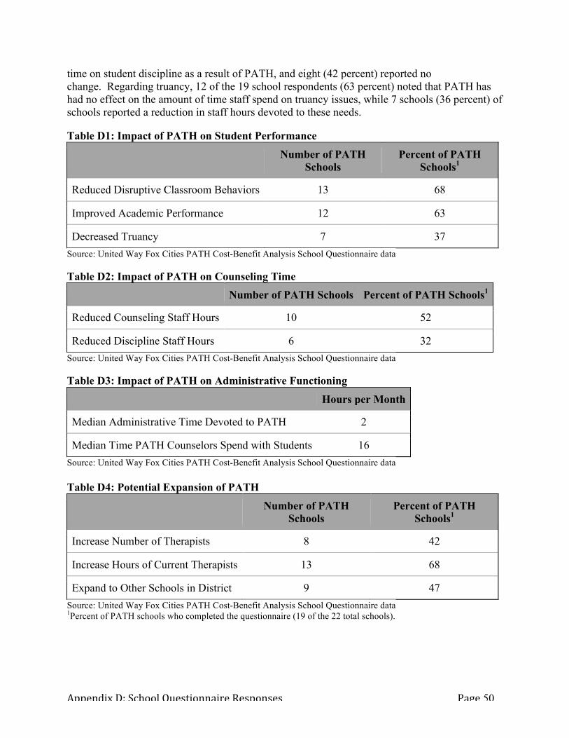
Appendix D: School Questionnaire Responses Page 50
time on student discipline as a result of PATH, and eight (42 percent) reported no change. Regarding truancy, 12 of the 19 school respondents (63 percent) noted that PATH has had no effect on the amount of time staff spend on truancy issues, while 7 schools (36 percent) of schools reported a reduction in staff hours devoted to these needs. Table D1: Impact of PATH on Student Performance
Number of PATH Schools
Percent of PATH Schools1
Reduced Disruptive Classroom Behaviors 13 68
Improved Academic Performance 12 63
Decreased Truancy 7 37
Source: United Way Fox Cities PATH Cost-Benefit Analysis School Questionnaire data Table D2: Impact of PATH on Counseling Time
Number of PATH Schools Percent of PATH Schools1
Reduced Counseling Staff Hours 10 52
Reduced Discipline Staff Hours 6 32
Source: United Way Fox Cities PATH Cost-Benefit Analysis School Questionnaire data Table D3: Impact of PATH on Administrative Functioning
Hours per Month
Median Administrative Time Devoted to PATH 2
Median Time PATH Counselors Spend with Students 16
Source: United Way Fox Cities PATH Cost-Benefit Analysis School Questionnaire data
Table D4: Potential Expansion of PATH
Number of PATH
Schools Percent of PATH
Schools1
Increase Number of Therapists 8 42
Increase Hours of Current Therapists 13 68
Expand to Other Schools in District 9 47
Source: United Way Fox Cities PATH Cost-Benefit Analysis School Questionnaire data 1Percent of PATH schools who completed the questionnaire (19 of the 22 total schools).

Appendix E: School Questionnaire Page 51
Appendix E: United Way Fox Cities PATH Cost-Benefit Analysis School Questionnaire
Students at the La Follette School of Public Affairs at UW-Madison are conducting a cost-benefit analysis of the PATH program for United Way Fox Cities. The purpose of this evaluation is to give a comprehensive overview of how PATH affects the lives of the youth it serves, in terms of both current impacts and future benefits. In order to produce the most accurate assessment of the program possible, we hope to gather information from school districts to complement data provided to us by United Way. Please take the time to complete the following questionnaire to the best of your ability. Your answers will be of immense value to us for completing our evaluation. If you have any questions about the evaluation, do not hesitate to contact our team's liaison, Cherie Wolter ([email protected]). Please direct all completed questionnaires to Mary Wisnet at United Way Fox Cities ([email protected]) by OCTOBER 15th. School District: ________________________________________________________________ Name of School: ________________________________________________________________ Name and Title of Individual Completing Questionnaire: ________________________________________________________________ Email address: ________________________________________________________________ May we contact you if we have additional questions? Y N 1. How has PATH impacted school functioning and student performance in your district? Check all that apply. __ Reduced counseling costs (staffing hours) __ Reduced discipline costs (staffing hours) __ Decreased truancy __ Reduction in disruptive classroom behaviors __ Improved academic performance __ Other: _____________________________ 2. In the average month, how many hours does administrative staff spend overseeing the PATH program in your district? _________ Explain: 3. On average, how many hours per month has PATH changed the time school counselors spend with students for mental health services? _________ Explain: 4. On average, how many hours per month has PATH changed the time school faculty and staff spend disciplining students? _________ Explain: 5. On average, how many hours per month has PATH changed the amount of time staff spend on truancy cases? _________ Explain:

Appendix E: School Questionnaire Page 52
6. Has your school witnessed a change in disruptive classroom behaviors as a result of PATH? Y N Explain: 7. To the best of your knowledge, approximately what percentage of the time are PATH therapists engaged with students? _________ Explain: 8. On average, approximately how much class time does a student miss each month as a result of participating in PATH? _________ Explain: 9. If your school district was given additional resources to expand the PATH program, how would these resources best be used? Check all that apply. __ Expand to additional schools in district If yes, which ones?: ____________________________________ __ Increase number of therapists in schools currently receiving PATH programming __ Increase number of hours for current therapists __ Other: _______________________________ Explain: 10. Do you have any other comments about how PATH has impacted your school? Thank you for completing this questionnaire!
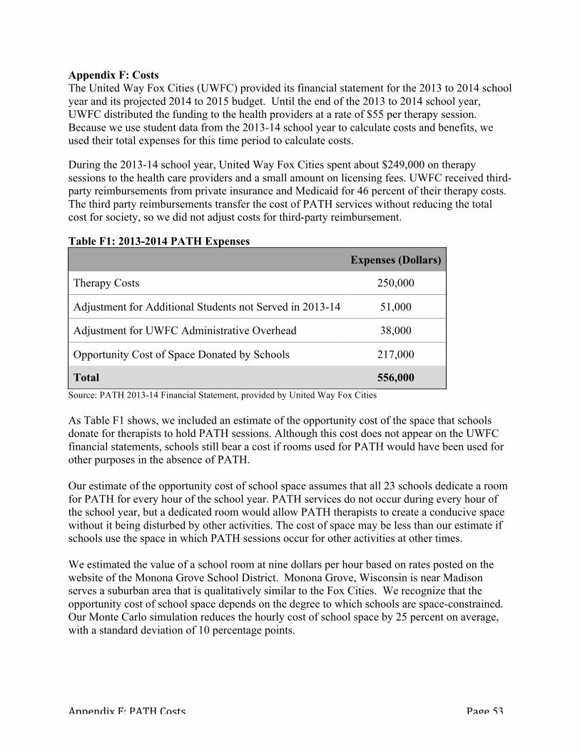
Appendix F: PATH Costs Page 53
Appendix F: Costs The United Way Fox Cities (UWFC) provided its financial statement for the 2013 to 2014 school year and its projected 2014 to 2015 budget. Until the end of the 2013 to 2014 school year, UWFC distributed the funding to the health providers at a rate of $55 per therapy session. Because we use student data from the 2013-14 school year to calculate costs and benefits, we used their total expenses for this time period to calculate costs. During the 2013-14 school year, United Way Fox Cities spent about $249,000 on therapy sessions to the health care providers and a small amount on licensing fees. UWFC received third-party reimbursements from private insurance and Medicaid for 46 percent of their therapy costs. The third party reimbursements transfer the cost of PATH services without reducing the total cost for society, so we did not adjust costs for third-party reimbursement. Table F1: 2013-2014 PATH Expenses
Expenses (Dollars)
Therapy Costs 250,000
Adjustment for Additional Students not Served in 2013-14 51,000
Adjustment for UWFC Administrative Overhead 38,000
Opportunity Cost of Space Donated by Schools 217,000
Total 556,000
Source: PATH 2013-14 Financial Statement, provided by United Way Fox Cities
As Table F1 shows, we included an estimate of the opportunity cost of the space that schools donate for therapists to hold PATH sessions. Although this cost does not appear on the UWFC financial statements, schools still bear a cost if rooms used for PATH would have been used for other purposes in the absence of PATH. Our estimate of the opportunity cost of school space assumes that all 23 schools dedicate a room for PATH for every hour of the school year. PATH services do not occur during every hour of the school year, but a dedicated room would allow PATH therapists to create a conducive space without it being disturbed by other activities. The cost of space may be less than our estimate if schools use the space in which PATH sessions occur for other activities at other times. We estimated the value of a school room at nine dollars per hour based on rates posted on the website of the Monona Grove School District. Monona Grove, Wisconsin is near Madison serves a suburban area that is qualitatively similar to the Fox Cities. We recognize that the opportunity cost of school space depends on the degree to which schools are space-constrained. Our Monte Carlo simulation reduces the hourly cost of school space by 25 percent on average, with a standard deviation of 10 percentage points.

Appendix F: PATH Costs Page 54
In the 2014-15 school year, UWFC started paying for PATH services by distributing block grants to the three different health providers based on their proportion of districts served. Total expenditures to all three providers amount to $439,000. See Table F2 for a breakdown of the projections. Table F2: 2014 to 2015 Projected Expenses
Expenses (Dollars)
Salaries 281,000
Benefits & Taxes 83,000
Travel Cost 21,000
Administrative Costs 54,000
Total Expenses 439,000
Source: PATH 2013-14 Financial Statement, provided by United Way Fox Cities Sources: Monona Grove School District. “Information on Renting District Facilities.” http://www.mononagrove.org/district/howtorentmgfacilities.cfm. Accessed December 16, 2014.

Appendix G: Avoided School Discipline Cost Page 55
Appendix G: Avoided Administrative Costs Associated with Behavioral Problems Behavior problems in school encompass a wide variety of actions, including acting out in class, bullying, and bringing illegal substances onto campus. These behavioral problems are correlated with a number of outcomes including poor school performance and reduced earnings later in life (Segal 2008). Our analysis focused on the school administrative costs pertaining to behavioral problems. We used data from our survey of PATH schools to estimate the incidence of out of school suspensions among PATH participants (Appendix D). These costs stem from the staff time required to document and administer in-school punishments and out-of school suspensions and may vary with administrative practices of each school. Estimations and Assumptions The calculation of changes in school staff time addressing discipline is similar to the calculation of freed guidance counselor time (Appendix I). Using the data gathered from our survey of PATH schools, we estimated an average monthly hourly reduction and standard deviation of administrator time spent on addressing behavioral problems. To estimate a dollar value of staff time, we used the average salary figures of guidance counselors from the Wisconsin Department of Public Instruction. Although other administrators may be involved in handling behavioral problems, these positions either do not have salaries listed the database or have similar salaries. We use an hourly wage rate of $47. Of the 19 schools that responded to our survey, eleven reported a decrease in time devoted to truancy and eight reported no change as a result of PATH. Among those schools reporting a decrease, three quantified the number of hours saved and four just said that time was saved. The average monthly reduction in staff time was 2.4 hours per school with a standard deviation of 1.6 hours. The Monte Carlo simulation gives each school an 11 out of 19 chance to save staff time for discipline to reflect that some schools report no savings. For each school that does save staff discipline time, the Monte Carlo randomly assigns it a monthly savings from a normal distribution based on schools’ survey responses, which we multiply by nine. When we multiply the estimated hours saved by the hourly wage rate discussed above, we estimate a benefit of saved school staff discipline time of $14,000. Sources: Wisconsin Department of Public Instruction. “Median Annual Teacher Earnings.” WISEdash. Accessed November 30. http://wisedash.dpi.wi.gov/Dashboard/portalHome.jsp.

Appendix H: School Staff Truancy Time Page 56
Appendix H: Avoided Truancy Costs Truancy is defined in the state of Wisconsin as any unexcused absence from school for either the full school day or part of the day (WI State Statute 118.15). Schools must document when a student is either tardy or has an unexcused absence. Unexcused absences, in addition to being correlated with negative student outcomes such as low academic performance or not graduating on time, also carry administrative costs for school personnel (Newsome 2008). Additional legal costs associated with student truancy may accrue for students who are habitually truant. However, due to potential alternative interventions at the school level for habitually truant students, we cannot provide an estimate of court costs in the form of additional administrative costs or fines levied against students and their families as part of this analysis. For a more information of this unquantifiable benefit, refer to Appendix N. This section discusses school staff directly pertaining to administrative costs associated with truancy. Estimations and Assumptions Changes in administrative costs associated with truancy were calculated similarly to those associated with changes in guidance counselor costs. Using the data from the 19 schools that responded to our survey of PATH schools, we estimated an average monthly hourly reduction in staff time spent addressing student truancies (Appendix D). To monetize this reduction in staff time, we used average salary figures for the guidance counselors at PATH participating schools provided in the Wisconsin Department of Instruction’s salary database, which indicates an hourly wage rate of $47. While other school personnel in addition to guidance counselors could address student truancies, these individuals either have similar salaries or do not have salaries listed in the database. Of the 19 schools that responded to our survey of schools, seven reported a decrease in time devoted to truancy and twelve reported no change. Of the schools reporting a change, four estimated the number of hours saved. The schools that estimated the number of hours saved on average 4.9 hours, with a standard deviation of 4.6 hours. As described in Appendix I for school staff discipline time, our Monte Carlo first simulated whether schools saved any time at all. Each school that saved time in the simulation was assigned a number of hours saved per month from a normal distribution based on schools’ survey responses and multiplied it by 9 months. Together with the wage rate for school staff, this method estimates that schools save $18,000 worth of staff time that otherwise would have been spent addressing truancy among PATH students. Sources: Wisconsin Department of Public Instruction. “2013-2014 PI-1202 Fall Staff Report All Staff File.” Data Pulled on June 9th, 2014. http://lbstat.dpi.wi.gov/sites/default/files/imce/lbstat/ exe/14staff.zip. Wisconsin State Statute 118.15: Compulsory School Attendance. http://docs.legis.wisconsin.gov/ statutes/statutes/118/15. Wisconsin Department of Public Instruction. WISEdash. “Truancy rates by School: 2013-2014.” Accessed November 25, 2014. http://wisedash.dpi.wi.gov/Dashboard/portalHome.jsp

Appendix I: Guidance Counselor Time Page 57
Appendix I: School Guidance Counselor Time Freed for Other Activities The Wisconsin Department of Public Instruction describes the responsibilities of high school guidance counselors as promoting a healthy school environment, advising students on post-secondary educational options, providing counseling services for students and families, and referring students to outside services. Because PATH provides in-school mental health services to students, once could expect to see a shift in guidance counselor time spent addressing mental health needs. To gauge how guidance counselor time devoted to mental health issues changed as a result of PATH, we surveyed the schools in the program (Appendix D). Guidance counselors have many responsibilities within a school. We asked schools whether guidance counselors reduced the time they spent addressing the mental health of PATH participants and increased the time they spent on other activities. Estimations and Assumptions In our survey of PATH schools, twelve of the 19 respondents reported that PATH freed guidance counselors for other activities. One school indicated that guidance counselors spent more time addressing the mental health of PATH participants because of PATH (Appendix D). The schools estimating the number of hours saved on average 10.2 hours, with a standard deviation of 15.1. The standard deviation of this estimate is large because it includes one school that estimated a negative number of hours saved. As in Appendices G and H, our Monte Carlo simulated whether schools freed guidance counselor time for other activities. We assigned each school that freed guidance counselor time a number of hours saved from a normal distribution based on schools’ survey responses. Combining the estimated hours saved over the course of the school year with the hourly wage rate for guidance counselors obtained from DPI data, we estimate that PATH frees guidance counselors for activities that generate $71,000 worth of benefits. Sources U.S. Office of Personnel Management, “Computing Hourly Wages Using 2,087 Divisor,” accessed November 26, 2014,http://www.opm.gov/policy-data-oversight/pay-leave/ pay-administration/fact-sheets/computing-hourly-rates-of-pay-using-the-2087-hour-divisor/. Wisconsin Department of Public Instruction. “Median Guidance Counselor Annual Earnings.” WISEdash. Accessed November 30. http://wisedash.dpi.wi.gov/Dashboard/portalHome.jsp. Wisconsin Department of Public Instruction. “Comprehensive School Counseling Programs.” Accessed November 26, 2014. http://sspw.dpi.wi.gov/sspw_counsl. Wisconsin State Office of Employee Relations. “Wisconsin Human Resources Handbook.” Accessed November 26, 2014. http://oser.state.wi.us/docview.asp?docid=3422.

Appendix J: Avoided Juvenile Crime Page 58
Appendix J: Benefit of Avoided Juvenile Crime Avoided juvenile crime is a benefit associated with the effect of CBT on students while they are in school. Our model accounts for PATH students who have already been in trouble with the law and may experience reduced criminal recidivism rates based on their CBT experience. We do not attempt to estimate the likelihood of avoided juvenile crime associated with CBT for students who have not already been in trouble with the law, due to lack of reliable effect size estimates for this possibility. The benefit of avoided juvenile crime is the cost that would have been incurred in the absence of PATH by the criminal justice system. Through our interviews and conversations with the United Way Fox Cities and mental health providers, we learned that the majority of participants in PATH who have already had “trouble with the law,” most were involved in underage drinking, habitual truancy (court involved), or other relatively minor, non-violent crimes. We were informed that more serious juvenile offenders are not likely involved in the PATH program and have alternate systems of care. This being said, it is possible that the costs per juvenile crime ($2,100) is over-estimated in the model because it is a weighted average of county court expenditures for all juvenile crimes, which includes more serious (and therefore more expensive) crimes than those committed by PATH participants. Estimates and Assumptions Of the students in PATH during the 2013-14 school year, 13 males and 17 females have had at least one incident reported as “trouble with the law.” For the purpose of modeling in the Monte Carlo, we designate them as prior juvenile offenders and evaluate the costs of incurred by the county justice system. According to Lipsey (2009), prior juvenile offenders have a 0.50 probability of committing another crime (recidivism) within the next twelve months. Comparatively, if juveniles receive a cognitive behavioral intervention, they have a 0.37 probability of committing another crime over the next year, a 26 percent reduction in recidivism. (1) BJuvenileCrime = NPV_JuvenileCrime * PATH_Trouble * (ES_Recidivism - ES_CBT_Recidivism) * Dk Variables: NPV_JuvenileCrime = NPV of reduced juvenile crime PATH_Trouble = Number of PATH participants in trouble with the law ES_Recidivism = Juvenile offender recidivism rate ES_CBT_Recidivism = Effect Size of CBT on juvenile recidivism Dk = Discount factor We calculated a weighted average ($2,100) of county expenditures on juvenile arrests across the three counties (Outagamie, Calumet, and Winnebago) that serve the school districts implementing the PATH program. There is a possibility that PATH participants can commit crime outside of the tri-county boundaries, however we make the assumption that students are most likely to remain within a certain distance to their home and any juvenile crime committed by this population is likely to be processed through these systems. To calculate this weighted average (and standard deviation), we divided total expenditures by total arrests in each county to get a expenditures per arrest rate, and then multiplied by the ratio of arrests in that county over total arrests.

Appendix J: Avoided Juvenile Crime Page 59
Table J1: Juvenile Crime Effect Size Estimates
Variables Point Estimate Notes
PATH_Trouble Males: 14 Females: 17 Total: 31
PATH Questionnaire School Responses
ES_Recidivism 0.50 Lipsey (2009)
ES_CBT_Recidivism 0.37 Lipsey (2009)
Cost Per Juvenile Crime (in 2014 dollars)
2,100 (196)
WI Department of Corrections State and County Juvenile Justice Services. June 2010.
Table J2: Juvenile Crime Expenditures (Weighted Average Calculation)
County Total
Juvenile Arrests
Total Expenditures on Juvenile Arrests (Dollars)
Expenditures per Juvenile Arrest
Outagamie 3,006 5,663,000 1,900
Winnebago 2,424 5,640,000 2,300
Calumet 247 774,000 3,100
Tri-County Total 5,677 12,077,000 2,100 (196)
Weighted Average = ((3006/5677)*1884.03) + ((2424/5677)*232.56) + ((247/5677)*3134.54) Std. Deviation = (2127.38 - 1884.03)2 + (2127.38 - 3134.54)2 + (2127.38 - 2326.56)2 / 5677 Sources: Lipsey, Mark W. "The primary factors that characterize effective interventions with juvenile offenders: A meta-analytic overview." Victims and offenders 4, no. 2 (2009): 124-147. PATH Questionnaire School Responses. Wisconsin Department of Corrections. State and County Juvenile Justice Services Report June 2010. (2012).
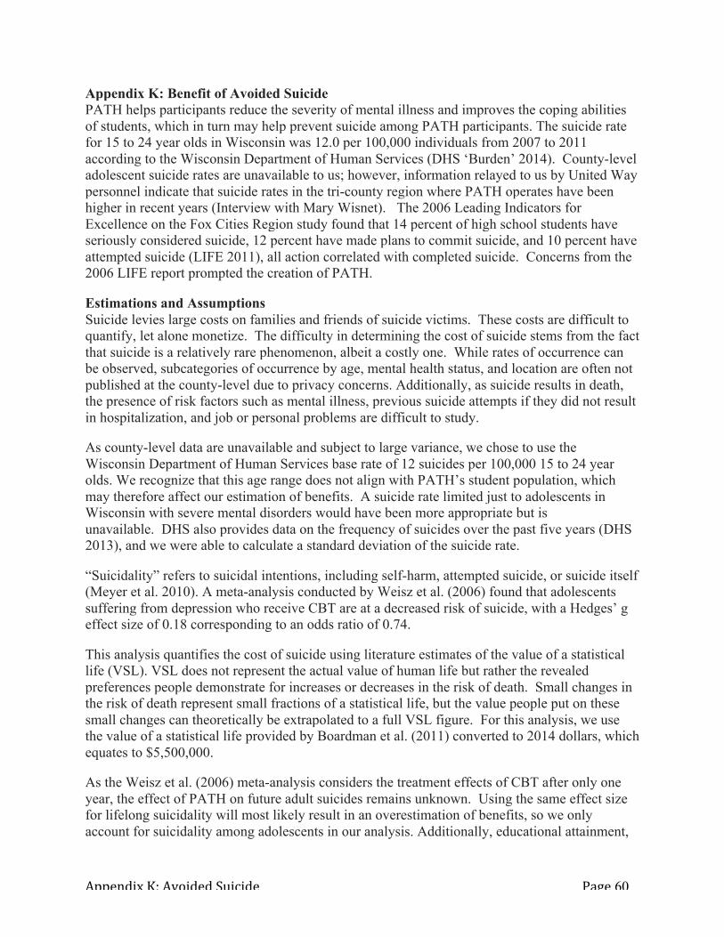
Appendix K: Avoided Suicide Page 60
Appendix K: Benefit of Avoided Suicide PATH helps participants reduce the severity of mental illness and improves the coping abilities of students, which in turn may help prevent suicide among PATH participants. The suicide rate for 15 to 24 year olds in Wisconsin was 12.0 per 100,000 individuals from 2007 to 2011 according to the Wisconsin Department of Human Services (DHS ‘Burden’ 2014). County-level adolescent suicide rates are unavailable to us; however, information relayed to us by United Way personnel indicate that suicide rates in the tri-county region where PATH operates have been higher in recent years (Interview with Mary Wisnet). The 2006 Leading Indicators for Excellence on the Fox Cities Region study found that 14 percent of high school students have seriously considered suicide, 12 percent have made plans to commit suicide, and 10 percent have attempted suicide (LIFE 2011), all action correlated with completed suicide. Concerns from the 2006 LIFE report prompted the creation of PATH. Estimations and Assumptions Suicide levies large costs on families and friends of suicide victims. These costs are difficult to quantify, let alone monetize. The difficulty in determining the cost of suicide stems from the fact that suicide is a relatively rare phenomenon, albeit a costly one. While rates of occurrence can be observed, subcategories of occurrence by age, mental health status, and location are often not published at the county-level due to privacy concerns. Additionally, as suicide results in death, the presence of risk factors such as mental illness, previous suicide attempts if they did not result in hospitalization, and job or personal problems are difficult to study. As county-level data are unavailable and subject to large variance, we chose to use the Wisconsin Department of Human Services base rate of 12 suicides per 100,000 15 to 24 year olds. We recognize that this age range does not align with PATH’s student population, which may therefore affect our estimation of benefits. A suicide rate limited just to adolescents in Wisconsin with severe mental disorders would have been more appropriate but is unavailable. DHS also provides data on the frequency of suicides over the past five years (DHS 2013), and we were able to calculate a standard deviation of the suicide rate. “Suicidality” refers to suicidal intentions, including self-harm, attempted suicide, or suicide itself (Meyer et al. 2010). A meta-analysis conducted by Weisz et al. (2006) found that adolescents suffering from depression who receive CBT are at a decreased risk of suicide, with a Hedges’ g effect size of 0.18 corresponding to an odds ratio of 0.74. This analysis quantifies the cost of suicide using literature estimates of the value of a statistical life (VSL). VSL does not represent the actual value of human life but rather the revealed preferences people demonstrate for increases or decreases in the risk of death. Small changes in the risk of death represent small fractions of a statistical life, but the value people put on these small changes can theoretically be extrapolated to a full VSL figure. For this analysis, we use the value of a statistical life provided by Boardman et al. (2011) converted to 2014 dollars, which equates to $5,500,000. As the Weisz et al. (2006) meta-analysis considers the treatment effects of CBT after only one year, the effect of PATH on future adult suicides remains unknown. Using the same effect size for lifelong suicidality will most likely result in an overestimation of benefits, so we only account for suicidality among adolescents in our analysis. Additionally, educational attainment,

Appendix K: Avoided Suicide Page 61
which is expected to increase for some PATH participants (Appendix L), is negatively correlated with suicide, though there is uncertainty around the magnitude of this effect. We use Equation (1) to model the benefits of avoided suicide due to CBT. The benefits of reducing suicide depend on the number of PATH participants (PATH_Tot); DHS’s suicide rate among 15 to 24 year-olds; the effect size of CBT on suicide (ES_CBT_Suicide), which refers to Weisz et al.’s (2006) effect size; and the VSL estimate provided by Boardman et al. (2011). These figures are summarized in Table K1. (1) BSuicide = PATH_Tot * (Rate_Suicide - ES_CBT_Suicide*(Rate_Suicide)) * VSL Table K1: Suicide Effect Size Estimates
Point Estimate Notes and Sources
Rate_Suicide .00012 (0.00001785)
WI DHS (2014)
ES_CBT_Suicide 0.74 z=1.80, p=.07 CI: .5377 to 1.026 (OR) Weisz (2006)
VSL $5,500,000 Low Value: $2,600,000 High Value: $7,900,000 Boardman et al. (2011)
Sources: Boardman, Anthony E., David H. Greenberg, Aidan R. Vining, and David L. Weimer. "Cost-Benefit Analysis, Concepts and Practice”, 4th ed. New Jersey: Pearson Education, Inc, 2011. Interview with Mary Wisnet, Community Development Program Officer: Health & Healing and Strengthening Families, United Way Fox Cities. November 14, 2014. Meyer, Roger E., Carl Salzman, Eric A. Youngstrom, Paula J. Clayton, Frederick K. Goodwin, J. John Mann, Larry D. Alphs et al. "Suicidality and risk of suicide--definition, drug safety concerns, and a necessary target for drug development: a consensus statement." J Clin Psychiatry 71, no. 8 (2010): e1-e21. Weisz, John R., Carolyn A. McCarty, and Sylvia M. Valeri. "Effects of psychotherapy for depression in children and adolescents: a meta-analysis. "Psychological bulletin 132, no. 1 (2006): 132. Wisconsin Department of Human Services. “The Burden of Suicide in Wisconsin: 2014.” Accessed November 26, 2014. http://www.dhs.wisconsin.gov/publications/P0/p00648-2014.pdf. Wisconsin Department of Human Services. “Wisconsin Population Estimates in 2014.” Accessed November 26, 2014. http://www.dhs.wisconsin.gov/population/.

Appendix L: Increased Lifetime Income Page 62
Appendix L: Benefit of Increased Lifetime Income Graduating from high school produces lasting impacts on one’s lifetime income (Cohen and Piquero 2008). Additionally, earnings rates are affected by one’s highest level of educational attainment: those with higher levels work at a higher wage rate and spend more time in the workforce (Bureau of Labor Statistics 2014b; Skoog and Ciecka 2001). In calculating PATH’s impact on lifetime income, we account for the ultimate level of educational attainment among the program’s participants. Individuals suffering from adolescent depression earn 19 percent less than the general population (Fletcher 2013), so we reduce our income figures by this amount. The discussion that follows presents our methods and assumptions for calculating this program benefit. Estimates and Assumptions In modeling the effect PATH has on the lifetime income of participants, we consider once again the effect PATH has on high school graduation and the subsequent impact on lifetime income. Our lifetime income benefit models therefore involve accounting for the number of PATH participants who graduate high school as a result of the intervention but otherwise would not have. We do not apply this income effect to PATH students who would be predicted to complete high school despite participating in PATH and students who participate in PATH but do not complete high school, as they do not receive an additional income benefit as a result of participating in the program. Our benefits estimate for the income effect of graduation only includes individuals for whom CBT causes them to graduate high school and would not have otherwise. Additionally, we assume that all PATH participants enter the labor force, earning at least the equivalent of a high school dropout. We do not take into consideration how income and productivity may be indirectly influenced by CBT through its potential to reduce mental health symptoms or help individuals develop skills relevant to job success. We omitted these potential income effects, believing they are relatively temporary and smaller than the effect of high school graduation itself on income. Our modeling strategy involves estimating the highest level of educational attainment reached by PATH participants as a result of the intervention and applying the difference in the median annual lifetime total income of Wisconsin adults at each attainment level from that of high school graduates. These income figures incorporate all sources of income, including unemployment insurance and retirement. We reduce these figures by the 19 percent reduction in earnings associated with adolescent depression reported by Fletcher (2013). Although this figure pertains only to individuals with adolescent depression and not all individuals with any mental illness as a youth, we are confident in this assumption given that mood disorders are among the most prevalent among PATH participants (Appendix B). We define four levels of educational attainment: (1) four-year high school graduate, (2) six-year high school graduate, (3) some college or a two-year degree, or (4) a bachelor’s degree or more. We obtain our high school dropout, some college or two-year degree, and bachelor’s degree rates from CPS data (Table L1). For high school graduates, we consider both students who graduate in four and six years (Grad_Adjl and Grad Adj2, respectively) and use the effect size estimate for high school graduation (ES_Grad), as described in the body of the report.

Appendix L: Increased Lifetime Income Page 63
We then apply the estimated lifetime income for PATH participants attaining each of these levels using the median annual pre-tax income of Wisconsin adults in 2014 gathered from 2014 Current Population Survey data (King et al. 2010; Table L2). These figures pertain to the entire adult population in Wisconsin and are not specific to individuals with a history of mental illness. Our benefits estimates therefore may not fully represent the population PATH serves, though we expect them to be comparable to the true underlying values. Table L1: 2014 Education Attainment Rates in Wisconsin
Male Female
Estimate SD Estimate SD
Four-Year High School Graduation Rate (Grad_Adj1) 0.90 n/a 0.97 n/a
Six-Year High School Graduation Rate (Grad_Adj2) 0.95 n/a 0.98 n/a
High School Diploma (EduAttain_HS) 0.29 0.46 0.27 0.45
Some College or Two-Year Degree (EduAttain_SomeCol) 0.13 0.34 0.14 0.34
Bachelor’s Degree or More (EduAttain_Col) 0.25 0.44 0.28 0.45
Source: King, Miriam, Steven Ruggles, J. Trent Alexander, Sarah Flood, Katie Genadek, Matthew B. Schroeder, Brandon Trampe, and Rebecca Vick. Integrated Public Use Microdata Series, Current Population Survey: Version 3.0. [Machine-readable database]. Minneapolis: University of Minnesota, 2010. Table L2: 2014 Median Annual Pre-Tax Total Income for Adults in Wisconsin, by Educational Attainment
Male (Dollars) Female (Dollars)
Estimate SD Estimate SD
HS Dropouts 19,900 24,000 10,300 12,200
HS Graduates 31,200 59,200 15,200 19,000
Some College and Two-Year Degree 40,000 44,900 25,000 33,900
Bachelor’s Degree and Above 68,500 94,800 40,000 36,000
Source: King, Miriam, Steven Ruggles, J. Trent Alexander, Sarah Flood, Katie Genadek, Matthew B. Schroeder, Brandon Trampe, and Rebecca Vick. Integrated Public Use Microdata Series, Current Population Survey: Version 3.0. [Machine-readable database]. Minneapolis: University of Minnesota, 2010. Modeling in Monte Carlo Simulation To model the effect of PATH on lifetime income based on level of educational attainment, we need to consider four specific groups of PATH participants: (1) four-year high school graduates, (2) six-year high school graduates, (3) some college and two-year degree recipients, and (4) bachelor’s degree or greater recipients.

Appendix L: Increased Lifetime Income Page 64
Equation 1 shows our calculations for the lifetime income benefit for four-year high school graduates by gender (k). Recognizing that the lifetime income effect differs between individuals who graduate high school in four years versus six, we calculate a benefit stream for each group. Equation 1 focuses on PATH participants who graduate in four years using Grad_Adj1. Here we multiply the expected number of four-year PATH high school graduates by the difference in median lifetime income of a high school graduate in Wisconsin and a high school dropout (NPV_HSk - NPV_Dropoutk), the effect size of adolescent depression on adult earnings (Dep_Earn), and a discount factor (∑Di). (1) BEarn_HS4 = ∑k {(NPV_HSk - NPV_Dropoutk) * Dep_Earn * [PATH_Totk * ES_Gradj * Grad_Adj1] * ∑Di} We modify Equation 1 to account for students whose highest level of educational attainment is a high school diploma but who graduate in six years (Equation 2). Here we assume that a student works, earning the equivalent of a high school dropout (NPV_Dropoutk), during the extra two years he or she spends in high school. Upon receiving a high school diploma, he or she then earns the equivalent of a high school graduate for the rest of his or her time in the labor force, receiving an income benefit of (NPV_HSk - NPV_Dropoutk). We again account for the earnings reduction due to adolescent depression (Dep_Earn). (2) BEarn_HS6 = ∑k {[PATH_Totk * ES_Gradj * Grad_Adj2] * [2 * NPV_Dropoutk + (NPV_HSk - NPV_Dropoutk)] * Dep_Earn * ∑Di}
Our final two educational attainment categories include PATH participants who graduate from high school and continue on to college. The first group is individuals who either attain a two-year degree or complete some college without graduating. The income benefits for this group are presented in Equation 3. Here we multiply the expected number of individuals who graduate from high school as a result of PATH by the two-year and some college attainment rate by gender for Wisconsin in 2014 (EduAttain_SomeColk). Applying the difference in net present value of lifetime income for this attainment group from that of dropouts (NPV_SomeColk - NPV_Dropoutk), the earnings reduction from adolescent depression (Dep_Earn), and the discount rate (∑Di) yields the income benefit for this group. (3) BEarn_SomeCol = (NPV_SomeColk - NPV_Dropoutk) * Dep_Earn * [PATH_Totk * ES_Gradj * EduAttain_SomeColk] * ∑Di
Calculating the income benefits for PATH participants obtaining a four-year degree or more is similar, but now we incorporate the educational attainment rate for this group in Wisconsin in 2014 (EduAttain_Colk) and the associated lifetime income (NPV_Colk - NPV_Dropoutk and reduction due to adolescent depression Dep_Earn: Equation 4) (4) BEarn_Col = (NPV_Colk - NPV_Dropoutk) * Dep_Earn* [PATH_Totk * ES_Gradj * EduAttain_Colk] * ∑Di
Summing the benefits calculated from Equations 1 through 4 produces the estimated lifetime benefits accruing as a result of PATH.

Appendix L: Increased Lifetime Income Page 65
Sources: Bureau of Labor Statistics. Employment Projections: Earnings and unemployment rates by educational attainment. 2014. http://www.bls.gov/emp/ep_table_001.htm. Cohen, Mark A., and Alex R. Piquero. "New evidence on the monetary value of saving a high risk youth." Journal of Quantitative Criminology 25, no. 1 (2008): 25-49. King, Mariam, Steven Ruggles, J. Trent Alexander, Sarah Flood, Katie Genadek, Matthew B. Schroeder, Brandon Trampe, and Rebecca Vick. Integrated Public Use Microdata Series, Current Population Survey: Version 3.0. [Machine-readable database]. Minneapolis: University of Minnesota, 2010. Skoog, Gary R., and James E. Ciecka. "Markov (Increment-Decrement) Model of Labor Force Activity: New Results Beyond Work-Life Expectancies, The." J. Legal Econ. 11 (2001): 1.

Appendix M: Avoided Adult Crime Page 66
Appendix M: Benefit of Avoided Adult Crime The estimate for the avoided costs of adult crime will be based primarily on the effect of high school graduation on long-term avoided crime outcomes. Levin et al. (2007), Cohen and Piquero (2008), Reynolds et al. (2011) and others find that educational attainment, and in particular high school graduation, has a significant effect on reducing adult crime rates. Because PATH increases the likelihood that students with mental disorders will graduate from high school, this effect can be used to predict avoided costs of adult crime. For our purposes, this specific effect is only applied to students who are predicted to graduate after receiving CBT who would not have graduated in the absence of PATH. It is not applied to students who drop out of high school or would be predicted to complete high school anyway. In order to link the effect of CBT treatment to the reduction in adult crime, we look at the duration of CBT treatment on juvenile depression, since depressive and mood disorders are the most prevalent disorders among PATH students (approximately 32.8 percent), and because these disorders tend to persist into adulthood. Estimates of the effect of CBT on juveniles treated for depression are not shown to be significant past a one-year horizon (Weisz et al. 2006). In other words, the effect is more immediate to PATH students and we cannot assume that the CBT treatment PATH students receive while in high school will have lasting effects beyond high school graduation. Thus, we cannot predict adult avoided crime for the other PATH participants based on the data at hand. We do, however, estimate elsewhere the avoided costs of juvenile crime for PATH participants. Estimates and Assumptions Estimates of the total avoided cost of adult crime of PATH students can be made by using estimates of the total present value of average lifetime cost-savings from reduced criminal activity for high school graduates, which Levin et al. (2007) estimated to be $30,200 for white males and $8,300 for white females. Consumer Price Index adjusted to 2014 dollars, these estimates are $38,000 and $10,500 respectively. In Equation 1 below we define these net present values with the following notation (k = males, females), NPV_Red_AdultCrimek. Among the 183 PATH participants, 2013-14 intake and discharge data show that 14 males and 17 females have had some “trouble with the law,” which we assume to be reflective of previous arrest. PATH therapists reported that “trouble with the law” included offenses such as underage drinking and truancy, therefore our estimates of all criminal activity may be overstated, as higher order correctional institutions may be handling more serious levels of crime. In the estimates below, we combine the Levin et al. (2007) estimates, PATH data on times in trouble with the law, and the high school graduation effect size associated with PATH to calculate an estimated avoided adult crime cost for the program. In Equation 1, we define the number of PATH students who have been in trouble with the law as, PATH_Troublek, where again k = males, females. We compute an estimate of avoided adult crime costs based on the effect size estimate for high school graduation, explained in Appendix C, and shown in Equation 2. (1) BAdultCrimek = [NPV_Red_AdultCrimek * PATH_Troublek * ES_Grad] * Dk Variables: NPV_Red_AdultCrimek = NPV of reduced adult crime by gender PATH_Troublek = Number of PATH participants in trouble with law by gender

Appendix M: Avoided Adult Crime Page 67
ES_Grad = ES of PATH on graduation Dk = Discount factor Estimates:
Point Estimate Notes
NPV_Red_AdultCrimek Males: $38,000 Females: $10,500
Levin, 2007
PATH_Troublek Males: 14 Females: 17
PATH Data
ES_Gradj .206 See Appendix O
Dk See Adult Crime Benefit Appendix
(2) BAdultCrimek = [Dk($38,054*14*.269) + Dk($10,458*17*.269)] Exclusions The possible benefit of increased lifetime income due to avoided lost income during incarceration is not included in this calculation. We assume that the benefit of high school graduation on lifetime income captures avoided lost earnings during incarceration. Sources: Cohen, Mark A., and Alex R. Piquero. "New evidence on the monetary value of saving a high risk youth." Journal of Quantitative Criminology 25, no. 1 (2008): 25-49. Levin, Henry, Clive Belfield, Peter Muennig, and Cecilia Rouse. The costs and benefits of an excellent education for all of America's children. Vol. 9. New York: Teachers College, Columbia University, 2007. Reynolds, Arthur J., Judy A. Temple, Barry AB White, Suh-Ruu Ou, and Dylan L. Robertson. "Age 26 Cost–Benefit Analysis of the Child-‐Parent Center Early Education Program." Child Development 82, no. 1 (2011): 379-404.

Appendix N: Unquantifiable Benefits Page 68
Appendix N: Unquantifiable Benefits We have identified several additional benefits to those monetized in this cost-benefit analysis, including reduced discipline costs, increased productivity, reduced need to access external treatment, and increased quality of life years. These benefits consist of a variety of ways that PATH could impact students; however, due to measurement difficulty or lack of appropriate effect sizes in the literature, we have chosen to exclude them from our fiscal analysis. Recognizing that these effects likely have lasting impacts on PATH participants, we devote this appendix to explaining how each of these benefits could impact PATH stakeholders in addition to summarizing why each was left out of our cost-benefit calculations. Discipline costs: Classroom disruptions Childhood mental illness is correlated with bullying and disruptive classroom behavior (August et al. 1996; Liber et al. 2013). These behaviors can levy costs associated with teacher and student distraction and adverse outcomes for other children who are the victims of bullying. However, the results of these effects are difficult to define, measure and attach a cost. Staff at PATH schools reported reductions in time spent on behavioral problems due to the program and we were able to quantify the effect of disruptive behavior in terms of administrative costs. Other possible costs such as impacts on other students’ ability to learn are not monetized as we do not have reliable estimates of these intangible costs. Productivity We do not attempt to monetize the benefit of possible increased lifetime productivity due to PATH for two reasons. First, increased productivity is in part captured in the benefit of increased lifetime earnings due to high school graduation. Second, the effect of CBT on productivity is limited to short-term effects. This is illustrated by looking at the effect of CBT on depression, since untreated depression is highly correlated with a decrease in labor force productivity (Stewart et al. 2003). Weisz et al. (2007) find that the effect CBT on juvenile depression (improved outcomes in three to six months post-treatment) does not persist beyond one year past the end of treatment. Therefore, we cannot assume that the CBT treatment PATH students receive would have lasting effects on future labor force productivity. We could not find estimates of the effect of early treatment of depression on the likelihood of pursuing treatment as an adult, which could give us a basis for estimating an effect of PATH on productivity through its effect on future depression treatment. However, the immediate, short-term benefits of CBT on PATH students in captured in the effect of CBT on decreasing the number of dropouts and increasing the number of students who go on to graduate from high school and gain the benefits associated with high school graduation. Reduced Need to Access External Treatment Since PATH participants are receiving in-school mental health treatment, one could infer that their frequency of visits to external providers would decline. However, the PATH intake and discharge data do not fully support this claim. Nearly 85 percent of participants saw no change in their frequency of hospitalizations and emergency room visits between one year prior to entering PATH and during their participation in the program. Approximately half of participants, however, saw a change in their number of doctor visits for mental health reasons; however, nearly 40 percent of this group saw an increase in physician visits while in PATH (see Appendix B). Because in the inconsistency on how PATH has influenced the external mental

Appendix N: Unquantifiable Benefits Page 69
health treatment access of students, we do not include this potential benefit of the program in our analysis. Additionally, quantifying such an effect would be difficult, as it would involve a thorough assessment of the insurance status of participants and the billing rates for the services they seek. An additional change in accessing external treatment could be the type of treatment accessed outside of school. Lack of access to preventative mental health care can lead to an increased emergency room use and hospitalization both of which are more expensive than preventative therapy (Guo 2008). Research on school based mental health centers in Ohio has indicated that emergency room visits and hospitalizations fall when mental health services are provided in schools. However as we lack a comprehensive analysis of the insurance status of PATH participants, the reasons for reported emergency room visits and the billing rates for the services that PATH participants might seek we cannot quantify the change in costs associated with access to preventative care. Quality of Life A quality adjusted life year (QALY) compares the effects of a variety of physical and mental health interventions both the quantity of years that patients can be expected to live as well as the expected quality of that time can be made (Weinstein 2008). We acknowledge that there may be a benefit of increased QALYs to students in the PATH program since, broadly speaking, reviews of school based mental health interventions have shown that CBT does improve mental health outcomes and thus potentially quality of life (Hoagwood 2007). However, QALYs are underutilized in mental health care, as there is concern that the tools used to estimate it are ill-suited for changes in mental health (Chisholm et al. 1997; Sherbourne 2001). Moreover the reliability of effect sizes on adult populations from the literature may not represent PATH students since there is evidence that adolescents value their health in a different manner than adults (Ratcliffe et al. 2012). Therefore, we do not attempt to monetize possible QALY benefits associated with PATH. Legal Costs due to Habitual Truancy The State of Wisconsin mandates compulsory student attendance and defines habitual truancy as five or more unexcused absences from school during a semester (WI Statue 118.15). Once a student is habitually truant schools can refer the habitually truant student and their family to truancy court after notifying parents, providing opportunities for counseling or alternative educational programs. If a student and his or her family is referred to truancy court the maximum penalty for the first offense is $500 and a 30 day sentence. The second maximum penalty is $1,000 and a 30-day sentence. While in some cases these costs can be high schools do not refer every habitually truant student to truancy court. As part of the administrative processes prior to referral a school can provide opportunities in alternative programs. PATH is an example of one of these programs. Others, such as the Appleton Area School district, have access to programs independent of PATH (WI Legislative Audit Bureau 2008). In addition while maximum penalties are set these are not necessarily the penalties levied on habitually truant students or their families. Truancy data provided in Appendix Q indicates that there is a difference in habitual truancy as defined by state statute between the times that students enter the program and while they are

Appendix N: Unquantifiable Benefits Page 70
participating, though the information on students currently in PATH might not reflect a full school year. If PATH was unavailable to these schools we cannot be sure that students who are habitually truant and currently participating in PATH would ultimately be referred to truancy court or would have their truancy addressed via other means. As such we have excluded this benefit. Sources: August, Gerald J., George M. Realmuto, Angus W. MacDonald III, Sean M. Nugent, and Ross Crosby. "Prevalence of ADHD and comorbid disorders among elementary school children screened for disruptive behavior." Journal of abnormal child psychology 24, no. 5 (1996): 571-595. Chisholm, D., A. Healey, and M. Knapp. "QALYs and mental health care." Social psychiatry and psychiatric epidemiology 32, no. 2 (1997): 68-75., Guo, Jeff J., Terrance J. Wade, and Kathryn N. Keller. "Impact of school-based health centers on students with mental health problems." Public Health Reports123, no. 6 (2008): 768. Hoagwood, Kimberly E., S. Serene Olin, Bonnie D. Kerker, Thomas R. Kratochwill, Maura Crowe, and Noa Saka. "Empirically based school interventions targeted at academic and mental health functioning." Journal of Emotional and Behavioral Disorders 15, no. 2 (2007): 66-92. Liber, Juliette M., Gerly M. De Boo, Hilde Huizenga, and Pier JM Prins. "School-based intervention for childhood disruptive behavior in disadvantaged settings: A randomized controlled trial with and without active teacher support." Journal of consulting and clinical psychology 81, no. 6 (2013): 975. Ratcliffe, Julie, Terry Flynn, Frances Terlich, Katherine Stevens, John Brazier, and Michael Sawyer. "Developing Adolescent-Specific Health State Values for Economic Evaluation." Pharmacoeconomics 30, no. 8 (2012): 713-727. Stewart, Walter F., Judith A. Ricci, Elsbeth Chee, Steven R. Hahn, and David Morganstein. "Cost of lost productive work time among US workers with depression." Jama 289, no. 23 (2003): 3135-3144. Sherbourne, Cathy D., Kenneth B. Wells, Naihua Duan, Jeanne Miranda, Jürgen Unützer, Lisa Jaycox, Michael Schoenbaum, Lisa S. Meredith, and Lisa V. Rubenstein. "Long-term effectiveness of disseminating quality improvement for depression in primary care." Archives of General Psychiatry 58, no. 7 (2001): 696-703. Weinstein, Milton C. "How much are Americans willing to pay for a quality-adjusted life year?" Medical care 46, no. 4 (2008): 343-345. Weisz, John R, Carolyn a McCarty, and Sylvia M Valeri. “Effects of Psychotherapy for Depression in Children and Adolescents: A Meta-Analysis.” Psychological Bulletin 132 (1), (2006):132–49.

Appendix N: Unquantifiable Benefits Page 71
Wisconsin State Statute 118.15: Compulsory School Attendance. http://docs.legis.wisconsin.gov/statutes/statutes/118/15 Wisconsin State Legislative Audit Bureau. “Best Practices Review: Truancy Reduction Efforts.” Wisconsin Legislative Council 2008, accessed November 30, 2014, http://legis.wisconsin.gov/lab/reports/08-0truancyfull.pdf

Appendix O: Expected High School Graduations Page 72
Appendix O: Expected High School Graduation Rate and Adjustment Factor Six-year Weighted Expected Graduation Rate The weighted average six-year high school graduation rate for the 2010-11 cohort for the eleven high schools served by PATH is 96.6 percent. The weighted average dropout rate for the same schools is 1.38 percent. Because not all students who do not drop out eventually graduate, the expected induced graduation rate of the PATH students who would have otherwise dropped out must be estimated by combining the avoided dropout rate with the expected graduation rate of non-dropouts. Based on calculations in the Appendix C, our expected proportion of PATH students who do not drop out is 71 percent. To adjust this effect size to reflect graduation, we do the following: 100 percent - 1.38 percent dropout rate = 98.6 percent students who do not drop out, but may not all graduate A ratio of the weighted average six-year graduation rate, 96.6 percent, and the 98.6 percent of students who do not drop out, but may not all graduate gives us an adjustment factor for students who do not drop out, but can be expected to graduate: 96.6/98.6 = 98 percent. We multiply this adjustment factor by 71 percent to give the adjusted expected number of graduates due to PATH. This gives us an estimated graduation rate for PATH participants of 69.6 percent. Performing the same calculation for the control groups of mentally ill students not participating in PATH yields an estimation of 49 percent. Therefore, PATH participants are 20.6 percentage points more likely to graduate high school than their non-participant counterparts. Four- and Six-year Weighted Average Expected Graduation Rates for Increased Lifetime Income by Gender These graduation rates were calculated by gender, using the method above for the 2010-11 and 2012-13 cohorts of students in PATH schools and are shown in Table 1. Table O1: Four- and Six- Year Wisconsin High School Graduation Rates
Males Females
Four-year Weighted Average High School Graduation Rate 0.90 0.97
Six-year Weighted Average High School Graduation Rate 0.95 0.98
Source: Wisconsin Department of Public Instruction. “Wisconsin high school graduation rates”. WISEdash. Accessed November 30, 2014. http://wisedash.dpi.wi.gov/Dashboard/portalHome.jsp
Sources: Wisconsin Department of Public Instruction. “Wisconsin high school graduation rates.” WISEdash. Accessed November 30. http://wisedash.dpi.wi.gov/Dashboard/portalHome.jsp.

Appendix P: Monte Carlo Equations Page 73
Appendix P: Monte Carlo Equations and Estimates This appendix summarizes the equations and estimates that were inputted into the Monte Carlo simulation. First we highlight how the short-term benefits of the analysis, namely truancy, behavioral problems, guidance counselor time, juvenile crime, and suicide, were modeled. Next we display how we calculated the graduation effect that drives our long-term benefits. Finally, we show the equations for our two long-term benefits: lifetime earnings and adult crime. Short-Term Benefits: Truancy Equation: BTruancy = Chg_TruancyHrs * AdminCost Variables: Chg_TruancyHrs= Change in hours spent on truancy per month AdminCost = Administrative cost per hour Estimates: Table P1: Truancy Effect Size Estimates
Point Estimate Source
Chg_TruancyHrs (all schools)
4.9 hrs/mth reduction SD: 4.6 hrs/mth
United Way Fox Cities PATH Cost-Benefit Analysis School Questionnaire data
AdminCost $47/hr WI Department of Public Instruction
Behavior and Discipline Problems Equation: BDiscipline = Chg_DisciplineHrs * AdminCost Variables: Chg_DisciplineHrs = Change in hours spent on truancy per month AdminCost = Administrative cost per hour Estimates: Table P2: Behavior and Discipline Effect Size Estimates
Point Estimate Source
Chg_DisciplineHrs 2.4 hrs/mth SD: 1.6 hrs/mth
United Way Fox Cities PATH Cost-Benefit Analysis School Questionnaire data
AdminCost $47/hr Wisconsin Department of Public Instruction
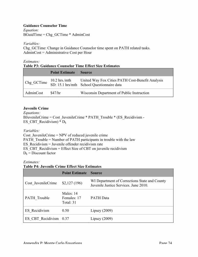
Appendix P: Monte Carlo Equations Page 74
Guidance Counselor Time Equation: BGuidTime = Chg_GCTime * AdminCost Variables: Chg_GCTime: Change in Guidance Counselor time spent on PATH related tasks. AdminCost = Administrative Cost per Hour Estimates: Table P3: Guidance Counselor Time Effect Size Estimates
Point Estimate Source
Chg_GCTime 10.2 hrs./mth SD: 15.1 hrs/mth
United Way Fox Cities PATH Cost-Benefit Analysis School Questionnaire data
AdminCost $47/hr Wisconsin Department of Public Instruction
Juvenile Crime Equations: BJuvenileCrime = Cost_JuvenileCrime * PATH_Trouble * (ES_Recidivism - ES_CBT_Recidivism) * Dk Variables: Cost_JuvenileCrime = NPV of reduced juvenile crime PATH_Trouble = Number of PATH participants in trouble with the law ES_Recidivism = Juvenile offender recidivism rate ES_CBT_Recidivism = Effect Size of CBT on juvenile recidivism Dk = Discount factor Estimates: Table P4: Juvenile Crime Effect Size Estimates
Point Estimate Source
Cost_JuvenileCrime $2,127 (196) WI Department of Corrections State and County Juvenile Justice Services. June 2010.
PATH_Trouble Males: 14 Females: 17 Total: 31
PATH Data
ES_Recidivism 0.50 Lipsey (2009)
ES_CBT_Recidivism 0.37 Lipsey (2009)

Appendix P: Monte Carlo Equations Page 75
Suicide Equation: BSuicide= PATH_Tot * (Rate_Suicide – ES_CBT_Suicide*Rate_Suicide) * VSL Variable List: PATH_Tot = Number of PATH participants ES_CBT_Suicide = Effect size of CBT on reducing suicidality VSL = Value of statistical life Estimates: Table P5: Suicide Effect Size Estimates Point
Estimate Low Value (CI)
High Value (CI)
Notes and Sources
Rate_Suicide 0.00012 n/a n/a SD: 0.000018 WI DHS (2014)
ES_CBT_Suicide 0.74 .5377 1.026 z=1.80, p=.07 Weisz (2006)
VSL $5,500,000 $2,600,000 $7,900,000 Boardman et al. (2011)
Graduation Effect Equation: ES_Grad = ExDOR * ES_CBT_DOR * Grad_Adj2 Variable List ES_Grad = Effect size of PATH on HS graduation ExDOR = Expected dropout rate of students with mental illness ES_CBT_DOR = Effect size of CBT on HS graduation Grad_Adjl = Adjusted graduation rate (l=1 4-year, l=2 6-year)

Appendix P: Monte Carlo Equations Page 76
Estimates: Table P6: Graduation Effect Size Estimates
Point Estimate Low Value (CI) High Value (CI) Notes and Sources
ExDOR 0.50 n/a n/a US DOE (2007)
ES_CBT_DOR 0.55 0.36 0.74 z=5.6, p<.0001 Cobb (2007)
Grad_Adj1 Males: 0.90 Females: 0.97
n/a n/a DPI
Grad_Adj2 Males: 0.95 Females: 0.98
n/a n/a DPI
Long-Term Benefits: Lifetime Income Equations: BEarn_HS4 = ∑k {(NPV_HSk - NPV_Dropoutk) * [PATH_Totk * ES_Gradj * Grad_Adj1] * ∑Di} BEarn_HS6 = ∑k {[PATH_Totk * ES_Gradj * Grad_Adj2] * [2 * NPV_Dropoutk + (NPV_HSk - NPV_Dropoutk)] * ∑Di} BEarn_SomeCol = (NPV_SomeColk - NPV_Dropoutk) * [PATH_Totk * ES_Gradj * EduAttain_SomeColk] * ∑Di BEarn_Col = (NPV_Colk - NPV_Dropoutk) * [PATH_Totk * ES_Gradj * EduAttain_Colk] * Di Variable List: BEarn_[x] = Lifetime income benefit at educational attainment level NPV_[x] = NPV of income at appropriate attainment level EduAttain_[x] = WI education attainment rate at appropriate level PATH_Totk = Number of PATH participants of gender k ES_Gradj = Effect size of CBT on HS graduation Grad_Adjl = Adjusted graduation rate (l=1 4-year, l=2 6-year) Di = Discount factor

Appendix P: Monte Carlo Equations Page 77
Estimates: Table P7: 2014 Education Attainment Rates in Wisconsin
Male Female
Estimate SD Estimate SD
Four-Year High School Graduation Rate (Grad_Adj1) 0.90 n/a 0.97 n/a
Six-Year High School Graduation Rate (Grad_Adj2) 0.95 n/a 0.98 n/a
High School Diploma (EduAttain_HS) 0.2958 0.45 0.2708 0.45
Some College or Two-Year Degree (EduAttain_SomeCol) 0.1327 0.33 0.1374 0.34
Bachelor’s Degree or More (EduAttain_Col) 0.2531 0.43 0.2779 0.45 Source: Miriam King, Steven Ruggles, J. Trent Alexander, Sarah Flood, Katie Genadek, Matthew B. Schroeder, Brandon Trampe, and Rebecca Vick. Integrated Public Use Microdata Series, Current Population Survey: Version 3.0. [Machine-readable database]. Minneapolis: University of Minnesota, 2010. Table P8: 2014 Median Annual Pre-Tax Earnings for Adults in Wisconsin, by Educational Attainment
Male (Dollars) Female (Dollars)
Estimate SD Estimate SD
HS Dropouts (NPV_Dropout) 19,900 24,000 10,300 12,000
HS Graduates (NPV_HS) 31,200 59,200 15,200 19,100
Some College and Two-Year Degree (NPV_SomeCol) 40,000 44,900 25,000 33,900
Bachelor’s Degree and Above (NPV_Col) 68,500 94,800 40,000 36,200 Source: Miriam King, Steven Ruggles, J. Trent Alexander, Sarah Flood, Katie Genadek, Matthew B. Schroeder, Brandon Trampe, and Rebecca Vick. Integrated Public Use Microdata Series, Current Population Survey: Version 3.0. [Machine-readable database]. Minneapolis: University of Minnesota, 2010. Adult Crime Equation: BAdultCrimek = [NPV_Red_AdultCrimek * PATH_Troublek * ES_Gradj] * Dk Variables: NPV_Red_AdultCrimek = NPV of reduced adult crime by gender PATH_Troublek = Number of PATH participants in trouble with law by gender ES_Gradj = ES of PATH on graduation Dk = Discount factor
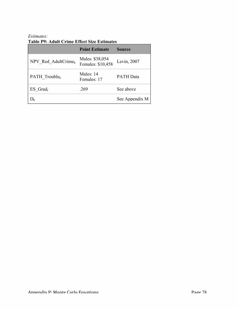
Appendix P: Monte Carlo Equations Page 78
Estimates: Table P9: Adult Crime Effect Size Estimates
Point Estimate Source
NPV_Red_AdultCrimek Males: $38,054 Females: $10,458 Levin, 2007
PATH_Troublek Males: 14 Females: 17 PATH Data
ES_Gradj .269 See above
Dk See Appendix M

Appendix Q: Stata Simulation Code Page 79
Appendix Q: Stata Code
/*Created fall 2014 for D Weimer PA 881 cost benefit analysis Monte Carlo simulation of costs and benefits of United Way of the Fox Valley (WI)Providing Access to Healing (PATH) program. Project group: Andy, Ann, Cherie, Maria, Sam*/ capture program drop Monte_Carlo /*Housekeeping to delete existing programs named Monte_Carlo*/ program Monte_Carlo /*Defines this program with the name Monte_Carlo, which is the main program that calls all the subprograms*/ log using PATH_monte_carlo, text replace /*Create log file*/ display "Executing: main Monte Carlo program" /*Output message to help with troubleshooting*/ display "Loading program: Load_Data" /*Output message to help with troubleshooting*/ quietly do Load_Data /*Load the do-‐file Load_Data, which inputs the number of students at each school level and student ages*/ Load_Data /*Execute the program Load_Data*/ display "Loading program: Treatment_Effect" /*Output message to help with troubleshooting*/ quietly do Treatment_Effect /*Load the do-‐file Treatment_Effect, which generates status quo probabilities and CBT effects for outcomes of interest*/ Treatment_Effect `1' /*Execute the program Treatment_Effect; argument is the rate at which CBT induces graduations*/ display "Loading program: Outcome_Value`2'" /*Output message to help with troubleshooting*/ quietly do Outcome_Value`2' /*Load the do-‐file Outcome_Value, which generates money values for outcomes of interest; separate do-‐file for low, middle, and high discount rate assumptions*/ Outcome_Value`2' /*Execute the program Outcome_Value with low, middle, or high discount rate assumption*/ display "Loading program: Simulate_Outcomes" /*Output message to help with troubleshooting*/ quietly do Simulate_Outcomes /*Load the do-‐file Simulate_Outcomes, which randomly assigns outcomes to individual students and sums the value of outcomes*/ Simulate_Outcomes /*Execute the program Simulate_Outcomes*/ end /*End Monte Carlo simulation program.*/

Appendix Q: Stata Simulation Code Page 80
/*This subprogram inputs the number of students at each age summed over all districts and sets observations.*/ /*This subprogram is executed early in the main program.*/ capture program drop Load_Data /*Housekeeping to delete existing programs named Load_Data*/ program Load_Data /*Defines this subprogram with the name Load_Data*/ display "Executing: Load_Data" /*Output message to help with troubleshooting*/ set obs 10000 /*Use 10000 observations for Monte Carlo simulation*/ set seed 2625713 scalar nF05 = 0 /*Input number of girls for each age.*/ scalar nF06 = 0 scalar nF07 = 0 scalar nF08 = 3 scalar nF09 = 0 scalar nF10 = 3 scalar nF11 = 2 scalar nF12 = 4 scalar nF13 = 18 scalar nF14 = 20 scalar nF15 = 21 scalar nF16 = 13 scalar nF17 = 11 scalar nF18 = 9 scalar nF19 = 1 scalar nM05 = 1 /*Input number of boys for each age.*/ scalar nM06 = 3 scalar nM07 = 0 scalar nM08 = 7 scalar nM09 = 7 scalar nM10 = 4 scalar nM11 = 5 scalar nM12 = 6 scalar nM13 = 11 scalar nM14 = 12 scalar nM15 = 11 scalar nM16 = 8 scalar nM17 = 1 scalar nM18 = 2 scalar nM19 = 0 gen F05age = 5 /*Input the age for each representative female for discounting later.*/

Appendix Q: Stata Simulation Code Page 81
gen F06age = 6 gen F07age = 7 gen F08age = 8 gen F09age = 9 gen F10age = 10 gen F11age = 11 gen F12age = 12 gen F13age = 13 gen F14age = 14 gen F15age = 15 gen F16age = 16 gen F17age = 17 gen F18age = 18 gen F19age = 19 gen M05age = 5 /*Input the age for each representative male for discounting later.*/ gen M06age = 6 gen M07age = 7 gen M08age = 8 gen M09age = 9 gen M10age = 10 gen M11age = 11 gen M12age = 12 gen M13age = 13 gen M14age = 14 gen M15age = 15 gen M16age = 16 gen M17age = 17 gen M18age = 18 gen M19age = 19 display "Finished executing: Load_Data" /*Output message to help with troubleshooting*/ end /*End this subprogram*/

Appendix Q: Stata Simulation Code Page 82
/*This subprogram generates status quo probabilities and CBT effects on outcomes of interest by randomly drawing such probabilities and effects from appropriate distributions.*/ /*This subprogram executes relatively early in the main program. Probabilities and effects estimated here are used by Simulate_Outcomes to simulate student outcomes.*/ capture program drop Treatment_Effect /*Housekeeping to delete existing programs named Treatment_Effect*/ program Treatment_Effect /*Defines this program as Treatment_Effect*/ display "Executing: Treatment_Effect" /*Output message to help with troubleshooting*/ /*Lists of representative students by gender*/ local girls "F05 F06 F07 F08 F09 F10 F11 F12 F13 F14 F15 F16 F17 F18 F19" local boys "M05 M06 M07 M08 M09 M10 M11 M12 M13 M14 M15 M16 M17 M18 M19" /*Probability of school experiencing change in staff time and expected change based on survey.*/ gen PSv_Truant = 0.37 /*Probability of CBT changing staff time addressing truancy at a given school.*/ gen PSv_Dscpln = 0.58 /*Probability of CBT changing staff time addressing discipline at a given school.*/ gen PSv_Counsl = 0.68 /*Probability of CBT changing guidance counselor time providing mental health services at a given school.*/ gen School_Wage = 47 /*Average 2013-‐14 guidance counselor hourly wage rate for relevant districts from DPI excluding benefits.*/ gen F_Prior_Rate = 17 / 105 /*Proportion of female students with prior contact with the law. Assumed to be independent of age.*/ gen M_Prior_Rate = 14 / 78 /*Proportion of male students with prior contact with the law. Assumed to be independent of age.*/ gen HS_4yr = 90 / 95 /*Probability that a graduation occurs on time rather than within 6 years based on average 4 and 6 year graduation rates for relevant school districts. Assumed to be independent of gender.*/ /*Cycle through representative females.*/ foreach girl of local girls { /*Status quo educational attainment and CBT improvement. CBT only improves chance of high school graduation.*/ gen `girl'HSg_SQ = 0.5 /*Status quo chance of graduating HS in 6 yrs for PATH participant.*/ gen `girl'SCol_SQ = rnormal(0.1402,0.3445) /*Status quo chance of completing some college given high school graduation.*/ gen `girl'Col_SQ = rnormal(0.2836,0.4482) /*Status quo chance of graduating college given high school graduation.*/

Appendix Q: Stata Simulation Code Page 83
replace `girl'SCol_SQ = `girl'SCol_SQ + `girl'Col_SQ /*Move range for some college outside of range for college.*/ gen `girl'HSg_CBTEf = `1' * 0.98 /*Percentage point reduction in dropouts due to CBT.*/ gen `girl'HSg_CBT = `girl'HSg_SQ + `girl'HSg_CBTEf /*CBT chance of graduating HS.*/ gen `girl'SCol_CBT = `girl'SCol_SQ /*Treatment assumed not to change probability of completing some college.*/ gen `girl'Col_CBT = `girl'Col_SQ /*Treatment assumed not to change probability of graduating college.*/ /*Estimate probability of commiting crime as a juvenile. Assumed independent of gender.*/ gen `girl'JCri_SQ = rnormal(0.5,0.01) /*Status quo probability of juvenile crime. Standard deviation is a guess.*/ gen `girl'JCri_CBTEf = rnormal(0.13,0.01) /*CBT reduction in probability of juvenile crime. Standard deviation is a guess.*/ gen `girl'JCri_CBT = `girl'JCri_SQ -‐ `girl'JCri_CBTEf /*CBT reduces probability of juvenile crimes.*/ /*Estimate status quo suicide risk and improvement from CBT. Assumed independent of gender.*/ gen `girl'Suic_SQ = rnormal(0.00012,0.00001) /*Rate of suicide for the general population in Wisconsin. Standard deviation is a guess.*/ gen `girl'Suic_CBTEf = rnormal(0.26,0.01) /*Percent of suicides prevented by CBT. Standard deviation is a guess. Effect revised Dec 15 per Ann D.*/ gen `girl'Suic_CBT = `girl'Suic_SQ * (1 -‐ `girl'Suic_CBTEf) drop `girl'HSg_CBTEf `girl'JCri_CBTEf `girl'Suic_CBTEf /*Clean up unneeded variables.*/ } /*Cycle through representative males.*/ foreach boy of local boys { /*Status quo educational attainment and CBT improvement. See above for line by line comments.*/ gen `boy'HSg_SQ = 0.5 gen `boy'SCol_SQ = rnormal(0.1397,0.3395) gen `boy'Col_SQ = rnormal(0.2664,0.4350) replace `boy'SCol_SQ = `boy'SCol_SQ + `boy'Col_SQ gen `boy'HSg_CBTEf = `1' * 0.95 gen `boy'HSg_CBT = `boy'HSg_SQ + `boy'HSg_CBTEf gen `boy'SCol_CBT = `boy'SCol_SQ gen `boy'Col_CBT = `boy'Col_SQ /*Estimate probability of commiting crime as a juvenile. Assumed independent of gender.*/
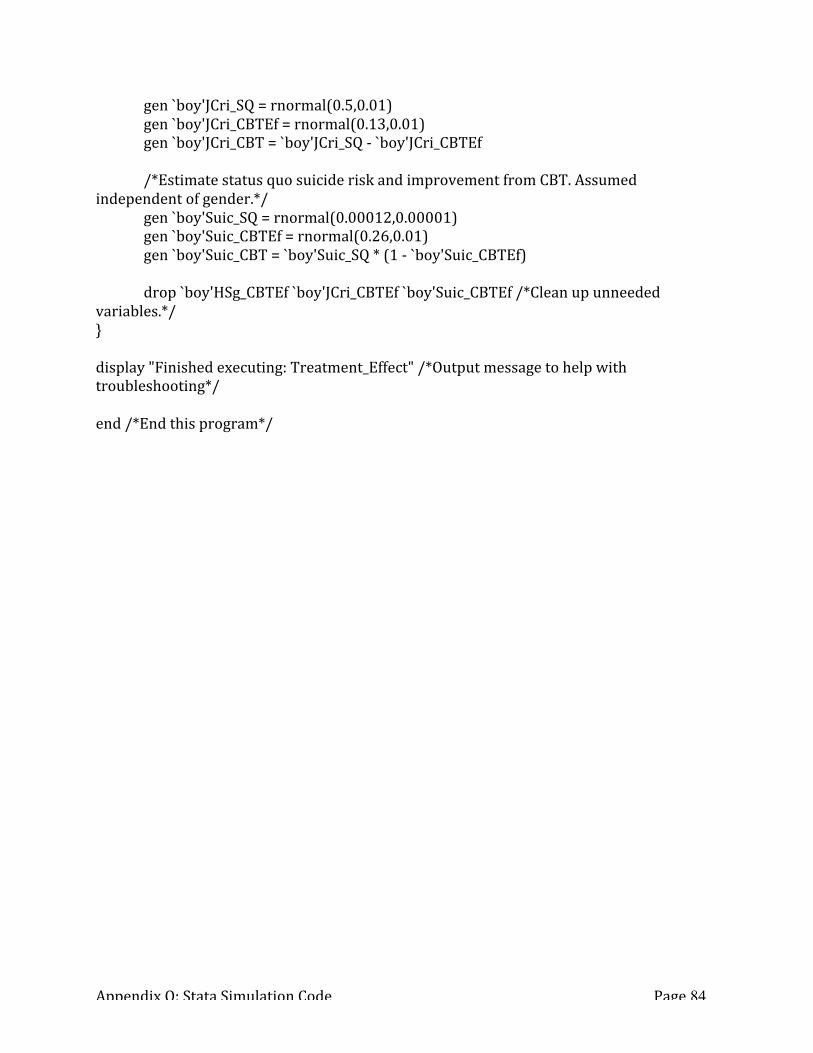
Appendix Q: Stata Simulation Code Page 84
gen `boy'JCri_SQ = rnormal(0.5,0.01) gen `boy'JCri_CBTEf = rnormal(0.13,0.01) gen `boy'JCri_CBT = `boy'JCri_SQ -‐ `boy'JCri_CBTEf /*Estimate status quo suicide risk and improvement from CBT. Assumed independent of gender.*/ gen `boy'Suic_SQ = rnormal(0.00012,0.00001) gen `boy'Suic_CBTEf = rnormal(0.26,0.01) gen `boy'Suic_CBT = `boy'Suic_SQ * (1 -‐ `boy'Suic_CBTEf) drop `boy'HSg_CBTEf `boy'JCri_CBTEf `boy'Suic_CBTEf /*Clean up unneeded variables.*/ } display "Finished executing: Treatment_Effect" /*Output message to help with troubleshooting*/ end /*End this program*/

Appendix Q: Stata Simulation Code Page 85
/*This subprogram randomly draws the money value of outcomes of interest. This subprogram executes midway through the main program, before net benefits are calculated. This version of the program uses the low discounting assumption: 2%.*/ capture program drop Outcome_ValueLow /*Housekeeping to delete existing programs named Outcome_ValueLow*/ program Outcome_ValueLow /*Defines this program as Outcome_ValueLow*/ display "Executing: Outcome_ValueLow" /*Output message to help with troubleshooting*/ quietly do Draw_Corr /*Load do-‐file for drawing present value of lifetime income by educational attainment from correlated distributions.*/ /*Lists of representative students by gender*/ local girls "F05 F06 F07 F08 F09 F10 F11 F12 F13 F14 F15 F16 F17 F18 F19" local boys "M05 M06 M07 M08 M09 M10 M11 M12 M13 M14 M15 M16 M17 M18 M19" gen VSL = 5513926.88 /*Value of a statistical life. Has minimal effect on net benefits because the suicide rate is so small.*/ gen depr = 0.02 /*Low discount rate assumption for sensitivity analysis.*/ /*Cycle through representative females.*/ foreach girl of local girls { Draw_Corr `girl' Dout 0 312618 681963 HSg4 0 461931 1039375 HSg6 0 432318 972744 SCol4 0 708682 1670514 SCol6 0 662024 1560531 Col4 102817 1060478 2018139 Col6 95852 988640 1881428 /*Discount from age 18 to current age. Present values of lifetime earnings use low discounting assumption.*/ gen D`girl'_earnDout = `girl'_earnDout / ((1 + depr) ^ (18 -‐ `girl'age)) replace D`girl'_earnDout = `girl'_earnDout if (`girl'age >= 18) /*Discount present value of lifetime earnings for females who graduate high school in 4 years.*/ gen D`girl'_earnHSg4 = `girl'_earnHSg4 / ((1 + depr) ^ (18 -‐ `girl'age)) if (`girl'age < 18) replace D`girl'_earnHSg4 = `girl'_earnHSg4 if (`girl'age >= 18) /*Discount present value of lifetime earnings for females who graduate high school in 6 years.*/ gen D`girl'_earnHSg6 = `girl'_earnHSg6 /((1 + depr) ^ (18 -‐ `girl'age)) replace D`girl'_earnHSg6 = `girl'_earnHSg6 if (`girl'age >= 18) /*Discount present value of lifetime earnings for females who finish some college after graduating high school in 4 years.*/ gen D`girl'_earnSCol4 = `girl'_earnSCol4 / ((1 + depr) ^ (18 -‐ `girl'age))

Appendix Q: Stata Simulation Code Page 86
replace D`girl'_earnSCol4 = `girl'_earnSCol4 if (`girl'age >= 18) /*Discount present value of lifetime earnings for females who finish some college after graduating high school in 6 years.*/ gen D`girl'_earnSCol6 = `girl'_earnSCol6 / ((1 + depr) ^ (18 -‐ `girl'age)) replace D`girl'_earnSCol6 = `girl'_earnSCol6 if (`girl'age >= 18) /*Discount present value of lifetime earnings for females who graduate college after graduating high school in 4 years.*/ gen D`girl'_earnCol4 = `girl'_earnCol4 / ((1 + depr) ^ (18 -‐ `girl'age)) replace D`girl'_earnCol4 = `girl'_earnCol4 if (`girl'age >= 18) /*Discount present value of lifetime earnings for females who graduate college after graduating high school in 6 years.*/ gen D`girl'_earnCol6 = `girl'_earnCol6 / ((1 + depr) ^ (18 -‐ `girl'age)) replace D`girl'_earnCol6 = `girl'_earnCol6 if (`girl'age >= 18) drop `girl'_earnDout `girl'_earnHSg4 `girl'_earnHSg6 `girl'_earnSCol4 `girl'_earnSCol6 `girl'_earnCol4 `girl'_earnCol6 /*Clean up unneeded variables*/ /*Estimate social cost per crime. Discounted to age of maximum crime production.*/ gen `girl'_Jcri = rnormal(2127,196) /*Expected cost of one juvenile crime. Independent of gender.*/ gen `girl'_Acri = rnormal(10458,1000) /*Expected lifetime reduction in social cost of adult crime due to graduating high school. Depends on gender. Standard deviation is a guess.*/ gen D`girl'_Jcri = `girl'_Jcri replace D`girl'_Jcri = `girl'_Jcri /((1 + depr) ^ (15 -‐ `girl'age)) if (`girl'age < 15) gen D`girl'_Acri = `girl'_Acri replace D`girl'_Acri = `girl'_Acri /((1 + depr) ^ (18 -‐ `girl'age)) if (`girl'age < 18) drop `girl'_Jcri `girl'_Acri /*Clean up unneeded variables*/ } /*Cycle through representative males.*/ foreach boy of local boys { Draw_Corr `boy' Dout 0 604914 1334518 HSg4 0 944941 2739118 HSg6 0 884365 2563524 SCol4 0 1135190 2406946 SCol6 0 1060452 2248478 Col4 0 1813801 4324791 Col6 0 1690933 4031826 /*Discount dropout*/ gen D`boy'_earnDout = `boy'_earnDout / ((1 + depr) ^ (18 -‐ `boy'age)) replace D`boy'_earnDout = `boy'_earnDout if (`boy'age >= 18) /*Discount high school graduate*/ gen D`boy'_earnHSg4 = `boy'_earnHSg4 / ((1 + depr) ^ (18 -‐ `boy'age)) if (`boy'age < 18)

Appendix Q: Stata Simulation Code Page 87
replace D`boy'_earnHSg4 = `boy'_earnHSg4 if (`boy'age >= 18) gen D`boy'_earnHSg6 = `boy'_earnHSg6 /((1 + depr) ^ (18 -‐ `boy'age)) replace D`boy'_earnHSg6 = `boy'_earnHSg6 if (`boy'age >= 18) /*Discount some college.*/ gen D`boy'_earnSCol4 = `boy'_earnSCol4 / ((1 + depr) ^ (18 -‐ `boy'age)) replace D`boy'_earnSCol4 = `boy'_earnSCol4 if (`boy'age >= 18) gen D`boy'_earnSCol6 = `boy'_earnSCol6 / ((1 + depr) ^ (18 -‐ `boy'age)) replace D`boy'_earnSCol6 = `boy'_earnSCol6 if (`boy'age >= 18) /*Discount college graduation.*/ gen D`boy'_earnCol4 = `boy'_earnCol4 / ((1 + depr) ^ (18 -‐ `boy'age)) replace D`boy'_earnCol4 = `boy'_earnCol4 if (`boy'age >= 18) gen D`boy'_earnCol6 = `boy'_earnCol6 / ((1 + depr) ^ (18 -‐ `boy'age)) replace D`boy'_earnCol6 = `boy'_earnCol6 if (`boy'age >= 18) drop `boy'_earnDout `boy'_earnHSg4 `boy'_earnHSg6 `boy'_earnSCol4 `boy'_earnSCol6 `boy'_earnCol4 `boy'_earnCol6 /*Estimate social cost per crime. Discounted to age of maximum crime production.*/ gen `boy'_Jcri = rnormal(2127,196) gen `boy'_Acri = rnormal(38054,1000) /*Standard deviation is a guess.*/ gen D`boy'_Jcri = `boy'_Jcri replace D`boy'_Jcri = `boy'_Jcri /((1 + depr) ^ (15 -‐ `boy'age)) if (`boy'age < 15) gen D`boy'_Acri = `boy'_Acri replace D`boy'_Acri = `boy'_Acri /((1 + depr) ^ (18 -‐ `boy'age)) if (`boy'age < 18) drop `boy'_Jcri `boy'_Acri /*Clean up unneeded variables*/ } /*Costs for the program overall. These do not vary from student to student, so they are estimated once for each Monte Carlo observation. Adjustment to include 20.4% of students with intake forms not during 2013-‐14 school year. 12.6% increase to account for United Way overhead, which does not appear in PATH financial statement provided.*/ gen Cost_Ther_Time = 248706 * 1.204 *1.126 gen Cost_License = 925 * 1.204 *1.126 /*Cost of space in schools is estimated at the rate they charge outside groups for school space.*/ gen Room_Rate = 9 /*Hourly rate from Monona Grove WI.*/ gen Space_Scarcity = rnormal(0.7,0.1) /*Room cost reduced because schools may not be at capacity; this is a guess.*/

Appendix Q: Stata Simulation Code Page 88
gen Cost_Space = Room_Rate * 1500 * 23 * Space_Scarcity /*Assumes each school dedicates a room to PATH full time.*/ gen Cost = Cost_Ther_Time + Cost_License + Cost_Space drop Room_Rate Space_Scarcity display "Finished executing Outcome_Value" /*Output message to help with troubleshooting*/ end /*End this program*/

Appendix Q: Stata Simulation Code Page 89
/*This subprogram randomly draws the money value of outcomes of interest. This subprogram executes midway through the main program, before net benefits are calculated. This version of the program uses the base discounting assumption: 3.5%.*/ capture program drop Outcome_ValueMid /*Housekeeping to delete existing programs named Outcome_ValueMid*/ program Outcome_ValueMid /*Defines this program as Outcome_ValueMid*/ display "Executing: Outcome_ValueMid" /*Output message to help with troubleshooting*/ quietly do Draw_Corr /*Load do-‐file for drawing present value of lifetime income by educational attainment from correlated distributions.*/ /*Lists of representative students by gender*/ local girls "F05 F06 F07 F08 F09 F10 F11 F12 F13 F14 F15 F16 F17 F18 F19" local boys "M05 M06 M07 M08 M09 M10 M11 M12 M13 M14 M15 M16 M17 M18 M19" gen VSL = 5513926.88 /*Value of a statistical life. Has minimal effect on net benefits because the suicide rate is so small.*/ gen depr = 0.035 /*Mid discount rate assumption for sensitivity analysis.*/ /*Cycle through representative females.*/ foreach girl of local girls { Draw_Corr `girl' Dout 0 236368 515627 HSg4 0 349262 748863 HSg6 0 320288 720669 SCol4 0 525036 1237620 SCol6 0 480697 1133105 Col4 74656 770016 1465375 Col6 68228 703714 1339200 /*Discount from age 18 to current age. Present values of lifetime earnings use base discounting assumption.*/ gen D`girl'_earnDout = `girl'_earnDout / ((1 + depr) ^ (18 -‐ `girl'age)) /*Discount from 18 to current age.*/ replace D`girl'_earnDout = `girl'_earnDout if (`girl'age >= 18) /*Restore to undiscounted value for age 18 and 19.*/ /*Discount present value of lifetime earnings for females who graduate high school in 4 years.*/ gen D`girl'_earnHSg4 = `girl'_earnHSg4 / ((1 + depr) ^ (18 -‐ `girl'age)) if (`girl'age < 18) replace D`girl'_earnHSg4 = `girl'_earnHSg4 if (`girl'age >= 18) /*Discount present value of lifetime earnings for females who graduate high school in 6 years.*/ gen D`girl'_earnHSg6 = `girl'_earnHSg6 /((1 + depr) ^ (18 -‐ `girl'age)) replace D`girl'_earnHSg6 = `girl'_earnHSg6 if (`girl'age >= 18)

Appendix Q: Stata Simulation Code Page 90
/*Discount present value of lifetime earnings for females who finish some college after graduating high school in 4 years.*/ gen D`girl'_earnSCol4 = `girl'_earnSCol4 / ((1 + depr) ^ (18 -‐ `girl'age)) replace D`girl'_earnSCol4 = `girl'_earnSCol4 if (`girl'age >= 18) /*Discount present value of lifetime earnings for females who finish some college after graduating high school in 6 years.*/ gen D`girl'_earnSCol6 = `girl'_earnSCol6 / ((1 + depr) ^ (18 -‐ `girl'age)) replace D`girl'_earnSCol6 = `girl'_earnSCol6 if (`girl'age >= 18) /*Discount present value of lifetime earnings for females who graduate college after graduating high school in 4 years.*/ gen D`girl'_earnCol4 = `girl'_earnCol4 / ((1 + depr) ^ (18 -‐ `girl'age)) replace D`girl'_earnCol4 = `girl'_earnCol4 if (`girl'age >= 18) /*Discount present value of lifetime earnings for females who graduate college after graduating high school in 6 years.*/ gen D`girl'_earnCol6 = `girl'_earnCol6 / ((1 + depr) ^ (18 -‐ `girl'age)) replace D`girl'_earnCol6 = `girl'_earnCol6 if (`girl'age >= 18) drop `girl'_earnDout `girl'_earnHSg4 `girl'_earnHSg6 `girl'_earnSCol4 `girl'_earnSCol6 `girl'_earnCol4 `girl'_earnCol6 /*Clean up unneeded variables*/ /*Estimate social cost per crime. Discounted to age of maximum crime production.*/ gen `girl'_Jcri = rnormal(2127,196) /*Expected cost of one juvenile crime. Independent of gender.*/ gen `girl'_Acri = rnormal(10458,1000) /*Expected lifetime reduction in social cost of adult crime due to graduating high school. Depends on gender. Standard deviation is a guess.*/ gen D`girl'_Jcri = `girl'_Jcri replace D`girl'_Jcri = `girl'_Jcri /((1 + depr) ^ (15 -‐ `girl'age)) if (`girl'age < 15) gen D`girl'_Acri = `girl'_Acri replace D`girl'_Acri = `girl'_Acri /((1 + depr) ^ (18 -‐ `girl'age)) if (`girl'age < 18) drop `girl'_Jcri `girl'_Acri /*Clean up unneeded variables*/ } /*Cycle through representative males.*/ foreach boy of local boys { Draw_Corr `boy' Dout 0 457370 1009017 HSg4 0 714462 2071025 HSg6 0 655192 1899217 SCol4 0 841019 1783214 SCol6 0 769996 1632625 Col4 0 1317006 3140241 Col6 0 1203605 2869853 /*Discount dropout*/ gen D`boy'_earnDout = `boy'_earnDout / ((1 + depr) ^ (18 -‐ `boy'age)) replace D`boy'_earnDout = `boy'_earnDout if (`boy'age >= 18)

Appendix Q: Stata Simulation Code Page 91
/*Discount high school graduate*/ gen D`boy'_earnHSg4 = `boy'_earnHSg4 / ((1 + depr) ^ (18 -‐ `boy'age)) if (`boy'age < 18) replace D`boy'_earnHSg4 = `boy'_earnHSg4 if (`boy'age >= 18) gen D`boy'_earnHSg6 = `boy'_earnHSg6 /((1 + depr) ^ (18 -‐ `boy'age)) replace D`boy'_earnHSg6 = `boy'_earnHSg6 if (`boy'age >= 18) /*Discount some college.*/ gen D`boy'_earnSCol4 = `boy'_earnSCol4 / ((1 + depr) ^ (18 -‐ `boy'age)) replace D`boy'_earnSCol4 = `boy'_earnSCol4 if (`boy'age >= 18) gen D`boy'_earnSCol6 = `boy'_earnSCol6 / ((1 + depr) ^ (18 -‐ `boy'age)) replace D`boy'_earnSCol6 = `boy'_earnSCol6 if (`boy'age >= 18) /*Discount college graduation.*/ gen D`boy'_earnCol4 = `boy'_earnCol4 / ((1 + depr) ^ (18 -‐ `boy'age)) replace D`boy'_earnCol4 = `boy'_earnCol4 if (`boy'age >= 18) gen D`boy'_earnCol6 = `boy'_earnCol6 / ((1 + depr) ^ (18 -‐ `boy'age)) replace D`boy'_earnCol6 = `boy'_earnCol6 if (`boy'age >= 18) drop `boy'_earnDout `boy'_earnHSg4 `boy'_earnHSg6 `boy'_earnSCol4 `boy'_earnSCol6 `boy'_earnCol4 `boy'_earnCol6 /*Estimate social cost per crime. Discounted to age of maximum crime production.*/ gen `boy'_Jcri = rnormal(2127,196) gen `boy'_Acri = rnormal(38054,1000) /*Standard deviation is a guess.*/ gen D`boy'_Jcri = `boy'_Jcri replace D`boy'_Jcri = `boy'_Jcri /((1 + depr) ^ (15 -‐ `boy'age)) if (`boy'age < 15) gen D`boy'_Acri = `boy'_Acri replace D`boy'_Acri = `boy'_Acri /((1 + depr) ^ (18 -‐ `boy'age)) if (`boy'age < 18) drop `boy'_Jcri `boy'_Acri /*Clean up unneeded variables*/ } /*Costs for the program overall. These do not vary from student to student, so they are estimated once for each Monte Carlo observation. Adjustment to include 20.4% of students with intake forms not during 2013-‐14 school year. 14.4% increase to account for United Way overhead, which does not appear in PATH financial statement provided.*/ gen Cost_Ther_Time = 248706 * 1.204 *1.126 gen Cost_License = 925 * 1.204 *1.126 /*Cost of space in schools is estimated at the rate they charge outside groups for school space.*/ gen Room_Rate = 9 /*Hourly rate from Monona Grove WI.*/

Appendix Q: Stata Simulation Code Page 92
gen Space_Scarcity = rnormal(0.7,0.1) /*Room cost reduced because schools may not be at capacity; this is a guess.*/ gen Cost_Space = Room_Rate * 1500 * 23 * Space_Scarcity /*Assumes each school dedicates a room to PATH full time.*/ gen Cost = Cost_Ther_Time + Cost_License + Cost_Space drop Room_Rate Space_Scarcity display "Finished executing Outcome_Value" /*Output message to help with troubleshooting*/ end /*End this program*/

Appendix Q: Stata Simulation Code Page 93
/*This subprogram randomly draws the money value of outcomes of interest. This subprogram executes midway through the main program, before net benefits are calculated. This version of the program uses the high discounting assumption: 5%.*/ capture program drop Outcome_ValueHigh /*Housekeeping to delete existing programs named Outcome_ValueHigh*/ program Outcome_ValueHigh /*Defines this program as Outcome_ValueHigh*/ display "Executing: Outcome_ValueHigh" /*Output message to help with troubleshooting*/ quietly do Draw_Corr /*Load do-‐file for drawing present value of lifetime income by educational attainment from correlated distributions.*/ /*Lists of representative students by gender*/ local girls "F05 F06 F07 F08 F09 F10 F11 F12 F13 F14 F15 F16 F17 F18 F19" local boys "M05 M06 M07 M08 M09 M10 M11 M12 M13 M14 M15 M16 M17 M18 M19" gen VSL = 5513926.88 /*Value of a statistical life. Has minimal effect on net benefits because the suicide rate is so small.*/ gen depr = 0.05 /*High discount rate assumption for sensitivity analysis.*/ /*Cycle through representative females.*/ foreach girl of local girls { Draw_Corr `girl' Dout 0 185600 404879 HSg4 0 274246 617072 HSg6 0 245887 553261 SCol4 0 403072 950127 SCol6 0 360906 850731 Col4 56051 578124 1100197 Col6 50111 516858 983605 /*Discount from age 18 to current age. Present values of lifetime earnings use base discounting assumption.*/ gen D`girl'_earnDout = `girl'_earnDout / ((1 + depr) ^ (18 -‐ `girl'age)) replace D`girl'_earnDout = `girl'_earnDout if (`girl'age >= 18) /*Discount present value of lifetime earnings for females who graduate high school in 4 years.*/ gen D`girl'_earnHSg4 = `girl'_earnHSg4 / ((1 + depr) ^ (18 -‐ `girl'age)) if (`girl'age < 18) replace D`girl'_earnHSg4 = `girl'_earnHSg4 if (`girl'age >= 18) /*Discount present value of lifetime earnings for females who graduate high school in 6 years.*/ gen D`girl'_earnHSg6 = `girl'_earnHSg6 /((1 + depr) ^ (18 -‐ `girl'age)) replace D`girl'_earnHSg6 = `girl'_earnHSg6 if (`girl'age >= 18) /*Discount present value of lifetime earnings for females who finish some college after graduating high school in 4 years.*/ gen D`girl'_earnSCol4 = `girl'_earnSCol4 / ((1 + depr) ^ (18 -‐ `girl'age))
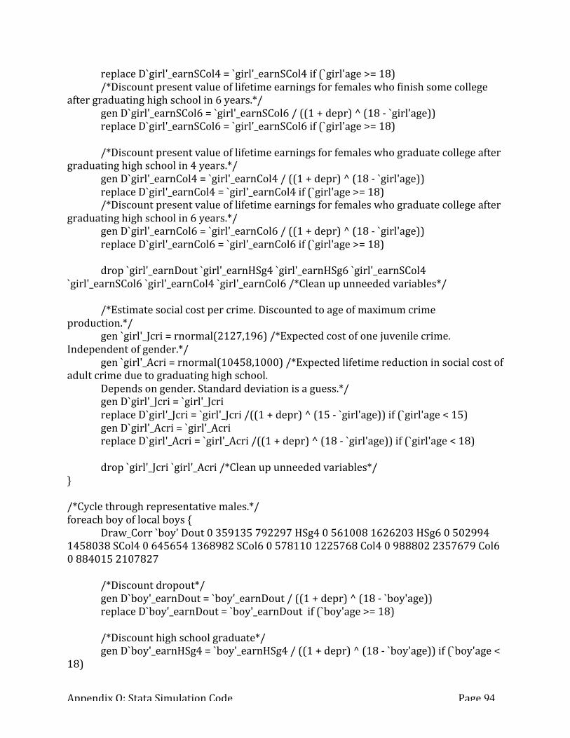
Appendix Q: Stata Simulation Code Page 94
replace D`girl'_earnSCol4 = `girl'_earnSCol4 if (`girl'age >= 18) /*Discount present value of lifetime earnings for females who finish some college after graduating high school in 6 years.*/ gen D`girl'_earnSCol6 = `girl'_earnSCol6 / ((1 + depr) ^ (18 -‐ `girl'age)) replace D`girl'_earnSCol6 = `girl'_earnSCol6 if (`girl'age >= 18) /*Discount present value of lifetime earnings for females who graduate college after graduating high school in 4 years.*/ gen D`girl'_earnCol4 = `girl'_earnCol4 / ((1 + depr) ^ (18 -‐ `girl'age)) replace D`girl'_earnCol4 = `girl'_earnCol4 if (`girl'age >= 18) /*Discount present value of lifetime earnings for females who graduate college after graduating high school in 6 years.*/ gen D`girl'_earnCol6 = `girl'_earnCol6 / ((1 + depr) ^ (18 -‐ `girl'age)) replace D`girl'_earnCol6 = `girl'_earnCol6 if (`girl'age >= 18) drop `girl'_earnDout `girl'_earnHSg4 `girl'_earnHSg6 `girl'_earnSCol4 `girl'_earnSCol6 `girl'_earnCol4 `girl'_earnCol6 /*Clean up unneeded variables*/ /*Estimate social cost per crime. Discounted to age of maximum crime production.*/ gen `girl'_Jcri = rnormal(2127,196) /*Expected cost of one juvenile crime. Independent of gender.*/ gen `girl'_Acri = rnormal(10458,1000) /*Expected lifetime reduction in social cost of adult crime due to graduating high school. Depends on gender. Standard deviation is a guess.*/ gen D`girl'_Jcri = `girl'_Jcri replace D`girl'_Jcri = `girl'_Jcri /((1 + depr) ^ (15 -‐ `girl'age)) if (`girl'age < 15) gen D`girl'_Acri = `girl'_Acri replace D`girl'_Acri = `girl'_Acri /((1 + depr) ^ (18 -‐ `girl'age)) if (`girl'age < 18) drop `girl'_Jcri `girl'_Acri /*Clean up unneeded variables*/ } /*Cycle through representative males.*/ foreach boy of local boys { Draw_Corr `boy' Dout 0 359135 792297 HSg4 0 561008 1626203 HSg6 0 502994 1458038 SCol4 0 645654 1368982 SCol6 0 578110 1225768 Col4 0 988802 2357679 Col6 0 884015 2107827 /*Discount dropout*/ gen D`boy'_earnDout = `boy'_earnDout / ((1 + depr) ^ (18 -‐ `boy'age)) replace D`boy'_earnDout = `boy'_earnDout if (`boy'age >= 18) /*Discount high school graduate*/ gen D`boy'_earnHSg4 = `boy'_earnHSg4 / ((1 + depr) ^ (18 -‐ `boy'age)) if (`boy'age < 18)

Appendix Q: Stata Simulation Code Page 95
replace D`boy'_earnHSg4 = `boy'_earnHSg4 if (`boy'age >= 18) gen D`boy'_earnHSg6 = `boy'_earnHSg6 /((1 + depr) ^ (18 -‐ `boy'age)) replace D`boy'_earnHSg6 = `boy'_earnHSg6 if (`boy'age >= 18) /*Discount some college.*/ gen D`boy'_earnSCol4 = `boy'_earnSCol4 / ((1 + depr) ^ (18 -‐ `boy'age)) replace D`boy'_earnSCol4 = `boy'_earnSCol4 if (`boy'age >= 18) gen D`boy'_earnSCol6 = `boy'_earnSCol6 / ((1 + depr) ^ (18 -‐ `boy'age)) replace D`boy'_earnSCol6 = `boy'_earnSCol6 if (`boy'age >= 18) /*Discount college graduation.*/ gen D`boy'_earnCol4 = `boy'_earnCol4 / ((1 + depr) ^ (18 -‐ `boy'age)) replace D`boy'_earnCol4 = `boy'_earnCol4 if (`boy'age >= 18) gen D`boy'_earnCol6 = `boy'_earnCol6 / ((1 + depr) ^ (18 -‐ `boy'age)) replace D`boy'_earnCol6 = `boy'_earnCol6 if (`boy'age >= 18) drop `boy'_earnDout `boy'_earnHSg4 `boy'_earnHSg6 `boy'_earnSCol4 `boy'_earnSCol6 `boy'_earnCol4 `boy'_earnCol6 /*Clean up unneeded variables*/ /*Estimate social cost per crime. Discounted to age of maximum crime production.*/ gen `boy'_Jcri = rnormal(2127,196) gen `boy'_Acri = rnormal(38054,1000) /*Standard deviation is a guess.*/ gen D`boy'_Jcri = `boy'_Jcri replace D`boy'_Jcri = `boy'_Jcri /((1 + depr) ^ (15 -‐ `boy'age)) if (`boy'age < 15) gen D`boy'_Acri = `boy'_Acri replace D`boy'_Acri = `boy'_Acri /((1 + depr) ^ (18 -‐ `boy'age)) if (`boy'age < 18) drop `boy'_Jcri `boy'_Acri /*Clean up unneeded variables*/ } /*Costs for the program overall. These do not vary from student to student, so they are estimated once for each Monte Carlo observation. Adjustment to include 20.4% of students with intake forms not during 2013-‐14 school year. 14.4% increase to account for United Way overhead, which does not appear in PATH financial statement provided.*/ gen Cost_Ther_Time = 248706 * 1.204 *1.126 gen Cost_License = 925 * 1.204 *1.126 /*Cost of space in schools is estimated at the rate they charge outside groups for school space.*/ gen Room_Rate = 9 /*Hourly rate from Monona Grove WI.*/ gen Space_Scarcity = rnormal(0.7,0.1) /*Room cost reduced because schools may not be at capacity; this is a guess.*/
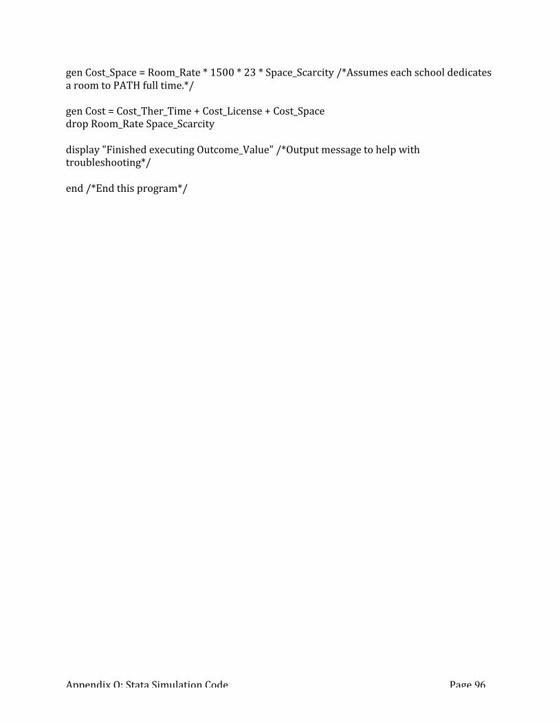
Appendix Q: Stata Simulation Code Page 96
gen Cost_Space = Room_Rate * 1500 * 23 * Space_Scarcity /*Assumes each school dedicates a room to PATH full time.*/ gen Cost = Cost_Ther_Time + Cost_License + Cost_Space drop Room_Rate Space_Scarcity display "Finished executing Outcome_Value" /*Output message to help with troubleshooting*/ end /*End this program*/

Appendix Q: Stata Simulation Code Page 97
/*Subprogram to generate random draws from correlated distributions. Used to estimate present value of lifetime income. This subprogram is called by subprogram Outcome_Value. Adapted from file binormalm.do provided by Professor D Weimer; thanks.*/ capture program drop Draw_Corr /*Housekeeping to delete existing programs named Draw_Corr*/ program Draw_Corr /*Defines this program as Draw_Corr*/ display "Executing: Draw_Corr" /*Output message to help with troubleshooting*/ /*Give names to inputs. Identify values to define income distribution for dropouts.*/ local Dout_Min `3' local Dout_Med `4' local Dout_Max `5' /*Identify values to define income distribution for 4 year high school graduates.*/ local HSg4_Min `7' local HSg4_Med `8' local HSg4_Max `9' /*Identify values to define income distribution for 6 year high school graduates.*/ local HSg6_Min `11' local HSg6_Med `12' local HSg6_Max `13' /*Identify values to define income distribution for 4 year high school graduates.*/ local SCol4_Min `15' local SCol4_Med `16' local SCol4_Max `17' /*Identify values to define income distribution for 4 year high school graduates.*/ local SCol6_Min `19' local SCol6_Med `20' local SCol6_Max `21' /*Identify values to define income distribution for 4 year high school graduates.*/ local Col4_Min `23' local Col4_Med `24' local Col4_Max `25' /*Identify values to define income distribution for 4 year high school graduates.*/ local Col6_Min `27' local Col6_Med `28' local Col6_Max `29' /*Draw correlated random index values from 4 normal distributions.*/ matrix C=(1,.85\.85,1) drawnorm `1'_DoutIndx `1'_HSgIndx, corr(C) means(0 0) sds(0.5 0.5) matrix D=(1,.80\.80,1) drawnorm `1'_SColIndx `1'_ColIndx, corr(C) means(0 0) sds(1.8 1.8)

Appendix Q: Stata Simulation Code Page 98
replace `1'_SColIndx = 0.15 * `1'_SColIndx + 0.85 * `1'_HSgIndx replace `1'_ColIndx = 0.15 * `1'_ColIndx + 0.85 * `1'_DoutIndx replace `1'_SColIndx = 0.55 * `1'_SColIndx + 0.45 * `1'_DoutIndx replace `1'_ColIndx = 0.55 * `1'_ColIndx + 0.45 * `1'_HSgIndx replace `1'_SColIndx = 0.908 * `1'_SColIndx + 0.092 * rnormal(0,1.8) replace `1'_ColIndx = 0.908 * `1'_ColIndx + 0.092 * rnormal(0,1.8) replace `1'_SColIndx = 1.10 * `1'_SColIndx replace `1'_ColIndx = 1.10 * `1'_ColIndx /*Summarize correlated index values randomly drawn to determine lifetime income by educational attainment.*/ sum `1'_DoutIndx `1'_HSgIndx `1'_SColIndx `1'_ColIndx corr `1'_DoutIndx `1'_HSgIndx `1'_SColIndx `1'_ColIndx /*Draw present value of lifetime income based on index values. For dropout.*/ gen `1'_earnDout = `Dout_Med' replace `1'_earnDout = `Dout_Med' + (`Dout_Min' -‐ `Dout_Med') * `1'_DoutIndx if (`1'_DoutIndx < 0) /*Below median*/ replace `1'_earnDout = `Dout_Med' + (`Dout_Max' -‐ `Dout_Med') * `1'_DoutIndx if (`1'_DoutIndx > 0) /*Above median*/ replace `1'_earnDout = 0 if (`1'_earnDout < 0) /*Censor negative values.*/ replace `1'_earnDout = `1'_earnDout * 0.81 /*Reduce earnings to account for lower productivity caused by mental disorder.*/ /*For 4 year high school graduate.*/ gen `1'_earnHSg4 = `HSg4_Med' replace `1'_earnHSg4 = `HSg4_Med' + (`HSg4_Min' -‐ `HSg4_Med') * `1'_HSgIndx if (`1'_HSgIndx < 0) /*Below median*/ replace `1'_earnHSg4 = `HSg4_Med' + (`HSg4_Max' -‐ `HSg4_Med') * `1'_HSgIndx if (`1'_HSgIndx > 0) /*Above median*/ replace `1'_earnHSg4 = 0 if (`1'_earnHSg4 < 0) /*Censor negative values.*/ replace `1'_earnHSg4 = `1'_earnHSg4 * 0.81 /*Reduce earnings to account for lower productivity caused by mental disorder.*/ /*For 6 year high school graduate.*/ gen `1'_earnHSg6 = `HSg6_Med' replace `1'_earnHSg6 = `HSg6_Med' + (`HSg6_Min' -‐ `HSg6_Med') * `1'_HSgIndx if (`1'_HSgIndx < 0) /*Below median*/ replace `1'_earnHSg6 = `HSg6_Med' + (`HSg6_Max' -‐ `HSg6_Med') * `1'_HSgIndx if (`1'_HSgIndx > 0) /*Above median*/ replace `1'_earnHSg6 = 0 if (`1'_earnHSg6 < 0) /*Censor negative values.*/ replace `1'_earnHSg6 = `1'_earnHSg6 * 0.81 /*Reduce earnings to account for lower productivity caused by mental disorder.*/ /*For some college completer after 4 year high school graduation.*/ gen `1'_earnSCol4 = `SCol4_Med'

Appendix Q: Stata Simulation Code Page 99
replace `1'_earnSCol4 = `SCol4_Med' + (`SCol4_Min' -‐ `SCol4_Med') * `1'_SColIndx if (`1'_SColIndx < 0) /*Below median*/ replace `1'_earnSCol4 = `SCol4_Med' + (`SCol4_Max' -‐ `SCol4_Med') * `1'_SColIndx if (`1'_SColIndx > 0) /*Above median*/ replace `1'_earnSCol4 = 0 if (`1'_earnSCol4 < 0) /*Censor negative values.*/ replace `1'_earnSCol4 = `1'_earnSCol4 * 0.81 /*Reduce earnings to account for lower productivity caused by mental disorder.*/ /*For some college completer after 6 year high school graduation.*/ gen `1'_earnSCol6 = `SCol6_Med' replace `1'_earnSCol6 = `SCol6_Med' + (`SCol6_Min' -‐ `SCol6_Med') * `1'_SColIndx if (`1'_SColIndx < 0) /*Below median*/ replace `1'_earnSCol6 = `SCol6_Med' + (`SCol6_Max' -‐ `SCol6_Med') * `1'_SColIndx if (`1'_SColIndx > 0) /*Above median*/ replace `1'_earnSCol6 = 0 if (`1'_earnSCol6 < 0) /*Censor negative values.*/ replace `1'_earnSCol6 = `1'_earnSCol6 * 0.81 /*Reduce earnings to account for lower productivity caused by mental disorder.*/ /*For college graduate after 4 year high school graduation.*/ gen `1'_earnCol4 = `Col4_Med' replace `1'_earnCol4 = `Col4_Med' + (`Col4_Min' -‐ `Col4_Med') * `1'_ColIndx if (`1'_ColIndx < 0) /*Below median*/ replace `1'_earnCol4 = `Col4_Med' + (`Col4_Max' -‐ `Col4_Med') * `1'_ColIndx if (`1'_ColIndx > 0) /*Above median*/ replace `1'_earnCol4 = 0 if (`1'_earnCol4 < 0) /*Censor negative values.*/ replace `1'_earnCol4 = `1'_earnCol4 * 0.81 /*Reduce earnings to account for lower productivity caused by mental disorder.*/ /*For college graduate after 6 year high school graduation.*/ gen `1'_earnCol6 = `Col6_Med' replace `1'_earnCol6 = `Col6_Med' + (`Col6_Min' -‐ `Col6_Med') * `1'_ColIndx if (`1'_ColIndx < 0) /*Below median*/ replace `1'_earnCol6 = `Col6_Med' + (`Col6_Max' -‐ `Col6_Med') * `1'_ColIndx if (`1'_ColIndx > 0) /*Above median*/ replace `1'_earnCol6 = 0 if (`1'_earnCol6 < 0) /*Censor negative values.*/ replace `1'_earnCol6 = `1'_earnCol6 * 0.81 /*Reduce earnings to account for lower productivity caused by mental disorder.*/ drop `1'_DoutIndx `1'_HSgIndx `1'_SColIndx `1'_ColIndx /*Clean up unneeded variables.*/ sum `1'_earnDout `1'_earnHSg4 `1'_earnHSg6 `1'_earnSCol4 `1'_earnSCol6 `1'_earnCol4 `1'_earnCol6 corr `1'_earnDout `1'_earnHSg4 `1'_earnHSg6 `1'_earnSCol4 `1'_earnSCol6 `1'_earnCol4 `1'_earnCol6 end

Appendix Q: Stata Simulation Code Page 100
/*This subprogram randomly assigns outcomes of interest to PATH participants based on probabilities defined in subprogram Treatment_Effect. It also sums up the value of outcomes. This is the last subprogram to run.*/ capture program drop Simulate_Outcomes /*Housekeeping to delete existing programs named Simulate_Outcomes*/ program Simulate_Outcomes /*Defines this program as Simulate_Outcomes*/ display "Executing: Simulate_Outcomes" /*Output message to help with troubleshooting*/ /*Lists of representative students by gender*/ local girls "F05 F06 F07 F08 F09 F10 F11 F12 F13 F14 F15 F16 F17 F18 F19" local boys "M05 M06 M07 M08 M09 M10 M11 M12 M13 M14 M15 M16 M17 M18 M19" /*List of representative schools*/ local schools "S1 S2 S3 S4 S5 S6 S7 S8 S9 S10 S11 S12 S12 S13 S14 S15 S16 S17 S18 S19 S20 S21 S22 S23" /*Start variables to count high school graduations, so we can calculate induced graduations.*/ gen HS_Grads_SQ = 0 gen HS_Grads_CBT = 0 /*Start variables that will accumulate benefits for females. The loops below will increment these variables with the outcomes accruing to each representative female.*/ gen F_Earn_SQ = 0 gen F_Earn_CBT = 0 gen F_JCri_SQ = 0 gen F_JCri_CBT = 0 gen F_ACri_SQ = 0 gen F_ACri_CBT = 0 gen F_Suic_SQ = 0 gen F_Suic_CBT = 0 /*Start variables that will accumulate benefits for males.*/ gen M_Earn_SQ = 0 gen M_Earn_CBT = 0 gen M_JCri_SQ = 0 gen M_JCri_CBT = 0 gen M_ACri_SQ = 0 gen M_ACri_CBT = 0 gen M_Suic_SQ = 0 gen M_Suic_CBT = 0 /*Start variables that will accumulate benefits for elementary school students.*/

Appendix Q: Stata Simulation Code Page 101
gen EL_Earn_SQ = 0 gen EL_Earn_CBT = 0 gen EL_JCri_SQ = 0 gen EL_JCri_CBT = 0 gen EL_ACri_SQ = 0 gen EL_ACri_CBT = 0 gen EL_Suic_SQ = 0 gen EL_Suic_CBT = 0 /*Start variables that will accumulate benefits for middle school students.*/ gen MS_Earn_SQ = 0 gen MS_Earn_CBT = 0 gen MS_JCri_SQ = 0 gen MS_JCri_CBT = 0 gen MS_ACri_SQ = 0 gen MS_ACri_CBT = 0 gen MS_Suic_SQ = 0 gen MS_Suic_CBT = 0 /*Start variables that will accumulate benefits for high school students.*/ gen HS_Earn_SQ = 0 gen HS_Earn_CBT = 0 gen HS_JCri_SQ = 0 gen HS_JCri_CBT = 0 gen HS_ACri_SQ = 0 gen HS_ACri_CBT = 0 gen HS_Suic_SQ = 0 gen HS_Suic_CBT = 0 /*Start variables that will track benefits that are not assigned to particular representative students.*/ gen Truant_Ben = 0 gen Dscpln_Ben = 0 gen Counsl_Ben = 0 /*Randomly simulate if CBT changes time spent by school staff addressing mental disorders changes. Draw independently for each school.*/ foreach school of local schools { /*Truancy*/ gen Sv_Truant`school' = runiform() gen Truant_Hrs`school' = rnormal(4.9,4.6) replace Truant_Ben = Truant_Ben + (Truant_Hrs`school' * School_Wage * 9) if (Sv_Truant`school' <= PSv_Truant) /*Discipline*/ gen Sv_Dscpln`school' = runiform()

Appendix Q: Stata Simulation Code Page 102
gen Dscpln_Hrs`school' = rnormal(2.4,1.6) replace Dscpln_Ben = Dscpln_Ben + (Dscpln_Hrs`school' * School_Wage * 9) if (Sv_Dscpln`school' <= PSv_Dscpln) /*Guidance counsel time*/ gen Sv_Counsl`school' = runiform() gen Counsl_Hrs`school' = rnormal(10.2,15.1) replace Counsl_Ben = Counsl_Ben + (Counsl_Hrs`school' * School_Wage * 9) if (Sv_Counsl`school' <= PSv_Counsl) drop Sv_Truant`school' Truant_Hrs`school' Sv_Dscpln`school' Dscpln_Hrs`school' Sv_Counsl`school' Counsl_Hrs`school' } /*Cycle through representative females.*/ foreach girl of local girls { display "`girl'" /*Output to keep track of progress through loop.*/ /*Randomly assign education outcomes to female PATH participants. The random variable for high school acheivement is equal to the random variable for college achievement to reflect that we expect chance of finishing high school to be correlated with chance of finishing college.*/ gen `girl'_HS = runiform() gen `girl'_Col = `girl'_HS /*Simulate status quo educational attainment for females.*/ gen `girl'HSg_SQO = (`girl'_HS <= `girl'HSg_SQ) /*Does she graduate high school in 6 years or less?*/ gen `girl'Dout_SQO = !`girl'HSg_SQO /*If she doesn't graduate in 6 years or less, she is assigned the dropout outcomes.*/ gen `girl'4or6_HS = runiform() gen `girl'HSg4_SQO = (`girl'HSg_SQO & (`girl'4or6_HS <= HS_4yr)) /*Simulate whether graduation takes place within 4 years.*/ gen `girl'HSg6_SQO = (`girl'HSg_SQO & (`girl'4or6_HS > HS_4yr)) /*Simulate whether graduation takes place within 6 years.*/ gen `girl'Col4_SQO = ((`girl'_Col <= `girl'Col_SQ) & `girl'HSg4_SQO) /*Does she graduate college (after on-‐time high school graduation)?*/ gen `girl'Col6_SQO = ((`girl'_Col <= `girl'Col_SQ) & `girl'HSg6_SQO) /*Does she graduate college (after late high school graduation)?*/ gen `girl'SCol4_SQO = ((`girl'_Col <= `girl'SCol_SQ) & `girl'HSg4_SQO & !`girl'Col4_SQO) /*If she doesn't graduate college, does she complete some college (after on-‐time high school graduation)?*/ gen `girl'SCol6_SQO = ((`girl'_Col <= `girl'SCol_SQ) & `girl'HSg6_SQO & !`girl'Col6_SQO) /*If she doesn't graduate college, does she complete some college (after late high school graduation)?*/
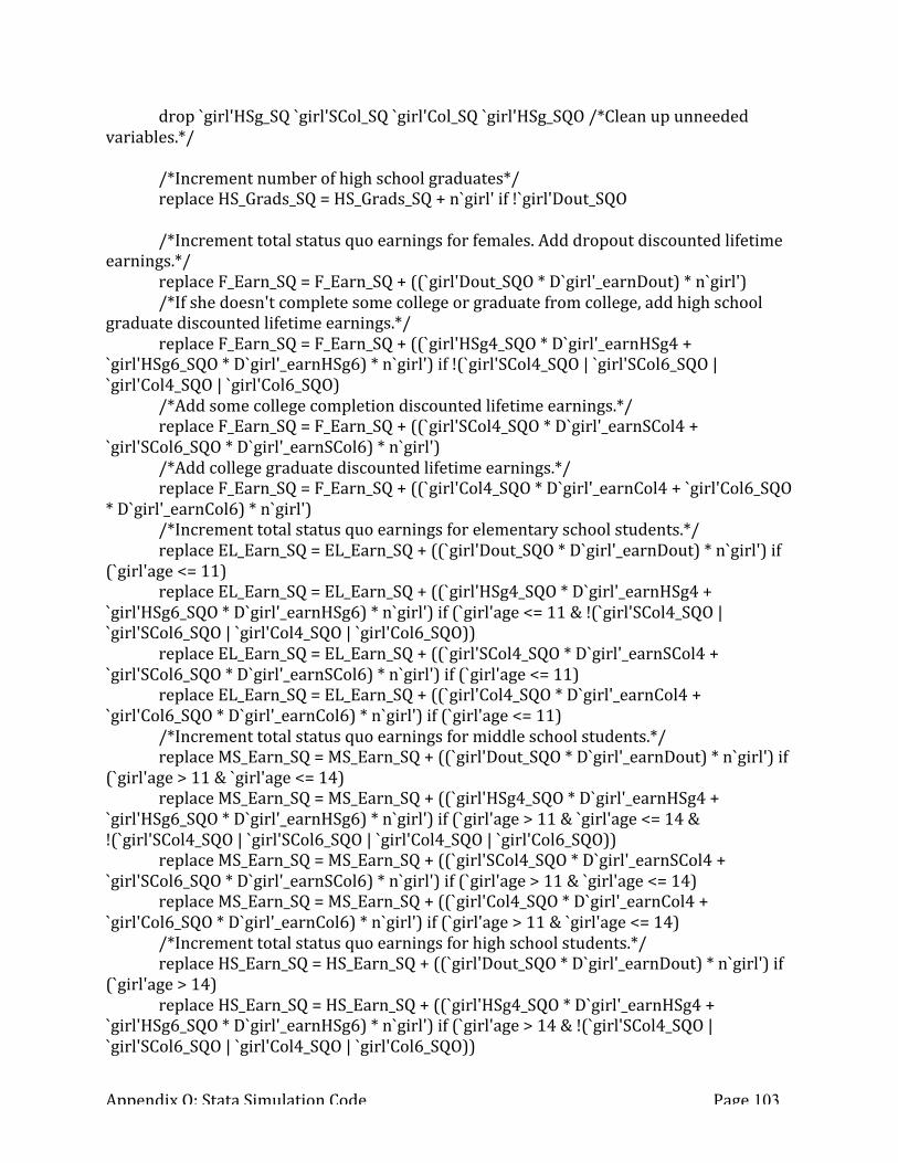
Appendix Q: Stata Simulation Code Page 103
drop `girl'HSg_SQ `girl'SCol_SQ `girl'Col_SQ `girl'HSg_SQO /*Clean up unneeded variables.*/ /*Increment number of high school graduates*/ replace HS_Grads_SQ = HS_Grads_SQ + n`girl' if !`girl'Dout_SQO /*Increment total status quo earnings for females. Add dropout discounted lifetime earnings.*/ replace F_Earn_SQ = F_Earn_SQ + ((`girl'Dout_SQO * D`girl'_earnDout) * n`girl') /*If she doesn't complete some college or graduate from college, add high school graduate discounted lifetime earnings.*/ replace F_Earn_SQ = F_Earn_SQ + ((`girl'HSg4_SQO * D`girl'_earnHSg4 + `girl'HSg6_SQO * D`girl'_earnHSg6) * n`girl') if !(`girl'SCol4_SQO | `girl'SCol6_SQO | `girl'Col4_SQO | `girl'Col6_SQO) /*Add some college completion discounted lifetime earnings.*/ replace F_Earn_SQ = F_Earn_SQ + ((`girl'SCol4_SQO * D`girl'_earnSCol4 + `girl'SCol6_SQO * D`girl'_earnSCol6) * n`girl') /*Add college graduate discounted lifetime earnings.*/ replace F_Earn_SQ = F_Earn_SQ + ((`girl'Col4_SQO * D`girl'_earnCol4 + `girl'Col6_SQO * D`girl'_earnCol6) * n`girl') /*Increment total status quo earnings for elementary school students.*/ replace EL_Earn_SQ = EL_Earn_SQ + ((`girl'Dout_SQO * D`girl'_earnDout) * n`girl') if (`girl'age <= 11) replace EL_Earn_SQ = EL_Earn_SQ + ((`girl'HSg4_SQO * D`girl'_earnHSg4 + `girl'HSg6_SQO * D`girl'_earnHSg6) * n`girl') if (`girl'age <= 11 & !(`girl'SCol4_SQO | `girl'SCol6_SQO | `girl'Col4_SQO | `girl'Col6_SQO)) replace EL_Earn_SQ = EL_Earn_SQ + ((`girl'SCol4_SQO * D`girl'_earnSCol4 + `girl'SCol6_SQO * D`girl'_earnSCol6) * n`girl') if (`girl'age <= 11) replace EL_Earn_SQ = EL_Earn_SQ + ((`girl'Col4_SQO * D`girl'_earnCol4 + `girl'Col6_SQO * D`girl'_earnCol6) * n`girl') if (`girl'age <= 11) /*Increment total status quo earnings for middle school students.*/ replace MS_Earn_SQ = MS_Earn_SQ + ((`girl'Dout_SQO * D`girl'_earnDout) * n`girl') if (`girl'age > 11 & `girl'age <= 14) replace MS_Earn_SQ = MS_Earn_SQ + ((`girl'HSg4_SQO * D`girl'_earnHSg4 + `girl'HSg6_SQO * D`girl'_earnHSg6) * n`girl') if (`girl'age > 11 & `girl'age <= 14 & !(`girl'SCol4_SQO | `girl'SCol6_SQO | `girl'Col4_SQO | `girl'Col6_SQO)) replace MS_Earn_SQ = MS_Earn_SQ + ((`girl'SCol4_SQO * D`girl'_earnSCol4 + `girl'SCol6_SQO * D`girl'_earnSCol6) * n`girl') if (`girl'age > 11 & `girl'age <= 14) replace MS_Earn_SQ = MS_Earn_SQ + ((`girl'Col4_SQO * D`girl'_earnCol4 + `girl'Col6_SQO * D`girl'_earnCol6) * n`girl') if (`girl'age > 11 & `girl'age <= 14) /*Increment total status quo earnings for high school students.*/ replace HS_Earn_SQ = HS_Earn_SQ + ((`girl'Dout_SQO * D`girl'_earnDout) * n`girl') if (`girl'age > 14) replace HS_Earn_SQ = HS_Earn_SQ + ((`girl'HSg4_SQO * D`girl'_earnHSg4 + `girl'HSg6_SQO * D`girl'_earnHSg6) * n`girl') if (`girl'age > 14 & !(`girl'SCol4_SQO | `girl'SCol6_SQO | `girl'Col4_SQO | `girl'Col6_SQO))

Appendix Q: Stata Simulation Code Page 104
replace HS_Earn_SQ = HS_Earn_SQ + ((`girl'SCol4_SQO * D`girl'_earnSCol4 + `girl'SCol6_SQO * D`girl'_earnSCol6) * n`girl') if (`girl'age > 14) replace HS_Earn_SQ = HS_Earn_SQ + ((`girl'Col4_SQO * D`girl'_earnCol4 + `girl'Col6_SQO * D`girl'_earnCol6) * n`girl') if (`girl'age > 14) /*Simulate CBT educational attainment for females. See comments on status quo simulation above.*/ gen `girl'HSg_CBTO = (`girl'_HS <= `girl'HSg_CBT) gen `girl'Dout_CBTO = !`girl'HSg_CBTO gen `girl'HSg4_CBTO = (`girl'HSg_CBTO & (`girl'4or6_HS <= HS_4yr)) gen `girl'HSg6_CBTO = (`girl'HSg_CBTO & (`girl'4or6_HS > HS_4yr)) gen `girl'Col4_CBTO = ((`girl'_Col <= `girl'Col_CBT) & `girl'HSg4_CBTO) gen `girl'Col6_CBTO = ((`girl'_Col <= `girl'Col_CBT) & `girl'HSg6_CBTO) gen `girl'SCol4_CBTO = ((`girl'_Col <= `girl'SCol_CBT) & `girl'HSg4_CBTO & !`girl'Col4_CBTO) gen `girl'SCol6_CBTO = ((`girl'_Col <= `girl'SCol_CBT) & `girl'HSg6_CBTO & !`girl'Col6_CBTO) drop `girl'HSg_CBT `girl'SCol_CBT `girl'Col_CBT `girl'HSg_CBTO /*Clean up unneeded variables.*/ /*Increment number of high school graduates*/ replace HS_Grads_CBT = HS_Grads_CBT + n`girl' if !`girl'Dout_CBTO /*Increment total CBT earnings for females.*/ replace F_Earn_CBT = F_Earn_CBT + ((`girl'Dout_CBTO * D`girl'_earnDout) * n`girl') replace F_Earn_CBT = F_Earn_CBT + ((`girl'HSg4_CBTO * D`girl'_earnHSg4 + `girl'HSg6_CBTO * D`girl'_earnHSg6) * n`girl') if !(`girl'SCol4_CBTO | `girl'SCol6_CBTO | `girl'Col4_CBTO | `girl'Col6_CBTO) replace F_Earn_CBT = F_Earn_CBT + ((`girl'SCol4_CBTO * D`girl'_earnSCol4 + `girl'SCol6_CBTO * D`girl'_earnSCol6) * n`girl') replace F_Earn_CBT = F_Earn_CBT + ((`girl'Col4_CBTO * D`girl'_earnCol4 + `girl'Col6_CBTO * D`girl'_earnCol6) * n`girl') /*Increment total status quo earnings for elementary school students.*/ replace EL_Earn_CBT = EL_Earn_CBT + ((`girl'Dout_CBTO * D`girl'_earnDout) * n`girl') if (`girl'age <= 11) replace EL_Earn_CBT = EL_Earn_CBT + ((`girl'HSg4_CBTO * D`girl'_earnHSg4 + `girl'HSg6_CBTO * D`girl'_earnHSg6) * n`girl') if (`girl'age <= 11 & !(`girl'SCol4_CBTO | `girl'SCol6_CBTO | `girl'Col4_CBTO | `girl'Col6_CBTO)) replace EL_Earn_CBT = EL_Earn_CBT + ((`girl'SCol4_CBTO * D`girl'_earnSCol4 + `girl'SCol6_CBTO * D`girl'_earnSCol6) * n`girl') if (`girl'age <= 11) replace EL_Earn_CBT = EL_Earn_CBT + ((`girl'Col4_CBTO * D`girl'_earnCol4 + `girl'Col6_CBTO * D`girl'_earnCol6) * n`girl') if (`girl'age <= 11) /*Increment total status quo earnings for middle school students.*/ replace MS_Earn_CBT = MS_Earn_CBT + ((`girl'Dout_CBTO * D`girl'_earnDout) * n`girl') if (`girl'age > 11 & `girl'age <= 14)

Appendix Q: Stata Simulation Code Page 105
replace MS_Earn_CBT = MS_Earn_CBT + ((`girl'HSg4_CBTO * D`girl'_earnHSg4 + `girl'HSg6_CBTO * D`girl'_earnHSg6) * n`girl') if (`girl'age > 11 & `girl'age <= 14 & !(`girl'SCol4_CBTO | `girl'SCol6_CBTO | `girl'Col4_CBTO | `girl'Col6_CBTO)) replace MS_Earn_CBT = MS_Earn_CBT + ((`girl'SCol4_CBTO * D`girl'_earnSCol4 + `girl'SCol6_CBTO * D`girl'_earnSCol6) * n`girl') if (`girl'age > 11 & `girl'age <= 14) replace MS_Earn_CBT = MS_Earn_CBT + ((`girl'Col4_CBTO * D`girl'_earnCol4 + `girl'Col6_CBTO * D`girl'_earnCol6) * n`girl') if (`girl'age > 11 & `girl'age <= 14) /*Increment total status quo earnings for high school students.*/ replace HS_Earn_CBT = HS_Earn_CBT + ((`girl'Dout_CBTO * D`girl'_earnDout) * n`girl') if (`girl'age > 14) replace HS_Earn_CBT = HS_Earn_CBT + ((`girl'HSg4_CBTO * D`girl'_earnHSg4 + `girl'HSg6_CBTO * D`girl'_earnHSg6) * n`girl') if (`girl'age > 14 & !(`girl'SCol4_CBTO | `girl'SCol6_CBTO | `girl'Col4_CBTO | `girl'Col6_CBTO)) replace HS_Earn_CBT = HS_Earn_CBT + ((`girl'SCol4_CBTO * D`girl'_earnSCol4 + `girl'SCol6_CBTO * D`girl'_earnSCol6) * n`girl') if (`girl'age > 14) replace HS_Earn_CBT = HS_Earn_CBT + ((`girl'Col4_CBTO * D`girl'_earnCol4 + `girl'Col6_CBTO * D`girl'_earnCol6) * n`girl') if (`girl'age > 14) drop D`girl'_earnDout D`girl'_earnHSg4 D`girl'_earnSCol4 D`girl'_earnCol4 D`girl'_earnHSg6 D`girl'_earnSCol6 D`girl'_earnCol6 /*Clean up unneeded variables.*/ drop `girl'_HS `girl'_Col `girl'4or6_HS /*Clean up unneeded variables.*/ /*Simulate juvenile crime outcome for each female student.*/ gen JCri`girl' = runiform() /*Generate random number to determine if she commits a juvenile crime.*/ gen Prior`girl' = runiform() /*Assumes only students with prior contact with the law commit juvenile crimes. Generate random number to determine if she has a prior contact with the law.*/ gen HasPrior`girl' = (Prior`girl' < F_Prior_Rate) /*Simulate whether she has a prior contact with the law.*/ gen `girl'JCri_SQO = 0 /*Initiate variable for status quo juvenile crime outcome.*/ gen `girl'JCri_CBTO = 0 /*Initiate variable for CBT juvenile crime outcome.*/ replace `girl'JCri_SQO = 1 if ((JCri`girl' <= `girl'JCri_SQ) & HasPrior`girl') /*Simulate comission of a juvenile crime under status quo. Assumes each representative student commits a maximum of one juvenile crime.*/ replace `girl'JCri_CBTO = 1 if ((JCri`girl' <= `girl'JCri_CBT) & HasPrior`girl') /*Simulate comission of a juvenile crime under CBT. Assumes each representative student commits a maximum of one juvenile crime.*/ /*Increment total status quo juvenile crime cost. The benefit to juvenile crime is an avoided cost. These variables accumulate the negative of the cost of juvenile crime. CBT has fewer juvenile crimes, so it has a smaller negative. When the status quo outcome (large negative) is subtracted from the CBT outcome (small negative), the difference is positive. This positive difference is the avoided cost of juvenile crime due to CBT. */

Appendix Q: Stata Simulation Code Page 106
replace F_JCri_SQ = F_JCri_SQ -‐ (D`girl'_Jcri * `girl'JCri_SQO * n`girl') replace EL_JCri_SQ = (EL_JCri_SQ -‐ (D`girl'_Jcri * `girl'JCri_SQO * n`girl')) if (`girl'age <= 11) replace MS_JCri_SQ = (MS_JCri_SQ -‐ (D`girl'_Jcri * `girl'JCri_SQO * n`girl')) if (`girl'age > 11 & `girl'age <= 14) replace HS_JCri_SQ = (HS_JCri_SQ -‐ (D`girl'_Jcri * `girl'JCri_SQO * n`girl')) if (`girl'age > 14) /*Increment total juvenile crime cost after CBT.*/ replace F_JCri_CBT = F_JCri_CBT -‐ (D`girl'_Jcri * `girl'JCri_CBTO * n`girl') replace EL_JCri_CBT = (EL_JCri_CBT -‐ (D`girl'_Jcri * `girl'JCri_CBTO * n`girl')) if (`girl'age <= 11) replace MS_JCri_CBT = (MS_JCri_CBT -‐ (D`girl'_Jcri * `girl'JCri_CBTO * n`girl')) if (`girl'age > 11 & `girl'age <= 14) replace HS_JCri_CBT = (HS_JCri_CBT -‐ (D`girl'_Jcri * `girl'JCri_CBTO * n`girl')) if (`girl'age > 14) drop `girl'JCri_SQ `girl'JCri_CBT D`girl'_Jcri JCri`girl' Prior`girl' HasPrior`girl' /*Clean up unneeded variables.*/ /*Simulate suicide outcome for each female student.*/ gen suic`girl' = runiform() /*Generate random number for suicide simulation.*/ gen `girl'suic_SQO = (suic`girl' <= `girl'Suic_SQ) /*Simulate status quo suicide.*/ gen `girl'suic_CBTO = (suic`girl' <= `girl'Suic_CBT) /*Simulate CBT suicide.*/ /*Increment total status quo suicide cost for females.*/ replace F_Suic_SQ = F_Suic_SQ -‐ (VSL * `girl'suic_SQO * n`girl') replace EL_Suic_SQ = (EL_Suic_SQ -‐ (VSL * `girl'suic_SQO * n`girl')) if (`girl'age <= 11) replace MS_Suic_SQ = (MS_Suic_SQ -‐ (VSL * `girl'suic_SQO * n`girl')) if (`girl'age > 11 & `girl'age <= 14) replace HS_Suic_SQ = (HS_Suic_SQ -‐ (VSL * `girl'suic_SQO * n`girl')) if (`girl'age > 14) /*Increment total suicide cost after CBT for females.*/ replace F_Suic_CBT = F_Suic_CBT -‐ (VSL * `girl'suic_CBTO * n`girl') replace EL_Suic_CBT = (EL_Suic_CBT -‐ (VSL * `girl'suic_CBTO * n`girl')) if (`girl'age <= 11) replace MS_Suic_CBT = (MS_Suic_CBT -‐ (VSL * `girl'suic_CBTO * n`girl')) if (`girl'age > 11 & `girl'age <= 14) replace HS_Suic_CBT = (HS_Suic_CBT -‐ (VSL * `girl'suic_CBTO * n`girl')) if (`girl'age > 14) drop `girl'Suic_SQ `girl'Suic_CBT suic`girl' /*Clean up unneeded variables.*/ /*Increment status quo avoided adult crime cost for females by expected reduction depending on graduation.*/ replace F_ACri_SQ = F_ACri_SQ + D`girl'_Acri * n`girl' if (`girl'HSg4_SQO | `girl'HSg6_SQO)

Appendix Q: Stata Simulation Code Page 107
replace EL_ACri_SQ = EL_ACri_SQ + D`girl'_Acri * n`girl' if ((`girl'HSg4_SQO | `girl'HSg6_SQO) & `girl'age <= 11) replace MS_ACri_SQ = MS_ACri_SQ + D`girl'_Acri * n`girl' if ((`girl'HSg4_SQO | `girl'HSg6_SQO) & `girl'age > 11 & `girl'age <= 14) replace HS_ACri_SQ = HS_ACri_SQ + D`girl'_Acri * n`girl' if ((`girl'HSg4_SQO | `girl'HSg6_SQO) & `girl'age > 14) /*Increment CBT avoided adult crime cost for females by expected reduction depending on graduation.*/ replace F_ACri_CBT = F_ACri_CBT + D`girl'_Acri * n`girl' if (`girl'HSg4_CBTO | `girl'HSg6_CBTO) replace EL_ACri_CBT = EL_ACri_CBT + D`girl'_Acri * n`girl' if ((`girl'HSg4_CBTO | `girl'HSg6_CBTO) & `girl'age <= 11) replace MS_ACri_CBT = MS_ACri_CBT + D`girl'_Acri * n`girl' if ((`girl'HSg4_CBTO | `girl'HSg6_CBTO) & `girl'age > 11 & `girl'age <= 14) replace HS_ACri_CBT = HS_ACri_CBT + D`girl'_Acri * n`girl' if ((`girl'HSg4_CBTO | `girl'HSg6_CBTO) & `girl'age > 14) drop `girl'age D`girl'_Acri /*Clean up unneeded variables.*/ } /*Cycle through representative males.*/ foreach boy of local boys { display "`boy'" /*Output to keep track of progress through loop.*/ gen `boy'_HS = runiform() gen `boy'_Col = `boy'_HS /*Simulate status quo educational attainment for males. See female loop above for detailed comments.*/ gen `boy'HSg_SQO = (`boy'_HS <= `boy'HSg_SQ) gen `boy'Dout_SQO = !`boy'HSg_SQO gen `boy'4or6_HS = runiform() gen `boy'HSg4_SQO = (`boy'HSg_SQO & (`boy'4or6_HS <= HS_4yr)) gen `boy'HSg6_SQO = (`boy'HSg_SQO & (`boy'4or6_HS > HS_4yr)) gen `boy'Col4_SQO = (`boy'_Col <= `boy'Col_SQ & `boy'HSg4_SQO) gen `boy'Col6_SQO = (`boy'_Col <= `boy'Col_SQ & `boy'HSg6_SQO) gen `boy'SCol4_SQO = (`boy'_Col <= `boy'SCol_SQ & `boy'HSg4_SQO & !`boy'Col4_SQO) gen `boy'SCol6_SQO = (`boy'_Col <= `boy'SCol_SQ & `boy'HSg6_SQO & !`boy'Col6_SQO) drop `boy'HSg_SQ `boy'SCol_SQ `boy'Col_SQ `boy'HSg_SQO /*Clean up unneeded variables.*/ /*Increment number of high school graduates*/

Appendix Q: Stata Simulation Code Page 108
replace HS_Grads_SQ = HS_Grads_SQ + n`boy' if !`boy'Dout_SQO /*Increment total status quo earnings for males.*/ replace M_Earn_SQ = M_Earn_SQ + ((`boy'Dout_SQO * D`boy'_earnDout) * n`boy') replace M_Earn_SQ = M_Earn_SQ + ((`boy'HSg4_SQO * D`boy'_earnHSg4 + `boy'HSg6_SQO * D`boy'_earnHSg6) * n`boy') if !(`boy'SCol4_SQO | `boy'SCol6_SQO | `boy'Col4_SQO | `boy'Col6_SQO) replace M_Earn_SQ = M_Earn_SQ + ((`boy'SCol4_SQO * D`boy'_earnSCol4 + `boy'SCol6_SQO * D`boy'_earnSCol6) * n`boy') replace M_Earn_SQ = M_Earn_SQ + ((`boy'Col4_SQO * D`boy'_earnCol4 + `boy'Col6_SQO * D`boy'_earnCol6) * n`boy') /*Increment total status quo earnings for elementary school students.*/ replace EL_Earn_SQ = EL_Earn_SQ + ((`boy'Dout_SQO * D`boy'_earnDout) * n`boy') if (`boy'age <= 11) replace EL_Earn_SQ = EL_Earn_SQ + ((`boy'HSg4_SQO * D`boy'_earnHSg4 + `boy'HSg6_SQO * D`boy'_earnHSg6) * n`boy') if (`boy'age <= 11 & !(`boy'SCol4_SQO | `boy'SCol6_SQO | `boy'Col4_SQO | `boy'Col6_SQO)) replace EL_Earn_SQ = EL_Earn_SQ + ((`boy'SCol4_SQO * D`boy'_earnSCol4 + `boy'SCol6_SQO * D`boy'_earnSCol6) * n`boy') if (`boy'age <= 11) replace EL_Earn_SQ = EL_Earn_SQ + ((`boy'Col4_SQO * D`boy'_earnCol4 + `boy'Col6_SQO * D`boy'_earnCol6) * n`boy') if (`boy'age <= 11) /*Increment total status quo earnings for middle school students.*/ replace MS_Earn_SQ = MS_Earn_SQ + ((`boy'Dout_SQO * D`boy'_earnDout) * n`boy') if (`boy'age > 11 & `boy'age <= 14) replace MS_Earn_SQ = MS_Earn_SQ + ((`boy'HSg4_SQO * D`boy'_earnHSg4 + `boy'HSg6_SQO * D`boy'_earnHSg6) * n`boy') if (`boy'age > 11 & `boy'age <= 14 & !(`boy'SCol4_SQO | `boy'SCol6_SQO | `boy'Col4_SQO | `boy'Col6_SQO)) replace MS_Earn_SQ = MS_Earn_SQ + ((`boy'SCol4_SQO * D`boy'_earnSCol4 + `boy'SCol6_SQO * D`boy'_earnSCol6) * n`boy') if (`boy'age > 11 & `boy'age <= 14) replace MS_Earn_SQ = MS_Earn_SQ + ((`boy'Col4_SQO * D`boy'_earnCol4 + `boy'Col6_SQO * D`boy'_earnCol6) * n`boy') if (`boy'age > 11 & `boy'age <= 14) /*Increment total status quo earnings for high school students.*/ replace HS_Earn_SQ = HS_Earn_SQ + ((`boy'Dout_SQO * D`boy'_earnDout) * n`boy') if (`boy'age > 14) replace HS_Earn_SQ = HS_Earn_SQ + ((`boy'HSg4_SQO * D`boy'_earnHSg4 + `boy'HSg6_SQO * D`boy'_earnHSg6) * n`boy') if (`boy'age > 14 & !(`boy'SCol4_SQO | `boy'SCol6_SQO | `boy'Col4_SQO | `boy'Col6_SQO)) replace HS_Earn_SQ = HS_Earn_SQ + ((`boy'SCol4_SQO * D`boy'_earnSCol4 + `boy'SCol6_SQO * D`boy'_earnSCol6) * n`boy') if (`boy'age > 14) replace HS_Earn_SQ = HS_Earn_SQ + ((`boy'Col4_SQO * D`boy'_earnCol4 + `boy'Col6_SQO * D`boy'_earnCol6) * n`boy') if (`boy'age > 14) /*CBT educational attainment for males.*/ gen `boy'HSg_CBTO = (`boy'_HS <= `boy'HSg_CBT) gen `boy'Dout_CBTO = !`boy'HSg_CBTO

Appendix Q: Stata Simulation Code Page 109
gen `boy'HSg4_CBTO = (`boy'HSg_CBTO & (`boy'4or6_HS <= HS_4yr)) /*Simulate whether graduation takes place within 4 years.*/ gen `boy'HSg6_CBTO = (`boy'HSg_CBTO & (`boy'4or6_HS > HS_4yr)) /*Simulate whether graduation takes place within 6 years.*/ gen `boy'Col4_CBTO = (`boy'_Col <= `boy'Col_CBT & `boy'HSg4_CBTO) gen `boy'Col6_CBTO = (`boy'_Col <= `boy'Col_CBT & `boy'HSg6_CBTO) gen `boy'SCol4_CBTO = (`boy'_Col <= `boy'SCol_CBT & `boy'HSg4_CBTO & !`boy'Col4_CBTO) gen `boy'SCol6_CBTO = (`boy'_Col <= `boy'SCol_CBT & `boy'HSg6_CBTO & !`boy'Col6_CBTO) drop `boy'HSg_CBT `boy'SCol_CBT `boy'Col_CBT `boy'HSg_CBTO /*Clean up unneeded variables.*/ /*Increment number of high school graduates*/ replace HS_Grads_CBT = HS_Grads_CBT + n`boy' if !`boy'Dout_CBTO /*Increment total CBT earnings for males.*/ replace M_Earn_CBT = M_Earn_CBT + ((`boy'Dout_CBTO * D`boy'_earnDout) * n`boy') replace M_Earn_CBT = M_Earn_CBT + ((`boy'HSg4_CBTO * D`boy'_earnHSg4 + `boy'HSg6_CBTO * D`boy'_earnHSg6) * n`boy') if !(`boy'SCol4_CBTO | `boy'SCol6_CBTO | `boy'Col4_CBTO | `boy'Col6_CBTO) replace M_Earn_CBT = M_Earn_CBT + ((`boy'SCol4_CBTO * D`boy'_earnSCol6 + `boy'SCol6_CBTO * D`boy'_earnSCol6) * n`boy') replace M_Earn_CBT = M_Earn_CBT + ((`boy'Col4_CBTO * D`boy'_earnCol6 + `boy'Col6_CBTO * D`boy'_earnCol6) * n`boy') /*Increment total CBT earnings for elementary school students.*/ replace EL_Earn_CBT = EL_Earn_CBT + ((`boy'Dout_CBTO * D`boy'_earnDout) * n`boy') if (`boy'age <= 11) replace EL_Earn_CBT = EL_Earn_CBT + ((`boy'HSg4_CBTO * D`boy'_earnHSg4 + `boy'HSg6_CBTO * D`boy'_earnHSg6) * n`boy') if (`boy'age <= 11 & !(`boy'SCol4_CBTO | `boy'SCol6_CBTO | `boy'Col4_CBTO | `boy'Col6_CBTO)) replace EL_Earn_CBT = EL_Earn_CBT + ((`boy'SCol4_CBTO * D`boy'_earnSCol6 + `boy'SCol6_CBTO * D`boy'_earnSCol6) * n`boy') if (`boy'age <= 11) replace EL_Earn_CBT = EL_Earn_CBT + ((`boy'Col4_CBTO * D`boy'_earnCol6 + `boy'Col6_CBTO * D`boy'_earnCol6) * n`boy') if (`boy'age <= 11) /*Increment total CBT earnings for middle school students.*/ replace MS_Earn_CBT = MS_Earn_CBT + ((`boy'Dout_CBTO * D`boy'_earnDout) * n`boy') if (`boy'age > 11 & `boy'age <= 14) replace MS_Earn_CBT = MS_Earn_CBT + ((`boy'HSg4_CBTO * D`boy'_earnHSg4 + `boy'HSg6_CBTO * D`boy'_earnHSg6) * n`boy') if (`boy'age > 11 & `boy'age <= 14 & !(`boy'SCol4_CBTO | `boy'SCol6_CBTO | `boy'Col4_CBTO | `boy'Col6_CBTO)) replace MS_Earn_CBT = MS_Earn_CBT + ((`boy'SCol4_CBTO * D`boy'_earnSCol6 + `boy'SCol6_CBTO * D`boy'_earnSCol6) * n`boy') if (`boy'age > 11 & `boy'age <= 14)
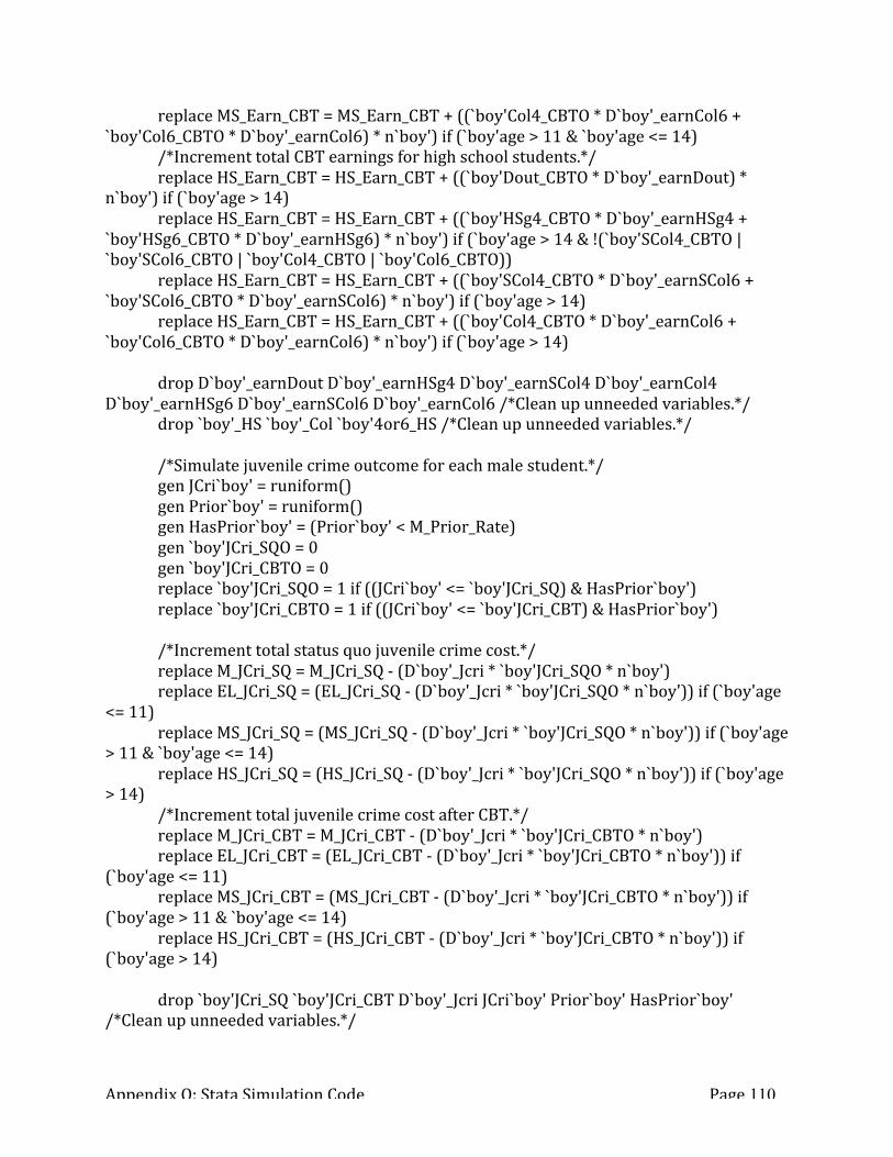
Appendix Q: Stata Simulation Code Page 110
replace MS_Earn_CBT = MS_Earn_CBT + ((`boy'Col4_CBTO * D`boy'_earnCol6 + `boy'Col6_CBTO * D`boy'_earnCol6) * n`boy') if (`boy'age > 11 & `boy'age <= 14) /*Increment total CBT earnings for high school students.*/ replace HS_Earn_CBT = HS_Earn_CBT + ((`boy'Dout_CBTO * D`boy'_earnDout) * n`boy') if (`boy'age > 14) replace HS_Earn_CBT = HS_Earn_CBT + ((`boy'HSg4_CBTO * D`boy'_earnHSg4 + `boy'HSg6_CBTO * D`boy'_earnHSg6) * n`boy') if (`boy'age > 14 & !(`boy'SCol4_CBTO | `boy'SCol6_CBTO | `boy'Col4_CBTO | `boy'Col6_CBTO)) replace HS_Earn_CBT = HS_Earn_CBT + ((`boy'SCol4_CBTO * D`boy'_earnSCol6 + `boy'SCol6_CBTO * D`boy'_earnSCol6) * n`boy') if (`boy'age > 14) replace HS_Earn_CBT = HS_Earn_CBT + ((`boy'Col4_CBTO * D`boy'_earnCol6 + `boy'Col6_CBTO * D`boy'_earnCol6) * n`boy') if (`boy'age > 14) drop D`boy'_earnDout D`boy'_earnHSg4 D`boy'_earnSCol4 D`boy'_earnCol4 D`boy'_earnHSg6 D`boy'_earnSCol6 D`boy'_earnCol6 /*Clean up unneeded variables.*/ drop `boy'_HS `boy'_Col `boy'4or6_HS /*Clean up unneeded variables.*/ /*Simulate juvenile crime outcome for each male student.*/ gen JCri`boy' = runiform() gen Prior`boy' = runiform() gen HasPrior`boy' = (Prior`boy' < M_Prior_Rate) gen `boy'JCri_SQO = 0 gen `boy'JCri_CBTO = 0 replace `boy'JCri_SQO = 1 if ((JCri`boy' <= `boy'JCri_SQ) & HasPrior`boy') replace `boy'JCri_CBTO = 1 if ((JCri`boy' <= `boy'JCri_CBT) & HasPrior`boy') /*Increment total status quo juvenile crime cost.*/ replace M_JCri_SQ = M_JCri_SQ -‐ (D`boy'_Jcri * `boy'JCri_SQO * n`boy') replace EL_JCri_SQ = (EL_JCri_SQ -‐ (D`boy'_Jcri * `boy'JCri_SQO * n`boy')) if (`boy'age <= 11) replace MS_JCri_SQ = (MS_JCri_SQ -‐ (D`boy'_Jcri * `boy'JCri_SQO * n`boy')) if (`boy'age > 11 & `boy'age <= 14) replace HS_JCri_SQ = (HS_JCri_SQ -‐ (D`boy'_Jcri * `boy'JCri_SQO * n`boy')) if (`boy'age > 14) /*Increment total juvenile crime cost after CBT.*/ replace M_JCri_CBT = M_JCri_CBT -‐ (D`boy'_Jcri * `boy'JCri_CBTO * n`boy') replace EL_JCri_CBT = (EL_JCri_CBT -‐ (D`boy'_Jcri * `boy'JCri_CBTO * n`boy')) if (`boy'age <= 11) replace MS_JCri_CBT = (MS_JCri_CBT -‐ (D`boy'_Jcri * `boy'JCri_CBTO * n`boy')) if (`boy'age > 11 & `boy'age <= 14) replace HS_JCri_CBT = (HS_JCri_CBT -‐ (D`boy'_Jcri * `boy'JCri_CBTO * n`boy')) if (`boy'age > 14) drop `boy'JCri_SQ `boy'JCri_CBT D`boy'_Jcri JCri`boy' Prior`boy' HasPrior`boy' /*Clean up unneeded variables.*/

Appendix Q: Stata Simulation Code Page 111
/*Simulate suicide outcome for each male student.*/ gen suic`boy' = runiform() gen `boy'suic_SQO = (suic`boy' <= `boy'Suic_SQ) gen `boy'suic_CBTO = (suic`boy' <= `boy'Suic_CBT) /*Increment total status quo suicide cost for males.*/ replace M_Suic_SQ = M_Suic_SQ -‐ (VSL * `boy'suic_SQO * n`boy') replace EL_Suic_SQ = (EL_Suic_SQ -‐ (VSL * `boy'suic_SQO * n`boy')) if (`boy'age <= 11) replace MS_Suic_SQ = (MS_Suic_SQ -‐ (VSL * `boy'suic_SQO * n`boy')) if (`boy'age > 11 & `boy'age <= 14) replace HS_Suic_SQ = (HS_Suic_SQ -‐ (VSL * `boy'suic_SQO * n`boy')) if (`boy'age > 14) /*Increment total suicide cost after CBT for males.*/ replace M_Suic_CBT = M_Suic_CBT -‐ (VSL * `boy'suic_CBTO * n`boy') replace EL_Suic_CBT = (EL_Suic_CBT -‐ (VSL * `boy'suic_CBTO * n`boy')) if (`boy'age <= 11) replace MS_Suic_CBT = (MS_Suic_CBT -‐ (VSL * `boy'suic_CBTO * n`boy')) if (`boy'age > 11 & `boy'age <= 14) replace HS_Suic_CBT = (HS_Suic_CBT -‐ (VSL * `boy'suic_CBTO * n`boy')) if (`boy'age > 14) drop `boy'Suic_SQ `boy'Suic_CBT suic`boy' /*Clean up unneeded variables.*/ /*Increment status quo avoided adult crime cost for females by expected reduction depending on graduation.*/ replace M_ACri_SQ = M_ACri_SQ + D`boy'_Acri * n`boy' if (`boy'HSg4_SQO | `boy'HSg6_SQO) replace EL_ACri_SQ = EL_ACri_SQ + D`boy'_Acri * n`boy' if ((`boy'HSg4_SQO | `boy'HSg6_SQO) & `boy'age <= 11) replace MS_ACri_SQ = MS_ACri_SQ + D`boy'_Acri * n`boy' if ((`boy'HSg4_SQO | `boy'HSg6_SQO) & `boy'age > 11 & `boy'age <= 14) replace HS_ACri_SQ = HS_ACri_SQ + D`boy'_Acri * n`boy' if ((`boy'HSg4_SQO | `boy'HSg6_SQO) & `boy'age > 14) /*Increment CBT avoided adult crime cost for females by expected reduction depending on graduation.*/ replace M_ACri_CBT = M_ACri_CBT + D`boy'_Acri * n`boy' if (`boy'HSg4_CBTO | `boy'HSg6_CBTO) replace EL_ACri_CBT = EL_ACri_CBT + D`boy'_Acri * n`boy' if ((`boy'HSg4_CBTO | `boy'HSg6_CBTO) & `boy'age <= 11) replace MS_ACri_CBT = MS_ACri_CBT + D`boy'_Acri * n`boy' if ((`boy'HSg4_CBTO | `boy'HSg6_CBTO) & `boy'age > 11 & `boy'age <= 14) replace HS_ACri_CBT = HS_ACri_CBT + D`boy'_Acri * n`boy' if ((`boy'HSg4_CBTO | `boy'HSg6_CBTO) & `boy'age > 14) drop `boy'age D`boy'_Acri /*Clean up unneeded variables.*/

Appendix Q: Stata Simulation Code Page 112
} /*Calculate induced graduations*/ gen Induced_Grads = HS_Grads_CBT -‐ HS_Grads_SQ drop HS_Grads_CBT HS_Grads_SQ /*Net earnings benefits.*/ gen F_Earn_Ben = F_Earn_CBT -‐ F_Earn_SQ gen M_Earn_Ben = M_Earn_CBT -‐ M_Earn_SQ gen EL_Earn_Ben = EL_Earn_CBT -‐ EL_Earn_SQ gen MS_Earn_Ben = MS_Earn_CBT -‐ MS_Earn_SQ gen HS_Earn_Ben = HS_Earn_CBT -‐ HS_Earn_SQ gen Earn_Ben = F_Earn_Ben + M_Earn_Ben sum F_Earn_Ben M_Earn_Ben EL_Earn_Ben MS_Earn_Ben HS_Earn_Ben Earn_Ben drop F_Earn_CBT F_Earn_SQ M_Earn_CBT M_Earn_SQ EL_Earn_CBT EL_Earn_SQ MS_Earn_CBT MS_Earn_SQ HS_Earn_CBT HS_Earn_SQ /*Net suicide benefits.*/ gen F_Suic_Ben = F_Suic_CBT -‐ F_Suic_SQ gen M_Suic_Ben = M_Suic_CBT -‐ M_Suic_SQ gen EL_Suic_Ben = EL_Suic_CBT -‐ EL_Suic_SQ gen MS_Suic_Ben = MS_Suic_CBT -‐ MS_Suic_SQ gen HS_Suic_Ben = HS_Suic_CBT -‐ HS_Suic_SQ gen Suic_Ben = F_Suic_Ben + M_Suic_Ben sum F_Suic_Ben M_Suic_Ben EL_Suic_Ben MS_Suic_Ben HS_Suic_Ben Suic_Ben drop F_Suic_CBT F_Suic_SQ M_Suic_CBT M_Suic_SQ EL_Suic_CBT EL_Suic_SQ MS_Suic_CBT MS_Suic_SQ HS_Suic_CBT HS_Suic_SQ /*Net juvenile crime benefits.*/ gen F_JCri_Ben = F_JCri_CBT -‐ F_JCri_SQ gen M_JCri_Ben = M_JCri_CBT -‐ M_JCri_SQ gen EL_JCri_Ben = EL_JCri_CBT -‐ EL_JCri_SQ gen MS_JCri_Ben = MS_JCri_CBT -‐ MS_JCri_SQ gen HS_JCri_Ben = HS_JCri_CBT -‐ HS_JCri_SQ gen JCri_Ben = F_JCri_Ben + M_JCri_Ben sum F_JCri_Ben M_JCri_Ben EL_JCri_Ben MS_JCri_Ben HS_JCri_Ben JCri_Ben drop F_JCri_CBT F_JCri_SQ M_JCri_CBT M_JCri_SQ EL_JCri_CBT EL_JCri_SQ MS_JCri_CBT MS_JCri_SQ HS_JCri_CBT HS_JCri_SQ /*Net adult crime benefits.*/ gen F_ACri_Ben = F_ACri_CBT -‐ F_ACri_SQ gen M_ACri_Ben = M_ACri_CBT -‐ M_ACri_SQ gen EL_ACri_Ben = EL_ACri_CBT -‐ EL_ACri_SQ gen MS_ACri_Ben = MS_ACri_CBT -‐ MS_ACri_SQ gen HS_ACri_Ben = HS_ACri_CBT -‐ HS_ACri_SQ gen ACri_Ben = F_ACri_Ben + M_ACri_Ben

Appendix Q: Stata Simulation Code Page 113
sum F_ACri_Ben M_ACri_Ben EL_ACri_Ben MS_ACri_Ben HS_ACri_Ben ACri_Ben drop F_ACri_CBT F_ACri_SQ M_ACri_CBT M_ACri_SQ EL_ACri_CBT EL_ACri_SQ MS_ACri_CBT MS_ACri_SQ HS_ACri_CBT HS_ACri_SQ /*Subtract costs from total benefits.*/ gen Net_Ben = Earn_Ben + Suic_Ben + JCri_Ben + ACri_Ben + Dscpln_Ben + Truant_Ben + Counsl_Ben -‐ Cost sum Earn_Ben Suic_Ben JCri_Ben ACri_Ben Dscpln_Ben Truant_Ben Counsl_Ben Net_Ben Cost histogram Net_Ben display "Finished executing: Simulate_Outcomes" /*Output message to help with troubleshooting*/ end /*End this subprogram*/