Embed Size (px)
Citation preview
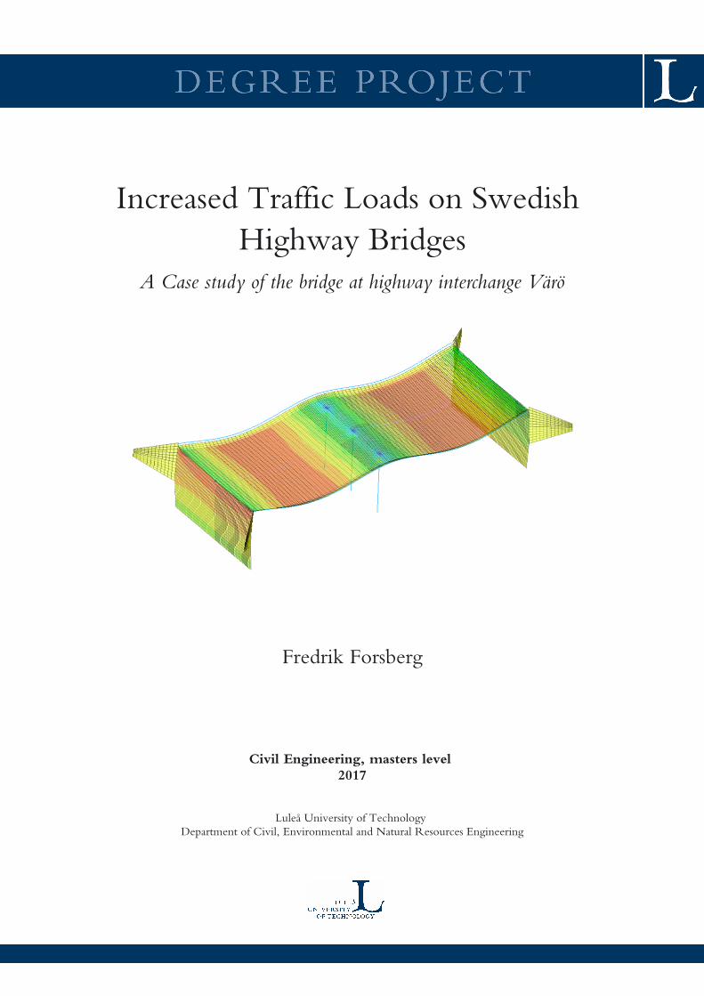
Increased Traffic Loads on Swedish
Highway Bridges
A Case study of the bridge at highway interchange Värö
Fredrik Forsberg
Civil Engineering, masters level
2017
Luleå University of Technology
Department of Civil, Environmental and Natural Resources Engineering

i
Preface
This Master Thesis, written for the consulting engineering group Ramböll at their bridge
department in Stockholm, is the final part of my Master of Science in Civil Engineering at Luleå
University of Technology. The thesis was initiated by Dr. Ali Farhang, head of the bridge
department at Ramböll Sweden, with the aim to investigate the effects of the planned traffic
load increase on Swedish road bridges.
I would like to thank Ali, along with his colleague Murtazah Khalil at the Ramböll bridge
department in Stockholm, who acted as supervisors during the work, for all the support they
provided throughout the Master Thesis work and for letting me perform my work at their
Stockholm office.
I would also like to thank my supervisor Professor Lennart Elfgren at the Division of Structural
Engineering at Luleå University of Technology for introducing me to the bridge subject as well
as all the support he offered me in the process of finalizing this Master thesis.
Stockholm, January 2017
Fredrik Forsberg
ii
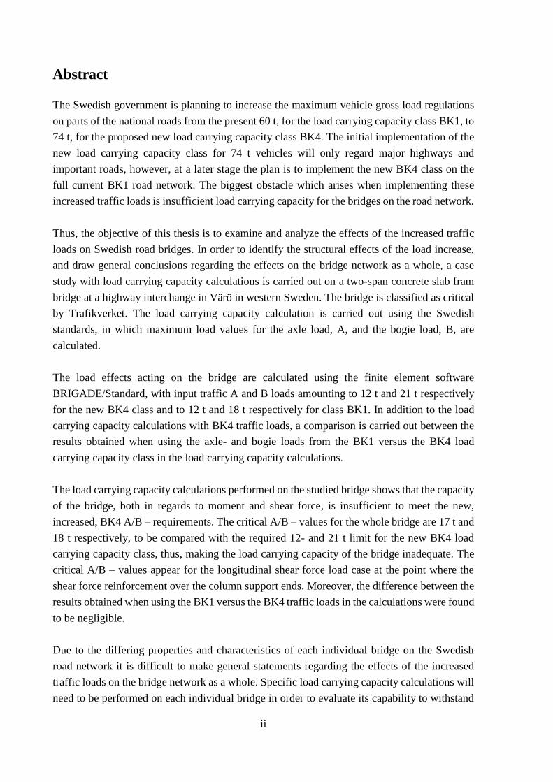
Abstract
The Swedish government is planning to increase the maximum vehicle gross load regulations
on parts of the national roads from the present 60 t, for the load carrying capacity class BK1, to
74 t, for the proposed new load carrying capacity class BK4. The initial implementation of the
new load carrying capacity class for 74 t vehicles will only regard major highways and
important roads, however, at a later stage the plan is to implement the new BK4 class on the
full current BK1 road network. The biggest obstacle which arises when implementing these
increased traffic loads is insufficient load carrying capacity for the bridges on the road network.
Thus, the objective of this thesis is to examine and analyze the effects of the increased traffic
loads on Swedish road bridges. In order to identify the structural effects of the load increase,
and draw general conclusions regarding the effects on the bridge network as a whole, a case
study with load carrying capacity calculations is carried out on a two-span concrete slab fram
bridge at a highway interchange in Värö in western Sweden. The bridge is classified as critical
by Trafikverket. The load carrying capacity calculation is carried out using the Swedish
standards, in which maximum load values for the axle load, A, and the bogie load, B, are
calculated.
The load effects acting on the bridge are calculated using the finite element software
BRIGADE/Standard, with input traffic A and B loads amounting to 12 t and 21 t respectively
for the new BK4 class and to 12 t and 18 t respectively for class BK1. In addition to the load
carrying capacity calculations with BK4 traffic loads, a comparison is carried out between the
results obtained when using the axle- and bogie loads from the BK1 versus the BK4 load
carrying capacity class in the load carrying capacity calculations.
The load carrying capacity calculations performed on the studied bridge shows that the capacity
of the bridge, both in regards to moment and shear force, is insufficient to meet the new,
increased, BK4 A/B – requirements. The critical A/B – values for the whole bridge are 17 t and
18 t respectively, to be compared with the required 12- and 21 t limit for the new BK4 load
carrying capacity class, thus, making the load carrying capacity of the bridge inadequate. The
critical A/B – values appear for the longitudinal shear force load case at the point where the
shear force reinforcement over the column support ends. Moreover, the difference between the
results obtained when using the BK1 versus the BK4 traffic loads in the calculations were found
to be negligible.
Due to the differing properties and characteristics of each individual bridge on the Swedish
road network it is difficult to make general statements regarding the effects of the increased
traffic loads on the bridge network as a whole. Specific load carrying capacity calculations will
need to be performed on each individual bridge in order to evaluate its capability to withstand

iii
the new increased BK4 traffic load. However, capacity calculations regarding the BK1 load
carrying capacity class can, with sufficient accuracy, be used to evaluate the capability of a
bridge to withstand the increased traffic loads in the BK4 load carrying capacity class, thus,
making it easier to evaluate the strengthening needs for the bridge network as a whole.
Keywords: BRIGADE/Standard, Concrete slab frame bridge, FEM, Load carrying capacity
calculation, Load carrying capacity class

iv
Sammanfattning
Sveriges regering planerar en utökning av den maximalt tillåtna bruttovikten för fordon på delar
av det allmänna vägnätet från den nuvarande begränsningen på 60 t, för bärighetsklass BK1,
till 74 t, för den nya föreslagna bärighetsklassen BK4. I det första skedet kommer den nya
bärighetsklassen, för fordon med bruttovikt upp till 74 t, bara att implementeras på stora
motorvägar och andra ur transportsynpunkt viktiga vägar, men, i ett senare skede finns också
planer på att implementera den nya bärighetsklassen, BK4, på hela det nuvarande BK1
vägnätet. Det största problemet som förväntas uppkomma under införandet av de nya, ökade,
trafiklasterna är otillräcklig bärighet på vägnätets broar.
Således är målet med denna uppsats att undersöka och analysera effekterna av dessa ökade
trafiklaster för broar på det Svenska vägnätet. För att identifiera effekterna, och dra generella
slutsatser, gällande denna ökade trafiklast för broarna på det Svenska vägnätet i sin helhet
kommer en fallstudie med bärighetsberäkningar utföras på en plattrambro vid trafikplats Värö
- en bro som Trafikverket bedömer som kritisk. Bärighetsberäkningen utförs enligt svenska
standarder, där maximala tillåtna värden på axellasten, A, och bogielasten, B, beräknas.
Lasteffekterna som verkar på bron beräknas med hjälp finita element programvaran
BRIGADE/Standard med trafiklaster, A och B, som uppgår till 12 respektive 21 t för den nya
BK4 bärighetsklassen och 12 respektive 18 t för bärighetsklass BK1. Som tillägg till
bärighetsberäkningarna med BK4 laster utförs också en jämförelse av resultaten som
uppkommer när axel- och bogielasterna från BK1 respektive BK4 används i beräkningarna.
Bärighetsberäkningarna på den studerade bron visar att brons kapacitet, både gällande moment
och tvärkraft, är otillräcklig när den belastas med de ökade BK4 trafiklasterna. De kritiska A-
och B- värdena för bron är 17 respektive 18 t, värden som skall jämföras med kraven på 12
respektive 21 t för den nya bärighetsklassen BK4 – därmed är brons bärighet otillräcklig. De
kritiska A- och B-värdena för bron uppkommer för lastfallet med longitudinell tvärkraft vid
punkten där tvärkraftsarmeringen över mittstödet slutar verka. Jämförelsen mellan
beräkningsresultaten som uppkom med trafiklaster enligt BK1 respektive BK4 visade att
skillnaden mellan beräkningsresultaten var försumbar.
På grund av de varierande egenskaperna hos varje enskild bro på det Svenska vägnätet är det
svårt att dra generella slutsatser gällande effekterna av lastökningen för vägnätet som helhet.
Specifika bärighetsberäkningar måste utföras på varje individuell bro för att kunna utvärdera
dess kapacitet att klara av de nya, ökade, BK4 trafiklasterna. Emellertid kan
bärighetsberäkningar som beträffar bärighetsklassen BK1, med tillräcklig tillförlitlighet,
användas för att bedöma en bros möjlighet att motstå de ökade trafiklasterna i den nya
bärighetsklassen BK4, vilket förenklar utvärderingen av vilka broar som kräver förstärkning.

v
Nyckelord: BRIGADE/Standard, Bärighetsberäkningar, Plattrambro, FEM, Bärighetsklasser
vi
Table of Contents
1 INTRODUCTION ........................................................................................................................................ 1
1.1 BACKGROUND ............................................................................................................................................ 1
1.2 GOAL AND OBJECTIVES .............................................................................................................................. 2
1.3 LIMITATIONS .............................................................................................................................................. 2
1.4 DISPOSITION ............................................................................................................................................... 3
2 METHODOLOGY ....................................................................................................................................... 5
2.1 LITERATURE REVIEW .................................................................................................................................. 5
2.2 CASE STUDY ............................................................................................................................................... 5
2.3 VALIDITY, RELIABILITY AND GENERALIZATION ......................................................................................... 6
3 LITERATURE REVIEW ............................................................................................................................ 7
3.1 LOAD CARRYING CAPACITY CLASSES ......................................................................................................... 7
3.2 ACTIONS ON BRIDGES ................................................................................................................................. 8
3.2.1 Permanent actions ....................................................................................................................................................... 9
3.2.2 Variable actions ............................................................................................................................................................ 9
3.2.3 Load combinations ................................................................................................................................................... 11
3.3 FEM ......................................................................................................................................................... 12
3.3.1 Modeling orthotropic slabs using FEM ............................................................................................................. 14
3.3.2 FEM result sections ................................................................................................................................................... 16
3.3.3 BRIGADE/Standard .................................................................................................................................................. 17
3.4 BRIDGE LOAD CARRYING CAPACITY CALCULATIONS ................................................................................ 20
3.4.1 General approach ...................................................................................................................................................... 20
3.4.2 Condition assessment ............................................................................................................................................... 21
3.5 LOAD CARRYING CAPACITY CALCULATIONS ACCORDING TO SWEDISH CODES ......................................... 22
3.6 CONCRETE SLAB FRAME BRIDGE ............................................................................................................. 25
4 CASE STUDY – BRIDGE AT HIGHWAY INTERCHANGE VÄRÖ ................................................. 27
4.1 BRIDGE AT HIGHWAY INTERCHANGE VÄRÖ ............................................................................................. 27
4.2 SYSTEM DRAWINGS AND CALCULATION ASSUMPTIONS ............................................................................ 29
4.3 MATERIAL PARAMETERS .......................................................................................................................... 29
4.4 REINFORCEMENT ...................................................................................................................................... 31
5 BRIGADE/STANDARD MODEL ............................................................................................................ 34
5.1 GEOMETRY AND BOUNDARY CONDITIONS ................................................................................................ 34
5.2 MESH GENERATION AND CONVERGENCE STUDY....................................................................................... 34
5.3 MATERIAL MODEL .................................................................................................................................... 36
5.4 ACTIONS .................................................................................................................................................. 37
5.4.1 Self-weight ................................................................................................................................................................... 38
5.4.2 Pavement ...................................................................................................................................................................... 38
5.4.3 Earth pressure ............................................................................................................................................................ 38
5.4.4 Surcharge ..................................................................................................................................................................... 38
5.4.5 Traffic load ................................................................................................................................................................... 39
5.4.6 Dynamic contribution factor ................................................................................................................................ 40
5.4.7 Braking force............................................................................................................................................................... 40
5.4.8 Load combinations ................................................................................................................................................... 41
5.5 RESULT SECTIONS .................................................................................................................................... 41
5.6 RESULT VERIFICATION ............................................................................................................................. 42
vii
6 RESISTANCE CALCULATIONS ........................................................................................................... 46
6.1 MOMENT RESISTANCE CALCULATION ...................................................................................................... 46
6.2 MOMENT RESISTANCE CALCULATION - CONNECTION BETWEEN SLAB AND ABUTMENT ........................... 48
6.3 SHEAR FORCE RESISTANCE CALCULATION ............................................................................................... 49
7 LOAD CARRYING CAPACITY CALCULATION .............................................................................. 53
7.1 MOMENT LOAD CARRYING CAPACITY CALCULATION ............................................................................... 53
7.2 SHEAR FORCE LOAD CARRYING CAPACITY CALCULATION ........................................................................ 54
8 RESULTS AND ANALYSIS..................................................................................................................... 56
8.1 RESULT SUMMARY ................................................................................................................................... 56
8.2 MOMENT LOAD CARRYING CAPACITY CALCULATION ............................................................................... 58
8.3 SHEAR FORCE LOAD CARRYING CAPACITY CALCULATION ........................................................................ 60
8.4 COMPARISON BETWEEN BK1 AND BK4 ................................................................................................... 63
8.5 POSSIBLE STRENGTHENING METHODS ...................................................................................................... 65
9 DISCUSSION AND CONCLUSIONS ..................................................................................................... 67
9.1 DISCUSSION ............................................................................................................................................. 67
9.2 CONCLUSIONS .......................................................................................................................................... 68
9.3 SUGGESTIONS FOR FURTHER RESEARCH ................................................................................................... 69
10 REFERENCES ........................................................................................................................................... 70
APPENDIX A – Map of the initially proposed BK4 road network
APPENDIX B – Vehicle limits
APPENDIX C – Type vehicles
APPENDIX D – Load coefficients for each load combination
APPENDIX E – Reinforcement drawings
APPENDIX F – Reinforcement list
APPENDIX G – Finite element mesh convergence
APPENDIX H – Moment resistance calculations
APPENDIX I – Shear force resistance calculations
APPENDIX J – Capacity calculation (traffic on own lane)
APPENDIX K – Capacity calculation (traffic in the middle of the carriageway, alone on the bridge)
APPENDIX L – Capacity calculation (traffic on own lane) – check with 18 t bogie load
viii
List of Figures
Figure 1 - Gross loads for different load carrying capacity classes (Trafikverket, 2014a). ....... 7
Figure 2 - Type load model c (Trafikverket, 2016a)................................................................ 11
Figure 3 - Sketch of type load model c. ................................................................................... 11
Figure 4 - Result section - moment (Pacoste, Plos & Johansson, 2012). ................................. 16
Figure 5 - Result section - shear force (Pacoste, Plos & Johansson, 2012). ............................ 17
Figure 6 - BRIGADE/Standard structure lines (Scanscot Technology AB, 2015a). ............... 18
Figure 7 - A BRIGADE/Standard four-node shell element with one integration point (Scanscot
Technology AB, 2015a). .......................................................................................................... 18
Figure 8 - BRIGADE/Standard coordinate system for shell elements (Scanscot Technology AB,
2015a)....................................................................................................................................... 18
Figure 9 - BRIGADE/Standard directions for the shell element moments (Scanscot Technology
AB, 2015a). .............................................................................................................................. 19
Figure 10 - BRIGADE/Standard directions for the shell element shear forces (Scanscot
Technology AB, 2015a). .......................................................................................................... 19
Figure 11 - BRIGADE/Standard traffic lanes (Scanscot Technology AB, 2015a). ................ 19
Figure 12 - Self- and pavement weight acting on the bridge (Scanscot Technology AB, 2015a).
.................................................................................................................................................. 20
Figure 13 - Bridge carriageway division. ................................................................................. 23
Figure 14 - Type vehicles passing the bridge on their own lanes. ........................................... 23
Figure 15 - Type vehicles in the middle of the carriageway, alone on the bridge – eccentricity
cases. ........................................................................................................................................ 24
Figure 16 - Superstructure cross-section, concrete slab frame bridge. .................................... 26
Figure 17 - Principal sketch of a concrete slab frame bridge................................................... 26
Figure 18 - Bridge location (Värö bridge). .............................................................................. 27
Figure 19 - Värö bridge from the west. .................................................................................... 28
Figure 20 - Overview drawing of Värö bridge (Trafikverket, 2016c). .................................... 28
Figure 21 - Bridge cross-section - Värö Bridge (Trafikverket, 2016c). .................................. 28
Figure 22 - System drawing. .................................................................................................... 29
Figure 23 - Shear force reinforcement distribution (Trafikverket, 2016c). ............................. 32
Figure 24 - Reinforcement - connection between abutment and slab (Trafikverket, 2016c). . 32
Figure 25 - BRIGADE/Standard bridge geometry. ................................................................. 34
Figure 26 - Support lines and mesh generation sections. ......................................................... 35
Figure 27 - Convergence test. .................................................................................................. 35
Figure 28 - Finite element mesh on the bridge. ....................................................................... 36
Figure 29 - Material manager - BRIGADE/Standard model. .................................................. 37
Figure 30 - Traffic lanes for traffic passing the bridge on its own lane. .................................. 39
Figure 31 - Traffic lanes for traffic passing the bridge in the middle of the carriageway, alone
on the bridge............................................................................................................................. 40
ix
Figure 32 - Result lines - Traffic passing the bridge on its own lane. ...................................... 41
Figure 33 - Result lines - Traffic passing the bridge in the middle of the carriageway, alone on
the bridge. ................................................................................................................................. 42
Figure 34 - Result sections - longitudinal shear force. ............................................................. 42
Figure 35 - Deformed bridge model - dead weight load case. ................................................. 43
Figure 36 - BRIGADE/Standard dead weight moment. ........................................................... 43
Figure 37 - FRAME ANALYSIS dead weight moment. ......................................................... 44
Figure 38 - BRIGADE/Standard dead weight shear force. ...................................................... 45
Figure 39 - FRAME ANALYSIS dead weight shear force. ..................................................... 45
Figure 40 - Critical section and critical point – moment. ......................................................... 46
Figure 41 - Critical point and critical result section line - shear force. .................................... 50
Figure 42 – Load carrying capacity: Bogie load - Result line 1. .............................................. 58
Figure 43 – Load carrying capacity calculation: Bogie load - Result line 2. ........................... 59
Figure 44 – Load carrying capacity calculation: Bogie load - Result line 3. ........................... 60
Figure 45 - Transversal shear force: Bogie load – load carrying capacity calculation - Result
line 5. ........................................................................................................................................ 62
Figure 46 - Longitudinal shear force: Bogie load – load carrying capacity calculation - Result
line 6. ........................................................................................................................................ 63
Figure 47 - Magnified longitudinal shear force diagram: Bogie load - load carrying capacity
calculation - Result line 6 ......................................................................................................... 63
Figure 48 - Principle sketch - widening of column top. ........................................................... 65
x
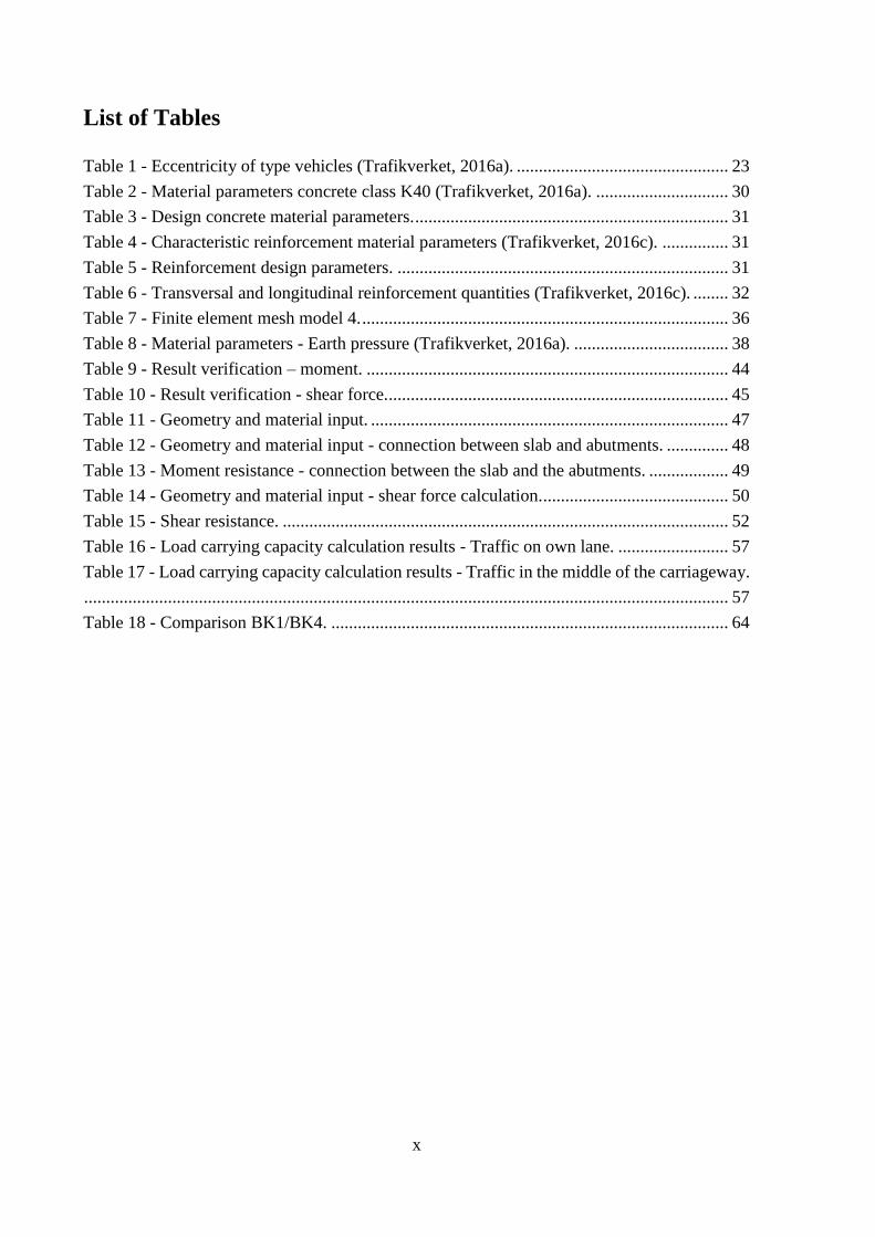
List of Tables
Table 1 - Eccentricity of type vehicles (Trafikverket, 2016a). ................................................ 23
Table 2 - Material parameters concrete class K40 (Trafikverket, 2016a). .............................. 30
Table 3 - Design concrete material parameters. ....................................................................... 31
Table 4 - Characteristic reinforcement material parameters (Trafikverket, 2016c). ............... 31
Table 5 - Reinforcement design parameters. ........................................................................... 31
Table 6 - Transversal and longitudinal reinforcement quantities (Trafikverket, 2016c). ........ 32
Table 7 - Finite element mesh model 4. ................................................................................... 36
Table 8 - Material parameters - Earth pressure (Trafikverket, 2016a). ................................... 38
Table 9 - Result verification – moment. .................................................................................. 44
Table 10 - Result verification - shear force. ............................................................................. 45
Table 11 - Geometry and material input. ................................................................................. 47
Table 12 - Geometry and material input - connection between slab and abutments. .............. 48
Table 13 - Moment resistance - connection between the slab and the abutments. .................. 49
Table 14 - Geometry and material input - shear force calculation. .......................................... 50
Table 15 - Shear resistance. ..................................................................................................... 52
Table 16 - Load carrying capacity calculation results - Traffic on own lane. ......................... 57
Table 17 - Load carrying capacity calculation results - Traffic in the middle of the carriageway.
.................................................................................................................................................. 57
Table 18 - Comparison BK1/BK4. .......................................................................................... 64
xi
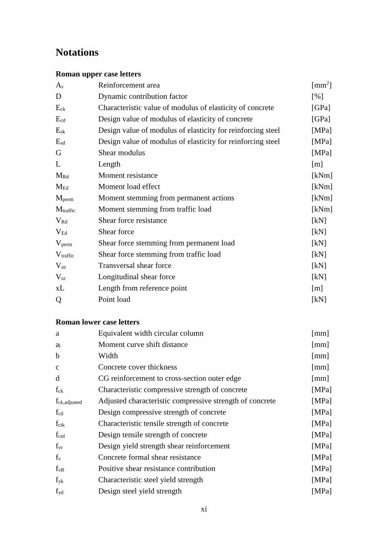
Notations
Roman upper case letters
As Reinforcement area [mm2]
D Dynamic contribution factor [%]
Eck Characteristic value of modulus of elasticity of concrete [GPa]
Ecd Design value of modulus of elasticity of concrete [GPa]
Esk Design value of modulus of elasticity for reinforcing steel [MPa]
Esd Design value of modulus of elasticity for reinforcing steel [MPa]
G Shear modulus [MPa]
L Length [m]
MRd Moment resistance [kNm]
MEd Moment load effect [kNm]
Mperm Moment stemming from permanent actions [kNm]
Mtraffic Moment stemming from traffic load [kNm]
VRd Shear force resistance [kN]
VEd Shear force [kN]
Vperm Shear force stemming from permanent load [kN]
Vtraffic Shear force stemming from traffic load [kN]
Vaz Transversal shear force [kN]
Vsz Longitudinal shear force [kN]
xL Length from reference point [m]
Q Point load [kN]
Roman lower case letters
a Equivalent width circular column [mm]
al Moment curve shift distance [mm]
b Width [mm]
c Concrete cover thickness [mm]
d CG reinforcement to cross-section outer edge [mm]
fck Characteristic compressive strength of concrete [MPa]
fck,adjusted Adjusted characteristic compressive strength of concrete [MPa]
fcd Design compressive strength of concrete [MPa]
fctk Characteristic tensile strength of concrete [MPa]
fctd Design tensile strength of concrete [MPa]
fsv Design yield strength shear reinforcement [MPa]
fv Concrete formal shear resistance [MPa]
fvR Positive shear resistance contribution [MPa]
fyk Characteristic steel yield strength [MPa]
fyd Design steel yield strength [MPa]

xii
h Height [mm]
k Proportionality factor for increasing/decreasing traffic point loads [-]
v Velocity [km/h]
x The height of the concrete cross-section compression zone [mm]
Greek letters
ν Poisson’s ratio [-]
ρ Weight [kN/m3]
ψ Factor [-]
η Factor [-]
γ Partial factor [-]
γn Partial factor [-]
γm Partial factor [-]
εs Reinforcement strain [-]
εsγ Reinforcement yield strength strain [-]
εcu Ultimate compressive strain in the concrete [-]
Other notations
∅ Diameter [mm]
xiii
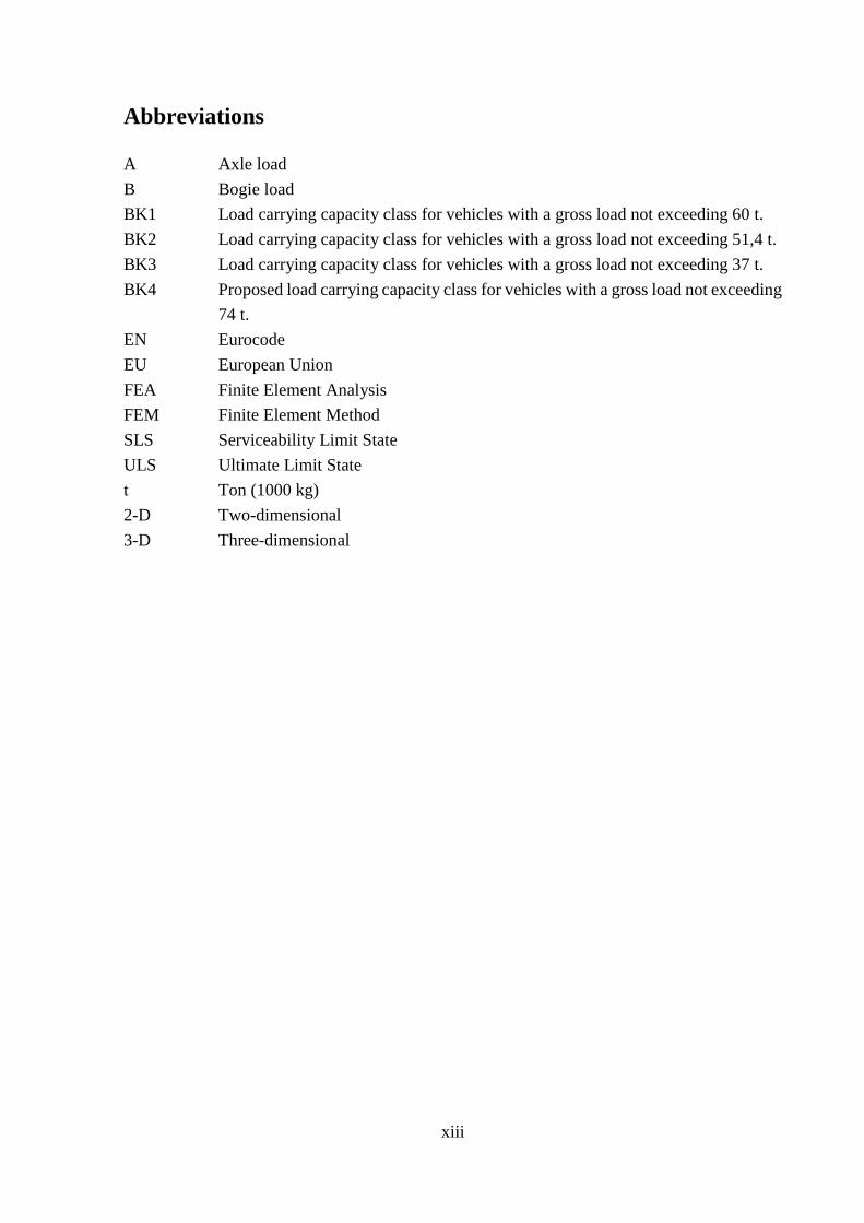
Abbreviations
A Axle load
B Bogie load
BK1 Load carrying capacity class for vehicles with a gross load not exceeding 60 t.
BK2 Load carrying capacity class for vehicles with a gross load not exceeding 51,4 t.
BK3 Load carrying capacity class for vehicles with a gross load not exceeding 37 t.
BK4 Proposed load carrying capacity class for vehicles with a gross load not exceeding
74 t.
EN Eurocode
EU European Union
FEA Finite Element Analysis
FEM Finite Element Method
SLS Serviceability Limit State
ULS Ultimate Limit State
t Ton (1000 kg)
2-D Two-dimensional
3-D Three-dimensional
1
1 Introduction
In this chapter, the background of the problem as well as the reason for its importance is
summarized and presented. The goals and objectives of the thesis are stated as well as the
limitations on the work.
1.1 Background The Swedish government is planning to increase the maximum allowed vehicle gross load on
parts of the public roads from the present 60 t to 74 t, which, according to Trafikverket (2015),
will mean that, at the initial stage, approximately 66 bridges will require strengthening.
Following this planned load increase Trafikverket (2014a) proposes the implementation of a
new load carrying capacity class called BK4 for 74 t vehicles with a maximum length of 25.5
m. The roads affected, in the initial stage, by this new load carrying capacity class are major
highways and important roads, namely E-roads: E4, E6, E10, E18, E20 and parts of the national
roads 40, 50, 55, and 56 on which 2/3 of the total road freight volume is transported, see
appendix A for a map of the proposed changes. At a later stage, the Swedish government is
planning to allow for 74 t vehicles on the whole BK1 road network, consisting of a total of
15 442 bridges. Approximately 1000 of these bridges will require strengthening according to
Trafikverket (2015), strengthening works that is expected to cost roughly 9,6 billion Swedish
Crowns.
According to Transportstyrelsen (2014), the change is supposed to streamline the Swedish road-
transport sector as an increased load on each truck will decrease the total number of trucks and
thereby create significant economic, environmental and safety related benefits. The
socioeconomic benefit for the initial changes, in which only the major highways are affected,
is, according to Trafikverket (2014a), approximated to be between 2,6 and 5,6 billion Swedish
crowns over the next 40 years.
Comparatively the EU has a general limit of 40 t on their roads and bridges, which, with the
planned changes makes the Swedish road infrastructure very internationally competitive
(Transportstyrelsen, 2014). The only other country within the EU to have significantly
increased the loads on their roads and bridges are Finland, who increased their maximum traffic
load to 76 t in 2013 (Kommunikationsministeriet, 2013).
The biggest obstacle which arises when implementing the new load carrying capacity class BK4
is insufficient load carrying capacity for the bridges on the proposed road network. In order to
identify the bridges that require strengthening a load carrying capacity calculation ais carried
out, in which maximum load values for the axle load, A, and the bogie load, B, is calculated.
These load values, A and B, is the common capacity representation for bridges in Sweden.

2
The Swedish road network presently consists of three load carrying capacity classes with a
fourth, the BK4, at the planning stage, all of which has their own A and B values as load
carrying capacity representation (Trafikverket, 2016a). The new load carrying capacity class
will require an uptick in the maximum A/B – values, from a respective 12 and 18 t limit for the
BK1 load carrying capacity class, to, according to Trafikverket (2015), a respective 12 and 21
t limit for the new load carrying capacity class BK4.
With the big variation of applicable bridge types, especially when implementing the increased
load on the whole BK1 road network, the decision is made to focus the calculation and analysis
on the most common bridge type in Sweden, the concrete slab frame bridge - which makes up
approximately 50 % of the Swedish bridge stock (Trafikverket, 2014b).
1.2 Goal and objectives The goal of this thesis is to examine the effects of the increased traffic load on Swedish road
bridges, or, more specifically, on a Swedish concrete slab frame bridge and try to draw general
conclusions regarding the effects of the increased traffic loads on the Swedish bridge network
as a whole.
1.3 Limitations Calculations and analysis will be performed on a concrete slab bridge, where a suitable bridge
will be assessed and studied on a case basis. The assumption is made that non-prestressed
concrete slab bridges will be more critical and thereby the thesis will focus on non-prestressed
bridges and disregard prestressed bridges.
The calculations will be performed in ultimate limit state; thus it follows that the effects of the
increased load in regards to fatigue is disregarded. Furthermore, the superstructure is deemed
to be the most critical part of the bridge in regards to the ultimate limit state capacity, thereby,
only the superstructure will be taken into account in this thesis.
Using the Swedish standards for load carrying capacity calculations on bridges, as well as the
calculation methodology used by Ramböll, the bridges are assessed with the assumption that
they are undamaged. In traditional load carrying capacity calculations on Swedish bridges the
capacity to withhold the load of military vehicles are calculated, however, as this thesis focuses
on the effect of the increased traffic load, calculations regarding military vehicles will not be
carried out. Furthermore, the effects of snow and wind are deemed insignificant in comparison
to other actions and are thereby disregarded.
3
1.4 Disposition This thesis consists of nine chapters, all of which are briefly summarized in the following
sections.
1 - Introduction
In this chapter, the background of the problem as well as the reason for its importance is
summarized and presented. The goals and objectives of the thesis are stated as well as the
limitations on the work.
2 - Methodology
This chapter describes the methods and approaches used in this master thesis as well as the
research validity, reliability and generalization.
3 - Literature review
In this chapter, general research regarding load carrying capacity calculations on highway
bridges are presented. Furthermore, the theory behind the Swedish load carrying capacity
classes for road bridges is presented and described as well as some general theory regarding
actions on road bridges. The theory behind, and the methods used, when performing load
carrying capacity calculations on Swedish road bridges are thoroughly examined. Some
background on the usage of FEM, both generally and using the software BRIGADE/Standard,
is also presented in this chapter. Finally, some general theory regarding concrete slab frame
bridges is also described in this paragraph.
4 - Case study – Bridge at highway interchange Värö
The studied concrete slab frame bridge, the bridge at highway interchange Värö is thoroughly
described. The bridge material properties and reinforcement design is also presented.
5 - BRIGADE/Standard model
The BRIGADE/Standard model used to calculate the load effects on the bridge is described.
Descriptions of the modelling of the bridge geometry, boundary conditions and material
properties is presented and in addition to this the model verification process is presented.
6 - Resistance calculations
Resistance calculations, regarding both moment and shear forces, for the critical points in the
bridge are performed and presented.
7 – Load carrying capacity calculations
Load carrying capacity calculations, in which A/B load limits are calculated, in regards to both
moment and shear forces are presented and carried out for all critical parts of the bridge.

4
8 - Results and analysis
The results of the load carrying capacity calculations are presented and analyzed for both
moment and shear force cases and a comparison between load carrying capacity calculations
using the BK1 input A/B – values and BK4 input values is performed.
9 - Discussion and conclusions
In this paragraph, the results of the load carrying capacity calculations performed on the bridge
at highway interchange Värö will be discussed and conclusions will be made, both in regards
to the specific bridge studied in this thesis, but also in regards to bridges on the Swedish road
network in general.
5
2 Methodology
This chapter describes the methods and approaches used in this master thesis as well as the
research validity, reliability and generalization.
2.1 Literature review In order to identify research and gain knowledge of the subject a literature review, in which
books, articles and research papers are studied, is performed. Studies regarding, both the old
load carrying capacity classes and the proposed new load carrying capacity class, for Swedish
roads and bridges were conducted, studies in which a representative from Trafikverket were
consulted when relevant questions emerged. Loads and actions on road bridges, both according
to the Swedish standards and Eurocode, are studied. The load carrying capacity calculation
process for bridges, both in general and with a focus on Swedish rules and regulations, is studied
in order to be able to analyze the bridge and its capacity to withstand the new, increased, traffic
loads. Drawings of relevant bridges, bridges assessed to be at risk when BK4 is implemented,
are obtained using the, by Trafikverket supplied, database BaTMan. Furthermore, studies of the
FE-software BRIGADE/Standard, as well as the finite element analysis method in general, were
also required to get an understanding of the software and its applications for concrete bridges
and load carrying capacity calculations.
2.2 Case study A case study with load carrying capacity calculations is performed on the bridge at highway
interchange Värö in order to analyze the structural effects of the increased load and identify
critical elements in the bridge. In order to calculate the design load effects on different
significant parts of the bridge, the bridge is modelled in the finite element software
BRIGADE/Standard - a software specifically designed to model bridges and bridge-like
structures. In order to make sure that the software produces reliable results the load effects
produced by the BRIGADE/Standard model are verified and controlled using the 2-D frame
analysis software, FRAME Analysis.
The resistance in regards to moment and shear force is calculated using hand-calculations for
all critical sections on the bridge. Calculations carried out using the relevant Swedish codes and
regulations for load carrying capacity calculations on concrete bridges as well as rules and
regulations for regular concrete structures. Using the calculated capacities and the load effects
produced by the BRIGADE/Standard software the design load carrying capacity, expressed by
the A/B – values, is calculated for all critical parts of the bridge and for all relevant load cases.
Using these calculated load carrying capacities the design load carrying capacity for the whole
bridge is determined. A thorough evaluation and analysis of the results are then carried out in
order to draw conclusions of the effects of the increased traffic loads, both in regards to the
specific bridge studied- and in regards to bridges on the Swedish road network in general. In
addition to this analysis, suggestions regarding future studies will be presented and discussed.
6
2.3 Validity, reliability and generalization It is important to design and plan the research structure in such a way that it links the case study
and data collection with the literature and initial goal and objective of the study, see paragraph
1.2, which should make sure that there is a clear view of what is to be achieved (Rowley, 2002).
In this case, a combined literature- and case study is conducted in order to examine the problem.
The motivation for this approach is the fact that each individual bridge, and bridge type, has its
own characteristics and flaws, thereby making a broader study hard to conduct.
It is important that the study is as generalizable as possible - that you can claim that the results
of your study can be applied to theory and that the results are applicable to other comparable
situations (Rowley, 2002). In this case, the generalization of the study is quite limited as each
individual bridge varies considerably in its characteristics. The results will be weaker if the
bridge types or loading conditions differ significantly from the case studied in this thesis.
The validity of a research refers to how well the study measures what it is supposed to measure
- how well the goals and objectives of the study is met and achieved (Rowley, 2002). It is
important to seek to reduce subjectivity in the study as much as possible. Furthermore, it is
important from a validity standpoint to make the study as transparent as possible. This will be
achieved by complete result transparency; full results will be presented in appendices and clear
explanations on every step of the calculation process will be presented.
Another issue with close ties to the validity and generalizability of a study is the reliability,
which is the degree of which it can be demonstrated that the study can be repeated with the
same result; that the assessment produces stable and consistent results (Rowley, 2002).
Reliability within the study will be achieved through thorough demonstrations and
documentations of studies and calculation procedures, thereby ensuring that the study could be
repeated with similar results. However, the reliability of the study faces the same difficulty as
the generalization; the result reliability will decrease significantly if the loading conditions or
considered bridge type is altered.
7
3 Literature review
In this chapter, general research regarding load carrying capacity calculations on highway
bridges are presented. Furthermore, the theory behind the Swedish load carrying capacity
classes for road bridges is presented and described as well as some general theory regarding
actions on road bridges. The theory behind, and the methods used, when performing load
carrying capacity calculations on Swedish road bridges are thoroughly examined. Some
background on the usage of FEM, both generally and using the software BRIGADE/Standard,
is also presented in this chapter. Finally, some general theory regarding concrete slab frame
bridges is also described in this paragraph.
3.1 Load carrying capacity classes Different load carrying capacity classes control the load capacity regulations of the Swedish
road- and bridge network. These load carrying capacity classes are in turn used to regulate the
traffic on each national road. Presently there are three different load carrying capacity classes,
BK1, BK2 and BK3 with a fourth, BK4, being proposed. The maximum gross load for each
load carrying capacity class depends on the length of the vehicle, counted as the distance
between the first- and last axle. As the length of the vehicle increases, so does the acceptable
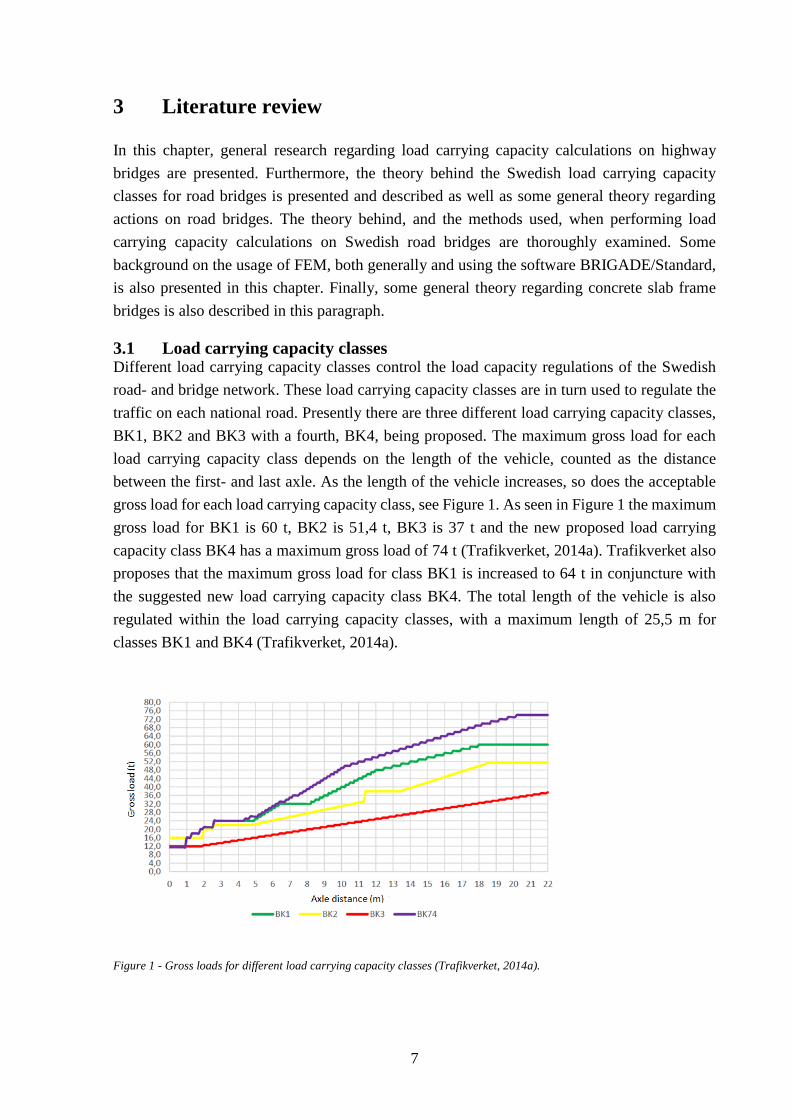
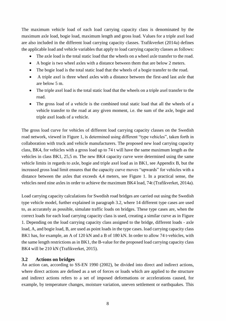
gross load for each load carrying capacity class, see Figure 1. As seen in Figure 1 the maximum
gross load for BK1 is 60 t, BK2 is 51,4 t, BK3 is 37 t and the new proposed load carrying
capacity class BK4 has a maximum gross load of 74 t (Trafikverket, 2014a). Trafikverket also
proposes that the maximum gross load for class BK1 is increased to 64 t in conjuncture with
the suggested new load carrying capacity class BK4. The total length of the vehicle is also
regulated within the load carrying capacity classes, with a maximum length of 25,5 m for
classes BK1 and BK4 (Trafikverket, 2014a).
Figure 1 - Gross loads for different load carrying capacity classes (Trafikverket, 2014a).
8
The maximum vehicle load of each load carrying capacity class is denominated by the
maximum axle load, bogie load, maximum length and gross load. Values for a triple axel load
are also included in the different load carrying capacity classes. Trafikverket (2014a) defines
the applicable load and vehicle variables that apply to load carrying capacity classes as follows:
The axle load is the total static load that the wheels on a wheel axle transfer to the road.
A bogie is two wheel axles with a distance between them that are below 2 meters.
The bogie load is the total static load that the wheels of a bogie transfer to the road.
A triple axel is three wheel axles with a distance between the first-and last axle that
are below 5 m.
The triple axel load is the total static load that the wheels on a triple axel transfer to the
road.
The gross load of a vehicle is the combined total static load that all the wheels of a
vehicle transfer to the road at any given moment, i.e. the sum of the axle, bogie and
triple axel loads of a vehicle.
The gross load curve for vehicles of different load carrying capacity classes on the Swedish
road network, viewed in Figure 1, is determined using different “type vehicles”, taken forth in
collaboration with truck and vehicle manufacturers. The proposed new load carrying capacity
class, BK4, for vehicles with a gross load up to 74 t will have the same maximum length as the
vehicles in class BK1, 25,5 m. The new BK4 capacity curve were determined using the same
vehicle limits in regards to axle, bogie and triple axel load as in BK1, see Appendix B, but the
increased gross load limit ensures that the capacity curve moves “upwards” for vehicles with a
distance between the axles that exceeds 4,4 meters, see Figure 1. In a practical sense, the
vehicles need nine axles in order to achieve the maximum BK4 load, 74t (Trafikverket, 2014a).
Load carrying capacity calculations for Swedish road bridges are carried out using the Swedish
type vehicle model, further explained in paragraph 3.2, where 14 different type cases are used
to, as accurately as possible, simulate traffic loads on bridges. These type cases are, when the
correct loads for each load carrying capacity class is used, creating a similar curve as in Figure
1. Depending on the load carrying capacity class assigned to the bridge, different loads - axle
load, A, and bogie load, B, are used as point loads in the type cases. load carrying capacity class
BK1 has, for example, an A of 120 kN and a B of 180 kN. In order to allow 74 t-vehicles, with
the same length restrictions as in BK1, the B-value for the proposed load carrying capacity class
BK4 will be 210 kN (Trafikverket, 2015).
3.2 Actions on bridges An action can, according to SS-EN 1990 (2002), be divided into direct and indirect actions,
where direct actions are defined as a set of forces or loads which are applied to the structure
and indirect actions refers to a set of imposed deformations or accelerations caused, for
example, by temperature changes, moisture variation, uneven settlement or earthquakes. This
9
thesis will largely focus on the direct actions on bridges, which are the most important ones
when conducting a load carrying capacity calculation (COST, 2004).
Furthermore, the actions can be classified by their variation in time, where the following,
perhaps more common, classifications are used (SS-EN 1990, 2002):
Permanent actions: Self-weight of structures, fixed equipment and road surfacing, and
indirect actions caused by shrinkage and uneven settlements.
Variable actions: Imposed loads, wind actions or snow loads.
Accidental actions: explosions, or impact from vehicles crashing into the structure.
These actions, and how they specifically are used in bridge load carrying capacity calculations
in Sweden, will be further explained in the following paragraphs.
3.2.1 Permanent actions
One of the main components when calculating the permanent actions on a structure is the self-
weight which, in the case of a road bridge, consists of the load-carrying part of the structure
(Trafikverket, 2016a). When calculating the self-weight according to Trafikverket (2016a),
reinforced concrete is assumed to have a specific weight of 24 kN/m3.
The specific weight of the pavement, 22 kN/m3 for asphalt pavement and 23 kN/m3 for concrete
pavement, also needs to be added to the permanent load. According to Trafikverket (2016a) the
shrinkage of the concrete is only considered for composite and prestressed concrete bridges and
thereby won’t have to be considered in this thesis. Furthermore, the earth pressure will have to
be considered using factors and coefficients according to Trafikverket (2016a).
3.2.2 Variable actions
3.2.2.1 Snow loads
Snow loads are, according to Trafikverket (2016a), only taken into account when the bridge in
question have a roof structure, thus, snow loads aren’t considered on the bridges in this thesis.
3.2.2.2 Wind loads
Using the same reasoning as with the snow loads, the wind loads on the structure is not
considered in this thesis.
3.2.2.3 Traffic loads
Traffic loads on road bridges in Sweden is primarily simulated and calculated using two
different load models, the Eurocode load model, where load model 1 is decisive for most
bridges, and the Swedish load model, defined by Trafikverket, called the type vehicle model.
These two load models are based on real traffic measurements on bridges and is designed to
simulate those traffic effects as accurately as possible (SS-EN 1991-2, 2003), (Trafikverket,
2016a).
10
The Eurocode load model 1 for bridges, see SS-EN 1991-2 (2003), is based on uniformly
distributed loads acting in combination with bogie loads on the, by lane, divided bridge surface.
The traffic loads on each lane are assigned a predetermined load value and adjustment factor,
depending on the specific, predisposed, lane placement on the bridge. However, for load
carrying capacity calculations regarding existing road bridges the Eurocode load model is
disregarded and the type vehicle model, defined by Trafikverket (Trafikverket, 2016a), is
applied on the bridge.
The type vehicle load model is using different type cases to represent real heavy vehicles and
traffic situations. The model consists of 14 different vertical loading scenarios, represented by
the letters a-n, where each scenario denotes a, by extensive tests and experiments formed
(Carlsson, 2006), load case, see Appendix C. The point loads, A and B, in each load model are
representing the axle -and bogie loads of real heavy vehicles and the uniformly distributed load,
q, are meant to represent lighter traffic in-between the heavier vehicles (Trafikverket, 2016a).
The capacity of road bridges is represented by a maximum traffic load, denoted by the
maximum axle load, A, and bogie load, B. The uniformly distributed load, q, which is evenly
distributed over the width of the loading field, is set as 5 kN/m in unfavorable loading
conditions and 0 kN/m in favorable loading conditions. When conducting a load carrying
capacity calculation, the result of the calculations are capacity values for the point loads A and
B. These calculated A and B values are then compared to the limits and requirements of each
load carrying capacity class. Load carrying capacity class BK1 has, for example, an A
requirement of 12 t and a B requirement of 18 t and the new, proposed, load carrying capacity
class BK4 has an A requirement of 12 t and a B requirement of 21 t (Trafikverket, 2015).
The type vehicle models, always centrally placed, are acting on notional load lanes with a width
of 3 m. The number and placement of the notional load lanes should always represent the most
unfavorable possible influence on the bridge, where the number of notional load lanes depends
on how many that fits on the carriageway. However, the maximum number of load lanes is four.
The number of notional load lanes on which type vehicles are placed are a maximum of two
lanes where the type vehicles on one notional lane are multiplied with a factor of 1,0 and the
other with a factor of 0,8. The remaining lanes are only affected by the uniformly distributed
load, q, see (Trafikverket, 2016a).
The transverse distance between the wheels are, according to Trafikverket (2016a), spanning
between 1,7 m to 2,3 m and the wheels themselves have a distribution of 0,3 m in the transverse
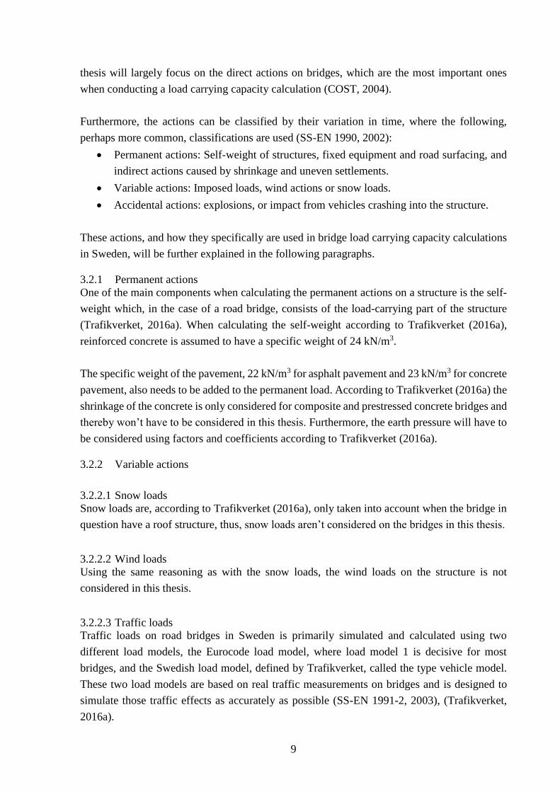
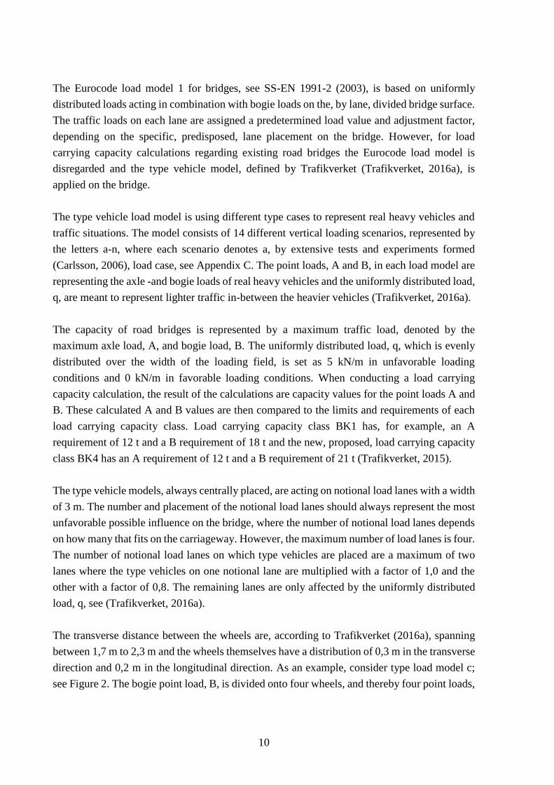
direction and 0,2 m in the longitudinal direction. As an example, consider type load model c;
see Figure 2. The bogie point load, B, is divided onto four wheels, and thereby four point loads,
11
a sketch of this can be seen in Figure 3 along with a sketch of the distances between the axles
and the dimensions of the wheels.
Figure 2 - Type load model c (Trafikverket, 2016a).
Figure 3 - Sketch of type load model c.
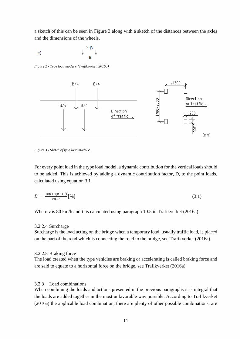
For every point load in the type load model, a dynamic contribution for the vertical loads should
to be added. This is achieved by adding a dynamic contribution factor, D, to the point loads,
calculated using equation 3.1
𝐷 = 180+8(𝑣−10)
20+𝐿[%] (3.1)
Where v is 80 km/h and L is calculated using paragraph 10.5 in Trafikverket (2016a).
3.2.2.4 Surcharge
Surcharge is the load acting on the bridge when a temporary load, usually traffic load, is placed
on the part of the road which is connecting the road to the bridge, see Trafikverket (2016a).
3.2.2.5 Braking force
The load created when the type vehicles are braking or accelerating is called braking force and
are said to equate to a horizontal force on the bridge, see Trafikverket (2016a).
3.2.3 Load combinations
When combining the loads and actions presented in the previous paragraphs it is integral that
the loads are added together in the most unfavorable way possible. According to Trafikverket
(2016a) the applicable load combination, there are plenty of other possible combinations, are
12
load combination A which is the primary load combination for bridge capacity calculations in
the ultimate limit state, ULS. Trafikverket (2016a) states that the amount of variable loads
considered is limited at a maximum of four loads, where the ones considered, as one would
suspect, are the most unfavorable ones. The most unfavorable of the variable loads are given
the higher load coefficient value, ψγ. Coefficients, both the higher- and lower ones, are
presented in Appendix D.
3.3 FEM The finite element method (FEM) or finite element analysis (FEA) is an approximate numerical
method used for solving complex differential equations regarding a wide range of physical
problems, including complex structural engineering problems. Broo, Lundgren and Plos (2008)
suggests that the finite element method can be especially effective and helpful when assessing
existing structures, such as bridges, because of their complexity in a geometrical sense and the
complexity of the actions on the structures. When using FEM to evaluate existing structures,
higher capacities are often reached compared to the results achieved from more traditional
forms of calculation. Broo, Lundgren and Plos (2008) suggests that the reason for the higher
estimated capacities primarily is a more favorable load distribution as the structure in most FEM
software products is analyzed in three dimensions.
When using the finite element method for structural problems, the complex structures are
subdivided into a finite number of elements. Elements, interconnected by nodes, whose relation
between their nodal displacements and nodal reactions can be specified by a limited number of
functions and parameters, called shape, or form, functions. The displacements, strains and
stresses of an element is calculated by assembling all of the elements into vectors or matrices
and solving the general system, see equation 3.2 (Rombach, 2004).
[𝐊] ∗ {𝐮} = {𝐅} (3.2)
The stiffness of all the elements are represented by the global stiffness matrix [K], the loads on
the structure are represented by the vector {F} and the nodal displacements, the typical result
of a FEM calculation, are denoted by the vector {u}. In order to find the form or shape functions
that, as closely as possible, approximates the behavior of the structure different methods can be
used. For simple problems, basic equilibrium relations can be used to find the relation between
the nodal forces and their displacements. However, as the complexity of the structure increases
so does the complexity of the methods used - leading to the usage of virtual work- and virtual
displacement principles (Rombach, 2004).
The first step of conducting a finite element analysis of a structure in a more practical sense is,
according to Samuelsson & Wiberg (1998), to simplify the structure in regards to various
parameters such as boundary conditions, geometry, material parameters and loads. A material
deformation behavior, typically linear elastic behavior, is also assigned to the structure. The
13
next step is to divide the structure into finite elements, a process where it is important to
consider both the element type and size, as this greatly can influence the future calculations and
results. The stiffness matrix, an integral part of the finite element method, is calculated for each
element and then put together to form a global stiffness matrix for the whole structure.
Geometry- and boundary conditions are then assigned to the model in order to solve the
equation system for the whole structure and create relevant results.
Perhaps the most important step, when conducting a finite element analysis, is to perform
extensive result verification in order to make sure that the results of the FEM calculations are
reasonable and correct. Almost no software is, as Rombach (2004) puts it “free from errors”
which makes a critical distrust, leading to post processing checks of the FEM results integral
when using FEA on structural problems. The errors can sometimes stem from simple software
glitches but it should always be kept in mind that the finite element method is a numerical
method based on lots of assumptions and simplifications, the result of any calculation can only
be as accurate as the underlying assumptions and the underlying numerical model.
These boundary, support, element and load assumptions and simplifications can greatly affect
the results, for example, Pacoste, Plos, and Johansson (2012) states that the support conditions
in a finite element model of a structure often have a decisive influence on the analysis results.
Davidson (2003) supports this statement and states that the modeling of the supports for slabs,
regular or bridge slabs, significantly can affect the moment load effect over that support.
It is especially important to be cautious when modelling point loads, for example tires of
passing vehicles, as point loads can create discontinuity zones on which singularities, infinite
stresses and internal forces, can occur. Rombach (2004) clarifies that these stresses only occur
in the numerical model, and not in the real structure, and are caused by the simplifications and
assumptions regarding the element behavior. These discontinuity zone behaviors are not always
as drastic as the creation of infinite stresses, they can be subtler and harder to recognize, creating
local stress surges that significantly changes the result of the calculation, a phenomenon that
underlines the importance of proper result interpretation and analysis. To avoid and, at least
partially, limit this problem, point loads are often modelled as uniformly distributed loads, for
example, the point loads from the wheels of vehicles passing a bridge is evenly distributed over
the whole wheel-area.
Both closely knitted to- and significantly affecting this problem is the process and decisions
involved when dividing the structure into finite elements, a process called discretization. The
size and shape of the elements can significantly affect the result and Rambach (2004) stresses
that the discretization phase is where most of the mistakes when performing FEM calculations
occurs. To emphasize this, Davidson (2003) states that the size of the finite elements, also called
the mesh size, significantly affects the moment and shear forces that are calculated in certain
14
points of the structure, making the discretization face essential in order to achieve reliable
results from the FEM calculation. One method to limit the risk and probability of mistakes in
the discretization and element mesh generation phase is to perform a convergence study. A
process in which the element mesh size in the model is continuously reduced until the results,
for example the moment curve for the dead weight load case, converges. This process makes
sure that the element mesh sizes, in a global perspective, is properly modelled and that the
element mesh is dense enough.
Another important aspect to consider is which material analysis model is used in the FEM
calculations. Typically, in order to simplify the analysis and to be able to use the superposition
principle when evaluating the effects of load combinations, linear analysis is adopted, even
though concrete slabs usually, due to cracking and reinforcement distribution, display clear
non-linear response. This is, at least in ultimate limit state, reasonable since concrete slabs
typically have good plastic deformability. Since the design is based on a moment (and force)
distribution that satisfies equilibrium, the load carrying capacity will be adequate if the structure
has sufficient plastic deformation capacity (Pacoste, Plos & Johansson, 2012).
There are multiple different types of elements that can be used to divide the structure, Broo,
Lundgren and Plos (2008) states that in order to model an entire structure, like a whole bridge,
structural finite elements are used, such as, beam, shell and truss elements. Typically, when
performing FEM calculations on concrete slabs and slab bridges the elements are specified as
shell elements. Davidson (2003) adds that using 3D shell elements, sometimes in combination
with beam elements, is the most common and effective method when modelling concrete
bridges using FEM.
3.3.1 Modeling orthotropic slabs using FEM
When modelling concrete bridges using FEA an important aspect to consider - and choice to
make - is whether the slab is considered to have an isotropic or orthotropic behavior. Usually
when performing FEA the assumption is made that the slab, or structure, has an isotropic
behavior. However, when considering the reinforcement and cracks in the concrete, which
usually disrupts the isotropic behavior, concrete slabs doesn’t have an isotropic behavior and
thereby the model might produce more accurate results when modelled in a, at least partially,
orthotropic way (Rombach, 2004).
Bridges and slabs are generally not equally reinforced in both the longitudinal and transversal
direction. Thereby, the concrete will behave differently in different directions, and the relative
stiffness due to reinforcement orientation- and quantity will produce a stress distribution with
significant differences from the stress distribution produced by an analysis assuming isotropic
conditions. Old bridge slabs were generally designed using a two-dimensional, and thereby
partially orthotropic, stress distribution, creating significantly higher stresses in the longitudinal
direction compared to the transversal direction. Thus, the amount of reinforcement in the
15
longitudinal direction compared to the reinforcement amounts in the transversal direction is
often significantly higher in old concrete bridges.
This creates a problem when analyzing these older bridges with modern numerical methods
such as FEM. The FEM software, which as mentioned earlier usually is using an assumption of
isotropic material behavior, will thereby produce significantly larger stresses in the transversal
direction compared to the stresses obtained from the two-dimensional model used in the original
design calculations. Thus, the older bridges, which have been operational for decades, will,
when making load carrying capacity calculations using modern methods, often be deemed
unsafe (COST, 2004).
One solution to this problem is to scale the material properties in accordance with the amount
of reinforcement in transversal and longitudinal direction, creating a scaled orthotropic material
model or, also called, a transversally orthotropic model. Two of the three directions are said to
be equally stiff, creating a model that has different stiffness’s in the longitudinal and transversal
directions. Kwak & Filippou (1990) clarifies that the usage of orthotropic finite element
material models is especially efficient and accurate for FEM using shell elements, which is the
usual element model used when modeling concrete bridges in finite element software.
Unlike isotropic material models, which are parametrized by a single Young’s modulus of
elasticity, the transversally orthotropic material model has two different Young’s moduli – Ea
and Es (Li & Barbic, 2014). These different modules of elasticity can be scaled in different
ways in the finite element material model. One suitable solution, which is used in the load
carrying capacity calculation performed in this thesis, is to scale the modulus of elasticity in
accordance to the relation between the amount of longitudinal and transversal reinforcement.
When assigning the material shear modulus to the transversally orthotropic finite element
model, Huber (1923) proposes that the shear modulus in the longitudinal direction is calculated
using the classical formula, see equation 3.3 and that, the shear modulus in the transversal
direction is calculated using the geometrical mean of the two different modules of elasticity,
see equation 3.4. The poisson ratio, 𝜐, defined as the ratio between the lateral strain and the
axial strain, is, according to Rombach (2004), said to be 0,2 when modelling concrete slabs
using finite element analysis.
𝐺 = 𝐸
2(1+𝜐) (3.3)
𝐺 = √𝐸𝑎𝐸𝑠
2(1+𝜐) (3.4)
16
3.3.2 FEM result sections
Another important aspect to consider when post-processing and acquiring results from the FEM
calculations is that unrealistic cross-sectional moments and shear forces can occur in the finite
element model due to simplifications in the modeling (Pacoste, Plos & Johansson, 2012).
These unrealistic moments and shear forces usually occurs over the supports, making the
modeling and choice of result sections over and around the supports crucial in order to obtain
accurate and reasonable results from the finite element model.
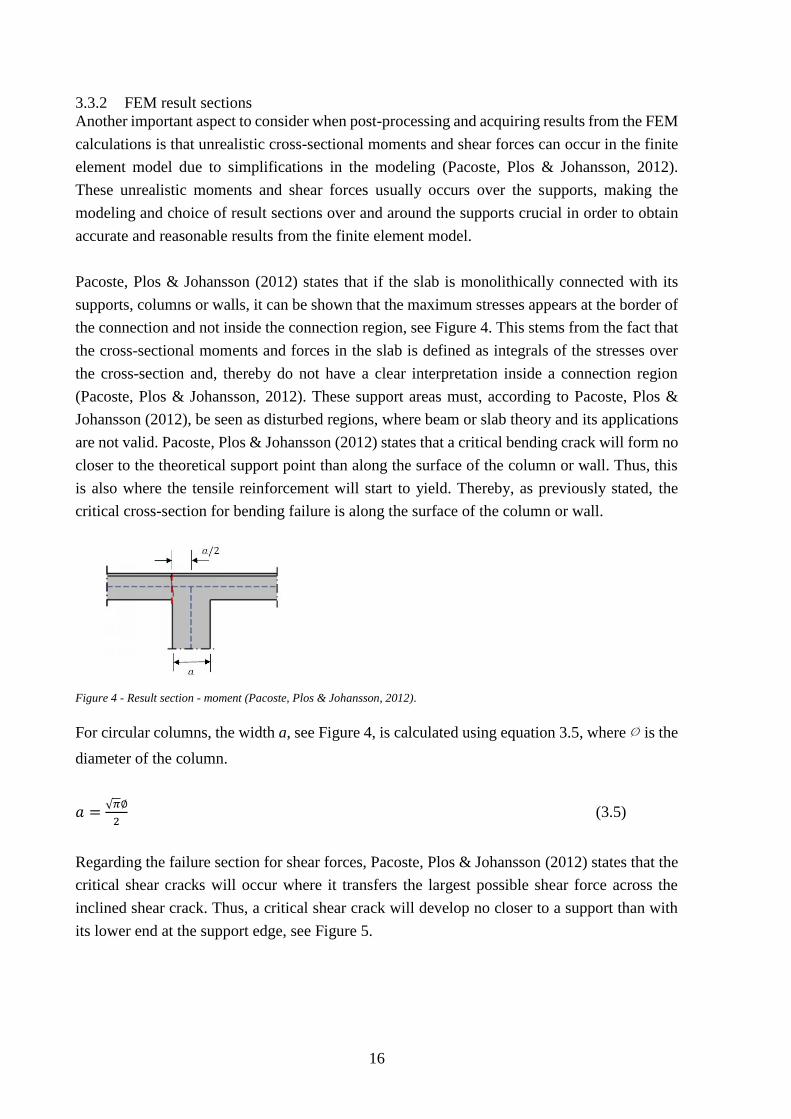
Pacoste, Plos & Johansson (2012) states that if the slab is monolithically connected with its
supports, columns or walls, it can be shown that the maximum stresses appears at the border of
the connection and not inside the connection region, see Figure 4. This stems from the fact that
the cross-sectional moments and forces in the slab is defined as integrals of the stresses over
the cross-section and, thereby do not have a clear interpretation inside a connection region
(Pacoste, Plos & Johansson, 2012). These support areas must, according to Pacoste, Plos &
Johansson (2012), be seen as disturbed regions, where beam or slab theory and its applications
are not valid. Pacoste, Plos & Johansson (2012) states that a critical bending crack will form no
closer to the theoretical support point than along the surface of the column or wall. Thus, this
is also where the tensile reinforcement will start to yield. Thereby, as previously stated, the
critical cross-section for bending failure is along the surface of the column or wall.
Figure 4 - Result section - moment (Pacoste, Plos & Johansson, 2012).
For circular columns, the width a, see Figure 4, is calculated using equation 3.5, where ∅ is the
diameter of the column.
𝑎 =√𝜋∅
2 (3.5)
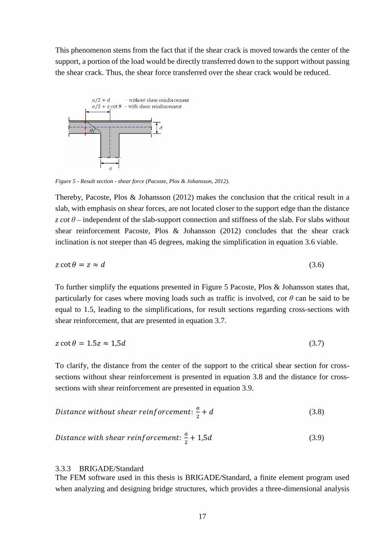
Regarding the failure section for shear forces, Pacoste, Plos & Johansson (2012) states that the
critical shear cracks will occur where it transfers the largest possible shear force across the
inclined shear crack. Thus, a critical shear crack will develop no closer to a support than with
its lower end at the support edge, see Figure 5.
17
This phenomenon stems from the fact that if the shear crack is moved towards the center of the
support, a portion of the load would be directly transferred down to the support without passing
the shear crack. Thus, the shear force transferred over the shear crack would be reduced.
Figure 5 - Result section - shear force (Pacoste, Plos & Johansson, 2012).
Thereby, Pacoste, Plos & Johansson (2012) makes the conclusion that the critical result in a
slab, with emphasis on shear forces, are not located closer to the support edge than the distance
z cot θ – independent of the slab-support connection and stiffness of the slab. For slabs without
shear reinforcement Pacoste, Plos & Johansson (2012) concludes that the shear crack
inclination is not steeper than 45 degrees, making the simplification in equation 3.6 viable.
𝑧 cot 𝜃 = 𝑧 ≈ 𝑑 (3.6)
To further simplify the equations presented in Figure 5 Pacoste, Plos & Johansson states that,
particularly for cases where moving loads such as traffic is involved, cot θ can be said to be
equal to 1.5, leading to the simplifications, for result sections regarding cross-sections with
shear reinforcement, that are presented in equation 3.7.
𝑧 cot 𝜃 = 1.5𝑧 ≈ 1,5𝑑 (3.7)
To clarify, the distance from the center of the support to the critical shear section for cross-
sections without shear reinforcement is presented in equation 3.8 and the distance for cross-
sections with shear reinforcement are presented in equation 3.9.
𝐷𝑖𝑠𝑡𝑎𝑛𝑐𝑒 𝑤𝑖𝑡ℎ𝑜𝑢𝑡 𝑠ℎ𝑒𝑎𝑟 𝑟𝑒𝑖𝑛𝑓𝑜𝑟𝑐𝑒𝑚𝑒𝑛𝑡: 𝑎
2+ 𝑑 (3.8)
𝐷𝑖𝑠𝑡𝑎𝑛𝑐𝑒 𝑤𝑖𝑡ℎ 𝑠ℎ𝑒𝑎𝑟 𝑟𝑒𝑖𝑛𝑓𝑜𝑟𝑐𝑒𝑚𝑒𝑛𝑡: 𝑎
2+ 1,5𝑑 (3.9)
3.3.3 BRIGADE/Standard
The FEM software used in this thesis is BRIGADE/Standard, a finite element program used
when analyzing and designing bridge structures, which provides a three-dimensional analysis
18
concept and a graphical user interface for pre- and post-processing (Scanscot Technology AB,
2015b).
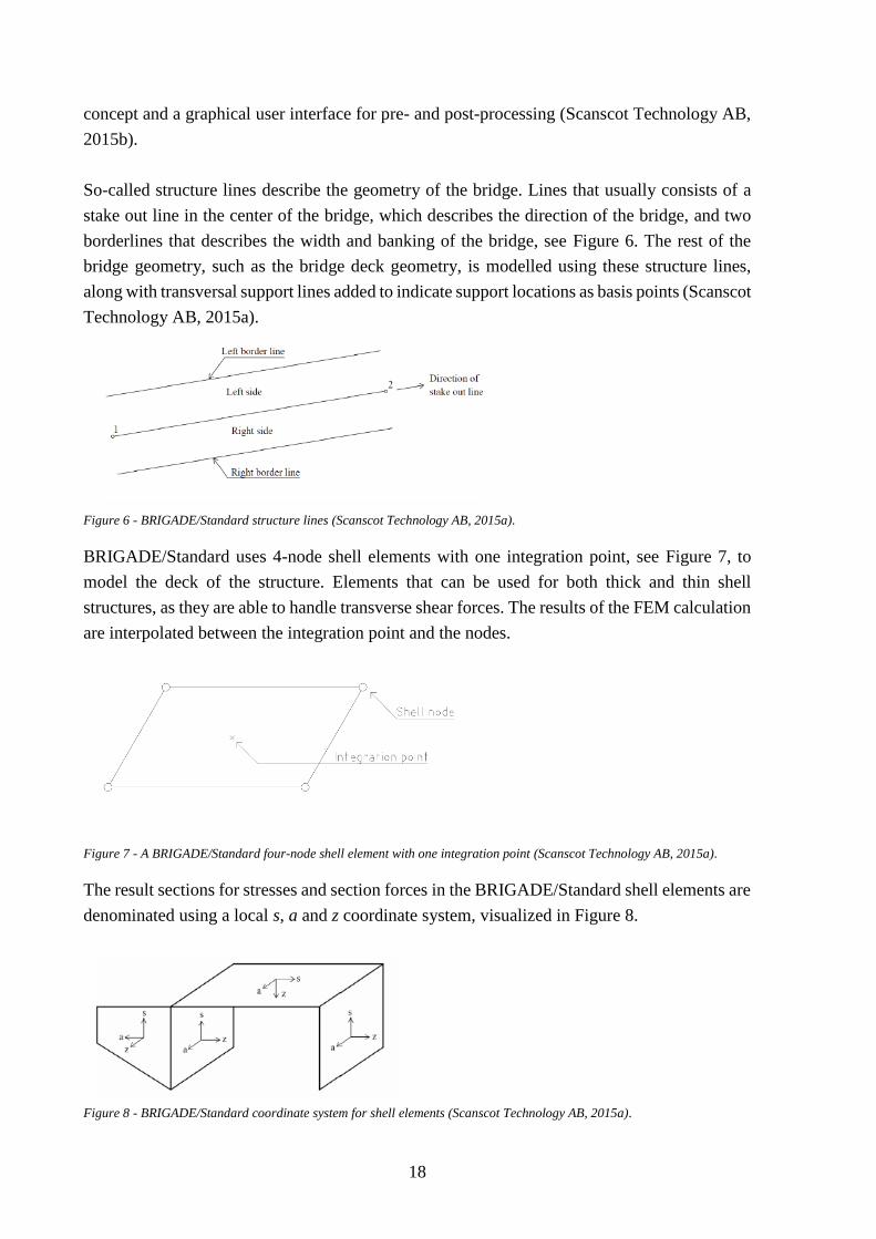
So-called structure lines describe the geometry of the bridge. Lines that usually consists of a
stake out line in the center of the bridge, which describes the direction of the bridge, and two
borderlines that describes the width and banking of the bridge, see Figure 6. The rest of the
bridge geometry, such as the bridge deck geometry, is modelled using these structure lines,
along with transversal support lines added to indicate support locations as basis points (Scanscot
Technology AB, 2015a).
Figure 6 - BRIGADE/Standard structure lines (Scanscot Technology AB, 2015a).
BRIGADE/Standard uses 4-node shell elements with one integration point, see Figure 7, to
model the deck of the structure. Elements that can be used for both thick and thin shell
structures, as they are able to handle transverse shear forces. The results of the FEM calculation
are interpolated between the integration point and the nodes.
Figure 7 - A BRIGADE/Standard four-node shell element with one integration point (Scanscot Technology AB, 2015a).
The result sections for stresses and section forces in the BRIGADE/Standard shell elements are
denominated using a local s, a and z coordinate system, visualized in Figure 8.
Figure 8 - BRIGADE/Standard coordinate system for shell elements (Scanscot Technology AB, 2015a).
19
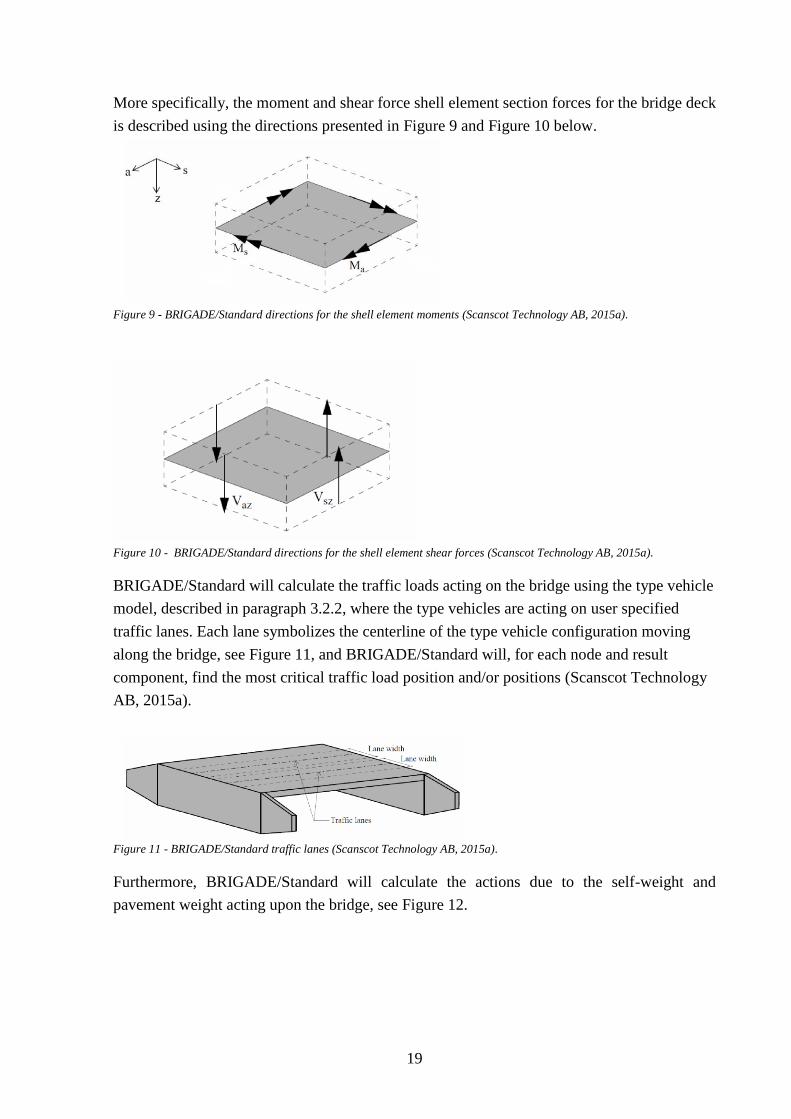
More specifically, the moment and shear force shell element section forces for the bridge deck
is described using the directions presented in Figure 9 and Figure 10 below.
Figure 9 - BRIGADE/Standard directions for the shell element moments (Scanscot Technology AB, 2015a).
Figure 10 - BRIGADE/Standard directions for the shell element shear forces (Scanscot Technology AB, 2015a).
BRIGADE/Standard will calculate the traffic loads acting on the bridge using the type vehicle
model, described in paragraph 3.2.2, where the type vehicles are acting on user specified
traffic lanes. Each lane symbolizes the centerline of the type vehicle configuration moving
along the bridge, see Figure 11, and BRIGADE/Standard will, for each node and result
component, find the most critical traffic load position and/or positions (Scanscot Technology
AB, 2015a).
Figure 11 - BRIGADE/Standard traffic lanes (Scanscot Technology AB, 2015a).
Furthermore, BRIGADE/Standard will calculate the actions due to the self-weight and
pavement weight acting upon the bridge, see Figure 12.
20
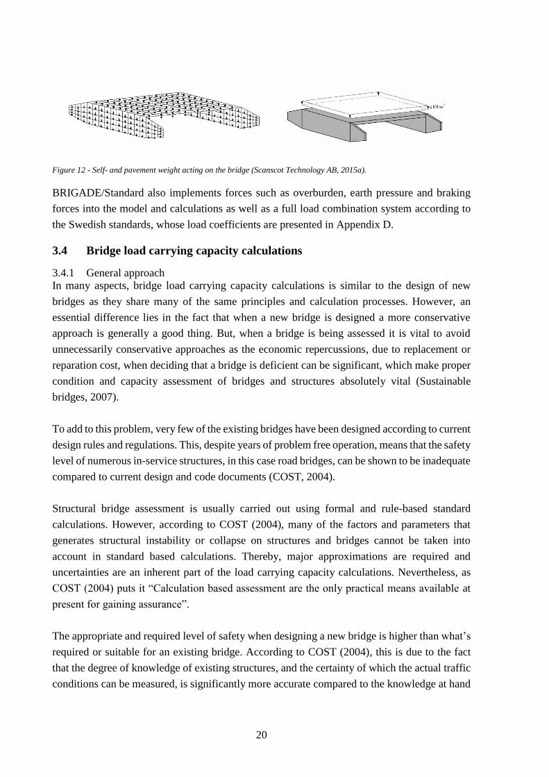
Figure 12 - Self- and pavement weight acting on the bridge (Scanscot Technology AB, 2015a).
BRIGADE/Standard also implements forces such as overburden, earth pressure and braking
forces into the model and calculations as well as a full load combination system according to
the Swedish standards, whose load coefficients are presented in Appendix D.
3.4 Bridge load carrying capacity calculations
3.4.1 General approach
In many aspects, bridge load carrying capacity calculations is similar to the design of new
bridges as they share many of the same principles and calculation processes. However, an
essential difference lies in the fact that when a new bridge is designed a more conservative
approach is generally a good thing. But, when a bridge is being assessed it is vital to avoid
unnecessarily conservative approaches as the economic repercussions, due to replacement or
reparation cost, when deciding that a bridge is deficient can be significant, which make proper
condition and capacity assessment of bridges and structures absolutely vital (Sustainable
bridges, 2007).
To add to this problem, very few of the existing bridges have been designed according to current
design rules and regulations. This, despite years of problem free operation, means that the safety
level of numerous in-service structures, in this case road bridges, can be shown to be inadequate
compared to current design and code documents (COST, 2004).
Structural bridge assessment is usually carried out using formal and rule-based standard
calculations. However, according to COST (2004), many of the factors and parameters that
generates structural instability or collapse on structures and bridges cannot be taken into
account in standard based calculations. Thereby, major approximations are required and
uncertainties are an inherent part of the load carrying capacity calculations. Nevertheless, as
COST (2004) puts it “Calculation based assessment are the only practical means available at
present for gaining assurance”.
The appropriate and required level of safety when designing a new bridge is higher than what’s
required or suitable for an existing bridge. According to COST (2004), this is due to the fact
that the degree of knowledge of existing structures, and the certainty of which the actual traffic
conditions can be measured, is significantly more accurate compared to the knowledge at hand

21
when designing a new bridge. Thereby, the partial safety factors can, in theory, be reduced with
a maintained degree of structural safety (COST, 2004).
3.4.2 Condition assessment
Although a proper condition assessment will not be performed in this thesis - the assumption is
made that the bridge is undamaged - it still has an integral part in the general maintenance and
capacity assessment of a nations highway- and railway bridges. A condition assessment is
undertaken to provide information on the overall condition of a structure or its elements.
Information regarding the extents of possible defects and their effects on the bridge capacity
and life span can also be derived and calculated following a bridge condition assessment
(COST, 2004).
BRIME (2001) describes the main objectives of a bridge condition assessment as follows:
Identify deterioration processes
Provide an indication of the condition of a structure and/or of its components or
elements
Identify further work
Rank a structure according to the need for future work
Optimize expenditure on further works
When performing a condition assessment Plos et al. (2008) states that it is important to properly
assess the material properties and bridge deterioration on the specific bridge in order to, in a
later stage of the assessment, be able to use the most relevant and correct material parameters.
Deterioration of bridges can, according to BRIME (2001), be divided into three sub categories:
Deterioration arising from faults in design, building materials or components
Defects due to the construction method or defects occurring during the production
process
Deterioration caused by external influences
Furthermore, BRIME (2001) states that the most common form of deterioration for concrete
bridges specifically is corrosion of the reinforcement, and thereby impairment of the
reinforcement strength, caused by the ingress of carbon dioxide and, or, chloride ions.
Furthermore, methods for assessment of bridges and their Life Cycle Costs have been studied
in e.g. the European projects Sustainable Bridges (2007) and Mainline (2014).
Another aspect worth considering is the inherent conservative material capacity assumptions
that are used when performing capacity calculations. Specifically, when calculating the shear
force resistance for cross-sections without shear reinforcement, Vc, which, especially for slabs,
are very uncertain and thus, underestimated in most national codes and calculation regulations.
These, perhaps overly, conservative underestimations of the shear force capacity of concrete
slabs is discussed and described in many sources, but, perhaps most notably by Nilimaa (2015)
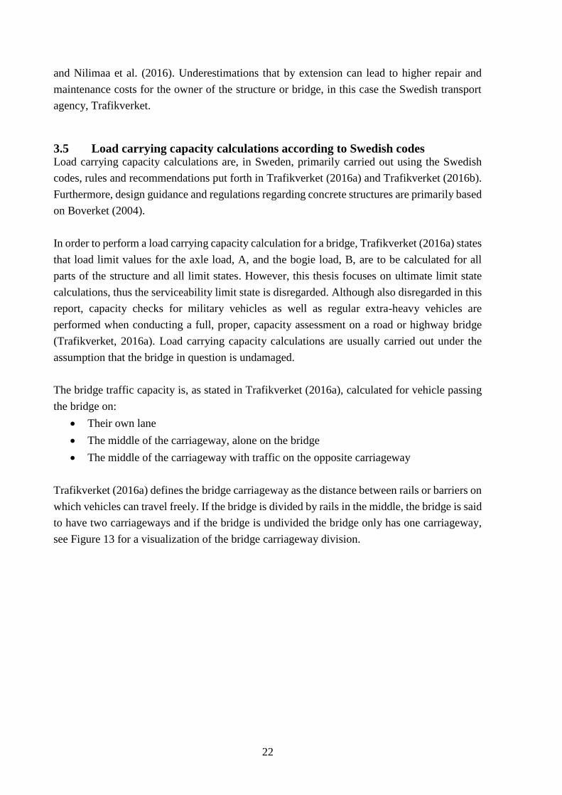
22
and Nilimaa et al. (2016). Underestimations that by extension can lead to higher repair and
maintenance costs for the owner of the structure or bridge, in this case the Swedish transport
agency, Trafikverket.
3.5 Load carrying capacity calculations according to Swedish codes Load carrying capacity calculations are, in Sweden, primarily carried out using the Swedish
codes, rules and recommendations put forth in Trafikverket (2016a) and Trafikverket (2016b).
Furthermore, design guidance and regulations regarding concrete structures are primarily based
on Boverket (2004).
In order to perform a load carrying capacity calculation for a bridge, Trafikverket (2016a) states
that load limit values for the axle load, A, and the bogie load, B, are to be calculated for all
parts of the structure and all limit states. However, this thesis focuses on ultimate limit state
calculations, thus the serviceability limit state is disregarded. Although also disregarded in this
report, capacity checks for military vehicles as well as regular extra-heavy vehicles are
performed when conducting a full, proper, capacity assessment on a road or highway bridge
(Trafikverket, 2016a). Load carrying capacity calculations are usually carried out under the
assumption that the bridge in question is undamaged.
The bridge traffic capacity is, as stated in Trafikverket (2016a), calculated for vehicle passing
the bridge on:
Their own lane
The middle of the carriageway, alone on the bridge
The middle of the carriageway with traffic on the opposite carriageway
Trafikverket (2016a) defines the bridge carriageway as the distance between rails or barriers on
which vehicles can travel freely. If the bridge is divided by rails in the middle, the bridge is said
to have two carriageways and if the bridge is undivided the bridge only has one carriageway,
see Figure 13 for a visualization of the bridge carriageway division.
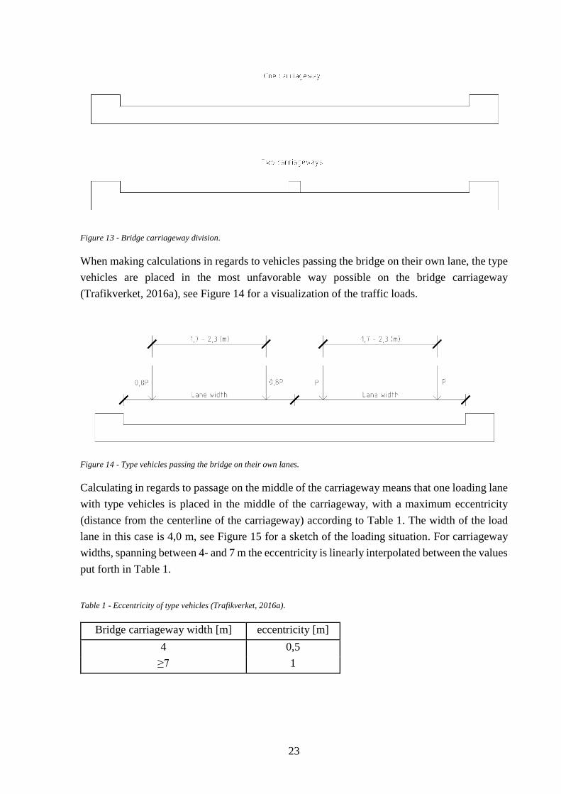
23
Figure 13 - Bridge carriageway division.
When making calculations in regards to vehicles passing the bridge on their own lane, the type
vehicles are placed in the most unfavorable way possible on the bridge carriageway
(Trafikverket, 2016a), see Figure 14 for a visualization of the traffic loads.
Figure 14 - Type vehicles passing the bridge on their own lanes.
Calculating in regards to passage on the middle of the carriageway means that one loading lane
with type vehicles is placed in the middle of the carriageway, with a maximum eccentricity
(distance from the centerline of the carriageway) according to Table 1. The width of the load
lane in this case is 4,0 m, see Figure 15 for a sketch of the loading situation. For carriageway
widths, spanning between 4- and 7 m the eccentricity is linearly interpolated between the values
put forth in Table 1.
Table 1 - Eccentricity of type vehicles (Trafikverket, 2016a).
Bridge carriageway width [m] eccentricity [m]
4 0,5
≥7 1
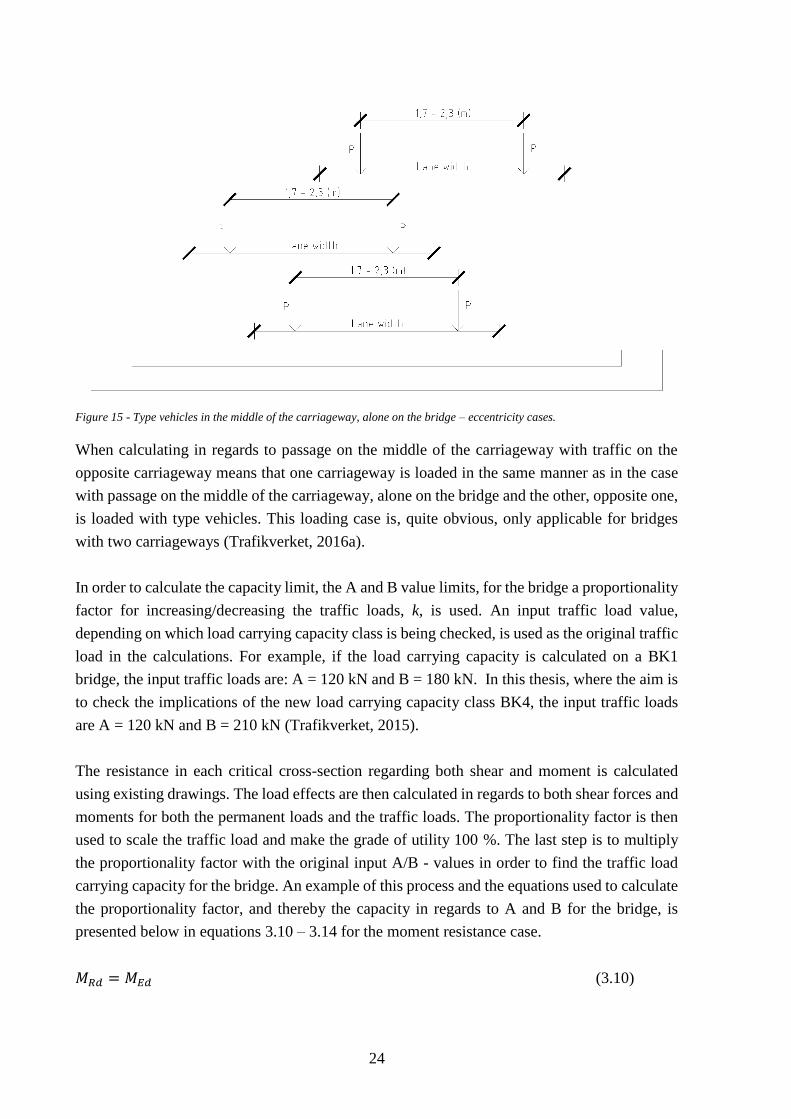
24
Figure 15 - Type vehicles in the middle of the carriageway, alone on the bridge – eccentricity cases.
When calculating in regards to passage on the middle of the carriageway with traffic on the
opposite carriageway means that one carriageway is loaded in the same manner as in the case
with passage on the middle of the carriageway, alone on the bridge and the other, opposite one,
is loaded with type vehicles. This loading case is, quite obvious, only applicable for bridges
with two carriageways (Trafikverket, 2016a).
In order to calculate the capacity limit, the A and B value limits, for the bridge a proportionality
factor for increasing/decreasing the traffic loads, k, is used. An input traffic load value,
depending on which load carrying capacity class is being checked, is used as the original traffic
load in the calculations. For example, if the load carrying capacity is calculated on a BK1
bridge, the input traffic loads are: A = 120 kN and B = 180 kN. In this thesis, where the aim is
to check the implications of the new load carrying capacity class BK4, the input traffic loads
are A = 120 kN and B = 210 kN (Trafikverket, 2015).
The resistance in each critical cross-section regarding both shear and moment is calculated
using existing drawings. The load effects are then calculated in regards to both shear forces and
moments for both the permanent loads and the traffic loads. The proportionality factor is then
used to scale the traffic load and make the grade of utility 100 %. The last step is to multiply
the proportionality factor with the original input A/B - values in order to find the traffic load
carrying capacity for the bridge. An example of this process and the equations used to calculate
the proportionality factor, and thereby the capacity in regards to A and B for the bridge, is
presented below in equations 3.10 – 3.14 for the moment resistance case.
𝑀𝑅𝑑 = 𝑀𝐸𝑑 (3.10)
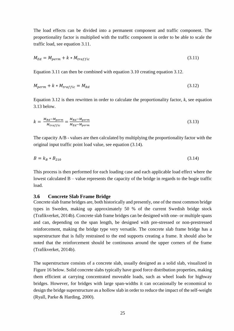
25
The load effects can be divided into a permanent component and traffic component. The
proportionality factor is multiplied with the traffic component in order to be able to scale the
traffic load, see equation 3.11.
𝑀𝐸𝑑 = 𝑀𝑝𝑒𝑟𝑚 + 𝑘 ∗ 𝑀𝑡𝑟𝑎𝑓𝑓𝑖𝑐 (3.11)
Equation 3.11 can then be combined with equation 3.10 creating equation 3.12.
𝑀𝑝𝑒𝑟𝑚 + 𝑘 ∗ 𝑀𝑡𝑟𝑎𝑓𝑓𝑖𝑐 = 𝑀𝑅𝑑 (3.12)
Equation 3.12 is then rewritten in order to calculate the proportionality factor, k, see equation
3.13 below.
𝑘 = 𝑀𝑅𝑑−𝑀𝑝𝑒𝑟𝑚
𝑀𝑡𝑟𝑎𝑓𝑓𝑖𝑐=
𝑀𝑅𝑑−𝑀𝑝𝑒𝑟𝑚
𝑀𝐸𝑑−𝑀𝑝𝑒𝑟𝑚 (3.13)
The capacity A/B - values are then calculated by multiplying the proportionality factor with the
original input traffic point load value, see equation (3.14).
𝐵 = 𝑘𝐵 ∗ 𝐵210 (3.14)
This process is then performed for each loading case and each applicable load effect where the
lowest calculated B – value represents the capacity of the bridge in regards to the bogie traffic
load.
3.6 Concrete Slab Frame Bridge Concrete slab frame bridges are, both historically and presently, one of the most common bridge
types in Sweden, making up approximately 50 % of the current Swedish bridge stock
(Trafikverket, 2014b). Concrete slab frame bridges can be designed with one- or multiple spans
and can, depending on the span length, be designed with pre-stressed or non-prestressed
reinforcement, making the bridge type very versatile. The concrete slab frame bridge has a
superstructure that is fully restrained to the end supports creating a frame. It should also be
noted that the reinforcement should be continuous around the upper corners of the frame
(Trafikverket, 2014b).
The superstructure consists of a concrete slab, usually designed as a solid slab, visualized in
Figure 16 below. Solid concrete slabs typically have good force distribution properties, making
them efficient at carrying concentrated moveable loads, such as wheel loads for highway
bridges. However, for bridges with large span-widths it can occasionally be economical to
design the bridge superstructure as a hollow slab in order to reduce the impact of the self-weight
(Ryall, Parke & Harding, 2000).
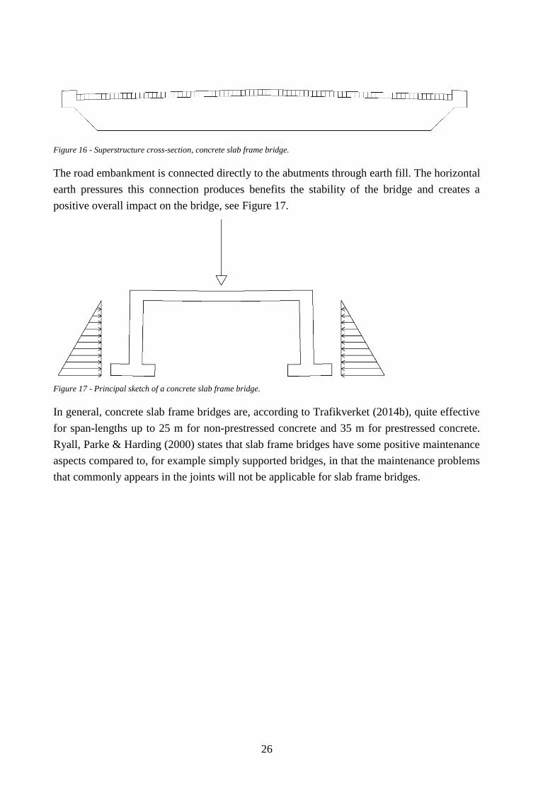
26
Figure 16 - Superstructure cross-section, concrete slab frame bridge.
The road embankment is connected directly to the abutments through earth fill. The horizontal
earth pressures this connection produces benefits the stability of the bridge and creates a
positive overall impact on the bridge, see Figure 17.
Figure 17 - Principal sketch of a concrete slab frame bridge.
In general, concrete slab frame bridges are, according to Trafikverket (2014b), quite effective
for span-lengths up to 25 m for non-prestressed concrete and 35 m for prestressed concrete.
Ryall, Parke & Harding (2000) states that slab frame bridges have some positive maintenance
aspects compared to, for example simply supported bridges, in that the maintenance problems
that commonly appears in the joints will not be applicable for slab frame bridges.
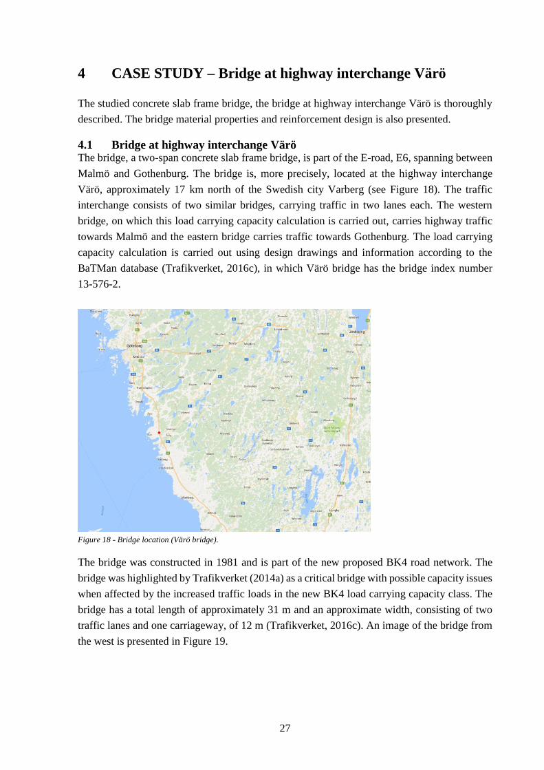
27
4 CASE STUDY – Bridge at highway interchange Värö
The studied concrete slab frame bridge, the bridge at highway interchange Värö is thoroughly
described. The bridge material properties and reinforcement design is also presented.
4.1 Bridge at highway interchange Värö The bridge, a two-span concrete slab frame bridge, is part of the E-road, E6, spanning between
Malmö and Gothenburg. The bridge is, more precisely, located at the highway interchange
Värö, approximately 17 km north of the Swedish city Varberg (see Figure 18). The traffic
interchange consists of two similar bridges, carrying traffic in two lanes each. The western
bridge, on which this load carrying capacity calculation is carried out, carries highway traffic
towards Malmö and the eastern bridge carries traffic towards Gothenburg. The load carrying
capacity calculation is carried out using design drawings and information according to the
BaTMan database (Trafikverket, 2016c), in which Värö bridge has the bridge index number
13-576-2.
Figure 18 - Bridge location (Värö bridge).
The bridge was constructed in 1981 and is part of the new proposed BK4 road network. The
bridge was highlighted by Trafikverket (2014a) as a critical bridge with possible capacity issues
when affected by the increased traffic loads in the new BK4 load carrying capacity class. The
bridge has a total length of approximately 31 m and an approximate width, consisting of two
traffic lanes and one carriageway, of 12 m (Trafikverket, 2016c). An image of the bridge from
the west is presented in Figure 19.
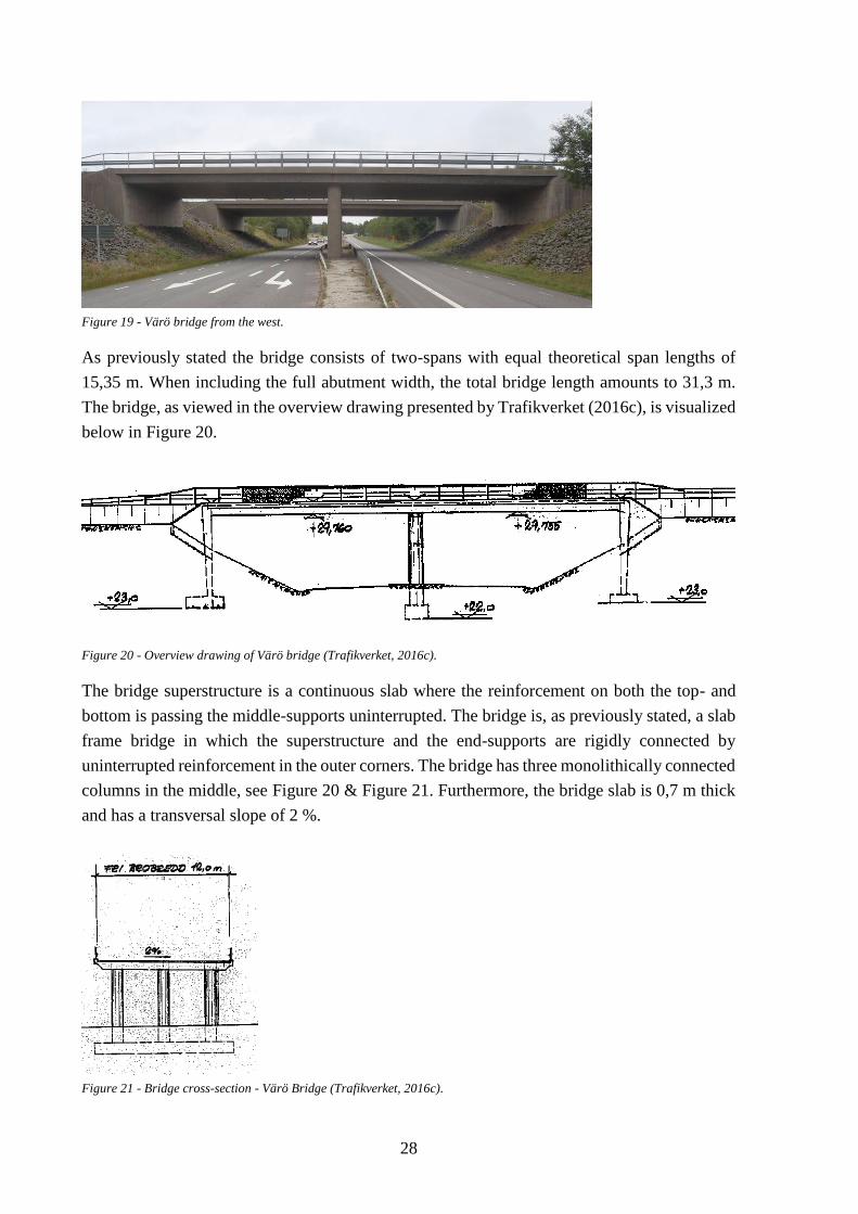
28
Figure 19 - Värö bridge from the west.
As previously stated the bridge consists of two-spans with equal theoretical span lengths of
15,35 m. When including the full abutment width, the total bridge length amounts to 31,3 m.
The bridge, as viewed in the overview drawing presented by Trafikverket (2016c), is visualized
below in Figure 20.
Figure 20 - Overview drawing of Värö bridge (Trafikverket, 2016c).
The bridge superstructure is a continuous slab where the reinforcement on both the top- and
bottom is passing the middle-supports uninterrupted. The bridge is, as previously stated, a slab
frame bridge in which the superstructure and the end-supports are rigidly connected by
uninterrupted reinforcement in the outer corners. The bridge has three monolithically connected
columns in the middle, see Figure 20 & Figure 21. Furthermore, the bridge slab is 0,7 m thick
and has a transversal slope of 2 %.
Figure 21 - Bridge cross-section - Värö Bridge (Trafikverket, 2016c).
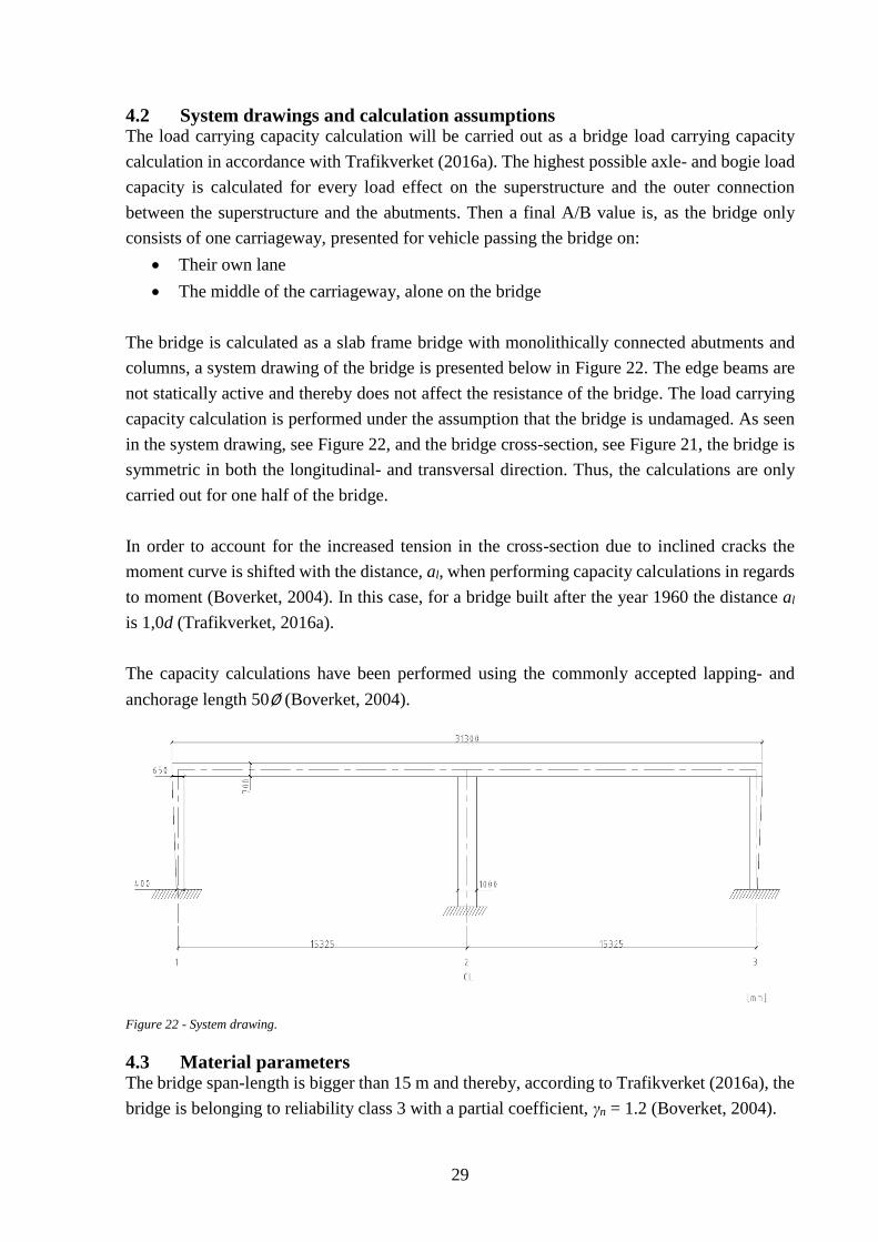
29
4.2 System drawings and calculation assumptions The load carrying capacity calculation will be carried out as a bridge load carrying capacity
calculation in accordance with Trafikverket (2016a). The highest possible axle- and bogie load
capacity is calculated for every load effect on the superstructure and the outer connection
between the superstructure and the abutments. Then a final A/B value is, as the bridge only
consists of one carriageway, presented for vehicle passing the bridge on:
Their own lane
The middle of the carriageway, alone on the bridge
The bridge is calculated as a slab frame bridge with monolithically connected abutments and
columns, a system drawing of the bridge is presented below in Figure 22. The edge beams are
not statically active and thereby does not affect the resistance of the bridge. The load carrying
capacity calculation is performed under the assumption that the bridge is undamaged. As seen
in the system drawing, see Figure 22, and the bridge cross-section, see Figure 21, the bridge is
symmetric in both the longitudinal- and transversal direction. Thus, the calculations are only
carried out for one half of the bridge.
In order to account for the increased tension in the cross-section due to inclined cracks the
moment curve is shifted with the distance, al, when performing capacity calculations in regards
to moment (Boverket, 2004). In this case, for a bridge built after the year 1960 the distance al
is 1,0d (Trafikverket, 2016a).
The capacity calculations have been performed using the commonly accepted lapping- and
anchorage length 50∅ (Boverket, 2004).
Figure 22 - System drawing.
4.3 Material parameters The bridge span-length is bigger than 15 m and thereby, according to Trafikverket (2016a), the
bridge is belonging to reliability class 3 with a partial coefficient, γn = 1.2 (Boverket, 2004).
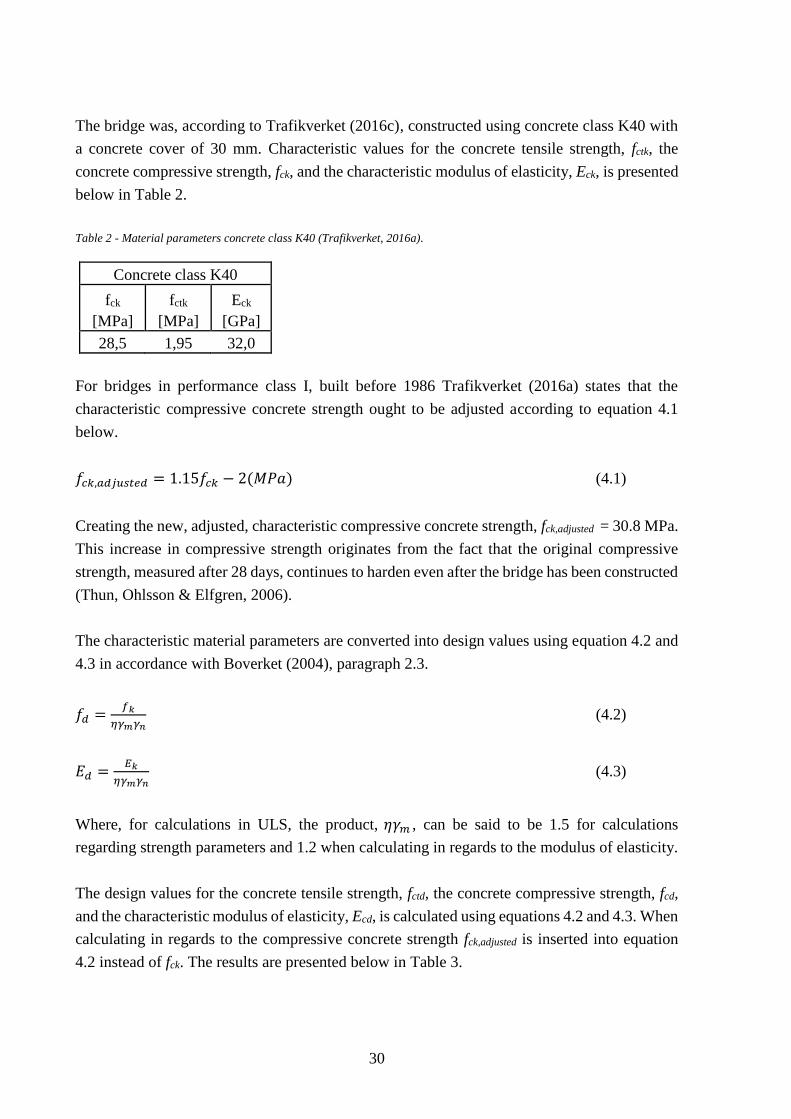
30
The bridge was, according to Trafikverket (2016c), constructed using concrete class K40 with
a concrete cover of 30 mm. Characteristic values for the concrete tensile strength, fctk, the
concrete compressive strength, fck, and the characteristic modulus of elasticity, Eck, is presented
below in Table 2.
Table 2 - Material parameters concrete class K40 (Trafikverket, 2016a).
Concrete class K40
fck fctk Eck
[MPa] [MPa] [GPa]
28,5 1,95 32,0
For bridges in performance class I, built before 1986 Trafikverket (2016a) states that the
characteristic compressive concrete strength ought to be adjusted according to equation 4.1
below.
𝑓𝑐𝑘,𝑎𝑑𝑗𝑢𝑠𝑡𝑒𝑑 = 1.15𝑓𝑐𝑘 − 2(𝑀𝑃𝑎) (4.1)
Creating the new, adjusted, characteristic compressive concrete strength, fck,adjusted = 30.8 MPa.
This increase in compressive strength originates from the fact that the original compressive
strength, measured after 28 days, continues to harden even after the bridge has been constructed
(Thun, Ohlsson & Elfgren, 2006).
The characteristic material parameters are converted into design values using equation 4.2 and
4.3 in accordance with Boverket (2004), paragraph 2.3.
𝑓𝑑 =𝑓𝑘
𝜂𝛾𝑚𝛾𝑛 (4.2)
𝐸𝑑 =𝐸𝑘
𝜂𝛾𝑚𝛾𝑛 (4.3)
Where, for calculations in ULS, the product, 𝜂𝛾𝑚 , can be said to be 1.5 for calculations
regarding strength parameters and 1.2 when calculating in regards to the modulus of elasticity.
The design values for the concrete tensile strength, fctd, the concrete compressive strength, fcd,
and the characteristic modulus of elasticity, Ecd, is calculated using equations 4.2 and 4.3. When
calculating in regards to the compressive concrete strength fck,adjusted is inserted into equation
4.2 instead of fck. The results are presented below in Table 3.
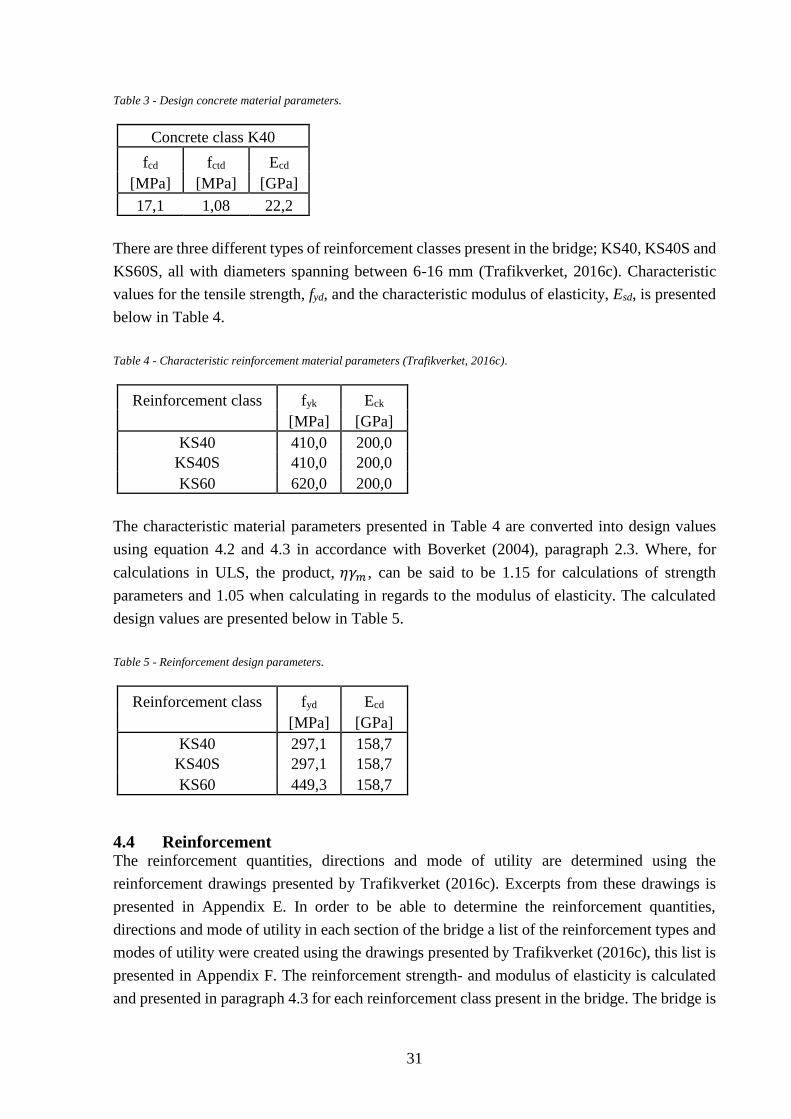
31
Table 3 - Design concrete material parameters.
Concrete class K40
fcd fctd Ecd
[MPa] [MPa] [GPa]
17,1 1,08 22,2
There are three different types of reinforcement classes present in the bridge; KS40, KS40S and
KS60S, all with diameters spanning between 6-16 mm (Trafikverket, 2016c). Characteristic
values for the tensile strength, fyd, and the characteristic modulus of elasticity, Esd, is presented
below in Table 4.
Table 4 - Characteristic reinforcement material parameters (Trafikverket, 2016c).
Reinforcement class fyk Eck
[MPa] [GPa]
KS40 410,0 200,0
KS40S 410,0 200,0
KS60 620,0 200,0
The characteristic material parameters presented in Table 4 are converted into design values
using equation 4.2 and 4.3 in accordance with Boverket (2004), paragraph 2.3. Where, for
calculations in ULS, the product, 𝜂𝛾𝑚 , can be said to be 1.15 for calculations of strength
parameters and 1.05 when calculating in regards to the modulus of elasticity. The calculated
design values are presented below in Table 5.
Table 5 - Reinforcement design parameters.
Reinforcement class fyd Ecd
[MPa] [GPa]
KS40 297,1 158,7
KS40S 297,1 158,7
KS60 449,3 158,7
4.4 Reinforcement The reinforcement quantities, directions and mode of utility are determined using the
reinforcement drawings presented by Trafikverket (2016c). Excerpts from these drawings is
presented in Appendix E. In order to be able to determine the reinforcement quantities,
directions and mode of utility in each section of the bridge a list of the reinforcement types and
modes of utility were created using the drawings presented by Trafikverket (2016c), this list is
presented in Appendix F. The reinforcement strength- and modulus of elasticity is calculated
and presented in paragraph 4.3 for each reinforcement class present in the bridge. The bridge is
32
shear reinforced on a 4,6 m wide strip over the column supports in the middle of the bridge, see
the dashed area on Figure 23 below. The rest of the bridge has no shear reinforcement.
Figure 23 - Shear force reinforcement distribution (Trafikverket, 2016c).
The reinforcement in the connection between the slab and the abutments is presented in Figure
24 and Appendix F, where the indexes, diameters and s-distances of the bars is presented. The
reinforcement is uninterrupted over the corner of the connection, thereby making sure that the
bridge exhibits the structural properties of a slab frame bridge.
Figure 24 - Reinforcement - connection between abutment and slab (Trafikverket, 2016c).
In order to be able to model the bridge accurately in regards to orthotropic and isotropic material
behavior, further discussed and explained in paragraph 3.3.1, the transversal- and longitudinal
reinforcement quantities were summarized and the quotient between the transversal- and
longitudinal reinforcement were calculated, see Table 6.
Table 6 - Transversal and longitudinal reinforcement quantities (Trafikverket, 2016c).
Reinforcement quantities As,tot Distribution width

33
[mm2/m] [m]
Transversal reinforcement span 1131 13,325
Transversal reinforcement support 3035 2
Mean transversal reinforcement 1379 15,325
Longitudinal reinforcement span 3657 13,325
Longitudinal reinforcement support 5054 2
Mean longitudinal reinforcement 3839 15,325
When dividing the mean longitudinal reinforcement with the mean transversal reinforcement
the quotient between them is 2,8. Thus, there is, on average, 2,8 times more reinforcement in
the longitudinal direction compared with the transversal direction, information that will be used
later on when modelling the BRIGADE/Standard model.
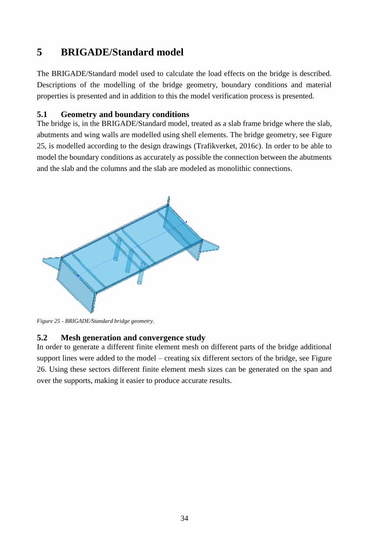
34
5 BRIGADE/Standard model
The BRIGADE/Standard model used to calculate the load effects on the bridge is described.
Descriptions of the modelling of the bridge geometry, boundary conditions and material
properties is presented and in addition to this the model verification process is presented.
5.1 Geometry and boundary conditions The bridge is, in the BRIGADE/Standard model, treated as a slab frame bridge where the slab,
abutments and wing walls are modelled using shell elements. The bridge geometry, see Figure
25, is modelled according to the design drawings (Trafikverket, 2016c). In order to be able to
model the boundary conditions as accurately as possible the connection between the abutments
and the slab and the columns and the slab are modeled as monolithic connections.
Figure 25 - BRIGADE/Standard bridge geometry.
5.2 Mesh generation and convergence study In order to generate a different finite element mesh on different parts of the bridge additional
support lines were added to the model – creating six different sectors of the bridge, see Figure
26. Using these sectors different finite element mesh sizes can be generated on the span and
over the supports, making it easier to produce accurate results.
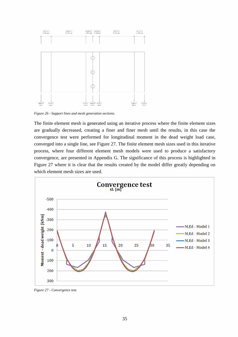
35
Figure 26 - Support lines and mesh generation sections.
The finite element mesh is generated using an iterative process where the finite element sizes
are gradually decreased, creating a finer and finer mesh until the results, in this case the
convergence test were performed for longitudinal moment in the dead weight load case,
converged into a single line, see Figure 27. The finite element mesh sizes used in this iterative
process, where four different element mesh models were used to produce a satisfactory
convergence, are presented in Appendix G. The significance of this process is highlighted in
Figure 27 where it is clear that the results created by the model differ greatly depending on
which element mesh sizes are used.
Figure 27 - Convergence test.
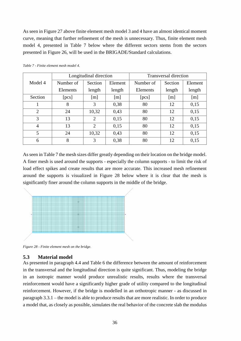
36
As seen in Figure 27 above finite element mesh model 3 and 4 have an almost identical moment
curve, meaning that further refinement of the mesh is unnecessary. Thus, finite element mesh
model 4, presented in Table 7 below where the different sectors stems from the sectors
presented in Figure 26, will be used in the BRIGADE/Standard calculations.
Table 7 - Finite element mesh model 4.
Model 4
Longitudinal direction Transversal direction
Number of
Elements
Section
length
Element
length
Number of
Elements
Section
length
Element
length
Section [pcs] [m] [m] [pcs] [m] [m]
1 8 3 0,38 80 12 0,15
2 24 10,32 0,43 80 12 0,15
3 13 2 0,15 80 12 0,15
4 13 2 0,15 80 12 0,15
5 24 10,32 0,43 80 12 0,15
6 8 3 0,38 80 12 0,15
As seen in Table 7 the mesh sizes differ greatly depending on their location on the bridge model.
A finer mesh is used around the supports - especially the column supports - to limit the risk of
load effect spikes and create results that are more accurate. This increased mesh refinement
around the supports is visualized in Figure 28 below where it is clear that the mesh is
significantly finer around the column supports in the middle of the bridge.
Figure 28 - Finite element mesh on the bridge.
5.3 Material model As presented in paragraph 4.4 and Table 6 the difference between the amount of reinforcement
in the transversal and the longitudinal direction is quite significant. Thus, modeling the bridge
in an isotropic manner would produce unrealistic results, results where the transversal
reinforcement would have a significantly higher grade of utility compared to the longitudinal
reinforcement. However, if the bridge is modelled in an orthotropic manner - as discussed in
paragraph 3.3.1 – the model is able to produce results that are more realistic. In order to produce
a model that, as closely as possible, simulates the real behavior of the concrete slab the modulus
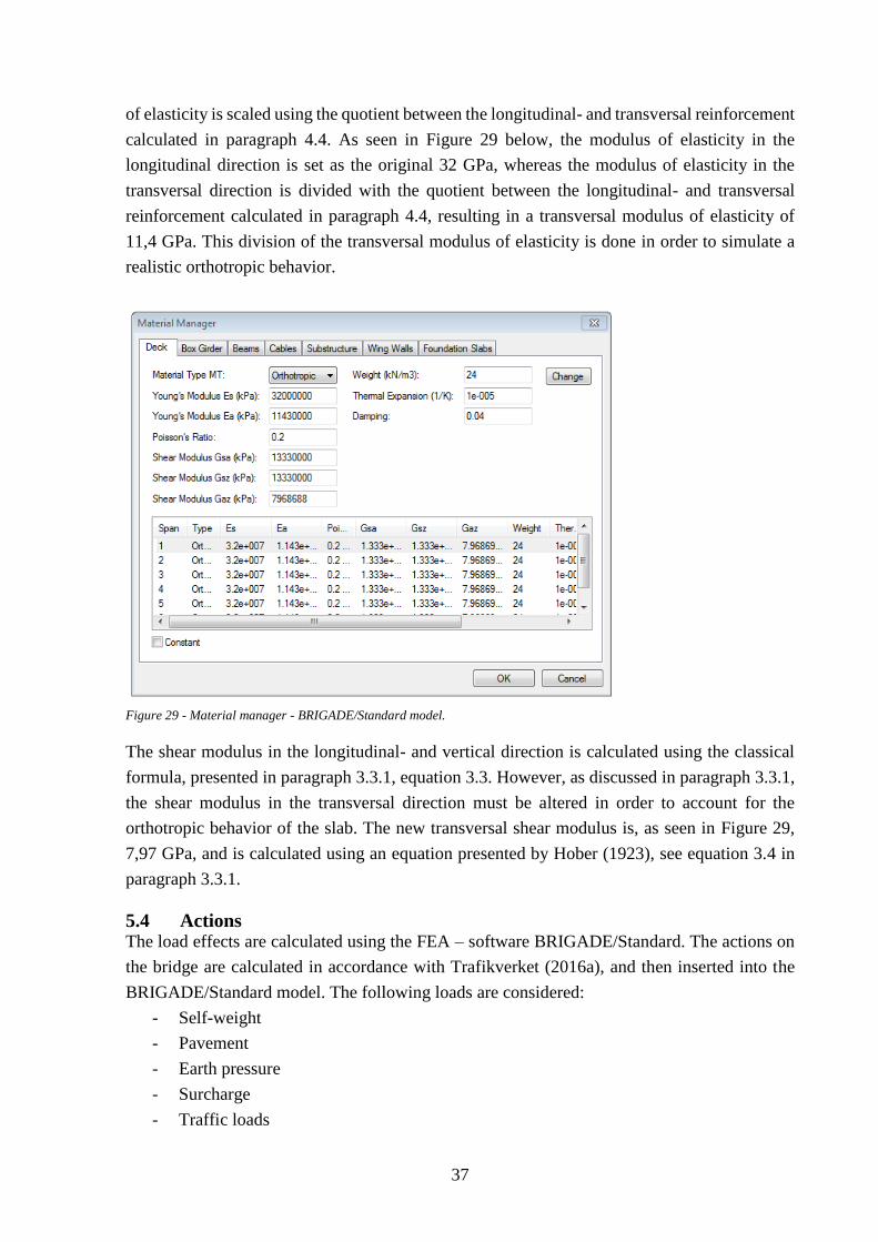
37
of elasticity is scaled using the quotient between the longitudinal- and transversal reinforcement
calculated in paragraph 4.4. As seen in Figure 29 below, the modulus of elasticity in the
longitudinal direction is set as the original 32 GPa, whereas the modulus of elasticity in the
transversal direction is divided with the quotient between the longitudinal- and transversal
reinforcement calculated in paragraph 4.4, resulting in a transversal modulus of elasticity of
11,4 GPa. This division of the transversal modulus of elasticity is done in order to simulate a
realistic orthotropic behavior.
Figure 29 - Material manager - BRIGADE/Standard model.
The shear modulus in the longitudinal- and vertical direction is calculated using the classical
formula, presented in paragraph 3.3.1, equation 3.3. However, as discussed in paragraph 3.3.1,
the shear modulus in the transversal direction must be altered in order to account for the
orthotropic behavior of the slab. The new transversal shear modulus is, as seen in Figure 29,
7,97 GPa, and is calculated using an equation presented by Hober (1923), see equation 3.4 in
paragraph 3.3.1.
5.4 Actions The load effects are calculated using the FEA – software BRIGADE/Standard. The actions on
the bridge are calculated in accordance with Trafikverket (2016a), and then inserted into the
BRIGADE/Standard model. The following loads are considered:
- Self-weight
- Pavement
- Earth pressure
- Surcharge
- Traffic loads
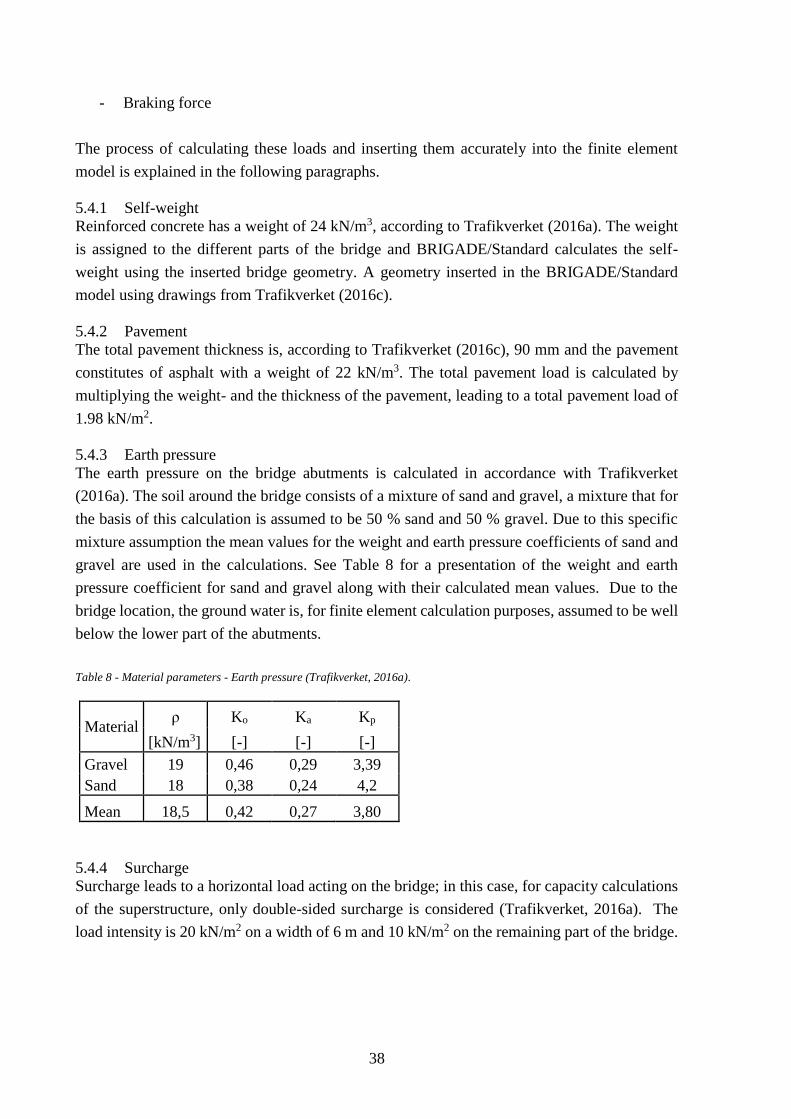
38
- Braking force
The process of calculating these loads and inserting them accurately into the finite element
model is explained in the following paragraphs.
5.4.1 Self-weight
Reinforced concrete has a weight of 24 kN/m3, according to Trafikverket (2016a). The weight
is assigned to the different parts of the bridge and BRIGADE/Standard calculates the self-
weight using the inserted bridge geometry. A geometry inserted in the BRIGADE/Standard
model using drawings from Trafikverket (2016c).
5.4.2 Pavement
The total pavement thickness is, according to Trafikverket (2016c), 90 mm and the pavement
constitutes of asphalt with a weight of 22 kN/m3. The total pavement load is calculated by
multiplying the weight- and the thickness of the pavement, leading to a total pavement load of
1.98 kN/m2.
5.4.3 Earth pressure
The earth pressure on the bridge abutments is calculated in accordance with Trafikverket
(2016a). The soil around the bridge consists of a mixture of sand and gravel, a mixture that for
the basis of this calculation is assumed to be 50 % sand and 50 % gravel. Due to this specific
mixture assumption the mean values for the weight and earth pressure coefficients of sand and
gravel are used in the calculations. See Table 8 for a presentation of the weight and earth
pressure coefficient for sand and gravel along with their calculated mean values. Due to the
bridge location, the ground water is, for finite element calculation purposes, assumed to be well
below the lower part of the abutments.
Table 8 - Material parameters - Earth pressure (Trafikverket, 2016a).
Material ρ Ko Ka Kp
[kN/m3] [-] [-] [-]
Gravel 19 0,46 0,29 3,39
Sand 18 0,38 0,24 4,2
Mean 18,5 0,42 0,27 3,80
5.4.4 Surcharge
Surcharge leads to a horizontal load acting on the bridge; in this case, for capacity calculations
of the superstructure, only double-sided surcharge is considered (Trafikverket, 2016a). The
load intensity is 20 kN/m2 on a width of 6 m and 10 kN/m2 on the remaining part of the bridge.
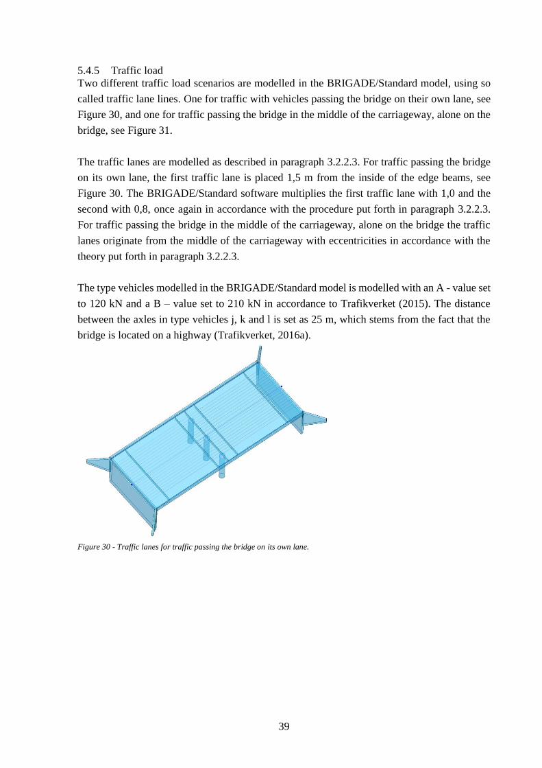
39
5.4.5 Traffic load
Two different traffic load scenarios are modelled in the BRIGADE/Standard model, using so
called traffic lane lines. One for traffic with vehicles passing the bridge on their own lane, see
Figure 30, and one for traffic passing the bridge in the middle of the carriageway, alone on the
bridge, see Figure 31.
The traffic lanes are modelled as described in paragraph 3.2.2.3. For traffic passing the bridge
on its own lane, the first traffic lane is placed 1,5 m from the inside of the edge beams, see
Figure 30. The BRIGADE/Standard software multiplies the first traffic lane with 1,0 and the
second with 0,8, once again in accordance with the procedure put forth in paragraph 3.2.2.3.
For traffic passing the bridge in the middle of the carriageway, alone on the bridge the traffic
lanes originate from the middle of the carriageway with eccentricities in accordance with the
theory put forth in paragraph 3.2.2.3.
The type vehicles modelled in the BRIGADE/Standard model is modelled with an A - value set
to 120 kN and a B – value set to 210 kN in accordance to Trafikverket (2015). The distance
between the axles in type vehicles j, k and l is set as 25 m, which stems from the fact that the
bridge is located on a highway (Trafikverket, 2016a).
Figure 30 - Traffic lanes for traffic passing the bridge on its own lane.
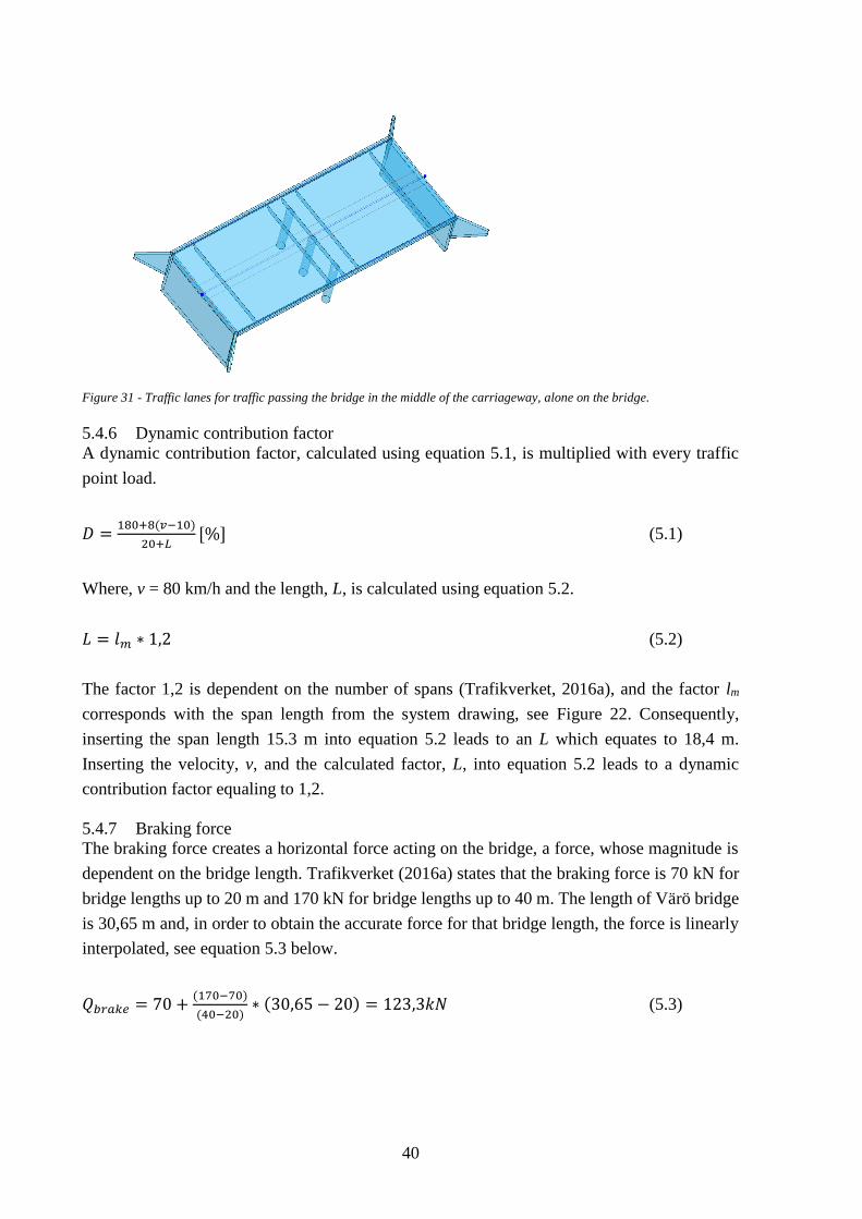
40
Figure 31 - Traffic lanes for traffic passing the bridge in the middle of the carriageway, alone on the bridge.
5.4.6 Dynamic contribution factor
A dynamic contribution factor, calculated using equation 5.1, is multiplied with every traffic
point load.
𝐷 =180+8(𝑣−10)
20+𝐿[%] (5.1)
Where, v = 80 km/h and the length, L, is calculated using equation 5.2.
𝐿 = 𝑙𝑚 ∗ 1,2 (5.2)
The factor 1,2 is dependent on the number of spans (Trafikverket, 2016a), and the factor lm
corresponds with the span length from the system drawing, see Figure 22. Consequently,
inserting the span length 15.3 m into equation 5.2 leads to an L which equates to 18,4 m.
Inserting the velocity, v, and the calculated factor, L, into equation 5.2 leads to a dynamic
contribution factor equaling to 1,2.
5.4.7 Braking force
The braking force creates a horizontal force acting on the bridge, a force, whose magnitude is
dependent on the bridge length. Trafikverket (2016a) states that the braking force is 70 kN for
bridge lengths up to 20 m and 170 kN for bridge lengths up to 40 m. The length of Värö bridge
is 30,65 m and, in order to obtain the accurate force for that bridge length, the force is linearly
interpolated, see equation 5.3 below.
𝑄𝑏𝑟𝑎𝑘𝑒 = 70 +(170−70)
(40−20)∗ (30,65 − 20) = 123,3𝑘𝑁 (5.3)
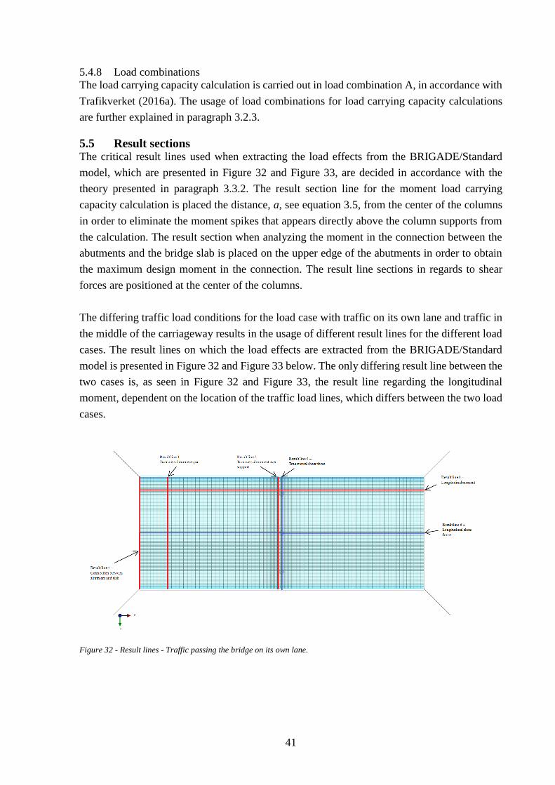
41
5.4.8 Load combinations
The load carrying capacity calculation is carried out in load combination A, in accordance with
Trafikverket (2016a). The usage of load combinations for load carrying capacity calculations
are further explained in paragraph 3.2.3.
5.5 Result sections The critical result lines used when extracting the load effects from the BRIGADE/Standard
model, which are presented in Figure 32 and Figure 33, are decided in accordance with the
theory presented in paragraph 3.3.2. The result section line for the moment load carrying
capacity calculation is placed the distance, a, see equation 3.5, from the center of the columns
in order to eliminate the moment spikes that appears directly above the column supports from
the calculation. The result section when analyzing the moment in the connection between the
abutments and the bridge slab is placed on the upper edge of the abutments in order to obtain
the maximum design moment in the connection. The result line sections in regards to shear
forces are positioned at the center of the columns.
The differing traffic load conditions for the load case with traffic on its own lane and traffic in
the middle of the carriageway results in the usage of different result lines for the different load
cases. The result lines on which the load effects are extracted from the BRIGADE/Standard
model is presented in Figure 32 and Figure 33 below. The only differing result line between the
two cases is, as seen in Figure 32 and Figure 33, the result line regarding the longitudinal
moment, dependent on the location of the traffic load lines, which differs between the two load
cases.
Figure 32 - Result lines - Traffic passing the bridge on its own lane.
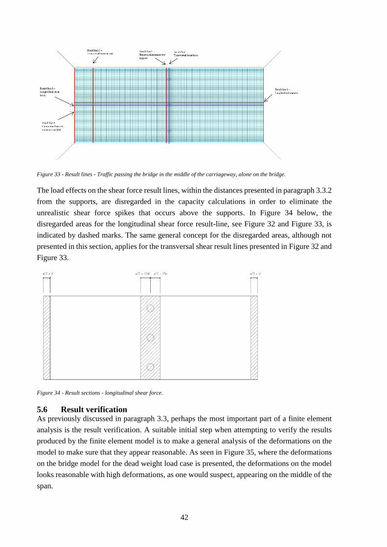
42
Figure 33 - Result lines - Traffic passing the bridge in the middle of the carriageway, alone on the bridge.
The load effects on the shear force result lines, within the distances presented in paragraph 3.3.2
from the supports, are disregarded in the capacity calculations in order to eliminate the
unrealistic shear force spikes that occurs above the supports. In Figure 34 below, the
disregarded areas for the longitudinal shear force result-line, see Figure 32 and Figure 33, is
indicated by dashed marks. The same general concept for the disregarded areas, although not
presented in this section, applies for the transversal shear result lines presented in Figure 32 and
Figure 33.
Figure 34 - Result sections - longitudinal shear force.
5.6 Result verification As previously discussed in paragraph 3.3, perhaps the most important part of a finite element
analysis is the result verification. A suitable initial step when attempting to verify the results
produced by the finite element model is to make a general analysis of the deformations on the
model to make sure that they appear reasonable. As seen in Figure 35, where the deformations
on the bridge model for the dead weight load case is presented, the deformations on the model
looks reasonable with high deformations, as one would suspect, appearing on the middle of the
span.
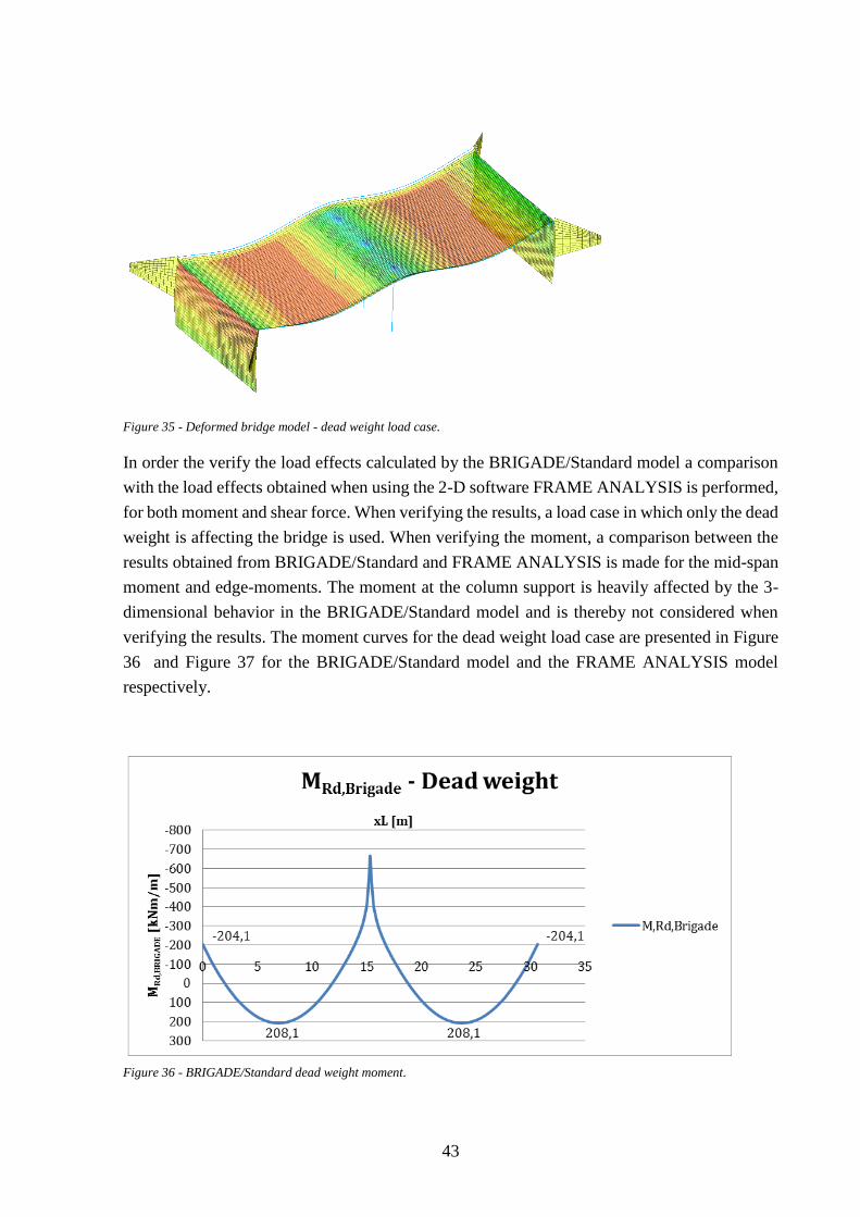
43
Figure 35 - Deformed bridge model - dead weight load case.
In order the verify the load effects calculated by the BRIGADE/Standard model a comparison
with the load effects obtained when using the 2-D software FRAME ANALYSIS is performed,
for both moment and shear force. When verifying the results, a load case in which only the dead
weight is affecting the bridge is used. When verifying the moment, a comparison between the
results obtained from BRIGADE/Standard and FRAME ANALYSIS is made for the mid-span
moment and edge-moments. The moment at the column support is heavily affected by the 3-
dimensional behavior in the BRIGADE/Standard model and is thereby not considered when
verifying the results. The moment curves for the dead weight load case are presented in Figure
36 and Figure 37 for the BRIGADE/Standard model and the FRAME ANALYSIS model
respectively.
Figure 36 - BRIGADE/Standard dead weight moment.
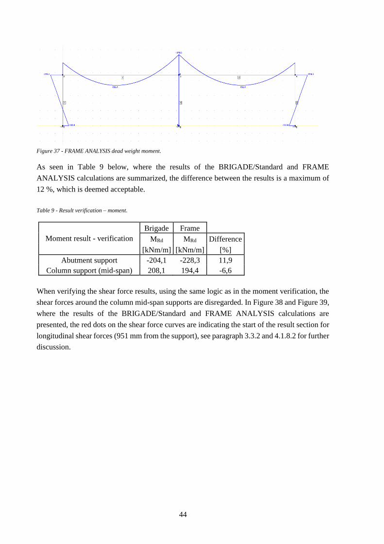
44
Figure 37 - FRAME ANALYSIS dead weight moment.
As seen in Table 9 below, where the results of the BRIGADE/Standard and FRAME
ANALYSIS calculations are summarized, the difference between the results is a maximum of
12 %, which is deemed acceptable.
Table 9 - Result verification – moment.
Moment result - verification
Brigade Frame
MRd MRd Difference
[kNm/m] [kNm/m] [%]
Abutment support -204,1 -228,3 11,9
Column support (mid-span) 208,1 194,4 -6,6
When verifying the shear force results, using the same logic as in the moment verification, the
shear forces around the column mid-span supports are disregarded. In Figure 38 and Figure 39,
where the results of the BRIGADE/Standard and FRAME ANALYSIS calculations are
presented, the red dots on the shear force curves are indicating the start of the result section for
longitudinal shear forces (951 mm from the support), see paragraph 3.3.2 and 4.1.8.2 for further
discussion.
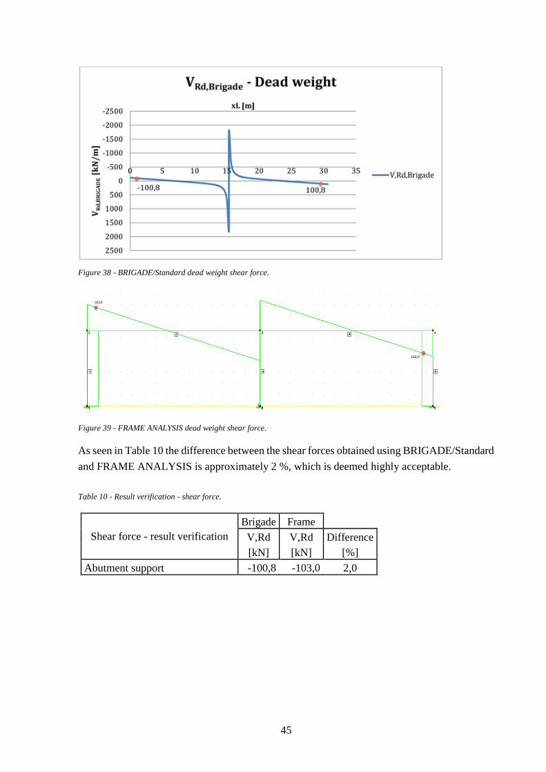
45
Figure 38 - BRIGADE/Standard dead weight shear force.
Figure 39 - FRAME ANALYSIS dead weight shear force.
As seen in Table 10 the difference between the shear forces obtained using BRIGADE/Standard
and FRAME ANALYSIS is approximately 2 %, which is deemed highly acceptable.
Table 10 - Result verification - shear force.
Shear force - result verification
Brigade Frame
V,Rd V,Rd Difference
[kN] [kN] [%]
Abutment support -100,8 -103,0 2,0
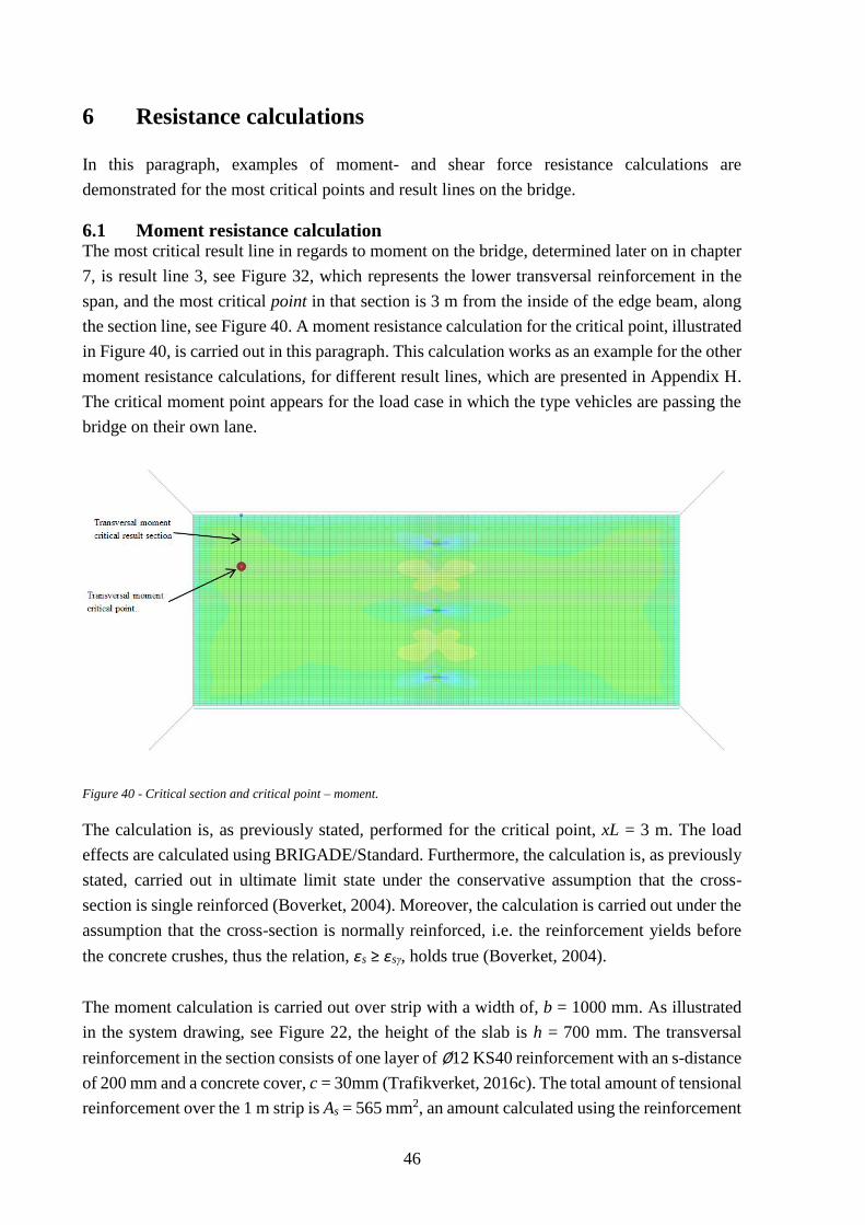
46
6 Resistance calculations
In this paragraph, examples of moment- and shear force resistance calculations are
demonstrated for the most critical points and result lines on the bridge.
6.1 Moment resistance calculation The most critical result line in regards to moment on the bridge, determined later on in chapter
7, is result line 3, see Figure 32, which represents the lower transversal reinforcement in the
span, and the most critical point in that section is 3 m from the inside of the edge beam, along
the section line, see Figure 40. A moment resistance calculation for the critical point, illustrated
in Figure 40, is carried out in this paragraph. This calculation works as an example for the other
moment resistance calculations, for different result lines, which are presented in Appendix H.
The critical moment point appears for the load case in which the type vehicles are passing the
bridge on their own lane.
Figure 40 - Critical section and critical point – moment.
The calculation is, as previously stated, performed for the critical point, xL = 3 m. The load
effects are calculated using BRIGADE/Standard. Furthermore, the calculation is, as previously
stated, carried out in ultimate limit state under the conservative assumption that the cross-
section is single reinforced (Boverket, 2004). Moreover, the calculation is carried out under the
assumption that the cross-section is normally reinforced, i.e. the reinforcement yields before
the concrete crushes, thus the relation, εs ≥ εsγ, holds true (Boverket, 2004).
The moment calculation is carried out over strip with a width of, b = 1000 mm. As illustrated
in the system drawing, see Figure 22, the height of the slab is h = 700 mm. The transversal
reinforcement in the section consists of one layer of ∅12 KS40 reinforcement with an s-distance
of 200 mm and a concrete cover, c = 30mm (Trafikverket, 2016c). The total amount of tensional
reinforcement over the 1 m strip is As = 565 mm2, an amount calculated using the reinforcement
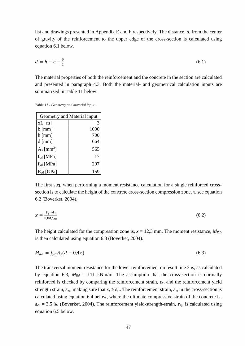
47
list and drawings presented in Appendix E and F respectively. The distance, d, from the center
of gravity of the reinforcement to the upper edge of the cross-section is calculated using
equation 6.1 below.
𝑑 = ℎ − 𝑐 −∅
2 (6.1)
The material properties of both the reinforcement and the concrete in the section are calculated
and presented in paragraph 4.3. Both the material- and geometrical calculation inputs are
summarized in Table 11 below.
Table 11 - Geometry and material input.
Geometry and Material input
xL [m] 3
b [mm] 1000
h [mm] 700
d [mm] 664
As [mm2] 565
fcd [MPa] 17
fyd [MPa] 297
Ecd [GPa] 159
The first step when performing a moment resistance calculation for a single reinforced cross-
section is to calculate the height of the concrete cross-section compression zone, x, see equation
6.2 (Boverket, 2004).
𝑥 =𝑓𝑦𝑑𝐴𝑠
0,8𝑏𝑓𝑐𝑑 (6.2)
The height calculated for the compression zone is, x = 12,3 mm. The moment resistance, MRd,
is then calculated using equation 6.3 (Boverket, 2004).
𝑀𝑅𝑑 = 𝑓𝑦𝑑𝐴𝑠(𝑑 − 0,4𝑥) (6.3)
The transversal moment resistance for the lower reinforcement on result line 3 is, as calculated
by equation 6.3, MRd = 111 kNm/m. The assumption that the cross-section is normally
reinforced is checked by comparing the reinforcement strain, εs, and the reinforcement yield
strength strain, εsγ, making sure that εs ≥ εsγ. The reinforcement strain, εs, in the cross-section is
calculated using equation 6.4 below, where the ultimate compressive strain of the concrete is,
εcu = 3,5 ‰ (Boverket, 2004). The reinforcement yield-strength-strain, εsγ, is calculated using
equation 6.5 below.
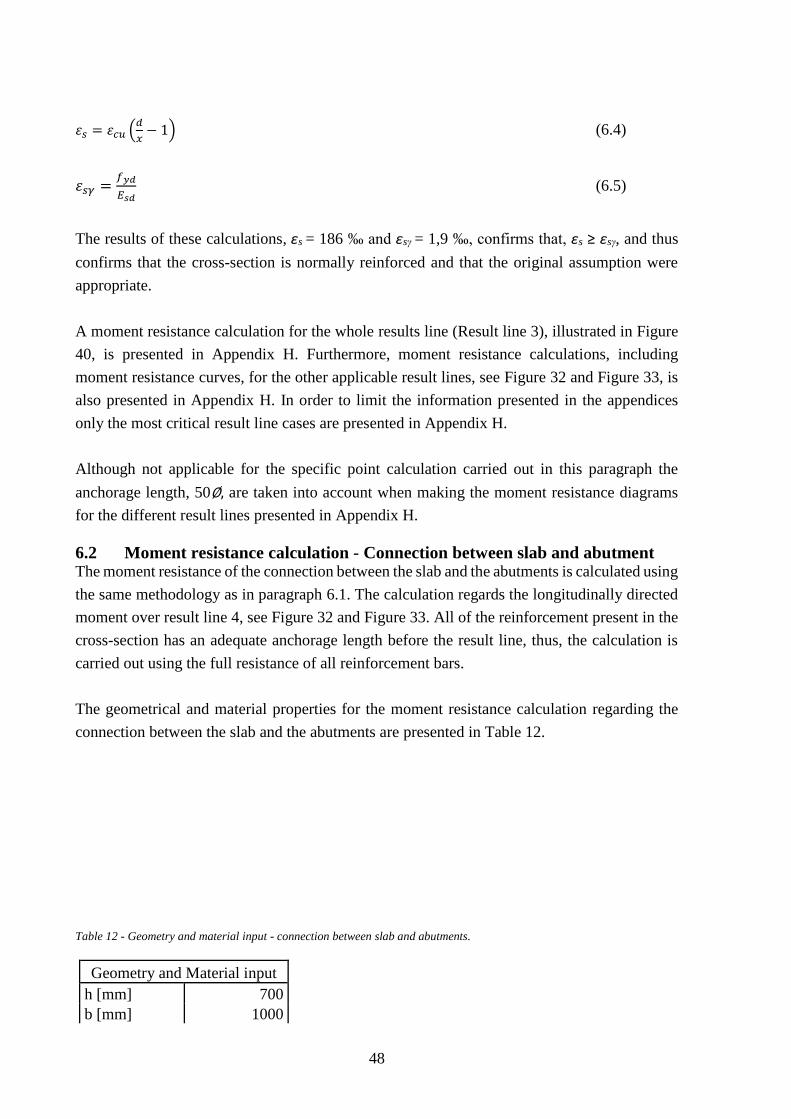
48
𝜀𝑠 = 𝜀𝑐𝑢 (𝑑
𝑥− 1) (6.4)
𝜀𝑠𝛾 =𝑓𝑦𝑑
𝐸𝑠𝑑 (6.5)
The results of these calculations, εs = 186 ‰ and εsγ = 1,9 ‰, confirms that, εs ≥ εsγ, and thus
confirms that the cross-section is normally reinforced and that the original assumption were
appropriate.
A moment resistance calculation for the whole results line (Result line 3), illustrated in Figure
40, is presented in Appendix H. Furthermore, moment resistance calculations, including
moment resistance curves, for the other applicable result lines, see Figure 32 and Figure 33, is
also presented in Appendix H. In order to limit the information presented in the appendices
only the most critical result line cases are presented in Appendix H.
Although not applicable for the specific point calculation carried out in this paragraph the
anchorage length, 50∅, are taken into account when making the moment resistance diagrams
for the different result lines presented in Appendix H.
6.2 Moment resistance calculation - Connection between slab and abutment The moment resistance of the connection between the slab and the abutments is calculated using
the same methodology as in paragraph 6.1. The calculation regards the longitudinally directed
moment over result line 4, see Figure 32 and Figure 33. All of the reinforcement present in the
cross-section has an adequate anchorage length before the result line, thus, the calculation is
carried out using the full resistance of all reinforcement bars.
The geometrical and material properties for the moment resistance calculation regarding the
connection between the slab and the abutments are presented in Table 12.
Table 12 - Geometry and material input - connection between slab and abutments.
Geometry and Material input
h [mm] 700
b [mm] 1000
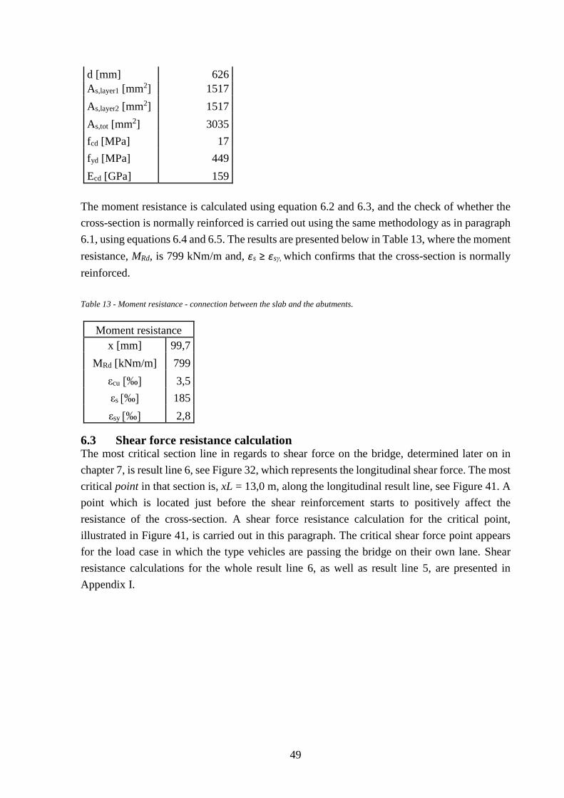
49
d [mm] 626
As,layer1 [mm2] 1517
As,layer2 [mm2] 1517
As,tot [mm2] 3035
fcd [MPa] 17
fyd [MPa] 449
Ecd [GPa] 159
The moment resistance is calculated using equation 6.2 and 6.3, and the check of whether the
cross-section is normally reinforced is carried out using the same methodology as in paragraph
6.1, using equations 6.4 and 6.5. The results are presented below in Table 13, where the moment
resistance, MRd, is 799 kNm/m and, εs ≥ εsγ, which confirms that the cross-section is normally
reinforced.
Table 13 - Moment resistance - connection between the slab and the abutments.
Moment resistance
x [mm] 99,7
MRd [kNm/m] 799
εcu [‰] 3,5
εs [‰] 185
εsy [‰] 2,8
6.3 Shear force resistance calculation The most critical section line in regards to shear force on the bridge, determined later on in
chapter 7, is result line 6, see Figure 32, which represents the longitudinal shear force. The most
critical point in that section is, xL = 13,0 m, along the longitudinal result line, see Figure 41. A
point which is located just before the shear reinforcement starts to positively affect the
resistance of the cross-section. A shear force resistance calculation for the critical point,
illustrated in Figure 41, is carried out in this paragraph. The critical shear force point appears
for the load case in which the type vehicles are passing the bridge on their own lane. Shear
resistance calculations for the whole result line 6, as well as result line 5, are presented in
Appendix I.
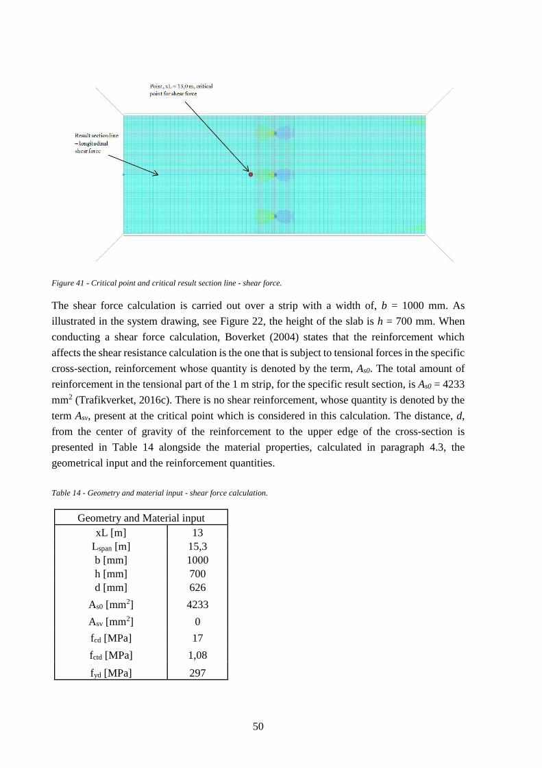
50
Figure 41 - Critical point and critical result section line - shear force.
The shear force calculation is carried out over a strip with a width of, b = 1000 mm. As
illustrated in the system drawing, see Figure 22, the height of the slab is h = 700 mm. When
conducting a shear force calculation, Boverket (2004) states that the reinforcement which
affects the shear resistance calculation is the one that is subject to tensional forces in the specific
cross-section, reinforcement whose quantity is denoted by the term, As0. The total amount of
reinforcement in the tensional part of the 1 m strip, for the specific result section, is As0 = 4233
mm2 (Trafikverket, 2016c). There is no shear reinforcement, whose quantity is denoted by the
term Asv, present at the critical point which is considered in this calculation. The distance, d,
from the center of gravity of the reinforcement to the upper edge of the cross-section is
presented in Table 14 alongside the material properties, calculated in paragraph 4.3, the
geometrical input and the reinforcement quantities.
Table 14 - Geometry and material input - shear force calculation.
Geometry and Material input
xL [m] 13
Lspan [m] 15,3
b [mm] 1000
h [mm] 700
d [mm] 626
As0 [mm2] 4233
Asv [mm2] 0
fcd [MPa] 17
fctd [MPa] 1,08
fyd [MPa] 297
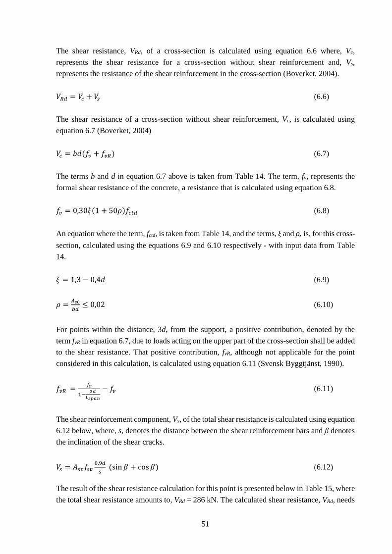
51
The shear resistance, VRd, of a cross-section is calculated using equation 6.6 where, Vc,
represents the shear resistance for a cross-section without shear reinforcement and, Vs,
represents the resistance of the shear reinforcement in the cross-section (Boverket, 2004).
𝑉𝑅𝑑 = 𝑉𝑐 + 𝑉𝑠 (6.6)
The shear resistance of a cross-section without shear reinforcement, Vc, is calculated using
equation 6.7 (Boverket, 2004)
𝑉𝑐 = 𝑏𝑑(𝑓𝑣 + 𝑓𝑣𝑅) (6.7)
The terms b and d in equation 6.7 above is taken from Table 14. The term, fv, represents the
formal shear resistance of the concrete, a resistance that is calculated using equation 6.8.
𝑓𝑣 = 0,30𝜉(1 + 50𝜌)𝑓𝑐𝑡𝑑 (6.8)
An equation where the term, fctd, is taken from Table 14, and the terms, ξ and ρ, is, for this cross-
section, calculated using the equations 6.9 and 6.10 respectively - with input data from Table
14.
𝜉 = 1,3 − 0,4𝑑 (6.9)
𝜌 =𝐴𝑠0
𝑏𝑑≤ 0,02 (6.10)
For points within the distance, 3d, from the support, a positive contribution, denoted by the
term fvR in equation 6.7, due to loads acting on the upper part of the cross-section shall be added
to the shear resistance. That positive contribution, fvR, although not applicable for the point
considered in this calculation, is calculated using equation 6.11 (Svensk Byggtjänst, 1990).
𝑓𝑣𝑅 =𝑓𝑣
1−3𝑑
𝐿𝑠𝑝𝑎𝑛
− 𝑓𝑣 (6.11)
The shear reinforcement component, Vs, of the total shear resistance is calculated using equation
6.12 below, where, s, denotes the distance between the shear reinforcement bars and β denotes
the inclination of the shear cracks.
𝑉𝑠 = 𝐴𝑠𝑣𝑓𝑠𝑣0,9𝑑
𝑠 (sin 𝛽 + cos 𝛽) (6.12)
The result of the shear resistance calculation for this point is presented below in Table 15, where
the total shear resistance amounts to, VRd = 286 kN. The calculated shear resistance, VRd, needs
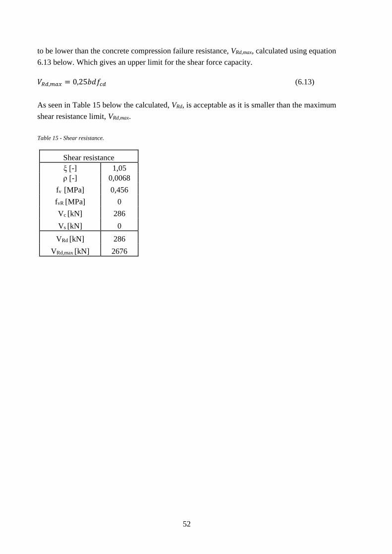
52
to be lower than the concrete compression failure resistance, VRd,max, calculated using equation
6.13 below. Which gives an upper limit for the shear force capacity.
𝑉𝑅𝑑,𝑚𝑎𝑥 = 0,25𝑏𝑑𝑓𝑐𝑑 (6.13)
As seen in Table 15 below the calculated, VRd, is acceptable as it is smaller than the maximum
shear resistance limit, VRd,max.
Table 15 - Shear resistance.
Shear resistance
ξ [-] 1,05
ρ [-] 0,0068
fv [MPa] 0,456
fvR [MPa] 0
Vc [kN] 286
Vs [kN] 0
VRd [kN] 286
VRd,max [kN] 2676
53
7 Load carrying capacity calculation
In this paragraph, load carrying capacity calculations, in which A/B load limits are calculated,
in regards to both moment and shear forces are presented and carried out for all critical parts of
the bridge.
7.1 Moment load carrying capacity calculation Moment load carrying capacity calculations, in which the design A/B limits are calculated for
each result line on the bridge, are presented in Appendix J for the load case in which the traffic
is passing the bridge on its own lane and Appendix K for vehicles passing the bridge in the
middle of the carriageway, alone on the bridge. In this paragraph, a moment load carrying
capacity calculation will be carried out for the most critical, in regards to moment, B-value
point on the bridge. The full load carrying capacity calculation results are as previously stated
presented in Appendix J and Appendix K respectively. Furthermore, the most relevant and
critical load carrying capacity calculation results are presented and analyzed in paragraph 8.2.
The location of the critical point in regards to moment, as well as the direction of the result line,
is illustrated in Figure 40, and as previously stated in paragraph 6.1, the critical point of the
bridge appears for the load case in which the type vehicles are passing the bridge on their own
lane. The moment effect curve, calculated using BRIGADE/Standard, is, as described in
paragraph 4.2, shifted with the factor al for all result line calculations. Calculations, with shifted
moment effect curves, that are presented in Appendix J and Appendix K.
The moment resistance of the point regarded in this calculation is, as calculated in paragraph
6.1, MRd = 111 kNm/m. As described in paragraph 3.5 the proportionality factor, kB, can be
calculated using equation 7.1.
𝑘𝐵 = 𝑀𝑅𝑑−𝑀𝑝𝑒𝑟𝑚
𝑀𝑡𝑟𝑎𝑓𝑓𝑖𝑐 (7.1)
The moment stemming from the permanent load, Mperm, and the moment stemming from the
traffic load, Mtraffic, are calculated using BRIGADE/Standard for each point- and load case on
the bridge. In regards to the critical point in this calculation the permanent moment is, Mperm =
11,4 kNm/m, and the traffic induced moment is, Mtraffic = 105,5 kNm/m. Inserting these
moments, alongside the moment resistance, MRd, into equation 7.1 results in a proportionality
factor equaling to, kB = 0,944, for this critical point.
The load carrying capacity B - value are then calculated by multiplying the proportionality
factor, kB, with the original input traffic point load value, in this case - for calculations regarding
the B-limit - B = 210 kN, see equation 7.2.
54
𝐵𝑑𝑖𝑚 = 𝑘𝐵 ∗ 𝐵210 (7.2)
Multiplying the proportionality factor with the input B-value, as seen in equation 7.2, produces
the design load carrying capacity B – limit in regards moment on that specific point in the
bridge, which equals to, Bdim = 198 kN.
7.2 Shear force load carrying capacity calculation Shear force load carrying capacity calculations, in which the design A/B limits are calculated
for each result line on the bridge, are presented in Appendix J for the load case in which the
traffic is passing the bridge on its own lane and Appendix K for vehicles passing the bridge in
the middle of the carriageway - alone on the bridge. In this paragraph, a shear force load
carrying capacity calculation will be carried out for the most critical B-value load carrying
capacity point on the bridge. The full load carrying capacity calculation results are as previously
stated presented in Appendix J and Appendix K respectively. Furthermore, the most relevant
and critical load carrying capacity calculation results are presented and analyzed in paragraph
8.3.
The location of the critical point, as well as the direction of the result line, is illustrated in Figure
41, and as previously stated in paragraph 6.3, the critical point of the bridge appears for the load
case in which the type vehicles are passing the bridge on their own lane. As discussed in
paragraph 3.3.2 the critical point in regards to shear force around the supports can appear no
closer to the support than the distance calculated by equation 3.8 for cross-sections without
shear reinforcement and equation 3.9 for cross-sections with shear reinforcement. In this case -
for longitudinal shear forces on result line 6 - the critical points appear no closer than 951 mm
to the abutment supports and 1382 mm to the column supports. Limits that are calculated by
inserting, d = 626 mm, and the respective a – values for the supports into equations 3.8 and 3.9.
These disregarded points on the bridge are, in the full result line load carrying capacity
calculations presented in Appendices J and K, marked red to indicate that they are disregarded.
The shear resistance for the point regarded in this calculation is, as calculated in paragraph 6.3,
VRd = 286 kN/m. As described in paragraph 3.5 the proportionality factor, k, can be calculated
using equation 7.3.
𝑘𝐵 = 𝑉𝑅𝑑−𝑉𝑝𝑒𝑟𝑚
𝑉𝐸𝑑−𝑉𝑝𝑒𝑟𝑚 (7.3)
The shear force stemming from the permanent load, Vperm, and the total shear force, VEd, are
calculated using BRIGADE/Standard for each point- and load case on the bridge. In regards to
the critical point in this calculation the permanent shear force is, Vperm = 153,2 kN/m, and the
total shear force is, VEd = 301,1 kN/m. Inserting these shear forces, alongside the shear force
55
resistance, VRd, into equation 7.3 results in a proportionality factor, k = 0,896, for this critical
point.
The load carrying capacity B - value are then calculated by multiplying the proportionality
factor with the original input traffic point load value, in this case for calculations regarding the
B-limit, B = 210 kN, see equation 7.4.
𝐵𝑑𝑖𝑚 = 𝑘𝐵 ∗ 𝐵210 (7.4)
Multiplying the proportionality factor with the input B-value, as seen in equation 7.4, produces
the design load carrying capacity B - limit in regards shear force on that specific point on the
bridge, which equals to, Bdim = 188 kN.
56
8 Results and Analysis
The results of the load carrying capacity calculations are presented and analyzed for both
moment and shear force cases and a comparison between capacity calculations using the BK1
input A/B – values and BK4 input values is performed.
8.1 Result summary The results of the load carrying capacity calculations are presented in Table 16 and Table 17,
where the design A/B - values for the whole bridge is 178 kN and 188 kN respectively. Design
values that appear for the longitudinal shear force result-section, result line 6, for the load case
in which the type vehicles are passing the bridge on their own lanes. Thus, the load carrying
capacity of the bridge in regards to axle- and bogie load is 17 t and 18 t respectively, load
carrying capacity values that is sufficient for the present BK1 load carrying capacity class, but
not, in regards to the B-value limit, adequate for the proposed new load carrying capacity class,
BK4, where the B – value limit is 21 t.
The design A/B – values in regards to moment is, as seen in Table 16, 234 kN and 198 kN
respectively, values that appear on result line 3 which represents the transversal moment in the
span. The most critical moment load carrying capacity values in regards to bogie load of each
slab moment result line, both in transversal and longitudinal direction, are, as seen in Table 16
and Table 17, 206 kN, 231 kN and 198 kN. Values, whose close proximity to each other in both
the transversal and longitudinal direction indicates that the model was modelled in a correct
and efficient manner in regards to the differing strengths in the longitudinal and transversal
directions for the orthotropic slab, a process that is further explained in paragraph 3.3.1. If the
design A/B – values in one direction, for example the transversal, would have been significantly
lower than the ones in the longitudinal direction the conclusion could be made that the capacity
calculation is incorrect – that the capacity, if the longitudinal and transversal material properties
were modelled correctly, could be higher – and, thus, that the calculated capacity is too
conservative. It is important to note that the modelling of the transversal versus the longitudinal
material properties just is a way to, as closely as possible, simulate the orthotropic behavior of
the slab.
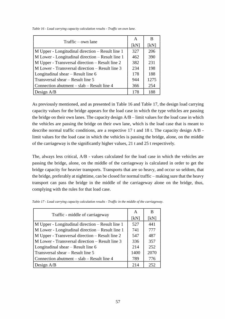
57
Table 16 - Load carrying capacity calculation results - Traffic on own lane.
Traffic – own lane A B
[kN] [kN]
M Upper - Longitudinal direction – Result line 1 327 206
M Lower - Longitudinal direction – Result line 1 462 390
M Upper - Transversal direction – Result line 2 382 231
M Lower - Transversal direction – Result line 3 234 198
Longitudinal shear – Result line 6 178 188
Transversal shear – Result line 5 944 1275
Connection abutment – slab – Result line 4 366 254
Design A/B 178 188
As previously mentioned, and as presented in Table 16 and Table 17, the design load carrying
capacity values for the bridge appears for the load case in which the type vehicles are passing
the bridge on their own lanes. The capacity design A/B – limit values for the load case in which
the vehicles are passing the bridge on their own lane, which is the load case that is meant to
describe normal traffic conditions, are a respective 17 t and 18 t. The capacity design A/B -
limit values for the load case in which the vehicles is passing the bridge, alone, on the middle
of the carriageway is the significantly higher values, 21 t and 25 t respectively.
The, always less critical, A/B - values calculated for the load case in which the vehicles are
passing the bridge, alone, on the middle of the carriageway is calculated in order to get the
bridge capacity for heavier transports. Transports that are so heavy, and occur so seldom, that
the bridge, preferably at nighttime, can be closed for normal traffic – making sure that the heavy
transport can pass the bridge in the middle of the carriageway alone on the bridge, thus,
complying with the rules for that load case.
Table 17 - Load carrying capacity calculation results - Traffic in the middle of the carriageway.
Traffic - middle of carriageway A B
[kN] [kN]
M Upper - Longitudinal direction – Result line 1 527 441
M Lower - Longitudinal direction – Result line 1 741 777
M Upper - Transversal direction – Result line 2 547 487
M Lower - Transversal direction – Result line 3 336 357
Longitudinal shear – Result line 6 214 252
Transversal shear – Result line 5 1400 2070
Connection abutment – slab – Result line 4 789 776
Design A/B 214 252
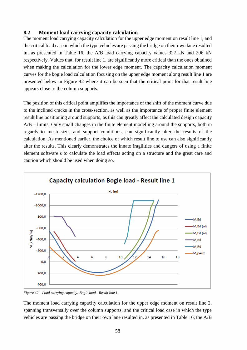
58
8.2 Moment load carrying capacity calculation The moment load carrying capacity calculation for the upper edge moment on result line 1, and
the critical load case in which the type vehicles are passing the bridge on their own lane resulted
in, as presented in Table 16, the A/B load carrying capacity values 327 kN and 206 kN
respectively. Values that, for result line 1, are significantly more critical than the ones obtained
when making the calculation for the lower edge moment. The capacity calculation moment
curves for the bogie load calculation focusing on the upper edge moment along result line 1 are
presented below in Figure 42 where it can be seen that the critical point for that result line
appears close to the column supports.
The position of this critical point amplifies the importance of the shift of the moment curve due
to the inclined cracks in the cross-section, as well as the importance of proper finite element
result line positioning around supports, as this can greatly affect the calculated design capacity
A/B – limits. Only small changes in the finite element modelling around the supports, both in
regards to mesh sizes and support conditions, can significantly alter the results of the
calculation. As mentioned earlier, the choice of which result line to use can also significantly
alter the results. This clearly demonstrates the innate fragilities and dangers of using a finite
element software’s to calculate the load effects acting on a structure and the great care and
caution which should be used when doing so.
Figure 42 – Load carrying capacity: Bogie load - Result line 1.
The moment load carrying capacity calculation for the upper edge moment on result line 2,
spanning transversally over the column supports, and the critical load case in which the type
vehicles are passing the bridge on their own lane resulted in, as presented in Table 16, the A/B
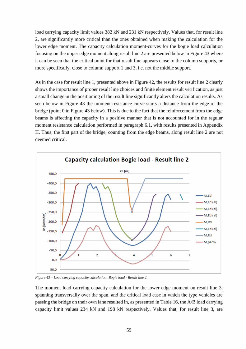
59
load carrying capacity limit values 382 kN and 231 kN respectively. Values that, for result line
2, are significantly more critical than the ones obtained when making the calculation for the
lower edge moment. The capacity calculation moment-curves for the bogie load calculation
focusing on the upper edge moment along result line 2 are presented below in Figure 43 where
it can be seen that the critical point for that result line appears close to the column supports, or
more specifically, close to column support 1 and 3, i.e. not the middle support.
As in the case for result line 1, presented above in Figure 42, the results for result line 2 clearly
shows the importance of proper result line choices and finite element result verification, as just
a small change in the positioning of the result line significantly alters the calculation results. As
seen below in Figure 43 the moment resistance curve starts a distance from the edge of the
bridge (point 0 in Figure 43 below). This is due to the fact that the reinforcement from the edge
beams is affecting the capacity in a positive manner that is not accounted for in the regular
moment resistance calculation performed in paragraph 6.1, with results presented in Appendix
H. Thus, the first part of the bridge, counting from the edge beams, along result line 2 are not
deemed critical.
Figure 43 – Load carrying capacity calculation: Bogie load - Result line 2.
The moment load carrying capacity calculation for the lower edge moment on result line 3,
spanning transversally over the span, and the critical load case in which the type vehicles are
passing the bridge on their own lane resulted in, as presented in Table 16, the A/B load carrying
capacity limit values 234 kN and 198 kN respectively. Values that, for result line 3, are
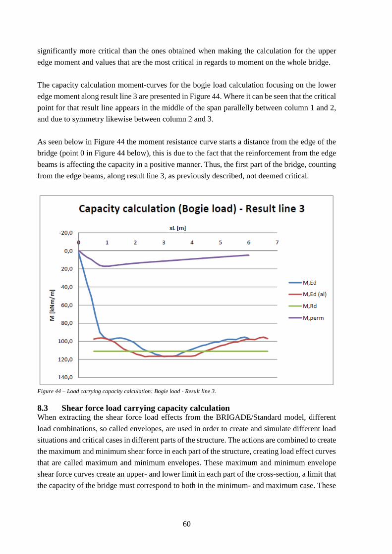
60
significantly more critical than the ones obtained when making the calculation for the upper
edge moment and values that are the most critical in regards to moment on the whole bridge.
The capacity calculation moment-curves for the bogie load calculation focusing on the lower
edge moment along result line 3 are presented in Figure 44. Where it can be seen that the critical
point for that result line appears in the middle of the span parallelly between column 1 and 2,
and due to symmetry likewise between column 2 and 3.
As seen below in Figure 44 the moment resistance curve starts a distance from the edge of the
bridge (point 0 in Figure 44 below), this is due to the fact that the reinforcement from the edge
beams is affecting the capacity in a positive manner. Thus, the first part of the bridge, counting
from the edge beams, along result line 3, as previously described, not deemed critical.
Figure 44 – Load carrying capacity calculation: Bogie load - Result line 3.
8.3 Shear force load carrying capacity calculation When extracting the shear force load effects from the BRIGADE/Standard model, different
load combinations, so called envelopes, are used in order to create and simulate different load
situations and critical cases in different parts of the structure. The actions are combined to create
the maximum and minimum shear force in each part of the structure, creating load effect curves
that are called maximum and minimum envelopes. These maximum and minimum envelope
shear force curves create an upper- and lower limit in each part of the cross-section, a limit that
the capacity of the bridge must correspond to both in the minimum- and maximum case. These
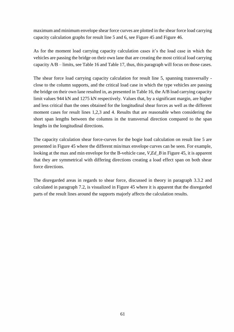
61
maximum and minimum envelope shear force curves are plotted in the shear force load carrying
capacity calculation graphs for result line 5 and 6, see Figure 45 and Figure 46.
As for the moment load carrying capacity calculation cases it’s the load case in which the
vehicles are passing the bridge on their own lane that are creating the most critical load carrying
capacity A/B – limits, see Table 16 and Table 17, thus, this paragraph will focus on those cases.
The shear force load carrying capacity calculation for result line 5, spanning transversally -
close to the column supports, and the critical load case in which the type vehicles are passing
the bridge on their own lane resulted in, as presented in Table 16, the A/B load carrying capacity
limit values 944 kN and 1275 kN respectively. Values that, by a significant margin, are higher
and less critical than the ones obtained for the longitudinal shear forces as well as the different
moment cases for result lines 1,2,3 and 4. Results that are reasonable when considering the
short span lengths between the columns in the transversal direction compared to the span
lengths in the longitudinal directions.
The capacity calculation shear force-curves for the bogie load calculation on result line 5 are
presented in Figure 45 where the different min/max envelope curves can be seen. For example,
looking at the max and min envelope for the B-vehicle case, V,Ed_B in Figure 45, it is apparent
that they are symmetrical with differing directions creating a load effect span on both shear
force directions.
The disregarded areas in regards to shear force, discussed in theory in paragraph 3.3.2 and
calculated in paragraph 7.2, is visualized in Figure 45 where it is apparent that the disregarded
parts of the result lines around the supports majorly affects the calculation results.
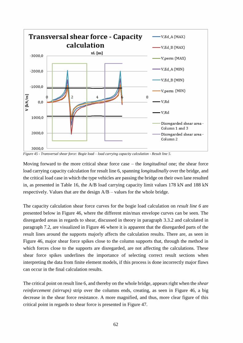
62
Figure 45 - Transversal shear force: Bogie load – load carrying capacity calculation - Result line 5.
Moving forward to the more critical shear force case – the longitudinal one; the shear force
load carrying capacity calculation for result line 6, spanning longitudinally over the bridge, and
the critical load case in which the type vehicles are passing the bridge on their own lane resulted
in, as presented in Table 16, the A/B load carrying capacity limit values 178 kN and 188 kN
respectively. Values that are the design A/B – values for the whole bridge.
The capacity calculation shear force curves for the bogie load calculation on result line 6 are
presented below in Figure 46, where the different min/max envelope curves can be seen. The
disregarded areas in regards to shear, discussed in theory in paragraph 3.3.2 and calculated in
paragraph 7.2, are visualized in Figure 46 where it is apparent that the disregarded parts of the
result lines around the supports majorly affects the calculation results. There are, as seen in
Figure 46, major shear force spikes close to the column supports that, through the method in
which forces close to the supports are disregarded, are not affecting the calculations. These
shear force spikes underlines the importance of selecting correct result sections when
interpreting the data from finite element models, if this process is done incorrectly major flaws
can occur in the final calculation results.
The critical point on result line 6, and thereby on the whole bridge, appears right when the shear
reinforcement (stirrups) strip over the columns ends, creating, as seen in Figure 46, a big
decrease in the shear force resistance. A more magnified, and thus, more clear figure of this
critical point in regards to shear force is presented in Figure 47.
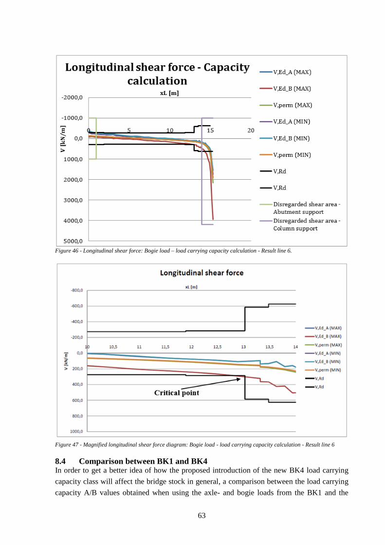
63
Figure 46 - Longitudinal shear force: Bogie load – load carrying capacity calculation - Result line 6.
Figure 47 - Magnified longitudinal shear force diagram: Bogie load - load carrying capacity calculation - Result line 6
8.4 Comparison between BK1 and BK4 In order to get a better idea of how the proposed introduction of the new BK4 load carrying
capacity class will affect the bridge stock in general, a comparison between the load carrying
capacity A/B values obtained when using the axle- and bogie loads from the BK1 and the
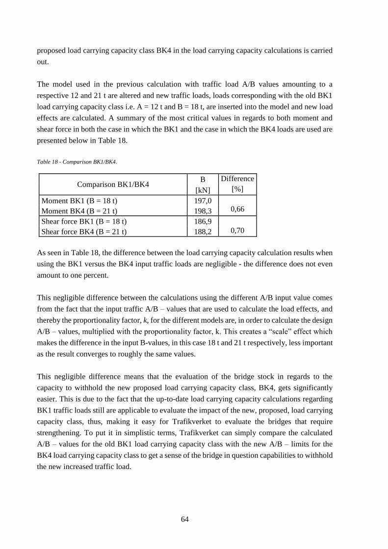
64
proposed load carrying capacity class BK4 in the load carrying capacity calculations is carried
out.
The model used in the previous calculation with traffic load A/B values amounting to a
respective 12 and 21 t are altered and new traffic loads, loads corresponding with the old BK1
load carrying capacity class i.e. A = 12 t and B = 18 t, are inserted into the model and new load
effects are calculated. A summary of the most critical values in regards to both moment and
shear force in both the case in which the BK1 and the case in which the BK4 loads are used are
presented below in Table 18.
Table 18 - Comparison BK1/BK4.
Comparison BK1/BK4 B Difference
[kN] [%]
Moment BK1 (B = 18 t) 197,0
0,66 Moment BK4 (B = 21 t) 198,3
Shear force BK1 (B = 18 t) 186,9
Shear force BK4 (B = 21 t) 188,2 0,70
As seen in Table 18, the difference between the load carrying capacity calculation results when
using the BK1 versus the BK4 input traffic loads are negligible - the difference does not even
amount to one percent.
This negligible difference between the calculations using the different A/B input value comes
from the fact that the input traffic A/B – values that are used to calculate the load effects, and
thereby the proportionality factor, k, for the different models are, in order to calculate the design
A/B – values, multiplied with the proportionality factor, k. This creates a “scale” effect which
makes the difference in the input B-values, in this case 18 t and 21 t respectively, less important
as the result converges to roughly the same values.
This negligible difference means that the evaluation of the bridge stock in regards to the
capacity to withhold the new proposed load carrying capacity class, BK4, gets significantly
easier. This is due to the fact that the up-to-date load carrying capacity calculations regarding
BK1 traffic loads still are applicable to evaluate the impact of the new, proposed, load carrying
capacity class, thus, making it easy for Trafikverket to evaluate the bridges that require
strengthening. To put it in simplistic terms, Trafikverket can simply compare the calculated
A/B – values for the old BK1 load carrying capacity class with the new A/B – limits for the
BK4 load carrying capacity class to get a sense of the bridge in question capabilities to withhold
the new increased traffic load.
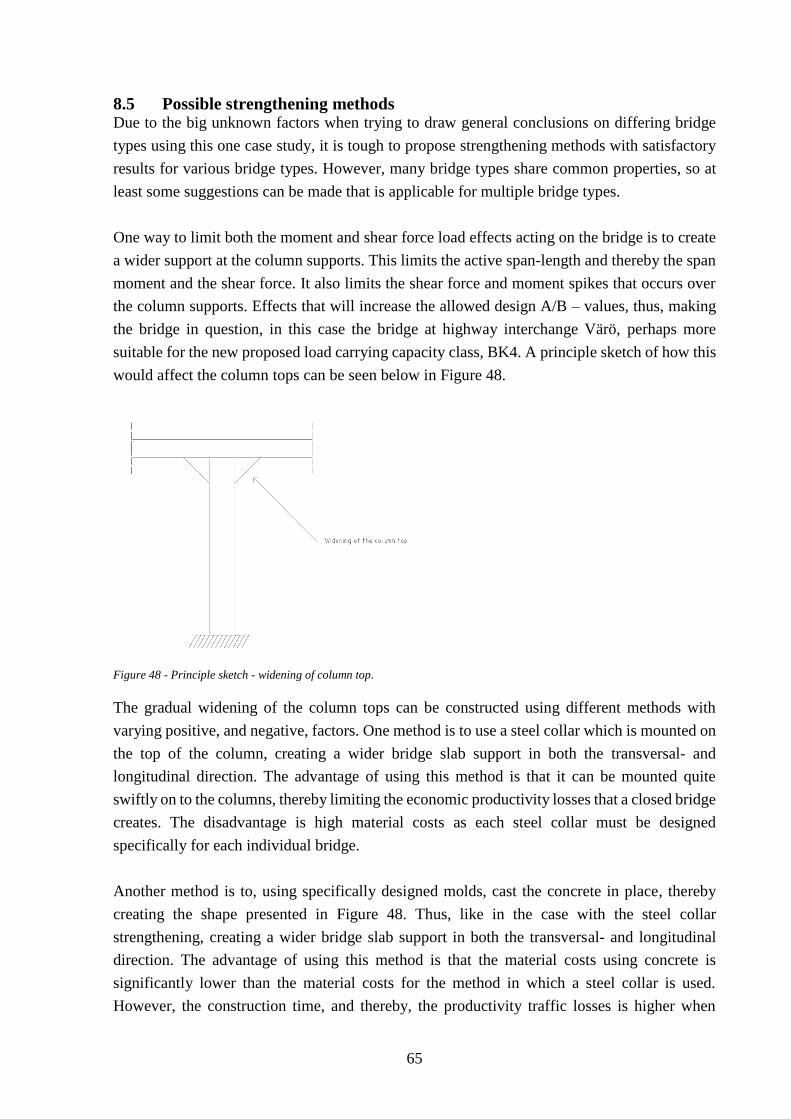
65
8.5 Possible strengthening methods Due to the big unknown factors when trying to draw general conclusions on differing bridge
types using this one case study, it is tough to propose strengthening methods with satisfactory
results for various bridge types. However, many bridge types share common properties, so at
least some suggestions can be made that is applicable for multiple bridge types.
One way to limit both the moment and shear force load effects acting on the bridge is to create
a wider support at the column supports. This limits the active span-length and thereby the span
moment and the shear force. It also limits the shear force and moment spikes that occurs over
the column supports. Effects that will increase the allowed design A/B – values, thus, making
the bridge in question, in this case the bridge at highway interchange Värö, perhaps more
suitable for the new proposed load carrying capacity class, BK4. A principle sketch of how this
would affect the column tops can be seen below in Figure 48.
Figure 48 - Principle sketch - widening of column top.
The gradual widening of the column tops can be constructed using different methods with
varying positive, and negative, factors. One method is to use a steel collar which is mounted on
the top of the column, creating a wider bridge slab support in both the transversal- and
longitudinal direction. The advantage of using this method is that it can be mounted quite
swiftly on to the columns, thereby limiting the economic productivity losses that a closed bridge
creates. The disadvantage is high material costs as each steel collar must be designed
specifically for each individual bridge.
Another method is to, using specifically designed molds, cast the concrete in place, thereby
creating the shape presented in Figure 48. Thus, like in the case with the steel collar
strengthening, creating a wider bridge slab support in both the transversal- and longitudinal
direction. The advantage of using this method is that the material costs using concrete is
significantly lower than the material costs for the method in which a steel collar is used.
However, the construction time, and thereby, the productivity traffic losses is higher when

66
casting the concrete in place, perhaps making the steel collar method more advantageous
overall.
67
9 Discussion and conclusions
In this paragraph, the results of the load carrying capacity calculations performed on the bridge
at highway interchange Värö will be discussed and conclusions will be made, both in regards
to the specific bridge studied in this thesis, but also in regards to bridges on the Swedish road
network in general.
9.1 Discussion When the proposal of a new load carrying capacity class, in which the maximum traffic load is
increased to 74 t, was put forth, the suggestion was made to decrease the general safety margin
on the new proposed BK4 road network. A decrease of the safety margin is principally possible,
however, this will mean that the grade of utility is increased which, in turn, decreases the bridge
life length and thus increases the bridge life cycle costs. Drawbacks added to the obvious one -
that the safety of the bridge network is lowered. Thus, Trafikverket came to the conclusion that
the bridges with insufficient A/B – load carrying capacity would need to be strengthened in
order to, with a long term view, cope with the increased traffic loads.
There are approximately 15 000 bridges on the Swedish national road network. An amount that
highlights the importance of proper bridge maintenance and load carrying capacity calculations
on a broader spectrum in order to make sure that the road network is safely- and economically
maintained. Bridges, of which a vast majority will be affected by the increased traffic load if
the Swedish government decides to implement the new BK4 load carrying capacity class on the
whole original BK1 road network. The sheer amount of bridges affected plainly underlines the
importance of load carrying capacity calculations, now and in the future. Preferably calculations
which, in order to account for the 3-D and orthotropic behavior of bridges, are performed using
a modern a finite element modelling software.
The finite element method can be a terrific tool, to both accurately and swiftly analyze the loads
and actions acting on bridges and structures. However, the simplicity and general user
friendliness of modern finite element analysis software can also cause problems and create big
unforeseen risks due to the fact that inexperienced engineers can obtain inaccurate results. It is
integral that, when using a finite element software, the engineer understands, at least at an
elementary level, the theory behind the finite element calculations and recognizes the
importance of proper result verification. If not, the usage of finite element modelling in
calculations can be a significant source of error and thus, lead to increased risks and potential
for hazards.
Small changes regarding for example mesh sizes can greatly affect the results obtained,
especially over supports and around point loads. It is important to perform an extensive
convergence study to make sure that the chosen mesh sizes are accurate. The simulation of the
orthotropic behavior of a concrete bridge slab is also critical as the results can differ
68
significantly between models using, the more common but largely inaccurate, isotropic material
model and models using the more accurate orthotropic material model. Changes in how the
orthotropic material parameters themselves are modelled can also significantly affect the
calculation results obtained by the, in this case BRIGADE/Standard, finite element software.
Another critical aspect, which severely can alter the load effects obtained in the finite element
model, is the choice and interpretation of result section lines, specifically around the supports.
This aspect underlines the importance of proper result interpretation and also underlines the
dangers of using finite element models to calculate the load effects on structures as just small
changes in the location of the result line and the choice of result section around the supports
significantly alters the results.
It is also important to note and take into account that the calculation assumptions used when
performing a load carrying capacity calculation according to Swedish standards, for example
that the cross-sections are single-reinforced or the approaches used when calculating the shear
force capacity, are very conservative. These conservative calculation assumptions used in load
carrying capacity calculations are, of course, creating a wider safety margin in regards to the
calculated capacity A/B – limits. However, the conservative assumptions can also be too
conservative, making the load carrying capacity calculations uneconomical, thus, creating a
balancing act between the economic factors and the safety factors when determining if a bridge
is in need of strengthening.
9.2 Conclusions The load carrying capacity calculations performed on the studied bridge, the bridge at highway
interchange Värö, shows that the capacity of the bridge, both in regards to moment and shear
force is insufficient to meet the new, increased, BK4 A/B – loads. The critical A/B – values for
the whole bridge are 17 t and 18 t respectively, to be compared with the required 12/21 t limit
for the new BK4 load carrying capacity class. Thus, making the load carrying capacity of the
bridge inadequate.
The critical capacity A/B values in regards to shear force, and as previously mentioned for the
whole bridge, are 178 and 188 kN respectively. Values that occurs on the longitudinal shear
force result line at the point where the shear force reinforcement (stirrups) strip over the column
supports ends. The critical capacity A/B values in regards to moment are 234 and 198 kN
respectively. Values that occur on the transversal moment result line in the middle of the span
for the lower edge moment. Both the critical moment- and shear force A/B values appear, as
one would suspect, for the load case in which the type vehicles are passing the bridge on their
own lane.
Due to the differing properties and characteristics of each individual bridge on the Swedish
road network specific load carrying capacity calculations will need to be performed on each
69
individual bridge in order to evaluate its capability to withstand the increased BK4 traffic loads.
Thus, making general statements regarding the effects on the bridge network as a whole difficult
to make. However, as shown in paragraph 8.4, capacity calculations regarding the BK1 load
carrying capacity class can, with sufficient accuracy, be used to check the capability of a bridge
to withstand the new increased traffic loads in the BK4 load carrying capacity class. Thus,
making it easier for Trafikverket to evaluate the strengthening needs for the bridge network as
a whole due to the increased, BK4, traffic loads.
9.3 Suggestions for further research As previously mentioned, general and broad conclusions, based on this one case study,
regarding the effects of the load increase on the Swedish bridge network as a whole are tough
to draw with great conviction. Thus, more studies, both in regards to slab frame bridges, which
are studied in this thesis, and other common Swedish bridge types such as regular slab bridges,
beam bridges and steel girder bridges are required in order to draw conclusions regarding the
effects of the planned load increase on the Swedish bridge network as a whole. Due to the great
structural diversity, even amongst bridges of the same “type” - with the same general
characteristics, extensive studies regarding the various different bridge types present on the
Swedish road network are necessary and important to ensure the safety on the Swedish road
network.
Furthermore, studies regarding how to properly strengthen and reinforce the bridges deemed
unsafe are required. The suggestions put forth in this thesis are just that – suggestions – and
requires calculation based, preferably using finite element software’s in order to get a 3-D view
of the structure, studies to fully analyze their suitability and the advantages and disadvantages
of each method. Studies to find and analyze the suitability of alternate methods to the ones put
forth in this thesis also needs to be performed.
General studies regarding how to properly model the orthotropic behavior of concrete slabs in
finite element analysis software’s would also be beneficial, both when performing load carrying
capacity calculations like in this thesis, but also for calculations and design regarding new
bridges and structures. Finally, general studies regarding the load carrying capacity calculation
process is required in order to analyze whether the simplifications, and the calculation process
in general, produces accurate and reliable results.
70
10 References
Boverket, (2004). Boverkets handbok om betongkonstruktioner, BBK 04. Karlskrona: Boverket.
ISBN 91-7147-816-7
BRIME, (2001). Bridge Management in Europe, Assessment of Highway Bridges – Final
Report. 4th RTD Framework Programme.
Broo, H., Lundgren, K & Plos, M., (2008). A guide to non-linear finite element modellingo f
shear and torsion in concrete bridges. Department of Civil and Environmental Engineering,
Chalmers University of Technology, Göteborg.
Carlsson, F. (2006). Modelling of Traffic Loads on Bridges: Based on Measurements of Real
Traffic Loads in Sweden. Lund University, Diss. Lund: Lunds universitet, 2006.
COST, (2004). COST 345 Procedures Required for the Assessment of Highway Structures –
Final Report. European Co-operation in the Field of Scientific and Technical Research.
European Commission – Directorate General Transport and Energy.
Davidson, M. (2003). Strukturanalys av brokonstruktioner med finita elementmetoden –
Fördelning av krafter och moment. Brosamverkan Väst, Göteborg.
Huber, M., (1923). The theory of crosswise reinforced ferroconcrete slabs and its application
to various important constructional problems involving rectangular slabs. Der Bauingeniur 4,
12 (1923), 354-360.
Kommunikationsministeriet, (2013). Nya mått och vikter på tunga fordon ger ökad
konkurrenskraft. PM 2013-06-06. Retrieved 29 September, 2016 from
Kommunikationsministeriet, https://www.lvm.fi/sv/-/nya-matt-och-vikter-pa-tunga-fordon-
ger-okad-konkurrenskraft-791804
Kwak, H.G, & Filippou, F.C., (1990). Finite element analysis of reinforced concrete structures
under monotonic load. Research Report of department of Civil Engineering. U.C. Berkeley,
No. UCB/SEMM-90/14; 1990. P. 33-9.ö
Leduc, G., (2009). Longer and Heavier Vehicles – An overview of technical aspects. JRC
Scientific Technical Reports. European Commission. Luxemburg.
Li, Y, & Barbic, J., (2014). Stable Orthotropic Materials. In Symp. On Computer Animation
(SCA), 41-46.
71
MAINLINE (2014). MAINtenance, renewaL and Improvement of rail transport INfrastructure
to reduce Economic and environmental impacts. A European FP7 Research Project during
2011-2014. Some 20 reports are available at http://www.mainline-project.eu/
Nilimaa, J., (2015). Concrete Bridges: Improved Load Capacity. Doctoral Thesis. Luleå: Luleå
University of Technology; 2015, 176 p.
Nilimaa, J., Bagge, B., Häggström, J., Blanksvärd, T., Sas, G., Täljsten, B. & Elfgren, L.,
(2016). More Realistic Codes for Existing Bridges. 19th IABSE Congress Stockholm 21-23
September 2016: Challenges in Design and Construction of an Innovative and Sustainable Built
Environment. Zurich, 2016, pp. 399-407. ISBN 978-3-85748-144-4.
Pacoste, C., Plos, M. & Johansson, M., (2012). Recommendations for finite element analysis
for the design of reinforced concrete slabs. KTH Royal Institute of Technology, Stockholm,
Sverige.
Plos, M., Gylltoft, K., Lundgren., Cervenka J., Herwig , A., Brühwiler, E., … Rosell, E, (2008).
Structural assessment of concrete bridges. Nordic Concrete Research, (2), 99-111.
Rombach, G.A., (2004). Finite element design of concrete structures – Practical problems and
their solutions. Thomas Telford Publishing. London.
Rowley, J. (2002). Using Case Studies in Research. Management research news, 25(1), 16-27.
Ryall, M.J., Parke, G.A.R & Harding, J.E., (2000). Manual of bridge engineering. Thomas
Telford Publishing, London.
Samuelsson, A. & Wiberg N.-E, (1998). The Finite Element Method – Basics. Studentlitteratur,
Lund.
Scanscot Technology AB, (2015a). BRIGADE/Standard Theory Manual. Version 4.3. Scanscot
Technology AB, Sweden.
Scanscot Technology AB, (2015b). BRIGADE/Standard User’s Manual. Version 4.3. Scanscot
Technology AB, Sweden.
Sustainable Bridges, (2007). Guideline for Load and Resistance Assessment of Existing
European Railway Bridges – Advices on the use of advanced methods. Sustainable Bridges.
Sixth Framework Programme.

72
Svensk Byggtjänst, (1990). Betonghandbok. Konstruktion, utgåva 2. Svensk byggtjänst, ISBN:
9789173325332.
SS-EN 1990, (2002) Eurocode 0: Basis of structural design. Stockholm, Sweden, SIS Förlag
AB.
SS-EN 1991-2, (2003) Eurocode 1: Actions on structures – Part 2: Traffic loads on bridges.
Stockholm, Sweden, SIS Förlag AB.
Thun, H., Ohlsson, U., & Elfgren, L., (2006). Concrete strength in old Swedish concrete
bridges. Nordic Concrete Research, ISSN 0800-6377, Vol.35, nr 1-2, 47-60 s.
Trafikverket, (2014a). Tyngre fordon på det allmänna vägnätet – rapportering av
regeringsuppdrag; Pub 2014:102. Trafikverket. (ISBN: 978-91-7467-629-7).
Trafikverket, (2014b). BaTMan - Kodförteckning och beskrivning av brotyper. Borlänge,
Sverige, Trafikverket.
Trafikverket, (2015). Fördjupade analyser av att tillåta tyngre fordon på det allmänna vägnätet
– Rapportering av regeringsuppdrag. Pub 2015:207. Trafikverket. (ISBN: 978-91-7467-847-
5.
Trafikverket, (2016a). Bärighetsberäkning av broar, KRAV. Version 3.0. TDOK 2013:0267.
Trafikverket.
Trafikverket, (2016b). Bärighetsberäkning av broar, RÅD. Version 3.0. TDOK 2013:0273.
Trafikverket.
Trafikverket, (2016c). BaTMan BRO OCH TUNNEL MANAGEMENT. [online] Available at:
http://www.batman.trafikverket.se [Accessed 20 October 2016].
Transportstyrelsen, (2014). Rapport om tyngre och längre fordonståg på det allmänna
vägnätet; Dnr TSV 2014-1419. Transportstyrelsen.
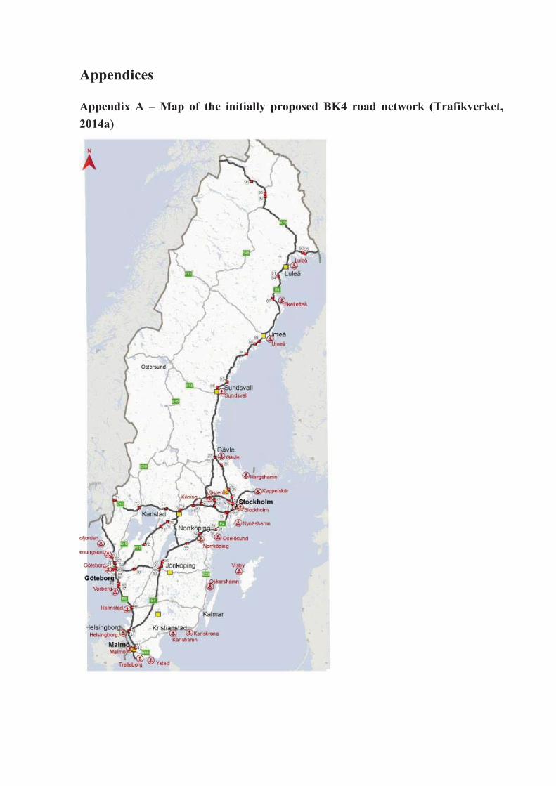
Appendices Appendix A – Map of the initially proposed BK4 road network (Trafikverket, 2014a)
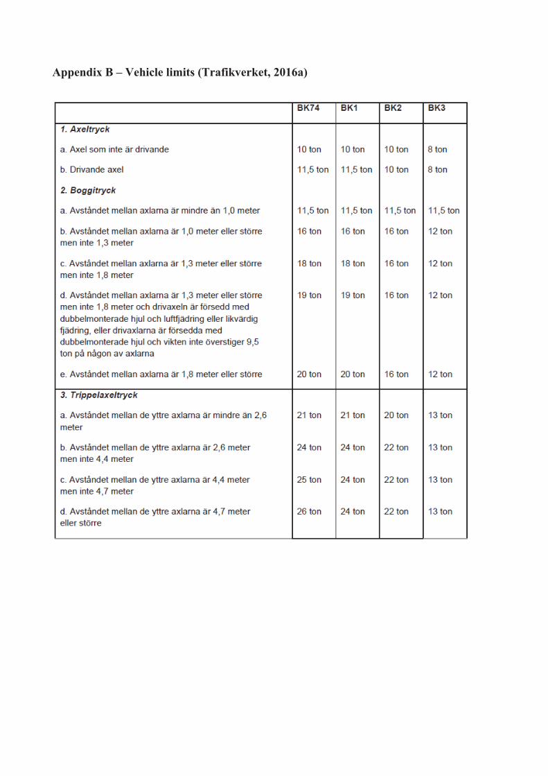
Appendix B – Vehicle limits (Trafikverket, 2016a)
Appendix C – Type vehicles (Trafikverket, 2016a) (Measurements in m)
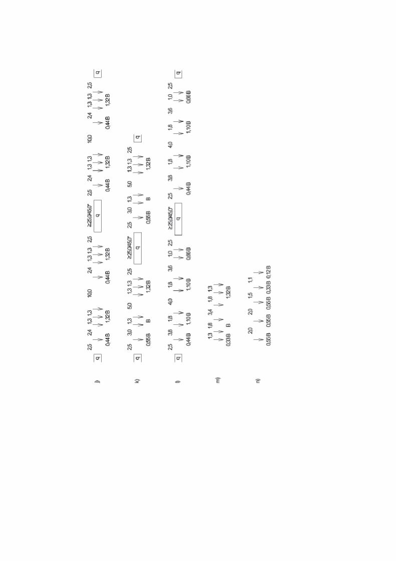
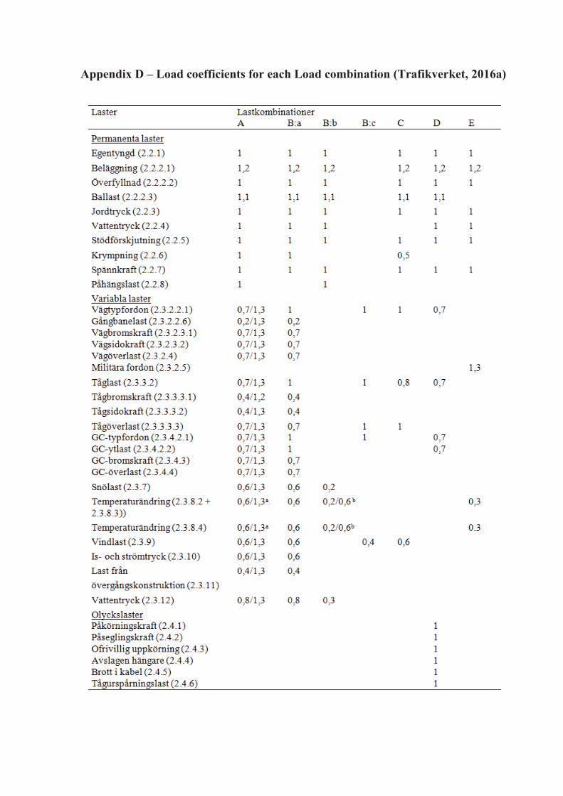
Appendix D – Load coefficients for each Load combination (Trafikverket, 2016a)
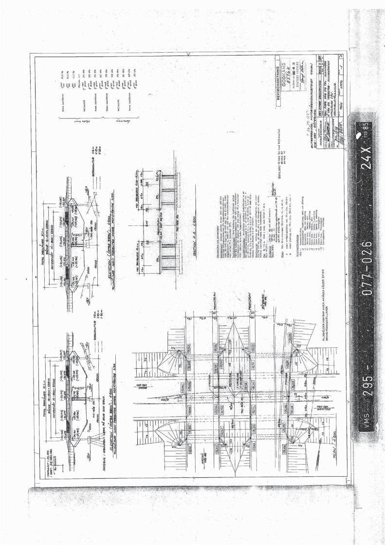
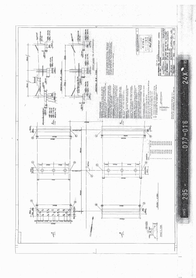
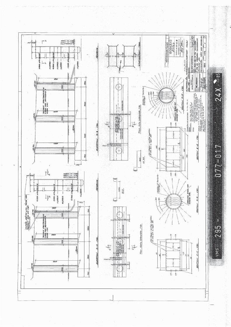
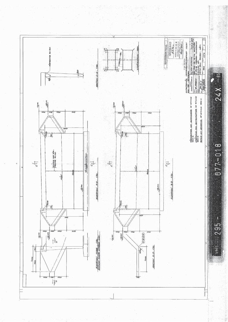
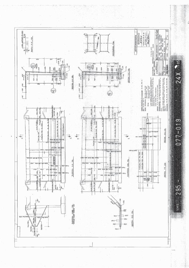
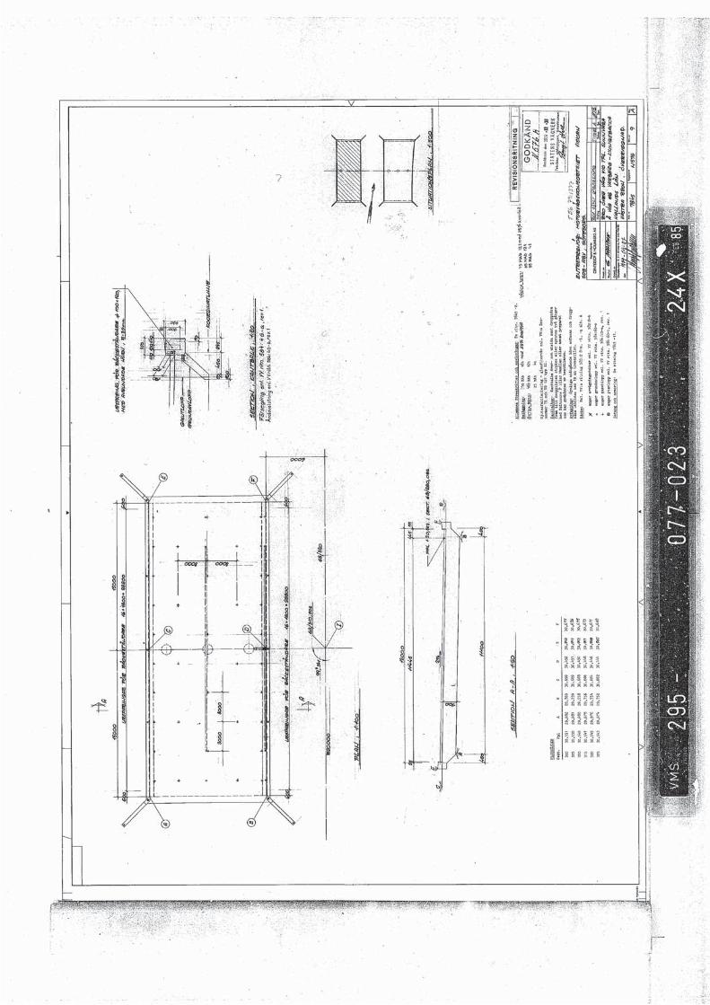
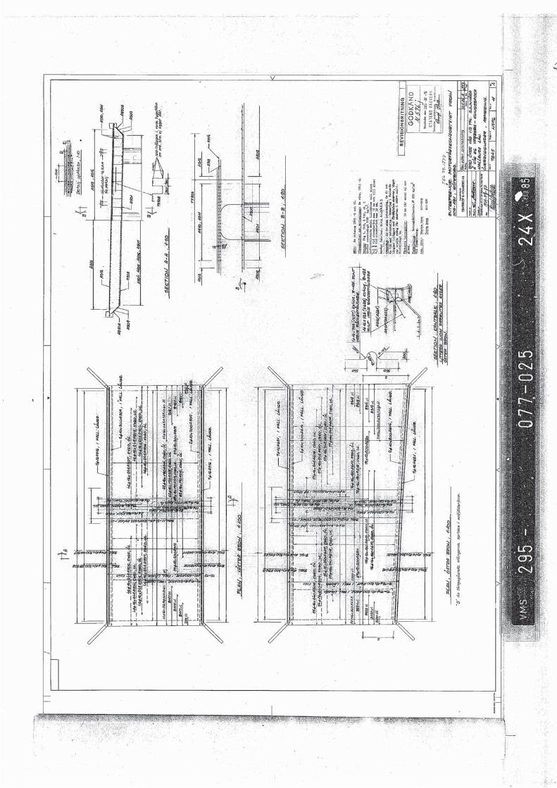
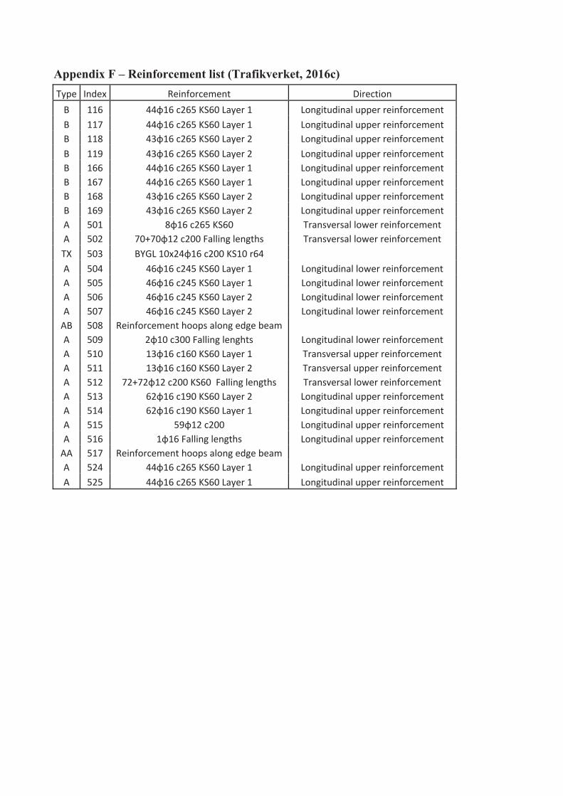
Appendix F – Reinforcement list (Trafikverket, 2016c) Type Index Reinforcement Direction
B 116 44φ16 c265 KS60 Layer 1 Longitudinal upper reinforcement B 117 44φ16 c265 KS60 Layer 1 Longitudinal upper reinforcement B 118 43φ16 c265 KS60 Layer 2 Longitudinal upper reinforcement B 119 43φ16 c265 KS60 Layer 2 Longitudinal upper reinforcement B 166 44φ16 c265 KS60 Layer 1 Longitudinal upper reinforcement B 167 44φ16 c265 KS60 Layer 1 Longitudinal upper reinforcement B 168 43φ16 c265 KS60 Layer 2 Longitudinal upper reinforcement B 169 43φ16 c265 KS60 Layer 2 Longitudinal upper reinforcement A 501 8φ16 c265 KS60 Transversal lower reinforcement A 502 70+70φ12 c200 Falling lengths Transversal lower reinforcement TX 503 BYGL 10x24φ16 c200 KS10 r64 A 504 46φ16 c245 KS60 Layer 1 Longitudinal lower reinforcement A 505 46φ16 c245 KS60 Layer 1 Longitudinal lower reinforcement A 506 46φ16 c245 KS60 Layer 2 Longitudinal lower reinforcement A 507 46φ16 c245 KS60 Layer 2 Longitudinal lower reinforcement
AB 508 Reinforcement hoops along edge beam A 509 2φ10 c300 Falling lenghts Longitudinal lower reinforcement A 510 13φ16 c160 KS60 Layer 1 Transversal upper reinforcement A 511 13φ16 c160 KS60 Layer 2 Transversal upper reinforcement A 512 72+72φ12 c200 KS60 Falling lengths Transversal lower reinforcement A 513 62φ16 c190 KS60 Layer 2 Longitudinal upper reinforcement A 514 62φ16 c190 KS60 Layer 1 Longitudinal upper reinforcement A 515 59φ12 c200 Longitudinal upper reinforcement A 516 1φ16 Falling lengths Longitudinal upper reinforcement
AA 517 Reinforcement hoops along edge beam A 524 44φ16 c265 KS60 Layer 1 Longitudinal upper reinforcement A 525 44φ16 c265 KS60 Layer 1 Longitudinal upper reinforcement
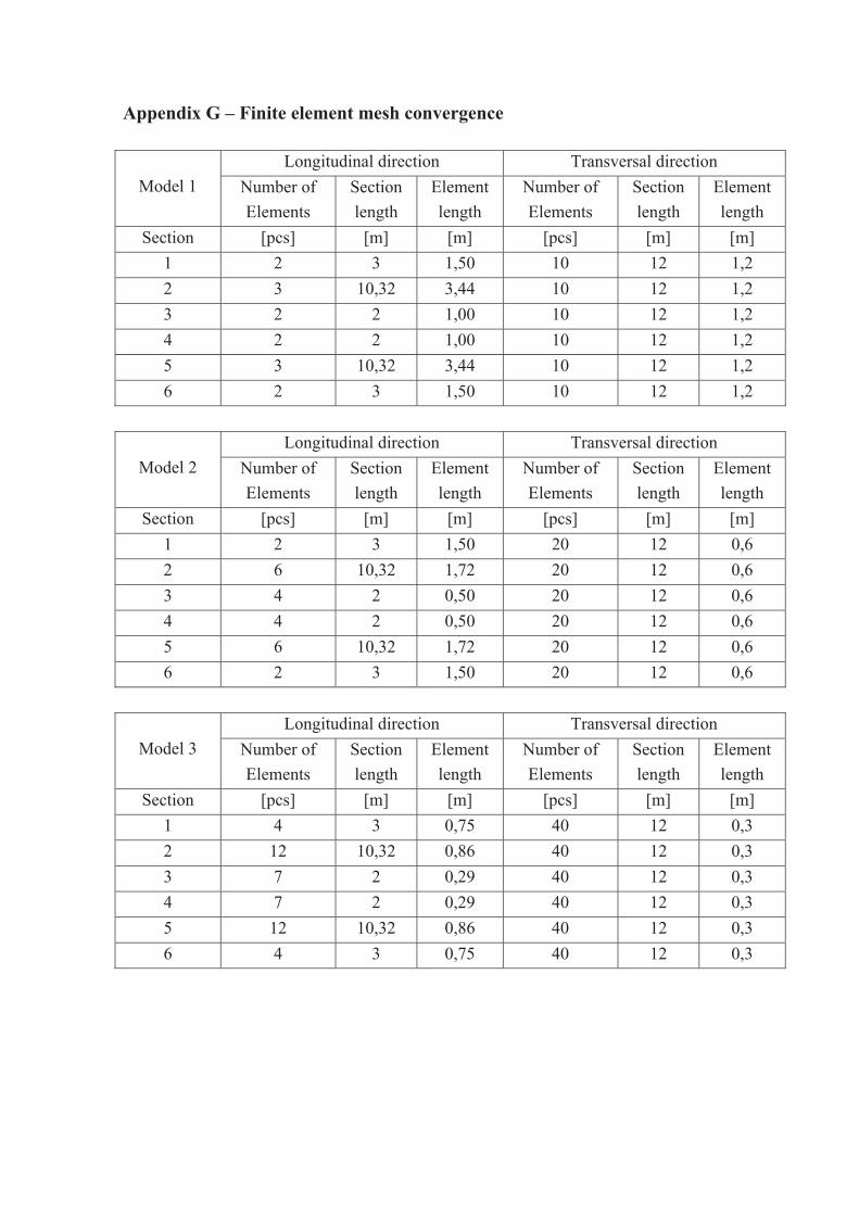
Appendix G – Finite element mesh convergence
Model 1
Longitudinal direction Transversal direction Number of Elements
Section length
Element length
Number of Elements
Section length
Element length
Section [pcs] [m] [m] [pcs] [m] [m] 1 2 3 1,50 10 12 1,2 2 3 10,32 3,44 10 12 1,2 3 2 2 1,00 10 12 1,2 4 2 2 1,00 10 12 1,2 5 3 10,32 3,44 10 12 1,2 6 2 3 1,50 10 12 1,2
Model 2 Longitudinal direction Transversal direction
Number of Elements
Section length
Element length
Number of Elements
Section length
Element length
Section [pcs] [m] [m] [pcs] [m] [m] 1 2 3 1,50 20 12 0,6 2 6 10,32 1,72 20 12 0,6 3 4 2 0,50 20 12 0,6 4 4 2 0,50 20 12 0,6 5 6 10,32 1,72 20 12 0,6 6 2 3 1,50 20 12 0,6
Model 3 Longitudinal direction Transversal direction
Number of Elements
Section length
Element length
Number of Elements
Section length
Element length
Section [pcs] [m] [m] [pcs] [m] [m] 1 4 3 0,75 40 12 0,3 2 12 10,32 0,86 40 12 0,3 3 7 2 0,29 40 12 0,3 4 7 2 0,29 40 12 0,3 5 12 10,32 0,86 40 12 0,3 6 4 3 0,75 40 12 0,3
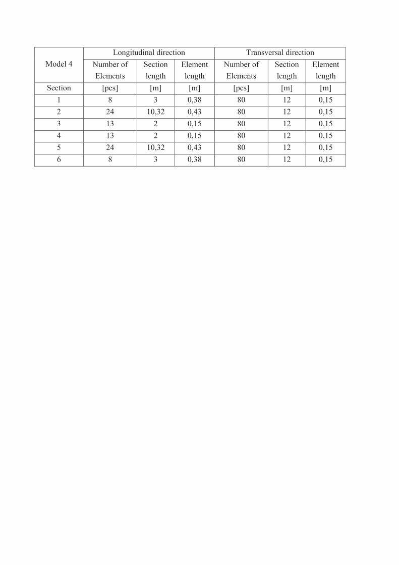
Model 4
Longitudinal direction Transversal direction Number of Elements
Section length
Element length
Number of Elements
Section length
Element length
Section [pcs] [m] [m] [pcs] [m] [m] 1 8 3 0,38 80 12 0,15 2 24 10,32 0,43 80 12 0,15 3 13 2 0,15 80 12 0,15 4 13 2 0,15 80 12 0,15 5 24 10,32 0,43 80 12 0,15 6 8 3 0,38 80 12 0,15
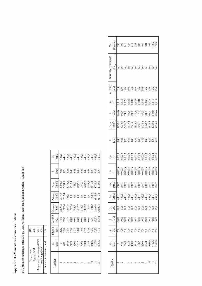
App
endi
x H
- M
omen
t res
ista
nce
calc
ulat
ions
UL
S M
omen
t res
ista
nce
calc
ulat
ions
, Upp
er r
einf
orce
men
t lon
gitu
dina
l dir
ectio
n
646
626
633
800
16
xL
Laye
r 1
Laye
r 2A
s,lay
er 1
A
s,lay
er 2
As,t
otd
f yd
[mm
][p
cs]
[pcs
][m
m2 ]
[mm
2 ][m
m2 ]
[mm
][M
Pa]
10
11,3
27,
5522
76,2
1517
,437
93,6
6344
9,3
269
67,
557,
5515
17,4
1517
,430
34,9
626
449,
33
2648
7,55
3,77
1517
,475
8,7
2276
,262
644
9,3
437
297,
550,
0015
17,4
0,0
1517
,464
644
9,3
549
003,
770,
0075
8,7
0,0
758,
764
644
9,3
666
125,
630,
0011
32,7
0,0
1132
,764
644
9,3
770
621,
860,
0037
4,0
0,0
374,
064
644
9,3
885
047,
120,
0014
32,2
0,0
1432
,264
644
9,3
990
445,
260,
0010
58,2
0,0
1058
,264
644
9,3
1010
485
5,26
5,26
1058
,210
58,2
2116
,462
644
9,3
1111
025
10,5
310
,53
2116
,421
16,4
4232
,962
644
9,3
CL
1532
510
,53
10,5
321
16,4
2116
,442
32,9
626
449,
3
xLh
bf cd
f yd
E sd
cusy
dA
s,tot
xs
a l (1
,0d)
Nor
mal
ly re
info
rced
?M
Rd
[mm
][m
m]
[mm
][M
Pa]
[MPa
][G
Pa]
[-][-]
[mm
][m
m2 ]
[mm
][-]
[mm
]s >
sy
[kN
m/m
]1
070
010
0017
,144
9,3
158,
70,
0035
0,00
2863
337
93,6
124,
60,
014
633
Yes
993
269
670
010
0017
,144
9,3
158,
70,
0035
0,00
2862
630
34,9
99,7
0,01
862
6Y
es79
93
2648
700
1000
17,1
449,
315
8,7
0,00
350,
0028
626
2276
,274
,80,
026
626
Yes
610
437
2970
010
0017
,144
9,3
158,
70,
0035
0,00
2864
615
17,4
49,8
0,04
264
6Y
es42
75
4900
700
1000
17,1
449,
315
8,7
0,00
350,
0028
646
758,
724
,90,
087
646
Yes
217
666
1270
010
0017
,144
9,3
158,
70,
0035
0,00
2864
611
32,7
37,2
0,05
764
6Y
es32
17
7062
700
1000
17,1
449,
315
8,7
0,00
350,
0028
646
374,
012
,30,
181
646
Yes
108
885
0470
010
0017
,144
9,3
158,
70,
0035
0,00
2864
614
32,2
47,0
0,04
564
6Y
es40
49
9044
700
1000
17,1
449,
315
8,7
0,00
350,
0028
646
1058
,234
,80,
062
646
Yes
301
1010
485
700
1000
17,1
449,
315
8,7
0,00
350,
0028
626
2116
,469
,50,
028
626
Yes
569
1111
025
700
1000
17,1
449,
315
8,7
0,00
350,
0028
626
4232
,913
9,0
0,01
262
6Y
es10
85C
L15
325
700
1000
17,1
449,
315
8,7
0,00
350,
0028
626
4232
,913
9,0
0,01
262
6Y
es10
85
d 1 la
yer [
mm
]d 2
laye
rs [m
m]
d 2 la
yers
with
1 e
xtra
bar
in la
yer 1
[mm
]A
ncho
rage
[mm
]
Sect
ion
Sect
ion
Ref
eren
ce d
iam
eter
[mm
]
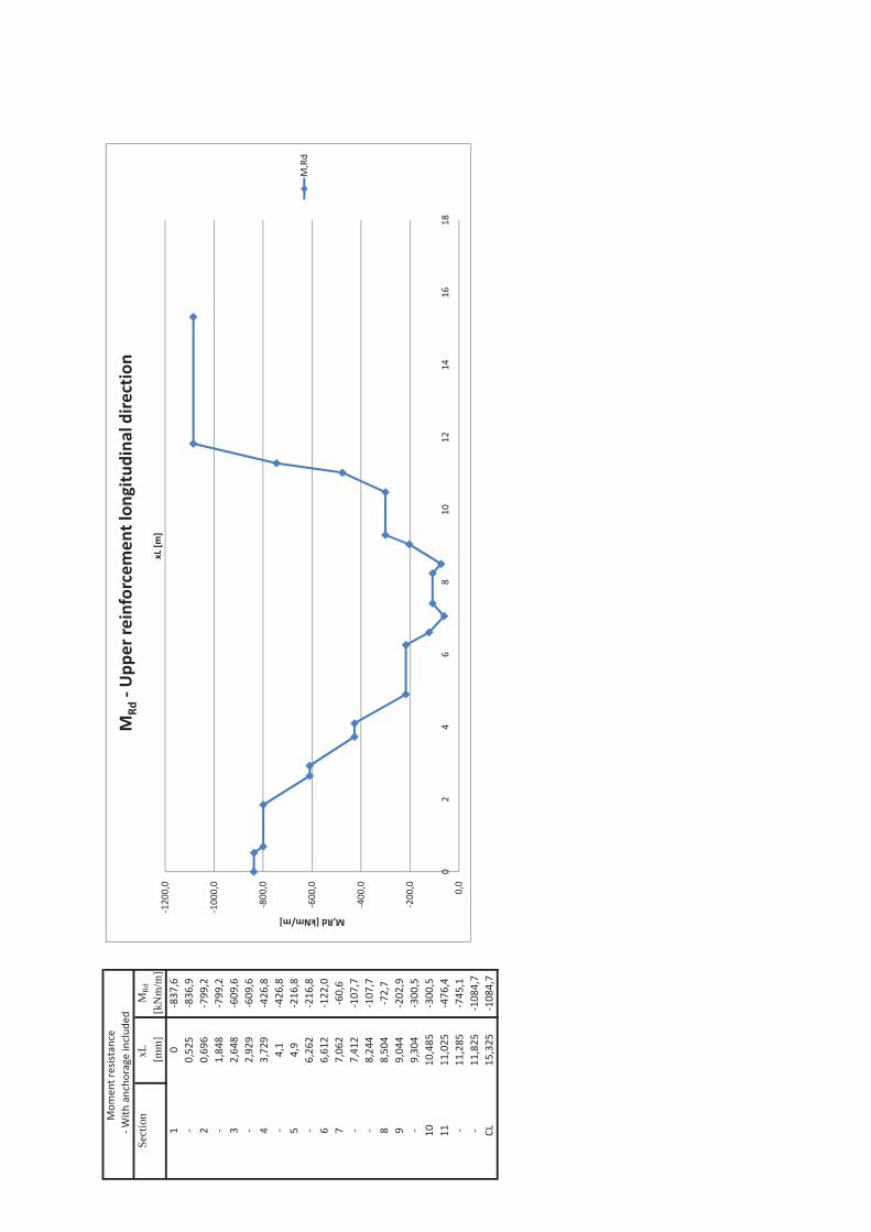
Sect
ion
xL
MR
d
[mm
][k
Nm
/m]
10
837,6
0,52
583
6,9
20,69
679
9,2
1,84
879
9,2
32,64
860
9,6
2,92
960
9,6
43,72
942
6,8
4,1
426,8
54,9
216,8
6,26
221
6,8
66,61
212
2,0
77,06
260
,67,41
210
7,7
8,24
410
7,7
88,50
472
,79
9,04
420
2,9
9,30
430
0,5
1010
,485
300,5
1111
,025
476,4
11,285
745,1
11,825
1084
,7CL
15,325
1084
,7
With
anchorageinclud
edMom
entresistance
1200
,0
1000
,0
800,0
600,0
400,0
200,0
0,0
02
46
810
1214
1618
M,Rd[kNm/m]
xL[m
]
MRd
Upp
erreinforcem
entlon
gitudina
ldire
ction
M,Rd
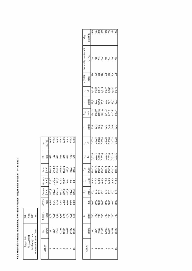
UL
S M
omen
t res
ista
nce
calc
ulat
ions
, low
er r
einf
orce
men
t lon
gitu
dina
l dir
ectio
n - r
esul
t lin
e 1
646
626
800
16
xL
Laye
r 1
Laye
r 2A
s,lay
er 1
A
s,lay
er 2
As,t
otd
f yd
[mm
][p
cs]
[pcs
][m
m2 ]
[mm
2 ][m
m2 ]
[mm
][M
Pa]
10
4,08
4,08
820,7
820,7
1641
,362
644
9,3
211
164,08
8,16
820,7
1641
,324
62,0
626
449,3
326
488,16
8,16
1641
,316
41,3
3282
,662
644
9,3
411
386
8,16
4,08
1641
,382
0,7
2462
,062
644
9,3
512
918
4,08
4,08
820,7
820,7
1641
,362
644
9,3
614
089
4,08
0,00
820,7
0,0
820,7
646
449,3
714
849
4,08
0,00
820,7
0,0
820,7
646
449,3
CL15
325
4,08
0,00
820,7
0,0
820,7
626
449,3
xL
h b
f cdf y
dE s
dcu
syd
As,t
otx
sa l
(1,0
d)N
orm
ally
rein
forc
ed?
MR
d
[mm
][m
m]
[mm
][M
Pa]
[MPa
][G
Pa]
[- ][-]
[mm
][m
m2 ]
[mm
][-]
[mm
]s >
sy
[kN
m/m
]1
070
010
0017
,144
9,3
158,73
0,00
350,00
2862
616
41,3
53,9
0,03
762
6Yes
446
211
1670
010
0017
,144
9,3
158,73
0,00
350,00
2862
624
62,0
80,9
0,02
462
6Yes
657
326
4870
010
0017
,144
9,3
158,73
0,00
350,00
2862
632
82,6
107,8
0,01
762
6Yes
860
411
386
700
1000
17,1
449,3
158,73
0,00
350,00
2862
624
62,0
80,9
0,02
462
6Yes
657
512
918
700
1000
17,1
449,3
158,73
0,00
350,00
2862
616
41,3
53,9
0,03
762
6Yes
446
614
089
700
1000
17,1
449,3
158,73
0,00
350,00
2864
682
0,7
27,0
0,08
064
6Yes
234
714
849
700
1000
17,1
449,3
158,73
0,00
350,00
2864
682
0,7
27,0
0,08
064
6Yes
234
CL15
325
700
1000
17,1
449,3
158,73
0,00
350,00
2862
682
0,7
27,0
0,07
862
6Yes
227
Ref
eren
ce d
iam
eter
[mm
]
Sect
ion
Sect
iond 1
laye
r [m
m]
d 2 la
yers
[mm
]A
ncho
rage
[mm
]
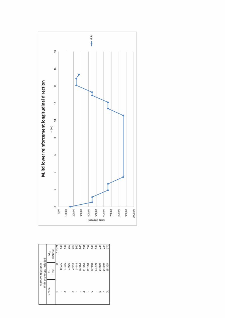
Sect
ion
xL
MR
d
[mm
][k
Nm
/m]
10
153,21
0,52
544
62
1,11
644
61,91
665
73
2,64
865
73,44
886
010
,586
860
411
,386
657
12,118
657
512
,918
446
13,289
446
614
,089
234
714
,849
234
CL15
,325
270
With
anchorageinclud
edMom
entresistance
0,00
100,00
200,00
300,00
400,00
500,00
600,00
700,00
800,00
900,00
1000
,00
02
46
810
1214
1618
M,Rd[kNm/m]
xL[m
]
M,Rdlower
reinforcem
entlon
gitudina
ldire
ction
M,Rd
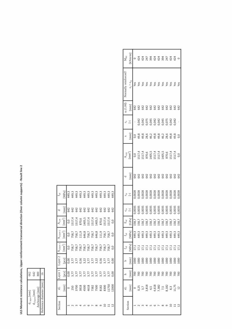
ULS
Mom
entresistancecalculations,U
pper
reinforcem
enttransversaldirection(Overcolum
nsupp
orts)
662
642
800
16
Sect
ion
xL
Laye
r 1
Laye
r 2A
s,lay
er 1
A
s,lay
er 2
As,t
otd
f yd
[mm
][p
cs]
[pcs
][m
m2 ]
[mm
2 ][m
m2 ]
[mm
][M
Pa]
10
0,00
0,00
0,0
0,0
0,0
642
449,3
225
03,77
3,77
758,7
758,7
1517
,464
244
9,3
337
003,77
3,77
758,7
758,7
1517
,464
244
9,3
438
183,77
0,56
758,7
111,9
870,6
642
449,3
545
003,77
3,22
758,7
646,8
1405
,564
244
9,3
646
183,77
3,77
758,7
758,7
1517
,464
244
9,3
773
823,77
3,77
758,7
758,7
1517
,464
244
9,3
875
003,77
3,22
758,7
646,8
1405
,564
244
9,3
981
823,77
0,56
758,7
111,9
870,6
642
449,3
1083
003,77
3,77
758,7
758,7
1517
,464
244
9,3
1111
750
3,77
3,77
758,7
758,7
1517
,464
244
9,3
1212
000
0,00
0,00
0,0
0,0
0,0
642
449,3
xL
h b
f cdf y
dE s
dcu
syd
As,t
otx
sa l
(1,0
d)N
orm
ally
rein
forc
ed?
MR
d
[mm
][m
m]
[mm
][M
Pa]
[MPa
][G
Pa]
[-][-]
[mm
][m
m2 ]
[mm
][-]
[mm
]s >
sy
[kN
m/m
]1
070
010
0017
,144
9,3
158,7
0,00
350,00
2864
20,0
0,0
642
Yes
02
0,25
700
1000
17,1
449,3
158,7
0,00
350,00
2864
215
17,4
49,8
0,04
264
2Yes
424
33,7
700
1000
17,1
449,3
158,7
0,00
350,00
2864
215
17,4
49,8
0,04
264
2Yes
424
43,81
870
010
0017
,144
9,3
158,7
0,00
350,00
2864
287
0,6
28,6
0,07
564
2Yes
247
54,5
700
1000
17,1
449,3
158,7
0,00
350,00
2864
214
05,5
46,2
0,04
564
2Yes
394
64,61
870
010
0017
,144
9,3
158,7
0,00
350,00
2864
215
17,4
49,8
0,04
264
2Yes
424
77,38
270
010
0017
,144
9,3
158,7
0,00
350,00
2864
215
17,4
49,8
0,04
264
2Yes
424
87,5
700
1000
17,1
449,3
158,7
0,00
350,00
2864
214
05,5
46,2
0,04
564
2Yes
394
98,18
270
010
0017
,144
9,3
158,7
0,00
350,00
2864
287
0,6
28,6
0,07
564
2Yes
247
108,3
700
1000
17,1
449,3
158,7
0,00
350,00
2864
215
17,4
49,8
0,04
264
2Yes
424
1111
,75
700
1000
17,1
449,3
158,7
0,00
350,00
2864
215
17,4
49,8
0,04
264
2Yes
424
1212
700
1000
17,1
449,3
158,7
0,00
350,00
2864
20,0
0,0
642
Yes
0
Sect
iond 1 la
yer [
mm
]d 2
laye
rs [m
m]
Anc
hora
ge [m
m]
Ref
eren
ce d
iam
eter
[mm
]
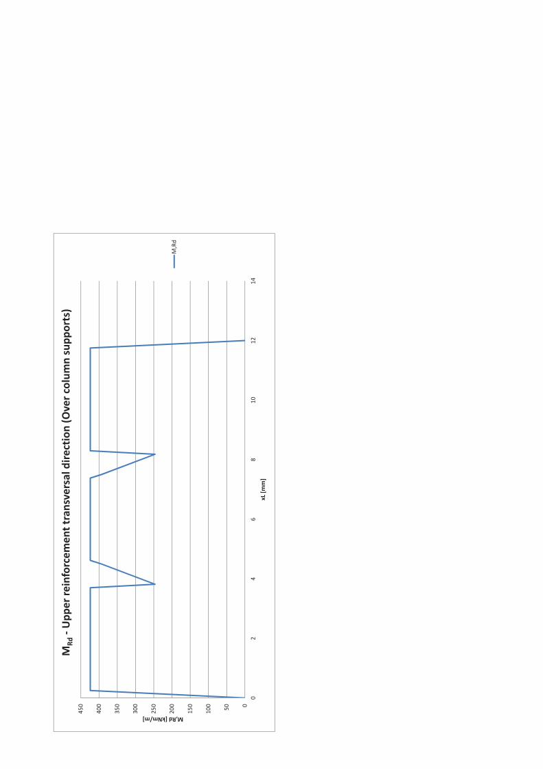
050100
150
200
250
300
350
400
450
02
46
810
1214
M,Rd[kNm/m]
xL[m
m]
MRd
Upp
erreinforcem
enttransversaldirection(Overcolum
nsupp
orts)
M,Rd
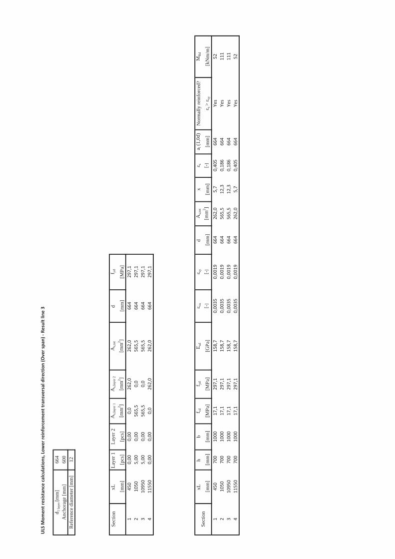
ULS
Mom
entresistancecalculations,Low
erreinforcem
enttransversaldirection(Overspa
n)
664
600
12
Sect
ion
xL
Laye
r 1
Laye
r 2A
s,lay
er 1
A
s,lay
er 2
As,t
otd
f yd
[mm
][p
cs]
[pcs
][m
m2 ]
[mm
2 ][m
m2 ]
[mm
][M
Pa]
145
00,00
0,00
0,0
262,0
262,0
664
297,1
210
505,00
0,00
565,5
0,0
565,5
664
297,1
310
950
5,00
0,00
565,5
0,0
565,5
664
297,1
411
550
0,00
0,00
0,0
262,0
262,0
664
297,1
xLh
bf cd
f yd
E sd
cusy
d A
s,tot
xs
a l (1
,0d)
Nor
mal
ly re
info
rced
?M
Rd
[mm
][m
m]
[mm
][M
Pa]
[MPa
][G
Pa]
[-][-]
[mm
][m
m2 ]
[mm
][-]
[mm
]s >
sy
[kN
m/m
]1
450
700
1000
17,1
297,1
158,7
0,00
350,00
1966
426
2,0
5,7
0,40
566
4Yes
522
1050
700
1000
17,1
297,1
158,7
0,00
350,00
1966
456
5,5
12,3
0,18
666
4Yes
111
310
950
700
1000
17,1
297,1
158,7
0,00
350,00
1966
456
5,5
12,3
0,18
666
4Yes
111
411
550
700
1000
17,1
297,1
158,7
0,00
350,00
1966
426
2,0
5,7
0,40
566
4Yes
52
d 1 la
yer [
mm
]A
ncho
rage
[mm
]R
efer
ence
dia
met
er [m
m]
Sect
ion
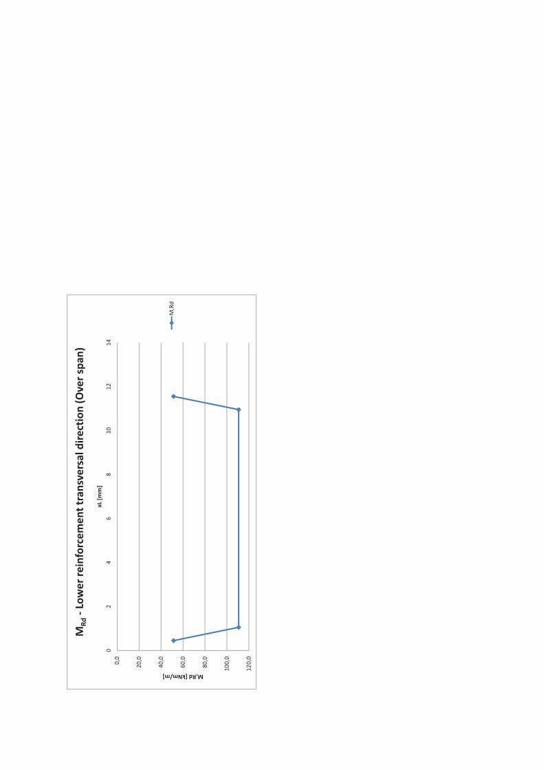
0,0
20,0
40,0
60,0
80,0
100,0
120,0
02
46
810
1214
M,Rd[kNm/m]xL
[mm]
MRd
Lower
reinforcem
enttransversaldirection(Overspa
n)
M,Rd
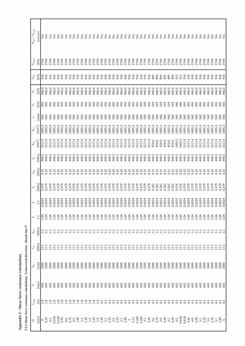
App
endi
x I -
She
ar fo
rce
resi
stan
ce c
alcu
latio
nsU
LS
Shea
r fo
rce
resi
stan
ce c
alcu
latio
ns, T
rans
vers
al d
irec
tion
- Res
ult l
ine
5
xL
L spa
n d
b wf cd
f ctd
f vf v
Rf sv
As0
A
svs
Vc
Vs
VR
dV
dmax
VR
d < V
dmax
[mm
][m
][m
m]
[mm
][M
Pa]
[MPa
][-
][-
][M
Pa]
[MPa
][M
Pa]
[mm
2 ][m
m2 ]
[mm
][k
N]
[kN
][k
N]
[kN
][y
es/n
o]0
1,8
642
1000
17,1
1,1
1,04
0,00
240,37
90,32
449,3
1517
,410
05,3
560
450
466,0
916
2744
Yes
0,15
1,8
642
1000
17,1
1,1
1,04
0,00
240,37
90,32
449,3
1517
,410
05,3
560
450
466,0
916
2744
Yes
0,3
1,8
642
1000
17,1
1,1
1,04
0,00
240,37
90,32
449,3
1517
,410
05,3
560
450
466,0
916
2744
Yes
0,41
81,8
642
1000
17,1
1,1
1,04
0,00
240,37
90,32
449,3
1517
,410
05,3
560
450
466,0
916
2744
Yes
0,41
81,8
642
1000
17,1
1,1
1,04
0,00
240,37
90,32
449,3
1517
,410
05,3
560
450
466,0
916
2744
Yes
0,45
1,8
642
1000
17,1
1,1
1,04
0,00
240,37
90,32
449,3
1517
,410
05,3
560
450
466,0
916
2744
Yes
0,6
1,8
642
1000
17,1
1,1
1,04
0,00
240,37
90,32
449,3
1517
,410
05,3
560
450
466,0
916
2744
Yes
0,75
1,8
642
1000
17,1
1,1
1,04
0,00
240,37
90,32
449,3
1517
,410
05,3
560
450
466,0
916
2744
Yes
0,9
1,8
642
1000
17,1
1,1
1,04
0,00
240,37
90,32
449,3
1517
,410
05,3
560
450
466,0
916
2744
Yes
1,05
1,8
642
1000
17,1
1,1
1,04
0,00
240,37
90,32
449,3
1517
,410
05,3
560
450
466,0
916
2744
Yes
1,2
1,8
642
1000
17,1
1,1
1,04
0,00
240,37
90,32
449,3
1517
,410
05,3
560
450
466,0
916
2744
Yes
1,35
1,8
642
1000
17,1
1,1
1,04
0,00
240,37
90,32
449,3
1517
,410
05,3
560
450
466,0
916
2744
Yes
1,5
1,8
642
1000
17,1
1,1
1,04
0,00
240,37
90,32
449,3
1517
,410
05,3
560
450
466,0
916
2744
Yes
1,65
1,8
642
1000
17,1
1,1
1,04
0,00
240,37
90,32
449,3
1517
,410
05,3
560
450
466,0
916
2744
Yes
1,8
1,8
642
1000
17,1
1,1
1,04
0,00
240,37
90,32
449,3
1517
,410
05,3
560
450
466,0
916
2744
Yes
1,95
4,2
642
1000
17,1
1,1
1,04
0,00
240,37
90,32
449,3
1517
,410
05,3
560
450
466,0
916
2744
Yes
2,1
4,2
642
1000
17,1
1,1
1,04
0,00
240,37
90,32
449,3
1517
,410
05,3
560
450
466,0
916
2744
Yes
2,25
4,2
642
1000
17,1
1,1
1,04
0,00
240,37
90,32
449,3
1517
,410
05,3
560
450
466,0
916
2744
Yes
2,4
4,2
642
1000
17,1
1,1
1,04
0,00
240,37
90,32
449,3
1517
,410
05,3
560
450
466,0
916
2744
Yes
2,55
4,2
642
1000
17,1
1,1
1,04
0,00
240,37
90,32
449,3
1517
,410
05,3
560
450
466,0
916
2744
Yes
2,7
4,2
642
1000
17,1
1,1
1,04
0,00
240,37
90,32
449,3
1517
,410
05,3
560
450
466,0
916
2744
Yes
2,85
4,2
642
1000
17,1
1,1
1,04
0,00
240,37
90,32
449,3
1517
,410
05,3
560
450
466,0
916
2744
Yes
34,2
642
1000
17,1
1,1
1,04
0,00
240,37
90,32
449,3
1517
,410
05,3
560
450
466,0
916
2744
Yes
3,15
4,2
642
1000
17,1
1,1
1,04
0,00
240,37
90,32
449,3
1517
,410
05,3
560
450
466,0
916
2744
Yes
3,18
24,2
642
1000
17,1
1,1
1,04
0,00
240,37
90,32
449,3
1517
,410
05,3
560
450
466,0
916
2744
Yes
3,18
24,2
642
1000
17,1
1,1
1,04
0,00
240,37
90,32
449,3
1517
,410
05,3
560
450
466,0
916
2744
Yes
3,3
4,2
642
1000
17,1
1,1
1,04
0,00
240,37
90,32
449,3
1517
,410
05,3
560
450
466,0
916
2744
Yes
3,45
4,2
642
1000
17,1
1,1
1,04
0,00
240,37
90,32
449,3
1517
,410
05,3
560
450
466,0
916
2744
Yes
3,6
4,2
642
1000
17,1
1,1
1,04
0,00
140,36
20,31
449,3
870,6
1005
,356
042
946
6,0
895
2744
Yes
3,75
4,2
642
1000
17,1
1,1
1,04
0,00
140,36
20,31
449,3
870,6
1005
,356
042
946
6,0
895
2744
Yes
3,9
4,2
642
1000
17,1
1,1
1,04
0,00
140,36
20,31
449,3
870,6
1005
,356
042
946
6,0
895
2744
Yes
4,05
4,2
642
1000
17,1
1,1
1,04
0,00
140,36
20,31
449,3
870,6
1005
,356
042
946
6,0
895
2744
Yes
4,2
4,2
642
1000
17,1
1,1
1,04
0,00
140,36
20,31
449,3
870,6
1005
,356
042
946
6,0
895
2744
Yes
4,35
4,2
642
1000
17,1
1,1
1,04
0,00
140,36
20,31
449,3
870,6
1005
,356
042
946
6,0
895
2744
Yes
4,5
4,2
642
1000
17,1
1,1
1,04
0,00
220,37
60,32
449,3
1405
,510
05,3
560
446
466,0
912
2744
Yes
4,61
84,2
642
1000
17,1
1,1
1,04
0,00
220,37
60,32
449,3
1405
,510
05,3
560
446
466,0
912
2744
Yes
4,61
84,2
642
1000
17,1
1,1
1,04
0,00
240,37
90,32
449,3
1517
,410
05,3
560
450
466,0
916
2744
Yes
4,65
4,2
642
1000
17,1
1,1
1,04
0,00
240,37
90,32
449,3
1517
,410
05,3
560
450
466,0
916
2744
Yes
4,8
4,2
642
1000
17,1
1,1
1,04
0,00
240,37
90,32
449,3
1517
,410
05,3
560
450
466,0
916
2744
Yes
4,95
4,2
642
1000
17,1
1,1
1,04
0,00
240,37
90,32
449,3
1517
,410
05,3
560
450
466,0
916
2744
Yes
5,1
4,2
642
1000
17,1
1,1
1,04
0,00
240,37
90,32
449,3
1517
,410
05,3
560
450
466,0
916
2744
Yes
5,25
4,2
642
1000
17,1
1,1
1,04
0,00
240,37
90,32
449,3
1517
,410
05,3
560
450
466,0
916
2744
Yes
5,4
4,2
642
1000
17,1
1,1
1,04
0,00
240,37
90,32
449,3
1517
,410
05,3
560
450
466,0
916
2744
Yes
5,55
4,2
642
1000
17,1
1,1
1,04
0,00
240,37
90,32
449,3
1517
,410
05,3
560
450
466,0
916
2744
Yes
5,7
4,2
642
1000
17,1
1,1
1,04
0,00
240,37
90,32
449,3
1517
,410
05,3
560
450
466,0
916
2744
Yes
5,85
4,2
642
1000
17,1
1,1
1,04
0,00
240,37
90,32
449,3
1517
,410
05,3
560
450
466,0
916
2744
Yes
64,2
642
1000
17,1
1,1
1,04
0,00
240,37
90,32
449,3
1517
,410
05,3
560
450
466,0
916
2744
Yes
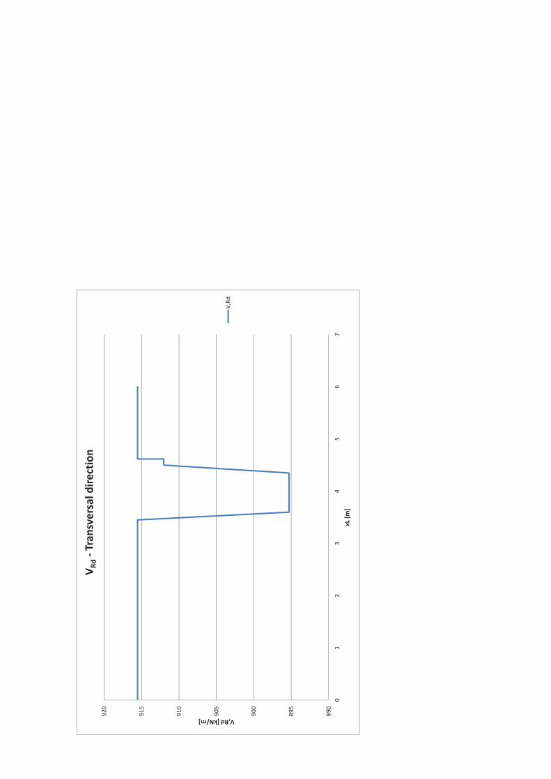
890
895
900
905
910
915
920
01
23
45
67
V,Rd[kN/m]
xL[m
]
V Rd
Tran
sversaldire
ction
V,Rd
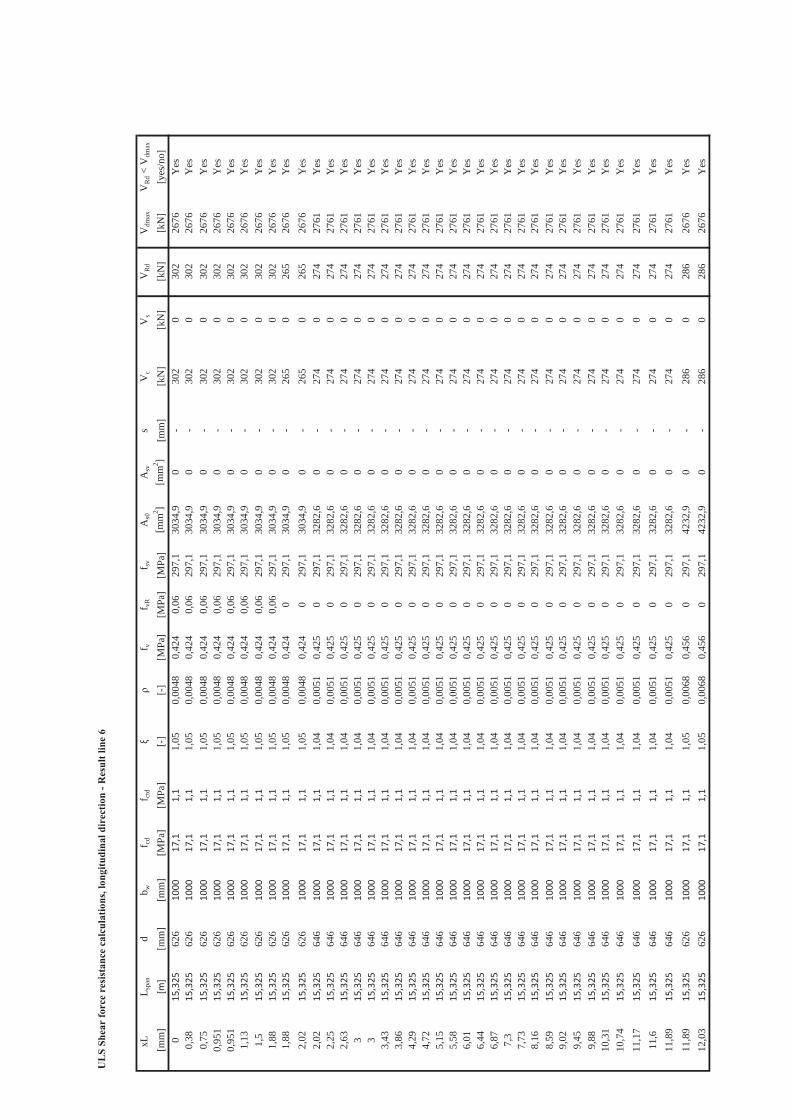
UL
S Sh
ear
forc
e re
sist
ance
cal
cula
tions
, lon
gitu
dina
l dir
ectio
n - R
esul
t lin
e 6
xL
L spa
n d
b wf cd
f ctd
f vf v
Rf sv
As0
A
svs
Vc
Vs
VR
dV
dmax
VR
d < V
dmax
[mm
][m
][m
m]
[mm
][M
Pa]
[MPa
][-
][-
][M
Pa]
[MPa
][M
Pa]
[mm
2 ][m
m2 ]
[mm
][k
N]
[kN
][k
N]
[kN
][y
es/n
o]0
15,325
626
1000
17,1
1,1
1,05
0,00
480,
424
0,06
297,
130
34,9
0-
302
030
226
76Y
es0,
3815
,325
626
1000
17,1
1,1
1,05
0,00
480,
424
0,06
297,
130
34,9
0-
302
030
226
76Y
es0,
7515
,325
626
1000
17,1
1,1
1,05
0,00
480,
424
0,06
297,
130
34,9
0-
302
030
226
76Y
es0,
951
15,325
626
1000
17,1
1,1
1,05
0,00
480,
424
0,06
297,
130
34,9
0-
302
030
226
76Y
es0,
951
15,325
626
1000
17,1
1,1
1,05
0,00
480,
424
0,06
297,
130
34,9
0-
302
030
226
76Y
es1,
1315
,325
626
1000
17,1
1,1
1,05
0,00
480,
424
0,06
297,
130
34,9
0-
302
030
226
76Y
es1,
515
,325
626
1000
17,1
1,1
1,05
0,00
480,
424
0,06
297,
130
34,9
0-
302
030
226
76Y
es1,
8815
,325
626
1000
17,1
1,1
1,05
0,00
480,
424
0,06
297,
130
34,9
0-
302
030
226
76Y
es1,
8815
,325
626
1000
17,1
1,1
1,05
0,00
480,
424
029
7,1
3034
,90
-26
50
265
2676
Yes
2,02
15,325
626
1000
17,1
1,1
1,05
0,00
480,
424
029
7,1
3034
,90
-26
50
265
2676
Yes
2,02
15,325
646
1000
17,1
1,1
1,04
0,00
510,
425
029
7,1
3282
,60
-27
40
274
2761
Yes
2,25
15,325
646
1000
17,1
1,1
1,04
0,00
510,
425
029
7,1
3282
,60
-27
40
274
2761
Yes
2,63
15,325
646
1000
17,1
1,1
1,04
0,00
510,
425
029
7,1
3282
,60
-27
40
274
2761
Yes
315
,325
646
1000
17,1
1,1
1,04
0,00
510,
425
029
7,1
3282
,60
-27
40
274
2761
Yes
315
,325
646
1000
17,1
1,1
1,04
0,00
510,
425
029
7,1
3282
,60
-27
40
274
2761
Yes
3,43
15,325
646
1000
17,1
1,1
1,04
0,00
510,
425
029
7,1
3282
,60
-27
40
274
2761
Yes
3,86
15,325
646
1000
17,1
1,1
1,04
0,00
510,
425
029
7,1
3282
,60
-27
40
274
2761
Yes
4,29
15,325
646
1000
17,1
1,1
1,04
0,00
510,
425
029
7,1
3282
,60
-27
40
274
2761
Yes
4,72
15,325
646
1000
17,1
1,1
1,04
0,00
510,
425
029
7,1
3282
,60
-27
40
274
2761
Yes
5,15
15,325
646
1000
17,1
1,1
1,04
0,00
510,
425
029
7,1
3282
,60
-27
40
274
2761
Yes
5,58
15,325
646
1000
17,1
1,1
1,04
0,00
510,
425
029
7,1
3282
,60
-27
40
274
2761
Yes
6,01
15,325
646
1000
17,1
1,1
1,04
0,00
510,
425
029
7,1
3282
,60
-27
40
274
2761
Yes
6,44
15,325
646
1000
17,1
1,1
1,04
0,00
510,
425
029
7,1
3282
,60
-27
40
274
2761
Yes
6,87
15,325
646
1000
17,1
1,1
1,04
0,00
510,
425
029
7,1
3282
,60
-27
40
274
2761
Yes
7,3
15,325
646
1000
17,1
1,1
1,04
0,00
510,
425
029
7,1
3282
,60
-27
40
274
2761
Yes
7,73
15,325
646
1000
17,1
1,1
1,04
0,00
510,
425
029
7,1
3282
,60
-27
40
274
2761
Yes
8,16
15,325
646
1000
17,1
1,1
1,04
0,00
510,
425
029
7,1
3282
,60
-27
40
274
2761
Yes
8,59
15,325
646
1000
17,1
1,1
1,04
0,00
510,
425
029
7,1
3282
,60
-27
40
274
2761
Yes
9,02
15,325
646
1000
17,1
1,1
1,04
0,00
510,
425
029
7,1
3282
,60
-27
40
274
2761
Yes
9,45
15,325
646
1000
17,1
1,1
1,04
0,00
510,
425
029
7,1
3282
,60
-27
40
274
2761
Yes
9,88
15,325
646
1000
17,1
1,1
1,04
0,00
510,
425
029
7,1
3282
,60
-27
40
274
2761
Yes
10,3
115
,325
646
1000
17,1
1,1
1,04
0,00
510,
425
029
7,1
3282
,60
-27
40
274
2761
Yes
10,7
415
,325
646
1000
17,1
1,1
1,04
0,00
510,
425
029
7,1
3282
,60
-27
40
274
2761
Yes
11,1
715
,325
646
1000
17,1
1,1
1,04
0,00
510,
425
029
7,1
3282
,60
-27
40
274
2761
Yes
11,6
15,325
646
1000
17,1
1,1
1,04
0,00
510,
425
029
7,1
3282
,60
-27
40
274
2761
Yes
11,8
915
,325
646
1000
17,1
1,1
1,04
0,00
510,
425
029
7,1
3282
,60
-27
40
274
2761
Yes
11,8
915
,325
626
1000
17,1
1,1
1,05
0,00
680,
456
029
7,1
4232
,90
-28
60
286
2676
Yes
12,0
315
,325
626
1000
17,1
1,1
1,05
0,00
680,
456
029
7,1
4232
,90
-28
60
286
2676
Yes
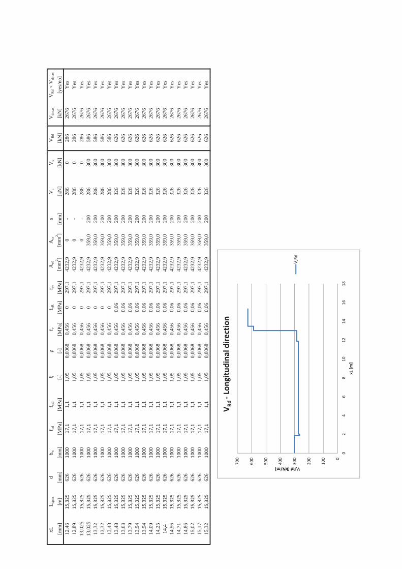
xL
L spa
n d
b wf cd
f ctd
f vf v
Rf sv
As0
A
svs
Vc
Vs
VR
dV
dmax
VR
d < V
dmax
[mm
][m
][m
m]
[mm
][M
Pa]
[MPa
][-
][-
][M
Pa]
[MPa
][M
Pa]
[mm
2 ][m
m2 ]
[mm
][k
N]
[kN
][k
N]
[kN
][y
es/n
o]12
,46
15,325
626
1000
17,1
1,1
1,05
0,00
680,
456
029
7,1
4232
,90
-28
60
286
2676
Yes
12,8
915
,325
626
1000
17,1
1,1
1,05
0,00
680,
456
029
7,1
4232
,90
-28
60
286
2676
Yes
13,0
2515
,325
626
1000
17,1
1,1
1,05
0,00
680,
456
029
7,1
4232
,90
-28
60
286
2676
Yes
13,0
2515
,325
626
1000
17,1
1,1
1,05
0,00
680,
456
029
7,1
4232
,935
9,0
200
286
300
586
2676
Yes
13,3
215
,325
626
1000
17,1
1,1
1,05
0,00
680,
456
029
7,1
4232
,935
9,0
200
286
300
586
2676
Yes
13,3
215
,325
626
1000
17,1
1,1
1,05
0,00
680,
456
029
7,1
4232
,935
9,0
200
286
300
586
2676
Yes
13,4
815
,325
626
1000
17,1
1,1
1,05
0,00
680,
456
029
7,1
4232
,935
9,0
200
286
300
586
2676
Yes
13,4
815
,325
626
1000
17,1
1,1
1,05
0,00
680,
456
0,06
297,
142
32,9
359,
020
032
630
062
626
76Y
es13
,63
15,325
626
1000
17,1
1,1
1,05
0,00
680,
456
0,06
297,
142
32,9
359,
020
032
630
062
626
76Y
es13
,79
15,325
626
1000
17,1
1,1
1,05
0,00
680,
456
0,06
297,
142
32,9
359,
020
032
630
062
626
76Y
es13
,94
15,325
626
1000
17,1
1,1
1,05
0,00
680,
456
0,06
297,
142
32,9
359,
020
032
630
062
626
76Y
es13
,94
15,325
626
1000
17,1
1,1
1,05
0,00
680,
456
0,06
297,
142
32,9
359,
020
032
630
062
626
76Y
es14
,09
15,325
626
1000
17,1
1,1
1,05
0,00
680,
456
0,06
297,
142
32,9
359,
020
032
630
062
626
76Y
es14
,25
15,325
626
1000
17,1
1,1
1,05
0,00
680,
456
0,06
297,
142
32,9
359,
020
032
630
062
626
76Y
es14
,415
,325
626
1000
17,1
1,1
1,05
0,00
680,
456
0,06
297,
142
32,9
359,
020
032
630
062
626
76Y
es14
,56
15,325
626
1000
17,1
1,1
1,05
0,00
680,
456
0,06
297,
142
32,9
359,
020
032
630
062
626
76Y
es14
,71
15,325
626
1000
17,1
1,1
1,05
0,00
680,
456
0,06
297,
142
32,9
359,
020
032
630
062
626
76Y
es14
,86
15,325
626
1000
17,1
1,1
1,05
0,00
680,
456
0,06
297,
142
32,9
359,
020
032
630
062
626
76Y
es15
,02
15,325
626
1000
17,1
1,1
1,05
0,00
680,
456
0,06
297,
142
32,9
359,
020
032
630
062
626
76Y
es15
,17
15,325
626
1000
17,1
1,1
1,05
0,00
680,
456
0,06
297,
142
32,9
359,
020
032
630
062
626
76Y
es15
,32
15,325
626
1000
17,1
1,1
1,05
0,00
680,
456
0,06
297,
142
32,9
359,
020
032
630
062
626
76Y
es
0
100
200
300
400
500
600
700
02
46
810
1214
1618
V,Rd[kN/m]
xL[m
]
V Rd
Long
itudina
ldire
ction
V,Rd
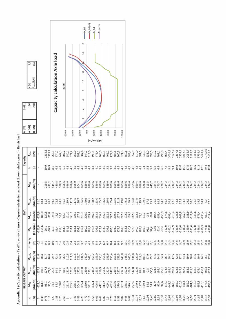
App
endi
x J
(Cap
acity
cal
cula
tion
- Tra
ffic
on
own
lane
) - C
apac
ity c
alcu
latio
n A
xle
load
(Low
er r
einf
orce
men
t) -
Res
ult l
ine
1
a l[m
]0,63
1
xLM
EdM
perm
Mtraffic
xL+/
a lM
EdM
perm
Mtraffic
MRd
A dim
A[kN]
120
k[]
3,9
[m]
[kNm/m
][kNm/m
][kNm/m
][m
][kNm/m
][kNm/m
][kNm/m
][kNm/m
][]
[kN]
B[kN]
210
A dim[kN]
462
022
2,0
227,9
11,0
0,6
222,0
227,9
11,0
0,38
161,6
180,0
18,4
0,3
161,6
180,0
18,4
0,75
96,1
127,8
31,7
0,1
96,1
127,8
31,7
219,5
10,9
1313
,51,13
30,5
77,0
46,6
0,5
30,5
77,0
46,6
431,2
10,9
1309
,71,5
30,3
29,4
59,7
0,9
30,3
29,4
59,7
445,7
8,0
955,1
1,88
86,4
14,1
72,3
1,2
86,4
14,1
72,3
480,8
6,5
774,7
2,25
138,0
53,1
84,9
1,6
138,0
53,1
84,9
578,3
6,2
742,3
2,63
184,5
88,0
96,5
2,0
184,5
88,0
96,5
656,6
5,9
707,2
323
1,8
121,0
110,8
2,4
231,8
121,0
110,8
656,6
4,8
580,1
323
3,1
121,2
111,9
2,4
233,1
121,2
111,9
656,6
4,8
574,2
3,43
268,1
150,6
117,5
2,8
268,1
150,6
117,5
695,0
4,6
555,9
3,86
304,5
177,8
126,7
3,2
304,5
177,8
126,7
804,1
4,9
593,1
4,29
335,4
201,0
134,5
3,7
335,4
201,0
134,5
859,6
4,9
587,6
4,72
360,9
220,0
140,9
4,1
360,9
220,0
140,9
859,6
4,5
544,7
5,15
381,2
235,1
146,1
4,5
381,2
235,1
146,1
859,6
4,3
513,0
5,58
396,4
246,2
150,2
4,9
396,4
246,2
150,2
859,6
4,1
490,1
6,01
406,5
253,5
153,0
5,4
406,5
253,5
153,0
859,6
4,0
475,4
6,44
412,1
256,9
155,2
5,8
412,1
256,9
155,2
859,6
3,9
466,0
6,87
413,2
256,6
156,6
6,2
413,2
256,6
156,6
859,6
3,9
462,1
7,3
409,1
252,5
156,6
6,7
409,1
252,5
156,6
859,6
3,9
465,2
7,73
402,6
247,2
155,4
8,4
402,6
247,2
155,4
859,6
3,9
472,9
8,16
393,0
239,4
153,6
8,8
393,0
239,4
153,6
859,6
4,0
484,5
8,59
379,2
227,7
151,5
9,2
379,2
227,7
151,5
859,6
4,2
500,5
9,02
361,3
212,3
149,0
9,7
361,3
212,3
149,0
859,6
4,3
521,3
9,45
338,1
192,9
145,3
10,1
338,1
192,9
145,3
859,6
4,6
550,6
9,88
310,1
169,5
140,5
10,5
310,1
169,5
140,5
859,6
4,9
589,4
10,31
277,6
142,8
134,8
10,9
277,6
142,8
134,8
769,6
4,6
557,9
10,74
240,4
112,6
127,9
11,4
240,4
112,6
127,9
660,4
4,3
514,0
11,17
197,8
78,6
119,3
11,8
197,8
78,6
119,3
656,6
4,8
581,5
11,6
149,3
40,2
109,1
12,2
149,3
40,2
109,1
626,8
5,4
645,3
12,03
95,1
2,8
97,9
12,7
95,1
2,8
97,9
513,5
5,3
633,0
12,46
34,4
50,8
85,2
13,1
34,4
50,8
85,2
445,7
5,8
699,0
12,89
32,9
104,4
71,6
13,5
32,9
104,4
71,6
384,4
6,8
819,2
13,32
92,0
156,4
64,5
14,0
92,0
156,4
64,5
270,7
6,6
795,1
13,32
92,6
156,9
64,3
14,0
92,6
156,9
64,3
270,7
6,6
798,0
13,48
117,9
174,6
56,7
14,1
117,9
174,6
56,7
234,2
7,2
865,4
13,63
142,2
192,4
50,2
14,3
142,2
192,4
50,2
234,2
8,5
1020
,213
,79
162,9
210,4
47,5
14,4
162,9
210,4
47,5
234,2
9,4
1122
,713
,94
186,0
228,8
42,8
14,6
186,0
228,8
42,8
234,2
10,8
1297
,814
,09
210,6
247,8
37,2
14,7
210,6
247,8
37,2
234,2
13,0
1554
,414
,25
234,4
267,7
33,3
14,9
234,4
267,7
33,3
234,2
15,1
1807
,614
,425
9,0
288,9
29,9
15,0
259,0
288,9
29,9
234,2
17,5
2098
,714
,56
281,6
311,6
30,0
15,2
281,6
311,6
30,0
234,2
18,2
2186
,914
,71
317,0
338,6
21,6
15,3
317,0
338,6
21,6
234,2
26,5
3183
,714
,86
356,8
376,4
19,6
15,5
356,8
376,4
19,6
234,2
31,2
3738
,415
,02
416,3
430,4
14,1
15,7
416,3
430,4
14,1
234,2
47,1
5648
,215
,17
475,8
480,1
8,0
15,8
475,8
480,1
8,0
234,2
89,4
1072
2,6
15,32
499,8
517,4
17,6
16,0
499,8
517,4
17,6
234,2
42,8
5136
,3
Capa
city
BRIGAD
EOUTP
UT
Shift
600,0
400,0
200,0
0,0
200,0
400,0
600,0
800,0
1000
,0
02
46
810
1214
1618
M[kNm/m]
xL[m
]
Capa
city
calculationAx
leload
M,Ed
M,Ed(al)
M,Rd
M,perm
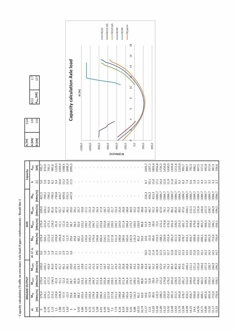
Cap
acity
cal
cula
tion
Axl
e lo
ad (U
pper
rei
nfor
cem
ent)
- R
esul
t lin
e 1
a l[m
]0,64
xLM
EdM
perm
Mtraffic
xL+/
a lM
EdM
perm
Mtraffic
MRd
A dim
A[kN]
120
k[]
2,7
[m]
[kNm/m
][kNm/m
][kNm/m
][m
][kNm/m
][kNm/m
][kNm/m
][kNm/m
][]
[kN]
B[kN]
210
A dim[kN]
327
037
9,4
270,4
109,0
0,6
379,4
270,4
109,0
811,5
5,0
595,7
0,38
324,1
221,0
103,1
1,0
324,1
221,0
103,1
799,2
5,6
673,0
0,75
271,0
177,1
93,9
1,4
271,0
177,1
93,9
799,2
6,6
795,1
1,13
215,2
134,3
81,0
1,8
215,2
134,3
81,0
799,2
8,2
985,6
1,5
159,8
91,9
67,9
2,1
159,8
91,9
67,9
730,8
9,4
1129
,31,88
106,8
51,1
55,7
2,5
106,8
51,1
55,7
640,7
10,6
1269
,42,25
57,4
12,3
45,1
2,9
57,4
12,3
45,1
609,6
13,2
1588
,52,63
12,3
23,9
36,1
3,3
12,3
23,9
36,1
532,5
15,4
1848
,33
29,6
58,7
29,0
3,6
29,6
58,7
29,0
447,9
17,5
2095
,53
29,8
58,9
29,1
29,8
58,9
29,1
3,43
68,2
92,0
23,7
68,2
92,0
23,7
3,86
103,4
123,2
19,8
103,4
123,2
19,8
4,29
133,6
150,7
17,1
133,6
150,7
17,1
4,72
159,3
174,6
15,3
159,3
174,6
15,3
5,15
179,4
194,7
15,3
179,4
194,7
15,3
5,58
194,8
211,1
16,3
194,8
211,1
16,3
6,01
206,4
223,8
17,4
206,4
223,8
17,4
6,44
214,1
232,8
18,7
214,1
232,8
18,7
6,87
217,9
238,1
20,2
217,9
238,1
20,2
7,3
217,8
239,5
21,7
217,8
239,5
21,7
7,73
211,3
234,7
23,3
211,3
234,7
23,3
8,16
199,8
224,9
25,0
199,8
224,9
25,0
8,59
184,6
211,4
26,8
184,6
211,4
26,8
9,02
165,6
194,4
28,8
165,6
194,4
28,8
9,45
142,9
173,7
30,9
142,9
173,7
30,9
9,88
116,3
149,5
33,2
116,3
149,5
33,2
10,31
85,2
120,9
35,8
85,2
120,9
35,8
10,74
50,0
88,8
38,8
50,0
88,8
38,8
11,17
10,6
52,9
42,4
10,5
10,6
52,9
42,4
316,3
8,7
1045
,711
,632
,913
,846
,711
,032
,913
,846
,745
6,3
10,1
1207
,112
,03
80,6
28,4
52,2
11,4
80,6
28,4
52,2
813,3
15,0
1803
,412
,46
132,5
73,5
58,9
11,8
132,5
73,5
58,9
1083
,717
,120
56,8
12,89
188,2
121,2
67,0
12,3
188,2
121,2
67,0
1084
,714
,417
26,2
13,32
250,9
174,8
76,1
12,7
250,9
174,8
76,1
1084
,712
,014
34,8
13,32
252,4
176,2
76,2
12,7
252,4
176,2
76,2
1084
,711
,914
30,9
13,48
281,3
201,0
80,3
12,8
281,3
201,0
80,3
1084
,711
,013
20,8
13,63
311,5
226,5
85,0
13,0
311,5
226,5
85,0
1084
,710
,112
11,6
13,79
343,8
253,3
90,5
13,2
343,8
253,3
90,5
1084
,79,2
1103
,013
,94
378,7
281,7
97,0
13,3
378,7
281,7
97,0
1084
,78,3
993,7
14,09
416,1
312,0
104,1
13,5
416,1
312,0
104,1
1084
,77,4
890,7
14,25
456,7
344,6
112,1
13,6
456,7
344,6
112,1
1084
,76,6
792,3
14,4
500,8
379,6
121,2
13,8
500,8
379,6
121,2
1084
,75,8
698,1
14,56
550,1
418,5
131,6
13,9
550,1
418,5
131,6
1084
,75,1
607,5
14,71
606,1
461,5
144,6
14,1
606,1
461,5
144,6
1084
,74,3
517,2
14,86
661,6
504,3
157,3
14,2
661,6
504,3
157,3
1084
,73,7
442,8
15,02
691,0
532,4
158,7
14,4
691,0
532,4
158,7
1084
,73,5
417,6
15,17
713,0
546,1
166,9
14,5
713,0
546,1
166,9
1084
,73,2
387,3
15,32
750,4
556,1
194,2
14,7
750,4
556,1
194,2
1084
,72,7
326,6
Capa
city
BRIGAD
EOUTP
UT
Shift
1200,0
1000,0
800,0
600,0
400,0
200,0
0,0
200,0
400,0
02
46
810
1214
1618
M[kNm/m]
xL[m
]
Capa
city
calculationAx
leload
M,Ed
M,Ed(al)
M,Ed(al)
M,Rd
M,Rd
M,perm
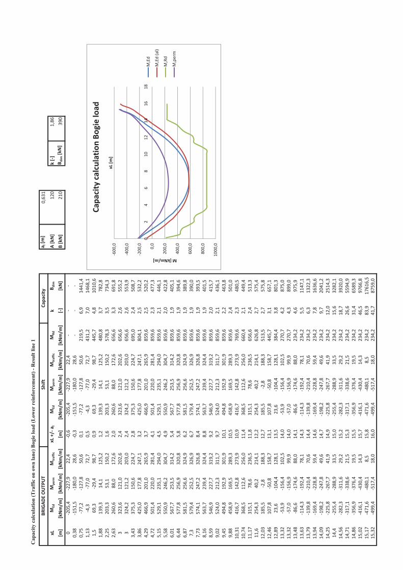
Cap
acity
cal
cula
tion
Bog
ie lo
ad (L
ower
rei
nfor
cem
ent)
- R
esul
t lin
e 1
a l[m
]0,63
1
xLM
EdM
perm
Mtraffic
xL+/
a lM
EdM
perm
Mtraffic
MRd
B dim
A[kN]
120
k[]
1,86
[m]
[kNm/m
][kNm/m
][kNm/m
][m
][kNm/m
][kNm/m
][kNm/m
][kNm/m
][]
[kN]
B[kN]
210
B dim[kN]
390
020
5,4
227,9
22,4
0,6
205,4
227,9
22,4
0,38
151,5
180,0
28,6
0,3
151,5
180,0
28,6
0,75
77,2
127,8
50,6
0,1
77,2
127,8
50,6
219,5
6,9
1441
,41,13
4,3
77,0
72,7
0,5
4,3
77,0
72,7
431,2
7,0
1468
,11,5
69,3
29,4
98,7
0,9
69,3
29,4
98,7
445,7
4,8
1010
,61,88
139,3
14,1
125,2
1,2
139,3
14,1
125,2
480,8
3,7
782,8
2,25
203,3
53,1
150,2
1,6
203,3
53,1
150,2
578,3
3,5
734,3
2,63
260,6
88,0
172,6
2,0
260,6
88,0
172,6
656,6
3,3
691,8
332
3,6
121,0
202,6
2,4
323,6
121,0
202,6
656,6
2,6
555,2
332
4,2
121,2
203,0
2,4
324,2
121,2
203,0
656,6
2,6
553,9
3,43
375,3
150,6
224,7
2,8
375,3
150,6
224,7
695,0
2,4
508,7
3,86
425,0
177,8
247,1
3,2
425,0
177,8
247,1
804,1
2,5
532,2
4,29
466,9
201,0
265,9
3,7
466,9
201,0
265,9
859,6
2,5
520,2
4,72
501,4
220,0
281,4
4,1
501,4
220,0
281,4
859,6
2,3
477,3
5,15
529,1
235,1
294,0
4,5
529,1
235,1
294,0
859,6
2,1
446,1
5,58
550,9
246,2
304,7
4,9
550,9
246,2
304,7
859,6
2,0
422,8
6,01
567,7
253,5
314,2
5,4
567,7
253,5
314,2
859,6
1,9
405,1
6,44
577,8
256,9
320,8
5,8
577,8
256,9
320,8
859,6
1,9
394,6
6,87
581,5
256,6
324,9
6,2
581,5
256,6
324,9
859,6
1,9
389,8
7,3
579,4
252,5
326,9
6,7
579,4
252,5
326,9
859,6
1,9
390,0
7,73
574,1
247,2
326,8
8,4
574,1
247,2
326,8
859,6
1,9
393,5
8,16
563,7
239,4
324,4
8,8
563,7
239,4
324,4
859,6
1,9
401,5
8,59
546,9
227,7
319,2
9,2
546,9
227,7
319,2
859,6
2,0
415,7
9,02
524,0
212,3
311,7
9,7
524,0
212,3
311,7
859,6
2,1
436,1
9,45
494,8
192,9
301,9
10,1
494,8
192,9
301,9
859,6
2,2
463,8
9,88
458,9
169,5
289,3
10,5
458,9
169,5
289,3
859,6
2,4
501,0
10,31
416,7
142,8
273,9
10,9
416,7
142,8
273,9
769,6
2,3
480,5
10,74
368,5
112,6
256,0
11,4
368,5
112,6
256,0
660,4
2,1
449,4
11,17
315,1
78,6
236,5
11,8
315,1
78,6
236,5
656,6
2,4
513,3
11,6
254,3
40,2
214,1
12,2
254,3
40,2
214,1
626,8
2,7
575,4
12,03
185,5
2,8
188,3
12,7
185,5
2,8
188,3
513,5
2,7
575,8
12,46
107,8
50,8
158,7
13,1
107,8
50,8
158,7
445,7
3,1
657,1
12,89
23,6
104,4
128,1
13,5
23,6
104,4
128,1
384,4
3,8
801,3
13,32
53,9
156,4
102,5
14,0
53,9
156,4
102,5
270,7
4,2
875,0
13,32
57,0
156,9
99,9
14,0
57,0
156,9
99,9
270,7
4,3
899,0
13,48
86,6
174,6
88,0
14,1
86,6
174,6
88,0
234,2
4,6
975,9
13,63
114,3
192,4
78,1
14,3
114,3
192,4
78,1
234,2
5,5
1147
,113
,79
139,8
210,4
70,6
14,4
139,8
210,4
70,6
234,2
6,3
1322
,313
,94
169,4
228,8
59,4
14,6
169,4
228,8
59,4
234,2
7,8
1636
,614
,09
198,2
247,8
49,6
14,7
198,2
247,8
49,6
234,2
9,7
2041
,214
,25
225,8
267,7
41,9
14,9
225,8
267,7
41,9
234,2
12,0
2514
,314
,425
5,4
288,9
33,5
15,0
255,4
288,9
33,5
234,2
15,6
3282
,114
,56
282,3
311,6
29,2
15,2
282,3
311,6
29,2
234,2
18,7
3920
,014
,71
317,1
338,6
21,5
15,3
317,1
338,6
21,5
234,2
26,6
5594
,914
,86
356,9
376,4
19,5
15,5
356,9
376,4
19,5
234,2
31,4
6589
,315
,02
416,1
430,4
14,3
15,7
416,1
430,4
14,3
234,2
46,5
9766
,815
,17
471,6
480,1
8,5
15,8
471,6
480,1
8,5
234,2
83,9
1761
6,5
15,32
499,4
517,4
18,0
16,0
499,4
517,4
18,0
234,2
41,7
8759
,0
Capa
city
BRIGAD
EOUTP
UT
Shift
600,0
400,0
200,0
0,0
200,0
400,0
600,0
800,0
1000
,0
02
46
810
1214
1618
M[kNm/m]
xL[m
]
Capa
city
calculationBo
gieload
M,Ed
M,Ed(al)
M,Rd
M,perm
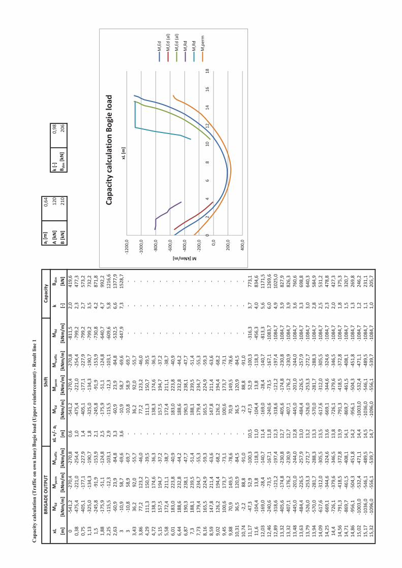
Cap
acity
cal
cula
tion
Bog
ie lo
ad (U
pper
rei
nfor
cem
ent)
- R
esul
t lin
e 1
a l[m
]0,64
xLM
EdM
perm
Mtraffic
xL+/
a lM
EdM
perm
Mtraffic
MRd
B dim
A[kN]
120
k[]
0,98
[m]
[kNm/m
][kNm/m
][kNm/m
][m
][kNm/m
][kNm/m
][kNm/m
][kNm/m
][]
[kN]
B[kN]
210
B dim[kN]
206
054
1,2
270,4
270,8
0,6
541,2
270,4
270,8
811,5
2,0
419,6
0,38
475,4
221,0
254,4
1,0
475,4
221,0
254,4
799,2
2,3
477,3
0,75
405,1
177,1
227,9
1,4
405,1
177,1
227,9
799,2
2,7
573,2
1,13
325,0
134,3
190,7
1,8
325,0
134,3
190,7
799,2
3,5
732,2
1,5
245,8
91,9
153,9
2,1
245,8
91,9
153,9
730,8
4,2
871,8
1,88
175,9
51,1
124,8
2,5
175,9
51,1
124,8
640,7
4,7
992,2
2,25
115,5
12,3
103,1
2,9
115,5
12,3
103,1
609,6
5,8
1216
,62,63
60,9
23,9
84,8
3,3
60,9
23,9
84,8
532,5
6,6
1377
,93
10,9
58,7
69,6
3,6
10,9
58,7
69,6
447,9
7,3
1528
,73
10,8
58,9
69,7
10,8
58,9
69,7
3,43
36,2
92,0
55,7
36,2
92,0
55,7
3,86
77,2
123,2
46,0
77,2
123,2
46,0
4,29
111,3
150,7
39,5
111,3
150,7
39,5
4,72
138,3
174,6
36,3
138,3
174,6
36,3
5,15
157,5
194,7
37,2
157,5
194,7
37,2
5,58
172,4
211,1
38,7
172,4
211,1
38,7
6,01
183,0
223,8
40,9
183,0
223,8
40,9
6,44
188,6
232,8
44,2
188,6
232,8
44,2
6,87
190,3
238,1
47,7
190,3
238,1
47,7
7,3
188,1
239,5
51,4
188,1
239,5
51,4
7,73
179,4
234,7
55,3
179,4
234,7
55,3
8,16
165,5
224,9
59,3
165,5
224,9
59,3
8,59
147,8
211,4
63,6
147,8
211,4
63,6
9,02
126,2
194,4
68,2
126,2
194,4
68,2
9,45
100,6
173,7
73,1
100,6
173,7
73,1
9,88
70,9
149,5
78,6
70,9
149,5
78,6
10,31
36,5
120,9
84,5
36,5
120,9
84,5
10,74
2,2
88,8
91,0
2,2
88,8
91,0
11,17
47,3
52,9
100,3
10,5
47,3
52,9
100,3
316,3
3,7
773,1
11,6
104,4
13,8
118,3
11,0
104,4
13,8
118,3
456,3
4,0
834,6
12,03
169,0
28,4
140,7
11,4
169,0
28,4
140,7
813,3
5,6
1171
,512
,46
240,6
73,5
167,1
11,8
240,6
73,5
167,1
1083
,76,0
1269
,612
,89
318,6
121,2
197,4
12,3
318,6
121,2
197,4
1084
,74,9
1025
,013
,32
405,6
174,8
230,8
12,7
405,6
174,8
230,8
1084
,73,9
827,9
13,32
407,1
176,2
230,9
12,7
407,1
176,2
230,9
1084
,73,9
826,3
13,48
445,0
201,0
244,0
12,8
445,0
201,0
244,0
1084
,73,6
760,6
13,63
484,4
226,5
257,9
13,0
484,4
226,5
257,9
1084
,73,3
698,8
13,79
526,0
253,3
272,7
13,2
526,0
253,3
272,7
1084
,73,0
640,3
13,94
570,0
281,7
288,3
13,3
570,0
281,7
288,3
1084
,72,8
584,9
14,09
617,6
312,0
305,5
13,5
617,6
312,0
305,5
1084
,72,5
531,2
14,25
669,1
344,6
324,6
13,6
669,1
344,6
324,6
1084
,72,3
478,8
14,4
726,1
379,6
346,5
13,8
726,1
379,6
346,5
1084
,72,0
427,3
14,56
791,3
418,5
372,8
13,9
791,3
418,5
372,8
1084
,71,8
375,3
14,71
869,7
461,5
408,1
14,1
869,7
461,5
408,1
1084
,71,5
320,7
14,86
956,1
504,3
451,8
14,2
956,1
504,3
451,8
1084
,71,3
269,8
15,02
1003
,053
2,4
471,1
14,4
1003
,053
2,4
471,1
1084
,71,2
246,2
15,17
1036
,054
6,1
489,5
14,5
1036
,054
6,1
489,5
1084
,71,1
231,1
15,32
1096
,055
6,1
539,7
14,7
1096
,055
6,1
539,7
1084
,71,0
205,7
Capa
city
BRIGAD
EOUTP
UT
Shift
1200,0
1000,0
800,0
600,0
400,0
200,0
0,0
200,0
400,0
02
46
810
1214
1618
M[kNm/m]
xL[m
]
Capa
city
calculationBo
gieload
M,Ed
M,Ed(al)
M,Ed(al)
M,Rd
M,Rd
M,perm
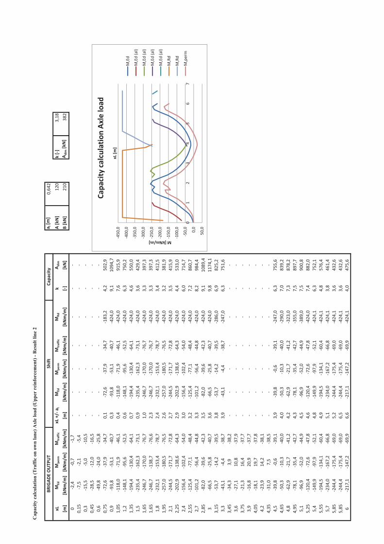
Cap
acity
cal
cula
tion
Axl
e lo
ad (U
pper
rei
nfor
cem
ent)
- R
esul
t lin
e 2
a l[m
]0,64
2
xLM
EdM
perm
Mtraffic
xL+/
a lM
EdM
perm
Mtraffic
MRd
A dim
A[kN]
120
k[]
3,18
[m]
[kNm/m
][kNm/m
][kNm/m
][m
][kNm/m
][kNm/m
][kNm/m
][kNm/m
][]
[kN]
B[kN]
210
A dim[kN]
382
02,4
0,7
1,7
0,15
7,5
2,1
5,4
0,3
15,5
5,0
10,5
0,45
28,5
12,0
16,5
0,6
49,8
24,0
25,8
0,75
72,6
37,9
34,7
0,1
72,6
37,9
34,7
183,2
4,2
502,9
0,9
93,8
53,1
40,7
0,3
93,8
53,1
40,7
424,0
9,1
1094
,71,05
118,0
71,9
46,1
0,4
118,0
71,9
46,1
424,0
7,6
915,9
1,2
148,1
95,6
52,5
0,6
148,1
95,6
52,5
424,0
6,3
750,2
1,35
194,4
130,4
64,1
0,7
194,4
130,4
64,1
424,0
4,6
550,0
1,5
235,4
162,3
73,1
0,9
235,4
162,3
73,1
424,0
3,6
429,4
1,65
246,7
170,0
76,7
1,0
246,7
170,0
76,7
424,0
3,3
397,3
1,65
246,7
138,7
76,6
2,3
246,7
170,0
76,7
424,0
3,3
397,3
1,8
232,1
153,4
78,7
2,4
232,1
153,4
78,7
424,0
3,4
412,5
1,95
257,0
180,5
76,5
2,6
257,0
180,5
76,5
424,0
3,2
381,9
2,1
244,5
171,7
72,8
2,7
244,5
171,7
72,8
424,0
3,5
415,9
2,25
202,9
138,6
64,3
2,9
202,9
138,6
64,3
424,0
4,4
533,0
2,4
156,4
102,4
54,0
3,0
156,4
102,4
54,0
424,0
6,0
714,7
2,55
125,4
77,1
48,4
3,2
125,4
77,1
48,4
424,0
7,2
860,7
2,7
101,2
56,4
44,8
3,3
101,2
56,4
44,8
424,0
8,2
984,4
2,85
82,0
39,6
42,3
3,5
82,0
39,6
42,3
424,0
9,1
1089
,43
66,5
25,8
40,7
3,6
66,5
25,8
40,7
424,0
9,8
1174
,13,15
53,7
14,2
39,5
3,8
53,7
14,2
39,5
286,0
6,9
825,2
3,3
43,1
4,4
38,7
3,9
43,1
4,4
38,7
247,0
6,3
751,6
3,45
34,3
3,9
38,2
3,6
27,1
10,8
37,9
3,75
21,3
16,4
37,7
3,9
16,8
20,9
37,7
4,05
18,1
19,7
37,8
4,2
23,9
14,2
38,1
4,35
31,0
7,5
38,5
4,5
39,8
0,6
39,1
3,9
39,8
0,6
39,1
247,0
6,3
755,6
4,65
50,3
10,3
40,0
4,0
50,3
10,3
40,0
290,0
7,0
839,2
4,8
62,9
21,7
41,2
4,2
62,9
21,7
41,2
323,0
7,3
878,2
4,95
78,1
35,4
42,7
4,3
78,1
35,4
42,7
355,0
7,5
897,7
5,1
96,9
52,0
44,9
4,5
96,9
52,0
44,9
389,0
7,5
900,8
5,25
120,4
72,6
47,8
4,6
120,4
72,6
47,8
424,0
7,4
882,0
5,4
149,9
97,9
52,1
4,8
149,9
97,9
52,1
424,1
6,3
752,1
5,55
194,5
134,1
60,4
4,9
194,5
134,1
60,4
424,1
4,8
576,4
5,7
234,0
167,2
66,8
5,1
234,0
167,2
66,8
424,1
3,8
461,4
5,85
244,4
175,4
69,0
5,2
244,4
175,4
69,0
424,1
3,6
432,6
5,85
244,4
175,4
69,0
6,5
244,4
175,4
69,0
424,1
3,6
432,6
621
7,1
147,2
69,9
6,6
217,1
147,2
69,9
424,1
4,0
475,6
Capa
city
BRIGAD
EOUTP
UT
Shift
450,0
400,0
350,0
300,0
250,0
200,0
150,0
100,0
50,0 0,0
50,0
01
23
45
67
M[kNm/m]
xL[m
]
Capa
city
calculationAx
leload
M,Ed
M,Ed(al)
M,Ed(al)
M,Ed(al)
M,Ed(al)
M,Rd
M,Rd
M,perm
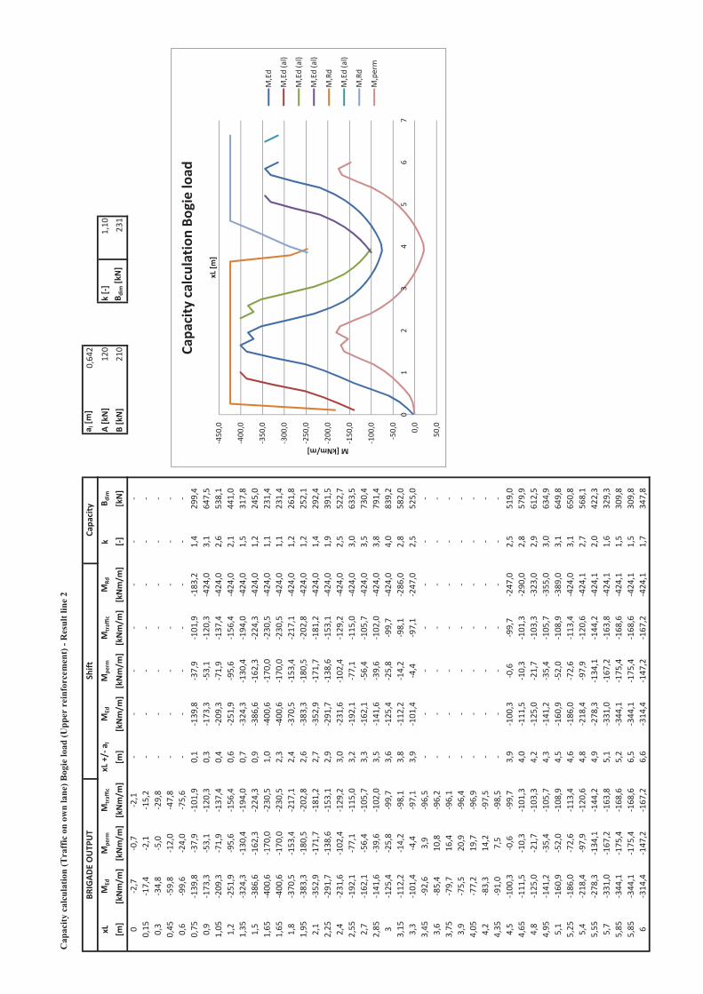
Cap
acity
cal
cula
tion
Bog
ie lo
ad (U
pper
rei
nfor
cem
ent)
- R
esul
t lin
e 2
a l[m
]0,64
2
xLM
EdM
perm
Mtraffic
xL+/
a lM
EdM
perm
Mtraffic
MRd
B dim
A[kN]
120
k[]
1,10
[m]
[kNm/m
][kNm/m
][kNm/m
][m
][kNm/m
][kNm/m
][kNm/m
][kNm/m
][]
[kN]
B[kN]
210
B dim[kN]
231
02,7
0,7
2,1
0,15
17,4
2,1
15,2
0,3
34,8
5,0
29,8
0,45
59,8
12,0
47,8
0,6
99,6
24,0
75,6
0,75
139,8
37,9
101,9
0,1
139,8
37,9
101,9
183,2
1,4
299,4
0,9
173,3
53,1
120,3
0,3
173,3
53,1
120,3
424,0
3,1
647,5
1,05
209,3
71,9
137,4
0,4
209,3
71,9
137,4
424,0
2,6
538,1
1,2
251,9
95,6
156,4
0,6
251,9
95,6
156,4
424,0
2,1
441,0
1,35
324,3
130,4
194,0
0,7
324,3
130,4
194,0
424,0
1,5
317,8
1,5
386,6
162,3
224,3
0,9
386,6
162,3
224,3
424,0
1,2
245,0
1,65
400,6
170,0
230,5
1,0
400,6
170,0
230,5
424,0
1,1
231,4
1,65
400,6
170,0
230,5
2,3
400,6
170,0
230,5
424,0
1,1
231,4
1,8
370,5
153,4
217,1
2,4
370,5
153,4
217,1
424,0
1,2
261,8
1,95
383,3
180,5
202,8
2,6
383,3
180,5
202,8
424,0
1,2
252,1
2,1
352,9
171,7
181,2
2,7
352,9
171,7
181,2
424,0
1,4
292,4
2,25
291,7
138,6
153,1
2,9
291,7
138,6
153,1
424,0
1,9
391,5
2,4
231,6
102,4
129,2
3,0
231,6
102,4
129,2
424,0
2,5
522,7
2,55
192,1
77,1
115,0
3,2
192,1
77,1
115,0
424,0
3,0
633,5
2,7
162,1
56,4
105,7
3,3
162,1
56,4
105,7
424,0
3,5
730,4
2,85
141,6
39,6
102,0
3,5
141,6
39,6
102,0
424,0
3,8
791,4
312
5,4
25,8
99,7
3,6
125,4
25,8
99,7
424,0
4,0
839,2
3,15
112,2
14,2
98,1
3,8
112,2
14,2
98,1
286,0
2,8
582,0
3,3
101,4
4,4
97,1
3,9
101,4
4,4
97,1
247,0
2,5
525,0
3,45
92,6
3,9
96,5
3,6
85,4
10,8
96,2
3,75
79,7
16,4
96,1
3,9
75,5
20,9
96,4
4,05
77,2
19,7
96,9
4,2
83,3
14,2
97,5
4,35
91,0
7,5
98,5
4,5
100,3
0,6
99,7
3,9
100,3
0,6
99,7
247,0
2,5
519,0
4,65
111,5
10,3
101,3
4,0
111,5
10,3
101,3
290,0
2,8
579,9
4,8
125,0
21,7
103,3
4,2
125,0
21,7
103,3
323,0
2,9
612,5
4,95
141,2
35,4
105,7
4,3
141,2
35,4
105,7
355,0
3,0
634,9
5,1
160,9
52,0
108,9
4,5
160,9
52,0
108,9
389,0
3,1
649,8
5,25
186,0
72,6
113,4
4,6
186,0
72,6
113,4
424,0
3,1
650,8
5,4
218,4
97,9
120,6
4,8
218,4
97,9
120,6
424,1
2,7
568,1
5,55
278,3
134,1
144,2
4,9
278,3
134,1
144,2
424,1
2,0
422,3
5,7
331,0
167,2
163,8
5,1
331,0
167,2
163,8
424,1
1,6
329,3
5,85
344,1
175,4
168,6
5,2
344,1
175,4
168,6
424,1
1,5
309,8
5,85
344,1
175,4
168,6
6,5
344,1
175,4
168,6
424,1
1,5
309,8
631
4,4
147,2
167,2
6,6
314,4
147,2
167,2
424,1
1,7
347,8
Capa
city
BRIGAD
EOUTP
UT
Shift
450,0
400,0
350,0
300,0
250,0
200,0
150,0
100,0
50,0 0,0
50,0
01
23
45
67
M[kNm/m]
xL[m
]
Capa
city
calculationBo
gieload
M,Ed
M,Ed(al)
M,Ed(al)
M,Ed(al)
M,Rd
M,Ed(al)
M,Rd
M,perm
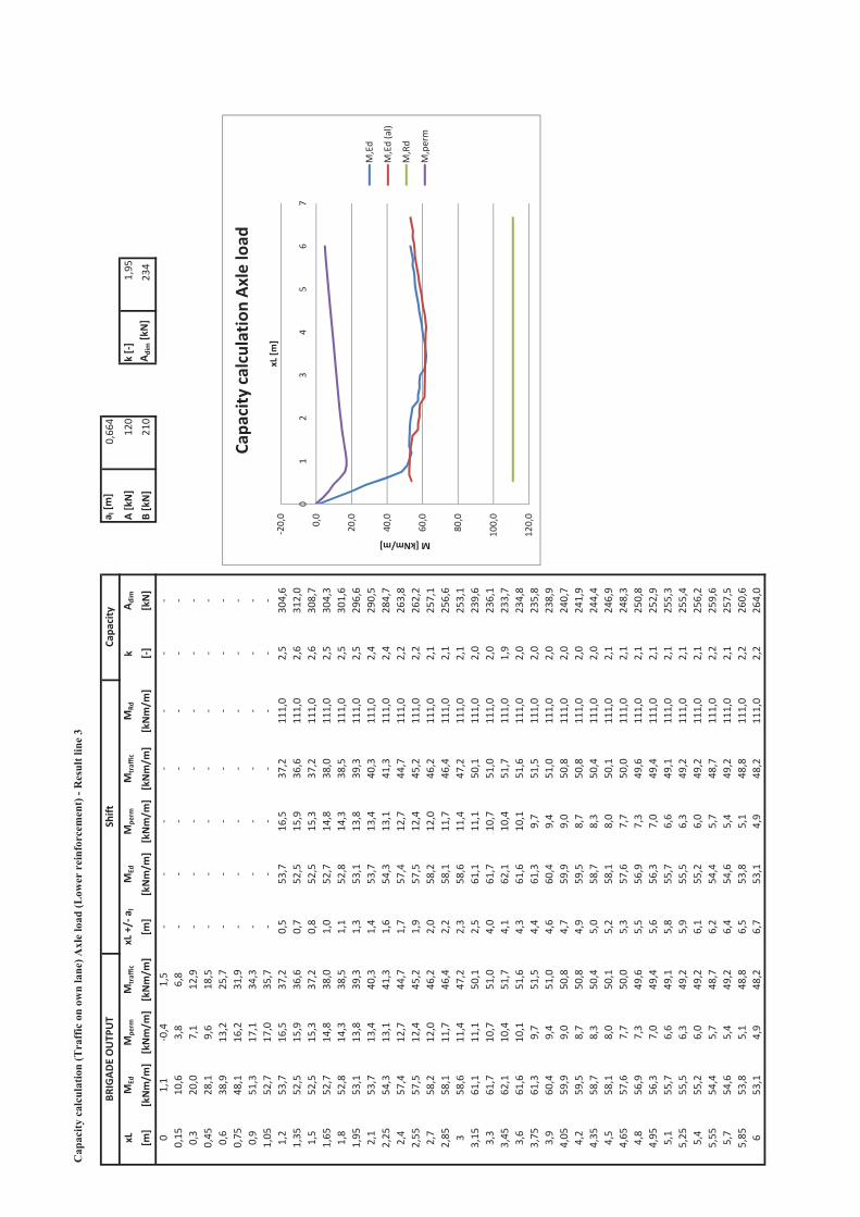
Cap
acity
cal
cula
tion
Axl
e lo
ad (L
ower
rei
nfor
cem
ent)
- R
esul
t lin
e 3
a l[m
]0,66
4
xLM
EdM
perm
Mtraffic
xL+/
a lM
EdM
perm
Mtraffic
MRd
A dim
A[kN]
120
k[]
1,95
[m]
[kNm/m
][kNm/m
][kNm/m
][m
][kNm/m
][kNm/m
][kNm/m
][kNm/m
][]
[kN]
B[kN]
210
A dim[kN]
230
1,1
0,4
1,5
0,15
10,6
3,8
6,8
0,3
20,0
7,1
12,9
0,45
28,1
9,6
18,5
0,6
38,9
13,2
25,7
0,75
48,1
16,2
31,9
0,9
51,3
17,1
34,3
1,05
52,7
17,0
35,7
1,2
53,7
16,5
37,2
0,5
53,7
16,5
37,2
111,0
2,5
304,6
1,35
52,5
15,9
36,6
0,7
52,5
15,9
36,6
111,0
2,6
312,0
1,5
52,5
15,3
37,2
0,8
52,5
15,3
37,2
111,0
2,6
308,7
1,65
52,7
14,8
38,0
1,0
52,7
14,8
38,0
111,0
2,5
304,3
1,8
52,8
14,3
38,5
1,1
52,8
14,3
38,5
111,0
2,5
301,6
1,95
53,1
13,8
39,3
1,3
53,1
13,8
39,3
111,0
2,5
296,6
2,1
53,7
13,4
40,3
1,4
53,7
13,4
40,3
111,0
2,4
290,5
2,25
54,3
13,1
41,3
1,6
54,3
13,1
41,3
111,0
2,4
284,7
2,4
57,4
12,7
44,7
1,7
57,4
12,7
44,7
111,0
2,2
263,8
2,55
57,5
12,4
45,2
1,9
57,5
12,4
45,2
111,0
2,2
262,2
2,7
58,2
12,0
46,2
2,0
58,2
12,0
46,2
111,0
2,1
257,1
2,85
58,1
11,7
46,4
2,2
58,1
11,7
46,4
111,0
2,1
256,6
358
,611
,447
,22,3
58,6
11,4
47,2
111,0
2,1
253,1
3,15
61,1
11,1
50,1
2,5
61,1
11,1
50,1
111,0
2,0
239,6
3,3
61,7
10,7
51,0
4,0
61,7
10,7
51,0
111,0
2,0
236,1
3,45
62,1
10,4
51,7
4,1
62,1
10,4
51,7
111,0
1,9
233,7
3,6
61,6
10,1
51,6
4,3
61,6
10,1
51,6
111,0
2,0
234,8
3,75
61,3
9,7
51,5
4,4
61,3
9,7
51,5
111,0
2,0
235,8
3,9
60,4
9,4
51,0
4,6
60,4
9,4
51,0
111,0
2,0
238,9
4,05
59,9
9,0
50,8
4,7
59,9
9,0
50,8
111,0
2,0
240,7
4,2
59,5
8,7
50,8
4,9
59,5
8,7
50,8
111,0
2,0
241,9
4,35
58,7
8,3
50,4
5,0
58,7
8,3
50,4
111,0
2,0
244,4
4,5
58,1
8,0
50,1
5,2
58,1
8,0
50,1
111,0
2,1
246,9
4,65
57,6
7,7
50,0
5,3
57,6
7,7
50,0
111,0
2,1
248,3
4,8
56,9
7,3
49,6
5,5
56,9
7,3
49,6
111,0
2,1
250,8
4,95
56,3
7,0
49,4
5,6
56,3
7,0
49,4
111,0
2,1
252,9
5,1
55,7
6,6
49,1
5,8
55,7
6,6
49,1
111,0
2,1
255,3
5,25
55,5
6,3
49,2
5,9
55,5
6,3
49,2
111,0
2,1
255,4
5,4
55,2
6,0
49,2
6,1
55,2
6,0
49,2
111,0
2,1
256,2
5,55
54,4
5,7
48,7
6,2
54,4
5,7
48,7
111,0
2,2
259,6
5,7
54,6
5,4
49,2
6,4
54,6
5,4
49,2
111,0
2,1
257,5
5,85
53,8
5,1
48,8
6,5
53,8
5,1
48,8
111,0
2,2
260,6
653
,14,9
48,2
6,7
53,1
4,9
48,2
111,0
2,2
264,0
Capa
city
BRIGAD
EOUTP
UT
Shift
20,0 0,0
20,0
40,0
60,0
80,0
100,0
120,0
01
23
45
67
M[kNm/m]
xL[m
]
Capa
city
calculationAx
leload
M,Ed
M,Ed(al)
M,Rd
M,perm
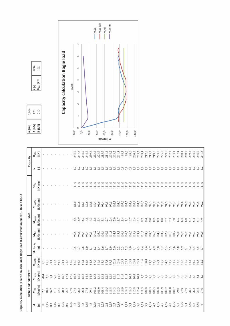
Cap
acity
cal
cula
tion
Bog
ie lo
ad (L
ower
rei
nfor
cem
ent)
- R
esul
t lin
e 3
a l [m
]0,
664
xLM
Ed
Mpe
rmM
traf
ficxL
+/-
a lM
Ed
Mpe
rmM
traf
ficM
Rd
Bdi
mA
[kN
]12
0k
[-]
0,94
[m]
[kN
m/m
][k
Nm
/m]
[kN
m/m
][m
][k
Nm
/m]
[kN
m/m
][k
Nm
/m]
[kN
m/m
][-
][k
N]
B [k
N]
210
Bdi
m [k
N]
198
02,
3-0
,42,
7-
--
--
--
0,15
18,8
3,8
15,0
--
--
--
-0,
336
,27,
129
,1-
--
--
--
0,45
51,1
9,6
41,5
--
--
--
-0,
672
,513
,259
,3-
--
--
--
0,75
90,3
16,2
74,1
--
--
--
-0,
995
,717
,178
,6-
--
--
--
1,05
97,9
17,0
81,0
--
--
--
-1,
297
,516
,581
,00,
597
,516
,581
,011
1,0
1,2
245,
01,
3596
,515
,980
,60,
796
,515
,980
,611
1,0
1,2
247,
81,
596
,415
,381
,10,
896
,415
,381
,111
1,0
1,2
248,
01,
6597
,414
,882
,61,
097
,414
,882
,611
1,0
1,2
244,
71,
899
,114
,384
,81,
199
,114
,384
,811
1,0
1,1
239,
61,
9510
1,2
13,8
87,4
1,3
101,
213
,887
,411
1,0
1,1
233,
62,
110
5,0
13,4
91,6
1,4
105,
013
,491
,611
1,0
1,1
223,
72,
2510
8,4
13,1
95,4
1,6
108,
413
,195
,411
1,0
1,0
215,
72,
411
0,5
12,7
97,8
1,7
110,
512
,797
,811
1,0
1,0
211,
12,
5511
1,8
12,4
99,5
1,9
111,
812
,499
,511
1,0
1,0
208,
22,
711
4,3
12,0
102,
32,
011
4,3
12,0
102,
311
1,0
1,0
203,
22,
8511
5,3
11,7
103,
62,
211
5,3
11,7
103,
611
1,0
1,0
201,
33
116,
911
,410
5,5
2,3
116,
911
,410
5,5
111,
00,
919
8,3
3,15
116,
511
,110
5,5
2,5
116,
511
,110
5,5
111,
00,
919
9,0
3,3
116,
510
,710
5,8
4,0
116,
510
,710
5,8
111,
00,
919
9,0
3,45
115,
810
,410
5,4
4,1
115,
810
,410
5,4
111,
01,
020
0,5
3,6
113,
410
,110
3,3
4,3
113,
410
,110
3,3
111,
01,
020
5,2
3,75
111,
39,
710
1,6
4,4
111,
39,
710
1,6
111,
01,
020
9,4
3,9
109,
89,
410
0,4
4,6
109,
89,
410
0,4
111,
01,
021
2,6
4,05
108,
39,
099
,34,
710
8,3
9,0
99,3
111,
01,
021
5,7
4,2
106,
58,
797
,94,
910
6,5
8,7
97,9
111,
01,
021
9,6
4,35
104,
88,
396
,45,
010
4,8
8,3
96,4
111,
01,
122
3,6
4,5
103,
98,
095
,95,
210
3,9
8,0
95,9
111,
01,
122
5,6
4,65
102,
27,
794
,55,
310
2,2
7,7
94,5
111,
01,
122
9,6
4,8
101,
07,
393
,75,
510
1,0
7,3
93,7
111,
01,
123
2,3
4,95
100,
77,
093
,75,
610
0,7
7,0
93,7
111,
01,
123
3,1
5,1
99,0
6,6
92,3
5,8
99,0
6,6
92,3
111,
01,
123
7,4
5,25
97,9
6,3
91,6
5,9
97,9
6,3
91,6
111,
01,
124
0,1
5,4
97,9
6,0
91,9
6,1
97,9
6,0
91,9
111,
01,
124
0,0
5,55
98,1
5,7
92,4
6,2
98,1
5,7
92,4
111,
01,
123
9,3
5,7
96,3
5,4
90,9
6,4
96,3
5,4
90,9
111,
01,
224
4,0
5,85
95,5
5,1
90,5
6,5
95,5
5,1
90,5
111,
01,
224
6,0
697
,04,
992
,26,
797
,04,
992
,211
1,0
1,2
241,
8
BR
IGA
DE
OU
TPU
TSh
iftC
apac
ity
20,0 0,0
20,0
40,0
60,0
80,0
100,0
120,0
140,0
01
23
45
67
M[kNm/m]
xL[m
]
Capa
city
calculationBo
gieload
M,Ed
M,Ed(al)
M,Rd
M,perm
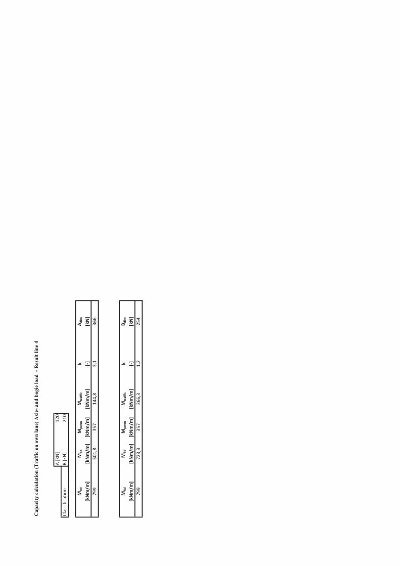
Cap
acity
cal
cula
tion
Axl
e- a
nd b
ogie
load
- R
esul
t lin
e 4
A[kN]
120
Classification
B[kN]
210
MRd
MEd
Mpe
rmM
traffic
kA d
im
[kNm/m
][kNm/m
][kNm/m
][kNm/m
][]
[kN]
799
501,8
357
144,8
3,1
366
MRd
MEd
Mpe
rmM
traffic
kB d
im
[kNm/m
][kNm/m
][kNm/m
][kNm/m
][]
[kN]
799
723,3
357
366,3
1,2
254
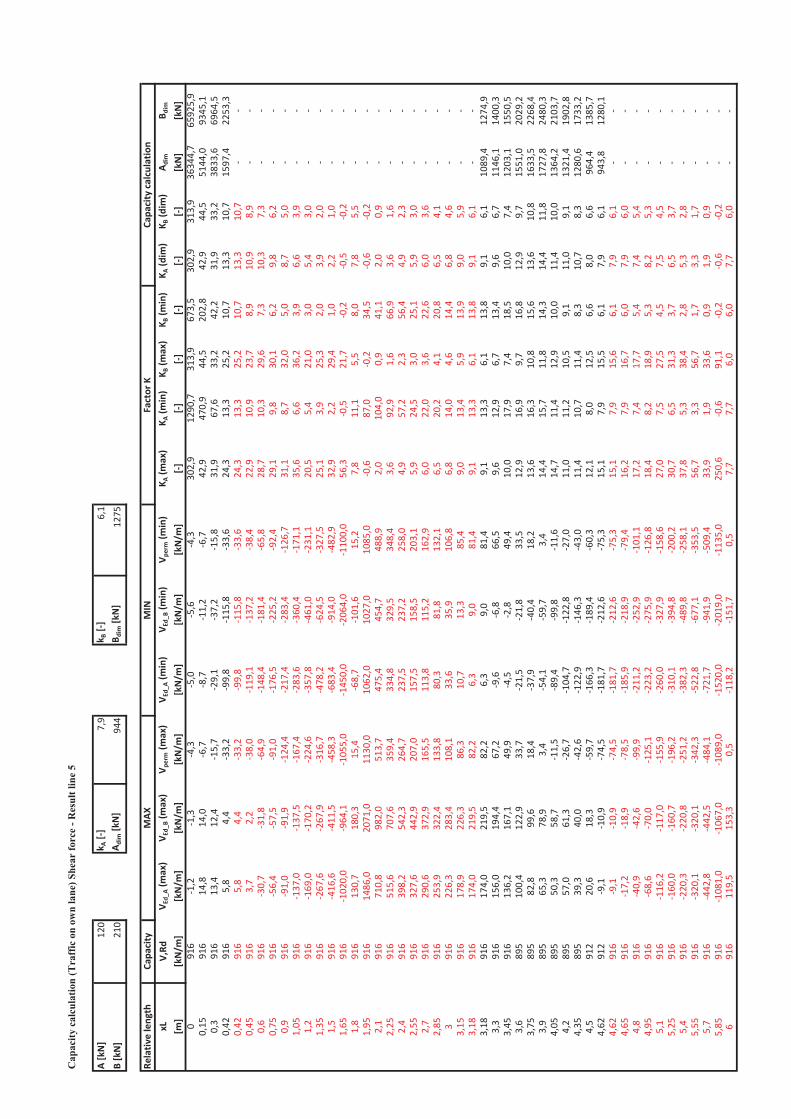
Cap
acity
cal
cula
tion
Shea
r fo
rce
- Res
ult l
ine
5
A[kN]
120
k A[]
7,9
k B[]
6,1
B[kN]
210
A dim[kN]
944
B dim[kN]
1275
Relativ
elength
Capa
city
xLV,Rd
V Ed_
A(m
ax)
V Ed_
B(m
ax)
V perm(m
ax)
V Ed_
A(m
in)
V Ed_
B(m
in)
V perm(m
in)
K A(m
ax)
K A(m
in)
K B(m
ax)
K B(m
in)
K A(dim
)K B
(dim
)A d
imB d
im
[m]
[kN/m
][kN/m
][kN/m
][kN/m
][kN/m
][kN/m
][kN/m
][]
[][]
[][]
[][kN]
[kN]
091
61,2
1,3
4,3
5,0
5,6
4,3
302,9
1290
,731
3,9
673,5
302,9
313,9
3634
4,7
6592
5,9
0,15
916
14,8
14,0
6,7
8,7
11,2
6,7
42,9
470,9
44,5
202,8
42,9
44,5
5144
,093
45,1
0,3
916
13,4
12,4
15,7
29,1
37,2
15,8
31,9
67,6
33,2
42,2
31,9
33,2
3833
,669
64,5
0,42
916
5,8
4,4
33,2
99,8
115,8
33,6
24,3
13,3
25,2
10,7
13,3
10,7
1597
,422
53,3
0,42
916
5,8
4,4
33,2
99,8
115,8
33,6
24,3
13,3
25,2
10,7
13,3
10,7
0,45
916
3,7
2,2
38,0
119,1
137,2
38,4
22,9
10,9
23,7
8,9
10,9
8,9
0,6
916
30,7
31,8
64,9
148,4
181,4
65,8
28,7
10,3
29,6
7,3
10,3
7,3
0,75
916
56,4
57,5
91,0
176,5
225,2
92,4
29,1
9,8
30,1
6,2
9,8
6,2
0,9
916
91,0
91,9
124,4
217,4
283,4
126,7
31,1
8,7
32,0
5,0
8,7
5,0
1,05
916
137,0
137,5
167,4
283,6
360,4
171,1
35,6
6,6
36,2
3,9
6,6
3,9
1,2
916
169,0
170,2
224,6
357,8
461,0
231,1
20,5
5,4
21,0
3,0
5,4
3,0
1,35
916
267,6
267,9
316,7
478,2
624,5
327,5
25,1
3,9
25,3
2,0
3,9
2,0
1,5
916
416,6
411,5
458,3
683,4
914,0
482,9
32,9
2,2
29,4
1,0
2,2
1,0
1,65
916
1020
,096
4,1
1055
,014
50,0
2064
,011
00,0
56,3
0,5
21,7
0,2
0,5
0,2
1,8
916
130,7
180,3
15,4
68,7
101,6
15,2
7,8
11,1
5,5
8,0
7,8
5,5
1,95
916
1486
,020
71,0
1130
,010
62,0
1027
,010
85,0
0,6
87,0
0,2
34,5
0,6
0,2
2,1
916
710,8
982,0
513,7
475,4
454,7
488,9
2,0
104,0
0,9
41,1
2,0
0,9
2,25
916
515,6
707,6
359,4
334,8
329,5
348,4
3,6
92,9
1,6
66,9
3,6
1,6
2,4
916
398,2
542,3
264,7
237,5
237,2
258,0
4,9
57,2
2,3
56,4
4,9
2,3
2,55
916
327,6
442,9
207,0
157,5
158,5
203,1
5,9
24,5
3,0
25,1
5,9
3,0
2,7
916
290,6
372,9
165,5
113,8
115,2
162,9
6,0
22,0
3,6
22,6
6,0
3,6
2,85
916
253,9
322,4
133,8
80,3
81,8
132,1
6,5
20,2
4,1
20,8
6,5
4,1
391
622
6,3
283,4
108,1
33,6
35,9
106,8
6,8
14,0
4,6
14,4
6,8
4,6
3,15
916
178,9
226,3
86,3
10,7
13,3
85,4
9,0
13,4
5,9
13,9
9,0
5,9
3,18
916
174,0
219,5
82,2
6,3
9,0
81,4
9,1
13,3
6,1
13,8
9,1
6,1
3,18
916
174,0
219,5
82,2
6,3
9,0
81,4
9,1
13,3
6,1
13,8
9,1
6,1
1089
,412
74,9
3,3
916
156,0
194,4
67,2
9,6
6,8
66,5
9,6
12,9
6,7
13,4
9,6
6,7
1146
,114
00,3
3,45
916
136,2
167,1
49,9
4,5
2,8
49,4
10,0
17,9
7,4
18,5
10,0
7,4
1203
,115
50,5
3,6
895
100,4
122,9
33,7
21,5
21,8
33,5
12,9
16,9
9,7
16,8
12,9
9,7
1551
,020
29,2
3,75
895
82,8
99,6
18,4
37,9
40,4
18,2
13,6
16,3
10,8
15,6
13,6
10,8
1633
,522
68,4
3,9
895
65,3
78,9
3,4
54,1
59,7
3,4
14,4
15,7
11,8
14,3
14,4
11,8
1727
,824
80,3
4,05
895
50,3
58,7
11,5
89,4
99,8
11,6
14,7
11,4
12,9
10,0
11,4
10,0
1364
,221
03,7
4,2
895
57,0
61,3
26,7
104,7
122,8
27,0
11,0
11,2
10,5
9,1
11,0
9,1
1321
,419
02,8
4,35
895
39,3
40,0
42,6
122,9
146,3
43,0
11,4
10,7
11,4
8,3
10,7
8,3
1280
,617
33,2
4,5
912
20,6
18,3
59,7
166,3
189,4
60,3
12,1
8,0
12,5
6,6
8,0
6,6
964,4
1385
,74,62
912
9,1
10,9
74,5
181,7
212,6
75,3
15,1
7,9
15,5
6,1
7,9
6,1
943,8
1280
,14,62
916
9,1
10,9
74,5
181,7
212,6
75,3
15,1
7,9
15,6
6,1
7,9
6,1
4,65
916
17,2
18,9
78,5
185,9
218,9
79,4
16,2
7,9
16,7
6,0
7,9
6,0
4,8
916
40,9
42,6
99,9
211,2
252,9
101,1
17,2
7,4
17,7
5,4
7,4
5,4
4,95
916
68,6
70,0
125,1
223,2
275,9
126,8
18,4
8,2
18,9
5,3
8,2
5,3
5,1
916
116,2
117,0
155,9
260,0
327,9
158,6
27,0
7,5
27,5
4,5
7,5
4,5
5,25
916
160,0
160,7
196,2
310,1
394,8
200,2
30,7
6,5
31,3
3,7
6,5
3,7
5,4
916
220,3
220,8
251,2
382,3
489,8
258,1
37,8
5,3
38,4
2,8
5,3
2,8
5,55
916
320,1
320,1
342,3
522,8
677,1
353,5
56,7
3,3
56,7
1,7
3,3
1,7
5,7
916
442,8
442,5
484,1
721,7
941,9
509,4
33,9
1,9
33,6
0,9
1,9
0,9
5,85
916
1081
,010
67,0
1089
,015
20,0
2019
,011
35,0
250,6
0,6
91,1
0,2
0,6
0,2
691
611
9,5
153,3
0,5
118,2
151,7
0,5
7,7
7,7
6,0
6,0
7,7
6,0
MAX
MIN
Factor
KCa
pacity
calculation
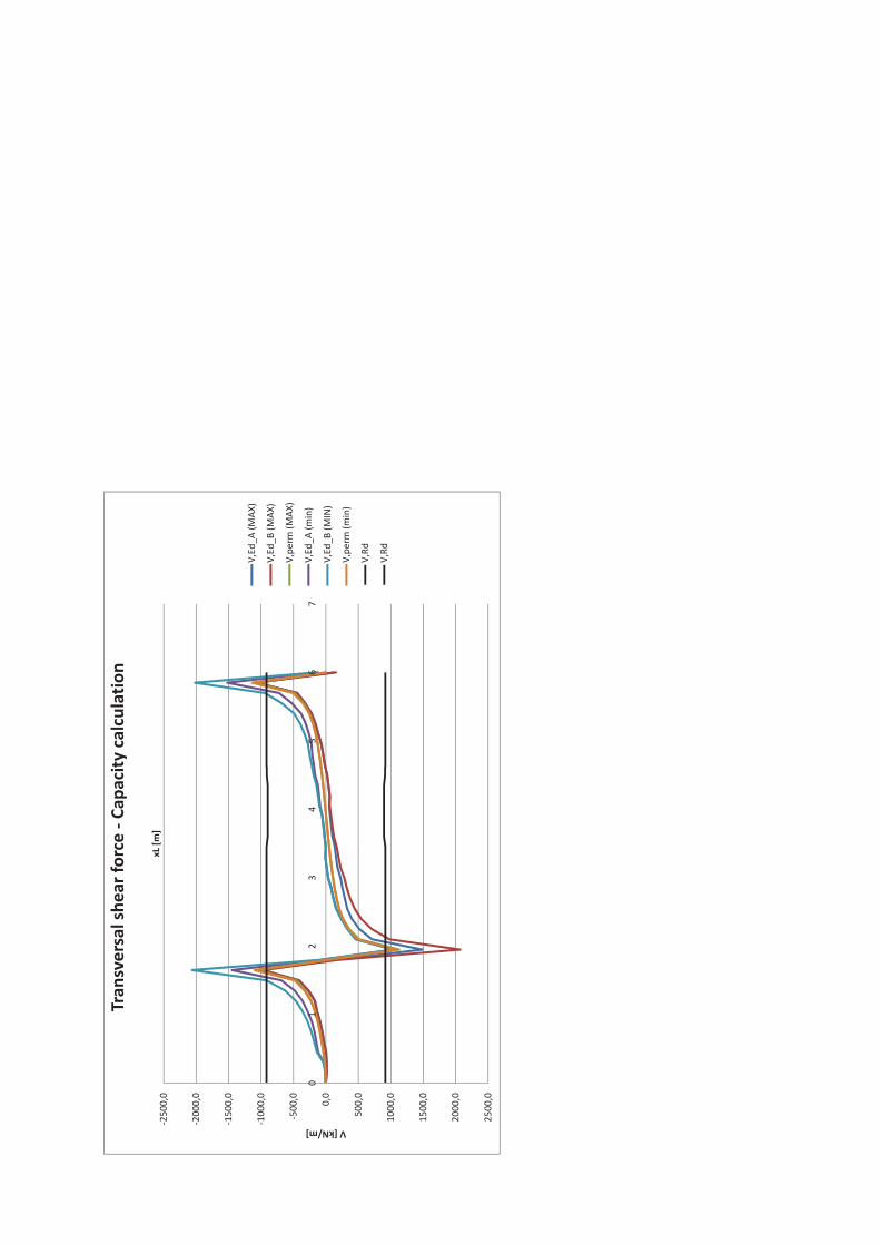
2500
,0
2000
,0
1500
,0
1000
,0
500,0
0,0
500,0
1000
,0
1500
,0
2000
,0
2500
,0
01
23
45
67
V[kN/m]
xL[m
]
Tran
sversalshe
arforce
Capa
city
calculation
V,Ed
_A(M
AX)
V,Ed
_B(M
AX)
V,pe
rm(M
AX)
V,Ed
_A(m
in)
V,Ed
_B(M
IN)
V,pe
rm(m
in)
V,Rd
V,Rd
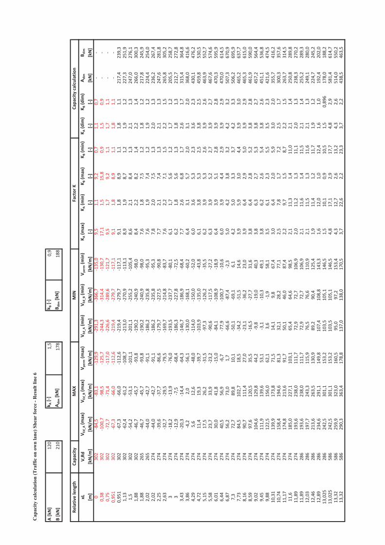
Cap
acity
cal
cula
tion
hear
forc
e - R
esul
t lin
e 6
A[kN]
120
k A[]
1,5
k B[]
0,9
B[kN]
210
A dim[kN]
178
B dim[kN]
188
Relativ
elength
Capa
city
xLV,Rd
V Ed_
A(m
ax)
V Ed_
B(m
ax)
V perm(m
ax)
V Ed_
A(m
in)
V Ed_
B(m
in)
V perm(m
in)
K A(m
ax)
K A(m
in)
K B(m
ax)
K B(m
in)
K A(dim
)K B
(dim
)A d
imB d
im
[m]
[kN/m
][kN/m
][kN/m
][kN/m
][kN/m
][kN/m
][kN/m
][]
[][]
[][]
[][kN]
[kN]
030
284
,583
,112
9,9
291,3
366,7
135,0
9,5
1,1
9,2
0,7
1,1
0,7
0,38
302
100,7
98,5
125,7
244,3
314,4
130,7
17,1
1,5
15,8
0,9
1,5
0,9
0,75
302
72,7
71,4
117,0
226,6
289,6
121,7
9,5
1,7
9,2
1,1
1,7
1,1
0,95
130
267
,366
,011
2,6
219,4
279,7
117,1
9,1
1,8
8,9
1,1
1,8
1,1
0,95
130
267
,366
,011
2,6
219,4
279,7
117,1
9,1
1,8
8,9
1,1
1,8
1,1
217,4
239,3
1,13
302
62,4
61,2
108,7
213,0
270,9
113,1
8,9
1,9
8,7
1,2
1,9
1,2
227,3
251,9
1,5
302
54,2
53,1
101,1
201,1
255,2
105,4
8,6
2,1
8,4
1,3
2,1
1,3
247,0
276,1
1,88
302
46,7
45,7
93,8
190,2
240,9
98,0
8,4
2,2
8,2
1,4
2,2
1,4
266,0
300,3
1,88
265
46,7
45,7
93,8
190,2
240,9
98,0
7,6
1,8
7,5
1,2
1,8
1,2
217,8
245,9
2,02
265
44,0
42,7
91,1
186,2
235,8
95,3
7,6
1,9
7,4
1,2
1,9
1,2
224,4
254,0
2,02
274
44,0
42,7
91,1
186,2
235,8
95,3
7,8
2,0
7,5
1,3
2,0
1,3
236,2
267,4
2,25
274
39,6
37,7
86,6
179,7
227,5
90,8
7,7
2,1
7,4
1,3
2,1
1,3
247,6
281,8
2,63
274
32,7
29,5
79,5
169,7
214,8
83,7
7,6
2,2
7,1
1,5
2,2
1,5
265,8
305,2
327
418
,213
,976
,019
3,5
237,7
80,1
6,1
1,7
5,6
1,2
1,7
1,2
205,5
258,7
327
412
,97,5
68,4
186,3
227,8
72,5
6,2
1,8
5,6
1,3
1,8
1,3
212,7
272,8
3,43
274
20,3
14,4
64,3
146,7
186,9
68,4
7,7
2,6
6,8
1,7
2,6
1,7
315,4
364,8
3,86
274
4,2
2,0
56,1
130,0
168,1
60,2
6,4
3,1
5,7
2,0
3,1
2,0
368,0
416,6
4,29
274
5,6
12,6
48,0
114,0
150,0
52,0
6,0
3,6
5,3
2,3
3,6
2,3
430,1
476,2
4,72
274
11,4
19,3
39,7
103,9
135,0
43,8
6,1
3,8
5,3
2,5
3,8
2,5
459,8
530,5
5,15
274
17,5
26,2
31,5
97,3
126,2
35,5
6,2
3,9
5,3
2,6
3,9
2,6
463,9
552,7
5,58
274
23,7
33,9
23,2
90,6
117,5
27,2
6,3
3,9
5,2
2,7
3,9
2,7
467,6
574,6
6,01
274
30,0
41,8
15,0
84,1
108,9
18,9
6,4
3,9
5,1
2,8
3,9
2,8
470,3
595,9
6,44
274
40,5
56,9
6,7
77,9
100,7
10,6
6,0
3,9
4,4
2,9
3,9
2,9
470,0
614,5
6,87
274
56,2
73,0
1,7
66,6
87,4
2,3
5,0
4,2
3,8
3,2
4,2
3,2
507,3
670,9
7,3
274
72,7
89,8
10,1
50,1
69,1
6,1
4,2
5,0
3,3
3,7
4,2
3,3
506,2
695,9
7,73
274
84,5
102,7
18,5
34,2
51,5
14,6
3,9
5,9
3,0
4,4
3,9
3,0
465,2
637,7
8,16
274
90,7
111,4
27,0
23,1
36,2
23,0
3,9
6,4
2,9
5,0
3,9
2,9
465,3
615,0
8,59
274
97,6
120,5
35,5
16,5
27,7
31,6
3,8
6,4
2,8
5,2
3,8
2,8
461,9
590,0
9,02
274
104,6
129,8
44,2
9,8
19,0
40,3
3,8
6,3
2,7
5,3
3,8
2,7
457,2
564,4
9,45
274
111,9
139,6
53,1
3,1
10,3
49,1
3,8
6,2
2,6
5,4
3,8
2,6
451,1
536,8
9,88
274
122,5
156,0
62,1
3,6
1,9
58,1
3,5
6,1
2,3
5,5
3,5
2,3
421,6
474,5
10,31
274
139,9
173,8
71,5
14,1
9,8
67,4
3,0
6,4
2,0
5,9
3,0
2,0
355,7
416,2
10,74
274
158,4
194,6
81,3
32,1
28,2
77,1
2,5
7,8
1,7
7,2
2,5
1,7
300,3
357,6
11,17
274
174,8
213,6
91,7
50,1
46,0
87,4
2,2
9,7
1,5
8,7
2,2
1,5
263,7
314,5
11,6
274
185,0
227,1
103,1
65,4
64,6
98,5
2,1
11,3
1,4
11,0
2,1
1,4
250,8
289,8
11,89
274
193,6
238,0
111,7
72,9
72,7
106,9
2,0
11,2
1,3
11,1
2,0
1,3
238,3
270,2
11,89
286
193,6
238,0
111,7
72,9
72,7
106,9
2,1
11,6
1,4
11,5
2,1
1,4
255,2
289,3
12,03
286
197,7
243,3
115,9
76,5
76,6
110,9
2,1
11,5
1,3
11,6
2,1
1,3
249,1
280,0
12,46
286
213,6
263,5
130,9
89,2
90,4
125,4
1,9
11,4
1,2
11,7
1,9
1,2
224,7
245,2
12,89
286
234,6
291,1
149,8
107,4
108,8
143,3
1,6
12,0
1,0
12,4
1,6
1,0
192,4
202,0
13,025
286
242,5
301,1
153,2
103,5
105,1
146,5
1,5
10,1
0,9
10,5
1,5
0,89
617
8,0
188,2
13,025
586
242,5
301,1
153,2
103,5
105,1
146,5
4,8
17,1
2,9
17,7
4,8
2,9
581,4
614,7
13,32
586
259,9
323,0
160,5
95,0
97,2
153,4
4,3
12,7
2,6
13,2
4,3
2,6
514,0
550,2
13,32
586
290,3
363,4
178,8
137,0
138,0
170,5
3,7
22,6
2,2
23,3
3,7
2,2
438,5
463,5
MAX
MIN
Factor
KCa
pacity
calculation
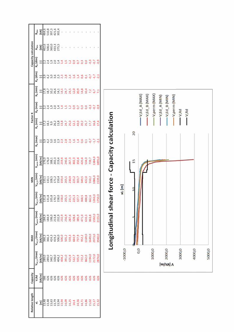
Relativ
elength
Capa
city
xLV,Rd
V Ed_
A(m
ax)
V Ed_
B(m
ax)
V perm(m
ax)
V Ed_
A(m
in)
V Ed_
B(m
in)
V perm(m
in)
K A(m
ax)
K A(m
in)
K B(m
ax)
K B(m
in)
K A(dim
)K B
(dim
)A d
imB d
im
[m]
[kN/m
][kN/m
][kN/m
][kN/m
][kN/m
][kN/m
][kN/m
][]
[][]
[][]
[][kN]
[kN]
13,48
586
289,0
366,3
184,9
131,8
133,1
176,0
3,9
17,2
2,2
17,8
3,9
2,2
462,6
464,6
13,48
626
289,0
366,3
184,9
131,8
133,1
176,0
4,2
18,1
2,4
18,7
4,2
2,4
508,6
510,8
13,63
626
340,7
424,3
198,0
105,8
108,5
188,1
3,0
9,9
1,9
10,2
3,0
1,9
360,0
397,3
13,79
626
328,0
419,2
213,8
170,7
171,2
202,3
3,6
26,2
2,0
26,6
3,6
2,0
433,3
421,6
13,94
626
404,2
506,0
232,9
158,0
159,4
219,4
2,3
13,8
1,4
14,1
2,3
1,4
275,5
302,4
13,94
626
404,2
506,0
232,9
158,0
159,4
219,4
2,3
13,8
1,4
14,1
2,3
1,4
14,09
626
391,0
505,2
256,9
205,5
205,5
240,6
2,8
24,7
1,5
24,7
2,8
1,5
14,25
626
425,9
559,3
287,6
231,5
230,9
267,3
2,4
25,0
1,2
24,5
2,4
1,2
14,4
626
512,7
664,9
328,6
225,3
225,2
302,3
1,6
12,1
0,9
12,0
1,6
0,9
14,56
626
555,9
737,9
385,9
327,7
303,7
350,4
1,4
43,0
0,7
20,9
1,4
0,7
14,71
626
722,2
952,2
471,0
368,5
349,5
420,4
0,6
20,2
0,3
14,8
0,6
0,3
14,86
626
862,0
1169
,061
0,3
488,8
422,0
534,0
0,1
25,7
0,0
10,4
0,1
0,0
15,02
626
1194
,016
49,0
863,8
662,6
550,2
739,7
0,7
17,7
0,3
7,2
0,7
0,3
15,17
626
2172
,029
73,0
1592
,012
63,0
1086
,013
84,0
1,7
16,6
0,7
6,7
1,7
0,7
15,32
626
2874
,039
40,0
2155
,017
50,0
1539
,018
95,0
2,1
17,4
0,9
7,1
2,1
0,9
MAX
MIN
Factor
KCa
pacity
calculation
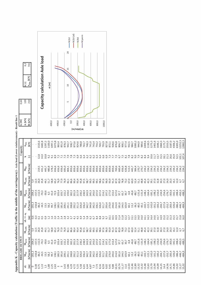
Cap
acity
cal
cula
tion
(Tra
ffic
in th
e m
iddl
e of
the
carr
iage
way
)A
xle
load
(Low
er r
einf
orce
men
t) -
Res
ult l
ine
1
a l [m
]0,64
xLM
Ed
Mpe
rmM
traf
ficxL
+/-
a lM
Ed
Mpe
rmM
traf
ficM
Rd
kA
dim
A [k
N]
120
k [-
]6,2
[m]
[kN
m/m
][k
Nm
/m]
[kN
m/m
][m
][k
Nm
/m]
[kN
m/m
][k
Nm
/m]
[kN
m/m
][-
][k
N]
B [k
N]
210
Adi
m [k
N]
741
020
1,3
204,2
5,4
0,6
201,3
204,2
5,4
0,38
150,8
157,5
12,5
0,3
150,8
157,5
12,5
0,75
86,5
112,5
26,0
0,1
86,5
112,5
26,0
219,5
12,8
1533
,61,13
34,5
70,3
35,8
0,5
34,5
70,3
35,8
431,2
14,0
1682
,81,5
13,5
30,6
44,1
0,9
13,5
30,6
44,1
445,7
10,8
1297
,21,88
58,2
6,5
51,7
1,2
58,2
6,5
51,7
480,8
9,2
1100
,02,25
99,7
41,0
58,8
1,6
99,7
41,0
58,8
578,3
9,1
1097
,12,63
138,1
72,9
65,2
2,0
138,1
72,9
65,2
656,6
8,9
1073
,83
180,3
103,4
76,9
2,4
180,3
103,4
76,9
656,6
7,2
863,4
318
1,6
103,7
77,9
2,4
181,6
103,7
77,9
656,6
7,1
851,9
3,43
209,1
132,2
76,9
2,8
209,1
132,2
76,9
695,0
7,3
878,3
3,86
241,1
159,0
82,1
3,2
241,1
159,0
82,1
804,1
7,9
942,7
4,29
268,8
182,3
86,6
3,7
268,8
182,3
86,6
859,6
7,8
938,7
4,72
292,2
201,9
90,4
4,1
292,2
201,9
90,4
859,6
7,3
873,6
5,15
311,3
217,9
93,4
4,5
311,3
217,9
93,4
859,6
6,9
824,6
5,58
326,0
230,2
95,8
4,9
326,0
230,2
95,8
859,6
6,6
788,8
6,01
336,4
238,9
97,5
5,4
336,4
238,9
97,5
859,6
6,4
763,7
6,44
342,7
243,9
98,7
5,8
342,7
243,9
98,7
859,6
6,2
748,3
6,87
344,8
245,3
99,5
6,2
344,8
245,3
99,5
859,6
6,2
741,0
7,3
342,5
243,0
99,5
6,7
342,5
243,0
99,5
859,6
6,2
743,4
7,73
336,1
237,0
99,1
8,4
336,1
237,0
99,1
859,6
6,3
754,2
8,16
326,0
227,4
98,6
8,8
326,0
227,4
98,6
859,6
6,4
769,7
8,59
311,7
214,2
97,6
9,2
311,7
214,2
97,6
859,6
6,6
793,9
9,02
293,4
197,3
96,0
9,7
293,4
197,3
96,0
859,6
6,9
827,8
9,45
270,9
177,0
93,9
10,1
270,9
177,0
93,9
859,6
7,3
872,1
9,88
244,6
153,4
91,3
10,5
244,6
153,4
91,3
859,6
7,7
928,6
10,31
214,9
127,0
87,9
10,9
214,9
127,0
87,9
769,6
7,3
876,8
10,74
181,6
97,7
83,9
11,4
181,6
97,7
83,9
660,4
6,7
804,7
11,17
144,5
65,7
78,8
11,8
144,5
65,7
78,8
656,6
7,5
900,1
11,6
103,9
30,7
73,2
12,2
103,9
30,7
73,2
626,8
8,1
977,4
12,03
60,1
6,8
67,0
12,7
60,1
6,8
67,0
513,5
7,8
932,5
12,46
13,2
46,8
60,0
13,1
13,2
46,8
60,0
445,7
8,2
984,7
12,89
36,3
88,7
52,4
13,5
36,3
88,7
52,4
384,4
9,0
1083
,213
,32
80,5
131,6
51,1
14,0
80,5
131,6
51,1
270,7
7,9
944,9
13,32
83,1
131,9
48,8
14,0
83,1
131,9
48,8
270,7
8,2
989,6
13,48
102,7
148,1
45,4
14,1
102,7
148,1
45,4
234,2
8,4
1009
,613
,63
122,1
164,4
42,3
14,3
122,1
164,4
42,3
234,2
9,4
1130
,513
,79
142,0
181,1
39,1
14,4
142,0
181,1
39,1
234,2
10,6
1275
,313
,94
161,2
198,2
37,0
14,6
161,2
198,2
37,0
234,2
11,7
1401
,614
,09
183,2
216,0
32,8
14,7
183,2
216,0
32,8
234,2
13,7
1646
,114
,25
204,7
234,9
30,3
14,9
204,7
234,9
30,3
234,2
15,5
1860
,314
,422
7,6
254,6
27,0
15,0
227,6
254,6
27,0
234,2
18,1
2175
,714
,56
252,7
276,7
24,0
15,2
252,7
276,7
24,0
234,2
21,3
2553
,514
,71
283,4
303,6
20,3
15,3
283,4
303,6
20,3
234,2
26,6
3187
,014
,86
326,0
342,1
16,1
15,5
326,0
342,1
16,1
234,2
35,9
4306
,215
,02
386,4
398,4
12,0
15,7
386,4
398,4
12,0
234,2
52,5
6305
,015
,17
446,7
450,3
6,7
15,8
446,7
450,3
6,7
234,2
102,1
1225
2,5
15,32
484,9
488,5
6,7
16,0
484,9
488,5
6,7
234,2
107,4
1288
2,5
Cap
acity
BR
IGA
DE
OU
TPU
TSh
ift
600,0
400,0
200,0
0,0
200,0
400,0
600,0
800,0
1000,0
05
1015
20
M[kNm/m]
xL[m
]
Capa
city
calculationAx
leload
M,Ed
M,Ed(al)
M,Rd
M,perm
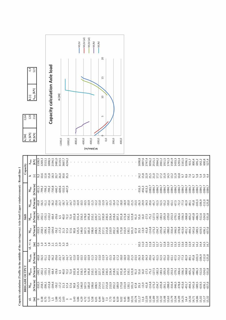
Cap
acity
cal
cula
tion
(Tra
ffic
in th
e m
iddl
e of
the
carr
iage
way
) Axl
e lo
ad (U
pper
rei
nfor
cem
ent)
- R
esul
t lin
e 1
a l [m
]0,64
xLM
Ed
Mpe
rmM
traf
ficxL
+/-
a lM
Ed
Mpe
rmM
traf
ficM
Rd
kA
dim
A [k
N]
120
k [-
]4,4
[m]
[kN
m/m
][k
Nm
/m]
[kN
m/m
][m
][k
Nm
/m]
[kN
m/m
][k
Nm
/m]
[kN
m/m
][-
][k
N]
B [k
N]
210
Adi
m [k
N]
527
031
0,5
249,7
60,8
0,6
310,5
249,7
60,8
811,5
9,2
1108
,90,38
258,5
202,1
56,5
1,0
258,5
202,1
56,5
799,2
10,6
1269
,30,75
206,1
155,1
51,1
1,4
206,1
155,1
51,1
799,2
12,6
1513
,11,13
153,8
110,2
43,6
1,8
153,8
110,2
43,6
799,2
15,8
1898
,51,5
104,6
68,4
36,2
2,1
104,6
68,4
36,2
730,8
18,3
2194
,51,88
59,2
29,6
29,6
2,5
59,2
29,6
29,6
640,7
20,7
2481
,02,25
17,2
6,5
23,7
2,9
17,2
6,5
23,7
609,6
26,0
3119
,52,63
21,3
40,0
18,7
3,3
21,3
40,0
18,7
532,5
30,6
3667
,73
57,4
72,2
14,7
3,6
57,4
72,2
14,7
447,9
35,3
4234
,23
57,6
72,4
14,7
57,6
72,4
14,7
3,43
90,8
102,8
12,0
90,8
102,8
12,0
3,86
125,5
131,4
10,9
125,5
131,4
10,9
4,29
146,0
156,5
10,5
146,0
156,5
10,5
4,72
167,5
178,0
10,5
167,5
178,0
10,5
5,15
185,0
195,8
10,9
185,0
195,8
10,9
5,58
198,6
210,1
11,5
198,6
210,1
11,5
6,01
208,5
220,7
12,2
208,5
220,7
12,2
6,44
214,6
227,7
13,0
214,6
227,7
13,0
6,87
217,1
230,9
13,9
217,1
230,9
13,9
7,3
215,8
230,5
14,7
215,8
230,5
14,7
7,73
210,9
226,4
15,5
210,9
226,4
15,5
8,16
202,2
218,6
16,4
202,2
218,6
16,4
8,59
189,9
207,1
17,2
189,9
207,1
17,2
9,02
173,8
191,8
18,0
173,8
191,8
18,0
9,45
153,9
172,8
18,9
153,9
172,8
18,9
9,88
130,1
150,1
20,0
130,1
150,1
20,0
10,31
101,3
122,8
21,5
101,3
122,8
21,5
10,74
67,8
91,3
23,5
67,8
91,3
23,5
11,17
29,3
55,6
26,3
10,5
29,3
55,6
26,3
316,3
14,2
1698
,811
,613
,916
,029
,911
,013
,916
,029
,945
6,3
15,8
1897
,612
,03
61,8
27,5
34,3
11,4
61,8
27,5
34,3
813,3
22,9
2747
,412
,46
114,8
75,2
39,6
11,8
114,8
75,2
39,6
1083
,725
,530
56,2
12,89
173,2
127,5
45,7
12,3
173,2
127,5
45,7
1084
,721
,025
15,1
13,32
234,7
182,3
52,5
12,7
234,7
182,3
52,5
1084
,717
,220
64,2
13,32
235,8
183,3
52,5
12,7
235,8
183,3
52,5
1084
,717
,220
61,2
13,48
261,1
205,9
55,2
12,8
261,1
205,9
55,2
1084
,715
,919
11,5
13,63
288,0
229,0
59,0
13,0
288,0
229,0
59,0
1084
,714
,517
41,3
13,79
316,4
253,3
63,1
13,2
316,4
253,3
63,1
1084
,713
,215
81,9
13,94
346,5
279,1
67,5
13,3
346,5
279,1
67,5
1084
,711
,914
33,3
14,09
378,8
306,6
72,2
13,5
378,8
306,6
72,2
1084
,710
,812
93,4
14,25
413,6
336,3
77,3
13,6
413,6
336,3
77,3
1084
,79,7
1161
,514
,445
1,7
368,8
82,9
13,8
451,7
368,8
82,9
1084
,78,6
1036
,114
,56
494,3
405,2
89,1
13,9
494,3
405,2
89,1
1084
,77,6
915,7
14,71
541,6
445,8
95,8
14,1
541,6
445,8
95,8
1084
,76,7
800,4
14,86
589,5
486,3
103,3
14,2
589,5
486,3
103,3
1084
,75,8
695,2
15,02
619,5
512,6
106,9
14,4
619,5
512,6
106,9
1084
,75,4
642,2
15,17
636,1
524,0
112,0
14,5
636,1
524,0
112,0
1084
,75,0
600,8
15,32
657,6
531,8
125,8
14,7
657,6
531,8
125,8
1084
,74,4
527,4
Cap
acity
BR
IGA
DE
OU
TPU
TSh
ift
1200,0
1000,0
800,0
600,0
400,0
200,0
0,0
200,0
400,0
05
1015
20
M[kNm/m]
xL[m
]
Capa
city
calculationAx
leload
M,Ed
M,Ed(al)
M,Ed(al)
M,Rd
M,Rd
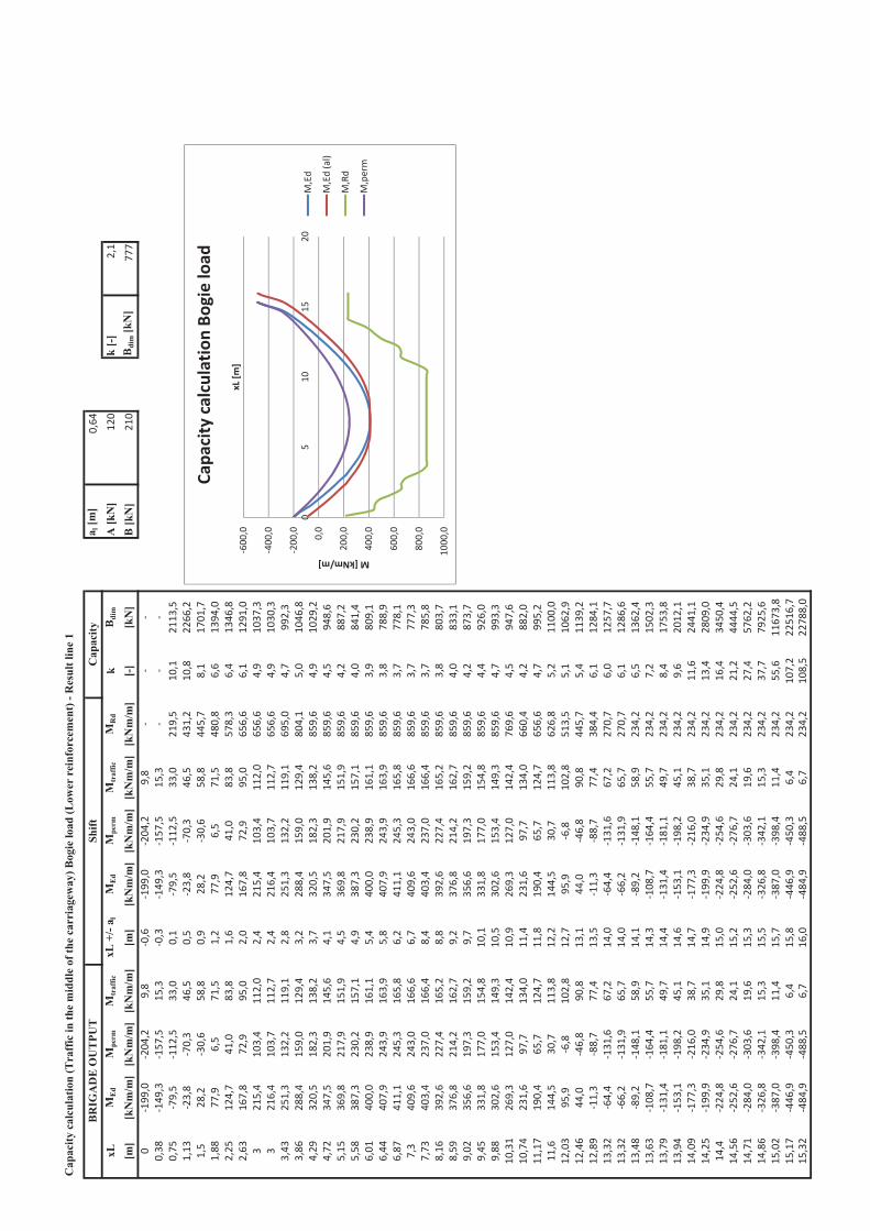
Cap
acity
cal
cula
tion
(Tra
ffic
in th
e m
iddl
e of
the
carr
iage
way
) Bog
ie lo
ad (L
ower
rei
nfor
cem
ent)
- R
esul
t lin
e 1
a l [m
]0,64
xLM
Ed
Mpe
rmM
traf
ficxL
+/-
a lM
Ed
Mpe
rmM
traf
ficM
Rd
kB
dim
A [k
N]
120
k [-
]2,1
[m]
[kN
m/m
][k
Nm
/m]
[kN
m/m
][m
][k
Nm
/m]
[kN
m/m
][k
Nm
/m]
[kN
m/m
][-
][k
N]
B [k
N]
210
Bdi
m [k
N]
777
019
9,0
204,2
9,8
0,6
199,0
204,2
9,8
0,38
149,3
157,5
15,3
0,3
149,3
157,5
15,3
0,75
79,5
112,5
33,0
0,1
79,5
112,5
33,0
219,5
10,1
2113
,51,13
23,8
70,3
46,5
0,5
23,8
70,3
46,5
431,2
10,8
2266
,21,5
28,2
30,6
58,8
0,9
28,2
30,6
58,8
445,7
8,1
1701
,71,88
77,9
6,5
71,5
1,2
77,9
6,5
71,5
480,8
6,6
1394
,02,25
124,7
41,0
83,8
1,6
124,7
41,0
83,8
578,3
6,4
1346
,82,63
167,8
72,9
95,0
2,0
167,8
72,9
95,0
656,6
6,1
1291
,03
215,4
103,4
112,0
2,4
215,4
103,4
112,0
656,6
4,9
1037
,33
216,4
103,7
112,7
2,4
216,4
103,7
112,7
656,6
4,9
1030
,33,43
251,3
132,2
119,1
2,8
251,3
132,2
119,1
695,0
4,7
992,3
3,86
288,4
159,0
129,4
3,2
288,4
159,0
129,4
804,1
5,0
1046
,84,29
320,5
182,3
138,2
3,7
320,5
182,3
138,2
859,6
4,9
1029
,24,72
347,5
201,9
145,6
4,1
347,5
201,9
145,6
859,6
4,5
948,6
5,15
369,8
217,9
151,9
4,5
369,8
217,9
151,9
859,6
4,2
887,2
5,58
387,3
230,2
157,1
4,9
387,3
230,2
157,1
859,6
4,0
841,4
6,01
400,0
238,9
161,1
5,4
400,0
238,9
161,1
859,6
3,9
809,1
6,44
407,9
243,9
163,9
5,8
407,9
243,9
163,9
859,6
3,8
788,9
6,87
411,1
245,3
165,8
6,2
411,1
245,3
165,8
859,6
3,7
778,1
7,3
409,6
243,0
166,6
6,7
409,6
243,0
166,6
859,6
3,7
777,3
7,73
403,4
237,0
166,4
8,4
403,4
237,0
166,4
859,6
3,7
785,8
8,16
392,6
227,4
165,2
8,8
392,6
227,4
165,2
859,6
3,8
803,7
8,59
376,8
214,2
162,7
9,2
376,8
214,2
162,7
859,6
4,0
833,1
9,02
356,6
197,3
159,2
9,7
356,6
197,3
159,2
859,6
4,2
873,7
9,45
331,8
177,0
154,8
10,1
331,8
177,0
154,8
859,6
4,4
926,0
9,88
302,6
153,4
149,3
10,5
302,6
153,4
149,3
859,6
4,7
993,3
10,31
269,3
127,0
142,4
10,9
269,3
127,0
142,4
769,6
4,5
947,6
10,74
231,6
97,7
134,0
11,4
231,6
97,7
134,0
660,4
4,2
882,0
11,17
190,4
65,7
124,7
11,8
190,4
65,7
124,7
656,6
4,7
995,2
11,6
144,5
30,7
113,8
12,2
144,5
30,7
113,8
626,8
5,2
1100
,012
,03
95,9
6,8
102,8
12,7
95,9
6,8
102,8
513,5
5,1
1062
,912
,46
44,0
46,8
90,8
13,1
44,0
46,8
90,8
445,7
5,4
1139
,212
,89
11,3
88,7
77,4
13,5
11,3
88,7
77,4
384,4
6,1
1284
,113
,32
64,4
131,6
67,2
14,0
64,4
131,6
67,2
270,7
6,0
1257
,713
,32
66,2
131,9
65,7
14,0
66,2
131,9
65,7
270,7
6,1
1286
,613
,48
89,2
148,1
58,9
14,1
89,2
148,1
58,9
234,2
6,5
1362
,413
,63
108,7
164,4
55,7
14,3
108,7
164,4
55,7
234,2
7,2
1502
,313
,79
131,4
181,1
49,7
14,4
131,4
181,1
49,7
234,2
8,4
1753
,813
,94
153,1
198,2
45,1
14,6
153,1
198,2
45,1
234,2
9,6
2012
,114
,09
177,3
216,0
38,7
14,7
177,3
216,0
38,7
234,2
11,6
2441
,114
,25
199,9
234,9
35,1
14,9
199,9
234,9
35,1
234,2
13,4
2809
,014
,422
4,8
254,6
29,8
15,0
224,8
254,6
29,8
234,2
16,4
3450
,414
,56
252,6
276,7
24,1
15,2
252,6
276,7
24,1
234,2
21,2
4444
,514
,71
284,0
303,6
19,6
15,3
284,0
303,6
19,6
234,2
27,4
5762
,214
,86
326,8
342,1
15,3
15,5
326,8
342,1
15,3
234,2
37,7
7925
,615
,02
387,0
398,4
11,4
15,7
387,0
398,4
11,4
234,2
55,6
1167
3,8
15,17
446,9
450,3
6,4
15,8
446,9
450,3
6,4
234,2
107,2
2251
6,7
15,32
484,9
488,5
6,7
16,0
484,9
488,5
6,7
234,2
108,5
2278
8,0
BR
IGA
DE
OU
TPU
TSh
iftC
apac
ity
600,0
400,0
200,0
0,0
200,0
400,0
600,0
800,0
1000
,0
05
1015
20
M[kNm/m]
xL[m
]
Capa
city
calculationBo
gieload
M,Ed
M,Ed(al)
M,Rd
M,perm
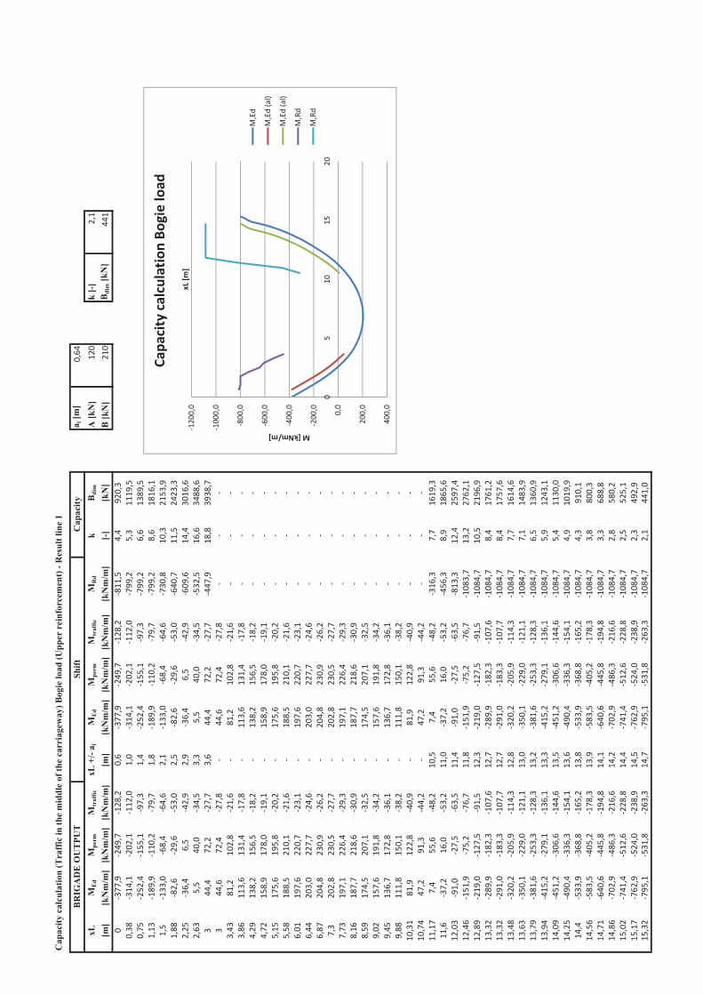
Cap
acity
cal
cula
tion
(Tra
ffic
in th
e m
iddl
e of
the
carr
iage
way
) Bog
ie lo
ad (U
pper
rei
nfor
cem
ent)
- R
esul
t lin
e 1
a l [m
]0,64
xLM
Ed
Mpe
rmM
traf
ficxL
+/-
a lM
Ed
Mpe
rmM
traf
ficM
Rd
kB
dim
A [k
N]
120
k [-
]2,1
[m]
[kN
m/m
][k
Nm
/m]
[kN
m/m
][m
][k
Nm
/m]
[kN
m/m
][k
Nm
/m]
[kN
m/m
][-
][k
N]
B [k
N]
210
dim
[kN
]44
10
377,9
249,7
128,2
0,6
377,9
249,7
128,2
811,5
4,4
920,3
0,38
314,1
202,1
112,0
1,0
314,1
202,1
112,0
799,2
5,3
1119
,50,75
252,4
155,1
97,3
1,4
252,4
155,1
97,3
799,2
6,6
1389
,51,13
189,9
110,2
79,7
1,8
189,9
110,2
79,7
799,2
8,6
1816
,11,5
133,0
68,4
64,6
2,1
133,0
68,4
64,6
730,8
10,3
2153
,91,88
82,6
29,6
53,0
2,5
82,6
29,6
53,0
640,7
11,5
2423
,32,25
36,4
6,5
42,9
2,9
36,4
6,5
42,9
609,6
14,4
3016
,62,63
5,5
40,0
34,5
3,3
5,5
40,0
34,5
532,5
16,6
3488
,63
44,4
72,2
27,7
3,6
44,4
72,2
27,7
447,9
18,8
3938
,73
44,6
72,4
27,8
44,6
72,4
27,8
3,43
81,2
102,8
21,6
81,2
102,8
21,6
3,86
113,6
131,4
17,8
113,6
131,4
17,8
4,29
138,2
156,5
18,2
138,2
156,5
18,2
4,72
158,9
178,0
19,1
158,9
178,0
19,1
5,15
175,6
195,8
20,2
175,6
195,8
20,2
5,58
188,5
210,1
21,6
188,5
210,1
21,6
6,01
197,6
220,7
23,1
197,6
220,7
23,1
6,44
203,0
227,7
24,6
203,0
227,7
24,6
6,87
204,8
230,9
26,2
204,8
230,9
26,2
7,3
202,8
230,5
27,7
202,8
230,5
27,7
7,73
197,1
226,4
29,3
197,1
226,4
29,3
8,16
187,7
218,6
30,9
187,7
218,6
30,9
8,59
174,5
207,1
32,5
174,5
207,1
32,5
9,02
157,6
191,8
34,2
157,6
191,8
34,2
9,45
136,7
172,8
36,1
136,7
172,8
36,1
9,88
111,8
150,1
38,2
111,8
150,1
38,2
10,31
81,9
122,8
40,9
81,9
122,8
40,9
10,74
47,2
91,3
44,2
47,2
91,3
44,2
11,17
7,4
55,6
48,2
10,5
7,4
55,6
48,2
316,3
7,7
1619
,311
,637
,216
,053
,211
,037
,216
,053
,245
6,3
8,9
1865
,612
,03
91,0
27,5
63,5
11,4
91,0
27,5
63,5
813,3
12,4
2597
,412
,46
151,9
75,2
76,7
11,8
151,9
75,2
76,7
1083
,713
,227
62,1
12,89
219,0
127,5
91,5
12,3
219,0
127,5
91,5
1084
,710
,521
96,9
13,32
289,9
182,3
107,6
12,7
289,9
182,3
107,6
1084
,78,4
1761
,213
,32
291,0
183,3
107,7
12,7
291,0
183,3
107,7
1084
,78,4
1757
,613
,48
320,2
205,9
114,3
12,8
320,2
205,9
114,3
1084
,77,7
1614
,613
,63
350,1
229,0
121,1
13,0
350,1
229,0
121,1
1084
,77,1
1483
,913
,79
381,6
253,3
128,3
13,2
381,6
253,3
128,3
1084
,76,5
1360
,913
,94
415,2
279,1
136,1
13,3
415,2
279,1
136,1
1084
,75,9
1243
,114
,09
451,2
306,6
144,6
13,5
451,2
306,6
144,6
1084
,75,4
1130
,014
,25
490,4
336,3
154,1
13,6
490,4
336,3
154,1
1084
,74,9
1019
,914
,453
3,9
368,8
165,2
13,8
533,9
368,8
165,2
1084
,74,3
910,1
14,56
583,5
405,2
178,3
13,9
583,5
405,2
178,3
1084
,73,8
800,3
14,71
640,6
445,8
194,8
14,1
640,6
445,8
194,8
1084
,73,3
688,8
14,86
702,9
486,3
216,6
14,2
702,9
486,3
216,6
1084
,72,8
580,2
15,02
741,4
512,6
228,8
14,4
741,4
512,6
228,8
1084
,72,5
525,1
15,17
762,9
524,0
238,9
14,5
762,9
524,0
238,9
1084
,72,3
492,9
15,32
795,1
531,8
263,3
14,7
795,1
531,8
263,3
1084
,72,1
441,0
Cap
acity
BR
IGA
DE
OU
TPU
TSh
ift
1200,0
1000,0
800,0
600,0
400,0
200,0
0,0
200,0
400,0
05
1015
20
M[kNm/m]
xL[m
]
Capa
city
calculationBo
gieload
M,Ed
M,Ed(al)
M,Ed(al)
M,Rd
M,Rd
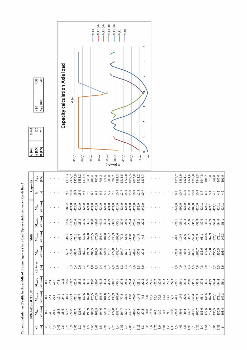
Cap
acity
cal
cula
tion
(Tra
ffic
in th
e m
iddl
e of
the
carr
iage
way
) Axl
e lo
ad (U
pper
rei
nfor
cem
ent)
- R
esul
t lin
e 2
a l [m
]0,64
2xL
ME
dM
perm
Mtr
affic
xL +
/- a l
ME
dM
perm
Mtr
affic
MR
dk
Adi
mA
[kN
]12
0k
[-]
4,56
[m]
[kN
m/m
][k
Nm
/m]
[kN
m/m
][m
][k
Nm
/m]
[kN
m/m
][k
Nm
/m]
[kN
m/m
][-
][k
N]
B [k
N]
210
Adi
m [k
N]
547
00,8
0,7
0,2
0,15
4,5
2,1
2,4
0,3
9,7
5,1
4,6
0,45
19,3
12,1
7,3
0,6
35,6
24,1
11,5
0,75
53,7
38,1
15,6
0,1
53,7
38,1
15,6
183,2
9,3
1113
,30,9
72,0
53,3
18,7
0,3
72,0
53,3
18,7
424,0
19,8
2377
,71,05
93,7
72,1
21,6
0,4
93,7
72,1
21,6
424,0
16,3
1954
,91,2
121,0
95,7
25,3
0,6
121,0
95,7
25,3
424,0
13,0
1555
,21,35
162,1
130,6
31,5
0,7
162,1
130,6
31,5
424,0
9,3
1118
,41,5
199,9
162,8
37,1
0,9
199,9
162,8
37,1
424,0
7,0
845,3
1,65
209,5
170,5
39,0
1,0
209,5
170,5
39,0
424,0
6,5
780,6
1,65
209,5
170,5
39,0
2,3
209,5
170,5
39,0
424,0
6,5
780,6
1,8
194,6
153,4
41,2
2,4
194,6
153,4
41,2
424,0
6,6
788,2
1,95
224,4
181,0
43,4
2,6
224,4
181,0
43,4
424,0
5,6
671,6
2,1
216,1
172,2
43,9
2,7
216,1
172,2
43,9
424,0
5,7
688,8
2,25
177,0
138,9
38,1
2,9
177,0
138,9
38,1
424,0
7,5
897,2
2,4
132,7
102,6
30,1
3,0
132,7
102,6
30,1
424,0
10,7
1281
,32,55
104,7
77,3
27,4
3,2
104,7
77,3
27,4
424,0
12,7
1518
,52,7
82,1
56,6
25,5
3,3
82,1
56,6
25,5
424,0
14,4
1727
,02,85
64,2
39,8
24,4
3,5
64,2
39,8
24,4
424,0
15,8
1892
,53
49,6
26,0
23,6
3,6
49,6
26,0
23,6
424,0
16,9
2024
,83,15
37,4
14,3
23,1
3,8
37,4
14,3
23,1
286,0
11,8
1413
,23,3
27,2
4,5
22,8
3,9
27,2
4,5
22,8
247,0
10,7
1278
,73,45
18,8
3,8
22,6
3,6
11,9
10,7
22,6
3,75
6,3
16,4
22,7
3,9
2,0
20,9
22,9
4,05
3,6
19,6
23,2
4,2
9,6
14,1
23,7
4,35
17,0
7,3
24,3
4,5
25,9
0,8
25,1
3,9
25,9
0,8
25,1
247,0
9,8
1178
,74,65
36,6
10,5
26,1
4,0
36,6
10,5
26,1
290,0
10,7
1286
,94,8
49,4
22,0
27,3
4,2
49,4
22,0
27,3
323,0
11,0
1321
,14,95
64,7
35,7
29,0
4,3
64,7
35,7
29,0
355,0
11,0
1321
,65,1
83,5
52,4
31,1
4,5
83,5
52,4
31,1
389,0
10,8
1299
,05,25
106,7
72,9
33,8
4,6
106,7
72,9
33,8
424,0
10,4
1248
,35,4
135,6
98,1
37,4
4,8
135,6
98,1
37,4
424,1
8,7
1044
,85,55
177,6
134,5
43,1
4,9
177,6
134,5
43,1
424,1
6,7
806,7
5,7
217,8
167,9
49,9
5,1
217,8
167,9
49,9
424,1
5,1
615,8
5,85
230,5
176,1
54,4
5,2
230,5
176,1
54,4
424,1
4,6
547,0
5,85
230,5
176,1
54,4
6,5
230,5
176,1
54,4
424,1
4,6
547,0
620
3,4
147,3
56,1
6,6
203,4
147,3
56,1
424,1
4,9
591,9
BR
IGA
DE
OU
TPU
TSh
iftC
apac
ity
450,0
400,0
350,0
300,0
250,0
200,0
150,0
100,0
50,0 0,0
01
23
45
67
M[kNm/m]
xL[m
]
Capa
city
calculationAx
leload
M,Ed
M,Ed(al)
M,Ed(al)
M,Ed(al)
M,Ed(al)
M,Rd
M,Rd
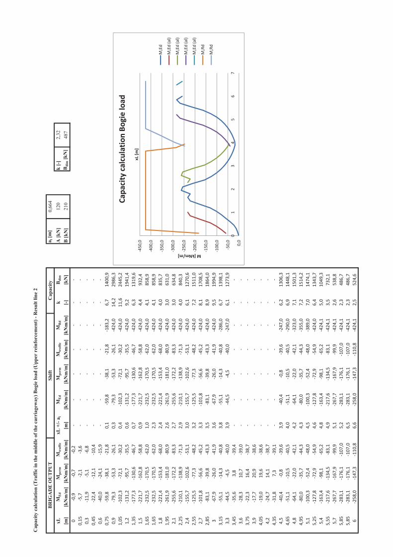
Cap
acity
cal
cula
tion
(Tra
ffic
in th
e m
iddl
e of
the
carr
iage
way
) Bog
ie lo
ad (U
pper
rei
nfor
cem
ent)
- R
esul
t lin
e 2
a l [m
]0,
664
xLM
Ed
Mpe
rmM
traf
ficxL
+/-
a lM
Ed
Mpe
rmM
traf
ficM
Rd
kdi
mA
[kN
]12
0k
[-]
2,32
[m]
[kN
m/m
][k
Nm
/m]
[kN
m/m
][m
][k
Nm
/m]
[kN
m/m
][k
Nm
/m]
[kN
m/m
][-
][k
N]
B [k
N]
210
dim
[kN
]48
70
0,9
0,7
0,2
0,15
5,7
2,1
3,6
0,3
11,9
5,1
6,8
0,45
22,4
12,1
10,4
0,6
40,0
24,1
15,9
0,75
59,8
38,1
21,8
0,1
59,8
38,1
21,8
183,2
6,7
1400
,90,9
79,3
53,3
26,1
0,3
79,3
53,3
26,1
424,0
14,2
2986
,31,05
102,3
72,1
30,2
0,4
102,3
72,1
30,2
424,0
11,6
2445
,21,2
131,2
95,7
35,5
0,6
131,2
95,7
35,5
424,0
9,2
1941
,41,35
177,3
130,6
46,7
0,7
177,3
130,6
46,7
424,0
6,3
1319
,61,5
221,7
162,8
58,8
0,9
221,7
162,8
58,8
424,0
4,4
932,4
1,65
232,5
170,5
62,0
1,0
232,5
170,5
62,0
424,0
4,1
858,9
1,65
232,5
170,5
62,0
2,3
232,5
170,5
62,0
424,0
4,1
858,9
1,8
221,4
153,4
68,0
2,4
221,4
153,4
68,0
424,0
4,0
835,7
1,95
261,9
181,0
80,9
2,6
261,9
181,0
80,9
424,0
3,0
631,0
2,1
255,6
172,2
83,3
2,7
255,6
172,2
83,3
424,0
3,0
634,8
2,25
210,1
138,9
71,3
2,9
210,1
138,9
71,3
424,0
4,0
840,3
2,4
155,7
102,6
53,1
3,0
155,7
102,6
53,1
424,0
6,1
1270
,62,55
125,5
77,3
48,2
3,2
125,5
77,3
48,2
424,0
7,2
1511
,02,7
101,8
56,6
45,2
3,3
101,8
56,6
45,2
424,0
8,1
1708
,52,85
83,1
39,8
43,3
3,5
83,1
39,8
43,3
424,0
8,9
1864
,03
67,9
26,0
41,9
3,6
67,9
26,0
41,9
424,0
9,5
1994
,93,15
55,1
14,3
40,8
3,8
55,1
14,3
40,8
286,0
6,7
1398
,13,3
44,5
4,5
40,0
3,9
44,5
4,5
40,0
247,0
6,1
1273
,93,45
35,6
3,8
39,4
3,6
28,3
10,7
39,0
3,75
22,3
16,4
38,7
3,9
17,7
20,9
38,6
4,05
19,0
19,6
38,6
4,2
24,7
14,1
38,7
4,35
31,8
7,3
39,1
4,5
40,4
0,8
39,6
3,9
40,4
0,8
39,6
247,0
6,2
1306
,34,65
51,1
10,5
40,5
4,0
51,1
10,5
40,5
290,0
6,9
1448
,14,8
64,1
22,0
42,1
4,2
64,1
22,0
42,1
323,0
7,1
1501
,34,95
80,0
35,7
44,3
4,3
80,0
35,7
44,3
355,0
7,2
1514
,25,1
100,3
52,4
48,0
4,5
100,3
52,4
48,0
389,0
7,0
1474
,15,25
127,8
72,9
54,9
4,6
127,8
72,9
54,9
424,0
6,4
1343
,75,4
163,4
98,1
65,2
4,8
163,4
98,1
65,2
424,1
5,0
1049
,35,55
217,6
134,5
83,1
4,9
217,6
134,5
83,1
424,1
3,5
732,1
5,7
267,7
167,9
99,9
5,1
267,7
167,9
99,9
424,1
2,6
538,8
5,85
283,1
176,1
107,0
5,2
283,1
176,1
107,0
424,1
2,3
486,7
5,85
283,1
176,1
107,0
6,5
283,1
176,1
107,0
424,1
2,3
486,7
625
8,0
147,3
110,8
6,6
258,0
147,3
110,8
424,1
2,5
524,6
Cap
acity
BR
IGA
DE
OU
TPU
TSh
ift
450,0
400,0
350,0
300,0
250,0
200,0
150,0
100,0
50,0 0,0
01
23
45
67
M[kNm/m]
xL[m
]
Capa
city
calculationBo
gieload
M,Ed
M,Ed(al)
M,Ed(al)
M,Ed(al)
M,Ed(al)
M,Rd
M,Rd
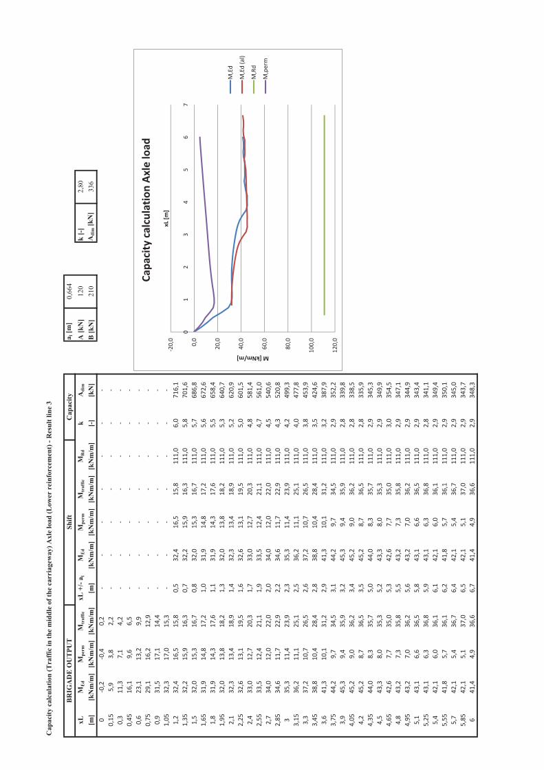
Cap
acity
cal
cula
tion
(Tra
ffic
in th
e m
iddl
e of
the
carr
iage
way
) Axl
e lo
ad (L
ower
rei
nfor
cem
ent)
- R
esul
t lin
e 3
a l [m
]0,
664
xLM
Ed
Mpe
rmM
traf
ficxL
+/-
a lM
Ed
Mpe
rmM
traf
ficM
Rd
kA
dim
A [k
N]
120
k [-
]2,
80[m
][k
Nm
/m]
[kN
m/m
][k
Nm
/m]
[m]
[kN
m/m
][k
Nm
/m]
[kN
m/m
][k
Nm
/m]
[-]
[kN
]B
[kN
]21
0A
dim
[kN
]33
60
0,2
0,4
0,2
0,15
5,9
3,8
2,2
0,3
11,3
7,1
4,2
0,45
16,1
9,6
6,5
0,6
23,1
13,2
9,9
0,75
29,1
16,2
12,9
0,9
31,5
17,1
14,4
1,05
32,3
17,0
15,3
1,2
32,4
16,5
15,8
0,5
32,4
16,5
15,8
111,0
6,0
716,1
1,35
32,2
15,9
16,3
0,7
32,2
15,9
16,3
111,0
5,8
701,6
1,5
32,0
15,3
16,7
0,8
32,0
15,3
16,7
111,0
5,7
686,8
1,65
31,9
14,8
17,2
1,0
31,9
14,8
17,2
111,0
5,6
672,6
1,8
31,9
14,3
17,6
1,1
31,9
14,3
17,6
111,0
5,5
658,4
1,95
32,0
13,8
18,2
1,3
32,0
13,8
18,2
111,0
5,3
640,7
2,1
32,3
13,4
18,9
1,4
32,3
13,4
18,9
111,0
5,2
620,9
2,25
32,6
13,1
19,5
1,6
32,6
13,1
19,5
111,0
5,0
601,5
2,4
33,0
12,7
20,3
1,7
33,0
12,7
20,3
111,0
4,8
581,4
2,55
33,5
12,4
21,1
1,9
33,5
12,4
21,1
111,0
4,7
561,0
2,7
34,0
12,0
22,0
2,0
34,0
12,0
22,0
111,0
4,5
540,6
2,85
34,6
11,7
22,9
2,2
34,6
11,7
22,9
111,0
4,3
520,8
335
,311
,423
,92,3
35,3
11,4
23,9
111,0
4,2
499,3
3,15
36,2
11,1
25,1
2,5
36,2
11,1
25,1
111,0
4,0
477,8
3,3
37,2
10,7
26,5
2,6
37,2
10,7
26,5
111,0
3,8
453,9
3,45
38,8
10,4
28,4
2,8
38,8
10,4
28,4
111,0
3,5
424,6
3,6
41,3
10,1
31,2
2,9
41,3
10,1
31,2
111,0
3,2
387,9
3,75
44,2
9,7
34,5
3,1
44,2
9,7
34,5
111,0
2,9
352,2
3,9
45,3
9,4
35,9
3,2
45,3
9,4
35,9
111,0
2,8
339,8
4,05
45,2
9,0
36,2
3,4
45,2
9,0
36,2
111,0
2,8
338,5
4,2
45,2
8,7
36,5
3,5
45,2
8,7
36,5
111,0
2,8
335,9
4,35
44,0
8,3
35,7
5,0
44,0
8,3
35,7
111,0
2,9
345,3
4,5
43,3
8,0
35,3
5,2
43,3
8,0
35,3
111,0
2,9
349,9
4,65
42,6
7,7
35,0
5,3
42,6
7,7
35,0
111,0
3,0
354,5
4,8
43,2
7,3
35,8
5,5
43,2
7,3
35,8
111,0
2,9
347,1
4,95
43,2
7,0
36,2
5,6
43,2
7,0
36,2
111,0
2,9
344,9
5,1
43,1
6,6
36,5
5,8
43,1
6,6
36,5
111,0
2,9
343,4
5,25
43,1
6,3
36,8
5,9
43,1
6,3
36,8
111,0
2,8
341,1
5,4
42,1
6,0
36,1
6,1
42,1
6,0
36,1
111,0
2,9
349,4
5,55
41,8
5,7
36,1
6,2
41,8
5,7
36,1
111,0
2,9
350,1
5,7
42,1
5,4
36,7
6,4
42,1
5,4
36,7
111,0
2,9
345,0
5,85
42,1
5,1
37,0
6,5
42,1
5,1
37,0
111,0
2,9
343,7
641
,44,9
36,6
6,7
41,4
4,9
36,6
111,0
2,9
348,3
Cap
acity
BR
IGA
DE
OU
TPU
TSh
ift
20,0 0,0
20,0
40,0
60,0
80,0
100,0
120,0
01
23
45
67
M[kNm/m]
xL[m
]
Capa
city
calculationAx
leload
M,Ed
M,Ed(al)
M,Rd
M,perm
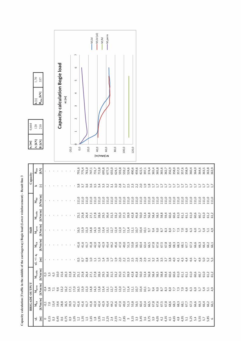
Cap
acity
cal
cula
tion
(Tra
ffic
in th
e m
iddl
e of
the
carr
iage
way
) Bog
ie lo
ad (L
ower
rei
nfor
cem
ent)
- R
esul
t lin
e 3
a l [m
]0,
664
xLM
Ed
Mpe
rmM
traf
ficxL
+/-
a lM
Ed
Mpe
rmM
traf
ficM
Rd
kB
dim
A [k
N]
120
k [-
]1,
70[m
][k
Nm
/m]
[kN
m/m
][k
Nm
/m]
[m]
[kN
m/m
][k
Nm
/m]
[kN
m/m
][k
Nm
/m]
[-]
[kN
]B
[kN
]21
0B
dim
[kN
]35
70
0,1
0,4
0,3
0,15
7,0
3,8
3,3
0,3
13,4
7,1
6,3
0,45
19,6
9,6
10,0
0,6
28,8
13,2
15,6
0,75
36,5
16,2
20,3
0,9
39,9
17,1
22,8
1,05
41,2
17,0
24,2
1,2
41,6
16,5
25,1
0,5
41,6
16,5
25,1
111,0
3,8
791,6
1,35
41,6
15,9
25,8
0,7
41,6
15,9
25,8
111,0
3,7
775,4
1,5
41,7
15,3
26,4
0,8
41,7
15,3
26,4
111,0
3,6
761,0
1,65
41,8
14,8
27,1
1,0
41,8
14,8
27,1
111,0
3,6
747,1
1,8
42,0
14,3
27,8
1,1
42,0
14,3
27,8
111,0
3,5
731,7
1,95
42,4
13,8
28,6
1,3
42,4
13,8
28,6
111,0
3,4
713,8
2,1
42,9
13,4
29,5
1,4
42,9
13,4
29,5
111,0
3,3
695,8
2,25
43,4
13,1
30,4
1,6
43,4
13,1
30,4
111,0
3,2
677,3
2,4
44,2
12,7
31,5
1,7
44,2
12,7
31,5
111,0
3,1
655,0
2,55
45,6
12,4
33,2
1,9
45,6
12,4
33,2
111,0
3,0
624,1
2,7
47,0
12,0
35,0
2,0
47,0
12,0
35,0
111,0
2,8
593,8
2,85
49,0
11,7
37,3
2,2
49,0
11,7
37,3
111,0
2,7
559,2
351
,311
,439
,92,3
51,3
11,4
39,9
111,0
2,5
524,6
3,15
53,8
11,1
42,8
2,5
53,8
11,1
42,8
111,0
2,3
490,6
3,3
56,5
10,7
45,8
2,6
56,5
10,7
45,8
111,0
2,2
459,6
3,45
60,4
10,4
50,0
2,8
60,4
10,4
50,0
111,0
2,0
422,5
3,6
63,4
10,1
53,4
2,9
63,4
10,1
53,4
111,0
1,9
397,1
3,75
66,5
9,7
56,8
3,1
66,5
9,7
56,8
111,0
1,8
374,4
3,9
67,8
9,4
58,4
3,2
67,8
9,4
58,4
111,0
1,7
365,4
4,05
67,6
9,0
58,5
3,4
67,6
9,0
58,5
111,0
1,7
365,8
4,2
67,5
8,7
58,8
3,5
67,5
8,7
58,8
111,0
1,7
365,6
4,35
67,8
8,3
59,4
3,7
67,8
8,3
59,4
111,0
1,7
362,7
4,5
68,6
8,0
60,6
3,8
68,6
8,0
60,6
111,0
1,7
356,9
4,65
68,3
7,7
60,6
4,0
68,3
7,7
60,6
111,0
1,7
358,0
4,8
68,3
7,3
61,0
4,1
68,3
7,3
61,0
111,0
1,7
357,0
4,95
68,1
7,0
61,1
4,3
68,1
7,0
61,1
111,0
1,7
357,6
5,1
67,7
6,6
61,1
4,4
67,7
6,6
61,1
111,0
1,7
358,9
5,25
67,3
6,3
61,0
4,6
67,3
6,3
61,0
111,0
1,7
360,4
5,4
66,6
6,0
60,6
4,7
66,6
6,0
60,6
111,0
1,7
364,0
5,55
66,3
5,7
60,7
4,9
66,3
5,7
60,7
111,0
1,7
364,6
5,7
66,4
5,4
61,0
5,0
66,4
5,4
61,0
111,0
1,7
363,5
5,85
66,2
5,1
61,2
5,2
66,2
5,1
61,2
111,0
1,7
363,8
666
,14,9
61,2
5,3
66,1
4,9
61,2
111,0
1,7
363,9
BR
IGA
DE
OU
TPU
TSh
iftC
apac
ity
20,0 0,0
20,0
40,0
60,0
80,0
100,0
120,0
01
23
45
67
M[kNm/m]
xL[m
]
Capa
city
calculationBo
gieload
M,Ed
M,Ed(al)
M,Rd
M,perm
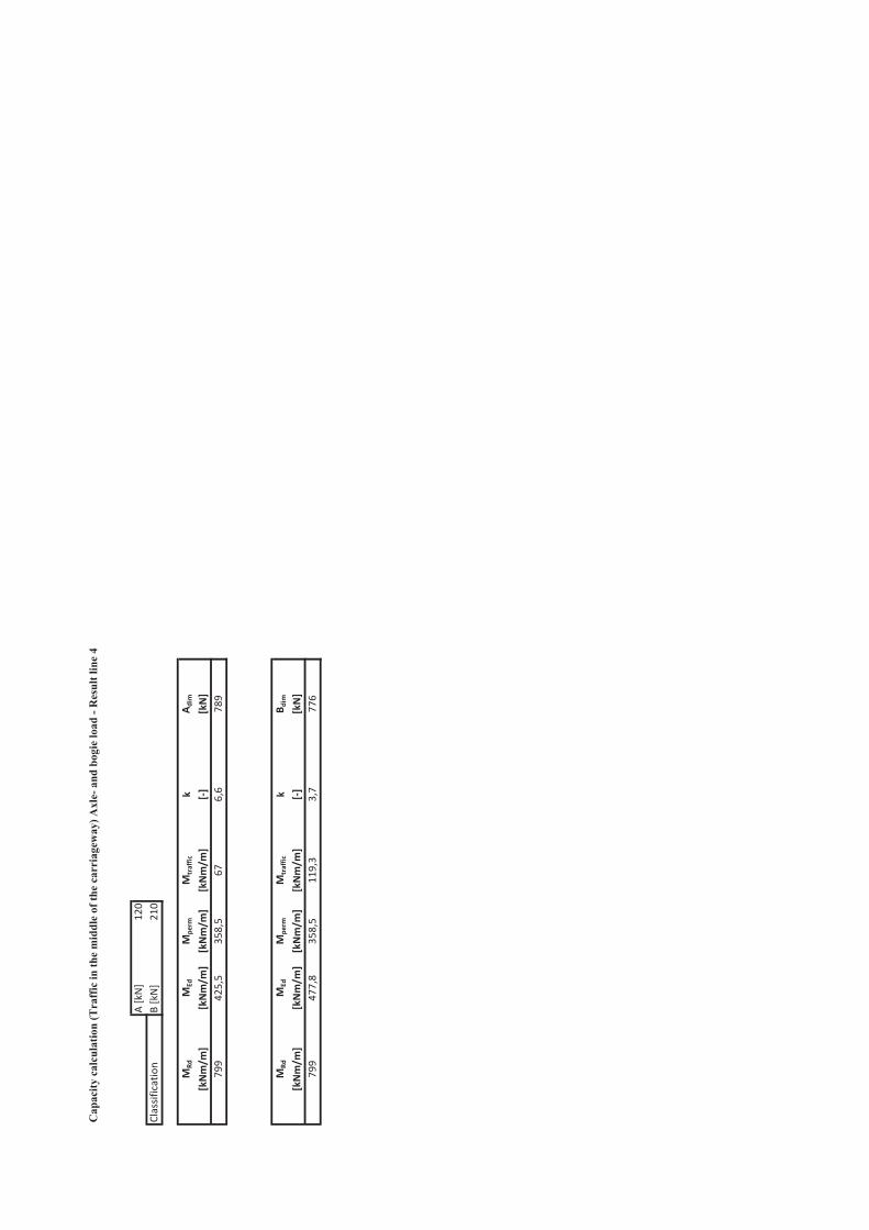
Cap
acity
cal
cula
tion
(Tra
ffic
in th
e m
iddl
e of
the
carr
iage
way
) Axl
e- a
nd b
ogie
load
- R
esul
t lin
e 4
A[kN]
120
Classification
B[kN]
210
MRd
MEd
Mpe
rmM
traffic
kA d
im
[kNm/m
][kNm/m
][kNm/m
][kNm/m
][]
[kN]
799
425,5
358,5
676,6
789
MRd
MEd
Mpe
rmM
traffic
kB d
im
[kNm/m
][kNm/m
][kNm/m
][kNm/m
][]
[kN]
799
477,8
358,5
119,3
3,7
776
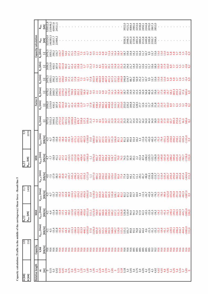
Cap
acity
cal
cula
tion
(Tra
ffic
in th
e m
iddl
e of
the
carr
iage
way
) She
ar fo
rce
- Res
ult l
ine
5
A[kN]
120
k A[]
11,7
k B[]
9,9
B[kN]
210
A dim[kN]
1400
B dim[kN]
2070
Relativ
elength
Capa
city
xLV,Rd
V Ed_
A(m
ax)
V Ed_
B(m
ax)
V perm(m
ax)
V Ed_
A(m
in)
V Ed_
B(m
in)
V perm(m
in)
K A(m
ax)
K A(m
in)
K B(m
ax)
K B(m
in)
K A(dim
)K B
(dim
)A d
imB d
im
[m]
[kN/m
][kN/m
][kN/m
][kN/m
][kN/m
][kN/m
][kN/m
][]
[][]
[][]
[][kN]
[kN]
091
64,1
4,1
4,3
4,6
4,7
4,3
7075
,626
96,0
4278
,224
76,3
2696
,024
76,3
3235
24,4
5200
12,8
0,15
916
6,5
6,4
6,7
7,5
7,7
6,7
5152
,312
19,9
2994
,410
03,1
1219
,910
03,1
1463
83,3
2106
48,2
0,3
916
15,4
15,4
15,7
17,9
18,9
15,8
3449
,143
0,5
2660
,729
0,2
430,5
290,2
5165
7,7
6094
7,8
0,42
916
32,8
32,8
33,2
38,3
41,1
33,6
2721
,618
7,4
2342
,511
6,7
187,4
116,7
2248
4,2
2451
1,5
0,42
916
32,8
32,8
33,2
38,3
41,1
33,6
2721
,618
7,4
2342
,511
6,7
187,4
116,7
0,45
916
37,6
37,5
37,9
43,8
47,2
38,4
2577
,016
1,8
2270
,210
0,0
161,8
100,0
0,6
916
64,3
64,2
64,8
75,2
81,3
65,8
1815
,590
,015
81,2
54,6
90,0
54,6
0,75
916
90,2
90,0
90,9
105,7
114,5
92,4
1397
,861
,711
70,3
37,2
61,7
37,2
0,9
916
123,3
123,0
124,3
145,3
157,6
126,7
1039
,842
,479
9,9
25,5
42,4
25,5
1,05
916
166,4
165,3
167,2
196,3
213,0
171,1
1353
,429
,556
9,9
17,8
29,5
17,8
1,2
916
222,9
220,3
224,2
265,7
287,9
231,1
876,7
19,8
292,2
12,1
19,8
12,1
1,35
916
313,9
308,4
316,1
377,1
408,4
327,5
559,8
11,9
160,0
7,3
11,9
7,3
1,5
916
446,1
433,6
456,9
559,3
607,0
482,9
127,1
5,7
58,9
3,5
5,7
3,5
1,65
916
1033
,010
12,0
1052
,012
71,0
1383
,011
00,0
103,6
1,1
49,2
0,7
1,1
0,7
1,8
916
57,6
111,1
15,4
1,1
1,1
15,0
21,3
57,8
9,4
57,8
21,3
9,4
1,95
916
1326
,015
23,0
1130
,010
77,0
1076
,010
82,0
1,1
399,5
0,5
332,9
1,1
0,5
2,1
916
605,9
700,9
513,7
484,2
482,7
487,4
4,4
438,4
2,1
298,5
4,4
2,1
2,25
916
424,7
487,5
359,4
346,0
345,8
347,7
8,5
743,1
4,3
664,9
8,5
4,3
2,4
916
315,3
360,6
264,7
256,2
254,7
257,5
12,9
902,3
6,8
418,9
12,9
6,8
2,55
916
249,5
284,0
207,0
200,6
200,4
202,9
16,7
486,3
9,2
447,4
16,7
9,2
2,7
916
202,9
229,9
165,5
160,4
160,2
162,7
20,1
468,8
11,6
431,3
20,1
11,6
2,85
916
168,0
189,2
133,8
129,4
128,7
131,9
22,9
419,0
14,1
327,3
22,9
14,1
391
614
0,7
157,2
108,1
103,6
102,3
106,8
24,8
319,5
16,4
227,2
24,8
16,4
3,15
916
118,8
131,3
86,3
81,6
79,0
85,3
25,5
266,2
18,4
158,6
25,5
18,4
3,18
916
115,1
126,8
82,2
77,4
74,5
81,3
25,3
255,0
18,7
146,8
25,3
18,7
3,18
916
115,1
126,8
82,2
77,4
74,5
81,3
25,3
255,0
18,7
146,8
25,3
18,7
3036
,339
22,0
3,3
916
101,7
110,4
67,2
62,0
57,9
66,5
24,6
220,2
19,6
114,7
24,6
19,6
2948
,341
21,2
3,45
916
89,8
94,4
49,9
44,1
38,5
49,4
21,7
184,8
19,4
88,7
21,7
19,4
2601
,040
84,4
3,6
895
93,5
94,3
33,7
27,3
20,1
33,4
14,4
152,2
14,2
69,6
14,4
14,2
1729
,429
85,6
3,75
895
76,8
75,0
18,4
11,1
2,2
18,2
15,0
128,5
15,5
56,9
15,0
15,5
1801
,032
53,6
3,9
895
60,2
57,9
3,4
29,1
32,4
3,3
15,7
27,7
16,4
25,2
15,7
16,4
1884
,434
38,8
4,05
895
44,4
42,3
11,5
81,7
87,4
11,6
16,2
12,6
16,9
11,7
12,6
11,7
1513
,824
50,1
4,2
895
9,6
10,5
26,7
98,8
108,2
27,0
54,0
12,1
56,8
10,7
12,1
10,7
1449
,822
44,8
4,35
895
21,5
22,6
42,6
116,1
129,5
43,0
44,4
11,7
46,8
9,9
11,7
9,9
1399
,820
70,0
4,5
912
31,1
32,3
59,7
103,8
122,7
60,3
34,0
19,6
35,5
13,7
19,6
13,7
2350
,728
67,3
4,62
912
22,2
24,2
74,5
113,7
136,9
75,3
18,9
21,8
19,6
13,6
18,9
13,6
2266
,628
52,0
4,62
916
22,2
24,2
74,5
113,7
136,9
75,3
19,0
21,9
19,7
13,6
19,0
13,6
4,65
916
19,8
22,0
78,5
116,4
140,8
79,4
16,9
22,6
17,6
13,6
16,9
13,6
4,8
916
43,1
45,3
99,9
135,4
165,8
101,1
17,9
23,7
18,6
12,6
17,9
12,6
4,95
916
70,3
72,3
125,0
205,7
241,9
126,8
19,0
10,0
19,7
6,9
10,0
6,9
5,1
916
139,5
140,1
155,8
243,4
288,2
158,6
65,7
8,9
68,2
5,8
8,9
5,8
5,25
916
193,1
193,1
196,0
293,0
349,8
200,2
383,3
7,7
383,3
4,8
7,7
4,8
5,4
916
246,4
246,5
251,0
362,4
435,4
258,1
253,6
6,3
259,2
3,7
6,3
3,7
5,55
916
334,7
334,9
341,8
455,8
556,7
353,5
177,1
5,5
182,2
2,8
5,5
2,8
5,7
916
444,4
445,7
482,9
637,4
783,7
509,4
36,3
3,2
37,6
1,5
3,2
1,5
5,85
916
1083
,010
83,0
1087
,014
04,0
1728
,011
35,0
500,6
0,8
500,6
0,4
0,8
0,4
691
611
2,4
134,0
0,5
111,3
132,6
0,3
8,2
8,2
6,9
6,9
8,2
6,9
MAX
MIN
Factor
KCa
pacity
calculation
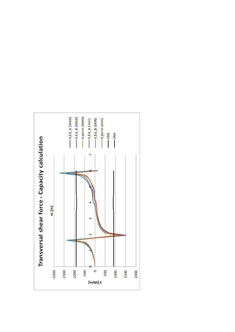
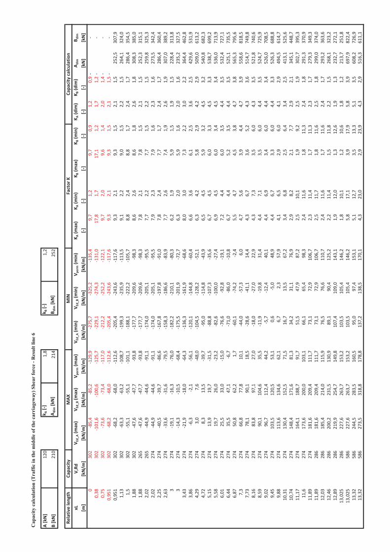
Cap
acity
cal
cula
tion
(Tra
ffic
in th
e m
iddl
e of
the
carr
iage
way
) She
ar fo
rce
- Res
ult l
ine
6
A[kN]
120
k A[]
1,8
k B[]
1,2
B[kN]
210
A dim[kN]
214
B dim[kN]
252
Relativ
elength
Capa
city
xLV,Rd
V Ed_
A(m
ax)
V Ed_
B(m
ax)
V perm(m
ax)
V Ed_
A(m
in)
V Ed_
B(m
in)
V perm(m
in)
K A(m
ax)
K A(m
in)
K B(m
ax)
K B(m
in)
K A(dim
)K B
(dim
)A d
imB d
im
[m]
[kN/m
][kN/m
][kN/m
][kN/m
][kN/m
][kN/m
][kN/m
][]
[][]
[][]
[][kN]
[kN]
030
285
,485
,212
9,9
275,7
325,2
135,4
9,7
1,2
9,7
0,9
1,2
0,9
0,38
302
101,6
100,6
125,7
229,1
274,3
131,0
17,8
1,7
17,1
1,2
1,7
1,2
0,75
302
73,6
73,4
117,0
212,2
252,2
122,1
9,7
2,0
9,6
1,4
2,0
1,4
0,95
130
268
,268
,011
2,6
205,4
243,6
117,6
9,3
2,1
9,3
1,5
2,1
1,5
0,95
130
268
,268
,011
2,6
205,4
243,6
117,6
9,3
2,1
9,3
1,5
2,1
1,5
252,5
307,9
1,13
302
63,3
63,2
108,7
199,3
235,9
113,5
9,1
2,2
9,0
1,5
2,2
1,5
264,1
324,0
1,5
302
55,1
55,1
101,1
188,1
222,2
105,7
8,8
2,4
8,8
1,7
2,4
1,7
286,4
354,5
1,88
302
47,6
47,7
93,8
177,7
209,6
98,3
8,6
2,6
8,6
1,8
2,6
1,8
308,3
385,0
1,88
265
47,6
47,7
93,8
177,7
209,6
98,3
7,8
2,1
7,8
1,5
2,1
1,5
252,3
315,1
2,02
265
44,9
44,6
91,1
174,0
205,1
95,5
7,7
2,2
7,7
1,5
2,2
1,5
259,8
325,3
2,02
274
44,9
44,6
91,1
174,0
205,1
95,5
7,9
2,3
7,9
1,6
2,3
1,6
273,5
342,4
2,25
274
40,5
39,7
86,6
167,8
197,8
91,0
7,8
2,4
7,7
1,7
2,4
1,7
286,4
360,4
2,63
274
33,6
31,6
79,5
158,3
186,6
83,9
7,7
2,6
7,4
1,9
2,6
1,9
307,0
389,2
327
419
,116
,376
,018
2,2
210,1
80,3
6,2
1,9
5,9
1,5
1,9
1,5
228,4
313,8
327
414
,310
,568
,417
5,5
201,9
72,7
6,3
2,0
5,9
1,6
2,0
1,6
235,2
327,5
3,43
274
21,9
18,0
64,3
136,3
161,9
68,6
8,0
3,0
7,3
2,2
3,0
2,2
364,4
462,8
3,86
274
6,3
2,1
56,1
120,1
144,8
60,4
6,6
3,6
6,1
2,5
3,6
2,5
429,6
531,9
4,29
274
3,0
7,6
48,0
104,5
128,2
52,1
6,3
4,2
5,8
2,9
4,2
2,9
509,0
613,2
4,72
274
8,3
13,5
39,7
95,0
114,8
43,9
6,5
4,5
5,9
3,2
4,5
3,2
540,8
682,3
5,15
274
13,9
19,7
31,5
88,8
107,3
35,6
6,7
4,5
6,0
3,3
4,5
3,3
538,7
699,2
5,58
274
19,7
26,0
23,2
82,6
100,0
27,4
6,9
4,5
6,0
3,4
4,5
3,4
536,0
713,9
6,01
274
25,5
33,0
15,0
76,6
92,8
19,1
7,2
4,4
6,0
3,5
4,4
3,5
532,4
727,1
6,44
274
35,5
47,1
6,7
71,0
86,0
10,8
6,7
4,4
5,2
3,5
4,4
3,5
525,1
735,5
6,87
274
50,8
62,2
1,7
60,1
74,2
2,4
5,5
4,7
4,5
3,8
4,7
3,8
565,3
795,6
7,3
274
66,8
77,8
10,1
44,0
57,3
6,0
4,7
5,6
3,9
4,4
4,7
3,9
558,6
818,5
7,73
274
78,1
90,1
18,5
28,6
41,1
14,4
4,3
6,7
3,6
5,2
4,3
3,6
514,7
749,8
8,16
274
83,8
97,1
27,0
18,0
27,0
22,9
4,3
7,3
3,5
6,0
4,3
3,5
521,8
740,6
8,59
274
90,1
104,6
35,5
11,9
19,8
31,4
4,4
7,1
3,5
6,0
4,4
3,5
524,7
725,9
9,02
274
96,7
112,4
44,2
5,7
12,4
40,1
4,4
6,9
3,4
6,0
4,4
3,4
526,0
708,5
9,45
274
103,5
120,5
53,1
0,6
5,0
48,9
4,4
6,7
3,3
6,0
4,4
3,3
526,3
688,8
9,88
274
113,6
134,6
62,1
6,7
2,3
57,9
4,1
6,5
2,9
6,0
4,1
2,9
494,5
614,7
10,31
274
130,4
152,5
71,5
16,7
13,5
67,2
3,4
6,8
2,5
6,4
3,4
2,5
413,1
525,6
10,74
274
148,4
171,6
81,3
34,2
31,1
76,9
2,9
8,2
2,1
7,7
2,9
2,1
345,1
448,7
11,17
274
164,1
188,7
91,7
51,5
47,9
87,2
2,5
10,1
1,9
9,2
2,5
1,9
302,7
395,3
11,6
274
173,6
200,0
103,1
66,1
65,4
98,3
2,4
11,6
1,8
11,3
2,4
1,8
291,3
370,9
11,89
274
181,6
209,4
111,7
73,1
72,9
106,7
2,3
11,4
1,7
11,3
2,3
1,7
279,3
349,3
11,89
286
181,6
209,4
111,7
73,1
72,9
106,7
2,5
11,7
1,8
11,6
2,5
1,8
299,0
374,0
12,03
286
185,4
214,0
115,9
76,5
76,6
110,7
2,4
11,6
1,7
11,6
2,4
1,7
293,2
363,6
12,46
286
200,2
231,5
130,9
89,1
90,4
125,2
2,2
11,4
1,5
11,8
2,2
1,5
268,1
323,2
12,89
286
219,9
254,7
149,8
107,4
109,0
143,1
1,9
12,0
1,3
12,6
1,9
1,3
232,7
272,1
13,025
286
227,6
263,7
153,2
103,5
105,4
146,2
1,8
10,1
1,2
10,6
1,8
1,2
213,7
251,8
13,025
586
227,6
263,7
153,2
103,5
105,4
146,2
5,8
17,1
3,9
17,9
5,8
3,9
697,9
822,4
13,32
586
244,5
283,5
160,5
95,0
97,4
153,1
5,1
12,7
3,5
13,3
5,1
3,5
608,2
726,9
13,32
586
273,5
318,8
178,8
137,2
138,5
170,1
4,3
23,0
2,9
23,9
4,3
2,9
516,3
611,1
MAX
MIN
Factor
KCa
pacity
calculation
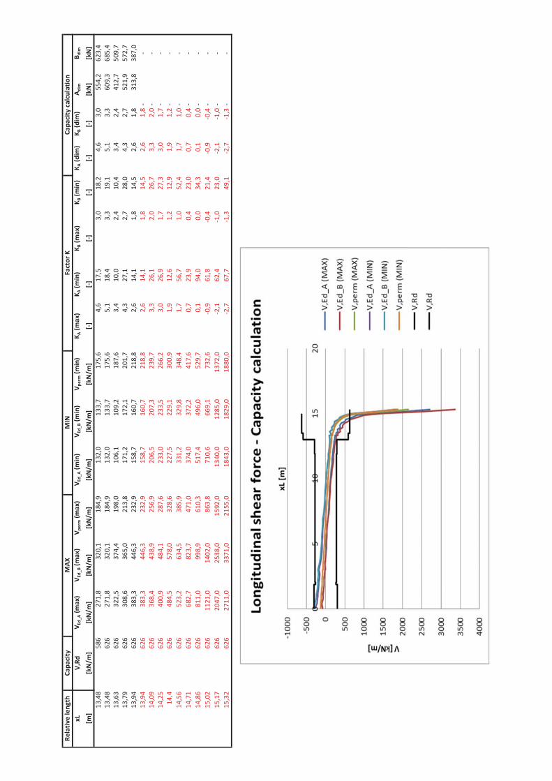
Relativ
elength
Capa
city
xLV,Rd
V Ed_
A(m
ax)
V Ed_
B(m
ax)
V perm(m
ax)
V Ed_
A(m
in)
V Ed_
B(m
in)
V perm(m
in)
K A(m
ax)
K A(m
in)
K B(m
ax)
K B(m
in)
K A(dim
)K B
(dim
)A d
imB d
im
[m]
[kN/m
][kN/m
][kN/m
][kN/m
][kN/m
][kN/m
][kN/m
][]
[][]
[][]
[][kN]
[kN]
13,48
586
271,8
320,1
184,9
132,0
133,7
175,6
4,6
17,5
3,0
18,2
4,6
3,0
554,2
623,4
13,48
626
271,8
320,1
184,9
132,0
133,7
175,6
5,1
18,4
3,3
19,1
5,1
3,3
609,3
685,4
13,63
626
322,5
374,4
198,0
106,1
109,2
187,6
3,4
10,0
2,4
10,4
3,4
2,4
412,7
509,7
13,79
626
308,6
365,0
213,8
171,2
172,1
201,7
4,3
27,1
2,7
28,0
4,3
2,7
521,9
572,7
13,94
626
383,3
446,3
232,9
158,7
160,7
218,8
2,6
14,1
1,8
14,5
2,6
1,8
313,8
387,0
13,94
626
383,3
446,3
232,9
158,7
160,7
218,8
2,6
14,1
1,8
14,5
2,6
1,8
14,09
626
368,4
438,9
256,9
206,5
207,3
239,7
3,3
26,1
2,0
26,7
3,3
2,0
14,25
626
400,9
484,1
287,6
233,0
233,5
266,2
3,0
26,9
1,7
27,3
3,0
1,7
14,4
626
484,5
578,0
328,6
227,5
229,1
300,9
1,9
12,6
1,2
12,9
1,9
1,2
14,56
626
523,2
634,5
385,9
331,2
329,8
348,4
1,7
56,7
1,0
52,4
1,7
1,0
14,71
626
682,7
823,7
471,0
374,0
372,2
417,6
0,7
23,9
0,4
23,0
0,7
0,4
14,86
626
811,0
998,9
610,3
517,4
496,0
529,7
0,1
94,0
0,0
34,3
0,1
0,0
15,02
626
1121
,014
02,0
863,8
710,6
669,1
732,6
0,9
61,8
0,4
21,4
0,9
0,4
15,17
626
2047
,025
38,0
1592
,013
40,0
1285
,013
72,0
2,1
62,4
1,0
23,0
2,1
1,0
15,32
626
2711
,033
71,0
2155
,018
43,0
1829
,018
80,0
2,7
67,7
1,3
49,1
2,7
1,3
MAX
MIN
Factor
KCa
pacity
calculation
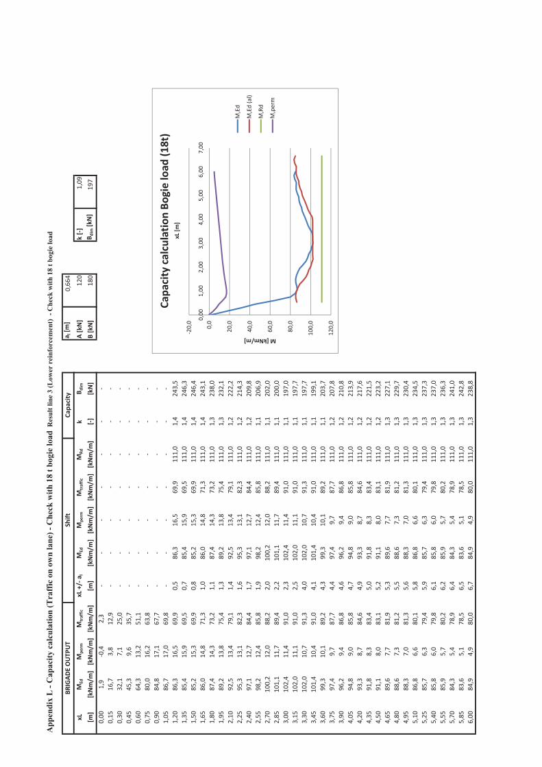
Cap
acity
cal
cula
tion
Res
ult l
ine
3 -
Che
ck w
ith 1
8 t b
ogie
load
a l[m
]0,66
4
xLM
EdM
perm
Mtraffic
xL+/
a lM
EdM
perm
Mtraffic
MRd
B dim
A[kN]
120
k[]
1,09
[m]
[kNm/m
][kNm/m
][kNm/m
][m
][kNm/m
][kNm/m
][kNm/m
][kNm/m
][]
[kN]
B[kN]
180
B dim[kN]
197
0,00
1,9
0,4
2,3
0,15
16,7
3,8
12,9
0,30
32,1
7,1
25,0
0,45
45,3
9,6
35,7
0,60
64,3
13,2
51,1
0,75
80,0
16,2
63,8
0,90
84,8
17,1
67,7
1,05
86,7
17,0
69,8
1,20
86,3
16,5
69,9
0,5
86,3
16,5
69,9
111,0
1,4
243,5
1,35
85,4
15,9
69,5
0,7
85,4
15,9
69,5
111,0
1,4
246,3
1,50
85,2
15,3
69,9
0,8
85,2
15,3
69,9
111,0
1,4
246,4
1,65
86,0
14,8
71,3
1,0
86,0
14,8
71,3
111,0
1,4
243,1
1,80
87,4
14,3
73,2
1,1
87,4
14,3
73,2
111,0
1,3
238,0
1,95
89,2
13,8
75,4
1,3
89,2
13,8
75,4
111,0
1,3
232,1
2,10
92,5
13,4
79,1
1,4
92,5
13,4
79,1
111,0
1,2
222,2
2,25
95,3
13,1
82,3
1,6
95,3
13,1
82,3
111,0
1,2
214,3
2,40
97,1
12,7
84,4
1,7
97,1
12,7
84,4
111,0
1,2
209,8
2,55
98,2
12,4
85,8
1,9
98,2
12,4
85,8
111,0
1,1
206,9
2,70
100,2
12,0
88,2
2,0
100,2
12,0
88,2
111,0
1,1
202,0
2,85
101,1
11,7
89,4
2,2
101,1
11,7
89,4
111,0
1,1
200,0
3,00
102,4
11,4
91,0
2,3
102,4
11,4
91,0
111,0
1,1
197,0
3,15
102,0
11,1
91,0
2,5
102,0
11,1
91,0
111,0
1,1
197,7
3,30
102,0
10,7
91,3
4,0
102,0
10,7
91,3
111,0
1,1
197,7
3,45
101,4
10,4
91,0
4,1
101,4
10,4
91,0
111,0
1,1
199,1
3,60
99,3
10,1
89,2
4,3
99,3
10,1
89,2
111,0
1,1
203,7
3,75
97,4
9,7
87,7
4,4
97,4
9,7
87,7
111,0
1,2
207,8
3,90
96,2
9,4
86,8
4,6
96,2
9,4
86,8
111,0
1,2
210,8
4,05
94,8
9,0
85,8
4,7
94,8
9,0
85,8
111,0
1,2
213,9
4,20
93,3
8,7
84,6
4,9
93,3
8,7
84,6
111,0
1,2
217,6
4,35
91,8
8,3
83,4
5,0
91,8
8,3
83,4
111,0
1,2
221,5
4,50
91,1
8,0
83,1
5,2
91,1
8,0
83,1
111,0
1,2
223,2
4,65
89,6
7,7
81,9
5,3
89,6
7,7
81,9
111,0
1,3
227,1
4,80
88,6
7,3
81,2
5,5
88,6
7,3
81,2
111,0
1,3
229,7
4,95
88,3
7,0
81,3
5,6
88,3
7,0
81,3
111,0
1,3
230,4
5,10
86,8
6,6
80,1
5,8
86,8
6,6
80,1
111,0
1,3
234,5
5,25
85,7
6,3
79,4
5,9
85,7
6,3
79,4
111,0
1,3
237,3
5,40
85,8
6,0
79,8
6,1
85,8
6,0
79,8
111,0
1,3
237,0
5,55
85,9
5,7
80,2
6,2
85,9
5,7
80,2
111,0
1,3
236,3
5,70
84,3
5,4
78,9
6,4
84,3
5,4
78,9
111,0
1,3
241,0
5,85
83,6
5,1
78,5
6,5
83,6
5,1
78,5
111,0
1,3
242,8
6,00
84,9
4,9
80,0
6,7
84,9
4,9
80,0
111,0
1,3
238,8
Capa
city
BRIGAD
EOUTP
UT
Shift
20,0 0,0
20,0
40,0
60,0
80,0
100,0
120,00,
001,00
2,00
3,00
4,00
5,00
6,00
7,00
M[kNm/m]
xL[m
]
Capa
city
calculationBo
gieload
(18t)
M,Ed
M,Ed(al)
M,Rd
M,perm
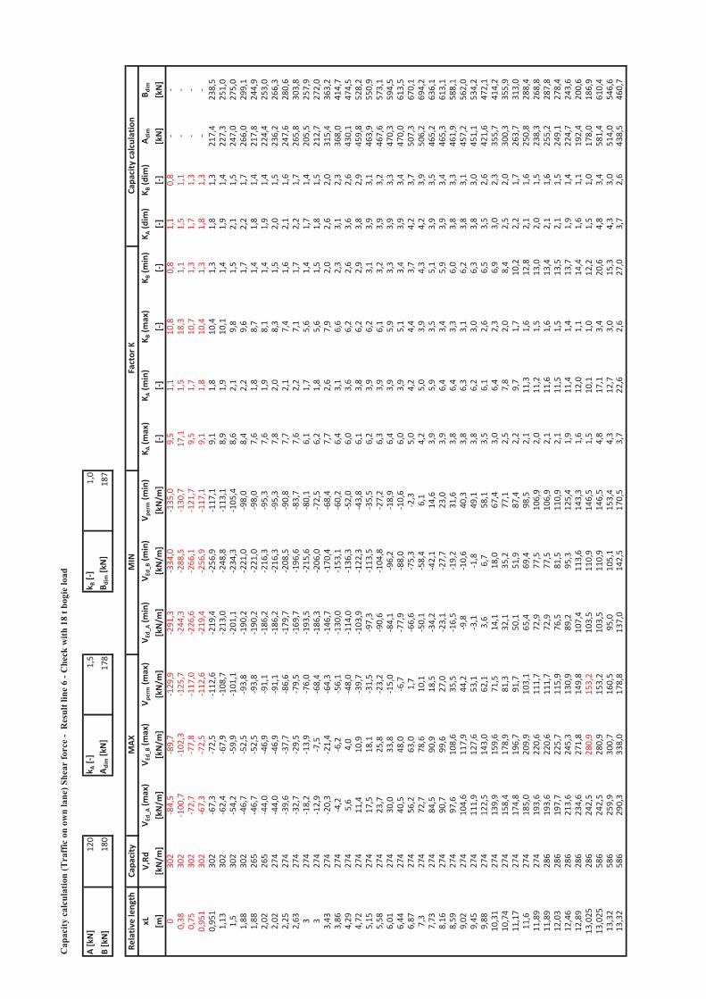
Cap
acity
cal
cula
tion
Shea
r fo
rce
- R
esul
t lin
e 6
- Che
ck w
ith 1
8 t b
ogie
load
A[kN]
120
k A[]
1,5
k B[]
1,0
B[kN]
180
A dim[kN]
178
B dim[kN]
187
Relativ
elength
Capa
city
xLV,Rd
V Ed_
A(m
ax)
V Ed_
B(m
ax)
V perm(m
ax)
V Ed_
A(m
in)
V Ed_
B(m
in)
V perm(m
in)
K A(m
ax)
K A(m
in)
K B(m
ax)
K B(m
in)
K A(dim
)K B
(dim
)A d
imB d
im
[m]
[kN/m
][kN/m
][kN/m
][kN/m
][kN/m
][kN/m
][kN/m
][]
[][]
[][]
[][kN]
[kN]
030
284
,589
,712
9,9
291,3
334,0
135,0
9,5
1,1
10,8
0,8
1,1
0,8
0,38
302
100,7
102,3
125,7
244,3
288,5
130,7
17,1
1,5
18,3
1,1
1,5
1,1
0,75
302
72,7
77,8
117,0
226,6
266,1
121,7
9,5
1,7
10,7
1,3
1,7
1,3
0,95
130
267
,372
,511
2,6
219,4
256,9
117,1
9,1
1,8
10,4
1,3
1,8
1,3
0,95
130
267
,372
,511
2,6
219,4
256,9
117,1
9,1
1,8
10,4
1,3
1,8
1,3
217,4
238,5
1,13
302
62,4
67,9
108,7
213,0
248,8
113,1
8,9
1,9
10,1
1,4
1,9
1,4
227,3
251,0
1,5
302
54,2
59,9
101,1
201,1
234,3
105,4
8,6
2,1
9,8
1,5
2,1
1,5
247,0
275,0
1,88
302
46,7
52,5
93,8
190,2
221,0
98,0
8,4
2,2
9,6
1,7
2,2
1,7
266,0
299,1
1,88
265
46,7
52,5
93,8
190,2
221,0
98,0
7,6
1,8
8,7
1,4
1,8
1,4
217,8
244,9
2,02
265
44,0
46,9
91,1
186,2
216,3
95,3
7,6
1,9
8,1
1,4
1,9
1,4
224,4
253,0
2,02
274
44,0
46,9
91,1
186,2
216,3
95,3
7,8
2,0
8,3
1,5
2,0
1,5
236,2
266,3
2,25
274
39,6
37,7
86,6
179,7
208,5
90,8
7,7
2,1
7,4
1,6
2,1
1,6
247,6
280,6
2,63
274
32,7
29,5
79,5
169,7
196,6
83,7
7,6
2,2
7,1
1,7
2,2
1,7
265,8
303,8
327
418
,213
,976
,019
3,5
215,6
80,1
6,1
1,7
5,6
1,4
1,7
1,4
205,5
257,9
327
412
,97,5
68,4
186,3
206,0
72,5
6,2
1,8
5,6
1,5
1,8
1,5
212,7
272,0
3,43
274
20,3
21,4
64,3
146,7
170,4
68,4
7,7
2,6
7,9
2,0
2,6
2,0
315,4
363,2
3,86
274
4,2
6,2
56,1
130,0
153,1
60,2
6,4
3,1
6,6
2,3
3,1
2,3
368,0
414,7
4,29
274
5,6
4,0
48,0
114,0
136,3
52,0
6,0
3,6
6,2
2,6
3,6
2,6
430,1
474,5
4,72
274
11,4
10,9
39,7
103,9
122,3
43,8
6,1
3,8
6,2
2,9
3,8
2,9
459,8
528,2
5,15
274
17,5
18,1
31,5
97,3
113,5
35,5
6,2
3,9
6,2
3,1
3,9
3,1
463,9
550,9
5,58
274
23,7
25,8
23,2
90,6
104,8
27,2
6,3
3,9
6,1
3,2
3,9
3,2
467,6
573,1
6,01
274
30,0
33,8
15,0
84,1
96,2
18,9
6,4
3,9
5,9
3,3
3,9
3,3
470,3
594,5
6,44
274
40,5
48,0
6,7
77,9
88,0
10,6
6,0
3,9
5,1
3,4
3,9
3,4
470,0
613,5
6,87
274
56,2
63,0
1,7
66,6
75,3
2,3
5,0
4,2
4,4
3,7
4,2
3,7
507,3
670,1
7,3
274
72,7
78,6
10,1
50,1
58,4
6,1
4,2
5,0
3,9
4,3
4,2
3,9
506,2
694,2
7,73
274
84,5
90,9
18,5
34,2
42,1
14,6
3,9
5,9
3,5
5,1
3,9
3,5
465,2
636,1
8,16
274
90,7
99,6
27,0
23,1
27,7
23,0
3,9
6,4
3,4
5,9
3,9
3,4
465,3
613,1
8,59
274
97,6
108,6
35,5
16,5
19,2
31,6
3,8
6,4
3,3
6,0
3,8
3,3
461,9
588,1
9,02
274
104,6
117,9
44,2
9,8
10,6
40,3
3,8
6,3
3,1
6,2
3,8
3,1
457,2
562,0
9,45
274
111,9
127,6
53,1
3,1
1,8
49,1
3,8
6,2
3,0
6,3
3,8
3,0
451,1
534,2
9,88
274
122,5
143,0
62,1
3,6
6,7
58,1
3,5
6,1
2,6
6,5
3,5
2,6
421,6
472,1
10,31
274
139,9
159,6
71,5
14,1
18,0
67,4
3,0
6,4
2,3
6,9
3,0
2,3
355,7
414,2
10,74
274
158,4
178,9
81,3
32,1
35,2
77,1
2,5
7,8
2,0
8,4
2,5
2,0
300,3
355,9
11,17
274
174,8
196,7
91,7
50,1
51,9
87,4
2,2
9,7
1,7
10,2
2,2
1,7
263,7
313,0
11,6
274
185,0
209,9
103,1
65,4
69,4
98,5
2,1
11,3
1,6
12,8
2,1
1,6
250,8
288,4
11,89
274
193,6
220,6
111,7
72,9
77,5
106,9
2,0
11,2
1,5
13,0
2,0
1,5
238,3
268,8
11,89
286
193,6
220,6
111,7
72,9
77,5
106,9
2,1
11,6
1,6
13,4
2,1
1,6
255,2
287,8
12,03
286
197,7
225,7
115,9
76,5
81,5
110,9
2,1
11,5
1,5
13,5
2,1
1,5
249,1
278,4
12,46
286
213,6
245,3
130,9
89,2
95,3
125,4
1,9
11,4
1,4
13,7
1,9
1,4
224,7
243,6
12,89
286
234,6
271,8
149,8
107,4
113,6
143,3
1,6
12,0
1,1
14,4
1,6
1,1
192,4
200,6
13,025
286
242,5
280,9
153,2
103,5
110,9
146,5
1,5
10,1
1,0
12,2
1,5
1,0
178,0
186,9
13,025
586
242,5
280,9
153,2
103,5
110,9
146,5
4,8
17,1
3,4
20,6
4,8
3,4
581,4
610,4
13,32
586
259,9
300,7
160,5
95,0
105,1
153,4
4,3
12,7
3,0
15,3
4,3
3,0
514,0
546,6
13,32
586
290,3
338,0
178,8
137,0
142,5
170,5
3,7
22,6
2,6
27,0
3,7
2,6
438,5
460,7
MAX
MIN
Factor
KCa
pacity
calculation
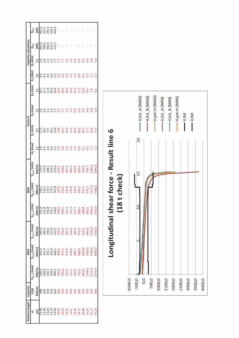
Relativ
elength
Capa
city
xLV,Rd
V Ed_
A(m
ax)
V Ed_
B(m
ax)
V perm(m
ax)
V Ed_
A(m
in)
V Ed_
B(m
in)
V perm(m
in)
K A(m
ax)
K A(m
in)
K B(m
ax)
K B(m
in)
K A(dim
)K B
(dim
)A d
imB d
im
[m]
[kN/m
][kN/m
][kN/m
][kN/m
][kN/m
][kN/m
][kN/m
][]
[][]
[][]
[][kN]
[kN]
13,48
586
289,0
341,4
184,9
131,8
139,1
176,0
3,9
17,2
2,6
20,7
3,9
2,6
462,6
461,6
13,48
626
289,0
341,4
184,9
131,8
139,1
176,0
4,2
18,1
2,8
21,7
4,2
2,8
508,6
507,5
13,63
626
340,7
393,1
198,0
105,8
119,7
188,1
3,0
9,9
2,2
11,9
3,0
2,2
360,0
395,0
13,79
626
328,0
391,0
213,8
170,7
175,5
202,3
3,6
26,2
2,3
30,9
3,6
2,3
433,3
418,9
13,94
626
404,2
468,2
232,9
158,0
167,8
219,4
2,3
13,8
1,7
16,4
2,3
1,7
275,5
300,8
13,94
626
404,2
468,2
232,9
158,0
167,8
219,4
2,3
13,8
1,7
16,4
2,3
1,7
14,09
626
391,0
471,1
256,9
205,5
210,2
240,6
2,8
24,7
1,7
28,5
2,8
1,7
14,25
626
425,9
521,9
287,6
231,5
235,8
267,3
2,4
25,0
1,4
28,4
2,4
1,4
14,4
626
512,7
618,6
328,6
225,3
235,8
302,3
1,6
12,1
1,0
14,0
1,6
1,0
14,56
626
555,9
689,7
385,9
327,7
310,1
350,4
1,4
43,0
0,8
24,2
1,4
0,8
14,71
626
722,2
886,0
471,0
368,5
359,3
420,4
0,6
20,2
0,4
17,1
0,6
0,4
14,86
626
862,0
1093
,061
0,3
488,8
437,4
534,0
0,1
25,7
0,0
12,0
0,1
0,0
15,02
626
1194
,015
42,0
863,8
662,6
576,2
739,7
0,7
17,7
0,4
8,4
0,7
0,4
15,17
626
2172
,027
84,0
1592
,012
63,0
1127
,013
84,0
1,7
16,6
0,8
7,8
1,7
0,8
15,32
626
2874
,036
97,0
2155
,017
50,0
1588
,018
95,0
2,1
17,4
1,0
8,2
2,1
1,0
MAX
MIN
Factor
KCa
pacity
calculation

About the Author
Fredrik Forsberg was born in Skellefteå, Sweden, on
December 29th, 1991. He attended primary and
secondary school in his hometown, Skellefteå. Then
he proceeded to study civil engineering at Luleå
University of Technology. After an exchange
semester in Hong Kong, he went back to Luleå to
pursue a master’s degree in structural engineering.
He wrote his master thesis at the engineering
consultant firm Ramböll. He has then proceeded to
start his professional career as a structural engineer
at the engineering consultant company, Sweco in
Stockholm.