Embed Size (px)
Citation preview
Geosci. Model Dev., 4, 957–992, 2011www.geosci-model-dev.net/4/957/2011/doi:10.5194/gmd-4-957-2011© Author(s) 2011. CC Attribution 3.0 License.
GeoscientificModel Development
Incorporation of the C-GOLDSTEIN efficient climate model intothe GENIE framework: “eb go gs” configurations of GENIE
R. Marsh1, S. A. Muller1, A. Yool2, and N. R. Edwards3
1National Oceanography Centre Southampton, University of Southampton, Waterfront Campus, European Way,Southampton SO14 3ZH, UK2National Oceanography Centre, Waterfront Campus, European Way, Southampton SO14 3ZH, UK3Department of Earth and Environmental Sciences, CEPSAR, The Open University, Milton Keynes, UK
Received: 8 December 2008 – Published in Geosci. Model Dev. Discuss.: 9 January 2009Revised: 30 September 2011 – Accepted: 19 October 2011 – Published: 15 November 2011
Abstract. A computationally efficient, intermediate com-plexity ocean-atmosphere-sea ice model (C-GOLDSTEIN)has been incorporated into the Grid ENabled Integrated Earthsystem modelling (GENIE) framework. This involved de-coupling of the three component modules that were re-coupled in a modular way, to allow replacement with al-ternatives and coupling of further components within theframework. The climate model described here (referred toas “ebgo gs” for short) is the most basic version of GENIEin which atmosphere, ocean and sea ice all play an activerole. Among improvements on the original C-GOLDSTEINmodel, latitudinal grid resolution is generalized to allow awider range of surface grids to be used. The ocean, atmo-sphere and sea-ice components of the “ebgo gs” configura-tion of GENIE are individually described, along with detailsof their coupling. The setup and results from simulationsusing four different meshes are presented. The four alter-native meshes comprise the widely-used 36× 36 equal-area-partitioning of the Earth surface with 16 depth layers in theocean, a version in which horizontal and vertical resolutionare doubled, a setup matching the horizontal resolution ofthe dynamic atmospheric component available in the GENIEframework, and a setup with enhanced resolution in high-latitude areas. Results are presented for a spin-up experimentwith a baseline parameter set and wind forcing typically usedfor current studies in which “ebgo gs” is coupled with theocean biogeochemistry module of GENIE, as well as for anexperiment with a modified parameter set, revised wind forc-ing, and additional cross-basin transport pathways (Indone-sian and Bering Strait throughflows). The latter experimentis repeated with the four mesh variants, with common pa-
Correspondence to:R. Marsh([email protected])
rameter settings throughout, except for time-step length. Se-lected state variables and diagnostics are compared in tworegards: (i) between simulations at lowest resolution that areobtained with the baseline and modified configurations, pre-dominantly in order to evaluate the revision of the wind forc-ing, the modification of some key parameters, and the effectof additional transport pathways across the Arctic Ocean andthe Indonesian Archipelago; (ii) between simulations withthe four meshes, in order to explore various effects of meshchoice.
1 Introduction
To comprehensively model climate change on multi-millennial timescales, to jointly explore and statisticallyanalyse large subsets of model parameter space of com-bined climate-system components, or to run a multitude oflong-term scenarios for anthropogenic climate forcing, wepresently need to use “Earth System Models” (ESMs) whichinclude all the necessary components and processes, andwhich are of high computational efficiency. Such ESMsmust specifically represent the atmosphere, ocean, sea-ice,and, for some purposes ice sheets and biogeochemical cy-cles. For long-timescale palaeoclimate studies of Earth sys-tem dynamics, over several millions of years, changes in ge-ography, orography and bathymetry must also be accommo-dated. These models must be computationally much fasterthan the general circulation models that are used to simulateclimate change on shorter (centennial) timescales, to enablemodel integration over long timescales, and/or to accomplishlarge ensembles. A new generation of such ESMs of Inter-mediate Complexity (EMICs) has emerged in recent years(Claussen et al., 2002). In EMICs, computational speed isachieved through a combination of simplified physics, low
Published by Copernicus Publications on behalf of the European Geosciences Union.

958 R. Marsh et al.: Incorporation of the C-GOLDSTEIN efficient climate model into the GENIE framework
resolution and efficient numerics (e.g., asynchronous cou-pling, implicit time-stepping). EMICs have been used op-erationally to explore long-term climate change and commit-ment (IPCC, 2007a), and for a variety of palaeoclimate stud-ies (e.g.,IPCC, 2007b). In one such application,Plattneret al. (2008) found no systematic difference in predictionsbetween EMICs and higher-complexity models.
As a contribution to the EMIC class of models, the Grid-ENabled Integrated Earth system modelling (GENIE) frame-work is both flexible and scaleable in complexity (Lentonet al. (2006, 2007, 2009); http://www.genie.ac.uk). Furtheradvantages of the GENIE structure include the availabilityof grid-based tools for launching and analysing experiments(Lenton et al., 2007), and the use of a version-control infras-tructure and the automatic routine testing of the code and anymodifications on a daily basis. Further information on thegeneral GENIE infrastructure can be found elsewhere (seehttp://source.ggy.bris.ac.uk/wiki/GENIE).
At the present time, the GENIE framework supports twomain levels of complexity (dimensionality and physics) inthe atmosphere, GENIE-1 and GENIE-2 (seeLenton et al.,2007). The present paper describes a basic version ofGENIE-1, originally known as C-GOLDSTEIN (Edwardsand Marsh(2005), henceforth EM05). This configura-tion of GENIE-1 is commonly referred to by the shorthand“eb go gs”, where “eb” refers to the Energy and MoistureBalance Model (EMBM) of the atmosphere (by analogy,“ig” is commonly used to refer to the IGCM, the fully-dynamical atmospheric model component available in theGENIE framework), “go” refers to the Global Ocean-LinearDrag Salt and Temperature Equation Integrator (GOLD-STEIN) ocean model, and “gs” refers to the sea ice schemeused in conjuction with GOLDSTEIN.
The purpose of this paper is to provide a basic descrip-tion of ebgo gs, emphasizing recent updates on earlier ver-sions (e.g.,Lenton et al., 2007). The standard version ofeb go gs described in this paper is based on GENIE ver-sion 2.7.4 (tagged as “rel-2-7-4” in the source code reposi-tory). Adjustments to the code introduced after the releaseof GENIE version 2.7.4 were required for one of the alter-native mesh options. GENIE version 2.7.7 has been verifiedto reproduce the results when set up using the configurationspresented herein and the parameter and topography-relatedconfiguration files from the present study are planned (at thetime of this writing) to be included in an upcoming GENIErelease version (planned to be GENIE version 2.7.8, and tobe tagged as “rel-2-7-8”). A further purpose is the descrip-tion and basic evaluation of a range of meshes which cannow be accomodated in the ebgo gs model, motivated bya range of scientific foci and requirements, which includevery high computational efficiency of the model, previouslyestablished model configurations, increased zonal or merid-ional resolution to better accomodate regional geographic ortopographic features or localised processes, or compatibilitywith other model components.
We outline, and present results from, a baseline setup ofthe ebgo gs model, which is currently in wide use as astandard configuration in conjunction with the simulation ofbiogeochemical cycles in GENIE, employing the BIOGEMand ATCHEM (Ridgwell et al., 2007a) (and often also theSEDGEM (Ridgwell and Hargreaves, 2007)) model compo-nents (henceforth referred to as the “biogem” configuration).This particular configuration of GENIE-1 was included asmodel “GENIE-16” (emphasizing 16 levels in the ocean) inthe multi-model inter-comparison study ofCao et al.(2009).We further outline three horizontal meshes as alternativesto the widely-used horizontal resolution of 36 by 36 equal-area grid cells for GENIE-1, and present selected results ob-tained in spin-up experiments with each. All experimentsare carried out with code on the GENIE development branch“Marsh et al-2009-GMDD”, which contains specific differ-ences not available in the release version “rel-2-7-4” (which,except in the case of one of the alternative meshes, do not af-fect the baseline performance of the model) and the specificparameter and topography-related configuration files for theset-ups shown here (unless they have already been present).Some aspects of, and results from, the “biogem” configura-tion used here are reported elsewhere (e.g.,Cao et al., 2009).Variants of ebgo gs in the “rel-2-7-4” release version havebeen subject to tuning exercises, results of which will be re-ported elsewhere.
The paper is organized as follows. In Sect.2, we describethe model, with four sub-sections that describe the individualmodel components, coupling, time-stepping and meshes, andmodel parameters and inputs. In Sect.3, we present the re-sults obtained from default spin-up model runs, using a stan-dard mesh (in two configurations), and selected results ob-tained with the three alternative meshes. In Sect.4, we dis-cuss the wider use of GENIE, emphasizing that the ebgo gssetup underpins more complete model representations of theEarth System, already used to investigate phenomena such asabrupt climate change and biogeochemical cycles, in studiesof past or future Earth System dynamics.
2 Model description
2.1 Model components
The three components of ebgo gs – the frictional-geostrophic GOLDSTEIN ocean model, an EMBM of theatmosphere, and a thermodynamic-dynamic model of sea ice– are largely based on the respective model components ofthe C-GOLDSTEIN climate model of EM05, and are eachdescribed in turn below. In addition to the three modules,run-time interpolation of the wind forcing fields has beenimplemented as an independent model component (“genie-wind”), with potential future extension of this module inmind. The current functionality of this module is limited tothe interpolation of externally provided wind and wind-stress
Geosci. Model Dev., 4, 957–992, 2011 www.geosci-model-dev.net/4/957/2011/

R. Marsh et al.: Incorporation of the C-GOLDSTEIN efficient climate model into the GENIE framework 959
datasets during model initialization, and hence no specificdescription of this model component is provided in this sec-tion (see Sect. 2.4 for further details).
2.1.1 Ocean
GOLDSTEIN is a 3-D frictional-geostrophic ocean modelbased on the reduced physics of the thermocline equations,described for a single-basin configuration inEdwards et al.(1998). A global ocean version which constitutes a precur-sor to the ocean component of C-GOLDSTEIN was intro-duced inEdwards and Shepherd(2002) with idealized globalgeography and resolution intermediate between box modelsand models with an approximation of realistic sub-basin-scale topographic features. The presently-decribed versionof GOLDSTEIN is essentially as described in EM05, witha few modifications, outlined below. Various further addi-tions or improvements to GOLDSTEIN include: a surfacemixed layer scheme (based on the scheme byKraus andTurner(1967)); a bottom-boundary layer scheme (based onthe scheme byKillworth and Edwards(1999)); an overflowscheme using the parameterisation ofDanabasoglu et al.,2010; revised surface boundary conditions replacing vir-tual salinity and tracer fluxes with volume fluxes (followingHuang(1993)); a more general equation of state through theparameterisation of thermobaricity (K. Oliver, personel com-munication, 2008); an enhanced diapycnal mixing scheme(Oliver and Edwards, 2008); the additional convection stepused byMuller et al.(2006) preceding the conventional con-vection scheme. Incorporation of these improvements intothe GENIE framework are already available as options or arecurrently in progress, and have been described elsewhere orare anticipated to be documented in future publications.
The prognostic variables at each model grid point are tem-perature and salinity (actually the difference relative to areference salinity, default value 34.9), as well as the three-dimensional velocity field. In summary, the following phys-ical processes are explicitly represented:
– Horizontal and vertical transport of heat, salinity, andother specified tracers (for example, tracers of biogeo-chemical cycles, which are transported as passive trac-ers within GOLDSTEIN), through advection, convec-tion and mixing (comprising the combined parameter-isation for isoneutral mixing and eddy-induced advec-tion (Griffies, 1998), which can optionally be revertedto basic horizontal and vertical mixing);
– Surface exchange of heat with the atmosphere and seaice, provided by the EMBM coupling scheme (seeSect.2.2), or through coupling with an alternative at-mospheric component, is applied as a surface boundarycondition;
– Surface exchange of moisture with the atmosphere, seaice and land, provided (as for heat exchange) by theEMBM coupling scheme (see Sect.2.2);
– Surface input of momentum (zonal and meridional windstress at locations where velocities are defined), pro-vided by the new model component “genie-wind” (al-though technically a model component, its current solepurpose is to interpolate prescribed wind speed andwind stress fields onto the configured model grid dur-ing model initialization). Alternatively, if ‘genie-wind’is deactivated, the wind stress fields are obtained fromthe EMBM, where they can be read in pre-interpolatedform (this option is used in the simulation “biogem” de-scribed below).
We have incorporated three separate modifications relativeto the original GOLDSTEIN model of EM05, two of whichare options which generalize the application to different gridsand geographies, while one represents a minor adjustment ofthe dynamics:
– We have refined the calculation of barotropic flow topermit an arbitrary number of islands (disconnectedland-masses). As noted in EM05, barotropic flowaround islands, and hence through straits, can be cal-culated from the solution of a set of linear constraintsarising from the integration of the depth-averaged mo-mentum equations around each island. The stan-dard C-GOLDSTEIN model setup of EM05 evaluatesbarotropic flow around Antarctica as the single con-tribution arising from such constraints. While EM05explored the effect of additionally-enabled barotropictransport along the Bering Strait in a sensitivity simu-lation, no transport across the Indonesian Archipelagowas enabled. Barotropic flows through Bering Straitand the Indonesian Throughflow (ITF) have significanteffects on the modern global circulation (Hirst and God-frey, 1993; Hu and Meehl, 2005), and the modifica-tion of the scheme for the solution of the barotropicstreamfunction in GOLDSTEIN enables the representa-tion of both flows in the coarse model grids used for thepresent study. Two of the model geographies introducedhere feature the additional inclusion of barotropic flowaround the North Pole (the North Pole is implicitly rep-resented by a meridional no-flow condition at the north-ern model grid boundary), and an additional contribu-tion to the barotropic streamfunction around Greenlandis included, enabling net transport through the DavisStrait.
– A wider variety of horizontal mesh structure and reso-lution can now be accommodated, by generalizing themodel equations to allow an arbitrary latitudinal distri-bution of grid point rows. The original code assumedequal spacing in sine of latitude, which, in conjuctionwith equal spacing in the longitude, results in equal-area cells. Three different mesh options are currentlyavailable: (i) constant spacing in the sine of latitude (pa-rameter “igrid” set to 0); (ii) constant spacing in degrees
www.geosci-model-dev.net/4/957/2011/ Geosci. Model Dev., 4, 957–992, 2011

960 R. Marsh et al.: Incorporation of the C-GOLDSTEIN efficient climate model into the GENIE framework
(“igrid” set to 1); (iii) a copy of the latitudinal axis of theIGCM atmospheric model component (“igrid” set to 2).
– An adjustment has been made to the variable upstream-weighting coefficients in the advection scheme thatoriginally did not consistently take account of the gridcurvature. The upstream weighting is an approximationof theFiadeiro and Veronis(1977) scheme – seeMulleret al.(2006) for further details.
In addition to these modifications, a scaling error in thenon-dimensionalization of coefficients in the equation ofstate, which remained at the same “hard-wired” values whenthe default depth scale was updated from 4000 m to 5000 m,was discovered and corrected in June 2006 (Ridgwell et al.,2007a). The overall effect of this correction was a 25 % in-crease in the dimensional values of wind, currents, overturn-ing, diffusivities and inverse timescales.
Except for the tracers transported by GOLDSTEIN, allquantities appearing in the model equations are in non-dimensionalized form. With the exception of the depthscale, dimensional scale values and constants specific to theocean component are as previously reported (Edwards et al.,1998; Edwards and Shepherd, 2001), and are listed here inTable A1.
2.1.2 Atmosphere
The Energy Moisture Balance Model (EMBM) of the at-mosphere is based closely on that of the UVic Earth Sys-tem Model (Weaver et al., 2001), essentially as described inEM05, with two exceptions (see below). Further enhance-ments of the EMBM include features that become avail-able when the atmospheric component is coupled with theEfficient Numerical Terrestrial Scheme (ENTS) land modelcomponent, as well as forcing mechanisms related to pre-scribed ice sheets, both of which are beyond the scope of thepresent manuscript and have been described byWilliamsonet al.(2006) andHolden et al.(2009) respectively. The prog-nostic variables are air temperature and specific humidity inthe atmospheric boundary layer. The heat and moisture bal-ances of the atmosphere are outlined in Eqs. (1) and (2) ofEM05.
In the EMBM, vertical fluxes are in SI units, while hori-zontal velocities and fluxes are non-dimensionalized, as forGOLDSTEIN. In contrast to the length of the time-step forupdating the state of the ocean and sea-ice, as well as forevaluating heat and moisture fluxes between the three modelcomponents, the length of the time-step used in the EMBMtransport equations is shorter (typically by a factor of five)and the transport equation is solved using an implicit scheme.
In summary, the following physical processes are explic-itly represented in the EMBM module:
– Horizontal transport of heat and moisture in the atmo-sphere by winds and mixing;
– Precipitation, instantaneously removing all moisturecorresponding to the excess above a relative humiditythreshold (the threshold is configurable, but typicallythe default value of 85 % is used);
– Surface exchange of heat with ocean, sea ice and land,according to balance of incoming shortwave radiation (afunction of planetary and sea ice albedo), sensible andlatent heat fluxes, re-emitted long-wave radiation, andoutgoing planetary long-wave radiation (a function ofradiative gases: CO2; water vapour; CH4; N2O);
– Surface exchange of moisture with the ocean, sea iceand land, according to the balance of precipitation,evaporation/sublimation and runoff, the latter throughinstantaneous re-allocation of precipitation over land tocoastal grid-boxes according to simple representation ofcatchments (see Sect.2.3and Fig.1).
Two important changes have been incorporated since weoriginally described the EMBM in EM05. Firstly, the sea-sonal cycle of insolation is included by default; incomingshortwave radiation is computed for each latitude and pointthrough the annual cycle at which exchange fluxes are evalu-ated, using modern day parameters for eccentricity, obliquityand precession. Secondly, the same flexibility of the horizon-tal mesh structure as allowed for the ocean module has beenimplemented. Scale values, constants, and configurable pa-rameters specific to the atmosphere are listed in Table A2. Inone further modification, the meridional profile of heat dif-fusivity at high southern latitudes may be scaled (reduced)southward of a specified latitude, according to a tuneable pa-rameter, to improve the reprsentation of regional air temper-atures and air-sea heat exchange.
2.1.3 Sea ice
We implement the sea ice model described inWeaver et al.(2001), details of which are provided in the Appendix ofEM05. The model comprises thermodynamics plus advec-tion with ocean current at the uppermost level of the oceanmodel. The prognostic variables are ice thickness, and iceareal fraction, or concentration. The transport of sea ice in-cludes sources and sinks for these variables, computed by thecoupling scheme that is technically part of the EMBM, hencethis is where the thermodynamic sea-ice calculations are un-dertaken. As an update from the version used by EM05, thesame horizontal mesh types can now be selected as for theEMBM and GOLDSTEIN ocean model components.
Not specified inWeaver et al.(2001) is the formula ofMillero (1978) (Eq. 9 of EM05), which we use forTf (So),
Geosci. Model Dev., 4, 957–992, 2011 www.geosci-model-dev.net/4/957/2011/

R. Marsh et al.: Incorporation of the C-GOLDSTEIN efficient climate model into the GENIE framework 961
the freezing point for seawater as a function of surface salin-ity:
Tf (So) = −0.0575So +0.0017S3/2o −0.0002S2
o (1)
whereSo is in practical salinity units. Also, in addition to theclimatological albedo everywhere, we further apply a surfacealbedo over sea ice,αice, allowed to vary as a function of airtemperatureTa , following Holland et al.(1993), and expand-ing on Eq. (7) in EM05:
αice = 0.70 if Ta < −7.5◦C
αice = 0.40−0.04T if −7.5◦C< Ta < +5◦C
αice = 0.20 if Ta > +5◦C
(2)
The surface temperature of the sea ice,Ti , is also diag-nosed for use in bulk flux formulae as the temperature“seen” by the atmosphere over sea ice. As outlined byWeaver et al.(2001), Ti is found as an iterative solution. Thesea-ice transport scheme has been modified to optionally usethe same implicit time-step formulation as is used for the at-mospheric transport. This option can be necessary with rela-tively fine horizontal resolution at high latitudes.
In the sea-ice model, vertical fluxes are in SI units, whilehorizontal fluxes are non-dimensionalized. In summary, thefollowing physical processes are explicitly represented:
– Horizontal transport of sea-ice concentration and thick-ness;
– Surface exchange of heat with the atmosphere, accord-ing to the balance of incoming shortwave radiation, sen-sible and latent heat fluxes, and re-emitted long-waveradiation;
– Exchange of heat with the ocean, according to the bal-ance of freezing and melting;
– Surface exchange of freshwater between the atmosphereand ocean; precipitation is assumed to pass straight tothe ocean, ignoring ice, and sublimed water from theocean surface is added directly to the atmosphere;
– Exchange of freshwater with the ocean, according to thebalance of freezing and melting.
Following each sea-ice transport time-step, sea-ice con-centration is constrained to the range from 0 to 1, and seaice with height less than a minimum of 0.01 m is removed,both as described in the appendix of EM05. Constants andscale values specific to the sea-ice component are listed inTable A3.
2.2 Coupling strategy
Apart from advective drift of sea ice with ocean surface cur-rents, and given prescribed wind forcing, the three ebgo gs
model components are coupled through vertical heat andfreshwater fluxes. As the details of each flux componentare fully outlined inWeaver et al.(2001), we only outlinehere how these components enter the coupling, recapitulat-ing and enlarging on the C-GOLDSTEIN model descriptionof EM05. Positive fluxes are defined as directed into the cor-responding model component.
While the coupling scheme forms part of the EMBM mod-ule, it is called directly by the main GENIE programme. Weemploy asynchronous coupling: one “ocean” and “sea ice”time-step per set number of “atmosphere” time-steps, theocean, atmosphere and sea ice being forced with heat andfreshwater fluxes evaluated by the coupling scheme for eachocean and sea ice time-step. For the simulations peresentedherein, the number of atmospheric timesteps (per ocean/sea-ice timestep) is set to 5, to ensure numerical stability in up-dating the atmosphere.
2.2.1 Heat fluxes
Following Weaver et al.(2001), heat is exchanged betweenthe three components as follows. The corresponding totalheat flux into the atmosphere,Qta , is computed as:
Qta = QSWCA +QLH +QLW +QSH−QPLW (3)
QSW is the net shortwave radiation at the top of the atmo-sphere, accounting for planetary albedo (see Fig.5e). CA
is an absorption coefficient, parameterizing heat absorptionby water vapour, dust, ozone and clouds. Over the oceans,CA = 0.3, i.e., the ocean absorbs 70 % ofQSW. Over land,CA = 1.0; with the most rudimentary terrestrial representa-tion, land has no heat capacity, and all net shortwave radi-ation must be absorbed in the overlying atmosphere.QLHis the latent heat released through condensation and subse-quent precipitation.QLW is net (upward minus downward)re-emitted long-wave radiation (the upward part from theocean or sea ice).QSH is the sensible heat flux from eitherocean or sea ice.QPLW is the outgoing planetary long-waveradiation.
The total heat flux from the atmosphere into an ocean grid-box (including sea ice),Qt , is partitioned according to frac-tional sea ice cover,Ai :
Qt = (1−Ai)Qto +AiQt i (4)
whereQto is the total heat flux into the ice-free ocean fromthe atmosphere,
Qto = QSW,o (1−CA)−QLW,o −QSH,o −ρoLvEo (5)
andQti is the total heat flux into sea ice from the atmosphere:
Qti = QSW,i (1−CA)−QLW,i −QSH,i −ρoLsEi (6)
whereQSW,o andQLW,o, andQSW,i andQLW,i , are short-wave and longwave heat fluxes into the ocean and sea ice re-spectively, andρoLvEo andρoLsEi are the latent heat fluxes
www.geosci-model-dev.net/4/957/2011/ Geosci. Model Dev., 4, 957–992, 2011

962 R. Marsh et al.: Incorporation of the C-GOLDSTEIN efficient climate model into the GENIE framework
120E 180 120W 60W 0 60E
Longitude
90S
60S
45S
30S
15S
Eq
15N
30N
45N
60N
90N
Lati
tude
a) 3636s16l
120E 180 120W 60W 0 60E
Longitude
90S
60S
45S
30S
15S
Eq
15N
30N
45N
60N
90N
Lati
tude
b) "biogem"
120E 180 120W 60W 0 60E
Longitude
90S
60S
45S
30S
15S
Eq
15N
30N
45N
60N
90N
Lati
tude
c) 7272s32l
0 60E 120E 180 120W 60W
Longitude
90S
60S
45S
30S
15S
Eq
15N
30N
45N
60N
90N
Lati
tude
d) 6432i16l
120E 180 120W 60W 0 60E
Longitude
90S
60S
45S
30S
15S
Eq
15N
30N
45N
60N
90N
Lati
tude
e) 3660l16l
5.0
4.2
3
3.5
8
3.0
1
2.5
2
2.1
1.7
4
1.4
3
1.1
6
0.9
3
0.7
3
0.5
6
0.4
1
0.2
8
0.1
7
0.0
8
Depth (km)
Fig. 1. Model ocean bathymetry at different resolution, for each configuration. The arrows indicate direction of runoff. The paths aroundislands used for the computation of the barotropic streamfunction are superimposed in cyan.
over open ocean and sea ice, respectively (ρo is the density ofseawater,Lv andLs are the latent heat of vaporization andsublimation, andEo andEi are the evaporation and subli-mation rates). Note that bothQSW,o andQSW,i are calcu-lated according to planetary albedo (see Fig.5e), butQSW,i
is further modified by sea ice albedo (see Eq.2), while sensi-ble and latent heat fluxes are computed according to propertydifferences between the atmosphere and either ocean or seaice.
The heat flux from sea ice into the ocean, in the sea icefraction of an ocean grid-box,Qb, is defined by a correctedform of Eq. (10) of EM05:
Qb =ρoCpo1z
τi
(Tf (So)−To
)(7)
whereTo is the temperature of the uppermost ocean level,1z the thickness of the uppermost ocean layer,Cpo is thespecific heat of seawater beneath sea ice, andτi is a relax-ation timescale, held constant at 17.5 days. This timescale
Geosci. Model Dev., 4, 957–992, 2011 www.geosci-model-dev.net/4/957/2011/

R. Marsh et al.: Incorporation of the C-GOLDSTEIN efficient climate model into the GENIE framework 963
120E 180 120W 60W 0 60E
Longitude
90S
60S
45S
30S
15S
Eq
15N
30N
45N
60N
90N
Lati
tude
a) 3636s16l
120E 180 120W 60W 0 60E
Longitude
90S
60S
45S
30S
15S
Eq
15N
30N
45N
60N
90N
Lati
tude
b) "biogem"
120E 180 120W 60W 0 60E
Longitude
90S
60S
45S
30S
15S
Eq
15N
30N
45N
60N
90N
Lati
tude
c) 7272s32l
0 60E 120E 180 120W 60W
Longitude
90S
60S
45S
30S
15S
Eq
15N
30N
45N
60N
90N
Lati
tude
d) 6432i16l
120E 180 120W 60W 0 60E
Longitude
90S
60S
45S
30S
15S
Eq
15N
30N
45N
60N
90N
Lati
tude
e) 3660l16l
Wind stress (0.5 N m−2 )
0.0
1.6
5
3.3
4.9
5
6.6
8.2
5
9.9
11
.55
13
.2
14
.85
16
.5
Interpolated surface wind speed (m s−1 )
Fig. 2. Annual-mean wind stress (arrows) and derived surface wind speed (colours) for each configuration.
imposes an upper limit of that order of magnitude for the(ocean) time-step in the coupling scheme.
Given Eqs. (5) and (7), the net surface heat flux into theocean,QH , is given by:
QH = (1−Ai)Qto +AiQb (8)
From Eqs. (3), (5) and (6), the atmosphere, ocean and seaice are directly coupled throughQSH and QLW . There isalso “indirect” coupling through latent heat fluxes. Evapo-rative cooling of the ocean is followed by latent heat release
in the atmosphere upon condensation of the evaporated wa-ter vapour and subsequent precipitation. This coupling maybe “non-local”: evaporated water vapour may be transportedaway from an oceanic source, to condense out elsewhere.Equations (7) and (8) describe the thermal influences of seaice and the ocean on each other.
2.2.2 Freshwater fluxes
The total freshwater flux into the atmosphere, through ex-changes with other components, is simply the evaporation
www.geosci-model-dev.net/4/957/2011/ Geosci. Model Dev., 4, 957–992, 2011

964 R. Marsh et al.: Incorporation of the C-GOLDSTEIN efficient climate model into the GENIE framework
120E 180 120W 60W 0 60E
Longitude
90S
60S
45S
30S
15S
Eq
15N
30N
45N
60N
90N
Lati
tude
a) 3636s16l
120E 180 120W 60W 0 60E
Longitude
90S
60S
45S
30S
15S
Eq
15N
30N
45N
60N
90N
Lati
tude
b) "biogem"
120E 180 120W 60W 0 60E
Longitude
90S
60S
45S
30S
15S
Eq
15N
30N
45N
60N
90N
Lati
tude
c) 7272s32l
0 60E 120E 180 120W 60W
Longitude
90S
60S
45S
30S
15S
Eq
15N
30N
45N
60N
90N
Lati
tude
d) 6432i16l
120E 180 120W 60W 0 60E
Longitude
90S
60S
45S
30S
15S
Eq
15N
30N
45N
60N
90N
Lati
tude
e) 3660l16l
Zonal wind-speed components (10 m s−1 )
Meridional wind-speed components (10 m s−1 )
0.0 1.2
2.4
3.6
4.8
6.0
7.2
8.4
9.6
10.8
12.0
Interpolated wind speed (m s−1 )
Fig. 3. Annual-mean surface winds (speed and zonal/meridional components), as used in the EMBM, for each configuration.
rate over the open ocean fraction of a grid-box plus the subli-mation rate over the sea ice fraction, minus the precipitationrate. The freshwater flux into the ocean is applied asFS , animplied salinity flux:
FS = −S0(P +R−(1−Ai)Eo +AiFw,i) (9)
whereS0 is a representative salinity,P is the precipitationrate,R is the runoff rate, andFw,i is the net freshwater flux(into the ocean) associated with freezing and melting of seaice (see EM05 for further details).
Geosci. Model Dev., 4, 957–992, 2011 www.geosci-model-dev.net/4/957/2011/

R. Marsh et al.: Incorporation of the C-GOLDSTEIN efficient climate model into the GENIE framework 965
120E 180 120W 60W 0 60E
Longitude
90S
60S
45S
30S
15S
Eq
15N
30N
45N
60N
90N
Lati
tude
a) 3636s16l - "biogem"
Wind stress (0.5 N m−2 )
120E 180 120W 60W 0 60E
Longitude
90S
60S
45S
30S
15S
Eq
15N
30N
45N
60N
90N
Lati
tude
b) 3636s16l - "biogem"
Zonal wind-speed components (5 m s−1 )
Meridional wind-speed components (5 m s−1 )
120E 180 120W 60W 0 60E
Longitude
90S
60S
45S
30S
15S
Eq
15N
30N
45N
60N
90N
Lati
tude
0.0
0.0
0.0
0.0
0.0
0.0 0.0
0.0
0.0 0.0
0.0
0.0
1.0
1.0
1.0
1.0
1.0
1.0
1.0
1.0
1.0
1.0
1.0
2.0 2.0
2.0 2.02.0
2.0
2.0
2.0
3.0
3.0
3.0
3.0
4.0
4.0
4.0
5.0
5.06.0
c) 3636s16l - "biogem"
-10.0
0
-8.0
0
-6.0
0
-4.0
0
-2.0
0
0.0
0
2.0
0
4.0
0
6.0
0
8.0
0
10.0
0
Surface wind speed (m s−1 )
120E 180 120W 60W 0 60E
Longitude
90S
60S
45S
30S
15S
Eq
15N
30N
45N
60N
90N
Lati
tude
0.0
0.00.0
0.0
0.0
0.0
0.0
0.0
0.0
0.0
0.00.0
0.0
0.0
0.0
0.0
0.00.0
0.1 0.1
d) 3636s16l - "biogem"
-1.3
5
-1.0
5
-0.7
5
-0.4
5
-0.1
5
0.1
5
0.4
5
0.7
5
1.0
5
1.3
5
Ekman Pumping (10−5 m s−1 )
120E 180 120W 60W 0 60E
Longitude
90S
60S
45S
30S
15S
Eq
15N
30N
45N
60N
90N
Lati
tude
a) 3636s16l - "biogem"
Wind stress (0.5 N m−2 )
120E 180 120W 60W 0 60E
Longitude
90S
60S
45S
30S
15S
Eq
15N
30N
45N
60N
90N
Lati
tude
b) 3636s16l - "biogem"
Zonal wind-speed components (5 m s−1 )
Meridional wind-speed components (5 m s−1 )
120E 180 120W 60W 0 60E
Longitude
90S
60S
45S
30S
15S
Eq
15N
30N
45N
60N
90N
Lati
tude
0.0
0.0
0.0
0.0
0.0
0.0 0.0
0.0
0.0 0.0
0.0
0.0
1.0
1.0
1.0
1.0
1.0
1.0
1.0
1.0
1.0
1.0
1.0
2.0 2.0
2.0 2.02.0
2.0
2.0
2.0
3.0
3.0
3.0
3.0
4.0
4.0
4.0
5.0
5.06.0
c) 3636s16l - "biogem"
-10
.00
-8.0
0
-6.0
0
-4.0
0
-2.0
0
0.0
0
2.0
0
4.0
0
6.0
0
8.0
0
10
.00
Surface wind speed (m s−1 )
120E 180 120W 60W 0 60E
Longitude
90S
60S
45S
30S
15S
Eq
15N
30N
45N
60N
90NLa
titu
de
0.0
0.00.0
0.0
0.0
0.0
0.0
0.0
0.0
0.0
0.00.0
0.0
0.0
0.0
0.0
0.00.0
0.1 0.1
d) 3636s16l - "biogem"
-1.3
5
-1.0
5
-0.7
5
-0.4
5
-0.1
5
0.1
5
0.4
5
0.7
5
1.0
5
1.3
5
Ekman Pumping (10−5 m s−1 )
Fig. 4. Difference in wind stress forcing(a), advective wind transport fields(b), surface wind speed(c), and Ekman pumping(d) betweenthe 3636s16l and “biogem” setups. Note, the Ekman pumping was computed on the model grid as the vertical component of 1/(ρf )∇×
(τzonal,τmerid.,0), wheref is the latitude-dependent Coriolis parameter,ρ is 1000 m s−1 andτzonal andτmerid. are the horizontal zonaland meridional wind stress component fields, respectively, not including the up-scaling of the wind stresses as applied by the ocean modelcomponent.
Runoff is routed according to prescribed runoff directionsfor each land grid-box (see Sect.2.3 and Fig. 1). Withno snow scheme, we do not store precipitation on sea ice.Instead, any such precipitation is added to the underlyingocean, as if the sea ice is permeable.
The atmosphere and ocean are locally coupled throughE
andP , while the ocean is further forced non-locally by theatmosphere throughR. Sea ice and the ocean are coupled
throughFw,i : brine rejection on freezing increases salinity;fresh water released on melting decreases salinity.
2.3 Meshes, time-stepping and numerics
In this paper, we present the results obtained with four dis-tinct meshes:
www.geosci-model-dev.net/4/957/2011/ Geosci. Model Dev., 4, 957–992, 2011

966 R. Marsh et al.: Incorporation of the C-GOLDSTEIN efficient climate model into the GENIE framework
90S 60S 30S Eq 30N 60N 90N
Latitude
0
1
2
3
4
5
6
Diffu
sivit
y (
10
6 m
2 s−
1)
a) Zonal heat diffusivity
90S 60S 30S Eq 30N 60N 90N
Latitude
0
0.2
0.4
0.6
0.8
1.0
1.2
1.4
Diffu
sivit
y (
10
6 m
2 s−
1)
b) Zonal moisture diffusivity
90S 60S 30S Eq 30N 60N 90N
Latitude
0
1
2
3
4
5
6
Diffu
sivit
y (
10
6 m
2 s−
1)
c) Meridional heat diffusivity
90S 60S 30S Eq 30N 60N 90N
Latitude
0
0.2
0.4
0.6
0.8
1.0
1.2
1.4
Diffu
sivit
y (
10
6 m
2 s−
1)
d) Meridional moisture diffusivity
90S 60S 30S Eq 30N 60N 90N
Latitude
0
0.1
0.2
0.3
0.4
0.5
0.6
Alb
edo
e) Planetary albedo
3636s16l
"biogem"
7272s32l
6432i16l
3660l16l
Fig. 5. Meridional profiles of zonal(a, b) and meridional(c, d) heat(a, c)and moisture(b, d) diffusivity coefficients, as well as of planetaryalbedo(e), for each configuration.
– The default mesh, identified as “3636s16l” (also used inthe “biogem” configuration);
– Doubling 3636s16l resolution in all spatial dimensions,we obtain a mesh identified as “7272s32l”;
– For preferential resolution of latitude (in equal incre-ments of 3◦), but the same resolution of longitude as3636s16l, is a mesh identified as “3660l16l”;
– For near-equal increments of latitude and longitude(equal increments in longitude of 5.625◦ and similarnear-equal increments of latitude), is a mesh identifiedas “6432i16l”, exactly matching the surface grid resolu-tion of the dynamical atmospheric component availablein GENIE (Lenton et al., 2007).
In referring to different meshes, the convention used hereis to specify the number of grid cells for longitude first, fol-lowed by that for latitude, then appending “s” where we
specify constant increments in sine of latitude, “l” where wespecify constant increments in latitude, and “i” in a specialcase where we match the mesh of the IGCM dynamical at-mospheric model. The spacing in the longitudinal directionis always in equal increments of longitude, which results inequal-area partitioning of the mesh for the “s” variant. Fi-nally, we specify the number of ocean depth levels followedby an “l”. The depth levels are exactly logarithmically-spaced, with a maximum depth of 5000 m, and we now rou-tinely specify a lowest resolution of 16 depth levels. Thisdefault number of levels is doubled over earlier implemen-tations (e.g., EM05,Lenton et al., 2006, Ridgwell et al.,2007a), as the benefits in terms of resolved physics and bio-geochemistry are considered to out-weigh the extra computa-tional cost (roughly a doubling of computation time over cor-responding 8-level configurations). Depths and thicknessesassociated with ocean layers in the 16-level meshes are listedin Table A4.
Geosci. Model Dev., 4, 957–992, 2011 www.geosci-model-dev.net/4/957/2011/

R. Marsh et al.: Incorporation of the C-GOLDSTEIN efficient climate model into the GENIE framework 967
0.001 0.005 0.05 0.5 5
Time (ka)
2.5
5
7.5
10
12.5
15
17.5
Maxim
um
overt
urn
ing s
trength
(Sv)
a) Atlantic MOC Jan
Feb
Mar
Apr
May
Jun
Jul
Aug
Sep
Oct
Nov
Dec
0.001 0.005 0.05 0.5 5
Time (ka)
-35
-30
-25
-20
-15
-10
-5
0
Min
imum
overt
urn
ing s
trength
(Sv)
b) Pacific MOC
3636s16l
"biogem"
7272s32l
6432i16l
3660l16l
Jan
Feb
Mar
Apr
May
Jun
Jul
Aug
Sep
Oct
Nov
Dec
0.001 0.005 0.05 0.5 5
Time (ka)
-2.5
0
2.5
5
7.5
10
12.5
15
17.5
20
Air
tem
pera
ture
(◦C
)
c) Air temperature
Northern hemisphere
Southern hemisphere
Jan
Feb
Mar
Apr
May
Jun
Jul
Aug
Sep
Oct
Nov
Dec
0.001 0.005 0.05 0.5 5
Time (ka)
0
10
20
30
40
50
Sea-i
ce v
olu
me (
10
12 m
3)
d) Sea-ice volume Jan
Feb
Mar
Apr
May
Jun
Jul
Aug
Sep
Oct
Nov
Dec
Fig. 6. Time series of the maximum of the sub-surface overturning rate in the Atlantic(a), minimum of the sub-surface overturning ratein the Pacific(b), hemispherically-averaged air temperature(c), and hemispherically-integrated sea-ice volume(d). For each spin-up, 1-yrrunning averages of the evolution of the diagnostic values are shown over 5000 yr (left side of panels, note logarithmic time axes), alongsidevalues at the beginning of each month for year 5000 (right side of panels).
The motivation for these four meshes is according to sci-entific focus. The 3636s-type meshes afford great efficiencyand have been most widely used, for very large ensembles(e.g.,Marsh et al., 2004), multiple biogeochemical simula-tions (e.g.,Cameron et al., 2005, Ridgwell et al., 2007a),and very long simulations, of the order of 1 Ma, to investi-gate rock weathering and the carbon cycle (Colbourn, 2011);notably the 16-layer version has now been established as astandard model setup (e.g.,Cao et al., 2009). The 7272s32lmesh tests the effect of doubled spatial resolution in isola-tion, by exactly replicating the land mask and bottom depthsof the 3636s16l configuration. The 3660l16l mesh providesnotable enhancement of the high-latitude meridional resolu-tion compared to the other configurations, intended to im-prove representation of water mass formation, deep sink-ing and cryospheric processes. The 6432i16l mesh exactlymatches the surface exchange mesh of the IGCM, eliminat-
ing the need for the interpolation that can degrade simula-tions, and has higher zonal and polar resolution than the3636s16l mesh but lower meridional resolution in low lati-tudes (Lenton et al., 2007).
GENIE bathymetries are generated by first averaging5-min (3636s16l and 7272s32l) or 2-min (3660l16l and6432i16l) gridded elevation data, originated as ETOPO5(National Geophysical Data Center, 1988) and ETOPO2(US Department of Commerce, National Oceanic and Atmo-spheric Administration, 2006) respectively, in model grid-cells. Manual intervention is currently necessary to handlenarrow land bridges (e.g., Central America) and straits (e.g.,Bering Strait, Indonesian Archipelago) that are typically “av-eraged out” by automatic procedures. The land-sea maskof the 3636s16l, “biogem”, and 7272s32l setups are essen-tially identical to that used by EM05. The bathymetry of the3636s16l setup corresponds to the bathymetry of “biogem”
www.geosci-model-dev.net/4/957/2011/ Geosci. Model Dev., 4, 957–992, 2011

968 R. Marsh et al.: Incorporation of the C-GOLDSTEIN efficient climate model into the GENIE framework
120E 180 120W 60W 0 60E
Longitude
90S
60S
45S
30S
15S
Eq
15N
30N
45N
60N
90N
Lati
tude
-20.0-15.0
-15.0
-10.0
-10.0
-5.0
-5.0
0.0
0.0
5.0
5.0
10.0
10.0
15.0
15.0
20.0
20.0
a) 3636s16l
-25.0
-20.0
-15.0
-10.0
-5.0
0.0
5.0
10.0
15.0
20.0
25.0
Air temperature ( ◦ C)
120E 180 120W 60W 0 60E
Longitude
90S
60S
45S
30S
15S
Eq
15N
30N
45N
60N
90N
Lati
tude
5.0
5.0
10.0
10.0
15.0
15.0
20.0
20.0
20.0
b) 3636s16l
0.0
3.0
6.0
9.0
12.0
15.0
18.0
21.0
24.0
27.0
30.0
Specific humidity (g kg−1 )
120E 180 120W 60W 0 60E
Longitude
90S
60S
45S
30S
15S
Eq
15N
30N
45N
60N
90N
Lati
tude
-4.0-3.0
-2.0
-2.0
-1.0
-1.0
-1.0
1.02.03.04.0
-5.0
0.0
0.0
0.0
0.0
0.0
5.0 10.015.0
c) 3636s16l - "biogem"
-15.0
-12.0
-9.0
-6.0
-3.0
0.0
3.0
6.0
9.0
12.0
15.0
Air temperature ( ◦ C)
120E 180 120W 60W 0 60E
Longitude
90S
60S
45S
30S
15S
Eq
15N
30N
45N
60N
90N
Lati
tude
-1.5
-1.0
-1.0
-1.0-0.5
-0.5
-0.5
0.0
0.0
0.0
0.0
0.5 0.5
0.5
0.5
0.5 0.5
0.5
1.0
1.0
1.0
1.5
d) 3636s16l - "biogem"
-2.0
-1.6
-1.2
-0.8
-0.4
0.0
0.4
0.8 1.2
1.6
2.0
Specific humidity (g kg−1 )
Fig. 7. Annual-mean air temperature (◦C) (a) and specific humidity (g kg−1) (b) for 3636s16l and “biogem” configurations; “3636s16l”minus “biogem” differences for annually-averaged air temperature(c) and specific humidity(d).
(which is identical to the bathymetry of the “GENIE-16”setup described byCao et al., 2009), except for one formerland grid cell which now represents the location of the ITF.The bathymetry of the corresponding grid cell was set to adepth (728.8 m) approximating that of the Makassar Strait.The land/sea masks for 6432i16l and 3660l16l are from pre-vious 8-layer model setups (the former outlined inLentonet al. (2007)), again with the exception of modified gridcells to represent the Makassar Strait, and (in the former) theDavis Strait. The 16-layer bathymetries for the 3660l16l and6432i16l setups were generated by averaging depths fromthe ETOPO2 bathymetry onto the model grid first, then it-eratively reducing/elevating averaged ocean depths in smalldecrements/increments in order to reduce large absolute val-ues of the horizontal second derivative below a value of2× 10−8 m−2. Further shallow depths at and around theDrake Passage were lowered to a minimal depth of 557.8 m.
Figure1 shows ocean topography discretized on the fourdifferent meshes. Also required, for a given horizontal mesh,
is a runoff direction for land grid-cells (north, south, east,west), and these directions are also indicated in Fig.1. To-pography and catchment area representations are combinedin single mesh-specific files. The solution of the barotropicstreamfunction requires two further files, identifying discon-nected land masses and specifying closed paths in model co-ordinates around these land masses. One further file speci-fies grid-cells representative of the Atlantic, the Pacific andthe Southern Ocean (except in the “biogem” configuration,where the model auto-detects the basin mask). The protocolfor these filenames, and the respective original data sources,are provided in Table1.
In principle, the model code would allow arbitrary vari-ation of resolution with latitude. However, horizontal reso-lutions higher than 7272s32l are liable to lead to a degrada-tion of efficiency owing to numerical boundary instabilitiesthat require an implicit scheme for solution (Edwards andShepherd, 2001). At sufficiently high resolution, an insta-bility related to baroclinic eddy formation is likely to occur,
Geosci. Model Dev., 4, 957–992, 2011 www.geosci-model-dev.net/4/957/2011/

R. Marsh et al.: Incorporation of the C-GOLDSTEIN efficient climate model into the GENIE framework 969
120E 180 120W 60W 0 60E
Longitude
90S
60S
45S
30S
15S
Eq
15N
30N
45N
60N
90N
Lati
tude
-9.0
-7.0
-7.0
-7.0
-5.0-5.0
-5.0-5.0
-5.0
-3.0
-3.0-1.0
-1.0
-1.0
-1.0
1.0
1.0
1.0
1.0
3.0
3.0
a) 3636s16l Model - Data
120E 180 120W 60W 0 60E
Longitude
90S
60S
45S
30S
15S
Eq
15N
30N
45N
60N
90N
Lati
tude
-15.0-13.0-11.0-9.0
-9.0
-7.0
-7.0
-7.0
-5.0
-5.0
-5.0
-5.0
-3.0
-3.0-3.0
-3.0
-1.0
-1.0
-1.0
1.0 1.0
1.0
3.03.0
b) "biogem" Model - Data
120E 180 120W 60W 0 60E
Longitude
90S
60S
45S
30S
15S
Eq
15N
30N
45N
60N
90N
Lati
tude
-11.0-9.0
-9.0
-7.0
-7.0
-7.0
-5.0
-5.0
-5.0
-5.0
-5.0
-5.0
-3.0
-3.0
-3.0
-1.0
-1.0-1
.0
-1.0
-1.0
1.0
1.0
1.0
3.0 3.0
c) 7272s32l Model - Data
0 60E 120E 180 120W 60W
Longitude
90S
60S
45S
30S
15S
Eq
15N
30N
45N
60N
90N
Lati
tude
-15.0-13.0-11.0
-9.0
-9.0
-7.0
-7.0
-7.0
-5.0
-5.0
-5.0
-5.0
-5.0
-5.0
-3.0
-3.0
-3.0
-1.0
-1.0
-1.0
1.0
1.0
1.0
3.0
3.0
3.0
d) 6432i16l Model - Data
120E 180 120W 60W 0 60E
Longitude
90S
60S
45S
30S
15S
Eq
15N
30N
45N
60N
90N
Lati
tude
-15.0-13.0-11.0
-11.0
-9.0
-9.0-9.0
-7.0
-7.0
-7.0
-5.0
-5.0
-5.0
-5.0
-5.0
-3.0
-3.0
-3.0
-1.0
-1.0
-1.0-1.0
1.0
1.0
1.0
1.0
3.0
3.0
e) 3660l16l Model - Data
-15
.0
-13
.0
-11
.0
-9.0
-7.0
-5.0
-3.0
-1.0 1.0
3.0
5.0
7.0
9.0
11
.0
13
.0
15
.0
Temperature ( ◦ C)
Fig. 8. Annual-mean “model minus observation” differences of surface air temperature, for the five experiments. Observation-based fieldsare long-term averages of 1000 mb temperature fields from the NCEP/DOE 2 reanalysis (Kanamitsu et al., 2002).
although the model does not include sufficient physics to rep-resent eddies correctly. In practice, the atmosphere and seaice share the same horizontal resolution as the ocean. Al-though the GENIE framework provides a facility for the cou-pling of modules with different horizontal resolution, in thecase of the ebgo gs configuration, the use of non-matchingmeshes across the model components would lead to unneces-sary interpolation with associated errors and degradation inperformance.
In eb go gs, we use a mixture of explicit and implicit nu-merics, with the latter chosen for atmospheric and sea icetransport (except in the “biogem” configuration, where thesea-ice time-step uses the explicit option). According to thehorizontal mesh in use, time-steps are specified as follows:
– number of ocean and sea ice time-steps: 96 yr−1
(3636s16l); 192 yr−1 (7272s32l, 3660l16l, 6432i16l);
www.geosci-model-dev.net/4/957/2011/ Geosci. Model Dev., 4, 957–992, 2011

970 R. Marsh et al.: Incorporation of the C-GOLDSTEIN efficient climate model into the GENIE framework
120E 180 120W 60W 0 60E
Longitude
90S
60S
45S
30S
15S
Eq
15N
30N
45N
60N
90N
Lati
tude
0.02.0
4.0
4.0
6.06.0
6.06.0
8.08.0
8.0 8.0
10.010.0
10.0 10.0
12.012.0
12.0 12.0
14.014.0
14.0 14.0
16.0 16.016.0
16.0 16.0
18.0 18.018.0
18.0 18.0
20.0 20.020.0
20.020.0
22.0
22.0
22.0
22.022.0
24.0 24.0
24.0
24.024.026.0 26.0
28.0
a) 3636s16l
-4.0
0.0
4.0
8.0
12
.0
16
.0
20
.0
24
.0
28
.0
32
.0
Sea-surface temperature ( ◦ C)
120E 180 120W 60W 0 60E
Longitude
90S
60S
45S
30S
15S
Eq
15N
30N
45N
60N
90N
Lati
tude
34.0
34.5
35.035.0
35.0
35.0 35.0
35.5
35.5
35.5
35.5
b) 3636s16l
31
.5
32
.0
32
.5
33
.0
33
.5
34
.0
34
.5
35
.0
35
.5
36
.0
36
.5
37
.0
37
.5
38
.0
Sea-surface salinity (psu)
120E 180 120W 60W 0 60E
Longitude
90S
60S
45S
30S
15S
Eq
15N
30N
45N
60N
90N
Lati
tude
1024.0
1025.0
1025.0
1026.01026.0
1026.0
1026.0
1027.01027.0 1027.0
1027.0
1027.0
1028.01028.0
1029.0
c) 3636s16l
10
20
.0
10
21
.0
10
22
.0
10
23
.0
10
24
.0
10
25
.0
10
26
.0
10
27
.0
10
28
.0
10
29
.0
10
30
.0
Sea-surface density (kg m−3 )
120E 180 120W 60W 0 60E
Longitude
90S
60S
45S
30S
15S
Eq
15N
30N
45N
60N
90N
Lati
tude
1.01.0
1.0
2.02.0
2.0
3.03.03.0
3.0
4.05.0 5.06.0
d) 3636s16l
0.0
1.0
2.0
3.0
4.0
5.0
6.0
7.0
8.0
Average number of convective model layers (timestep−1 )
Fig. 9. Annual-mean ocean surface temperature in◦C (a), salinity in psu(b) and density in kg m−3 (c), and average convection depth level(d), for 3636s16l. Density is computed from temperature and salinity, using the model equation of state (Eq. 11 inEdwards and Shepherd,2001). The convection depth level is a grid-specific diagnostic model output averaged over the whole spin-up simulation.
– number of atmosphere time-steps: asynchronous withdefault of 5 atmospheric time-steps per ocean time-step(i.e., 480 yr−1 or 960 yr−1, depending on the horizontalresolution).
The default 3636s16l time-step of 96 yr−1 is chosen to con-veniently resolve each month with 8 time-steps.
2.4 Prescribed inputs and key parameters
Input/output fields to/from the three components of ebgo gsare listed in Table 2. Present values for key parameters ofthe three components are listed in Table3. As EM05 origi-nally defined these parameters in the context of four govern-ing equations, we provide only a brief summary here. Advec-tive and diffusive transports of heat (moisture) in the EMBMare parameterized by six (three) key parameters. Ocean mix-ing in GOLDSTEIN is parameterized by isopycnal and di-apycnal diffusivities. Two further key parameters control theocean circulation: momentum drag is proportional to an in-verse timescale, and EM05 further introduced “a constant
scaling factor,W ... which multiplies the observed windstresses in order to obtain stronger and more realistic wind-driven gyres”. Horizontal diffusion of sea ice thickness andconcentration is in proportion to sea ice diffusivity.
The choice of parameter values in Table3 has been guidedby experimental experience. Optimally-tuned parameter val-ues for similar model setups of GENIE or closely-relatedmodels have previously been obtained byHargreaves et al.(2004), Beltran et al.(2006), Price et al.(2006, 2009), andMatsumoto et al.(2008), using a variety of methods. ThePrice et al.(2006) study includes the results of the two pre-ceding tuning exercises that used different methodologies,whereas the latter two tunings follow the methodology ofPrice et al.(2006). Note that resulting parameter values fromthese studies apply to the default horizontal mesh (3636s16lor 3636s08l setups), and are not likely to be optimal for otherresolutions.
Geosci. Model Dev., 4, 957–992, 2011 www.geosci-model-dev.net/4/957/2011/

R. Marsh et al.: Incorporation of the C-GOLDSTEIN efficient climate model into the GENIE framework 971
120E 180 120W 60W 0 60E
Longitude
90S
60S
45S
30S
15S
Eq
15N
30N
45N
60N
90N
Lati
tude
-2.0
-2.0
-1.0
-1.0
-1.0
-1.0
-1.0
-1.0
-1.0
-1.0
0.0 0.0
0.0
0.0
0.0
a) 3636s16l - "biogem"
-4.0
-3.0
-2.0
-1.0
0.0
1.0
2.0
3.0
4.0
Sea-surface temperature ( ◦ C)
120E 180 120W 60W 0 60E
Longitude
90S
60S
45S
30S
15S
Eq
15N
30N
45N
60N
90N
Lati
tude
-0.2
-0.2 -0.2
0.00.0
0.0
0.0
0.2 0.20.2
0.2
0.2
0.2 0.2
0.4
0.4
0.4
b) 3636s16l - "biogem"
-1.0
-0.8
-0.6
-0.4
-0.2
0.0
0.2
0.4
0.6
0.8
1.0
Sea-surface salinity (psu)
120E 180 120W 60W 0 60E
Longitude
90S
60S
45S
30S
15S
Eq
15N
30N
45N
60N
90N
Lati
tude
0.0
0.0
0.20.2
0.2
0.2
0.2 0.2
0.4 0.4
0.4
0.4
0.4
0.4
0.4
0.4
0.60.6
0.60.6
0.8
0.8
c) 3636s16l - "biogem"
-1.6
-1.2
-0.8
-0.4
0.0
0.4
0.8 1.2
1.6
Sea-surface density (kg m−3 )
120E 180 120W 60W 0 60E
Longitude
90S
60S
45S
30S
15S
Eq
15N
30N
45N
60N
90N
Lati
tude
0.0 0.0
0.0
0.0 0.0
0.0
0.0
0.0
0.0
1.01.01.0
1.0
2.0
2.0
2.0
2.0
3.0
d) 3636s16l - "biogem"
-4.0
-3.0
-2.0
-1.0
0.0
1.0
2.0
3.0
4.0
Average number of convective model layers (timestep−1 )
Fig. 10. “3636s16l” minus “biogem” differences of the properties and diagnostic shown in Fig.9.
One specific tuned parameter set, the “GENIE-16”setup of Cao et al. (2009), is presently favoured whencoupling ebgo gs with the biogeochemical module of GE-NIE (A. Ridgwell, personel communication, 2011), hereinreferred to as the “biogem” configuration (Table3, where weidentify the unmodified values in parentheses). This config-uration is based on a parameter set originally tuned beforethe model was subsequently modified by extending the crosssection of the Drake Passage, through local modifications ofthe bathymetry, and by reducing the meridional diffusivityfor heat over and around Antarctica as described in the Ap-pendix A ofCao et al.(2009) (A. Ridgwell, personel commu-nication, 2011), and outlined here in Sect. 2.1.2. The valueof −56◦ N (note sign convention) for the northward extentof the heat diffusion adjustment has been introduced to re-place the mesh-specific setting and, for the “3636s16l” and“biogem” cases, both settings have identical effects.
Three parameters from the “biogem” set – the reductionof meridional heat diffusivity at southern high latitudes, themeridional slope for atmospheric heat diffusivity and hori-
zontal sea ice diffusivity – have been modified (in the case ofsea ice diffusivity the implicit numerical scheme option wasalso additionally enabled). The corresponding parameter set(see Table3), subsequently referred to as the “default” pa-rameter set, ensures numerical stability across a wider rangeof meshes. This parameter set is compatible, and used, withall four mesh options presented in this study, to facilitatecomparison of results. The reduction of meridional heat dif-fusivity at southern high latitudes (relative to “biogem”) fur-ther acts to reduce errors in ocean and atmospheric tempera-ture (see “Results” below).
In addition to these key parameters, the EMBM also re-quires several prescribed input fields (see Table1). In the“biogem” configuration, these fields comprise: (i) Windstress components (Fig. 2c), interpolated onto the model gridfrom the wind stress climatology ofJosey et al.(1998), readin by and provided via the EMBM module to the oceancomponent; (ii) Zonal and meridional wind speed fields(Fig. 3c), interpolated from annual-mean NCEP/NCARreanalysis onto the model grid, as used by EM05, where the
www.geosci-model-dev.net/4/957/2011/ Geosci. Model Dev., 4, 957–992, 2011

972 R. Marsh et al.: Incorporation of the C-GOLDSTEIN efficient climate model into the GENIE framework
60S 45S 30S 15S Eq 15N 30N 45N 60N
Latitude
5
4
3
2
1
0
Depth
(km
)
-1.0
0.0
0.0
1.0
2.0
2.0
3.0
3.0
4.0
4.0
5.0
5.06.0
7.08.09.0
10.0
15.020.0
a) 3636s16l Atlantic
-2.0
0.0
2.0
4.0
6.0
8.0
10
.0
12
.0
14
.0
16
.0
18
.0
20
.0
22
.0
24
.0
26
.0
28
.0
Temperature ( ◦ C)
60S 45S 30S 15S Eq 15N 30N 45N 60N
Latitude
5
4
3
2
1
0
Depth
(km
)
34.634.734.834.9
34.935.0
35.0
35.1 35.1
35.2
35.2
35.335.435.5 35.6
b) 3636s16l Atlantic
34
.2
34
.3
34
.4
34
.5
34
.6
34
.7
34
.8
34
.9
35
.0
35
.1
35
.2
35
.3
35
.4
35
.5
35
.6
35
.7
35
.8
35
.9
36
.0
Salinity (psu)
60S 45S 30S 15S Eq 15N 30N 45N 60N
Latitude
5
4
3
2
1
0
Depth
(km
)
-1.0
0.0
1.0
2.03.0
4.05.06.07.0 8.09.0
10.0
15.020.025.0
c) 3636s16l Pacific
-2.0
0.0
2.0
4.0
6.0
8.0
10
.0
12
.0
14
.0
16
.0
18
.0
20
.0
22
.0
24
.0
26
.0
28
.0
Temperature ( ◦ C)
60S 45S 30S 15S Eq 15N 30N 45N 60N
Latitude
5
4
3
2
1
0
Depth
(km
)
34
.134.2
34.334.4
34.534.634.734.8
34.935.035.135.2
d) 3636s16l Pacific
33
.8
33
.9
34
.0
34
.1
34
.2
34
.3
34
.4
34
.5
34
.6
34
.7
34
.8
34
.9
35
.0
35
.1
35
.2
35
.3
35
.4
Salinity (psu)
Fig. 11. Zonally-averaged meridional sections of annual-mean temperature and salinity in the Atlantic(a, b) and Pacific(c, d).
wind speed components in the two highest-latitude grid rowsare zonally-averaged (10-m winds are used, although theyrepresent vertically-averaged zonal advection of heat, as wellas zonal and meridional vertically-averaged zonal and merid-ional advection of moisture).
For new configurations, the reading of wind-related forc-ing fields from pre-interpolated and mesh-labelled files hasbeen replaced with a run-time interpolation scheme con-tained in “genie-wind”. This approach facilitates the flexi-ble configuration of alternative meshes in GENIE-1, as nomesh-specific preparation of the wind-related forcing files isrequired. The surface winds and wind stresses here are long-term averages of 1000 mb wind fields and momentum fluxfields, respectively. We use monthly means for 1979–2009,from the NCEP/DOE 2 Reanalysis dataset (Kanamitsu et al.,2002), from the NCEP/DOE 2 Reanalysis data provided bythe NOAA/OAR/ESRL PSD, Boulder, Colorado USA, fromtheir websitehttp://www.esrl.noaa.gov/psd/. Interpolationsof these fields onto the model meshes are shown in Figs. 2a,c–e and 3a, c–e. As the reanalysis wind stress fields are glob-
ally defined, this facility avoids inconsistencies in the wind-stress forcing fields, previously introduced through limitedspatial coverage of the observation-based wind stress clima-tology of Josey et al.(1998). This problem typically oc-curred close to continental boundaries, where the model landmask deviates from the location of continents as assumedfor the parent dataset. While the new approach producesdefined values for the whole model ocean domain, it mis-interprets some orographically-induced momentum fluxes aswind-stress forcing of the ocean (particularly in the 7272s32lsetup, for which the land-sea mask is coarsely resolved in re-lation to the model mesh). Also, the previous forcing fieldsfeatured no wind stress for some months or the full year oversea ice-covered areas, resulting in zero or reduced windstresson the combined ocean and sea ice system in such regions,which may or may not coincide with sea ice cover in themodel. While sea ice in ebgo gs is not directly forced bywind stress, it is advected with ocean surface currents thatare thus forced.
Geosci. Model Dev., 4, 957–992, 2011 www.geosci-model-dev.net/4/957/2011/

R. Marsh et al.: Incorporation of the C-GOLDSTEIN efficient climate model into the GENIE framework 973
60S 45S 30S 15S Eq 15N 30N 45N 60N
Latitude
5
4
3
2
1
0
Depth
(km
)
-3.2
-3.0
-2.8
-2.5
-2.2
-2.2
-2.0
-2.0
-1.8
-1.8
-1.5
-1.5
-1.5
-1.2
-1.0 -1.0
-1.0
-0.8 -0.8
-0.8
-0.5-0.20.0
0.0
0.2
a) 3636s16l - "biogem" Atlantic
-3.5
-3.2
5
-3.0
-2.7
5
-2.5
-2.2
5
-2.0
-1.7
5
-1.5
-1.2
5
-1.0
-0.7
5
-0.5
-0.2
5
0.0
0.2
5
0.5
0.7
5
1.0
Temperature ( ◦ C)
60S 45S 30S 15S Eq 15N 30N 45N 60N
Latitude
5
4
3
2
1
0
Depth
(km
)
-0.2
-0.2
-0.2
-0.2
-0.2
-0.2
-0.1 -0.1
-0.1
-0.1-0.00.0
0.10.
1
0.1
b) 3636s16l - "biogem" Atlantic
-0.3
5
-0.3
-0.2
5
-0.2
-0.1
5
-0.1
-0.0
5 -0
0.0
5
0.1
0.1
5
0.2
0.2
5
0.3
Salinity (psu)
60S 45S 30S 15S Eq 15N 30N 45N 60N
Latitude
5
4
3
2
1
0
Depth
(km
)
-2.5
-2.2
-2.2
-2.0
-2.0
-1.8
-1.8
-1.5
-1.5
-1.5
-1.2
-1.2
-1.2
-1.0
-1.0
-1.0
-0.8
-0.8
-0.8
-0.5
-0.5
-0.2
-0.20.0
0.00.20.5
0.81.0
c) 3636s16l - "biogem" Pacific
-3.5
-3.2
5
-3.0
-2.7
5
-2.5
-2.2
5
-2.0
-1.7
5
-1.5
-1.2
5
-1.0
-0.7
5
-0.5
-0.2
5
0.0
0.2
5
0.5
0.7
5
1.0
1.2
5
1.5
Temperature ( ◦ C)
60S 45S 30S 15S Eq 15N 30N 45N 60N
Latitude
5
4
3
2
1
0
Depth
(km
)
-0.1
-0.1
-0.1
-0.0
-0.0
0.0
0.1
0.1 0.1
0.1
0.20.2
0.20.20.3
d) 3636s16l - "biogem" Pacific
-0.3
5
-0.3
-0.2
5
-0.2
-0.1
5
-0.1
-0.0
5
0.0
0.0
5
0.1
0.1
5
0.2
0.2
5
0.3
0.3
5
0.4
0.4
5
0.5
0.5
5
0.6
0.6
5
Salinity (psu)
Fig. 12. “3636s16l” minus “biogem” differences for the property sections in Fig.11.
With this model update in mind, we undertake here a com-parison of the new and legacy wind forcing (Fig.4). Ampli-tudes of wind stress are typically bigger in the reanalysis-based wind stress forcing, notably in the Southern Ocean(Fig. 4a). Differences in the surface winds (Fig.4b) reflectthe different structure of the 10 m and 1000 mb fields (in re-analysis products).
Figure2 also shows the surface wind speed, derived by themodel from the wind-stress climatology, which is used by thecoupling scheme to parameterise air-sea (and air-sea ice) ex-change of heat and moisture. Note that the model zonallyaverages the surface winds of the two highest-latitude gridrows, which represents a much broader area in the “3636s”-type and “7272s”-type meshes compared to the other meshtypes. Differences of the derived surface wind stress fieldsbetween 3636s16l and “biogem” (Fig.4c) are prominent nearseasonally or perennially sea-ice covered areas in the South-ern Ocean and near continental boundaries where the windstress field is influenced by orography and/or was set to zeroin the forcing fields used by “biogem”. Differences between
Ekman pumping diagnosed for the two different wind stressclimatologies (Fig.4d) include enhanced upwelling along thewestern continental boundaries of northern South Americaand Africa, but a weaker upwelling off the Brazilian coast.
Figure5 shows meridional profiles of the heat and mois-ture diffusivities for the different experiments (Fig.5a–d),and the prescribed climatological albedo (Fig.5e). Themeridional profile of heat diffusivity in the atmosphere iscontrolled by five tunable parameters (the first five ‘eb’ pa-rameters in Table3). Note the sharp inflexion in the merid-ional component of heat diffusivity, from high to low val-ues moving southwards, at around 56◦ S. This “feature” ofour diffusivity profile enforces the thermal isolation of highsouthern latitudes, designed to improve the realism of simu-lated Antarctic climate, Southern Ocean sea ice, and the for-mation of Antarctic Bottom Water (see Sect.3.2).
www.geosci-model-dev.net/4/957/2011/ Geosci. Model Dev., 4, 957–992, 2011

974 R. Marsh et al.: Incorporation of the C-GOLDSTEIN efficient climate model into the GENIE framework
90S 60S 45S 30S 15S Eq 15N 30N 45N 60N 90N
Latitude
5
4
3
2
1
0
Depth
(km
)
-2.5
-1.5
-1.5
-1.5
-1.5
-0.5
-0.5 -0
.5 -0.5
-0.5
0.5
0.5
0.5
1.5
1.5
2.5
3.54.55.5
a) 3636s16l Model - Data Atlantic
90S 60S 45S 30S 15S Eq 15N 30N 45N 60N 90N
Latitude
5
4
3
2
1
0
Depth
(km
)
-1.5
-1.5-0.5
-0.5
-0.5 -0.50.5
0.5
0.5
0.5
0.5
0.5
1.5
1.5
1.5
1.5
2.5
3.54
.55.
56.5
b) "biogem" Model - Data Atlantic
90S 60S 45S 30S 15S Eq 15N 30N 45N 60N 90N
Latitude
5
4
3
2
1
0
Depth
(km
)
-2.5
-2.5
-1.5
-1.5
-1.5
-0.5
-0.5
0.5 0.5
0.5
0.5
1.5
2.53.5
c) 7272s32l Model - Data Atlantic
90S 60S 45S 30S 15S Eq 15N 30N 45N 60N 90N
Latitude
5
4
3
2
1
0
Depth
(km
)
-3.5
-2.5-1.5
-1.5
-1.5
-1.5
-0.5
-0.5-0.5
-0.5
-0.5
-0.5
0.50.5
0.5
1.5
d) 6432i16l Model - Data Atlantic
90S 60S 45S 30S 15S Eq 15N 30N 45N 60N 90N
Latitude
5
4
3
2
1
0
Depth
(km
)
-3.5
-2.5-2
.5
-1.5
-1.5
-1.5
-1.5
-1.5
-1.5
-0.5
-0.5
-0.5
-0.5
-0.5
-0.5
-0.5
0.51.5
e) 3660l16l Model - Data Atlantic
-7.5
-6.5
-5.5
-4.5
-3.5
-2.5
-1.5
-0.5
0.5
1.5
2.5
3.5
4.5
5.5
6.5
7.5
Temperature ( ◦ C)
Fig. 13. Annual-mean “model minus observation” differences of zonally-averaged temperature in the Atlantic, for the five experiments.Observations have been interpolated and extrapolated (see text) from theLocarnini et al.(2006) climatology.
2.5 Model evaluation against observations
For basic model evaluation, selected annual-mean observa-tions (see Table1) are interpolated onto each mesh (usingsimple bi-linear interpolation), and to each depth level inthe ocean. Points of the model grid not fully enclosed byeight points within the ocean domain of the data-based prod-ucts have been extrapolated by horizontally searching forthe nearest oceanic grid point in the data-based field (ver-tically interpolated to the respective model depth layer). At-mospheric observations of 2 m and 1000 mb air temperature,2 m specific humidity, and 1000 mb relative humidity arefrom the NCEP/DOE 2 Reanalysis data provided by the
NOAA/OAR/ESRL PSD, Boulder, Colorado, USA, fromtheir websitehttp://www.esrl.noaa.gov/psd/. As for the winddata, these datasets were long-term averaged over 1979-2009. Ocean observations of in-situ temperature and salin-ity are from theLocarnini et al.(2006) andAntonov et al.(2006) climatologies. Model-observation differences, con-sidered as errors, are evaluated for various fields of the atmo-sphere and the ocean components as root mean square (RMS)errors, with weighting to account for both the number ofmodel points in the respective field and for differences in theobserved variance of the data-based fields (analogous to theerror measure used by EM05), in a variant also weighting theindividual model points according to variable grid-cell areas
Geosci. Model Dev., 4, 957–992, 2011 www.geosci-model-dev.net/4/957/2011/
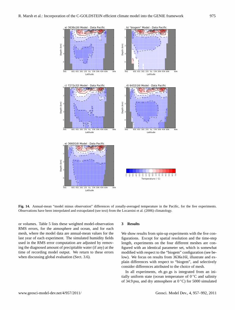
R. Marsh et al.: Incorporation of the C-GOLDSTEIN efficient climate model into the GENIE framework 975
90S 60S 45S 30S 15S Eq 15N 30N 45N 60N 90N
Latitude
5
4
3
2
1
0
Depth
(km
)
-2.5
-2.5
-2.5
-1.5
-0.5
-0.5
0.5
0.5
1.5
1.5
2.53.5
a) 3636s16l Model - Data Pacific
90S 60S 45S 30S 15S Eq 15N 30N 45N 60N 90N
Latitude
5
4
3
2
1
0
Depth
(km
)
-2.5
-1.5-0.5
-0.5
-0.5
0.5
0.5
1.5
1.5
2.5 2.52.5 3.5
b) "biogem" Model - Data Pacific
90S 60S 45S 30S 15S Eq 15N 30N 45N 60N 90N
Latitude
5
4
3
2
1
0
Depth
(km
)
-2.5
-2.5
-2.5
-2.5
-1.5
-1.5
-1.5
-0.5
-0.5
0.5
0.5
1.5
1.5
1.5 2.5
c) 7272s32l Model - Data Pacific
90S 60S 45S 30S 15S Eq 15N 30N 45N 60N 90N
Latitude
5
4
3
2
1
0
Depth
(km
)
-2.5
-2.5
-2.5
-1.5
-0.5 -0.5
-0.5 0.50.5
1.51.5
1.5
2.53.5
d) 6432i16l Model - Data Pacific
90S 60S 45S 30S 15S Eq 15N 30N 45N 60N 90N
Latitude
5
4
3
2
1
0
Depth
(km
)
-2.5
-2.5
-1.5
-0.5
-0.5
0.50.51.5
1.5
2.53.5
e) 3660l16l Model - Data Pacific
-7.5
-6.5
-5.5
-4.5
-3.5
-2.5
-1.5
-0.5
0.5
1.5
2.5
3.5
4.5
5.5
6.5
7.5
Temperature ( ◦ C)
Fig. 14. Annual-mean “model minus observation” differences of zonally-averaged temperature in the Pacific, for the five experiments.Observations have been interpolated and extrapolated (see text) from theLocarnini et al.(2006) climatology.
or volumes. Table5 lists these weighted model-observationRMS errors, for the atmosphere and ocean, and for eachmesh, where the model data are annual-mean values for thelast year of each experiment. The simulated humidity fieldsused in the RMS error computation are adjusted by remov-ing the diagnosed amount of precipitable water (if any) at thetime of recording model output. We return to these errorswhen discussing global evaluation (Sect.3.6).
3 Results
We show results from spin-up experiments with the five con-figurations. Except for spatial resolution and the time-steplength, experiments on the four different meshes are con-figured with an identical parameter set, which is somewhatmodified with respect to the “biogem” configuration (see be-low). We focus on results from 3636s16l, illustrate and ex-plain differences with respect to “biogem”, and selectivelyconsider differences attributed to the choice of mesh.
In all experiments, ebgo gs is integrated from an ini-tially uniform state (ocean temperature of 0◦C and salinityof 34.9 psu, and dry atmosphere at 0◦C) for 5000 simulated
www.geosci-model-dev.net/4/957/2011/ Geosci. Model Dev., 4, 957–992, 2011
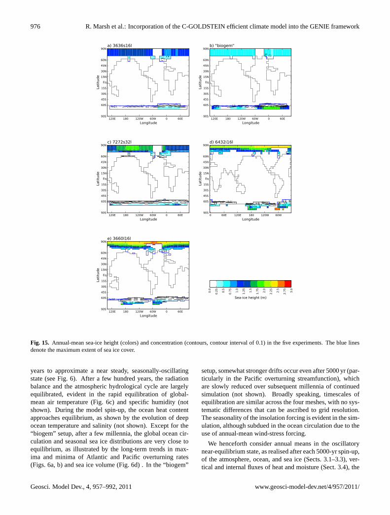
976 R. Marsh et al.: Incorporation of the C-GOLDSTEIN efficient climate model into the GENIE framework
120E 180 120W 60W 0 60E
Longitude
90S
60S
45S
30S
15S
Eq
15N
30N
45N
60N
90N
Lati
tude
0.2 0.2 0.4 0.6
0.6
a) 3636s16l
120E 180 120W 60W 0 60E
Longitude
90S
60S
45S
30S
15S
Eq
15N
30N
45N
60N
90N
Lati
tude
0.20.4 0.4
0.4
0.6 0.60.60.8
b) "biogem"
120E 180 120W 60W 0 60E
Longitude
90S
60S
45S
30S
15S
Eq
15N
30N
45N
60N
90N
Lati
tude
0.2 0.40.6
0.6
0.8
0.8 0.8 0.8
c) 7272s32l
0 60E 120E 180 120W 60W
Longitude
90S
60S
45S
30S
15S
Eq
15N
30N
45N
60N
90N
Lati
tude
0.20.2
0.20.4
0.40.4
0.60.6 0.6
0.80.8
0.80.8
d) 6432i16l
120E 180 120W 60W 0 60E
Longitude
90S
60S
45S
30S
15S
Eq
15N
30N
45N
60N
90N
Lati
tude
0.20.2
0.2
0.2
0.4 0.4
0.4
0.6 0.60.8
0.8
0.8 0.8
e) 3660l16l
0.0
0.2
5
0.5
0.7
5
1.0
1.2
5
1.5
1.7
5
2.0
2.2
5
2.5
2.7
5
3.0
Sea-ice height (m)
Fig. 15. Annual-mean sea-ice height (colors) and concentration (contours, contour interval of 0.1) in the five experiments. The blue linesdenote the maximum extent of sea ice cover.
years to approximate a near steady, seasonally-oscillatingstate (see Fig. 6). After a few hundred years, the radiationbalance and the atmospheric hydrological cycle are largelyequilibrated, evident in the rapid equilibration of global-mean air temperature (Fig.6c) and specific humidity (notshown). During the model spin-up, the ocean heat contentapproaches equilibrium, as shown by the evolution of deepocean temperature and salinity (not shown). Except for the“biogem” setup, after a few millennia, the global ocean cir-culation and seasonal sea ice distributions are very close toequilibrium, as illustrated by the long-term trends in max-ima and minima of Atlantic and Pacific overturning rates(Figs.6a, b) and sea ice volume (Fig.6d) . In the “biogem”
setup, somewhat stronger drifts occur even after 5000 yr (par-ticularly in the Pacific overturning streamfunction), whichare slowly reduced over subsequent millennia of continuedsimulation (not shown). Broadly speaking, timescales ofequilibration are similar across the four meshes, with no sys-tematic differences that can be ascribed to grid resolution.The seasonality of the insolation forcing is evident in the sim-ulation, although subdued in the ocean circulation due to theuse of annual-mean wind-stress forcing.
We henceforth consider annual means in the oscillatorynear-equilibrium state, as realised after each 5000-yr spin-up,of the atmosphere, ocean, and sea ice (Sects.3.1–3.3), ver-tical and internal fluxes of heat and moisture (Sect.3.4), the
Geosci. Model Dev., 4, 957–992, 2011 www.geosci-model-dev.net/4/957/2011/
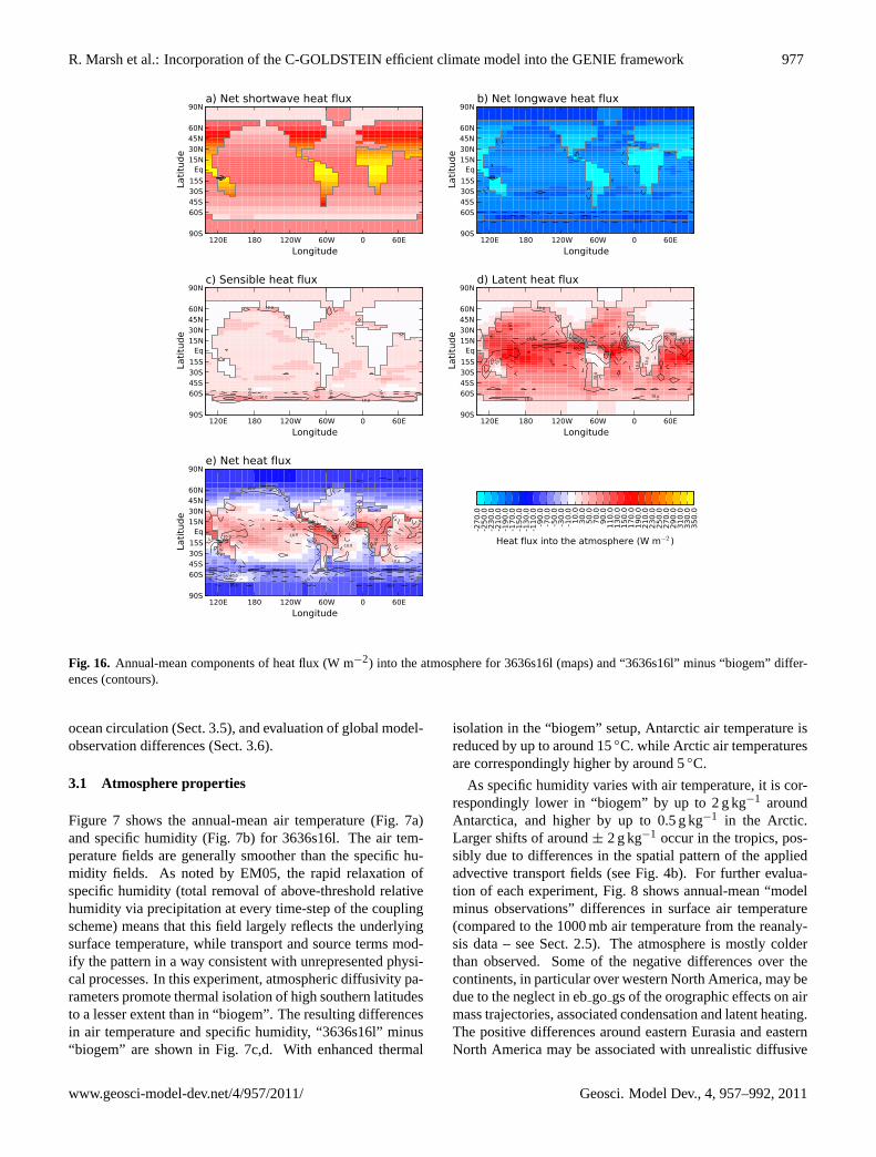
R. Marsh et al.: Incorporation of the C-GOLDSTEIN efficient climate model into the GENIE framework 977
120E 180 120W 60W 0 60E
Longitude
90S
60S45S30S15S
Eq15N30N45N60N
90N
Lati
tude
a) Net shortwave heat flux
120E 180 120W 60W 0 60E
Longitude
90S
60S45S30S15S
Eq15N30N45N60N
90N
Lati
tude
-30.0
-10.0
b) Net longwave heat flux
120E 180 120W 60W 0 60E
Longitude
90S
60S45S30S15S
Eq15N30N45N60N
90N
Lati
tude
-10.0
-10.0
-10.0
10.010.0
10.0
c) Sensible heat flux
120E 180 120W 60W 0 60E
Longitude
90S
60S45S30S15S
Eq15N30N45N60N
90N
Lati
tude
-10.0
-10.0
-10.
0-10.0
10.010.0
10.0
10.0
10.0
10.0
10.0
10.0
10.0
d) Latent heat flux
120E 180 120W 60W 0 60E
Longitude
90S
60S45S30S15S
Eq15N30N45N60N
90N
Lati
tude
-30.0 -30.0
-10.0
-10.0
-10.0
-10.0
-10.0
-10.0
10.0
10.0 10.0 10.0
10.0
10.0
10.0
10.0
10.0
10.0
10.0
10.010.0
e) Net heat flux-2
70.0
-250.0
-230.0
-210.0
-190.0
-170.0
-150.0
-130.0
-110.0
-90.0
-70.0
-50.0
-30.0
-10.0
10.0
30.0
50.0
70.0
90.0
110.0
130.0
150.0
170.0
190.0
210.0
230.0
250.0
270.0
290.0
310.0
330.0
350.0
Heat flux into the atmosphere (W m−2 )
Fig. 16. Annual-mean components of heat flux (W m−2) into the atmosphere for 3636s16l (maps) and “3636s16l” minus “biogem” differ-ences (contours).
ocean circulation (Sect.3.5), and evaluation of global model-observation differences (Sect.3.6).
3.1 Atmosphere properties
Figure 7 shows the annual-mean air temperature (Fig.7a)and specific humidity (Fig.7b) for 3636s16l. The air tem-perature fields are generally smoother than the specific hu-midity fields. As noted by EM05, the rapid relaxation ofspecific humidity (total removal of above-threshold relativehumidity via precipitation at every time-step of the couplingscheme) means that this field largely reflects the underlyingsurface temperature, while transport and source terms mod-ify the pattern in a way consistent with unrepresented physi-cal processes. In this experiment, atmospheric diffusivity pa-rameters promote thermal isolation of high southern latitudesto a lesser extent than in “biogem”. The resulting differencesin air temperature and specific humidity, “3636s16l” minus“biogem” are shown in Fig.7c,d. With enhanced thermal
isolation in the “biogem” setup, Antarctic air temperature isreduced by up to around 15◦C. while Arctic air temperaturesare correspondingly higher by around 5◦C.
As specific humidity varies with air temperature, it is cor-respondingly lower in “biogem” by up to 2 g kg−1 aroundAntarctica, and higher by up to 0.5 g kg−1 in the Arctic.Larger shifts of around± 2 g kg−1 occur in the tropics, pos-sibly due to differences in the spatial pattern of the appliedadvective transport fields (see Fig.4b). For further evalua-tion of each experiment, Fig.8 shows annual-mean “modelminus observations” differences in surface air temperature(compared to the 1000 mb air temperature from the reanaly-sis data – see Sect.2.5). The atmosphere is mostly colderthan observed. Some of the negative differences over thecontinents, in particular over western North America, may bedue to the neglect in ebgo gs of the orographic effects on airmass trajectories, associated condensation and latent heating.The positive differences around eastern Eurasia and easternNorth America may be associated with unrealistic diffusive
www.geosci-model-dev.net/4/957/2011/ Geosci. Model Dev., 4, 957–992, 2011

978 R. Marsh et al.: Incorporation of the C-GOLDSTEIN efficient climate model into the GENIE framework
120E 180 120W 60W 0 60E
Longitude
90S
60S45S30S15S
Eq15N30N45N60N
90N
Lati
tude
10.0 10.010.0
30.0 30.0
a) Net shortwave heat flux
120E 180 120W 60W 0 60E
Longitude
90S
60S45S30S15S
Eq15N30N45N60N
90N
Lati
tude
-10.0 -10.0
10.0
b) Net longwave heat flux
120E 180 120W 60W 0 60E
Longitude
90S
60S45S30S15S
Eq15N30N45N60N
90N
Lati
tude
-30.0 -10.010.0 10.0
10.0
c) Sensible heat flux
120E 180 120W 60W 0 60E
Longitude
90S
60S45S30S15S
Eq15N30N45N60N
90N
Lati
tude
-10.0 -10.0-10.0
-10.0
-10.0
-10.0
-10.0
10.0 10.0
10.0 10.010.0
d) Latent heat flux
120E 180 120W 60W 0 60E
Longitude
90S
60S45S30S15S
Eq15N30N45N60N
90N
Lati
tude
-30.0 -10.0 -10.0-1
0.0
-10.
0
-10.0
-10.0
10.010.0
10.0
10.0 10.010.0
10.010.0
10.010.0
30.0
e) Net heat flux-2
70.0
-250.0
-230.0
-210.0
-190.0
-170.0
-150.0
-130.0
-110.0
-90.0
-70.0
-50.0
-30.0
-10.0
10.0
30.0
50.0
70.0
90.0
110.0
130.0
150.0
170.0
190.0
210.0
230.0
250.0
270.0
290.0
310.0
330.0
350.0
Heat flux into the ocean (W m−2 )
Fig. 17. Annual-mean components of surface heat flux (W m−2) into the ocean for 3636s16l (maps) and “3636s16l” minus “biogem”differences (contours).
transport into the continental interior of heat released over thewarm western boundary currents. The largest negative differ-ences in “biogem” and 3636s16l are a too-cold Antarctica in“biogem” and a too-cold Arctic in 3636s16l, for reasons dis-cussed above. Between the four meshes for which parametersettings are fixed, differences are again relatively invariant.
3.2 Ocean properties
Figure 9 shows the annual-mean sea surface temperature(Fig. 9a), salinity (Fig.9b) and density (Fig.9c), along witha diagnostic of convection averaged over the full spin-up du-ration (Fig. 9d). The latter illustrates localized centres ofdeep convection in the North Atlantic and notably aroundAntarctica. ‘3636s16l minus “biogem” differences of theseproperties and diagnostics are shown in Fig.10. South of55–60◦ S, surface temperatures are mostly lower in “biogem”by up to 1◦C (Fig. 10a), although in many locations in thisregion, sea ice formation restricts minimum temperature to
the freezing point for seawater, and differences are conse-quently small. North of this region, with the exception ofa few locations, temperatures are higher, by up to 3◦C, in“biogem”, consistent with reduced southward heat transport.In 3636s16l, temperature at coastal grid-cells is generally re-duced by around 1–3◦C, most notably in upwelling regionsand this is likely due to the revised wind forcing (see Fig.4c,d). The largest positive surface salinity differences are lo-cated in the Arctic, associated with differences in sea iceand associated freeze/melt fluxes (see Sects.3.3 and 3.4).The largest negative salinity differences are caused by theopening of the ITF in the 3636s16l setup (Fig.10b). The re-duced salinity downstream the ITF corresponds to a negativeanomaly in density in the uppermost ocean layer (Fig.10c).Despite subtle differences in surface density in the South-ern Ocean, there is considerably more convective mixing in3636s16l (Fig.10d). Convection associated with dense wa-ter formation is locally strongest immediately adjacent toAntarctica, on average spanning about 8 depth levels (which,
Geosci. Model Dev., 4, 957–992, 2011 www.geosci-model-dev.net/4/957/2011/
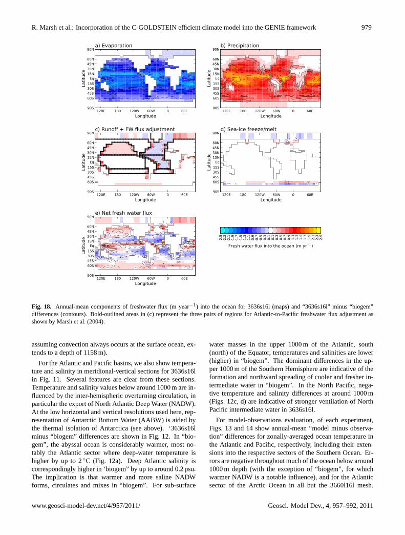
R. Marsh et al.: Incorporation of the C-GOLDSTEIN efficient climate model into the GENIE framework 979
120E 180 120W 60W 0 60E
Longitude
90S
60S45S30S15S
Eq15N30N45N60N
90N
Lati
tude
-0.3-0.1
-0.1
-0.1 -0.1
-0.1
-0.1
0.1
0.10.1 0
.1
0.1
0.10.1
0.1
0.1
0.1
0.1
0.1
0.1
a) Evaporation
120E 180 120W 60W 0 60E
Longitude
90S
60S45S30S15S
Eq15N30N45N60N
90N
Lati
tude
-0.1-0.1
-0.1
-0.1
0.1
0.1
0.1 0.1
0.1
0.10.1
0.1
0.1
0.1
0.1 0.1
0.1
0.1
0.1
0.3
0.3
0.3
b) Precipitation
120E 180 120W 60W 0 60E
Longitude
90S
60S45S30S15S
Eq15N30N45N60N
90N
Lati
tude
-0.1
-0.1
0.1
0.1
0.1
c) Runoff + FW flux adjustment
120E 180 120W 60W 0 60E
Longitude
90S
60S45S30S15S
Eq15N30N45N60N
90N
Lati
tude
-0.10.1
0.1
d) Sea-ice freeze/melt
120E 180 120W 60W 0 60E
Longitude
90S
60S45S30S15S
Eq15N30N45N60N
90N
Lati
tude
-0.3
-0.1-0.1
-0.1-0
.1
-0.1
-0.1
-0.1
-0.1
-0.1
0.1
0.1
0.1
0.10.1 0.1
0.1
0.10.1
0.1
0.1
0.1
0.1
0.1
0.3
0.3
e) Net fresh water flux-2
.5-2
.3-2
.1-1
.9-1
.7-1
.5-1
.3-1
.1-0
.9-0
.7-0
.5-0
.3-0
.10.1
0.3
0.5
0.7
0.9 1.1
1.3
1.5
1.7
1.9
2.1
2.3
2.5
Fresh water flux into the ocean (m yr−1 )
Fig. 18. Annual-mean components of freshwater flux (m year−1) into the ocean for 3636s16l (maps) and “3636s16l” minus “biogem”differences (contours). Bold-outlined areas in (c) represent the three pairs of regions for Atlantic-to-Pacific freshwater flux adjustment asshown byMarsh et al.(2004).
assuming convection always occurs at the surface ocean, ex-tends to a depth of 1158 m).
For the Atlantic and Pacific basins, we also show tempera-ture and salinity in meridional-vertical sections for 3636s16lin Fig. 11. Several features are clear from these sections.Temperature and salinity values below around 1000 m are in-fluenced by the inter-hemispheric overturning circulation, inparticular the export of North Atlantic Deep Water (NADW).At the low horizontal and vertical resolutions used here, rep-resentation of Antarctic Bottom Water (AABW) is aided bythe thermal isolation of Antarctica (see above). ‘3636s16lminus “biogem” differences are shown in Fig.12. In “bio-gem”, the abyssal ocean is considerably warmer, most no-tably the Atlantic sector where deep-water temperature ishigher by up to 2◦C (Fig. 12a). Deep Atlantic salinity iscorrespondingly higher in ‘biogem” by up to around 0.2 psu.The implication is that warmer and more saline NADWforms, circulates and mixes in “biogem”. For sub-surface
water masses in the upper 1000 m of the Atlantic, south(north) of the Equator, temperatures and salinities are lower(higher) in “biogem”. The dominant differences in the up-per 1000 m of the Southern Hemisphere are indicative of theformation and northward spreading of cooler and fresher in-termediate water in “biogem”. In the North Pacific, nega-tive temperature and salinity differences at around 1000 m(Figs.12c, d) are indicative of stronger ventilation of NorthPacific intermediate water in 3636s16l.
For model-observations evaluation, of each experiment,Figs. 13 and14 show annual-mean “model minus observa-tion” differences for zonally-averaged ocean temperature inthe Atlantic and Pacific, respectively, including their exten-sions into the respective sectors of the Southern Ocean. Er-rors are negative throughout much of the ocean below around1000 m depth (with the exception of “biogem”, for whichwarmer NADW is a notable influence), and for the Atlanticsector of the Arctic Ocean in all but the 3660l16l mesh.
www.geosci-model-dev.net/4/957/2011/ Geosci. Model Dev., 4, 957–992, 2011
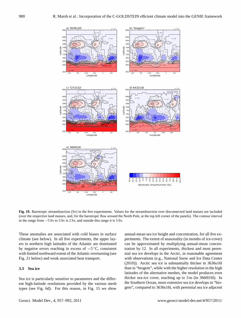
980 R. Marsh et al.: Incorporation of the C-GOLDSTEIN efficient climate model into the GENIE framework
120E 180 120W 60W 0 60E
Longitude
90S
60S
45S
30S
15S
Eq
15N
30N
45N
60N
90N
Lati
tude
Ψ =58.7Ψ
=-7
.9
Ψ =0.2
Ψ =0.2
Ψ =0.0
Ψ =0.2
-15.0 -15.0
-5.0
-5.0
-5.0
5.0
5.0
5.0
15.0
15.0
25.035.045.055.0 65.0
a) 3636s16l
120E 180 120W 60W 0 60E
Longitude
90S
60S
45S
30S
15S
Eq
15N
30N
45N
60N
90N
Lati
tude
Ψ =36.5
Ψ=
0.0
Ψ =0.0
Ψ =0.0
Ψ =0.0
Ψ =0.0
-15.0
-5.0
-5.0
5.0
5.0
5.0
15.0
15.0
25.035.0
b) "biogem"
120E 180 120W 60W 0 60E
Longitude
90S
60S
45S
30S
15S
Eq
15N
30N
45N
60N
90N
Lati
tude
Ψ =86.9
Ψ=
-8.7
Ψ =0.9
Ψ =0.9
Ψ =0.0
Ψ =0.9
-15.0
-15.0
-5.0
-5.0
-5.0 5.0
5.0
5.0
5.0
15.0
15.0
25.0
25.0
35.0 45.055.0
65.075.085.0 95.0
c) 7272s32l
0 60E 120E 180 120W 60W
Longitude
90S
60S
45S
30S
15S
Eq
15N
30N
45N
60N
90N
Lati
tude
Ψ =46.5
Ψ =0.0
Ψ=
-8.1
Ψ =0.7
Ψ =-0.6
Ψ =-0.5
-15.0-15.0
-5.0
-5.0
-5.0
5.0
5.0
5.0
15.0
15.0
25.035.0
45.0
d) 6432i16l
120E 180 120W 60W 0 60E
Longitude
90S
60S
45S
30S
15S
Eq
15N
30N
45N
60N
90N
Lati
tude
Ψ =58.1
Ψ=
-10
.1
Ψ =2.3
Ψ =1.4
Ψ =0.0
Ψ =0.6
-15.0-15.0
-5.0
-5.0
-5.0
5.0
5.0
5.0
15.0
15.0
25.0
35.045.055.0 65.0
e) 3660l16l
-45
.0
-35
.0
-25
.0
-15
.0
-5.0
5.0
15
.0
25
.0
35
.0
45
.0
55
.0
65
.0
75
.0
85
.0
95
.0
10
5.0
Barotropic streamfunction (Sv)
Fig. 19. Barotropic streamfunction (Sv) in the five experiments. Values for the streamfunction over disconnected land masses are included(over the respective land masses, and, for the barotropic flow around the North Pole, at the top left corner of the panels). The contour intervalin the range from−5 Sv to 5 Sv is 2 Sv, and outside this range it is 5 Sv.
These anomalies are associated with cold biases in surfaceclimate (see below). In all five experiments, the upper lay-ers in northern high latitudes of the Atlantic are dominatedby negative errors reaching in excess of−5◦C, consistentwith limited northward extent of the Atlantic overturning (seeFig. 21below) and weak associated heat transport.
3.3 Sea ice
Sea ice is particularly sensitive to parameters and the differ-ent high-latitude resolutions provided by the various meshtypes (see Fig.6d). For this reason, in Fig.15 we show
annual-mean sea ice height and concentration, for all five ex-periments. The extent of seasonality (in months of ice-cover)can be approximated by multiplying annual-mean concen-tration by 12. In all experiments, thickest and most peren-nial sea ice develops in the Arctic, in reasonable agreementwith observations (e.g.,National Snow and Ice Data Center(2010)). Arctic sea ice is substantially thicker in 3636s16lthan in “biogem”, while with the higher resolution in the highlatitudes of the alternative meshes, the model produces eventhicker sea-ice cover, reaching up to 3 m (in 3660l16l). Inthe Southern Ocean, more extensive sea ice develops in “bio-gem”, compared to 3636s16l, with perennial sea ice adjacent
Geosci. Model Dev., 4, 957–992, 2011 www.geosci-model-dev.net/4/957/2011/

R. Marsh et al.: Incorporation of the C-GOLDSTEIN efficient climate model into the GENIE framework 981
90S 60S 45S 30S 15S Eq 15N 30N 45N 60N 90N
Latitude
5
4
3
2
1
Depth
(km
)
-6.0
-6.0
-5.0
-5.0
-4.0
-4.0
-3.0
-3.0 -2.0
-1.0
0.0
1.0
2.0
3.0
4.0
5.0
6.07.0 8.0
9.0
9.0
10.0 11.0
12.0
-5.0
-5.0
0.0
5.0
10.0
15.0
20.0 25.0
30.0
35.0
40.0
-25.0
-20.
0-1
5.0
-10.0
-5.0
-5.0
0.0
5.0
10.0
15.0
20.025.0
a) 3636s16l
90S 60S 45S 30S 15S Eq 15N 30N 45N 60N 90N
Latitude
5
4
3
2
1
Depth
(km
)
-7.0
-6.0
-6.0
-5.0
-4.0
-3.0
-2.0
-1.0
0.0
0.0
1.0
2.0
3.0
4.0
5.0
6.07.0
8.0
9.0
10.0
11.0
12.0
13.0
-5.0
0.0
5.0
10.0
15.0
20.025.0
-20.0
-15.
0-1
0.0
-5.0
0.0
5.0
10.0
15.020.025.0
b) "biogem"
90S 60S 45S 30S 15S Eq 15N 30N 45N 60N 90N
Latitude
5
4
3
2
1
Depth
(km
)
-4.0
-3.0
-2.0
-2.0
-1.0
-1.0
0.0
0.0
0.0
1.0
1.0
2.0 3.0
4.0
5.0
6.0
7.0
8.0
9.0 10.0
11.012.0
-5.0
0.0
0.05.0
10.0
15.0
20.025.0
30.0
35.040.0
45.0 -35.0-30.0
-25.0-20.0-15.0-10.0
-5.0
-5.00.00.0
5.0
10.015.020.025.0
30.035.0
c) 7272s32l
90S 60S 45S 30S 15S Eq 15N 30N 45N 60N 90N
Latitude
5
4
3
2
1
Depth
(km
)
-4.0
-3.0
-3.0
-2.0
-2.0
-2.0
-1.0
-1.0
0.0
0.0
0.0
1.0
2.0
3.0
4.0
5.0
6.0
7.08.0 9.0
9.0
10.0
11.0
12.0
-5.0
-5.0
0.0
5.0
10.0
15.020
.0
25.0
30.0
35.040.0-15.0
-10.0
-5.0
-5.0
0.0 0.0
5.010.015.0
20.0
d) 6432i16l
90S 60S 45S 30S 15S Eq 15N 30N 45N 60N 90N
Latitude
5
4
3
2
1
Depth
(km
)
-5.0-4.0-3
.0
-3.0
-3.0
-2.0
-2.0
-2.0
-2.0
-1.0
-1.0 -1
.0
0.0
0.0 0
.0
0.0
1.0
2.0 3.0
4.05.
06.
0
7.0
8.0
9.0
10.0
10.0
11.0
12.0
13.014.0
-10.0
-5.0
0.0
5.0
10.0
15.0
20.0
25.0
30.0 35.0
40.0-2
5.0
-20.
0-1
5.0
-10.0
-5.0
-5.0
0.00.0
5.0
10.0
15.0
20.0
25.0
e) 3660l16l
-63
.0-5
7.0
-51
.0-4
5.0
-39
.0-3
3.0
-27
.0-2
1.0
-15
.0-9
.0-3
.03
.09
.01
5.0
21
.02
7.0
33
.03
9.0
45
.05
1.0
57
.06
3.0
Overturning streamfunction (Sv)
Fig. 20. Global meridional overturning streamfunctions (Sv) in the five experiments. Contour interval below around 500 m depth and northof 30◦S is 1 Sv, outside this region 5 Sv.
to Antarctica (albeit very little) only in the former experi-ment (see Fig.6d). This is attributed to the larger reductionof atmospheric heat diffusivity in the former experiment. Seaice in both hemispheres is broadly similar in 3636s16l and7272s32l (Fig.15a, c). More realistic sea ice distribution(in particular around Antarctica) is obtained with the higherpolar resolution in 6432i16l and 3660l16l (Fig.15d, e), bycomparison with observations. The reasons for differencesbetween meshes may not be directly related to spatial res-olution, but may rather be due to feedbacks involving theatmosphere and the ocean.
3.4 Vertical and internal fluxes of heat and moisture
For 3636s16l only, Figs.16–18 show annual-mean verticaland internal components of heat and freshwater flux, for bothatmosphere and ocean. While these year-5000 annual meansmay be subject to slight inter-annual variability, they are stillrepresentative for typical flux fields of the near-equilibriumstate at the end of the simulations.
The short-wave heat flux into the atmosphere (Fig.16a)declines polewards due to the angle of incidence of insolation(accounting for orbital parameters), and is further reducedwith latitude by planetary albedo (see Fig. 5e). Further de-markation at land-sea boundaries, with stronger fluxes over
www.geosci-model-dev.net/4/957/2011/ Geosci. Model Dev., 4, 957–992, 2011
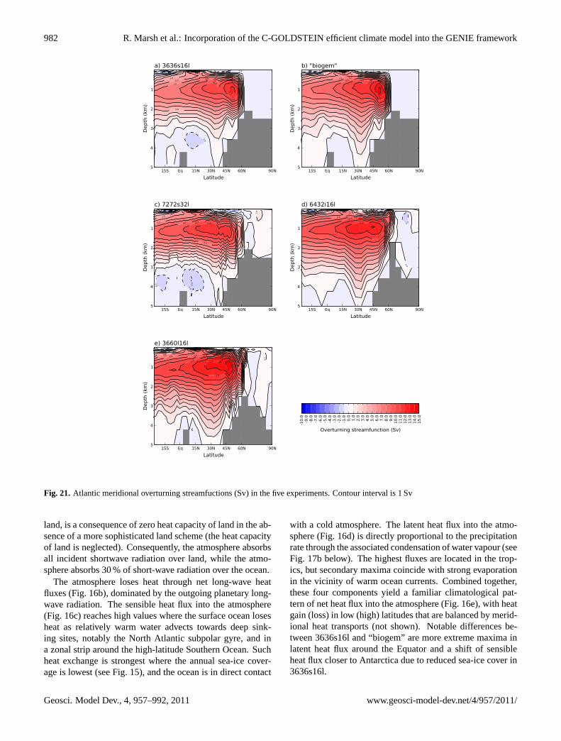
982 R. Marsh et al.: Incorporation of the C-GOLDSTEIN efficient climate model into the GENIE framework
15S Eq 15N 30N 45N 60N 90N
Latitude
5
4
3
2
1
Depth
(km
)
-2.0
-1.0 -1.0
-1.0
0.0
0.0
1.0 2.03.0
4.0
5.0
6.0
7.0
7.0
8.0
8.0 9.010.0
11.0
12.0
a) 3636s16l
15S Eq 15N 30N 45N 60N 90N
Latitude
5
4
3
2
1
Depth
(km
)
-1.0
0.0
1.02.0 3.04.0 5.06.0
7.0
7.0
8.0
8.0
9.0
9.0 10.0
11.0
12.013.0
b) "biogem"
15S Eq 15N 30N 45N 60N 90N
Latitude
5
4
3
2
1
Depth
(km
)
-5.0-4.0-3.0-3.0-2.0
-2.0
-2.0
-1.0 -1.0
-1.0
-1.0
0.0
0.0
1.0
1.0
2.0
3.04.0
5.0
6.0
7.0
8.0
8.0
9.0
9.0
10.0
10.0
11.0
11.0
c) 7272s32l
15S Eq 15N 30N 45N 60N 90N
Latitude
5
4
3
2
1
Depth
(km
)
-1.0
-1.00
.0
0.0
1.02.03.04.05.0
6.07.08.0
8.0 9.010.0
11.0
12.0
d) 6432i16l
15S Eq 15N 30N 45N 60N 90N
Latitude
5
4
3
2
1
Depth
(km
)
0.0
1.0
1.0
2.0
3.04.0 5.0
6.07.0 8.0
9.0
9.0 10.0
10.0
11.0
12.0
13.0
14.0
e) 3660l16l
-10
.0-9
.0-8
.0-7
.0-6
.0-5
.0-4
.0-3
.0-2
.0-1
.00
.01
.02
.03
.04
.05
.06
.07
.08
.09
.01
0.0
11
.01
2.0
13
.01
4.0
15
.0
Overturning streamfunction (Sv)
Fig. 21. Atlantic meridional overturning streamfuctions (Sv) in the five experiments. Contour interval is 1 Sv
land, is a consequence of zero heat capacity of land in the ab-sence of a more sophisticated land scheme (the heat capacityof land is neglected). Consequently, the atmosphere absorbsall incident shortwave radiation over land, while the atmo-sphere absorbs 30 % of short-wave radiation over the ocean.
The atmosphere loses heat through net long-wave heatfluxes (Fig.16b), dominated by the outgoing planetary long-wave radiation. The sensible heat flux into the atmosphere(Fig. 16c) reaches high values where the surface ocean losesheat as relatively warm water advects towards deep sink-ing sites, notably the North Atlantic subpolar gyre, and ina zonal strip around the high-latitude Southern Ocean. Suchheat exchange is strongest where the annual sea-ice cover-age is lowest (see Fig.15), and the ocean is in direct contact
with a cold atmosphere. The latent heat flux into the atmo-sphere (Fig.16d) is directly proportional to the precipitationrate through the associated condensation of water vapour (seeFig. 17b below). The highest fluxes are located in the trop-ics, but secondary maxima coincide with strong evaporationin the vicinity of warm ocean currents. Combined together,these four components yield a familiar climatological pat-tern of net heat flux into the atmosphere (Fig.16e), with heatgain (loss) in low (high) latitudes that are balanced by merid-ional heat transports (not shown). Notable differences be-tween 3636s16l and “biogem” are more extreme maxima inlatent heat flux around the Equator and a shift of sensibleheat flux closer to Antarctica due to reduced sea-ice cover in3636s16l.
Geosci. Model Dev., 4, 957–992, 2011 www.geosci-model-dev.net/4/957/2011/

R. Marsh et al.: Incorporation of the C-GOLDSTEIN efficient climate model into the GENIE framework 983
Table 1. Mesh-specific files required for the ebgo gs experiments shown:<world > is “wv3jh2” for 3636s16l, “worjh2” for “biogem”,“w32jh2” for 7272s32l, “igcm16” for 6432i16l, and “3660l2” for 3660l16l; filenames with the prefix “+” are read in by all configurationsbut are only actively used when the run-time interpolation of wind forcing fields is not enabled (herein only by configuration “biogem”); theprefix “*” denotes files not required for “biogem”; the prefix “%” denotes alternative fields used for the error estimation.
File Purpose Source Read by
Bathymetry, land-sea mask, runoff direction, islands
<world >.k1 Land-sea mask, bathymetry (in model levels),runoff directions
Based on ETOPO05 (National Geophysical Data Center,1988) or ETOPO02v2 (U. S. Department of Commerceand Atmospheric Administration), modified (see descrip-tion in Sect.2.3)
“eb”,“go,“gs”
<world >.psiles Land-sea mask and island index for barotropicstreamfunction
Derived from<world>.k1 “go”
<world >.paths Island boundary data for barotropic streamfunc-tion
Derived from<world>.k1 “go”
* <world >.bmask Optional basin mask definition (Atlantic, Pacific,Southern Ocean)
Derived from<world>.k1 “go”
Wind forcing
+uncep.silo Zonal moisture advection field NCEP/NCAR reanalysis “eb”
+vncep.silo Meridional moisture advection field NCEP/NCAR reanalysis “eb”
+taux u.interp Ocean wind-stress component SOC climatology (Josey et al., 1998) “eb”
+taux v.interp Ocean wind-stress component SOC climatology (Josey et al., 1998) “eb”
+tauy u.interp Ocean wind-stress component SOC climatology (Josey et al., 1998) “eb”
+tauy v.interp Ocean wind-stress component SOC climatology (Josey et al., 1998) “eb”
* NCEP-DOEReanalysis2 ltaa 1000 mbwind speed.nc
Zonal and meridional 1000 mb wind speed fieldsNCEP-DOE Reanalysis 2 “eb”
* NCEP-DOEReanalysis2 ltaa windstress.nc
Zonal and meridional momentum flux into the at-mosphere (negative wind stress)
NCEP/DOE Reanalysis 2 (Kanamitsu et al., 2002) “eb”
Model-data error computation
%NCEP-DOEReanalysis2 ltaa 1000 mb T r.nc
Observational 1000 mb air temperature and rela-tive humidity fields
NCEP/DOE Reanalysis 2 (Kanamitsu et al., 2002) “eb”
%NCEP-DOEReanalysis2 ltaa surface T q.nc
Observational 10 m air temperature and specifichumidity fields
NCEP/DOE Reanalysis 2 (Kanamitsu et al., 2002) “eb”
WOA05an TS.nc Observational ocean temperature (in situ) andsalinity fields
World Ocean Atlas 2005 (Locarnini et al., 2006; Antonovet al., 2006)
“go”
The short-wave heat flux into the ocean (Fig.17a) is a con-stant 70 % of net shortwave radiation at the top of the atmo-sphere (30 % being absorbed in the overlying atmosphere)over most of the ocean surface. Varying with latitude asthe atmospheric counterpart, short-wave heat flux into theocean is further reduced at high latitudes due to the higheralbedo associated with sea ice. The net long-wave heat flux(Fig. 17b) is small relative to the atmospheric counterpart,representing the balance of re-radiated long-wave heat fluxesby the ocean (upward) and the atmosphere (downward). Thesensible heat flux into the ocean (Fig.17c), negative every-where, is identical and opposite to the counterpart flux intothe atmosphere (over the ice-free ocean). The latent heat fluxinto the ocean (Fig.17d), again negative everywhere, mirrorsthe pattern of evaporation (see Fig.18a below). Combined
together (Fig.17e), these four components yield a pattern ofnet heat flux into the ocean at low latitudes, with strong lo-calized heat loss over western boundary currents and at sitesof high latitude convection (see Fig.9d), again balanced bymeridional heat transport (not shown). The largest differ-ences between the net surface heat fluxes in 3636s16l and“biogem” are found around Antarctica, associated with re-duced sea-ice extent in 3636s16l.
Evaporation is equivalently a negative freshwater flux intothe ocean (Fig.18a), with largest absolute values over thesubtropical gyres. Precipitation (Fig.18b) to an extent co-incides with strong evaporation. As is typical of low com-plexity atmospheric models such as the EMBM, precipitationover land is poorly represented, even with moisture advectionby specified winds. Substantial areas of continental interior
www.geosci-model-dev.net/4/957/2011/ Geosci. Model Dev., 4, 957–992, 2011

984 R. Marsh et al.: Incorporation of the C-GOLDSTEIN efficient climate model into the GENIE framework
Table 2. Input/output fields to/from the individual modules. Note, while for ebgo gs configurations (as for C-GOLDSTEIN, see EM05),we define neither land temperature nor standing water on land, differences between air and land temperatures, as well as land moisture, areimportant coupling quantities when other land options are used, and so are made available when ebgo gs is coupled to the land surfacescheme (“ENTS”) ofWilliamson et al.(2006). Also, when the atmospheric chemistry module (“ATCHEM”) is included, further input to theatmosphere include greenhouse gas concentrations. When the ocean module is coupled to the ocean biogeochemistry module (“BIOGEM”)a range of fields from the three modules are made available to BIOGEM, including a number of passive oceanic tracers which are subjectedto ocean transport and are modified by BIOGEM.
Field “eb” “go” “gs” “genie-wind”
surface air temperature (◦C) out in in
specific humidity (g kg−1) out in in
prescribed, fixed wind speed (N m−2) (zonalcomponent on ‘u’ grid, meridional compo-nent on ‘v’ grid)
out in out (if selected, supersedesoutput from the EMBM)
prescribed, fixed wind stress (m s−1) (zonaland meridional components on both ‘u’ and‘v’ grids)
out in out (if selected, supersedesoutput from the EMBM)
shortwave radiation (W m−2) out in
sea-surface temperature (◦C) in out in
sea-surface salinity (◦C) in out in
surface ocean current (non-dimensionalised,both zonal and meridional components)
out in
sea-ice fraction in out
sea-ice temperature (◦C) in out
sea-ice thickness (m) in out
sea-ice temperature (◦C) in out
are too arid. This is a serious problem if coupling with mod-els of vegetation and the terrestrial carbon cycle. For thisreason, the EMBM is necessarily enhanced in the case ofsuch coupling (see Sect. 2.1.2), as outlined in Williamsonet al. (2006), but such enhancement requires coupling withthe land scheme – an elaboration on the ebgo gs config-urations that are documented here. The precipitation thatdoes fall over continents instantaneously reaches the oceanas runoff (shown in combination with the Atlantic-to-Pacificfreshwater flux adjustment in Fig.18c). The consequenceof seasonal freezing and melting of sea ice is a net freshwa-ter flux that effectively removes freshwater in regions of seaice formation and adds freshwater in regions of sea ice melt(Fig. 18d). Combined together (Fig.18e), these four compo-nents yield net freshwater gain at low and middle latitudes,with net freshwater loss in the subtropics. Locally, strongestnet freshwater gain is associated with major rivers. In com-parision with “biogem”, the most prominent differences infreshwater input to the ocean are due to enhanced precipita-tion in the tropics in 3636s16l and consequent higher runoffat low latitudes. The enhanced precipitation is in turn asso-
ciated with warmer low-latitude climate in biogem (comparemodel-data differences in Fig.8a, b).
3.5 Ocean circulation
Figure 19 shows the barotropic streamfunction for each ofthe five experiments and Table4 lists the transport strengthsthrough selected straits between isolated land masses. Thehorizontal circulation is dominated by the circumpolar flow,which is sensitive to wind and buoyancy forcing, in combina-tion with friction. Barotropic flow around disconnected landmasses is computed following the evaluation of closed-pathintegrals around the islands, individually specified for eachof the five configurations (see Fig.1). While in the analyt-ical limit of the integration, the barotropic values over theislands are independent of the exact location of these paths,truncation errors due to the discretisation of the integral areintroduced. A multiplicity of potential paths exists for thediscretised model geographies, and so the realised steady-state solution depends on the choice of the path. For thestrength of circumpolar flow, we obtain a range of values byspecifying the path integral around Antarctica for different
Geosci. Model Dev., 4, 957–992, 2011 www.geosci-model-dev.net/4/957/2011/
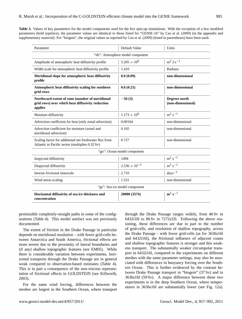
R. Marsh et al.: Incorporation of the C-GOLDSTEIN efficient climate model into the GENIE framework 985
Table 3. Values of key parameters for the model components used for the five spin-up simulations. With the exception of a few modifiedparameters (bold typeface), the parameter values are identical to those listed for “GENIE-16” byCao et al.(2009) (in the appendix andsupplementary material). For “biogem”, the original values as reported byCao et al.(2009) (listed in parentheses) have been used.
Parameter Default Value Units
“eb”: Atmosphere model component
Amplitude of atmospheric heat diffusivity profile 5.205× 10⁶ m2 2 s−1
Width scale for atmospheric heat diffusivity profile 1.410 Radians
Meridional slope for atmospheric heat diffusivityprofile
0.0 (0.09) non-dimensional
Atmospheric heat diffusivity scaling for southerngrid-rows
0.6 (0.25) non-dimensional
Northward extent of zone (number of meridionalgrid rows) over which heat diffusivity reductionapplies
−56 (3) Degrees north(non-dimensional)
Moisture diffusivity 1.173× 10⁶ m2 s−1
Advection coefficient for heat (only zonal advection) 0.00104 non-dimensional
Advection coefficient for moisture (zonal andmeridional advection)
0.165 non-dimensional
Scaling factor for additional net freshwater flux fromAtlantic to Pacific sector (multiplies 0.32 Sv)
0.727 non-dimensional
“go”: Ocean model component
Isopycnal diffusivity 1494 m2 s−1
Diapycnal diffusivity 2.536× 10⁻⁵ m2 s−1
Inverse frictional timescale 2.710 days−1
Wind stress scaling 1.531 non-dimensional
“gs”: Sea ice model component
Horizontal diffusivity of sea ice thickness andconcentration
20000 (3574) m2 s−1
permissible completely-straight paths in some of the config-urations (Table4). This model artefact was not previouslydocumented.
The extent of friction in the Drake Passage in particulardepends on meridional resolution – with fewer grid-cells be-tween Antarctica and South America, frictional effects aremore severe due to the proximity of lateral boundaries and(if any) shallow topographic features (see EM05). Whilethere is considerable variation between experiments, hori-zontal transports through the Drake Passage are in generalweak compared to observation-based estimates (Table4).This is in part a consequence of the non-viscous represen-tation of frictional effects in GOLDSTEIN (seeKillworth ,2003).
For the same wind forcing, differences between themeshes are largest in the Southern Ocean, where transport
through the Drake Passage ranges widely, from 46 Sv in6432i16l to 86 Sv in 7272s32l. Following the above rea-soning, these differences are due in part to the numberof grid-cells, and resolution of shallow topography, acrossthe Drake Passage - with fewer grid-cells (as for 3636s16land 6432i16l), the frictional influence of adjacent coastsand shallow topographic features is stronger and this weak-ens transport. The substantially weaker circumpolar trans-port in 6432i16l, compared to the experiments on differentmeshes with the same parameter settings, may also be asso-ciated with differences in buoyancy forcing over the South-ern Ocean. This is further evidenced by the contrast be-tween Drake Passage transport in “biogem” (37 Sv) and in3636s16l (59 Sv). A major difference between these twoexperiments is in the deep Southern Ocean, where temper-atures in 3636s16l are substantially lower (see Fig.12a).
www.geosci-model-dev.net/4/957/2011/ Geosci. Model Dev., 4, 957–992, 2011

986 R. Marsh et al.: Incorporation of the C-GOLDSTEIN efficient climate model into the GENIE framework
Table 4. Annual-mean net transport through straits (positive transport is directed northward or westward) simulated by the five configurationsand data-based estimates. The last row lists the net transport through the Drake Passage simulated with configurations where the location forthe path integral around Antarctica was varied among all permissible straight paths (the value in parentheses indicates the grid row for thispath on the respective mesh).
3636s16l “biogem” 7272s32l 6432i16l 3660l16l Data-based estimates
Drake Passage 58.9 Sv 36.7 Sv 86.1 Sv 45.8 Sv 55.9 Sv 140± 6 Sv(Ganachaud and Wunsch,2000)
IndonesianThroughflow
−7.9 Sv (closed) −8.8 Sv −7.9 Sv −10.1 Sv Total:−16± 5 Sv(Ganachaud and Wunsch,2000)
Makassar Strait only:−9.3± 2.5 Sv(Nov 1996− Jul 1998)(Gordon et al., 1999);−11.6± 3.3 Sv(Jan 2004 – Nov 2006)(Gordon et al., 2008)
Bering Strait 0.2 Sv (diffusive ex-change only)
0.9 Sv 0.7 Sv 2.3 Sv 0.83± 0.25 Sv(Roach et al., 1995)
Davis Strait (diffusive and baroclinic only) −1.4 Sv −0.8 Sv −2.3± 0.7 Sv(2004–2005)(Curry et al., 2011)
North circumpo-lar
(closed) −0.1 Sv 0.8 Sv
Alternative locations for the path integral around Antarctica
Drake Passage 58.9 Sv(3)
57.8 Sv(4)
36.7 Sv(3)
39.8 Sv(4)
86.1 Sv(5)
75.5 Sv(6)
80.9 Sv(7)
82.5 Sv(8)
45.8 Sv(5)
37.5 Sv(6)
63.3 Sv(7)
55.9 Sv(10)
55.0 Sv(11)
56.3 Sv(12)
80.9 Sv(13)
With relatively smaller corresponding salinity differences,deep waters adjacent to Antarctica are consequently denser,isopycnals slope more steeply upwards across the SouthernOcean, and a substantially stronger circumpolar current issupported by the lateral pressure gradient.
Table4 lists net volume transport along pathways into andout of, as well as within, the Arctic Ocean, which are facil-itated in the grids with higher resolution in this area. Netflow through the Bering Strait is into the Arctic Ocean andranges from 0.2 to 2.3 Sv across the four mesh variants withidentical wind forcing, bracketing the data-based estimateof Roach et al.(1995). In 3636s16l and 7272s32l, this isbalanced by simulated outflow of Arctic waters across theGreenland, Iceland, and Norwegian (GIN) Seas (contrary todata-based estimates which, if assumed not to have changedsubstantially between the respective dates of their measure-ments, suggest net inflow across this section (Roach et al.,1995; Curry et al., 2011)). The 3660l16l simulation featuresnet outflow across the GIN Sea, partially offset by outflowthrough the Davis Strait. Net transport through the DavisStrait in the 6432i16l setup exceeds the net inflow through
the Bering Strait, and consequently must be balanced by netinflow across the GIN Seas. Enhanced spatial resolution inthe region of the GIN Seas seems to facilitate the develop-ment of cyclonic circulation in the high-latitude northern At-lantic and its northward extension representing the recircula-tion of Atlantic waters across the Barents Sea and along theEast Greenland Current, which is best expressed in 6432i16l(Fig. 19d). Simulated ITF strength is within, or slightly be-low, the data-based estimates for the transport along Makas-sar Strait (Gordon et al., 1999, 2008), but systematically be-low the estimate ofGanachaud and Wunsch(2000) for thetotal transport across the Indonesian Archipelago.
In Sect.3.2, we showed that there are large differencesin deep and bottom water properties, attributed to differ-ences in deep water formation at high latitudes in the North-ern and Southern Hemispheres. As the overturning circu-lation is in general sensitive to the resolution at high lat-itudes, in Figs.20 and 21 we show annual-mean merid-ional overturning streamfuctions (for the global ocean andthe Atlantic, respectively) for all five experiments. Substan-tial differences are apparent in both hemispheres, notably in
Geosci. Model Dev., 4, 957–992, 2011 www.geosci-model-dev.net/4/957/2011/

R. Marsh et al.: Incorporation of the C-GOLDSTEIN efficient climate model into the GENIE framework 987
Table 5. Weighted and unweighted root mean square errors, for the atmosphere and ocean, for each experiment. Annual-mean observationsare gridded onto each mesh (see Table1 and Sect.3.6 for the sources of the datasets and further details). The computation of the sums overindividual grid points follows the method of EM05, the integrals over the respective model domain additionally weights the individual gridpoints according to the volume or area of the corresponding grid box or cell. Note that an error value of 1 would be achieved by hypotheticalmodel output of a uniform field with the same average value as the data-based field.
Experiment 3636s16l “biogem” 3660l16l 7272s32l 6432i16l
Sums over individual grid points
RMS Error (Ocean temperature) 0.328 0.322 0.352 0.312 0.339RMS Error (Sea-surface temperature) 0.242 0.270 0.200 0.233 0.195RMS Error (Ocean salinity) 0.701 0.687 0.759 0.720 0.750RMS Error (Sea-surface salinity) 0.675 0.682 0.852 0.717 0.858RMS Error (Atm. temperature (10 m)) 0.361 0.350 0.305 0.351 0.311RMS Error (Atm. temperature (1000 mb)) 0.354 0.459 0.363 0.364 0.336RMS Error (Atm. specific humidity (10 m)) 0.455 0.429 0.361 0.444 0.365RMS Error (Atm. relative humidity (1000 mb)) 1.211 1.232 1.119 1.211 1.124
Integral over domain of model component
RMS Error (Ocean temperature) 0.461 0.394 0.501 0.439 0.482RMS Error (Sea-surface temperature) 0.242 0.270 0.238 0.233 0.234RMS Error (Ocean salinity) 0.792 0.806 0.779 0.808 0.777RMS Error (Sea-surface salinity) 0.675 0.682 0.812 0.717 0.775RMS Error (Atm. temperature (10 m)) 0.361 0.350 0.351 0.351 0.353RMS Error (Atm. temperature (1000 mb)) 0.354 0.459 0.364 0.364 0.358RMS Error (Atm. specific humidity (10 m)) 0.455 0.429 0.453 0.444 0.453RMS Error (Atm. relative humidity (1000 mb)) 1.211 1.232 1.175 1.211 1.182
the Southern Ocean, although the Atlantic overturning is in“Conveyor” mode for each experiment. This is facilitatedby the specification of an explicit additional Atlantic-Pacificmoisture flux, effectively a flux correction (default value0.727× 0.32 Sv = 0.23 Sv – unmodified from the value usedin “biogem”). Without this additional flux, the typical pat-tern of Atlantic overturning does not develop, in all con-figurations. In the Pacific, the overturning streamfunction(not shown) is characterized by the northward import and up-welling of deep water. For the five configurations, annually-averaged Atlantic overturning reaches 11–15 Sv. A cleardifference between experiments is the presence or absenceof an AABW cell in the Atlantic sector (anti-clockwiseoverturning as shown by negative values below 3000 m inFig.21): absent in “biogem”, 6432i16l and 3660l16l; presentin 3636s16l and 7272s32l. This abyssal cell is sensitive todifferences in deep-water density, in turn dependent on pro-cesses at North Atlantic and Southern Ocean deep water for-mation sites.
3.6 Global evaluation
The global errors listed in Table 5 indicate relatively littlevariation, across the four experiments using the “default” pa-rameter set, in the different measures of RMS error, indicat-ing that global-mean quantities are relatively insensitive tothe choice of mesh, given the identical parameter settings.
The most notable differences are a better simulation of rel-ative humidity in the atmosphere and a worse sea-surfacesalinity distribution in 3660l16l and 6432i16l, respectively.Differences in errors between the “biogem” setup and thesimulations with the “default” parameter set are slightly moresubstantial, largest difference being found for the air temper-ature field. When the dimensions of the grid cell areas (orvolumes) representing the model points are taken into ac-count, the different emphasis on spatial resolution for thedifferent meshes can be seen in the RMS errors. Sea-surfacetemperature, for example, is closer to observations with en-hanced resolution in the high latitudes, while sea-surfacesalinity is more realistic in the simulations with enhancedlatitudinal resolution in the lower latitudes. These errors arepresented here to illustrate how different versions of GENIEmay be systematically co-evaluated with a new model op-tion. However, since no attempt has been made here to tunekey parameters for each of the new meshes, the correspond-ing simulations cannot be adequately evaluated on the basisof the errors listed in Table5.
4 Summary and discussion
We have described the basic climate model, “eggo gs”,that is facilitated by the GENIE framework. While someof the model description is retrospective and can be found
www.geosci-model-dev.net/4/957/2011/ Geosci. Model Dev., 4, 957–992, 2011

988 R. Marsh et al.: Incorporation of the C-GOLDSTEIN efficient climate model into the GENIE framework
elsewhere (Edwards and Marsh, 2005; Lenton et al., 2006,2007), we describe a series of improvements and documenta version tagged as “rel-2-7-4” (which remains applicablein the more recent model release version 2.7.7, tagged as“rel-2-7-7”). Earlier versions of “GENIE-1”, such as inRidgwell et al.(2007a) and (Lenton et al., 2006), includedC-GOLDSTEIN (Edwards and Marsh, 2005) as the phys-ical core, a model code structurally different from GENIEand correspondingly inflexible. Furthermore, in more recentstudies with “eggo gs” (e.g., (Lenton et al., 2007)), we used8 levels in the ocean on low-resolution meshes. We now usea minimum of 16 levels, and along with some refinementsin ocean physics, comparison of key diagnostics indicatesthat the ocean circulation is substantially improved. For ex-ample, we can now simulate an abyssal cell in the Atlanticsector (see Fig.21a,c in the present mansucript), previouslyabsent (see Fig. 4a, c in Lenton et al., 2007). In summary, wehave presented several new options, to illustrate the poten-tial wider use of GENIE, namely the choice of four standardmeshes, and two sets of wind forcing climatologies, alongwith a standard means for model evaluation with observa-tions.
While the resulting models show generally similar climateand ocean states, it is clear that both the choice of mesh,and corresponding resolution, as well as the choice of windforcing climatologies, have a significant effect on some ofthe results. While these dependencies complicate interpreta-tion, there is no reason to suppose that they are peculiar toGENIE. Using the default 3636s16l mesh for ensembles inwhich we sample wide ranges of uncertainty in key param-eters (to be reported in a subsequent paper), our experienceis that selected outputs (e.g., meridional overturning and heattransports) vary more widely than between the mesh variantsintroduced here. However, certain diagnostics (e.g., sea ice)and localized ocean circulation are more sensitive to changesin resolution, wind forcing, or strait flows, than to key pa-rameters.
While grid resolution influences model behaviour, bothglobally and regionally, it also determines computational ef-ficiency. For example, the computational cost of a givenlength integration using the 3636s16l mesh is significantlyless than with the 6432i16l mesh, due to the different num-ber of ocean grid cells, even though resolution in latitude isactually higher close to the Equator in the former. How-ever, the advantage of better meridional resolution towardsthe poles, with the 6432i- and 3660l-type meshes, is thatgeostrophic circumpolar flow in the Arctic can be repre-sented. This would also be possible in principle at 7272s res-olution, but replicating the 3636s16l geography (used here),where Greenland encompasses the North Pole.
It could be argued that, because no more physics is in-cluded, little advantage is gained with meshes that are con-siderably more costly in computational terms. While the6432i16l and 3660l16l meshes accommodate many moregrid-points in the Arctic, connectivity of the Arctic and North
Atlantic remains limited, with the majority of deep sink-ing still located at around 60◦ N. However, previous stud-ies (Lenton et al., 2007) suggest that substantially less ad-ditional (implicit) Atlantic-Pacific moisture flux may be re-quired to ensure a “Conveyor mode” THC in the case of the6432i16l mesh, while the strength and structure of barotropicinflow/outflow to/from the Arctic Ocean exhibits the bestcomparison with data-based estimates (Roach et al., 1995;Curry et al., 2011). The 6432i16l mesh is also designedto match that of a low resolution dynamical model for theatmosphere (the GENIE-2 level of complexity), eliminatingthe need for interpolation between meshes. We re-emphasizehere our decision to use default parameters throughout, forthe purpose of mesh inter-comparison, and we postulate thatany one of the alternative meshes may yet produce sub-stantially more realistic results (than the 3636s16l mesh) ifkey parameters are re-tuned as in earlier studies (Hargreaveset al., 2004; Beltran et al., 2006; Price et al., 2006, 2009).
A “unique selling point” of GENIE is the combinationof flexibility and computational efficiency. Swapping theEMBM for an atmospheric general circulation model of in-termediate complexity (by using the GENIE-2 configuration“ig go sl”, which comprises the IGCM, “ig”, GOLDSTEIN,‘go’, and a slab sea-ice model, “sl”), it has been possible tocomprehensively evaluate the stability of the thermohalinecirculation through both equilibrium experiments (Lentonet al., 2007), and “classic” hysteresis experiments (Lentonet al., 2009). Such studies are only just becoming feasiblewith coarse-resolution climate models of fuller complexity(e.g., Hawkins et al., 2011). However, even with GENIE-2, such experiments are highly ambitious in both ensemblesize (totalling around half a million years of simulation, forLenton et al.(2007)) and duration (nearly 1 month of con-tinuous computing to carry out the 7000 yr of simulation,for Lenton et al., 2009). The clear advantage of ebgo gsremains the speed of computation – by comparison withGENIE-2, simulations are around two orders of magnitudefaster.
This substantial advantage of GENIE-1 over GENIE-2 (ormodels of comparable complexity), in computational effi-ciency, survives the addition of biogeochemical cycles. Thecost for ocean transport of the multitude of biogeochemicaltracers is a computational slow-down by only around oneorder of magnitude (depending on the number of enabledtracers) and this becomes crucial for the feasibility of longintegrations required in the simulation of sediment dynam-ics. So far, ebgo gs has therefore proved to be an idealphysical framework for a wide range of multi-millennial ex-periments to investigate the dynamics of biogeochemical cy-cles, and the carbon cycle in particular (e.g.,Ridgwell et al.,2007a,b; Panchuk et al., 2008; Cao et al., 2009; Goodwinet al., 2009; Ridgwell and Schmidt, 2010; Goodwin andRidgwell, 2010). The new flexibility in generation of arbi-trary meshes and boundary conditions (e.g., wind forcing)now provides us with a modelling framework that is more
Geosci. Model Dev., 4, 957–992, 2011 www.geosci-model-dev.net/4/957/2011/

R. Marsh et al.: Incorporation of the C-GOLDSTEIN efficient climate model into the GENIE framework 989
Table A1.: Dimensional scale values, constants, parameters, and offsets used by the GOLDSTEIN ocean model component, from some ofwhich further scale values are derived (see alsoEdwards et al., 1998; Edwards and Shepherd, 2001.)
Description Value Units
Horizontal velocity scale 0.05 m s−1
Horizontal length scale; Radius of the Earth 6 370 000 m
Depth scale; Maximum depth of the ocean 5000 m
Coriolis parameter scale; Value of the Coriolis parameter at the Poles14.5842× 10−5 s−1
Gravitational acceleration scale; Gravitational acceleration constant9.81 m s−1
Density scale; Density of pure water 1000 kg m−3
Heat scale; Heat capacity of seawater 3981.1 J kg−1 K−1
Salinity offset; Reference salinity Configurable parameter(default value 34.9)
psu
Velocity relaxation parameter Configurable parameter(default value 0.9)
Non-dimensional
Table A2.: Dimensional scale values, constants, and some configurable parameters of the atmospheric model component (including arudimentary land scheme).
Description Value Units
Horizonal velocity scale 0.05 m s−1
Horizontal length scale; Radius of the Earth 6 370 000 m
Ocean water density scale 1000 kg m−3
Air density 1.25 kg m−3
Water density 1000 kg m−3
Atmospheric scale height – heat 8400 m
Atmospheric scale – moisture 1800 m
Heat capacity of air 1004 J kg−1 K−1
Latent heat of vaporization 2.501× 10⁶ J kg−1
Latent heat of fusion of ice 3.34× 10⁵ J kg−1
Drag coefficient 0.0013 Non-dimensional
Solar Constant Configurable in global model context (de-fault value 1368)
W m−2
Reference CO2 conentration 278 ppmv
Reference CH4 concentration 700× 10−3 ppmv
Reference N2O concentration 275× 10−3 ppmv
Radiative forcing sensitivity (CO2) Configurable (default value 5.77) W m−2
Radiative forcing sensitivity (CH4) 0.036 see IPCC (2001)
Radiative forcing sensitivity (N2O) 0.120 see IPCC (2001)
Fractional absorption coefficient of shortwaveradiation in the atmosphere (over ocean only)
0.300 non-dimensional
www.geosci-model-dev.net/4/957/2011/ Geosci. Model Dev., 4, 957–992, 2011

990 R. Marsh et al.: Incorporation of the C-GOLDSTEIN efficient climate model into the GENIE framework
Table A3.: Dimensional scale values, and constants of the sea-icemodel component.
Description Value Units
Horizontal velocity scale 0.05 m s−1
Horizontal length scale; Radius of the Earth 6370000 mWater density 1000 kg m−3
Latent heat of fusion of ice 3.34× 10⁵ J kg−1
Specific heat of sea water under ice 4044 J kg−1 K−1
Representative ice density 913 kg m−3
Minimum sea-ice thickness 0.01 m
Table A4.: Depths and thicknesses associated with ocean layers inthe “biogem”, 3636s16l, 3660l16l and 6432i16l meshes.
Layer Upper depth Mid depth Thickness(s) (m) (m) (m)
16 0.0 38.91 80.815 80.8 126.0 93.9114 174.8 227.3 109.113 283.8 344.8 126.712 410.6 481.4 147.211 557.8 640.1 171.010 728.8 824.5 198.79 927.5 1039 230.88 1158 1287 268.17 1426 1576 311.56 1738 1912 361.85 2100 2302 420.34 2520 2755 488.33 3008 3281 567.22 3576 3893 658.91 4235 4603 765.5
amenable for investigations of Earth System dynamics at se-lected time-slices in the geological past.
Future papers will report a series of updates on the presentresults, as progress continues in several areas: parameter tun-ing; methodologies for palaeoclimate experiments; furtherdevelopments of GENIE-1 components that enhance com-plexity and/or add new mechanisms. In summary, futuredevelopments of GENIE-1 are expected to lead to improve-ments on the results reported here, and in general to advancethe model’s applicability for future climate change and pale-oclimate studies.
Appendix A
Variables in the ocean, atmosphere and sea ice componentsof eb go gs are non-dimensionalized according to dimen-sional scales. Tables A1–A3 list the respective values fordimensional scalings, along with constants, offsets, and se-lected parameters, for the three components. Table A4 listsdepths and thicknesses associated with ocean layers in the“biogem”, 3636s16l, 3660l16l and 6432i16l meshes.
Acknowledgements.This work was mainly carried out as partof the “GENIE-LAMP: Long-term Access to the GENIE Mod-elling Platform” project (Contract Ref. R8/H12/125), fundedby the UK Natural Environment Research Council (NERC),and S. A. M. acknowledges employment by the Department ofEarth and Environmental Sciences of The Open University, andby the School of Environmental Sciences of the University ofEast Anglia, to work on this project. Preceding projects whichsubstantially contributed to model development, GENIE (NER/T/S/2002/00217), led by Paul Valdes (University of Bristol),and GENIEfy (NE/ C515904), led by Tim Lenton (University ofEast Anglia), were also funded by NERC. The development ofalternative ocean meshes was in part funded by the NERC project“The role of the cryosphere on modulating the THC of the NorthAtlantic” (Ref. NER/T/S/2002/00462). The GENIE frameworkwas originally developed by Gethin Williams and Dan Lunt at theUniversity of Bristol, and we further acknowledge contributionsto model development from a wide range of members of theGENIE community, including contributors who were not part ofthe projects mentioned above. Finally, we thank two anonymousreviewers for extensive and constructive comments that helped usto substantially improve the manuscript.
Edited by: M. Kawamiya
References
Antonov, J. I., Locarnini, R. A., Boyer, T. P., Mishonov, A. V., andGarcia, H. E.: NOAA Atlas NESDIS 62, World Ocean Atlas2005, 2, Salinity, 2006.
Beltran, C., Edwards, N. R., Haurie, A., Vial, J.-P., and Zachary,D. S.: Oracle-Based Optimization Applied to Climate ModelCalibration, Environ. Modell. Assess., 11, 31–43, 2006.
Cameron, D. R., Lenton, T. M., Ridgwell, A. J., Shepherd, J. G.,Marsh, R., and Yool, A.: A factorial analysis of the marinecarbon cycle controls on atmospheric CO2, Glob. Biogeochem.lCy., 19, 1–12,doi:10.1029/2005GB002489, 2005.
Cao, L., Eby, M., Ridgwell, A., Caldeira, K., Archer, D., Ishida,A., Joos, F., Matsumoto, K., Mikolajewicz, U., Mouchet, A.,Orr, J. C., Plattner, G.-K., Schlitzer, R., Tokos, K., Totterdell,I., Tschumi, T., Yamanaka, Y., and Yool, A.: The role of oceantransport in the uptake of anthropogenic CO2, Biogeosciences,6, 375–390,doi:10.5194/bg-6-375-2009, 2009.
Claussen, M., Mysak, L. A., Weaver, A. J., Crucifix, M., Fichefet,T., Loutre, M.-F., Weber, S. L., Alcamo, J., Alexeev, V. A.,Berger, A., Calov, R., Ganopolski, A., Goosse, H., Lohmann, G.,Lunkeit, F., Mokhov, I. I., Petoukhov, V., Stone, P., and Wang,Z.: Earth system models of intermediate complexity: closing thegap in the spectrum of climate system models, Clim. Dynam.,18, 579–586, 2002.
Colbourn, G.: Weathering effects on the carbon cycle in an EarthSystem Model, Ph.D. thesis, School of Environmental Sciences,University of East Anglia, Norwich, UK, 2011.
Curry, B., Lee, C. M., and Petrie, B.: Volume, Freshwater, and HeatFluxes through Davis Strait, 2004–2005, J. Phys. Oceanogr., 41,429–436, 2011.
Danabasoglu, G., Large, W. G., and Briegleb, B. P.: Climate im-pacts of parameterized Nordic Sea overflows, J. Geophys. Res.,
Geosci. Model Dev., 4, 957–992, 2011 www.geosci-model-dev.net/4/957/2011/

R. Marsh et al.: Incorporation of the C-GOLDSTEIN efficient climate model into the GENIE framework 991
115, C11005,doi:10.1029/2010JC006243, 2010.Edwards, N. R. and Marsh, R.: Uncertainties due to transport-
parameter sensitivity in an efficient 3-D ocean-climate model,Clim. Dynam., 24, 415–433, 2005.
Edwards, N. R. and Shepherd, J. G.: Multiple thermohaline statesdue to variable diffusivity in a hierarchy of simple models, OceanModell., 3, 67–94, 2001.
Edwards, N. R. and Shepherd, J. G.: Bifurcations of the thermo-haline circulation in a simplified three-dimensional model of theworld ocean and the effects of interbasin connectivity, Clim. Dy-nam., 19, 31–42, 2002.
Edwards, N. R., Willmott, A. J., and Killworth, P. D.: On the role oftopography and wind stress on the stability of the thermohalinecirculation, J. Phys. Oceanogr., 28, 756–778, 1998.
Fiadeiro, M. E. and Veronis, G.: Weighted-mean schemes for finite-difference approximation to advection-diffusion equation, Tel-lus, 29, 512–522, 1977.
Ganachaud, A. and Wunsch, C.: Improved estimates of globalocean circulation, heat transport and mixing from hydrographicdata, Nature, 408, 453–457, 2000.
Goodwin, P. and Ridgwell, A.: Ocean-atmosphere parti-tioning of anthropogenic carbon dioxide on multimillen-nial timescales, Glob. Biogeochem. Cy., 24, GB2012,doi:10.1029/2008GB003449, 2010.
Goodwin, P., Williams, R. G., Ridgwell, A., and Follows, M. J.: Cli-mate sensitivity to the carbon cycle modulated by past and futurechanges in ocean chemistry, Nat. Geosci.,doi:10.1038/ngeo416,2009.
Gordon, A. L., Susanto, R. D., and Ffield, A.: Throughflow withinMakassar Strait, Geophys. Res. Lett., 26, 3325–3328, 1999.
Gordon, A. L., Susanto, R. D., Ffield, A., Huber, B. A., Pra-nowo, W., and Wirasantosa, S.: Makassar Strait through-flow, 2004 to 2006, Geophys. Res. Lett., 35, L24605,doi:10.1029/2008GL036372, 2008.
Griffies, S. M.: The Gent-McWilliams skew flux, J. Phys.Oceanogr., 28, 831–841, 1998.
Hargreaves, J. C., Annan, J. D., Edwards, N. R., and Marsh, R.:An efficient climate forecasting method using an intermediatecomplexity Earth System Model and the ensemble Kalman fil-ter, Clim. Dynam., 23, 745–760,doi:10.1007/s00382-004-0471-4, 2004.
Hawkins, E., Smith, R. S., Allison, L. C., Gregory, J. M., Woollings,T. J., Pohlmann, H., and de Cuevas, B.: Bistability of the At-lantic overturning circulation in a global climate model and linksto ocean freshwater transport, Geophys. Res. Lett., 38, L10605,doi:10.1029/2011GL047208, 2011.
Hirst, A. C. and Godfrey, J. S.: The Role of Indonesian Through-flow in a Global Ocean GCM, J. Phys. Oceanogr., 23, 1057–1086, 1993.
Holden, P. B., Edwards, N. R., Oliver, K. I. C., Lenton, T. M., andWilkinson, R. D.: A probabilistic calibration of climate sensi-tivity and terrestrial carbon change in GENIE-1, Clim. Dynam.,doi:10.1007/s00382-009-0630-8, 2009.
Holland, D. A., Mysak, L. A., and Manak, D. K.: Sensitivity studyof a dynamic thermodynamic sea ice model, J. Geophys. Res.,98, 2561–2586, 1993.
Hu, A. and Meehl, G. A.: Bering Strait throughflow and thethermohaline circulation, Geophys. Res. Lett., 32, L24610,doi:10.1029/2005GL024424, 2005.
Huang, R. X.: Real freshwater flux as a natural boundary conditionfor salinity balance and thermohaline circulation forced by evap-oration and precipitation, J. Phys. Oceanogr., 23, 2428–2446,1993.
IPCC: WG1 AR4 Report, chap. 10: Global Climate Projections,2007a.
IPCC: WG1 AR4 Report, chap. 6: Palaeoclimate, 2007b.Josey, S. A., Kent, E. C., and Taylor, P. K.: The Southampton
Oceanography Centre (SOC) Ocean-Atmosphere Heat, Momen-tum and Freshwater Flux Atlas, Southampton OceanographyCentre Rep. 6, Southampton, UK, 30 pp. + figures, 1998.
Kanamitsu, M., Ebisuzaki, W., W., Yang, J., S.-K., Hnilo, J. J., Fior-ino, M., and Potter, G. L.: NCEP-DOE AMIP-II Reanalysis (R-2), B. Atmos. Meteor. Soc., 1631–1643, 2002.
Killworth, P. D.: Some physical and numerical details of frictionalgeostrophic models, Southampton Oceanography Centre InternalReport, No. 90, 2003.
Killworth, P. D. and Edwards, N. R.: A Turbulent Bottom Bound-ary Layer Code for Use in Numerical Ocean Models, J. Phys.Oceanogr., 29, 1221–1238, 1999.
Kraus, E. B. and Turner, J. S.: A one dimensional model of theseasonal thermocline. Part II, Tellus, 19, 98–105, 1967.
Lenton, T. M., Williamson, M. S., Edwards, N. R., Marsh, R., Price,A. R., Ridgwell, A. J., Shepherd, J. G., and the GENIE team:Millennial timescale carbon cycle and climate change in an effi-cient Earth system model, Clim. Dynam., 26, 687–711, 2006.
Lenton, T. M., Marsh, R., Price, A. R., Lunt, D. J., Aksenov, Y.,J. D. Annan, J. D., Cooper-Chadwick, T., Cox, S. J., Edwards,N. R., Goswami, S., Hargreaves, J. C., Harris, P. P., Jiao, Z., Liv-ina, V. N., Payne, A. J., Rutt, I. C., Shepherd, J. G., J., V. P.,Williams, G., Williamson, M. S., and Yool, A.: Effects of at-mospheric dynamics and ocean resolution on bi-stability of thethermohaline circulation examined using the Grid ENabled Inte-grated Earth system modelling (GENIE) framework, Clim. Dy-nam., 28,doi:10.1007/s00382-007-0254-9, 2007.
Lenton, T. M., Myerscough, R. J., Marsh, R., Livina, V. N., Price,A. R., Cox, S. J., and the GENIE team: Using GENIE to studya tipping point in the climate system, Phil. Trans. Roy. Soc. A,367, 871–884,doi:10.1098/rsta.2008.0171, 2009.
Locarnini, R. A., Mishonov, A. V., Antonov, J. I., Boyer, T. P., andGarcia, H. E.: NOAA Atlas NESDIS 61, World Ocean Atlas2005, 1: Temperature, 2006.
Muller, S. A., Joos, F., Edwards, N. R., and Stocker, T. F.: Watermass distribution and ventilation time scales in a cost-efficient,3-dimensional ocean model, J. Climate, 19, 5479–5499, 2006.
Marsh, R., Yool, A., Lenton, T. M., Gulamali, M. Y., Edwards,N. R., Shepherd, J. G., Krznaric, M., Newhouse, S., andCox, S. J.: Bistability of the thermohaline circulation identifiedthrough comprehensive 2-parameter sweeps of an efficient cli-mate model, Clim. Dynam., 23, 761–777,doi:10.1007/s00382-004-0474-1, 2004.
Matsumoto, K., Tokos, K. S., Price, A. R., and Cox, S. J.: Firstdescription of the Minnesota Earth System Model for Oceanbiogeochemistry (MESMO 1.0), Geosci. Model Dev., 1, 1–15,doi:10.5194/gmd-1-1-2008, 2008.
Millero, F. J.: Annex 6, freezing point of seawater, Unesco Tech.Papers in the Marine Sciences, 29–35, 1978.
National Geophysical Data Center: Data Announcement 88-MGG-02, Digital relief of the Surface of the Earth, NOAA, National
www.geosci-model-dev.net/4/957/2011/ Geosci. Model Dev., 4, 957–992, 2011
992 R. Marsh et al.: Incorporation of the C-GOLDSTEIN efficient climate model into the GENIE framework
Geophysical Data Center, Boulder, Colorado, 1988.National Snow and Ice Data Center: Sea Ice Index, Archived
Monthly Sea Ice Data and Images, seehttp://nsidc.org/data/seaiceindex/archives/index.html, 2010.
Oliver, K. I. C. and Edwards, N. R.: Location of potential energysources and the export of dense water from the Atlantic Ocean,Geophys. Res. Lett., 35, L22604,doi:10.1029/2008GL035537,2008.
Panchuk, K., A. Ridgwell, A., and Kump, L. R.: Sedimentary re-sponse to Paleocene Eocene Thermal Maximum carbon release:A model-data comparison, Geology, 36, 315–318, 2008.
Plattner, G., Knutti, R., Joos, F., Stocker, T. F., von Bloh, W.,Brovkin, V., Cameron, D., Driesschaert, E., Dutkiewicz, S., Eby,M., Edwards, N. R., Fichefet, T., Hargreaves, J. C., Jones, C. D.,Loutre, M. F., Matthews, H. D., Mouchet, A., M¨ uller, S. A.,Nawrath, S., Price, A., Sokolov, A., Strassmann, K. M., andWeaver, A. J.: Long-term climate commitments projected withclimate – carbon cycle models, J. Climate, 21, 2721–2751, 2008.
Price, A. R., Voutchkov, I. I., Pound, G. E., Edwards, N. R., Lenton,T. M., Cox, S. J., and the GENIE team: Multiobjective tuningof Grid-enabled Earth System Models using a Non-dominatedSorting Genetic Algorithm (NSGA-II), in: Proceedings of the2nd International Conference on eScience and Grid Computing,Amsterdam, Netherlands, 2006.
Price, A. R., Myerscough, R. J., Voutchkov, I. I., Marsh, R., andCox, S. J.: Multi-objective optimization of GENIE Earth systemmodels, Phil. Trans. R. Soc. A, 367, 2623–2633, 2009.
Ridgwell, A. and Hargreaves, J. C.: Regulation of atmospheric CO2by deep-sea sediments in an Earth system model, Global Bio-geochem. Cy., 21, GB2008,doi:10.1029/2006GB002764, 2007.
Ridgwell, A. and Schmidt, D. N.: Past constraints on the vulnera-bility of marine calcifiers to massive CO2 release, Nat. Geosci.,doi:10.1038/ngeo755, 2010.
Ridgwell, A., Hargreaves, J. C., Edwards, N. R., Annan, J. D.,Lenton, T. M., Marsh, R., Yool, A., and Watson, A.: Marine geo-chemical data assimilation in an efficient Earth System Modelof global biogeochemical cycling, Biogeosciences, 4, 87–104,doi:10.5194/bg-4-87-2007, 2007a.
Ridgwell, A., Zondervan, I., Hargreaves, J. C., Bijma, J., andLenton, T. M.: Assessing the potential long-term increase ofoceanic fossil fuel CO2 uptake due to CO2-calcification feed-back, Biogeosciences, 4, 481–492,doi:10.5194/bg-4-481-2007,2007b.
Roach, A. T., Aagaard, K., Pease, C. H., Salo, S. A., Weingartner,T., Pavlov, V., and Kulakov, M.: Direct measurements of trans-port and water properties through the Bering Strait, J. Geophys.Res., 100, 18443–18457, 1995.
U. S. Department of Commerce, N. O. and Atmospheric Ad-ministration, N. G. D. C.: 2-minute Gridded Global Re-lief Data (ETOPO2v2),http://www.ngdc.noaa.gov/mgg/fliers/06mgg01.html, 2006.
Weaver, A. J., Eby, M., Wiebe, E. C., Bitz, C. M., Duffy, P. B.,Ewen, T. L., Fanning, A. F., Holland, M. M., MacFadyen, A.,Matthews, H. D., Meissner, K. J., Saenko, O., Schmittner, A.,Wang, H. X., and Yoshimori, M.: The UVic Earth System Cli-mate Model: Model description, climatology, and applicationsto past, present and future climates, Atmos. Ocean, 39, 361–428,2001.
Williamson, M. S., Lenton, T. M., Shepherd, J. G., and Edwards,N. R.: An Efficient Numerical Terrestrial Scheme (ENTS) forEarth System Modelling, Ecol. Model., 198, 362–374, 2006.
Geosci. Model Dev., 4, 957–992, 2011 www.geosci-model-dev.net/4/957/2011/