Incorporation of groundwater losses and well level data in ... · Incorporation of groundwater losses and well level data in rainfall-runoff models illustrated using the ... Solutions

Incorporation of groundwater losses and well level data in rainfall-runoff models illustrated using the PDM

25

Hydrology and Earth System Sciences, 6(1), 25–38 (2002) © EGS


R.J. Moore and V.A. BellCentre for Ecology and Hydrology, Wallingford, Oxon, OX10 8BB, UK

Email for corresponding author: [email protected]

AbstractIntermittent streamflow is a common occurrence in permeable catchments, especially where there are pumped abstractions to water supply.Many rainfall-runoff models are not formulated so as to represent ephemeral streamflow behaviour or to allow for the possibility of negativerecharge arising from groundwater pumping. A groundwater model component is formulated here for use in extending existing rainfall-runoff models to accommodate such ephemeral behaviour. Solutions to the Horton-Izzard equation resulting from the conceptual model ofgroundwater storage are adapted and the form of nonlinear storage extended to accommodate negative inputs, water storage below whichoutflow ceases, and losses to external springs and underflows below the gauged catchment outlet. The groundwater model component isdemonstrated through using it as an extension of the PDM rainfall-runoff model. It is applied to the River Lavant, a catchment in SouthernEngland on the English Chalk, where it successfully simulates the ephemeral streamflow behaviour and flood response together with welllevel variations.

Keywords: groundwater, rainfall-runoff model, ephemeral stream, well level, spring, abstraction

IntroductionEphemeral rivers pose special problems for rainfall-runoffmodelling. A water balance needs to be maintained overperiods when flow ceases in order to simulate correctly thetime at which flow restarts. The water balance of catchmentswhere groundwater influences dominate is often affectedby the artificial influence of pumped abstractions. Also thelack of a water balance closure within the surface catchment,due to subsurface transfers of water across the catchmentboundary, requires special consideration. External springflow and underflow beneath the gauging station can beimportant influences.

The purpose here is to develop a generic model componentfor representing groundwater storage under the influenceof pumped abstractions, spring flows and underflows. Thismodel component can be used as part of the configurationof a rainfall-runoff model for application to groundwaterdominated catchments. Application of the model componentis illustrated here by using it to create an extended form ofthe PDM rainfall-runoff model, widely used in the UK forflow forecasting (Moore, 1999; Institute of Hydrology, 1992,1996; CEH, 2000). By way of background, the first part of

the paper reviews the basic form of the PDM model. It thenfocuses on the PDM’s nonlinear storage representation ofan aquifer and how this can be extended to representephemeral flows at times when recharge fails to offset“groundwater losses”, particularly those associated withpumped abstractions.

Application of the extended PDM rainfall-runoff modelis demonstrated using the Lavant catchment situated on theChalk of southern England. At times of high groundwaterlevels, this catchment can become highly responsive torainfall causing flooding of the town of Chichester. It isdemonstrated how both the long-term seasonal response andthe dynamic storm response of the catchment are capturedby the model when used to simulate both flows andgroundwater levels.

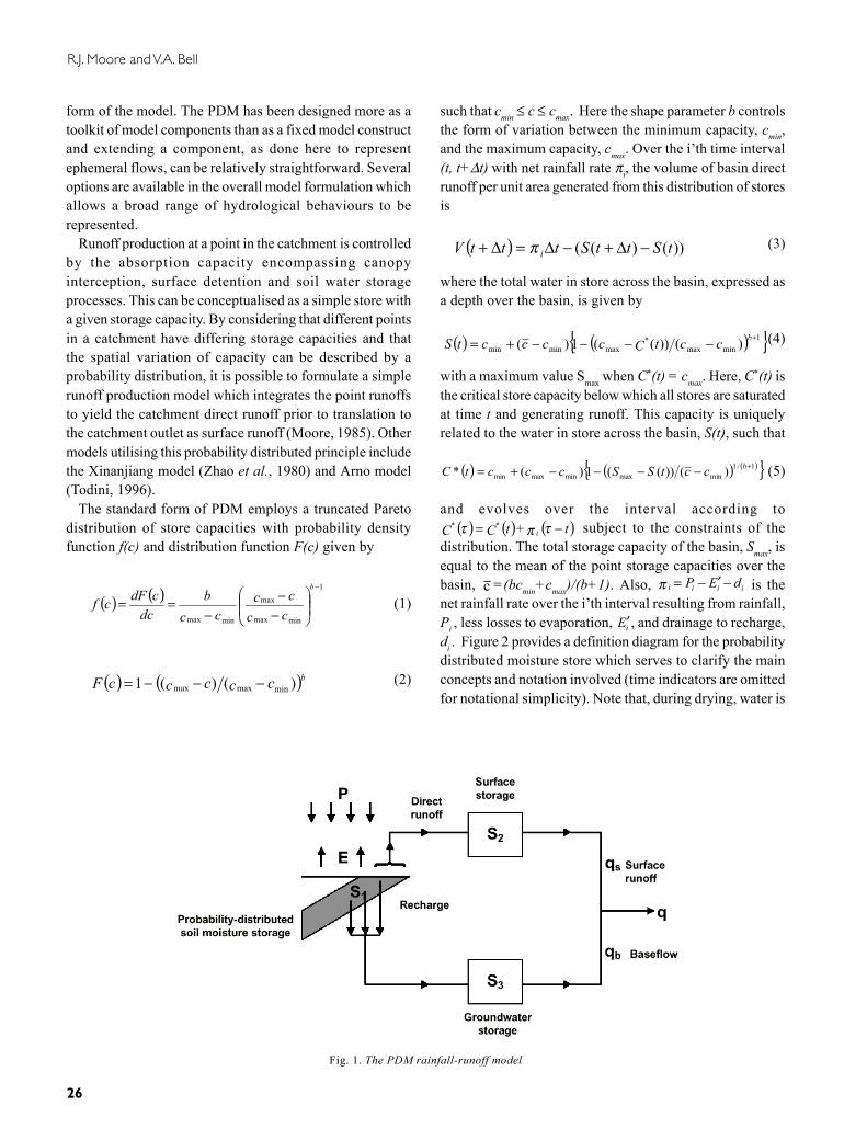
The Probability Distributed ModelThe Probability Distributed Model, or PDM, is a fairlygeneral conceptual rainfall-runoff model which transformsrainfall and evaporation data to flow at the catchment outlet(Moore, 1985, 1986, 1999). Figure 1 illustrates the general

R.J. Moore and V.A. Bell

26

form of the model. The PDM has been designed more as atoolkit of model components than as a fixed model constructand extending a component, as done here to representephemeral flows, can be relatively straightforward. Severaloptions are available in the overall model formulation whichallows a broad range of hydrological behaviours to berepresented.

Runoff production at a point in the catchment is controlledby the absorption capacity encompassing canopyinterception, surface detention and soil water storageprocesses. This can be conceptualised as a simple store witha given storage capacity. By considering that different pointsin a catchment have differing storage capacities and thatthe spatial variation of capacity can be described by aprobability distribution, it is possible to formulate a simplerunoff production model which integrates the point runoffsto yield the catchment direct runoff prior to translation tothe catchment outlet as surface runoff (Moore, 1985). Othermodels utilising this probability distributed principle includethe Xinanjiang model (Zhao et al., 1980) and Arno model(Todini, 1996).

The standard form of PDM employs a truncated Paretodistribution of store capacities with probability densityfunction f(c) and distribution function F(c) given by

(1)

(2)

such that cmin ≤ c ≤ cmax. Here the shape parameter b controlsthe form of variation between the minimum capacity, cmin,and the maximum capacity, cmax. Over the i’th time interval(t, t+∆t) with net rainfall rate πi, the volume of basin directrunoff per unit area generated from this distribution of storesis

( ) ))()(( tSttStttV i −∆+−∆=∆+ π (3)

where the total water in store across the basin, expressed asa depth over the basin, is given by

( ) ( ){ }1minmax

*maxminmin )())((1)( +−−−−+= bcctCcccctS (4)

with a maximum value Smax when C*(t) = cmax. Here, C*(t) isthe critical store capacity below which all stores are saturatedat time t and generating runoff. This capacity is uniquelyrelated to the water in store across the basin, S(t), such that

(5)

and evolves over the interval according to( ) ( ) ( ) t +tCC i

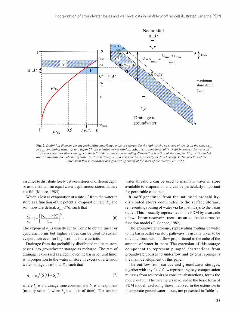
** −= τπτ subject to the constraints of thedistribution. The total storage capacity of the basin, Smax, isequal to the mean of the point storage capacities over thebasin, c =(bcmin+cmax)/(b+1). Also, iiii dEP −′−=π is thenet rainfall rate over the i’th interval resulting from rainfall,Pi , less losses to evaporation, iE′, and drainage to recharge,di . Figure 2 provides a definition diagram for the probabilitydistributed moisture store which serves to clarify the mainconcepts and notation involved (time indicators are omittedfor notational simplicity). Note that, during drying, water is

( ) ( ) cccc

ccb

dccdFcf

b

max min

max1

max min

−

−−

==−

Fig. 1. The PDM rainfall-runoff model

ccc maxmin ≤≤

( ) ( )cccccF bminmaxmax )()(1 −−−=

( ) ( ) ( ){ }1/1minmaxminmaxmin )())((1)(* +−−−−+= bcctSSccctC


27

assumed to distribute freely between stores of different depthso as to maintain an equal water depth across stores that arenot full (Moore, 1985).

Water is lost as evaporation at a rate iE′ from the water instore as a function of the potential evaporation rate, Ei, andsoil moisture deficit, Smax-S(t), such that

( )( ) eb

i

i

StSS

EE

−−=

′

max

max1 . (6)

The exponent be is usually set to 1 or 2 to obtain linear orquadratic forms but higher values can be used to sustainevaporation even for high soil moisture deficits.

Drainage from the probability-distributed moisture storepasses into groundwater storage as recharge. The rate ofdrainage (expressed as a depth over the basin per unit time)is in proportion to the water in store in excess of a tensionwater storage threshold, St , such that

( )( )tb

gi StSkd g−= −1 (7)

where kg is a drainage time constant and bg is an exponent(usually set to 1 when kg has units of time). The tension

water threshold can be used to maintain water in storeavailable to evaporation and can be particularly importantfor permeable catchments.

Runoff generated from the saturated probability-distributed stores contributes to the surface storage,representing routing of water via fast pathways to the basinoutlet. This is usually represented in the PDM by a cascadeof two linear reservoirs recast as an equivalent transferfunction model (O’Connor, 1982).

The groundwater storage, representing routing of waterto the basin outlet via slow pathways, is usually taken to beof cubic form, with outflow proportional to the cube of theamount of water in store. The extension of this storagecomponent to represent pumped abstractions fromgroundwater, losses to underflow and external springs isthe main development of this paper.

The outflow from surface and groundwater storages,together with any fixed flow representing, say, compensationreleases from reservoirs or constant abstractions, forms themodel output. The parameters involved in the basic form ofPDM model, excluding those involved in the extension toincorporate groundwater losses, are presented in Table 1.

Fig. 2. Definition diagram for the probability distributed moisture stores. On the right is shown stores of depths in the range cminto cmax containing water up to a depth C*. An addition of net rainfall, π∆t, over a time interval (t, t+∆t) increases the water instore and generates direct runoff. On the left is shown the corresponding distribution function of store depth, F(c), with shadedareas indicating the volumes of water in store initially, S, and generated subsequently as direct runoff, V. The fraction of the

catchment that is saturated and generating runoff at the start of the interval is F(C*).

maximum store depth cmax

��

��

��

��

1 0.5 0

F(c)

cmax

Sπ ∆t V

c

C*+ π ∆t

C*

cmin ��

Direct runoff

C*

0

π ∆t

C*+π ∆t 1

maxminmax +

+==

b

cbcSc

cmin

F(c)

Net rainfall π ∆t

Drainage to groundwater

1

c

F(C*)


28

Groundwater storageThe probability-distributed store of the PDM partitionsrainfall into direct runoff, groundwater recharge and soilmoisture storage. Direct runoff is routed through surfacestorage: a “fast response system” representing channel andother fast translation flow paths. Groundwater recharge fromsoil water drainage is routed through subsurface storage: a“slow response system” representing groundwater and otherslow flow paths. The routing of recharge through thegroundwater system can be represented by a variety of typesof nonlinear storage. For notational convenience, S(t) is againused to denote the volume of stored water, expressed as adepth over the basin, but now it relates to a nonlineargroundwater storage and not to a probability-distributedmoisture storage.

The rate of outflow per unit area from a nonlinear storage,q ≡ q(t), is considered to be proportional to some power, m,of the volume of water held in the storage per unit area,

S ≡ S(t), so that

00, , m>k> Skq m= (8)

where k is a time constant with units of inverse time. Thestorage here can be conceptualised as a reservoir with abottom outlet representing aquifer storage and the releaseof water from it as the baseflow component of catchmentflow. Combining the nonlinear storage equation above withthe equation of continuity

q, u = dtdS − (9)

where u ≡ u(t) is the input to the store, gives

( ) ,<b<,, q>q qu = adtdq b 10 ∞−− (10)

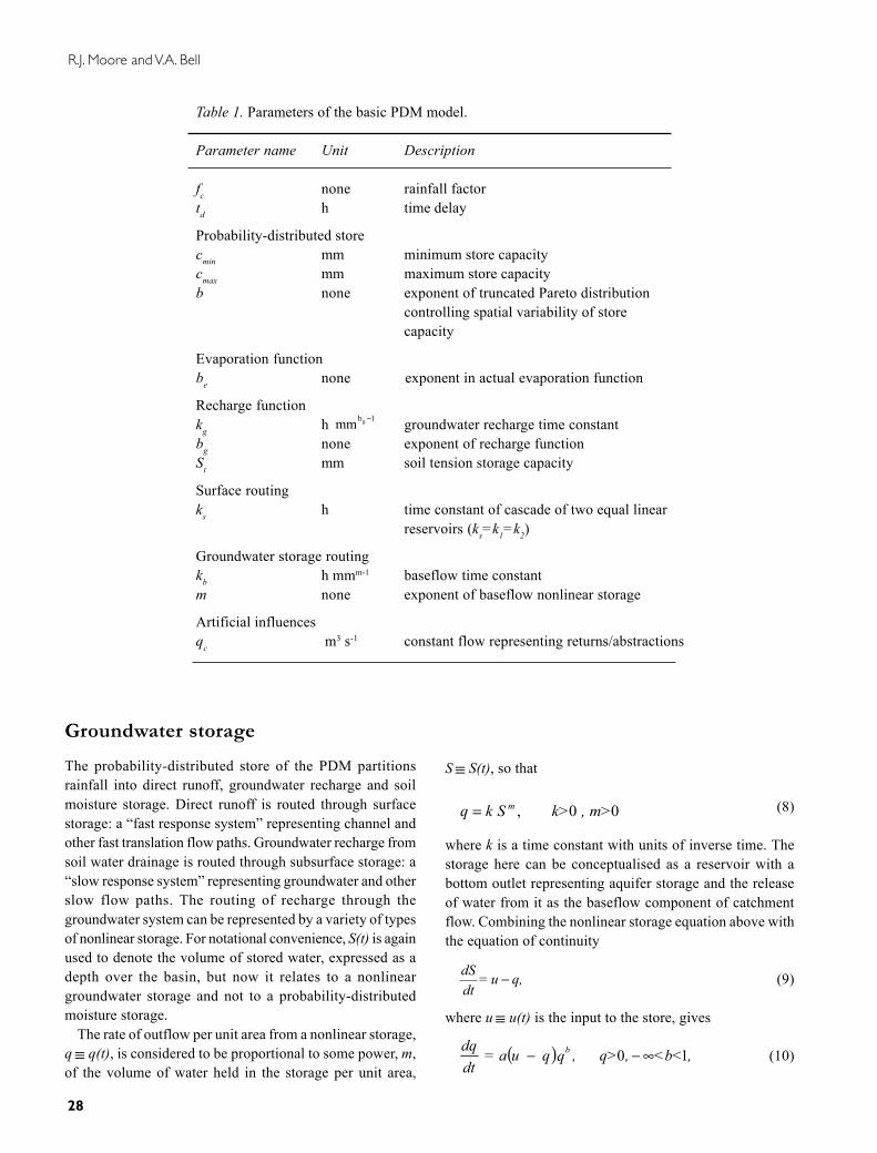
Table 1. Parameters of the basic PDM model.

Parameter name Unit Description

fc none rainfall factortd h time delay

Probability-distributed storecmin mm minimum store capacitycmax mm maximum store capacityb none exponent of truncated Pareto distribution

controlling spatial variability of storecapacity

Evaporation functionbe none exponent in actual evaporation function

Recharge functionkg h groundwater recharge time constantbg none exponent of recharge functionSt mm soil tension storage capacity

Surface routingks h time constant of cascade of two equal linear

reservoirs (ks=k1=k2)

Groundwater storage routingkb h mmm-1 baseflow time constantm none exponent of baseflow nonlinear storage

Artificial influencesqc m3 s-1 constant flow representing returns/abstractions

1bgmm −


29

where a=mk1/m and b=(m-1)/m are two parameters. Theinput, in the present context, is the groundwater recharge inthe form of the rate of drainage from the soil per unit area.This ordinary differential equation has become known asthe Horton-Izzard model (Dooge, 1973) and can be solvedexactly for any rational value of m (Gill, 1976, 1977).

Horton (1945) considered nonlinear storage models asdescriptors of the overland flow process. He found that theexponent m for fully turbulent flow is 5/3, and for fullylaminar flow is 3. This allowed Horton to define an “indexof turbulence”, I=¾(3-m), ranging from 1 for turbulent flowto 0 for laminar flow. Horton (1938) found a solution interms of tanh (the hyperbolic tangent) when m=2 (thequadratic storage function), corresponding to I=0.75, whichhe referred to as the “75% turbulent flow” case. It is givena conceptual interpretation as an “unconfined or non-artesian” storage element by Ding (1967) based on Wernerand Sundquist’s (1951) theoretical analysis of flow from adeep non-artesian aquifer based on Darcy’s law and Dupuit’sassumption (they also show that m=1 is appropriate forconfined or artesian aquifers). Todd (1959) provides anaccessible introduction to the groundwater theory involved.The quadratic storage function was used by Mandeville(1975) as the basis of the Isolated Event Model (IEM) usedin the UK Flood Study (NERC, 1975) and later adapted forreal-time flood forecasting by Brunsdon and Sargent (1982).It is also used in the Thames Catchment Model (TCM) torepresent release from groundwater storage (Greenfield,1984).

The choice of nonlinear storage to use in the PDM includesthe linear, quadratic, exponential, cubic and generalnonlinear forms. The theoretical work of Werner andSundquist (1951) and Ding (1967) suggests the use of linearand quadratic forms for confined (artesian) and unconfinedaquifers respectively. However, a cubic form correspondingto the laminar flow case (I=0, m=3), has been found usefulin practical applications of the PDM where the hydrographrecession is initially steep but subsequently is sustained andslowly decreasing. In this case where q=kS3, an approximatesolution utilising a method due to Smith (1977) yields thefollowing recursive equation for storage, given a constantinput u over the interval (t, t+∆t):

( ) ( )( )

( ){ }( ).)(1)(3exp3

1 322 tkSuttkS

tkStSttS −−∆−−=∆+

(11)

Discharge may then be obtained simply using the nonlinearrelation

( ) ( ). t+t Skttq ∆=∆+ 3 (12)

Solutions for the other nonlinear forms are presented inAppendix A. When used to represent groundwater storage,the input u will be the drainage rate per unit area, di, fromthe probability-distributed moisture storage, and the outputq(t) will be the “baseflow” component of flow per unit areaqb(t). The parameterisation kb=k -1 with units h mmm-1 is alsoused. Explicit allowance for groundwater abstractions isincorporated in the extension of the PDM which can alsoutilise well level data. The theoretical basis of this extensionis outlined next.

Incorporation of pumped abstractionsWater held in groundwater storage can be lost to the surfacecatchment by pumped abstractions, by underflow below thegauged catchment outlet or by spring flow external to thesurface catchment. Losses via underflow and spring flowwill be considered later. In the case of abstractions, A, thenonlinear storage theory introduced in the previous sectionrequires extension to consider the case of negative net inputto storage, u, and the possibility of storages being drawndown below a level at which flow at the catchment outletceases. This extension allows for the modelling of ephemeralstreams typical of catchments on the English Chalk.

Formally, the input to the nonlinear storage, u, may bedefined as recharge d, less abstractions, A, dropping the timesuffix for notational simplicity. With u=d–A, the prospectarises of negative inputs to storage leading to the cessationof flow. Consider the time interval (t, t+∆t) within whichcessation of flow occurs after a time T´. Using the cubicstorage, q=kS3, for the purposes of illustration, then Eqn.11 gives the time to flow cessation, T´, by solving

( )( )

( )( ){ } ( )( )tkSuTtkStkS

tS 322 13exp

310 −−′−−=

which gives

( )( )( ) .31ln

31

3

3

2

−+−=′

tkSutkS

tkST (13)

An extended form of storage is now conceptualised which,instead of emptying at zero flow, allows for furtherwithdrawal of water for abstraction (Fig. 3). The “negativestorage” at the end of the interval can then be calculated as

( ) ( )

( )( )( )

( )( )( )

−+

∆+∆=

−+

∆+∆=

′−∆=∆+

tqutq

ttqatu

tkSutkS

ttkStu

TTuttS

31ln11

31ln3

11

3/2

3

3

2 (14)

where a = 3k1/3.


30

With further abstractions from storage the negative storagecan be calculated by simple continuity. When rechargeexceeds abstractions the storage is replenished and at sometime flow is initiated once more. The time interval withinthe model interval ∆t in which this occurs is calculated bysimple continuity and the residual time interval used in Eqn.11 in place of ∆t (with S(t)=0). The normal calculationsapply whilst the storage is in surplus. Expressions for thetime to flow cessation, T´, and the initial negative storage,S(t+∆t), for other types of nonlinear store are given inAppendix B. As previously indicated, in practice theparameterisation kb=k-1 with units h mmm-1 is used.

To cater for situations where information on allabstractions affecting the catchment water balance does notexist, an abstraction model which scales and adds to knownabstractions is included in the overall model formulation;thus A=cA+fAAr where Ar is the recorded total abstractionfor a time interval and cA and fA are parameters.

Incorporation of well level dataIf well measurements of groundwater level are available itis possible to relate the model storage, S≡S(t), to the welllevel, Wº≡Wº(t). Well measurements normally record thedepth of the water table from the ground surface. By

introducing a maximum groundwater storage, S gmax , then

the groundwater storage deficit can be calculated as

SSD g −= max(15)

for both positive and negative values of S. This storagedeficit can be used to calculate the depth to the water tableas

.DYW s= (16)

Here, Ys is the specific yield of the groundwater reservoir,defined as the volume of water produced per unit aquiferarea per unit decline in hydraulic head. This dimensionlessparameter takes values typically in the range 0.01 to 0.3(Freeze and Cherry, 1979). An additional datum correctioncorresponding to the height of the ground surface at thewell, hw, is required to relate W to observed well levels, Wº,when these are referenced to Ordnance Datum; then themodelled depth W is comparable with the observed depthhw - Wº. The above provides the basis of incorporating welllevel measurements into both the model calibration processand the model state updating procedure. The use of welllevel data in model calibration is illustrated in the case studythat follows. Their use for model data assimilation as part

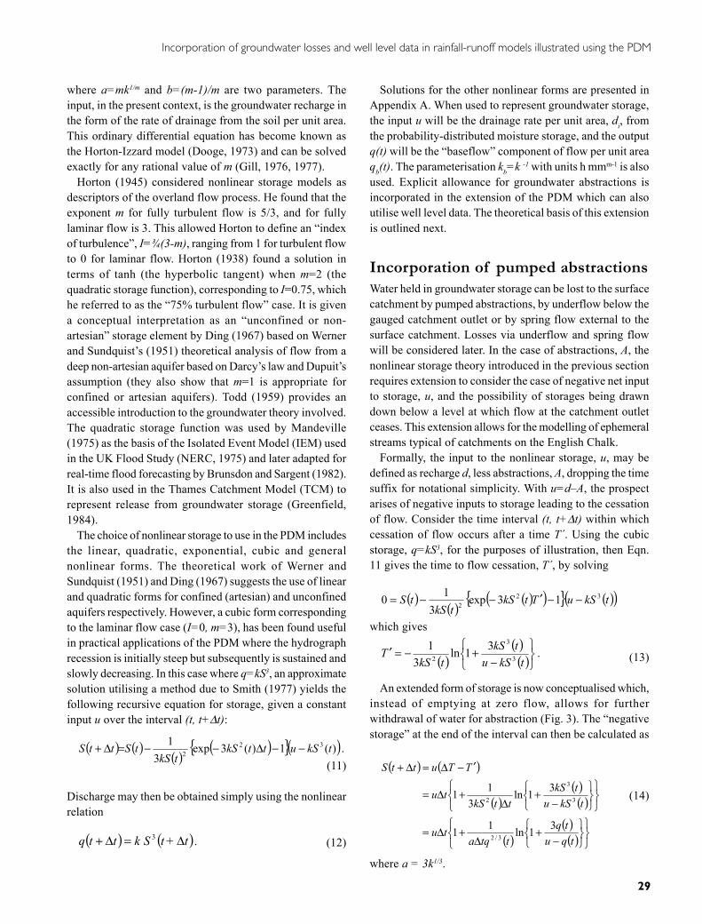
Fig. 3. Conceptualisation of extended nonlinear storage

Losses

gSmax

Dmax

D

Baseflow )1( bb qq ′−= α

u = d – A

flow spring External be qq ′= α

S

bq′

flow Underuq


31

of a real-time state correction procedure is beyond the scopeof the present paper, which focuses on the simulationperformance of the model.

Incorporation of losses to underflowand external springsHaving extended the theory of nonlinear storage models toaccommodate pumped abstractions, it is now appropriateto consider the conceptualisation of losses to underflow andexternal spring flow. Flow emerging from the catchmentbeneath the ground surface of the gauging station is referredto here as underflow. It is reasonable to suppose thatunderflow is controlled by the hydraulic head and thus thewater in storage. If Dmax is the maximum deficit forunderflow to occur then the rate of underflow can be definedas

( ) ,max1 DDkq uu −= − (17)

where ku is the underflow time constant (units of time). Thisis depicted in Fig. 3 as an additional lower outlet to thenonlinear storage. Note that this conceptualisation of

underflow excludes any local phenomenon more stronglylinked to local river flow than to the groundwater system.

The normal outflow from the nonlinear storage arisingfrom positive values of storage, S, has been assumed to bethe baseflow component of the flow at the catchment outlet.An extension allows a fraction, α, to contribute as springsexternal to the catchment with flow, qe, whilst the remainingfraction, (1–α), contributes as the baseflow, qb, at thecatchment outlet (Fig. 3).

The additional parameters introduced into the extendedform of the model are summarised in Table 2.

The Lavant catchment: a case studyapplicationINTRODUCTION

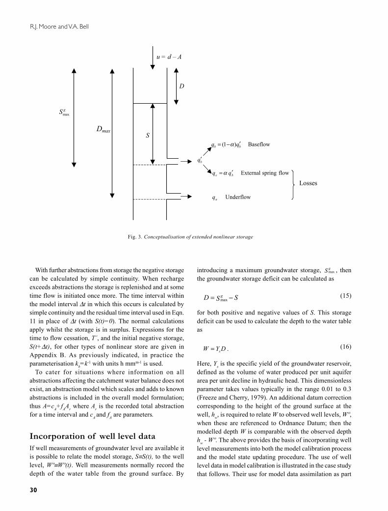
The Lavant catchment in southern England was selected asa case study to develop and evaluate the extension of thePDM model to groundwater-dominated catchments. It hasexperienced serious flooding at times of high water tablelevels and its water balance is affected by pumpedabstractions, external springflow and underflows beneaththe gauging station (Thomson et al., 1988).

The surface catchment extends over an area of 87 km2 toits gauging station at Graylingwell, situated north-east ofthe main town of Chichester. It is an ephemeral Chalk streamon the dip-slope of the South Downs, characterised by highpermeability and a rural land use of agriculture withsignificant woodland and only a little urban developmentclose to Graylingwell. Significant groundwater abstractions

Table 2. Additional parameters of the extended PDMmodel

Parameter name Unit Description

Underflowku h underflow time constantDmax mm maximum deficit for

underflow t

External springsα none fraction of groundwater

outflow contributingto external springs

AbstractioncA mm h-1 constant abstractionfA none factor on recorded

abstractions

Well level

S gmax

mm maximum groundwaterstorage

Ys none specific yield ofaquifer

hw m well level datum

Fig. 4. The Lavant catchment to Graylingwell gauging stationshowing abstraction, well level and raingauge sites (grid co-ordinates in km); inset map shows location of catchment in southernEngland.

��


32

from wells at Brick Kiln and Lavant reduce river flows.The gauging structure is a flat-V weir with a weir capacityof 6 m3 s-1. Bypassing occurs during extreme events, suchas the January 1994 flood peak of 7.1 m3 s-1 estimated at8.1 m3 s-1.

Figure 4 provides a map of the catchment to the gaugingstation at Graylingwell showing the location of theabstraction and well level sites used in this study and therecording raingauge at Chichester, a town which can sufferflooding from the River Lavant.

THE CHICHESTER FLOOD OF 1994

The “Chichester Flood” of January 1994, whilst modest byinternational standards, was noteworthy in the UK andresulted in relatively large damages in the Lavant catchmentand Chichester in particular (Posford Duvivier, 1994).Whilst groundwater levels were fairly low at the start of thewinter, these rose quickly from 28 November to mid-Januaryas a result of 350 mm of rain, 40% of which fell in just sixdays. The well at Chilgrove (Grid Reference: 4836 1144)became artesian from 7 January for 18 days and flows inthe Lavant rose from 0.3 m3 s-1 in mid-December to a peakof 8.1 m3 s-1 on 10 January. The normally slow-respondingflow regime became flashy as the Chalk became saturated.Above a well level of 69.5 mAOD at Chilgrove, river flowsstarted to increase markedly faster than groundwater levels.It has been speculated that above this level a zone of highpermeability Chalk functions as an overflow, providing arapid flow path to the river system.

HYDROGEOLOGY

A key feature of the Chalk is its particular form of dualporosity. The Chalk matrix is so fine-grained and the porethroats so small in size that the pore water suctions remainhigh, stopping the pores from draining fully. This meansthat even above the water table the matrix remains largelysaturated and evaporation rates are maintained. This isrepresented in the PDM model by the tension watercomponent controlled by the storage tension thresholdparameter, St, below which free drainage is inhibited whilstwater is made available for evaporation. The zone abovethe water table (at atmospheric pressure) is still describedas unsaturated, since pore water pressures are less thanatmospheric pressure. At high pore water suctions (potentialsof less than –5 kPa) hydraulic conductivity is quite constantat between 1 and 6 mm d-1. With decreasing suctions a rapidincrease in conductivity occurs with typical values in therange 100 to 1000 mm d-1 as the fracture network becomessaturated and dominates the flow regime. It is estimated that10 to 30% of recharge is via fracture or bypass flow rather

than as “piston” flow through the Chalk matrix. This is notrepresented explicitly in the current form of the model.

Because of the high porosity (15 to 45%) the matrix isnot readily drained; the effective groundwater storage thusdepends primarily on the fracture network and larger poresand is probably only 1% of the total saturated Chalk volume.Pumping tests yield typical values of 0.002 for the storagecoefficient and 500 m2 d-1 for transmissivity. However,estimates of hydraulic conductivity using a gas permeametergive typical values of 0.0025 m d-1, implying a very lowtransmissivity of 0.25 m2 d-1 for a 100 m thick aquifer. Thisserves to highlight the importance of secondary permeabilityto groundwater flow in Chalk. Further details of the Chalkaquifer of the South Downs can be found in the recent surveyedited by Jones and Robins (1999).

MODEL APPLICATION

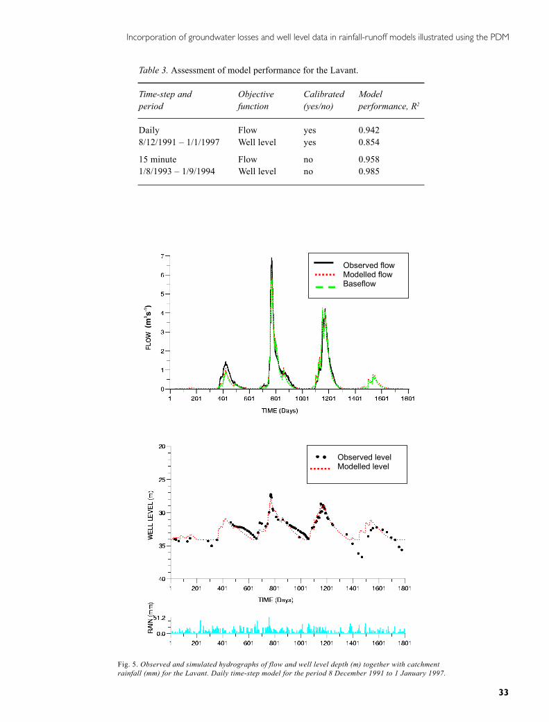
The extended PDM model was first applied to the Lavantcatchment using a daily time-step over the period 8December 1991 to 1 January 1997. Potential evaporationwas represented by a simple sine curve over the year with amean value of 1.4 mm day-1. The calibration to observedflow data gave an R2 value of 0.942 (Table 3), accountingfor 94% of the variability in the observed flow series. Thesimulated flow hydrograph shown in the upper part of Fig.5 demonstrates the model’s ability to reproduce theephemeral behaviour of the river, including the inceptionand cessation time of runoff, as well as the flood peaks.Calibration to the well level data for West Dean Nurserygave an R2 value of 0.854. The well level hydrograph shownin the middle part of Fig. 5 shows very good agreementuntil the winter of 1995/96. At this point the modelled welllevels rise and the River Lavant begins to flow whilst inreality the well levels fall steeply before recovering to normallevels and there is no river flow. This failing of the model isunder investigation. The lower graph shows catchmentaverage rainfall in mm over the five-year period.

Note that a formal split sample test involving independentcalibration and evaluation periods has not been invokedsince there are only three flood peaks over the five-yearrecord. Model performance is regarded as satisfactory onthe basis of visual inspection of the hydrographs, payingespecial attention to the time of initiation and cessation ofrunoff, the flood peak magnitude and the shape of the riseand recession of the hydrograph. The R2 statistic has beenchosen for presentation here as an overall measure of“goodness-of-fit”; however, other performance measureswere assessed, including root mean square error and biasstatistics. Comments on the model parameters available forcalibration relevant to the robustness of the fitted model aremade at the end of this section.


33

Table 3. Assessment of model performance for the Lavant.

Time-step and Objective Calibrated Modelperiod function (yes/no) performance, R2

Daily Flow yes 0.9428/12/1991 – 1/1/1997 Well level yes 0.854

15 minute Flow no 0.9581/8/1993 – 1/9/1994 Well level no 0.985

Fig. 5. Observed and simulated hydrographs of flow and well level depth (m) together with catchmentrainfall (mm) for the Lavant. Daily time-step model for the period 8 December 1991 to 1 January 1997.

Observed level Modelled level

Observed flow Modelled flow Baseflow

��

��


34

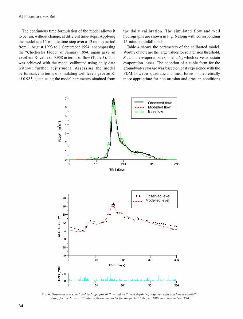
The continuous time formulation of the model allows itto be run, without change, at different time-steps. Applyingthe model at a 15-minute time-step over a 13 month periodfrom 1 August 1993 to 1 September 1994, encompassingthe “Chichester Flood” of January 1994, again gave anexcellent R2 value of 0.958 in terms of flow (Table 3). Thiswas achieved with the model calibrated using daily datawithout further adjustment. Assessing the modelperformance in terms of simulating well levels gave an R2

of 0.985, again using the model parameters obtained from

the daily calibration. The simulated flow and wellhydrographs are shown in Fig. 6 along with corresponding15-minute rainfall totals.

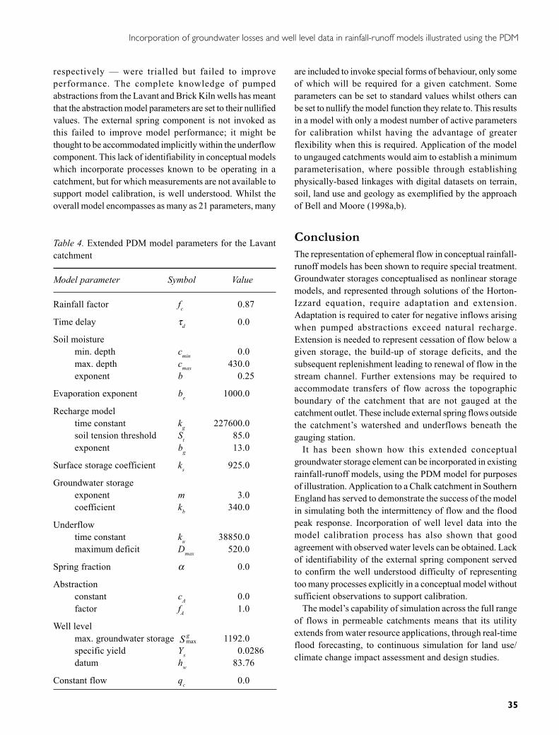
Table 4 shows the parameters of the calibrated model.Worthy of note are the large values for soil tension threshold,St , and the evaporation exponent, be , which serve to sustainevaporation losses. The adoption of a cubic form for thegroundwater storage was based on past experience with thePDM; however, quadratic and linear forms — theoreticallymore appropriate for non-artesian and artesian conditions

Fig. 6. Observed and simulated hydrographs of flow and well level depth (m) together with catchment rainfall(mm) for the Lavant. 15 minute time-step model for the period 1 August 1993 to 1 September 1994.

Observed level Modelled level

Observed flow Modelled flow Baseflow

��

��


35

respectively — were trialled but failed to improveperformance. The complete knowledge of pumpedabstractions from the Lavant and Brick Kiln wells has meantthat the abstraction model parameters are set to their nullifiedvalues. The external spring component is not invoked asthis failed to improve model performance; it might bethought to be accommodated implicitly within the underflowcomponent. This lack of identifiability in conceptual modelswhich incorporate processes known to be operating in acatchment, but for which measurements are not available tosupport model calibration, is well understood. Whilst theoverall model encompasses as many as 21 parameters, many

are included to invoke special forms of behaviour, only someof which will be required for a given catchment. Someparameters can be set to standard values whilst others canbe set to nullify the model function they relate to. This resultsin a model with only a modest number of active parametersfor calibration whilst having the advantage of greaterflexibility when this is required. Application of the modelto ungauged catchments would aim to establish a minimumparameterisation, where possible through establishingphysically-based linkages with digital datasets on terrain,soil, land use and geology as exemplified by the approachof Bell and Moore (1998a,b).

ConclusionThe representation of ephemeral flow in conceptual rainfall-runoff models has been shown to require special treatment.Groundwater storages conceptualised as nonlinear storagemodels, and represented through solutions of the Horton-Izzard equation, require adaptation and extension.Adaptation is required to cater for negative inflows arisingwhen pumped abstractions exceed natural recharge.Extension is needed to represent cessation of flow below agiven storage, the build-up of storage deficits, and thesubsequent replenishment leading to renewal of flow in thestream channel. Further extensions may be required toaccommodate transfers of flow across the topographicboundary of the catchment that are not gauged at thecatchment outlet. These include external spring flows outsidethe catchment’s watershed and underflows beneath thegauging station.

It has been shown how this extended conceptualgroundwater storage element can be incorporated in existingrainfall-runoff models, using the PDM model for purposesof illustration. Application to a Chalk catchment in SouthernEngland has served to demonstrate the success of the modelin simulating both the intermittency of flow and the floodpeak response. Incorporation of well level data into themodel calibration process has also shown that goodagreement with observed water levels can be obtained. Lackof identifiability of the external spring component servedto confirm the well understood difficulty of representingtoo many processes explicitly in a conceptual model withoutsufficient observations to support calibration.

The model’s capability of simulation across the full rangeof flows in permeable catchments means that its utilityextends from water resource applications, through real-timeflood forecasting, to continuous simulation for land use/climate change impact assessment and design studies.

Table 4. Extended PDM model parameters for the Lavantcatchment

Model parameter Symbol Value

Rainfall factor fc 0.87

Time delay τd 0.0

Soil moisturemin. depth cmin 0.0max. depth cmax 430.0exponent b 0.25

Evaporation exponent be 1000.0

Recharge modeltime constant kg 227600.0soil tension threshold St 85.0exponent bg 13.0

Surface storage coefficient ks 925.0

Groundwater storageexponent m 3.0coefficient kb 340.0

Underflowtime constant ku 38850.0maximum deficit Dmax 520.0

Spring fraction α 0.0

Abstractionconstant cA 0.0factor fA 1.0

Well levelmax. groundwater storage S g

max 1192.0specific yield Ys 0.0286datum hw 83.76

Constant flow qc 0.0


36

AcknowledgementsThe research has been carried out with the support of theScience Budget of the Centre for Ecology and Hydrology(CEH). Dick Bradford of CEH Wallingford is thanked fordiscussion of the hydrogeological processes operating inthe Lavant catchment. The Environment Agency is thankedfor providing the data supporting this investigation.

ReferencesBell, V.A. and Moore, R.J., 1998a. A grid-based distributed flood

forecasting model for use with weather radar data: Part 1.Formulation. Hydrol. Earth Syst. Sci., 2, 265-281.

Bell, V.A. and Moore, R.J., 1998b. A grid-based distributed floodforecasting model for use with weather radar data: Part 2. CaseStudies. Hydrol. Earth Syst. Sci., 2, 283-298.

Brunsdon, G.P. and Sargent, R.J., 1982. The Haddington floodwarning system, in Advances in Hydrometry (Proc. ExeterSymp.), IAHS Publ. no. 134, 257-272.

Central Water Planning Unit, 1977. Dee Weather Radar and Real-time Hydrological Forecasting Project. Report by the SteeringCommittee, 172 pp.

Centre for Ecology and Hydrology, 2000. PDM Rainfall-RunoffModel, Version 2.0, CEH Wallingford, UK..

Ding, J.Y., 1967. Flow routing by direct integration method, Proc.Int. Hydrology Symp., Fort Collins, 1, 113-120.

Dooge, J.C.I., 1973. Linear theory of hydrologic systems, Tech.Bull. 1468, Agric. Res. Service, US Dept. Agric., Washington,327 pp.

Freeze, R.A. and Cherry, J.A., 1979. Groundwater. Prentice Hall,604pp.

Gill, M.A., 1976. Exact solution of gradually varied flow, J.Hydraul. Div., ASCE, 102, HY9, 1353-1364.

Gill, M.A., 1977. Algebraic solution of the Horton-Izzard turbulentoverland flow model of the rising hydrograph, Nord. Hydrol.,8, 249-256.

Greenfield, B.J., 1984. The Thames Water Catchment Model.Internal Report, Technology and Development Division, ThamesWater, UK.

Horton, R.E., 1938. The interpretation and application of runoffplot experiments with reference to soil erosion problems. SoilSci. Soc. Amer., Proc., 3, 340349.

Horton, R.E., 1945. Erosional development of streams and theirdrainage basins: hydrophysical approach to quantitativemorphology, Bull. Geol. Soc. Amer., 56, 275-370.

Institute of Hydrology, 1992. PDM: A generalized rainfall-runoffmodel for real-time use, Developers’ Training Course, NationalRivers Authority River Flow Forecasting System, Version 1.0,March 1992, Wallingford, UK. 26pp.

Institute of Hydrology, 1996. A guide to the PDM. Version 1.0,January 1996, Wallingford, UK. 45pp.

Jones, H.K. and Robins, N.S. (Eds.), 1999. National GroundwaterSurvey. The Chalk aquifer of the South Downs. BritishGeological Survey Hydrogeological Report Series. BritishGeological Survey, Keyworth, UK, 111pp.

Lambert, A.O., 1972. Catchment models based on ISO-functions.J. Instn. Water Engineers, 26, 413-422.

Mandeville, A.N., 1975. Non-linear conceptual catchmentmodelling of isolated storm event, PhD thesis, University ofLancaster.

Moore, R.J., 1983. Flood forecasting techniques. WMO/UNDPRegional Training Seminar on Flood Forecasting, Bangkok,Thailand, 37pp.

Moore, R.J., 1985. The probability-distributed principle and runoffproduction at point and basin scales. Hydrol. Sci. J., 30, 273-297.

Moore, R.J., 1986. Advances in real-time flood forecastingpractice. Symposium on Flood Warning Systems, Winter meetingof the River Engineering Section, Inst. Water Engineers andScientists, 23 pp.

Moore, R.J., 1999. Real-time flood forecasting systems:Perspectives and prospects. In: Floods and landslides:Integrated Risk Assessment, R. Casale and C. Margottini (Eds.),147-189, Springer.

Natural Environment Research Council, 1975. Flood StudiesReport, Vol. 1, Chap 7, 513-531.

O’Connor, K.M., 1982. Derivation of discretely coincident formsof continuous linear time-invariant models using the transferfunction approach, J. Hydrol., 59, 1-48.

Posford Duvivier, 1994. River Lavant Flood Investigation. ReportCommissioned by National Rivers Authority Southern Region.

Smith, J.M., 1977. Mathematical Modelling and DigitalSimulation for Engineers and Scientists, Wiley, Chichester, UK.332 pp.

Thomson, J.M., Ellis, J. and Headworth, H.G., 1988. South DownsInvestigation. Report on the Resources of the Chichester ChalkBlock. Southern Water Sussex Division, 79pp plus figs.

Todd, D.K., 1959. Groundwater hydrology. Wiley, Chichester, UK.336pp.

Todini, E., 1996. The ARNO rainfall-runoff model. J. Hydrol.,175, 339-382.

Werner, P.H. and Sundquist, K.J., 1951. On the groundwaterrecession curve for large watersheds, Proc. AIHS GeneralAssembly, Brussels, Vol. II, IAHS Pub. No. 33, 202-212.

Zhao, R.J., Zhuang, Y., Fang, L.R., Lin, X.R. and Zhang, Q.S.,1980. The Xinanjiang model. In: Hydrological Forecasting(Proc. Oxford Symp., April 1980), IAHS Publ. no. 129, 351-356.

Appendix A:

Solutions to the Horton-IzzardequationThe Horton-Izzard equation (Dooge, 1973) for a flow perunit area, q ≡ q(t), and an input per unit area u ≡ u(t), is

( ) ,<b<,, q>q qu = adtdq b 10 ∞−− (A.1)

where a=mk1/m and b=(m-1)/m are two parameters relatedto those of the nonlinear storage equation q = k Sm, whereS ≡ S(t) denotes storage per unit area at time t. This ordinarydifferential equation can be solved exactly for any rationalvalue of m (Gill, 1976, 1977). Recursive solutions arepresented here for linear (m=1), quadratic (m=2),exponential (b=1) and cubic (m=3) cases for a constant inputu over the interval (t, t+T), and for the general case whenu=0.


37

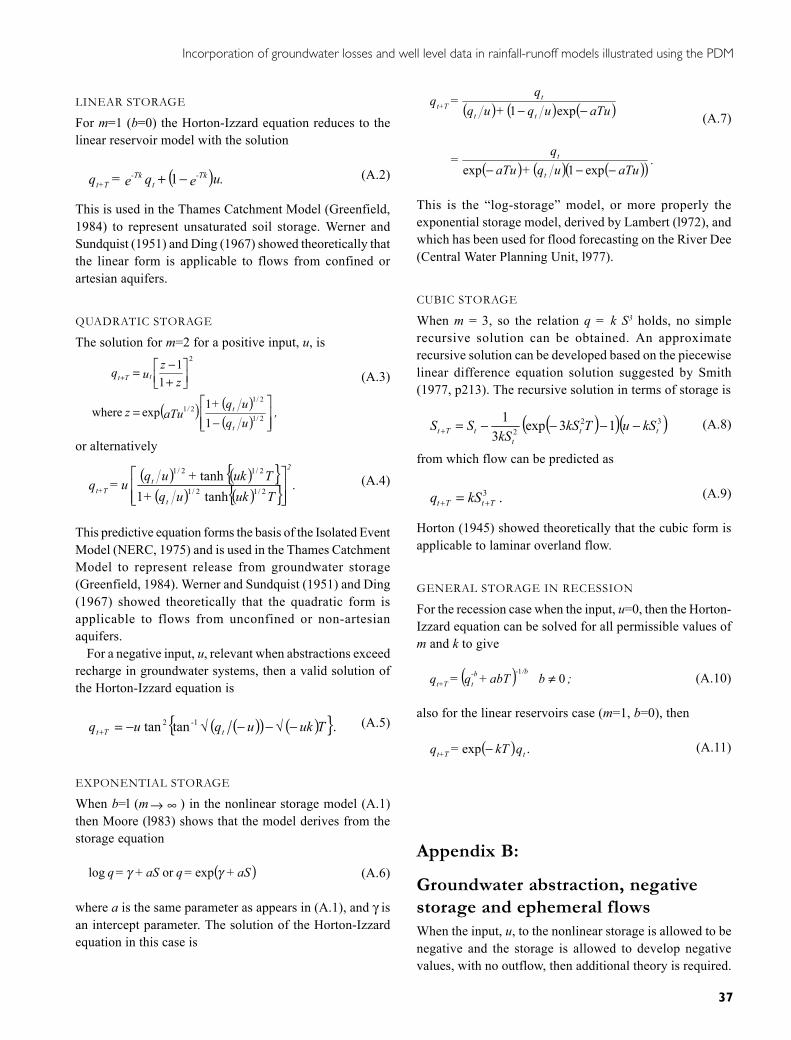
LINEAR STORAGE

For m=1 (b=0) the Horton-Izzard equation reduces to thelinear reservoir model with the solution

( )u.eqe=q -Tkt

-TkT+t −+ 1 (A.2)

This is used in the Thames Catchment Model (Greenfield,1984) to represent unsaturated soil storage. Werner andSundquist (1951) and Ding (1967) showed theoretically thatthe linear form is applicable to flows from confined orartesian aquifers.

QUADRATIC STORAGE

The solution for m=2 for a positive input, u, is

( ) ( )( )

,uquq+

aTu z

zz

uq

t

t/

tTt

−=

+−=+

2/1

2/121

2

11

exp where

11

(A.3)

or alternatively

( ) ( ){ }( ) ( ){ } .

Tuk uq + Tuk + uqu = q

t

t

2

T+t

2/12/1

2/12/1

tanh1tanh (A.4)

This predictive equation forms the basis of the Isolated EventModel (NERC, 1975) and is used in the Thames CatchmentModel to represent release from groundwater storage(Greenfield, 1984). Werner and Sundquist (1951) and Ding(1967) showed theoretically that the quadratic form isapplicable to flows from unconfined or non-artesianaquifers.

For a negative input, u, relevant when abstractions exceedrecharge in groundwater systems, then a valid solution ofthe Horton-Izzard equation is

( )( ) ( ){ }.tan tan -12 Tukuquq tTt −√−−√−=+(A.5)

EXPONENTIAL STORAGE

When b=l (m ∞→ ) in the nonlinear storage model (A.1)then Moore (l983) shows that the model derives from thestorage equation

( )aS+ = q aS+ = q γγ exporlog (A.6)

where a is the same parameter as appears in (A.1), and γ isan intercept parameter. The solution of the Horton-Izzardequation in this case is

( ) ( ) ( )

( ) ( ) ( )( ) . aTuuq+aTu

q =

aTuuq+uq

q = q

t

t

tt

tT+t

−−−

−−

exp1exp

exp1 (A.7)

This is the “log-storage” model, or more properly theexponential storage model, derived by Lambert (l972), andwhich has been used for flood forecasting on the River Dee(Central Water Planning Unit, l977).

CUBIC STORAGE

When m = 3, so the relation q = k S3 holds, no simplerecursive solution can be obtained. An approximaterecursive solution can be developed based on the piecewiselinear difference equation solution suggested by Smith(1977, p213). The recursive solution in terms of storage is

( )( )( )322 13exp

31

ttt

tTt kSuTkSkS

SS −−−−=+ (A.8)

from which flow can be predicted as

. 3TtTt kSq ++ = (A.9)

Horton (1945) showed theoretically that the cubic form isapplicable to laminar overland flow.

GENERAL STORAGE IN RECESSION

For the recession case when the input, u=0, then the Horton-Izzard equation can be solved for all permissible values ofm and k to give

( ) ; b abT + q = q/b--b

tT+t 01

≠ (A.10)

also for the linear reservoirs case (m=1, b=0), then

( ) .exp qkT = q tT+t − (A.11)

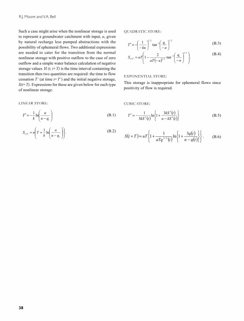
Appendix B:

Groundwater abstraction, negativestorage and ephemeral flowsWhen the input, u, to the nonlinear storage is allowed to benegative and the storage is allowed to develop negativevalues, with no outflow, then additional theory is required.


38

Such a case might arise when the nonlinear storage is usedto represent a groundwater catchment with input, u, givenby natural recharge less pumped abstractions with thepossibility of ephemeral flows. Two additional expressionsare needed to cater for the transition from the normalnonlinear storage with positive outflow to the case of zerooutflow and a simple water balance calculation of negativestorage values. If (t, t+T) is the time interval containing thetransition then two quantities are required: the time to flowcessation T´ (at time t+T´) and the initial negative storage,S(t+T). Expressions for these are given below for each typeof nonlinear storage.

LINEAR STORE:

−

−=′tqu

uk

T ln1 (B.1)

.ln1

−

+=+t

Tt quu

kTuS (B.2)

QUADRATIC STORE:

2/11

2/1

tan1

−

−−=′ −

uq

kuT t (B.3)

( ) .tan212/1

12/1

−−−= −

+ uq

uaTuTS t

Tt

(B.4)

EXPONENTIAL STORE:

This storage is inappropriate for ephemeral flows sincepositivity of flow is required.

CUBIC STORE:

( )( )( )

−+−=′

tkSutkS

tkST 3

3

2

31ln3

1 (B.5)

( ) ( )( )( ) .31ln11 3/2

−++=+

tqutq

taTquTTtS (B.6)

Documents

Incorporation of groundwater losses and well level data in ... · Incorporation of groundwater losses and well level data in rainfall-runoff models illustrated using the ... Solutions