Incorporating Spatial Similarity into Ensemble Clustering

M. Hidayath AnsariDept. of Computer Sciences

University ofWisconsin-MadisonMadison, WI, USA

ansari@cs.wisc.edu

Nathanael FillmoreDept. of Computer Sciences

University ofWisconsin-MadisonMadison, WI, USA

nathanae@cs.wisc.edu

Michael H. CoenDept. of Computer Sciences

Dept. of Biostatistics andMedical Informatics

University ofWisconsin-MadisonMadison, WI, USA

mhcoen@cs.wisc.edu

ABSTRACTThis paper addresses a fundamental problem in ensembleclustering – namely, how should one compare the similarityof two clusterings? The vast majority of prior techniquesfor comparing clusterings are entirely partitional, i.e., theyexamine assignments of points in set theoretic terms afterthey have been partitioned. In doing so, these methods ig-nore the spatial layout of the data, disregarding the factthat this information is responsible for generating the clus-terings to begin with. In this paper, we demonstrate theimportance of incorporating spatial information into form-ing ensemble clusterings. We investigate the use of a re-cently proposed measure, called CDistance, which uses bothspatial and partitional information to compare clusterings.We demonstrate that CDistance can be applied in a well-motivated way to four areas fundamental to existing ensem-ble techniques: the correspondence problem, subsampling,stability analysis and diversity detection.

Categories and Subject DescriptorsI5.3 [Clustering]: Similarity Measures

KeywordsEnsemble methods, Comparing clusterings, Clustering sta-bility, Clustering robustness

1. INTRODUCTIONMany of the most exciting recent advances in clustering

seek to take advantage of “ensembles” of outputs of cluster-ing algorithms.

Ensemble methods have the potential to provide severalimportant benefits over single clustering algorithms. As dis-cussed in [1], advantages of ensemble techniques in clusteringproblems include improved robustness across datasets anddomains, increased stability of clustering solutions, and per-haps most importantly, the ability to construct clusterings

Permission to make digital or hard copies of all or part of this work forpersonal or classroom use is granted without fee provided that copies arenot made or distributed for profit or commercial advantage and that copiesbear this notice and the full citation on the first page. To copy otherwise, torepublish, to post on servers or to redistribute to lists, requires prior specificpermission and/or a fee.MultiClust KDD 2010 Washington, DC, USACopyright 2010 ACM X-XXXXX-XX-X/XX/XX ...$10.00.

not individually attainable by any single algorithm.Ensemble methods generally rely, at least implicitly–and

often explicitly–on a notion of a distance or similarity be-tween clusterings. This is not surprising; for example, if thestability of a clustering algorithm is taken to mean that thealgorithm does not produce highly different outputs on verysimilar inputs, then in order to measure stability one mustbe able to determine exactly how similar such outputs areto each other. These inputs can be perturbed versions ofeach other or one may be a subsample of the other. Like-wise, in order to create an integrated ensemble clusteringfrom several individual clusterings information about whichclusterings are more similar or less similar or which parts ofwhich clusterings are compatible with each other and can becombined is frequently useful.

Previous approaches to ensemble clustering have gener-ally used “partitional” techniques to measure similarity be-tween clusterings, i.e., they do not take into account spatialinformation about the points in each clustering, but onlytheir identities. Such techniques include the Hubert-Arabieindex [14], the Rand index [19], van Dongen’s metric [22],Variation of Information [17], and nearly all other previouswork on comparing clusterings [5]. As Table 1 shows, it is inmany contexts a major weakness to ignore spatial informa-tion in clustering comparisons, because ignoring the locationof data points for which labels change across clusterings canlead to a misleading quantification of the difference betweenthe clusterings.

The present paper proposes the use of a very recentlyintroduced method for comparing clusterings, called CDis-tance [5], which incorporates spatial information aboutpoints in each clustering. Specifically, as we show later inSection 3 and in more detail in [5], CDistance gives us ameasure of the extent to which the constituent clusters ofeach clustering overlap with the other. We have found thatCDistance is an effective tool to measure the similarity ofmultiple clusterings.

It should be stressed that the goal of this paper is notto introduce an end-to-end ensemble clustering frameworkbut rather to introduce more robust alternatives for stepsin the generation, evaluation and combination of clusteringscommonly used in ensemble methods. We provide a brieftheoretical treatment of selected issues arising in popular en-semble clustering techniques. Specifically, we identify fourcritical areas in which CDistance can be used in existing en-semble clustering techniques: the correspondence problem,subsampling, stability analysis, and detecting diversity.

In Section 2 we establish preliminary definitions and no-tation, and in Section 3 we construct CDistance. We givea short introduction to ensemble clustering in Section 4. InSection 5 we discuss how CDistance can be applied in thesetting of ensemble clustering. We discuss related work inSection 6, and indicate directions for future work in Sec-tion 7.

2. PRELIMINARIESAs a brief introduction (further detail is provided in Sec-

tion 3), CDistance works as follows. Given two clusteringswe first compute a pairwise distance matrix between eachcluster in one to clusters in the other. The distance func-tion used takes into account the interpoint distances betweenelements of the two clusters being compared and is calledOptimal Transportation Distance. The clusterings can thenbe thought of as two subsets (consisting of their clustersas elements) of a metric space with Optimal Transporta-tion Distance as the metric, where we know the value of themetric at each point of interest (the entries of the matrix).We then compute the so-called Similarity Distance betweenthese two collections; Similarity Distance between two pointsets in a metric space measures the degree to which theyoverlap in that space, in a sense we will make precise.

In the following subsections, we construct the componentsrequired to compute CDistance. CDistance is defined interms of optimal transportation distance and naive trans-portation distance, and we begin by briefly describing these.

2.1 ClusteringA (hard) clustering A is a partition of a dataset D into

sets A1, A2, . . . , AK called clusters such that

Ai ∩Aj = ∅ for all i 6= j, and

K⋃k=1

Ak = D.

We assume D, and therefore A1, . . . , Ak, are finite subsetsof a metric space (Ω, dΩ).

2.2 Optimal Transportation DistanceThe optimal transportation problem [13, 18] asks what is

the cheapest way to move a set of masses from sources tosinks, who are some distance away? Here cost is definedas the total mass × distance moved. For example, one canthink of the sources as factories and the sinks as warehousesto make the problem concrete. We assume that the sourcesare shipping exactly as much mass as the sinks are expecting.

Formally, in the optimal transportation problem, we aregiven weighted point sets (A, p) and (B, q), where A =a1, . . . , a|A| is a finite subset of the metric space (Ω, dΩ),p = (p1, . . . , p|A|) is a vector of associated nonnegativeweights summing to one, and similar definitions hold forB and q.

The optimal transportation distance between (A, p) and(B, q) is defined as

dOT(A,B; p, q, dΩ) =

|A|∑i=1

|B|∑j=1

f∗ij dΩ(ai, bj),

where the optimal flow F ∗ = (f∗ij) between (A, p) and (B, q)

is the solution of the linear program

minimize

|A|∑i=1

|B|∑j=1

fij dΩ(ai, bj) over F = (fij) subj. to

fij ≥ 0, 1 ≤ i ≤ |A|, 1 ≤ j ≤ |B|∑|B|j=1 fij = pi, 1 ≤ i ≤ |A|∑|A|i=1 fij = qj , 1 ≤ j ≤ |B|∑|A|

i=1

∑|B|j=1 fij = 1.

It is useful to view the optimal flow as a representationof the maximally cooperative way to transport masses be-tween sources and sinks. Here, cooperative means that thesources are allowed to exchange delivery obligations in orderto transport their masses with a globally minimal cost.

2.3 Naive Transportation DistanceIn contrast with the optimal algorithm proposed above,

we define here a naive solution to the transportation prob-lem. Here, the sources are all responsible for individuallydistributing their masses proportionally to the sinks. In thiscase, none of the sources cooperate, leading to inefficiencyin shipping the overall mass to the sinks.

Formally, in the naive transportation problem, we aregiven weighted point sets (A, p) and (B, q) as above. Wedefine the naive transportation distance between (A, p) and(B, q) as

dNT(A,B; p, q, dΩ) =

|A|∑i=1

|B|∑j=1

pi qj dΩ(ai, bj).

2.4 Similarity DistanceOur next definition concerns the relationship between the

optimal transportation distance and the naive transporta-tion distance. Here we are interested in the degree to whichcooperation reduces the cost of moving the source A onto thesink B.

Formally, we are given weighted point sets (A, p) and(B, q) as above. We define the similarity distance between(A, p) and (B, q) as the ratio

dS(A,B; p, q, dΩ) =dOT(A,B; p, q, dΩ)

dNT(A,B; p, q, dΩ).

When A and B perfectly overlap, there is no cost to mov-ing A onto B, so both the optimal transportation distanceand the similarity distance between A and B are 0. On theother hand, when A and B are very distant from each other,each point in A is much closer to all other points in A thanto any points in B, and vice-versa. Thus, in this case, co-operation does not yield any significant benefit, so dOT isnearly as large as dNT, and dS is close to 1. (This behavioris illustrated in Figure 1.)

In this sense, the similarity distance between two pointsets measures the degree to which they spatially overlap,or are “similar”, to each other. (Note, the relationship isactually inverse; similarity distance is the degree of spatialoverlap subtracted from one.) Another illustration of thisbehavior is given in Figure 2. Each panel in this figureshows two overlapping point sets to which we assign uni-form weight distributions. The degree of spatial overlap ofthe two point sets in Example A is far higher than the de-gree of spatial overlap of the point sets in Example B, eventhough in absolute terms the amount of work required to

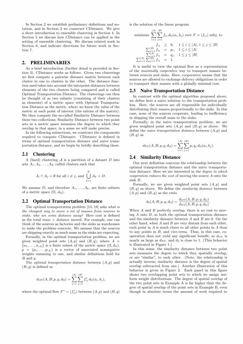
Table 1: Distances to Modified Clusterings [5]. Each row in Table 1(a) depicts a dataset with points coloredaccording to a reference clustering R (left column) and two different modifications of this clustering (centerand right columns). For each example, Table 1(b) presents the distance between the reference clusteringand each modification for the indicated clustering comparison techniques. The column labeled “?” indicateswhether the technique provides sensible output. In Examples 1–3, we only modify cluster assignments; thepoints are stationary. Since the pairwise relationships among the points change in the same way in eachmodification, only ADCO and CDistance detect that the modifications are not identical with respect to thereference. In Example 4, the reference clustering is modified by moving three points of the bottom rightcluster by small amounts. However, in Modification 1, the points do not move across a bin boundary, whereasin Modification 2, the points do move across a bin boundary. As a result, ADCO detects no change betweenModification 1 and the reference clustering but detects a large change between Modification 2 and thereference clustering, even though the two modifications differ by only a small amount. CDistance correctlyreports a similar change between Modification 1 and the reference and Modification 2 and the reference.(Since the points actually move, other clustering comparison techniques are not applicable to this example.)

Table 1(a)Reference Clustering (R) Modification 1 Modification 2

Example 1

Example 2

Example 3

1

2

1

2

1

2

Example 4

Table 1(b)Technique Example 1 Example 2 Example 3 Example 4

Name d(R,1) d(R,2) ? d(R,1) d(R,2) ? d(R,1) d(R,2) ? d(R,1) d(R,2) ?

Hubert 0.38 0.38 7 0.04 0.04 7 0.25 0.25 7 N/A N/A 71− Rand 0.00 0.00 7 0.05 0.05 7 0.00 0.00 7 N/A N/A 7van Dongen 0.18 0.18 7 0.05 0.05 7 0.13 0.13 7 N/A N/A 7VI 5.22 5.22 7 11.31 11.31 7 5.89 5.89 7 N/A N/A 7Zhou 8.24 8.24 7 0.90 0.90 7 10.0 10.0 7 N/A N/A 7ADCO 0.11 0.17 3 0.02 0.04 3 0.07 0.09 3 0.00 0.07 7

CDistance 0.61 0.73 3 0.06 0.18 3 0.41 0.56 3 0.08 0.09 3

−2 0 2 4 6 8−3

−2

−1

0

1

2

3

∆

0 2 4 6 80

0.2

0.4

0.6

0.8

1

Separating distance ∆

Sim

ilarity

Dis

tance

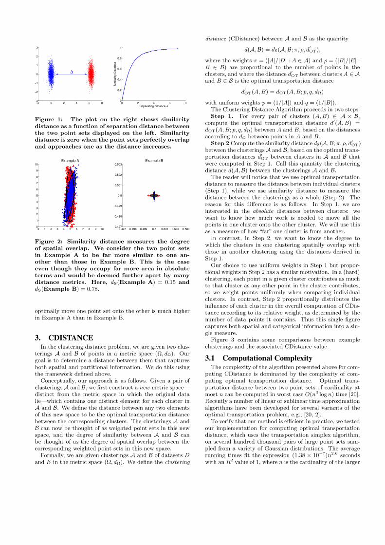
Figure 1: The plot on the right shows similaritydistance as a function of separation distance betweenthe two point sets displayed on the left. Similaritydistance is zero when the point sets perfectly overlapand approaches one as the distance increases.

0 1 2 3 4 5 6 7 8 9 100

1

2

3

4

5

6

7

8

9

10

Example A

0.497 0.498 0.499 0.5 0.501 0.502 0.5030.497

0.498

0.499

0.5

0.501

0.502

0.503

Example B

Figure 2: Similarity distance measures the degreeof spatial overlap. We consider the two point setsin Example A to be far more similar to one an-other than those in Example B. This is the caseeven though they occupy far more area in absoluteterms and would be deemed further apart by manydistance metrics. Here, dS(Example A) = 0.15 anddS(Example B) = 0.78.

optimally move one point set onto the other is much higherin Example A than in Example B.

3. CDISTANCEIn the clustering distance problem, we are given two clus-

terings A and B of points in a metric space (Ω, dΩ). Ourgoal is to determine a distance between them that capturesboth spatial and partitional information. We do this usingthe framework defined above.

Conceptually, our approach is as follows. Given a pair ofclusterings A and B, we first construct a new metric space—distinct from the metric space in which the original datalie—which contains one distinct element for each cluster inA and B. We define the distance between any two elementsof this new space to be the optimal transportation distancebetween the corresponding clusters. The clusterings A andB can now be thought of as weighted point sets in this newspace, and the degree of similarity between A and B canbe thought of as the degree of spatial overlap between thecorresponding weighted point sets in this new space.

Formally, we are given clusterings A and B of datasets Dand E in the metric space (Ω, dΩ). We define the clustering

distance (CDistance) between A and B as the quantity

d(A,B) = dS(A,B;π, ρ, d′OT),

where the weights π = (|A|/|D| : A ∈ A) and ρ = (|B|/|E| :B ∈ B) are proportional to the number of points in theclusters, and where the distance d′OT between clusters A ∈ Aand B ∈ B is the optimal transportation distance

d′OT(A,B) = dOT(A,B; p, q, dΩ)

with uniform weights p = (1/|A|) and q = (1/|B|).The Clustering Distance Algorithm proceeds in two steps:Step 1. For every pair of clusters (A,B) ∈ A × B,

compute the optimal transportation distance d′(A,B) =dOT(A,B; p, q, dΩ) between A and B, based on the distancesaccording to dΩ between points in A and B.

Step 2 Compute the similarity distance dS(A,B;π, ρ, d′OT)between the clusteringsA and B, based on the optimal trans-portation distances d′OT between clusters in A and B thatwere computed in Step 1. Call this quantity the clusteringdistance d(A,B) between the clusterings A and B.

The reader will notice that we use optimal transportationdistance to measure the distance between individual clusters(Step 1), while we use similarity distance to measure thedistance between the clusterings as a whole (Step 2). Thereason for this difference is as follows. In Step 1, we areinterested in the absolute distances between clusters: wewant to know how much work is needed to move all thepoints in one cluster onto the other cluster. We will use thisas a measure of how “far” one cluster is from another.

In contrast, in Step 2, we want to know the degree towhich the clusters in one clustering spatially overlap withthose in another clustering using the distances derived inStep 1.

Our choice to use uniform weights in Step 1 but propor-tional weights in Step 2 has a similar motivation. In a (hard)clustering, each point in a given cluster contributes as muchto that cluster as any other point in the cluster contributes,so we weight points uniformly when comparing individualclusters. In contrast, Step 2 proportionally distributes theinfluence of each cluster in the overall computation of CDis-tance according to its relative weight, as determined by thenumber of data points it contains. Thus this single figurecaptures both spatial and categorical information into a sin-gle measure.

Figure 3 contains some comparisons between exampleclusterings and the associated CDistance value.

3.1 Computational ComplexityThe complexity of the algorithm presented above for com-

puting CDistance is dominated by the complexity of com-puting optimal transportation distance. Optimal trans-portation distance between two point sets of cardinality atmost n can be computed in worst case O(n3 logn) time [20].Recently a number of linear or sublinear time approximationalgorithms have been developed for several variants of theoptimal transportation problem, e.g., [20, 2].

To verify that our method is efficient in practice, we testedour implementation for computing optimal transportationdistance, which uses the transportation simplex algorithm,on several hundred thousand pairs of large point sets sam-pled from a variety of Gaussian distributions. The averagerunning times fit the expression (1.38 × 10−7)n2.6 secondswith an R2 value of 1, where n is the cardinality of the larger

1 2

3

1

2

3

(a)

1 2

3

1 2

3

(b)

1

2

3

1

2

34

5

6

(c)

1 2

1

2

(d)

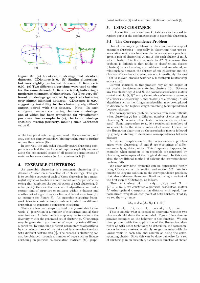
Figure 3: (a) Identical clusterings and identicaldatasets. CDistance is 0. (b) Similar clusterings,but over slightly perturbed datasets. CDistance is0.09. (c) Two different algorithms were used to clus-ter the same dataset. CDistance is 0.4, indicating amoderate mismatch of clusterings. (d) Two very dif-ferent clusterings generated by spectral clusteringover almost-identical datasets. CDistance is 0.90,suggesting instability in the clustering algorithm’soutput paired with this dataset. Note: In eachsubfigure, we are comparing the two clusterings,one of which has been translated for visualizationpurposes. For example, in (a), the two clusteringsspatially overlap perfectly, making their CDistancevalue 0.

of the two point sets being compared. For enormous pointsets, one can employ standard binning techniques to furtherreduce the runtime [15].

In contrast, the only other spatially aware clustering com-parison method that we know of requires explicitly enumer-ating the exponential space of all possible permutations ofmatches between clusters in A to clusters in B [3].

4. ENSEMBLE CLUSTERINGAn ensemble clustering is a consensus clustering of a

dataset D based on a collection of R clusterings. The goalis to combine aspects of each of these clusterings in a mean-ingful way so as to obtain a more robust and “superior” clus-tering that combines the contributions of each clustering. Itis frequently the case that one set of algorithms can find acertain kind of structure or patterns within a dataset andanother set of algorithms can find a different structure (foran example see Figure 7). An ensemble clustering frame-work tries to constructively combine inputs from differentclusterings to generate a consensus clustering.

There are two main steps involved in any ensemble frame-work: 1) generation of a number of clusterings, and 2) theircombination. An intermediate step may be to evaluate thediversity within the generated set of clusterings. Clusteringsmay be generated by a number of ways: by using differentalgorithms, by supplying different parameters to algorithms,by clustering subsets of the data and by clustering the datawith different feature sets [8]. The consensus clustering canalso be obtained through a number of ways such as linkageclustering on pairwise co-association matrices [21], graph-

based methods [9] and maximum likelihood methods [1].

5. USING CDISTANCEIn this section, we show how CDistance can be used to

replace parts of the combination step in ensemble clustering.

5.1 The Correspondence ProblemOne of the major problems in the combination step of

ensemble clustering - especially in algorithms that use co-association matrices - has been the correspondence problem:given a pair of clusterings A and B, for each cluster A in A,which cluster B in B corresponds to A? The reason thisproblem is difficult is that unlike in classification, classes(clusters) in a clustering are unlabeled and unordered, sorelationships between the clusters of one clustering and theclusters of another clustering are not immediately obvious- nor is it even obvious whether a meaningful relationshipexists at all.

Current solutions to this problem rely on the degree ofset overlap to determine matching clusters [10]. Betweenany two clusterings A and B, the pairwise association matrixcontains at the (i, j)th entry the number of elements commonto cluster i of clustering A and cluster j of clustering B. Analgorithm such as the Hungarian algorithm may be employedto determine the highest weight matching (correspondence)between clusters.

The correspondence problem becomes even more difficultwhen clustering A has a different number of clusters thanclustering B. What are the cluster correspondences in thatcase? Some approaches (e.g., [6]) restrict all members ofan ensemble to the same number of clusters. Others usethe Hungarian algorithm on the association matrix followedby greedy matching to determine correspondences betweenclusters.

A further complication to the correspondence problemarises when clusterings A and B are clusterings of differ-ent underlying data points. This frequently happens, forexample, when members of an ensemble are generated byclustering subsamples of the original dataset. In this casealso, the traditional method of solving the correspondenceproblem fails.

We show how both problems can be approached neatlyusing CDistance in this section and section 5.2. We for-mulate an elegant solution to the correspondence problem,that also addresses these complications, using a variant ofthe first step of CDistance, as follows.

Given clusterings A = A1, . . . , An and B =B1, . . . , Bm, we construct a pairwise association matrixM using optimal transportation distance with equal, “un-normalized” weights on each point of both clusters. That is,we set the (i, j) entry

Mij = dOT(Ai, Bj ; 1,1, dΩ),

where 1 = (1, . . . , 1), for i = 1, . . . , n and j = 1, . . . ,m.This is exactly what is needed to determine whether two

clusters should share the same label. Figure 6 has demon-strative examples on the behavior of this function. We canthen proceed with the application of the Hungarian algo-rithm as with other techniques to determine the correspon-dences between clusters, or simply assign the entry with thelowest value in each row and column as being the corre-sponding cluster. Since this can be done pair-wise for a setof clusterings in an ensemble, a consensus function of choice

may then be applied in order to generate the integrated clus-tering.

The idea is that we can conjecture with more confidencethat two clusters correspond to each other if we know theyoccupy similar regions in space, rather than if their pointsshare membership more than with other clusters. Looking atthe actual data and the space it occupies is more informativethan looking at the labels alone.

Another advantage that comes with this method is theabsence of any requirement on the point sets being the samein the two clusterings. For label-based correspondence solu-tions, set arithmetic is performed on point labels, the under-lying points of which must stay the same in both clusterings.The generality of dOT allows any two point sets to be givento it as input.

Finally, yet another advantage with using this techniqueis that it is able to determine matches between a whole clus-ter on one side and smaller clusters on the other side thatwhen taken together correspond to the first cluster. An il-lustration of this can be seen in Figures 4 and 5 where thecriss-crossing lines indicate matches between clusters withzero or almost-zero dOT value.

5.2 SubsamplingMany ensemble clustering methods use subsampling to

generate multiple clusterings (e.g., [9]). A fraction of thedata is sampled at random, with or without replacement,and clustered in each run. Comparison, if needed, is typi-cally performed via one of a number of partitional methods.In this subsection, we illustrate how, instead of relying ona partitional method, CDistance can be used to compareclusterings from subsampled datasets.

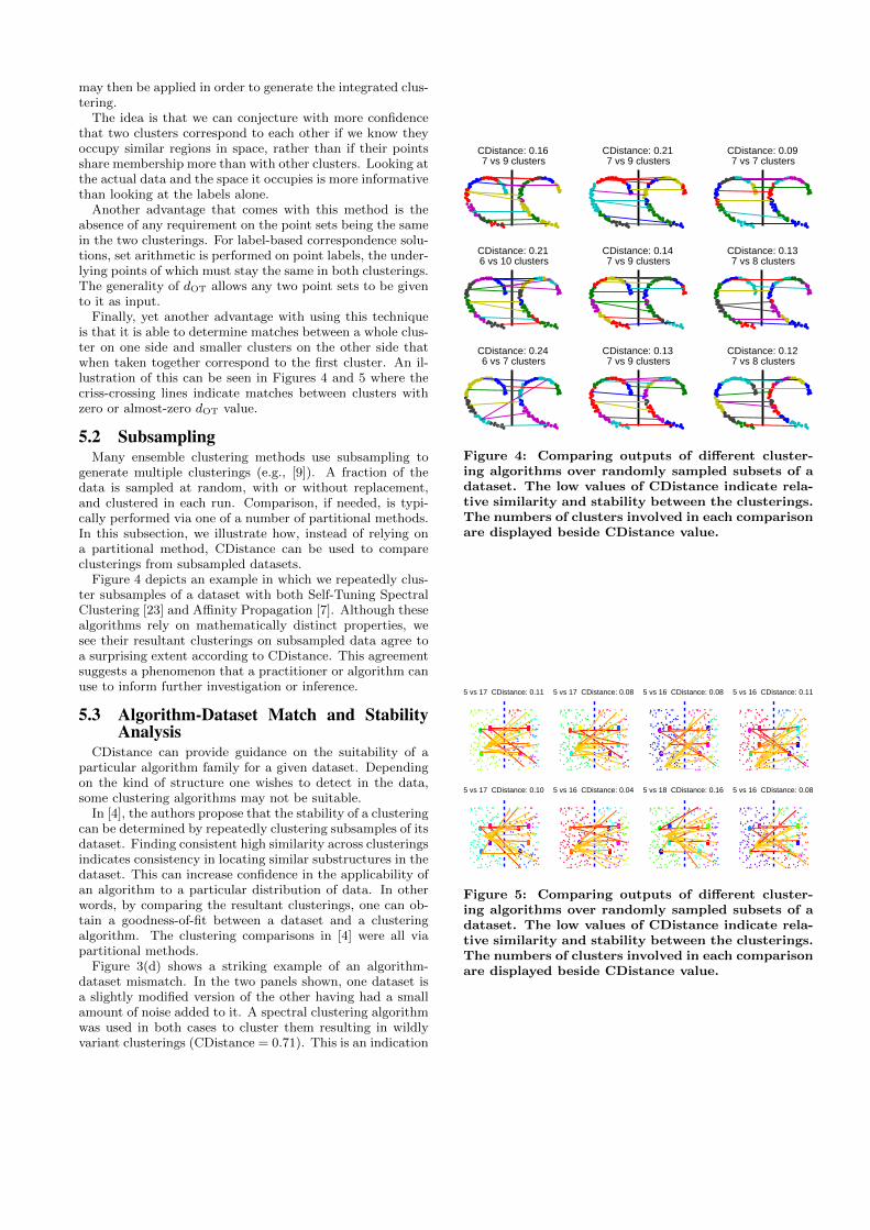
Figure 4 depicts an example in which we repeatedly clus-ter subsamples of a dataset with both Self-Tuning SpectralClustering [23] and Affinity Propagation [7]. Although thesealgorithms rely on mathematically distinct properties, wesee their resultant clusterings on subsampled data agree toa surprising extent according to CDistance. This agreementsuggests a phenomenon that a practitioner or algorithm canuse to inform further investigation or inference.

5.3 Algorithm-Dataset Match and StabilityAnalysis

CDistance can provide guidance on the suitability of aparticular algorithm family for a given dataset. Dependingon the kind of structure one wishes to detect in the data,some clustering algorithms may not be suitable.

In [4], the authors propose that the stability of a clusteringcan be determined by repeatedly clustering subsamples of itsdataset. Finding consistent high similarity across clusteringsindicates consistency in locating similar substructures in thedataset. This can increase confidence in the applicability ofan algorithm to a particular distribution of data. In otherwords, by comparing the resultant clusterings, one can ob-tain a goodness-of-fit between a dataset and a clusteringalgorithm. The clustering comparisons in [4] were all viapartitional methods.

Figure 3(d) shows a striking example of an algorithm-dataset mismatch. In the two panels shown, one dataset isa slightly modified version of the other having had a smallamount of noise added to it. A spectral clustering algorithmwas used in both cases to cluster them resulting in wildlyvariant clusterings (CDistance = 0.71). This is an indication

CDistance: 0.16 7 vs 9 clusters

CDistance: 0.21 7 vs 9 clusters

CDistance: 0.09 7 vs 7 clusters

CDistance: 0.21 6 vs 10 clusters

CDistance: 0.14 7 vs 9 clusters

CDistance: 0.13 7 vs 8 clusters

CDistance: 0.24 6 vs 7 clusters

CDistance: 0.13 7 vs 9 clusters

CDistance: 0.12 7 vs 8 clusters

Figure 4: Comparing outputs of different cluster-ing algorithms over randomly sampled subsets of adataset. The low values of CDistance indicate rela-tive similarity and stability between the clusterings.The numbers of clusters involved in each comparisonare displayed beside CDistance value.

5 vs 17 CDistance: 0.11 5 vs 17 CDistance: 0.08 5 vs 16 CDistance: 0.08 5 vs 16 CDistance: 0.11

5 vs 17 CDistance: 0.10 5 vs 16 CDistance: 0.04 5 vs 18 CDistance: 0.16 5 vs 16 CDistance: 0.08

Figure 5: Comparing outputs of different cluster-ing algorithms over randomly sampled subsets of adataset. The low values of CDistance indicate rela-tive similarity and stability between the clusterings.The numbers of clusters involved in each comparisonare displayed beside CDistance value.

that spectral clustering is not an appropriate algorithm touse on this dataset.

In Figures 4 and 5 we see multiple clusterings generatedby clustering subsamples and clustering data with smallamounts of noise added respectively. In both cases we seethat CDistance maintains a relatively low value across in-stances and can conclude that the clusterings remain stablewith this dataset and algorithm combination.

5.4 Detecting DiversitySome amount of diversity in clusters constituting the en-

semble is crucial to the improvement of the final generatedclustering [12]. In the previous subsection we noted thatCDistance was able to detect similarity between clusteringsof subsets of a dataset. A corollary of that is that CDistanceis also able to detect diversity in members of an ensem-ble. Previous methods have used the Adjusted Rand Indexor other such metrics to quantify diversity. As we demon-strate in Section 6, these measures are surprisingly insensi-tive to large differences in clusterings. CDistance providesa smoother, spatially-sensitive measure of the similarity ordissimilarity of two clusterings leading to a more effectivecharacterization of diversity within an ensemble. Measure-ment of diversity using CDistance can guide the generationstep by indicating whether the members of an ensemble aresufficiently diverse or differ from each other only minutely.

5.5 Graph-based methodsSeveral ensemble clustering frameworks employ graph-

based algorithms for the combination step [11, 8]. One pop-ular idea is to construct a suitable graph taking into ac-count the similarity between clusterings and derive a graphcut or partition that optimizes some objective function. [9]describes three main graph-based methods: instance-based,cluster-based and hypergraph partitioning, also discussed in[21]. The cluster-based formulation in particular requiresa measure of similarity between clusters, originally the Jac-card Index. The unsuitability of this index and other relatedindices are discussed in Section 6.

CDistance can be easily substituted here as a more in-formative way of measuring similarity between clusteringsspecifically because it exploits both spatial and partitionalinformation about the data.

5.6 ExampleAs an example of CDistance being used in an ensemble

clustering framework we applied it to an image segmenta-tion problem. Segmentations of images can be viewed asclusterings of their constituent pixels.

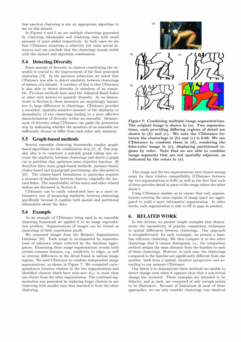
We examined images from the Berkeley SegmentationDatabase [16]. Each image is accompanied by segmenta-tions of unknown origin collected by the database aggre-gators. Examining these image segmentations reveals bothcertain common features, e.g., sensitivity to edges, as wellas extreme differences in the detail found in various imageregions. We used CDistance to combine independent imagesegmentations, as shown in Figure 7. We computed corre-spondences between clusters in the two segmentations andidentified clusters which have near-zero dOT to more thanone cluster from the other segmentation. The combined seg-mentation was generated by replacing larger clusters in oneclustering with smaller ones that matched it from the otherclustering.

Figure 7: Combining multiple image segmentations.The original image is shown in (a). Two segmenta-tions, each providing differing regions of detail areshown in (b) and (c). We note the CDistance be-tween the clusterings in (b) and (c) is 0.09. We useCDistance to combine them in (d), rendering thefalse-color image in (e), displaying partitioned re-gions by color. Note that we are able to combineimage segments that are not spatially adjacent, asindicated by the colors in (e).

This image and the two segmentations were chosen amongmany for their relative compatibility (CDistance betweenthe two segmentations is 0.09) as well as the fact that eachof them provides detail in parts of the image where the otherdoesn’t.

Using CDistance enables us to ensure that only segmen-tations covering the same regions of image space are aggre-gated to yield a more informative segmentation. In otherwords, each segmentation is able to fill in gaps in another.

6. RELATED WORKIn this section, we present simple examples that demon-

strate the insensitivity of popular comparison techniquesto spatial differences between clusterings. Our approachis straightforward: for each technique, we present a base-line reference clustering. We then compare it to two otherclusterings that it cannot distinguish, i.e., the comparisonmethod assigns the same distance from the baseline to eachof these clusterings. However, in each case, the clusteringscompared to the baseline are significantly different from oneanother, both from a spatial, intuitive perspective and ac-cording to our measure CDistance.

Our intent is to demonstrate these methods are unable todetect change even when it appears clear that a non-trivialchange has occurred. These examples are intended to bedidactic, and as such, are composed of only enough pointsto be illustrative. Because of limitations in most of theseapproaches, we can only consider clusterings over identical

2 3 4 52

3

4

5

6

12

2 3 4 52

3

4

5

6

1 2

2 3 4 52

3

4

5

6

12

2 3 4 52

3

4

5

6

1

2

3

2 3 42

3

4

5

6

1 2

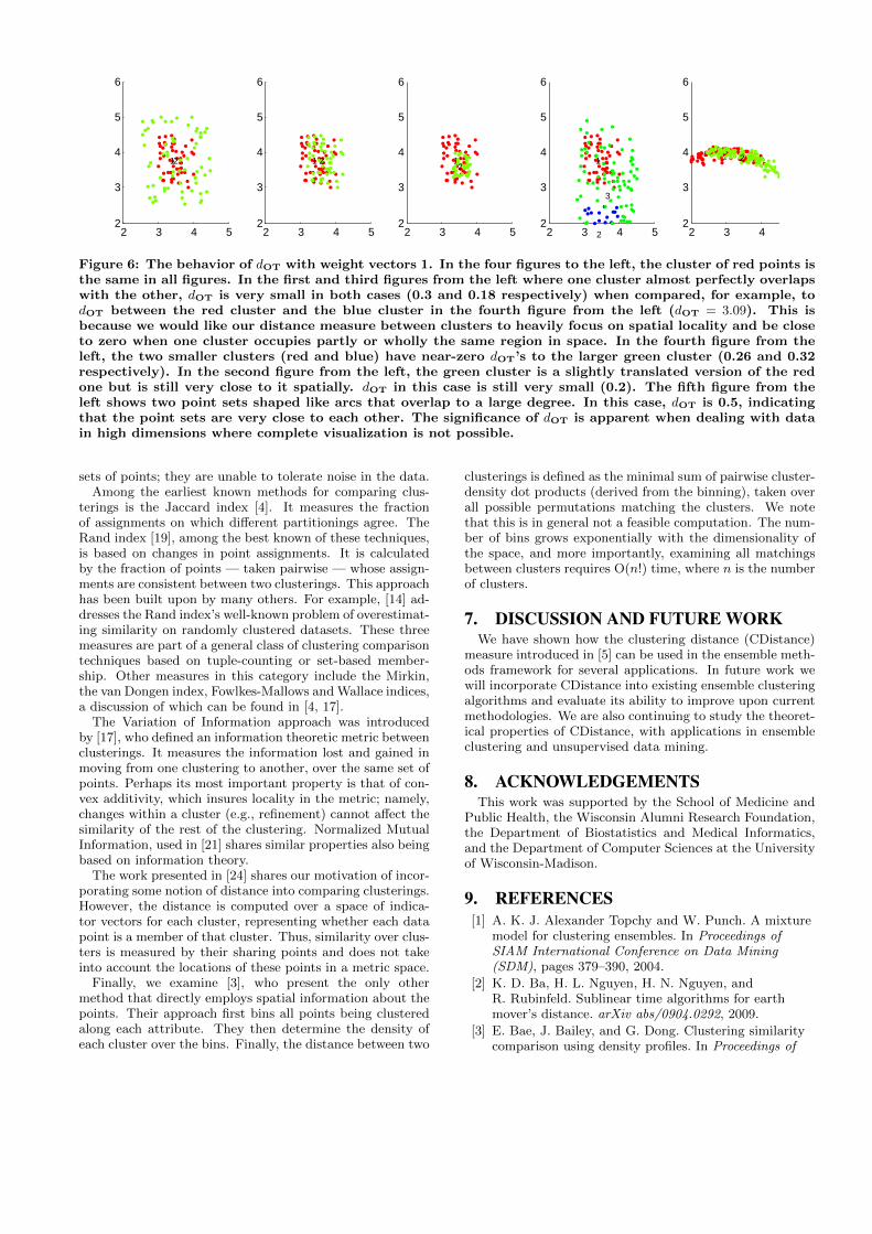
Figure 6: The behavior of dOT with weight vectors 1. In the four figures to the left, the cluster of red points isthe same in all figures. In the first and third figures from the left where one cluster almost perfectly overlapswith the other, dOT is very small in both cases (0.3 and 0.18 respectively) when compared, for example, todOT between the red cluster and the blue cluster in the fourth figure from the left (dOT = 3.09). This isbecause we would like our distance measure between clusters to heavily focus on spatial locality and be closeto zero when one cluster occupies partly or wholly the same region in space. In the fourth figure from theleft, the two smaller clusters (red and blue) have near-zero dOT’s to the larger green cluster (0.26 and 0.32respectively). In the second figure from the left, the green cluster is a slightly translated version of the redone but is still very close to it spatially. dOT in this case is still very small (0.2). The fifth figure from theleft shows two point sets shaped like arcs that overlap to a large degree. In this case, dOT is 0.5, indicatingthat the point sets are very close to each other. The significance of dOT is apparent when dealing with datain high dimensions where complete visualization is not possible.

sets of points; they are unable to tolerate noise in the data.Among the earliest known methods for comparing clus-

terings is the Jaccard index [4]. It measures the fractionof assignments on which different partitionings agree. TheRand index [19], among the best known of these techniques,is based on changes in point assignments. It is calculatedby the fraction of points — taken pairwise — whose assign-ments are consistent between two clusterings. This approachhas been built upon by many others. For example, [14] ad-dresses the Rand index’s well-known problem of overestimat-ing similarity on randomly clustered datasets. These threemeasures are part of a general class of clustering comparisontechniques based on tuple-counting or set-based member-ship. Other measures in this category include the Mirkin,the van Dongen index, Fowlkes-Mallows and Wallace indices,a discussion of which can be found in [4, 17].

The Variation of Information approach was introducedby [17], who defined an information theoretic metric betweenclusterings. It measures the information lost and gained inmoving from one clustering to another, over the same set ofpoints. Perhaps its most important property is that of con-vex additivity, which insures locality in the metric; namely,changes within a cluster (e.g., refinement) cannot affect thesimilarity of the rest of the clustering. Normalized MutualInformation, used in [21] shares similar properties also beingbased on information theory.

The work presented in [24] shares our motivation of incor-porating some notion of distance into comparing clusterings.However, the distance is computed over a space of indica-tor vectors for each cluster, representing whether each datapoint is a member of that cluster. Thus, similarity over clus-ters is measured by their sharing points and does not takeinto account the locations of these points in a metric space.

Finally, we examine [3], who present the only othermethod that directly employs spatial information about thepoints. Their approach first bins all points being clusteredalong each attribute. They then determine the density ofeach cluster over the bins. Finally, the distance between two

clusterings is defined as the minimal sum of pairwise cluster-density dot products (derived from the binning), taken overall possible permutations matching the clusters. We notethat this is in general not a feasible computation. The num-ber of bins grows exponentially with the dimensionality ofthe space, and more importantly, examining all matchingsbetween clusters requires O(n!) time, where n is the numberof clusters.

7. DISCUSSION AND FUTURE WORKWe have shown how the clustering distance (CDistance)

measure introduced in [5] can be used in the ensemble meth-ods framework for several applications. In future work wewill incorporate CDistance into existing ensemble clusteringalgorithms and evaluate its ability to improve upon currentmethodologies. We are also continuing to study the theoret-ical properties of CDistance, with applications in ensembleclustering and unsupervised data mining.

8. ACKNOWLEDGEMENTSThis work was supported by the School of Medicine and

Public Health, the Wisconsin Alumni Research Foundation,the Department of Biostatistics and Medical Informatics,and the Department of Computer Sciences at the Universityof Wisconsin-Madison.

9. REFERENCES[1] A. K. J. Alexander Topchy and W. Punch. A mixture

model for clustering ensembles. In Proceedings ofSIAM International Conference on Data Mining(SDM), pages 379–390, 2004.

[2] K. D. Ba, H. L. Nguyen, H. N. Nguyen, andR. Rubinfeld. Sublinear time algorithms for earthmover’s distance. arXiv abs/0904.0292, 2009.

[3] E. Bae, J. Bailey, and G. Dong. Clustering similaritycomparison using density profiles. In Proceedings of

the 19th Australian Joint Conference on ArtificialIntelligence, pages 342–351. Springer LNCS, 2006.

[4] A. Ben-Hur, A. Elisseeff, and I. Guyon. A stabilitybased method for discovering structure in clustereddata. In Pacific Symposium on Biocomputing, pages6–17, 2002.

[5] M. H. Coen, M. H. Ansari, and N. Fillmore.Comparing clusterings in space. In ICML 2010:Proceedings of the 27th International Conference onMachine Learning (to appear), 2010.

[6] S. Dudoit and J. Fridlyand. Bagging to improve theaccuracy of a clustering procedure. Bioinformatics,19(9):1090–1099, 2003.

[7] D. Dueck and J. Frey, B. Non-metric affinitypropagation for unsupervised image categorization.IEEE International Conference on Computer Vision,0:1–8, 2007.

[8] X. Z. Fern and C. E. Brodley. Random projection forhigh dimensional data clustering: A cluster ensembleapproach. In Proceedings of 20th InternationalConference on Machine Learning, pages 186–193,2003.

[9] X. Z. Fern and C. E. Brodley. Solving cluster ensembleproblems by bipartite graph partitioning. In ICML’04: Proceedings of the twenty-first internationalconference on Machine learning, page 36, New York,NY, USA, 2004. ACM.

[10] A. Fred. Finding consistent clusters in data partitions.In In Proc. 3d Int. Workshop on Multiple Classifier,pages 309–318. Springer, 2001.

[11] A. L. N. Fred and A. K. Jain. Data clustering usingevidence accumulation. In ICPR, pages 276–280, 2002.

[12] S. T. Hadjitodorov, L. I. Kuncheva, and L. P.Todorova. Moderate diversity for better clusterensembles. Inf. Fusion, 7(3):264–275, 2006.

[13] F. Hillier and G. Lieberman. Introduction toMathematical Programming. McGraw-Hill, 1995.

[14] L. Hubert and P. Arabie. Comparing partitions.Journal of Classification, 2:193–218, 1985.

[15] E. Levina and P. Bickel. The earth mover’s distance isthe mallows distance: Some insights from statistics. InICCV, 2001.

[16] D. Martin, C. Fowlkes, D. Tal, and J. Malik. Adatabase of human segmented natural images and itsapplication to evaluating segmentation algorithms andmeasuring ecological statistics. In Proc. 8th Int’l Conf.Computer Vision, volume 2, pages 416–423, July 2001.

[17] M. Meila. Comparing clusterings: an axiomatic view.In ICML, 2005.

[18] S. T. Rachev and L. Ruschendorf. MassTransportation Problems: Volume I: Theory(Probability and its Applications). Springer, 1998.

[19] W. M. Rand. Objective criteria for the evaluation ofclustering methods. J. Amer. Statist. Assoc., pages846–850, 1971.

[20] S. Shirdhonkar and D. Jacobs. Approximate earth

moveraAZs distance in linear time. In CVPR, 2008.

[21] A. Strehl and J. Ghosh. Cluster ensembles — aknowledge reuse framework for combining multiplepartitions. J. Mach. Learn. Res., 3:583–617, 2003.

[22] S. van Dongen. Performance criteria for graph

clustering and markov cluster experiments. Technicalreport, National Research Institute for Mathematicsand Computer Science in the Netherlands, 2000.

[23] L. Zelnik-Manor and P. Perona. Self-tuning spectralclustering. In NIPS, 2004.

[24] D. Zhou, J. Li, and H. Zha. A new mallows distancebased metric for comparing clusterings. In Proceedingsof the 22nd International Conference on MachineLearning, pages 1028–1035, 2005.