Final Report: Incorporating Spatial Analysis of ForecastPerformance into the MET Package at the DTCM. E. Baldwin, Dept. of Earth and Atmospheric Sciences, Purdue Univ.

and K. L. Elmore, Cooperative Inst. for Mesoscale Meteorological Studies, Univ. of Oklahoma

1. Introduction

Among the vexing issues model developers face is understanding the spatial distribution

of forecast errors. In particular, the spatial distribution of long-term quantitative precipitation

forecast (QPF) errors are not discussed in the literature. Yet, insight into the spatial distribution of

such errors can lend valuable insight to model developers, helping them identify model processes

that lead to those errors and developing better model physics to address them.

Yet, almost all QPF verification statistics are comprehensive in nature: they are applied to

the entire model grid as a whole, yielding a single value. The root-mean-square error (RMSE) is

arguably the least useful in this regard and is used here as a primary example. It is easily imple-

mented but yields no insight whatsoever as to where QPF does particularly well or particularly

poorly. The equitable threat score (ETS) is another example. Regardless, most forecast model ver-

ification deals with comprehensive statistics applied to error grids in a wholesale way. At best,

they are applied to large regions defined over the CONUS in an attempt to understand something

about the spatial distribution of errors.

This work is aimed at directly and explicitly evaluating spatial bias errors in numerical

model forecasts. While precipitation is used as the driving example, this technique’s generality

must not be underestimated: this technique is applicable to any quantity or parameter that can be

both analyzed and forecast. The list of candidate variables is as long and varied as gridded analy-

sis can embrace. The list conceptually includes diagnosed fields, such as moisture advection,

3

energy flux, and momentum flux to name a few. In short: any conceivable diagnostic variable is

subject to spatial field significance verification. This technique can (and probably should) be

applied to the difference in these variables between two different models.

2. Methodology

The methodology used here descends directly from parametric ideas presented in Livezey

and Chen (1983). This generalizes the Livezey and Chen approach, making it non-parametric

through the use of bootstrap resampling and Monte Carlo techniques (Elmore et al. 2006).

Briefly, There are two separate significance levels that must be considered: local signifi-

cance and field significance. Local significance tests statistical significance based upon the

timeseries of errors at individual grid points. A moving blocks bootstrap (Efron and Tibshirani

1993; Davison and Hinkley 1997; Wilks 1997) is used to create 95% confidence intervals

(αp=0.05) around the mean bias errors at each grid point. A moving blocks bootstrap is used

because there is serial dependence in the errors at each grid point (the typical lag-1 autocorrela-

tion in the precipitation error ranges from almost 0.7 to -0.4). A moving blocks bootstrap differs

from a regular bootstrap in that the data are resampled in contiguous blocks, rather than by indi-

vidual values (Fig. 1). This technique helps preserve the autoregressive structure within the data.

Because moving blocks bootstrap resampling invariably results in some whitening of the time

series, more sophisticated methods for post-blackening must be employed if serial dependence is

a serious concern (Davison and Hinkley 1997). If the lag-1 autocorrelation at gridpoints that dis-

play the strongest autocorrelation is used as a benchmark, a block size of 7 seems reasonable for

these data and this application (Fig. 2)..

4

If the resulting confidence interval about the mean error does not contain zero, then the

individual grid point is considered to possess statistically significant bias. If the confidence inter-

val contains zero, the mean error at that grid point is not significantly different from zero. Hence,

the result of this test is binomial at each grid point. While this process is similar in concept to the

t-test, it is completely free from parametric assumptions.

Field significance is not quite so straightforward and depends on spatial correlation. Spa-

tial correlation describes how variations at one grid point are reflected at other grid points, due to

physical processes covering areas larger than the grid spacing. Spatial correlation is present in

nearly all meteorological fields. Were this not the case, plotted fields would possess no spatial

coherence and would look like noise. The more structure a field possesses, the noisier it looks; the

less structure it possesses, the smoother it looks. Fields rich in structure, but lacking in repeating

patterns, tend to lack spatial correlation. The amount of structure in a field may be likened to how

many independent modes are contained in the field (Livezey and Chen 1983; Wang and Shen

1999).

FIGURE 1. A schematic diagram of the moving blocks bootstrap for time series data. The black dotsare the original time series. A bootstrap resample of the time series (empty circles) is generated bychoosing a block length (“3” in this example) and sampling with replacement from all possiblecontiguous blocks. Note that the block size need not be a multiple of the time series length, andthat the set of blocks used for any particular resampling need not start at the first position (fromEfron and Tibshirani 1993, used with permission).

5

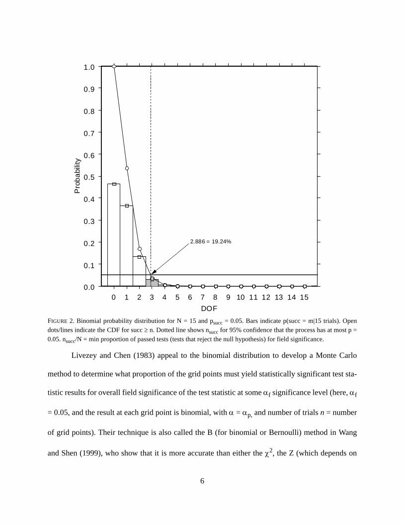
Livezey and Chen (1983) appeal to the binomial distribution to develop a Monte Carlo

method to determine what proportion of the grid points must yield statistically significant test sta-

tistic results for overall field significance of the test statistic at some αf significance level (here, αf

= 0.05, and the result at each grid point is binomial, with α = αp, and number of trials n = number

of grid points). Their technique is also called the B (for binomial or Bernoulli) method in Wang

and Shen (1999), who show that it is more accurate than either the χ2, the Z (which depends on

FIGURE 2. Binomial probability distribution for N = 15 and psucc = 0.05. Bars indicate p(succ = m|15 trials). Opendots/lines indicate the CDF for succ ≥ n. Dotted line shows nsucc for 95% confidence that the process has at most p =0.05. nsucc/N = min proportion of passed tests (tests that reject the null hypothesis) for field significance.

0 1 2 3 4 5 6 7 8 9 10 11 12 13 14 15DOF

0.0

0.1

0.2

0.3

0.4

0.5

0.6

0.7

0.8

0.9

1.0P

roba

bilit

y

2.886 = 19.24%

6

the Fisher Z transformation), or the S (which assumes that the ratio of the mean variance over the

variance of the mean yields the spatial degrees of freedom) methods. Wang and Shen (1999) also

show that about 3000 Monte Carlo trials are needed for a standard error of about 10% in the spa-

tial degrees-of-freedom estimate (or, alternatively, the estimate of the proportion of the grid occu-

pied by significant errors). For the sake of accuracy, 5000 Monte Carlo trials are used here.

Briefly, the Monte Carlo process under the B method proceeds as follows: 1) generate a

series of random numbers whose length equals the length of the error time series1. For example, if

there are 100 days of data, then this series contains 100 elements. 2) Compute the correlation

between this series and the time series of errors at each grid point; there are as many correlation

values as there are grid points. 3) Determine what proportion of these correlation values are statis-

tically significant (HOW IS THIS DONE?). After all trials are complete, determine the (1 - αf)

quantile of the resulting distribution. If the proportion of gridpoints with significant bias exceed

this threshold, the spatial bias has field significance. Thus, The B method returns the proportion of

gridpoints that could have significant errors at αp purely by chance, at some field-significance

level, αf. If the proportion of gridpoints with significant errors falls within the upper αf tail of the

Monte Carlo distribution, the errors possess field significance at αf. To compare the errors

1.Note that the random number series need not be normally distributed, though random

numbers drawn from an N(0,1) distribution are used here. If U is the vector of random

numbers and X is the time series at a grid point, then all that is required is that

E(XU) = E(U)E(X). In many cases, uniform random numbers are more stable, cheaper,

and easier to generate.

7

between two different models requires only the difference between two error fields; the rest of the

process remains identical.

Schematically, the steps of performing the analysis are:

1) Grid point significance:

a) Generate a matrix of forecast errors for each day, at each grid point. Thus, there will be

as many columns of data as there are days, and as many rows as there are grid points.

b) Estimate the lag-1 decorrelation period and use it to determine the block size for the

moving-blocks bootstrap.

c) At each gridpoint, estimate the distribution of the mean forecast bias using a moving

blocks bootstrap. Moving blocks bootstrap processes will never do harm to the resulting confi-

dence interval, even if there is no serial correlation.

d) Compute mean error and confidence limits based on the desired α-level at each grid

point.

e) Using the confidence limits computed in c), determine what proportion of grid points

contain significant bias errors, given by the number of grid points with bias errors significant at

αp divided by the total number of grid points.

2) Spatial mode computation:

a) Use the Mote Carlo method developed in Livezey and Chen (1983) to estimate the dis-

tribution of the proportion of gridpoints could contain significant bias purely by chance.

b) Compare this to the proportion of gridpoints that posses significant bias errors. If the

proportion of gridpoints with significant bias errors falls within the upper αf tail of the Monte

Carlo distribution, then the bias errors have field significance.

8

As stated above, this approach is attractive because, save for an estimation of the lag-1

decorrelation period, the entire process is automated through the moving blocks bootstrap and

Monte Carlo approach; at no point in the analysis does the analyst have to actually know the spa-

tial degrees-of-freedom or its structure. In addition, this approach is practically nonparametric,

depending only upon resampling techniques and Monte Carlo simulation (the Monte Carlo simu-

lation step uses as the null distribution the binomial distribution with as many independent trials

as there are gridpoints and so is not strictly distribution-free). Of course, the analyst must still

examine the resulting error fields and make subjective judgements about their reasonability.

3. Data and Results

All data come from 29 days of April, 2011 Purdue WRF runs and analyze 24 h total pre-

cipitation (12-36h forecast period ending at 12 UTC each day). These data are converted into

ASCII files for ingest into R (all necessary R code is provided in Appendix 1; the test data are

available at http://wxp.eas.purdue.edu/wrfdata/dtcproject/). The data consist of 393,253 grid

points all of which are used in this example (WRF model grid points in the simulation domain

were masked out/removed from the test data based upon observed radar coverage). However, the

data are remapped to a much coarser grid for plotting and display within R.

The lag-1 autocorrelation is show in Fig. 2 Based on the structure of these data, a block

size of 5 is deemed sufficient for the moving blocks bootstrap. Fig. 3 shows the bias error in mm.

Based on the Monte Carlo procedure, 13.1% of the gridpoints will demonstrate statistically signif-

icant errors based upon random chance alone. In this field, 31.9% of the gridpoints possess signif-

icant bias errors and so this field displays field significance at p = 0.05.

9

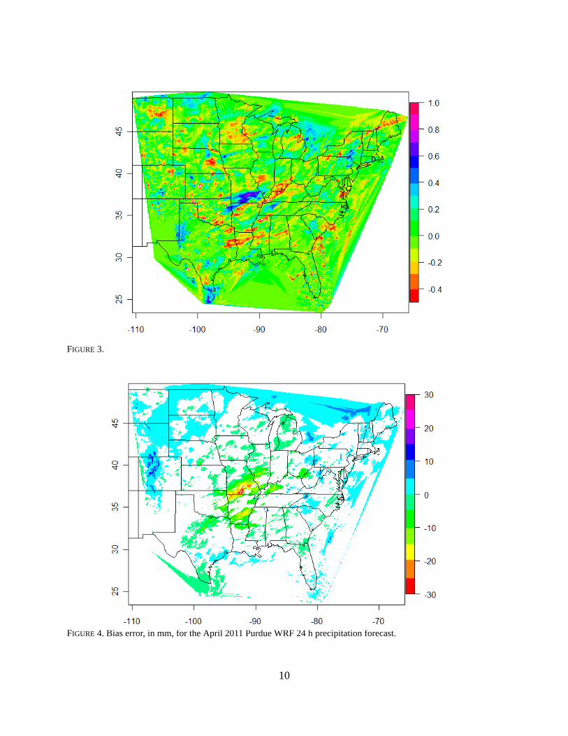
FIGURE 3.

FIGURE 4. Bias error, in mm, for the April 2011 Purdue WRF 24 h precipitation forecast.

10

These plots are not optimal as they are produced within R. Because the interpolation pro-

cess employed for creating plottable objects, some artifacts exist within the plots that do not

within the data itself. Also, there is clearly a single large area of errors that can be attributed to a

significant flooding episode in southern MO. Because warm season precipitation events tend to be

convective in nature, the most useful information is probably generated by longer periods than

only one month. Ideally, several months, say, May through August, should be used. Even more

advisable is to stitch together as many years of data as possible.

Finally, while numerical forecast models strive for ever finer spatial resolution, there is lit-

tle reason to retail such resolution for an analysis such as this. Because long periods are averaged,

such fine resolution is of little value and adds considerably to the required CPU time and memory

all for no benefit. Users are best served if the data to be analyzed is remapped to a grid similar to

the AWIPS 212 (~40km grid spacing).

4. Summary

A general technique is developed and displayed for determining spatially significant bias

errors in any diagnosed variable. R code is developed and provided for the general application of

field significance and then used to generate spatial bias errors in 24 h precipitation totals for the

Purdue WRF in April 2011. While the example is performed on a regular grid, regular grids are

not required: any array of points for which there are two forecast or analyzed values can be com-

pared in this manner.

Visualization is done in R for illustrative purposes, but R is not the best vehicle for visual-

ization: the interpolation step needed to generate plottable objects is onerously long. A far better

11

approach is to format the output fields in NETCDF and use external, interactive plotting pack-

ages, such as IDV or NCL for visualization.

Because this technique is a computationally intense process, grid size is important.

because errors are averaged over time, high resolution is not particularly beneficial because fine-

scale errors are not themselves spatially consistent. Hence, interpolating fine grids to coarser res-

olution is an overall beneficial step and will lead to interpretable results with far fewer resource

requirements.

References

Davison, A. C. and D. V. Hinkley, 1997: Bootstrap Methods and their Application. Cambridge

University Press, 582 pp.

Efron, B., and R. J. Tibshirani, 1993: An Introduction to the Bootstrap. Chapman and Hall, 436

pp.

Elmore, K. L., M. E. Baldwin, D. M. Schultz, 2006: Field significance revisited: Spatial bias

errors in forecasts as applied to the Eta model. Mon. Wea. Rev., 134, 519–531.

Hamill, T. M., 1999: Hypothesis tests for evaluating numerical precipitation forecasts. Mon. Wea.

Rev., 127, 155–167.

Livezey, R. E., and W. Y. Chen, 1983: Statistical field significance and its determination by Monte

Carlo techniques. Mon. Wea. Rev., 111, 46–59.

Wang, X. and S. S. Shen, 1999: Estimation of spatial degrees of freedom of a climate field. J. Cli-

mate, 12, 1280-1291.

12

Wilks, D. S., 1997: Resampling hypothesis tests for autocorrelated fields. J. Climate, 10, 65–82.

13

Appendix 1 - R code and documentation

## Must load package akima for access to the interp() function.# Must load package maps() for access to mapping functions.# Must load package fields() for access to plot.image function.####example of how to read the text file.#wrfdata <- read.fwf("F:\\verification\\DTC_2010\\wrfdata.txt", widths = rep(5,29),buffersize = 100000)nmqdata <- read.fwf("F:\\verification\\DTC_2010\\nmqdata.txt", widths = rep(5,29),buffersize = 100000)## Here are some functions that may be helpful in reconstructing # field significance verification capability available in S+.# samp.blockBootstrap <- function(n, B, size = n - reduceSize, reduceSize = 0, block-Length){# Simple block bootstrap, overlapping blocks, no wrap-around, # no matching of ends.# To change blockLength use blockBootstrap()if(blockLength > n) stop("blockLength must be <= n")nblocks <- ceiling(size/blockLength)x <- sample(0:(n - blockLength), size = B * nblocks, replace = T)dim(x) <- c(nblocks, B)# x = random indices for block starts, -1apply(x, 2, function(y, L)1:L + rep(y, each = L), L = blockLength)[1:size, , drop = F]

}##blockBootstrap <- function(blockLength){# return a copy of samp.blockBootstrap with the desired blockLengthf <- samp.blockBootstrapf$blockLength <- blockLengthf

}## Need a version of colMeans that works with R's bootstrap. Here's one.#mycolMeans <- function(x, d){## Input# x - data frame or matrix# d - index for which rows of the column to use## Output# out - a vector of the column means#if (is.data.frame(x)) x <- as.matrix(x)out <- colMeans(x[d,])return(out)

14

}##mycolMeans <- function(x, d){## Input# x - data frame or matrix# d - index for which rows of the column to use## Output# out - a vector of the column means#if (is.data.frame(x))

x <- as.matrix(x)out <- colMeans(x[d,], na.rm = TRUE)return(out)

}#

gdpt.ci.R.boot <- function(errfield.mat, CI = c(0.025, 0.975), Bci = 1000, blksz = 7,BCa = F){## This function tries to recreate capabilities within the S-Plus resample# library for field significance. Missing data (NA) is permitted. Note: this function

uses the# blockBootstrap sampler and, if requested, the BCa confidence limit estimator.## INPUT# errfield.mat - a numeric m X t matrix of error values at each gridpoint arrayed# with m gridpoints and t times of observations.# CI - a numeric vector containing the confidence interval limits.# BCI - numeric vector defining the number of bootstrap replicates.# BCa - logical. Default is F. If T, BCa confidence intervals are computed. These# sometimes lead to lengthy warning messages.## OUTPUT# data frame containing columns labeled Lower, Mean, and Upper that contain# the Lower and Upper CI limits and the bootstrap mean value.## KLE 01/14/05# 01/23/09## Ported to R: 03/30/2011#Nrows <- dim(errfield.mat)[1]## The number of samples for each gridpoint is the number of rows in transposed input

matrix.#replicates.mat <- matrix(NA, ncol = Nrows, nrow = Bci)terrfield.mat <- t(errfield.mat)CI.limits <- data.frame(Upper = numeric(Nrows), Mean = numeric(Nrows), Lower =

numeric(Nrows))## Create the moving blocks indices.#indices <- samp.blockBootstrap(dim(terrfield.mat)[1], B = Bci, blockLength = blksz)## Use these indicies to generate replicates for each grid point.#

15

for (i in 1:Bci){replicates.mat[i,] <- colMeans(terrfield.mat[indices[,i],])

}## Now, use colMeans again to find the mean bias error at each grid point.#CI.limits$Mean <- colMeans(replicates.mat)## Compute empriical confidence limits for each grid point.#CI.limits$Lower <- apply(replicates.mat, 2, probs = CI[1])CI.limits$Upper <- apply(replicates.mat, 2, probs = CI[2])return(CI.limits)

}## Now for the Monte Carlo part...#MC.dof.t <- function(data.mat, ntrials = 5000, field.sig = 0.05, norm = F){## This function has default values for an alpha-level # of 0.05 for a correlation test at each grid point.# This function yields a vector of the proportion of grid points that# exhibit a significant correlation to a random process for each# Monte-Carlo trial of the Livezey and Chen (1983) Monte-Carlo# technique for determing spatial degrees of freedom.## If every gridpoint is independent from its neighbor, then the# coverage of significant test statistic values will exceed # the coverage that could occur by chance, which is given# by the value of the EDF at the (1 - field.sig) percentile, only# field.sig% of the time.## The EDF from this vector yields the threshold of coverage needed# for p = (1-field.sig)% field significance based on the percent # coverage at the (1 - field.sig) percentile (the upper field.sig% of the# EDF). If the area covered by signficant results exceeds this value, then# the test statistic has field significance.## Input --# data.mat -- data matrix in S-mode (rows are time series of# grid point values).# ntrials -- number of monte-carlo trials# gridpt.sig -- alpha level for the Benoulli test at each grid point.# field.sig -- alpha level for significant correlation at each grid point.# bootit -- default F, If true, a bootstrap estimate of the (1 - field.sig)# percentile will be performed.# norm -- default T; use a N(0,1) for the correlation test. Otherwise, use# a uniform distribution.## Refs: Livezey and Chen (1983), Wang and Shen (1999)## KLE -- V1.0 01/10/2005# Ported to R 03/03/2011## data.mat <- na.omit.cols(data.mat)## How many data points are in the grid?#

16

npts <- dim(data.mat)[1]## What is the length of the time series at each point?#t.len <- dim(data.mat)[2]## Set up a vector to contain the results of each Monte Carlo trial.#B.dof.test <- numeric(ntrials)cor.value <- numeric(npts)t.data.mat <- t(data.mat)for(j in 1:ntrials) {#

#generate an N(0,1) vector the length of the time series at each grid point.#if(norm) rr <- rnorm(t.len) else rr <- runif(t.len)## correlate that vector with the time series at each grid point.#cor.value <- abs(cor(t.data.mat, rr, use = "pairwise.complete.obs"))## determine what proportion of points generate a significnat correlation with the# random data vector.#B.dof.test[j] <- sum(field.sig > sig.cor.t(cor.value, len = t.len), na.rm = T)/npts

}sig.coverage <- quantile(B.dof.test, probs = 1 - field.sig, na.rm = T)out <- list(MC.vec = B.dof.test, minsigcov = sig.coverage)return(out)

}#MC.dof.Z <- function(data.mat, ntrials = 3000, field.sig = 0.05, norm = F){## This function has default values for an alpha-level # of 0.05 for a correlation test at each grid point.# This function yields a vector of the proportion of grid points that# exhibit a significant correlation to a random process for each# Monte-Carlo trial of the Livezey and Chen (1983) Monte-Carlo# technique for determing spatial degrees of freedom.## If every gridpoint is independent from its neighbor, then the# coverage of significant test statistic values will exceed # the coverage that could occur by chance, which is given# by the value of the EDF at the (1 - field.sig) percentile, only# field.sig% of the time.## The EDF from this vector yields the threshold of coverage needed# for p = (1-field.sig)% field significance based on the percent # coverage at the (1 - field.sig) percentile (the upper field.sig% of the# EDF). If the area covered by signficant results exceeds this value, then# the test statistic has field significance.## Input --# data.mat -- data matrix in S-mode (rows are time series of# grid point values).# ntrials -- number of monte-carlo trials# gridpt.sig -- alpha level for the Benoulli test at each grid point.# field.sig -- alpha level for significant correlation at each grid point.

17

# bootit -- default F, If true, a bootstrap estimate of the (1 - field.sig)# percentile will be performed.# norm -- default T; use a N(0,1) for the correlation test. Otherwise, use# a uniform distribution.## Refs: Livezey and Chen (1983), Wang and Shen (1999)## KLE -- V1.0 01/10/2005# Ported to R 03/30/2011## data.mat <- na.omit.cols(data.mat)## How many data points are in the grid?#npts <- dim(data.mat)[1]## What is the length of the time series at each point?#t.len <- dim(data.mat)[2]## Set up the vector to contain the results of each Monte Carlo trial.#B.dof.test <- numeric(ntrials)cor.value <- numeric(npts)t.data.mat <- t(data.mat)for(j in 1:ntrials) {## generate an N(0,1) vector the length of the time series at each grid point.#if(norm) rr <- rnorm(t.len) else rr <- runif(t.len)## correlate that vector with the time series at each grid point.#cor.value <- abs(cor(t.data.mat, rr, use = "all.obs"))## determine what proportion of points generate a significnat correlation with the# random data vector.#B.dof.test[j] <- sum(field.sig > sig.cor.Z(cor.value, len = t.len), na.rm = T)/npts

}sig.coverage <- quantile(B.dof.test, probs = 1 - field.sig, na.rm = T)out <- list(MC.vec = B.dof.test, minsigcov = sig.coverage)return(out)

}## Correlation significance test functions follow.# This version uses Fisher's Z-transform, which requires# the fisherz function. #fisherz <- function(r){## The sampling distribution of Pearson's r is not normally distributed. Fisher# developed a transformation now called "Fisher's Z transformation" that transforms# Pearson's r to the normally distributed variable Z.## A function to perfoem Fisher's Z transformation on a correlation value, allowing# a t-test for significant correlation. Note that a boostrap test for significant# correlation could certainly be used and so eliminating the need for this function,

18

# but at the cost of significantly increased computational load.## Input -# r - the correlation## Output -# W - the transformed corelation## v1.0# KLE 2 Feb 2009# Ported to R -- 03/30/2011#W <- 0.5 * (log((1 + r)/(1 - r)))return(W)

}## There are two versions of the test for significant correlation: one uses a N(0,1) dis-tribution# and Fisher's Z trandofrmation. The other neglects the fact that Pearson's r isn't nor-mally distributed# and goes about its business. I see little practical significance between which one isused and so# provide both just because I'm a really nice guy.## To insure you do this "right," use sig.cor.Z and Fisher's Z transformation. Yes, yes,we certainly# could do this with bootstrapping, but do you really want to wait that long? I didn'tthink so.#sig.cor.Z <- function(r, len = 40, H0 = 0){## A function to find the significance of a correlation from H0 using Fisher's Z trans-

form.## Input - # r - the correlation# len - the length of the crrelated vectors# Ho0- the null hypothesis correlation default = 0## Output - # palpha.cor - the p-value of the correlation.## KLE 02/20/2009# Ported to R -- 03/30/2011#W <- fisherz(abs(r))stderr <- 1/sqrt(len - 3)zscore <- (W - H0)/stderrpalpha.cor <- 1 - pnorm(zscore)return(palpha.cor)

}#sig.cor.t <- function(r, len = 40){## A function to determine if a correlation is significantly different from x## Input -

19

# r - the (unsigned) correlation coefficient # len - the length of the vectors used to generate the correlation (default = 40)# Alpha - the significance level (default = 0.05)## Output -# palpha.cor - the p-level of the correlation## v1.0# KLE 2/3/2009# Ported to R -- 03/30/2011#t <- abs(r) * sqrt((len - 2)/(1 - r^2))palpha.cor <- 1 - pt(t, len - 2)return(palpha.cor)

}## Is there sufficient coverage of significant values to reach filed significance?# sig.coverage will tell all...# sig.coverage <- function(DF){## This is a simple counting function tailored to the particular data frame it receievs.# Input -# dataframe - oOutput from gdpt.ci.R.boot(); the data frame of bootstrapped mean bias# errors and the upper and lower bootstrapped confidence limits. NAs are not allowed.## Output -# numeric - the propertion of DF that contains bias errors significantly differentfrom zero.## KLE V1.0 03/2005.sig <- sum(inside(DF))/length(inside(DF))return(.sig)

}## This one is remarkably handy for determining if the statistic at a point is inside oroutside # the bootstrapped conficence limits.#inside <- function(DF){## A function to determine if the mean error at a data point is# inside the confidence limits.# # Input# DF - data frame containing mean error values and upper and lower# confidence limits## Output# logical T if outside, F if inside.## KLE V2.0 01/2005#result <- !is.na(CI.fun(DF$Upper - DF$Lower, DF$Mean))return(result)

}CI.fun <- function(CI.field, mean.field, replacement = NA)

20

{test <- ifelse((0.5 * CI.field < abs(mean.field)), mean.field,replacement)

return(test)}## Compute the ACF for n lags at all grid points.#acf.n.fun <- function(mat, maxlag = 1){## Compute the ACF for n lags at all grid points.#nrows <- dim(mat)[1]acf.1 <- matrix(nrow = nrows, ncol = maxlag)for(i in 1:nrows) {acf.1[i, ] <- acf(mat[i, ], lag.max = maxlag, "correlation", plot = F)$acf[2:(1 + maxlag)]

}if(maxlag == 1)acf.1 <- as.vector(acf.1)

return(acf.1)}## Because these grids are potentially very large, the job must be broken into man-agleable parts.#manage.size <- function(mat, max.size = 50000){## This function simply generates a sequence that is in max.size increments. This ver-

sion is# intended for the verification of precipitation data DTC exercise. #increments <- seq(from = 1, to = dim(mat)[1], by = max.size)increments <- c(increments, dim(mat)[1])return (increments)

}## Example of using the "chunks."#ls(name = "wrf"## How can we look at the ACF for the errors?# Try this for a lag of 5...#wrferr1.acf <- acf.n.fun(wrferr1, 5)## Gotta get rid of all thos NaN values...#wrferr1.acf <- ifelse(is.nan(wrferr1.acf), NA, wrferr1.acf)## Looks like a block size of about 5 or so will do.#df1 <- gdpt.ci.R.boot(wrferr1[chunks[1]:(chunks[1]+49999),])df2 <- gdpt.ci.R.boot(wrferr1[chunks[2]:(chunks[2]+49999),])df3 <- gdpt.ci.R.boot(wrferr1[chunks[3]:(chunks[3]+49999),])df4 <- gdpt.ci.R.boot(wrferr1[chunks[4]:(chunks[4]+49999),])df5 <- gdpt.ci.R.boot(wrferr1[chunks[5]:(chunks[5]+49999),])df6 <- gdpt.ci.R.boot(wrferr1[chunks[6]:(chunks[6]+49999),])df7 <- gdpt.ci.R.boot(wrferr1[chunks[7]:(chunks[7]+49999),])

21

df8 <- gdpt.ci.R.boot(wrferr1[chunks[8]:chunks[9],])wrferr1ci.df <- rbind(c(df1, df2, df3, df4, df5, df6, df7, df8))## Take a look at the distribution of ACF values for all of those cases where the ACFexceeds# 0.25 for lag-1.#plot(x = c(rep(1, 11972), rep(2, 11972), rep(3, 11972), rep(4, 11972), rep(5, 11972)),y = wrferr1.acf[which(wrferr1.acf[,1] > 0.35), ])## How much of the data will have significant errors based on the Monte Carlo test?#wrferrMC <- MC.dof.Z(wrferr1)## How much of the data display significant bias errors?#sig.coverage(wrferr1.ci)## Once the preliminaries have been handled, a function can be built to generate a dataobject that# can be plotted.#DTC.precip.fldsig.fun <- function(fcst.df, verif.df, blksize = 5, latlon){## A function that ingests DTC data frames and perfoms most field# significance operations, generating objects suitabel for plotting.## INPUT# fcst - data frame of forceast values# verif - data frame of verification values# blksize - (integer, default 5) block size for moving blocks bootstrap# latlon - data frame of latitudes (col name "Lat") and longintudes (col name "Lon")

in degrees,# with west longitude negative.## OUTPUT# A list consisting of:# # P95 - a data frame giving the mean error and bootstrap 95% empirical confidence

interval for# the mean error.# lat - latitudes# lon - longitudes# mean.i - an interpolated object of the mean error, ready for plotting.# thk.i - an interpolated object of the thickness of the 95% confidence limits, ready

for plotting.# err - the error matrix# sig.results - proprtion of data points with significant bias errors.## KLE 30 Sep 2008 v1.0# Version for R: 30 June 2011#fcst.mat <- as.matrix(fcst.df)verif.mat <- as.matrix(verif.df)err.mat <- fcst.mat - verif.matmaxsize <- 50000chunks <- manage.size(err.mat, max.size = maxsize)df1 <- gdpt.ci.R.boot(wrferr1[chunks[1]:(chunks[1]+(maxsize - 1)),])

22

df2 <- gdpt.ci.R.boot(wrferr1[chunks[2]:(chunks[2]+(maxsize - 1)),])df3 <- gdpt.ci.R.boot(wrferr1[chunks[3]:(chunks[3]+(maxsize - 1)),])df4 <- gdpt.ci.R.boot(wrferr1[chunks[4]:(chunks[4]+(maxsize - 1)),])df5 <- gdpt.ci.R.boot(wrferr1[chunks[5]:(chunks[5]+(maxsize - 1)),])df6 <- gdpt.ci.R.boot(wrferr1[chunks[6]:(chunks[6]+(maxsize - 1)),])df7 <- gdpt.ci.R.boot(wrferr1[chunks[7]:(chunks[7]+(maxsize - 1)),])df8 <- gdpt.ci.R.boot(wrferr1[chunks[8]:chunks[9],])p95.df <- rbind(df1, df2, df3, df4, df5, df6, df7, df8)# p95.df <- gdpt.ci.R.boot(err.mat, blksz = blksize)lons <- latlon$Lonlats <- latlon$Lonx0 <- seq(min(lons), max(lons), length = 101)y0 <- seq(min(lats), max(lats), length = 101)mean.i <- interp(latlon$Lon, latlon$Lat, p95.df$Mean, xo = x0, yo = y0)thk.i <- interp(latlon$Lon, latlon$Lat, (p95.df$Upper - p95.df$Lower), xo = x0, yo =

y0)sig.results <- is.sig(err.mat, p95.df)output <- list(p95 = p95.df, lat = lats, lon = lons, mean.i = mean.i, thk.i = thk.i,

err = err.mat, sig.results = sig.results)

return(output)}## Build plottable object.#plot.obj.fun <- function(p95.df, latlon){lons <- latlon$Lonlats <- latlon$Lonx0 <- seq(min(lons), max(lons), length = 101)y0 <- seq(min(lats), max(lats), length = 101)mean.i <- interp(latlon$Lon, latlon$Lat, p95.df$Mean, xo = x0, yo = y0)thk.i <- interp(latlon$Lon, latlon$Lat, (p95.df$Upper - p95.df$Lower), xo = x0, yo =

y0)output <- list(mean.i = mean.i, thk.i = thk.i)return(output)

}#is.sig <- function(X, blockboot.results.df, n = 3000, fld.sig = 0.05){## Input -# X - matrix of errors at gridpoints. n gridpoints by m days# blockboot.results.df - dataframe of errors and CI at each# gridpoint.# n - number of Monte Carlo trials.# field.sig - significnace alpha for field significance.## Output -# List# name - Name of the data beig tested# results - The minimum amount of areal coverage needed for # significance at the given fld.sig# actual - The actual coverage of sigificant gridpoint# results.# issig - Logical variable: T for significant results, F for

# non-significant results.## KLE 01/2005 #

23

# Remove missing rows#X <- X[!is.na(blockboot.results.df[, 1]), ]blockboot.results.df <- blockboot.results.df[!is.na(blockboot.results.df[, 1]), ]

sig.results <- MC.dof(data.mat = X, ntrials = n, field.sig = fld.sig)$minsigcov

actual.coverage <- sig.coverage(blockboot.results.df)sig <- (actual.coverage > sig.results)output <- list(name = as.character(deparse(substitute(X))), required = as.numeric(sig.results), actual = as.numeric(actual.coverage), issig = as.logical(sig))

return(output)}## New inside() function#signif <- function(lower, upper){## A simple function to determine if the mean is significant based on the signs of the # lower and upper confidence limits. If the signs of the CI limits are different, the# mean value is not significant. However, if the sign of one limit is zero or if the# sign of both limits are the same, then the mean is significant.## KLE V1.0 02/2006#significance <- Fupper.sign <- sign(upper)lower.sign <- sign(lower)if (lower.sign == -1 & (upper.sign == 0 | upper.sign == -1)) significance <- Telseif ((lower.sign == 0 | lower.sign == 1) & upper.sign == 1) significance <- Telsesignificance <- Freturn(significance)}## The interpolation command for the mean error field#x0 <- seq(min(lons), max(lons), length = 401)y0 <- seq(min(lats), max(lats), length = 401)mean.i <- interp(DTC.latlon$Lon, DTC.latlon$Lat, wrferr.p95.1$Mean, xo = x0, yo = y0)## Interpolation command for the CI thickness field. Note that the "inside" function is# really a quick hack that assumes the CI is symmetric. This is seldom true, but works# for plotting purposes.#thk.i <- interp(DTC.latlon$Lon, DTC.latlon$Lat, (wrferr.p95.1$Upper -wrferr.p95.1$Lower), xo = x0, yo = y0)## Now, mask out the gridpoints for which the error is not significant.#mean.i$z <- CI.fun(thk.i$z, mean.i$z)## Plot the results#map(database = "state", xlim = xlim, ylim = ylim, col = "black")image.plot(mean.i, col = rainbow(12), zlim = c(-30, 30), breaks = seq(-30,30,5),lab.breaks = names(seq(-30,30,5)))

24

map(database = "state", xlim = xlim, ylim = ylim, col = "black", add = T)# # Plot ACF image#acf1plot.i <- interp(DTC.latlon$Lon, DTC.latlon$Lat, wrferrlag1, xo = x0, yo = y0)#map(database = "state", xlim = xlim, ylim = ylim, col = "black")image.plot(acf1plot.i, col = rainbow(15), zlim = c(-0.5, 1), breaks = seq(-0.5,1,.1),lab.breaks = names(seq(-0.5,1,.1)))map(database = "state", xlim = xlim, ylim = ylim, col = "black", add = T)## Plot thickness image#map(database = "state", xlim = xlim, ylim = ylim, col = "black")image.plot(thk.i, col = rainbow(20), zlim = c(0, 60), breaks = seq(0,60,3), lab.breaks= names(seq(0,60,3)))map(database = "state", xlim = xlim, ylim = ylim, col = "black", add = T)

25