Incorporating Satisfaction into Customer Value Analysis:

Optimal Investment in Lifetime Value

Teck-Hua Ho, Young-Hoon Park, and Yong-Pin Zhou∗

July 2005

∗Teck-Hua Ho is William Halford Jr. Family Professor of Marketing, Hass School of Business, University of

California, Berkeley, CA 94720-1900; phone: (510) 643-4272; fax: (510) 643-1420; email: hoteck@haas.berkeley.edu.

Young-Hoon Park is Assistant Professor of Marketing, Johnson Graduate School of Management, Cornell University,

Ithaca, NY 14853-6201; phone: (607) 255-3217; fax: (607) 254-4590; email: yp34@cornell.edu. Yong-Pin Zhou is

Assistant Professor of Operations Management, Business School, University of Washington, Seattle, WA 98195-3200;

phone: (206) 221-5324; fax: (206) 543-3968; email: yongpin@u.washington.edu. All authors contributed equally and

are listed in alphabetical order. The authors would like to thank the editor, the area editor, and four anonymous

Marketing Science reviewers for helpful comments and suggestions. The first author acknowledges partial funding

support from the Wharton-SMU (Singapore Management University) Research Center.

Incorporating Satisfaction into Customer Value Analysis:Optimal Investment in Lifetime Value

Abstract

We extend Schmittlein et al.’s model (1987) of customer lifetime value to include satisfaction.Customer purchases are modeled as Poisson events and their rates of occurrence depend on thesatisfaction of the most recent purchase encounter. Customers purchase at a higher rate whenthey are satisfied than when they are dissatisfied. A closed-form formula is derived for predictingtotal expected dollar spending from a customer base over a time period (0, T ]. This formulareveals that approximating the mixture arrival processes by a single aggregate Poisson processcan systematically under-estimate the total number of purchases and revenue.

Interestingly, the total revenue is increasing and convex in satisfaction. If the cost is suf-ficiently convex, our model reveals that the aggregate model leads to an over-investment incustomer satisfaction. The model is further extended to include three other benefits of cus-tomer satisfaction: (1) satisfied customers are likely to spend more per trip on average thandissatisfied customers; (2) satisfied customers are less likely to leave the customer base thandissatisfied customers; and (3) previously satisfied customers can be more (or less) likely to besatisfied in the current visit than previously dissatisfied customers. We show that all the mainresults carry through to these general settings.

Keywords: Customer Satisfaction, Customer Value Analysis, Hidden Markov Model, Non-stationarity, Stochastic Processes

1 Introduction

Customers are assets and their values grow and decline (Shugan 2005). Segmenting customers

based on their lifetime value is a powerful way to target them because marketing mix activities can

then aim at enhancing customer value. In fact, predicting and managing customer lifetime value

has become central to marketing because the health of a firm is intimately linked to the health of

its customer base. This paper develops an analytical framework for forecasting customer lifetime

value based on her satisfaction with the firm.

The relevance of this research is evident in the burgeoning practitioner literature on customer

relationship management. Industry observers have emphasized the importance of incorporating

satisfaction metrics into customer valuation and exhorted firms to balance customer satisfaction

and cost control (e.g., Forrester Research 2003, Jupiter Research 2000). This paper provides a

formal methodology to assess investment in customer satisfaction by linking it to likely future

shopping and purchase patterns and hence revenue flow.

Our analytical modeling framework rests on two premises. First, we posit that customer sat-

isfaction is a key controllable determinant of customer lifetime value. That is, ceteris paribus, a

satisfied customer has a higher lifetime value than a dissatisfied customer. This premise is both

intuitively appealing and empirically sound. Several studies have shown that customer satisfac-

tion is a good predictor for likelihood of repeat purchases and revenue growth (e.g., Anderson and

Sullivan 1993, Jones and Sasser 1995). In addition, prior research has shown that customers react

negatively to poor service (e.g., stockouts) by switching to another firm on subsequent shopping

trips (Fitzsimons 2000).

Second, customer satisfaction can be increased by investing in costly technology or productive

processes. For instance, a call center that increases its number of customer representatives will

reduce queueing time. Similarly, a catalog firm can improve its logistics processes to shorten delivery

time and reduce the incidence of wrong shipments. The investment in these costly productive

processes, however, requires a formal quantification of their revenue implication. A goal of this

research is to derive a precise relationship between revenue and customer satisfaction by developing

a micro-level stochastic purchase model.

We build on the seminal work of Schmittlein et al. (hereafter, abbreviated as SMC) (1987)

and Schmittlein and Peterson (1994). Their model assumes that customer purchase arrivals are

2

Poisson events. Customers are allowed to die (i.e., switch to another firm or leave the product

category entirely) in a Poisson manner so that the number of active customers can decline over

time. Customers are heterogeneous in their purchase intensity and death propensity. The amount

spent on each purchase is normally distributed and is assumed to be independent of the arrival and

death processes. They derive an elegant formula to predict the total expected dollar spending from

a customer base over a time period.

There are three behavioral mechanisms by which customer satisfaction can affect this classical

stochastic purchase model. First, a satisfied customer is likely to have a higher purchase arrival

rate and make more trips to the firm. In other words, the firm can increase its market share of

the product category by making the customer happy. Second, a satisfied customer is less likely to

switch to another seller or leave the product category entirely. That is, a satisfied customer has

a lower death rate. Third, a satisfied customer may increase her average spending in the product

category on each purchase visit.

The basic model in Section 2 extends SMC to capture situations where arrival rate depends on

satisfaction. We derive a closed-form formula for determining the total expected dollar spending

and characterize the optimal level of customer satisfaction. Section 3 extends the basic model to

capture the effects of satisfaction on death rate and average expenditure. Furthermore, we extend

the basic model to allow satisfaction in the current visit to depend on satisfaction in the previous

visit. We show analytically that most qualitative insights remain unchanged with these extensions.

Section 4 conducts a comprehensive numerical analysis to illustrate the main theoretical results for

the general case. Section 5 concludes and suggests future research directions.

This paper makes three contributions. First, we extend the SMC framework to include satis-

faction in predicting customer lifetime value. We derive a closed-form formula to predict the total

expected dollar spending from a customer base. This formula allows the firm to predict lifetime

value based on customer satisfaction, a key indicator of customer health. Second, we show that the

total number of purchases is convex and increasing in customer satisfaction. In addition, we find

that one will systematically under-estimate the total expected dollar spending if one ignores the

non-stationarity in customer arrivals and departures due to the variation in customer satisfaction.

Third, the analytical framework allows the firm to actively manage its productive processes to in-

crease customer lifetime value. We prove that if the cost is sufficiently convex, a firm will over-invest

3

in productive processes when it fails to account for the variation in customer satisfaction.

2 The Basic Model

We consider a firm that offers a homogeneous product or service to a group of N customers. The

customers are ordered such that customer i is a heavier user than customer j if 1 ≤ i < j ≤ N . The

production process is inherently stochastic so that a customer is satisfied with probability p, and

dissatisfied with probability (1− p) at each purchase encounter.1 We assume that the production

process does not discriminate customers and that it is independent of previous purchase encounters

so that customer satisfaction can be modeled as independently and identically distributed Bernoulli

trials.

The inter-purchase time of a customer is assumed to have an exponential distribution. The

exponential rate varies with the outcome of each purchase encounter and differs across customers.2

For customer i, i ∈ {1, . . . , N}, her next purchase comes with arrival rate λiD if she is dissatisfied,

and λiS if she is satisfied.3 Customers visit more often when they are satisfied such that λiS > λiD

for all i. Our model can accommodate any parameter values.4

We assume a Markovian property so that the arrival rate depends only on the most recent

purchase encounter. This assumption is reasonable if customers exhibit a kind of “recency effect”

and react strongly to the most recent purchase encounter. In Section 3.3, we will extend the basic

model to allow a customer’s current satisfaction to correlate with her satisfaction in the previous

purchase encounter.5 When a customer defects, she is “dead”; otherwise, the customer is “alive”.1Our model may be extended to investigate more than two levels of satisfaction (e.g., three levels such as below

expectation, met expectation, above expectation). For ease of exposition, we restrict ourselves to dichotomous levels

such as happy versus unhappy, above expectation versus below expectation, satisfied versus dissatisfied, and so on.2Like Schmittlein et al. (1987), we assume exponential inter-purchase times for its analytical tractability. The

exponential assumption (i.e., purchase events are Poisson arrivals) has been applied extensively in the marketing

literature because of its parsimony and empirical performance (see for example Fader et al. 2003, 2004, Morrison

and Schmittlein 1981, Park and Fader 2004). The exponential assumption appears to work well for some product

categories (e.g., frequently purchased consumer goods) (Schmittlein et al. 1987). It should be noted that we do not

have a stationary Poisson process. We allow purchase and death rates to be dependent on customer satisfaction.

Besides customer satisfaction, other marketing mix variables can also influence the rate of purchase arrivals. For

instance, Ho et al. (1998) show that rational customers tend to shop more often with more frequent price promotion.

Similarly, Bawa and Shoemaker (2004) show that free sample can significantly increase a customer’s future purchase

arrival rate. Thus, the purchase and departure processes are non-stationary. In fact, our model shows customer

satisfaction can be an important source of non-stationarity in customer value analysis.3Anderson et al. (2004) empirically show that the difference in arrival rates can be significant in catalog purchases.4We explicitly capture heterogeneity by allowing each customer to have a personal set of arrival and departure rates.

Allowing heterogeneity is important because Rust and Verhoef (2005) show that response to marketing interventions

in intermediate-term customer relationship management is highly heterogeneous.5We do not consider the related questions of sizing of customer segment (i.e., which customers to serve) and optimal

4

Clearly, a customer’s satisfaction may affect her propensity to defect. For ease of exposition,

we assume that each customer i has a defection rate µi that is independent of satisfaction. In

Section 3.2, we relax this assumption to allow the defection rate to vary by satisfaction level.

On each purchase encounter, a customer spends a random dollar amount that is independent

of purchase outcome (i.e., whether she is satisfied or dissatisfied). The dollar spending follows

a general random distribution with expectation Q̄. This assumption is reasonable for necessity

product markets (e.g., hospital visits) where spending is mainly driven by needs. In Section 3.1, we

relax this assumption to allow it to be contingent on the purchase outcome in order to capture some

discretionary product markets (e.g., restaurants) where customers may modify spending based on

service outcome.

We are interested in addressing the following three managerial questions: (1) What is the ex-

pected number of customers remain “alive” at time T?; (2) What is the expected total dollar

spending from the customer base during (0, T ]?; (3) Given a cost of providing customer satisfac-

tion, what is the optimal customer satisfaction probability p∗ that maximizes total profit from the

customer base?

We will address these questions one by one. (Proofs of all the results can be found in the

Appendix.) We first derive the probability of a customer being alive at time T . Because the

death rate for customer i, µi, is independent of the satisfaction level, the “departure time” for the

customer has an exponential distribution with rate µi. Therefore,

Pr[Customer i is alive at time T ] = e−µiT . (1)

Since customers’ departure processes are independent of each other, the expected number of cus-

tomers who remain alive at time T is given by:

E[Number of customers at time T ] =N∑

i=1

e−µiT . (2)

2.1 Total Expected Dollar Spending During (0, T ]

Because customers purchase more frequently when they are satisfied, their total expected dollar

spending during (0, T ] depends on whether they are satisfied or dissatisfied at time t = 0.

contact frequency (e.g., number of catalogs to send). See Elsner et al. (2004) for a nice model and application. We

also do not study product choice on each visit. See Ho and Chong (2003) for a model of stock-keeping unit choice.

5

Define γi = pλiD + (1− p)λiS . If all the customers are dissatisfied at time 0, the total expected

dollar spending from the customer base during (0, T ] is:

RD = Q̄N∑

i=1

[λiDλiS

γiµi

(1− e−µiT

)− pλiD(λiS − λiD)γi(γi + µi)

(1− e−(γi+µi)T

)]. (3)

If all the customers are satisfied at time 0, the total expected dollar spending from the customer

base during (0, T ] is:

RS = Q̄

N∑

i=1

[λiDλiS

γiµi

(1− e−µiT

)+

(1− p)λiS(λiS − λiD)γi(γi + µi)

(1− e−(γi+µi)T

)]. (4)

Clearly, RS > RD so that customers spend more when they are initially happy. Let ∆R = RS−RD.

It can be easily shown that ∆R increases with the difference in arrival rates (λiS−λiD). Thus, ∆R

is higher if purchase rate is more responsive to satisfaction. Since ∆R decreases with the death

rate µi, we infer that the impact of satisfaction is more pronounced in markets where customers

have a longer expected life.

The total expected dollar spending from the customer base is R = pRS +(1−p)RD. Proposition

1 provides a closed-form expression for predicting the total expected dollar spending:

Proposition 1 The total expected dollar spending during (0,T] from the customer base is:

R = Q̄N∑

i=1

[λiDλiS

γiµi

(1− e−µiT

)+

p(1− p)(λiS − λiD)2

γi(γi + µi)

(1− e−(γi+µi)T

)]. (5)

Since the purchase arrival rate depends on the satisfaction outcome of one’s previous visit, the

inter-purchase time is a hyper-exponential random variable. It is exponential with mean 1/λiD

with probability (1− p) and with mean 1/λiS with probability p. In the rest of the paper, we will

use the term SMC-p to refer to the model that ignores the non-stationarity in purchase arrivals and

that estimates the dollar spending by using the SMC formula with an aggregate arrival rate. The

aggregate arrival rate of customer i in the SMC-p model, λei , should give an average inter-purchase

time that is identical to that of the hyper-exponential random variable. Consequently, we have:

1λe

i

=1− p

λiD+

p

λiS⇒ λe

i =λiDλiS

pλiD + (1− p)λiS=

λiDλiS

γi. (6)

Note that the SMC-p model indirectly captures customer satisfaction through the aggregate pur-

chase arrival rate, λei . The SMC formula predicts that the expected total dollar spending is:

Re = Q̄

N∑

i=1

[λe

i

µi

(1− e−µiT

)]. (7)

6

The importance of the three revenue formulas, equations (3)–(5), can be assessed by a comparison

with that of the SMC-p model, equation (7). Equations (3)–(5) and (7) imply the following simple

revenue equalities: RD = Re− ηD, RS = Re + ηS , and R = Re + η, where ηD, ηS and η are strictly

positive, or equivalently, RD < Re, RS > Re and R > Re.6 The inequalities involving RD and RS

are intuitive. The first suggests that when the customer base is initially dissatisfied, their dollar

spending is less than that given by the SMC-p model. The second implies that when the customer

base is initially satisfied, their dollar spending is more than that given by the SMC-p model. Both

results simply capture the fact that customers buy more when they are satisfied.

The revenue inequality involving R is surprising. It shows that the total expected dollar spend-

ing from the customer base is higher than that given by the SMC-p model. We state this important

result formally below.

Proposition 2 The SMC-p model under-estimates the total dollar spending by an amount η, where

η = Q̄N∑

i=1

[p(1− p)(λiS − λiD)2

γi(γi + µi)

(1− e−(γi+µi)T

)]. (8)

Several points are worth noting. First, when p = 0 (i.e., the customer is always dissatisfied),

p = 1, (i.e., the customer is always satisfied) or λiS = λiD (i.e., customer arrival rates are not

affected by satisfaction), the bias vanishes. That is, our model and the SMC-p model give the

same prediction. To the best of our knowledge, this is the first generalization of SMC model

to incorporate customer satisfaction. The formula allows one to quantify the marginal value of

customer satisfaction so that a firm can weigh this value against the incremental cost of providing

a better service. In addition, the quantification fills an important gap in operations management

literature where the marginal value of customer satisfaction is often assumed exogenously. Second,

the bias increases in the total number of customers (N) and increases linearly in the average dollar

spent (Q̄) per trip. Third, the bias increases in a quadratic manner in the incremental purchase

rate from satisfaction, i.e., λiS −λiD. This result implies that the bias is more dramatic in markets6The expression for η is given in Proposition 2, and ηD and ηS are given by:

ηD = Q̄

NXi=1

[pλiD(λiS − λiD)

γi(γi + µi)(1− e−(γi+µi)T )],

ηS = Q̄

NXi=1

[(1− p)λiS(λiS − λiD)

γi(γi + µi)(1− e−(γi+µi)T )].

7

where customers are more sensitive to service quality. Fourth, the bias is larger when customers

have a longer expected life (i.e., a low death rate, µi).

From Proposition 1, one can show that the total expected dollar spending as a function of the

probability of adequate service p is increasing. The proposition below establishes a stronger result

that it has an increasing return to scale in p.

Proposition 3 The total expected dollar spending during (0,T] from the customer base is convexin the probability of adequate service. That is, d2R

dp2 > 0.

This is an important and surprising result. One would have expected customer satisfaction to

have a diminishing return. The result provides a formal justification for why many firms invest

relentlessly in customer satisfaction. Our result suggests that this is optimal as long as the costs

are either linear or not “too convex” in p. We shall show below (see Proposition 4) that it can be

problematic if the costs are sufficiently convex (which can occur in practice).

2.2 Optimal Investment in Customer Satisfaction

Proposition 3 suggests that the total expected dollar spending as a function of the probability of

adequate service p is convex. To determine the optimal service, one must know the shape of the

cost function. In general, it is reasonable to expect the total cost to be increasing in the probability

of adequate service (p) and the total expected number of customer visits (Λ). An informal survey

of several call center outsourcing firms suggests that the following two-part tariff pricing structure

is often employed:

TC(p) = F (p) + c(p) · Λ.

For analytical tractability, we assume a constant marginal cost per purchase encounter and set

c(p) = c. From Proposition 1, we have R = Q̄Λ. Thus, the profit function can be written as

follows:

π = R− TC = (Q̄− c) · Λ− F (p) def= Rm − F (p). (9)

It is clear that the modified revenue function, Rm, is convex in p (just as R is). We consider two

separate cases of F (p). First, F (p) is concave (possibly linear) in p. As the company invests more in

customer satisfaction, it receives an increasing marginal revenue but incurs a constant or decreasing

marginal cost. Therefore, the better the service, the higher the profit. It is optimal for companies

8

to seek to achieve a perfect customer satisfaction of 100%. Second, F (p) is strictly convex in p.

Here, it costs more to improve each additional incremental level of customer satisfaction. More

often than not, this is the case we face in reality. It is not immediately clear what the shape of

the profit function looks like as a function of p. Intuitively, when the cost function is “less convex”

than the revenue function (i.e., both marginal revenue and marginal cost are increasing in p, but

the former outpaces the latter), it again makes sense to pursue a perfect customer satisfaction. If

the cost function is “more convex” than the revenue function, however, the profit will eventually

decrease as p becomes higher and higher. This means that an interior optimal point exists for p.

That is, it is optimal to invest in customer satisfaction up to a level less than 100%.

We now analyze the latter case in detail. Examples of service delivery systems that have a

convex cost function are common. They include:

• M/M/m queueing systems: If the cost is directly proportional to either the service rate of

the individual servers or the number of servers, m, the cost function is convex as long as

customer satisfaction is measured by the probability of not having to wait in the queue at all

or by the average waiting time in the system (for details, see Kleinrock 1975).

• M/M/m/K finite-waiting-space queueing systems: If the cost is directly proportional to

either the service rate of the individual servers or the number of servers, m, the cost function

is convex as long as customer satisfaction is measured by the proportion of lost customers

due to finite waiting space.

• The classical single-period newsvendor inventory setup: Under this setup, customer satisfac-

tion is defined by the probability that the demand is being fully met. Thus, if the uncertain

demand is distributed with a cumulative distribution G(·) and the newsvendor carries x units

of inventory, customer satisfaction, p, is given by G(x). To achieve this level of customer

satisfaction, the newsvendor must incur an inventory holding cost of h · x where h is the unit

inventory holding cost per unit time. Consequently, the inventory holding cost necessary to

achieve a customer satisfaction of p is h·G−1(p). As long as G−1 is convex in p (or equivalently,

G is concave in x), the cost function is convex. Any distribution that has a monotonically

non-increasing probability density function satisfies such a condition. For example, exponen-

tial distribution, some Weibull and Gamma distributions, and uniform distribution all have

9

a monotonically non-increasing probability density function.

To obtain managerial insights, we use a simple convex cost function that is quadratic: F (p) =

a+bp2. Here, parameter a represents the cost necessary to achieve the lowest customer satisfaction,

and b represents how fast the cost increases in p. As we stated before, when b is small such that

the cost function is less convex than the revenue function, the profit is convex, and the optimal

service level is achieved at either p = 0 or p = 1. The interesting case is when the cost function is

more convex than the revenue function. Again, we compare our optimal investment in customer

satisfaction with that of SMC-p model. Similar to equation (9), we define the SMC-p profit to be

πe = Re − TC(p) = Rem − F (p), where

Rem = (Q̄− c)

N∑

i=1

[λe

i

µi

(1− e−µiT

)]. (10)

From Proposition 2, we have π = πe + ηm where

ηm = (Q̄− c)N∑

i=1

[p(1− p)(λiS − λiD)2

γi(γi + µi)(1− e−(γi+µi)T )].

One can show that there exists a threshold value of customer satisfaction, p̄ ∈ (0, 1), such that ηm

is decreasing in p for p > p̄ (i.e., η′m < 0 for p > p̄).

The following proposition states that the firm may over-invest in customer satisfaction when

they do not explicitly account for the non-stationarity in customer arrivals due to variation in

customer satisfaction.

Proposition 4 Let p∗ be the maximizer of π, and pe∗ be the maximizer of πe. If

b >(Q̄− c

)max

{N∑

i=1

(λiS(λiS − λiD)2

λ2iD

)(1− e−µiT

µi

),

N∑

i=1

(λiS(λiS − λiD)

2λiD

)(1− e−µiT

µi

)},

and pe∗ > p̄ then pe∗ ≥ p∗.7

Proposition 4 states that when the firm pursues a high customer satisfaction strategy, it tends to

over-invest if it uses the SMC-p model to determine the optimal customer satisfaction (i.e., if it

ignores non-stationarity in purchase arrivals due to variation in customer satisfaction).

This result appears counter-intuitive. Since the SMC-p model under-estimates the total profit

by ηm, one would expect it to prescribe a lower optimal customer satisfaction level. However, it7Similarly we can show that there exists a p such that if pe∗ ≤ p then pe∗ ≤ p∗. This case is less important because

customer satisfaction is often high in practice. We choose to leave this out.

10

is the first derivative of ηm, η′m, not ηm itself, that matters in determining the optimal customer

satisfaction. To see this, we note that marginal cost equals marginal revenue at the optimal customer

satisfaction. Both models have the same identical marginal cost; they differ only in their marginal

revenue. Since ηm = π−πe, the derivative of ηm plays an important role. As indicated above, there

exists a threshold p̄ such that η′m < 0 for p > p̄. Therefore, when pe∗ > p̄, the additional negative

marginal revenue η′m makes the total marginal revenue of our model smaller than that of SMC-p.

Consequently, our model prescribes a lower optimal customer satisfaction.

We can show that as the departure rate µi gets smaller, the threshold p̄ also gets smaller (see

the Proof of Proposition 4 in the Appendix). This yields an interesting implication: If the firm has

a more loyal customer base, it is more likely to over-invest in customer satisfaction if it uses the

SMC-p model. Therefore, the importance of capturing non-stationarity in purchase arrivals is even

more critical when the firm enjoys a high customer loyalty.

3 Model Extensions

Section 2 presents a model that explicitly captures the impact of customer satisfaction on the rate

of purchase arrival. In this section, we extend the model in three important ways. First, we allow

customer satisfaction to influence the average expenditure on each visit so that customers spend

more on the current visit if they were satisfied with their previous visit. Second, we let customers’

departure processes to be contingent on satisfaction. This extension captures the intuition that

unhappy customers are more likely to switch to another firm or leave the product category entirely.

Third, we allow customer satisfaction to correlate over time so that customers’ past satisfaction

may influence their current satisfaction.

3.1 Contingent Spending Amount

We let the average expenditure on each visit to depend on whether the customer was previously

satisfied with the firm. If a customer is satisfied, she spends a random amount with an average

of QS ; and when a customer is dissatisfied, she spends a random amount with an average of QD.

Clearly, we have QS ≥ QD.

Recall that the death rate of customer i remains at µi. Hence, the probability of customer i

being alive at time T is still e−µiT . Similarly, the expected number of active customers at time T

11

is∑N

i=1 e−µiT .

Since customer satisfaction at each visit is independently and identically distributed, p fraction

of the visits will be satisfactory and (1 − p) fraction of the visits dissatisfactory. Therefore, the

average amount a customer spends is simply QS times the number of satisfactory visits, plus QD

times the number of dissatisfactory visits. The following proposition provides the revised formula

for the total expected dollar spending during (0,T] from the customer base:

Proposition 5 The total expected dollar spending during (0,T] from the customer base is:

R = [pQS + (1− p)QD] ·N∑

i=1

[λiDλiS

γiµi

(1− e−µiT

)+

p(1− p)(λiS − λiD)2

γi(γi + µi)

(1− e−(γi+µi)T

)]. (11)

Similarly, we show that the SMC-p model under-estimates the above expression by an amount given

by:

η = [pQS + (1− p)QD] ·N∑

i=1

[p(1− p)(λiS − λiD)2

γi(γi + µi)(1− e−(γi+µi)T )

]. (12)

Again, the revised revenue function is convex in p. Also, the SMC-p model still leads to an over-

investment in customer satisfaction. Hence, we conclude that all the main results presented in

Section 2 generalize to this more realistic setting.

3.2 Contingent Death Rate

We allow the departure process to be contingent on whether customers are satisfied. Customer i

defects with a rate of µiD if she is dissatisfied and with a rate of µiS if she is satisfied. As we shall

see below, this extension has significantly increased the complexity of the analysis.

Let PAi be the probability that customer i is alive at time T . Let βi1 and βi2 be the two roots

of the quadratic equation:

β2 + [pλiD + (1− p)λiS + µiD + µiS ]β + [µiSµiD + (1− p)λiSµiD + pλiDµiS ] = 0.

The probability that customer i is alive at time T is given in the following lemma:

Lemma 1PAi = Ai e

βi1T + Bi eβi2T , (13)

where

Ai =p (βi1 + λiD + µiD)

[(1− p)λiS(µiS − µiD) + βi2µiS + µ2

iS

]

p(1− p)λiDλiSβi1 − βi1[βi1 + µiD + pλiD][βi2 + µiS + (1− p)λiS ],

Bi =(1− p)

[βi1µiD + µ2

iD + pλiD (µiD − µiS)](βi2 + λiS + µiS)

p(1− p)λiDλiSβi2 − βi2[βi1 + µiD + pλiD][βi2 + µiS + (1− p)λiS ].

12

It is clear that the expected number of customers remaining at the end of T is∑N

i=1 PAi.

Equation (13) is more complex than the one given in equation (1) where the death rate is

independent of customer satisfaction. Note that the probability of being alive for each customer

is a superposition of two exponential terms. It can be shown that when µS = µD, equation (13)

reduces to equation (1).

Proposition 6 The total expected dollar spending from the customer base during (0,T ] is

R = Q̄N∑

i=1

[Ci

(1− eβi1T

)+ Di

(1− eβi2T

)], (14)

where

Ci =pλiS (βi1 + λiD + µiD) [βi2 + µiS + (1− p)(λiS − λiD)]

p(1− p)λiDλiSβi1 − βi1[βi1 + µiD + pλiD][βi2 + µiS + (1− p)λiS ],

Di =(1− p)λiD (βi2 + λiS + µiS) [βi1 + µiD + p(λiD − λiS)]

p(1− p)λiDλiSβi2 − βi2[βi1 + µiD + pλiD][βi2 + µiS + (1− p)λiS ].

Even though the revenue expression is much more complex, we can again show that it is convex

in p. We cannot however analytically prove that the corresponding SMC-p model still leads to a

systematic downward bias in revenue forecast and an over-investment in customer satisfaction. An

extensive numerical analysis in Section 4 suggests that both results do carry through to this more

realistic setting as well.

3.3 Serial Correlation in Customer Satisfaction

The basic model assumes that the satisfaction outcomes of successive purchase encounters are

independent of each other. This is reasonable if customer satisfaction is primarily driven by factors

determined by the service provider, such as the inventory level at a store and the number of servers

at a counter. There exist scenarios in which customer satisfaction may correlate over time so that

current satisfaction may depend on past satisfaction. This serial correlation could either be negative

or positive. For example, if a customer was dissatisfied last time, her service expectation for the

forthcoming visit may be lower as a consequence and hence she is more likely to feel satisfied. On

the other hand, one can also argue that if the customer was satisfied last time, she is likely to be

more positive in assessing the current visit and hence more likely to be satisfied.

We use a Hidden Markov Model (HMM) to model this serial correlation of customer satisfaction.

Our extension is similar to a model developed by Netzer et al. (2005). Specifically, we use a two-

state Markov chain to capture the transition of customer satisfaction over time. Let p1 be the

13

probability of satisfaction if the customer was dissatisfied last time and p2 be the probability of

satisfaction if the customer was satisfied last time. Then the transition probability of satisfaction

is 1− p1 p1

1− p2 p2

.

Given the transition probability matrix, the steady-state (or long-run average) probabilities of a

customer being dissatisfied and satisfied are 1−p2

1−p2+p1and p1

1−p2+p1respectively. If one focuses on the

“steady-state” behavior, one can use p = p1

1−p2+p1in our basic model to revise the total expected

dollar spending formula.

Proposition 7 Let p = p1

1−p2+p1. Then the total expected dollar spending during (0,T] from the

customer base is:

R = (1− p2 + p1) · Q̄ ·N∑

i=1

[λiDλiS

γiµi

(1− e−µiT

)+

p(1− p)(λiS − λiD)2

γi(γi + µi)

(1− e−(γi+µi)T

)]. (15)

The revised revenue function differs from the original revenue function given in (5) only by a

multiplicative factor, (1− p2 + p1). That is, ignoring the time-dependency of satisfaction will cause

the revenue forecast to be off by a factor of (1 − p2 + p1). If customer satisfaction is positively

correlated over time, we have p1 < p2 and the basic model over-states the revenue. If satisfaction

is negatively correlated over time, we have p1 > p2 and the basic model under-states the revenue.

Clearly, both models give the same prediction when there is no time-dependence (i.e., p1 = p2). All

the main results carry to this more general setting as we vary the steady state customer satisfaction,

p = p1

1−p2+p1, as long as we keep 1− p2 + p1 fixed.

4 Numerical Study

The general model allows two distinct arrival and death rates for a customer, one when the customer

is satisfied and the other when she is not. As discussed in Sections 2 and 3, ignoring the non-

stationarity in customer arrivals or departures due to variation in customer satisfaction (i.e., using

the SMC-p model) can lead to a systematic downward bias in estimating the total expected dollar

spending. In addition, we show that the SMC-p model leads to an over-investment in customer

satisfaction and suboptimal profits.

To illustrate the above points, we present a systematic numerical analysis using a two-segment

market (heavy versus light users). We use equation (6) to determine the “equivalent” arrival rates

14

for the SMC-p model. We derive the “equivalent” death rates by equating (1) and (13). The

numerical study also allows us to quantify the nature and magnitude of the potential biases of the

SMC-p model.

We choose the model parameters such that satisfied customers are twice as quickly to return

and half as quickly to defect. The light user segment has λLS = 1.2, λLD = 0.6, µLS = 0.3, and µLD

= 0.6 and the heavy user segment has λHS = 2.0, λHD = 1.0, µHS = 0.5, and µHD = 1.0. These

values are consistent with previous empirical estimates (see for example Morrison and Schmittlein

1981, Schmittlein et al. 1987). Without loss of generality, we normalize T to 1.0. The size of the

customer base (N) is set to 1000 and the average expenditure Q̄ is set to 1.0.

Based on the above parameters, we simulate hypothetical purchases for each of the 1000 cus-

tomers. The probability of adequate service p and the size of the heavy user segment δ are varied

systematically. We assess the predictive performance of our model and the SMC-p model in fore-

casting the total expected dollar spending. For each model, we measure prediction error by the

mean absolute deviation. The relative performance of the two models is evaluated by the relative

difference in their mean absolute deviations, i.e., MADe−MADMAD where MADe and MAD are the

prediction error of the SMC-p and our models respectively. If our model is better, we will see a

positive value in the relative error measure (i.e., MADe > MAD). Table 1 shows the relative error

measure across three levels of p (0.2, 0.5, 0.8) and δ (0.2, 0.5, 0.8) values. Clearly, our model

dominates the SMC-p model. It also shows that the relative error measure can be as high as 31%

and appears to be highest when p = 0.5.

Insert Table 1 about here

We investigate the relative magnitude of the total expected dollar spending between the SMC-p

model and our model, i.e., R−Re

R = ηR . If this difference is small, we have evidence that the SMC-p

model is robust to misspecification involving non-stationarity in purchase arrivals and departures

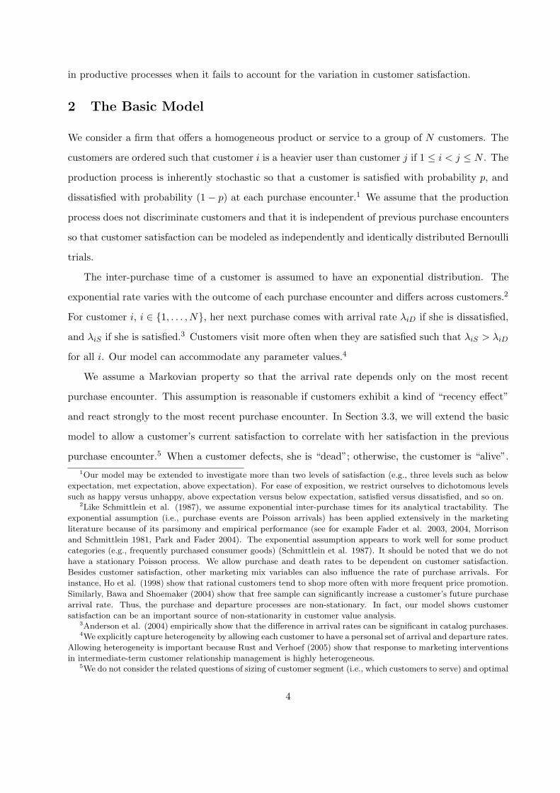
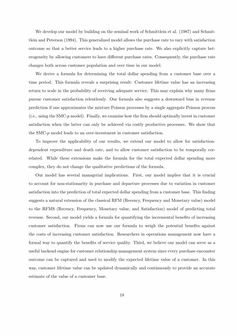
due to variation in customer satisfaction. Figure 1 shows the importance of accounting for non-

stationarity in purchase arrivals due to variation in customer satisfaction. As shown, the relative

difference in total expected dollar spending varies from 4% to 8% as we change the probability of

adequate service. Similar to the relative error measure reported above, the difference appears to

be highest when p = 0.5. This finding reinforces the analytical result that the SMC-p model leads

to a downward bias in predicting total expected dollar spending.

15

Insert Figure 1 about here

We observe a smaller variation in the relative difference in revenue when we vary the size of the

heavy segment (δ). For instance, when p = 0.8, the relative revenue difference ηR is 5.54%, 5.09%,

and 5.59% for δ = 0.2, 0.5, 0.8 respectively. We conclude that the relative revenue difference is more

sensitive to the probability of adequate service p than the segment size δ.

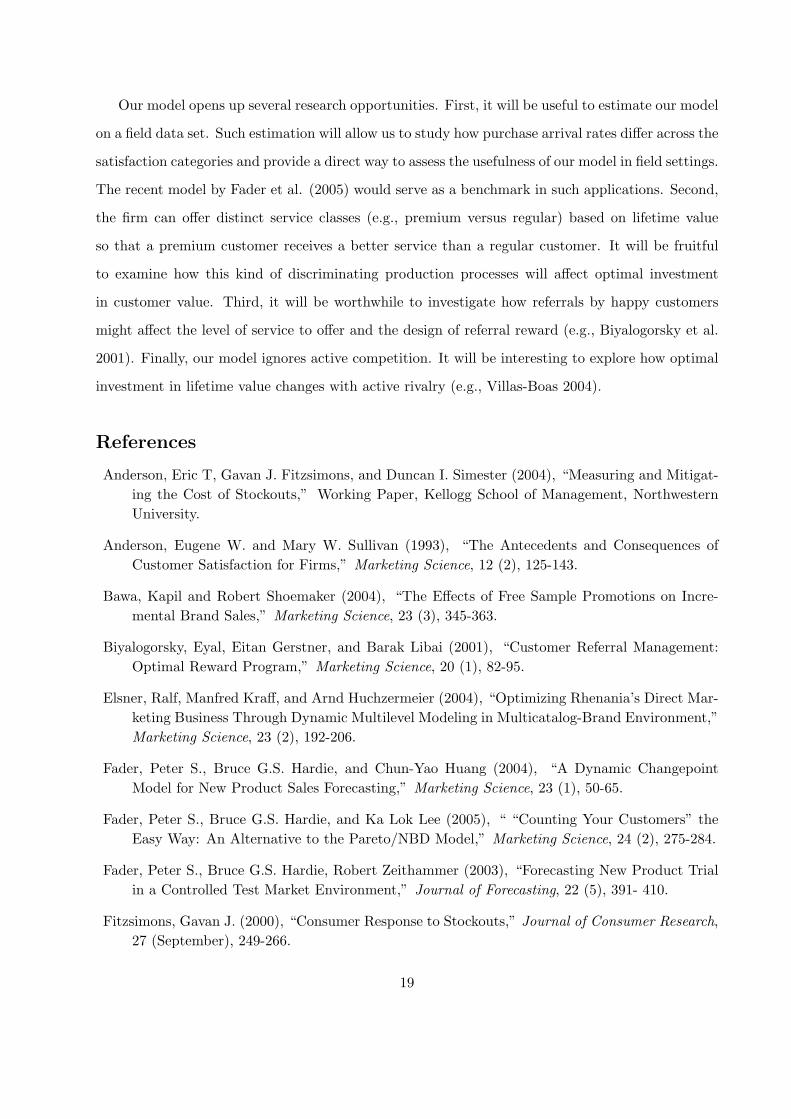
We now examine the degree of over-investment in customer satisfaction and its impact on profit

for the SMC-p model. To this end, we set the constant marginal cost per purchase encounter (c) to

0.3 and the cost necessary to achieve the lowest customer satisfaction (a) to 100. We choose the cost

parameter b to ensure that F (p) is sufficiently convex to capture realistic scenarios. Consequently,

we set b to 400, 425, 450.

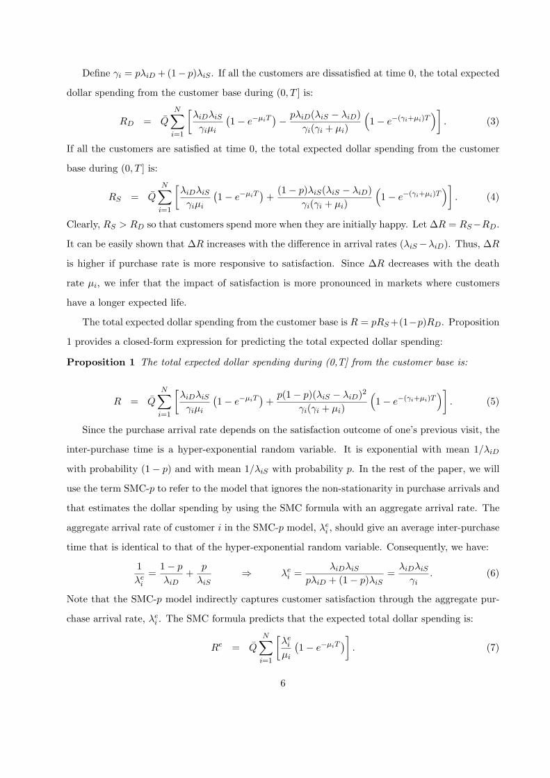
Figure 2 shows the difference between the optimal levels of customer satisfaction between the

SMC-p model and our model, i.e., (pe∗ − p∗). As expected, the optimal customer satisfaction of

the SMC-p model (pe∗) is always greater than that of our model (p∗). In particular, when δ is 0.5,

this difference is 22%, 30%, 37% for the three different levels of cost parameters used. Clearly, the

cost parameter b plays an important role in deciding the degree of bias in the optimal investment

in customer satisfaction.

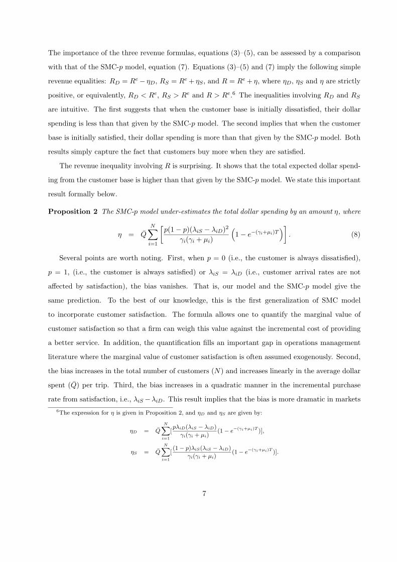
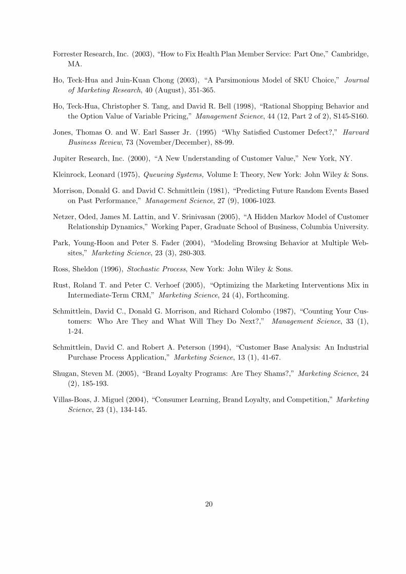
Figure 3 translates the investment bias in customer satisfaction associated with the SMC-p

model into the impact on profit. The figure reports the relative profit loss of the SMC-p model and

shows that when δ is 0.5, the firm can increase its profit by 2.12%, 4.88%, 8.40% if it optimally

provides a lower level of customer satisfaction under the three cost scenarios. When δ is close to

1.0, similar to Figure 2, the bias vanishes and the two models give the same prediction.

Insert Figures 2 and 3 about here

We also vary the relative magnitudes of arrival and death rates and study their impact on the

three measures of interest: ηR , (pe∗−p∗), and π(p∗)−π(pe∗ )

π(p∗) . In the simulation described below, δ and

b are set to 0.5 and 400 respectively.

We vary the ratio in arrival rates between satisfied and dissatisfied customers, λyD

λyS, for y = H,L

from 0.4 to 0.6 (note that this ratio is set to 0.5 for the base case shown in Figures 1–3). Table

2 shows the sensitivity analysis results. As expected, we find that as the ratio increases (i.e.,

the arrival rates between satisfied and dissatisfied customers are closer in magnitude), the relative

16

revenue difference ηR becomes smaller. However, the relative difference between the optimal levels

of customer satisfaction (pe∗ − p∗) increases which results in a significant relative profit loss for the

SMC-p model. For example, when λHDλHS

= λLDλLS

= 0.6, the relative profit loss, i.e., π(p∗)−π(pe∗ )π(p∗) is

9.37%.

We also vary the ratio in arrival rates between heavy and light users, λLxλHx

, where x = S, D from

0.5 to 0.7 (note that this ratio is set to 0.6 for the base case shown in Figures 1–3). Table 3 shows

the sensitivity analysis results. The highest relative profit loss is as high as 11.00% and occurs

when λLSλHS

= 0.5 and λLDλHD

= 0.7.

Insert Tables 2 and 3 about here

Similarly, we conduct a sensitive analysis involving the ratio in death rates between satisfied

and dissatisfied customers, µyS

µyD, for y = H, L from 0.4 to 0.6 in Table 4 and the ratio in death rates

between heavy and light users, µLxµHx

for x = S, D from 0.4 to 0.6 in Table 5. Tables 4 and 5 show

the simulation results. The impact on the relative profit loss is smaller when compared with the

above sensitivity analysis involving ratios in arrival rates. For instance, the highest relative profit

loss is 5.24% in Table 4 and is 3.26% in Table 5.

Insert Tables 4 and 5 about here

Taken together, the significant differences in revenue and profit between the SMC-p model and

our model highlight the importance of accounting for non-stationarity in purchase arrivals due to

variation in customer satisfaction. Our results show that firms must not use an aggregate approach

in analyzing customer satisfaction. Also, they must weigh the benefits of customer satisfaction

against its costs. It is not always optimal to pursue customer satisfaction relentlessly.

5 Discussion

In this paper, we present a model that incorporates satisfaction into customer value analysis.

By doing so, we incorporate the behavioral customer satisfaction research into the quantitative

customer value analysis literature. This is significant because customer satisfaction is an important,

if not the most important, contributor of customer lifetime value. Also, customer lifetime value is

inherently tied to repeat purchases and it seems odd to ignore customer satisfaction in estimating

lifetime value.

17

We develop our model by building on the seminal work of Schmittlein et al. (1987) and Schmit-

tlein and Peterson (1994). This generalized model allows the purchase rate to vary with satisfaction

outcome so that a better service leads to a higher purchase rate. We also explicitly capture het-

erogeneity by allowing customers to have different purchase rates. Consequently, the purchase rate

changes both across customer population and over time in our model.

We derive a formula for determining the total dollar spending from a customer base over a

time period. This formula reveals a surprising result: Customer lifetime value has an increasing

return to scale in the probability of receiving adequate service. This may explain why many firms

pursue customer satisfaction relentlessly. Our formula also suggests a downward bias in revenue

prediction if one approximates the mixture Poisson processes by a single aggregate Poisson process

(i.e., using the SMC-p model). Finally, we examine how the firm should optimally invest in customer

satisfaction when the latter can only be achieved via costly productive processes. We show that

the SMC-p model leads to an over-investment in customer satisfaction.

To improve the applicability of our results, we extend our model to allow for satisfaction-

dependent expenditure and death rate, and to allow customer satisfaction to be temporally cor-

related. While these extensions make the formula for the total expected dollar spending more

complex, they do not change the qualitative predictions of the formula.

Our model has several managerial implications. First, our model implies that it is crucial

to account for non-stationarity in purchase and departure processes due to variation in customer

satisfaction into the prediction of total expected dollar spending from a customer base. This finding

suggests a natural extension of the classical RFM (Recency, Frequency and Monetary value) model

to the RFMS (Recency, Frequency, Monetary value, and Satisfaction) model of predicting total

revenue. Second, our model yields a formula for quantifying the incremental benefits of increasing

customer satisfaction. Firms can now use our formula to weigh the potential benefits against

the costs of increasing customer satisfaction. Researchers in operations management now have a

formal way to quantify the benefits of service quality. Third, we believe our model can serve as a

useful backend engine for customer relationship management system since every purchase encounter

outcome can be captured and used to modify the expected lifetime value of a customer. In this

way, customer lifetime value can be updated dynamically and continuously to provide an accurate

estimate of the value of a customer base.

18

Our model opens up several research opportunities. First, it will be useful to estimate our model

on a field data set. Such estimation will allow us to study how purchase arrival rates differ across the

satisfaction categories and provide a direct way to assess the usefulness of our model in field settings.

The recent model by Fader et al. (2005) would serve as a benchmark in such applications. Second,

the firm can offer distinct service classes (e.g., premium versus regular) based on lifetime value

so that a premium customer receives a better service than a regular customer. It will be fruitful

to examine how this kind of discriminating production processes will affect optimal investment

in customer value. Third, it will be worthwhile to investigate how referrals by happy customers

might affect the level of service to offer and the design of referral reward (e.g., Biyalogorsky et al.

2001). Finally, our model ignores active competition. It will be interesting to explore how optimal

investment in lifetime value changes with active rivalry (e.g., Villas-Boas 2004).

References

Anderson, Eric T, Gavan J. Fitzsimons, and Duncan I. Simester (2004), “Measuring and Mitigat-ing the Cost of Stockouts,” Working Paper, Kellogg School of Management, NorthwesternUniversity.

Anderson, Eugene W. and Mary W. Sullivan (1993), “The Antecedents and Consequences ofCustomer Satisfaction for Firms,” Marketing Science, 12 (2), 125-143.

Bawa, Kapil and Robert Shoemaker (2004), “The Effects of Free Sample Promotions on Incre-mental Brand Sales,” Marketing Science, 23 (3), 345-363.

Biyalogorsky, Eyal, Eitan Gerstner, and Barak Libai (2001), “Customer Referral Management:Optimal Reward Program,” Marketing Science, 20 (1), 82-95.

Elsner, Ralf, Manfred Kraff, and Arnd Huchzermeier (2004), “Optimizing Rhenania’s Direct Mar-keting Business Through Dynamic Multilevel Modeling in Multicatalog-Brand Environment,”Marketing Science, 23 (2), 192-206.

Fader, Peter S., Bruce G.S. Hardie, and Chun-Yao Huang (2004), “A Dynamic ChangepointModel for New Product Sales Forecasting,” Marketing Science, 23 (1), 50-65.

Fader, Peter S., Bruce G.S. Hardie, and Ka Lok Lee (2005), “ “Counting Your Customers” theEasy Way: An Alternative to the Pareto/NBD Model,” Marketing Science, 24 (2), 275-284.

Fader, Peter S., Bruce G.S. Hardie, Robert Zeithammer (2003), “Forecasting New Product Trialin a Controlled Test Market Environment,” Journal of Forecasting, 22 (5), 391- 410.

Fitzsimons, Gavan J. (2000), “Consumer Response to Stockouts,” Journal of Consumer Research,27 (September), 249-266.

19

Forrester Research, Inc. (2003), “How to Fix Health Plan Member Service: Part One,” Cambridge,MA.

Ho, Teck-Hua and Juin-Kuan Chong (2003), “A Parsimonious Model of SKU Choice,” Journalof Marketing Research, 40 (August), 351-365.

Ho, Teck-Hua, Christopher S. Tang, and David R. Bell (1998), “Rational Shopping Behavior andthe Option Value of Variable Pricing,” Management Science, 44 (12, Part 2 of 2), S145-S160.

Jones, Thomas O. and W. Earl Sasser Jr. (1995) “Why Satisfied Customer Defect?,” HarvardBusiness Review, 73 (November/December), 88-99.

Jupiter Research, Inc. (2000), “A New Understanding of Customer Value,” New York, NY.

Kleinrock, Leonard (1975), Queueing Systems, Volume I: Theory, New York: John Wiley & Sons.

Morrison, Donald G. and David C. Schmittlein (1981), “Predicting Future Random Events Basedon Past Performance,” Management Science, 27 (9), 1006-1023.

Netzer, Oded, James M. Lattin, and V. Srinivasan (2005), “A Hidden Markov Model of CustomerRelationship Dynamics,” Working Paper, Graduate School of Business, Columbia University.

Park, Young-Hoon and Peter S. Fader (2004), “Modeling Browsing Behavior at Multiple Web-sites,” Marketing Science, 23 (3), 280-303.

Ross, Sheldon (1996), Stochastic Process, New York: John Wiley & Sons.

Rust, Roland T. and Peter C. Verhoef (2005), “Optimizing the Marketing Interventions Mix inIntermediate-Term CRM,” Marketing Science, 24 (4), Forthcoming.

Schmittlein, David C., Donald G. Morrison, and Richard Colombo (1987), “Counting Your Cus-tomers: Who Are They and What Will They Do Next?,” Management Science, 33 (1),1-24.

Schmittlein, David C. and Robert A. Peterson (1994), “Customer Base Analysis: An IndustrialPurchase Process Application,” Marketing Science, 13 (1), 41-67.

Shugan, Steven M. (2005), “Brand Loyalty Programs: Are They Shams?,” Marketing Science, 24(2), 185-193.

Villas-Boas, J. Miguel (2004), “Consumer Learning, Brand Loyalty, and Competition,” MarketingScience, 23 (1), 134-145.

20

p0.2 0.5 0.8

0.2 14.11% 30.78% 25.73%δ 0.5 9.15% 19.25% 14.46%

0.8 7.29% 12.33% 8.98%

Table 1: Relative Difference in the Mean Absolute Deviations

ηR pe∗ − p∗ π(p∗)−π(pe∗ )

π(p∗)λHDλHS

→ 0.4 0.5 0.6 0.4 0.5 0.6 0.4 0.5 0.60.4 13.72% 9.73% 6.90% 0% 11% 27% 0.00% 0.35% 3.44%

λLDλLS

0.5 11.48% 7.73% 5.07% 0% 22% 34% 0.00% 2.12% 6.31%0.6 9.91% 6.33% 3.81% 15% 31% 41% 0.65% 4.61% 9.37%

Table 2: The Impact of Changes in λDλS

on Revenue Bias, Over-investment in Satisfaction, andProfit Loss

ηR pe∗ − p∗ π(p∗)−π(pe∗ )

π(p∗)λLSλHS

→ 0.5 0.6 0.7 0.5 0.6 0.7 0.5 0.6 0.70.5 7.31% 9.35% 11.31% 19% 13% 0% 5.45% 0.57% 0.00%

λLDλHD

0.6 6.01% 7.73% 9.47% 37% 22% 0% 8.18% 2.12% 0.00%0.7 5.12% 6.53% 8.04% 43% 30% 11% 11.00% 4.16% 0.32%

Table 3: The Impact of Changes in λLλH

on Revenue Bias, Over-investment in Satisfaction, andProfit Loss

ηR pe∗ − p∗ π(p∗)−π(pe∗ )

π(p∗)µHSµHD

→ 0.4 0.5 0.6 0.4 0.5 0.6 0.4 0.5 0.60.4 8.21% 7.70% 7.19% 9% 19% 26% 0.25% 1.47% 3.34%

µLSµLD

0.5 8.24% 7.73% 7.22% 13% 22% 29% 0.58% 2.12% 4.26%0.6 8.27% 7.75% 7.24% 17% 25% 32% 1.02% 2.86% 5.24%

Table 4: The Impact of Changes in µSµD

on Revenue Bias, Over-investment in Satisfaction, andProfit Loss

ηR pe∗ − p∗ π(p∗)−π(pe∗ )

π(p∗)µHSµHD

→ 0.5 0.6 0.7 0.5 0.6 0.7 0.5 0.6 0.70.5 7.20% 7.21% 7.22% 22% 24% 27% 2.00% 2.61% 3.26%

µLSµLD

0.6 7.70% 7.73% 7.75% 20% 22% 25% 1.57% 2.12% 2.73%0.7 8.18% 8.21% 8.24% 18% 20% 23% 1.20% 1.70% 2.26%

Table 5: The Impact of Changes in µLµH

on Revenue Bias, Over-investment in Satisfaction, andProfit Loss

21

0.2 0.5 0.80

1

2

3

4

5

6

7

8

9

10

p

η / R

(%

)

δ = 0.2δ = 0.5δ = 0.8

Figure 1: Relative Revenue Difference Between the General and the SMC-p Models

0.5 0.6 0.7 0.8 0.9 1.0 −10

0

10

20

30

40

50

δ

pe* − p

* (%

)

b = 400b = 425b = 450

Figure 2: Difference Between Optimal Levels of Customer Satisfaction of the SMC-p and theGeneral Models

0.5 0.6 0.7 0.8 0.9 1.0 −1

0

1

2

3

4

5

6

7

8

9

10

δ

[π(p

* ) −

π(p

e* )] /

π(p* )

(%)

b = 400b = 425b = 450

Figure 3: Relative Profit Loss of the SMC-p Model

22

Appendix

A Revenue Function

In this section, we derive the revenue function. Specifically, we prove Propositions 1, 2, and 3.

To simplify analysis, we first derive the expected revenue from a generic customer and ignore her

subscript i. We then aggregate the revenue function over all customers.

The main technique we use to study the embedded Markov Chain of the Continuous Time

Markov Chain (CTMC) is the so-called “uniformization” (see Ross 1996, pp. 282-284).

Because λS > λD, the uniformized rate is λS . Once uniformized, the CTMC spends an

exponential(λS) amount of time in each state. Moreover, the transition probabilities in the uni-

formized chain are as follows (the rows and columns are ordered as: state D for dissatisfied and

state S for satisfied):

P =

(1− p)

(λDλS

)+

(1− λD

λS

)= 1− p

(λDλS

)p

(λDλS

)

1− p p

. (16)

Note that of all the transitions from state D into state D, only (1−p)(λD/λS)1−p(λD/λS) fraction are real tran-

sitions corresponding to customer purchases; the other 1−λD/λS

1−p(λD/λS) fraction are fictitious transitions

due to uniformization.

A.1 Proof of Proposition 1

Suppose the customer starts in state i and has had n arrivals in the uniformized Markov chain.

Because each real transition corresponds to a purchase by the customer, we would like to know

how many of the n arrivals correspond to real transitions. Let N ij(n) be the random number of real

transitions into state j in the first n transitions of the uniformized embedded Markov chain, where

i, j ∈ {D, S}. Moreover, let N̄ ij(n) be its expected value.

As an example, let us examine NDD (n). If the customer starts in state D, then with probability

(1 − p)(λD/λS), she makes a real transition into state D, in which case NDD (n) = 1 + ND

D (n − 1);

with probability (1−λD/λS), she makes a fictitious transition into state D, in which case NDD (n) =

0 + NDD (n − 1); and with probability pλD/λS , she makes a real transition into state S, in which

case NDD (n) = 0 + NS

D(n − 1). Overall, we have N̄DD (n) = (1 − p)(λD/λS)(1 + N̄D

D (n − 1)) +

(1 − λD/λS)N̄DD (n − 1) + p(λD/λS)N̄S

D(n − 1) = (1 − p)(λD/λS) + (1 − pλD/λS)N̄DD (n − 1) +

23

p(λD/λS)N̄SD(n− 1). Repeating this analysis, we arrive at the following equation,

N̄D

D (n) N̄DS (n)

N̄SD(n) N̄S

S (n)

=

(1− p)λD

λS

pλDλS

1− p p

+

1− pλD

λS

pλDλS

1− p p

N̄D

D (n− 1) N̄DS (n− 1)

N̄SD(n− 1) N̄S

S (n− 1)

.

If we use matrix notation N̄(n) to denote

N̄D

D (n) N̄DS (n)

N̄SD(n) N̄S

S (n)

, and let W =

0 0

(1− p)/p 1

,

the above equation becomes N̄(n) = PW + PN̄(n− 1).

Noting that N̄(0) = 0, or N̄(1) = PW, we conclude:

N̄(n) =

(n∑

k=1

Pk

)W. (17)

We need to diagonalize P in order to calculate Pk. We first calculate its eigenvalues:

0 = |αI − P | = (α− 1)[α− p

(1− λD

λS

)].

The two eigenvalues are α1 = 1 and α2 = p(1− λD

λS

). It is straightforward to calculate their cor-

responding eigenvectors: X1 =

1

1

and X2 =

pλDλS

p− 1

respectively. Therefore, (X1, X2) =

1 pλD

λS

1 p− 1

and (X1, X2)−1 =

p− 1, −pλD

λS

−1, 1

/∆, where ∆ = p − 1 − pλD

λS. It is clear that

1 + ∆ = α2 and 1− α2 = −∆.

Now that P = (X1, X2)

α1

α2

(X1, X2)−1, we have

N̄(n) = (X1, X2)

∑nk=1 αk

1

∑nk=1 αk

2

(X1, X2)−1W

=

−n(1−p)λD

λS+ (1−p)λD

λS

(α2−αn+1

21−α2

), −npλD

λS+ pλD

λS

(α2−αn+1

21−α2

)

−n(1−p)λD

λS− (1−p)2

p

(α2−αn+1

21−α2

), −npλD

λS+ (p− 1)

(α2−αn+1

21−α2

)

/∆. (18)

A.1.1 Customer Starts “Dissatisfied”

We first condition on n, the number of transitions in the uniformized Markov chain. If a customer

starts in state D, then the expected number of purchases (among the n transitions) is:

N̄DD(n) + N̄D

S (n) =[−n(1− p)λD

λS+

(1− p)λD

λS

(α2 − αn+1

2

1− α2

)− npλD

λS+

pλD

λS

(α2 − αn+1

2

1− α2

)]/∆

= −K1n + K2α2 −K2αn+12 , (19)

24

where K1 = λDλS∆ = −λD

(1−p)λS+pλD= −λD

γ and K2 = λDλS∆(1−α2) = −λDλS

[(1−p)λS+pλD]2= −λDλS

γ2 . Recall

that γ is defined as γ = (1− p)λS + pλD.Next, we calculate the unconditioned expected number of purchases:

∫ T

0

∞∑n=0

[(−K1n + K2α2 −K2αn+12

) e−λSt(λSt)n

n!

]µe−µtdt

+∫ ∞

T

∞∑n=0

[(−K1n + K2α2 −K2αn+12

) e−λST (λST )n

n!

]µe−µtdt

=∫ T

0

[−K1λSt + K2α2 −K2α2e

−(1−α2)λSt]µe−µtdt +

∫ ∞

T

[−K1λST + K2α2 −K2α2e

−(1−α2)λST]µe−µtdt

=λDλS

γµ

(1− e−µT

)− pλD(λS − λD)γ(γ + µ)

(1− e−(γ+µ)T

). (20)

Note that the purchase amount is independent of the number of purchases. Thus, the total expected

purchase amount is a simple product of the two averages. Activating the subscript i, we see that

the overall expected revenue from customer i becomes:

riD = Q̄

[λiDλiS

γiµi

(1− e−µiT

)− pλiD(λiS − λiD)γi(γi + µi)

(1− e−(γi+µi)T

)].

A.1.2 Customer Starts “Satisfied”

Similarly, we first condition on n, the number of transitions in the uniformized Markov chain. If a

customer starts in state S, the expected number of purchase visits (among the n transitions) is:

N̄SD(n) + N̄S

S(n) =[−n(1− p)λD

λS− (1− p)2

p

(α2 − αn+1

2

1− α2

)+−npλD

λS+ (p− 1)

(α2 − αn+1

2

1− α2

)]/∆

= −K1n + K3α2 −K3αn+12 , (21)

where K3 = p−1p∆(1−α2) = (1−p)λ2

Spγ2 .

Next, we calculate the unconditioned expected number of purchase during (0, T ]:∫ T

t

∞∑n=0

[(−K1n + K3α2 −K3αn+12

) e−λSt(λSt)n

n!

]µe−µtdt

+∫ ∞

T

∞∑n=0

[(−K1n + K3α2 −K3αn+12

) e−λST (λST )n

n!

]µe−µtdt

=∫ T

t

[−K1λSt + K3α2 −K3α2e

−(1−α2)λSt]µe−µtdt +

∫ ∞

t

[−K1λST + K3α2 −K3α2e

−(1−α2)λST]µe−µtdt

=λDλS

γµ

(1− e−µT

)+

(1− p)λS(λS − λD)γ(γ + µ)

(1− e−(γ+µ)T

). (22)

Similarly, the overall expected revenue from customer i becomes:

riS = Q̄

[λiDλiS

γiµi

(1− e−µiT

)+

(1− p)λiS(λiS − λiD)γi(γi + µi)

(1− e−(γi+µi)T

)].

25

Finally, RD =∑

i riD and RS =∑

i riS give us (3) and (4) respectively. The total expected

revenue from the whole customer base is calculated as:

R =N∑

i=1

[p · riS + (1− p) · riD] = Q̄N∑

i=1

[λiDλiS

γiµi

(1− e−µiT

)+

p(1− p)(λiS − λiD)2

γi(γi + µi)

(1− e−(γi+µi)T

)].

A.2 Proof of Proposition 2

Equation (7) gives the expected revenue in the SMC-p model. Taking difference between Re andRD =

∑Ni=1 riD, RS =

∑Ni=1 riS , and R, we obtain:

ηD = Q̄

N∑

i=1

pλiD(λiS − λiD)γi(γi + µi)

(1− e−(γi+µi)T )

ηS = Q̄

N∑

i=1

(1− p)λiS(λiS − λiD)γi(γi + µi)

(1− e−(γi+µi)T )

η = Q̄

N∑

i=1

p(1− p)(λiS − λiD)2

γi(γi + µi)(1− e−(γi+µi)T ).

It is easy to see that all three are non-negative.

A.3 Proof of Proposition 3

Because R =∑N

i=1[p · riS + (1− p) · riD], we have R′′ =∑N

i=1[r′′iD + 2 (riS − riD)′ + p (riS − riD)′′].

To show that R′′ ≥ 0, the following lemma suffices:

Lemma 2

(i) The first two derivatives of riD are non-negative.

(ii) The first two derivatives of (riS − riD) are non-negative.

Part (i) We will suppress the subscript i to simplify exposition. To show that rD has non-negative

first and second derivatives, it suffices to show that the N̄DD(n) + N̄D

S (n) has non-negative first and

second derivatives. From the proof of Proposition 1, we have:

N̄DD(n) + N̄D

S (n) =λD

λS∆

(n∑

k=1

αk2 − n

)=

λD

λS

n∑

k=1

(αk

2 − 1α2 − 1

)=

λD

λS

n∑

k=1

(k−1∑

i=0

αi2

).

Because any derivative of αi2 = pi

(1− λD

λS

)iis non-negative with respect to p as long as i ≥ 0, the

sum clearly has non-negative first and second derivatives with respect to p.

26

Part (ii)

rS − rD = Q̄

(λS − λD

γ + µ

)(1− e−(γ+µ)T

).

Now define f(x) = 1−e−Tx

x .

• f ′(x) =Te−Txx−(1−e−Tx)

x2 . If we let g(x) = Te−Txx − (1− e−Tx

), then g(0) = 0 and g′(x) =

−T 2xe−Tx ≤ 0. So g(x) ≤ 0, and f ′(x) ≤ 0 for x ≥ 0. Therefore, f(γ +µ) has a non-negative

first derivative with respect to p because γ′(p) = −(λS − λD) ≤ 0.

• f ′′(x) =2−e−Tx(T 2x2+2Tx+2)

x3 . If we let g(x) = 2 − e−Tx(T 2x2 + 2Tx + 2), then g(0) = 0.

Moreover, g′(x) = T 3x2e−Tx ≥ 0. So g(x) ≥ 0, and hence f ′′(x) ≥ 0, for x ≥ 0. It follows

that f ′′(γ + µ) has a non-negative second derivative with respect to p.

B Profit Function

In this section, we prove Proposition 4. We need the following lemma first.

Lemma 3 Let g(γ) = (λS−γ)(γ−λD)γ(γ+µ)

(1− e−(γ+µ)T

). Then g(γ) is unimodal in γ.

Proof: Let f = (λS−γ)(γ−λD)γ(γ+µ) , then (all derivatives are with respect to γ)

f ′

f= (ln(f))′ = − 1

λS − γ+

1γ − λD

− 1γ− 1

γ + µ. (23)

Let u = 1λS−γ > 0, v = 1

γ−λD> 0, w = 1

γ > 0, y = 1γ+µ > 0, and x = −u + v − w − y. Then by

equation (23), we have f ′f = x (i.e., f ′ = fx). Note also that v > w > y.

Because x′ = −u2 − v2 + w2 + y2,

x2 − x′ = 2(u2 + v2 − vu− vw − vy + uw + uy + wy). (24)

There are two cases:

(1) v ≥ u + w + y. In this case, equation (24) becomes:

x2 − x′ = 2(u2 + v(v − u− w − y) + uw + uy + wy) ≥ 0.

(2) v < u + w + y. In this case, equation (24) becomes:

x2 − x′ = 2(u(u + w + y − v) + (v − w)(v − y)) ≥ 0.

27

So in either case, we have shown that x2 ≥ x′.

Next, g′ =(f

(1− e−(γ+µ)T

))′= f ′ − (f ′ − fT )e−(γ+µ)T . Whenever g′ = 0, we must have

e−(γ+µ)T = f ′f ′−fT = x

x−T . Because 0 < e−(γ+µ)T < 1, we must have x < 0. Moreover,

g′′ = f ′′ + [2f ′T − fT 2 − f ′′]e−(γ+µ)T = f ′′ +[2f ′T − fT 2 − f ′′]x

x− T

=−f ′′T + 2f ′Tx− fT 2x

x− T=−(fx)′T + 2f ′Tx− fT 2x

x− T

=f ′xT − fx′T − f ′T 2

x− T= f ′T − fx′T

x− T= fxT − fx′T

x− T= fT

[x− x′

x− T

].

Because x2 ≥ x′ and x ≤ 0, we know x(x − T ) ≥ x′ and x ≤ x′x−T . So by now we have shown

that whenever g′ = 0, g′′ ≤ 0. This means that g has local maxima. Moreover, there would be

one (because g is a continuous function on a compact set) and only one (because there is a local

minimum between any two local maxima) local maximum. This maximum is the unique solution

to e−(γ+µ)T = xx−T , which can be further simplified to

T

e(γ+µ)T − 1=

1λS − γ

− 1γ − λD

+1γ

+1

γ + µ. (25)

Because γ = (1− p)λS + pλD, g as a function of p has exactly one local maximum and no local

minimum. Moreover, because g(p)|p=0 = g(p)|p=1 = 0 and g(p)|0<p<1 > 0, it must be true that the

maximum is interior. To the left of local maximum, g(p) is increasing in p and to the right of it,

g(p) is decreasing. ¤.

Recall that because γi = pλiD + (1− p)λiS , ηm can be expressed as

ηm = (Q̄− c)N∑

i=1

[(λiS − γi)(γi − λiD)

γi(γi + µi)(1− e−(γi+µi)T )

]. (26)

Lemma 3 shows that each summand in (26) is unimodal. Let the modes be p̄i and let p̄ =

maxi{p̄i}. It is clear that when p > p̄, η′ < 0.

When the cost increases slowly, i.e., when b is small, the company would optimally invest to

achieve the maximum possible service quality. This is intuitive because revenue is convex and

increases quickly. So when b is small, the optimal p should be 1. To avoid such trivial conclusions,

here we focus only on large b. Specifically, we assume that

b >(Q̄− c

)max

{N∑

i=1

(λiS(λiS − λiD)2

λ2iD

)(1− e−µiT

µi

),

N∑

i=1

(λiS(λiS − λiD)

2λiD

)(1− e−µiT

µi

)}.

28

Recall that

Rem = (Q̄− c)

N∑

i=1

λei

(1− e−µiT

µi

)= (Q̄− c)

N∑

i=1

(λiDλiS

γi

)(1− e−µiT

µi

).

Because γ′i(p) = λiD − λiS ,

[Rem(p)]′ = (Q̄− c)

N∑

i=1

(λiDλiS(λiS − λiD)

γ2i

)(1− e−µiT

µi

),

[Rem(p)]′′ = 2(Q̄− c)

N∑

i=1

(λiDλiS(λiS − λiD)2

γ3i

)(1− e−µiT

µi

),

[Rem(p)]′′′ = 6(Q̄− c)

N∑

i=1

(λiDλiS(λiS − λiD)3

γ4i

)(1− e−µiT

µi

).

Note that [Rem(p)]′′′ ≥ 0, and when p = 1, γi = λiD. Therefore,

[Rem(p)]′′ ≤ [Re

m(1)]′′ = 2(Q̄− c)N∑

i=1

(λiS(λiS − λiD)2

λ2iD

)(1− e−µiT

µi

)< 2b = F ′′(p), ∀p.

Thus, we have shown that πe(p) = Rem(p)− F (p) is concave. We note that [πe(0)]′ > 0, so 0 is

not a maximum. Also, because

[Rem(p)]′ |p=1 = (Q̄− c)

N∑

i=1

(λiS(λiS − λiD)

λiD

)(1− e−µiT

µi

)< 2b = F ′(1),

we have [πe(1)]′ < 0 so the maximizer pe∗ is interior. Moreover, it is the only p that satisfies

[πe(p)]′ = 0.

Next, we study π(p). It is clear that 0 won’t be the maximizer of π(p) because R′m(0) >

0, F ′(0) = 0 ⇒ π′(0) = R′m(0)−F ′(0) > 0. Moreover, because [πe(1)]′ ≤ 0 and η′m(1) < 0, we also

have π′(1) = [πe(1)]′+ η′m(1) < 0, so 1 won’t be the maximizer of π(p) either. So now we study the

interior p∗, which must satisfy π′(p∗) = 0.

Finally, we show that pe∗ ≥ p̄ ⇒ pe∗ ≥ p∗. We use contradiction. Suppose pe∗ ≥ p̄ and pe∗ < p∗.

Because πe(p) is concave in p and [πe(p∗e)]′ = 0, we must also have [πe(p∗)]′ < 0. Moreover,

p∗ > pe∗ ≥ p̄ ⇒ η′m(p∗) < 0. Therefore, we have π′(p∗) = [πe(p∗)]′ + η′m(p∗) < 0, which is a

contradiction.

Equation (25) helps us to get more insights into the property of p̄. For example, we can rearrange

it to be:

T

e(γ+µ)T − 1− 1

γ + µ=

1λS − γ

− λD

γ(γ − λD).

29

We know exT −1 increases in x much faster than xT , so as µ decreases the left-hand side of this

equation increases. We also know that the right-hand side is increasing in γ. So as µ gets smaller,

γ should change in such a way to balance the left-hand side, or make the right-hand side increase

as well. Either way, γ should increase. And the corresponding p should decrease. This implies

that when the customers in general are more loyal, this threshold p̄ is lower, and the companies are

more likely to over-invest in service quality.

C Extension: Contingent Death Rate

Again, in this section we will suppress the customer subscript i whenever there is no possibility

of confusion. Now that the death rates also vary by which state the customer is in, we need to

modify the Markov chain we developed in Appendix A accordingly. First of all, we introduce a new

state 0 to indicate that a customer has departed, thus increasing the state space by one dimension.

Second, because µD > µS , the uniformization rate becomes ω = µD +λS . Then the original CTMC

is equivalent to a Markov process that spends an i.i.d. exponential(ω) time in each state and has

the following transition probabilities among states:

1 0 0µDω

(1−p)λD+(λS−λD)ω = λS−pλD

ωpλDω

µSω

(1−p)λS

ωpλS+(µD−µS)

ω

. (27)

C.1 Proof of Lemma 1

Denote by qij(n) the probability that if a customer starts in state i she will end up in state j after

n transitions. Note that the one-step transition probabilities, qij(1), are the probabilities in (27).

The quantities of interest to us are 1 − qD0(n) and 1 − qS0(n). They are the probabilities that if

the customer is alive and dissatisfied (satisfied, respectively) currently, the probability that she will

still be alive after n transitions.

It is straightforward to derive the following:

qD0(n) =µD

ω+

λS − pλD

ωqD0(n− 1) +

pλD

ωqS0(n− 1) , (28)

qS0(n) =µS

ω+

(1− p)λS

ωqD0(n− 1) +

pλS + (µD − µS)ω

qS0(n− 1) . (29)

30

If we let Q(n) =

qD0(n)

qS0(n)

and Y =

µDω

µSω

, then equations (28) and (29) are equivalent to

Q(n) = Y + P̂Q(n− 1) =

(n−1∑

k=0

P̂ k

)Y, (30)

where P̂ =

λS−pλDω

pλDω

(1−p)λS

ωpλS+(µD−µS)

ω

is a sub-matrix of the transition matrix (27).

To calculate∑n−1

k=0 P̂ k, we need to diagonalize P̂ . We redefine α1 ≥ α2 to be the two eigenvalues

of P̂ . They satisfy

0 = α2 +pλD − (1 + p)λS − (µD − µS)

ωα +

pλS(λS − λD) + (λS − pλD)(µD − µS)ω2

. (31)

Let X1, X2 be the eigenvectors, then we have P̂ = (X1, X2)

α1

α2

(X1, X2)

−1, and

Q(n) = (X1, X2)

1−αn1

1−α1

1−αn2

1−α2

(X1, X2)

−1 Y.

Note that Q(n) is the probability of a customer being “dead” conditioning on n events in the

uniformized Markov chain. We now uncondition it.

We know that the uniformized Markov chain has exponential(ω) time between two events so

during (0,T ] the number of events in the uniformized Markov chain is Poisson with rate ω. So 1− PAD

1− PAS

=

∞∑

n=0

Q(n)e−ωT (ωT )n

n!

=∞∑

n=0

(X1, X2)

1−αn1

1−α1

1−αn2

1−α2

(X1, X2)

−1 Y

e−ωT (ωT )n

n!

= (X1, X2)

1−e−(1−α1)ωT

1−α1

1−e−(1−α2)ωT

1−α2

(X1, X2)

−1 Y.

Then, the probability of a customer (who may be satisfied or dissatisfied at time 0) being alive at

time T is:

(1− p, p)

1− PAD

1− PAS

= (1− p, p) (X1, X2)

1−e−(1−α1)ωT

1−α1

1−e−(1−α2)ωT

1−α2

(X1, X2)

−1 Y. (32)

31

To simplify the expression, we will make the following substitutions: β1 = −(1 − α1)ω and β2 =

−(1− α2)ω. Then, after some simple manipulation of (31), β1 and β2 are the two roots of:

0 = β2 + (pλD + (1− p)λS + µD + µS)β + [µSµD + (1− p)λSµD + pλDµS ].

With this substitution and some more arithmetic manipulation, (32) can be simplified to Aeβ1T +

Beβ2T , where

A =p (β1 + λD + µD)

[(1− p)λS(µS − µD) + β2µS + µ2

S

]

p(1− p)λDλSβ1 − β1[β1 + µD + pλD][β2 + µS + (1− p)λS ],

B =(1− p)

[β1µD + µ2

D + pλD (µD − µS)](β2 + λS + µS)

p(1− p)λDλSβ2 − β2[β1 + µD + pλD][β2 + µS + (1− p)λS ].

C.2 Proof of Proposition 6

Let N̄D(n) be the expected number of purchases in the next n uniformized transitions when cus-

tomer is dissatisfied at time 0, and N̄S(n) be the expected number of purchases in the next n

uniformized transitions when customer is satisfied at time 0. We then have the following

N̄D(n) =λD

ω+

pλD

ωN̄S(n− 1) +

λS − pλD

ωN̄D(n− 1) (33)

N̄S(n) =λS

ω+

(1− p)λS

ωN̄D(n− 1) +

pλS + µD − µS

ωN̄S(n− 1). (34)

If we let N̄(n) =

N̄D(n)

N̄S(n)

and Z =

λDω

λSω

, equations (33) and (34) are equivalent to:

N̄(n) = Z + P̂ N̄(n− 1) =

(n−1∑

k=0

P̂ k

)Z.

We have already diagonalized P̂ , so

N̄(n) = (X1, X2)

1−αn1

1−α1

1−αn2

1−α2

(X1, X2)

−1 Z.

Again, we need to uncondition N(n) on n:

∞∑

n=0

N̄1(n)

N̄2(n)

e−ωT (ωT )n

n!

=∞∑

n=0

(X1, X2)

1−αn1

1−α1

1−αn2

1−α2

(X1, X2)

−1 Z

e−ωT (ωT )n

n!

= (X1, X2)

1−e−(1−α1)ωT

1−α1

1−e−(1−α2)ωT

1−α2

(X1, X2)

−1 Z.

32

We again make the substitution β1 = −(1 − α1)ω and β2 = −(1− α2)ω. For a random customer,

she is satisfied at time 0 with probability p and dissatisfied with probability (1−p), so the expected

revenue from her is

r = (1− p, p) (X1, X2)

1−eβ1T

−β1/ω

1−eβ2ωT

−β2/ω

(X1, X2)

−1 Z.

After some straightforward arithmetic manipulation,

r = Q̄

{pλS (β1 + λD + µD) (β2 + µS + (1− p)(λS − λD))

p(1− p)λDλSβ1 − β1[β1 + µD + pλD][β2 + µS + (1− p)λS ]

(1− eβ1T

)

+(1− p)λD (β2 + λS + µS) (β1 + µD + p(λD − λS))

p(1− p)λDλSβ2 − β2[β1 + µD + pλD][β2 + µS + (1− p)λS ]

(1− eβ2T

)}.

D Extension: Hidden Markov Model of Customer Satisfaction

D.1 Proof of Proposition 7

The proof is a straightforward extension of the derivation in Appendix A. For ease of exposition,

we will first suppress the customer subscript i. Due to the dependency of customer satisfaction

over time, the transition probability matrix in the uniformized chain, (16), now becomes:

P =

(1− p1)

(λDλS

)+

(1− λD

λS

)= 1− p1

(λDλS

)p1

(λDλS

)

1− p2 p2

.

As in Appendix A, we will let N ij(n) be the random number of real transitions into state j in

the first n transitions of the uniformized embedded Markov chain if the system starts in state i.

Moreover, let N̄ ij(n) be its expected value.

If we use matrix-vector notation N̄(n) to denote

N̄D

D (n) N̄DS (n)

N̄SD(n) N̄S

S (n)

, then the solution is:

N̄(n) =

(n∑

k=1

Pk

)V, (35)

where V =

(p2−p1)λD

p2λS−p1λD0

(1−p2)(λS−λD)p2λS−p1λD

1

.

Again, as in Appendix A, we first diagonalize P. The two eigenvalues are found to be α1 = 1

and α2 = p2− p1λDλS

, and their corresponding eigenvectors are X1 =

1

1

and X2 =

p1λDλS

p2 − 1

33

respectively. Therefore, (X1, X2) =

1 p1λD

λS

1 p2 − 1

and (X1, X2)−1 =

p2 − 1, −p1λD

λS

−1, 1

/∆,

where ∆ = p2 − 1− p1λDλS

. Therefore,

N̄(n) =

(n∑

k=1

Pk

)V

=

1 p1λD

λS

1 p2 − 1

n

α2−αn+12

1−α2

p2 − 1 −p1λD

λS

−1 1

(p2−p1)λD

p2λS−p1λD0

(1−p2)(λS−λD)p2λS−p1λD

1

/∆

=

−n(1−p2)λD

λS− p1λD

λS

(1− λD−λS

p1λD−p2λS

)α2−αn+1

21−α2

, −np1λDλS

+ p1λDλS

α2−α2n+1

1−α2

(1− p2)(−nλD

λS+ α2−αn+1

21−α2

(1− λS−λD

p2λS−p1λD

)), −np1λD

λS+ (p2 − 1)α2−α2

n+1

1−α2

/∆.

We will again proceed in two separate cases.

1. When a customer starts “dissatisfied”. Then the expected number of purchases (among the

first n transitions) is:

N̄DD(n) + N̄D

S (n) = −K1n + K2α2 −K2αn+12 , (36)

where K1 = −λD(1−p2+p1)γ and K2 = −p1(λD−λS)λDλS

(p1λD−p2λS)γ2 . Recall that γ is defined as γ = (1− p2)λS +

p1λD = (1− α2)λS = −λS∆.Next, we calculate the unconditioned expected number of purchases:

∫ T

0

∞∑n=0

[(N̄D

D(n) + N̄DS (n)

) e−λSt(λSt)n

n!

]µe−µtdt +

∫ ∞

T

∞∑n=0

[(N̄D

D(n) + N̄DS (n)

) e−λST (λST )n

n!

]µe−µtdt

=λDλS(1− p2 + p1)

γµ

(1− e−µT

)− p1λD(λS − λD)γ(γ + µ)

(1− e−(γ+µ)T

). (37)

Because the purchase amount is independent of the number of purchases, the total expected

purchase amount is a simple product of the two averages. We find the overall expected revenue

from customer i to be:

riD = Q̄

[λiDλiS(1− p2 + p1)

γiµi

(1− e−µiT

)− p1λiD(λiS − λiD)γi(γi + µi)

(1− e−(γi+µi)T

)].

2. When a customer starts “satisfied”. Similarly, the expected number of purchases (among

the first n transitions) is:

N̄SD(n) + N̄S

S(n) = −K1n + K3α2 −K3αn+12 , (38)

where K3 = (1−p2)λ2S(λS−λD)

(p2λs−p1λD)γ2 .

34

Next, we calculate the unconditioned expected number of purchase during (0, T ]:∫ T

0

∞∑n=0

[(N̄S

D(n) + N̄SS(n)

) e−λSt(λSt)n

n!

]µe−µtdt +

∫ ∞

T

∞∑n=0

[(N̄S

D(n) + N̄SS(n)

) e−λST (λST )n

n!

]µe−µtdt

=λDλS(1− p2 + p1)

γµ

(1− e−µT

)+

(1− p2)λS(λS − λD)γ(γ + µ)

(1− e−(γ+µ)T

). (39)

Similarly, the overall expected revenue from customer i to be:

riS = Q̄

[λiDλiS(1− p2 + p1)

γiµi

(1− e−µiT

)+

(1− p2)λiS(λiS − λiD)γi(γi + µi)

(1− e−(γi+µi)T

)].

Finally, the total expected revenue from the whole customer base becomes

R =N∑

i=1

[p · riS + (1− p) · riD],

where p is the long-run fraction of time a customer is satisfied, p = p1

1−p2+p1.

R =N∑

i=1

[p1

1− p2 + p1· riS +

1− p2

1− p2 + p1· riD]

= Q̄N∑

i=1

[λiDλiS(1− p2 + p1)

γiµi

(1− e−µiT

)+

p1(1− p2)(λiS − λiD)2

(1− p2 + p1)γi(γi + µi)

(1− e−(γi+µi)T

)]

= (1− p2 + p1)Q̄N∑

i=1

[λiDλiS

γiµi

(1− e−µiT

)+

p(1− p)(λiS − λiD)2

γi(γi + µi)

(1− e−(γi+µi)T

)].

35