Embed Size (px)
Citation preview

INCORPORATING SAFETY INTO RURAL HIGHWAY DESIGN
_________________________________________
A thesis
submitted in partial fulfilment
of the requirements for the Degree
of
Doctor of Philosophy in Transportation Engineering
in the
University of Canterbury
by
Glen F. Koorey
_________________________________________
Department of Civil & Natural Resources Engineering
University Of Canterbury
October 2009


Glen F Koorey Incorporating Safety Into Rural Highway Design
i
ABSTRACT
The objectives of this research were to explore ways to assess the safety performance of
(predominantly two-lane) rural highways in New Zealand (NZ) and in particular identify
driver/road/environmental factors affecting crashes on rural curves. Following a wide-ranging
literature review, the Interactive Highway Safety Design Model (IHSDM) was identified as
worthy of further investigation for adaptation to use in NZ. To help with this investigation, a
comprehensive database was developed of road, traffic, crash and environmental data for all NZ
State Highways, divided into variable-length road elements.
A number of tasks were identified and undertaken to adapt IHSDM for general use here,
including calibrating the Crash Prediction Module (CPM), developing a Design Policy file based
on local agency standards, and developing an importing routine for NZ highway geometry and
crash data. To assess the effectiveness of IHSDM for predicting the relative safety of rural road
alignments, a series of tests were undertaken to confirm its appropriateness for use in NZ. These
included “before and after” design consistency checks of a bridge replacement, a “before and
after” crash comparison of a major highway realignment, and checks of actual versus predicted
crash numbers along longer lengths of highway in varying terrain.
These initial investigations have shown that IHSDM is a promising tool for safety and
operational assessment of highway alignments (both existing and proposed) in NZ.
Incorporating crash history data generally improves IHSDM’s accuracy in crash numbers, and
appears to provide a better level of “local calibration” than by using sub-national (e.g. regional or
terrain-specific) calibration parameters. Reported fatal/injury crash data generally provide more
robust and precise measures than non-injury crashes. Correct specification of the extreme
attributes of sub-standard elements (e.g. minimum radius, maximum roadside hazard) appears to
be crucial to getting suitably accurate crash estimates on existing alignments. However,
IHSDM’s current lack of consideration for bridges and inconsistent adjacent elements are
notable omissions that limit the ability of the CPM to assess sub-standard existing routes with as
much accuracy as well-designed newer alignments.
Keywords: road safety, New Zealand, rural roads, IHSDM, crash prediction

Glen F Koorey Incorporating Safety Into Rural Highway Design
ii
ACKNOWLEDGEMENTS
First and foremost, I would like to thank my darling wife Dianna for her patience and
understanding while she has had to play second fiddle (or third, or fourth...) during the past
seven-odd years of my studies. You get to be at the front again now...
Thanks also to my four wonderful children for understanding why Daddy had to “do his
homework report” on weekends rather than be able to play with them.
My sincere gratitude to my supervisors, Prof Alan Nicholson and Dr Mofreh Saleh, for their
ongoing support, feedback and guidance. Thanks also to Frank Greenslade, former Dept
transport lab manager, for his assistance over the years with my fieldwork.
There are a variety of other Department staff, industry/research colleagues and friends I wish to
thank for their ongoing support, assistance, data sharing, advice and encouragement:
• Opus International Consultants, esp. Mike Meister, Shelley Perfect, Mark Cochrane, Peter
Cenek, Marian Loader, Bill Pitt.
• Beca Infrastructure, esp. Dr Shane Turner, Alistair Smith.
• MWH, esp. Dr Fergus Tate, Mike Smith, Patrick Murray.
• Transit NZ (now part of NZTA), esp. Barry Stratton, Dr Dennis Davis.
• Kerryn Offord, fellow PhD student in UC’s Dept of Psychology.
• Dr Sam Charlton at the University of Waikato.
• Departmental visitors over the years, including Prof. Nick Garber, Prof. Shalom Hakkert,
Prof. Bhagwant Persaud, Prof. Ezra Hauer, Prof. Martin Snaith, Prof. Eric Hildebrand.
• LTSA/LTNZ/NZTA staff, esp. Wayne Osmers, Geoff Holland, Mike Keall.
• FHWA IHSDM staff, esp. Mike Dimaiuta.
• Lucy Richardson (SIAS) and Shaun Hardcastle (BasePlus) for their Paramics support.
• Ingmar Andreasson, Centre for Traffic Simulation Research, Sweden.
• Tony Keyte, whose Masters research provided useful findings for this thesis.
• Kyle Nicholson, for assisting with field data collection.
• Fellow staff colleague and part-time PhD student Mike Spearpoint for the encouragement to
“pick me” when it came to the “elephant in the room” that is a PhD thesis.
• Other department staff who have provided guidance or assisted by clearing my other
workload where possible.
• Everyone else I have missed, who have helped to make this thesis a reality!

Glen F Koorey Incorporating Safety Into Rural Highway Design
iii
I also need to acknowledge the many musical artists that graced my MP3 collection and helped
me to keep going during the long hours of my studies
Finally I would like to acknowledge the generous financial assistance and other support for parts
of my studies from the following organisations:
• Opus Central Laboratories (esp. Bill Pitt)
• Transfund NZ’s Research Programme (now part of NZ Transport Agency)
• The University of Canterbury’s Doctoral Scholarship programme (esp. Jane Bolton, Toni
Hodge, Adrian Carpinter)
• The Road Safety Trust’s Doctoral Scholarship programme (esp. Bill Frith and Kiri Manuera)
• The Dept of Civil & Natural Resources Engineering’s research funding

Glen F Koorey Incorporating Safety Into Rural Highway Design
iv
TABLE OF CONTENTS
Abstract............................................................................................................................................ i Acknowledgements......................................................................................................................... ii Table of Contents .......................................................................................................................... iv List of Figures .............................................................................................................................. vii List of Tables ............................................................................................................................... viii Glossary ......................................................................................................................................... ix
1 INTRODUCTION................................................................................................................. 1 1.1 Objectives........................................................................................................................ 2 1.2 Study Method.................................................................................................................. 3
2 LITERATURE REVIEW OF RURAL ROAD SAFETY MODELS............................... 5 2.1 Review of Relevant Safety Model Research................................................................... 6
2.1.1 Effects of Road Geometry and Environmental Features ........................................ 7 2.1.2 Speed and Safety................................................................................................... 11 2.1.3 Traffic Conflicts Research .................................................................................... 13 2.1.4 Driver Behaviour on Curves ................................................................................. 15
2.2 Vehicle Speed Prediction .............................................................................................. 18 2.2.1 Derived Speeds from Road Geometry Data.......................................................... 20
2.3 Types of Road Safety Models....................................................................................... 25 2.3.1 Levels of Model Detail ......................................................................................... 26 2.3.2 Crash Frequencies, Crash Rates and Traffic Exposure......................................... 27 2.3.3 Mathematical Form of Prediction Models ............................................................ 28 2.3.4 Incorporation of Existing Crash Data ................................................................... 32 2.3.5 Common Factors Used in Models......................................................................... 33 2.3.6 Crash Types and Severity ..................................................................................... 35
2.4 Overseas Models ........................................................................................................... 36 2.4.1 Interactive Highway Safety Design Model........................................................... 36 2.4.2 SafeNET................................................................................................................ 42 2.4.3 Road Safety Risk Manager ................................................................................... 44 2.4.4 Other Safety Models ............................................................................................. 46
2.5 New Zealand Models .................................................................................................... 47 2.5.1 State Highway Road Geometry Data .................................................................... 48 2.5.2 Economic Evaluation Manual............................................................................... 50 2.5.3 Crash Reduction Monitoring System.................................................................... 54 2.5.4 Safety Audit Models ............................................................................................. 55
2.6 Discussion ..................................................................................................................... 56 2.6.1 Development of New Zealand Rural Road Safety Models................................... 57
2.7 Implications for this Study............................................................................................ 60
3 PRELIMINARY HIGHWAY DATA COLLECTION AND PROCESSING............... 62 3.1 SH RAMM Data Analysis ............................................................................................ 64
3.1.1 State Highway Location System........................................................................... 64 3.1.2 RAMM Database Structure................................................................................... 65 3.1.3 Use of Pavement Condition Data.......................................................................... 67
3.2 Aggregation of Highway Data ...................................................................................... 68 3.2.1 Choice of Road Element Sectioning Approach .................................................... 70
3.3 Derivation of Database Measures ................................................................................. 73

Glen F Koorey Incorporating Safety Into Rural Highway Design
v
3.4 Road Geometry Data Processing...................................................................................75 3.4.1 Aggregation Method used in this Study................................................................75 3.4.2 Accuracy of Road Geometry Data ........................................................................83 3.4.3 Geometry Database Analysis Procedures .............................................................92
3.5 Crash Data Processing...................................................................................................96 3.6 Crash and Road Element Matching...............................................................................97
3.6.1 Determining Crash Vehicle Directions .................................................................97 3.6.2 Crash Location Accuracy ......................................................................................98 3.6.3 Crash Matching Process Used.............................................................................100
4 DESKTOP DATA CRASH ANALYSIS .........................................................................103 4.1 Crash Type Incidence on New Zealand Rural Highways ...........................................103
4.1.1 Contributory Factors ...........................................................................................107 4.2 Effect of Road Curvature on Crashes..........................................................................110 4.3 Implications for Analysis ............................................................................................114
5 APPLICATION OF IHSDM TO NEW ZEALAND......................................................116 5.1 User Requirements to Run and Install IHSDM...........................................................117 5.2 Calibration of Crash Prediction Module .....................................................................118
5.2.1 Crash Prediction Model Calibration Factors.......................................................120 5.2.2 Modification of the relative Crash Severity Proportions ....................................122 5.2.3 Modification of the relative Crash Type Proportions..........................................124 5.2.4 Issues with IHSDM’s Calibration Factor Approach ...........................................127 5.2.5 Disaggregation of Model Calibration Factors.....................................................128
5.3 Editing Design Policy Files.........................................................................................134 5.4 Importing NZ Road Alignment Data ..........................................................................136
5.4.1 Common Highway Alignment Information Formats ..........................................138 5.4.2 Development of Road Alignment Importing Routine.........................................142
5.5 Vehicle Fleet and Desired Speed Updating.................................................................143
6 VALIDATION OF IHSDM WITH LOCAL DATA......................................................144 6.1 SH1 Awatere Bridge Replacement Realignment ........................................................144
6.1.1 Design Consistency Assessment .........................................................................147 6.1.2 Crash Prediction Assessment ..............................................................................150
6.2 SH1 Hawkswood-Siberia-Ferniehurst Realignments..................................................151 6.2.1 SH1 HSF Alignment Design Consistency ..........................................................153 6.2.2 SH1 HSF Realignment Crash History.................................................................155 6.2.3 LTNZ EEM Crash Predictions............................................................................157 6.2.4 IHSDM Crash Predictions...................................................................................160
6.3 Validation of NZ Highway Crash Numbers................................................................165 6.3.1 Crash Prediction Results .....................................................................................168 6.3.2 Assessment of Crash Prediction Findings...........................................................170
7 DISCUSSION ....................................................................................................................173 7.1 IHSDM Case Study Findings......................................................................................173 7.2 Applicability of IHSDM for Road Safety Modelling in New Zealand .......................175
8 CONCLUSION..................................................................................................................177 8.1 Review of Research Objectives...................................................................................177 8.2 Recommendations for Further Research .....................................................................179
9 CONTRIBUTION TO THE STATE OF THE ART .....................................................183

Glen F Koorey Incorporating Safety Into Rural Highway Design
vi
10 REFERENCES.................................................................................................................. 184
A APPENDICES ................................................................................................................... 197 A.1 LTNZ CAS Crash Movement Codes .......................................................................... 197 A.2 LTNZ Road Safety Report Categories........................................................................ 198 A.3 Structure of Analysis Database Tables ....................................................................... 199 A.4 Geometry Database Processing Steps in Detail .......................................................... 206 A.5 Algorithm Flowcharts for Key Database Routines ..................................................... 209 A.6 Detailed IHSDM Calibration Process and Example of Calibration Spreadsheet ....... 212 A.7 Statistical Analysis of IHSDM Calibration Factors.................................................... 218 A.8 Typical IHSDM XML Import Files ............................................................................ 225 A.9 SH1 HSF Realignment Crash Data............................................................................. 229 A.10 SH1 HSF Realignment EEM Crash Analysis ............................................................. 232 A.11 SH1 HSF Realignment IHSDM Crash Analysis......................................................... 234 A.12 Supplementary Notes: Testing of Field Survey Equipment........................................ 243
A.12.1 Investigation of Possible Data Collection Measures........................................... 243 A.12.2 Field Trials of Equipment ................................................................................... 249

Glen F Koorey Incorporating Safety Into Rural Highway Design
vii
LIST OF FIGURES
Figure 2.1 Rural Road Modelling – Suggested Framework (from Koorey & Gu 2001) .......... 5 Figure 2.2 Speed Profile Model (based on Fitzpatrick & Collins 2000) ................................ 19 Figure 2.3 Mean Limiting Speeds on Upgrades (from Bennett 2004).................................... 24 Figure 2.4 IHSDM Crash Modification Factor for Shoulder Width....................................... 39 Figure 2.5 Network Editor in SAFENET................................................................................ 43 Figure 2.6 State Highway Road Geometry Data..................................................................... 49 Figure 2.7 Type B/C/D Injury Crashes for Rural Curves (from LTNZ 2006)........................ 52 Figure 3.1 State Highway Route Position System .................................................................. 64 Figure 3.2 Sectioning of Road Geometry Data into Horizontal Elements.............................. 70 Figure 3.3 Distribution of Road Geometry Elements (2000 m Cut-Off Value) ..................... 78 Figure 3.4 Distribution of Road Geometry Elements (1000 m Cut-Off Value) ..................... 79 Figure 3.5 Curvature Distribution of Road Geometry Records .............................................. 84 Figure 3.6 Average Curvature Bias vs Rate of Curvature ...................................................... 85 Figure 3.7 Gradient Distribution of Road Geometry Records ................................................ 87 Figure 3.8 Average Gradient Bias vs Level of Gradient......................................................... 88 Figure 3.9 Comparison of Gradients in Opposing Directions SH 1N RS675/8-12 ................ 89 Figure 3.10 Crossfall Distribution of Road Geometry Records................................................ 90 Figure 3.11 Crossfall Distribution of “Curved” Geometry Records (<500 m Radius)............. 91 Figure 3.12 Relationships between various Tables used in Data Analysis............................. 102 Figure 5.1 NZ Highway and Crash Data Inputs into IHSDM .............................................. 117 Figure 5.2 Selection of Data used for IHSDM Analysis....................................................... 120 Figure 5.3 State Highway Indexed Traffic Growth (from Transit NZ 2008) ....................... 121 Figure 5.4 Calibration of IHSDM to Local Crash Data (Single Calibration Factor)............ 127 Figure 5.5 Calibration of IHSDM to Local Crash Data (Multiple Calibration Factors)....... 128 Figure 5.6 Variation in Crash Risk across NZ Regions (from NRSC 2000) ........................ 132 Figure 5.7 IHSDM Policy Table Editor ................................................................................ 135 Figure 5.8 Conventional Data Conversion Approach between Packages............................. 139 Figure 5.9 Data Conversion between Packages using a Common File Format .................... 140 Figure 6.1 SH1 Awatere Bridge Replacement – Location.................................................... 144 Figure 6.2 SH1 Awatere Bridge Replacement – Site Detail................................................. 145 Figure 6.3 SH1 Awatere Bridge Replacement – Old/New Alignments ............................... 146 Figure 6.4 SH1 Awatere Old Alignment – Speed Profile Consistency ................................ 148 Figure 6.5 SH1 Awatere Old Alignment – Stopping Sight Distance Assessment................ 148 Figure 6.6 SH1 Awatere New Alignment – Speed Profile Consistency............................... 149 Figure 6.7 SH1 Awatere New Alignment – Stopping Sight Distance Assessment .............. 149 Figure 6.8 SH1 Hawkswood - Siberia - Ferniehurst (HSF) Realignment – Site Plan .......... 152 Figure 6.9 SH1 HSF Realignment – Old Alignment ............................................................ 152 Figure 6.10 SH1 HSF Realignment – New Alignment........................................................... 153 Figure 6.11 SH1 HSF Old Alignment – Speed Profile Consistency ...................................... 154 Figure 6.12 SH1 HSF Old Alignment – Location of Crashes by Direction 1994-98 ............. 157 Figure 6.13 Crash Rates along SH1 HSF Realignment 1994-98 (“Before” period)............... 163 Figure 6.14 “Before” and “After” Crash Numbers on SH1 HSF Realignment ...................... 164 Figure 6.15 Location of Highway Test Sections..................................................................... 166 Figure 6.16 2000-02 Crash Numbers on SH1S Christchurch-Ashburton (RS365 - 430)....... 171 Figure 6.17 2000-02 Crash Numbers on SH1N Waipu-Wellsford (RS203 - 248) ................. 171 Figure 6.18 2000-02 Crash Numbers on SH2 Rimutaka Saddle (RS921 - 946) .................... 172 Figure 7.1 Effect of Calibration and Crash History Data on IHSDM Crash Estimates........ 174 Figure A.1 Plan view of crashes in vicinity of SH1 HSF Realignment................................. 231 Figure A.2 Layout for curve speed surveys ........................................................................... 245 Figure A.3 Typical curve speed optical sensor and reflector (from Koorey et al 2002) ....... 246

Glen F Koorey Incorporating Safety Into Rural Highway Design
viii
Figure A.4 Types of curve tracking behaviour (from Spacek 2000)..................................... 248 Figure A.5 Autoscope Solo Pro Imaging System.................................................................. 250 Figure A.6 View of the Autoscope test site (circled) when driving from Christchurch........ 251 Figure A.7 View from the Autoscope test site towards Christchurch ................................... 251 Figure A.8 Autoscope camera and survey tent ...................................................................... 252 Figure A.9 Survey equipment used to monitor Autoscope camera ....................................... 252 Figure A.10 Virtual detectors at the Autoscope test site (looking towards Christchurch) ...... 253 Figure A.11 Accurange laser rangefinders being tested in Christchurch ................................ 256 Figure A.12 Determining Vehicles Speeds/Positions using a TIRTL (from CEOS 2005) ..... 257
LIST OF TABLES
Table 1.1 Comparison of Key Crash Statistics, Reported Injury Crashes 2005...................... 2 Table 3.1 Length, VKT and Social Crash Costs of NZ Roads (from MoT 2003) ................ 62 Table 3.2 Distribution of Geometric Elements with Varying Cut-Off Values...................... 77 Table 3.3 Summary of Sections of Highway excluded from further analysis....................... 95 Table 4.1 Crash Type Numbers on NZ Rural State Highways 2001-05 ............................. 104 Table 4.2 Length and VKT of NZ Rural State Highways in 2002 by Number of Lanes.... 105 Table 4.3 Crash Type Numbers on NZ Rural Local Roads 2001-05 .................................. 106 Table 4.4 Top Contributory Factor Code Groups in NZ Rural Crashes 2001-05 ............... 107 Table 4.5 Top Contributory Factor Codes in NZ Rural Crashes 2001-2005 ...................... 108 Table 4.6 Top Road/Environment Factor Code Groups in NZ Rural Crashes 2001-05 ..... 109 Table 4.7 NZ Single/Multiple-Vehicle Rural Crashes by Road Curvature 2001-05 .......... 111 Table 4.8 NZ Rural Crash Types by Road Curvature 2001-05........................................... 112 Table 4.9 Road Element Characteristics vs Curvature of Related Crashes 2001-05 .......... 113 Table 4.10 2001-05 Crash Curvature Distribution vs Road Element Curvature................... 113 Table 5.1 IHSDM Calibration Factors for New Zealand Use - Highway Segments .......... 122 Table 5.2 Percentage Distributions for Crash Severity Level - Highway Segments........... 123 Table 5.3 Equivalency of Crash Types between IHSDM and New Zealand ...................... 125 Table 5.4 Percentage Distributions for Crash Types - Highway Segments ........................ 126 Table 5.5 IHSDM Calibration Factors by Number of Lanes (1996-2000 Data)................. 129 Table 5.6 IHSDM Calibration Factors by Traffic Volume (1996-2000 Data).................... 130 Table 5.7 IHSDM Calibration Factors by Terrain (1996-2000 Data) ................................. 131 Table 5.8 IHSDM Calibration Factors by Region (1996-2000 Data) ................................. 133 Table 5.9 IHSDM Road Data included in Import File Routines......................................... 142 Table 6.1 Crash Numbers at SH1S Awatere Bridge 2001-05 (43/5.9-8.6)......................... 150 Table 6.2 Crash Numbers on SH1 HSF Realignment 1994-2006 (RP 7.5 - 16.1).............. 155 Table 6.3 Statistical Comparison of SH1 HSF Realignment Crash Reductions ................. 156 Table 6.4 SH1 HSF Realignment EEM Crash Estimates 1994-98 (“Before” period) ........ 159 Table 6.5 SH1 HSF Realignment EEM Crash Estimates 2002-06 (“After” period)........... 160 Table 6.6 Crash Numbers on SH1 HSF Realignment 1994-98 (“Before” period) ............. 162 Table 6.7 Crash Numbers on SH1 HSF Realignment 2002-06 (“After” period)................ 164 Table 6.8 IHSDM Calibration Factors for 2000-02 Crashes............................................... 167 Table 6.9 2000-02 Crash Numbers on SH1S Christchurch-Ashburton (RS365 - 430)....... 168 Table 6.10 2000-02 Crash Numbers on SH1N Waipu-Wellsford (RS203 - 248)................. 169 Table 6.11 2000-02 Crash Numbers on SH2 Rimutaka Saddle (RS921 - 946) .................... 170

Glen F Koorey Incorporating Safety Into Rural Highway Design
ix
GLOSSARY
A number of technical or New Zealand-specific terms have been used in this thesis. To help
minimise any misunderstandings, the following glossary explains some of the key terms used.
Some of these term definitions have been sourced from either LTNZ (2006) or Transit NZ
(2000). Readers are also referred to Austroads (2008) for other common Australasian roading
terminology.
TERM DEFINITION
85th Percentile The value of a variable characteristic measure for some population (or
sample), which exceeds or equals the measure found in 85% of the
population. For example, an 85th percentile observed speed was only
exceeded by 15% of the observed population.
AADT Annual Average Daily Traffic: the total yearly volume of traffic in both
directions at a site divided by the number of days in a year. Often
determined from shorter-term traffic counts using suitable scaling factors.
Usually expressed in “vehicles per day” (vpd), AADT provides a good
comparative estimate of the traffic volume at a location (i.e. from site to site,
or from year to year), irrespective of when traffic counting has been
undertaken there.
AMF Accident Modification Factor (sometimes also referred to as Crash
Modification Factors). A function used to adjust crash predictions up or
down to account for the characteristics of a particular road feature at the site,
e.g. shoulder width, horizontal curvature.
Approach Speed The initial speed of vehicles approaching a horizontal curve or other hazard,
prior to their slowing down to negotiate the curve/hazard.
Auxiliary Lane Additional carriageway space adjacent to through traffic lanes available for
traffic to undertake speed change, weaving or overtaking manoeuvres.
Typical facilities include acceleration/deceleration lanes, passing lanes,
climbing lanes, and slow vehicle bays.
Black spot Common term for a location (usually a short section of road) with an
unusually high number of crashes; similarly, problematic sections of road are
sometimes called black routes.

Glen F Koorey Incorporating Safety Into Rural Highway Design
x
TERM DEFINITION
Carriageway The portion of a road corridor (usually sealed) devoted to the use of vehicles,
including any shoulders or auxiliary lanes. Sometimes also known as the
roadway. Two-way traffic on the same carriageway is referred to as a
single carriageway road, whereas roads that have separate carriageways in
each direction are known as dual or divided carriageway roads.
CAS Crash Analysis System. Software developed by LTSA c.2000 to record and
analyse road crashes in New Zealand. The data is housed on a central server
accessible to road safety practitioners using web-based client software.
CPM Crash Prediction Module, one of the six software tools of IHSDM, this one
responsible for estimation of the number and severity of crashes on proposed
alignments.
Crash An event involving one or more road vehicles that results in personal
physical injury and/or damage to property. Crashes are also referred to as
accidents or collisions; this is largely a case of personal preference. More
formally, a crash can be defined as a “rare, random multi-factor event
preceded by a situation in which one or more persons have failed to cope
with their environment”.
Crash
Migration
An apparent transfer of crash numbers from one site to an adjacent one
following the treatment of the first. The theory is that, with the removal of
the danger from the first site, the next site is now more likely to “catch out”
drivers and cause problems.
Crash Rate The average number of crashes for a given exposure measure, e.g. “crashes
per 106 vehicles”, “crashes per year”. Although such measures tend to imply
a linear relationship with the exposure measure, often this is not the case.
Crossfall The slope at right angles to the alignment of any part of the road
carriageway. Also sometimes referred to as superelevation or camber.
Usually measured in percentage of vertical dimension to horizontal
dimension, e.g. 5% = 5 cm rise for every 100 cm horizontally.
Cross-Section A view, generally at right angles to the alignment, showing the shape of the
road to be constructed or as constructed. Also refers to the widths/slopes of
the elements across the road, i.e. traffic lanes, shoulders, roadside, etc.

Glen F Koorey Incorporating Safety Into Rural Highway Design
xi
TERM DEFINITION
DCM Design Consistency Module, one of the six software tools of IHSDM, this
one responsible for evaluating the extent to which a roadway design
conforms to drivers’ expectations (especially speed profiles).
Design Speed A speed used for the design of minimum geometric features of a road.
Generally the design speed chosen should be at least equal to the 85th
percentile operating speed observed or predicted for that section of road.
Desired Speed The speed adopted by drivers on a section of road when not influenced by
road geometry (e.g. curves) or other environmental factors.
EEM Economic Evaluation Manual, produced by Land Transport NZ (previously
called the Project Evaluation Manual or PEM). This sets out the procedures
for evaluation of the costs and benefits of proposed roading projects.
Exposure A measure of the number of potential opportunities to have a crash. Typical
measures used are the number of vehicles travelling through a site, or the
number of vehicle-kilometres travelled (VKT) over a length of road.
Factor Codes Standard numeric codes used in CAS to abbreviate and describe common
factors (driver, vehicle, and road environment) that may have contributed to
a crash, e.g. positive breath-alcohol test, dazzling sun, failed to give way,
brake failure, etc. Sometimes also misleadingly referred to as “cause codes”.
Free Speed A measure of speeds only from vehicles not following other vehicles and
thus unaffected by the behaviour of other same-direction traffic. Also
known as unimpeded speed.
Geometric
Element
The parts of a road design that make up the vertical and horizontal
alignments. Vertical alignments typically comprise grades and vertical
curves, whereas horizontal alignments comprise tangents, spirals, and
horizontal curves.
Grade A length of carriageway sloping longitudinally, with a constant gradient.
The gradient is usually measured in percentage of vertical dimension to
horizontal dimension, e.g. 5% = 5 m rise for every 100 m horizontally.

Glen F Koorey Incorporating Safety Into Rural Highway Design
xii
TERM DEFINITION
Horizontal
Curve
A circular curve in the horizontal plane of the road alignment. Usually
expressed in terms of radius, although they also be described in terms of
length and angular deflection (e.g. “degree of curve” is usually measured in
terms of degrees per unit length of curve).
IHSDM Interactive Highway Safety Design Model, a software package developed by
the US Federal Highway Administration (FHWA) to help with assessing the
safety and operational effects of road design options.
Injury Crashes Any crashes where at least one person is hurt (usually requiring some
medical treatment) or killed. By law in New Zealand, all injury crashes must
be reported to the Police (within 24 hours), although many are not. Road
injuries are sometimes also referred to as casualties.
Intersection
Crashes
Crashes occurring at the junction of two or more streets (whether
uncontrolled or controlled by priority signs, roundabout, or traffic signals),
and usually up to 50 m from the intersection as well.
LTNZ Land Transport New Zealand. Government agency involved in overseeing
land transport funding and transport policy, since Dec 2004. From Aug 2008,
LTNZ has formed part of the NZ Transport Agency (NZTA).
Median Some form of separation space between opposing traffic flows. It may take
the form of an unsealed or grassed area, painted (flush) markings, a kerbed
island or a physical barrier.
Mid-block
Crashes
Crashes occurring on a road section (or “link”), away from or excluding
crashes at major intersections. Crashes at minor intersections are sometimes
included too (as well as driveways usually).
Movement
Codes
Standard 2-letter alphabetic codes used to describe the movement of
vehicle(s) and pedestrians involved in a crash before impact or leaving the
roadway, e.g. “lost control off roadway to left” (CB). The codes are also
grouped into Movement Categories (based on the first letter of each code)
and Road Safety Categories (based on common crash types, such as
Overtaking, Intersection, Pedestrian, etc). Refer to Appendix A.1 for more
details.

Glen F Koorey Incorporating Safety Into Rural Highway Design
xiii
TERM DEFINITION
Non-injury
Crash
Crashes where no reported injuries occur; sometimes referred to as
“property-damage only” (PDO) crashes. In New Zealand, it is not
mandatory to report such crashes
Operating
Speed
The actual speeds at which vehicles traverse a section of road; these may be
observed or predicted by a model. Often, only free speeds are of interest.
Passing Lane An auxiliary lane, including diverge and merge tapers, that allows vehicles to
overtake slower vehicles. Typically between 800 m – 2 km in length.
Pavement The portion of the road constructed above the existing ground formation to
support and provide a running surface for vehicular traffic. Typically
comprises some sub-surface aggregate material and a road surfacing.
PRM Policy Review Module, one of the six software tools of IHSDM, this one
responsible for verifying compliance of proposed roadway designs with
specified national/state highway design policies and guidelines.
RCA Road Controlling Authorities, responsible for managing the roads in their
district. Typically these are either City/District councils (for local roads) or
Transit NZ / NZTA (for State Highways).
Regression to
the Mean
The tendency of sampled means for crash numbers, to migrate towards the
true mean as the length of the sample period increases. Sites are often chosen
for treatment due to the high number of crashes that have occurred recently.
Because of the random nature of crashes, these sites may have a true mean
lower than that observed. Thus, the number of crashes occurring may reduce
over time without any remedial works being undertaken, i.e. regress
downwards towards the true mean. This can have the effect of making a
safety treatment seem more effective than it really is (called “bias-by-
selection”).
Route Position A method of locating sites on New Zealand State Highways, based on the
distance from regularly-spaced “reference stations”, e.g. Route Position
123/4.56 means “4.56 km from Reference Station 123” (the latter usually
being approximately 123 km from the start of the highway).

Glen F Koorey Incorporating Safety Into Rural Highway Design
xiv
TERM DEFINITION
Seal A thin road surfacing whereby a layer of binder is sprayed onto the pavement
surface and a layer of aggregate stones is rolled in. A sealed road differs
from an unsealed road that is only constructed from pavement aggregate.
Severity Categorisation of crashes according to the most severe injury sustained. The
four severity categories used in New Zealand are:
• Fatal: When death ensues within 30 days of the crash.
• Serious: Injuries requiring medical attention or admission to hospital,
e.g. fractures, concussion, severe cuts.
• Minor: Non-serious injuries that require minor first aid or cause
discomfort or pain (sometimes called “slight” injury).
• Non-injury: When no injuries occur, e.g. property damage only.
Severity is usually determined on site by the attending Police officer (if one
is present).
Shoulder That part of the carriageway outside the traffic lanes but still flush with it
and traversable. Shoulders may be sealed or unsealed.
Sight Distance The distance, measured along the carriageway, over which objects or hazards
are visible to the driver.
Skid Resistance The frictional resistance provided by the pavement surface to the vehicle
tyres during cornering or braking (usually differs for each action).
Social Costs of
Crashes
The assessed value to society of each road crash. This can be determined a
variety of economic methods, such as “willingness-to-pay”. These values are
commonly used to assess the economic benefits of treating crash sites. In
New Zealand, the current value of a fatal crash is ~$4.0 million, a severe
crash ~$420 000, a minor crash ~$24 000, while a non-injury crash is only
worth ~$2000. Note that often there are multiple casualties in one crash and
these figures reflect this.
Speed
Environment
A measure of the geometric standard of a section of road, usually related to
the 85th percentile desired speeds of drivers on long straights within that
section and the surrounding terrain.
Glen F Koorey Incorporating Safety Into Rural Highway Design
xv
TERM DEFINITION
Speed Limit The maximum legal speed that vehicles are permitted to drive at; also known
as the (sign-)posted speed or regulatory speed. In New Zealand, the usual
rural speed limit is 100 km/h, although it may be lower.
Speed Profile The observed or predicted changes in vehicle speed along a road. Often
plotted graphically (speed vs distance) to identify design inconsistencies.
Spiral A horizontal transition curve of varying radius used to connect tangents to
circular curves. Typically geometric forms such as Euler or clothoid spirals
are used, with the length of the spiral being based on the required amount of
change in crossfall from the straight to curved road.
Tangent A horizontally straight section of road between curves.
Traffic Volume A measure of the number of vehicles passing a fixed point during a known
period of time; sometimes referred to as traffic flow. Usually measured in
terms of either vehicles per hour (vph) or vehicles per day (vpd or AADT).
Turning
Movement
The traffic volume making a specified turn (i.e. to another road) at an
intersection. The vehicles are sometimes also referred to as turning traffic.
Under-
reporting
The lack of full reporting to Police on all crashes. While it is usually
assumed that all fatal crashes are reported, only a proportion of non-fatal
crashes that occur are typically officially recorded, with lower severity
crashes being less likely to be reported. Crashes in more remote locations,
single-vehicle crashes, and/or crashes involving pedestrians and cyclists are
also more likely to be under-reported.
Vertical Curve A (usually parabolic) curve in the vertical plane used to connect road
sections of different grade. Can be sub-categorised into crest (or summit)
curves and sag (or valley) curves. Generally characterised by its “K value”,
a measure of the flatness of the curve that is the ratio of the length of curve
to the absolute change in gradient.
VKT Vehicle-kilometres travelled. A common measure of exposure based on the
volume of traffic and the distance they travel, e.g. 1000 vehicles travelling
2 km each = 2000 VKT. Crash rates for road sections are often given in units
such as “crashes per 108 VKT”.


Glen F Koorey Incorporating Safety Into Rural Highway Design
1
1 INTRODUCTION
Although being a comparatively developed country, New Zealand (NZ) has both a low
population density and relatively difficult terrain. As a result, large roading expenditure has
been limited and the country continues to rely largely on two-lane roads of varying standard to
link the major urban areas.
Many of these roads have “evolved” from the original pioneer trails, rather than being properly
designed for modern motor vehicles. Therefore, they often contain many sub-standard curves
out of character with the surrounding environment, as well as a lack of passing opportunities.
Both the motoring public and roading authorities have identified these as major concerns that
need to be identified and ultimately remedied.
In evaluating proposals for improving these roads, a key consideration is the expected crash1 risk
of both the existing and proposed alignments. This information helps to:
(1) prioritise existing sections of road for investigation
(2) determine the relative cost-effectiveness of different improvement options
A major distinction between the assessment of urban and rural road safety is the importance that
roading features have in determining the likely crash rates in rural areas. The distinction shows
up in the greater number of single-vehicle crashes on rural roads, and the influence that road
features have on both the likelihood and severity of these crashes. In an urban environment,
drivers are usually more constrained by speed limits and other road users. At the higher speeds
found on rural roads, sight distances also become more important when considering crashes
involving multiple vehicles or unexpected obstructions.
Table 1.1 shows a comparison of some of the key crash statistics between urban and rural roads
in NZ for one calendar year (MoT 2006a). Note in this case, the distinction between the two
groups is on the basis of speed limit; speed limits of 80 km/h and greater are considered “rural”.
1 “Crashes” are also sometimes referred to as “accidents” or “collisions”. For consistency, the former term will be used throughout this document, except where referring to external references.

Glen F Koorey Incorporating Safety Into Rural Highway Design
2
Table 1.1 Comparison of Key Crash Statistics, Reported Injury Crashes 2005
Variable Urban Roads Rural Roads
Proportion of all injury and fatal crashes (10,800 in total) 58.4% 41.6%
Proportion of all fatal crashes (341 in total) 27.6% 72.4%
Proportion of all objects struck (5941 in total) 41.3% 58.7%
Proportion of objects struck in fatal crashes (259 in total) 24.3% 75.7%
For all urban or rural crashes only: 6313 4487
Proportion of “intersection/driveway” crashes 37.2% 13.7%
Proportion of “lost-control” crashes 20.2% 52.8%
Proportion of “pedestrian” crashes 13.4% 0.9%
Proportion of single-vehicle crashes 23.1% 54.2%
Proportion of crashes during darkness 31.1% 34.2%
Proportion of crashes in wet/icy/snow conditions 19.7% 30.3%
At present, the crash prediction tools available in New Zealand for rural roads are relatively
simplistic and more suited to isolated features such as a single curve (e.g. LTNZ 2006). As road
safety becomes more advanced in NZ, and many of the “easy fixes” (e.g. black spot treatments)
have been implemented, more sophisticated models will probably be required to determine the
often minor effects of changing small aspects of road alignment or cross-section. These will
allow incremental improvements to the relative safety of rural roads to be better identified and
incorporated into designs for future works.
1.1 Objectives
The original objectives of this research were:
• To explore ways to assess the safety performance of (predominantly two-lane) rural
highways.
• To identify driver/road/environmental factors affecting crashes on rural roads in New
Zealand, particularly horizontal curves.
• To observe driver behaviour on selected rural curves, particularly speed choice and lateral
placement, and relate these to measurable road/environment factors.
• To develop a suitably robust model for predicting the relative safety of a rural road
alignment, based on the previous investigations.

Glen F Koorey Incorporating Safety Into Rural Highway Design
3
Subsequently, following the main literature review, the Interactive Highway Safety Design
Model (IHSDM, FHWA 2006) was identified as worthy of further investigation for use in New
Zealand. However, this also negated the need (for now) to undertake the field work and analysis
required to develop a separate NZ-specific model. The latter two objectives regarding driver
behaviour and model development were therefore amended accordingly:
• To identify the tasks required to adapt IHSDM for use in New Zealand and to undertake the
necessary adaptations.
• To assess the effectiveness of IHSDM in New Zealand for predicting the relative safety of a
rural road alignment, by validating it against local highway and crash data.
This work was achieved by a combination of literature review, desktop analysis of highway and
crash data, development and testing of highway models, and some field survey and data
collection at relevant sites.
1.2 Study Method
The following research tasks have been undertaken:
1. Literature Review of Rural Road Safety Models
A review was made of current models of rural highway crash risks, to consider their
potential application in NZ (Koorey 2003). Further work was undertaken to review road
safety models available for all roading situations (Koorey & Wilkie 2002), including rural
roads, and additional independent review of other material obtained was also made. From
these investigations, the IHSDM model (FHWA 2006) was identified as most worthy of
further investigation for adaptation to NZ use. Section 2 describes this investigation.
2. Preliminary Highway Data Collection and Processing
Electronic road, traffic, crash and environmental data for all NZ State Highways was
obtained and processed to produce a database of variable-length road elements. The
resulting database was used for the desktop crash analysis (Task 3 below), the calibration
of IHSDM for NZ (Task 4 below), and the validation of IHSDM (Task 5 below). Section 3
describes this database work.

Glen F Koorey Incorporating Safety Into Rural Highway Design
4
3. Desktop Data Crash Analysis
The compiled crash information from Task 2 was analysed to identify key relationships
between various parameters and certain types of crashes. In particular, the main safety
areas to focus on were identified and the effect of curvature on crashes was also
investigated. Section 4 describes this analysis work.
4. Identification of Tasks Required to Adapt IHSDM to New Zealand
A number of different modules comprise the IHSDM package, and the appropriateness of
each had to be assessed for use in NZ conditions. A number of tasks were identified and
scoped to adapt IHSDM for general use here. Key tasks completed for this study included
calibrating the crash prediction model, developing a Design Policy file based on local
agency standards, and developing an importing routine for NZ highway geometry and
crash data. Section 5 describes this investigation and calibration work.
5. Validation of IHSDM to Local Data
Having calibrated IHSDM for NZ conditions, a series of tests were undertaken to confirm
its appropriateness for use in this country. These included “before and after” design
consistency checks of a bridge replacement, a “before and after” crash comparison of a
major highway realignment, and checks of actual versus predicted crash numbers along
longer lengths of highway in varying terrain. Section 6 describes this validation work.
Section 7 then discusses the implications of the findings for road safety modelling in New
Zealand, followed by conclusions and recommendations in Section 8.
The aim was to ultimately provide a tool for road designers in New Zealand to evaluate the
safety effects of various design decisions and the relative merits of existing and proposed
alignments.

Glen F Koorey Incorporating Safety Into Rural Highway Design
5
2 LITERATURE REVIEW OF RURAL ROAD SAFETY MODELS
Consideration of rural road safety models forms part of a wider assessment of rural road models
in general. Koorey & Gu (2001) developed a framework for future development of detailed rural
simulation modelling in New Zealand. It identified key outputs desired from such models
(largely in terms of project appraisal), and identified various input factors (such as road and
traffic conditions) that could affect these outputs. Figure 2.1 provides an overview of the
requirements that an ideal rural simulation model needs to take account of. The various inputs
on the left-hand side, categorised for clarity, interact in various ways to produce the outputs on
the right-hand side.
Figure 2.1 Rural Road Modelling – Suggested Framework (from Koorey & Gu 2001)
GradientNo. of LanesMedian BarriersCurvature/CrossfallLane/Shoulder WidthSurface FrictionSight DistanceRoughness
Vehicle MassEngine PowerEngine Type (Fuel)Aerodynamic DragRolling ResistanceAxle ConfigurationEye HeightStability
ROADSECTION
VEHICLEVEHICLE
EMISSIONS
DRIVER COMFORT
RURALROAD
MODEL
TRAFFIC
VolumeCompositionDirectional SplitDesired SpeedsHeadways (Gaps)Level of BunchingTemp. Traffic MgmtIncidents (Crashes)
Side RoadsSpeed LimitsWarning SignsRoadside HazardsRoadside DevelopmtWeather/VisibilityEdge DelineationRoad Markings
ROADENVIRONMENT
Age/GenderDriver TrainingDriving ExperienceTrip FrequencyTrip PurposeTrip LengthDistractionsFatigue
VEHICLE SPEED
CRASHRISK
RUNNING COSTS
DRIVER
The above framework provides an over-arching basis for specification of a model that provides
all of the required information for project appraisal in NZ, using as wide a set of information as
possible. For example, travel time costs can be determined from vehicle speeds, and crash costs

Glen F Koorey Incorporating Safety Into Rural Highway Design
6
determined from the combination of crash risk and vehicle speed. In fact, it could be argued that
determination of vehicle speed is the key output from such a rural road model, from which
virtually all other parameters such as vehicle running costs and crash risk can be subsequently
determined.
Koorey (2003) used this framework as a basis for evaluating rural road simulation models that
might be applicable for NZ highway planning. The review noted that most simulation models
developed to date have been designed specifically for evaluation of efficiency issues (e.g. travel
time savings and reductions in time spent following other vehicles) rather than assessment of
safety benefits. Analysis of both within the same package would be preferable for project
development purposes.
2.1 Review of Relevant Safety Model Research
Koorey & Wilkie (2002) undertook a review of road safety network risk models for the NZ Land
Transport Safety Authority2. The aim of this study was to review the “state of the art”
internationally to:
(1) Identify relevant models or programmes in use or under development overseas,
(2) Compare these with NZ’s data holdings and programmes,
(3) Assess the possible options for developing NZ risk models,
(4) Recommend the most appropriate path for developing NZ risk model(s).
The relevant findings from this study (i.e. those relating to rural road safety models or to safety
models in general) have been summarised below.
Road safety project benefits in NZ are currently either determined by applying estimated
reductions to existing crash rates or by assigning typical crash rates to new or changed facilities.
Generally NZ’s existing crash analysis procedures are static “crash rate” models that relate
typical crash rates and environmental modifying factors to actual traffic volumes. For project
appraisal, existing analysis is usually as prescribed in Land Transport New Zealand’s Economic
Evaluation Manual (LTNZ 2006). Cenek et al (1997) investigated the relationship between
crashes and road geometry further than most, using Poisson crash risk models to estimate the
2 In Dec 2004, Land Transport Safety Authority (LTSA), the national road safety agency, and Transfund New Zealand, the national transport funding agency, were merged to form Land Transport New Zealand (LTNZ). LTNZ then subsequently combined with Transit NZ, the national State Highway agency, in Aug 2008 to form the NZ Transport Agency (NZTA). As a result, many references may refer to the actions of the previous agencies.

Glen F Koorey Incorporating Safety Into Rural Highway Design
7
effects of changes in geometry. More recently, Turner (2001) produced detailed models for
predicting various intersection and link (mid-block) crash rates based on traffic volumes.
Another potential approach is to use micro-simulation to analyse driver/vehicle behaviour and
identify the frequency of situations that put road users at more risk than others. Because of the
relatively rare nature of crashes, it is not expected that these models would necessarily simulate a
vehicle crashing (indeed, they are generally designed not to). Rather, proxies for unsafe
behaviour can be used to assess likely crash rates, e.g. the number of aborted overtaking
manoeuvres (as determined by changes in simulated vehicle intentions or “states”), or the
number of vehicles exceeding the “safe” curve speed (the definition of which can vary greatly).
This “traffic conflicts” approach has been applied for over two decades now to intersection-
related crashes; however its application to non-intersection situations is still relatively untapped
(largely because of the relatively lower “exposure” levels). Further discussion on this is given in
Section 2.1.3.
Fildes & Lee (1993) noted that, when considering safety, there is a distinction between features
or treatments that affect the likelihood of being involved in a crash (crash involvement) and
those that affect the likelihood of sustaining an injury given a crash (crash consequence). This is
important when assessing the relative effects of highway features both on-road (e.g. curvature,
crossfall) and off-road (e.g. drains, safety barriers). A safety model, for example, may need to
separately consider the likelihood of running off the road (which in itself may be harmless) and
the likelihood of subsequently hitting an object or rolling over.
The discussion below highlights some of the key issues identified in developing road safety
models. Further issues are also considered in the review of road safety models in Section 2.4.
2.1.1 Effects of Road Geometry and Environmental Features
A major distinction between the assessment of urban and rural road safety is the importance that
roading features have in determining the likely crash rates of rural highways. In an urban
environment, drivers are usually more constrained by either speed limits or other road users. The
distinction shows up in the greater proportion of single-vehicle crashes on rural roads (as shown
in Table 1.1), and the influence that road features have on both the likelihood and severity of
these crashes. At higher speeds, sight distances also become more important when considering
crashes involving multiple vehicles.
Glen F Koorey Incorporating Safety Into Rural Highway Design
8
Halcrow Fox (1981) examined the associations between open road geometry (on both single and
dual carriageways) and injury crash rates in the UK, in order to assess the road safety
implications of more flexible design standards. In particular, horizontal radius, gradient, and
sight distance were considered. These attributes were determined for 100-m sections of road,
with over 30km of single carriageway (typically 9-10m wide) road examined, away from
intersections and frontage development.
Clearly defined and highly statistically significant associations were found on single
carriageways. Crash rates increased with decreasing horizontal radii less than 500m and with
increasing downhill gradients. There was a less significant increase in crash rate with decreasing
sight distance, partly because sight distance was also correlated to horizontal radius.
Interestingly, right-hand bends had a higher crash rate than left-hand bends, perhaps because of
the lack of recovery space for typical run-off-the-road crashes.
Halcrow Fox (1981) also gave a list of factors cited in other studies as contributors to crash rates
(in decreasing order of frequency):
• Horizontal curvature
• No. of lanes, road width, lane widths
• Gradients (steepness)
• Average Daily Traffic (ADT)
• Sight distances
• Gradients (length)
• Degree of access control
• Edge treatment (incl. hard shoulders)
• Day/night / road lighting
• Existence of median
• Presence of roadside obstacles
• Weather, wetness of road surface
• Type or amount of roadside development
• Cross-fall
• Skidding resistance, surface texture
• No. of intersections
• Operating speed / speed limit

Glen F Koorey Incorporating Safety Into Rural Highway Design
9
• Regional environment, socio-economic factors
• Design speed
• Presence of signs, signals, barriers, breath-alcohol testing
• Proportion of commercial traffic
• Amount of intersecting traffic
• Vertical curvature
Lamm et al (2000) provides a comprehensive summary of various German studies investigating
the relationship between various road design parameters and crash rates on two-lane rural roads.
Some of the factors found to be related to higher crash rates were:
• Narrow pavement widths (especially < ~6m)
• Smaller horizontal curve radii (especially < ~300-400m)
• Higher Curvature Change Rates for curves; as defined below
• Vertical grades > 6% (particularly downgrades)
• Limited forward sight distances (especially < ~100m)
• Small ratio between the radii of the current curve and the preceding curve (especially < ~0.2)
• The lack of spiral transition curves for curves of < ~300m radius
The dominant factor was Curvature Change Rate (CCR), which is defined as the rate of angular
deflection per length of curve. For a purely circular curve, this can be defined as:
RCCR
π
310180×= (degrees / km) (1)
where
R = Circular curve radius (m)
For curves with transition elements before and after the circular arc, CCR is calculated by:
( )21
213
2210180
TCT
TCT
LLLR
LR
LR
L
CCR++
⎟⎠⎞⎜
⎝⎛ ++××
=π
(degrees / km) (2)
where
R = Circular curve radius (m)
LC = Length of circular curve (m)
LT1, LT2 = Length of preceding and succeeding transition elements (m)

Glen F Koorey Incorporating Safety Into Rural Highway Design
10
Similar calculations can also be defined for more irregular curves. Lamm et al (2000) found that
curves with CCRs > ~180 deg/km (~320m circular radius) had considerably higher crash rates; at
720 deg/km the crash rate was five times higher than at 180 deg/km.
Another related measure, particularly in North America, is the “degree of curve” (DC), which is
normally defined as the angular deflection per 100 ft. The advantage of “curvature” measures
like CCR and DC over the more conventional horizontal radius measure is that relatively straight
sections of road can also be represented as zero (or near-zero) curvature values, as opposed to
having infinite (or very high) radius values. Sections of irregular curve radius can also be
described using a single average curvature measure, which is usually more meaningful than an
average radius (especially when there are one-off large radius values recorded).
Cenek et al (1997) examined the relationship between crashes and road geometry, using over
8000 km of rural NZ State Highway traffic, geometry and crash data (divided into 200 m
sections in each direction). Poisson regression models were derived to describe the relationship
between variables, and to determine the relative risk between different road environments.
Distinctive patterns emerged, such as the increasing crash risk as the absolute horizontal
curvature or absolute gradient increased.
Austroads (2000) examined nine lengths of highway in Australia and related geometric attributes
such as curvature, pavement width and gradient with recorded crash rates. Although some trends
were evident, such as increasing crash rates with increased horizontal curvature, the analysis
appeared to suffer from not combining the results of different highways, with smaller subgroup
samples and noticeable variation among results evident. One important difference to the
previous study by Cenek et al (1997) is that the roads were divided to produce reasonably
uniform sections in terms of geometry, resulting in sections of varying length. Assuming that all
relevant data can be equally divided in this way (e.g. crashes), this approach is intuitively more
useful than sections of consistent length but variable geometry within.
Nicholson & Gibbons (2000) investigated the effects of sight distance on driver speeds on a
hilly, winding road alignment in NZ. They found that a large proportion of drivers were
travelling too fast to stop in the available sight distance, ranging from 44% to 82% over six
different sites. Crash numbers were also correlated to the areas where speeds were found to be
excessive for the available sight distance. Driver speeds appeared to be influenced more by the

Glen F Koorey Incorporating Safety Into Rural Highway Design
11
level of discomfort experienced while driving around a curve, than by the sight distance
restriction.
2.1.2 Speed and Safety
A prime concern when investigating road safety is to understand the effect that a proposed
alignment will have on driver speed selection. “Inappropriate” speed (i.e. travelling too fast for
the conditions) has been identified as a key factor in approximately 20% of rural road crashes
(MoT 2006b), highlighting the relative importance of speed management in road safety.
Inappropriate speed choices result when drivers’ perceptions of risk are not in keeping with the
actual risk i.e. a driver’s perception of safe speed does not equate to the actual safe speed
(perhaps because they have misjudged or under-estimated the relative curvature of a bend).
Roading improvements to address this issue can be costly and it may be more prudent to modify
drivers’ expectations, through signage and delineation, sight distance alterations, or other means
(although the previous findings by Nicholson and Gibbons 2000 suggest that available sight
distance may not be a major factor taken into consideration by drivers).
A common thread across many safety issues is the relative speeds of the vehicles involved in
crashes. This has implications for both the likelihood and severity of crashes on rural roads. For
example, a large variance in vehicle speeds within a traffic stream appears to increase the
likelihood of vehicle interaction and associated rear-end or overtaking crashes, while a greater
travelling speed at the time of collision increases the expected severity of a crash (Fildes & Lee
1993). It is important therefore to have a good understanding of likely speed distributions at an
area under investigation.
Various simulation models of rural roads have been developed for modelling operational effects
of treatments such as passing lanes and realignments, e.g. TRARR from Australia (Shepherd
1994), TWOPAS from the US (St John & Harwood 1986), and VTISim from Sweden (Tapani
2005). It seems reasonable that the speed prediction outputs from such (properly-calibrated)
models could also provide useful guidance when considering the safety implications of these
roads. This is particularly useful where there are substantial changes in vehicle speed along the
road or there are notable differences in speeds between vehicle types. Donnell et al (2001)
reviewed the literature on operating speed model development for passenger cars and trucks on
rural two-lane highways. After considering the simulation models available, the authors selected
TWOPAS to evaluate its predictive capabilities and to develop operating speed profile models

Glen F Koorey Incorporating Safety Into Rural Highway Design
12
for trucks using field and simulation data. They found that TWOPAS predicted passenger car
speeds on curves to within ±7 km/h, although generally it tended to overestimate the speed
reduction observed. A series of regression models developed to predict 85th percentile truck
speeds had coefficients of determination of only R2 = 0.5 - 0.6, with the main inputs to the
models being curve radius, grade of approach / departure tangents, and lengths of approach /
departure tangents.
A frequently-cited safety issue is the lack of consistency between vehicle speed profiles and the
surrounding speed environments. This has been shown to have considerable effects on the
overall safety of a rural route (Koorey & Tate 1997). Koorey & Tate used road geometry data to
determine predicted speeds for each 10 m road element; see Section 2.2.1 for details of the
procedure used. By calculating rolling averages over short and long lengths (e.g. 100 m vs
1000 m), a speed profile could be determined and compared with a surrounding “speed
environment” measure. Cross-analysis with the crash rates for the same sections showed a clear
pattern of increasing crashes as the difference in these two measures increased.
Lamm et al (1995) identified three speed-related consistency criteria on highway links that can
be considered detrimental to road safety:
• Vehicle operating speeds are greater than the design speeds for road elements
• The differences in operating speeds of adjacent road elements are too great
• The side-friction needed on curves is less than that available from the road surface
For each criterion, values were determined to rate road sections as “good”, “fair”, or “poor”. For
example, a road element is considered “good” where the observed 85th percentile vehicle speeds
V85 are <10 km/h different than the design speed Vd , “poor” where |V85-Vd | > 20 km/h, and
“fair” in between. In this way, existing or proposed roads can be assessed for whether their
design consistency parameters are acceptable (“good”), tolerable (“fair”), or should not be
permitted (“poor”). Lamm et al (1995) found good correlations between the grading of these
criteria and crash rates across a range of different countries.
Richl & Sayed (2005) noted that where an assessment is being made of a proposed road
alignment, actual vehicle operating speeds cannot be obtained for use with the above criteria;
hence a vehicle speed prediction model of some sort will be needed. They found a large number
of speed prediction models available (most incorporating some form of road curvature input
variable); however they varied greatly in their ability to accurately match observed speeds under
Glen F Koorey Incorporating Safety Into Rural Highway Design
13
all road environment conditions and hence provide a reasonable assessment of the consistency
criteria given above.
Krammes et al (1995) used a speed prediction routine as one measure of highway consistency,
the other measure being a “driver workload” function (see Section 2.1.4). Relevant highway
data, such as the location and degree of curves, was entered into a computer program to
automatically assess the relative consistency (in terms of predicted driving speeds and driver
workloads) along the highway.
Section 2.2 will expand on the theoretical and empirical evidence to date for predicting vehicle
speeds.
2.1.3 Traffic Conflicts Research
Crashes are relatively rare events, given the number of vehicles that can pass a point without
incident. This often makes it hard to assess the comparative safety of a particular roading feature
from historical crash data alone. A research method that has been developed over the past 30
years is that of the “traffic conflicts technique” (TCT), whereby observers record the incidence
of certain vehicle conflicts and, from this, infer the expected safety performance of a site. The
TCT was widely investigated and promoted in the US and Europe during the 1970’s and 80’s. In
NZ a workshop in 1980 introduced the concepts (NRB 1980), but TCT has not been used widely
in NZ.
Perkins & Harris (1967) pioneered this technique and defined a traffic conflict as occurring when
“a driver takes evasive action, brakes or weaves, to avoid a collision” (Perkins 1969).
Subsequent studies have refined this definition, and various countries have adopted slightly
different procedures, but the essence has remained the same. Attempts to relate traffic conflict
numbers with crash numbers have met with varying success, although this may be a consequence
of often inaccurate crash data collection. Older & Shippey (1977) also pointed out that the
technique assumes that crashes are preceded by evasive action; yet filmed evidence shows that
this is not always the case (e.g. hazard not noticed, driver fatigue).
To date, traffic conflicts research has largely concentrated on intersections, for which it is easier
to identify and collect sufficient numbers of conflicts in a practical amount of time. It is a more
difficult proposition to try to use similar techniques for relatively low-volume rural highway

Glen F Koorey Incorporating Safety Into Rural Highway Design
14
sections, particularly given the greater incidence of single-vehicle crashes. Indeed, Güttinger
(1977) questioned whether conflict observation is possible in the case of “one-sided” (sic)
crashes, such as collisions with objects. As a result, little research has explored this area in
detail.
One exception was the work in Finland reported by Kulmala (1982), which considered rural
features. Three “crawler” lanes were replaced by overtaking lanes and conflicts observed (it is
not clear exactly what type of conflicts were looked for). Although conflicts increased after the
first two weeks, observations three months after the change showed a notable (~50%) reduction.
Locally, similar conflict observation techniques have been applied to the merge areas of slow
vehicle bays on SH29 (Nicholson & Brough 2000) to determine the priority rankings for
treatment.
The above techniques are based on observations at fixed locations. Some researchers have
investigated conflicts along a route. Risser & Schützenhöfer (1984) reported on a study
conducted in Austria recording traffic conflicts in moving vehicles. The aim was to find out
typical drivers’ errors resulting from unadjusted behaviour and often leading to traffic conflicts.
In this study, 200 subjects drove a standardised route, with two observers in the cars collecting
data. The data included near-misses in the absence of other road-users and deviations from the
normal road area.
Similarly, Charlesworth & Cairney (1988) investigated “unsafe driving actions” (UDAs). These
included following too close, travelling too fast for conditions, turning too wide or sharply,
crossing lane lines, and improper braking or evasive action. An analysis of crash data identified
key UDAs; some techniques to observe these behaviours in the normal driving population were
then piloted. This included moving car-following techniques on rural routes while recording
dangerous overtaking, lane encroachment and speeding. LTNZ’s crash database could be used
to identify key UDAs reported in crashes here, for subsequent observation.
Another way of examining traffic conflicts is to consider the number of “conflict opportunities”
rather than the number of actual conflicts. For example, two vehicles approaching each other
have the opportunity for a head-on conflict, but in most cases will pass safely. Kaub (1992) used
this approach to estimate passing-related crashes. He used a “Statistically Probable Conflict
Opportunity” (SPCO) crash model that related the probability of conflict opportunities with the

Glen F Koorey Incorporating Safety Into Rural Highway Design
15
probability of a crash occurring. A linear relationship between the two was usually sufficient.
For passing, the probability of a conflict was defined as:
P(Conflict) = P(Passing) × P(Opposed) (3)
where
P(Passing) = the likelihood of same-direction vehicles interacting, based on
volume, speeds, etc. The pioneering work of Wardrop (1952) provides
a good example of this type of relationship.
P(Opposed) = the likelihood of opposing traffic, based on opposing volume,
overtaking time, etc. Koorey et al (1999) used this approach when
developing a simplified passing opportunities model.
This approach has appeal in that all of the required data (volumes, speeds, crash numbers, etc)
are readily available. Similar conflict opportunity models could be developed for other crash
situations, such as lost-control and head-on crashes. The key difficulty is in identifying the
features that must be included in the model. Some sites may have specific deficiencies that are
causing a greater than normal crash rate and these would need to be incorporated. The above
equation also implies independence between the two contributing probabilities when it is very
likely that this is not the case (e.g. opposing traffic volumes are probably correlated to volumes
in the same direction).
Steyer et al (2000) described another interesting approach to the problem of predicting safety on
rural two-lane curves. A “driving conflict technique” was developed that takes into account the
appearance of the curve to the driver, the consistency of the alignment, and the predicted driving
behaviour (speed, lateral placement, etc). Comparison of these parameters with the crash record
at each curve allows for relationships to be inferred. Further work is required to validate the
method in the field, but it appears to be a promising means of assessing non-intersection
conflicts.
2.1.4 Driver Behaviour on Curves
While there is a considerable body of work considering highway safety in terms of engineering
features and vehicle-road interactions, another fruitful area of investigation is to consider it from
the perspective of driver behaviour. Indeed, in some jurisdictions this is explicitly considered in
roadway review and design; in Ontario, Canada for example, multi-disciplinary teams evaluating

Glen F Koorey Incorporating Safety Into Rural Highway Design
16
existing roads include a human factors expert as well as the more traditional traffic engineer and
highway designer (Bahar & Smiley 2000).
Two issues in particular are relevant to highway safety:
• How drivers react to (potentially) hazardous features such as curves, in terms of their
identification of the hazard, their perception of its relative magnitude, and their subsequent
actions to negotiate the hazard.
• The relative “workload” imposed on the driver by the road environment, in terms of its
complexity and variability, and the subsequent effect on the driver’s response to hazards.
Messer (1980) describes a procedure developed to quantitatively assess the consistency of
geometric features on rural roads, based on driver expectation and workload. For each geometric
feature n (such as horizontal/vertical curves, cross-section changes, bridges, intersections, etc),
its workload could be calculated thus:
WLn = Rf × S × E × U + C × WLn-1 (4)
where
WLn = Workload value for feature n
Rf = Workload potential rating for feature on a scale from 0 (no problem) to 6
(critical problem), based on its type, frequency, and crash potential
S = Sight-distance factor, increasing where there is insufficient forward sight
distance to the feature (also based on 85th percentile speeds)
E = Feature expectation factor, increasing where the feature is not similar to
the previous one
U = Driver unfamiliarity factor, increasing where the type of road carries more
drivers not familiar with the particular section of highway
C = Feature carryover factor, increasing as the separation distance from the
preceding feature decreases
WLn-1 = Workload value for preceding feature n-1
The resulting workload values could then be rated for “level of consistency” to identify
geometric features likely to have a greater crash potential. Krammes & Glascock (1992)
attempted to correlate this workload method with crashes on five two-lane rural highways in
Texas. They found that highway segments with high workload values were more likely to have

Glen F Koorey Incorporating Safety Into Rural Highway Design
17
crashes on them, even when controlling for exposure. Their findings also suggested that
highways with moderate levels of average driver workload along their length may have lower
crash rates than those with lower levels of average workload (where driver inattentiveness may
be an issue).
One potential problem when attempting to correlate horizontal geometry with driver behaviour
and subsequent crash patterns is that drivers may not strictly follow the traffic lane path through
the curve. Often there is a tendency to try to ease the radius of curvature by “cutting the corner”
or by entering and leaving the curve from out wide. Such behaviour may also be dependent on
the available sight distance through the curve, i.e. drivers are more likely to cut the corner if they
can see right around the curve and can see no oncoming traffic.
Wong and Nicholson (1993) describe an in-depth study of the behaviour of drivers negotiating
two horizontal curve sites in NZ before and after realignment. Vehicle speeds and lateral
positions throughout the curves were determined by video monitoring of the sites. The results
showed that vehicle path radii can differ quite noticeably from the nominal curve radius, due to
variations in lateral placement as vehicles traverse the curves (e.g. by “cutting the corner”). It
was found that drivers were 3-4 times more likely to cross the centreline when an opposing
vehicle was not present. The authors also found that vehicle speeds were not very well
correlated with the observed path radius driven. This has implications if roadway curvature data
is being used to predict safety effects on the basis of likely vehicle behaviour such as speed.
Other studies have tried to incorporate driver behaviour on curves into their prediction models.
Levison et al (2001) for example, when developing the driver performance model for the US
IHSDM package (discussed further in Section 2.4.1) derived a “virtual radius”, Rv, to reflect the
typical path negotiated by drivers around a curve:
Rv = R + Dmax × cos(θ/2) / [1 - cos(θ/2)] (5)
where
R = Actual curve radius (m)
Dmax = Maximum allowable lateral deflection through the curve (m)
θ = Deflection angle of curve (degrees)

Glen F Koorey Incorporating Safety Into Rural Highway Design
18
Similarly, Steyer et al (2000), in trying to relate driver conflicts with road alignment, suggested
that driving path radius, Rd, was related to both the actual curve radius and the overall angular
deflection, as well as the direction of curve:
Rd = 136.2 (A / R)-0.4338 for outside curves (6)
= 74.5 (A / R)-0.6017 for inside curves (7)
where
R = Actual curve radius (m)
A = Deflection angle of curve (gons; 400 gons = 360º)
Steyer et al also suggested that drivers based their speed decisions on the “apparent” radius of
curves, whereby the actual curve radius perceived is distorted by vertical curvature,
superelevation, and gradient. Appelt (2000) provided calculations for the determination of the
various image distortion factors to convert the design radius to an apparent radius, and produced
practical design guidance based on this information. A horizontal curve within a vertical sag, for
example, would appear not as tight as it actually was and it was suggested that, to avoid this, sag
curve radii should ideally be at least 12 times greater than the accompanying horizontal curve
radius. Appelt also noted that drivers tend to use the inside edge of their driving lane to
determine their driving path. Hassan and Easa (2003) also found evidence of driver perception
of this effect, using both driver assessments of pictorial scenarios and field observations of curve
speeds. The relative safety effect of this interaction of horizontal and vertical alignment was also
noted by Easa and You (2009), who found that the most significant predictors for collisions on
horizontal curves on 3-D alignments included the product of grade value and grade length.
2.2 Vehicle Speed Prediction
Lee et al (2000) provide a useful summary of the key factors generally considered to affect free
(unimpeded) vehicle speeds:
• Horizontal radius of curves, particularly when coupled with limited sight distance
• Vertical gradients, particularly for heavy vehicles and particularly for upgrades
The main assumption used by Lee et al, and applied in many other studies, is that drivers
generally attempt to maintain an upper “desired speed” on tangents, decelerating when
approaching horizontal curves or other constraints and accelerating again afterwards.

Glen F Koorey Incorporating Safety Into Rural Highway Design
19
Fitzpatrick & Collins (2000) outlined a similar method for predicting 85th percentile vehicle
speeds on rural two-lane highways. Starting with the desired speed, it identified any curve or
gradient limitations on speeds and then attempted to adjust speeds along the highway, using
typical acceleration/deceleration rates, to match these limitations. Figure 2.2 illustrates the
general model; where possible, vehicle speeds return to the desired speed in between limiting
elements (point “1” on the diagram). Otherwise, vehicle speeds increase until they are required
to decrease again for the next limiting element (point “2”). If there is insufficient distance to
accelerate or decelerate the required amount between elements (point “3”), then this operation
may also take place within the geometric elements (or in some applications could be flagged as a
potential location of inconsistent design). The approach produced a relatively simple derived
speed profile along the highway that could then be applied to various issues such as safety and
vehicle operating costs.
Figure 2.2 Speed Profile Model (based on Fitzpatrick & Collins 2000)
(adapted from Fitzpatrick & Collins 2000)
This method was incorporated into the IHSDM model’s speed prediction routine, discussed later
in Section 2.4.1 (Fitzpatrick et al 2000). This latter study also found that the presence of spiral
transitions did not have a statistically significant effect on 85th percentile speeds at the centre of
horizontal curves.
Bennett (1994) provided a comprehensive review and survey of free speeds on rural two-lane
highways in NZ. He also identified horizontal curvature and vertical gradient as having the
greatest influences on travelling speeds, and developed a speed prediction model that took these
Desired Speed
85th %ile Speed
Running Distance
Limiting Speed of Geometric Element (e.g. curve, gradient)
Calculated Speed Profile
1
2 3

Glen F Koorey Incorporating Safety Into Rural Highway Design
20
factors into account. The surrounding road environment (generally in terms of terrain and road
type) was also important, as defined by measures such as “bendiness” (the average amount of
horizontal curvature over a length of road) and approach speeds. Of much lesser effect were
pavement roughness, sight distance, and road width. However, being a free speed study, no
consideration was made of the effects of vehicle interaction or speed-volume effects, and
Bennett recommended that work be done to integrate his model with a vehicle interaction model.
Of particular interest in Bennett’s work was the use of a “limiting” speed model, where vehicle
speeds were based on the constraining speeds from a number of different speed prediction
models. The general format is:
VSS = min(VDRIVE, VBRAKE, VCURVE, VROUGH, VDESIR) (8)
where VSS = the predicted “steady-state” vehicle speed
VDRIVE = the limiting driving speed on uphill gradients
VBRAKE = the limiting braking speed on downhill gradients (esp. for trucks)
VCURVE = the limiting curve speed on horizontal curves
VROUGH = the limiting roughness speed due to poor road surface
VDESIR = the limiting desired speed based on speed environment
While the limiting function could be a simple absolute minimum of the various prediction
models, Bennett also investigated the use of a probabilistic limiting model, which provides a
smoother transition between constraints. Having determined a steady-state speed for each
homogenous section of road, Bennett then used acceleration and deceleration models to
transition vehicle speeds between adjacent sections and derive a more accurate vehicle speed
profile.
2.2.1 Derived Speeds from Road Geometry Data
Increasingly, highway jurisdictions have data available about the geometric parameters of their
road network. These are typically either collected by on-road survey techniques (e.g. vehicles
with accelerometers and/or GPS, such as reported in Roper 2003) or inferred from other sources
such as as-built construction plans or aerial photos. By using the road geometry data, it is
possible to derive some proxy measures for vehicle speeds along these sections. These can be
generated efficiently and automatically over an entire highway network from the base data,
either using simple computer tools such as spreadsheets or programmatically. Koorey (2005)

Glen F Koorey Incorporating Safety Into Rural Highway Design
21
describes how this process has been used for a number of applications in NZ, and the underlying
theory is described below.
In traditional road design, the “design speed” of a horizontal curve section can be calculated3
using the following equation:
v2 = g R × (e + f) (9)
where v = Design speed (m/s)
g = Acceleration due to gravity (approximately 9.81 m/s2)
R = Horizontal radius (m)
e = Superelevation or “crossfall” (ratio of vertical : horizontal)
f = Coefficient of side friction (between the tyres and the road)4
Essentially this equation reflects the centrifugal force outwards of a cornering vehicle being
balanced by the inward forces due to the superelevation of the road and the tyre-road interface.
Usually the design speed is, by definition, at least equal to the 85th percentile operating speed,
and is therefore a better measure of vehicle speeds at specific locations than the regulatory speed.
For some applications (e.g. some traffic models) the mean speed may be more appropriate and,
for typical rural road speed distributions in NZ, LTNZ (2006) notes that, in the absence of speed
distribution data, this can be estimated as 0.885 of the 85th percentile speed. However, this
appears to be based on the assumption that the standard deviation of observed speeds is
approximately equal to 13% of the mean speed. Historically this may have been so, but more
recent data (e.g. MoT 2006c) would suggest that the proportion is now less than 10%; hence
mean speed is likely to be at least 0.91 of the 85th percentile speed.
In practical applications and in many design manuals, road design usually does not deal with
vehicle speeds in m/s. Therefore, the following approximation is often used in design:
V2 = 127 R × (e + f) (10)
where V = Design speed (km/h)
3 In practice, design speed is usually selected first (based on consistency of adjacent road elements) and, from this, other parameters such as radius and superelevation are then determined using the above formula. 4 More formally, f is the ratio of the resistance to sideways motion to the normal component of the force between the tyres of a vehicle and the road pavement.
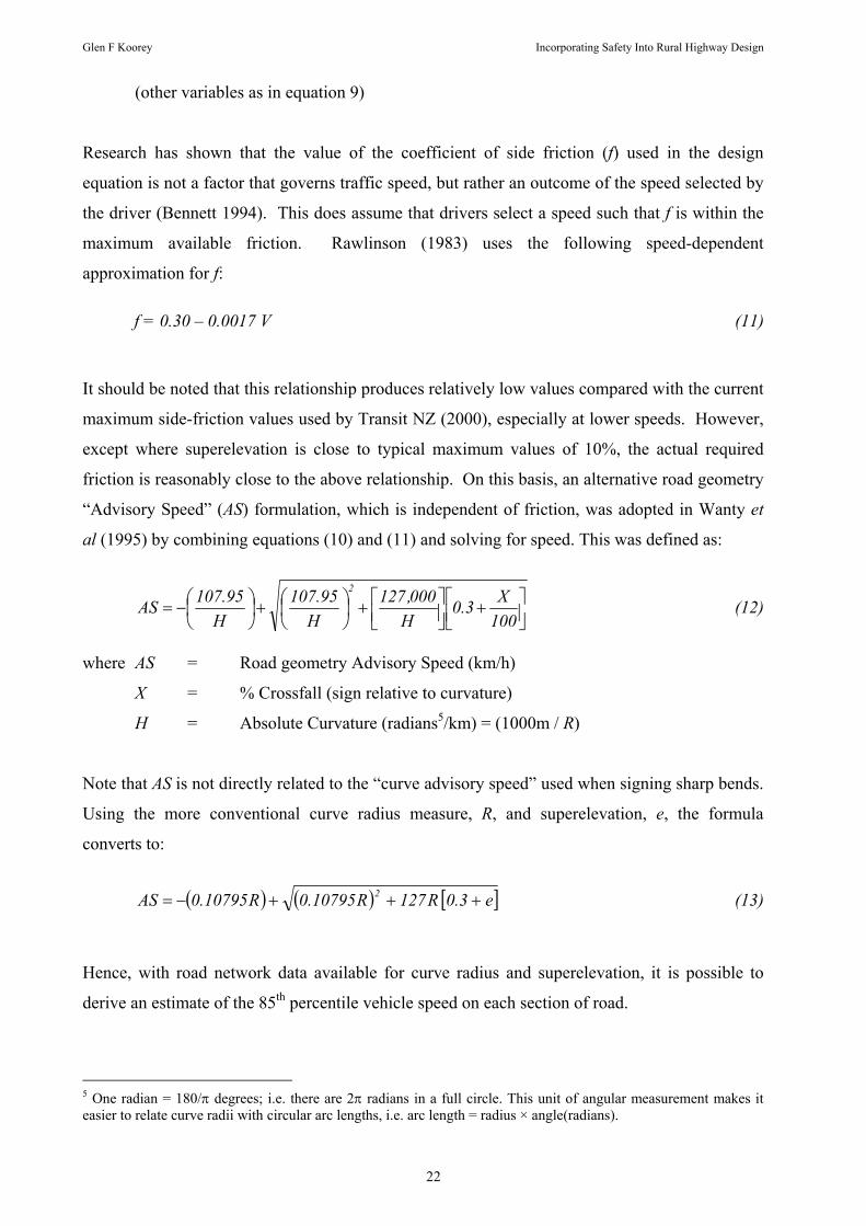
Glen F Koorey Incorporating Safety Into Rural Highway Design
22
(other variables as in equation 9)
Research has shown that the value of the coefficient of side friction (f) used in the design
equation is not a factor that governs traffic speed, but rather an outcome of the speed selected by
the driver (Bennett 1994). This does assume that drivers select a speed such that f is within the
maximum available friction. Rawlinson (1983) uses the following speed-dependent
approximation for f:
f = 0.30 – 0.0017 V (11)
It should be noted that this relationship produces relatively low values compared with the current
maximum side-friction values used by Transit NZ (2000), especially at lower speeds. However,
except where superelevation is close to typical maximum values of 10%, the actual required
friction is reasonably close to the above relationship. On this basis, an alternative road geometry
“Advisory Speed” (AS) formulation, which is independent of friction, was adopted in Wanty et
al (1995) by combining equations (10) and (11) and solving for speed. This was defined as:
⎥⎦⎤
⎢⎣⎡ +⎥⎦⎤
⎢⎣⎡+⎟
⎠⎞
⎜⎝⎛+⎟
⎠⎞
⎜⎝⎛−=
100X3.0
H000,127
H95.107
H95.107AS
2
(12)
where AS = Road geometry Advisory Speed (km/h)
X = % Crossfall (sign relative to curvature)
H = Absolute Curvature (radians5/km) = (1000m / R)
Note that AS is not directly related to the “curve advisory speed” used when signing sharp bends.
Using the more conventional curve radius measure, R, and superelevation, e, the formula
converts to:
( ) ( ) [ ]e3.0R127R10795.0R10795.0AS 2 +++−= (13)
Hence, with road network data available for curve radius and superelevation, it is possible to
derive an estimate of the 85th percentile vehicle speed on each section of road.
5 One radian = 180/π degrees; i.e. there are 2π radians in a full circle. This unit of angular measurement makes it easier to relate curve radii with circular arc lengths, i.e. arc length = radius × angle(radians).

Glen F Koorey Incorporating Safety Into Rural Highway Design
23
The relationship between road geometry and vehicle speed given by equation (13) was validated
by comparing predicted AS values with 85th percentile mid-curve vehicle speeds measured at 31
curve sites, 22 of which were located on the flat, thus minimising gradient effects (Wanty et al
1995). The results showed a clear linear relationship, with a reasonably good coefficient of
determination (R2) of about 0.71. More recently, Tate & Turner (2007) also found that the
calculated AS values on curves along 130km of State Highway (over 450 curves with a range of
alignments) matched observed 85th percentile speeds quite well, and a function using averaged
AS values over 1000m had a correlation of R2=0.88 when compared with observed 85th
percentile speeds over the same length.
The “design speed” approach to speed derivation is intended for analysing the most restrictive
geometric elements, such as tight curves. Therefore, it is not surprising that the above formula
tends to give very high values for speed on straighter sections (indeed, an infinite value for
sections with zero curvature). To allow for this in speed profile analysis, speeds should be
capped to reflect more realistic “desired” speeds of drivers. For example, annual speed surveys
in NZ (MoT 2006c) found that typical 85th percentile free (i.e. unimpeded) speeds on straight
open roads in 2005 were about 104 km/h, although the figure differed between regions from
99 km/h to 110 km/h. The geometry-derived speeds are also less relevant in urban situations,
where speed limits rather than road geometry tend to govern vehicle speeds, so an upper bound
can be applied in these areas (e.g. 60 km/h cap, say, in a 50 km/h area). It is also possible to
incorporate a check that limits any extreme required acceleration between adjacent 10-m
sections, especially for heavy vehicles.
Longitudinal gradient effects can also be incorporated into the AS measure to limit speeds on
slopes. Figure 2.3 shows calculated mean limiting speeds on uphill gradients, based on empirical
observations by Bennett (1994); note that the units on the vertical axis should be in km/h.
Different vehicle classes are shown, ranging from passenger cars (PC) to heavy commercial
vehicles (HCV). It should be noted that these are mean speeds; a conversion is required to
produce 85th percentile speeds, such as that mentioned earlier in this section.

Glen F Koorey Incorporating Safety Into Rural Highway Design
24
Figure 2.3 Mean Limiting Speeds on Upgrades (from Bennett 2004)
It can be seen that, for passenger cars, there is a reasonably linear reduction in speeds from 4%
gradient and above. Therefore, a simple formula to limit speeds on gradients can be
approximated thus:
AS ≤ 125 - G × 5 (14)
where G = % Gradient (positive = uphill)
This helps to reduce the estimated speeds on straight uphill slopes. For example, on an 8% uphill
grade, the AS value cannot exceed 85 km/h. The above formula applies to passenger car speeds;
as can be seen by Figure 2.3, a different calculation is needed for truck speeds. A similar speed
reduction in trucks also needs to be applied to steep downhill grades as well, due to limitations
on braking at speed.
Using these calculations, speed profiles can be produced from road geometry data over a length
of highway. “Local operating speed” can be taken as the average speed over a short length
surrounding the 10m section of interest (to help “iron out” any irregularities in the data and
approximate the actual changes in speed that a vehicle will make), while “speed environment” is
better approximated by the average speed over a much longer distance (to reflect typical speeds
experienced by the driver in the immediate past). Koorey & Tate (1997) used this approach
when studying the effects of speed on crashes and found that lengths of 100 m and 1000 m for
calculating “local speed” and “speed environment” respectively seemed to give sensible results.
The resulting analysis can then identify any sections where local speed is considerably less than

Glen F Koorey Incorporating Safety Into Rural Highway Design
25
the surrounding speed. More recently Tate & Turner (2007) found that the average speed over
the preceding 500m provided a better predictor of curve negotiation speed than the preceding
1000m.
The above measures of “speed environment” are somewhat at odds with more traditional
definitions for speed environment that consider the highway standard over longer distances. At
highway speeds it typically takes less than a minute to travel 1000 m, and this suggests that
drivers have relatively short-term memories in terms of their expectations for the next curve. It
may be of interest to also test the correlation with longer preceding highway distances (e.g. 2-
5 km) against curve negotiation speeds; certainly this does not appear to have been done in any
local studies.
2.3 Types of Road Safety Models
Technically there are two main ways to assess road network features for traffic safety:
1. Empirical studies, involving the collection of road and traffic data from road sites and
identifying a statistical relationship between these characteristics and the crash frequency.
2. Theoretical studies, which consider the logical factors and the chain of events that would lead
to a crash, and the likelihood of these factors/events occurring.
In practice, the empirical approach is much more widely used, although the initial consideration
of factors to include and the model forms to look at is usually based on some theoretical
reasoning. The empirical studies can be further broken down into three approaches:
• Cross-sectional or “mass data” studies, involving the collection of a large number of sites
with varying features and using cross-tabulation or regression techniques to infer
relationships.
• Comparison or “case-control” studies, involving the collection of data from sites with crash
histories and equivalent sites without crash problems to identify the differences.
• Before-and-After or “dose-response” studies, involving the study of sites where safety
treatments have been implemented to see the change in crash occurrence.
Each method has its advantages and disadvantages; their applicability will depend somewhat on
the data available to the analyst and the intended problem to be investigated (e.g. determination
of absolute or relative crash rates).

Glen F Koorey Incorporating Safety Into Rural Highway Design
26
Cardoso et al (1997) noted that many models differed in their development in terms of what type
of data they were calibrated against. For example, while some models used crash data from a
wide and randomly selected sample of the road network, others were based specifically on sites
with notably high and/or low crash frequencies. The latter relationships tended to show much
better goodness of fit, but their applicability to more general examination of locations with a
wide range of crash frequencies may be limited. This is particularly so where a full range of
values for different features has not been examined, and extrapolation of values may not be
appropriate. Any models developed should indicate the limits of the various input ranges to
ensure valid outputs.
2.3.1 Levels of Model Detail
Examination of the various models reveals a certain “hierarchy” regarding the level of detail
incorporated in them. Broadly they can be categorised (in increasing level of detail) into:
• Flow-based models, where the only variables are the traffic flow(s) on the road facility in
question. This means that all of the other typical features of the element being modelled
must be captured in the constant coefficients of the relationship. For example, a model may
be developed to apply to all four-leg urban signalised intersections, with the only inputs
being the opposing traffic flows. Clearly this approach can cause problems where the
attributes of some features (e.g. approach geometry, signal phasing, and number of lanes in
the above example) can vary widely, with known and notable effects on safety.
• Feature-based models, where a number of measurable road features will be included as
variables in the relationship. This allows for the relative effect of these elements on safety to
be more precisely incorporated into the model. For example, a two-lane rural highway
model may require data on seal width, horizontal curvature and access density. But the
features are still all treated as independent items that have no effect on each other, often an
unrealistic assumption. In the above example, the likelihood of wider seal widths may be
directly correlated with the likelihood of less horizontal curvature.
• Feature-interaction models, where related road feature measures may be combined to form
more complex function variables in the relationship. For example, a “driver workload”
variable may be derived in a model as a measure of road classification, access/intersection
density, and horizontal alignment. Alternatively, two correlated variables, such as
carriageway width and average “hilliness” may be multiplied together in a linear model. In
Glen F Koorey Incorporating Safety Into Rural Highway Design
27
theory, feature-interaction models can capture a greater proportion of the explanatory power
of the variables, but with a cost of increased computational requirements.
There are fairly pragmatic reasons for having models at differing levels of the hierarchy. Firstly,
different road facilities have varying numbers of crashes associated with them, and it makes
sense to focus on the areas of greatest need first. Therefore, more detailed (and presumably
more accurate) models can be developed for the high-priority areas, with existing simpler models
applied initially to account for the remaining crashes. Secondly, more detailed models require
additional data collection and subsequent analysis to develop. If this information is not readily
available, then the researchers will have to resort to using simpler models. Finally, the intended
application of the model may dictate the level of detail required. For example, a simple model
may be used to quickly compare a large number of sites at a strategic level; a more detailed
model can then be used to examine the (apparently) most problematic sites in more depth.
2.3.2 Crash Frequencies, Crash Rates and Traffic Exposure
A common thread to most models is that traffic volume (often expressed in terms of average
daily traffic) has the largest effect on predicted crash numbers. Volume may be explicitly built
into a model of absolute crash numbers or it may be implicitly referred to in a model of crash
rates (often expressed in units of crashes/10n vehicles or crashes/10n veh-km). This exposure
effect may be linear in simple models (i.e. {NumberCrashes} = {CrashRate} × {Volume}) but
non-linear methods are increasingly being used to reflect the changes in vehicle interaction at
different volumes, and the subsequent effect on crash type incidence. For example, single-
vehicle crashes are likely to reduce relative to increasing traffic volume (because of the greater
chance of encountering another vehicle instead), whereas multiple-vehicle crashes are likely to
increase. Under-reporting of crashes may also be affecting available crash numbers at different
volume levels. One way to get around this is to produce separate crash rates for different traffic
volume bands (as is done for Land Transport NZ’s existing crash procedures; LTNZ 2006), but
this still produces anomalies either side of the arbitrary boundaries between bands.
Because of this, it seems that a prudent approach would be to derive road network risk models in
terms of the number of crashes expected, rather than producing just crash rates. This will allow
the effect of traffic volume to be correctly incorporated into each model. This approach is being
increasingly prescribed in economic appraisal procedures (Hauer & Persaud 1996, Turner 2002).

Glen F Koorey Incorporating Safety Into Rural Highway Design
28
Intersections present an interesting challenge in terms of measuring exposure. Some previous
models have simply summed that approaching flows from all legs. However, this would mean
that a certain amount of traffic split equally over two intersecting roads would present a similar
crash hazard to a site where the same amount of traffic was mostly carried by one road; usually
this is not the case. As a result, most researchers have favoured the alternative of multiplying the
opposing traffic flows. A further refinement has been to not necessarily use exponents of one;
for example, multiplying by the square-roots of the respective volumes. A lot of research right
back to Tanner (1953) has assumed a square-root relationship; whilst computationally this has
simplified things (particularly in the past when complex statistical modelling was not easily
available), from first principles there is no strong reason to use a 0.5 exponent over anything
else. Even more specifically, work like Turner (2001) has broken down the relationships into the
products of different conflicting turning movement flows to predict the likelihood of different
crash types. At this level, it appears even less likely that consistent exponents can be applied to
the relevant traffic volumes in each case.
Most mid-block (non-intersection) models examined are based on a linear relationship to road
length, with crash rates expressed in terms of “crashes per 10n vehicle-kilometres” (or veh-
miles). However, for some analyses of specific features, such as curves and bridges, it was
deemed more appropriate to estimate crash numbers per feature, irrespective of length (e.g.
Deacon 1986, LTNZ 2006). In the case of locations such as railway crossings, which are
essentially “point” features, this assumption certainly seems valid.
Other exposure variables have been proposed from time to time. For example, Chapman (1971)
cites examples of “conflict area” being used for intersection crashes and travel time being used
for road link crashes. The use of various “conflict” measures has also been proposed, as
discussed previously in Section 2.1.3.
2.3.3 Mathematical Form of Prediction Models
The literature review has identified a number of different approaches to modelling road network
risk. In the past, computational difficulty has limited the complexity of the relationships used,
but now a wider and more appropriate range of options can be fitted. The general approaches
identified are:
• “Linear” models, that relate crash risk to an additive combination of factors, e.g.

Glen F Koorey Incorporating Safety Into Rural Highway Design
29
{CrashRate} = {Constant} + K1×{Factor1} + K2×{Factor2} + K3×{Factor3} + … (15)
where K1, K2, etc are determined by linear regression. A fairly long list of factors may be
considered initially, but generally only factors that are statistically significant explanatory
variables (in terms of their effect on the overall relationship) are retained. Section 2.3.5
discusses some of the more common factors used. The {FactorN} terms may be the direct
value of the attribute (e.g. shoulder width in metres) or an alternative such as the reciprocal
value (1/{CurveRadius} is commonly used, for example). An extension on this is to use
higher-order exponents, such as K1×{Factor1}2, to better reflect the relative change in effect
of different factors; perhaps now technically this should be termed a “polynomial” model
instead.
Linear models assume an independence between different factors, i.e. a certain change in one
factor has a known change on the overall crash rate, irrespective of the other factors. For
example, an increase in carriageway width by 1 m would always result in a decrease in the
predicted crash rate of (say) 5 crashes per 100-million veh-km, irrespective of the values of
the other factors. This is often an unrealistic assumption and more recent safety models have
tended to be non-linear.
• “Multiplicative” models, that relate crash risk to all factors in conjunction with each other,
e.g.
{CrashRate} = {Constant} × {Factor1}K1 × {Factor2}K2 × {Factor3}K3 × … (16)
where K1, K2, etc are determined by generalised linear regression. Sometimes the factors are
the exponents instead of the base, i.e. K1{Factor1}. A specific variation of this is to use the
Poisson distribution to create relationships of the form
{CrashRate} = e ({Constant} + K1×{Factor1} + K2×{Factor2} + K3×{Factor3} + …) (17)
Poisson regression models (or similar negative-binomial models) are often preferred to the
previous forms shown, as they better represent the usual distribution of crash numbers in
reality. This is particularly important where a substantial number of sites have very low
crash numbers (i.e. zero or one) that have to be reconciled with the occasional sites with high
crash frequencies.
Multiplicative models are generally better than linear models in that a certain change in one
factor has a varying change on the overall crash rate, depending on the size of the other
factors. For example, an increase in carriageway width by 1m would always result in a

Glen F Koorey Incorporating Safety Into Rural Highway Design
30
decrease in the predicted crash rate of (say) 10%, but it is impossible to know the absolute
change in crashes without knowing the values of the other dependent model variables. The
assumption that the relative change will always be the same is still not necessarily true, but is
probably more accurate than the previous linear approach.
• “Modifier” models, with deficiency-specific risk reductions that identify the relative changes
in crash risk between different standards of road features. These methods generally do not
determine the absolute crash risk, mainly because they assess each deficiency in isolation
(i.e. they do not consider other site-specific attributes). As a result, they are most practical
for locations where an estimate of the change in the existing (known) crash rate is desired. A
modifying factor of 0.8 for example, suggests that the proposed feature will result in a 20%
reduction in crashes, compared with the base case.
Some models (e.g. Austroads 2001, Harwood et al 2000) have attempted to combine this
approach with absolute crash rates, e.g.
{CrashRate} = {BaseCrashRate} × {ModifyingFactor1} × {ModifyingFactor2} × ... (18)
The base crash rate is often determined for a road type with defined (usually “best case”)
geometric attributes. Alternatively, it may simply represent the “average” for all facilities.
Modifying factors are then used to adjust the relative risk of sites that have different
standards. For example, if the base case has 3.5m lanes, then a road with only 3.0m lanes
may have a factor of (say) 1.3 applied to the base crash rate to reflect a greater crash risk on
the narrower road. The modifying factors may be calculated directly from underlying road
measures via some mathematical relationship, or a series of categorical values may be
determined for different road feature standards.
This approach has some attractions in terms of its transparency (i.e. the relative effect of each
factor is easy to discern) and its modularity (i.e. individual factors can be modified as better
information becomes available, without affecting the rest of the model). The potential
difficulty with these models (as with the multiplicative models) is the assumption that the
same risk modification applies in all cases, irrespective of the site context. Attempts to
combine multiple risk modifiers at the same site may also be inappropriate, depending on the
inter-relationship between different features.
The above examples suggest that the individual factors are treated separately. However, in many
cases the best-performing relationships include aggregated factors, e.g.

Glen F Koorey Incorporating Safety Into Rural Highway Design
31
({Factor1}×{Factor2})K12. This is the basis of many feature-interaction models, discussed in
Section 2.3.1. If some factors are known to have some co-linearity (i.e. are somewhat dependent
on each other), combining them in a single factor may be one way to get around this problem.
In their study of rural carriageway crash relationships, Halcrow Fox (1981) found that simple
exponential (power) curves generally fitted the associations at least as well as more complex
models. The effects of elements in combination were assumed to be multiplicative, which was
satisfactory for single-carriageway data.
If the factor is of a categorical rather than a numeric nature, a series of proxy values may also be
used to convert them into numerical equivalents, e.g. the presence or not of a passing lane, the
level of access control. This approach is also sometimes used to split continuous values into a
series of groups instead, where a categorical relationship is more appropriate, e.g. lane widths
greater or less than “xxx metres”, “high” or “low” speed limits.
One problem to be wary of is when general “base crash rate” models are used to determine the
relative safety effect of changing a particular road or intersection type to another type. It may
not be valid to compare the two base rates, as the sample of facilities they are based on may be
quite different. Hauer and Persaud (1996) give the example that installing STOP signs where
previously there were YIELD (GIVE WAY) signs is likely to reduce the crash rate. Yet the
average observed crash rate at STOP-controlled sites is generally higher than YIELD-controlled
sites, due to other site-specific factors. This issue was also identified in a NZ study determining
benefits of rural four-laning (BRC 2000). While the additional lanes and median provided
certain safety and operational benefits, it was also recognised that a new four-lane facility was
likely to have a better alignment than the existing two-lane facility, with corresponding benefits
associated with that.
Most of the models identified produce a single answer (point estimate) for the predicted number
of crashes (or predicted relative savings). In reality however, it is better to assume that the true
answer lies within a range of values, especially given the variability and vagaries of the data
typically used to develop the relationship and to apply it in practice. The type of model form can
help to indicate the likely distribution of expected results, be it a Normal distribution, Poisson
distribution or whatever. It would be desirable to incorporate this inherent uncertainty into our
models to accurately reflect the level of confidence that we have in our answers. Ultimately this
uncertainty could feed through to the economic appraisal stage of projects, to identify both the

Glen F Koorey Incorporating Safety Into Rural Highway Design
32
possible range and most likely value of benefits to be achieved. The GradeDec 2000 model for
example (FRA 2000) uses simulation of repeated trials to determine the likely range of benefits
from changes to railway crossing configurations.
2.3.4 Incorporation of Existing Crash Data
One problem in trying to predict crashes at a particular location is how to take into account every
single aspect of the site’s geometry and other features. A site may, for example, have a certain
combination of features that produce a less safe environment, but this may not be easily captured
by recording standard parameters such as road width and curvature. Conversely, a site may be
safer than expected, perhaps because its complex appearance makes drivers take more care.
While a more detailed crash prediction model could try to identify each of the features that
contribute to the relative safety of the site, it becomes more difficult to so with any precision
once the major features have been identified.
A method to try to resolve this is to combine the existing crash history at the site with the
predicted crashes for a typical site of this nature. This allows the expected crash rate to be scaled
up or down to allow for localised effects. The most common approach is known as the
“Empirical Bayes” (EB) method, alluding to the use of Bayesian probability theory. A form of
EB prediction has been introduced into Land Transport NZ’s crash analysis procedures (Turner
2002).
Hauer (1997) outlines the basic method. Consider a site with a recorded history of H crashes
over a known period. A crash prediction model for similar sites estimates M crashes for the site
over the same period. The combined weighted average of the two gives a crash estimate, E,
which can be calculated as:
E = w × M + (1-w) × H (19)
where
Weighting w = 1 / [1 + M/k] = k / [k + M] (20)
k is termed the “over-dispersion parameter” (usually derived from the model form being used,
e.g. negative binomial) and reflects the relative lack of confidence in the particular crash
prediction model (strictly speaking, it reflects the difference between the variance and the mean
of the crash distribution). It can be seen that a lower k value or a higher predicted crash
frequency M result in a lower weighting on the crash prediction model and more emphasis on the

Glen F Koorey Incorporating Safety Into Rural Highway Design
33
crash history. More complex calculations can also be derived for situations where a variety of
crash history periods are used, including the use of more general “Hierarchical Bayes” methods
(Schlüter 1996).
When implementing a Bayesian method, existing crash data and a suitable crash prediction
model are the key requirements. The difficulty is usually in determining the k values for the
prediction models, which is somewhat based on the relative statistical variance predicted by each
relationship. Therefore, more work will be needed to establish these variance measures in future
crash risk models used in NZ.
Persaud and Lyon (2006) note that the use of EB procedures can also be quite advantageous to
counter both the effects of “regression to the mean” and low mean crash numbers. Such
problems are quite prevalent in two-lane rural roads such as many of those found in NZ.
2.3.5 Common Factors Used in Models
Apart from traffic volume and road length, a wide range of road factors have been tried in
different crash risk models worldwide. Other major factors regularly identified include:
• Road type (hierarchical classification, median-divided, number of lanes)
• Intersection type (form of control, number of legs, turn-lanes)
• Road environment (speed limit, adjacent land use, access control, lighting)
• Road geometry (terrain, horizontal curvature, vertical grade, sight distance)
• Cross-section (lane/shoulder width, medians, roadside hazards)
• Delineation (warning signs, lane/edge lines, marker posts/reflectors)
• Road surface (sealed/unsealed, skid resistance)
• Traffic speed (mean speed, speed variance, required speed reduction)
• Specific features (bridges, railway crossings, traffic calming)
• Road users (proportion of trucks, cycling facilities, pedestrian crossings)
While the selection of factors to look at is often dictated somewhat by basic theory (e.g. the
sealed shoulder width is likely to have an effect on the incidence of run-off-road crashes), in
many studies the choice of variables to use has been dependent on their ready availability to the
researchers. For example, a road inventory may have information on carriageway widths but not
on horizontal curvature. If the researchers have sufficient resources they may be able to
Glen F Koorey Incorporating Safety Into Rural Highway Design
34
independently collect additional field data on horizontal curvature at a number of sites, otherwise
that factor cannot be included in the study.
Clearly there is some interaction between some of the variables listed. For example, the terrain
of the road is likely to influence the expected horizontal curvature and subsequent mean speeds.
The design standards used on different classes of roads are also likely to produce some
correlation between physically unrelated road features. However, many studies have not
included all of these factors together, or have combined them into a single variable. Another
way to improve the explanatory power of the relationships is to fit separate models to different
road or intersection types.
Generally different models will be produced for intersection and non-intersection crashes,
reflecting the most appropriate road factors and traffic exposure measures for each case. In some
cases, it may be difficult to analyse all intersections (particularly minor ones) separately from
their adjacent through-roads because of a lack of data about the features and traffic at each
intersection. To get around this for road safety prediction, some means of modelling these
“combination” road sections is necessary. This mirrors a common practice in traffic network
modelling where only “major” intersections and links are modelled, with minor intersections and
links in between not explicitly specified. For example, SafeNET (Burrow 1999) uses the
concept of “composite” road links between major junctions, where the number of intermediate
junctions is one factor used in the crash prediction model. Mountain et al (1996) found that such
models in combination with existing crash data via an EB procedure gave the best results.
While developing separate models for different road/intersection categories has many
advantages, it is important to appreciate that there is a limit to this approach. The basic reason
comes to down to data availability – every time the base data set is disaggregated into further
sub-categories, the sample sizes within the various “data cells” get smaller, making it harder to
develop sufficiently accurate models. The compromise is to combine smaller categories together
into the same relationship (i.e. with the same factors and coefficients), with possibly a constant
multiplier to differentiate between the two categories, e.g.
{CrashRate} = {Constant} × K1{Factor1} × K2
{Factor2} × … × KN{0 if Category A, 1 if Category B} (21)
Sometimes intermediate factors have been developed to capture the combined effects of multiple
features. For example, “driver workload” is a commonly used factor to attempt to describe the

Glen F Koorey Incorporating Safety Into Rural Highway Design
35
behavioural context of the driving task in a given road environment. Typical features used to
develop driver workload measures include road type, alignment geometry/consistency, and
cross-section changes.
One has to be wary to not necessarily infer cause-and-effect from having a factor included in an
empirical model. It merely represents significant statistical association with the resulting crash
rate. It does not always follow that the coefficients of individual factors in a multi-factor model
can be used to determine the likely savings from individual feature changes. Where various
factors have some correlation between them, the effect is even less clear. The safety effect of a
factor not included in the model may be attributed to a related factor that is included instead.
2.3.6 Crash Types and Severity
Many factors listed above have their greatest effect on only a proportion of all crashes. For
example, lighting should affect only night-time crashes, roadside improvements should only
affect run-off-the-road crashes. While it may be possible to determine the typical proportion of
all crashes that meet these categories and hence the overall effect on crashes of changing a
feature, it is probably more transparent to have models that apply the effects only to the crash
types in question. The intersection crash models of Turner (2001) for example separate the
effects of different intersection types on rear-end crashes, right-turn-against crashes, crossing
crashes, etc.
Another consideration when developing models to ultimately derive social costs of crashes is
that the effect on crash severity is not necessarily related to the crash frequency or rate. Removal
or mitigation of roadside hazards for example may not reduce the incidence of run-off-road
crashes but it is likely to have a noticeable effect on their severity. The likelihood of under-
reporting of lower severity crashes on remote or quiet roads may also mean that the apparent
average severity is affected by traffic volume. While crash severity could be incorporated into
the road safety risk models, in most cases it is treated as a separate step. Therefore, care needs to
be taken to ensure that the effects of different road features are adequately represented in terms
of both crash incidence and severity.
Koorey & Tate (1997) investigated the effects of speed environment (determined by road
geometry using methods described in Section 2.2.1) on rural injury crash severity, using the
average social costs of crashes for each severity category as specified in NZ economic

Glen F Koorey Incorporating Safety Into Rural Highway Design
36
evaluation. They found that locations with speed environments of ~110 km/h had average crash
costs approximately double that of sites with 70 km/h speed environments.
One possible approach to these issues is to determine a default distribution of crash types and
severities for the base road/intersection type being modelled. Additional modification factors
can then be used to adjust these distributions (or at least their social cost implications) for other
levels of facility present. For example, the presence of a separate right-turn lane at an
intersection will probably reduce the proportion of rear-end and turning crashes.
2.4 Overseas Models
Road network risk models have been identified from overseas for virtually every kind of facility.
However, some facilities, e.g. rural two-lane roads, appear to have had considerably more
research done than other facilities, e.g. urban roundabouts. As well as reflecting the frequency of
use of each facility worldwide, research has also often focused on areas of greatest safety
concern, e.g. rural horizontal curves.
The following sections summarise some of the interesting approaches to road network risk
modelling identified overseas.
2.4.1 Interactive Highway Safety Design Model
A noteworthy overseas project underway is the Interactive Highway Safety Design Model
(IHSDM), being carried out by the US Federal Highways Administration (FHWA). IHSDM is a
suite of evaluation tools for assessing the safety impacts of geometric design decisions, to help
planners and designers maximise the safety benefits of highway projects within the constraints of
cost, environmental and other considerations (FHWA 2006).
Developed since 1993 by the FHWA, this publicly available software can help planners and
designers identify and assess treatments for potential safety problems on existing or proposed
highway sections (Krammes 2000). The initial development effort focused on two-lane rural
highways, with the first public release in 2003. IHSDM has also been designed to allow for local
customisation to suit various jurisdictions (see details of this in Section 5). This makes IHSDM
also potentially very applicable to the bulk of NZ’s rural State Highway network.
Glen F Koorey Incorporating Safety Into Rural Highway Design
37
IHSDM consists of several analysis modules, to assess different aspects of highway designs:
• Crash Prediction Module (CPM), to estimate the number and severity of crashes on specified
roadway segments.
• Design Consistency Module (DCM), to provide information on the extent to which a
roadway design conforms to drivers’ expectations (especially speed profiles).
• Driver/Vehicle Module (DVM), to estimate drivers’ speed and path choice along a roadway
and subsequent measures including lateral acceleration and friction demand (beta version
only available).
• Intersection Diagnostic Review Module (IRM), which uses an expert system to evaluate
intersection design alternatives, and suggest countermeasures to safety problems.
• Policy Review Module (PRM), to verify compliance of designs with specified national/state
highway design policies and guidelines.
• Traffic Analysis Module (TAM), to estimate via traffic simulation the operational effects of
road designs under current and projected traffic flows, e.g. travel times, time spent following,
vehicle interactions.
At one stage a Roadside Safety Module (RSM) was also being considered, to evaluate the
impacts of decisions such as the placement of guardrails, embankment slopes, continuous
obstacles, and other hazards. This appears to have been abandoned, with some aspects of it
incorporated into the other modules (e.g. crash prediction of roadside hazards into the CPM).
These modules have been packaged together as a single application, together with associated
support tools. For example, a major requirement of the program is the ability to explicitly
specify in detail the design aspects of the highway proposal to be investigated. As well as a
built-in highway editor, the FHWA have also been working to develop import tools for major
CAD/design software packages (e.g. GEOPAK), and ultimately to allow for IHSDM modules to
be integrated within these packages.
Although all of the modules provide outputs of relevance to the safe design of a highway, it is
the CPM that is of most direct interest to this study. Harwood et al (2000) developed the CPM
algorithm used in IHSDM, consisting of base models and “accident modification factors”
(AMFs) for both roadway segments and at-grade intersections, as described below.

Glen F Koorey Incorporating Safety Into Rural Highway Design
38
The base models provide an estimate of the safety performance of a roadway or intersection for a
set of assumed nominal or base conditions, while the AMFs adjust these predictions to account
for the effects on safety of various site features. For roadway segments these features include
lane width, shoulder width, shoulder type, horizontal curves, grades, driveway density, two-way
left-turn lanes (i.e. “flush medians”), passing lanes, and roadside hazards.
In this way, the CPM algorithm can be used to estimate the relative safety of existing or
proposed roadways (including multiple project options). The system can be calibrated to adapt
the predicted results to the safety conditions for a particular highway jurisdiction, and actual site
crash history data can also be incorporated via an Empirical Bayes method.
The IHSDM base model for rural roadway segments is a negative binomial regression
relationship, which includes exposure, lane and shoulder widths, driveway density, roadside
hazard rating, horizontal curvature, and vertical gradient and curvature. The form of the base
model for roadway segments is:
Nbr = EXPO exp(0.6409 + 0.1388STATE - 0.0846LW - 0.0591SW + 0.0668RHR + 0.0084DD) (ΣWHi exp(0.0450DEGi)) (ΣWVi exp (0.4652Vi)) (ΣWGi exp(0.1048GRi)) (22)
where:
Nbr = predicted number of total crashes per year on a particular roadway segment EXPO = exposure in million vehicle-miles of travel per year = volume × length STATE = location of roadway segment (0 in Minnesota, 1 in Washington) LW = average lane width (ft) SW = average shoulder width (ft) RHR = roadside hazard rating, using a qualitative 1 to 7 scale (Zeeger et al 1987) DD = driveway density (driveways per mi) on the roadway segment WHi = weight factor for the ith horizontal curve in the roadway segment DEGi = degree of curvature for ith horizontal curve (degrees per 100 ft) WVj = weight factor for the jth crest vertical curve in the roadway segment Vj = vertical curve rate for jth crest vertical curve = grade change / curve length WGk = weight factor for the kth straight grade segment GRk = absolute value of grade for the kth straight grade (percent).
(see Harwood et al 2000 for full details of the model)6
6 It should be noted that, while the underlying models have been developed using Imperial units of measurement (such as feet and miles), IHSDM can be customised to allow either Imperial or metric (SI) inputs and outputs.

Glen F Koorey Incorporating Safety Into Rural Highway Design
39
When a model is required for default road conditions, standard values are entered for the various
road features (e.g. no curvature, 6-ft shoulders) to produce a simpler exposure-based model.
Similar equations have been developed for various intersection types, with more pertinent
variables such as the presence of turning lanes and intersection skewness. AMFs can then be
applied to the base models where necessary; for example, Figure 2.4 shows diagrammatically
how crash risk is predicted to change in the model for roads with shoulders other than the default
6-feet width.
Figure 2.4 IHSDM Crash Modification Factor for Shoulder Width
1.10
1.50
1.07
1.30
1.02
1.15
1.00
0.98
0.87
0.80
0.90
1.00
1.10
1.20
1.30
1.40
1.50
1.60
0 500 1000 1500 2000 2500
Average Daily Traffic Volume (veh/day)
Acc
iden
t Mod
ifica
tion
Fact
or
0.0m (0-ft) shoulders
0.6m (2-ft) shoulders
1.2m (4-ft) shoulders
1.8m (6-ft) shoulders
2.4m (8-ft) shoulders
This factor applies to single-vehicle run-off-road, multiple-vehicle same-direction sideswipe accidents, and multiple-vehicle opposite-direction accidents.
(adapted from Harwood et al 2000)
The general formula predicting roadway segment crash frequency, combining the base models
and AMFs, is shown below:
Nrs = Nbr (AMF1r × AMF2r × … × AMFnr) (23)
where:
Nrs = predicted total number of roadway segment crashes per year
Nbr = predicted number of crashes per year for nominal or base conditions
AMF1r … AMFnr = accident modification factors for roadway segments

Glen F Koorey Incorporating Safety Into Rural Highway Design
40
It should be noted that the general form of the crash prediction models and accident modification
factors used in IHSDM also forms the basis of the forthcoming Highway Safety Manual (Hughes
et al 2004), scheduled for release in late 2009, which intends to provide practitioners with crash
analysis and prediction guidance over a wide variety of road and intersection types.
One factor that does not appear to be well allowed for in the existing CPM is the effect of speed
consistency. All of the factors used in the base model and AMFs are measures ascertained for
each road element down the highway; there appears to be no allowance for interaction between
adjacent elements. While the DCM can be used to identify where there are any speed
inconsistencies between adjacent sections, it seems clear that this issue should also have an effect
on the predicted crash numbers. For example Koorey & Tate (1997) demonstrated the effect of
approach speed (or more pertinently, the difference between approach and curve speeds) on
crash rates for curves.
Potts et al (2000) investigated the effect of preceding tangent lengths on curve safety. They
found a relatively weak relationship between increasing tangent lengths and increasing crash
rates for curves with radii <340 m and proposed a simple AMF to incorporate this factor into
CPM algorithm. However, it appears that this has not been undertaken yet for the existing
IHSDM implementation.
In practice, this may not be an issue when using IHSDM to develop and evaluate new
alignments. Probably the DCM would be used first to ensure that a reasonably consistent
alignment is provided before using the CPM to estimate the likely crash rate. However, if
IHSDM is also to be used as a tool to assess existing road alignments, then the CPM might not
accurately reflect the observed crash rate. This has major implications if IHSDM is being
calibrated for local conditions using crash data from sub-standard or inconsistent alignments.
The CPM also makes little allowance for the effects of including spiral transition curves either
side of the circular arc. For example, according to Harwood et al (2000), the AMF for horizontal
curves would only be decreased by ~ 3% with spirals present. This is not likely to produce a
large effect at most sites in terms of driver safety, and most research is fairly inconclusive about
the benefits of spirals (e.g. Tom 1995, Council 1998). Design practice around the world is also
very mixed about the incorporation or not of spirals in horizontal curve design (Weale 2006).
Lamm et al (2000) however found that, for a database of 1500 km of German rural roads, curve-

Glen F Koorey Incorporating Safety Into Rural Highway Design
41
related crashes reduced quite noticeably for curve radii <300 m that had spirals (e.g. about 20%
fewer for curves of 100 m radius); above that radius they appeared to provide no benefit.
The results from IHSDM can be reported in a number of different formats. Various text-based
reports and graphical plots can be produced and customised to suit the user’s needs. For
example, plots can chart road geometry data and also show a speed profile along the highway,
which is used by the DCM to identify inconsistencies in speed environment. This plotting layout
is very similar to that commonly produced in NZ for State Highway strategy studies.
Levison et al (2001) outlines the theoretical development being incorporated into the
Driver/Vehicle Model (DVM), not yet available. The DVM has six major computational
functions:
• Perception (identify sight distance limitations, distances/positions/speeds, allowance for
errors)
• Speed Decision (use comfort and posted speeds to determine acceleration/deceleration)
• Path Decision (assume either curve cutting or follow lane for different drivers)
• Speed Control (time delay between changing pedals, pedal depression rate)
• Path Control (assume feedback loop to correct errors after action/perception delay)
• Attention (currently assumed to have full attention to driving, otherwise delays in reactions)
This kind of breakdown of driver behaviour is a useful way of considering the task of driving
around a curve. Levison et al also suggested that drivers make one of a number of assumptions
when presented with a limited sight distance situation, such as a curve:
• Drivers familiar with the road may drive according to the remembered alignment
• Drivers may assume a long straight just beyond the visible range
• Drivers may assume a possible hazard just outside the visible range
• Drivers may assume that the unseen geometry will be similar to the current alignment
The assumption used has implications for what speed a driver will choose, free of any traffic
constraints. It is important therefore to identify what proportion of drivers fall into each
category, although it is not immediately clear how this might be achieved accurately.

Glen F Koorey Incorporating Safety Into Rural Highway Design
42
Some key assumptions used in the DVM to date are:
• The driver is experienced at the driving task in general (controls, steering, etc), but not
necessarily familiar with the highway geometry presented.
• Drivers make appropriate decisions/actions, given good perceptual information.
• The driving environment is relatively relaxed (i.e. not emergency situations)
• Only vehicle path and speed tasks are considered. Other tasks such as monitoring traffic
signs and other traffic are generally not included.
Although the above assumptions help to simplify the behavioural model required, it has to be
accepted that exceptions to all of these assumptions (e.g. inexperienced drivers, distractions) are
often major factors in many crashes.
Further details about the features and operation of the current version of IHSDM, including the
calibration process, can be found in Section 5.
2.4.2 SafeNET
SafeNET (Software for Accident Frequency Estimation for Networks) is a software package,
developed in the UK by TRL, to assist traffic engineers in the design of safer road networks in
towns and cities (TRL 2002). SafeNET provides a rapid assessment of the safety effects of
potential network management changes, such as a change of intersection control or redistributed
traffic volumes. Graphical and textual outputs enable the user to see how such changes affect the
crash frequency on the network.
A network of road links and intersections can be graphically created within the program (see
Figure 2.5), or data can be imported from certain traffic modelling packages, e.g. CONTRAM.
A range of road and intersection types can be chosen from, primarily in an urban context.

Glen F Koorey Incorporating Safety Into Rural Highway Design
43
Figure 2.5 Network Editor in SAFENET
Burrow (1999) summarises the key facets of the safety modelling within SafeNET. The package
implements a number of (generalised linear) crash-risk models of various roading components,
developed from different UK studies for the Department for Environment, Transport and the
Regions (DETR). These allow estimates to be made of the crash frequency (number of crashes
per year) for particular elements of the road network (intersections of different types and road
sections). The total number of crashes predicted in the network is then obtained as a sum of the
estimates for each element.
An interesting aspect of this package is the ability to model at a series of “levels” of complexity.
The detail of inputs provided generally determines the detail of outputs (i.e. crash types, vehicles
involved). At the coarsest level, only simple flow data (AADTs) are used. At the next level,
turning movements and general feature descriptions can also be provided. The highest level also
uses geometric details, vehicle compositions, land use, and so on to produce even more precise
crash predictions.
By default, SafeNET will predict the crash frequency by only using the traffic and road data
provided. However, by entering data for the historical injury crashes over a number of years,
SafeNET can modify the prediction to take account of prevailing local conditions. The
modification is made using the well-established Empirical Bayes technique, discussed in
Section 2.3.4.

Glen F Koorey Incorporating Safety Into Rural Highway Design
44
Although SafeNET is primarily designed for modelling urban road networks, with various forms
of intersection control and traffic management features, it does allow rural road links and priority
intersections to be included. However, the level of detail for rural links is very limited, with no
allowance for key geometric elements such as curvature and sight distances (although urban
links can have “bendiness” specified). Development of a model with a similar approach to
SafeNET but more specifically focused on rural highways merits investigation however.
2.4.3 Road Safety Risk Manager
In 1998 AUSTROADS commissioned ARRB Transport Research to develop a procedure to rank
the recommendations derived from the road safety audit of existing roads; often the number of
recommendations produced greatly exceeds the immediate implementation budget available.
Based on the findings of this project, a risk management approach to prioritising road safety
treatments was developed. Following trialling by Australasian road authorities, customised
software was developed to form the Road Safety Risk Manager (RSRM) program (McInerney
2001), which has now been released for general use. While the model is primarily targeted at
Australian road safety practitioners, work has been done to incorporate suitable NZ values for
various parameters to allow its application here (e.g. discounting rates used).
The analysis method is based on the measurement of risk as a function of exposure, likelihood
and severity, and provides users with the ability to analyse the relative risks of a hazard and its
proposed treatment. More than 50 different types of roading deficiencies have been quantified to
date, across a variety of different road types and severity outcomes. Following inclusion of
treatment costs, the derived “risk reduction-cost ratio” (i.e. the reduction in relative risk per unit
of cost) forms the basis of prioritising the proposed works. During initial testing it became
evident that the process could be applied to all road safety treatments, not just those from
existing road safety audits.
For different road and intersection types, general crash risk factors have been derived to
differentiate the relative risk of each facility, all other things being equal. The other key risk
scaling factor is the traffic exposure, based on how much of the prevailing daily traffic volume
could face the hazard being investigated (e.g. 50% of AADT for a hazard on one side of a
divided road).

Glen F Koorey Incorporating Safety Into Rural Highway Design
45
The relative risks for each deficiency type are based on a literature review of many crash studies.
A continuous range of treatments/standards is presented for the user to select the appropriate
level of risk present. The “best case” (safest) scenario is given a relative risk of 1.00, with lesser
standards resulting in higher risk values. For example a feature with a relative risk of 1.20 is
expected to have 20% more crashes than the safest case. The descriptions of standards are (by
their nature) usually somewhat subjective, and so some engineering judgement is required to
select a reasonable value. These risks are scaled by the general crash risk factors to allow for
their effect on different facilities.
To set the relative risk in context, a number of influencing factors are provided (appropriate to
each deficiency) that allow the base relative risk to be scaled according to the particular site in
question. For example a roadside hazard on a narrow road with a winding alignment is likely to
pose a greater risk than the same hazard on a wide straight road. Influencing factors can be
changed in a similar way to the relative risk factors above, with 1.00 being the best case.
The other key effect on the hazard risk is the relative severity of the crashes caused. The user
identifies the likely make-up of crash types and their relative severity is determined, based on the
average social costs of each crash type. Where a roadside (“clear zone”) hazard is involved, the
calculations are also based on the type of object and its distance away from the road.
The data for each hazard is combined to produce an overall Hazard Risk Score. On its own, this
number has no practical significance but it does enable comparisons with other hazards and with
proposed treatments. In theory these risk scores provide a proxy for the expected social costs of
crashes associated with the site, although comparing them with true crash rates and costs does
not appear to be straightforward.
A similar process is undertaken for any proposed treatments to the hazard, producing an
alternative Hazard Risk Score. By providing information on the cost of implementing the
treatment, a Risk Cost Ratio for each treatment can then be calculated. These can then be
compared against each other, in a similar way to how Benefit-Cost Ratios are compared for
projects here.
Although further work is required to improve some of the risk factors used and improve the
analysis method, the existing program provides a considerable advance on previously subjective

Glen F Koorey Incorporating Safety Into Rural Highway Design
46
means of prioritising road safety projects and certainly a faster assessment than doing a similar
exercise manually.
2.4.4 Other Safety Models
Hunt & Mahdi (1995) describe the development and assessment of a model for predicting crash
frequency on rural single carriageway roads. A database describing the crash frequency, layout,
geometric design and traffic characteristics of 500 0.5-km sections of single carriageway road
was assembled, with a microsimulation model, OSCA, used to generate many of the traffic
parameters. Available data included factors such as AADT, “bendiness” and the number of side-
road accesses, while traffic data such as mean spot speed and percentage of impeded vehicles
was generated at 50m intervals. A multiple linear regression relationship for crash frequency
was found to provide the best fit to the data (as opposed to a multiplicative model), although the
fit was still relatively poor for sites with high/low crash frequencies. The most statistically
significant factor was the difference between the 50m interval mean speed and the overall mean
speed of a road section, rather similar to the measures of local speed versus speed environment
mentioned previously. The model could be applied to evaluate variations in crash frequency that
would be associated with changes in layout, geometric design, or traffic flow on rural single
carriageway roads.
In Europe, the SAFESTAR (Safety standards for road design and redesign) project is a research
study focusing on traffic safety for what is known as the “Trans-European Roadway Network”
(TERN) that links the major European centres. The aim is to develop safety standards for
highway design and redesign on all classes on road involved (Wegman & Slop, 1995). Nine
European research institutes are collaborating on SAFESTAR, with the Institute for Road Safety
Research (SWOV, Netherlands) coordinating these activities. Of the eight priority areas being
investigated, two of particular relevance are “cross-sections of rural roads” and “design of curves
in rural roads”, and working papers have been produced documenting the findings to date
(Cardoso et al 1997, VTT 1999). Although the project does not include the specific
development of road safety models, the literature review has identified a large number of
relationships developed in the past from which to produce best practice guidelines. Some of
these could be used for development of models for NZ.
The Finnish National Road Administration (FinnRA) evaluates yearly traffic safety improvement
targets using a program called TARVA (named for the Finnish words that mean “Evaluation of

Glen F Koorey Incorporating Safety Into Rural Highway Design
47
Safety Effects Using Effect Coefficients”). Introduced in 1995, TARVA uses crash models
together with crash history to estimate the expected number of crashes on the road if no
measures would be implemented. The effects of measures can then be evaluated using a
standard set of incidence and severity reduction factors for different treatments. Relatively
simple relationships, largely based on vehicle exposure, are primarily used to estimate average
risk for homogenous road sections, with more complex models available if necessary that
include sight distances, road widths, etc. FinnRA found that, when combined with historical
crash data, more complicated models did not significantly improve the prediction effects (Peltola
2000). It may be possible to adopt or incorporate a system like this for strategic safety planning
here.
As well as specific models, a number of overseas reports reviewed also provide broad critiques
of approaches to modelling safety. Hauer & Persaud (1996) for example, consider the problem
of how to adapt the US project appraisal software MicroBENCOST to produce suitable safety
evaluations for Canadian projects. In a NZ context, it is a similar exercise to that of how best to
develop safety evaluation procedures such as those found in Land Transport NZ’s EEM (LTNZ
2006).
None of the overseas models examined to date appear to be immediately usable here for
prediction of absolute crash numbers, given the comparative differences in roading, social and
legislative environments. However, in many cases, the models could perhaps provide a
reasonable estimate of the relative change in crashes between two situations, enabling
practitioners to apply this relativity to existing crash numbers. More importantly the underlying
model forms and relationships can be used as templates for developing similar models for NZ.
2.5 New Zealand Models
Until recently, there had been little NZ research based on local road network data, with many
studies, such as Travers Morgan (1992) referring mainly to findings from overseas and assuming
that they will apply here. A few specific studies had been carried out, such as Matthews &
Barnes’ (1988) study of factors affecting curve crashes, and Frith & Harte’s (1986) review of
safety effects of intersection control changes. The development of national project appraisal
procedures over the last decade (LTNZ 2006) has hastened the derivation of appropriate crash
prediction information. Many of the initial typical crash rates for various facilities were
developed from LTNZ crash data in the early 1990s. Since then, further generic volume-based

Glen F Koorey Incorporating Safety Into Rural Highway Design
48
models for many different facilities have been proposed, such as the review of link and
intersection crash rates carried out by Gabites Porter (1995) and more recently one by Turner
(2001). More specific investigations of various treatments have also been carried out, such as
the safety effects of median barriers (BCHF 1998) and passing lanes (Koorey et al 1999).
2.5.1 State Highway Road Geometry Data
Since 1992, NZ’s 10,800 km State Highway (SH) network has been regularly surveyed to collect
data on horizontal curvature, gradient and cross-fall at 10-metre intervals. In the autumn of
1992, NZ's entire sealed SH network was surveyed in both directions with the Australian Road
Research Board's Road Geometry Data Acquisition System (RGDAS) instrumented vehicle.
Some 22,000 lane-kilometres were surveyed, and represented the first national network
application of the RGDAS system which had been previously used for route planning and crash
site investigations by Australian state road authorities.
RGDAS was developed in the mid 1980's by the Australian Road Research Board (ARRB) to
automatically measure and record road alignment data in a dedicated vehicle travelling at
highway speed. The measurement system comprises a rate gyroscope and two accelerometers
aligned longitudinally and transversely. The items recorded by RGDAS are:
• relative position along highway (km);
• (longitudinal) gradient (%);
• crossfall or superelevation (%);
• horizontal “curvature” (= 1000 m / horizontal-radius);
• survey vehicle speed (km/h); and
• any comments or features, such as road works, intersection or bridge locations
The recorded road alignment parameters were in turn used to calculate an “advisory speed” (see
Section 2.2.1), altitude change, vertical curvature, compass bearing, and relative mapping co-
ordinates.
Post survey, the alignment data are smoothed using a moving average technique. The resulting
data is stored, at 10 m intervals, in fixed-width text files and can be readily imported into a range
of software packages. More complete details of the RGDAS system can be found in Rawlinson
(1983).

Glen F Koorey Incorporating Safety Into Rural Highway Design
49
Figure 2.6 shows an example of typical State Highway road geometry data, stored in an Access
database table. In this case, the data is for SH3, with the Route Position (“RP”) of each segment
record measured in kilometres from Reference Station 158 (see Section 3.1.1 for more details
about Transit NZ’s Route Position location system). The raw data listed include longitudinal
gradient, horizontal radius (“HzRad”) and its inverse, horizontal curvature (“HzCurv”), and
crossfall (“XFALL”). A “Curve” field has also been added to indicate the relative direction of
any curve and an advisory speed (“AdvSpd”) has been derived for each 10 m segment, as
discussed in Section 2.2.1.
Figure 2.6 State Highway Road Geometry Data
The RGDAS system can only perform relative, dead-reckoning mapping. Hence, it can produce
a shape for the path of the road between end-points, but it does not initially know the correct
orientation or position of the road. Software provided with RGDAS allows for broad map
corrections by giving known east/north co-ordinate pairs, altitudes and road bearings. However,
for many applications of RGDAS, the correct orientation of the road is secondary to the accurate
definition of the curve geometry at a localised level. A newer version of RGDAS, renamed
Gipsi-Trac, incorporates GPS to automatically provide accurate co-ordinate data (ARRB 2007).
The main limitation of the RGDAS accuracy is the smoothing of features. For example, if a
curve is shorter than the smoothing length (about 56 m) then some portion of adjoining straight
is always included when calculating the geometry values pertaining to the curve. This will

Glen F Koorey Incorporating Safety Into Rural Highway Design
50
increase the radius of such short curves and introduces errors in the other measured road
geometry parameters. This generally provides relatively conservative values for analysis; so any
identified effects of deficiencies will always be understated. The other problem is accuracy of
data location, especially when comparing data at the same point from opposing directions.
More recently, Transit NZ have repeated the exercise as part of their annual high speed data
collection programme (e.g. skid resistance and road roughness). In 1998, basic geometry data
(with no mapping information) was collected while, since 2000, centreline GPS co-ordinates
were also collected. It is notable that, initially, limited smoothing was applied to the more recent
data, resulting in more erratic sequences of curvature data being observed by the author (more
discussion about the data accuracy can be found in Section 3.4.2). Currently, geometry data are
smoothed with a 30m moving average and reported at every 10m. The data have also been
incorporated into Transit NZ’s RAMM (Road Assessment and Maintenance Management)
inventory system for simpler integration with other data (Transit NZ 2007). As well as State
Highways, some local authorities now also collect geometry data on their roads using this
service.
Although it took a few years to appreciate its worth, the introduction of road geometry data on
NZ’s State Highway network opened up a whole range of studies that previously would have
been too difficult to complete. In particular integrating it with RAMM road inventory data, to
provide additional data such as traffic volumes and seal widths, enables relatively large sample
sizes to be analysed. Cenek et al (1997) undertook the first major statistical study of this new
data source, finding crash risk increases for road sections with greater horizontal curvature and
gradient. Koorey & Tate (1997) used the geometry data to develop speed measures for
assessment of curve safety, particularly in relation to speeds in advance of the curve, and also
updated Land Transport NZ’s typical rural crash rates by terrain. The same database was also
used by McLarin (1997) to determine the relative crash risk of two-, three-, and four-lane rural
highways. Koorey (2005) describes in more detail a number of other novel applications in
highway research and operations that this valuable data source has lent itself to.
2.5.2 Economic Evaluation Manual
Project appraisal of safety benefits is currently prescribed by procedures in the Economic
Evaluation Manual or EEM (LTNZ 2006), also formerly known as the Project Evaluation
Manual or PEM. Crash benefits are either determined by applying estimated reductions to

Glen F Koorey Incorporating Safety Into Rural Highway Design
51
existing crash numbers (“accident-by-accident analysis”) or by assigning typical crash rates to
new or changed facilities (“accident rate analysis”). A new third option, developed by Turner
(2002), also allows a “weighted accident procedure” that combines the previous two methods,
making use of both historical and predictive crash data (where available and appropriate) by
means of an Empirical Bayes process, as described in Section 2.3.4.
Many of the original predictive crash models were simple “crash rates”, where the values are
linearly scaled by the traffic volumes (AADTs) and (if appropriate) the road section length to
estimate the number of crashes. They also only predicted the total number of crashes and the
number of each crash type. Turner (2001) re-analysed local crash data and produced a range of
new prediction models for various intersection and road link situations. Although generally still
based on AADT and section length, the new relationships use varying exponents to better reflect
the relative (non-linear) influence of traffic flow. They also provide a breakdown of predicted
crash numbers by different types (e.g. rear-end, overtaking, etc), although this relies on having
known turning volumes to disaggregate intersection crash numbers like this. Rural road link
rates also allow differences in general terrain and seal width to be taken into account. Although
most facilities have been covered, further research is still required on models for three-leg
roundabouts and multi-leg intersections.
Rural highway crash predictions are covered by the EEM in a number of ways:
• For two-lane rural roads in 80 and 100 km/h speed limit areas, the typical accident rate AT
(reported injury accidents per year) is calculated using the exposure-based equation:
AT = (b0 × Sadj) × X (24)
where
b0 = Coefficient depending on traffic volume (AADT) and terrain type (level, rolling, mountainous)
Sadj = Adjustment factor for traffic lane and sealed shoulder widths
X = Traffic exposure in 100 million vehicle kilometres per year
Although this model captures the important effects of cross-section, the effects of horizontal
and vertical alignment are only broadly captured by the terrain type. A change in alignment
of one section of highway would not be reflected in this model by a change in predicted crash
numbers.
• For isolated curves, the following model predicts the number of curve-related (movement
codes B, C and D) crashes in each direction:
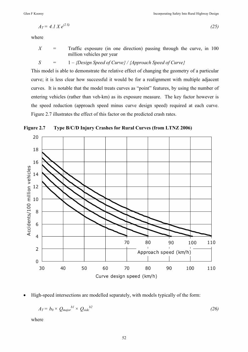
Glen F Koorey Incorporating Safety Into Rural Highway Design
52
AT = 4.1 X e(2 S) (25)
where
X = Traffic exposure (in one direction) passing through the curve, in 100 million vehicles per year
S = 1 – {Design Speed of Curve} / {Approach Speed of Curve}
This model is able to demonstrate the relative effect of changing the geometry of a particular
curve; it is less clear how successful it would be for a realignment with multiple adjacent
curves. It is notable that the model treats curves as “point” features, by using the number of
entering vehicles (rather than veh-km) as its exposure measure. The key factor however is
the speed reduction (approach speed minus curve design speed) required at each curve.
Figure 2.7 illustrates the effect of this factor on the predicted crash rates.
Figure 2.7 Type B/C/D Injury Crashes for Rural Curves (from LTNZ 2006)
• High-speed intersections are modelled separately, with models typically of the form:
AT = b0 × Qmajorb1 × Qside
b2 (26)
where
Glen F Koorey Incorporating Safety Into Rural Highway Design
53
Qmajor = Two-way link volume (AADT) for the major intersecting road
Qside = Two-way link volume (AADT) for the minor or side intersecting road
b0,1,2 = Various coefficients depending on the geometry of the intersection (3-leg, 4-leg, etc) and its form of control (priority, roundabout, etc)
More sophisticated models are also available for some specific crash types, using the daily
volumes of the relevant conflicting flows (e.g. right-turn vs opposing through traffic).
• Additional crash prediction models or modification factors are also available for other
notable features, such as auxiliary lanes and bridges.
Clearly there is scope for incorporating other geometric or environmental features into the
models for more detailed estimation. The safety of rural alignments for example is greatly
affected by the changes in horizontal and vertical curvature down the road, more than a
simplistic terrain measure can capture. Other possible items include access/parking density,
roadside clearances, intersection geometry and traffic composition. It is important to note
however that many of the existing prediction models for different road facilities are implicitly
incorporating some of these effects, e.g. a commercial local street typically will have different
access characteristics to a major arterial road.
There is also scope to expand on the list provided in the EEM of typical crash reductions for
various treatments, both in urban and rural situations. To date these have been compiled in a
fairly ad hoc manner, as local and overseas research has come along. In terms of typical
treatments on rural roads, the list currently includes:
• Installation of route/intersection lighting
• Construction of passing lanes or crawler lanes
• Provision of turning lanes/bays
• Providing road markings/delineation
• Installation of traffic islands
• Removal/mitigation of roadside hazards (e.g. clear zones, guardrails)
A number of important treatments still appear to be missing, including:
• Installation of curve advisory speed or other warning signs
• Construction of slow vehicle bays
• Visibility/sight distance improvements

Glen F Koorey Incorporating Safety Into Rural Highway Design
54
• Use of speed calming treatments
2.5.3 Crash Reduction Monitoring System
One means of obtaining additional crash reduction information is via LTNZ’s Crash Reduction
Monitoring (CRM) Programme (LTNZ 2004). Set up in 1989, this programme identifies sites
where there are similar crash patterns and recommends low cost engineering treatments aimed at
reducing those crashes. Sites where road safety works have been carried out (perhaps following
a Crash Investigation Study) are monitored for changes in crash numbers and overall findings
reported on a somewhat regular basis. Typical treatments that have been reported on to date
include installing chevron arrows at bends, installing traffic signal or roundabouts, and road
lighting improvements. Site details in the CRM database are quite extensive and include a range
of on-site road features, such as road widths, curvature, delineation/marking, and signage. This
makes it theoretically possible to control for various factors during analysis.
Kraus (1991) outlines two key problems with the CRM programme. Firstly, where sites are
selected for treatment on the basis of high crash counts, there is likely to be some reduction in
crashes in subsequent years even if no works were carried out, otherwise known as “regression
to the mean”. LTNZ acknowledge this problem, but no adjustment to the published results has
been determined yet. However, the effect should be relatively minimal if long before/after
analysis periods (such as five years) have been used. Secondly, in many cases, a number of
other treatments are carried out at the sites at the same time (e.g. upgrade signs and improve
lighting), making it difficult to distinguish the specific benefits of each treatment. This could
lead to an overstatement of the benefits attributable to a particular treatment. Conversely it could
also lead to an understatement of benefits if the treatments are not supportive of each other.
The monitoring database also suffers somewhat from the relatively low numbers of sites and the
low number of crashes often found at sites. NZ’s small population base means that there is only
a limited pool of suitable sites to work with. The time required to collect suitable “after” crash
data (following an often-lengthy implementation period) also makes for slow progress to
produce findings from recent safety improvements. Nonetheless, the programme represents a
dataset that is hard to match around the world.

Glen F Koorey Incorporating Safety Into Rural Highway Design
55
2.5.4 Safety Audit Models
Safety audit of both projects and existing roads in NZ has to date been a largely subjective
exercise (Transit NZ 1993, Transfund NZ 1998). However, quantitative processes are now being
considered more, to provide some consistency between both auditors and road controlling
authorities. Austroads’ Road Safety Risk Manager (see Section 2.4.3) is an example of a tool for
these purposes, and its applicability for NZ auditing purposes was reviewed by Brodie & Koorey
(2002) and found to be relatively promising.
Wilkie & Tate (2002) developed an assessment method for safety auditing of existing roads,
based on comparing the relative risk of various features observed with the risk for a “base case”
facility. For example, the default standard for a “medium volume” (1000 < AADT < 4000) rural
road is for 3.5m lanes, 0.75m shoulders, and no street lighting. A road with “narrow” lane
widths was considered to have approximately a 10% increase in crash risk relative to the base
case; a similar approach could be applied to other features present. This approach is similar to
the modification factors used in models like IHSDM. For auditing purposes, this method has the
advantage of not having roads with different functions being compared with each other; there are
usually various reasons (volumes, terrain, etc) why different standards are used on different
facilities.
This quantitative approach has now been developed into a new procedure called Road
Infrastructure Safety Assessment or RISA (Appleton et al 2006). The process is better suited to
audits of linear facilities (i.e. mid-block sections), with various safety-related measures (e.g.
roadside hazards, lack of road markings) being recorded along a road section during an audit.
Assessment of intersections is currently limited to a more qualitative “pass/fail” process, based
on comparisons with design standards and guidelines. While the process seems to work
reasonably well for rural roads, there are difficulties in applying the same method to urban areas,
largely due to the greater number of intersections and accesses, and increased road user
interaction.

Glen F Koorey Incorporating Safety Into Rural Highway Design
56
2.6 Discussion
The road safety models featured above display a wide variety of techniques and make use of
differing sets of data, indicating the complexity of the task of accurately estimating safety
effects. Some general observations can be made:
• It is important to distinguish between the underlying road safety model theory (i.e. the
relationships) and the application package itself. RSRM and IHSDM, for example, would
both indicate that a narrower carriageway is generally less safe than a wider one, however
their use of this information in each case is quite different. While developing usable safety
tools for practitioners is a worthwhile aim, the first priority is to ensure that adequate
information about road safety effects has been captured in some form of “knowledge base”.
• Driving speed, and its relationship to the surrounding speed environment in particular, is an
important factor in assessing the relative safety of locations. Speed factors also show up as a
major cause of crashes in NZ. An accurate means of predicting vehicle speeds is therefore
necessary.
• Traffic or driving conflict models may have some limited applications for predicting certain
types of rural crashes, but they are still relatively difficult to develop and validate,
particularly where the measured conflicts are fairly rare (e.g. non-intersection measures).
• There are uses for both simple volume-based models and more detailed feature-based models
in different contexts. The ability to be able to develop one should not preclude the separate
development of the other.
• There is a move away from the use of crash rates (per exposure) to methods that produce
total crash numbers, often by means that are not linearly related to exposure. This appears to
be a more realistic approach.
• Crashes at intersections and road links should be considered separately in any network risk
models. The nature of the factors involved and the best exposure measures to use suggest
that different relationships for each are desirable. In some cases, it may be acceptable to
include crashes for minor side-roads into road link crash models, particularly at the more
strategic level and where the side-roads have little operational effect on the main route.
• Likewise, different types of road and intersection facilities should be separately investigated
for risk factors. Not only may different factors be statistically significant for different
facilities, the relative effect of changing the same factor may also differ. For example,
removal of roadside hazards is likely to have a greater relative effect on rural roads than

Glen F Koorey Incorporating Safety Into Rural Highway Design
57
urban roads, because of the different speed environments. Any factors that are not explicitly
incorporated in the models can also be represented by the particular coefficients used in each
relationship, e.g. the differing levels of access control on a residential street and an urban
arterial.
• A promising road safety prediction approach appears to be models involving a base road type
whose crash rate is then adjusted by modifying factors to account for local site differences.
As well as being intuitively easy to understand, there also appear to be advantages in their
development and maintenance.
• Inclusion of actual historical crash data should greatly help adjust crash predictions for local
effects that are difficult to account for otherwise. This allows a relatively simple but
effective model to be developed and used fairly quickly, ahead of further research into the
other factors.
• The scope of the model will dictate the data used. For example, a nationwide strategic
highway crash model here in NZ could make use of the relevant data already available in
highway databases. For more site-specific models, however, some detailed on-site data
collection may be required, e.g. to assess roadside hazards and to determine sight distance
constraints.
• A road safety model based on measurable engineering attributes would probably still benefit
from setting these measures in a driver behaviour context, particularly given that it is often a
combination of atypical road features and atypical driver behaviour that cause crashes.
• Overseas models would probably require some adjustment to their parameters to give
suitable estimates in NZ. Few appear to allow for this calibration by users, with IHSDM
being a notable exception. However, in many cases, the models could perhaps provide a
reasonable estimate of the relative change in crash risks between two situations, enabling
practitioners to apply this relativity to the existing crash numbers. Even this assumption
however has to be tested in the NZ context before applying the models in general practice.
Overall, there is enough information available now to consider what is the best way to
incorporate road network safety modelling into NZ in the future.
2.6.1 Development of New Zealand Rural Road Safety Models
Although development of NZ-based road safety information is ongoing, there is still quite a
reliance on information from overseas models. Overseas data do have a use here, particularly to

Glen F Koorey Incorporating Safety Into Rural Highway Design
58
identify the “big ticket” items (i.e. road features that have major safety effects, or that occur
commonly on our roads). However, it is unwise to expect that the findings from countries with
often quite different roading, social and legislative environments will be directly translatable to
NZ circumstances. A more profitable (albeit more laborious) approach is to carry out NZ-
specific studies, using the most promising findings and methodologies from overseas as a guide.
For example, the Highway Safety Manual being developed in the US (Hughes et al 2004) will
provide a useful starting point for developing similar models for NZ use.
At the simplest level for development of road safety models, the basic data required are sites or
road segments of the same basic category with known crash numbers, traffic volumes, and
lengths (for non-intersection models). More detailed models will then require additional
information on the factors deemed relevant, e.g. average horizontal curvature, road width, access
control, etc.
NZ is luckier than many countries in now having a fairly well integrated system for collating
relevant road data (e.g. traffic volumes, crashes, road geometry, skid resistance), particularly on
State Highways. This advantage should be maximised in both developing and using any crash
models here.
The scope of the model will dictate the data used. For example, more strategic crash models
could make use of general data already available in RCA databases. For more site-specific
models however, some detailed on-site data collection may be required. Some suggested levels
of differentiation are:
• At the national/regional/RCA strategic level, to identify sections of hazardous or sub-
standard road. Readily available road data, particularly from databases such as RAMM,
would be used to enable rapid evaluation of the relative safety of different parts of the road
network.
• At the project scoping level, to assess the relative merits of different options. Some data
collected on-site (e.g. roadside hazards, sight distance constraints) would be combined with
other site data already available to the RCA.
• At the project design level, to determine the precise benefits of the proposed design.
Detailed alignment and cross-section information, perhaps from a road design package, and
other on-site information would be used to predict the expected performance of the proposal.

Glen F Koorey Incorporating Safety Into Rural Highway Design
59
• At the road safety audit level, to identify and prioritise existing deficiencies. Site-specific
details of the deficiencies would be combined with general data about the site context.
Each of these applications would require a different level of data collection (largely dictated by
the cost-effectiveness of obtaining additional data) and a different level of output precision
(determined somewhat by the need for absolute or relative safety measures). Therefore, it is
likely that separate models for each application, or at least the ability to use only a subset of a
model for some less specific applications, would be required.
However, there is no reason why all of the above models cannot be based on the same
knowledge base of road safety research, and indeed it makes practical sense to do so. A common
national repository on the safety effects of different road features would provide consistency
across the different application levels.
It may be reasonable to develop separate crash relationships for State Highways and local
authority roads. Because of the differing standards and funding mechanisms there are likely to
be considerable differences in crash rates, even if various road factors are taken into
consideration, although this hypothesis will need testing. There are also differences in the road
data available for each (e.g. all State Highways have geometry data available), which may dictate
the form of any models developed for each. Some would argue that differences between local
authorities (e.g. large mainly-urban cities versus small mainly-rural districts) would suggest even
further disaggregation of models, although the cost-effectiveness of this would need to be
considered.
Research to identify suitable crash modification factors must take into account a number of
“confounding” effects, including:
• General trends in road safety, e.g. effects of enforcement and education initiatives
• Changes in traffic volumes at the investigated sites over time
• Other physical changes that have also taken place at the investigated sites in the same period
• “Regression to the mean” and “selection by bias” effects of sites chosen for treatment
• Network effects resulting from a treatment e.g. “crash migration” and traffic redistribution
The existing MoT Crash Reduction Monitoring (CRM) Programme (described in Section 2.5.3)
represents the best opportunity to collate the required information nationally and to produce the
necessary modification factors. However, more resources need to be put into it to improve data

Glen F Koorey Incorporating Safety Into Rural Highway Design
60
collection (including exposure data), data completeness and accuracy levels. The programme
should also incorporate findings from treatments made for non-safety reasons (e.g. changes in
intersection control due to capacity, passing lane additions) and data from relevant local research
studies, to improve the sample size available for analysis. Separate dedicated NZ research in
some areas will also need to be carried out to supplement the CRM Programme findings.
All relationships and factors developed for use in NZ should have associated with them an
indication of the relative confidence placed in the values. For example, a factor that has been
studied repeatedly locally with consistent results should be given a higher level of confidence
than a factor based on one overseas study with some analysis flaws. This would enable analysts
to determine whether it might be appropriate to depart from the default value in some cases.
Alternatively, results could be presented as interval (rather than point) estimates; the relative
width of the interval would give an indication of the relative precision. If probabilistic risk
models are developed, it would also give a clearer indication of the possible safety outcomes and
the greatest sources of uncertainty.
The ability to integrate or link a rural road safety model to existing road design packages would
be of immense practical value, enabling faster specification of road layouts for assessment and
subsequent project reporting and re-work. Many of these packages already have the ability to
estimate construction costs from a specified design; the calculation also of traditional road user
benefits like crash reductions, travel-time savings and vehicle operating costs would provide a
total package for determining cost-effective options. In this way designers could produce an
optimal alignment that balances construction cost against reasonable safety and operating costs.
This could be both at the strategic route location level (e.g. a route construction cost optimisation
package like Australia’s Quantm; Quantm Ltd 2007) and at the detailed design level (e.g. CAD
design packages like MX-ROADS, 12D and GEOPAK).
2.7 Implications for this Study
One of the original intentions of this research was to obtain enough information to develop a NZ-
specific crash risk model for use in the design of rural highway alignments. From the literature
review, however, it seems far more pragmatic to investigate further the IHSDM model and look
at how to adapt this for use in NZ. Of all the models reviewed, IHSDM provides the greatest
scope for local customisation, such as making use of NZ design policies and incorporating
available road geometry data.

Glen F Koorey Incorporating Safety Into Rural Highway Design
61
This approach reduces the need to undertake as much basic driver behaviour observation studies
locally as originally intended, although vehicle speed data is still required to calibrate IHSDM’s
speed prediction module.
The IHSDM model allows for crash prediction and design assessment of both intersection and
road link elements of rural highways. The background research has clearly identified the
statistically significant differences in relevant factors and causal mechanisms that apply to each
situation. In the NZ context, non-intersection crashes are considerably more prevalent in rural
areas. Often there are quite long (>5km) lengths of rural highway in NZ between side-roads,
especially side-roads with notable traffic volumes. Rural intersection crashes have also been the
subject of some notable crash prediction research in NZ already (e.g. Turner 2001). Therefore,
for the purposes of this research, the study will focus on the ability of IHSDM to be used as a
tool for assessing the safety of rural two-lane road link sections.
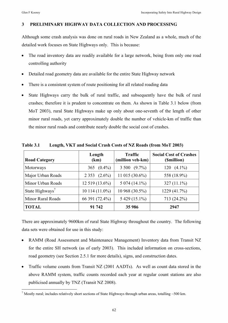
Glen F Koorey Incorporating Safety Into Rural Highway Design
62
3 PRELIMINARY HIGHWAY DATA COLLECTION AND PROCESSING
Although some crash analysis was done on rural roads in New Zealand as a whole, much of the
detailed work focuses on State Highways only. This is because:
• The road inventory data are readily available for a large network, being from only one road
controlling authority
• Detailed road geometry data are available for the entire State Highway network
• There is a consistent system of route positioning for all related roading data
• State Highways carry the bulk of rural traffic, and subsequently have the bulk of rural
crashes; therefore it is prudent to concentrate on them. As shown in Table 3.1 below (from
MoT 2003), rural State Highways make up only about one-seventh of the length of other
minor rural roads, yet carry approximately double the number of vehicle-km of traffic than
the minor rural roads and contribute nearly double the social cost of crashes.
Table 3.1 Length, VKT and Social Crash Costs of NZ Roads (from MoT 2003)
Road Category
Length (km)
Traffic (million veh-km)
Social Cost of Crashes ($million)
Motorways 365 (0.4%) 3 500 (9.7%) 120 (4.1%)
Major Urban Roads 2 353 (2.6%) 11 015 (30.6%) 558 (18.9%)
Minor Urban Roads 12 519 (13.6%) 5 074 (14.1%) 327 (11.1%)
State Highways7 10 114 (11.0%) 10 968 (30.5%) 1229 (41.7%)
Minor Rural Roads 66 391 (72.4%) 5 429 (15.1%) 713 (24.2%)
TOTAL 91 742 35 986 2947
There are approximately 9600km of rural State Highway throughout the country. The following
data sets were obtained for use in this study:
• RAMM (Road Assessment and Maintenance Management) Inventory data from Transit NZ
for the entire SH network (as of early 2003). This included information on cross-sections,
road geometry (see Section 2.5.1 for more details), signs, and construction dates.
• Traffic volume counts from Transit NZ (2001 AADTs). As well as count data stored in the
above RAMM system, traffic counts recorded each year at regular count stations are also
publicised annually by TNZ (Transit NZ 2008). 7 Mostly rural; includes relatively short sections of State Highways through urban areas, totalling ~500 km.

Glen F Koorey Incorporating Safety Into Rural Highway Design
63
• Reported crash data from Land Transport NZ. All rural crashes (injury or non-injury)
between 1996-2006 were obtained; initially just 1996-2000 data from the Accident
Investigation System (AIS), with more detailed follow-up information subsequently obtained
from AIS’ successor, the Crash Analysis System (CAS).
The collected data were combined in a single Microsoft Access database (although some
preliminary processing was done in separate databases). Subsequent processing of the data was
required for three main purposes:
• The traffic and roading environment data were compared with the reported crash data to
identify key factors affecting crash rates. Data for the whole country were used; this is
discussed further in Section 4.
• The State Highway road geometry and crash data were used to develop crash rate figures to
allow for calibration of the IHSDM model for NZ conditions. Further details about this are
discussed in Section 5.2.
• Specific geometry and crash data were extracted for the case study sites used to validate the
IHSDM model; these are described further in Sections 6.2 and 6.3. Earlier (1998) geometry
data were also used to compare the before and after alignments in Section 6.2.
It was also originally intended that potential sites for further field data collection would be pre-
selected via a desktop analysis of the initial data. For this exercise, only State Highway locations
in the South Island with sufficiently high traffic volume would be used for analysis. Curve
locations could be identified, with relevant information for each curve to be summarised for use
when searching in the field for the sites. The additional field data could then be used for a more
detailed analysis of crashes and road environment features. Although this still presents a useful
research objective in its own right, ultimately it was not necessary for the revised research tasks.
The proposed additional field data also warranted further investigations into methods for
collecting survey data at sites, particularly with regard to the speeds and lateral positions of
vehicles at curves. As explained above, the need for this has not eventuated; however some
preliminary investigations were made. Details of these are presented in Appendix A.12.

Glen F Koorey Incorporating Safety Into Rural Highway Design
64
3.1 SH RAMM Data Analysis
Before continuing, it is important to understand the way that State Highway data is referenced
and stored. Further details on this matter can be found in Transit NZ (2004) and Transit NZ
(2006).
3.1.1 State Highway Location System
State Highways in NZ use a system of linear location referencing to identify the locations of
parts of the network. As explained in Transit NZ (2004), the ‘route position’ (RP) is the key to
defining a position along the highway. It is a unique address given to each location and is
expressed as a distance (displacement) from the preceding ‘reference station’ (RS) when
travelling in the ‘increasing’ direction along the route. Reference stations are the primary
benchmarks (points where all measurements start), and are numbered to reflect the approximate
distance (in km) from the start of the highway. They generally occur at intervals of
approximately 10 to 20 km, including virtually all junctions with other State Highways and at
Territorial Local Authority boundaries. Figure 3.1 explains graphically how the system is used to
locate a certain position along a State Highway.
Figure 3.1 State Highway Route Position System
Sometimes, for convenience there are also intermediate reference posts provided between the
RSs, known as “established route positions” (ERP). These may be used to assist with accurate
location in the field or to locate notable features, e.g. a large roundabout, a major bridge or the
start of a divided carriageway section.
A change in the highway route, such as a realignment, will mean changes in the route positions
both within and beyond the altered road section. However, Transit’s RS system means that such
changes to the highway alignment will only affect location measurements through to the next
Start of Highway
RS 0
Reference Station RS 16 RS 31
4.56 km
Route Position RP 123/4.56
etc
Increasing Direction Decreasing Direction Not to Scale
Approx. 16 km
(Approx. 123km from Start)
RS 123 Approx. 15 km
Glen F Koorey Incorporating Safety Into Rural Highway Design
65
reference station. Over time, reference stations may also be renumbered to reflect the new
distance from the start of the highway, but this is not a critical step.
3.1.2 RAMM Database Structure
The Road Assessment and Maintenance Management (RAMM) system is Transit NZ’s central
asset register where road attribute and location data are stored (Transit NZ 2006). This provides
an inventory of all State Highway data that describes the physical road environment and
demands placed upon it. The RAMM inventory can be broken into four components:
• Physical Inventory: Data held about the physical features along the road (e.g. surfacing
type, drainage, signs, pavement structure, road geometry).
• Condition Data: Condition data held about the road or associated road features (e.g.
roughness, texture, condition rating, pavement strength).
• Demand Data: Information held about the physical environment and demands placed on the
asset (e.g. traffic volumes, loading, climate, road hierarchy, land use, regional
administration).
• Event Data: Historic information held about events that occur on the asset that are not part
of physical inventory (e.g. crash records, routine maintenance).
The data are generally based around the location referencing system described above, and thus
RSs and ERPs are often used as boundaries of data records. A unique “RoadID” value is used in
all RAMM tables to identify road sections between adjacent RSs and/or ERPs. However, the
nature of the data often means that sub-sections between these reference points are used to
further divide data. For example, roadway data records may be terminated at side-road
intersections or at changes in roadway width, surfacing, kerbing or speed limit. Because of the
considerable highway maintenance investigation work done using the data (e.g. pavement
deterioration modelling), sectioning is also often done on the basis of similar pavement condition
measures (HTC 2002). In the context of this research, it is notable however that RAMM data are
not ever sectioned in terms of horizontal or vertical geometric elements.
RAMM data are stored as tables in a relational database. For this research, some of the most
relevant RAMM tables are:
• road_names: A lookup table of all RAMM RoadID values against the equivalent SH/RS
location. The State Highway network is divided into about 1600 road sections, with at least

Glen F Koorey Incorporating Safety Into Rural Highway Design
66
one section per Reference Station (divided carriageways are usually treated as two opposing
road sections).
• hsd_geom: Contains road geometry data (radius, crossfall, gradient) collected by high-speed
data collection at 10 m intervals in each travel direction (approximately 20 000 lane-km).
The data collection is currently by means of a “SCRIM+” vehicle, which surveys the
highway network annually at speeds of up to 60 km/h and also collects a variety of pavement
condition measures such as skid resistance and roughness.
• pave_layer: Contains information on each new pavement layer (e.g. basecourse, sub-base)
installed when a section of road was last reconstructed. There are over 22 000 pavement
layers on the SH network, although typically a single location has a multiple number of
construction layers and subsequent overlays recorded.
• carr_way: Summary data for each road section, including traffic and land-use information,
number of lanes and road width. Over 8000 SH carriageway sections are recorded in
RAMM, with boundaries typically at major changes in cross-section or traffic.
• sign: An inventory of every traffic sign located next to the road, including the position, size,
type, and legend of each sign. Nearly 150 000 signs are recorded on the SH network.
Note that, although crash data is recorded in RAMM by Transit NZ, Cenek & Davies (2004)
found there is often a disparity between what is recorded there and what is originally collected
via CAS. This can be due to the time lag in transferring CAS data into RAMM or due to
difficulties in locating the crashes correctly within the State Highway route position system.
Therefore, the decision was made to source the crash data for this study from CAS and link it
later with RAMM data, as described in Sections 3.5 and 3.6.
By linking these RAMM tables and performing particular queries and matching operations on
them, a list of suitable road sections (partitioned by horizontal geometric element or other
measure) could be obtained. The process is described in the following sections.
During the database work, it was observed that there were many inconsistencies and errors in the
data (especially when comparing between regions), necessitating many manual inspections and
corrections of the tables. For example, there were differences between regions in the coding of
road sections as urban or rural, with urban or peri-urban motorways being a notable example.
The coding of the types, legends and facing directions of signs also varied from area to area,
making it hard to reconcile these with urban/rural areas, intersections and other features. Most of
Glen F Koorey Incorporating Safety Into Rural Highway Design
67
these inconsistencies showed up easily enough by means of simple queries and sorted lists of
table data; any discrepancies could then be identified and rectified. However, this was a time-
consuming exercise because of the size of the databases concerned. It would be desirable if
Transit NZ could undertake a similar audit and correction of its master RAMM data, thus
simplifying analysis tasks for future users.
3.1.3 Use of Pavement Condition Data
Among the many data sets available in RAMM is a variety of pavement condition measurements
such as skid resistance, roughness, rutting depth and texture depth. Typically on State Highways
these are collected annually at 10 m or 20 m intervals in each wheelpath using the SCRIM+
survey vehicle that travels at highway speeds. Unlike many other more constant highway
measurements, pavement condition tends to deteriorate over time with traffic, e.g. skid resistance
reduces and roughness increases. The relative condition of a road at a given time therefore has
the potential to influence the crash risk of that location.
Cenek & Davies (2004) examined such factors when they related crash risk on NZ State
Highways to a range of road condition, traffic and geometry measures over the period 1997-
2002. Using first one-way and two-way ANOVA tables and then Poisson regression modelling,
they found that crash rates were higher on roads with lower skid resistance (SCRIM) measures,
and the difference was more pronounced when focusing on wet-weather crashes only. Crash rate
also increased with increased roughness, but the effect of texture depth or rutting on crash rates
was not statistically significant. Applying the resulting model to wet-weather injury crashes
found a 35% predicted crash rate reduction per 0.1 increase in side-friction coefficient (20%
reduction for all injury crashes).
For this study, the decision has been made to focus on road geometry attributes only as these will
not generally change until a major site improvement is undertaken (e.g. seal widening,
realignment, shape correction). For crash analysis using data over a long period of time such as
five years, these geometric attributes can be held constant (by ignoring reconstructed sites),
whereas pavement condition will invariably change over this period. However, if we aggregate
sites with similar geometric attributes for the purposes of crash risk determination it is likely
that, across the entire State Highway network, each sub-group of sites will have a wide range of
pavement conditions represented during the study period. The net effect will be to “average out”
the relative differences in pavement condition and thus represent the typical crash risk for a site

Glen F Koorey Incorporating Safety Into Rural Highway Design
68
with pavement conditions of “about the norm”. It may, however, be worth revisiting this
assumption in future research.
One problem with this approach could be where pavement condition is a factor in decisions to
reconstruct a relatively unsafe section of highway. For example, a prediction model like
IHSDM, calibrated using the aggregated crash risk data, could highlight sites that present higher-
than-normal crash risks and that should be considered for reconstruction. However, it may be
that highlighted sites with poor pavement condition are prioritised ahead of the other highlighted
sites, due to the additional vehicle running and maintenance cost savings. IHSDM’s base
prediction model would not be able to reflect this relative priority. This may be less of an issue,
however, if historical site crash data are incorporated in the model via the Empirical Bayes
option and these data indicate additional pavement-related risks at some sites.
It should also be noted that, while IHSDM’s CPM model takes account of geometric attributes
such as horizontal curvature, vertical gradient and cross-section width, it does not account for
changes in pavement condition. The only relevant consideration is in the calibration process
where it is acknowledged that the localised crash rates may be adjusted to reflect a greater
prevalence of wet or icy pavement conditions (Harwood et al 2000). In practice, this calibration
adjustment could also reflect a different standard of pavement condition in different jurisdictions.
Again, the Empirical Bayes process may allow for even more site-specific pavement conditions
to be highlighted at different locations.
3.2 Aggregation of Highway Data
The data were stored in records with a varying range of fixed or variable lengths. To be able to
combine the information in a practical manner for analysis, some thought needed to be given to
techniques for aggregating data. Two techniques used in the past are worthy of discussion here
and were touched on previously in Section 2.1.1.
Cenek et al (1997) examined the relationship between crashes and road geometry, using over
8000 lane-km of rural NZ SH data, divided into fixed-length 200-m sections. This fixed-length
dataset was also used for the research by Koorey & Tate (1997). More recently, Cenek & Davies
(2004) updated the previous research by including pavement condition data (such as skid
resistance and texture) but undertook statistical crash analysis using individual 10 m road
geometry segments.

Glen F Koorey Incorporating Safety Into Rural Highway Design
69
Meanwhile, Austroads (2000) examined nine lengths of highway in Australia (2900 lane-km)
and related geometric attributes such as pavement width and gradient with recorded crash rates.
Compared with the previous studies mentioned, the roads were divided to produce sections that
were reasonably uniform in terms of geometry, resulting in sections of varying length. Similar
studies have been made elsewhere using inventories of roadway “elements” (e.g. Fitzpatrick et al
2006, O’Cinneide et al 2005, Cafiso et al 2008), although in some cases, the geometric data
available has been limited to attributes such as cross-section rather than horizontal/vertical
alignment, or only categorised in broad groupings or longer “homogenous” sections.
The latter (“road element”) approach seems intuitively more useful than sections of constant
length. In many cases a fixed-length section may have variable geometry within it, by virtue of
where the section boundaries lie in relation to road elements such as curves and gradients.
Although the very large number of sections analysed by Cenek et al (1997) and other “fixed-
length” studies helped to minimise the effects of this problem, a more logical division by road
geometry should only improve the relationships developed.
Which approach is used however often depends upon the type of data available. If road
geometry data has already been collected systematically at constant intervals along a road then,
in practical terms, it is easier to divide road data using a fixed interval length, and one suspects
that this was a key factor in the method used by the “fixed-length” studies in NZ. For the
Austroads study (involving a smaller dataset), it appears that the division of road sections was
undertaken manually via inspection of the geometry data and maps. Other “road element”
studies have either manually collected data for each element on site, or route data from GIS
databases or aerial photos has been used to identify road elements.
Clearly it would be desirable to be able to automate the process of defining road elements, where
constant-interval geometry data is available, as in NZ. For example, an automated routine could
be developed in the database that sought to identify where horizontal curves began and ended.
This could be by means of monitoring the recorded curve radius and triggering the start of a new
curve when the radius fell below a particular value (e.g. 2000m). This technique was previously
used successfully in research on rural simulation models (Koorey 2003) to generate straight and
curved road elements for Paramics models that required input data in this format. Koorey (2005)
describes how similar methods were also used to identify curves on highways for reviewing
curve advisory speeds and for assessing curve widening requirements for large vehicles. Figure
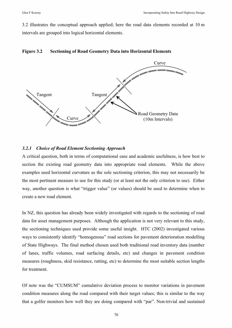
Glen F Koorey Incorporating Safety Into Rural Highway Design
70
3.2 illustrates the conceptual approach applied; here the road data elements recorded at 10 m
intervals are grouped into logical horizontal elements.
Figure 3.2 Sectioning of Road Geometry Data into Horizontal Elements
3.2.1 Choice of Road Element Sectioning Approach
A critical question, both in terms of computational ease and academic usefulness, is how best to
section the existing road geometry data into appropriate road elements. While the above
examples used horizontal curvature as the sole sectioning criterion, this may not necessarily be
the most pertinent measure to use for this study (or at least not the only criterion to use). Either
way, another question is what “trigger value” (or values) should be used to determine when to
create a new road element.
In NZ, this question has already been widely investigated with regards to the sectioning of road
data for asset management purposes. Although the application is not very relevant to this study,
the sectioning techniques used provide some useful insight. HTC (2002) investigated various
ways to consistently identify “homogenous” road sections for pavement deterioration modelling
of State Highways. The final method chosen used both traditional road inventory data (number
of lanes, traffic volumes, road surfacing details, etc) and changes in pavement condition
measures (roughness, skid resistance, rutting, etc) to determine the most suitable section lengths
for treatment.
Of note was the “CUMSUM” cumulative deviation process to monitor variations in pavement
condition measures along the road compared with their target values; this is similar to the way
that a golfer monitors how well they are doing compared with “par”. Non-trivial and sustained
Tangent
Curve
Curve
Tangent
Road Geometry Data (10m Intervals)
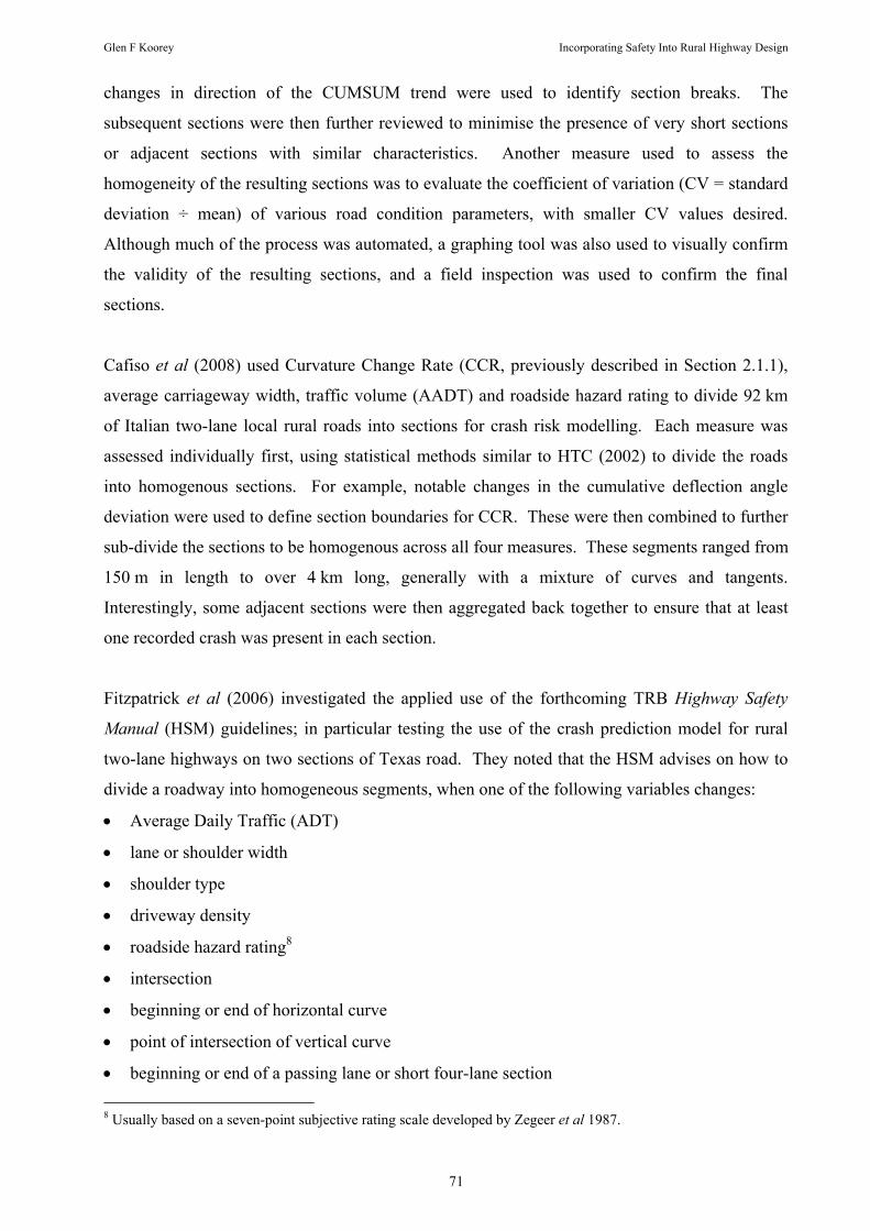
Glen F Koorey Incorporating Safety Into Rural Highway Design
71
changes in direction of the CUMSUM trend were used to identify section breaks. The
subsequent sections were then further reviewed to minimise the presence of very short sections
or adjacent sections with similar characteristics. Another measure used to assess the
homogeneity of the resulting sections was to evaluate the coefficient of variation (CV = standard
deviation ÷ mean) of various road condition parameters, with smaller CV values desired.
Although much of the process was automated, a graphing tool was also used to visually confirm
the validity of the resulting sections, and a field inspection was used to confirm the final
sections.
Cafiso et al (2008) used Curvature Change Rate (CCR, previously described in Section 2.1.1),
average carriageway width, traffic volume (AADT) and roadside hazard rating to divide 92 km
of Italian two-lane local rural roads into sections for crash risk modelling. Each measure was
assessed individually first, using statistical methods similar to HTC (2002) to divide the roads
into homogenous sections. For example, notable changes in the cumulative deflection angle
deviation were used to define section boundaries for CCR. These were then combined to further
sub-divide the sections to be homogenous across all four measures. These segments ranged from
150 m in length to over 4 km long, generally with a mixture of curves and tangents.
Interestingly, some adjacent sections were then aggregated back together to ensure that at least
one recorded crash was present in each section.
Fitzpatrick et al (2006) investigated the applied use of the forthcoming TRB Highway Safety
Manual (HSM) guidelines; in particular testing the use of the crash prediction model for rural
two-lane highways on two sections of Texas road. They noted that the HSM advises on how to
divide a roadway into homogeneous segments, when one of the following variables changes:
• Average Daily Traffic (ADT)
• lane or shoulder width
• shoulder type
• driveway density
• roadside hazard rating8
• intersection
• beginning or end of horizontal curve
• point of intersection of vertical curve
• beginning or end of a passing lane or short four-lane section 8 Usually based on a seven-point subjective rating scale developed by Zegeer et al 1987.

Glen F Koorey Incorporating Safety Into Rural Highway Design
72
• beginning or end of a two-way left-turn lane (TWLTL)
The authors commented that, in practice, this is not always easy to achieve. Firstly, any such
division will depend on the data available; most roading jurisdictions are not likely to have
information on all of these variables easily to hand (the Texas Dept of Transportation only had
about half). Secondly, such divisions may not always make sense, for example if an intersection
occurs midway through a horizontal curve.
The approach used ultimately by Fitzpatrick et al (2006) was to subdivide the roadway into
horizontal curve and tangent segments and predict the number of mid-block crashes for each
segment. Then, for segments that had intersections, the segment length was reduced by 0.1 miles
(160 m) per intersection (with a subsequent reduction in the predicted mid-block crashes), to
reflect the length of road that would be considered by the intersection crash prediction model
instead. The number of crashes for the intersections was then predicted and combined with the
predicted number of tangent or curve crashes to create a segment total. However, subsequent
discussion with the HSM authors revealed that the 0.1 mile reduction was unnecessary as the two
models (mid-block and intersection) were only calculating non-intersection and intersection
crash types respectively anyway.
Fitzpatrick et al (2006) also noted that, even without subdividing for the variables not available,
the sub-division process sometimes produced some extremely short segments (as small as 5 m
long). They concluded that the HSM needed to provide better advice on minimum section
lengths (and how to avoid or manage very short segments) as well as advice on which are the
more important variables to consider when subdividing the roadway.
Another issue to consider when determining sectioning lengths is its effect on the distribution of
crash numbers over the sections. For example, Lord et al (2005) noted that the incidence in many
studies of a higher-than-expected proportion of sites with zero crash counts can be attributed to
(among other reasons) data with relatively small spatial or time intervals. Under-reporting of
actual crash numbers was another reason cited by Lord et al (2005) and this issue is particularly
prevalent in rural areas. Smaller size sites will also tend to produce relatively low mean crash
numbers, which can be difficult to model or validate.
Cafiso et al (2008) attempted to minimise this problem by aggregating road segments so that
each segment had at least one recorded crash. Other studies have attempted to identify a

Glen F Koorey Incorporating Safety Into Rural Highway Design
73
minimum length for road segments e.g. Resende & Benekohal (1997) concluded that, to get
reliable prediction models, rural crash rates should be computed from road sections 0.5 miles
(0.8 km) or longer. Thomas (1996) noted that the statistical form of the crash count distribution
varies as the length of the road segment increases, with a Poisson distribution most appropriate
only for very short segments and much more variability evident in longer segments (where a
Negative Binomial distribution may be more appropriate).
Another likely problem with shorter segment lengths is the chance that a crash officially located
in one segment was in fact triggered by a feature of the road in an upstream segment. This is
discussed further in Section 3.6.2, and is another reason for trying to produce relatively long
segment lengths where the crash and potential contributory features are more likely to be located
in the same segment.
3.3 Derivation of Database Measures
Starting with the basic road geometry data of horizontal radius, crossfall and longitudinal
gradient in each direction, a variety of measures were determined for subsequent use in this
study.
With the exception of regulatory speed limits, no speed measure is available over the entire
roading network. However, by using the road geometry data, it is possible to derive some proxy
measures, using the techniques described in Section 2.2.1. Using these methods allowed for
speed measures to be generated efficiently over the entire SH network. These were calculated
automatically from the base data, using database code (Visual Basic) routines.
For each 10 m geometric record, a variety of speed measures were developed to enable the most
appropriate one to be used in different circumstances:
• The “advisory speed” (AdvSpd) uses radius, gradient and crossfall to estimate a suitable
travelling speed, as explained in Section 2.2.1. Some extreme values of adverse
superelevation (>25%)9 caused less-than-zero speeds to be calculated, so a cap of ±25% was
put on the data. Maximum speeds on straights were capped at 100 km/h.
9 It is not clear whether such records of extreme superelevation reflect truly steep road crossfall at these locations, or are a product of survey vehicle dynamics on the very tight curves that were usually present at these locations.

Glen F Koorey Incorporating Safety Into Rural Highway Design
74
• A 50m rolling average of the advisory speed (i.e. the current advisory speed record and the
previous four records) was used to produce a “local speed” (LocSpd) indicative of a vehicle
speed profile.
• A 500m rolling average was used for a “local speed environment” (SpdEnv), indicative of
the approach speed to the current location.
• Additional rolling averages were also taken using the previous 1 km, 2 km, and 5 km of
records respectively (Env1km, Env2km, Env5km), indicative of the surrounding terrain.
Note that, where the prior State Highway length was less than the distance being averaged over,
that shorter length was used instead. As a result, the longer averages near the start of each
highway (in each driving direction) are less reliable as long-distance indicators of speed change.
When aggregating the 10 m records into longer elements, the following statistics were collected:
• The minimum AdvSpd, LocSpd and SpdEnv values within the element were recorded. This
is to record the “worst case” constraint of the element, e.g. the tightest bend or steepest grade.
• The average LocSpd and SpdEnv values throughout the element were also recorded to
measure the relative severity of the element, particularly in relation to the immediately prior
approach road.
• The Env1km, Env2km and Env5km values on entry to the element were collected to relative
speed environment prior to this element.
Other statistics about geometric attributes were also collected:
• The general orientation of the element (left/right/straight) was recorded based on the total
deflection angle measured (also stored). The deflection angle was inferred for each 10 m
record, based on the recorded horizontal radius and using the Curvature Change Rate (CCR)
formula described in Section 2.1.1. For example, a record with a 500m radius results in a
1.15° deflection over 10 m.
• The average curvature of the element (in degrees/km) was calculated by dividing the total
element deflection angle by the element length.
• The minimum and average (absolute) radius within the element was recorded. The average
absolute curvature (= 1000 m / radius) was also recorded as this tends to give a more accurate

Glen F Koorey Incorporating Safety Into Rural Highway Design
75
measure of the overall curvature of an element than average radius, which is greatly affected
by large radius (i.e. straight) records.
• The average vertical gradient, as well as entry and exit gradients are recorded for each
element. From this information, a general description of the vertical alignment can also be
inferred in terms of curvature (sag curve, summit curve, grade, mixed) and direction (uphill,
downhill, flat).
• The average, minimum and maximum crossfalls throughout the element were all recorded.
Once these data were collated, additional information could also be linked to each element such
as the crash data, traffic volumes, speed limits and average cross-section width that applied to
that particular part of the road.
3.4 Road Geometry Data Processing
A Microsoft Access 2000 database was created to hold the raw SH data and subsequent
processed information. Various queries, macros, and Visual Basic procedures were created to
process the original data and produce various new data-sets, as described below. These routines
were largely based on previous tools developed by the author for use in SH Strategy Studies,
curve advisory speed reviews, and highway research projects (as described in Koorey 2005).
Because of the size of the raw dataset (originally over 10 000 km of SH including over 2 million
road geometry records), many of the routines could take up to 20 minutes to complete
processing.
A key constraint for crash analysis was that sections of road that had been reconstructed in the
past five years had to be eliminated. Clearly it was not reasonable to ascribe the crash history
prior to reconstruction to their current road geometry. Fortunately the RAMM data include
information about pavement construction dates, which can be used to identify and eliminate
recent road reconstruction projects. Other anomalous sections of highway (e.g. as discussed in
Sections 3.4.1 and 3.4.2) were also identified by manual inspection or various automated means
and eliminated from consideration.
3.4.1 Aggregation Method used in this Study
For the NZ situation, as with many of the studies mentioned in Section 3.2.1, only some of the
possible highway data are automatically recorded by location, such as traffic volume and

Glen F Koorey Incorporating Safety Into Rural Highway Design
76
(average) roadway widths. By default there is no record of horizontal and vertical curves,
although the 10 m road geometry data allows inference of these geometric elements to be
determined. Similarly, intersection locations (and their other attributes), roadside hazards or
driveways are not recorded in a specific database, although their locations and features can be
determined manually or indirectly through other sources (e.g. traffic signs database, video log of
the road).
For a study like this, it is therefore rather difficult to relate the existing RAMM data to physical
geometric road elements present on the highway, without extensive data collection and/or
processing. It would be of immense value if Transit NZ were to follow the model of the Texas
DoT in Fitzpatrick et al (2006) where a special road inventory table, called “Geo-Hini”, has been
created to link road positions with horizontal curvature and another table, “P-Hini”, records point
features such as intersections.
Given the importance of horizontal curvature in this study (and as demonstrated by the relevant
literature), segmentation by horizontal element seems an appropriate approach. Many existing
curves in NZ have “evolved”, rather than having ever been formally designed, so identification
of spiral transition curves was considered unnecessary. Instead, the study data were simply
divided into relatively straight segments (i.e. tangents) and relatively “bendy” segments (i.e.
curves).
If horizontal radius is used to determine the division between segments, some thought needs to
be given to a suitable cut-off value. Sections of State Highway in NZ that are essentially straight
are recorded as having large radius values (e.g. typically >3000 m), the value and sign (i.e.
direction of curvature) somewhat dependent on the path variations of the survey vehicle. A low
cut-off value (e.g. 1000 m) may be appropriate given that it is typically curves with radii below
this figure that produce safety problems (in fact, some of the literature mentioned in Section
2.1.1 would suggest that only curve radii below 400 m are of real significance). However, if
curves are to be recorded in their entirety (i.e. the part that deflects from the tangent lines) then a
low cut-off value may omit a sizeable portion of many curves (it may also limit the number of
curve-related crashes that are identified within each curve element). Conversely, too high a
value may create too many “false curve” records that contribute little to the analysis of crashes
on curves. A curve radius of greater than 2000 m, for example, produces a horizontal deflection
of less than 3° per 100 m. False curvature readings, due to path variations made by the survey
vehicle, are also more likely to be seen at higher radius values.

Glen F Koorey Incorporating Safety Into Rural Highway Design
77
To assess the suitability of the cut-off radius used, a trial was undertaken to divide the road
geometry data available into elements using two different cut-off values for curves; 1000 m and
2000 m. Visual Basic code was created to “walk down” each highway, identify the start of new
horizontal elements by virtue of the recorded radius, and to collate statistics on the attributes of
each element. A “look-ahead” routine was included in the algorithm code so that three
consecutive geometry records had to be above or below the cut-off value before an element was
terminated; this was to avoid one-off rogue values. Some trial and error was also required to
identify aspects of the algorithm logic creating other spurious elements and subsequently fix
them. The number of elements and their length distribution could then be assessed; Table 3.2
summarises the key details.
Table 3.2 Distribution of Geometric Elements with Varying Cut-Off Values
Cut-Off Radius Used 2000 m 1000 m
Number of Curve Elements 67 737 53 441
Average Curve Length 142 m 134 m
Number of 10 m Curve Segments 2269 (3.3%) 451 (0.1%)
Number of Curve Segments < 100 m 28 322 (41.8%) 21 837 (40.9%)
Number of Curve Segments > 1000 m 107 14
Maximum Curve Length 9840 m 4910 m
Number of Tangent Elements 39 456 37 778
Average Tangent Length 282 m 366 m
Number of 10 m Tangent Segments 14 14
Number of Tangent Segments < 100 m 16 625 (42.1%) 13 308 (35.2%)
Number of Tangent Segments > 1000 m 2113 (5.4%) 2876 (7.6%)
Maximum Tangent Length 15 010 m 18 280 m
As might be expected, the smaller cut-off value produced fewer geometric elements overall and
also reduced the proportion of short (< 100 m) elements as well. Either way, there are a still
large number of short elements created, which may not be useful for analysis purposes. It may
be prudent to add a post-processing step to combine some of the shortest elements with their
adjacent counterparts.
Interestingly, the average curve element length is hardly affected by the cut-off value, whereas
the average tangent length increases by more than 30% with the lower cut-off value. A smaller

Glen F Koorey Incorporating Safety Into Rural Highway Design
78
cut-off value also tends to result in more of the longer elements being tangents rather than
curves. This reflects the fact that previous sequences of (say) “tangent → 1500 m radius curve
→ tangent” have now been replaced by a single, longer tangent. These global statistics however
mask the underlying distribution somewhat. Figure 3.3 and Figure 3.4 show the distribution of
curve and tangent element lengths (up to 1000 m long) using the cut-off values of 2000 m and
1000 m respectively.
Figure 3.3 Distribution of Road Geometry Elements (2000 m Cut-Off Value)
0
500
1000
1500
2000
2500
3000
3500
4000
4500
5000
10 60 110 160 210 260 310 360 410 460 510 560 610 660 710 760 810 860 910 960Element Length (m)
Freq
uenc
y
Curves (67737 Elements)
Tangents (39456 Elements)
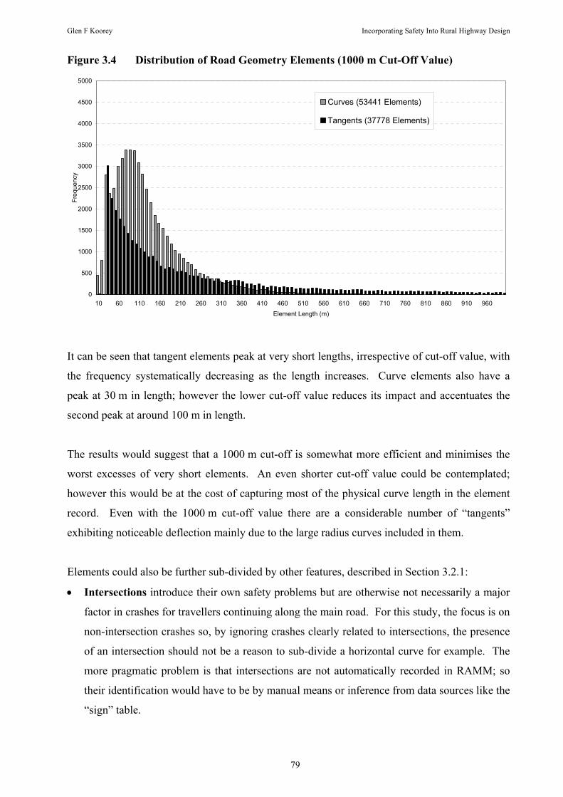
Glen F Koorey Incorporating Safety Into Rural Highway Design
79
Figure 3.4 Distribution of Road Geometry Elements (1000 m Cut-Off Value)
0
500
1000
1500
2000
2500
3000
3500
4000
4500
5000
10 60 110 160 210 260 310 360 410 460 510 560 610 660 710 760 810 860 910 960Element Length (m)
Freq
uenc
y
Curves (53441 Elements)
Tangents (37778 Elements)
It can be seen that tangent elements peak at very short lengths, irrespective of cut-off value, with
the frequency systematically decreasing as the length increases. Curve elements also have a
peak at 30 m in length; however the lower cut-off value reduces its impact and accentuates the
second peak at around 100 m in length.
The results would suggest that a 1000 m cut-off is somewhat more efficient and minimises the
worst excesses of very short elements. An even shorter cut-off value could be contemplated;
however this would be at the cost of capturing most of the physical curve length in the element
record. Even with the 1000 m cut-off value there are a considerable number of “tangents”
exhibiting noticeable deflection mainly due to the large radius curves included in them.
Elements could also be further sub-divided by other features, described in Section 3.2.1:
• Intersections introduce their own safety problems but are otherwise not necessarily a major
factor in crashes for travellers continuing along the main road. For this study, the focus is on
non-intersection crashes so, by ignoring crashes clearly related to intersections, the presence
of an intersection should not be a reason to sub-divide a horizontal curve for example. The
more pragmatic problem is that intersections are not automatically recorded in RAMM; so
their identification would have to be by manual means or inference from data sources like the
“sign” table.

Glen F Koorey Incorporating Safety Into Rural Highway Design
80
• Average Daily Traffic is not likely to change greatly along rural highway sections, except at
major intersections. Although this could mean that a road element has somewhat differing
traffic volumes either side of an intersection, the need for entering or departing traffic to
speed up or slow down near the intersection should mean that this traffic does not greatly
contribute here to non-intersection crashes, which are typically at full highway speed.
• Sealed lane or shoulder widths tend to be fairly consistent over long distances, reflecting
the practice of resealing relatively long (>1 km) road lengths at a time. The exception may
be on some tight horizontal curves where additional widening is provided to allow large
vehicles to negotiate them without encroaching on the opposing traffic lane. Given that this
widening is usually related to a curve element, using the same element boundaries for width
and curvature seems prudent. For major seal width changes midway along a tangent, it may
also be sensible to further sub-divide the road there.
• Vertical alignment can also be determined from the available geometry data, such as the
location of grades and vertical curves. Inspection of the State Highway data suggests that,
due to the vagaries of the existing alignments, such division would be at least as hard to do as
that for horizontal curvature and would also produce many relatively short elements, often
splitting horizontal elements into even shorter lengths. Of more practical interest would be
the interaction of vertical geometry with horizontal elements, particularly the presence of
sharp vertical curves or steep grades. This could be done by analysing the changes in vertical
grade over each horizontal element and categorising the nature of the vertical alignment
present.
• Passing lanes or short four-lane sections are identified by the number of lanes recorded in
RAMM’s “carr_way” table, although passing lane direction is not identified and such
sections may be divided into multiple carriageway records. Again, it would be immensely
useful for similar studies if a separate record of passing lane locations and attributes was
maintained, avoiding the need for further database interrogation. It is presumed that most
changes in lane numbers occur on tangents, so they should not affect horizontal curves
greatly; however this needs to be checked.
• Speed limits usually reflect changes in both land-use and cross-section, so are a logical
division point. Given that this study is focusing on rural highways, such a demarcation is
also necessary to eliminate urban sections of highway. As it is, most speed limit boundaries
are already reflected in RAMM’s “carr_way” records; the “sign” table also records the
location of speed limit signs. Neither of these is consistent however; again, a separate table
of speed limit changes would be of immense value.

Glen F Koorey Incorporating Safety Into Rural Highway Design
81
• Other potential dividing features include changes in accessway density, centreline
treatments, roadside hazards, and adjacent land-use. However, generally there is no readily
available data source for this information for the entire State Highway network. Some of
these factors are also captured sufficiently using other features; for example, a speed limit
change often reflects changes in accessway density and land-use.
A difficult aspect to capture in a segmentation process like this is the interaction between
different factors; for example, modern road design emphasises the integration of horizontal
alignment, vertical alignment and cross-section. For example, most research suggests that
vertical alignment itself does not contribute greatly to crash risk (although steep grades are noted
as riskier). However, vertical curvature can hide from view difficult horizontal curvature or
distort its apparent curvature (e.g. as identified by Hassan & Easa 2003). Given that horizontal
curvature generally has the larger risk, the approach used above has been to identify the general
“shape” of the vertical curvature in each element, so that its influence can be considered. Using
the database developed for this study, this could form the basis of an interesting future research
project in its own right. Similarly, sight distance is not explicitly covered in IHSDM (although
somewhat captured by the other alignment variables). Using existing tools, it is relatively easy
to generate sight distance values given geometric alignment information, although some field
work is required to determine available lateral offsets to obstructions. Again, this could be
another factor to consider in any future crash risk model development work.
On balance, it seems that division by horizontal element should remain the primary means of
data aggregation. Major changes in cross-section (seal width or number of lanes) and speed
limits should also be identified and used to further demarcate highway data, so long as they
occur not too close to a horizontal curvature boundary (e.g. ≥50 m). Information about vertical
alignment can also be collected over the resulting elements. This is the approach that has been
adopted for this study.
The question remains about how to deal with the remaining very short elements, say those <50m.
While the winding geometry in many parts of NZ will indeed result in some relatively short
curves, it may be difficult to confidently ascribe the features of such a curve to a particular crash
located there (especially given the vagaries of accurate crash location, discussed in Section
3.6.2). It may be better to either group short elements with adjacent elements or at least not
terminate them until they have reached a specified minimum length. This may be particularly so
if the element in question does not involve notable angular deflection or speed reduction.

Glen F Koorey Incorporating Safety Into Rural Highway Design
82
A consistent automated means of identifying when to extend/join short elements is difficult to
achieve. An inspection of the short elements being produced revealed a few common features:
• Some of the short elements were tight curves at an intersection; for example, at the very
start/end of a highway, where the highway traversed a roundabout, or where the highway
changed to another road. In many cases this occurred in an urban area and so will ultimately
be excluded from analysis anyway. It seems also appropriate to identify and remove other
short right-angle bends from analysis, where intersection crashes are likely to be most
prevalent.
• For short “tangents”, many included curve radii in the 1000-2000 m range, leading into the
subsequent curve. Invariably, all tangents <50 m long had no more than 2° of total angular
deflection, which would not greatly influence the description of the subsequent curve
element if combined together.
• Approximately 1000 short “curve” elements had a total angular deflection of less than 2°
(with a maximum length of 90 m). Such curves would be hardly noticed by motorists and, in
some cases, appear to actually be parts of essentially straight road sections. It would therefore
be pragmatic to combine these sections with adjacent tangents.
• While many short elements could be extended into or joined with the next adjacent element,
there remain some for which this does not seem appropriate; usually in the vicinity of tight
reverse curves.
A pragmatic approach for the latter point might be to create an additional element type called
(say) “reverse curves” that can encompass a series of short mixed elements. However, while this
may be useful for crash analysis, it poses extra difficulties for use with IHSDM, which requires
the specification of tangent or curve elements when defining highway alignments.
Therefore, this study retained the use of just “tangent” and “curve” elements. However, any
tangents <50 m long or curves with less than 2° of total deflection were not terminated, but
instead combined with the subsequent data. It should be noted that these cut-off values are
somewhat arbitrarily chosen, but should at least eliminate the most unnecessarily short elements.

Glen F Koorey Incorporating Safety Into Rural Highway Design
83
3.4.2 Accuracy of Road Geometry Data
For the current data, the geometry measurement system utilises inclinometers and gyroscopes to
sense the vehicle attitude as it travels along the road. Inclinometers measure the forward or back
tilt of the vehicle for gradient and the side-to-side tilt of the axles for crossfall. Gyroscopes are
used to sense the movement of the vehicle around corners and hills to calculate the horizontal
and vertical curvature. The resulting geometry data is smoothed with a 30m moving average and
reported at every 10m. Before proceeding further, it is pertinent to consider the relative accuracy
of these data.
On inspection of the underlying data following preliminary analysis, some of the longest
elements created also appear to be reflecting anomalies in the data. For example, some of the
longest “curves” are not mirrored by the road geometry data in the opposite direction (or indeed
evidenced by a plan view of the relevant highway). In the data for the 2000 m cut-off value, the
longest (9840 m) “curve” occurs along a relatively straight section of SH1N where the opposing
geometry has (more correctly) recorded two long straights connected by a 140 m curve of 11°
deflection. Meanwhile some “tangents” exhibit unusual amounts of curve deflection, at least in
one direction. On SH73 in the data for the 1000 m cut-off value, an 8750 m tangent has 340° of
deflection recorded; in the opposing direction the equivalent (9590 m) tangent has only 52° of
deflection calculated; still higher than expected given that the plan view shows essentially a dead
straight line. The deflection in both elements is calculated as bearing to the right (in the driving
direction), which suggests that the geometry survey recording vehicle had a systematic bias in it.
Further analysis of the geometry data (using the 1000 m cut-off) uncovers the scale of this
directional bias. Although there are only 1% more right-hand curves overall than left-hand ones,
for curves longer than 500 m there are 19% more right-hand ones (and with a total recorded
deflection 13% higher than the left-hand curves). Given that data is recorded in both highway
directions, one would have expected reasonable parity. For tangent elements, about 78% could
be considered “not straight” (i.e. have a total deflection angle >0.5°). Although there are 4%
more “right-hand” tangents than left-hand ones, that slight dominance in numbers is not shown
in the longer elements. However, for “not straight” tangents longer than 500 m, the average
deflection to the right is 35% higher compared with left-hand tangents (14° versus 10° for
elements longer than 1000 m).
Even here, the above figures are masked by the large number of sections of the road where the
recorded curvature is a reasonably accurate representation. The question remains about how to

Glen F Koorey Incorporating Safety Into Rural Highway Design
84
treat the more anomalous sections displaying biased curvature (and consequently abnormal
deflections). A pragmatic approach to minimise the bias is to adjust all curvature records
slightly to the left. After this, the most obvious and extreme elements remaining can then be
identified manually and removed from further analysis.
Figure 3.5 shows the curvature distribution of the 10 m geometry records10. It can be seen that
there is a slight bias towards more right-hand curved sections, with 6% more such records than
left-hand ones. Collating over all of the data results in an average curvature bias of 0.034
radians/km to the right. While this will have little effect on sections with a tight horizontal radius
(e.g. a 250 m radius left-hand curve, or 4 rad/km, may in fact have a radius of 248 m, if adjusted
for this bias), it will have quite an effect on relatively straight sections (e.g. a 59 000 m radius
right-hand curve may in fact be a 59 000 m radius left-hand curve, if adjusted for this bias).
Figure 3.5 Curvature Distribution of Road Geometry Records
0
20 000
40 000
60 000
80 000
100 000
120 000
140 000
160 000
0.0 0.5 1.0 1.5 2.0 2.5 3.0 3.5 4.0 4.5 5.0Curvature (rad/km)
Freq
uenc
y
Lefthand (934631 Records)
Righthand (996704 Records)
(Note: there are 165 833 records with zero curvature)
Further inspection of the curvature data reveals variation in the level of bias as the rate of
curvature increases. Figure 3.6 illustrates the change in average bias, with records grouped in
10 Note that, because horizontal geometry data is derived in the field from lateral acceleration (which is a function of 1/Radius), it is more appropriate to compare the horizontal curvature values rather than the horizontal radius values. In the following analysis, curvature (radians/km) = 1000 / radius (m), e.g. 2000 m radius = 0.5 radians/km curvature. By convention, left-hand curves in the direction of travel are denoted by negative curvature values and right-hand curves by positive values.

Glen F Koorey Incorporating Safety Into Rural Highway Design
85
1 rad/km intervals (left-hand and right-hand curves together). It can be seen that generally the
bias increases as curvature increases (the relatively low overall average bias reflects the large
frequency of records with small curvature). However, there are notable exceptions; for example
the records with 7-8 rad/km of curvature (125 - 143 m radius) have a very low bias (this anomaly
is not likely to be due to a small dataset; there are over 16 000 records with curvature in this
range).
Figure 3.6 Average Curvature Bias vs Rate of Curvature
0.00
0.05
0.10
0.15
0.20
0.25
0.30
0.35
0 1 2 3 4 5 6 7 8 9 10 11 12 13 14 15
Curvature (rad/km)
Ave
rage
Cur
vatu
re B
ias
(to ri
ght)
Overall Average Bias: 0.034 to right
The data suggests that a curvature-dependent bias is present; this may be a consequence of more
extreme dynamic forces acting on the survey vehicle during sections of higher curvature, so that
any inherent vehicle bias is exaggerated more. It should be noted however that, in terms of
measured radius, there will still be less relative effect of higher biases on sections with higher
curvature (e.g. a 100 m radius or 10 rad/km left-hand curve may in fact have a radius of 98 m, if
adjusted for a bias of 0.165 rad/km observed in Figure 3.6). It is the sections with low curvature
(particularly <1 rad/km) that will be affected the most. Therefore, a standard correction of -0.03
rad/km (based on the average bias of low-curvature elements as shown in Figure 3.6) was
applied to all of the original horizontal geometry data (both curvature and radius values) before
further processing.
Cenek et al (1997) investigated the accuracy of the earlier RGDAS geometry data and also found
discrepancies in the recorded curvature. This was particularly evident when the inferred

Glen F Koorey Incorporating Safety Into Rural Highway Design
86
coordinates from the geometry data were mapped; different runs along the same highway could
show considerable “drift” over long distances. However, at a smaller scale, the shapes of
individual curves were still very recognisable compared with a true route map. For analysis that
is more concerned with the performance of (relatively short) individual elements, this should
limit the problems caused by such drift. RGDAS horizontal radius was also compared with that
measured from aerial maps and, due to the moving-average smoothing process used, found to be
overestimated by up to 70% for curves with small (<50 m) radii but generally within ±10% for
larger curves.
Cenek et al (1997) also noted that distance measurements for RGDAS data were sometimes
incorrect (relative to the true location of geometric features) by 100-200 m along highways, with
a 95% confidence error bound of 72 m. This can have implications both for matching with crash
positions and also matching the same curve in opposing directions. A random inspection was
undertaken throughout the current dataset (1000 m cut-off value) to find matching elements in
each direction (generally identified by having similar curvature and length values). It was found
that almost all notable (i.e. >100 m in length) curve and tangent elements could be matched in
each direction and that typically the location of the element in opposing directions was within
about 50 m of each other, with occasional highway sections getting up to 100-150 m apart at
worst. Typically the element in the increasing RP direction had the slightly higher route
position; however part of that “slippage” can probably be attributed to the element-creating
algorithm that checks for a trend before terminating an element (decreasing RP data was
processed in reverse order, i.e. direction of driving).
Gradient bias was also investigated by summarising and analysing the vertical grade geometry
data. Figure 3.7 illustrates the distribution of gradients found in the dataset11.
11 By convention, downhill gradients in the direction of travel are denoted by negative gradient values, with positive values for uphill gradients.

Glen F Koorey Incorporating Safety Into Rural Highway Design
87
Figure 3.7 Gradient Distribution of Road Geometry Records
0
10 000
20 000
30 000
40 000
50 000
60 000
70 000
80 000
0 1 2 3 4 5 6 7 8 9 10Gradient (%)
Freq
uenc
y
Uphill (880686 Records)
Downhill (1143666 Records)
(Note: there are 72 816 records with zero gradient)
Although the average uphill gradient differs by less than 0.1% in grade from the average
downhill gradient, the most striking feature is that there are 30% more records with downhill
gradients. This leads to an overall average gradient (or bias) of -0.22% in grade. There are also
a greater number of extreme downhill gradients, with 25 235 records having a gradient steeper
than -10% (maximum -26.3%) compared with 11 565 uphill records greater than 10%
(maximum 18.1%), and a tenfold difference in numbers for gradients over 15%. All of this
suggests a systematic bias in gradient recording by the survey vehicle, which may be a
consequence of the vehicle dynamics or calibration.
Figure 3.8 illustrates the change in average gradient bias as gradient increases, with records
grouped in 1% grade intervals (uphill and downhill combined). It can be seen that generally the
bias is quite low at small gradients, averaging about 0.1% in the downhill direction. However,
from about 7% gradient and steeper, there is a striking increase in the relative bias observed
(based on the weighted average of all records within each interval), mainly as a result of the
greater proportion of records with gradients in the downhill direction.

Glen F Koorey Incorporating Safety Into Rural Highway Design
88
Figure 3.8 Average Gradient Bias vs Level of Gradient
0
1
2
3
4
5
6
7
0 1 2 3 4 5 6 7 8 9 10 11 12 13
Gradient (%)
Ave
rage
Gra
dien
t Bia
s (d
ownh
ill)
Overall Average Bias: 0.22 downhill
This unusual pattern warranted further investigation, so another analysis was undertaken
comparing the relative difference in gradients in each direction for records at the same location.
In theory, the two records at each location should have equal but opposite gradient measures, e.g.
+3.0% and -3.0%. If instead the two observed gradients were (say) +2.5% and -3.5%, this would
indicate a bias of 0.5% downhill. Locational discrepancies in the data may mean that often the
two directions are not perfectly matched, but on average the overall gradient differences should
still be close to zero if no survey vehicle bias is present.
An analysis was made of the relative gradient difference between records in opposite directions.
Focusing on the extreme values, there were only 10 pairs with a positive (uphill) bias of >7%
(maximum of +8.6%) compared with 389 pairs with a negative (downhill) bias of >7%
(maximum of -14.6%). Further inspection was made of the pairs with more than 10% negative
bias and it was noted that they came from only about 15 locations. Figure 3.9 shows one of these
locations on State Highway 1N with the two gradient profiles plotted. To enable easier
comparison, both profiles have been plotted in terms of gradient in the “increasing RP” direction;
it can be seen that there is a “shift” of about 70 m between the two profiles, which would explain
some of the gradient variation between the two directions. While generally the two profiles
match rather well, it is clear that there is a notable divergence in the middle section where the
gradient is quite steep. Inspection of the other anomalous sections reveals a similar pattern
where steep uphill gradients have suddenly fallen away to negative values for a brief period; the
data almost suggests that the survey vehicle has momentarily stalled and rolled backwards

Glen F Koorey Incorporating Safety Into Rural Highway Design
89
(downhill) before recovering, all the while still recording its movements. Generally these
problems also occurred in locations with tight horizontal curves (<100 m radius), which suggests
that this has contributed to the surveying problems encountered (e.g. tight curves require reduced
speed, making it harder for the vehicle to maintain momentum on a steep uphill grade). In some
cases, a large enough shift between directions coupled with a rapid change in gradient also
produced a large difference in gradients.
Figure 3.9 Comparison of Gradients in Opposing Directions SH 1N RS675/8-12
-20
-15
-10
-5
0
5
10
15
20
296.0 296.5 297.0 297.5 298.0 298.5 299.0 299.5 300.0
Running Distance (km)
Incr
RP
Gra
dien
t (%
)
Incr RP
Decr RP
Given the relative rarity of the anomalous sections in the current data set, the most pragmatic
approach was to identify and exclude the worst of them from further analysis. For the remaining
data, a standard correction of +0.2% gradient (based on the average bias shown in Figure 3.8)
was applied to all of the original vertical geometry data before further processing. Of most
interest is the identification of vertical curves or steep grades within the data and, on a local
scale, these are still readily identified within the data.
Cenek et al (1997) also found slight discrepancies in the earlier RGDAS gradient data compared
with measured field data, with an average absolute error of 0.6% gradient. Their analysis
however did not investigate the presence of any overall bias in the recorded data.

Glen F Koorey Incorporating Safety Into Rural Highway Design
90
Crossfall (or superelevation) data was also examined for any apparent anomalies. Figure 3.10
shows the distribution of crossfall values found in the dataset, separated according to whether
crossfall is lowered or elevated relative to the road centreline12.
Figure 3.10 Crossfall Distribution of Road Geometry Records
0
5 000
10 000
15 000
20 000
25 000
30 000
35 000
40 000
45 000
0 1 2 3 4 5 6 7 8 9 10
Crossfall (%)
Freq
uenc
y
Elevated (608917 Records)
Lowered (1470199 Records)
(Note: there are 17 988 records with zero crossfall)
Unlike curvature and gradient, it is not expected that there will be a match between the elevated
and lowered crossfalls, because the normal crossfall on straights is to be lowered on both sides,
typically at -2% to -3%. This feature is very evident from the peak of the data shown; although
at about -1.7% it seems a little less than expected. Only on curves are crossfalls typically
elevated and lowered in equal measure on either side of the road, e.g. -6.0% on the inside lane of
a curve and +6.0% on the outside lane.
Examination of just the “very straight” (>5000 m radius) geometric records confirms the above
uneven pattern, with a peak frequency at -1.6% and very few records elevated or lowered by
more than 6-7%. By contrast, examination of just the “curved” (<500 m radius) geometric
records shows a more even picture, albeit still skewed somewhat. Figure 3.11 shows the
distribution for the curved records; it is clear that there is a difference of about 1.5% between the
respective peak frequencies for elevated and lowered crossfalls and the calculated overall
12 By convention, elevated crossfalls (relative to the centreline) in the direction of travel are normally denoted by positive crossfall values and lowered crossfalls by negative values.

Glen F Koorey Incorporating Safety Into Rural Highway Design
91
average shows a similar bias of +0.74%. This is also reflected in a slightly larger proportion of
elevated crossfall records compared with lowered crossfalls, and more extreme elevated crossfall
values being measured (540 records >15%, with a maximum of +35.6%) compared with lowered
crossfalls (52 records >15%, with a maximum of -17.8%). As might be expected, most of these
extreme crossfall records occur in areas with very tight curvature, typically with horizontal radii
of <50 m.
Figure 3.11 Crossfall Distribution of “Curved” Geometry Records (<500 m Radius)
0
500
1 000
1 500
2 000
2 500
3 000
3 500
0 1 2 3 4 5 6 7 8 9 10
Crossfall (%)
Freq
uenc
y
Elevated (237333 Records)
Lowered (224491 Records)
The above analysis suggests that a correction of -0.7% (to negate the calculated overall bias
shown in Figure 3.11) should be applied to the crossfall records; this may be a consequence of an
unevenly loaded or improperly calibrated survey vehicle. As well as bringing the peak
frequencies for curves closer together, the peak frequency for straights will also be more in line
with expectations, i.e. between -2% and -3%.
In Cenek et al (1997), RGDAS crossfall data for some sampled sites showed good agreement
with measured site values (mean absolute error of 1.0% crossfall), but the smoothing of the
RGDAS data appeared to slightly dampen the actual peak crossfalls. No examination of overall
bias was undertaken. Interestingly there were no observed extreme values of superelevation (e.g.
>25%), as noticed in the current data set and discussed in Section 3.3.

Glen F Koorey Incorporating Safety Into Rural Highway Design
92
Data accuracy issues such as those identified above are a concern and suggest that agencies like
Transit NZ who collect such geometry data (and their survey contractors) need to check the data
collected more thoroughly for such anomalies before accepting it into their databases; a
recommendation to this effect is made in the Conclusions. However, the issues identified are not
considered problematic for the purposes of this study. Generally they represented a small part of
the network (<1%) that were identified and eliminated from further analysis, or a small
correction was used to minimise any inherent systematic bias in the data.
3.4.3 Geometry Database Analysis Procedures
Database analysis involved the following procedures; more details are given in Appendix A.4. If
necessary, the steps could be re-run in the same order, to resolve any problems identified in the
data or analysis.
1. State Highway 2002 RAMM data for all of NZ were imported into Access tables. Details of
various RAMM tables are given in Appendix A.3.
2. An ‘Include?’ field was added to the road_names table to allow specification of those road
sections to include in a particular analysis. For example, initial testing used only State
Highways in the South Island and ignored any motorway on/off-ramps. Ultimately sub-
sections within urban areas or that had been reconstructed recently also needed to be
removed from analysis. However, if there are continuity breaks along a particular SH, these
will upset the calculation of running distances and derived speeds; it is preferable to remove
the required sections later. Therefore, an ‘Exclude?’ field was added to remove sub-sections
of whole SHs later (e.g. urban sections). If more precise exclusion was necessary, separate
queries were used to extract the exact section of highway.
3. A Geometry table was created to take the raw RAMM high-speed geometry data and present
it in a more directly usable form (e.g. by allowing sorting by SH route position). This data is
at 10m intervals in both directions. A unique ID consisting of [direction + SH + RS + RP]
was generated for each record. Initially there were some duplicate record IDs being created.
Examination revealed a number of duplicate geometry records mainly in the Auckland &
Wellington urban areas, due to multiple traffic lanes each being measured (this did not seem
to be a problem in rural areas with multiple lanes such as passing lanes). As these urban areas
were to be ultimately removed from consideration anyway, they were not included in the
initial processing steps. Because Auckland bisects SH1N, the northern portion was
designated highway “1NA” to avoid a discontinuity in the highway. One-off problems
identified elsewhere along the highway network were generally as a result of recent

Glen F Koorey Incorporating Safety Into Rural Highway Design
93
realignments and were fixed manually by inspection to eliminate duplicate records.
Ultimately these sections were eliminated anyway, because of the recent change in road
alignment. For now, over 2 090 000 geometry records were created.
4. Adjustments were made to the geometry data to correct for the biases identified in Section
3.4.2, specifically the curvature, gradient and crossfall values and any consequential changes
to other derived fields (e.g. curve direction).
5. The ‘Odo’ field in the Geometry table was updated with the running distance down the road.
This field is used later to sort entire highways in order of consecutive 10m segments for road
geometry processing. Negative values are used for decreasing directions, with the absolute
value corresponding to the equivalent increasing direction at the same location.
6. Derived speed measures were updated in the Geometry table. These speed measures
described both the immediate local speed and prior speed environment and are explained
further in Section 3.3.
7. A ShowCarrwayInfo table was created from the RAMM road_names and carr_way tables
to present useful road segment information, including carriageway width and traffic volume
data, alongside SH Route Positions. Only segments of potential interest were included (e.g.
ignoring major urban areas); this produced over 6300 records. This information would be
used to help determine sections of highway to exclude or divide
8. A SegmentDivides table was created of locations such as cross-section or roadway changes,
where elements may also be divided. The table included changes in the number of traffic
lanes, such as passing lanes and one-lane bridges, and major changes in carriageway width,
such as bridges or urban boundaries. The data was also manually inspected and edited to
eliminate any unnecessary segment boundaries (e.g. boundaries between adjacent 3-lane
carriageway sections). Over 1500 locations were identified.
9. A GeomElements table was created to store details of the curves and tangents identified in
the Geometry table. A macro was run in both directions to scan the Geometry table and
determine where each geometric element started and finished. As discussed in Section 3.4.1,
changes in curve radius and cross-section were the main features used to determine when an
element had ended, with minimum length checks also in place to avoid too many very short
elements. The SegmentDivides table was monitored in parallel to identify additional
element boundaries, so long as they were not too near the most recent boundary. Running
statistics were kept on attributes such as radius, gradient, deflection angle, and the various
speed measures, as described in Section 3.3. When an element was terminated the statistics

Glen F Koorey Incorporating Safety Into Rural Highway Design
94
were collated and a new record was created containing the details of the element. More than
83 400 elements were created (in both directions combined), including 50 900 curve
elements.
10. The data in GeomElements is given in the direction of travel, i.e. an element in the
decreasing direction has its starting RP higher than its end RP. While useful for some data
analysis applications to be coded this way, it makes it hard to match against other data sets. A
GeomElementsDirn table was created to list all of the geometric elements with the start
locations given as the lowest route position (irrespective of element direction).
11. The data in the ShowCarrwayInfo table were compared against the data in the
GeomElementsDirn table to find sections that overlapped. While RAMM carriageway
records do not span across RS boundaries, it is possible for geometric elements to do so;
therefore a range of different matching combinations had to be identified and checked for.
These matches were listed in the ElemCarrwayInfo table, with information on the relative
length in common; over 90 500 matches were identified.
12. Lane and shoulder widths were inferred from the ShowCarrwayInfo table data on
carriageway width and number of lanes. There were a few anomalous widths resulting from
this approach (e.g. negative shoulder widths), mainly due to unusual or clearly incorrect
RAMM values (e.g. median or island widths were sometimes included). Therefore, a series
of automatic and manual checks were used to inspect the ElemCarrwayInfo table for any
inconsistencies with respect to carriageway, lane or shoulder widths and to correct them.
13. A list of speed limit changes was created, based on data from the Signs table. The resulting
SpeedSigns table was then manually reviewed to identify speed limit zones and remove any
inconsistencies. The aim was to identify changes between urban and rural highway
segments, so progressive series of speed limits (e.g. 100 → 80 → 60) were simplified to
identify the changeover between “rural” speed limits (80-100 km/h) and “urban” speed limits
(50-70 km/h). Speed limit changes were listed in increasing RP order down each highway; if
the highway did not start with a 100 km/h limit, a record was needed at the start to reflect the
appropriate initial speed limit. Over 800 relevant speed limit changes were identified.
14. A SegmentExcludes table was created to determine sections to be excluded from further
analysis. Various queries were used to identify different exclusion criteria including urban
speed limit sections, major intersections, zones within 50 m of the start/end of highways, and
recent realignments or other construction works. Anomalous sections of data identified in
Section 3.4.2 were also identified and excluded. Table 3.3 summarises the various types of
sections excluded from consideration; overall they comprised approximately 10% of the total

Glen F Koorey Incorporating Safety Into Rural Highway Design
95
network length. It should be noted that the actual length of geometric elements excluded is
somewhat greater than this, as any element that partially overlaps these locations is also
excluded.
Table 3.3 Summary of Sections of Highway excluded from further analysis
Type of Exception Number of Sections Total Length (km) Urban Areas (≤70 km/h) 422 924.21 Common sections of State Highway 9 0.0013 Start of Highways (first 50 m) 42 2.10 End of Highways (last 50 m) 34 1.70 Sharp Intersections (e.g. on to new road) 24 1.38 Length Mismatches (unsealed, RS gaps) 5 28.06 Recent new road construction or sealing 4 20.38 Recent Realignments (1998-2002) 59 99.40 Gradient Mismatches (refer section 3.4.2) 33 6.06 Total Sections Excluded 1083.29 (10.3%) Remaining Length of Highway 9402.90 (89.7%)
15. The ExcludeElements query was run to deselect all geometric elements whose extents
include locations listed in the SegmentExcludes table.
16. A linking table, RoadElems, was created to combine road element data with other related
information, including cross-section widths, number of lanes, traffic volumes and ultimately
crash data. An ‘Include’ field was also used to identify those elements to be used in various
analyses. Over 81 600 matching records were created.
17. A GeomCrashLinks table was created to match all SH crashes in the DataCoded table
(developed as described in Section 3.5 below) to the appropriate geometric element in the
GeomElements table.
18. As discussed in Section 5.2.3 later, the NZ crash data need to be matched to their equivalent
IHSDM crash types. Therefore, an AxCodeIhsdmTypes table was created, listing the
equivalent IHSDM crash type for each crash in the DataCoded table.
13 No actual length of road excluded as the highway data is recorded against the other common State Highway. The purpose of these records is to exclude any geometric elements that straddle the missing section.

Glen F Koorey Incorporating Safety Into Rural Highway Design
96
3.5 Crash Data Processing
For general crash data tabulations and analysis with the RAMM data, all reported rural crashes
(on both SH and local roads) between 1996-2006 were extracted from CAS and imported into an
Access database. The dataset comprised over 117 000 records, including more than 43 000 injury
and fatal crashes. The standard CAS coded data report does not include some data fields useful
for this study, so additional data on curve advisory speeds, road surfaces, number of lanes, and
“hilliness” were obtained for each crash from LTNZ. The database processing involved a
number of steps:
1. The raw data (original coded report and extra data fields) were copied to a new table
DataCoded. Additional processing by queries was done to add separated-out information on
crash date, driver/vehicle/environment factors, crash severity, single vehicle crashes, and SH
route position where relevant. An ‘Include?’ field was also added to allow for processing of
subsets of data (e.g. based on year, crash severity, or SH status).
2. Inspection of the crash data following this processing found that the dataset also included
urban high-speed motorways and on/off-ramps; the definition of “rural” was based on speed
limits ≥ 80 km/h. There were also crashes recorded at non-road locations such as carparks,
rivers and beaches. For this study, such crash data were not considered relevant, so these
records were identified and removed; the resulting dataset now comprised over 90 000
records including 37 000 injury and fatal crashes.
3. A small sample (<400 records) were also identified as having incomplete SH route position
data, so these were manually located (e.g. based on reported distance to side roads or by
using map-grid coordinates) and corrected. In many cases, for example, CAS reported
crashes at the intersection of two SHs without giving specific route position details. There
still remained about 30 records where the precise SH location was recorded as being
unknown, so they were excluded from the geometric element analyses and only included in
the total counts; most were non-injury crashes anyway. Pertinent information was added to a
‘Comments’ field to identify those records that had been amended.
4. A more difficult problem to resolve was to relate the existing SH numbers and route
positions with those in 2002 when the RAMM data were sourced. For example, SH 1F,
running from Cape Reinga to Kaitaia, had now been incorporated into SH 1N, with a
subsequent renumbering of all reference stations along the entire 1000 km length. Additional
reference stations had also been inserted at junctions with new SHs. This required extensive
post-processing using a “translation table”, SH-RSRP-Fixes, to produce route positions that

Glen F Koorey Incorporating Safety Into Rural Highway Design
97
correlated with the 2002 data. Most other sections were relatively straightforward to handle,
e.g. by treating new SH sections as still being “local roads” for analysis purposes.
3.6 Crash and Road Element Matching
Matching crash data with the road data ideally requires two main elements:
• Determining the travel direction of the “key vehicle”, to enable assignment to either the
increasing or decreasing RP elements.
• Locating the route position of the crash within the extents of a particular road element in the
given direction, and thus “assigning” it to that element.
The following sections discuss some of the issues involved in these tasks and the subsequent
processing work undertaken.
3.6.1 Determining Crash Vehicle Directions
The travelling direction of the “key vehicle” (i.e. the vehicle in each crash movement type
usually at fault or most affected by the environment) is reported in CAS using one of the four
primary compass headings. If it is presumed that the road environment up to and at the crash
location may have contributed to the crash occurrence, this information can be used to relate
crash risk with the road features recorded in the geometry database. Determining the
increasing/decreasing RP direction of crashes however requires an indication of the general
compass direction of the highway route. This exercise becomes slightly more complicated if the
road is winding, so that (for example) a highway heading generally south features tight curves
that result in vehicles sometimes bearing north. It is not clear which direction may be assigned
to the crash either by the attending traffic officer or the LTNZ staff later. However, one suspects
that the global heading for the route is far more likely to be reported; while an officer on site may
not be able to determine the exact bearing of the road at that location they are likely to know the
general heading of the highway in each direction towards destinations further away.
Koorey & Tate (1997) encountered similar difficulties when attempting to match earlier crash
and geometry data for assessing crash rates on curves. The compass bearing of the geometry
data was compared with the stated direction of the key vehicle in the crash data, and each crash
was subsequently assigned to either the increasing or decreasing RP road segment. If this was
inconclusive, curve-related crashes (e.g. some of movement types B and D) were matched with
Glen F Koorey Incorporating Safety Into Rural Highway Design
98
the curvature direction of the road. The remaining 5% of unmatched crashes (111 out of the
original 2158 analysed) were randomly assigned to one of the two directions. Although this
would introduce a slight increase in the unexplained variance, it was necessary to include all
crashes to avoid bias in the calculated crash rates.
A table RSRPBearings was created, listing every reference station section along the State
Highway network and indicating the primary north/south and east/west bearings of the section in
increasing RP direction. Although this was largely based on the general map direction of the
section in question, this was adjusted where it was felt that the overall direction of the highway
was more likely to be referred to (e.g. driving from Canterbury to the West Coast would
probably be referred to as a westerly direction, irrespective of localised highway bearings).
Another factor to consider with multi-vehicle crashes is that the key vehicle is not always the
vehicle most at fault or most affected beforehand by the road environment. While this is more an
issue for intersection crash types, it can also cause some problems for opposing-direction crashes
such as head-on collisions. For example, with crash movement type BD, it is not clear whether
one vehicle was cutting the corner, the other was swinging wide, or both were at fault.
Fortunately, as discussed above, such crashes are relatively rare (e.g. BD crashes make up <0.3%
of all reported rural mid-block crashes), so incorrect assignment of these crashes is not likely to
have a notable effect.
3.6.2 Crash Location Accuracy
Assigning a crash to a particular geometric element requires a reasonably accurate recording of
where the crash occurred. It should be noted that a number of rural SH crashes have not been
precisely located, particularly in more remote areas. For example, the reporting traffic officer
may describe a location as “3km north of Smiths Creek”; however if they have not precisely
measured the distance by trip-meter or obtained a GPS location fix, then this may be an
approximation up to half a kilometre out either way. Some crashes may not have had an
attending officer (being reported to the Police later by motorists), and therefore the location may
only have been as good as the description given.
Inspection of the crash data shows that, for SH crashes measured from a feature at least 2km
away, over 47% of the 6200 such crashes reported distances in multiples of 1000m. This
“1000-m rounding” proportion seems much higher than would be expected with normal random

Glen F Koorey Incorporating Safety Into Rural Highway Design
99
crash location (technically, crash location precision to within 10 m is possible, although at least
100 m precision would seem reasonable for rural locations). The 1000-m rounding proportion is
~55% for SH crashes ≥5km from a feature (~1100 crashes) and over ~73% for feature distances
≥10km, although there were only ~150 SH crashes in this category.
Interestingly, there is only a minor difference in the 1000-m rounding proportions for injury and
non-injury SH crashes respectively. Given the lesser attention generally placed on non-injury
crashes in NZ, it might have been expected that their reported locations would also suggest less
precision. However, non-injury crashes in the database are only slightly more over-represented
when considering feature distances rounded to the nearest kilometre, by no more than 5% over
injury crashes. It was suspected that this negligible difference might be due to a bias towards
more injury crashes being reported at remote locations (and thus more likely to have rounded
distances), but the relative proportion of non-injury crashes is largely unchanged as the feature
distance increases.
Koorey & Tate (1997) encountered similar issues when matching SH crash data with RGDAS
geometry data in their study. Although various manual checks were undertaken to match crashes
to the appropriate road section, about 40% of the original crash dataset was discarded before
further analysis (note however that this included whole sections of road discarded because of
matching difficulties).
For this study a pragmatic approach has been taken to maintain as large a sample as possible for
detailed data matching. This can be justified by the following considerations:
• Some of the crashes with apparently rounded feature distances will in fact be displaying
accurate distances to the feature (e.g. a crash that occurs exactly 3.00 km from a reported
side-road, rather than one that is only known to be between 2.50 - 3.50 km away).
• The crashes will be matched to geometric elements (curves and tangents) that will often be
hundreds of metres in length, if not longer. Therefore, there is a good chance that many
crashes will be matched with the appropriate geometric element anyway.
• Although some crash records may still report the feature distance as recorded by the
investigating traffic officer, subsequent processing by Land Transport NZ (e.g. using GPS
measurements and other site information recorded in the crash report) may have identified a
more accurate location for the crash; hence the corresponding route position extracted from
the crash data is likely to be more reliable.

Glen F Koorey Incorporating Safety Into Rural Highway Design
100
• Only injury crashes will be analysed further by matching with geometry data, and they
comprise fewer than 40% of the SH crashes with feature distances rounded to the nearest
kilometre. Overall this number is fewer than 10% of SH injury crashes in the database,
before the above considerations are even taken into account.
One other concern that is harder to assess without more detail is where a vehicle has ended up at
a particular location, but the initial cause of the crash occurred further back along the road. At
typical highway speeds, vehicle momentum can lead to a locational discrepancy in the order of
hundreds of metres. It is difficult to know whether investigating traffic officers take this into
account when reporting crash details, and this merits further study in the future. Again, this can
be partly allowed for by the process of matching crashes to relatively long geometric elements,
but there will still be a number of crashes assigned to a geometric element adjacent to the one
that contributed to the crash.
The State Highway geometry data is also collected in conjunction with GPS coordinates of the
centreline. The SCRIM+ survey vehicle is fitted with Trimble GPS equipment sampling the
Omni-Star satellite to record the differential GPS coordinates of the centreline; tilt sensors for
crossfall and gradient together with a gyroscope provide alignment details when out of sight of
satellites. Given that all crashes are given a map-grid position, an alternative matching approach
would be to match crash coordinates with the nearest centreline position. However, this does not
address any underlying concerns about the accuracy of the original crash report location. For
large-scale analysis purposes such as this study, it is also more pragmatic to use the linear route-
position referencing system for matches than a spatial system.
3.6.3 Crash Matching Process Used
The original intention for this study was to create a database that matched crashes with the road
data in each direction. This would allow crashes to be related to the environment encountered
immediately beforehand by the vehicle most likely at fault. However, for the purposes of
IHSDM use, the crashes only need to be assigned to a particular section of road irrespective of
direction. Therefore, for the current research, matching of all crashes was simply undertaken
against the set of road elements in the Increasing RP direction. This greatly simplified the
processing task and eliminated the problems of determining crash vehicle directions as discussed
in Section 3.6.1. It is still the intention to use the database later to investigate the directional
effects of road environment on crashes, and the structure of the data tables easily allows for this.

Glen F Koorey Incorporating Safety Into Rural Highway Design
101
Because of the use of the subsequent dataset for determining crash rates, it is important that no
road elements are retained that cannot be matched with the crash data. For example, a section of
State Highway that has had its status revoked since 2002 may not match to any SH crashes,
because they are recorded using their local road (non-SH) location instead of by RS/RP. The net
effect would be that the road section would appear to have zero crashes, thus biasing the overall
figures. A manual check was undertaken to ensure that all such sections were identified and
excluded from further analysis.
The focus of this current study is on the mid-block (non-intersection) crash prediction of
IHSDM. Therefore, all intersection crashes needed to be deselected from further analysis. A
simplistic approach to this would be to eliminate any crashes at or in the vicinity of side-roads;
however this would also eliminate crashes that occurred there but were not affected at all by the
presence of the intersection (e.g. lost control on the immediately preceding curve). Similarly,
one could simply remove all crashes with intersection crash types; however this would remove
such crashes that may occur at other mid-block locations such as driveways. Therefore, only
intersection crash types (movement codes H*, J*, K*, L*) located at intersections (location code
“I”) were removed from analysis.
Figure 3.12 summarises the development of the data described in the preceding sections,
showing the relationships between various tables created from the original CAS and RAMM
data. The final tables, DataCoded, GeomElements, GeomCrashLink and RoadElems (shown
shaded), are then used to produce the necessary road and crash data for IHSDM as described in
Section 5. Appendix A.4 details the various steps used to process the necessary queries and
macros in the database, while Appendix A.5 outlines the algorithm flowcharts for the two main
VisualBasic routines to create the tables Geometry and GeomElements.

Glen F Koorey Incorporating Safety Into Rural Highway Design
102
Figure 3.12 Relationships between various Tables used in Data Analysis
CAS (MoT) RAMM (Transit NZ)
MS Access filter query
MS Access query
MS Access queries/macros
VisualBasic routine
MS Access queries and manual edits
MS Access query
MS Access query
MS Access queries and manual edits
Speed signs (RAMM) and manual additions
MS Access queries and manual edits
ShowCarrwayInfoCarr'way & traffic
data for each RAMM section
GeomElements Geometric info for each road element
(curve/tangent)
Geometry Geometry data and analysis at 10m intervals
RoadNames Lookup table of all RAMM RoadIDs
vs SH/RS
DataCoded Processed CAS crash data used
for queries
SegmentExcludes SH sections to exclude from
analysis (towns, realignm'ts, etc)
GeomCrashLink Links Crash Data to
appropriate (Incr) Geom Element
SegmentDivides Locations of change in x-section, speed, etc
ElemCarrwayInfo Matched geom element & RAMM carrway data
RoadElems Averages RAMM
Carr'way/traffic data over each geom element

Glen F Koorey Incorporating Safety Into Rural Highway Design
103
4 DESKTOP DATA CRASH ANALYSIS
It is pertinent to consider the relative proportion of crashes actually occurring on New Zealand
highways, so that attention can be focused in the right areas. It would be overzealous, for
example, to concentrate on an accurate prediction model for certain types of crashes if they
actually made up (say) less than 1% of the total reported numbers.
4.1 Crash Type Incidence on New Zealand Rural Highways
Crash data was extracted from the CAS (Crash Analysis System), which stores details of all
injury and non-injury traffic crashes reported to the Police (LTNZ 2007). Section 3.5 elaborates
on the processing of this data to provide the following analyses. Over the past decade in NZ
there have been typically:
• 250 - 300 reported rural fatal crashes per year (out of 350 - 450 total fatal crashes per year)
• 3000 - 4000 reported rural injury crashes per year (out of 8000 - 10000 in total per year)
• 6500 - 7500 reported non-injury crashes per year (out of 24 000 - 28 000 in total per year)
Whilst reporting of fatal crashes is usually very close to 100%, crashes of lesser severity tend to
be under-reported. Alsop & Langley (2001) suggested that fewer than 65% of road crash
injuries in NZ get reported to the Police, with minor injuries and single-vehicle crashes less
likely to be reported. It does appear however that reporting rates in NZ have increased
noticeably since about 2000, based on anecdotal evidence from Police and LTNZ officials. For
now, further analysis will concentrate on reported injury (including fatal) crashes only.
Table 4.1 summarises the numbers of reported injury crashes on rural (80-100 km/h) State
Highways for 2001-0514. Data for one-, two-, three- and four-lane highways are presented
(based on the number of lanes reported in CAS), categorised by the standard LTNZ road safety
crash reporting categories (detailed in Appendix A.2). Sites with three or four lanes generally
reflect undivided roads with auxiliary passing lanes in one or both directions. By default, urban
(or peri-urban) motorways would be reported under this dataset (by virtue of their high speed
limits), however it is not appropriate to include them in this study so these records have been
14 The use of a five-year crash count period reflects a balance between getting sufficient crash numbers to identify trends and minimise regression-to-the-mean effects, and having a short enough time period to minimise the effect of longer-term changes in crash counts (e.g. due to reporting rate improvements, road treatments and road safety policy changes). A five-year count period was identified by Nicholson (1987) as a good balance between these competing aims, and has been used for most analyses in this study.

Glen F Koorey Incorporating Safety Into Rural Highway Design
104
manually identified and removed. Some four-lane divided expressways still remain and it is
difficult to separate them from undivided highways with opposing passing lanes present, unless
the presence of a central median has been correctly recorded
Note that sites coded with more than four lanes or fewer than one lane have been excluded. For
sites with more than four lanes, inspection of these crashes reveals that they are almost
completely located on sections of motorway. Sites coded with only one lane often referred to
single-lane bridges and narrow rural roads, although some slip lanes or on/off-ramps were also
included here. Sites coded with zero lanes were generally off-road locations such as carparks
and beaches (and these have largely been removed from further analysis) or the actual number of
lanes has not been correctly reported.
Table 4.1 Crash Type Numbers on NZ Rural State Highways 2001-05
Number of Lanes Crash Types
1 2 3 4 ALL
Curved Rd - Head On / Lost Ctrl 62 4570 274 32 4938 (47.2%)
Straight Rd - Head On / Lost Ctrl 33 2009 135 45 2222 (21.2%)
Rear-end / Obstruction 9 1193 118 37 1357 (13.0%)
Intersection 4 789 168 65 1026 (9.8%)
Overtaking 1 573 90 15 679 (6.5%)
Pedestrian/Misc 2 212 11 10 235 (2.2%)
TOTAL 111 (1.1%)
9346 (89.4%)
796 (7.6%)
204 (2.0%) 10457
Crash numbers for two-lane highways clearly dominate the rural scene, reflecting their
prevalence in NZ. Interestingly, that figure is not really changing, despite the increasing
provision of additional lanes on highways. For example the proportions of injury crashes on
three and four-lane rural State Highways during 1996-2000 were 8.1% and 2.3% respectively;
those figures have changed to 7.6% and 2.0% respectively for the 2001-05 period. The actual
proportion of highway length with three or four lanes is still much less than this, as indicated in
Table 4.2 (derived from Transit NZ RAMM data). However, when compared against the traffic

Glen F Koorey Incorporating Safety Into Rural Highway Design
105
exposure (in terms of vehicle-km travelled), the proportions of VKT are very similar to the crash
proportions.
Table 4.2 Length and VKT of NZ Rural State Highways in 2002 by Number of Lanes
Number of Lanes 1 2 3 4 ALL
Length of Rural SH (km) 8.3 9317.6 305.4 49.5 9680.8
Percentage of Length (%) <0.1% 96.3% 3.2% 0.5% 100%
106 Vehicle-Km Travelled / year15 7.2 9186.3 910.4 226.3 10330.2
Percentage of VKT (%) <0.1% 88.9% 8.8% 2.2% 100%
For two-lane highways, head-on/lost-control crashes on curves comprise almost half (49%) of all
reported crashes, with similar crashes on straights contributing the next highest proportion
(21%). While comprising only 13% of two-lane rural crashes, rear-end/obstruction crashes play
a much greater role on three and four-lane highways (18% of the latter), probably reflecting the
increasing levels of congestion and traffic interaction on the latter type of roads. Intersection and
overtaking-related crashes make up still smaller proportions, although intersection crashes are
relatively common on four-lane highways (32%). Pedestrian and other miscellaneous crash
types account for less than 3% of the crashes, largely due to the absence of their contributing
features on rural highways (e.g. pedestrians crossing, parking) and so these will not be examined
further in great detail.
Typically, it is only State Highways that have warranted detailed modelling and realignment or
other such treatments. However, other rural roads (sealed arterials in particular) are likely to
have similar crash characteristics, so it instructive to examine the relative breakdown of other
rural crashes too. Table 4.3 summarises the numbers of reported injury crashes on rural local
(non-SH) roads for 2001-05; overall they made up 42% of all reported rural crashes in NZ.
15 Note: there was also approximately 65km of motorway in rural areas, with about 740 × 106 VKT in 2002. These have been ignored in the crash statistics.

Glen F Koorey Incorporating Safety Into Rural Highway Design
106
Table 4.3 Crash Type Numbers on NZ Rural Local Roads 2001-05
Number of Lanes Crash Types
1 2 3 4 ALL
Curved Rd - Head On / Lost Ctrl 294 3929 27 10 4260 (55.6%)
Straight Rd - Head On / Lost Ctrl 112 1224 6 9 1351 (17.6%)
Rear-end / Obstruction 19 620 7 15 661 (8.6%)
Intersection 18 771 28 22 839 (11.0%)
Overtaking 6 318 7 6 337 (4.4%)
Pedestrian/Misc 15 191 2 4 212 (2.8%)
TOTAL 464 (6.1%)
7053 (92.1%)
77 (1.0%)
66 (0.9%) 7660
As might be expected, there are relatively few three- or four-lane road crashes, reflecting the
relative lack of local roads warranting such additional capacity. The two-lane statistics also
seem to reflect attributes more likely to be found on non-SH roads, such as a greater proportion
of curved road alignments, lower standards of intersection layout and control, and less
overtaking demand.
Another relevant statistic (from Table 1.1) is that 54% of the reported crashes on rural roads
involved only one vehicle – and given the lower reporting rate for single-vehicle crashes (see
Alsop & Langley 2001), the true proportion is probably higher. For two-lane highways, analysis
of CAS data shows that the overall proportion of single-vehicle crashes is even greater (58%);
this finding is reflected in the prevalence of lost-control crashes in the data. This has
implications for how road safety models might be developed; a multi-vehicle “traffic conflicts”
model for example (see Section 2.1.3 for further discussion) will clearly have more limited use.
For three and four-lane highways however, the proportions of single-vehicle crashes are lower
(40% and 33% respectively), reflecting the increased traffic interaction likely to be present, and
multi-vehicle models may be more useful.

Glen F Koorey Incorporating Safety Into Rural Highway Design
107
4.1.1 Contributory Factors
An analysis of contributory factor codes16 may help to identify key unsafe driving actions
(UDAs) in NZ, as undertaken in Australia by Charlesworth & Cairney (1988). The top road user
and vehicle factors identified in the above crashes are listed in Table 4.4 (in descending order of
frequency), with those identified more than 10% of the time for a particular crash type shown in
bold (note that pedestrian and miscellaneous crashes are included in “All Crashes”).
Table 4.4 Top Contributory Factor Code Groups in NZ Rural Crashes 2001-05
Percentage of Crashes Affected in Each Category Contributory Factor Group
All Crashes
Curve – Head-On / Lost Ctrl
Straight – Head-On / Lost Ctrl
Rear-end / Obstruct’n Intersect’n O’taking
Lost control 38.2% 55.3% 38.5% 5.9% 2.1% 23.2%
Too fast 23.7% 37.4% 11.0% 8.9% 3.8% 16.0%
Alcohol or drugs 20.6% 24.6% 24.6% 9.1% 7.4% 14.7%
Failed to keep left 13.8% 17.0% 22.5% 2.3% 0.4% 4.8%
Fatigue 11.8% 11.4% 28.6% 1.6% 0.4% 0.8%
Did not see / look for other party 10.8% 0.3% 0.4% 25.6% 62.4% 18.4%
Failed to give way 9.8% 0.2% 0.9% 2.7% 86.6% 1.1%
Attention diverted 8.1% 7.1% 11.9% 11.8% 4.9% 3.7%
Inexperience 7.6% 10.1% 7.2% 2.3% 3.7% 5.4%
Inattentive, failed to notice 6.6% 3.7% 3.5% 30.7% 0.6% 7.8%
Crashes with No Factors 2.0% 1.0% 1.0% 10.5% 0.3% 0.3%
It should be noted that crashes can be coded with multiple factors, and there were also a small
proportion of crashes (2.0%) with no factors recorded. In total, 33 617 factors were coded for
the 18 117 injury crashes during this period. Hence the percentages given in each column can
add up to more than 100%. The top 10 factor groups listed above contribute 81% of all
user/vehicle factors coded.
Note that, for some specific crash types, the largest contributory factor groups fell outside the top
groups for crashes overall. Rear-end/obstruction crashes for example had 15.9% with “vehicle
interaction” factors attributed, but the factor was only noted in 2.2% of all crashes. Similarly,
16 These are sometimes referred to as “cause codes”, but this is a misleading term, given that they only reflect what the attending traffic officer has recorded (often for the purposes of establishing any driving offences), and may not cover all of the true causal mechanisms related to the crash.

Glen F Koorey Incorporating Safety Into Rural Highway Design
108
“overtaking” factors featured (not surprisingly) in 57.3% of overtaking crashes, but only 2.4% of
all crashes.
More specific analysis of individual factor codes can also be undertaken to identify the main
crash problems. Ignoring alcohol-related factors, Table 4.5 lists the top 20 individual factor
codes recorded with crashes (in descending order of frequency), with those identified more than
5% of the time for a particular crash type shown in bold.
Table 4.5 Top Contributory Factor Codes in NZ Rural Crashes 2001-2005
Percentage of Crashes Affected in Each Category Contributory Factor
(note: alcohol-related causes not specifically listed)
All Crashes
Curve – Head-On / Lost Ctrl
Straight – Head-On / Lost Ctrl
Rear-end / Obstruct’n Intersect’n O’taking
Too fast entering corner 17.5% 33.2% 0.3% 0.8% 0.6% 5.2% Lost control when turning 11.1% 21.0% 0.8% 0.2% 0.1% 2.4% Lost ctrl due to road conditions 9.5% 14.5% 8.2% 1.1% 0.2% 4.7% Fatigue (drowsy, tired, asleep) 9.4% 9.0% 23.0% 1.0% 0.3% 0.6% Didn't check when req’d to give way to traffic from another dir’n 5.9% 0.0% 0.1% 1.3% 54.1% 0.9%
Lost control while returning to seal from unsealed shoulder 5.7% 7.4% 9.4% 0.2% 0.0% 1.2%
Too far left/right 5.3% 4.6% 12.4% 2.0% 0.1% 2.6% Swung wide on bend 3.6% 7.0% 0.1% 0.0% 0.0% 0.2% Lost ctrl under heavy braking 3.4% 4.5% 3.2% 2.2% 1.1% 2.9% Failed to give way at GW sign 3.2% 0.1% 0.0% 0.1% 30.0% 0.2% Failed to give way when turning to non-turning traffic 3.1% 0.0% 0.1% 1.2% 28.0% 0.2%
Failed to notice car slowing or stopped in front 3.1% 0.1% 0.6% 25.3% 0.1% 1.4%
New driver showed inexperience 3.0% 3.9% 3.2% 1.1% 1.6% 2.5% Lost control 2.9% 2.1% 7.7% 0.2% 0.1% 4.0% Didn't check behind when changing lanes position or dir’n 2.7% 0.0% 0.1% 16.0% 0.2% 15.4%
Too fast 2.7% 2.6% 3.2% 3.1% 0.7% 4.5% Attention diverted by cigarette, radio, glove box etc 2.6% 2.5% 5.0% 2.1% 0.4% 0.3%
Lost ctrl avoiding another party 2.3% 1.9% 3.8% 1.7% 0.5% 6.5% Too fast to g’way at intersect’n 2.2% 0.3% 6.1% 4.1% 0.6% 5.5% Following too closely 2.1% 0.2% 0.5% 15.0% 0.2% 3.1%
Most of the major factors for each crash type are captured in the above list, although “failed to
give way at stop sign” also featured in 18.2% of intersection crashes, but only 1.9% of all
crashes. It is also pertinent to note that the above list only reflects 55% of all recorded factors, so
there is still a high proportion of crashes that have causes other than these top ones attributed to

Glen F Koorey Incorporating Safety Into Rural Highway Design
109
them (or none at all). However, it will suffice for identifying a list of UDAs for further
investigation.
Using such data, more detailed analysis can be made within each crash type to identify the main
causes, e.g. fatigue shows up as a key factor in head-on/lost-control crashes on straight roads.
The above figures however have to be viewed with some reservations, given the vagaries in
reporting by the attending traffic officer at different crash types, and the often-limited evidence
apparent from both the site and the vehicle occupants.
A similar analysis can also be made of the road and environmental factors recorded with crashes.
The enforcement focus of attending traffic officers is clear however, given that there are over
33 000 user/vehicle factors recorded for rural crashes in 2001-05, but only 6100
road/environment factors over the same period. Table 4.6 summarises the most prevalent road
and environmental factor code groups recorded (in descending order of frequency), with those
identified more than 5% of the time for a particular crash type shown in bold.
Table 4.6 Top Road/Environment Factor Code Groups in NZ Rural Crashes 2001-05
Percentage of Crashes Affected in Each Category Road/Environment
Factor Group
All
Crashes
Curve – Head-On / Lost Ctrl
Straight – Head-On / Lost Ctrl
Rear-end / Obstruct’n Intersect’n O’taking
Road slippery 12.4% 19.5% 7.7% 3.4% 1.3% 6.9% Entering or leaving land use 5.4% 0.5% 0.6% 16.7% 19.6% 19.4% Road surface 4.7% 6.1% 6.1% 1.9% 0.2% 2.0% Weather problem 4.2% 4.2% 3.3% 6.0% 4.8% 2.9% Visibility limited 3.1% 1.7% 1.1% 5.8% 7.5% 8.5% Animal(s) 2.2% 0.5% 1.6% 13.8% 0.0% 0.1% Signs/signals fault 0.7% 0.9% 0.3% 0.2% 0.7% 0.3% Road obstructed 0.6% 0.4% 0.5% 2.2% 0.0% 0.1% Unknown 0.3% 0.2% 0.5% 0.3% 0.0% 0.1% Street lighting fault 0.2% 0.2% 0.1% 0.5% 0.3% 0.2% Road marking fault 0.1% 0.1% 0.0% 0.1% 0.3% 0.0% Crashes with No Such Factors 71.5% 71.7% 81.5% 55.7% 70.9% 63.4%
The most evident feature of this data is the high proportion of crashes without any
road/environment factors recorded. What factors are recorded in many cases are often of a
temporal nature, such as weather or the temporary presence of gravel or some obstruction.
Certainly it is very difficult to glean many clues regarding the underlying geometric standard of

Glen F Koorey Incorporating Safety Into Rural Highway Design
110
the road, and it cannot generally be expected that traffic officers would have the necessary skills
to identify relevant deficiencies.
As was done with user/vehicle factors, a more detailed analysis can be done of individual
road/environment factor codes. However, the relative numbers are generally very small (most
factors featuring in fewer than 2% of all crashes), with “road slippery due to rain” the most
prevalent factor (5.9% of all crashes and 9.2% of head-on/lost-ctrl crashes on curved roads). It is
probably therefore more useful to relate crash data to other available road and environmental
data, to discern any patterns.
4.2 Effect of Road Curvature on Crashes
As discussed in Section 2, road geometry (and particularly horizontal curvature) has been found
to have a considerable effect on the incidence of crashes. This has been a major motivating
factor for the development of the combined geometry and crash database described in Section 3.
However, it is possible to undertake some simple geometric analyses of crash data using the
“curvature” field recorded with each crash. This is the degree of horizontal curvature of the road
at the crash location as estimated by the reporting police officer.
The curvature is coded as either “straight road”, “easy curve”, “moderate curve”, or “severe
curve”. Note that this record is not validated against actual road curvature data and there are also
no specific guidelines as to what constitutes each category. It is therefore quite possible (and
fairly common) for crashes at the same location to have different curvature descriptors recorded.
Cenek et al (1997) also noted anomalies when comparing earlier (1987-1992) crash data with
1992 RGDAS geometry data; often the reported and measured curvature measures did not
reconcile with each other. They also noted little difference between the speed distributions for
“easy” and “moderate” curves and suggested that they be combined for analysis.
Table 4.7 summarises the numbers of single and multiple vehicle rural crashes in 2001-05 by
reported curvature. State Highway and local road crashes have been separated out, and it can be
seen that there does appear to be a much greater proportion of severe or moderate curve crash
locations in the latter category, probably reflecting the lower design standards that many of these
roads have. Similarly there are a greater proportion of multiple-vehicle crashes on State
Highways than local roads, probably reflecting the relative differences in traffic volume. When
comparing the different curvature descriptors, the most striking difference is the greater

Glen F Koorey Incorporating Safety Into Rural Highway Design
111
proportion of multiple-vehicle crashes on straight roads, compared with the other three curve
categories where there is less to separate them. Again, there is likely to be a correlation between
road straightness and traffic volume, as greater volumes can usually warrant a better standard of
alignment.
Table 4.7 NZ Single/Multiple-Vehicle Rural Crashes by Road Curvature 2001-05
State Highways Curvature Single Vehicle Multiple Vehicle Total Straight 5405 45.8% 6393 54.2% 11798 46.0% Easy 3891 64.0% 2187 36.0% 6078 23.7% Moderate 4782 74.9% 1605 25.1% 6387 24.9% Severe 990 71.0% 405 29.0% 1395 5.4% Total 15068 58.7% 10590 41.3% 25658
Local Roads Curvature Single Vehicle Multiple Vehicle Total Straight 3492 49.5% 3564 50.5% 7056 39.2% Easy 2402 70.4% 1009 29.6% 3411 19.0% Moderate 4247 75.2% 1398 24.8% 5645 31.4% Severe 1248 66.1% 640 33.9% 1888 10.5% 11389 63.3% 6611 36.7% 18000
ALL ROADS Curvature Single Vehicle Multiple Vehicle Total Straight 8897 47.2% 9957 52.8% 18854 43.2% Easy 6293 66.3% 3196 33.7% 9489 21.7% Moderate 9029 75.0% 3003 25.0% 12032 27.6% Severe 2238 68.2% 1045 31.8% 3283 7.5% 26457 60.6% 17201 39.4% 43658
When looking at the different crash types found on roads with different curvature, further
patterns emerge. Table 4.8 summarises the rural crash types in 2001-05 by road curvature. Not
surprisingly, the respective proportions of “curve head-on / lost control” and “straight head-on /
lost control” vary by curvature, with very few of the former in the “straight road” category, and
very few of the latter in the “severe curve” category.
Interestingly, the proportion of most crash types reduce as the curvature increases, with the
balance taken up by the “curve head-on / lost control” type. The most extreme case is for “rear-
end / obstruction” crashes, which comprise 41% of all crashes on straight roads but then fall to
no more than 1% of all crashes on the other curvature categories. Given the often limited sight
distance on roads with more curvature, this does seem somewhat surprising; although a possible
mitigating factor may be the lower speeds typically evident on winding roads.

Glen F Koorey Incorporating Safety Into Rural Highway Design
112
Table 4.8 NZ Rural Crash Types by Road Curvature 2001-05
State Highways Straight Road Easy Curve Moderate Curve Severe Curve TOTAL Curve Head-On / Lost-Ctrl 366 3.1% 4182 68.8% 5411 84.7% 1269 91.0% 11228 43.8%
Rear-End / Obstruction 5025 42.6% 64 1.1% 32 0.5% 4 0.3% 5125 20.0%
Straight Head-On / Lost-Ctrl 3242 27.5% 877 14.4% 430 6.7% 42 3.0% 4591 17.9%
Overtaking 1644 13.9% 464 7.6% 155 2.4% 16 1.1% 2279 8.9% Intersection 1166 9.9% 357 5.9% 253 4.0% 38 2.7% 1814 7.1% Pedestrian/Misc 355 3.0% 134 2.2% 106 1.7% 26 1.9% 621 2.4%
Local Roads Straight Road Easy Curve Moderate Curve Severe Curve TOTAL Curve Head-On / Lost-Ctrl 495 7.0% 2604 76.3% 5139 91.0% 1761 93.3% 9999 55.6%
Rear-End / Obstruction 2837 40.2% 30 0.9% 33 0.6% 20 1.1% 2920 16.2%
Straight Head-On / Lost-Ctrl 1608 22.8% 335 9.8% 200 3.5% 39 2.1% 2182 12.1%
Overtaking 1262 17.9% 259 7.6% 127 2.2% 28 1.5% 1676 9.3% Intersection 621 8.8% 116 3.4% 97 1.7% 18 1.0% 852 4.7% Pedestrian/Misc 233 3.3% 67 2.0% 49 0.9% 22 1.2% 371 2.1%
ALL ROADS Straight Road Easy Curve Moderate Curve Severe Curve TOTAL Curve Head-On / Lost-Ctrl 861 4.6% 6786 71.5% 10550 87.7% 3030 92.3% 21227 48.6%
Rear-End / Obstruction 7862 41.7% 94 1.0% 65 0.5% 24 0.7% 8045 18.4%
Straight Head-On / Lost-Ctrl 4850 25.7% 1212 12.8% 630 5.2% 81 2.5% 6773 15.5%
Overtaking 2906 15.4% 723 7.6% 282 2.3% 44 1.3% 3955 9.1% Intersection 1787 9.5% 473 5.0% 350 2.9% 56 1.7% 2666 6.1% Pedestrian/Misc 588 3.1% 201 2.1% 155 1.3% 48 1.5% 992 2.3%
Looking at the division of crash types by curvature, one wonders whether there is a “crash type
bias”, whereby a curve-related crash is more likely to result in the attending police officer
considering that the alignment is tighter than it really is. Thus, it may be misleading to infer too
much about the effect of reported curvature on crash types, as the latter may influence the
former.
As indicated before, the curve descriptor used for crash records is subjectively determined by the
reporting police officer. It is not clear therefore how well the descriptions actually match the
actual geometric characteristics at the site. To investigate this further, an analysis has been done
relating each State Highway crash (during 2001-05) to its equivalent road element, as determined
in Section 3.6. The overall geometric characteristics of the road elements have been grouped by
the reported curve descriptors; Table 4.9 summarises some of the key characteristics. To
minimise the effect of spurious short elements, the analysis only considers crashes within road
elements at least 100 m long. This should reduce the problem of crashes being incorrectly
attributed to the wrong element and also focus on road elements that should be more readily
identifiable by a police officer on site.

Glen F Koorey Incorporating Safety Into Rural Highway Design
113
Table 4.9 Road Element Characteristics vs Curvature of Related Crashes 2001-05
CAS Curve Descriptor
Total No. of
Crashes(%)
Average Curvature (deg/km)
Minimum Curvature(deg/km)
Maximum Curvature(deg/km)
Average Length
(m)
Average Deflect’n
Angle (deg)
Average MinRad
Value (m)Straight Road 6939 (41.8%) 31.3 0.0 1301.5 1558 17.7 888 Easy Curve 4177 (25.2%) 99.1 0.0 1330.1 493 24.4 610 Moderate Curve 4541 (27.4%) 164.7 0.0 1330.1 362 36.4 463 Severe Curve 938 (5.7%) 300.5 0.0 1345.5 292 56.6 334
It can be seen that the average horizontal curvature of the corresponding road element within
each curve descriptor group increases with greater severity of curve reported, as might be
expected. Related deflection and minimum radius measures also reflect the expected trend.
However, it is interesting to note that, at the extremes, there are still some very straight and very
curved elements being included in all categories.
The data was analysed differently by grouping together the road elements with similar measured
curvature and determining the proportion of crashes having each curve descriptor. Table 4.10
summarises the resulting distribution; again, only elements of at least 100 m in length were used.
Table 4.10 2001-05 Crash Curvature Distribution vs Road Element Curvature
Average Curvature (deg/km)
Straight Road
Easy Curve
Moderate Curve
Severe Curve
Total Crashes
0-50 5834 (62.1%) 1922 (20.4%) 1438 (15.3%) 206 (2.2%) 9400 50-100 296 (33.1%) 378 (42.3%) 196 (21.9%) 23 (2.6%) 893 100-150 411 (22.3%) 742 (40.3%) 617 (33.5%) 72 (3.9%) 1842 150-200 176 (11.9%) 541 (36.7%) 692 (46.9%) 65 (4.4%) 1474 200-250 123 (11.2%) 285 (26.0%) 589 (53.6%) 101 (9.2%) 1098 250-300 36 (6.3%) 101 (17.8%) 343 (60.4%) 88 (15.5%) 568 300-350 20 (5.5%) 76 (21.1%) 205 (56.8%) 60 (16.6%) 361 350-400 12 (5.2%) 31 (13.5%) 133 (58.1%) 53 (23.1%) 229 400-450 8 (3.8%) 44 (21.2%) 109 (52.4%) 47 (22.6%) 208 450-500 6 (4.2%) 19 (13.2%) 74 (51.4%) 45 (31.3%) 144
>500 17 (4.5%) 38 (10.1%) 145 (38.4%) 178 (47.1%) 378
Again, while there is a clear shift through the categories from “straight road” to “severe curve”
as the measured curvature increases, there still remain a notable proportion of crashes with
descriptors right across the spectrum. For example, it is curious that 4.5% of crashes on road
elements with an average curvature >500 degrees/km (equivalent to a radius < 115 m) are

Glen F Koorey Incorporating Safety Into Rural Highway Design
114
described as having occurred on a “straight road”. Numerically however, it is only a relatively
small number of crashes (17), so it is possible that they have been incorrectly matched to an
adjacent road element with tighter curvature. However, when looking at the data set overall,
there appears to be a large number of crashes that are similarly anomalous and it seems difficult
to attribute them all to element matching error.
4.3 Implications for Analysis
The crash analysis highlights the significance of curve-related crashes on rural roads, particularly
two-lane roads. Approximately half of all rural crashes were lost-control or head-on crashes on
curved roads. An even greater proportion of rural crashes were reported to have occurred on
easy, moderate or severe curves. Therefore, the development of any road safety model for NZ
rural roads clearly must focus on the ability to predict how road curvature affects crashes.
Given that the top five crash types (curve lost-ctrl/head-on, straight lost-ctrl/head-on, rear-
end/obstruction, intersection, overtaking) contribute at least 6% each to crashes on rural
highways, they should ultimately all be considered for safety modelling. The relative priorities
will need to consider the actual proportion of different road environments (e.g. straight versus
curved roads), relative risks per potential vehicle “exposure”, as well as the existing availability
of research on each crash type. On sheer numbers alone, development of crash prediction
measures for head-on/lost-control crashes on curves is the first priority. As more four-laning
becomes common, development of accurate measures for the other crash types will become
equally important.
Analysis of the contributory factors highlights a range of common road user influences,
particularly the effects of speeding and inattention. However, there is relatively little guidance
on how the road environment may have affected the crash. This is largely due to the primary
focus of the reporting police officers being on the deficiencies of road users. For these officers
to collect objective road environment data on site may require resources or training that they do
not have. It is difficult therefore to use the reported information in the crash database alone to
ascertain the presence of deficiencies in the road environment and their effects on crash risk.
The curvature analysis also highlights some anomalies in how crashes are distributed across the
various reported curvature descriptors; there is also a lack of clear guidance on what falls under
the different curvature categories.

Glen F Koorey Incorporating Safety Into Rural Highway Design
115
It is for these reasons that a more objective crash analysis using measured road geometry data is
probably prudent. However, while such an analysis can be currently undertaken with the State
Highway data; generally for local roads there is no such geometry data collected.
Therefore, three levels of crash analysis could be investigated:
• A general analysis of rural crashes on local (non-State Highway) roads, as has been done
above. This can only consider the factors available from the LTNZ crash database, given the
general lack of other data for these roads
• A more thorough analysis of NZ State Highways, using the “desktop” data obtained and
processed, as outlined in Section 3. This can relate rural crashes to available information
such as curvature, gradient, and cross-section.
• A detailed analysis of sites where additional field data has also been collected, e.g. observed
vehicle speeds and lateral positions, available sight distance, roadside hazards, and vehicle
bunching. This can extend the range of possible variables that can be considered in any crash
prediction model; although in practice the sample size will be much smaller than that used
for the above analyses.
It may be that the findings from the more detailed analyses can be used to inform crash
prediction at the sites with less available data, e.g. the average levels of roadside hazards from
detailed studies could be used to infer typical roadside hazard levels at other similar sites.
With the change in focus of this study to assessing IHSDM, it is not the intention for now to
develop a separate NZ-specific crash prediction model. However, depending on the relative
success in adapting IHSDM for NZ use, this is still a future option using the combined crash and
road database that has been developed.

Glen F Koorey Incorporating Safety Into Rural Highway Design
116
5 APPLICATION OF IHSDM TO NEW ZEALAND
Because of the wide variety of design practices and roading environments from state to state
within the US, IHSDM was deliberately designed to allow for local customisation. Bansen &
Passetti (2005) describe an example of how the model was customised to analyse a 23-mile two-
lane highway in the US. Already other countries (e.g. Canada, Spain) have recognised the ability
to also customise it for their own jurisdictions (Robinson et al 2005, Castro et al 2005).
Therefore, the IHSDM package appears to be a suitable tool for using in safety analysis in New
Zealand, rather than developing a totally new road safety model for this country. A similar
process could also be used to adapt IHSDM for other jurisdictions, such as Australian states.
Following initial review of IHSDM (see Section 2.4.1), a number of tasks have been identified to
make IHSDM suitable for use in NZ, including:
• Calibrating the Crash Prediction Module with NZ crash patterns
• Developing a NZ Design Policy file based on local agency standards and guidelines
• Developing an importing routine for NZ highway geometry and crash data
• Modifying the model’s vehicle fleet in its traffic simulation module
• Validating the speed prediction routines for NZ conditions
The complexity and detail within IHSDM means however that such customisation requires
considerable effort. More detailed discussion about the tasks involved to do this is given in the
following sections. The development of a NZ design policy file was largely undertaken as part
of a separate research project (Keyte 2006), as discussed in Section 5.3.
The highway and crash data collected and processed in Section 3 plays a major role in
developing the necessary inputs to IHSDM. Figure 5.1 presents a simplified representation of
the data analysis process, starting with CAS crash data and Transit NZ geometry and highway
(RAMM) data.

Glen F Koorey Incorporating Safety Into Rural Highway Design
117
Figure 5.1 NZ Highway and Crash Data Inputs into IHSDM
5.1 User Requirements to Run and Install IHSDM
Although “beta” versions of IHSDM (i.e. prior to public release) have been investigated since
2001, initially the main part of this research was undertaken using the IHSDM version released
for general public use in Sep 2004 (v2.08). Updated versions were released in May 2007
(v3.00d) and Mar 2008 (v4.05) and these have been used for the final evaluation. The
differences between these versions are largely cosmetic in nature, in terms of how the program
presents the workflow of tasks. The underlying models for crash prediction, speed estimation,
etc have not been changed.
IHSDM is available for downloading from a public website (www.ihsdm.org); new users have to
register their details to obtain access to the download webpage. A full version of IHSDM is
typically ~50MB in size to download; including associated help documentation and support
software (e.g. Java run-time engine). Minor updates may require a smaller “patch” file to
download instead.
Rural Crash Data (CAS)
Road Geometry Data (TNZ)
SH Crash Locations
Road Element Sections
Other SH Data
• Speed Limits
• Road Widths
• Realignments
Road Alignment Data (XML)
IHSDM
NZ Crash Calibration Stats
Matched Roadway & Crash Data
NZ Design Policy File
NZ Vehicle Fleet/Speed Data
SH Location Info (TNZ)
Import Routine

Glen F Koorey Incorporating Safety Into Rural Highway Design
118
IHSDM’s help documentation notes that IHSDM is targeted at the Microsoft Windows
95/98/NT/2000/ME/XP/Vista environment (although in theory, the Java-based software should
be operable on other systems with suitable Java engines). As well as the appropriate Windows
operating system, a suitable HTML web browser with Adobe Reader plug-in is also required for
viewing (output) reports e.g., Firefox, Netscape Navigator, or Microsoft Internet Explorer.
The following minimum hardware requirements are specified:
• 450 MHz x86 compatible CPU
• 256 MB RAM
• 800 x 600 high-colour (16 bit) display
• 150 MB free disk space for program files, as well as 125 MB free space in the C: drive for
the installer's temporary files.
These are relatively low specifications, so IHSDM can be readily run on most modern PCs sold
since the early 2000’s.
As is typically the case with most software, IHSDM performance can be expected to improve
greatly if better-than-minimum hardware is used. Initially for this research, most operations
were carried out on either an un-networked 800MHz CPU with 512MB RAM or a networked
2800MHz CPU with 1024MB RAM. No performance problems were ever noticed, nor were any
notable differences found in performance between the two machines.
As well as a simple “stand-alone” installation, IHSDM can also be implemented in a client-
workstation setup, whereby all or some of the IHSDM system files are maintained on a central
server accessed by various other workstations. This setup has advantages for large organisations
wishing to simplify ongoing maintenance of IHSDM. For the purposes of this research however,
IHSDM was only used in a stand-alone configuration.
5.2 Calibration of Crash Prediction Module
Section 2.4.1 describes in detail the underlying crash prediction model used in IHSDM’s CPM,
as developed by Harwood et al (2000). The CPM algorithm is intended for application by
highway agencies to estimate the safety performance of an existing or proposed roadway. The
algorithm can be used to compare the anticipated safety performance of two or more geometric
alternatives for a proposed highway improvement. The CPM also includes an Empirical Bayes

Glen F Koorey Incorporating Safety Into Rural Highway Design
119
procedure that can be applied to combine the safety predictions provided by the algorithm with
actual site-specific crash history data.
A calibration procedure is provided for adapting the predicted CPM results to the safety
conditions encountered by any particular highway agency. This process allows for adjustment of
three factors:
• An overall “calibration factor”, a scaling factor to adjust the overall crash numbers
• Modification of the relative proportions of crashes by severity
• Modification of the relative proportions of crashes by crash type
IHSDM provides spreadsheet templates to assist with the derivation of suitable calibration
parameters for any given jurisdiction. The spreadsheet compares the default predicted number of
crashes with the actual recorded crashes, adjusted for the relative traffic volumes and total
mileages on roads with different geometries (gradient, curvature, lane width, etc). Two levels of
data detail are provided for, “Level 1” and “Level 2”, depending on what is available in a
jurisdiction. Simpler calculations can be determined (albeit with less accuracy in theory) where
detailed information is not available for some of these parameters. It is important to remember
that the ability to directly include historical crash data within IHSDM also helps to calibrate the
model better to local conditions.
The minimum information required for a “Level 1” road segment calibration is stratification of
the road network by AADT and terrain. If available, additional data can be provided giving the
length of network with tangents, curves and gradients; otherwise default proportions are used.
Some standard values also need to be specified with regards to typical road features such as
shoulder type (paved/gravel/grass), average shoulder/lane widths, Roadside Hazard Rating,
average driveway density (driveways/mile), and presence of passing lanes.
For a “Level 2” road segment calibration, more data is needed on shoulder and lane widths to
further stratify the road network. The number of miles of tangents and curves for each
combination of AADT, lane width and shoulder width ranges (a total of 80 combinations) are
entered into the spreadsheet. Similar data is entered on all level (flat) and all on-grade roadway
miles for each AADT/lane/shoulder combination.
The process to derive these values for NZ conditions is described in detail in the following
sections. For NZ, detailed highway data are available for the State Highway network, comprising

Glen F Koorey Incorporating Safety Into Rural Highway Design
120
approximately 10 400 km of inter-urban arterial routes; this was reduced to about 8850 km of
segments for analysis, following the processing steps described in Section 3.4.3. Using the
database analysis work described in Section 3.6.3, the various road types and crash data on this
network could then be summarised, to produce local calibration values for the CPM. All of the
IHSDM calibration inputs are specified in Imperial or US customary units (miles, feet); therefore
conversion routines were required to scale the NZ data given in km and metres.
Separate calibration factor analyses were produced for the periods 1996-2000 and 2002-2006,
approximately reflecting the “before” and “after” periods for the SH1 HSF Realignment project
described in Section 6.2. Crash data from the 1996-2000 period can also be compared with the
rest of the geometry data available (2001/02 base).
Three main tables were used to undertake the analysis, linked together by common element IDs
(the development of these tables was described in Section 3.6.3). Within each table, an
“Include?” field could then be set for each record so that subsets of the data could be analysed
(e.g. 1996-2000 crash data on three-lane roads); only data with the “Include?” set to “True” in all
three tables would be selected for analysis by subsequent database queries. Figure 5.2 shows the
linkages between the tables and the possible criteria used for selection via the “Include?” field.
Figure 5.2 Selection of Data used for IHSDM Analysis
5.2.1 Crash Prediction Model Calibration Factors The IHSDM calibration spreadsheets were used to determine a scaling factor to adjust the overall
crash numbers. This was based on a dataset of over 18 000 reported non-intersection crashes on
State Highways during 1996-2000 and 20 800 such crashes during 2002-06. The highway data
GeomElements Geometric info for each road
element (curve/tangent) Sections Included by default: • Rural only (80-100km/h) • Away from start/end of Hwys • No recent realignments • No new roads / seal extens’ns• Not major intersections • No data errors/anomalies
DataCoded Processed CAS crash data
used for queries Possible “Include?” Criteria: • Time Period (‘96-‘00, ‘02-‘06) • Severity (Injury / Non-Injury) • State Hwy / Local Rd • Crash Type (Movement Code) • Single / Multiple Vehs involved • Intersection / Mid-block
GeomCrashLink Links Crash Data to appropriate
(Incr) Geometric Element
RoadElems Averages RAMM Carr'way/traffic
data over each geom element Possible “Include?” Criteria: • Number of Lanes (1/2/3/4) • Traffic Volume (AADT) • Lane Widths • Shoulder Widths • Highway Region
(Anomalous data also excluded)
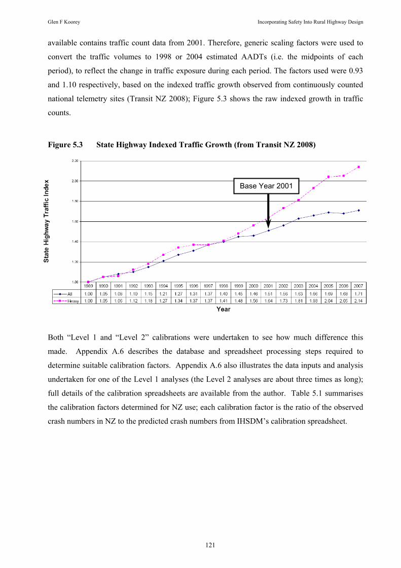
Glen F Koorey Incorporating Safety Into Rural Highway Design
121
available contains traffic count data from 2001. Therefore, generic scaling factors were used to
convert the traffic volumes to 1998 or 2004 estimated AADTs (i.e. the midpoints of each
period), to reflect the change in traffic exposure during each period. The factors used were 0.93
and 1.10 respectively, based on the indexed traffic growth observed from continuously counted
national telemetry sites (Transit NZ 2008); Figure 5.3 shows the raw indexed growth in traffic
counts.
Figure 5.3 State Highway Indexed Traffic Growth (from Transit NZ 2008)
Both “Level 1 and “Level 2” calibrations were undertaken to see how much difference this
made. Appendix A.6 describes the database and spreadsheet processing steps required to
determine suitable calibration factors. Appendix A.6 also illustrates the data inputs and analysis
undertaken for one of the Level 1 analyses (the Level 2 analyses are about three times as long);
full details of the calibration spreadsheets are available from the author. Table 5.1 summarises
the calibration factors determined for NZ use; each calibration factor is the ratio of the observed
crash numbers in NZ to the predicted crash numbers from IHSDM’s calibration spreadsheet.
Base Year 2001

Glen F Koorey Incorporating Safety Into Rural Highway Design
122
Table 5.1 IHSDM Calibration Factors for New Zealand Use - Highway Segments
Crash Analysis Period 1996-2000 2002-2006
Number of Observed Crashes 18 052 20 805
Predicted No. of Crashes (IHSDM Level 1) 20 423.9 24 433.4
Level 1 Factor 0.884 0.851
Predicted No. of Crashes (IHSDM Level 2) 20 508.3 24 536.6
Level 2 Factor 0.880 0.848
The results suggest that the crash numbers in NZ are lower than those observed in the US (and
getting better over time). While this could reflect a slightly better road safety record in NZ, it
could also indicate a better reporting rate in the US; certainly there is more incentive to report
many crashes there, either for lawsuit liability reasons or because of legal reporting obligations
(unlike NZ, most US jurisdictions have a minimum property damage value for which it is
mandatory to report a crash; in all of the US states used for the IHSDM default factors, the
minimum reporting threshold was US$500-$1000).
It is interesting to note that the calibration factors above do not vary much between Level 1 and
Level 2. This suggests that the much simpler Level 1 data requirements may be sufficient for a
reasonably accurate crash prediction in NZ.
Further investigation of IHSDM calibration factors when the network is disaggregated into
various sub-categories is discussed in Section 5.2.5. The above factors suggest however that NZ
crash numbers overall are sufficiently different enough to warrant using NZ-specific calibration
factors.
5.2.2 Modification of the relative Crash Severity Proportions The default IHSDM crash severity proportions are based on Highway Safety Information System
(HSIS) data for Illinois, Michigan, Minnesota, and North Carolina in the mid-1990s (Vogt &
Bared 1998). A similar analysis was undertaken for the NZ injury and non-injury crash data from
included State Highway sections (excluding intersection crashes) in the research database.
Separate analyses were produced for the periods 1996-2000 and 2002-2006, approximately
reflecting the “before” and “after” periods for the SH1 HSF Realignment project. Table 5.2
summarises the respective proportions.

Glen F Koorey Incorporating Safety Into Rural Highway Design
123
Table 5.2 Percentage Distributions for Crash Severity Level - Highway Segments
Crash Severity Level IHSDM Defaults NZ Values 1996-2000 NZ Values 2002-2006
Fatal 1.3% 4.4% 3.1%
Incapacitating Injury 5.4% 11.6% 10.4%
Non-incapacitating injury 10.9% 25.0% 28.2%
Possible injury 14.5% - -
Total fatal plus injury 32.1% 40.9% 41.8%
Property-damage-only 67.9% 59.1% 58.2%
Note: due to rounding, individual values may not sum exactly to the totals.
It should be noted that the US data includes three levels of injury crashes (“incapacitating”,
“non-incapacitating”, and “possible”) whereas NZ data only has two injury levels (“serious” and
“minor”). It appears that “minor” crash numbers in NZ compare well with the combined
proportion of “non-incapacitating” and “possible” injury crashes. For simplicity, the proportion
of “possible injury” crashes for NZ data has been set to zero, with the other two injury levels
assumed to match their NZ equivalents. “Property-damage-only” crashes are assumed, by
definition, to equate to NZ’s “non-injury” crash data.
Notwithstanding the above adjustment, it can be seen that there are fewer reported property-
damage-only crashes in NZ, perhaps reflecting the lack of legal obligation to do so.
Correspondingly there is a greater proportion of injury or fatal crashes reported in NZ; however
the figures are noticeably skewed towards the more serious severities. Fatal crashes in NZ make
up two to three times as many of the reported crashes as in the IHSDM defaults (it is heartening
at least to see that the proportion has decreased over time). One could speculate that this reflects
a greater propensity to report crashes of lesser severity in the US, because of the possibility of
personal lawsuits, whereas many more in NZ may go unreported to the Police. Alternatively, it
may reflect that NZ’s speed limits for two-lane rural roads tend to be higher than for similar
roads in the US, resulting in a higher likelihood of fatal and severe crashes.
One notable observation of the existing IHSDM crash prediction process is that the same crash
severity proportions given in Table 5.2 are applied to all road section estimates of crash numbers.
This seems somewhat unrealistic, as the average severity is likely to be affected by the crash type
and surrounding environment. For example, a greater proportion of head-on crashes is likely to
lead to relatively more fatal or serious injury crashes. Similarly, a road environment with more
severe roadside hazards (e.g. non-frangible trees) or where higher vehicle operating speeds can
be expected is also likely to experience more severe crashes on average.

Glen F Koorey Incorporating Safety Into Rural Highway Design
124
The only situation where crash severity is taken into account in IHSDM is in the Empirical
Bayes analysis, where property-damage-only and fatal-and-injury crash estimates are calculated
separately based on the relative numbers of observed crashes in each case. It would be desirable
however if the IHSDM process also took into account (say) the specified design speed and
roadside hazard rating of each road element to adjust the relative crash severity proportions
accordingly.
5.2.3 Modification of the relative Crash Type Proportions The default IHSDM crash type proportions are also based on the same HSIS data as before.
Again, an analysis of crash types was undertaken using the NZ injury and non-injury crash data
from included State Highway sections.
An initial difficulty was to determine which crashes in the NZ data equated to which IHSDM
categories. This was made somewhat complicated because of the mixed methods for categorising
crashes in the US system. For example, while some crash types are by vehicle movement (e.g.
“angle collision”, “ran off road”, etc), others are categorised by the parties involved (e.g.
collision with animal, parked vehicle, etc), or the resulting outcome (e.g. “overturned”). NZ
crash data also includes bicycles and pedestrians amongst the coded “vehicles”, recording these
as multiple-vehicle crashes instead of single-vehicle crashes when only one motor vehicle is
involved. Thus, a simple translation table was not easy to achieve without a series of database
processing steps. Even then, it is acknowledged that a perfect translation is not likely. For
example, CAS data does not record specifically whether a vehicle overturned; however it is
probably reasonable to relate this category to “lost control on road” crashes, which is the usual
cause of such single-vehicle overturning events.
This is only an issue for comparison purposes; for use in IHSDM, it is only important that the
user knows what the reported categories refer to in terms of assigned NZ crash types. It is
certainly not recommended that NZ should adopt a similar system to the US for its crash type
coding, as there appear to be few advantages for general road safety research and analysis in
doing this.
Table 5.3 summarises the key linkages between the two categorisation systems (refer to
Appendix A.1 for the CAS movement codes referred to).
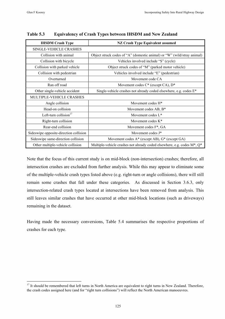
Glen F Koorey Incorporating Safety Into Rural Highway Design
125
Table 5.3 Equivalency of Crash Types between IHSDM and New Zealand
IHSDM Crash Type NZ Crash Type Equivalent assumed SINGLE-VEHICLE CRASHES
Collision with animal Object struck codes of “A” (domestic animal) or “W” (wild/stray animal) Collision with bicycle Vehicles involved include “S” (cycle)
Collision with parked vehicle Object struck codes of “M” (parked motor vehicle) Collision with pedestrian Vehicles involved include “E” (pedestrian)
Overturned Movement code CA Ran off road Movement codes C* (except CA), D*
Other single-vehicle accident Single-vehicle crashes not already coded elsewhere, e.g. codes E*
MULTIPLE-VEHICLE CRASHES Angle collision Movement codes H*
Head-on collision Movement codes AB, B* Left-turn collision17 Movement codes L* Right-turn collision Movement codes K* Rear-end collision Movement codes F*, GA
Sideswipe opposite-direction collision Movement codes J* Sideswipe same-direction collision Movement codes A* (except AB), G* (except GA)
Other multiple-vehicle collision Multiple-vehicle crashes not already coded elsewhere, e.g. codes M*, Q*
Note that the focus of this current study is on mid-block (non-intersection) crashes; therefore, all
intersection crashes are excluded from further analysis. While this may appear to eliminate some
of the multiple-vehicle crash types listed above (e.g. right-turn or angle collisions), there will still
remain some crashes that fall under these categories. As discussed in Section 3.6.3, only
intersection-related crash types located at intersections have been removed from analysis. This
still leaves similar crashes that have occurred at other mid-block locations (such as driveways)
remaining in the dataset.
Having made the necessary conversions, Table 5.4 summarises the respective proportions of
crashes for each type.
17 It should be remembered that left turns in North America are equivalent to right turns in New Zealand. Therefore, the crash codes assigned here (and for “right turn collisions”) will reflect the North American manoeuvres.

Glen F Koorey Incorporating Safety Into Rural Highway Design
126
Table 5.4 Percentage Distributions for Crash Types - Highway Segments
IHSDM Crash Type IHSDM Defaults NZ Values 1996-2000 NZ Values 2002-2006SINGLE-VEHICLE CRASHES
Collision with animal 30.9% 3.6% 3.6% Collision with bicycle 0.3% 0.5% 0.3%
Collision with parked vehicle 0.7% 0.9% 0.6% Collision with pedestrian 0.5% 0.7% 0.5%
Overturned 2.3% 1.0% 0.7% Ran off road 28.1% 55.6% 58.1%
Other single-vehicle accident 3.6% 3.3% 3.6%
Total single-vehicle accidents 66.3% 65.7% 67.3% MULTIPLE-VEHICLE CRASHES
Angle collision 3.9% 0.04% 0.03% Head-on collision 1.9% 13.6% 11.4% Left-turn collision 4.2% 0.8% 0.5%
Right-turn collision 0.6% 0.4% 0.3% Rear-end collision 13.9% 5.7% 7.3%
Sideswipe opposite-direction collision 2.4% 0.7% 0.6% Sideswipe same-direction collision 2.6% 8.1% 7.8%
Other multiple-vehicle collision 4.1% 4.9% 4.6%
Total multiple-vehicle accidents 33.7% 34.3% 32.7%
While the relative proportions of single and multiple vehicle crashes are quite similar, there are
some discrepancies between the proportions within each sub-category. As discussed above, some
of this is due to differences in the definitions for each category within the US and NZ crash data.
There is however a notable difference in the proportion of single-vehicle collisions involving
animals, which is not as prevalent a hazard in NZ. The bulk of this difference appears to have
been made up by a notable increase in the proportion of “ran off road” crashes (although the NZ
“lost control” codes used would also include some crashes where the vehicles may have
remained on the road and overturned instead). With regards to multiple-vehicle crashes, the
biggest difference is in the proportion of head-on crashes; although it is speculated that some of
these in the NZ data would have been coded “sideswipe opposite direction” under the US
system. Similar coding discrepancies may explain the difference in “sideswipe same direction”
crashes. It is less clear why there are considerably fewer rear-end crashes reported in NZ, as the
coding for these appears more straightforward, however it is possible that a number of crashes
with E*, G*, K* and M* CAS movement codes could also physically result in a rear-end
collision.
As with crash severity, another key issue is the fact that the respective crash type proportions are
fixed for all IHSDM analyses, regardless of the environment being investigated. As indicated in

Glen F Koorey Incorporating Safety Into Rural Highway Design
127
Section 4, this is a highly unrealistic assumption. The relative proportions of crash types are
likely to vary at least with regards to traffic volumes, the number of lanes, and the curvature of
the road. At the very least it would be desirable to determine a relationship in IHSDM between
the expected proportions of single-vehicle and multiple-vehicle crashes, with the respective crash
sub-types in each category scaled accordingly in relation to this.
5.2.4 Issues with IHSDM’s Calibration Factor Approach
It is noteworthy that the form of the crash prediction models cannot be adjusted, except by means
of scaling the overall predicted crash numbers and crash severity/type proportions. This could be
problematic if crash incidence in another jurisdiction varies differently in relation to the key
inputs. For example, consider the hypothetical example illustrated in Figure 5.4, where local
observed crash data is being compared with the uncalibrated IHSDM prediction model. Clearly
the IHSDM model in this example under-predicts the expected number of crashes, so a
calibration factor is used to scale up the prediction model to better fit the observed data.
However, when plotted against the traffic volume at each site, it is apparent that even the
calibrated IHSDM model is not a good fit to the observed data; at low volumes the model under-
predicts the expected number of crashes, while at high volumes it over-predicts.
Figure 5.4 Calibration of IHSDM to Local Crash Data (Single Calibration Factor)
Traffic Volume (AADT)
Local Observed Crash Data
Uncalibrated IHSDM Crash Model
Calibrated IHSDM Crash Model

Glen F Koorey Incorporating Safety Into Rural Highway Design
128
Without the ability to adjust the “shape” of the prediction model (e.g. the exponent applied to the
traffic volume input), the only way to produce a more accurate crash estimate with IHSDM is to
determine separate calibration factors for different traffic volume categories. An example of this
is illustrated in Figure 5.5; it can be seen that the differences between the observed and predicted
crash numbers are much smaller now. Similarly, different calibration factors might be required
for roads with (say) different construction standards, types of terrain, or in different regions of a
jurisdiction.
Figure 5.5 Calibration of IHSDM to Local Crash Data (Multiple Calibration Factors)
Pragmatically speaking, the problem then becomes one of how far to disaggregate the road
network and create separate calibration factors for each subset. While this may improve the
accuracy of the predicted outputs, it comes at the cost of model simplicity. IHSDM users would
have to select a different set of calibration parameters depending on where their project is, and a
larger set of factors would need to be regularly updated as crash patterns change.
5.2.5 Disaggregation of Model Calibration Factors To test the relative accuracy of the base calibration factors determined in Section 5.2.1 when
working with a smaller part of the network, the (1996-2000) crash and network data were
subdivided into various categories and new calibration factors recalculated for each subset. The
hypothesis to be tested is that the factors for the subsets do not significantly differ in comparison
Traffic Volume (AADT)
Local Observed Crash Data
Uncalibrated IHSDM Crash Model
Calibrated IHSDM Crash Model 1
Calibrated IHSDM Crash Model 2
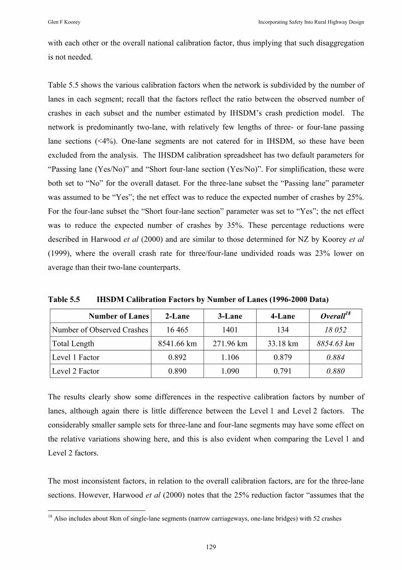
Glen F Koorey Incorporating Safety Into Rural Highway Design
129
with each other or the overall national calibration factor, thus implying that such disaggregation
is not needed.
Table 5.5 shows the various calibration factors when the network is subdivided by the number of
lanes in each segment; recall that the factors reflect the ratio between the observed number of
crashes in each subset and the number estimated by IHSDM’s crash prediction model. The
network is predominantly two-lane, with relatively few lengths of three- or four-lane passing
lane sections (<4%). One-lane segments are not catered for in IHSDM, so these have been
excluded from the analysis. The IHSDM calibration spreadsheet has two default parameters for
“Passing lane (Yes/No)” and “Short four-lane section (Yes/No)”. For simplification, these were
both set to “No” for the overall dataset. For the three-lane subset the “Passing lane” parameter
was assumed to be “Yes”; the net effect was to reduce the expected number of crashes by 25%.
For the four-lane subset the “Short four-lane section” parameter was set to “Yes”; the net effect
was to reduce the expected number of crashes by 35%. These percentage reductions were
described in Harwood et al (2000) and are similar to those determined for NZ by Koorey et al
(1999), where the overall crash rate for three/four-lane undivided roads was 23% lower on
average than their two-lane counterparts.
Table 5.5 IHSDM Calibration Factors by Number of Lanes (1996-2000 Data)
Number of Lanes 2-Lane 3-Lane 4-Lane Overall18
Number of Observed Crashes 16 465 1401 134 18 052
Total Length 8541.66 km 271.96 km 33.18 km 8854.63 km
Level 1 Factor 0.892 1.106 0.879 0.884
Level 2 Factor 0.890 1.090 0.791 0.880
The results clearly show some differences in the respective calibration factors by number of
lanes, although again there is little difference between the Level 1 and Level 2 factors. The
considerably smaller sample sets for three-lane and four-lane segments may have some effect on
the relative variations showing here, and this is also evident when comparing the Level 1 and
Level 2 factors.
The most inconsistent factors, in relation to the overall calibration factors, are for the three-lane
sections. However, Harwood et al (2000) notes that the 25% reduction factor “assumes that the
18 Also includes about 8km of single-lane segments (narrow carriageways, one-lane bridges) with 52 crashes

Glen F Koorey Incorporating Safety Into Rural Highway Design
130
passing lane is operationally warranted and that the length of the passing lane is appropriate for
the operational conditions on the roadway”. Based on the previous work by Koorey et al (1999),
it is suspected that some of the existing passing lane segments in NZ do not fully meet these
criteria, and thus their safety effect may be considerably less than 25%. This would result in
calibration factors closer to the overall average.
Table 5.6 summarises the calibration factors when the data is disaggregated by traffic volume.
The five traffic volume categories are those used by the IHSDM calibration routine.
Table 5.6 IHSDM Calibration Factors by Traffic Volume (1996-2000 Data)
AADT (vpd) <1000 1000 - 3000 3000 - 5000 5000 - 10 000 > 10 000
No. Observed Crashes 1987 4936 4244 4405 2480
Total Length 3061.29 km 3312.31 km 1322.72 km 872.84 km 286.26 km
Level 1 Factor 1.104 0.864 0.911 0.908 0.742
Level 2 Factor 1.120 0.860 0.914 0.910 0.739
No clear trend emerges in terms of changing traffic volume. Although the calibration factors for
high volume (> 10 000 vpd) roads are lower than the other volume bands, it should be noted that
over 21% of road length with such volumes have three or four lanes (as opposed to <4% for the
total network). The above calculations assume that all road sections have no three/four-lane
segments; allowing for these would bring the calibration factors more in line with the others.
This would suggest that the “shape” of the IHSDM crash prediction model is reasonably
appropriate for NZ, in terms of variations by traffic volume. The only other category to be wary
of is the “<1000 vpd” group, where possibly lower design standards are producing a higher
calibration factor.
Crash patterns may also vary by terrain, i.e. in terms of how vertical alignment changes.
IHSDM’s calibration routine seeks data on the relative proportion of road length in “flat”,
“hilly”, and “mountainous” terrain; however nowhere are these terms described in clear
quantitative terms. It appears that this data is only used to generate default values in the
calibration spreadsheet when more detailed stratification by traffic volume and road alignment is
not available. The calibration spreadsheet lists some information from the HSIS data where the
average gradients for flat, rolling and mountainous sections are given as 1.5%, 2.0% and 3.7%
respectively. These values however seem quite closely grouped and suggest that the
categorisation of road sections in HSIS by terrain is not a very precise exercise either. McLarin

Glen F Koorey Incorporating Safety Into Rural Highway Design
131
(1997) suggested a categorisation based on both vertical and horizontal alignment data (gradient
G and horizontal curvature H), thus:
Flat: |Gave| ≤ 1.5% AND (Gmax - Gmin) ≤ 6% AND (Hmax - Hmin) ≤ 5 rad/km
Rolling: 1.5% < |Gave| ≤ 4.5% OR 6% < (Gmax - Gmin) ≤ 12% OR 5 rad/km < (Hmax - Hmin) ≤ 15 rad/km
Mountainous: |Gave| > 4.5% OR (Gmax - Gmin) > 12% OR (Hmax - Hmin) > 15 rad/km
McLarin’s analysis was using fixed length segments of varying alignment, whereas the current
analysis sub-divides the data into tangent and curve sections; therefore a categorisation by
difference in horizontal curvature would not be as meaningful.
An alternative measure is to use “hilliness”, usually defined as the rate of rises or falls along a
road. For example, a constant grade of 1% has a hilliness of 10 m per km. Based on the above
work and inspection of the geometric elements database, the following terrain definitions will be
used for this analysis:
Flat: Hilliness ≤ 10 m/km
Rolling: 10 m/km < Hilliness ≤ 40 m/km
Mountainous: Hilliness > 40 m/km
This strikes a reasonable balance between the extremes of terrain while ensuring sufficient
numbers in each category. Table 5.7 summarises the calibration factors when the data is
disaggregated by these terrain categories.
Table 5.7 IHSDM Calibration Factors by Terrain (1996-2000 Data)
Terrain Flat Rolling Mountainous
Number of Observed Crashes 7469 7247 3336
Total Length 3666.08 km 3731.97 km 1457.05 km
Level 1 Factor 0.843 0.921 0.915
Level 2 Factor 0.839 0.918 0.912

Glen F Koorey Incorporating Safety Into Rural Highway Design
132
There does not appear to be any clear trend as terrain worsens, and the calibration factors are all
reasonably similar. While one would expect attributes such as horizontal curvature to also vary
with terrain, this is already allowed for in the calibration process. Again, it is likely that there are
more three/four-lane roads in flat terrain than hilly/mountainous terrain, which probably helps
explain the lower calibration factors for the former. This suggests that we can probably ignore
the effects of terrain.
Another source of variation in crash rates is by region, where local topography, climate, and
safety programmes may have an effect. Figure 5.6 shows the variation in crash risk (social cost
in cents per veh-km) by region and road type (from National Road Safety Committee 2000). The
average cost for State Highways is shown by the dashed line; it can be seen that Northland is
considerably above the average, Waikato is virtually on the average and Otago is considerably
below the average.
Figure 5.6 Variation in Crash Risk across NZ Regions (from NRSC 2000)
These three regions have been chosen for more specific analysis (other possible regions for
investigation had smaller overall road lengths or social costs and so were not considered further).
Table 5.8 summarises the calibration factors when the data is disaggregated by each region.

Glen F Koorey Incorporating Safety Into Rural Highway Design
133
Table 5.8 IHSDM Calibration Factors by Region (1996-2000 Data)
Region (Relative crash risk)
Northland (Above Average)
Waikato (Average)
Otago (Below Average)
Number of Observed Crashes 1379 3757 1282
Total Length 627.57 km 1455.72 km 1146.64 km
Level 1 Factor 0.914 0.791 0.822
Level 2 Factor 0.916 0.789 0.823
Again, no obvious trend is apparent; although the worst performing region (Northland) does has
higher calibration factors as might be expected. The results may also be complicated by the
other variations within each region; for example Waikato has the highest average traffic density
whereas Northland has the greatest proportion of mountainous road terrain.
It should be noted that in many of the above disaggregations, there are also notable differences in
the crash severity and crash type proportions. For example, sections with higher traffic volumes
typically experienced a greater proportion of multiple vehicle crashes and, not surprisingly, these
differences are also reflected in the data for crashes on three/four-lane roads. Similarly, sections
in mountainous terrain had a lower proportion of fatal crashes, probably reflecting the lower
likelihood of travelling at higher speeds. Therefore, any development of calibration factors for
sub-categories may also require the development of suitable proportion values for crash severity
and type.
An attempt was made to undertake some statistical analysis of the above calibration factors, to
determine whether there were statistically significant differences within each set of factors and
also in comparison with the overall calibration factors. This was not a straightforward exercise,
as the distribution of the calibration factors is not likely to follow a standard distribution (e.g.
Normal distribution). Appendix A.7 details the analyses undertaken. In summary, the results
generally tend to support having the same overall IHSDM calibration factor for virtually all
situations. However, some caution needs to be taken when dealing with rural road sections with
particularly low (<1000 vpd) or particularly high (>10,000 vpd) traffic volumes. The results
may also not be as accurate in some regions of the country.
Even here there are two factors that should assist the use of a common calibration factor:

Glen F Koorey Incorporating Safety Into Rural Highway Design
134
• The use of local crash history data in IHSDM will help to further refine the crash estimates in
the same way that a localised calibration factor might.
• From a practical application context, it is not clear whether these statistical tests (which
combine crash numbers over the entire data-set) are that useful. For example, on a road
section with (say) <5 crashes, a calibration factor of 0.88 versus 0.84 will not produce a large
difference in the predicted number of crashes.
The above analysis by disaggregrated subsets also confirms the earlier finding that there is little
difference between the values derived using the Level 1 and Level 2 calibration procedures.
Generally the difference was less than 0.01; the key exception being for four-lane roads where
only 134 crashes and 33 km of highway were used in the analysis. Therefore, for simplification,
only Level 1 calibration factors will be used for future analysis.
5.3 Editing Design Policy Files
IHSDM is currently provided with US standards and guidelines (e.g. AASHTO 2004) on which
to base its decisions about design consistency and policy compliance (as used in the PRM and
DCM modules). These however are specified in external files, and the program is designed to be
able to accept alternative criteria, such as state department or local design policies.
IHSDM’s System Administration Tool (SAT) allows users to create or edit policy files to use
with the program. The interface allows various policy files to be present in the system, with the
user specifying which one to use for each analysis. The SAT allows users to either create a
completely new policy file (requiring users to enter in values for each data item) or to “clone” a
copy of an existing policy file and then modify it to suit. Of note is that there appears to be no
obvious way to remove a policy file from the SAT list, or to import a policy file developed
elsewhere. However, editing then closing any policy file forces IHSDM to re-compile all policy
files that it finds in the “policy” sub-directory.
Most NZ road design is undertaken in accordance with two main guidelines. State Highways are
managed by Transit NZ and are designed using the State Highway Geometric Design Manual
(SHGDM, Transit NZ 2000). Local councils generally adopt either the SHGDM or the
Austroads Rural Road Design guide (Austroads 2003); more often than not, Austroads is used.
Transit NZ is also apparently considering looking to use the updated Austroads standards in the

Glen F Koorey Incorporating Safety Into Rural Highway Design
135
near future (Davis 2007), and so it was decided to produce a local policy file based on Austroads
standards.
Much of the policy file used by IHSDM consists of lookup tables to enable the software to
analyse appropriate values. An example of a large lookup table in the Policy File is the
Horizontal Curve Elements tab, shown in Figure 5.7 (also note all of the other tabs shown).
Figure 5.7 IHSDM Policy Table Editor
The creation of a policy file for NZ roads has its challenges. For a start, IHSDM has over thirty
different data tables to be modified (e.g. default shoulder widths, stopping sight distances,
friction factors), as well as a set of default “scalars” (e.g. minimum lane widths, maximum
design speed, driver eye heights). Also, whilst there are many similarities between geometric
standards in North America and NZ, there are also a number of areas where standards do not
match well.
For example, the Austroads guidelines generally define varying standards based on traffic
volumes. Many of IHSDM’s policy sections required different standards by road hierarchy e.g.
arterial, collector and local roads. Only some features, such as lane and shoulder widths, also

Glen F Koorey Incorporating Safety Into Rural Highway Design
136
allow standards to be applied for different volume bands. Given that the initial IHSDM
assessment within NZ was on State Highways, the resulting local policy file produced had only
one classification, namely Arterial. Ultimately, however, it may be useful to use the other
IHSDM road hierarchy categories to set up standards for lower-volume roads. It could be argued
that different State Highways should also have different standards; this is already reflected for
example in the range of minimum seal width standards that are used in NZ for State Highways of
varying volumes (Transit NZ 2000).
IHSDM also seeks more detailed information in some areas than is usually specified by
Austroads, e.g. clear zone requirements such as roadside slopes and ditch details. The vertical
curvature requirements are also quite different, particularly with the required safe stopping sight
distances (partly due to differences in driver eye heights). Sometimes, AASHTO and Austroads
use different terminology as well, complicating the conversion process. Where no matching
Austroads standard could be found, the equivalent IHSDM (AASHTO 2004) values were
retained.
Austroads often provides both a table and formula to derive the design standards for differing
speeds, horizontal radius, etc. It was decided therefore that the most appropriate way to generate
the equivalent tables for IHSDM was in a spreadsheet. This enables formulae to be used to
derive the table values, but also allows future users of the policy file to upgrade the values
should the Austroads standards change. Updating tables then simply involves copying from the
spreadsheet and pasting into the relevant table of the IHSDM Policy Editor.
Keyte (2006) developed a Design Policy file for use in NZ, based on the Austroads guidelines.
This has been reviewed, minor amendments made, and used for the IHSDM work in this study.
The resulting IHSDM configuration file is nearly 10,000 lines long so is not repeated here, but is
available on request from the author.
5.4 Importing NZ Road Alignment Data
IHSDM allows a number of different ways for road data to be created or directly imported into
the program:
• Alignment data can be manually entered using IHSDM’s Highway Editor tool, although this
can be very time consuming, given the amount of design detail that IHSDM may require.

Glen F Koorey Incorporating Safety Into Rural Highway Design
137
• IHSDM “comma separated values” (CSV) files can be imported. These are text-based and
contain formatted geometric and non-geometric data related to one or more highways.
Although these can be created manually, typically they are produced by another IHSDM user
exporting a CSV file from another roading project. This file format is being phased out of
more recent versions of IHSDM.
• Industry standard LandXML files can be imported (see Section 5.4.1 for more details).
Again, these can be created manually, but most roading design software packages, such as
Geopak, 12D or MX-Road, can produce LandXML files directly from their alignment data.
Thus new proposed alignments can be readily imported to test with IHSDM.
Typically the data required by IHSDM comprise geometric elements (such as horizontal
curves/tangents, vertical curves/grades and cross-section features), together with general road
environment data (such as design speeds, terrain and traffic volumes). For proposed alignments,
obtaining these data is usually relatively straightforward as most of the necessary information
will already be determined in some road design program. Assessing existing alignments requires
further work, and two possible approaches are discussed below.
Where a field survey has been undertaken for a specific realignment project, the user may be
able to use that data to assess the existing alignment. However, the alignment information is
likely to be recorded as a series of discrete survey points that require conversion to the
appropriate geometric elements required by IHSDM. Many roading design packages can readily
convert such points to geometric data via a best-fit method controlled by the user. The best-fit
method often is not entirely accurate due to the inherent inaccuracies of surveys undertaken at
(typically) 20 m centres and the difficulty in getting software to determine tangent points as one
might do visually.
IHSDM’s checks for geometric consistency are however not sensitive to absolute accuracies for
horizontal and vertical curve radii. A number of variables contribute to the checks for
consistency including desired speed, location of curves adjacent to each other and the like. On
this basis it was clear from the IHSDM results of Keyte (2006) that the method of visually
tracing the survey points and producing geometric elements was generally sufficient for most
purposes.
Another approach is to use road geometry data available for the network. As described in
Section 3.4, database routines can be developed to “walk” down a given highway dataset and
Glen F Koorey Incorporating Safety Into Rural Highway Design
138
identify the approximate start and end of each geometric element (e.g. based on horizontal
curvature). Then summary information about the road geometry segments within the extents of
each element can be produced, and a record added to a table of elements. This technique has
previously been used to create rural road link data in the Paramics micro-simulation model
(Koorey 2003).
5.4.1 Common Highway Alignment Information Formats
The work described above raises the issue of standardising the way in which road alignment is
represented in different software packages. This is an increasingly important issue if roading
practitioners are to make use of common information for different applications; for example:
• Existing road geometry data is captured in the field and stored in an inventory database (e.g.
RAMM).
• Road design packages (e.g. MX-ROAD, 12D) import existing road alignments and create
new alignment designs for cost estimation, benefit analysis and eventual construction.
• Traffic analysis software (e.g. TRARR, TWOPAS) import existing and proposed road
alignments to assess the operational effects of realignments and passing facilities.
• Crash analysis software (e.g. IHSDM, EEM) use road alignment information to predict the
expected number of crashes.
• Final alignment data from reconstructed highways is used to update road inventory
databases.
There are no doubt other application possibilities either in use already or yet to be considered. A
key issue however is the ability to transfer road alignment information from one software
package or data source to another.
Traditionally, in both this field and other sectors, such data conversion was often undertaken by
means of proprietary import and export routines. For example a road design tool like 12D (12D
Solutions Pty Ltd 2007) has the ability to import from and export to a range of formats, including
CAD Data Exchange Format (*.DXF), ArcView (*.shp), AutoCAD (*.DWG), Microstation
(*.DGN), MOSS/MX GENIO, LandXML (*.XML), Sokkia SDR and plain delimited text. If
this approach is also taken by other packages, it results in a data transfer relationship somewhat
like Figure 5.8.

Glen F Koorey Incorporating Safety Into Rural Highway Design
139
Figure 5.8 Conventional Data Conversion Approach between Packages
It can be seen from Figure 5.8 that, typically, transfers from one data source or software package
to another are a haphazard exercise. Some software packages are able to read (but perhaps not
write to) the proprietary formats of other packages, some packages have shared common formats
(especially if the packages are developed by the same organisation), and some packages are able
to use common (perhaps industry standard) formats. Widely used data sources or inventories
may store data in common public formats or may be only easily accessible by certain packages.
For any missing links in the data transfer diagram, the user will have to either manually enter
data into the new package or create their own customised automated data transfer routines. If
privately-specified proprietary formats are used by some packages, this can limit the ability to
obtain all of the required data easily.
One possible approach is for each software package to develop data conversion tools (both
import and export) for every other relevant package. However, developing and maintaining a
range of conversion tools for a wide variety of other packages can be a major effort for any
software developer. Any time that a new package, data source or file format appears on the
scene, or an existing package or format is updated, all developers would need to update their
conversion code accordingly and distribute it to their users.
A more pragmatic approach is to find a common intermediary data format that all packages can
read and write. This “Esperanto” format can then act as a translating tool between any two
Software Package AAA
Software Package BBB
Software Package CCC
Inventory Database ZZZ
Plain Text Data
Software Package DDD
Common BBB-CCC
DataAAA Format
Data
XYZ Common Format
Public Data Source YYY

Glen F Koorey Incorporating Safety Into Rural Highway Design
140
packages; widely used data sources could also be stored in the same format. Should a software
package be updated, there will not be a requirement for other providers to also provide data
conversion updates to their packages. Figure 5.9 illustrates this approach (note that there may
still be other data formats that can be shared between some packages).
Figure 5.9 Data Conversion between Packages using a Common File Format
Although in general this is an attractive approach to data management and transfer, one potential
remaining problem is in the loss of data detail due to different data requirements of each
package. For example, one software tool (e.g. a road design package) may require information
about road widths but not about existing crashes whereas, for another tool (e.g. a crash prediction
model), existing crash history may be a key input but it may not make any use of road width
information. Therefore, transfer of data between packages may potentially lead to degradation of
information if the same parameters are not saved. Alternatively, agreement may need to be
reached on sufficiently universal data to be uniformly recorded using the common format (even
if some packages do not make use of all of it themselves), with other more specialised data
obtained or transferred by other means.
Common data formats have been investigated and implemented in a wide range of sectors;
Spearpoint (2006) for example describes the development of a common industry database format
to describe building construction elements, including fire protection data. In the transportation
sector, a number of initiatives have been proposed and investigated, including Transportation
Spatial Information Infrastructure (TSII, Burggraf 2005), Traffic Model Markup Language
(TMML, University of Florida 2007) and TransXML (Ziering et al 2007). Many of these are
Software Package AAA
Software Package BBB
Software Package CCC
Inventory Database ZZZ
Software Package DDD
XYZ Common Format
Public Data Source YYY

Glen F Koorey Incorporating Safety Into Rural Highway Design
141
quite application-specific however, focusing for example on just traffic and ITS operations or
traffic network models.
A common feature of most recent information transfer systems developed is the use of
eXtensible Markup Language (XML) for their specification language. XML is derived from the
family of Standard Generalised Markup Languages (SGMLs), which is an international standard
for semantic tagging of electronic documents (W3C 2008). Typically the document format uses
a series of plain-text tags to enclose various data elements and their attributes, e.g.
<TAG property=SomeAttribute>SomeElement</TAG>
Hypertext Markup Language (HTML), used to create webpages, is probably the most familiar
SGML to the general public. Unlike HTML, where the available tags are pre-defined, XML is
essentially a “meta-language” that allows one to define a particular data structure to suit a certain
application. The extensibility of the XML language means that new elements or attributes can
be easily added to an existing data structure. Also, a well-behaved XML reading tool will
simply ignore a data field it does not recognise, thus allowing more information to be transferred
than a particular application may use.
In the field of roadway design, LandXML has developed into the predominant industry standard
(see www.landxml.org for more details). LandXML’s civil design background reflects a broader
specification than just roading. As well as providing the ability to specify road alignment, cross-
section, intersection, traffic and crash information, LandXML also provides support for raw or
reduced surveying data, land parcels and boundaries, bridges, channels, pipe networks, and
railway lines. Many design software packages have incorporated LandXML import and export
provision and IHSDM now uses it as its standard data storage format.
The author has used a common road alignment file format before to convert road geometry data
between various road design packages and the TRARR simulation software (Koorey 2000).
However, that was a plain text format. With regards to this research, it seems sensible to
develop data conversion tools that produce valid LandXML files from NZ road geometry data,
suitable for direct import into IHSDM or other packages.

Glen F Koorey Incorporating Safety Into Rural Highway Design
142
5.4.2 Development of Road Alignment Importing Routine
Using the road geometry elements produced for this study, conversion procedures were
developed to create LandXML files for use in IHSDM. This allows existing sections of State
Highway to be assessed for safety and consistency using IHSDM.
A test highway was first created in IHSDM, containing a variety of different geometric and
traffic elements. The resulting highway data was then exported to a LandXML file to provide a
template for creating other files. Database queries and code were then developed to produce an
equivalent LandXML file for a selected section of State Highway; in fact, two separate import
files were created for the road and crash data respectively. The relative AADTs to be used in
IHSDM could be adjusted to a particular year using a special table in the database based on the
same Transit NZ count index data referred to in Section 5.2.1. The resulting files were then
imported into IHSDM to confirm the correctness of the coding and debugging undertaken
accordingly. Appendix A.8 lists examples of the road and crash data LandXML files generated
by this routine.
Due to the data available, not every design aspect available in IHSDM could be coded in the
import files. In some cases, necessary data was assumed to apply throughout the length of the
road section for simplification. Other data was not required for use with the CPM and could thus
be ignored for now. Table 5.9 summarises the elements included or otherwise in the resulting
LandXML files.
Table 5.9 IHSDM Road Data included in Import File Routines
Detailed Data Included (for every geometric element)
Simplified Data Included (for road section overall)
Data Not Included
Horizontal element details (tangent/curve, radius, direction)
Vertical alignment details within each element
Traffic Volume (AADT)
Traffic lane widths
Sealed shoulder widths
Presence of 3-lane or 4-lane sections
Existing crashes (location, year, severity, intersection-related)
Posted speed limit
Desired speed
Functional road class
Roadside hazard rating
Initial elevation and bearing
Driveway density
Crossfall (superelevation)
Location of bridges
Roadside slopes
Roadside obstructions
No-overtaking zones
Location of intersections
Design/Peak Hour Volumes

Glen F Koorey Incorporating Safety Into Rural Highway Design
143
5.5 Vehicle Fleet and Desired Speed Updating
Both the Design Consistency and Traffic Analysis modules require the specification of standard
vehicles to determine vehicle speeds and interactions along the modelled alignment. IHSDM
comes with a pre-defined suite of vehicle classes for passenger cars, trucks and “recreational
vehicles”. Given the respective differences between North America and Australasia, however, it
cannot be expected that this vehicle fleet and driving behaviour will adequately represent local
vehicles and drivers. For example, many US states operate under a 55 mph (88 km/h) rural
speed limit regime, as opposed to NZ’s standard 100 km/h rural limit. NZ also tends to have
generally smaller passenger cars than the US.
Fortunately a similar conversion exercise has been done before in NZ with the introduction of
the TRARR model to this country. TRARR is a simulation model developed by ARRB for
analysing effects of changes in road and traffic characteristics on rural roads (Shepherd 1994). It
is commonly used in NZ for examining the travel time and vehicle operating costs of various
options for improving passing opportunities such as the introduction of passing lanes and
realignments. Because the default vehicle parameters are Australian-based, research was
undertaken by Tate (1995) to produce a NZ-specific set of parameters. This data would allow
for a similar conversion to IHSDM’s default vehicle fleet, although it must be acknowledged that
the data is now somewhat outdated. More recently, Greenwood (2003) developed a vehicle fleet
profile, based on that used by the Highway Development and Management model version 4
(HDM-4), to investigate congestion effects on fuel consumption and vehicle emissions in NZ. A
recent project to update TRARR also updated the vehicle fleet data (Taranto 2006), so there may
be some scope to use this to inform the conversion process.
For appropriate speed data, NZ’s Ministry of Transport conducts annual surveys of free speeds
on open road straights (MoT 2006c). Other recent research has collected vehicle speeds on
curves (e.g. Koorey 2003), which can be used to calibrate IHSDM speed predictions.
IHSDM’s CPM does not rely on vehicle fleet or speed data, so the default parameters have been
left alone for this work. However, future investigation of the Traffic Analysis module in
particular will require an accurate calibration of these characteristics to reflect the NZ fleet.
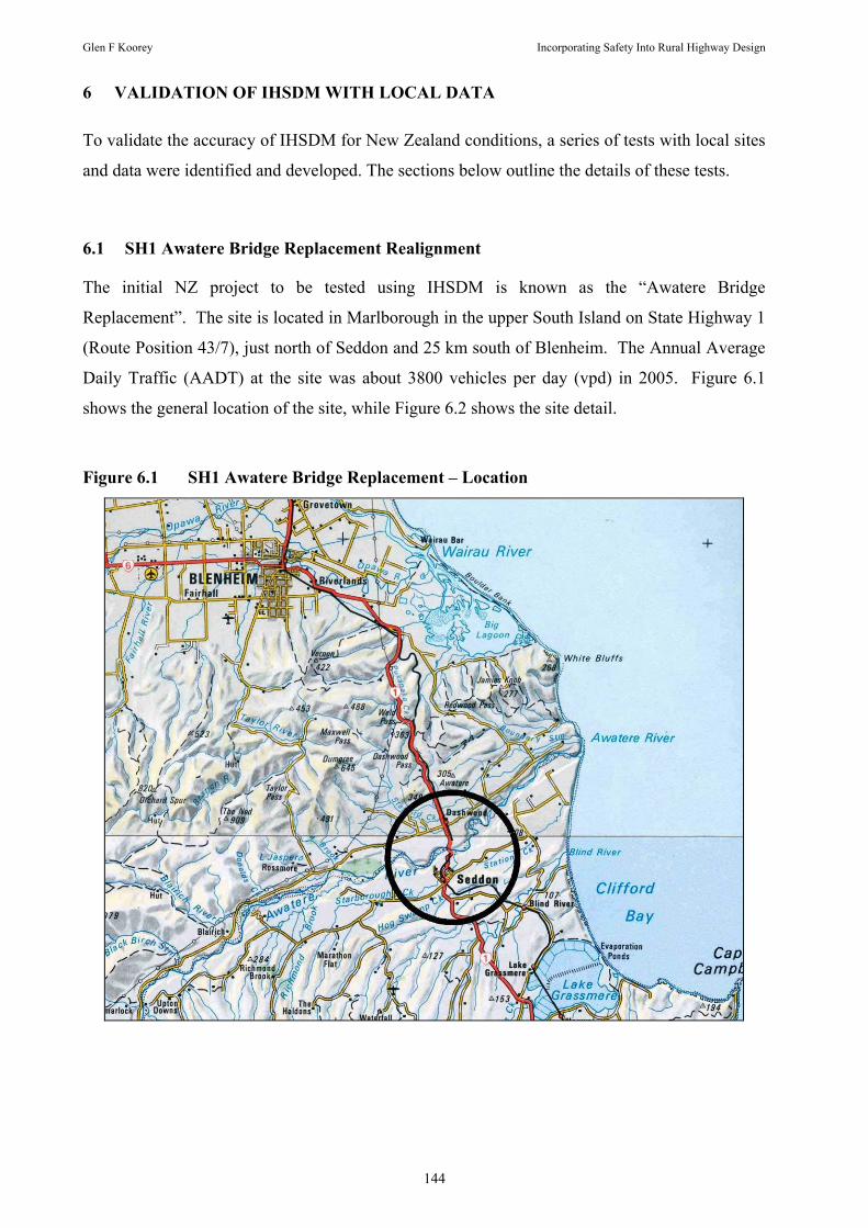
Glen F Koorey Incorporating Safety Into Rural Highway Design
144
6 VALIDATION OF IHSDM WITH LOCAL DATA
To validate the accuracy of IHSDM for New Zealand conditions, a series of tests with local sites
and data were identified and developed. The sections below outline the details of these tests.
6.1 SH1 Awatere Bridge Replacement Realignment
The initial NZ project to be tested using IHSDM is known as the “Awatere Bridge
Replacement”. The site is located in Marlborough in the upper South Island on State Highway 1
(Route Position 43/7), just north of Seddon and 25 km south of Blenheim. The Annual Average
Daily Traffic (AADT) at the site was about 3800 vehicles per day (vpd) in 2005. Figure 6.1
shows the general location of the site, while Figure 6.2 shows the site detail.
Figure 6.1 SH1 Awatere Bridge Replacement – Location

Glen F Koorey Incorporating Safety Into Rural Highway Design
145
Figure 6.2 SH1 Awatere Bridge Replacement – Site Detail
Keyte (2006) used this site for testing the Design Consistency and Policy Review Modules
(having developed a suitable Design Policy file for NZ, as described in Section 5.3). Further
amendment of the highway data has been made here followed by revised DCM/PRM analyses,
as well as a CPM analysis.19
The old alignment featured a road winding down the river terraces to a long single-lane bridge
across the Awatere River. There were considerable delays travelling across the bridge, which
also had notable maintenance costs (it has a rail bridge above the road structure). The new
alignment (constructed in 2006-07) introduces a more direct path down to a new two-lane bridge.
Figure 6.3 shows the old and new horizontal alignments; note that the urban area of Seddon
(60 km/h posted speed limit) starts at approximately station 2710 m on the old alignment and has
generally been ignored in this analysis.
19 It should be noted that Keyte chose this site as he had access to the bridge alignment design data, which had been designed by the consulting company he worked for. Further analysis of the site in this thesis has been undertaken largely because of the convenient access to Keyte’s data (G.Koorey being his research supervisor).

Glen F Koorey Incorporating Safety Into Rural Highway Design
146
Figure 6.3 SH1 Awatere Bridge Replacement – Old/New Alignments
Old Alignment New Alignment
The project was primarily chosen on the basis that the electronic alignment data were easily
obtainable and the old horizontal and vertical alignments were substandard (although it should be
noted that there was not a major crash problem). The design was complete since 2004 to Transit
NZ’s standards so it can be reasonably assumed that it also largely complied with the Austroads
(2003) standards.

Glen F Koorey Incorporating Safety Into Rural Highway Design
147
The IHSDM software follows a simple process in the evaluation of geometric consistency. This
process firstly involves importing and defining alignment data, then choosing a standard to
compare the alignment against, and finally evaluating the results.
The import data used for this project was extracted from the roading design package MX-Roads.
As was described in Section 5.4, the process was relatively simple, utilising the proposed new
alignment elements (designed by the consultant) and the inferred old alignment elements (best-fit
from the field survey points).
6.1.1 Design Consistency Assessment
The plots below (Figure 6.4 - Figure 6.7) illustrate the respective differences between the old and
new alignments, using the Design Consistency and Policy Review Modules. Note that travelling
from left to right on the plots is in the southbound direction. As discussed in Section 5.3, a
modified policy file was created that incorporated Transit NZ and Austroads standards into this
assessment.
The location of the old single-lane bridge can be seen by the reduced design speed section
between stations 1580 - 1860 m, with tight curves at both ends. Note that the new alignment is
approximately 140 m shorter than the old alignment. Whilst the old alignment had a number of
sections with large speed drops or insufficient stopping sight distance (similar calculations can
be determined for passing sight distance), the new alignment largely eliminates these. It should
be noted that IHSDM’s stopping sight distance calculations only consider the design speed of the
section and do not currently allow for gradient to be taken into account.
It can be seen that the speed profile in the new alignment (bottom part of Figure 6.6) is much
faster and far more consistent than for the old alignment (Figure 6.4), as evidenced by the
smaller number of warning “flags” showing (and no yellow or red ones). Similarly, the
calculated stopping sight distances for the new alignment (bottom part of Figure 6.7) are
generally above the “minimum required sight distance” line, unlike those in the old alignment
(Figure 6.5). Additional supporting can also be presented, such as horizontal and vertical
curvature, and it can be seen that the new alignment is particularly less severe in terms of
horizontal curvature. The plots are all customisable in terms of data shown, scales used, colours
and line styles, etc, and can be exported as image files for use in other documents.
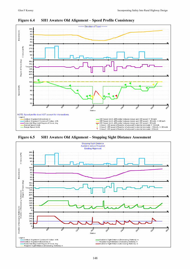
Glen F Koorey Incorporating Safety Into Rural Highway Design
148
Figure 6.4 SH1 Awatere Old Alignment – Speed Profile Consistency
Figure 6.5 SH1 Awatere Old Alignment – Stopping Sight Distance Assessment
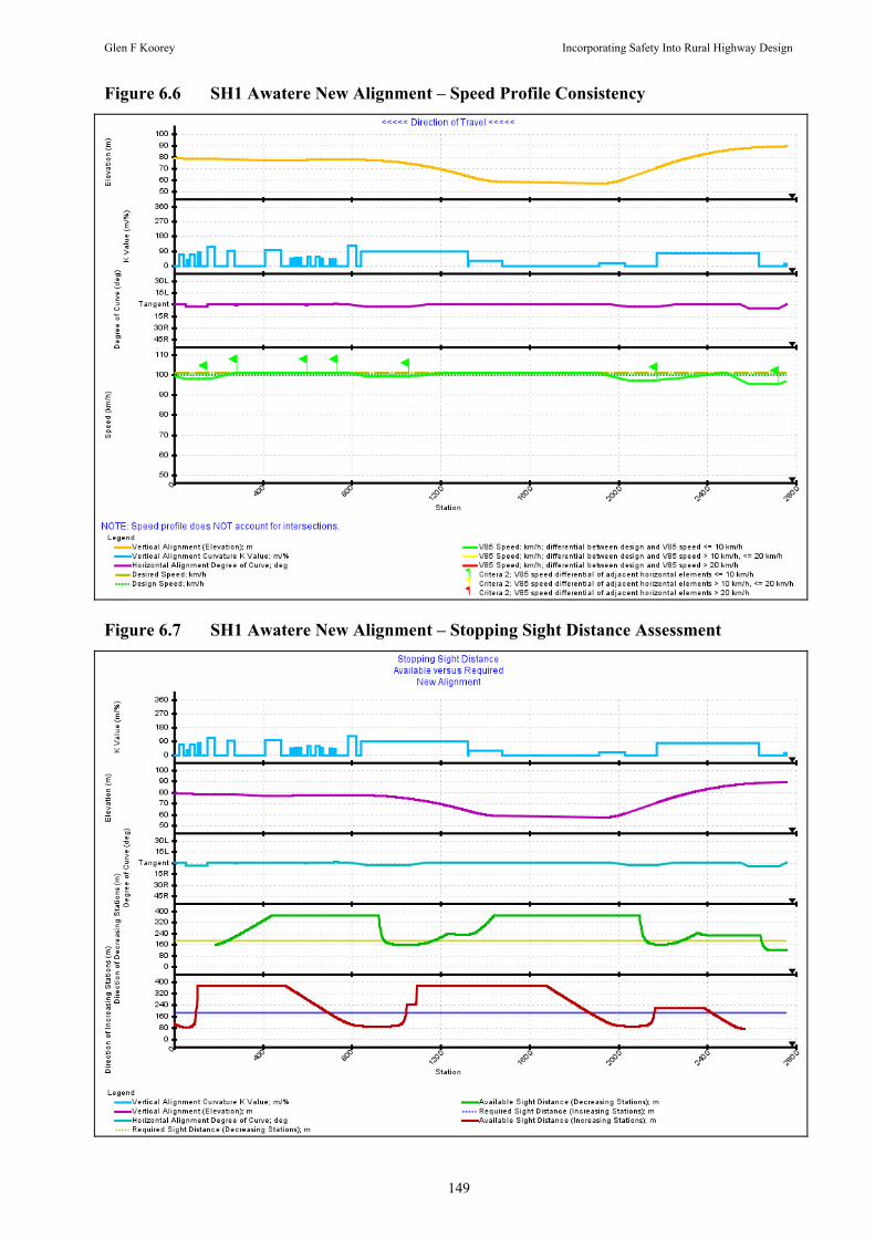
Glen F Koorey Incorporating Safety Into Rural Highway Design
149
Figure 6.6 SH1 Awatere New Alignment – Speed Profile Consistency
Figure 6.7 SH1 Awatere New Alignment – Stopping Sight Distance Assessment

Glen F Koorey Incorporating Safety Into Rural Highway Design
150
It can be seen that the Design Consistency and Policy Review modules present a simple
illustration of any design flaws inherent in the road design being analysed. Even without
recourse to the crash data, locations with notable inconsistencies in operating speeds (thus
presenting a likely safety risk) are clearly identified for further investigation and improvement.
6.1.2 Crash Prediction Assessment
The Awatere Bridge project was initiated predominantly by travel time and maintenance
concerns on the old alignment, rather than safety concerns. Nevertheless, it is worth
investigating how IHSDM predicts the safety performance of the old route. Therefore, an
analysis was undertaken using the CPM to estimate the number of crashes in the five years
immediately preceding construction in 2006. Table 6.1 summarises the analysis, comparing the
observed 2001-05 crash data with IHSDM’s predictions, with and without crash history data.
For simplicity the NZ 2002-06 calibration factors have been used; this period saw only 1.8%
more reported rural SH crashes than 2001-05, a negligible difference.
Table 6.1 Crash Numbers at SH1S Awatere Bridge 2001-05 (43/5.9-8.6)
Source of Crash Numbers Fatal & Injury Non-Injury Total Inj
+ Non-Inj
Crash History (CAS) 1996-2000 0 5 5
Observed (CAS) 2001-05 3 5 8
IHSDM (no crash history) 6.2 8.7 14.9
IHSDM (96-00 crash history) 2.1 6.0 8.1
It can be seen that the CPM alone over-predicts the number of crashes at the site. The addition
of local crash history data from 1996-2000 however greatly improves the estimate. Given the
relatively small crash numbers involved, it would be difficult to expect greater accuracy.
One important aspect of this project that is not currently well incorporated into IHSDM is the old
narrow bridge. Harwood et al (2000) noted that, while the expert panel developing the IHSDM
crash prediction model strongly desired to include a bridge width factor in the algorithm, there
was no existing research that they considered suitable for inclusion. The panel recommended
that a well designed study of the relationship between bridge width and crashes on rural two-lane
highways be undertaken, but no subsequent research on this has been identified. In fact, the NZ
research by Turner (2000) appears to be the most comprehensive study to date.

Glen F Koorey Incorporating Safety Into Rural Highway Design
151
IHSDM’s highway editor allows for the specification of bridge elements in an alignment, with
data on bridge length and width. However, this information is not currently being used in the
CPM. Therefore, the only way to reflect the issues with the bridge section at Awatere was to
enter details about the narrowed traffic lane and shoulder widths along this section and the
roadside hazards created by the bridge side-rails. Even here the specification is imprecise, as
one-lane road sections cannot be specified. In this case however, the major crash problems are
the tight curves on each approach, and these are captured by the old road alignment data.
Reconstruction of the Awatere Bridge highway section was only completed in late 2007; hence
validation of the crash prediction models for the new alignment cannot be undertaken for a few
years. Further testing of IHSDM was therefore considered using either:
• highway sections that were realigned some years ago, where geometry data for both
alignments and sufficient before/after crash data are available; or
• longer highway sections with geometry data available, where the existing crash history can
be compared with IHSDM.
6.2 SH1 Hawkswood-Siberia-Ferniehurst Realignments
To validate the crash prediction abilities of IHSDM, an older realignment site has been selected
for studying. The site actually consists of two adjacent projects constructed at approximately the
same time (1999-2001), the Hawkswood Deviation and the (more northerly) Siberia to
Ferniehurst Realignment (collectively referred to as the “SH1 HSF Realignment” for short).
They are located in North Canterbury in the upper central South Island on State Highway 1S
(Route Position 195/7.5-16.1), approximately 20 km north of Cheviot and 40 km south of
Kaikoura. Immediately south of the site is a relatively straight high-speed alignment, while
immediately north the alignment is fairly similar to the case study section (but more
mountainous further north). The AADT at this site was approximately 2100 vpd during
construction in 2000 and about 2500 vpd more recently in 2005.
Figure 6.8 shows the overall site plan. The new alignment is indicated by the solid black line;
sections of the old alignment that have been removed are indicated by hatched lines. Parts of the
old highway have been retained for local property access, with three new intersections
constructed. As well as providing a more consistent design, the new 7 km alignment reduces the
travel distance by approximately 2 km.

Glen F Koorey Incorporating Safety Into Rural Highway Design
152
Figure 6.8 SH1 Hawkswood - Siberia - Ferniehurst (HSF) Realignment – Site Plan
The old alignment was a particularly winding and sub-standard section of highway, especially in
comparison with the high-speed alignment immediately south of it. Figure 6.9 shows a typical
section of the old alignment near the Hawkswood Stream; note the low-speed curves. As well as
the very tight Hawkswood Stream crossing, the old route also had narrow and poorly aligned
sections at the Chilly Stream bridge and the Main Trunk Line railway overbridge. Throughout
the alignment, there are many curves with radii <100 m and some as low as 20 m.
Figure 6.9 SH1 HSF Realignment – Old Alignment

Glen F Koorey Incorporating Safety Into Rural Highway Design
153
The new alignment takes a more direct route, involving substantial earthworks to achieve this.
Horizontal radii now range between 400 m and 800 m. Figure 6.10 shows the northern portion
of the new alignment, looking north towards the Conway River, with the new embankment
crossing Chilly Stream. The dotted line indicates the line of the old alignment; the truck shown
is near the intersection of the old and new roads. At the southern end of the realignment, a new
overbridge crosses the Main Trunk Line.
Figure 6.10 SH1 HSF Realignment – New Alignment
6.2.1 SH1 HSF Alignment Design Consistency
The road alignment data before and after the HSF Realignment works were obtained and
processed using the database from Section 3. Each section was exported to an IHSDM file,
using the routine described in Section 5.4.2, and then imported into IHSDM for processing.
Additional information was added manually in IHSDM about other features of note, such as
narrow bridges. Figure 6.11 shows the geometric and speed details for the old alignment as
processed by IHSDM’s DCM. Note that travelling from left to right on the plot is in the
southbound direction (the data for the opposite travelling direction is very similar).

Glen F Koorey Incorporating Safety Into Rural Highway Design
154
Figure 6.11 SH1 HSF Old Alignment – Speed Profile Consistency
It can be seen that there are a considerable number of speed changes throughout the section, with
about three estimated as being greater than 20 km/h in difference. IHSDM appears to be fairly
generous in its assessment of the 85th percentile speeds along this route; contrast with the “design
speeds” shown, which are actually based on the “MinLocSpd” values in the geometry database
and relate reasonably well with the numerous curve advisory speeds along the route. However,
the curve radii values exported to IHSDM actually represent the average curvature in each
element, rather than the smallest measured radius present, and will therefore tend to over-
estimate minimum curve radius for elements of varying radii. Countering this somewhat is the
fact that typically many drivers follow a path that cuts across curves, thus increasing the path
radius taken (e.g. Wong and Nicholson 1993 found that observed curve path radii were up to
95% greater than the adjacent centreline radii). Either way, the graph clearly shows the
considerable design inconsistencies (and hence safety issues) in the old alignment.
The new alignment represents a vast improvement, with no 85th percentile speeds estimated at
below 93 km/h by the DCM and all adjacent elements being within 10 km/h of each other (rather
similar to the plot shown in Figure 6.6). Therefore, it would be expected that this new alignment
should provide a notable improvement in safety.

Glen F Koorey Incorporating Safety Into Rural Highway Design
155
As discussed in Section 2.4.1, one notable omission in the IHSDM crash prediction model is the
relative consistency between adjacent elements. Although this is clearly highlighted in the
DCM, as seen above, the relative safety issues may not necessarily be translated fully when
analysed in the CPM (although crash history data may help).
6.2.2 SH1 HSF Realignment Crash History
Table 6.2 summarises the crash history of the site, both before, during, and after construction of
the realignments. The crash statistics are dominated by lost-control cornering and head-on
crashes; full details of the crash data can be found in Appendix A.9. Although, interestingly,
there has been an increase in fatal crashes (possibly as a result of higher average travel speeds on
the new alignment), the number of reported non-injury and injury crashes has fallen dramatically
since the completion of the works. Also, despite creating three new side-road intersections, no
crashes have been reported at these locations.
Table 6.2 Crash Numbers on SH1 HSF Realignment 1994-2006 (RP 7.5 - 16.1)
Time Period Fatal Serious Minor Total Injury Non-Injury Total Inj
+ Non-Inj
1994 – 98 0 7 9 16 (3.2/yr) 17 33 (6.6/yr)
1999 – 2001 1 0 5 6 (2.0/yr) 8 14 (4.7/yr)
2002 – 06 2 0 3 5 (1.0/yr) 7 12 (2.4/yr)
This of course has to be considered against the background of general changes nationwide in
crash numbers during this period. For example, the annual number of reported fatal crashes
nationally fell from an average of 472 per year during 1994-98 to an average of 366 per year
during 2002-06, a reduction of 22%. The picture for injury crashes is less clear, as the numbers
of reported injury crashes have been increasing since 2000 (by about 47% in 6 years). In
comparing the 1994-98 and 2002-06 periods, the number of reported injury crashes in NZ
actually rose by 2%. If only rural crashes are considered, whereas the number of fatal crashes
has fallen by 19% between these periods, the number of injury crashes has increased by 15%; for
rural State Highways the values are -23% and +12% respectively. Anecdotal evidence from
Police and LTNZ officials suggest that this partly reflects a dramatic improvement in crash
reporting rates rather than a notable drop in safety performance. As an alternative point of
comparison, the number of overnight hospitalisations due to motor vehicle crashes fell by 28%
between the same two periods; however they have risen by 5% between 2000 and 2006 (MoT

Glen F Koorey Incorporating Safety Into Rural Highway Design
156
2007). Again, however, this could reflect changes in hospital practice, in terms of keeping
patients overnight “for observation”.
Crash numbers are also related to exposure, so another reason for discrepancies between “before
& after” crash numbers may be differences between traffic growth nationally and at the HSF
Realignment. To minimise this effect, examination of other crashes closer to the realignment
may be more pertinent. As well as comparing the crash record of adjacent road sections likely to
be covered by the same vehicles, potential crash migration as a result of the realignment can also
be identified. Therefore, Table 6.3 summarises the fatal and injury crash data for both the HSF
Realignment site and adjacent sections of rural State Highway, approximately 17 km either side
(from the Hurunui District boundary at Oaro summit to north of Cheviot township).
Table 6.3 Statistical Comparison of SH1 HSF Realignment Crash Reductions
Fatal & Injury Crashes Before Period 1994-1998
After Period 2002-2006
Total Crashes
SH1 HSF Realignment 16 5 21
Rest of SH1 RP185/0 - 217/11 28 49 78
Total Crashes in the District 44 54 98
The above numbers suggest that the HSF Realignment is out of step with the surrounding district
and statistical analysis supports this. The Chi-squared test statistic (1 d.o.f) for the above data
equals 9.030. This implies that the probability of this result happening by chance is only 0.27%.
Therefore, this suggests that the crash reduction observed at the HSF Realignment is statistically
significant at greater than the 99% level.
Whether this reduction may be partly a result of crash migration is less clear. The sections
immediately adjacent to the HSF Realignment show no notable change in crash numbers
between periods; it is the road sections approximately 7km and further away that appear to have
experienced an approximate doubling in crash numbers in the after period. However, this is
complicated by the fact that another realignment at Glen Colwyn, approximately 3km north of
HSF, was completed not long after this project.
Figure 6.12 shows the location of all crashes during the “before” period, split out by direction of
the key vehicle (i.e. the vehicle in each crash movement type usually at fault or most affected by
the environment). It can be seen that there is a slight tendency for crashes at each end to be

Glen F Koorey Incorporating Safety Into Rural Highway Design
157
related to vehicles entering the section, rather than leaving. This is more noticeable at the
southern end (right-hand side of plot), where northbound vehicles entered the old alignment from
a very high-speed alignment immediately south extending for several kilometres, whereas the
alignment immediately to the north is more similar. Some grouping of crashes is also evident
around three major features in the southern half of the section.
Figure 6.12 SH1 HSF Old Alignment – Location of Crashes by Direction 1994-98
7.5 8.0 8.5 9.0 9.5 10.0 10.5 11.0 11.5 12.0 12.5 13.0 13.5 14.0 14.5 15.0 15.5 16.0
Route Position (km)
Southbound (Increasing RP)
Northbound (Decreasing RP)
Railway O'bridge (RP 14.62)
Hawkswood Strm Bridge (RP 13.58)
45km/h Curve (RP 12.32)
6.2.3 LTNZ EEM Crash Predictions
Before assessing the performance of IHSDM on this site, it is pertinent to consider how well the
existing LTNZ crash prediction methods fare, as specified in the Economic Evaluation Manual
(LTNZ 2006). Section 2.5.2 described the main features of the existing EEM methods, in
particular the “Accident Rate Analysis” method. Because the EEM crash prediction models only
estimate the number of injury or fatal crashes, non-injury crashes are ignored for this analysis.
It should be noted that the EEM procedures include calculations to allow for under-reporting
when using reported crash data to estimate existing crash costs; for example, it is assumed that
only approximately half of all severe injury crashes are reported to the Police. However, the
EEM analyses involving crash prediction models do not explicitly consider unreported crash
numbers. The IHSDM CPM also does not calculate and include an estimate of unreported
crashes as part of its analysis; instead it is assumed that the calibration factors will reflect the

Glen F Koorey Incorporating Safety Into Rural Highway Design
158
local crash reporting rate and allow for direct comparison with the reported crash numbers.
Although for economic analysis purposes later, scaling these numbers up to allow for unreported
crashes makes sense, the same under-reporting factor would probably be used with both the
observed and predicted crash numbers. Therefore, it is not considered necessary at the crash
prediction stage to allow for under-reporting.
The crash prediction models in the EEM have been adjusted over the years to reflect changes in
typical crash patterns observed. To adjust the existing (2006) models to earlier analysis periods,
a general factor is provided in the EEM to scale the base estimates to the analysis period. For
example, with an analysis period of 1994-98 (mid-point of 1996), a scaling factor of 1.10 is used
to adjust the predicted crash numbers accordingly. Similarly, AADT estimates from the mid-
point years (1996 and 2004) were used to estimate the overall crash numbers for the “before”
and “after” analysis periods with the appropriate level of traffic.
Two different approaches to using the EEM were investigated:
• A “simplified” method used just the rural mid-block typical crash rate (in this case, 18 injury
crashes per 108 veh-km for rolling terrain) to estimate the number of crashes along the entire
section length. It was expected that this approach would underestimate the number of
crashes, as it does not explicitly consider particularly sub-standard road elements within the
section.
• A “detailed” method also included some analysis of sub-standard curves and bridges using
the EEM prediction models supplied for these. For the remaining length of highway, the
typical mid-block crash rate was applied, as done in the simplified method. Arguably this
method is still conservative, as the prediction model for sub-standard curves only estimates
the number of “type B/C/D” (i.e. head-on / lost-control) crashes; however in this case all
observed injury crashes were in this category anyway. Curves and bridges are also treated as
“point” features in the EEM, so arguably the mid-block crash rate could have still been
applied to the affected element lengths as well.
The latter method is not normally undertaken in practice, as the respective crash prediction
models for curves and bridges are usually only applied to isolated features being treated
individually. However, it was deemed the most pragmatic way to incorporate the available crash
prediction knowledge in the EEM. Appendix A.10 details the spreadsheet calculations used to
calculate the crash estimates. For simplification, the same speed reduction at a curve has been
applied to travel from both directions, although this is not strictly correct.

Glen F Koorey Incorporating Safety Into Rural Highway Design
159
The EEM procedures also allow the use of crash history if necessary, by means of the
“weighted” crash analysis. While such data are available for the old alignment from 1989-93
(i.e. prior to the analysis period), the new alignment does not have any relevant previous crash
history. Therefore, for this analysis the actual observed crash counts for each analysis period
were also used as “crash history data”.
Table 6.4 summarises the various crash estimates calculated for the old alignment during the
“before” period of 1994-98. For the detailed analysis method, 17 curves (with estimated curve
speed reductions of >20 km/h) and two narrow bridges were analysed separately; these
represented the most extreme elements present. The curve speeds were based on the calculated
minimum “LocSpd” values from the road geometry (derived in Section 3.3), which generally
matched signposted curve advisory speeds fairly well, while the approach speeds were based on
the average “SpdEnv” values.
Table 6.4 SH1 HSF Realignment EEM Crash Estimates 1994-98 (“Before” period)
Fatal & Injury Crashes Without Crash History
With 1989-93 Crash History
With 1994-98 Crash History
Observed Crashes - (14 in 89-93) 16 in 94-98
EEM Accident Rate Analysis (simplified) 5.2 8.5 9.3
EEM Accident Rate Analysis (detailed) 9.8 11.1 11.7
As expected, the simplified analysis method under-estimates crash numbers substantially, even
when crash history is included. The detailed analysis provides a better estimate, albeit still ~27%
less than the actual observed crash numbers at best. This illustrates the benefits of a detailed
element-by-element crash analysis, which is what IHSDM is also trying to achieve. Using crash
history data also clearly improves the original estimates; in this case, there is little difference
between the two history periods used.
The low crash values produced above could reflect somewhat the fact that parts of the old
alignment have more in common with mountainous terrain than rolling terrain. Some elements
of the route have gradients above 6% and the tight horizontal curves result in operating speeds
often below 50 km/h. The typical crash rate for mountainous terrain is 26 injury crashes per 108
veh-km, therefore using a crash rate somewhere between 18 — 26 might be more appropriate for
this alignment; this would produce estimates more comparable with the observed crash numbers.

Glen F Koorey Incorporating Safety Into Rural Highway Design
160
Table 6.5 summarises the crash estimates for the new alignment during the “after” period of
2002-06. As might be expected, the new alignment contains no sub-standard bridges or curves,
therefore the simplified analysis method was considered sufficient to predict crash numbers on
this section.
Table 6.5 SH1 HSF Realignment EEM Crash Estimates 2002-06 (“After” period)
Fatal & Injury Crashes Without Crash History
With 2002-06 Crash History
Observed Crashes - 5 in 02-06
EEM Accident Rate Analysis (simplified) 3.8 4.3
This time the simplified method estimate is much more accurate and that is improved even
further with crash history data. This demonstrates the ability of crash prediction models to
estimate well-designed alignments with reasonable precision, as there is typically more
consistency (in terms of safety) between the various elements that make up the alignment.
In summary, the existing LTNZ EEM crash prediction procedures provide a reasonable estimate
of the actual crash numbers, despite considering only a few key variables (terrain, AADT, sub-
standard curves, etc). Although the performance of the EEM crash prediction model was not as
good for the old alignment; for economic evaluation this is usually not an issue. Typically the
safety assessment of the existing alignment would be based on the social costs of the previously
observed crash numbers alone; the crash prediction models would only be required for the new
alignment.
6.2.4 IHSDM Crash Predictions
The previously imported road alignment data was used in IHSDM’s CPM to estimate crash
numbers on the old and new alignments. The crash history data before and after the HSF
Realignment works were also exported from the database to an IHSDM file and then imported
into IHSDM for processing. For the “before” period, a 1996 count year was used for traffic
volumes (i.e. the mid-point of the period), while 2004 was used for the “after” period.
The Level 1 calibration factors derived for all NZ State Highway crashes over 1996-2000 (see
Section 5.2.1) were used for the “before” analysis (scaling factor of 0.884). Because the
“before” analysis period was in fact 1994-98, an adjustment to this factor was used to reflect the

Glen F Koorey Incorporating Safety Into Rural Highway Design
161
relative difference in crash numbers between the two periods. The earlier period had 9.3% more
rural State Highway crashes throughout NZ as a whole, therefore the adjusted calibration factor
was taken to be 0.966 (= 0.884 × 1.093).
The IHSDM CPM analysis was undertaken both with and without the local crash history being
incorporated (using Empirical Bayes). In normal practice, historical crash data is used to predict
the likely crash numbers of a future time period. IHSDM checks for this by ensuring that the
crash history analysis period and the analysis period for crash prediction do not overlap.
However, this presents a slight problem if trying to check the accuracy of the prediction model
during the “before” period (in this case 1994-98) with data from the same period. At least three
possible options present themselves:
• Obtain historical crash data from prior to the “before” period (e.g. 1989-93) and use this to
estimate the number of crashes. It should be noted that as NZ crash data goes further back in
time there is less emphasis on collecting non-injury crash data and this appears to be evident
in the data from this period.
• Split the “before period” into two parts (e.g. 3 years and 2 years) and use the crash history
from the first part (1994-96) to predict the crash numbers in the second part (1997-98). For
comparison with the other methods, the predicted numbers could be scaled up to a five-year
period, although any change in traffic volumes over the period needs to be allowed for.
• Predict the number of crashes in the five years immediately following the “before” period
(i.e. 1999-2003), using the crash history from 1994-98. However, the numbers will over-
estimate those expected during the “before” period unless a 0% growth in traffic volumes is
assumed.
For the “before” analysis, all three options have been tested. IHSDM produces a detailed
summary report of each analysis; a sample of one of them is given in Appendix A.11. Table 6.6
summarises the resulting crash numbers; the estimated values are taken from “Table 4” of
IHSDM’s outputs. Note that both injury and non-injury crash numbers have been presented; for
the crash prediction model without crash history the relative proportion of each remains fixed by
the calibration factors used (in this case 59.1% are non-injury).

Glen F Koorey Incorporating Safety Into Rural Highway Design
162
Table 6.6 Crash Numbers on SH1 HSF Realignment 1994-98 (“Before” period)
Source of Crash Numbers Fatal & Injury Non-Injury Total Inj
+ Non-Inj
Crash History (CAS) 1989-93 14 3 17
Crash History (CAS) 1994-96 10 (3yrs) 9 (3yrs) 19 (3yrs)
Observed (CAS) 1994-98 16 17 33
IHSDM (no crash history) 9.4 13.6 23.0
IHSDM (89-93 crash history) 12.5 9.8 22.3
IHSDM (94-96 crash history) 13.2 16.6 29.8
IHSDM (94-98 crash history) 12.7 16.3 29.0
Evidently the base crash prediction model is relatively conservative when it comes to sub-
standard alignments like this; without crash history data the model underestimates the actual
number of crashes by about 30%. This may also reflect why the site was chosen for realignment,
if it had experienced a higher-than-expected number of crashes. Alternatively, the under-
estimation could be the result of not accounting for the relative speed inconsistencies between
adjacent elements, as discussed in Section 6.2.1. However, as might be anticipated, the addition
of crash history data pushes the prediction estimate much closer to the observed total number
(approximately 10% under now). In this case, it appears to matter little which set of crash
history data is used, particularly for the fatal/injury crash numbers.
It is of interest to see whether IHSDM is basing its assessment on the same sub-standard road
elements that are actually causing the crashes. Figure 6.13 compares the correlation between
observed and predicted crash rates (crashes/km per year) along the old HSF alignment for each
geometric element. Major bridges and curves of interest along the route have been highlighted,
and it can be seen that many of the observed crashes during the “before” period occurred in the
vicinity of these features (although not always matched to the same element).

Glen F Koorey Incorporating Safety Into Rural Highway Design
163
Figure 6.13 Crash Rates along SH1 HSF Realignment 1994-98 (“Before” period)
55
65 65 65
45
35
45
55
65
0
1
2
3
4
5
6
7
7.5 8.0 8.5 9.0 9.5 10.0 10.5 11.0 11.5 12.0 12.5 13.0 13.5 14.0 14.5 15.0 15.5 16.0Route Position (km)
Cra
sh R
ate
(cra
shes
/km
per
yr)
Observed Crashes '94-'98IHSDM (No Crash History)IHSDM ('89-'93 Crash History)IHSDM ('94-'98 Crash History)Notable Curves (advisory speed)
Chilly Strm BridgeRP 8.94
Hawkswood Strm BridgeRP 13.58
Railway O'bridgeRP 14.62
The IHSDM predicted crash rates without crash history data show a fairly consistent rate
throughout the alignment, with slight peaks at the major curves. However, they do not correlate
particularly well with the observed crash history at some of the more extreme elements (e.g.
railway overbridge). The fact that IHSDM’s CPM does not currently take directly into account
bridge features seems to lead to underestimation of the safety issues at these locations. Using the
1989-93 crash history data improves on the predictions in some locations where there has been a
consistent crash trend while, as expected, using the 1994-98 crash history data adjust the crash
rate trends much closer to the observed crash rates during this period.
A similar crash prediction analysis was undertaken for the “after” period, using the calibration
factors derived in Section 5.2.1 for this period (scaling factor of 0.851). As with the “before”
analysis above, crashes for the five-year period immediately following the “after” period (i.e.
2007-11) were predicted when including crash history data from 2002-06 (assuming 0% traffic
growth, as discussed earlier). The earlier crash history from the “before” period would not be
suitable in this case because the alignment was substantially changed. Table 6.7 summarises the
resulting crash numbers.
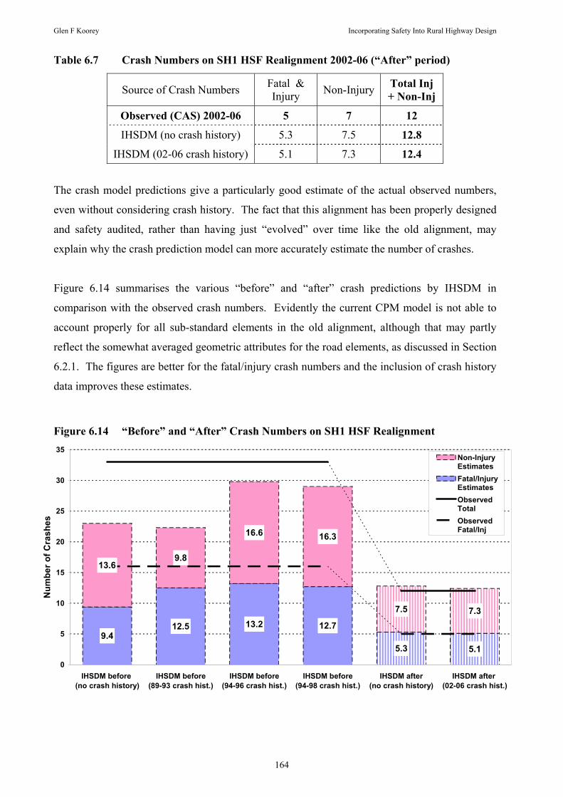
Glen F Koorey Incorporating Safety Into Rural Highway Design
164
Table 6.7 Crash Numbers on SH1 HSF Realignment 2002-06 (“After” period)
Source of Crash Numbers Fatal & Injury Non-Injury Total Inj
+ Non-Inj
Observed (CAS) 2002-06 5 7 12
IHSDM (no crash history) 5.3 7.5 12.8
IHSDM (02-06 crash history) 5.1 7.3 12.4
The crash model predictions give a particularly good estimate of the actual observed numbers,
even without considering crash history. The fact that this alignment has been properly designed
and safety audited, rather than having just “evolved” over time like the old alignment, may
explain why the crash prediction model can more accurately estimate the number of crashes.
Figure 6.14 summarises the various “before” and “after” crash predictions by IHSDM in
comparison with the observed crash numbers. Evidently the current CPM model is not able to
account properly for all sub-standard elements in the old alignment, although that may partly
reflect the somewhat averaged geometric attributes for the road elements, as discussed in Section
6.2.1. The figures are better for the fatal/injury crash numbers and the inclusion of crash history
data improves these estimates.
Figure 6.14 “Before” and “After” Crash Numbers on SH1 HSF Realignment
9.412.5 13.2 12.7
5.3 5.1
13.69.8
16.6 16.3
7.5 7.3
0
5
10
15
20
25
30
35
IHSDM before (no crash history)
IHSDM before (89-93 crash hist.)
IHSDM before (94-96 crash hist.)
IHSDM before (94-98 crash hist.)
IHSDM after (no crash history)
IHSDM after (02-06 crash hist.)
Num
ber o
f Cra
shes
Non-InjuryEstimatesFatal/InjuryEstimatesObservedTotalObservedFatal/Inj

Glen F Koorey Incorporating Safety Into Rural Highway Design
165
6.3 Validation of NZ Highway Crash Numbers
Further tests were undertaken to check predicted crash numbers for three longer road sections of
varying location and terrain. The CPM was tested using a variety of different calibration factors,
based on the whole SH network, the network in the same region as the road section, and
highways with the same terrain. The effect of crash history data was also examined.
In selecting possible sections for testing, there was a desire to identify sections with reasonable
traffic volumes and lengths, so as to get reasonable crash numbers, and with a variety of
locations and terrains. One minor issue with selecting higher volume sections is that there could
be a bias if much of the country has lower traffic volumes (and often by implication, a lower
design standard). However, the previous analysis in Section 5.2.5 (see Table 5.6) suggests that
there is little difference for road sections between 1000 - 10,000 veh/day, so staying within those
bounds should minimise the effects of volume.
Three road sections were identified for further investigation; Figure 6.15 shows the locations of
the sections to be tested:
• SH1S in mid-Canterbury between Christchurch and Ashburton (RS365-430). This is ~65km
of very flat terrain with typical traffic volumes of 7000-9000 veh/day in 2001.
• SH1N north of Auckland between Waipu and Wellsford (RS203-248). This is ~42km of
rolling terrain with typical traffic volumes of 6000-7000 veh/day in 2001.
• SH2 northeast of Wellington over the Rimutaka Saddle (RS921-946). This is ~24km of
mountainous terrain with typical traffic volumes of 4000-5000 veh/day in 2001.

Glen F Koorey Incorporating Safety Into Rural Highway Design
166
Figure 6.15 Location of Highway Test Sections
Some thought needed to be given to an appropriate analysis period. The road geometry data
available was from 2001-02 and it is known that some major realignment works were undertaken
on parts of these test sections since then (e.g. SH2 Kaitoke realignment). To be reasonably
comfortable about the accuracy of the observed or predicted crash numbers, at least three years
was considered necessary for analysis periods. Therefore, a 2000-02 crash prediction period was
used, with the optional use of crash history data from 1997-99.
The required road and crash data were extracted from the database developed in Section 3 and
imported into IHSDM. National, regional and terrain-based IHSDM calibration factors were
then determined for the 2000-02 period. Table 6.8 summarises the main factors for each data set.
SH1N Waipu - Wellsford
SH1S Christchurch -
Ashburton
SH2 Rimutaka Saddle

Glen F Koorey Incorporating Safety Into Rural Highway Design
167
Table 6.8 IHSDM Calibration Factors for 2000-02 Crashes
Data Set IHSDM Scaling Factor % Fatal/Injury % Non-injury
All State Highways in NZ 0.856 40.0% 60.0%
North of Auckland 0.865 37.8% 62.2%
Canterbury region 0.723 41.7% 58.3%
Wellington region 0.838 26.6% 73.4%
All Flat Terrain 0.783 40.5% 59.5%
All Rolling Terrain 0.892 39.7% 60.3%
All Mountainous Terrain 0.946 39.4% 60.6%
As with the earlier analysis on the 1996-2000 data (Section 5.2.5), there are some distinct
variations between the data subsets in terms of the scaling factors. There is a general trend
towards more crashes as the terrain becomes more hilly, as might be expected, although the
average severity decreases slightly. The crash severity proportions are all reasonably similar
with the notable exception of the Wellington region, which has a much higher proportion of non-
injury crashes for some unknown reason.
It is important to recognise that, while the available road data allow for quite precise
specification of many details of the road sections studied (e.g. traffic volumes, cross-section
widths, horizontal alignment), other required inputs have simply been assumed or ignored for the
entire section, e.g. roadside hazards, driveway density, bridge locations (Table 5.9 summarised
the level of detail that was provided for each type of data). Therefore, the following crash
predictions may be missing some crucial information that explains certain crash locations, e.g.
the presence of a sub-standard bridge or busy driveway. For future investigations of a similar
nature, it would be desirable to have such additional data readily available.
While the use of crash history data will help to adjust notable site differences, it would still be
expecting a lot for the crash predictions to be extremely precise. Other IHSDM studies (e.g.
Donnell et al 2007, Saito & Chuo 2008) have regularly reported differences between observed
and predicted crash numbers of more than 20%, if not 50%. However, the findings can be used
to assess the relative differences between the different calibration factors and the use of crash
history data. In practice, if analysing a particular site with more detailed information available
(particularly of key hazards), it would be reasonable to expect IHSDM to produce a better
estimate.

Glen F Koorey Incorporating Safety Into Rural Highway Design
168
6.3.1 Crash Prediction Results
Table 6.9 summarises the observed and predicted crash numbers for the SH1S Christchurch-
Ashburton section. When IHSDM was first used to calculate the estimates using crash history
with Empirical Bayes, the resulting numbers were more than double the true figures (i.e. over
300 total crashes estimated) and heading away from the crash history data. Inspection of
IHSDM’s generated calculation files revealed that the CPM was incorrectly basing its estimate
on all of the recorded crash data, from 1996-2006, resulting in a much higher estimate. To get
around this “bug” (subsequently reported to the developers), all crash data except for the 1997-
99 period was deleted from IHSDM and the crash estimates re-calculated.
Table 6.9 2000-02 Crash Numbers on SH1S Christchurch-Ashburton (RS365 - 430)
Source of Crash Numbers Fatal & Injury Non-Injury Total Inj
+ Non-Inj %
Difference
Crash History (CAS) 1997-99 29 40 69
Observed (CAS) 2000-02 38 48 86 -
IHSDM (no crash history, NZ calibration factor) 86.2 129.5 215.7 +151%
IHSDM (no crash history, Canterbury calibration factor) 75.9 106.2 182.1 +112%
IHSDM (no crash history, Flat terrain calibration factor) 79.9 117.4 197.3 +129%
IHSDM (97-99 crash history, NZ calibration factor) 63.3 92.4 155.7 +81%
IHSDM (97-99 crash history, Canterbury calibration factor) 59.5 84.5 144.0 +67%
IHSDM (97-99 crash history, Flat terrain calibration factor) 60.9 88.6 149.5 +74%
While the region and terrain specific factors improve on using the NZ overall calibration factor,
it can be seen that IHSDM does not predict the number of crashes in this case very well using the
crash model alone, with estimated crash numbers more than double what was observed during
2000-02. Incorporating crash history data considerably improves these figures, but even the best
estimate (Canterbury region with crash history) is still 67% too high. The errors for just the
fatal/injury crashes are slightly better, being 57% too high at best.
One wonders whether the exceptionally good geometric conditions present in this road section
(i.e. very long flat straights) have proven to be too good for IHSDM’s calibration factors. The

Glen F Koorey Incorporating Safety Into Rural Highway Design
169
NZ, Canterbury and even Flat terrain factors would all include sections of road with less-than-
optimal alignment and roadside features, with inevitably higher crash rates because of this. This
may explain the over-estimation of crash numbers along the Christchurch-Ashburton section. It
could also suggest that IHSDM does not sufficiently acknowledge the safety benefits of
consistency from one road element to the next, as was discussed in Section 2.4.1.
Table 6.10 summarises the observed and predicted crash numbers for the SH1N Waipu-
Wellsford section. This time the crash prediction model provides a much better estimate, being
typically only 25-30% too high (better for just the fatal/injury crashes). The crash history is less
useful, as the previous three years had a much higher number of non-injury crashes recorded;
however the fatal/injury crash estimates remain relatively unaffected, being only 13% over at
best.
Table 6.10 2000-02 Crash Numbers on SH1N Waipu-Wellsford (RS203 - 248)
Source of Crash Numbers Fatal & Injury Non-Injury Total Inj
+ Non-Inj %
Difference
Crash History (CAS) 1997-99 58 123 181
Observed (CAS) 2000-02 53 72 125 -
IHSDM (no crash history, NZ calibration factor) 62.3 93.5 155.8 +25%
IHSDM (no crash history, Nthld/Akld calibration factor) 59.4 97.9 157.3 +26%
IHSDM (no crash history, Rolling terrain calibration factor) 64.5 97.8 162.3 +30%
IHSDM (97-99 crash history, NZ calibration factor) 61.5 115.9 177.4 +42%
IHSDM (97-99 crash history, Nthld/Akld calibration factor) 60.1 118.0 178.1 +42%
IHSDM (97-99 crash history, Rolling terrain calibration factor) 62.5 117.9 180.4 +44%
Table 6.11 summarises the observed and predicted crash numbers for the SH2 Rimutaka Saddle
section. This time the overall crash model estimates are slightly less than the actual observed
numbers (14-24% under), although this is largely due to the much higher number of non-injury
crashes observed. The crash history data improves these figures further, with the fatal/injury
figures in particular being quite accurate (only 7% over at best).

Glen F Koorey Incorporating Safety Into Rural Highway Design
170
Table 6.11 2000-02 Crash Numbers on SH2 Rimutaka Saddle (RS921 - 946)
Source of Crash Numbers Fatal & Injury Non-Injury Total Inj
+ Non-Inj %
Difference
Crash History (CAS) 1997-99 42 107 149
Observed (CAS) 2000-02 38 107 145 -
IHSDM (no crash history, NZ calibration factor) 45.3 68.0 113.3 -22%
IHSDM (no crash history, Wellington calibration factor) 29.5 81.4 110.9 -24%
IHSDM (no crash history, Mountain terrain calibrat’n factor) 49.4 75.8 125.2 -14%
IHSDM (97-99 crash history, NZ calibration factor) 40.6 84.9 125.5 -13%
IHSDM (97-99 crash history, Wellington calibration factor) 33.4 91.0 124.4 -14%
IHSDM (97-99 crash history, Mountain terrain calibrat’n factor) 42.2 88.3 130.5 -10%
6.3.2 Assessment of Crash Prediction Findings
The following figures (Figure 6.16 to Figure 6.18) summarise the above crash estimates using
the various calibration factors, in comparison with the observed crash numbers. The estimates
with and without crash history data are grouped by calibration factor. Fatal/injury and non-
injury crash numbers are separated out and the estimates using crash history data are shown with
diagonal hatching.

Glen F Koorey Incorporating Safety Into Rural Highway Design
171
Figure 6.16 2000-02 Crash Numbers on SH1S Christchurch-Ashburton (RS365 - 430)
86.263.3
75.959.5
79.960.9
129.5
92.4
106.2
84.5
117.4
88.6
0
50
100
150
200
250
NZ calibration, no crash history
NZ calibration, with crash history
Canty calibration, no crash history
Canty calibration, with crash history
Flat calibration, no crash history
Flat calibration, with crash history
Num
ber o
f Cra
shes
Non-InjuryEstimatesFatal/InjuryEstimatesObservedTotal (86)ObservedFatal/Inj (38)
Figure 6.17 2000-02 Crash Numbers on SH1N Waipu-Wellsford (RS203 - 248)
62.3 61.5 59.4 60.1 64.5 62.5
93.5115.9
97.9118.0
97.8117.9
0
50
100
150
200
250
NZ calibration, no crash history
NZ calibration, with crash history
NthAkl calibration,no crash history
NthAkl calibration,with crash history
Rolling calibrat'n,no crash history
Rolling calibrat'n,with crash history
Num
ber o
f Cra
shes
Non-InjuryEstimatesFatal/InjuryEstimatesObservedTotal (125)ObservedFatal/Inj (53)

Glen F Koorey Incorporating Safety Into Rural Highway Design
172
Figure 6.18 2000-02 Crash Numbers on SH2 Rimutaka Saddle (RS921 - 946)
45.3 40.629.5 33.4
49.4 42.2
68.0 84.981.4
91.075.8 88.3
0
50
100
150
200
250
NZ calibration, no crash history
NZ calibration, with crash history
Wgtn calibration,no crash history
Wgtn calibration,with crash history
Mnt'n calibrat'n,no crash history
Mnt'n calibrat'n,with crash history
Num
ber o
f Cra
shes
Non-InjuryEstimatesFatal/InjuryEstimatesObservedTotal (145)ObservedFatal/Inj (38)
Reviewing the above findings highlights a few key points:
• As suspected, it is difficult for IHSDM’s CPM to achieve an exceptionally good match,
particularly when the input is not sufficiently detailed. However, this somewhat reflects its
main purpose, which is to assess the relative merits of proposed design alignments, rather
than assess existing alignments (which typically have more sub-standard design elements).
• IHSDM’s CPM performed much better when predicting crash numbers on sections with
consistent geometric characteristics, e.g. new alignments that have been properly designed.
• Using crash history generally improved the IHSDM estimates (or did not make them
noticeably worse); this was particularly true for fatal/injury crash numbers, which seemed to
be more stable over time.
• No clear advantage was seen by using region or terrain specific calibration factors instead of
factors for NZ overall. It would appear that the success of these factors depends somewhat
on how representative the section under investigation is of the particular data set used for
calibration.
• The crash model estimates for fatal/injury crashes generally were slightly more accurate than
those for non-injury crashes; this probably reflects the vagaries in reporting practice still
evident in NZ for the latter.

Glen F Koorey Incorporating Safety Into Rural Highway Design
173
7 DISCUSSION
Having now assessed the use of IHSDM under New Zealand conditions, it is pertinent to
consider its applicability for road safety modelling here in light of the earlier discussion in
Section 2.
7.1 IHSDM Case Study Findings
The initial investigations in Section 6 have shown that IHSDM is a promising tool for safety and
operational assessment of highway alignments in NZ. While some localised calibration is useful
to adjust the crash number estimates to NZ conditions, it is not clear that more site-specific
calibration (e.g. by region or terrain) will improve on one nationwide set of calibration
parameters.
However, it is clear that crash history data is generally needed to obtain a reasonable level of
precision in the CPM, particularly for sections with inconsistent or sub-standard design elements.
Indeed, using crash history data appears to provide a better level of “local calibration” than
attempting to derive specialised calibration parameters, and requires far less effort.
Given the general usefulness of using crash history data to improve the CPM estimates, one
could question whether determining a NZ-specific calibration factor is also necessary
(particularly given the amount of effort required to do so). However in most cases, having both
crash history data and NZ-specific calibration will provide a considerable improvement over the
crash history data alone. Figure 7.1 illustrates this diagrammatically.
For a particular section of road, IHSDM can produce a crash estimate, either without any
localised calibration or with a NZ-specific calibration factor (horizontal lines in middle of figure;
in this example the NZ-calibrated estimate is lower, as was found for most of the datasets in this
study). If the actual observed number of crashes at this site is higher or lower than these
estimates (perhaps due to factors unaccounted for in IHSDM), then allowing for crash history
data (using Empirical Bayes) will generally improve these estimates. The arrows shown indicate
how such crash data might improve the crash estimates, producing estimate values closer to the
observed values. As can be seen, whether using a NZ calibration factor produces a more
accurate result than without such a factor will depend on whether the observed crash data is
higher or lower than the base estimates. However, in this example, it is more likely that the
observed data will be below the uncalibrated estimate than above it (as the NZ calibration is

Glen F Koorey Incorporating Safety Into Rural Highway Design
174
based on this data); therefore it is more likely that the NZ-calibrated estimates will be more
accurate.
Figure 7.1 Effect of Calibration and Crash History Data on IHSDM Crash Estimates
The example in Figure 7.1 suggests a hierarchy of increasing accuracy when using IHSDM to
estimate crash numbers:
1. Uncalibrated model with no crash history data
2. Locally calibrated model with no crash history data
3. Uncalibrated model with crash history data
4. Locally calibrated model with crash history data
The other factor to consider with regards to localised calibration is that, for new sites being
analysed, there is no crash history data available. In these cases, a properly calibrated IHSDM
model will provide the best estimate of expected crash numbers, and the consistent nature
expected of a new alignment should provide an accurate estimate from IHSDM.
It may be that reported fatal/injury data provide a more consistent set to work with and to
estimate crash numbers for; the vagaries of non-injury crash reporting rates can have
considerable effects on the prediction process. For economic analysis purposes, this may be
sufficient anyway, given the considerably higher social costs associated with fatal/injury crashes
compared with non-injury crashes.
IHSDM Crash Estimate (No Calibration)
IHSDM Crash Estimate (NZ Calibration)
Observed Crash Number (High)
Observed Crash Number (Low)
IHSDM Crash Estimate (No Calibration,
with Crash History)
IHSDM Crash Estimate (NZ Calibration,
with Crash History)
IHSDM Crash Estimate (No Calibration,
with Crash History)
IHSDM Crash Estimate (NZ Calibration,
with Crash History)

Glen F Koorey Incorporating Safety Into Rural Highway Design
175
The level of detail applied to the specification of the road alignment is important for an accurate
crash estimate in IHSDM, particularly for existing alignments with sub-standard elements.
Correct specification of the extreme attributes of these elements (e.g. minimum radius, maximum
roadside hazard) appears to be crucial to getting reasonably precise crash estimates at these
locations. Fortunately, New Zealand is generally well served on the State Highway network
with the necessary data to provide this detail. Even then however, the lack of consideration for
bridges and inconsistent adjacent elements are notable omissions from IHSDM’s crash
prediction model, and they can only be partly rectified by adjusting other attributes (such as
lane/shoulder width). While this may not be much of an issue when assessing properly designed
alignments, it limits the ability of IHSDM’s CPM to be used to assess some existing routes with
sub-standard elements (although the DCM highlights these elements well).
Arguably, IHSDM’s CPM was not designed for use with sub-standard existing alignments. A
likely expected approach is to use the Design Consistency and Policy Review modules first to
assess existing routes or initial design proposals. Only when a final design is developed would
the CPM come into use. However, this overlooks the potential for the CPM to be a valuable
network and alignment screening tool in its own right, assuming that its prediction model allows
for a wider range of sub-standard design elements.
7.2 Applicability of IHSDM for Road Safety Modelling in New Zealand
With regards to the earlier discussion in Section 2.6.1, IHSDM appears to be able to fulfil road
safety modelling needs in NZ at a number of different levels:
• At the national/regional/RCA strategic level, entire lengths of highway can be imported
into IHSDM (as done in Section 6.3) to identify sections of hazardous or sub-standard road.
This requires development and maintenance of a database similar to that created in Section 3.
For this application, the Design Consistency Module may be of more use than the CPM.
• At the project scoping level, various simplified design options could be developed and
assessed against the existing alignment. Either a design package could be used to create
alignments for export into IHSDM (as done in Section 6.1) or simple alignments could be
created directly in IHSDM. The DCM could check for general consistency and the CPM
could then estimate the relative safety performance of each option.
• At the project design level, the precise benefits of the chosen design can be determined in
IHSDM, using detailed alignment and cross-section information from a road design package.

Glen F Koorey Incorporating Safety Into Rural Highway Design
176
There may also be an iterative process, whereby feedback from IHSDM’s modules (e.g.
design consistency, policy review) can be used to improve the design. The final expected
crash numbers for economic analysis can be determined by the CPM (as done in
Section 6.2); travel time benefits could also be assessed using the Traffic Analysis Module.
• At the road safety audit level, IHSDM’s various modules (e.g. policy and intersection
review) could be used to identify and prioritise existing deficiencies. Saito & Chuo (2008)
suggested that IHSDM could be a useful tool for engineering decision-making during safety
audits of two-lane rural highways. However, the outputs from IHSDM still demand
knowledge and experience in highway design, and the data input required for meaningful
audits may not be cost-effective.
To assist with some of these tasks, greater integration between IHSDM and other associated
design and analysis packages should continue to be fostered. This could be in the form of
programmatic add-ons to facilitate data transfer, or through greater use of common file formats
such as LandXML.
As discussed in Section 5.2.4, the rigid nature of IHSDM’s underlying crash prediction model
structure is potentially an obstacle to more widespread use of this tool. Although the case studies
produced reasonable results under NZ conditions (particularly with the assistance of crash
history data), the ability to put alternative crash models (e.g. different variables or exponents)
into IHSDM would be very useful. This of course needs to be undertaken with some care; the
development of a statistically robust crash prediction model is not an easy task at the best of
times and therefore any such substitution should be guided by road safety modelling specialists.
The first key question to be addressed in each case is whether any proposed model does actually
improve (from a statistical perspective) on the existing one. Thus, increasing attention is
focusing on the relative “transferability” of road safety models across jurisdictions (e.g. Persaud
et al 2008).
Of course, to successfully apply alternative models for NZ requires the continuing development
and refinement of appropriate models for use here. While NZ is fortunate to already have a
comprehensive set of prediction models to date (e.g. Turner 2001), it is difficult for models to
retain their currency for too long. It is here that the database (and related procedures) developed
in this study could be of immense value to identify improved and updated crash risk relationships
in the future.

Glen F Koorey Incorporating Safety Into Rural Highway Design
177
8 CONCLUSION
8.1 Review of Research Objectives
It is pertinent here to review the stated objectives of this research, as given in Section 1.1:
1. To explore ways to assess the safety performance of (predominantly two-lane) rural
highways.
2. To identify driver/road/environmental factors affecting crashes on rural roads in New
Zealand, particularly horizontal curves.
3. To identify the tasks required to adapt IHSDM for use in New Zealand and to undertake
the necessary adaptations.
4. To assess the effectiveness of IHSDM in New Zealand for predicting the relative safety of
a rural road alignment, by validating it against local highway and crash data.
The discussions below assess the success in meeting these original objectives and any resulting
conclusions (particularly in Objective 4).
1. Assessing the Safety Performance of Rural Highways
A comprehensive review has identified a range of methods for assessing safety performance,
particularly in mid-block situations. Although the tools to undertake this often vary with the task
being done (e.g. strategic network review, detailed design analysis, safety audit), the underlying
safety models used can be essentially the same. A promising approach appears to be models
(usually of Poisson or negative binomial form) involving a base road type whose crash rate is
then adjusted by modifying factors to account for local site differences. Inclusion of actual
historical crash data is also recommended to help adjust crash predictions for local effects that
are difficult to account for otherwise. To help with the subsequent objectives, a comprehensive
database was developed, containing electronic road, traffic, crash and environmental data for all
NZ State Highways, divided into variable-length road elements.
2. Driver/Road/Environmental Factors affecting Crashes on NZ Rural Roads
A detailed crash analysis highlighted the significance of curve-related crashes on rural roads in
NZ, particularly two-lane roads where approximately half of all rural crashes were lost-control or
head-on crashes on curved roads. Therefore, the development of any road safety model for NZ
rural roads clearly must focus on the ability to predict how road curvature affects crashes.

Glen F Koorey Incorporating Safety Into Rural Highway Design
178
However, there remains a wider range of crash types that also contribute considerably to the
overall crash pattern (e.g. rear-end/obstruction, overtaking) and must also ultimately be
considered within safety modelling. This will be particularly prevalent as more rural
realignment work and four-laning becomes common, and vehicle interaction starts to affect crash
numbers more. Analysis of crash contributory factors highlights the effects of speeding and
inattention; however, there is relatively little guidance on how the road environment may have
affected rural crashes. Even available measures such as reported curvature highlight some
anomalies in how these descriptors are used and how crashes are distributed across them. It is
for these reasons that more objective crash analysis using measured road geometry data is
sensible, although at present such analysis is generally limited to only State Highways because of
the data being unavailable for local roads.
3. Identification of Tasks Required to Adapt IHSDM to New Zealand
A number of tasks were identified to make IHSDM suitable for use in NZ. The crash prediction
model was calibrated to match NZ crash patterns, both nationally and for a series of subsets
defined by traffic volume, number of lanes, region and terrain. Although there were some
differences in calibration parameters between the various subsets, generally they did not seem to
be statistically significantly different to warrant their use instead of overall national parameters.
A NZ Design Policy file was developed based on local agency standards and guidelines.
Importing routines were developed to export highway geometry and crash data from the State
Highway database into formats suitable for use in IHSDM. Further tasks were also considered to
modify IHSDM’s vehicle fleet and validate its speed prediction routines for NZ conditions.
4. Validation of IHSDM to Local Data
A series of NZ sites and projects were tested in IHSDM to assess its crash prediction abilities
and other related features such as design consistency. These initial investigations have shown
that IHSDM is a promising tool for safety and operational assessment of highway alignments
(both existing and proposed) in NZ. Where possible, incorporating crash history data generally
improves the precision in crash number estimates, and appears to provide a better level of “local
calibration” than by using sub-national calibration parameters. Reported fatal/injury crash data
generally provide more robust and precise measures than non-injury crashes. Correct
specification of the extreme attributes of sub-standard elements (e.g. minimum radius, maximum
roadside hazard) appears to be crucial to getting suitably precise crash estimates on existing
alignments. However, IHSDM’s current lack of consideration for bridges and inconsistent
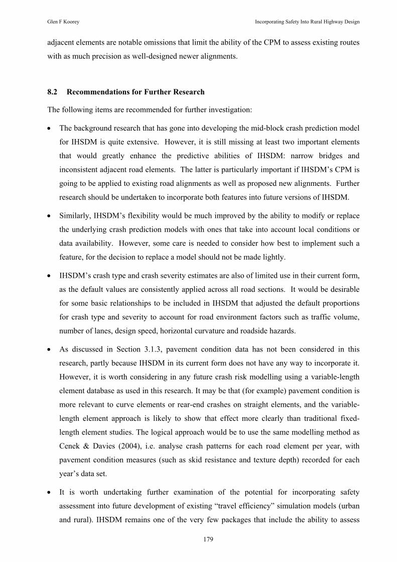
Glen F Koorey Incorporating Safety Into Rural Highway Design
179
adjacent elements are notable omissions that limit the ability of the CPM to assess existing routes
with as much precision as well-designed newer alignments.
8.2 Recommendations for Further Research
The following items are recommended for further investigation:
• The background research that has gone into developing the mid-block crash prediction model
for IHSDM is quite extensive. However, it is still missing at least two important elements
that would greatly enhance the predictive abilities of IHSDM: narrow bridges and
inconsistent adjacent road elements. The latter is particularly important if IHSDM’s CPM is
going to be applied to existing road alignments as well as proposed new alignments. Further
research should be undertaken to incorporate both features into future versions of IHSDM.
• Similarly, IHSDM’s flexibility would be much improved by the ability to modify or replace
the underlying crash prediction models with ones that take into account local conditions or
data availability. However, some care is needed to consider how best to implement such a
feature, for the decision to replace a model should not be made lightly.
• IHSDM’s crash type and crash severity estimates are also of limited use in their current form,
as the default values are consistently applied across all road sections. It would be desirable
for some basic relationships to be included in IHSDM that adjusted the default proportions
for crash type and severity to account for road environment factors such as traffic volume,
number of lanes, design speed, horizontal curvature and roadside hazards.
• As discussed in Section 3.1.3, pavement condition data has not been considered in this
research, partly because IHSDM in its current form does not have any way to incorporate it.
However, it is worth considering in any future crash risk modelling using a variable-length
element database as used in this research. It may be that (for example) pavement condition is
more relevant to curve elements or rear-end crashes on straight elements, and the variable-
length element approach is likely to show that effect more clearly than traditional fixed-
length element studies. The logical approach would be to use the same modelling method as
Cenek & Davies (2004), i.e. analyse crash patterns for each road element per year, with
pavement condition measures (such as skid resistance and texture depth) recorded for each
year’s data set.
• It is worth undertaking further examination of the potential for incorporating safety
assessment into future development of existing “travel efficiency” simulation models (urban
and rural). IHSDM remains one of the very few packages that include the ability to assess

Glen F Koorey Incorporating Safety Into Rural Highway Design
180
both the operational and safety aspects of a proposed roadway design. Many packages are
available for modelling the former aspect of road links and networks (e.g. TRARR, Paramics,
SATURN) and the ability to consider the safety aspects of such proposals at the same time
would be very valuable. Alternatively, the ability to easily import traffic network data into a
safety assessment package, such as done with SAFENET, is a slightly less convenient option
instead.
• Similarly, it would pay to investigate integrating or linking rural road safety models to
existing road design packages, enabling faster specification of safe road layouts for project
assessment. As well as crash reductions, design packages could also evaluate other
traditional road user benefits like travel-time savings and vehicle operating costs.
• This research has focused on the mid-block (non-intersection) aspects of rural road crash
prediction. It would be of value to also further investigate the ability of IHSDM to evaluate
the safety of intersections on rural two-lane roads in NZ. It may be possible to expand on the
work of Turner (2001) and subsequent research, such as Turner & Roozenburg (2006), who
developed crash prediction models for rural intersections, to develop appropriate NZ
calibration factors for IHSDM.
• This research has also focused on IHSDM’s Crash Prediction Module and, to a lesser extent,
its Design Consistency Module and Policy Review Module. Further investigation needs to be
done to also assess the practical usefulness of the Driver/Vehicle Module, Intersection
Diagnostic Review Module, and Traffic Analysis Module. Given NZ’s continued work to
provide realignments and passing opportunities, the Traffic Analysis Module in particular
shows promise as a potential replacement for TRARR modelling.
• The integrated system for collating relevant road data (e.g. traffic volumes, crashes, road
geometry, skid resistance) on State Highways greatly assisted the development of suitable
analysis models in this study. This advantage should be maximised in further developing and
using any crash models here, particularly for local (non-State Highway) roads. Continuing
encouragement should be given to developing and linking RCA electronic databases for road
inventory, traffic volumes, and crashes. Further thought should also be given to what
additional data not already collected or stored in these databases should be, e.g. intersection
geometric attributes, speed limits, passing lane locations, roadside hazard ratings, side-access
frequency.
• The RAMM data used in this study were generally sectioned for either administrative or
pavement management purposes, e.g. boundaries between adjacent councils or seal lengths.

Glen F Koorey Incorporating Safety Into Rural Highway Design
181
For any study investigating road geometry, it is therefore rather difficult to relate the existing
RAMM data to physical geometric road elements present on the highway, without the
extensive data processing undertaken in this study. It would be of immense value if
Transit NZ were to follow the model of the Texas DoT, where a special road inventory table
(“Geo-Hini”) has been created to link road positions with horizontal curvature (as discussed
in Section 3.4.1). Such information would be particularly pertinent if IHSDM is to be used
in NZ on State Highways.
• Notwithstanding the afore-mentioned value of the State Highway databases, many
inconsistencies and errors in the RAMM data were observed (especially when comparing
between regions), necessitating regular manual inspections and corrections of the tables.
These inconsistencies included differences in the coding of road sections as urban or rural,
and the coding of the types, legends and facing directions of signs. Most of these
inconsistencies showed up easily enough by means of simple queries and sorted lists of table
data, although this was a time-consuming exercise because of the size of the databases
concerned. It is recommended that Transit NZ (now NZTA) undertake a similar audit of its
existing RAMM data, to simplify analysis tasks for future users.
• Another data consistency problem that presented itself in this study was the apparent bias in
road geometry readings for many sections of State Highway. This led to anomalous results
such as long curves being recorded where there was only a long straight. Although steps
were taken to isolate and minimise this problem, it is not clear if more recent road geometry
data also suffer from similar problems. It is recommended that Transit NZ (now NZTA)
investigate the quality and consistency of its high-speed geometry data collection (using
methods similar to those described in Section 3.4.2), to try to minimise this problem in the
future.
• The database developed for this study has considerable potential to be used for a variety of
other applications. For example, strategic analyses can be undertaken of the entire State
Highway network to identify those sections with inconsistent alignments, in terms of safe
vehicle speeds. By linking crashes directionally to the geometric road elements, further work
can also be done to identify the most important road environment factors and to develop NZ-
specific crash prediction models for rural links. The vertical alignment data could also be
analysed further to better understand its influence on the crash risk due to horizontal curves.
• The existing MoT Crash Reduction Monitoring Programme represents the best opportunity to
produce NZ-specific crash modification factors. However, more resources need to be put
into it to improve data collection (including exposure data), data completeness and accuracy

Glen F Koorey Incorporating Safety Into Rural Highway Design
182
levels. The programme should also incorporate findings from treatments made for non-
safety reasons (e.g. changes in intersection control due to capacity) and data from relevant
local research studies, to improve the sample size available for analysis.
• The use of crash data related with road environment factors requires an accurate
understanding of the location of each crash. From the investigations in this study, clearly
many rural crashes are poorly located and based on vague descriptions of the crash location.
Traffic officers may also be basing their location on where the vehicle came to rest rather
than where the driver first encountered a problem. This makes it hard to relate crashes with
specific road features such as curves. GPS location of crashes would help to confirm more
precisely where they occurred, but such equipment is not yet standard in Police cars nor
always used properly. For future research in this area, it would be of immense value if Police
vehicles or officers were equipped with GPS locating equipment and also trained in more
detail on issues relating to accurate crash location identification.

Glen F Koorey Incorporating Safety Into Rural Highway Design
183
9 CONTRIBUTION TO THE STATE OF THE ART
This research has made at least the following contributions to the “state of the art”:
• A comprehensive database of road, traffic, crash and environmental data for all NZ State
Highways was developed, divided into variable-length road elements, from which further
research can also be undertaken. The processes and routines to develop this database have
also been documented for similar exercises elsewhere.
• Detailed investigation and correction of biases in the highway geometry data and a
systematic process for dividing the highway data into variable-length elements were
undertaken, both of which would have application in other similar studies.
• NZ calibration factors were derived for IHSDM’s CPM, both nationally for all State
Highways and for a series of subsets defined by traffic volume, number of lanes, region and
terrain. The automated process to do this is presented and could be replicated in other
jurisdictions. The research also demonstrated that “Level 1” calibration almost certainly
provides as accurate a calibration factor as the more complex “Level 2” calibration process.
• Importing routines were developed to export highway geometry and crash data from the State
Highway database into formats suitable for use in IHSDM. This process could be adapted to
generate similar IHSDM input files from other road geometry databases.
• A series of NZ case studies were tested in IHSDM to assess its crash prediction abilities and
other features such as design consistency. These provide useful examplars on how similar
validation tests could be applied in other jurisdictions calibrating IHSDM locally.
• Useful guidelines on calibrating and using IHSDM in local jurisdictions were developed,
which have not been replicated anywhere else to date. The findings include the benefits of
incorporating crash history data to improves the precision in crash number estimates, and the
more robust nature of IHSDM’s fatal/injury crash estimates compared with non-injury
crashes.
• Practical problems and deficiencies in using IHSDM were also identified, including the need
to correctly specify the extreme attributes of sub-standard elements and the limitations with
IHSDM’s current lack of consideration for bridges and inconsistent adjacent elements.
• Useful guidance was provided on the relative merits of various types of survey equipment for
monitoring vehicle speeds and lateral placement while traversing horizontal curves.
Various recommendations for future research have also been identified in Section 8.2.

Glen F Koorey Incorporating Safety Into Rural Highway Design
184
10 REFERENCES
12D Solutions Pty Ltd, 2007. 12D Reference Manual v8. Sydney, Australia.
AASHTO (American Association of State Highway and Transportation Officials), 2004. A
Policy on Geometric Design of Highways and Streets, 5th Ed., Washington DC, USA.
Alsop J., Langley J., 2001. Under-reporting of motor vehicle traffic crash victims in New
Zealand. Accident Analysis and Prevention, Vol. 33, No.3, pp.353–359.
Appelt V., 2000. New Approaches to the Assessment of the Spatial Alignment of Rural Roads –
Apparent Radii and Visual Distortion. Proceedings of the 2nd International Symposium on
Highway Geometric Design, June 2000, Mainz, Germany, pp.620-631.
Appleton I., Hannah J., Noone M.J., Wilkie S., 2006. Road Infrastructure Safety Assessment.
22nd ARRB Conference – Research into Practice, Canberra Australia, Oct-Nov 2006
ARRB Transport Research 2007. Gipsi-Trac Geometry Package. Website:
http://www.arrb.com.au/documents/PB-GIPSI-Trac.pdf.
Austroads, 2000. Relationship Between Crash Risk and Geometric Characteristics of Rural
Highways. Austroads Publication AP-R162/00, 73pp.
Austroads, 2001. Economic evaluation of road investment proposals - Improved prediction
models for road crash savings. Austroads Publication AP-R184/01, Sydney, 87pp.
Austroads, 2003. Rural Road Design: Guide to the Geometric Design of Rural Roads, Austroads
Publication AP-G1/03, Sydney, Australia.
Austroads, 2008. Glossary of Austroads Terms. Austroads Publication AP-C87/08, Sydney,
Australia, 141pp.
Bahar G., Smiley A., 2000. The Integration of Human Factors and Explicit Safety in Highway
Geometric Design. Proceedings of the 2nd International Symposium on Highway
Geometric Design, June 2000, Mainz, Germany, pp.36-47.
Bansen J., Passetti K., 2005. Application of the IHSDM: A Case Study, 3rd International
Symposium on Highway Geometric Design, Chicago, USA, Jun 2005.

Glen F Koorey Incorporating Safety Into Rural Highway Design
185
Beca Carter Hollings & Ferner Ltd (BCHF), 1998. Safety benefits of median barriers on New
Zealand motorways. Transfund NZ Research Report No. 107, Wellington.
Bennett C.R., 1994. A Speed Prediction Model for Rural Two Lane Highways. University of
Auckland, School of Engineering Report 541.
BRC, 2000. Willingness to Pay for Four-Laning: Final Report. Report for Transit NZ by BRC
Marketing & Social Research, Opus Central Laboratories, and David Hensher.
Brodie C., Koorey G., 2002. ARRB Road Safety Risk Manager: Software Review. Transfund
NZ Report No. OG/0206/12S.
Burggraf D.S., 2005. Transportation Spatial Information Infrastructure. Transport Canada
Publication no. TP 14388E, April 2005.
Burrow I., 1999. SafeNET – Software to aid Urban Safety Management. Traffic Engineering
and Control, Vol.40 No.3, March 1999, pp.123-128.
Cafiso S., Di Graziano A., Di Silvestro G., La Cava G., 2008. Safety Performance Indicators for
Local Rural Roads: Comprehensive Procedure from Low-Cost Data Survey to Accident
Prediction Model. 87th Transportation Research Board (TRB) Annual Meeting,
Washington DC, USA, Jan 2008.
Cardoso J., Flouda A., Dimitropoulos I., Kanellaidas G., 1997. Design Consistency of
Horizontal Alignment in Rural Roads. SAFESTAR Task 5.1 Report.
Castro M., Pardillo-Mayora J.M., Sánchez J.F., 2005. Alignment Indices as a Tool to Evaluate
Safety and Design Consistency in Two Lane Rural Roads, 3rd International Symposium on
Highway Geometric Design, Chicago, USA, Jun 2005.
Cenek P.D., Davies R.B., McLarin M.W., Griffith-Jones G., Locke N.J., 1997. Road
Environment and Traffic Crashes. Transfund NZ Research Report No. 79. Wellington,
New Zealand, 132 pp.
Cenek P.D., Davies R.B., 2004. Crash risk relationships for improved safety management of
roads. Towards Sustainable Land Transport Symposium, Wellington, Nov 2004.
CEOS Industrial Pty Ltd, 2005. TIRTL Installation Manual. Version 1.0.0.

Glen F Koorey Incorporating Safety Into Rural Highway Design
186
Chapman, R.A., 1971. Some relationships between road accident frequencies and measures of
exposure to risk. PhD Thesis, University College, University of London, UK.
Charlesworth, K.D., Cairney, P.T., 1988. Development of Techniques for Studying Unsafe
Driving Actions. ARRB Special Report SR39. 123pp.
Council F.M., 1998. Safety Benefits of Spiral Transitions on Horizontal Curves on Two-Lane
Rural Roads. Transportation Research Record 1635, pp10-17. Transportation Research
Board, Washington DC, USA.
Davis D., 2007. Pers. Comm., 10/01/07.
Deacon J., 1986. Relationship between accidents and horizontal curvature. Appendix D in
Designing safer roads. Special Report 214, Transportation Research Board,
Washington DC, USA.
Donnell E.T., Ni Y., Adolini M., Elefteriadou L., 2001. Speed Prediction Models for Trucks on
Two-Lane Rural Highways. Transportation Research Record 1751, pp.44-55.
Transportation Research Board, Washington DC, USA.
Donnell E.T., Stodart B.P., Gross F., Opiela K., 2007. Appraisal of the Interactive Highway
Safety Design Model’s Crash Prediction and Design Consistency Module Results: Case
Studies from Pennsylvania. 86th Transportation Research Board (TRB) Annual Meeting,
Washington DC, USA, Jan 2007.
Easa S.M., You Q.C., 2009. Collision Prediction Models for Three-Dimensional Two-Lane
Highways: Horizontal Curves. Transportation Research Record 2092, pp.48-56.
Transportation Research Board, Washington DC, USA.
FHWA (Federal Highways Administration), 2006. Interactive Highway Safety Design Model
(IHSDM), website home page & overview (http://www.tfhrc.gov/safety/ihsdm/ihsdm.htm),
(US) Federal Highway Administration.
Fildes B.N., Lee S.J., 1993. The Speed Review: Road Environment, Behaviour, Speed Limits,
Enforcement and Crashes. Report prepared for Road Safety Bureau (NSW RTA) and the
Federal Office of Road Safety, Australia.
Fitzpatrick K., Collins J.M., 2000. Speed Profile Model for Two-Lane Rural Highways.
Transportation Research Record 1737, (US) Transportation Research Board, pp.42-49.

Glen F Koorey Incorporating Safety Into Rural Highway Design
187
Fitzpatrick K., Elefteriadou L., Harwood D.W., Collins J.M., McFadden J., Anderson I.B.,
Krammes R.A., Irizarry N., Parma K.D., Bauer K.M., Passetti K., 2000. Speed Prediction
for Two-Lane Rural Highways. Report No. FHWA-RD-99-171, Office of Safety Research
and Development, (US) Federal Highway Administration.
Fitzpatrick K., Schneider IV W., Carvell J., 2006. Using the Rural Two-Lane Highway Draft
Prototype Chapter. 85th Transportation Research Board (TRB) Annual Meeting,
Washington DC, USA, Jan 2006
FRA, 2000. GradeDec 2000: System for Grade Crossing Investment Analysis. Model
Documentation Reference. US Federal Railroad Administration (FRA), Office of Policy
and Program Development, October 2000.
Frith W.R., Harte D.S., 1986. The Safety Implications of Some Control Changes at Urban
Intersections. Accident Analysis & Prevention, Vol.18, No.3, pp.183-192.
Gabites Porter Consultants, 1995. System-wide road accident analysis: a study of accident rates
on road systems of five cities in NZ (amended report 1995). Transit NZ Research Report
No. 39, 72 pp.
Greenwood I.D., 2003. A New Approach to Estimate Congestion Impacts for Highway
Evaluation - Effects on Fuel Consumption and Vehicle Emissions. PhD thesis, Dept of
Civil & Environmental Engineering, University of Auckland. 206 pp.
Güttinger V.A., 1977. Conflict Observation Technique in Traffic Situations. Proceedings of the
1st Workshop on Traffic Conflicts Techniques, Oslo, Norway, Sep. 1977. pp.1-15.
Halcrow Fox & Associates, 1981. Effects on Safety of Marginal Design Elements. (UK)
Department of Transport, March 1981.
Harwood D.W., Council F.M., Hauer E., Hughes W.E., Vogt A., 2000. Prediction of the
Expected Safety Performance of Rural Two-Lane Highways. Report No.
FHWA-RD-99-207, Office of Safety Research and Development, (US) Federal Highway
Administration.
Hassan Y., Easa S. M., 2003. Effect of Vertical Alignment on Driver Perception of Horizontal
Curves. ASCE Journal of Transportation Engineering, American Society for Civil
Engineering, Vol. 129, No. 4, July 1, 2003

Glen F Koorey Incorporating Safety Into Rural Highway Design
188
Hauer E., 1997. Observational before-after studies in road safety: estimating the effect of
highway and traffic engineering measures on road safety. Pergamon, New York. 289 pp.
Hauer E., Persaud B., 1996. Safety Analysis of Roadway Geometric and Ancillary Features.
Transportation Association of Canada Research Report, 171 pp.
HTC, 2002. Sectioning Improvement. Transit NZ Project 801/004995 Final Report. HTC
Infrastructure Management Ltd, Auckland.
Hughes W., Eccles K., Harwood D., Potts I., Hauer E., 2004. Development of a Highway Safety
Manual. NCHRP Web Document 62 (Project 17-18[4]): Contractor’s Final Report,
National Cooperative Highway Research Program, Transportation Research Board,
Washington DC, USA, March 2004, 303 pp.
Hunt J., Mahdi T., 1995. A model to predict accident frequency on rural single carriageway
roads. Proceedings, Road Safety in Europe and Strategic Highway Research Program
(SHRP), Prague, the Czech Republic, September 20-22, 1995, VTI Konferens No. 4A,
Part 1, pp. 55-72.
Kaub A.R., 1992. A microcomputer Model to Estimate the Benefits of Volume Generated
Auxiliary Passing Lanes on Two-lane Two-way Highways. Proceedings 4th International
Conference on Microcomputers in Transportation, ASCE, July 1992, pp.356-367.
Keyte T., 2006. Calibration of Interactive Highway Safety Design Model: The Design
Consistency Policy Module. Master of Engineering in Transportation Research Project
Report, Dept of Civil Engineering, University of Canterbury, Christchurch, New Zealand.
Koorey G.F., 2000. TRARR Users Manual. Technical Support Document CEP 505, Opus
International Consultants, Nov 2000.
Koorey G.F., 2003. Assessment of Rural Road Simulation Modelling Tools. Transfund NZ
Research Report No.245. Wellington, New Zealand, 124 pp.
Koorey G.F., 2005. The Use of Road Geometry Data for Highway Applications, 3rd
International Symposium on Highway Geometric Design, Chicago, USA, Jun 2005.
Koorey G.F., Gu J., 2001. Assessing Passing Opportunities – Stage 3. Transfund NZ Research
Report No. 220. Wellington, New Zealand, 119 pp.

Glen F Koorey Incorporating Safety Into Rural Highway Design
189
Koorey G.F., Farrelly P.M., Mitchell T.J., Nicholson C.S., 1999. Assessing Passing
Opportunities – Stage 2. Transfund NZ Research Report No.146. Wellington, New
Zealand, 81 pp.
Koorey G.F., Page S.J., Stewart P.F., Ellis A.E., Henderson R.J., Gu J., Cenek P.D., 2002.
Curve Advisory Speeds in New Zealand. Transfund NZ Research Report No. 226.
Wellington, New Zealand, 112pp.
Koorey, G.F., Tate, F.N., 1997. Review of Accident Analysis Procedures for Project Evaluation
Manual. Transfund NZ Research Report No.85. Wellington, New Zealand, 54 pp.
Koorey G.F., Wilkie S.M., 2002. A Review of Road Safety Network Risk Models. Central
Laboratories Report: 02-529573.00 for Land Transport Safety Authority, Opus
International Consultants Ltd.
Krammes R., 2000. Interactive Highway Safety Design Model for Safety Evaluation of Highway
Designs. Proceedings of the 2nd International Symposium on Highway Geometric Design,
June 2000, Mainz, Germany, pp.571-576.
Krammes R.A., Glascock S.W., 1992. Geometric Inconsistencies and Accident Experience on
Two-Lane Rural Highways. Transportation Research Record 1356, pp.1-10.
Transportation Research Board, Washington, DC, USA.
Krammes R.A., Rao K.S., Oh H., 1995. Highway Geometric Design Consistency Evaluation
Software. Transportation Research Record 1500, pp.19-24. Transportation Research
Board, Washington, DC, USA.
Kraus C.L., 1991. Monitoring the Effects of the Accident Investigation Programme. Master of
Engineering Thesis, Dept of Civil Engineering, University of Canterbury.
Kulmala R., 1982. Traffic Conflict Studies in Finland. Proceedings of the 3rd International
Workshop on Traffic Conflicts Techniques, International Committee on Traffic Conflicts
Techniques (ICTCT), Leidschendam, Netherlands, April 1982. Institute for Road Safety
Research (SWOV) Report R-82-27. pp. 50-59.
Lamm R., Choueiri E., Psarianos B., Soilemezoglu G., 1995. A Practical Safety Approach to
Highway Geometric Design. International Case Studies: Germany, Greece, Lebanon,
United States. 1st International Symposium on Highway Geometric Design, Aug-Sep 1995,
Boston, US. Ch.11.

Glen F Koorey Incorporating Safety Into Rural Highway Design
190
Lamm R., Beck A., Zumkeller K., 2000. Analysis and Evaluation of Interrelationships between
Traffic Safety and Highway Geometric Design on Two-Lane Rural Roads. Proceedings of
the 2nd International Symposium on Highway Geometric Design, June 2000, Mainz,
Germany, pp.557-570.
Lee S., Lee D., Choi J., 2000. Validation of the 10MPH Rule in Highway Design Consistency
Procedure. Proceedings of the 2nd International Symposium on Highway Geometric
Design, June 2000, Mainz, Germany, pp.364-376.
Levison W.H., Simsek O., Bittner A.C.Jr, Hunn S.J., 2001. Computational Techniques Used in
the Driver Performance Model of the Interactive Highway Safety Design Model.
Transportation Research Record 1779, (US) Transportation Research Board, pp.17-25.
Lord D., Washington S.P., Ivan J.N. 2005. Poisson, Poisson-gamma and zero-inflated regression
models of motor vehicle crashes: balancing statistical fit and theory. Accident Analysis and
Prevention, Vol.37 No.1, pp.35–46, Elsevier.
LTNZ (Land Transport New Zealand), 2004. Overall Results of Crash Reduction Study
Monitoring. October 2004. Website:
http://www.landtransport.govt.nz/roads/crash-reduction-programme.html.
LTNZ (Land Transport New Zealand), 2005. Coded crash reports from the Crash Analysis
System (CAS). Interpretation guide, Version 3.0. June 2005. Website:
http://www.landtransport.govt.nz/research/cas/coded-crash-reports.html.
LTNZ (Land Transport New Zealand), 2006. Economic Evaluation Manual, Vol. 1. Manual no.
EEM1, 1st edition. Wellington.
LTNZ (Land Transport New Zealand), 2007. Crash Analysis System (CAS). Website:
http://www.landtransport.govt.nz/research/cas/.
Manandhar D., Shibasaki R., 2001. Vehicle-borne Laser Mapping System (VLMS) - A New
Observation System for 3-D Mapping of Urban Areas. Proceeding of IEEE/ISPRS Joint
Workshop on Remote Sensing and Data Fusion over Urban Areas, pp.5-9.
Matthews L.R., Barnes J.W., 1988. Relation between road environment and curve accidents.
Road Traffic Safety Seminar, NZ Road Traffic Safety Research Council, 14-16 Sep 1988,
Vol.1 pp.206-230.

Glen F Koorey Incorporating Safety Into Rural Highway Design
191
McInerney R., 2001. The Road Safety Risk Manager: A software tool to prioritise road safety
treatments. Draft report RC1576 for Austroads.
McLarin M.W., 1997. Typical Accident Rates for Rural Passing Lanes and Unsealed Roads.
Transfund NZ Research Report No. 89. Wellington, New Zealand.
Messer C.J., 1980. Methodology for Evaluating Geometric Design Consistency. Transportation
Research Record 757, pp.7-14. Transportation Research Board, Washington, DC, USA.
MoT (Ministry of Transport), 2003. Road Safety to 2010 Strategy, NZ Ministry of Transport.
Website: http://www.transport.govt.nz/road-safety-2010-index/
MoT (Ministry of Transport), 2006a. Motor Vehicle Crashes in New Zealand 2005, NZ Ministry
of Transport. Website: http://www.transport.govt.nz/annual-statistics-2005/
MoT (Ministry of Transport), 2006b. Speed Statistics, NZ Ministry of Transport.
Website: http://www.transport.govt.nz/speed-index/
MoT (Ministry of Transport), 2006c. Open Road Car Speeds, NZ Ministry of Transport.
Website: http://www.transport.govt.nz/speed1/
MoT (Ministry of Transport), 2007. Monthly Overview of Crash Statistics, NZ Ministry of
Transport. Website: http://www.transport.govt.nz/monthlyoverview/
Mountain L., Fawaz B., Jarrett D., 1996. Accident prediction models for roads with minor
junctions. Accident Analysis and Prevention, Vol.28 No.6, pp.695-707.
National Roads Board (NRB), 1980. Traffic Conflicts Technique Workshop – An introduction to
the GMR Traffic Conflicts procedures manual, Wellington.
Nicholson A.J., 1987. The Estimation of Accident Rates and Countermeasure Effectiveness.
Traffic Engineering and Control, 28(10), pp.518-523.
Nicholson A.J., Gibbons J.N., 2000. Superelevation, sight distance and speed. Proceedings,
Engineering for Road Safety Symposium, Rotorua, Sep 2000. 11pp.
NRSC (National Road Safety Committee), 2000. Road Safety Strategy 2010. A consultation
document. October 2000, Wellington.

Glen F Koorey Incorporating Safety Into Rural Highway Design
192
O’Cinneide D., Murphy J., Ryan T., 2005. The Effect of Geometric Elements on Interurban
Accident Rates, 3rd International Symposium on Highway Geometric Design, Chicago,
USA, Jun 2005.
Older S.J., Shippey J., 1977. Traffic Conflict Studies in the United Kingdom. Proceedings of
the 1st Workshop on Traffic Conflicts Techniques, Oslo, Norway, Sep. 1977. pp.1-15.
Opus Central Laboratories, 2002. Crash Risk Relationships for Improved Safety Management of
Roads. 2002-03 Transfund NZ Research Programme Proposal, May 2002.
Peltola H., 2000. Background and Principles of the Finnish Safety Evaluation Tool, TARVA.
Proceedings 13th ICTCT (International Cooperation on Theories and Concepts in Traffic
Safety) Workshop, Corfu, Greece, Oct 2000.
Perkins S.R., 1969. Traffic Conflicts Technique Procedures Manual. General Motors Research
Laboratory Report 895.
Perkins S.R., Harris J.L., 1967. Traffic Conflict Characteristics: Accident Potential at
Intersections. General Motors Research Laboratory Report 718.
Persaud B, Lyon C., 2006. Empirical Bayes Before-After Safety Studies: Lessons Learned From
Two Decades of Experience. Transportation Research Board 85th Annual Meeting,
Washington DC, US.
Persaud B., Turner S., Chou M., Koorey G., Lyon C., 2008. International Road Safety
Comparisons Using Accident Prediction Models, 87th Transportation Research Board
(TRB) Annual Meeting, Washington DC, USA, Jan 2008.
Potts I.B., Harwood D.W., Bauer K.M., 2000. Effect of Preceding Tangent Length on Safety for
Horizontal Curves. Proceedings of the 2nd International Symposium on Highway
Geometric Design, June 2000, Mainz, Germany, pp.279-287.
Quantm Ltd, 2007. About Quantm. Website: http://www.quantm.net/publish/page.cfm?contentID=1
Rawlinson W.R., 1983. The ARRB Road Geometry Instrumented Vehicle - General Description.
ARRB Internal Report AIR 276-2, ARRB, Vermont South, Victoria, Australia.
Resende P., Benekohal R., 1997. Effects of Roadway Section Length on Accident Modeling.
Traffic Congestion and Traffic Safety in the 21st Century Conference. ASCE, Chicago,
USA, Jun 1997.

Glen F Koorey Incorporating Safety Into Rural Highway Design
193
Richl L., Sayed T., 2005. Effect of Speed Prediction Models on Design Consistency, 3rd
International Symposium on Highway Geometric Design, Chicago, USA, Jun 2005.
Risser R., Schützenhöfer A., 1984. Application of Traffic-Conflict Technique in Austria.
International Calibration Study of Traffic Conflict Techniques, E. Asmussen ed.,
pp.141-151. Springer-Verlag.
Robinson J.B.L., Morrall J., Smith G., Biglow B., 2005. Developments & Emerging Issues in
Canadian Geometric Design Practices: Country Report, 3rd International Symposium on
Highway Geometric Design, Chicago, USA, Jun 2005.
Roper P., 2003. Data Collection Technology at ARRB Transport Research. Australasian Road
Safety Research Policing & Education Conference, Sydney, Australia, Sep 2003.
Saito M., Chuo K., 2008. Evaluation of the Applicability of the Interactive Highway Safety
Design Model to Safety Audits of Two-lane Rural Highways. Report No. UT-02.08, Utah
Department of Transportation, Salt Lake City, US, Mar 2008.
Schlüter P.J., 1996. Identification of hazardous motor vehicle accident sites: some Bayesian
considerations. PhD thesis, Dept of Mathematics and Statistics, University of Canterbury.
144pp.
Shepherd R., 1994. TRARR 4 User Manual. Australian Road Research Board (ARRB),
Victoria, Australia.
Spacek P., 2000. Track Behaviour and Accident Occurrence in Curves on Two-Lane Highways
in Rural Areas. Proceedings of the 2nd International Symposium on Highway Geometric
Design, June 2000, Mainz, Germany, pp.288-298.
Spearpoint M.J, 2006. Integration of Building Product Models with Fire Simulation Software.
PhD thesis, Dept of Civil Engineering, University of Canterbury. 355 pp.
Steyer R., Sossoumihen A., Weise G., 2000. Traffic Safety on Two-Lane Rural Roads – New
Concepts and Findings. Proceedings of the 2nd International Symposium on Highway
Geometric Design, June 2000, Mainz, Germany, pp.299-312.
St. John A.D., Harwood D.W., 1986. A User’s Guide to TWOPAS – A Microscopic Simulation
Model of Traffic on Two-Lane Two-Way Highways. Federal Highways Administration
Glen F Koorey Incorporating Safety Into Rural Highway Design
194
Tanner J.C., 1953. Accidents at Rural Three-Way Junctions, Journal of the Institution of
Highway Engineers, 2(11), pp.56-67.
Tapani A., 2005. A Versatile Model for Rural Road Traffic Simulation. 84th Transportation
Research Board (TRB) Annual Meeting, Washington DC, USA, Jan 2005.
Taranto V., 2006. Pers. Comm., 15/03/06.
Tate F.N., 1995. Assessing Passing Opportunities – Stage 1. Transit NZ Research Project PR3-
0097 draft report. Wellington, New Zealand.
Tate F., Turner S., 2007. Road Geometry and Drivers Speed Choice. IPENZ Transportation
Group Conference, Tauranga, Oct 2007.
Thomas I. 1996. Spatial Data Aggregation: Exploratory Analysis of Road Accidents. Accident
Analysis and Prevention, Vol. 28, No.2, pp.251–264.
Tom G.K.J., 1995. Accidents on Spiral Transition Curves. ITE Journal, Vol. 65 No.9, pp.49-53.
Transfund New Zealand, 1998. Safety Audit Procedures for Existing Roads. Wellington.
Transit New Zealand, 1993. Safety Audit Policy and Procedures. Wellington.
Transit New Zealand, 2000. State Highway Geometric Design Manual (Draft). Wellington,
New Zealand.
Transit New Zealand, 2004. State Highway Location Referencing Management System (LRMS)
Manual. Manual No. SM051, Jul 2004, Wellington.
Transit New Zealand, 2006. State Highway Database Operations Manual. Manual No. SM050,
Mar 2006, Wellington.
Transit New Zealand, 2007. High Speed Data Collection. Website:
http://www.transit.govt.nz/hsdc/index.jsp
Transit New Zealand, 2008. State Highway Traffic Data Booklet 2003-2007. Jun 2008,
Wellington.
Travers Morgan (NZ) Ltd, 1992. Accident Counter Measures: Literature Review, Transit NZ
Research Report No. 10, Wellington.

Glen F Koorey Incorporating Safety Into Rural Highway Design
195
TRL, 2002. SafeNET - An Interactive Design Tool for Traffic Engineers. Transport Research
Laboratory, Crowthorne, UK. Website: http://www.trlsoftware.co.uk/productSafenet.htm.
Turner S.A., 2001. Accident Prediction Models. Transfund NZ Research Report No.192. 80 pp.
Turner S.A., 2002. Alternative Accident Evaluation Procedure. Discussion paper for Transfund
New Zealand, 24 pp.
Turner S., Roozenburg A., 2006. Rural Intersection Safety. IPENZ Transportation Group
Conference, Queenstown, Oct 2006.
University of Florida, 2007. Representation of Traffic Analysis Tool Outputs in a Common
Format Using XML. Draft Working Paper 385-5 (NCHRP Project 3-85), University of
Florida Transportation Research Center and T-Concepts Corp.
Vogt A., Bared J.G., 1998. Accident Models for Two-Lane Rural Roads: Segments and
Intersections, Report No. FHWA-RD-98-133, Federal Highway Administration, Oct 1998.
VTT, 1999. Cross Section of Rural Roads. SAFESTAR Final Report WP4. VTT (Communities
& Infrastructure), Finland.
W3C, 2008. Extensible Markup Language (XML). World Wide Web Consortium.
Website: http://www.w3.org/XML/
Wanty D.K., McLarin M.W., Davies R.B., Cenek P.D., 1995. Application of the road geometry
data acquisition system (RGDAS). 7th World Conference on Transport Research, Sydney,
Australia. (not published in the proceedings)
Wardrop, J.G. 1952. Some theoretical aspects of road traffic research. Proceedings, Institution of
Civil Engineers, Part 2, pp.325-378.
Weale K.H.M., 2006. Designing for the Road User: Maximum Spiral Transition Lengths.
IPENZ Transportation Group Conference, Queenstown, Oct 2006.
Wegman F.C.M., Slop M., 1995. Safety Effects of Road Design Standards in Europe. 1st
International Symposium on Highway Geometric Design, Aug-Sep 1995, Boston, US.
Ch. 39.

Glen F Koorey Incorporating Safety Into Rural Highway Design
196
Wilkie S.M., Tate F.N., 2002. Transfund New Zealand Safety Audit of Existing Roads:
Developing a less Subjective Assessment. Central Laboratories Report 02 529562.00,
Opus International Consultants.
Wong Y.D., 1989. Driver Behaviour at Horizontal Curves. PhD thesis, Dept of Civil
Engineering, University of Canterbury. 292 pp.
Wong Y.D., Nicholson A.J., 1993. Speed and lateral placement on horizontal curves. Road and
Transport Research, Vol.2, No.1, March 1993, ARRB, Australia.
Zegeer C.V, Hummer J., Reinfurt D., Herf L., Hunter W., 1987. Safety Effects of Cross-Section
Design for Two-Lane Roads. Report No. FHWA-RD-87/008. (US) Federal Highway
Administration (FHWA), TRB National Research Council, Washington D.C., Oct. 1987.
Ziering E., Harrison F., Scarponcini P., 2007. TransXML: XML Schemas for Exchange of
Transportation Data. NCHRP Report 576, (US) Transportation Research Board.

Glen F Koorey Incorporating Safety Into Rural Highway Design
197
A APPENDICES
A.1 LTNZ CAS Crash Movement Codes
Note: the “key vehicle” is shown as the bold arrow

Glen F Koorey Incorporating Safety Into Rural Highway Design
198
A.2 LTNZ Road Safety Report Categories
(refer to Appendix A.1 for movement codes)
Head-on / Lost control on a curved road:
BB, BC, BD, BF, BO, DA, DB, DC, DO
Head-on / Lost control on a straight road:
BA, BE, CA, CB, CC, CO
Rear end/obstruction:
EA, EB, EC, ED, EE, EO, FA, FB, FC, FD, FE, FF, FO, GA, GD, GF, GO, MA, MB, MC, MD, ME, MF, MG, MO
Overtaking:
AA, AB, AC, AD, AE, AF, AG, AO, GB, GE
Intersection (Crossing/Turning):
GC, HA, HO, JC, JO, KA, KB, KC, KO, LA, LB, LO, JA
Pedestrian vs. Vehicle:
NA, NB, NC, ND, NE, NF, NG, NO, PA, PB, PC, PD, PE, PF, PO
Miscellaneous:
QA, QB, QC, QD, QE, QF, QG, QO

Glen F Koorey Incorporating Safety Into Rural Highway Design
199
A.3 Structure of Analysis Database Tables
(for more information, refer to Transit NZ 2006 and LTNZ 2005)
Note: Not-relevant fields have been omitted from these details
Table: 2002_geometry
Properties Description: RAMM data of road geometry (10m intervals) Source: Transit NZ RAMM HSD_geom file No. of Records: 2,196,344
Fields Name Type Size Comments survey_date Date/Time Date that geometry data was collected road_id Long Integer RAMM Road ID start_m Long Integer Displacement (m) of road section end_m Long Integer 10m after start_m lane Text 255 Usually L1 (increasing RP) or R1 (decreasing RP) gradient Single Real Positive if uphill (%) curvature Long Integer Horizontal radius (m); positive if left-hand curve crossfall Single Real Positive if rising to centreline (%)
Table: Roadnames
Properties Description: Lookup table of all RAMM RoadIDs vs SH/RS Source: Transit NZ RAMM Roadnames_all file No. of Records: 1604
Fields Name Type Size Comments Include? Yes/No Identify all suitable road sections (no on/off ramps) Exclude? Yes/No Exclude any road sections in urban areas road_id Long Integer Unique integer ID for each record road_name Text 255 Usually SH and RS suburb Text 255 Locality details town Text 255 Locality details SH Text 5 3-character zero-padded value, e.g. “02A” stat_type Text 5 Ref. Stn. (RS) or Established Route Position (ERP) RS Integer Reference station number RP_start Single Real Start position of segment (km) SH_dirn Text 255 (I)ncreasing or (D)ecreasing RP; blank if both SH_common Text 255 Name of SH with common highway section ramp_type Text 255 ON or OFF ramp, if applicable external_name Text 255 General description of road length area region Integer Number of regional area (1-14) council Integer Number of local council (1-73) island Text 10 North Is (NI) or South Is (SI) added_on Date/Time Details of when added by RAMM database operator added_by Text 255 “ ” chgd_on Date/Time Details of when changed by RAMM operator chgd_by Text 255 “ “

Glen F Koorey Incorporating Safety Into Rural Highway Design
200
Table: Geometry
Properties Description: Geometry data and analysis at 10m intervals Source: From 2002_geometry and Roadnames tables via MakeGeometry query No. of Records: 2,097,168
Fields Name Type Size Comments ID Text 20 Unique ID from Dirn-SH-RS/RP RoadID Long Integer RAMM Road ID Dirn Text 5 Direction of lane: "Incr" or "Decr" SH Text 3 State Highway (3 chars left-filled with zeroes) RS Integer Reference Station RP Single Real Route Position (km) RSRP Text 15 Combined RS & RP Gradient Single Real Longitudinal Gradient (%): +ve = uphill in travelling
direction HzRad Long Integer Horizontal Radius (m): +ve = right-hand curve AbsRad Long Integer Absolute magnitude of HzRad (m) HzCurv Single Real Horizontal Curvature (rad/km) = 1000/HzRad XFall Single Real Crossfall (%): +ve = rises to the right Curve Text 9 Curve Direction: "Left", "Right" or "Straight" AdvSpd Single Real Raw derived 85%ile speed based on geometry LocSpd Single Real Local speed = typical driving speed profile SpdEnv Single Real Speed Environment, based on previous 500m Env1km Single Real Speed Environment, based on previous 1km Env2km Single Real Speed Environment, based on previous 2km Env5km Single Real Speed Environment, based on previous 5km AbsXF Single Real Absolute magnitude of XFall if sign is same as
HzRad; negative otherwise Odo Single Real Running distance (odometer) (km) Comment Text 255 Any notable features
Table: GeomElements
Properties Description: Geometric information for each road element (curve/straight) Source: From Geometry table via FindElements macro No. of Records: 85,458
Fields Name Type Size Comments ElemID Text 30 Unique ID, from element direction + start position ElemDirn Text 5 (Incr)easing or (Decr)easing Route Position ElemSH Text 3 State Highway (3 chars left-filled with zeroes) StartRS Integer Reference Station at start of element StartRP Single Real Route Position (km) at start of element StartODO Single Real Running distance (km) at start of element EndRS Integer Reference Station at end of element EndRP Single Real Route Position (km) at end of element EndODO Single Real Running distance (km) at end of element ElemType Text 20 Curve or Tangent Orientn Text 2 left-hand (LH) or right-hand (RH) curve orientation

Glen F Koorey Incorporating Safety Into Rural Highway Design
201
Length Long Integer Length (m) of element DeflnAng Single Real Calculated deflection angle of element CurvDegKm Single Real Average curvature (degrees/km) of element MinRad Long Integer Minimum radius recorded within element MinAdvSpd Single Real Minimum AdvSpd value recorded within element MinLocSpd Single Real Minimum LocSpd value recorded within element MinSpdEnv Single Real Minimum SpdEnv value recorded within element AveRad Long Integer Average radius recorded throughout element AveCurv Single Real Average curvature recorded throughout element AveGrad Single Real Average gradient recorded throughout element EntryGrad Single Real Gradient at start of element ExitGrad Single Real Gradient at end of element VertCurv Text 20 Description of vertical curvature within element HillinessMKm Single Real Average rises and falls within element (metres/km) AveLocSpd Single Real Average radius recorded throughout element AveSpdEnv Single Real Average radius recorded throughout element EntryEnv1km Single Real Env1km value at start of element EntryEnv2km Single Real Env2km value at start of element EntryEnv5km Single Real Env5km value at start of element AveXF Single Real Average crossfall recorded throughout element MinXF Single Real Minimum crossfall value recorded within element MaxXF Single Real Maximum crossfall value recorded within element Comment Text 255 Any notable features about this element Include? Yes/No Include only elements without problem features, e.g.
start/end of highway, urban areas, etc PrevElemID Text 30 Link to ElemID of previous element, if any
Table: Carr_way
Properties Description: RAMM traffic summary data for each carriageway section Source: Transit NZ RAMM Carr_way file No. of Records: 8242
Fields Name Type Size Comments carr_way_no Integer Unique ID for each carriageway road_id Long Integer RAMM Road ID for carr’way section carrway_start_m Long Integer Displacement (m) to start of carr’way section carrway_end_m Long Integer Displacement (m) to end of carr’way section start_name Text 255 Feature at start of carr’way, e.g. side-street end_name Text 255 Feature at end of carr’way, e.g. side-street cway_area Text 255 Name of regional network contract area cway_subarea Integer Number of network sub-contract urban_rural Text 255 (R)ural or (U)rban cway_hierarchy Text 255 SH road category (R1/R2/R3/R4/Urban/M’way) lanes Integer Number of traffic lanes in total lane_width Single Real Average traffic lane width (m) length_m Long Integer Length of carr’way section (m) cway_width Single Real Average width of total sealed carr’way (m) irr_width Text 255 (R)egular or (I)rregular carr’way width notes Text 255 Any relevant comments about this section loading_pc_heavy Integer Percent of heavy vehicles (%)

Glen F Koorey Incorporating Safety Into Rural Highway Design
202
traffic_adt_est Long Integer Estimate of AADT on carr’way section traffic_adt_count Long Integer Actual traffic count obtained on section
Table: DataCoded
Properties Description: Processed crash data used for queries Source: From raw LTNZ CAS data No. of Records: 90,592
Fields Name Type Size Comments STREET1 Text 255 Name of main road that crash occurred on ATI Text 5 (A)t a feature or at (I)ntersection of STREET2 DST Long Integer Distance (m) away from STREET2 DIR Text 5 Compass direction (N/S/E/W) away from STREET2 STREET2 Text 255 Name of side street or feature (e.g. bridge) DAY Byte Day of the month when crash occurred MTH Byte Number of month (1-12) when crash occurred YR Integer Year when crash occurred AXNO Long Integer Unique ID number for each crash record DOW Text 5 Day of week when crash occurred (Sun - Sat) TIME Text 5 24-hr time when crash occurred MVMT Text 5 LTNZ crash movement code (AA-QO) VEHS Text 25 Type of vehicles/road-users involved and their
direction of travel (N/S/E/W) FAC1 Text 255 LTNZ Road User & Vehicle factor codes (100-799) ENV1 Text 25 LTNZ Road & Environment factor codes (800-999) OBJ Text 5 Codes for Objects struck (A-Z) CRV Text 5 St(R)aight, (E)asy, (M)oderate or (S)evere curvature WET Text 5 (W)et, (D)ry or (I)ce/snow road surface LIT Text 5 Natural light conditions and any streetlighting WTH Text 5 Weather conditions - (F)ine, (M)ist, (L)ight rain, etc INT Text 5 Intersection type, if any - (D)riveway, (T)-junction,
(X)-roads, (R)oundabout, etc CTL Text 5 Form of intersection control - (S)top, (G)ive way,
(T)raffic signals, etc MKG Text 5 Road markings - (C)entreline, (R)aised island,
pedestrian (X)ing, (N)one, etc SPD Byte Posted speed limit (km/h) FAT Byte Number of fatal injuries SER Byte Number of serious injuries MIN Byte Number of minor injuries EAST Long Integer Easting map grid reference of crash location NORTH Long Integer Northing map grid reference of crash location SEV Text 9 Severity of worst injuries (fatal/serious/minor/none) DATE Date/Time Date of crash ADVSPD Byte Posted advisory speed, if any RDSURF Text 5 (S)ealed or (U)nsealed NUMLANES Byte Number of traffic lanes FLATHILL Text 5 (F)lat or (H)illy terrain INCLUDE? Yes/No Used to select subsets of crash data SH? Yes/No Is this crash on the SH network?

Glen F Koorey Incorporating Safety Into Rural Highway Design
203
SH Text 3 State Highway number, if any RS Integer SH Reference station, if any RP Single Real SH Route position, if any SingleVeh? Yes/No Was there only one vehicle involved? Comments Text 50 Describe any corrections made to the data
Table: MvmtCodes
Properties Description: Lookup table of LTNZ Crash movement codes Source: Manually entered from LTNZ Crash Coding guide No. of Records: 86
Fields Name Type Size Comments Mvmt Text 255 LTNZ crash movement code (AA-QO) Description Text 255
Table: CauseCodes
Properties Description: Lookup table of LTNZ Crash cause codes Source: Manually entered from LTNZ Crash Coding guide No. of Records: 405
Fields Name Type Size Comments CsCode Double Real LTNZ cause code (100-999) Description Text 255 Standard description of cause code
Table: GeomCrashLink
Properties Description: Links SH Crash Data to appropriate (Incr) Geom Element Source: From GeomElements and DataCoded tables via AddGeomCrashLinks query No. of Records: 52,898
Fields Name Type Size Comments AxNo Long Integer Unique ID number for each crash record ElemID Text 30 Unique ID for related geometric element (Incr dir’n)
Table: Pave_layer
Properties Description: RAMM data for every pavement layer Source: Transit NZ RAMM Pave_layer file No. of Records: 22,841
Fields Name Type Size Comments layer_id Long Integer Unique ID for each layer road_id Long Integer RAMM Road ID for pavement layer section start_m Long Integer Displacement (m) to start of pavement section end_m Long Integer Displacement (m) to end of pavement section

Glen F Koorey Incorporating Safety Into Rural Highway Design
204
start_name Text 255 Feature at start of section, e.g. side-street end_name Text 255 Feature at end of section, e.g. side-street layer_subgrade Text 255 (S)ubgrade or pavement (L)ayer layer_date Date/Time Date of layer installation offset Single Real Offset (m) from LHS of carriageway width Single Real Width (m) of pavement layer thickness Long Integer Thickness (mm) of pavement layer pave_material Text 255 Type of pavement material e.g. AP40, M/4 notes Text 255 Any notable features of construction
Table: SegmentDivides
Properties Description: Locations of change in cross-section, speed, etc Source: From ShowCarrwayInfo query No. of Records: 1518
Fields Name Type Size Comments ID Text 20 Unique ID, based on SH/RS/RP SH Text 50 State Highway RS Integer Ref Stn at dividing point RP Single Real Route Position (km) at dividing point Description Text 50 Reason for dividing elements, e.g. width change
Table: SegmentExcludes
Properties Description: SH sections to exclude from analysis (towns, realignm'ts, etc) Source: From multiple queries No. of Records: 541
Fields Name Type Size Comments ID Text 20 Unique ID, based on SH/RS/RP at start SH Text 3 State Highway StartRS Integer Ref Stn at start of excluded section StartRP Single Real Route Position at start of excluded section EndRS Integer Ref Stn at end of excluded section EndRP Single Real Route Position at end of excluded section Description Text 50 Reason for excluding section, e.g. urban area LengthKm Single Real Length (km) of excluded section
Table: Sign
Properties Description: RAMM data for all road signs Source: Transit NZ RAMM Sign file No. of Records: 149,574
Fields Name Type Size Comments road_id Long Integer RAMM Road ID for road section with sign cway_start_m Long Integer Start displacement (m) of carr’way section

Glen F Koorey Incorporating Safety Into Rural Highway Design
205
sign_id Long Integer Unique ID number for sign post_count Integer Number of posts for signs sign_type Text 255 Specific sign code from MOTSAM location Long Integer Displacement (m) to sign location side Text 255 (C)entre, (L)eft or (R)ight of carr’way offset Single Real Offset (m) from centreline to sign sign_angle Integer Angle of sign in relation to Increasing RP direction quantity Long Integer Number of signs at site indicating_dir Text 255 (L)eft or (R)ight direction on sign legend_note Text 255 Description or text on sign legend2_note Text 255 Text on opposite side of sign sign_width Long Integer Width of sign (mm) sign_height Long Integer Height of sign (mm) general_note Text 255 General comments about sign/installation
Table: SpeedSigns
Properties Description: List of urban/rural speed limit signs, in Increasing RP order Source: From Sign and Roadnames tables via the MakeSpeedSigns query No. of Records: 804
Fields Name Type Size Comments road_id Long Integer RAMM Road ID for road section with sign SH Text 5 State Highway number of sign RS Integer SH Reference station of sign RP Single Real SH Route position of sign SpeedLimit Integer Posted speed limit starting at this location sign_type Text 255 Specific sign code from MOTSAM MinOfSide Text 255 (C)entre, (L)eft or (R)ight of carr’way sign_angle Integer Angle of sign in relation to Increasing RP direction indicating_dir Text 255 (L)eft or (R)ight direction on sign legend_note Text 255 Description or text on sign legend2_note Text 255 Text on opposite side of sign
Table: TNZ-AADT-Factors
Properties Description: SH Traffic Volume scaling factors Source: Manually created from Transit NZ State Highway volumes data No. of Records: 20
Fields Name Type Size Comments Year Text 50 Year of traffic factor or “Base” value Factor Single 4 Scaling factor, from TNZ data BaseFactor Single 4 Scaling factor, relative to 2001 values Comment Text 50 Comments about various years

Glen F Koorey Incorporating Safety Into Rural Highway Design
206
A.4 Geometry Database Processing Steps in Detail
(These steps can be re-run in this order to enable any manual adjustments to the data or changes
to macro/query code to be incorporated.)
1. Import State Highway 2002 RAMM data for all of NZ into Access tables. Details of various
RAMM tables are given in Appendix A.3. A series of import specifications were saved in
Access to match the imported data to suitable fields within Access.
2. Add an ‘Include?’ (yes/no) field to the Roadnames table to allow specification of those road
sections to include in a particular analysis. Similarly, add an ‘Exclude?’ (yes/no) field to
remove sub-sections of whole SHs later (e.g. urban sections). The section of SH1N north of
Auckland is also redesignated highway “1NA” in the Roadnames table.
3. Create the Geometry table to take the raw RAMM high-speed geometry data and present it
in a more directly usable form (e.g. by allowing sorting by SH route position). If necessary,
run the ClearGeometry query to empty the Geometry table for re-processing. The
AddGeometry query then adds the included road geometry data (and related SH location
information) to the Geometry table at 10m intervals in both directions. A unique ID
consisting of [direction + SH + RS + RP] is generated for each record (check for any
duplicate record IDs being created).
4. Run the AdjustGeomBiases query to correct the biases in the curvature, gradient and
crossfall values and make any consequential changes to other derived fields.
5. Run the macro AddRunningDist twice (in both directions) to update the ‘Odo’ field in the
Geometry table with the running distance down the road.
6. Run the macro CalcAdvSpds in both directions to update the derived speed measures in the
Geometry table.
7. Use the AddShowCarrwayInfo query to add new records to the ShowCarrwayInfo table
from the RAMM ‘roadnames’ and ‘carr_way’ information, including carriageway width and
traffic volume data. If necessary, run the ClearShowCarrwayInfo query first to empty the
ShowCarrwayInfo table.
8. Create the SegmentDivides table using the AddPassLaneSegments and
AddPassLaneSegments2 queries (to identify changes in the number of traffic lanes, such as
passing lanes and one-lane bridges) and the AddCwayWidthSegments query (to identify
major changes in carriageway width, such as bridges or urban boundaries). Manually inspect

Glen F Koorey Incorporating Safety Into Rural Highway Design
207
the data and edit to eliminate any unnecessary segment boundaries (e.g. boundaries between
adjacent 3-lane carriageway sections).
9. Create the GeomElements table to store details of the curves and tangents identified in the
Geometry table. If necessary, run the ClearGeomElements to empty the table first for re-
processing. Run the macro FindElements in both directions to scan the Geometry table and
determine where each geometric element started and finished.
10. Use the MakeGeomElementsDirn query to create a new GeomElementsDirn table. This
lists all of the geometric elements with the start locations given as the lowest route position
(irrespective of element direction). Check that the running distance (Odo) values have been
identified; if necessary manually add missing values.
11. Run the three queries GetElemCarrwayInfo1/2/3 to place information into the
ElemCarrwayInfo table for each match between the geometric elements in
GeomElementsDirn and the RAMM data in ShowCarrwayInfo. If necessary, run the
ClearElemCarrwayInfo query first to empty the ElemCarrwayInfo table.
12. Run the ElemCarrwayInfoLane1/2 and ElemCarrwayInfoShdr queries to correct
inconsistent carriageway/lane/shoulder widths in the ElemCarrwayInfo table. Manually
inspect the table for any remaining inconsistencies with respect to carriageway, lane or
shoulder widths.
13. Use the MakeSpeedSigns query to create a list of speed limit changes from the Signs table.
Manually review the resulting SpeedSigns table to identify speed limit zones and remove
any inconsistencies. The ShowCarrwayInfo table, which collates combined data from the
road_names and carr_way tables, can be used to assist with determination of urban and
rural road sections. List the speed limit changes in increasing RP order down each highway;
if the highway did not start with a 100 km/h limit, a record is needed at the start to reflect the
appropriate initial speed limit.
14. Create the SegmentExcludes table to determine elements to be excluded from further
analysis, by running the ExcludeUrbanSpdStart, ExcludeUrbanSpdEnd1/2/3,
ExcludeLenMismatch, ExcludeStartOfHwys and ExcludeEndOfHwys queries. Any
anomalous sections of data identified in Section 3.4.2 should also be manually included for
exclusion; use the GradientDiffsExtremes query to help locate sections. Manually identify
other sections of highway to be excluded such as recent realignments and new road
construction/sealing; use the FindRecentPaveLayers and GeomElemLenMismatch queries
and Transit NZ historical documentation to help locate sections. Manually review the

Glen F Koorey Incorporating Safety Into Rural Highway Design
208
SegmentExcludes table to remove any overlapping or incorrect exclusion sections. Run the
AddExcludeOdos1/2 queries to match running distances to the identified positions; if
necessary manually add missing values.
15. Run the ExcludeElements query to deselect all records in the GeomElements table whose
extents include locations listed in the SegmentExcludes table. Run the IncludeAllElements
query first if necessary to reset the data.
16. Run the AddRoadElems query to average the grouped carriageway data in
ElemCarrwayInfo with each of the geometric elements in GeomElements. If necessary, run
the ClearRoadElems query first to empty the RoadElems table.
17. Run the AddGeomCrashLinks query to match all SH crashes in the DataCoded table to the
appropriate geometric element in the GeomElements table. The results are stored in the
GeomCrashLinks table.
18. Run a series of queries (1V1AddAnimalAx… 2V8AddOthMultVehAx) to add records for
each crash in the DataCoded table into the AxCodeIhsdmTypes table, listing the equivalent
IHSDM crash type.

Glen F Koorey Incorporating Safety Into Rural Highway Design
209
A.5 Algorithm Flowcharts for Key Database Routines
VisualBasic Function CalcAdvSpds This procedure calculates the local speed profiles and speed environments based on the road geometry data. These are based on rolling averages of the RGDAS "advisory speed" formula, over 50m and 500m respectively. Longer speed environment values over distances of 1km, 2km and 5km are also calculated and stored. The RGDAS advisory speed is based on horizontal curvature (AbsRad) and crossfall (AbsXF) and constrained by maximum open road speeds and gradients (Grad), referred to in Section 2.2.1.
Determine which direction to do (Increasing/Decreasing RP Direction)
Move to first Geometry data record
Reset running average tables and totals
End of Geometry data?
New State Highway?
Open Geometry table data in travelling order for chosen direction
Calculate running averages for local speed (previous 50m), speed environment (500m) and previous 1km, 2km, 5km
Determine RGDAS advisory speed from AbsRad, AbsXF, Grad (see Section 2.2.1)
END
START
Update current record in Geometry table with calculated running averages
Move to next Geometry data record
Read AbsRad, AbsXF, Grad fields from current Geometry data record
Yes
Yes
No
No

Glen F Koorey Incorporating Safety Into Rural Highway Design
210
VisualBasic Function FindElems This procedure identifies geometric elements (curves/tangents) within the geometry data and lists them along with descriptive/summary details in a new table. A “curve” starts and ends when its radius rises above MaxRad = 1000m. The minimum length, MinLen, for a tangent element = 50m. A curve element must have at least 2° of angular deflection. Additional locations for terminating elements are also listed in the SegmentDivides table.
Determine which direction to do (Increasing/Decreasing RP Direction)
Create new GeomElements table to contain curve/straight elements
Reset element statistics (total Length / Curvature / Deflection, min / max / ave of
Radius / Speeds / X’fall / Gradient)
End of Geometry data?
Open Geometry table data in travelling order and move to first data record
Update average/min/max values with current Geometry record fields
Increment element length
START
Move to next Geometry data record and read current data fields
Read AbsRad and other fields from current Geometry data record
Yes No
Open SegmentDivides table data in travelling order and move to first record
Assign element ID, SH, Start RS/RP, Start running distance, Direction (incr/decr), Curve
orientation (left/right/straight)
AbsRad < MaxRad?
Current element = curve (check for short curves:
next 2 records < 0.9 × MaxRad
TO NEXT PAGE TO NEXT PAGE
Yes
No
FROM NEXT PAGE
FROM NEXT PAGE
Current element = tangent (check for short tangents:
next 2 records > 1.1 × MaxRad
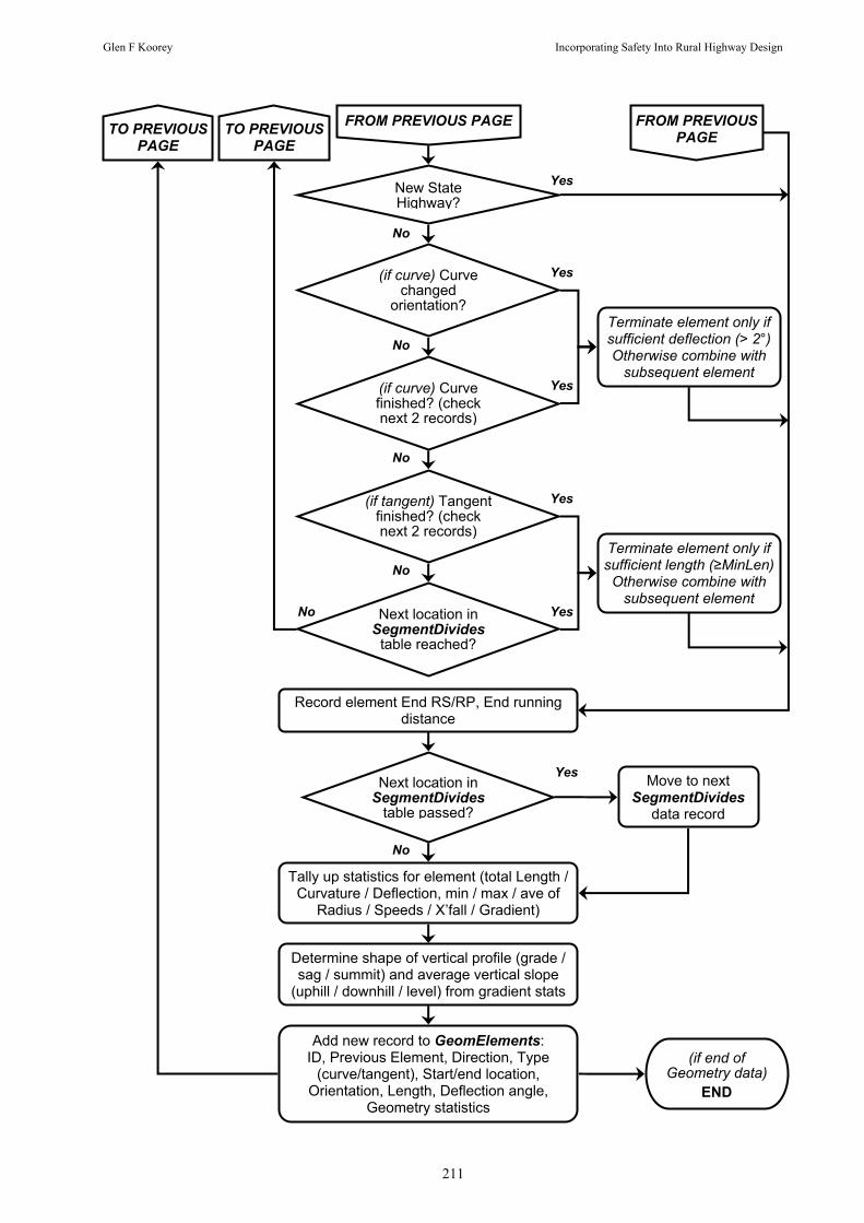
Glen F Koorey Incorporating Safety Into Rural Highway Design
211
(if curve) Curve changed
orientation?
Tally up statistics for element (total Length / Curvature / Deflection, min / max / ave of
Radius / Speeds / X’fall / Gradient)
Next location in SegmentDivides
table reached?
Add new record to GeomElements: ID, Previous Element, Direction, Type
(curve/tangent), Start/end location, Orientation, Length, Deflection angle,
Geometry statistics
Determine shape of vertical profile (grade / sag / summit) and average vertical slope
(uphill / downhill / level) from gradient stats
(if end of Geometry data)
END
Yes
Yes
No
No
Record element End RS/RP, End running distance
FROM PREVIOUS PAGETO PREVIOUS PAGE
(if curve) Curve finished? (check next 2 records)
(if tangent) Tangent finished? (check next 2 records)
Next location in SegmentDivides
table passed?
Move to next SegmentDivides
data record
FROM PREVIOUSPAGE
No
No
Yes
Yes
Yes
TO PREVIOUS PAGE
No
New State Highway?
Yes
No
Terminate element only if sufficient deflection (> 2°)Otherwise combine with
subsequent element
Terminate element only if sufficient length (≥MinLen)Otherwise combine with
subsequent element

Glen F Koorey Incorporating Safety Into Rural Highway Design
212
A.6 Detailed IHSDM Calibration Process and Example of Calibration Spreadsheet
Database Processing Steps to generate IHSDM calibration factors
1. Open the TNZ-AADT-Factors table and enter the appropriate AADT scaling factor for the
selected time period in the “BaseFactor” field of the “Base” row. For example, for the 1996-
2000 analysis period select the mid-point value from the 1998 row, i.e. 0.927. Also enter the
year in the “Comment” field (i.e. “1998” in the above example).
2. Select the crashes to use for the calibration factors, in terms of time period, SH/local,
midblock/intersection, injury/non-injury. A variety of queries are available to select or
deselect the required data, e.g. AxIncludeAll, AxExcludeLocal, AxInclude1996-00.
3. Select the road elements to use for the calibration factors, in terms of traffic volume, region,
terrain and number of lanes. A variety of queries are available to select or deselect the
required data, e.g. ElemExcludeAll, ElemInclude3Lane, ElemIncludeRegn09Wgtn,
ElemIncludeTerrFlat.
4. Take a new copy of the standard IHSDM spreadsheet CPM_Segment_Calibration.xls to
use for the calibration calculations and save it with an appropriate name, e.g.
CPM_Segment_Calibration-96-00-3Lane.xls.
5. Run the CPM-TotalAxBySev query to determine the split of crashes by severity, and copy
the values onto the Readme tab of the spreadsheet for information.
6. Run the CPM-TotalAxByIhsdmType query to determine the split of crashes by IHSDM
crash type, and copy the values onto the Readme tab of the spreadsheet for information.
7. Run the CPM1-AADT-Curv-Miles query to determine statistics for curved and tangent
elements by traffic volume, and copy the values into Table 3 of the Level1 tab of the
spreadsheet.
8. Run the CPM1-Gradient-Miles query to determine statistics for level and gradient elements
by traffic volume, and copy the values into Table 4 of the Level1 tab of the spreadsheet.
9. Run the CPM1-AADT-Miles query to determine mileage and cross-section statistics by
traffic volume, and copy the values into Tables 5 and 9 of the Level1 tab of the spreadsheet.
10. Run the CPM1-Terrain-Miles query to determine the total mileage by terrain, and copy the
values into Table 6 of the Level1 tab of the spreadsheet.

Glen F Koorey Incorporating Safety Into Rural Highway Design
213
11. Check that the default parameter values in Table 8 of the spreadsheet are appropriate.
Generally the key assumptions are: average Roadside Hazard Rating = 4, average driveway
density = 3 / mile, no passing-lane or four-lane sections.
12. Enter the number of crashes and the number of crash years into Table 12 of the spreadsheet.
Click the Generate button to calculate the appropriate calibration scaling factor, Cr.
(An example of the resulting Level 1 spreadsheet calculations are shown after these instructions)
13. Open the IHSDM Administration Tool and copy the calibration values for scaling factor,
crash severity proportions, and crash type proportions into a Crash Prediction calibration data
set. Save with an appropriate name and it can now be selected for CPM use in IHSDM.
14. Repeat the process for the Level 2 calibration, by running the CPM2-AADT-Curv-Miles,
CPM2-Gradient-Miles, CPM2-AADT-Miles and CPM1-Terrain-Miles queries and copying
the values into the Level2 tab of the spreadsheet. Enter the appropriate values into Tables 8
and 12 and click the Generate button to calculate the appropriate calibration scaling factor.
Further subsets of road and crash data can be selected using the same database procedures and
additional spreadsheets created to calculate the appropriate calibration values for these.

Glen F Koorey Incorporating Safety Into Rural Highway Design
214
Example of CPM (level 1) calibration spreadsheet data - all 1996-2000 SH crashes in NZ
For doing Level 1 calibration for highway segments the State/Agency must have the ability to:(1) Stratify all two-lane rural roads by ADT; and(2) Identify all non-intersection related accidents reported on those two lane rural roads.
Instructions for using the spreadsheet:
Follow the instructions below to calculate the CPM calibration factor for highway segments from Level 1 data (Steps described in the text boxes are from the CPM Engineer's Manual and are for information only).
(1) Fill out "Estimated miles of paved, two-lane rural highways" for the five ADT groups in Table 5 below (Replace the test case numbers that are in RED).
(2) Fill out "Proportion of paved, two-lane rural highways (percentage)" in Table 6 below (Replace the test case numbers that are in RED).
(3) If the "Number of Tangent Miles", "Number of Curved Miles", "Average Degree of Curvature for Curved Miles" and "Average Length of Curve" for each ADT group are available, fill-in the corresponding columns in Table 3 below (auto-generated numbers are in PINK). If these data are not available but the "Weighted Average Curve Length" values (see Table 7) are available, then fill out Table 7 and push the "Auto Generate" button in Table 3 (default numbers are in PINK). If neither the data for Table 3 nor Table 7 are available, then press the "Auto Generate" button in Table 3 to produce estimates based on data entered in Tables 5 and 6, according to the rules documented in the CPM Engineer's Manual.
(4) If the "Number of Level Miles", "Number of Miles on Grade" and "Average Percent Grade for Miles on Grade" for each ADT group are available, fill-in the corresponding columns in Table 4 below (auto-generated numbers are in PINK). If these data are not available, then press the "Auto Generate" button in Table 4 to produce estimates based on data entered in Tables 5 and 6, according to the rules documented in the CPM Engineer's Manual.
(5) Review the values in Tables 8 and 9. These are the default/recommended values to be used in the model. If you prefer to use different values, replace the recommended values with your values. (recommended values are in PINK).
Note 1: If any of the mileages or ADT Mean Value is 0, enter a very small number (such as 0.01) rather than zero.Note 2: Pressing the "Auto Generate" buttons in Tables 3, 4, 7, 8, and 9 brings back the default/recommended values in these tables.
(6) Go to Table 10 and push the "Calculate" button at the bottom of this table. The program will automatically calculate the predicted number of non-intersection-related crashes per year for the five ADT intervals in Table 9. The predicted crashes for tangents and curves for each ADT interval are stored in Table 11, columns E and F. The total predicted crashes are shown in column G. The total for all ADT ranges is stored in cell G102.
(7) In Table 12, enter the number of years for which crash data are available in cell C107, and the number of actual recorded crashes in cell E107 (if the number of years is more than 10 the table should be modified).
The value in cell E119 in Table 12 is the calculated calibration factor for highway segments (Cr). This represents the ratio of actual recorded crashes to predicted crashes. The calibration factor can be entered into IHSDM via the AdminTool.
Step 1. Develop Estimates of Paved Rural Two-Lane Highway Mileage by Curve and Grade. The State will first need to estimate the following for all paved rural, two-lane highways in the State for each of five ADT groups:· Number of miles of tangent roadway.· Number of miles of roadway on horizontal curves.· Average degree of curvature for horizontal curves.· Number of miles of level roadway.· Number of miles of roadway on grade.· Average grade percent for roadway on grade.

Glen F Koorey Incorporating Safety Into Rural Highway Design
215
Total Mileage 5502 Step 1, A: For States with Alignment (Curve and Grade) Inventory Files Table 1. Horizontal Alignment Defaults from
HSIS Data Table 2. Vertical Alignment Defaults from HSIS Data
% of Non-tangent Miles Avg. Degree of Curve % of Non-flat
Miles Avg. Grade %
Flat 19 2 Flat 87 1.5 Rolling 24 4 Rolling 91 2.0 Mountainous 38 8 Mountainous 97 3.7 Table 3. Estimate Mileage by ADT Level and Horizontal Alignment
ADT Interval Number of Tangent Miles
Number of Curved Miles
Average Degree of Curvature for Curved Miles (D)
Average Radius of Horizontal
Curvea
Average Length of Curve (mi)
< 1000 1110.30 791.72 7.61 752 0.0849 1,001 - 3,000 1261.74 790.73 7.08 809 0.0929 3,001 - 5,000 581.99 239.95 5.55 1032 0.1011 5,001 - 10,000 402.98 144.22 4.76 1204 0.1002 > 10,000 125.83 52.64 4.01 1430 0.0954
3482.85 2019.26 Table 4. Estimate Mileage by ADT Level and Vertical Alignment
ADT Interval Number of Level Miles
(Ml)
Number of Miles on Grade (Mg)
Average Percent Grade for Miles on Grade (Pg)
Average Percent Gradea
< 1000 625.96 1276.06 4.03 2.70 1,001 - 3,000 860.28 1192.20 3.91 2.27 3,001 - 5,000 404.56 417.38 3.58 1.82 5,001 - 10,000 291.69 255.52 3.07 1.43 > 10,000 95.47 83.00 3.32 1.55
2277.95 3224.16 Step 1, B: For States without Alignment (Curve and Grade) Inventory Files Table 5. Estimate Mileage by ADT Interval Table 6. Estimate Proportion of Mileage by Terrain
ADT Interval Estimated miles of paved, two-lane rural highways Terrain Proportion of paved, two-lane
rural highways (percentage) < 1000 1902.02 Flat 41.4 1001 - 3000 2052.47 Rolling 42.1 3001 - 5000 821.94 Mountainous 16.5 5001 - 10000 547.21 Total 100.0 > 10000 178.46 5502.11
Table 7. Weighted Average Curve Length from MI and WA Data
Calculated Average Length of Curve for the following Average Degree of curve
Degree of Weighted Average Curve Length Curve Miles Feet Miles Feet
< 1000 2 0.184 974 0.0000 0 7.61 4 0.120 636 0.0000 0

Glen F Koorey Incorporating Safety Into Rural Highway Design
216
8 0.081 427 0.0847 447 1001 - 3000 2 0.184 974 0.0000 0 7.08
4 0.120 636 0.0000 0 8 0.081 427 0.0899 475
3001 - 5000 2 0.184 974 0.0000 0 5.55 4 0.120 636 0.0000 0 8 0.081 427 0.1051 555
5001 - 10000 2 0.184 974 0.0000 0 4.76 4 0.120 636 0.0000 0 8 0.081 427 0.1129 596
> 1000 2 0.184 974 0.0000 0 4.01 4 0.120 636 0.0000 0 8 0.081 427 0.1204 636
Step 2. Accept or Modify Default Values for Other Geometric Parameters Table 8. Default Values
Shoulder type (Paved/Gravel/Turf) Paved
Roadside Hazard Rating (RHR) 4 Driveway density (driveways/mi) 3 Presence of spiral transition curve(0/1/2) 0 Superelevation AMF (AMF4) 1 Passing lane (Yes/No) No Short four-lane section (Yes/No) No Two Way Left Turn Lane No Table 9. Default Values
ADT Interval (Vehicles/day) ADT Lane Width Shoulder Width
(vehicles/day) (ft) (ft) < 1000 595 10.9 0.5 1,001 - 3,000 1726 11.4 1.8 3,001 - 5,000 4037 11.4 3.7 5,001 - 10,000 6656 11.5 4.9 > 10,000 13978 11.4 6.2
Step 3. Calculate Estimate of Annual Non-Intersection Accidents Using the Accident Prediction Algorithm Table 10. Effective values for single ADT Groups and calculated predicted number of crashes
ADT Group 5 Mileage for Tangents
Mileage for Curves
Prediction from Level1-
Tangents
Prediction from Level1-Curves
ADT 13977.56524 125.826404 52.638564 425.8 245.7 Lane Width 11.41026384
Shoulder Width 6.173925069 Length of horizontal curve (mi) 0.095360 Radius of horizontal curve (ft) 1430
Percent Grade 1.55 Table 11. Final values for ADT Groups and calculated predicted number of crashes
ADT Interval (Vehicles/day)
Mileage of rural two lane highways Predicted number of
non-intersection accident per year** Tangent Curve Total Tangent Curve Total

Glen F Koorey Incorporating Safety Into Rural Highway Design
217
< 1000 1110.301049 791.720149 1902.021198 157.5 203.3 361 1,001 - 3,000 1261.741954 790.731964 2052.473918 553.7 585.9 1140 3,001 - 5,000 581.994974 239.946234 821.941208 577.4 356.1 933 5,001 - 10,000 402.984329 144.222804 547.207133 648.0 331.4 979
> 10,000 125.826404 52.638564 178.464968 425.8 245.7 671 2362 1722 4085
Step 4. Determine Actual Annual Non-Intersection Accidents from State Data for the Last Three Years Table 12. Calibration Factor calculation
Recorded crashes for years 5 years 18052 Year 1 predicted crashes 4085 Year 2 predicted crashes 4085 Year 3 predicted crashes 4085 Year 4 predicted crashes 4085 Year 5 predicted crashes 4085 Year 6 predicted crashes 0 Year 7 predicted crashes 0 Year 8 predicted crashes 0 Year 9 predicted crashes 0 Year 10 predicted crashes 0 Total 20423.9
Ratio (Calculated Calibration Factor Cr for segments) 0.884
Note: The CPM (level 2) calibration spreadsheet is similar but more detailed, breaking down the
horizontal/vertical geometry data (Tables 3 & 4) and AADT/mileage data (Tables 5 & 9) into 80
subsets with combinations of three attributes:
• AADT: <1000 vpd, 1000-3000 vpd, 3000-5000 vpd, 5000-10,000 vpd, >10,000 vpd
• Traffic lane width: <9.5 ft, 9.5-10.5 ft, 10.5-11.5 ft, >11.5 ft
• Shoulder width: <3 ft, 3-5 ft, 5-7 ft, >7 ft

Glen F Koorey Incorporating Safety Into Rural Highway Design
218
A.7 Statistical Analysis of IHSDM Calibration Factors
Pearson Chi-square (χ2) Tests
This is a goodness-of-fit test, which tests a null hypothesis that the frequency distribution of
certain events observed in a sample is consistent with a particular theoretical distribution. A
common case for this is where the events each cover an outcome of a categorical variable. The
chi-square statistic for this test is calculated by finding the difference between each observed and
theoretical frequency for each possible outcome, squaring them, dividing each by the theoretical
frequency, and taking the sum of the results:
( )∑=
−=
n
i i
ii
EEOX
1
22
where
X 2 = the test statistic (which asymptotically approaches a χ2 distribution) Oi = an observed frequency for each category i Ei = an expected (theoretical) frequency, asserted by the null hypothesis n = the number of possible outcomes/categories of each event
The chi-square statistic can then be used to calculate a p-value20 by comparing the value of the
statistic to a chi-square distribution (with the number of degrees of freedom equal to the number
of possible outcomes/categories minus 1).
In this study, the test made is to compare the observed number of crashes in each category (e.g.
number of lanes, traffic volume band) with the expected number of crashes from IHSDM if the
same calibration factor was used for all categories (scaled to produce the same total number of
crashes as that observed). The null hypothesis is that these two distributions are consistent, i.e.
the same calibration factor can be used for all categories.
The following table summarises the results across the different categories. Two minor
adjustments to the IHSDM predicted numbers have been made, as discussed in Section 5.2.5:
• The “three-lane” value has been increased to allow for a 10% reduction in crashes rather than
the predicted 25% crash reduction factor.
• The “>10000 vpd” value has been reduced by 10% to account for the higher proportion of
4-lane sections (which have a 35% crash reduction factor) in this group.
20 The probability of obtaining a result at least as extreme as the one that was actually observed, given that the null hypothesis is true, i.e. in this case, the probability that the result happened by chance. For most practical purposes, generally if the p-value is smaller than 0.05 (5% significance level) then the null hypothesis is rejected.

Glen F Koorey Incorporating Safety Into Rural Highway Design
219
Chi-square tests (1996-2000 crash data, Level 1 calibration factors only): Category Observed Accs Predicted Accs Calibr'n Factor Expected Accs X2 Value
(* = adjusted value) O (IHSDM) P C = O / P E = P × C’ = (O-E)2/E Overall 1996-2000 18052 20423.9 0.884 (provided for comparison only) Number of Lanes: 2-Lanes 16465 18453.0 0.892 16504.1 0.093 3-Lanes* 1401 1520.2* 0.922 1359.6 1.260 4-Lanes 134 152.4 0.879 136.3 0.039 (1-Lane not included) 18000 20125.6 C’ = 0.894 18000 1.392
P(diff by chance) 0.4987 (2 d.o.f.) Traffic Volumes: AADT1: <1000 1987 1799.1 1.104 1621.6 82.333 AADT2: 1000-3000 4936 5711.9 0.864 5148.4 8.762 AADT3: 3000-5000 4244 4659.6 0.911 4199.9 0.463 AADT4: 5000-10000 4405 4851.0 0.908 4372.4 0.243 AADT5: >10000* 2480 3006.3* 0.825 2709.7 19.469 18052 20027.9 C’ = 0.901 18052 111.269 P(diff by chance) 0.0000 (4 d.o.f.) Terrain: Flat 7469 8863.0 0.843 7851.6 18.646 Rolling 7247 7866.7 0.921 6969.0 11.089 Mountainous 3336 3647.6 0.915 3231.4 3.388 18052 20377.3 C’ = 0.886 18052 33.123 P(diff by chance) 0.0000 (2 d.o.f.) Region: Northland (above ave) 1379 1509.1 0.914 1239.1 15.785 Waikato (average) 3757 4747.1 0.791 3897.9 5.094 Otago (below ave) 1282 1560.0 0.822 1280.9 0.001
(not all regions 6418 7816.2 C’ = 0.821 6418 20.880 Included) P(diff by chance) 0.0000 (2 d.o.f.)
It can be seen that generally the tests reject the null hypothesis at any practical level of
significance, i.e. it is not considered true that the same calibration factor can be applied to
crashes in each category. The one exception is by number of lanes; however this result is very
sensitive to the adjustment applied to the 3-lane category (e.g. changing the reduction to 15%
instead of 10% reduces the p-value to 0.005). In the case of the traffic volume categories, it can
be seen that the bulk of the difference (in terms of X2 values) is at the high and low ends (despite
the adjustment to the “>10000 vpd” crash numbers). There also appears to be region-specific
effects, with some regions being notably different than expected, while others are quite
comparable (a similar effect was also found in the analysis in Section 6.3).
It may be that, because of the large crash numbers being used here, the statistical power of this
test makes it difficult not to reject the null hypothesis. A smaller site-by-site comparison could
be a more realistic test, but the practicalities of undertaking this on 40,000 road segments in the
database preclude this from being done easily.

Glen F Koorey Incorporating Safety Into Rural Highway Design
220
It would be useful to undertake some tests that compare each sub-category with the calibration
factor for the whole data-set, to see whether only some sub-categories might need a special
calibration factor applied to them. Generally to do this, the variation in the crash numbers needs
to be taken account of, so that the expected variation in the calibration factors can be determined.
In this case, the observed crash numbers for each year over the five-year analysis period have
been separately extracted so that some basic descriptive statistics can be derived. The following
table summarises the data: Observed Accidents Category 1996 1997 1998 1999 2000 Total Mean StdDev Var’nce Var/Mn Overall 1996-2000 3943 3491 3471 3690 3457 18052 3610.4 208.7 43545 12.1 Number of Lanes: 2-Lanes 3557 3202 3160 3377 3169 16465 3293.0 171.8 29525 9.0 3-Lanes 354 253 279 281 234 1401 280.2 45.61 2081 7.4 4-Lanes 25 23 23 24 39 134 26.8 6.87 47.2 1.8 3936 3478 3462 3682 3442 18000 3600.0 211.3 44628 12.4 Traffic Volumes: AADT1: <1000 400 404 367 389 427 1987 397.4 21.92 480.3 1.2 AADT2: 1000-3000 986 947 920 1028 1055 4936 987.2 55.67 3099 3.1 AADT3: 3000-5000 963 827 812 848 794 4244 848.8 66.85 4469 5.3 AADT4: 5000-10000 1038 829 861 934 743 4405 881.0 111.4 12402 14.1 AADT5: >10000 556 484 511 491 438 2480 496.0 42.89 1840 3.7 3943 3491 3471 3690 3457 18052 3610.4 208.7 43545 12.1 Terrain: Flat 1608 1465 1448 1498 1450 7469 1493.8 66.9 4476 3.0 Rolling 1595 1371 1411 1516 1354 7247 1449.4 102.9 10589 7.3 Mountainous 740 655 612 676 653 3336 667.2 46.84 2194 3.3 3943 3491 3471 3690 3457 18052 3610.4 208.7 43545 12.1 Region: Northland (above ave) 313 234 282 296 254 1379 275.8 31.83 1013 3.7 Waikato (average) 921 700 728 754 654 3757 751.4 101.8 10362 13.8 Otago (below ave) 268 250 238 243 283 1282 256.4 18.72 350.3 1.4 1502 1184 1248 1293 1191 6418 1283.6 130 16887 13.2
It is interesting to note that the coefficients of dispersion (variance/mean) for all data-sets are
greater than one (and often much greater), suggesting that a Poisson distribution would not be an
appropriate approximation in this case.
This data can now be used to produce a series of calibration factors for each year (based on
IHSDM’s predicted crash numbers), with associated descriptive statistics from which to
undertake comparison tests.

Glen F Koorey Incorporating Safety Into Rural Highway Design
221
Welch t-Tests
A t-test is any statistical hypothesis test in which the test statistic has a Student’s t-distribution if
the null hypothesis is true. It is applied when the population is assumed to be Normally
distributed but the sample sizes are small enough that the statistic on which inference is based is
not Normally distributed because it relies on an uncertain estimate of standard deviation. A t-test
is commonly used to test the null hypothesis that the means of two populations (each
characterised by its mean, standard deviation and number of data points) are equal. The standard
Student’s t-test assumes that the underlying distributions are Normal, and that the variances of
the two populations are also equal; the Welch's t-test variant is used when the latter assumption
is dropped.
Welch's t-test defines the statistic t by the following formula:
2
22
1
21
21
Ns
Ns
XXt
+
−=
where Xi, si 2 and Ni are the ith sample mean, sample variance and sample size, respectively. The
degrees of freedom ν associated with this variance estimate is approximated using the Welch-
Satterthwaite equation:
( ) ( )11 222
42
121
41
2
2
22
1
21
222
42
121
41
2
2
22
1
21
−⋅+
−⋅
⎟⎟⎠
⎞⎜⎜⎝
⎛+
=
⋅+
⋅
⎟⎟⎠
⎞⎜⎜⎝
⎛+
=
NNs
NNs
Ns
Ns
Ns
Ns
Ns
Ns
νν
ν
Once t and ν have been computed, these statistics can be used with the t-distribution to test the
null hypothesis that the two population means are equal (using a two-tailed test). In particular,
the test will yield a p-value that might give evidence sufficient to reject the null hypothesis.
For this study, Welch’s t-test will be used to test whether the mean of the overall 1996-2000
calibration factor is significantly different than the mean of the calibration factor for each sub-
category. The following table summarises the calculations; for each sub-category, the mean and
standard deviation (“St.Dev”) of the five yearly samples are calculated. The difference in means
with the overall ’96-’00 factor (“Diff”) is then statistically tested, using the above formulae to
determine a t value (“t-val”) and degrees of freedom ν (“d.o.f.”). The resulting p-value (“p-val”)
indicates the probability that the means differ by chance (i.e. they are not significantly different).
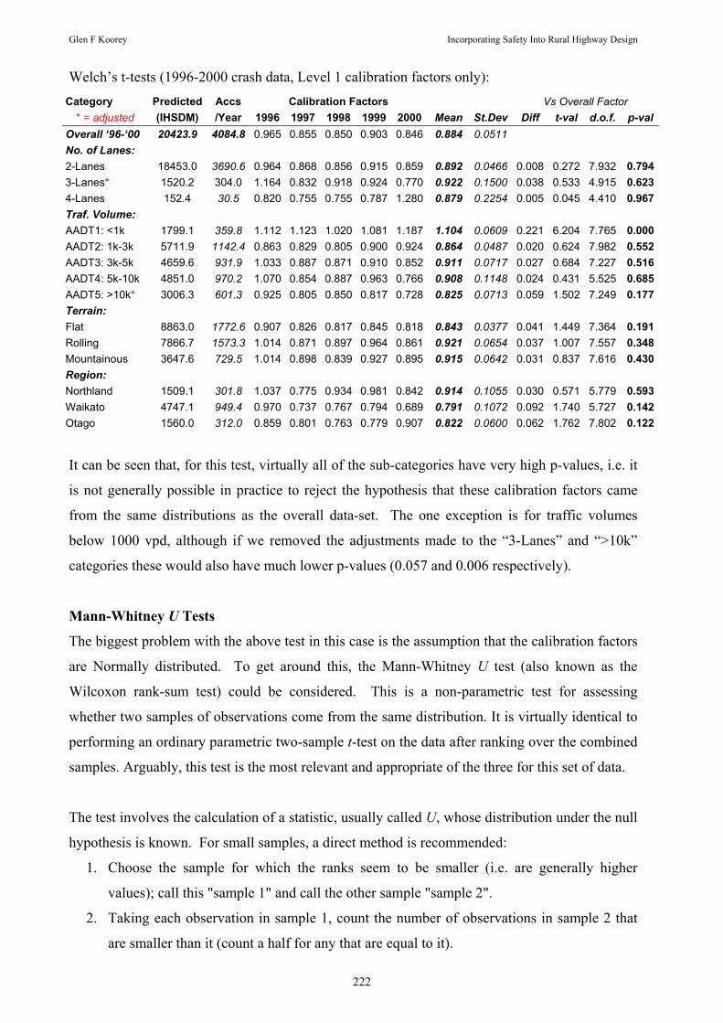
Glen F Koorey Incorporating Safety Into Rural Highway Design
222
Welch’s t-tests (1996-2000 crash data, Level 1 calibration factors only): Category Predicted Accs Calibration Factors Vs Overall Factor
* = adjusted (IHSDM) /Year 1996 1997 1998 1999 2000 Mean St.Dev Diff t-val d.o.f. p-val Overall ‘96-‘00 20423.9 4084.8 0.965 0.855 0.850 0.903 0.846 0.884 0.0511 No. of Lanes: 2-Lanes 18453.0 3690.6 0.964 0.868 0.856 0.915 0.859 0.892 0.0466 0.008 0.272 7.932 0.7943-Lanes* 1520.2 304.0 1.164 0.832 0.918 0.924 0.770 0.922 0.1500 0.038 0.533 4.915 0.6234-Lanes 152.4 30.5 0.820 0.755 0.755 0.787 1.280 0.879 0.2254 0.005 0.045 4.410 0.967Traf. Volume: AADT1: <1k 1799.1 359.8 1.112 1.123 1.020 1.081 1.187 1.104 0.0609 0.221 6.204 7.765 0.000AADT2: 1k-3k 5711.9 1142.4 0.863 0.829 0.805 0.900 0.924 0.864 0.0487 0.020 0.624 7.982 0.552AADT3: 3k-5k 4659.6 931.9 1.033 0.887 0.871 0.910 0.852 0.911 0.0717 0.027 0.684 7.227 0.516AADT4: 5k-10k 4851.0 970.2 1.070 0.854 0.887 0.963 0.766 0.908 0.1148 0.024 0.431 5.525 0.685AADT5: >10k* 3006.3 601.3 0.925 0.805 0.850 0.817 0.728 0.825 0.0713 0.059 1.502 7.249 0.177Terrain: Flat 8863.0 1772.6 0.907 0.826 0.817 0.845 0.818 0.843 0.0377 0.041 1.449 7.364 0.191Rolling 7866.7 1573.3 1.014 0.871 0.897 0.964 0.861 0.921 0.0654 0.037 1.007 7.557 0.348Mountainous 3647.6 729.5 1.014 0.898 0.839 0.927 0.895 0.915 0.0642 0.031 0.837 7.616 0.430Region: Northland 1509.1 301.8 1.037 0.775 0.934 0.981 0.842 0.914 0.1055 0.030 0.571 5.779 0.593Waikato 4747.1 949.4 0.970 0.737 0.767 0.794 0.689 0.791 0.1072 0.092 1.740 5.727 0.142Otago 1560.0 312.0 0.859 0.801 0.763 0.779 0.907 0.822 0.0600 0.062 1.762 7.802 0.122
It can be seen that, for this test, virtually all of the sub-categories have very high p-values, i.e. it
is not generally possible in practice to reject the hypothesis that these calibration factors came
from the same distributions as the overall data-set. The one exception is for traffic volumes
below 1000 vpd, although if we removed the adjustments made to the “3-Lanes” and “>10k”
categories these would also have much lower p-values (0.057 and 0.006 respectively).
Mann-Whitney U Tests
The biggest problem with the above test in this case is the assumption that the calibration factors
are Normally distributed. To get around this, the Mann-Whitney U test (also known as the
Wilcoxon rank-sum test) could be considered. This is a non-parametric test for assessing
whether two samples of observations come from the same distribution. It is virtually identical to
performing an ordinary parametric two-sample t-test on the data after ranking over the combined
samples. Arguably, this test is the most relevant and appropriate of the three for this set of data.
The test involves the calculation of a statistic, usually called U, whose distribution under the null
hypothesis is known. For small samples, a direct method is recommended:
1. Choose the sample for which the ranks seem to be smaller (i.e. are generally higher
values); call this "sample 1" and call the other sample "sample 2".
2. Taking each observation in sample 1, count the number of observations in sample 2 that
are smaller than it (count a half for any that are equal to it).

Glen F Koorey Incorporating Safety Into Rural Highway Design
223
3. The total of these counts is U.
The maximum possible value of U is the product of the sample sizes for the two samples, while
the expected value (if the two distributions are exactly equal) is half this value.
The U-value can then be tested to see whether it is significantly different than the expected
value. For large samples, the normal approximation:
z = (U - mU - 0.5) / σU
can be used, where z is a standard normal deviate whose significance can be checked in tables of
the normal distribution. mU and σU are the mean and standard deviation of U if the null
hypothesis is true, and are given by
221 nnmU ⋅=
( )12
12121 ++=
nnnnUσ
The table below summarises the resulting calculations. After ordering the calibration factors in
each case, the U statistic is determined (“U-val”) and the corresponding z statistic (“z-val”)
computed. The resulting p-value (“p-val”) indicates the probability that the means differ by
chance (i.e. they are not significantly different).
Mann-Whitney U-tests (1996-2000 crash data, Level 1 calibration factors only):
n1 = n2 = 5 mU= 12.5 σU= 4.79 Vs Overall Factor Category Calibration Factors (ordered) Mean U-val U - mU z-val p-val
Overall 1996-2000 0.846 0.850 0.855 0.903 0.965 0.884 Number of Lanes: 2-Lanes 0.856 0.859 0.868 0.915 0.964 0.892 17 4.5 0.836 0.202 3-Lanes* 0.770 0.832 0.918 0.924 1.164 0.922 13 0.5 0.000 0.500 4-Lanes 0.755 0.755 0.787 0.820 1.280 0.879 18 5.5 1.044 0.148 Traffic Volume: AADT1: <1k 1.020 1.081 1.112 1.123 1.187 1.104 24 11.5 2.298 0.011 AADT2: 1k-3k 0.805 0.829 0.863 0.900 0.924 0.864 19 6.5 1.253 0.105 AADT3: 3k-5k 0.852 0.871 0.887 0.910 1.033 0.911 17 4.5 0.836 0.202 AADT4: 5k-10k 0.766 0.854 0.887 0.963 1.070 0.908 17 4.5 0.836 0.202 AADT5: >10k* 0.728 0.805 0.817 0.850 0.925 0.825 19.5 7 1.358 0.087 Terrain: Flat 0.817 0.818 0.826 0.845 0.907 0.843 19.5 7 1.358 0.087 Rolling 0.861 0.871 0.897 0.964 1.014 0.921 18 5.5 1.044 0.148 Mountainous 0.839 0.895 0.898 0.927 1.014 0.915 15 2.5 0.418 0.338 Region: Northland 0.775 0.842 0.934 0.981 1.037 0.914 14 1.5 0.209 0.417 Waikato 0.689 0.737 0.767 0.794 0.970 0.791 20 7.5 1.462 0.072 Otago 0.763 0.779 0.801 0.859 0.907 0.822 22 9.5 1.880 0.030

Glen F Koorey Incorporating Safety Into Rural Highway Design
224
This time the results are not as conclusive as the t-tests, although still generally not rejecting the
hypothesis that these calibration factors came from the same distributions as the overall data-set.
Again, the low/high traffic volume bands show strong tendencies to depart from the overall data,
as do some of the regional sub-sets.
In summary, the results generally tend to support the desire to maintain the same overall IHSDM
calibration factor for virtually all situations. However, some caution needs to be taken when
dealing with rural road sections with particularly low (<1000 vpd) or particularly high
(>10,000 vpd) traffic volumes. The results may also not be as accurate in some regions of the
country.
Even here there are two factors that will assist the use of a common calibration factor:
• The use of local crash history data in IHSDM will help to further refine the crash estimates in
the same way that a localised calibration factor might.
• From a practical application context, it is not clear whether these statistical tests (which
combine crash numbers over the entire data-set) are that useful. For example, on a road
section with (say) <5 crashes, a calibration factor of 0.88 versus 0.84 will not produce a large
difference in the predicted number of crashes.

Glen F Koorey Incorporating Safety Into Rural Highway Design
225
A.8 Typical IHSDM XML Import Files
Road Alignment Data Import File (old SH1 HSF alignment)
Notes: • Station values are given in metres from the start of the highway, e.g. 193 900. • Each database geometric element generates individual XML tags for traffic lane
(“ThruLane”), shoulder (“ShoulderSection”), traffic volume (“AnnualAveDailyTraffic”), horizontal alignment (“HTangent” or “HSimpleCurve”) and vertical alignment (“VPI” or “VTangent”).
• Where necessary, additional tags are also created for 3-lane or 4-lane road segments. • Default values for the entire highway section are given by the program for speed limit,
desired speed, road class and roadside hazard rating. <?xml version="1.0" encoding="ISO-8859-1"?> <!-- ++++++++++++++++++++++++++++++++++++++++++++++++++++++++++++++++++++ + Interactive Highway Safety Design Model (IHSDM) + + www.ihsdm.org + + (IHSDM 2007 Release v4.0.5 (Mar 05, 2008)) + + (Packaged: Mar 07, 2008 (09:01)) + + Developed for + + Federal Highway Administration (FHWA) + + Network Export Data Set + + (Generated from MakeIHSDM() VB function) + + (Version: 1.1 Date: Tue Dec 02 2008 by G.Koorey) + ++++++++++++++++++++++++++++++++++++++++++++++++++++++++++++++++++++ + Network export from Thesis-RAMM-Data.mdb database + + Created: Sun Dec 07 2008 12:28:36 NZDT + + by: Glen Koorey ([email protected], +64-3-3642951) + ++++++++++++++++++++++++++++++++++++++++++++++++++++++++++++++++++++ --> <NetworkExport xmlns="http://www.ihsdm.org/schema/NetworkExport-1.0" version="2.0" vxVersionDate="Mar 5, 2008" vxFullID="IHSDM 2007 Release, v4.0.5 (Mar 05, 2008)" vxShortID="v4.0.5 (Mar 05, 2008)" vxRelease="IHSDM 2007 Release" vxVersionNum="4.0.5" datasetUnitSystem="metric" > <Roadway title="SH1SO (HSF old alignment)" comment="Basic highway alignment details" versionComment="Created with Access VB routine MakeIHSDM()" minStation="193900" maxStation="215440" headingSta="193900" headingAngle="0" coordSta="193900" coordX="0.0" coordY="0.0" elevSta="193900" elevHeight="0" > <PostedSpeed startStation="193900" endStation="215440" sideOfRoad="both" speedLimit="100.00" /> <RDesiredSpeed startStation="193900" endStation="215440" dcmDesiredSpeed="105.00" /> <FunctionalClass startStation="193900" endStation="215440" funcClass="arterial" /> <RoadsideHazardRating startStation="193900" endStation="215440" hazardRating="4" /> <ThruLane startStation="193900" endStation="194070" sideOfRoad="both" width="3.50" /> <ShoulderSection startStation="193900" endStation="194070"

Glen F Koorey Incorporating Safety Into Rural Highway Design
226
sideOfRoad="both" startSlope = "-3.00" endSlope = "-3.00" startWidth = "0.75" endWidth="0.75" material="paved" priority="1" />
<AnnualAveDailyTraffic startStation="193900" endStation="194070" adtYear="1996" adtRate = "1653" adtGrowth = "3.500" /> <DesignSpeed startStation="193900" endStation="194070" designSpeed="88.1" /> <ThruLane startStation="194070" endStation="194250" sideOfRoad="both" width="3.50" /> <ShoulderSection startStation="194070" endStation="194250" sideOfRoad="both" startSlope = "-3.00" endSlope = "-3.00" startWidth = "0.75" endWidth="0.75" material="paved" priority="1" />
<AnnualAveDailyTraffic startStation="194070" endStation="194250" adtYear="1996" adtRate = "1653" adtGrowth = "3.500" /> <DesignSpeed startStation="194070" endStation="194250" designSpeed="78.9" /> <ThruLane startStation="194250" endStation="194420" sideOfRoad="both" width="3.50" /> <ShoulderSection startStation="194250" endStation="194420" sideOfRoad="both" startSlope = "-3.00" endSlope = "-3.00" startWidth = "0.75" endWidth="0.75" material="paved" priority="1" />
<AnnualAveDailyTraffic startStation="194250" endStation="194420" adtYear="1996" adtRate = "1653" adtGrowth = "3.500" /> <DesignSpeed startStation="194250" endStation="194420" designSpeed="60.7" /> : (etc) : <ThruLane startStation="212170" endStation="215440" sideOfRoad="both" width="3.50" /> <ShoulderSection startStation="212170" endStation="215440" sideOfRoad="both" startSlope = "-3.00" endSlope = "-3.00" startWidth = "0.50" endWidth="0.50" material="paved" priority="1" />
<AnnualAveDailyTraffic startStation="212170" endStation="215440" adtYear="1996" adtRate = "1653" adtGrowth = "3.500" /> <DesignSpeed startStation="212170" endStation="215440" designSpeed="101.0" /> <CrossSlope station="0.0" sideOfRoad="both" crossSlope="-3.0000" crossSlopeCode="ncs" /> <DrivewayDensity startStation="193900.0" endStation="215440.0" density="2.0000" /> <Bridge startStation="202840.0" endStation="202850.0" width="5.70000000" projectType="existing" /> <Bridge startStation="208520.0" endStation="208540.0" width="6.10000000" projectType="existing" /> <HorizontalElements > <HTangent startStation="193900" endStation="194070" /> <HSimpleCurve startStation="194070" endStation="194250" radius="723" curveDirection="left" /> <HSimpleCurve startStation="194250" endStation="194420" radius="171" curveDirection="right" /> <HTangent startStation="194420" endStation="194590" /> : (etc) : <HSimpleCurve startStation="211690" endStation="212170" radius="477" curveDirection="left" /> <HTangent startStation="212170" endStation="215440" /> </HorizontalElements> <VerticalElements >

Glen F Koorey Incorporating Safety Into Rural Highway Design
227
<VPI station="193985" backGrade="2.6" backLength="85" forwardGrade="8.2" forwardLength="85" /> <VPI station="194160" backGrade="8.6" backLength="90" forwardGrade="1.2" forwardLength="90" /> <VPI station="194335" backGrade="0.4" backLength="85" forwardGrade="-3.7" forwardLength="85" /> : (etc) : <VTangent startStation="211690" endStation="212170" grade="0.6" /> <VTangent startStation="212170" endStation="215440" grade="1.3" /> </VerticalElements> </Roadway> </NetworkExport>

Glen F Koorey Incorporating Safety Into Rural Highway Design
228
IHSDM Crash Data Import File (1994-2000 crashes on old SH1 HSF alignment)
Notes: • No intersection crashes are present in this section. • Station values are given in metres from the start of the highway, e.g. 193 900. • Crashes are either fatal/injury (“fi”) or property-damage-only (“pdo”).
<?xml version="1.0" encoding="ISO-8859-1"?> <!-- ++++++++++++++++++++++++++++++++++++++++++++++++++++++++ + Interactive Highway Safety Design Model (IHSDM) + + www.ihsdm.org + + (IHSDM 2007 Release v4.0.5 (Mar 05, 2008)) + + (Packaged: Mar 07, 2008 (09:01)) + + Developed for + + Federal Highway Administration (FHWA) + + Crash Data File + + (Generated from MakeIHSDMCrash() VB function) + + (Version: 1.1 Date: Tue Dec 02 2008 by G.Koorey) + ++++++++++++++++++++++++++++++++++++++++++++++++++++++++ + Network export from Thesis-RAMM-Data.mdb database + + File written: Fri Dec 05 2008 00:16:56 NZDT + + by: Glen Koorey ([email protected]) + ++++++++++++++++++++++++++++++++++++++++++++++++++++++++ --> <CrashData datasetUnitSystem="metric" > <Crash year="1997" station="201850" severity="pdo" intersectionRelated="false" /> <Crash year="1998" station="201880" severity="fi" intersectionRelated="false" /> <Crash year="1994" station="201880" severity="fi" intersectionRelated="false" /> : (etc) : <Crash year="1995" station="210350" severity="fi" intersectionRelated="false" /> <Crash year="1994" station="211220" severity="fi" intersectionRelated="false" /> </CrashData>
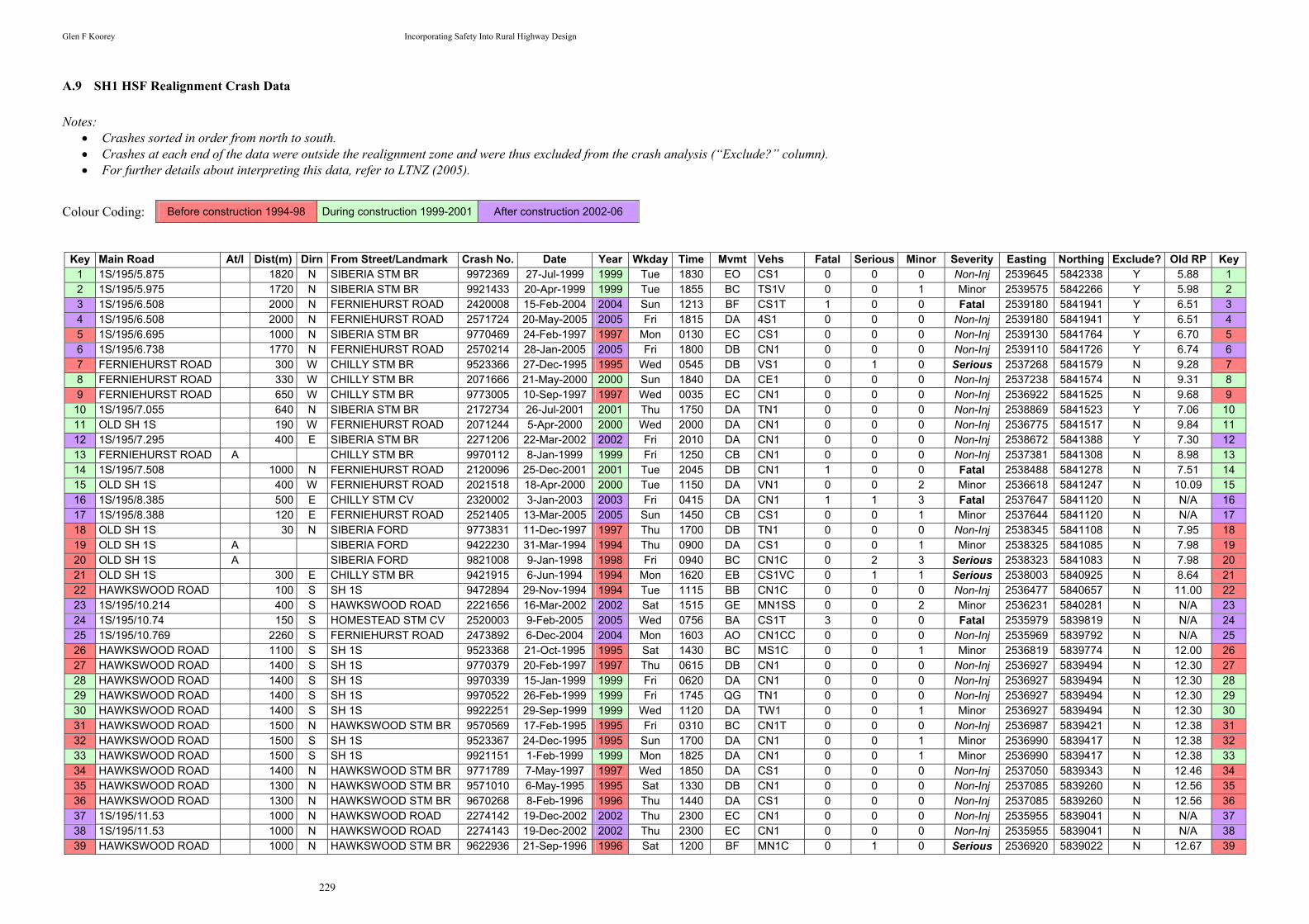
Glen F Koorey Incorporating Safety Into Rural Highway Design
229
A.9 SH1 HSF Realignment Crash Data
Notes: • Crashes sorted in order from north to south. • Crashes at each end of the data were outside the realignment zone and were thus excluded from the crash analysis (“Exclude?” column). • For further details about interpreting this data, refer to LTNZ (2005).
Colour Coding: Before construction 1994-98 During construction 1999-2001 After construction 2002-06
Key Main Road At/I Dist(m) Dirn From Street/Landmark Crash No. Date Year Wkday Time Mvmt Vehs Fatal Serious Minor Severity Easting Northing Exclude? Old RP Key
1 1S/195/5.875 1820 N SIBERIA STM BR 9972369 27-Jul-1999 1999 Tue 1830 EO CS1 0 0 0 Non-Inj 2539645 5842338 Y 5.88 1 2 1S/195/5.975 1720 N SIBERIA STM BR 9921433 20-Apr-1999 1999 Tue 1855 BC TS1V 0 0 1 Minor 2539575 5842266 Y 5.98 2 3 1S/195/6.508 2000 N FERNIEHURST ROAD 2420008 15-Feb-2004 2004 Sun 1213 BF CS1T 1 0 0 Fatal 2539180 5841941 Y 6.51 3 4 1S/195/6.508 2000 N FERNIEHURST ROAD 2571724 20-May-2005 2005 Fri 1815 DA 4S1 0 0 0 Non-Inj 2539180 5841941 Y 6.51 4 5 1S/195/6.695 1000 N SIBERIA STM BR 9770469 24-Feb-1997 1997 Mon 0130 EC CS1 0 0 0 Non-Inj 2539130 5841764 Y 6.70 5 6 1S/195/6.738 1770 N FERNIEHURST ROAD 2570214 28-Jan-2005 2005 Fri 1800 DB CN1 0 0 0 Non-Inj 2539110 5841726 Y 6.74 6 7 FERNIEHURST ROAD 300 W CHILLY STM BR 9523366 27-Dec-1995 1995 Wed 0545 DB VS1 0 1 0 Serious 2537268 5841579 N 9.28 7 8 FERNIEHURST ROAD 330 W CHILLY STM BR 2071666 21-May-2000 2000 Sun 1840 DA CE1 0 0 0 Non-Inj 2537238 5841574 N 9.31 8 9 FERNIEHURST ROAD 650 W CHILLY STM BR 9773005 10-Sep-1997 1997 Wed 0035 EC CN1 0 0 0 Non-Inj 2536922 5841525 N 9.68 9
10 1S/195/7.055 640 N SIBERIA STM BR 2172734 26-Jul-2001 2001 Thu 1750 DA TN1 0 0 0 Non-Inj 2538869 5841523 Y 7.06 10 11 OLD SH 1S 190 W FERNIEHURST ROAD 2071244 5-Apr-2000 2000 Wed 2000 DA CN1 0 0 0 Non-Inj 2536775 5841517 N 9.84 11 12 1S/195/7.295 400 E SIBERIA STM BR 2271206 22-Mar-2002 2002 Fri 2010 DA CN1 0 0 0 Non-Inj 2538672 5841388 Y 7.30 12 13 FERNIEHURST ROAD A CHILLY STM BR 9970112 8-Jan-1999 1999 Fri 1250 CB CN1 0 0 0 Non-Inj 2537381 5841308 N 8.98 13 14 1S/195/7.508 1000 N FERNIEHURST ROAD 2120096 25-Dec-2001 2001 Tue 2045 DB CN1 1 0 0 Fatal 2538488 5841278 N 7.51 14 15 OLD SH 1S 400 W FERNIEHURST ROAD 2021518 18-Apr-2000 2000 Tue 1150 DA VN1 0 0 2 Minor 2536618 5841247 N 10.09 15 16 1S/195/8.385 500 E CHILLY STM CV 2320002 3-Jan-2003 2003 Fri 0415 DA CN1 1 1 3 Fatal 2537647 5841120 N N/A 16 17 1S/195/8.388 120 E FERNIEHURST ROAD 2521405 13-Mar-2005 2005 Sun 1450 CB CS1 0 0 1 Minor 2537644 5841120 N N/A 17 18 OLD SH 1S 30 N SIBERIA FORD 9773831 11-Dec-1997 1997 Thu 1700 DB TN1 0 0 0 Non-Inj 2538345 5841108 N 7.95 18 19 OLD SH 1S A SIBERIA FORD 9422230 31-Mar-1994 1994 Thu 0900 DA CS1 0 0 1 Minor 2538325 5841085 N 7.98 19 20 OLD SH 1S A SIBERIA FORD 9821008 9-Jan-1998 1998 Fri 0940 BC CN1C 0 2 3 Serious 2538323 5841083 N 7.98 20 21 OLD SH 1S 300 E CHILLY STM BR 9421915 6-Jun-1994 1994 Mon 1620 EB CS1VC 0 1 1 Serious 2538003 5840925 N 8.64 21 22 HAWKSWOOD ROAD 100 S SH 1S 9472894 29-Nov-1994 1994 Tue 1115 BB CN1C 0 0 0 Non-Inj 2536477 5840657 N 11.00 22 23 1S/195/10.214 400 S HAWKSWOOD ROAD 2221656 16-Mar-2002 2002 Sat 1515 GE MN1SS 0 0 2 Minor 2536231 5840281 N N/A 23 24 1S/195/10.74 150 S HOMESTEAD STM CV 2520003 9-Feb-2005 2005 Wed 0756 BA CS1T 3 0 0 Fatal 2535979 5839819 N N/A 24 25 1S/195/10.769 2260 S FERNIEHURST ROAD 2473892 6-Dec-2004 2004 Mon 1603 AO CN1CC 0 0 0 Non-Inj 2535969 5839792 N N/A 25 26 HAWKSWOOD ROAD 1100 S SH 1S 9523368 21-Oct-1995 1995 Sat 1430 BC MS1C 0 0 1 Minor 2536819 5839774 N 12.00 26 27 HAWKSWOOD ROAD 1400 S SH 1S 9770379 20-Feb-1997 1997 Thu 0615 DB CN1 0 0 0 Non-Inj 2536927 5839494 N 12.30 27 28 HAWKSWOOD ROAD 1400 S SH 1S 9970339 15-Jan-1999 1999 Fri 0620 DA CN1 0 0 0 Non-Inj 2536927 5839494 N 12.30 28 29 HAWKSWOOD ROAD 1400 S SH 1S 9970522 26-Feb-1999 1999 Fri 1745 QG TN1 0 0 0 Non-Inj 2536927 5839494 N 12.30 29 30 HAWKSWOOD ROAD 1400 S SH 1S 9922251 29-Sep-1999 1999 Wed 1120 DA TW1 0 0 1 Minor 2536927 5839494 N 12.30 30 31 HAWKSWOOD ROAD 1500 N HAWKSWOOD STM BR 9570569 17-Feb-1995 1995 Fri 0310 BC CN1T 0 0 0 Non-Inj 2536987 5839421 N 12.38 31 32 HAWKSWOOD ROAD 1500 S SH 1S 9523367 24-Dec-1995 1995 Sun 1700 DA CN1 0 0 1 Minor 2536990 5839417 N 12.38 32 33 HAWKSWOOD ROAD 1500 S SH 1S 9921151 1-Feb-1999 1999 Mon 1825 DA CN1 0 0 1 Minor 2536990 5839417 N 12.38 33 34 HAWKSWOOD ROAD 1400 N HAWKSWOOD STM BR 9771789 7-May-1997 1997 Wed 1850 DA CS1 0 0 0 Non-Inj 2537050 5839343 N 12.46 34 35 HAWKSWOOD ROAD 1300 N HAWKSWOOD STM BR 9571010 6-May-1995 1995 Sat 1330 DB CN1 0 0 0 Non-Inj 2537085 5839260 N 12.56 35 36 HAWKSWOOD ROAD 1300 N HAWKSWOOD STM BR 9670268 8-Feb-1996 1996 Thu 1440 DA CS1 0 0 0 Non-Inj 2537085 5839260 N 12.56 36 37 1S/195/11.53 1000 N HAWKSWOOD ROAD 2274142 19-Dec-2002 2002 Thu 2300 EC CN1 0 0 0 Non-Inj 2535955 5839041 N N/A 37 38 1S/195/11.53 1000 N HAWKSWOOD ROAD 2274143 19-Dec-2002 2002 Thu 2300 EC CN1 0 0 0 Non-Inj 2535955 5839041 N N/A 38 39 HAWKSWOOD ROAD 1000 N HAWKSWOOD STM BR 9622936 21-Sep-1996 1996 Sat 1200 BF MN1C 0 1 0 Serious 2536920 5839022 N 12.67 39

Glen F Koorey Incorporating Safety Into Rural Highway Design
230
Key Main Road At/I Dist(m) Dirn From Street/Landmark Crash No. Date Year Wkday Time Mvmt Vehs Fatal Serious Minor Severity Easting Northing Exclude? Old RP Key 40 HAWKSWOOD ROAD 2000 N HAWKSWOOD OBR 9822216 13-Feb-1998 1998 Fri 1255 BF CN1T 0 1 2 Serious 2536897 5839001 N 12.70 40 41 HAWKSWOOD ROAD 600 N HAWKSWOOD STM BR 9671245 29-Apr-1996 1996 Mon 1140 DA CN1 0 0 0 Non-Inj 2536829 5838665 N 13.06 41 42 HAWKSWOOD ROAD 200 N HAWKSWOOD STM BR 9670495 10-Mar-1996 1996 Sun 1620 BC CS1C 0 0 0 Non-Inj 2536540 5838600 N 13.42 42 43 HAWKSWOOD ROAD 200 N HAWKSWOOD STM BR 9623278 26-Dec-1996 1996 Thu 1700 DA MN1 0 0 2 Minor 2536540 5838600 N 13.42 43 44 HAWKSWOOD ROAD 200 N HAWKSWOOD STM BR 9721756 21-May-1997 1997 Wed 1400 DA CS1 0 0 1 Minor 2536540 5838600 N 13.42 44 45 HAWKSWOOD ROAD 200 N HAWKSWOOD STM BR 9722661 14-Nov-1997 1997 Fri 1950 DB CS1 0 0 2 Minor 2536540 5838600 N 13.42 45 46 HAWKSWOOD ROAD 1200 N HAWKSWOOD OBR 9970584 12-Mar-1999 1999 Fri 1800 DB CS1 0 0 0 Non-Inj 2536534 5838576 N 13.42 46 47 HAWKSWOOD ROAD 500 N HAWKSWOOD STM BR 9771788 26-May-1997 1997 Mon 0655 DA CS1 0 0 0 Non-Inj 2536813 5838574 N 13.12 47 48 HAWKSWOOD ROAD A HAWKSWOOD STM BR 9470927 9-May-1994 1994 Mon 1410 BC CN1T 0 0 0 Non-Inj 2536644 5838479 N 13.62 48 49 HAWKSWOOD ROAD A HAWKSWOOD STM BR 9622387 17-May-1996 1996 Fri 0450 DA CN1 0 1 1 Serious 2536644 5838479 N 13.62 49 50 HAWKSWOOD ROAD A HAWKSWOOD STM BR 9971727 15-Jun-1999 1999 Tue 1600 DA CS1 0 0 0 Non-Inj 2536644 5838479 N 13.62 50 51 1S/195/12.124 3300 N LEADER RIV BR 2370373 31-Jan-2003 2003 Fri 0645 DA CN1 0 0 0 Non-Inj 2535999 5838451 N N/A 51 52 HAWKSWOOD ROAD 1000 N HAWKSWOOD OBR 9871880 17-Jul-1998 1998 Fri 1700 DB CS1 0 0 0 Non-Inj 2536645 5838448 N 13.65 52 53 HAWKSWOOD ROAD 1000 N HAWKSWOOD OBR 9873186 2-Aug-1998 1998 Sun 1530 BC CS1V 0 0 0 Non-Inj 2536645 5838448 N 13.65 53 54 HAWKSWOOD ROAD 40 S HAWKSWOOD STM BR 9721807 1-Jun-1997 1997 Sun 1545 DA MN1 0 0 1 Minor 2536646 5838439 N 13.66 54 55 1S/195/12.276 3400 N LEADER ROAD EAST 2273664 5-Nov-2002 2002 Tue 1700 AD CS1 0 0 0 Non-Inj 2535964 5838306 N N/A 55 56 HAWKSWOOD ROAD 100 N HAWKSWOOD OBR 9770798 21-Mar-1997 1997 Fri 1720 BD CS1C 0 0 0 Non-Inj 2535857 5838081 N 14.50 56 57 1S/195/12.606 A HAWKSWOOD OBR 2121736 20-Apr-2001 2001 Fri 1900 DA CN1 0 0 1 Minor 2535753 5838058 N N/A 57 58 1S/195/12.606 A HAWKSWOOD OBR 2173370 22-Sep-2001 2001 Sat 0900 DB VS1 0 0 0 Non-Inj 2535753 5838058 N N/A 58 59 HAWKSWOOD ROAD 40 W HAWKSWOOD OBR 9523365 21-Nov-1995 1995 Tue 1200 BC CN1C 0 0 1 Minor 2535723 5838050 N 14.66 59 60 HAWKSWOOD ROAD A HAWKSWOOD OBR 9473377 27-Nov-1994 1994 Sun 0013 BD VS1T 0 0 0 Non-Inj 2535763 5838048 N 14.62 60 61 OLD SH 1S 300 S HAWKSWOOD OBR 9571233 28-Apr-1995 1995 Fri 0920 DA CN1 0 0 0 Non-Inj 2535534 5837905 N 14.92 61 62 1S/195/13.23 700 S HAWKSWOOD ROAD 2673491 21-Sep-2006 2006 Thu 0400 DA VS1 0 0 0 Non-Inj 2535462 5837544 N N/A 62 63 OLD SH 1S 2400 N LEADER ROAD EAST 2123017 27-May-2001 2001 Sun 2055 CB CS1 0 0 1 Minor 2535439 5837474 N 15.13 63 64 1S/195/13.326 2350 N LEADER ROAD EAST 2371803 30-May-2003 2003 Fri 0530 EC TS1 0 0 0 Non-Inj 2535425 5837455 N N/A 64 65 OLD SH 1S 210 N LEADER ROAD EAST 9422444 17-Jul-1994 1994 Sun 1930 DA CN1 0 0 4 Minor 2535228 5837256 N 15.50 65 66 1S/195/13.924 1500 N LEADER RIV BR 9421479 28-Feb-1994 1994 Mon 0220 CB VN1 0 1 2 Serious 2535169 5836934 N 15.95 66 67 1S/195/13.924 1500 N LEADER RIV BR 2321486 31-Mar-2003 2003 Mon 2000 CB CN1 0 0 1 Minor 2535169 5836934 N N/A 67 68 1S/195/14.424 1000 N LEADER RIV BR 9521793 11-May-1995 1995 Thu 0720 CC CS1 0 1 0 Serious 2535114 5836437 Y 16.52 68 69 1S/195/14.424 1000 N LEADER RIV BR 2173268 9-Aug-2001 2001 Thu 1500 CA TS1 0 0 0 Non-Inj 2535114 5836437 Y 16.52 69

Glen F Koorey Incorporating Safety Into Rural Highway Design
231
Figure A.1 Plan view of crashes in vicinity of SH1 HSF Realignment
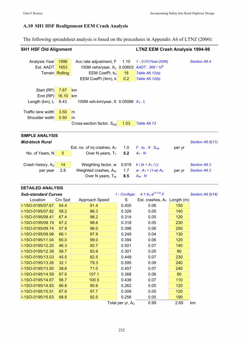
Glen F Koorey Incorporating Safety Into Rural Highway Design
232
A.10 SH1 HSF Realignment EEM Crash Analysis
The following spreadsheet analysis is based on the procedures in Appendix A6 of LTNZ (2006):
SH1 HSF Old Alignment LTNZ EEM Crash Analysis 1994-98
Analysis Year 1996 Acc rate adjustment, F 1.10 1 - 0.01(Year-2006) Section A6.4 Est. AADT 1653 100M vehs/year, XV 0.00603 AADT . 365 / 108
Terrain Rolling EEM Coeff't, b0 18 Table A6.12(a) EEM Coeff't (/km), k 0.2 Table A6.12(b)
Start (RP) 7.67 km End (RP) 16.10 km
Length (km), L 8.43 100M veh-km/year, X 0.05086 XV . L
Traffic lane width 3.50 m Shoulder width 0.50 m
Cross-section factor, Sadj 1.03 Table A6.13
SIMPLE ANALYSIS
Mid-block Rural Section A6.5(11) Est. no. of inj crashes, AT 1.0 F . b0 . X . Sadj per yr
No. of Years, N 5 Over N years, TT 5.2 AT . N
Crash history, AS 14 Weighting factor, w 0.619 k / (k + AT / L) Section A6.3 per year 2.8 Weighted crashes, AW 1.7 w . AT + (1-w) AS per yr Section A6.3
Over N years, TW 8.5 AW . N
DETAILED ANALYSIS
Sub-standard Curves 1 - Crv/Appr 4.1 XV.e(2.0 S).F Section A6.5(14)Location Crv Spd Approach Speed S Est. crashes, AT Length (m)
I-1SO-0195/07.67 54.4 91.4 0.405 0.06 150 I-1SO-0195/07.82 58.2 86.3 0.326 0.05 140 I-1SO-0195/08.41 67.4 98.2 0.314 0.05 120 I-1SO-0195/09.19 67.2 98.6 0.318 0.05 230 I-1SO-0195/09.74 57.9 96.0 0.398 0.06 250 I-1SO-0195/09.99 66.1 87.9 0.249 0.04 130 I-1SO-0195/11.04 60.0 99.0 0.394 0.06 120 I-1SO-0195/12.25 46.3 92.7 0.501 0.07 140 I-1SO-0195/12.39 58.7 83.9 0.301 0.05 80 I-1SO-0195/13.03 45.5 82.5 0.448 0.07 230 I-1SO-0195/13.26 32.1 79.3 0.595 0.09 240 I-1SO-0195/13.50 38.6 71.0 0.457 0.07 240 I-1SO-0195/14.59 67.6 107.1 0.368 0.06 80 I-1SO-0195/14.67 56.7 100.5 0.436 0.07 110 I-1SO-0195/14.83 66.8 90.6 0.262 0.05 120 I-1SO-0195/15.51 67.6 97.7 0.308 0.05 120 I-1SO-0195/15.63 68.8 92.5 0.256 0.05 190
Total per yr, AC 0.99 2.69 km

Glen F Koorey Incorporating Safety Into Rural Highway Design
233
Sub-standard Bridges EEM Coeff't, c 26.57 e(3.5 - AADT/7500) Section A6.5(17) 0.96 c (0.5-0.25RW + 0.025RW 2) b0.XV.F
Location Width Reduced width, RW b0 Est. crashes, AT Length (m) I-1SO-0195/08.94 5.70 -1.30 22.12 0.15 10 I-1SO-0195/14.62 6.10 -0.90 19.01 0.13 20
Total per yr, AB 0.27 0.03 km
Remaining Mid-block Rural Section A6.5(11)Length (km), L' 5.71 100M veh-km/year, X' 0.03445 XV . L'
Est. no. of inj crashes, AM 0.7 F . b0 . X' . Sadj per yr
Overall Total Combined crashes, A'T 2.0 AM + AC + AB per yr No. of Years, N 5 Over N years, T'T 9.8 A'T . N
Crash history, AS 14 Weighting factor, w' 0.706 k / (k + A'T / L) Section A6.3
per year 2.8 Weighted crashes, A'W 2.3 w'.A'T + (1-w') AS per yr Section A6.3 Over N years, T'W 11.7 A'W . N
SH1 HSF New Alignment LTNZ EEM Crash Analysis 2002-06
Analysis Year 2004 Acc rate adjustment, F 1.02 1 - 0.01(Year-2006) Section A6.4 Est. AADT 2089 100M vehs/year, XV 0.00762 AADT . 365 / 108
Terrain Rolling EEM Coeff't, b0 18 Table A6.12(a) EEM Coeff't (/km), k 0.2 Table A6.12(b)
Start (RP) 7.67 km End (RP) 14.00 km
Length (km), L 6.33 100M veh-km/year, X 0.04827 XV . L
Traffic lane width 3.50 m Shoulder width 0.75 m
Cross-section factor, Sadj 0.86 Table A6.13
SIMPLE ANALYSIS (no sub-standard curves or bridges)
Mid-block Rural Section A6.5(11) Est. no. of inj crashes, AT 0.8 F . b0 . X . Sadj per yr
No. of Years, N 5 Over N years, TT 3.8 AT . N
Crash history, AS 5 Weighting factor, w 0.624 k / (k + AT / L) Section A6.3 per year 1 Weighted crashes, AW 0.9 w . AT + (1-w) AS per yr Section A6.3
Over N years, TW 4.3 AW . N

Glen F Koorey Incorporating Safety Into Rural Highway Design
234
A.11 SH1 HSF Realignment IHSDM Crash Analysis
The following is a sample report from IHSDM’s CPM module; in this case the SH1 HSF old
alignment predicting 1994-98 crash numbers without crash history:
Crash Prediction Evaluation Report
IHSDM Version: 4.0.5 IHSDM 2007 Release Report Date: 30/12/2008 17:08:18 Name: Glen Koorey ([email protected], +64-3-3642951) Organization: Telephone: E-Mail: Project: SH1 HSF Realignment (18/10/2008 13:04) Evaluation: CPM 94-98 no crash history (17:07) Highway Information: SH1SO (HSF Old Alignment) (v2) Crash Prediction Module Version: 1.4.1 (Nov 05, 2007) Evaluation Length: 8.4300 kilometers Crash History Data: None Table of Contents
Highway Data Summary Proposed Highway Segment Data Table Proposed Horizontal Curve Data Table Proposed Segment Traffic Volume Table Expected Crash Summary Expected Crash Rates and Frequencies Table Expected Crash Type Distribution Expected Crash Frequencies and Rates Expected Crash Frequencies and Rates by Horizontal Design Element Crash Prediction Results Plot
Highway Segment Summary Highway Segment Data from the CPM Engineer's Manual
Table 1: Proposed Highway Segment Data
Station Lane Width
ShoulderWidth
ShoulderType
PassingLane Seg
# Start End
Length (m) Right
(m) Left (m) Right Left Right Left
Drvwy Density
(dwys/km)
RoadsideHazardRating
Horiz Curve
Number Grade
(%) Right Left
CenterTWLTL
1 201570.000 201645.000 75.00 3.50 3.50 0.5 0.5 paved paved 2.0 4.0 2 1.60 no no no 2 201645.000 201720.000 75.00 3.50 3.50 0.5 0.5 paved paved 2.0 4.0 2 0.90 no no no 3 201720.000 201790.000 70.00 3.50 3.50 0.5 0.5 paved paved 2.0 4.0 3 0.90 no no no 4 201790.000 201860.000 70.00 3.50 3.50 0.5 0.5 paved paved 2.0 4.0 3 2.00 no no no 5 201860.000 201900.000 40.00 3.50 3.50 0.5 0.5 paved paved 2.0 4.0 4 2.00 no no no 6 201900.000 201940.000 40.00 3.50 3.50 0.5 0.5 paved paved 2.0 4.0 4 3.00 no no no 7 201940.000 202015.000 75.00 3.50 3.50 0.5 0.5 paved paved 2.0 4.0 5 3.00 no no no 8 202015.000 202090.000 75.00 3.50 3.50 0.5 0.5 paved paved 2.0 4.0 5 2.00 no no no 9 202090.000 202200.000 110.00 3.50 3.50 0.5 0.5 paved paved 2.0 4.0 - 2.00 no no no
10 202200.000 202310.000 110.00 3.50 3.50 0.5 0.5 paved paved 2.0 4.0 - 2.40 no no no 11 202310.000 202370.000 60.00 3.50 3.50 0.5 0.5 paved paved 2.0 4.0 6 2.40 no no no

Glen F Koorey Incorporating Safety Into Rural Highway Design
235
Station Lane Width
ShoulderWidth
ShoulderType
PassingLane Seg
# Start End
Length (m) Right
(m) Left (m) Right Left Right Left
Drvwy Density
(dwys/km)
RoadsideHazardRating
Horiz Curve
Number
Grade (%)
Right Left
CenterTWLTL
12 202370.000 202430.000 60.00 3.50 3.50 0.5 0.5 paved paved 2.0 4.0 6 2.30 no no no 13 202430.000 202500.000 70.00 3.50 3.50 0.5 0.5 paved paved 2.0 4.0 - 2.30 no no no 14 202500.000 202590.000 90.00 3.50 3.50 0.5 0.5 paved paved 2.0 4.0 7 2.30 no no no 15 202590.000 202720.000 130.00 3.50 3.50 0.5 0.5 paved paved 2.0 4.0 - 2.30 no no no 16 202720.000 202830.000 110.00 3.50 3.50 0.5 0.5 paved paved 2.0 4.0 - 4.10 no no no 17 202830.000 202850.000 20.00 2.85 2.85 0.0 0.0 N/A N/A 2.0 4.0 - 4.10 no no no 18 202850.000 202860.000 10.00 2.85 2.85 0.0 0.0 N/A N/A 2.0 4.0 8 4.10 no no no 19 202860.000 202930.000 70.00 3.50 3.50 0.5 0.5 paved paved 2.0 4.0 8 4.10 no no no 20 202930.000 203010.000 80.00 3.50 3.50 0.5 0.5 paved paved 2.0 4.0 8 1.80 no no no 21 203010.000 203050.000 40.00 3.50 3.50 0.5 0.5 paved paved 2.0 4.0 - 1.80 no no no 22 203050.000 203090.000 40.00 3.50 3.50 0.5 0.5 paved paved 2.0 4.0 - 2.80 no no no 23 203090.000 203320.000 230.00 3.50 3.50 0.5 0.5 paved paved 2.0 4.0 9 2.80 no no no 24 203320.000 203560.000 240.00 3.50 3.50 0.5 0.5 paved paved 2.0 4.0 - 2.80 no no no 25 203560.000 203640.000 80.00 3.50 3.50 0.5 0.5 paved paved 2.0 4.0 10 2.80 no no no 26 203640.000 203765.000 125.00 3.50 3.50 0.5 0.5 paved paved 2.0 4.0 11 2.80 no no no 27 203765.000 203890.000 125.00 3.50 3.50 0.5 0.5 paved paved 2.0 4.0 11 6.60 no no no 28 203890.000 203955.000 65.00 3.50 3.50 0.5 0.5 paved paved 2.0 4.0 12 6.60 no no no 29 203955.000 204020.000 65.00 3.50 3.50 0.5 0.5 paved paved 2.0 4.0 12 8.30 no no no 30 204020.000 204060.000 40.00 3.50 3.50 0.5 0.5 paved paved 2.0 4.0 13 8.30 no no no 31 204060.000 204100.000 40.00 3.50 3.50 0.5 0.5 paved paved 2.0 4.0 13 9.50 no no no 32 204100.000 204375.000 275.00 3.50 3.50 0.5 0.5 paved paved 2.0 4.0 - 9.50 no no no 33 204375.000 204650.000 275.00 3.50 3.50 0.5 0.5 paved paved 2.0 4.0 - 3.80 no no no 34 204650.000 204750.000 100.00 3.50 3.50 0.5 0.5 paved paved 2.0 4.0 14 3.80 no no no 35 204750.000 204940.000 190.00 3.50 3.50 0.5 0.5 paved paved 2.0 4.0 - 3.80 no no no 36 204940.000 205000.000 60.00 3.50 3.50 0.5 0.5 paved paved 2.0 4.0 15 3.80 no no no 37 205000.000 205060.000 60.00 3.50 3.50 0.5 0.5 paved paved 2.0 4.0 15 4.10 no no no 38 205060.000 205460.000 400.00 3.50 3.50 0.5 0.5 paved paved 2.0 4.0 - 4.10 no no no 39 205460.000 205500.000 40.00 3.50 3.50 0.5 0.5 paved paved 2.0 4.0 16 4.10 no no no 40 205500.000 205540.000 40.00 3.50 3.50 0.5 0.5 paved paved 2.0 4.0 16 3.30 no no no 41 205540.000 205880.000 340.00 3.50 3.50 0.5 0.5 paved paved 2.0 4.0 - 3.30 no no no 42 205880.000 206010.000 130.00 3.50 3.50 0.5 0.5 paved paved 2.0 4.0 17 3.30 no no no 43 206010.000 206080.000 70.00 3.50 3.50 0.5 0.5 paved paved 2.0 4.0 - 3.30 no no no 44 206080.000 206150.000 70.00 3.50 3.50 0.5 0.5 paved paved 2.0 4.0 - 8.40 no no no 45 206150.000 206220.000 70.00 3.50 3.50 0.5 0.5 paved paved 2.0 4.0 18 8.40 no no no 46 206220.000 206290.000 70.00 3.50 3.50 0.5 0.5 paved paved 2.0 4.0 18 3.70 no no no 47 206290.000 206330.000 40.00 3.50 3.50 0.5 0.5 paved paved 2.0 4.0 19 3.70 no no no 48 206330.000 206370.000 40.00 3.50 3.50 0.5 0.5 paved paved 2.0 4.0 19 -3.50 no no no 49 206370.000 206460.000 90.00 3.50 3.50 0.5 0.5 paved paved 2.0 4.0 20 -3.50 no no no 50 206460.000 206550.000 90.00 3.50 3.50 0.5 0.5 paved paved 2.0 4.0 20 -0.30 no no no 51 206550.000 206740.000 190.00 3.50 3.50 0.5 0.5 paved paved 2.0 4.0 21 -0.30 no no no 52 206740.000 206930.000 190.00 3.50 3.50 0.5 0.5 paved paved 2.0 4.0 21 -5.60 no no no 53 206930.000 207045.000 115.00 3.50 3.50 0.5 0.5 paved paved 2.0 4.0 22 -5.60 no no no 54 207045.000 207160.000 115.00 3.50 3.50 0.5 0.5 paved paved 2.0 4.0 22 -6.40 no no no 55 207160.000 207280.000 120.00 3.50 3.50 0.5 0.5 paved paved 2.0 4.0 23 -6.40 no no no 56 207280.000 207400.000 120.00 3.50 3.50 0.5 0.5 paved paved 2.0 4.0 23 -5.30 no no no 57 207400.000 207520.000 120.00 3.50 3.50 0.5 0.5 paved paved 2.0 4.0 24 -5.30 no no no 58 207520.000 207640.000 120.00 3.50 3.50 0.5 0.5 paved paved 2.0 4.0 24 4.60 no no no 59 207640.000 207685.000 45.00 3.50 3.50 0.5 0.5 paved paved 2.0 4.0 25 4.60 no no no 60 207685.000 207730.000 45.00 3.50 3.50 0.5 0.5 paved paved 2.0 4.0 25 3.80 no no no 61 207730.000 207745.000 15.00 3.50 3.50 0.5 0.5 paved paved 2.0 4.0 26 3.80 no no no 62 207745.000 207760.000 15.00 3.50 3.50 0.5 0.5 paved paved 2.0 4.0 26 -2.40 no no no 63 207760.000 207905.000 145.00 3.50 3.50 0.5 0.5 paved paved 2.0 4.0 - -2.40 no no no 64 207905.000 208050.000 145.00 3.50 3.50 0.5 0.5 paved paved 2.0 4.0 - -3.10 no no no 65 208050.000 208120.000 70.00 3.50 3.50 0.5 0.5 paved paved 2.0 4.0 27 -3.10 no no no 66 208120.000 208305.000 185.00 3.50 3.50 0.5 0.5 paved paved 2.0 4.0 - -3.10 no no no

Glen F Koorey Incorporating Safety Into Rural Highway Design
236
Station Lane Width
ShoulderWidth
ShoulderType
PassingLane Seg
# Start End
Length (m) Right
(m) Left (m) Right Left Right Left
Drvwy Density
(dwys/km)
RoadsideHazardRating
Horiz Curve
Number
Grade (%)
Right Left
CenterTWLTL
67 208305.000 208490.000 185.00 3.50 3.50 0.5 0.5 paved paved 2.0 4.0 - -4.60 no no no 68 208490.000 208510.000 20.00 3.50 3.50 0.5 0.5 paved paved 2.0 4.0 28 -4.60 no no no 69 208510.000 208530.000 20.00 3.05 3.05 0.0 0.0 N/A N/A 2.0 4.0 28 -4.60 no no no 70 208530.000 208550.000 20.00 3.05 3.05 0.0 0.0 N/A N/A 2.0 4.0 28 -4.40 no no no 71 208550.000 208570.000 20.00 3.50 3.50 0.5 0.5 paved paved 2.0 4.0 28 -4.40 no no no 72 208570.000 208625.000 55.00 3.50 3.50 0.5 0.5 paved paved 2.0 4.0 29 -4.40 no no no 73 208625.000 208680.000 55.00 3.50 3.50 0.5 0.5 paved paved 2.0 4.0 29 -5.50 no no no 74 208680.000 208705.000 25.00 3.50 3.50 0.5 0.5 paved paved 2.0 4.0 30 -5.50 no no no 75 208705.000 208730.000 25.00 3.50 3.50 0.5 0.5 paved paved 2.0 4.0 30 -6.90 no no no 76 208730.000 208790.000 60.00 3.50 3.50 0.5 0.5 paved paved 2.0 4.0 31 -6.90 no no no 77 208790.000 208850.000 60.00 3.50 3.50 0.5 0.5 paved paved 2.0 4.0 31 -5.20 no no no 78 208850.000 208880.000 30.00 3.50 3.50 0.5 0.5 paved paved 2.0 4.0 32 -5.20 no no no 79 208880.000 208910.000 30.00 3.50 3.50 0.5 0.5 paved paved 2.0 4.0 32 -6.90 no no no 80 208910.000 208965.000 55.00 3.50 3.50 0.5 0.5 paved paved 2.0 4.0 33 -6.90 no no no 81 208965.000 209020.000 55.00 3.50 3.50 0.5 0.5 paved paved 2.0 4.0 33 -2.60 no no no 82 209020.000 209150.000 130.00 3.50 3.50 0.5 0.5 paved paved 2.0 4.0 34 -2.60 no no no 83 209150.000 209280.000 130.00 3.50 3.50 0.5 0.5 paved paved 2.0 4.0 34 0.20 no no no 84 209280.000 209345.000 65.00 3.50 3.50 0.5 0.5 paved paved 2.0 4.0 - 0.20 no no no 85 209345.000 209410.000 65.00 3.50 3.50 0.5 0.5 paved paved 2.0 4.0 - 4.30 no no no 86 209410.000 209470.000 60.00 3.50 3.50 0.5 0.5 paved paved 2.0 4.0 35 4.30 no no no 87 209470.000 209530.000 60.00 3.50 3.50 0.5 0.5 paved paved 2.0 4.0 35 8.30 no no no 88 209530.000 209625.000 95.00 3.50 3.50 0.5 0.5 paved paved 2.0 4.0 36 8.30 no no no 89 209625.000 209720.000 95.00 3.50 3.50 0.5 0.5 paved paved 2.0 4.0 36 -0.20 no no no 90 209720.000 210000.000 280.00 3.50 3.50 0.5 0.5 paved paved 2.0 4.0 - -0.20 no no no
Horizontal Curve Summary Horizontal Curve Data from the CPM Engineer's Manual
Table 2: Proposed Horizontal Curve Data Station Horizontal
Curve Number Start End
Length ofCurve (m) Radius (m) Superelevation (%)
Design Speed (km/h)
Spiral Transition
1 201510.000 201570.000 60.00 571.00 Left 3.0 Right 3.0 adverse 100 none
2 201570.000 201720.000 150.00 177.00 Left 3.0 adverse Right 3.0 50 none
3 201720.000 201860.000 140.00 211.00 Left 3.0 Right 3.0 adverse 60 none
4 201860.000 201940.000 80.00 860.00 Left 3.0 adverse Right 3.0 90 none
5 201940.000 202090.000 150.00 263.00 Left 3.0 Right 3.0 adverse 70 none
6 202310.000 202430.000 120.00 182.00 Left 3.0 Right 3.0 adverse 70 none
7 202500.000 202590.000 90.00 662.00 Left 3.0 Right 3.0 adverse 100 none
8 202850.000 203010.000 160.00 521.00 Left 3.0 Right 3.0 adverse 90 none
9 203090.000 203320.000 230.00 171.00 Left 3.0 adverse Right 3.0 70 none
10 203560.000 203640.000 80.00 640.00 Left 3.0 Right 3.0 adverse 100 none
11 203640.000 203890.000 250.00 164.00 Left 3.0 adverse Right 3.0 60 none
12 203890.000 204020.000 130.00 237.00 Left 3.0 Right 3.0 adverse 70 none
13 204020.000 204100.000 80.00 151.00 Left 3.0 adverse Right 3.0 60 none
14 204650.000 204750.000 100.00 454.00 Left 3.0 adverse Right 3.0 90 none
15 204940.000 205060.000 120.00 177.00 Left 3.0 adverse Right 3.0 60 none
16 205460.000 205540.000 80.00 350.00 Left 3.0 Right 3.0 adverse 90 none
17 205880.000 206010.000 130.00 384.00 Left 3.0 adverse Right 3.0 90 none

Glen F Koorey Incorporating Safety Into Rural Highway Design
237
Station Horizontal Curve
Number Start End Length ofCurve (m) Radius (m) Superelevation (%)
Design Speed (km/h)
Spiral Transition
18 206150.000 206290.000 140.00 93.00 Left 3.0 Right 3.0 adverse 50 none
19 206290.000 206370.000 80.00 118.00 Left 3.0 adverse Right 3.0 60 none
20 206370.000 206550.000 180.00 318.00 Left 3.0 Right 3.0 adverse 70 none
21 206550.000 206930.000 380.00 301.00 Left 3.0 adverse Right 3.0 80 none
22 206930.000 207160.000 230.00 105.00 Left 3.0 Right 3.0 adverse 50 none
23 207160.000 207400.000 240.00 72.00 Left 3.0 adverse Right 3.0 30 none
24 207400.000 207640.000 240.00 78.00 Left 3.0 Right 3.0 adverse 40 none
25 207640.000 207730.000 90.00 116.00 Left 3.0 adverse Right 3.0 50 none
26 207730.000 207760.000 30.00 447.00 Left 3.0 Right 3.0 adverse 70 none
27 208050.000 208120.000 70.00 630.00 Left 3.0 adverse Right 3.0 100 none
28 208490.000 208570.000 80.00 199.00 Left 3.0 Right 3.0 adverse 70 none
29 208570.000 208680.000 110.00 139.00 Left 3.0 adverse Right 3.0 60 none
30 208680.000 208730.000 50.00 335.00 Left 3.0 Right 3.0 adverse 80 none
31 208730.000 208850.000 120.00 185.00 Left 3.0 adverse Right 3.0 70 none
32 208850.000 208910.000 60.00 312.00 Left 3.0 Right 3.0 adverse 80 none
33 208910.000 209020.000 110.00 168.00 Left 3.0 adverse Right 3.0 60 none
34 209020.000 209280.000 260.00 493.00 Left 3.0 Right 3.0 adverse 90 none
35 209410.000 209530.000 120.00 241.00 Left 3.0 Right 3.0 adverse 70 none
36 209530.000 209720.000 190.00 199.00 Left 3.0 adverse Right 3.0 70 none
Proposed Segment Traffic Volume Segment Traffic Volume from the CPM Engineer's Manual
Interpolated values rendered in blue font.
Table 3: Proposed Segment Traffic Volume Station Evaluation Period ADT (veh/day) Segment
# Start End 1994 1995 1996 1997 1998
1 to 90 201570.000 210000.000 1,582 1,645 1,711 1,779 1,850
Expected Crash Rates and Frequencies Expected Crash Frequencies and Rate from the CPM Engineer's Manual
Table 4: Expected Crash Rates and Frequencies Description Prediction
Total Crashes 23.03 Fatal and Injury Crashes (41%) 9.42 Property-damage-only Crashes (59%) 13.61 Average Future Road ADT (vehicles/day) 1,713 Crash Rate per kilometers per year 0.5 Fatal and Injury Crash Rate per kilometers per year 0.2 Property-damage-only Crash Rate per kilometers per year 0.3

Glen F Koorey Incorporating Safety Into Rural Highway Design
238
Description Prediction Total travel (million vehicle-kilometers) 26.36 Crash Rate per million vehicle-kilometers 0.9 Fatal and Injury Crash Rate per million vehicle-kilometers 0.4 Property-damage-only Crash Rate per million vehicle-kilometers 0.5
Expected Crash Type Distribution Expected Crash Type Distributions from the CPM Engineer's Manual
Table 5: Expected Crash Type Distribution Crash Type Highway Segment Intersections Total
Single-vehicle accidents Collision with animal 0.8 (3.58%) 0.0 (0.0%) 0.8 (3.58%) Collision with bicycle 0.1 (0.5%) 0.0 (0.0%) 0.1 (0.5%) Collision with parked vehicle 0.2 (0.89%) 0.0 (0.0%) 0.2 (0.89%) Collision with pedestrian 0.2 (0.72%) 0.0 (0.0%) 0.2 (0.72%) Overturned 0.2 (1.04%) 0.0 (0.0%) 0.2 (1.04%) Ran off road 12.8 (55.65%) 0.0 (0.0%) 12.8 (55.65%)Other single-vehicle accident 0.8 (3.36%) 0.0 (0.0%) 0.8 (3.36%) Total single-vehicle accidents 15.1 (65.74%) 0.0 (0.0%) 15.1 (65.74%)Multiple-vehicle accidents Angle collision 0.0 (0.04%) 0.0 (0.0%) 0.0 (0.04%) Head-on collision 3.1 (13.65%) 0.0 (0.0%) 3.1 (13.65%) Left-turn collision 0.2 (0.81%) 0.0 (0.0%) 0.2 (0.81%) Right-turn collision 0.1 (0.43%) 0.0 (0.0%) 0.1 (0.43%) Rear-end collision 1.3 (5.68%) 0.0 (0.0%) 1.3 (5.68%) Sideswipe opposite-direction 0.2 (0.66%) 0.0 (0.0%) 0.2 (0.66%) Sideswipe same-direction 1.9 (8.07%) 0.0 (0.0%) 1.9 (8.07%) Other multiple-vehicle collision 1.1 (4.92%) 0.0 (0.0%) 1.1 (4.92%) Total multiple-vehicle collisions 7.9 (34.26%) 0.0 (0.0%) 7.9 (34.26%) Total accidents 23.0 (100.0%) 0.0 (0.0%) 23.0 (100.0%)
Expected Crash Frequencies and Rates Expected Crash Frequencies and Rate from the CPM Engineer's Manual
Table 6: Expected Crash Frequencies and Rates Station Expected Crash Rates
Intersection Name/
Cross Road From To Length
(km)
Expected No. of
Crashes for
EvaluationPeriod
(crashes/km/yr) (crashes/million vehicle-km)
Expected Crash Rate
/million entering
veh
Expected no. of
crashes/yearfor
intersection
201570.000 201645.000 0.0750 0.26 0.7 1.09

Glen F Koorey Incorporating Safety Into Rural Highway Design
239
Station Expected Crash Rates
Intersection Name/
Cross Road From To Length
(km)
Expected No. of
Crashes for
EvaluationPeriod
(crashes/km/yr) (crashes/million vehicle-km)
Expected Crash Rate
/million entering
veh
Expected no. of
crashes/yearfor
intersection
201645.000 201720.000 0.0750 0.25 0.7 1.08
201720.000 201790.000 0.0700 0.23 0.7 1.04
201790.000 201860.000 0.0700 0.23 0.7 1.06
201860.000 201900.000 0.0400 0.09 0.5 0.73
201900.000 201940.000 0.0400 0.09 0.5 0.75
201940.000 202015.000 0.0750 0.23 0.6 0.96
202015.000 202090.000 0.0750 0.22 0.6 0.95
202090.000 202200.000 0.1100 0.16 0.3 0.48
202200.000 202310.000 0.1100 0.16 0.3 0.48
202310.000 202370.000 0.0600 0.24 0.8 1.28
202370.000 202430.000 0.0600 0.24 0.8 1.28
202430.000 202500.000 0.0700 0.10 0.3 0.48
202500.000 202590.000 0.0900 0.23 0.5 0.81
202590.000 202720.000 0.1300 0.19 0.3 0.48
202720.000 202830.000 0.1100 0.17 0.3 0.49
202830.000 202850.000 0.0200 0.04 0.4 0.67
202850.000 202860.000 0.0100 0.03 0.7 1.05
202860.000 202930.000 0.0700 0.17 0.5 0.77
202930.000 203010.000 0.0800 0.18 0.5 0.74
203010.000 203050.000 0.0400 0.06 0.3 0.47
203050.000 203090.000 0.0400 0.06 0.3 0.48
203090.000 203320.000 0.2300 0.71 0.6 0.98
203320.000 203560.000 0.2400 0.36 0.3 0.48
203560.000 203640.000 0.0800 0.22 0.5 0.86
203640.000 203765.000 0.1250 0.37 0.6 0.95
203765.000 203890.000 0.1250 0.39 0.6 1.01
203890.000 203955.000 0.0650 0.23 0.7 1.14
203955.000 204020.000 0.0650 0.24 0.7 1.17
204020.000 204060.000 0.0400 0.25 1.3 2.00
204060.000 204100.000 0.0400 0.25 1.3 2.04
204100.000 204375.000 0.2750 0.46 0.3 0.54
204375.000 204650.000 0.2750 0.42 0.3 0.49
204650.000 204750.000 0.1000 0.29 0.6 0.92
204750.000 204940.000 0.1900 0.29 0.3 0.49
204940.000 205000.000 0.0600 0.24 0.8 1.30
205000.000 205060.000 0.0600 0.25 0.8 1.31
205060.000 205460.000 0.4000 0.61 0.3 0.49
205460.000 205500.000 0.0400 0.14 0.7 1.16
205500.000 205540.000 0.0400 0.14 0.7 1.14
205540.000 205880.000 0.3400 0.52 0.3 0.49
205880.000 206010.000 0.1300 0.37 0.6 0.90
206010.000 206080.000 0.0700 0.11 0.3 0.49
206080.000 206150.000 0.0700 0.12 0.3 0.53
206150.000 206220.000 0.0700 0.42 1.2 1.91
206220.000 206290.000 0.0700 0.39 1.1 1.77
206290.000 206330.000 0.0400 0.28 1.4 2.23

Glen F Koorey Incorporating Safety Into Rural Highway Design
240
Station Expected Crash Rates
Intersection Name/
Cross Road From To Length
(km)
Expected No. of
Crashes for
EvaluationPeriod
(crashes/km/yr) (crashes/million vehicle-km)
Expected Crash Rate
/million entering
veh
Expected no. of
crashes/yearfor
intersection
206330.000 206370.000 0.0400 0.28 1.4 2.22
206370.000 206460.000 0.0900 0.24 0.5 0.84
206460.000 206550.000 0.0900 0.22 0.5 0.80
206550.000 206740.000 0.1900 0.41 0.4 0.69
206740.000 206930.000 0.1900 0.45 0.5 0.75
206930.000 207045.000 0.1150 0.45 0.8 1.26
207045.000 207160.000 0.1150 0.46 0.8 1.28
207160.000 207280.000 0.1200 0.55 0.9 1.46
207280.000 207400.000 0.1200 0.54 0.9 1.44
207400.000 207520.000 0.1200 0.53 0.9 1.42
207520.000 207640.000 0.1200 0.53 0.9 1.41
207640.000 207685.000 0.0450 0.29 1.3 2.06
207685.000 207730.000 0.0450 0.29 1.3 2.04
207730.000 207745.000 0.0150 0.08 1.0 1.62
207745.000 207760.000 0.0150 0.07 1.0 1.58
207760.000 207905.000 0.1450 0.22 0.3 0.48
207905.000 208050.000 0.1450 0.22 0.3 0.48
208050.000 208120.000 0.0700 0.20 0.6 0.92
208120.000 208305.000 0.1850 0.28 0.3 0.48
208305.000 208490.000 0.1850 0.29 0.3 0.50
208490.000 208510.000 0.0200 0.10 1.0 1.59
208510.000 208530.000 0.0200 0.13 1.3 2.03
208530.000 208550.000 0.0200 0.13 1.3 2.02
208550.000 208570.000 0.0200 0.10 1.0 1.58
208570.000 208625.000 0.0550 0.28 1.0 1.62
208625.000 208680.000 0.0550 0.28 1.0 1.65
208680.000 208705.000 0.0250 0.12 1.0 1.54
208705.000 208730.000 0.0250 0.12 1.0 1.57
208730.000 208790.000 0.0600 0.26 0.9 1.36
208790.000 208850.000 0.0600 0.25 0.8 1.33
208850.000 208880.000 0.0300 0.14 0.9 1.44
208880.000 208910.000 0.0300 0.14 0.9 1.48
208910.000 208965.000 0.0550 0.26 0.9 1.49
208965.000 209020.000 0.0550 0.24 0.9 1.39
209020.000 209150.000 0.1300 0.28 0.4 0.69
209150.000 209280.000 0.1300 0.27 0.4 0.67
209280.000 209345.000 0.0650 0.09 0.3 0.46
209345.000 209410.000 0.0650 0.10 0.3 0.49
209410.000 209470.000 0.0600 0.21 0.7 1.13
209470.000 209530.000 0.0600 0.23 0.8 1.20
209530.000 209625.000 0.0950 0.32 0.7 1.08
209625.000 209720.000 0.0950 0.28 0.6 0.95
209720.000 210000.000 0.2800 0.40 0.3 0.46
Expected Crash Frequencies and Rates by Horizontal Design Element Results by Homogeneous Analysis Sections from the CPM Engineer's Manual

Glen F Koorey Incorporating Safety Into Rural Highway Design
241
Table 7: Expected Crash Frequencies and Rates by Horizontal Design Element Station Expected Crash Rates Design Element
(Horizontal Curve Number
or Tangent) From To
Length(km)
Expected No.of Crashes for
Evaluation Period
(crashes/km/yr) (crashes/millionvehicle-km)
Curve 2 201570.000 201720.000 0.1500 0.51 0.7 1.08
Curve 3 201720.000 201860.000 0.1400 0.46 0.7 1.05
Curve 4 201860.000 201940.000 0.0800 0.19 0.5 0.74
Curve 5 201940.000 202090.000 0.1500 0.45 0.6 0.95
Tangent 202090.000 202310.000 0.2200 0.33 0.3 0.48
Curve 6 202310.000 202430.000 0.1200 0.48 0.8 1.28
Tangent 202430.000 202500.000 0.0700 0.10 0.3 0.48
Curve 7 202500.000 202590.000 0.0900 0.23 0.5 0.81
Tangent 202590.000 202850.000 0.2600 0.41 0.3 0.50
Curve 8 202850.000 203010.000 0.1600 0.39 0.5 0.77
Tangent 203010.000 203090.000 0.0800 0.12 0.3 0.48
Curve 9 203090.000 203320.000 0.2300 0.71 0.6 0.98
Tangent 203320.000 203560.000 0.2400 0.36 0.3 0.48
Curve 10 203560.000 203640.000 0.0800 0.22 0.5 0.86
Curve 11 203640.000 203890.000 0.2500 0.77 0.6 0.98
Curve 12 203890.000 204020.000 0.1300 0.47 0.7 1.15
Curve 13 204020.000 204100.000 0.0800 0.50 1.3 2.02
Tangent 204100.000 204650.000 0.5500 0.88 0.3 0.51
Curve 14 204650.000 204750.000 0.1000 0.29 0.6 0.92
Tangent 204750.000 204940.000 0.1900 0.29 0.3 0.49
Curve 15 204940.000 205060.000 0.1200 0.49 0.8 1.31
Tangent 205060.000 205460.000 0.4000 0.61 0.3 0.49
Curve 16 205460.000 205540.000 0.0800 0.29 0.7 1.15
Tangent 205540.000 205880.000 0.3400 0.52 0.3 0.49
Curve 17 205880.000 206010.000 0.1300 0.37 0.6 0.90
Tangent 206010.000 206150.000 0.1400 0.22 0.3 0.51
Curve 18 206150.000 206290.000 0.1400 0.81 1.2 1.84
Curve 19 206290.000 206370.000 0.0800 0.56 1.4 2.23
Curve 20 206370.000 206550.000 0.1800 0.46 0.5 0.82
Curve 21 206550.000 206930.000 0.3800 0.86 0.5 0.72
Curve 22 206930.000 207160.000 0.2300 0.91 0.8 1.27
Curve 23 207160.000 207400.000 0.2400 1.09 0.9 1.45
Curve 24 207400.000 207640.000 0.2400 1.06 0.9 1.41
Curve 25 207640.000 207730.000 0.0900 0.58 1.3 2.05
Curve 26 207730.000 207760.000 0.0300 0.15 1.0 1.60
Tangent 207760.000 208050.000 0.2900 0.44 0.3 0.48
Curve 27 208050.000 208120.000 0.0700 0.20 0.6 0.92
Tangent 208120.000 208490.000 0.3700 0.57 0.3 0.49
Curve 28 208490.000 208570.000 0.0800 0.45 1.1 1.80
Curve 29 208570.000 208680.000 0.1100 0.56 1.0 1.63
Curve 30 208680.000 208730.000 0.0500 0.24 1.0 1.55
Curve 31 208730.000 208850.000 0.1200 0.50 0.8 1.34
Curve 32 208850.000 208910.000 0.0600 0.27 0.9 1.46
Curve 33 208910.000 209020.000 0.1100 0.49 0.9 1.44

Glen F Koorey Incorporating Safety Into Rural Highway Design
242
Station Expected Crash Rates Design Element (Horizontal
Curve Number or Tangent)
From To
Length(km)
Expected No.of Crashes for
Evaluation Period
(crashes/km/yr) (crashes/million vehicle-km)
Curve 34 209020.000 209280.000 0.2600 0.55 0.4 0.68
Tangent 209280.000 209410.000 0.1300 0.19 0.3 0.48
Curve 35 209410.000 209530.000 0.1200 0.44 0.7 1.17
Curve 36 209530.000 209720.000 0.1900 0.61 0.6 1.02
Tangent 209720.000 210000.000 0.2800 0.40 0.3 0.46
Crash Prediction Results Plot Expected Crash Rate Plots from the CPM Engineer's Manual
Figure 1: Crash Prediction Results

Glen F Koorey Incorporating Safety Into Rural Highway Design
243
A.12 Supplementary Notes: Testing of Field Survey Equipment
Originally it was intended to undertake a series of field surveys at selected curve sites to monitor
vehicle speeds and lateral placement while traversing the curve. The aim was to relate the
physical characteristics of the road environment with the typical actions observed of drivers. A
driver behaviour model, similar to that described by Levison et al (2001), could then be derived
for incorporation into an overall rural safety model, possibly seeking to relate different
behaviours to proportions of drivers. For practical application it would probably be based on
more easily measured road/environment parameters.
With the change in focus during the study to investigate adapting the IHSDM model, the need
for field data to develop a local model became less important. The investigations undertaken in
this area however still provide a useful account for any similar future surveys, and are therefore
recorded here for the benefit of other researchers. Some field data were also still needed to
calibrate and validate the case studies used in testing the IHSDM adaptation.
A.12.1 Investigation of Possible Data Collection Measures
The two key measures proposed to be investigated were:
1. Vehicle (free) speed profiles through a curve, with particular emphasis on the minimum
speed observed for each vehicle.
2. Lateral position through the curve of each vehicle, with respect to the traffic lanes.
A variety of simple measuring techniques are traditionally used for measurement of vehicle
speeds, such as rubber pneumatic tubes, handheld laser/radar guns, and piezo-electric wires.
These techniques however can suffer from a number of potential problems:
• On a curved alignment, it can be difficult to get a true vehicle speed (especially using a
speed-gun), as the vehicle’s direction relative to the observer is constantly changing.
• Physical measurement devices, such as tubes and wires, can be damaged at a faster rate on
curves due to the additional braking and turning forces by vehicles crossing them.
• Whilst vehicle speeds are likely to be reasonably constant along a straight section of road,
vehicle speeds will be constantly changing while negotiating a curve, particularly where the
desirable curve speed is considerably less than the approach speeds. If the aim is to
determine the minimum speed within the curve (and the location of this is likely to vary with

Glen F Koorey Incorporating Safety Into Rural Highway Design
244
each vehicle), additional speed measuring points will probably be needed along the length of
the curve.
• It can be more difficult to safely install any physical on-road speed measures at a curved site,
due to the limited sight distance of approaching vehicles.
• Manual survey techniques such as speed-guns preclude long survey periods of more than a
few hours.
Some of these issues also affect the measurement of vehicle lateral position, where there are
fewer readily available devices for measuring as well.
Wong (1989) used a series of linked video cameras to observe vehicles travelling around two
curve sites. By subsequently analysing the video frames using a special on-screen grid, he was
able to determine both the speed and lateral position of each vehicle throughout each curve. This
work however entailed considerable effort to extract the data from the video records and produce
the final results.
Therefore, an automated means of recording the necessary data was investigated. This would
allow maximum data collection time with minimal data processing requirement. It was
envisaged that using some form of electro-magnetic sensing devices would be a promising
approach.
A.12.1.1 Equipment used for Curve Advisory Speed Study
Koorey et al (2002) investigated the effects of curve advisory speed signs in New Zealand. Part
of the study involved collection of vehicle speeds at a number of curve sites, and it provides a
useful case study here. Using a series of electromagnetic wave beams across the road was
suggested as a practical solution for this type of survey. Investigations revealed that red-light
optical beams and sensors were readily available that could provide the necessary equipment.
Figure A.2 shows the survey layout used. An ordinary tube-based counter was used to collect
vehicle speeds and vehicle types on the approach to the curve. Up to six optical sensors could
then be placed around the curve at pre-determined locations. Vehicles travelling through the
curve would momentarily break the light beams, and this would be recorded via an attached
laptop.

Glen F Koorey Incorporating Safety Into Rural Highway Design
245
By comparing the time between beam breaks of adjacent sensors, the average speed between the
two points could be calculated. In this way, up to five speeds through the curve could be
determined for each vehicle. Vehicle types could also be determined by the length of vehicles
recorded breaking the optical beams (inferred from the vehicle speeds and the length of time the
beam was broken).
Figure A.2 Layout for curve speed surveys
Approach Counter 1 Optical 2 Sensors 3 4 5 6 A key component was the development of equipment and software suitable for collecting the
data. As well as recording accurately, the equipment had to be sufficiently robust for overnight
placement at remote sites. Figure A.3 shows a typical optical sensor (behind guardrail) and
reflector post developed for this project. On one side of the road the sensor transmitted a light
beam to the reflector on the opposite side, which sent the beam back to a receiver in the sensor.

Glen F Koorey Incorporating Safety Into Rural Highway Design
246
Figure A.3 Typical curve speed optical sensor and reflector (from Koorey et al 2002)
To allow for the variable shape of the terrain, each sensor was installed in a plastic housing fitted
to a wooden base, which could be pinned or weighted down. The construction allowed the light
beam to be aligned with the reflector and then locked in place.
In some cases, reflectors were mounted on sight rails or fixed into slopes to suit the local terrain.
In all cases, the equipment was made as inconspicuous as possible, with the devices often
blending in with the surrounding marker posts. Shielding was used in many cases to prevent the
reflectors from causing a distraction at night to approaching traffic.
The data acquisition system consisted of a terminal box, a 486 laptop computer with a LabView
Card fitted, and a lead-acid battery to power everything. The system was housed in a locked
weatherproof steel box, which for security was pinned to the ground or chained to an object.
Customised software running on the laptop monitored when the beams were broken. As far as
possible according to the program logic, opposing traffic crossing at the same time and closely
following vehicles were ignored, to provide only isolated free speed measurements. Post-
processing software later computed the relative speed between each set of adjacent sensors and
also the estimated vehicle length, based on the time the sensor remained broken.

Glen F Koorey Incorporating Safety Into Rural Highway Design
247
On using this equipment, it was found that too little of the source light was being reflected back
to the sensor for it to be reliable in the field. Initial placement of the equipment also proved
rather difficult to line up, both in terms of “sighting” the adjacent reflector and the sensitivity of
the beam to very slight adjustments. Using larger reflectors helped to improve the situation,
although some kind of sighting equipment would also help. Other factors affecting reliable
sensing included:
• large distances between the sensor and the reflector
• the total surface area of the reflective surface
• the amount of misting or rain droplets forming on the reflectors and the sensor window
• any movement in the equipment due to wind, public interference or passing trucks
The equipment was typically left on-site for about 24 hours to collect sufficient data. Although
the equipment yielded some very useful results, the installation difficulties caused considerable
project delays, and a fair amount of work was required to eliminate “noisy data” (e.g. opposing
vehicles crossing at the same time). Because the study was focused on curve speeds, the
equipment was also unable to determine the lateral position of observed vehicles. Nevertheless,
Koorey et al (2002) recommended that “Further development of the optical speed-detection
equipment should be investigated, to produce a more robust system with fewer data collection
errors.”
A.12.1.2 Spacek Vehicle Tracking Study
A similar survey approach to the previous section was undertaken by Spacek (2000) in
Switzerland. In this study, vehicles were tracked around a series of curves to determine their
speed profiles and tracking behaviour. Road marker posts, with vehicle presence detectors and
distance detectors inside them, were installed around each of the surveyed curves. Their design
mimicked the standard marker posts used in the area, so as not to arouse suspicion by drivers.
The series of detectors were able to record data on the direction, speed, length, and relative
distance away of each passing vehicle. From this information, various types of curve tracking
behaviours were identified and observed vehicle tracks were classified into one of the following
categories:
• “Ideal” behaviour; corresponding to a vehicle driving consistently along the centre of the
lane
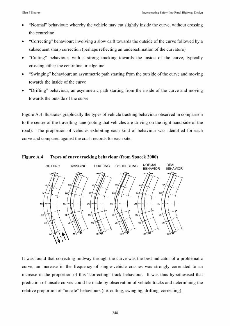
Glen F Koorey Incorporating Safety Into Rural Highway Design
248
• “Normal” behaviour; whereby the vehicle may cut slightly inside the curve, without crossing
the centreline
• “Correcting” behaviour; involving a slow drift towards the outside of the curve followed by a
subsequent sharp correction (perhaps reflecting an underestimation of the curvature)
• “Cutting” behaviour; with a strong tracking towards the inside of the curve, typically
crossing either the centreline or edgeline
• “Swinging” behaviour; an asymmetric path starting from the outside of the curve and moving
towards the inside of the curve
• “Drifting” behaviour; an asymmetric path starting from the inside of the curve and moving
towards the outside of the curve
Figure A.4 illustrates graphically the types of vehicle tracking behaviour observed in comparison
to the centre of the travelling lane (noting that vehicles are driving on the right hand side of the
road). The proportion of vehicles exhibiting each kind of behaviour was identified for each
curve and compared against the crash records for each site.
Figure A.4 Types of curve tracking behaviour (from Spacek 2000)
It was found that correcting midway through the curve was the best indicator of a problematic
curve; an increase in the frequency of single-vehicle crashes was strongly correlated to an
increase in the proportion of this “correcting” track behaviour. It was thus hypothesised that
prediction of unsafe curves could be made by observation of vehicle tracks and determining the
relative proportion of “unsafe” behaviours (i.e. cutting, swinging, drifting, correcting).

Glen F Koorey Incorporating Safety Into Rural Highway Design
249
The detectors used in this study had two distinct advantages over the previous study of Koorey
et al (2002):
• The devices also collected vehicle position information as well as vehicle speed/type
• The devices did not rely on a reflector post on the other side, instead simply bouncing a
signal off each passing vehicle back to the sensor.
Although, details of the construction of these devices are relatively sketchy in Spacek (2000), the
key appears to be to obtain sensors that can emit and receive an electromagnetic signal that can
be reflected off any sizeable object (such as a vehicle).
A.12.2 Field Trials of Equipment
Based on the initial review of survey options described above, some different equipment was
obtained with a view to assessing their merits in accurately recording vehicle speed and position
data.
A.12.2.1 Autoscope Trials
The Autoscope series of products, developed by Image Sensing Systems Inc of USA, provide an
integrated colour video camera and machine vision processor in one unit. They are typically used
to detect passing vehicles for various traffic applications (traffic signal control, incident
monitoring, violation enforcement, etc).
The key feature of the Autoscope system is the ability to define using software “virtual”
detectors within the camera’s field of vision. These can replicate typical physical vehicle speed
and count detectors, with the image processing software determining when a vehicle has “passed
over” the defined detectors. Physical points within the field of view are defined for calibration,
to allow the Autoscope to calculate speeds. A complex set of detectors can be defined for a
particular camera view, without needing to ever physically touch the road in question.
The University of Canterbury obtained an Autoscope Solo Pro camera and field trials were
carried out to assess its effectiveness; Figure A.5 shows the camera. Initial trials were carried
out on a local university road to try out the equipment and software, followed by testing on a
nearby rural State Highway to monitor vehicle speeds and positions continuously throughout a
curve.
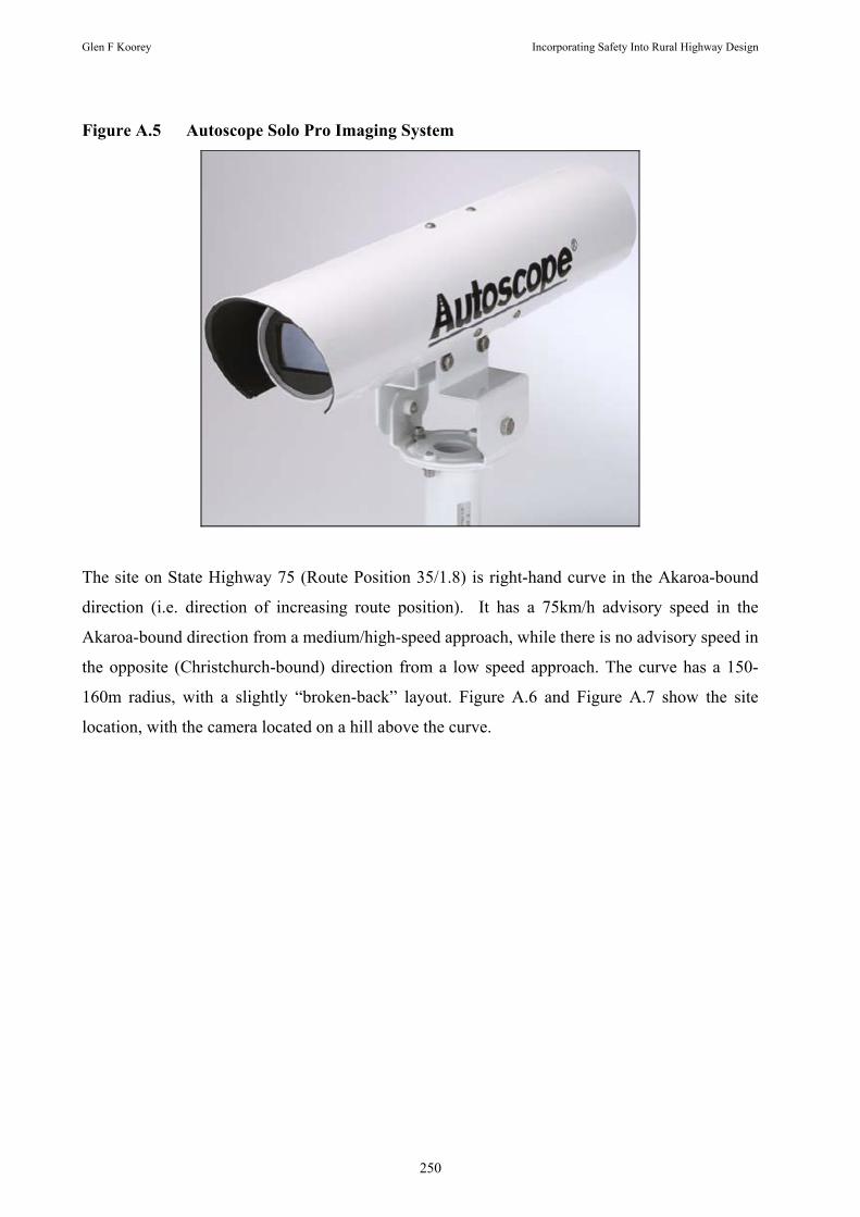
Glen F Koorey Incorporating Safety Into Rural Highway Design
250
Figure A.5 Autoscope Solo Pro Imaging System
The site on State Highway 75 (Route Position 35/1.8) is right-hand curve in the Akaroa-bound
direction (i.e. direction of increasing route position). It has a 75km/h advisory speed in the
Akaroa-bound direction from a medium/high-speed approach, while there is no advisory speed in
the opposite (Christchurch-bound) direction from a low speed approach. The curve has a 150-
160m radius, with a slightly “broken-back” layout. Figure A.6 and Figure A.7 show the site
location, with the camera located on a hill above the curve.

Glen F Koorey Incorporating Safety Into Rural Highway Design
251
Figure A.6 View of the Autoscope test site (circled) when driving from Christchurch
Figure A.7 View from the Autoscope test site towards Christchurch
To minimise the effect of the survey on traffic behaviour, the camera and equipment tent were
camouflaged as much as possible using nearby vegetation (see Figure A.8). Because of the

Glen F Koorey Incorporating Safety Into Rural Highway Design
252
remoteness of the survey location, the Autoscope equipment and connected laptop and video
recorder/monitor were powered by an inverter that converted a 12V battery charge to 240V AC
power (see Figure A.9 ).
Figure A.8 Autoscope camera and survey tent
Figure A.9 Survey equipment used to monitor Autoscope camera

Glen F Koorey Incorporating Safety Into Rural Highway Design
253
Once on site and established, the first task was to identify and mark survey points on the road
and then use these to define virtual detectors within the Autoscope software. Figure A.10
illustrates the layout used in the test survey. For this survey, presence/count detectors (indicated
on the Figure by thick bars) and speed detectors (indicated on the Figure by hollow rectangles)
were located in each direction at 50 m intervals around the curve and approach. About 40 m
from the curve apex, two directional presence detectors (indicated on the Figure by thick arrows)
were defined to detect vehicles travelling in the Akaroa-bound direction that crossed over the
centreline.
Figure A.10 Virtual detectors at the Autoscope test site (looking towards Christchurch)
Once the Autoscope was set up, traffic was monitored for approximately half an hour and data
were collected by the laptop. The data obtained from the Autoscope are recorded in a tab-
delimited text file, with one data line for the start or end of each triggering of a defined detector.
Conventional video footage was also recorded to allow for review later on.

Glen F Koorey Incorporating Safety Into Rural Highway Design
254
The format of the collected data, where all event types are recorded together in chronological
order, required considerable post-processing to identify and group data relevant to the same
vehicle, especially when multiple vehicles were in the vicinity. A sample of fewer than 100
vehicles took approximately 3 hours to process manually. However, in practice, many of these
closely-spaced vehicles would be eliminated from analysis because of the influence on them by
adjacent vehicles. An automated database routine could theoretically also be developed to more
efficiently produce the required data from a larger sample.
The results from this trial indicate that:
• The Autoscope appears to be reasonably accurate for measuring vehicle speeds within 100 m
of the camera. However, increasing distances appeared to affect the likelihood of detectors
further away being triggered, with many vehicles not being registered 100 m or 150 m away
from the curve apex. Of those that were detected, the recorded speeds were often well below
the vehicle speeds observed by video. This was understandable given that the screen
resolution, on which detectors further away were based, was much coarser relative to the
road and hence less accurate.
• To overcome the distance resolution issue, longer-distance surveys would require the use of
multiple cameras (e.g. around a curve). This is similar to the approach taken by Wong
(1989), although more work would be required to set up virtual detectors for each camera
view. Another possible treatment could be to use more powerful high-resolution zoom
cameras.
• The longitudinal presence detectors appeared to work well in identifying when vehicles cross
over the opposing lane line. A series of such detectors could therefore be quite successful in
determining the relative lateral position of vehicles around curves. This would of course
require additional work to set up and post-process however. Again, the relative level of
precision that could be obtained (e.g. 0.5 m lateral intervals would give reasonably useful
data) would be dependent on the resolution that could be obtained from the camera.
• Because of the way that the Autoscope detects vehicles, the data is a little susceptible to other
movement within the field of vision. This includes getting false readings from vehicle
shadows and moving vegetation (particularly noticeable in windy conditions). Even the
camera mounting location can cause problems if it is not securely fixed in windy conditions.
To minimise such problems requires a combination of site preparation (e.g. trimming back
vegetation, secure mountings) and defining additional “redundant” on-screen detectors that
must also be triggered to confirm a vehicle’s presence.

Glen F Koorey Incorporating Safety Into Rural Highway Design
255
There are also some major logistical issues with regards to site set-up at temporary remote
locations that would need to be addressed for similar future research:
• To obtain good coverage of the site, the Autoscope camera needs to be located in an elevated
position; this may preclude some sites from survey or require additional overhead supports
(while still attempting to remain inconspicuous). Either way, considerable effort may be
needed to place the camera in such a location.
• The transient nature of the survey location requires that the virtual detectors must be defined
only once the camera is in place. This is a reasonably time-consuming process, both in terms
of setting out and measuring physical calibration points by the road and defining the virtual
detectors on screen. Only if permanent camera mounting locations were installed could
repeat surveys be undertaken more efficiently.
• The tent to house the monitoring equipment proved to be rather cramped and hot for working
in; it was also difficult to camouflage (its bright colour did not help). Shifting the tent and
equipment to the elevated location also had its difficulties on the test site. In the future it
may be better to obtain a very long cable to the camera and locate the monitoring equipment
in a more unobtrusive and easily accessible location at a lower elevation.
A.12.2.2 Other Survey Devices Considered
Two AccuRange laser rangefinders were also purchased by the University. These can be
mounted inconspicuously on the side of the road and measure the distance to any passing vehicle
that interrupts its infrared laser directed across the road; a series of these devices can determine
travel speeds between successive points. Figure A.11 shows the devices set up on the side of the
road. The laser rangefinders were tested on campus and in the field (urban street), with
promising results. The accuracy of the results appeared to be affected by the presence or
otherwise of a backing board on the other side of the road; however, for many typical road
widths, the distance to such a board starts to get beyond the normal range of the devices, thus
negating its intended effect.

Glen F Koorey Incorporating Safety Into Rural Highway Design
256
Figure A.11 Accurange laser rangefinders being tested in Christchurch
Another possibility considered was the use of a high-speed laser scanning survey device (or
“laser scanner”), often used for complex land or industrial surveys or for quick site data
recording by Police at road crash sites. A laser scanner is essentially a laser distance measuring
device housed in a unit with rotating mirrors, which allows the laser beam to be sent out over a
wide range of directions horizontally and vertically whilst the readings are sampled at a high
frequency (typically >5000 points per second).
In theory, a laser scanner could enable vehicle speeds and positions to be monitored continuously
throughout a curve. Although laser scanners do not appear to have been used previously for
vehicle monitoring surveys, the literature review to date suggests that it should be feasible,
subject to the appropriate software and scanning technique being available. Normally surveys
are only interested in static objects (such as terrain or buildings) and software is used to filter out
any items moving between scans. In this instance, the aim would be filter out the static data and
retain the moving (vehicle) information. Manandhar & Shibasaki (2001) demonstrated an
interesting variant whereby urban environment survey data were collected while driving in a
vehicle fitted with three laser scanners, thus requiring matching of static objects from a moving
perspective.

Glen F Koorey Incorporating Safety Into Rural Highway Design
257
Another device identified that offered both speed and position detection was the TIRTL (“The
Infra-Red Traffic Logger”), manufactured by CEOS Industrial Pty Ltd in Australia. The TIRTL
(pronounced “turtle” and fittingly shaped somewhat like one) consists of two infra-red
transmitting and receiving devices placed on either side of a road. The transmitting device emits
four separate infra-red beams across the road (below axle height). When these beams are broken
by passing vehicles, the receiving device can determine various attributes about each vehicle
based on the relative timing of the beam “events”. Figure A.12 shows how vehicles interact with
the infra-red beams. Because of the unique “cross-over” arrangement of the beams, the TIRTL
is able to determine the relative lateral position of the vehicle as well as the more traditional
speed and classification.
Figure A.12 Determining Vehicles Speeds/Positions using a TIRTL (from CEOS 2005)
The University has purchased a pair of TIRTL devices; however field studies have not yet been
undertaken.