Portland State University Portland State University

PDXScholar PDXScholar

Dissertations and Theses Dissertations and Theses

6-2-2021

Incorporating Conditional ß-Mean based Equity Incorporating Conditional ß-Mean based Equity

Metric in Coverage based Facility Location Problems Metric in Coverage based Facility Location Problems

Rohan Sirupa Portland State University

Follow this and additional works at: https://pdxscholar.library.pdx.edu/open_access_etds

Part of the Transportation Engineering Commons

Let us know how access to this document benefits you.

Recommended Citation Recommended Citation Sirupa, Rohan, "Incorporating Conditional ß-Mean based Equity Metric in Coverage based Facility Location Problems" (2021). Dissertations and Theses. Paper 5714. https://doi.org/10.15760/etd.7587

This Thesis is brought to you for free and open access. It has been accepted for inclusion in Dissertations and Theses by an authorized administrator of PDXScholar. Please contact us if we can make this document more accessible: pdxscholar@pdx.edu.

Incorporating Conditional β-Mean based Equity Metric in Coverage based Facility

Location Problems

by

Rohan Sirupa

A thesis submitted in the partial fulfillment of therequirements for the degree of

Master of Sciencein

Civil and Environmental Engineering

Thesis Committee:Avinash Unnikrishnan, Chair

Miguel A. FigliozziChristopher M. Monsere

Portland State University2021

© 2021 Rohan Sirupa

Abstract

A classical maximum coverage facility location problem (MCLP) tries to

maximize the coverage by serving all possible demands within the specified cover-

age radius. Depending on the applications, several families of MCLP variants have

been developed - each with its unique set of additional constraints. One specific

application is locating Emergency medical service (EMS) units. EMS units such

as ambulances or drones with emergency supplies are located using models such

as the maximum expected survival location problem (MEXSLP). However, a clas-

sical MEXSLP model tends to locate EMS units near densely populated regions,

resulting in increased response times for lowly populated regions. If equity is to be

taken into consideration, the EMS units would be placed more uniformly across

the region which might result in reduced overall coverage.

In this thesis, a conditional expectation measure called the conditional β-

mean (CBM) is considered and integrated into the facility location models. First,

the CBM measure is integrated into the MCLP, resulting in the development of a

new MCLP model. Using an alternative and more intuitive definition for CBM,

another modified MCLP model incorporated with CBM is developed. These new

MCLP models incorporated with CBM are single objective facility location mod-

els with flexible coverage radius constraints. Two standard test cases and a Port-

land Metropolitan region dataset are used to test the MCLP models. A simple

greedy based heuristic is developed, and its performance is compared to a state-

i

of-the-art Mixed Integer Programming solver Gurobi. The integration of CBM

into the MCLP model has improved its coverage. The proposed heuristic provides

reliable solutions and saves considerable computational time.

Using the same CBM measure, equity is incorporated into the MEXSLP

model. We propose two different approaches to estimate CBM and develop two

modified MEXSLP models improving the quality of service provided to outlying

and lowly populated areas. The two MEXSLP models modified with CBM are

linear, and the decision maker has the leverage to chose the level of equity in the

solution using the parameter β. The same Portland dataset is used for testing

the MEXSLP models. Integration of CBM into the MEXSLP has improved the

service in Portland suburbs by locating few EMS units closer to them.

ii

To my family

iii

Acknowledgements

This work is a product of the best wishes and support of a lot of people. I

will try and do my best to acknowledge everyone.

First and foremost, I would like to sincerely thank Prof. Avinash Unnikrish-

nan, who has been a mentor in the truest sense. I would like to especially thank

him for his continuous guidance, patience, and support towards this thesis and

research. He sure is an exceptional advisor, and I can’t think of any other person

who can inspire me better. I truly feel fortunate for the opportunity I had to learn

in an environment with total academic freedom and support, where showing up

to every meeting with more questions than answers was met with enthusiasm and

encouragement.

I would also like to thank Prof. Miguel Figliozzi and Prof. Christopher Mon-

sere for agreeing to serve on my thesis committee and adding value to this work.

I am very grateful to the National Science Foundation (NSF) for enabling this

work through much needed financial support. This research is a product of NSF

grants awarded to Prof. Unnikrishnan (Grant numbers: 1562109 and 1826337).

I am also thankful for the support I received from the Civil and Environmental

Engineering department through the teaching assistantships.

I would like to mention Darshan Chauhan, who is a fellow classmate, lab-

mate, friend, senior, mentor, and almost like a brother. I cannot thank him

iv

enough for all the motivation, encouragement, support, and guidance he provided

at every step, every turn, and every dead-end of this journey.

A special thanks to Dr. Arkamitra Kar for encouraging me to pursue grad-

uate studies and for the fantastic opportunities he has given me. I would like

to thank Prof. Sridhar Raju, Dr. Chandu Parimi, and Dr. Anasua Guharay for

introducing me to the field of research during my undergraduate studies.

A lot of people enriched my time in Portland. I would like to thank my fellow

classmates and friends Santiago, Jaclyn, Mike, Frank, Katherine, and Travis for

the mutual exchange of knowledge, fun, laughter, and occasional frustrations

with homework and projects. I would also like to thank Dr. Jason Anderson

for sharing his knowledge, inspiring me with his work, and showing me the fun

in research. Thanks to Sam, Kiley, and Sarah for not just being great staff but

helping me through all the administrative hurdles.

Special thanks to my friends Pratik, Pranav, Rushabh, Raghu, Munisha,

and Srinivas for being there for me during some of my most challenging times

and helping me see the path when I lost my track. Thanks to all other friends

at Goose Hollow for all their help, support, evening runs, workouts, bubble tea

walks, weekend trips, and all other stuff we cherish from the last two and half

years.

Finally, a very big shout out to my beloving family: dad Krishna, mother

Sravani, and sister Lahari, who always believed in me, supported me, encouraged

v

me, and made sure I was doing fine all through my journey here over my daily

calls to India. My love to all my long-distance friends from India who remind me

of the fun we had, the hardships we shared, and the time we spent.

A hearty thanks to all others whom I could not acknowledge here but have

been a part of this marvelous journey.

vi

Contents

Abstract i

Dedication iii

Acknowledgments iv

List of Tables x

List of Figures xi

1 Introduction 1

1.1 Motivation and Background . . . . . . . . . . . . . . . . . . . . . . . 1

1.2 Conditional β-Mean . . . . . . . . . . . . . . . . . . . . . . . . . . . 3

1.3 Organization . . . . . . . . . . . . . . . . . . . . . . . . . . . . . . . 5

2 Literature Review 6

2.1 Facility Location Problems and Models . . . . . . . . . . . . . . . . . 6

2.2 Emergency Medical Services Applications and Models . . . . . . . . . 11

2.3 Equity Measures for FLP . . . . . . . . . . . . . . . . . . . . . . . . . 21

2.4 Conditional β-Mean . . . . . . . . . . . . . . . . . . . . . . . . . . . 27

2.5 Contributions . . . . . . . . . . . . . . . . . . . . . . . . . . . . . . . 29

3 Facility Location Problem Application 30

vii

3.1 MCLP Problem Description . . . . . . . . . . . . . . . . . . . . . . . 30

3.2 MCLP-CBM-I Model . . . . . . . . . . . . . . . . . . . . . . . . . . . 31

3.3 MCLP-CBM-II Model . . . . . . . . . . . . . . . . . . . . . . . . . . 38

4 EMS Location Problem Application 45

4.1 MEXSLP Problem Description . . . . . . . . . . . . . . . . . . . . . 45

4.2 MEXSLP-CBM-I Model . . . . . . . . . . . . . . . . . . . . . . . . . 48

4.3 MEXSLP-CBM-II Model . . . . . . . . . . . . . . . . . . . . . . . . . 54

5 Analysis 59

5.1 MCLP-CBM Models Analysis . . . . . . . . . . . . . . . . . . . . . . 59

5.1.1 Analysis on Portland Metropolitan Data . . . . . . . . . . . . 59

5.1.2 Analysis on Standard Test Dataset . . . . . . . . . . . . . . . 63

5.2 Greedy Heuristic and Application . . . . . . . . . . . . . . . . . . . . 65

5.2.1 Heuristic Methodology . . . . . . . . . . . . . . . . . . . . . . 65

5.2.2 Heuristic Performance Analysis . . . . . . . . . . . . . . . . . 66

5.3 EMS Applications/MEXSLP Models Analysis . . . . . . . . . . . . . 70

5.4 Summary . . . . . . . . . . . . . . . . . . . . . . . . . . . . . . . . . 80

6 Conclusions 82

Bibliography 85

A Appendix: Portland Metropolitan Dataset 96

viii

B Appendix: Standard P-Median Test Cases 104

ix

List of Tables

5.1 MCLP Models - Objective and Gurobi Gap using PDX Dataset. . . . 62

5.2 MCLP Models - Objective and Gurobi Gap using P-Median Dataset. 64

5.3 Heuristic Results for MCLP-CBM Models using P-Median Dataset . . 67

5.4 Heuristic Results for MCLP-CBM Models for PDX Data . . . . . . . 68

5.5 Heuristic Performance . . . . . . . . . . . . . . . . . . . . . . . . . . 70

5.6 MEXSLP Models - Objective and GAP Values. . . . . . . . . . . . . 71

5.7 MEXSLP Model Travel Time Statistics. . . . . . . . . . . . . . . . . 77

5.8 MEXSLP-CBM-I Model Travel Time Statistics. . . . . . . . . . . . . 77

5.9 MEXSLP-CBM-II Model Travel Time Statistics. . . . . . . . . . . . . 78

x

List of Figures

5.1 Demand points and potential facilities in the Portland Metropolitan Re-

gion. . . . . . . . . . . . . . . . . . . . . . . . . . . . . . . . . . . . . 60

5.2 MEXSLP solution (p = 20) . . . . . . . . . . . . . . . . . . . . . . . . . . 73

5.3 MEXSLP CBM-I and MEXSLP CBM-II solutions (p = 20 and β = 1%) . . . . . 73

5.4 MEXSLP CBM-I and MEXSLP CBM-II solutions (p = 20 and β = 20%). Size

of star corresponds to EMS units at that location. . . . . . . . . . . . . . . . 74

5.5 MEXSLP solution (p = 40). . . . . . . . . . . . . . . . . . . . . . . . . . 74

5.6 MEXSLP CBM-I and MEXSLP CBM-II solutions (p = 40 and β = 1%) . . . . . 75

5.7 MEXSLP models solutions (p = 40 and β = 20%). Size of star corre-

sponds to EMS units at that location. . . . . . . . . . . . . . . . . . . . 76

5.8 Distribution of Travel Times from facilities to demand (p = 20 and β = 20%) . . 79

xi

1 Introduction

1.1 Motivation and Background

The Maximum Covering Location Problem (MCLP) was first introduced in

Church and ReVelle (1974). Since then it has been popular and paved path for

many problems to locate facilities for public and private services, such as postal,

police, ambulances, and warehouses. Later, Current and Storbeck (1988) proposed

the Capacitated Maximum Covering Location Problem (CMCLP) where each

open facility has a specific capacity, and the total demand assigned to any facility

cannot exceed this capacity. The structure of such a problem would only allow

covering the demand points within the coverage radius, and anything outside will

be left unserved. This approach seems reasonable for many systems, but there is

no such hardbound on the coverage radius for public services, such as postal, med-

ical, or police. They are available to serve the entire jurisdiction. Coverage radius

is a tool aiming to provide a minimum service level to the largest number, but not

to restrict its services.

One of the major applications of MCLP models is in finding optimal sites to

places the EMS units such as ambulances. In these models, the facility locations

are chosen such that the response times are minimum. Response time is the time

1

needed for an EMS unit to arrive at the patient after the emergency call is made.

Li et al. (2011) provides a brief study of such covering models for EMS.

One strong assumption made in these EMS covering models is that the pa-

tient is considered uncovered if it is not within the coverage area, i.e., if a patient

cannot be reached within the predetermined response time threshold by any EMS

unit, then the patient is left out as uncovered in the model. Nevertheless, even if

a patient is located very far, it would be served by the closest available EMS unit.

Even if an EMS unit arrives in time less than the response time threshold, there

is no guarantee that a patient will survive. It has always been a probability; the

shorter the response time greater is the probability of survival.

This idea helped develop the Maximum Survival Location Problems (MSLP)

and Maximum Expected Survival Location Problems (MEXSLP) models, where

the objective is to maximize the aggregated sum of the survival probability of

all demand sites. Erkut et al. (2008) explains the application of various survival

location problems.

The objective of most of the research on EMS location problems has been to

maximize the demand served, i.e., to help as many people as possible using avail-

able resources. However, sometimes it might be reasonable to consider solutions

other than the one with the maximum number of people being served on time.

For instance, with the current objective, the model is inevitably forced to allocate

resources closer to the densely populated areas, resulting in longer response times

2

for patients in low-density or remote areas. This is an efficient way of utilizing

resources, but the question is whether the solution is equitable.

Intuitively, if everyone gets service within the same response time, the so-

lution would be fair and equitable. However, achieving the same level of service

for remote areas as we get for the densely populated urban areas requires a much

higher volume of resources. So, providing the same level of service for everyone

might not be truly fair. A genuinely fair solution is achieved by having a balance

between efficiency and equality. We chose the conditional β-mean measure for

obtaining equity, and in the next section, we go through more details about this

measure.

1.2 Conditional β-Mean

To capture fairness or equity among the customers or facilities, we consider the

conditional β-mean measure proposed in Ogryczak and Zawadzki (2002). The

conditional β-mean measure is closely related to the concept of Conditional Value-

at-Risk (CVaR), which has been popularly used in financial optimization problems

(Rockafellar et al., 2000), and recently even in various managerial and engineering

problems (Filippi et al., 2020). If the outcomes are from a discrete probability dis-

tribution, the conditional β-mean corresponds to be the CVaR of this distribution

with parameter β. The application of conditional β-mean in this work is inspired

from Filippi et al. (2019a), and it is defined is as follows:

3

Definition: Given a β ∈ (0, 1], the conditional β-mean measure is defined as

the average of the highest or lowest (100 ∗ β)% outcomes of demand taken into

account.

Depending on whether the highest or lowest outcomes are being considered,

we get the worst-case or best-case for conditional β-mean. When the parameter

β is 0, the conditional β-mean is the highest or lowest outcome, and when β is

1, the corresponding conditional β-mean is the same as a standard mean. In

the case of discrete problems, if there are m possible outcomes and β = k/m,

then conditional β-mean represents the mean of the highest k outcomes, which is

similar to the k-centrum solution concept.

Intuitively, by definition of conditional β-mean, maximizing or minimizing

this measure would shorten the tail in the distribution of outcomes and reduce

the extremities. So, conditional β-mean can be used to capture equity by reducing

dispersion in outcomes.

Conditional β-mean has the following properties, which makes it suitable for

application of equity and fairness concepts in facility location problems, (Filippi

et al., 2019b)

i. This measure is a Schur-Convex function, thus making it a suitable inequality

measure.

ii. By definition, it acts as an upper bound on the standard mean of outcomes.

4

iii. Can be implemented in Mixed Integer Linear Programs (MILP) models with

a limited number of constraints and variables.

1.3 Organization

The remaining part of the thesis is organized as follows: Chapter-2 reviews the

relevant literature related to facility location problems, emergency medical ser-

vices location problems, equity measures in facility location problems, and appli-

cation of conditional β-mean. Chapter-3 provides the problem description and

formulations of two maximum covering facility location models incorporating

conditional β-mean measure. Chapter-4 provides the problem description and for-

mulations of two emergency medical service location models incorporating condi-

tional β-mean measure for equity purposes. Chapter-5 examines the performance

of the developed conditional β-mean models with other regular models using a

state-of-the-art Mixed Integer Programming (MIP) solver. A simple heuristic is

also proposed in this chapter to solve two of the proposed models. A sensitivity

analysis is performed to estimate the impact of the conditional β-mean constraint

and the impact of other parameters on objective functions. The final chapter,

chapter-6, provides the summary of this work and scope of future directions for

research.

5

2 Literature Review

This chapter reviews relevant literature on the following topics: (i) facility

location problems, (ii) location model applications in Emergency Medical Services

(EMS), (iii) papers focusing on modeling equity metrics in the facility location

problems, and (iv) facility location models which have integrated conditional β-

mean equity measure.

2.1 Facility Location Problems and Models

The goal of the Facility Location Problem (FLP) is to identify locations to open

facilities to satisfy customer demands and optimize specific objectives. The facility

type can vary from storehouses, postal services, emergency services, nuclear power

plants, garbage disposal sites, etc. Depending on the application, the objectives

and constraints of the FLP will be different.

The FLP can be solved for public or private sector services. For a private

sector facility location analysis, it is reasonable to assume that the model’s objec-

tive is to minimize the total costs involved in the system, which primarily includes

set-up, distribution, and maintenance costs. In contrast, the public sector facil-

ity location problems are more concerned with the quality or level of service. An

6

example of an objective for public sector applications is maximizing the demand

coverage.

Toregas et al. (1971) and Toregas and ReVelle (1972) introduced the Location

Set Covering Problem to find the minimum number of facilities required to cover

all users within the desired service distance, which is also called the service or

coverage radius. If there is a limitation on the number of facilities, achieving

complete coverage is not possible. For such cases, Church and ReVelle (1974)

developed the Maximum Covering Location Problem (MCLP), whose objective is

to attain the highest coverage by maximizing the population being covered within

the service radius.

Church and ReVelle (1974) also includes another model called MCLP with

mandatory closeness constraints, which focuses on covering as many people as

possible within the coverage radius, and shows concern for the quality of service

being provided for people outside the coverage radius, S. In short, the model cov-

ers the maximum population possible within the coverage radius but also ensures

that everyone has at least one facility in a distance S ′, called the mandatory cov-

erage radius. This is an approach to make the solution fairer for every person in

the system. Lower the difference between S and S ′, the fairer solution is to people

outside coverage radius.

Another important issue in locating both public or private facilities is the

capacity. In most cases, any open facility can only handle a certain amount of

7

demand, leading to constraints on their capacity or workload. Considering this,

a new model called the Capacitated MCLP was proposed in Chung et al. (1983)

and Current and Storbeck (1988) with capacitated facilities. These models are an

extension of the maximum covering models with additional capacity constraints.

Pirkul and Schilling (1991) further extended the Capacitated MCLP model

by providing backup service to users. Pirkul and Schilling (1991) presents the

formulation and solution procedure for this model, where all facilities are capac-

itated, and every demand has a primary and secondary backup facility. Pirkul

and Schilling (1988) considered a similar problem of allocating capacitated facili-

ties with backup service providers, but instead of maximizing the coverage, their

objective was to minimize the average distance traveled.

Haghani (1996) presents two different formulations and two different solu-

tion procedures for capacitated MCLP models. The first formulation is a mixed-

integer linear programming model. The second formulation aims to maximize

the weighted covered demand while minimizing the average distance between

uncovered demands and open facilities. By which, this formulation tries to accom-

modate the uncovered demands with facilities having excess capacity.

Albareda-Sambola et al. (2009) introduces the Capacity and Distance Con-

strained Plant Location Problem (CDCPLP), an extension of the discrete capac-

itated facility location problem. This model has constraints on facility capacity

and maximum distance traveled by the vehicles. First is the limited capacity of a

8

facility to serve demands from customers. Next is that each vehicle can only travel

a limited distance to complete their assigned facility-customer-facility round trips.

CDCPLP model identifies the facilities to open, finds the number of vehicles re-

quired at each facility, and assigns each customer to a specific facility and vehicle

to minimize all costs involved while not violating the facility capacity or vehi-

cle distance constraints. CDCPLP is similar to the capacitated facility location

problem, but it includes fleet management.

With the recent development of Unmanned Aerial Vehicles (UAVs) or drones,

several companies like Amazon, Google, and UPS are evaluating their potential

for use in commercial delivery services. Drones are not restricted by the avail-

ability of existing infrastructure and not affected by traffic, making them suitable

for emergency services, such as delivering critical medical supplies. With such

applications in mind, FLP models incorporating drones have been developed and

studied. Chauhan et al. (2019) proposed a maximum coverage facility location

problem with drones (MCFLPD) model, a complicated version of MCFLP as

it has additional drone constraints range, availability, and payload. MCFLPD

model is similar to the CDCPLP model in Albareda-Sambola et al. (2009), while

CDCPLP focuses on minimizing the cost, MCFLPD focuses on maximizing the

coverage. Also, CDCPLP assumes a fixed number of drones in each facility, while

MCFLPD assumes a fixed number of drones in the entire system, which gives

a new drone allocation feature and adds more complexity to the problem. In

9

Chauhan et al. (2019), the model is not based on one-to-many deliveries in a trip.

It is assumed that all deliveries are one-to-one, i.e., they leave from a facility,

complete the delivery and come back to the same facility.

Most of the FLP models discussed so far are static and deterministic does

not account for uncertainty in the system. The system’s uncertainty could be

dealt with either by optimizing the expected scenario or optimizing the worst-case

scenario. Sheppard (1974) was among the first to use scenario planning in facility

location. This model minimizes the expected cost across all scenarios. Schilling

(1982) suggests an approach where the initial decisions implemented are the ones

that are common in most scenarios and delay other decisions till uncertainty is

not resolved. Snyder et al. (2007) states that scenario planning allows decision-

makers to model dependence among random parameters, making it suitable for

uncertainties in FLP. Snyder et al. (2007) studies the stochastic facility location

problem with risk pooling, which locates distribution centers while minimizing the

total fixed location costs, transportation costs, and inventory costs.

Besides this scenario planning, uncertainty can also be captured using a

measure called α-reliable regret. Daskin et al. (1997) presented a model called

the α-reliable minimax regret and combined it with a p-median model. In many

situations, minimizing the α-reliable maximum regret is appropriate compared

to any average or worst-case regret. However, computationally, it is not easy to

solve and obtain. So, Chen et al. (2006) proposes a new model called α-reliable

10

mean-excess regret or mean-excess model. This measure explicitly accounts for the

magnitude of regrets in the distribution’s tail, making it computationally much

easier to solve or apply over the α-reliable minimax model.

Ghosh and McLaerty (1982) proposes a model where the sum of regrets is

minimized over all possible scenarios. The objective of minimizing the sum of

regrets is equivalent to minimizing the expected regret with all scenarios having

the same probability.

There is a significant amount of work in FLP and several extensive reviews

of various FLP variants. ReVelle and Eiselt (2005), Revelle et al. (2008), and

Daskin (2011) provide a detailed review of various FLP variants and associated

formulations and solution methods. Farahani et al. (2012), Berman et al. (2010),

and Schilling (1993) provide an exhaustive review of MCLP variants. For the FLP

under uncertainty, an in-depth review is provided by Berman and Krass (2001);

Correia and Saldanha-da Gama (2019); Snyder et al. (2016) and Snyder (2006).

2.2 Emergency Medical Services Applications and Models

The concept of coverage is an appealing measure for the performance of facility

location problems, especially in locating Emergency Medical Services (EMS),

where the quality of service is crucial. An important factor pertaining to the

quality of service in any EMS system is timeliness in providing these services.

11

Most of the EMS locating models are variations of the classical MCLP in-

troduced in Church and ReVelle (1974). So, in other words, most of the covering

models discussed in the previous section can be modified to the requirements of

an EMS system. This MCLP model assumes that the vehicles are always free

and doesn’t include any adjustments for vehicles such as ambulances being busy.

Considering that ambulances might be busy serving other users, Daskin (1983)

proposed an extension of the MCLP model called the Maximal Expected Cover-

ing Location Problem (MEXCLP). MEXCLP assumes that the probability of an

ambulance being busy is the same across the system. Recognizing that this might

not be the case, other location models have been developed. Batta et al. (1989)

modified the MEXCLP model and introduced the Adjusted MEXCLP (AMEX-

CLP), which recognizes that servers do not operate independently they might

have different busy probabilities depending on the location.

In emergency service systems queuing is undesirable. When a service request

occurs, the nearest ambulance is dispatched. Assume another request arrives at

the same facility before the return of the ambulance. Now instead of forming a

queue at this facility, an ambulance should be sent from the next closest facility

having resources. Though both the MEXCLP and AMEXCLP have considered

the possibility of an ambulance being busy, neither of them addressed the stated

issue.

This need for a backup facility is important in regions/zones with heavy

12

demand or population. An effective way of solving such a problem would be pro-

viding a backup facility for each demand point along with an assumption of a

reasonable threshold on each facility’s workload.

Berlin (1974) is one of the earliest works on locating facilities with backup

services. They first used a sequential approach on a location set covering problem

(Toregas and ReVelle, 1972) to find the minimum number of ambulances and

their dispatching sites. Then using a simulation model estimated the utilization of

each ambulance. Daskin and Stern (1981) proposed another model by modifying

the set covering problem using a hierarchical multi-objective formulation which

minimized the required number of facilities and maximized the number of times

demand is covered at the same time. Ruefli and Storbeck (1982) created another

hierarchical maximum covering model where demands are covered by primary

facilities, and secondary facilities provide backup to the primary facilities.

Hogan and ReVelle (1986) developed a coverage maximizing model where

each demand zone is assigned with two facilities, a primary facility and an-

other secondary backup facility if the primary is busy serving another. Pirkul

and Schilling (1988) and Pirkul and Schilling (1991) also considered a similar

model providing backup services while assuming that all facilities are capacitated.

Narasimhan et al. (1992) proposed an extension of such a model to provide multi-

ple levels of backup services.

Another approach for ambulance or EMS location problems is using multiple

13

objectives. Daskin et al. (1988) integrated various covering models, including

multiple excesses, backup, and expected coverage models. This multi-objective

model is a reformulated version of the hierarchical objective model in Daskin

and Stern (1981) and allows the decision-maker to have a trade-off between extra

coverage and the number of facilities.

Araz et al. (2007) proposed a multi-objective facility covering location

model based on the models provided in Hogan and ReVelle (1986) and Pirkul

and Schilling (1988). Their model consists of three objectives: (i) maximize the

demand covered by a single vehicle, (ii) maximize the demand with a backup

service, (iii) minimize the total distance from facilities located farther than a spec-

ified distance standard for demand points. They proposed to solve this model

using a fuzzy goal programming approach.

In the literature, there are other works which consider different coverage

assumptions regarding, such as allowing partial coverage or even restrict coverage,

which include Revelle et al. (1996), Berman and Krass (2002) and Karasakal and

Karasakal (2004). However, these models aren’t discussed in detail here as they do

not focus on maximizing the coverage. Brotcorne et al. (2003) can be referred for

a more detailed review of literature on the ambulance or EMS location problems.

All the EMS location models discussed so far do not consider the possibility

of having multiple types of EMS units or levels of severity in a patient’s condition.

Batta et al. (1989) studied one such EMS model considering multiple casualty

14

types with probabilistic travel times, but with just one type of server, i.e., the

EMS unit.

In literature, certain studies focus on two-tiered EMS systems considering two

types of EMS units: Basic Life Support (BLS) and Advanced Life Support (ALS).

The BLS units are equipped with basic equipment, whereas the ALS units are

equipped with life-saving procedures, including the equipment provided in BLS

units.

Belanger et al. (2019) summarize and discusses the modern approaches in

EMS modeling, addressing the problems related to EMS fleet management, EMS

vehicle location or relocation, and their dispatching decisions. Their work begins

with the literature on static ambulance location models followed by multi-period

relocation models, dynamic relocation models, and approaches related to ambu-

lance dispatching decisions.

Schilling et al. (1979) proposed two optimization models (TEAM and FLEET)

to maximize the fraction of demand covered by both the BLS and ALS units in

the system. ReVelle and Marianov (1991) and Marianov and ReVelle (1992) ex-

tended the FLEET model to maximize the coverage provided by both EMS units

while ensuring individual and joint reliability requirements.

Mandell (1998) proposes a probabilistic covering model, which unlike Batta

et al. (1989), considers multiple types of medical units but not multiple casu-

alty types. This model considers both BLS and ALS units but assumes a patient

15

or call is covered if and only if an ALS unit can respond within a prespecified

amount of time.

Marianov and Serra (2001) introduce another model that maximizes the cov-

erage considering a limited number of BLS and ALS EMS units in a hierarchical

system with congestion. Here, demand is considered covered when both types of

units are within the prespecified distance and do not have to wait in the queue

with more than a fixed number of demands. Both the models proposed in Mandell

(1998) and Marianov and Serra (2001) assume two types of EMS units, but they

do not consider multiple types of demands.

McLay (2009) extended the MEXCLP proposed in Daskin (1983), introducing

the Maximum Expected Coverage Location Problem with two types of servers

(MEXCLP2) to optimally locate two types of EMS units while serving multi-

ple types of customers. In MEXCLP2, the ALS units are non-transport quick

response vehicles, and BLS units are ambulances with the ability to transport

patients. Here, for every call, both types of units are dispatched so that the am-

bulance can transport the patient to the hospital after ALS units provide the

necessary treatment.

Next, Boujemaa et al. (2018) aims to account for the inherent uncertainty

from demands and designs a robust two-tiered EMS system. This study proposes

a two-stage stochastic location-allocation model that simultaneously determines

EMS units’ location, the type and number of units to be dispatched, and the

16

demands covered by each EMS station.

Grannan et al. (2015) developed a military medical evacuation (MEDEVAC)

system to respond and transport casualties based on their severity using two types

of air ambulances. They proposed a binary linear programming model to locate

air assets and create response districts using a preferred dispatch list. This model

defines three categories for casualties and aims to maximize the proportion of

highest priority casualty responded to within a prespecified response time thresh-

old while not violating the performance constraints on other types of casualties.

Gendreau et al. (1997) proposed a model called the double standard model

(DSM), which determines the location of EMS vehicles while maximizing the

proportion of demand covered twice within a predefined distance. Later, Liu et al.

(2014) and Liu et al. (2016) extended this DSM model considering multiple types

of EMS vehicles and demands with various priority levels.

Gendreau et al. (2001) proposed an ambulance relocation model accounting

for the dynamic nature of the EMS systems. This relocation problem is developed

on the DSM problem, proposed in Gendreau et al. (1997), by adding a penalty

term in the objective function, which takes in the cost of relocation of vehicles.

Mason (2013) also proposed a dynamic ambulance relocation model named

the real-time multi-view generalized cover repositioning model (RtMvGcRM).

Like Gendreau et al. (2001), RtMvGcRM’s objective is to maximize the quality

of service while minimizing the relocation costs. However, RtMvGcRM considers

17

multiple types of ambulances having varying performance in the system.

Van Barneveld et al. (2017) developed a model for an EMS system in the

Netherlands with two types of units: Rapid Responder Ambulances (RRA) and

Regular Transport Ambulances (RTA). Among the two, RRA units are faster,

but they cannot transport a patient. They use compliance tables to identify the

desired locations to place EMS units considering they get busy. They extend

the ambulance relocation model from Gendreau et al. (2006) and the MEXCLP2

model from McLay (2009) to propose an integer linear programming model com-

puting these compliance tables.

Yoon et al. (2021) propose a two-stage stochastic programming model that

determines how to locate and dispatch different types of EMS units. This model

is called the Scenario-based Ambulance Location for Two types (SALT) model,

considering two types of EMS units, ALS and BLS units, and two types of call-

priorities, high and low. High-priority calls are assumed to be life-threatening and

require ALS units, whereas, for low-priority calls, either BLS or ALS units are

sufficient. They proposed a data-driven approach of sampling call arrival scenarios

directly from the call logs to avoid distributional assumptions and capture the

Spatio-temporal correlation between calls.

Besides all these, Hammami and Jebali (2019) propose a two-tiered EMS

model to determine the location and modular capacity of ambulance stations that

minimize the total cost while respecting the predefined response time threshold.

18

Their approach considers advanced trip information such as total service time,

busy fraction, and modular capacity of base stations. Compared to other tradi-

tional approaches, this approach is unique in that it considers the travel time from

the demand to the trauma center in the total service time. However, unlike other

EMS models, this model focuses on minimizing cost instead of maximizing the

total coverage.

Besides the ambulance stations, an EMS system also contains trauma care

centers. Now we will discuss models which identify the locations of both the EMS

stations and trauma centers. Branas and Revelle (2001) proposed the Trauma

Resource Allocation Model for Ambulances and Hospitals (TRAMAH), which is

the first of its kind to locate both trauma centers and air ambulance depots. This

model has the computational flexibility to locate both these assets as either sep-

arate resources or in tandem. TRAMAH can be used to develop an EMS system

from absolute nothing or to improve an existing system.

Lee et al. (2012) present a mathematical model and its solution methodol-

ogy to identify the optimal location for trauma centers and air ambulances. The

model proposes a method that uses integer programming and simulation to up-

date busy fractions in the model iteratively.

Cho et al. (2014) also studied the problem of simultaneously locating trauma

centers and helicopters. In their work, they endogenize the calculation of the

helicopter’s busy fractions into the optimization problem. Later, Lee and Jang

19

(2018) extended this model into a multi-period model by introducing another

aspect: when to locate. However, the original model is quite challenging to solve,

and the addition of time-dependent parameters makes it much more difficult.

Jayaraman and Srivastava (1995) also proposed a model that tries to maxi-

mize the expected coverage of the demands while simultaneously locating facilities

and allocating multiple types of equipment to them.

After locating EMS units, the next most important question is how to dis-

patch these EMS units in real-time? Bandara et al. (2012), Sudtachat et al.

(2014), Yoon and Albert (2018), and Yoon and Albert (2020) have answered

this problem using the Markov Decision Process (MDP) which dynamically de-

termines which EMS unit to be dispatched using real-time system status. These

dispatching policies are developed to maximize patients’ survival probability by

incorporating the arrival call’s degree of urgency. The optimal policy provides an

ordered preference list of EMS units to dispatch based on priority.

It is to be noted that, even though all the above-mentioned models have

a different approach to estimate coverage and provide better quality of service,

all of them have a primary objective of maximizing coverage, i.e., capture the

maximum population possible within the predefined service radius. Implementing

this approach alone can bring disparities among the users regarding access to

public services, especially among rural and urban communities. In the following

section, we discuss literature on how such disparities were answered using equity

20

measures.

2.3 Equity Measures for FLP

With a single objective of maximizing coverage, models tend to locate facilities

closer to urban areas having a dense population, leading to adverse outcomes in

rural areas. Even if more EMS units are made available, these models tend to

concentrate units in favor of the urban population unless the coverage is closer to

100%.

Li et al. (2011) states that the literature has thoughtfully investigated the

efficiency of EMS facility location, but the solutions’ equity has been overlooked.

Aringhieri et al. (2017) says that “equity is one of the most challenging concerns

in the healthcare sector, like EMS systems, as it evaluates the fairness of how

resources are allocated to patients”. According to Oliver and DeSarbo (1988),

fairness is the perception of customers on how the ratio of their outcomes to in-

puts is comparable to the other parties in the system.

The words “equity” and “fairness” are often used interchangeably in the

existing literature and mean the same. However, the words “equality” and “eq-

uity” necessarily might not mean the same. In general, equality means providing

every individual with the same amount of resources or opportunities. Whereas

equity recognizes the difference in circumstances of every individual and provides

resources as needed to achieve the same outcome.

21

The MCLP with mandatory closeness constraints proposed in Church and

ReVelle (1974) can be considered as an attempt to provide a fairer solution for

uncovered demand points. As stated in this model, the closer the service and

coverage radii, the fairer the solution is to people outside the coverage radius.

Pirkul and Schilling (1991) also provides a similar extension for their capacitated

MCLP model considering a maximal response or service distance, which is meant

to be a tool to ensure a minimum level of service but not to hold back any re-

sources. However, their results state that improved service to uncovered demands

is attained only at the cost of reduced coverage, i.e., there is always a trade-off

between total service and total coverage.

In some EMS location problems, equity has been evaluated indirectly by

choice of model. One way of ensuring fairness in outcomes is by adding chance

or reliability constraints that enforce a minimum level of service throughout the

system (Ball and Lin, 1993; ReVelle and Hogan, 1989). However, such indirect

approaches neither evaluate equity explicitly nor examine the interaction between

equity and efficiency measures.

Maximin modeling is a popular approach to incorporate equity, where the

objective is to maximize the level of service received by customers hardest to get.

This approach has been used in various research efforts usually as bi-objective

models (Chanta, 2011; Current et al., 1990; Erkut and Neuman, 1992; Kostreva

et al., 2004; Zhan and Liu, 2011). These bi-objective models are often formulated

22

by combining one efficiency measure and another equity measure. However, these

studies do not prescribe anything about weighing the two objectives. Instead,

they provide a range of options for the decision-maker to choose from. This ap-

proach yielded poor performance of the system, which is its major drawback.

Chanta et al. (2014a) considers a bi-objective model whose primary objective

is to maximize the expected coverage while the secondary objective is to improve

fairness regarding access to rural areas. Chanta et al. (2014a) proposes three al-

ternatives for the secondary objectives, which are: (i) minimizing the maximum

distance between every uncovered demand and the open facility closest to it, (ii)

minimizing the number of rural demand points that are uncovered, and (iii) min-

imizing the total number of uncovered demand points, this includes both urban

and rural areas. Their results indicate that the model with the first alternative as

a secondary objective dominates the other two alternatives.

Savas (1978) broadly describes four principles for evaluating equity in public

services, which are equal payments, equal outputs, equal inputs, and equal satis-

faction, and explains how each principle can be selected and implemented. Marsh

and Schilling (1994) provides a comprehensive review of twenty equity measures

in facility location problems, focusing on differences in service outcomes. They

compare functional forms of equity and not how these forms can lead to vari-

ous decisions in reality. They observe and state that there is not much consensus

on the best way or suitable way to measure equity. Barbati and Piccolo (2016)

23

considers ten popular equity measures, introduces few new properties associated

with these measures that could better describe their behavior in the context of

optimization, and performs computational analysis to verify if these properties

are satisfied or not by ten selected measures. Some of the measures considered in

Marsh and Schilling (1994) and Barbati and Piccolo (2016) are: Center (CEN),

Range (RG), Mean Absolute Deviation (MAD), Variance (VAR), Maximum

Deviation (MD), Absolute Deviation (AD), Summation of Maximum Absolute

Differences (SMAD), Schutz’s Index (SI), Coefficient of Variation (CV) and Gini

coefficient (GC). These measures are formulated such that the level of inequality

in the distribution of resources is captured, i.e., lower the value, fairer is the so-

lution. Most of these measures capture various characteristics of the distribution

of travel times or distances. Most of these measures do not satisfy the principle of

Pareto efficiency that it is possible to improve fairness by making some individuals

worse-off. Optimizing fairness measures not obeying Pareto efficiency can lead

to locating facilities far away from customers (Barbati and Piccolo, 2016; Filippi

et al., 2019a). The following example can help us understand this. Consider three

customers located on a straight line, now if we plan to open a facility to serve all

of them, intuitively, the fairest location to open would be at infinity.

Following are some of the studies that have implemented the above measures

to achieve fairness. Lopez-de-los Mozos and Mesa (2001) studied the MAD mea-

sure and its properties when implemented in facility location problems. Drezner

24

et al. (2009) analyzed the Gini coefficient’s application, as an equity measure, in

a facility location problem with uniformly distributed demand points. Ogryczak

(2000) formulated a similar model which minimizes the mean distance and MAD

measure. Ohsawa et al. (2006) proposes a model where efficiency is sought by op-

timizing the sum of squared facility-user distances, while equity is measured using

the sum of absolute differences of distances. Lejeune and Prasad (2013) solved a

tree network facility location model by formulating the median objective as an

efficiency measure and the Gini coefficient as a measure for equity.

Few equity measures that gained popularity later are envy, quintile share

ratio, and conditional β-mean. Espejo et al. (2009) applies the concept of envy

in an uncapacitated discrete facility location problem. This model attempts to

locate p facilities with the objective being to minimize the total envy experienced

by all demand sites. Total envy is defined as the sum of absolute deviations from

the general preferences expressed by all demand sites. Chanta et al. (2011) locates

facilities in an EMS system by minimizing the total envy of all demand points,

where envy is defined as the dissatisfaction of a demand point with respect to the

other points. Chanta et al. (2014b) proposes a similar facility location problem

with the objective being to minimize envy, which is evaluated using a survival

function while having a constraint on minimum survival rate. Rey et al. (2018)

applies the concept of envy in the context of humanitarian logistics to collect and

redistribute surplus perishable food for hunger relief.

25

Drezner et al. (2014) uses the Quintile Share Ratio as an objective function in

facility location analysis. There the Quintile Share Ratio is calculated as the ratio

of the bottom quintile to the top quintile. The bottom quintile is defined as the

total cost paid by the 20% of demand paying the lowest per-unit cost. Similarly,

the top quintile is defined as the total cost of the 20% demand paying the highest

per-unit cost. The denominator of the objective in Drezner et al. (2014) is what

we define as CBM with β = 0.2, i.e., Conditional 0.2-Mean.

In the literature, the concept of equity is also adapted with references other

than distribution of distances, such as distance between pairs of facilities, max-

imum demand assigned to a facility, total demand assigned to a single facility,

and more. Baron et al. (2007) considered a facility location problem with the ob-

jective being to minimize the maximum demand assigned to every facility in the

system. Similarly, Berman and Huang (2008) solved for a facility configuration

that minimizes the maximum total demand assigned for a facility on the network.

Marın (2011) addressed a discrete facility location model which tries to balance

the difference between the maximum and minimum demand sites allotted to each

facility.

Espejo et al. (2009) proposed a unique discrete facility location problem in

which users provide a preference order on potential sites to open facilities. This is

an approach aiming to minimize the total envy experienced by users. Prokopyev

et al. (2009) proposed a problem called the equitable dispersion problem, whose

26

objective is to minimize the range and MAD of the distribution of distances be-

tween pairs of open facilities. McLay and Mayorga (2013) discuss the distinction

between equity from a server and patient perspective.

Jagtenberg and Mason (2020) discussed how to place ambulances across

a region in a fair way, using a fairness measure called Bernoulli-Nash Welfare

Function. The classical ambulance location models aim to improve the system’s

efficiency by maximizing the overall performance, which contrasts with fairness.

The most efficient ambulance configurations benefit people living in cities at the

expense of people living in rural/remote areas. These fairness measures provide a

solution that has a more balanced performance or service across the region/sys-

tem. Their model also involves various performance concepts such as survival

function and the probability of ambulance arrival within the response time thresh-

old. Jagtenberg and Mason (2020) focused on providing the decision-maker with a

model that results in one quite fair solution instead of a Pareto frontier.

2.4 Conditional β-Mean

In our study, the fairness or equity measure incorporated with the facility location

problems is Conditional β-Mean (CBM). In this section, we briefly discuss the

literature related to CBM.

CBM is a measure that can capture both the performance and fairness of a

system. CBM was proposed in Ogryczak and Zawadzki (2002) as a possible fair-

27

ness measure in facility location problems. CBM is related to CVaR, which is

a quite popular risk measure in financial optimization Rockafellar et al. (2000).

Technically, minimizing CBM is similar to minimizing CVaR over a discrete dis-

tribution. CVaR has gained popularity in engineering contexts in recent days

(Filippi et al., 2017).

Chapman and Mitchell (2018) applies a fairness measure inspired from CVaR

in the context of humanitarian logistics. Their objective function includes three

terms, the weighted average of the fixed opening costs of facilities, CVaR of trav-

eling costs, and the average traveling costs for customers to reach facilities. Here,

the traveling distances from customers to facilities are known and fixed, i.e., there

is not any uncertainty. So, the CVaR calculated here is what we defined as CBM.

However, the constraints used to calculate CVaR in their work are nonlinear. In

Drezner et al. (2014), the denominator of the Quintile Share Ratio objective cal-

culates the total cost paid by the 20% demands paying the highest to get served.

By definition, the mean of this value is equivalent to CBM with β = 0.2, i.e.,

Conditional 0.2-Mean.

Filippi et al. (2019a) defined and analyzed a new problem called the Fair

Single Source Capacitated Facility Location problem (F-SSCFLP). This problem

is represented as a bi-objective model where the objectives are to minimize total

costs and improve fairness. In their work, the CBM is used as the fairness mea-

sure and is defined as the average cost paid by the β% customers who have to

28

travel the most to reach the nearest facility. Filippi et al. (2019a) analysis states

that CBM is more flexible than a classical minimax objective problem, and per-

forms better than MAD or Range measures. Jagtenberg and Mason (2020) also

states that CBM to be a potential alternative for maximin models.

2.5 Contributions

Unlike the existing works where CBM is incorporated using a bi-objective func-

tion, here, CBM is incorporated as a constraint with single objective function.

Existing works on incorporating CBM in facility location models focus on min-

imizing cost whereas this thesis is concerned on maximizing coverage. As CBM

is calculated for each open facility, the proposed MCLP models maintain equity

concerning facilities. An alternative approach to estimate CBM is proposed, as-

suming this approach to be faster to solve and intuitively easier to understand. A

greedy based heuristic is proposed in this work, and its performance is compared

to a state-of-the-art Mixed Integer Programming solver.

The existing MEXSLP models to solve EMS location problems in Erkut et al.

(2008) and Jagtenberg and Mason (2020) are nonlinear. Here, we propose two

linear MEXSLP formulations, where equity is incorporated in MEXSLP model

using CBM. In these EMS location models, the level of equity can be chosen by

the decision maker using the parameter β.

29

3 Facility Location Problem Application

This chapter focuses on incorporating CBM into the maximum covering facil-

ity location problem (MCLP). First, a classical MCLP with capacitated facilities

is explained. Next, the concept of CBM is integrated into the classical MCLP

as a constraint and a new model called MCLP-CBM-I is developed. Lastly, by

proposing an alternate way of defining and calculating CBM, another variant of

the MCLP called MCLP-CBM-II is developed.

3.1 MCLP Problem Description

In the classical maximum coverage facility location problem (MCLP), we con-

sider a set I with all demand points, and a set J with all potential locations to

open facilities. The primary objective of this model is to find optimal locations to

open facilities such that maximum possible demand is served while satisfying the

constraints on facility’s capacity and distance.

In this problem, sometimes, certain facilities may be associated with more

costs, in terms of travel distance or travel time, only to satisfy a little more de-

mand. Here we use the concept of CBM, to reduce the disparity among the

distances traveled from open facilities to demand points they serve. We try to

30

achieve this objective by limiting the CBM of the distances from a facility to its

demand points to be less than the facility’s coverage radius.

3.2 MCLP-CBM-I Model

This MCLP-CBM-I model is a modified version of a capacitated MCLP, incor-

porated with CBM on facilities. Here, the CBM for each facility is calculated as

the average distance of the farthest β% demands served by it. In a capacitated

MCLP, any open facility cannot serve demand points outside its coverage radius.

In MCLP-CBM-I, it is assumed that the CBM of a facility cannot exceed its cov-

erage radius, allowing the model to utilize a facility’s total capacity and serve

demands that are close-by but outside the coverage radius. The nomenclature of

MCLP-CBM-I model is provided below and we start with formulation MODEL-

1A.

Nomenclature

Sets

I Set of all demand points

J Set of all potential facility locations

Indices

i ∈ I

j ∈ J

Parameters

31

dij Distance between demand point i ∈ I and facility location j ∈ J

p Maximum number of facilities that could be opened

Uj Capacity of facility location j ∈ J

wi Demand of point i ∈ I

rj Coverage radius of facility at location j ∈ J

β Percentile of demand to be used while estimating CBM

Variables

xij 1, if demand point i ∈ I is served by facility j ∈ J ; 0, otherwise

yj 1, if facility at location j ∈ J is open; 0, otherwise

Mβj CBM of the distances travelled by facility j ∈ J to serve demand points

Primal Formulation

MODEL 1A: Max∑

i∈I

∑

j∈J

wixij (3.2.1)

∑

j∈J

xij ≤ 1 ∀i ∈ I (3.2.2)

∑

j∈J

yj ≤ p (3.2.3)

∑

i∈I

wixij ≤ Ujyj ∀j ∈ J (3.2.4)

xij ≤ yj ∀i ∈ I, j ∈ J (3.2.5)

∑

i∈I

xij ≥ yj ∀j ∈ J (3.2.6)

Mβj ≤ rj ∀j ∈ J (3.2.7)

32

xij ∈ {0, 1} ∀i ∈ I, j ∈ J (3.2.8)

yj ∈ {0, 1} ∀j ∈ J (3.2.9)

where, ∀j ∈ J , we define

W βj = β

∑

i∈I

wixij (3.2.10)

Mβj = Max

{

1

W βj

∑

i∈I

dijxijzij

}

(3.2.11)

∑

i∈I

zij ≤ W βj (3.2.12)

zij ≤ wi ∀i ∈ I (3.2.13)

zij ≥ 0 (3.2.14)

MODEL-1A represents the formulation of a capacitated maximum covering

problem with equity incorporated using CBM constraints. The goal of the ob-

jective function in equation 3.2.1 is to maximize the total demand served by the

open facilities. Constraint 3.2.2 ensures that each demand point is only served by

one facility. Constraint 3.2.3 limits the number of facilities that could be open to

p. Constraint 3.2.4 ensures that the total demand served by a facility is less than

its capacity. Constraint 3.2.5 makes sure that demands point are only assigned to

open facilities. Equation 3.2.5 is a redundant constraint, as it is implicitly incor-

porated within equation 3.2.4. However, the presence of equation 3.2.5 improves

33

the linear relaxation and makes solving the model easier. Constraint 3.2.6 en-

forces that each open facility serves at least one demand point. Equations 3.2.8

and 3.2.9 define the binary variables in this model. As stated earlier in this sec-

tion, constraint 3.2.7 enforces each facility’s CBM to be lower than their coverage

radius.

Equations 3.2.10-3.2.14 represent another optimization problem defined to

calculate the CBM. The objective function in equation 3.2.11 gives the CBM for

each facility j ∈ J . Equation 3.2.10 calculates the amount of demand served by

facility j corresponding to β. Constraints 3.2.12 and 3.2.13 collectively help in

finding the farthest β share of demands. Equation 3.2.14 defines the variables of

the objective function in equation 3.2.11.

Dualizing CBM Formulation

Consider the equation provided below,

1

W βj

∑

i∈I

dijxijzij ≤ rj ∀j ∈ J

If this equation is provided as a constraint to the maximizing objective in

equation 3.2.1, it is incentivized to allocate weights zij to demand points nearest

to the facility, which naturally implies minimize the LHS.

However, the objective is to allocate weights to the farthest demand points

served by the facility, so it is maximized in equation 3.2.11. Since the maximiza-

34

tion in equation 3.2.7 and 3.2.11 conflicts with the global maximization in equa-

tion 3.2.1, dualization is used to swap-off and combine both objectives.

The CBM formulation, in equations 3.2.11-3.2.14, is dualized with respect to

z variables. The resultant dualized formulation for CBM is given as:

Mβj =

1

W βj

Min{

W βj γj +

∑

i∈I

wiδij

}

(3.2.15)

γj + δij ≥ dijxij ∀i ∈ I (3.2.16)

δij ≥ 0 ∀i ∈ I (3.2.17)

γj ≥ 0 (3.2.18)

In equation 3.2.15, the parameter W βj is independent of z variables, so it

is taken out of the minimization function. The variable γ is the dual variable

associated with constraint 3.2.12, and the variable δ is the dual variable associated

with constraint 3.2.13. Now, after dualization, the updated formulation is given

as:

Max∑

i∈I

∑

j∈J

wixij

(3.2.2)− (3.2.6)

W βj γj +

∑

i∈I

wiδij ≤ rjWβj ∀j ∈ J (3.2.19)

γj + δij ≥ dijxij ∀i ∈ I, j ∈ J (3.2.20)

35

xij, yj ∈ {0, 1} ∀i ∈ I, j ∈ J (3.2.21)

δij, γj ≥ 0 ∀i ∈ I, j ∈ J (3.2.22)

Using equation 3.2.10, equation 3.2.19 can be expanded and re-written as

equation 3.2.23.

β∑

i∈I

wixijγj +∑

i∈I

wiδij ≤ β∑

i∈I

wixijrj ∀j ∈ J (3.2.23)

Consider the product of the two variables xij and γj as θij, i.e., θij = xijγj.

This product of variables can be linearized as in Coelho (2013) by replacing con-

straint 3.2.23 with the following set of constraints. Here, M is a very large num-

ber, with a value higher than any variable in model.

β∑

i∈I

wiθij +∑

i∈I

wiδij ≤ β∑

i∈I

wixijrj ∀j ∈ J (3.2.24)

θij ≤ Mxij ∀i ∈ I, j ∈ J (3.2.25)

θij ≤ γj ∀i ∈ I, j ∈ J (3.2.26)

θij ≥ γj − (1− xij)M ∀i ∈ I, j ∈ J (3.2.27)

θij ≥ 0 ∀i ∈ I, j ∈ J (3.2.28)

Now, after performing dualization and adding above changes to MODEL-1A,

36

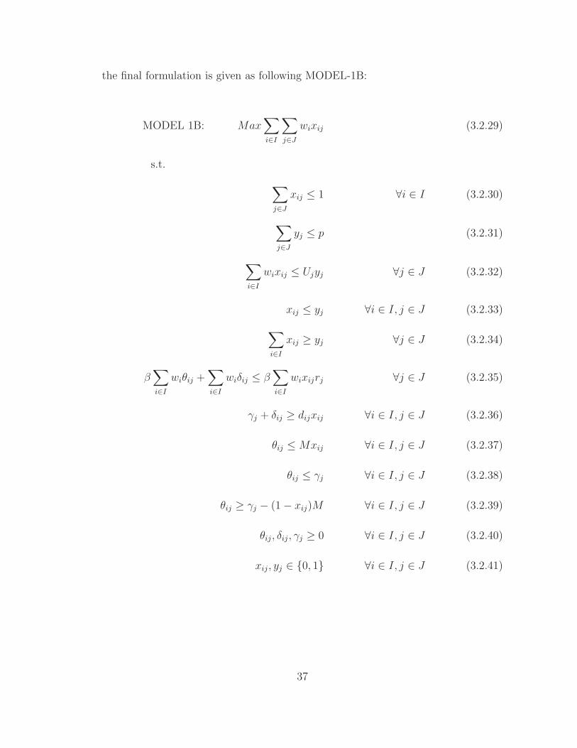
the final formulation is given as following MODEL-1B:

MODEL 1B: Max∑

i∈I

∑

j∈J

wixij (3.2.29)

s.t.

∑

j∈J

xij ≤ 1 ∀i ∈ I (3.2.30)

∑

j∈J

yj ≤ p (3.2.31)

∑

i∈I

wixij ≤ Ujyj ∀j ∈ J (3.2.32)

xij ≤ yj ∀i ∈ I, j ∈ J (3.2.33)

∑

i∈I

xij ≥ yj ∀j ∈ J (3.2.34)

β∑

i∈I

wiθij +∑

i∈I

wiδij ≤ β∑

i∈I

wixijrj ∀j ∈ J (3.2.35)

γj + δij ≥ dijxij ∀i ∈ I, j ∈ J (3.2.36)

θij ≤ Mxij ∀i ∈ I, j ∈ J (3.2.37)

θij ≤ γj ∀i ∈ I, j ∈ J (3.2.38)

θij ≥ γj − (1− xij)M ∀i ∈ I, j ∈ J (3.2.39)

θij, δij, γj ≥ 0 ∀i ∈ I, j ∈ J (3.2.40)

xij, yj ∈ {0, 1} ∀i ∈ I, j ∈ J (3.2.41)

37

3.3 MCLP-CBM-II Model

In this section, we provide another version of the MCLP model incorporated with

CBM. In this model, instead of β% demands, CBM for a facility is defined as the

average distance of the farthest β number of demands served by it. So, here the

parameter β is a positive integer. Adopting the nomenclature and formulation

of MODEL-1A, the following MODEL-2A with the new definition of CBM is

developed.

While solving an MCLP, though rare, the number of demands served by a

facility can be less than β. To calculate the average distances of demands, an

exact number of demands served by a facility is necessary in such cases. A new

variable αj is introduced, whose value would be either number of facilities served

or β, whichever is lower. The following variables and parameters are added to the

nomenclature of MODEL-1A.

Parameters

β Maximum number of points to be used for estimating CBM

Variables

αj Number of demand points actually considered for estimating CBM of

facility j ∈ J

38

Primal Formulation

MODEL 2A: Max∑

i∈I

∑

j∈J

wixij (3.3.1)

∑

j∈J

xij ≤ 1 ∀i ∈ I (3.3.2)

∑

j∈J

yj ≤ p (3.3.3)

∑

i∈I

wixij ≤ Ujyj ∀j ∈ J (3.3.4)

xij ≤ yj ∀i ∈ I, j ∈ J (3.3.5)

Mβj ≤ rj ∀j ∈ J (3.3.6)

αj ≤ βj ∀j ∈ J (3.3.7)

∑

i∈I

xij ≥ αj + yj − 1 ∀j ∈ J (3.3.8)

xij, yj ∈ {0, 1} ∀i ∈ I, j ∈ J (3.3.9)

αj ∈ N ∀j ∈ J (3.3.10)

where, ∀j ∈ J , we define

Mβj = Max

{

1

αj

∑

i∈I

dijxijzij

}

(3.3.11)

∑

i∈I

zij ≤ αj (3.3.12)

zij ≤ 1 ∀i ∈ I (3.3.13)

zij ≥ 0 ∀i ∈ I (3.3.14)

39

MODEL-2A represents the formulation of a capacitated maximum covering

problem with equity incorporated using CBM constraints. The objective function

and constraints, in equations 3.3.1-3.3.5, have the same purpose as in MODEL-

1A.

Constraint 3.3.7 ensures that αj value is not more than βj, the user-defined

threshold. Next, if a facility j ∈ J is open, yj = 1, which will make the constraint

3.3.8 appear as∑

i∈I xij ≥ αj. So, the αj does not exceed the total number of

demand points served by a facility if this total is lower than β. When a facility

j ∈ J is closed, all corresponding xij are made 0 by constraint 3.3.5, and αj has

the possibility to assume 1 to make the model feasible. Equation 3.3.9 is defin-

ing the binary variables. Equation 3.3.10 defines the αj variables to be positive

integers or natural numbers.

Equations 3.3.11-3.3.14 are part of the maximization problem defined to

estimate CBM. The objective function in equation 3.3.11 calculates the CBM of

distances for each facility j ∈ J . Constraint 3.3.12 helps in finding the farthest αj

demand points for facility j ∈ J . Equations 3.3.13 and 3.3.14 define the upper and

lower bounds of the variables in the objective function in equation 3.3.11.

Dual CBM Formulation

Similar to the model in previous section, the maximization in equation 3.3.11

conflicts with the global maximization in equation 3.3.1. So, the CBM formu-

lation, in equations 3.3.11-3.3.14, is dualized with respect to z variables. The

40

resultant dualized formulation is as follows:

Mβj =

1

αj

Min{

αjγj +∑

i∈I

δij

}

(3.3.15)

γj + δij ≥ dijxij ∀i ∈ I (3.3.16)

δij ≥ 0 ∀i ∈ I (3.3.17)

γj ≥ 0 (3.3.18)

In equation 3.3.15, the parameter αj is independent of z variables, so it is

outside the minimization function. The variable γ is the dual variable associated

with constraint 3.3.12, and the variable δ is the dual variable associated with

constraint 3.3.13. Now, after dualization, the updated formulation is given as:

Max∑

i∈I

∑

j∈J

wixij

(3.3.2)− (3.3.5), (3.3.7), (3.3.8)

αjγj +∑

i∈I

δij ≤ rjαj ∀j ∈ J (3.3.19)

γj + δij ≥ dijxij ∀i ∈ I, j ∈ J (3.3.20)

xij, yj ∈ {0, 1} ∀i ∈ I, j ∈ J (3.3.21)

αj ∈ N ∀j ∈ J (3.3.22)

δij, γj ≥ 0 ∀i ∈ I, j ∈ J (3.3.23)

41

In equation 3.3.19, the product of integer variable αj and continuous variable

γj rises non-linearity in the model, and this will be linearized in two steps. In first

step, the integer variable αj is converted into a series of binary variables. Next,

the product of binary and continuous variables is linearized as in Coelho (2013).

With constraint 3.3.7, αj would never exceed βj. Now for each αj, consider a

set Kj such that Kj ∈ {1, 2, 3, ...., βj}. Now introduce new binary variables φjk,

where j ∈ J and k ∈ Kj.

The following equations 3.3.24 and 3.3.25 will ensure αj to remain as a inte-

ger variable.

αj =∑

k∈Kj

kφjk ∀j ∈ J (3.3.24)

∑

k∈Kj

φjk = 1 ∀j ∈ J (3.3.25)

With equation 3.3.24, equation 3.3.19 can be re-written as equation 3.3.26.

∑

k∈Kj

kφjkγj +∑

i∈I

δij ≤ rj∑

k∈Kj

kφjk ∀j ∈ J (3.3.26)

Now consider the product of φjk and γj as ǫjk, i.e., φjkγj = ǫjk. Now equation

3.3.26 can be replaced with the following set of equations for linearization.

∑

k∈Kj

kǫjk +∑

i∈I

δij ≤ rj∑

k∈Kj

kφjk ∀j ∈ J (3.3.27)

42

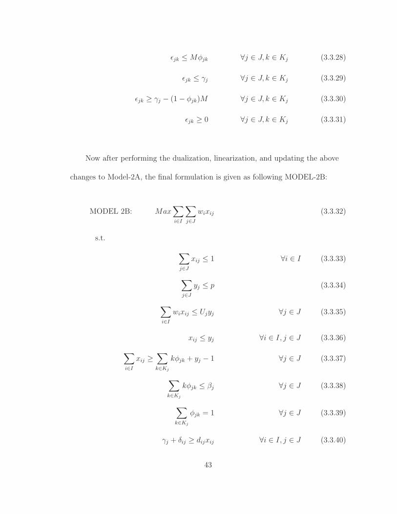
ǫjk ≤ Mφjk ∀j ∈ J, k ∈ Kj (3.3.28)

ǫjk ≤ γj ∀j ∈ J, k ∈ Kj (3.3.29)

ǫjk ≥ γj − (1− φjk)M ∀j ∈ J, k ∈ Kj (3.3.30)

ǫjk ≥ 0 ∀j ∈ J, k ∈ Kj (3.3.31)

Now after performing the dualization, linearization, and updating the above

changes to Model-2A, the final formulation is given as following MODEL-2B:

MODEL 2B: Max∑

i∈I

∑

j∈J

wixij (3.3.32)

s.t.

∑

j∈J

xij ≤ 1 ∀i ∈ I (3.3.33)

∑

j∈J

yj ≤ p (3.3.34)

∑

i∈I

wixij ≤ Ujyj ∀j ∈ J (3.3.35)

xij ≤ yj ∀i ∈ I, j ∈ J (3.3.36)

∑

i∈I

xij ≥∑

k∈Kj

kφjk + yj − 1 ∀j ∈ J (3.3.37)

∑

k∈Kj

kφjk ≤ βj ∀j ∈ J (3.3.38)

∑

k∈Kj

φjk = 1 ∀j ∈ J (3.3.39)

γj + δij ≥ dijxij ∀i ∈ I, j ∈ J (3.3.40)

43

∑

k∈Kj

kǫjk +∑

i∈I

δij ≤ rj∑

k∈Kj

kφjk ∀j ∈ J (3.3.41)

ǫjk ≤ Mφjk ∀j ∈ J, k ∈ Kj (3.3.42)

ǫjk ≤ γj ∀j ∈ J, k ∈ Kj (3.3.43)

ǫjk ≥ γj − (1− φjk)M ∀j ∈ J, k ∈ Kj (3.3.44)

xij, yj, φjk ∈ {0, 1} ∀i ∈ I, j ∈ J, k ∈ Kj (3.3.45)

δij, γj, ǫjk ≥ 0 ∀i ∈ I, j ∈ J, k ∈ Kj (3.3.46)

Kj = {1, 2, 3, ...., βj} ∀j ∈ J (3.3.47)

44

4 EMS Location Problem Application

This chapter focuses on incorporating CBM into an EMS facility location

problem. First, an EMS location problem called the maximum expected survival

location problem (MEXSLP) is explained. Next, a new model called MEXSLP-

CBM-I is proposed and developed by integrating the concept of CBM into the

classical MEXSLP as a constraint. Lastly, an alternative way of incorporating

CBM is defined, and another variant of the MEXSLP called MEXSLP-CBM-II is

developed.

4.1 MEXSLP Problem Description

Daskin (1983) introduced the maximum expected covering location problem

(MEXCLP), which considers the busy probabilities of facilities and aims to al-

locate the available EMS units across the potential facility locations in the sys-

tem. Erkut et al. (2008) introduced a similar model called the maximum expected

survival location problem (MEXSLP). The parameters in MEXSLP consider the

probability of survival of patients while allocating EMS units to potential loca-

tions.

In MEXCLP, a demand point is covered if there are EMS units within the

45

response time threshold. However, if no units are present in the said threshold,

the next closest unit will be sent to the demand location. In MEXSLP, if the

closest EMS unit is not available, the next closest is chosen for service, and this is

achieved by maximizing the overall expected probability of survival in the system.

The MEXSLP model provided in Erkut et al. (2008) is nonlinear. Jagtenberg

and Mason (2020) presented a linear version of the same, which again turns non-

linear after they incorporate equity into their model. Though MEXSLP is more

realistic than other models, it does not necessarily provide an equitable solution

for urban, suburban and rural localities. Since the population or fraction of the

population is used as weights for the objective function in MEXSLP, their solu-

tions allocate most EMS units nearer to densely populated or urban areas. This

could result in longer travel times for people in suburban and rural areas.

The CBM measure is used in this study to reduce this disparity among

densely and sparsely populated localities. CBM measures the average value of

service provided for the β% of demand that is worst off. Filippi et al. (2019a) uses

this measure in a bi-objective model to equitably locate facilities. In our model,

CBM is used as a constraint such that the CBM of travel times of each demand

point does not exceed the response time threshold.

There are several functions to estimate the probability of survival in the

literature. Next, we present two such survival functions that were highlighted in

Jagtenberg and Mason (2020). The first function was introduced in Valenzuela

46

et al. (1997); it uses the time from collapse to performing CPR (tCPR) and the

time from collapse to defibrillation (tdefib) as variables. This function is given by:

f(t) = (1 + e−0.260+0.106tCPR+0.139tdefib)−1 (4.1.1)

The second function was introduced in De Maio et al. (2003), which uses the

EMS unit response time (t) as a variable to estimate the probability of survival

and it is given by:

f(t) = (1 + e0.679+0.262t)−1 (4.1.2)

Functions defined in equations 4.1.1 and 4.1.2, are monotonically decreasing

with respect to travel time. Though we mentioned only two such functions, the

models stated in this chapter are valid for any monotonically decreasing survival

functions.

Our study assumes that all the EMS units in the system are ALS units, and

all the calls received are life-threatening, requiring immediate treatment. It is also

assumed that all the patients are first treated by the ALS units on-site, next they

are transported to the nearest hospitals or trauma centers, and lastly, these ALS

47

EMS units go back to their initial assigned stations. So, relocation or re-routing of

EMS units are not considered.

4.2 MEXSLP-CBM-I Model

This model considers a set I containing all demand points and another set J with

all potential locations to set up facilities with EMS units. Each facility location

can have multiple EMS units, and there is only p number of units in the entire

system. In this model, a unique priority number is assigned to all p units concern-

ing each demand point. Units closer to the demand location get higher priority,

i.e., lower priority number. Every demand points i ∈ I is assumed to have atleast

one potential facility location whose travel time is less than the response time

threshold.

The EMS unit closest to the demand point might not be available all the

time, so a busy probability is considered for each unit. This busy probability

is assumed to be the same for all facilities. Parameter q represents the average

fraction of time a unit is busy or unavailable for service.

This model aims to maximize the expected probability of survival for this

system while allocating the available EMS units optimally and equitably. The

MEXSLP part of the formulation takes care of placing the units optimally. The

CBM measure is used to achieve equity.

48

We consider the equation 4.1.2 for calculating probability of survival, which

is a monotonically decreasing function of time. So, maximizing to find facilities

with the highest probability of survival would give the same output as minimizing

to find facilities with the lowest travel times. The β facilities with the highest

survival probability are the ones with the lowest travel times. The CBM for each

demand point is measured as the average time needed by the nearest β% EMS

units to arrive at the location. This CBM of each location is kept lower than the

response time threshold T .

Nomenclature

Sets

I Set of all demand points

J Set of all potential facility locations

Indices

i ∈ I

j ∈ J

Parameters

49

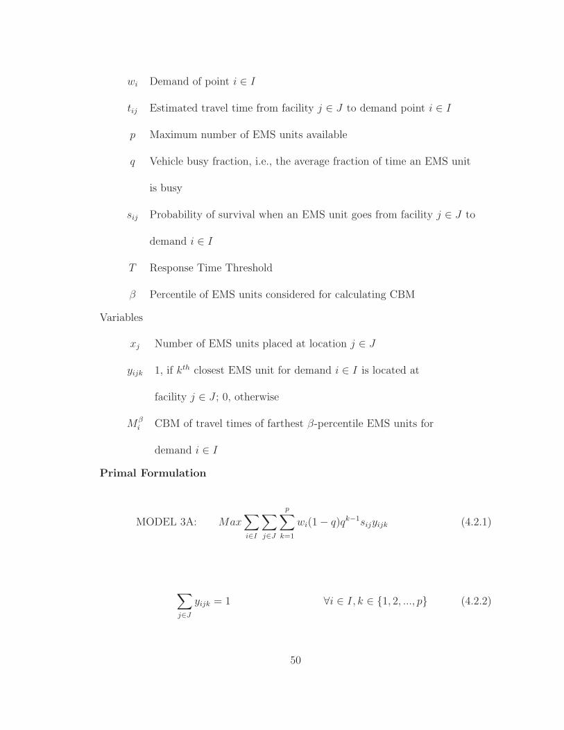
wi Demand of point i ∈ I

tij Estimated travel time from facility j ∈ J to demand point i ∈ I

p Maximum number of EMS units available

q Vehicle busy fraction, i.e., the average fraction of time an EMS unit

is busy

sij Probability of survival when an EMS unit goes from facility j ∈ J to

demand i ∈ I

T Response Time Threshold

β Percentile of EMS units considered for calculating CBM

Variables

xj Number of EMS units placed at location j ∈ J

yijk 1, if kth closest EMS unit for demand i ∈ I is located at

facility j ∈ J ; 0, otherwise

Mβi CBM of travel times of farthest β-percentile EMS units for

demand i ∈ I

Primal Formulation

MODEL 3A: Max∑

i∈I

∑

j∈J

p∑

k=1

wi(1− q)qk−1sijyijk (4.2.1)

∑

j∈J

yijk = 1 ∀i ∈ I, k ∈ {1, 2, ..., p} (4.2.2)

50

p∑

k=1

yijk = xj ∀i ∈ I, j ∈ J (4.2.3)

∑

j∈J

xj ≤ p (4.2.4)

Mβi ≤ T ∀i ∈ I (4.2.5)

xj ∈ Z+ ∪ {0} ∀j ∈ J (4.2.6)

yijk ∈ {0, 1} ∀i ∈ I, j ∈ J, k ∈ {1, 2, ..., p} (4.2.7)

where, ∀i ∈ I, we define

W βi = β

∑

j∈J

p∑

k=1

yijk (4.2.8)

Mβi = Min

{

1

W βi

∑

j∈J

p∑

k=1

tijyijkzijk

}

(4.2.9)

∑

j∈J

p∑

k=1

zijk ≥ W βi (4.2.10)

zijk ∈ {0, 1} ∀j ∈ J, k ∈ {1, 2, ..., p} (4.2.11)

The objective function in equation 4.2.1 aims to maximize the expected sur-

vival probability of the entire system.∑

j∈J

∑p

k=1(1 − q)qk−1sijyijk part of the

objective function calculates the expected survival probability for each demand

location i ∈ I. Constraint 4.2.17 and 4.2.18 ensures that each demand location

has only one EMS unit which is kth closest to it. Constraint 4.2.17 also ensures

that each unit gets a unique priority number specific to each demand location.

51

Constraint 4.2.19 limits the total number of units allocated in the system to be p.

Constraint 4.2.5 enforces the CBM measure of each demand location to be lower

than the response time threshold. Equations 4.2.6 and 4.2.7 define the model

variables.

Equations 4.2.8-4.2.11 represent the formulation of CBM optimization prob-

lem. Objective function in equation 4.2.9 gives the mean travel time of β% units

nearest to demand i. Constraint 4.2.10 enforces the number of units in CBM cal-

culation to be β% for each demand i. Equation 4.2.11 defines the binary variables

in CBM problem. Constraints 4.2.9 and 4.2.10 together find the β% units nearest

to demand point i. From constraint 4.2.17,∑

j∈J

∑p

k=1yijk = p, so W β

i becomes p.

The objective function in equation 4.2.1 is naturally incentivized to mini-

mize yijk to reduce travel times so that the probability of survival is maximized.

Equation 4.2.9 is also incentivized to allocate weights to minimize the travel times

to find the shortest routes. Since both the objectives are in harmony, the inner

minimization can be removed, and the combined formulation is as follows:

Max∑

i∈I

∑

j∈J

p∑

k=1

wi(1− q)qk−1sijyijk

(4.2.17)− (4.2.19)

1

βp

{

∑

j∈J

p∑

k=1

tijyijkzijk

}

≤ T ∀i ∈ I (4.2.12)

52

∑

j∈J

p∑

k=1

zijk ≥ βp ∀i ∈ I (4.2.13)

xj ∈ Z+ ∪ {0} ∀j ∈ J (4.2.14)

yijk, zijk ∈ {0, 1} ∀i ∈ I, j ∈ J, k ∈ {1, 2, ..., p} (4.2.15)

By definition of variable yijk tells if facility j ∈ J has the kth nearest unit for

demand point i ∈ I. For any demand i, the variables yijk with k ∈ {1, 2, ..., ⌈pβ⌉}

provide the nearest β% units. So, equations 4.2.12 and 4.2.13 can be replaced

with equation 4.2.20, and all the zijk variables can be eliminated. After all the

above stated changes, the final combined formulation is given as following MODEL-

3B.

MODEL 3B: Max∑

i∈I

∑

j∈J

p∑

k=1

wi(1− q)qk−1sijyijk (4.2.16)

s.t.

∑

j∈J

yijk = 1 ∀i ∈ I, k ∈ {1, 2, ..., p} (4.2.17)

p∑

k=1

yijk = xj ∀i ∈ I, j ∈ J (4.2.18)

∑

j∈J

xj ≤ p (4.2.19)

1

⌈βp⌉

∑

j∈J

⌈βp⌉∑

k=1

tijyijk ≤ T ∀i ∈ I (4.2.20)

53

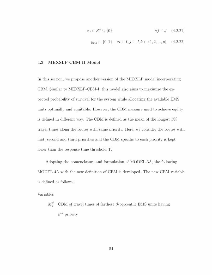
xj ∈ Z+ ∪ {0} ∀j ∈ J (4.2.21)

yijk ∈ {0, 1} ∀i ∈ I, j ∈ J, k ∈ {1, 2, ..., p} (4.2.22)

4.3 MEXSLP-CBM-II Model

In this section, we propose another version of the MEXSLP model incorporating

CBM. Similar to MEXSLP-CBM-I, this model also aims to maximize the ex-

pected probability of survival for the system while allocating the available EMS

units optimally and equitable. However, the CBM measure used to achieve equity

is defined in different way. The CBM is defined as the mean of the longest β%

travel times along the routes with same priority. Here, we consider the routes with

first, second and third priorities and the CBM specific to each priority is kept

lower than the response time threshold T.

Adopting the nomenclature and formulation of MODEL-3A, the following

MODEL-4A with the new definition of CBM is developed. The new CBM variable

is defined as follows:

Variables

Mβk CBM of travel times of farthest β-percentile EMS units having

kth priority

54

Primal Formulation

MODEL 4A: Max∑

i∈I

∑

j∈J

p∑

k=1

wi(1− q)qk−1sijyijk (4.3.1)

s.t.

∑

j∈J

yijk = 1 ∀i ∈ I, k ∈ {1, 2, ..., p} (4.3.2)

p∑

k=1

yijk = xj ∀i ∈ I, j ∈ J (4.3.3)

∑

j∈J

xj ≤ p (4.3.4)

Mβk ≤ T ∀k ∈ {1, 2, 3} (4.3.5)

xj ∈ Z+ ∪ {0} ∀j ∈ J (4.3.6)

yijk ∈ {0, 1} ∀i ∈ I, j ∈ J, k ∈ {1, 2, ..., p} (4.3.7)

where, ∀k ∈ {1, 2, 3}, we define

W βk = β

∑

i∈I

∑

j∈J

yijk (4.3.8)

Mβk = Max

{

1

W βk

∑

i∈I

∑

j∈J

tijyijkzijk

}

(4.3.9)

∑

i∈I

∑

j∈J

zijk ≤ W βk (4.3.10)

zijk ≤ 1 ∀i ∈ I, j ∈ J (4.3.11)

55

zijk ≥ 0 ∀i ∈ I, j ∈ J (4.3.12)

MODEL-4A represents the formulation of a maximum expected survival loca-

tion problem incorporated with CBM with respect first three priority EMS units,

to provide equity in service for patients. Equations 4.3.1-4.3.7 define the same

objective and constraints on this model as in MODEL-3A. Though constraint

4.3.5 is similar to constraint 4.2.5, what it enforces is different. Constraint 4.3.5

enforces the CBM for top three priority EMS units to be lower than the response

time threshold.

Equations 4.3.8-4.3.12 represent the formulation of CBM optimization prob-

lem. The objective function in equation 4.3.9 gives the CBM of routes with given

priority k. Equation 4.3.8 calculates the β% of routes in system with kth prior-

ity. Constraints 4.3.10 and 4.3.11 together find the longest β% routes with kth

priority. Equation 4.3.12 defines the variables in CBM optimization problem.

Dualizing CBM Formulation

Consider the equation provided below,

1

W βk

∑

i∈I

∑

j∈J

tijyijkzijk ≤ T ∀k ∈ {1, 2, 3}

If this equation is provided as a constraint to the maximizing objective in

56

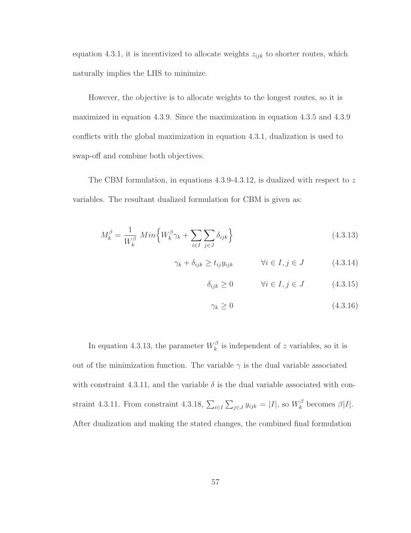
equation 4.3.1, it is incentivized to allocate weights zijk to shorter routes, which

naturally implies the LHS to minimize.

However, the objective is to allocate weights to the longest routes, so it is

maximized in equation 4.3.9. Since the maximization in equation 4.3.5 and 4.3.9

conflicts with the global maximization in equation 4.3.1, dualization is used to

swap-off and combine both objectives.

The CBM formulation, in equations 4.3.9-4.3.12, is dualized with respect to z

variables. The resultant dualized formulation for CBM is given as:

Mβk =

1

W βk

Min{

W βk γk +

∑

i∈I

∑

j∈J

δijk

}

(4.3.13)

γk + δijk ≥ tijyijk ∀i ∈ I, j ∈ J (4.3.14)

δijk ≥ 0 ∀i ∈ I, j ∈ J (4.3.15)

γk ≥ 0 (4.3.16)

In equation 4.3.13, the parameter W βk is independent of z variables, so it is

out of the minimization function. The variable γ is the dual variable associated

with constraint 4.3.11, and the variable δ is the dual variable associated with con-

straint 4.3.11. From constraint 4.3.18,∑

i∈I

∑

j∈J yijk = |I|, so W βk becomes β|I|.

After dualization and making the stated changes, the combined final formulation

57

is given as following MODEL-4B.

MODEL 4B: Max∑

i∈I

∑

j∈J

p∑

k=1

wi(1− q)qk−1sijyijk (4.3.17)

s.t.

∑

j∈J

yijk = 1 ∀i ∈ I, k ∈ {1, 2, ..., p} (4.3.18)

p∑

k=1

yijk = xj ∀i ∈ I, j ∈ J (4.3.19)

∑

j∈J

xj ≤ p (4.3.20)

β|I|γk +∑

i∈I

∑

j∈J

δijk ≤ β|I|T ∀k ∈ {1, 2, 3} (4.3.21)

γk + δijk ≥ tijyijk ∀i ∈ I, j ∈ J, k ∈ {1, 2, 3} (4.3.22)

δijk, γk ≥ 0 ∀i ∈ I, j ∈ J, k ∈ {1, 2, 3} (4.3.23)

xj ∈ Z+ ∪ {0} ∀j ∈ J (4.3.24)

yijk ∈ {0, 1} ∀i ∈ I, j ∈ J, k ∈ {1, 2, ..., p} (4.3.25)

58

5 Analysis

This chapter provides analysis on the CBM incorporated MCLP and MEXSLP

models developed in chapters 3 and 4. Here we will see that the implementation

of CBM will improve EMS units’ spread or uniformity in the concentration of

EMS units. Also, the implementation of CBM in MCLP will help in creating a

flexible coverage radius and increase total coverage in the whole service area.

The primary data used for testing is the Portland Metropolitan Region

dataset presented in Chauhan et al. (2019). Besides, the Portland Metropolitan

dataset, a p-median model test case from Osman and Christofides (1994) available

on J. E. Beasley’s OR-library, is also used for MCLP models testing. All the com-

putational runs are performed on a Windows 10 desktop having Intel Core i7-7700

CPU 3.6 GHz, 4 Cores, 8 Logical Processors, and 32 GB of RAM. Gurobi Opti-

mizer 9.0 is used as the MILP solver in this study [Gurobi Optimization (2020)].

5.1 MCLP-CBM Models Analysis

5.1.1 Analysis on Portland Metropolitan Data

The Portland Metropolitan dataset consists of 122 demand points and 104 po-

tential facility locations. Each demand point is the centroid of a zip code area,

59

and each facility location is the location of a community center in the Portland

Metropolitan Area. Here, the demand points and facility locations do not over-

lap with each other. Figure 5.1 shows the locations of all demand and potential

facilities considered for this study.

Figure 5.1: Demand points and potential facilities in the Portland MetropolitanRegion.

From the American Community Survey (2020), the number of Hispanic and

Non-Hispanic people below the poverty line is estimated, and this population data

is used for demands wi in this study (refer Appendix-A). The capacity of each

facility U is calculated as it is suggested in Pirkul and Schilling (1989), using the

below equation:

60

U =

∑

i∈I wi

0.8p

The above equation ensures all open facilities’ combined capacity to be 25%

higher than the total demand to be served. As in Chauhan et al. (2019), the time

required to travel the euclidian distance from facilities to demand sites is used

as distance dij in this study. The coverage radius rj is assumed to be the 20th

percentile of all the distances in dij matrix.

In MCLP models, the objective function is the total demand covered by all

facilities in the service region. Table 5.1 provides the coverage and Gurobi gap

values from three models: MCLP, MCLP-CBM-I, and MCLP-CBM-II models. All

three MCLP models were tested with several combinations of p and β. The num-

ber of facilities to open p varying from 1 to 25 in multiples of 5. The β parameter

used for calculating CBM to be 0.1%, 10%, 20%, 30%, and 40% for MCLP-CBM-I

model, and it to be 1, 2, 3, 5, and 10 for MCLP-CBM-II model.

For the analysis in table 5.1, the Gurobi solver was given a time limit of two

hours. In two hours, the gap in Gurobi solutions of MCLP-CBM-I is very high,

stating that the solution has not converged. In comparison, the MCLP-CBM-II

model has much lower gaps, showing convergence in solution.

Besides convergence, as expected table 5.1 shows that coverage and β are

61

Table 5.1: MCLP Models - Objective and Gurobi Gap using PDX Dataset.

pMCLP

β(%)MCLP CBM-I

β(#)MCLP CBM-II

Coverage(%) Coverage(%) Gap(%) Coverage(%) Gap(%)

1 63.87

0.1 63.87 46.23 1 63.87 010 65.35 53.01 2 63.87 020 67.39 48.38 3 64.01 030 70.78 25.53 5 68.44 040 74.79 22.35 10 71.07 0

5 91.66

0.1 88.31 13.24 1 91.66 010 88.08 13.53 2 92.26 3.9820 89.55 11.67 3 91.84 8.0530 91.50 9.28 5 93.74 6.6840 98.01 2.03 10 96.00 4.17

10 96.84

0.1 94.83 5.46 1 96.84 0.0110 94.46 5.86 2 96.84 2.0420 97.52 2.54 3 96.89 3.2130 97.97 2.07 5 98.71 1.3140 98.04 2 10 99.99 0.01

15 98.12

0.1 96.57 3.55 1 98.12 010 96.63 3.49 2 98.22 1.1420 98.77 1.25 3 98.51 1.5230 97.08 3 5 99.59 0.4140 99.36 0.65 10 100.00 0

20 92.49

0.1 91.76 1.79 1 92.49 010 91.63 1.94 2 92.70 0.6120 91.50 2.08 3 92.71 0.7530 92.76 0.69 5 93.41 040 93.41 0 10 93.41 0

25 92.77

0.1 92.46 1.02 1 92.77 010 91.16 2.47 2 93.24 0.0220 92.82 0.63 3 93.26 0.1630 93.07 0.36 5 93.40 0.0140 93.41 0 10 93.41 0

62

directly proportional. Higher the β, the higher the total coverage. Incorporating

CBM in the MCLP loosens the constraint on coverage radius and allows the fa-

cilities with excess capacity to serve demands lying outside the coverage radius.

As the β increases, the facility’s reach increases, allowing the model to increase its

coverage. When β gets lower, CBM tightens the constraint, and the MCLP-CBM

models work similarly to a regular MCLP. When β is 0.1% in MCLP-CBM-I or 1

in MCLP-CBM-II, the coverage provided by MCLP and MCLP-CBM models are

the same. This validates our hypothesis that either of the MCLP-CBM models

working similar to a regular MCLP when β is low.

Both the MCLP-CBM models provided coverage close to each other and bet-

ter than a regular MCLP. Though the coverage has improved, the gap in Gurobi

solutions is in MCLP-CBM-I is way too high. Next, we will test the MCLP-CBM

models using two standard test cases from Osman and Christofides (1994).

5.1.2 Analysis on Standard Test Dataset

The p-median dataset used in Osman and Christofides (1994) contains several

test cases for maximum covering problems, out of which two were considered for

this study. First, having 50 sites acting both as a potential facility and a demand

point. Second has 100 sites which also act both as a potential facility location and

a demand point. Model parameters such as dij, p, Uj and wi are extracted from

the dataset (refer Appendix-B). The coverage radius rj is assumed to be the 5th

63

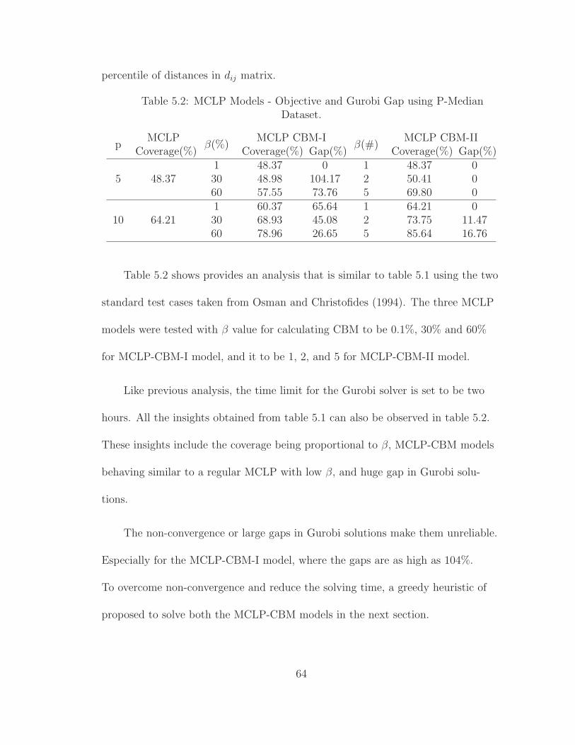
percentile of distances in dij matrix.

Table 5.2: MCLP Models - Objective and Gurobi Gap using P-MedianDataset.

pMCLP

β(%)MCLP CBM-I

β(#)MCLP CBM-II

Coverage(%) Coverage(%) Gap(%) Coverage(%) Gap(%)

5 48.371 48.37 0 1 48.37 030 48.98 104.17 2 50.41 060 57.55 73.76 5 69.80 0

10 64.211 60.37 65.64 1 64.21 030 68.93 45.08 2 73.75 11.4760 78.96 26.65 5 85.64 16.76

Table 5.2 shows provides an analysis that is similar to table 5.1 using the two

standard test cases taken from Osman and Christofides (1994). The three MCLP

models were tested with β value for calculating CBM to be 0.1%, 30% and 60%

for MCLP-CBM-I model, and it to be 1, 2, and 5 for MCLP-CBM-II model.

Like previous analysis, the time limit for the Gurobi solver is set to be two

hours. All the insights obtained from table 5.1 can also be observed in table 5.2.

These insights include the coverage being proportional to β, MCLP-CBM models

behaving similar to a regular MCLP with low β, and huge gap in Gurobi solu-

tions.

The non-convergence or large gaps in Gurobi solutions make them unreliable.

Especially for the MCLP-CBM-I model, where the gaps are as high as 104%.

To overcome non-convergence and reduce the solving time, a greedy heuristic of

proposed to solve both the MCLP-CBM models in the next section.

64

5.2 Greedy Heuristic and Application

5.2.1 Heuristic Methodology

The greedy heuristic works as follows:

i. Create two running arrays I and J with all demand points and potential

facility locations.

ii. Create a weight array. For each unopened facility location, the weight is

defined as the sum of all wi whose value is less than facility’s capacity and

located with in its coverage radius rj.

iii. Find and open the facility with the highest weight.

iv. Now solve the MCLP-CBM model with the single newly opened facility and

all unserved demand points, using Gurobi.

v. After solving the model with single facility, remove the opened facility and

demand points assigned to it from arrays I and J , respectively.

vi. Using the shortened arrays I and J , again follow the procedure in steps (ii)

to (v).

vii. Keep repeating this cycle until required number of facilities are found and

opened.

65

5.2.2 Heuristic Performance Analysis

This greedy heuristic was tested with both the datasets discussed earlier. Their

results obtained after solving with heuristic are provided in tables 5.3 and 5.4.

These results include total coverage, solving time, and difference from Gurobi’s

solution. Observing these results, the heuristic seems to provide reliable results.

To get the coverage provided Gurobi in two hours, the greedy heuristic only needs

few seconds to minutes.

To understand the heuristic’s performance, table 5.5 is prepared. Table 5.5

has the maximum, minimum, and average values of solving time and solution

difference from Gurobi for both the datasets. In the best scenario, the greedy

heuristic has solved the MCLP-CBM model under a second and obtain coverage

equivalent to Gurobi. In the worst scenario, this heuristic solved the model in

about two minutes and with coverage 10% lower than Gurobi. Overall, the heuris-

tic can be expected to solve the model in 10 sec to obtain the same coverage as

obtained using Gurobi for two hours.

66

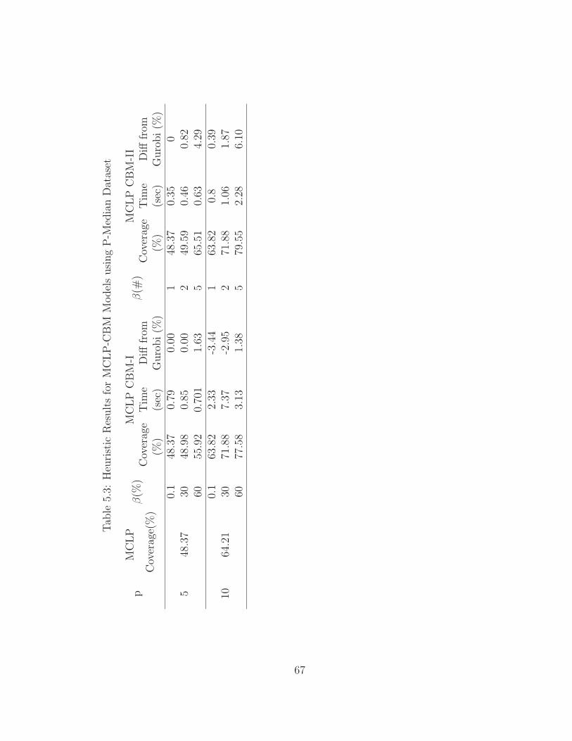
Tab

le5.3:

Heuristic

ResultsforMCLP-C

BM

ModelsusingP-M

edianDataset

pMCLP

β(%

)MCLPCBM-I

β(#

)MCLPCBM-II

Coverage(%)

Coverage

(%)

Tim

e(sec)

Diff

from

Gurobi(%

)Coverage

(%)

Tim

e(sec)

Diff

from

Gurobi(%

)

548.37

0.1

48.37

0.79

0.00

148.37

0.35

030

48.98

0.85

0.00

249.59

0.46

0.82

6055.92

0.701

1.63

565.51

0.63

4.29

1064.21

0.1

63.82

2.33

-3.44

163.82

0.8

0.39

3071.88

7.37

-2.95

271.88

1.06

1.87

6077.58

3.13

1.38

579.55

2.28

6.10

67

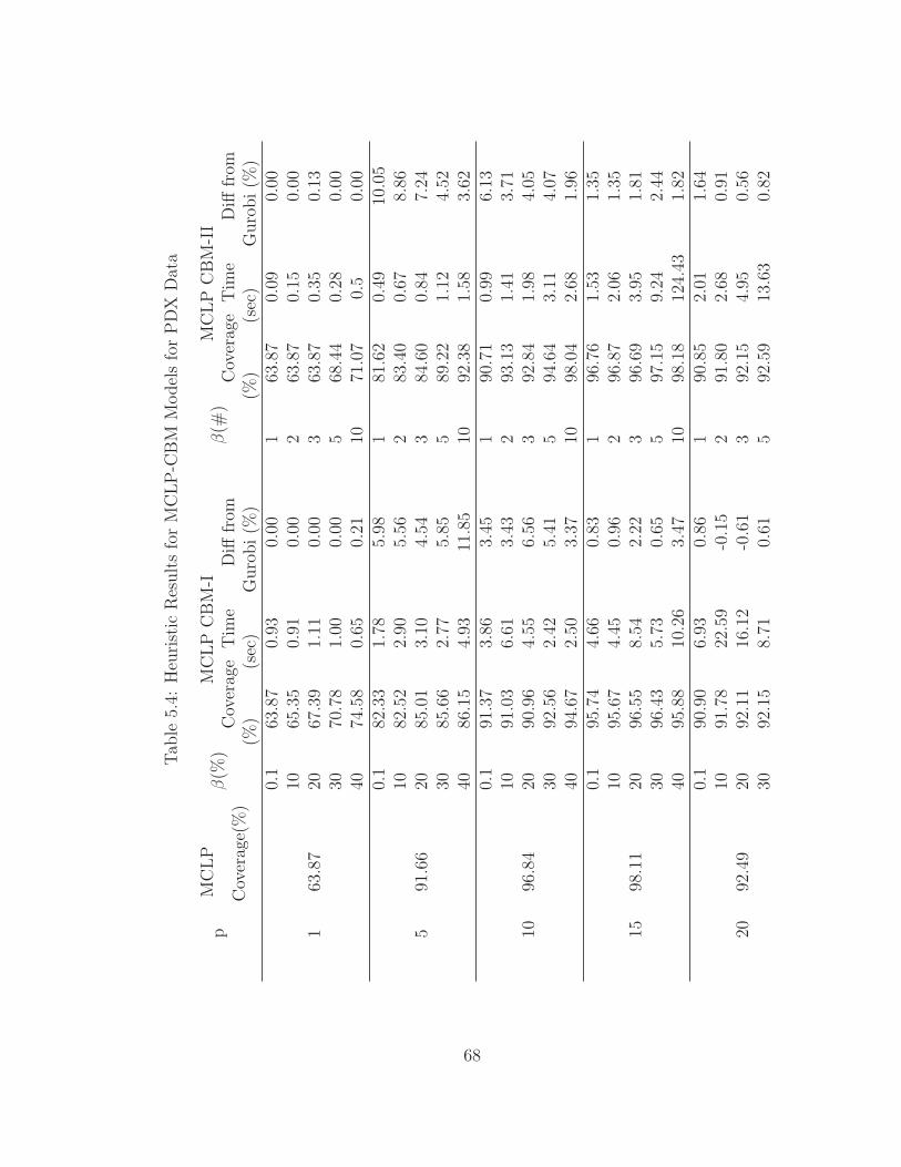
Tab

le5.4:

Heuristic

ResultsforMCLP-C

BM

ModelsforPDX

Data

pMCLP

β(%

)MCLPCBM-I

β(#

)MCLPCBM-II

Coverage(%)

Coverage

(%)

Tim

e(sec)

Diff

from

Gurobi(%

)Coverage

(%)

Tim

e(sec)

Diff

from

Gurobi(%

)

163.87

0.1

63.87

0.93

0.00

163.87

0.09

0.00

1065.35

0.91

0.00

263.87

0.15

0.00

2067.39

1.11

0.00

363.87

0.35

0.13

3070.78

1.00

0.00

568.44

0.28

0.00

4074.58

0.65

0.21

1071.07

0.5

0.00

591.66

0.1

82.33

1.78

5.98

181.62

0.49

10.05

1082.52

2.90

5.56

283.40

0.67

8.86

2085.01

3.10

4.54

384.60

0.84

7.24

3085.66

2.77

5.85

589.22

1.12

4.52

4086.15

4.93

11.85

1092.38

1.58

3.62

1096.84

0.1

91.37

3.86

3.45

190.71

0.99

6.13

1091.03

6.61

3.43

293.13

1.41

3.71

2090.96

4.55

6.56

392.84

1.98

4.05

3092.56

2.42

5.41

594.64

3.11

4.07

4094.67

2.50

3.37

1098.04

2.68

1.96

1598.11

0.1

95.74

4.66

0.83

196.76

1.53

1.35

1095.67

4.45

0.96

296.87

2.06

1.35

2096.55

8.54

2.22

396.69

3.95

1.81

3096.43

5.73

0.65

597.15

9.24

2.44

4095.88

10.26

3.47

1098.18

124.43

1.82

2092.49

0.1

90.90

6.93

0.86

190.85

2.01

1.64

1091.78

22.59

-0.15

291.80

2.68

0.91

2092.11

16.12

-0.61

392.15

4.95

0.56

3092.15

8.71

0.61

592.59

13.63

0.82

68

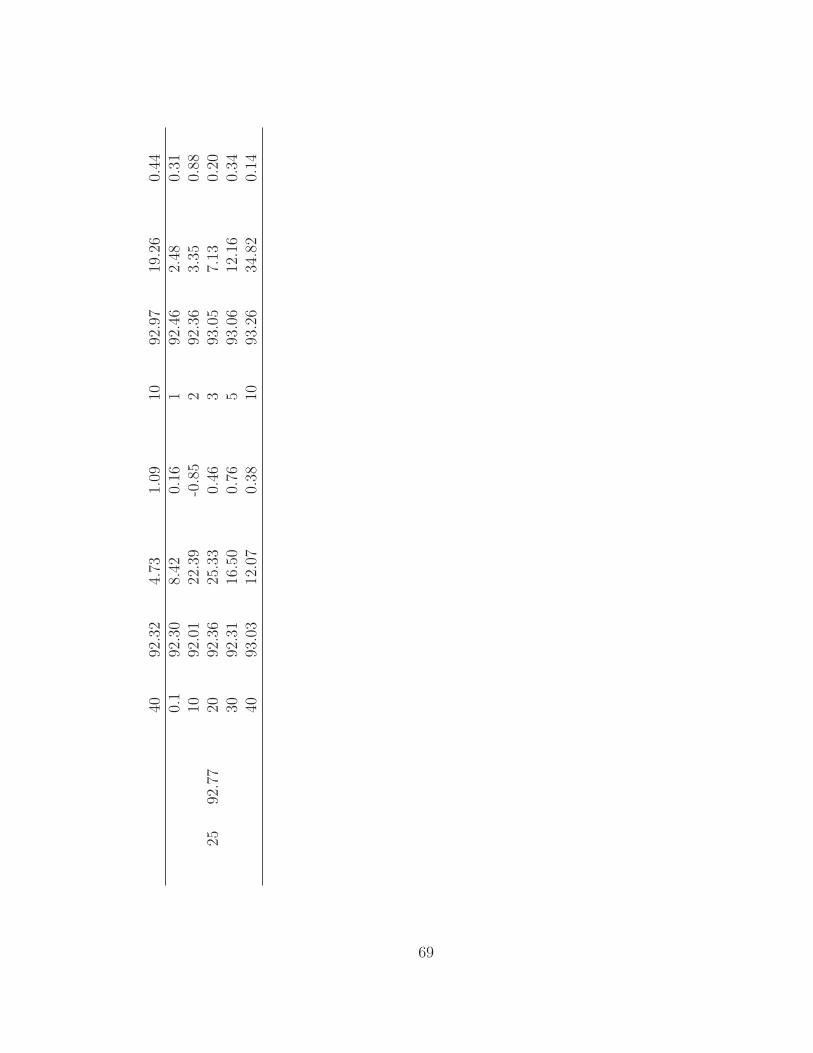
4092.32

4.73

1.09

1092.97

19.26

0.44

2592.77

0.1

92.30

8.42

0.16

192.46

2.48

0.31

1092.01

22.39

-0.85

292.36

3.35

0.88

2092.36

25.33

0.46

393.05

7.13

0.20

3092.31

16.50

0.76

593.06

12.16

0.34

4093.03

12.07

0.38

1093.26

34.82

0.14

69

Table 5.5: Heuristic Performance

Dataset Average Median MaximumMinimum

J. E. BeasleySolving Time (sec) 1.73 0.83 7.37 0.35

Difference inSolution (%)

0.84 0.60 6.10 -3.44

PDXSolving Time (sec) 7.96 3.11 124.43 0.09

Difference inSolution (%)

2.27 0.93 11.85 -0.85

5.3 EMS Applications/MEXSLP Models Analysis

The same Portland Metropolitan data provided by Chauhan et al. (2019) and

explained in section 5.1.1 is used for the study in this section. Demand wi are es-

timated as explained in section 5.1.1. The probability of survival sij is calculated

by the approach in De Maio et al. (2003) using the equation 4.1.2. The same eu-

clidean distance matrix dij in the previous section is used as travel time tij matrix

in this study. The travel time threshold T is assumed to be 20 minutes, and q is

assumed to be 0.2, i.e., the EMS units are busy 20% of the time.

The objective function of MEXSLP models calculates the Aggregated Prob-

ability of Survival (APS) of the entire population in the service region. Table

5.6 provides the APS and Gurobi gap values for three models: regular MEXSLP,

MEXSLP-CBM-I, and MEXSLP-CBM-II models. In this analysis, all three mod-

els are tested with several combinations of p and β. The number of EMS units

to be located p varies from 10 to 40 in multiples of 10. The β parameter used in

calculating CBM is considered to be 1%, 5%, 10%, or 20%.

70

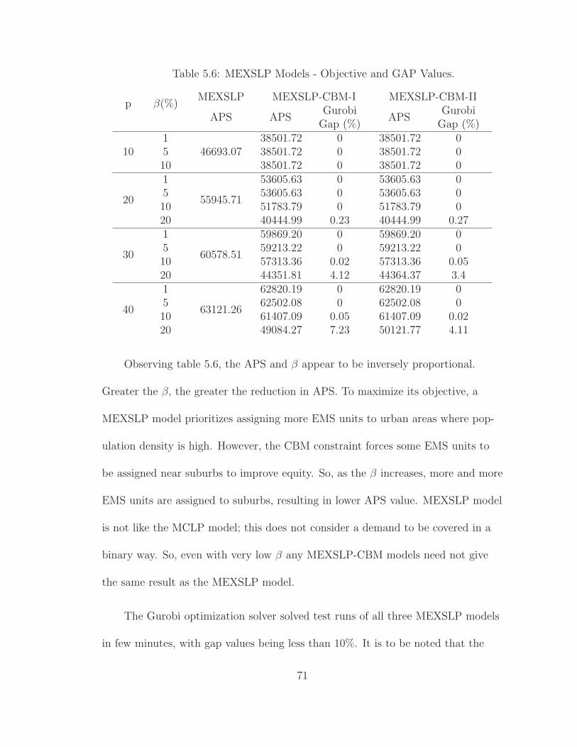
Table 5.6: MEXSLP Models - Objective and GAP Values.

p β(%)MEXSLP MEXSLP-CBM-I MEXSLP-CBM-II

APS APSGurobiGap (%)

APSGurobiGap (%)

101

46693.0738501.72 0 38501.72 0

5 38501.72 0 38501.72 010 38501.72 0 38501.72 0

20

1

55945.71

53605.63 0 53605.63 05 53605.63 0 53605.63 010 51783.79 0 51783.79 020 40444.99 0.23 40444.99 0.27

30

1

60578.51

59869.20 0 59869.20 05 59213.22 0 59213.22 010 57313.36 0.02 57313.36 0.0520 44351.81 4.12 44364.37 3.4

40

1

63121.26

62820.19 0 62820.19 05 62502.08 0 62502.08 010 61407.09 0.05 61407.09 0.0220 49084.27 7.23 50121.77 4.11

Observing table 5.6, the APS and β appear to be inversely proportional.

Greater the β, the greater the reduction in APS. To maximize its objective, a

MEXSLP model prioritizes assigning more EMS units to urban areas where pop-

ulation density is high. However, the CBM constraint forces some EMS units to

be assigned near suburbs to improve equity. So, as the β increases, more and more

EMS units are assigned to suburbs, resulting in lower APS value. MEXSLP model

is not like the MCLP model; this does not consider a demand to be covered in a

binary way. So, even with very low β any MEXSLP-CBM models need not give

the same result as the MEXSLP model.

The Gurobi optimization solver solved test runs of all three MEXSLP models

in few minutes, with gap values being less than 10%. It is to be noted that the

71

models were tested with even higher values of β, but they either resulted in higher

gap values or turned infeasible. This infeasibility occurs because maximizing

coverage always opposes maximizing equity. So, using a large β parameter is not

advisable.

Figure 5.2-5.7 shows the facility locations where EMS units are placed for

MEXSLP, MEXSLP-CBM-I, and MEXSLP-CBM-II models. These solutions are

obtained by solving models using Gurobi. In these figures, blue dots represent

demand points and red stars represent open facilities, and the size of red star is

corresponding to number of EMS units at that site.

Figures 5.2 and 5.5 show the locations of EMS units when a regular MEXSLP

model is solved to locate 20 and 40 units, respectively. When β is low, both the

CBM incorporated MEXSLP models, give the exact same solution. Such solutions

of MEXSLP-CBM-I and MEXSLP-CBM-II are plotted and shown in figures 5.3

and 5.6, when p = 20 and p = 40, respectively. Similarly, when p is low, both

these models provide same solutions even with higher β values. Figure 5.4 shows

such a result of these models with p = 20 and β = 20%. However, when both p

and β are high, MEXSLP-CBM-I and MEXSLP-CBM-II models provide different

solutions and these results are shown in figure 5.7.

72

Figure 5.2: MEXSLP solution (p = 20)

Figure 5.3: MEXSLP CBM-I and MEXSLP CBM-II solutions (p = 20 and β = 1%)

73

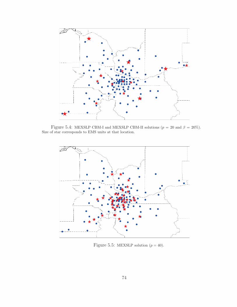
Figure 5.4: MEXSLP CBM-I and MEXSLP CBM-II solutions (p = 20 and β = 20%).Size of star corresponds to EMS units at that location.

Figure 5.5: MEXSLP solution (p = 40).

74

Figure 5.6: MEXSLP CBM-I and MEXSLP CBM-II solutions (p = 40 and β = 1%)

75

(a) MEXSLP CBM-I

(b) MEXSLP CBM-II

Figure 5.7: MEXSLP models solutions (p = 40 and β = 20%). Size of starcorresponds to EMS units at that location.

In MEXSLP model, if there are n EMS units, every unit has a priority num-

76

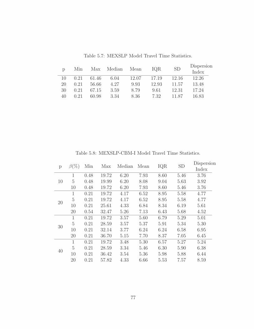
Table 5.7: MEXSLP Model Travel Time Statistics.

p Min Max Median Mean IQR SDDispersionIndex

10 0.21 61.46 6.04 12.07 17.19 12.16 12.2620 0.21 56.66 4.27 9.93 12.93 11.57 13.4830 0.21 67.15 3.59 8.79 9.61 12.31 17.2440 0.21 60.98 3.34 8.36 7.32 11.87 16.83

Table 5.8: MEXSLP-CBM-I Model Travel Time Statistics.

p β(%) Min Max Median Mean IQR SDDispersionIndex

101 0.48 19.72 6.20 7.93 8.60 5.46 3.765 0.48 19.99 6.20 8.08 9.04 5.63 3.9210 0.48 19.72 6.20 7.93 8.60 5.46 3.76

20

1 0.21 19.72 4.17 6.52 8.95 5.58 4.775 0.21 19.72 4.17 6.52 8.95 5.58 4.7710 0.21 25.61 4.33 6.84 8.34 6.19 5.6120 0.54 32.47 5.26 7.13 6.43 5.68 4.52

30

1 0.21 19.72 3.57 5.60 6.79 5.29 5.015 0.21 28.59 3.57 5.37 5.91 5.34 5.3010 0.21 32.14 3.77 6.24 6.24 6.58 6.9520 0.21 36.70 5.15 7.70 8.37 7.05 6.45

40

1 0.21 19.72 3.48 5.30 6.57 5.27 5.245 0.21 28.59 3.34 5.46 6.30 5.90 6.3810 0.21 36.42 3.54 5.36 5.98 5.88 6.4420 0.21 57.82 4.33 6.66 5.53 7.57 8.59

77

Table 5.9: MEXSLP-CBM-II Model Travel Time Statistics.

p β(%) Min Max Median Mean IQR SDDispersionIndex

101 0.48 19.99 6.20 8.08 9.04 5.63 3.925 0.48 19.99 6.20 8.08 9.04 5.63 3.9210 0.48 19.72 6.20 7.93 8.60 5.46 3.76

20

1 0.21 19.72 4.17 6.52 8.95 5.58 4.775 0.21 19.72 4.17 6.52 8.95 5.58 4.7710 0.21 25.61 4.33 6.84 8.34 6.19 5.6120 0.54 31.45 5.22 7.02 6.48 5.37 4.11

30

1 0.21 19.72 3.57 5.60 6.79 5.29 5.015 0.21 28.59 3.57 5.37 5.91 5.34 5.3010 0.21 25.96 3.71 5.80 6.11 5.82 5.8420 0.21 40.68 4.33 6.68 5.32 6.09 5.56

40

1 0.21 19.72 3.48 5.30 6.57 5.27 5.245 0.21 28.59 3.34 5.46 6.30 5.90 6.3810 0.21 46.84 3.54 5.52 5.55 6.75 8.2620 0.21 29.83 4.23 5.92 5.24 5.24 4.63

ber assigned to it with respect to a demand point. Now we will analyze the travel

times of all the first priority EMS routes. Table 5.7 provide multiple statistical

measures for travel times of the first priority routes for a regular MEXSLP model.

Tables 5.8 and 5.9 provide the same for MEXSLP-CBM-I and MEXSLP-CBM-II

models.

Comparing tables 5.7-5.9, the reduction in maximum travel time and Inter-

quartile range due to CBM is higher when p is low. And, as p increases the effect

of CBM on model decreases. Incorporation of CBM in MEXSLP model has no

significant effect on median or mean travel time. In terms of dispersion and SD,

both the MEXSLP-CBM models appear to be more effective for lower values of β

and p. Overall, incorporating CBM into MEXSLP did help in reducing skewness

78

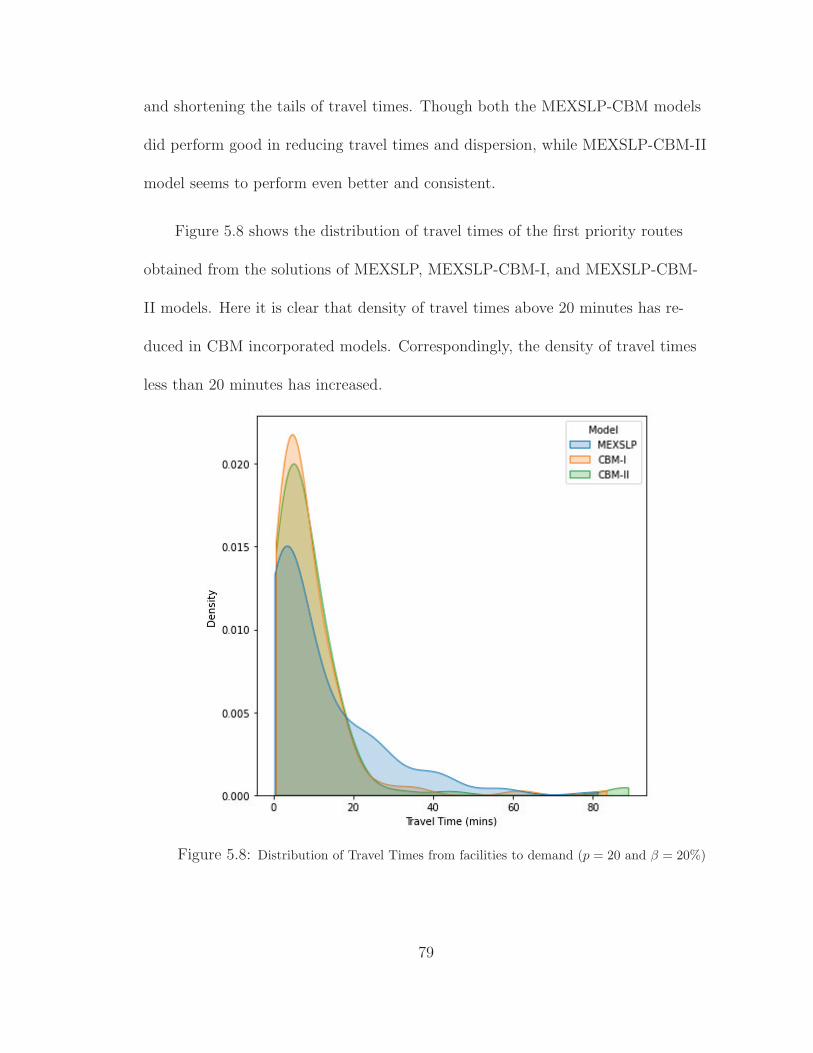
and shortening the tails of travel times. Though both the MEXSLP-CBM models

did perform good in reducing travel times and dispersion, while MEXSLP-CBM-II

model seems to perform even better and consistent.

Figure 5.8 shows the distribution of travel times of the first priority routes

obtained from the solutions of MEXSLP, MEXSLP-CBM-I, and MEXSLP-CBM-

II models. Here it is clear that density of travel times above 20 minutes has re-

duced in CBM incorporated models. Correspondingly, the density of travel times

less than 20 minutes has increased.

Figure 5.8: Distribution of Travel Times from facilities to demand (p = 20 and β = 20%)

79

5.4 Summary

In this chapter, computational analyses are performed on four CBM models de-

veloped in chapters 3 and 4. First, the two MCLP-CBM models’ computational

performance from chapter 3 is compared to a regular MCLP by solving them

using a state-of-the-art MIP solver. MCLP-CBM-I model is defined such that

the CBM part in it is calculated using β% of demands served by such facility.

MCLP-CBM-II model is defined such that the CBM is calculated using β number

of demands served by a facility. Both the MCLP-CBM models are tested with

two different types of datasets, one taken from Chauhan et al. (2019) and the

other from Osman and Christofides (1994). Results analyses of both the datasets

show that incorporating CBM has helped MCLP utilize the excess capacity by

assigning it to appropriate demand points outside coverage radius. MCLP-CBM-II

model always showed better convergence over the MCLP-CBM-I model.

Though MCLP-CBM models provided better coverage, their solutions are

less reliable due to their higher gap values from MIP solver. To overcome the

issue of convergence and solve the models faster, an Enhanced Greedy (EG) based

heuristic was proposed. Compared to the MIP solver, EG heuristic achieves better

quality solutions in a very short time. This has been observed and verified with

both datasets.

Next, the computational performance of the two MEXSLP-CBM models

80

from chapter 4 are compared to a regular MEXSLP model. MEXSLP is a model

that specially focuses on locating emergency supplies or EMS units. Due to the

population density of urban areas, MEXSLP model locates the majority of the

EMS units closer to urban areas, affecting the quality of service in suburban re-

gions. The incorporation of CBM into the MEXSLP has resulted in improving the

quality of service provided for suburban regions. Unlike the other nonlinear EMS

models incorporating equity, MEXSLP-CBM models in this study are linear and

easy to solve using a MIP solver.

81

6 Conclusions

For any facility location problem, the primary goal is to locate facilities while

optimizing specific objectives and satisfying constraints. Facility location prob-

lems such as Maximum Covering Problem (MCLP) have been popular to locate

facilities such as postal services, police, emergency services, garbage disposal,

and more. A classical MCLP is designed such that a demand point is considered

covered if it has an open facility within the coverage radius and unserved if it is

outside the radius. There is no hardbound coverage radius for public services such

as postal or medical. In such cases, coverage radius is only used to maintain a

minimum level of service while serving the maximum demand possible.

Similarly, in FLP focusing on EMS, the assumption of a patient being cov-

ered only when it is in the coverage radius is not practical. When it comes to

medical services, successful coverage is always a just probability. If a patient stays

closer to an EMS unit, their probability of survival is higher, and when they stay

far, their probability of survival is lower. So, irrespective of their location, in

EMS, all demands are served based on availability. MEXSLP is an excellent ex-

ample of such a model whose objective is to maximize the aggregated sum of the

survival probability of all demand points.

With a single objective of maximizing coverage, models tend to locate fa-

82

cilities closer to urban areas having a dense population, leaving minimal to no

resources available for suburban and rural regions. Even if more EMS units are

made available, these models tend to concentrate units in favor of the denser

population unless 100% coverage is possible. Maximizing coverage could be an

efficient way of utilizing resources, but it is not equitable.

In literature, there have been various studies with various approaches and

measures to obtain equity. However, there are not models which are linear and

incorporate equity. So, in our study, we chose CBM as the measure for equity

in the MEXSLP model. Also, we use the same CBM to provide soft or flexible

bounds on the coverage radius of MCLP models. As explained in earlier chapters,

CBM has few unique characteristics, allowing us to implement it in a MILP model

with as limited constraints and variables as possible.

In this study, four models were proposed and developed, incorporated with

CBM: MCLP-CBM-I, MCLP-CBM-II, MEXSLP-CBM-I, and MEXSLP-CBM-II.

Though both the MCLP-CBM models have the same objectives, the way CBM

is defined and calculated is different. MCLP-CBM-I model uses the standard

definition of CBM where β is a percentage. In the MCLP-CBM-II model, the idea

of CBM is similar, but instead of percentage, β is defined as an integer. Defining

β in this way made the model computationally efficient. Besides, with β being

integer, the calculation of CBM is relatively simple and straight.

Overall, both the MCLP-CBM models increase coverage by assigning de-

83

mands outside the coverage radius to facilities having excess capacity or resources.

An enhanced greedy-based heuristic is proposed for solving the MCLP-CBM mod-

els to reduce run-time and improve convergence within solutions. The developed

enhanced greedy heuristic provides coverage almost as good as a standard MIP

solver while saving more than 95% of time.

For EMS applications, two linear MEXSLP models were proposed while in-

corporating equity using CBM. Being linear, both these can be easily solved by

any standard MIP solver. Both the MEXSLP-CBM models have a different ap-

proach for estimating CBM. Both models are efficient in incorporating equity and

reducing the response time for suburban regions, giving them a higher probability

of survival in case of emergencies. Geo-plots in section 5.3 show the capability of

these models to locate EMS units across the service area sparsely are, providing

equity concerning the level of service in suburban regions.

The models developed in this study assume only one type of EMS unit, a

single type of patient severity, and do not account for vehicle routing. All of these

are the limitations of this study and can be potential directions for future re-

search.

84

Bibliography

M. Albareda-Sambola, E. Fernandez, and G. Laporte. The capacity and distance

constrained plant location problem. Computers & Operations Research, 36(2):

597–611, 2009.

American Community Survey. U.S. Census Bureau, 2014-2018

American Community Survey 5-Year Estimates, Table S1701, 2020.

https://data.census.gov/cedsci/, last accessed on 6/15/2020.

C. Araz, H. Selim, and I. Ozkarahan. A fuzzy multi-objective covering-based ve-

hicle location model for emergency services. Computers & Operations Research,

34(3):705–726, 2007.

R. Aringhieri, M. E. Bruni, S. Khodaparasti, and J. T. van Essen. Emergency

medical services and beyond: Addressing new challenges through a wide litera-

ture review. Computers & Operations Research, 78:349–368, 2017.

M. O. Ball and F. L. Lin. A reliability model applied to emergency service vehicle

location. Operations research, 41(1):18–36, 1993.

D. Bandara, M. E. Mayorga, and L. A. McLay. Optimal dispatching strategies for

emergency vehicles to increase patient survivability. International Journal of

Operational Research, 15(2):195–214, 2012.

M. Barbati and C. Piccolo. Equality measures properties for location problems.

Optimization Letters, 10(5):903–920, 2016.

O. Baron, O. Berman, D. Krass, and Q. Wang. The equitable location problem on

the plane. European Journal of Operational Research, 183(2):578–590, 2007.

R. Batta, J. M. Dolan, and N. N. Krishnamurthy. The maximal expected covering

location problem: Revisited. Transportation science, 23(4):277–287, 1989.

V. Belanger, A. Ruiz, and P. Soriano. Recent optimization models and trends in

location, relocation, and dispatching of emergency medical vehicles. European

Journal of Operational Research, 272(1):1–23, 2019.

85

G. N. Berlin. Facility location and vehicle allocation for provision of an emergency

service. 1974.

O. Berman and R. Huang. The minimum weighted covering location problem with

distance constraints. Computers & Operations Research, 35(2):356–372, 2008.

O. Berman and D. Krass. 11 facility location problems with stochastic demands

and congestion. Facility location: Applications and theory, 329, 2001.

O. Berman and D. Krass. The generalized maximal covering location problem.

Computers & Operations Research, 29(6):563–581, 2002.

O. Berman, Z. Drezner, and D. Krass. Generalized coverage: New developments in

covering location models. Computers & Operations Research, 37(10):1675–1687,

2010.

R. Boujemaa, A. Jebali, S. Hammami, A. Ruiz, and H. Bouchriha. A stochastic

approach for designing two-tiered emergency medical service systems. Flexible

Services and Manufacturing Journal, 30(1):123–152, 2018.

C. C. Branas and C. S. Revelle. An iterative switching heuristic to locate hospi-

tals and helicopters. Socio-Economic Planning Sciences, 35(1):11–30, 2001.

L. Brotcorne, G. Laporte, and F. Semet. Ambulance location and relocation

models. European journal of operational research, 147(3):451–463, 2003.

S. Chanta. Improving quality of service in ems systems by reducing disparities

between service zones. 2011.

S. Chanta, M. E. Mayorga, M. E. Kurz, and L. A. McLay. The minimum p-

envy location problem: a new model for equitable distribution of emergency

resources. IIE Transactions on Healthcare Systems Engineering, 1(2):101–115,

2011.

S. Chanta, M. E. Mayorga, and L. A. McLay. Improving emergency service in

rural areas: a bi-objective covering location model for ems systems. Annals of

Operations Research, 221(1):133–159, 2014a.

86

S. Chanta, M. E. Mayorga, and L. A. McLay. The minimum p-envy location

problem with requirement on minimum survival rate. Computers & Industrial

Engineering, 74:228–239, 2014b.

A. G. Chapman and J. E. Mitchell. A fair division approach to humanitarian

logistics inspired by conditional value-at-risk. Annals of Operations Research,

262(1):133–151, 2018.

D. Chauhan, A. Unnikrishnan, and M. Figliozzi. Maximum coverage capacitated

facility location problem with range constrained drones. Transportation Re-

search Part C: Emerging Technologies, 99:1–18, 2019.

G. Chen, M. S. Daskin, Z.-J. M. Shen, and S. Uryasev. The α-reliable mean-

excess regret model for stochastic facility location modeling. Naval Research

Logistics (NRL), 53(7):617–626, 2006.

S.-H. Cho, H. Jang, T. Lee, and J. Turner. Simultaneous location of trauma

centers and helicopters for emergency medical service planning. Operations

Research, 62(4):751–771, 2014.

C. Chung, D. Schilling, and R. Carbone. The capacitated maximal covering prob-

lem: A heuristic. In Proceedings of Fourteenth Annual Pittsburgh Conference on

Modeling and Simulation, volume 1983, pages 1423–1428, 1983.

R. Church and C. ReVelle. The maximal covering location problem. In Papers of

the Regional Science Association, volume 32, pages 101–118. Springer-Verlag,

1974.

P. Coelho. Linearization of the product of two variables. Canada Research Chair

in Integrated Logistics, 2013.

I. Correia and F. Saldanha-da Gama. Facility location under uncertainty. In

Location science, pages 185–213. Springer, 2019.

J. Current, H. Min, and D. Schilling. Multiobjective analysis of facility location

decisions. European journal of operational research, 49(3):295–307, 1990.

J. R. Current and J. E. Storbeck. Capacitated covering models. Environment and

planning B: planning and Design, 15(2):153–163, 1988.

87

M. S. Daskin. A maximum expected covering location model: formulation, proper-

ties and heuristic solution. Transportation science, 17(1):48–70, 1983.

M. S. Daskin. Network and discrete location: models, algorithms, and applications.

John Wiley & Sons, 2011.

M. S. Daskin and E. H. Stern. A hierarchical objective set covering model for

emergency medical service vehicle deployment. Transportation Science, 15(2):

137–152, 1981.

M. S. Daskin, K. Hogan, and C. ReVelle. Integration of multiple, excess, backup,

and expected covering models. Environment and Planning B: Planning and

Design, 15(1):15–35, 1988.

M. S. Daskin, S. M. Hesse, and C. S. Revelle. α-reliable p-minimax regret: A new

model for strategic facility location modeling. Location science, 5(4):227–246,

1997.

V. J. De Maio, I. G. Stiell, G. A. Wells, D. W. Spaite, O. P. A. L. S. S. Group,

et al. Optimal defibrillation response intervals for maximum out-of-hospital

cardiac arrest survival rates. Annals of emergency medicine, 42(2):242–250,

2003.

T. Drezner, Z. Drezner, and J. Guyse. Equitable service by a facility: Minimizing

the gini coefficient. Computers & operations research, 36(12):3240–3246, 2009.

T. Drezner, Z. Drezner, and B. Hulliger. The quintile share ratio in location

analysis. European Journal of Operational Research, 238(1):166–174, 2014.

E. Erkut and S. Neuman. A multiobjective model for locating undesirable facili-

ties. Annals of operations Research, 40(1):209–227, 1992.

E. Erkut, A. Ingolfsson, and G. Erdogan. Ambulance location for maximum

survival. Naval Research Logistics (NRL), 55(1):42–58, 2008.

I. Espejo, A. Marın, J. Puerto, and A. M. Rodrıguez-Chıa. A comparison of

formulations and solution methods for the minimum-envy location problem.

Computers & Operations Research, 36(6):1966–1981, 2009.

88

R. Z. Farahani, N. Asgari, N. Heidari, M. Hosseininia, and M. Goh. Covering

problems in facility location: A review. Computers & Industrial Engineering, 62

(1):368–407, 2012.

C. Filippi, G. Guastaroba, and M. Speranza. Applications of conditional value-at-

risk beyond finance: A literature review. In Technical Report 2. University of

Brescia, Department of Economics and Management, 2017.

C. Filippi, G. Guastaroba, and M. Speranza. On single-source capacitated facility

location with cost and fairness objectives. European Journal of Operational

Research, 2019a.

C. Filippi, W. Ogryczak, and M. G. Speranza. Bridging k-sum and cvar optimiza-

tion in milp. Computers & Operations Research, 105:156–166, 2019b.

C. Filippi, G. Guastaroba, and M. G. Speranza. Conditional value-at-risk beyond

finance: a survey. International Transactions in Operational Research, 27(3):

1277–1319, 2020.

M. Gendreau, G. Laporte, and F. Semet. Solving an ambulance location model by

tabu search. Location science, 5(2):75–88, 1997.

M. Gendreau, G. Laporte, and F. Semet. A dynamic model and parallel tabu

search heuristic for real-time ambulance relocation. Parallel computing, 27(12):

1641–1653, 2001.

M. Gendreau, G. Laporte, and F. Semet. The maximal expected coverage relo-

cation problem for emergency vehicles. Journal of the Operational Research

Society, 57(1):22–28, 2006.

A. Ghosh and S. McLaerty. Locating stores in uncertain environments: A scenario

planning approach. 1982.

B. C. Grannan, N. D. Bastian, and L. A. McLay. A maximum expected covering

problem for locating and dispatching two classes of military medical evacuation

air assets. Optimization Letters, 9(8):1511–1531, 2015.

L. Gurobi Optimization. Gurobi optimizer reference manual, 2020. URL http:

//www.gurobi.com.

89

A. Haghani. Capacitated maximum covering location models: Formulations and

solution procedures. Journal of advanced transportation, 30(3):101–136, 1996.

S. Hammami and A. Jebali. Designing modular capacitated emergency medical

service using information on ambulance trip. Operational Research, pages 1–20,

2019.

K. Hogan and C. ReVelle. Concepts and applications of backup coverage. Man-

agement science, 32(11):1434–1444, 1986.

C. Jagtenberg and A. Mason. Fairness in the ambulance location problem: Maxi-

mizing the bernoulli-nash social welfare. Available at SSRN 3536707, 2020.

V. Jayaraman and R. Srivastava. A service logistics model for simultaneous siting

of facilities and multiple levels of equipment. Computers & Operations Research,

22(2):191–204, 1995.

O. Karasakal and E. K. Karasakal. A maximal covering location model in the

presence of partial coverage. Computers & Operations Research, 31(9):1515–

1526, 2004.

M. M. Kostreva, W. Ogryczak, and A. Wierzbicki. Equitable aggregations and

multiple criteria analysis. European Journal of Operational Research, 158(2):

362–377, 2004.

T. Lee and H. Jang. An iterative method for simultaneously locating trauma

centers and helicopters through the planning horizon. Operations research for

health care, 19:185–196, 2018.

T. Lee, S.-H. Cho, H. Jang, and J. G. Turner. A simulation-based iterative

method for a trauma center—air ambulance location problem. In Proceedings of

the 2012 Winter Simulation Conference (WSC), pages 1–12. IEEE, 2012.

M. A. Lejeune and S. Y. Prasad. Effectiveness–equity models for facility location

problems on tree networks. networks, 62(4):243–254, 2013.

X. Li, Z. Zhao, X. Zhu, and T. Wyatt. Covering models and optimization tech-

niques for emergency response facility location and planning: a review. Mathe-

matical Methods of Operations Research, 74(3):281–310, 2011.

90

Y. Liu, H. Chen, and B. Wu. Controllability of boolean control networks with

impulsive effects and forbidden states. Mathematical methods in the Applied

Sciences, 37(1):1–9, 2014.

Y. Liu, Z. Li, J. Liu, and H. Patel. A double standard model for allocating lim-

ited emergency medical service vehicle resources ensuring service reliability.

Transportation research part C: emerging technologies, 69:120–133, 2016.

M. C. Lopez-de-los Mozos and J. A. Mesa. The maximum absolute deviation

measure in location problems on networks. European Journal of Operational

Research, 135(1):184–194, 2001.

M. B. Mandell. Covering models for two-tiered emergency medical services sys-

tems. Location Science, 6(1-4):355–368, 1998.

V. Marianov and C. ReVelle. A probabilistic fire-protection siting model with

joint vehicle reliability requirements. Papers in Regional Science, 71(3):217–241,

1992.

V. Marianov and D. Serra. Hierarchical location–allocation models for congested

systems. European Journal of Operational Research, 135(1):195–208, 2001.

A. Marın. The discrete facility location problem with balanced allocation of

customers. European Journal of Operational Research, 210(1):27–38, 2011.

M. T. Marsh and D. A. Schilling. Equity measurement in facility location analy-

sis: A review and framework. European journal of operational research, 74(1):

1–17, 1994.

A. J. Mason. Simulation and real-time optimised relocation for improving am-

bulance operations. In Handbook of Healthcare Operations Management, pages

289–317. Springer, 2013.

L. A. McLay. A maximum expected covering location model with two types of

servers. IIE Transactions, 41(8):730–741, 2009.

L. A. McLay and M. E. Mayorga. A dispatching model for server-to-customer sys-

tems that balances efficiency and equity. Manufacturing & Service Operations

Management, 15(2):205–220, 2013.

91

S. Narasimhan, H. Pirkul, and D. A. Schilling. Capacitated emergency facility

siting with multiple levels of backup. Annals of Operations Research, 40(1):

323–337, 1992.

W. Ogryczak. Inequality measures and equitable approaches to location problems.

European Journal of Operational Research, 122(2):374–391, 2000.

W. Ogryczak and M. Zawadzki. Conditional median: a parametric solution con-

cept for location problems. Annals of Operations Research, 110(1-4):167–181,

2002.

Y. Ohsawa, F. Plastria, and K. Tamura. Euclidean push–pull partial covering

problems. Computers & operations research, 33(12):3566–3582, 2006.

R. L. Oliver and W. S. DeSarbo. Response determinants in satisfaction judg-

ments. Journal of consumer research, 14(4):495–507, 1988.

I. H. Osman and N. Christofides. Capacitated clustering problems by hybrid

simulated annealing and tabu search. International Transactions in Operational

Research, 1(3):317–336, 1994.

H. Pirkul and D. Schilling. The capacitated maximal covering location problem

with backup service. Annals of Operations Research, 18(1):141–154, 1989.

H. Pirkul and D. A. Schilling. The siting of emergency service facilities with

workload capacities and backup service. Management Science, 34(7):896–908,

1988.

H. Pirkul and D. A. Schilling. The maximal covering location problem with

capacities on total workload. Management Science, 37(2):233–248, 1991.

O. A. Prokopyev, N. Kong, and D. L. Martinez-Torres. The equitable dispersion

problem. European Journal of Operational Research, 197(1):59–67, 2009.

C. ReVelle and K. Hogan. The maximum availability location problem. Trans-

portation science, 23(3):192–200, 1989.

C. ReVelle and V. Marianov. A probabilistic fleet model with individual vehicle

reliability requirements. European Journal of Operational Research, 53(1):

93–105, 1991.

92

C. Revelle, J. Schweitzer, and S. Snyder. The maximal conditional covering prob-

lem. INFOR: Information Systems and Operational Research, 34(2):77–91,

1996.

C. S. ReVelle and H. A. Eiselt. Location analysis: A synthesis and survey. Euro-

pean journal of operational research, 165(1):1–19, 2005.

C. S. Revelle, H. A. Eiselt, and M. S. Daskin. A bibliography for some funda-

mental problem categories in discrete location science. European Journal of

Operational Research, 184(3):817–848, 2008.

D. Rey, K. Almi’ani, and D. J. Nair. Exact and heuristic algorithms for finding

envy-free allocations in food rescue pickup and delivery logistics. Transportation

Research Part E: Logistics and Transportation Review, 112:19–46, 2018.

R. T. Rockafellar, S. Uryasev, et al. Optimization of conditional value-at-risk.

Journal of risk, 2:21–42, 2000.

T. W. Ruefli and J. E. Storbeck. Behaviorally linked location hierarchies. Envi-

ronment and Planning B: Planning and Design, 9(3):257–268, 1982.

E. S. Savas. On equity in providing public services. Management Science, 24(8):

800–808, 1978.

D. Schilling, D. J. Elzinga, J. Cohon, R. Church, and C. ReVelle. The team/fleet

models for simultaneous facility and equipment siting. Transportation science,

13(2):163–175, 1979.

D. A. Schilling. Strategic facility planning: The analysis of options. Decision

Sciences, 13(1):1–14, 1982.

D. A. Schilling. A review of covering problems in facility location. Location

Science, 1:25–55, 1993.

E. S. Sheppard. A conceptual framework for dynamic location—allocation analy-

sis. Environment and Planning a, 6(5):547–564, 1974.

L. V. Snyder. Facility location under uncertainty: a review. IIE transactions, 38

(7):547–564, 2006.

93

L. V. Snyder, M. S. Daskin, and C.-P. Teo. The stochastic location model with

risk pooling. European Journal of Operational Research, 179(3):1221–1238,

2007.

L. V. Snyder, Z. Atan, P. Peng, Y. Rong, A. J. Schmitt, and B. Sinsoysal. Or/ms

models for supply chain disruptions: A review. IIE Transactions, 48(2):89–109,

2016.

K. Sudtachat, M. E. Mayorga, and L. A. McLay. Recommendations for dispatch-

ing emergency vehicles under multitiered response via simulation. International

Transactions in Operational Research, 21(4):581–617, 2014.

C. Toregas and C. ReVelle. Optimal location under time or distance constraints.

In Papers of the Regional Science Association, volume 28, pages 131–143.

Springer, 1972.

C. Toregas, R. Swain, C. ReVelle, and L. Bergman. The location of emergency

service facilities. Operations research, 19(6):1363–1373, 1971.

T. D. Valenzuela, D. J. Roe, S. Cretin, D. W. Spaite, and M. P. Larsen. Esti-

mating effectiveness of cardiac arrest interventions: a logistic regression survival

model. Circulation, 96(10):3308–3313, 1997.

T. Van Barneveld, R. D. van der Mei, and S. Bhulai. Compliance tables for an

ems system with two types of medical response units. Computers & Operations

Research, 80:68–81, 2017.

S. Yoon and L. Albert. Dynamic resource assignment for emergency response with

multiple types of vehicles. Under review at Operations Research, 2018.

S. Yoon and L. A. Albert. A dynamic ambulance routing model with multiple

response. Transportation Research Part E: Logistics and Transportation Review,

133:101807, 2020.

S. Yoon, L. A. Albert, and V. M. White. A stochastic programming approach for

locating and dispatching two types of ambulances. Transportation Science, 55

(2):275–296, 2021.

94

S.-l. Zhan and N. Liu. A multi-objective stochastic programming model for emer-

gency logistics based on goal programming. In 2011 Fourth International Joint

Conference on Computational Sciences and Optimization, pages 640–644. IEEE,

2011.

95

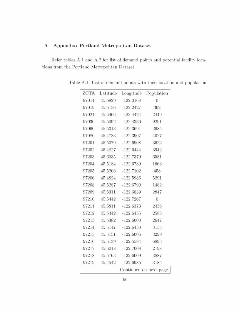
A Appendix: Portland Metropolitan Dataset

Refer tables A.1 and A.2 for list of demand points and potential facility loca-

tions from the Portland Metropolitan Dataset.

Table A.1: List of demand points with their location and population.

ZCTA Latitude Longitude Population

97014 45.5829 -122.0168 0

97019 45.5156 -122.2427 362

97024 45.5466 -122.4424 2440

97030 45.5092 -122.4336 9291

97060 45.5313 -122.3691 2685

97080 45.4783 -122.3907 4027

97201 45.5079 -122.6908 3622

97202 45.4827 -122.6444 3942

97203 45.6035 -122.7379 6531

97204 45.5184 -122.6739 1663

97205 45.5206 -122.7102 458

97206 45.4824 -122.5986 5291

97208 45.5287 -122.6790 1482

97209 45.5311 -122.6839 2847

97210 45.5442 -122.7267 0

97211 45.5811 -122.6373 2436

97212 45.5442 -122.6435 2583

97213 45.5382 -122.6000 2647

97214 45.5147 -122.6430 3155

97215 45.5151 -122.6006 3299

97216 45.5139 -122.5584 6893

97217 45.6018 -122.7008 2198

97218 45.5763 -122.6009 3887

97219 45.4542 -122.6985 3185

Continued on next page

96

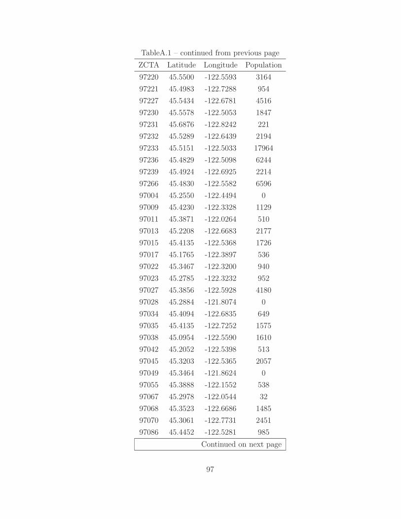
TableA.1 – continued from previous page

ZCTA Latitude Longitude Population

97220 45.5500 -122.5593 3164

97221 45.4983 -122.7288 954

97227 45.5434 -122.6781 4516

97230 45.5578 -122.5053 1847

97231 45.6876 -122.8242 221

97232 45.5289 -122.6439 2194

97233 45.5151 -122.5033 17964

97236 45.4829 -122.5098 6244

97239 45.4924 -122.6925 2214

97266 45.4830 -122.5582 6596

97004 45.2550 -122.4494 0

97009 45.4230 -122.3328 1129

97011 45.3871 -122.0264 510

97013 45.2208 -122.6683 2177

97015 45.4135 -122.5368 1726

97017 45.1765 -122.3897 536

97022 45.3467 -122.3200 940

97023 45.2785 -122.3232 952

97027 45.3856 -122.5928 4180

97028 45.2884 -121.8074 0

97034 45.4094 -122.6835 649

97035 45.4135 -122.7252 1575

97038 45.0954 -122.5590 1610

97042 45.2052 -122.5398 513

97045 45.3203 -122.5365 2057

97049 45.3464 -121.8624 0

97055 45.3888 -122.1552 538

97067 45.2978 -122.0544 32

97068 45.3523 -122.6686 1485

97070 45.3061 -122.7731 2451

97086 45.4452 -122.5281 985

Continued on next page

97

TableA.1 – continued from previous page

ZCTA Latitude Longitude Population

97089 45.4266 -122.4431 674

97222 45.4409 -122.6181 4847

97267 45.4084 -122.6129 3773

98601 45.9434 -122.3625 520

98604 45.8057 -122.5108 2335

98606 45.7297 -122.4564 805

98607 45.6422 -122.3800 634

98629 45.8766 -122.6192 997

98642 45.8077 -122.6939 745

98660 45.6790 -122.7205 0

98661 45.6401 -122.6250 7311

98662 45.6885 -122.5778 5303

98663 45.6574 -122.6632 3600

98664 45.6195 -122.5772 5072

98665 45.6795 -122.6606 3136

98675 45.8285 -122.3429 0

98682 45.6732 -122.4817 1008

98683 45.6033 -122.5102 2207

98684 45.6306 -122.5148 4580

98685 45.7152 -122.6931 1343

98686 45.7234 -122.6244 1651

97016 46.0603 -123.2670 905

97018 45.8971 -122.8106 1986

97048 46.0448 -122.9820 574

97051 45.8793 -122.9500 0

97053 45.8280 -122.8833 1800

97054 45.9422 -122.9496 453

97056 45.7720 -122.9694 0

97064 45.8591 -123.2355 385

97101 45.0902 -123.2287 743

97111 45.2845 -123.1952 4490

Continued on next page

98

TableA.1 – continued from previous page

ZCTA Latitude Longitude Population

97114 45.1879 -123.0766 560

97115 45.2752 -123.0395 926

97127 45.2461 -123.1114 576

97128 45.2119 -123.2822 1545

97132 45.3242 -122.9873 3811

97148 45.3584 -123.2485 0

97347 45.0771 -123.6564 0

97396 45.1040 -123.5490 848

97005 45.4910 -122.8036 5637

97006 45.5170 -122.8598 12425

97007 45.4543 -122.8796 3590

97008 45.4602 -122.8042 6272

97062 45.3693 -122.7623 2746

97106 45.6657 -123.1190 84

97109 45.7378 -123.1812 0

97113 45.4972 -123.0443 4865

97116 45.5808 -123.1657 926

97117 45.6314 -123.2884 0

97119 45.4689 -123.2002 84

97123 45.4402 -122.9801 297

97124 45.5698 -122.9496 6710

97125 45.6711 -123.1969 169

97133 45.6861 -123.0227 0

97140 45.3531 -122.8659 726

97144 45.7416 -123.3002 0

97223 45.4403 -122.7766 3395

97224 45.4055 -122.7951 3250

97225 45.5016 -122.7700 2053

97229 45.5510 -122.8093 2586

98605 45.7769 -121.6655 278

98610 45.8659 -122.0652 20

Continued on next page

99

TableA.1 – continued from previous page

ZCTA Latitude Longitude Population

98616 46.1933 -122.1329 0

98639 45.6699 -121.9897 0

98648 45.7063 -121.9563 808

98651 45.7399 -121.5835 0

98671 45.6144 -122.2384 446

Table A.2: List of all potential facility locations.

ID Latitude Longitude

0 45.816915 -122.745904

1 45.862462 -122.660465

2 45.781175 -122.527274

3 45.691966 -122.545208

4 45.661016 -122.636015

5 45.625946 -122.536095

6 45.633546 -122.661322

7 45.643123 -122.62553

8 45.581972 -122.390494

9 45.579675 -122.354185

10 45.692315 -121.894119

11 45.737978 -121.538641

12 45.468176 -123.143827

13 45.598709 -122.99608

14 45.299255 -122.974962

15 45.304587 -122.936475

16 45.074026 -123.614063

17 45.212504 -123.194003

18 45.243158 -123.116017

19 45.275328 -123.013592

Continued on next page

100

TableA.2 – continued from previous page

ID Latitude Longitude

20 45.219097 -123.07598

21 45.097883 -123.396

22 45.076501 -123.483198

23 46.103447 -123.202116

24 46.09329 -122.943955

25 45.862614 -122.808992

26 45.845853 -122.825924

27 45.537161 -122.265823

28 45.285214 -122.336807

29 45.042412 -122.667712

30 45.149914 -122.577736

31 45.534584 -122.624656

32 45.570834 -122.609652

33 45.553662 -122.675926

34 45.533931 -122.685373

35 45.483126 -122.804126

36 45.516737 -122.607121

37 45.562518 -122.666622

38 45.598603 -122.785298

39 45.566168 -122.674643

40 45.550222 -122.661925

41 45.507636 -122.421495

42 45.520641 -123.104218

43 45.505128 -122.485559

44 45.426612 -122.606107

45 45.43116 -122.582194

46 45.477062 -122.704034

47 45.491318 -122.601435

48 45.303592 -122.75862

49 45.382808 -122.732116

50 45.38628 -122.767007

Continued on next page

101

TableA.2 – continued from previous page

ID Latitude Longitude

51 45.385564 -122.760503

52 45.423316 -122.768484

53 45.536846 -122.435763

54 45.52117 -123.057904

55 45.53678 -122.834329

56 45.396788 -122.269086

57 45.44495 -122.795228

58 45.529033 -122.8065

59 45.252484 -122.686501

60 45.598734 -122.996086

61 45.352466 -122.598023

62 45.381646 -122.592285

63 45.44613 -122.619198

64 45.285227 -122.336833

65 45.383843 -122.597554

66 45.597585 -123.001208

67 45.562264 -122.667592

68 45.466562 -122.753479

69 45.522859 -122.982042

70 45.36081 -122.845148

71 45.431575 -122.715113

72 45.353494 -122.866459

73 45.409146 -122.796286

74 45.482443 -122.588652

75 45.440127 -122.836567

76 45.507387 -122.797111

77 45.569566 -122.67361

78 45.46818 -122.709993

79 45.494571 -122.630546

80 45.508503 -122.717893

81 45.149984 -122.577833

Continued on next page

102

TableA.2 – continued from previous page

ID Latitude Longitude

82 45.519883 -122.624607

83 45.550336 -122.685718

84 45.542171 -122.664863

85 45.475815 -122.722125

86 45.44866 -122.806375

87 45.561751 -122.681869

88 45.35486 -122.605961

89 45.515352 -122.974841

90 45.470952 -122.678958

91 45.514686 -122.976902

92 45.527798 -122.709669

93 45.58773 -122.711377

94 45.515807 -122.553233

95 45.526807 -122.578529

96 45.464824 -122.651252

97 45.592235 -122.75215

98 45.479782 -122.618847

99 45.42624 -122.667851

100 45.369921 -122.648819

101 45.479756 -122.804003

102 45.539572 -122.962627

103 45.310153 -122.798166

103

B Appendix: Standard P-Median Test Cases

The OR-Library on J.E.Beasley website provides about twenty standard p-

median test cases with capacitated facilities. In all these test cases, the demand

points themselves act as potential facility locations. These test cases can be ac-

cessed through: http://people.brunel.ac.uk/˜mastjjb/jeb/orlib/

pmedcapinfo.html

Details of the two standard test cases used in this work are provided in this

section. Table B.1 provides the coordinates and demand values of 50 sites in

the first test case. Tables B.2 provides the same for 100 sites in the second test

case. No. of facilities to open from the first and second test cases are 5 and 10

respectively. The capacity of each open facility is given as 120.

Table B.1: List of demand-facility sites in test case-1 with their locations anddemand values.

ID X-Coordinate Y-Coordinate Demand

1 2 62 3

2 80 25 14

3 36 88 1

4 57 23 14

5 33 17 19

6 76 43 2

7 77 85 14

8 94 6 6

9 89 11 7

10 59 72 6

11 39 82 10

12 87 24 18

13 44 76 3

14 2 83 6

15 19 43 20

Continued on next page

104

TableB.1 – continued from previous page

ID X-Coordinate Y-Coordinate Demand

16 5 27 4

17 58 72 14

18 14 50 11

19 43 18 19

20 87 7 15

21 11 56 15

22 31 16 4

23 51 94 13

24 55 13 13

25 84 57 5

26 12 2 16

27 53 33 3

28 53 10 7

29 33 32 14

30 69 67 17

31 43 5 3

32 10 75 3

33 8 26 12

34 3 1 14

35 96 22 20

36 6 48 13

37 59 22 10

38 66 69 9

39 22 50 6

40 75 21 18

41 4 81 7

42 41 97 20

43 92 34 9

44 12 64 1

45 60 84 8

46 35 100 5

Continued on next page

105

TableB.1 – continued from previous page

ID X-Coordinate Y-Coordinate Demand

47 38 2 1

48 9 9 7

49 54 59 9

50 1 58 2

Table B.2: List of demand-facility sites in test case-2 with their locations anddemand values.

ID X-Coordinate Y-Coordinate Demand

1 6 5 12

2 36 29 7

3 61 45 1

4 97 80 11

5 51 74 1

6 11 81 3

7 18 92 4

8 28 89 18

9 25 3 12

10 98 60 17

11 3 33 12

12 84 21 13

13 88 7 10

14 37 31 8

15 78 39 13

16 59 91 17

17 87 5 14

18 5 41 19

19 80 95 2

20 7 53 1

21 11 77 5

Continued on next page

106

TableB.2 – continued from previous page

ID X-Coordinate Y-Coordinate Demand

22 25 7 8

23 8 6 12

24 52 12 19

25 63 71 15

26 33 2 15

27 31 54 18

28 69 29 3

29 50 52 1

30 21 30 12

31 14 86 9

32 33 25 6

33 94 91 2

34 42 1 18

35 59 60 12

36 36 69 19

37 61 3 14

38 88 96 15

39 73 22 9

40 72 69 12

41 7 26 2

42 38 24 2

43 45 36 6

44 99 52 7

45 48 44 12

46 70 76 18

47 51 50 17

48 53 40 18

49 39 55 19

50 47 73 19

51 70 15 5

52 50 15 13

Continued on next page

107

TableB.2 – continued from previous page

ID X-Coordinate Y-Coordinate Demand

53 83 79 7

54 67 4 18

55 23 41 17

56 41 85 1

57 50 16 19

58 83 64 9

59 30 95 14

60 47 39 12

61 20 41 1

62 97 76 4

63 88 49 7

64 54 97 2

65 44 51 17

66 14 19 19

67 60 70 20

68 83 52 13

69 18 42 1

70 71 39 6

71 94 49 8

72 28 8 12

73 88 49 17

74 33 60 5

75 50 83 15

76 57 14 18

77 58 11 11

78 57 87 7

79 52 88 1

80 89 83 2

81 31 92 1

82 26 2 10

83 61 68 3

Continued on next page

108

TableB.2 – continued from previous page

ID X-Coordinate Y-Coordinate Demand

84 37 15 8

85 60 41 17

86 51 55 11

87 56 20 5

88 19 11 4

89 21 95 9

90 42 48 6

91 48 89 11

92 37 71 14

93 6 31 6

94 47 12 13

95 2 58 4

96 27 4 18

97 28 54 16

98 61 81 7

99 79 91 10

100 78 13 4

109