Inconsistent depreciation and double-taxation: the Trans

Inconsistent

the Trans-Alaskan Pipeline System

ABSTRACT

The Trans Alaska Pipeline System is subject to an annual state ad valorem property tax. In 2005 the state changed the assessment method from an income approach to a cost approach. Under the income approach assessed value was based on production depreciation. Under the cost approach value was based on replacement cost new less straight-line depreciation. When the assessment means was changed there was no adjustment for past depreciation. This inconsistency in depreciation treatment caused assets to be depreciated more than once over time, with the result being a double taxation of the property. Keywords: property tax, depreciation, double

Journal of Legal Issues and Cases in Business

Inconsistent depreciation, Page

Inconsistent depreciation and double-taxation:

Alaskan Pipeline System property tax

Roger Marks Roger Marks & Associates

The Trans Alaska Pipeline System is subject to an annual state ad valorem property tax. In 2005 the state changed the assessment method from an income approach to a cost approach. Under the income approach assessed value was based on tariff income, which included units

Under the cost approach value was based on replacement cost new less

When the assessment means was changed there was no adjustment for past depreciation. eciation treatment caused assets to be depreciated more than once over

time, with the result being a double taxation of the property.

Keywords: property tax, depreciation, double-taxation, Alaska, assessment


Inconsistent depreciation, Page 1

axation:

ax

The Trans Alaska Pipeline System is subject to an annual state ad valorem property tax. In 2005 the state changed the assessment method from an income approach to a cost approach.

ncluded units-of-Under the cost approach value was based on replacement cost new less

When the assessment means was changed there was no adjustment for past depreciation. eciation treatment caused assets to be depreciated more than once over

I. INTRODUCTION

The Trans Alaska Pipeline System (barrels of Alaska North Slope (ANS) oil marine tankers, mostly to West Coast markets. Construction of the pipeline began in 1974operations commencing in 1977. incurred through 2006. Throughput peaked at 2.1 million barrels per day (mmbd) in 1988. Now it carries less than 600,000 mmbd. The pipeline is subject to an (Alaska Stat. § 43.56). The taxable property means the "real and tangible personal property"(Alaska Stat. § 43.56.210(5)), which consists of the machinery, equipment, and real property between the first pump station and the Valdez Marine Terminal inclusive. The Alaska Department of Revenue "full and true value" (Alaska Stat. § 43.56.010(a)). determined "with due regard to the economic value of the property based on the estimated life of the proven reserves of gas or unrefined oil then technically, economically, and legally deliverable into the transportation facility" Economic value is determined by the use of replacement cost less depreciation, capitalization of estimated future net income, analysis of sales, or other acceptable methodsCode)). In 2005 DOR changed the assessment method from an income approach to a cost approach. Under the income approach assessed value was based on the net present value of the projected future annual net tariff cash flow over the economic life of the pipeline. One of the significant tariff cash flow elements was depreciation, which was based on a units(UOP) method at the time. Under use in operations. Under the cost approach assessed value was based on replacement cost new less depreciation. DOR employed straightdepreciation an equal amount of useful life. The assessments for the years 2006resulted in two non-jury de novo trialsin the Superior Court for the State of Alaska, Third Judicial District at Anchorage. The trial for the 2006 assessment was held in 20092009 assessments (consolidated) was held in 2011Judge Sharon L. Gleason (JG) presided in both trials. At this time the decisions for both trials are on appeal to the Alaska Supreme Court. The parties to the trial consisted of a) the pipeline owners (ExxonMobil Pipeline Co., Unocal Pipeline Co., ConocoPhillips Transportation Alaska, Inc., Koch Alaska Pipeline Co., and Alyeska Pipeline Service Co. [State of Alaska Dept. of Revenueare entitled to a share of the tax (of Valdez). The author was an expert



Pipeline System (TAPS) is the means for transporting the billions of barrels of Alaska North Slope (ANS) oil 800 miles to the port of Valdez, where it is moved by marine tankers, mostly to West Coast markets. Construction of the pipeline began in 1974

in 1977. The original cost was $7.2 billion, with another $1.Throughput peaked at 2.1 million barrels per day (mmbd) in 1988. Now

600,000 mmbd. The pipeline is subject to an annual state (Alaska) ad valorem property tax of 20 mills

(Alaska Stat. § 43.56). The taxable property means the "real and tangible personal property"which consists of the machinery, equipment, and real property

first pump station and the Valdez Marine Terminal inclusive. The Alaska Department of Revenue (DOR) assesses the value of the property based on

Alaska Stat. § 43.56.010(a)). The full and true value of pipeline property is with due regard to the economic value of the property based on the estimated life of

the proven reserves of gas or unrefined oil then technically, economically, and legally portation facility" (Alaska Stat. § 43.56.060(e)(2)).

Economic value is determined by the use of "standard appraisal methods such as replacement cost less depreciation, capitalization of estimated future net income, analysis of sales, or other acceptable methods" (15 AAC 56.110(c) (Regulation per Alaska Administrative

In 2005 DOR changed the assessment method from an income approach to a cost approach. Under the income approach assessed value was based on the net present value of the

uture annual net tariff cash flow over the economic life of the pipeline. One of the significant tariff cash flow elements was depreciation, which was based on a units

Under UOP costs are allocated over time in proportion to the asset’s

Under the cost approach assessed value was based on replacement cost new less straight-line (SL) depreciation in assessing. Under straight

depreciation an equal amount of depreciation expense is allocated to each period of the asset’s

The assessments for the years 2006-2009 were appealed in an adjudication process that jury de novo trials, covering a multiplicity of issues, including

in the Superior Court for the State of Alaska, Third Judicial District at Anchorage. The trial for the 2006 assessment was held in 2009, with a decision rendered in 2010. The trial for the 20072009 assessments (consolidated) was held in 2011, with a decision rendered in the same year

presided in both trials. At this time the decisions for both trials are on appeal to the Alaska Supreme Court.

The parties to the trial consisted of a) the pipeline owners (BP Pipelines [ExxonMobil Pipeline Co., Unocal Pipeline Co., ConocoPhillips Transportation Alaska, Inc.,

and Alyeska Pipeline Service Co. [as agent for the ownersState of Alaska Dept. of Revenue, and c) the municipalities the pipeline passes through

(North Slope Borough, Fairbanks North Star Borough,

n expert witness for the pipeline owners at the second trial



) is the means for transporting the billions of to the port of Valdez, where it is moved by

marine tankers, mostly to West Coast markets. Construction of the pipeline began in 1974, with The original cost was $7.2 billion, with another $1.7 billion

Throughput peaked at 2.1 million barrels per day (mmbd) in 1988. Now

annual state (Alaska) ad valorem property tax of 20 mills (Alaska Stat. § 43.56). The taxable property means the "real and tangible personal property"

which consists of the machinery, equipment, and real property

es the value of the property based on its of pipeline property is

with due regard to the economic value of the property based on the estimated life of the proven reserves of gas or unrefined oil then technically, economically, and legally

standard appraisal methods such as replacement cost less depreciation, capitalization of estimated future net income, analysis of

(15 AAC 56.110(c) (Regulation per Alaska Administrative

In 2005 DOR changed the assessment method from an income approach to a cost approach. Under the income approach assessed value was based on the net present value of the

uture annual net tariff cash flow over the economic life of the pipeline. One of the significant tariff cash flow elements was depreciation, which was based on a units-of-production

ortion to the asset’s

Under the cost approach assessed value was based on replacement cost new less Under straight-line

depreciation expense is allocated to each period of the asset’s

2009 were appealed in an adjudication process that , including depreciation,

in the Superior Court for the State of Alaska, Third Judicial District at Anchorage. The trial for . The trial for the 2007-

, with a decision rendered in the same year. presided in both trials. At this time the decisions for both trials are

[Alaska] Inc., ExxonMobil Pipeline Co., Unocal Pipeline Co., ConocoPhillips Transportation Alaska, Inc.,

as agent for the owners], b) the the pipeline passes through, which

, Fairbanks North Star Borough, and City

at the second trial.

When the assessment means was changed with the ensuing change in depreciation method from UOP to SL , there was no adjustment for past depreciation. Because of depreciation the value calculated one year affects thyears; there is an interdependency of value in time. This inconsistency in depreciation treatment caused assets to be depreciated more than once over time, with the result being a double taxation of the property. This account will explorhow that happens. This issue was not addressed in first trial(Marks) In her decision on the first trial, as the issue was not without comment the unadjusted In the second trial the issue was contested. depreciation approach. The following II. BACKGROUND

Between 1975 and 1980 a cost approach was used to value TAPS for the ad valorem tax. Between 1981 and 1985 a combination of a cost and income approach was used. The income approach was based on the net cash income of the annual pipeline tariff cash receiptpipeline cash expenses. The assessed value of TAPS was the net present value of the projected future annual net income amounts over the life of the pipeline. Beginning with the initial operation of TAPS there had been a tariff dispute between theowners and the State of Alaska. By 1986 a settlement had been crafted, including the Federal Energy Regulatory Commission (FERC) as a party. The settlement included the establishing of a detailed calculation for determining the tariff. It was called the TAPS Settlement Methodology, or TSM, and is described below. A pure income approach was used 2002-2004 the assessed value was based on a negotiated settlement between the TAPS owners and the municipalities, based on both cost and income, not find values other than those in the agreement In summary, for the 24-year period between 1981 and 2004 the income approacmaterial bearing. Under TSM the tariff, and subsequently the income approach,main elements: - Depreciation - Recovery of deferred return - After-tax margin - Operating costs - DR&R allowance - Income tax allowance The main cash expenses consisted of: - Operating costs - DR&R allowance - Income tax allowance The main elements of net - Depreciation



When the assessment means was changed in 2005 from an income to a cost approach, with the ensuing change in depreciation method from UOP to SL , there was no adjustment for past depreciation. Because of depreciation the value calculated one year affects thyears; there is an interdependency of value in time.

This inconsistency in depreciation treatment caused assets to be depreciated more than once over time, with the result being a double taxation of the property. This account will explor

ot addressed in first trial. The author addressed it in the second trial.

decision on the first trial, as the issue was not contested, JG simply accepted unadjusted depreciation approach employed by DOR.

In the second trial the issue was contested. However, JG again did not adjust the The following is an economic evaluation of that decision.

Between 1975 and 1980 a cost approach was used to value TAPS for the ad valorem tax. etween 1981 and 1985 a combination of a cost and income approach was used. The income

approach was based on the net cash income of the annual pipeline tariff cash receiptpipeline cash expenses. The assessed value of TAPS was the net present value of the projected future annual net income amounts over the life of the pipeline.

Beginning with the initial operation of TAPS there had been a tariff dispute between theowners and the State of Alaska. By 1986 a settlement had been crafted, including the Federal Energy Regulatory Commission (FERC) as a party.

The settlement included the establishing of a detailed calculation for determining the he TAPS Settlement Methodology, or TSM, and is described below.

income approach was used between 1986, when the TSM began, and 2002004 the assessed value was based on a negotiated settlement between the TAPS owners

based on both cost and income, provided the Department of Revenue did not find values other than those in the agreement. A cost approach was implemented in 2005.

year period between 1981 and 2004 the income approac

, and subsequently the income approach, consisted of the following

Recovery of deferred return tax margin

DR&R allowance Income tax allowance cash expenses consisted of:

DR&R allowance (pre-payment of a future expense) Income tax allowance

net cash flow were:



from an income to a cost approach, with the ensuing change in depreciation method from UOP to SL , there was no adjustment for past depreciation. Because of depreciation the value calculated one year affects the value in other

This inconsistency in depreciation treatment caused assets to be depreciated more than once over time, with the result being a double taxation of the property. This account will explore

. The author addressed it in the second trial.

, JG simply accepted

did not adjust the that decision.

Between 1975 and 1980 a cost approach was used to value TAPS for the ad valorem tax. etween 1981 and 1985 a combination of a cost and income approach was used. The income

approach was based on the net cash income of the annual pipeline tariff cash receipts less pipeline cash expenses. The assessed value of TAPS was the net present value of the projected

Beginning with the initial operation of TAPS there had been a tariff dispute between the owners and the State of Alaska. By 1986 a settlement had been crafted, including the Federal

The settlement included the establishing of a detailed calculation for determining the he TAPS Settlement Methodology, or TSM, and is described below.

between 1986, when the TSM began, and 2001. From 2004 the assessed value was based on a negotiated settlement between the TAPS owners

provided the Department of Revenue did A cost approach was implemented in 2005.

year period between 1981 and 2004 the income approach had a

consisted of the following

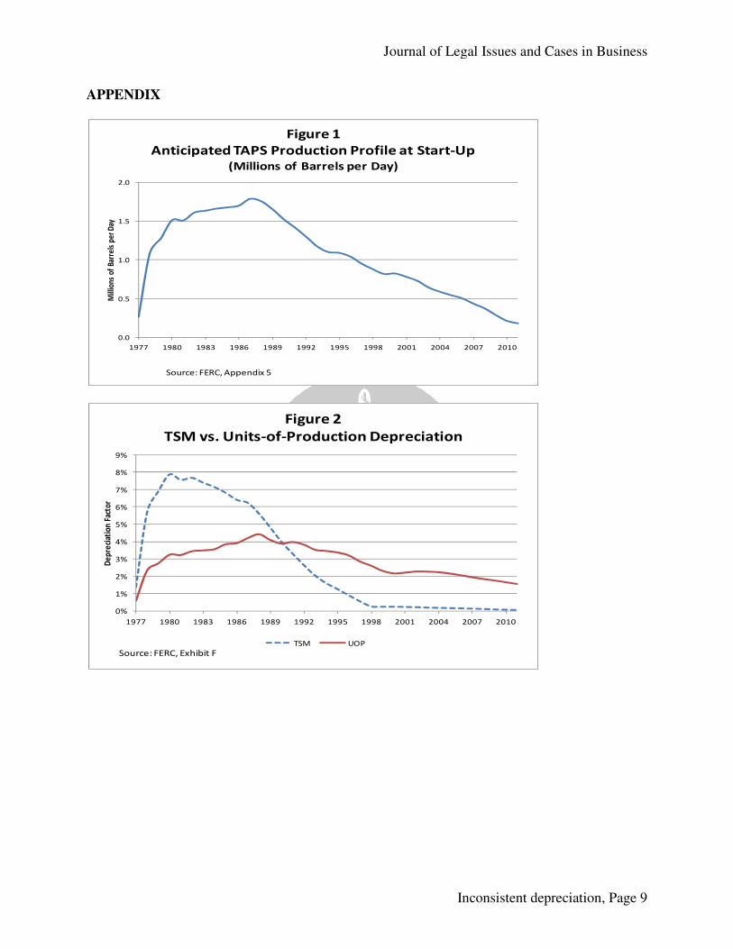
- Recovery of deferred return - After-tax margin - Relatively smaller amounts for and net additions to deferred tax TSM was a unique construct. In industries where the future level of economic activity varies over an asset’s life(such as the natural gas pipeline or extraction industries), it is not unusual to use a schedule based upon “unit of throughput” (or this method, the depreciation allowance in any year is calculated by multiplying the unrecovered investment in the asset production for that year to the total expected throughput remaining life of the asset. The TSM employs a unit of throughput depreciation schedule which, through depreciation, was accelerated in order to meet the Protestants’ objective of ensuring a declining tariff The Protestants’ (State of Alaska) required that a large fraction years of TAPS. C earn their rate of return cost arising from pre one-fifth of its 1977 economic life still remains. The depreciation factors for TSM 2011, with UOP depreciation. Theto front-end load depreciation even morefactors were designed to recover all costs by 2011.considered the life of TAPS.) This was intentionally instituted to amount in early years, resulting in a low amount in later yearsdevelopment. Moreover, it reflected the expected oil flow through TAPS, with high amounts early on and lower amounts later. The early higher depreciation caused the tariff to be higher The anticipated production profile for TAPS at 1 (Appendix). Its expected life was 35 years, from 1977 The comparison between depreciation would have been between 1977the TSM and UOP are similar, with TSM accentuated by the throughput adjustment factor. The recovery of deferred return and aftertariff income) were also calculated using the same deprreturn was based on depreciation of the original deferred return plus an inflation adjustment.recovery of deferred return under TSM was higher earlier on because of the high depreciation factors. Since the rate base for the inflation component was based on an amount reduced by depreciation, the higher earlier depreciation created a lower rate base and a smaller inflation



Recovery of deferred return tax margin

Relatively smaller amounts for additions to new depreciable property in service d net additions to deferred tax

was a unique construct. One aspect was its accelerated treatment of depreciation:In industries where the future level of economic activity varies over an asset’s life(such as the natural gas pipeline or extraction industries), it is not unusual to

schedule based upon “unit of throughput” (or “unit of production”). Under method, the depreciation allowance in any year is calculated by multiplying unrecovered investment in the asset by the ratio of the throughput or

production for that year to the total expected throughput or production over the remaining life of the asset.

The TSM employs a unit of throughput depreciation schedule which, through depreciation, was accelerated in order to meet the Protestants’ objective of ensuring a declining tariff profile.

(State of Alaska) objective of ensuring a declining tariff profile required that a large fraction of the original investment be depreciated in the early

Consequently, the rate base – the amount upon which the owners their rate of return – shrinks rapidly. For example, by 1990 the depreciated

cost arising from pre-operational investment in TAPS would be approximately fifth of its 1977 historical cost, even though about two-thirds of the system’s

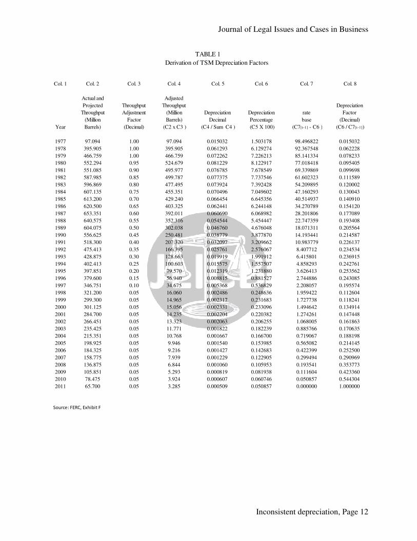
economic life still remains. (FERC) for TSM were based on actual and projected throughput through

depreciation. The UOP factors were adjusted by a throughput adjustment factor end load depreciation even more, as indicated in Table 1 (Appendix). The depreciation

factors were designed to recover all costs by 2011. (In the earlier years of TAPS this was

This was intentionally instituted to accelerate, or front-end load the tariff with a high amount in early years, resulting in a low amount in later years, in order to encourage future

Moreover, it reflected the expected oil flow through TAPS, with high amounts early on and lower amounts later.

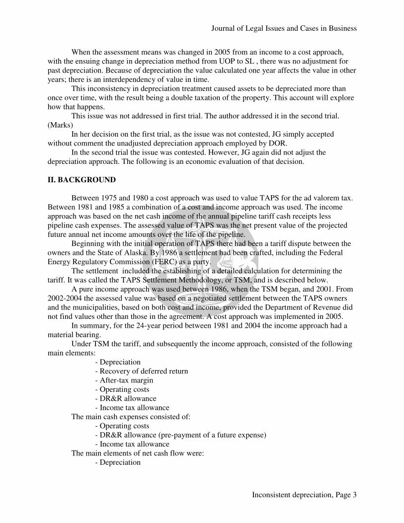
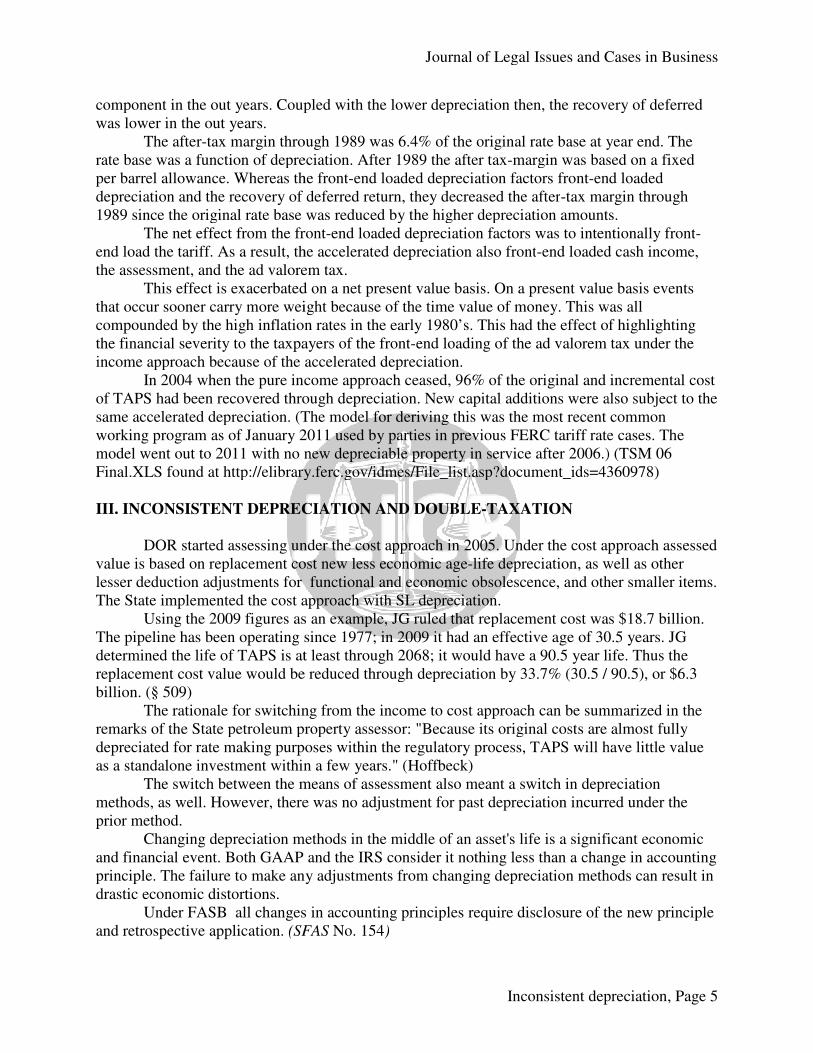
he early higher depreciation caused the tariff to be higher than under SLhe anticipated production profile for TAPS at the time of start-up is indicated in Figure

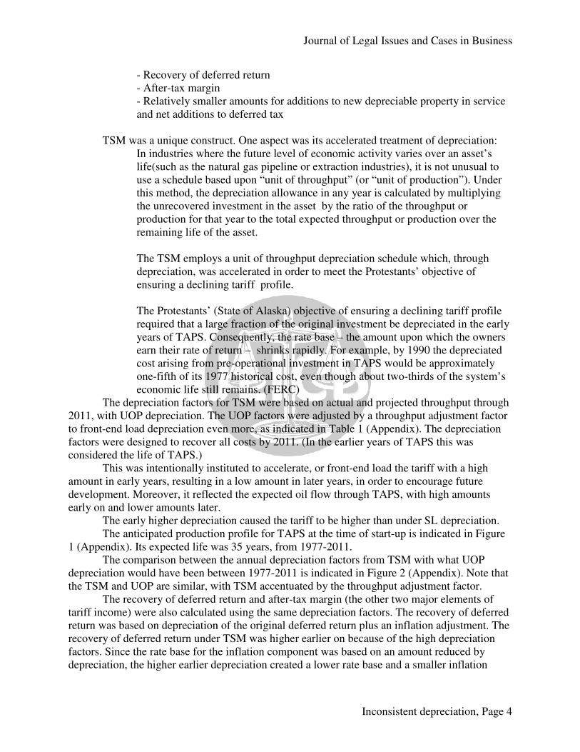
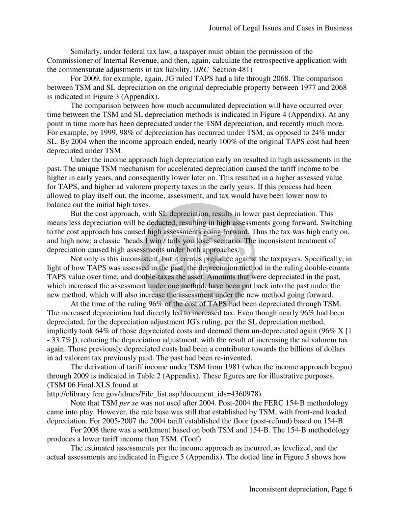
Its expected life was 35 years, from 1977-2011. the annual depreciation factors from TSM with what

depreciation would have been between 1977-2011 is indicated in Figure 2 (Appendix)are similar, with TSM accentuated by the throughput adjustment factor.

The recovery of deferred return and after-tax margin (the other two major elements of tariff income) were also calculated using the same depreciation factors. The recovery of deferred return was based on depreciation of the original deferred return plus an inflation adjustment.recovery of deferred return under TSM was higher earlier on because of the high depreciation

te base for the inflation component was based on an amount reduced by depreciation, the higher earlier depreciation created a lower rate base and a smaller inflation



additions to new depreciable property in service

treatment of depreciation: In industries where the future level of economic activity varies over an asset’s life(such as the natural gas pipeline or extraction industries), it is not unusual to

“unit of production”). Under method, the depreciation allowance in any year is calculated by multiplying

by the ratio of the throughput or production over the

The TSM employs a unit of throughput depreciation schedule which, through depreciation, was accelerated in order to meet the Protestants’ objective of

objective of ensuring a declining tariff profile of the original investment be depreciated in the early

the amount upon which the owners For example, by 1990 the depreciated

operational investment in TAPS would be approximately thirds of the system’s

were based on actual and projected throughput through factors were adjusted by a throughput adjustment factor

The depreciation (In the earlier years of TAPS this was

end load the tariff with a high to encourage future

Moreover, it reflected the expected oil flow through TAPS, with high amounts

SL depreciation. is indicated in Figure

the annual depreciation factors from TSM with what UOP e 2 (Appendix). Note that

are similar, with TSM accentuated by the throughput adjustment factor. tax margin (the other two major elements of

eciation factors. The recovery of deferred return was based on depreciation of the original deferred return plus an inflation adjustment. The recovery of deferred return under TSM was higher earlier on because of the high depreciation

te base for the inflation component was based on an amount reduced by depreciation, the higher earlier depreciation created a lower rate base and a smaller inflation

component in the out years. Coupled with the lower depreciation then, the recovery of defewas lower in the out years. The after-tax margin through 1989 was 6.4% of the original rate base at year end. The rate base was a function of depreciation. After 1989 the after taxper barrel allowance. Whereas the frontdepreciation and the recovery of deferred return, they decreased the after1989 since the original rate base was reduced by the higher depreciation amounts. The net effect from the frontend load the tariff. As a result, the accelerated depreciation also frontthe assessment, and the ad valorem tax. This effect is exacerbatedthat occur sooner carry more weight because of the time value of money. This was all compounded by the high inflation rates in the early 1980’s. the financial severity to the taxpayers of the frontincome approach because of the accelerated depreciation. In 2004 when the pure income approach ceased, of TAPS had been recovered through depreciation.same accelerated depreciation. (The model for deriving this was the most recent common working program as of January 2011 used by parties in previous FERC tariff rate cases. The model went out to 2011 with no new depreciable property in service after 2006.) Final.XLS found at http://elibrary.ferc.gov/idmes/File_list.asp?document_ids=4360978) III. INCONSISTENT DEPRECIATION AND DOUBLE

DOR started assessing under value is based on replacement cost new less lesser deduction adjustments for functional The State implemented the cost approach with Using the 2009 figures as an example, JG ruled that replacement cost was $18.The pipeline has been operating since 1977; in 2009determined the life of TAPS is at least through 20replacement cost value would be reduced through depreciation by billion. (§ 509) The rationale for switching remarks of the State petroleum property assessor:depreciated for rate making purposes within the regulatory process, TAPS will have little value as a standalone investment within a few years. The switch between the means of assessment also meant a switch in depreciation methods, as well. However, there was no adjustment for past depreciation incurred under the prior method. Changing depreciation methods in the middle of an asset's life is a significant economic and financial event. Both GAAP and the IRS consider it nothing less than a change in accounting principle. The failure to make any adjustments from changing depreciatidrastic economic distortions. Under FASB all changes in accounting principles require and retrospective application. (SFAS



component in the out years. Coupled with the lower depreciation then, the recovery of defe

tax margin through 1989 was 6.4% of the original rate base at year end. The rate base was a function of depreciation. After 1989 the after tax-margin was based on a fixed per barrel allowance. Whereas the front-end loaded depreciation factors front-end loaded depreciation and the recovery of deferred return, they decreased the after-tax margin through 1989 since the original rate base was reduced by the higher depreciation amounts.

The net effect from the front-end loaded depreciation factors was to intentionally frontend load the tariff. As a result, the accelerated depreciation also front-end loaded cash income, the assessment, and the ad valorem tax.

This effect is exacerbated on a net present value basis. On a present value basis events that occur sooner carry more weight because of the time value of money. This was all compounded by the high inflation rates in the early 1980’s. This had the effect of highlighting

l severity to the taxpayers of the front-end loading of the ad valorem tax under the income approach because of the accelerated depreciation.

when the pure income approach ceased, 96% of the original and incremental red through depreciation. New capital additions were also subject to the

same accelerated depreciation. (The model for deriving this was the most recent common working program as of January 2011 used by parties in previous FERC tariff rate cases. The

went out to 2011 with no new depreciable property in service after 2006.) Final.XLS found at http://elibrary.ferc.gov/idmes/File_list.asp?document_ids=4360978)

NCONSISTENT DEPRECIATION AND DOUBLE-TAXATION

nder the cost approach in 2005. Under the cost approach assessed based on replacement cost new less economic age-life depreciation, as well as other

lesser deduction adjustments for functional and economic obsolescence, and other smaller items. implemented the cost approach with SL depreciation.

figures as an example, JG ruled that replacement cost was $18.en operating since 1977; in 2009 it had an effective age of 30

determined the life of TAPS is at least through 2068; it would have a 90.5 year life. Thus the replacement cost value would be reduced through depreciation by 33.7% (30.5 /

The rationale for switching from the income to cost approach can be summarized in the remarks of the State petroleum property assessor: "Because its original costs are almost fully depreciated for rate making purposes within the regulatory process, TAPS will have little value

within a few years." (Hoffbeck) he switch between the means of assessment also meant a switch in depreciation

methods, as well. However, there was no adjustment for past depreciation incurred under the

Changing depreciation methods in the middle of an asset's life is a significant economic and financial event. Both GAAP and the IRS consider it nothing less than a change in accounting principle. The failure to make any adjustments from changing depreciation methods

all changes in accounting principles require disclosure of the new principle FAS No. 154)



component in the out years. Coupled with the lower depreciation then, the recovery of deferred

tax margin through 1989 was 6.4% of the original rate base at year end. The margin was based on a fixed

end loaded tax margin through

1989 since the original rate base was reduced by the higher depreciation amounts. end loaded depreciation factors was to intentionally front-

end loaded cash income,

on a net present value basis. On a present value basis events that occur sooner carry more weight because of the time value of money. This was all

his had the effect of highlighting end loading of the ad valorem tax under the

original and incremental cost New capital additions were also subject to the

same accelerated depreciation. (The model for deriving this was the most recent common working program as of January 2011 used by parties in previous FERC tariff rate cases. The

went out to 2011 with no new depreciable property in service after 2006.) (TSM 06 Final.XLS found at http://elibrary.ferc.gov/idmes/File_list.asp?document_ids=4360978)

Under the cost approach assessed depreciation, as well as other

economic obsolescence, and other smaller items.

figures as an example, JG ruled that replacement cost was $18.7 billion. 30.5 years. JG

.5 year life. Thus the / 90.5), or $6.3

can be summarized in the Because its original costs are almost fully

depreciated for rate making purposes within the regulatory process, TAPS will have little value

he switch between the means of assessment also meant a switch in depreciation methods, as well. However, there was no adjustment for past depreciation incurred under the

Changing depreciation methods in the middle of an asset's life is a significant economic and financial event. Both GAAP and the IRS consider it nothing less than a change in accounting

on methods can result in

disclosure of the new principle

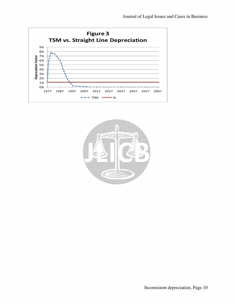
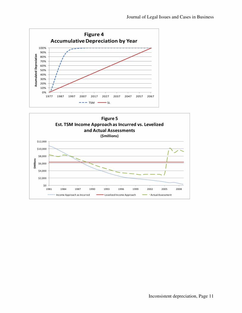
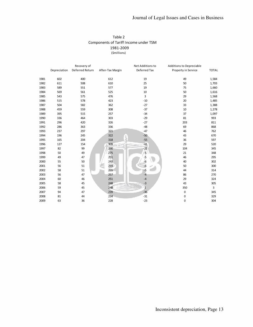
Similarly, under federal tax law, a taxpayer must obtain the permission of the Commissioner of Internal Revenue, and then, again, calculate the retrospective application with the commensurate adjustments in tax liability. For 2009, for example, again, between TSM and SL depreciation is indicated in Figure 3 (Appendix) The comparison between time between the TSM and SL depreciation methodspoint in time more has been depreciated under the TSM depreciationFor example, by 1999, 98% of depreciation has occurred under TSMSL. By 2004 when the income approach ended, nearly 100% ofdepreciated under TSM. Under the income approach high depreciation past. The unique TSM mechanism for accelerated depreciation caused the tariff income to be higher in early years, and consequently lower later on. This resulted in a higher assessed value for TAPS, and higher ad valorem property taxes in the early years. If this process had been allowed to play itself out, the income, assessment, and tax would have been lower now to balance out the initial high taxes. But the cost approach, with means less depreciation will be deductedto the cost approach has caused high assessments going forward. Thus the tax was high early on, and high now: a classic "heads I windepreciation caused high assessments under both approaches. Not only is this inconsistent, but it creates prejudice against the taxpayers. Specifically, in light of how TAPS was assessed in the past, the depreciation method in the ruling doubleTAPS value over time, and doublewhich increased the assessment under one method, have been put back into the past under the new method, which will also increase the assessment under the new method going forward. At the time of the ruling 96The increased depreciation had directly led to increased tax. Even though depreciated, for the depreciation implicitly took 64% of those dep- 33.7%]), reducing the depreciationagain. Those previously depreciated costs had been a contributor towards the billions of dollarsin ad valorem tax previously paid. The derivation of tariff income through 2009 is indicated in Table 2 (Appendix)(TSM 06 Final.XLS found at http://elibrary.ferc.gov/idmes/File_list.asp?document_ids=4360978) Note that TSM per se was not used after 2004. Postcame into play. However, the rate base was still that established by TSM, with frontdepreciation. For 2005-2007 the 2004 tariff established the floor (post For 2008 there was a settlement based on both TSM and 154produces a lower tariff income than TSM. The estimated assessments per the income approach as incurred, as levelized, and the actual assessments are indicated in Figure 5 (Appendix).



Similarly, under federal tax law, a taxpayer must obtain the permission of the Revenue, and then, again, calculate the retrospective application with

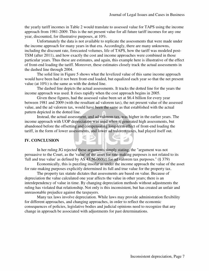
commensurate adjustments in tax liability. (IRC Section 481) again, JG ruled TAPS had a life through 2068. The

depreciation on the original depreciable property between 1977 and is indicated in Figure 3 (Appendix).

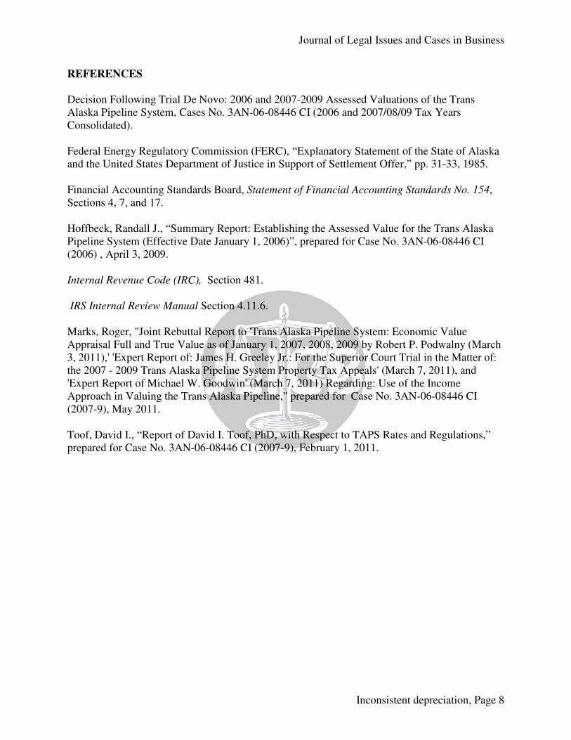
how much accumulated depreciation will have occurred over depreciation methods is indicated in Figure 4 (Appendix).

point in time more has been depreciated under the TSM depreciation, and recently% of depreciation has occurred under TSM, as opposed to

2004 when the income approach ended, nearly 100% of the original TAPS

Under the income approach high depreciation early on resulted in high assessmentsThe unique TSM mechanism for accelerated depreciation caused the tariff income to be

higher in early years, and consequently lower later on. This resulted in a higher assessed value valorem property taxes in the early years. If this process had been

allowed to play itself out, the income, assessment, and tax would have been lower now to balance out the initial high taxes.

But the cost approach, with SL depreciation, results in lower past depreciation. This means less depreciation will be deducted, resulting in high assessments going forward. to the cost approach has caused high assessments going forward. Thus the tax was high early on,

: a classic "heads I win / tails you lose" scenario. The inconsistent treatment of high assessments under both approaches.

Not only is this inconsistent, but it creates prejudice against the taxpayers. Specifically, in light of how TAPS was assessed in the past, the depreciation method in the ruling double

, and double-taxes the asset. Amounts that were depreciated in the past, which increased the assessment under one method, have been put back into the past under the new method, which will also increase the assessment under the new method going forward.

96% of the cost of TAPS had been depreciated through TSM. The increased depreciation had directly led to increased tax. Even though nearly

depreciation adjustment JG's ruling, per the SL depreciation method, % of those depreciated costs and deemed them un-depreciated again

depreciation adjustment, with the result of increasing the ad valorem tax again. Those previously depreciated costs had been a contributor towards the billions of dollarsin ad valorem tax previously paid. The past had been re-invented.

he derivation of tariff income under TSM from 1981 (when the income approach began) is indicated in Table 2 (Appendix). These figures are for illustrative purposes.

http://elibrary.ferc.gov/idmes/File_list.asp?document_ids=4360978) was not used after 2004. Post-2004 the FERC 154-

came into play. However, the rate base was still that established by TSM, with front2007 the 2004 tariff established the floor (post-refund) based on 154

For 2008 there was a settlement based on both TSM and 154-B. The 154-produces a lower tariff income than TSM. (Toof)

The estimated assessments per the income approach as incurred, as levelized, and the actual assessments are indicated in Figure 5 (Appendix). The dotted line in Figure 5 shows how



Similarly, under federal tax law, a taxpayer must obtain the permission of the Revenue, and then, again, calculate the retrospective application with

The comparison between 1977 and 2068

will have occurred over is indicated in Figure 4 (Appendix). At any

recently much more. , as opposed to 24% under

TAPS cost had been

resulted in high assessments in the The unique TSM mechanism for accelerated depreciation caused the tariff income to be

higher in early years, and consequently lower later on. This resulted in a higher assessed value valorem property taxes in the early years. If this process had been

allowed to play itself out, the income, assessment, and tax would have been lower now to

past depreciation. This resulting in high assessments going forward. Switching

to the cost approach has caused high assessments going forward. Thus the tax was high early on, The inconsistent treatment of

Not only is this inconsistent, but it creates prejudice against the taxpayers. Specifically, in light of how TAPS was assessed in the past, the depreciation method in the ruling double-counts

ere depreciated in the past, which increased the assessment under one method, have been put back into the past under the new method, which will also increase the assessment under the new method going forward.

TAPS had been depreciated through TSM. nearly 96% had been

depreciation method, depreciated again (96% X [1

adjustment, with the result of increasing the ad valorem tax again. Those previously depreciated costs had been a contributor towards the billions of dollars

(when the income approach began) These figures are for illustrative purposes.

-B methodology came into play. However, the rate base was still that established by TSM, with front-end loaded

refund) based on 154-B. -B methodology

The estimated assessments per the income approach as incurred, as levelized, and the The dotted line in Figure 5 shows how

the yearly tariff incomes in Table approach from 1981-2009. This is the net present value for all future tariff incomes for any one year, discounted, for illustrative purposes, at 10%. Unfortunately the data is not available to replicate the assessments that were mathe income approach for many years in that era. Accordingly, there are many unknowns, including the discount rate, forecasted volumes, life of TAPS, how the tariff was modeled postTSM (after 2011), and how exactly the cost and income approaches wparticular years. Thus these are estimates, and again, this example here is illustrative of the effect of front-end loading the tariff. Moreover, these estimates closely track the actual assessments in the dashed line through 2004. The solid line in Figure 5 shows what the levelized value of this same income approach would have been had it not been frontvalue (at 10%) is the same as with the dotted line. The dashed line depicts the actual assessments. It tracks the dotted line for the years the income approach was used. It rises rapidly when the cost approach begins in 2005. Given these figures, had the assessed value been set at $6.4 billion for every year between 1981 and 2009 (with the resultant ad valorem tax), the net present value of the assessed value, and the ad valorem tax, would have been the same as that established with the actual pattern depicted in the dotted line. Instead, the actual assessment, and income approach with UOP depreciation abandoned before the offsetting and compensating tariff, in the form of lower assessments, and lower ad valorem taxes,

IV. CONCLUSION

In her ruling JG rejected these persuasive to the Court, as the 'value'full and true value' as defined by AS 43.56.060(e) for ad valorem tax purposes. Economically, this is puzzling insofar as under the income for rate-making purposes explicitly determined its full and true value for the property tax. The property tax statute dictates that depreciation the value calculated one year affects the value in other years; there interdependency of value in time. By changing depreciation methodsruling has violated that relationship.unreasonable prejudice against the taxpayers. Many tax laws involve depreciation. While laws may provide administration flexibility for different approaches, and changing consequences of policies, legislative bodies and judicial opinions need to recognize that anychange in approach be associated with adjustments for past determinations.



the yearly tariff incomes in Table 2 would translate to assessed value for TAPS using the income 2009. This is the net present value for all future tariff incomes for any one

year, discounted, for illustrative purposes, at 10%. Unfortunately the data is not available to replicate the assessments that were ma

the income approach for many years in that era. Accordingly, there are many unknowns, including the discount rate, forecasted volumes, life of TAPS, how the tariff was modeled postTSM (after 2011), and how exactly the cost and income approaches were combined in those particular years. Thus these are estimates, and again, this example here is illustrative of the effect

end loading the tariff. Moreover, these estimates closely track the actual assessments in

The solid line in Figure 5 shows what the levelized value of this same income approach would have been had it not been front-end loaded, but equalized each year so that the net present value (at 10%) is the same as with the dotted line.

depicts the actual assessments. It tracks the dotted line for the years the income approach was used. It rises rapidly when the cost approach begins in 2005.

Given these figures, had the assessed value been set at $6.4 billion for every year 1 and 2009 (with the resultant ad valorem tax), the net present value of the assessed

value, and the ad valorem tax, would have been the same as that established with the actual pattern depicted in the dotted line.

Instead, the actual assessment, and ad valorem tax, was higher in the earlier yearswith UOP depreciation was used when it generated high assess

offsetting and compensating long-term effect of front-end loadinglower assessments, and lower ad valorem taxes, had played itself out.

these arguments simply stating, the "argument was not value' of the asset for rate-making purposes is not related to its

defined by AS 43.56.060(e) for ad valorem tax purposes."his is puzzling insofar as under the income approach the value of the asset

making purposes explicitly determined its full and true value for the property tax.The property tax statute dictates that assessments are based on value. Because of

depreciation the value calculated one year affects the value in other years; there is an interdependency of value in time. By changing depreciation methods without adjustmentsruling has violated that relationship. Not only is this inconsistent, but has created an unfair and unreasonable prejudice against the taxpayers.

x laws involve depreciation. While laws may provide administration flexibility different approaches, and changing approaches, in order to reflect the economic

consequences of policies, legislative bodies and judicial opinions need to recognize that anychange in approach be associated with adjustments for past determinations.



APS using the income 2009. This is the net present value for all future tariff incomes for any one

Unfortunately the data is not available to replicate the assessments that were made under the income approach for many years in that era. Accordingly, there are many unknowns, including the discount rate, forecasted volumes, life of TAPS, how the tariff was modeled post-

ere combined in those particular years. Thus these are estimates, and again, this example here is illustrative of the effect

end loading the tariff. Moreover, these estimates closely track the actual assessments in

The solid line in Figure 5 shows what the levelized value of this same income approach end loaded, but equalized each year so that the net present

depicts the actual assessments. It tracks the dotted line for the years the income approach was used. It rises rapidly when the cost approach begins in 2005.

Given these figures, had the assessed value been set at $6.4 billion for every year 1 and 2009 (with the resultant ad valorem tax), the net present value of the assessed

value, and the ad valorem tax, would have been the same as that established with the actual

ad valorem tax, was higher in the earlier years. The was used when it generated high assessments, but

end loading the had played itself out.

argument was not making purposes is not related to its

" (§ 379) the value of the asset

making purposes explicitly determined its full and true value for the property tax. assessments are based on value. Because of

is an without adjustments the

Not only is this inconsistent, but has created an unfair and

x laws involve depreciation. While laws may provide administration flexibility approaches, in order to reflect the economic

consequences of policies, legislative bodies and judicial opinions need to recognize that any

REFERENCES

Decision Following Trial De Novo: 2006 and 2007Alaska Pipeline System, Cases No. 3ANConsolidated). Federal Energy Regulatory Commission (FERC), “Explanatory Statement of the State of Alaska and the United States Department of Justice in Support of Settlement Offer,” pp. 31 Financial Accounting Standards Board, Sections 4, 7, and 17. Hoffbeck, Randall J., “Summary Report: Establishing the Assessed Value for the Trans Alaska Pipeline System (Effective Date January 1, 2006)”, prepared for Case No. 3AN(2006) , April 3, 2009. Internal Revenue Code (IRC), Section 481. IRS Internal Review Manual Section Marks, Roger, "Joint Rebuttal Report to 'Trans Alaska Pipeline System: Economic Value Appraisal Full and True Value as of January 1, 2007, 2008, 2009 b3, 2011),' 'Expert Report of: James H. Greeley Jr.: For the Superior Court Trial in the Matter of: the 2007 - 2009 Trans Alaska Pipeline System Property Tax Appeals' (March 7, 2011), and 'Expert Report of Michael W. Goodwin' (MaApproach in Valuing the Trans Alaska Pipeline," prepared for Case No. 3AN(2007-9), May 2011. Toof, David I., “Report of David I. Toof, PhD, with Respect to TAPS Rates and Regulations,” prepared for Case No. 3AN-06-08446 CI (2007



Decision Following Trial De Novo: 2006 and 2007-2009 Assessed Valuations of the Trans Alaska Pipeline System, Cases No. 3AN-06-08446 CI (2006 and 2007/08/09 Tax Yea

Federal Energy Regulatory Commission (FERC), “Explanatory Statement of the State of Alaska and the United States Department of Justice in Support of Settlement Offer,” pp. 31

Financial Accounting Standards Board, Statement of Financial Accounting Standards No.

Hoffbeck, Randall J., “Summary Report: Establishing the Assessed Value for the Trans Alaska Pipeline System (Effective Date January 1, 2006)”, prepared for Case No. 3AN-06

Section 481.

Section 4.11.6.

Marks, Roger, "Joint Rebuttal Report to 'Trans Alaska Pipeline System: Economic Value Appraisal Full and True Value as of January 1, 2007, 2008, 2009 by Robert P. Podwalny (March 3, 2011),' 'Expert Report of: James H. Greeley Jr.: For the Superior Court Trial in the Matter of:

2009 Trans Alaska Pipeline System Property Tax Appeals' (March 7, 2011), and 'Expert Report of Michael W. Goodwin' (March 7, 2011) Regarding: Use of the Income Approach in Valuing the Trans Alaska Pipeline," prepared for Case No. 3AN-06

Toof, David I., “Report of David I. Toof, PhD, with Respect to TAPS Rates and Regulations,” 08446 CI (2007-9), February 1, 2011.



2009 Assessed Valuations of the Trans 08446 CI (2006 and 2007/08/09 Tax Years

Federal Energy Regulatory Commission (FERC), “Explanatory Statement of the State of Alaska and the United States Department of Justice in Support of Settlement Offer,” pp. 31-33, 1985.

g Standards No. 154,

Hoffbeck, Randall J., “Summary Report: Establishing the Assessed Value for the Trans Alaska 06-08446 CI

Marks, Roger, "Joint Rebuttal Report to 'Trans Alaska Pipeline System: Economic Value y Robert P. Podwalny (March

3, 2011),' 'Expert Report of: James H. Greeley Jr.: For the Superior Court Trial in the Matter of: 2009 Trans Alaska Pipeline System Property Tax Appeals' (March 7, 2011), and

rch 7, 2011) Regarding: Use of the Income 06-08446 CI

Toof, David I., “Report of David I. Toof, PhD, with Respect to TAPS Rates and Regulations,”

APPENDIX

0.0

0.5

1.0

1.5

2.0

1977 1980 1983 1986 1989

Mill

ions

of

Barr

els

per D

ay

Anticipated TAPS Production Profile at Start(Millions of Barrels per Day)

Source: FERC, Appendix 5

0%

1%

2%

3%

4%

5%

6%

7%

8%

9%

1977 1980 1983 1986 1989

Dep

reci

atio

n Fa

ctor

TSM vs. Units-of

Source: FERC, Exhibit F



1989 1992 1995 1998 2001 2004 2007 2010

Figure 1

Anticipated TAPS Production Profile at Start-Up(Millions of Barrels per Day)

1989 1992 1995 1998 2001 2004 2007 2010

Figure 2

of-Production Depreciation

TSM UOP



0%

1%

2%

3%

4%

5%

6%

7%

8%

9%

1977 1987 1997 2007

Dep

reci

atio

n Fa

ctor

Figure 3

TSM vs. Straight Line Depreciation



2007 2017 2027 2037 2047 2057 2067

Figure 3

TSM vs. Straight Line Depreciation

TSM SL



0%

10%

20%

30%

40%

50%

60%

70%

80%

90%

100%

1977 1987 1997 2007

Acc

um

ula

ted

De

pre

ciat

ion

Figure 4

Accumulative Depreciation by Year

TSM

$0

$2,000

$4,000

$6,000

$8,000

$10,000

$12,000

1981 1984 1987 1990

$M

illio

ns

Est. TSM Income Approach as Incurred vs. Levelized

and Actual Assessments

Income Approach as Incurred



2017 2027 2037 2047 2057 2067

Figure 4

Accumulative Depreciation by Year

TSM SL

1990 1993 1996 1999 2002 2005 2008

Figure 5

Est. TSM Income Approach as Incurred vs. Levelized

and Actual Assessments($millions)

Levelized Income Approach Actual Assessment



2008

Derivation of TSM Depreciation Factors

Col. 1 Col. 2 Col. 3

Actual and

Projected Throughput

Throughput Adjustment

(Million Factor

Year Barrels) (Decimal)

1977 97.094 1.00

1978 395.905 1.00

1979 466.759 1.00

1980 552.294 0.95

1981 551.085 0.90

1982 587.985 0.85

1983 596.869 0.80

1984 607.135 0.75

1985 613.200 0.70

1986 620.500 0.65

1987 653.351 0.60

1988 640.575 0.55

1989 604.075 0.50

1990 556.625 0.45

1991 518.300 0.40

1992 475.413 0.35

1993 428.875 0.30

1994 402.413 0.25

1995 397.851 0.20

1996 379.600 0.15

1997 346.751 0.10

1998 321.200 0.05

1999 299.300 0.05

2000 301.125 0.05

2001 284.700 0.05

2002 266.451 0.05

2003 235.425 0.05

2004 215.351 0.05

2005 198.925 0.05

2006 184.325 0.05

2007 158.775 0.05

2008 136.875 0.05

2009 105.851 0.05

2010 78.475 0.05

2011 65.700 0.05

Source: FERC, Exhibit F



TABLE 1

Derivation of TSM Depreciation Factors

Col. 4 Col. 5 Col. 6 Col. 7

Adjusted

Throughput

(Million Depreciation Depreciation rate

Barrels) Decimal Percentage base

(C2 x C3 ) (C4 / Sum C4 ) (C5 X 100) (C7[t-1] - C6 )

97.094 0.015032 1.503178 98.496822

395.905 0.061293 6.129274 92.367548

466.759 0.072262 7.226213 85.141334

524.679 0.081229 8.122917 77.018418

495.977 0.076785 7.678549 69.339869

499.787 0.077375 7.737546 61.602323

477.495 0.073924 7.392428 54.209895

455.351 0.070496 7.049602 47.160293

429.240 0.066454 6.645356 40.514937

403.325 0.062441 6.244148 34.270789

392.011 0.060690 6.068982 28.201806

352.316 0.054544 5.454447 22.747359

302.038 0.046760 4.676048 18.071311

250.481 0.038779 3.877870 14.193441

207.320 0.032097 3.209662 10.983779

166.395 0.025761 2.576067 8.407712

128.663 0.019919 1.991912 6.415801

100.603 0.015575 1.557507 4.858293

79.570 0.012319 1.231880 3.626413

56.940 0.008815 0.881527 2.744886

34.675 0.005368 0.536829 2.208057

16.060 0.002486 0.248636 1.959422

14.965 0.002317 0.231683 1.727738

15.056 0.002331 0.233096 1.494642

14.235 0.002204 0.220382 1.274261

13.323 0.002063 0.206255 1.068005

11.771 0.001822 0.182239 0.885766

10.768 0.001667 0.166700 0.719067

9.946 0.001540 0.153985 0.565082

9.216 0.001427 0.142683 0.422399

7.939 0.001229 0.122905 0.299494

6.844 0.001060 0.105953 0.193541

5.293 0.000819 0.081938 0.111604

3.924 0.000607 0.060746 0.050857

3.285 0.000509 0.050857 0.000000



Col. 7 Col. 8

Depreciation

Factor

(Decimal)

- C6 ) (C6 / C7[t-1])

98.496822 0.015032

92.367548 0.062228

85.141334 0.078233

77.018418 0.095405

69.339869 0.099698

61.602323 0.111589

54.209895 0.120002

47.160293 0.130043

40.514937 0.140910

34.270789 0.154120

28.201806 0.177089

22.747359 0.193408

18.071311 0.205564

14.193441 0.214587

10.983779 0.226137

8.407712 0.234534

6.415801 0.236915

4.858293 0.242761

3.626413 0.253562

2.744886 0.243085

2.208057 0.195574

1.959422 0.112604

1.727738 0.118241

1.494642 0.134914

1.274261 0.147448

1.068005 0.161863

0.885766 0.170635

0.719067 0.188198

0.565082 0.214145

0.422399 0.252500

0.299494 0.290969

0.193541 0.353773

0.111604 0.423360

0.050857 0.544304

0.000000 1.000000

Components of Tariff Income under TSM

Recovery of

Depreciation Deferred Return

1981 602 400

1982 611 508

1983 589 551

1984 569 561

1985 543 575

1986 515 578

1987 504 582

1988 459 559

1989 395 515

1990 336 464

1991 296 420

1992 286 363

1993 237 297

1994 196 245

1995 165 204

1996 127 154

1997 82 99

1998 50 49

1999 49 47

2000 55 50

2001 56 51

2002 58 51

2003 56 47

2004 60 46

2005 58 45

2006 59 45

2007 94 47

2008 81 44

2009 63 36



Table 2

Components of Tariff Income under TSM

1981-2009 ($millions)

Net Additions to Additions to Depreciable

After-Tax Margin Deferred Tax Property in Service

612 19 49

610 25 50

577 19 75

525 10 50

476 3 29

423 -10 20

362 -27 33

308 -37 10

257 -34 37

303 -29 81

326 -27 203

336 -48 69

321 -47 46

322 -50 43

318 -55 36

309 -41 29

290 -21 104

275 -5 21

251 -5 46

243 -6 40

249 -6 50

255 -5 44

257 -4 86

251 -4 29

248 -3 43

248 1 350

239 -36 0

234 -31 0

228 -23 0



Additions to Depreciable

Property in Service TOTAL

1,584

1,703

1,660

1,616

1,568

1,485

1,388

1,278

1,097

993

811

868

762

670

597

520

345

348

295

302

300

314

270

324

305

3

345

329

304

Documents

Inconsistent depreciation and double-taxation: the Trans