Incompressible MHD simulations - Ilmatieteen laitosspace.fmi.fi/graduateschool/Lectures10/vortrag.pdfIncompressible MHD simulations Felix Spanier 1 Lehrstuhl für Astronomie Universität

Incompressible MHD simulations

Felix Spanier 1

Lehrstuhl für AstronomieUniversität Würzburg

Simulation methods in astrophysics

Felix Spanier (Uni Würzburg) Simulation methods in astrophysics 1 / 20

Outline

Where do we need incompressible MHD?Theory of HD&MHDTurbulenceNumerical methods for HDNumerical methods for MHD


Heliosphere

Closest available space plasma:The solar wind

includes shocksand density fluctuation

The large scale evolution seems tobe compressible. . .


Heliosphere

. . . but in the frame of the solar wind,we find

a turbulent spectrumAlfvén waves travelling

Sounds like incompressibleturbulence!


Interstellar medium

Infamous picturethis is usually used to suggestturbulenceit really shows densityfluctuationsDensity fluctuations? That’scompressible turbulence?Really?


Interstellar medium

Damping rates

1e-30

1e-25

1e-20

1e-15

1e-10

1e-05

1

1e-17 1e-16 1e-15 1e-14 1e-13 1e-12 1e-11 1e-10 1e-09 1e-08 1e-07 1e-06

ViskosJouleLandauNeutral

-3-1

ge

/ e

r c

ms

-1k / cm

Alfvén wave damping

1e-30

1e-25

1e-20

1e-15

1e-10

1e-05

1

100000

1e+10

1e-17 1e-16 1e-15 1e-14 1e-13 1e-12 1e-11 1e-10 1e-09 1e-08 1e-07 1e-06

ViskosJoule

Neutral

-3-1

e/

g c

ms

e

r-1k / cm

Sound wave damping


Interstellar medium

So is this incompressible MHD?Wave damping suggests that for large k only Alfvén waves surviveDensity fluctuations suggest there is compressible turbulenceTwo solutions:Alfvén turbulence with enslaved density fluctuationsNot waves but shocks govern the ISM


Euler EquationForce on a volume element of fluid

F = −∮

p df (1)

Divergence theorem

F = −∫∇p dV (2)

Newton’s law for one volume element

mdudt

= F (3)

Using density instead of total mass∫ρ

dudt

dV = −∫∇p dV (4)

ρdudt

= −∇p (5)

⇒ Lagrange picture


Euler EquationChanging to material derivative

du =∂u∂t

dt + (dr∇)u (1)

⇒ dudt

=∂u∂t

+ (u∇)u (2)

Euler’s equation∂u∂t

+ (u∇)u = −1ρ∇p (3)

Here the velocity is a function of space and time

u = u(r , t) (4)

This can now be applied to the momentum transport equation

∂

∂t(ρui ) = ρ

∂ui

∂t+ ui

∂ρ

∂t(5)


Euler Equation

Partial derivative of u is known from Euler

∂ui

∂t= −uk

∂ui

∂xk− 1ρ

∂p∂xi

(1)

⇒ ∂

∂t(ρui ) = −ρuk

∂ui

∂xk− ∂p∂xi− ui

∂ρuk

∂xk(2)

= − ∂p∂xi− ∂

∂xk(ρuiuk ) (3)

= −δik∂p∂xk− ∂

∂xk(ρuiuk ) (4)

∂ρui

∂t= − ∂

∂xkΠik (5)

Πik = −pδik − ρuiuk (6)

Πik = stress tensor


Continuity equation

∂

∂t

∫ρ dV = −

∮ρu dV (7)∫ (

∂ρ

∂t+∇·(ρu)

)dV = 0 (8)

∂ρ

∂t+∇·(ρu) = 0 (9)

For incompressible fluids (ρ=const)

∇·u = 0 (10)


Viscid fluid

Πik = pδik + ρuiuk − σik (11)

σik = shear stressFor Newtonian fluids this depends on derivatives of the velocity

σik = a∂ui

∂xk+ b

∂uk

∂xi+ c

∂ul

∂xlδik (12)

Coefficients have to fulfillno viscosity in uniform fluids(u=const)no viscosity in uniform rotating floew

It follows a = b

σik = η

(∂ui

∂xk+∂uk

∂xi− 2

3δik∂ul

∂xl

)+ ζδik

∂ul

∂xl(13)


Viscid fluid

Stress tensor for incompressible fluids

∂ui

∂xi= 0 (11)

⇒ σik = η

(∂ui

∂xk+∂uk

∂xi

)(12)

∂σik

∂xk= η

∂2ui

∂x2k

(13)

And we find the Navier-Stokes-equation :

∂u∂t

+ (u∇)u +∇p = ν∆u (14)

ν = ηρ = Viscosity

Pressure∆p = −(u∇)u + ν∆u (15)


Vorticity

Using ∇·u = 0 one can take the curl of the Navier-Stokes-equation ,resulting in a PDE for ω = ∇×u

∂

∂t(∇×u)−∇× (u × (∇×u)) = −ν∇× (∇× (∇×u)) (16)

⇒ ∂ω

∂t= (ω∇)u + ν∆ω (17)

ω is quasi-scalar for 2d-velocitiesWe need the stream function Ψ to derive velocities

ω = ∇×u (18)u = ∇×Ψ (19)

∆Ψ = −ω (20)


The MHD equations

Compressible MHD

∂ρ

∂t+∇ · (ρv) = 0

ρ∂v∂t

+ ρ(v · ∇)v = −∇p − 14π

B ×∇× B

∂B∂t

= ∇× (v × B)

SolutionsDifferent wave modes are solutions to the MHD equations

Alfvén modes (incompressible, aligned to the magnetic field)Fast magnetosonic (compressible)slow magnetosonic (compressible)


The MHD equations

Incompressible MHD

∇ · v = 0

ρ∂v∂t

+ ρ(v · ∇)v = −∇p − 14π

B ×∇× B

∂B∂t

= ∇× (v × B)


Alfvén modes (incompressible, aligned to the magnetic field)


The MHD equations

Elsasser variables

w− = v + b − vAez

w+ = v − b + vAez

⇒ v =w+ + w−

2

⇒ b =−w+ + w− − 2vAez

2


Alfvén modes (incompressible, aligned to the magnetic field)w± correspond to forward/backward moving waves


Short review of Kolmogorov

Kolmogorov assumes energy transport which is scale invariantTime-scale depends on eddy-turnover timesDetailed analysis of the units reveals 5/3-law

Simplified picture – but enough to illustrate what we are doing next

0.001

0.01

0.1

1

1 10 100 1000

Inertial-

k

E(k)

Production-

range range

Dissipation-range


Short review of Kolmogorov

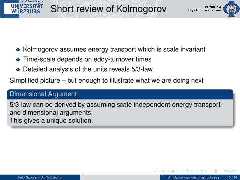
Kolmogorov assumes energy transport which is scale invariantTime-scale depends on eddy-turnover timesDetailed analysis of the units reveals 5/3-law

Simplified picture – but enough to illustrate what we are doing next

Dimensional Argument

5/3-law can be derived by assuming scale independent energy transportand dimensional arguments.This gives a unique solution.


Kraichnan-Iroshnikov

General idea: Turbulence is governed by Alfvén wavesCollision of Alfvén waves is mechanism of choiceEddy-turnover time is then replaced by Alfvén time scale



Energy E =∫

(V 2 + B2)dx is conservedCascading to smaller energiesDimensional arguments cannot be used to derive τλ = λ/vλDimensionless factor vλ/vA can enter


Kraichnan-IroshnikovWave-packet interaction

w− = v + b − vAez

w+ = v − b + vAez

Solutions: w± = f (r ∓ vAt)

Figure: Packets interact, energy is conserved, shape is not



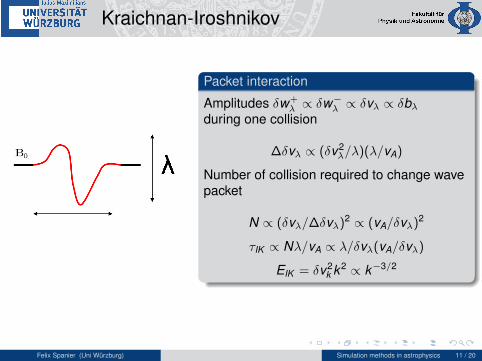
Packet interaction

Amplitudes δw+λ ∝ δw

−λ ∝ δvλ ∝ δbλ

during one collision

∆δvλ ∝ (δv2λ/λ)(λ/vA)

Number of collision required to change wavepacket

N ∝ (δvλ/∆δvλ)2 ∝ (vA/δvλ)2

τIK ∝ Nλ/vA ∝ λ/δvλ(vA/δvλ)

EIK = δv2k k2 ∝ k−3/2


Goldreich-Sridhar

3/2 spectrum not that often observeLet’s get a new theoryWe come back to Kraichnan-Iroshnikov: Alfvén waves govern thespectrumTurbulent energy is transported through multi-wave interactionGoldreich and Sridhar made up a number of articles dealing with thisproblemThey distinguish between strong and weak turbulence


Goldreich-Sridhar

Weak Turbulence

What is weak turbulence?Weak turbulence describes systems, where waves propagate if oneneglects non-linearities. If one includes non-linearities wave amplitude willchange slowly over many wave periods.The non-linearity is derived pertubatevily from the interaction of severalwaves


Goldreich-Sridhar

Weak TurbulenceGoldreich-Sridhar claim that Kraichnan-Iroshnikov can be seen asthree-wave interaction of Alfvén wavesThey also believe, this is a forbidden process, since resonancecondition reads

kz1 + kz2 = kz

| kz1 | + | kz2 | = | kz |

4-wave coupling is now their choice!


Goldreich-Sridhar

Weak Turbulence

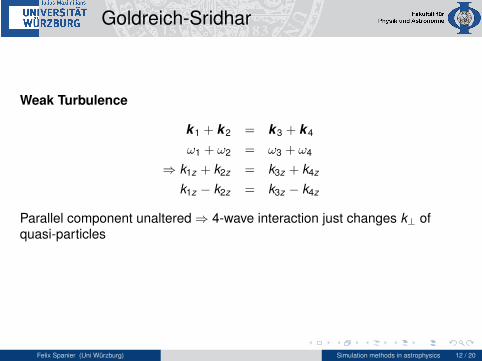
k1 + k2 = k3 + k4

ω1 + ω2 = ω3 + ω4

⇒ k1z + k2z = k3z + k4z

k1z − k2z = k3z − k4z

Parallel component unaltered⇒ 4-wave interaction just changes k⊥ ofquasi-particles


Goldreich-Sridhar

Weak Turbulence

| δvλ |∼∣∣∣∣d2vλ

dt2 (kzvA)−2∣∣∣∣

d2vλdt2 ∼

ddt

(k⊥v2λ) ∼ k⊥vλ

dvλdt∼ k2⊥v3

λ

since (v · ∇) ∼ vλk⊥ for Alfvén waves∣∣∣∣δvλvλ

∣∣∣∣ ∼ (k⊥v⊥kzvλ

)2

⇒ N ∼(

k⊥v⊥kzvλ

)4

∑v2λ =

∫E(kz , k⊥)d3k

constant rate of cascade⇒ E(kz , k⊥) ∼ ε(kz)vak−10/3⊥

This spectrum now hold, when the velocity change is small


Goldreich-Sridhar

Strong TurbulenceAssume perturbation vλ on scales λ‖ ∼ k−1

z and λ⊥ ∼ k−1⊥

ζλ ∼k⊥vλkzvλ

Anisotropy parameter

N ∼ ζ−4λ

isotropic excitationk⊥∼kz∼L−1

∼(

vA

vL

)4

(k⊥L)−4/3

Everything is fine as long as ζλ � 1GS assume frequency renormalization when this is not given


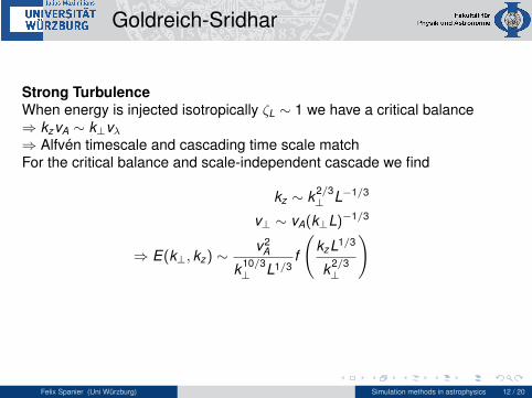
Goldreich-Sridhar

Strong TurbulenceWhen energy is injected isotropically ζL ∼ 1 we have a critical balance⇒ kzvA ∼ k⊥vλ⇒ Alfvén timescale and cascading time scale matchFor the critical balance and scale-independent cascade we find

kz ∼ k2/3⊥ L−1/3

v⊥ ∼ vA(k⊥L)−1/3

⇒ E(k⊥, kz) ∼v2

A

k10/3⊥ L1/3

f

(kzL1/3

k2/3⊥

)


Goldreich-SridharStrong Turbulence

Consequences

A cutoff scaleexistsEddies areelongated

Figure: From Cho, Lazarian, Vishniac (2003)


Turbulence Conclusion

There is a number of turbulence models out thereIt is not yet clear which is correctAll analytical turbulence models are incompressibleThe only thing we know for sure is that there is power law in thespectral energy distribution


Numerical methods

Methods for the Navier-Stokes-equation

Projection solve compressible equations, project on incompressible partVorticity use vector potential to always fulfill divergence-free conditionSpectral use Fourier space to do the same as above

Methods are presented for the Navier-Stokes-equation but also apply toMHDSpectral methods will be presented for Elsässer variables in detail


Projection method

Different possible schemesHere a scheme proposed by [1].

Step 1: Intermediate Solution

We are looking for a solution u∗, which is not yet divergence free

u∗ − un

∆t= − ((u∇)u)n+1/2 −∇pn−1/2 + ν∆un (21)

This requires some standard scheme to solve the Navier-Stokes-equation(cf. Pekka’s talk)


Projection method

Step 2: Dissipation

Use Crank-Nicholson for stability in the dissipation step

ν∆un → 12ν∆ (un + u∗) (21)

yields

u∗∗ = un −∆t ((u∇)u +∇p) (22)(1− ν∆t

2∆

)u∗ =

(1 +

ν∆t2

∆

)u∗∗ (23)


Projection method

Step 3: Projection step

To project u∗ on the divergence-free part, an auxiliary field φ is calculated,which fulfills

∇· (u∗ −∆t∇φ) = 0 (21)

∆φ =∇·u∗

∆t(22)

un+1 = u∗ −∆t∇φn+1 (23)

Here a Poisson equation has to be solved. This is the tricky part and is themost time consuming.


Projection method

Step 4: Pressure gradient

Finally the pressure is updated. This can be calculated using thedivergence of the Navier-Stokes-equation

pn+1/2 = pn−1/2 + φn+1 − ν∆t2

∆φn+1 (21)


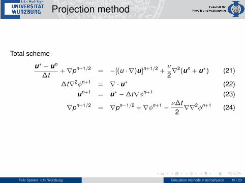
Projection method

Total scheme

u∗ − un

∆t+∇pn+1/2 = −[(u · ∇)u]n+1/2 +

ν

2∇2(un + u∗) (21)

∆t∇2φn+1 = ∇ · u∗ (22)un+1 = u∗ −∆t∇φn+1 (23)

∇pn+1/2 = ∇pn−1/2 +∇φn+1 − ν∆t2∇∇2φn+1 (24)


Vorticity-Streamline

The natural formulation for divergence-free flows is the stream functionu = ∇×Ψ

Step 1: Calculate velocity

un = ∇×Ψn (25)



Step 2: Solve the Navier-Stokes-equation

∂tu = − (u∇) u + ν∆u (25)



Step 3: Calculate Vorticity

∂tω = ∇×(∂tu) (25)ωn+1 = ωn + dt ·∆ω (26)



Step 4: Calculate Streamfunction

Solve Poisson equation∆Ψn+1 = −ωn+1 (25)

Problem: This would result in a mesh-drift instability. Use staggered grid!



Complete scheme

u = ∇×Ψ (25)

(ux )i,j+1/2 =Ψi,j+1 −Ψi , j

dy(26)

(uy )i+1/2,j =Ψi+1,j −Ψi , j

dx(27)

ui+1/2,j+1/2 =

(1/2

((ux )i+1,j+1/2 + (ux )i,j+1/2

)1/2

((uy )i+1/2,j+1 + (uy )i+1/2,j

) ) (28)


Spectral methods

Basic idea: Use Fourier transform to transform PDE into ODEProblem: This is complicated for the nonlinear terms.

Spectral Navier-Stokes-equation

∂uα∂t

= −ikγ

(δαβ −

kαkβk2

)(uβuγ

)− νk2uα (29)

kαuα = 0

Quantities with a tilde are fouriertransformed.What’s so special about the red and green term?


Spectral methods

The green termStart with the Navier-Stokes-equation

∂u∂t

+ (u∇)u +∇p = 0 (29)

we can identifyikγδαβ uβuγ = (u∇)u (30)

and taking the divergence of the Navier-Stokes-equation

∆p = ∇ · (u∇)u (31)

so the second term is the gradient of the pressure

ikγ

(kαkβk2

)(uβuγ

)= −∇p (32)


Spectral methods

Step 1: Fouriertransform

Starting with uα the velocity has to be transformed into uαThen uαuβ can be calculated (only 6 tensor elements are needed)This is transformed back to Fourier space uαuβ


Spectral methods

Step 2: Anti-Aliasing

In the high wavenumber regime of uα we will find flawed data.Due to the fact, that not all data is correctly attributed for by the Fouriertransform, aliased data has to be removedFor |k | > 1/2kmax set uαuβ(k) = 0


Spectral methods

Step 3: Update velocity

u∗α = unα −∆t(ikγ

(δαβ −

kαkβk2

)(uβuγ

)− νk2uα) (29)


Spectral methods

Step 4: Projection

Project u∗α on its divergence free part

un+1 = u∗ − k(k · u∗)k2 (29)


Spectral methods

Why to use Spectral Methods?

ProEasy to implementRelies on fast FFT-algorithmsEasy to parallelize

Contrahigh aliasing-loss


Fourier Transforms

Fourier transforms are available in large numbers on the marketFFTW 2 ubiquitious library, allows parallel usageFFTW 3 the improved version, no parallel support

Intel MKL includes DFT, much faster than FFTW, simple parallelizedversion, limited to Intel-like systems

P3DFFT UC San Diego’s Fortran based FFT, highly parallelizable,requires FFTW-3

Sandia FFT Sandia Lab’s C based FFT, highly parallelizable, requiresFFTW-2


Parallel Computing

Usually a parallel fluid simulation requires exchange of field bordersbetween processors.Spectral methods are slightly different:

The calculation of uαuβ and the update step are completely local. Theyhave no derivatives and do not need neighboring pointsEvery non-local interaction is done in the FFT

So the only thing we have to do, is using local coordinates and a parallelFFT


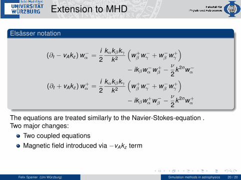
Extension to MHD

Elsässer notation

(∂t − vAkz) w−α =i2

kαkβkγk2

(w+β w−γ + w−β w+

γ

)− ikβw−α w+

β −ν

2k2nw−α

(∂t + vAkz) w+α =

i2

kαkβkγk2

(w+β w−γ + w−β w+

γ

)− ikβw+

α w−β −ν

2k2nw+

α

The equations are treated similarly to the Navier-Stokes-equation .Two major changes:

Two coupled equationsMagnetic field introduced via −vAkz term


[1] D. L. Brown, R. Cortez, and M. L. Minion. Accurate Projection Methodsfor the Incompressible Navier-Stokes Equations. Journal ofComputational Physics, 168:464–499, Apr. 2001.


Documents

Incompressible MHD simulations - Ilmatieteen laitosspace.fmi.fi/graduateschool/Lectures10/vortrag.pdfIncompressible MHD simulations Felix Spanier 1 Lehrstuhl für Astronomie Universität