Incomplete Pass-Through and the Welfare E¤ectsof Exchange Rate Variability¤

Alan Sutherlandy

University of St Andrews and CEPR

June 2002

AbstractThis paper considers the implications of incomplete exchange rate pass-

through for optimal monetary and exchange rate policy. A two-country modelis presented which allows an explicit derivation of welfare functions in termsof a weighted sum of the second moments of producer prices and the nominalexchange rate. From a single country perspective the optimal exchange ratevariance depends on the degree of pass-through, the size and openness of theeconomy, the elasticity of labour supply and the volatility of foreign producerprices. The optimal coordinated equilibrium can be supported by requiringnational central banks to minimise loss functions which are a weighted sumof the variances of producer prices and the exchange rate, where the weighton the exchange rate variance depends on the degree of pass-through.Keywords: Monetary policy, pass-through, exchange rate variability.JEL: E52, E58, F41

¤I am grateful for comments and suggestions from Philippe Bacchetta, John Dri¢ll, MichaelB Devereux, Jordi Gali, Peter Spencer, Stephen Wright, Jacques Melitz and seminar participantsat Birkbeck College, the ECB, Strathclyde University, ESSIM and a CEPR RTN Workshop onInternational Capital Markets. This research was supported by the ESRC Evolving MacroeconomyProgramme grant number L138251046.

yDepartment of Economics, University of St Andrews, St Andrews, Fife, KY16 9AL, UK. Email:ajs10@st-and.ac.uk Web: www.st-and.ac.uk/~ajs10/home.html

1 IntroductionA number of recent papers have analysed the welfare e¤ects of monetary policy inmodels of closed and open economies. It has been shown that, in a closed economy,welfare maximising monetary policy should aim to stabilise the consumer price in-dex.1 While in an open economy it has been shown that the optimal target formonetary policy is the producer price index.2 The same result emerges when thereis home bias in consumption or there are non-traded goods.3

The surprising implication of the models considered in all these papers is thatexchange rate volatility has no direct impact on welfare. Welfare depends onlyon the variance of prices - consumer prices in the case of a closed economy orproducer prices in the case of an open economy. But Bacchetta and van Wincoop(2000), Devereux and Engel (1998, 2000) and Corsetti and Pesenti (2001b) showthat incomplete pass-through from exchange rate changes to local currency pricesimplies that exchange rate volatility can have a direct impact on welfare. Thus, byimplication, when there is incomplete pass-through, optimal monetary policy shouldtake account of exchange rate volatility.4

This paper analyses the welfare e¤ects of exchange rate volatility by consideringin more detail the links between exchange rate volatility, incomplete pass-throughand welfare.5 A two-country model is developed which allows an explicit deriva-tion of a welfare function.6 It is shown that welfare can be written in terms of aweighted sum of the second moments of home and foreign producer prices and theexchange rate. The weight on the variance of the exchange rate depends inter aliaon the degree of pass-through (as implied by the work cited above) and the degreeof openness. When there is complete pass-through the weight on the variance of theexchange rate is zero. In this case optimal monetary policy for the home countrycompletely stabilises the price of home produced goods. But when there is incom-plete pass-through the optimal monetary policy should take account of exchangerate volatility.7

1See Aoki (2001), Goodfriend and King (2001), King and Wolman (1999) and Woodford (2001).2See Aoki (2001), Benigno and Benigno (2001a) and Clarida, Gali and Gertler (2001a).3See Gali and Monacelli (2000) and Sutherland (2001a).4Monacelli (1999) analyses a small open economy with imperfect pass-through and shows that

the performance of simple monetary rules can be improved by including an exchange rate feedbackterm.

5In addition to the theoretical motivation for studying models of incomplete pass-through thereis considerable evidence which suggests that incomplete pass-through is an important empiricalfeature of pricing behaviour. See for instance Engel (1999) and Engel and Rogers (1996), Goldbergand Knetter (1997) and Knetter (1989, 1993).

6The basic framework adopted here is an open economy general equilibrium model (with monop-olistic competition and nominal stickiness) in the tradition of Svensson and van Wijnbergen (1987)and Obstfeld and Rogo¤ (1995, 1998, 2000). See Lane (2001) for a survey of recent developmentsin this literature.

7It should be noted that imperfect pass-through is not the only reason for supposing thatthe strict price targeting results need to be modi…ed. In a closed economy context the presence

1

The results of this paper show that there is no simple relationship between ex-change rate volatility and welfare.8 Optimal policy for the home economy mayinvolve stabilising or destabilising the exchange rate depending on the degree ofpass-through, the size and openness of the home economy, the elasticity of laboursupply and monetary policy in the foreign country. When pass-through is incom-plete, labour supply is elastic and foreign monetary policy is being used to stabiliseforeign producer prices, then home welfare is decreasing in exchange rate volatil-ity. In these circumstances it is optimal for the home monetary authority to allowsome volatility in home producer prices in order to achieve a more stable nominalexchange rate. But when labour supply is inelastic and/or foreign monetary policyis causing volatility in foreign producer prices, then home welfare may be increasingin exchange rate volatility. In these circumstances it may be optimal for the homemonetary authority to increase the variance of the nominal exchange rate. In thecase of foreign monetary shocks this increased exchange rate volatility arises be-cause it is possible (and welfare improving) for the home monetary authority to usemovements in the nominal exchange rate to o¤set the destabilising e¤ects of foreignproducer price movements.This paper also brie‡y considers the implications of imperfect pass-through for

international policy coordination. In a model with perfect pass-through (and utilitywhich is logarithmic in consumption) Obstfeld and Rogo¤ (2002) show that bothnon-cooperative policy making (represented by a Nash equilibrium in monetary pol-icy rules) and optimal coordinated policymaking imply the same rules for monetarypolicy. Corsetti and Pesenti (2001b), on the other hand, show that, when there isless than perfect pass-through, there are potential welfare gains to monetary policycoordination. A similar result holds in the model of this paper. Rather than demon-strating this result, this paper brie‡y considers how the coordinated policy outcomein this model can be supported by delegating monetary policy to independent mone-tary authorities in each county. It is found that the coordinated policy outcome canbe supported if monetary authorities are assigned loss functions which depend onthe variance of producer prices and the variance of the exchange rate. The weight on

of non-optimal ‘cost-push’ shocks implies that the optimal policy allows for some ‡exibility inconsumer prices in order to allow some stabilisation of the output gap. This is often referredto as ‘‡exible in‡ation targeting’ following the terminology suggested by Svensson (1999, 2000).Clarida, Gali and Gertler (2001b) and Benigno and Benigno (2001b) show that the same resultholds in an open economy context, but with consumer prices being substituted by producer prices.Sutherland (2002a) also analyses this issue and shows that nominal income targeting can be a goodapproximation to fully optimal policy when the variance of cost-push shocks is high. A furthercase where the strict price targeting results must be modi…ed is where the elasticity of substitutionbetween home and foreign goods is greater than unity. Sutherland (2002b) analyses this case andshows that exchange rate volatility can become an important factor in welfare even when there isfull pass-through.

8The model presented in this paper focuses on the e¤ects of labour supply and foreign monetaryshocks. The relationship between welfare and exchange rate volatility is found to depend on thesource of shocks so, in a more general model, where more sources of shocks are present, therelationship may in fact be more complicated than suggested here.

2

the variance of the exchange rate in each national loss function is found to dependon the degree of openness and the degree of pass-through. If the home and foreigneconomies are very open and pass-through is low then the coordinated policy regimemay require central banks to give signi…cant weight to exchange rate stabilisation.The paper proceeds as follows. Section 2 presents the structure of the model.

Section 3 derives the solution of the model and the welfare function. Section 4analyses the implications of the home country welfare function for optimal priceand exchange rate volatility for the home economy. Section 5 considers internationalpolicy coordination and the optimal coordinated regime. Section 6 concludes thepaper.

2 The Model

2.1 Market Structure

The world exists for a single period9 and consists of two countries, the home economyand the rest of the world (the foreign economy). Each country is populated by agentswho consume a basket of goods consisting of all home and foreign produced goods.Each agent is a monopoly producer of a single di¤erentiated product.There are two categories of agent in each country. The …rst set of agents supply

goods in a market where prices are set in advance of the realisation of shocks and thesetting of monetary policy. Agents in this market are contracted to meet demand atthe pre-…xed prices. Agents in this group will be referred to as ‘…xed-price agents’.The second set of agents supply goods in a market where prices are set after shocksare realised and monetary policy is set. Agents in this group will be referred to as‘‡exible-price agents’.10 The proportion of …xed-price agents in the total populationis denoted à so à is a measure of the degree of price stickiness in the economy. Thetotal population of the home economy is indexed on the unit interval with …xed-price agents indexed [0,Ã] and ‡exible-price agents indexed (Ã; 1]. The populationof the foreign country is ! with …xed-price agents indexed [0; Ã!] and ‡exible-priceagents indexed (Ã!;!]. Prices and quantities relating to …xed-price agents will beindicated with the subscript ‘1’ while those relating to ‡exible-price agents will beindicated with the subscript ‘2’.

9The model can easily be recast as a multi-period structure but this adds no signi…cant insights.A true dynamic model, with multi-period nominal contracts and asset stock dynamics would beconsiderably more complex and would require much more extensive use of numerical methods.Newly developed numerical techniques are available to solve such models and this is likely to bean interesting line of future research (see Kim and Kim (2000), Sims (2000), Schmitt-Grohé andUribe (2001) and Sutherland (2001b)). However, the approach adopted in this paper yields usefulinsights which would not be available in a more complex model.10This structure can be thought of as a static version of the Calvo (1983) staggered price setting

framework. A …xed/‡exible price structure similar to the one used here has previously been usedin Aoki (2001) and Woodford (2001). The division of agents into …xed and ‡exible price groups istaken to be a …xed institutional feature of the economy.

3

This framework provides the minimal structure necessary to study the e¤ects ofprice variability on welfare while allowing some degree of price stickiness. The …xed-price agents provide the nominal rigidity that is necessary to give monetary policya role while the ‡exible-price agents provide the partial aggregate price ‡exibilitythat allows an analysis of the connection between price volatility and welfare.

2.2 Preferences

All agents in the home economy have utility functions of the same form. The utilityof agent z of type i is given by

U (z) = E

·logC (z) + log

M (z)

P¡ K¹y¹i (z)

¸(1)

where i = 1 for a …xed-price agent and i = 2 for a ‡exible-price agent, C is aconsumption index de…ned across all home and foreign goods, M denotes end-of-period nominal money holdings, P is the consumer price index, yi (z) is sales ofgood z, E is the expectations operator and K is a log-normal stochastic shock(E[logK] = 0 and V ar[logK] = ¾2K).The consumption index C is de…ned as

C =C1¡ºH CºF

(1¡ º)1¡ººº (2)

whereº = (1¡ n) °

where n is the share of the home population in the world population, i.e. n =1=(1 + !) and 0 · n · 1, CH and CF are indices of consumption of home andforeign produced goods and 0 · ° · 1. The parameter º measures the overallshare of foreign goods in the consumption basket of home agents. It depends on twofactors, the share of foreign goods in the total measure of goods in the world (i.e.1 ¡ n) and the degree of openness of the home economy, which is measured by °.° = 0 implies a completely closed economy while ° = 1 implies a completely openeconomy.11

The form of the utility function implies a unit elasticity of substitution betweenhome and foreign goods. This ensures that there is no idiosyncratic income riskbetween the home country and the rest of the world. The structure of …nancialmarkets is therefore irrelevant.12

11This structure is similar to the modelling of “home bias” in Gali and Monacelli (2000). It isalso formally identical to the modelling of non-traded goods in Obstfeld and Rogo¤ (2000) andSutherland (2001a). In the latter two papers the relative price of nontraded and home producedtraded goods is …xed at unity so consumption of nontraded goods can be thought of as home biasin consumption.12This assumption was introduced into a deterministic open economy model by Corsetti and

Pesenti (2001a) and has proved to be a key assumption allowing a tractable solution to stochasticmodels of the type used in this paper.

4

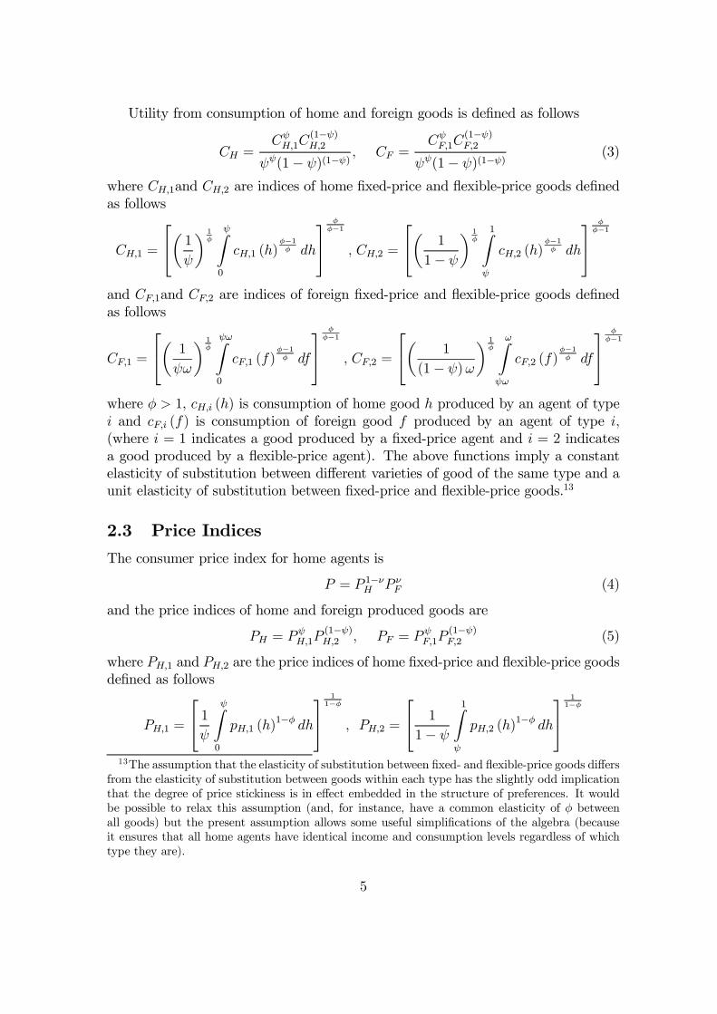
Utility from consumption of home and foreign goods is de…ned as follows

CH =CÃH;1C

(1¡Ã)H;2

ÃÃ(1¡ Ã)(1¡Ã) ; CF =CÃF;1C

(1¡Ã)F;2

ÃÃ(1¡ Ã)(1¡Ã) (3)

where CH;1and CH;2 are indices of home …xed-price and ‡exible-price goods de…nedas follows

CH;1 =

24µ 1Ã

¶ 1Á

ÃZ0

cH;1 (h)Á¡1Á dh

35Á

Á¡1

; CH;2 =

24µ 1

1¡ ö 1

Á

1ZÃ

cH;2 (h)Á¡1Á dh

35Á

Á¡1

and CF;1and CF;2 are indices of foreign …xed-price and ‡exible-price goods de…nedas follows

CF;1 =

24µ 1

Ã!

¶ 1Á

Ã!Z0

cF;1 (f)Á¡1Á df

35Á

Á¡1

; CF;2 =

24µ 1

(1¡ Ã)!¶ 1

Á

!ZÃ!

cF;2 (f)Á¡1Á df

35Á

Á¡1

where Á > 1, cH;i (h) is consumption of home good h produced by an agent of typei and cF;i (f) is consumption of foreign good f produced by an agent of type i;(where i = 1 indicates a good produced by a …xed-price agent and i = 2 indicatesa good produced by a ‡exible-price agent). The above functions imply a constantelasticity of substitution between di¤erent varieties of good of the same type and aunit elasticity of substitution between …xed-price and ‡exible-price goods.13

2.3 Price Indices

The consumer price index for home agents is

P = P 1¡ºH P ºF (4)

and the price indices of home and foreign produced goods are

PH = PÃH;1P

(1¡Ã)H;2 ; PF = P

ÃF;1P

(1¡Ã)F;2 (5)

where PH;1 and PH;2 are the price indices of home …xed-price and ‡exible-price goodsde…ned as follows

PH;1 =

24 1Ã

ÃZ0

pH;1 (h)1¡Á dh

351

1¡Á

; PH;2 =

24 1

1¡ Ã

1ZÃ

pH;2 (h)1¡Á dh

351

1¡Á

13The assumption that the elasticity of substitution between …xed- and ‡exible-price goods di¤ersfrom the elasticity of substitution between goods within each type has the slightly odd implicationthat the degree of price stickiness is in e¤ect embedded in the structure of preferences. It wouldbe possible to relax this assumption (and, for instance, have a common elasticity of Á betweenall goods) but the present assumption allows some useful simpli…cations of the algebra (becauseit ensures that all home agents have identical income and consumption levels regardless of whichtype they are).

5

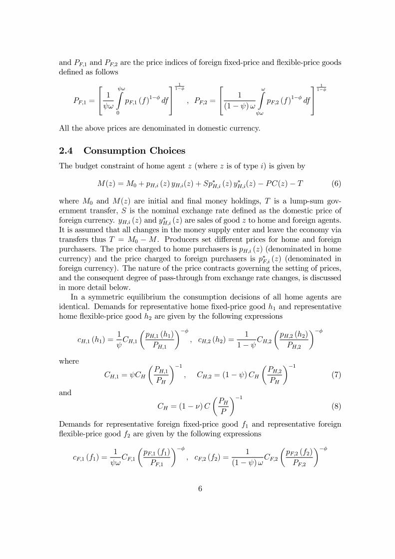
and PF;1 and PF;2 are the price indices of foreign …xed-price and ‡exible-price goodsde…ned as follows

PF;1 =

24 1

Ã!

Ã!Z0

pF;1 (f)1¡Á df

351

1¡Á

; PF;2 =

24 1

(1¡ Ã)!

!ZÃ!

pF;2 (f)1¡Á df

35 11¡Á

All the above prices are denominated in domestic currency.

2.4 Consumption Choices

The budget constraint of home agent z (where z is of type i) is given by

M(z) =M0 + pH;i (z) yH;i(z) + Sp¤H;i (z) y

¤H;i(z)¡ PC(z)¡ T (6)

where M0 and M(z) are initial and …nal money holdings, T is a lump-sum gov-ernment transfer, S is the nominal exchange rate de…ned as the domestic price offoreign currency. yH;i (z) and y¤H;i (z) are sales of good z to home and foreign agents.It is assumed that all changes in the money supply enter and leave the economy viatransfers thus T = M0 ¡M . Producers set di¤erent prices for home and foreignpurchasers. The price charged to home purchasers is pH;i (z) (denominated in homecurrency) and the price charged to foreign purchasers is p¤F;i (z) (denominated inforeign currency). The nature of the price contracts governing the setting of prices,and the consequent degree of pass-through from exchange rate changes, is discussedin more detail below.In a symmetric equilibrium the consumption decisions of all home agents are

identical. Demands for representative home …xed-price good h1 and representativehome ‡exible-price good h2 are given by the following expressions

cH;1 (h1) =1

ÃCH;1

µpH;1 (h1)

PH;1

¶¡Á; cH;2 (h2) =

1

1¡ ÃCH;2µpH;2 (h2)

PH;2

¶¡Áwhere

CH;1 = ÃCH

µPH;1PH

¶¡1; CH;2 = (1¡ Ã)CH

µPH;2PH

¶¡1(7)

and

CH = (1¡ º)CµPHP

¶¡1(8)

Demands for representative foreign …xed-price good f1 and representative foreign‡exible-price good f2 are given by the following expressions

cF;1 (f1) =1

Ã!CF;1

µpF;1 (f1)

PF;1

¶¡Á; cF;2 (f2) =

1

(1¡ Ã)!CF;2µpF;2 (f2)

PF;2

¶¡Á

6

where

CF;1 = ÃCF

µPF;1PF

¶¡1; CF;2 = (1¡ Ã)CF

µPF;2PF

¶¡1(9)

and

CF = ºC

µPFP

¶¡1(10)

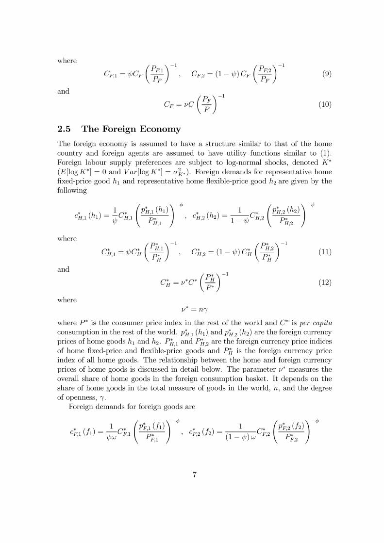
2.5 The Foreign Economy

The foreign economy is assumed to have a structure similar to that of the homecountry and foreign agents are assumed to have utility functions similar to (1).Foreign labour supply preferences are subject to log-normal shocks, denoted K¤

(E[logK¤] = 0 and V ar[logK¤] = ¾2K¤). Foreign demands for representative home…xed-price good h1 and representative home ‡exible-price good h2 are given by thefollowing

c¤H;1 (h1) =1

ÃC¤H;1

Ãp¤H;1 (h1)P ¤H;1

!¡Á; c¤H;2 (h2) =

1

1¡ ÃC¤H;2

Ãp¤H;2 (h2)P ¤H;2

!¡Áwhere

C¤H;1 = ÃC¤H

µP ¤H;1P ¤H

¶¡1; C¤H;2 = (1¡ Ã)C¤H

µP ¤H;2P ¤H

¶¡1(11)

and

C¤H = º¤C¤

µP ¤HP ¤

¶¡1(12)

whereº¤ = n°

where P ¤ is the consumer price index in the rest of the world and C¤ is per capitaconsumption in the rest of the world. p¤H;1 (h1) and p

¤H;2 (h2) are the foreign currency

prices of home goods h1 and h2. P ¤H;1 and P¤H;2 are the foreign currency price indices

of home …xed-price and ‡exible-price goods and P ¤H is the foreign currency priceindex of all home goods. The relationship between the home and foreign currencyprices of home goods is discussed in detail below. The parameter º¤ measures theoverall share of home goods in the foreign consumption basket. It depends on theshare of home goods in the total measure of goods in the world, n, and the degreeof openness, °.Foreign demands for foreign goods are

c¤F;1 (f1) =1

Ã!C¤F;1

Ãp¤F;1 (f1)

P ¤F;1

!¡Á; c¤F;2 (f2) =

1

(1¡ Ã)!C¤F;2

Ãp¤F;2 (f2)

P ¤F;2

!¡Á

7

where

C¤F;1 = ÃC¤F

µP ¤F;1P ¤F

¶¡1; C¤F;2 = (1¡ Ã)C¤F

µP ¤F;2P ¤F

¶¡1(13)

and

C¤F = (1¡ º¤)C¤µP ¤FP ¤

¶¡1(14)

These consumption levels are per capita of the foreign population. The totaldemands from foreign agents are obtained by multiplying each expression by !:

2.6 The Balance of Payments

Using the above relationships it is simple to verify that …xed-price and ‡exible-priceagents have the same consumption levels. It is also possible to verify that …nancialmarkets are irrelevant. To see this latter point note that current account balanceimplies

!SP ¤HC¤H = PFCF (15)

which implies µC¤

C

¶¡1=SP ¤

P(16)

This equation shows that, when the current account is in balance, the ratio of mar-ginal utilities across the two countries is equal to the ratio of aggregate prices (i.e.the real exchange rate). This implies that there can be no Pareto improving reallo-cation of consumption across countries. Financial markets are therefore redundant.

2.7 Price Contracts and the Degree of Pass-Through

Agents are required to enter into separate price contracts for sales in home andforeign markets. The price contract signed by home …xed-price agents for sales toforeign consumers is assumed to enforce a …xed degree of indexation to unanticipatedexchange rate changes. Home …xed-price agent z selling to foreign consumers choosesa price pH;1(z) denominated in home currency. The actual foreign currency pricecharged is determined by the following formula (which is part of the contract)

p¤H;1(z) =pH;1(z)

S

µS

SE

¶1¡´1(17)

where SE is the ex ante expected exchange rate and 0 · ´1 · 1. This structureallows a full range of degrees of pass-through. ´1 = 1 implies producer currencypricing and full pass-through. ´1 = 0 implies local currency pricing and zero pass-through.14

14Implicitly the assumption of separate price contracts for home and foreign sales allows agents toprice discriminate between home and foreign markets. In a deterministic context there would be no

8

Foreign …xed-price producers also set separate prices for home and foreign con-sumers. The contract for foreign sales to home consumers also enforces a …xed degreeof indexation to unanticipated exchange rate changes. Foreign …xed-price agent zselling to home consumers sets a price p¤F;1(z) in terms of foreign currency. Theactual home currency price charged is given by the following formula

pF;1(z) = Sp¤F;1(z)

µS

SE

¶¡(1¡´2)(18)

where 0 · ´2 · 1. This structure allows a full range of degrees of pass-through.´2 = 1 implies producer currency pricing and full pass-through. ´2 = 0 implies localcurrency pricing and zero pass-through.

2.8 Optimal Price Setting

First consider the prices set by ‡exible-price producers. Flexible-price producersin both countries are able to set prices after shocks have been realised and mone-tary policy has been set. This, coupled with the assumption of equal elasticity ofdemand in the two countries, implies that ‡exible-price …rms have no incentive toprice discriminate between home and foreign consumers. It therefore follows thatpH;2(z) = Sp¤H;2(z). This is true for all ‡exible-price producers so PH;2 = SP ¤H;2.The …rst order condition for the choice of price is derived in the Appendix and isgiven by the following

PH;2 =Á

Á¡ 1KY¹¡12 PC (19)

where

Y2 =1

(1¡ Ã)¡CH;2 + !C

¤H;2

¢= C

µPH;2P

¶¡1(20)

where Y2 is the output of ‡exible-price agents expressed per capita of the populationof ‡exible-price agents. (The output expression has been simpli…ed by using PH;2 =SP ¤H;2 and PC = SP

¤C¤.) The same price is chosen by all ‡exible-price producersso the argument z is omitted from these expressions. This condition holds ex postfor all realisations of the shock variables. Notice that the optimal price depends onthe product of three factors. The …rst term, Á=(Á¡ 1); is the mark-up. The middleincentive to price discriminate because elasticities of demand are equal at home and abroad. But,in a stochastic context, given the di¤erent stochastic characteristics of home and foreign demand,price discrimination in fact becomes optimal for …xed-price agents. However, this incentive toprice discriminate is incidental to the analysis of this paper. The important point is that there areseparate contracts. The structure of contracts is taken to be a …xed institutional feature of theeconomy. This structure follows, and is formally identical to, the structure …rst used by Corsettiand Pesenti (2001b) to model incomplete pass-through. Recently a number of authors have begunto consider the implications of endogenous choice of the degree of pass-through (see Bacchetta andvan Wincoop (2001), Devereux and Engel (2001) and Corsetti and Pesenti (2002)).

9

term, KY ¹¡12 , is the marginal disutility of work e¤ort. And the last term, PC, ismade up of factors which a¤ect the demand for goods.Now consider the price setting problem for …xed-price agents. There are two

…rst order conditions (derived in the Appendix) for the choice of prices for the home…xed-price producer. One for the price charged to home consumers as follows

PH;1 = E [VH;1] where VH;1 =µY1Y2

¶¹¡1PH;2 (21)

And one for the price charged to foreign consumers as follows

P ¤H;1 = S¡´1E

£V ¤H;1

¤where V ¤H;1 =

µY1Y2

¶¹¡1PH;2S

´1¡1 (22)

whereY1 =

1

Ã

¡CH;1 + !C

¤H;1

¢(23)

where Y1 is the total output of …xed-price agents expressed per capita of the popula-tion of …xed-price agents. All …xed-price producers make the same choice of price sothe argument z is omitted from these conditions. Notice that …xed-price producersset their home price equal to the expected value of the price set by ‡exible-priceproducers adjusted by a factor which re‡ects the di¤erent level of work e¤ort (andhence di¤erent marginal disutility of labour) of …xed-price agents. The price chargedto foreign consumers is adjusted by a further factor which re‡ects the e¤ects of theexchange rate on demand when there is incomplete pass-through.The …rst order conditions for foreign price setting have a similar structure. For-

eign ‡exible-price producers have no incentive to price discriminate and their pricesare given by

P ¤F;2 =Á

Á¡ 1K¤Y ¤¹¡12 P ¤C¤ (24)

where

Y ¤2 =1

1¡ õ1

!CF;2 + C

¤F;2

¶= C¤

µP ¤F;2P ¤

¶¡1(25)

and the prices set by foreign …xed-price agents are given by

P ¤F;1 = E£V ¤F;1

¤where V ¤F;1 =

µY ¤1Y ¤2

¶¹¡1P ¤F;2 (26)

and

PF;1 = S´2E [VF;1] where VF;1 =

µY ¤1Y ¤2

¶¹¡1P ¤F;2S

1¡´2 (27)

where

Y ¤1 =1

Ã

µ1

!CF;1 + C

¤F;1

¶(28)

10

The fact that …xed-price agents must set prices before shocks are realised clearlyimplies that risk premia will be built into contract prices. This is apparent becauseof the expectational terms in the above price setting conditions for …xed-price agents.The risk premia will depend on the variances of the V terms in the above pricingconditions. The log-normal structure of the model will allow an explicit derivationof expressions for these risk premia.

2.9 Money Demand

The …rst order condition for the choice of money holdings is

M

P= C (29)

The money supply is …xed by the monetary authority.

3 Model Solution and WelfareOne of the main advantages of the model just described is that it provides a verynatural and tractable measure of welfare which can be derived from the aggregateutility of agents. Following Obstfeld and Rogo¤ (1998, 2000) it is assumed that theutility of real balances is small enough to be neglected. It is therefore possible tomeasure ex ante aggregate home-country welfare using the following

­ = E

·Ã

µlogC ¡ K

¹Y ¹1

¶+ (1¡ Ã)

µlogC ¡ K

¹Y ¹2

¶¸(30)

The Appendix shows that the following relationships hold

E [KY ¹1 ] =Á¡ 1Á

; E [KY ¹2 ] =Á¡ 1Á

(31)

so the welfare measure can be written as

­ = E logC ¡ Á¡ 1Á¹

(32)

It proves useful to consider the solution of the model in terms of the ex anteexpected log deviation of variables from the deterministic equilibrium. De…ne thedeterministic equilibrium of the model as the solution which results whenK = K¤ =1 with ¾2K = ¾2K¤ = 0 and for any variable X de…ne X = log

¡X= ¹X

¢where ¹X is

the value of variable X in the deterministic equilibrium. Notice that welfare can beexpressed in terms of the deviation from the deterministic equilibrium as follows

­D = ­¡ ¹­ = EhCi

(33)

11

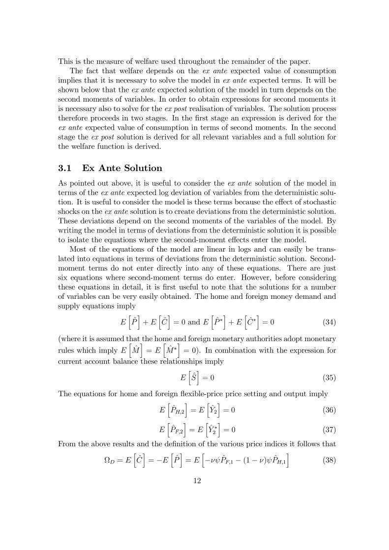
This is the measure of welfare used throughout the remainder of the paper.The fact that welfare depends on the ex ante expected value of consumption

implies that it is necessary to solve the model in ex ante expected terms. It will beshown below that the ex ante expected solution of the model in turn depends on thesecond moments of variables. In order to obtain expressions for second moments itis necessary also to solve for the ex post realisation of variables. The solution processtherefore proceeds in two stages. In the …rst stage an expression is derived for theex ante expected value of consumption in terms of second moments. In the secondstage the ex post solution is derived for all relevant variables and a full solution forthe welfare function is derived.

3.1 Ex Ante Solution

As pointed out above, it is useful to consider the ex ante solution of the model interms of the ex ante expected log deviation of variables from the deterministic solu-tion. It is useful to consider the model is these terms because the e¤ect of stochasticshocks on the ex ante solution is to create deviations from the deterministic solution.These deviations depend on the second moments of the variables of the model. Bywriting the model in terms of deviations from the deterministic solution it is possibleto isolate the equations where the second-moment e¤ects enter the model.Most of the equations of the model are linear in logs and can easily be trans-

lated into equations in terms of deviations from the deterministic solution. Second-moment terms do not enter directly into any of these equations. There are justsix equations where second-moment terms do enter. However, before consideringthese equations in detail, it is …rst useful to note that the solutions for a numberof variables can be very easily obtained. The home and foreign money demand andsupply equations imply

EhPi+ E

hCi= 0 and E

hP ¤i+ E

hC¤i= 0 (34)

(where it is assumed that the home and foreign monetary authorities adopt monetary

rules which imply EhMi= E

hM¤i= 0). In combination with the expression for

current account balance these relationships imply

EhSi= 0 (35)

The equations for home and foreign ‡exible-price price setting and output imply

EhPH;2

i= E

hY2

i= 0 (36)

EhPF;2

i= E

hY ¤2i= 0 (37)

From the above results and the de…nition of the various price indices it follows that

­D = EhCi= ¡E

hPi= E

h¡ºÃPF;1 ¡ (1¡ º)ÃPH;1

i(38)

12

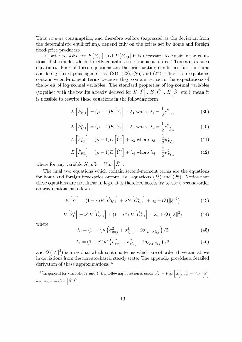
Thus ex ante consumption, and therefore welfare (expressed as the deviation fromthe deterministic equilibrium), depend only on the prices set by home and foreign…xed-price producers.In order to solve for E [PF;1] and E [PH;1] it is necessary to consider the equa-

tions of the model which directly contain second-moment terms. There are six suchequations. Four of these equations are the price-setting conditions for the homeand foreign …xed-price agents, i.e. (21), (22), (26) and (27). These four equationscontain second-moment terms because they contain terms in the expectations ofthe levels of log-normal variables. The standard properties of log-normal variables(together with the results already derived for E

hPi; E

hCi; E

hSietc.) mean it

is possible to rewrite these equations in the following form

EhPH;1

i= (¹¡ 1)E

hY1

i+ ¸1 where ¸1 =

1

2¾2VH;1 (39)

EhP ¤H;1

i= (¹¡ 1)E

hY1

i+ ¸2 where ¸2 =

1

2¾2V ¤H;1 (40)

EhP ¤F;1

i= (¹¡ 1)E

hY ¤1i+ ¸3 where ¸3 =

1

2¾2V ¤F;1 (41)

EhPF;1

i= (¹¡ 1)E

hY ¤1i+ ¸4 where ¸4 =

1

2¾2VF;1 (42)

where for any variable X, ¾2X = V arhXi:

The …nal two equations which contain second-moment terms are the equationsfor home and foreign …xed-price output, i.e. equations (23) and (28). Notice thatthese equations are not linear in logs. It is therefore necessary to use a second-orderapproximations as follows

EhY1

i= (1¡ º)E

hCH;1

i+ ºE

hC¤H;1

i+ ¸5 +O

¡k»k3¢ (43)

EhY ¤1i= º¤E

hCF;1

i+ (1¡ º¤)E

hC¤F;1

i+ ¸6 +O

¡k»k3¢ (44)

where¸5 = (1¡ º)º

³¾2cH;1 + ¾

2c¤H;1

¡ 2¾cH;1;c¤H;1´=2 (45)

¸6 = (1¡ º¤)º¤³¾2cF;1 + ¾

2c¤F;1

¡ 2¾cF;1;c¤F;1´=2 (46)

and O¡k»k3¢ is a residual which contains terms which are of order three and above

in deviations from the non-stochastic steady state. The appendix provides a detailedderivation of these approximations.15

15In general for variablesX and Y the following notation is used: ¾2X = V arhXi, ¾2Y = V ar

hYi

and ¾X;Y = CovhX; Y

i.

13

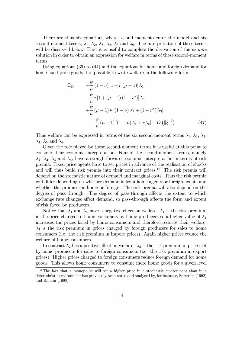
There are thus six equations where second moments enter the model and sixsecond-moment terms, ¸1, ¸2, ¸3, ¸4, ¸5 and ¸6. The interpretation of these termswill be discussed below. First it is useful to complete the derivation of the ex antesolution in order to obtain an expression for welfare in terms of these second-momentterms.Using equations (39) to (44) and the equations for home and foreign demand for

home …xed-price goods it is possible to write welfare in the following form

­D = ¡Ã¹(1¡ º) [1 + º (¹¡ 1)]¸1

¡Ã¹º [1 + (¹¡ 1) (1¡ v¤)]¸4

+Ã

¹(¹¡ 1) º [(1¡ º)¸2 + (1¡ º¤)¸3]

¡Ã¹(¹¡ 1) [(1¡ º)¸5 + º¸6] +O

¡k»k3¢ (47)

Thus welfare can be expressed in terms of the six second-moment terms ¸1, ¸2, ¸3,¸4, ¸5 and ¸6.Given the role played by these second-moment terms it is useful at this point to

consider their economic interpretation. Four of the second-moment terms, namely¸1, ¸2, ¸3 and ¸4, have a straightforward economic interpretation in terms of riskpremia. Fixed-price agents have to set prices in advance of the realisation of shocksand will thus build risk premia into their contract prices.16 The risk premia willdepend on the stochastic nature of demand and marginal costs. Thus the risk premiawill di¤er depending on whether demand is from home agents or foreign agents andwhether the producer is home or foreign. The risk premia will also depend on thedegree of pass-through. The degree of pass-through a¤ects the extent to whichexchange rate changes a¤ect demand, so pass-through a¤ects the form and extentof risk faced by producers.Notice that ¸1 and ¸4 have a negative e¤ect on welfare. ¸1 is the risk premium

in the price charged to home consumers by home producers so a higher value of ¸1increases the prices faced by home consumers and therefore reduces their welfare.¸4 is the risk premium in prices charged by foreign producers for sales to homeconsumers (i.e. the risk premium in import prices). Again higher prices reduce thewelfare of home consumers.In contrast ¸2 has a positive e¤ect on welfare. ¸2 is the risk premium in prices set

by home producers for sales to foreign consumers (i.e. the risk premium in exportprices). Higher prices charged to foreign consumers reduce foreign demand for homegoods. This allows home consumers to consume more home goods for a given level16The fact that a monopolist will set a higher price in a stochastic environment than in a

deterministic environment has previously been noted and analysed by, for instance, Sorensen (1992)and Rankin (1998).

14

of work e¤ort. In e¤ect the reduction of foreign demand has a “crowding in” e¤ecton home consumption of home goods. The extent to which ¸2 makes a positivecontribution to welfare depends on the slope of the disutility of labour function(which is determined by ¹). The larger is ¹ the more reluctant home agents are tovary work e¤ort and the stronger is the crowding in/out e¤ect of changes in foreigndemand.17

The last two second-moment terms, ¸5 and ¸6, have a di¤erent interpretationfrom the other four. These terms enter the model via the equations for the outputof home and foreign …xed-price agents. These terms are e¤ectively capturing theine¢ciency that arises when the prices charged by …xed-price agents to home andforeign consumers diverge ex post due to exchange rate changes and incomplete pass-through.18 This represents a distortion which implies that …xed-price agents haveto work harder to supply a given level of utility to home and foreign consumers.This e¤ect is captured by the second-order terms appearing in the approximated…xed-price output equation.19 ¸5 and ¸6 have a negative e¤ect on home welfare.Before considering the ex post solution of the model it is useful to note that, by

writing the welfare function in the form shown in (47), it is possible to see a directlink between the welfare function in this paper and the welfare functions derived inRotemberg and Woodford (1999) and Woodford (2001). These authors emphasisethat the welfare cost of in‡ation volatility arises because changes in the absolute pricelevel cause changes in relative output prices between producers with ‡exible pricesand producers with …xed prices. These changes in relative prices produce a welfarereducing distortion in relative outputs across producers. In the context of the modelof this paper such distortions would take the form of changes in the output of …xed-price agents relative to the output of ‡exible-price agents. But it is apparent fromthe price setting equations (21), (22), (26) and (27) and from the de…nitions of therisk premia in (39), (40), (41) and (42) that a major determinant of the risk premiain this model is volatility in the relative outputs of …xed-price and ‡exible-priceagents. In fact, when there is complete pass-through, the only determinants of therisk premia are relative outputs. Furthermore, welfare is entirely determined by therisk premia. Thus the risk premia in prices and their role in determining welfare are17The positive welfare e¤ect of reducing exports is partly a consequence of the unit elasticity of

substitution between home and foreign goods in the utility function. This assumption implies thatthe elasticity of demand for home goods is unity, so total national export revenue is independentof the volume of exports. In such a situation, any factor (such as the risk premium in exportprices) which reduces export volume is obviously welfare enhancing for home agents. In a moregeneral model, where the elasticity of demand for home goods is greater than unity, there wouldbe a welfare maximising export volume and the welfare e¤ects of the risk premium in export priceswould depend on whether export volume is above or below the welfare maximising level.18Ex ante …xed-price agents may rationally set di¤erent prices for home and foreign consumers

(because of the di¤ering stochastic characteristics of the two sources of demand). However, theseprices are also ex post subject to di¤erent degrees of indexation to exchange rate changes and thismay cause a non-optimal divergence of the two prices.19Notice that when there is complete pass-through the output equations become log-linear and

¸5 and ¸6 are zero.

15

capturing exactly the same e¤ects as those emphasised by Rotemberg and Woodford(1999) and Woodford (2001). It is interesting to note that the application of theRotemberg and Woodford method (with some amendments) to the model of thispaper produces exactly the same results as presented here. The results presentedhere are therefore independent of the emphasis on risk premia.

3.2 Ex Post Solution

In order to solve for the second moments of the model it is necessary to obtain theex post solution to the model. Note that for any variable X, E[X] depends onlyon second-order terms. So to obtain a second-order accurate expression for V ar[X]it is su¢cient to consider …rst-order accurate solutions to X. It is thus possible toconsider the model in terms of the realised ex post log deviation of variables fromtheir values in the deterministic steady state. The aim is to express the welfarefunction in terms of the second moments of PH;2; P ¤F;2 and S so here variables aresolved in terms of PH;2; P ¤F;2 and S.Current account balance implies

P + C = S + P ¤ + C¤ (48)

Home and foreign ‡exible-price outputs are given by

Y2 = P + C ¡ PH;2 and Y ¤2 = P ¤ + C¤ ¡ P ¤F;2 (49)

Home and foreign …xed-price demand schedules imply

CH;1 = P + C and C¤H;1 = P¤ + C¤ + ´1S (50)

C¤F;1 = P¤ + C¤ and CF;1 = P + C ¡ ´2S (51)

so the output levels of home and foreign …xed-price agents are

Y1 = P + C ¡ º (1¡ ´1) S +O¡k»k2¢ (52)

Y ¤1 = P¤ + C¤ + º¤ (1¡ ´2) S +O

¡k»k2¢ (53)

where O¡k»k2¢ is a residual which contains terms of order two and above in devia-

tions from the non-stochastic steady state. It is now possible to derive the followingexpressions for VH;1, V ¤H;1, V

¤F;1 and VF;1

VH;1 = ¹PH;2 ¡ (¹¡ 1) º (1¡ ´1) S +O¡k»k2¢ (54)

V ¤H;1 = ¹PH;2 ¡ [(¹¡ 1) º + 1] (1¡ ´1) S +O¡k»k2¢ (55)

V ¤F;1 = ¹P¤F;2 + (¹¡ 1) º¤ (1¡ ´2) S +O

¡k»k2¢ (56)

VF;1 = ¹P¤F;2 + [(¹¡ 1) º¤ + 1] (1¡ ´2) S +O

¡k»k2¢ (57)

16

and to derive the following expression for the ¸s

¸1 =1

2

n(¹¡ 1)2 º2 (1¡ ´1)2 ¾2S + ¹2¾2PH;2

¡2 (¹¡ 1) º (1¡ ´1)¹¾S;PH;2ª+O

¡k»k3¢ (58)

¸2 =1

2

n[(¹¡ 1) º + 1]2 (1¡ ´1)2 ¾2S + ¹2¾2PH;2¡2 [(¹¡ 1) º + 1] (1¡ ´1)¹¾S;PH;2

ª+O

¡k»k3¢ (59)

¸3 =1

2

n(¹¡ 1)2 º¤2 (1¡ ´2)2 ¾2S + ¹2¾2P ¤F;2

+2 (¹¡ 1) º¤ (1¡ ´2)¹¾S;P¤F;2o+O

¡k»k3¢ (60)

¸4 =1

2

n[(¹¡ 1) º¤ + 1]2 (1¡ ´2)2 ¾2S + ¹2¾2P¤F;2+2 [(¹¡ 1) º¤ + 1] (1¡ ´2)¹¾S;P ¤F;2

o+O

¡k»k3¢ (61)

¸5 =1

2(1¡ º) º (1¡ ´1)2 ¾2S +O

¡k»k3¢ (62)

¸6 =1

2(1¡ º¤) º¤ (1¡ ´2)2 ¾2S +O

¡k»k3¢ (63)

These expressions can be used to derive the following expression for home wel-fare20

­D = ¡Ã¹ (1¡ º)2 (1¡ Ã)2 ¾

2PH¡ ùº

2 (1¡ Ã)2¾2P¤F¡ ùº (1¡ ´2)

(1¡ Ã) ¾S;P¤F

+ú

2

£¡(¹¡ 1) (1¡ º¤)2 ¡ ¹¢ (1¡ ´2)2 + (¹¡ 1) º (1¡ º) (1¡ ´1)2¤¾2S

+O¡k»k3¢ (64)

The following expression for foreign welfare can also be derived

­¤D = ¡Ã¹ (1¡ º¤)

2 (1¡ Ã)2 ¾2P ¤F¡ ùº¤

2 (1¡ Ã)2¾2PH+ùº¤ (1¡ ´1)(1¡ Ã) ¾S;PH

+ú¤

2

£¡(¹¡ 1) (1¡ º)2 ¡ ¹¢ (1¡ ´1)2 + (¹¡ 1) º¤ (1¡ º¤) (1¡ ´2)2¤¾2S

+O¡k»k3¢ (65)

The implications of these welfare functions for optimal monetary policy are discussedin the next section.20Note that use has been made of the fact that ¾2PH;2 = ¾

2pH=(1¡Ã)2 and ¾2P¤

F;2= ¾2p¤F

=(1¡Ã)2.

17

4 Optimal Monetary Policy and Exchange RateVolatility

It is useful to discuss the implications of the home welfare function, as derivedin equation (64), by …rst considering the special case where the home economy isin…nitesimally small relative to the foreign economy. This has the advantage thatit is possible to treat the foreign economy as exogenous with respect to events inthe home economy. In particular, it is possible to treat foreign monetary policy asindependent from the choice of home monetary policy.

4.1 The Small Open Economy Case

The small open economy welfare functions can be derived by taking the limit of (64)and (65) as the population of the foreign country, !; tends to in…nity. This impliesn! 0; º¤ ! 0 and º ! °: The welfare functions therefore become

­D = ¡Ã¹ (1¡ °)2 (1¡ Ã)2 ¾

2PH¡ ù°

2 (1¡ Ã)2¾2P ¤F¡ ù° (1¡ ´2)

(1¡ Ã) ¾S;P ¤F

+ð

2

£¡ (1¡ ´2)2 + (¹¡ 1) ° (1¡ °) (1¡ ´1)2¤¾2S+O

¡k»k3¢ (66)

for the home economy and

­¤D = ¡Ã¹

2 (1¡ Ã)2¾2P ¤F+O

¡k»k3¢ (67)

for the foreign economy.It is immediately apparent from (67) that the optimal monetary policy for the

foreign country is completely to stabilise the price of foreign produced goods. Theinitial discussion of home welfare and monetary policy will be based on the assump-tion that the foreign monetary authority follows this monetary rule. Thus ¾2P¤F = 0and ¾S;P¤F = 0: The implications of relaxing this assumption will be considered later.The …rst and most obvious result that emerges from (66) is that, when there is

complete pass-through (i.e. ´1 = ´2 = 1), home welfare depends only on the varianceof PH .21 Thus the optimal policy rule for the home economy will stabilise PH . Whenthere is complete pass-through PH is equivalent to the producer price index. Thisresult is in line with the result obtained by other authors for open economies.22

Furthermore when ° = 0 (implying the home economy is completely closed) PH isequivalent to the CPI so the optimal policy involves complete stabilisation of the21When there is complete pass-through the equation for …xed-price output becomes log-linear so

the solution becomes exact and the residual terms in all the above equations become zero.22See Aoki (2001), Benigno and Benigno (2001a) and Clarida, Gali and Gertler (2001a).

18

CPI. This result corresponds to the result emphasised by other authors for closedeconomies.23

The reason why price stabilisation is optimal can be explained with reference tothe risk premium in the prices of …xed-price agents. When ´1 = ´2 = 1 notice that¸1 = ¸2, ¸3 = ¸4 and ¸5 = ¸6 = 0. The risk premium in the prices of …xed-priceagents is generated by the volatility of work e¤ort of …xed-price agents. This dependson the volatility of relative prices between …xed-price and ‡exible-price goods. Expost the relative price depends entirely on the price of ‡exible-price goods. If theprice of ‡exible-price goods is completely stabilised then all risk is removed from…xed-price agents so the risk premium is minimised.24 This maximises welfare.Now consider the e¤ects of incomplete pass-through. It is useful to distinguish

between the e¤ects of ´1 and ´2. First consider the e¤ects of ´2 < 1. It is clearfrom (66) that when ´2 < 1 home welfare depends negatively on the volatility of theexchange rate. The size of this e¤ect depends on the openness of the economy andthe degree of pass-through. Thus when ´2 < 1 it is no longer optimal to completelystabilise PH . Instead it is optimal to trade-o¤ some volatility in PH in order toreduce the volatility of the exchange rate.The reason why exchange rate stabilisation becomes welfare improving with in-

complete pass-through in import prices can be explained with reference to the riskpremium in the prices of foreign …xed-price agents (i.e. the risk premium in importprices). Notice that the only e¤ect of ´2 < 1 is to make ¸3; ¸4 > 0. The smaller is´2 the more the exchange rate a¤ects the home demand for foreign goods. Thus areduction in exchange rate volatility reduces the risk premium in import prices andtherefore increases home welfare.25 This e¤ect is larger when the share of foreigngoods is large in the consumption basket of home agents (i.e. when ° is close tounity). Notice that in a completely open economy with ´2 < 1 a …xed nominalexchange rate is optimal.Now consider the e¤ects of ´1 < 1. Notice that if ¹ = 1, ´1 has no e¤ect on the

home welfare function.26 It is clear from (66) that when ´2 = 1, ¹ > 1 and ´1 < 1exchange rate volatility has a positive e¤ect on welfare. Again it is no longer optimalsimply to stabilise PH . But in this case it becomes optimal to increase (rather thanreduce) exchange rate volatility.23See Aoki (2001), Goodfriend and King (2001), King and Wolman (1999) and Woodford (2001).24In terms of the Rotemberg and Woodford (1999) and Woodford (2001) interpretation of the

welfare e¤ects of monetary policy, minimising the variance of prices reduces the volatility of relativeoutput levels between ‡exible-price and …xed-price producers. It is clear from the form in whichthe risk premia are expressed that the risk premia ¸1 and ¸2 are minimised exactly when relativeoutput levels are stabilised.25This is the result emphasised by Corsetti and Pesenti (2001b).26Other authors who have considered incomplete pass-through in related models have assumed

¹ = 1 (see for instance Devereux and Engel (1998, 2000), Devereux, Engel and Tille (1999) andCorsetti and Pesenti (2001b)). Notice that with ¹ = 1 the equation for …xed-price output becomesirrelevant so the welfare function ceases to be an approximation (i.e. the residual term in thewelfare function becomes zero).

19

The positive welfare e¤ect of exchange rate volatility arises because of the riskpremium in home prices for sales to foreign agents (i.e. the risk premium in exportprices). When ´1 < 1 higher exchange rate volatility raises ¸2 and this makes apositive contribution to home welfare. ¸2 makes a positive contribution to welfarebecause higher prices for exports reduces foreign demand and this allows home agentsto consume more home goods for a given level of work e¤ort. Notice that the e¤ectof ´1 < 1 on welfare is zero when the economy is completely closed (° = 0) andwhen it is completely open (° = 1). Obviously when the economy is completelyclosed the degree of pass-through is irrelevant. When the economy is completelyopen, home agents do not consume home goods so there is no welfare bene…t fromreducing foreign demand for home goods.Some of the properties of the optimal volatilities of the exchange rate and home

producer prices are illustrated in Figures 1 and 2. For the purposes of illustrationthe two pass-through parameters, ´1 and ´2, are assumed to be equal and are variedbetween 0 and 1. Baseline parameter values are n = 0 (i.e. the home countryis a small open economy), ° = 0:4, ¹ = 2, Ã = 0:5 and ¾2K = ¾2K¤ = 1. Theforeign economy is assumed to follow a monetary policy which fully stabilises foreignproducer prices.27

Notice from Figure 1 that the optimal volatility of home prices is zero when thereis full pass-through. The solid line in Figure 1 shows that the optimal volatility ofhome producer prices rises as the degree of pass-through is reduced below unity,while the solid line in Figure 2 shows that the optimal volatility of the exchangerate declines.Figures 1 and 2 also illustrate the e¤ects of varying the openness of the economy

(as measured by the parameter °). The dashed lines show the case where ° = 0:8,which represents a much more open economy than the baseline case (where ° = 0:4).The dashed line in Figure 1 shows that, as in the baseline case, the optimal volatilityof home producer prices is zero when there is full pass-through and rises as thedegree of pass-through falls below unity. But notice that in the ° = 0:8 case theoptimal volatility of home producer prices rises much more than in the baseline case.Likewise, the dashed line in Figure 2 shows that, as in the baseline case, the optimalvolatility of the exchange rate declines as the degree of pass-through falls belowunity. But the decline in the optimal volatility of the exchange rate is much morethan in the baseline case. In the ° = 0:8 case, the optimal volatility of the exchangerate falls by approximately half as the degree of pass-through is reduced from unityto zero. This illustrates the much greater welfare impact of exchange rate volatilityin more open economies.Figures 3 and 4 show the e¤ects of varying the elasticity of labour supply. The

27The optimal volatilities of prices and the exchange rate are derived by assuming the homemonetary authority follows a rule of the form M = ±KK + ±K¤K¤where ±K and ±K¤ are feedbackcoe¢cients which are chosen ex ante by the monetary authority to maximise welfare. Attention isrestricted to ex ante optimal monetary rules and it is assumed that the monetary authority is ableto precommit to the optimal rule.

20

solid lines are the baseline case where ¹ = 2 while the dashed lines are the casewhere ¹ = 10 (i.e. where labour supply is less elastic). The dashed lines showthat, when labour supply is inelastic, the optimal volatility of the exchange raterises slightly as the degree of pass-through is reduced. The contrast between the¹ = 2 and ¹ = 10 cases arises from the contrasting welfare e¤ects of the riskpremia in import and export prices. As explained above, when there is incompletepass-through, exchange rate volatility increases both import and export prices. Theincrease in import prices reduces welfare but the increase in export prices increaseswelfare. The relative importance of these two e¤ects depends on the elasticity oflabour supply. When labour supply is very inelastic (¹ = 10) the export price e¤ectdominates and it becomes optimal to increase the volatility of the exchange rate.28

4.2 Foreign Price Shocks

The analysis so far has been based on the assumption that the foreign monetaryauthority completely stabilises foreign producer prices. This would be the opti-mal policy for the foreign economy. It is interesting, however, to consider the casewhere the foreign monetary authority follows a non-optimal policy. This might, forinstance, be a passive monetary rule which …xes the foreign money stock. Alterna-tively it may be an arbitrary rule which creates shocks in the foreign money supply.In either case the net result will be some volatility in foreign producer prices. Thehome welfare function (66) shows that any variance in foreign producer prices willhave a negative e¤ect on the welfare of home agents. Although there is nothing thehome monetary authority can do to a¤ect the volatility of foreign producer prices,it is apparent from (66) that, when there is imperfect pass-through in import prices,the home monetary authority can partly o¤set the negative welfare impact by creat-ing a negative correlation between the nominal exchange rate and foreign producerprices. In other words the home monetary authority can use the exchange rate asa ‘shock absorber’ which partly insulates home welfare from foreign price shocks.Notice that this necessarily involves creating some volatility in the exchange rate.This will o¤set the incentive to stabilise the exchange rate discussed in the previoussub-section.Figures 5 and 6 illustrate the implications of volatility of foreign producer prices.

In the baseline case (illustrated with the solid lines) foreign producer prices are as-sumed to be fully stabilised by the foreign monetary authority. The dashed linesshow the case where foreign monetary policy shocks generate shocks in foreign pro-ducer prices such that ¾P¤F = 0:5. In this case, as the degree of pass-through falls, theoptimal volatility of the exchange rate rises. The e¤ect is quantitatively quite large.When the degree of pass-through is zero the optimal volatility is approximately 25%28This incentive to create exchange rate volatility arises because of the incentive to reduce the

volume of exports. As pointed out in footnote 17, this e¤ect is mainly a consequence of the unitelasticity of demand for exports. In a more general model, where the elasticity of demand is greaterthan unity, it is likely that the incentive to reduce export volumes would be much less important.

21

higher than when there is full pass-through.

4.3 The Large Economy Case

Now consider the implications of moving away from the small open economy as-sumption. For the purposes of this analysis it is useful to revert to the assumptionthat the foreign monetary authority completely stabilises foreign producer prices.Strictly this would not be optimal for the foreign economy because the home econ-omy would now be large enough to have spillover e¤ects which would in‡uence theforeign economy. Some of the implications of these spillover e¤ects will be discussedin the next section.The e¤ects of increasing the size of the home country are very easy to determine

from (64). First note that all the results so far discussed continue to hold for alarge economy (i.e. when n > 0). Thus, exchange rate volatility has no impact onhome welfare when there is complete pass-through. And it may have a negative orpositive impact on welfare when there is incomplete pass-through depending on theopenness of the economy, the elasticity of labour supply and the volatility of foreignproducer prices.But notice from (64) that, for given values of other parameters, increasing n

increases the coe¢cient on the home price variance in the welfare function andreduces the coe¢cient on the exchange rate variance. Thus, other things beingequal, a large economy should place less weight on exchange rate volatility andmore weight on home price volatility in policy decisions. In other words a largeeconomy should be more inward looking.Figures 7 and 8 illustrate the e¤ects of varying the size of the home economy.

The solid lines are the baseline case where n = 0 while the dashed lines are the casewhere n = 0:5. As in previous cases, the optimal volatility of home prices rises asthe degree of pass-through falls and the optimal volatility of the exchange rate falls.But these e¤ects are less pronounced when the home economy is large.

5 Policy Coordination and DelegationAs pointed out above, other than in the small open economy case, there are spillovere¤ects of home country monetary policy onto welfare in the foreign economy. It istherefore not plausible to assume that foreign monetary policy is exogenous to homecountry policy choices. In such circumstances there are potential gains to interna-tional policy coordination. In a model with perfect pass-through (and utility whichis logarithmic in consumption) Obstfeld and Rogo¤ (2002) show that in fact suchgains do not exist. They show that both non-cooperative policy making (representedby a Nash equilibrium in monetary policy rules) and optimal coordinated policy-

22

making imply the same monetary policy rules.29 Corsetti and Pesenti (2001b), onthe other hand, show that, when there is less than perfect pass-through, there canindeed be welfare gains to monetary policy coordination.30 A similar result holds inthe model of this paper.Rather than demonstrating this result, this section brie‡y considers how the

coordinated policy outcome in this model can be supported by delegating monetarypolicy to independent monetary authorities in each county.31 The coordinated policyis the choice of monetary rules which maximises aggregate world welfare, i.e. thechoice of feedback parameters, ±K; ±K¤; ±¤K and ±

¤K¤ ; in monetary rules of the form

M = ±KK + ±K¤K¤ (68)

M¤ = ±¤KK + ±¤K¤K¤ (69)

to maximise­W = n­D + (1¡ n)­¤D (70)

It is possible to show that the coordinated policy rules will be chosen if monetarypolicy is delegated to independent central banks in the home and foreign countrywhere these central banks are required to minimise the following loss functions (re-spectively for the home and foreign central banks)

L = ¾2PH + (1¡ Ã)2 º!¾2S (71)

L¤ = ¾2P¤F + (1¡ Ã)2 º¤!¤¾2S (72)

where

! =[(1¡ º + ¹º) (1¡ ´1)¡ ¹+ ¹º¤ (1¡ ´2)] (1¡ ´1) + (1¡ º¤) (1¡ ´2)2

¹ [1¡ (1¡ ´1) º ¡ (1¡ ´2) º¤]

!¤ =[(1¡ º¤ + ¹º¤) (1¡ ´2)¡ ¹+ ¹º (1¡ ´1)] (1¡ ´2) + (1¡ º) (1¡ ´1)2

¹ [1¡ (1¡ ´1) º ¡ (1¡ ´2) º¤]Thus the loss function for the home central bank is a weighted sum of the varianceof home producer prices and the variance of the nominal exchange rate and the lossfunction for the foreign central bank is the weighted sum of the variance of foreignproducer prices and the variance of the nominal exchange rate.29Benigno and Benigno (2001a) show that the absence of gains from coordination in the Obstfeld

and Rogo¤ (2002) model arises from the assumption of a unit elasticity of substitution betweenhome and foreign goods. Sutherland (2001b) shows that the gains from coordination can be quitelarge when the elasticity of substitution di¤ers from unity.30More precisely, they show that there are gains from coordination when there is an intermediate

degree of pass-through, but there are no gains from coordination when there is full pass-throughor zero pass-through.31That is, monetary authorities which are independent from the political authorities in each

country and independent from each other.

23

Notice that the weight on the exchange rate is zero in each loss function whenthere is complete pass-through. Producer price targeting is therefore the optimalcoordinated equilibrium when there is complete pass-through.32 But when thereis incomplete pass-through the weight on the exchange rate is non-zero. So, whenthere is incomplete pass-through, coordinated policy makers should deviate fromproducer price targeting in order to give some weight to the exchange rate variance.Benigno and Benigno (2001b) have shown that, in the presence of ‘cost-push’

shocks, optimal coordinated policy can be supported by ‘‡exible in‡ation targeting’.In the examples studied by these authors the coordinated policy regime assigns eachmonetary authority a loss function which depends on the variance of producer pricein‡ation and the variance of the ‘output gap’ (i.e. the deviation of real output fromits ‡exible price level). The loss functions given by (71) and (72) can be thought ofas an alternative form of ‡exible in‡ation targeting where the monetary authorityallows deviations from strict in‡ation targeting in order to pursue some objectivefor the nominal exchange rate.33

Figure 9 plots the value of (1¡ Ã)2 º! (i.e. the weight on the exchange ratevariance in the home loss function) for two alternative parameter sets. The solidlines illustrate the case where n = 0:5, ° = 0:4, ¹ = 2, Ã = 0:5 and ¾2K = ¾

2K¤ = 1:

The dashed lines show the case where ° = 0:8: These plots show that the weighton the exchange rate can be large and positive when the degree of pass-through islow and the economy is very open. In these cases the exchange rate variance wouldbe an important term in the loss function and coordinated policy would imply asigni…cant degree of nominal exchange rate stabilisation and a signi…cant deviationfrom strict producer price targeting.

6 Concluding CommentsThe central feature of the model presented in this paper is that welfare can bewritten in terms of a weighted sum of the second moments of home and foreignproducer prices and the nominal exchange rate. It is shown that the weight on thesecond moments of the exchange rate depends on the degree of pass-through andthe size and openness of the economy and the elasticity of labour supply.32Producer price targeting would also be the Nash equilibrium in this model when there is

complete pass-through. Note, however, that this is only true because the elasticity of substitutionbetween home and foreign goods is assumed to be unity. Sutherland (2002b) shows that, whenthere is a non-unit elasticity of substitution, a Nash equilibrium in delegated monetary regimes(where each country chooses a loss function for its central bank to maximise individual countrywelfare) would result in a non-zero weight on the exchange rate variance, even when there is fullpass-through.33A more general model, where there is both imperfect pass-through and cost-push shocks, would

presumably imply a cooperative policy regime which is supported by loss functions which includethe variance of producer prices, the variance of the nominal exchange rate and the variance of theoutput gap.

24

When there is complete pass-through the weight on the second moments of theexchange rate is zero. In this case the optimal monetary policy for the home countrycompletely stabilises home producer prices. In a closed economy the producer priceindex is equivalent to the consumer price index, so consumer price targeting becomesoptimal in this case.When there is incomplete pass-through welfare depends on the variance of the

exchange rate. There is a complicated (but fully characterised) relationship betweenthe degree of pass-through, the degree of openness, the elasticity of labour supplyand the volatility of foreign producer prices and the e¤ect of exchange rate volatilityon welfare. When labour supply is elastic and foreign prices are stable a reductionin the volatility of the exchange rate is unambiguously welfare improving. Thesize of the welfare e¤ect depends on the degree of pass-through and the size andopenness of the home economy. In contrast to this, when labour supply is relativelyinelastic and/or foreign producer prices are not stable, it is found that increasingexchange rate variability can be welfare improving. Again, the size of this welfaree¤ect depends on the degree of pass-through and the size and openness of the homeeconomy.These results are obtained by considering the welfare and the policy problem of

the home economy while assuming the foreign economy follows a …xed monetaryrule. The analysis is extended to consider some of the implications of incompletepass-through for international policy coordination. It is shown that the coordinatedoutcome can be supported by requiring national central banks to minimise lossfunctions which are a weighted sum of the variances of producer prices and thenominal exchange rate.It must be emphasised that the model analysed in this paper includes only a

limited range of shocks, namely shocks to the disutility of labour in the home andforeign countries and shocks to foreign monetary policy. It is apparent from theresults reported that the way in which the variance of the exchange rate enters thewelfare function di¤ers depending on the sources of shocks. An extension of theanalysis of this paper to alternative sources of shocks will therefore be an interestingtopic for further research.It is also apparent from the analysis of this paper that the welfare maximising

monetary strategy becomes more complex as more realistic aspects are added to thebasic model. It quickly becomes obvious that the optimality of a simple strategyof strict consumer or producer price targeting does not carry over to more generalcases.34 In addition, even when the optimal monetary strategy can be summarisedby a relatively simple loss function, it becomes doubtful that the fully optimalmonetary policy can in practice be implemented. The fully optimal policy mayinvolve responding to unobservable or unmeasurable variables or require a complexbalance between di¤erent targets where the optimal weights to be placed on di¤erenttargets are unmeasurable or uncertain. It would therefore be interesting to use the34This becomes more obvious if such issues as cost-push shocks and the expenditure switching

e¤ect are considered (see Sutherland (2002a, 2002b).

25

model developed in this paper to analyse the welfare performance of non-optimalbut simple targeting rules. This may also be a productive topic for further research.

AppendixOptimal Price Setting: The price setting problem facing ‡exible-price producerz is the following:

MaxU(z) = logC(z) + log

µM

P

¶¡ K¹y¹2 (z) (73)

subject toPC(z) = pH;2 (z) y2(z) +M0 ¡M ¡ T (74)

pH;2 (z) = Sp¤H;2 (z) (75)

PH;2 = SP¤H;2 (76)

y2 (z) = yH;2 (z) + y¤H;2 (z) (77)

yH;2 (z) = cH;2 (z) =1

1¡ ÃCH;2µpH;2 (z)

PH;2

¶¡Á(78)

y¤H;2 (z) = !c¤H;2 (z) =

!

1¡ ÃC¤H;2

Ãp¤H;2 (z)

P ¤H;2

!¡Á(79)

The …rst order condition with respect to pH;2 (z) is

y2(z)

PC(z)¡ Á

·pH;2 (z)

PC(z)¡Ky¹¡12 (z)

¸y2(z)

pH;2 (z)= 0 (80)

In equilibrium all ‡exible-price agents choose the same price and consumption levelso

Y2PC

¡ Á·PH;2PC

¡KY ¹¡12

¸Y2PH;2

= 0 (81)

whereY2 =

1

1¡ áCH;2 + !C

¤H;2

¢(82)

Rearranging yields the expression in the main text.The price setting problem facing …xed-price producer z is the following:

MaxU(z) = E

½logC(z) + log

µM

P

¶¡ K¹y¹1 (z)

¾(83)

subject to

PC(z) = pH;1 (z) yH;1(z) + Sp¤H;1 (z) y

¤H;1(z) +M0 ¡M ¡ T (84)

26

y1 (z) = yH;1 (z) + y¤H;1 (z) (85)

yH;1 (z) = cH;1 (z) =1

ÃCH;1

µpH;1 (z)

PH;1

¶¡Á(86)

y¤H;1 (z) = !c¤H;1 (z) =

!

ÃC¤H;1

Ãp¤H;1 (z)P ¤H;1

!¡Á(87)

p¤H;1(z) =pH;1(z)

S

µS

SE

¶1¡´1(88)

The …rst order condition with respect to pH;1 (z) is

E

½yH;1 (z)

PC(z)¡ Á

·pH;1 (z)

PC(z)¡Ky¹¡11 (z)

¸yH;1 (z)

pH;1 (z)

¾= 0 (89)

In equilibrium all ‡exible-price agents choose the same price and consumption levelso

E

½CH;1PC

¡ Á·PH;1PC

¡KY ¹¡11

¸CH;1PH;1

¾= 0 (90)

whereY1 =

1

Ã

¡CH;1 + !C

¤H;1

¢(91)

Rearranging yields the expression given in the main text.The …rst order condition with respect to pH;1 (z) implies

E

(y¤H;1 (z)S

1¡´1

PC(z)S1¡´1E

¡ Á·p¤H;1 (z)S

PC(z)¡Ky¹¡11 (z)

¸y¤H;1 (z)

p¤H;1 (z)S´1S1¡´1E

)= 0 (92)

In equilibrium all ‡exible-price agents choose the same price and consumption levelso

E

(C¤H;1S

1¡´1

PCS1¡´1E

¡ Á·P ¤H;1S

PC¡KY ¹¡11

¸C¤H;1

P ¤H;1S´1S1¡´1E

)= 0 (93)

Rearranging yields the expression given in the main text.

Simplifying the Welfare Function: The price setting conditions for …xed-priceproducers can be rewritten as follows

E

·PH;1CH;1PC

¸=

Á

Á¡ 1E£KY ¹¡11 CH;1

¤(94a)

E

·SP ¤H;1C

¤H;1

PC

¸=

Á

Á¡ 1E£KY ¹¡11 C¤H;1

¤(95)

27

so

E

·PH;1CH;1 + !SP

¤H;1C

¤H;1

PC

¸=

Á

Á¡ 1ÃE [KY¹1 ] (96)

The price setting condition for ‡exible-price producers is as follows

PH;2PC

=Á

Á¡ 1KY¹¡12 (97)

and it follows that

E

·PH;2CH;2PC

¸=

Á

Á¡ 1E£KY ¹¡12 CH;2

¤(98)

E

·SP ¤H;2C

¤H;2

PC

¸=

Á

Á¡ 1E£KY ¹¡12 C¤H;2

¤(99)

and

E

·PH;2CH;2 + !SP

¤H;2C

¤H;2

PC

¸=

Á

Á¡ 1 (1¡ Ã)E [KY¹2 ] (100)

The budget constraint for individual agents combined with the government budgetconstraint implies

PH;1CH;1 + !SP¤H;1C

¤H;1 = ÃPC (101)

for …xed-price producers and

PH;2CH;2 + !SP¤H;2C

¤H;2 = (1¡ Ã)PC (102)

for ‡exible-price producers. Using the above equations the following are obtained

E [KY ¹1 ] =Á¡ 1Á

; E [KY ¹2 ] =Á¡ 1Á

(103)

These relationships are used in the main text to simply the welfare measure.

Approximating …xed-price Output: The output of …xed-price agents is givenby

Y1 =1

Ã

¡CH;1 + !C

¤H;1

¢(104)

In a symmetric deterministic equilibrium

1

Ã

¹CH;1¹Y1

= 1¡ º and 1Ã

! ¹C¤H;1¹Y1

= º (105)

Taking a second-order approximation of the left and right hand sides of (104) yields

Y1 ¡ ¹Y =1

Ã

¡CH;1 ¡ ¹CH;1

¢+1

Ã

¡C¤H;1 ¡ ¹C¤H;1

¢+O

¡k»k3¢ (106)

28

where O¡k»k3¢ indicates a residual which includes terms of order three and above in

deviations from the non-stochastic steady state. To a second-order approximationX ¡ ¹X = ¹X(X + X2=2) +O

¡k»k3¢ soY1 = (1¡ º)

µCH;1 +

1

2C2H;1

¶+º

µC¤H;1 +

1

2C¤2H;1

¶¡ 12Y 21 +O

¡k»k3¢ (107)

Squaring the right hand side of this expression and deleting terms of order higherthan two yields

Y 21 = (1¡ º)2C2H;1 + º2C¤2H;1 + 2(1¡ º)ºCH;1C¤H;1 +O¡k»k3¢ (108)

substituting this back into (107) yields

Y1 = (1¡ º)CH;1 + ºC¤H;1+1

2(1¡ º)º

hC2H;1 + C

¤2H;1 ¡ 2CH;1C¤H;1

i+O

¡k»k3¢ (109)

Note that for any variable X it is possible to write

X = (logX ¡ E [logX]) + ¡E [logX]¡ log ¹X¢or

X = (logX ¡ E [logX]) + EhXi

so(logX ¡ E [logX]) = X ¡ E

hXi

Furthermore note that EhXiis of second-order magnitude (because it depends only

on second-moment terms). So, to a second-order approximation

¾2X = E£(logX ¡ E [logX])2¤ = E hX2

i+O

¡k»k3¢Taking expectations of (109) therefore yields

EhY1

i= (1¡ º)E

hCH;1

i+ ºE

hC¤H;1

i+1

2(1¡ º)º

h¾2CH;1 + ¾

2C¤H;1

¡ 2¾CH;1C¤H;1i+O

¡k»k3¢ (110)

which is the approximation used in the text.A similar procedure can be used to derive a second-order approximation for

foreign …xed-price output.

29

References[1] Aoki, Kosuke (2001) “Optimal Monetary Policy Responses to Relative Price

Changes” Journal of Monetary Economics, 48, 55-80.

[2] Bacchetta, Philippe and Eric van Wincoop (2000) “Does Exchange Rate Stabil-ity Increase Trade and Welfare?” American Economic Review, 90, 1093-1109.

[3] Bacchetta, Philippe and Eric van Wincoop (2001) “A Theory of the CurrencyDenomination of International Trade” unpublished manuscript, University ofLausanne.

[4] Benigno, Gianluca and Pierpaolo Benigno (2001a) “Price Stability as a NashEquilibrium in Monetary Open Economy Models” CEPR Discussion Paper No2757.

[5] Benigno, Gianluca and Pierpaolo Benigno (2001b) “Implementing MonetaryCooperation through In‡ation Targeting” unpublished manuscript, Bank ofEngland and New York University.

[6] Calvo, Guillermo A (1983) “Staggered Price Setting in a Utility-MaximisingFramework” Journal of Monetary Economics, 12, 383-398.

[7] Clarida, Richard H, Jordi Gali and Mark Gertler (2001a) “Optimal MonetaryPolicy in Open versus Closed Economies: An Integrated Approach” AmericanEconomic Review (Papers and Proceedings), 91, 248-252.

[8] Clarida, Richard H, Jordi Gali and Mark Gertler (2001b) “A Simple Frameworkfor International Monetary Policy Analysis” unpublished manuscript, ColumbiaUniversity, Pompeu-Fabra and New York University.

[9] Corsetti, Giancarlo and Paolo Pesenti (2001a) “Welfare and MacroeconomicInterdependence” Quarterly Journal of Economics, 116, 421-446.

[10] Corsetti, Giancarlo and Paolo Pesenti (2001b) “International Dimensions ofOptimal Monetary Policy” NBER Working Paper No 8230.

[11] Corsetti, Giancarlo and Paolo Pesenti (2002) “Self-Validating Optimum Cur-rency Areas” NBER Working Paper 8783.

[12] Devereux, Michael B and Charles Engel (1998) “Fixed versus Floating Ex-change Rates: How Price Setting A¤ects the Optimal Choice of Exchange RateRegime” NBER Working paper 6867.

[13] Devereux, Michael B and Charles Engel and Cedric Tille (1999) “Exchange RatePass-Through and the Welfare E¤ects of the Euro” NBER Working Paper No7382.

30

[14] Devereux, Michael B and Charles Engel (2000) “Monetary Policy in an OpenEconomy Revisited: Price Setting and Exchange Rate Flexibility” NBERWork-ing Paper No 7665.

[15] Devereux, Michael B and Charles Engel (2001) “Endogenous Currency of PriceSetting in a Dynamic Open Economy Model” NBER Working Paper No 8559.

[16] Engel, Charles (1999) “Accounting for US Real Exchange Rate Changes” Jour-nal of Political Economy, 107, 506-538.

[17] Engel, Charles and John H Rogers (1996) “HowWide is the Border?” AmericanEconomic Review, 86, 1112-1125.

[18] Gali, Jordi and Tommaso Monacelli (2000) “Optimal Monetary Policy andExchange Rate Volatility in a Small Open Economy” unpublished manuscript,Pompeu-Fabra, New York University.

[19] Goldberg, Pinelopi K and Michael M Knetter (1997) “Goods Prices and Ex-change Rates: What Have We Learned” Journal of Economic Literature, 35,1243-72.

[20] Goodfriend, Marvin and Robert G King (2001) “The Case for Price Stability”NBER Working Paper No 8423.

[21] King, Robert G and Alexander L Wolman (1999) “What Should the MonetaryAuthority Do When Prices are Sticky?” in John B Taylor (ed)Monetary PolicyRules, University of Chicago Press, Chicago.

[22] Kim, Jinill and Sunghyun HKim (2000) “SpuriousWelfare Reversals in Interna-tional Business Cycle Models” unpublished manuscript, University of Virginia(forthcoming in the Journal of International Economics).

[23] Knetter, Michael M (1989) “Price Discrimination by US and German Ex-porters” American Economic Review, 79, 198-210.

[24] Knetter, Michael M (1993) “International Comparisons of Pricing to MarketBehaviour” American Economic Review, 83, 473-486.

[25] Lane, Philip (2001) “The New Open Economy Macroeconomics: A Survey”Journal of International Economics, 54-235-266.

[26] Monacelli, Tommaso (1999) “Open Economy Policy Rules under ImperfectPass-Through” unpublished manuscript, New York University.

[27] Obstfeld, Maurice and Kenneth Rogo¤ (1995) “Exchange Rate Dynamics Re-dux” Journal of Political Economy, 103, 624-660.

31

[28] Obstfeld, Maurice and Kenneth Rogo¤ (1998) “Risk and Exchange Rates”NBER Working paper 6694.

[29] Obstfeld, Maurice and Kenneth Rogo¤ (2000) “New Directions in StochasticOpen Economy Models” Journal of International Economics, 50, 117-154.

[30] Obstfeld, Maurice and Kenneth Rogo¤ (2002) “Global Implications of Self-Oriented National Monetary Rules” Quarterly Journal of Economics, 117, 503-36.

[31] Rankin, Neil (1998) “Nominal Rigidity and Monetary Uncertainty” EuropeanEconomic Review, 42, 185-200.

[32] Rotemberg, Julio J and Michael Woodford (1999) “Interest Rate Rules in anEstimated Sticky Price Model” in John B Taylor (ed) Monetary Policy Rules,University of Chicago Press, Chicago.

[33] Schmitt-Grohé, Stephanie and Martin Uribe (2001) “Solving Dynamic Gen-eral Equilibrium Models using a Second-Order Approximation to the PolicyFunction” CEPR Discussion Paper No 2963.

[34] Sims, Christopher (2000) “Second-Order Accurate Solutions of Discrete TimeDynamic Equilibrium Models” unpublished manuscript, Princeton University.

[35] Sorensen, Jan Rose (1992) “Uncertainty and Monetary Policy in a Wage Bar-gaining Model” Scandinavian Journal of Economics 94, 443-455.

[36] Sutherland, Alan J (2001a) “In‡ation Targeting in a Small Open Economy”CEPR Discussion Paper 2726.

[37] Sutherland, Alan J (2001b) “A Simple Second-Order Solution Method for Dy-namic General Equilibrium Models” unpublished manuscript, University of StAndrews.

[38] Sutherland, Alan J (2002a) “Cost-Push Shocks and the Optimal Choice ofMonetary Target in an Open Economy” unpublished manuscript, University ofSt Andrews.

[39] Sutherland, Alan J (2002b) “The Expenditure Switching E¤ect, Welfare andMonetary Policy in an Open Economy” unpublished manuscript, University ofSt Andrews.

[40] Svensson, Lars E O and Sweder van Wijnbergen (1987) “Excess Capacity, Mo-nopolistic Competition and International Transmission of Monetary Distur-bances” Economic Journal, 99, 785-805.

[41] Svensson, Lars E O (1999) “In‡ation Targeting as a Monetary Policy Rule”Journal of Monetary Economics, 43, 607-654.

32

[42] Svensson, Lars E O (2000) “Open-economy In‡ation Targeting” Journal ofInternational Economics, 50, 155-184.

[43] Woodford, Michael (2001) “In‡ation Stabilisation andWelfare” NBERWorkingPaper No 8071.

33

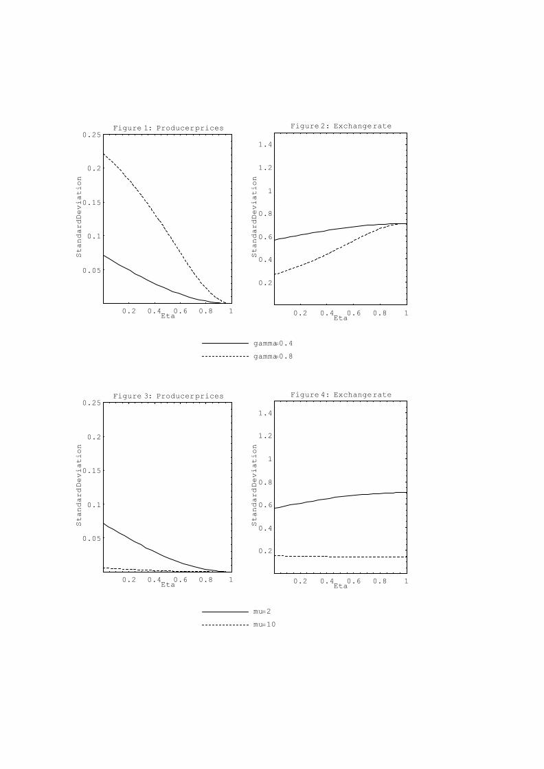
0.2 0.4 0.6 0.8 1Eta

0.05

0.1

0.15

0.2

0.25

dradnatSnoitaiveD

Figure 1: Producerprices

0.2 0.4 0.6 0.8 1Eta

0.2

0.4

0.6

0.8

1

1.2

1.4

dradnatSnoitaiveD

Figure 2: Exchangerate

gamma=0.4

gamma=0.8

0.2 0.4 0.6 0.8 1Eta

0.05

0.1

0.15

0.2

0.25

dradnatSnoitaiveD

Figure 3: Producerprices

0.2 0.4 0.6 0.8 1Eta

0.2

0.4

0.6

0.8

1

1.2

1.4

dradnatSnoitaiveD

Figure 4: Exchangerate

mu=2

mu=10

0.2 0.4 0.6 0.8 1Eta

0.05

0.1

0.15

0.2

0.25

dradnatSnoitaiveD

Figure 5: Producerprices

0.2 0.4 0.6 0.8 1Eta

0.2

0.4

0.6

0.8

1

1.2

1.4

dradnatSnoitaiveD

Figure 6: Exchangerate

StDev@PfD=0.0

StDev@PfD=0.5

0.2 0.4 0.6 0.8 1Eta

0.05

0.1

0.15

0.2

0.25

drad

natSnoitaiveD

Figure 7: Producerprices

0.2 0.4 0.6 0.8 1Eta

0.2

0.4

0.6

0.8

1

1.2

1.4

drad

natSnoitaiveD

Figure 8: Exchangerate

n=0.0

n=0.5

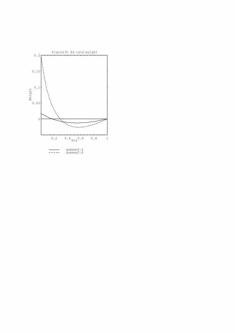
0.2 0.4 0.6 0.8 1Eta

0

0.05

0.1

0.15

0.2

thgieW

Figure 9: Ex rate weight

gamma=0.4gamma=0.8