IZA DP No. 2164

Income Taxes and Entrepreneurial Choice:Empirical Evidence from Germany

Frank M. FossenViktor Steiner

DI

SC

US

SI

ON

PA

PE

R S

ER

IE

S

Forschungsinstitutzur Zukunft der ArbeitInstitute for the Studyof Labor

June 2006

Income Taxes and Entrepreneurial Choice:

Empirical Evidence from Germany

Frank M. Fossen DIW Berlin

Viktor Steiner

Free University of Berlin, DIW Berlin and IZA Bonn

Discussion Paper No. 2164 June 2006

IZA

P.O. Box 7240 53072 Bonn

Germany

Phone: +49-228-3894-0 Fax: +49-228-3894-180

Email: iza@iza.org

Any opinions expressed here are those of the author(s) and not those of the institute. Research disseminated by IZA may include views on policy, but the institute itself takes no institutional policy positions. The Institute for the Study of Labor (IZA) in Bonn is a local and virtual international research center and a place of communication between science, politics and business. IZA is an independent nonprofit company supported by Deutsche Post World Net. The center is associated with the University of Bonn and offers a stimulating research environment through its research networks, research support, and visitors and doctoral programs. IZA engages in (i) original and internationally competitive research in all fields of labor economics, (ii) development of policy concepts, and (iii) dissemination of research results and concepts to the interested public. IZA Discussion Papers often represent preliminary work and are circulated to encourage discussion. Citation of such a paper should account for its provisional character. A revised version may be available directly from the author.

IZA Discussion Paper No. 2164 June 2006

ABSTRACT

Income Taxes and Entrepreneurial Choice: Empirical Evidence from Germany

Entrepreneurial activity is often regarded as an engine for economic growth and job creation. Through tax policy, governments possess a potential lever to influence the decisions of economic agents to start and close small businesses. In Germany, the top marginal income tax rates were reduced exclusively for entrepreneurs in 1994 and 1999/2000. These tax reforms provided two naturally defined control groups that enable us to exploit the legislation changes as “natural experiments”. First, the tax rate reductions did not apply to freelance professionals (Freiberufler), and second, entrepreneurs with earnings below a certain threshold were not affected. Using data from two different sources, the SOEP and the Mikrozensus (LFS), we analyse the effect of the tax cuts on transitions into and out of self-employment and on the rate of self-employment. We apply a “difference-in-difference-in-difference” estimation technique within a discrete time hazard rate model. The results indicate that the decrease in tax rates did not have a significant effect on the self-employment decision. JEL Classification: H24, H25, J23 Keywords: taxation, entrepreneurship, natural experiment, difference-in-difference-in-

difference estimation Corresponding author: Viktor Steiner DIW Berlin Königin-Luise-Straße 5 14195 Berlin Germany Email: vsteiner@diw.de

1 Introduction

Do taxes play a role in the decision to become and to remain an entrepreneur? Extensive

research exists on the individual determinants of being an entrepreneur, but the influence of

taxes is less understood and controversial. Governments in Germany and elsewhere have

discussed and implemented various policies to promote entrepreneurship, following the view

that entrepreneurs are vital to the dynamism and innovative capacity of an economy. More

specifically, entrepreneurship is often regarded as an engine to create new jobs and as a means

to escape unemployment. This is of particular interest to the current policy debate in Germany

and other countries with high rates of unemployment. As among the various potential

determinants of entrepreneurship, taxation is under direct control of the government, tax

policy is frequently suggested as an instrument to stimulate entrepreneurship. A better

understanding of the impact of taxes on firm foundations and closures is crucial to evaluate

these efforts.

Economic theory does not provide unambiguous guidelines with respect to taxation and

entrepreneurship. On the one hand, Gentry and Hubbard (2000) argued that a progressive tax

schedule decreases the expected after-tax return from a risky project and thus discourages

entry into entrepreneurship. On the other hand, the classic view of Domar and Musgrave

(1944) demonstrated that governments may encourage entrepreneurship by sharing risk

through progressive taxation. Even if the tax system treats income from wage employment

and self-employment differently, the ambiguity remains: Bruce (2002) illustrated that the

effect of a differential tax treatment on the decision to be self-employed depends on

individual preferences over return and risk.

The empirical literature has exploited tax reforms as natural experiments to analyse the effects

of taxation with individual micro data since Feldstein (1995). Few empirical studies exist

about taxation and entrepreneurship, though. Most of this literature only considers entries into

self-employment or the propensity to being self-employed, and it is mostly limited to US data

(e.g. Cullen and Gordon 2002; Moore 2004). Only Bruce (2002) studies exits from self-

employment, also in the U.S.A..

We analyse two tax legislation changes in Germany that exhibit specific features which make

them especially suitable to be exploited as natural experiments. These tax reforms were

introduced as a tax relief for small and medium sized enterprises. In the first reform, the top

marginal tax rate of the personal income tax schedule, which was 53% for all types of income,

was limited to 47% exclusively for self-employment income from a trade business above a

2

certain threshold. This tax rate limit was further reduced in a second reform (in two steps

down to 45% in 1999 and to 43% in 2000, combined with lower associated income

thresholds). Importantly, the law makes two distinctions that naturally define treatment and

control groups for our interpretation of the reforms as experiments. First, as mentioned before,

only individuals with income from trade above the threshold defined by the law benefited

from the limitation of the top marginal tax rate. Thus, tradesmen with income below the

threshold serve as a control group. Second, the law does not apply to all self-employed

individuals, but only to tradesmen (Gewerbetreibende) as opposed to so-called freelancers

(Freiberufler). The latter are self-employed persons who have one of various professions that

have traditionally been classified as freelance professions by the German income tax law, e.g.

physicians, lawyers, architects, and journalists. This distinction enables us to track the

freelancers as additional control group. Other influential factors, such as additional tax

legislation changes that came into effect in the period under investigation, affected both the

treatment and control groups. Thus, they do not distort our analysis under the assumption that

the groups were influenced by these other factors in the same way.

In short, this paper provides four main contributions. Firstly, to draw a complete picture of the

impact of taxation on entrepreneurship, firm start-ups, firm closures and the resulting number

of entrepreneurs are of equal importance. This paper analyses entries into and exits from self-

employment and the overall probability of being self-employed to provide this integrated

view. Secondly, this is the first empirical study of entrepreneurial choice and taxation in

Germany. It compares the results based on two different datasets: the German Socio

Economic Panel (waves 1984-2001) and the Mikrozensus (Labour Force Survey; repeated

cross-sections of 1996-2001). The third contribution is the econometric analysis of spell data

and the application of a discrete time hazard model. This enables us to control for the

important effect of the duration of an individual’s self-employment spell on the decision to

exit entrepreneurship, and equally for the effect of the employment or unemployment spell

duration on the decision to enter entrepreneurship. Survival analysis has been applied to study

entrepreneurial choice (Evans and Leighton 1989; Taylor 1999), but these studies did not

consider the impact of taxes; Schuetze and Bruce (2004) pointed out that ignoring the survival

of self-employed ventures has been a significant shortcoming of the existing tax related

literature. The forth contribution of this paper stems from the fact that the two German tax

reforms we analyse luckily provide two independent dimensions to define a control group.

This allows us to apply a “difference-in-difference-in-difference” estimator (Gruber 1994) to

3

isolate the effect of the reforms. This method controls for reform-independent trends in a

more robust way than the conventional difference-in-difference technique.

The remainder of the paper is organised as follows. The following section summarises prior

studies about entrepreneurship and taxation. Section 3 explains the legislation changes that are

relevant to this analysis. In section 4, we introduce the two German datasets we use, elaborate

on the definition of the treatment and control groups, and provide descriptive statistics about

entrepreneurship in Germany. Section 5 describes the econometric methods we apply. The

results are presented and discussed in section 6, and section 7 concludes.

2 Literature Review

2.1 Theory Theoretic approaches to the impact of taxes on entrepreneurial activity provide ambiguous

results. Gentry and Hubbard (2000), on the one hand, assumed risk-neutral agents and argued

that a progressive tax schedule is comparable to a “success tax” by lowering the expected

after-tax return from a risky project. Domar and Musgrave (1944) provided a contrasting

view, assuming risk-averse agents and imperfect financial markets with respect to risk-

sharing: Through a progressive tax schedule, governments share risk with entrepreneurs by

smoothing net profits and losses and thus encourage risky entrepreneurial activity. Cullen and

Gordon (2002) added another argument for the view that higher income tax rates may

increase the propensity to become self-employed in the U.S.A.. American firms always have

the option to avoid high personal tax rates by incorporating ex post and being taxed at the

lower corporate tax rate. Thus, a firm generating tax losses will prefer to be not incorporated

so that the entrepreneur can deduct these losses against other personal income, while a profit

generating firm will prefer to incorporate. This option to choose the organisational form based

on the outcome can thus be interpreted as a net subsidy to risk taking. Better (legal) tax

avoidance and (illegal) tax evasion opportunities available to the self-employed can also

explain a positive relationship between the tax rate and the self-employment rate.

The tax reforms we consider in this study represent a reduction of the top marginal tax rates

exclusively for self-employed tradesmen, but not for wage and salary employees. Thus, the

legislation changes introduced a differential tax treatment of the two alternative sectors self-

employment and dependent employment. Bruce (2002) provided a theoretical framework for

the analysis of a tax system with differential treatment. In his simple portfolio choice model,

which is similar to Tobin (1958), individuals can allocate some fixed amount of labour

4

between wage employment and self-employment. The gross return on wage employment w is

assumed to be certain, whereas the gross return on self-employment s is uncertain with

expected value µs and variance σs2. For each labour supply portfolio p, i.e. for each

combination of time allocated to wage employment and self-employment, one can calculate

the expected return µp and variance σp2. The individual can select the combination of

expected return and risk that yields the highest utility level, subject to a budget constraint,

which is given by the interrelationship between expected return and variance of the portfolio.

The different tax rates τw for wage employment and τs for self-employment enter this budget

constraint in such a way that they shift the budget line downward in comparison to a case

without taxes, and they make the slope steeper if τw > τs, i.e. if the self-employed are tax-

advantaged, as is the case in the tax reforms we study. Figure 1 depicts how an individual

adjusts her labour supply after the tax rate for self-employment is decreased, while the tax rate

for wage employment is left unchanged. B is the budget line before, and B’ after the reform.

w’ represents the after-tax return to wage work, which is the same before and after the reform.

Figure 1: Effect of differential taxes on portfolio choice (example) µp

w’

µp’

µs

I

I’ B’

B

σp σp’ σs

5

In the example shown in the figure, the individual devoted all of her time to self-employment

before the reform (µp = µs, σp = σs,) but after the tax rate on self-employment is lowered, she

shifts time from self-employment to wage employment. The actual direction and magnitude of

the effect will be individual-specific, depending on individual tax rates and preferences over

return and risk. This ambiguity does not change if individuals are restricted to boundary

solutions, i.e. they supply all labour either to wage employment or to self-employment.

2.2 Empirical Literature Various recent empirical studies about the impact of taxes on entrepreneurship have followed

the approach to analyse individual taxpayer or income survey panels and to exploit changes in

the tax legislation as natural experiments. The idea is to isolate the effect of the tax reform by

comparing the activity of the same taxpayers before and after the reform, trying to control for

other influential factors. This approach has been introduced by the new tax responsiveness

literature, which studies the elasticity of taxable income with respect to income tax rates.

Feldstein (1995) analysed the 1986 Tax Reform Act in the U.S.A., which reduced the income

tax rates while broadening the tax base, and estimated a substantial elasticity of taxable

income with respect to marginal tax rates. Gruber and Saez (2002) addressed identification

problems faced by previous work and provided new evidence of a significant tax rate

elasticity. Gottfried and Schellhorn (2003) studied the effect of the German income tax reform

in 1990 using a taxpayer panel. The estimate they obtained for the elasticity of taxable income

was very small when they used the whole sample. For the subgroup of self-employed

taxpayers, however, the estimated elasticity was much higher than for other taxpayers,

suggesting that entrepreneurs respond substantially to tax rates.

The empirical literature about the impact of taxation on entrepreneurship reflects the

fundamental theoretical ambiguity that was described in the previous section. Most empirical

studies examine either the decision to enter self-employment or the propensity of being self-

employed, but ignore entrepreneurial survival. Nevertheless, even the effects of the tax system

on the better studied entry and occupational choice decisions remain controversial. Using the

Canadian Survey of Consumer Finances and the US Current Population Surveys for the

period 1983-1994, Schuetze (2000) reported that higher income tax rates, as well as

unemployment rates, were associated with an increase in the rates of male self-employment in

Canada and the U.S.A.. Georgellis and Wall (2002) found a U-shaped relationship between

marginal tax rates and entrepreneurship using a spatial panel approach. At low tax rates the

relationship was negative, and at high rates it was positive. Bruce (2000 and 2002) studied the

6

effect of taxes on entering and also on exiting self-employment. Analysing the US Panel

Study of Income Dynamics, he found that decreasing an individual’s expected marginal tax

rate on self-employment income reduced the probability of entry, while a similar decrease in

the average tax rate increased this probability. Similarly, higher tax rates on self-employment

income were found to reduce the probability of exit. Both of these studies involved the use of

exogenous changes in tax rules to generate instrumental variables for addressing the possible

endogeneity of individual-specific tax rates. Moore (2004) used repeated cross section data

from the Survey of Consumer Finances in the USA and exploited the 1986 and 1993 tax rate

reforms as natural experiments. This strategy allowed him to apply the difference-in-

difference technique to account for the tax rate endogeneity. The results suggest that the

marginal and average income tax rates are negatively related to the propensity to become self-

employed. A recent cross-sectional study by Parker (2003) casted doubt on the importance of

tax policy on the self-employment decision. By examining two 1994 cross sections of UK

data he found no evidence that the decision to be self-employed is sensitive to taxes or

opportunities for evasion.

Rather than studying entrepreneurial entry and exit, other panel data studies examined the

effect of taxation on the activity of entrepreneurs in business. Carroll et al. (2000a,b;2001)

used taxpayer panel data from the Statistics of Income (SOI) Individual Tax Files for 1985

and 1988. Relying on exogenous variation provided by the Tax Reform Act of 1986, they

examined how entrepreneurs’ income tax situations affect the growth of small firms’ receipts,

the amount of labour they hire, and the volume of capital investment they undertake. The

results suggest that higher marginal tax rates reduce overall firm growth (as measured by

receipts), the probability of hiring employees, and mean investment expenditures. Harhoff and

Ramb (2001) shed light on the effect of taxation on investment in Germany. Using firm-level

balance sheet panel data provided by the Deutsche Bundesbank, they analysed the relationship

between capital user costs and investment and obtained a negative user cost elasticity of

investment. This result suggests that taxes, which also increase the user costs of capital,

depress investments, and this way it seems plausible that they also influence the decision to

found or close firms. The following section introduces the tax reforms we exploit in order to

identify the effect of taxation on entrepreneurship.

7

3 Tax Reforms as Natural Experiments – The Location Preservation Act and the Tax Relief Act

To understand the effect of income taxes on entrepreneurial choice, we analyse specific

legislation changes in Germany in the 1990s that reduced the top marginal income tax rates

exclusively for self-employed tradesmen (Gewerbetreibende)1. These tax reforms make it

possible to study the impact of income taxes on entrepreneurial choice without distortions

from a simultaneous change in the tax environment in the alternative sector, i.e. wage and

salary employment. The legislation changes we exploit as natural experiments are known as

tax rate limitation for income from trade (Tarifbegrenzung für gewerbliche Einkünfte),

enacted in § 32c of the income tax law (Einkommensteuergesetz, ESt). The context of these

reforms was a reduction of the corporation tax (Körperschaftsteuer). These tax cuts were

implemented with the intention to make Germany a more competitive business location in the

globalised economy. However, a reduction of the corporation tax rate without complementary

measures would have favoured corporations, which are typically relatively large, over not

incorporated companies, e.g. sole proprietors and partnerships, which are typically small and

medium sized. These businesses are not subject to corporation tax; the sole proprietors or

partners pay progressive personal income taxes instead. Thus, the legislator decided to reduce

the tax burden of not incorporated companies at the same time as lowering the corporation tax

rate.

The first reform we analyse is the Location Preservation Act (Standortsicherungsgesetz,

StandOG) of September 13th, 1993. It reduced the corporation tax rate for retention earnings

from 50% to 45%. In the same act, by first introducing § 32c ESt, the general top marginal

personal income tax rate of 53% was limited to 47% for earnings from trade businesses above

DM 100,278 (€ 51,271). The law went into effect on January 1st, 1994. According to the

financial report 1994 of the Federal Ministry of Finance, the limitation of the top income tax

rate for tradesmen led to reduced tax earnings of € 716 million in the first year.

The second reform relevant to our analysis is the Tax Relief Act (Steuerentlastungsgesetz,

StEntG 1999/2000/2002) of March 24th, 1999, which was put into effect retroactively on

January 1st, 1999. It further reduced the corporation tax rate for retention earnings to 40% and

limited the top marginal personal income tax rate for earnings from a trade to 45% (above

DM 93,744 or € 47,931) in 1999 and to 43% (above DM 84,834 or € 43,375) in 2000. The

fiscal impact of the tax rate limitation for tradesmen at 45% was a reduction in tax revenues of

€ 593 million in 1999, and the tax rate limitation at 43% further lowered tax revenues by 1 The term tradesmen (Gewerbetreibende) is used to distinguish from freelancers (Freiberufler) – see section 4.3.

8

€ 700 million in 2000, according to the financial report 1999 of the Federal Ministry of

Finance.

The general top marginal tax rate for all personal income other than from trade businesses,

e.g. wages and salaries, was still left unchanged at 53% in 1999. Reductions of the general

personal income tax rates were faded in in 2000 and continued in the following years (the top

marginal income tax rate was reduced to 51% in 2000 and to 48.5% in 2001 – the latter

reduction had been scheduled for 2002 by the aforementioned Tax Relief Act but was pulled

forward by the Tax Reduction Act in 2000). The Tax Relief Act included a variety of

complementary measures, partly intended to compensate parts of the fiscal impact. However,

we do not expect these and other legislation changes to distort our analysis because there is no

reason to belief that they affected the treatment group in a different way than the comparison

group.

Figure 2 visualises how the two laws whose effects we analyse make the top marginal income

tax rate for tradesmen depart from the general top marginal income tax rate to follow the

reductions of the corporation tax rate on retention earnings.

Figure 2: Tax rate reductions for enterprises in Germany

30%

35%

40%

45%

50%

55%

60%

1991 1993 1995 1997 1999

Corporation tax rate(retention earnings)General top marg.income tax rateTop marg. income taxrate for tradesmen

StEntlG 1999/2000/2002

StandOG 1994

Following these reforms, the Tax Reduction Act (Steuersenkungsgesetz, StSenkG 2000) of

October 23rd, 2000 not only scheduled further personal income tax rate reductions for 2003

(top marginal rate: 45%) and 2005 (top rate: 42%), but also introduced a corporation tax

reform at a larger scale, coming into effect on January 1st, 2001. Among other measures, the

corporation tax rate for both retention earnings and distributed earnings was reduced to 25%.

9

For our analysis it is important to note that this reform replaced the limitation of the top

personal income tax rate for tradesmen (§ 32c of ESt) with a different tax relief for the same

group: § 32c of ESt was abolished, and in turn, tradesmen were granted a lump sum deduction

of the community trade tax (Gewerbesteuer) from their personal income tax liability. Thus,

the treatment group is affected in a different way than the control group by this reform. To

avoid a bias of our analysis, we limit our data to observations prior to the time the Tax

Reduction Act 2000 could influence the actors.

4 Data

4.1 Socio-Economic Panel and Mikrozensus We base our analysis on two different annual micro data sets from Germany. The first data

source is the German Socio-economic Panel (SOEP) provided by the German Institute of

Economic Research (DIW Berlin). It is a representative panel survey containing detailed

information about the socio-economic situation of about 5 to 12 thousand households in

Germany and the individuals living in these households.2 We are using 18 waves from 1984

(the first wave available) to 2001. The second data source is the Mikrozensus (micro census),

which is provided by the Federal Statistical Office. It is an official representative household

survey, similar to the Current Population Survey in the U.S.A. and the Labour Force Survey

in the UK. The German part of the European Union’s Labour Force Survey is organised as a

sub-sample of the Mikrozensus. The Mikrozensus gives information about the German

population and labour market, involving 1% of all households in Germany every year, i.e.

about 370,000 households per year.3 For scientific purposes, a scientific use file is available

which is factually anonymised for reasons of data protection; it includes 70% of the records.

We are drawing on 5 cross sections from 1996 to 2000. We are not including years before

1996 because that was the first year which includes a retrospective question on a respondent’s

employment status in the year prior to the interview (t-1), an information we need to identify

transitions. Thus, using the Mikrozensus we can only analyse the second reform in 1999,

while using the SOEP we can include the first reform of 1994 as well. The retrospective

question on last year’s employment status was only posed in a 45% sub-sample of the

Mikrozensus (selected at random), so we base our analysis on this sub-sample.

2 For a description of the SOEP see also Haisken-DeNew and Frick (2001). 3 More information about the Mikrozensus can be found at http://www.destatis.de/themen/e/thm_mikrozen.htm.

10

We decided to use both the SOEP and the Mikrozensus for our analysis to exploit the

advantages of each dataset and to ensure their specific disadvantages are not driving our

results. The panel structure of the SOEP allows us to tract individuals over time and observe

their spells in a certain employment status. This makes it possible to model the hazard of

changing the employment state (e.g. leaving self-employment) controlling for duration

dependence. The SOEP also includes retrospective questions about a respondent’s age at his

most recent occupational change and the age at his first job. This allows us to calculate the

correct duration of an employment or self-employment spell even if the spell had begun

before the respondent first entered the panel. Thus, we can account for left-censoring which is

otherwise a typical problem in survival analysis using stock sample data. Moreover, the SOEP

provides a rich variety of control variables. For example, retrospective questions about the

individual employment history enable us to calculate a respondents’ lifetime work and

unemployment experience. The number of observations in the SOEP is limited, however,

which becomes notable when we analyse to the self-employed and their transitions. It is also

possible that entrepreneurs are underrepresented in the sample, because they often dispose of

relatively little free time and may be less willing to answer the SOEP questionnaire over many

consecutive years than other groups.

In comparison with the SOEP, the main advantage of the Mikrozensus is its larger sample

size.4 Furthermore, as the Mikrozensus is an official census, most questions in the

Mikrozensus are subject to compulsory response. So there is no reason to expect that

entrepreneurs, including those with high income, are underrepresented. On the other hand, the

Mikrozensus only provides cross-sectional data. We have information about a respondent’s

employment status in the year prior to the interview from the retrospective question, so we

can identify and model transitions, but we cannot observe the duration of individual

employment or self-employment spells, and thus cannot control for duration dependence.5

Another disadvantage of the Mikrozensus is that only information on net income is available,

coded in 18 categories until 1999 and in 24 categories from 2000 onward; the SOEP, in

contrast, provides gross and net incomes measured on metric scale, and income from self-

employment can be distinguished from wage and salary income.6

4 For example, the unweighted number of exits from (entries into) self-employment within the treatment group in the observation period after the 1999 reform is 134 (1,679) in the SOEP and 1,729 (17,276) in the Mikrozensus. 5 There is a retrospective question asking what year the respondent entered his current occupational position, but this information does not enable us to determine the spell duration before a transition. 6 Respondents are asked to state what their average monthly income in both employment types was in the year prior to the interview.

11

4.2 Sample Design The SOEP dataset is converted into person-year format, i.e. one record is created for every

year a person is interviewed in. The Mikrozensus dataset is organised similarly (here, each

person is only observed in a single year). In both datasets, we restrict the sample to

individuals between 18 and 65 years of age and exclude those currently in education,

vocational training, or military service, and civil servants. The excluded individuals

presumably have a limited occupational choice set, or at least they have different determinants

of occupational choice that could distort our analysis.

Like in most empirical studies about entrepreneurial choice, we use self-employment as a

measurable proxy for the concept of entrepreneurship. Individuals are classified as self-

employed when they report self-employment as their primary activity.7 We exclude farmers

and family members who help in a family business from the datasets, because we assume the

former have different determinants of occupational choice than other entrepreneurs, and

helping family members are not entrepreneurs in the sense that they run their own business.

In this study, first of all we are interested in transitions into and out of self-employment. In the

SOEP, we can identify a transition when we observe the same individual over two

consecutive years t and t+1, and in t+1, the individual has a different employment status than

in t. Interviews for the SOEP are carried out from January to September, with most interviews

being conducted during the first three months of the year. Thus, it is more likely that the

transition actually occurred in t, and we set a transition dummy equal to one in year t (see

Figure 3). The first legislation change we analyse, the Location Preservation Act, was passed

in September 1993 and came into effect on January 1st 1994. Most transitions we assign to

year 1993 (i.e. transitions between the interview periods in 1993 and 1994) are probably not

influenced by the reform, taking into account that adjusting expectations and eventually

changing occupation as a reaction to the reform took some time. In contrast, transitions we

assign to 1994 are potentially influenced by the reform. Consequently, all observations from

1994 onward are marked by a “post 1994 reform” dummy. The second reform, the Tax Relief

Act 1999/2000/2002, was passed in March 1999. The more generous top marginal tax rate

limitation went into effect in two steps, on January 1st 1999 (retroactively) and January 1st

2000. We assume that actors perceived both steps as a single reform and adjusted their

expectations and behaviour after the bill was passed. Thus, most transitions we observe in

7 In principle, with this approach we should also be able to catch conversions of the legal form of a company as a reaction to the tax reforms: An unincorporated firm is run by a self-employed sole proprietor or by various self-employed partners, but in an incorporated firm, which is a legal entity, the managers are employees. It is not entirely clear, though, if all respondents make this distinction correctly when answering the question.

12

1998 are not assumed to be influenced by the reform, but most transitions in 1999 are, and a

“post 1999 reform” dummy is assigned to all observations from 1999 onward. For the joint

estimation of the effects of the two reforms, we convert the “post 1994 reform” to a “post-

1994, pre-1999 reform” dummy variable that is zero for all observations from 1999 onward to

avoid an overlap of the two reform dummy variables. Regarding the interpretation of the

“difference-in-difference-in-difference” estimators this implies the coefficients associated

with the second reform measure the cumulated effect of the two reforms.

We decided not to include observations that are potentially influenced by the Tax Reduction

Act 2000, because this reform affected tradesmen in a different way than freelancers, as

mentioned in section 3, and is likely to have affected people differently across income classes,

as shown by Haan and Steiner (2005). The bill was passed on October 23rd, 2000, and the

corporate tax reform came into effect on January 1st, 2001. Transitions we observe in 2000 are

most likely not to be influenced by the reform, especially taking into account the time lag

before agents adjust their behaviour, but transitions in 2001 are likely to be influenced. Thus,

we exclude the years 2001 and later. The 2001 wave is only used to determine if individuals

had a transition in 2000 and to obtain retrospective information about their incomes in 2000.

Additionally to analysing transitions, we also want to study the prevalence of self-

employment. Thus, we estimate the probability that someone is observed being self-employed

in a particular year (point in time). For this estimation we have to shift the time scale one

year. A person observed in the state of self-employment can only have been influenced by a

reform after having had the opportunity for a transition. Thus, the “post 1994, pre 1999

reform” dummy ranges from 1995 to 1999 in this model, and the “post 1999 reform” dummy

now starts no earlier than in 2000. Following the same logic, the last year we include for this

estimation is 2001. The first year is 1985, because we include last year’s employment status

as an explanatory variable here. This information must be inferred from the wave in the

previous year, and 1984 was the first SOEP wave.

In the Mikrozensus, we observe each person only in a single year t, but the person’s

employment status in the previous year t-1 can be derived from a retrospective question,

which was included in all cross-sections since 1996. Thus, we set the transition variable in

year t to one if an individual’s employment status in year t-1 differs from the status in year t.

The reference week of the employment status question is always the last week in April, so the

transition is actually more likely to have occurred in t-1. Taking this into consideration, the

“post 1999 reform” dummy has to span the cross-sections 2000 and 2001, that means

transitions occurred after April 1999 and before April 2001. We exclude later cross-sections

13

to avoid interactions with the Tax Reduction Act 2000. We can use the same sample for the

estimation of the probability of being of self-employed.

Figure 3: SOEP sample construction

Approx. Sur(mainly Janua

4.3 Definition of the Trea The tax reforms we chose t

which the treatment and con

were only applicable to

(Freiberufler). Second, only

affected by the reforms. Tabl

Table 1: Treatment and cont

Tradesmen (Gewerbetreibende) Freelancers (Freiberufler)

1997

Self-e1

vey Period ry to March)

tment and Cont

o study, describe

trol groups can

tradesmen (Ge

individuals with

e 1 sketches the d

rol groups Gross income

Contro

Contro

1998

January 1999Relief Act cam

effect

mployed 998

Self-em19

Exit in 1998 (pre reform)

Wag

rol Groups

d in section 3,

be distinguished

werbetreibende)

a gross income

efinition of the t

below threshold

l Group

l Group

14

1999

: Tax e into

ployed 99

Exit in 1999 (post reform)

e Worker 1999

Wag

provide two dim

. First, the legis

as opposed t

above a certain t

reatment group.

Gross income ab

Treatmen

Control

2000

Jan. 1 1997

Jan. 1

Jan. 1 Jan. 1

e Work2000

ensions

lation c

o free

hreshol

ove thr

t Group

Group

Jan. 1

er

along

hanges

lancers

d were

eshold

The distinction between tradesmen and freelancers is simple in the analysis of self-

employment spells using the SOEP data, because self-employed individuals are classified as

freelancers or “other self-employed” individuals here. As we excluded farmers, we can

classify “other self-employed” as tradesmen.8 Classification gets more difficult when we

study transitions from dependently or not employed to self-employed individuals, or the

individual propensity to be self-employed. In these models we also have to assign a label

“potential tradesman” or “potential freelancer” for dependently employed and not working

individuals. Thus, we classify all the professions individuals can report into trade and

freelance professions according to the catalogue in the German income tax law and the

prevailing jurisdiction.9 That means, we label someone as a “potential freelancer” if he reports

a profession that would be a freelance profession if he were self-employed, no matter if he is

actually self-employed or not. For example, a physician can be employed in a hospital,

unemployed/not working, or self-employed. In the latter case she would be a freelancer in the

sense of the law. Thus, we interpret all physicians as “potential freelancers”, i.e. she would be

a freelancer if she decided to become self-employed. All individuals not classified as

“potential freelancers” are labelled as “potential tradesmen”. We apply the same procedure for

the Mikrozensus data; here, we apply the procedure for the analysis of self-employment spells

as well, because the Mikrozensus does not provide the information if a self-employed person

is a freelancer.

This approach is only valid under the assumption that individuals do not change their

profession between potential freelance professions and potential trade professions when they

decide to enter or exit self-employment, because that would mean individuals are switching

from control to treatment group or vice versa. We are confident that this assumption is

realistic, though, because most professions require specific education and work experience;

this is especially true for freelance professions which are usually specialised academic

professions. Some exceptions may exist, but should not bias our estimates because there is no

reason to expect that switchers follow a systematic rule.

In both datasets we use, individuals who are unemployed and those not participating in the

labour force usually do not report a profession. So our data does not provide obvious criteria

to determine if they are likely to become a tradesman or a freelancer if they become self-

8 To be precise, in the German tax legislation it is also possible to be self-employed without being tradesman, freelancer, or farmer, e.g. private asset managers and executors of a will. These infrequent professions are neither coded in the SOEP nor in the Mikrozensus, however, and because of their small number, they can be neglected in our analysis. 9 Tabl in the appendix lists the professions we classify as “potential freelance professions”; all other professions are classified as “potential trade professions”. Note that classification is sometimes ambiguous, so this can only be an approximation.

e A 1

15

employed. By assumption, we label them as “potential tradesmen”. This somewhat arbitrary

classification will not distort our estimation of the effect of the tax reforms, however, because

it is unlikely that the income of formerly unemployed or not working individuals will be

above the threshold in the first year of starting up their own business. Thus, they are part of

the control group anyway and the distinction between tradesman and freelancer is not relevant

here.

Apart from distinguishing between tradesmen and freelancers, the second dimension for

separating out the treatment group requires determining if the individuals’ gross income from

self-employment are above the threshold defined by the income tax law, since only tradesmen

with income above the threshold benefited from the top marginal tax rate limitations. As the

threshold first set in 1994 was reduced in 1999 and 2000 (see section 3 for the exact nominal

thresholds), we create a dummy variable indicating if an individual’s income is above the

1994 threshold and another one indicating if it is above the 2000 threshold. We do not treat

the 1999 threshold separately, first because it is not substantially different from the 2000

threshold, and second, because the two steps of the second reform (1999 and 2000) were part

of the same act, the Tax Relief Act 1999/2000/2002, and we treat the act as a single reform. In

1999, when the act was passed, agents already knew about the threshold and tax rate they

would face in 2000, and it is likely that they adjusted their expectations and their behaviour

with respect to the legislation in 2000, and not to the temporary situation in 1999.

For the self-employed, we observe their income from self-employment directly.10 For the

dependently employed, unemployed and not working individuals, we have to estimate the

counter-factual income they would earn if they decided to be self-employed. Both using the

SOEP and the Mikrozensus, we select the self-employed and estimate Mincer-type earnings

regressions of income from self-employment on a set of demographic and human capital and

work related variables. More precisely, we choose education dummies, age and its square,

number of children, dummies indicating marital status, and regional dummies as explanatory

variables; using the SOEP, we can also include lifetime experience in full-time and part-time

employment and unemployment, the duration of the self-employment spell and its square, and

firm size and industry dummies11; using the Mikrozensus, we also include dummies indicating

the city size. We estimate these earnings regressions separately for males and females and for

each year. Then we use the estimated equations to predict counter-factual income from self-

10 To use the Mikrozensus, we have to make the assumption that the self-employed do not have additional wage and salary or capital income. 11 The industry dummies are normalised in such a way that the base category represents the average industry effect. This allows to predict earnings accurately for the unemployed and not working individuals as well, for whom we do not observe an industry, by assigning them the average effect across all industries.

16

employment for those who are not self-employed.12 In the model of the probability of being

self-employed, we also use predicted income from self-employment for the self-employed in

order to treat all observations in the same way.

The Mikrozensus has two limitations concerning the income information: First, only net

income is given; and second, the information is only available in form of a categorical

variable with 18 net income classes until 1999 and 24 classes from 2000 onward. To deal with

the second problem, we approximate a self-employed person’s net income by the interval

midpoint of his income class and use it as the dependent variable in the regression of self-

employment earnings described above. To address the other problem, we use a simple

function to compute a proxy for gross income from the predicted net income. As we are not

interested in an individual’s exact income, but only need to know if the gross income exceeds

the threshold, we consider these approximations to be sufficient. Bach, Corneo and Steiner

(2005) calculated average income tax rates for different income deciles in Germany for the

year 1998. The thresholds we are interested in lied in the 8th income decile, where the average

income tax rate was 14.5% (including the so-called solidarity surcharge –

Solidaritätszuschlag). The other way round, net earnings have to be multiplied by 1.168 to

calculate gross earnings. For our analysis it does not matter that the true progressive tax

schedule is flatter for income deciles at the bottom of the distribution and steeper for top

deciles. As we are only interested in determining if an individual’s gross income is above the

threshold, we can replace the true monotonically increasing function, which calculates gross

income from net income, by any other monotonically increasing function, as long as it crosses

the gross income threshold at the same value of net earnings as the true function. This

condition is satisfied by the linear function with the slope 1.168 which replicates the average

tax rate of the 8th decile. In a future refined version of this research, however, a more accurate

tax function that takes into account the marital status and other influential individual factors

should be applied. Note that using the SOEP, the problem of calculating gross income does

not occur, as gross income is directly provided.

We have to make a choice whether to use real or nominal incomes. As the income threshold

defined by the tax law refers to nominal income, at first sight it seems reasonable to use

nominal incomes in order to decide who is really affected by the law. If we used nominal

incomes, however, individuals would creep up from the low income group to the high income

group with time just due to inflation. Haan and Steiner (2005) showed that this bracket

creeping effect is quite strong in the German tax system. For the application of the difference-

12 The regression and prediction results are available from the authors upon request.

17

in-difference estimation method, such a systematic flow from the control group to the

treatment group has to be avoided. What really matters for the analysis is a split between

richer and poorer individuals, and we need a definition that is consistent and stable over time.

Thus, we decide to deflate all incomes (and also the thresholds defined by the law) using the

Consumer Price Index.

4.4 Descriptive Statistics In this study, we analyse the rates of transitions into and out of self-employment and the

overall rate of self-employment as an occupational choice. The mean annual entry and exit

rates and the average self-employment rate, based both on the SOEP and the Mikrozensus

samples, are shown in Table 2. The exit rates are given as percentages of self-employed

persons, whereas the entry rates are given as percentages of employed, unemployed and

inactive people. As the latter group is much larger in size, the entry rates are naturally much

smaller then the exit rates.

Table 2: Mean yearly transition and self-employment rates (in %) Outcome variable Weighted mean value (percent) Size of sub-sample (person-years)

SOEP 1984-2001 Yearly exit rate from self-employment 12.47 4,1031 Yearly entry rate into self-employment 1.31 95,9422 Self-employment rate 6.16 92,0793

Mikrozensus 1996-2001 Yearly exit rate from self-employment 12.07 40,2894 Yearly entry rate into self-employment 1.15 662,6175 Self-employment rate 6.57 741,545 1 currently self-employed individuals, waves 1984-2000 2 individuals who are not currently self-employed, waves 1984-2000 3 individuals whose employment status in the previous year (t-1) is observed, waves 1984-2001 4 individuals who were self-employed in the previous year (t-1) 5 individuals who were dependently employed, unemployed or inactive in the previous year (t-1)

From the static view we move on to a dynamic view. Figure 4 shows the development of self-

employment in Germany between 1984 and 2003, based on the weighted SOEP data. The

most evident finding is that the number of self-employed persons has increased significantly

during the last 20 years. The growing importance of self-employment in the German labour

market has been described in other studies, e.g. by Duschek et al. (2003), who investigated the

period 1985 to 2001 using the Mikrozensus, and is backed by official statistics provided by

the Federal Agency for Employment (Bundesagentur für Arbeit 2004). Figure 4 also depicts

the numbers of self-employed tradesmen and of those with income above the thresholds

defined by the tax law (see section 3), revealing that these sub-groups follow roughly the

same trend.

18

Figure 4: Number and composition of self-employed persons in Germany (SOEP, weighted)

0

500,000

1,000,000

1,500,000

2,000,000

2,500,000

3,000,000

3,500,000

4,000,000

1984 1986 1988 1990 1992 1994 1996 1998 2000 2002 2004

Total self-employed

Tradesmen

Tradesmen above 1999thresholdTradesmen above 1994threshold

The development of the transition rates into and out of self-employment over the years is

shown in Figure 5, based on weighted SOEP data for all years and weighted Mikrozensus data

for 1996-2001 only. Again, the exit rates are much higher than the entry rates, because the

exit rates are measured relative to the small number of self-employed persons, whereas the

entry rates are measured relative to the large number of employed, unemployed and inactive

people. For the years 1996-2001, the figure also shows that the rate of exit from self-

employment is much more volatile when measured using the SOEP than when measured

using the Mikrozensus, which can be explained by the larger standard error in the SOEP due

to the much smaller sample size. The directions of the movements of the exit rates based on

the two datasets are the same in all these years, however, which graphically confirms that both

datasets actually reflect the same process, where the SOEP sample just has a greater standard

error.

19

Figure 5: Transition rates into and out of self-employment (weighted)

0

5

10

15

20

25

1984 1986 1988 1990 1992 1994 1996 1998 2000 2002

SOEP: exits (% of self-employed people)

SOEP: entries (% ofemployed andunemployed/inactivepeople)Mikrozensus: exits (% ofself-employed)

Mikrozensus: entries (% ofemployed, unemployed andnot employed people)

Do self-employed people differ in observable characteristics from those in the alternative

employment states, i.e. dependent employment or unemployment/inactivity, and how?

Extensive literature suggests that there are significant differences; one reason might be that

entrepreneurship requires specific human capital (see, for example, Lazear 2004 and

Blanchflower 2004). Table 3 and Table 4 show descriptive statistics based on the SOEP and

the Mikrozensus, respectively, and confirm that there are important differences between the

groups.13 Among the self-employed, the share of females is much smaller (30-34%,

depending on the dataset) than among the employees (44-47%), and it is highest among the

inactive and unemployed persons (63-78%). With a mean of 44-45 years, self-employed

people are on average older than employees, who are on average 40-41 years old. Self-

employed individuals are most likely to have a university degree, and unemployed/inactive

people are the least likely. Among the three groups, employees most often completed an

apprenticeship. In the SOEP data, we can observe if the father is or was self-employed, which

is true for 23% of the self-employed persons, but only for 10% of those not self-employed.

Using the Mikrozensus, we also evaluate information about the spouse’s working status and

income. 52% of the self-employed have a spouse who is working, but only 45% of the

13 Differences between the two datasets can in part be explained by the different period of observation, which is 1984-2000 in case of the SOEP and 1996-2001 in case of the Mikrozensus; another reason are different definitions of some variables. For the exact definitions of the variables in the two datasets, see and

in the appendix. Table A 2

Table A 3

20

employees and only 33% of the unemployed/inactive people. In spite of this, the average

spouse’s income is highest in the group of inactive and unemployed people, probably because

a married person is more likely to opt out of working if the spouse has a high income.

The retrospective question about last year’s employment status available in the Mikrozensus

provides some interesting insights. 78% of self-employed persons were already self-employed

the year before, indicating a substantial state dependence. This finding strongly suggests that

it is necessary to control for duration dependence in the econometric model (see section 5.2).

12% of the self-employed were dependently employed in the year before, but only 1.5% were

unemployed and another 1.5% were inactive; transitions from employment to self-

employment seem to be the most relevant route of entry into self-employment. Employment

and unemployment/inactivity also exhibit strong state dependence: 88% of employees were

already employees the year before, and 85% of the unemployed/inactive were in the same

state before (15.9% were unemployed and 69.4% were inactive).

Based on our finding that observable differences between the three employment state groups

are evident in the two datasets, we can conclude that it is necessary to control for these

observable characteristics in the empirical model (see section 5.1).

Table 3: Weighted mean characteristics by employment status (SOEP 1984-2000)

Variable Unit Self-employed persons1) Employees Unemployed/

inactive persons Female % 33.59 44.32 78.27 East Germany % 11.42 14.61 12.80 High school % 33.06 17.28 9.95 Apprenticeship % 41.25 51.23 42.62 Higher technical college % 27.89 19.83 17.53 University % 25.90 13.63 6.95 Age years 44.06 40.54 43.73 Full time work experience years 17.11 15.26 10.30 Part time work experience years 1.47 1.64 1.48 Unemployment experience years 0.35 0.40 1.13 Disabled % 3.64 5.90 9.42 German % 95.38 90.80 87.82 Children under 17 in household number 0.62 0.57 0.78 Married % 65.79 62.13 75.59 Separated % 3.03 1.75 1.97 Divorced % 9.67 7.95 7.04 Self-employed father % 22.62 9.99 9.53 Home ownership % 55.34 40.40 42.77 Employment status spell duration years 6.61 8.37 3.46 Person-year observations2) number 8831 107169 39185 1) Individuals are classified as self-employed when they report non-farm self- employment as their primary activity (excluding help in family business) 2) Individuals between 18 and 65 years

21

Table 4: Weighted mean characteristics by employment status (Mikrozensus 1996-2001)

Variable Unit Self-employed1) persons Employees Unemployed/

inactive persons

Female % 29.57 46.74 62.99 East Germany % 20.23 22.13 25.06 Age years 44.58 40.14 49.57 Secondary school: no answer % 6.20 5.73 11.69 Sec. school: Gymnasium % 29.43 15.04 8.23 Sec. school: Realschule % 34.58 39.62 24.68 Sec. school: Hauptschule % 29.79 39.61 55.39 Professional qualification: no answer % 15.26 17.92 36.48 Apprenticeship % 41.02 63.52 53.72 Master craftsman % 17.92 7.04 4.03 Advanced technical college % 7.60 4.79 2.39 University % 18.20 6.72 3.37 German % 94.36 93.68 91.04 Children under 18 in household number 0.65 0.63 0.50 Married % 70.35 63.67 71.18 Spouse's income per month € 1,000 0.917 0.707 0.955 Spouse's working status: no answer % 32.95 38.81 31.21 Spouse is working % 52.25 44.95 32.60 Spouse is not working % 14.80 16.24 36.19 Other household income per month € 1,000 1.180 1.102 1.208 City size: up to 20,000 % 45.02 45.43 42.86 City size: 20,000-500,000 % 37.61 40.11 41.75 City size: more than 500,000 % 17.37 14.47 15.39 Empl. status previous year: no answer % 7.10 5.58 3.36 Employee in previous year % 12.40 88.31 10.85 Self-employed in previous year % 77.53 0.84 0.53 Unemployed in previous year % 1.47 2.87 15.85 Not employed in previous year % 1.50 2.39 69.41

Person-year observations2) number 71344 616087 356772 1) Individuals are classified as self-employed when they report non-farm self-employment as their primary activity (excluding help in family business) 2) Individuals between 18 and 65 years

In section 4.3 we described how we defined treatment and control groups to be able to

interpret the tax reforms we analyse as natural experiments. Table 5 presents descriptive

statistics for the treatment group “tradesmen with income above the 1999 (reform) threshold”

and the control groups “tradesmen with lower income” and “freelance professionals”. To get a

picture of the characteristics of the actual self-employed tradesmen and freelancers, we base

this analysis on the sub-sample of the self-employed. We use the SOEP to derive the statistics,

because the SOEP directly distinguishes between self-employed tradesmen and freelancers, so

there is no ambiguity in separating the groups in contrast to the Mikrozensus, where we have

to base the group assignment on the reported profession (see section 4.3).

22

The table reveals important differences between the treatment and the control groups. Only

9% of the treatment group members are female, whereas 39% of the tradesmen with income

below the threshold and 35% of the freelancers are women. 63% of the freelancers have a

university degree, but only 24% of the tradesmen above the income threshold and even only

13% of those below the threshold. The reason is that almost all freelance professions are

academic professions, whereas many of those we call tradesmen are craftsmen, shopkeepers

etc. Those in the treatment group are also more likely to have a self-employed father (26% vs.

19% in the two control groups). Not surprisingly, home ownership is more common among

the high-income treatment group than among the other groups.

Table 5: Weighted mean characteristics by treatment and control groups (self-employed persons1) in the SOEP 1984-2000)

Variable Unit Tradesmen with income above 1999 threshold

Tradesmen with lower income

Freelance professionals

Female % 9.07 38.88 35.13 East Germany % 6.30 14.78 11.88 High School % 28.09 21.56 65.31 Apprenticeship % 47.42 47.12 22.60 Higher Technical College % 32.75 29.77 18.86 University % 24.07 13.23 62.63 Age years 43.89 43.43 42.19 Full Time Work Experience years 20.22 17.26 12.22 Part Time Work Experience years 0.23 1.73 1.95 Unemployment experience years 0.32 0.45 0.36 Disabled % 4.59 2.86 1.45 German % 96.34 96.40 95.45 Children number 0.67 0.65 0.73 Married % 67.04 67.39 61.05 Separated % 2.56 2.11 3.93 Divorced % 11.62 8.86 13.20 Self-employed Father % 26.03 18.99 19.44 Home Ownership % 61.82 54.56 47.62 Employment Status Spell Duration years 8.04 6.59 5.88 Actual Weekly Work Hours hours 54.90 47.78 39.63 Person-year observations2) number 782 3252 1288 1) Individuals are classified as self-employed when they report non-farm self- employment as their primary activity (excluding help in family business) 2) Individuals between 18 and 65 years

23

5 Empirical Methodology

In this section, we describe the econometric methods we rely on to analyse the effect of the

tax rate reductions on entrepreneurial choice. Our identification strategy for the treatment

effect, the difference-in-difference-in-difference (DDD) technique, is described in section 5.1.

To control for observable covariates, most notably the important effect of the duration of an

employment spell on the decision to switch employment state, we employ the DDD method

within a discrete time hazard rate model, which will be derived in section 5.2. Additionally,

we apply a selection model for the probability of being self-employed (section 5.3). In section

5.4, we describe which control variables we chose and the motivation for this choice.

5.1 Identification In this study we follow the “natural experiment approach”. As researchers cannot study the

effects of taxation in a laboratory experiment, the basic idea of this strategy is to interpret a

legislation reform itself as an experiment. It is crucial to find a naturally occurring comparison

group which can mimic the properties of the control group in a randomized laboratory setting.

If such a comparison group can be identified, one can compare the difference in average

behaviour of the eligible group before and after the reform with the difference in behaviour of

the comparison group. This “difference in difference” represents the average treatment effect

on the treated, i.e. the average effect of the reform on those affected by the reform (see, for

example, Blundell and Costa Dias 2000).

The two tax reforms we exploit as natural experiments in this study were described in

section 3. These legislation changes affected tradesmen with incomes above a certain

threshold defined by the tax law and provided naturally identified comparison groups, namely

freelance professionals and individuals with incomes below the threshold (see section 4.3).

The outcome variables we are interested in are transitions into and out of self-employment

and the decision to be self-employed. Applying the “difference-in-difference” (DD) approach

in this context means to compare the difference in the average outcome variables of the high-

income tradesmen before and after each reform with the before and after contrast of the

comparison groups to measure the average effect of the reforms on the high-income

tradesmen, which is the average treatment effect on the treated. As the tax reforms we study

provide two independent dimensions to distinguish the treatment group from the control

groups, i.e. the separations by profession and by income, we can go beyond the simple DD

approach and apply a “difference-in-difference-in-difference” (DDD) estimator (Gruber

24

1994). We implement the method in a regression framework to be able to control for

observable covariates that affect the outcome variables of interest. This way we can account

for observable differences between treatment and control groups (see section 4.4) and for

changing compositions of these groups, and the efficiency of the estimated treatment effects is

improved. The following regression equation for the linear probability model illustrates the

DDD estimator:

( )1 2 3

4 5 6

7

8 9

10 11 12

13

Prob 1 , , , , ,

( ) ( ) ( )( )

( ) ( ) (( )

it it t it t it it

it t it

it t t it it it

it t it

t it

it t t it it it

it t it

it it

y a b c d e X

a b ca b b c a ca b c

d ea d d e a ea d e

X

α

δ δ δδ δ δδδ δδ δ δδ

β ε

= =

+ + ++ × + × + ×

+ × ×+ ++ × + × + ×+ × ×

+ +

)

( 1 )

In this equation, i indexes individuals and t indexes years. Prob(·) is the response probability

(the outcome variable yit is a dummy indicating transition into or out of self-employment, or

being self-employed, depending on the model). α is the intercept, Xit is the row vector of

covariates, β is the corresponding column vector of coefficients, and εit is the error term. a to

e denominate dummy variables ( = 0 in the base case):

ait = 1 if i is classified as a potential tradesman in t.

bt = 1 if t is after the 1994 reform and before the 1999 reform.

cit = 1 if i’s income in t is above the threshold defined in 1994.

dt = 1 if t is after the 1999 reform.

eit = 1 if i’s income in t is above the threshold defined in 1999.

The second-level interactions control for differences in the behaviour of the treatment and

control groups that are not due to the tax reforms we study. The linear effects in the

interactions with b and d capture reform-independent differential time trends that affect all

tradesmen or all high-income individuals, and the other interactions control for time-invariant

differences between high-income tradesmen and other people. The coefficient of the third-

level interaction, δ7, is the DDD estimate of the impact of the 1994 reform. It captures the

effect of the 1994 reform on the response probability of the treated, i.e. tradesmen with

income above the 1994 threshold. To measure the impact of the 1999 reform as well, we

include d and e and their interactions. δ13 is the DDD estimate of the cumulative effect of the

1994 and the 1999 reforms. It represents the change in the response probability of tradesmen

with income above the 1999 threshold after the 1999 reform. Using the Mikrozensus, we can

25

only analyse the second reform because cross-sections in years before 1996 did not have

information crucial to the analysis (see section 4.1).

The identifying assumption of the DDD estimator is comparably weak: It requires that there

be no time trend that affects tradesmen with income above the threshold in a different way

than tradesmen and high income individuals in general. That means, if a contemporaneous

shock affects all tradesmen, or if it affects all individuals with high income, our assumption is

not violated, because the DDD method controls for such shocks. Other legislation changes

that concerned companies, for example, affected all self-employed individuals and thus do not

bias the DDD estimator. The identifying assumption includes the requirement that there be no

systematic composition changes within the treatment and comparison groups. In our setting,

these groups can change composition; individuals can switch groups when their income

moves across the threshold, for example. There is no reason, though, to suspect such

composition changes are systematic. More importantly, we can statistically control for

composition changes due to observable characteristics in our regression framework.

In principle, given these identifying assumptions, the model given by equation ( 1 ) could be

estimated by the “ordinary least squares” (OLS) method. This approach has various

shortcomings, however. The estimation of the coefficients would be inefficient because of the

inherent heteroscedasticity of the error terms due to the binary dependent variable, and the

data-coherency condition would be violated, since expected values of the dependent variable

would fall outside the 0/1 interval. These limitations could be overcome by applying logit or

probit models, but even then, the model would not be appropriate to study transitions between

employment states since it does not account for censoring of observation periods.

5.2 Econometric specification Instead of the simple linear probability model given above for illustration, we implement

hazard rate models to explain the transitions into and out of self-employment. This enables us

to estimate the probability of a transition conditional on the duration of the current spell in

self-employment, employment or unemployment/inactivity. Conceptually, the duration of

these spells can be any integer number of days. We use yearly data, because interviews for

both the SOEP and the Mikrozensus are conducted once a year, and the covariates are not

available on a higher frequency. As the hazard rate is still small even in intervals of a year

(see Table 2), a discrete time logistic hazard model based on years can be interpreted as an

approximation for an underlying continuous time model in which the within-year durations

follow a log-logistic distribution (Sueyoshi 1995).

26

We model exit from self-employment and entry into self-employment analogously; in the

following, a spell refers to a self-employment spell in the exit model and to an employment or

unemployment/inactive spell in the entry model. Individuals can experience multiple spells in

the observation period. The discrete non-negative random variable Tik describes the duration

of the k-th spell of individual i. When a spell terminates in year t (measured from the

beginning of the spell), Tik takes on the value Tik = t. The hazard rate λik(t) is defined as the

probability that spell k of person i ends in period t, i.e. a transition occurs14, conditional on

survival until the beginning of t:

( ) (( ), , ( ),ik i ik ik it X t P T t T t X t )λ ε = = ≥ ε . ( 2 )

where Xi(t) is a vector of characteristics of individual i in interval t, including the DDD

dummy variables a-e and their interactions as described in section 5.1, and ε is a time-

invariant individual effect.

The probability of remaining in the current spell (“survival”) in period t, conditional on

having survived until the beginning of t, is the complementary probability

( ) ( ), ( ), 1 ( ),ik ik i ik iP T t T t X t t X tε λ> ≥ = − ε . ( 3 )

The survivor function, which gives the unconditional probability of remaining in the current

spell until the end of period t, can be written as the product of the survival probabilities in all

periods before and in t:

( ) ( ) ((1

, , 1t

i ik i ik iS t X P T t X Xτ

))( ),ε ε λ τ τ=

= > = −∏ ε . ( 4 )

Consequently, the unconditional probability of a transition in period t is the probability of

survival until the beginning of period t multiplied by the hazard rate in period t:

( ) ( ) ((1

1

, ( ), 1 ( ),t

ik i ik i ik iP T t X t X t Xτ

))ε λ ε λ τ τ−

=

= = −∏ ε

. ( 5 )

We employ the maximum likelihood method to estimate the model. For a spell completed

with a transition into or out of self-employment (in the entry or exit model, respectively), the

contribution to the likelihood function is given by equation ( 5 ). For a right-censored spell,

i.e. we only know that a person “survived” till the end of the observation period, but do not

know when the spell will end, the likelihood contribution is given by the survivor

function ( 4 ). Combining these two cases, the likelihood contribution of a spell k of an

individual i can be written as

14 In the entry model, a transition from employment to unemployed/inactive or vice versa is treated as censored, because we are only interested in transitions to self-employment.

27

( ) ( )( ) ( )( )

1

( ),. , , 1 ( ),

1 ( ),

ikik

ct

ik ik i iknot left censoredik i i ik i

ik ik i ik

t X tL param c X X

t X t τ

λ εε λ τ τ ε

λ ε−

=

= −

− ∏ ( 6 )

where cik is a censoring indicator defined such that cik = 1 if a spell is completed and cik = 0 if

a spell is right-censored. If a spell is left-censored in the SOEP, i.e person i enters the panel

after the spell k has already lasted uik years, we have to condition on survival up to the end of

period uik, which means dividing expression ( 6 ) by S(uik). Then the likelihood contribution

of the spell is

( ) ( )( )

( )( )

(( ))

( )( ) ( )( )

1

1

1

1 ( ),( ),, ,

1 ( ), 1 ( ),

( ),1 ( )

1 ( ),

ik

ik

ik

ikik

ik

tc

ik iik ik i ik

ik i i uik ik i ik

ik i

ct

ik ik i ikik i

uik ik i ik

Xt X tL parameters c X

t X t X

t X tX

t X t

τ

τ

τ

λ τ τ ελ εε

λ ε λ τ τ ε

λ ε,λ τ τ ε

λ ε

=

=

= +

− =

− −

= −

−

∏

∏

∏

( 7 )

Note that this more general notation includes equation ( 6 ) for spells that are not left censored

(uik=0). In the SOEP, the retrospective employment history questions enable us to recover uik

for self-employment and employment spells, so we do not have a left-censoring problem.15

The overall likelihood contribution of an individual i is the product of the likelihood

contributions of the Ki spells he experienced in the observation period, and the sample

likelihood function is given by the product of the individual likelihood contributions:

( )1 1

, ,iKN

iki k

L parameters c X Lε= =

= ∏∏ ( 8 )

The log-likelihood function is

( )

( )( ) ( )

1 1

1 1 1 1 1

log , , log

( ),log log 1 ( ),

1 ( ),

i

i i ik

ik

KN

iki k

K K tN Nik ik i ik

ik ik ii k i k uik ik i ik

L parameters c X L

t X tc X

t X t τ

ε

λ ελ τ τ ε

λ ε

= =

= = = = = +

=

= + − −

∑∑

∑∑ ∑∑ ∑ ( 9 )

We define a new binary indicator variable yikτ = 1 if person i completes spell k in period τ,

and yikτ = 0 otherwise. The yikτ correspond to the transition dummy variables introduced in

section 4.2. Effectively adding some zeros to the sum, we can write

15 For unemployment spells, however, we do not know how much time the unemployment period has lasted if a person is already unemployed when first entering the panel, so here a potential left censoring problem remains. For simplification, we assume the unemployment spell starts with entry into the panel in these cases. Moreover, if a person switched jobs within dependent employment or self-employment before entering the panel, the only information we have is the time passed since the job change, but not the duration of the overall spell in dependent employment or self-employment, respectively. We assume such job changes without changing the employment state did not occur in the partly observed spells before entering the panel.

28

( )( )

( ) ( )

( ) ( )( )1 1 1 1 1 1

1 1 1

log , ,

( ),log log 1 ( ),

1 ( ),

log ( ), (1 ) log 1 ( ),

i ik i ik

ik ik

i ik

ik

K t K tN Nik i

ik ik ii k u i k uik i

K tN

ik ik i ik ik ii k u

L parameters y X

Xy X

X

y X y X

ττ τ

τ ττ

ε

λ τ τ ελ τ τ ε

λ τ τ ε

λ τ τ ε λ τ τ ε

= = = + = = = +

= = = +

= + − −

= + − −

∑∑ ∑ ∑∑ ∑

∑∑ ∑

( 10 )

The last expression has exactly the same form as the standard likelihood function for a binary

regression model in which yikτ is the dependent variable and in which the data is organised in

person-period format. This derivation represents a generalisation of the “easy estimation

method” available for discrete time hazard models (see Jenkins, 1995) with respect to

multiple spell data.

Even conditional on the explanatory variables, all observations for a given individual, both

within and between spells, can be expected to be correlated due to the individual effect ε,

which represents the unobserved heterogeneity in the population that is not controlled for by

the included control variables. This unobserved heterogeneity could, for example, relate to the

ability to be an entrepreneur, attitude towards risk and the motivation to be independent. We

specify the individual effect ε in a nonparametric way and assume an arbitrary discrete

probability distribution with a small number M of mass points εm with the probabilities P(εm)

(cf. Heckman and Singer, 1984, and Steiner, 2001). Here, we assume M = 2 mass points for

each model. The following conditions have to be satisfied:

( )

1

1

( ) ( ) 0 (zero expected valueassumption);

( ) 1 (probabilitiessum up to unity);

0 (indiv. effect is uncorrelated with explanatory var.).

M

m mm

M

mm

E P

P

E X

ε ε ε

ε

ε

=

=

= =

=

=

∑

∑ ( 11 )

We estimate the mass points εm and their probabilities P(εm) jointly with the parameters of the

model by adjusting the likelihood function:

( )

( ) ( ) ( )( )(1 )

11 1 1

,

( ), 1 ( ),i ik

ik ik

ik

K tN M y y

m ik i m ik i mmi k u

L parameters y X

P X Xτ τ

τ

ε λ τ τ ε λ τ τ ε−

== = = +

=

− ∑∏ ∏ ∏ ( 12 )

This maximum likelihood function is valid under the assumption that all observations are

independent conditional on the explanatory variables and the individual effect.

We still have to specify the functional form of the hazard rate. We choose a logistic hazard

model. As mentioned before, this model is consistent with an underlying continuous time

29

model in which the within-interval durations follow a log-logistic distribution. The hazard rate

is specified as

( ) ( )( )

exp ( ) ( )( ),

1 exp ( ) ( )i

ik ii

f t X tt X t

f t X tβ ε

λ εβ ε

+ +=

+ + +

, ( 13 )

where the function f(t) represents the dependence of the hazard rate on the spell duration

(baseline hazard) which we specify as a polynomial function of the third degree. Given the

logit specification of the hazard rate, the likelihood function ( 12 ) can be maximised with

respect to the coefficients of the baseline hazard, the explanatory variables, and the mass

points and their respective probabilities, subject to the constraints on the individual effects, by

standard numerical optimisation procedures.16

As mentioned in section 4.1, using the Mikrozensus, no information about the duration of a

spell is available. Hence, in contrast to the SOEP, we have to assume that the hazard rate does

not depend on spell duration, i.e. the coefficients of the baseline hazard are assumed to be

zero. Moreover, as we observe each individual in a single cross-section only, we do not need

to control for individual heterogeneity and exclude ε from the model specification. As a

result, the model estimated on the basis of the Mikrozensus is equivalent to a simple binary

logit model.

5.3 Self-employment Selection Model We use the hazard rate models described above to estimate transition rates into and out of

self-employment. In principle, the long-term equilibrium self-employment rate can be

calculated based on the flows into and out of self-employment. As a consistency check of our

estimations of the transition rates, we decided to additionally estimate the probability of being

self-employed in a given year. This enables us to estimate the short term effect of the

variables, especially the DDD variables, on the self-employment rate directly.

For the analysis of the probability of being self-employed, we include the dependently

employed, the self-employed, the unemployed and the inactive individuals in the sample. We

specify a logit model of binary choice. Using the SOEP, again we control for individual

unobserved heterogeneity nonparametrically with two mass points, as described in section

5.2. As additional explanatory variables we include dummies indicating the employment

status in the year prior to the interview.

16 We use the Stata programme gllamm version 2.3.10. for the estimations. A descriptions of gllamm is provided by Rabe-Hesketh and Skrondal (2004).

30

5.4 Motivation of Variables The descriptive statistics in section 4.4 revealed that there are important observable

differences between the treatment and comparison groups. It is thus necessary to control for

these differences in the econometric models, as explained in section 5.1. Due to different

sample designs in the SOEP and the Mikrozensus, some of the variables we include are

defined differently in the two datasets, and some variables are only included in one of the

datasets; see Table A 2 and Table A 3 in the appendix for a list of the chosen explanatory

variables and their exact definitions. In both datasets, we include age and its square, the

number of children, and dummy variables indicating gender, location in eastern Germany,

marital status, education and professional qualification. Using the SOEP, we generate

variables representing full time and part time work experience and unemployment experience

in years and their square terms. By including this information, we account for the view that

work experience builds up human capital, while unemployment experience might devaluate it.

Importantly, these effects might have a different impact on self-employment than on

dependent employment (Niefert 2005). Using the Mikrozensus, we add some different control

variables: employment status of the respondent’s spouse and the spouse’s income (if the

respondent is married), other household income, and the size of the respondent’s residence

city in the year prior to interview (to avoid the potential endogeneity of the city size).17

In the SOEP-based hazard rate models of transition into and out of self-employment, we

include the duration of the spell in the current employment state (see section 5.2). In the

Mikrozensus, the only information provided is the employment state in the previous year.

Note that in the model of exit from self-employment, the current spell is necessarily a self-

employment spell, while in the model of entry into self-employment, we distinguish between

the possible spell types before entering self-employment: “employed” or

“unemployed/inactive”, as the base category, in the SOEP; and “employed”, “inactive”, or

“unemployed”, as the base category, in the Mikrozensus.

In the model of the probability of being self-employed, the sample additionally contains those

who were self-employed in the year prior to the interview, and those for whom no information

about last year’s employment status is available (in the Mikrozensus). Using the Mikrozensus,

this means the categories “self-employed in the previous year” and “no information” are

17 Liquidity constraints are another potentially important factor in the decision to be an entrepreneur, as pointed out by an extensive literature, e.g. Evans and Jovanovic (1989) and Schäfer and Talavera (2005). Neither the SOEP nor the Mikrozensus provide unproblematic information about a respondent’s wealth, however. Home ownership could be used as a proxy for wealth, for example, but we decide not to include this or similar variables because such wealth indicators are potentially endogenous.

31

added to the categories already included in the entry model. Using the SOEP, for this model

we include dummy variables indicating the employment state in the previous year

(“employed” and “self-employed”, “unemployed/inactive” is the base category) instead of the

spell duration variables.18

6 Estimation Results

As described above, we estimated three models: The probability of exit from self-

employment, the probability of entry into self-employment and the probability of being self-

employed. Each model was estimated both with the SOEP and the Mikrozensus datasets.

Table 6 reports the results based on the SOEP, and Table 7 the results based on the

Mikrozensus. The left three columns of the tables show the logit coefficients of the three

different models (exit, entry and self-employed status) and their robust standard errors. The

right three columns provide the estimated marginal effects for the three models, evaluated at

the respective sample means. The marginal effects indicate the change in the estimated

probabilities in percentage points (“0.01” in the table means “1%”), given an increase of the

corresponding explanatory variable by one unit if the variable is measured on a metric scale;

for dummy variables, the “marginal” effects measure the probability change corresponding to

a discrete switch of the variable from zero to one.19 When interpreting the economic

significance of the marginal effects, it is useful to relate them to the magnitude of the overall

probabilities. The corresponding means of the outcome variables in the two data samples are

given in Table 2. For the exact definitions of the explanatory variables, see Table A 2 and

Table A 3 in the appendix.

18 Consequently, here we can only include person-year observations for which another observation of the same individual in the previous year is available. This introduces left truncation in the model of the probability of being self-employed using the SOEP, which means that those who frequently switch between employment states are potentially underrepresented in this model. 19 The interaction effects are calculated as double or triple differences, as pointed out by Ai and Norton (2003). The corresponding standard errors are found by applying the Delta method.

32

Table 6: Self-employment transition and state probabilities: Logit estimation results and marginal effects (SOEP 1984-2001) exit: logit coeff. entry: logit coeff. state: logit coeff. exit: marg. eff. entry: marg. eff. state: marg. eff. a: tradesman1 -0.261 0.222 -1.299 -0.026 0.002 -0.028 (0.243) (0.293) (0.191)*** (0.025) (0.002) (0.007)*** b: after 94 reform1 0.437 0.373 -0.417 0.044 0.004 -0.004 (0.448) (0.394) (0.282) (0.046) (0.004) (0.003) c: threshold 941 -0.044 -0.005 0.516 -0.004 -0.000 0.007 (0.961) (0.419) (0.295) (0.092) (0.004) (0.005) a x b2 -0.144 -0.178 0.375 -0.020 -0.002 0.012 (0.348) (0.362) (0.244) (0.038) (0.004) (0.008) b x c2 -0.329 -0.934 -0.286 -0.034 -0.009 -0.006 (1.279) (0.893) (0.472) (0.120) (0.007) (0.006) a x c2 0.235 0.320 -0.259 0.023 0.004 -0.020 (1.093) (0.460) (0.326) (0.113) (0.004) (0.016) a x b x c (DDD 94)2 0.320 0.791 0.270 0.039 0.006 0.017 (1.436) (0.939) (0.512) (0.149) (0.007) (0.018) d: after 99 reform1 0.594 0.280 0.266 0.062 0.003 0.003 (0.452) (0.493) (0.312) (0.050) (0.005) (0.004) e: threshold 991 -2.483 0.673 0.170 -0.172 0.008 0.002 (0.795)** (0.380) (0.270) (0.038)*** (0.006) (0.003) a x d2 -0.241 -0.375 -0.125 -0.033 -0.004 -0.009 (0.385) (0.471) (0.295) (0.044) (0.005) (0.012) d x e2 -0.155 -0.643 -0.388 -0.064 -0.008 -0.005 (1.020) (0.700) (0.422) (0.063) (0.009) (0.005) a x e2 0.826 -0.692 0.413 0.051 -0.008 0.002 (0.888) (0.407) (0.289) (0.038) (0.006) (0.010) a x d x e (DDD 99)2 -0.314 0.796 0.542 0.019 0.009 0.019 (1.205) (0.745) (0.455) (0.066) (0.009) (0.016) female1 0.453 -0.425 -0.828 0.046 -0.004 -0.010 (0.194)* (0.086)*** (0.077)*** (0.020)* (0.001)*** (0.001)*** east1 -0.533 -0.361 0.026 -0.048 -0.003 0.000 (0.213)* (0.102)*** (0.079) (0.018)** (0.001)*** (0.001) highschool1 -0.324 0.252 0.445 -0.031 0.003 0.006 (0.227) (0.112)* (0.092)*** (0.021) (0.001)* (0.001)*** apprenticeship1 0.102 0.106 0.131 0.010 0.001 0.001 (0.212) (0.091) (0.081) (0.021) (0.001) (0.001) highertechncol1 -0.337 0.424 0.537 -0.032 0.005 0.007 (0.236) (0.108)*** (0.090)*** (0.021) (0.001)*** (0.001)*** university1 0.207 0.460 0.149 0.021 0.005 0.002 (0.247) (0.126)*** (0.102) (0.025) (0.002)** (0.001) age -0.181 0.214 0.096 -0.018 0.002 0.001 (0.073)* (0.033)*** (0.030)** (0.007)* (0.000)*** (0.000)** agesq 0.002 -0.003 -0.001 0.000 -0.000 -0.000 (0.001)* (0.000)*** (0.000)*** (0.000)* (0.000)*** (0.000)*** ftexp10 -0.508 -0.011 0.333 -0.049 -0.000 0.004 (0.334) (0.152) (0.129)* (0.032) (0.001) (0.001)* ftexpsq100 0.037 -0.012 -0.025 0.004 -0.000 -0.000 (0.075) (0.040) (0.030) (0.007) (0.000) (0.000) ptexp10 -0.258 1.427 0.915 -0.025 0.013 0.010 (0.631) (0.278)*** (0.228)*** (0.061) (0.003)*** (0.003)*** ptexpsq100 -0.127 -0.718 -0.295 -0.012 -0.007 -0.003 (0.316) (0.168)*** (0.118)* (0.031) (0.002)*** (0.001)* unemexp10 2.986 0.608 -1.718 0.290 0.006 -0.020 (1.422)* (0.634) (0.527)** (0.139)* (0.006) (0.006)** unemexpsq100 -1.712 -1.450 0.007 -0.166 -0.014 0.000 (2.075) (1.008) (0.781) (0.202) (0.009) (0.009) disabled1 0.035 -0.323 -0.538 0.003 -0.003 -0.005 (0.465) (0.172) (0.151)*** (0.046) (0.001)* (0.001)*** german1 -0.105 0.039 0.089 -0.010 0.000 0.001 (0.321) (0.139) (0.131) (0.033) (0.001) (0.001) nchild -0.010 0.089 -0.014 -0.001 0.001 -0.000 (0.090) (0.038)* (0.035) (0.009) (0.000)* (0.000) married1 0.227 0.096 -0.181 0.022 0.001 -0.002 (0.222) (0.104) (0.091)* (0.021) (0.001) (0.001) separated1 0.150 0.566 0.361 0.015 0.007 0.005 (0.461) (0.217)** (0.200) (0.048) (0.003)* (0.003) divorced1 0.466 -0.055 0.073 0.049 -0.001 0.001 (0.306) (0.168) (0.133) (0.035) (0.001) (0.002) fatherse1 -0.592 0.637 0.638 -0.053 0.008 0.010 (0.206)** (0.108)*** (0.090)*** (0.017)** (0.002)*** (0.002)***

33

Table 6 continued exit: logit coeff. entry: logit coeff. state: logit coeff. exit: marg. eff. entry: marg. eff. state: marg. eff. empl1 -0.130 -1.320 -0.001 -0.021 (0.173) (0.092)*** (0.002) (0.002)*** selfemplpy1 4.720 0.394 (0.093)*** (0.021)*** duration -0.127 -0.411 -0.012 -0.004 (0.055)* (0.126)** (0.005)* (0.001)*** dur_sq 0.008 0.038 0.001 0.000 (0.004)* (0.021) (0.000)* (0.000) dur_p3 -0.000 -0.001 -0.000 -0.000 (0.000) (0.001) (0.000) (0.000) dur_e 0.088 0.001 (0.131) (0.001) dur_sq_e -0.021 -0.000 (0.021) (0.000) dur_p3_e 0.001 0.000 (0.001) (0.000) _cons 2.928 -8.783 -4.746 (1.371)* (0.671)*** (0.588)*** ε1 -0.882 -0.326 -0.790 0.054 0.004 0.004 (0.159)*** (0.077)*** (0.169)*** (0.009)*** (0.001)*** (0.000)*** π1

3 0.670 1.954 0.452 (0.268)* (0.263)*** (0.306) ll -1403.94 -5962.26 -6858.07 -1403.94 -5915.88 -6858.07 N 41034 959705 920796 41034 959705 920796 Robust standard errors in paranthesis. Year dummies also included, but not shown for brevity. 1 marginals for discrete change of dummy variable from 0 to 1 2 marginals are double difference (triple difference, respectively) 3 log-odd of probability P(ε1) 4 currently self-employed individuals, waves 1984-2000 5 individuals who are not currently self-employed, waves 1984-2000 6 individuals whose employment status in the previous year (t-1) is observed, waves 1984-2001 * p<0.05, ** p<0.01, *** p<0.001

34

Table 7: Self-employment transition and state probabilities: Logit estimation results and marginal effects (Mikrozensus 1996-2001) exit: logit coeff. entry: logit coeff. state: logit coeff. exit: marg. eff. entry: marg. eff. state: marg. eff. a: tradesman1 1.036 -1.006 -1.058 0.068 -0.013 -0.022 (0.080)*** (0.046)*** (0.036)*** (0.004)*** (0.001)*** (0.001)*** d: after 99 reform1 0.016 0.038 -0.019 0.001 0.000 -0.000 (0.132) (0.077) (0.060) (0.011) (0.001) (0.001) e: threshold 991 -0.651 -0.158 0.028 -0.045 -0.001 0.000 (0.175)*** (0.078)* (0.061) (0.010)*** (0.001)* (0.001) a x d2 0.172 -0.019 -0.055 0.018 -0.001 -0.000 (0.128) (0.076) (0.059) (0.007)** (0.001) (0.002) d x e2 -0.175 0.109 0.062 -0.009 0.001 0.001 (0.308) (0.116) (0.092) (0.018) (0.001) (0.001) a x e2 -0.506 -0.021 -0.131 -0.061 0.002 -0.002 (0.200)* (0.092) (0.071) (0.007)*** (0.001) (0.002) a x d x e (DDD 99)2 -0.045 -0.203 -0.127 -0.019 -0.002 -0.003 (0.348) (0.145) (0.110) (0.012) (0.002) (0.003) female1 0.469 -0.765 -0.743 0.042 -0.006 -0.010 (0.036)*** (0.028)*** (0.020)*** (0.003)*** (0.000)*** (0.000)*** east1 -0.147 -0.449 -0.267 -0.012 -0.003 -0.003 (0.043)*** (0.033)*** (0.022)*** (0.003)*** (0.000)*** (0.000)*** age -0.224 0.118 0.176 -0.018 0.001 0.002 (0.012)*** (0.010)*** (0.007)*** (0.001)*** (0.000)*** (0.000)*** agesqr 0.002 -0.001 -0.002 0.000 -0.000 -0.000 (0.000)*** (0.000)*** (0.000)*** (0.000)*** (0.000)*** (0.000)*** schoolna1 -0.456 0.454 0.464 -0.032 0.004 0.007 (0.094)*** (0.057)*** (0.037)*** (0.005)*** (0.001)*** (0.001)*** gymnasium1 -0.348 0.686 0.564 -0.027 0.007 0.009 (0.062)*** (0.047)*** (0.035)*** (0.004)*** (0.001)*** (0.001)*** realschule1 -0.283 0.384 0.334 -0.023 0.003 0.005 (0.041)*** (0.034)*** (0.023)*** (0.003)*** (0.000)*** (0.000)*** qualifna1 0.050 0.206 0.090 0.004 0.002 0.001 (0.051) (0.040)*** (0.028)** (0.004) (0.000)*** (0.000)** mastercraft1 -0.791 0.780 0.796 -0.054 0.009 0.015 (0.054)*** (0.038)*** (0.027)*** (0.003)*** (0.001)*** (0.001)*** advtechncol1 0.174 0.265 0.124 0.015 0.002 0.002 (0.072)* (0.054)*** (0.041)** (0.007)* (0.001)*** (0.001)** university1 -0.024 0.507 0.399 -0.002 0.005 0.006 (0.076) (0.053)*** (0.041)*** (0.006) (0.001)*** (0.001)*** german1 -0.123 0.001 0.106 -0.011 0.000 0.001 (0.065) (0.050) (0.038)** (0.006) (0.000) (0.000)** nchild17 0.016 0.053 0.031 0.001 0.000 0.000 (0.019) (0.015)*** (0.011)** (0.002) (0.000)*** (0.000)** married1 0.299 -0.589 -0.484 0.023 -0.005 -0.007 (0.418) (0.452) (0.267) (0.031) (0.004) (0.004) spouseinc1000 -0.018 0.088 0.083 -0.001 0.001 0.001 (0.020) (0.011)*** (0.009)*** (0.002) (0.000)*** (0.000)*** spouseworkna1 -0.310 -0.120 0.041 -0.024 -0.001 0.001 (0.418) (0.453) (0.268) (0.031) (0.003) (0.004) spouseworking1 -0.876 0.418 0.538 -0.075 0.003 0.007 (0.044)*** (0.038)*** (0.026)*** (0.004)*** (0.000)*** (0.000)*** othrinc1000 0.015 0.010 -0.006 0.001 0.000 -0.000 (0.014) (0.012) (0.008) (0.001) (0.000) (0.000) medcity1 0.109 -0.006 -0.080 0.009 -0.000 -0.001 (0.036)** (0.026) (0.019)*** (0.003)** (0.000) (0.000)*** bigcity1 0.227 0.164 0.034 0.020 0.001 0.000 (0.047)*** (0.034)*** (0.025) (0.004)*** (0.000)*** (0.000) employedpy1 -0.285 -0.260 -0.002 -0.003 (0.043)*** (0.041)*** (0.000)*** (0.001)*** notemplpy1 -1.078 -1.077 -0.007 -0.011 (0.058)*** (0.055)*** (0.000)*** (0.000)*** emplstatepyna1 1.751 0.054 (0.043)*** (0.003)*** selfemplpy1 5.936 0.772 (0.041)*** (0.007)*** _cons 2.792 -5.533 -7.129 (0.498)*** (0.493)*** (0.308)*** ll -13223.18 -38477.41 -62883.84 -13223.18 -38477.41 -62883.84 N 402893 6626174 741545 402893 6626174 741545 Robust standard errors in paranthesis. Year dummies also included, but not shown for brevity. 1 marginals for discrete change of dummy variable from 0 to 1 2 marginals are double difference (triple difference, respectively) 3 individuals who were self-employed in the previous year (t-1) 4 individuals who were dependently employed, unemployed or inactive in the previous year (t-1) * p<0.05, ** p<0.01, *** p<0.001

35

The variables of primary interest are the interaction dummy variables whose coefficients are

the DDD estimates of the tax reform effects. For the 1994 tax reform, the relevant interaction

variable is a x b x c (DDD 94) (available only in the SOEP estimation), and for the 1999

reform, it is the variable a x d x e (DDD 99). The coefficients of these variables capture the

average treatment effect on the treated, i.e. the impact of the top marginal tax rate limitation

on tradesmen with income above the threshold. The coefficient of the a x d x e (DDD 99)

variable represents the cumulative effect of both the 1994 and the 1999 reforms, because the

dummy variables for the periods after the 1994 and the 1999 reforms are defined

consecutively and do not overlap. Formally, to calculate the additional effect of the 1999

reform, one has to subtract the marginal effect of the a x b x c (DDD 94) dummy from the

marginal effect of the a x d x e (DDD 99) dummy.

In none of the estimations, any of the coefficients of the DDD variables are significant at the

10% level. The two DDD coefficients corresponding to the reforms in 1994 and 1999 in the

SOEP models are not jointly significant either (p-values 46% and more). We cannot reject the

null hypothesis that the two tax reforms had no effect on the entry rate, the exit rate or the

overall self-employment rate of those affected by the reforms. In case of the SOEP, it could

be argued that the significance tests fail due to the relatively small sample size; especially the

number of transitions per year in the treatment group is small. The Mikrozensus, however,

provides a large number of observations, and the effects remain insignificant. This adds

evidence to the conclusion that the tax reforms did not affect transitions into and out of self-

employment and thus also had no significant effect on the total number of the self-

employed.20

Our general finding that taxes are insignificant for entrepreneurial choice is in line with two

recent studies: Schuetze and Bruce (2004) reviewed the literature and concluded that there is

little support for the view that lower taxes for the self-employed promote entrepreneurship;

and Parker (2003) also re-assessed the existing literature and additionally analysed British

micro-data, concluding that “it could not even be robustly established that the self-employed

respond to pecuniary incentives generally, let alone tax-related ones specifically”. Our

20 As an additional robustness test, we repeated the three estimations using the full sample of the Mikrozensus; as mentioned before, the retrospective question about last year’s employment status is only available in the 45% sub-sample used in the remainder of this paper. The coefficients of the DDD variables in the estimations of exits and entries remain insignificant. Only in the estimation of the probability of being self-employment, the coefficient of the DDD variable becomes positive and significant at the 5% level, but not at the 1% level, with a marginal effect of 0.2 percentage points. Given that the sub-sample is selected at random, and considering that the flows remain insignificant, we have no explanation for this finding.

36

empirical finding is also a plausible reflection of the theoretical ambiguity regarding the effect

of a differential tax treatment on entrepreneurial choice, as outlined in section 2.1.

The estimation results indicate that personal characteristics other than taxation are more

important determinants of the decision to be self-employed. Everything else equal, higher age

both increases the probability of entering into self-employment and the probability of being

self-employed (until a certain age, with decreasing marginal rates). Both the positive linear

and the negative square terms are significant at least at the 1% level based on both the SOEP

and the Mikrozensus. The hazard of exit from self-employment is found to decrease with age

(until a certain age again, with decreasing absolute margins). The significance level is 0.1%

using the Mikrozensus and 5% using the SOEP; the lower significance level in the SOEP

could be explained by the fact that the “work experience” and “spell duration” covariates,

which are correlated with age, are also included, and by the smaller sample size.

Gender effects are also evident and consistent in all models (dummy variable female). Women

have lower probabilities of both entering self-employment and being self-employed, and self-

employed women are shown to have a higher probability of leaving self-employment. All

these effects are highly significant21 except for exit from self-employment in the SOEP

estimation, which is significant only at the 5% level. The marginal effects at the sample

means indicate the economic significance. Ceteris paribus, the probability of entering self-

employment is 0.4 percentage points lower for women than for men estimated on the SOEP,

and 0.6 percentage points lower estimated on the Mikrozensus. Compared to the average

probability of entering self-employment in a given year of 1.31 % and 1.15 %, respectively,

these are relatively large effects.22

Having a university degree c.p. highly significantly increases the propensity of entering self-

employment by 0.5 percentage points in both datasets. In the Mikrozensus, the probability of

being self-employed is also positively influenced by a university degree; in the SOEP, this is

not significant.

Key variables in the hazard rate models are those related to the duration of the spell in the

current employment state. This information is only available in the SOEP. In the model of exit

from self-employment, the coefficient of the duration variable is negative and significant and

that of its square term dur_sq is positive and significant, indicating that the hazard of exit first

21 With “highly significant” we refer to a significance level of 0.1%. 22 Note that marginal effects may differ between the two datasets because mean values of explanatory variables are, in some cases, quite different in magnitude in the SOEP and the Mikrozensus, partly due to different observation periods. Differences in marginal effects could, however, also be related to misspecification of the models estimated on the Mikrozensus data, because due to data limitations we cannot control for duration dependence effects.

37

decreases with the duration of the self-employment spell and later increases. The term of the

duration variable to the power of three (dur_p3) is not significant.23

In the model of entry into self-employment, the individuals at risk can be in one of two

different spell types: they can be dependently employed or unemployed/inactive, where

unemployed/inactive is the base category. The dummy variable empl equals one if an

individual is dependently employed. The duration, dur_sq and dur_p3 variables capture the

spell duration, regardless of whether the spell is an employment or an unemployment/inactive

spell. The variables dur_e, dur_sq_e and dur_p3_e are interaction variables of the respective

duration variables and the empl dummy. The estimation results reveal that the coefficient of

the duration variable is negative and significant, which indicates state dependence. The

interactions with empl are insignificant. Thus, irrespective of whether a spell is an

employment or an unemployment/inactive spell, the more years a person has stayed in a

certain state, the less likely he or she is to enter self-employment.

In the SOEP model of the probability of being self-employed in year t, instead of the duration

variables we included variables indicating the employment state in the previous year t-1,

where unemployed/inactive is the base category. The coefficient of selfemplpy, the dummy

indicating that the individual was self-employed in t-1, is positive and highly significant,

indicating state dependence of self-employment. The coefficient of the dummy variable empl,

which indicates that the individual was dependently employed in t-1 in this model, is negative

and highly significant, showing that employees in t-1 are c.p. less likely to be self-employed

in t than those unemployed or inactive in t-1.

In the Mikrozensus data, we do not observe the duration of spells in a certain employment

state, but only the employment state in t-1, so we included corresponding dummy variables in

the Mikrozensus models. In the model of entry into self-employment, the possible

employment states in t-1 are dependent employment (dummy variable employedpy), inactivity

(dummy notemplpy) and unemployment (base category). The coefficients of the employedpy

and notemplpy dummies are negative and highly significant, indicating that entry from

employment and inactivity is less likely than from unemployment, everything else equal. This

is a different result than that of the SOEP model of entry, where the empl dummy and its

interactions are insignificant, perhaps due to the smaller sample size. In the Mikrozensus

model of the probability of being self-employed in t, two more employment state categories in

t-1 are possible, “self-employment” (dummy variable selfemplpy) and “no information”

(dummy emplstatepyna); again, unemployment is the base category. All dummy variables 23 The sign and significance level of the linear duration effect do not change if the terms of higher order are excluded from the estimation.

38

indicating the employment status in t-1 are highly significant. The sign of the selfemplpy

dummy is positive, confirming the finding in the SOEP model that self-employment is state

dependent. The signs of the employedpy and notemplpy dummies are negative, which is

consistent with the results of the entry model which showed that entry from employment or

inactivity is c.p. less likely than from unemployment, and also with the SOEP model of the

probability of being self-employed.

7 Conclusion

In this paper we have studied the impact of taxation on entrepreneurship by providing an

integrated view on the probability of entry into self-employment, exit from self-employment,

and the resulting overall propensity of being self-employed. We exploited two German tax

reforms in 1994 and 1999/2000 as natural experiments to identify responses to taxes. These

legislative changes represented tax rate limitation for income from trade (Tarifbegrenzung für

gewerbliche Einkünfte) and were implemented to promote small and medium sized

enterprises. The top marginal income tax rates were limited exclusively for self-employed

tradesmen, but not for the alternative sector, i.e. wage and salary employment, introducing a

differential tax treatment. Moreover, the tax reforms provided two naturally defined

comparison groups which were not affected by the reforms, the so-called freelance

professionals and tradesmen with income below a certain threshold defined by the tax law,

enabling us to apply a “difference-in-difference-in-difference” estimator to isolate the effect

of the reforms. We used two different large and high quality datasets from Germany: the

German Socio Economic Panel (SOEP) and the Mikrozensus (Labour Force Survey). Using

the SOEP, we applied discrete time hazard models to control for the important effect of the

duration of a spell in the certain employment state.

The results based on both datasets consistently show that the two German tax reforms did not

have a significant effect on transition rates into or out of self-employment, or on the overall

self-employment rate. Thus, the tax reforms do not seem to have fostered entrepreneurship. In

contrast, individual characteristics, such as age, gender and education, have significant effects

in most cases. Duration dependence is shown to be an important factor. The hazard of exit

from self-employment decreases during the first years of being self-employed. Likewise,

longer employment, unemployment or inactivity spells reduce the probability of entry into

self-employment.

39

Intuitively, the finding that the differential tax treatment of the self-employed does not

significantly influence the choice between self-employment and dependent employment might

be surprising. Both theoretical and empirical literature, however, indicate that the direction of

the effect is ambiguous, if there is an effect at all. On the one hand, proportional taxes may

harm entrepreneurship by reducing the expected return on a risky entrepreneurial project, but

on the other hand, they may encourage entrepreneurship by serving as insurance against the

uncertainty of income from self-employment. If the effect of taxation depends on individual

preferences such as attitude towards risk, it is possible that the aggregate effect is zero. Recent

reviews of the existing literature about the impact of taxation on entrepreneurship are also in

line with our results. Parker (2003) concluded that the self-employed do not seem to respond

to tax-related incentives, and Schuetze and Bruce (2004) came to the conclusion that “the

literature appears to provide little support for the common view that taxes should be lower for

the self-employed”.

For policy makers who wish to promote entrepreneurship, these results may suggest that

taxation is not a suitable policy instrument to meet the intended objective; alternative

instruments may be required. As the results in this research area are still tentative, more

research is needed to provide clear evidence-based policy advice with regard to taxes and

entrepreneurship. A better understanding of the roles played by the influence of taxes on the

average return and on the risk associated with entrepreneurial activity may help clarify the

picture of the impact of taxation on entrepreneurship.

40

References Ai, Chunrong and Edward C. Norton, “Interaction Terms in Logit and Probit Models,”

Economics Letters 80 (2003), pp. 123-129. Bach, Stefan, Giacomo Corneo, and Viktor Steiner, “Top Incomes and Top Taxes in

Germany,“ German Institute for Economic Research. DIW Discussion Paper No. 532 (DIW Berlin 2005).

Blanchflower, David G., “Self-Employment: More May Not Be Better,” National Bureau

of Economic Research. NBER Discussion Paper No. 10286 (2004). Blundell, Richard and Monica Costa Dias, “Alternative Approaches to Evaluation in

Empirical Microeconomics,” The Institute for Fiscal Studies. cemmap working paper CWP10/02 (2002).

Bruce, Donald, “Effects of the United States Tax System on Transitions into Self-

Employment,” Labour Economics, Vol. 7, Issue 5 (2000), pp. 545-574. Bruce, Donald, “Taxes and Entrepreneurial Endurance: Evidence from the Self-Employed,”

National Tax Journal, Vol. LV, No. 1 (2002). Bundesministerium der Finanzen, “Stand und voraussichtliche Entwicklung der

Finanzwirtschaft im gesamtwirtschaftlichen Zusammenhang (Finanzbericht 1994),“ (1994).

Bundesministerium der Finanzen, “Stand und voraussichtliche Entwicklung der

Finanzwirtschaft im gesamtwirtschaftlichen Zusammenhang (Finanzbericht 1999),“ (1999).

Bundesagentur für Arbeit, “Arbeitsmarkt 2004,“ Amtliche Nachrichten der Bundesagentur

für Arbeit, 53. Jahrgang, Sondernummer (2005). Carroll, Robert, Holtz-Eakin, Douglas, Rider, Mark and Harvey S. Rosen, “Income Taxes

and Entrepreneurs’ Use of Labor,” Journal of Labor Economics, 18 (2000a), pp. 324-351.

Carroll, Robert, Douglas Holtz-Eakin, Mark Rider, and Harvey S. Rosen, “Entrepreneurs,

Income Taxes, and Investment,” in Joel B. Smelrod, ed., Does Atlas Shrug? (New York: Russell Sage Foundation, 2000b), pp. 427-455.

Carroll, Robert, Douglas Holtz-Eakin, Mark Rider, and Harvey S. Rosen, “Personal Income

Taxes and the Growth of Small Firms,” in James Poterba, ed., Tax Policy and the Economy 15 (Cambridge, MA: MIT Press, 2001).

Cullen, Julie Berry and Gordon, Roger H., “Taxes and Entrepreneurial Activity: Theory

and Evidence for the U.S.,” National Bureau of Economic Research. NBER Working Paper No. W9015 (2002).

41

Domar, Evsey D. and Richard A. Musgrave, “Proportional Income Taxation and Risk-Taking,” Quarterly Journal of Economics, 58 (1944), pp. 387-422.

Duschek, Klaus-Jürgen, Esther Hansch, Michael-Burkhard Piorkowsky, and Sabine Fleißig,

“Existenzgründungen im Kontext der Arbeits- und Lebensverhältnisse in Deutschland,“ Federal Statistical Office Germany: Project report for the Federal Ministry of Family Affairs, Senior Citizens, Women and Youth (Bonn 2003).

Evans, David S. and Boyan Jovanovic, “An Estimated Model of Entrepreneurial Choice

under Liquidity Constraints,” Journal of Political Economy, 97 (1989), pp. 808-827. Evans, David S. and Linda S. Leighton, “Some Empirical Aspects of Entrepreneurship,”

American Economic Review, Vol. 79, No. 3 (1989), pp. 519-535. Feldstein, Martin, “The Effect of Marginal Tax Rates on Taxable Income: A Panel Study of

the 1986 Tax Reform Act,” Journal of Political Economy 103 (1995), pp. 551-572. Gentry, William M. and R. Glenn Hubbard, “Tax Policy and Entrepreneurial Entry,”

American Economic Review, Vol. 90 (2000), pp. 283-287. Georgellis, Yannis and Howard J. Wall, “Entrepreneurship and the Policy Environment,”

The Federal Reserve Bank of St. Louis. Working Paper 2002-019B (2002). Gottfried, Peter, and Hannes Schellhorn, “Die Elastizität des zu versteuernden

Einkommens. Messung und erste Ergebnisse zur empirischen Evidenz für die Bundesrepublik Deutschland,“ Institut für Angewandte Wirtschaftsforschung. IAW Diskussionspapiere, No. 14 (2003).

Gruber, Jonathan, “The Incidence of Mandated Maternity Benefits,“ The American

Economic Review, Vol. 84, No. 3 (1994), pp. 622-641. Gruber, Jonathan, and Emmanuel Saez, “The Elasticity of Taxable Income: Evidence and

Implications,” Journal of Public Economics 84 (2002), pp. 1-32. Haan, Peter, and Viktor Steiner, “Distributional Effects of the German Tax Reform 2000 -

A Behavioral Microsimulation Analysis,” Journal of Applied Social Science Studies 125 (2005), pp. 39-49.

Haisken-DeNew, John and Joachim R. Frick, “Desktop Companion to the German Socio-

Economic Panel Study (SOEP),” German Institute for Economic Research (DIW Berlin 2001).

Harhoff, Dietmar and Fred Ramb, “Investment and Taxation in Germany - Evidence from

Firm-Level Panel Data,”, in: Investing Today for the World of Tomorrow - Studies on the Investment Process in Europe, Deutsche Bundesbank (editor) (Heidelberg: Springer, 2001), pp. 47-84.

Heckman, James J. and Burton Singer, “A Method for Minimizing the Impact of

Distributional Assumptions in Econometric Models for Duration Data,” Econometrica, Vol. 52, No. 2 (1984), pp. 271-320.

42

Jenkins, Stephen P., “Easy Ways to Estimate Discrete Time Duration Models,“ Oxford Bulletin of Economics and Statistics 57 (1995), pp. 129-138.

Lazear, Edward P., “Balanced Skills and Entrepreneurship,” American Economic Review,

Papers & Proceedings, 94 (2004), pp. 208-211. Moore, Kevin, “The Effects of the 1986 and 1993 Tax Reforms on Self-Employment,”

Board of Governors of the Federal Reserve System (U.S.). Finance and Economics Discussion Series Working Paper No. 2004-05 (2004).

Niefert, Michaela, “The Impact of Self-Employment Experience on Wages and the Risk of

Unemployment,” presented at Vereinstagung 2005 in Bonn, ZEW Mannheim (2005). Parker, Simon C., “Does Tax Evasion Affect Occupational Choice?,” Oxford Bulletin of

Economics and Statistics 63 (2003), pp. 379-394. Rabe-Hesketh, Sophia and Anders Skrondal, “Generalized Latent Variable Modeling:

Multilevel, Longitudinal, and Structural Equation Models,” (London: Chapman & Hall 2004).

Schäfer, Dorothea and Oleksandr Talavera, “Entrepreneurship, Windfall Gains and

Financial Constraints: The Case of Germany,” German Institute for Economic Research. DIW Discussion Paper No. 480 (DIW Berlin 2005).

Schuetze, Herbert J., “Taxes, Economic Conditions and Recent Trends in Male Self-

employment: A Canada-U.S. Comparison,” Labour Economics 7 (5) (2000). Schuetze, Herbert J., and Donald Bruce, “Tax Policy and Entrepreneurship,“ Swedish

Economic Policy Review 11 (2004), pp. 223-265. Steiner, Viktor, “Unemployment Persistence in the West German Labour Market: Negative

Duration Dependence or Sorting?,” Oxford Bulletin of Economics and Statistics, Blackwell Publishing, vol. 63(1) (2001), pp. 91-113.

Sueyoshi, Glenn T., “A Class of Binary Response Models for Grouped Duration Data,”

Journal of Applied Econometrics, Vol. 10, No. 4 (1995), pp. 411-431. Taylor, Mark P., “Survival of The Fittest? An Analysis of Self-Employment Duration in

Britain,” The Economic Journal, 109 (1999), pp. C140-C155. Tobin, James, “Liquidity Preference as Behavior Towards Risk,” Review of Economic

Studies 25, No. 2 (1958), pp. 65-86.

43

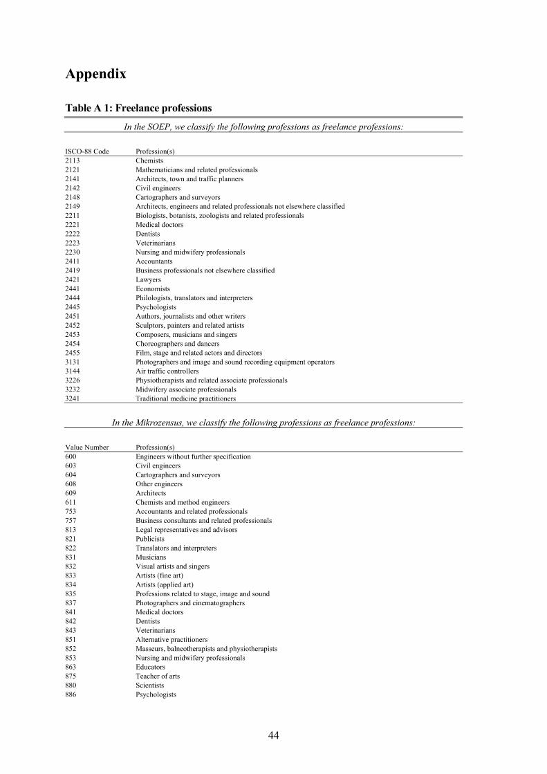
Appendix Table A 1: Freelance professions

In the SOEP, we classify the following professions as freelance professions: ISCO-88 Code Profession(s) 2113 Chemists 2121 Mathematicians and related professionals 2141 Architects, town and traffic planners 2142 Civil engineers 2148 Cartographers and surveyors 2149 Architects, engineers and related professionals not elsewhere classified 2211 Biologists, botanists, zoologists and related professionals 2221 Medical doctors 2222 Dentists 2223 Veterinarians 2230 Nursing and midwifery professionals 2411 Accountants 2419 Business professionals not elsewhere classified 2421 Lawyers 2441 Economists 2444 Philologists, translators and interpreters 2445 Psychologists 2451 Authors, journalists and other writers 2452 Sculptors, painters and related artists 2453 Composers, musicians and singers 2454 Choreographers and dancers 2455 Film, stage and related actors and directors 3131 Photographers and image and sound recording equipment operators 3144 Air traffic controllers 3226 Physiotherapists and related associate professionals 3232 Midwifery associate professionals 3241 Traditional medicine practitioners

In the Mikrozensus, we classify the following professions as freelance professions: Value Number Profession(s) 600 Engineers without further specification 603 Civil engineers 604 Cartographers and surveyors 608 Other engineers 609 Architects 611 Chemists and method engineers 753 Accountants and related professionals 757 Business consultants and related professionals 813 Legal representatives and advisors 821 Publicists 822 Translators and interpreters 831 Musicians 832 Visual artists and singers 833 Artists (fine art) 834 Artists (applied art) 835 Professions related to stage, image and sound 837 Photographers and cinematographers 841 Medical doctors 842 Dentists 843 Veterinarians 851 Alternative practitioners 852 Masseurs, balneotherapists and physiotherapists 853 Nursing and midwifery professionals 863 Educators 875 Teacher of arts 880 Scientists 886 Psychologists

44

Table A 2: Definition of variables (SOEP) Variable Definition

DDD variables: a Dummy for individuals classified as a potential tradesman in t b Dummy for years after the 1994 reform and before the 1999 reform c d Dummy for years after the 1999 reform e Dummy for individuals whose income in t is above the threshold defined in 1999Other covariates: female Dummy for females east Dummy for individuals who live in one of the 5 new eastern federal states or East

Berlin highschool Dummy for individuals who have a high school degree ("Fachhochschulreife" or

"Abitur") apprenticeship Dummy for individuals who finished an apprenticeship ("Lehre") highertechnical Dummy for individuals who finished a higher technichal college or similar

("Berufsschule", "Schule Gesundheitswesen", "Fachschule", "Meister", "Beamtenausbildung", or "Sonstige Ausbildung")

university Dummy for individuals who have a university degree age Age of individual agesqr Age squared ftexp10 Years of full time work experience. Uses information from the lifetime

empoyment history in the SOEP (see text for details). Divided by 10. ftexpsq100 Fill time work experience squared and divided by 100 ptexp10 Years of part time work experience. Uses information from the lifetime

empoyment history in the SOEP (see text for details). Divided by 10. ptexpsq100 Part time work experience squared and divided by 100 unemexp10 Years of unemployement experience. Uses information from the lifetime

empoyment history in the SOEP (see text for details). Divided by 10. unemexpsq100 Unemployment experience squared and divided by 100 disabled Dummy for handicapped / physically challenged individuals german Dummy for German nationality nchild Number of children under 17 in the household married Dummy for married and not separated individuals. Omitted category for marital

status is "single"/"widowed". separated Dummy for married, but separated individuals divorced Dummy for divorced individuals fatherse Dummy for individuals whose father is/was self-employed empl Entry model: Dummy for individuals who are employed in t

Self-employment state model: Dummy for individuals who were employed in t-1selfemplpy Dummy for individuals who were self-employed in t-1 duration Duration of current spell (self-employment or employment). Uses information

from lifetime job biography in the SOEP (see text for details). dur_sq Square of duration variable dur_p3 Duration variable to the power of 3 dur_e Interaction variable of duration and empl dur_sq_e Interaction variable of dur_sq and empl dur_p3_e Interaction variable of dur_p3_e and empl Dummy variables are equal to one if condition holds and zero otherwise.

Dummy for individuals whose income in t is above the threshold defined in 1994

45

46

Table A 3: Definition of variables (Mikrozensus, if different from SOEP)

Variable Definition Highest school leaving degree achieved schoolna Dummy for no information, or not applicable gymnasium Dummy for individuals with university entrance diploma ("Fachabitur" or

"Abitur") realschule Qualification for entrance in advanced technical college ("Allg. polytech.

Oberschulabschluss (ehem. DDR)", "Realschulabschluss", or "Fachhochschulreife")

hauptschule Dummy for individuals with other high school diploma ("Hauptschulabschluss" or "Volksschulabschluss"). Omitted category for school leaving degree.

Highest professional qualification qualifna Dummy for no information, or not applicable mastercraft Dummy for master craftsmen and technicians ("Meister", "Techniker") advtechncol Dummy for individuals who graduated from an advanced technichal college

("Fachhochschulabschuss") university Dummy for individuals who graduated from a university apprenticeship Dummy for individuals who finished an apprenticeship ("Anlernausbildung",

"Lehrausbildung", or "Fachschule ehem. DDR"). Omitted category for professional qualification.

Employment status of spouse spouseworkna Dummy for no information, or not applicable spouseworking Dummy for individuals whose spouse is working spsnotworking Dummy for individuals whose spouse is not working. Omitted category for

employment status of spouse. Employment status in previous year emplstatepyna Dummy for no information, or not applicable selfemplpy Dummy for individuals who were self-employed in the previous year employedpy Dummy for individuals who were employed in the previous year notemplpy Dummy for individuals who were inactive in the previous year unemplpy Dummy for individuals who were unemployed in the previous year. Omitted

category for employment status in the previous year. City size medcity Dummy for cities between 20,000 and 500,000 inhabitants (previous year) bigcity Dummy for cities with more than 500,000 inhabitants (previous year) village Dummy for cities with up to 20,000 inhabitants (previous year). Omitted

category for city size. east Dummy for individuals who live in one of the 5 new eastern federal states or

Berlin nchild Number of children under 18 in the household married Dummy for married individuals spouseinc1000 Spouse's net income in € 1000 in April (0 if unmarried) otherinc1000 Other net household income in € 1000 in April

(= net household income in April - net individual income in April, if positive) Dummy variables are equal to one if condition holds and zero otherwise.