Income, Psychological Well-being, and the Dynamics of

Poverty∗

M. Alloush†

August 13, 2018

Abstract

Evidence across disciplines suggests that economic well-being affects an individual’s

psychological well-being, and also that psychological disorders can have substantial

negative effects on individual income. Together, these studies suggest a feedback loop

that may trap some in poverty. However, estimating the causal links between income

and psychological well-being is difficult due to this simultaneous causality. In this pa-

per, I overcome this endogeneity with a panel GMM approach to estimate a dynamic

system of equations that identifies both causal links. Using a nationally representative

panel dataset from South Africa, I find evidence of impacts in both directions. The

average effect of changes in psychological well-being on income is mainly driven by a

large effect among those near the threshold for clinical depression. Meanwhile, the

effect of changes in income on psychological well-being is especially pronounced among

the poor, indicating the possibility of a strong feedback loop among an especially vul-

nerable subgroup – the poor with low levels of psychological well-being. An impulse

response function analysis indicates that this bi-directionality can nearly double the

long-term impact of shocks, while simulations show that this relationship can explain

prolonged poverty spells and low resilience to shocks. A formal test for poverty traps

shows that individuals with low levels of psychological well-being exhibit markedly dif-

ferent income dynamics that suggest the existence of a multi-equilibrium poverty trap.

Job Market Paper: Latest version available here.

∗I am grateful for the support and guidance of my advisors Michael Carter, Travis Lybbert, Dalia Ghanem,and Ashish Shenoy throughout this project. This paper has benefited from discussions with Bulat Gafarov,Malcolm Keswell, Michael Gechter, and Takuya Ura among other conference and seminar participants. Ithank Murray Leibbrandt and the team at the South Africa Labor and Development Research Unit for theirhelpful comments and for their commitment to keeping the psychological well-being module in the NationalIncome Dynamics Study of South Africa.†University of California, Davis, Department of Agricultural and Resource Economics. One Shields Ave,

Davis, CA 95616. Email: mmism@ucdavis.edu

1 Introduction

Psychological disorders account for nearly 13% of the overall global disease burden (Collins et

al., 2011). The cross-sectional rate of depression – the most common psychological disorder1

– is estimated to be 4.4% worldwide, and this number is even higher in developing countries

(5.5%). From an economic point of view, psychological well-being is important in part be-

cause it likely exacerbates poverty. However, despite the ubiquity of psychological disorders,

rigorous empirical evidence on their micro-economic consequences is limited, especially in

developing countries. This is, at least partially, due to the difficulty of empirically untangling

the causal relationship between psychological well-being and income. While a change in an

individual’s psychological well-being can influence their earnings, economic well-being likely

plays a significant role in determining their state of mental health. This endogeneity makes

it difficult to pin down estimates of causal links using observational data. In this paper, I fill

this gap by estimating both causal links simultaneously using a panel Generalized Method of

Moments (GMM) approach and a nationally representative dataset from South Africa and

investigating the implications of this relationship on the dynamics of poverty.

The bi-directionality between psychological and economic well-being and its potential

to push some individuals into a vicious cycle of poverty is well established in the psychology

literature. The social drift hypothesis posits that individuals with psychological disorders

are more likely to enter into or remain in poverty due to reduced productivity, loss of earn-

ings, and wasteful spending. At the same time, the social causation hypothesis states that

conditions of poverty increase the risk of mental illness, and affect psychological well-being

through malnutrition, violence, and social exclusion (Lund et al., 2011). However, most

evidence on the causal links between economic and psychological well-being is limited in its

1Depressive disorders are characterized by sadness, feelings of tiredness, loss of interest or pleasure,disturbed sleep or appetite, feelings of guilt or low self-worth, and poor concentration. They can be longlasting or recurrent, substantially impairing an individual’s ability to function at work or school or cope withdaily life. Depressive disorders include two main sub-categories: major depressive disorder/episode, whichinvolves symptoms such as depressed mood, loss of interest and enjoyment, and decreased energy typicallylasting about 6 months; and dysthymia, a persistent or chronic form of mild depression that has similarsymptoms to depressive episode, but tend to be less severe and longer lasting.

1

scope and is based on very narrow subpopulations. Given the prevalence of psychological

disorders around the world, the question as to whether the relationship between income

and psychological well-being poses an impediment for some to achieve their full economic

potential should be of interest to economists and policymakers alike. Understanding this

relationship may allow for more effective poverty-alleviation policy.

In this paper, I overcome the difficulty of identification due to simultaneous causality

by extending panel data methods developed by Arellano and Bond (1991) and developing

a GMM approach to estimate a system of dynamic and simultaneous equations in order

to answer two main questions.2 First, does psychological well-being affect an individual’s

own income? Second, does economic well-being (proxied by income and other variables

such as food expenditure and wealth) play a significant role in determining an individual’s

psychological well-being? The answer I find to both is yes on average but with significant

heterogeneity.

A closer analysis shows that changes in the low end of the Center for Epidemiologic

Studies Depression (CES-D) scale do not seem to affect income;3 however, near the threshold

used by psychologists to screen for depression, I find large effects on individual income. The

estimates predict that a 1 standard deviation (SD) increase in the CES-D score (increase

in depressive symptoms) decreases income by nearly 23% for the average individual. More-

over, the results suggest that one possible avenue through which this occurs is a decreased

likelihood of being economically active. Turning to the opposite direction of causality, I find

that a 10% increase in household income per capita reduces an individual’s CES-D score

2I develop this approach based on methods by Anderson & Hsiao (1981) and Arellano & Bond (1991)and show that a system of dynamic and simultaneous equations can be estimated with at least four roundsof data (proof and simulations are available in the Appendix). While this panel GMM approach does notdepend on exogenous shocks to income or psychological well-being, it requires assumptions on the error termsfor the estimates to be consistent. The main specification used assumes no serial correlation in the errors.This rules out correlation in shocks to income and psychological well-being over time after state dependence,individual fixed effects, and other time varying observable characteristics are taken into account. The resultsare robust to the use of a less restrictive specification that allows for first-order serial correlation.

3Low CES-D scores indicate fewer depressive symptoms and can be viewed as high levels of psychologicalwell-being.

2

by 0.2 points (0.05 SD) on average.4 I also find similar statistically significant estimates

when using other measures of economic well-being, namely, food expenditure per capita and

a household wealth index. Investigating the heterogeneity by baseline income levels I find

that this impact is larger among the poor.

These results indicate that income and psychological well-being are intertwined and

that a particularly vulnerable group, namely the poor with low levels of psychological well-

being, may be disproportionately affected by shocks. An impulse response function analysis

shows that this relationship can nearly double the long-term overall impact of shocks to

either income or psychological well-being on average. Furthermore, simulations using the

estimated system of dynamic equations shows that this feedback loop can explain prolonged

poverty spells and low resilience. This should inform policymakers about the potentially

large impacts of negative income shocks on an especially vulnerable group. Formal tests

do not detect a poverty trap among the whole sample, but when restricting the sample to

individuals who exhibit low levels of psychological well-being, the income dynamics look

markedly different and suggest the existence of a multi-equilibrium poverty trap.

One of the main contributions of this paper is estimating the impact of psychological

well-being and depression on income. Only a handful of studies measure the causal effects of

mental health on employment and income in an empirically robust manner among represen-

tative populations. The existing evidence shows that decreased mental health significantly

reduces the likelihood of employment (Chatterji, Alegria, & Takeuchi, 2011; Frijters, John-

ston, & Shields, 2014; Peng, Meyerhoefer, & Zuvekas, 2015). Furthermore, experimental

studies in the psychology and medical literature show that among those already suffering

from depression who have sought treatment, interventions such as therapy and antidepres-

sants positively influence several economic outcomes such as increased labor force participa-

tion at the extensive and intensive margins (Bolton et al., 2003; Ran et al., 2003). This paper

4Back-of-the-envelope calculations suggest that the estimated magnitude of the effect of changes in house-hold income is similar to the effect of cash transfers experimentally estimated by Haushofer and Shapiro(2016).

3

adds to this literature by estimating the effects of changes in psychological well-being on in-

come in a nationally representative sample in a developing country while also demonstrating

the nonlinearity of these effects.

This analysis also adds to a growing literature on the impact of income on psychological

well-being.5 Recent empirical evidence based mainly on exogenous income shocks finds that

higher income improves psychological well-being (Frijters, Haisken-DeNew, & Shields, 2004,

2005; Gardner & Oswald, 2007; Haushofer & Shapiro, 2016; McInerney, Mellor, & Nicholas,

2013). My work adds to this literature by using an econometric approach that is not based

on shocks and estimates the effect of changes in income, some of which may be earned. More

broadly, this paper contributes to a growing field aimed at understanding the multitude of

stresses faced in poverty. The psychological consequences of poverty are gaining increased

attention among behavioral economists investigating the mechanisms through which poverty

can affect economic decision-making (Mani, Mullainathan, Shafir, & Zhao, 2013; Schilbach,

2015; Schilbach, Schofield, & Mullainathan, 2016). It is likely that one avenue through

which this may occur is lower levels of mental health (Haushofer & Fehr, 2014). Specifically

relevant to this paper is the theoretical work by De Quidt and Haushofer (2016) which shows

the potential negative effects depression can have on labor supply. My paper adds to this

field by empirically estimating both causal links–that of psychological well-being on income

and the effect of income on psychological well-being–and exploring the implications of this

bi-directional relationship on poverty dynamics.

While the results do mainly stress the potential negative consequences of the rela-

tionship between poverty and psychological well-being, there is a positive story to tell.

Poverty-alleviation programs may have an added benefit of positive impacts on psychological

5It is important to differentiate between psychological well-being and subjective well-being which is thesubject of many different studies over the years (see for example Clark, D’Ambrosio, and Ghislandi (2013);Graham and Pettinato (2002); Kahneman and Deaton (2010); Stevenson and Wolfers (2013); Winkelmannand Winkelmann (1998)). In this paper, the CES-D scale measures psychological well-being and I contrastmy results with results from another working paper using questions on life satisfaction and happiness whichmeasure subjective well-being (Alloush, 2018). The estimates of the impact of changes in income on thesemeasures are different in meaningful ways which suggests that the measures – despite being correlated –capture different states of well-being.

4

well-being, which is an important goal in itself, and moreover may enhance an individual’s

capability to further increase their economic well-being. In this sense, psychological well-

being is both a constitutive freedom and an instrumental one (Sen, 1999). Thus, the results

in this paper suggest that psychological well-being is an important dimension of poverty that

may explain some of the persistence of poverty and low resilience. It reaffirms the conclu-

sion of Haushofer and Fehr (2014) that stresses the importance of considering psychological

variables as avenues for novelty in poverty-alleviation programs. The estimates in this paper

suggest that exogenously lowering depressive symptoms among the vulnerable group identi-

fied above6 by 1 SD would decrease extreme poverty rates in South Africa by 5 percentage

points (from 21%).

The rest of this paper is structured as follows. Section 2 discusses psychological well-

being and depression, their economic relevance, and measurement. In Section 3, I introduce

the dataset and highlight relevant descriptive statistics. Section 4 outlines the main empirical

strategy and the key assumptions required for consistency, and Section 5 presents the results.

Section 6 discusses some implications for poverty dynamics using impulse response function

analysis, simulations, and a test for poverty traps. Section 7 concludes.

2 Psychological Well-being and Depression

In this paper, I use the Center for Epidemiologic Studies Depression (CES-D) scale as a

measure of psychological well-being. While this scale can be used as a continuum that

proxies for psychological well-being Siddaway, Wood, and Taylor (2017), a high score on the

continuum identifies individuals who are likely suffering from depression, the most common

psychological disorder. In this section, I present some of the evidence on the connection

between depression and economic well-being in both the psychology and economics literature

and I further discuss the CES-D scale.

6The poor with low levels of psychological well-being.

5

2.1 Significance

It is estimated that nearly 4.4% of the world’s population suffers from depression at any point

in time and improved measurement in recent years has suggested that it is the leading cause

of disability worldwide and contributes to nearly 14% of the global disease burden (Collins

et al., 2011; Friedrich, 2017). A major depressive episode (MDE) is often debilitating to an

individual, and its impact can be substantial. It is associated with diminished quality of life,

significant functional impairment, and higher risk of mortality (Hays, Wells, Sherbourne,

Rogers, & Spritzer, 1995; Spijker et al., 2004). Reduced functioning in occupational and

social roles is pervasive among those suffering from depression, and studies find that these

disabilities decrease if depressive symptoms are alleviated but are chronic if depressive symp-

toms persist (Ormel, Oldehinkel, Brilman, & Brink, 1993).7 While some of these effects may

be experienced with gradual increases in depressive symptoms, the impacts are especially

pronounced with the onset of an MDE and continue to worsen with the severity of depression

(Siddaway et al., 2017; Spijker et al., 2004).8

Prominent psychiatrist Aaron Beck’s (1967) exposition on depression provides a de-

tailed analysis of the symptoms and behavioral changes associated with depression. De

Quidt and Haushofer (2016) summarize Beck’s seminal work on depression and highlight

ways in which several different symptoms and consequences of depression could be of in-

terest to economists. An MDE can affect individuals in various ways including effectively

altering elements of an individual’s economic decision-making process. In brief, depression

is associated with negative expectations and low self-evaluation, indecisiveness and paralysis

of the will, withdrawal and rumination, as well as fatigue and reduced gratification. There

is an extensive literature in psychology illustrating the effect of depression on preferences,

perception, and cognitive and executive functioning.9 De Quidt and Haushofer (2016) show,

7While the impacts of some psychological disorders have been shown to differ across cultures, the findingson depression show consistency across many different contexts (Ormel et al., 1994).

8The functional impairments associated with an MDE are likely to affect an individual’s earnings, however,these causal effects have not been well estimated in the general population.

9For example lower levels of mental well-being show reduced responsiveness to reward and an increased

6

using a theoretical model, how an altered self-evaluation could adversely affect labor supply.

It is possible and likely that depression – through its many symptoms – can have a substan-

tial impact on one’s economic decision-making and consequent outcomes. This paper shows,

in reduced form, how changes in depressive symptoms affect an individual’s income.

2.2 Economics and Depression

Experimental evidence in psychology and medicine have shown that among a sample of indi-

viduals diagnosed with depression, decreasing depressive symptoms through therapy and/or

antidepressants significantly improves several economic outcomes including employment at

the intensive and extensive margins (Bolton et al., 2003; Ran et al., 2003). These studies

involve samples that are not random: specifically, it involves patients who are suffering from

depression and sought treatment. In economics, studies that look at the impact of psy-

chological well-being on economic outcomes are rare; however, recent work uses exogenous

negative shocks to psychological well-being (using death of friends as an instrumental vari-

able) to show significant negative impacts on employment (Frijters et al., 2014). Using panel

data from Australia, the authors find that, among adults, a one standard deviation decrease

in mental health decreased the likelihood of employment by 30%.

Recent interest in economics has mainly focused on the reverse causal link, the effect

of income and poverty on mental health. Several studies use exogenous shocks to income to

show that income does affect mental health (Frijters et al., 2004, 2005; Gardner & Oswald,

2007). For example, Gardner and Oswald (2007) compare British lottery players to a control

group of other lottery players and find that those who win the lottery show higher levels of

psychological well-being. In recent work, changes in wealth due to the great recession are

negative evaluation of self (Harvey et al., 2004; Snyder, 2013). Moreover, depressive symptoms are associatedwith altered decision-making: individuals choose fewer advantageous options in economic games, are morerisk averse (Smoski et al., 2008), and are less flexible in their choices (Cella, Dymond, & Cooper, 2010).Other studies find that depression is generally associated with impaired decision-making ability and moresuboptimal decisions than those in the control groups (Murphy et al., 2001; Yechiam, Busemeyer, & Stout,2004). Depressive symptoms are shown to be associated with lower cognitive functioning (Hubbard et al.,2016).

7

shown to affect the likelihood of depression (McInerney et al., 2013).10

Recent experimental studies on the impact of cash transfers have increasingly focused

on the potential psychological benefits of these transfers. In a recent paper, Haushofer and

Shapiro (2016) find that large once-off cash transfers to poor households in Kenya reduced

stress by 0.26 SD and decreased depressive symptoms – measured by a 1.2-point reduction

in the CES-D 20 scale.11 Furthermore, Banerjee et al. (2015), in a multi-country study, find

that a multi-faceted poverty graduation program improved mental health by 0.1 SD.12 The

authors find that these effects are sustained two years after the program. Other experimental

and quasi-experimental studies suggest that cash transfer programs reduce the incidence of

depression among beneficiaries (Macours, Schady, & Vakis, 2012; Ozer, Fernald, Weber,

Flynn, & VanderWeele, 2011).

There is a clear pattern in these studies: income does affect psychological well-being.

However, it would be a stretch to generalize these results to speak about the impacts of

naturally occurring changes in income, some of which may be earned, on psychological well-

being. Many of the causal estimates are driven by either shocks or unearned cash inflow

(such as lotteries). Moreover, cash transfers mainly target the poor and thus impacts of

these programs cannot necessarily be generalized to be the impact of income on mental

health in the general population. This paper adds to the literature by estimating both

relationships using nationally representative data from a developing country.

2.3 CES-D

The measure of psychological well-being used in this paper is the 10-item Center for Epi-

demiologic Studies Depression (CES-D) scale. The CES-D scale was developed for use in

10Related research on the consequences of unemployment shows that unemployment due to plant closuresdecreased levels of mental health of both the unemployed and his/her spouse (Fasani, Farre, & Mueller,2015; Marcus, 2013).

11The CES-D scale in Haushofer and Shapiro (2016) is the CES-D 20 scale which is the original longerversion of the CES-D 10 that is used in this paper. I discuss the comparability of two scales in Section 2.3.

12The index of mental health used by these authors includes CES-D scores. It is important to note thatthese programs involve more than just a transfer of income or assets and thus the effects on psychologicalwell-being cannot be attributed only to increases in income.

8

studies to assess depressive symptoms and screen for depression in the general population

(Radloff, 1977). It is widely-used to measure depressive symptoms (Santor, Gregus, & Welch,

2006), and in its original format it contains 20 questions that ask individuals how often in

the last week they felt certain emotions related to depression and are scored accordingly. For

negative feelings such as how often an individual felt loneliness or an inability to get going,

the respondent gets a 0 score if they respond with “Not at all or rarely,” 1 for “Some or little

of the time,” 2 for “Occasionally,” and 3 for “All the time.” For positive statements such as

“feeling hopeful,” the scores are reversed. The answer numbers are then added for all the

questions to get an overall CES-D score with a range of 0 to 60.13 A higher overall CES-D

score indicates that one is experiencing more pronounced depressive symptoms. Analysis of

the shortened 10-item CES-D scale attained satisfactory prediction accuracy and reliability

in assessing significant depressive symptoms and correlate very highly with the full 20-item

questionnaire (Zhang et al., 2012). Furthermore, the CES-D scale is shown to be reliable

and stable over short periods of time (Gonzalez et al., 2017; Saylor, Edwards, & McIntosh,

1987).

While CES-D was developed to screen for depression, it is often viewed as a continuum

of psychological well-being (Siddaway et al., 2017; Wood, Taylor, & Joseph, 2010). However,

scores beyond certain thresholds indicate that an individual may be suffering from depression.

In the 10-item CES-D used in this paper, a score of 10 or more is the threshold that is usually

used. This suggests that when considering the impact of decreased psychological well-being,

the effects may be nonlinear and especially pronounced around this threshold.

It is important to consider whether the CES-D is valid in South Africa as a measure of

psychological well-being. Language and culture likely affect the way questions are understood

and answered (Samuels & Stavropoulou, 2016). However, the CES-D 10 is widely used in

South Africa and has been verified for use as an effective initial screening tool by several

different studies (Hamad, Fernald, Karlan, & Zinman, 2008; Johnes & Johnes, 2004; Myer

13The range is 0 to 30 for the CES-D 10 used in the paper.

9

et al., 2008). In addition, Hamad et al. (2008) found that the CES-D scale is internally

consistent in South Africa. A recent study by Baron, Davies, and Lund (2017) suggests that

11 may be a more appropriate threshold to screen for depression using the CES-D 10 among

most populations in South Africa.

Another characteristic of CES-D that makes it useful is that its questions do not

explicitly mention psychiatric illnesses. This helps mitigate the effect of stigma on the

quality of data. Mental illnesses are highly stigmatized in South African communities (Hugo,

Boshoff, Traut, Zungu-Dirwayi, & Stein, 2003), and this is evident in the data where the

rate of response when asked about specific mental illnesses are extremely low. On the other

hand, response rate on the CES-D section is high where on average 89% of individuals across

all four waves answer all 10 questions.

I use the CES-D scale as the main measure of psychological well-being throughout this

paper, which facilitates comparison with other literature on mental health and depression.

The next section presents the source of the data and presents some descriptive statistics and

highlights key correlations with CES-D.

3 Data and Descriptive Statistics

3.1 Data

The data used in this analysis come from the South Africa National Income Dynamics Study

(NIDS), a panel survey conducted by the South Africa Labor and Development Research

Unit at the University of Cape Town. The first survey wave of this study was conducted

in 2008 with households interviewed every two years since then. The survey study began

with a nationally representative sample of over 28,000 individuals (17,000 adults) in 7,300

households. Data is collected on many socio-economic variables that include expenditure,

labor market participation and economic activity, fertility and mortality, migrations, in-

come, education, and anthropometric measures. The data are publicly available and can be

10

downloaded from the NIDS website.14

I use data from all four available waves of the NIDS. I restrict the sample to adults

who completed the adult questionnaire in all four waves (years 2008, 2010, 2012, and 2014)

which effectively includes only those who were at least 16 years old in the first wave. The

resulting sample size is 6,975 individuals. Table 1 presents some descriptive statistics of the

this sample: it is slightly poorer on average and a larger share is female than the nationally

representative fourth wave sample of NIDS.15

The NIDS dataset contains detailed information on household income and expendi-

ture in addition to individual income. While I mainly choose to use household income per

capita throughout the analysis, I also use food expenditure per capita and a wealth index

as measures of economic well-being to test the robustness of the results. On the other hand,

when estimating the effect of mental well-being on income, I use an individual’s own income

as the dependent variable as an individual’s mental well-being may influence her own income

more directly than household-level measures of income.16

Most importantly to this analysis, NIDS contains the 10-item Center for the Epidemi-

ological Studies Depression (CES-D) Scale. This is unprecedented in a nationally represen-

tative panel survey in a developing country.

3.2 Descriptive Statistics

South Africa is a middle-income country with one of the highest levels of income inequality

in the world. Recent reports estimate that nearly 54% of the population is living in poverty

and about 20% live in extreme poverty (Leibbrandt, Finn, & Woolard, 2012). The mean

household income per capita (standard deviation in brackets) has increased from 1,672 ZAR

14Website can be found at http://www.nids.uct.ac.za/15Comparing means and variances for key variables across those who completed the individual question-

naire in all four waves and those who did not (and consequently were not in the sample used in this analysis)showed to discernible differences.

16For both measures of income, extreme changes in both household and individual income suggest mis-measurement or very unusual cases. I trim the sample of the top and bottom 0.5% of changes in householdincome and individual income. Results are robust to trimming the top 1,2.5, and 5% instead.

11

(3,314) to 2,242 ZAR (2,934) in 2014.17 In the sample used in this analysis, the mean CES-D

score (standard deviation in brackets) for the four waves starting in 2008 is 8.17 (4.39), 7.13

(4.18), 7.16 (4.35), 6.95 (4.20). There seems to be a downward trend in the average CES-D

score. The incidence of scores above 10 show a similar pattern and decrease from about 35%

in 2008 to 25% in 2014. Figure 1 shows histograms of the CES-D scores in 2014 (top left)

and 2012 (top right) and the changes in CES-D between 2012 and 2014 (bottom left). While

the changes for the whole sample are centered around 0, the changes for those with scores

in wave three that are eight and above are centered below zero. However, it is clear that

a significant portion of this sub-sample experiences increases in their CES-D scores despite

already having high scores.

Figure 2 graphs average CES-D score among income per capita and expenditure per

capita deciles for all four waves. It is clear from the figure that the average CES-D scale

decreases among those in higher income and expenditure deciles. These figures illustrate

correlation, but are not causal. The next section outlines the empirical strategy to estimate

the causal relationships between income and CES-D.

4 System of Equations and Estimation Strategy

The main source of endogeneity when studying the relationship between mental health and

income is reverse causality. Psychological well-being has an impact on an individual’s own

earnings, but at the same time, income or the level of economic well-being affects their

psychological well-being. Conceptually, the relationship between income and psychological

well-being can be described using a system of simultaneous equations. To simplify, I assume

that household income per capita is a proxy for economic well-being and plays a role in

determining psychological well-being, whereas an individual’s psychological well-being affects

their own personal earnings. That only household income per capita affects psychological

well-being and not own income is an assumption that I make throughout the analysis in this

17Income and expenditure numbers are adjusted for inflation and are in November 2014 prices.

12

paper.18 I represent the relationship between income and psychological well-being with the

following system of equations:

yi,t = f(Di,t, yi,t−1,xi,t) + νi + ei,t

Di,t = g(hi,t, Di,t−1,xi,t) + ρi + ui,t

where yi,t is individual income, Di,t is a measure of psychological well-being, and hi,t is

household income per capita for individual i in time t which is a function of an individual’s

income.19 In this analysis I consider only linear specifications for f(.) and g(.); νi and ρi are

individual fixed effects; and ei,t and ui,t are the unobserved error terms for their respective

equations. xi,t is a vector of time varying individual characteristics for individual i at time

t. While the focus of this paper is not on the dynamics of income and psychological well-

being, I allow for state dependence in the underlying process by having lagged levels of

personal income (yi,t−1) and psychological well-being (Di,t−1) as explanatory variables in the

equations.

To outline and justify my estimation strategy, I present a simple linear form of the

above system of equations:

yi,t = β0 + α1Di,t + β1yi,t−1 + Γxi,t + νi + ei,t

Di,t = b0 + a1hi,t + b1Di,t−1 + Θxi,t + ρi + ui,t

To control for the individual fixed effects vi and ρi that might be important determinants of

both income and psychological well-being, I use the first-differenced version of both equations

18This assumption is nontrivial. However, the results in Appendix C (Table A5) suggest that the datadoes not contradict this assumption. Including both individual income and household income per capitaas regressors for psychological well-being yields statistically insignificant results for individual income, evenwhen the sample is restricted to economically active individuals. This is also the case when using otherproxies for economic well-being such as food expenditure and a wealth index.

19This can be represented with a third equation hi,t = k(yi,t, Xi,t) + θi + εi,t, where k(.) is an unknownfunction, θi is an individual fixed effect and εi,t is an unobserved error term. I do not estimate this equationas it is outside of the scope of this analysis.

13

which results in the following:

∆yi,t = α1∆Di,t + β1∆yi,t−1 + Γ∆xi,t + ∆ei,t (1)

∆Di,t = a1∆hi,t + b1∆Di,t−1 + Θ∆xi,t + ∆ui,t (2)

In this system of equations, I am interested in estimating the coefficients of four en-

dogenous variables, namely α1, β1, a1, and b1. By considering each single equation separately,

panel data methods suggests that, assuming ei,t and ui,t are serially uncorrelated, the lagged

levels yi,t−2, yi,t−3, ... and Di,t−2, Di,t−3, ... may be used as instruments to estimate the param-

eters of the equation (1), while hi,t−2, hi,t−3, ... and Di,t−2, Di,t−3, ... may be used to estimate

equation (2).

I extend this panel data method to estimate a system of simultaneous equations. I

show below that the assumptions on ei,t and ui,t required for consistent estimation of the

coefficients with four waves of panel data can be weaker than the sequential exogeneity often

assumed when using lagged levels as instruments for first differences (Arellano & Bond, 1991;

Bond, 2002). To estimate the above system of equations, and given that the NIDS dataset

has four waves of data, I first use the following instruments matrix:

ZAi,t =

Di,t−2 Di,t−3 yi,t−3 0 0 0

0 0 0 Di,t−3 hi,t−2 hi,t−3

=

z1i,t′ 0

0 z2i,t′

where z1i,t =

(Di,t−2 Di,t−3 yi,t−3

)– the vector of instruments for equation (1) – and

z2i,t =

(Di,t−3 hi,t−2 hi,t−3

)– the vector of instruments for equation (2). The assumptions

required for matrix ZAi,t to provide moment conditions to consistently estimate the system of

equations are:

E [ei,t | yi,t−2, yi,t−3, . . . ;Di,t−1, Di,t−2, . . . ;xi,t,xi,t−1, . . . ] = 0 (A1)

14

and

E [ui,t | hi,t−1, hi,t−2, . . . ;Di,t−2, Di,t−3, . . . ;xi,t,xi,t−1, . . . ] = 0 (A2)

Proposition. If assumptions A1 and A2 hold, then the matrix of instruments ZAi,t implies

moment conditions that identify the coefficients of the system of equations (equations (1) and

(2)).

The proof is straightforward and shown in Appendix A. Provided A1 and A2 hold, the

matrix of instruments ZAi,t implies the following moment conditions:

E(ZA

i,t′Ui,t

)= 0

Simulation results verify that under an error structure that satisfies assumptions A, using a

two-step GMM and instruments matrix ZAi,t leads to consistent estimates of the coefficients

α1, β1, a1, and b1.20

For A1 and A2 to hold, the error term of each equation may not be correlated with

t− 2 lagged values of its own dependent variable and t− 1 lagged values of the simultaneous

variable. However, the simultaneity of the equations inherently implies that both error

terms cannot be serially correlated. After controlling for state dependence (through the

lagged dependent), individual fixed effects, and observable time varying characteristics, the

remaining unobserved errors may not be correlated across time.21 The time between waves

in the NIDS dataset is two years which makes this assumption more plausible. Simulations

illustrate the bias that first order serial correlation in each of the error terms would cause.

It is worth noting that the bias caused by serial correlation in the error terms is evident only

when there is simultaneity in the model; when there are no effects that leads to simultaneity

(α1 and a1 are equal to zero), the specification will consistently estimate these coefficients

20Simulation results are available in Appendix B21Effectively, this assumption means that a shock to income in one period can affect income next period

through state dependence, but it cannot affect the likelihood of shocks in the next period. Similarly forshocks to psychological well-being.

15

to be zero.22

Throughout the rest of the paper, the main results are based on the assumption that

A1 and A2 hold. I refer to these as set of assumptions A. I also present results that I estimate

using the moment conditions implied by the following instruments matrix:

ZBi,t =

Di,t−3 yi,t−3 0 0

0 0 Di,t−3 Yi,t−3

The following less restrictive set of assumptions – which I refer to as assumptions B – are

required for ZBi,t to imply the moment conditions E

(ZB

i,t′Ui,t

)= 0:

E [ei,t | yi,t−2, yi,t−3, . . . ;Di,t−2, Di,t−3, . . . ;xi,t,xi,t−1, . . . ] = 0 (B1)

and

E [ui,t | Yi,t−2, Yi,t−3, . . . ;Di,t−2, Di,t−3, . . . ;xi,t,xi,t−1, . . . ] = 0 (B2)

Proposition. If assumptions B1 and B2 hold, then the matrix of instruments ZBi,t implies

moment conditions that identify the coefficients of the system of equations (equations (1) and

(2)). In addition, ZBi,t also provides moment conditions to identify the coefficients under the

more restrictive set of assumptions A.

The proof is shown in Appendix A and follows the same logic as the proof for ZAi,t.

Removing the lagged t − 2 level variables from the matrix of instruments allows for less

restrictive assumptions on the error terms. In addition, a matrix of instruments that provides

consistent estimates under less restrictive assumptions on the error terms will also do so under

more restrictive assumptions.

Under B1 and B2, the error terms may be serially correlated across one time period.

Assuming income shocks to be correlated over one time period is common in the literature on

income dynamics and state dependence of income and employment (Guvenen, 2007; Magnac,

22This can be seen in simulation results shown in Appendix B Table A2 and A3.

16

2000; Meghir & Pistaferri, 2004).23 Moreover, the error terms ei,t and ui,t may be correlated

with ui,t−1 and ei,t−1, respectively. Throughout the results section below, I show, where

appropriate, estimates based on both set of assumptions A and B. The estimates do not

differ significantly throughout and the results from assumptions B indicate that the main

results are robust to less restrictive assumptions. A Hausman-type test does not reject

that the estimates using the two instruments matrices are the same.24 This suggests, albeit

indirectly, that the error terms are not strongly serially correlated. Although the dataset has

four waves of data, after taking the first difference and using lagged levels t− 2 and t− 3 as

instruments, I effectively have one observation per individual. Thus, I cannot directly test

for serial correlation. However, when using ZAi,t, if a test of overidentifying restrictions rejects

the validity of the instruments, it would be another indirect evidence of serial correlation;

the validity of the instruments is not rejected in any of the results presented in the rest of

the paper.

5 Results

5.1 System GMM

In Section 4, I consider a simple linear version of the system of equations to illustrate the

estimation strategy. The results presented in the rest of the paper are mainly estimates of

the following more flexible system of equations:25

∆yi,t = α1∆Di,t + β1∆yi,t−1 + Γ∆xi,t + ∆ei,t (3)

23The time periods considered are often of higher frequency. The time between each wave in this paper istwo years – and income is reported for the past month – making serial correlation less likely.

24Neither regression gives results that can be realistically described as fully efficient, thus when testing forthe statistical significance of the difference of the estimates (A Hausman-type test), I estimate variance ofthe difference using a bootstrap.

25With this system of equations I add a quadratic term of hi,t. Intuitively, changes in income may affectpsychological well-being at a decreasing rate. The assumptions required for validity do not change. I addquadratic terms of the instrumental variables to the instrument vectors. The results are robust to higherorder specifications.

17

∆Di,t = a1∆hi,t + a2∆h2i,t + b1∆Di,t−1 + Θ∆xi,t + ∆ui,t (4)

I estimate the above system of equation with the following instruments matrix:

ZAi,t =

Di,t−2 Di,t−3 yi,t−3 hi,t−3 0 0 0 0 0

0 0 0 0 Di,t−3 hi,t−2 h2i,t−2 hi,t−3 h2i,t−3

The two-step GMM results for the whole sample are shown in Table 2. The results in column

1 show that changes in CES-D do not, on average affect, individual income. Changes in

household income per capita, on the other hand, do have a statistically significant impact

on CES-D.

Column 2 shows the estimates using the following instruments matrix:

ZBi,t =

Di,t−3 yi,t−3 hi,t−3 0 0 0

0 0 0 Di,t−3 hi,t−3 h2i,t−3

This instruments matrix requires the less restrictive assumptions B that allow for serial

correlation in the error terms across 1 time period. The results in column 2 show similar

patterns. A Hausman-type test shows that the differences in the estimates in column 1 and

2 are not statistically significant suggesting that there is no serial correlation in the error

terms. In addition, testing for overidentifying restrictions provides Hansen J-test statistics

that do not reject the validity of the instruments. This is the case for all of the GMM results

presented in the rest of the paper. All standard errors shown in the tables are cluster robust

standard errors clustered at the PSU level.26

The system GMM results for the whole sample show a negative yet statistically in-

significant estimate of the effect of CES-D on individual income. In the next section, I

exclude the elderly and explore the nonlinearities suggested in the literature on depression

and CES-D discussed in Section 2.1. On the other hand, the two system GMM results show

26PSUs are defined geographic areas based on the 2001 census in South Africa based on which the samplingfor NIDS took place.

18

similar effects of income on depressive symptoms whereby a ZAR 250 increase in household

income per capita decreases the CES-D scale (lowers depressive symptoms) by about 0.85

points on average.27 The quadratic term is statistically significant suggesting that increases

in income decrease depressive symptoms at a decreasing rate. This side of the simultaneous

equations, the effect of income on psychological well-being, is analyzed in more detail in

Section 5.3.

5.2 The Impact of CES-D on Individual Income

5.2.1 General Results

To further study the effect of depressive symptoms on individual income, I focus specifically

on equation (3) from the system of equations above:

∆yi,t = α1∆Di,t + β1∆yi,t−1 + Γ∆xi,t + ∆ei,t (3)

I restrict the sample to working age adults between ages 22 and 60,28 and I use the same two-

step system GMM as above to estimate the coefficients. Table 3 presents the estimates for

equation (3) using both instruments matrices ZAi,t and ZB

i,t. The difference between column 1

and 2 is the inclusion of the lagged individual income in column 2. The point estimates are

different suggesting that failing to account for the state-dependent nature of income biases

the results. A similar and more stark pattern is evident when using instruments matrix ZBi,t.

The results indicate that, among working age individuals, increases in depressive symptoms

decrease individual income. The magnitude of this effect is large as average monthly income

among employed individuals is ZAR 4,316.29

The psychology literature on the CES-D scale indicates that the score of 10 or above

27Mean and median of household income per capita are ZAR 2,242 and ZAR 1,024, respectively. Thistranslates to USD 199 or USD 418 adjusted for purchasing power. Mean CES-D score is 7.1 and the standarddeviation is 4.2.

28Labor force participation drops sharply to under 20% after age 60.29Overall mean of monthly income among working age individuals is ZAR 2,779.

19

suggests that a person may be suffering from what would be clinically diagnosed as de-

pression. In South Africa specifically, a recent study by Baron et al. (2017) finds that, on

average, a threshold of 11 is more appropriate among the South African population. Changes

within the lower range of the score (0-8) track changes in psychological well-being, but these

changes may not affect an individual’s economic behavior in a meaningful way. While the

CES-D may be viewed as a continuum of psychological well-being (Siddaway et al., 2017;

Wood et al., 2010), the functional impairment and/or other symptoms that could affect an

individual’s income may not be evident until an they are experiencing depression. In the

rest of this section, I analyze the data with the CES-D score of 10-12 in mind as a threshold

where large impacts may be present.

To investigate whether there are significant nonlinearities in the data, I systematically

restrict the sample to individuals who in either wave 3 or 4 (or both) were above a certain

threshold CES-D score. For example, at the threshold of 7, I restrict the sample to contain

only individuals who had a CES-D score of 7 or more in wave 3, wave 4, or both. This

excludes those who did not experience enough psychological distress to attain scores above

the threshold in either waves. Table 4 shows the results for thresholds ranging from 7 to 12.

The results suggest that there may be nonlinearities in the effect of changes in CES-D on

income as the point estimates are larger for individuals who report CES-D scores closer to

the depression thresholds. For those who cross or are always higher than the threshold of 10

or 11, the results predict that a 1-point increase in CES-D score decreases individual income

by ZAR 400-500, more than double the estimated overall affect in Table 3.

To test the robustness of these effects, I split individual income into two categories:

earned income composed of wages, income from day labor and self-employment, and other

income which, in the NIDS sample, constituted mainly income from rent, government grants,

and other forms of assistance. In theory, depression should mainly affect earned income and

should not affect other forms of income. I rerun the same specification from Table 4 and find

that the results for earned income, presented graphically in Figure 3, mirror the results for

20

individual income in Table 4. On the other hand, the estimates for other income are small

and statistically insignificant indicating that changes in CES-D do not, as suspected, affect

other income.

5.2.2 The Marginal Effect Curve

The regressions and figure above indicate the existence of nonlinearity in the marginal effect

of CES-D on income. A 1-point change in the CES-D score when an individual has CES-D

score of 3 may be different from when the baseline CES-D score is 9, for example. To capture

this heterogeneity and estimate the marginal effect at each baseline CES-D score, an ideal

dataset would have a very large number of observations at each baseline (wave 3) CES-D

score and all individuals would experience a change of 1 or -1 in their CES-D score between

waves 3 and 4. Applying the same specification as above for all the individuals for a sample

restricted to individuals at each baseline CES-D score would estimate the marginal effect

of CES-D on individual income at each CES-D score.30 Applying this exactly in the NIDS

dataset leads to very small sample sizes. However, increasing the bandwidth to 1 in local

linear regression terms,31 and restricting the sample to individuals who experience changes

less than or equal to the absolute value of 4 in their CES-D score between wave 3 and 4

(instead of 1)32 gives sample sizes that allow me to estimate the marginal effects. I view

this estimation approach as a type of local linear regression adapted to a first differenced

equation with a discrete variable.

The results of this estimation method are illustrated in Figure 4. While psychologists

offer a clear hypothesis that changes in CES-D matter mainly in the region around the score

of 10, I present a conservative Bonferroni corrected confidence interval to control for the

30This implicitly assumes that individuals at different levels of baseline CES-D are identical on all char-acteristics except baseline CES-D score and income.

31In this discrete variable case, when estimating the marginal effect at CES-D = 5 in wave 3, I wouldinclude individuals who have CES-D of 4,5, or 6 in wave 3. Observations where baseline CES-D3 = j ± 1were weighted at 1/3 that of j. The results are robust to a range of different weighting specifications.

32Results (in Appendix C Table A6) in which the sample is restricted to individuals who experience smallerand larger changes (3 and 5) exhibit a similar pattern around the threshold of 10, but have slightly differentpoint estimates.

21

family-wise error rate (in red).33 The estimates suggest that when an individual is at the

threshold of 10, a 1-point increase in their CES-D score decreases income by 441 ZAR. This

estimate is significant at the 1% level even after a Bonferroni adjustment to the p-value. The

model estimates slightly smaller marginal effects at CES-D scores 11, 12, and 13 that are

statistically significant at the 5% level. Moreover, the largest estimate is at the CES-D score

of 9. The marginal effect of an increase in CES-D of 1 is estimated to -529 ZAR. If I consider

an individual with an average CES-D score of 7 in period 3, an almost 1 SD increase in their

CES-D (4 points) is estimated to decrease their individual income by ZAR 971 or about 0.25

SD on average. The average income for an employed individual with CES-D equal to 7 is

ZAR 4,250; the estimates predict that a 4-point increase in CES-D score would decrease the

individual’s income by nearly 23%.34

While overall changes in CES-D do seem to, on average, affect an individual’s income

in a statistically significant way, the results presented in this section suggest that there

are significant nonlinearities. Depression is increasingly likely among individuals with CES-

D scores of 10 and above. The results above show that for those who experience that

threshold, changes in CES-D score have large impacts on their income; the results suggest

that exogenously decreasing the depressive symptoms of working age individuals with CES-

D greater than or equal to 10 by one standard deviation35 would decrease extreme poverty

rates in South Africa by nearly four percentage points (from 20.8% to 16.9%).

5.2.3 Mechanisms and Other Effects

Table 5 presents results that investigate some of the possible mechanisms through which

changes in CES-D might affect individual income, in addition to other consequences of

increased depressive symptoms. All the results in Table 5 are estimated using a single

33To obtain the point estimates mapped out in Figure 4, I run 13 separate regressions. I update theconfidence intervals to correct for multiple testing.

34Just over 20% of individuals with CES-D scores of 6,7, or 8 in wave 3 experience a change greater thanor equal to 4 between wave 3 and wave 4.

35Interventions such as cognitive behavioral therapy often achieve changes that are larger on average.

22

equation GMM specification for the variable of interest, mi,t, that is similar to the system

specification above. The estimated equation is the following:

∆mi,t = ζ1∆Di,t + ζ2∆mi,t−1 + ζ3∆xi,t + ∆εi,t

using the the instruments vector zmi,t =

(Di,t−2 Di,t−3 mi,t−3

). The estimates in column

1 of Table 5 suggest that one of the likely mechanisms through which an increase in CES-D

decreases income is through decreased labor force participation. The results predict that a

1-point increase in CES-D scale results in a 7.1 percentage-point decrease in the likelihood

of labor force participation. The point estimates for employment (given participation in the

labor force) and for hours worked (given employment) in column 2 and 3, respectively, show

similar negative effects of increases in CES-D.

The results in column 4-6 of Table 5 look at other indirect mechanisms. Estimates

in column 4 show that after controlling for household income and food expenditure, an

increase in CES-D significantly increases the share of expenditure that goes to temptation

goods;36 a 1-point increase in CES-D increases the share of temptation good spending by

0.69 percentage points. Compared to a base level of 4.2%, this means that temptation good

spending increases by nearly 16%. This is in line with the prediction of the theoretical

model of De Quidt and Haushofer (2016) which states that depression would lead to greater

consumption of temptation goods.

Moreover, using a social cohesion index (for individuals) constructed in a manner sim-

ilar to the index constructed by Burns, Njozela, and Shaw (2016) for South Africa (using the

same NIDS data), I find that increases in depressive symptoms as measured by increases in

CES-D scores lower perceptions of social cohesion for an individual in a statistically signifi-

cant way (column 5). This index is constructed using questions about trust, perceptions of

inequality, and fairness; this result suggests that the impact of psychological well-being may

have wide social implications.

36I define cigarettes, alcohol, gambling, and store-bought sweets as temptation goods.

23

Finally, column 6 shows that changes in CES-D change an individual’s perception

about the future. Higher CES-D scores cause lower levels of hopefulness about an individual’s

future income and social status. This finding is expected as low levels of hopefulness and

negative perceptions of the future are symptoms of depression.

Further analysis of these relationships (Figures A2 and A3 in Appendix D) shows that,

while not always statistically significant (possibly due to small sample sizes), the effect of

CES-D on some of these variables exhibits a similar nonlinear pattern to the one on income.

For those who pass or always exceed the threshold of 10, an increase in their CES-D score

decreases the likelihood of being economically active, employment rates, hours worked, and

increases the share of temptation good spending. However, measures of social cohesion and

hopefulness do not seem to exhibit this pattern.

The results from this section show that psychological well-being has important eco-

nomic consequences. For the nearly 30% of the sample with a CES-D score of 9 or above

(as seen in Figure 1), changes in psychological well-being can have a significant economic

impact.

5.3 The Impact of Income on Psychological Well-Being

The results from Section 5.1 show that changes in income affect psychological well-being for

the average individual in the sample. To further explore this impact, I focus on equation (4)

in the system of equations above:

∆Di,t = a1∆hi,t + a1∆h2i,t + b1∆Di,t−1 + Θ∆xi,t + ∆ui,t

When looking at the impact of household income per capita, I use the system esti-

mation strategy used in Section 5.1. For other measures of economic well-being, namely

food expenditure per capita and a household wealth index, I use a similar single equation

estimation strategy and an equivalent vector of instruments to estimate the coefficients of

24

the equation above.37

Table 6 presents the estimates for different variations of equation (4) using two-step

GMM estimation. Columns 1-3 present results for the vector of instruments zAi,t that provides

consistent estimates under assumptions A. The results show that for three different measures

of economic well-being – household income per capita, food expenditure per capita, and a

household wealth index – a change in economic well-being affects the CES-D score in a

statistically significant way. The estimates in column 1 and 4 are the same estimates from

Table 2. The model suggests a decreasing marginal effect of household income per capita

due to the statistically significant quadratic term. Table 8 shows results using the natural

log of household income per capita. The model estimates that a 10% increase in household

income per capita decreases an individual’s CES-D score by 0.206 points.

To test the robustness of these results, I replace household income with other measures

of economic well-being, namely food expenditure and wealth. The results are similar in

signs and statistical significance for both food expenditure per capita and the wealth. The

estimates in Table 6 predict that a ZAR 100 (mean food expenditure per capita is nearly

ZAR 400) decrease in food expenditure increases CES-D score by 0.8 points. Also a large

1-SD increase in wealth measured by the wealth index is predicted to decrease CES-D scores

by near 3.2 points.38

Columns 4-6 show estimates for the econometric specification that requires less re-

strictive assumptions. The results are similar to those in columns 1-3 which demonstrates

that the results are robust to specifications that allow for serial correlation with different

measures of economic well-being.

Intuitively, it seems as though the impact of income on psychological well-being may

37I consider a quadratic specification for impact of food expenditure per capita (fe) on CES-

D, and I use zAfei,t =(fei,t−2 fe2i,t−2 fei,t−3 fe2i,t−3 Di,t−3

)under assumptions A and zBfei,t =(

fei,t−3 fe2i,t−3 Di,t−3)

under assumptions B. When considering the wealth index (w), I use zAwi,t =(wi,t−2 wi,t−3 Di,t−3

)under assumptions A and zBwi,t =

(wi,t−3 Di,t−3

)under assumptions B.

38In another paper that uses the same data and a similar econometric specification and data from severalcountries including South Africa, I find that measures of subjective well-being, namely life satisfaction andreported happiness are positively affected by increases in income.

25

be larger for the poor. To test this, I restrict my sample to the poorest 54% and 20% - which

Leibbrandt et al. (2014) suggest is the poverty and extreme poverty head count percentages

in South Africa. The results in Table 7 clearly show larger point estimates for the poor.

The magnitude of the estimated effects of changes in household income on psychological

well-being are in line with other experimentally estimated impacts. In Haushofer and Shapiro

(2016), the unconditional cash transfer of nearly PPP $45 per capita targeting the poor led to

an additional increase in revenue of nearly $16 on average. The treated households showed an

overall decrease in nearly 1.2 in their CES-D20 score. Back-of-the-envelope calculation and

an equivalent PPP adjustment shows that a similar increase in income among the poorest

20% in South Africa would lead to nearly 0.64 reduction in CES-D. Noting that Haushofer

of Shapiro use CES-D20 in their analysis and abstracting away from the complexity of

predicting CES-D20 scores with CES-D10, the estimates in this analysis on the impact of

household income per capita on CES-D are similar in size.

5.3.1 Alternative Instrument

To check for the robustness of the estimates of the impact of income on psychological well-

being using the panel GMM approach, I use an alternative plausible instrument for household

income. Between 2008 (wave 1) and 2012 (wave 3), the government of South Africa expanded

the eligibility age for the child grant program from 14 to 16 in early 2010, and from 16 to

18 in 2012. This grant is means tested on the income of the caregiver and has high rates

of take up (Woolard, Buthelezi, & Bertscher, 2012). I construct a variable that counts the

number of children per household that were eligible due to each expansion and use this as

an instrument for household income per capita. The results are shown in column 7 of Table

6. The estimates again predict that an increase in income decreases an individual’s CES-D

score which reflects a decrease in depressive symptoms. Moreover, the point estimates are

close in magnitude to the point estimates calculated using the panel GMM method above.

26

5.3.2 Heterogeneity

The results for the poor subsample suggest that there may be heterogeneity in the effect

of income on psychological well-being based on the individual’s baseline level of economic

well-being. Intuitively, this makes sense: a 100 ZAR increase in household income per capita

for a wealthy family may not have the same effect on psychological well-being as it would for

individuals in a poor family. Even when considering percent changes in household income,

a 10% increase in income for a upper middle income household whose basic material needs

are mostly taken care of might not be affected psychologically as much as a poor household

struggling to make ends meet. This can be seen in Table 8 where the point estimates for the

effect of changes in the log of income on CES-D are larger among the poor.

To systematically analyze these heterogeneous effects, I use an estimation strategy

that mirrors the one I use above to estimate the nonlinear impact of CES-D on income.

However, I use discrete household income per capita deciles to define the samples for the

estimated regressions. Again, I correct the confidence intervals for multiple testing using a

conservative Bonferroni approach. I present results for both absolute changes in income and

food expenditure per capita in Figure 5. It is clear from the results that the point estimates of

the effect of changes in income on psychological well-being is larger for the poorer population.

For the poorest three deciles, a change in income affects their CES-D score in statistically

significant ways. Changes in food expenditure show significant impacts on CES-D for the

poorest four deciles. The effect of changes in income and food expenditure on psychological

well-being are not statistically significant for upper household income deciles.39 It may be

that after basic material needs are met, additional income does not affect psychological

well-being. Figure 6 shows the results for percent changes in household income per capita

and food expenditure per capita which show similar results, however, the magnitude of the

marginal effect of a percent change in income is relatively constant for the first three deciles.40

39This may be due to smaller sample sizes, however, the point estimates are closer to zero.40While changes in income among individuals in the upper income deciles does not affect psychological well-

being, this does not mean that it does not change their subjective well-being. While they are correlated, life

27

The results in this section demonstrate the effect of income and other measures of

economic well-being on psychological well-being as measured by CES-D. These effects are

especially pronounced for the poorer part of the sample. This suggests that a shock to income

may have significant psychological consequences for vulnerable portions of the population.

6 Implications for Income Dynamics and Poverty

Above, I estimate a system of simultaneous and dynamic equations that indicate the extent

to which psychological well-being is intertwined with income and poverty. In this section, I

show that psychological well-being may play an important role in the dynamics of income

and the persistence of poverty. In section 6.1, I borrow from the structural vector auto-

regression literature and show how the bi-directional relationship exacerbates the impacts

of shocks to either variable over time. In section 6.2, I use simulations to illustrate the

impact this relationship can have on the persistence of poverty. Finally in section 6.3, I test

for poverty traps using the method developed by Arunachalam and Shenoy (2017) on two

subsamples: those with high overall levels of psychological well-being and those who report

low levels of psychological well-being.

6.1 Impulse Response Function

In this section, I borrow from the structural vector auto-regression literature to look at how

the estimated dynamic and bi-directional relationship between income and psychological

well-being alters the way shocks in a certain time period affect the two variables in the

future. While in the system of equations above, I distinguish between household income and

individual income, in this section, I abstract away from this distinction and I treat them as

satisfaction and happiness are different from mental health and the impact of income on them is heterogeneousin a different way than for CES-D. In another paper focused specifically on income and measures of subjectivewell-being, I show that changes in income causes changes in measures of subjective well-being change forindividuals in most of the baseline income and wealth distribution (Alloush, 2018). It may be that whenbasic needs are not satisfied, psychological well-being improves, but after they are, psychological well-beingisn’t necessarily affected by income but measures of subjective well-being are.

28

the same variable: first I consider a single person household where the two are by default

equalized, and then I generalize the result by tempering the effect of changes in CES-D on

household income and reducing it to 0.5 times the estimated effect on individual income.41

In addition, since I am considering small marginal changes, I ignore the estimated quadratic

term. The simplified system of equations is the following:

∆hi,t = α1∆Di,t + β1∆hi,t−1 + ∆ei,t

∆Di,t = a1∆hi,t + b1∆Di,t−1 + ∆ui,t

I can represent the above equations in the following matrix form:

AYi,t = BYi,t−1 + εi,t

where Yi,t =

(∆hi,t ∆Di,t

)′, εi,t =

(∆ei,t ∆ui,t

)′, A =

1 −α1

−a1 1

and B =

β1 0

0 b1

, which can be rewritten as:

Yi,t = A−1BYi,t−1 + A−1εi,t

A Wold decomposition of the above equation gives the following:

Yi,t =∞∑j=0

(A−1B)jA−1εi,t−j

The above decomposition allows me to look at the effects of shocks (in ε) on Yi,t over

41This is the lower bound of the 95% confidence interval of the estimated effect of changes in individualincome on household income per capita (these results are shown in Table A9 in the Appendix).

29

time. For example, a shock in income in t− j has the following effect on Yi,t:

δYi,tδei,t−j

= (A−1B)jA−1e1

where e1 =

(1 0

)′. Figure 7 shows the plot of the impulse response function of a

negative shock to income over time in this system of equations compared to an AR(1)

process for a household with a single individual and Figure 8 shows the general result. This

relationship accentuates the effect of the initial shock but also has an added impact over

time. Calculating the overall effect of a shock to income (for the general result) shows that

this relationship nearly doubles the total long-term impact of a shock.42 The dynamics of

income and psychological well-being are similarly affected by shocks to either one: Figure

A4 in the Appendix illustrates how shocks to either income or psychological well-being affect

both variables and how these shocks are exacerbated both initially and over time.

6.2 Poverty Dynamics: Simulations

Section 6.1 suggests that the bi-directional relationship can exacerbate the effects of shocks

which may help explain low levels of resilience among some. Can the this relationship also

help explain the persistence poverty? The results suggest a strong feedback loop for the poor

with low levels of psychological well-being. To illustrate the implications of the relationship

on poverty dynamics, I use the estimated system of dynamic equations to simulate income

and CES-D over time.43 I independently and randomly draw income and CES-D values at

time 0 with means and variances reflecting those of individual income and CES-D in the

NIDS dataset. At time zero, CES-D score is independent of income and the cumulative

42This is achieved by adding the infinite sum ofδYi,t+j

δei,t.∑∞j=0(A−1B)jA−1e1 which is a geometric series

and converges to (I −A−1B)−1A−1e1.43In these simulation, I implicitly assume that the path of income over time is not changing, and extrap-

olating what happens over a longer period of time using estimates from 1 time period: a first difference andlagged instruments effectively mean that I use 1 observation per individual. In addition, for simplicity Iassume that there are no intra-household responses to changes in individual income and that all householdsface the same income path.

30

distribution functions (CDFs) of income across the two groups (low versus high CES-D

scores) are identical (shown on the left side of Figure 9.A). If psychological well-being played

no role in determining income (the counterfactual), the two CDFs would look identical over

time; this is illustrated in Figure 9.A (plot on the right) where I show the CDFs of income

after five time periods (or 10 years) simulated using the estimated equations without the

simultaneous causality.44

However, simulating the model with the full relationship estimated above, it is clear

that those who randomly start in period 0 with high levels of CES-D are worse off after

five time periods (Figure 9.B). Focusing on the poverty reference line, it is clear that after

five time periods, poverty rates among those starting with high levels of CES-D is nearly 10

percentage points higher than those who start with low levels of CES-D. This difference is

only evident in the lower part of the income distribution. While not necessarily implying a

poverty trap, this suggests that the randomly assigned initial CES-D scores play an important

role in determining poverty levels in the future.

In Section 6.1, the impulse response analysis showed that the feedback loop between

income and psychological well-being is expected to worsen the impact of an income shock in

time 0 and over time. I illustrate the implications of this on poverty levels in Figure 10 with

CDFs of income after shocks at time 0 to either income (Figure 10.A) or psychological well-

being (Figure 9.B). In this case, the counterfactual to consider is the income paths shown in

Figure 9.B, where psychological well-being interacts with income but there are no shocks in

time 0. These shocks increase overall poverty rates, however, they also increase the difference

in poverty rates between the two groups over time. Five time periods after a 20% income

shock, the poverty rate among those who experience the shock with high levels of CES-D is

nearly 20% points higher than the others. In the NIDS sample, over 30% of individuals in

the lower half of the household income per capita distribution have a CES-D score of nine or

above. The results suggests that an across-the-board shock to either income or psychological

44As noted earlier, the time difference between waves in the NIDS dataset is 2 years.

31

well-being affects some individuals – the poor with low levels of psychological well-being

(approximately 18% of the NIDS sample) – disproportionately. This analysis identifies a

group which is slower to exit poverty but also whose resilience to shocks may be hampered.

These simulations suggest that poverty and high CES-D scores predict a higher likeli-

hood of being poor in the future. I test whether this is evident in the NIDS data by running

a simple linear regression for predictors of poverty in wave 4. In addition to a battery of

controls, I use dummy variables for poverty and high CES-D scores in wave 1, and their in-

teraction as explanatory variables. I find that poverty in period 1 predicts poverty in period

4. Moreover, the interaction of poverty and high CES-D scores in wave 1 predict a higher

likelihood of poverty in wave 4 in a statistically significant way (Appendix Table A9).

6.3 Poverty Traps

Do these effects create a poverty trap?45 In general, micro-level poverty traps can occur

when individuals or households experience some self-reinforcing behavior or mechanism that

causes poverty to persist. Thus, a feedback loop involving income with large enough effects

could lead to a poverty trap. The results above show that for those in the lower part of the

income distribution, changes in economic well-being affect their psychological well-being in

significant ways. At the same time, the results indicate that changes in psychological well-

being near the depression threshold lead to significant changes in individual income and,

consequently, their household income.46 Thus, a strong feedback loop may exist for the poor

experiencing low levels of psychological well-being.

To test for this, I use the method introduced by Arunachalam and Shenoy (2017).

45The literature on poverty traps is long and the evidence of traps is mixed and context specific. Inaddition, the difficulty in identifying these traps is well established. For more see Antman and McKenzie(2007); Barrett and Carter (2013); Lybbert, Barrett, Desta, and Coppock (2004); McKenzie and Woodruff(2006) among many others.

46Estimating the model with household income as the dependent variable (in equation (1)) instead ofindividual income, shows a similar pattern around the depression threshold. However, the point estimatesare smaller (as would be expected when dividing individual income by household size) but also shows lessstatistical significance overall suggesting that there might be intra-household economic responses to a decreasein a member’s income.

32

This method is based on the notion that households just under the poverty trap thresholds

are likely to experience negative income growth as they are being pulled towards the low

steady state; whereas households just above the threshold will have a lower likelihood of

suffering a negative income growth and experience a pull towards the higher steady state. If

no poverty trap exists, the likelihood of experiencing negative income growth increases with

baseline income.

Figure 11 shows the likelihood of experience a negative income growth between wave 3

and wave 4 based on the household income per capita decile in wave 3. I split the sample into

two based on the psychological well-being of the household head in wave 1 and 2. Households

with heads that have low levels of psychological well-being generally have higher likelihood

of experiencing negative income growth overall. In addition, the trend shows a kink at

decile 6 where the likelihood of experiencing a decrease in income increases sharply and then

decreases for decile 7. For the other household, the trend shows an increasing likelihood of

experiencing negative income growth. While the two are not statistically different from each

other, the dynamics estimated for households with heads with low psychological well-being

are suggestive of a multi-equilibrium poverty trap.

7 Conclusion

This paper explores the bi-directional relationship between income and psychological well-

being. Despite its importance, this relationship is understudied in economics likely because

of the difficulty in establishing causality in observational data. In addition, experimental

variation in improvements in psychological well-being may be achieved among very specific

samples (those suffering from psychological distress who sought treatment), however, the

effects are not necessarily symmetric to the effects of decreases in psychological well-being.

A similar critique could be made when it comes to the impacts of negative shocks to in-

come on psychological well-being. Recently, large-scale and high-quality panel datasets that

33

track mental health are becoming available and these allow for the use and development of

econometric methods that answer important questions. With the assumptions required to

infer causality from observational data in mind, the goal of this paper is to shed light on

the relationship between psychological well-being and income in the general population in a

way that cannot necessarily be done with experimental studies. My hope is that the results

from this paper guide and encourage future research on this topic.

The four-wave panel dataset from South Africa allows for identification using GMM.

However, taking into account individual fixed effects and using t− 3 lagged levels as instru-

ments effectively reduces the sample to one observation per individual. This inhibits the

ability to test for serial correlation, for example. Applying this GMM specification to longer

panels will be a fruitful exercise in the future. With assumptions on serial correlation in

mind, I estimate both causal links and find significant impacts in both directions. Using the

estimates of this paper, I find that nearly 40 percent of the overall decrease in CES-D score

for the sample in South Africa between 2008 and 2014 can be explained by the increase in

overall food expenditure per capita.

The results of this paper add to the discussion on unexpectedly large impacts of some

poverty alleviation programs. Several recent studies have documented increases in income

and behavioral changes among the ultra-poor that far exceed the expected benefits of the

assistance programs (for example Atkin (2011); Beaman, Duflo, Pande, and Topalova (2012)).

Giving some form of aid that alters the initial circumstances of households may change

behavior – such as expenditure and investment – in a way that is expected and can be

explained by increases in income (direct and indirect) due to aid. But dollar for dollar, the

benefits of some programs exceed even the most optimistic predictions; from a structural

point of view, the relevant parameters that could explain these large changes would have to

have unrealistic values. Recently, some economists have attributed these changes to hope.

Prior to these aid programs, poor households were held back partly because of hopelessness.

But aid has ostensibly given them hope, and this has translated into even better economic

34

outcomes (Lybbert & Wydick, 2018). In this paper, I show that a related and possibly

deeper mechanism may be at play here. A stable income through aid likely improves levels

of psychological well-being which allows individuals to realize their capabilities and further

improve their economic well-being in a way that exceeds initial expectations.

The evidence in this paper suggests that aside from being a constitutive and important

outcome in itself, psychological well-being is also an instrumental one. The impact of poverty

on psychological well-being may hinder an individual’s ability to bounce back after an income

shock or escape poverty. Understanding the impact of negative versus positive economic

shocks on psychological well-being may be a fruitful future endeavor. In addition, shedding

light on the mechanisms through which changes in psychological well-being affect income is

important. In this paper and in De Quidt and Haushofer (2016), entering and exiting the

labor force is the main mechanism. However, researchers in psychology have shown various

ways different mental disorders affect preferences and even cognitive ability. Understanding

these mechanisms is germane to the design of effective poverty alleviation policy.

35

References

Alloush, M. (2018). Economic Well-being and Happiness. Working Paper .Antman, F., & McKenzie, D. (2007). Poverty traps and nonlinear income dynamics with

measurement error and individual heterogeneity. Journal of Development Studies ,43 (6), 1057–1083.

Arellano, M., & Bond, S. (1991). Some tests of specification for panel data: Monte Carlo ev-idence and an application to employment equations. The Review of Economic Studies ,58 (2), 277.

Arunachalam, R., & Shenoy, A. (2017). Poverty traps, convergence, and the dynamics ofhousehold income. Journal of Development Economics , 126 (December 2016), 215–230.

Atkin, D. (2011). Working for the Future: Female Factory Work and Child Health in Mexico.Working Paper(May).

Banerjee, A., Duflo, E., Goldberg, N., Karlan, D., Osei, R., Pariente, W., . . . Udry, C.(2015). A multifaceted program causes lasting progress for the very poor: Evidencefrom six countries. Science, 348 (6236), 12 60799–1– 1260799–16.

Baron, E. C., Davies, T., & Lund, C. (2017). Validation of the 10-item Centre for Epidemio-logical Studies Depression Scale (CES-D-10) in Zulu, Xhosa and Afrikaans populationsin South Africa. BMC Psychiatry , 17 (1), 6.

Barrett, C. B., & Carter, M. R. (2013). The economics of poverty traps and persistentpoverty: Empirical and policy implications. Journal of Development Studies , 49 (7),976–990.

Beaman, L., Duflo, E., Pande, R., & Topalova, P. (2012). Female Leadership Raises Aspi-rations and Educational Attainment for Girls: A Policy Experiment in India. Science,335 (6068), 582–586. doi: 10.1126/science.1212382

Beck, A. T. (1967). Depression: Causes and Treatment (1st ed.). Philadelphia: Universityof Pennsylvania Press.

Bolton, P., Bass, J., Neugebauer, R., Verdeli, H., Clougherty, K. F., Wickramaratne, P., . . .Weissman, M. (2003). Group Interpersonal Psychotherapy for Depression in RuralUganda: A Randomized Controlled Trial. Jama, 289 (23), 3117–3124.

Bond, S. (2002). Dynamic Panel Data Models: A Guide to Micro Data Methods andPractice. Portuguese Economic Journal , 1 , 141–162.

Burns, J., Njozela, L., & Shaw, I. (2016). Towards measuring social cohesion in SouthAfrica. Cape Town.

Cella, M., Dymond, S., & Cooper, A. (2010). Impaired flexible decision-making in majordepressive disorder. Journal of Affective Disorders , 124 (1-2), 207–210.

Chatterji, P., Alegria, M., & Takeuchi, D. (2011). Psychiatric disorders and labor marketoutcomes: Evidence from the National Comorbidity Survey-Replication. Journal ofHealth Economics , 30 (5), 858–868.

Clark, A., D’Ambrosio, C., & Ghislandi, S. (2013). Poverty and Well-Being: Panel Evidencefrom Germany. Paris School of Economics - Working Paper(2007).

Collins, P. Y., Patel, V., Joestl, S., March, D., Insel, T. R., & Daar, A. S. (2011). Grandchallenges in global mental health. Nature, 475 (N.A), 37–30.

De Quidt, J., & Haushofer, J. (2016). Depression for Economists. NBER Working Paper ,1–33.

36

Fasani, F., Farre, L., & Mueller, H. (2015). Feeling Useless : The Effect of Unemploymenton Mental Health in the Great Recession. IZA Discussion Paper .

Friedrich, M. (2017). Depression Is the Leading Cause of Disability Around the World.Journal of the American Medical Association, 317 (15), 1517. doi: 10.1001/jama.2017.3826

Frijters, P., Haisken-DeNew, J. P., & Shields, M. A. (2004). Money Does Matter ! Evi-dence from Increasing Real Income and Life Satisfaction in East Germany FollowingReunification. The American Economic Review , 94 (3), 730–740.

Frijters, P., Haisken-DeNew, J. P., & Shields, M. A. (2005). The causal effect of incomeon health: Evidence from German reunification. Journal of Health Economics , 24 (5),997–1017.

Frijters, P., Johnston, D. W., & Shields, M. A. (2014). The Effect of Mental Health onEmployment: Evidence from Australian Panel Data. Health economics , 23 , 1058–1071.

Gardner, J., & Oswald, A. J. (2007). Money and mental wellbeing: A longitudinal study ofmedium-sized lottery wins. Journal of Health Economics , 26 (1), 49–60.

Gonzalez, P., Nunez, A., Merz, E., Brintz, C., Weitzman, O., Navas, E. L., . . . Gallo, L. C.(2017). Measurement properties of the Center for Epidemiologic Studies DepressionScale (CES-D 10): Findings from HCHS/SOL. Psychological Assessment , 29 (4), 372–381.

Graham, C., & Pettinato, S. (2002). Frustrated Achievers: Winners, Losers and SubjectiveWell-Being in New Market Economies. The Journal of Development Studies , 38 (4),100–140.

Guvenen, F. (2007). Learning your earning: Are labor income shocks really very persistent?American Economic Review , 97 (3), 687–712.

Hamad, R., Fernald, L. C. H., Karlan, D. S., & Zinman, J. (2008). Social and economiccorrelates of depressive symptoms and perceived stress in South African adults. Journalof epidemiology and community health, 62 (6), 538–544.

Harvey, P. O., Le Bastard, G., Pochon, J. B., Levy, R., Allilaire, J. F., Dubois, B., & Fossati,P. (2004). Executive functions and updating of the contents of working memory inunipolar depression. Journal of Psychiatric Research, 38 (6), 567–576.

Haushofer, J., & Fehr, E. (2014, may). On the psychology of poverty. Science, 344 (6186),862–7.

Haushofer, J., & Shapiro, J. (2016). The short-term impact of unconditional cash transfersto the poor: Experimental evidence from kenya. Quarterly Journal of Economics ,131 (4), 1973–2042. doi: 10.1093/qje/qjw025

Hays, R. D., Wells, K. B., Sherbourne, C. D., Rogers, W., & Spritzer, K. (1995). Functioningand well-being outcomes of patients with depression compared with chronic generalmedical illnesses. Archives of General Psychiatry , 52 (1), 11–9.

Hubbard, N. A., Hutchison, J. L., Turner, M., Montroy, J., Bowles, R. P., & Rypma, B.(2016). Depressive thoughts limit working memory capacity in dysphoria. Cognitionand Emotion, 30 (2), 193–209.

Hugo, C. J., Boshoff, D. E. L., Traut, A., Zungu-Dirwayi, N., & Stein, D. J. (2003). Commu-nity attitudes toward and knowledge of mental illness in South Africa. Social Psychiatryand Psychiatric Epidemiology , 38 (12), 715–719.

37

Johnes, G., & Johnes, J. (2004). International Handbook on the Economics of Education.Knowledge Creation Diffusion Utilization, 28 (6), 1578–1580.

Kahneman, D., & Deaton, A. (2010). High income improves evaluation of life but not emo-tional well-being. Proceedings of the National Academy of Sciences , 107 (38), 16489–93.doi: 10.1073/pnas.1011492107

Leibbrandt, M., Finn, A., & Woolard, I. (2012). Describing and decomposing post-apartheidincome inequality in South Africa. Development Southern Africa, 29 (1), 19–34.

Lund, C., De Silva, M., Plagerson, S., Cooper, S., Chisholm, D., Das, J., . . . Patel, V. (2011).Poverty and mental disorders: Breaking the cycle in low-income and middle-incomecountries. The Lancet , 378 (9801), 1502–1514.

Lybbert, T. J., Barrett, C. B., Desta, S., & Coppock, D. L. (2004, oct). Stochastic wealthdynamics and risk management among a poor population. The Economic Journal ,114 (498), 750–777.

Lybbert, T. J., & Wydick, B. (2018). Poverty, Aspirations, and the Economics of Hope.Economic Development and Cultural Change.

Macours, K., Schady, N., & Vakis, R. (2012, apr). Cash Transfers, Behavioral Changes, andCognitive Development in Early Childhood: Evidence from a Randomized Experiment.American Economic Journal: Applied Economics , 4 (2), 247–273. doi: 10.1257/app.4.2.247

Magnac, T. (2000). Subsidised Training and Youth Employment : Distinguishing UnobservedHeterogeneity from State Dependence in Labour Market Histories. The EconomicJournal , 110 (466), 805–837.

Mani, A., Mullainathan, S., Shafir, E., & Zhao, J. (2013, aug). Poverty impedes cognitivefunction. Science, 341 (6149), 976–80.

Marcus, J. (2013). The effect of unemployment on the mental health of spouses - Evidencefrom plant closures in Germany. Journal of Health Economics , 32 (3), 546–558.

McInerney, M., Mellor, J. M., & Nicholas, L. H. (2013). Recession depression: Mentalhealth effects of the 2008 stock market crash. Journal of Health Economics , 32 (6),1090–1104.

McKenzie, D. J., & Woodruff, C. (2006). Do Entry Costs Provide an Empirical Basis forPoverty Traps? Evidence from Mexican Microenterprises. Economic Development andCultural Change, 55 (1), 3–42.

Meghir, C., & Pistaferri, L. (2004). Income Variance Dynamics and Heterogeneity. Econo-metrica, 72 (1), 1–32.

Murphy, F. C., Rubinsztein, J. S., Michael, A., Rogers, R. D., Robbins, T. W., Paykel,E. S., & Sahakian, B. J. (2001). Decision-making cognition in mania and depression.Psychological medicine, 31 (4), 679–693.

Myer, L., Smit, J., Roux, L. L., Parker, S., Stein, D. J., & Seedat, S. (2008). Common mentaldisorders among HIV-infected individuals in South Africa: prevalence, predictors, andvalidation of brief psychiatric rating scales. AIDS patient care and STDs , 22 (2), 147–158.

Ormel, J., Oldehinkel, T., Brilman, E., & Brink, W. v. (1993). Outcome of Depression andAnxiety in Primary Care. Archives of General Psychiatry , 50 (10), 759.

Ormel, J., VonKorff, M., Ustun, B., Pini, S., Korten, A., & Oldehinkel, T. (1994). CommonMental Disorders and Disability Across Cultures: Results from the WHO Collaborative

38

Study on Psychological Problems in General Health Care. Journal of the AmericanMedical Association, 272 (22), 1741–1748.

Ozer, E. J., Fernald, L. C. H., Weber, A., Flynn, E. P., & VanderWeele, T. J. (2011). Doesalleviating poverty affect mothers’ depressive symptoms? A quasi-experimental investi-gation of Mexico’s Oportunidades programme. International Journal of Epidemiology ,40 (6), 1565–1576.

Peng, L., Meyerhoefer, C. D., & Zuvekas, S. H. (2015). The Short-Term Effect of DepressiveSymptoms on Labor Market Outcomes. Health Economics , 19 (11).

Radloff, L. S. (1977). The CES-D Scale: A Self-Report Depression Scale for Research in theGeneral Population. Applied Psychological Measurement , 1 (3), 385–401.

Ran, M. S., Xiang, M. Z., Chan, C. L. W., Leff, J., Simpson, P., Huang, M. S., . . . Li,S. G. (2003). Effectiveness of psychoeducational intervention for rural Chinese familiesexperiencing schizophrenia - A randomised controlled trial. Social Psychiatry andPsychiatric Epidemiology , 38 (2), 69–75.

Samuels, F., & Stavropoulou, M. (2016). Being Able to Breathe Again’: The Effects ofCash Transfer Programmes on Psychosocial Wellbeing. The Journal of DevelopmentStudies , 52 (8), 1099–1114.

Santor, D. A., Gregus, M., & Welch, A. (2006). Eight Decades of Measurement in Depression.Measurement: Interdisciplinary Research & Perspective, 4 (3), 135–155.

Saylor, C. F., Edwards, G. L., & McIntosh, J. A. (1987). Children’s Depression Inventory:Reliability over repeated administrations. Journal of Clinical Child . . . , 16 (4), 339–341.

Schilbach, F. (2015). Alcohol and Self-Control: A Field Experiment in India. WorkingPaper .

Schilbach, F., Schofield, H., & Mullainathan, S. (2016). The psychological lives of the poor.American Economic Review Paper & Proceedings , 106 (5), 435–440.

Sen, A. (1999). Development as Freedom. Oxford Press , 1–50.Siddaway, A. P., Wood, A. M., & Taylor, P. J. (2017). The Center for Epidemiologic Studies-

Depression (CES-D) scale measures a continuum from well-being to depression: Testingtwo key predictions of positive clinical psychology. Journal of Affective Disorders , 213 ,180–186.

Smoski, M. J., Lynch, T. R., Rosenthal, M. Z., Cheavens, J. S., Chapman, A. L., & Krishnan,R. R. (2008). Decision-making and risk aversion among depressive adults. Journal ofBehavior Therapy and Experimental Psychiatry , 39 (4), 567–576.

Snyder, H. R. (2013). Major depressive disorder is associated with broad impairmentson neuropsychological measures of executive function: a meta-analysis and review.Psychological bulletin, 139 (1), 81–132.

Spijker, J., Graaf, R., Bijl, R. V., Beekman, a. T. F., Ormel, J., & Nolen, W. a. (2004). Func-tional disability and depression in the general population. Results from the NetherlandsMental Health Survey and Incidence Study (NEMESIS). Acta psychiatrica Scandinav-ica, 110 (3), 208–14.

Stevenson, B., & Wolfers, J. (2013). Subjective Well-Being and Income: Is There AnyEvidence of Satiation? American Economic Review: Papers & Proceedings , 103 (1033),598–604. doi: 10.1257/aer.103.3.598

Winkelmann, L., & Winkelmann, R. (1998). Why are the Unemployed So Unhappy ?

39

Evidence from Panel Data. Economica, 65 (257), 1–15.Wood, A. M., Taylor, P. J., & Joseph, S. (2010). Does the CES-D measure a continuum from

depression to happiness? Comparing substantive and artifactual models. PsychiatryResearch, 177 (1-2), 120–123.

Woolard, I., Buthelezi, T., & Bertscher, J. (2012). Child Grants: Analysis of the NIDSWave 1 and 2 Datasets. NIDS Discussion Paper , 7 (84).

World Heath Organization. (2017). Depression and Other Common Mental Disorders: GlobalHealth Estimates (Tech. Rep.). Geneva: World Health Organization.

Yechiam, E., Busemeyer, J. R., & Stout, J. C. (2004). Using Cognitive Models to MapRelations between Neuropsychological Disorders and Human Decision Making Deficits.Psychological Science, 16 (12), 973–978.

Zhang, W., O’Brien, N., Forrest, J. I., Salters, K. A., Patterson, T. L., Montaner, J. S. G.,. . . Lima, V. D. (2012). Validating a shortened depression scale (10 item CES-D)among HIV-Positive people in British Columbia, Canada. PLoS ONE , 7 (7), 1–5.

40

Tables

Table 1: Whole Sample vs Sample used in paper (NIDS)

Wave 4 NIDS Main Study Sample

VARIABLES - Wave 4 Mean Mean

Household Income Per Capita (ZAR) 2,568 2,302Household Food Expenditure Per Capita (ZAR) 408 379Individual Income (ZAR) 2,888 2,574CES-D score 7.17 7.17Household Size 4.7 4.83Female 0.55 0.6Age 41.9 43.7

Observations 11,687 6,975

Notes: Wave 4 NIDS sample excludes anyone under the age of 21 to be comparable to the study sample.The sample in this study include individuals who completed the individual section of the survey includingthe CES-D section for all four rounds of NIDS. The two are comparable, however the sample used in thisstudy appears to be slightly poorer and a larger fraction is female.

41

Table 2: System GMM Estimates

Assumptions A Assumptions B

(1) (2)

Dependent Variable: Individual Income

CES-Dt -39.61 -212.58(92.04) (161.92)

individualincomet-1 0.669*** 0.472***(0.183) (0.166)

Dependent Variable: CES-D

hhincome percapitat -.00356*** -.00470***(0.00085) (0.00096)

hhincome percapita2t 0.00000024*** 0.00000034***

(0.000) (0.000)

CES-Dt-1 0.411*** 0.291(0.148) (0.493)

Controls Yes Yes

Observations 6,974 6,974

Cluster robust standard errors in parentheses: *** p<0.01, ** p<0.05, * p<0.1Notes: Controls include household size and marital status. Two-stage GMM forthe whole sample under the two assumptions (A and B) show similar statisticallysignificant results for the impact of income on CES-D but different statisticallyinsignificant point estimates for the impact of CES-D on income.

42

Table 3: Impact of CES-D and Depression on Individual Income

Assumptions A Assumptions B

Individual Income Individual Income(1) (2) (3) (4)

CES-Dt -386.33*** -211.70* -1,231.44** -317.53**(126.56) (111.92) (554.83) (153.20)

individualincomet-1 0.288** 0.1547(0.140) (0.113)

Controls Yes Yes Yes

Observations 5,499 5,499 5,499 5,499

Cluster robust standard errors in parentheses: *** p<0.01, ** p<0.05, * p<0.1Notes: Controls include household size and marital status. Using two different in-strument matrices, I find similar results on the average effect of CES-D on individualincome (Column 2 and 4) when restricting the sample to working age adults. Theresults here illustrate that excluding the lagged dependent variable significantly altersthe results. It is worth noting that for working age adults, the coefficients on the otherequation in the system are similar to those for the whole sample in Table 2.

Table 4: Impact of CES-D on Individual Income - Thresholds

Individual Income(1) (2) (3) (4) (5) (6)

CES-D Threshold = 7 8 9 10 11 12

CES-Dt -136.227 -182.203 -245.625 -394.765** -496.814*** -422.051***(161.88) (169.38) (157.51) (158.09) (144.94) (129.62)

Lagged Dependent Yes Yes Yes Yes Yes YesControls Yes Yes Yes Yes Yes Yes

Observations 3,905 3,366 2,885 2,378 1,917 1,517

Cluster robust standard errors in parentheses: *** p<0.01, ** p<0.05, * p<0.1Notes: Controls include household size and marital status. It is clear that those who experience the threshold of10 show statistically significant negative effects of CES-D on income. This suggest nonlinearities in the effect ofCES-D on individual income. Results are based on the instruments requiring assumptions A. The results from theless restrictive assumptions B are similar and exhibit a similar pattern around the threshold.

43

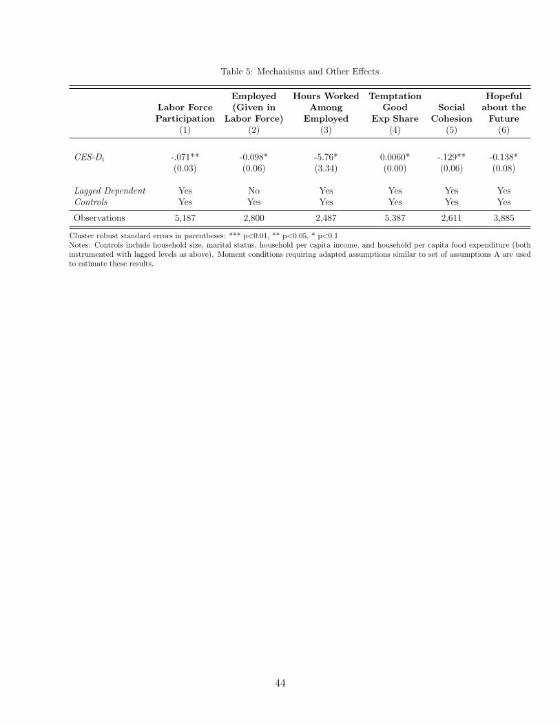
Table 5: Mechanisms and Other Effects

Employed Hours Worked Temptation HopefulLabor Force (Given in Among Good Social about theParticipation Labor Force) Employed Exp Share Cohesion Future

(1) (2) (3) (4) (5) (6)

CES-Dt -.071** -0.098* -5.76* 0.0060* -.129** -0.138*(0.03) (0.06) (3.34) (0.00) (0.06) (0.08)

Lagged Dependent Yes No Yes Yes Yes YesControls Yes Yes Yes Yes Yes Yes

Observations 5,187 2,800 2,487 5,387 2,611 3,885

Cluster robust standard errors in parentheses: *** p<0.01, ** p<0.05, * p<0.1Notes: Controls include household size, marital status, household per capita income, and household per capita food expenditure (bothinstrumented with lagged levels as above). Moment conditions requiring adapted assumptions similar to set of assumptions A are usedto estimate these results.

44

Table 6: Full Sample shows larger point estimates of Expenditure/Income on CES-D

Assumptions A Assumptions B AlternativeInstrument

CES-D CES-D CES-D(1) (2)* (3)* (4) (5)* (6)* (7)

hhincome percapitat -0.00356*** -0.00470*** -0.0041**(0.0009) (0.001) (0.002)

hhincome percapita2t 0.00000024*** 0.00000034*** 0.00

(0.000000074) (0.0000001) (0.00)

foodexp percapitat -0.00801** -0.0101**(0.00317) (0.004)

foodexp percapita2t 0.00 0.00

(0.00) (0.00)

wealthindext -3.179** -3.327**(1.23) (1.46)

CES-Dt-1 0.411*** -0.281 0.0546 0.291 0.0824 0.053 0.033(0.148) (0.43) (0.04) (0.493) (0.50) (0.04) (0.05)

Controls Yes Yes Yes Yes Yes Yes Yes

Observations 6,975 6,099 6,975 6,975 6,103 6,975 34,961

Cluster robust standard errors in parentheses: *** p<0.01, ** p<0.05, * p<0.1Controls include household size, marital status, household per capita income, and household per capita food expenditure.*Single equation GMM used to estimate coefficients.

45

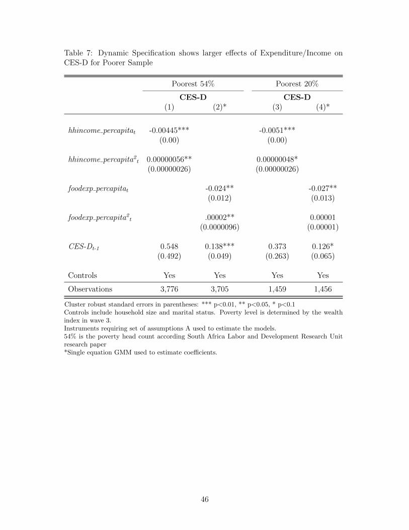
Table 7: Dynamic Specification shows larger effects of Expenditure/Income onCES-D for Poorer Sample

Poorest 54% Poorest 20%

CES-D CES-D(1) (2)* (3) (4)*

hhincome percapitat -0.00445*** -0.0051***(0.00) (0.00)

hhincome percapita2t 0.00000056** 0.00000048*

(0.00000026) (0.00000026)

foodexp percapitat -0.024** -0.027**(0.012) (0.013)

foodexp percapita2t .00002** 0.00001

(0.0000096) (0.00001)

CES-Dt-1 0.548 0.138*** 0.373 0.126*(0.492) (0.049) (0.263) (0.065)

Controls Yes Yes Yes Yes

Observations 3,776 3,705 1,459 1,456

Cluster robust standard errors in parentheses: *** p<0.01, ** p<0.05, * p<0.1Controls include household size and marital status. Poverty level is determined by the wealthindex in wave 3.Instruments requiring set of assumptions A used to estimate the models.54% is the poverty head count according South Africa Labor and Development Research Unitresearch paper*Single equation GMM used to estimate coefficients.

46

Table 8: Log Transformations Yield Similar Results

Full Sample Poorest 54% Poorest 20%

CES-D CES-D CES-D(1) (2) (3) (4) (5) (6)

Log(hhincome percapitat) -2.06** -2.55*** -4.44***(0.833) (0.668) (1.429)

Log(foodexp percapitat) -2.390 -3.060** -4.705**(1.71) (1.54) (2.11)

Controls Yes Yes Yes Yes Yes Yes

Observations 6,968 6,100 3,633 3,274 1,374 1,374

Cluster robust standard errors in parentheses: *** p<0.01, ** p<0.05, * p<0.1Controls include lagged dependent, household size, and marital status. Poverty level is determined by the wealthindex in wave 3.Instruments requiring Assumptions A used. Less restrictive Assumptions B produce similar results.Using Log transformations allows for the easier percentage interpretation.

47

Figures

Figure 1: Histograms of the CES-D scores in wave four and wave three show that a significantportion of the population are above the threshold of 10 used by psychologists to screen fordepression. The two lower histograms compare changes between wave three and wave fourfor the whole sample and specifically for individuals with CES-D scores in wave three of 8and above. A significant portion of those with scores of 8 or above exhibit a positive changewhich indicates worsening depressive symptoms.

48

Figure 2: Average CES-D scores decrease with income and expenditure deciles indicatingthat psychological well-being is correlated with economic well-being. Standard deviationswithin each decile range from 3.8 to 4.8 and do not exhibit a pattern.

49

Figure 3: Impact of CES-D on earned (upper) and unearned (lower) income based on CES-Dscore threshold show that, as hypothesized, changes in CES-D that include or are above thethresholds only affect earned income.

50

Figure 4: Impact of CES-D on Individual Income based on CES-D score in Wave 3. Thisfigure was based on 13 local linear regressions with a bandwidth of 1 and restricted toindividuals who experienced changes with absolute value less than or equal to the 4 onthe CES-D scale. Red dashed confidence intervals correct for multiple testing. The bluevertical line at 10 indicates the threshold used by psychologists to screen for depression. Thepoint estimates are presented in Appendix C Table A6. This figure was estimated with ZA

i,t,however, estimating the figure with matrix ZB

i,t showed very a very similar pattern and pointestimates.

51

Figure 5: The figures above show the marginal effect of changes in income (ZAR) (upper)and food expenditure per capita changes (lower). The marginal effect of changes in house-hold income per capita on CES-D are evident only for those in the lower income deciles.Despite much smaller sample sizes for each regression, the effect of income on CES-D is sta-tistically significant for the lowest three (and four for food expenditure) deciles even after aconservative Bonferroni CI correction for multiple testing. The impact of changes in incomeand food expenditure per capita on psychological well-being is not statistically different fromzero for the upper deciles.

52

Figure 6: The same pattern as in Figure 6 emerges when considering percent changes inincome, however, the statistically significant estimates for the lowest 4 household incomedeciles are relatively similar in magnitude.

53

Figure 7: Impulse response function: the effect of a shock to income in time 0 on futureincome for a household with one individual.

54

Figure 8: Impulse response function: the effect of a shock to income in time 0 on futureincome.

55

Figure 9: Top (A) shows income at time 0 and after 5 periods; if CES-D plays no role theninitial levels of CES-D will not affect the distribution of income over time. In the lower partof the Figure (B), the full system of equations estimated above shows that when psychologicalwell-being plays a role, those who randomly begin with lower levels of psychological well-being will have higher rates of poverty in the future.

56

Figure 10: The effect of psychological well-being on poverty rates over time is accentuatedafter negative shocks to either income or psychological well-being. The difference in thepoverty rate in the two groups after an across-the-board negative shock to either income orpsychological well-being is larger than those in Figure 9.B.

57

Figure 11: Probability of experiencing negative income growth (between Wave 3 and 4)by household income per capita decile for two subsamples: Households with a head thatexperiences low psychological well-being in Wave 1 and 2 and all other households.

58

Appendix

A. Proofs

The proposition states that under assumptions A, instruments matrix ZAi,t would imply mo-

ment conditions to consistently estimate the coefficients of the following system of equations

(3) and (4) in Section 4. The moment conditions are:

E(ZA

i,t′Ui,t

)= 0

where Ui,t is a vector of the first-differenced unobserved error terms ∆ei,t and ∆ui,t. I expand

the left hand side of the equation below:

E

[(z1i,t′ 0

0 z2i,t′

)(∆ei,t

∆ui,t

)]= E

[(z1i,t′∆ei,t

z2i,t′∆ui,t

)]=

(E[z1i,t

′ei,t − z1i,t′ei,t−1]E[z2i,t

′ui,t − z2i,t′ui,t−1]

)

Distributing further and applying the law of iterated expectations gives:

Di,t−2E [ei,t | Di,t−2]−Di,t−2E[ei,t−1|Di,t−2]

Di,t−3E [ei,t | Di,t−3]−Di,t−3E[ei,t−1|Di,t−3]

yi,t−3E [ei,t | yi,t−3]− yi,t−3E[ei,t−1|yi,t−3]Di,t−3E[ui,t|Di,t−3]−Di,t−3E[ui,t−1|Di,t−3]

hi,t−2E[ui,t|hi,t−2]− hi,t−2E[ui,t−1|hi,t−2]hi,t−3E[ui,t|hi,t−3]− hi,t−3E[ui,t−1|hi,t−3]

Assumptions A

E [ei,t | yi,t−2, yi,t−3, . . . ;Di,t−1, Di,t−2, . . . ;xi,t,xi,t−1, . . . ] = 0 (A1)

and

E [ui,t | hi,t−1, hi,t−2, . . . ;Di,t−2, Di,t−3, . . . ;xi,t,xi,t−1, . . . ] = 0 (A2)

It is clear that under assumptions A, each term in the vector above would be equal to zero.

Thus, assumptions A imply the moment conditions E(ZA

i,t′Ui,t

)= 0.47

The assumptions required for instruments matrix ZBi,t to imply the moment conditions

E(ZB

i,t′Ui,t

)= 0 are less restrictive and are the following:

E [ei,t | yi,t−2, yi,t−3, . . . ;Di,t−2, Di,t−3, . . . ;xi,t,xi,t−1, . . . ] = 0 (B1)

47There are six moment conditions and four coefficients and thus the coefficients are identified.

59

and

E [ui,t | hi,t−2, hi,t−3, . . . ;Di,t−2, Di,t−3, . . . ;xi,t,xi,t−1, . . . ] = 0 (B2)

Similarly, it is clear when expanding the left hand side that assumptions B imply the moment

conditions: Di,t−3E [ei,t | Di,t−3]−Di,t−3E[ei,t−1|Di,t−3]

yi,t−3E [ei,t | yi,t−3]− yi,t−3E[ei,t−1|yi,t−3]Di,t−3E[ui,t|Di,t−3]−Di,t−3E[ui,t−1|Di,t−3]

hi,t−3E[ui,t|hi,t−3]− hi,t−3E[ui,t−1|hi,t−3]

= 0

Simulation results illustrating this estimation strategy and the assumptions required

are presented in the next Appendix section B.

60

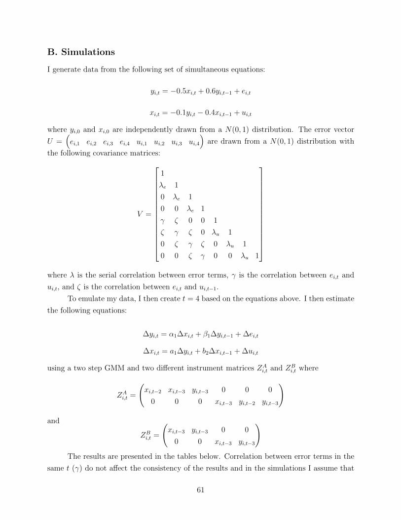
B. Simulations

I generate data from the following set of simultaneous equations:

yi,t = −0.5xi,t + 0.6yi,t−1 + ei,t

xi,t = −0.1yi,t − 0.4xi,t−1 + ui,t

where yi,0 and xi,0 are independently drawn from a N(0, 1) distribution. The error vector

U =(ei,1 ei,2 ei,3 ei,4 ui,1 ui,2 ui,3 ui,4

)are drawn from a N(0, 1) distribution with

the following covariance matrices:

V =

1

λe 1

0 λe 1

0 0 λe 1

γ ζ 0 0 1

ζ γ ζ 0 λu 1

0 ζ γ ζ 0 λu 1

0 0 ζ γ 0 0 λu 1

where λ is the serial correlation between error terms, γ is the correlation between ei,t and

ui,t, and ζ is the correlation between ei,t and ui,t−1.

To emulate my data, I then create t = 4 based on the equations above. I then estimate

the following equations:

∆yi,t = α1∆xi,t + β1∆yi,t−1 + ∆ei,t

∆xi,t = a1∆yi,t + b2∆xi,t−1 + ∆ui,t

using a two step GMM and two different instrument matrices ZAi,t and ZB

i,t where

ZAi,t =

(xi,t−2 xi,t−3 yi,t−3 0 0 0

0 0 0 xi,t−3 yi,t−2 yi,t−3

)

and

ZBi,t =

(xi,t−3 yi,t−3 0 0

0 0 xi,t−3 yi,t−3

)The results are presented in the tables below. Correlation between error terms in the

same t (γ) do not affect the consistency of the results and in the simulations I assume that

61

γ = −0.4. It is clear that only in Table A1 does ZAi,t provide consistent estimates. This

is when λ and ζ are zero. Interestingly, if λ is different from zero but the model has no

simultaneity (β1 and α1 are zero) then ZAi,t will consistently estimate the coefficients of zero.

These results are presented in the bottom half of table A1-3. If there is simultaneity, ZAi,t

will reject zero with high probability but the coefficients will be estimated with bias.

However the results in Table A4 show that if ζ 6= 0 then ZAi,t will not provide consistent

estimates of coefficients equal to zero.

ZBi,t, however, consistently estimates all the coefficients for non-zero values of λ and ζ.

However, serial correlation across more than 1 time period would create bias. This is not

shown in the simulations but is obvious from both sets of Assumptions A and B.

62

Table A1: Simulation Results 1/4

λe = 0, λu = 0, γ = 0.4, ζ = 0

ZAi,t ZB

i,t

N bias ssd sse/ssd p5 p10 bias ssd sse/ssd p5 p10

Main Equation

β1 = −0.5

200 0.003 0.285 0.886 0.573 0.667 -0.172 2.943 1.847 0.511 0.571500 0.002 0.167 0.960 0.851 0.902 0.005 0.461 0.798 0.609 0.670

1000 -0.001 0.114 0.983 0.983 0.993 0.015 0.290 0.782 0.755 0.8035000 0.002 0.049 1.019 1.000 1.000 0.006 0.082 0.947 0.989 0.994

β2 = 0.6

200 -0.019 0.261 0.931 0.714 0.818 -0.090 1.147 1.793 0.173 0.300500 -0.011 0.157 0.987 0.965 0.983 -0.004 0.462 0.783 0.636 0.769

1000 -0.002 0.113 0.976 1.000 1.000 0.009 0.224 0.922 0.945 0.9745000 -0.002 0.049 0.992 1.000 1.000 0.003 0.078 0.994 1.000 1.000

α1 = −0.1

200 0.093 4.622 0.927 0.257 0.331 -1.710 52.881 1.499 0.245 0.298500 -0.007 0.255 0.874 0.189 0.272 0.040 0.884 0.747 0.163 0.213

1000 0.006 0.177 0.887 0.192 0.278 0.017 0.482 0.652 0.145 0.2005000 0.000 0.072 0.959 0.366 0.460 0.003 0.123 0.983 0.195 0.261

α2 = −0.4

200 0.015 0.631 1.079 0.940 0.948 -0.317 8.785 1.536 0.411 0.513500 -0.001 0.053 0.992 0.997 0.998 -0.003 0.198 0.964 0.757 0.840

1000 -0.001 0.037 1.003 1.000 1.000 0.000 0.147 0.760 0.970 0.9865000 0.000 0.016 1.010 1.000 1.000 0.000 0.045 0.978 1.000 1.000

No Simultaneity

β1 = 0

200 0.003 0.183 0.889 0.054 0.106 -0.014 2.735 0.973 0.081 0.153500 -0.003 0.104 0.980 0.044 0.087 0.017 0.493 0.750 0.066 0.108

1000 -0.002 0.070 1.021 0.033 0.080 0.009 0.206 0.952 0.053 0.0895000 0.001 0.031 1.018 0.046 0.082 0.005 0.084 0.951 0.053 0.107

β2 = 0.6

200 -0.036 0.351 0.930 0.351 0.558 -0.051 1.431 1.032 0.131 0.268500 0.006 0.215 0.983 0.928 0.962 0.034 0.552 0.674 0.696 0.837

1000 0.023 0.153 0.982 1.000 1.000 0.034 0.196 0.984 0.984 0.9945000 0.028 0.067 1.001 1.000 1.000 0.032 0.079 1.000 1.000 1.000

α1 = 0

200 0.009 0.485 0.781 0.101 0.164 0.022 1.698 1.367 0.115 0.176500 0.015 0.260 0.927 0.051 0.112 0.044 0.727 0.947 0.071 0.114

1000 0.015 0.181 0.934 0.061 0.116 0.015 0.321 0.902 0.051 0.0955000 0.002 0.078 0.960 0.057 0.116 0.004 0.127 0.981 0.054 0.106

α2 = −0.4

200 -0.026 0.136 0.944 0.846 0.888 -0.016 0.297 1.338 0.581 0.659500 -0.022 0.078 1.025 0.991 0.997 -0.021 0.131 1.158 0.921 0.956

1000 -0.021 0.056 0.991 1.000 1.000 -0.017 0.078 0.985 0.997 0.9995000 -0.021 0.025 0.994 1.000 1.000 -0.021 0.034 0.976 1.000 1.000

Simulated using 1000 replications. N: Number of observationsbias: Bias of the estimated coefficientssd: Standard Deviation of the estimated coefficientssse/ssd: Mean of the ratio of the estimated standard error to ssdp5,p10: Probability of rejecting null where coefficient equals 0

63

Table A2: Simulation Results 2/4

λe = 0.25, λu = 0.25, γ = 0.4, ζ = 0

ZAi,t ZB

i,t

N bias ssd sse/ssd p5 p10 bias ssd sse/ssd p5 p10

Main Equation

β1 = −0.5

200 0.019 0.169 0.909 0.864 0.909 0.073 2.614 0.946 0.631 0.708500 0.026 0.105 0.932 0.990 0.996 0.011 0.168 0.902 0.838 0.880

1000 0.027 0.074 0.924 1.000 1.000 0.003 0.102 1.001 0.968 0.9805000 0.031 0.033 0.938 1.000 1.000 0.003 0.045 0.981 1.000 1.000

β2 = 0.6

200 0.004 0.207 0.928 0.909 0.948 -0.013 0.595 1.262 0.683 0.784500 -0.006 0.130 0.945 0.997 0.999 -0.002 0.159 0.967 0.976 0.988

1000 -0.006 0.094 0.928 1.000 1.000 0.004 0.104 1.006 1.000 1.0005000 -0.010 0.042 0.934 1.000 1.000 0.000 0.045 0.993 1.000 1.000

α1 = −0.1

200 0.101 0.469 0.762 0.138 0.187 0.022 1.172 0.647 0.197 0.245500 0.140 0.241 0.901 0.056 0.102 0.053 0.487 0.725 0.130 0.173

1000 0.149 0.174 0.878 0.061 0.125 0.008 0.227 0.955 0.139 0.2005000 0.149 0.074 0.920 0.096 0.181 0.001 0.095 0.984 0.227 0.317

α2 = −0.4

200 -0.048 0.084 0.979 0.964 0.981 0.008 0.177 0.958 0.761 0.816500 -0.041 0.053 0.963 0.999 1.000 -0.005 0.096 0.965 0.982 0.988

1000 -0.040 0.037 0.973 1.000 1.000 0.001 0.062 0.977 1.000 1.0005000 -0.038 0.017 0.965 1.000 1.000 0.001 0.027 0.965 1.000 1.000

No Simultaneity

β1 = 0

200 0.001 0.093 0.952 0.046 0.109 -0.157 4.698 1.849 0.063 0.117500 -0.002 0.056 0.991 0.047 0.091 0.009 0.161 0.897 0.049 0.093

1000 -0.001 0.038 1.027 0.039 0.084 0.004 0.099 1.006 0.042 0.0865000 0.000 0.017 1.012 0.043 0.091 0.002 0.044 0.967 0.057 0.099

β2 = 0.6

200 0.011 0.240 0.942 0.854 0.932 -0.118 3.869 1.863 0.629 0.760500 0.023 0.147 0.981 0.997 0.999 0.024 0.174 0.971 0.981 0.991

1000 0.030 0.104 0.981 1.000 1.000 0.033 0.115 1.004 1.000 1.0005000 0.030 0.046 0.999 1.000 1.000 0.031 0.050 0.995 1.000 1.000

α1 = 0

200 0.004 0.352 0.852 0.081 0.138 0.056 0.774 0.780 0.080 0.138500 0.006 0.202 0.955 0.045 0.096 0.051 0.375 0.912 0.048 0.100

1000 0.008 0.141 0.964 0.057 0.111 0.011 0.241 0.965 0.052 0.1045000 0.001 0.063 0.969 0.058 0.120 0.002 0.104 0.983 0.061 0.109

α2 = −0.4

200 -0.032 0.104 0.965 0.943 0.962 -0.014 0.142 0.918 0.824 0.861500 -0.025 0.062 1.025 0.999 1.000 -0.021 0.075 1.018 0.991 0.995

1000 -0.022 0.045 0.991 1.000 1.000 -0.019 0.053 0.991 1.000 1.0005000 -0.021 0.020 0.996 1.000 1.000 -0.020 0.024 0.968 1.000 1.000

Simulated using 1000 replications. N: Number of observationsbias: Bias of the estimated coefficientssd: Standard Deviation of the estimated coefficientssse/ssd: Mean of the ratio of the estimated standard error to ssdp5,p10: Probability of rejecting null where coefficient equals 0

64

Table A3: Simulation Results 3/4

λe = 0.5, λu = 0.5, γ = 0.4, ζ = 0

ZAi,t ZB

i,t

N bias ssd sse/ssd p5 p10 bias ssd sse/ssd p5 p10

Main Equation

β1 = −0.5

200 0.047 0.103 0.863 0.990 0.993 0.010 0.258 0.692 0.816 0.860500 0.061 0.067 0.838 1.000 1.000 0.008 0.104 0.906 0.965 0.975

1000 0.065 0.047 0.853 1.000 1.000 0.003 0.065 0.997 1.000 1.0005000 0.069 0.022 0.834 1.000 1.000 0.001 0.029 0.997 1.000 1.000

β2 = 0.6

200 -0.016 0.151 0.873 0.993 0.996 -0.002 0.170 0.972 0.923 0.956500 -0.039 0.097 0.877 1.000 1.000 -0.002 0.098 0.978 0.999 1.000

1000 -0.044 0.070 0.864 1.000 1.000 0.002 0.066 1.002 1.000 1.0005000 -0.051 0.032 0.854 1.000 1.000 0.000 0.029 0.982 1.000 1.000

α1 = −0.1

200 0.268 0.447 0.735 0.077 0.125 0.076 0.779 0.712 0.171 0.205500 0.317 0.253 0.847 0.094 0.198 0.037 0.321 0.883 0.126 0.165

1000 0.324 0.181 0.837 0.254 0.375 0.004 0.188 0.989 0.151 0.2175000 0.334 0.080 0.854 0.932 0.964 0.001 0.083 0.979 0.268 0.371

α2 = −0.4

200 -0.066 0.078 0.944 0.990 0.996 -0.003 0.122 0.956 0.906 0.938500 -0.055 0.051 0.933 1.000 1.000 -0.003 0.065 1.010 0.998 0.999

1000 -0.052 0.036 0.930 1.000 1.000 0.001 0.046 0.987 1.000 1.0005000 -0.047 0.016 0.927 1.000 1.000 0.001 0.021 0.962 1.000 1.000

No Simultaneity

β1 = 0

200 -0.001 0.051 0.986 0.048 0.103 0.010 0.221 0.721 0.062 0.096500 -0.001 0.033 0.962 0.052 0.118 0.007 0.090 0.931 0.046 0.099

1000 0.000 0.022 1.014 0.045 0.094 0.004 0.059 0.991 0.044 0.0905000 0.000 0.010 0.994 0.051 0.101 0.001 0.026 1.001 0.056 0.094

β2 = 0.6

200 0.033 0.158 0.947 0.992 0.998 0.023 0.191 0.968 0.931 0.952500 0.029 0.097 0.976 1.000 1.000 0.026 0.110 0.976 1.000 1.000

1000 0.031 0.068 0.987 1.000 1.000 0.032 0.075 0.996 1.000 1.0005000 0.030 0.030 0.992 1.000 1.000 0.031 0.033 0.982 1.000 1.000

α1 = 0

200 0.000 0.277 0.906 0.075 0.132 0.058 0.577 0.835 0.066 0.124500 0.002 0.166 0.977 0.044 0.097 0.039 0.310 0.948 0.052 0.098

1000 0.004 0.117 0.980 0.061 0.105 0.006 0.205 0.992 0.049 0.0965000 0.002 0.053 0.971 0.056 0.114 0.001 0.092 0.979 0.054 0.117

α2 = −0.4

200 -0.033 0.084 0.970 0.982 0.990 -0.019 0.105 0.944 0.935 0.959500 -0.026 0.050 1.029 1.000 1.000 -0.021 0.059 1.021 0.999 1.000

1000 -0.023 0.037 0.997 1.000 1.000 -0.020 0.042 0.994 1.000 1.0005000 -0.021 0.016 1.014 1.000 1.000 -0.020 0.019 0.976 1.000 1.000

Simulated using 1000 replications. N: Number of observationsbias: Bias of the estimated coefficientssd: Standard Deviation of the estimated coefficientssse/ssd: Mean of the ratio of the estimated standard error to ssdp5,p10: Probability of rejecting null where coefficient equals 0

65

Table A4: Simulation Results 4/4

λe = 0.5, λu = 0.5, γ = 0.4, ζ = −0.1

ZAi,t ZB

i,t

N bias ssd sse/ssd p5 p10 bias ssd sse/ssd p5 p10

Main Equation

β1 = −0.5

200 -0.014 0.103 0.873 0.996 0.998 0.010 0.194 0.838 0.795 0.844500 0.001 0.067 0.850 1.000 1.000 0.010 0.108 0.880 0.961 0.968

1000 0.005 0.047 0.866 1.000 1.000 0.004 0.066 0.987 0.998 1.0005000 0.009 0.022 0.853 1.000 1.000 0.001 0.028 1.004 1.000 1.000

β2 = 0.6

200 -0.026 0.137 0.898 0.993 0.994 0.004 0.165 0.986 0.932 0.968500 -0.051 0.091 0.878 1.000 1.000 -0.001 0.101 0.960 0.995 0.997

1000 -0.054 0.065 0.874 1.000 1.000 0.002 0.067 0.989 1.000 1.0005000 -0.060 0.029 0.872 1.000 1.000 0.000 0.030 0.980 1.000 1.000

α1 = −0.1

200 0.297 0.467 0.775 0.068 0.130 0.062 1.005 0.579 0.167 0.221500 0.365 0.287 0.841 0.090 0.219 0.040 0.362 0.801 0.140 0.200

1000 0.377 0.200 0.854 0.307 0.442 0.008 0.192 0.985 0.158 0.2255000 0.386 0.087 0.881 0.975 0.986 0.000 0.084 0.984 0.283 0.377

α2 = −0.4

200 -0.113 0.076 0.952 0.997 0.999 -0.005 0.131 0.916 0.925 0.949500 -0.104 0.049 0.947 1.000 1.000 -0.003 0.068 0.983 0.995 0.997

1000 -0.102 0.034 0.960 1.000 1.000 -0.001 0.046 1.000 1.000 1.0005000 -0.098 0.016 0.916 1.000 1.000 0.001 0.021 0.970 1.000 1.000

No Simultaneity

β1 = 0

200 -0.069 0.052 0.956 0.324 0.445 0.014 0.177 0.821 0.081 0.127500 -0.068 0.032 0.958 0.584 0.691 0.009 0.093 0.917 0.049 0.101

1000 -0.067 0.022 0.985 0.841 0.904 0.004 0.060 0.983 0.051 0.0995000 -0.067 0.010 0.973 1.000 1.000 0.001 0.026 1.010 0.045 0.100

β2 = 0.6

200 0.000 0.140 0.941 0.995 0.998 0.028 0.184 0.973 0.936 0.963500 -0.010 0.087 0.956 1.000 1.000 0.027 0.111 0.963 0.999 0.999

1000 -0.010 0.060 0.982 1.000 1.000 0.032 0.075 0.986 1.000 1.0005000 -0.011 0.027 0.983 1.000 1.000 0.031 0.033 0.980 1.000 1.000

α1 = 0

200 0.049 0.286 0.897 0.073 0.139 0.057 0.549 0.852 0.063 0.117500 0.061 0.169 0.984 0.117 0.210 0.035 0.322 0.900 0.054 0.119

1000 0.066 0.117 1.004 0.245 0.370 0.011 0.201 0.995 0.042 0.0915000 0.065 0.052 1.011 0.901 0.946 0.000 0.090 0.989 0.049 0.101

α2 = −0.4

200 -0.066 0.080 1.015 0.995 1.000 -0.021 0.103 0.956 0.945 0.969500 -0.060 0.049 1.061 1.000 1.000 -0.021 0.061 0.995 0.997 0.999

1000 -0.059 0.035 1.046 1.000 1.000 -0.021 0.042 1.000 1.000 1.0005000 -0.057 0.016 1.038 1.000 1.000 -0.020 0.019 0.984 1.000 1.000

Simulated using 1000 replications. N: Number of observationsbias: Bias of the estimated coefficientssd: Standard Deviation of the estimated coefficientssse/ssd: Mean of the ratio of the estimated standard error to ssdp5,p10: Probability of rejecting null where coefficient equals 0

66

C. Tables

Table A5: Individual Income and Household Income Per Capita

Assumptions A Assumptions B

CES-D CES-D CES-D(1) (2) (3)*

hhincome percapita t -0.00123 -0.0033*** -0.0034**(0.00078) (0.00118) (0.00150)

hhincome percapita2 t 0.00000*** 0.00000*** 0.00000***(0.00) (0.00) (0.00)

individualincome t -0.00005 0.00094 0.00095(0.00040) (0.00077) (0.00081)

individualincome2 t -0.00005 0.00094 0.00095(0.00) (0.00) (0.00)

CES-D (t-1) -0.414 0.0298 -0.541(0.223) (0.655) (0.599)

Controls Yes Yes Yes

Observations 4,173 4,173 2,708

Cluster robust standard errors in parentheses: *** p<0.01, ** p<0.05, * p<0.1Controls include household size and marital status.*Results from (3) restrict the sample to those who are economically active.Including both household income per capita and individual income as regressors(instrumented by lagged levels) shows that household income per capita plays amore important role in determining psychological well-being.

67

Tab

leA

6:E

stim

ates

for

Fig

ure

4an

dro

bu

stn

ess

chec

ks

for

the

sam

ple

sele

ctio

n

CE

S-D

inW

ave

3

12

34

56

78

910

1112

13

∆C

ES

-D≤

339

2.2*

**73

5.2*

*12

1.3

141.

9-5

1-3

0910

3.8

369.

1-6

66.4

-602

.9**

-509

.3**

-680

.1**

*-7

24.8

**(1

02.8

)(3

73.7

)(4

43.3

)(3

58.3

)(5

18.2

)(4

99.7

)(4

53.3

)(6

17.6

)(4

38.7

)(2

82.1

)(2

20.9

)(1

81.8

)(3

27.8

)

∆C

ES

-D≤

4∗32

6.6*

**63

9.8*

**34

532

1.4

-83.

7-3

33.8

-229

.6-2

50.1

-529

.6**

*-4

41.5

***

-347

.7**

*-3

04.7

***

-422

.2**

*(8

5.7)

(208

.1)

(241

.8)

(257

.7)

(381

.3)

(399

.7)

(329

.5)

(323

.2)

(185

.7)

(110

.9)

(95.

6)(8

3.2)

(119

.1)

∆C

ES

-D≤

535

1.7*

**49

6.4*

**27

8.1*

**18

4.7

-36.

8-1

19.5

-201

.1-3

66.4

-375

.1**

-290

.5**

*-1

52.2

**-1

90.6

***

-308

.1**

*(1

03.4

)(1

74.2

)(1

05.7

)(1

83.9

)(3

17.6

)(4

34.8

)(2

75.6

)(2

46.1

)(1

48.6

)(7

8.6)

(59.

6)(4

9.3)

(61.

3)

Clu

ster

robust

stan

dar

der

rors

inpar

enth

eses

:**

*p<

0.01,

**p<

0.0

5,

*p<

0.1

Con

trol

sin

clude

hou

sehol

dsi

zean

dm

arit

alst

atus.

Res

ult

ssh

own

wit

hou

tco

rrec

tion

for

mult

iple

test

ing.

Incl

udin

gin

the

sam

ple

those

who

exp

erie

nce

larg

erch

anges

incr

ease

sth

esa

mple

dec

rease

dth

em

agnit

ude

of

the

esti

mate

dm

argi

nal

effec

ts,

how

ever

thes

ees

tim

ates

are

bec

ome

less

and

less

mar

gin

al.

How

ever

,th

eth

resh

old

iscl

earl

yev

iden

tfo

rdiff

eren

tsp

ecifi

cati

ons.

68

Tab

leA

7:E

stim

ates

for

Fig

ure

s6-

9

Wav

e3

Hou

seh

old

Inco

me

Per

Cap

ita

Dec

ile

12

34

56

78

910

Dep

end

ent

Var

iab

leC

ES

-D

hhin

com

epe

rcap

ita

t-0

.003

8***

-0.0

026*

**-0

.002

11**

*-0

.001

48**

-0.0

0067

-0.0

0015

0.00

023

0.00

026

0.00

057*

*0.

0006

8**

(0.0

01)

(0.0

01)

(0.0

01)

(0.0

01)

(0.0

01)

(0.0

01)

(0.0

01)

(0.0

00)

(0.0

00)

(0.0

00)

Log

(hhi

nco

me

perc

apit

at)

-1.4

67**

*-1

.394

77**

*-1

.492

***

-1.2

98**

-0.7

84-0

.166

0.58

70.

779

2.77

7*0.

905

(0.4

17)

(0.4

60)

(0.4

98)

(0.5

80)

(0.6

88)

(0.7

34)

(0.9

69)

(1.3

94)

(1.4

78)

(1.3

85)

food

exp

perc

apit

at

-0.0

21**

*-0

.019

9***

-0.0

187*

**-0

.014

2***

-0.0

072*

*-0

.002

-0.0

0003

-0.0

0096

0.00

058

0.00

50*

(0.0

07)

(0.0

05)

(0.0

05)

(0.0

04)

(0.0

04)

(0.0

03)

(0.0

03)

(0.0

03)

(0.0

02)

(0.0

03)

Log

(foo

dexp

perc

apit

at)

-2.6

6***

-2.8

9***

-3.1

23**

*-2

.71*

**-1

.67*

*-0

.843

-0.4

91-0

.102

0.20

24.

50**

(0.9

2)(0

.84)

(0.9

4)(0

.97)

(0.8

4)(0

.84)

(1.0

2)(1

.26)

(1.2

5)(2

.24)

Dep

end

ent

Var

iab

le:

Lif

eS

atis

fact

ion

Log

(hhi

nco

me

perc

apit

at)

1.15

***

1.47

***

1.53

***

0.96

***

1.01

**1.

69**

*1.

38**

*2.

44**

*1.

25*

1.38

(0.2

6)(0

.25)

(0.2

7)(0

.31)

(0.4

1)(0

.40)

(0.4

7)(0

.70)

(0.7

1)(0

.86)

Dep

end

ent

Var

iable

:S

elf-

rep

orte

dh

app

ines

s

Log

(hhi

nco

me

perc

apit

at)

0.10

2***

0.14

1***

0.18

6***

0.23

1***

0.28

0***

0.19

6***

0.22

9***

0.28

5**

0.29

10.

251

(0.0

35)

(0.0

39)

(0.0

46)

(0.0

48)

(0.0

70)

(0.0

72)

(0.0

66)

(0.1

31)

(0.1

80)

(0.2

07)

Clu

ster

robu

stst

and

ard

erro

rsin

par

enth

eses

:**

*p<

0.0

1,**

p<

0.05

,*

p<

0.1

Con

trol

sin

clu

de

hou

seh

old

size

and

mar

ital

stat

us.

Res

ult

ssh

own

wit

hou

tco

rrec

tion

for

mult

iple

test

ing.

Incl

udin

gin

the

sam

ple

those

who

exp

erie

nce

larg

erch

ange

sin

crea

ses

the

sam

ple

dec

reas

edth

em

agnit

ude

ofth

ees

tim

ate

dm

argi

nal

effec

ts,

how

ever

thes

ees

tim

ates

are

bec

ome

less

and

less

mar

ginal

.H

owev

er,

the

thre

shol

dis

clea

rly

evid

ent

for

diff

eren

tsp

ecifi

cati

ons.

69

Table A8: Testing Predictions ofSimulations

Wave 4 Poort(1)

Poort-3 0.047***(0.0168)

HighCES-Dt-3 -0.0061(.0116)

Poort-3*HighCES-Dt-3 0.056***(.0194)

Controls Yes

N 10,671R-Squared 0.3139

Cluster robust standard errors in paren-theses: *** p<0.01, ** p<0.05, * p<0.1Controls include age, age squared, sex, re-gion, employment status, education lev-els, language, race, and perceived health.

70

D. Figures

Figure A1: Testing for nonlinearity in the effect of CES-D on economic activity shows similarpatterns to individual income.

71

Figure A2: Marginal effects curve for economic active shows a similar pattern to individualincome, however the effects seem to start a little earlier in CES-D scale.

72

Figure A3: Although not always achieving statistical significance, the mechanisms showsimilar threshold patterns.

73

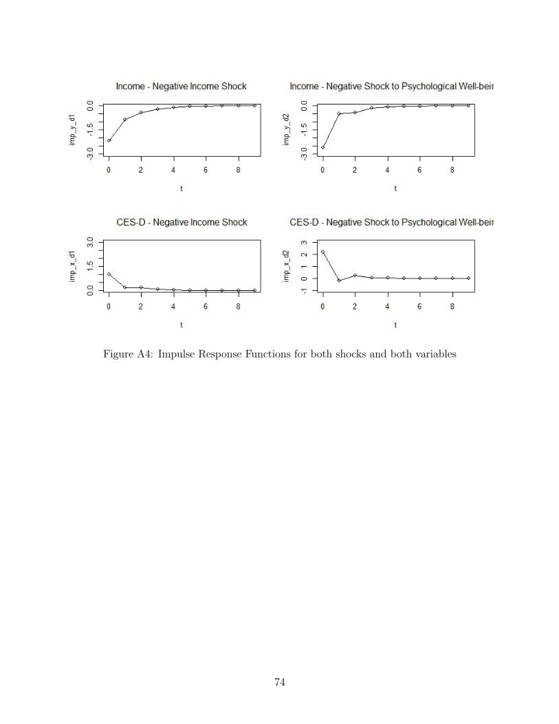
Figure A4: Impulse Response Functions for both shocks and both variables

74