lable at ScienceDirect

Social Science & Medicine 70 (2010) 1358–1366

Contents lists avai

Social Science & Medicine

journal homepage: www.elsevier .com/locate/socscimed

Income inequality, perceived happiness, and self-rated health: Evidence fromnationwide surveys in Japanq,qq

Takashi Oshio a,*, Miki Kobayashi b

a Hitotsubashi University, Institute of Economic Research, 2-1 Naka, Kunitachi, Tokyo 186-8603, Japanb Graduate School of Economics, Kobe University, 2-1 Rokkodai-cho, Nada-ku, Kobe 657-8501 Japan

a r t i c l e i n f o

Article history:Available online 12 February 2010

Keywords:JapanHappinessSelf-rated healthIncome inequalityOccupational status

q The data from Comprehensive Survey of Living Coand Welfare were made available by the Ministry ofJapan under the project entitled ‘‘Research on Socialbutions with reference to Income, Asset and ConsumThe micro-data from this survey were accessed and anOshio.

qq The data for this secondary analysis, the Japa(JGSS), was provided by the Social Science Japan Datafor Social Science Research on Japan, Institute of SocTokyo. The JGSS are designed and carried out by the JUniversity of Commerce (Joint Usage/Research CenteSurveys accredited by Minister of Education, CuTechnology), in collaboration with the Institute of SociTokyo.

* Corresponding author. Tel.: þ81 78 803 6818; faxE-mail address: oshio@ier.hit-u.ac.jp (T. Oshio).

0277-9536/$ – see front matter � 2010 Elsevier Ltd.doi:10.1016/j.socscimed.2010.01.010

a b s t r a c t

In this study, we examined how regional inequality is associated with perceived happiness and self-ratedhealth at an individual level by using micro-data from nationwide surveys in Japan. We estimated thebivariate ordered probit models to explore the associations between regional inequality and twosubjective outcomes, and evaluated effect modification to their sensitivities to regional inequality usingthe categories of key individual attributes. We found that individuals who live in areas of high inequalitytend to report themselves as both unhappy and unhealthy, even after controlling for various individualand regional characteristics and taking into account the correlation between the two subjectiveoutcomes. Gender, age, educational attainment, income, occupational status, and political views modifythe associations of regional inequality with the subjective assessments of happiness and health. Notably,those with an unstable occupational status are most affected by inequality when assessing bothperceived happiness and health.

� 2010 Elsevier Ltd. All rights reserved.

Introduction

Perceived happiness and good health are the key elements ofindividual well-being, but they tend to be discussed separately.Many studies on social epidemiology have investigated the asso-ciation between health and socioeconomic factors. It is now widelyrecognized that inequalities in health status associated withsocioeconomic status are substantial (Kawachi & Kennedy, 1997;Subramainan, Kawachi, & Kennedy, 2001). In particular, evidencesuggesting that income and educational attainment significantlyaffect health has important implications on economic and

nditions of People on HealthHealth, Labor and Welfare ofSecurity Benefit and Contri-

ption’’ in 2008 (No. 1211006).alyzed exclusively by Takashi

nese General Social SurveysArchive, Information Center

ial Science, the University ofGSS Research Center at Osakar for Japanese General Sociallture, Sports, Science and

al Science at the University of

: þ81 75 467 4594.

All rights reserved.

educational policies (Lleras-Muney, 2005; Smith, 1999). In recentyears, the association between income distribution in society andindividual health has been increasingly focused upon. As surveyedby Subramanian and Kawachi (2004), many attempts of multilevelanalyses indicated a significant correlation between regionalincome inequality and health.

Meanwhile, many economists have been examining the factorsthat determine perceived happiness, given that individual well-being and social welfare are central issues to be addressed ineconomics. Since the late 1990s, economists have started tocontribute large-scale empirical analyses of the determinants ofperceived happiness in different countries and periods, as surveyedby Frey and Stutter (2002). For example, Blanchflower and Oswald(2004) and Easterlin (2001) showed that income increases thelevel of perceived happiness. More recently, Alesina, Di Tell, andMacCulloch (2004) observed that higher inequality in society tendsto reduce individual happiness as in the case of self-rated health, byusing micro-data of the United States and European countries.

In general, happiness is a more complicated and multi-dimensional concept than health, because the former coversphysical, mental, socioeconomic, and many other aspects of indi-vidual well-being. It is, however, incorrect to view the relationbetween the two subjective outcomes in a unidirectional manner;although health is considered to be a key component of happiness,it is likely to affect health or its subjective assessment. Indeed, someempirical studies have reported that healthier individuals tend to

T. Oshio, M. Kobayashi / Social Science & Medicine 70 (2010) 1358–1366 1359

feel happier (Perneger, Hudelson, & Bovier, 2004), while a betterassessment of happiness can lead to a higher level of self-ratedhealth (Pettit & Kline, 2001). Further, it is possible that perceivedhappiness and self-assessed health reflect the different facets ofa common underlying construct such as the general physical andmental well-being, as emphasized by Subramanian, Kim, andKawachi (2005). The common socioeconomic factorsdincludingincome, age, gender, educational attainment, and relations withfamily members and neighborsdmay affect both outcomes, albeitnot in a uniform manner.

Following these previous studies on social epidemiology andhappiness, we attempt to examine how regional inequality isassociated with both perceived happiness and self-rated health atan individual level by using the micro-data obtained from nation-wide surveys in Japan. Our analysis has three distinctive features ascompared to the existing studies. First, we explicitly took intoaccount a possible correlation between perceived happiness andself-rated health. To this end, we estimated the ordered probitmodels of happiness and health simultaneously, rather than sepa-rately estimating them. This attempt was inspired by a multilevelanalysis conducted by Subramanian et al. (2005), who investigated(i) the individual determinants of perceived happiness and self-rated health and (ii) the correlations between the two outcomesat the community and individual levels. However, they did notexplore the impact of regional inequality on the two subjectiveoutcomes.

Second, our analysis extended the existing empirical analyses ofsocial epidemiology, which have concentrated largely on theimpact of regional inequality on health, by investigating the impacton perceived happiness as well. Alesina et al. (2004) was an earlyexample that analyzed the impact of regional inequality onperceived happiness, but it did not examine the impact on self-rated health. We examined how regional inequality affects bothoutcomes based on a common dataset and the simultaneousequation system.

Finally, we evaluated effect modification to sensitivities toregional inequality of perceived happiness and self-rated healthusing the categories of key individual attributes. It is widelyrecognized that these attributes influence the individual assess-ment of well-being, but the manner in which they modify theassociations of regional inequality remains virtually unexplored.The observed correlations between regional inequality andsubjective outcomes for the society as a whole may be misleading,if the associations differ substantially across individuals withdifferent characteristics. Alesina et al. (2004) pointed out that thepoor and left-wingers are sensitive to inequality in Europe, while inthe United States, the perceived happiness of these groups isuncorrelated with inequality. It is also relevant to compare thesensitivities of self-rated health.

Our analysis was based on the data collected from nationwidesurveys in Japan. There have been a growing number of empiricalanalyses on happiness and self-rated health in Japan in recentyears, against the background of rising concerns for the risk ofwidening income inequality and rising poverty (Tachibanaki,2005). Indeed, multilevel analyses of the association betweenregional inequality and self-rated health at a nationwide level hasbeen initiated by Shibuya, Hashimoto, and Yano (2002) andrecently followed by Oshio and Kobayashi (2009). Ichida et al.(2009) is another recent example that discussed this issue usinga multilevel model in Japan.

With respect to happiness, Ohtake (2004) and Sano and Ohtake(2007) in their original survey observed that unemploymentreduces happiness. Based on the same survey, Ohtake and Tomioka(2004) provides tentative evidence that the Gini coefficient and theperception of rising inequality have a weak but positive correlation

with happiness, a result that appears to be counter-intuitive. Ouranalysis in this paper is expected to add something new to thefindings from these preceding studies and make the case in Japancomparable with those in other advanced countries.

Methods

Source of data

We utilized the micro-data obtained from the following twonationwide surveys in Japan, following Oshio and Kobayashi(2009): (i) the Comprehensive Survey of Living Conditions ofPeople on Health and Welfare (CSLCPHW), which was compiled bythe Ministry of Health, Labour, and Welfare, and (ii) the JapaneseGeneral Social Survey (JGSS), which was compiled and conductedby the Institute of Regional Studies at the Osaka University ofCommerce in collaboration with the Institute of Social Science atthe University of Tokyo.

We used the CSLCPHW to construct prefecture-level variablesand the JGSS to construct individual-level variables, followingOshio and Kobayashi (2009). The CSLCPHW had sufficiently largesamples to obtain the reliable estimates of the Gini coefficient andthe mean household income in each prefecture, but it had limitedinformation about demographic and socioeconomic factors at theindividual level. In contrast, the JGSS had rich individual levelinformation, but its sample size was not large enough to calculateprefecture-level variables. By matching these data from the twodatasets depending on where each respondent resided, we con-ducted a multilevel analysis based on the three-year pooled data.

More specifically, we collected micro-data from 2001, 2004, and2007 CSLCPHWs, which include household income data of 2000,2003, and 2006, respectively. We ascertained the pre-tax income ofeach household. Further, to obtain detailed information about thesocioeconomic background of each respondent, we collected datafrom 2000, 2003, and 2006 JGSSs. Next, we matched these data foreach year depending on where each respondent resided.

The CSLCPHW randomly selected 2000 districts from the Pop-ulation Census divisions, which were stratified in each of the 47prefectures according to the population size. Next, all the house-holds in each district were interviewed. The original sample sizewas 30,386, 25,091, and 24,578 households (with a response rate of79.5, 70.1, and 67.7 percent) in 2000, 2003, and 2006, respectively.In this survey, we collected information about household income inorder to calculate the income inequality measures and the meanincome for each of the 47 prefectures. While both pre-tax and post-tax household incomes were available from the CSLCPHW, wefocused on pre-tax household, following Oshio and Kobayashi(2009) and Shibuya et al. (2002). Like most previous studies, weequivalized household income by dividing it by the root of thenumber of household members.

The JGSS divided Japan into six blocks and subdivided themaccording to the population size into three (in 2000 and 2003) orfour (in 2006) groups. Next, the JGSS selected 300 (in 2000) or 489(in 2003 and 2006) locations from each stratum using the Pop-ulation Census divisions and randomly selected 12–15 individualsaged between 20 and 89 from each survey location. Data werecollected through a combination of interviews and self-administered questionnaires. The number of respondents was2893, 1957, and 2124 (with a response rate of 63.9, 55.0, and 59.8percent) in 2000, 2003, and 2006 surveys, respectively. From thesesurveys, we obtained perceived happiness, self-rated health,educational background, and subjective assessments about indi-viduals’ relationships with the community and other people.

In this empirical analysis, we eliminated the respondents agedbelow 25 and above 80 whose sample sizes were limited, students,

T. Oshio, M. Kobayashi / Social Science & Medicine 70 (2010) 1358–13661360

and those whose key variables were missing. As a result, in ourestimation, a total of 4466 individuals (aged between 25 and 80)responded (1872 in 2000, 1237 in 2003, and 1357 in 2006). Thesummary statistics of all variables are presented in Table 1. Webriefly explain the dependent and independent variables used inour empirical analysis in what follows.

Perceived happiness and self-rated healthWith respect to perceived happiness, the JGSS asked the

respondents to choose from among 1 (¼ happy), 2, 3, 4, and 5(¼ unhappy) in response to the question, ‘‘How happy are you?’’

Table 1Selected descriptive statistics (pooled data for 2000, 03, 06).

Mean S.D. Min Max

(1) Prefecture-level variables: N¼ 141 (47 prefectures� 3 years, not weighted)

Gini coefficient 0.370 0.027 0.308 0.436Mean household income(million yen)a

3.104 0.496 1.677 4.437

Per capita budget expenditure(million yen)b

0.451 0.128 0.195 0.873

Proportion of people aged 65and above (%)

20.8 3.1 12.8 27.6

(2) Individual-level variables: N¼ 4466 (1872 in 2000; 1237 in 2003; 1357 in 2006)

Household income (thousand yen)a 3683 2543 0 32,200Age 52.7 14.4 25 80Number of children 1.83 1.08 0 10Social capital 0.56 0.21 0 1

Categorical variables Percentage

GenderMales 49.4 (reference)d

Females 50.6

Age groupYoung (aged 25–39) 22.7 (reference)Middle (aged 40–59) 41.2Old (aged 60–79) 36.1

Marital statusMarried 81.1 (reference)Unmarried 8.7Divorced/widowed 10.2

Educational attainmentJunior high school or lower 21.2 (reference)High school or lower 48.5College or higher 30.3

Income classLow 33.3 (reference)Middle 32.9High 33.7

Occupational statusRegular employeec 37.2 (reference)Non-regular employee 14.2Self-employed 9.4Family worker 2.8Unemployed 1.3Retired 9.7Homemaker 19.9Other 4.5

Size of residential areaSmall 31.8 (reference)Medium 40.7Large 27.5

(3) Regional blocksHokkaido, Tohoku, Kanto 1&2, Hokuriku, Tokai, Kinki 1&2, Chugoku, Shikoku,

Kyushu 1&2

a Household size adjusted, pre-tax, and evaluated at 2005 prices.b Evaluated at 2005 prices.c Includes a management executive.d Indicates the reference group for each category group in regression models.

With respect to self-rated health, it asked them to choose fromamong 1 (¼ excellent), 2, 3, 4, and 5 (¼ poor) in response to thequestion, ‘‘How would you rate your health condition?’’ Wereversed the order of choices such that ‘‘unhappy’’ and ‘‘poor’’equaled 1 and ‘‘happy’’ and ‘‘excellent’’ equaled 5.

Individual-level predictorsWe considered both individual- and prefecture-level factors as

predictors in our analysis, following various preceding studies(Subramanian & Kawachi, 2004). The former factors were dividedinto two groups. The first group comprised factors used aspredictors for both perceived happiness and self-rated health. Thesecond group comprised those used only for perceived happinessmodels, because they appeared to be at least partly affected by orsimultaneously determined by the status of health or self-ratedhealth.

To begin with the first group, household income is one of themost important variables and is expected to substantially affectboth perceived happiness and self-rated health. The JGSS askedrespondents to choose their household annual income for theprevious year from among 19 categories. We took the median valueof each category, equivalized it, and evaluated it at the 2005consumer prices. Next, we divided income groups into three classesof almost the same size as ‘‘low’’ (with equivalized householdincome below 2309 thousand yen), ‘‘middle’’ (2309–4041 thousandyen), and ‘‘high’’ (above 4041 thousand yen). In addition tohousehold income, we considered educational attainment, that is,whether the respondents completed their education at ‘‘junior highschool or lower,’’ ‘‘high school,’’ or ‘‘college or higher’’ level. Withrespect to demographic factors, we considered gender, age, andmarital status (married, unmarried, and separated/divorced). Agegroups were divided into ‘‘young’’ (aged 25–39), ‘‘middle’’ (40–59),and ‘‘old’’ (60–79).

We also collected the following four aspects of an individual’srelationship with or assessment of social capital from the JGSS,reflecting the previous analysis of the association between socialcapital and self-rated health (Fujiwara & Kawachi, 2008; Kim &Kawachi, 2006; Subramanian, Kim, & Kawachi, 2002): (i) whetherhe/she is satisfied with his/her relationships with friends (yes¼ 1);(ii) whether he/she is satisfied with the place where he/she lives(yes¼ 1); (iii) whether he/she thinks that most people can betrusted (yes¼ 1); and (iv) whether he/she belongs to any hobbygroup or club (yes¼ 1). For the first two aspects, the JGSS askedrespondents to choose from among 1 (¼ satisfied), 2, 3, 4, and 5(¼ dissatisfied). We categorized 1 and 2 as ‘‘yes.’’ To avoid multi-colinearity from incorporating each of these similar variables intomodels separately, we tentatively used the mean of four binaryanswers as the composite index of social capital.

Finally, we considered the size of the area where a respondentlives. The JGSS asked each respondent to choose from among 1(¼ small), 2 (¼ medium), and 3 (¼ large) in terms of the area, andwe used these answers as three categorized variables.

With respect to the second group of variables that were usedonly to predict perceived happiness, occupational status is poten-tially most important. Many economic researches have observedthat unemployment or an unstable occupational status reducessubjective well-being even after controlling for income (Clark &Oswald, 1994; Di Tella, MacCulloch, & Oswald, 2001; Korpi, 1997;Winkelmann & Winkelmann, 1998). The JGSS asked each respon-dent about his/her occupational status. We summarized theanswers into eight categories: regular employee (includinga management executive), non-regular employee, self-employment, family worker, unemployed, retired, homemaker,and other. Retired people and homemakers are not a part of thelabor force and are not paid.

T. Oshio, M. Kobayashi / Social Science & Medicine 70 (2010) 1358–1366 1361

Finally, we considered the number of children, which has alsobeen widely used as a predictor of perceived happiness. We alsoused its squared value as an explanatory variable, considering thepossibility of its nonlinear associations with perceived happiness.

Prefecture-level predictorsThe most important variable at a prefecture level is the Gini

coefficient, which was calculated from the CSLCPHW. The Ginicoefficient is one of the most widely used inequality measures, andKawachi and Kennedy (1997) showed that the choice of inequalitymeasures does not significantly affect the relationship betweenincome inequality and health. We also controlled for (log-trans-formed) prefecture mean income, the proportion of people aged 60and above (in both perceived happiness and self-rated healthmodels), and per capita budget expenditure of the local govern-ment (in perceived happiness models only).

Additionally, we included indicator variables for 12 regionalblocks, each of which comprised three to six prefectures (exceptHokkaido) in order to control for the unspecified characteristics ofa region wider than a prefecture and those for three years to controlfor year-specific factors.

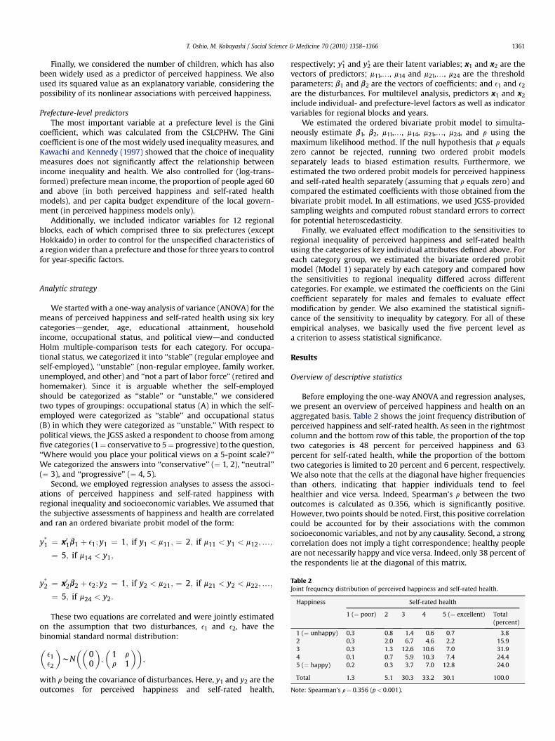
Table 2Joint frequency distribution of perceived happiness and self-rated health.

Happiness Self-rated health

1 (¼ poor) 2 3 4 5 (¼ excellent) Total(percent)

1 (¼ unhappy) 0.3 0.8 1.4 0.6 0.7 3.82 0.3 2.0 6.7 4.6 2.2 15.93 0.3 1.3 12.6 10.6 7.0 31.94 0.1 0.7 5.9 10.3 7.4 24.45 (¼ happy) 0.2 0.3 3.7 7.0 12.8 24.0

Total 1.3 5.1 30.3 33.2 30.1 100.0

Note: Spearman’s r¼ 0.356 (p< 0.001).

Analytic strategy

We started with a one-way analysis of variance (ANOVA) for themeans of perceived happiness and self-rated health using six keycategoriesdgender, age, educational attainment, householdincome, occupational status, and political viewdand conductedHolm multiple-comparison tests for each category. For occupa-tional status, we categorized it into ‘‘stable’’ (regular employee andself-employed), ‘‘unstable’’ (non-regular employee, family worker,unemployed, and other) and ‘‘not a part of labor force’’ (retired andhomemaker). Since it is arguable whether the self-employedshould be categorized as ‘‘stable’’ or ‘‘unstable,’’ we consideredtwo types of groupings: occupational status (A) in which the self-employed were categorized as ‘‘stable’’ and occupational status(B) in which they were categorized as ‘‘unstable.’’ With respect topolitical views, the JGSS asked a respondent to choose from amongfive categories (1¼ conservative to 5¼ progressive) to the question,‘‘Where would you place your political views on a 5-point scale?’’We categorized the answers into ‘‘conservative’’ (¼ 1, 2), ‘‘neutral’’(¼ 3), and ‘‘progressive’’ (¼ 4, 5).

Second, we employed regression analyses to assess the associ-ations of perceived happiness and self-rated happiness withregional inequality and socioeconomic variables. We assumed thatthe subjective assessments of happiness and health are correlatedand ran an ordered bivariate probit model of the form:

y*1 ¼ x01b1 þ e1; y1 ¼ 1; if y1 < m11; ¼ 2; if m11 < y1 < m12;.;

¼ 5; if m14 < y1;

y*2 ¼ x02b2 þ e2; y2 ¼ 1; if y2 < m21; ¼ 2; if m21 < y2 < m22;.;

¼ 5; if m24 < y2:

These two equations are correlated and were jointly estimatedon the assumption that two disturbances, e1 and e2, have thebinomial standard normal distribution:

�e1e2

�wN

��00

�;

�1 rr 1

��;

with r being the covariance of disturbances. Here, y1 and y2 are theoutcomes for perceived happiness and self-rated health,

respectively; y1* and y2

* are their latent variables; x1 and x2 are thevectors of predictors; m11,., m14 and m21,., m24 are the thresholdparameters; b1 and b2 are the vectors of coefficients; and e1 and e2

are the disturbances. For multilevel analysis, predictors x1 and x2

include individual- and prefecture-level factors as well as indicatorvariables for regional blocks and years.

We estimated the ordered bivariate probit model to simulta-neously estimate b1, b2, m11,., m14, m21,., m24, and r using themaximum likelihood method. If the null hypothesis that r equalszero cannot be rejected, running two ordered probit modelsseparately leads to biased estimation results. Furthermore, weestimated the two ordered probit models for perceived happinessand self-rated health separately (assuming that r equals zero) andcompared the estimated coefficients with those obtained from thebivariate probit model. In all estimations, we used JGSS-providedsampling weights and computed robust standard errors to correctfor potential heteroscedasticity.

Finally, we evaluated effect modification to the sensitivities toregional inequality of perceived happiness and self-rated healthusing the categories of key individual attributes defined above. Foreach category group, we estimated the bivariate ordered probitmodel (Model 1) separately by each category and compared howthe sensitivities to regional inequality differed across differentcategories. For example, we estimated the coefficients on the Ginicoefficient separately for males and females to evaluate effectmodification by gender. We also examined the statistical signifi-cance of the sensitivity to inequality by category. For all of theseempirical analyses, we basically used the five percent level asa criterion to assess statistical significance.

Results

Overview of descriptive statistics

Before employing the one-way ANOVA and regression analyses,we present an overview of perceived happiness and health on anaggregated basis. Table 2 shows the joint frequency distribution ofperceived happiness and self-rated health. As seen in the rightmostcolumn and the bottom row of this table, the proportion of the toptwo categories is 48 percent for perceived happiness and 63percent for self-rated health, while the proportion of the bottomtwo categories is limited to 20 percent and 6 percent, respectively.We also note that the cells at the diagonal have higher frequenciesthan others, indicating that happier individuals tend to feelhealthier and vice versa. Indeed, Spearman’s r between the twooutcomes is calculated as 0.356, which is significantly positive.However, two points should be noted. First, this positive correlationcould be accounted for by their associations with the commonsocioeconomic variables, and not by any causality. Second, a strongcorrelation does not imply a tight correspondence; healthy peopleare not necessarily happy and vice versa. Indeed, only 38 percent ofthe respondents lie at the diagonal of this matrix.

T. Oshio, M. Kobayashi / Social Science & Medicine 70 (2010) 1358–13661362

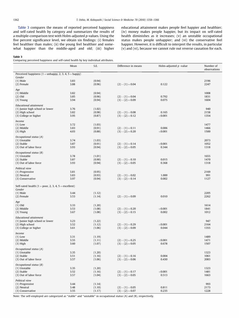
Table 3 compares the means of reported perceived happinessand self-rated health by category and summarizes the results ofa multiple-comparison test with Holm-adjusted p-values. Using thefive percent significance level, we obtain six findings: (i) femalesfeel healthier than males; (ii) the young feel healthier and some-what happier than the middle-aged and old; (iii) higher

Table 3Comparing perceived happiness and self-rated health by key individual attributes.

Mean S.E. Dif

Perceived happiness (1¼ unhappy, 2, 3, 4, 5¼ happy)Gender(1) Male 3.83 (0.94)(2) Female 3.88 (0.96) (2)

Age(1) Middle 3.82 (0.94)(2) Old 3.85 (0.96) (2)(3) Young 3.94 (0.94) (3)

Educational attainment(1) Junior high school or lower 3.76 (1.02)(2) High school 3.82 (0.98) (2)(3) College or higher 3.95 (0.87) (3)

Income(1) Low 3.72 (1.03)(2) Middle 3.83 (0.91) (2)(3) High 4.03 (0.88) (3)

Occupational status (A)(1) Unstable 3.74 (1.03)(2) Stable 3.87 (0.91) (2)(3) Out of labor force 3.93 (0.94) (3)

Occupational status (B)(1) Unstable 3.78 (1.01)(2) Stable 3.87 (0.90) (2)(3) Out of labor force 3.93 (0.94) (3)

Political view(1) Progressive 3.81 (0.95)(2) Neutral 3.83 (0.93) (2)(3) Conservative 3.97 (0.94) (3)

Self-rated health (1¼ poor, 2, 3, 4, 5¼ excellent)Gender(1) Male 3.44 (1.12)(2) Female 3.53 (1.14) (2)

Age(1) Old 3.33 (1.20)(2) Middle 3.53 (1.08) (2)(3) Young 3.67 (1.08) (3)

Educational attainment(1) Junior high school or lower 3.23 (1.22)(2) High school 3.52 (1.12) (2)(3) College or higher 3.61 (1.06) (3)

Income(1) Low 3.31 (1.19)(2) Middle 3.55 (1.11) (2)(3) High 3.60 (1.07) (3)

Occupational status (A)(1) Unstable 3.35 (1.20)(2) Stable 3.51 (1.16) (2)(3) Out of labor force 3.57 (1.06) (3)

Occupational status (B)(1) Unstable 3.35 (1.20)(2) Stable 3.52 (1.16) (2)(3) Out of labor force 3.57 (1.04) (3)

Political view(1) Progressive 3.44 (1.14)(2) Neutral 3.48 (1.10) (2)(3) Conservative 3.55 (1.17) (3)

Note: The self-employed are categorized as ‘‘stable’’ and ‘‘unstable’’ in occupational stat

educational attainment makes people feel happier and healthier;(iv) money makes people happier, but its impact on self-ratedhealth diminishes as it increases; (v) an unstable occupationalstatus makes people unhappier; and (vi) the conservative feelhappier. However, it is difficult to interpret the results, in particular(v) and (vi), because we cannot rule out reverse causation for each.

ference in means Holm-adjusted p -value Number ofobservations

2196� (1)¼ 0.04 0.122 2247

1008� (1)¼ 0.04 0.792 1831� (2)¼ 0.09 0.075 1604

940� (1)¼ 0.08 0.165 2158� (2)¼ 0.12 <0.001 1354

1477� (1)¼ 0.11 0.006 1466� (2)¼ 0.20 <0.001 1500

2073� (1)¼ 0.14 <0.001 1052� (2)¼ 0.05 0.344 1318

1655� (1)¼ 0.10 0.015 1470� (2)¼ 0.05 0.368 1318

2169� (1)¼ 0.02 1.000 991� (2)¼ 0.14 0.002 1127

2205� (1)¼ 0.09 0.010 2262

1614� (1)¼ 0.20 <0.001 1841� (2)¼ 0.15 0.002 1012

947� (1)¼ 0.29 <0.001 2164� (2)¼ 0.09 0.044 1355

1489� (1)¼ 0.25 <0.001 1471� (2)¼ 0.05 0.678 1507

1323� (1)¼ 0.16 0.004 1061� (2)¼ 0.06 0.430 2083

1323� (1)¼ 0.17 <0.001 1481� (2)¼ 0.05 0.513 1663

993� (1)¼ 0.05 0.811 2173� (2)¼ 0.07 0.235 1228

us (A) and (B), respectively.

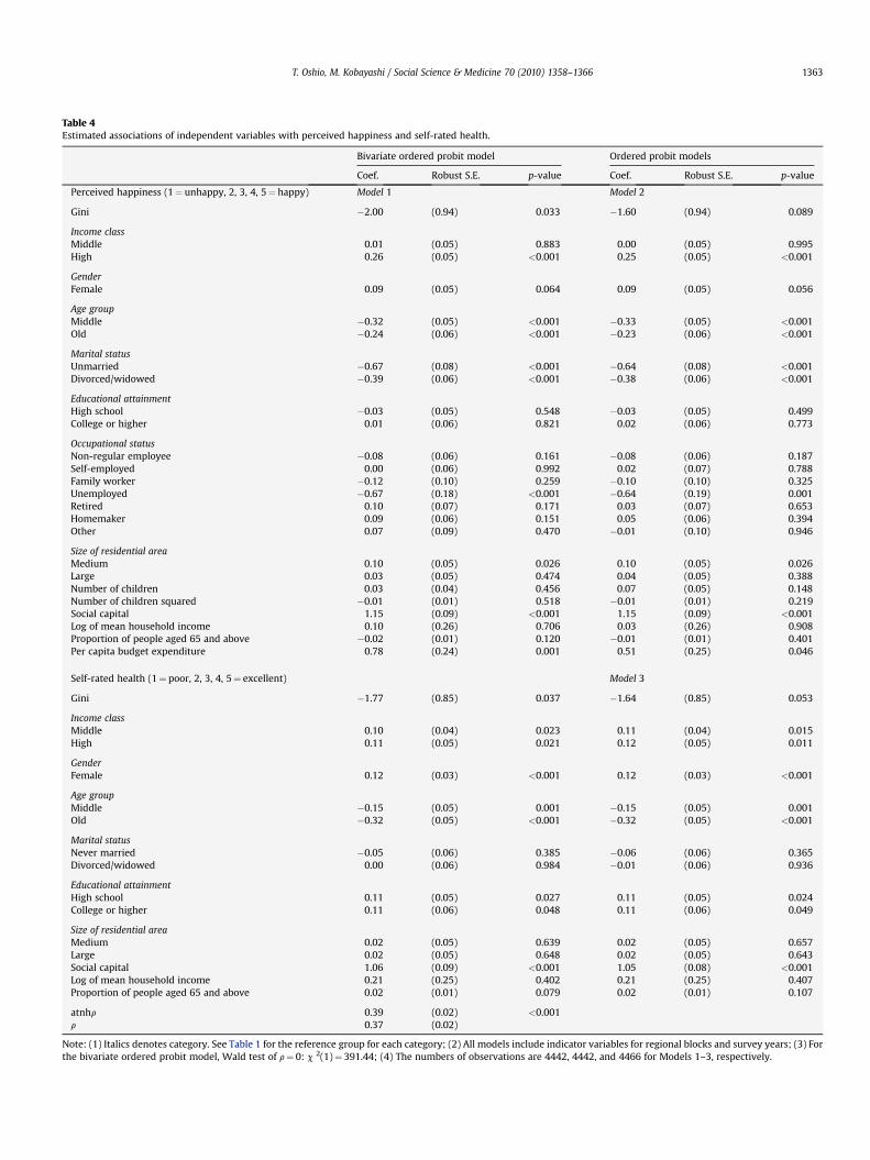
Table 4Estimated associations of independent variables with perceived happiness and self-rated health.

Bivariate ordered probit model Ordered probit models

Coef. Robust S.E. p-value Coef. Robust S.E. p-value

Perceived happiness (1¼ unhappy, 2, 3, 4, 5¼ happy) Model 1 Model 2

Gini �2.00 (0.94) 0.033 �1.60 (0.94) 0.089

Income classMiddle 0.01 (0.05) 0.883 0.00 (0.05) 0.995High 0.26 (0.05) <0.001 0.25 (0.05) <0.001

GenderFemale 0.09 (0.05) 0.064 0.09 (0.05) 0.056

Age groupMiddle �0.32 (0.05) <0.001 �0.33 (0.05) <0.001Old �0.24 (0.06) <0.001 �0.23 (0.06) <0.001

Marital statusUnmarried �0.67 (0.08) <0.001 �0.64 (0.08) <0.001Divorced/widowed �0.39 (0.06) <0.001 �0.38 (0.06) <0.001

Educational attainmentHigh school �0.03 (0.05) 0.548 �0.03 (0.05) 0.499College or higher 0.01 (0.06) 0.821 0.02 (0.06) 0.773

Occupational statusNon-regular employee �0.08 (0.06) 0.161 �0.08 (0.06) 0.187Self-employed 0.00 (0.06) 0.992 0.02 (0.07) 0.788Family worker �0.12 (0.10) 0.259 �0.10 (0.10) 0.325Unemployed �0.67 (0.18) <0.001 �0.64 (0.19) 0.001Retired 0.10 (0.07) 0.171 0.03 (0.07) 0.653Homemaker 0.09 (0.06) 0.151 0.05 (0.06) 0.394Other 0.07 (0.09) 0.470 �0.01 (0.10) 0.946

Size of residential areaMedium 0.10 (0.05) 0.026 0.10 (0.05) 0.026Large 0.03 (0.05) 0.474 0.04 (0.05) 0.388Number of children 0.03 (0.04) 0.456 0.07 (0.05) 0.148Number of children squared �0.01 (0.01) 0.518 �0.01 (0.01) 0.219Social capital 1.15 (0.09) <0.001 1.15 (0.09) <0.001Log of mean household income 0.10 (0.26) 0.706 0.03 (0.26) 0.908Proportion of people aged 65 and above �0.02 (0.01) 0.120 �0.01 (0.01) 0.401Per capita budget expenditure 0.78 (0.24) 0.001 0.51 (0.25) 0.046

Self-rated health (1¼ poor, 2, 3, 4, 5¼ excellent) Model 3

Gini �1.77 (0.85) 0.037 �1.64 (0.85) 0.053

Income classMiddle 0.10 (0.04) 0.023 0.11 (0.04) 0.015High 0.11 (0.05) 0.021 0.12 (0.05) 0.011

GenderFemale 0.12 (0.03) <0.001 0.12 (0.03) <0.001

Age groupMiddle �0.15 (0.05) 0.001 �0.15 (0.05) 0.001Old �0.32 (0.05) <0.001 �0.32 (0.05) <0.001

Marital statusNever married �0.05 (0.06) 0.385 �0.06 (0.06) 0.365Divorced/widowed 0.00 (0.06) 0.984 �0.01 (0.06) 0.936

Educational attainmentHigh school 0.11 (0.05) 0.027 0.11 (0.05) 0.024College or higher 0.11 (0.06) 0.048 0.11 (0.06) 0.049

Size of residential areaMedium 0.02 (0.05) 0.639 0.02 (0.05) 0.657Large 0.02 (0.05) 0.648 0.02 (0.05) 0.643Social capital 1.06 (0.09) <0.001 1.05 (0.08) <0.001Log of mean household income 0.21 (0.25) 0.402 0.21 (0.25) 0.407Proportion of people aged 65 and above 0.02 (0.01) 0.079 0.02 (0.01) 0.107

atnhr 0.39 (0.02) <0.001r 0.37 (0.02)

Note: (1) Italics denotes category. See Table 1 for the reference group for each category; (2) All models include indicator variables for regional blocks and survey years; (3) Forthe bivariate ordered probit model, Wald test of r¼ 0: c 2(1)¼ 391.44; (4) The numbers of observations are 4442, 4442, and 4466 for Models 1–3, respectively.

T. Oshio, M. Kobayashi / Social Science & Medicine 70 (2010) 1358–1366 1363

T. Oshio, M. Kobayashi / Social Science & Medicine 70 (2010) 1358–13661364

Results of ordered probit models

Following the results of the descriptive analysis reported inTables 2 and 3, Table 4 presents the estimation results of thebivariate ordered probit model for perceived happiness and self-rated health (Model 1) and two ordered probit models that areseparately estimated for each outcome (Models 2 and 3). The tablesummarizes the estimated coefficients on each predictor and theirrobust standard errors. The results of the bivariate ordered probitmodel (Model 1) are divided into the top part (perceived happi-ness) and the bottom part (self-rated health).

We first note that the coefficient on the Gini coefficient issignificantly negative for both perceived happiness and self-ratedhealth (�2.00 and �1.77, respectively), indicating that regionalinequality is negatively associated with both outcomes. The esti-mate of r is 0.39, with a standard error of 0.02. The Wald statistic forthe test of the null hypothesis that r equals zero is 391.44, which iswell above 6.63dthe critical value of the chi-squared with a singlerestriction at the one percent level. Hence, we can reject thishypothesis and conclude that a correlation between omitted vari-ables after the influences of key factors in the two equations issignificantly positive.

The table also shows the results of the ordered probit models,which are estimated separately for perceived happiness and self-rated health (Models 2 and 3). The pattern of significance of eachvariable is mostly unchanged from the bivariate probit model(Model 1). However, the absolute value of the coefficient on theGini coefficient declines modestly for both the outcomes (from 2.00to 1.60 for perceived happiness and from 1.77 to 1.64 for self-rated

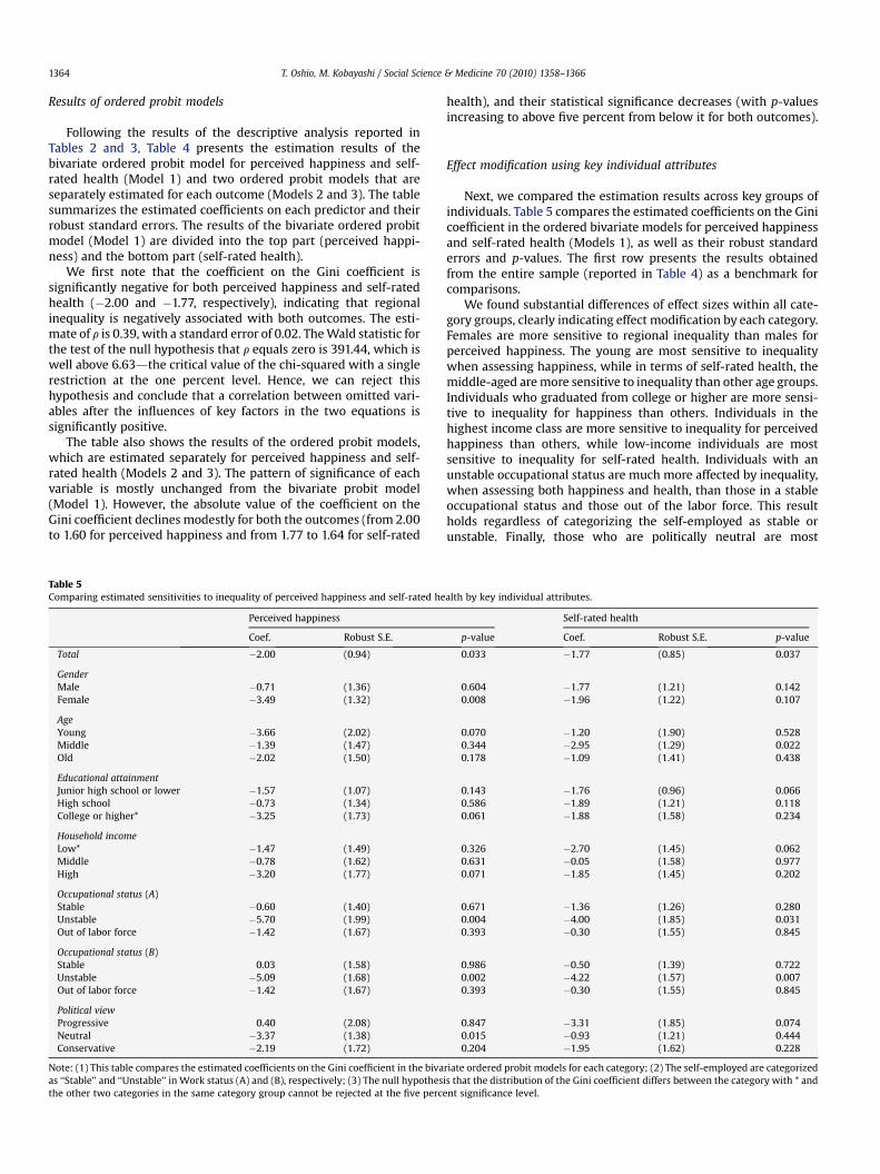
Table 5Comparing estimated sensitivities to inequality of perceived happiness and self-rated he

Perceived happiness

Coef. Robust S.E.

Total �2.00 (0.94)

GenderMale �0.71 (1.36)Female �3.49 (1.32)

AgeYoung �3.66 (2.02)Middle �1.39 (1.47)Old �2.02 (1.50)

Educational attainmentJunior high school or lower �1.57 (1.07)High school �0.73 (1.34)College or higher* �3.25 (1.73)

Household incomeLow* �1.47 (1.49)Middle �0.78 (1.62)High �3.20 (1.77)

Occupational status (A)Stable �0.60 (1.40)Unstable �5.70 (1.99)Out of labor force �1.42 (1.67)

Occupational status (B)Stable 0.03 (1.58)Unstable �5.09 (1.68)Out of labor force �1.42 (1.67)

Political viewProgressive 0.40 (2.08)Neutral �3.37 (1.38)Conservative �2.19 (1.72)

Note: (1) This table compares the estimated coefficients on the Gini coefficient in the bivaas ‘‘Stable’’ and ‘‘Unstable’’ in Work status (A) and (B), respectively; (3) The null hypothesthe other two categories in the same category group cannot be rejected at the five perc

health), and their statistical significance decreases (with p-valuesincreasing to above five percent from below it for both outcomes).

Effect modification using key individual attributes

Next, we compared the estimation results across key groups ofindividuals. Table 5 compares the estimated coefficients on the Ginicoefficient in the ordered bivariate models for perceived happinessand self-rated health (Models 1), as well as their robust standarderrors and p-values. The first row presents the results obtainedfrom the entire sample (reported in Table 4) as a benchmark forcomparisons.

We found substantial differences of effect sizes within all cate-gory groups, clearly indicating effect modification by each category.Females are more sensitive to regional inequality than males forperceived happiness. The young are most sensitive to inequalitywhen assessing happiness, while in terms of self-rated health, themiddle-aged are more sensitive to inequality than other age groups.Individuals who graduated from college or higher are more sensi-tive to inequality for happiness than others. Individuals in thehighest income class are more sensitive to inequality for perceivedhappiness than others, while low-income individuals are mostsensitive to inequality for self-rated health. Individuals with anunstable occupational status are much more affected by inequality,when assessing both happiness and health, than those in a stableoccupational status and those out of the labor force. This resultholds regardless of categorizing the self-employed as stable orunstable. Finally, those who are politically neutral are most

alth by key individual attributes.

Self-rated health

p-value Coef. Robust S.E. p-value

0.033 �1.77 (0.85) 0.037

0.604 �1.77 (1.21) 0.1420.008 �1.96 (1.22) 0.107

0.070 �1.20 (1.90) 0.5280.344 �2.95 (1.29) 0.0220.178 �1.09 (1.41) 0.438

0.143 �1.76 (0.96) 0.0660.586 �1.89 (1.21) 0.1180.061 �1.88 (1.58) 0.234

0.326 �2.70 (1.45) 0.0620.631 �0.05 (1.58) 0.9770.071 �1.85 (1.45) 0.202

0.671 �1.36 (1.26) 0.2800.004 �4.00 (1.85) 0.0310.393 �0.30 (1.55) 0.845

0.986 �0.50 (1.39) 0.7220.002 �4.22 (1.57) 0.0070.393 �0.30 (1.55) 0.845

0.847 �3.31 (1.85) 0.0740.015 �0.93 (1.21) 0.4440.204 �1.95 (1.62) 0.228

riate ordered probit models for each category; (2) The self-employed are categorizedis that the distribution of the Gini coefficient differs between the category with * andent significance level.

T. Oshio, M. Kobayashi / Social Science & Medicine 70 (2010) 1358–1366 1365

sensitive to inequality for perceived happiness, while progressiveindividuals are most sensitive to self-rated health.

However, we should be cautious in interpreting these resultsbecause comparisons of estimated coefficients on the Gini coeffi-cient do not make sense if the Gini coefficient is distributeddifferently between categories. To check this, we applied theKolmogorov–Smirnov tests between each category and theremaining one or two categories in each category group. We foundthat the null hypothesis that the Gini coefficient is distributeddifferently between categories cannot be rejected at the fivepercent significance level for two cases: between individuals whograduated from colleges or higher and others and between lowincome-individuals and others.

Discussion

Our estimation results confirmed the negative impact ofregional inequality on both perceived happiness and self-ratedhealth, a result consistent with those of the previous studies thatanalyzed the two outcomes separately. The novelty of our analysisis that it obtained this result even after controlling for variousindividual and regional characteristics and taking into account thecorrelation between the two subjective outcomes.

We also found that key socioeconomic factors tend to affectperceived happiness and self-rated health in the same directionswith statistical significance. More specifically, both our ANOVA andregression analyses confirm that higher-income, younger age, anda higher level of social capital make people feel both happier andhealthier. It is likely that these relations account for the observedpositive correlation between the two subjective outcomes. Thisresult also suggests that it is incorrect to view the relation betweenthe two subjective outcomes in a unidirectional manner. Further-more, the comparisons between the bivariate ordered probit model(which estimated perceived happiness and self-rated healthjointly) and two ordered probit models (which estimated the twooutcomes separately) revealed that separate estimations tend tounderestimate the magnitude of the association of regionalinequality.

Another notable finding is that key individual attributes modifythe association of regional inequality with subjective assessmentsof happiness and health. Notably, the widening inequality mostdirectly reduces the well-being of those in an unstable status andwho face the most serious uncertainty about future employmentand income. Alesina et al. (2004) found that the rich and the right-wingers are largely unaffected by inequality, while inequality hasstrong negative effects on the perceived happiness of the poor andleft-wingers in Europe. They also observed that the poor and theleft-wingers are not affected by inequality, while the effect on therich is negative and well-defined in the United States. The case ofJapan differs from that of both Europe and the United States; whilethe rich Japanese are affected by inequality, and the politicallyneutral rather than progressive or conservative ones are mostsensitive to it. In addition, the association of inequality tends toshow different patterns across individual features betweenperceived happiness and self-rated health.

It should be noted, however, that those with an unstable occu-pational status are strongly affected by inequality in terms of bothperceived happiness and health. Along with the fact that they areunhappier than others, as seen from Table 3, it suggests thatoccupational status is one of the key determinants of individualwell-being. These facts should be taken seriously, given the steadilydeclining proportion of regular employees in the labor market inJapan.

We recognize that this analysis has various limitations. First, wedealt with happiness as only a single item based on the survey

results of its subjective assessment. This approach followed manyempirical studies of happiness and was also parallel to the analysisof self-rated health. However, it cannot be free from criticism thathappiness should be multi-dimensional and that it cannot besummarized as a single item. Given this feature of happiness, thevalidity of perceived happiness observed from surveys should beaddressed further.

Second, while we took into account the correlation betweenperceived happiness and health when estimating regressionmodels, the manner in which these two aspects of individualwelfare interact with each other remains to be addressed. Third, asis often the case with a multilevel analysis of this type, pathways ormediation process from income inequality in society with respectto subjective outcomes at an individual level should be furtherinvestigated. Fourth, we disregarded the possibility that subjectiveoutcomes change individual characteristics, which we assumed tobe exogenous. These issues should be explicitly addressed in futureresearch.

Acknowledgments

We received the financial support provided by Grant-in-Aid forScientific Research on Innovative Areas (21119004) and Grant-in-Aid for Scientific Research (B) (21330057). We also thank threeanonymous referees for helpful comments.

References

Alesina, A., Di Tell, R., & MacCulloch, R. (2004). Inequality and happiness: areEuropeans and Americans different? Journal of Public Economics, 88,2009–2042.

Blanchflower, D. G., & Oswald, A. J. (2004). Well-being over time in Britain and theUSA. Journal of Public Economics, 88, 1359–1386.

Clark, A. E., & Oswald, A. J. (1994). Unhappiness and unemployment. EconomicJournal, 104, 648–659.

Di Tella, R., MacCulloch, R. J., & Oswald, A. J. (2001). Preferences over inflation andunemployment: evidence from surveys of happiness. American EconomicReview, 91, 335–341.

Easterlin, R. A. (2001). Income and happiness: towards a unified theory. EconomicJournal, 111, 465–484.

Frey, B. S., & Stutter, A. (2002). What can economists learn from happiness research?Journal of Economic Literature, 40, 402–435.

Fujiwara, T., & Kawachi, I. (2008). A prospective study of individual-level socialcapital and major depression in the United States. Journal of Epidemiology andCommunity Health, 62, 627–633.

Ichida, Y., Kondo, K., Hirai, H., Hanibuchi, T., Yoshikawa, G., & Murata, C. (2009).Social capital, income inequality and self-rated health in Chita peninsula, Japan:a multilevel analysis of older people in 25 communities. Social Science &Medicine, 69, 489–499.

Kawachi, I., & Kennedy, B. P. (1997). The relationship of income inequality tomortality: does the choice of indicator matter? Social Science & Medicine, 45,121–127.

Kim, D., & Kawachi, I. (2006). A multilevel analysis of key forms of community- andindividual-level social capital as predictors. Journal of Urban Health, 83,813–826.

Korpi, T. (1997). Is well-being related to employment status? Unemployment, labormarket policies and subjective well-being among Swedish youth. LabourEconomics, 4, 125–147.

Lleras-Muney, A. (2005). The relationship between education and adult mortality inthe United States. Review of Economic Studies, 72, 189–221.

Ohtake, F. (2004). Unemployment and happiness. The Japanese Journal of LabourStudies, 528, 59–68, (in Japanese).

Ohtake, F., & Tomioka, J. (2004). Happiness and income inequality in Japan. A paperpresented at International Forum for Macroeconomic Issues, ESRI CollaborationProject, February 2004.

Oshio, T., & Kobayashi, M. (2009). Income inequality, area-level poverty, perceivedaversion to inequality and self-rated health in Japan. Social Science & Medicine,69, 317–326.

Perneger, Th. V., Hudelson, P. M., & Bovier, P. A. (2004). Health and happiness inyoung Swiss adults. Quality of Life Research, 13, 171–178.

Pettit, J. W., & Kline, J. P. (2001). Are happy people healthier? The specific role ofpositive affect in predicting self-reported health symptoms. Journal of Researchin Personality, 35, 521–536.

Sano, S., & Ohtake, F. (2007). Labor and happiness. The Japanese Journal of LabourStudies, 558, 4–18, (in Japanese).

T. Oshio, M. Kobayashi / Social Science & Medicine 70 (2010) 1358–13661366

Shibuya, K., Hashimoto, H., & Yano, E. (2002). Individual income, income distribu-tion, and self rated health in Japan: cross sectional analysis of nationallyrepresentative sample. British Medical Journal, 324, 16–19.

Smith, J. P. (1999). Healthy bodies and thick wallets: the dual relation betweenhealth and economics status. Journal of Economic Perspectives, 13, 145–166.

Subramainan, S. V., Kawachi, I., & Kennedy, B. P. (2001). Does the state you live inmake a difference? Multilevel analysis of self-rated health in the US. SocialScience & Medicine, 53, 9–19.

Subramanian, S. V., & Kawachi, I. (2004). Income inequality and health: what havewe learned so far? Epidemiologic Reviews, 26, 78–91.

Subramanian, S. V., Kim, D., & Kawachi, I. (2002). Social trust and self-rated health inUS communities: a multilevel analysis. Journal of Urban Health, 79, S21–S34.

Subramanian, S. V., Kim, D., & Kawachi, I. (2005). Covariation in the socioeconomicdeterminants of self rated health and happiness: a multivariate multilevelanalysis of individuals and communities in the USA. Journal of Epidemiology andCommunity Health, 59, 664–669.

Tachibanaki, T. (2005). Confronting income inequality in Japan. Cambridge: MITPress.

Winkelmann, L., & Winkelmann, R. (1998). Why are the unemployed so unhappy?Evidence from panel data. Economica, 65, 1–15.