Income Inequality and Ethnicity - World Banksiteresources.worldbank.org/INTDECINEQ/Resources/Income... · 2005-06-24 · JUNE 9-10, 20002 Income Inequality and Ethnicity: An International

SECOND INEQUALITY AND PRO-POOR GROWTHSPRING CONFERENCE

THE WORLD BANKWASHINGTON, D.C.

JUNE 9-10, 20002

Income Inequality and Ethnicity: An International View

Brooks B. Robinson

For additional information please contact:

Brooks RobinsonBureau of Economic AnalysisU.S. Department of Commerce1441 L Street, N.W.Washington, DC 20230United States of [email protected]: (202) 606-9778Facsimile: (202) 606-5320

The ideas expressed herein are solely the author’s, as are any errors and omissions, and do not represent the policies or views of the Bureau of Economic Analysis nor the U.S. Department of Commerce.

This paper was originally prepared for the 27th General Conference of the International Association for Research in Income and Wealth, Stockholm, Sweden, August 18 – 24, 2002.

Abstract

There is substantial evidence that ethnicity (defined as race, language, and religion) can be a determinant of earnings within the United States ( Borjas, 1992 and 1999; Easterly, 2000; Light and Gold, 2000; Loury, 1977; and Lundberg and Startz, 1998), and that it affects income equality within the nation. An extrapolation of this fact to the international level motivates the following broader falsifiable hypothesis: Nations with relatively greater ethnic diversity do not experience relatively greater income inequality. This paper explores the theoretical literature that assesses the role of ethnicity in determining earnings and the resultant impact on income distribution. It presents a pooled cross-section time series econometric model that tests the hypothesis for 32 nations and smaller groupings of nations. The models produce mixed results.

1.0 Introduction

1.1 There is substantial evidence that ethnicity (defined as race, language, and religion) can be a determinant of earnings within the United States (U.S.) (Borjas, 1992 and 1999; Easterly, 2000; Light and Gold, 2000; Loury, 1977; and Lundberg and Startz, 1998), and that it affects U.S. income equality. An extrapolation of this fact to the international level motivates the following broader falsifiable hypothesis: Nations with relatively greater ethnic diversity do not experience relatively greater income inequality. This paper explores the theoretical literature that assesses the role of ethnicity in determining earnings and the resultant impact on income distribution. It presents pooled cross-section time series econometric models that test the hypothesis for 32 nations and smaller groupings of nations. The models produce mixed results. Note that data limitations precluded our use of ideal measures of income inequality in our models; i.e., the measures are not human-capital-adjusted.

1.2 The paper evolves in six sections. Section two is a discussion of the literature that explains reasons for income inequality. Section three explores the relationship between income distribution and ethnicity. In section four, we consider recent articles on the role of ethnicity in determining income inequality. An econometric model and the data required to operationalize it are discussed in section five. The results are presented in section six. We summarize and conclude in section seven.

2.0 Why income inequality?

2.1 We can trace concern about the distribution of income in the Modern Era to the 19th

Century and Vilfredo (Wilfred) Pareto (1897, p. 212). It was on social scientists’ agenda throughout the 20th Century. Focusing on the last quarter century, Sahota (1978, pp. 2-3) cites nine major one-dimensional-type theories that surfaced during the century that sought to explain why incomes are distributed unequally.1 The “more complete theories” promulgated mainly by Becker (1967), Stiglitz (1969), and Griliches (1977) to explain income inequality in developed economies integrate several of the nine major theories to produce multidimensional theories that provide more comprehensive explanations of income inequality. Sahota and Rocca (1977), Sundrum (1991), Persson and Tabellini (1995), and de Janvry and Sadoulet (2000) use multidimensional explanations for income inequality within and between developing nations. Recent contributors to the literature that identify multiple factors to explain income inequality for developed and developing economies include Smeeding et al (1993), Wolff (1996), Pi (1996), and Deininger and Squire (1996).

2.2 Although there is not complete agreement on all of the factors that determine income inequality or the relative importance of these factors, it stands to reason that many factors have a role to play. Good arguments exist for the contribution made by each of the following factors in determining earnings: Innate ability; luck; individual

1 The nine theories are: Ability, stochastic outcomes, individual choice, human capital, educational inequality, inheritance, life cycle, public income distribution, and distributive justice.

2

decisions; the acquisition of skills and abilities through study, training, and work; access to quality education; age; access to and control of the political system; the legal environment in which one lives; and location (i.e., whether one engages in economic activity in an urban versus a rural setting). However, given current and past Census Bureau statistics on U.S. average annual earnings, it is hard to overlook another factor in determining income--ethnicity.2

2.3 This paper is in the vein of the more complete theories in that it considers at least six one-dimensional theories (individual choice, education as a signal for an endowment of human capital, inheritance, public redistribution of income, distributive justice, and location) as it seeks to explain the role of ethnicity as a determinant of income distribution. As a starting point, we acknowledge the following stylized facts about the U.S. Ethnic capital, a concept derived from human capital theory, plays a role in limiting individual choice. Ethnoracial groups, especially when they form enclaves, may experience educational inequality.3 The relationship between racial ethnics and lower than average income and wealth, produces lower than average contemporaneous and intergenerational transfers of income and wealth through inheritances.4 Similarly, the socio-economic conditions of ethnoracial groups do not position them well to act as rent seekers to capture income and wealth that might be redistributed by the public sector to special interest groups.5 Generally, economic agents operating in urban versus rural environments achieve differing levels of earnings. Finally, political systems may not permit ethnics to access institutions and use those institutions to reconfigure income distribution within the society.

3.0 Ethnic economics: capital and earnings

3.1 We define “ethnic” to mean ethnoracial groups within countries that may or may not speak languages other than the nations’ official language, and they may practice other than the primary religions of nations. Generally speaking, U.S. ethnoracial groups are African-Americans, Hispanics, Asians, and Native-Americans. For Central and South America, ethnics are descendants of former aboriginal tribes, members of existing aboriginal tribes, and immigrants or descendants thereof. For countries on

2 For the years 1997-99, the U.S. Department of Commerce, Bureau of the Census reported that average income for non-Hispanic white households was $43,287, while it was $26,608 for Black, $29,110 for Hispanic, and $30,784 for American Indian and Alaska Native households. Asian and Pacific Islander households experienced average income of $48,614. The average for all households was $39,657.3 The U.S. Department of Education, National Center for Education Statistics, reports in the Digest for Education Statistics for 1999 that 87.7 percent of all whites 25 years and over graduated from high school and 27.7 percent of them possessed 4 or more years of college. For Blacks, the statistics were 77.4 percent and 15.5 percent, respectively. For Hispanics, 56.1 percent graduated from high school, while 10.9 percent had 4 or more years of college. 4 The U.S. Department of Commerce, Bureau of the Census reports that, for 1995, the average net worth of white households was $112,840, while it was $30,531 for Blacks, and $38,986 for Hispanics. Hence, the statement that ethnics have less wealth to transfer contemporaneously or intertemporally to heirs. Moreover, Hurd and Smith (1999, p. 10) state that “African-American and Hispanic households have lower probabilities of leaving an estate.”5 “Small groups of non-wealthy and non-vocal members are unlikely to exert effective political pressure.” See Rowley et al (1995), p. 92.

3

the continent of Africa, ethnics are tribal groups and immigrant groups or their descendants. For Europe, ethnics derive their uniqueness from their cultures--usually the result of historical and persistent enclave formation. Large ethnoracial immigrant enclaves mainly of Africans and Asians are a relatively recent phenomenon in Europe. For Asia, ethnics are usually from other countries or the descendants of immigrants; e.g., the Chinese of Indonesia or the Chinese and Indians of Malaysia. In fact, immigration and/or forced relocation are key reasons for ethnoracial minorities in many countries.6

3.2 Racial ethnicity, in and of itself, may not be as important as language or religion in determining how some economic agents operate. In this paper, we will test whether language, religion, and race exhibit separate or combined effects vis-à-vis income inequality.

3.3 The genesis of ethnicity as a determinant of income inequality is found in the writings of Johnson (1973). Within the context of the nature versus nurture debate, Johnson identified the environment as an important factor in enhancing skill development and invented the “cultural capital” concept (Johnson, 1973, p. 186). The central theme of cultural capital was that the environment contributed to skill development and, therefore, played a major role in determining earning power. Four years later, Loury (1977) used the phrase “cultural capital” to promulgate the idea that income differences can persist over time as a result of spillovers that accrue from the uniqueness of racial ethnic environments. Lundberg and Statz (1998) echo Loury’s concept.

3.4 Borjas (1999) extended and elevated Loury’s theme by metamorphosizing “ethnic capital” out of cultural capital. Using ethnic cohorts within longitudinal studies, Borjas showed that intergenerational earning differences between ethnic groups persist. He attributed much of this persistence to the expectations, role models, distribution of jobs, networking opportunities, attitudes, economic opportunities, and other influences on earnings potential that are pervasive in ethnic communities; i.e., ethnic capital (p. 148).

3.5 Light and Gold (2000) extended the ethnic capital concept; they focused on ethnic economies and reported on a variety of studies that assessed the income producing capabilities of such economies. They concluded that self-employed, owner ethnics probably earn more in human-capital-adjusted income than do ethnics who work as employees in the broader economy. However, they showed that employees of ethnic-owned firms earn less than their counterparts in mainstream economy jobs. There are three important caveats to these findings. First, most ethnic-owned firms have no employees (ibid., p. 71). Second, relatively speaking, most ethnic groups reflect very low levels of entrepreneurship; in fact, on average, only about 11 percent of most ethnoracial groups work in ethnic economies (ibid., p. 51). Third, ethnic-owned firms

6 This paper differs significantly from papers that use culture (primarily defined as religion) to explain between-nation income inequality (e.g., Granato et al. (1996)), because ethnicity (defined as race, language, and religion) is a broader concept.

4

generate below expected payroll levels (ibid., pp. 65-7). Given the foregoing, it is safe to conclude that, although the value of ethnic capital may be significant, ethnic economies do not play a very strong role in raising working ethnics’ incomes to a level comparable to the nation’s mean—thereby sustaining, and possibly extending, income inequality within the nation.

4.0 Additional evidence on the role of ethnicity in determining income inequality

4.1 This section considers recent articles by Easterly (1999), Lazear (1995), Coppin and Olsen (1998), and Malan (2000) that explore the effects of ethnicity on income inequality. In each case, the authors indicate that ethnic diversity within nations contributes to income inequality.

4.2 Easterly analyzes the role of ethnicity in the success developing nations experience in their search for economic growth. He states that it is important for developing nations to achieve a “middle class concensus” and a low degree of ethnic polarization. Although Easterly does not address directly the question of whether greater ethnic diversity engenders greater income inequality within nations, he does so indirectly. Generally, he shows that greater diversity contributes to adverse outcomes for growth, which has direct implications for greater income inequality.

4.3 Lazear examines the role that language and culture play in the efficient functioning of an economy. He contends that the lower is the degree of language diversity in an economy, the greater is the prospect for assimilation by ethnic groups. The inference is that a more equal distribution of income can be achieved in economies that are linguistically homogeneous.

4.4 Coppin and Olsen consider income inequality within Trinidad and Tobago. They highlight the racial discriminatory aspects of ethnicity vis-à-vis earnings. Although Africans and Indians constitute the majority of the population in Trinidad and Tobago, they are disproportionately represented in low earning jobs, primarily as a result of low educational achievement. This latter outcome contributes to income inequality within the nation.

4.5 Using a social accounting matrix approach, Malan explores income distribution within South African. Malan reveals that while income inequality was little changed for South Africa from the mid-1970’s to the mid-1990’s (a Gini Coefficient ranging from the mid-to-upper 60’s), the share of earnings for Africans versus Whites changed dramatically over this period. African’s increased their income share from 27 to 45 percent of the total during this period; White’s share decreased to 42 percent from 62 percent. Nevertheless, these data support the conclusion that nations with considerable ethnic diversity (there are Coloured and Indian ethnic groups in South Africa also) may experience relatively higher levels of income inequality than nations with less diversity.

5

4.6 These selected studies support the hypothesis that ethnoracial diversity, combined with linguistic and religious diversity, contributes to increased income inequality within nations. Unfortunately the lack of high quality and consistent historical data on income inequality for the countries just mentioned precluded their inclusion in our study. However, we build on these authors’ work in developing our model to test how ethnicity contributes to income inequality.

5.0 Econometric model and the data

5.1 In this section, we develop an econometric model that incorporates data from nations from around the world that may or may not reflect multiple ethnic groups within their populations. We inquire whether nations with multiple, large and distinct ethnic groups experience more income inequality. We structure our econometric model so that it permits us to reject the hypothesis that nations with more ethnic groups within their populations do not experience greater income inequality. The model assumes the following form:7

Equation 1

.8 9765

3

1421 tttttit

it PIAPOLtPCIPRLITETHII

5.2 The variables are described briefly below (for a full description of the variables, see Appendix B):

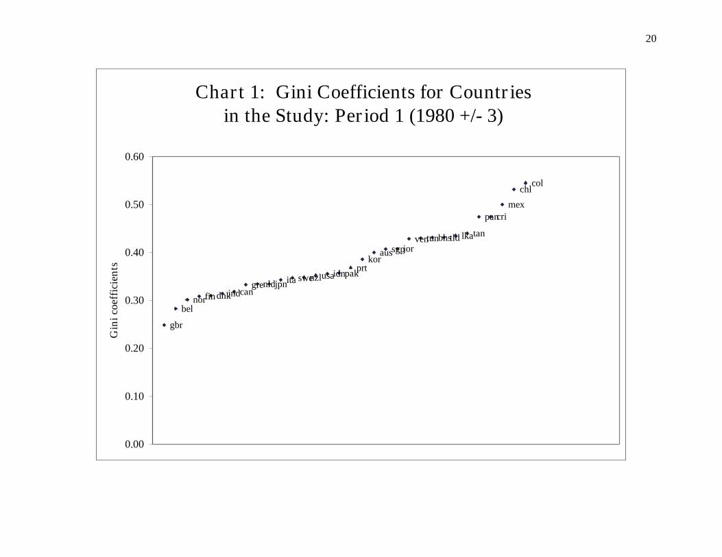
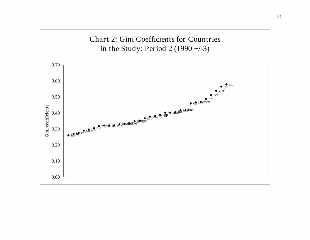
II Income inequality is represented by high quality Gini coefficients. Charts 1 and 2 depict the Gini’s for the nations in the study.8

ETH Ethnicity is a composite variable: Racial ethnicity, language, and religion. We test two of the variables (racial ethnicity and religion) in two ways: As the number (in levels) of racial ethnic groups that constitute more than five percent of a nation’s population, and as a diffusion index or Herfindahl Index-type concentration ratio.9

7 After reviewing the work of Barro (1991) and Clarke (1992) we considered expanding the model to include “growth” variables to avoid specification bias in our models; particularly those variables that capture the effects of international economics on a nation’s growth and income distribution. Specifically, trade, money, inflation, and monetary system maturity variables were tested, but standard F-tests revealed that the impact of these variables on the explanatory power of the model was negligible. 8 Heeding the warnings of Atkinson and Brandolini (2001), the data set used for this analysis was constructed to ensure continuity. That is, only countries with Gini Coefficients that were based on consistent coverage, observational units, and income measures were included in the model. As Malan (2000) points out, Theil entropy indexes are required to identify the sources of within country income inequality (i.e., the contributions of specific subgroups to income inequality). However, Theil indexes are not widely available, and we resort to Gini Coefficients for our analysis; they provide an overall measure of within country income inequality.9 The diffusion or Herfindahl Index-type concentration ratio is calculated as:

000,102

1 xi

n

i,

where xi is the percent of the population represented by the ith separately identified groups in a nation’s population.

6

Language is tested only in level form as the number of primary languages spoken by over five percent of a population. If one or more of the three ETH variables are statistically and theoretically significant at the five percent level, then we will be able to reject the null hypothesis that ethnicity does not contribute significantly to the income inequality of nations. We hypothesize that there are inverse relationships between Gini Coefficients and racial ethnicity and religion concentration ratios; we hypothesize that the opposite is true for the racial ethnic, language, and religion variables stated in levels.

LIT The literate population of a country as defined by that country; it proxies for human capital. It reflects the existing level of education in a country. We expect the parameter estimate to reveal a negative relationship between human capital and income distribution.

PR The public redistribution of income to individuals is proxied for by the ratio of central government budget expenditures to total gross national/domestic product. This variable infers the extent to which central governments may be able to engage in income redistribution, which impacts income distribution. Ideally, this proxy would be replaced with a variable that reflects total government human-capital-augmenting expenditures (e.g., expenditures on education, health, and housing), plus the value of redistributed income. We expect a negative sign on the coefficient for this variable.

PCI This variable is the natural logarithmic transformation of the real value of per capita income. We view this variable as a proxy for private-sector contemporaneous and intergenerational redistribution of income and wealth. The higher is per capita income, given some marginal propensity to consume, the higher should be the level of wealth or saving in a country and prospects for private redistribution of income. This variable captures the effects of inheritance and gifts on income inequality. A negative sign is expected on the parameter estimate for this variable.

POL Polity is our proxy for distributive justice and access to a nation’s political system. It is assumed that the greater is the degree of democratic policies, procedures, and institutions in a nation, the greater is the prospects for efficient markets. The POL variable is from Marshall and Jaggers (2000); it is an index ranging from 0 to 10 (10 symbolizing a high level of polity and 0 the total absence of polity). The variable measures the presence of, and related constraints to, institutions and procedures through which citizens can express preferences about alternative policies and leaders. It also reflects the level of civil liberty in a nation. We expect an inverse relationship between this variable and Gini Coefficients.

PIA This variable represents the percent of the population in the agricultural sector or rural areas versus those residing in urban areas. It captures possible inequality effects that are locational in nature; i.e., inequality produced when economic agents operate in rural versus urban environments. We expect a negative sign on this variable’s coefficient.

7

5.3 We test ordinary least squares (OLS) and pooled time series models where time (t) is 1980 and 1990 (+/- 3 years) and the cross sections are 32 of the world’s nations (see Appendix A).

5.4 We feature pooled time series cross-section models of the error component variety, and we use a Generalized Least Squares (GLS) technique described in Judge et al and White to estimate the models.10 The general model is represented by equation 2:

Equation 2

eXy it

K

kkitkiit

21

where yi= (yi1, yi2, …, yiT)', Xi is a (T X K) matrix of observations on the above described K explanatory variables for the ith nation in the study, and where β= (β1, β2, …, βK)' is a vector of parameters to be estimated (where β1= 1 + μi, and 1 is the mean intercept, while μi represents the difference from this mean for the ith nation), and the disturbance ei= (ei1, ei2, …, eiT)' is such that E[ei]=0, E[eiei']= 2

e IT and that

E[eiej']=0 for i≠j. Also, E[μi]=0, E[2i ]=

2 , and E[μiμj]=0 for i≠j. Underlying this model are the following assumptions:

Slope coefficients (β2-9) are constant across nations;The intercept (β1) varies randomly across nations;11

The μj , eit , and Xi are uncorrelated;The N nations included in the model are viewed as a “random” sample from a

larger population; andDisturbances are identical for all ith nations; they reflect a constant correlation

across time for each nation, but they are uncorrelated across nations.

Following Sayrs’ (1989, p.33) recommendation, we estimate ordinary least squares (OLS) models as a check on the pooled model results. We use a Cochrane-Orcutt method to correct for first-order autocorrelation that is assumed to characterize error terms in the OLS models.

6.0 Results

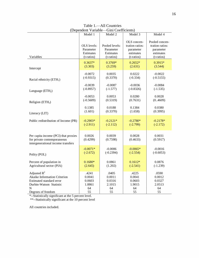
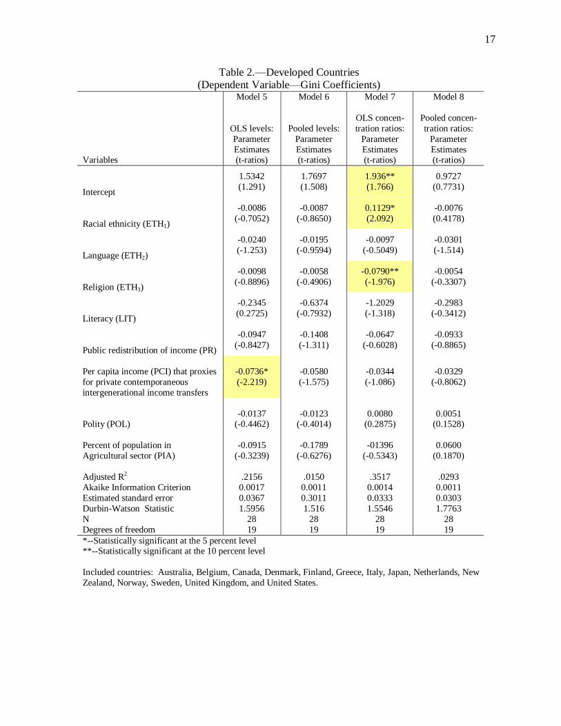
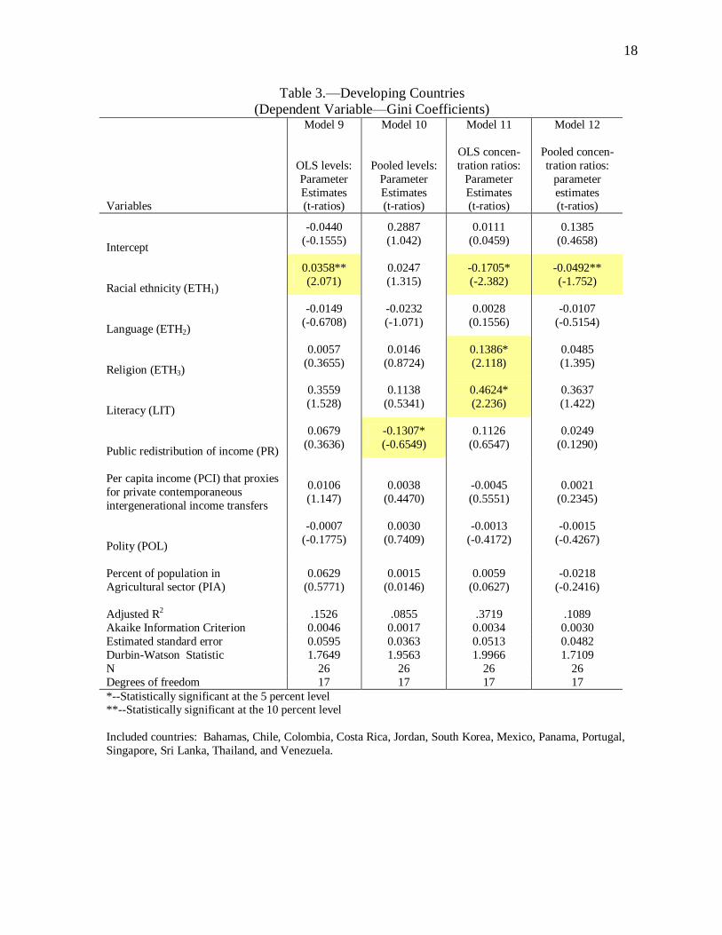
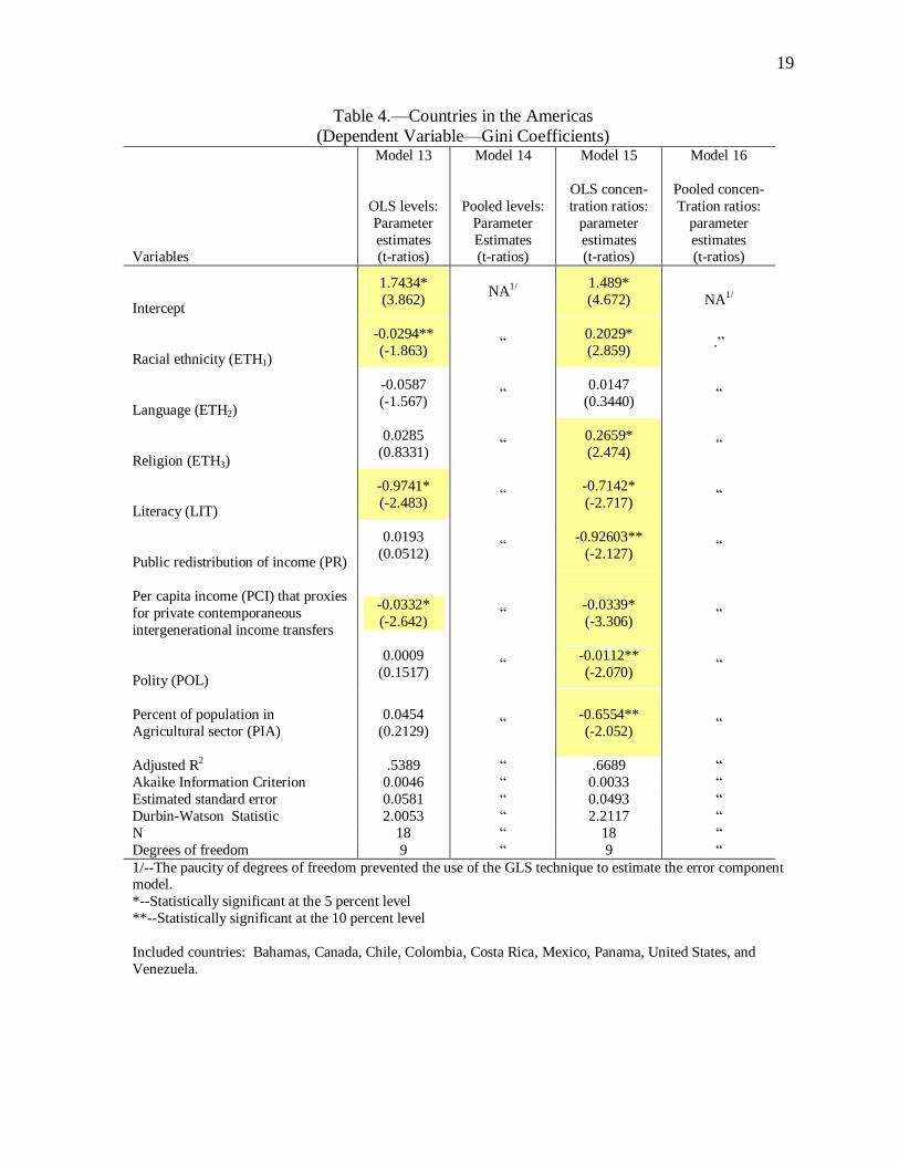
6.1 Tables 1 through 4 present the results of OLS and pooled regression models in level and concentration ratio forms (only the Eth1 and Eth3 variables are stated as concentration ratios in the latter models). Table 1 shows results for the all countries (32) models, table 2 presents results for 14 developed countries, table 3 shows results for 13 developing countries, and table 4 presents results for nine countries located in

10 See Sections 8.2 and 8.3 in Judge et al and Chapter 21 in White.11 For this study, we do not present intercepts for individual nations, rather we present estimated model intercepts that are derived from the GLS and OLS methods.

8

the Americas.12 In general, models that include concentration ratio variables reflect lower Akaike Information Criterion (AIC) statistics. Also, for statistically significant parameter estimates, the results are relatively consistent across models; i.e., the size and arithmetic signs of coefficients are consistent. Note that we were unable to estimate the pooled error component models in table 4 (Americas) using the GLS technique due to the paucity of degrees of freedom; we were only able to use OLS to estimate these models. This is unfortunate because the estimated Americas models reflect the best fit.

6.2 The ETH1 variable (racial ethnicity) is statistically and theoretically significant only for developing countries and the Americas models (table 3, models 9, 11, and 12; table 4, models 13 and 15). The level model indicates that, ceteris paribus, a 1-unit increase in the number of racial ethnic groups in a country results in a minimum of a 3 percent increase in income inequality. Similarly, the concentration ratio models indicate that a one percent decrease in the diffusion index for racial ethnic groups (that is, an increase in the proportion of such groups in a country) results in a 5 to 20 percent increase in income inequality. The all countries and developed countries models do not reflect this outcome.

6.3 The ETH2 (language) variable reflects no theoretical or statistical significance in the four models. The expectation was that countries with more languages spoken by significant portions of the population would reflect higher income inequality. The fact that this outcome was not confirmed by the models contradicts Lazear’s (1995) finding that language is a significant contributor to economic efficiency and growth, and thereby has an effect on income distribution. Our finding may be supported by the fact that that commerce is conducted often using one (an official) language in a country (although there may be several significant languages spoken in a country), which minimizes the role of language in determining earnings and, consequently, income inequality.

6.4 Although the ETH3 (religion) variable reflects some statistical significance in the developing countries and Americas models, theoretical significance is observed only in a model for developed countries. A diffusion index model (model 7) for developed countries indicates that income inequality is greater for countries having greater religious diversity. However, a diffusion index model for developing countries (model 11) indicates that countries with a more homogenous religious structure will experience greater income inequality, which is contrary to the theory that we hypothesized. An Americas diffusion index model (model 15) produced a similar outcome. This divergence in outcomes may be indicative of the cultural attitudes of different nations. Apparently, religious affiliation may be less important in commercial transactions for developing countries and countries in the Americas where religious diversity is an historical norm, while religious affiliation may impact commercial transactions more dramatically in developed countries where less

12 Developed (high income) and developing (middle-income) countries were determined based on criteria established in the United Nations Development Program Human Development Indicators.

9

religious diversity has been the norm.13 Where statistically and theoretically significant (model 7), the results imply that a 1 percent decrease in the concentration of religious groups in a country is associated with a nearly 8 percent increase in income inequality.14

6.5 The LIT variable is statistically and theoretically significant in the Americas models (models 13 and 15). The parameter estimates are large and indicate that nations in the Americas with high levels of literacy (education/human capital) have greater income equality. This outcome is consistent with our hypothesis. Interestingly, one of the developing countries models (model 11) indicates that higher levels of literacy are associated with greater income inequality. For these nations, the implication is that factors other than education/human capital (e.g., tradition and culture) determine access to jobs and earnings and the related degree of income equality/inequality.

6.6 The PR variable reflects a consistent pattern of theoretical significance across models. As discussed above, public redistribution of income, serves to generate greater income equality. Where statistically significant, the parameter estimates are sizeable (see models 1-4, 10, and 15).

6.7 The PCI variable, too, reflects a pattern of theoretical and statistical significance in selected models (models 5, 13, and 15). As a proxy for private redistribution of income and wealth, this variable confirms that as real per capita income increases, inheritances and gifts likely increase; the latter help generate declines in income inequality. The parameter estimates are small-to-moderate in size.

6.8 The developed and developing countries models reflect no statistically significant polity (POL) variables. This variable is theoretically and statistically significant in one of the Americas models (model 15) and two of the all countries models (models 1 and 3). These POL variables indicate that countries with higher levels of polity reflect greater income equality. Nevertheless, the magnitude of the polity effect on income equality is small.

6.9 The PIA (percentage of the population in the agricultural sector) variable reflects theoretical and statistical significance in two of the all countries (models 1 and 3) and one of the Americas (model 15) models. PIA variables in these models indicate that countries with higher percentages of their population in the agricultural sector reflect greater income inequality. The parameter estimates are sizeable for the all countries models, but they are very large for the Americas model.

13 Historically, many developed countries have been primarily Christian, while many developing countries have experienced a more diverse religious tradition. In the Americas, for example, although many nations have been primarily Christian ( both Catholic and Protestant), ethnoracial groups within these countries have practiced non-Christian religions. 14 For more on this finding, see Granato et al (1996).

10

7.0 Conclusion

7.1 The 14 models presented in tables 1 through 4 confirm that the racial and religious ethnic composition of a nation can have an effect on the size distribution of income of that nation. Although ethnicity does not appear to generate large and sweeping effects, the income distribution of certain types of nations may be affected by ethnicity. Racial ethnicity, as we theorized, appears to be a factor in determining income inequality for developing nations, while religious ethnicity seems to be an important determinant of the income distribution for developed nations. Consequently, we can reject the hypothesis that nations with greater ethnic diversity reflect less income inequality—with appropriate caveats. Also, these findings are in support of the theory that “institutions matter;” i.e., different nations with differing institutional regimes are affected differently by ethnicity. It is important to note that these outcomes are more apparent in the OLS models than in the featured pooled cross-section time series error component models.

7.2 Although the parameter estimates associated with the above-cited findings are not very large, it should be remembered that a small change in a Gini index toward greater income equality can imply a significant improvement in the quality of life for numerous individuals. Consider, for example, the impact of a small change toward income equality in the Gini indexes for very populace nations such as Indonesia, the U.S., India, or China—millions of lives stand to be affected. Therefore, werecommend further research to confirm the results of this study.

7.3 As enhancements to this study, we suggest the following improvements:

Expand the study to include more nations.15

Extend the study to include a longer time period; Gini Coefficients for 2000 should be available soon for most nations included in the study. These data would expand the data set by one-third.

Expand the data analysis by testing alternative time series cross-section models.

As an improvement for the distant future, replace the proxy variables (literacy for education/human capital; government expenditures as a percent of GDP for public redistribution of income; and real per capita income for private redistribution of income in the form of bequests and gifts) with actual data for these concepts.

7.4 What we know is that income inequality exists. If there is an interest in reducing income inequality, one approach is to stimulate human-capital-augmenting investment in education, health, housing, childcare, etc. Another approach is to stimulate economic transactions that directly or indirectly redistribute income. Many of these transactions will not occur unless the transactors trust each other. Ethnicity is just one factor that serves as a barrier to trust; whether the lack of trust is the result

15 In particular, it is important expand the model to cover additional nations from the Americas so that the error component model can be estimated.

11

of racial, language, or religious differences. What this study tells us is that ethnicity helps explain income inequality. Consequently, economists can benefit from factoring ethnicity into our analyses as we attempt to refine our explanations for current and future economic outcomes--especially income inequality.

12

8.0 References

Acemoglu, D. and J. Ventura (2001). The World Income Distribution. NationalBureau of Economic Research Working Paper Series No. 8083.

Atkinson, A. and Brandolini, A. (2001). “Promise and Pitfalls in the Use of ‘Secondary’ Data-Sets: Income Inequality in OECD Countries as a Case Study.” Journal of Economic Literature. Volume XXXIX, No. 3, pp. 771-99.

Barro, R. (1991). “Economic Growth in a Cross-Section of Countries.” The Quarterly Journal of Economics. Volume CVI, Issue 2. pp. 407-42.

Becker, G. S. (1967). Human Capital and the Personal Distribution of Income: An Analytical Approach. Woytinsky Lecture No. 1. University of Michigan, Institute of Public Administration. Ann Arbor, Michigan.

Borjas, G. J. (1999). Heaven’s Door: Immigration Policy and the American Economy.Princeton University Press. Princeton, New Jersey.

Central Intelligence Agency. World Fact Book, 1972, 1981, 1983, 1992, 1993. Washington, DC.

Clark, G. (1992). “More Evidence on Income Distribution and Growth.” A World Bank Policy Research Working Paper, WPS 1064.

Coppel, J., Dumont, J., and Visco, I. (2001). Trends in Immigration and EconomicConsequences. Organization for Economic Cooperation and Development.

Economic Department Working Paper No. 284.

Coppin, A. and Olsen, R. (1998). “Earnings and Ethnicity in Trinidad and Tobago.” The Journal of Development Studies. Vol. 34, No. 3, February, pp. 116-34.

Cowell, F. A. (1995). Measuring Inequality. Prentice Hall/Harvester Wheatsheaf. NewYork, New York.

Deininger, K. and Squire, L. (1996). “A New Data Set Measuring Income Inequality.” TheWorld Bank Economic Review. Vol. 10, No. 3, pp. 565-91.

De Janvry, A. and Sadoulet, E. (2000). “Growth, Poverty, and Inequality in Latin America: A Causal Analysis, 1970-94.” Review of Income and Wealth. Vol. 46, No. 3, pp. 267-287.

Easterly, W. (1999). The Middle Class Consensus and Economic Development. WorldBank. Washington, DC. <http://econworldbank.org/docs/1100.pdf>

13

Granato, J, Inglehart, R. and Leblang, D. (1996). “The Effect of Cultural Values on Economic Development: Theory, Hypotheses, and Some Empirical Tests.” American Journal of Political Science. Vol. 40, No. 3, pp. 607-31.

Griliches, Z. (1977). “Estimating the Returns to Schooling: Some Econometric Problems.” Econometrica. January, Volume 45, No. 1, pp. 1-22.

Hurd, M. D. and Smith, J. P. “Anticipated and Actual Bequests.” A paper prepared for aNational Bureau of Economic Research (NBER) conference on the Economics of Aging in Carefree, Arizona . September 1999. <www.nber/org/books/wise599/bequests12-22-00.pdf>

International Monetary Fund (1999). International Financial Statistics Yearbook. Washington, DC.

Johnson, H.G. (1973). The Theory of Income Distribution. Gays-Mills. London, England.

Judge, G., Griffiths, W., Hill, R., and Lee, T. (1980). The Theory and Practice of Econometrics. John Wiley and Sons. New York, New York.

Lazear, E. (1995). “Culture and Language.” National Bureau of Economic Research. Working Paper 5249. Cambridge, Massachusetts.

Light, I. and Gold, S. (2000). Ethnic Economies. Academic Press. San Diego, California.

Loury, G. C. (1977). “A Dynamic Theory of Racial Income Differences,” in Women,Minorities, and Employment Discrimination. Phyllis A. Wallace and Annette A. LaMond, editors. Lexington Books. Lexington, Massachusetts. Pp. 153-86.

Lundberg, S. and Startz, R. (1998). “On the Persistence of Racial Inequality.” Journal ofLabor Economics, April, pp. 292-323.

Malan, A. (2000). “Changes in Income Distribution in South Africa—A Social Accounting Matrix Approach. A paper prepared for the 13th International Conference of Input-Output Techniques in Macerata, Italy.

Marshall, M. and Jaggers, K. (2000). Polity IV Project: Dataset Users Manual. Center forInternational Development and Conflict Management. University of Maryland. College Park, Maryland. <www.bsos.umd.edu/cidcm/inscr/polity>.

Milanovic, B. (1999). True World Income Distribution, 1988 and 1993: First Calculation Based on Household Surveys Alone. World Bank Development Research Group.

Pareto, V. (1897). Cours d’Economie Politique. Lausanne: Rouge.

14

Persson, T. and Tabellini, G. (1995). “Is Inequality Harmful for Growth?” American Economic Review. Vol. 84, No. 3, pp 600-21.

Pi, C. R. (1996). Expressions of Culture in Economic Development. Avebury Ashgate Publishing Company. Brookfield, Vermont.

Rowley, C. Thorbecke, W. and Wagner, R. (1995). Trade Protection in the United States.Edward Elgar. Brookfield, Vermont.

Rubin, R. M., White-Means, S. I., and Daniel, L. M. (2000). “Income Distribution of OlderAmericans.” Monthly Labor Review. Vol. 123, No. 11., pp. 19-30.

Sahota, G. S. and Rocca, C. A. (1977). “An Interregional Multisectoral Model of Growthand Distribution in Brazil.” Abstract presented at the 1977 Annual Convention of the Eastern Economic Association.

____________ (1978). “Theories of Personal Income Distribution: A Survey.” Journal ofEconomic Literature. Vol. XVI, March, pp. 1-55.

Sayrs, L. (1989). Pooled Time Series Analysis. Sage University Press. Newbury Park, California.

Smeeding, T., Saunders, P., Coder, J., Jenkins, S., Fritzell, J., Hagenaars, A., Hauser, R. and Wolfson, M. (1993). “Poverty, Inequality, and Family Living Standards Impacts Across Seven Nations: the Effect of Noncash Subsidies for Health, Education and Housing.” Review of Income and Wealth. Vol. 39, No. 3, pp.229-256.

Stiglitz, J. E. (1969). “Distribution of Income and Wealth Among Individuals.” Econometrica. July, Vol. 37, No. 3, pp. 382-97.

Sundrum, R. M. (1990). Income Distribution in Less Developed Countries. Routledge.New York, New York.

United Nations (1997). 1993 Demographic Yearbook. New York, New York.

____________(1988). 1985/86 Statistical Yearbook. New York, New York.

____________ (1997). 1995 Statistical Yearbook. New York, New York.

United Nations Development Program (2001). Human Development Indicators.http://www.undp.org/hdr2001/back.pdf.

United Nations University—World Institute for Development Economics Research and theUnited Nations Development Programme (2000). World Income Inequality Database. Data and documentation at: http://www.wider.unu.edu/wiid/download.htm

15

U.S. Department of Commerce (1995). Bureau of the Census. Asset Ownership of Households: 1995. <www.census.gov/hhes/www/wealth/1995wlth95-5.html> Washington, DC.

____________ (1980 and 1990). Bureau of the Census. Census of Population. Washington,DC.

____________ (1998, 1999, and 2000). Bureau of the Census. Current Population Survey,March. <www.cenus.gov/hhes/income/income99/99tableb.html>. Washington, DC.

U.S. Department of Education (2000). National Center for Education Statistics. Digest ofEducation Statistics. <www.nces.ed.gov/pubs2000/Digest99/d99t008.html>Washington, DC.

U.S. Department of Labor. Bureau of Labor Statistics. Consumer Price Index. Washington,D.C. <http://146.142.4.24/csi-bin/survermost> (CPIU).

White, K. (1993). Shazam Econometrics Computer Program. User’s Reference Manual Version 7.0. McGraw-Hill Book Company. New York, New York.

Wolff, E. (1996). “International Comparisons of Wealth Inequality.” Review of Income and Wealth. Series 42, No. 4, pp. 433-51.

World Bank. Updated version of a data set constructed by Deininger and Squire (1996)available on the World Bank’s Web site: <www.worldbank.org/research/growth/dddeisqu.htm>

16

Table 1.—All Countries(Dependent Variable—Gini Coefficients)

Variables

Model 1

OLS levels:ParameterEstimates(t-ratios)

Model 2

Pooled levels:ParameterEstimates(t-ratios)

Model 3

OLS concen-tration ratios:

parameterestimates(t-ratios)

Model 4

Pooled concen-tration ratios:


Intercept

0.3637*(3.303)

0.3769*(3.259)

0.2652*(2.631)

0.3915*(3.544)

Racial ethnicity (ETH1)

-0.0072(-0.9315)

0.0035(0.3370)

0.0222(-0.334)

-0.0022(-0.5155)

Language (ETH2)

-0.0039(-0.8957)

-0.0087(-1.577)

-0.0036(-0.8326)

-0.0084(-1.535)

Religion (ETH3)

-0.0053(-0.5609)

0.0053(0.5319)

0.0280(0.7631)

0.0028(0..4609)

Literacy (LIT)

0.1385(1.601)

0.0188(0.3370)

0.1384(1.658)

0.0380(0.3995)

Public redistribution of Income (PR) -0.2903*(-2.911)

-0.2121*(-2.112)

-0.2780*(-2.799)

-0.2178*(-2.172)

Per capita income (PCI) that proxies for private contemporaneous intergenerational income transfers

0.0026(0.4299)

0.0039(0.7598)

0.0028(0.4633)

0.0031(0.5917)

Polity (POL)

-0.0071*(-2.672)

-0.0006(-0.2394)

-0.0065*(-2.554)

-0.0016(-0.6053)

Percent of population in Agricultural sector (PIA)

0.1680*(2.645)

0.0861(1.202)

0.1612*(-2.541)

0.0876(-1.239)

Adjusted R2 .4241 .0405 .4225 .0590Akaike Information Criterion 0.0041 0.0011 0.0041 0.0012Estimated standard error 0.0603 0.0316 0.0603 0.0327Durbin-Watson Statistic 1.8861 2.1015 1.9015 2.0513N 64 64 64 64Degrees of freedom 55 55 55 55*--Statistically significant at the 5 percent level. **--Statistically significant at the 10 percent level

All countries included.

17

Table 2.—Developed Countries(Dependent Variable—Gini Coefficients)

Variables

Model 5


Model 6


Model 7


ParameterEstimates(t-ratios)

Model 8



Intercept

1.5342(1.291)

1.7697(1.508)

1.936**(1.766)

0.9727(0.7731)


-0.0086(-0.7052)

-0.0087(-0.8650)

0.1129*(2.092)

-0.0076(0.4178)

Language (ETH2)

-0.0240(-1.253)

-0.0195(-0.9594)

-0.0097(-0.5049)

-0.0301(-1.514)

Religion (ETH3)

-0.0098(-0.8896)

-0.0058(-0.4906)

-0.0790**(-1.976)

-0.0054(-0.3307)

Literacy (LIT)

-0.2345(0.2725)

-0.6374(-0.7932)

-1.2029(-1.318)

-0.2983(-0.3412)

Public redistribution of income (PR)

-0.0947(-0.8427)

-0.1408(-1.311)

-0.0647(-0.6028)

-0.0933(-0.8865)


-0.0736*(-2.219)

-0.0580(-1.575)

-0.0344(-1.086)

-0.0329(-0.8062)

Polity (POL)-0.0137

(-0.4462)-0.0123

(-0.4014)0.0080

(0.2875)0.0051

(0.1528)


-0.0915(-0.3239)

-0.1789(-0.6276)

-01396(-0.5343)

0.0600(0.1870)

Adjusted R2 .2156 .0150 .3517 .0293Akaike Information Criterion 0.0017 0.0011 0.0014 0.0011Estimated standard error 0.0367 0.3011 0.0333 0.0303Durbin-Watson Statistic 1.5956 1.516 1.5546 1.7763N 28 28 28 28Degrees of freedom 19 19 19 19*--Statistically significant at the 5 percent level **--Statistically significant at the 10 percent level

Included countries: Australia, Belgium, Canada, Denmark, Finland, Greece, Italy, Japan, Netherlands, New Zealand, Norway, Sweden, United Kingdom, and United States.

18

Table 3.—Developing Countries (Dependent Variable—Gini Coefficients)

Variables

Model 9


Model 10


Model 11



Model 12



Intercept

-0.0440(-0.1555)

0.2887(1.042)

0.0111(0.0459)

0.1385(0.4658)


0.0358**(2.071)

0.0247(1.315)

-0.1705*(-2.382)

-0.0492**(-1.752)

Language (ETH2)

-0.0149(-0.6708)

-0.0232(-1.071)

0.0028(0.1556)

-0.0107(-0.5154)

Religion (ETH3)

0.0057(0.3655)

0.0146(0.8724)

0.1386*(2.118)

0.0485(1.395)

Literacy (LIT)

0.3559(1.528)

0.1138(0.5341)

0.4624*(2.236)

0.3637(1.422)


0.0679(0.3636)

-0.1307*(-0.6549)

0.1126(0.6547)

0.0249(0.1290)


0.0106(1.147)

0.0038(0.4470)

-0.0045(0.5551)

0.0021(0.2345)

Polity (POL)

-0.0007(-0.1775)

0.0030(0.7409)

-0.0013(-0.4172)

-0.0015(-0.4267)


0.0629(0.5771)

0.0015(0.0146)

0.0059(0.0627)

-0.0218(-0.2416)

Adjusted R2 .1526 .0855 .3719 .1089Akaike Information Criterion 0.0046 0.0017 0.0034 0.0030Estimated standard error 0.0595 0.0363 0.0513 0.0482Durbin-Watson Statistic 1.7649 1.9563 1.9966 1.7109N 26 26 26 26Degrees of freedom 17 17 17 17*--Statistically significant at the 5 percent level**--Statistically significant at the 10 percent level

Included countries: Bahamas, Chile, Colombia, Costa Rica, Jordan, South Korea, Mexico, Panama, Portugal, Singapore, Sri Lanka, Thailand, and Venezuela.

19

Table 4.—Countries in the Americas (Dependent Variable—Gini Coefficients)

Variables

Model 13

OLS levels:Parameterestimates(t-ratios)

Model 14


Model 15



Model 16

Pooled concen-Tration ratios:


Intercept

1.7434*(3.862) NA1/ 1.489*

(4.672) NA1/


-0.0294**(-1.863) “ 0.2029*

(2.859) .”

Language (ETH2)

-0.0587(-1.567) “ 0.0147

(0.3440) “

Religion (ETH3)

0.0285(0.8331) “ 0.2659*

(2.474) “

Literacy (LIT)

-0.9741*(-2.483) “ -0.7142*

(-2.717) “


0.0193(0.0512) “ -0.92603**

(-2.127) “


-0.0332*(-2.642) “ -0.0339*

(-3.306) “

Polity (POL)

0.0009(0.1517) “ -0.0112**

(-2.070) “


0.0454(0.2129) “ -0.6554**

(-2.052) “

Adjusted R2 .5389 “ .6689 “Akaike Information Criterion 0.0046 “ 0.0033 “Estimated standard error 0.0581 “ 0.0493 “Durbin-Watson Statistic 2.0053 “ 2.2117 “N 18 “ 18 “Degrees of freedom 9 “ 9 “1/--The paucity of degrees of freedom prevented the use of the GLS technique to estimate the error component model.*--Statistically significant at the 5 percent level**--Statistically significant at the 10 percent level

Included countries: Bahamas, Canada, Chile, Colombia, Costa Rica, Mexico, Panama, United States, and Venezuela.

20

Chart 1: Gini Coefficients for Countries in the Study: Period 1 (1980 +/- 3)

gbr

belnorfindnkindcan

grenldjpnita swenzlusaidnpakprtkor

aussgpjorventunbhstld lkatan

pancrimex

chlcol

0.00

0.10

0.20

0.30

0.40

0.50

0.60

Gin

i coe

ffic

ient

s

21

Chart 2: Gini Coefficients for Countriesin the Study: Period 2 (1990 +/-3)

fin belcansweindnldnorita gbrpakidndnkkorjpngre

prt usatansgpnzltunjor ausbhs

cri lkamextld

colven

panchl

0.00

0.10

0.20

0.30

0.40

0.50

0.60

0.70

Gin

i coe

ffic

ient

s

22

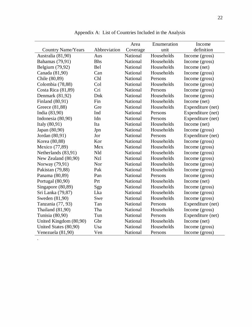
Appendix A: List of Countries Included in the Analysis

Country Name/Years AbbreviationArea

CoverageEnumeration

unitIncome

definitionAustralia (81,90) Aus National Households Income (gross)Bahamas (79,91) Bhs National Households Income (gross)Belgium (79,92) Bel National Households Income (net)Canada (81,90) Can National Households Income (gross)Chile (80,89) Chl National Persons Income (gross)Colombia (78,88) Col National Households Income (gross)Costa Rica (81,89) Cri National Persons Income (gross)Denmark (81,92) Dnk National Households Income (gross)Finland (80,91) Fin National Households Income (net)Greece (81,88) Gre National Households Expenditure (net)India (83,90) Ind National Persons Expenditure (net)Indonesia (80,90) Idn National Persons Expenditure (net)Italy (80,91) Ita National Households Income (net)Japan (80,90) Jpn National Households Income (gross)Jordan (80,91) Jor National Persons Expenditure (net)Korea (80,88) Kor National Households Income (gross)Mexico (77,89) Mex National Households Income (gross)Netherlands (83,91) Nld National Households Income (gross)New Zealand (80,90) Nzl National Households Income (gross)Norway (79,91) Nor National Households Income (gross)Pakistan (79,88) Pak National Households Income (gross)Panama (80,89) Pan National Persons Income (gross)Portugal (80,90) Prt National Households Income (net)Singapore (80,89) Sgp National Households Income (gross)Sri Lanka (79,87) Lka National Households Income (gross)Sweden (81,90) Swe National Households Income (gross)Tanzania (77, 93) Tan National Persons Expenditure (net)Thailand (81,90) Tha National Households Income (gross)Tunisia (80,90) Tun National Persons Expenditure (net)United Kingdom (80,90) Gbr National Households Income (net)United States (80,90) Usa National Households Income (gross)Venezuela (81,90) Ven National Persons Income (gross).

23

Appendix B: Sources for Data Variables

II Income inequality is represented by high quality Gini Coefficients from the Deininger and Squire (1996) data-set that is available from the World Bank (1996), augmented by Gini’s from the United Nations University--World Institute for Development Economics Research and the United Nations Development Programme (1999) World Income Inequality Database (WIID). Observations in the data set bear the DSACC or DSCS labels. The Gini’s enter the data set in decimal form; e.g., .3659.

ETH Ethnicity is a composite variable: racial ethnicity, language, and religion.16 These data are primarily derived from the U.S. Central Intelligence Agency (CIA) World Fact Book (WFB).17

LIT Literacy is from the WFB. We used the percentage of the literate population of a country as defined by that country. The literacy variable enters the data set in decimal form; e.g., .79.

PR Public redistribution of income is proxied for by the ratio of central government budget expenditures to total gross national/domestic product as reported in the International Monetary Funds’ International Financial Statistics (IFS).18

PCI Per capita income is viewed as an exogenous variable in this context.19 The variable is the natural logarithmic transformation of the real value of per capita income (stated in dollars) reported in the United Nations Statistical Yearbook (UNSY). The per capita income estimates are transformed into real values (1990=100) by deflation using the Consumer Price Index for the related countries as reported in the IFS.20 We view this variable as a proxy for wealth that can be transmitted to heirs.

POL The POL variable is an index ranging from 0 to 10 (10 symbolizing a high levels of polity and 0 the total absence of polity) that was assigned to nations by Marshall and Jaggers (2000) as part of the University of Maryland’s Polity IV Project.

PIA The percent of the population in the agricultural sector or rural areas is from the WFBand is the percent of the labor force in agriculture.

16 It is important to note that the only distinction made for adherents of Christianity is that Roman Catholics are distinguished from all protestant faiths.17 As an exception, the racial make-up of the U.S. population for 1980 and 1990 was obtained for the U.S. Census of Population. The WFB percentages that represented ethnic or religious groups summed to 100.18Total government expenditures is line 82 and gross domestic product is line 99b in the IFS.19 Per capita income is viewed as both theoretically and statistically exogenous in this context. The extent of income distribution is not directly contingent up the amount of income generated by a nation, nor by the population of a nation—the two components of the per capita income calculation. Moreover, the calculation of a Gini Coefficient is unrelated to the calculation of per capita income.20 The Consumer Price Indexes appear on line 64 in the IFS.

Documents

Income Inequality and Ethnicity - World Banksiteresources.worldbank.org/INTDECINEQ/Resources/Income... · 2005-06-24 · JUNE 9-10, 20002 Income Inequality and Ethnicity: An International