WP/12/08

Income Inequality and

Current Account Imbalances

Michael Kumhof, Claire Lebarz,

Romain Rancière, Alexander W. Richter

and Nathaniel A. Throckmorton

© 2012 International Monetary Fund WP/12/08

IMF Working Paper

Research Department

Income Inequality and Current Account Imbalances

Prepared by Michael Kumhof, Claire Lebarz, Romain Rancière, Alexander W. Richter

and Nathaniel A. Throckmorton

Authorized for distribution by Douglas Laxton

January 2012

Abstract

This Working Paper should not be reported as representing the views of the IMF.

The views expressed in this Working Paper are those of the author(s) and do not necessarily represent

those of the institutions with which the authors are affiliated. Working Papers describe research in

progress by the author(s) and are published to elicit comments and to further debate.

This paper studies the empirical and theoretical link between increases in income inequality

and increases in current account deficits. Cross-sectional econometric evidence shows that

higher top income shares, and also financial liberalization, which is a common policy

response to increases in income inequality, are associated with substantially larger external

deficits. To study this mechanism we develop a DSGE model that features workers whose

income share declines at the expense of investors. Loans to workers from domestic and

foreign investors support aggregate demand and result in current account deficits. Financial

liberalization helps workers smooth consumption, but at the cost of higher household debt

and larger current account deficits. In emerging markets, workers cannot borrow from

investors, who instead deploy their surplus funds abroad, leading to current account surpluses

instead of deficits.

JEL Classification Numbers: E2; F32; F41.

Keywords: Current account imbalances; income inequality; financial liberalization.

Authors’ Email Addresses: mkumhof@imf.org; claire.lebarz@gmail.com; romainranciere@gmail.com;

richtera@indiana.edu; nathrock@indiana.edu.

2

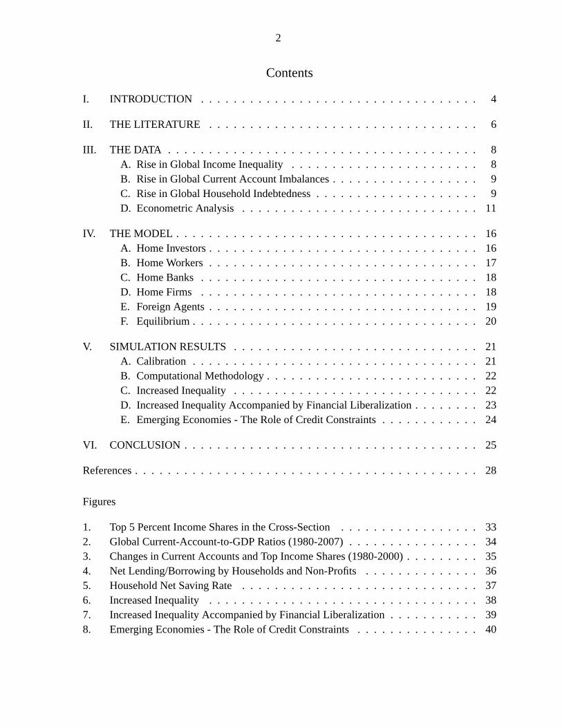
Contents

I. INTRODUCTION . . . . . . . . . . . . . . . . . . . . . . . . . . . . . . . . . . 4

II. THE LITERATURE . . . . . . . . . . . . . . . . . . . . . . . . . . . . . . . . . 6

III. THE DATA . . . . . . . . . . . . . . . . . . . . . . . . . . . . . . . . . . . . . . 8A. Rise in Global Income Inequality . . . . . . . . . . . . . . . . . . . . . . . 8B. Rise in Global Current Account Imbalances . . . . . . . . . . . . . . . . . . 9C. Rise in Global Household Indebtedness . . . . . . . . . . . . . . . . . . . . 9D. Econometric Analysis . . . . . . . . . . . . . . . . . . . . . . . . . . . . . 11

IV. THE MODEL . . . . . . . . . . . . . . . . . . . . . . . . . . . . . . . . . . . . . 16A. Home Investors . . . . . . . . . . . . . . . . . . . . . . . . . . . . . . . . . 16B. Home Workers . . . . . . . . . . . . . . . . . . . . . . . . . . . . . . . . . 17C. Home Banks . . . . . . . . . . . . . . . . . . . . . . . . . . . . . . . . . . 18D. Home Firms . . . . . . . . . . . . . . . . . . . . . . . . . . . . . . . . . . 18E. Foreign Agents . . . . . . . . . . . . . . . . . . . . . . . . . . . . . . . . . 19F. Equilibrium . . . . . . . . . . . . . . . . . . . . . . . . . . . . . . . . . . . 20

V. SIMULATION RESULTS . . . . . . . . . . . . . . . . . . . . . . . . . . . . . . 21A. Calibration . . . . . . . . . . . . . . . . . . . . . . . . . . . . . . . . . . . 21B. Computational Methodology . . . . . . . . . . . . . . . . . . . . . . . . . . 22C. Increased Inequality . . . . . . . . . . . . . . . . . . . . . . . . . . . . . . 22D. Increased Inequality Accompanied by Financial Liberalization . . . . . . . . 23E. Emerging Economies - The Role of Credit Constraints . . . . . . . . . . . . 24

VI. CONCLUSION . . . . . . . . . . . . . . . . . . . . . . . . . . . . . . . . . . . . 25

References . . . . . . . . . . . . . . . . . . . . . . . . . . . . . . . . . . . . . . . . . . 28

Figures

1. Top 5 Percent Income Shares in the Cross-Section . . . . . . . . . . . . . . . . . 332. Global Current-Account-to-GDP Ratios (1980-2007) . . . . . . . . . . . . . . . . 343. Changes in Current Accounts and Top Income Shares (1980-2000) . . . . . . . . . 354. Net Lending/Borrowing by Households and Non-Profits . . . . . . . . . . . . . . 365. Household Net Saving Rate . . . . . . . . . . . . . . . . . . . . . . . . . . . . . 376. Increased Inequality . . . . . . . . . . . . . . . . . . . . . . . . . . . . . . . . . 387. Increased Inequality Accompanied by Financial Liberalization . . . . . . . . . . . 398. Emerging Economies - The Role of Credit Constraints . . . . . . . . . . . . . . . 40

3

Tables

1. Variable Definitions . . . . . . . . . . . . . . . . . . . . . . . . . . . . . . . . . . 412. GMM Estimation (Dependent Variable: CA/GDP) . . . . . . . . . . . . . . . . . 423. ARDL Estimation (Dependent Variable: CA/GDP) . . . . . . . . . . . . . . . . . 43

4

I. INTRODUCTION

Global current account imbalances were a major source of financial sector fragility in therun-up to the 2007 worldwide financial crisis. Several authors, including Obstfeld and Rogoff(2009), Blanchard and Milesi-Ferretti (2009), Portes (2009), and Caballero et al. (2008),either partly attribute the crisis to the amplification effects of large current account imbalancesand low world real interest rates, or suggest that the root causes of global current accountimbalances and the financial crisis coincide.1 The pre-crisis concern with U.S. current accountdeficits centered on the possibility of a run on the U.S. dollar and the danger of the dollarlosing its status as the world’s reserve currency.2 While this has not happened, the perceptionthat it is still a possibility arguably continues to contribute to financial vulnerabilityworldwide. Competing explanations for U.S. current account deficits include low public andprivate saving rates in the United States3, high public saving rates in the rest of the world(Bernanke (2005)), global underinvestment (Prasad et al. (2007), Rajan (2010)),demographics and productivity (Feroli (2003), Ferrero (2007)), and the role of the U.S. dollaras the world’s reserve currency. But the phenomenon of persistently high current accountdeficits is not limited to the United States. We also observe deficits in a number of otherdeveloped economies, especially those in the English-speaking world. By studying thesimilarities between these countries’ experiences, and their differences to surplus countries,we should therefore be able to learn more about the deeper structural reasons for persistentlylarge current account deficits.

We argue in this paper that what unites the experiences of the deficit countries is a steepincrease in income inequality over recent decades that exhibits a clear empirical andtheoretical link to deteriorations in those countries’ current accounts. Our data andcross-country econometric analysis shows that increases in inequality can account for asubstantial part of the observed current account deteriorations in countries like the UnitedStates or the United Kingdom. Moreover, our theoretical analysis lays out a dynamicstochastic general equilibrium model where current account deficits arise endogenously inresponse to higher domestic income inequality. The poor and middle class, who are assumedto not have direct access to international capital markets, start to borrow from the rich whenthey receive a smaller share of aggregate output. The drop in their consumption is thereforeless than the drop in their income, while consumption (and investment) of the rich increases

1Other reasons for the crisis mentioned in the literature include excessive financial liberalization (Keys et al.(2010)), and excessively loose monetary policy either in the United States (Taylor (2009)) or globally (Bank forInternational Settlements (2008)).

2See Obstfeld and Rogoff (2001), Roubini and Setser (2004), Mann (2004) and Mussa (2004).

3The theoretical case for the link between low public saving rates and current account deficits is made inKumhof and Laxton (2010). Empirical evidence is provided in Bluedorn and Leigh (2011).

5

steeply. The net effect is an increase in domestic demand and therefore a current accountdeficit. In other words, the rich fund a significant part of their increased domestic lending byintermediating foreign savings.

The increase in income inequality is typically accompanied, or more commonly followed, bypolitical interventions that try to support the living standards of those who suffer fromstagnating real incomes. However, this is generally not done by directly confronting thesources of inequality, but rather by temporarily alleviating its consequences through access tocheap borrowing, in other words through financial liberalization. For the U.S. case, thisargument has been prominently made by Rajan (2010). While financial liberalizationsucceeds in temporarily preventing a large drop in the consumption of poor and middle classhouseholds, this comes at the expense of ultimately much higher domestic debt levels, higherdebt service, and therefore lower consumption. Financial liberalization generates a strongadditional stimulus to workers’ and therefore aggregate demand, while at the same timeslowing down capital accumulation and thus aggregate supply, as investors increasingly preferfinancial over real assets. This puts additional downward pressure on current accounts.

We also examine emerging economies, many of which have experienced rising incomeinequality accompanied by current account surpluses rather than deficits. We find that theirlarge surpluses can also be explained by increases in income inequality, but in this case againstthe background of domestic financial markets that do not allow the poor and middle class torespond to lower incomes by borrowing. A short-sighted response to global imbalances mighttherefore be to reduce these “financial market imperfections” in surplus countries. However, ifthis policy is administered without addressing the underlying income inequalities, it willresult in a global rather than a regional increase in domestic indebtedness of the poor andmiddle class. While this would reduce cross-border financial fragilities, it would exacerbatedomestic financial fragilities. In the long run there is therefore no alternative to directlyaddressing the income inequality problem. Financial liberalization only buys time, but at theexpense of an eventually much larger debt problem. On the other hand, reducing incomeinequality would reduce the tendency towards current account deficits in financially developedcountries, and towards current account surpluses in financially less developed countries.

Our work builds on Kumhof and Rancière (2010), who show that in the United States there isa striking, but often overlooked, similarity between the pre-crisis periods of the GreatDepression and the Great Recession, in that both periods exhibited a simultaneous increase inincome inequality and in the indebtedness of the poor and middle class. The perception thathousehold indebtedness had become unsustainably high was a key factor that contributed toeventually triggering these crises. Kumhof and Rancière (2010) present a dynamic stochasticgeneral equilibrium model where a financial crisis, driven by income inequality, high leverageand financial fragility, arises endogenously. High leverage is the ultimate result, after a periodof several decades, of a shock to relative bargaining powers over income that favors highincome households at the expense of all remaining households. This shock increases credit

6

demand at the bottom of the income distribution, due to a consumption smoothing or habitpersistence motive, and at the same time it increases credit supply at the top of the incomedistribution, due to a wealth accumulation motive as in Carroll (2000). In other words, highincome households recycle their gains from the bargaining process back to poor and middleincome households through interest-bearing loans that keep growing over a period of decades.

Kumhof and Rancière (2010) replicate several important stylized facts, including the sharplyincreasing debt-to-income ratio of the bottom 95% of the income distribution and a rapidlygrowing financial sector (Philippon (2008)). However, two of the predictions of their modelare counterfactual, and this is due to the choice of a closed economy setting, and toabstracting from financial liberalization. First, the model predicts a collapse in aggregateconsumption that is driven by poor and middle class households. This is in contrast to theU.S. credit-fueled consumption boom, which was significantly financed through foreignsavings. Second, the model predicts an increase in real interest rates, which is contrary to thedata. This again abstracts from the interest-rate lowering effects of foreign savings, but inaddition it abstracts from financial liberalization, which contributed to lower U.S. interestrates and further fueled the credit and consumption boom. This paper extends the frameworkof Kumhof and Rancière (2010) to an open economy setting and adds financial liberalizationshocks, which addresses both of these concerns.

The rest of the paper is organized as follows. Section II discusses the related empirical andtheoretical literature. Section III discusses the stylized facts and presents an econometricpanel data analysis of current account determinants that adds proxies for income inequalityand financial liberalization to a standard set of regressors. Section IV presents the model.Section V presents model simulations that study the effects of increasing income inequalityand of financial liberalization. Section VI concludes.

II. THE LITERATURE

This section discusses the literature that is relevant to different aspects of our work. We beginwith a survey of the empirical literature and then turn to the theoretical literature.

The empirical literature on the distribution of income and wealth focuses on describinglong-run changes in the data (Piketty and Saez (2003), Piketty (2010), Atkinson et al. (2011)).This literature concludes that the most significant change in most countries’ incomedistribution has been a sharp increase in top income shares. Our model reflects this feature bystudying the interactions between two types of agents that represent the top 5% and thebottom 95% of the income distribution.

A small but growing empirical literature has tried to connect growing income inequality togrowing household indebtedness and to the U.S. origins of the financial crisis of 2007/8, most

7

prominently Rajan (2010) and Reich (2010).4 Both authors suggest that increases inborrowing have enabled the U.S. poor and the middle class to maintain or increase their levelof consumption while their real earnings were stalling. However, this literature has so farlimited itself to presenting stylized facts without interpreting them through the prism of ageneral equilibrium model. One consequence has been an ongoing debate as to whether theincrease in credit was mainly driven by credit demand or credit supply. Kumhof and Rancière(2010) provide a general equilibrium model, and show that a shock to the income distributionmust imply a simultaneous increase in both credit demand and credit supply, but with a moreimportant role for credit supply, especially when the income shock is persistent.

Atkinson et al. (2011) document that the rise in top income shares over recent decades hasbeen widespread. It has been observed not only in the United States but also in majorEnglish-speaking countries (Australia, Canada, New Zealand, United Kingdom) since theearly 1980s, and, to a lesser extent and more recently, in some Nordic and peripheralEuropean countries. Building on the work of Lebarz (2011), we document that these countriesalso exhibited high and growing levels of household borrowing and growing current accountdeficits. In other words, we find that the global increase in income inequality is systematicallyrelated to the global increase in current account imbalances. Moreover, the same countriesexhibited financial liberalizations during this period, and we find that there is a strongempirical relationship between financial liberalization and higher current account deficits.

There is a large literature that seeks to determine the fundamental factors that have shapedobserved changes in the income distribution over the last thirty years, both in the UnitedStates and in other countries. They include increases in returns to education and increased useof performance pay (Lemieux et al. (2009), Lemieux (2006)), changes in unionization (Cardet al. (2004)), foreign competition and jobs offshoring (Roberts (2010)), and governmentintervention in support of the rich (Hacker and Pierson (2010)). This paper does not need totake a stand on a preferred explanation. Instead, we take the change in bargaining power overincome as a primitive shock and explore its macroeconomic implications, similar to theapproach of Blanchard and Giavazzi (2003).

Two strands of the theoretical literature are relevant to our paper. The literature on financialfragility has so far focused on the role of heterogeneity between patient and inpatienthouseholds, including Diamond and Dybvig (1983) and more recent financial acceleratormodels applied to household debt and housing cycles (Iacoviello (2005)). In these models,patient agents accumulate more wealth relative to impatient agents, while in our model agentswho derive utility from wealth accumulate positive stocks of real and financial wealth overtime. We find that this is appealing on the grounds of plausibility. Moreover, this paperdocuments that heterogeneity in income, indebtedness and financial fragility across income

4Berg and Ostry (2011) find, in a cross-section of countries, that countries with greater inequality exhibitgrowth spells that are more frequently interrupted by growth breakdowns.

8

groups are an important feature of the data for several countries. Therefore, our analysis of itsimplications should complement existing analyses based on heterogeneity in the degree ofpatience.

The theoretical literature on income inequality (Krueger and Perri (2006), Iacoviello (2008))relates income inequality to increases in household debt by showing that an increase in thevariance of idiosyncratic income shocks across all households generates a higher demand forinsurance through credit markets. Broer (2009) extends that work to the open economy settingand finds that a rise in individual risk in the United States makes default on foreign borrowingless attractive, which allows higher household foreign borrowing against future income. Thismechanism can operate alongside the mechanism we study in this paper, which is based onhighly persistent5 income inequality across two specific household groups, high incomehouseholds and low/middle income households, instead of idiosyncratic income shocks acrossall households. We find that our model, when calibrated to the United Kingdom, matches theobserved increase in the debt-to-income ratio of the bottom 95% of the income distribution bymatching the change in the income share of the bottom 95%.

III. THE DATA

In subsections III.A – III.C we document that over the last three decades the world economyhas experienced increases in global current account imbalances, and simultaneous increases inincome inequality and financial liberalization in deficit countries. Subsection III.D presentseconometric estimates of current account regressions that add income inequality and financialliberalization to a common list of explanatory variables.

A. Rise in Global Income Inequality

This paper quantifies income inequality as the share of aggregate income going to the top 5%of the population, ordered by income. A number of research projects have studied theevolution of top income shares for over 20 countries. This work is documented in Atkinson etal. (2011), in a two-volume book by Atkinson and Piketty (2007, 2010), and in the world topincomes database.6 Atkinson et al. (2011) document that most countries’ top income shares

5On the question of transitory versus persistent income shocks, the recent work of Kopczuk, Saez and Song(2010) shows that the increase in the variance of U.S. annual earnings observed since the 1970 reflects an increasein the variance of permanent rather than transitory earnings.

6This database is available at http://g-mond.parisschoolofeconomics.eu/topincomes/. It covers Argentina,Australia, Canada, China, Finland, France, Germany, India, Indonesia, Ireland, Italy, Japan, Netherlands, NewZealand, Norway, Portugal, Singapore, Spain, Sweden, Switzerland, the United Kingdom and the United States.

9

declined in the first part of the 20th century, mainly because of negative shocks to top capitalincomes during the World Wars and the Great Depression. At that time, top incomes mostlyconsisted of capital income, so that the drop in top income shares represented a drop in topwealth concentration. Top incomes did not start to rise again for two to three decadesfollowing World War II. Globally, as shown in Figure 1, top 5% income shares followed aU-shape in the post-war era, with declines during the immediate post-war decades followedby increases in recent decades (the pattern for top 1% income shares looks very similar).However, the curvature of the U-shape varies considerably across countries. Top incomeshares increased substantially, starting in the early 1980s, for the United States, the UnitedKingdom, Canada, Australia, Ireland and New Zealand (U-shape). Moderate or late increases(L/U-shape) were seen in Southern Europe (Spain, Portugal, Italy) and the Nordic countries(Sweden, Finland, Norway), and small or no increases (L-shape) in Continental Europe(Germany, France, Netherlands, Switzerland) and in Japan.

B. Rise in Global Current Account Imbalances

Figure 2, which uses data from the IMF’s World Economic Outlook 2010, shows theevolution of global current account balances starting in 1980. Among the deficit countries,many exhibited a nearly simultaneous large increase in income inequality, including theUnited States, the United Kingdom, Italy, Ireland and Portugal. Conversely, OECD countriesthat exhibited stable top income shares, including Germany, Japan, Switzerland and France,also experienced balanced current accounts or surpluses. As Figure 3 illustrates, fromapproximately 1980 to 2000 (data coverage varies by country) there is a very strong negativecross-country correlation, of almost -0.8, between changes in top income shares and changesin current account balances among OECD countries. That is, an increase of one percentagepoint of the top 5% income share over the period corresponds to a deterioration of thecurrent-account-to-GDP ratio of 0.8 percentage points. However, this correlation vanisheswhen emerging economies are included. A strength of our model is that it offers anexplanation for both facts, where the key difference between OECD and developing countriesis the state of development of financial markets.

C. Rise in Global Household Indebtedness

The cause of the increase in global current account imbalances is a growing need, on the partof deficit countries, to finance a part of growing domestic household indebtedness throughforeign savings provided by surplus countries.

Figure 4 displays OECD data on household net borrowing as a percentage of GDP, for thethree sets of countries identified above. Households in U-shaped Anglo-Saxon countries

10

increasingly became net borrowers, while households in L-shaped Continental Europeancountries (plus Japan) became net lenders, with a trend that has been fairly stable since 1997.The trend for L/U shaped countries is intermediate, they were net lenders until 2002 but halfof them became net borrowers by 2007, during the same period when their income inequalityincreased the most. The OECD also produces data on the evolution of household sectorsaving as a percentage of disposable income, which are shown in Figure 5 for the same threesets of countries. The pattern is the same as for household borrowing to GDP ratios, withsharply decreasing saving rates for U-shaped countries, stable saving rates for L-shapedcountries, and an intermediate pattern for L/U-shaped countries.

However, our theory stresses increases in borrowing among low and middle incomehouseholds rather than aggregate borrowing or saving rates. This requires a more detailedlook at data where there is much less uniform cross-country coverage available. While aseries of very useful papers on the evolution of income, consumption, and wealth inequalityhas been published under the Cross Sectional Facts for Macroeconomists project by theReview of Economic Dynamics, data on the evolution of leverage across the incomedistribution are difficult to find. Where they are available, the evidence, for U-shapedcountries, suggests that the rise in leverage at the aggregate level has mostly been due tohigher leverage of low and middle income households.

For the United States, Slesnick (2001), Heathcote et al. (2010) and Krueger and Perri (2006)stress that the rise in income inequality has been much more pronounced than the increase inconsumption inequality, which implies increased borrowing for the purpose of consumptionsmoothing. Kopczuk et al. (2010) show that the increase in income inequality was notaccompanied by an increase in income mobility, and that it was lifetime rather than transitoryincome shocks that were the driving force behind rising income inequality. Kumhof andRancière (2010) show that the rise in aggregate household leverage has been exclusively dueto an increase in leverage for the bottom 95% of the income distribution.

Starting in the late 1980s, the United Kingdom experienced similar diverging trends betweenincome and consumption inequality, which are documented in Blundell and Preston (1998)and Blundell and Etheridge (2010). They also find similar results to Kopczuk et al. (2010)concerning transitory versus lifetime income shocks. Data on saving rates across the incomedistribution are documented by Crossley and O’Dea (2010), who show that from 1975 to 2007the median saving rate of the top quintile of the income distribution increased, while that ofthe bottom quintile decreased. Data on leverage across the wealth distribution are onlyavailable for the years 2000 and 2005, and they show that aggregate leverage is mostly due toborrowing by the bottom 95% of households (see Lebarz (2011)).

For Canada, Brzozowski et al. (2010) find that income inequality has increased substantiallyover the last 30 years. As for the United States and the United Kingdom, this has beenaccompanied by a much smaller rise in consumption inequality, and similar results to

11

Kopczuk et al. (2010) concerning transitory versus lifetime income shocks. As shown inLebarz (2011), the observed increase in aggregate household leverage was mostly driven bythe bottom 95% of households. For Australia and New Zealand, Lebarz (2011) documentssimilar facts as for the United States, the United Kingdom and Canada.

The Italian, Swedish and Spanish cases, which are discussed in Jappelli and Pistaferri (2010),Domeij and Floden (2010), and Pijoan-Mas and Sanchez-Marcos (2010), are different fromthe above countries in that they did not observe a clear increase in leverage that was limited tolower and middle income groups.

For the case of the Germany (an L-shaped country), the evolution of income inequality,consumption inequality, and wealth inequality has been documented by Fuchs-Schündeln etal. (2010). They find that inequality was relatively stable in West Germany until Germanreunification, and then trended upwards for wages and market incomes. However, disposableincomes and consumption display only a modest increase in inequality over the same period.7

D. Econometric Analysis

Figure 3 provides evidence of a strongly negative cross-country correlation of around -0.8between changes in top 5% income shares and changes in current accounts. Over the last 30years, countries that have experienced an increase in income inequality have tended to seetheir current account balances deteriorate. However, there are a number of other candidateexplanations for current account deteriorations, some of which are likely correlated withchanges in the income distribution. To account for this issue, we perform a multivariateanalysis of current account determinants using an unbalanced panel of 18 OECD countriesover the period 1968-2006.8 We build our econometric specifications starting from thebenchmark of the panel estimation literature on current account determinants developed byChinn and Prasad (2003), Gruber and Kamin (2007), Chinn and Ito (2008, 2009), and Chinnet al. (2011). We then test whether top income shares and proxies for financial liberalizationhave additional explanatory power when they are added to the explanatory variablescommonly used in this literature.

Econometric Methodology

Before turning to regressions, we test for the presence of a unit root in our panel using theheterogenous panel unit root test of Im et al. (2003). We find that the current account-to-GDP

7Bach et al. (2011) find an increase in German top income shares starting in the late 1990s. However, theyuse different sources besides the World Top Incomes database, whose last available German data point (at thismoment) is 1998.

8The sample of countries is constrained by the availability of data on top income shares, see footnote 7.

12

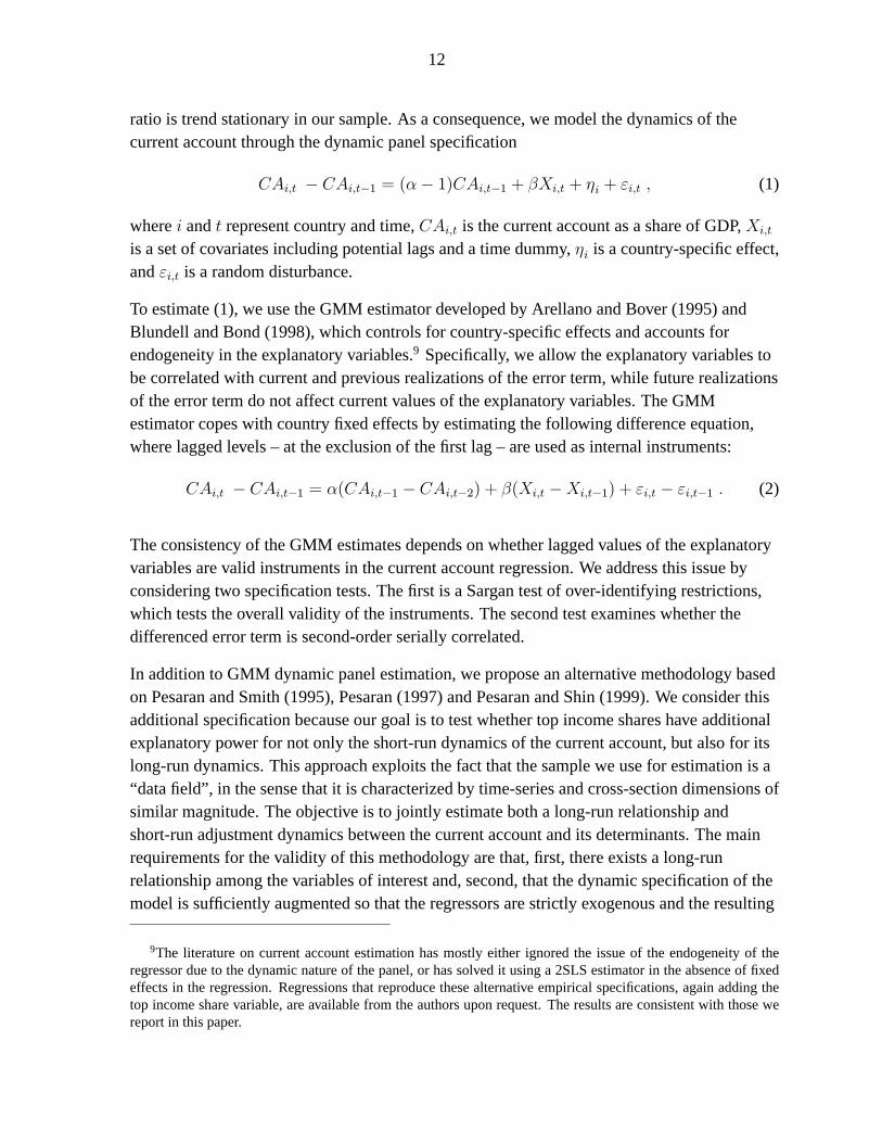
ratio is trend stationary in our sample. As a consequence, we model the dynamics of thecurrent account through the dynamic panel specification

CAi;t � CAi;t�1 = (�� 1)CAi;t�1 + �Xi;t + �i + "i;t ; (1)

wherei andt represent country and time,CAi;t is the current account as a share of GDP,Xi;t

is a set of covariates including potential lags and a time dummy,�i is a country-specific effect,and"i;t is a random disturbance.

To estimate (1), we use the GMM estimator developed by Arellano and Bover (1995) andBlundell and Bond (1998), which controls for country-specific effects and accounts forendogeneity in the explanatory variables.9 Specifically, we allow the explanatory variables tobe correlated with current and previous realizations of the error term, while future realizationsof the error term do not affect current values of the explanatory variables. The GMMestimator copes with country fixed effects by estimating the following difference equation,where lagged levels – at the exclusion of the first lag – are used as internal instruments:

CAi;t � CAi;t�1 = �(CAi;t�1 � CAi;t�2) + �(Xi;t �Xi;t�1) + "i;t � "i;t�1 : (2)

The consistency of the GMM estimates depends on whether lagged values of the explanatoryvariables are valid instruments in the current account regression. We address this issue byconsidering two specification tests. The first is a Sargan test of over-identifying restrictions,which tests the overall validity of the instruments. The second test examines whether thedifferenced error term is second-order serially correlated.

In addition to GMM dynamic panel estimation, we propose an alternative methodology basedon Pesaran and Smith (1995), Pesaran (1997) and Pesaran and Shin (1999). We consider thisadditional specification because our goal is to test whether top income shares have additionalexplanatory power for not only the short-run dynamics of the current account, but also for itslong-run dynamics. This approach exploits the fact that the sample we use for estimation is a“data field”, in the sense that it is characterized by time-series and cross-section dimensions ofsimilar magnitude. The objective is to jointly estimate both a long-run relationship andshort-run adjustment dynamics between the current account and its determinants. The mainrequirements for the validity of this methodology are that, first, there exists a long-runrelationship among the variables of interest and, second, that the dynamic specification of themodel is sufficiently augmented so that the regressors are strictly exogenous and the resulting

9The literature on current account estimation has mostly either ignored the issue of the endogeneity of theregressor due to the dynamic nature of the panel, or has solved it using a 2SLS estimator in the absence of fixedeffects in the regression. Regressions that reproduce these alternative empirical specifications, again adding thetop income share variable, are available from the authors upon request. The results are consistent with those wereport in this paper.

13

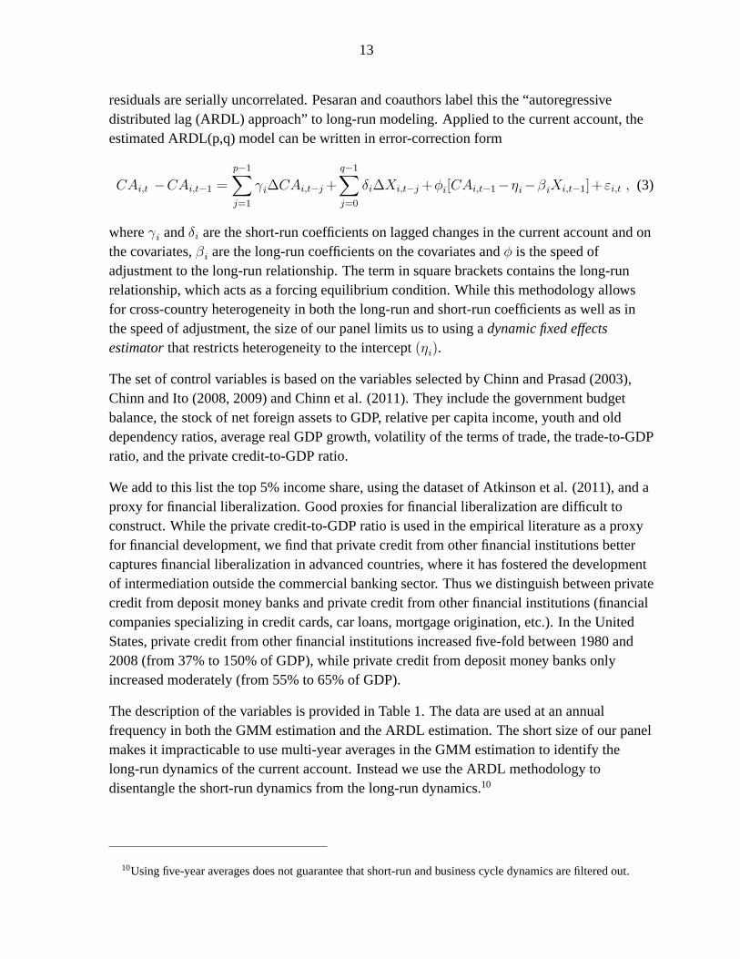
residuals are serially uncorrelated. Pesaran and coauthors label this the “autoregressivedistributed lag (ARDL) approach” to long-run modeling. Applied to the current account, theestimated ARDL(p,q) model can be written in error-correction form

CAi;t �CAi;t�1 =p�1Xj=1

i�CAi;t�j+

q�1Xj=0

�i�Xi;t�j+�i[CAi;t�1��i��iXi;t�1]+"i;t ; (3)

where i and�i are the short-run coefficients on lagged changes in the current account and onthe covariates,�i are the long-run coefficients on the covariates and� is the speed ofadjustment to the long-run relationship. The term in square brackets contains the long-runrelationship, which acts as a forcing equilibrium condition. While this methodology allowsfor cross-country heterogeneity in both the long-run and short-run coefficients as well as inthe speed of adjustment, the size of our panel limits us to using adynamic fixed effectsestimatorthat restricts heterogeneity to the intercept(�i).

The set of control variables is based on the variables selected by Chinn and Prasad (2003),Chinn and Ito (2008, 2009) and Chinn et al. (2011). They include the government budgetbalance, the stock of net foreign assets to GDP, relative per capita income, youth and olddependency ratios, average real GDP growth, volatility of the terms of trade, the trade-to-GDPratio, and the private credit-to-GDP ratio.

We add to this list the top 5% income share, using the dataset of Atkinson et al. (2011), and aproxy for financial liberalization. Good proxies for financial liberalization are difficult toconstruct. While the private credit-to-GDP ratio is used in the empirical literature as a proxyfor financial development, we find that private credit from other financial institutions bettercaptures financial liberalization in advanced countries, where it has fostered the developmentof intermediation outside the commercial banking sector. Thus we distinguish between privatecredit from deposit money banks and private credit from other financial institutions (financialcompanies specializing in credit cards, car loans, mortgage origination, etc.). In the UnitedStates, private credit from other financial institutions increased five-fold between 1980 and2008 (from 37% to 150% of GDP), while private credit from deposit money banks onlyincreased moderately (from 55% to 65% of GDP).

The description of the variables is provided in Table 1. The data are used at an annualfrequency in both the GMM estimation and the ARDL estimation. The short size of our panelmakes it impracticable to use multi-year averages in the GMM estimation to identify thelong-run dynamics of the current account. Instead we use the ARDL methodology todisentangle the short-run dynamics from the long-run dynamics.10

10Using five-year averages does not guarantee that short-run and business cycle dynamics are filtered out.

14

Results

Table 2 reports the GMM estimation results. The Sargan and serial-correlation specificationtests fail to reject the hypothesis of correct identification. The first column lists the set ofpossible regressors, and the remaining columns show the results of five alternativespecifications. The first is a baseline specification with a commonly used list of explanatoryvariables for the current account, while the remaining columns add the top income shares(either 5% or 1%) and different measures of private credit as additional explanatory variables.

All regressions find a significant positive coefficient of 0.73 to 0.77 on the once-laggedcurrent account deficit, which is similar in magnitude to the estimate in Debelle and Faruqee(1996). Trade openness has a positive and significant effect on current account balances, aresult in line with Chinn and Ito (2008) and Chinn et al. (2011). Demography variables alsoaffect the current account balance in the expected direction. For instance, the old dependencyratio negatively affects the current account balance because of dissaving by the old. Thegovernment structural balance does not have a significant effect on the current accountbalance.11

All regressions report a significant coefficient near -0.1 for the top 5% income share, and near-0.3 for the top 1% income share. The interpretation of these estimates is that an increase inthe top 5% income share by one percentage point results, ceteris paribus, in a deterioration ofthe current account balance by approximately 0.1 percentage points of GDP in the currentperiod. However, given the persistent dynamics of both current account balances and topincome shares, the effect of such an increase is persistent, with the medium-term deteriorationof the current account estimated to range between 0.25 and 0.3 percentage points.12 Similarly,we estimate that a one percentage point increase in the top 1% income share would lead to adeterioration of the current account of 0.6 percentage points. Between the late 1970s and2006, the United Kingdom experienced an increase in the top 5% income share of around 10percentage points, and similar magnitudes were observed in the United States. This suggests acurrent account deterioration of at least around 1 percent of GDP and, in the longer run, ofover 2 percent of GDP. This is roughly equal to the actual current account deteriorationexperienced by the United Kingdom over this period, which suggests that this channel iseconomically significant.

Table 2 shows that, while our proxy for financial liberalization is negatively related to thecurrent account in all regressions, these results are not statistically significant in the GMM

11This is in contrast with the recent results of Bluedorn and Leigh (2011). These authors use “action-based”measures of fiscal policy rather than changes in the cyclically-adjusted government balance, and find a significanteffect on the current account.

12The dynamics of the current account are modeled through the autoregressive specificationCAt =�1CAt�1+�2CAt�2+�Xt+ut, where the top 5% income share is included inXt. To estimate the medium-runeffect of a one percentage point increase in the top 5% income share, we compute the ratio�= (1� �1 � �2).

15

regressions. We will show that this changes in the ARDL regressions, which are able toseparately identify the long-run effects of financial liberalization.

Table 3 presents the results of the ARDL estimation of long- and short-run parameters linkingthe current account balance to its determinants. The consistency and efficiency of the dynamicfixed effects estimates relies on several specification conditions. The first is that the regressionresiduals are serially uncorrelated and that the explanatory variables are exogenous. Wesatisfy these conditions by including 2 lags of the current account balance and 1 lag of the top5% income share and of each control variable. We do not expand the lag structure furtherbecause of restrictions imposed by degrees of freedom. The second specification conditionrequires accounting for both country-specific effects and cross-country common factors. Byallowing for a different intercept for each country, we control for country-specific effects, andby using cross-sectionally demeaned data,13 we eliminate cross-country common factors.

The coefficient on the error-correction term is negative and less than one in absolute value,which is consistent with stationarity of current account dynamics and convergence towardsthe long-run equilibrium relationship.14 The current account is negatively related in the longrun to the old dependency ratio. Moreover, it is positively related to the trade-to-GDP ratioand negatively related to the private-credit-to-GDP ratio, which is consistent with the GMMresults.

Once again, we find that the current account balance is negatively and significantly linked tothe top 5% and top 1% income shares in the long run. The estimates are lower than for theGMM estimation, but still economically very significant, with magnitudes near -0.15.15 Theshort-run coefficients are correctly signed but not significant.

Private credit from other financial institutions has a negative long-run impact on currentaccount balances, and the estimates are always highly statistically significant and robust tochanges in explanatory variables. For a given country, we estimate that a one percentage pointincrease in the cross sectional deviation of this ratio corresponds to an approximately 5percentage point deterioration in the current-account-to-GDP ratio. For instance, between1980 and 2008 the ratio of private credit from other financial institutions to GDP experienceda much more sizeable increase in the United States than the mean increase in the other

13Cross-sectional demeaning is performed using gdp weights as is standard in the empirical literature on thecurrent account. Demeaned variables are constructed asgXi;t = Xi;t � �Ji=1(gdpi;tXi;t)=�Ji=1gdpi;t, whereiindexes each country in the sample ofJ countries.

14If � is the lagged coeficient for the current account in the ARDL(1; q) representationCAi;t = �CAi;t�1 +Pqj=0 �Xi;t�j+�i+"i;t, then the coefficent of convergence is� = �(1��):We can thus verify that the estimate

of around� = 0:7 obtained in the GMM estimation corresponds to our estimate for� of about�0:3:

15The long run coefficient estimate for the top 1% income share varies between -0.3 and -0.4, which is alsoslightly lower than the GMM estimate.

16

countries of the panel. The cross-sectional deviation is 0.7 percentage points, which explainsa deterioration of around0:7 � 5 = 3:5 percentage points of the current account-to-GDP ratio.If financial liberalization is an endogenous response to an increase in inequality, as Rajan(2010) claims for the United States, estimated coefficients for top income shares may capturepart of the effect of financial liberalization.

IV. THE MODEL

The world economy consists of two countries, Home and Foreign, with Home’s share of theworld population given by!. The Foreign economy features a representative household andfirm, while the Home economy consists of investors, who own the economy’s capital stockand are net lenders in financial markets, workers, who earn income exclusively through wagelabor and are net borrowers in financial markets, and firms, who combine capital and labor toproduce aggregate output.

A. Home Investors

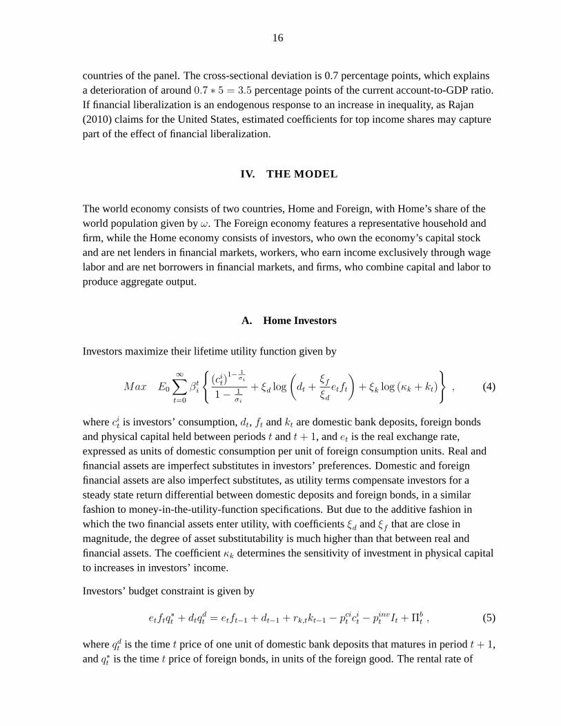
Investors maximize their lifetime utility function given by

Max E0

1Xt=0

�ti

((cit)

1� 1�i

1� 1�i

+ �d log

�dt +

�f�detft

�+ �k log (�k + kt)

); (4)

wherecit is investors’ consumption,dt, ft andkt are domestic bank deposits, foreign bondsand physical capital held between periodst andt+ 1, andet is the real exchange rate,expressed as units of domestic consumption per unit of foreign consumption units. Real andfinancial assets are imperfect substitutes in investors’ preferences. Domestic and foreignfinancial assets are also imperfect substitutes, as utility terms compensate investors for asteady state return differential between domestic deposits and foreign bonds, in a similarfashion to money-in-the-utility-function specifications. But due to the additive fashion inwhich the two financial assets enter utility, with coefficients�d and�f that are close inmagnitude, the degree of asset substitutability is much higher than that between real andfinancial assets. The coefficient�k determines the sensitivity of investment in physical capitalto increases in investors’ income.

Investors’ budget constraint is given by

etftq�t + dtq

dt = etft�1 + dt�1 + rk;tkt�1 � pcit cit � pinvt It +�

bt ; (5)

whereqdt is the timet price of one unit of domestic bank deposits that matures in periodt+ 1,andq�t is the timet price of foreign bonds, in units of the foreign good. The rental rate of

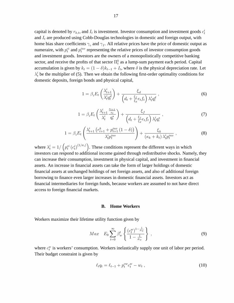
17

capital is denoted byrk;t, andIt is investment. Investor consumption and investment goodscitandIt are produced using Cobb-Douglas technologies in domestic and foreign output, withhome bias share coefficients c and I . All relative prices have the price of domestic output asnumeraire, withpcit andpinvt representing the relative prices of investor consumption goodsand investment goods. Investors are the owners of a monopolistically competitive bankingsector, and receive the profits of that sector�bt as a lump-sum payment each period. Capitalaccumulation is given bykt = (1� �)kt�1 + It, where� is the physical depreciation rate. Let�it be the multiplier of (5). Then we obtain the following first-order optimality conditions fordomestic deposits, foreign bonds and physical capital,

1 = �iEt

��it+1�itq

dt

�+

�d�dt +

�f�detft

��itq

dt

; (6)

1 = �iEt

��it+1�it

et+1et

q�t

�+

�f�dt +

�f�detft

��itq

�t

; (7)

1 = �iEt

�it+1

�rkt+1 + p

invt+1 (1� �)

��itp

invt

!+

�k(�k + kt)�

itpinvt

; (8)

where�it = 1=�pcit (c

it)(1=�i)

�. These conditions represent the different ways in which

investors can respond to additional income gained through redistributive shocks. Namely, theycan increase their consumption, investment in physical capital, and investment in financialassets. An increase in financial assets can take the form of larger holdings of domesticfinancial assets at unchanged holdings of net foreign assets, and also of additional foreignborrowing to finance even larger increases in domestic financial assets. Investors act asfinancial intermediaries for foreign funds, because workers are assumed to not have directaccess to foreign financial markets.

B. Home Workers

Workers maximize their lifetime utility function given by

Max E0

1Xt=0

�tw

((cwt )

1� 1�w

1� 1�w

); (9)

wherecwt is workers’ consumption. Workers inelastically supply one unit of labor per period.Their budget constraint is given by

`tqt = `t�1 + pcwt c

wt � wt ; (10)

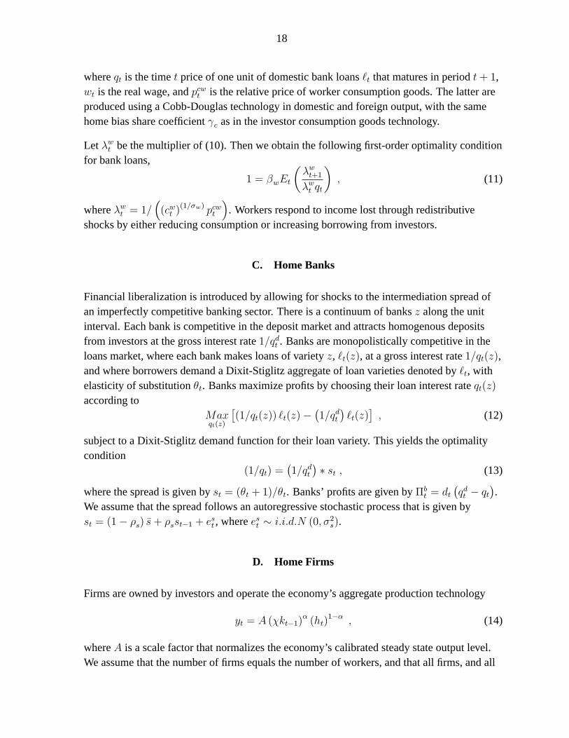
18

whereqt is the timet price of one unit of domestic bank loans`t that matures in periodt+ 1,wt is the real wage, andpcwt is the relative price of worker consumption goods. The latter areproduced using a Cobb-Douglas technology in domestic and foreign output, with the samehome bias share coefficient c as in the investor consumption goods technology.

Let �wt be the multiplier of (10). Then we obtain the following first-order optimality conditionfor bank loans,

1 = �wEt

��wt+1�wt qt

�; (11)

where�wt = 1=�(cwt )

(1=�w) pcwt

�. Workers respond to income lost through redistributive

shocks by either reducing consumption or increasing borrowing from investors.

C. Home Banks

Financial liberalization is introduced by allowing for shocks to the intermediation spread ofan imperfectly competitive banking sector. There is a continuum of banksz along the unitinterval. Each bank is competitive in the deposit market and attracts homogenous depositsfrom investors at the gross interest rate1=qdt . Banks are monopolistically competitive in theloans market, where each bank makes loans of varietyz, `t(z), at a gross interest rate1=qt(z),and where borrowers demand a Dixit-Stiglitz aggregate of loan varieties denoted by`t, withelasticity of substitution�t. Banks maximize profits by choosing their loan interest rateqt(z)

according toMaxqt(z)

�(1=qt(z)) `t(z)�

�1=qdt

�`t(z)

�; (12)

subject to a Dixit-Stiglitz demand function for their loan variety. This yields the optimalitycondition

(1=qt) =�1=qdt

�� st ; (13)

where the spread is given byst = (�t + 1)=�t. Banks’ profits are given by�bt = dt�qdt � qt

�.

We assume that the spread follows an autoregressive stochastic process that is given byst = (1� �s) �s+ �sst�1 + est , whereest � i:i:d:N (0; �2s).

D. Home Firms

Firms are owned by investors and operate the economy’s aggregate production technology

yt = A (�kt�1)� (ht)

1�� ; (14)

whereA is a scale factor that normalizes the economy’s calibrated steady state output level.We assume that the number of firms equals the number of workers, and that all firms, and all

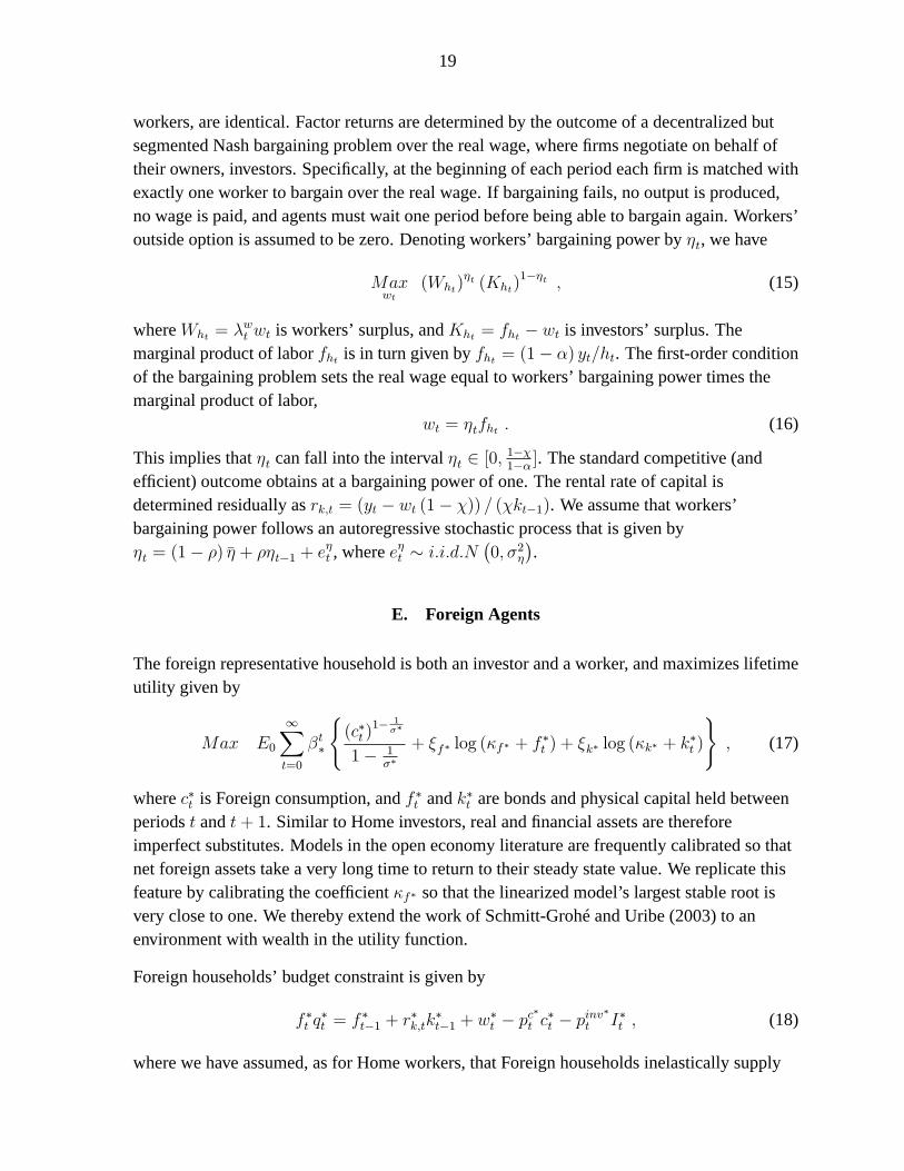
19

workers, are identical. Factor returns are determined by the outcome of a decentralized butsegmented Nash bargaining problem over the real wage, where firms negotiate on behalf oftheir owners, investors. Specifically, at the beginning of each period each firm is matched withexactly one worker to bargain over the real wage. If bargaining fails, no output is produced,no wage is paid, and agents must wait one period before being able to bargain again. Workers’outside option is assumed to be zero. Denoting workers’ bargaining power by�t, we have

Maxwt

(Wht)�t (Kht)

1��t ; (15)

whereWht = �wt wt is workers’ surplus, andKht = fht � wt is investors’ surplus. The

marginal product of laborfht is in turn given byfht = (1� �) yt=ht. The first-order conditionof the bargaining problem sets the real wage equal to workers’ bargaining power times themarginal product of labor,

wt = �tfht : (16)

This implies that�t can fall into the interval�t 2 [0; 1��1�� ]. The standard competitive (andefficient) outcome obtains at a bargaining power of one. The rental rate of capital isdetermined residually asrk;t = (yt � wt (1� �)) = (�kt�1). We assume that workers’bargaining power follows an autoregressive stochastic process that is given by�t = (1� �) �� + ��t�1 + e

�t , wheree�t � i:i:d:N

�0; �2�

�.

E. Foreign Agents

The foreign representative household is both an investor and a worker, and maximizes lifetimeutility given by

Max E0

1Xt=0

�t�

((c�t )

1� 1��

1� 1��

+ �f� log (�f� + f�t ) + �k� log (�k� + k

�t )

); (17)

wherec�t is Foreign consumption, andf �t andk�t are bonds and physical capital held betweenperiodst andt+ 1. Similar to Home investors, real and financial assets are thereforeimperfect substitutes. Models in the open economy literature are frequently calibrated so thatnet foreign assets take a very long time to return to their steady state value. We replicate thisfeature by calibrating the coefficient�f� so that the linearized model’s largest stable root isvery close to one. We thereby extend the work of Schmitt-Grohé and Uribe (2003) to anenvironment with wealth in the utility function.

Foreign households’ budget constraint is given by

f �t q�t = f

�t�1 + r

�k;tk

�t�1 + w

�t � pc

�

t c�t � pinv

�

t I�t ; (18)

where we have assumed, as for Home workers, that Foreign households inelastically supply

20

one unit of labor. Capital accumulation is given byk�t = (1� ��)k�t�1 + I�t . Let��t be the

multiplier of (18). Then��t = 1=�(c�t )

(1=��) pc�t

�, and the first-order optimality conditions for

foreign bonds and physical capital are

1 = ��Et

���t+1��t q

�t

�+

�f�

(�f� + f �t )��t q�t

; (19)

1 = ��Et

��t+1

�rk

�t+1 + p

inv�t+1 (1� ��)

���tp

inv�t

!+

�k�

(�k� + k�t )��tpinv�t

: (20)

The Foreign aggregate production technology is given by

y�t = A� �k�t�1��� (h�t )1��� ; (21)

wherey�t is Foreign output,A� is a scale factor that normalizes Foreign’s steady state outputlevel,k�t is Foreign capital andh�t is Foreign labor. Foreign factor prices are determined incompetitive factor markets. We therefore havew�th

�t = (1� ��)y�t andr�k;tk

�t�1 = �

�y�t .Foreign consumption and investment goodsc�t andI�t are produced using Cobb-Douglastechnologies in domestic and foreign output.

F. Equilibrium

In equilibrium all households maximize their respective lifetime utilities, and goods, labor andfinancial markets clear. The Home and Foreign goods market clearing conditions are

!yt = !��ciht + I

ht

�+ ! (1� �) cwht + (1� !)

�ch

�

t + Ih�

t

�; (22)

(1� !) y�t = (1� !)�cf

�

t + If�

t

�+ !�

�cift + I

ft

�+ ! (1� �) cwft : (23)

For Home and Foreign labor, the inelastic labor supply assumptions implyht = 1� � andh�t = 1. The market clearing conditions for domestic and international financial markets aregiven by

(1� �) `t = �dt ; (24)

!�ft + (1� !) f �t = 0 : (25)

Finally, we have the current account equation, written from the perspective of Home:

�etftq�t = �etft�1 +

1� !!

�ch

�

t + Ih�

t

�� et

���cift + I

ft

�+ (1� �) cwft

�: (26)

21

V. SIMULATION RESULTS

This section discusses the model’s calibration, the computational methodology, andsimulation results.

A. Calibration

The steady state of the model is calibrated to UK data. We choose the United Kingdom fortwo reasons. First, it is among the countries that experienced the largest increases in incomeinequality since the late 1970s. Second, its share in world GDP is more representative ofseveral other deficit countries than the United States. Since we are interested in the periodfrom the late 1970s until just before the 2007 financial crisis, we use data for the period1979-2007, depending on availability, to calibrate the model. We calibrate the initial steadystate workers’ debt-to-income ratio and net-foreign-liabilities-to-GDP ratio to their 1980values (1979 values were not available), given that our interest is in the subsequent evolutionof these variables.

The relative country size! is calibrated so that Home accounts for 4.5% of world GDP, whichequals both the 1979 value and the 1979-2007 sample average for the United Kingdom. Weset the domestic population size of investors to� = 0:05.

In the utility functions, the intertemporal elasticity of substitution equals 0.5 for all agents.The Home coefficient on domestic financial investments�d is set to obtain an initial workers’debt-to-income ratio of 60 percent, which equals the UK value for 1980 according to Debelle(2004). The Home coefficient on foreign bond holdings�f is set to obtain an initial netforeign liabilities to GDP ratio of 8 percent, also equal to the UK value in 1980. We calibrate�f� so that the elasticity of international interest rates with respect to net foreign liabilities ispositive but very small.

The remaining coefficients of agents’ utility functions imply a steady state gross real interestrate on domestic and foreign loans and a steady state gross return to capital after depreciationequal to 1.05, while the steady state gross deposit rate equals 1.02, implying a steady statebanking spreads equal to 3 percent.

We set the coefficients�k and��k to ensure that the elasticity of physical investment withrespect to income shocks is significantly lower than the elasticity of financial investment.Since investors own the entire capital stock, their per capita capital stock is very large relativeto per capita loans. Introducing capital and loans into the utility function additively wouldimply that the elasticity of these two forms of wealth with respect to income shocks would bevery similar. This would imply a very large, and unrealistic, increase in the elasticity ofphysical investment. Introducing the two forms of wealth separably, and calibrating�k and��k

22

appropriately, allows us to avoid that implication. It also allows us to obtain a unique steadystate value for the stocks of loans and deposits.

The factor share coefficient of the production technology� is calibrated to obtain aninvestment-to-GDP ratio of 17.5 percent, which is approximately equal to both the value inthe early 1980s and the sample average for 1979-2007. The depreciation rate equals 10percent per annum. The Cobb-Douglas share coefficients of the trade technologies arecalibrated to produce consumption goods imports-to-GDP ratios of 6 percent, and investmentgoods imports-to-GDP ratios of 7.2 percent, based on 1979-2007 sample averages.

Finally, we calibrate the persistence of the two shock processes to�� = �s = 0:995. This isbased on the observation that changes to realized top income shares and to UK financialsystem regulation have been close to permanent. We assume that this was fully expected byhouseholds. Calibration of the two shock processes as unit roots is infeasible forcomputational reasons.

B. Computational Methodology

Our model is designed to match the persistent growth in both income inequality andhousehold debt observed over past decades. Because this implies highly persistent and verylarge deviations of state variables from their initial steady state values, a local solution methodis inadequate to accurately capture the long-run dynamics. Thus, we obtain a global nonlinearsolution using a time-iterative policy function algorithm, which exploits the theory ofmonotone operators. Monotone operators have useful theoretical and numerical properties.For example, a monotone operator is used to prove existence and uniqueness of equilibrium ofnon-optimal economies by Coleman (1991). This solution technique discretizes the statespace and iteratively solves for updated policy functions that satisfy equilibrium until aspecified tolerance criterion is reached. For additional information and examples of how thealgorithm is applied to conventional real business cycle and new Keynesian models seeRichter et al. (2011).

C. Increased Inequality

Figure 6 simulates a cumulative 10 percent decline in workers’ bargaining power over aperiod of 18 years. By the end of the third decade following the initial shock this leads to areal wage drop of around 7 percent and an increase in the return to capital of around 3percentage points. The bottom right panel shows that this income redistribution closelymatches the change in the top 5% income share in UK data for the period 1979-2007.

The third row shows workers’ responses to their income losses. Higher loans from investors

23

increase workers’ leverage, or debt-to-income ratio, from 60 percent to 140 percent after 30years. This increase, while very large, is still less than what was observed in the data. In theshort run, higher debt allows workers to reduce their consumption by less than the drop intheir wage, but in the longer run workers’ consumption continues to fall even when their realwage starts to recover (mainly due to a rising capital stock). The reason is that by this timedebt service consumes a far larger and growing portion of workers’ disposable income,around 7 percent compared to 3 percent in the original steady state.

The second row shows that investors respond to their income gains by increasing consumption(by 50 percent after 30 years), increasing physical investment (by 12 percent after 30 years),and increasing loans to workers (by 110 percent after 30 years, with significant further growththereafter).16 However, in an open economy there is a fourth possibility, increased loans toworkers financed by borrowing from foreign investors. Or, to put it differently, in an openeconomy workers can obtain loans not only from domestic investors, but also from foreigninvestors. In the model loans from foreign investors are intermediated by domestic investors.This effect is shown in the fourth row, which shows a decline in net foreign assets that reaches8 percent of GDP by year 30, accompanied by a deterioration in the current account thatreaches just over 0.4 percent of GDP around year 20, with the current account graduallyclosing thereafter. However, this effect is significantly smaller than the current accountdeterioration experienced by the United Kingdom since the late 1970s.17

The current account deteriorates because aggregate demand grows faster than aggregatesupply. Investors’ consumption and investment demand grows rapidly as their income shareincreases, while workers’ consumption demand, which represents a much larger share ofaggregate demand, declines as their income share decreases. This decline however is limitedby the presence of financial markets that channel a large share of investors’ gains back toworkers as interest bearing loans, and that in addition are able to draw on foreign savings toincrease loans even further. As we will show in Section IV.E, without these financial marketsthe current account would go into a surplus rather than a deficit.

D. Increased Inequality Accompanied by Financial Liberalization

Figure 7 first reproduces the simulation of Figure 6 as a black solid line, and then adds analternative scenario, shown as a blue dashed line, where the same loss in bargaining power isaccompanied by a reduction in the banking spread by 150 basis points over the first 10 years.This is a simple representation of UK financial liberalization during the “Thatcher years”.

16As mentioned above, calibration of the parameter�k in investors’ preferences is critical for determining therelative changes in physical versus financial investments.

17Data for the UK current account-to-GDP ratio are presented as 5-year moving averages, to dampen the sub-stantial short-run volatility of this variable.

24

The main effect of this change is to make investors direct a much larger share of theiradditional income to financial rather than real investments. Workers borrow much moreheavily, to the point that their consumption does not drop at all during the first decade despitea steep loss in income. Relative to the previous scenario, this further stimulates aggregatedemand, and at the same time it restrains aggregate supply by slowing down capitalaccumulation, thereby causing a much larger increase in the rate of return to capital thanbefore. Workers’ debt-to-income ratio now reaches around 170 percent after 30 years, whichis much closer to matching (in fact, slightly exceeding) actual UK values during the period,while still matching the observed top 5% income share. In the long run this high debt burdenincreases debt servicing costs even further, so that by around year 20 workers’ consumptiondrops below the values observed in the previous scenario.

However, the most dramatic change is observed for the current account, which nowdeteriorates by around 2 percentage points by year 10, and by 1.5 percentage points in thelonger run. This is very close to observed UK current account behavior during the period. Thereason is that aggregate demand now increases faster and aggregate supply increases moreslowly than in the previous scenario. Furthermore, the compression in spreads results in acombination of lower loan interest rates and higher deposit interest rates. Higher deposit ratesraise the attractiveness of domestic deposits relative to foreign bonds for domestic investors,given that the interest rate on foreign loans does not change significantly because of the smallsize of Home relative to the rest of the world. This creates an incentive to invest in domesticdeposits financed by foreign loans, which then fuels the stronger growth in aggregatedemand.18

E. Emerging Economies - The Role of Credit Constraints

So far both the empirical and the theoretical parts of our paper have focused exclusively ondeveloped economies, and have found that greater income inequality, with or without addedfinancial liberalization, creates pressures for the current account to deteriorate. However,greater inequality has been a more general worldwide phenomenon that has also beenobserved in many of the emerging economies that have been among the major suppliers offunds to the deficit countries. In other words these countries have run current accountsurpluses instead of deficits, despite worsening inequality.

This raises the question of whether emerging economies’ experiences contradict our results.In this subsection we show that, with an appropriate modification of the model, they provide

18While these results suggest that the rise in income inequality can explain almost the entire deterioration inUK current account deficits since the late 1970s, this does not imply that the deterioration was unavoidable. Forexample, tighter fiscal or financial sector policies could have leaned against these effects.

25

further support by helping to explain the supply side of global current account imbalances.The key difference in our specification of an emerging economy is the nature of financialmarkets. In many of these countries it is much more difficult for the poor and middle class toborrow than in the United States or the United Kingdom, because of what is generally referredto as “financial market imperfections”. Conversely, it is more difficult for the rich to investtheir additional income in domestic financial instruments, while access to foreign financialinstruments remains available. For illustrative purposes we model “financial marketimperfections” in the simplest possible way, by assuming that Home workers are restricted toconsuming their wage income, with zero debt, and with foreign financial wealth as the onlyfinancial asset entering investors’ utility function. For ease of comparison with the previoussimulations, all other aspects of the baseline calibration remain exactly as they were for theUnited Kingdom. In other words, this is a generic emerging economy, rather than beingcalibrated to a specific country. The shocks are only to bargaining power, since a reduction inspreads cannot occur in the absence of a domestic credit market.

Figure 8 shows the results as a red dash-dotted line overlaid on our previous results. Relativeto the previous simulations, workers’ consumption drops more steeply, given their inability toborrow, while investors increase investments in the two alternatives that remain available tothem, physical capital and foreign financial assets. This results in an external surplus, becausewithout domestic financial markets investors channel their funds abroad and generate foreignrather than domestic demand. The increase in investors’ consumption and investment istherefore no longer sufficient to offset the now significantly steeper decrease in workers’consumption. As aggregate demand drops relative to aggregate supply, the current accountimproves, with a surplus that exceeds 0.5 percent of GDP by year 20 and that gradually closesthereafter. While this is clearly not the entire explanation for the large surpluses of countrieslike China, it does make a significant contribution to that explanation, and it does resolve theapparent contradiction mentioned at the beginning of this subsection.

VI. CONCLUSION

This paper makes both an empirical and a theoretical case that increases in income inequalitytend to lead to increases in current account deficits in developed economies.

Our stylized facts and cross-sectional econometric evidence are strongly supportive of thishypothesis. They suggest that the magnitude of the effect is large, to the point that for theUnited Kingdom it can approximately explain the entire current account deteriorationexperienced between the late 1970s and 2007. Furthermore, financial liberalization, which hasoften been a policy response to increased income inequality, is also empirically associatedwith larger external deficits.

26

We build a dynamic stochastic general equilibrium model that helps us to understand thetransmission mechanism from higher income inequality to higher domestic indebtedness andeventually to higher foreign indebtedness. The key feature of that model is that the economyconsists of two groups of households, a small group of the very rich (investors) and themajority (workers), who compete over income shares in a bargaining game. When workers’income share declines at the expense of investors, investors respond by lending part of theincome they gained back to workers. In addition, in an open economy they benefit from theability to intermediate foreign savings to domestic workers. This lending stimulates aggregatedemand to the point that, despite a significant drop in workers’ consumption, the currentaccount deteriorates.

If the policy response to greater inequality includes financial liberalization, this does helpworkers to smooth consumption in the short run, but this comes at the cost of higherhousehold debt, higher debt service, and therefore ultimately lower consumption in the longrun. Furthermore, it leads to much larger current account deficits as investors take advantageof the attractive lending environment by intermediating even larger foreign savings. This hasthe effect of not only further stimulating aggregate demand, but also of holding backaggregate supply as investors prefer financial over real investments, thereby slowing downcapital accumulation.

Finally, the model can also be used to understand the supply side of global current accountimbalances, the export of funds, and therefore current account surpluses of many importantemerging economies. At first these experiences may suggest a shortcoming of our approach,because many of these surplus countries also experienced steep increases in incomeinequality. But on closer inspection this case actually strengthens our results, as long as themodel is modified appropriately to take account of the fact that typical emerging economiesare characterized by what is commonly referred to as “financial market imperfections”. Whatthis means is that in such economies workers cannot borrow from investors when their incomeshare declines, and that instead they have to reduce their consumption (relative to an oftenfast-growing trend, of course). In such economies higher inequality necessitates anexport-oriented growth model, where the domestic wealthy end up deploying their additionalincome in foreign rather than domestic financial assets. Reduced domestic demand andinvestment in foreign financial assets imply current account surpluses instead of deficits.

A short-sighted response to global imbalances could therefore be to reduce these “financialmarket imperfections” in surplus countries. However, if lending is liberalized withoutaddressing the underlying income inequalities, the result would simply be an increase inindebtedness inside surplus countries (between the rich and the rest of the population), ratherthan between countries. In other words, there would be a globalized rather than a regionalincrease in domestic indebtedness of the poor and middle class. While this would reducecross-border financial imbalances, it would exacerbate domestic debt-to-income ratios. Wehave abstracted from the possibility of crises for the purpose of this paper, but those higher

27

debt-to-income ratios would very likely increase the vulnerability to crises, as in Kumhof andRancière (2010). In the long run, there is therefore simply no way around addressing theincome inequality problem itself. Financial liberalization in surplus countries only buys time,but at the expense of an eventually much larger debt problem.

Many of the policy options for reducing income inequality, which involve either reducingworkers’ relative tax burdens or strengthening their bargaining power over wages, are fraughtwith difficulties (Kumhof and Rancière (2010)). These include the danger of drivinginvestment to other jurisdictions if reductions in labor income taxes are financed throughincreases in capital income taxes. Solutions might include more progressive labor incometaxes that leave average tax rates unchanged, or alternatively the financing of lower laborincome taxes across all income levels through increases in taxes that do not distort economicincentives, including appropriately designed taxes on rents, specifically on profits frominvestments in land, natural resources, and the financial sector. As for strengthening thebargaining power of workers directly, the difficulties of doing so, due for example tointernational competition, must be weighed against the potentially very serious consequencesof further financial difficulties if current trends in household indebtedness—both domesticand international—should continue.

28

REFERENCES

Arellano, M., and Bover, O. (1995), “Another Look at the Instrumental-Variable Estimationof Error-Components Models.”Journal of Econometrics,68, 29–51.

Atkinson, A., Piketty, T. and Saez, E. (2011), “Top Incomes in the Long Run of History”,Journal of Economic Literature, 49, 3-71.

Atkinson, A. and Piketty, T. (2007), “Top Incomes over the Twentieth Century: A Contrastbetween Continental European and English-Speaking Countries”.

Atkinson, A. and Piketty, T. (2010), “Top Incomes over the Twentieth Century: A GlobalPerspective”.

Bach, S., Corneo, G. and Steiner, V. (2011), “Effective Taxation of Top Incomes inGermany”, Discussion Paper.

Bank for International Settlements (2008), 78th Annual Report.

Berg, A. and Ostry, J. (2011), “Inequality and Unsustainable Growth: Two Sides of the SameCoin?”, International Monetary Fund, Staff Discussion Note SDN/11/08.

Bernanke, B. (2005), “The Global Savings Glut and the US Current Account Deficit”,Sandridge Lecture, Virginia Association of Economics.

Blanchard, O. and Giavazzi, F. (2003), “Macroeconomic Effects Of Regulation AndDeregulation In Goods And Labor Markets”,Quarterly Journal of Economics, 118(3),879-907.

Blanchard, O. and Milesi-Ferretti, G.M. (2009), “Global Imbalances: In Midstream?”, IMFStaff Position Note.

Bluedorn, J. and Leigh, D. (2011), “Revisiting the Twin Deficits Hypothesis: The Effect ofFiscal Consolidation on the Current Account”, IMF Economic Review (forthcoming).

Blundell, R. and Bond, S., (1998), "Initial conditions and moment restrictions in dynamicpanel data models," Journal of Econometrics,87(1), 115-143.

Blundell, R. and Etheridge, B. (2008), “Consumption, Income and Earnings Inequality in theUK”, Working Paper, Institute for Fiscal Studies and University College London.

Blundell, R. and Preston, I. (1998), “Consumption Inequality and Income Uncertainty”,Quarterly Journal of Economics, 113, 603-640.

Broer, T. (2008), “Domestic or Global Imbalances? Rising Inequality and the Fall in the USCurrent Account”, Working Paper.

Brzozowski, M. (2009), “Consumption, Income, and Wealth Inequality in Canada”,Reviewof Economic Dynamics, 13(1), 52-75.

Caballero, R., Farhi, E. and Gourinchas, P.O. (2008), “An Equilibrium Model of Global

29

Imbalances and Low Interest Rates”,American Economic Review, 98(1), 358-393.

Card, D., Lemieux, T. and Riddell, D. (2004), “Unions and Wage Inequality”,Journal ofLabor Market Research,25(4),520-562.

Carroll, C.D. (2000), “Why Do the Rich Save So Much?”, in Joel B. Slemrod, Ed.,DoesAtlas Shrug? The Economic Consequences of Taxing the Rich, Cambridge, MA:Harvard University Press.

Chinn, M., Eichengreen, B. and Ito, T. (2011), “A Forensic Analysis of Global Imbalances”,NBER Working Papers No. 17513.

Chinn, M. and Ito, T. (2008), “Global Current Account Imbalances: American Fiscal Policyversus East Asian Savings”,Review of International Economics, 16, 479–498.

Chinn, M. and Prasad, E. (2003), “Medium-term Determinants of Current Accounts inIndustrial and Developing Countries: An Empirical Exploration”,Journal ofInternational Economics, 59, 47–76.

Coleman, J. (1991), “Equilibrium in a Production Economy with an Income Tax”,Econometrica, 59, 1091-1104.

Crossley, T. and O’Dea, C. (2010), “The Wealth and Saving of UK Families on the Eve ofthe Crisis”, Working Paper, Institute for Fiscal Studies.

Debelle, G. (2004), “Household Debt and the Macroeconomy”, BIS Quarterly Review,March.

Diamond, D. and Dybvig, P. (1983), “Bank Runs, Deposit Insurance, and Liquidity”,Journalof Political Economy, 91(3), 401-419.

Domeij, D. and Floden, M. (2010), “Inequality Trends in Sweden 1978-2004”,Review ofEconomic Dynamics, 13(1), 179-208.

Faruqee, H. and Debelle, G. (1996), “What Determines the Current Account? ACross-Sectional and Panel Approach”, IMF Working Papers WP/96/58, InternationalMonetary Fund.

Feroli, M. (2003), “Capital Flows Among the G7 Nations: A Demographic Perspective”,Working Paper, Federal Reserve Board, Division of Research and Statistics.

Ferrero, A. (2007), “The Long-Run Determinants of the U.S. External Imbalances”, FederalReserve Bank of New York, Staff Report No. 295.

Fuchs-Schundeln, N., Krueger, D. and Sommer, M. (2010), “An Equilibrium Model ofGlobal Imbalances and Low Interest Rates”,Review of Economic Dynamics, 13(1),103-132.

Gabaix, X. and Landier, A., (2008), “Why Has CEO Pay Increased So Much?”,QuarterlyJournal of Economics,123(1),49-100.

Gruber, J. and Kamin, S. (2005), “Explaining the Global Pattern of Current Account

30

Imbalances”, Federal Reserve Board, International Finance Discussion Paper No. 846.

Hacker, J. and Pierson, P. (2010),Winner-Take-All Politics, New York: Simon & Schuster.

Heathcote,J., Perri, F. and Violante, G.L. (2010), “Unequal We Stand: An EmpiricalAnalysis of Economic Inequality in the United States: 1967-2006”,Review ofEconomic Dynamics, 13(1), 15-51.

Iacoviello, M. (2005), “House Prices, Borrowing Constraints, and Monetary Policy in theBusiness Cycle”,American Economic Review, 95(3), 739-764.

Iacoviello, M. (2008), “Household Debt and Income Inequality, 1963-2003”,Journal ofMoney, Credit and Banking, 40(5), 929-965.

Im, K., Pesaran, M. and Shin, Y. (2003), “Testing for Unit Roots in Heterogeneous Panels”,Journal of Econometrics, 115, 53–74.

Ito, T. and Chinn, M. (2009), “East Asia and Global Imbalances: Saving, Investment, andFinancial Development”, in: Financial Sector Development in the Pacific Rim, EastAsia Seminar on Economics, Volume 18, National Bureau of Economic Research,117–150.

Jappelli, T. and Pistaferri, L. (2010), “Does Consumption Inequality Track IncomeInequality in Italy?”,Review of Economic Dynamics, 13(1), 133-153.

Keys, B.J., Mukherjee, T., Seru, A. and Vig, V. (2010), “Did Securitization Lead to LaxScreening? Evidence from Subprime Loans”, Quarterly Journal of Economics,125(1),307-62.

Kopczuk, W., Saez, E. and Song, J. (2010), “Earnings Inequality and Mobility in the UnitedStates: Evidence from Social Security Data since 1937”, Quarterly Journal ofEconomics,125(1), 91-128.

Krueger, D. and Perri, F. (2006), “Does Income Inequality Lead to Consumption Inequality?Evidence and Theory”,Review of Economic Studies, 73(1), 163-193.

Kumhof, M. and Laxton, D. (2010), “Fiscal Deficits and Current Account Deficits”, IMFWorking Papers, WP/09/237.

Kumhof, M. and Rancière, R. (2010), “Inequality, Leverage and Crises”, IMF WorkingPapers, WP/10/268.

Lebarz, C. (2011), “Inequalities, Household Leverage and Global Imbalances”, Master’sThesis, Paris School of Economics.

Lemieux, T. (2006), “Post-Secondary Education and Increasing Wage Inequality”,AmericanEconomic Review, 96(2), 195-199.

Lemieux, T., MacLeod, B. and Parent, D. (2009), “Performance Pay and Wage Inequality”,Quarterly Journal of Economics, 124(1), 1-49.

Levitin, A. and Wachter, S. (2010), “Explaining the Housing Bubble”, Georgetown Business,

31

Economics and Regulatory Law Research Paper No. 10-16.

Mann, C. (2004), “Managing Exchange Rates: Achievement of Global Re-balancing orEvidence of Global Codependency?”,Business Economics.

Mussa, M. (2004), “Exchange Rate Adjustments Needed to Reduce Global PaymentsImbalances”, in C.F. Bergsten, J. Williamson, eds.,Dollar Adjustment: How Far?Against What?

Obstfeld, M. and Rogoff, K. (2001), “The Six Major Puzzles in InternationalMacroeconomics: Is There a Common Cause?”,NBER Macroeconomics Annual, 15,339-412.

Obstfeld, M. and Rogoff, K. (2009), “Global Imbalances and the Financial Crisis: Productsof Common Causes”, Working Paper, UC Berkeley and Harvard University.

Pesaran, H., (1997), “The Role of Econometric Theory in Modeling the Long Run”,Economic Journal, 107, 178–191.

Pesaran, H., and Shin, Y., (1999). “An Autoregressive Distributed Lag Modelling Approachto Cointegration.” In Econometrics and Economic Theory in the 20th Century:TheRagnar Frisch Centennial Symposium, chap. 4, pp. 371–413. Cambridge UniversityPress.

Pesaran, H., and Smith, R. (1995), “Estimating Long-Run Relationships from DynamicHeterogeneous Panels.”Journal of Econometrics, 68, 79–113.

Philippon, T. (2008), “The Evolution of the U.S. Financial Industry from 1860 to 2007”,Working Paper, New York University.

Pijoan-Mas, J. and Sanchez-Marcos, V. (2010), “Spain is Different: Falling Trends ofInequality”,Review of Economic Dynamics, 13(1), 154-178.

Piketty, T. (2010), “On the Long-Run Evolution of Inheritance: France 1820-2050”, WorkingPaper, Paris School of Economics.

Piketty, T. and Saez, E. (2003), “Income Inequality in the United States, 1913-1998”,Quarterly Journal of Economics, 118,1-39.

Portes, R. (2009), “Global Imbalances”, Working Paper, London Business School and CEPR.

Prasad, E.S., Rajan, R.G. and Subramanian, A. (2007), “Foreign Capital and EconomicGrowth”, NBER Working Papers 13619, National Bureau of Economic Research, Inc.

Rajan, R. (2010),Fault Lines: How Hidden Fractures Still Threaten the World Economy,Princeton: Princeton University Press.

Reich, R. (2010),Aftershock: The Next Economy and America’s Future, New York: RandomHouse.

Richter, A., Throckmorton, N. and Walker, T. (2011), “Accuracy, Speed and Robustness ofPolicy Function Iteration”, Manuscript, Indiana University.

32

Roberts, P.C. (2010),How the Economy Was Lost, AK Press.

Roubini, N. and Setser, B. (2004), “The US as a Net Debtor: The Sustainability of the USExternal Imbalances”, Working Paper, New York University.

Schmitt-Grohé, S. and Uribe, M. (2003), “Closing Small Open Economy Models”,Journalof International Economics, 61, 163-185.

Slesnick, D. (2001), “Consumption and Social Welfare: Living Standards and TheirDistribution in the United States”, Working Paper.

Taylor, J.B. (2009),Getting Off Track: How Government Actions and Interventions Caused,Prolonged, and Worsened the Financial Crisis, Hoover Institution Press.

33

Figure 1. Top 5 Percent Income Shares in the Cross-Section

Anglo-Saxon Countries (U-shape)

1910 1920 1930 1940 1950 1960 1970 1980 1990 200010

15

20

25

30

35

40

45

Inco

me S

hare

 of T

op 5

%

US UK Canada Australia New Zealand

Continental Europe and Japan (L-shape)

1910 1920 1930 1940 1950 1960 1970 1980 1990 200010

15

20

25

30

35

40

45

Inco

me S

hare

 of T

op 5

%

France Germany Netherlands Switzerland Japan

Southern Europe and Nordic Countries (L/U-shape)

1910 1920 1930 1940 1950 1960 1970 1980 1990 200010

15

20

25

30

35

40

45

Inco

me S

hare

 of T

op 5

%

Sweden Finland Norway Spain P ortugal Italy

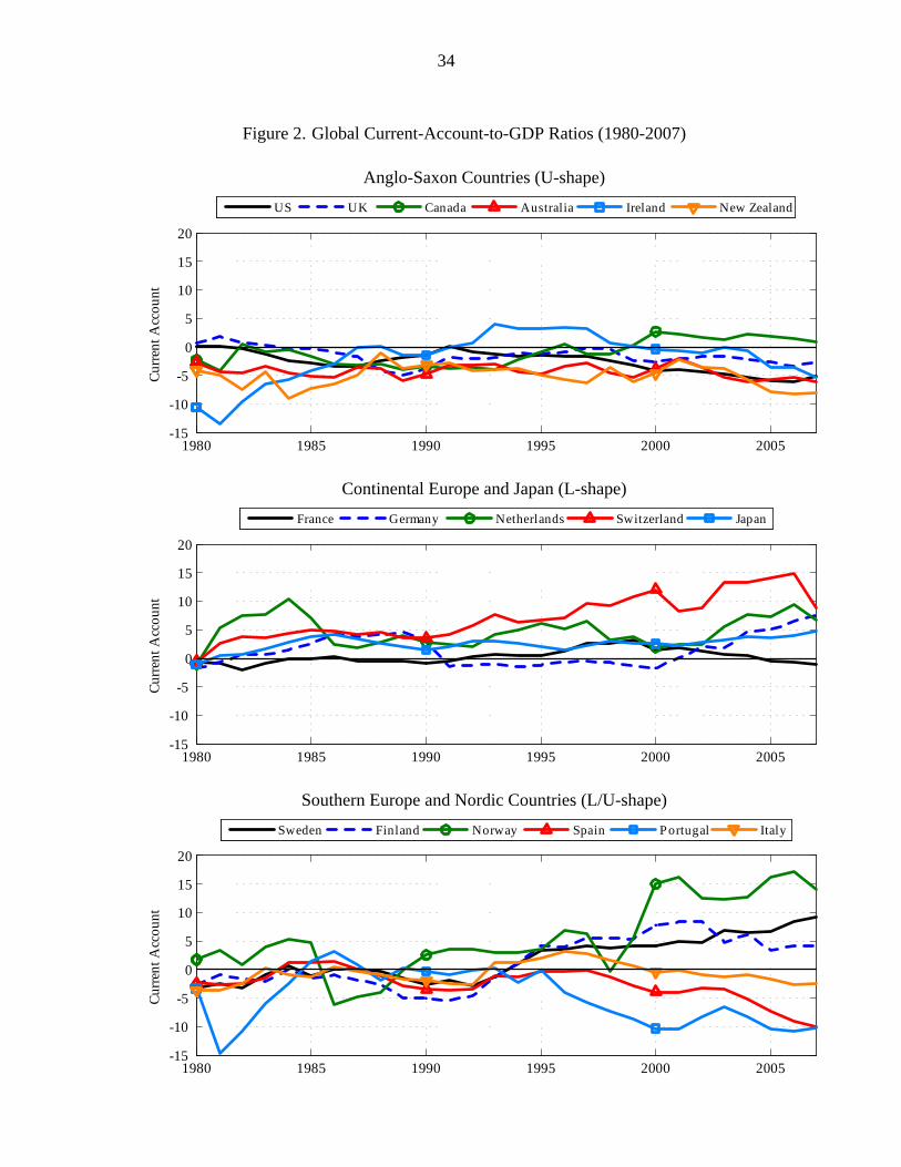
34

Figure 2. Global Current-Account-to-GDP Ratios (1980-2007)

Anglo-Saxon Countries (U-shape)

1980 1985 1990 1995 2000 2005­15

­10

­5

0

5

10

15

20

Curre

nt A

ccou

nt

US UK Canada Australia Ireland New Zealand

Continental Europe and Japan (L-shape)

1980 1985 1990 1995 2000 2005­15

­10

­5

0

5

10

15

20

Curre

nt A

ccou

nt

France Germany Netherlands Switzerland Japan

Southern Europe and Nordic Countries (L/U-shape)

1980 1985 1990 1995 2000 2005­15

­10

­5

0

5

10

15

20

Curre

nt A

ccou

nt

Sweden Finland Norway Spain P ortugal Italy

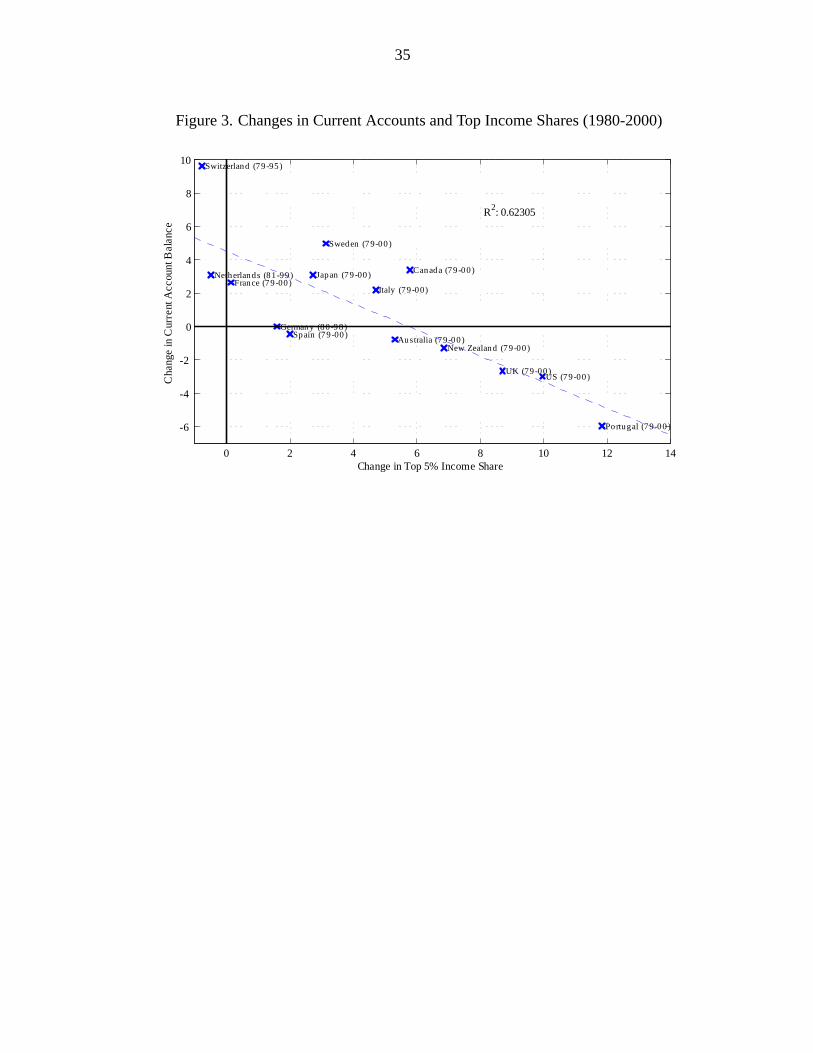
35

Figure 3. Changes in Current Accounts and Top Income Shares (1980-2000)

0 2 4 6 8 10 12 14

­6

­4

­2

0

2

4

6

8

10

Australia (79­00)

Canada (79­00)France (79­00)

Germany  (80­98)

Italy  (79­00)

Japan  (79­00)Netherlands (81­99)

New Zealand  (79­00)

Portugal (79­00)

Spain  (79­00)

Sweden  (79­00)

Switzerland  (79­95)

UK (79­00)US (79­00)

Change in Top 5% Income Share

Cha

nge 

in C

urre

nt A

ccou

nt B

alan

ce

R2: 0.62305

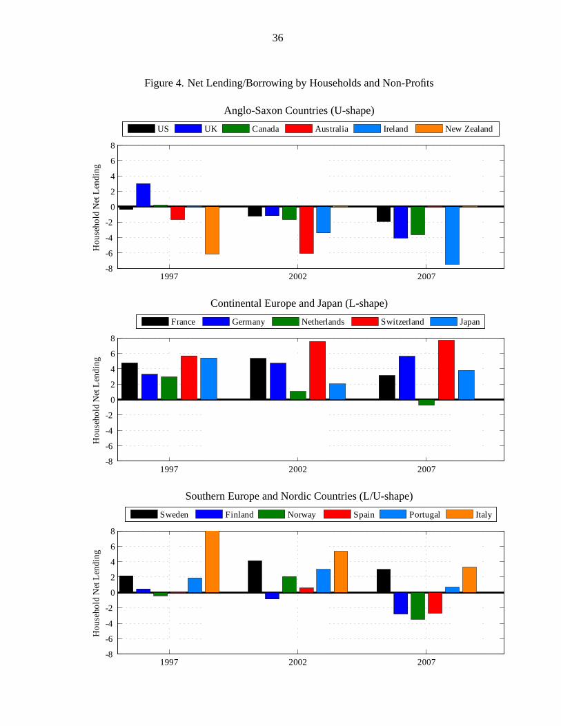
36

Figure 4. Net Lending/Borrowing by Households and Non-Profits

Anglo-Saxon Countries (U-shape)

1997 2002 2007­8

­6

­4

­2

0

2

4

6

8

Hou

seho

ld N

et L

endi

ng

US UK Canada Australia Ireland New Zealand

Continental Europe and Japan (L-shape)

1997 2002 2007­8

­6

­4

­2

0

2

4

6

8

Hou

seho

ld N

et L

endi

ng

France Germany Netherlands Switzerland Japan

Southern Europe and Nordic Countries (L/U-shape)

1997 2002 2007­8

­6

­4

­2

0

2

4

6

8

Hou

seho

ld N

et L

endi

ng

Sweden Finland Norway Spain Portugal Italy

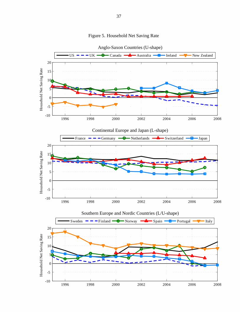
37

Figure 5. Household Net Saving Rate

Anglo-Saxon Countries (U-shape)

1996 1998 2000 2002 2004 2006 2008­10

­5

0

5

10

15

20

Hou

seho

ld N

et S

avin

g Ra

te

US UK Canada Australia Ireland New Zealand

Continental Europe and Japan (L-shape)

1996 1998 2000 2002 2004 2006 2008­10

­5

0

5

10

15

20

Hou

seho

ld N

et S

avin

g Ra

te

France Germany Netherlands Switzerland Japan

Southern Europe and Nordic Countries (L/U-shape)

1996 1998 2000 2002 2004 2006 2008­10

­5

0

5

10

15

20

Hou

seho

ld N

et S

avin

g Ra

te

Sweden Finland Norway Spain Portugal Italy

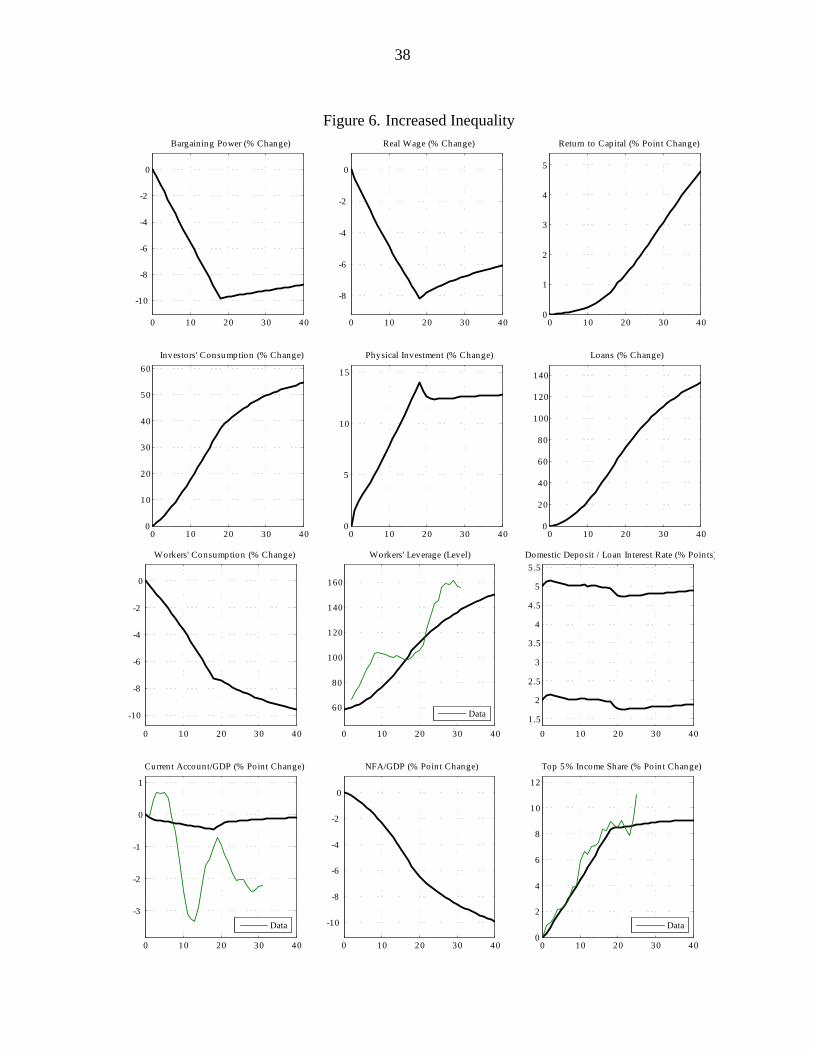
38

Figure 6. Increased Inequality

0 10 20 30 40

­10

­8

­6

­4

­2

0

Bargaining Power (% Change)

0 10 20 30 40

­8

­6

­4

­2

0

Real Wage (% Change)

0 10 20 30 400

1

2

3

4

5

Return  to  Capital (% Point Change)

0 10 20 30 400

10

20

30

40

50

60Investors' Consumption (% Change)

0 10 20 30 400

5

10

15

Physical Investment (% Change)

0 10 20 30 400

20

40

60

80

100

120

140

Loans (% Change)

0 10 20 30 40

­10

­8

­6

­4

­2

0

Workers' Consumption (% Change)

0 10 20 30 40

60

80

100

120

140

160

Workers' Leverage (Level)

0 10 20 30 401.5

2

2.5

3

3.5

4

4.5

5

5.5Domestic Deposit / Loan Interest Rate (% Points)

0 10 20 30 40

­3

­2

­1

0

1

Current Account/GDP (% Point Change)

0 10 20 30 40

­10

­8

­6

­4

­2

0

NFA/GDP (% Point Change)

0 10 20 30 400

2

4

6

8

10

12

Top 5% Income Share (% Point Change)

Data

Data

Data

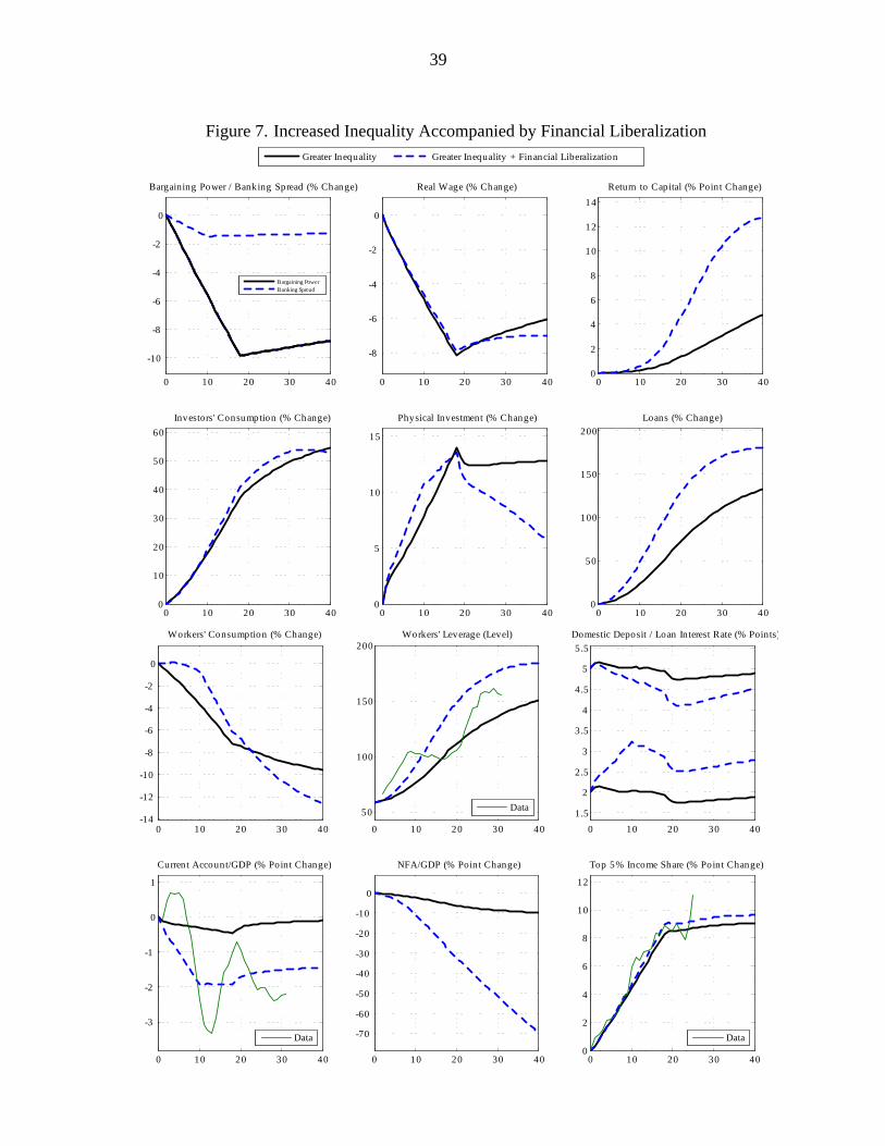
39

Figure 7. Increased Inequality Accompanied by Financial Liberalization

0 10 20 30 40

­10

­8

­6

­4

­2

0

Bargaining Power / Banking Spread (% Change)

0 10 20 30 40

­8

­6

­4

­2

0

Real Wage (% Change)

0 10 20 30 400

2

4

6

8

10

12

14Return  to  Capital (% Point Change)

0 10 20 30 400

10

20

30

40

50

60Investors' Consumption (% Change)

0 10 20 30 400

5

10

15

Physical Investment (% Change)

0 10 20 30 400

50

100

150

200Loans (% Change)

Greater Inequality Greater Inequality  + Financial Liberalization

Bargaining PowerBanking Spread

0 10 20 30 40­14

­12

­10

­8

­6

­4

­2

0

Workers' Consumption (% Change)

0 10 20 30 40

50

100

150

200Workers' Leverage (Level)

0 10 20 30 401.5

2

2.5

3

3.5

4

4.5

5

5.5Domestic Deposit / Loan Interest Rate (% Points)

0 10 20 30 40

­3

­2

­1

0

1

Current Account/GDP (% Point Change)

0 10 20 30 40

­70

­60

­50

­40

­30

­20

­10

0

NFA/GDP (% Point Change)

0 10 20 30 400

2

4

6

8

10

12

Top 5% Income Share (% Point Change)

Data

Data

Data

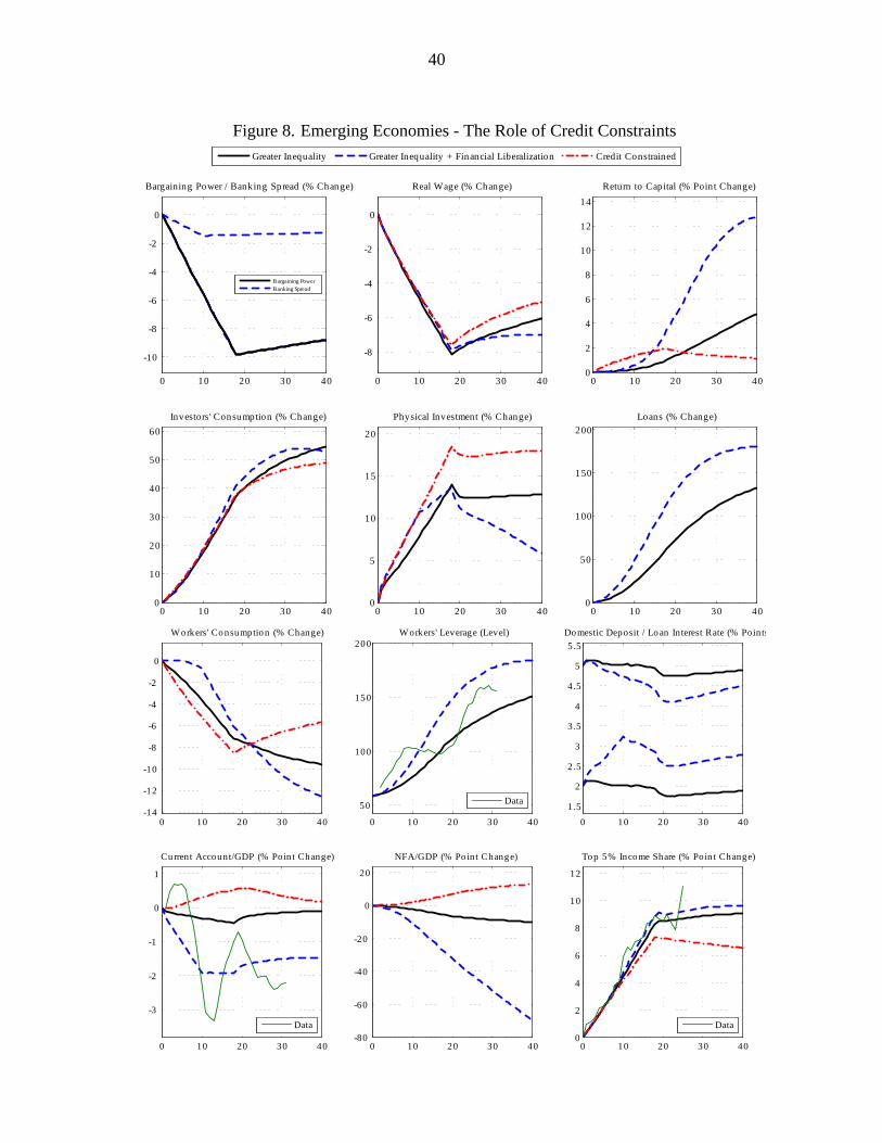
40

Figure 8. Emerging Economies - The Role of Credit Constraints

0 10 20 30 40

­10

­8

­6

­4

­2

0

Bargaining Power / Banking Spread (% Change)

0 10 20 30 40

­8

­6

­4

­2

0

Real Wage (% Change)

0 10 20 30 400

2

4

6

8

10

12

14Return  to  Capital (% Point Change)

0 10 20 30 400

10

20

30

40

50

60Investors' Consumption (% Change)

0 10 20 30 400

5

10

15

20

Physical Investment (% Change)

0 10 20 30 400

50

100

150

200Loans (% Change)

Greater Inequality Greater Inequality  + Financial Liberalization Credit Constrained

Bargaining PowerBanking Spread

0 10 20 30 40­14

­12

­10

­8

­6

­4

­2

0

W orkers' Consumption (% Change)

0 10 20 30 40

50

100

150

200W orkers' Leverage (Level)

0 10 20 30 401.5

2

2.5

3

3.5

4

4.5

5

5.5Do mestic Deposit / Loan Interest Rate (% Points)

0 10 20 30 40

­3

­2

­1

0

1

Current Account/GDP (% Poin t Change)

0 10 20 30 40­80

­60

­40

­20

0

20

NFA/GDP (% Po int Change)

0 10 20 30 400

2

4

6

8

10

12

Top 5% Income Share (% Poin t Change)

Data

Data

Data

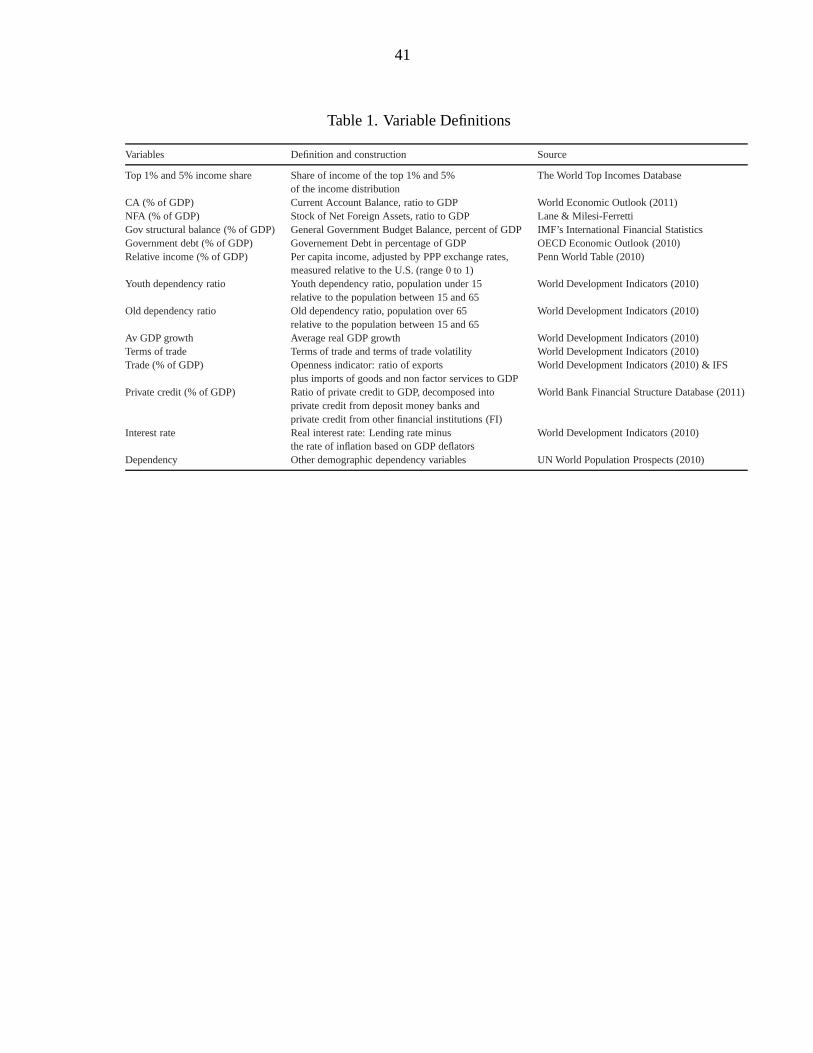
41

Table 1. Variable Definitions

KUMHOF ET AL.: INCOME INEQUALITY AND CURRENT ACCOUNT IMBALANCES

Table 1: Variable Definitions

Variables Definition and construction Source

Top 1% and 5% income share Share of income of the top 1% and 5% TheWorld Top Incomes Databaseof the income distribution

CA (% of GDP) Current Account Balance, ratio to GDP World Economic Outlook (2011)NFA (% of GDP) Stock of Net Foreign Assets, ratio to GDP Lane & Milesi-FerrettiGov structural balance (% of GDP) General Government Budget Balance, percent of GDP IMF’s International Financial StatisticsGovernment debt (% of GDP) Governement Debt in percentage of GDP OECD Economic Outlook (2010)Relative income (% of GDP) Per capita income, adjusted by PPP exchange rates, Penn World Table (2010)

measured relative to the U.S. (range 0 to 1)Youth dependency ratio Youth dependency ratio, population under 15 World Development Indicators (2010)

relative to the population between 15 and 65Old dependency ratio Old dependency ratio, population over 65 World Development Indicators (2010)

relative to the population between 15 and 65Av GDP growth Average real GDP growth World Development Indicators (2010)Terms of trade Terms of trade and terms of trade volatility World Development Indicators (2010)Trade (% of GDP) Openness indicator: ratio of exports World Development Indicators (2010) & IFS

plus imports of goods and non factor services to GDPPrivate credit (% of GDP) Ratio of private credit to GDP, decomposed into World Bank Financial Structure Database (2011)

private credit from deposit money banks andprivate credit from other financial institutions (FI)

Interest rate Real interest rate: Lending rate minus World Development Indicators (2010)the rate of inflation based on GDP deflators

Dependency Other demographic dependency variables UN World Population Prospects (2010)

27

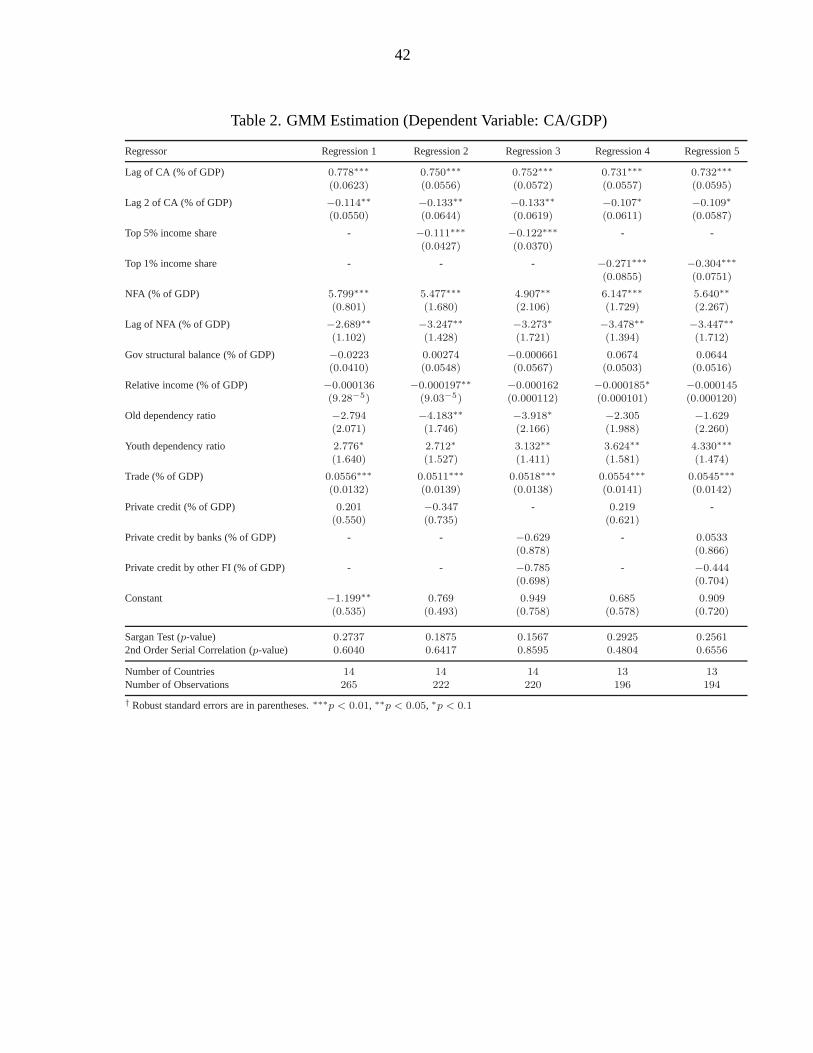
42

Table 2. GMM Estimation (Dependent Variable: CA/GDP)

KUMHOF ET AL.: INCOME INEQUALITY AND CURRENT ACCOUNT IMBALANCES

Table 2: Dynamic Panel GMM Estimation† (Dependent variable: CA (% of GDP))

Regressor Regression 1 Regression 2 Regression 3 Regression4 Regression 5

Lag of CA (% of GDP) 0.778∗∗∗ 0.750∗∗∗ 0.752∗∗∗ 0.731∗∗∗ 0.732∗∗∗

(0.0623) (0.0556) (0.0572) (0.0557) (0.0595)

Lag 2 of CA (% of GDP) −0.114∗∗ −0.133∗∗ −0.133∗∗ −0.107∗ −0.109∗

(0.0550) (0.0644) (0.0619) (0.0611) (0.0587)

Top 5% income share - −0.111∗∗∗ −0.122∗∗∗ - -(0.0427) (0.0370)

Top 1% income share - - - −0.271∗∗∗ −0.304∗∗∗

(0.0855) (0.0751)

NFA (% of GDP) 5.799∗∗∗ 5.477∗∗∗ 4.907∗∗ 6.147∗∗∗ 5.640∗∗

(0.801) (1.680) (2.106) (1.729) (2.267)

Lag of NFA (% of GDP) −2.689∗∗ −3.247∗∗ −3.273∗ −3.478∗∗ −3.447∗∗

(1.102) (1.428) (1.721) (1.394) (1.712)

Gov structural balance (% of GDP) −0.0223 0.00274 −0.000661 0.0674 0.0644(0.0410) (0.0548) (0.0567) (0.0503) (0.0516)

Relative income (% of GDP) −0.000136 −0.000197∗∗ −0.000162 −0.000185∗ −0.000145(9.28−5) (9.03−5) (0.000112) (0.000101) (0.000120)

Old dependency ratio −2.794 −4.183∗∗ −3.918∗ −2.305 −1.629(2.071) (1.746) (2.166) (1.988) (2.260)

Youth dependency ratio 2.776∗ 2.712∗ 3.132∗∗ 3.624∗∗ 4.330∗∗∗

(1.640) (1.527) (1.411) (1.581) (1.474)

Trade (% of GDP) 0.0556∗∗∗ 0.0511∗∗∗ 0.0518∗∗∗ 0.0554∗∗∗ 0.0545∗∗∗

(0.0132) (0.0139) (0.0138) (0.0141) (0.0142)

Private credit (% of GDP) 0.201 −0.347 - 0.219 -(0.550) (0.735) (0.621)

Private credit by banks (% of GDP) - - −0.629 - 0.0533(0.878) (0.866)

Private credit by other FI (% of GDP) - - −0.785 - −0.444(0.698) (0.704)

Constant −1.199∗∗ 0.769 0.949 0.685 0.909(0.535) (0.493) (0.758) (0.578) (0.720)

Sargan Test (p-value) 0.2737 0.1875 0.1567 0.2925 0.25612nd Order Serial Correlation (p-value) 0.6040 0.6417 0.8595 0.4804 0.6556

Number of Countries 14 14 14 13 13Number of Observations 265 222 220 196 194

† Robust standard errors are in parentheses.∗∗∗p < 0.01, ∗∗p < 0.05, ∗p < 0.1

28

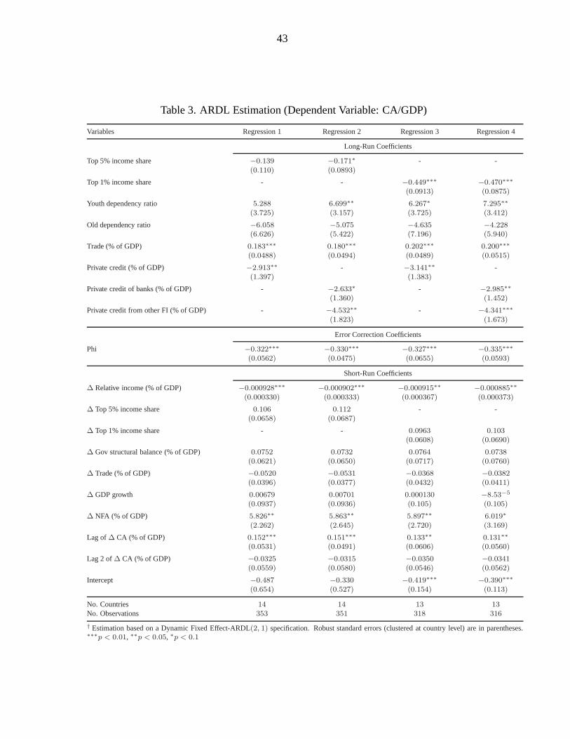
43

Table 3. ARDL Estimation (Dependent Variable: CA/GDP)

KUMHOF ET AL.: INCOME INEQUALITY AND CURRENT ACCOUNT IMBALANCES

Table 4: ARDL Estimation† (Dependent variable: CA (% of GDP))

Variables Regression 1 Regression 2 Regression 3 Regression 4

Long-Run Coefficients

Top 5% income share −0.139 −0.171∗ - -(0.110) (0.0893)

Top 1% income share - - −0.449∗∗∗ −0.470∗∗∗

(0.0913) (0.0875)

Youth dependency ratio 5.288 6.699∗∗ 6.267∗ 7.295∗∗

(3.725) (3.157) (3.725) (3.412)

Old dependency ratio −6.058 −5.075 −4.635 −4.228(6.626) (5.422) (7.196) (5.940)

Trade (% of GDP) 0.183∗∗∗ 0.180∗∗∗ 0.202∗∗∗ 0.200∗∗∗

(0.0488) (0.0494) (0.0489) (0.0515)

Private credit (% of GDP) −2.913∗∗ - −3.141∗∗ -(1.397) (1.383)

Private credit of banks (% of GDP) - −2.633∗ - −2.985∗∗

(1.360) (1.452)

Private credit from other FI (% of GDP) - −4.532∗∗ - −4.341∗∗∗

(1.823) (1.673)

Error Correction Coefficients

Phi −0.322∗∗∗ −0.330∗∗∗ −0.327∗∗∗ −0.335∗∗∗

(0.0562) (0.0475) (0.0655) (0.0593)

Short-Run Coefficients

∆ Relative income (% of GDP) −0.000928∗∗∗ −0.000902∗∗∗ −0.000915∗∗ −0.000885∗∗

(0.000330) (0.000333) (0.000367) (0.000373)

∆ Top 5% income share 0.106 0.112 - -(0.0658) (0.0687)

∆ Top 1% income share - - 0.0963 0.103(0.0608) (0.0690)

∆ Gov structural balance (% of GDP) 0.0752 0.0732 0.0764 0.0738(0.0621) (0.0650) (0.0717) (0.0760)

∆ Trade (% of GDP) −0.0520 −0.0531 −0.0368 −0.0382(0.0396) (0.0377) (0.0432) (0.0411)

∆ GDP growth 0.00679 0.00701 0.000130 −8.53−5

(0.0937) (0.0936) (0.105) (0.105)

∆ NFA (% of GDP) 5.826∗∗ 5.863∗∗ 5.897∗∗ 6.019∗

(2.262) (2.645) (2.720) (3.169)

Lag of∆ CA (% of GDP) 0.152∗∗∗ 0.151∗∗∗ 0.133∗∗ 0.131∗∗

(0.0531) (0.0491) (0.0606) (0.0560)

Lag 2 of∆ CA (% of GDP) −0.0325 −0.0315 −0.0350 −0.0341(0.0559) (0.0580) (0.0546) (0.0562)

Intercept −0.487 −0.330 −0.419∗∗∗ −0.390∗∗∗

(0.654) (0.527) (0.154) (0.113)

No. Countries 14 14 13 13No. Observations 353 351 318 316

† Estimation based on a Dynamic Fixed Effect-ARDL(2, 1) specification. Robust standard errors (clustered at country level) are in parentheses.∗∗∗p < 0.01, ∗∗p < 0.05, ∗p < 0.1

30