Income, Health and Happiness

353

Income, Health and Happiness

Peter Saunders" Social Policy Research Centre The University of New South Wales

Abstract

This article utilises unit record data from the 1989-90 National Health Survey to explore the relationships between low income and perceptions of health and happiness. After describing how the key variables were constructed, attention is focused on the incidence of perceived poor health and unhappiness among those individuals living in income units on either side of a poverty threshold related to the Henderson poverty line. The results reveal that those in poverty generally have poorer health and are less happy than those above the poverty threshold. The observed differences are statistically significant f o r many income unit types, particularly non-aged single people und couples with children. Attention then turns to exploring how health and happiness vary across the deciles of the income distribution. Again, significant dq- ferences are revealed, particularly when more sophisticated distributional measures are employed. Finally, consideration is given to the possibility that the results reflect reverse causality, and that the observed correlations in- corporate the role of intervening variables.

* This version of the article has benefited from the comments made by two referees on an earlier version. Excellent research assistance has been provided by George Mathe- son. The usual caveats apply.

1. Introduction

It is generally taken as axiomatic in economics that to have a higher income is to be better off and to be better off is to be happier. However, even acknowledging that these propositions only hold in principle when all else is held con- stant, the validity of both has been brought into question in Sen's theoretical analysis of the standard of living (Sen 1987). At the empirical level, recent Australian research on living standards has focused attention on the need to consider the implications of using alternative income concepts (Australian Bureau of Statistics 1992; Travers & Richardson 1993), as well as on the relationship between the alternative income measures and well-being on the one hand (Johnson, Manning & Hellwig 1995; Dwyer & Larkin 1996), and between objective and subjective indicators of well-being on the other (Travers & Richardson 1993).

Recent empirical studies of living standards and perceptions of well-being by Headey and Wearing (1992), Brownlee and McDonald (1993) and Travers and Richardson (1993) have highlighted the complexities of the issue and drawn attention to the rather limited contri- bution of neoclassical welfare economics in understanding the subtle nuances which influence subjective assessments of happiness and well-being. All three studies show that the correlations between income and happiness are positive, but weak.

Headey and Wearing conclude from their analysis that:

income and status, or material well-being and prestige, are not of paramount importance to

354 The Australian Economic Review 4th Quarter 1996

subjective well-being and psychological distress. [Headey & Wearing 1992, p. 801

Travers and Richardson, using data from the 1987 Australian Standard of Living Study (ASLS), show that how one chooses to repre- sent the results can influence what conclusions are drawn from them. Thus they show that although the percentage of respondents who reported themselves to be ‘very happy’ increases across the quintiles of the income distribution, there is relatively little quintile variation in the percentages who are either ‘very happy’ or ‘fairly happy’ (Travers & Richardson 1993, Figures 4.1 to 4.3) or in the percentages reporting their health status to be poor (Figures 4.7 to 4.9). However, the same data show more sub- stantial quintile differences if the quintile means are expressed relative to the overall mean scores for each variable (Figures 4.4 to 4.6 and 4.10 to 4.12).

Further, multivariate regression analysis using individual data reveals that there is no significant relationship between subjective happiness and either equivalent (need-adjusted) disposable income or full income, which includes an estimate of the value of leisure and owner- ship of assets (Travers & Richardson 1993, Table 4.1). Travers and Richardson themselves find this result somewhat puzzling, stating that: ‘We do not actually believe that higher incomes make people miserable’ (p. 127), and refer to their descriptive statistics which suggest, as noted above, that ‘there is a weak but positive association between happiness and income’ (p. 127). Taken together, these results suggest that while income and happiness are linked, the relationship between them is more apparent in aggregate data on broad income averages and is not consistently linear over all income ranges.

The possibility of a non-linear relationship between income and happiness which may also be mediated by intervening variables receives support from Travers and Richardson themselves, who summarise their findings by noting that:

in terms of self-assessed contentment, once there is enough to get by, money and possessions are not very important-avoidance of stress arising from shortage of cash, is, however. Non-material

dimensions of life, such as support and company, health, social standing, marriage and not being worse off than previously, are all important. [Travers & Richardson 1993, p. 1311

This raises the possibility that, over time, the relationship between income and happiness may not be symmetrical; increases in income may lead to little change in perceived happiness, while a decline in income may make people very unhappy, or at least less happy than they were previously-a possibility which receives support from Travers and Richardson’s regression results (see Table 4.1 and p. 127).

Such a finding is also consistent with results reported by Saunders and Matheson (1993) which indicate that the income level which people regard as necessary for them to be able to ‘make ends meet’ is conditioned by a number of historical and social factors as well as by past levels of disposable income. In combina- tion, these factors are likely to influence how changing incomes translate into changing perceptions of well-being.

Recent analysis of data collected by the Aus- tralian Institute of Family Studies (AIFS) in the course of conducting its Australian Living Standards Study (ALSS) also suggests that the relationship between income and well-being exists, but is rather weak. Although the AIFS study was restricted to families with children under 20, Brownlee and McDonald (1993) show that while the degree of satisfaction with ‘overall living standards’ and with ‘life as a whole’ both increase with income, in neither case is the variation very large (Brownlee & McDonald 1993, Charts 20 to 23).’

If income is not consistently correlated with perceived levels of well-being, what factors are? When people are asked this question directly, many stress the importance of good health, at least as they themselves perceive it. As the World Bank has recently put it: ‘Good health, as people know from their own experience, is a crucial part of well-being’ (World Bank 1993, p. 17).

This is confirmed by the findings from both the ALSS and ASLS research referred to above. Travers and Richardson find that although there is a strong age pattern in levels of

Saunders: Income. Health and Happiness 355

perceived health, there are also marked differences across the income quintiles within age categories (Travers & Richardson 1993, Fig- ures 4.10 to 4.12). Brownlee and McDonald find a broadly similar pattern among parents who participated in the ALSS, and even though the percentage reporting their health as being either ‘fair’ or ‘poor’ is low overall, it varies systematically across the deciles of equivalent income (Brownlee & McDonald 1993, Charts 19 and 20). This caused the authors to conclude that while the poor may not be happy, they are less sad than they had expected them to be (Brownlee & McDonald 1993, p. 32).

In summary, all three studies suggest that although there are links between economic well- being and subjective assessments of happiness and health, the relationships appear to be not only relatively weak, but also complex and probably non-linear. Such differences as do exist often only become apparent when com- paring those at the extremes of the income distribution. In addition, there is evidence which suggests that subjective health status vanes systematically with income and that to the extent that health affects perceptions of happiness, income and happiness will also be related indirectly.

The aim of this article is to present some further evidence which bears upon the important issues raised in this body of research. The article is organised as follows. Section 2 briefly describes the data and explains how an estimate of income was imputed onto the data file. In Section 3, the data are used to study how subjective assessments of health and happiness vary according to the poverty status of respondents. Section 4 then presents results linking health and happiness to income over the whole income distribution. The main conclusions are summarised in Section 5.

2. Methods

The data analysed in the remainder of the article were collected as part of the National Health Survey (NHS) which was conducted by the Australian Bureau of Statistics (ABS) in 1990. The NHS data have been supplemented by data from the Survey of Income and Housing

Costs and Amenities (SIHCA) which was also undertaken in 1990. Unit record data from these two major social surveys have been integrated to form a data set containing a range of information on health status as well as an estimate of the incomes of each of the more than 28 000 adult records on the integrated data file. The size of the resulting data set far exceeds that of either the ALSS and ASLS samples, thus permitting a more thorough investigation of the linkages between income, health and happiness.

Although the NHS collected an enormous wealth of information on health status, one of its main limitations for economic analysis is that the income variable is a gross (before-tax) measure and, for reasons of confidentiality, was collapsed into eleven broad income ranges. This prevents the imputation of income tax and hence the estimation of disposable income which is needed to estimate well-being and assign poverty status.* Despite these limitations, analysis of the relationship between income and health using the NHS gross income data has been undertaken by the National Health Strategy (1992) and subsequently by the Australian Institute of Health and Welfare (AIHW 1992) and researchers based there (Mathers 1994a, 1994b, 1995).

In order to derive an estimate of gross income, a regression model was estimated using the SIHCA data and then employed to predict a value for gross income on the NHS data file from the information provided on the income bracket of each re~pondent .~ The regression model was supplemented for the 2 per cent or so of respondents with reported gross incomes over $60 000, for whom the parameters of the Pareto distribution were estimated from the SIHCA data and used to randomly impute incomes in the $60 OOO+ range.4

Once gross income had been estimated, an income tax imputation model similar to that developed by Saunders and Hobbes (1988) was used to estimate income tax and Medicke levy liabilities in order to estimate disposable income. Individual incomes were then aggre- gated up to derive the disposable income of each income unit and equivalent disposable income was then estimated by adjusting for need


using the (detailed) Henderson equivalence scale.’

Finally, the estimates were used to determine the poverty status of each income unit. For this purpose, a poverty threshold set 20 per cent above the Henderson poverty line was used. This procedure was justified partly because of the limitations of the income data, but also so as to include in the poverty group both the ‘poor’ and the ‘rather poor’, following the work of the Commission of Inquiry into Pov- erty (1 975).6 Finally, the same income estimates were used to rank individuals according to the position of their income unit in the overall distribution.

The methodology used in the remainder of this article involves estimating the differences which exist between a range of indicators for those whose incomes place them on either side of the poverty threshold or in different deciles of the income distribution. Statistical tests were then conducted to assess whether or not the observed differences were significant.

3. Poverty, Health and Happiness

In light of the focus on subjective health and happiness which forms the basis of the research summarised in the Introduction, the following analysis focuses on these two indicators. Two specific questions were asked as part of the NHS which relate to the subjective health status and happiness of respondents. Both were asked relatively early, immediately following a series of questions seeking background demographic information and health insurance coverage, but before the more detailed questions on recent ill- ness, the use of health services and lifestyles.

It should be emphasised that although no at- tempt was made in the survey to validate these

(and other) reported medical conditions against an independent medical assessment, they are nonetheless an important basis for analysing difSerences in the health status of different groups in the population.

The precise questions asked in each case were as follows:

Question 7.0 In general, would you say that your health is excellent, good, fair or poor?

Question 7.1 I now want to ask you about how you feel generally. Overall, would you say that you’re very happy, happy, unhappy or very unhappy?

In responding to each of these questions, respondents were asked to choose between four alternative responses. One of the consequences of providing so few response categories is that the responses may be biased because people may be unwilling to describe themselves as being ‘unhappy’ or ‘very unhappy’, for example, but may be more prepared to admit to being somewhat unhappy if a more finely grained set of possible responses is a ~ a i l a b l e . ~ The limitations of this aspect of the NHS data should not be lost sight of in considering the results which follow.

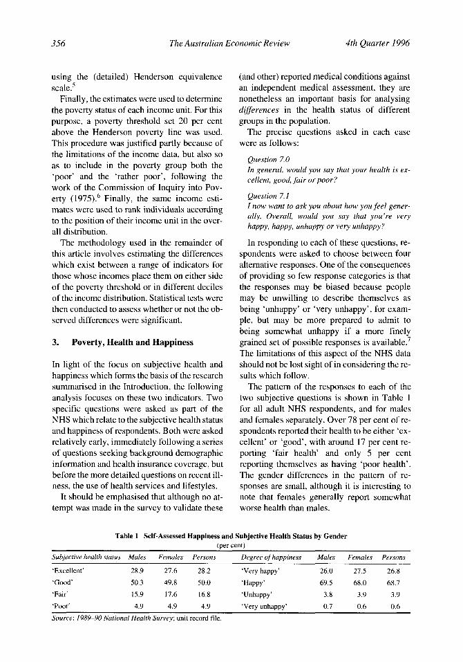
The pattern of the responses to each of the two subjective questions is shown in Table 1 for all adult NHS respondents, and for males and females separately. Over 78 per cent of respondents reported their health to be either ‘excellent’ or ‘good’, with around 17 per cent reporting ‘fair health’ and only 5 per cent reporting themselves as having ‘poor health’. The gender differences in the pattern of responses are small, although it is interesting to note that females generally report somewhat worse health than males.

Table 1 Self-Assessed Happiness and Subjective Health Status by Gender (per cent)

Subjective health stutus Mules Females Persons Degree of happiness Mules Femules Persons

‘Excellent’ 28.9 27.6 28.2 ‘Very happy’ 26.0 27.5 26.8

‘Good’ 50.3 49.8 50.0 ‘Happy’ 69.5 68.0 68.7

‘Fair’ 15.9 17.6 16.8 ‘Unhappy’ 3.8 3.9 3.9

‘Poor’ 4.9 4.9 4.9 ‘Very unhappy’ 0.7 0.6 0.6 Source: 1989-90 National Health Survey; unit record file.

Saunders: Income. Health and Happiness 357

The proportion reporting their health to be either ‘fair’ or ‘poor’ in Table 1 is well below the corresponding proportion found by Brown- lee and McDonald (1993).’ They found that the proportion reporting their health to be either ‘fair’ or ‘poor’ was between 5 per cent and 15 per cent, depending on the level of income. These differences are explored in more detail and comparisons drawn between parents and children in McDonald and Brownlee (1994, Figure 7>.9

In relation to self-assessed happiness, the results in Table 1 suggest that the majority of Australians appear to be quite content with their lot-or at least were so in 1989-90. Over- all, almost 27 per cent of respondents said they felt ‘very happy’ and a further 69 per cent were ‘happy’, with only 4.5 per cent reporting themselves to be either ‘unhappy’ or ‘very unhappy’. These figures are similar to those reported by Travers and Richardson (1993). In this case there are virtually no gender differences in the degree of happiness shown by men and women.

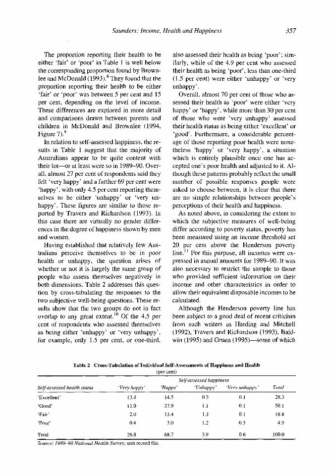
Having established that relatively few Aus- tralians perceive themselves to be in poor health or unhappy, the question arises of whether or not it is largely the same group of people who assess themselves negatively in both dimensions. Table 2 addresses this question by cross-tabulating the responses to the two subjective well-being questions. These results show that the two groups do not in fact overlap to any great extent.” Of the 4.5 per cent of respondents who assessed themselves as being either ‘unhappy’ or ‘very unhappy’, for example, only 1.5 per cent, or one-third,

also assessed their health as being ‘poor’; sim- ilarly, while of the 4.9 per cent who assessed their health as being ‘poor’, less than one-third (1.5 per cent) were either ‘unhappy’ or ‘very unhappy’.

Overall, almost 70 per cent of those who assessed their health as ‘poor’ were either ‘very happy’ or ‘happy’, while more than 30 per cent of those who were ‘very unhappy’ assessed their health status as being either ‘excellent’ or ‘good’. Furthermore, a considerable percentage of those reporting poor health were nonetheless ‘happy’ or ‘very happy’, a situation which is entirely plausible once one has accepted one’s poor health and adjusted to it. Al- though these patterns probably reflect the small number of possible responses people were asked to choose between, it is clear that there are no simple relationships between people’s perceptions of their health and happiness.

As noted above, in considering the extent to which the subjective measures of well-being differ according to poverty status, poverty has been measured using an income threshold set 20 per cent above the Henderson poverty line.’’ For this purpose, all incomes were expressed in annual amounts for 1989-90. It was also necessary to restrict the sample to those who provided sufficient information on their income and other characteristics in order to allow their equivalent disposable incomes to be calculated.

Although the Henderson poverty line has been subject to a good deal of recent criticism from such writers as Harding and Mitchell (1992), Travers and Richardson (1993), Bald- win (1995) and Gruen (1995)-some of which

Table 2 Cross-Tabulation of Individual Self-Assessments of Happiness and Health (per cent)

Self- assessed happiness Self-assessed health status ‘Very happy’ ‘Happy ’ ‘Unhappy ’ ‘Very unhappy’ Total

‘Excellent’ 13.4 14.5 0.3 0.1 28.3

‘Good’ 11.0 37.9 1.1 0.1 50.1

‘Fair’ 2.0 13.4 1.3 0.1 16.8

‘Poor’ 0.4 3.0 1.2 0.3 4.9

Total 26.8 68.7 3.9 0.6 100.0

Source: 1989-90 National Health Survey; unit record tile.


have been addressed by Saunders (1995)-its use here is justified primarily on the grounds of its familiarity. To use an alternative poverty line would only serve to confuse the issues under discussion. It is also worth emphasising that this is not a study of poverty per se, but rather an investigation of differences in the cir- cumstances of those above and below the poverty threshold. For this purpose, where the poverty line is set can be regarded as being of secondary importance.12

The results which follow consider the relationship between the subjective indicators of the well-being and health of individuals and the

poverty status of the income unit of which they are a member. Although it is implicit in the measurement of poverty on an income unit basis that income is assumed to be shared equally amongst all individuals in the income unit, this assumption is unlikely to be appropriate in all cases. Where income is not shared equally within the unit, some individuals within it will experience more deprivation than others. This may in turn lead to differences in perceived health status or well-being, even amongst individuals who, because they belong to the same income unit, are assumed to have the same standard of living and hence the same

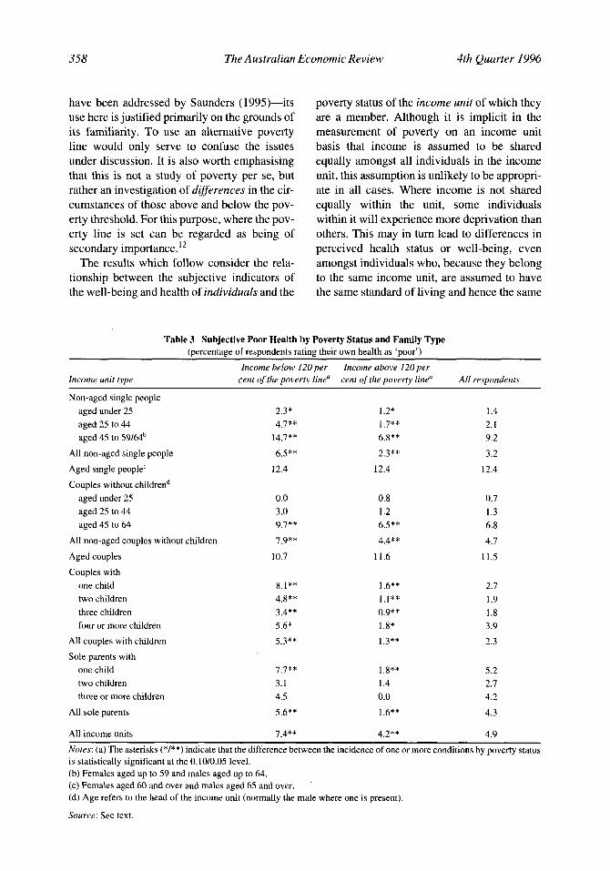
Table 3 Subjective Poor Health by Poverty Status and Family Type (percentage of respondents rating their own health as 'poor')

Income below 120per Income ubove 120per Income unit type cent of the poverty linea cent of the poverry line" All respondents

Non-aged single people aged under 25 2.3* 1.2* 1.4

aged 45 to 59/mb 14.7** 6.8** 9.2

All non-aged single people 6.5** 2.3** 3.2

Aged single people' 12.4 12.4 12.4

Couples without childrend

aged 25 to 44 4.7** 1.7** 2.1

aged under 25 0.0 0.8 0.7 aged 25 to 44 3.0 1.2 1.3 aged 45 to 64 9.7** 6.5** 6.8

All non-aged couples without children 7.9** 4.4** 4.7

Aged couples 10.7 11.6 11.5 Couples with

one child 8.1** 1.6** 2.7 two children 4.8** 1.1** 1.9 three children 3.4** 0.9** 1.8 four or more children 5.6* 1.8* 3.9

All couples with children 5.3** 1.3** 2.3 Sole parents with

one child 7.7** 1.8** 5.2 two children 3.1 1.4 2.7 three or more children 4.5 0.0 4.2

All sole parents 5.6** 1.6** 4.3

All income units 7.4** 4.2** 4.9

Notes: (a) The asterisks (*/**) indicate that the difference between the incidence of one or more conditions by poverty status is statistically significant at the 0.10/0.05 level. (b) Females aged up to 59 and males aged up to 64. (c) Females aged 60 and over and males aged 65 and over. (d) Age refers to the head of the income unit (normally the male where one is present).

Source: See text.

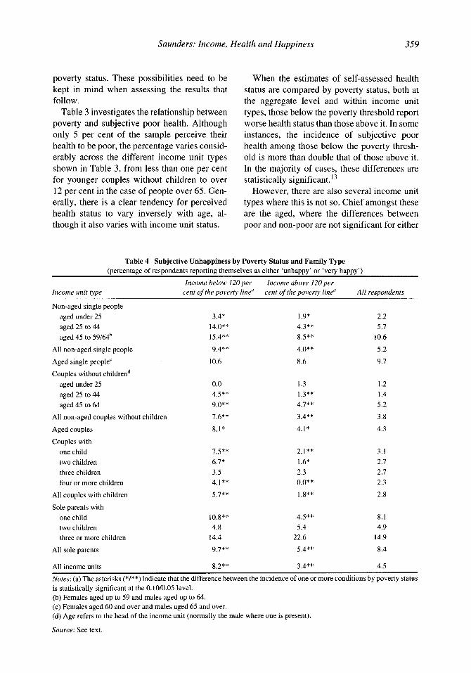
Saunders: Income, Health and Happiness 359

poverty status. These possibilities need to be kept in mind when assessing the results that follow.

Table 3 investigates the relationship between poverty and subjective poor health. Although only 5 per cent of the sample perceive their health to be poor, the percentage varies considerably across the different income unit types shown in Table 3 , from less than one per cent for younger couples without children to over 12 per cent in the case of people over 65. Gen- erally, there is a clear tendency for perceived health status to vary inversely with age, although it also varies with income unit status.

When the estimates of self-assessed health status are compared by poverty status, both at the aggregate level and within income unit types, those below the poverty threshold report worse health status than those above it. In some instances, the incidence of subjective poor health among those below the poverty threshold is more than double that of those above it. In the majority of cases, these differences are statistically significant."

However, there are also several income unit types where this is not so. Chief amongst these are the aged, where the differences between poor and non-poor are not significant for either

Table 4 Subjective Unhappiness by Poverty Status and Family Type (percentage of respondents reporting themselves as either 'unhappy' or 'very happy')

Income below 120per Income above 120per Income unit type cent of the poverty line" cent of the poverty line" All respondents

Non-aged single people aged under 25 aged 25 to 44 aged 45 to 59/64b

All non-aged single people

Aged single people'

Couples without childrend aged under 25 aged 25 to 44 aged 45 to 64

All non-aged couples without children

Aged couples

Couples with one child two children three children four or more children

All couples with children

Sole parents with one child two children three or more children

All sole parents

All income units

3.4* 14.0** 15.4**

9.4** 10.6

0.0 4.5** 9.0**

1.6**

8.1*

I S * * 6.7* 3.5 4.1**

5.7**

10.8** 4.8

14.4 9.7**

8.2**

1.9* 4.3** 8.5**

4.0** 8.6

1.3 1.3** 4.7**

3.4**

4.1*

2.1** 1.6* 2.3 o.o** 1.8**

4.5** 5.4

22.6 5.4**

3.4**

2.2 5.7

10.6

5.2 9.7

1.2 1.4 5.2 3.8

4.3

3.1 2.7 2.7 2.3 2.8

8.1 4.9

14.9

8.4

4.5

Notes: (a) The asterisks (*/**) indicate that the difference between the incidence of one or more conditions by poverty status is statistically significant at the 0.10/0.05 level. (b) Females aged up to 59 and males aged up to 64. (c) Females aged 60 and over and males aged 65 and over. (d) Age refers to the head of the income unit (normally the male where one is present).

Source: See text.

360 The Austruliun Economic Review 4th Quarter I996

single people or for couples-nor are they very large in absolute size in either case. The other two groups where the differences are not significant are younger childless couples and sole parents with two or more children. In these cases, the non-significance of the differences probably reflects the high level of subjective health among younger couples and the small number of sole parents with more than one child.

Table 4 compares the extent of unhappiness among income units situated on either side of the poverty threshold. The measure of the degree of unhappiness used includes those who indicated that they were either ‘unhappy’ or ‘very unhappy’. Although the overall percentage of ‘unhappy’ respondents is not great (at 4.5 per cent), both income unit type and age are again factors associated with the extent of perceived unhappiness. The proportion who report themselves as ‘unhappy’ or ‘very unhappy’ varies from around one per cent for younger couples without children, to over 10 per cent for single people in their forties and fifties, and to almost 15 per cent for small numbers of sole parents with more than two children. These variations appear to reflect the stage of the life cycle of respondents and possibly also their labour force and marital status.

When those who are on either side of the poverty cut-off are compared, there is clear evidence that poverty is significantly correlated with unhappiness. This is as one would expect and as others have found. There may thus be some truth in the proposition that the poor are ‘happy with their lot’ but these results indicate that they are also a good deal less happy than the rest of the population.

The degree of unhappiness amongst the poor is almost two and a half times higher than amongst the rest of the population, and a differential of about this magnitude is apparent for most of the individual income unit types shown in Table 4. In some cases, the differential unhappiness factor exceeds three, particularly for couples with children. Whilst many of the differences shown in Table 4 are statistically significant, for those groups where this is not so, this may again reflect small sample size (for example, in the case of sole parents with three

or more children), or the low level of reported unhappiness amongst both poor and non-poor groups (for example, in the case of younger couples without children).

Overall, the results presented in Tables 3 and 4 provide considerable support for the view that those whose incomes are below the poverty line, or only marginally above it, perceive themselves as being both in worse health and more unhappy than other Australians. These associations hold at both the aggregate level and also for most of the income unit types typ- ically studied in poverty research. However, it is clear that there are several other factors- specifically, but not exclusively, age-which also affect the differences revealed in the results.

4. Relative Income, Health and Happiness

We now consider how the proportion of people who report themselves as being in ‘poor health’ varies not with their poverty status, but with their position in the overall income distribution. The sequencing of this section follows that of the previous section and the analysis thus begins by considering how distributional position affects self-assessed health status.

The procedure adopted for this purpose involves deriving the distribution of equivalent disposable income amongst income units (using the detailed Henderson equivalence scale), separating that distribution into deciles (each containing 10 per cent of individuals when ranked in ascending order of the level of equivalent disposable income of the income unit to which they belong) and then calculating the average value of each indicator for individuals who are located in each decile of the resulting distribution. This method draws upon the most sophisticated distributional measures as described, for example, in the recent study of income distribution in OECD countries undertaken by Atkinson, Rainwater and Smeeding (1995).

In order to assess how much difference these measurement techniques make to the results, the analysis was also undertaken using a more conventional distributional measure in which


no equivalence adjustment was made, and in which disposable income (and the derivation of the distributional deciles) refers to income units rather than to individuals. In this latter case, because each decile contains 10 per cent of income units, they will each contain slightly more or less than 10 per cent of individuals, while the scope of the subjective ‘happiness’ and ‘health’ indicators will also be correspond- ingly slightly different in scope.

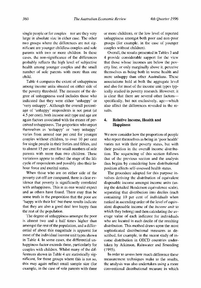
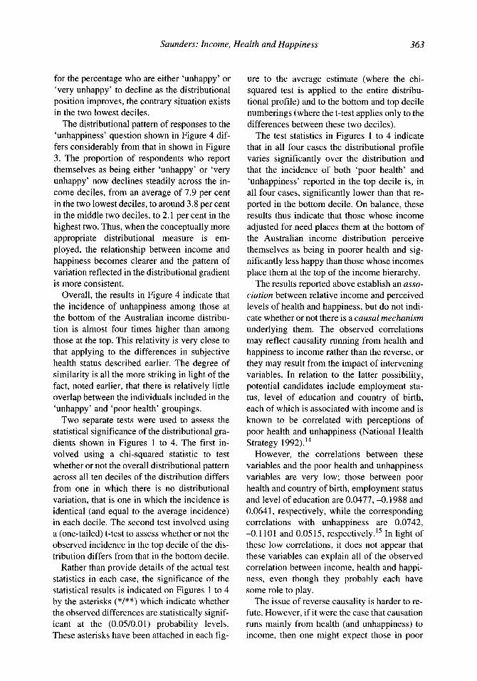
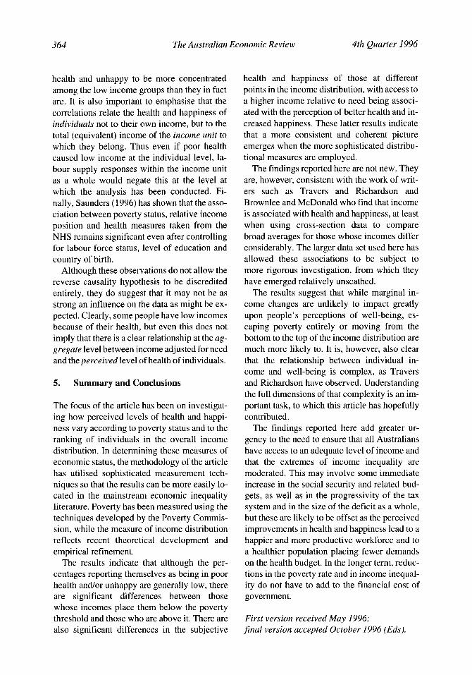
Figures 1 and 2 illustrate how subjective health status varies with income across the deciles of the two alternative measures of income distribution. As before, the percentages shown in these two figures refer to those re-

spondents who reported their health status as being ‘poor’ at the time of the NHS interview. It is clear that the basis on which the income distribution is measured makes a considerable difference to the pattern of results which emerges. In the case of Figure 1, where no equivalence adjustment is made to reflect differences in need, the relationship between distributional position and subjective health status displays no consistent pattern. Although the percentage reporting their health as ‘poor’ is generally higher in the lower deciles, there is no clear tendency for that proportion to decline consistently as income rises. Instead, the percentage reporting poor health first rises from

Figure 1 Self-Assessed Poor Health and the Distribution of Actual Disposable Income among Income Units (percentages reporting their overall health a5 ‘poor’)

per cent

14-1

average = 4.5 per cent**

I** 2 3 4 5 6 7 8 9 lo** decile

Figure 2 Self-Assessed Poor Health and the Distribution of Equivalent Disposable Income among Individuals (percentages reporting their overall health as ‘poor’)

per cent

1 average = 4.5 per cent** - - - - - - _ _ - - - .

I * * 2 3 4 5 6 7 8 9 lo** decile

362 The Australian Economic Review 4th Quarter I996

around 5 per cent to almost 13 per cent in the first two deciles, then declines to around 8 per cent over the next three deciles before falling sharply to around 2 per cent in the middle of the distribution, and then declining to around one per cent in the top decile.

In contrast, in Figure 2 where an equivalence adjustment is made and results are presented on an individual basis, the percentage reporting their health to be poor declines more consistently as income adjusted for need increases. Even here, however, the proportion reporting themselves to be in poor health reaches a max- imum in the third and fifth deciles, not at the very bottom of the distribution. In this case, the

percentage reporting poor health declines from 6.5 per cent on average in the two lowest deciles to 1.6 per cent in the two highest deciles-a relativity of over four to one.

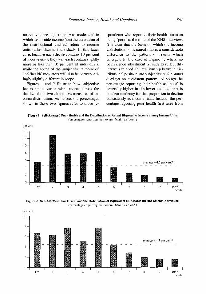
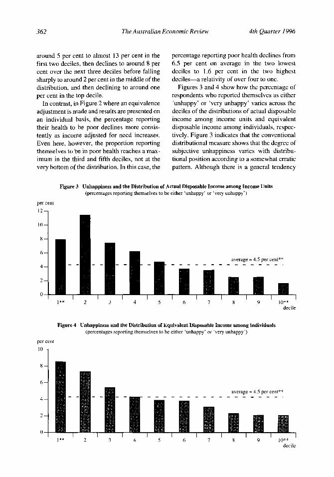
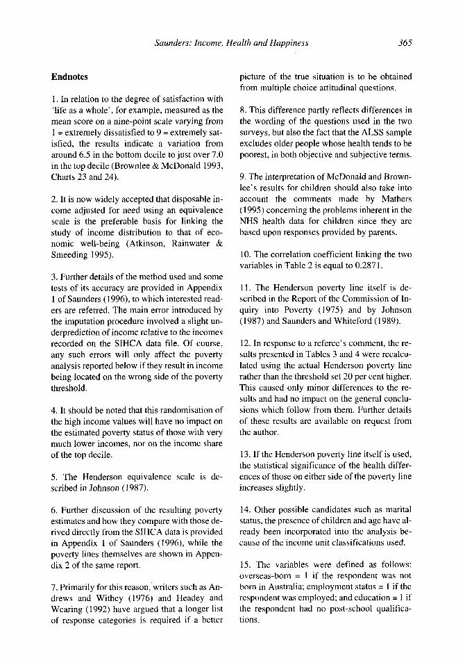
Figures 3 and 4 show how the percentage of respondents who reported themselves as either ‘unhappy’ or ‘very unhappy’ varies across the deciles of the distributions of actual disposable income among income units and equivalent disposable income among individuals, respectively. Figure 3 indicates that the conventional distributional measure shows that the degree of subjective unhappiness varies with distributional position according to a somewhat erratic pattern. Although there is a general tendency

Figure 3 Unhappiness and the Distribution of Actual Disposable Income among Income Units (percentages reporting themselves to be either ‘unhappy’ or ‘very unhappy’)

per cent 12

10

8

6

4

2

0

average = 4.5 per cent** - - - - - - - - - - - .

1 ** 2 3 4 5 6 I 8 9 lo** decile

Figure 4 Unhappiness and the Distribution of Equivalent Disposable Income among Individuals (percentages reporting themselves to be either ‘unhappy’ or ‘very unhappy’)

per cent

l o 1

average = 4.5 per cent** - - _ - - - - _ - - - - _ _ - - _ .

I** 2 3 4 5 6 7 8 9 lo** decile


for the percentage who are either ‘unhappy’ or ‘very unhappy’ to decline as the distributional position improves, the contrary situation exists in the two lowest deciles.

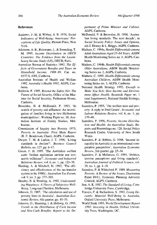
The distributional pattern of responses to the ‘unhappiness’ question shown in Figure 4 differs considerably from that in shown in Figure 3. The proportion of respondents who report themselves as being either ‘unhappy’ or ‘very unhappy’ now declines steadily across the income deciles, from an average of 7.9 per cent in the two lowest deciles, to around 3.8 per cent in the middle two deciles, to 2.1 per cent in the highest two. Thus, when the conceptually more appropriate distributional measure is employed, the relationship between income and happiness becomes clearer and the pattern of variation reflected in the distributional gradient is more consistent.

Overall, the results in Figure 4 indicate that the incidence of unhappiness among those at the bottom of the Australian income distribution is almost four times higher than among those at the top. This relativity is very close to that applying to the differences in subjective health status described earlier. The degree of similarity is all the more striking in light of the fact, noted earlier, that there is relatively little overlap between the individuals included in the ‘unhappy’ and ‘poor health’ groupings.

Two separate tests were used to assess the statistical significance of the distributional gra- dients shown in Figures 1 to 4. The first involved using a chi-squared statistic to test whether or not the overall distributional pattern across all ten deciles of the distribution differs from one in which there is no distributional variation, that is one in which the incidence is identical (and equal to the average incidence) in each decile. The second test involved using a (one-tailed) t-test to assess whether or not the observed incidence in the top decile of the distribution differs from that in the bottom decile.

Rather than provide details of the actual test statistics in each case, the signifkance of the statistical results is indicated on Figures 1 to 4 by the asterisks (*/**) which indicate whether the observed differences are statistically significant at the (0.05/0.01) probability levels. These asterisks have been attached in each fig-

ure to the average estimate (where the chi- squared test is applied to the entire distributional profile) and to the bottom and top decile numberings (where the t-test applies only to the differences between these two deciles).

The test statistics in Figures 1 to 4 indicate that in all four cases the distributional profile varies significantly over the distribution and that the incidence of both ‘poor health’ and ‘unhappiness’ reported in the top decile is, in all four cases, significantly lower than that reported in the bottom decile. On balance, these results thus indicate that those whose income adjusted for need places them at the bottom of the Australian income distribution perceive themselves as being in poorer health and significantly less happy than those whose incomes place them at the top of the income hierarchy.

The results reported above establish an association between relative income and perceived levels of health and happiness, but do not indicate whether or not there is a causal mechanism underlying them. The observed correlations may reflect causality running from health and happiness to income rather than the reverse, or they may result from the impact of intervening variables. In relation to the latter possibility, potential candidates include employment status, level of education and country of birth, each of which is associated with income and is known to be correlated with perceptions of poor health and unhappiness (National Health Strategy 1992).14

However, the correlations between these variables and the poor health and unhappiness variables are very low; those between poor health and country of birth, employment status and level of education are 0.0477,-0.1988 and 0.0641, respectively, while the corresponding correlations with unhappiness are 0.0742, -0.1101 and 0.0515, re~pectively.’~ In light of these low correlations, it does not appear that these variables can explain all of the observed correlation between income, health and happiness, even though they probably each have some role to play.

The issue of reverse causality is harder to re- fute. However, if it were the case that causation runs mainly from health (and unhappiness) to income, then one might expect those in poor


health and unhappy to be more concentrated among the low income groups than they in fact are. It is also important to emphasise that the correlations relate the health and happiness of individuals not to their own income, but to the total (equivalent) income of the income unit to which they belong. Thus even if poor health caused low income at the individual level, labour supply responses within the income unit as a whole would negate this at the level at which the analysis has been conducted. Fi- nally, Saunders (1996) has shown that the association between poverty status, relative income position and health measures taken from the NHS remains significant even after controlling for labour force status, level of education and country of birth.

Although these observations do not allow the reverse causality hypothesis to be discredited entirely, they do suggest that it may not be as strong an influence on the data as might be expected. Clearly, some people have low incomes because of their health, but even this does not imply that there is a clear relationship at the aggregate level between income adjusted for need and the perceived level of health of individuals.

5. Summary and Conclusions

The focus of the article has been on investigat- ing how perceived levels of health and happiness vary according to poverty status and to the ranking of individuals in the overall income distribution. In determining these measures of economic status, the methodology of the article has utilised sophisticated measurement techniques so that the results can be more easily located in the mainstream economic inequality literature. Poverty has been measured using the techniques developed by the Poverty Commis- sion, while the measure of income distribution reflects recent theoretical development and empirical refinement.

The results indicate that although the percentages reporting themselves as being in poor health and/or unhappy are generally low, there are significant differences between those whose incomes place them below the poverty threshold and those who are above it. There are also significant differences in the subjective

health and happiness of those at different points in the income distribution, with access to a higher income relative to need being associated with the perception of better health and in- creased happiness. These latter results indicate that a more consistent and coherent picture emerges when the more sophisticated distributional measures are employed.

The findings reported here are not new. They are, however, consistent with the work of writers such as Travers and Richardson and Brownlee and McDonald who find that income is associated with health and happiness, at least when using cross-section data to compare broad averages for those whose incomes differ considerably. The larger data set used here has allowed these associations to be subject to more rigorous investigation, from which they have emerged relatively unscathed.

The results suggest that while marginal income changes are unlikely to impact greatly upon people’s perceptions of well-being, es- caping poverty entirely or moving from the bottom to the top of the income distribution are much more likely to. It is, however, also clear that the relationship between individual income and well-being is complex, as Travers and Richardson have observed. Understanding the full dimensions of that complexity is an important task, to which this article has hopefully contributed.

The findings reported here add greater ur- gency to the need to ensure that all Australians have access to an adequate level of income and that the extremes of income inequality are moderated. This may involve some immediate increase in the social security and related bud- gets, as well as in the progressivity of the tax system and in the size of the deficit as a whole, but these are likely to be offset as the perceived improvements in health and happiness lead to a happier and more productive workforce and to a healthier population placing fewer demands on the health budget. In the longer term, reduc- tions in the poverty rate and in income inequality do not have to add to the financial cost of government.

First version received May 1996; final version accepted October 1996 (Eds).


Endnotes

1. In relation to the degree of satisfaction with ‘life as a whole’, for example, measured as the mean score on a nine-point scale varying from 1 = extremely dissatisfied to 9 = extremely sat- isfied, the results indicate a variation from around 6.5 in the bottom decile to just over 7.0 in the top decile (Brownlee & McDonald 1993, Charts 23 and 24).

2. It is now widely accepted that disposable income adjusted for need using an equivalence scale is the preferable basis for linking the study of income distribution to that of economic well-being (Atkinson, Rainwater & Smeeding 1995).

3. Further details of the method used and some tests of its accuracy are provided in Appendix 1 of Saunders (1996), to which interested read- ers are referred. The main error introduced by the imputation procedure involved a slight un- derprediction of income relative to the incomes recorded on the SIHCA data file. Of course, any such errors will only affect the poverty analysis reported below if they result in income being located on the wrong side of the poverty threshold.

4. It should be noted that this randomisation of the high income values will have no impact on the estimated poverty status of those with very much lower incomes, nor on the income share of the top decile.

5. The Henderson equivalence scale is described in Johnson ( I 987).

6. Further discussion of the resulting poverty estimates and how they compare with those de- rived directly from the SIHCA data is provided in Appendix 1 of Saunders (1996), while the poverty lines themselves are shown in Appen- dix 2 of the same report.

7. Primarily for this reason, writers such as An- drews and Withey (1976) and Headey and Wearing (1992) have argued that a longer list of response categories is required if a better

picture of the true situation is to be obtained from multiple choice attitudinal questions.

8. This difference partly reflects differences in the wording of the questions used in the two surveys, but also the fact that the ALSS sample excludes older people whose health tends to be poorest, in both objective and subjective terms.

9. The interpretation of McDonald and Brown- lee’s results for children should also take into account the comments made by Mathers (1995) concerning the problems inherent in the NHS health data for children since they are based upon responses provided by parents.

10. The correlation coefficient linking the two variables in Table 2 is equal to 0.287 1.

11. The Henderson poverty line itself is described in the Report of the Commission of In- quiry into Poverty (1975) and by Johnson (1987) and Saunders and Whiteford (1989).

12. In response to a referee’s comment, the results presented in Tables 3 and 4 were recalcu- lated using the actual Henderson poverty line rather than the threshold set 20 per cent higher. This caused only minor differences to the results and had no impact on the general conclusions which follow from them. Further details of these results are available on request from the author.

13. If the Henderson poverty line itself is used, the statistical significance of the health differences of those on either side of the poverty line increases slightly.

14. Other possible candidates such as marital status, the presence of children and age have al- ready been incorporated into the analysis because of the income unit classifications used.

15. The variables were defined as follows: overseas-born = 1 if the respondent was not born in Australia; employment status = 1 if the respondent was employed; and education = 1 if the respondent had no post-school qualifica- tions.

366 The Australian Economic Review 4th Quarter I996

References

Andrews, F. M. & Withey, S. B. 1976, Social Indicators of Well-Being: Americans’ Per- ceptions of Life Quality, Plenum Press, New York.

Atkinson, A. B., Rainwater, L. & Smeeding, T. M. 1995, Income Distribution in OECD Countries: The Evidence from the Lu.xem- bourg Income Study (LIS), OECD, Paris.

Australian Bureau of Statistics 1992, The Ef- fects of Government Benefits und Taxes on Household Income, 1988-89, Cat. no. 6537.0, ABS, Canberra.

Australian Institute of Health and Welfare 1992, Australia’s Health 1992, AGPS, Can- berra.

Baldwin, P. 1995, Beyond the Safety Net: The Future of Social Security, Office of the Min- ister for Social Security, Parliament House, Canberra.

Brownlee, H. & McDonald, P. 1993, ‘In search of poverty and affluence: An investigation of families living in two Melbourne municipalities’, Working Paper no. 10, Aus- tralian Institute of Family Studies, Mel- bourne.

Commission of Inquiry into Poverty 1975, Poverty in Australia: First Main Report (R. F. Henderson, Chair), AGPS, Canberra.

Dwyer, T. M. & Larkin, J. T. 1996, ‘Living standards in decline?’, Business Council Bulletin, no. 127, pp. 6-17.

Gruen, F. H. 1995, ‘The Australian welfare state: Neither egalitarian saviour nor economic millstone?’, Economic and Industrial Relations Review, vol. 6, no. I , pp. 125-38.

Harding, A. & Mitchell, D. 1992, ‘The effi- ciency and effectiveness of the tax-transfer system in the 1980s’, Australian Tax Forum, vol. 9, no. 3, pp. 277-303.

Headey, B. & Wearing, A. 1992, Understand- ing Happiness: A Theory qfsubjective Well- Being, Longman Cheshire, Melbourne.

Johnson, D. 1987, ‘The calculation and use of poverty lines in Australia’, Australian Eco- nomic Review, 4th quarter, pp. 45-55.

Johnson, D., Manning, I. & Hellwig, 0. 1995, Trends in the Distribution of Cash Income and Non-Cash Benefits: Report to the De-

partment of Prime Minister and Cabinet, AGPS, Canberra.

McDonald, P. & Brownlee, H. 1994, ‘Austra- lian living standards: The next decade’, in Social Security Policy: Issues and Options, eds J. Disney & L. Briggs, AGPS, Canberra.

Mathers, C . 1994a, Health Differentials among Adult Australians Aged 25-64 Years, AIHW Health Monitoring Series no. 1, AGPS, Can- berra.

Mathers, C . 1994b, Health Differentials among Older Australians, AIHW Health Monitor- ing Series no. 2, AGPS, Canberra.

Mathers, C. 1995, Health Differentials among Australian Children, AIHW Health Moni- toring Series no. 3, AGPS, Canberra.

National Health Strategy 1992, Enough to Make You Sick: How Income and Environ- ment Affect Health, Research Paper no. 1 (and Supplement), National Health Strategy, Melbourne.

Saunders, P. 1995, ‘The welfare state and poverty: A reply to Fred Gruen’, Economic and Labour Relations Review, vol. 6, no. 1, pp. 13948.

Saunders, P. 1996, Poverty, Income Distribu- tion and Health: An Australian Study, Re- ports and Proceedings no. 128, Social Policy Research Centre, University of New South Wales.

Saunders, P. & Hobbes, G. 1988, ‘Income inequality in Australia in an international com- parative perspective’, Australian Economic Review, 3rd quarter, pp. 25-34.

Saunders, P. & Matheson, G. 1993, ‘Politics, income perceptions and living standards’, Australian Journal of Political Science, vol. 28, no. 1, pp. 1-18.

Saunders, P. & Whiteford, P. 1989, Measuring Poverty: A Review of the Issues, Discussion Paper 89/11, Economic Planning Advisory Council, AGPS, Canberra.

Sen, A. K. 1987, The Standard of Living, Cam- bridge University Press, Cambridge.

Travers, P. & Richardson, S. 1993, Living De- cently: Material Well-Being in Australia, Oxford University Press, Melbourne.

World Bank 1993, World Development Report 1993: Investing in Health, Oxford Univer- sity Press, Washington, DC.

Documents

Income, Health and Happiness