Embed Size (px)
Citation preview

Inclusive Growth and its Regional Dimension
P. K. Nayak, Sadhan Kumar Chattopadhyay, Arun Vishnu Kumar and V. Dhanya*
Indian economy is elevated to a high growth path triggered mainly by macroeconomic reforms and expansion of economic activities across the sectors. However, there are some serious concerns about a number of imbalances in the growth scenario – inter-sectoral, inter-regional and inter-state. These imbalances have defi nitely a serious impact on the goal of “inclusive growth” as envisaged in the Eleventh Five Year Plan. The study reveals that still poverty ratio is very high in the economy despite high growth. There is no signifi cant increase in employment in the unorganised sector of the economy. The study shows that while the contribution of the agriculture sector in the real GDP has declined fairly fast, the share of the employment in the agriculture sector has not declined to that extent. As a result, the average productivity in this sector has remained very low as compared to other developing countries. Since a large section of the population continues to be dependent on the agriculture sector, directly or indirectly, this has serious implications for ‘inclusiveness’ of the growth dynamics. The study has emphasised the role of fi nance in growth and attempted to analyse the regional dimension of fi nancial inclusion, although in a limited sense, in terms of state-wise and sector-wise allocation of credit over the years. It was observed that the distribution of bank credit across sectors and regions is not equitable. Given the level of potential output, Indian economy is well poised to achieve an impressive growth in near future. The strength and resilience of the Indian economy were well tested while weathering the global turbulence of recent time. The paper arrives at the conclusion that furtherance of macroeconomic reforms, harnessing synergistic links among the sectors and availing of opportunities provided by the forces of globalization and intensive use of technology can enable us to achieve higher level of inclusive growth. Sustainable inclusive growth presupposes inclusive governance through empowerment, grassroot participation and increased public accountability.
JEL Classifi cation : C12, D92, F43, G21, O47
Keywords : Inclusive growth, inequality, fi nancial inclusion
Reserve Bank of India Occasional PapersVol. 31, No. 3, Winter 2010
* Dr. P. K. Nayak is Assistant Adviser, REMD, DEPR Central Offi ce and Shri Sadhan Kumar Chattopadhyay, Shri Arun Vishnu Kumar and Smt. V. Dhanya are Research Offi cers attached to DEPR, RO of Kolkata, Bangalore and Kochi, respectively. The views expressed in this paper are of the authors and not of the organization they are working with.
Introduction
Inclusive growth has become a buzzword across the globe. Inclusiveness – a concept that encompasses equity, equality of

92 RESERVE BANK OF INDIA OCCASIONAL PAPERS
opportunity, and protection in market and employment transitions – is an essential ingredient of any successful growth strategy (Commission on Growth and Development, World Bank, 2008). The Commission of Growth and Development (2008) considers systematic inequality of opportunity as “toxic” as it will derail the growth process through political channels or confl ict.
Indian economy has been registering a steady growth in the recent years. However, poverty continues to be a major concern. While some level of growth is obviously a necessary condition for sustained poverty reduction, there is an increasingly unanimous view that growth by itself is not a suffi cient condition for eradicating poverty (Ali and Son, 2007). Growth can marginalise the poor sections and increase inequality. High and rising levels of inequality can hinder poverty reduction, which in turn, can slowdown the growth process. One important indication of inadequate inclusion in India is that poverty reduction has been muted in the last decade even with rising growth. The poverty rate has declined by less than 1 per cent per annum over the past decade, markedly below trends in neighboring countries such as Nepal and Bangladesh where both average income levels and growth are lower (World Bank, 2007).
The importance of inclusive growth is well acknowledged among the policy makers. The approach paper of 11th Five Year Plan adopted in December 2006 describes the need for inclusive growth in its discussion. The approach plan points out that the growth oriented policies should be combined with policies ensuring broad based per capita income growth, benefi ting all sections of the population, especially those who have thus far remained deprived.
While the need for inclusive growth is stressed, it is to be seen, whether it is the inadequate growth of certain sectors like agriculture or the inability of certain groups like SC/STs to form part of the growth process or the lack of both physical and fi nancial infrastructure that pull back the particular regions/sections from enjoying the economic growth. It is possible that a combination of all these factors is preventing certain sections/areas to be out of the growth process. In

INCLUSIVE GROWTH AND ITS REGIONAL DIMENSION 93
that case it is necessary to know the major determinants that pull down inclusive growth. The inter linkages between different development indicators and growth in the context of various regions and sections needs to be analysed to understand the nuances of India’s growth process. In this context, a study on regional perspectives of inclusive growth is of utmost importance.
With this backdrop, the paper is organized as follows. Section II deals with the concept of inclusive growth. Section III analyses the inter-state growth performance. Here we look into the growth of Net State Domestic Product and per capita income from 1980-81 onwards. We also examine the sectoral contributions of economic growth across different states. Section IV discusses socio-economic inclusiveness as well as the poverty and unemployment which help in understanding the inclusiveness of our growth processes vis-à-vis select developing countries. Section V deals with relationship between fi nance and growth. It also highlights state-wise, sector-wise allocation of credit over the years. Section VI concludes the paper.
Section II: Concept of Inclusive Growth
Inclusive growth implies participation in the process of growth and also sharing of benefi t from growth. Thus inclusive growth is both an outcome and a process. On the one hand, it ensures that everyone can participate in the growth process, both in terms of decision-making for organizing the growth progression as well as in participating in the growth itself. On the other hand, it makes sure that everyone shares equitably the benefi ts of growth. In fact, participation without benefi t sharing will make growth unjust and sharing benefi ts without participation will make it a welfare outcome.
In view of the above, inclusive growth can be observed from long-term perspective as the focus is on productive employment rather than on direct income redistribution, as a means of increasing income for excluded groups. Under the absolute defi nition, growth is considered to be pro-poor as long as poor benefi t in absolute terms, as refl ected in some agreed measure of poverty (Ravallion and Chen,

94 RESERVE BANK OF INDIA OCCASIONAL PAPERS
2003). In contrast, in the relative defi nition, growth is pro-poor if and only if the incomes of poor people grow faster than those of the population as a whole, i.e., inequality declines. However, while absolute pro-poor growth can be the result of direct income redistribution schemes, for growth to be inclusive, productivity must be improved and new employment opportunities created, so that the excluded section forms part of the growth process. In short, inclusive growth is about raising the pace of growth and enlarging the size of the economy, while leveling the playing fi eld for investment and increasing productive employment opportunities.
The concept of inclusive growth has gained wide importance in several countries including India (Bolt, 2004). The Approach Paper of the Eleventh Five Year Plan provides “an opportunity to restructure policies to achieve a new vision based on faster, more broad-based and inclusive growth. It is designed to reduce poverty and focus on bringing the various divides that continue to fragment our society” (GOI, 2006: 1). In fact, Indian economy has come a long way from so called “Hindu Rate of growth” economy to high growth economy and is compared with China in many respects. In the last fi ve years (2005-06 to 2009-10) the growth rate has averaged at 8.6 per cent making India as one of the fastest growing economies in the World. Of course, transition to high growth is an impressive achievement, but growth is not the only measure of development. Our ultimate goal is to achieve broad based improvement in the living standards of all our people. Rapid growth is essential for this outcome because it provides the basis for expanding incomes and employment and also provides the resources needed to fi nance programmes for social upliftment. However, it is not suffi cient by itself. It is to ensure that its benefi ts, in terms of income and employment, are percolated down to all the sections of the society, including the poor and weaker sections. For this to happen, the growth must be inclusive in the broadest sense. It must be spread across all states and not just limited to some. It must generate suffi cient volumes of high quality employment to provide the means for uplifting large numbers of our population from the low income and low quality occupations in which too many of them have

INCLUSIVE GROWTH AND ITS REGIONAL DIMENSION 95
been traditionally locked. It is argued that “rapid, sustained and inclusive growth will take place when large numbers of people move from low-productivity jobs to high-productivity ones. The less effective the growth process is in creating jobs, both in terms of numbers and quality, the greater the political threat and, consequently, the less sustainable the growth process itself” (Gokarn, 2010). Various indicators have raised concerns that India’s growth is not inclusive or its benefi ts are not widely shared. One, the agriculture sector has been growing at a rate of 2-3 per cent per annum which has led to a fall in its share in the total income. With the level of employment in the agriculture sector remaining more or less constant, the slow growth in income means that the productivity in the agriculture sector has remained low. Regardless of the magnitude of increase and the differential across the two sectors, the stark fact is that average labour productivity outside agriculture is about 5 times that in agriculture (Gokarn, 2010). Two, the poverty impact of growth has been muted: poverty declined from 36 per cent in 1993/94 to 28 per cent in 2004/05, a 0.8 percentage point reduction per annum compared to 1.6 per cent poverty reduction per annum in our neighbouring countries, viz., Bangladesh and Nepal (World Bank, 2007). It is observed that close to 300 million still live in deep poverty at less than a dollar a day. Three, growth rates were generally lower in the poorer states during the 1980s and 1990s1. Four, employment is dominated by informal sector jobs. Five, it is observed that public services are weak in the poorer regions. Six, female labour force participation rates have remained low despite rising education levels among women due to absence of opportunities. Seven, there exists signifi cant wage discrimination among casual laborers, women get about half the wages of men. Less than one third of this gap can be explained by conventional factors such as skills, location, industry, etc. Eight, although SC groups have made progress, large sections of SC and ST groups are agricultural workers, the poorest earners. Finally, access to fi nance has been low in rural areas, 87 per cent of the poorest
1 However, in the current period (2000 to 2009), some of these States, viz., Uttaranchal, Orissa, Nagaland, Jharkhand, Tripura, Sikim, and Chattisgarh have performed better with more than 8 per cent growth rates.
96 RESERVE BANK OF INDIA OCCASIONAL PAPERS
households surveyed (marginal farmers) do not have access to credit, the rich pay a relatively low rate of interest (33 per cent), the poor pay rates of 104 per cent and get only 8 per cent of the credit (World Bank, 2007). Growth has diverged across regions, leaving behind the large populous states of North, Central and North-East India. Growth has not been creating enough good jobs that provide stable earnings for households to climb and stay out of poverty.
Section III: Economic Growth – Spatial and Temporal Analysis
III.1: Overall Growth
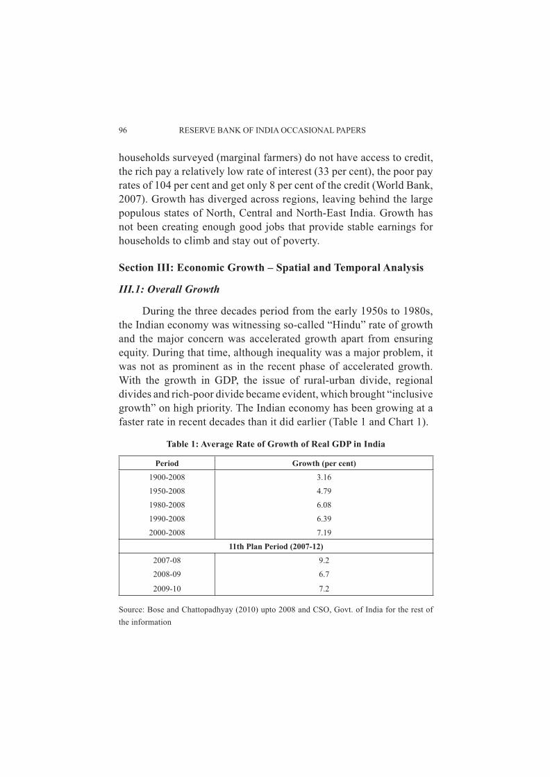
During the three decades period from the early 1950s to 1980s, the Indian economy was witnessing so-called “Hindu” rate of growth and the major concern was accelerated growth apart from ensuring equity. During that time, although inequality was a major problem, it was not as prominent as in the recent phase of accelerated growth. With the growth in GDP, the issue of rural-urban divide, regional divides and rich-poor divide became evident, which brought “inclusive growth” on high priority. The Indian economy has been growing at a faster rate in recent decades than it did earlier (Table 1 and Chart 1).
Table 1: Average Rate of Growth of Real GDP in India
Period Growth (per cent)
1900-2008 3.16
1950-2008 4.79
1980-2008 6.08
1990-2008 6.39
2000-2008 7.19
11th Plan Period (2007-12)
2007-08 9.2
2008-09 6.7
2009-10 7.2
Source: Bose and Chattopadhyay (2010) upto 2008 and CSO, Govt. of India for the rest of the information

INCLUSIVE GROWTH AND ITS REGIONAL DIMENSION 97
Sector wise performance
While the growth rate of the Indian economy has been increasing in recent times, one phenomenon which was observed was that the growth performance of the three major sectors of the economy, namely, agriculture, industry and services, has been diverse. The growth in the agriculture sector has been the most volatile and also the least among the three sectors most of the times. While the growth in the industrial sector has remained more or less constant, growth rate in the services sector has risen sharply (Chart 1).
The consequence of the diverse growth rate in the three sectors has resulted in a structural change in the contribution of the sectors in the total GDP. The share of the agriculture sector in the overall GDP has declined more or less consistently since independence from 55.3 per cent in 1950-51 to 17.0 per cent in 2008-09. The share of the industrial sector has increased from 10.6 per cent in 1950-51 to about 19.0 per cent in 2008-09. The share of the services sector has nearly doubled from 34.1 per cent in 1950-51 to 64.5 per cent in 2008-09 (Chart 2).
Since a large section of the population continues to be dependent on the agriculture sector, directly or indirectly, this has serious implications for ‘inclusiveness’.

98 RESERVE BANK OF INDIA OCCASIONAL PAPERS
Potential Output2
The Indian economy grew at about 9.0 per cent during 2003-08, which decelerated to 7.0 per cent during 2008-10. Although a part of the gap is due to cyclical factor, different estimation methods suggest that the potential output growth would be around 8.0 per cent during the post-crisis period and 8.5 per cent during the pre-crisis period3. It is argued that the loss in potential output could be due to a slowdown of investment in various sectors, more specifi cally in the agriculture sector. In fact, the public investment in agriculture in real terms has witnessed steady decline from the Sixth Five Year Plan to the Tenth
2 Potential Output is defi ned as the maximum level of output that an economy can sustain without creating macroeconomic imbalances.3 See RBI Annual Report, 2009-10
Table 2: Plan-wise investment in Agriculture
See RBI Annual Report 2009-10 Investment (` crore)Sixth Plan (1980-85) 64012Seventh Plan (1985-90) 52108Eighth Plan (1992-97) 45565Ninth Plan (1997-2002) 42226Tenth Plan (2002-2007) 67260Eleventh Plan (2007-2012) -
Source: Economic Survey, 2010, Government of India.

INCLUSIVE GROWTH AND ITS REGIONAL DIMENSION 99
Plan. Trends in public investment in agriculture and allied sectors reveal that it has consistently declined in real terms (at 1999-2000 prices) from ` 64,012 crore in Sixth Plan to ` 42,226 crore during the Ninth Plan. However, during the Tenth Plan this has increased in absolute terms to ` 67,260 crore. It can also be observed that the public investment has gone down over the year, while private investment remained stagnant (Table 3). The gross capital formation (GCF) in agriculture and allied sectors as a proportion of total GDP stood at 2.66 per cent in 2004-05 and improved to 3.34 per cent in 2008-09. Similarly, GCF in agriculture and allied sectors relative to GDP in this sector has also shown an improvement from 14.07 per cent in 2004-05 to 21.31 per cent in 2008-09.
Table 3: Public and Private Investment in Agriculture & Allied Sector at 2004-05 Prices
Investment in agriculture & allied sector (` crore)
Share in total investment (per cent)
Total Public Private Public Private
2004-05 78848 16183 62665 20.5 79.5
2005-06 93121 19909 73211 21.4 78.6
2006-07 94400 22978 71422 24.3 75.7
2007-08 110006 23039 86967 20.9 79.1
2008-09 138597 24452 114145 17.6 82.4
Source: Central Statistics Offi ce, GoI.
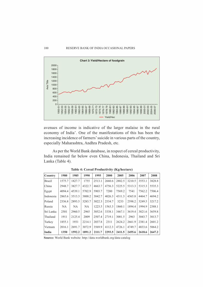
Declining investment in the agriculture sector had a direct bearing on the productivity of foodgrains in the country. As can be observed from Chart 3, although average yield/hectare (productivity) of foodgrains in India has increased over the years, the productivity is low compared to many other developing countries. The productivity of foodgrains has increased from 522 kg/hectare in 1950-51 to 1854 in 2007-08. While in 1979-80 the yield per hectare was 876 kg/hectare, it became 1380 kg/hectare in 1990. However, productivity growth remained stagnant at a very low level throughout the period. Various studies have been done on the agriculture sector and its associated issues. More recent, among these, studies is done by Mishra (2007) which states that ‘poor agriculture income and absence of non-farm
100 RESERVE BANK OF INDIA OCCASIONAL PAPERS
avenues of income is indicative of the larger malaise in the rural economy of India’. One of the manifestations of this has been the increasing incidence of farmers’ suicide in various parts of the country, especially Maharashtra, Andhra Pradesh, etc.
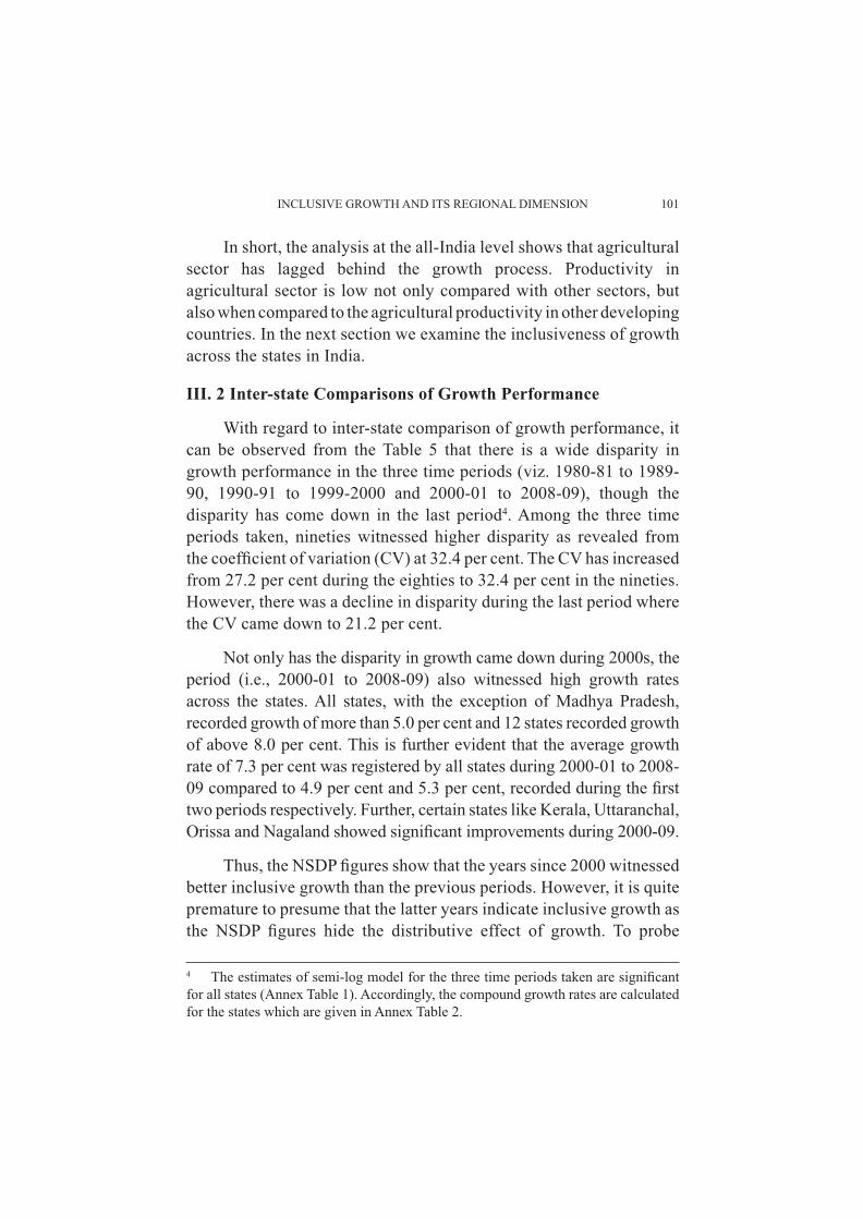
As per the World Bank database, in respect of cereal productivity, India remained far below even China, Indonesia, Thailand and Sri Lanka (Table 4).
Table 4: Cereal Productivity (Kg/hectare)
Country 1980 1985 1990 1995 2000 2005 2006 2007 2008
Brazil 1575.7 1827.7 1755 2513.1 2660.6 2882.5 3210.5 3553.1 3828.8
China 2948.7 3827.7 4322.7 4663.7 4756.3 5225.5 5313.3 5315.3 5535.3
Egypt 4094.4 4539.1 5702.9 5903.7 7280 7569.2 7541 7562.2 7506.4
Indonesia 2865.6 3513.3 3800.2 3842.7 4026.3 4311.3 4365.8 4464.7 4694.2
Poland 2336.8 2893.5 3283.7 3022.3 2534.7 3233 2598.2 3249.5 3217.2
Russia NA NA NA 1223.5 1563.3 1860.1 1894.4 1994.9 2388.1
Sri Lanka 2501 2960.5 2965 3052.6 3338.1 3467.1 3619.4 3821.6 3659.8
Thailand 1911 2125.4 2009 2507.4 2719.1 3001.5 2963 3043.7 3013.7
Turkey 1855.1 1931 2214.1 2037.8 2311 2624.2 2661.9 2381.4 2601.2
Vietnam 2016.1 2691.7 3072.9 3569.9 4112.3 4726.1 4749.7 4833.6 5064.2
India 1350 1592.2 1891.2 2111.7 2293.5 2411.5 2455.6 2618.6 2647.2
Source: World Bank website: http://data.worldbank.org/data-catalog
INCLUSIVE GROWTH AND ITS REGIONAL DIMENSION 101
In short, the analysis at the all-India level shows that agricultural sector has lagged behind the growth process. Productivity in agricultural sector is low not only compared with other sectors, but also when compared to the agricultural productivity in other developing countries. In the next section we examine the inclusiveness of growth across the states in India.
III. 2 Inter-state Comparisons of Growth Performance
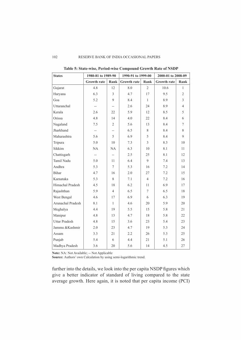
With regard to inter-state comparison of growth performance, it can be observed from the Table 5 that there is a wide disparity in growth performance in the three time periods (viz. 1980-81 to 1989-90, 1990-91 to 1999-2000 and 2000-01 to 2008-09), though the disparity has come down in the last period4. Among the three time periods taken, nineties witnessed higher disparity as revealed from the coeffi cient of variation (CV) at 32.4 per cent. The CV has increased from 27.2 per cent during the eighties to 32.4 per cent in the nineties. However, there was a decline in disparity during the last period where the CV came down to 21.2 per cent.
Not only has the disparity in growth came down during 2000s, the period (i.e., 2000-01 to 2008-09) also witnessed high growth rates across the states. All states, with the exception of Madhya Pradesh, recorded growth of more than 5.0 per cent and 12 states recorded growth of above 8.0 per cent. This is further evident that the average growth rate of 7.3 per cent was registered by all states during 2000-01 to 2008-09 compared to 4.9 per cent and 5.3 per cent, recorded during the fi rst two periods respectively. Further, certain states like Kerala, Uttaranchal, Orissa and Nagaland showed signifi cant improvements during 2000-09.
Thus, the NSDP fi gures show that the years since 2000 witnessed better inclusive growth than the previous periods. However, it is quite premature to presume that the latter years indicate inclusive growth as the NSDP fi gures hide the distributive effect of growth. To probe
4 The estimates of semi-log model for the three time periods taken are signifi cant for all states (Annex Table 1). Accordingly, the compound growth rates are calculated for the states which are given in Annex Table 2.
102 RESERVE BANK OF INDIA OCCASIONAL PAPERS
further into the details, we look into the per capita NSDP fi gures which give a better indicator of standard of living compared to the state average growth. Here again, it is noted that per capita income (PCI)
Table 5: State-wise, Period-wise Compound Growth Rate of NSDP
States 1980-81 to 1989-90 1990-91 to 1999-00 2000-01 to 2008-09Growth rate Rank Growth rate Rank Growth rate Rank
Gujarat 4.8 12 8.0 2 10.6 1
Haryana 6.3 3 4.7 17 9.5 2
Goa 5.2 9 8.4 1 8.9 3
Uttaranchal -- -- 2.6 24 8.9 4
Kerala 2.6 22 5.9 12 8.5 5
Orissa 4.8 14 4.0 22 8.4 6
Nagaland 7.5 2 5.6 13 8.4 7
Jharkhand -- -- 6.5 8 8.4 8
Maharashtra 5.6 5 6.9 5 8.4 9
Tripura 5.0 10 7.3 3 8.3 10
Sikkim NA NA 6.3 10 8.1 11
Chattisgarh -- -- 2.5 25 8.1 12
Tamil Nadu 5.0 11 6.4 9 7.4 13
Andhra 5.3 7 5.3 16 7.2 14
Bihar 4.7 16 2.0 27 7.2 15
Karnataka 5.3 8 7.1 4 7.2 16
Himachal Pradesh 4.5 18 6.2 11 6.9 17
Rajashthan 5.9 4 6.5 7 6.5 18
West Bengal 4.6 17 6.9 6 6.3 19
Arunachal Pradesh 8.1 1 4.6 20 5.9 20
Meghalya 4.4 19 5.5 15 5.8 21
Manipur 4.8 13 4.7 18 5.8 22
Uttar Pradesh 4.8 15 3.6 23 5.4 23
Jammu &Kashmir 2.0 23 4.7 19 5.3 24
Assam 3.3 21 2.2 26 5.3 25
Punjab 5.4 6 4.4 21 5.1 26
Madhya Pradesh 3.6 20 5.6 14 4.5 27
Note: NA: Not Available; -- Not ApplicableSource: Authors’ own Calculation by using semi-logarithmic trend.

INCLUSIVE GROWTH AND ITS REGIONAL DIMENSION 103
also has limited value in examining inclusive growth as it gives little revelation on the distribution of income across the population.
Chart 4 gives the distribution of Per capita income across states. It shows that there is a wide disparity across States with Bihar at the lowest and Goa at the top position. The CV is as high as 41.0 per cent.
We further examine the inequality across the States in respect of per capita NSDP across the time periods. Annex Table 2 provides the estimates of semi-log function. For Jammu Kashmir (1980-81 to 1989-90), Bihar and Uttaranchal for 1990-91 to 1999-00 and Nagaland for 1990-91 to 1999-00 and 2000-01 to 2008-09, the fi gures came insignifi cant. The growth rates for the rest of the states are given in Table 6.
Compared to NSDP, the disparity is higher in the case of per capita income. However, similar to NSDP, the 1990s witnessed higher disparity which came down in 2000s. The CV increased from 48.0 per cent during the eighties to 53.5 per cent in the nineties before coming down to 32.9 per cent during the last period.
Though the inequality in terms of growth rates have come down in 2000s, inequality measured by Gini coeffi cient of the level variables, have shown an increase over the period. Gini coeffi cient has increased

104 RESERVE BANK OF INDIA OCCASIONAL PAPERS
Table 6: State-wise, Period-wise Compound Growth Rate of Per Capita NSDP
States 1980-81 to 1989-90 1990-91 to 1999-00 2000-01 to 2008-09Growth rate Rank Growth rate Rank Growth rate Rank
Gujarat 2.8 12 6.0 2 9.1 1Orissa 2.9 11 2.4 17 8.2 2Kerala 1.1 21 4.8 7 8.0 3Chattisgarh - - 0.9 23 7.8 4Haryana 3.7 2 2.2 19 7.3 5Andhra Pradesh 3.0 10 3.8 12 7.0 6Uttaranchal - - 0.0 - 7.0 7Goa 3.6 3 6.8 1 6.9 8Maharashtra 3.2 8 4.7 8 6.8 9Sikkim NA - 3.4 14 6.6 10Jharkhand - - 4.7 9 6.6 11Karnataka 3.2 9 5.4 4 6.6 12Tamil Nadu 3.5 6 5.3 5 6.5 13Bihar 2.5 14 0.0 - 5.9 14Tripura 2.0 18 5.4 3 5.8 15Rajashthan 3.2 7 4.0 11 5.8 16Meghalya 1.4 19 2.8 15 5.7 17West Bengal 2.3 16 5.1 6 5.4 18Himachal Pradesh 2.7 13 4.4 10 5.2 19Arunachal Pradesh 4.8 1 2.1 20 5.1 20Manipur 2.1 17 2.3 18 4.0 21Jammu &Kashmir 0.0 - 2.0 21 3.7 22Assam 1.1 22 0.3 25 3.4 23UP 2.4 15 1.3 22 3.4 24Punjab 3.5 4 2.5 16 3.3 25Madhya Pradesh 1.2 20 3.4 13 2.6 26Nagaland 3.5 5 0.0 - 0.0 -
Notes: NA denotes Note Available Source: Authors’ own Calculation by using semi-logarithmic trend.
from 0.164 in 1980-81 to 0.245 in 2007-08 (Chart 5). Gini coeffi cient has been calculated for 22 states omitting Chattisgarh, Jharkhand, Uttaranchal, Mizoram, Sikkim and Nagaland due to non-availability of continuous data series5.
5 The Gini coeffi cient is calculated using Deaton’s formula:
G= N + 1 2N - 1 N(N - 1)u
( i=1 PiXi)n

INCLUSIVE GROWTH AND ITS REGIONAL DIMENSION 105
In general, growth rates of states have improved in the last time period with the exception of Madhya Pradesh and Punjab. Both the states showed dismal performance in case of NSDP and Per capita income. On the other hand, Kerala and Orissa showed signifi cant improvement in the last decade, with Kerala registering tremendous improvement both in the growth and level of income. Orissa, which ranked 17 in terms of PCI growth during the nineties, improved its position to the second. However, in terms of the level of PCI, it is still low at ` 15,702.
From the perspective of inclusive growth, an analysis of growth performance of states is not enough. It calls for a more detailed analysis of various sectors of the economy and various sections of population. As a fi rst step, we look into the sectoral shares and growth in each state.
Table 7 provides the share of each sector in NSDP across the three time periods. In all the states, the share of primary sector has declined over the time period considered and tertiary sector showing an increase in share and secondary sector registering marginal or no increase6. However, Maharashtra which is often hailed as industrial
6 We have followed the CSO allocation of sectors and accordingly construction is included in the secondary sector.

106 RESERVE BANK OF INDIA OCCASIONAL PAPERS
Table 7: Shares of each sector in NSDP across states (Contd.) Primary Secondary Tertiary Primary Secondary Tertiary
ANDHRA Pradesh ARUNACHAL PRADESH
1980-81 to 1989-90 48.7 13.3 38.0 50.9 16.7 32.4
1990-91 to 1999-00 37.1 18.0 44.9 42.2 19.7 38.1
2000-01 to 2008-09 30.6 18.4 51.0 28.6 28.0 43.4
ASSAM BIHAR
1980-81 to 1989-90 49.0 15.6 35.4 50.3 9.4 40.3
1990-91 to 1999-00 44.3 13.7 42.0 41.6 9.6 48.8
2000-01 to 2008-09 34.4 14.5 51.1 32.5 12.6 54.9
CHATTISGARH GOA
1980-81 to 1989-90 – – – 32.9 22.5 44.6
1990-91 to 1999-00 40.5 21.5 38.0 20.7 27.9 51.4
2000-01 to 2008-09 35.6 22.5 41.9 13.3 36.0 50.6
GUJARAT HARYANA
1980-81 to 1989-90 40.4 25.8 33.8 46.1 24.3 29.6
1990-91 to 1999-00 29.1 32.0 38.8 39.4 26.3 34.4
2000-01 to 2008-09 20.8 33.2 46.0 25.8 26.6 47.6
HIMACHAL JAMMU KASHMIR
1980-81 to 1989-90 47.1 21.6 31.3 38.7 25.6 35.8
1990-91 to 1999-00 34.8 31.1 34.2 33.3 25.4 41.2
2000-01 to 2008-09 24.9 37.2 37.9 31.9 21.5 46.6
JHARKAND KARNATAKA
1980-81 to 1989-90 – – – 45.2 20.1 34.7
1990-91 to 1999-00 29.8 31.1 39.1 36.1 22.0 41.9
2000-01 to 2008-09 27.1 29.8 43.2 22.0 24.3 53.6
KERALA MADHYA PRADESH
1980-81 to 1989-90 31.0 20.1 48.9 45.9 12.0 42.2
1990-91 to 1999-00 26.5 21.4 52.1 38.9 14.7 46.4
2000-01 to 2008-09 17.0 22.1 60.9 30.6 18.2 51.2
MAHARASHTRA MANIPUR
1980-81 to 1989-90 25.7 30.4 43.9 39.6 19.9 40.5
1990-91 to 1999-00 20.1 29.1 50.7 32.4 19.6 48.0
2000-01 to 2008-09 16.3 23.6 60.1 28.1 26.8 45.2

INCLUSIVE GROWTH AND ITS REGIONAL DIMENSION 107
Table 7: Shares of each sector in NSDP across states (Concld.)MEGHALAYA MIZORAM
1980-81 to 1989-90 39.1 12.4 48.51990-91 to 1999-00 31.2 12.9 55.9 24.2 14.1 61.62000-01 to 2008-09 30.6 17.3 52.1 18.3 17.6 64.2
NAGALAND ORISSA1980-81 to 1989-90 24.6 6.8 68.5 52.5 15.6 32.01990-91 to 1999-00 23.9 16.1 60.1 41.9 16.8 41.42000-01 to 2008-09 34.5 14.1 51.4 32.8 16.9 50.3
PUNJAB RAJASTHAN1980-81 to 1989-90 46.5 15.7 37.8 47.6 16.7 35.71990-91 to 1999-00 43.6 19.6 36.8 41.0 19.2 39.82000-01 to 2008-09 36.0 21.5 42.6 32.8 22.6 44.6
SIKKIM TAMIL Nadu1980-81 to 1989-90 – – – 26.1 30.3 43.61990-91 to 1999-00 31.3 18.5 50.2 22.2 28.6 49.22000-01 to 2008-09 21.0 26.1 52.9 14.3 26.5 59.2
TRIPURA UTTAR PRADESH1980-81 to 1989-90 51.2 9.7 39.1 44.2 17.8 38.01990-91 to 1999-00 37.3 9.6 53.1 38.3 19.8 41.92000-01 to 2008-09 26.4 20.6 53.0 33.4 21.4 45.2
UTTARAKHAND WEST BENGAL1980-81 to 1989-90 – – – 40.0 15.6 44.41990-91 to 1999-00 30.3 18.8 51.0 37.6 14.8 47.62000-01 to 2008-09 23.5 28.4 48.2 28.0 16.1 55.9
Source: Central Statistics Offi ce, Government of India.
capital of India, witnessed a decline in the share of secondary sector and witnessed an increase in tertiary sector. In all the states, tertiary sector occupies the major share of NSDP which conforms with the earlier studies showing India’s difference in development path with the general East Asian growth path (Bhattacharya and Mitra, 1990; Bhattacharya and Sakthivel, 2004).
However, in terms of growth rates, secondary sector registered highest growth rate in most of the states during the period 2000-01 to

108 RESERVE BANK OF INDIA OCCASIONAL PAPERS
2008-09 as is revealed from Table 8. On the other hand, tertiary sector which registered high growth during the nineties witnessed a slowdown or marginal growth in most of the states during the last period.
Table 8: Sector-wise Growth Rates of NSDP across States (Contd.)Primary Secondary Tertiary Primary Secondary Tertiary
ANDHRA PRADESH ARUNACHAL PRADESH
1980-81 to 1989-90 2.0 7.1 7.6 8.8 6.6 7.4
1990-91 to 1999-00 2.8 7.0 9.2 0.6 6.8 9.2
2000-01 to 2008-09 6.0 9.8 6.1 2.4 12.4 6.1
ASSAM BIHAR
1980-81 to 1989-90 2.7 1.2 0.9 2.8 7.9 5.8
1990-91 to 1999-00 2.9 3.6 0.7 NS NS 4.8
2000-01 to 2008-09 4.1 7.6 7.2 2.5 17.7 8.7
GOA GUJARAT
1980-81 to 1989-90 NS 5.6 7.2 NS 8.1 7.3
1990-91 to 1999-00 2.7 8.7 10.1 4.0 9.4 9.2
2000-01 to 2008-09 6.3 7.5 10.5 10.6 13.6 9.5
HARYANA HIMACHAL
1980-81 to 1989-90 3.9 9.7 7.2 1.6 6.7 5.9
1990-91 to 1999-00 1.8 5.2 7.7 0.8 11.2 7.6
2000-01 to 2008-09 3.6 10.2 12.1 1.4 9.7 7.8
JAMMU KASHMIR KARNATAKA
1980-81 to 1989-90 NS 5.6 3.4 2.7 6.7 7.1
1990-91 to 1999-00 4.1 NS 6.2 4.5 6.8 9.4
2000-01 to 2008-09 3.1 8.6 5.1 1.7 10.9 9.3
KERALA MADHYA PRADESH
1980-81 to 1989-90 1.3 2.2 3.6 1.7 4.6 5.2
1990-91 to 1999-00 2.0 6.7 8.5 3.6 8.8 5.9
2000-01 to 2008-09 0.8 12.4 9.9 5.3 4.1 4.3
MAHARASHTRA MANIPUR
1980-81 to 1989-90 3.1 6.0 6.4 2.0 7.0 7.0
1990-91 to 1999-00 4.5 6.0 8.3 2.8 2.5 5.9
2000-01 to 2008-09 5.1 7.7 9.2 2.2 13.6 4.4

INCLUSIVE GROWTH AND ITS REGIONAL DIMENSION 109
Table 8: Sector-wise Growth Rates of NSDP across States (Concld.)
MEGHALAYA NAGALAND
1980-81 to 1989-90 1.4 0.7 6.5 5.5 18.2 8.5
1990-91 to 1999-00 4.4 8.0 5.8 6.1 10.6 4.9
2000-01 to 2008-09 5.8 13.2 5.8 7.6 9.7 4.5
ORISSA PUNJAB
1980-81 to 1989-90 3.0 7.1 6.3 5.3 7.2 4.0
1990-91 to 1999-00 2.9 NS 6.3 2.4 6.7 5.8
2000-01 to 2008-09 5.6 14.7 10.1 2.5 8.3 5.8
RAJASTHAN TAMIL NADU
1980-81 to 1989-90 3.4 7.1 8.9 3.5 2.8 2.3
1990-91 to 1999-00 3.9 9.4 8.0 4.1 5.3 7.7
2000-01 to 2008-09 6.1 9.1 8.4 6.2 9.0 8.6
TRIPURA UTTAR PRADESH
1980-81 to 1989-90 2.5 NS 8.5 2.5 8.3 5.8
1990-91 to 1999-00 3.0 11.2 8.8 2.6 3.7 4.3
2000-01 to 2008-09 6.0 7.1 7.7 2.1 10.1 5.7
WEST BENGAL
1980-81 to 1989-90 5.8 3.0 4.4
1990-91 to 1999-00 5.0 6.2 8.6
2000-01 to 2008-09 2.3 8.8 8.1
Note: NS denotes Not Signifi cantSource: Central Statistics Offi ce, Government of India
The analysis in this section revealed that the growth process was mostly driven by the growth in the services sector. Further, the inequality in growth has come down in the time period since 2000, though the inequality remains at high level. Further, there was a change in growth performance in the last decade with many underperformers moving up and top performers coming down which is refl ected in the declining inequality. In the next section, we look into the socio-economic inclusiveness of the growth process.

110 RESERVE BANK OF INDIA OCCASIONAL PAPERS
IV: Socio-Economic Inclusiveness
While discussing inclusive growth, a major factor to be examined is the socio-economic inclusiveness of the people. Inclusive growth being a long term process necessarily emanates from the inclusive nature of socio-economic development across regions and people. But, considering the time constraint, we are limiting our analysis of socio-economic inclusiveness to certain indicators which we feel is able to reveal the social development of the country. We start the analysis by looking into the poverty and unemployment fi gures over the years. As far as possible, we have tried to compare India’s position with other developing countries
The ultimate objective of planned development is to ensure human well-being through sustained improvement in the quality of life of the people, particularly the poor and the vulnerable segments of population. The development of human resources contributes to sustained growth and productive employment. Development strategy therefore needs to continuously strive for broad-based improvement in standards of living. High growth is essential to generate resources for social spending. However, the benefi ts of growth should be shared equitably among all sections of society. This is the main logic behind emphasizing the concept of inclusive growth as has been pursued in the Eleventh Five Year Plan.
As per the UNDP Human Development Report 2009 (HRD 2009), India ranked 134 out of 182 countries of the world placing it at the same rank as in 2006 (the Human Development Index (HDI) for India in 2007 was 0.612).7 However, the HDI value of India has increased gradually from 0.427 in 1980 to 0.556 in 2000 and went up to 0.612 in 2007, but it is still in the medium Human Development category with even countries like China, Sri Lanka and Indonesia having better ranking (Table 9). In fact, India lags behind in various
7 HDI is based on three indicators, viz., GDP per capita (PPP US $), life expectancy at birth, and education as measured by adult literacy rate and gross enrolment ratio (combined for primary, secondary and tertiary education)

INCLUSIVE GROWTH AND ITS REGIONAL DIMENSION 111
social indicators of development. There is a huge gap between India and developed world and even many developing countries in respect of health and education, which needs to be bridged at a faster pace. According to HDR, life expectancy at birth in India was 63.4 years in 2007 as against 80.5 years in Norway, 81.4 years in Australia, 74.0 years in Sri Lanka and 72.9 years in China. Adult literacy rate (aged 15 and above) in 1999-2007 was 66.0 per cent in India as against near 100 per cent in China and 92.0 per cent in Indonesia. In the case of combined gross enrolment ratio in education also India was much below the level achieved by some other comparable countries, like China, Norway, and Thailand etc.
Table 9: Human Development Index
Country 1980 1985 1990 1995 2000 2005 2006 2007
Poland … … 0.806 0.823 0.853 0.871 0.876 0.880Brazil 0.685 0.694 0.710 0.734 0.790 0.805 0.808 0.813Russia … … 0.821 0.777 … 0.804 0.811 0.817Turkey 0.628 0.674 0.705 0.73 0.758 0.796 0.802 0.806Thailand 0.658 0.684 0.706 0.727 0.753 0.777 0.78 0.783China 0.533 0.556 0.608 0.657 0.719 0.756 0.763 0.772Sri Lanka 0.649 0.670 0.683 0.696 0.729 0.752 0.755 0.759Indonesia 0.522 0.562 0.624 0.658 0.673 0.723 0.729 0.734Vietnam … 0.561 0.599 0.647 0.69 0.715 0.720 0.725Egypt 0.496 0.552 0.58 0.631 0.665 0.696 0.700 0.703India 0.427 0.453 0.489 0.511 0.556 0.596 0.604 0.612
Source: Human Development Report, 2009
Poverty
Poverty is a major issue in the emerging economies, though its intensity varies across countries as refl ected in the World Bank’s data on the poverty head count ratio at $1.25 a day (PPP). South Asia continues to have a signifi cant amount of poor people, mainly due to the high poverty ratios in India and Bangladesh (Table 10). It is observed that compared to India, China has made signifi cant progress in reducing poverty in the last 15 years.

112 RESERVE BANK OF INDIA OCCASIONAL PAPERS
Table 10: Poverty headcount ratio at $1.25 a day (PPP)(% of population)
Country 1990 2005Argentina n.a. 3.4 (2006)Bangladesh n.a. 49.6Brazil 15.5 5.2 (2007)Chile 4.4 2.0 (2006)China 60.2 15.9East Asia & Pacifi c 54.7 16.8India n.a. 41.6Indonesia n.a. 29.4 (2007)Pakistan n.a. 22.6South Asia 51.7 40.3
Source: World Bank website.
As per the offi cial estimates, the incidence of poverty has declined over the years though it remains still at a very high level. The percentage of the population below the offi cial poverty line has come down from 36 per cent in 1993–94 to 28 per cent in 2004–05 (Table 11). However, not only is the rate still high, but also the rate of decline in poverty has not accelerated along with the growth in GDP, and the incidence of poverty among certain marginalized groups, for example the poverty rate of the STs, has hardly declined. Moreover, the absolute number of poor people below poverty line has declined only marginally from 320 million in 1993–94 to 302 million in 2004–05. This performance is all the more disappointing since the poverty line on which the estimate of the poor is based is the same as it was in 1973–74 when per capita incomes were much lower. If we take the World Bank measurement of poverty about 41.6 per cent (as per PPP) of population is below poverty line, which is much higher than the offi cial national poverty ratio of about 28 per cent.
Table 11: Trends in Poverty in IndiaYear Poverty (head count index) percentage Number of poor (million)
Rural Urban Total1973-74 56 49 55 3211983 46 41 45 3231993-94 37 32 36 3202004-05 28 26 28 302
Source: Mahendra S. Dev (2007).

INCLUSIVE GROWTH AND ITS REGIONAL DIMENSION 113
It can further be stated that around 80.0 per cent of the poor are from rural areas. Poverty is mostly concentrated in few states, viz, Bihar, Uttar Pradesh and Madhya Pradesh, Orissa, Chattisgarh and Jharkhand (Annex Table 3). Poverty is concentrated among agricultural labourers, casual workers, Scheduled Castes and Scheduled Tribes.
There are concerns of inequality also in the country. During the last four decades there is hardly any decrease in inequality in the country. It may be observed from Table 12 that while there is a marginal decrease in inequality in the rural area, it has increased in the
Table 12: Gini Coeffi cient for Per Capita Consumption Expenditure1973-74 1977-78 1983 1993-94 1999-2000 2004-05
(URP)*2004-05 (MRP)*
Rural Urban Rural Urban Rural Urban Rural Urban Rural Urban Rural Urban Rural UrbanIndia 0.28 0.30 0.34 0.34 0.30 0.33 0.28 0.34 0.26 0.34 0.30 0.37 0.25 0.35Andhra Pradesh
0.29 0.29 0.30 0.32 0.29 0.31 0.29 0.32 0.24 0.31 0.29 0.37 0.24 0.34
Assam 0.20 0.30 0.18 0.32 0.19 0.25 0.18 0.29 0.20 0.31 0.19 0.32 0.17 0.30Bihar 0.27 0.26 0.26 0.30 0.26 0.30 0.22 0.31 0.21 0.32 0.20 0.33 0.17 0.31Jharkhand – – – – – – – – – – 0.22 0.35 0.20 0.33Gujarat 0.23 0.25 0.29 0.31 0.25 0.26 0.24 0.29 0.23 0.29 0.27 0.31 0.25 0.32Haryana 0.29 0.31 0.29 0.31 0.27 0.30 0.30 0.28 0.24 0.29 0.32 0.36 0.31 0.36Himachal Pradesh
0.24 0.27 0.26 0.30 0.27 0.31 0.28 0.43 0.23 0.30 0.30 0.32 0.26 0.26
Jammu & Kashmir
0.22 0.22 0.22 0.33 0.22 0.24 0.23 0.28 0.17 0.22 0.24 0.24 0.20 0.24
Karnataka 0.28 0.29 0.32 0.34 0.30 0.33 0.27 0.32 0.24 0.32 0.26 0.36 0.23 0.36Kerala 0.31 0.37 0.35 0.36 0.33 0.37 0.29 0.34 0.27 0.32 0.34 0.40 0.29 0.35Madhya Pradesh
0.29 0.27 0.33 0.38 0.29 0.29 0.28 0.33 0.24 0.32 0.27 0.39 0.24 0.37
Chhatisgarh – – – – – – – – – – 0.29 0.43 0.24 0.35Maharashtra 0.26 0.33 0.46 0.36 0.28 0.33 0.30 0.35 0.26 0.35 0.31 0.37 0.27 0.35Orissa 0.26 0.34 0.30 0.32 0.27 0.29 0.24 0.30 0.24 0.29 0.28 0.35 0.25 0.33Punjab 0.27 0.29 0.30 0.38 0.28 0.32 0.26 0.28 0.24 0.29 0.28 0.39 0.26 0.32Rajasthan 0.28 0.29 0.46 0.30 0.34 0.30 0.26 0.29 0.21 0.28 0.25 0.37 0.20 0.30Tamil Nadu 0.27 0.31 0.32 0.33 0.32 0.35 0.31 0.34 0.28 0.38 0.32 0.36 0.26 0.34Uttar Pradesh 0.24 0.29 0.30 0.33 0.29 0.31 0.28 0.32 0.25 0.33 0.29 0.37 0.23 0.34Uttaranchal – – – – – – – – – – 0.28 0.32 0.22 0.30West Bengal 0.30 0.32 0.29 0.32 0.28 0.33 0.25 0.33 0.22 0.34 0.27 0.38 0.24 0.36Delhi 0.15 0.35 0.29 0.33 0.29 0.33 0.24 0.21 0.29 0.34 0.26 0.33 0.24 0.32
Note: URP - Uniform Reference Period; MRP - Mixed Reference Period. – : Not available.Source: Planning Commission, Government of India.

114 RESERVE BANK OF INDIA OCCASIONAL PAPERS
urban area. A state-wise breakup of Gini coeffi cients, including a division between rural and urban households, gives similar picture. Most of the States have shown some increase in urban inequality during the same period, but none of the states displayed any increase in consumption inequality over the period 1973-74 to 2004-05.
Employment and Unemployment Situation
Nature and extent of employment is crucial for poverty reduction and inclusive growth. It can be observed from Table 13 that although employment in the industrial and services sector has increased in 2004 in comparison to 1961, agriculture still remains the major sector which continues to employ the largest segment of the population.
Table 13: Sector-wise Employment(per cent)
Sector 1961 2004Agriculture 75.9 56.4Industry 11.7 18.2Tertiary 12.4 25.4Total 100 100
Source: Mahendra S. Dev (2007)
Employment growth in the organized sector, both public and private combined, has declined during the period 1994 and 2007. This has happened due to the decline of employment in the public organized sector. Employment in the organized sector grew at 1.20 per cent per annum during 1983-94, but declined to (-) 0.03 per cent per annum during 1994-2007 (Table 14). However, the decline in employment during the later period was mainly due to a decline in employment in
Table 14: Rate of Growth of employment in organized Sector(per cent per annum)
Sector 1983-94 1994-2007Public Sector 1.53 -0.57Private Sector 0.44 1.30Total Organized 1.20 -0.03
Source: Economic Survey, 2009-10, Government of India.

INCLUSIVE GROWTH AND ITS REGIONAL DIMENSION 115
the public sector establishments from 1.53 per cent in the earlier period to (-) 0.57 per cent in the later period, whereas the private sector showed moderate growth of 1.30 per cent per annum.
According to NSSO data, compared to 1999-2000, during 2004-05, the unemployment rate in terms of the usual status remained almost the same in rural and urban areas for males, though it has increased by around 2 percentage points for females. As can be observed from Table 15, overall unemployment rates are not too high. However, urban unemployment rates are higher than the rural rates. The unemployment rates according to current daily status (CDS) approach are higher than the rates obtained according to ‘usual status’ approach and ‘weekly status’ approach, thereby indicating a high degree of intermittent unemployment. The unemployment rate, measured through the usual status is very low in the rural areas.
Table 15: Unemployment rates in India according to usual status, current weekly status and current daily status during 1972-73 to 2004-05
Year (round) Male FemaleUsual Status CWS CDS Usual Status CWS CDS
Rural
1972-73 (27th round) 1.2 3.0 6.8 0.5 5.5 11.21977-78 (32nd round) 2.2 3.6 7.1 5.5 4.1 9.21983 (38th round) 2.1 3.7 7.5 1.4 4.3 9.01987-88 (43rd round) 2.8 4.2 4.6 3.5 4.4 6.71993-94 (50th round) 2.0 3.1 5.6 1.3 2.9 5.61999-2000 (55th round) 2.1 3.9 7.2 1.5 3.7 7.02004-05 (61st round) 2.1 3.8 8.0 3.1 4.2 8.7
Urban1972-73 (27th round) 4.8 6.0 8.0 6.0 9.2 13.71977-78 (32nd round) 6.5 7.1 9.4 17.8 10.9 14.51983 (38th round) 5.9 6.7 9.2 6.9 7.5 11.01987-88 (43rd round) 6.1 6.6 8.8 8.5 9.2 12.01993-94 (50th round) 5.4 5.2 6.7 8.3 7.9 10.41999-2000 (55th round) 4.8 5.6 7.3 7.1 7.3 9.42004-05 (61st round) 4.4 5.2 7.5 9.1 9.0 11.6
Note: CWS: Current weekly status, CDS: Current daily status.Source: NSSO, 61st round.
116 RESERVE BANK OF INDIA OCCASIONAL PAPERS
Rural Population
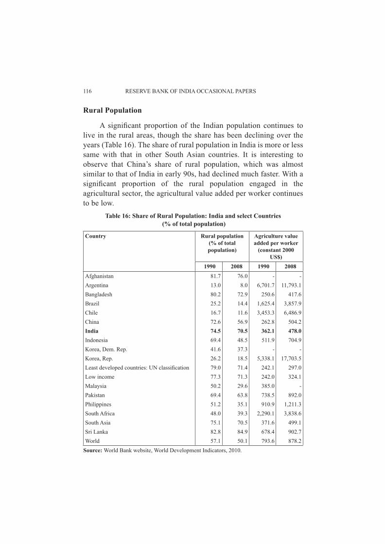
A signifi cant proportion of the Indian population continues to live in the rural areas, though the share has been declining over the years (Table 16). The share of rural population in India is more or less same with that in other South Asian countries. It is interesting to observe that China’s share of rural population, which was almost similar to that of India in early 90s, had declined much faster. With a signifi cant proportion of the rural population engaged in the agricultural sector, the agricultural value added per worker continues to be low.
Table 16: Share of Rural Population: India and select Countries (% of total population)
Country Rural population(% of total population)
Agriculture value added per worker
(constant 2000 US$)
1990 2008 1990 2008Afghanistan 81.7 76.0 - -Argentina 13.0 8.0 6,701.7 11,793.1Bangladesh 80.2 72.9 250.6 417.6Brazil 25.2 14.4 1,625.4 3,857.9Chile 16.7 11.6 3,453.3 6,486.9China 72.6 56.9 262.8 504.2India 74.5 70.5 362.1 478.0Indonesia 69.4 48.5 511.9 704.9Korea, Dem. Rep. 41.6 37.3 - -Korea, Rep. 26.2 18.5 5,338.1 17,703.5Least developed countries: UN classifi cation 79.0 71.4 242.1 297.0Low income 77.3 71.3 242.0 324.1Malaysia 50.2 29.6 385.0 -Pakistan 69.4 63.8 738.5 892.0Philippines 51.2 35.1 910.9 1,211.3South Africa 48.0 39.3 2,290.1 3,838.6South Asia 75.1 70.5 371.6 499.1Sri Lanka 82.8 84.9 678.4 902.7World 57.1 50.1 793.6 878.2
Source: World Bank website, World Development Indicators, 2010.

INCLUSIVE GROWTH AND ITS REGIONAL DIMENSION 117
Rural Health
India has made signifi cant strides in terms of availability of improved water source in the rural areas (Table 17). It is comparable with many countries across the world. However, in terms of inclusive growth on the provision of improved rural sanitation, our achievement has been low.
Gender Disparity
Another important indicator of inclusive growth is the trend in gender disparity. India has made signifi cant strides in terms of reducing the gender disparities as refl ected in various indicators. For instance, the female life expectancy at birth, the female literacy levels and the share of women employed in the non-agricultural sector have improved
Table 17: Availability of Improved Water Source and Sanitation in Rural Areas (as % of rural population with access)
Country Improved Water Source
Improved Rural Sanitation
1990 2006 1995 2006Afghanistan 17.0 29.0 25.0Argentina 72.0 80.0 59.0 83.0Bangladesh 76.0 78.0 21.0 32.0Brazil 54.0 58.0 37.0 37.0Chile 49.0 72.0 58.0 74.0China 55.0 81.0 48.0 59.0India 65.0 86.0 8.0 18.0Indonesia 63.0 71.0 40.0 37.0Korea, Dem. Rep. n.a. 100.0 60.0 n.a.Least developed countries: UN classifi cation 45.3 55.1 17.8 27.3Low income 45.2 59.7 23.4 33.3Malaysia 96.0 96.0 n.a. 93.0Pakistan 81.0 87.0 22.0 40.0Philippines 75.0 88.0 55.0 72.0South Africa 62.0 82.0 46.0 49.0South Asia 67.7 83.8 12.2 23.0Sri Lanka 62.0 79.0 74.0 86.0World 62.0 77.5 37.3 44.2
Source: World Bank website, World Development Indicators, 2010.
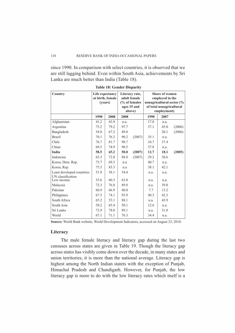
118 RESERVE BANK OF INDIA OCCASIONAL PAPERS
since 1990. In comparison with select countries, it is observed that we are still lagging behind. Even within South Asia, achievements by Sri Lanka are much better than India (Table 18).
Table 18: Gender DisparityCountry Life expectancy
at birth, female (years)
Literacy rate, adult female
(% of females ages 15 and
above)
Share of women employed in the
nonagricultural sector (% of total nonagricultural
employment)1990 2008 2008 1990 2007
Afghanistan 41.2 43.9 n.a. 17.8 n.a.Argentina 75.2 79.2 97.7 37.1 45.0 (2006)Bangladesh 54.8 67.2 49.8 20.1 (2006)Brazil 70.1 76.2 90.2 (2007) 35.1 n.a.Chile 76.7 81.7 98.7 34.7 37.4China 69.5 74.9 90.5 37.8 n.a.India 58.5 65.2 50.8 (2007) 12.7 18.1 (2005)Indonesia 63.3 72.8 88.8 (2007) 29.2 30.6Korea, Dem. Rep. 73.7 69.3 n.a 40.7 n.a.Korea, Rep. 75.5 83.3 n.a 38.1 42.1Least developed countries: UN classifi cation
51.8 58.1 54.4 n.a. n.a.
Low income 55.6 60.3 63.0 n.a. n.a.Malaysia 72.3 76.8 89.8 n.a. 39.0Pakistan 60.9 66.9 40.0 7.7 13.2Philippines 67.5 74.1 93.9 40.3 42.3South Africa 65.2 53.1 88.1 n.a. 43.9South Asia 58.2 65.4 50.1 12.6 n.a.Sri Lanka 72.9 78.0 89.1 n.a. 31.0World 67.1 71.1 76.3 34.4 n.a.
Source: World Bank website, World Development Indicators, accessed on August 23, 2010.
Literacy
The male female literacy and literacy gap during the last two censuses across states are given in Table 19. Though the literacy gap across states has visibly come down over the decade, in many states and union territories, it is more than the national average. Literacy gap is highest among the North Indian statets with the exception of Punjab, Himachal Pradesh and Chandigarh. However, for Punjab, the low literacy gap is more to do with the low literacy rates which itself is a

INCLUSIVE GROWTH AND ITS REGIONAL DIMENSION 119
Table 19: Male-female Literacy Gap in IndiaStates /UT Literacy Rate 1991
censusLiteracy
GapLiteracy Rate 2001
censusLiteracy
Gap
Male Female Male FemaleRajasthan 55.0 20.4 34.6 75.7 43.9 31.9D &N Haveli 53.6 27.0 26.6 71.2 40.2 31.0Jharkhand 55.8 25.5 30.3 67.3 38.9 28.4Uttar Pradesh 54.8 24.4 30.5 68.8 42.2 26.6Bihar 51.4 22.0 29.4 59.7 33.1 26.6Madhya Pradesh 58.5 29.4 29.2 76.1 50.3 25.8Chhattisgarh 58.1 27.5 30.6 77.4 51.9 25.5Orissa 63.1 34.7 28.4 75.4 50.5 24.8Uttarakhand 72.8 41.6 31.2 83.3 59.6 23.7Jammu & Kashmir N.A N.A N.A 66.6 43.0 23.6Haryana 69.1 40.5 28.6 78.5 55.7 22.8Gujarat 73.4 48.9 24.5 79.7 57.8 21.9Daman & Diu 82.7 59.4 23.3 86.8 65.6 21.2Arunachal Pradesh 51.5 29.7 21.8 63.8 43.5 20.3Andhra Pradesh 55.1 32.7 22.4 70.3 50.4 19.9Manipur 71.6 47.6 24.0 80.3 60.5 19.8Karnataka 67.3 44.3 22.9 76.1 56.9 19.2Maharashtra 76.6 52.3 24.2 86.0 67.0 18.9Tamil Nadu 73.8 51.3 22.4 82.4 64.4 18.0Himachal Pradesh 75.4 52.3 23.2 85.4 67.4 17.9West Bengal 67.8 46.6 21.3 77.0 59.6 17.4Assam 61.9 43.0 18.8 71.3 54.6 16.7Tripura 70.6 49.7 20.9 81.0 64.9 16.1Sikkim 65.7 46.8 18.9 76.0 60.4 15.6Puducherry 83.7 65.6 18.1 88.6 73.9 14.7Goa 83.6 67.1 16.6 88.4 75.4 13.1Delhi 82.0 67.0 15.0 87.3 74.7 12.6Lakshadweep 90.2 72.9 17.3 92.5 80.5 12.1Punjab 65.7 50.4 15.3 75.2 63.4 11.9A&N Islands 79.0 65.5 13.5 86.3 75.2 11.1Nagaland 67.6 54.8 12.9 71.2 61.5 9.7Chandigargh 82.0 72.3 9.7 86.1 76.5 9.7Kerala 93.6 86.2 7.5 94.2 87.7 6.5Meghalaya 53.1 44.9 8.3 65.4 59.6 5.8Mizoram 85.6 78.6 7.0 90.7 86.8 4.0INDIA 64.1 39.3 24.9 75.3 53.7 21.6
Source: Selected Socio Economic Statistics, India, CSO
worrisome phenomenon considering that Punjab ranks fi fth in terms of per capita NSDP.

120 RESERVE BANK OF INDIA OCCASIONAL PAPERS
In the case of infant mortality rates, the disparity is very high (Table 20). It ranges from 10 in Goa to 70 in Madhya Pradesh.
Table 20: State-wise Infant Mortality Rates (per 1000)States/Union Territories
1961 2007 2008Male Female Person Male Female Person Male Female Person
Goa 60 56 57 11 13 13 10 11 10Kerala 55 48 52 14 10 13 10 13 12Manipur 31 33 32 13 9 12 13 15 14Puducherry 77 68 73 31 22 25 22 27 25Nagaland 76 58 68 18 29 21 23 29 26Chandigarh 53 53 53 25 28 27 27 29 28Andaman 78 66 77 38 23 34 29 32 31Lakshadweep 124 88 118 25 23 24 29 34 31Tamil 89 82 86 38 31 35 30 33 31Daman & Diu 60 56 57 29 23 27 26 37 31Arunachal Pradesh 141 111 126 41 15 37 30 34 32Maharashtra 96 89 92 41 24 34 33 33 33Sikkim 105 87 96 36 20 34 34 32 33Tripura 106 116 111 40 32 39 34 35 34Dadra 102 93 98 38 18 34 33 35 34Delhi 66 70 67 41 35 36 34 37 35West 103 57 95 39 29 37 34 37 35Mizoram 73 65 69 27 16 23 37 38 37Punjab 74 79 77 47 35 43 39 43 41Himachal Pradesh 101 89 92 49 25 47 43 45 44Uttarakhand – – – 52 25 48 44 45 44Karnataka 87 74 81 52 35 47 44 46 45Jharkhand – – – 51 31 48 45 48 46Jammu Kashmir 78 78 78 53 38 51 48 51 49Gujarat 81 84 84 60 36 52 49 51 50Andhra Pradesh 100 82 91 60 37 54 51 54 52Haryana 87 119 94 60 44 55 51 57 54Bihar 95 94 94 59 44 58 53 58 56Chhatisgarh – – – 61 49 59 57 58 57Meghalaya 81 76 79 57 46 56 58 58 58Rajasthan 114 114 114 72 40 65 60 65 63Assam na na na 68 41 66 62 65 64Uttar Pradesh 131 128 130 72 51 69 64 70 67Orissa 119 111 115 73 52 71 68 70 69Madhya Pradesh 158 140 150 77 50 72 68 72 70India 122 108 115 61 37 55 52 55 53
Source: Economic Survey 2009-10.

INCLUSIVE GROWTH AND ITS REGIONAL DIMENSION 121
Another aspect of looking into the development of the region is the provision of basic facilities. Table 21 provides the data on the percentage of population with housing amenities. While there is signifi cant improvement in the availability of electricity, there is huge difference in rural urban. While only 8 per cent of urban population is not having electricity, the share is 44 per cent in the case of rural areas.
Table 21: Percentage of population living with Housing Amenities (Lighting)1999-2000 2005-06
R U R UNo lighting 0.5 0.3 0.5 0.2Kerosene 50.6 10.3 42.2 7.2Other oil 0.2 0.1 0.2 0.1Gas 0.1 0.1 0.1 0.1Candle 0.1 0.0 0.2 0.3Electricity 48.4 89.1 56.3 92Other 0.1 0.1 0.5 0.1Not recorded 0.0 0.0 0.0 0.0All 100 100 100 100
R Rural; U: UrbanSource: Selected Socio Economic Statistics, India, CSO
The above indicators provided signifi cant facts on differences in the socio-economic conditions across regions. However, it is possible that within regions, certain groups are marginalized. This was evident when we looked into the poverty ratio across different class of population. In the following Tables we looked into the entitlement to different population groups (Tables 22 and 23).
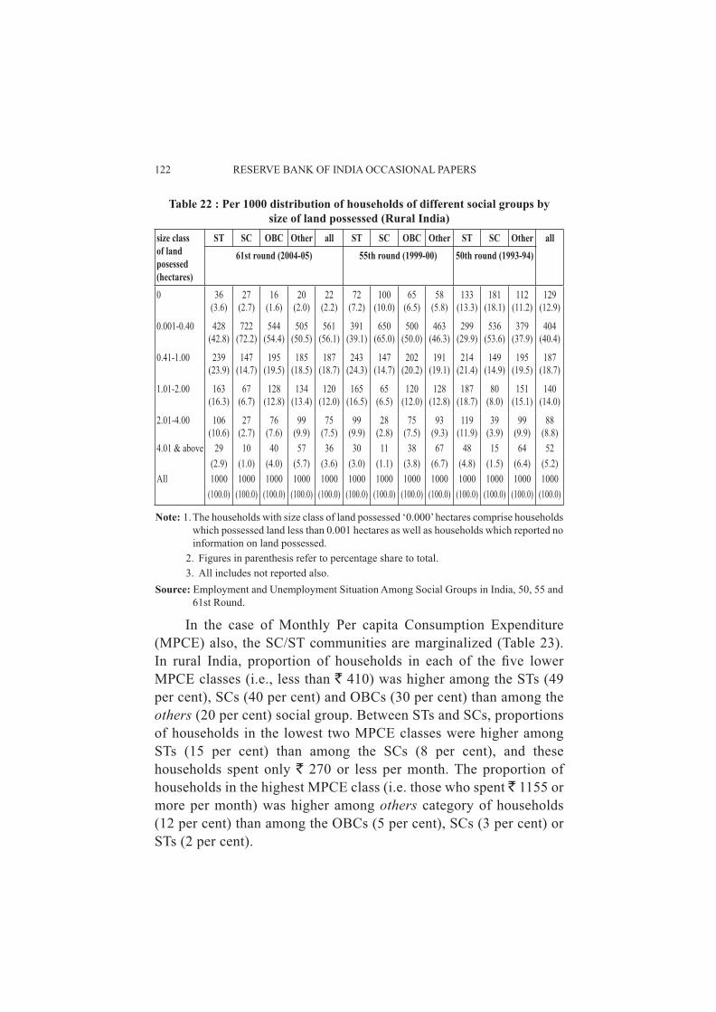
In rural India, among the social groups, the proportion of households possessing land less than 0.001 hectares, during 2004-05, was the highest for ST households (nearly 4 per cent). The corresponding proportion for SC households was about 3 per cent and for OBC and others category of households around 2 per cent each. The survey results also show that the proportion of households possessing land of size 4.01 hectares or more was maximum for other category of households (6 per cent), followed by the OBC (4 per cent), ST (about 3 per cent) and SC households (1 per cent).
122 RESERVE BANK OF INDIA OCCASIONAL PAPERS
Table 22 : Per 1000 distribution of households of different social groups by size of land possessed (Rural India)
size class of land posessed (hectares)
ST SC OBC Other all ST SC OBC Other ST SC Other all61st round (2004-05) 55th round (1999-00) 50th round (1993-94)
0 36 27 16 20 22 72 100 65 58 133 181 112 129(3.6) (2.7) (1.6) (2.0) (2.2) (7.2) (10.0) (6.5) (5.8) (13.3) (18.1) (11.2) (12.9)
0.001-0.40 428 722 544 505 561 391 650 500 463 299 536 379 404(42.8) (72.2) (54.4) (50.5) (56.1) (39.1) (65.0) (50.0) (46.3) (29.9) (53.6) (37.9) (40.4)
0.41-1.00 239 147 195 185 187 243 147 202 191 214 149 195 187(23.9) (14.7) (19.5) (18.5) (18.7) (24.3) (14.7) (20.2) (19.1) (21.4) (14.9) (19.5) (18.7)
1.01-2.00 163 67 128 134 120 165 65 120 128 187 80 151 140(16.3) (6.7) (12.8) (13.4) (12.0) (16.5) (6.5) (12.0) (12.8) (18.7) (8.0) (15.1) (14.0)
2.01-4.00 106 27 76 99 75 99 28 75 93 119 39 99 88(10.6) (2.7) (7.6) (9.9) (7.5) (9.9) (2.8) (7.5) (9.3) (11.9) (3.9) (9.9) (8.8)
4.01 & above 29 10 40 57 36 30 11 38 67 48 15 64 52(2.9) (1.0) (4.0) (5.7) (3.6) (3.0) (1.1) (3.8) (6.7) (4.8) (1.5) (6.4) (5.2)
All 1000 1000 1000 1000 1000 1000 1000 1000 1000 1000 1000 1000 1000(100.0) (100.0) (100.0) (100.0) (100.0) (100.0) (100.0) (100.0) (100.0) (100.0) (100.0) (100.0) (100.0)
Note: 1. The households with size class of land possessed ‘0.000’ hectares comprise households which possessed land less than 0.001 hectares as well as households which reported no information on land possessed.
2. Figures in parenthesis refer to percentage share to total. 3. All includes not reported also.Source: Employment and Unemployment Situation Among Social Groups in India, 50, 55 and
61st Round.
In the case of Monthly Per capita Consumption Expenditure (MPCE) also, the SC/ST communities are marginalized (Table 23). In rural India, proportion of households in each of the fi ve lower MPCE classes (i.e., less than ` 410) was higher among the STs (49 per cent), SCs (40 per cent) and OBCs (30 per cent) than among the others (20 per cent) social group. Between STs and SCs, proportions of households in the lowest two MPCE classes were higher among STs (15 per cent) than among the SCs (8 per cent), and these households spent only ` 270 or less per month. The proportion of households in the highest MPCE class (i.e. those who spent ` 1155 or more per month) was higher among others category of households (12 per cent) than among the OBCs (5 per cent), SCs (3 per cent) or STs (2 per cent).

INCLUSIVE GROWTH AND ITS REGIONAL DIMENSION 123
Table 23: Per 1000 distribution of households by household monthly per capita consumer expenditure for each social group
Monthly per-capita consumer expenditure (`)
Rural Monthly per-capita consumer expenditure (`)
UrbanST SC OBC Others all ST SC OBC Others all
less than 235 91 35 20 12 29 less than 335 81 70 34 16 33(9.1) (3.5) (2.0) (1.2) (2.9) (8.1) (7.0) (3.4) (1.6) (3.3)
235-270 62 43 24 16 30 335-395 54 58 42 15 32(6.2) (4.3) (2.4) (1.6) (3.0) (5.4) (5.8) (4.2) (1.5) (3.2)
270-320 113 94 70 37 71 395-485 84 120 88 46 73(11.3) (9.4) (7.0) (3.7) (7.1) (8.4) (12.0) (8.8) (4.6) (7.3)
320-365 117 115 89 60 90 485-580 122 131 116 63 93(11.7) (11.5) (8.9) (6.0) (9.0) (12.2) (13.1) (11.6) (6.3) (9.3)
365-410 108 113 95 71 94 580-675 84 131 120 69 97(10.8) (11.3) (9.5) (7.1) (9.4) (8.4) (13.1) (12.0) (6.9) (9.7)
410-455 92 108 95 73 92 675-790 75 110 107 78 93(9.2) (10.8) (9.5) (7.3) (9.2) (7.5) (11.0) (10.7) (7.8) (9.3)
455-510 94 112 113 92 106 790-930 85 109 109 90 99(9.4) (11.2) (11.3) (9.2) (10.6) (8.5) (10.9) (10.9) (9.0) (9.9)
510-580 93 114 121 122 117 930-1100 113 78 98 102 97(9.3) (11.4) (12.1) (12.2) (11.7) (11.3) (7.8) (9.8) (10.2) (9.7)
580-690 97 107 135 142 127 1100-1380 135 82 104 127 113(9.7) (10.7) (13.5) (14.2) (12.7) (13.5) (8.2) (10.4) (12.7) (11.3)
690-890 82 93 122 153 119 1380-1880 92 70 96 157 121(8.2) (9.3) (12.2) (15.3) (11.9) (9.2) (7.0) (9.6) (15.7) (12.1)
890-1155 30 37 63 108 65 1880-2540 43 28 49 112 75(3.0) (3.7) (6.3) (10.8) (6.5) (4.3) (2.8) (4.9) (11.2) (7.5)
1155 & above 19 27 53 115 60 2540 & above 33 14 34 126 74(1.9) (2.7) (5.3) (11.5) (6.0) (3.3) (1.4) (3.4) (12.6) (7.4)
all classes 1000 1000 1000 1000 1000 all classes 1000 1000 1000 1000 1000
Note: Figures in parenthesis refers to percentage share to total.Source: Employment and Unemployment Situation among Social Groups in India, NSSO 61st Round.
In urban India too, proportion of households in each of the fi ve lower MPCE classes (i.e. less than ` 675) was higher among SCs, STs and OBCs than among the other categories of households. About 51 per cent of the SCs of urban India spent less than ` 675 per month during 2004-05; the corresponding percentages being 43, 40 and 21 for the STs, OBCs and the others, respectively. The proportion of households in the lowest MPCE class (i.e. those spending less than

124 RESERVE BANK OF INDIA OCCASIONAL PAPERS
` 335 per month) was higher among the STs (8 per cent) than that among SCs (7 per cent). The proportion of urban households spending ` 2540 or more per month was higher among other (13 per cent) categories of households than among the OBCs or STs (3 per cent each) or SCs (1 per cent).
The analysis in this section has shown that India’s achievement in terms of various social indicators are not that commendable compared to that of the growth in GDP. India lags behind many developing countries in terms of povery and other social indicators. There are sections of population that remains marginalized irrespective of the high growth. Urban Inequality in terms of consumption expenditure have increased in almost all states, while rural inequality has come down in most of the states.
So far, we have examined the various facets of inclusive growth by looking into the various indicators of economic and social development. A major pre-requisite of economic development is fi nance. Access to fi nance and awareness on the availability of fi nance can play a major role in promoting economic growth. In the next section we look into the interplay between institutional fi nance and economic growth.
Section V: Institutional Finance and Growth
There is a general consensus among economists that fi nancial development spurs economic growth. Theoretically, fi nancial development creates enabling conditions for growth through either a supply-leading (fi nancial development spurs growth) or a demand-following (growth generates demand for fi nancial products) channel. A large body of empirical research supports the view that development of the fi nancial system contributes to economic growth (Rajan and Zingales, 2003). Empirical evidence consistently emphasizes the nexus between fi nance and growth, though direction of causality is debatable. At the cross-country level, evidence indicates that various measures of fi nancial development (including assets of the fi nancial intermediaries, liquid liabilities of fi nancial institutions, domestic credit to private sector, stock and bond market capitalization) are robustly and positively

INCLUSIVE GROWTH AND ITS REGIONAL DIMENSION 125
related to economic growth (King and Levine, 1993; Levine and Zervos, 1998). Other studies establish a positive relationship between fi nancial development and industrial growth (Rajan and Zingales, 1998). Even the recent endogenous growth literature, building on ‘learning by doing’ processes, assigns a special role to fi nance (Aghion and Hewitt, 1998 and 2005).
For any productive activity, capital investment is vital and capital investment is possible only when fi nance is available. The endogenous growth literature stresses the importance of fi nancial development for economic growth as many important services are provided by a country’s fi nancial system. Thus, as part of our inclusive growth study it is useful to examine if there is fi nance-growth nexus in our economy. Before the nationalization of banks in 1969, most of the needy sectors, viz, agriculture, small scale sector and other productive sectors were deprived of the institutional fi nance. Major sections of the population under these sectors were under the clutches of the money lenders. So in a way they were mostly excluded from the growth process of the economy because of their indebtedness. Now, after 60 years of Independence of our country, although banking sector has developed to a great extent, it is worth examining whether formal fi nance did play any role in our growth process. At this stage, it is important to examine the relationship between fi nance and growth at the aggregated level8.
The Model
Empirical work on causality between fi nancial development and economic growth is sparse, owing to a lack of suffi ciently long time series data for developing countries. Jung (1986) was among the fi rst to test for causality by applying a Granger-causality procedure. He used annual data on per capital GNP and two measures of fi nancial development: the ratio of currency to M1 and the ratio of M2 to GDP, for 56 developed and developing countries. However, his results were inconclusive because
8 Ideally it should have been an analysis at the disaggregated level using panel data framework, but due to time constraint and non-availability of data at the disaggregated level we have done the exercise at the aggregated level.

126 RESERVE BANK OF INDIA OCCASIONAL PAPERS
they varied according to the fi nancial development indicator used and the development level of the various countries. For example, using the currency ratio as a measure for fi nancial development, Granger causality from fi nancial development to economic growth in LDCs was more frequently observed than the reverse and an opposite conclusion was obtained for the developed countries. However, when the M2/GDP ratio was used, causality from fi nancial development to economic growth was as frequently observed as causality from economic growth to fi nancial development both in LDCs and developed countries. Jung’s test was conducted in a levels vector autoregression (VAR) framework without testing for stationarity of the data. As data are very likely to be nonstationary, Jung’s fi ndings are debatable (Granger and Newbold, 1974). In a frequently-cited paper, Demetriades and Hussein (1996) tested for cointegration among variables and used an error correction model for 16 countries to test for a possible long-run causal relationship between fi nancial development and economic growth. Their fi ndings showed little evidence to support the view that fi nance leads economic growth.
In the present paper, we examine the causal relationship between fi nancial and economic development from a time-series perspective for India. For this, we apply the most current econometric techniques, in particular testing causality applying cointegration tests and error correction models after pre-testing for unit roots in all variables and choosing the optimal lag order in our VAR system. These tests are essential for attaining the proper inferences. We use three different measures of fi nancial development and relatively long annual time series data. We also include a third variable, namely the share of fi xed investment in GDP, in the system. This allows us to test channels through which fi nancial development and investment are explaining changes in the growth rate of per capita GDP beyond the sample period.
Measurement and Data Sources
Financial Development Indicators
Financial development is usually defi ned as a process that marks improvements in quantity, and effi ciency of fi nancial intermediary

INCLUSIVE GROWTH AND ITS REGIONAL DIMENSION 127
services. This process involves the interaction of many activities and institutions. Consequently, it cannot be captured by a single measure. In this study we employ three commonly used measures of fi nancial development for the sake of testing the robustness of our fi ndings.
The fi rst, M3Y, represents the ratio of money stock, M3, to nominal GDP. M3Y has been used as a standard measure of fi nancial development in numerous studies (Gelb, 1989, world Bank, 1989; King and Levine, 1993a, b; Calderon and Liu 2003). According to Demetriades and Hussein (1996), this indicator accords well with McKinnon’s outside money model where the accumulation of lumpy money balances is necessary before self-fi nanced investment can take place. However, it confl icts somewhat with the debt-intermediation approach developed by Gurley and Shaw (1995) and the endogenous growth literature, because a large part of the broad money stock in developing countries is currency held outside banks. As such, an increase in the M3/GDP ratio may refl ect an extensive use of currency rather than an increase in bank deposits, and for this reason this measure is less indicative of the degree of fi nancial intermediation by banking institutions. Financial intermediaries serve two main functions: to provide liquidity services and saving opportunities, the latter being relevant for promoting investment and consequently growth. For this reason, Demetriades and Hussein (1996) proposed to subtract currency outside banks from M3 and to take the ratio of M3 minus currency to GDP as a proxy for fi nancial development. On this basis, we chose QMY, the ratio of M3 minus currency to GDP, to serve as our second measure of fi nancial development.
Our third measure of fi nancial development is PRIVY, the ratio of bank credit to the private sector to nominal GDP. This indicator is frequently used to provide direct information about the allocation of fi nancial assets. A ratio of M3 (including or excluding currency) to GDP may increase as a result of an increase in private fi nancial saving. On the other hand, with high reserve requirements, credit to the private sector which eventually is responsible for the quantity and quality of investment and therefore to economic growth, may not increase. Therefore, an increase in this ratio does not necessarily

128 RESERVE BANK OF INDIA OCCASIONAL PAPERS
mean an increase in productive investments. Rather, the private credit GDP ratio can be a better estimate of the proportion of domestic assets allocated to productive activity in the private sector. Figure 6 shows that M3Y had increased tremendously starting 1979 to reach around 90 per cent in 2008. However, the high M3Y rate does not necessarily imply a larger pool of resources for the private sector and therefore is not a good indicator of fi nancial development, in contradiction, to PRIVY. Two explanations for this behavior were given by Roe (1998). The fi rst is the possibility that the dominating state-owned banks did not have a profi t maximizing goal. The second is that banks preferred to serve the interest of their non-private clients, and offered loans to public enterprises even at the expense of their profi tability. The latter is most evidently related to the quantity and effi ciency of investment and hence to economic growth (Gregorio and Guidotti, 1995). PRIVY has been used extensively in numerous works (King and Levine, 1993a, b, Gregorio and Guidotti, 1995, Levine and Zeroves, 1993, Demetriades and Hussein, 1996, Beck et al, 2000 among others), with different defi nitions of the stock of private credit depending on the institutions supplying the credit.
Other Variables
Following standard practice, we use real GDP per capita, GDPPC, as our measure for economic development (see Gelb, 1989, Roubini and Sala-i-Martin, 1992, King and Levine, 1993a,b Demetriades and Hussein, 1996). In addition to the per capita real GDP and the fi nancial development indicator, we introduced a third variable in our VAR system, the share of investment in GDP, IY. This variable is considered to be one of the few economic variables with a robust correlation of economic growth regardless of the information set (Levine and Renelt, 1992). Including the investment variable in our regressions enables us to identify the channels through which fi nancial development causes economic growth. If fi nancial development causes economic development, given the investment variable, then this causality supports the endogenous growth theories that fi nance affects economic growth mainly through the enhancement of investment effi ciency. Furthermore, we can then test if fi nancial

INCLUSIVE GROWTH AND ITS REGIONAL DIMENSION 129
development causes economic growth through an increase of investment resources. We can examine this supposition indirectly by testing the causality between fi nancial development indicators and investment on the one hand and between investment and economic growth on the other. All the variables in our data set are expressed in natural logarithms.
Data Sources
We used the following data resources: All data have been obtained from the Handbook of Statistics on Indian Economy published by the Reserve Bank of India. Our sample covers the period 1950-2008; the choice of this period is governed by data availability.
The Econometric methodology
Standard Granger Causality (SGC)
According to Granger’s (1969) approach, a variable Y is caused by a variable X if Y can be predicted better from past values of both Y and X than from past values of Y alone. For a simple bivariate model, we can test if X is Granger-causing Y by estimating Equation (1) and then test the null hypothesis in equation (2) by using the standard Wald test.

130 RESERVE BANK OF INDIA OCCASIONAL PAPERS
(1)
(2)
where, µ is a constant and ut is a white noise process. Variable X is said to Granger cause variable Y if we reject the null hypothesis (2), where γ12 is the vector of the coeffi cients of the lagged values of the variable X. Similarly, we can test if Y causes X by replacing Y for X and vice versa in Equation (1).
However, before conducting causality tests, we have examined whether the series is stationary. The series {Xt} will be integrated of order d, that is, Xt ~I(d), if it is stationary after differencing it d times. A series that is I(0) is stationary. To test for unit roots in our variable, we use Augmented Dickey Fuller (ADF) test.
The next step is to test for cointegration if the variables are nonstationary in their level. Generally, a set of variables is said to be cointegrated if a linear combination of the individual series, which are I(d), is stationary. Intuitively, if Xt ~I(d) and Yt ~I(d), a regression is run, such as:
(3)
If the residuals, εt , are I(0), then Xt and Yt are cointegrated. We use Johansen’s (1988) approach, which allows us to estimate and test for the presence of multiple cointegrated relationships, r, in a single-step procedure. A class of models embodies the notion of correction has been developed and is referred as the Error Correction Model (ECM). In general, an ECM derived from the Johansen test can be expressed as:
(4)
(5)
(6)

INCLUSIVE GROWTH AND ITS REGIONAL DIMENSION 131
where ECTt-1 is the error correction term lagged one period, Z is a third endogenous variable in the system, and βij, k describes the effect of the k-th lagged value of variable j on the current value of variable; i,j = Y, X, Z. The εit are mutually uncorrelated white noise residuals.
Granger causality from variable j to variable i in the presence of cointegration is evaluated by testing the null hypothesis that βij,k = αi = 0 for all k in the equation where i is the dependent variable, using the standard F test. By rejecting the null, we conclude that variable j Granger-causes variable i. These tests differ from standard causality tests in that they include error correction terms (ECTt-1) that account for the existence of cointegration among the variables. At least one variable in Equations (4) to (6) should move to bring the relation back into equilibrium if there is a true economic relation, and therefore at least one of the coeffi cients of the error correction terms has to be signifi cantly different from zero (Granger, 1988).
Empirical Results
Granger Causality Results
The fi rst of our empirical work was to determine the degree of integration of each variable. The ADF test results for the levels and fi rst differences are reported in Table 24. The results show that all the
Table 24: ADF Unit Root Test Results
Variable ADF with trend and intercept
Levels First differences
ADF k* ADF k*
LGDPPC -3.403 0 -6.827*** 0LPRIVATE -1.183 0 -6.922*** 0LM3Y -2.643 0 -7.976*** 0LQMY -1.969 1 -19.601*** 0LIY -3.836 0 -7.884*** 0
LGDPPC, LPRIVATE, LM3Y, LQMY and LIY are the natural logarithms of real per capita GDP, share of credit to private sector in GDP, share of M3 in GDP, share of M3 minus currency outside of banking in GDP, and the share of gross fi xed capital formation in GDP, respectively.K* the optimal lag lengths chosen by Schwarz selection criterion with maximum of 9 lags.*, **, and *** indicate signifi cance at the 10% , 5% and 1% levels, respectively.

132 RESERVE BANK OF INDIA OCCASIONAL PAPERS
Table 25: Johansen Cointegration Test Results
Variables P* r*
r = 0 r = 1 r = 2LGDPPC, LIY, LPRIVATE 29.809*** 11.979 3.041 1 1LGDPPC, LIY, LM3Y 37.175*** 10.289 2.333 1 1LGDPPC, LIY, LQMY 37.860*** 10.606 1.927 1 1
*; **; *** indicate signifi cance at the 10%, 5% and 1% levels, respectively. is the maximum eigen value statistic.
p* represents the optimal lag length based on AIC from the unrestricted VAR model.r* is the number of co-integration vectors based on Johansen’s method.
variables are nonstationary i.e. I(1) in their levels, but stationary in their fi rst differences.9
The second step was to test for a cointegration relationship among the relevant variables. The results of Johansen’s maximum eigenvalue test (λmax) support the existence of a unique long run relation between per capita GDP, the investment ratio and fi nancial development under the various measures of the latter. In all cases, we reject the null hypothesis of a no-cointegration relationship at least at the 5% level (Table 25). It is also observed from Granger causality test that the null hypothesis
Table 26: Results of Granger Causality Tests (Direct)
Null Hypothesis
Financial Development Indicator
Financial Development does not Granger cause income growthF-Statistic Prob
LPRIVATE 6.63*** 0.003LM3 9.69*** .0003LMQ 7.89*** 0.001Panel B
Null HypothesisFinancial Development Indicator
Income growth does not Granger cause fi nancial developmentF-Statistic Prob
LPRIVATE 1.49 0.235LM3 3.90** 0.0264LMQ 1.49 0.236
***: signifi cant at 1% level of signifi cance; **: signifi cant at 5% level of signifi cance
9 Using Phillips-Perron test we obtained similar results.
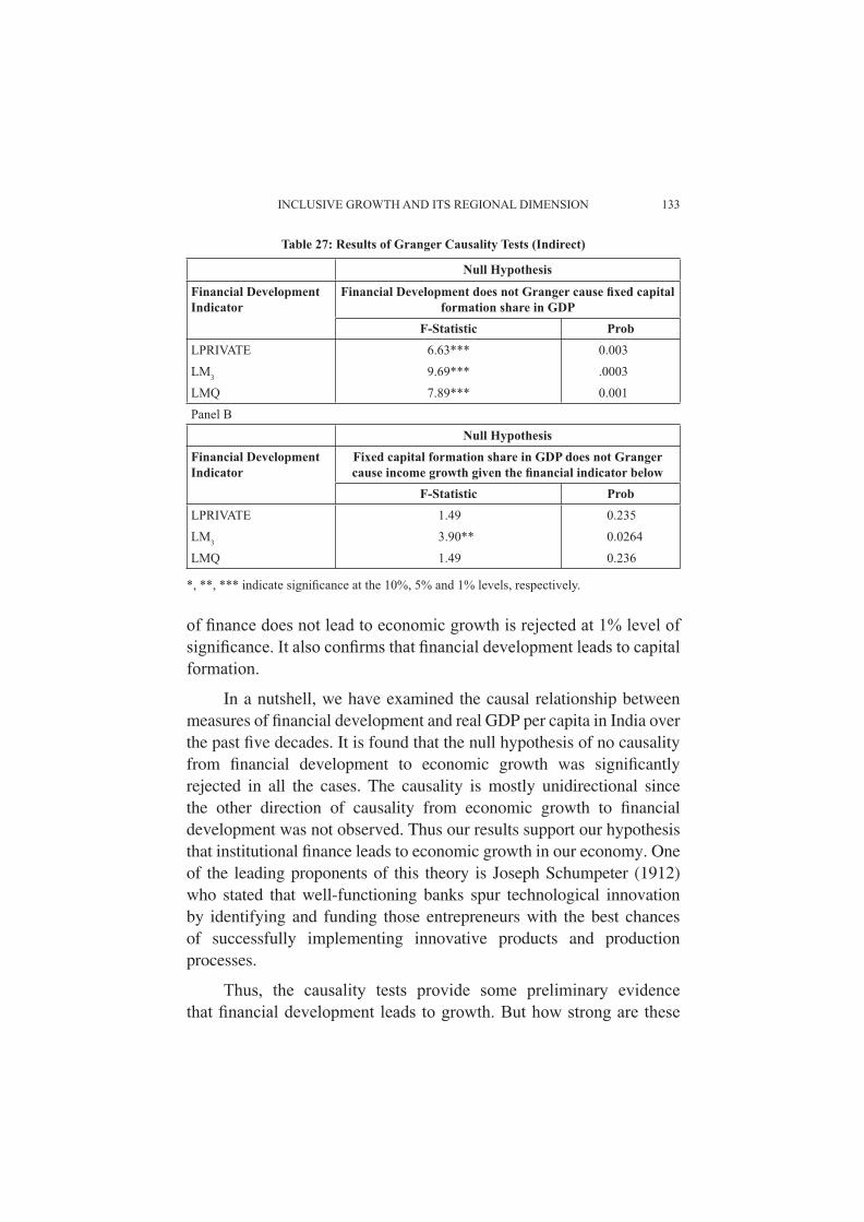
INCLUSIVE GROWTH AND ITS REGIONAL DIMENSION 133
of fi nance does not lead to economic growth is rejected at 1% level of signifi cance. It also confi rms that fi nancial development leads to capital formation.
In a nutshell, we have examined the causal relationship between measures of fi nancial development and real GDP per capita in India over the past fi ve decades. It is found that the null hypothesis of no causality from fi nancial development to economic growth was signifi cantly rejected in all the cases. The causality is mostly unidirectional since the other direction of causality from economic growth to fi nancial development was not observed. Thus our results support our hypothesis that institutional fi nance leads to economic growth in our economy. One of the leading proponents of this theory is Joseph Schumpeter (1912) who stated that well-functioning banks spur technological innovation by identifying and funding those entrepreneurs with the best chances of successfully implementing innovative products and production processes.
Thus, the causality tests provide some preliminary evidence that fi nancial development leads to growth. But how strong are these
Table 27: Results of Granger Causality Tests (Indirect)
Null Hypothesis
Financial Development Indicator
Financial Development does not Granger cause fi xed capital formation share in GDP
F-Statistic ProbLPRIVATE 6.63*** 0.003LM3 9.69*** .0003LMQ 7.89*** 0.001Panel B
Null HypothesisFinancial Development Indicator
Fixed capital formation share in GDP does not Granger cause income growth given the fi nancial indicator below
F-Statistic ProbLPRIVATE 1.49 0.235LM3 3.90** 0.0264LMQ 1.49 0.236
*, **, *** indicate signifi cance at the 10%, 5% and 1% levels, respectively.

134 RESERVE BANK OF INDIA OCCASIONAL PAPERS
relationships? What is the pattern of the response from one year to the next? These questions can be answered within the framework of impulse response analysis and analysis of variance decomposition of the forecast errors, which we have also dealt with in this section.
We fi rst report the results which demonstrate how the forecast error variance of our focus variables can be broken down into components that can be attributed to each of the variables in the VAR. It can be observed from Table 28 that credit (LPRIVY) explains 63.5 per cent of the forecast error variance of GDP (LGPDPC) and it becomes the most important variable affecting economic growth whereas gross fi xed capital formation (LIY) as the second one explaining 18.4 per cent of forecast error variance of GDP. It is also observed that LGDPPC explains 13.2 per cent of its forecast error variance. The fact that GDP growth is explained by its past values suggests that current period economic growth infl uences future growth trends or that the phenomenon is due to a “lag effect” in the business cycle.
Table 28 also shows that both credit to private sector and fi xed capital formation appear to have strong lagged effects and are, to a larger extent, explained by their own past values (around 67 per cent in case of credit and 60 per cent in case of fi xed capital formation). It is interesting to note that economic growth explains more than 46 per cent of the forecast error variance of M3 which appears to be quite logical.
However, the fact that credit to private sector contributes more than gross fi xed capital formation to GDP growth in India implies that its primary source of growth is extensive use credit in the private sector.
Table 28: Variance Decomposition Percentage of 20-year Error VarianceVariance decomposition of After 20 years, % of Decomposition due to
LGDPPC LIY LM3Y LPRIVY LQMYLGDPPC 13.2 18.4 0.9 63.5 4.1LIY 9.1 60.0 1.3 27.4 2.2LM3Y 46.2 8.2 15.5 24.8 5.3LPRIVY 18.6 5.5 3.9 67.1 5.0LQMY 13.7 3.0 16.7 53.9 12.8
INCLUSIVE GROWTH AND ITS REGIONAL DIMENSION 135
To investigate further the impact of credit on GDP growth as compared to other variables, we then have used impulse response function to trace the time paths of GDP in response to one-unit shock to the variables such as three different fi nancial indicators and gross fi xed capital formation. A graphical illustration of an impulse response function can provide an intuitive insight into dynamic relationships because it shows the response of a variable to a “shock” in itself or another variable over time. For example, it allows us to examine how GDP growth responds over time to a “shock” in credit and compare it with the effects on other variables.
Chart 7 depicts the time paths of the responses of GDP growth to “shocks” in fi nancial indicators and gross fi xed capital formation. It can be observed that all the fi nancial indicators have a positive impact on economic growth. However, the response of GDP to a shock in credit has a longer and stronger effect than other variables and series is not convergent even after 20 years. On the other hand, impacts of other fi nancial indicators (viz., LM3 and LQMY) on growth are smaller and “die out” quickly from the 3rd year. However, in this case also it is found that gross fi xed capital formation has second largest impact on economic growth and the effect is longer as well.
Therefore, we can argue that fi nancial development does promote economic growth in India. It can also be argued that the innovations in bank credit were the most important source of the variance of forecast errors for economic growth. Similarly, economic growth was not found to have greater impacts on investments (LIY) (LGDPPC explaining 9.1 per cent of forecast error variance on LIY) than bank credit, LPRIVY (LPRIVY explains 27.4 per cent of LIY). This suggests that economic growth have a greater infl uence on availability funds than investment behavior.
It may also be observed that GDPPC also affects fi nancial development indicators. Table 28 shows that LGDPPC explains about 18.6 per cent of forecast error variance of bank credit, 46.2 of forecast error variance of LM3 and 13.7 per cent of forecast error variance of LQMY. Therefore, the above fi ndings suggest that there is a bi-directional
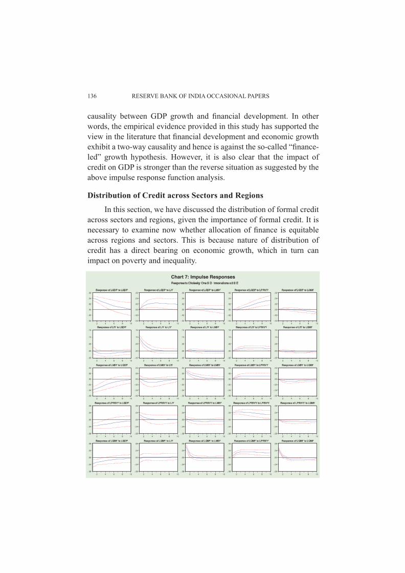
136 RESERVE BANK OF INDIA OCCASIONAL PAPERS
causality between GDP growth and fi nancial development. In other words, the empirical evidence provided in this study has supported the view in the literature that fi nancial development and economic growth exhibit a two-way causality and hence is against the so-called “fi nance-led” growth hypothesis. However, it is also clear that the impact of credit on GDP is stronger than the reverse situation as suggested by the above impulse response function analysis.
Distribution of Credit across Sectors and Regions
In this section, we have discussed the distribution of formal credit across sectors and regions, given the importance of formal credit. It is necessary to examine now whether allocation of fi nance is equitable across regions and sectors. This is because nature of distribution of credit has a direct bearing on economic growth, which in turn can impact on poverty and inequality.
Chart 7: Impulse Responses
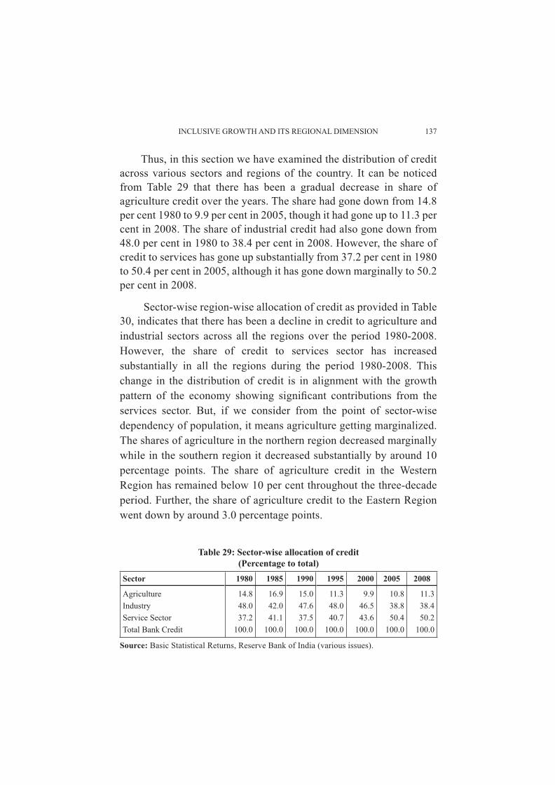
INCLUSIVE GROWTH AND ITS REGIONAL DIMENSION 137
Thus, in this section we have examined the distribution of credit across various sectors and regions of the country. It can be noticed from Table 29 that there has been a gradual decrease in share of agriculture credit over the years. The share had gone down from 14.8 per cent 1980 to 9.9 per cent in 2005, though it had gone up to 11.3 per cent in 2008. The share of industrial credit had also gone down from 48.0 per cent in 1980 to 38.4 per cent in 2008. However, the share of credit to services has gone up substantially from 37.2 per cent in 1980 to 50.4 per cent in 2005, although it has gone down marginally to 50.2 per cent in 2008.
Sector-wise region-wise allocation of credit as provided in Table 30, indicates that there has been a decline in credit to agriculture and industrial sectors across all the regions over the period 1980-2008. However, the share of credit to services sector has increased substantially in all the regions during the period 1980-2008. This change in the distribution of credit is in alignment with the growth pattern of the economy showing signifi cant contributions from the services sector. But, if we consider from the point of sector-wise dependency of population, it means agriculture getting marginalized. The shares of agriculture in the northern region decreased marginally while in the southern region it decreased substantially by around 10 percentage points. The share of agriculture credit in the Western Region has remained below 10 per cent throughout the three-decade period. Further, the share of agriculture credit to the Eastern Region went down by around 3.0 percentage points.
Table 29: Sector-wise allocation of credit(Percentage to total)
Sector 1980 1985 1990 1995 2000 2005 2008
Agriculture 14.8 16.9 15.0 11.3 9.9 10.8 11.3Industry 48.0 42.0 47.6 48.0 46.5 38.8 38.4Service Sector 37.2 41.1 37.5 40.7 43.6 50.4 50.2Total Bank Credit 100.0 100.0 100.0 100.0 100.0 100.0 100.0
Source: Basic Statistical Returns, Reserve Bank of India (various issues).

138 RESERVE BANK OF INDIA OCCASIONAL PAPERS
Table 30: Sector-wise Region-wise allocation of credit
Northern Region
Southern Region
Western Region
Eastern Region
1980Agriculture 24.8 22.2 8.7 13.5Industry 39.3 44.0 62.7 59.4Service Sector 35.9 33.8 28.7 27.1Total Bank Credit 100.0 100.0 100.0 100.01985Agriculture 26.6 55.1 7.8 14.4Industry 37.0 21.2 43.1 51.7Service Sector 36.3 23.8 49.0 33.9Total Bank Credit 100.0 100.0 100.0 100.01990Agriculture 23.8 19.6 7.6 13.4Industry 40.7 43.3 55.7 50.2Service Sector 35.5 37.0 36.8 36.4Total Bank Credit 100.0 100.0 100.0 100.01995Agriculture 19.3 15.7 5.3 12.0Industry 42.3 42.2 55.2 47.6Service Sector 38.4 42.1 39.4 40.3Total Bank Credit 100.0 100.0 100.0 100.02000Agriculture 19.9 13.9 4.7 8.5Industry 39.9 39.9 54.5 45.4Service Sector 40.3 46.2 40.8 46.0Total Bank Credit 100.0 100.0 100.0 100.02005Agriculture 21.6 13.6 8.6 8.6Industry 30.4 33.9 74.0 36.0Service Sector 48.0 52.5 17.3 55.3Total Bank Credit 100.0 100.0 100.0 100.02008Agriculture 22.3 12.5 6.2 10.6Industry 32.1 32.9 45.0 37.1Service Sector 45.6 54.6 48.8 52.2Total Bank Credit 100.0 100.0 100.0 100.0
Source: Basic Statistical Returns, Reserve Bank of India (various issues)
Access to bank fi nances can also be gauged from the credit-deposit ratio which has been provided in Table 31. It can be observed from the Table that there is wide disparity in CD ratio across the

INCLUSIVE GROWTH AND ITS REGIONAL DIMENSION 139
Table 31: Region-wise, State-wise Credit-Deposit Ratio
Region/State/ 1980-(JUNE)
1985-(JUNE)
1990 1995 2000 2005 2009
Northern Region 76.1 63.7 54.8 48.6 51.1 59.5 68.5Haryana 66.1 67.6 61.2 45.5 42.4 51.4 61.5Himachal Pradesh 28.6 44.0 38.6 26.0 23.8 36.3 38.5Jammu & bKashmir 31.5 42.8 31.8 28.6 33.5 46.7 46.3Punjab 38.6 44.6 45.5 41.4 39.4 50.1 65.5Rajasthan 65.9 70.5 62.2 47.7 46.7 68.7 80.2North-Eastern Region
35.6 48.9 51.7 35.6 28.1 35.0 35.8
Arunachal Pradesh 6.2 21.5 20.1 12.4 15.7 22.0 24.8Assam 40.6 53.3 55.5 38.7 32.0 35.3 38.3Manipur 25.1 70.5 69.9 58.2 37.4 42.4 38.7Meghalaya 14.1 26.5 24.6 17.0 16.3 43.6 27.6Mizoram 6.0 22.8 34.2 16.5 23.3 47.8 58.7Nagaland 23.7 39.6 42.6 37.8 15.3 22.9 30.7Tripura 51.3 72.9 72.2 47.5 25.7 28.6 29.8Eastern Region 56.1 52.0 52.6 47.1 37.0 45.5 48.9Bihar 41.8 41.7 40.0 32.5 22.5 27.7 27.3Jharkhand - - - - - 29.6 32.0Orissa 61.1 92.8 81.3 54.5 41.5 61.8 50.8West Bengal 60.9 51.9 54.9 53.9 45.5 52.3 60.8Central Region 45.7 52.7 52.8 39.0 33.9 40.8 44.8Chhattisgarh - - - - - 43.6 53.3Madhya Pradesh 52.0 62.6 68.6 49.6 49.1 43.6 57.4Uttar Pradesh 43.5 49.2 47.0 35.1 28.2 37.9 42.1Uttarakhand - - - - - 24.3 25.6Western Region 70.5 79.9 74.0 63.2 75.4 83.5 85.2Gujrat 51.8 54.7 61.3 46.6 49.0 46.5 63.2Maharashtra 79.2 90.8 79.7 69.5 86.4 94.9 90.8Southern Region 77.6 84.4 87.4 69.4 66.2 78.1 88.4Andhra Pradesh 71.5 78.3 87.1 73.0 64.2 74.8 97.6Karnataka 77.8 86.7 91.0 65.8 63.3 73.8 76.6Kerala 67.5 68.5 64.0 44.8 41.5 54.6 60.4Tamil Nadu 88.0 98.6 99.4 86.7 88.6 101.2 108.9
Source: Statistical Tables Relating to Banks in India, Reserve Bank of India (various issues)
140 RESERVE BANK OF INDIA OCCASIONAL PAPERS
regions and states. The ratio remains above 80 per cent in the Southern and Western Regions during 2009, which has increased from above 75 per cent in 1985. On the other hand, the situation is not encouraging in the Northern Region where the CD ratio has become 68.5 per cent in 2009, gone down from 76.1 per cent in 1980. The condition is much worse in the Eastern, North-Eastern and Central Regions. While the CD ratio in the N-E Region and Central Region remained constant at 36 per cent and 45 per cent, respectively during the three decade period, it has gone down signifi cantly from 56.1 per cent in 1980 to 48.9 per cent in 2009 in the Eastern Region.
Financial Inclusion
A developed fi nancial system broadens access to funds; conversely, in an underdeveloped fi nancial system, access to funds is limited and people are constrained by the availability of their funds and have to resort to high cost informal sources such as money lenders. Lower the availability of funds and higher their cost, fewer would be the economic activities that can be fi nanced and hence lower the resulting economic growth (Rakesh Mohan, 2006)10.
Financial inclusion can be defi ned as delivery of banking services at an affordable cost to the vast sections of disadvantaged and low-income groups. In the case of credit, the proper defi nition of the fi nancially excluded would include households who are denied credit in spite of their demand. Although credit is the major component, fi nancial inclusion covers various other services such as savings, insurance, payments and remittance facilities by the formal fi nancial system to those who tend to be excluded.
Credit to farmer households is one of the important elements of fi nancial inclusion. As per the results of the All-India Debt and Investment Survey (AIDIS), the share of non-institutional sources of credit in total credit for cultivator households had declined sharply
10 Mohan, Rakesh (2006): ‘‘Economic Growth, Financial Deepening and Financial Inclusion”, Presented at the Annual Bankers’ Conference at Hyderabad, November 2006.

INCLUSIVE GROWTH AND ITS REGIONAL DIMENSION 141
from about 93 per cent in 1951 to about 31 per cent in 1991, with the share of money lenders having declined from 69.7 per cent to 17.5 per cent. In 2002, however, the share of money lenders had again increased to 27 per cent, while that of non-institutional sources rose to 39 per cent (Table 32).
Coincidentally, it is also a fact that there has been a slowdown in the rate of agricultural growth during the last decade and it is particularly striking in respect of foodgrain production. Banks have been mainly focusing on crop loans since the period of green revolution. There is, therefore, reason to believe that fi nancial exclusion may have actually increased in the rural areas.
It can be observed from Table 33 that the share of direct accounts with a credit limit of less than ̀ 25000 in total direct accounts declined from 93.4 per cent in 1980 to 35.8 per cent in 2008. The decline in share is observed across all the sectors.
It can also be observed from Table 34 that there is an inverse proportional relation between size class distribution of land and non-indebtedness. In other words, minimum size class had the lowest inclusion.
Table 32: Relative Share of Borrowing of Cultivator Households@(per cent)
Sources of Credit 1951 1961 1971 1981 1991 2002$Non-institutional 92.7 81.3 68.3 36.8 30.6 38.9of which: Money Lenders 69.7 49.2 36.1 16.1 17.5 26.8Institutional 7.3 18.7 31.7 63.2 66.3 61.1of which: Co-operative societies, etc. 3.3 2.6 22 29.8 30 30.2 Commercial banks 0.9 0.6 2.4 28.8 35.2 26.3 Unspecifi ed - - - - - -Total 100 100 100 100 100 100
@: Borrowing refers to outstanding cash dues.$: AIDIS, NSSO, 59th Round, 2003.Source: All India Debt and Investment Surveys.

142 RESERVE BANK OF INDIA OCCASIONAL PAPERS
Role of Self-Help Groups
The RBI recognized the problem of fi nancial exclusion in the Annual Policy Statement in 2005 and since then several initiatives have been initiated in order to promote fi nancial inclusion especially in the groups of pensioners, self-employed and those employed in the unorganized sector. Some of these include “no frills” account, a simplifi ed general purpose credit card (GCC), introduction of pilot project for 100 per cent fi nancial inclusion, etc. On the other hand, NABARD has also taken several steps in this direction. The self-help group (SHG) – bank linkage programme of NABARD is an innovative programme. It started as a pilot programme in 1992. At present India
Table 33: Percentage of Small Borrowal Account (` 25,000 and less) to Total No. of Accounts
Occupation 1980 1990 2000 2008Agriculture 96.7 97.3 85.4 51.4Industry 56.9 83.4 69.4 34.4Transport Operators 68.6 81.4 48.2 14.6Professional & other services 96.5 91.6 76.5 22.0Personal loans - - 59.6 22.7Trade 86.3 96.0 77.1 44.0Finance 94.4 91.6 60.0 29.7All others 97.7 99.5 50.3 40.0Total 93.4 95.0 72.2 35.8
Note: For 1980, the small borrowal account is defi ned as ` 10, 000 and less.Source: Basic Statistical Returns, Reserve Bank of India (various issues)
Table 34: Distribution of size-class wise indebtedness of Farmers Households - 2002
Size Class Number Per centIncluded Excluded Total Included Excluded Total
Upto 0.40 ha 135820 169641 305471 44.5 55.5 100.00.41 to 1.00 ha 129211 154399 283610 45.6 54.4 100.01.01 to 2.00 ha 81920 78680 160600 51.0 49.0 100.0Upto 2.00 346951 402720 749671 46.3 53.7 100.02.01 to 4.00 ha 54409 39095 93504 58.2 41.8 100.04.01 and above 32882 17447 50329 65.3 34.7 100.0Above 2.00 ha 37291 56542 143833 60.7 39.3 100.0All sizes 434242 459262 893504 48.6 51.4 100.0
Source: Situational Assessment Survey of Farmers (59th Round NSSO).

INCLUSIVE GROWTH AND ITS REGIONAL DIMENSION 143
has around 22 lakh SHGs under this programme (Dev, 2006), comprising more than three crore poor households who are accessing credit through commercial and cooperative banks. Every year six lakh SHGs are added. The programme is now spread across the country. Following the success of SHG-linkage programme as also the Bangladesh Gramin Bank model, many of the NGOs have taken to fi nancial intermediation by adopting innovative delivery approaches. Following the RBI guideline in 2000, commercial banks including the RRBs are providing funds through micro-fi nance institutions for lending to poor clients. In fact, MFIs have been playing an important role in substituting moneylenders and reducing burden on formal fi nancial institutions.
With the objective of ensuring greater fi nancial inclusion and increasing the outreach of the banking sector, banks have been allowed to use the services of NGOs, self-help groups, MFIs and other civil society organizations as intermediaries in providing fi nancial and banking services through the use of business facilitator and correspondent models. Provisions for this kind of fi nancial intermediation have opened up new and diverse avenues to address the issue of fi nancial inclusion by banks. SHG linkage programme has already been successful in South India, viz., Kudumbasree programme in Kerala and Velugu in Andhra Pradesh. This has not only been successful in India, it is also popular and successful in countries like Bangladesh, Thailand, Mexico and Brazil.
Postal Savings and Remittance
Apart from the banking system, the post offi ces in India also provide the services of maintaining deposits and remittances. The Indian Postal Service with 155,516 post offi ces at end-March 2005 is the most widely spread post offi ce system in the world. The numbers of post offi ces were more than twice the number of bank branches in the country with a large presence in remote areas. A post offi ce in India, on an average, served 7,046 persons at end-March 2005. Indian post offi ces offer various types of small savings schemes and also provide other banking and fi nancial services. Small savings schemes

144 RESERVE BANK OF INDIA OCCASIONAL PAPERS
include deposits of various maturities and public provident funds. Other fi nancial services include money order, international remittance, mutual fund and postal life insurance. The number of savings bank accounts with the post offi ces, which provide cheque facility, was 60.3 million, i.e., about 19 per cent of the savings accounts with banks (about 320 million). The amount of savings deposits per account in post offi ces was around ` 2,500 at end-March 2005 as compared with around ` 15,000 with banks. This was because post offi ces largely cater to the banking needs of the low income groups. Apart from the savings bank accounts, post offi ces also offer several other fi nancial products.
Insurance Services
In most countries, a large segment of the population does not have access to formal insurance services. Micro-insurance services in a number of countries have begun to expand only in recent years. The Insurance Regulatory and Development Authority (IRDA) has been actively encouraging insurance services for low-income households. In 2002, the IRDA established rural and social sector targets for insurance companies. All insurers entering the business after the start of the IRDA Act, 1999 are required to comply with the obligations towards the rural and social sectors in a phased manner. In India, the total number of life insurance policies (individual single premium) was about 3.41 million in November 2007 (IRDA, 2008). This implies that there are only around 3.1 policies per thousand persons. The insurance penetration (insurance premium as percentage of GDP) in India was relatively higher as compared with several emerging market economies, but signifi cantly lower than that in advanced economies.
Section VI: Conclusion and Policy Prescriptions
The study found that bank fi nance has been playing a major role in our growth process. The empirical fi ndings of the study suggest that there is a bi-directional causality between GDP growth and fi nancial development. In other words, the study has supported the view in the literature that fi nancial development and economic growth exhibit a
INCLUSIVE GROWTH AND ITS REGIONAL DIMENSION 145
two-way causality and hence is against the so-called “fi nance-led” growth hypothesis. However, the impulse response function analysis undertaken by the study suggests that the impact of credit on GDP is stronger than the reverse situation.
In the post-reform period, the Indian economy is elevated to high growth path triggered mainly by the expansion of economic activities across the sectors. However, there are some serious concerns about a number of imbalances in the growth scenario – inter-sectoral, inter-regional and inter-state. These imbalances have defi nitely a serious impact on the goal of “inclusive growth” as envisaged in the Eleventh Five Year Plan. The study reveals that still poverty ratio is very high in the economy. There is no signifi cant increase in employment in the unorganised sector of the economy. The study also shows that while the contribution of the agriculture sector in the real GDP has declined fairly fast, the share of the employment in the agriculture sector has not declined to that extent. As a result, the average productivity in this sector has remained very low. Since a large section of the population continues to be dependent on the agriculture sector, directly or indirectly, this has serious implications for ‘inclusiveness’.
Inclusive growth implies delivering social justice to all, particularly the disadvantaged groups. One aspect of social justice is that all programmes that provide generalised access to essential services such as health, education, clean drinking water, sanitation etc. should be implemented in a way that ensures that disadvantaged groups get full access to these services. Further, designing and implementing schemes specifi cally targeted to these groups will go a long way in achieving inclusive growth. This may need an innovative approach of Public Private Partnership in providing basic needs to these groups.
In this context, innovations are needed in products and services which reduce costs, economise on energy and serve the needs of the common man in an affordable manner. Innovations are also needed in processes and delivery mechanisms, especially in government delivery mechanisms which need to be redesigned so that they can

146 RESERVE BANK OF INDIA OCCASIONAL PAPERS
deliver outcomes commensurate with the considerable resources they now absorb.
In India, there is dominance of unorganized sectors such as, agriculture, small and micro enterprises, weavers, artisans, craftsmen, etc., which provide bulk of employment. This has been highlighted by the National Commission for Enterprises in the Unorganised Sector. In view of the predominance of informal-sector workers in the workforce, there is an urgent need for expansion in the scope and coverage of social security schemes for these unorganized workers so that they are assured of a minimum level of social protection and ensure their contribution for growth. Further, rapid growth can promote the inclusiveness agenda if the growth is associated with faster growth in agriculture, rural infrastructure and greater absorption of labour in manufacturing. The latter requires a special thrust in the MSME area. Inclusiveness will also be promoted by various ongoing social sector oriented programmes aimed specifi cally at the weaker section of the society. However, a much greater effort is needed to improve the implementation of social sector programmes in the fi eld. These programmes receive assistance from the Central Government but they are implemented by State agencies. Much greater devolution of power to Panchayati Raj Institutions (PRIs) and Urban Local Bodies (ULBs), together with effective participation by the local community is needed to achieve better oversight and accountability. Progress in governance agenda is critical to achieve the goal of inclusiveness and should be given high priority by State Governments.
Financial institutions are to play crucial role in the overall scheme of inclusive growth. The nexus between fi nance and growth is well established and thus fi nancial inclusion has taken a central stage in the recent times. Innovation of different fi nancial products and process that increases the accessibility of common man to the fi nancial institution can be considered as sine qua non of inclusive growth. Further, the fi nancial institutions can play an important role in the inclusive growth strategy in promoting innovations by providing capital through various stages of product development. Infrastructure constraints have been considered as a binding constraint on growth.

INCLUSIVE GROWTH AND ITS REGIONAL DIMENSION 147
The promotion of infrastructure especially, in rural areas can be a catalyst of inclusive growth through better delivery of social services to the common man. Financial institution should play a crucial role in infrastructure fi nancing specially in rural areas.
In the globalised world order there has been interplay among macroeconomic reforms, globalization and technology, which can propel growth towards high trajectory. However, the synergetic links among the sectors can be reaped for achieving inclusive growth. Inclusive governance and inclusive growth go hand in hand. Empowerment and participation of people through further activation of Panchayati Raj Institutions and Urban Local Bodies can enable to achieve inclusive governance and public accountability, thus ensuring demand driven inclusive growth.

148 RESERVE BANK OF INDIA OCCASIONAL PAPERS
ReferencesAghion, P., and P. Hewitt (1998): Endogenous Growth Theory, MIT Press.
------- (2005): “Appropriate Growth Policy: A Unifying Framework”, The 2005 Joseph Schumpeter Lecture, European Economic Association, Amsterdam.
Ahluwalia, Montek S. (2000): “Economic Performance of States in Post- Reforms Period”, Economic and Political Weekly, May 6, 1637-48.
Ahluwalia, Montek S. (2002): “State Level Performance Under Economic Reforms In India”, in Anne Krueger, ed., Economic Policy Reforms and the Indian Economy, Chicago: University of Chicago Press.
Ali, Ifzai and Hyun Hwa Son (2007): “Measuring Inclusive Growth”, Asian Development Review, Vol.24, No.1, pp 11-31.
Balakrishnan, P. and Parameswaran, M. (2007): “Understanding Economic Growth in India: A Prerequisite”, Economic and Political Weekly, July 14, pp. 2915-2922.
------ (2007a): “Understanding Economic Growth in India, Further Observations”, Economic and Political Weekly, Nov.3, pp. 117-119.
Bhattacharya, B B and Arup Mitra (1990): “Excess Growth of Tertiary Sector in Indian Economy: Issues and Implications”, Economic and Political Weekly, November 3.
Bhattacharya, B.B, and S Sakthivel (2004): “Regional Growth and Disparity in India: Comparision of Pre-and Post-Reform Decades”, Economic and Political Weekly, Vol. 39, No. 10, pp. 1071-1077.
Beck, Thorsten, Ross Levine, and Narsan Loayzo (2000): “Finance and the Sources of Growth.” Journal of Financial Economics, 58 (1&2): 261-300.
Bolt, Richard (2004): “Accelerating Agriculture and Rural Development for Inclusive Growth: Policy Implications for Developing Asia”, ERD Policy Brief No 29, Asian Development Bank, Manila.
Bose, Amitava and Subhasankar Chattopadhyay (2010): “The Analytics of Changing Growth Rates”, Economic & Political Weekly, 10 July, pp 64-68.
Calderon, Cesar & Liu, Lin, (2003): “The direction of causality between fi nancial development and economic growth,” Journal of Development Economics, Elsevier, vol. 72(1), pp. 321-334, October.
Commission on Growth and Development (2008): “Growth Report: Strategies for Sustained Growth and Inclusive Development”, World Bank, Washington, DC.

INCLUSIVE GROWTH AND ITS REGIONAL DIMENSION 149
De Gregorio, Jose & Guidotti, Pablo E. (1995) : ‘‘Financial development and economic growth,’’ World Development, Elsevier, vol. 23(3), pages 433-448, March.Demetriades, Panicos O. & Hussein, Khaled A. (1996): “Does fi nancial development cause economic growth? Time-series evidence from 16 countries,” Journal of Development Economics, Elsevier, vol. 51(2), pages 387-411, December.Dev, Mahendra S. (2006): “Financial Inclusion: Issues and Challenges” Economic and Political Weekly, October 14.Dev, Mahendra S. (2007): “Inclusive Growth in India”, Oxford University Press.Dholakia, Ravindra H. (2009): “Regional Sources of Growth Acceleration in India”, Indian Institute of Ahemdabad, W.P. No. 2009-03-06, March.Gelb, A.H. (1989): “Financial Policies, Growth and Effi ciency”, Policy, Planning and Research Working Paper (202), World Bank.Gokarn, Subir (2010): “People, Jobs and Productivity: The ‘Simple’ Dynamics of Inclusive Growth”, Keynote address at CII Western Region’s Annual Regional Meeting and National Conference on “Achieving Double Digit Growth”, March 26.Government of India (2006): “Towards Faster and More Inclusive Growth: An Approach to the 11th Five Year Plan”, Planning Commission, New Delhi.------- (2009): Economic Survey, 2009-10, Ministry of Finance, New Delhi.Granger, C. (1969): “Investigating causal relations by econometric models and cross-spectral methods”, Econometrica, 37:424–438.Granger, C. W. J., and Newbold, P. (1977): “Forecasting Economic Time Series”, New York: Academic Press.Gurley, J.G. and E.S. Shaw (1955): “Financial Aspects of Economic Development” The American Economic Review vol.45, September:515-538.Jung, W.S. (1986): “Financial development and economic growth: international evidence”, Economic Development and Cultural Change, 34, 336-46.King, Robert. G. and R. Levine (1993a): “Finance and Growth: Schumpeter Might Be Right”, The Quarterly Journal of Economics, August, 717-737.King, R. and R. Levine (1993b): “Finance, entrepreneurship and growth: theory and evidence”, Journal of Monetary Economics, 513-542.Levine, R and D., Renelt (1992): “A sensitivity analysis of cross-country growth regressions”, American Economic Review, 82 (4), 942-963.

150 RESERVE BANK OF INDIA OCCASIONAL PAPERS
Levine, R. and S. Zervous (1998): “Stock Markets, Banks and Economic Growth”, American Economic Review, Vol.88, pp 537-58.Mishra, S (2006): “Risks, Farmers’ Suicide and Agrarian Crisis in India: Is there a way out?”, IGIDR Working Paper, No. WP-2007-014, September.Mohan, Rakesh (2006): “Economic Growth, Financial Deepening and Financial Inclusion”, Presented at the Annual Bankers’ Conference at Hyderabad, November 2006.Rajan, R.G. and L. Zingales (1998): “Power in a theory of the Firm”, Quarterly Journal of Economics, 113: 387-432.------ (2003): “Saving Capitalism from Capitalists”, Crown Business, New York.Rao, C H Hanumantha (2009): “Inclusive Growth: Recent Experience and Challenges Ahead”, Economic and Political Weekly, vol. XLIV No.13, March 28.Ravallion, M. and S. Chen (2003): “Measuring Pro-Poor Growth”, Economics Letters, Vol.78, pp.93-99.Reserve Bank of India (2010): First Quarter Review of Monetary Policy, 2010-11, July.Roe Alan (1998): The Egyptian Banking System: Liberalisation, Competition, and Privatization”, in El-Erian and Mohieldin (ed.), Financial Development in Emerging Markets: The Egyptian Experience, Egyptian Centre for Economic Studies, Cairo.Roubini and Sala-i-Martin (1992): Financial Repression and Economic Growth”, Journal of Development Economics, 39 (1), 5-30.Schumpeter, Joseph (1912): The Theory of Economic Development, Cambridge, MA: Harvard University Press.Singh, Nirvikar, Jake Kendall, R.K. Jain and Jai Chander (2010): “Regional Inequalities in India in the 1990s: Trends and Policy Implications”, DRG Study.Subbarao, D(2010): “Comments at the Peterson Institute for International Economics”, Washington, DC, April 26.United Nations Development Programme (2009): Human Development Report, 2009.World Bank (1989): World Development Report. Oxford University Press, New York.World Bank (2007): World DevelopmentReport. Oxford University Press, New York.

INCLUSIVE GROWTH AND ITS REGIONAL DIMENSION 151
Annexure: 1Inter-state Comparisons of Growth Performance
Data Source and Methodology
NSDP and Per capita NSDP fi gures are taken from Central Statistics Offi ce web site and RBI Handbook of Statistics on Indian Economy. For Maharashtra and Gujarat, latest fi gures were taken from the respective Government sites.
Data pertains to the period 1980-81 to 2008-09. Since the series follows three base year; 1980-81, 1993-94 and 1999-00, the fi rst two series is spliced to arrive at a general data series with base year 1999-00. A simple splicing method is used to arrive at combined series.
For comparing economic performance across states, we have looked into the decadal annual compounded growth rates of NSDP and Percapita NSDP. The annual compounded rate of growth has been worked out by applying the semi-log model with respect to time (t). Accordingly, the following regression is run:
Log (NSDP) = a + bt, where b represents instantaneous rate of growth. The compounded growth rate (r) is further arrived by applying the following equation
r = ((antilog of b)-1)*100

152 RESERVE BANK OF INDIA OCCASIONAL PAPERS
Annex Tables Annex Table 1:
Estimated Semi-log equation for NSDP of Indian States at different time period (Contd.)States 1980-81 to 1989-90 1990-91 to 1999-00 2000-01 to 2008-09
intercept Slope R2 Intercept Slope R2 Intercept Slope R2Andhra pradesh 10.5732 0.051527 0.842526 10.6341 0.051378 0.964858 10.2498 0.069682 0.98067
(216.00) (6.54) (195.00) (14.80) (104.00) (17.40)
Arunachal Pradesh 5.95267 0.078142 0.987864 6.45698 0.044635 0.858208 6.2195 0.056907 0.910578(313.0) (25.5) (63.9) (7.0) (34.7) (7.8)
Assam 9.80228 0.032034 0.900289 9.94893 0.021723 0.961399 9.30635 0.051242 0.994261(419.0) (8.5) (410.0) (14.1) (252.0) (34.8)
Bihar 10.0908 0.046374 0.9355 10.2884 0.019716 0.397433 9.31499 0.069664 0.856186(378.0) (10.8) (76.0) (2.3) (34.3) (6.5)
Chattisgarh – – – 9.59694 0.025136 0.922899 8.39508 0.077911 0.982403(173.0) (7.7) (84.8) (19.8)
Goa 7.21694 0.051007 0.808614 6.99611 0.080526 0.959159 6.72813 0.085471 0.978276(133.0) (5.8) (75.5) (13.7) (52.6) (16.4)
Gujarat 10.3199 0.047291 0.750582 9.97502 0.076888 0.919983 9.22783 0.101023 0.992622(173.0) (4.9) (78.9) (9.6) (112.0) (30.7)
Haryana 9.64176 0.060772 0.936346 9.82092 0.04606 0.962882 8.89974 0.091099 0.992915(277.0) (10.8) (195.0) (14.4) (122.0) (31.3)
Himachal 8.34033 0.044418 0.834337 8.18222 0.060239 0.976722 8.0766 0.066539 0.99351(192.00) (6.35) (158.00) (18.30) (149.00) (30.30)
Jammu &Kashmir 8.86246 0.019422 0.671891 8.6028 0.045464 0.996446 8.4406 0.051243 0.989902298 4.05 569 47.4 162 24.3
Jharkhand – – – 9.08807 0.062992 0.761319 8.474 0.080331 0.983812(33.7) (4.0) (86.6) (20.6)
Karnataka 10.2283 0.05135 0.967014 10.0295 0.068452 0.985817 9.91112 0.0692 0.96744(492.00) (15.30) (219.00) (23.60) (82.20) (14.40)
Kerala 10.1217 0.025487 0.758699 9.88953 0.056972 0.978393 9.29938 0.081749 0.986144(321.00) (5.02) (210.00) (19.00) (95.50) (20.70)
Maharashtra 11.0159 0.054251 0.928298 10.9624 0.066653 0.975856 10.5308 0.080261 0.987564(333.0) (10.2) (188.0) (18.0) (123.0) (23.6)
Manipur 7.01064 0.047103 0.989028 7.01452 0.045519 0.908185 6.73351 0.056317 0.971041(644.0) (26.9) (87.0) (8.9) (68.9) (14.2)
Meghalya 7.00259 0.042617 0.944976 6.93646 0.054009 0.91647 6.94765 0.056485 0.995793(310.0) (11.7) (76.3) (9.4) (188.0) (37.7)
Madhya Pradesh 10.2291 0.035133 0.875074 10.0585 0.054592 0.949548 10.1629 0.044431 0.937805(351.0) (7.5) (143.0) (12.3) (88.4) (9.5)
Nagaland 6.59308 0.07199 0.957531 6.82925 0.054845 0.927216 6.34915 0.080624 0.989596(198.0) (13.4) (79.7) (10.1) (65.2) (19.5)
Orissa 9.79262 0.046831 0.84239 9.73912 0.039493 0.911492 8.80232 0.080665 0.97913(220.0) (6.5) (142.0) (9.1) (78.7) (18.1)

INCLUSIVE GROWTH AND ITS REGIONAL DIMENSION 153
Annex Table 1: Estimated Semi-log equation for NSDP of Indian States at different time period (Concld.)
States 1980-81 to 1989-90 1990-91 to 1999-00 2000-01 to 2008-09intercept Slope R2 Intercept Slope R2 Intercept Slope R2
Punjab 10.0537 0.052986 0.988873 10.1411 0.043407 0.993927 9.97336 0.049419 0.967785(815.0) (26.7) (536.0) (36.2) (116.0) (14.5)
Rajashthan 9.99689 0.057704 0.804137 9.97146 0.06322 0.907635 9.85198 0.062781 0.89451(160.0) (5.7) (88.7) (8.9) (48.1) (7.7)
Sikkim – – – 5.42528 0.061551 0.980684 5.05634 0.078219 0.999562(82.0) (15.9) (307.0) (117.0)
Tamil Nadu 10.5695 0.048758 0.945066 10.463 0.062159 0.986675 10.158 0.071245 0.931188(410.00) (11.70) 260 24.3 (55.20) (9.73)
Tripura 7.15459 0.049262 0.856056 6.96475 0.070253 0.964515 6.82108 0.079646 0.991025(161.0) (6.9) (92.7) (14.7) (83.6) (23.5)
Uttar Pradesh 11.1236 0.046774 0.966067 11.2542 0.034893 0.939536 10.8457 0.052339 0.977068(578.0) (15.1) (228.0) (11.1) (142.0) (17.3)
Uttaranchal – – – 8.84264 0.025213 0.838858 7.63292 0.084926 0.991294(105.00) (5.10) 89 23.9
West Bengal 10.6529 0.044855 0.969848 10.4036 0.066381 0.99631 10.4801 0.061152 0.990478(614.0) (16.0) (462.0) (46.5) (174.0) (25.0)
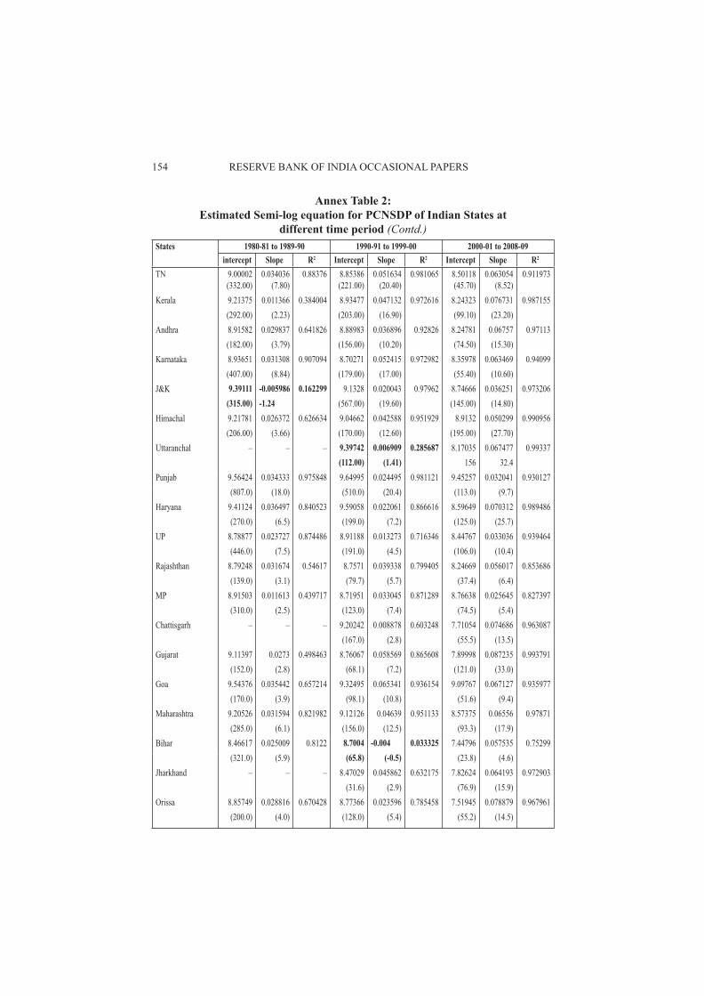
154 RESERVE BANK OF INDIA OCCASIONAL PAPERS
Annex Table 2: Estimated Semi-log equation for PCNSDP of Indian States at
different time period (Contd.)States 1980-81 to 1989-90 1990-91 to 1999-00 2000-01 to 2008-09
intercept Slope R2 Intercept Slope R2 Intercept Slope R2
TN 9.00002 0.034036 0.88376 8.85386 0.051634 0.981065 8.50118 0.063054 0.911973(332.00) (7.80) (221.00) (20.40) (45.70) (8.52)
Kerala 9.21375 0.011366 0.384004 8.93477 0.047132 0.972616 8.24323 0.076731 0.987155(292.00) (2.23) (203.00) (16.90) (99.10) (23.20)
Andhra 8.91582 0.029837 0.641826 8.88983 0.036896 0.92826 8.24781 0.06757 0.97113(182.00) (3.79) (156.00) (10.20) (74.50) (15.30)
Karnataka 8.93651 0.031308 0.907094 8.70271 0.052415 0.972982 8.35978 0.063469 0.94099(407.00) (8.84) (179.00) (17.00) (55.40) (10.60)
J&K 9.39111 -0.005986 0.162299 9.1328 0.020043 0.97962 8.74666 0.036251 0.973206(315.00) -1.24 (567.00) (19.60) (145.00) (14.80)
Himachal 9.21781 0.026372 0.626634 9.04662 0.042588 0.951929 8.9132 0.050299 0.990956(206.00) (3.66) (170.00) (12.60) (195.00) (27.70)
Uttaranchal – – – 9.39742 0.006909 0.285687 8.17035 0.067477 0.99337(112.00) (1.41) 156 32.4
Punjab 9.56424 0.034333 0.975848 9.64995 0.024495 0.981121 9.45257 0.032041 0.930127(807.0) (18.0) (510.0) (20.4) (113.0) (9.7)
Haryana 9.41124 0.036497 0.840523 9.59058 0.022061 0.866616 8.59649 0.070312 0.989486(270.0) (6.5) (199.0) (7.2) (125.0) (25.7)
UP 8.78877 0.023727 0.874486 8.91188 0.013273 0.716346 8.44767 0.033036 0.939464(446.0) (7.5) (191.0) (4.5) (106.0) (10.4)
Rajashthan 8.79248 0.031674 0.54617 8.7571 0.039338 0.799405 8.24669 0.056017 0.853686(139.0) (3.1) (79.7) (5.7) (37.4) (6.4)
MP 8.91503 0.011613 0.439717 8.71951 0.033045 0.871289 8.76638 0.025645 0.827397(310.0) (2.5) (123.0) (7.4) (74.5) (5.4)
Chattisgarh – – – 9.20242 0.008878 0.603248 7.71054 0.074686 0.963087(167.0) (2.8) (55.5) (13.5)
Gujarat 9.11397 0.0273 0.498463 8.76067 0.058569 0.865608 7.89998 0.087235 0.993791(152.0) (2.8) (68.1) (7.2) (121.0) (33.0)
Goa 9.54376 0.035442 0.657214 9.32495 0.065341 0.936154 9.09767 0.067127 0.935977(170.0) (3.9) (98.1) (10.8) (51.6) (9.4)
Maharashtra 9.20526 0.031594 0.821982 9.12126 0.04639 0.951133 8.57375 0.06556 0.97871(285.0) (6.1) (156.0) (12.5) (93.3) (17.9)
Bihar 8.46617 0.025009 0.8122 8.7004 -0.004 0.033325 7.44796 0.057535 0.75299(321.0) (5.9) (65.8) (-0.5) (23.8) (4.6)
Jharkhand – – – 8.47029 0.045862 0.632175 7.82624 0.064193 0.972903(31.6) (2.9) (76.9) (15.9)
Orissa 8.85749 0.028816 0.670428 8.77366 0.023596 0.785458 7.51945 0.078879 0.967961(200.0) (4.0) (128.0) (5.4) (55.2) (14.5)

INCLUSIVE GROWTH AND ITS REGIONAL DIMENSION 155
Annex Table 2: Estimated Semi-log equation for PCNSDP of Indian States at
different time period (Concld.)States 1980-81 to 1989-90 1990-91 to 1999-00 2000-01 to 2008-09
intercept Slope R2 Intercept Slope R2 Intercept Slope R2
West Bengal 8.98146 0.023097 0.894323 8.67193 0.049493 0.991886 8.5843 0.052152 0.982582(516.0) (8.2) (348.0) (31.3) (130.0) (19.9)
Arunachal Pradesh 8.7475 0.046875 0.965959 9.16177 0.020874 0.588061 8.56625 0.050063 0.920527(453.0) (15.1) (94.1) (3.4) (61.3) (9.0)
Assam 9.24938 0.010899 0.49811 9.35591 0.003058 0.480132 8.7036 0.03382 0.988998(385.0) (2.8) (527.0) (2.7) (257.0) (25.1)
Meghalya 9.05597 0.014292 0.706725 8.96752 0.027257 0.728313 8.40909 0.055695 0.98117(448.0) (4.4) (96.7) (4.6) (115.0) (19.1)
Tripura 8.77992 0.020009 0.501878 8.44203 0.052895 0.915865 8.4698 0.056538 0.960433(201.0) (2.8) (94.5) (9.3) (73.5) (12.1)
Manipur 8.99699 0.021184 0.951964 8.96394 0.023028 0.708844 8.56957 0.039074 0.959795(862.0) (12.6) (109.0) (4.4) (113.0) (12.9)
Nagaland 9.18135 0.034124 0.821393 9.45135 0.010186 0.206276 9.4809 0.010627 0.403184(263.0) (6.1) (84.9) (1.4) (68.1) (1.8)
Sikkim – – – 8.96817 0.032978 0.935847 8.2704 0.064281 0.998177(136.0) (8.5) (317.0) (61.9)

156 RESERVE BANK OF INDIA OCCASIONAL PAPERS
Annex Table 3: Poverty Rates Across States (%)
State/UT 1973-74 1977-78 1983-84 1987-88 1993-94 1999-2000
2004-05
Andhra Pradesh 48.9 39.3 28.9 25.9 22.2 15.8 15.8Arunachal Pradesh 51.9 58.3 40.9 36.2 39.4 33.5 17.6Assam 51.2 57.2 40.8 36.2 40.9 36.1 19.7Bihar 61.9 61.6 62.2 52.1 55.0 42.6 41.4Goa 44.3 37.2 18.9 24.5 14.9 14.4 13.8Gujarat 48.2 41.2 32.8 31.5 24.2 14.1 16.8Haryana 35.4 29.6 21.4 16.6 25.1 8.7 14.0Himachal 26.4 32.5 16.4 15.5 28.4 7.6 10.0Jammu 40.8 39.0 24.2 23.8 25.2 3.5 5.4Karnataka 54.5 48.8 38.2 37.5 33.2 20.0 25.0Kerala 58.8 52.2 40.4 31.8 25.4 12.7 15.0Madhya Pradesh 61.8 61.8 49.8 43.1 42.5 37.4 38.3Maharashtra 53.2 55.9 43.4 40.4 36.9 25.0 30.7Manipur 50.0 53.7 37.0 31.4 33.8 28.5 17.3Meghalaya 50.2 55.2 38.8 33.9 37.9 33.9 18.5Mizoram 50.3 54.4 36.0 27.5 25.7 19.5 12.6Nagaland 50.8 56.0 39.3 34.4 37.9 32.7 19.0Orissa 66.2 70.1 65.3 55.6 48.6 47.2 46.4Punjab 28.2 19.3 16.2 13.2 11.8 6.2 8.4Rajasthan 46.1 37.4 34.5 35.2 27.4 15.3 22.1Sikkim 50.9 55.9 39.7 36.1 41.4 36.6 20.1Tamil Nadu 54.9 54.8 51.7 43.4 35.0 21.1 22.5Tripura 51.0 56.9 40.0 35.2 39.0 34.4 18.9Uttar Pradesh 57.1 49.1 47.1 41.5 40.9 31.2 32.8West Bengal 63.4 60.5 54.9 44.7 35.7 27.0 24.7A&N Islands 55.6 55.4 52.1 43.9 34.5 21.0 22.6Chandigarh 28.0 27.3 23.8 14.7 11.4 5.8 7.1D&N Haveli 46.6 37.2 15.7 67.1 50.8 17.1 33.2Delhi 49.6 33.2 26.2 12.4 14.7 8.2 –Daman & Diu – – – – 15.8 4.4 10.5Lakshdweep 59.7 52.8 42.4 35.0 25.0 15.6 16.0Pondicherry 53.8 53.3 50.1 41.5 37.4 21.7 22.4All India 54.9 51.3 44.5 38.9 36.0 26.1 27.5