Luca Sandrini, Department of Economics and Management, University of Padova

INCENTIVES FOR LABOR-

AUGMENTING INNOVATION:

THE ROLE OF WAGE RATE

June 2019 Marco Fanno Working Papers - 232

Incentives for labor-augmenting innovation:

The role of wage rate*

Luca Sandrini�

June 5, 2019

Abstract

This paper analyzes how the incentives to produce and to adopt labor-augmenting

innovation are linked to the wage rate. I design a model of a vertically re-

lated industry, where downstream manufacturers can choose between a standard

low-quality capital input or a superior one produced by an upstream innovator.

High-quality capital input allows adopting �rms to have a higher labor produc-

tivity. I show that there is an inverted-U shaped relationship between the wage

rate and the incentive to invest in innovation based on two opposite forces: a

positive cost-reducing e�ect and a negative output contraction e�ect. Finally,

this paper provides some support for the introduction of a minimum wage, which

is found able to increase both the investments in innovative activities and the

social welfare.

JEL Code: J31, L13, O31

Key Words: labor-augmenting innovation, vertical relation, oligopoly, minimum

wage

*This paper was presented at the Augustin Cournot Doctoral Days 2019, University of Strasbourg,in April 2019. I wish to thank my PhD supervisor Professor Fabio Manenti for his precious help,suggestions and comments during the development and the writing of this work. Also, specialthanks go to my co-supervisor Professor Luciano Greco for his suggestions and availability. I amgrateful to Dr. Levent Eraydin for his comments as discussant of the paper during the ACDD2019.This research has been partially carried out during a visiting period of six months at the Schoolof Business and Social Sciences at Aarhus University. I am grateful to Professor Johannes Jansenfor his help during the early stage of this research. Finally, I wish to thank the participants of theXXXIII Jornadas de Economia Industrial and the XXX SIEP Conference for their useful commentson the earlier versions of this paper.

�Email address: luca.sandrini.3@phd.unipd.it. Dept. of Economics and Management, Universityof Padua (Italy).

1

1 Introduction

The relationship between technological progress and labor market conditions rep-

resents an issue that is increasingly attracting the attention of scholars and policy

makers. Usually, �rms adopt factor-augmenting technologies in order to replace the

more expensive factors of production, making better use of cheaper and relatively

more abundant ones (Dosi [1984], and Acemoglu [2002]). In particular, innovative

technologies often improve the productivity of labor thus allowing adopting �rms to

substitute labor with capital inputs. In this paper, I argue that the degree of such

substitution is in�uenced by the cost of labor as the higher the wage rate, the more

a �rm is willing to adopt such technologies. On the other hand, much more than

in the past, when large and vertically integrated �rms used to develop in-house the

innovations they used in production, these innovative technologies are developed by

upstream innovators who then sell them to downstream adopting �rms. As a conse-

quence, labor market conditions are likely to a�ect also the incentives to develop labor

augmenting innovations via their e�ect on the incentive to adopt such technologies by

downstream adopters. To the best of my knowledge, this paper is the �rst attempt

to analyze the role of labor market conditions, namely the wage level, in shaping the

incentives not only to adopt labor productivity enhancing technologies, but also to

produce such technologies. I do so by following an industrial organization approach

based on a model of a vertically related industrial sector where the innovation is

produced upstream and then sold downstream to manufacturers.

Examples of labor productivity augmenting technologies abound. One may think

to ICTs; developed by large upstream innovators, they allow adopting �rms to sig-

ni�cantly improve the productivity of labor. Another example are robots and cobots

(i.e., collaborative robots). In particular, cobots are industrial robots designed to

collaborate with humans in the production process. Di�erently from traditional in-

dustrial robots, cobots are �exible units that help workers perform their routinized

activities. Due to their �exibility, cobots are increasingly adopted by �rms where

industrial robots have never been adopted before. In particular, one of the most

interesting sector is logistics, where many �rms have introduced cobots in order to

increase the productivity of labor in piece picking tasks.

This is by no means the �rst paper that attempts to clarify how innovation and

vertical relations a�ect the market performance1. However, the novelty of this paper

1Cabral and Vasconcelos [2011], among others, analyze the e�ect of matching contracts on theprovision of strategic input in markets with partial vertical integration. Although this paper does notdeal with the issue of vertical integration, it is built on the authors' assumption of the presence of an

2

is to investigate how incentives to adopt innovation may be at odds with market power

for �rms competing in the market, and how upstream innovators exploit the compe-

tition (that they themselves promote) between manufacturers downstream. Several

studies attempt to show how innovation works, and how it a�ects the production pro-

cess, but the vast majority adopt a macro approach (Acemoglu and Restrepo [2017],

and Aghion et al. [2017], among others). Instead, in this paper I follow an industrial

organization approach in order to further highlight the nexus between innovation and

�rms' strategic interaction and market condition. This paper also represents a �rst

attempt to bridge two usually disconnected literatures: the macroeconomic literature

and the industrial organization one, with the aim of looking at innovation incentives

both from the labor market perspective and from that of �rms. In particular, I adopt

a production function that is directly inspired by the literature on automation (Ace-

moglu and Autor[2011], Acemoglu and Restrepo[2019]), where the quality of capital

input determines the amount of labor that is necessary for the production of the �nal

good2.

I model innovation in a vertically related market, in a way similar to Farrell and

Shapiro [2008], where an upstream �rm produces an innovative/superior technology

and sells it to a series of downstream �rms. However, di�erently from Farrell and

Shapiro [2008] who focus on the e�ects of weak patents protecting the innovation, I

analyze how labor costs a�ect �rms' decision to adopt the innovative technology and,

more in particular, how these costs a�ect the innovator's choice about how much

to invest in innovation. More speci�cally, I show how the wage level of the down-

stream segment of the industry may a�ect positively the amount of investment of the

upstream innovator and the downstream �rms' willingness to adopt the innovation.

This paper also extends the Acemoglu and Pischke's [1999] �ndings on �rms'

incentives to invest in labor-augmenting activities in an imperfect labor market. In

particular, I apply the authors' results to an oligopolistic framework in order to discuss

how the incentives for process innovation are a�ected by competition3. The existence

of a relationship between innovation and the degree of competition has been exten-

sively investigated in literature (Aghion et al. [2005], Vives [2008], among others).

alternative source of the input (and an alternative competitive price), that may lead the downstream�rms to refuse the provision of the input from the incumbent supplier.

2From an industrial organization perspective, increasing in labor productivity is hardly distin-guishable from automation in tasks. In fact, in both cases �rms are ending up with a more capitalintensive production function.

3Moreover, I show that innovation's pro�tability is not the only element that plays a role in af-fecting the incentive to innovate and to adopt innovation. Indeed, the conditions of the labor marketrepresent a direct condition for the innovator to prompt or shrink the investments in innovation.

3

However, this paper explicitly distinguishes the monopolistic advantage to produce

innovation (Schumpeter [1947]) from the competitive incentive to adopt innovation

(Arrow [1962]).

From the policy perspective, this paper suggests that the imposition of a minimum

wage may represent an important policy in order to improve the level of investments

in innovative activities, and to increase the social welfare. Interestingly, I show that

under particular market conditions, industrial performance improves along with the

wage level4. Rather oddly, relatively few papers have addressed the problem of how

an increase in a sector's minimum wage may a�ect private �rms' incentive to inno-

vate5. Finally, this paper suggests that, in order to promote a social e�cient level

of innovation, the policy maker should impose a switch-o� of the old technology. In

fact, this would allow the innovator to entirely extract downstream rent and invest

e�ciently.

The rest of the paper is organized as follows: Section 2 describes the model and

the timing of the game; Section 3 outlines the main results of the analysis, focusing

�rst on the nature of the innovation and the conditions enabling its production and

its adoption, then on the equilibrium outcomes of the game; a welfare analysis and

di�erent extensions to the main model are developed in Section 4 and 5, respectively;

�nally, Section 6 concludes.

2 The model

Assume there is an industry made of an upstream and a downstream segment. The

downstream segment is populated by n identical �rms (manufacturers, henceforth)

which compete in the production and distribution of the �nal good q. In order to

produce, downstream �rms employ labor and capital in �xed proportions, with the

proportions depending on the quality of the capital input. Just to give a relevant

example, the capital input can be seen as a personal computer, or, alternatively, as

an industrial collaborative robot. Technological progress improves the e�ciency of

4The role of the wage on the incentives to innovate has been the subject of a vast literature,particularly focusing on the rent sharing mechanism and the unionization structure (Grout [1984],Calabuig and Gonzalez-Maestre [2003], Haucap and Wey [2004], Manasakis and Petrakis [2009],and Mukherjee and Pennings [2011]); none of these paper, however, analyzes the problem usinga vertically related perspective. Moreover, these papers focus mainly on the e�ects of the degreeof centralization of the wage setting mechanism and not on the strategic interaction among �rms.Instead, this paper analyzes how the upstream innovator and the downstream �rms behave and howthis behavior is in�uenced by the wage level.

5See, Lordan and Neumark [2018], Petrakis and Vlassis [2004], and Kleinknecht et al. [1998]

4

PC/cobots, namely it increases the quality of the capital input, and this allows the

manufacturers to reduce the amount of labor necessary to produce a unit of the �nal

good.

Two types of capital inputs are available to downstream �rms: the current capital

input (the standard, henceforth) and an innovative one. The former is produced

competitively; it is of low quality and it is produced in accordance with the current

state of the art of the technology. The latter is produced by an upstream monopolist

(the supplier, henceforth) who owns a patent protecting the technology it uses to

produce the high quality input. I normalize to zero the quality of the current capital

input, while the high quality input produced by the supplier has quality α > 0.

Formally, the technology adopted to produce the �nal good is:

qi = min{L

1 − αi;K}

where L and K indicate the labor and the capital input, respectively. The parameter

αi = {0;α} represents the type of the capital input chosen by �rm i; a higher quality

increases the productivity of workers and allows the adopting manufacturers to reduce

the original amount of labor required to produce one unit of the �nal good.

The production function of both capital inputs requires one unit of labor for each

unit of capital input produced, K = L. Competition drives the price of the standard

capital input down to its marginal cost of production, that is the minimum wage paid

to upstream workers, w. As the price of the innovative capital input is concerned,

we assume that the supplier follows a two-part tari� scheme made of a per-unit price

and a �xed fee. Following standard theory of optimal non linear pricing, the supplier

sets the per-unit price at its marginal cost of production, that is the minimum wage

w, and then sets the �xed fee F to extract the downstream value it generates.

Downstream �rms observe the prices of the two types of capital inputs and decide

which one to buy. Clearly, the upstream supplier �nds optimal to set the �xed

fee F at the highest possible level, which is the one that makes downstream �rms

indi�erent between the standard or the new capital input. We assume that, in case of

indi�erence, downstream �rms buy the high quality input. Once taken their decision

about which capital to use, downstream �rms hire the desired amount of workers at

the minimum wage w - uniform and common to all the manufacturers regardless of the

technology adopted - and compete. I assume that competition occurs à la Cournot

and that market demand is linear P (Q) = δ −Q, where δ measures the market size,

and Q = ∑ni=1 qi is the total output of the downstream segment, with i = 1,2,3, .., n.

5

As mentioned, the supplier monopolistically produces a high quality capital input.

The actual level of quality is chosen by the supplier, which invests an amount I(α) =

γα2 of resources to produce a capital input of quality α, where γ is a cost parameter6.

Putting all these things together, we can now de�ne �rms' pro�ts functions, start-

ing from downstream �rms. In theory, there are two types of manufacturers: those

who adopt the new high quality capital input, and those who, instead, keep using

the standard technology. Let us indicate with m the number of �rms that adopt the

innovation, with m ≤ n. Firms' pro�t functions are:

Πd,i = qi (δ − qi −Q−i) − qi((2 − αi)w) − F (α), (1)

with F (0) = 0. As we discuss below, the optimal �xed fee set by the upstream in-

novator depends on the quality of the supplied technology, hence we indicate F (α).

The subscript d indicates the downstream segment of the industry.

As discussed above, the upstream supplier charges a two-part tari�, where the per

unit price is set at the cost w. Hence its only source of revenues comes from the �xed

fee paid by the m ≤ n manufacturers which adopt its high quality capital input. The

objective function of the innovator therefore is given by:

Πu =mF − γ α2 (2)

Where the subscript u indicates the upstream segment of the industry.

The timing of the game is as follows. At time 1, the supplier invests in R&D and

decides the optimal level of α. At time 2, the innovator sets the price of the high

quality capital input. At time 3, the manufacturers observe the prices of the two

types of capital input and decide which one to pick. Then, at time 4, manufacturers

hire the necessary amount of labor at price w and compete (Cournot competition).

As I am interested in the Subgame Perfect Nash Equilibrium, the game is solved by

backward induction.

6Through the paper I assume γ >n2 w2

(n+1)2≡ γ̄. This assumption is su�cient for the innovation to

be non drastic.

6

3 Results

3.1 Optimal level of quality of the new technology

Manufacturers choose their output to maximize pro�ts. There are two types of down-

stream manufacturers: those who adopt the new technology (they are m ≤ n), and

those who keep producing with the standard technology (they are m−n). In order to

simplify the problem, we impose symmetry among the �rms in the same subset. So,

the total output can be written as:

Q =mqh + (n −m)qs

where h and h stand for high quality and standard quality, respectively.

From the maximization of expression (1), the optimal output levels for the two

types of �rms are7:

qh =δ −w(2 − α(n −m + 1))

n + 1(3)

qs =δ −w(2 +mα)

n + 1(4)

where qh is the output level of �rms adopting the high quality capital input, and qs

that of �rms adopting the standard one. Using these two expressions the pro�ts of

the two types of manufacturers are:

Πh =(δ −w(2 − α(n −m + 1)))

2

(n + 1)2− F (α) (5)

Πs =(δ −w(2 +mα))

2

(n + 1)2(6)

As mentioned earlier, the innovator can in�uence the manufacturers' choice by

varying the price of the high quality capital input, and in particular the �xed fee

F (α). The higher the rent extracted, the weaker the appeal of the high quality input

and, conversely, the lower the �xed fee the more downstream manufacturers will be

induced to adopt the high quality input. Therefore, the optimal �xed fee set by the

supplier must depend on the chosen quality level, for reasons that are straightforward.

First, if α increases, the investment I(α) increases too, and the innovator must raise

the price in order to recover the initial investment. Second, the higher the quality

7See the appendix for the formal details.

7

of the capital input the smaller the amount of labor that the manufacturers need to

produce the �nal good. Employing less labor makes marginal costs to fall and pro�ts

to rise. This positive e�ect is stronger, the higher the level of quality α produced by

the innovator.

Let us analyze the maximum �xed fee the innovator can set in order to elicit

the adoption of the new technology for m �rms. Building on Bester and Petrakis

(1993), F is such that, for the mth manufacturer it must be indi�erent whether to

keep producing with the standard technology or to adopt the new one. Thus, the mth

manufacturer would adopt the new technology if and only if the following conditions

are satis�ed:

Πhd,m ≥ Πs

d,n−(m−1) and Πsd,n−m > Πh

d,m+1.

Using the de�nition of �rms' pro�ts, these two inequalities boil down to:

F ≤(δ −w(2 − α(n −m + 1)))

2

(n + 1)2−

(δ −w(2 + (m − 1)α))2

(n + 1)2(7a)

F >(δ −w(2 − α(n + 1 − (m + 1))))

2

(n + 1)2−

(δ −w(2 +mα))2

(n + 1)2(7b)

If condition (7a) applies, then none of the m adopters has incentives to deviate

and to produce with the standard technology, as they would not be able to gain any

extra pro�ts on top of what they gain with the new one. Also, when condition (7b)

applies, none of the �rms producing with the standard technology wants to adopt the

new one, as it would guarantee less pro�ts than the standard one. One can see that

condition (7a) is necessary and su�cient for the equilibrium to be stable8. Therefore,

the �xed fee that induces m �rms to adopt the new technology is:

F (α) =αnw (2(δ − 2w) + αw(n − 2(m − 1)))

(n + 1)2(8)

By setting the �xed fee, the upstream �rm decides how many �rms m adopt the

innovation, given a certain quality α. Formally, the optimal number of downstream

�rms maximizes the total revenues of the upstream supplier, TRu = mF (α). The

following corollary states under which conditions all downstream �rms adopt the

innovation:

Corollary 1. When the number of downstream �rms is not too large, the innovator

8See the appendix for the mathematical proof.

8

sets the adoption fee so that all the �rms buy the new technology. Formally, the

optimal number of contracts signed by the innovator is n if:

n <2(δ −w(2 − α))

3w

Proof. See the appendix.

Going backward, we are now in the position to solve for the optimal investment

by the upstream �rm. For the sake of simplicity, we solve the model assuming that

the condition in Corollary 1 holds and m = n. Therefore, the �rst stage innovator's

pro�ts given in expression (2) can be written as:

Πu = nF (α) − γ α2

=αn2w(2(δ − 2w) − α(n − 2)w)

(n + 1)2− γ α2. (9)

The innovators chooses α to maximize this expression. Simple di�erentiation

reveals that the upstream supplier chooses α = α∗, where:

α∗ =n2w(δ − 2w)

γ(n + 1)2 + (n − 2)n2w2.

It is useful to rewrite α∗ as:

α∗ =n(δ − 2w)

n + 1

n(n + 1)w

γ(n + 1)2 + (n − 2)n2w2= f(w) Q̄d(w), (10)

where Q̄d(w) = nq̄d(w) = n(δ − 2w)/(n+ 1) is the total output sold downstream when

all the manufacturers keep producing with the standard technology. I refer to Q̄d

and q̄d as �the benchmark�. From expression (10) the following proposition follows

immediately:

Proposition 1. The optimal level of investment undertaken by the upstream inno-

vator depends on the wage rate; α∗(w) increases with w when δ > δ̄, and decreases

otherwise, where δ̄ = 4γ(n+1)2wγ(n+1)2−(n−2)n2w2 . Moreover, α∗(0) = 0.

Proof. See the appendix.

This proposition represents one of the crucial results of the paper; see Figure 1 for

a visual representation. Formally, it follows from simple di�erentiation of eq. (10):

∂α∗

∂w= f ′w Q̄d + f(w) Q̄′

w.

9

Wage, w0

Optimal quality, α∗

α∗

w̄(δ̄)

Figure 1: the optimal quality, α∗

The e�ect of w on the level of investment undertaken by the innovator can be easily

interpreted by looking at α∗(w) as the interaction of two terms: the cost reducing

e�ect of an increase in w, f ′w, which is always positive, and the output contraction

e�ect Q′w, which is always negative. More precisely, when the wage rate increases,

manufacturers react by substituting labor with high quality capital input. Thus, the

higher the wage level in the downstream sector, the more downstream manufacturers

are induced to adopt the innovative capital input and to reduce their consumption

of labour; this clearly stimulates the innovator to invest in R&D and to increase α.

On the other hand, an increase in the wage rate raises the manufacturers' marginal

costs of production, thus inducing the total output to shrink. This is what I refer to

as the output contraction e�ect. If the total output shrinks, manufacturers employ

fewer workers and the e�ect of the innovative input is smaller. When the market is

large enough, the output contraction e�ect is dominated by the cost reducing e�ect

and the amount of innovation/level of quality o�ered by the innovator increases with

w.

One can see that, when γ < (n − 2)n2w2/(n + 1)2 ≡ ¯̄γ, the positive e�ects always

dominate the negative output contraction e�ect - i.e., the threshold δ̄ is negative. This

implies that when the costs associated with the innovative activity are small enough,

the cost reducing e�ect prompted by an increase in the wage rate is so high that it

always dominates the output contraction e�ect. Although this case is interesting per

se, the relevant scenarios occur when the dominance of one of the two e�ects is not

so obvious. Thus, the rest of the paper focuses on the case where γ > ¯̄γ.

10

Wage, w0

Π∗u(w)

w(δ̃)

Π∗u

Figure 2: the pro�ts of the innovator, Π∗u

3.2 Price of capital input and innovator's pro�ts

Once determined α∗, we can evaluate the equilibrium outcomes. Let us start from the

adoption fee and the upstream innovator's pro�ts. By substituting expression (10) in

expressions (8) and (9), we obtain:

F ∗ =n3w2(δ − 2w)2

(n + 1)2

2γ(n + 1)2 + (n − 2)n2w2

(γ(n + 1)2 + (n − 2)n2w2)2 ,

and

Π∗u = nF

∗ − γ α∗2 =n4w2(δ − 2w)2

(n + 1)2 (γ(n + 1)2 + (n − 2)n2w2).

It is useful to rewrite Π∗u as:

Π∗u =

nw

n + 1

n2w(δ − 2w)

γ(n + 1)2 + (n − 2)n2w2

n(δ − 2w)

n + 1= g(w)α∗(w) Q̄d (11)

From expression (11) it is immediate to obtain the following proposition:

Proposition 2. The innovator's pro�ts depend on the wage rate: Π∗u(w) increases

with w when δ > δ̃ and decreases otherwise, where δ̃ =2w(2γ(n+1)2+(n−2)n2w2)

γ(n+1)2 < δ̄. More-

over, Π∗u(0) = 0.

Proof. See the appendix.

11

Proposition 2 follows from simple di�erentiation of expression (11):

∂Π∗u

∂w= g′w α

∗(w) Q̄d + α′w g(w) Q̄d + Q̄

′w g(w)α∗(w)

The analysis follows the same logic as that used for α∗(w). The e�ect of a wage

rate increase on the innovator pro�ts, in fact, is given by the interaction of di�erent

forces of opposite signs. First, there is a clear positive rent expansion e�ect, g′w. If

the wage rate rises, manufacturers are more willing to adopt the innovation as it not

only increases productivity but it becomes also relatively cheaper. The gains from

the adoption of the innovative input is higher, the higher is the price of the input that

is partially displaced. The rent expansion e�ect is reinforced (or mitigated) by the

e�ect that a wage rate increase has on the quality of the innovation, α∗(w). As α′w >

0(resp. < 0), the rent generated by the innovation in the downstream segment rises

(resp. falls) and so do the innovator's pro�ts. Finally, a negative output contraction

e�ect, Q̄′w, operates as described in the previous paragraph. When the market is large

enough (δ > δ̃), the positive e�ects dominate and the pro�ts of the innovator increase

with w. Figure 2 shows the relationship between supplier's pro�ts and the wage rate.

One can see that an inverted-U relationship applies also to this case. Moreover, when

we compare the two thresholds, we can see that δ̄ > δ̃, for any γ > ¯̄γ.

3.3 Downstream manufacturers

Let us now turn to the downstream segment of the industry. As long as Corollary 1

applies, asymmetric equilibria are not possible: all the manufacturers either choose

the new technology, or they keep producing with the old one. Moreover, one can

see that when the adoption fee set by the innovator satis�es Condition (7a), then all

the manufacturers choose the new technology. Thus, we can rewrite the expressions

(3)-(6) as:

qh = q∗ =δ −w(2 − α∗)

n + 1, (12)

qs = ∅, (13)

Πhd = Π∗

d =(δ −w(2 − α∗))

2

(n + 1)2, (14)

Πsd = ∅. (15)

12

Wage, w0

δn+1

q∗h(w)

w(δ̌)

q̄d

q∗

Figure 3: downstream �rms' optimal output, q∗

By substituting eq. (9) into expressions (12) and (14), we obtain:

q∗ =γ(n + 1)2 + (n − 1)n2w2

γ(n + 1)2 + (n − 2)n2w2

δ − 2w

n + 1= ψ q̄d (16)

Π∗d =

(γ(n + 1)2 − n2w2)2

(γ(n + 1)2 + (n − 2)n2w2)2

(δ − 2w)2

(n + 1)2= ϑ Π̄d, (17)

where ψ > 1, and ϑ < 1, and where, as previously de�ned, q̄d indicates downstream

�rms output when they use the standard technology, and Π̄d = (δ − 2w)2/(n+ 1)2 the

corresponding level of pro�ts. From equation (16), Proposition 3 follows immediately:

Proposition 3. The manufacturers' optimal level of output depends on the wage rate:

q∗(w) increases with w when δ > δ̌ and decreases otherwise, where δ̌ = (n−2)(n−1)n2w3

γ(n+1)2 +

γ(n+1)2+(2n−1)n2w2

n2w . Moreover, q∗(0) = q̄d

Proof. See the appendix.

Corollary 2. The manufacturers are forced into a prisoner dilemma alike situation,

where the adoption of innovation is the only equilibrium, although it is not the e�cient

outcome: Π∗d < Π̄d.

Proof. Proof of Corollary 2 follows immediately from expression (17).

Proposition 3 follows from simple maximization of expression (16) and shows that,

under some conditions, the higher the wage rate faced by manufacturers, the higher

their output level. This counter-intuitive result is essentially driven by the e�ect that

13

a wage increase has on the quality of the innovation. As a matter of fact, when the

market is large enough (δ > δ̌), an increase in the wage rate generates a more than

proportional increase in α∗(w) and, via this e�ect, higher output levels. Interestingly,

an increase in total output implies also an increase in social welfare as it raises not

only the private but also the Consumers surplus. Figure 3 provides a graphical rep-

resentation of the relationship between the wage rate and the per-�rm output level.

Also, Corollary 2 states that the manufacturers are worse o� after the adoption of

innovation. However, adopting the innovation is the only equilibrium as the inno-

vator sets the price F according to conditions (7a) and (7b) in order to exploit the

competition in the downstream segment of the industry.

In order to be able to evaluate the impact of a minimum wage policy, it is impor-

tant to correctly compare the thresholds in propositions (1)- (3). We already know

that δ̄ > δ̃, for any γ > ¯̄γ, and it is easy to show that δ̌ > δ̃ under the same condition.

Instead, if we compare δ̄ and δ̌ we can derive the following conditions:

δ̌ ≥ δ̄ if γ ≥(n − 1)n2w2

n + 1≡ ˇ̄γ, (18a)

δ̌ < δ̄ otherwise. (18b)

with ˇ̄γ > ¯̄γ.

From conditions (18a) and (18b), we derive the size and the ordering of the thresholds

in propositions (1) - (3). In particular, let us assume that condition (18b) holds: in

this case we have that any positive e�ect on the level of quality implies a positive e�ect

on the industry output; in other words, whenever the cost reducing e�ect dominates

the output contraction e�ect (α′w > 0), not only the quality of innovation bene�ts

from an increase in the wage rate, but also the industry output increases. This is due

to the fact that the low level of innovation costs (γ) allows the innovator to be more

e�ective in investing in α∗ in response to an increase in the wage rate, making the

new technology capable of lowering the manufacturers' costs of production regardless

of the increase in the cost of labor.

On the other side, when condition (18a) holds, it means that an increase in the

wage rate following a minimum wage policy does not always imply an increase in the

industry output. In other words, in this case the innovation costs (γ) are relatively

large and they reduce the increase of α∗; thus, the adoption of the new technology

does not always make the manufacturers capable of recovering the negative e�ects of

14

Wage, w0

q∗h(w)

α∗(w)

Π∗u(w)

w(δ̃)w(δ̄)w(δ̌)

α∗

Π∗u

q∗h

(i) (ii) (iii) (iv)

Figure 4: e�ects of an increase in w when γ > ˇ̄γ

an increase in the cost of labor.

Propositions (1) - (3) fully characterize the impact of the wage rate on market

outcomes. For this reason they are important from a policy perspective; their combi-

nation reveals under which conditions a minimum wage policy might be e�ective. As

a matter of fact, a policy maker able to identify the size of the market can anticipate

the e�ects of the introduction of a minimum wage on the quality of the innovation,

on the pro�ts of the innovator, and on social welfare. For example, in the speci�c

case of a su�ciently large cost of the innovation, formally γ > ˇ̄γ, it follows that:

Remark 1. Given the parameters of the model, an increase in the wage rate:

1. increases the optimal level of quality, the pro�ts of the supplier and the social

welfare, in region (i);

2. increases the pro�ts of the supplier and the optimal level of quality, but decreases

the social welfare, in region (ii);

3. increases the pro�ts of the supplier, but decreases the optimal level of quality

and the social welfare, in region (iii);

4. decreases the optimal level of quality, the pro�ts of the supplier and the social

welfare, in region (iv).

15

The proof of this remark is immediate by looking at Figure 4.

4 Welfare analysis

One may wonder whether the level of the innovation undertaken by the upstream

�rm is also e�cient from the social point of view. It is easy to see that this is not

the case. To show this, let us consider the social welfare W , de�ned, as usual, as the

sum of Consumers and Private surplus. Using the above �ndings:

W =1

2

⎛

⎝δ − (δ − n

δ −w(2 − α)

n + 1)⎞

⎠

δ −w(2 − α)

n + 1+ n (

δ −w(2 − α)

n + 1)

2

− γ α2

It is easy to see that this function is concave in α; its maximization reveals that

the socially optimal level of the innovation is:

αw =n(n + 2)w(δ − 2w)

γ(n + 1)2 − n(n + 2)w2. (19)

It is immediate to check that the upstream �rm underinvests with respect to

the socially optimal level: αw > α∗. This result has a clear interpretation if one

thinks to the standard theory of non-linear wholesale pricing; this theory suggests

that by setting a two-part tari� wholesale price, i) an upstream �rm is able to fully

appropriate downstream �rms pro�ts and ii) this pricing scheme maximizes social

welfare. In our setting, the upstream �rm can only partially extract downstream

�rms' pro�ts; as a matter of fact, the presence of the standard technology puts some

competitive pressure on the innovator who, therefore, cannot fully extract the surplus

of downstream �rms. Due to this appropriability problem, the innovator is induced

to underinvest with respect to the social optimum. Paradoxically, to guarantee social

optimality, a policy maker should mandate a switch-o� of the old technology; in this

way, the innovator regains full appropriability of downstream rents and it invests

e�ciently.

Remark 2. A switch-o� of the old technology promotes a social e�cient level of

innovation.

16

5 Extensions

5.1 Linear Pricing

So far, we have assumed that the innovator was charging its technology according to

a two-part tari� scheme. This assumption is natural when observing how innovations

are usually licensed in practice. Nonetheless, one may wonder how the �ndings above

change if this assumption is removed and it is assumes that the innovator sets a linear

price r > w for the high quality capital input. In this section, I follow Kamien and

Tauman [2002] on patent licensing.

The upstream innovator sets the optimal price r solving the following maximiza-

tion problem:

maxr

Πu = n ⋅δ − r −w(1 − α)

n + 1(r −w) − γα2,

s.t. w(1 − α) + r ≤ 2w.

The result is easily derived:

r(α) = (1 + α)w. (20)

Going backward to t=0, we can now �nd the optimal level of innovation. Plugging

equation 20 into innovator's pro�ts, and maximizing it with respect to the optimal

quality, we can write the innovator's investment decision as:

α+ =nw(δ − 2w)

2γ(n + 1)< α∗, (21)

while the upstream innovator gains:

Π+u =

n2w2(δ − 2w)2

4γ(n + 1)2< Π∗

u. (22)

We can see that if the innovator charges a linear price, the equilibrium quality level

is lower than under a two-part tari� scheme. This is due to the fact that the price of

the innovation compensates the reduction in the labor costs following the adoption

of the innovative technology. Therefore, it is not possible for the manufacturer to

expand their output and increase the private surplus, which in turn implies that

the innovator can extract a lower rent from the downstream segment. However, the

results in proposition 1 hold with minor di�erences. In fact, if we rewrite expression

17

(21) as:

α+ = h(w) Q̄d

where, h′w < f ′w. This means that the cost reducing e�ect is lower under linear pricing

scheme than in the scenario where the supplier sets a two-part tari�, while the output

contraction e�ect is the same. Thus, the following proposition applies:

Proposition 4. The optimal level of investment undertaken by the upstream inno-

vator depends on the wage rate: α+(w) increases with w when δ > δ+, and decreases

otherwise, where δ+ = 4w ≤ δ̄. Moreover, α+(0) = 0.

Proof. See the appendix.

Instead, the results in Proposition 3 cannot be replicated with a linear pricing

scheme, as manufacturers do not reduce their costs of production (w(1−α)+ r = 2w)

after the adoption of the innovative technology. Let us write down the output function

of the downstream manufacturers:

q+ =δ − r(α+) −w(1 − α+)

n + 1

q+ =δ −w(1 + α+) −w(1 − α+)

n + 1=δ −w(1 − α+ + 1 + α+)

n + 1

q+ =δ − 2w

n + 1

The optimal output of the manufacturers does not depend on the level of innovation.

Therefore, any positive e�ect of a minimum wage policy on the quality of the inno-

vative technology does not apply to the output level. This is so because, from an

economic perspective, the wage rate policy and the pricing of innovation are strategic

complement and an increase of the former generates a proportional increase of the

latter. Thus, although a higher wage rate makes the innovation more convenient for

the manufacturers, the rise in the innovation's price prevents them from obtaining

any cost reduction. Consequently, we can state that, under linear pricing scheme, the

innovation has no e�ect on the Consumers surplus (the price of the �nal good does

not change), while it increases the Private surplus by transforming part of the wage

bill into pro�ts for the upstream innovator.

5.2 Total wage bill and pro�ts

In this section, I analyze the impact of the innovation on the remuneration of input

factors, namely the total wage bill and pro�ts. We already know that innovation's

18

main impact is to lower the requirement of labor input in the production of the �nal

good. Moreover, the manufacturers that adopt the innovative technology reduce the

necessary amount of labor input, in order to produce one unit of �nal good, from

1 to (1 − α). However, from eq. (16), we know that when all the �rms adopt the

innovative technology the total output increases and so does the demand for labor.

Also, since one unit of capital input is required to produce one unit of �nal good

and the capital input is produced by labor, increasing the output means also to

increase the demand for the labor necessary to produce more units of capital input.

Thus, it is not immediate to understand the net e�ect of the innovation on the total

wage bill. If the productivity increasing property of the innovation dominates the

expansion of output, we say that introducing the innovative technology would harm

labor remuneration. Vice versa, when the output expansion e�ect dominates on the

productivity e�ect, the displaced workers are hired back to expand the production.

In formula we have that:

LW = n((1 − α)δ − (2 − α)w

n + 1w +

δ − (2 − α)w

n + 1w)

LW = nδ − (2 − α)w

n + 1(2 − α)w

Let us focus on the e�ect of innovation on the wage bill we see that LW ′α. We

have that:∂LW

∂α= −

nw(δ − 2(2 − α)w)

n + 1

which is positive for δ < 2w(2 − α). If we look at the two extremes of this condition,

namely α = 0 and α = 1, we can see that in the latter case, the condition cannot

be satis�ed, as with δ < 2w there is no market at all. Instead, for small value of

the quality of innovation, the condition is more easily satis�ed. We can interpret

this result as we already mention. Small innovations have relatively small e�ects in

increasing the productivity of labor, while they do increase the production of the �nal

good. By combining together a small displacement e�ect and the output expansion,

we obtain a positive net e�ect on the total wage bill. Instead, if the displacement

of workers is large due to a high increase in productivity of labor (α is high), the

expansion of the output is insu�cient to hire the displaced workers back and the net

e�ect on the wage bill is negative. Interestingly, this result contradicts the one in

Acemoglu and Restrepo [2019], according to whom small innovations - or innovations

19

that generate small increase in automation - are the most harmful to labor demand.

Remark 3. When the quality of the innovation - i.e., the increase in labor productivity

that the innovative technology generates - is high, then its introduction engenders a

negative net e�ect on the total wage bill. This is so because when the innovation is

of high-quality, the displacement of workers due to increase in labor productivity is

higher than the increase in labor demand due to the output expansion.

Now, let us de�ne total industrial pro�ts as the sum of the net pro�ts of all the ac-

tive �rms, namely the upstream innovator and the downstream manufacturers. Since

innovator's revenues simply consist of a transfer of private surplus from downstream

manufacturers, we can write:

Πtot = nΠd − γ α2

Πtot = n(δ −w(2 − α))2

(n + 1)2− γ α2

Simple di�erentiation reveals ∂Πtot

∂α > 0 if δ >α(γ(n+1)2−nw2)+2nw2

nw . Interestingly, this

threshold moves in a similar direction as for total wage bill. More in particular, with

little innovations (α → 0) the condition gets close to δ > 2w, which is always satis�ed

as this is the condition for a market to exist. Instead, as the innovation increases, the

condition becomes stricter δ > γ(n+1)2nw +w although not prohibitive.

Remark 4. Small innovations tend to have bene�cial impacts on both total wage bill

and pro�ts. Large innovations are more likely to have a negative impact on the total

wage bill than on the total pro�ts.

5.3 Unionization and incentives to adopt the innovation

Finally, a consideration on unionization and its e�ect on incentives to adopt innova-

tion. Hitherto, we assumed the wage rate was given and did not vary as the quality

of the technology implied in the production process increased. This is not always the

case, however. From a theoretical perspective, higher productivity of labor should

automatically lead towards higher wage rates, and this is true for all kinds of la-

bor (Aghion et al. [2017]). From an empirical perspective this mechanism is more

puzzling, as automation may have both positive and negative e�ects on wages (Ace-

moglu and Restrepo [2019, 2017]). Anyway, evidence says that sectors with better

technological equipment are those that face higher increase in wage rate (Pianta and

Tancioni [2008]).

20

Moreover, at least in developed countries, variations in the wage rate are deter-

mined in accordance with a bargaining process between �rms and workers. Although

many level of bargaining are generally involved, many European countries have strong

unions and very centralized bargaining processes.

In this section, I explicitly address the problem of how the incentives to adopt

innovation vary if it directly a�ects the price of labor at the sector level. Before pro-

ceeding, let us just make some slight modi�cations to the model set up, in particular

regarding the wage rate. Let us assume that the industry has a very strong union

with full bargaining power. Therefore, the wage rate chosen by the union applies to

all the �rms in the downstream segment. Let us also assume that there are just two

manufacturers and that the wage rates in the upstream and downstream segments

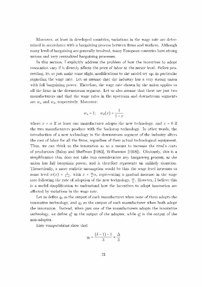
are wu and wd, respectively. Moreover:

wu = 1; wd(x) =1

1 − x

where x = α if at least one manufacturer adopts the new technology, and x = 0 if

the two manufacturers produce with the backstop technology. In other words, the

introduction of a new technology in the downstream segment of the industry alters

the cost of labor for all the �rms, regardless of their actual technological equipment.

Thus, we can think to the innovation as to a means to increase the rival's costs

of production (Salop and She�man [1983], Williamson [1968]). Obviously, this is a

simpli�cation that does not take into consideration any bargaining process, as the

union has full bargainin power, and it therefore represents an unlikely situation.

Theoretically, a more realistic assumption would be that the wage level increases to

some level w(x) = 11−x , with x = m

n α, representing a gradual increase in the wage

rate following the rate of adoption of the new technology, mn . However, I believe this

is a useful simpli�cation to understand how the incentives to adopt innovation are

a�ected by variations in the wage rate.

Let us de�ne q0 as the output of each manufacturer when none of them adopts the

innovative technology, and q2 as the output of each manufacturer when both adopt

the innovation. Instead, when just one of the manufacturers adopts the innovative

technology, we de�ne qh1 as the output of the adopter, while qs1 is the output of the

non-adopter.

Easy computations show that

q0 =(δ − 1) − 1

3≡

∆

3

21

q2 =(δ − 1) − 1−α

1−α3

≡∆

3

qh1 =∆

3+

α

3(1 − α)>

∆

3

qs1 =∆

3−

2α

3(1 − α)<

∆

3

where ∆ = δ − 2.

The �rst thing it is worth remarking is that the innovation does not bring any

advantage to the manufacturers when they behave symmetrically (q0 = q2). This is

due to the fact that, even if the innovation increases the productivity of labor, the

union is able to raise the wage rate up to the new productivity level. The net e�ect

is, therefore, nil.

Instead, asymmetric equilibria display some interesting features. Keeping in mind

that, by assumption, the introduction of the new technology by at least one �rm

makes the union raise the wage rate to the new potential productivity (the labor

productivity that the �rms would obtain by adopting the technology), we can see

that innovation is now guaranteeing some advantages to the adopting manufacturer.

Moreover, the adopter is now able to expand the output and gain some market share,

while the non-adopting rival is forced to reduce its output. Clearly, since the man-

ufacturer that keeps producing with the backstop technology cannot increase labor

productivity, the increase in the wage rate operated by the union increases its costs

of production. Consequently, the adopter, which does not gain anything in terms of

costs of productions - as the new higher wage zeros out the boost in labor productivity

- can nonetheless expand the output and gain more pro�ts.

This results highlight the fact that innovation still provides the manufacturers with

a unilateral incentive to adopt the innovation. The innovator, who sets the price of

the innovation in order to maximize its total revenues, can exploit this strategic e�ect

of the innovation and charges the manufacturers a price which satis�es conditions (7a)

and (7b), as reported in section 3.

Brie�y, since the pro�ts of the manufacturers in each scenario are:

Π0 = (∆

3)

2

; Π2 = (∆

3)

2

− F

Πh1 = (

∆

3+

α

3(1 − α))

2

− F

22

Πs1 = (

∆

3−

2α

3(1 − α))

2

we can easily derive the maximum adoption fee F as the one that satis�es Π2 = Πs1:

F =4α

9(1 − α)(∆ −

α

1 − α)

This is the price that allows the innovator to sell the innovation to both �rms, exploit-

ing their unilateral incentive to adopt the innovation to harm their respective rival.

We do not go backward to previous stages as the analytical computations become

intricate. However, we can see from the analyses above that incentives to adopt the

innovation exist also when the wage rate reacts to the introduction of a labor aug-

menting innovation. This is possible because of the strategic role of the innovation

to increase the rival's costs and, more in particular, to increase the cost of that input

the rival mostly relies on. From the considerations above, we can state:

Remark 5. When the innovation can be used strategically to increase the rivals' costs

of production, it also generates incentives for technology adoption in the downstream

segment. Moreover, strong centralized unions have ambiguous e�ects on incentives

to adoption. On the one hand, a central union decreases the cost reducing e�ect of

innovation, lowering the appeal of the innovative technology from the manufacturers'

perspective; on the other hand, however, by raising the wage rate after the adoption

of the innovation by all the manufacturers, it generates a positive strategic e�ect for

the adopters.

6 Discussions and conclusions

Using a model of a vertically related industry, this paper shows the relationship

that links the incentives to produce (and to adopt) a labor augmenting innovation

and the wage rate. This paper represents a novel attempt to understand the possible

implication of a minimum wage policy on the investments in R&D and on the industry

performance. The model suggests that, depending on the size of the market, a policy

aimed at increasing the minimum wage paid to workers can have a bene�cial impact

on both the incentive to produce and adopt the innovation and on the Consumer

Surplus. This model is particularly interesting when we consider technologies such

as ICT's cloud services and/or industrial cobots, where the new capital inputs are

able to improve the workers' performance and to increase the labor productivity of

the �rms. Interestingly, this model is able to explain why the producers of this kind

23

of innovations increase their market power, while at the same time they seem to

reduce the market power of the adopters. The results are con�rmed when the labor

market is dominated by a central union which controls the wage rate. In this case,

the innovation is not used as a tool to increase the e�ciency of the �rms, but as a

tool to increase the rivals' costs of production.

Finally, the model suggests that small innovations are those that are more likely

to have a better impact on the distribution of surplus among the factors of produc-

tion. This result is at odds with the �ndings in automation literature, where usually

larger automation processes are associated to higher returns for the labor share. Un-

fortunately, this model is unable to explain clearly how to identify the market size

thresholds properly, and consequently how a policy maker can evaluate the actual

e�ect of an employee-friendly policy in his/her particular situation. This aspect,as

well as the empirical testing of the predictions stated in the model, are left aside as

subjects of other researches.

References

[1] Acemoglu, D. (2002), Directed technical change, The Review of Economic Stud-

ies, 69 (4), pp. 781-809.

[2] Acemoglu, D., and Autor (2011), Skills, tasks and technologies: Implications for

employment and earnings, in Handbook of Labor Economics, 4, pp. 1043�1171.

[3] Acemoglu, D., and Pischke, J., S. (1999), The structure of wages and investment

in general training, The Journal of Political Economy, 107 (3), pp. 539-572.

[4] Acemoglu, D., and Restrepo, P. (2019), Automation and new rasks: how tech-

nology displaces and reinstates labor, Journal of Economic Perspectives, Vol 33

(2), pp. 3-30.

[5] Acemoglu, D., and Restrepo, P. (2017), Robots and jobs: Evidence from us labor

markets. NBER Working Paper No. 23285.

[6] Aghion, P., Bergeaud, A., Blundell, R., and Gri�th, R. (2017), Innovation, �rms,

and wage inequality.

24

[7] Aghion, P., Bloom, N., Blundell, R., Gri�th, R., and Howitt, P. (2005) Com-

petition and innovation: an inverted-U relationship, The Quarterly Journal of

Economics, Vol 120 (2), pp. 701-728.

[8] Arrow, K. (1962), `Economic welfare and the allocation of resources for inven-

tion,' in R. R. Nelson (ed.), The Rate and Direction of Inventive Activity. Prince-

ton University Press: Princeton, NJ, pp. 609�625.

[9] Autor, D. H., and Dorn, D. (2013), The growth of low-skill service jobs and the

polarization of the US labor market, The American Economic Review, 103 (5),

pp. 1553-1597.

[10] Autor, D. H., Dorn, D., Katz, L. F., Patterson, C., and Van Reenen, J. (2017),

The fall of the labor share and the rise of superstar �rms, NBER Working Paper

No. 23396.

[11] Bester, H., and Petrakis, E., (1993), The incentives for cost reduction in a dif-

ferentiated industry, International Journal of Industrial Organization, 11, pp.

519-534.

[12] Cabral, L., and Vasconcelos, H. (2011), Vertical integration and the right of �rst

refusal, Economics Letters, 113, pp. 50-53.

[13] Calabuig, V., and Gonzalez-Maestre, M. (2002), Union structure and incentives

for innovation, European Journal of Political Economy, 18, pp. 177-192.

[14] De Loecker, J., and Eeckhout, J. (2017), The rise of market power and the

macroeconomic implications, NBER Working Paper No. 23687.

[15] Dosi, G. (1984), Technical change and industrial transformation. The theory and

an application to the semiconductor industry. MacMillan, London.

[16] Farrell, J., and Shapiro, C. (2008), How strong are weak patents?, American

Economic Review, 98 (4), pp. 1347 -1369.

[17] Grout, P. A., (1984), Investments and wages in the absence of binding contracts:

A Nash bargaining approach, Econometrica, 52, pp. 449-460.

[18] Haucap J., and Wey, C. (2004), Unionisation structure and innovation incentives,

The Economic Journal, 114 (494), Conference Papers, pp. C149-C165.

25

[19] Kamien, M. I., and Tauman, Y. (2002), Patent Licensing: The Inside Story, The

Manchester School, 70, pp. 7�15.

[20] Kleinknecht, A., van Shaik, F.N., and Zhou, H. (2014), Is �exible labour good

for innovation? Evidence from �rm-level data, Cambridge Journal of Economics,

38, pp. 1207-1219.

[21] Manasakis, C., and Petrakis, E. (2009), Union structure and �rms' incentives

for cooperative R&D investments, Canadian Journal of Economics, 42 (2), pp.

665-693.

[22] Mukherjee, A., and Pennings, E. (2011), Unionization structure, licensing and

innovation, International Journal of Industrial Organization, 29 (2), pp. 232-241.

[23] Lordan, G., and Neumark, D. (2018), People versus machines: The impact of

minimum wages on automatable jobs, Labor Economics, 52, pp. 40-53.

[24] Pianta, M., and Tancioni, M. (2008), Innovations, wages and pro�ts, Journal of

Post Keynesian Economics, 31 (1), pp. 101-123.

[25] Petrakis, E., and Vlassis, M., (2004), Endogenous wage bargaining institutions

in oligopolistic sectors, Economic Theory, 24, pp. 55-73.

[26] Salop, S .C., and Sche�man, Y., (1983), Raising rivals' costs, American Economic

Review, 73 (2), pp. 267-271.

[27] Schumpeter, J.A. (1947), Capitalism, Socialism and Democracy, Harper &

Brothers Publishers, New York.

[28] Vives, X. (2008), Innovation and competitive pressure, Journal of Industrial

Economics, 56 (3), pp. 419-469.

[29] Williamson, O. E.,(1994), Wage rates as a barrier to entry: The Pennington case

in perspective, The Quarterly Journal of Economics, 82 (1), pp. 85-116.

26

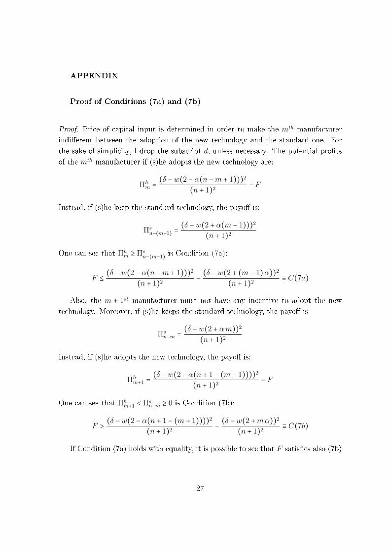
APPENDIX

Proof of Conditions (7a) and (7b)

Proof. Price of capital input is determined in order to make the mth manufacturer

indi�erent between the adoption of the new technology and the standard one. For

the sake of simplicity, I drop the subscript d, unless necessary. The potential pro�ts

of the mth manufacturer if (s)he adopts the new technology are:

Πhm =

(δ −w(2 − α(n −m + 1)))2

(n + 1)2− F

Instead, if (s)he keep the standard technology, the payo� is:

Πsn−(m−1) =

(δ −w(2 + α(m − 1)))2

(n + 1)2

One can see that Πhm ≥ Πs

n−(m−1) is Condition (7a):

F ≤(δ −w(2 − α(n −m + 1)))2

(n + 1)2−

(δ −w(2 + (m − 1)α))2

(n + 1)2≡ C(7a)

Also, the m + 1st manufacturer must not have any incentive to adopt the new

technology. Moreover, if (s)he keeps the standard technology, the payo� is

Πsn−m =

(δ −w(2 + αm))2

(n + 1)2

Instead, if (s)he adopts the new technology, the payo� is:

Πhm+1 =

(δ −w(2 − α(n + 1 − (m − 1))))2

(n + 1)2− F

One can see that Πhm+1 < Πs

n−m ≥ 0 is Condition (7b):

F >(δ −w(2 − α(n + 1 − (m + 1))))2

(n + 1)2−

(δ −w(2 +mα))2

(n + 1)2≡ C(7b)

If Condition (7a) holds with equality, it is possible to see that F satis�es also (7b)

27

with strict inequality:

C(7a) −C(7b) =2nα2w2

(n + 1)2> 0

The opposite is not true. Therefore, Condition (7a) is necessary and su�cient for the

equilibrium in the downstream subgame to be stable

Proof of Corollary 1

Proof. At time 2, the innovator sets the price in order to maximize the total revenues

mF , given the costs of innovations that are considered as sunk. Since the price of

the innovation is decreasing in m, the innovator faces a trade o� between quantity

and magnitude.

maxm

Πu =mF (m,α) − I(α)

m∗ =2(δ − 2w) +w(2α + n)

4w

Therefore, the optimal number of contracts from the innovator perspective is m =

min{m∗, n}. One can see that:

n <m∗ if n <2(δ −w(2 − α))

3w

Proof of Proposition 1

Proof. Optimal quality is derived from simple di�erentiation of eq.(9)

∂Πu

∂α=

2n2w(δ − 2w)

(n + 1)2+

2α(n − 2)n2w2

(n + 1)2− 2γ α

Equalizing marginal revenues and marginal costs, we obtain

α∗ =n2w(δ − 2w)

γ(n + 1)2 + (n − 2)n2w2

One can see that α∗ ∈ [0,1) if γ > n2w2

(n+1)2 ≡ γ̄.

28

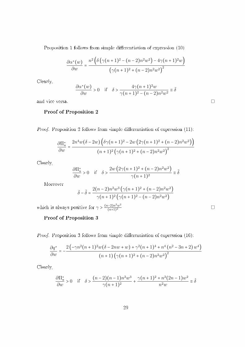
Proposition 1 follows from simple di�erentiation of expression (10)

∂α∗(w)

∂w=n2 (δ (γ(n + 1)2 − (n − 2)n2w2) − 4γ(n + 1)2w)

(γ(n + 1)2 + (n − 2)n2w2)2

Clearly,∂α∗(w)

∂w> 0 if δ >

4γ(n + 1)2w

γ(n + 1)2 − (n − 2)n2w2≡ δ̄

and vice versa.

Proof of Proposition 2

Proof. Proposition 2 follows from simple di�erentiation of expression (11):

∂Π∗u

∂w=

2n4w(δ − 2w) (δγ(n + 1)2 − 2w (2γ(n + 1)2 + (n − 2)n2w2))

(n + 1)2 (γ(n + 1)2 + (n − 2)n2w2)2

Clearly,

∂Π∗u

∂w> 0 if δ >

2w (2γ(n + 1)2 + (n − 2)n2w2)

γ(n + 1)2≡ δ̃

Moreover

δ̄ − δ̃ =2(n − 2)n2w3 (γ(n + 1)2 + (n − 2)n2w2)

γ(n + 1)2 (γ(n + 1)2 − (n − 2)n2w2)

which is always positive for γ > (n−2)n2w2

(n+1)2

Proof of Proposition 3

Proof. Proposition 3 follows from simple di�erentiation of expression (16):

∂q∗

∂w= −

2 (−γn2(n + 1)2w(δ − 2nw +w) + γ2(n + 1)4 + n4 (n2 − 3n + 2)w4)

(n + 1) (γ(n + 1)2 + (n − 2)n2w2)2

Clearly,

∂Π∗u

∂w> 0 if δ >

(n − 2)(n − 1)n2w3

γ(n + 1)2+γ(n + 1)2 + n2(2n − 1)w2

n2w≡ δ̌

29

Moreover

δ̌ − δ̄ =(γ(n + 1)2 + (n − 2)n2w2)

2(γ(n + 1)2 − (n − 1)n2w2)

γn2(n + 1)2w (γ(n + 1)2 − (n − 2)n2w2)

which is positive for γ > (n−1)n2w2

(n+1)2

Proof of Proposition 4

Proof. Proposition 4 follows from simple di�erentiation of eq. (20):

∂α+

∂w=nδ − 4nw

2γ(n + 1)= 0

⇒ δ+ = 4w

One can see that δ+ ≤ δ̄ if n ≥ 2.

30