Embed Size (px)
Citation preview
Incentives and Strategic Choices In The Secretary Problem
by
Nguyen Le Truong
A dissertation submitted in partial satisfaction of the
requirements for the degree of
Doctor of Philosophy
in
Engineering - Industrial Engineering and Operations Research
in the
Graduate Division
of the
University of California, Berkeley
Committee in charge:
Professor Ilan Adler, ChairProfessor Shachar Kariv
Professor Zuo-Jun Max Shen
Fall 2013
Incentives and Strategic Choices In The Secretary Problem
Copyright 2013by
Nguyen Le Truong
1
Abstract
Incentives and Strategic Choices In The Secretary Problem
by
Nguyen Le Truong
Doctor of Philosophy in Engineering - Industrial Engineering and Operations Research
University of California, Berkeley
Professor Ilan Adler, Chair
Optimal policies for various secretary problems have an undesirable trait: they wouldinterview applicants for the position, but those earlier ones are guaranteed to not get selected.Therefore, early applicants have incentive to not come in for their scheduled interviews, andas a direct consequence, the employer’s intention to learn from the population becomesuseless. Prior works have been done that tried to mitigate this issue, where the employersacrifices her overall probability of selecting the best applicant by assigning equal selectionprobability to all interview slots. Among our results, we show such approaches can be costlyfor an employer with objectives different from the classical one. Furthermore, we generalizethe classical setting to allow applicants to make independent choices with regard to theirtime of availability. This new game-theoretic approach solves the interviewing-without-hiringproblem that arose earlier, and surprisingly, improves the employer’s probability of selectingthe best applicant from one obtained in the classical setting.

i
To Mom, Dad, and Be Ti.
ii
Contents
Contents ii
1 Introduction 11.1 A Mathematical Puzzle . . . . . . . . . . . . . . . . . . . . . . . . . . . . . . 11.2 Solution To Puzzle . . . . . . . . . . . . . . . . . . . . . . . . . . . . . . . . 11.3 The Online Decision-Making Framework And Other Applications . . . . . . 21.4 What’s Next? . . . . . . . . . . . . . . . . . . . . . . . . . . . . . . . . . . . 3
2 Linear Programming And The Secretary Problem 52.1 Background . . . . . . . . . . . . . . . . . . . . . . . . . . . . . . . . . . . . 52.2 The Rank-Based Secretary Problem . . . . . . . . . . . . . . . . . . . . . . . 52.3 The Secretary Problem With Backward Solicitation . . . . . . . . . . . . . . 13
3 Participant Incentives and Consequences 163.1 Motivation . . . . . . . . . . . . . . . . . . . . . . . . . . . . . . . . . . . . . 163.2 An Incentive Compatible Hiring Mechanism Can Be Costly! . . . . . . . . . 173.3 Always-Hire Is Near-Optimal In The Asymptotic . . . . . . . . . . . . . . . 213.4 Incentive Compatibility In Generalized Utility-Based Problems . . . . . . . . 233.5 Online Auction Incentive Compatibility . . . . . . . . . . . . . . . . . . . . . 253.6 Implementation Of Incentive Compatible Hiring Mechanisms . . . . . . . . . 263.7 A Concluding Note On Incentive Compatibility . . . . . . . . . . . . . . . . 27
4 How To Win Jobs And Influence Employers 284.1 Introduction . . . . . . . . . . . . . . . . . . . . . . . . . . . . . . . . . . . . 284.2 An Extensive Secretary Game With Imperfect Information . . . . . . . . . . 294.3 A Strategic Secretary Game: Binding Contracts And Equilibria . . . . . . . 334.4 Concluding Notes On Game-Theoretic Approach . . . . . . . . . . . . . . . . 52
5 Concluding Notes 53
Bibliography 54
iii
Acknowledgments
Words alone are not enough to convey how thankful I am for the following people in my life.This dissertation, in one way or another, was shaped by their generosity, patience, love, andfriendship.
My advisor, Ilan Adler, for allowing me to follow my interests and explore on my own.His advices have served as my trustworthy compass, and his insights my terrain map fornavigating this jungle of academia in the last 6 years.
My committee members, Shachar Kariv and Max Shen, for teaching me fundamentalideas in game theory and optimization, both central to this work. Their courses are alsoamong the few that I thoroughly enjoyed while being a student here at Berkeley. Thank youfor being great teachers!
My office mates and Berkeley friends, Gemma Berenguer, Dan Bu, Huaning Cai, SheaChen, Yifen Chen, Kelly Choi, Shiman Ding, Qiaochu He, Tuan Hoang, Phoebe Lai, StewartLiu, Cheng Lu, Amber Richter, Gah-yi Vahn, K.C. Yang, Peng Yi, and Yan Zhang forlistening to my rants, holding midnight conversations on random subjects, hiking knownexplored wilderness, running in the rain, and countless other experiences that best not bebrought up here. I had fun with you all, and I hope you did with me, too!
My sister, for being a steady cheerleader throughout.
And my parents, for everything that they have done, and would have done, for me.
Thank you all! I love you!
Applause Here.
1
Chapter 1
Introduction
1.1 A Mathematical Puzzle
We begin by first describing what is known as the secretary problem. It first appeared asa puzzle in Martin Gardner [6]’s Scientific American column in 1960, and had been studiedextensively in the mathematical research community ever since. Its description below canbe found in [5]:
• There is one secretarial position available.
• The number n of applicants is known.
• The applicants are interviewed sequentially in random order, each orderbeing equally likely.
• It is assumed that you can rank all the applicants from best to worst withoutties. The decision to accept or reject an applicant must be based only onthe relative ranks of those applicants interviewed so far.
• An applicant once rejected cannot later be recalled.
• You are very particular and will be satisfied with nothing but the very best.(That is, your payoff is 1 if you choose the best of the n applicants and 0otherwise.)
What should you do?
1.2 Solution To Puzzle
We present here a solution proposed by Gilbert and Mosteller [7]. Suppose we are inter-viewing the ith applicant. We should choose this ith applicant now if the probability thathe is best overall exceeds the same probability obtain by the best strategy available bycontinuing on. It is clear that, at each state, we need only consider the best applicant sofar, as any other cannot be the best overall.
CHAPTER 1. INTRODUCTION 2
1. Let f(i) = Pr[select best overall with ith applicant | ith applicant is best so far]. Ob-serve that f(i) = i
n, and hence, is increasing in i.
2. Let g(i + 1) = Pr[select best overall with best strategy from (i + 1)st applicant on].Observe that g(i) is decreasing in i, as we can withhold from choosing in an earlierperiod and employ the best strategy in a later period, guaranteeing a result equally asgood.
With f(i) an increasing function in i, g(i) a decreasing in i, and we choose an applicantwhenever f(i) > g(i + 1), it follows that the optimal strategy has the form bypass the first(s− 1) applicants, and choose the best one thereafter. Here, s is the smallest value such thatf(s) > g(s+ 1).
Let us now focus only on these threshold-type strategies. The probability that we select
the best overall applicant given that we bypassed the first (s− 1) is s−1n
n∑k=s
1k−1 . To see this,
simply observe that in order to select the best overall, this best applicant must appear in aslot s ≤ k ≤ n, and the best of the first (k − 1) applicants must come in the first (s − 1)slots. This event occurs with probability s−1
k−1 ·1n, and summing over the range for k yields
the desired result.The above discussion leads us to the following theorem.
Theorem 1. In the secretary problem, the optimal strategy is to skip over the first (s − 1)applicants, and choose the best one thereafter. Here, s is the minimum value such that
s
n≥ s
n
n∑k=s+1
1
k − 1⇐⇒ 1 ≥
n∑k=s+1
1
k − 1
When n becomes sufficiently large, the optimal threshold is approximately ne, and the
probability for selecting the best overall applicant is about 1e.
where the last two claims in the theorem can be derived using integral calculus.
1.3 The Online Decision-Making Framework And
Other Applications
In reality, an employer oftentimes does not have to make a hiring decision immediatelyafter an interview. As such, one may cast doubt on the general framework of the secretaryproblem as being unrealistic. We concur with this assessment, and will delve deeper intothe issue later in this dissertation. In the mean time, we also make the observation thatapplicants generally do not give the employer unlimited time to make her decision either,and the classical setting of the secretary problem provides a structured, albeit extreme, wayto approach this problem. It is a nice starting point to begin our analysis.
CHAPTER 1. INTRODUCTION 3
We also note that other real world applications are highly relevant to the secretaryproblem, and present two below. Both belong to the e-commerce sector of the businessworld, and have been studied extensively in the literature. We will restrict ourselves to thehiring setting throughout this dissertation, but one should be aware of potential applicationsof the secretary problem to other places.
eBay is best known in the United States as an auction house where everything imaginableon Earth is being put up for sale daily. One of the key features for this online site is the BestOffer option, where arriving customers have an opportunity to offer a specific amount ofmoney in return for the listed item. Once an offer is received, the seller can choose to acceptit and end the listing, or reject it and continue with the process. Inherent to this problemis the sequential nature of customers’ arrivals, which lends its similarity to assumptions inthe secretary problem. One objective that the seller may have on mind is to maximize theprobability of selecting the highest paying customer, a goal shared by the employer in ourclassical secretary setting. Since customers generally allow the seller sometime to make herdecision, our game-theoretic framework (to be presented in Chapter 4) fits nicely into thisgeneral setting.
The secretary problem has also been used in other papers to model online auctions invarious settings. We mention here the setup for an online auction problem studied in [1].Consider a seller who wishes to auction off a single item to n bidders. Each bidder i has anarrival time ai ∈ [0, T ] and a valuation vi, both of which are private information. The numberof bidders n, and the time horizon T , are common knowledge to everyone. The bidder mayarrive at any time ti ≥ ai, and places a bid bi for the item, which can be different from hisvaluation vi. The mechanism then gets to decide whether to allocate the good to this bidder,and if so, the price this bidder will be charged with. It can be assumed that the bidder’sutility function takes the form vi−pi, where pi is the amount he has to pay. By placing certainassumptions on the set of arrival times a1, a2, . . . , an and valuations v1, v2, . . . , vn, theauthors proceed to design and optimize secretary-based auction mechanisms that are truthfulwith respect to both valuation and arrival at the assigned time. The maximization objectivecan be used for efficiency (probability that the mechanism allocates the good to the highestbidder) or revenue (the expected price charged).
1.4 What’s Next?
The general outline for this dissertation is as follows. In Chapter 2, we will presentlinear programs that can be used to solve two different variants of the secretary problem,and show how to obtain such linear programs using two different approaches: from firstprinciples, and from tools readily available in Markov Decision Processes. Variables in theselinear programs allow us to interpret decisions probabilistically, which are fundamental inintroducing incentives to participants of a sequential decision process.
Incentive compatibility is taken from works by Buchbinder et al. [2], and extended toanother well-known variant of the secretary problem in Chapter 3. From this rank-based
CHAPTER 1. INTRODUCTION 4
variant, we obtain conclusions which contrast those found by [2] for the classical setting. Onesuch result, in particular, shows a jump from constant objective value to Θ(log(n)) whenincentive compatible constraints are added. Another shows the same Θ(log(n)) objectivevalue even when incentive compatibility constraints are relaxed further.
In Chapter 4, we present new game-theoretic models for the classic variant of the secretaryproblem, one being an extensive game with imperfect information, and the other a strategic,simultaneous-move game. In the extensive game, we present the dominant strategy for allapplicants, and show an improvement in the employer’s objective value when everyone playsthis strategy. In the strategic game, among results that we will show is the existence of apure-strategy equilibrium for all cases of n 6= 4. Our new game-theoretic models also addressconcerns for incentive compatibility brought forth in [2].
Chapter 5 wraps up our dissertation.
5
Chapter 2
Linear Programming And TheSecretary Problem
2.1 Background
Buchbinder et al. [2] introduced a linear programming representation for several variantsof the secretary problem (henceforth will be referred to as BJS-approach). In their formu-lations, decision variables are probabilistic, and each can be interpreted as the probability afeasible hiring mechanism will select someone satisfying certain conditions. This chapter isbuilt on their works, where we show how to obtain such linear programs for two importantvariants of the secretary problem. One is fundamental for our analysis in Chapter 3, theother plays an important role in the game-theoretic approach in Chapter 4. Furthermore,we will obtain these representations using two different techniques. One approach uses firstprinciples as demonstrated by [2], whereas another uses tools readily available in the theoriesof linear programming and Markov Decision Processes. We believe our insight will be helpfulin cases where it is intuitively hard to come up with decision variables as in [2], due to thefact that our proposed process is mechanical in nature.
2.2 The Rank-Based Secretary Problem
An employer with the classic objective of hiring the best overall applicant is being pickyin an extreme way. She is never satisfied with anyone but the best, and may come awayfrom the hiring process empty-handed. This may be okay in certain hypothetical situations,but is not necessary in many others.
In the rank-based secretary problem, there are n applicants who apply for one availablejob. If we are allowed to observe them all, we would be able to rank them individually, frombest (rank 1) to worst (rank n). Suppose we assign these applicants to interview slots ina random order, and when the ith applicant is interviewed, we can only observe his rankrelative to those who came in before he did. We must make our hiring decision online: either
CHAPTER 2. LINEAR PROGRAMMING AND THE SECRETARY PROBLEM 6
accept him and end the job search, or reject him and continue with the job search. Our goalin this rank-based setting is to find a hiring strategy which minimizes the expected rank ofthe hiree.
Implicit in the statement of the problem is that not hiring anyone would yield a rank of∞ or n+ ε, where ε > 0 is any positive constant. In other words, hiring no one is worse thanhiring the worst applicant. All together, this objective function leads to a neat, easy-to-show(to be done in chapter 3) property in the optimal hiring policy: that it will always selectsomeone. In this dissertation, we choose to assign an objective value of n + 1 in the eventno one is selected. Choosing n + 1 over others, say ∞, will have implications in incentivecompatible settings to be explored in a later chapter.
Lindley [8] was the first to consider this version of the secretary problem. He was ableto derive a recurrence equation characterizing the optimal threshold policy, which is of theform:
while interviewing for the rth applicant, stop and accept if her apparent rank s ≤ s∗(r),continue if s > s∗(r).
The recurrence equation that needs to be solved to get s∗(r) is fairly complex, and it wasChow et. al. [3] who successfully showed the optimal stopping policy chooses an applicant
with expected rank∞∏j=1
(j+2j
)1/(j+1)
= 3.8695 as n→∞.
In the rank-based secretary problem, we seek to minimize the expected rank of theselected applicant. Observe that this objective is equivalent to maximizing the expected utilityof the selected applicant, where the utility for hiring an ith-rank applicant is (n + 1 − i).Let r∗n denote the optimal expected rank of the hiree when there are n applicants, and u∗nthe optimal expected utility of the hiree when there are n applicants. It is evident that theoptimal expected rank r∗n = n+ 1− u∗n. We choose to work with this alternative problem ofmaximizing the expected utility from now on.
LP Formulation For The Utility-Based Secretary Problem
Our first objective is to derive the linear programming formulation for the incentive com-patible utility-based secretary problem. We will give two different approaches to this result.The first uses known results in the theory of Markov Decision Process and linear program-ming, and is shown below. From the recurrence for this optimal stopping problem, we willconstruct an equivalent linear program (D′). We then make an appropriate substitution ofvariables to obtain a new linear program (D). Taking the dual of the linear program (D)will yield the desired LP (P ) below. We also note that (P ) is the linear program obtaineddirectly by using the approach as shown in [2]. This second, alternative approach will beexpounded in a later section.
From our approach, stop-continue binary decisions in the recursion are transformed intoprobabilistic decision variables. Although the nature of the secretary problems dictates a 0-1
CHAPTER 2. LINEAR PROGRAMMING AND THE SECRETARY PROBLEM 7
solution, the newer probabilistic variables come in handy when we consider adding incentivecompatible constraints, whose optimal solutions will no longer be binary. We will delay thisdiscussion until the next chapter.
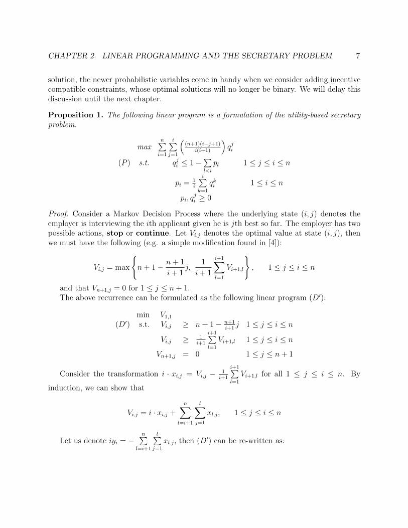
Proposition 1. The following linear program is a formulation of the utility-based secretaryproblem.
maxn∑i=1
i∑j=1
((n+1)(i−j+1)
i(i+1)
)qji
(P ) s.t. qji ≤ 1−∑l<i
pl 1 ≤ j ≤ i ≤ n
pi = 1i
i∑k=1
qki 1 ≤ i ≤ n
pi, qji ≥ 0
Proof. Consider a Markov Decision Process where the underlying state (i, j) denotes theemployer is interviewing the ith applicant given he is jth best so far. The employer has twopossible actions, stop or continue. Let Vi,j denotes the optimal value at state (i, j), thenwe must have the following (e.g. a simple modification found in [4]):
Vi,j = max
n+ 1− n+ 1
i+ 1j,
1
i+ 1
i+1∑l=1
Vi+1,l
, 1 ≤ j ≤ i ≤ n
and that Vn+1,j = 0 for 1 ≤ j ≤ n+ 1.The above recurrence can be formulated as the following linear program (D′):
min V1,1(D′) s.t. Vi,j ≥ n+ 1− n+1
i+1j 1 ≤ j ≤ i ≤ n
Vi,j ≥ 1i+1
i+1∑l=1
Vi+1,l 1 ≤ j ≤ i ≤ n
Vn+1,j = 0 1 ≤ j ≤ n+ 1
Consider the transformation i · xi,j = Vi,j − 1i+1
i+1∑l=1
Vi+1,l for all 1 ≤ j ≤ i ≤ n. By
induction, we can show that
Vi,j = i · xi,j +n∑
l=i+1
l∑j=1
xl,j, 1 ≤ j ≤ i ≤ n
Let us denote iyi = −n∑
l=i+1
l∑j=1
xl,j, then (D′) can be re-written as:
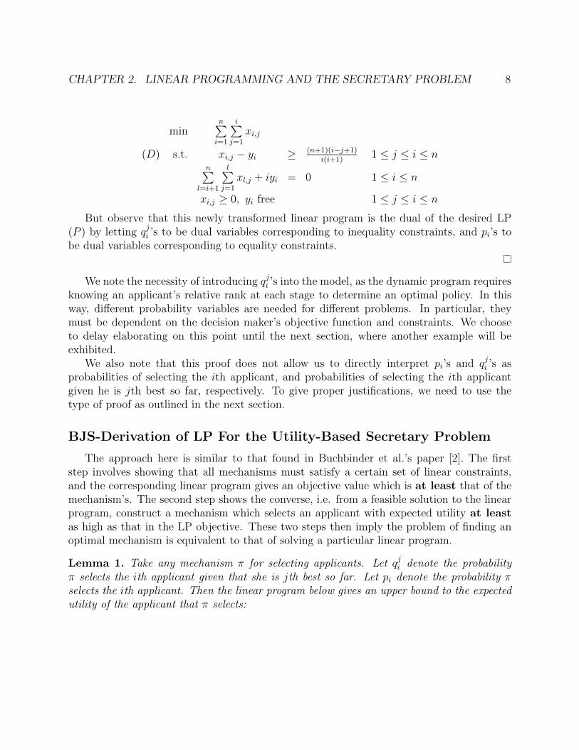
CHAPTER 2. LINEAR PROGRAMMING AND THE SECRETARY PROBLEM 8
minn∑i=1
i∑j=1
xi,j
(D) s.t. xi,j − yi ≥ (n+1)(i−j+1)i(i+1)
1 ≤ j ≤ i ≤ nn∑
l=i+1
l∑j=1
xl,j + iyi = 0 1 ≤ i ≤ n
xi,j ≥ 0, yi free 1 ≤ j ≤ i ≤ n
But observe that this newly transformed linear program is the dual of the desired LP(P ) by letting qji ’s to be dual variables corresponding to inequality constraints, and pi’s tobe dual variables corresponding to equality constraints.
We note the necessity of introducing qji ’s into the model, as the dynamic program requiresknowing an applicant’s relative rank at each stage to determine an optimal policy. In thisway, different probability variables are needed for different problems. In particular, theymust be dependent on the decision maker’s objective function and constraints. We chooseto delay elaborating on this point until the next section, where another example will beexhibited.
We also note that this proof does not allow us to directly interpret pi’s and qji ’s asprobabilities of selecting the ith applicant, and probabilities of selecting the ith applicantgiven he is jth best so far, respectively. To give proper justifications, we need to use thetype of proof as outlined in the next section.
BJS-Derivation of LP For the Utility-Based Secretary Problem
The approach here is similar to that found in Buchbinder et al.’s paper [2]. The firststep involves showing that all mechanisms must satisfy a certain set of linear constraints,and the corresponding linear program gives an objective value which is at least that of themechanism’s. The second step shows the converse, i.e. from a feasible solution to the linearprogram, construct a mechanism which selects an applicant with expected utility at leastas high as that in the LP objective. These two steps then imply the problem of finding anoptimal mechanism is equivalent to that of solving a particular linear program.
Lemma 1. Take any mechanism π for selecting applicants. Let qji denote the probabilityπ selects the ith applicant given that she is jth best so far. Let pi denote the probability πselects the ith applicant. Then the linear program below gives an upper bound to the expectedutility of the applicant that π selects:
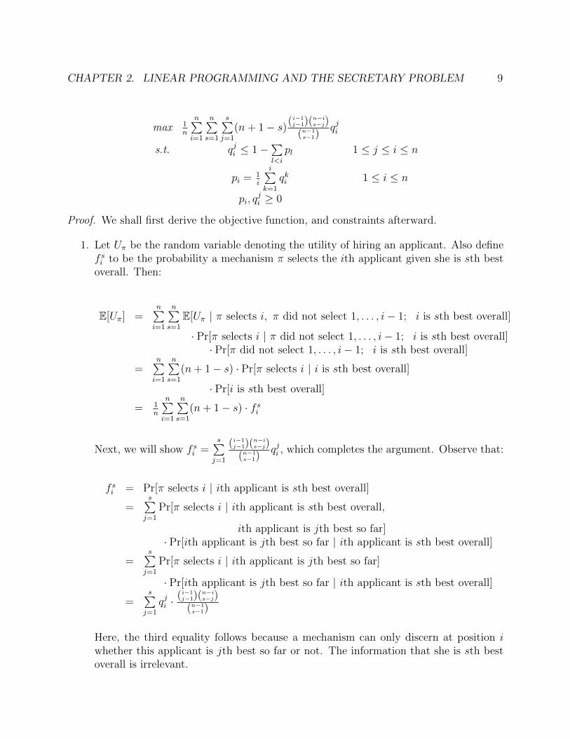
CHAPTER 2. LINEAR PROGRAMMING AND THE SECRETARY PROBLEM 9
max 1n
n∑i=1
n∑s=1
s∑j=1
(n+ 1− s)(i−1j−1)(
n−is−j)
(n−1s−1)
qji
s.t. qji ≤ 1−∑l<i
pl 1 ≤ j ≤ i ≤ n
pi = 1i
i∑k=1
qki 1 ≤ i ≤ n
pi, qji ≥ 0
Proof. We shall first derive the objective function, and constraints afterward.
1. Let Uπ be the random variable denoting the utility of hiring an applicant. Also definef si to be the probability a mechanism π selects the ith applicant given she is sth bestoverall. Then:
E[Uπ] =n∑i=1
n∑s=1
E[Uπ | π selects i, π did not select 1, . . . , i− 1; i is sth best overall]
· Pr[π selects i | π did not select 1, . . . , i− 1; i is sth best overall]· Pr[π did not select 1, . . . , i− 1; i is sth best overall]
=n∑i=1
n∑s=1
(n+ 1− s) · Pr[π selects i | i is sth best overall]
· Pr[i is sth best overall]
= 1n
n∑i=1
n∑s=1
(n+ 1− s) · f si
Next, we will show f si =s∑j=1
(i−1j−1)(
n−is−j)
(n−1s−1)
qji , which completes the argument. Observe that:
f si = Pr[π selects i | ith applicant is sth best overall]
=s∑j=1
Pr[π selects i | ith applicant is sth best overall,
ith applicant is jth best so far]· Pr[ith applicant is jth best so far | ith applicant is sth best overall]
=s∑j=1
Pr[π selects i | ith applicant is jth best so far]
· Pr[ith applicant is jth best so far | ith applicant is sth best overall]
=s∑j=1
qji ·(i−1j−1)(
n−is−j)
(n−1s−1)
Here, the third equality follows because a mechanism can only discern at position iwhether this applicant is jth best so far or not. The information that she is sth bestoverall is irrelevant.
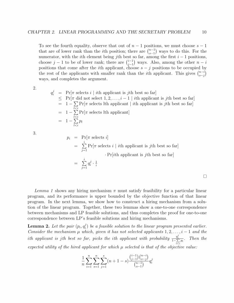
CHAPTER 2. LINEAR PROGRAMMING AND THE SECRETARY PROBLEM 10
To see the fourth equality, observe that out of n − 1 positions, we must choose s − 1that are of lower rank than the ith position; there are
(n−1s−1
)ways to do this. For the
numerator, with the ith element being jth best so far, among the first i− 1 positions,choose j − 1 to be of lower rank; there are
(i−1j−1
)ways. Also, among the other n − i
positions that come after the ith applicant, choose s − j positions to be occupied bythe rest of the applicants with smaller rank than the ith applicant. This gives
(n−is−j
)ways, and completes the argument.
2.qji = Pr[π selects i | ith applicant is jth best so far]≤ Pr[π did not select 1, 2, . . . , i− 1 | ith applicant is jth best so far]= 1−
∑l<i
Pr[π selects lth applicant | ith applicant is jth best so far]
= 1−∑l<i
Pr[π selects lth applicant]
= 1−∑l<i
pl
3.pi = Pr[π selects i]
=i∑
j=1
Pr[π selects i | ith applicant is jth best so far]
· Pr[ith applicant is jth best so far]
=i∑
j=1
qji · 1i
Lemma 1 shows any hiring mechanism π must satisfy feasibility for a particular linearprogram, and its performance is upper bounded by the objective function of that linearprogram. In the next lemma, we show how to construct a hiring mechanism from a solu-tion of the linear program. Together, these two lemmas show a one-to-one correspondencebetween mechanisms and LP feasible solutions, and thus completes the proof for one-to-onecorrespondence between LP’s feasible solutions and hiring mechanisms.
Lemma 2. Let the pair (pi, qji ) be a feasible solution to the linear program presented earlier.
Consider the mechanism µ which, given it has not selected applicants 1, 2, . . . , i− 1 and the
ith applicant is jth best so far, picks the ith applicant with probabilityqji
1−∑l<i
pl. Then the
expected utility of the hired applicant for which µ selected is that of the objective value:
1
n
n∑i=1
n∑s=1
s∑j=1
(n+ 1− s)(i−1j−1
)(n−is−j
)(n−1s−1
) qji
CHAPTER 2. LINEAR PROGRAMMING AND THE SECRETARY PROBLEM 11
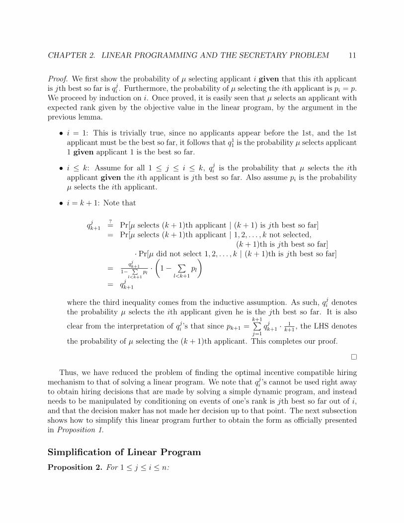
Proof. We first show the probability of µ selecting applicant i given that this ith applicantis jth best so far is qji . Furthermore, the probability of µ selecting the ith applicant is pi = p.We proceed by induction on i. Once proved, it is easily seen that µ selects an applicant withexpected rank given by the objective value in the linear program, by the argument in theprevious lemma.
• i = 1: This is trivially true, since no applicants appear before the 1st, and the 1stapplicant must be the best so far, it follows that q11 is the probability µ selects applicant1 given applicant 1 is the best so far.
• i ≤ k: Assume for all 1 ≤ j ≤ i ≤ k, qji is the probability that µ selects the ithapplicant given the ith applicant is jth best so far. Also assume pi is the probabilityµ selects the ith applicant.
• i = k + 1: Note that
qjk+1
?= Pr[µ selects (k + 1)th applicant | (k + 1) is jth best so far]= Pr[µ selects (k + 1)th applicant | 1, 2, . . . , k not selected,
(k + 1)th is jth best so far]· Pr[µ did not select 1, 2, . . . , k | (k + 1)th is jth best so far]
=qjk+1
1−∑
l<k+1
pl·(
1−∑
l<k+1
pl
)= qjk+1
where the third inequality comes from the inductive assumption. As such, qji denotesthe probability µ selects the ith applicant given he is the jth best so far. It is also
clear from the interpretation of qji ’s that since pk+1 =k+1∑j=1
qjk+1 · 1k+1
, the LHS denotes
the probability of µ selecting the (k + 1)th applicant. This completes our proof.
Thus, we have reduced the problem of finding the optimal incentive compatible hiringmechanism to that of solving a linear program. We note that qji ’s cannot be used right awayto obtain hiring decisions that are made by solving a simple dynamic program, and insteadneeds to be manipulated by conditioning on events of one’s rank is jth best so far out of i,and that the decision maker has not made her decision up to that point. The next subsectionshows how to simplify this linear program further to obtain the form as officially presentedin Proposition 1.
Simplification of Linear Program
Proposition 2. For 1 ≤ j ≤ i ≤ n:
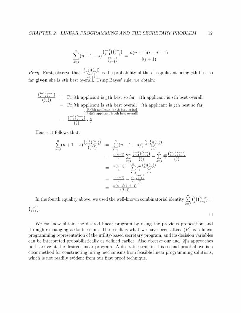
CHAPTER 2. LINEAR PROGRAMMING AND THE SECRETARY PROBLEM 12
n∑s=j
(n+ 1− s)(i−1j−1
)(n−is−j
)(n−1s−1
) =n(n+ 1)(i− j + 1)
i(i+ 1)
Proof. First, observe that(i−1j−1)(
n−is−j)
(n−1s−1)
is the probability of the ith applicant being jth best so
far given she is sth best overall. Using Bayes’ rule, we obtain:
(i−1j−1)(
n−is−j)
(n−1s−1)
= Pr[ith applicant is jth best so far | ith applicant is sth best overall]
= Pr[ith applicant is sth best overall | ith applicant is jth best so far]
· Pr[ith applicant is jth best so far]Pr[ith applicant is sth best overall]
=(s−1j−1)(
n−si−j)
(ni)
· ni
Hence, it follows that:
n∑s=j
(n+ 1− s)(i−1j−1)(
n−is−j)
(n−1s−1)
=n∑s=j
(n+ 1− s)ni
(s−1j−1)(
n−si−j)
(ni)
= n(n+1)i
n∑s=j
(s−1j−1)(
n−si−j)
(ni)
−n∑s=j
sni
(s−1j−1)(
n−si−j)
(ni)
= n(n+1)i−
n∑s=j
jni
(sj)(
n−si−j)
(ni)
= n(n+1)i− jn
i
(n+1i+1)(ni)
= n(n+1)(i−j+1)i(i+1)
In the fourth equality above, we used the well-known combinatorial identityn∑s=j
(sj
)(n−si−j
)=(
n+1i+1
).
We can now obtain the desired linear program by using the previous proposition andthrough exchanging a double sum. The result is what we have been after: (P ) is a linearprogramming representation of the utility-based secretary program, and its decision variablescan be interpreted probabilistically as defined earlier. Also observe our and [2]’s approachesboth arrive at the desired linear program. A desirable trait in this second proof above is aclear method for constructing hiring mechanisms from feasible linear programming solutions,which is not readily evident from our first proof technique.
CHAPTER 2. LINEAR PROGRAMMING AND THE SECRETARY PROBLEM 13
2.3 The Secretary Problem With Backward
Solicitation
It should be observed that the method presented earlier can be employed to derive BJS-style linear programs for other secretary problems. The main task in the process is findingan appropriate transformation of variables, which varies from problem to problem. In thosecases when employing a BJS approach proves difficult, the technique above can still be usedto gain insight to the problem at hand. In this section, we will illustrate the technique for aversion of the secretary problem which allows backward solicitation. This variant is centralto our later works in modeling a game-theoretic approach to the secretary problem.
Consider the classical secretary objective of maximizing the probability for choosing thebest overall applicant. We assume throughout this section that the employer has the optionto recall any previous applicant, and each will accept the employer’s offer with probabilityα(s, i). Here, s is the current round of interview, and i is the round when the employer firstinterviewed the relatively best applicant. As an example, suppose the employer is currentlyinterviewing the 5th applicant, and the applicant in the 3rd round is the best so far, thens = 5, and i = 3. If the employer decides to offer the job to the 3rd applicant, he willaccept with probability α(5, 3). If the applicant does not accept, the employer must moveon to interview the next one. Here, we do allow for multiple offers to the same applicantin different rounds (as oppose to [12]). That is, if an applicant rejects an offer this round,the employer may still offer that same applicant in the next round, albeit the probability ofacceptance may be different (depending on the structure of α(·, ·)).
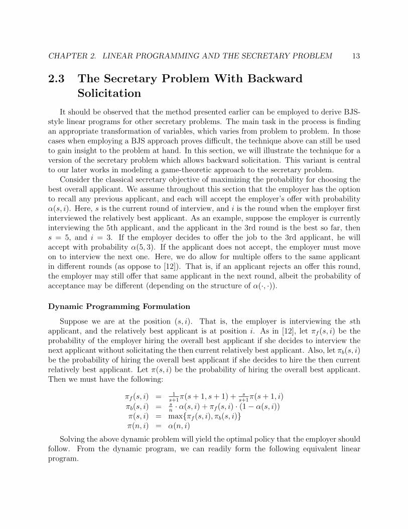
Dynamic Programming Formulation
Suppose we are at the position (s, i). That is, the employer is interviewing the sthapplicant, and the relatively best applicant is at position i. As in [12], let πf (s, i) be theprobability of the employer hiring the overall best applicant if she decides to interview thenext applicant without solicitating the then current relatively best applicant. Also, let πb(s, i)be the probability of hiring the overall best applicant if she decides to hire the then currentrelatively best applicant. Let π(s, i) be the probability of hiring the overall best applicant.Then we must have the following:
πf (s, i) = 1s+1
π(s+ 1, s+ 1) + ss+1
π(s+ 1, i)
πb(s, i) = sn· α(s, i) + πf (s, i) · (1− α(s, i))
π(s, i) = maxπf (s, i), πb(s, i)π(n, i) = α(n, i)
Solving the above dynamic problem will yield the optimal policy that the employer shouldfollow. From the dynamic program, we can readily form the following equivalent linearprogram.
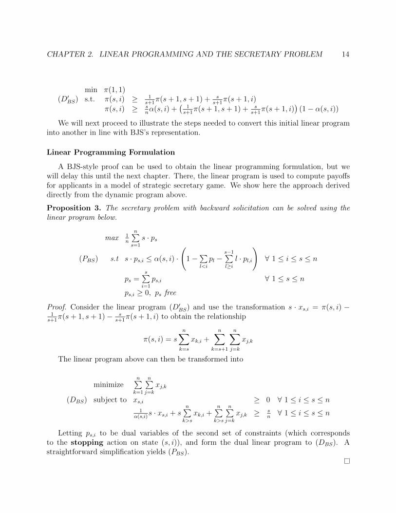
CHAPTER 2. LINEAR PROGRAMMING AND THE SECRETARY PROBLEM 14
min π(1, 1)(D′BS) s.t. π(s, i) ≥ 1
s+1π(s+ 1, s+ 1) + s
s+1π(s+ 1, i)
π(s, i) ≥ snα(s, i) +
(1s+1
π(s+ 1, s+ 1) + ss+1
π(s+ 1, i))
(1− α(s, i))
We will next proceed to illustrate the steps needed to convert this initial linear programinto another in line with BJS’s representation.
Linear Programming Formulation
A BJS-style proof can be used to obtain the linear programming formulation, but wewill delay this until the next chapter. There, the linear program is used to compute payoffsfor applicants in a model of strategic secretary game. We show here the approach deriveddirectly from the dynamic program above.
Proposition 3. The secretary problem with backward solicitation can be solved using thelinear program below.
max 1n
n∑s=1
s · ps
(PBS) s.t s · ps,i ≤ α(s, i) ·
(1−
∑l<i
pl −s−1∑l≥i
l · pl,i
)∀ 1 ≤ i ≤ s ≤ n
ps =s∑i=1
ps,i ∀ 1 ≤ s ≤ n
ps,i ≥ 0, ps free
Proof. Consider the linear program (D′BS) and use the transformation s · xs,i = π(s, i) −1s+1
π(s+ 1, s+ 1)− ss+1
π(s+ 1, i) to obtain the relationship
π(s, i) = s
n∑k=s
xk,i +n∑
k=s+1
n∑j=k
xj,k
The linear program above can then be transformed into
minimizen∑k=1
n∑j=k
xj,k
(DBS) subject to xs,i ≥ 0 ∀ 1 ≤ i ≤ s ≤ n
1α(s,i)
s · xs,i + sn∑k>s
xk,i +n∑k>s
n∑j=k
xj,k ≥ sn∀ 1 ≤ i ≤ s ≤ n
Letting ps,i to be dual variables of the second set of constraints (which correspondsto the stopping action on state (s, i)), and form the dual linear program to (DBS). Astraightforward simplification yields (PBS).
CHAPTER 2. LINEAR PROGRAMMING AND THE SECRETARY PROBLEM 15
General Strategy For Formulations
In general, if we have two possible actions to take, continue or stop, we should firstderive a linear program directly from the set of dynamic programming constraints, then forma BJS-style linear program through the use of a variable transformation for the continueconstraints. This would make the right hand side of these constraints to be 0, and thusguarantee non-negativity for the transformed variables. As such, when we form the duallinear program, only variables corresponding to the stop action would remain in place.These are the p’s and q’s in BJS’s and our works. Having derived necessary tools for ourlater analysis, we next consider incentive compatibility in the secretary problem.
16
Chapter 3
Participant Incentives andConsequences
3.1 Motivation
An inherent problem with the secretary problem’s optimal threshold policy is that itcompletely ignores applicants’ motives. Imagine yourself spending an entire day interviewing,only to find out later that you are not selected for the position. Worse still, this has nothingto do with your qualifications, but rather is due to the employer’s hiring scheme. If you areone of those applicants in earlier slots, you are a part of the learning phase and are beingused as guinea pigs in this selection process. Would you participate in an interview processknowing that you will not have any chance of getting selected? It is reasonable to assumethat this is not something anyone would want, and as such, these earlier applicants havestrong incentive to not show up to their scheduled interview slots in the first place. Thus,this is disaster from the employer’s point of view, as she now may not be able to observeand learn from early applicants as the optimal policy was designed to do.
Similar arguments could also be used for those e-commerce applications that we intro-duced at the beginning of this dissertation. Assuming the number of potential bidders areknown, someone who has recently arrived at an online auction listing may not put down anoffer or bid, as the seller will only use those early offers to gauge later potential bids. Thesetting is the same as before, where the seller’s potential for choosing the best offer hinges onhaving these early applicants showing up in their intended time slots. Although we analyzethe problem in a hiring framework throughout this chapter, it should be noted that similarlogic can be applied to other settings.
When slot i has a higher probability of getting selected than slot j, an applicant is saidto prefer slot i over slot j. We follow Buchbinder, Jain, and Singh [2] (henceforth willbe referred to as BJS) and say a hiring mechanism is incentive compatible (IC) when eachapplicant does not prefer other interviewing slots over his own. Thus two important questionsarise: first, does there exist an IC hiring mechanism? And second, if existence is guaranteed,
CHAPTER 3. PARTICIPANT INCENTIVES AND CONSEQUENCES 17
what is the optimal IC hiring mechanism? Obviously, selecting applicants randomly withequal probability constitutes an IC hiring mechanism, and hence the first question has anaffirmative answer. The key question then, is how much better than random selection canan employer do?
BJS considered incentives in this setting of the secretary problem. They gave an answerto the second question using a linear programming approach. There, they find that anoptimal IC hiring mechanism selects the best applicant with probability 1 − 1√
2≈ 0.29 as
n → ∞ (where the symbol ≈ denotes an approximation of the true value), as comparedto the more well known number 1
e≈ 0.368 (also in the limit n → ∞). Moreover, observe
that random selection hires the best applicant with probability 1n→ 0. As such, their
IC hiring mechanism does relatively well against the traditional optimal threshold hiringmechanism, and is a significant improvement over the trivial random selection mechanism.Let pπi denoted the unconditional probability a hiring mechanism π selects the applicantin the ith slot. BJS’s approach consists of formulating the secretary problem as a linearprogram, and adding constraints pπi = pπj for all i 6= j, which stipulates the mechanism mustselect all slots with the same probability.
In this chapter, we will show how to obtain linear programs derived in [2] as duals of someappropriately transformed linear program for a Markov Decision Process. Furthermore, wewill explore other versions of the secretary problem in the same manner as [2], and show manyconclusions which are vastly different from what BJS obtained in the traditional setting.One such result is that IC hiring mechanisms can have optimal value an order of magnitudedifferent from the non-IC case. For example, it will be shown that by introducing IC to therank-based problem, the employer will increase her expected rank from 3.8695, a constant,to one in the order of Θ(log(n)), which goes to infinity as n→∞.
3.2 An Incentive Compatible Hiring Mechanism Can
Be Costly!
We say an incentive compatible hiring mechanism (for a minimization problem) is costly
if its resulting optimal value z∗IC(n) has the property that limn→∞z∗(n)z∗IC(n)
= 0, where z∗(n)
is the optimal value for the traditional, non-incentive compatible case. Equivalently, fora maximization problem, we say the incentive compatible hiring mechanism is costly if
limn→∞z∗IC(n)
z∗(n)= 0. Observe that the classical secretary problem has been shown to be not
costly in [2]. This section shows that the rank-based secretary problem behaves differently,and that it is costly when one attempts to make it incentive compatible.
Per our discussion from the last chapter, the IC rank-based secretary problem can beposed as the following linear program:
CHAPTER 3. PARTICIPANT INCENTIVES AND CONSEQUENCES 18
maxn∑i=1
i∑j=1
(n+1)(i−j+1)i(i+1)
qji
(PIC) s.t. qji ≤ 1−∑l<i
pl 1 ≤ j ≤ i ≤ n
pi = 1i
i∑k=1
qki 1 ≤ i ≤ n
pi = p
p, qji ≥ 0
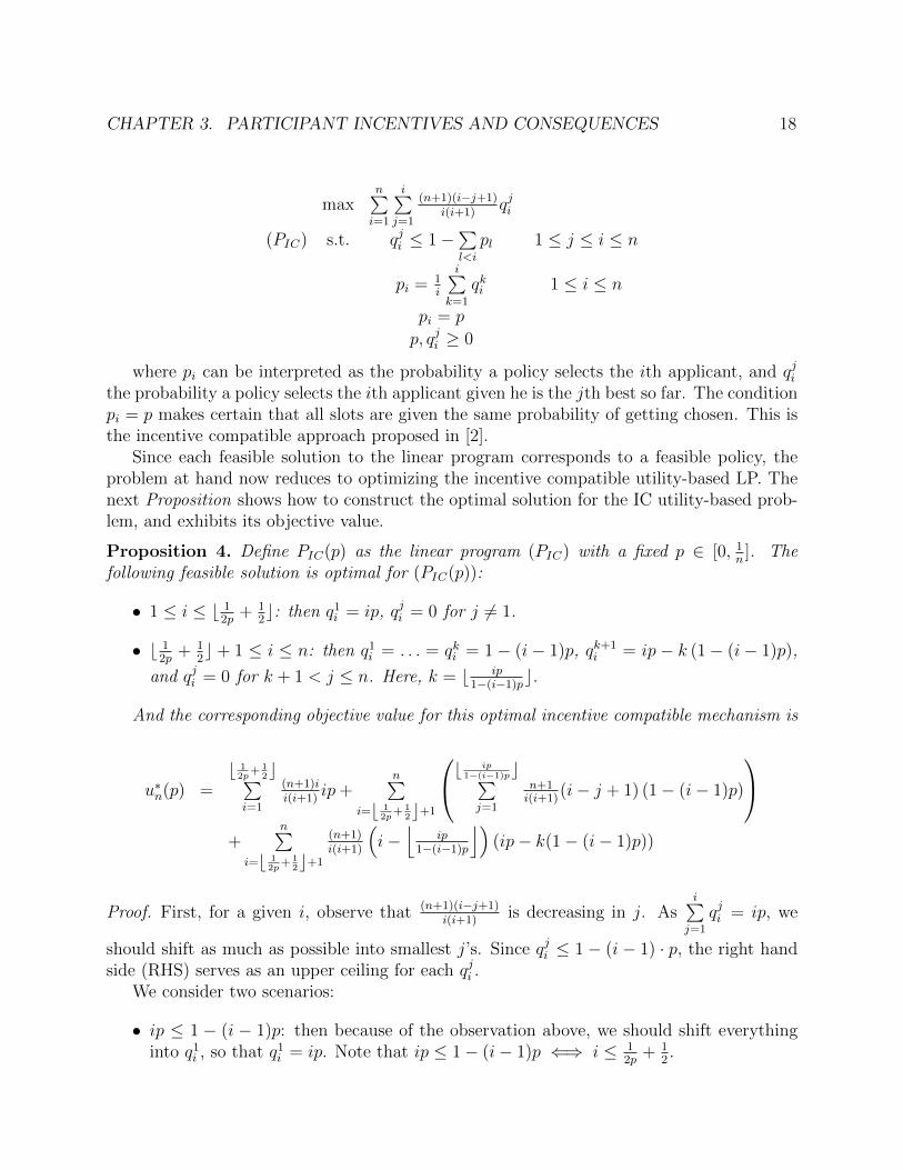
where pi can be interpreted as the probability a policy selects the ith applicant, and qjithe probability a policy selects the ith applicant given he is the jth best so far. The conditionpi = p makes certain that all slots are given the same probability of getting chosen. This isthe incentive compatible approach proposed in [2].
Since each feasible solution to the linear program corresponds to a feasible policy, theproblem at hand now reduces to optimizing the incentive compatible utility-based LP. Thenext Proposition shows how to construct the optimal solution for the IC utility-based prob-lem, and exhibits its objective value.
Proposition 4. Define PIC(p) as the linear program (PIC) with a fixed p ∈ [0, 1n]. The
following feasible solution is optimal for (PIC(p)):
• 1 ≤ i ≤ b 12p
+ 12c: then q1i = ip, qji = 0 for j 6= 1.
• b 12p
+ 12c + 1 ≤ i ≤ n: then q1i = . . . = qki = 1− (i− 1)p, qk+1
i = ip− k (1− (i− 1)p),
and qji = 0 for k + 1 < j ≤ n. Here, k = b ip1−(i−1)pc.
And the corresponding objective value for this optimal incentive compatible mechanism is
u∗n(p) =b 1
2p+ 1
2c∑i=1
(n+1)ii(i+1)
ip+n∑
i=b 12p
+ 12c+1
b ip1−(i−1)pc∑j=1
n+1i(i+1)
(i− j + 1) (1− (i− 1)p)
+
n∑i=b 1
2p+ 1
2c+1
(n+1)i(i+1)
(i−⌊
ip1−(i−1)p
⌋)(ip− k(1− (i− 1)p))
Proof. First, for a given i, observe that (n+1)(i−j+1)i(i+1)
is decreasing in j. Asi∑
j=1
qji = ip, we
should shift as much as possible into smallest j’s. Since qji ≤ 1− (i− 1) · p, the right handside (RHS) serves as an upper ceiling for each qji .
We consider two scenarios:
• ip ≤ 1 − (i − 1)p: then because of the observation above, we should shift everythinginto q1i , so that q1i = ip. Note that ip ≤ 1− (i− 1)p ⇐⇒ i ≤ 1
2p+ 1
2.
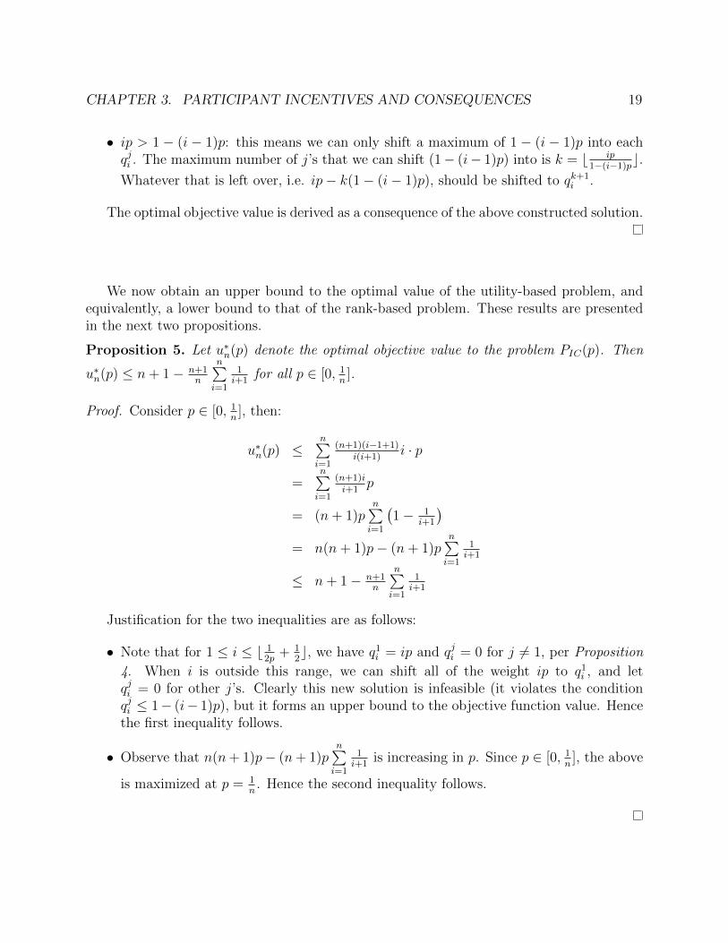
CHAPTER 3. PARTICIPANT INCENTIVES AND CONSEQUENCES 19
• ip > 1 − (i − 1)p: this means we can only shift a maximum of 1 − (i − 1)p into eachqji . The maximum number of j’s that we can shift (1− (i− 1)p) into is k = b ip
1−(i−1)pc.Whatever that is left over, i.e. ip− k(1− (i− 1)p), should be shifted to qk+1
i .
The optimal objective value is derived as a consequence of the above constructed solution.
We now obtain an upper bound to the optimal value of the utility-based problem, andequivalently, a lower bound to that of the rank-based problem. These results are presentedin the next two propositions.
Proposition 5. Let u∗n(p) denote the optimal objective value to the problem PIC(p). Then
u∗n(p) ≤ n+ 1− n+1n
n∑i=1
1i+1
for all p ∈ [0, 1n].
Proof. Consider p ∈ [0, 1n], then:
u∗n(p) ≤n∑i=1
(n+1)(i−1+1)i(i+1)
i · p
=n∑i=1
(n+1)ii+1
p
= (n+ 1)pn∑i=1
(1− 1
i+1
)= n(n+ 1)p− (n+ 1)p
n∑i=1
1i+1
≤ n+ 1− n+1n
n∑i=1
1i+1
Justification for the two inequalities are as follows:
• Note that for 1 ≤ i ≤ b 12p
+ 12c, we have q1i = ip and qji = 0 for j 6= 1, per Proposition
4. When i is outside this range, we can shift all of the weight ip to q1i , and letqji = 0 for other j’s. Clearly this new solution is infeasible (it violates the conditionqji ≤ 1− (i− 1)p), but it forms an upper bound to the objective function value. Hencethe first inequality follows.
• Observe that n(n+ 1)p− (n+ 1)pn∑i=1
1i+1
is increasing in p. Since p ∈ [0, 1n], the above
is maximized at p = 1n. Hence the second inequality follows.
CHAPTER 3. PARTICIPANT INCENTIVES AND CONSEQUENCES 20
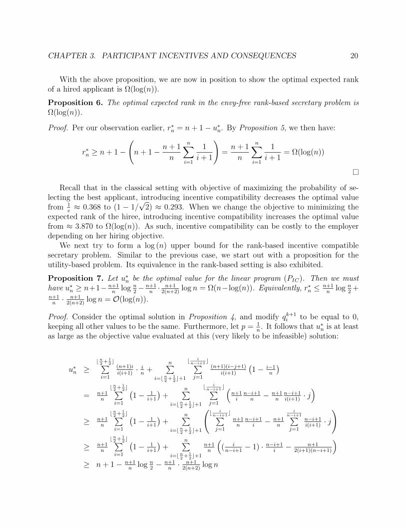
With the above proposition, we are now in position to show the optimal expected rankof a hired applicant is Ω(log(n)).
Proposition 6. The optimal expected rank in the envy-free rank-based secretary problem isΩ(log(n)).
Proof. Per our observation earlier, r∗n = n+ 1− u∗n. By Proposition 5, we then have:
r∗n ≥ n+ 1−
(n+ 1− n+ 1
n
n∑i=1
1
i+ 1
)=n+ 1
n
n∑i=1
1
i+ 1= Ω(log(n))
Recall that in the classical setting with objective of maximizing the probability of se-lecting the best applicant, introducing incentive compatibility decreases the optimal valuefrom 1
e≈ 0.368 to (1 − 1/
√2) ≈ 0.293. When we change the objective to minimizing the
expected rank of the hiree, introducing incentive compatibility increases the optimal valuefrom ≈ 3.870 to Ω(log(n)). As such, incentive compatibility can be costly to the employerdepending on her hiring objective.
We next try to form a log (n) upper bound for the rank-based incentive compatiblesecretary problem. Similar to the previous case, we start out with a proposition for theutility-based problem. Its equivalence in the rank-based setting is also exhibited.
Proposition 7. Let u∗n be the optimal value for the linear program (PIC). Then we musthave u∗n ≥ n+1− n+1
nlog n
2− n+1
n· n+12(n+2)
log n = Ω(n− log(n)). Equivalently, r∗n ≤ n+1n
log n2
+n+1n· n+12(n+2)
log n = O(log(n)).
Proof. Consider the optimal solution in Proposition 4, and modify qk+1i to be equal to 0,
keeping all other values to be the same. Furthermore, let p = 1n. It follows that u∗n is at least
as large as the objective value evaluated at this (very likely to be infeasible) solution:
u∗n ≥bn2+ 1
2c∑
i=1
(n+1)ii(i+1)
· in
+n∑
i=bn2+ 1
2c+1
b in−i+1
c∑j=1
(n+1)(i−j+1)i(i+1)
(1− i−1
n
)= n+1
n
bn2+ 1
2c∑
i=1
(1− 1
i+1
)+
n∑i=bn
2+ 1
2c+1
b in−i+1
c∑j=1
(n+1i
n−i+1n− n+1
nn−i+1i(i+1)
· j)
≥ n+1n
bn2+ 1
2c∑
i=1
(1− 1
i+1
)+
n∑i=bn
2+ 1
2c+1
(b in−i+1
c∑j=1
n+1n
n−i+1i− n+1
n
in−i+1∑j=1
n−i+1i(i+1)
· j
)
≥ n+1n
bn2+ 1
2c∑
i=1
(1− 1
i+1
)+
n∑i=bn
2+ 1
2c+1
n+1n
(( in−i+1
− 1) · n−i+1i− n+1
2(i+1)(n−i+1)
)≥ n+ 1− n+1
nlog n
2− n+1
n· n+12(n+2)
log n
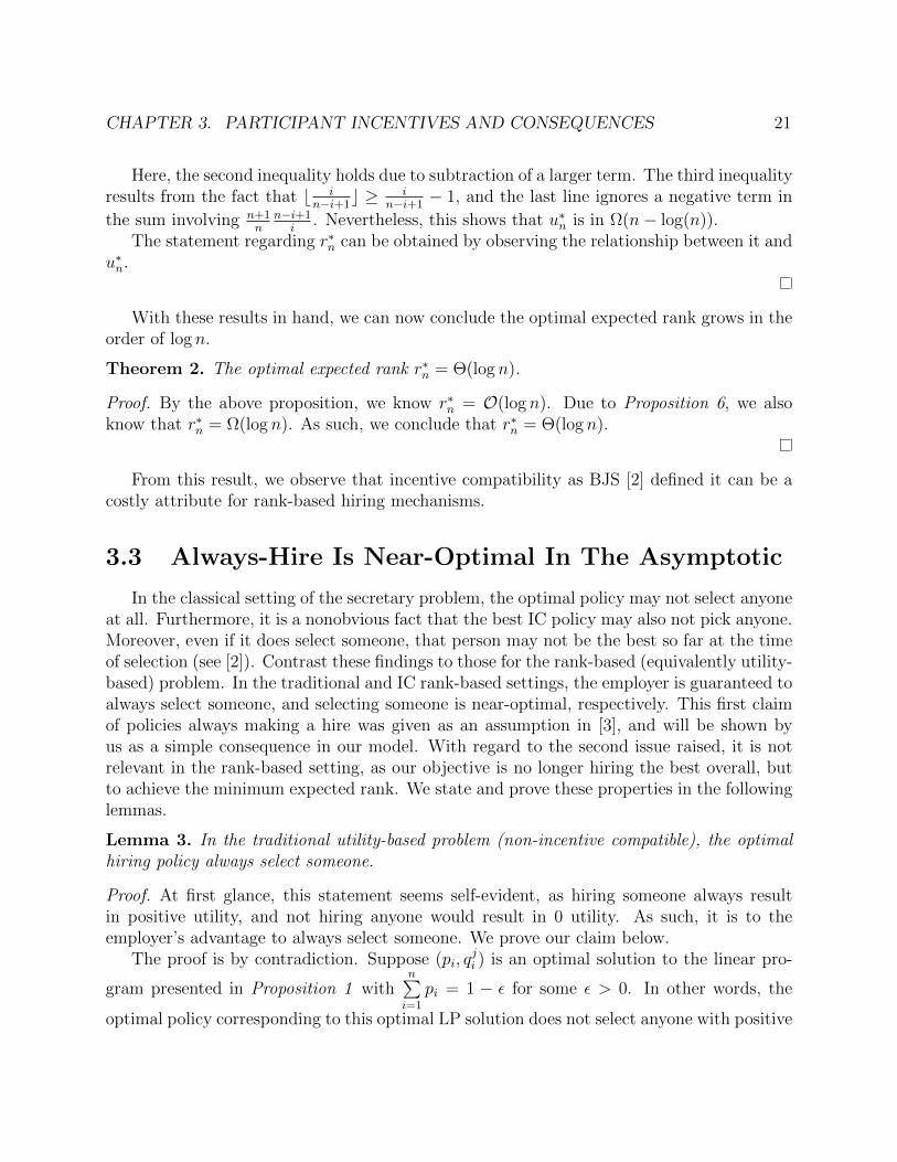
CHAPTER 3. PARTICIPANT INCENTIVES AND CONSEQUENCES 21
Here, the second inequality holds due to subtraction of a larger term. The third inequalityresults from the fact that b i
n−i+1c ≥ i
n−i+1− 1, and the last line ignores a negative term in
the sum involving n+1n
n−i+1i
. Nevertheless, this shows that u∗n is in Ω(n− log(n)).The statement regarding r∗n can be obtained by observing the relationship between it and
u∗n.
With these results in hand, we can now conclude the optimal expected rank grows in theorder of log n.
Theorem 2. The optimal expected rank r∗n = Θ(log n).
Proof. By the above proposition, we know r∗n = O(log n). Due to Proposition 6, we alsoknow that r∗n = Ω(log n). As such, we conclude that r∗n = Θ(log n).
From this result, we observe that incentive compatibility as BJS [2] defined it can be acostly attribute for rank-based hiring mechanisms.
3.3 Always-Hire Is Near-Optimal In The Asymptotic
In the classical setting of the secretary problem, the optimal policy may not select anyoneat all. Furthermore, it is a nonobvious fact that the best IC policy may also not pick anyone.Moreover, even if it does select someone, that person may not be the best so far at the timeof selection (see [2]). Contrast these findings to those for the rank-based (equivalently utility-based) problem. In the traditional and IC rank-based settings, the employer is guaranteed toalways select someone, and selecting someone is near-optimal, respectively. This first claimof policies always making a hire was given as an assumption in [3], and will be shown byus as a simple consequence in our model. With regard to the second issue raised, it is notrelevant in the rank-based setting, as our objective is no longer hiring the best overall, butto achieve the minimum expected rank. We state and prove these properties in the followinglemmas.
Lemma 3. In the traditional utility-based problem (non-incentive compatible), the optimalhiring policy always select someone.
Proof. At first glance, this statement seems self-evident, as hiring someone always resultin positive utility, and not hiring anyone would result in 0 utility. As such, it is to theemployer’s advantage to always select someone. We prove our claim below.
The proof is by contradiction. Suppose (pi, qji ) is an optimal solution to the linear pro-
gram presented in Proposition 1 withn∑i=1
pi = 1 − ε for some ε > 0. In other words, the
optimal policy corresponding to this optimal LP solution does not select anyone with positive
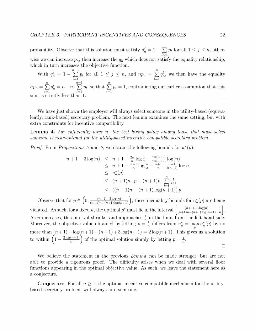
CHAPTER 3. PARTICIPANT INCENTIVES AND CONSEQUENCES 22
probability. Observe that this solution must satisfy qjn = 1−∑l<n
pl for all 1 ≤ j ≤ n, other-
wise we can increase pn, then increase the qjn which does not satisfy the equality relationship,which in turn increases the objective function.
With qjn = 1 −n−1∑l=1
pl for all 1 ≤ j ≤ n, and npn =n∑l=1
qln, we then have the equality
npn =n∑l=1
qln = n−n ·n−1∑l=1
pl, so thatn∑i=1
pi = 1, contradicting our earlier assumption that this
sum is strictly less than 1.
We have just shown the employer will always select someone in the utility-based (equiva-lently, rank-based) secretary problem. The next lemma examines the same setting, but withextra constraints for incentive compatibility.
Lemma 4. For sufficiently large n, the best hiring policy among those that must selectsomeone is near-optimal for the utility-based incentive compatible secretary problem.
Proof. From Propositions 5 and 7, we obtain the following bounds for u∗n(p):
n+ 1− 3 log(n) ≤ n+ 1− 2nn
log n2− 2n(n+2)
2n(n+2)log(n)
≤ n+ 1− n+1n
log n2− n+1
n· n+12(n+2)
log n
≤ u∗n(p)
≤ (n+ 1)n · p− (n+ 1)p ·n∑i=1
1i+1
≤ ((n+ 1)n− (n+ 1) log(n+ 1)) p
Observe that for p ∈(
0, (n+1)−3 log(n)(n+1)n−(n+1) log(n+1)
), these inequality bounds for u∗n(p) are being
violated. As such, for a fixed n, the optimal p∗ must lie in the interval[
(n+1)−3 log(n)(n+1)n−(n+1) log(n+1)
, 1n
].
As n increases, this interval shrinks, and approaches 1n
in the limit from the left hand side.Moreover, the objective value obtained by letting p = 1
ndiffers from u∗n = max
pu∗n(p) by no
more than (n+1)− log(n+1)− (n+1)+3 log(n+1) = 2 log(n+1). This gives us a solution
to within(
1− 2 log(n+1)n
)of the optimal solution simply by letting p = 1
n.
We believe the statement in the previous Lemma can be made stronger, but are notable to provide a rigourous proof. The difficulty arises when we deal with several floorfunctions appearing in the optimal objective value. As such, we leave the statement here asa conjecture.
Conjecture: For all n ≥ 1, the optimal incentive compatible mechanism for the utility-based secretary problem will always hire someone.
CHAPTER 3. PARTICIPANT INCENTIVES AND CONSEQUENCES 23
3.4 Incentive Compatibility In Generalized
Utility-Based Problems
In a generalized utility-based secretary problem, the employer will derive a utility of f(s)units for hiring the sth best overall applicant. Modeling this problem as a dynamic programor a linear program is similar to what we have shown previously. If we modify the classicalsecretary problem, and assign f(1) = n, and f(s) = 0 for all other s 6= 1, [2] showed that the
optimal incentive compatible policy selects a candidate with expected utility of(
1− 1√2
)n.
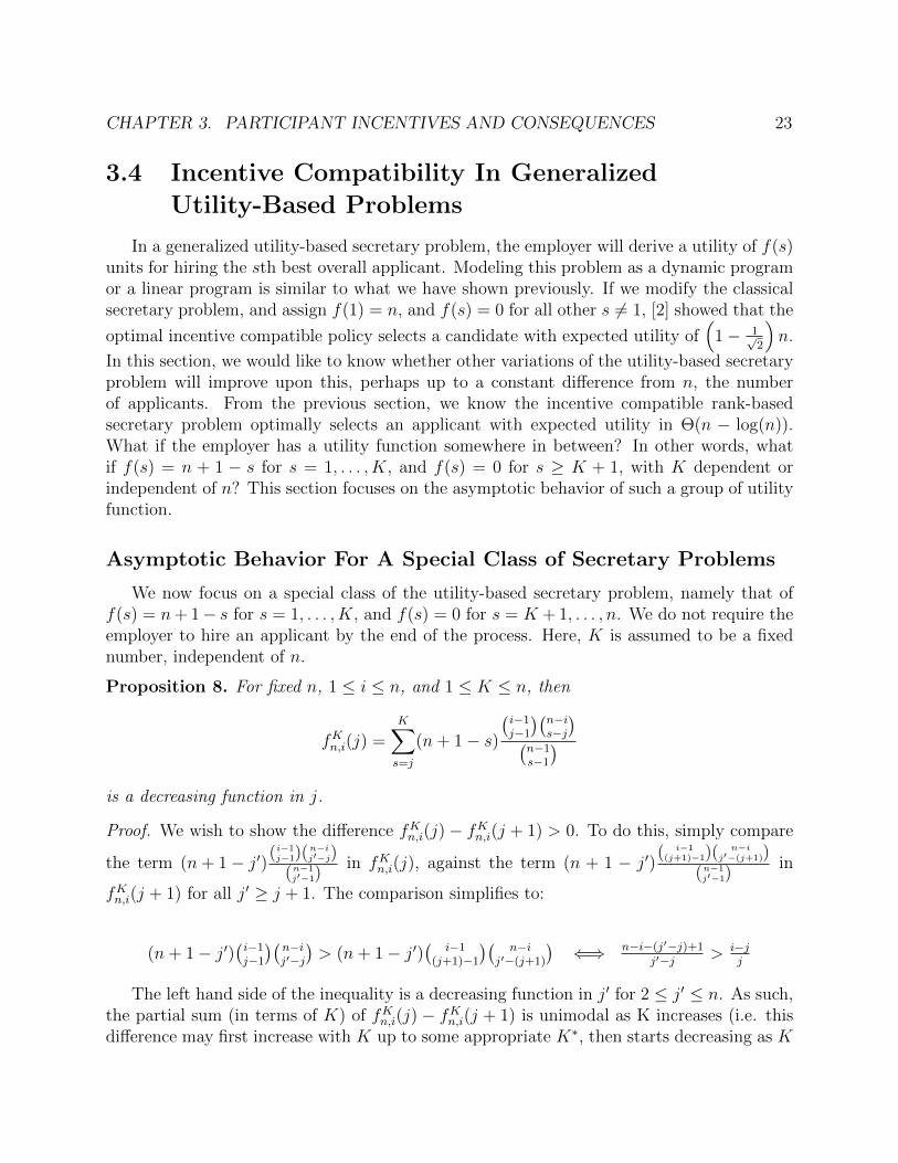
In this section, we would like to know whether other variations of the utility-based secretaryproblem will improve upon this, perhaps up to a constant difference from n, the numberof applicants. From the previous section, we know the incentive compatible rank-basedsecretary problem optimally selects an applicant with expected utility in Θ(n − log(n)).What if the employer has a utility function somewhere in between? In other words, whatif f(s) = n + 1 − s for s = 1, . . . , K, and f(s) = 0 for s ≥ K + 1, with K dependent orindependent of n? This section focuses on the asymptotic behavior of such a group of utilityfunction.
Asymptotic Behavior For A Special Class of Secretary Problems
We now focus on a special class of the utility-based secretary problem, namely that off(s) = n+ 1− s for s = 1, . . . , K, and f(s) = 0 for s = K + 1, . . . , n. We do not require theemployer to hire an applicant by the end of the process. Here, K is assumed to be a fixednumber, independent of n.
Proposition 8. For fixed n, 1 ≤ i ≤ n, and 1 ≤ K ≤ n, then
fKn,i(j) =K∑s=j
(n+ 1− s)(i−1j−1
)(n−is−j
)(n−1s−1
)is a decreasing function in j.
Proof. We wish to show the difference fKn,i(j)− fKn,i(j + 1) > 0. To do this, simply compare
the term (n+ 1− j′)(i−1j−1)(
n−ij′−j)
(n−1j′−1)
in fKn,i(j), against the term (n + 1 − j′)( i−1(j+1)−1)(
n−ij′−(j+1))
(n−1j′−1)
in
fKn,i(j + 1) for all j′ ≥ j + 1. The comparison simplifies to:
(n+ 1− j′)(i−1j−1
)(n−ij′−j
)> (n+ 1− j′)
(i−1
(j+1)−1
)(n−i
j′−(j+1)
)⇐⇒ n−i−(j′−j)+1
j′−j > i−jj
The left hand side of the inequality is a decreasing function in j′ for 2 ≤ j′ ≤ n. As such,the partial sum (in terms of K) of fKn,i(j) − fKn,i(j + 1) is unimodal as K increases (i.e. thisdifference may first increase with K up to some appropriate K∗, then starts decreasing as K
CHAPTER 3. PARTICIPANT INCENTIVES AND CONSEQUENCES 24
goes beyond this K∗). When K = j, clearly this difference is positive. Furthermore, whenK = n, this difference also stays positive due to the closed-form formula of our utility-basedobjective function. As such, we can conclude the difference must remain positive for all Kin between, i.e. fKn,i(j) is decreasing in j.
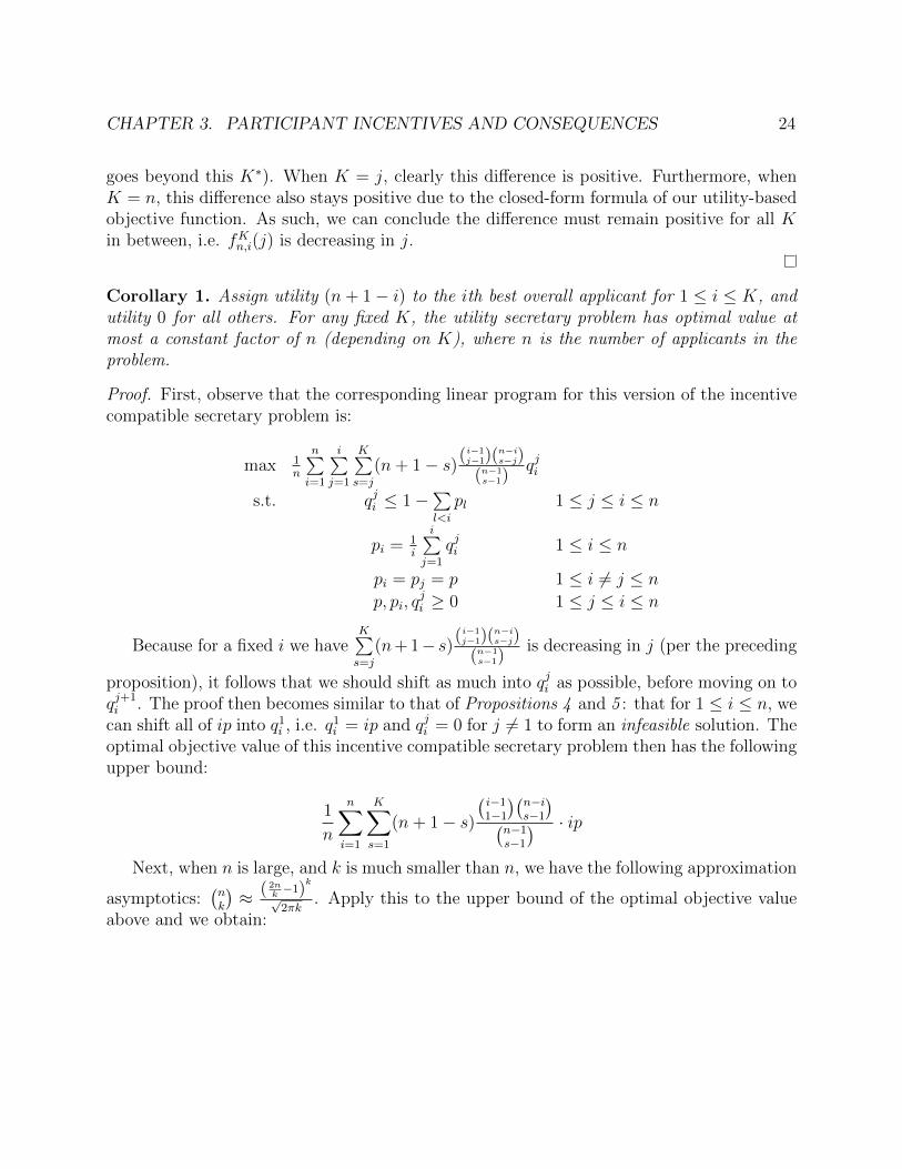
Corollary 1. Assign utility (n+ 1− i) to the ith best overall applicant for 1 ≤ i ≤ K, andutility 0 for all others. For any fixed K, the utility secretary problem has optimal value atmost a constant factor of n (depending on K), where n is the number of applicants in theproblem.
Proof. First, observe that the corresponding linear program for this version of the incentivecompatible secretary problem is:
max 1n
n∑i=1
i∑j=1
K∑s=j
(n+ 1− s)(i−1j−1)(
n−is−j)
(n−1s−1)
qji
s.t. qji ≤ 1−∑l<i
pl 1 ≤ j ≤ i ≤ n
pi = 1i
i∑j=1
qji 1 ≤ i ≤ n
pi = pj = p 1 ≤ i 6= j ≤ n
p, pi, qji ≥ 0 1 ≤ j ≤ i ≤ n
Because for a fixed i we haveK∑s=j
(n+ 1− s)(i−1j−1)(
n−is−j)
(n−1s−1)
is decreasing in j (per the preceding
proposition), it follows that we should shift as much into qji as possible, before moving on toqj+1i . The proof then becomes similar to that of Propositions 4 and 5 : that for 1 ≤ i ≤ n, we
can shift all of ip into q1i , i.e. q1i = ip and qji = 0 for j 6= 1 to form an infeasible solution. Theoptimal objective value of this incentive compatible secretary problem then has the followingupper bound:
1
n
n∑i=1
K∑s=1
(n+ 1− s)(i−11−1
)(n−is−1
)(n−1s−1
) · ip
Next, when n is large, and k is much smaller than n, we have the following approximation
asymptotics:(nk
)≈ ( 2n
k−1)
k
√2πk
. Apply this to the upper bound of the optimal objective valueabove and we obtain:
CHAPTER 3. PARTICIPANT INCENTIVES AND CONSEQUENCES 25
1n
n∑i=1
K∑s=1
(n+ 1− s) (n−is−1)
(n−1s−1)
ip ≈ 1n
n∑i=1
K∑s=1
(n+ 1− s)(
2(n−i)−(s−1)2(n−1)−(s−1)
)s−1· ip
≤ 1n
n∑i=1
K∑s=1
(n+ 1− s) [2(n−1)−(s−1)]s+1
[2(n−1)−(s−1)]s−1 · 14s(s+1)
· ip+ l.o.t.
= 1n
K∑s=1
(n+ 1− s) (2(n− 1)− (s− 1))2 · 14s(s+1)
· p+ l.o.t.
≤ 14n
K∑s=1
(n+ 1− s) (2(n− 1))2 · 1s(s+1)
· p+ l.o.t.
=((n− 1)2 ·
(1− 1
K+1
))· p+ l.o.t.
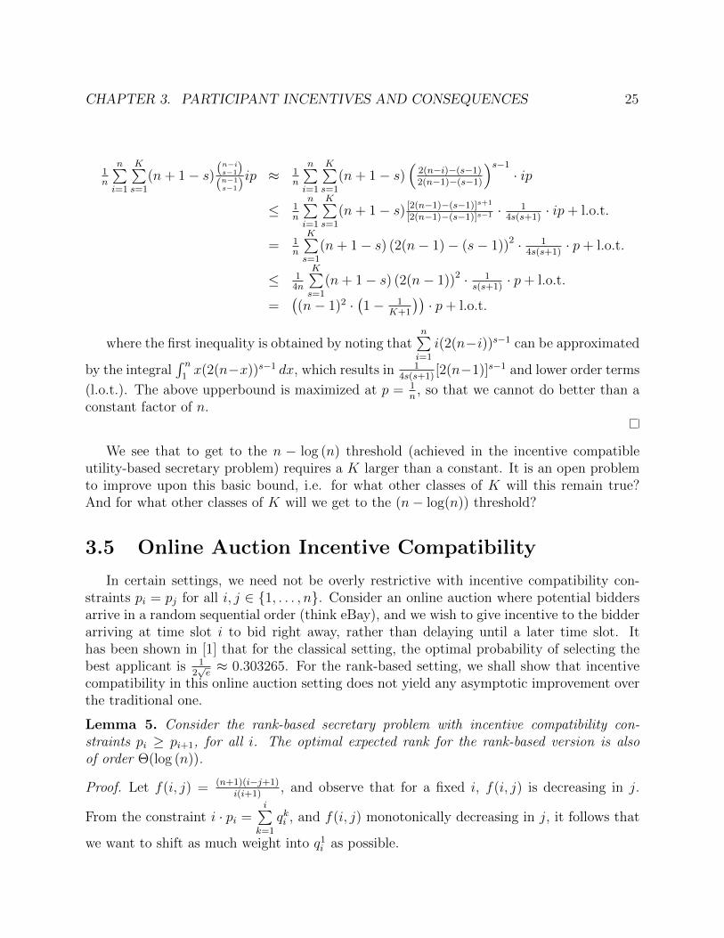
where the first inequality is obtained by noting thatn∑i=1
i(2(n−i))s−1 can be approximated
by the integral∫ n1x(2(n−x))s−1 dx, which results in 1
4s(s+1)[2(n−1)]s−1 and lower order terms
(l.o.t.). The above upperbound is maximized at p = 1n, so that we cannot do better than a
constant factor of n.
We see that to get to the n − log (n) threshold (achieved in the incentive compatibleutility-based secretary problem) requires a K larger than a constant. It is an open problemto improve upon this basic bound, i.e. for what other classes of K will this remain true?And for what other classes of K will we get to the (n− log(n)) threshold?
3.5 Online Auction Incentive Compatibility
In certain settings, we need not be overly restrictive with incentive compatibility con-straints pi = pj for all i, j ∈ 1, . . . , n. Consider an online auction where potential biddersarrive in a random sequential order (think eBay), and we wish to give incentive to the bidderarriving at time slot i to bid right away, rather than delaying until a later time slot. Ithas been shown in [1] that for the classical setting, the optimal probability of selecting thebest applicant is 1
2√e≈ 0.303265. For the rank-based setting, we shall show that incentive
compatibility in this online auction setting does not yield any asymptotic improvement overthe traditional one.
Lemma 5. Consider the rank-based secretary problem with incentive compatibility con-straints pi ≥ pi+1, for all i. The optimal expected rank for the rank-based version is alsoof order Θ(log (n)).
Proof. Let f(i, j) = (n+1)(i−j+1)i(i+1)
, and observe that for a fixed i, f(i, j) is decreasing in j.
From the constraint i · pi =i∑
k=1
qki , and f(i, j) monotonically decreasing in j, it follows that
we want to shift as much weight into q1i as possible.
CHAPTER 3. PARTICIPANT INCENTIVES AND CONSEQUENCES 26
Now consider a solution where all possible weights are shifted into q1i , leaving q2i = q3i =. . . = 0, so that it has value q1i = i · pi. The objective value for this particular solution is
thenn∑i=1
(n+1)ii(i+1)
· i · pi =n∑i=1
(n+1)ii+1· pi. Observe that (n+1)i
i+1is increasing in i, so that we want
to allocate more weight to pj than to pi whenever j > i. This, together with our incentivecompatibile constraints pi ≥ pj whenever j > i implies we must assign equal weights to all
pi’s. Sincen∑i=1
pi ≤ 1, we can only assign a maximum of 1n
to each pi. The objective value for
the infeasible solution pi = 1n
and q1i = ipi, q2i = q3i = . . . = 0 ∀i is n+ 1− n+1
n
n∑i=1
1i+1
. Since
this is an upper bound to the expected utility problem, it follows that the optimal expectedrank is of order Ω(log (n)).
Since pi ≥ pi+1 for all i is a relaxation of the more restrictive pi = pj for all i, j, and theoptimal expected rank for the latter problem is in Θ(log (n)), our claim follows by havingproved the optimal expected rank (for the version pi ≥ pi+1) also belongs to Ω(log (n)).
3.6 Implementation Of Incentive Compatible Hiring
Mechanisms
One may cast doubt on our original motivation for coming up with new hiring policies.It is true that if applicants know they will get interviewed but never offered a job, then theyhave incentive to not show up. But does the if ever happen? From an applicant’s point ofview, how is he to decide whether the employer chooses to use the classical threshold policyor some other hiring methods? If one comes in the 3rd interview slot out of 10 and does notget selected, is it because the employer uses a threshold hiring policy, or is it due to the factthat one is simply not the best candidate so far? There is an implicit trust in the employer,and her objective of selecting the best applicant does not align with actions to honor it.
To overcome aforementioned drawbacks, we propose executing the hiring policy througha 3rd party. The employer can submit her hiring algorithm, and applicants can submit theirinquiries regarding the hiring policy and get them answered through this central location.For example, an applicant can ask of the probability this policy will select someone in the3 position, or the value of n in this process, and get answers for these. We believe thischeck-and-balance approach will deliver desired incentives to applicants, and at the sametime, ensure the hiring algorithm’s integrity from being interfered with by the employer.
We recognize the fact that collusions between this 3rd party and the employer is also apotential problem. For this, we refer our readers to literatures on the design of collusion-freeprotocols.
CHAPTER 3. PARTICIPANT INCENTIVES AND CONSEQUENCES 27
3.7 A Concluding Note On Incentive Compatibility
In the last and current chapters, we showed the incentive compatibility property can becostly to the decision maker in an optimal stopping setting, with this greatly dependingon her objective function. This observation holds for both types of incentive compatibilityproposed in [2] and [1]. From a high-level perspective, we also showed Buchbinder, Jain, andSingh’s linear programming based approach for modeling secretary problems can be obtainedfrom known methods in the theory of Markov Decision Processes. Our insight allows for analternative approach in cases where BJS’s technique cannot be easily applied.
28
Chapter 4
How To Win Jobs And InfluenceEmployers
4.1 Introduction
In the classic secretary problem, n (commonly known) applicants present themselves oneby one to an employer. If the employer could wait before making a decision, she would beable to rank them from best to worst, and select the best candidate. The order for whichapplicants present themselves to the employer is random, i.e. it is equally likely from amongthe n! permutations. After an applicant is interviewed, the employer must make her hiringdecision on the spot: either to accept this applicant, or to reject him and moves on to thenext applicant without the possibility of going back. The employer’s objective is to designan algorithm that would maximize her probability of selecting the overall best applicant.
As shown in the first chapter, the employer’s optimal hiring policy is deceptively simple:to skip over all applicants from slots 1 to r∗− 1, and selects the applicant in slot r∗ ≤ j ≤ nif he happens to be the best among those observed so far. Here, r∗ is the smallest integer
between 1 and n which satisfies r∗
n≥ r∗
n
n∑k=r∗+1
1k−1 . This threshold policy is typical in
optimal stopping problems, where the decision maker spends some time learning about thepopulation, and starts working on the choosing process after a certain time point. A momentof reflection, however, indicates that the approach may not work with all subjects. When weare dealing with items, this policy is perfectly fine, as items do not think strategically. Whenwe are dealing with living, rational human beings, this policy begs for much improvement.One approach that tries to mitigate this concern was proposed by Buchbinder et al. [2],and was extended and generalized to the rank-based case in the previous chapter. There,the employer constrained herself to only hiring policies for which applicants have incentivesto remain in their interview slots. Here, we shall allow applicants more freedom in thehiring process, where they can make decisions which will affect everyone involved, fromother applicants to the employer herself.
We find it useful to pause here and make clear an assumption of applicants’ attitude
CHAPTER 4. HOW TO WIN JOBS AND INFLUENCE EMPLOYERS 29
toward different hiring mechanisms. Although it seems trivial, the statement helps resolvea thorny subject later in the section.
Assumption: An applicant finds it unacceptable if he is invited to the ith interviewslot, and this slot has probability 0 of getting hired.
We next focus on models where applicants can choose from a set of strategies which isdependent on one’s position in the process. Working with the classical setting of maximizingthe probability of hiring the best applicant, we now allow each applicant to submit a windowof availability to the employer. She, in turn, must make her decision on applicants before theirrespective deadlines. The timing and nature of how applicants can submit their windowsof availability play an important role in the analysis. The resulting mathematical problemsbecome quite interesting, and could potentially give us insights into how players in such anoptimal stopping process may, and should, behave.
4.2 An Extensive Secretary Game With Imperfect
Information
During each of the n time units, the employer would invite an applicant to come infor an interview. Her objective is to maximize the probability of hiring the best applicantamong these available n, while each of the applicants knows his respective interview slot andwants to maximize his probability of getting hired. After getting his interview, an applicantcommunicates to the employer a time window ti = j, where his job status must be decidedby time t = i + ti = i + j. As examples, if the applicant is interviewed on the 4th day, andoffers his time window t4 = 0, then the employer must make her decision for this applicantright away. Whereas if he gives his time window as t4 = 3, then the employer can make herdecision on or before the 7th day. Note that the set of available strategies is different fromapplicant to applicant, and hence the game is not symmetric. Furthermore, a later applicantonly has partial information about the game, i.e. the employer is still searching, and notactual time window values from earlier applicants. For example, the 4th applicant knowsthe employer is still looking to hire due to the fact that he is getting an interview now, buthe does not know exact values for each of the earlier ti’s. In this way, the sequential gamehas imperfect information, and is classified as such.
• Game: Extensive Classical Secretary Game With Imperfect Information
• Players: N = 0, 1, 2, . . . , n. Here, 0 denotes the employer, and 1 ≤ i ≤ n denotesthe ith applicant, who occupies the ith interview slot.
• Description: There are n applicants, each wanting to maximize his chance of landingthe job, and one employer who wishes to maximize her probability of selecting the best
CHAPTER 4. HOW TO WIN JOBS AND INFLUENCE EMPLOYERS 30
applicant among these n. The value n is commonly known among all applicants andthe employer. Time progresses from 1 to n. Before time 1, the employer assigns slotsrandomly to all participants. At any time i, the following events occur in this order.
1. If no one has been selected, the employer sends an invitation for, and interviewsthe ith applicant.
2. Applicant i tells the employer of his non-binding time window ti.
3. Employer decides if she wants to accept a previously interviewed, and still avail-able, applicant. If yes, the process ends. If not, the process continues to timei+ 1. The current ith applicant is taken to be available at this time i.
It may at first appear difficult to describe with precision certain components of this game.For example, what are terminal histories in such a game, and the utility derived by eachapplicant in one such terminal history? It turns out that an important class of players’strategies can be found even when the game tree is not explicitly enumerated. This set ofdominant actions is presented in the theorem below.
Theorem 3. Let r∗ be the smallest integer between 1 and n such that 1 ≥n∑
k=r∗+1
1k−1 . When
presenting their time windows, it is a dominant strategy for(a) those in slots r∗ + 1 ≤ i ≤ n to force the employer to make her decision right away,
i.e. ti = 0 for r∗ + 1 ≤ i ≤ n.(b) those in slots 1 ≤ i ≤ r∗ to allow the employer until time r∗ to make her decision,
i.e. ti = r∗ − i for 1 ≤ i ≤ r∗.
Proof. The proof is by backward induction.(a) Since the last applicant has no choice but to use tn = 0, the statement trivially holds
in this case. Assume the statement holds for applicants i, i+ 1, . . . , n, where r∗+ 2 ≤ i ≤ n.If the employer ever gets to the (i−1)st applicant, then this applicant has n−i+2 choices:
either ti−1 = 0, ti−1 = 1, . . . , ti−1 = n− i+ 1. We need only focus on the scenario that he isthe best so far out of the first n− 1 applicants, as he will not get selected otherwise. Fromthe induction hypothesis, we know all later applicants will force the employer to make herdecision immediately when she gets to them. As such, letting ti−1 = 0 will allow this (i−1)stapplicant to get selected with probability 1, whereas letting ti−1 > 0 will get him selectedwith probability strictly smaller than 1 as future applicants may be better candidates thanhe is. Therefore, he will choose to play ti−1 = 0.
(b) Now consider the (r∗− i)th applicant (again assuming he is the best so far). When hecomes in for the interview, he knows later applicants will all play tj = 0 for j ≥ r∗. As such,if he lets tr∗−i < i, his chance of getting hired is 0, as the employer has a higher probabilityof selecting the best one by delaying her decision until time r∗. If he allows the time windowto be tr∗−i = i, then his chance of getting hired is r∗−i
r∗. If he lets tr∗−i = t > i, his probability
CHAPTER 4. HOW TO WIN JOBS AND INFLUENCE EMPLOYERS 31
of getting selected is at most r∗−ir∗−i+t , which is strictly smaller than r∗−i
r∗. Therefore, he will
play tr∗−i = i. In this way, these applicants will wish to delay until time r∗.
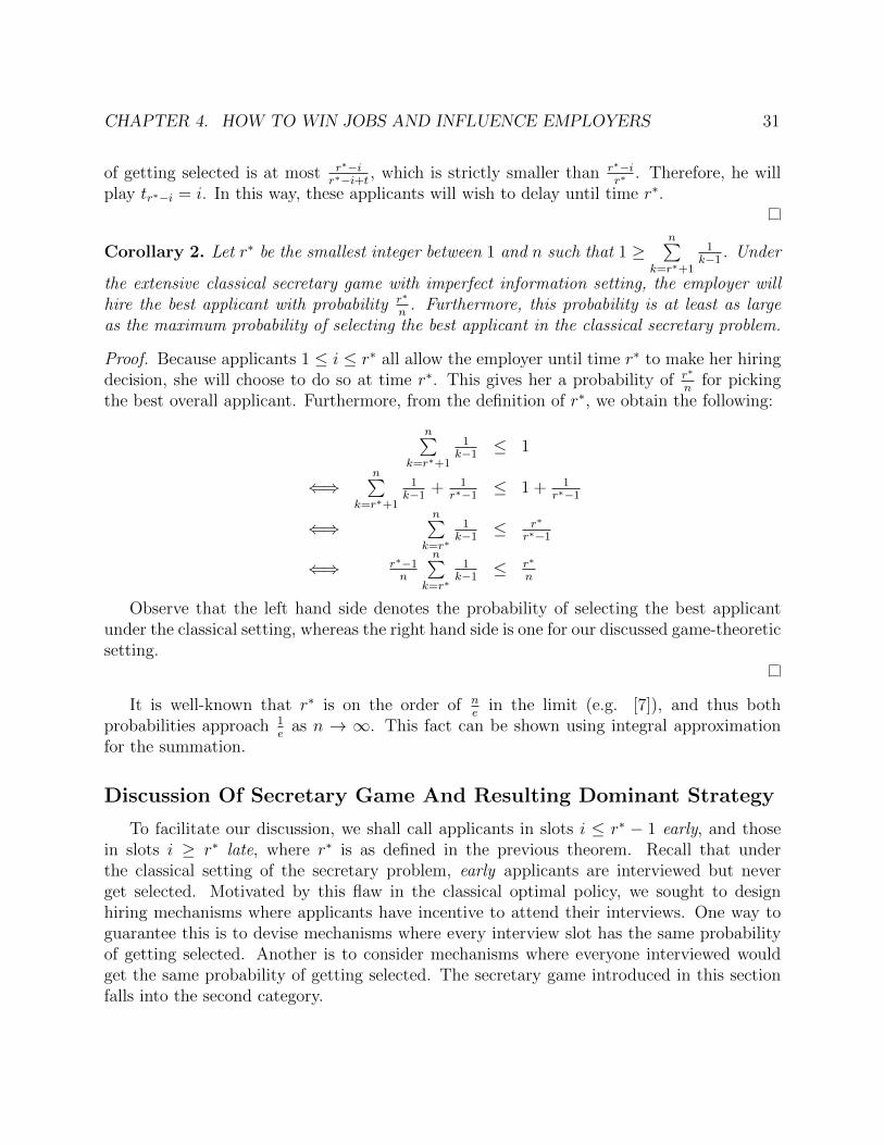
Corollary 2. Let r∗ be the smallest integer between 1 and n such that 1 ≥n∑
k=r∗+1
1k−1 . Under
the extensive classical secretary game with imperfect information setting, the employer willhire the best applicant with probability r∗
n. Furthermore, this probability is at least as large
as the maximum probability of selecting the best applicant in the classical secretary problem.
Proof. Because applicants 1 ≤ i ≤ r∗ all allow the employer until time r∗ to make her hiringdecision, she will choose to do so at time r∗. This gives her a probability of r∗
nfor picking
the best overall applicant. Furthermore, from the definition of r∗, we obtain the following:
n∑k=r∗+1
1k−1 ≤ 1
⇐⇒n∑
k=r∗+1
1k−1 + 1
r∗−1 ≤ 1 + 1r∗−1
⇐⇒n∑
k=r∗
1k−1 ≤
r∗
r∗−1
⇐⇒ r∗−1n
n∑k=r∗
1k−1 ≤
r∗
n
Observe that the left hand side denotes the probability of selecting the best applicantunder the classical setting, whereas the right hand side is one for our discussed game-theoreticsetting.
It is well-known that r∗ is on the order of ne
in the limit (e.g. [7]), and thus bothprobabilities approach 1
eas n → ∞. This fact can be shown using integral approximation
for the summation.
Discussion Of Secretary Game And Resulting Dominant Strategy
To facilitate our discussion, we shall call applicants in slots i ≤ r∗ − 1 early, and thosein slots i ≥ r∗ late, where r∗ is as defined in the previous theorem. Recall that underthe classical setting of the secretary problem, early applicants are interviewed but neverget selected. Motivated by this flaw in the classical optimal policy, we sought to designhiring mechanisms where applicants have incentive to attend their interviews. One way toguarantee this is to devise mechanisms where every interview slot has the same probabilityof getting selected. Another is to consider mechanisms where everyone interviewed wouldget the same probability of getting selected. The secretary game introduced in this sectionfalls into the second category.
CHAPTER 4. HOW TO WIN JOBS AND INFLUENCE EMPLOYERS 32
If the employer ever gets to a late applicant, it is optimal for him to force the employerto make her decision right away. Furthermore, these late applicants play an important rolein getting early ones to allow the employer until time r∗ to make her decision. As such,in our model, the employer uses these late applicants as threats against early ones. It isthe expectation of other players employing rational strategies in future periods that dictatestrategies for these early applicants. Moreover, these late applicants have incentive to cometo the interview if they are ever invited. Contrast this to the classical setting of the secretaryproblem, where early applicants are being used as guinea pigs to learn about the population,and have no incentive to participate in the interview even if they get invitations to come.It is in this way that our proposed game-theoretic model addresses the issue raised by BJSregarding incentives in the classical secretary setting.
Employer’s Incentive
Implicit in our assumption is the fact that there are truly n applicants participating in thehiring process. Consider a scenario where it is the employer who announces n to everyone.It is to his interest to inflate the announced value n, as that would allow him to select thebest applicant with probability 1. As an example, suppose the true value of n is 3, but theemployer announces a value of n = 5 instead. In other words, the first three applicants exist,but the last two are imaginary. These auxiliary applicants were created by the employer withthe sole purpose of enhancing her probability of hiring the best candidate. And it worksbeautifully if other applicants have no means to check on its validity. Everyone now playsunder the scenario of n = 5, and the three real applicants all allow the employer until time3 to make her hiring decision. At time t = 3, the employer can make an informed hire as allthree applicants are available. Her probability of selecting the best is 1.
As such, the hiring mechanism should ensure the correct value of n is being distributedto all applicants. A possible implementation is to have a central station where an applicantcan access the number n and his interview position. Further complications may arise dueto possible collusion between this central station and the employer, but we again defer suchimplementation details to related literatures in these areas of collusion-free protocol design.For now, we are content with the assumption that all players will have a way to accessaccurate information regarding the hiring process.
Some Final Words On This Extensive Secretary Game
By allowing applicants more options in making their decisions, it is a pleasantly surpris-ing fact that the employer can overcome shortcomings of the original optimal policy whileimproving her maximum probability of selecting the best candidate. Observe that the em-ployer’s objective and that of the best overall applicant are aligned, where both want to befound by the other. As such, when the must-decide-now restriction is lifted, applicants havemore room to strategize, and the result ends up benefiting the employer.
CHAPTER 4. HOW TO WIN JOBS AND INFLUENCE EMPLOYERS 33
4.3 A Strategic Secretary Game: Binding Contracts
And Equilibria
Continuing with our discussion from the last section, we next focus on the setting whereall applicants are required to make known of their time windows before the first interviewbegins. These commitments are binding once submited, so that they cannot be changedlater on, and each applicant must adhere to what he proposes. From these time windows,the employer can now use a corresponding optimal policy to maximize her probability ofselecting the best applicant. We provide further details for this simultaneous game below.
Computing The Payoff Matrix
When an applicant is assigned an interview slot by the employer, he must also makeknown his window of availability ti. So that an applicant in slot i will be available for hireduring times i + 0, i + 1, . . . , i + ti. Given the strategy profile ~t = (t1, t2, . . . , tn) played bythe applicants, the employer can devise an optimal hiring mechanism π(~t), which when used,
will give the probability Pπ(~t)i for selecting the applicant at position i.
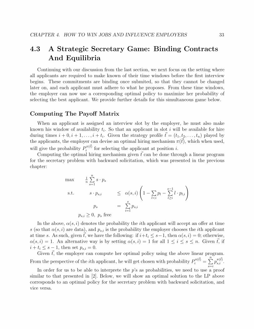
Computing the optimal hiring mechanism given ~t can be done through a linear programfor the secretary problem with backward solicitation, which was presented in the previouschapter:
max 1n
n∑s=1
s · ps
s.t. s · ps,i ≤ α(s, i)
(1−
∑l<i
pl −s−1∑l≥i
l · pl,i
)ps =
s∑i=1
ps,i
ps,i ≥ 0, ps free
In the above, α(s, i) denotes the probability the ith applicant will accept an offer at times (so that α(s, i) are data), and ps,i is the probability the employer chooses the ith applicantat time s. As such, given ~t, we have the following: if i+ti ≤ s−1, then α(s, i) = 0; otherwise,α(s, i) = 1. An alternative way is by setting α(s, i) = 1 for all 1 ≤ i ≤ s ≤ n. Given ~t, ifi+ ti ≤ s− 1, then set ps,i = 0.
Given ~t, the employer can compute her optimal policy using the above linear program.
From the perspective of the ith applicant, he will get chosen with probability Pπ(~t)i =
n∑s=i
pπ(~t)s,i .
In order for us to be able to interprete the p’s as probabilities, we need to use a proofsimilar to that presented in [2]. Below, we will show an optimal solution to the LP abovecorresponds to an optimal policy for the secretary problem with backward solicitation, andvice versa.
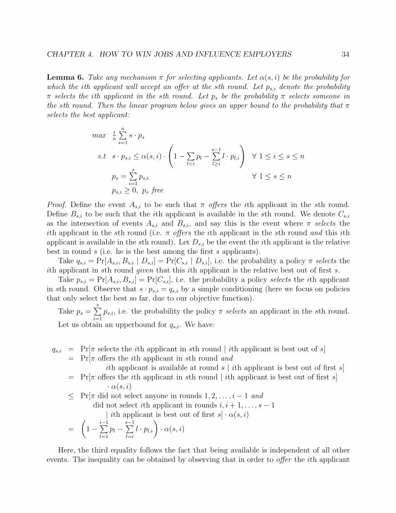
CHAPTER 4. HOW TO WIN JOBS AND INFLUENCE EMPLOYERS 34
Lemma 6. Take any mechanism π for selecting applicants. Let α(s, i) be the probability forwhich the ith applicant will accept an offer at the sth round. Let ps,i denote the probabilityπ selects the ith applicant in the sth round. Let ps be the probability π selects someone inthe sth round. Then the linear program below gives an upper bound to the probability that πselects the best applicant:
max 1n
n∑s=1
s · ps
s.t s · ps,i ≤ α(s, i) ·
(1−
∑l<i
pl −s−1∑l≥i
l · pl,i
)∀ 1 ≤ i ≤ s ≤ n
ps =s∑i=1
ps,i ∀ 1 ≤ s ≤ n
ps,i ≥ 0, ps free
Proof. Define the event As,i to be such that π offers the ith applicant in the sth round.Define Bs,i to be such that the ith applicant is available in the sth round. We denote Cs,ias the intersection of events As,i and Bs,i, and say this is the event where π selects theith applicant in the sth round (i.e. π offers the ith applicant in the sth round and this ithapplicant is available in the sth round). Let Ds,i be the event the ith applicant is the relativebest in round s (i.e. he is the best among the first s applicants).
Take qs,i = Pr[As,i, Bs,i | Ds,i] = Pr[Cs,i | Ds,i], i.e. the probability a policy π selects theith applicant in sth round given that this ith applicant is the relative best out of first s.
Take ps,i = Pr[As,i, Bs,i] = Pr[Cs,i], i.e. the probability a policy selects the ith applicantin sth round. Observe that s · ps,i = qs,i by a simple conditioning (here we focus on policiesthat only select the best so far, due to our objective function).
Take ps =s∑i=1
ps,i, i.e. the probability the policy π selects an applicant in the sth round.
Let us obtain an upperbound for qs,i. We have:
qs,i = Pr[π selects the ith applicant in sth round | ith applicant is best out of s]= Pr[π offers the ith applicant in sth round and
ith applicant is available at round s | ith applicant is best out of first s]= Pr[π offers the ith applicant in sth round | ith applicant is best out of first s]
· α(s, i)≤ Pr[π did not select anyone in rounds 1, 2, . . . , i− 1 and
did not select ith applicant in rounds i, i+ 1, . . . , s− 1| ith applicant is best out of first s] · α(s, i)
=
(1−
i−1∑l=1
pl −s−1∑l=i
l · pl,i)· α(s, i)
Here, the third equality follows the fact that being available is independent of all otherevents. The inequality can be obtained by observing that in order to offer the ith applicant
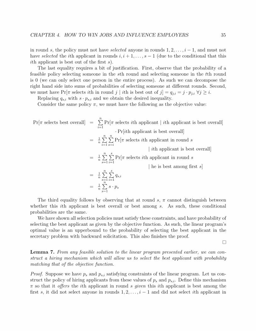
CHAPTER 4. HOW TO WIN JOBS AND INFLUENCE EMPLOYERS 35
in round s, the policy must not have selected anyone in rounds 1, 2, . . . , i− 1, and must nothave selected the ith applicant in rounds i, i+ 1, . . . , s− 1 (due to the conditional that thisith applicant is best out of the first s).
The last equality requires a bit of justification. First, observe that the probability of afeasible policy selecting someone in the sth round and selecting someone in the tth roundis 0 (we can only select one person in the entire process). As such we can decompose theright hand side into sums of probabilities of selecting someone at different rounds. Second,we must have Pr[π selects ith in round j | ith is best out of j] = qj,i = j · pj,i ∀j ≥ i.
Replacing qs,i with s · ps,i and we obtain the desired inequality.Consider the same policy π, we must have the following as the objective value:
Pr[π selects best overall] =n∑i=1
Pr[π selects ith applicant | ith applicant is best overall]
· Pr[ith applicant is best overall]
= 1n
n∑i=1
n∑s=i
Pr[π selects ith applicant in round s
| ith applicant is best overall]
= 1n
n∑s=1
s∑i=1
Pr[π selects ith applicant in round s
| he is best among first s]
= 1n
n∑s=1
s∑i=1
qs,i
= 1n
n∑s=1
s · ps
The third equality follows by observing that at round s, π cannot distinguish betweenwhether this ith applicant is best overall or best among s. As such, these conditionalprobabilities are the same.
We have shown all selection policies must satisfy these constraints, and have probability ofselecting the best applicant as given by the objective function. As such, the linear program’soptimal value is an upperbound to the probability of selecting the best applicant in thesecretary problem with backward solicitation. This also finishes the proof.
Lemma 7. From any feasible solution to the linear program presented earlier, we can con-struct a hiring mechanism which will allow us to select the best applicant with probabilitymatching that of the objective function.
Proof. Suppose we have ps and ps,i satisfying constraints of the linear program. Let us con-struct the policy of hiring applicants from these values of ps and ps,i. Define this mechanismπ so that it offers the ith applicant in round s given this ith applicant is best among thefirst s, it did not select anyone in rounds 1, 2, . . . , i − 1 and did not select ith applicant in
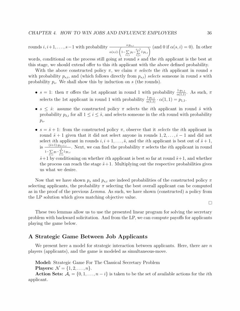
CHAPTER 4. HOW TO WIN JOBS AND INFLUENCE EMPLOYERS 36
rounds i, i+1, . . . , s−1 with probabilitys·ps,i
α(s,i)·(1−∑l<i
pl−s−1∑l≥i
l·pl,i
) (and 0 if α(s, i) = 0). In other
words, conditional on the process still going at round s and the ith applicant is the best atthis stage, we should extend offer to this ith applicant with the above defined probability.
With the above constructed policy π, we claim π selects the ith applicant in round swith probability ps,i, and (which follows directly from ps,i) selects someone in round s withprobability ps. We shall show this by induction on s (the rounds).
• s = 1: then π offers the 1st applicant in round 1 with probability 1·p1,1α(1,1)
. As such, π
selects the 1st applicant in round 1 with probability 1·p1,1α(1,1)
· α(1, 1) = p1,1.
• s ≤ s: assume the constructed policy π selects the ith applicant in round s withprobability ps,i for all 1 ≤ i ≤ s, and selects someone in the sth round with probabilityps.
• s = s + 1: from the constructed policy π, observe that it selects the ith applicant inround s + 1 given that it did not select anyone in rounds 1, 2, . . . , i − 1 and did notselect ith applicant in rounds i, i+ 1, . . . , s, and the ith applicant is best out of s+ 1,
is(s+1)·ps+1,i
1−∑l<i
pl−s∑
l=i
l·pl,i. Next, we can find the probability π selects the ith applicant in round
s+1 by conditioning on whether ith applicant is best so far at round s+1, and whetherthe process can reach the stage s+1. Multiplying out the respective probabilities givesus what we desire.
Now that we have shown ps and ps,i are indeed probabilities of the constructed policy πselecting applicants, the probability π selecting the best overall applicant can be computedas in the proof of the previous Lemma. As such, we have shown (constructed) a policy fromthe LP solution which gives matching objective value.
These two lemmas allow us to use the presented linear program for solving the secretaryproblem with backward solicitation. And from the LP, we can compute payoffs for applicantsplaying the game below.
A Strategic Game Between Job Applicants
We present here a model for strategic interaction between applicants. Here, there are nplayers (applicants), and the game is modeled as simultaneous-move.
Model: Strategic Game For The Classical Secretary ProblemPlayers: N = 1, 2, . . . , n.Action Sets: Ai = 0, 1, . . . , n− i is taken to be the set of available actions for the ith
applicant.
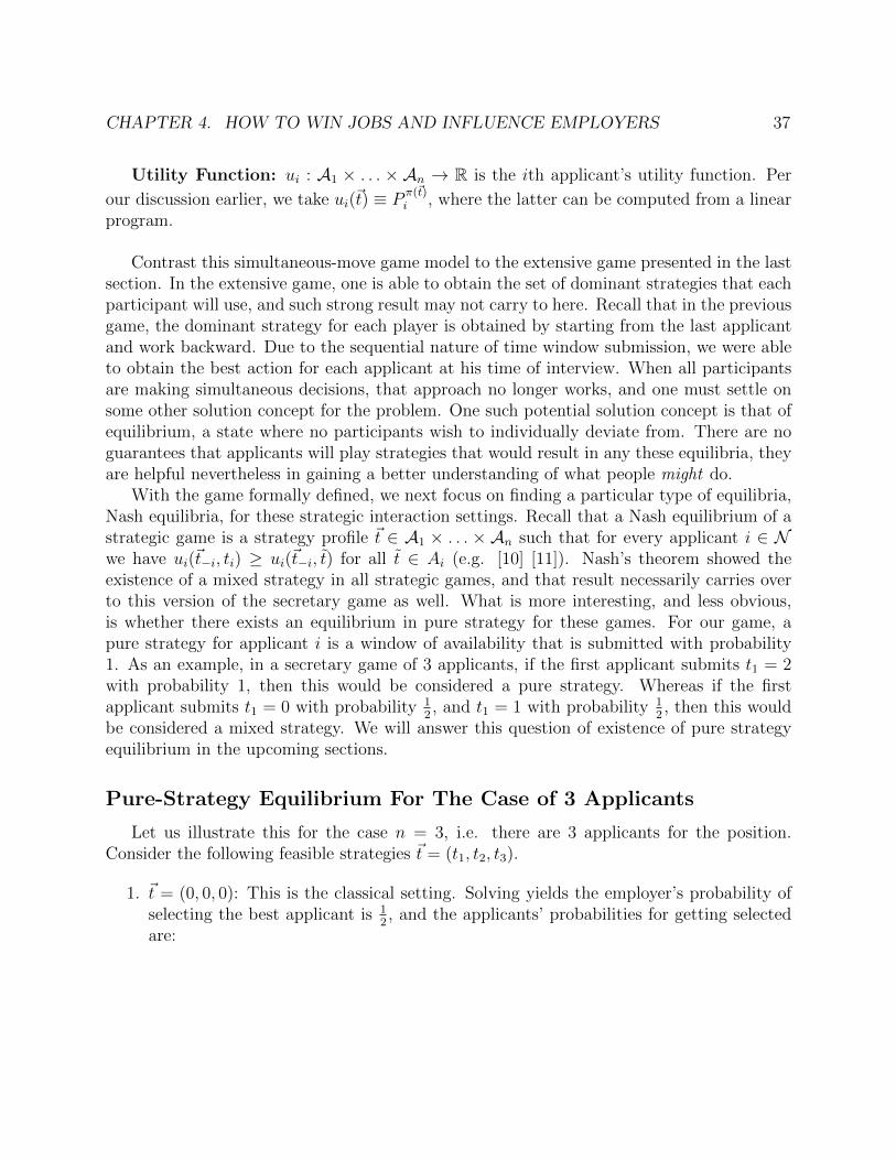
CHAPTER 4. HOW TO WIN JOBS AND INFLUENCE EMPLOYERS 37
Utility Function: ui : A1 × . . . × An → R is the ith applicant’s utility function. Per
our discussion earlier, we take ui(~t) ≡ Pπ(~t)i , where the latter can be computed from a linear
program.
Contrast this simultaneous-move game model to the extensive game presented in the lastsection. In the extensive game, one is able to obtain the set of dominant strategies that eachparticipant will use, and such strong result may not carry to here. Recall that in the previousgame, the dominant strategy for each player is obtained by starting from the last applicantand work backward. Due to the sequential nature of time window submission, we were ableto obtain the best action for each applicant at his time of interview. When all participantsare making simultaneous decisions, that approach no longer works, and one must settle onsome other solution concept for the problem. One such potential solution concept is that ofequilibrium, a state where no participants wish to individually deviate from. There are noguarantees that applicants will play strategies that would result in any these equilibria, theyare helpful nevertheless in gaining a better understanding of what people might do.
With the game formally defined, we next focus on finding a particular type of equilibria,Nash equilibria, for these strategic interaction settings. Recall that a Nash equilibrium of astrategic game is a strategy profile ~t ∈ A1 × . . . × An such that for every applicant i ∈ Nwe have ui(~t−i, ti) ≥ ui(~t−i, t) for all t ∈ Ai (e.g. [10] [11]). Nash’s theorem showed theexistence of a mixed strategy in all strategic games, and that result necessarily carries overto this version of the secretary game as well. What is more interesting, and less obvious,is whether there exists an equilibrium in pure strategy for these games. For our game, apure strategy for applicant i is a window of availability that is submitted with probability1. As an example, in a secretary game of 3 applicants, if the first applicant submits t1 = 2with probability 1, then this would be considered a pure strategy. Whereas if the firstapplicant submits t1 = 0 with probability 1
2, and t1 = 1 with probability 1
2, then this would
be considered a mixed strategy. We will answer this question of existence of pure strategyequilibrium in the upcoming sections.
Pure-Strategy Equilibrium For The Case of 3 Applicants
Let us illustrate this for the case n = 3, i.e. there are 3 applicants for the position.Consider the following feasible strategies ~t = (t1, t2, t3).
1. ~t = (0, 0, 0): This is the classical setting. Solving yields the employer’s probability ofselecting the best applicant is 1
2, and the applicants’ probabilities for getting selected
are:
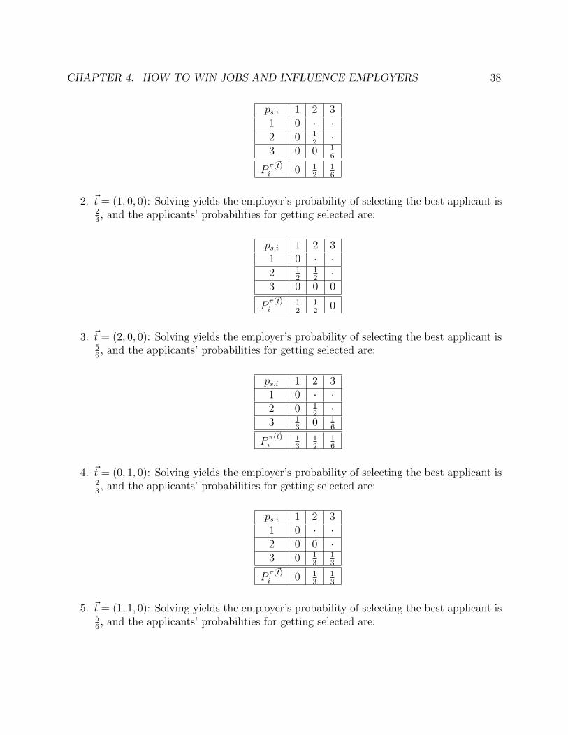
CHAPTER 4. HOW TO WIN JOBS AND INFLUENCE EMPLOYERS 38
ps,i 1 2 31 0 · ·2 0 1
2·
3 0 0 16
Pπ(~t)i 0 1
216
2. ~t = (1, 0, 0): Solving yields the employer’s probability of selecting the best applicant is23, and the applicants’ probabilities for getting selected are:
ps,i 1 2 31 0 · ·2 1
212·
3 0 0 0
Pπ(~t)i
12
12
0
3. ~t = (2, 0, 0): Solving yields the employer’s probability of selecting the best applicant is56, and the applicants’ probabilities for getting selected are:
ps,i 1 2 31 0 · ·2 0 1
2·
3 13
0 16
Pπ(~t)i
13
12
16
4. ~t = (0, 1, 0): Solving yields the employer’s probability of selecting the best applicant is23, and the applicants’ probabilities for getting selected are:
ps,i 1 2 31 0 · ·2 0 0 ·3 0 1
313
Pπ(~t)i 0 1
313
5. ~t = (1, 1, 0): Solving yields the employer’s probability of selecting the best applicant is56, and the applicants’ probabilities for getting selected are:
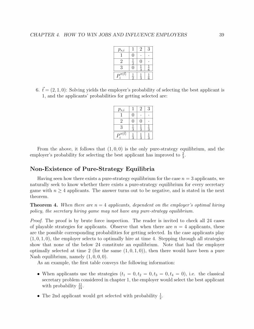
CHAPTER 4. HOW TO WIN JOBS AND INFLUENCE EMPLOYERS 39
ps,i 1 2 31 0 · ·2 1
20 ·
3 0 13
16
Pπ(~t)i
12
13
16
6. ~t = (2, 1, 0): Solving yields the employer’s probability of selecting the best applicant is1, and the applicants’ probabilities for getting selected are:
ps,i 1 2 31 0 · ·2 0 0 ·3 1
313
13
Pπ(~t)i
13
13
13
From the above, it follows that (1, 0, 0) is the only pure-strategy equilibrium, and theemployer’s probability for selecting the best applicant has improved to 2
3.
Non-Existence of Pure-Strategy Equilibria
Having seen how there exists a pure-strategy equilibrium for the case n = 3 applicants, wenaturally seek to know whether there exists a pure-strategy equilibrium for every secretarygame with n ≥ 4 applicants. The answer turns out to be negative, and is stated in the nexttheorem.
Theorem 4. When there are n = 4 applicants, dependent on the employer’s optimal hiringpolicy, the secretary hiring game may not have any pure-strategy equilibrium.
Proof. The proof is by brute force inspection. The reader is invited to check all 24 casesof playable strategies for applicants. Observe that when there are n = 4 applicants, theseare the possible corresponding probabilities for getting selected. In the case applicants play(1, 0, 1, 0), the employer selects to optimally hire at time 4. Stepping through all strategiesshow that none of the below 24 constitute an equilibrium. Note that had the employeroptimally selected at time 2 (for the same (1, 0, 1, 0)), then there would have been a pureNash equilibrium, namely (1, 0, 0, 0).
As an example, the first table conveys the following information:
• When applicants use the strategies (t1 = 0, t2 = 0, t3 = 0, t4 = 0), i.e. the classicalsecretary problem considered in chapter 1, the employer would select the best applicantwith probability 11
24.
• The 2nd applicant would get selected with probability 12.
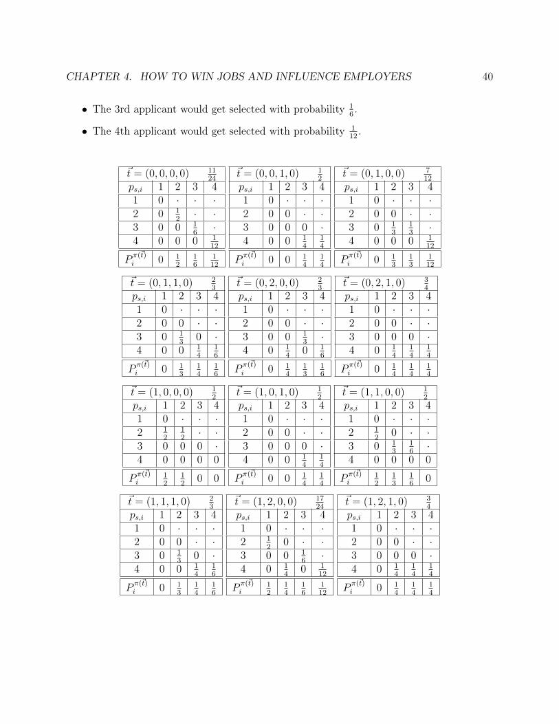
CHAPTER 4. HOW TO WIN JOBS AND INFLUENCE EMPLOYERS 40
• The 3rd applicant would get selected with probability 16.
• The 4th applicant would get selected with probability 112
.
~t = (0, 0, 0, 0) 1124
ps,i 1 2 3 41 0 · · ·2 0 1
2· ·
3 0 0 16·
4 0 0 0 112
Pπ(~t)i 0 1
216
112
~t = (0, 0, 1, 0) 12
ps,i 1 2 3 41 0 · · ·2 0 0 · ·3 0 0 0 ·4 0 0 1
414
Pπ(~t)i 0 0 1
414
~t = (0, 1, 0, 0) 712
ps,i 1 2 3 41 0 · · ·2 0 0 · ·3 0 1
313·
4 0 0 0 112
Pπ(~t)i 0 1
313
112
~t = (0, 1, 1, 0) 23
ps,i 1 2 3 41 0 · · ·2 0 0 · ·3 0 1
30 ·
4 0 0 14
16
Pπ(~t)i 0 1
314
16
~t = (0, 2, 0, 0) 23
ps,i 1 2 3 41 0 · · ·2 0 0 · ·3 0 0 1
3·
4 0 14
0 16
Pπ(~t)i 0 1
413
16
~t = (0, 2, 1, 0) 34
ps,i 1 2 3 41 0 · · ·2 0 0 · ·3 0 0 0 ·4 0 1
414
14
Pπ(~t)i 0 1
414
14
~t = (1, 0, 0, 0) 12
ps,i 1 2 3 41 0 · · ·2 1
212· ·
3 0 0 0 ·4 0 0 0 0
Pπ(~t)i
12
12
0 0
~t = (1, 0, 1, 0) 12
ps,i 1 2 3 41 0 · · ·2 0 0 · ·3 0 0 0 ·4 0 0 1
414
Pπ(~t)i 0 0 1
414
~t = (1, 1, 0, 0) 12
ps,i 1 2 3 41 0 · · ·2 1
20 · ·
3 0 13
16·
4 0 0 0 0
Pπ(~t)i
12
13
16
0
~t = (1, 1, 1, 0) 23
ps,i 1 2 3 41 0 · · ·2 0 0 · ·3 0 1
30 ·
4 0 0 14
16
Pπ(~t)i 0 1
314
16
~t = (1, 2, 0, 0) 1724
ps,i 1 2 3 41 0 · · ·2 1
20 · ·
3 0 0 16·
4 0 14
0 112
Pπ(~t)i
12
14
16
112
~t = (1, 2, 1, 0) 34
ps,i 1 2 3 41 0 · · ·2 0 0 · ·3 0 0 0 ·4 0 1
414
14
Pπ(~t)i 0 1
414
14
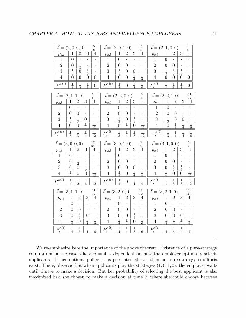
CHAPTER 4. HOW TO WIN JOBS AND INFLUENCE EMPLOYERS 41
~t = (2, 0, 0, 0) 58
ps,i 1 2 3 41 0 · · ·2 0 1
2· ·
3 13
0 16·
4 0 0 0 0
Pπ(~t)i
13
12
16
0
~t = (2, 0, 1, 0) 23
ps,i 1 2 3 41 0 · · ·2 0 0 · ·3 1
30 0 ·
4 0 0 14
16
Pπ(~t)i
13
0 14
16
~t = (2, 1, 0, 0) 34
ps,i 1 2 3 41 0 · · ·2 0 0 · ·3 1
313
13·
4 0 0 0 0
Pπ(~t)i
13
13
13
0
~t = (2, 1, 1, 0) 56
ps,i 1 2 3 41 0 · · ·2 0 0 · ·3 1
313
0 ·4 0 0 1
4112
Pπ(~t)i
13
13
14
112
~t = (2, 2, 0, 0) 56
ps,i 1 2 3 41 0 · · ·2 0 0 · ·3 1
30 1
3·
4 0 14
0 112
Pπ(~t)i
13
14
13
112
~t = (2, 2, 1, 0) 1112
ps,i 1 2 3 41 0 · · ·2 0 0 · ·3 1
30 0 ·
4 0 14
14
16
Pπ(~t)i
13
14
14
16
~t = (3, 0, 0, 0) 1724
ps,i 1 2 3 41 0 · · ·2 0 1
2· ·
3 0 0 16·
4 14
0 0 112
Pπ(~t)i
14
12
16
112
~t = (3, 0, 1, 0) 34
ps,i 1 2 3 41 0 · · ·2 0 0 · ·3 0 0 0 ·4 1
40 1
414
Pπ(~t)i
14
0 14
14
~t = (3, 1, 0, 0) 56
ps,i 1 2 3 41 0 · · ·2 0 0 · ·3 0 1
313·
4 14
0 0 112
Pπ(~t)i
14
13
13
112
~t = (3, 1, 1, 0) 1112
ps,i 1 2 3 41 0 · · ·2 0 0 · ·3 0 1
30 ·
4 14
0 14
16
Pπ(~t)i
14
13
14
16
~t = (3, 2, 0, 0) 1112
ps,i 1 2 3 41 0 · · ·2 0 0 · ·3 0 0 1
3·
4 14
14
0 16
Pπ(~t)i
14
14
13
16
~t = (3, 2, 1, 0) 1212
ps,i 1 2 3 41 0 · · ·2 0 0 · ·3 0 0 0 ·4 1
414
14
14
Pπ(~t)i
14
14
14
14
We re-emphasize here the importance of the above theorem. Existence of a pure-strategyequilibrium in the case where n = 4 is dependent on how the employer optimally selectsapplicants. If her optimal policy is as presented above, then no pure-strategy equilibriaexist. There, observe that when applicants play the strategies (1, 0, 1, 0), the employer waitsuntil time 4 to make a decision. But her probability of selecting the best applicant is alsomaximized had she chosen to make a decision at time 2, where she could choose between
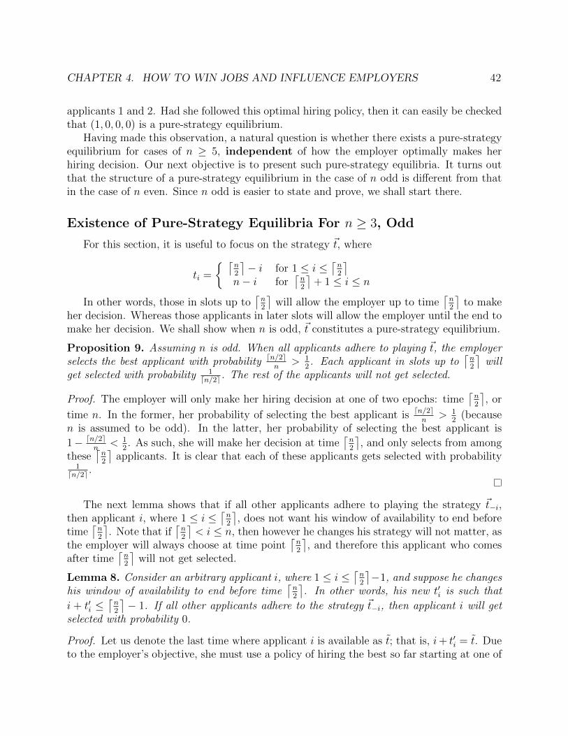
CHAPTER 4. HOW TO WIN JOBS AND INFLUENCE EMPLOYERS 42
applicants 1 and 2. Had she followed this optimal hiring policy, then it can easily be checkedthat (1, 0, 0, 0) is a pure-strategy equilibrium.
Having made this observation, a natural question is whether there exists a pure-strategyequilibrium for cases of n ≥ 5, independent of how the employer optimally makes herhiring decision. Our next objective is to present such pure-strategy equilibria. It turns outthat the structure of a pure-strategy equilibrium in the case of n odd is different from thatin the case of n even. Since n odd is easier to state and prove, we shall start there.
Existence of Pure-Strategy Equilibria For n ≥ 3, Odd
For this section, it is useful to focus on the strategy ~t, where
ti =
⌈n2
⌉− i for 1 ≤ i ≤
⌈n2
⌉n− i for
⌈n2
⌉+ 1 ≤ i ≤ n
In other words, those in slots up to⌈n2
⌉will allow the employer up to time
⌈n2
⌉to make
her decision. Whereas those applicants in later slots will allow the employer until the end tomake her decision. We shall show when n is odd, ~t constitutes a pure-strategy equilibrium.
Proposition 9. Assuming n is odd. When all applicants adhere to playing ~t, the employerselects the best applicant with probability dn/2e
n> 1
2. Each applicant in slots up to
⌈n2
⌉will
get selected with probability 1dn/2e . The rest of the applicants will not get selected.
Proof. The employer will only make her hiring decision at one of two epochs: time⌈n2
⌉, or
time n. In the former, her probability of selecting the best applicant is dn/2en
> 12
(becausen is assumed to be odd). In the latter, her probability of selecting the best applicant is
1− dn/2en
< 12. As such, she will make her decision at time
⌈n2
⌉, and only selects from among
these⌈n2
⌉applicants. It is clear that each of these applicants gets selected with probability
1dn/2e .
The next lemma shows that if all other applicants adhere to playing the strategy ~t−i,then applicant i, where 1 ≤ i ≤
⌈n2
⌉, does not want his window of availability to end before
time⌈n2
⌉. Note that if
⌈n2
⌉< i ≤ n, then however he changes his strategy will not matter, as
the employer will always choose at time point⌈n2
⌉, and therefore this applicant who comes
after time⌈n2
⌉will not get selected.
Lemma 8. Consider an arbitrary applicant i, where 1 ≤ i ≤⌈n2
⌉−1, and suppose he changes
his window of availability to end before time⌈n2
⌉. In other words, his new t′i is such that
i + t′i ≤⌈n2
⌉− 1. If all other applicants adhere to the strategy ~t−i, then applicant i will get
selected with probability 0.
Proof. Let us denote the last time where applicant i is available as t; that is, i+ t′i = t. Dueto the employer’s objective, she must use a policy of hiring the best so far starting at one of
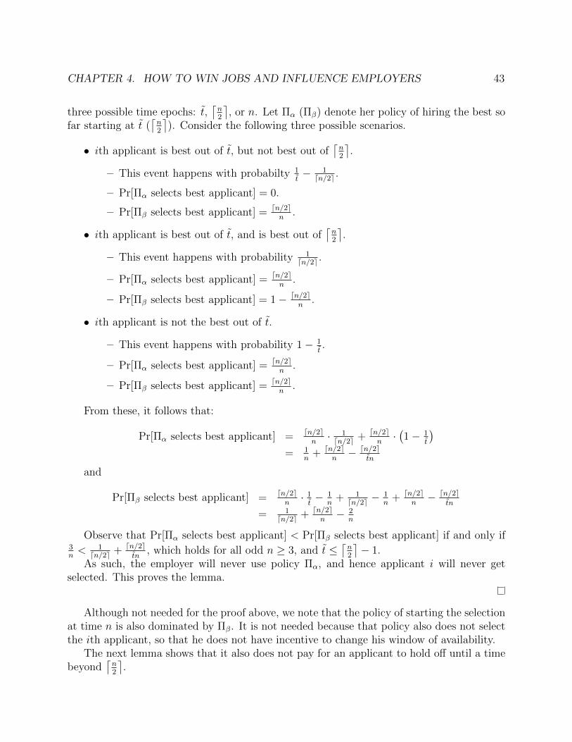
CHAPTER 4. HOW TO WIN JOBS AND INFLUENCE EMPLOYERS 43
three possible time epochs: t,⌈n2
⌉, or n. Let Πα (Πβ) denote her policy of hiring the best so
far starting at t (⌈n2
⌉). Consider the following three possible scenarios.
• ith applicant is best out of t, but not best out of⌈n2
⌉.
– This event happens with probabilty 1t− 1dn/2e .
– Pr[Πα selects best applicant] = 0.
– Pr[Πβ selects best applicant] = dn/2en
.
• ith applicant is best out of t, and is best out of⌈n2
⌉.
– This event happens with probability 1dn/2e .
– Pr[Πα selects best applicant] = dn/2en
.
– Pr[Πβ selects best applicant] = 1− dn/2en
.
• ith applicant is not the best out of t.
– This event happens with probability 1− 1t.
– Pr[Πα selects best applicant] = dn/2en
.
– Pr[Πβ selects best applicant] = dn/2en
.
From these, it follows that:
Pr[Πα selects best applicant] = dn/2en· 1dn/2e + dn/2e
n·(1− 1
t
)= 1
n+ dn/2e
n− dn/2e
tn
and
Pr[Πβ selects best applicant] = dn/2en· 1t− 1
n+ 1dn/2e −
1n
+ dn/2en− dn/2e
tn
= 1dn/2e + dn/2e
n− 2
n
Observe that Pr[Πα selects best applicant] < Pr[Πβ selects best applicant] if and only if3n< 1dn/2e + dn/2e
tn, which holds for all odd n ≥ 3, and t ≤
⌈n2
⌉− 1.
As such, the employer will never use policy Πα, and hence applicant i will never getselected. This proves the lemma.
Although not needed for the proof above, we note that the policy of starting the selectionat time n is also dominated by Πβ. It is not needed because that policy also does not selectthe ith applicant, so that he does not have incentive to change his window of availability.
The next lemma shows that it also does not pay for an applicant to hold off until a timebeyond
⌈n2
⌉.
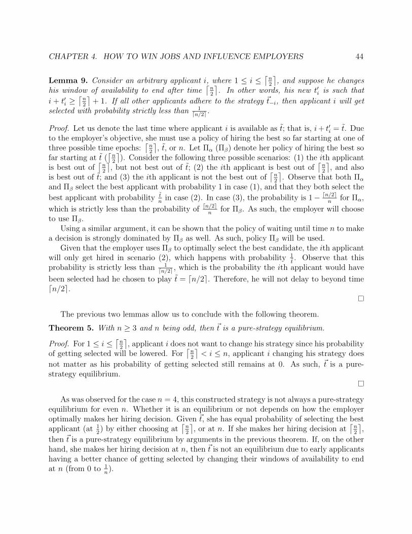
CHAPTER 4. HOW TO WIN JOBS AND INFLUENCE EMPLOYERS 44
Lemma 9. Consider an arbitrary applicant i, where 1 ≤ i ≤⌈n2
⌉, and suppose he changes
his window of availability to end after time⌈n2
⌉. In other words, his new t′i is such that
i + t′i ≥⌈n2
⌉+ 1. If all other applicants adhere to the strategy ~t−i, then applicant i will get
selected with probability strictly less than 1dn/2e .
Proof. Let us denote the last time where applicant i is available as t; that is, i+ t′i = t. Dueto the employer’s objective, she must use a policy of hiring the best so far starting at one ofthree possible time epochs:
⌈n2
⌉, t, or n. Let Πα (Πβ) denote her policy of hiring the best so
far starting at t (⌈n2
⌉). Consider the following three possible scenarios: (1) the ith applicant
is best out of⌈n2
⌉, but not best out of t; (2) the ith applicant is best out of
⌈n2
⌉, and also
is best out of t; and (3) the ith applicant is not the best out of⌈n2
⌉. Observe that both Πα
and Πβ select the best applicant with probability 1 in case (1), and that they both select the
best applicant with probability tn
in case (2). In case (3), the probability is 1− dn/2en
for Πα,
which is strictly less than the probability of dn/2en
for Πβ. As such, the employer will chooseto use Πβ.
Using a similar argument, it can be shown that the policy of waiting until time n to makea decision is strongly dominated by Πβ as well. As such, policy Πβ will be used.
Given that the employer uses Πβ to optimally select the best candidate, the ith applicantwill only get hired in scenario (2), which happens with probability 1
t. Observe that this
probability is strictly less than 1dn/2e , which is the probability the ith applicant would have
been selected had he chosen to play t = dn/2e. Therefore, he will not delay to beyond timedn/2e.
The previous two lemmas allow us to conclude with the following theorem.
Theorem 5. With n ≥ 3 and n being odd, then ~t is a pure-strategy equilibrium.
Proof. For 1 ≤ i ≤⌈n2
⌉, applicant i does not want to change his strategy since his probability
of getting selected will be lowered. For⌈n2
⌉< i ≤ n, applicant i changing his strategy does
not matter as his probability of getting selected still remains at 0. As such, ~t is a pure-strategy equilibrium.
As was observed for the case n = 4, this constructed strategy is not always a pure-strategyequilibrium for even n. Whether it is an equilibrium or not depends on how the employeroptimally makes her hiring decision. Given ~t, she has equal probability of selecting the bestapplicant (at 1
2) by either choosing at
⌈n2
⌉, or at n. If she makes her hiring decision at
⌈n2
⌉,
then ~t is a pure-strategy equilibrium by arguments in the previous theorem. If, on the otherhand, she makes her hiring decision at n, then ~t is not an equilibrium due to early applicantshaving a better chance of getting selected by changing their windows of availability to endat n (from 0 to 1
n).
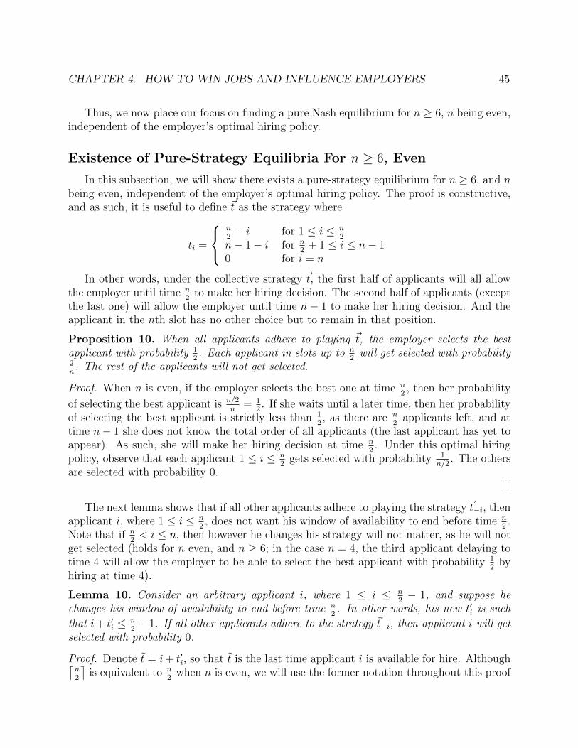
CHAPTER 4. HOW TO WIN JOBS AND INFLUENCE EMPLOYERS 45
Thus, we now place our focus on finding a pure Nash equilibrium for n ≥ 6, n being even,independent of the employer’s optimal hiring policy.
Existence of Pure-Strategy Equilibria For n ≥ 6, Even
In this subsection, we will show there exists a pure-strategy equilibrium for n ≥ 6, and nbeing even, independent of the employer’s optimal hiring policy. The proof is constructive,and as such, it is useful to define ~t as the strategy where
ti =
n2− i for 1 ≤ i ≤ n
2
n− 1− i for n2
+ 1 ≤ i ≤ n− 10 for i = n
In other words, under the collective strategy ~t, the first half of applicants will all allowthe employer until time n
2to make her hiring decision. The second half of applicants (except
the last one) will allow the employer until time n− 1 to make her hiring decision. And theapplicant in the nth slot has no other choice but to remain in that position.
Proposition 10. When all applicants adhere to playing ~t, the employer selects the bestapplicant with probability 1
2. Each applicant in slots up to n
2will get selected with probability
2n
. The rest of the applicants will not get selected.
Proof. When n is even, if the employer selects the best one at time n2, then her probability
of selecting the best applicant is n/2n
= 12. If she waits until a later time, then her probability
of selecting the best applicant is strictly less than 12, as there are n
2applicants left, and at
time n− 1 she does not know the total order of all applicants (the last applicant has yet toappear). As such, she will make her hiring decision at time n
2. Under this optimal hiring
policy, observe that each applicant 1 ≤ i ≤ n2
gets selected with probability 1n/2
. The othersare selected with probability 0.
The next lemma shows that if all other applicants adhere to playing the strategy ~t−i, thenapplicant i, where 1 ≤ i ≤ n
2, does not want his window of availability to end before time n
2.
Note that if n2< i ≤ n, then however he changes his strategy will not matter, as he will not
get selected (holds for n even, and n ≥ 6; in the case n = 4, the third applicant delaying totime 4 will allow the employer to be able to select the best applicant with probability 1
2by
hiring at time 4).
Lemma 10. Consider an arbitrary applicant i, where 1 ≤ i ≤ n2− 1, and suppose he
changes his window of availability to end before time n2. In other words, his new t′i is such
that i+ t′i ≤ n2− 1. If all other applicants adhere to the strategy ~t−i, then applicant i will get
selected with probability 0.
Proof. Denote t = i+ t′i, so that t is the last time applicant i is available for hire. Although⌈n2
⌉is equivalent to n
2when n is even, we will use the former notation throughout this proof
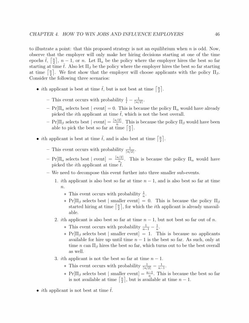
CHAPTER 4. HOW TO WIN JOBS AND INFLUENCE EMPLOYERS 46
to illustrate a point: that this proposed strategy is not an equilibrium when n is odd. Now,observe that the employer will only make her hiring decisions starting at one of the timeepochs t,
⌈n2
⌉, n − 1, or n. Let Πα be the policy where the employer hires the best so far
starting at time t. Also let Πβ be the policy where the employer hires the best so far startingat time
⌈n2
⌉. We first show that the employer will choose applicants with the policy Πβ.
Consider the following three scenarios:
• ith applicant is best at time t, but is not best at time⌈n2
⌉.
– This event occurs with probability 1t− 1dn/2e .
– Pr[Πα selects best | event] = 0. This is because the policy Πα would have alreadypicked the ith applicant at time t, which is not the best overall.
– Pr[Πβ selects best | event] = dn/2en
. This is because the policy Πβ would have beenable to pick the best so far at time
⌈n2
⌉.
• ith applicant is best at time t, and is also best at time⌈n2
⌉.
– This event occurs with probability 1dn/2e .
– Pr[Πα selects best | event] = dn/2en
. This is because the policy Πα would havepicked the ith applicant at time t.
– We need to decompose this event further into three smaller sub-events.
1. ith applicant is also best so far at time n− 1, and is also best so far at timen.
∗ This event occurs with probability 1n.
∗ Pr[Πβ selects best | smaller event] = 0. This is because the policy Πβ
started hiring at time⌈n2
⌉, for which the ith applicant is already unavail-
able.
2. ith applicant is also best so far at time n− 1, but not best so far out of n.
∗ This event occurs with probability 1n−1 −
1n.
∗ Pr[Πβ selects best | smaller event] = 1. This is because no applicantsavailable for hire up until time n− 1 is the best so far. As such, only attime n can Πβ hires the best so far, which turns out to be the best overallas well.
3. ith applicant is not the best so far at time n− 1.
∗ This event occurs with probability 1dn/2e −
1n−1 .
∗ Pr[Πβ selects best | smaller event] = n−1n
. This is because the best so faris not available at time
⌈n2
⌉, but is available at time n− 1.
• ith applicant is not best at time t.
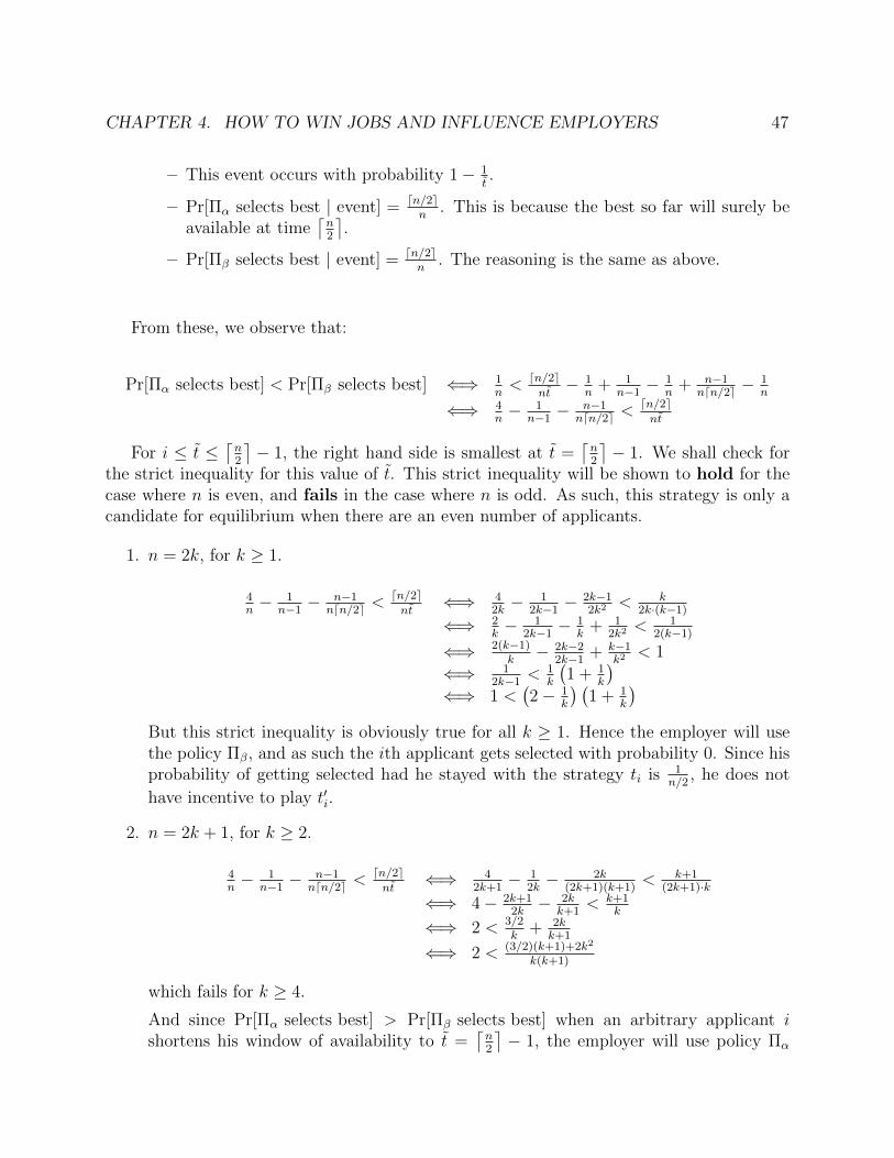
CHAPTER 4. HOW TO WIN JOBS AND INFLUENCE EMPLOYERS 47
– This event occurs with probability 1− 1t.
– Pr[Πα selects best | event] = dn/2en
. This is because the best so far will surely beavailable at time
⌈n2
⌉.
– Pr[Πβ selects best | event] = dn/2en
. The reasoning is the same as above.
From these, we observe that:
Pr[Πα selects best] < Pr[Πβ selects best] ⇐⇒ 1n< dn/2e
nt− 1
n+ 1
n−1 −1n
+ n−1ndn/2e −
1n
⇐⇒ 4n− 1
n−1 −n−1ndn/2e <
dn/2ent
For i ≤ t ≤⌈n2
⌉− 1, the right hand side is smallest at t =
⌈n2
⌉− 1. We shall check for
the strict inequality for this value of t. This strict inequality will be shown to hold for thecase where n is even, and fails in the case where n is odd. As such, this strategy is only acandidate for equilibrium when there are an even number of applicants.
1. n = 2k, for k ≥ 1.
4n− 1
n−1 −n−1ndn/2e <
dn/2ent
⇐⇒ 42k− 1
2k−1 −2k−12k2
< k2k·(k−1)
⇐⇒ 2k− 1
2k−1 −1k
+ 12k2
< 12(k−1)
⇐⇒ 2(k−1)k− 2k−2
2k−1 + k−1k2
< 1
⇐⇒ 12k−1 <
1k
(1 + 1
k
)⇐⇒ 1 <
(2− 1
k
) (1 + 1
k
)But this strict inequality is obviously true for all k ≥ 1. Hence the employer will usethe policy Πβ, and as such the ith applicant gets selected with probability 0. Since hisprobability of getting selected had he stayed with the strategy ti is 1
n/2, he does not
have incentive to play t′i.
2. n = 2k + 1, for k ≥ 2.
4n− 1
n−1 −n−1ndn/2e <
dn/2ent
⇐⇒ 42k+1− 1
2k− 2k
(2k+1)(k+1)< k+1
(2k+1)·k⇐⇒ 4− 2k+1
2k− 2k
k+1< k+1
k
⇐⇒ 2 < 3/2k
+ 2kk+1
⇐⇒ 2 < (3/2)(k+1)+2k2
k(k+1)
which fails for k ≥ 4.
And since Pr[Πα selects best] > Pr[Πβ selects best] when an arbitrary applicant ishortens his window of availability to t =
⌈n2
⌉− 1, the employer will use policy Πα
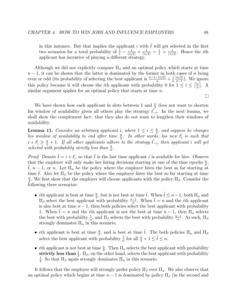
CHAPTER 4. HOW TO WIN JOBS AND INFLUENCE EMPLOYERS 48
in this instance. But that implies the applicant i with t will get selected in the firsttwo scenarios for a total probability of 1
t− 1dn/2e + 1
dn/2e = 1t> 1dn/2e . Hence the ith
applicant has incentive of playing a different strategy.
Although we did not explicitly compare Πβ and an optimal policy which starts at timen − 1, it can be shown that the latter is dominated by the former in both cases of n beingeven or odd (its probability of selecting the best applicant is n−1−dn/2e
n+ 1
ndn/2en−1 ). We ignore
this policy because it will choose the ith applicant with probability 0 for 1 ≤ i ≤⌈n2
⌉. A
similar argument applies for an optimal policy that starts at time n.
We have shown how each applicant in slots between 1 and n2
does not want to shorten
his window of availability given all others play the strategy ~t−i. In the next lemma, weshall show the complement fact: that they also do not want to lengthen their windows ofavailability.
Lemma 11. Consider an arbitrary applicant i, where 1 ≤ i ≤ n2, and suppose he changes
his window of availability to end after time n2. In other words, his new t′i is such that
i + t′i ≥ n2
+ 1. If all other applicants adhere to the strategy ~t−i, then applicant i will getselected with probability strictly less than 2
n.
Proof. Denote t = i + t′i, so that t is the last time applicant i is available for hire. Observethat the employer will only make her hiring decisions starting at one of the time epochs n
2,
t, n − 1, or n. Let Πα be the policy where the employer hires the best so far starting attime t. Also let Πβ be the policy where the employer hires the best so far starting at timen2. We first show that the employer will choose applicants with the policy Πβ. Consider the
following three scenarios:
• ith applicant is best at time n2, but is not best at time t. When t ≤ n−1, both Πα and
Πβ select the best applicant with probability n−1n
. When t = n and the ith applicantis also best at time n− 1, then both policies select the best applicant with probability1. When t = n and the ith applicant is not the best at time n − 1, then Πα selectsthe best with probability 1
n, and Πβ selects the best with probability n−1
n. As such, Πβ
strongly dominates Πα in this scenario.
• ith applicant is best at time n2, and is best at time t. The both policies Πα and Πβ
select the best applicant with probability tn
for all n2
+ 1 ≤ t ≤ n.
• ith applicant is not best at time n2. Then Πα selects the best applicant with probability
strictly less than 12. Πβ, on the other hand, selects the best applicant with probability
12. So that Πβ again strongly dominates Πα in this scenario.
It follows that the employer will strongly prefer policy Πβ over Πα. We also observe thatan optimal policy which begins at time n− 1 is dominated by policy Πβ (in the second and
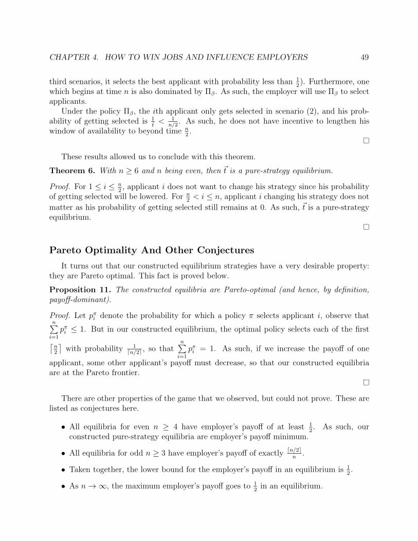
CHAPTER 4. HOW TO WIN JOBS AND INFLUENCE EMPLOYERS 49
third scenarios, it selects the best applicant with probability less than 12). Furthermore, one
which begins at time n is also dominated by Πβ. As such, the employer will use Πβ to selectapplicants.
Under the policy Πβ, the ith applicant only gets selected in scenario (2), and his prob-ability of getting selected is 1
t< 1
n/2. As such, he does not have incentive to lengthen his
window of availability to beyond time n2.
These results allowed us to conclude with this theorem.
Theorem 6. With n ≥ 6 and n being even, then ~t is a pure-strategy equilibrium.
Proof. For 1 ≤ i ≤ n2, applicant i does not want to change his strategy since his probability
of getting selected will be lowered. For n2< i ≤ n, applicant i changing his strategy does not
matter as his probability of getting selected still remains at 0. As such, ~t is a pure-strategyequilibrium.
Pareto Optimality And Other Conjectures
It turns out that our constructed equilibrium strategies have a very desirable property:they are Pareto optimal. This fact is proved below.
Proposition 11. The constructed equilibria are Pareto-optimal (and hence, by definition,payoff-dominant).
Proof. Let pπi denote the probability for which a policy π selects applicant i, observe thatn∑i=1
pπi ≤ 1. But in our constructed equilibrium, the optimal policy selects each of the first⌈n2
⌉with probability 1
dn/2e , so thatn∑i=1
pπi = 1. As such, if we increase the payoff of one
applicant, some other applicant’s payoff must decrease, so that our constructed equilibriaare at the Pareto frontier.
There are other properties of the game that we observed, but could not prove. These arelisted as conjectures here.
• All equilibria for even n ≥ 4 have employer’s payoff of at least 12. As such, our
constructed pure-strategy equilibria are employer’s payoff minimum.
• All equilibria for odd n ≥ 3 have employer’s payoff of exactly dn/2en
.
• Taken together, the lower bound for the employer’s payoff in an equilibrium is 12.
• As n→∞, the maximum employer’s payoff goes to 12
in an equilibrium.
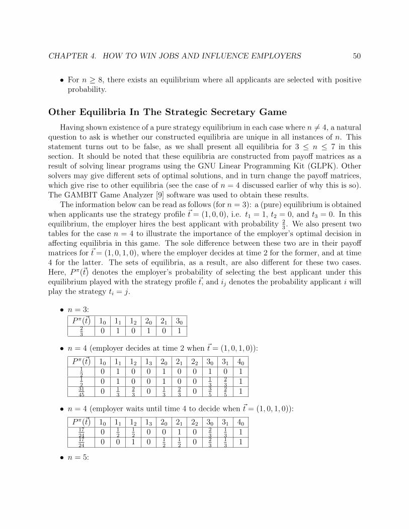
CHAPTER 4. HOW TO WIN JOBS AND INFLUENCE EMPLOYERS 50
• For n ≥ 8, there exists an equilibrium where all applicants are selected with positiveprobability.
Other Equilibria In The Strategic Secretary Game
Having shown existence of a pure strategy equilibrium in each case where n 6= 4, a naturalquestion to ask is whether our constructed equilibria are unique in all instances of n. Thisstatement turns out to be false, as we shall present all equilibria for 3 ≤ n ≤ 7 in thissection. It should be noted that these equilibria are constructed from payoff matrices as aresult of solving linear programs using the GNU Linear Programming Kit (GLPK). Othersolvers may give different sets of optimal solutions, and in turn change the payoff matrices,which give rise to other equilibria (see the case of n = 4 discussed earlier of why this is so).The GAMBIT Game Analyzer [9] software was used to obtain these results.
The information below can be read as follows (for n = 3): a (pure) equilibrium is obtainedwhen applicants use the strategy profile ~t = (1, 0, 0), i.e. t1 = 1, t2 = 0, and t3 = 0. In thisequilibrium, the employer hires the best applicant with probability 2
3. We also present two
tables for the case n = 4 to illustrate the importance of the employer’s optimal decision inaffecting equilibria in this game. The sole difference between these two are in their payoffmatrices for ~t = (1, 0, 1, 0), where the employer decides at time 2 for the former, and at time4 for the latter. The sets of equilibria, as a result, are also different for these two cases.Here, P π(~t) denotes the employer’s probability of selecting the best applicant under thisequilibrium played with the strategy profile ~t, and ij denotes the probability applicant i willplay the strategy ti = j.
• n = 3:
P π(~t) 10 11 12 20 21 3023
0 1 0 1 0 1
• n = 4 (employer decides at time 2 when ~t = (1, 0, 1, 0)):
P π(~t) 10 11 12 13 20 21 22 30 31 4012
0 1 0 0 1 0 0 1 0 112
0 1 0 0 1 0 0 13
23
13145
0 13
23
0 13
23
0 35
25
1
• n = 4 (employer waits until time 4 to decide when ~t = (1, 0, 1, 0)):
P π(~t) 10 11 12 13 20 21 22 30 31 401724
0 12
12
0 0 1 0 23
13
11724
0 0 1 0 12
12
0 23
13
1
• n = 5:
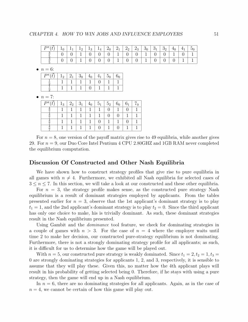
CHAPTER 4. HOW TO WIN JOBS AND INFLUENCE EMPLOYERS 51
P π(~t) 10 11 12 13 14 20 21 22 23 30 31 32 40 41 5035
0 0 1 0 0 0 1 0 0 1 0 0 1 0 135
0 0 1 0 0 0 1 0 0 1 0 0 0 1 1
• n = 6:
P π(~t) 12 21 30 40 41 50 6012
1 1 1 1 0 1 112
1 1 1 0 1 1 1
• n = 7:
P π(~t) 13 22 31 40 51 52 60 61 7047
1 1 1 1 1 0 1 0 147
1 1 1 1 1 0 0 1 147
1 1 1 1 0 1 1 0 147
1 1 1 1 0 1 0 1 1
For n = 8, one version of the payoff matrix gives rise to 49 equilibria, while another gives29. For n = 9, our Duo Core Intel Pentium 4 CPU 2.80GHZ and 1GB RAM never completedthe equilibrium computation.
Discussion Of Constructed and Other Nash Equilibria
We have shown how to construct strategy profiles that give rise to pure equilibria inall games with n 6= 4. Furthermore, we exhibited all Nash equilibria for selected cases of3 ≤ n ≤ 7. In this section, we will take a look at our constructed and these other equilibria.
For n = 3, the strategy profile makes sense, as the constructed pure strategy Nashequilibrium is a result of dominant strategies employed by applicants. From the tablespresented earlier for n = 3, observe that the 1st applicant’s dominant strategy is to playt1 = 1, and the 2nd applicant’s dominant strategy is to play t2 = 0. Since the third applicanthas only one choice to make, his is trivially dominant. As such, these dominant strategiesresult in the Nash equilibrium presented.
Using Gambit and the dominance tool feature, we check for dominating strategies ina couple of games with n > 3. For the case of n = 4 where the employer waits untiltime 2 to make her decision, our constructed pure-strategy equilibrium is not dominating.Furthermore, there is not a strongly dominating strategy profile for all applicants; as such,it is difficult for us to determine how the game will be played out.
With n = 5, our constructed pure strategy is weakly dominated. Since t1 = 2, t2 = 1, t3 =0 are strongly dominating strategies for applicants 1, 2, and 3, respectively, it is sensible toassume that they will play these. Given this, no matter how the 4th applicant plays willresult in his probability of getting selected being 0. Therefore, if he stays with using a purestrategy, then the game will end up in a Nash equilibrium.
In n = 6, there are no dominating strategies for all applicants. Again, as in the case ofn = 4, we cannot be certain of how this game will play out.
CHAPTER 4. HOW TO WIN JOBS AND INFLUENCE EMPLOYERS 52
For n = 7, again there are no dominating strategies for all applicants. It is not clearif participants will use strategies that would result in any of the presented equilibria con-structed. In fact, we conjecture that this pattern will continue for games of higher value ofn, namely the nonexistence of dominating strategies that would result in a Nash equilibrium.
4.4 Concluding Notes On Game-Theoretic Approach
In this chapter, we presented two game-theoretic approaches to the classical secretaryproblem. By allowing applicants the freedom to determine their windows of availabilitywith non-binding commitment, the employer can improve her probability of selecting thebest candidate and gain the desired property that everyone who is interviewed will get hiredwith the same probability. If the employer chooses to solicit every applicant’s window ofavailability before the first interview begins, and makes this a binding commitment, then theresulting simultaneous game is guaranteed to almost always have a pure-strategy equilibrium.The lone exception to this fact is when n = 4, where its existence is dependent on how theemployer optimally selects applicants. These equilibria are easy to characterize: applicantsbefore time
⌈n2
⌉will wait for a decision until this time, and applicants after time
⌈n2
⌉will
wait for a decision either at time n− 1, or at time n. For some values of n, our constructedequilibria are good indicators of how applicants will strategize. For many other values of n,we believe different equilibria, or none at all, might be agreed on instead. We used Gambitto enumerate all equilibria presented in this strategic game, and illustrated our argumentsfor particular cases of 3 ≤ n ≤ 7. Lastly, we showed certain properties of our constructedequilibria, and left a few interesting conjectures concerning this secretary game.
53
Chapter 5
Concluding Notes
We come to the end of this dissertation hoping to have made the case for the needto consider participants’ behavior in all optimization problems. Our setting throughoutthis dissertation has mostly been confined to a hiring process, and our argument was fornew approaches to the secretary problem. Our main nitpick is the complete ignorance ofhuman incentives in previous attempts at an optimal solution. We extended, compared, andconstrasted an old approach used on another variant of the problem, and showed results whichare markedly different from those found in prior works. We also proposed an alternativegame-theoretic solution, which makes use of the inherent competition between players inthe process, giving them more room to compete, and by doing so, improve the employer’schance of meeting her goal. Simple modifications, like those we have made, change thedynamic of the problem completely and provide new insights into how people should approachthe process. We believe our framework for analysis can be extended to other sequentialdecision settings, where strategic choices of participants play an important role in the process.Whether it’s job hunting, dating, or whatever else that you can think of, good luck searching!
54
Bibliography
[1] Niv Buchbinder, Kamal Jain, and Mohit Singh. “Incentives in Online Auctions viaLinear Programming”. In: WINE’10 Proceedings of the 6th International Conferenceon Internet and Network Economics (2010), pp. 106–117.
[2] Niv Buchbinder, Kamal Jain, and Mohit Singh. “Secretary Problems via Linear Pro-gramming”. In: IPCO’10: 14th International Conference On Integer Programming andCombinatorial Optimization (2010), pp. 163–176.
[3] Y.S. Chow et al. “Optimal Selection Based On Relative Rank”. In: Israel Journal ofMathematics 2.2 (1964), pp. 81–90.
[4] P.R. Freeman. “The Secretary Problem and its Extensions: A Review”. In: Interna-tional Statistical Review 51 (1983), pp. 189–206.
[5] P.R. Freeman. “Who Solved the Secretary Problem?” In: Statistical Science 4.3 (1989),pp. 282–296.
[6] M. Gardner. “Mathematical Games”. In: Scientific American (1960), pp. 150–153.
[7] J.P. Gilbert and F. Mosteller. “Recognizing The Maximum of a Sequence”. In: Journalof American Statistical Association 61 (1966), pp. 35–79.
[8] D.V. Lindley. “Dynamic Programming and Decision Theory”. In: Applied Statistics10.1 (1961), pp. 39–51.
[9] R.D. McKelvey, A.M. McLennan, and T.L. Turocy. “Gambit: Software Tools for GameTheory, Version 13.1.0”. In: (2013).
[10] John Nash. “Equilibrium points in n-person games”. In: Proceedings of the NationalAcademy of Sciences 36.1 (1950), pp. 48–49.
[11] John Nash. “Non-Cooperative Games”. In: The Annals of Mathematics 54.2 (1951),pp. 286–295.
[12] M.C.K. Yang. “Recognizing the Maximum of a Random Sequence Based On Rela-tive Rank With Backward Solicitation”. In: Journal of Applied Probability 11 (1974),pp. 504–512.