Embed Size (px)
Citation preview
K.7
Incentive Contracting Under Ambiguity Aversion Liu, Qi, Lei Lu, and Bo Sun
International Finance Discussion Papers Board of Governors of the Federal Reserve System
Number 1195 February 2017
Please cite paper as: Liu, Qi, Lei Lu, and Bo Sun (2017). Incentive Contracting Under Ambiguity Aversion. International Finance Discussion Papers 1195. https://doi.org/10.17016/IFDP.2017.1195
Board of Governors of the Federal Reserve System
International Finance Discussion Papers
Number 1195
February 2017
Incentive Contracting Under Ambiguity Aversion
Qi Liu, Lei Lu, Bo Sun
NOTE: International Finance Discussion Papers are preliminary materials circulated to stimulate discussion and critical comment. References to International Finance Discussion Papers (other than an acknowledgment that the writer has had access to unpublished material) should be cleared with the author or authors. Recent IFDPs are available on the Web at www.federalreserve.gov/pubs/ifdp/. This paper can be downloaded without charge from the Social Science Research Network electronic library at www.ssrn.com.
Incentive Contracting Under Ambiguity Aversion∗
Qi Liu
Peking University
Lei Lu
University of Manitoba
Bo Sun
Federal Reserve Board
Abstract
This paper studies a principal-agent model in which the information on future firm
performance is ambiguous and the agent is averse to ambiguity. We show that if
firm risk is ambiguous, while stocks always induce the agent to perceive a high risk,
options can induce him to perceive a low risk. As a result, options can be less costly
in incentivizing the agent than stocks in the presence of ambiguity. In addition,
we show that providing the agent with more incentives would induce the agent to
perceive a higher risk, and there is a discontinuous jump in the compensation cost as
incentives increase, which makes the principal reluctant to reset contracts frequently
when underlying fundamentals change. Thus, compensation contracts exhibit an
inertia property. Lastly, the model sheds some light on the use of relative performance
evaluation, and provides a rationale for the puzzle of pay-for-luck in the presence of
ambiguity.
Keywords: Ambiguity, Executive compensation, Options, Relative performance
evaluation
JEL Classification: G30, J33
∗We thank Nicholas Yannelis (the Editor) and two anonymous referees for helpful comments. The viewsexpressed herein are the authors’ and do not necessarily reflect the opinions of the Board of Governorsof the Federal Reserve System. Qi Liu acknowledges support by National Natural Science Foundation ofChina (No. 71502004).
1
1. Introduction
The vast and growing literature on the principal-agent relationship with moral hazard is
usually based on the assumption that both contracting parties are expected utility max-
imizers. In particular, there is only a single prior belief of the distribution of future firm
performances. However, lack of information in start-up companies and emerging industries
may cause individual knowledge about future firm performances to be ambiguous, that is,
multiple possible distributions exist.
We study a principal-agent model in which there are multiple possible probability dis-
tributions of future performances, and the agent is both risk-averse and ambiguity-averse.
The feature of ambiguity-aversion is consistent with the mounting experimental evidence,
including the most notable example Ellsberg Paradox (Ellsberg (1961)) and portfolio choice
experiments (Ahn, Choi, Gale, and Kariv (2009)). Gilboa and Schmeidler (1989) provide
an axiomatic basis for a “max-min” preference to model ambiguity-aversion. Following the
literature, we use the “max-min” preference to model the agent’s behavior. In particular,
if firm risk is ambiguous, the agent’s effort and utility are determined in the following
two steps: first, given the agent’s effort, the agent perceives a level of risk that minimizes
his utility; second, the agent chooses an effort level to maximize the utility that has been
minimized under possible risks.
Our analysis contributes to the compensation literature in that we provide a new,
coherent theoretical explanation for a number of empirical findings that have not been
consistently reconciled with the existing theory, namely, the optimality of option grants,
an inertia property of compensation contracts, and the varied use of relative performance
2
evaluation. We discuss each of them in turn.
First, we show that if there is ambiguity on firm risk, while stocks always induce the
agent to perceive the highest possible risk, options can induce him to perceive the lowest
possible risk. As a result, options can be less costly than stocks in incentivizing the agent in
the presence of ambiguity. In other words, the use of options will induce the agent to under-
estimate risk, leading to overconfidence on the part of managers. While the literature on
overconfident managers takes under-estimation of risk as assumptions, this paper derives
them as a result for an ambiguity-averse agent.
We illustrate the intuition as below: when firm risk is ambiguous, an increase in the firm
risk only increases the variance of stocks, but has no effects on the mean value of stocks. A
risk-averse and ambiguity-averse agent will always perceive the highest risk when he owns
stocks. Therefore, a high risk premium in compensation is required. On the other hand,
an increase in firm risk increases both the mean payoff and variance of options. While an
increase in the variance of options decreases the agent’s utility, an increase in the mean
payoff of options also has a positive effect on his utility. If the agent is not too risk-averse,
he could perceive a low risk. As a result, only a low risk premium is required. If the
reduction in risk premium is sufficiently large, options can be less costly than stocks in
providing appropriate incentives.
Our analysis thus provides a new rationale for the popularity of option compensation
that has triggered much debate in the literature. The calibration of a standard principal-
agent model shows that options should not be a part of an optimal contract (Dittmann
and Maug (2007)), rendering it puzzling as to why options are widely used in practice.
3
While risk-taking incentives have been proposed as the cause (Feltham and Wu (2001),
Dittmann and Yu (2011)),1 several papers show that it is not always true that giving
options to agents will make them more willing to take risk (e.g. Carpenter (2000), Ross
(2004)). Bettis, Bizjak, and Lemmon (2005) also show that managers exercise their options
earlier when volatility increases, and Hayes, Lemmon and Qiu (2010) find little evidence
to support the conventional wisdom that the convexity inherent in option compensation
is used to reduce risk-related agency problems. Our model shows that options can be a
cost-effective compensation vehicle in the presence of ambiguous payoff distributions.
Second, we show that compensation contracts may be irresponsive to changes in funda-
mentals, offering a new explanation for the empirical pattern that compensation contracts
are rather rigid (Bizjak, Lemmon, and Naveen (2008), Faulkender and Yang (2010)). In
particular, our analysis indicates that providing the agent with more incentives would in-
duce the agent to perceive a higher risk; When the target effort goes beyond a threshold,
the agent’s perception of risk will jump from the lowest risk to the highest one. This also
implies a discontinuous jump in the risk premium paid to the agent. Given the discon-
tinuous jump in the compensation cost, the principal will be reluctant to reset contracts
frequently when underlying fundamentals change. Compensation contracts, therefore, ex-
hibit an inertia property.
Lastly, when the correlation between observable shocks and unobservable shocks is
ambiguous, we find that while using relative performance evaluation (hereafter, RPE)
to filter out these observable returns from the agent’s payoff reduces the cost of stock
compensation, it can increase the cost of option compensation (because options induce
1Dittmann, Maug and Spalt (2010) justify the use of options based on loss-averse managers.
4
the agent to perceive a negative correlation between observable shocks and unobservable
shocks, and thus a low total firm risk). The model thus predicts that RPE should be
more frequently used for stock compensation than option compensation. Gong, Li and
Shin (2010) and Albuquerque (2012) find that RPE is less likely to be used if firms have
greater growth opportunities. De Angelis and Grinstein (2011) find that firms rely less
on RPE when they are smaller or belong to high-growth industries. To the extent that
firms with smaller sizes or greater growth opportunities are associated with more option
compensation in managerial pay (as it allows these companies to conserve current cash
flow while providing significant potential upside incentives; see empirical evidence in, for
example, Smith and Watts (1992) and Gaver and Gaver (1993)), the less frequent use of
RPE in these firms can be consistent with our theory. Moreover, we show that conditions
exist under which non-indexed options are less costly than indexed stock to induce effort.
This result also sheds some light on the pay-for-luck puzzle in the compensation literature
(Bertrand and Mullainathan (2001)).
This paper builds on the literature on agency problem with ambiguity-averse agents.
Karni (2009) develops axiomatic foundations of ambiguity aversion in a principal-agent
model. Weinschenk (2010) considers linear contracts and shows that the principal may
optimally provide no incentives for a subset of informative performance measures in the
presence of ambiguity.2 Mukerji (2010) studies the impact of ambiguity in procurement
contracts under cost uncertainty, and finds that the optimal pay for performance decreases
with both the ambiguity and the ambiguity aversion of the agent relative to that of the
2Since Weinschenk (2010) only considers linear contracts, the paper shows that the ambiguity-averseagent is always induced to perceive the lowest possible mean value of the shock. If the shock has asufficiently low possible mean value, the principal may choose not to contract on such a performancemeasure due to the participation constraint.
5
principal. Viero (2012) shows that the optimal contract can have distortion of effort even
when the agent is risk neutral, through motives to bet on the resolution of information
vagueness. Szydlowski (2012) shows that the agent receives excessively strong incentives
in a dynamic contracting setting when the principal is ambiguous about the agent’s cost
of effort. Kellner (2015) studies a principal-agent problem with multiple agents and shows
that ambiguity and ambiguity aversion can lead to the superiority of tournaments over wage
schemes that only depend on each agent’s own output level.3. A recent paper by Carroll
(2015) derives the optimality of linear contracts under the assumption that the principal is
uncertain what the agent can and cannot do. If the principal evaluates possible contracts by
their worst-case performance over unknown actions the agent might potentially take, then
the optimal contract is linear. Differen from the literature, our paper focuses on comparing
linear contracts (stock compensation) with non-linear contracts (option compensation) in
the presence of ambiguity.4 In particular, we show that option compensation can be less
costly, since it can induce the ambiguity-averse agent to perceive a low risk.
The remainder of the paper is organized as follows. Section 2 sets up the model and
contrasts it with a model without ambiguity. Section 3 discusses the contracting results
when there is ambiguity on firm risk. Section 4 discusses the robustness of results. Section
5 concludes. All proofs are contained in the Appendix.
3Kellner and Riener (2012) provide experimental evidence for Kellner (2015)4Our paper is also related to studies on principal-agent problems with uncertainty. For example,
He, Li, Wei and Yu (2014) prove a positive relation between uncertainty and incentives with ambiguity-neutral agents, which helps reconcile mixed empirical evidence on the relation between risk and incentives.Standard principal-agent models predict a negative relation between risk and incentives. But empiricalevidence is mixed. While some papers find a negative relation, others document no significant or even apositive relation. For a review of the literature, see Prendergast (2002).
6
2. Model
2.1 The benchmark model without ambiguity
Consider a one-period principal-agent model: the principal (she) hires an agent (he) to run
the firm. At time t = 0, after the contract is offered, the agent exerts an effort, denoted
by a, which is unobservable to the principal. we assume that a feasible set of effort lies in
a bounded interval, i.e. a ∈ [a, a]. The upper bound a reflects the fact that there is a limit
on the number of positive net-present-value (NPV) projects that the agent can undertake
or a limit on the number of working hours that the agent can spend. At time t = 1, firm
value is given by x = a+ l+ ǫ, where ǫ is a noise term, which is normally distributed with
mean zero and variance σ2. The noise is realized after the agent exerts effort, and l is a
constant term, which can be interpreted as firms’ base value or expected market returns
that are beyond the agent’s control.
The mean and variance of an option with an exercise price k are given by
mk = σ[φ− (1− Φ)η], (1)
σ2k = σ2[(1− Φ− φ2)− φ(2Φ− 1)η + Φ(1− Φ)η2]. (2)
where
η =k − a− l
σ,
φ =1√2π
exp
(
−1
2η2)
,
Φ =
∫ η
−∞
1√2π
exp
(
−1
2t2)
dt
7
Similar to Feltham and Wu (2001), we formally state the properties of the mean and
variance of an option with an exercise price k below.
Lemma 1. The mean value and variance of an option with an exercise price k (i.e., mk
and σ2k respectively) are increasing in a, l and σ, and decreasing in k.
Since the agent’s action is unobservable, the principal can only contingent the agent’s
pay on the realized firm value. For tractability, we restrict contracts to be either stock
compensation (fixed payment + stocks) or option compensation (fixed payment + options
with an exercise price k). An option compensation consists of a fixed payment αk and βk
shares of options with the exercise price k. The agent’s payoff with option compensation is
w = αk + βk max(x− k, 0). For stock compensation with a fixed payment αs and βs shares
of stocks, we consider it as a linear contract, and the payoff is represented by w = αs+βsx.
The agent is risk-averse and his expected utility is given by the following mean-variance
preference:5
E[u] = E[w]− 1
2λV ar[w]− g(a), (3)
where g(a) = 12a2 is the cost of exerting an effort a, and λ represents the agent’s risk-
aversion.
The principal is risk-neutral. Her objective is to maximize the expected firm value net
of the agent’s pay:6
maxw
E[x− w],
5Here we follow Feltham and Wu (2001) to use mean-variance preference for tractability. The mean-variance preference is usually a proxy for a standard expected utility (it is equivalent to the expectedexponential utility when the contract is linear), and captures the key feature of a general utility functionthat the agent likes a high payoff, but dislikes the variance of a payoff. In Section 4, we provide a robustnesscheck to show that the key mechanism for our main results still holds for a general utility function.
6Here we normalize the reservation utility to be 0.
8
subject to the individual rationality constraint (IR): E[u(a)] ≥ 0, and the incentive com-
patibility constraint (IC): a ∈ argmaxa E[u(a)].
In order to get closed-form solutions, we fix the target effort a, and study the optimal
way (stock versus options) to induce the effort. When the target effort is fixed, the prin-
cipal’s objective is equivalent to minimizing the cost of the agent’s contract. In the paper,
we will compare the cost of stock compensation, denoted by Cs, with the cost of option
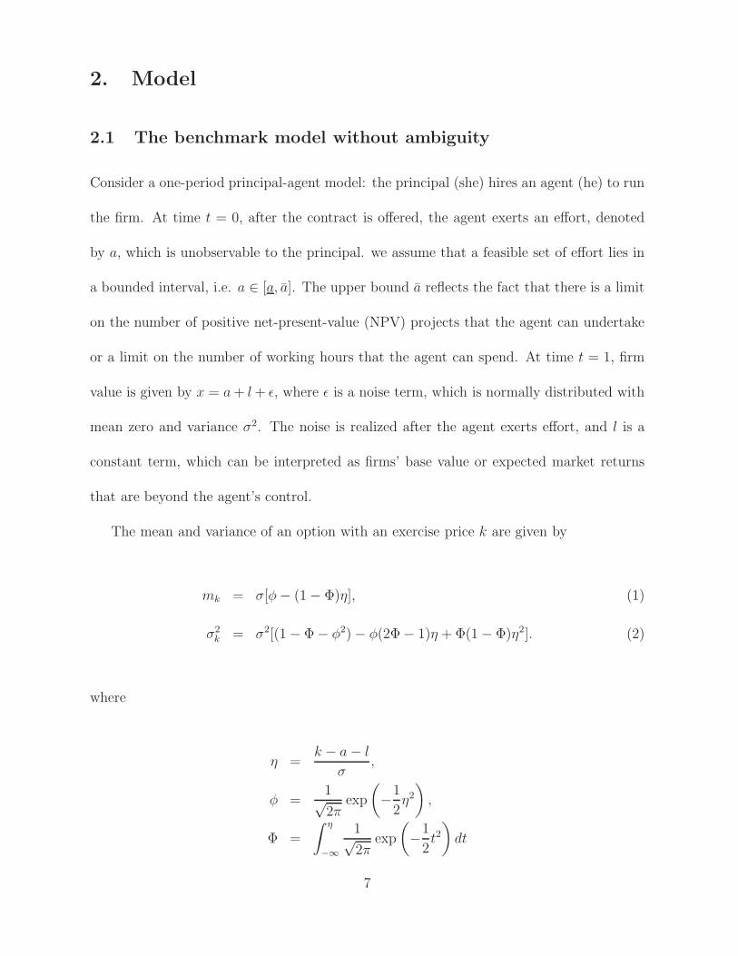
compensation, denoted by Ck, to implement the effort, and provide a graphical illustration
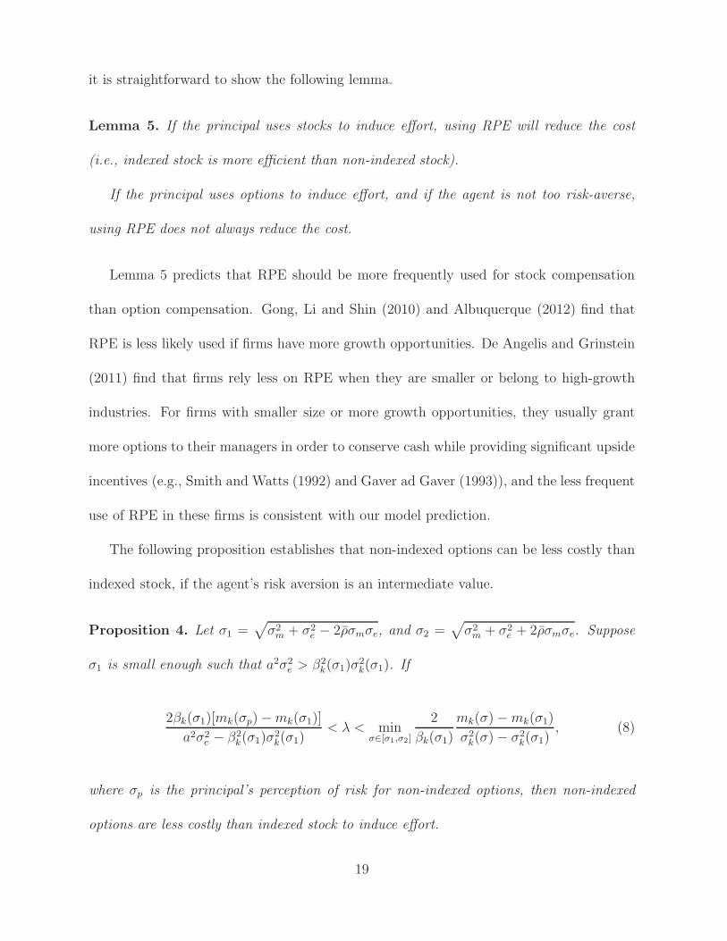
in Figure 1. The results are similar to those in Hall and Murphy (2000) and Feltham and
Wu (2001).
Proposition 1. Denote Cs as the cost of stock compensation to implement the target effort
a, and Ck as the cost of option compensation to implement a. For any k > 0, Cs < Ck.
There are two complementary perspectives on the choice between stock and option com-
pensation. One perspective highlights that options are more “expensive” since risk-averse
executives value options at significantly less than the cost to the company (e.g., Hall and
Murphy (2000)). The economic or opportunity cost of granting an option is the amount
the company could have received if it were to sell the option to an outside investor, who is
generally considered risk-neutral, free to trade the option and take actions to hedge away
the risk of the option. In contrast to outside investors, company executives cannot trade
their options and are forbidden from hedging the risks by short-selling company stock. In
addition, while outside investors tend to be well-diversified, company executives are inher-
ently undiversified, with their physical as well as human capital invested disproportionately
in their company. For these reasons, company executives will generally place a much lower
9
value on company stock options than would outside investors. The other perspective em-
phasizes that options provide more incentives for the same dollar outlay as an equivalent
investment in stocks. If the base salary is rigid, the cost of stock compensation or option
compensation is proportional to market value of stocks or options. In this case, options
are less costly in providing identical incentives. This is illustrated in the top graph of
Figure 1, which shows that market value is decreasing in the exercise price. However, if
the base salary is adjustable, since stocks provide more subjective values to the agent than
options, stock compensation can result in a lower base salary necessary compared to option
compensation. Then it can be shown that the cost of a contract is proportional to the risk
premium paid to the agent. As a result, stocks dominate options as shown in Proposition
1 and the bottom graph of Figure 1. The intuition here is also illustrated in Dittmann and
Maug (2007). Below we will show that options can be a desirable compensation instrument
in the presence of ambiguity.
2.2 A model with ambiguity aversion
In the benchmark model without ambiguity, the firm value x is normally distributed with
mean a + l and variance σ2. The agent infers his expected utility from this objective dis-
tribution. But in start-up companies and emerging industries, lack of reliable information
could cause the agent to face ambiguity regarding risk and returns. In this section, we
study the contracting implications when firm risk is ambiguous, that is, the value of σ lies
in a closed interval [σ1, σ2], σ1 ≤ σ2.
Following the literature on ambiguity-aversion, we assume that the agent is both risk-
10
averse and ambiguity-averse. When faced with ambiguity, given any level of effort, he first
minimizes his utility under possible distributions (i.e., his utility is inferred in the worst
case), and then choose an effort to maximize his utility that has been minimized under
possible distributions. The agent’s objective is thus given by
maxa
minσ∈[σ1,σ2]
E[u(a)] (4)
Note that when the agent exerts different levels of effort, the distributions of firm value
will be changed, and thus, his perception of distributions (i.e., the worst distribution for
the agent) can be different.
There is no asymmetric information between the principal and the agent regarding the
range of risk, that is, the principal’s perception of risk, denoted by σp, is σp ∈ [σ1, σ2]. Since
the principal can diversify her risk in the market, she may be less averse to ambiguity on
risk. Here we do not make any assumptions on the principal’s attitude towards ambiguity,7
and the key driving forces underlying our results is that the agent is ambiguity-averse.
Given the target effort a, the principal’s objective is to minimize the cost of implementing
a. Since the effort cost is always 12a2, we drop this constant term in the rest of the paper.
The cost below refers to the risk premium paid to the agent.
7It can be shown that if the principal is ambiguity-averse, σp = σ2.
11
3. Results
3.1 Optimality of options
Lemma 2. Let σa and σp be the agent’s and the principal’s perception of risk, respectively.
1) If the principal uses stock compensation to induce effort, then the agent’s perception
of risk is σa = σ2; the cost of stock compensation is Cs =12λa2σ2
2.
2) If the principal uses option compensation to induce effort, let βk(σ1) be the number
of options required to induce the target effort a if the agent’s perception of risk is σ1, i.e.,
a ∈ argmaxaE[u(a)|σa = σ1 and βk = βk(σ1)]. If the agent is granted βk(σ1) options with
an exercise price k, and
λ < minσ∈[σ1,σ2]
2
βk(σ1)
mk(σ)−mk(σ1)
σ2k(σ)− σ2
k(σ1), (5)
then the agent will exert the effort a, his perception of risk is σ1 and the cost of option
compensation is Ck =12λβ2
k(σ1)σ2k(σ1) + βk(σ1)[mk(σp)−mk(σ1)].
The intuition behind Lemma 2 is illustrated as follows. The mean and variance of stocks
are given by a+ l and σ2. An increase in σ has no effects on the mean value of stocks, but
increases the variance of stock. The risk-averse agent will always perceive the highest risk
σ2 when he owns stocks. However, for options, an increase in σ increases both the mean
value and variance of options. While an increase in the variance of options decreases the
agent’s utility, an increase in the mean value of options also has a positive effect on his
utility. Thus whether the agent perceives a high risk or low risk depends on which effect
dominates. If the agent is not too risk-averse, the effect from an increased mean value of
12
options is dominant, and thus the agent’s utility is minimized at a low risk. Therefore, the
agent will perceive a low risk.
In the presence of ambiguity, the cost of option compensation can be decomposed
into two parts: the risk premium paid to the agent and the wedge in the valuation of
options between the principal and the agent (because now their perceptions of risk may
be different). Since the mean value of stocks is not affected by risk, there is no difference
in the valuation of stock between the principal and the agent. Therefore, the cost of stock
compensation involves only the risk premium required. Stocks always induce the agent to
perceive a high risk. As a result, the principal has to pay a high risk premium. However, as
argued above, options can induce the agent to perceive a low risk. The perception of a low
risk has two counteracting effects on the cost of option compensation. On the one hand, it
reduces the risk premium; on the other hand, it increases the valuation wedge of options
between the principal and the agent. If the agent’s risk aversion is large enough, the first
effect will dominate, so that the cost of option compensation decreases. The following
proposition shows that options are less costly than stocks for intermediate values of the
risk aversion on the part of the agent (λ).
Proposition 2. Suppose σ1 is small enough such that a2σ22 > β2
k(σ1)σ2k(σ1). If the agent’s
risk aversion λ satisfies
2βk(σ1)[mk(σp)−mk(σ1)]
a2σ22 − β2
k(σ1)σ2k(σ1)
< λ < minσ∈[σ1,σ2]
2
βk(σ1)
mk(σ)−mk(σ1)
σ2k(σ)− σ2
k(σ1), (6)
then it is less costly to use options (with an exercise price k) than stocks to induce effort.
The right-hand side of the inequality ensures that the agent’s perception of risk is σ1
13
with options (by Lemma 2). Suppose βk(σ1) is larger, i.e., the number of options granted to
the agent to induce the target effort is larger. Since the agent is risk-averse and ambiguity-
averse, it will become more difficult to induce him to perceive a low risk. The upper bound
for λ has to be consequently decrease to ensure that the agent can be induced to perceive
a low risk with options. The other term in the right-hand side, minσ∈[σ1,σ2]mk(σ)−mk(σ1)
σ2k(σ)−σ2
k(σ1)
,
measures the increment of the mean value of options relative to the increment of the
variance of options, when firm risk goes up. As this term becomes higher, the increase in
firm risk has a larger effect on the mean value of options, implying that it will be easier to
induce the agent to perceive a low risk with options. The upper bound for λ increases as
a result.
The left-hand side of the inequality ensures that it is less costly to use options than
stocks to induce effort (by comparing the cost of both contracts from Lemma 2). If βk(σ1)
is higher, i.e., the principal needs to use more options to induce the target effort, option
compensation consequently becomes more costly. requiring the lower bound for λ to in-
crease. If σp is larger, which means that the principal recognizes a higher risk, and thus, a
higher value to options, then options in managerial compensation become less appealing.
Therefore, the lower bound for λ increases. Lastly, if σ2 becomes larger, a higher risk pre-
mium is required for stock compensation, making option compensation more appealing and
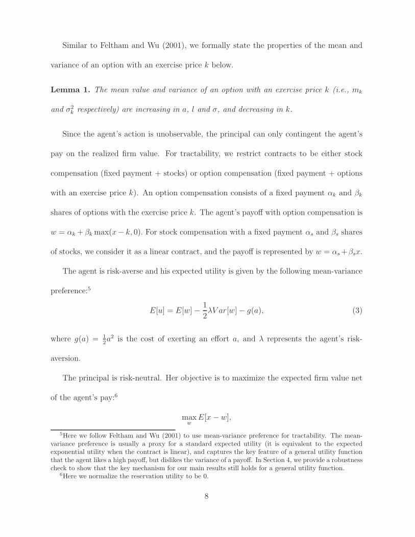
the lower bound for λ decrease. The following numerical example shows that the condition
(6) can be satisfied.
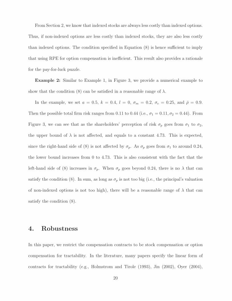
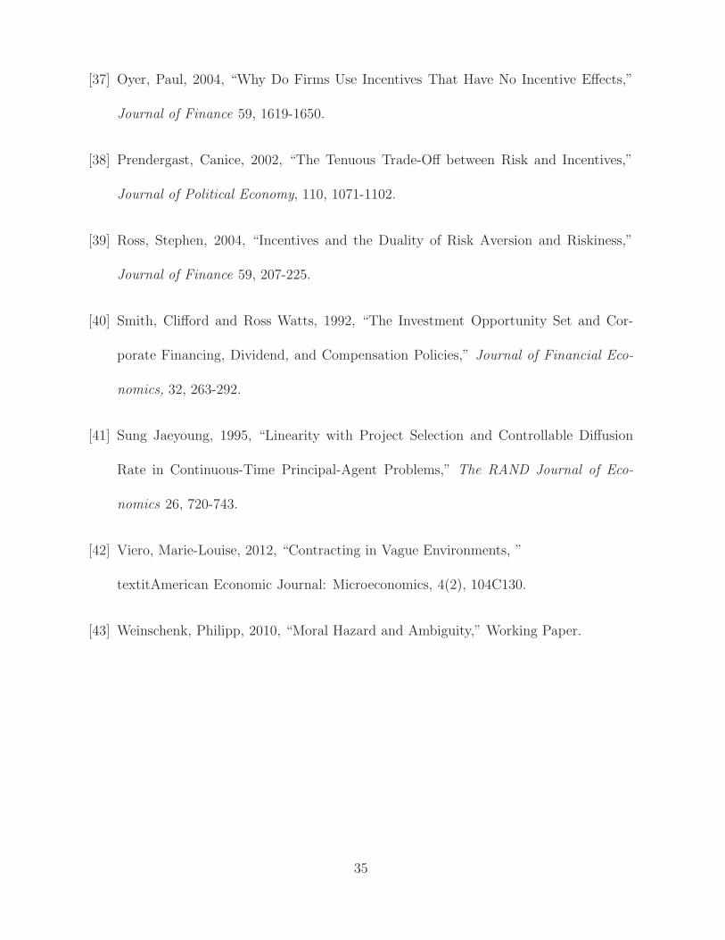
Example 1: In the condition (6), βk(σ1) depends on λ, so it is not clear whether this
condition can be satisfied in a reasonable range of λ. In the Appendix, we show that the
14
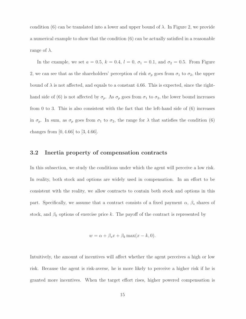
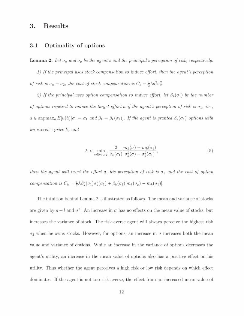
condition (6) can be translated into a lower and upper bound of λ. In Figure 2, we provide
a numerical example to show that the condition (6) can be actually satisfied in a reasonable
range of λ.
In the example, we set a = 0.5, k = 0.4, l = 0, σ1 = 0.1, and σ2 = 0.5. From Figure
2, we can see that as the shareholders’ perception of risk σp goes from σ1 to σ2, the upper
bound of λ is not affected, and equals to a constant 4.66. This is expected, since the right-
hand side of (6) is not affected by σp. As σp goes from σ1 to σ2, the lower bound increases
from 0 to 3. This is also consistent with the fact that the left-hand side of (6) increases
in σp. In sum, as σp goes from σ1 to σ2, the range for λ that satisfies the condition (6)
changes from [0, 4.66] to [3, 4.66].
3.2 Inertia property of compensation contracts
In this subsection, we study the conditions under which the agent will perceive a low risk.
In reality, both stock and options are widely used in compensation. In an effort to be
consistent with the reality, we allow contracts to contain both stock and options in this
part. Specifically, we assume that a contract consists of a fixed payment α, βs shares of
stock, and βk options of exercise price k. The payoff of the contract is represented by
w = α + βsx+ βk max(x− k, 0).
Intuitively, the amount of incentives will affect whether the agent perceives a high or low
risk. Because the agent is risk-averse, he is more likely to perceive a higher risk if he is
granted more incentives. When the target effort rises, higher powered compensation is
15
required to induce effort. As a result, the agent tends to perceive a high risk.
Lemma 3. Given two levels of effort a1 < a2, if a2 is implemented and the agent perceives
σ1, then a1 can also be implemented while keeping the agent’s perception of risk unchanged.
Lemma 3 shows that it becomes more difficult to induce the agent to perceive σ1, as the
target effort increases. The next lemma will show that under some conditions, the agent’s
perception of risk will quickly jump from σ1 to σ2. Given a contract, the agent’s utility is
jointly determined by the expected value and the variance of his compensation payments.
The expected value and variance both increase in the agent’s perception of risk. Note that
the expected value is proportional to the level of incentives, and the variance is proportional
to the variability in the level of incentives. If risk is not too small and incentives are weak,
the expected value dominates in determining the agent’s perception of risk, and therefore
the agent will perceive the lowest risk σ1; with strong incentives, however, the variance
component is a dominant force, and the agent will perceive the highest risk σ2.
Lemma 4. Suppose that the target effort a is implemented. If8
|k − a− l| < σ1 ·min
(
1,
√
1
2λaσ1
)
, (7)
then the agent’s perception of risk is either the lowest risk σ1 or the highest risk σ2.
Lemma 3 and 4 imply that there exists a cut-off effort level, denoted by a0, such that for
any effort level below a0, the principal can implement effort with a contract that enables
the agent to perceive the lowest risk. In this case, a low risk premium is required. However,
8In reality, firms usually use at-the-money options to compensate their managers. Then k is roughlyequal to E[x] = a+ l. The condition (7) is satisfied automatically.
16
for any effort level above a0, incentives required to induce effort are sufficiently strong that
the agent will perceive the highest risk. In this case, a high risk premium is required.
This implies that there will be a discontinuous jump in the cost of compensation contracts
when the target effort increases from below the threshold to above. Consider moderate
improvements in fundamentals around the threshold level (a0) that would typically raise
the optimal effort level and incentive pay, for example, the agent’s effort becomes more
productive due to expanded business opportunities. The principal will be reluctant to take
advantage of these improvements by adjusting compensation contracts, because enhanced
incentives would alter the agent’s perception of risk from low to high, and consequently
result in a substantial increase in the risk premium. Therefore, compensation contracts
exhibit an inertia property, that is, compensation contracts are irresponsive to changes
in fundamentals. This feature is consistent with the widespread use of benchmarking
(and thus a disconnection between pay and firm performance) in CEO compensation (e.g.,
Bizjak, Lemmon and Naveen (2008) and Faulkender and Yang (2010)).
Proposition 3. Suppose that the condition (7) holds. Then there exists a cut-off a0 such
that the cost of contracts will jump discontinuously when the target effort moves from below
a0 to above a0.
3.3 Relative performance evaluation
Theories have advocated that any returns that are beyond the agent’s control should be
isolated from the agent’s payoff. This is called relative performance evaluation (RPE).
However, empirical studies found that RPE is not frequently used in practice. For example,
17
Bertrand and Mullainathan (2001) document that CEOs are rewarded for general market
upswings beyond CEO’s control, i.e., paid for luck. In this section, we will argue that if the
correlation between observable shocks and unobservable shocks is ambiguous, while it is
efficient to use RPE for stock compensation, it may not be optimal to use RPE for option
compensation.
Specifically, suppose that the shock ǫ can be divided into two parts: ǫ = m+ e, where
m represents the part of the shock that is observable and contractible; e is the rest of the
shock that is unobservable. m is normally distributed with mean 0 and variance σ2m. e is
normally distributed with mean 0 and variance σ2e . Let ρ be the correlation between m
and e. We introduce ambiguity by assuming that ρ ∈ [−ρ, ρ], where 0 < ρ < 1.9
Since m is observable and contractible (which means that we can use RPE to filter
out m from firm value x and use x −m to evaluate the agent’s performance), we assume
that the principal can use four types of compensation: non-indexed stock compensation
(whose payoff has the form αs + βsx), indexed stock compensation (whose payoff has the
form αis + βis(x − m)), non-indexed option compensation (whose payoff has the form
αk + βk max(x − k, 0)), indexed option compensation (whose payoff has the form αik +
βik max(x−m− k, 0)). Then similar to the argument before, if the agent is granted non-
indexed stock compensation, his perception of risk will be the highest possible risk, that is
σ2m + σ2
e + 2ρσmσe; if the agent is granted indexed stock compensation, his perception of
risk will be σ2e ; if the agent is granted non-indexed option compensation and if he is not too
risk-averse, his perception of risk can be the lowest possible risk, that is σ2m+σ2
e−2ρσmσe; if
the agent is granted indexed option compensation, his perception of risk will be σ2e . Thus,
9Thus, the average correlation between m and e is zero.
18
it is straightforward to show the following lemma.
Lemma 5. If the principal uses stocks to induce effort, using RPE will reduce the cost
(i.e., indexed stock is more efficient than non-indexed stock).
If the principal uses options to induce effort, and if the agent is not too risk-averse,
using RPE does not always reduce the cost.
Lemma 5 predicts that RPE should be more frequently used for stock compensation
than option compensation. Gong, Li and Shin (2010) and Albuquerque (2012) find that
RPE is less likely used if firms have more growth opportunities. De Angelis and Grinstein
(2011) find that firms rely less on RPE when they are smaller or belong to high-growth
industries. For firms with smaller size or more growth opportunities, they usually grant
more options to their managers in order to conserve cash while providing significant upside
incentives (e.g., Smith and Watts (1992) and Gaver ad Gaver (1993)), and the less frequent
use of RPE in these firms is consistent with our model prediction.
The following proposition establishes that non-indexed options can be less costly than
indexed stock, if the agent’s risk aversion is an intermediate value.
Proposition 4. Let σ1 =√
σ2m + σ2
e − 2ρσmσe, and σ2 =√
σ2m + σ2
e + 2ρσmσe. Suppose
σ1 is small enough such that a2σ2e > β2
k(σ1)σ2k(σ1). If
2βk(σ1)[mk(σp)−mk(σ1)]
a2σ2e − β2
k(σ1)σ2k(σ1)
< λ < minσ∈[σ1,σ2]
2
βk(σ1)
mk(σ)−mk(σ1)
σ2k(σ)− σ2
k(σ1), (8)
where σp is the principal’s perception of risk for non-indexed options, then non-indexed
options are less costly than indexed stock to induce effort.
19
From Section 2, we know that indexed stocks are always less costly than indexed options.
Thus, if non-indexed options are less costly than indexed stocks, they are also less costly
than indexed options. The condition specified in Equation (8) is hence sufficient to imply
that using RPE for option compensation is inefficient. This result also provides a rationale
for the pay-for-luck puzzle.
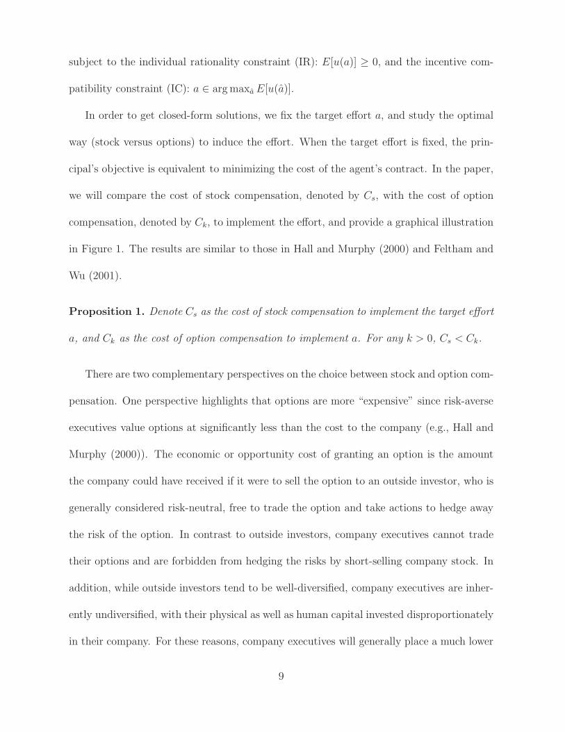
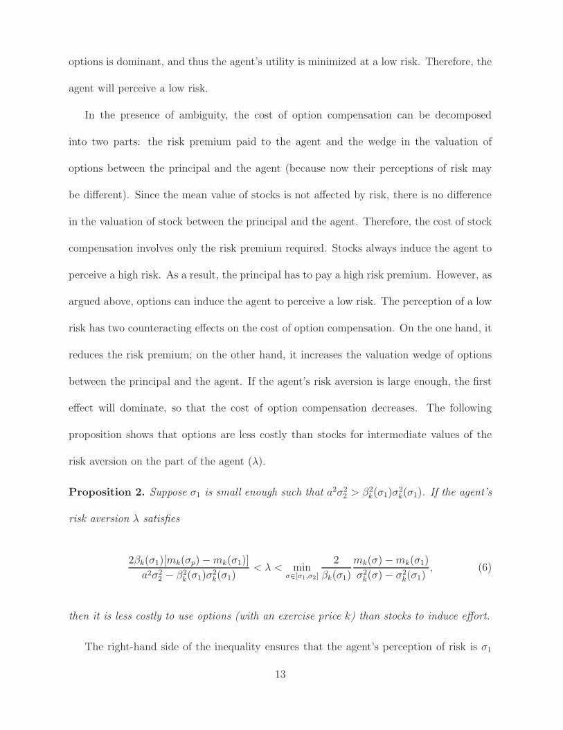
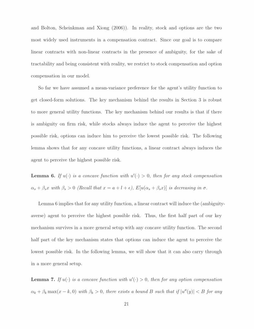
Example 2: Similar to Example 1, in Figure 3, we provide a numerical example to
show that the condition (8) can be satisfied in a reasonable range of λ.
In the example, we set a = 0.5, k = 0.4, l = 0, σm = 0.2, σe = 0.25, and ρ = 0.9.
Then the possible total firm risk ranges from 0.11 to 0.44 (i.e., σ1 = 0.11, σ2 = 0.44). From
Figure 3, we can see that as the shareholders’ perception of risk σp goes from σ1 to σ2,
the upper bound of λ is not affected, and equals to a constant 4.73. This is expected,
since the right-hand side of (8) is not affected by σp. As σp goes from σ1 to around 0.24,
the lower bound increases from 0 to 4.73. This is also consistent with the fact that the
left-hand side of (8) increases in σp. When σp goes beyond 0.24, there is no λ that can
satisfy the condition (8). In sum, as long as σp is not too big (i.e., the principal’s valuation
of non-indexed options is not too high), there will be a reasonable range of λ that can
satisfy the condition (8).
4. Robustness
In this paper, we restrict the compensation contracts to be stock compensation or option
compensation for tractability. In the literature, many papers specify the linear form of
contracts for tractability (e.g., Holmstrom and Tirole (1993), Jin (2002), Oyer (2004),
20
and Bolton, Scheinkman and Xiong (2006)). In reality, stock and options are the two
most widely used instruments in a compensation contract. Since our goal is to compare
linear contracts with non-linear contracts in the presence of ambiguity, for the sake of
tractability and being consistent with reality, we restrict to stock compensation and option
compensation in our model.
So far we have assumed a mean-variance preference for the agent’s utility function to
get closed-form solutions. The key mechanism behind the results in Section 3 is robust
to more general utility functions. The key mechanism behind our results is that if there
is ambiguity on firm risk, while stocks always induce the agent to perceive the highest
possible risk, options can induce him to perceive the lowest possible risk. The following
lemma shows that for any concave utility functions, a linear contract always induces the
agent to perceive the highest possible risk.
Lemma 6. If u(·) is a concave function with u′(·) > 0, then for any stock compensation
αs + βsx with βs > 0 (Recall that x = a+ l + ǫ), E[u(αs + βsx)] is decreasing in σ.
Lemma 6 implies that for any utility function, a linear contract will induce the (ambiguity-
averse) agent to perceive the highest possible risk. Thus, the first half part of our key
mechanism survives in a more general setup with any concave utility function. The second
half part of the key mechanism states that options can induce the agent to perceive the
lowest possible risk. In the following lemma, we will show that it can also carry through
in a more general setup.
Lemma 7. If u(·) is a concave function with u′(·) > 0, then for any option compensation
αk + βk max(x− k, 0) with βk > 0, there exists a bound B such that if |u′′(y)| < B for any
21
y, then E[u(αk + βk max(x− k, 0))] is increasing in σ.
Lemma 7 implies that as long as the agent is not too risk-averse, option compensation
can induce him to perceive the lowest possible risk. Thus, our results still hold in a setup
with a general utility function.
5. Conclusion
Standard principal-agent models usually assume that the distribution on the future firm
value is known. This paper attempts to study the choice of compensation contracts when
there are multiple possible distributions and the agent is averse to ambiguity. The paper
finds that when there are multiple possible distributions on firm value, different types
of contracts (linear contracts versus non-linear contracts) can induce an ambiguity-averse
agent to perceive different distributions, and therefore change the optimality of contracts.
In particular, while stocks are always less costly than options in motivating effort in the
absence of ambiguity, options can be more efficient than stocks in the presence of ambiguity
regarding firm risk. In addition, We find that compensation contracts exhibit an inertia
property and benchmark pay is reasonable. When ambiguity regarding the correlation
between observable shocks and unobservable shocks exists, CEO pay contingent on the
market-wide performances can be optimal. The model also predicts that RPE should be
more frequently used for stock compensation than option compensation.
22
Appendix
Proof of Proposition 1
For stock compensation, the agent’s utility is given by E[u] = αs+βs(a+ l)− 12λβ2
sσ2−
12a2. So to induce the effort a, we must have βs = a. For a fixed target effort a, the principal
wants to minimize the cost. So αs must be set so that the IR constraint is binding. Thus, it
is easy to derive that the cost of the contract (dropping the constant 12a2) is: Cs =
12λa2σ2.
we derive the agent’s utility for an option compensation as follows. E[u] = αk+βkmk−
12λβ2
kσ2k − 1
2a2. Taking partial derivative of mk and σ2
k w.r.t. a yields that
∂mk
∂a= 1− Φ
∂σ2k
∂a= 2Φmk
To induce the effort a, we must have that ∂E[u]∂a
≥ 0, which yields that
βk ≥(1− Φ)−
√∆
2λΦmk
,
where ∆ = (1− Φ)2 − 4aλΦmk. Similarly, we have the binding IR constraint. So the cost
is
Ck ≥1
2λ
(
(1− Φ)−√∆
2λΦmk
)2
σ2k =
2λa2σ2y1
(1 +√1− 4aλσy2)2
, (9)
23
where
y1 =(1− Φ− φ2)− φ(2Φ− 1)η + Φ(1− Φ)η2
(1− Φ)2,
y2 =Φ[φ − (1− Φ)η]
(1− Φ)2.
It can be shown that y′1(η) ≥ 0 and y′2(η) ≥ 0 (see Feltham and Wu (2001)). Thus,
Ck is increasing in k. As k goes to −∞, Φ goes to zero. So σ2y1 =σ2k
(1−Φ)2→ σ2, and
σy2 = Φmk
(1−Φ)2→ 0. Hence, the right-hand side of (9) goes to 1
2λa2σ2 when k goes to −∞.
Thus, we obtain that Cs < Ck.
Proof of Lemma 2
If the agent is granted with stocks, his utility E[u] = βs(a + l) − 12λβ2
sσ2 − 1
2a2 is
minimized at σ = σ2. So he will always perceive the highest risk σ2. Following the proof
of Proposition 1, we can show that Cs =12λa2σ2
2.
If the agent is granted with options, his utility is given by
E[u] = αk + βk(σ1)mk(σa)−1
2λβk(σ1)
2σk(σa)2 − 1
2a∗2
let
A1 = {a : E[u(a)|σa = σ1] < minσa∈(σ1,σ2]
E[u(a)]}
be the set of effort for which the agent’s utility is minimized at the lowest risk σ1. By
condition (5), the target effort a belongs to A1, i.e., a ∈ A1. Note that βk(σ1) is exactly
the number of options to induce the effort a given σa = σ1. If the agent perceives another
24
risk σ 6= σ1 and exerts an effort a, we must have
E[u(a)|σa = σ] ≤ E[u(a)|σa = σ1] ≤ E[u(a)|σa = σ1].
Therefore at the optimum, the agent will perceive the lowest risk σ1 and exert the target
effort a. The binding IR constraint yields that αk + βk(σ1)mk(σ1) =12λβk(σ1)
2σk(σ1)2 +
12a2. From the principal’s perspective, the cost (dropping the constant 1
2a2) is Ck = αk +
βk(σ1)mk(σp) =12λβk(σ1)
2σk(σ1)2 + βk(σ1)[mk(σp)−mk(σ1)].
Proof of Proposition 2
By Lemma 2, the right hand side of (6) ensures that an option of exercise price k
induces the agent to perceive σ1 and exert the effort a. The cost of the contract is Ck =
12λβk(σ1)
2σk(σ1)2 + βk(σ1)[mk(σp)−mk(σ1)]. Since the cost of stock compensation is Cs =
12λa2σ2
2, the left hand side of (6) ensures that the option compensation is less costly.
Analysis of Condition (6)
We first solve for the right-hand of (6) to obtain an upper bound of λ. Let M =
minσ∈[σ1,σ2]mk(σ)−mk(σ1)σ2k(σ)−σ2
k(σ1)
, which does not depend on λ. From the proof of Proposition 1, we
know that βk = (1−Φ)−√∆
2λΦmk, where ∆ = (1 − Φ)2 − 4aλΦmk. Plugging the formula of βk
into the right-hand side of (6), we can solve that the right-hand side of (6) is equivalent to
λ <K(2−2Φ(σ1)−K)4aΦ(σ1)mk(σ1)
, where K = 4MΦ(σ1)mk(σ1).
For the left-hand side of (6), it can be simplified to λβ2k(σ1)σ
2k(σ1)+2[mk(σp)−mk(σ1)]βk(σ1)−
25
λa∗2σ22 < 0. Note that λβ2
k = 1−ΦΦmk
βk − aΦmk
, so the left-hand side of (6) is equivalent to
[
(1− Φ(σ1))σ2k(σ1)
Φ(σ1)mk(σ1)+ 2[mk(σp)−mk(σ1)]
]
βk(σ1)−aσ2
k(σ1)
Φ(σ1)mk(σ1)− λa2σ2
2 < 0. (10)
It is easy to check that the left-hand side of (10) is convex in λ, and is non-negative when
λ = 0. So there could be three cases:
Case 1: the left-hand side of (10) never crosses with the x-axis, which means that (10)
will never be satisfied. In this case, the condition (6) cannot be satisfied.
Case 2: the left-hand side of (10) crosses with the x-axis once. Let λ1 denote the crossed
point, then the condition (6) is equivalent to λ1 < λ <K(2−2Φ(σ1)−K)4aΦ(σ1)mk(σ1)
.
Case 3: the left-hand side of (10) crosses with the x-axis twice. Let λ1 < λ2 denote the
two crossed points, then the condition (6) is equivalent to λ1 < λ < min(
K(2−2Φ(σ1)−K)4aΦ(σ1)mk(σ1)
, λ2
)
.
Proof of Lemma 3
Suppose the principal uses a contract w = α+βsx+βk max(x−k, 0) to induce the agent
to perceive σ1 and exert the target effort a2. Then we must have that for any σa ∈ (σ1, σ2],
α + βs(a2 + l) + βkmk(σ1)−1
2λ[
β2sσ
21 + β2
kσk(σ1)2 + 2βsβkσ0,k(σ1)
]
≤ α + βs(a2 + l) + βkmk(σa)−1
2λ[
β2sσ
2a + β2
kσk(σa)2 + 2βsβkσ0,k(σa)
]
,
where σ0,k denotes the covariance between stocks and options. The inequality can be
simplified to
1
2λ
[
β2s
βk
(σ2a − σ2
1) + βk(σk(σa)2 − σk(σ1)
2) + 2βs(σ0,k(σa)− σ0,k(σ1))
]
≤ mk(σa)−mk(σ1).
26

Note that σk(σ)2, σ0,k(σ) and mk(σ) are increasing in σ. As we gradually reduce βs and
βk, the inequality above can still hold, so the agent will continue to perceive the lowest risk
σ1. We keep reducing βs and βk until a1 is induced. Then we are done.
Proof of Lemma 4
When the effort a is induced, the agent’s utility is
E[u|σa] = α + βs(a + l) + βkmk(σa)−1
2λ[
β2sσ
2a + β2
kσk(σa)2 + 2βsβkσ0,k(σa)
]
− 1
2a2.
We can calculate that ∂2mk(σ)∂σ2 = φη2
σ; ∂2σk(σ)
2
∂σ2 = 2(1 − Φ − φ2 + φη − φ2η2 + φη3 − φΦη3);
∂2σ0,k(σ)
∂σ2 = 2(1− Φ) + 2φη + φη3.
Since a is induced, we must have
maxσ∈[σ1,σ2]
∂E[u|σ]∂a
≥ 0.
Let σ0 ∈ argmaxσ∈[σ1,σ2]∂E[u|σ]
∂a. Then we obtain that
βs + βk(1− Φ(σ0))−1
2λ
[
β2k
∂σk(σ0)2
∂a+ 2βsβk
∂σ0,k(σ0)
∂a
]
− a ≥ 0.
Since ∂σk(σ0)2
∂a> 0 and
∂σ0,k(σ0)
∂a> 0, βs + βk > a.
27
Taking the second-order derivative of E[u|σa] w.r.t. σa yields that
∂2E[u]
∂σ2a
= βk
φη2
σa
− 1
2λ[2β2
s
+ 2β2k(1− Φ− φ2 + φη − φ2η2 + φη3 − φΦη3) + 2βsβk(2(1− Φ) + 2φη + φη3)]
< βk
[
φη2
σa
− 1
2λ[2βk(1− Φ− φ2 + φη − φ2η2 + φη3 − φΦη3) + 2βs(2(1− Φ) + 2φη + φη3)]
]
If |k − a − l| < σ1 · min(
1,√
12λaσ1
)
, then |η(σa)| < min(
1,√
12λaσ1
)
. Thus, φη2
σa<
φ· 12λaσ1
σ1= 1
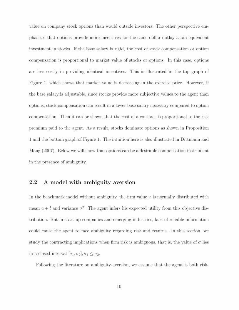
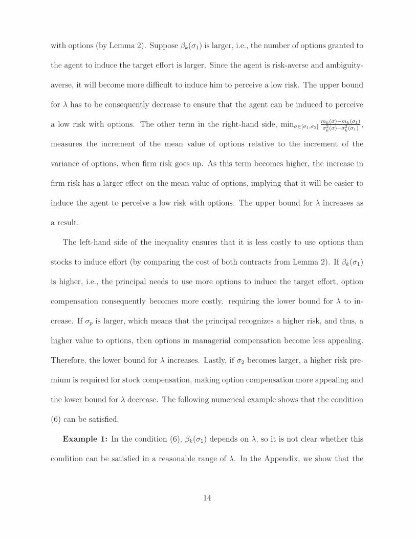
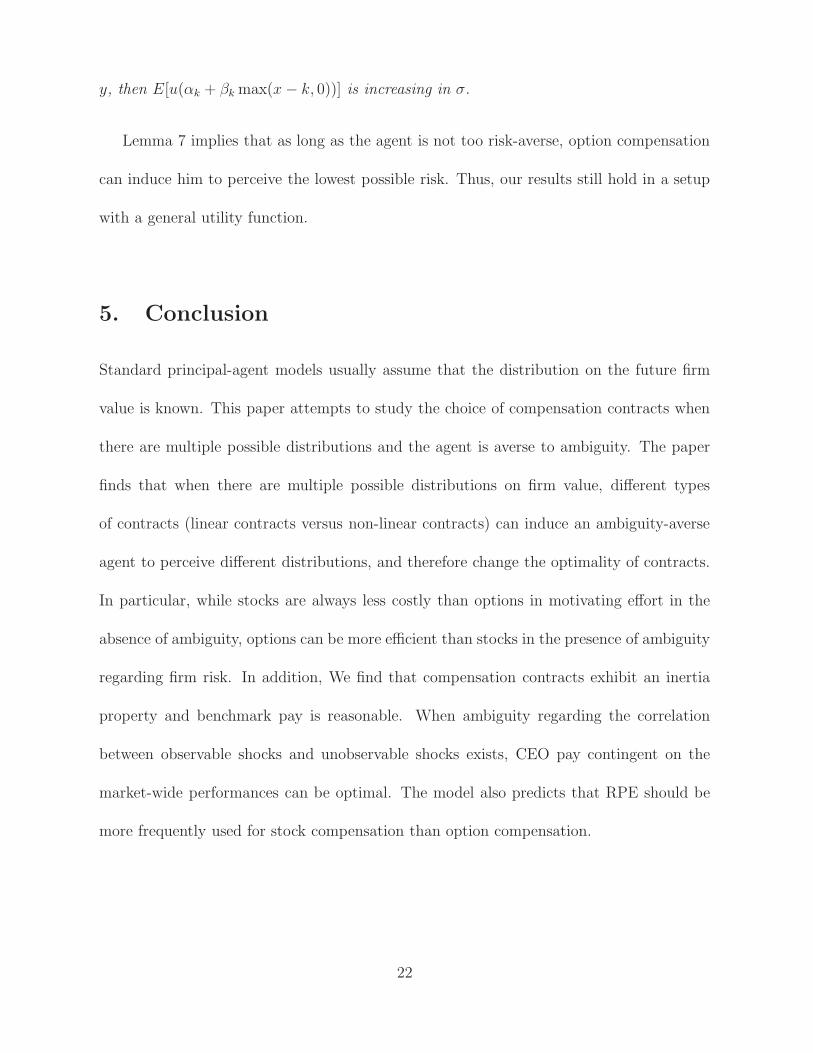
2λaφ. Using Matlab, we can draw the graph for the functions 1−Φ− φ2 +φη−
φ2η2 + φη3 − φΦη3 and 2(1−Φ) + 2φη + φη3 with |η| < 1. From Figure 4, we can see that
both functions are greater than 0.5 when |η| < 1. Note that φ < 1√2π
for any η. Thus,
∂2E[u]
∂σ2a
<1
2λβk
[
1√2π
a− (βs + βk)
]
< 0.
Thus, we prove that if |k − a − l| < σ1 · min(
1,√
12λaσ1
)
,∂2E[u]∂σ2
a< 0. Since E[u|σa] is
concave in σa, E[u|σa] must be minimized at σa = σ1 or σa = σ2. So the agent will perceive
either the lowest risk σ1 or the highest risk σ2.
Proof of Proposition 4
It is straightforward from the proofs of Lemma 2 and Proposition 2.
Proof of Lemma 6
28

We can calculate that
E[u(αs + βsx)] =
∫ ∞
−∞u(αs + βs(a+ l + y))
1
σ√2π
e−y2
2σ2 dy, let z =y
σ
=
∫ ∞
−∞u(αs + βs(a+ l + zσ))
1√2π
e−z2
2 dz.
Thus, taking the derivative w.r.t. σ yields that
∂
∂σE[u(αs + βsx)]
=
∫ ∞
−∞u′(αs + βs(a+ l + zσ))βsz
1√2π
e−z2
2 dz,
=
∫ ∞
0
u′(αs + βs(a+ l + zσ))βsz1√2π
e−z2
2 dz −∫ ∞
0
u′(αs + βs(a + l − zσ))βsz1√2π
e−z2
2 dz.
Since u is concave, it means that u′(·) is a decreasing function. So∫∞0
u′(αs + βs(a +
l + zσ))βsz1√2πe−
z2
2 dz <∫∞0
u′(αs + βs(a + l))βsz1√2πe−
z2
2 dz, and∫∞0
u′(αs + βs(a + l −
zσ))βsz1√2πe−
z2
2 dz >∫∞0
u′(αs + βs(a + l))βsz1√2πe−
z2
2 dz. Thus, ∂∂σE[u(αs + βsx)] < 0.
Hence, E[u(αs + βsx)] is decreasing in σ.
Proof of Lemma 7
Similar to the proof of Lemma 6, we can calculate that
E[u(αk + βk max(x− k, 0))]
=
∫ ∞
−∞u(αk + βk max(a+ l + σz − k, 0))
1
σ√2π
e−z2
2 dz,
= u(αk)Φ(k − a− l
σ) +
∫ ∞
k−a−lσ
u(αk + βk(a+ l + zσ − k))1√2π
e−z2
2 dz.
29

Taking the derivative w.r.t. σ yields that
∂
∂σE[u(αk + βk max(x− k, 0))] =
∫ ∞
k−a−lσ
u′(αk + βk(a + l + zσ − k))βkz1√2π
e−z2
2 dz
If k− a− l ≥ 0, then it is obvious that ∂∂σE[u(αk +βk max(x− k, 0))] > 0. If k− a− l < 0,
then since∫∞
k−a−lσ
u′(αk + βk(a + l + zσ − k))βkz1√2πe−
z2
2 dz =∫
a+l−kσ
k−a−lσ
u′(αk + βk(a + l +
zσ − k))βkz1√2πe−
z2
2 dz +∫∞
a+l−kσ
u′(αk + βk(a + l + zσ − k))βkz1√2πe−
z2
2 dz. The first part
equals to zero when u′′(·) = 0, and the second part is always positive, so there must exist
a bound B such that if |u′′(y)| < B for any y, then ∂∂σE[u(αk +βk max(x− k, 0))] > 0, i.e.,
E[u(αk + βk max(x− k, 0))] is increasing in σ.
30
References
[1] Ahn, David, Syngjoo Choi, Douglas Gale and Shachar Kariv, 2009, “Estimating
Ambiguity-Aversion in a Portfolio Choice Experiment,” Working Paper.
[2] Albuquerque, Ana, 2012, “Do Growth-Option Firms Use Less Relative Performance
Evaluation,” Working Paper.
[3] Bertrand, Marianne and Sendhil Mullainathan, 2001, “Are CEOs Rewarded for Luck?
The Ones Without Principals Are, ” Quarterly Journal of Economics, 116, 901-932.
[4] Bettis, J. Carr, John M. Bizjak and Michael L. Lemmon, 2005, “Exercise Behavior,
Valuation, and the Incentives Effects of Employee Stock Options,” Journal of Finan-
cial Economics 76, 445-470.
[5] Bizjak, John M., Michael Lemmon and Lalitha Naveen, 2008, “Does the Use Peer
Groups Contribute to Higher Pay and Less Efficient Compensation,” Journal of Fi-
nancial Economics 90, 152-168.
[6] Bolton, Patrick, Jose Scheinkman and Wei Xiong, 2006, “Executive Compensation
and Short-Termist Behaviour in Speculative Markets,” Review of Economic Studies
73, 577-610.
[7] Carpenter, Jennifer, 2000, “Does Option Compensation Increase Managerial Risk Ap-
petite,” Journal of Finance 55, 2311-2331.
[8] Carroll, Gabriel, 2015, “Robustness and Linear Contracts,” American Economic Re-
view 105(2), 536-563.
31
[9] De Angelis, David and Yaniv Grinstein, 2011, “Relative Performance Evaluation in
CEO Compensation: Evidence from the 2006 Disclosure Rules,” Working Paper.
[10] Dickhaut, John, Timothy Shields, and Jack Stecher, 2011, “Generating Ambiguity in
the Laboratory, ”Management Science 57(4), 705-712.
[11] Dittmann, Ingolf and Ernst Maug, 2007, “Lower Salaries and No Options? On the
Optimal Structure of Executive Pay, ” Journal of Finance 62, 303-343.
[12] Dittmann, Ingolf, Ernst Maug and Oliver Spalt, 2010, “Sticks or Carrots? Optimal
CEO Compensation When Managers Are Loss-Averse, ” Journal of Finance, forth-
coming.
[13] Dittmann, Ingolf and Ko-Chia Yu, 2011, “How Important Are Risk-Taking Incentives
in Executive Compensation? ” Working Paper.
[14] Easley, David and Maureen O’Hara, 2009, “Ambiguity and Nonparticipation: The
Role Regulation,” Review of Financial Studies 22, 1818-1843.
[15] Easley, David and Maureen O’Hara, 2010, “Liquidity and Valuation in an Uncertain
World,” Journal of Financial Economics 97, 1-11.
[16] Edmans, Alex and Xavier Gabaix, 2011, “Tractability in Incentive Contracting,” Re-
view of Financial Studies 24, 2865-2894.
[17] Ellsberg, D., 1961, “Risk, Ambiguity, and the Savage Axioms,” Quarterly Journal of
Economics 75, 643-669.
32
[18] Epstein, Larry G. and Tan Wang, 1994, “Intertemporal Asset Pricing under Knightian
Uncertainty,” Econometrica 62, 283-322.
[19] Epstein, Larry G. and Martin Schneider, 2008, “Ambiguity, Information Quality, and
Asset Pricing,” Journal of Finance 63, 197-228.
[20] Faulkender, Michael and Jun Yang, 2010, “Inside the Black Box: The Role and Com-
position of Compensation Peer Groups,” Journal of Financial Economics 96, 257-270.
[21] Feltham, Gerald A. and Martin G. H. Wu, 2001, “Incentive Efficiency of Stock versus
Options,” Review of Accounting Studies 6, 7-28.
[22] Gilboa, Itzchak and David Schmeidler, 1989, “Maxmin Expected Utility with
Nonunique Prior,” Journal of Mathematical Economics 18, 141-153.
[23] Gong, Guojin, Laura Yue Li and Jae Yong Shin, 2010, “Relative Performance Eval-
uation and Related Peer Groups in Executive Compensation Contracts,” Working
Paper.
[24] Grossman, Sanford and Oliver Hart, 1983, “An Analysis of the Principal-Agent Prob-
lem,” Econometrica 51, 7-45.
[25] Hayes, Rachel M., Michael Lemmon and Mingming Qiu, 2010, “Stock Options and
Managerial Incentives for Risk-Taking: Evidence from FAS 123R,” Working Paper.
[26] He, Zhiguo, Si Li, Bin Wei and Jianfeng Yu, 2014, “Uncertainty, Risk, and Incentives:
Theory and Evidence,” Management Science 60, 206-226.
33
[27] He, Zhiguo, Bin Wei, and Jianfeng Yu, 2014, “Optimal Long-term Contracting with
Learning,” Working Paper.
[28] Holmstrom, Bengt and Paul Milgrom, 1987, “Aggregation and Linearity in the Pro-
vision of Intertemporal Incentives,” Econometrica 55, 303-328.
[29] Holmstrom, Bengt and Jean Tirole, 1993, “Market Liquidity and Performance Moni-
toring,” Journal of Political Economy 101, 678-709.
[30] Illeditsch, Philipp, 2011, “Ambiguous Information, Portfolio Inertia, and Excess
Volatility,” Journal of Finance, forthcoming.
[31] Jin, Li, 2002, “CEO Compensation, Diversification, and Incentives,” Journal of Fi-
nancial Economics 66, 29-63.
[32] Karni, Edi, 2009, “A Reformulation of the Maxmin Expected Utility Model with
Application to Agency Theory,” Journal of Mathematical Economics 45, 97-112.
[33] Kellner, Christian, 2015, “Tournaments as Response to Ambiguity Aversion in Incen-
tive Contracts,” Journal of Economic Theory, 159, 627-655.
[34] Kellner, Christian and Gerhard Riener, 2012, “The Effect of Ambiguity Aversion on
Reward Scheme Choice,” Working Paper.
[35] Mukerji, Sujoy, 2010, “Ambiguity Aversion and Cost-Plus Procurement Contracts,”
Working Paper.
[36] Murphy, Kevin, 1999, “Executive Compensation ,” in O. Ashenfelter and D. Card
(eds), Handbook of Labor Economics (New York: Elsevier/North-Holland).
34
[37] Oyer, Paul, 2004, “Why Do Firms Use Incentives That Have No Incentive Effects,”
Journal of Finance 59, 1619-1650.
[38] Prendergast, Canice, 2002, “The Tenuous Trade-Off between Risk and Incentives,”
Journal of Political Economy, 110, 1071-1102.
[39] Ross, Stephen, 2004, “Incentives and the Duality of Risk Aversion and Riskiness,”
Journal of Finance 59, 207-225.
[40] Smith, Clifford and Ross Watts, 1992, “The Investment Opportunity Set and Cor-
porate Financing, Dividend, and Compensation Policies,” Journal of Financial Eco-
nomics, 32, 263-292.
[41] Sung Jaeyoung, 1995, “Linearity with Project Selection and Controllable Diffusion
Rate in Continuous-Time Principal-Agent Problems,” The RAND Journal of Eco-
nomics 26, 720-743.
[42] Viero, Marie-Louise, 2012, “Contracting in Vague Environments, ”
textitAmerican Economic Journal: Microeconomics, 4(2), 104C130.
[43] Weinschenk, Philipp, 2010, “Moral Hazard and Ambiguity,” Working Paper.
35
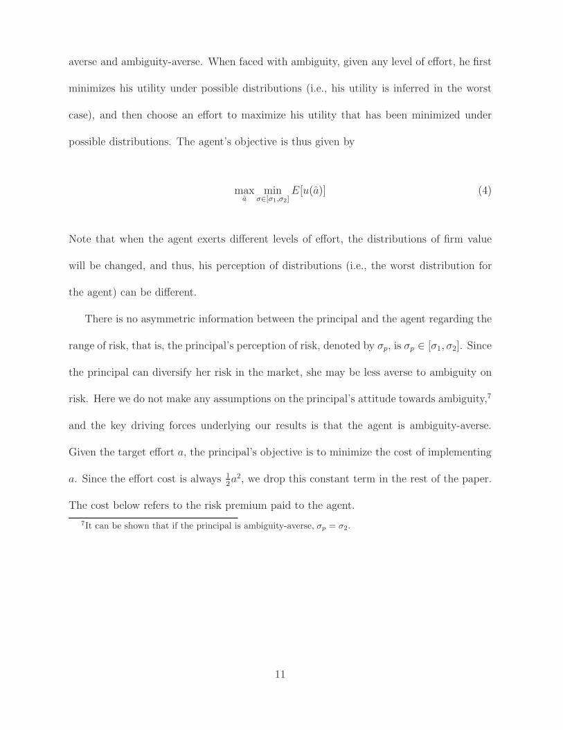
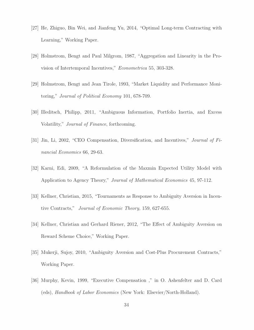
Figure 1: Market Value and Risk Premium
0 0.05 0.1 0.15 0.2 0.25 0.3 0.35 0.4 0.45 0.50
0.05
0.1
0.15
0.2
0.25
0.3
0.35
0 0.05 0.1 0.15 0.2 0.25 0.3 0.35 0.4 0.45 0.52.5
3
3.5
4
4.5
5x 10
−3
Exercise Price k
Ris
k P
rem
ium
M
arke
t Val
ue
βkmk
12λβ2
kσ2k
This picture describes a numerical example showing that how the market value and riskpremium of an option change with respect to the change in the exercise price k. In theexample, we set a = 0.5, l = 0, σ = 0.1, and λ = 2.
36
Figure 2: The relation between σp and lower and upper bound of λ
0.1 0.15 0.2 0.25 0.3 0.35 0.4 0.45 0.50
0.5
1
1.5
2
2.5
3
3.5
4
4.5
5
σp
lower
andupper
bou
ndof
λ
In the example, we set a = 0.5, k = 0.4, l = 0, σ1 = 0.1, and σ2 = 0.5. The dotted linerepresents the lower bound of λ (with respect to the change of σp). The solid line representsthe upper bound of λ (with respect to the change of σp).
37
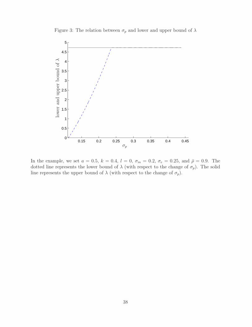
Figure 3: The relation between σp and lower and upper bound of λ
0.15 0.2 0.25 0.3 0.35 0.4 0.450
0.5
1
1.5
2
2.5
3
3.5
4
4.5
5
σp
lower
andupper
bou
ndof
λ
In the example, we set a = 0.5, k = 0.4, l = 0, σm = 0.2, σe = 0.25, and ρ = 0.9. Thedotted line represents the lower bound of λ (with respect to the change of σp). The solidline represents the upper bound of λ (with respect to the change of σp).
38
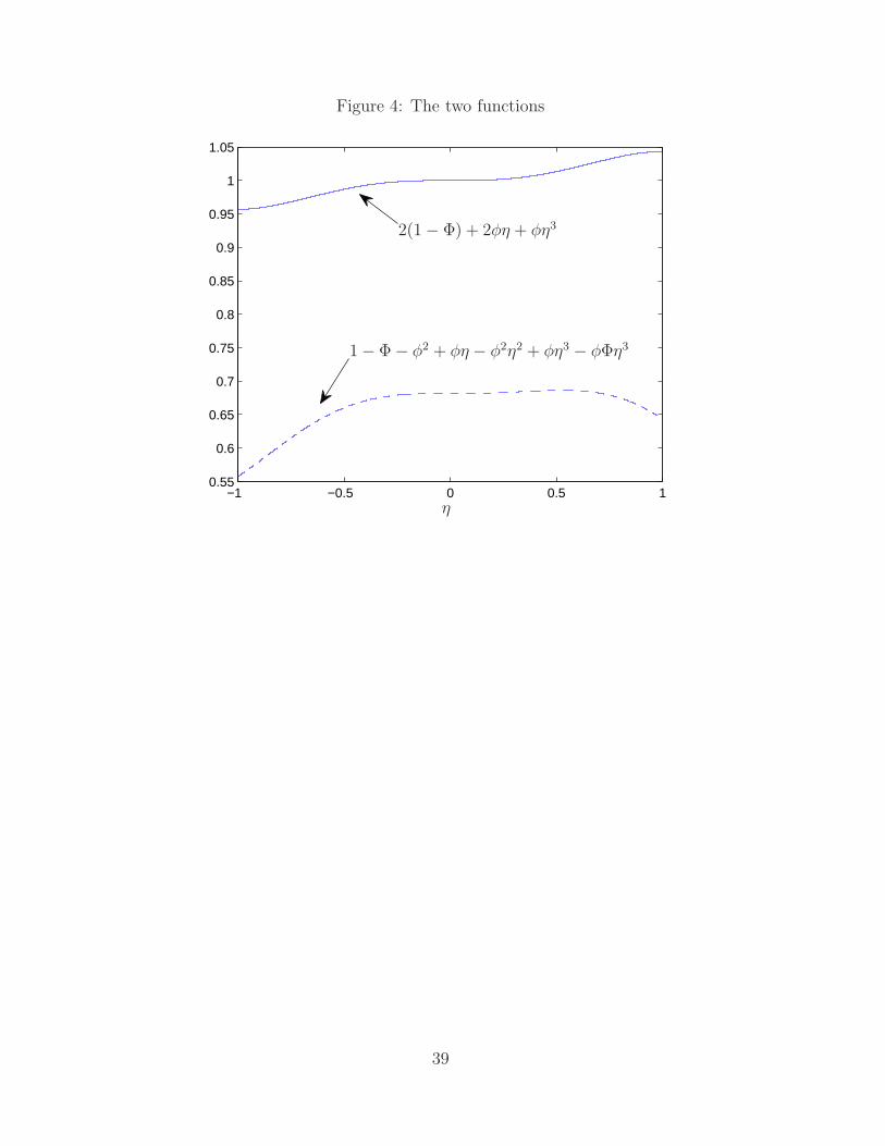
Figure 4: The two functions
−1 −0.5 0 0.5 10.55
0.6
0.65
0.7
0.75
0.8
0.85
0.9
0.95
1
1.05
η
2(1− Φ) + 2φη + φη3
1− Φ− φ2 + φη − φ2η2 + φη3 − φΦη3
39