Embed Size (px)
Citation preview

INC 693, 481 Dynamics System and Modelling:Lagrangian Method III
Dr.-Ing. Sudchai BoontoAssistant Professor
Department of Control System and Instrumentation Engineering
King Mongkut’s Unniversity of Technology Thonburi Thailand

First-order Equations for the Lagrangian Method
The second-order differential equation can be expressed in the from of
two first-order equations by defining an additional variable. Define the
additional variables as the generalized momenta, given by
pi =∂L∂qi
Sinced
dt
(∂L∂qi
)= pi
The Lagrangian equation
d
dt
(∂L∂qi
)− ∂L
∂qi+
∂R∂qi
= 0
pi −∂L∂qi
+∂R∂qi
= 0
These are first-order equations. The desirable form of the first-order
equations is such that the derivative quantities (qi and pi) may be
eqpressed as function of the fundamental variables.INC 693, 481 Dynamics System and Modelling: , Lagrangian Method III J 2/24 I }
First-order Equations for the Lagrangian MethodSpring Pendulum
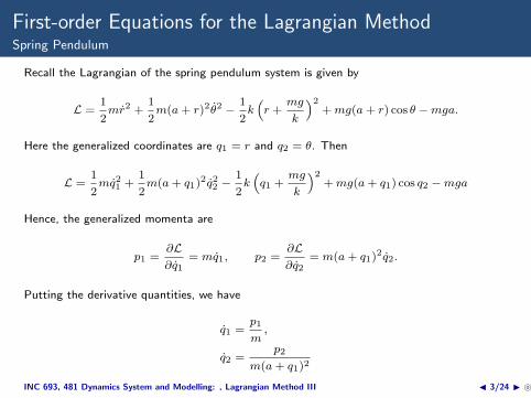
Recall the Lagrangian of the spring pendulum system is given by
L =1
2mr2 +
1
2m(a+ r)2θ2 −
1
2k(r +
mg
k
)2+mg(a+ r) cos θ −mga.
Here the generalized coordinates are q1 = r and q2 = θ. Then
L =1
2mq21 +
1
2m(a+ q1)
2q22 −1
2k(q1 +
mg
k
)2+mg(a+ q1) cos q2 −mga
Hence, the generalized momenta are
p1 =∂L∂q1
= mq1, p2 =∂L∂q2
= m(a+ q1)2q2.
Putting the derivative quantities, we have
q1 =p1
m,
q2 =p2
m(a+ q1)2
INC 693, 481 Dynamics System and Modelling: , Lagrangian Method III J 3/24 I }
First-order Equations for the Lagrangian MethodSpring Pendulum
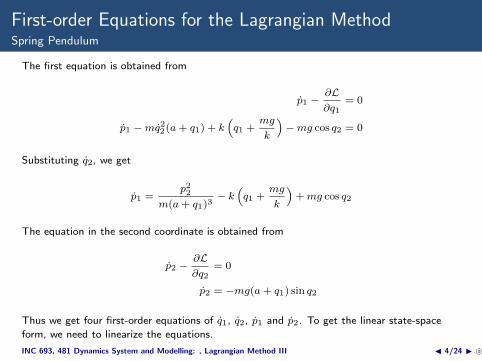
The first equation is obtained from
p1 −∂L∂q1
= 0
p1 −mq22(a+ q1) + k(q1 +
mg
k
)−mg cos q2 = 0
Substituting q2, we get
p1 =p22
m(a+ q1)3− k
(q1 +
mg
k
)+mg cos q2
The equation in the second coordinate is obtained from
p2 −∂L∂q2
= 0
p2 = −mg(a+ q1) sin q2
Thus we get four first-order equations of q1, q2, p1 and p2. To get the linear state-space
form, we need to linearize the equations.
INC 693, 481 Dynamics System and Modelling: , Lagrangian Method III J 4/24 I }
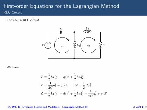
First-order Equations for the Lagrangian MethodRLC Circuit
Consider a RLC circuit
−+
E
C L2
RL1q1 q2
We have
T =1
2L1(q1 − q2)
2 +1
2L2q
22
V =1
2Cq21 − q1E, R =
1
2Rq22
L =1
2L1(q1 − q2)
2 +1
2L2q
22 −
1
2Cq21 + q1E
INC 693, 481 Dynamics System and Modelling: , Lagrangian Method III J 5/24 I }
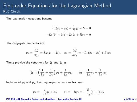
First-order Equations for the Lagrangian MethodRLC Circuit
The Lagrangian equations become
L1(q1 − q2) +1
Cq1 − E = 0
−L1(q1 − q2) + L2q2 +Rq2 = 0
The conjugate momenta are
p1 =∂L∂q1
= L1(q1 − q2), p2 =∂L∂q2
= −L1(q1 − q2) + L2q2
These provide the equations for q1 and q2 as
q1 =
(1
L1+
1
L2
)p1 +
1
L2p2, q2 =
1
L2p1 +
1
L2p2.
In terms of p1 and p2, the Lagrangian equations become
p1 = −1
Cq1 + E, p2 = −Rq2 = −
R
L2(p1 + p2).
INC 693, 481 Dynamics System and Modelling: , Lagrangian Method III J 6/24 I }
The Hamiltonian Formalism
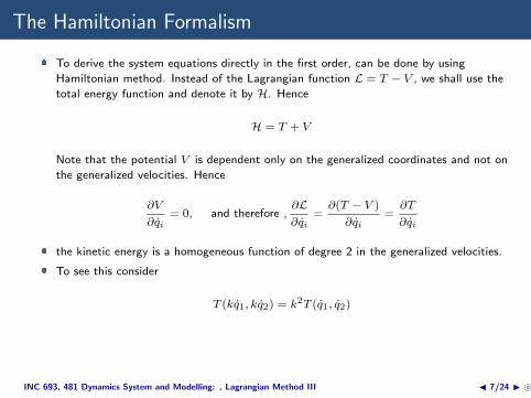
� To derive the system equations directly in the first order, can be done by using
Hamiltonian method. Instead of the Lagrangian function L = T − V , we shall use the
total energy function and denote it by H. Hence
H = T + V
Note that the potential V is dependent only on the generalized coordinates and not on
the generalized velocities. Hence
∂V
∂qi= 0, and therefore ,
∂L∂qi
=∂(T − V )
∂qi=
∂T
∂qi
� the kinetic energy is a homogeneous function of degree 2 in the generalized velocities.
� To see this consider
T (kq1, kq2) = k2T (q1, q2)
INC 693, 481 Dynamics System and Modelling: , Lagrangian Method III J 7/24 I }
The Hamiltonian Formalism
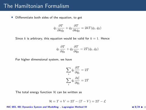
� Differentiate both sides of the equation, to get
q1∂T
∂kq1+ q2
∂T
∂kq2= 2kT (q1, q2)
Since k is arbitrary, this equation would be valid for k = 1. Hence
q1∂T
∂q1+ q2
∂T
∂q2= 2T (q1, q2)
For higher dimensional system, we have
∑i
qi∂T
∂qi= 2T
∑i
qi∂L∂qi
= 2T
The total energy function H can be written as
H = T + V = 2T − (T − V ) = 2T − LINC 693, 481 Dynamics System and Modelling: , Lagrangian Method III J 8/24 I }
The Hamiltonian Formalism
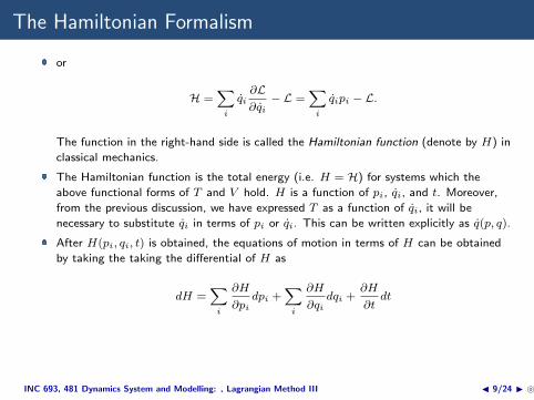
� or
H =∑i
qi∂L∂qi
− L =∑i
qipi − L.
The function in the right-hand side is called the Hamiltonian function (denote by H) in
classical mechanics.
� The Hamiltonian function is the total energy (i.e. H = H) for systems which the
above functional forms of T and V hold. H is a function of pi, qi, and t. Moreover,
from the previous discussion, we have expressed T as a function of qi, it will be
necessary to substitute qi in terms of pi or qi. This can be written explicitly as q(p, q).
� After H(pi, qi, t) is obtained, the equations of motion in terms of H can be obtained
by taking the taking the differential of H as
dH =∑i
∂H
∂pidpi +
∑i
∂H
∂qidqi +
∂H
∂tdt
INC 693, 481 Dynamics System and Modelling: , Lagrangian Method III J 9/24 I }
The Hamiltonian Formalism
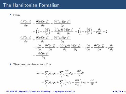
� From
∂H(q, p)
∂p=
∂(pq(p, q))
∂p−
∂L(q, q(p, q))∂p
=
(q + p
∂q
∂p
)−
L(q, q)∂q
∂q(p, q)
∂p=
(q + p
∂q
∂p
)− p
∂q
∂p= q
∂H(q, p)
∂q=
∂(pq(p, q))
∂q−
∂L(q, p(p, q))∂q
= p∂q
∂q−
∂L(q, q)∂q
−∂L(q, q)
∂q
∂q(p, q)
∂q= p
∂q
∂q−
∂L(q, q)∂q
− p∂q
∂q
= −∂L(q, q)
∂q
� Then, we can also write dH as
dH =∑i
qidpi −∑i
∂L∂qi
dqi −∂L∂t
dt
=∑i
qidpi +∑i
(−pi −
∂R∂qi
)dqi −
∂L∂t
dt
INC 693, 481 Dynamics System and Modelling: , Lagrangian Method III J 10/24 I }
The Hamiltonian Formalism
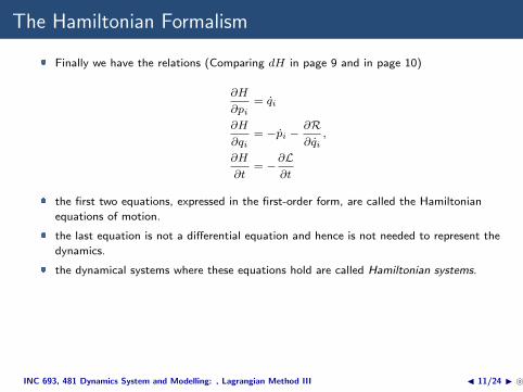
� Finally we have the relations (Comparing dH in page 9 and in page 10)
∂H
∂pi= qi
∂H
∂qi= −pi −
∂R∂qi
,
∂H
∂t= −
∂L∂t
� the first two equations, expressed in the first-order form, are called the Hamiltonian
equations of motion.
� the last equation is not a differential equation and hence is not needed to represent the
dynamics.
� the dynamical systems where these equations hold are called Hamiltonian systems.
INC 693, 481 Dynamics System and Modelling: , Lagrangian Method III J 11/24 I }
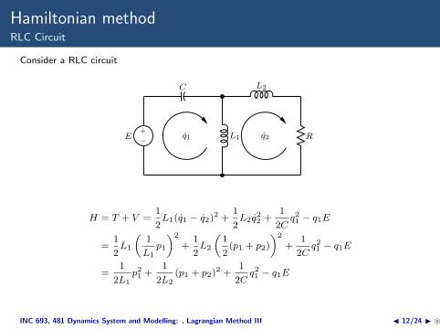
Hamiltonian methodRLC Circuit
Consider a RLC circuit
−+
E
C L2
RL1q1 q2
H = T + V =1
2L1(q1 − q2)
2 +1
2L2q
22 +
1
2Cq21 − q1E
=1
2L1
(1
L1p1
)2
+1
2L2
(1
2(p1 + p2)
)2
+1
2Cq21 − q1E
=1
2L1p21 +
1
2L2(p1 + p2)
2 +1
2Cq21 − q1E
INC 693, 481 Dynamics System and Modelling: , Lagrangian Method III J 12/24 I }
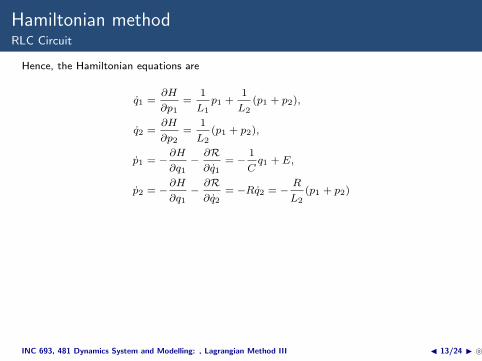
Hamiltonian methodRLC Circuit
Hence, the Hamiltonian equations are
q1 =∂H
∂p1=
1
L1p1 +
1
L2(p1 + p2),
q2 =∂H
∂p2=
1
L2(p1 + p2),
p1 = −∂H
∂q1−
∂R∂q1
= −1
Cq1 + E,
p2 = −∂H
∂q1−
∂R∂q2
= −Rq2 = −R
L2(p1 + p2)
INC 693, 481 Dynamics System and Modelling: , Lagrangian Method III J 13/24 I }
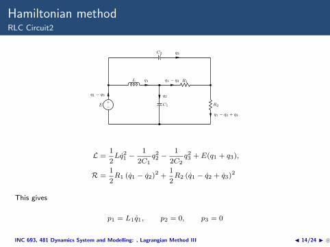
Hamiltonian methodRLC Circuit2
−+
q1 − q3
E
q1L q1 − q2 R1
q1 − q2 + q3
R2C1
q2
q3C2
L =1
2Lq21 −
1
2C1q22 −
1
2C2q23 + E(q1 + q3),
R =1
2R1 (q1 − q2)
2 +1
2R2 (q1 − q2 + q3)
2
This gives
p1 = L1q1, p2 = 0, p3 = 0
INC 693, 481 Dynamics System and Modelling: , Lagrangian Method III J 14/24 I }
Hamiltonian methodRLC Circuit2
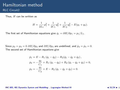
Thus, H can be written as
H =1
2L1p21 +
1
2C1q22 +
1
2C2q23 − E(q1 + q3).
The first set of Hamiltonian equations give q1 = ∂H/∂p1 = p1/L1.
Since p2 = p3 = 0 ∂H/∂p2 and ∂H/∂p3 are undefined, and p2 = p3 = 0.
The second set of Hamiltonian equations give
p1 = E −R1 (q1 − q2)−R2(q1 − q2 + q3) ,
p2 = −q2
C1+R1 (q1 − q2) +R2 (q1 − q2 + q3) = 0,
p3 = −q3
C2+ E −R2 (q1 − q2 + q3) = 0.
INC 693, 481 Dynamics System and Modelling: , Lagrangian Method III J 15/24 I }
Hamiltonian methodRLC Circuit2
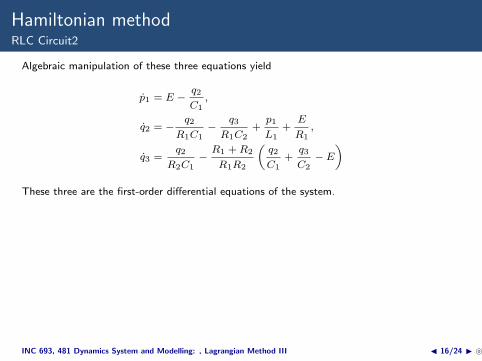
Algebraic manipulation of these three equations yield
p1 = E −q2
C1,
q2 = −q2
R1C1−
q3
R1C2+
p1
L1+
E
R1,
q3 =q2
R2C1−
R1 +R2
R1R2
(q2
C1+
q3
C2− E
)
These three are the first-order differential equations of the system.
INC 693, 481 Dynamics System and Modelling: , Lagrangian Method III J 16/24 I }
Hamiltonian methodSeparately excited DC motor and mechanical load system with a flexible shaft.
−+
E
q1 La Ra
q2
k
q3
l1
Const.
I1, R1
R2
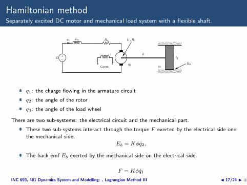
� q1: the charge flowing in the armature circuit
� q2: the angle of the rotor
� q3: the angle of the load wheel
There are two sub-systems: the electrical circuit and the mechanical part.
� These two sub-systems interact through the torque F exerted by the electrical side one
the mechanical side.
Eb = Kϕq2,
� The back emf Eb exerted by the mechanical side on the electrical side.
F = Kϕq1
INC 693, 481 Dynamics System and Modelling: , Lagrangian Method III J 17/24 I }
Hamiltonian methodSeparately excited DC motor and mechanical load system with a flexible shaft.
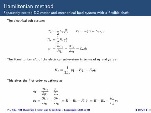
The electrical sub-system:
Te =1
2Laq
21 , Ve = −(E − Eb)q1
Re =1
2Raq
21
p1 =∂Le
∂q1=
∂Te
∂q1= Laq1
The Hamiltonian He of the electrical sub-system in terms of q1 and p1 as
He =1
2Lap21 − Eq1 + Ebq1
This gives the first-order equations as
q1 =∂He
∂p1=
p1
La
p1 =∂He
∂q1−
∂Re
∂q1= E − Eb −Raq1 = E − Eb −
Ra
Lap1
INC 693, 481 Dynamics System and Modelling: , Lagrangian Method III J 18/24 I }
Hamiltonian methodSeparately excited DC motor and mechanical load system with a flexible shaft.
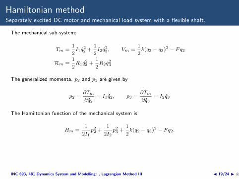
The mechanical sub-system:
Tm =1
2I1q
22 +
1
2I2q
23 , Vm =
1
2k(q2 − q3)
2 − Fq2
Rm =1
2R1q
22 +
1
2R2q
23
The generalized momenta, p2 and p3 are given by
p2 =∂Tm
∂q2= I1q2, p3 =
∂Tm
∂q3= I2q3
The Hamiltonian function of the mechanical system is
Hm =1
2I1p22 +
1
2I2p23 +
1
2k(q2 − q3)
2 − Fq2.
INC 693, 481 Dynamics System and Modelling: , Lagrangian Method III J 19/24 I }
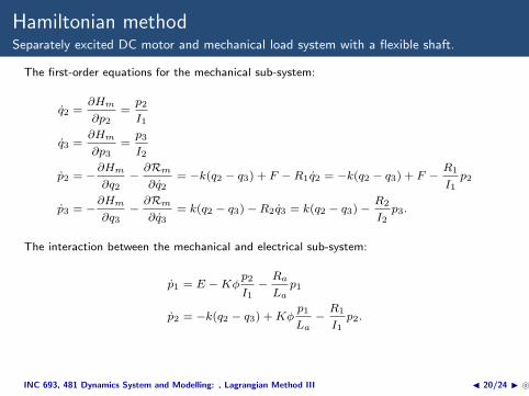
Hamiltonian methodSeparately excited DC motor and mechanical load system with a flexible shaft.
The first-order equations for the mechanical sub-system:
q2 =∂Hm
∂p2=
p2
I1
q3 =∂Hm
∂p3=
p3
I2
p2 = −∂Hm
∂q2−
∂Rm
∂q2= −k(q2 − q3) + F −R1q2 = −k(q2 − q3) + F −
R1
I1p2
p3 = −∂Hm
∂q3−
∂Rm
∂q3= k(q2 − q3)−R2q3 = k(q2 − q3)−
R2
I2p3.
The interaction between the mechanical and electrical sub-system:
p1 = E −Kϕp2
I1−
Ra
Lap1
p2 = −k(q2 − q3) +Kϕp1
La−
R1
I1p2.
INC 693, 481 Dynamics System and Modelling: , Lagrangian Method III J 20/24 I }
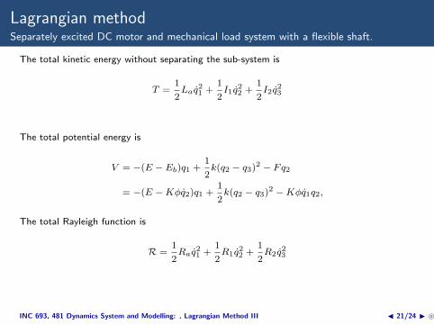
Lagrangian methodSeparately excited DC motor and mechanical load system with a flexible shaft.
The total kinetic energy without separating the sub-system is
T =1
2Laq
21 +
1
2I1q
22 +
1
2I2q
23
The total potential energy is
V = −(E − Eb)q1 +1
2k(q2 − q3)
2 − Fq2
= −(E −Kϕq2)q1 +1
2k(q2 − q3)
2 −Kϕq1q2,
The total Rayleigh function is
R =1
2Raq
21 +
1
2R1q
22 +
1
2R2q
23
INC 693, 481 Dynamics System and Modelling: , Lagrangian Method III J 21/24 I }
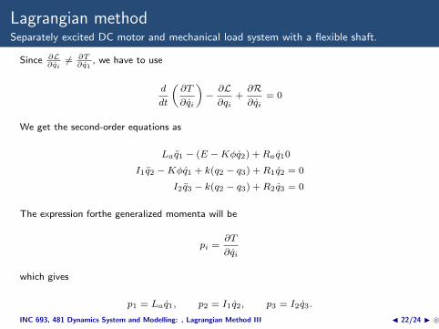
Lagrangian methodSeparately excited DC motor and mechanical load system with a flexible shaft.
Since ∂L∂qi
= ∂T∂q1
, we have to use
d
dt
(∂T
∂qi
)−
∂L∂qi
+∂R∂qi
= 0
We get the second-order equations as
Laq1 − (E −Kϕq2) +Raq10
I1q2 −Kϕq1 + k(q2 − q3) +R1q2 = 0
I2q3 − k(q2 − q3) +R2q3 = 0
The expression forthe generalized momenta will be
pi =∂T
∂qi
which gives
p1 = Laq1, p2 = I1q2, p3 = I2q3.
INC 693, 481 Dynamics System and Modelling: , Lagrangian Method III J 22/24 I }
Lagrangian methodSeparately excited DC motor and mechanical load system with a flexible shaft.
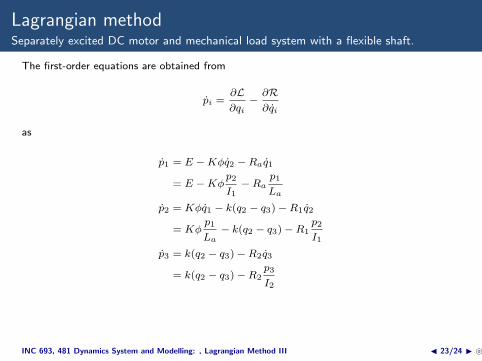
The first-order equations are obtained from
pi =∂L∂qi
−∂R∂qi
as
p1 = E −Kϕq2 −Raq1
= E −Kϕp2
I1−Ra
p1
La
p2 = Kϕq1 − k(q2 − q3)−R1q2
= Kϕp1
La− k(q2 − q3)−R1
p2
I1
p3 = k(q2 − q3)−R2q3
= k(q2 − q3)−R2p3
I2
INC 693, 481 Dynamics System and Modelling: , Lagrangian Method III J 23/24 I }
Reference
1. Wellstead, P. E. Introduction to Physical System Modelling,
Electronically published by:
www.control-systems-principles.co.uk, 2000
2. Banerjee, S., Dynamics for Engineers, John Wiley & Sons, Ltd.,
2005
3. Rojas, C. , Modeling of Dynamical Systems, Automatic Control,
School of Electrical Engineering, KTH Royal Institute of
Technology, Sweeden
4. Fabien, B., Analytical System Dynamics: Modeling and Simulation
Springer, 2009
5. Spong, M. W. and Hutchinson, S. and Vidyasagar, M., Robot
Modeling and Control, John Wiley & Sons, Inc.
INC 693, 481 Dynamics System and Modelling: , Lagrangian Method III J 24/24 I }


![IAC12/30/20 InspectionsandAppeals[481] 31 481—31.5(137F](https://img.pdfslide.us/doc/110x75/6266e12f0983034210142814/iac123020-inspectionsandappeals481-31-481315137f-.jpg)