Inflation Taxation and Welfare with Externalities and Leisure

Wai-Ming Ho∗

Associate ProfessorDepartment of Economics, York University

Email: waiming@yorku.ca

Jinli ZengAssociate Professor

Department of Economics, National University of SingaporeEmail: ecszjl@nus.edu.sg

Jie ZhangAssociate Professor

Department of Economics, National University of SingaporeEmail: ecszj@nus.edu.sg

andSchool of Economics, University of Queensland

Email: jzhang@uq.edu.au

Final version: October 20, 2005

JEL classification: E40; D62; D90

Keywords: Inflation; Money; Taxation; Welfare; Externality

Correspondence: Wai-Ming Ho, Department of Economics, Faculty of Arts, York University,

4700 Keele Street, Toronto, Ontario, Canada M3J 1P3

Phone: (416) 736 2100 ext.22319; Fax: (416) 736 5987; E-mail: waiming@yorku.ca

∗We would like to thank two anonymous referees for giving us very helpful comments and suggestions. Allremaining errors and omissions are our own.

Inflation Taxation and Welfare with Externalities and Leisure

Abstract

This paper examines how inflation taxation affects resource allocation and welfare in a neo-

classical growth model with leisure, a production externality and money in the utility function.

Switching from consumption taxation to inflation taxation to finance government spending reduces

real money balances relative to income, but increases consumption, labor, capital and output. The

net welfare effect of this switch depends crucially on the strength of the externality and on the

elasticity of intertemporal substitution: While it is always negative without the externality, it is

likely to be positive with a strong externality and elastic intertemporal substitution.

How inflation taxation affects resource allocation and welfare has received a great deal of atten-

tion. So far, this debate has been controversial. Most studies claim that inflation taxation reduces

welfare regardless of whether money demand is derived from a cash-in-advance constraint, from

a transaction technology with money as an intermediate input, or from real money balances in

the utility function (e.g. Friedman, 1969; Kimbrough, 1986; Prescott, 1987; Cole and Stockman,

1992; Schreft, 1992; Gillman, 1993; Gomme, 1993; Correia and Teles, 1996; Dotsey and Ireland,

1996; Aiyagari, Braun and Eckstein, 1998; Wu and Zhang, 1998, 2000; Lucas, 2000; and Erosa and

Ventura, 2002). In many of these studies, the optimal rule of money growth is to generate a degree

of deflation such that the nominal interest rate, i.e. the opportunity cost of holding money, equals

zero as described by the Friedman rule.

On the other hand, some studies support a rate of money growth for a positive nominal inter-

est rate by considering additional factors. In Phelps (1973), Braun (1994) and Palivos and Yip

(1995), inflation taxation leads to higher welfare than income taxation as a means of public finance.

Guidotti and Vegh (1993) derive optimal inflation taxation with increasing returns to scale in the

transaction-cost technology. Shi (1999) supports an optimal money-growth rate in excess of the

Friedman rule by assuming borrowing constraints. In Rebelo and Xie (1999), money does not affect

production in the steady state but can alter it during the transition toward the steady state; and

the transitional effect can be exploited by monetary policy to improve welfare if there is a produc-

tion externality. Most of these studies have fully inelastic labor supply, and ignore externalities

that are nevertheless prevalent in the real world. It remains to be seen how money growth affects

welfare with both a production externality and a labor-leisure trade-off. As shown in Turnovsky

(2000), the inclusion of an endogenous labor-leisure trade-off leads to fundamental changes in the

economy’s equilibrium structure as there is an equilibrium growth-leisure trade-off.

In this paper we examine how nominal money growth as a means of public finance affects

resource allocation and welfare in a neoclassical growth model with leisure, a production externality

and money in the utility function. For simplicity, we assume that government spending is a fixed

fraction of output and is not valued by private agents. The government may also tax consumption

to finance its spending, unlike Phelps (1973), Braun (1994) and Palivos and Yip (1995) where they

1

compare an income tax with the inflation tax. Individuals allocate income to consumption and

investment in both capital and real money balances, and allocate time to labor and leisure.

In this environment, switching from consumption taxation to inflation taxation drives up the

cost of holding money, and thus reduces the demand for real money balances relative to income as

is well known in the literature. Also well known is that economizing on money holdings accelerates

the circulation of money. Further, the decrease in real money balances reduces the marginal benefits

of consumption and leisure with a nonseparable utility function concerning these augments, which

tends to reduce consumption and leisure. However, the rise in the nominal money growth rate

has no direct effect on the cost of leisure (the real wage), and therefore leisure should decline and,

accordingly, labor should increase. The increased labor in turn raises the marginal product of

capital and stimulates capital accumulation, leading to higher output per capita.1

On the other hand, the accompanying decline in the consumption tax rate also lowers the cost of

consumption, tending to raise consumption. Given the standard constant elasticity of intertemporal

substitution (CEIS) form of the utility function in the literature on economic growth, the net effect

on the ratio of consumption to output is zero. Thus, as output rises with the nominal money

growth rate, so does consumption. The rise in output also works against the decline in the ratio of

real money balances to output in the determination of the effect of faster nominal money growth

on the level of real money balances. As a consequence, there are opposing effects of the switch

from consumption taxation to inflation taxation on welfare: The increase in consumption tends to

raise welfare but the decline in leisure tends to reduce welfare. How real money balances respond

to the tax switch also affects welfare. The net effects of the tax switch on real money balances and

welfare depend crucially on whether production externalities are taken into consideration.

First, consider the case that has no externality where the concern about monetary policy focuses

mainly on the benefit and cost of holding money. In the spirit of the Friedman rule, since the

social cost of producing money is zero, there should be a negative inflation tax such that the cost

of holding money (the nominal interest rate) can be as close to zero as possible. As a result, the

optimal inflation tax is negative along with a positive consumption tax, but the underlying nominal

money growth rate should exceed the rate that corresponds strictly to the Friedman rule because

2

of the tax distortions on leisure, output and consumption.

Now consider the case with a production externality in the form of learning-by-doing and

knowledge spillovers. In addition to the consideration above, we know that the private rate of return

on capital investment must be lower than the social rate due to the externality, which implies that

agents hold too little capital compared to the social optimum. Because of the under-investment in

capital, the private rate of return on labor must also be lower than the social rate, which implies

that agents have too much leisure and too little labor compared to the social optimum. The new

consideration is that we want agents to hold more capital, which can be achieved by applying a

higher inflation tax in order to induce them to switch out of real money balances into capital. The

positive effects of the switch to inflation taxation on labor, capital investment and output help the

economy correct the under-investment in capital and may thus improve welfare.

We find two key factors in the determination of the relative strength of the opposing effects of

the tax switch on welfare. First, a stronger production externality strengthens the positive welfare

effect, other things equal. Second, since the positive effect of the switch to inflation taxation on

output takes time to reach its full potential through promoting capital accumulation, the relative

strength of the positive welfare effect also depends on the elasticity of intertemporal substitution.

More elastic intertemporal substitution accelerates growth and hence strengthens the positive wel-

fare effect. We show that when output can fully adjust in the long run, the net welfare effect of

switching from consumption taxation to inflation taxation can be positive so long as the externality

is strong enough. However, when considering the entire equilibrium path in a tractable AK model

with a strong enough externality for endogenous growth, a positive net welfare effect of this tax

switch also requires the elasticity of intertemporal substitution to be sufficiently high.

The avenue through which inflation taxation affects production and welfare in this model differs

from those in the related work mentioned above. By reducing the consumption tax, raising the

inflation tax to finance a given government fiscal commitment can stimulate production in the

long run in our model, as opposed to the long-run neutrality of money growth in Rebelo and Xie

(1999) without a consumption tax. The difference originates mainly from the different assumptions

concerning labor supply (elastic in our model but fully inelastic in their model). If labor supply

3

were fully inelastic in our model, then switching from consumption taxation to inflation taxation

would have no real effect on consumption and production in the long run.

The rest of the paper proceeds as follows. Section 1 introduces the model and characterizes the

equilibrium. Section 2 presents results without sustainable growth in the absence of any externality

or in the presence of a weak production externality. Section 3 derives results with a strong enough

production externality for sustainable growth. We separate these cases because the analytical

approaches differ between cases with or without sustainable growth. Section 4 discusses briefly

what may happen with cash-in-advance constraints. The last section concludes. Proofs of results

will be relegated to the Appendix.

1. THE MODEL

We consider an economy populated by identical infinitely-lived households with measure one.

The representative household is endowed with one unit of time which is allocated to leisure lt and

labor 1− lt. There is no uncertainty in the form of shocks in preferences and technology.2

1.1 Production

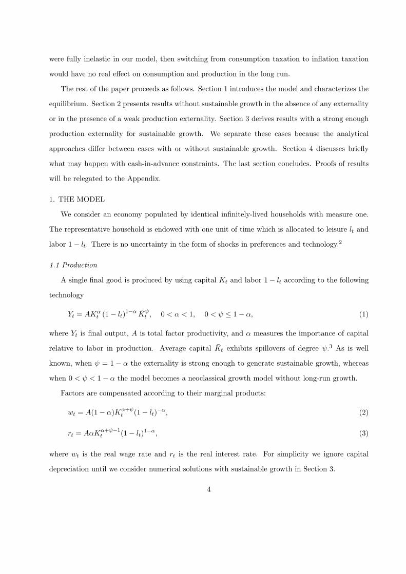
A single final good is produced by using capital Kt and labor 1− lt according to the following

technology

Yt = AKαt (1− lt)1−α Kψ

t , 0 < α < 1, 0 < ψ ≤ 1− α, (1)

where Yt is final output, A is total factor productivity, and α measures the importance of capital

relative to labor in production. Average capital Kt exhibits spillovers of degree ψ.3 As is well

known, when ψ = 1 − α the externality is strong enough to generate sustainable growth, whereas

when 0 < ψ < 1− α the model becomes a neoclassical growth model without long-run growth.

Factors are compensated according to their marginal products:

wt = A(1− α)Kα+ψt (1− lt)−α, (2)

rt = AαKα+ψ−1t (1− lt)1−α, (3)

where wt is the real wage rate and rt is the real interest rate. For simplicity we ignore capital

depreciation until we consider numerical solutions with sustainable growth in Section 3.

4

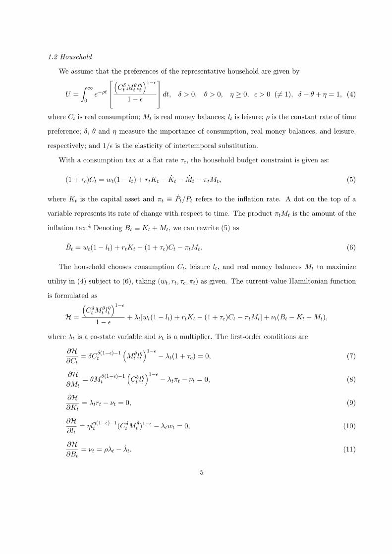
1.2 Household

We assume that the preferences of the representative household are given by

U =∫ ∞

0e−ρt

(CδtM

θt lηt

)1−ε

1− ε

dt, δ > 0, θ > 0, η ≥ 0, ε > 0 (6= 1), δ + θ + η = 1, (4)

where Ct is real consumption; Mt is real money balances; lt is leisure; ρ is the constant rate of time

preference; δ, θ and η measure the importance of consumption, real money balances, and leisure,

respectively; and 1/ε is the elasticity of intertemporal substitution.

With a consumption tax at a flat rate τc, the household budget constraint is given as:

(1 + τc)Ct = wt(1− lt) + rtKt − Kt − Mt − πtMt, (5)

where Kt is the capital asset and πt ≡ Pt/Pt refers to the inflation rate. A dot on the top of a

variable represents its rate of change with respect to time. The product πtMt is the amount of the

inflation tax.4 Denoting Bt ≡ Kt +Mt, we can rewrite (5) as

Bt = wt(1− lt) + rtKt − (1 + τc)Ct − πtMt. (6)

The household chooses consumption Ct, leisure lt, and real money balances Mt to maximize

utility in (4) subject to (6), taking (wt, rt, τc, πt) as given. The current-value Hamiltonian function

is formulated as

H =

(CδtM

θt lηt

)1−ε

1− ε+ λt[wt(1− lt) + rtKt − (1 + τc)Ct − πtMt] + νt(Bt −Kt −Mt),

where λt is a co-state variable and νt is a multiplier. The first-order conditions are

∂H∂Ct

= δCδ(1−ε)−1t

(M θt lηt

)1−ε− λt(1 + τc) = 0, (7)

∂H∂Mt

= θMθ(1−ε)−1t

(Cδt l

ηt

)1−ε− λtπt − νt = 0, (8)

∂H∂Kt

= λtrt − νt = 0, (9)

∂H∂lt

= ηlη(1−ε)−1t (CδtM

θt )

1−ε − λtwt = 0, (10)

∂H∂Bt

= νt = ρλt − λt. (11)

5

The transversality condition ruling out the Ponzi game is given by

limt→∞

e−ρtλtBt = 0. (12)

According to these conditions, the marginal gain in utility of each choice variable should equal

its marginal loss. In particular, a higher inflation cost of holding money induces households to

economize on real money balances in (8), other things equal.

These first-order conditions imply the following relationships:

[1− δ(1− ε)] CtCt− θ(1− ε)Mt

Mt− η(1− ε) l

l= rt − ρ, (13)

lt =η(1 + τc)Ct

δwt, (14)

Mt =θ(1 + τc)Ctδ(rt + πt)

. (15)

Equation (13) links consumption growth to real money growth, leisure growth, and the gap between

the real interest rate and the rate of time preference. In (14) and (15), the optimal levels of

consumption, real money balances, and the forgone wage income (leisure times the wage) are

proportional to one another given (τc, π, r), due to the homothetic CEIS utility function.

1.3 Government

The government uses a consumption tax and money issuing (seignorage revenue or an inflation

tax) to finance a government purchase Gt that is not valued by private agents. Throughout the

paper, we abstract from income taxation because it is dominated by consumption taxation in

this type of model. We assume that government spending is a fixed fraction β of final output,

i.e. Gt = βYt with β > 0, in the spirit of Ramsey. The task of the government is to select the

welfare-maximizing rates of the consumption and inflation taxes to finance the required government

spending subject to its budget constraint. Suppose that the government budget is balanced at each

point in time:

τcCt +˙M t

Pt= Gt = βYt, β > 0, (16)

where Mt is nominal money supply and ˙Mt/Pt is seignorage revenue.

6

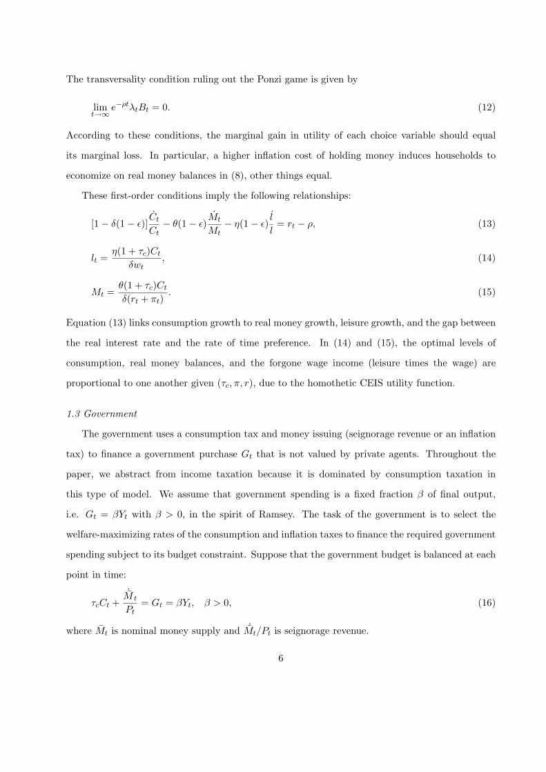
1.4 Equilibrium

The equilibrium is characterized by the wage and interest rate equations, the first-order condi-

tions of the household problem, the budget constraints of the household and the government, the

time constraint between leisure and labor, and the overall resource constraint Ct + Gt + Kt = Yt.

For analytical convenience, we transform the key variables (C,M,K) into their ratios to output

(ΓC,ΓM ,ΓK) in the system of equations determining the equilibrium. Also denote the growth rates

X/X for X = C,K,M, l as gX , and the growth rate of nominal money supply as σ. We then have

[1− δ(1− ε)]gC − θ(1− ε)gM − η(1− ε)gl = r − ρ, (17)

ΓM =θ(1 + τc)ΓCδ(r + π)

, (18)

l =η(1 + τc)ΓC(1− l)

δ(1− α), (19)

(1 + τc)ΓC = 1− gKΓK − gMΓM − πΓM , (20)

τcΓC + σΓM = β, (21)

ΓC + gKΓK = 1− β. (22)

From (20)-(22), we have

gM = σ − π, (23)

which says that the growth rate of real money balances gM equals the growth rate of nominal

money supply σ minus the inflation rate π.

In what follows, we shall investigate three cases. The first case has no externality, i.e. ψ = 0,

allowing us to link our work to the literature. In the other two cases we assume 0 < ψ < 1−α and

ψ = 1 − α, respectively, so that we can study the implications of the production externality. We

call 0 < ψ < 1 − α a weak externality case and ψ = 1 − α a strong externality case. In the cases

with 0 ≤ ψ < 1 − α there is no sustainable growth, whereas in the case with ψ = 1 − α there is

sustainable growth.

7

2. RESULTS WITHOUT SUSTAINABLE GROWTH

We first derive equilibrium solutions and results in the cases that have no externality or a weak

production externality, i.e. 0 ≤ ψ < 1 − α. In order to avoid the complexity in tracking down

transitional dynamics, we only focus on the steady-state equilibrium in these cases. The steady-

state equilibrium solution is derived in a few steps. First, it is obvious to have π = σ, that is,

without long-run growth in output, the rate of inflation is just equal to the rate of nominal money

growth.

Setting C = M = l = 0 and substituting (3) into (17), we obtain r = AαKα+ψ−1(1− l)1−α = ρ.

As the real interest rate r is equal to the rate of time preference ρ without sustainable growth in

output, the steady-state capital-labor ratio can be determined as

k∗ = K∗/(1− l∗) =

[Aα(1− l∗)ψ

ρ

]1/(1−α−ψ)

. (24)

According to this, the capital-labor ratio is increasing with (independent of) the quantity of labor in

equilibrium with (without) the production externality. Also, nominal money growth can only affect

the capital-labor ratio indirectly through the quantity of labor in the presence of the externality.

The solution for the ratio of consumption to output is given by

ΓC = 1− β. (25)

For a given β, increasing the rate of nominal money growth, accompanied by decreasing the con-

sumption tax rate for a balanced government budget, will have opposing effects on the ratio of

consumption to output. According to (25), the net effect is zero.

The solution for the ratio of real money balances to output is

ΓM =θ

δ(ρ+ σ) + σθ. (26)

As expected, the ratio of real money balances to output is certainly decreasing with the rate of

nominal money growth because a higher nominal money growth rate raises the cost of holding

money (the nominal interest rate) by increasing the inflation rate.

The solution for leisure is found to be

l∗ =η(ρ+ σ)

η(ρ+ σ) + (1− α)[δ(ρ+ σ) + σθ]. (27)

8

It is easy to verify that leisure is decreasing with the rate of nominal money growth. Consequently,

labor supply is increasing with the ratio of nominal money growth.

According to (24) and (27), the steady-state level of capital K∗ = k∗(1 − l∗) should also be

increasing with the rate of nominal money growth. The steady-state quantity of output is then

equal to

Y ∗ =

[A(1− l∗)1−α

(α

ρ

)α+ψ] 1

1−α−ψ

, ψ ∈ [0, 1− α). (28)

In this equation, the level of output is an increasing function of the quantity of labor, after we

substitute capital stock out using AαKα+ψ−1(1 − l)1−α = ρ. Since labor is increasing with the

rate of nominal money growth, so must be the steady-state level of output regardless of whether

the externality is absent (ψ = 0) or present (0 < ψ < 1 − α). The case with sustainable growth

(ψ = 1− α) will be analyzed separately later.

Using (21), (25) and (26), we have the budget-balance restriction on the policy parameters:

β =τcδ(ρ+ σ)

(1 + τc)[δ(ρ+ σ) + σθ]+

σθ

δ(ρ+ σ) + σθ, (29)

which implies that τc = β[δ(ρ+ σ) + σθ ]− σθ /(1− β)[δ(ρ+ σ) + σθ ].

Further, the velocity of money V is positively related to the rate of nominal money growth or

inflation. Specifically, by the identity MV = PY , the income velocity of money can be expressed

as V = Y/(M/P ) = Y/M = 1/ΓM in this model. Since the ratio of real money balances to output

ΓM is decreasing with the rate of nominal money growth, the velocity of money, V = 1/ΓM , must

be increasing with the rate of nominal money growth.

We give the effect of inflation taxation on resource allocation below and put the proof in the

Appendix.

Proposition 1: In the steady state with β > 0 and 0 ≤ ψ < 1 − α, switching from consumption

taxation toward inflation taxation reduces leisure and the ratio of real money balances to income,

but increases consumption, labor, capital, output, and the velocity of money. Also, the tax switch

reduces real money balances for ψ = 0 but may increase it for a large ψ ∈ (0, 1− α).

The results in Proposition 1 can be explained as follows. Holding government spending as a

fixed fraction of output, a reduction in the consumption tax rate goes hand-in-hand with a rise

9

in the nominal money growth rate for a balanced government budget. The consequent rise in the

inflation rate with π = σ drives up the cost of holding money in (8), and thus reduces the demand

for real money balances relative to income, as is well known in the literature. Also well known is

that economizing on money holdings accelerates the circulation of money. Moreover, the decrease in

real money balances reduces the marginal benefits of consumption and leisure with a nonseparable

utility function concerning these augments, which tends to reduce consumption and leisure as can

be seen in (7) and (10). However, this rise in the rate of nominal money growth has no direct effect

on the cost of leisure (the real wage), and therefore, leisure should decline and, accordingly, labor

should increase. The increased labor in turn raises the marginal product of capital, and hence

stimulates capital accumulation and raises output. Since consumption is equal to output net of

government spending in the steady state with K = 0, the switch from consumption taxation to

inflation taxation also raises steady-state consumption.

When the rate of nominal money growth rises along with a falling consumption tax, there are

two opposing effects on the level of real money balances: a positive one through the rise in output

and a negative one through the fall in the ratio of real money balances to output. In the absence

of any externality, the positive effect through the rise in output is weak and is dominated by the

negative one, resulting in a net decline in real money balances. With a sufficiently strong production

externality, however, the rise in output caused by faster nominal money growth can be substantial

and may dominate the negative effect on real money balances, leading to a possible net increase in

the level of real money balances.

It is important to note that the real effect of a higher nominal money growth rate (accompanied

by a lower consumption tax rate) on resource allocation in this model originates from endogenous

labor supply. If labor supply were fully inelastic, then the real effect of switching from consumption

taxation to inflation taxation on consumption and output would disappear.

To examine the welfare effect of inflation taxation, we now derive the solution for the welfare

level in the steady state. Since in the steady state CδtMθt lηt = Y δ+θΓδCΓθM l

η, we obtain the solution

10

for the welfare level by substituting (25)-(28) into (4): U∗ = Φ [F (τc, σ)]1−ε /(1− ε), where

F (τc, σ) ≡ (ρ+ σ)δ+η(1 + τc)−δ[δ(ρ+ σ) + θσ]ψ(δ+θ)1−α−ψ

η(ρ+ σ) + (1− α)[δ(ρ+ σ) + θσ]1−α−ηψ1−α−ψ

, (30)

Φ ≡ 1ρ

δδθθηη[A(1− α)1−α

(α

ρ

)α+ψ] δ+θ

1−α−ψ

1−ε

> 0.

The welfare level U∗ is a function of the rates of the consumption tax and nominal money growth

via the function F , while Φ > 0 is a constant and independent of the consumption tax and nominal

money growth. The welfare level U∗ refers to the steady state equilibrium when capital and output

fully adjust to a permanent policy change in the long run. Also, note that U∗ is monotonically

increasing with F . We thus focus on F in the welfare analysis below, with or without the production

externality.

2.1 No Externality

In the absence of any externality (ψ = 0), the welfare level in (30) reduces to

F o(τc, σ) ≡ (ρ+ σ)δ+η(1 + τc)−δ

η(ρ+ σ) + (1− α)[δ(ρ+ σ) + σθ]. (31)

The government chooses the tax rates (τc, σ) to maximize welfare in (31) subject to (29), holding

government spending as a fixed fraction β of output. We proceed in two stages. First, we look at

regimes where the government uses either consumption taxation or inflation taxation but not both.

Second, we consider their mix.

In the case with consumption taxation only, we have τc = β/(1− β) from (29) and

F o(τc) =ρ−θ(1− β)δ

η + δ(1− α),

where the assumption θ + η + δ = 1 has been used to simplify the expression.

Analogously, when inflation taxation is the only option, we have σ = βδρ/[ θ(1− β)− βδ ] and

F o(σ) =(ρθ)−θ(1− β)δ+η[θ(1− β)− βδ]θ

η + δ(1− α).

Intuitively, in order to use seignorage revenue to finance the required government spending, the

taste parameter for real money balances θ must be large enough relative to the ratio of government

11

spending to output β and to the taste parameter for consumption δ. The exact restriction on

these parameters can be found as follows. First, the government budget balance with the inflation

tax as the sole means is σΓM = β. Using the solution for ΓM , this budget balance restriction

becomes σθ/[δ(ρ + σ) + σθ] = β. In this equation, the ratio of seignorage revenue to output (the

left-hand side) is increasing with the rate of nominal money growth σ and achieves its maximum at

σ = ∞: θ/(δ+θ). This maximum ratio of seignorage revenue to output less the ratio of government

spending to output equals [θ(1−β)−βδ]/(δ+θ). Therefore, θ > βδ/(1−β) is essentially a necessary

condition for inflation taxation alone to finance the required government spending. We thus make

this as an assumption. Under this assumption, there is an upper limit on the ratio of government

spending to output β which in turn sets an upper limit on the rate of nominal money growth or on

the rate of inflation by π = σ.

We compare the two regimes in terms of welfare below. The proof is in the Appendix.

Proposition 2: In the steady state without any externality and with β > 0 and θ > βδ/(1 − β),

using pure consumption taxation to finance government spending obtains a higher welfare level than

using pure inflation taxation.

By Proposition 2, inflation taxation leads to a lower welfare level than does consumption taxa-

tion as a sole means of financing government spending in the long run. What happens when both

instruments are used together? The answer is given below, with the proof in the Appendix.

Proposition 3: In the steady state without any externality and with β > 0, if both consumption

taxation and inflation taxation are used to finance government spending, their optimal mix to

maximize welfare has the following features: τ∗c > β/(1− β) and σ∗ = π∗ < 0.

By Proposition 3, when there is no production externality, the rate of nominal money growth

should be negative and the consumption tax should be positive. The intuition is as follows. Since

real money balances and consumption enter the utility “symmetrically”, there is a “uniform taxation

principle” saying that the government should tax both at the same rate in order to avoid distorting

the margin between consumption and real money balances. See Atkinson and Stiglitz (1972) for

more discussions on the uniform taxation principle. This consideration implies that the rates of

12

consumption and inflation taxes should be equal. However, real money balances are also an asset,

and ideally the government also does not want to distort the return on money relative to the return

on capital so as to avoid distorting the margin between real money balances and capital. Since

capital income is not taxed in our model, this consideration implies that the inflation tax should

be zero. Combining the consumption-money consideration with the capital-money consideration

suggests that, in the absence of any externality, the consumption tax should exceed the inflation

tax. Moreover, in the spirit of the Friedman rule, because the social cost of producing money is

zero, there should be a negative inflation tax such that the cost of holding money (the nominal

interest rate) can be as close to zero as possible. As a result, the optimal inflation tax is negative

along with a positive consumption tax. However, the underlying nominal money growth rate should

exceed the rate that corresponds strictly to the Friedman rule, because of the distortions of the

consumption tax and the negative inflation tax on leisure and consumption.

Further, can inflation taxation improve on the case without any government intervention (with

a zero nominal-money growth rate, no government spending, and no taxes) in welfare terms? We

design a template to answer this question as follows. Suppose that we start with the no-government

case, i.e. β = τc = σ = 0. Then, we allow for inflation taxation and spend seignorage revenue on

subsidizing consumption. That is, there exists a function τc(σ) such that τcΓC = − σΓM , which

reduces to τc = − σθ/[δ(ρ + σ) + σθ]. Inserting this relationship that balances the government

budget into F o(τc, σ) to obtain F o(τc(σ), σ), we increase the rate of nominal money growth from

zero, leading to a subsidy on consumption τc < 0, and see what happens to welfare F o(τc(σ), σ).

The result is given below and the proof is in the Appendix.

Proposition 4: In the steady state without any externality and with β = 0, raising the inflation

tax from zero to subsidize consumption reduces welfare from the level of a competitive equilibrium

with no government intervention. The optimal monetary policy should generate deflation (π∗ < 0).

As stated in Propositions 2-4, in the absence of the production externality, inflation taxation

always reduces welfare, whether it is used alone or along with consumption taxation, or whether

there is a required public purchase or a consumption subsidy. In essence, as the rate of nominal

money growth rises along with a falling consumption tax rate, the losses in welfare arising from the

13

decreases in leisure and real money balances dominate the gain in welfare arising from the increase

in consumption.

The quantitative implications of the results are illustrated in Table 1, using numerical solutions

based on the parameterization α = 0.3, A = 0.3, ρ = 0.03, θ = 0.1, ε = 3.0, η = 0.3, and ψ = 0.

The values of α, ρ and ε are in line with those widely used in the literature, while the values of

other parameters are chosen such that the numerical results for the key variables of interest are

plausible. To make a welfare comparison across all cases in Table 1, we first select a benchmark case

and then compute the percentage change in income in the benchmark case such that we reach the

same welfare level in each of the other cases (see the note in Table 1 for this equivalent payment).

The first case (the benchmark case) in Table 1 has no government intervention. In the sec-

ond case, either or both of consumption taxation and inflation taxation may be used to finance

government spending as 10% of output (β = 0.1). When both instruments are used, their op-

timal mix is a positive consumption tax and a negative inflation tax (a deflation transfer at a

rate of nominal money growth −2.04%), implying higher real money balances than in the bench-

mark. Compared to the benchmark case regarding real allocation and welfare, this optimal mix

has higher leisure but lower levels of steady-state capital and output, and achieves a welfare gain

in the magnitude of 2.87% of the benchmark income. The reason for this welfare gain is a reduced

nominal interest rate (the opportunity cost of holding money) under the negative inflation tax,

r + σ = ρ + σ = 3% − 2.04% = 0.96%. Note that this nominal interest rate exceeds what the

Friedman rule suggests (i.e. a zero nominal interest rate), because of the distortion on leisure and

consumption. When the consumption tax is used alone to finance government spending as 10% of

output (at a tax rate 11.11%), there is no real effect on the allocation of time and output. This

is because with the CEIS utility function the positive substitution effect of the consumption tax

on leisure is fully offset by its negative income effect when government spending is not valued by

private agents.6 Since government spending is wasted, the consumption tax reduces welfare from

the no-intervention benchmark case in the magnitude of 8.64% of income. When the inflation tax

is used alone, there is a greater loss in welfare compared to the no-intervention case (21.86% of

income) because the inflation tax (at a 6% nominal money growth rate) reduces both leisure and

14

real money balances.

2.2 A Weak Production Externality

With a weak production externality ψ ∈ (0, 1 − α), we first compare pure inflation taxation

with pure consumption taxation as in Proposition 2. The proof is in the Appendix.

Proposition 5: In the steady state with β > 0 and θ > βδ/(1 − β), if ψ ∈ (0, 1 − α) is large

enough, then using pure inflation taxation to finance government spending obtains a higher welfare

level than using pure consumption taxation.

In addition, we investigate whether inflation taxation can improve on pure consumption taxation

as in Proposition 3. The proof is in the Appendix.

Proposition 6: In the steady state with β > 0, when consumption taxation is used to finance

government spending, inflation taxation (π∗ = σ∗ > 0) should also be used together if ψ ∈ (0, 1−α)

is large enough.

Further, we explore whether inflation taxation can improve on the case without any government

intervention as in Proposition 4. The proof is in the Appendix.

Proposition 7: In the steady state with β = 0, if ψ ∈ (0, 1−α) is large enough, then increasing the

inflation tax rate from zero to subsidize consumption increases welfare from the level of a competitive

equilibrium without any government intervention.

Unlike the results in Propositions 2 to 4, inflation taxation can raise welfare in Propositions 5 to

7 with a strong enough production externality, whether it is used alone or along with consumption

taxation, or whether there is a required government purchase or a consumption subsidy. This result

differs from that in Rebelo and Xie (1999) in two aspects. First, in their study it is unclear whether

the rate of nominal money growth should be positive. Second, with the same type of production

externality, the optimal monetary policy arises from its real effects on the steady-state equilibrium

in our model, but it emerges from its transitional effect in their model.

Why does the welfare consequence of inflation taxation depend on whether we take the pro-

duction externality into account? Intuitively, when there is a production externality, the private

15

rate of return on investment in capital is lower than the social rate, leading to under-investment

in capital. When the level of capital is below its socially optimal level, the private rate of return

on labor must also be lower than the social rate, leading to a suboptimal solution with too little

labor and too much leisure. Therefore, the positive effects of the inflation tax on labor and capital

accumulation help the economy correct the under-investment in capital and the under-supply of

labor. This possibility is further enhanced by another interesting finding in Proposition 1: With a

strong enough externality, the rise in the inflation tax may raise real money balances, rather than

reduces it as in the no-externality case. Thus, the rise in the inflation tax can improve welfare

when the externality is strong enough such that the welfare gain from increasing consumption and

possibly real money balances dominates the welfare loss from decreasing leisure. This mechanism

through which we support inflation taxation differs from those in the related literature.

For quantitative insights, we conduct a numerical analysis of the model with a weak production

externality ψ ∈ (0, 1− α) and report the results in Table 2. The degree of the externality is set at

ψ = 0.5 first and then 0.58 (below the value of 1−α = 0.7). In the former case, the welfare ranking

in a descending order is: the mix of consumption taxation and inflation taxation, consumption

taxation alone, and inflation taxation alone. In the latter case with a stronger externality, the mix

remains the best, while the ranking of the other two is reversed.

Table 3 reports the numerical results with no government purchase, i.e. β = 0, using otherwise

the same parameterization as in Table 2. The mixed case has a higher welfare level than the

no-intervention case in Table 3. Also, the inflation tax is positive and the consumption tax is

negative in their optimal mix. In other words, with a strong enough production externality, using

an inflation tax to subsidize consumption obtains a higher welfare level than having no intervention

at all. When ψ = 0.58, for example, the inflation tax (at a rate 3.169% of nominal money growth)

obtains a gain in welfare by a magnitude of 6.11% of income and raises long-run output by almost

25% (from 40.79 to 49.57), both of which are substantial.

3. RESULTS WITH SUSTAINABLE GROWTH

With ψ = 1 − α, the model becomes the well known Romer’s model (1986) in which the

externality is so strong that growth is sustainable even in the long run. As is also well known, this

16

type of model has no transitional dynamics. That is, the growth rate is constant at all points in

time and shared by output, capital, consumption, and real money balances, while labor, leisure and

the ratios of consumption and investment to output are all time-invariant. With these features,

we can obtain the solution for the system of equations implicitly on the entire equilibrium path as

follows.

Setting gl = 0 in (17) and gC = gM = g, we have:

g =r − ρ

1− (1− η)(1− ε), (32)

which implies

r = ρ+ [1− (1− η)(1− ε)]g ≡ R(g). (33)

Note that the coefficient on g is positive since η ∈ (0, 1) and ε > 0. Thus, the function R(g) is

increasing with the growth rate g.

Substituting (33) into (3) gives

l = 1−[R(g)αA

]1/(1−α)

. (34)

Since R′(g) > 0, there is an equilibrium growth-leisure trade-off as in Turnovsky (2000).

In addition, setting gM = g in (23) leads to

g = σ − π. (35)

Combining (18)-(22), (32), (35) and ΓK = K/Y = 1/[A(1− l)1−α] = α/R(g) together yields,[αA

R(g)

] 11−α

− 1 =η[ρ+ σ − (1− η)(1− ε)g][1− αg/R(g)](1− α)θσ + δ[ρ+ σ − (1− η)(1− ε)g]

, (36)

which determines the growth rate g implicitly. Once the growth rate is obtained, we can determine

the inflation rate, π = σ − g, as well as the following ratios:

ΓC = 1− β − αg

R(g), (37)

ΓM =θ

θσ + δ[ρ+ σ − (1− η)(1− ε)g]

[1− αg

R(g)

]. (38)

The ratio of capital investment to output is g ΓK = αg/R(g).

17

According to (33), the factor g/R(g) can be rewritten as 1/[1− (1− η)(1− ε) + ρ/g], which is

obviously increasing with the growth rate g. With this observation, the growth rate of output is

positively associated with the ratio of capital investment to output g ΓK = αg/R(g), and negatively

associated with the ratio of consumption to output ΓC in (37). These relationships reflect a typical

trade-off between current and future consumption. According to (38), the relationship between the

growth rate g and the ratio of real money balances to output ΓM is ambiguous in general. Also,

the solution for leisure l is given by (34), while the policy parameters (τc, σ) satisfy (21).

We now demonstrate how a switch from consumption taxation to inflation taxation under a

balanced government budget affects resource allocation and the growth rate of output below. The

proof is in the Appendix.

Proposition 8: Given β > 0 and ψ = 1 − α, if ρ is sufficiently small, then switching from

consumption taxation with σ near zero to inflation taxation to finance government spending reduces

leisure and the ratio of consumption to output and raises the growth rate of output.

As mentioned earlier, the growth rate is decreasing with both leisure and the fraction of output

spent on consumption. Therefore, when the switch from consumption taxation to inflation taxation

reduces both leisure and the fraction of output for consumption as in the previous case, it accelerates

economic growth in the present case with sustainable growth.

Further, given the solution for (ΓC,ΓM , l, g) and the initial capital stock K0, the solution for

the welfare level may be rewritten as

U =

[(AK0)1−ηΓδCΓθM l

η(1− l)(1−α)(1−η)]1−ε

(1− ε)[ρ− (1− η)(1− ε)g]. (39)

The expression of U in (39) measures the lifetime utility of the representative household on the

entire equilibrium path from the moment that a permanent policy change is implemented. That

is, a change in U captures both the short-run and long-run effects of a policy change on welfare.

Unfortunately, because there is no reduced-form solution for (g, l,ΓC,ΓM), it is difficult to conduct

a welfare analysis of government policy in the same way as in the previous section. We will instead

use a numerical approach to investigate the welfare effect of inflation taxation below.

18

The numerical analysis here differs from the ones in Section 2 in at least two aspects. First, since

the present case with sustainable growth (ψ = 1 − α) does not display transitional dynamics, the

entire equilibrium path (from the moment that the policy change is implemented) can be studied

numerically, by solving the nonlinear equations that characterize the equilibrium. By contrast,

in the previous case without sustainable growth (ψ ∈ (0, 1 − α)), we only analyzed the long-run

steady-state equilibrium to avoid the complexity in tracking down the transitional dynamics. When

considering the entire equilibrium path, there is a difference in time at which the various effects

of a policy change reach their full strength. For example, leisure and the ratio of consumption to

output fall immediately to their new solutions after a permanent rise in the inflation tax (a fall in

the consumption tax) in this model with sustainable growth. In contrast to the immediate decline

in leisure and in the ratio of consumption to output, the levels of capital and output will only

rise gradually over time after this policy switch, which will eventually raise future consumption.

In this adjustment process after the switch to inflation taxation, there is a trade-off between a

current welfare loss from the decline in leisure and current consumption and a future welfare gain

from the rise in future consumption. Therefore, when we consider the entire equilibrium path,

we expect that the net welfare effect of switching from consumption taxation to inflation taxation

will depend on the elasticity of intertemporal substitution measured by 1/ε. This is because more

elastic intertemporal substitution (lower ε) typically leads to faster consumption growth C/C in

(32), other things equal, as households are more willing to trade a current welfare loss for a future

welfare gain.

Second, in order to generate realistic values for the output growth rate and the real interest rate,

we need to introduce capital depreciation at a rate ξ. With capital depreciation, the real interest rate

equation becomes r = αA(1− l)1−α− ξ, and the resource constraint becomes C+G+ K+ ξK = Y.

The equilibrium analysis with capital depreciation is similar to the one with no depreciation.

The numerical solutions with sustainable growth and capital depreciation are reported in Table

4. In this table, we increase the rate of nominal money growth exogenously and let the consumption

tax rate fall to balance the government budget. In so doing, the consumption tax rate and the

amount of leisure decline quickly, while the inflation rate and the growth rate of output all increase.

19

The net welfare effect of this acceleration in nominal money growth is indeed dependent on the

elasticity of intertemporal substitution 1/ε. When ε = 0.40 (high elasticity), the welfare-maximizing

nominal money growth rate is equal to 2.2%, leading to a positive inflation rate. When ε = 3.0

(low elasticity), the welfare-maximizing nominal money growth rate is equal to -3.2%, leading to

deflation. Because the nominal interest rate in the latter case is still positive, r + π = 7.01% −

4.87% > 0, the welfare-maximizing nominal money growth rate is still greater than the one that

follows the Friedman rule.

4. DISCUSSION OF EXTENSION

Finally, our present model does not include cash-in-advance constraints. If money is introduced

into our model through cash-in-advance constraints instead of through money in the utility function,

we have obtained the following results.5 First, when there is no sustainable growth with ψ ∈

[0, 1 − α), the steady-state equilibrium level of labor or leisure is independent of both the level

of government spending and the division between consumption taxation and inflation taxation.

Second, when there in no sustainable growth with ψ ∈ [0, 1 − α), a switch from consumption

taxation to inflation taxation reduces the steady-state capital stock and welfare if both consumption

and investment are subject to the cash-in-advance constraint, but has no effect on them if the cash-

in-advance constraint is only imposed on consumption. This result is consistent with the finding

in Stockman (1981) that assumes fixed labor supply and treats seignorage revenue as lump-sum

transfers. Third, when there is sustained growth (ψ = 1−α), switching from consumption taxation

to inflation taxation will have no effect on resource allocation and welfare if the cash-in-advance

constraint is only imposed on consumption as in the case without sustainable growth. However,

when both consumption and capital investment are subject to the cash-in-advance constraint, we

find numerically that the switch to inflation taxation reduces labor, the output growth rate and

welfare.

Overall, whether the results will change when we take cash-in-advance constraints into account

depends crucially on whether investment is subject to this cash-in-advance constraint. If this

cash-in-advance constraint only restricts consumption spending, then there is no additional effect

of a switch from consumption taxation to inflation taxation. However, if the cash-in-advance

20

constraint also applies to capital investment spending, the additional effects of the tax switch on

real allocation and welfare are of the opposite signs compared to what we have found with money

in the utility function. The key reason for this result is that when the cash-in-advance constraint

applies to the purchase of capital, the complementarity between money and capital investment built

in this constraint implies that the effects of an inflation tax on real money balances and capital

accumulation are both negative. By contrast, with money in the utility function, there exists a

trade-off between real money balances and capital. Thus, one should interpret our results with

caution.

5. CONCLUSION

This paper considers a neoclassical growth model with leisure and money in the utility function

and with government spending as a fixed share in output and financed by seignorage revenue and/or

consumption taxation. We study the effects of switching from consumption taxation to inflation

taxation on resource allocation and welfare. Concerning resource allocation, we find that the switch

to inflation taxation decreases leisure and the ratios of consumption and real money balances to

income, but increases the levels of consumption, capital and output in the long run. With a strong

production externality, the positive output effect of the switch to inflation taxation may lead to

a positive net effect on the level of real money balances. In the case with sustainable growth

originating from a strong enough production externality, the switch from consumption taxation to

inflation taxation is likely to promote economic growth.

The welfare effect of switching from consumption taxation to inflation taxation is conditional

on the strength of the production externality and on the elasticity of intertemporal substitution.

In the absence of the externality, the switch to inflation taxation is always welfare reducing. With

a strong enough production externality and with inelastic intertemporal substitution, the welfare-

maximizing policy is a negative inflation tax and a positive consumption tax, but the underlying

nominal money growth rate exceeds the rate that follows the Friedman rule due to tax distortions on

labor and consumption. With a strong enough production externality and with elastic intertemporal

substitution, however, switching from consumption taxation to inflation taxation may raise welfare

by correcting the under-investment of capital and the under-supply of labor.

21

APPENDIX Proposition Proof of Proposition 1: First, from M = ΓMY , there are opposing

effects of a higher rate of nominal money growth on the level of real money balances (a decline in

ΓM and a rise in Y ). Using this equation and (26)-(28) to substitute out (ΓM , Y ) and differentiating

it with respect to σ, we obtain

signdMdσ

= sign

ψ(δ + θ)δ(ρ+ σ) + σθ

− (1− α)[η + (1− α)(δ + θ)]η(ρ+ σ) + (1− α)[δ(ρ+ σ) + θσ]

,

which is negative for ψ = 0. But it is positive if ψ is close enough to 1− α from below:

limψ→1−α

ψ(δ + θ)

δ(ρ+ σ) + σθ− (1− α)[η + (1− α)(δ + θ)]η(ρ+ σ) + (1− α)[δ(ρ+ σ) + θσ]

=(1− α)ρθη

[δ(ρ+ σ) + θσ]η(ρ+ σ) + (1− α)[δ(ρ+ σ) + θσ]> 0,

that is, dM/dσ > 0. Second, from C = ΓCY , knowing that dY/dσ > 0 and dΓC/dσ = 0 in our

earlier discussion, we have dC/dσ > 0. All the other results in this proposition follow our earlier

discussion.

Proof of Proposition 2: Using the F o’s defined in Section 2.1, we have

F o(τc)F o(σ)

=θθ

(1− β)η[θ(1− β)− βδ]θ≡ B(β).

Obviously, we have: (i) B = 1 at β = 0, and (ii) B′ > 0. These two results establish B > 1 for

β > 0. Therefore, the claim holds.

Proof of Proposition 3: Using the welfare function F o(τc, σ) in (31), we define the La-

grangian of the government maximizing welfare by choosing (τc, σ) subject to its budget constraint

(29) as:

L = F o + µ

τcδ(ρ+ σ)

(1 + τc)[δ(ρ+ σ) + σθ]+

σθ

δ(ρ+ σ) + σθ− β

,

where µ is the multiplier. The first-order condition with respect to τc is:

∂L∂τc

= − δF o

1 + τc+

δµ(ρ+ σ)(1 + τc)2[δ(ρ+ σ) + θσ]

= 0. (A1)

22

In order to see whether inflation taxation can contribute additionally to the value of the problem,

i.e. whether sign ∂L/∂σ > 0, it is convenient to start with pure consumption taxation where

τ∗c = β/(1 − β) and σ∗ = 0. If ∂L/∂σ < 0 at τ∗c = β/(1 − β) and σ∗ = 0, then there should be

deflation σ∗ = π∗ < 0 and accordingly τ∗c > β/(1− β). At this starting point τ∗c = β/(1− β) and

σ∗ = 0, we have F o/µ = (1− β)/δ and F o > 0 by using the definition of F o and (A1).

Differentiating the Lagrangian with respect to σ, we get

∂L∂σ

= − F o[η + (δ + θ)(1− α)]η(ρ+ σ) + (1− α)[δ(ρ+ σ) + θσ]

+F o(δ + η)ρ+ σ

+µδρθ

[δ(ρ+ σ) + θσ]2(1 + τc).

Using F o/µ = (1− β)/δ and F o > 0 in this equation and rearranging terms, we have:

sign∂L∂σ

= sign −θ(1− α) < 0 at τ∗c = β/(1− β) and σ∗ = 0.

The claim follows.

Proof of Proposition 4: As discussed earlier, we start with σ = τc = β = 0 and then

increase the inflation tax rate (the nominal money growth rate) subject to τc = − σθ/[δ(ρ+σ)+θσ].

Under this constraint of the government budget balance without government spending (β = 0), the

solution for the welfare level in (31) becomes

F o(τc(σ), σ) =δ−δ(ρ+ σ)η[δ(ρ+ σ) + θσ]δ

η(ρ+ σ) + (1− α)[δ(ρ+ σ) + θσ].

The sign of dF o/dσ at σ = τc = 0 is given by: [ η + (1− α)δ ](η + δ + θ)− [ η + (1− α)(δ + θ)] =

− θ(1− α) < 0. Thus, the optimal rate of the inflation tax should be negative.

Proof of Proposition 5: Recall that using pure consumption taxation to finance government

spending means τc = β/(1−β) and σ = 0. Substituting these into the definition of F (τc, σ) in (30),

we have

F (τc) =ρ−θ(1− β)δδ

ψ(δ+θ)1−α−ψ

[η + δ(1− α)]1−α−ηψ1−α−ψ

.

Similarly, with pure inflation taxation, σ = βδρ/[θ(1− β)− βδ] and τc = 0, we have

F (σ) =(ρθ)−θ(1− β)δ+η[θ(1− β)− βδ]θδ

ψ(δ+θ)1−α−ψ

[η(1− β) + δ(1− α)]1−α−ηψ1−α−ψ

.

23

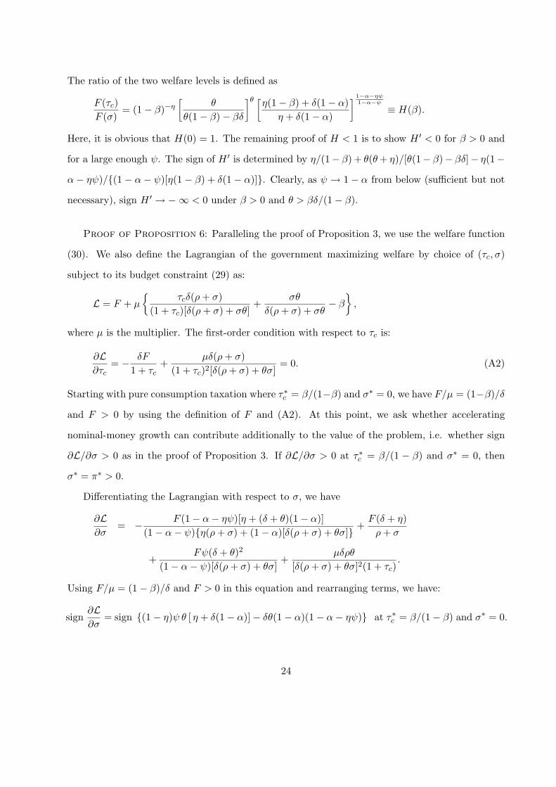
The ratio of the two welfare levels is defined as

F (τc)F (σ)

= (1− β)−η[

θ

θ(1− β)− βδ

]θ [η(1− β) + δ(1− α)

η + δ(1− α)

] 1−α−ηψ1−α−ψ

≡ H(β).

Here, it is obvious that H(0) = 1. The remaining proof of H < 1 is to show H ′ < 0 for β > 0 and

for a large enough ψ. The sign of H ′ is determined by η/(1− β) + θ(θ+ η)/[θ(1− β)− βδ]− η(1−

α− ηψ)/(1− α− ψ)[η(1− β) + δ(1− α)]. Clearly, as ψ → 1− α from below (sufficient but not

necessary), sign H ′ → −∞ < 0 under β > 0 and θ > βδ/(1− β).

Proof of Proposition 6: Paralleling the proof of Proposition 3, we use the welfare function

(30). We also define the Lagrangian of the government maximizing welfare by choice of (τc, σ)

subject to its budget constraint (29) as:

L = F + µ

τcδ(ρ+ σ)

(1 + τc)[δ(ρ+ σ) + σθ]+

σθ

δ(ρ+ σ) + σθ− β

,

where µ is the multiplier. The first-order condition with respect to τc is:

∂L∂τc

= − δF

1 + τc+

µδ(ρ+ σ)(1 + τc)2[δ(ρ+ σ) + θσ]

= 0. (A2)

Starting with pure consumption taxation where τ∗c = β/(1−β) and σ∗ = 0, we have F/µ = (1−β)/δ

and F > 0 by using the definition of F and (A2). At this point, we ask whether accelerating

nominal-money growth can contribute additionally to the value of the problem, i.e. whether sign

∂L/∂σ > 0 as in the proof of Proposition 3. If ∂L/∂σ > 0 at τ∗c = β/(1 − β) and σ∗ = 0, then

σ∗ = π∗ > 0.

Differentiating the Lagrangian with respect to σ, we have

∂L∂σ

= − F (1− α− ηψ)[η + (δ + θ)(1− α)](1− α− ψ)η(ρ+ σ) + (1− α)[δ(ρ+ σ) + θσ]

+F (δ + η)ρ+ σ

+Fψ(δ + θ)2

(1− α− ψ)[δ(ρ+ σ) + θσ]+

µδρθ

[δ(ρ+ σ) + θσ]2(1 + τc).

Using F/µ = (1− β)/δ and F > 0 in this equation and rearranging terms, we have:

sign∂L∂σ

= sign (1− η)ψ θ [ η + δ(1− α)]− δθ(1− α)(1− α− ηψ) at τ∗c = β/(1− β) and σ∗ = 0.

24

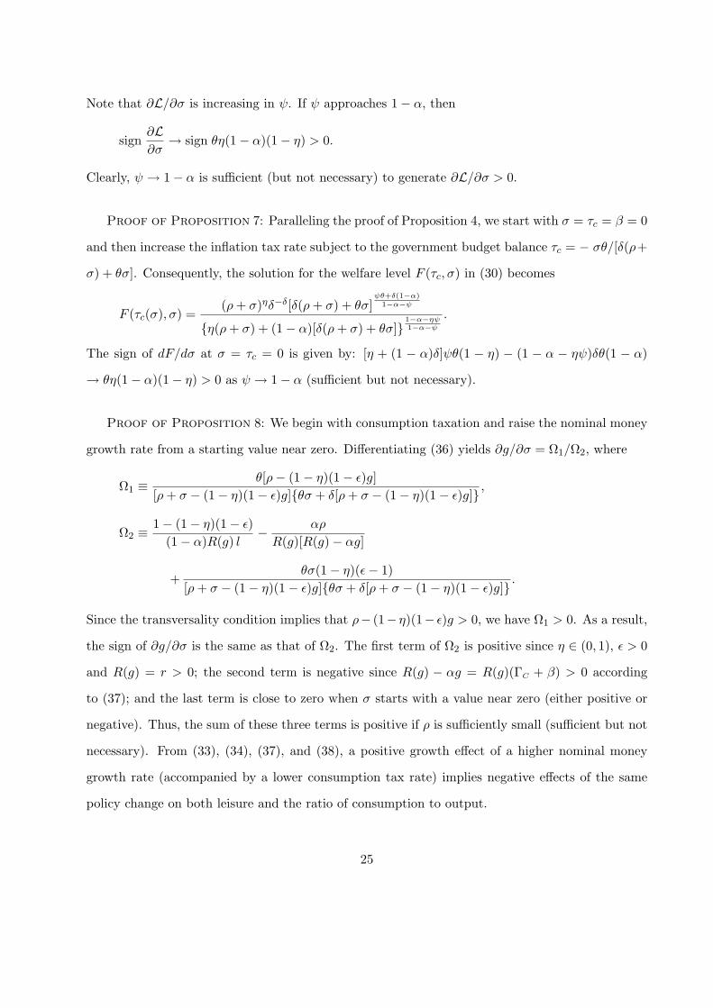
Note that ∂L/∂σ is increasing in ψ. If ψ approaches 1− α, then

sign∂L∂σ

→ sign θη(1− α)(1− η) > 0.

Clearly, ψ → 1− α is sufficient (but not necessary) to generate ∂L/∂σ > 0.

Proof of Proposition 7: Paralleling the proof of Proposition 4, we start with σ = τc = β = 0

and then increase the inflation tax rate subject to the government budget balance τc = − σθ/[δ(ρ+

σ) + θσ]. Consequently, the solution for the welfare level F (τc, σ) in (30) becomes

F (τc(σ), σ) =(ρ+ σ)ηδ−δ[δ(ρ+ σ) + θσ]

ψθ+δ(1−α)1−α−ψ

η(ρ+ σ) + (1− α)[δ(ρ+ σ) + θσ]1−α−ηψ1−α−ψ

.

The sign of dF/dσ at σ = τc = 0 is given by: [η + (1 − α)δ]ψθ(1 − η) − (1 − α − ηψ)δθ(1 − α)

→ θη(1− α)(1− η) > 0 as ψ → 1− α (sufficient but not necessary).

Proof of Proposition 8: We begin with consumption taxation and raise the nominal money

growth rate from a starting value near zero. Differentiating (36) yields ∂g/∂σ = Ω1/Ω2, where

Ω1 ≡θ[ρ− (1− η)(1− ε)g]

[ρ+ σ − (1− η)(1− ε)g]θσ + δ[ρ+ σ − (1− η)(1− ε)g],

Ω2 ≡1− (1− η)(1− ε)

(1− α)R(g) l− αρ

R(g)[R(g)− αg]

+θσ(1− η)(ε− 1)

[ρ+ σ − (1− η)(1− ε)g]θσ + δ[ρ+ σ − (1− η)(1− ε)g].

Since the transversality condition implies that ρ− (1− η)(1− ε)g > 0, we have Ω1 > 0. As a result,

the sign of ∂g/∂σ is the same as that of Ω2. The first term of Ω2 is positive since η ∈ (0, 1), ε > 0

and R(g) = r > 0; the second term is negative since R(g) − αg = R(g)(ΓC + β) > 0 according

to (37); and the last term is close to zero when σ starts with a value near zero (either positive or

negative). Thus, the sum of these three terms is positive if ρ is sufficiently small (sufficient but not

necessary). From (33), (34), (37), and (38), a positive growth effect of a higher nominal money

growth rate (accompanied by a lower consumption tax rate) implies negative effects of the same

policy change on both leisure and the ratio of consumption to output.

25

Footnotes

1. This positive long-run relationship between inflation and output is in line with some previous

predictions (e.g., Tobin, 1965; van der Ploeg and Alogoskoufis, 1994; Espinosa-Vega and Yip,

1999). Empirical evidence in this regard is mixed. In low inflation countries, a permanent

rise in the inflation rate permanently raises the level of output in the postwar era as found

by Bullard and Keating (1995). However, there is no such a permanent positive effect of

inflation on output in high inflation countries in both Bullard and Keating (1995) and Bruno

and Easterly (1998).

2. In other words, our model abstracts from how optimal monetary policy should respond to

such shocks, which has been examined in some studies; see e.g. Williamson (1996) and Rebelo

and Xie (1999, Section 4).

3. The rationale for the externality is that firms and workers enhance their knowledge through

learning-by-doing, which also benefits other firms through spillovers to some extent as knowl-

edge is partly a public good in nature (e.g. Arrow, 1962). Moreover, Arrow’s idea of linking

learning-by-doing to investment builds on the evidence of strong positive effects of experience

on productivity, and on evidence that patents — a proxy for learning — closely follow invest-

ment in some industries; see Barro and Sala-i-Martin (1995, p. 147). More recent evidence

also supports the idea of the spillovers both within and across industries (e.g. Bernstein and

Nadiri, 1989; Nakanishi, 2002).

4. With endogenous labor supply, government debt is welfare reducing as shown in Burbidge

(1983), and is hence omitted for simplicity.

5. The results are derived from the same CEIS utility function nesting a Cobb-Douglas rela-

tionship between leisure and consumption (excluding money by setting θ = 0), the same

production function, and a cash-in-advance constraint on consumption expenditure, or on

investment expenditure as well. Also, government spending is assumed as a fixed fraction of

output.

26

6. From (27), we get l∗ = η/(η + δ(1 − α)) when σ = 0. However, if tax revenue is made as

lump-sum transfers to households, rather than wasted, the consumption tax raises leisure and

reduces output.

27

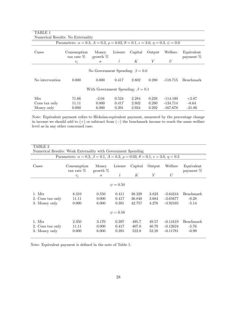
TABLE 1Numerical Results: No Externality

Parameters: α = 0.3, A = 0.3, ρ = 0.03, θ = 0.1, ε = 3.0, η = 0.3, ψ = 0.0

Cases Consumption Money Leisure Capital Output Welfare Equivalenttax rate % growth % payment %

τc σ l K Y U

No Government Spending: β = 0.0

No intervention 0.000 0.000 0.417 2.802 0.280 -118.715 Benchmark

With Government Spending: β = 0.1

Mix 71.66 -2.04 0.524 2.284 0.228 -114.100 +2.87Cons tax only 11.11 0.000 0.417 2.802 0.280 -134.714 -8.64Money only 0.000 6.000 0.391 2.924 0.292 -167.678 -21.86

Note: Equivalent payment refers to Hicksian-equivalent payment, measured by the percentage changein income we should add to (+) or subtract from (−) the benchmark income to reach the same welfarelevel as in any other concerned case.

TABLE 2Numerical Results: Weak Externality with Government Spending

Parameters: α = 0.3, β = 0.1, A = 0.3, ρ = 0.03, θ = 0.1, ε = 3.0, η = 0.3

Cases Consumption Money Leisure Capital Output Welfare Equivalenttax rate % growth % payment %

τc σ l K Y U

ψ = 0.50

1. Mix 8.310 0.550 0.411 38.229 3.823 -3.64244 Benchmark2. Cons tax only 11.11 0.000 0.417 36.840 3.684 -3.65677 -0.283. Money only 0.000 6.000 0.391 42.757 4.276 -3.92165 -5.14

ψ = 0.58

1. Mix 2.350 3.170 0.397 495.7 49.57 -0.11619 Benchmark2. Cons tax only 11.11 0.000 0.417 407.8 40.79 -0.12624 -5.763. Money only 0.000 6.000 0.391 522.8 52.28 -0.11781 -0.99

Note: Equivalent payment is defined in the note of Table 1.

28

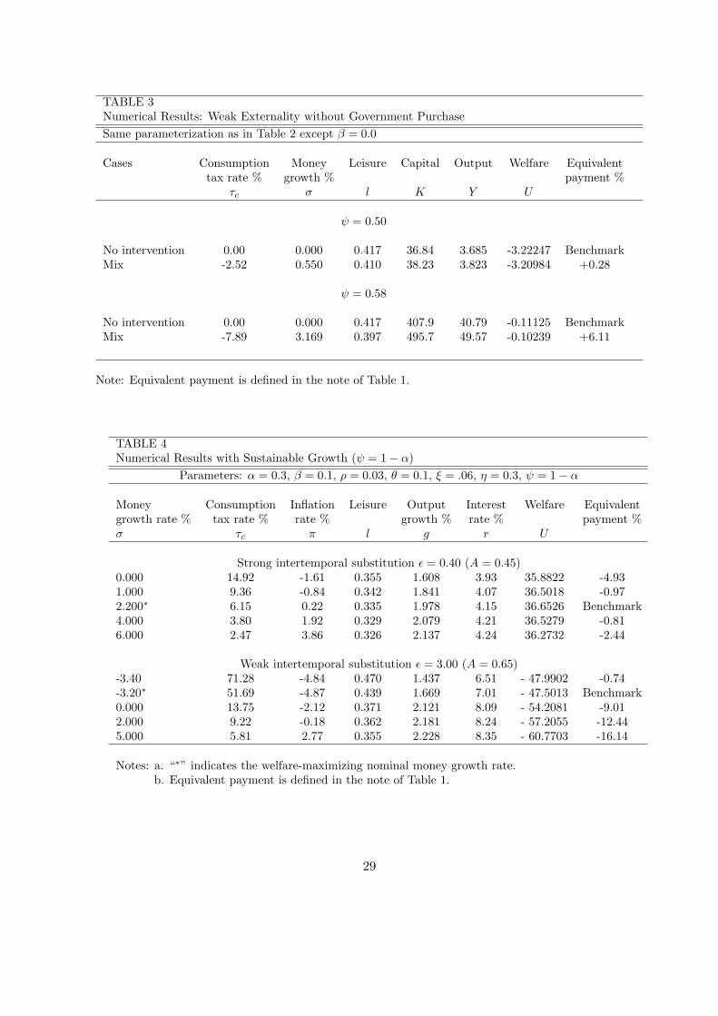
TABLE 3Numerical Results: Weak Externality without Government PurchaseSame parameterization as in Table 2 except β = 0.0

Cases Consumption Money Leisure Capital Output Welfare Equivalenttax rate % growth % payment %

τc σ l K Y U

ψ = 0.50

No intervention 0.00 0.000 0.417 36.84 3.685 -3.22247 BenchmarkMix -2.52 0.550 0.410 38.23 3.823 -3.20984 +0.28

ψ = 0.58

No intervention 0.00 0.000 0.417 407.9 40.79 -0.11125 BenchmarkMix -7.89 3.169 0.397 495.7 49.57 -0.10239 +6.11

Note: Equivalent payment is defined in the note of Table 1.

TABLE 4Numerical Results with Sustainable Growth (ψ = 1− α)

Parameters: α = 0.3, β = 0.1, ρ = 0.03, θ = 0.1, ξ = .06, η = 0.3, ψ = 1− α

Money Consumption Inflation Leisure Output Interest Welfare Equivalentgrowth rate % tax rate % rate % growth % rate % payment %σ τc π l g r U

Strong intertemporal substitution ε = 0.40 (A = 0.45)0.000 14.92 -1.61 0.355 1.608 3.93 35.8822 -4.931.000 9.36 -0.84 0.342 1.841 4.07 36.5018 -0.972.200∗ 6.15 0.22 0.335 1.978 4.15 36.6526 Benchmark4.000 3.80 1.92 0.329 2.079 4.21 36.5279 -0.816.000 2.47 3.86 0.326 2.137 4.24 36.2732 -2.44

Weak intertemporal substitution ε = 3.00 (A = 0.65)-3.40 71.28 -4.84 0.470 1.437 6.51 - 47.9902 -0.74-3.20∗ 51.69 -4.87 0.439 1.669 7.01 - 47.5013 Benchmark0.000 13.75 -2.12 0.371 2.121 8.09 - 54.2081 -9.012.000 9.22 -0.18 0.362 2.181 8.24 - 57.2055 -12.445.000 5.81 2.77 0.355 2.228 8.35 - 60.7703 -16.14

Notes: a. “∗” indicates the welfare-maximizing nominal money growth rate.b. Equivalent payment is defined in the note of Table 1.

29

LITERATURE CITED

Aiyagari, S. Rao, R. Anton Braun, and Zvi Eckstein (1998). “Transaction Services, Inflation and

Welfare.” Journal of Political Economy 106, 1274-1301.

Arrow, Kenneth J. (1962). “The Economic Implications of Learning by Doing.” Review of Eco-

nomic Studies 29, 155-173.

Atkinson, Anthony B., and Joseph E. Stiglitz (1972). “The Structure of Indirect Taxation and

Economic Efficiency.” Journal of Public Economics 1, 97-119.

Barro, Robert J., and Xavier Sala-i-Martin (1995). Economic Growth. New York: McGraw-Hill.

Bernstein, Jeffrey I., and M. Ishaq Nadiri (1989). “Research and Development and Intraindustry

Spillovers: An Empirical Application of Dynamic Duality.” Review of Economic Studies 56,

249-469.

Braun, R. Anton (1994). “How Large Is the Optimal Inflation Tax?” Journal of Monetary Eco-

nomics 34, 201-214.

Bruno, Michael, and William Easterly (1998). “Inflation Crisis and Long-Run Growth.” Journal

of Monetary Economics 41, 3-26.

Bullard, James, and John W. Keating (1995). “The Long-Run Relationship between Inflation and

Output in Postwar Economies.” Journal of Monetary Economics 36, 477-496.

Burbidge, John B. (1983). “Government Debt in an Overlapping-Generations Model with Be-

quests and Gifts.” American Economic Review 73, 222-227.

Cole, Harold L., and Alan C. Stockman (1992). “Specialization, Transactions Technologies, and

Money Growth.” International Economic Review 33, 283-298.

Correia, Isabel, and Pedro Teles (1996). “Is the Friedman Rule Optimal When Money Is an

Intermediate Good?” Journal of Monetary Economics 38, 223-244.

Dotsey, Michael, and Peter N. Ireland (1996). “The Welfare Cost of Inflation in General Equilib-

rium.” Journal of Monetary Economics 37, 29-47.

Erosa, Andres, and Gustavo Ventura (2002). “On Inflation as a Regressive Consumption Tax.”

Journal of Monetary Economies 49, 761-795.

30

Espinosa-Vega, Marco A., and Chong K. Yip (1999). “Fiscal and Monetary Policy Interactions

in an Endogenous Growth Model with Financial Intermediaries.” International Economic

Review 40, 595-615.

Friedman, Milton (1969). The Optimal Quantity of Money and Other Essays. Chicago: Aldine.

Gillman, Max (1993). “The Welfare Cost of Inflation in Cash-in-Advance Economy with Costly

Credit.” Journal of Monetary Economy 31, 97-115.

Gomme, Paul (1993). “Money and Growth Revisited: Measuring the Costs of Inflation in an

Endogenous Growth Model.” Journal of Monetary Economics 32, 51-77.

Guidotti, Pablo E., and Carlos A. Vegh (1993). “The Optimal Inflation Tax When Money Reduces

Transactions Costs: A Reconsideration.” Journal of Monetary Economics 31, 189-205.

Kimbrough, Kent P. (1986). “The Optimal Quantity of Money Rule in the Theory of Public

Finance.” Journal of Monetary Economics 18, 277-284.

Lucas, Robert E., Jr (2000). “Inflation and Welfare.” Econometrica 68, 247-274.

Nakanishi, Yasuo (2002). “Empirical Evidence of Inter-Industry R&D Spillover in Japan.” Journal

of Economic Research 7, 91-104.

Palivos, Theodore, and Chong K. Yip (1995). “Government Expenditure Financing in an Endoge-

nous Growth Model: A Comparison.” Journal of Money, Credit and Banking 27, 1159-1178.

Phelps, Edmund S. (1973). “Inflation in the Theory of Public Finance.” Swedish Journal of

Economics 75, 67-82.

Prescott, Edward C. (1987). “A Multiple Means-of-Payment Model.” In New Approaches to

Monetary Economics: Proceedings of the Second International Symposium in Economic The-

ory and Econometrics, edited by William A. Barnett and Kenneth J. Singleton, pp. 42-51.

Cambridge: Cambridge University Press.

Rebelo, Sergio, and Danyang Xie (1999). “One the Optimality of Interest Rate Smoothing.”

Journal of Monetary Economics 43, 263-282.

Romer, Paul M. (1986). “Increasing Returns and Long-Run Growth.” Journal of Political Econ-

omy 94, 1002-1037.

31

Schreft, Stacey L. (1992). “Transaction Costs and the Use of Cash and Credit.” Economic Theory

2, 283-294.

Shi, Shouyong (1999). “Money, Capital, and Redistributive Effects of Monetary Policies.” Journal

of Economic Dynamics and Control 23, 565-590.

Stockman, Alan C. (1981). “Anticipated Inflation and the Capital Stock in a Cash-in-Advance

Economy.” Journal of Monetary Economics 8, 387-393.

Tobin, James (1965). “Money and Economic Growth.” Econometrica 33, 671-684.

Turnovsky, Stephen J. (2000). “Fiscal Policy, Elastic Labor Supply, and Endogenous Growth.”

Journal Monetary Economics 45, 185-210.

van der Ploeg, Frederick, and George S. Alogoskoufis (1994). “Money and Endogenous Growth.”

Journal of Money, Credit and Banking 26, 771-791.

Williamson, Stephen D. (1996). “Sequential Markets and the Suboptimality of the Friedman

Rule.” Journal of Monetary Economics 37, 549-572.

Wu, Yangru, and Junxi Zhang (1998). “Endogenous Growth and the Welfare Costs of Inflation:

A Reconsideration.” Journal of Economic Dynamics and Control 22, 465-483.

Wu, Yangru, and Junxi Zhang (2000). “Monopolistic Competition, Increasing Returns to Scale,

and the Welfare Costs of Inflation.” Journal of Monetary Economics 46, 417-440.

32