Inflation Targets, Credibility, and Persistence

In a Simple Sticky-Price Framework

Jeremy RuddFederal Reserve Board∗

Karl WhelanCentral Bank of Ireland∗∗

July 23, 2003

AbstractThis paper presents a re-formulated version of a canonical sticky-price model that hasbeen extended to account for variations over time in the central bank’s inflation tar-get. We derive a closed-form solution for the model, and analyze its properties undervarious parameter values. The model is used to explore topics relating to the effects ofdisinflationary monetary policies and inflation persistence. In particular, we employ themodel to illustrate and assess the critique that standard sticky-price models generatecounterfactual predictions for the effects of monetary policy.

∗Corresponding author. Mailing address: Mail Stop 80, 20th and C Streets NW, Washington, DC 20551.

E-mail: jeremy.b.rudd@frb.gov.∗∗E-mail: karl.whelan@centralbank.ie. We thank Gregory Mankiw and Olivier Blanchard for useful dis-

cussions on several of the topics considered here. The views expressed in this paper are our own, and do

not necessarily reflect the views of the Board of Governors, the staff of the Federal Reserve System, or the

Central Bank of Ireland.

1 Introduction

An important trend in macroeconomic research in recent years involves the increased use

of optimization-based sticky-price models to analyze how monetary policy affects the econ-

omy and how optimal policy should be designed. Much of this analysis employs a simple

baseline model that features a “new-Keynesian” Phillips curve to characterize inflation, an

“expectational IS curve” to determine output growth, and a policy rule that describes how

the central bank sets short-term interest rates; representative examples of studies that use

this framework include Clarida, Galı, and Gertler (1999), McCallum (2001), and Wood-

ford (2003).

One limitation of existing work in this area is that applications of the baseline model

have typically been restricted to contexts in which the central bank maintains a fixed infla-

tion target, with particular attention being paid to the effects of the type of monetary policy

“shock” that is usually analyzed in the empirical VAR literature (namely, a temporary de-

viation from a stable policy rule). In this paper, we present a re-formulated version of the

baseline sticky-price model that has been extended to account for variations over time in

the central bank’s inflation target. We derive a fully specified closed-form solution for the

model in which output and inflation are related both to policy shocks (as usually defined)

and to expected future changes in the inflation target. The model provides a simple but

flexible framework for understanding a number of issues that have previously been dealt

with using a range of different specifications. In particular, the model sheds light on some

important existing critiques regarding the general ability of sticky-price models to capture

the effects of disinflationary monetary policies.

One such critique that we consider stems from Laurence Ball’s (1994) well-known ex-

ample of a sticky-price economy in which an announcement of a gradual reduction in the

rate of growth of the money supply results in a boom in output. This has commonly

been seen as an important counterfactual prediction of these models in light of the large

observed costs of disinflation; moreover, Ball’s result appears at odds with the position of

Woodford (2003) and others that these models adequately capture the effect of a monetary

tightening on output. We use our framework to demonstrate how these apparently con-

tradictory results can be reconciled by noting that they reflect the effects of two different

types of shocks in our model. Specifically, in the more general framework that we derive

here, Ball’s example of a gradual disinflation that is achieved through a deceleration in the

money supply is equivalent to an example where the central bank’s target inflation rate is

1

gradually reduced. In our framework, a credible announcement of future reductions in the

inflation target will indeed result in increased output today (at least for most parameter

values). However, we also demonstrate that another aspect of Ball’s result—specifically,

that inflation can be reduced without output’s ever declining below its baseline level—

relies on a highly restrictive assumption about pricing behavior (namely, that firms do not

discount their future profits).

We then use an extended version of our basic framework in order to assess the idea—

first proposed by Ball (1995)—that allowing for imperfect central bank credibility in the

baseline model can restore the prediction that disinflations involve significant output losses.

Specifically, we derive a general approach for modelling the effect of shocks to the inflation

target when the public imperfectly perceives the target’s true value, and use this setup to

demonstrate that a reduction in the inflation target under these circumstances is directly

analogous to a contractionary policy shock. Some of our results relating to credibility and

imperfect knowledge are consistent with those found elsewhere in the literature. However,

by integrating this analysis into the baseline sticky-price model—and by providing explicit

closed-form solutions and a simpler, more flexible, framework for analyzing these issues—we

believe our approach carries significant advantages over previous work.

An additional critique of sticky-price models that we address within our framework

relates to their ability to match empirical impulse responses to monetary policy shocks.

We frame our discussion around Mankiw’s (2001) recent influential critique of the new-

Keynesian Phillips curve. Mankiw uses a variant of the new-Keynesian inflation equation

to calibrate the output response that results from a gradual decline in inflation to a new,

lower rate. He argues that the model’s predictions (which involve a temporary increase

in output) are inconsistent with VAR-based evidence on impulse responses to monetary

policy shocks; this failure, he claims, provides an alternative way to view Ball’s original

critique of sticky-price models. As we discuss, however, Mankiw’s critique misses the mark

in that it fails to compare like with like: The permanent decline in inflation described in

Mankiw’s example must correspond to a change in the inflation target, which is different

from the type of temporary policy shock that is examined in the VAR literature. Thus,

this example does not imply that the baseline sticky-price model is incapable of generating

a simultaneous decline in output and inflation in response to a monetary policy shock; put

differently, the “Ball critique” does not extend to the shocks considered in empirical VARs.

All this said, it is still the case that the baseline sticky-price model has trouble in

2

matching an important aspect of empirical impulse response functions; namely, the observed

lagged response of inflation to monetary policy (and other) shocks. We therefore briefly

assess the conjecture that standard sticky-price models become capable of explaining the

degree of inflation persistence that is apparent in the postwar period once one allows shifts

in monetary policy regimes to occur with imperfect credibility. We conclude, however, that

this hypothesis provides an unconvincing explanation for the observed pattern of inflation

persistence in postwar U.S. data.

2 Variable Inflation Targets in a Sticky-Price Model

This section derives and analyzes the closed-form solution to a sticky-price monetary busi-

ness cycle model in which the central bank’s inflation target can vary over time. As the

model is otherwise quite standard, we briefly outline its derivation and then focus on those

features of the model that are affected by the presence of a variable policy target.

2.1 The Model

The baseline model consists of three equations that characterize inflation, output, and

interest rates. We describe each in turn.

Inflation Equation: The new-Keynesian Phillips curve that describes inflation dynamics

in the baseline model can be derived from a number of different types of sticky-price mod-

els. The most commonly used formulation invokes Calvo-style pricing, in which a random

fraction (1− θ) of firms reset their price each period while all other firms keep their prices

unchanged. A general formulation of the problem faced by such firms involves setting the

(log) time-t reset price, zt, so as to minimize

L(t) =∞∑

k=0

(θβ)k Et(zt − p∗t+k

)2, (1)

where p∗t+k is the log of the optimal price that the firm would set in period t − k if there

were no price frictions.1 (This loss function can be motivated more generally as a second-

order Taylor approximation to the underlying profit function.) If we assume imperfect1This formulation has been widely used in the sticky-price literature. See Devereux and Yetman (2003)

and Walsh (1998) for two recent examples.

3

competition, the frictionless optimal price will be a markup µ over nominal marginal cost;

hence, the loss function becomes

L(t) =∞∑

k=0

(θβ)k Et (zt − pt+k −mct+k − µ)2 , (2)

where mct+k is log real marginal cost at time t+ k.

The solution to this problem takes the form

zt = (1− θβ)∞∑

k=0

(θβ)k Et (pt+k +mct+k + µ) . (3)

If we define the markup over marginal cost at time t+ k of a firm that last reset its price

at time t as

µt+k,t ≡ zt − pt+k −mct+k, (4)

then we see that the pricing rule simply implies that firms will price to set a weighted

average of expected future markups equal to the frictionless optimal markup, µ:

(1− θβ)∞∑

k=0

(θβ)k Etµt+k,t = µ. (5)

This pricing rule can be combined with the definition of the aggregate price level,

pt = θpt−1 + (1− θ) zt, (6)

in order to derive an expression for inflation.2 Specifically, we obtain a new-Keynesian

Phillips curve of the form:

πt = βEtπt+1 +(1− θ) (1− θβ)

θ(mct + µ) , (7)

in which inflation, πt, is related to next period’s expected inflation rate and the current

deviation of real marginal cost from its frictionless optimal level.3

2Although the definition of the price level given by equation (6) involves taking a weighted average of

log prices, it exactly corresponds to a Divisia index. Such indexes are almost identical to the Fisher chain-

aggregation formulae that are currently used to construct price indexes in the U.S. National Accounts (see

Whelan, 2002).3Section 1 of the Appendix provides the details of this derivation. Note that −µ is the frictionless optimal

level of real marginal cost: Absent pricing frictions, the firm’s optimal price p∗t is a markup µ over nominal

marginal cost mcnt ; hence, real marginal cost in the frictionless world, mcn

t − p∗t , equals −µ, which implies

that mct − (−µ) = mct + µ is the deviation of real marginal cost from its frictionless optimal level.

4

Finally, under the assumption that these real marginal cost deviations are proportional

to the output gap yt (defined in turn as the deviation between actual output and its fric-

tionless optimal level), we can write the inflation equation as:

πt = βEtπt+1 + γyt. (8)

Output Equation: The output gap is determined by an “intertemporal IS curve” of the

form

yt = Etyt+1 − σ (it − Etπt+1 − rnt ) , (9)

in which the output gap yt is negatively related to the gap between the ex ante real interest

rate and a potentially time-varying “natural rate” of interest.4 Note that, if the economy is

to be in a steady-state equilibrium with a constant level of output and a constant inflation

rate π∗, then it will be necessary to have

it = rnt + π∗. (10)

Monetary Policy Rule: Monetary policy is assumed to operate according to a Taylor-

type interest-rate feedback rule,

it = rnt + π∗t + εt + θπ (πt − π∗t ) + θy (yt − y∗t ) , (11)

where εt represents deviations from the nominal interest rate that is required in order to

keep the economy at the target rate of inflation (π∗t ) and target level of the output gap (y∗t )in the long run. This εt term may also vary over time, and can therefore be equated with

a monetary policy shock.5

Unlike standard implementations of the baseline model, we assume that the target

inflation rate, π∗t , can vary over time. Importantly, this also implies a varying target

level of output; this is because, as Woodford (2003) and others have discussed, the new-

Keynesian Phillips curve implies a long-run tradeoff between the level of output and the4The usual basis for this equation is a loglinearized consumption Euler equation. In the baseline model,

consumption is equated with all output—whence equation (9)—although most authors interpret the relation

as summarizing the full effect of real interest rates on aggregate expenditure.5We assume that the interest-rate feedback rule respects the Taylor principle, which calls for the central

bank to raise real rates in response to an increase in inflation. Here, this condition—which is necessary for

a determinate rational-expectations equilibrium to exist—requires θπ to be greater than 1− 1−βγ

θy.

5

level of inflation. In particular, if the central bank’s target for the output gap is to be

consistent with its inflation target, it must be the case that

y∗t =1− βγ

π∗t . (12)

The existence of a positive long-run relationship between inflation and output reflects

a negative long-run tradeoff between inflation and firms’ average markup over marginal

cost. That this average markup can vary at all from its frictionless optimal level µ in a

nonstochastic steady state may appear a little surprising given that each firm’s pricing rule

calls for it to keep a weighted average of its expected markups equal to µ (see equation 5).

However, as we show in section 2 of the Appendix, the fact that firms discount their

future profits at a nonzero rate causes the average economy-wide markup to lie below the

frictionless optimal markup in a positive-inflation steady state. In addition, this gap will

widen as inflation increases—which is in turn consistent (by assumption) with a widening

gap between actual output and its frictionless level.

2.2 A Closed-Form Solution

We can obtain the model’s closed-form solution as follows. The inflation equation can be

re-written as

πt − π∗t = βEt

(πt+1 − π∗t+1

)+ γ (yt − y∗t ) + βEt∆π∗t+1, (13)

which in turn implies that

Et(πt+1 − π∗t+1) = β−1 (πt − π∗t )− β−1γ (yt − y∗t )− Et∆π∗t+1. (14)

Substituting the Taylor rule into the IS curve and re-arranging yields the following

expression for the output gap:

yt = Etyt+1 − σ(εt +

(θπ − β−1

)(πt − π∗t ) +

(θy + β−1γ

)(yt − y∗t )

), (15)

which can be re-written as

Et(yt+1 − y∗t+1)

= (1 + σθy + σβ−1γ)(yt − y∗t ) + σ(θπ − β−1)(πt − π∗t ) + σεt − Et∆y∗t+1

= (1 + σθy + σβ−1γ)(yt − y∗t ) + σ(θπ − β−1)(πt − π∗t ) + σεt − 1− βγ

Et∆π∗t+1. (16)

6

These expressions imply an expectational difference equation system that can be written

in matrix form as Etxt+1 = Axt +Bet, where

A ≡ 1 + σθy + σβ−1γ σθπ − σβ−1

−β−1γ β−1

, xt ≡

yt − y∗tπt − π∗t

,

B ≡ σ −1−β

γ

0 −1

, and et ≡

εt

Et∆π∗t+1

.

The closed-form solution of the model is therefore given by

xt = −A−1∞∑

k=0

A−kBEtet+k, (17)

which implies expressions for yt and πt of the form

yt = y∗t +∞∑

k=0

ψykEtεt+k +

∞∑k=0

µykEt∆π∗t+k+1 (18)

πt = π∗t +∞∑

k=0

ψπkEtεt+k +

∞∑k=0

µπkEt∆π∗t+k+1. (19)

2.3 Properties of the Closed-Form Solution

It is immediately apparent that the responses of inflation and the output gap to policy

shocks and expected future changes in the inflation target will depend on the values of the

weights ψπk , ψy

k, µπk , and µy

k, which will in turn depend on the specific values that we assume

for the model’s structural parameters β, σ, γ, θy, and θπ. For example, it can be shown

that the effect on (yt − y∗t ) of the expectation of a once-off unit increase in next period’s

inflation target is given by1−β

γ − σ(θπβ − 1)

1 + σθy + σγθπ, (20)

which can be positive or negative.6

Figure 1 plots µπk and µy

k for the two calibrations that we employ. The values of β, γ, θy,

and θπ that we assume are taken from McCallum (2001), and are set such that β = 0.99,

γ = 0.03, θπ = 1.5, and θy = 0.5. For σ, which measures the elasticity of output growth

with respect to changes in the real interest rate, we consider two calibrations: σ = 0.46See section 3 of the Appendix for a derivation of this expression.

7

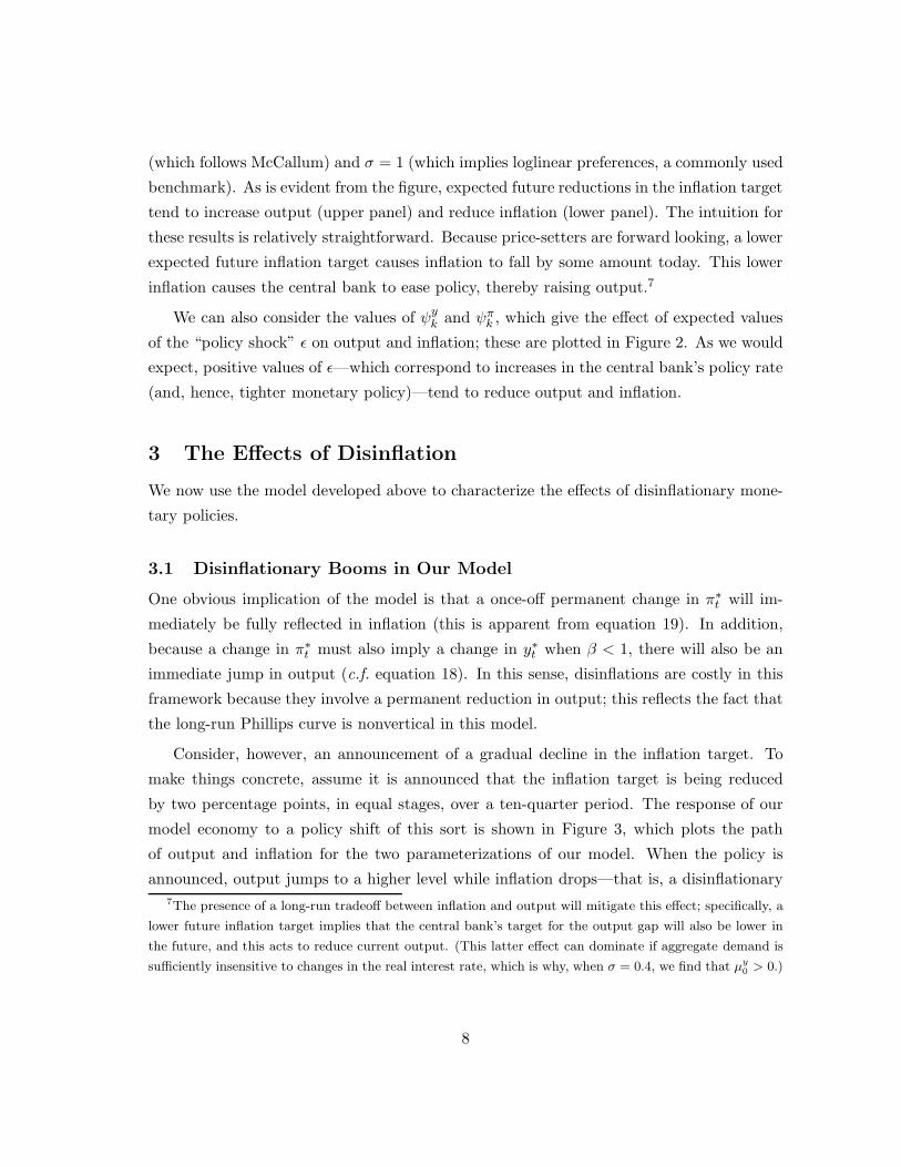
(which follows McCallum) and σ = 1 (which implies loglinear preferences, a commonly used

benchmark). As is evident from the figure, expected future reductions in the inflation target

tend to increase output (upper panel) and reduce inflation (lower panel). The intuition for

these results is relatively straightforward. Because price-setters are forward looking, a lower

expected future inflation target causes inflation to fall by some amount today. This lower

inflation causes the central bank to ease policy, thereby raising output.7

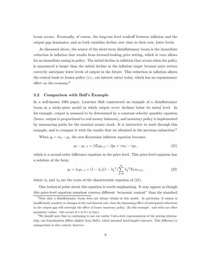
We can also consider the values of ψyk and ψπ

k , which give the effect of expected values

of the “policy shock” ε on output and inflation; these are plotted in Figure 2. As we would

expect, positive values of ε—which correspond to increases in the central bank’s policy rate

(and, hence, tighter monetary policy)—tend to reduce output and inflation.

3 The Effects of Disinflation

We now use the model developed above to characterize the effects of disinflationary mone-

tary policies.

3.1 Disinflationary Booms in Our Model

One obvious implication of the model is that a once-off permanent change in π∗t will im-

mediately be fully reflected in inflation (this is apparent from equation 19). In addition,

because a change in π∗t must also imply a change in y∗t when β < 1, there will also be an

immediate jump in output (c.f. equation 18). In this sense, disinflations are costly in this

framework because they involve a permanent reduction in output; this reflects the fact that

the long-run Phillips curve is nonvertical in this model.

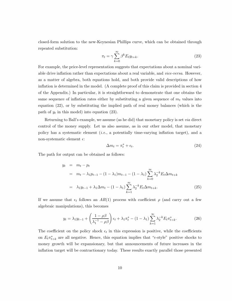
Consider, however, an announcement of a gradual decline in the inflation target. To

make things concrete, assume it is announced that the inflation target is being reduced

by two percentage points, in equal stages, over a ten-quarter period. The response of our

model economy to a policy shift of this sort is shown in Figure 3, which plots the path

of output and inflation for the two parameterizations of our model. When the policy is

announced, output jumps to a higher level while inflation drops—that is, a disinflationary7The presence of a long-run tradeoff between inflation and output will mitigate this effect; specifically, a

lower future inflation target implies that the central bank’s target for the output gap will also be lower in

the future, and this acts to reduce current output. (This latter effect can dominate if aggregate demand is

sufficiently insensitive to changes in the real interest rate, which is why, when σ = 0.4, we find that µy0 > 0.)

8

boom occurs. Eventually, of course, the long-run level tradeoff between inflation and the

output gap dominates, and so both variables decline over time to their new, lower levels.

As discussed above, the source of the short-term disinflationary boom is the immediate

reduction in inflation that results from forward-looking price setting, which in turn allows

for an immediate easing in policy. The initial decline in inflation that occurs when the policy

is announced is larger than the initial decline in the inflation target because price setters

correctly anticipate lower levels of output in the future. This reduction in inflation allows

the central bank to loosen policy (i.e., cut interest rates) today, which has an expansionary

effect on the economy.8

3.2 Comparison with Ball’s Example

In a well-known 1994 paper, Laurence Ball constructed an example of a disinflationary

boom in a sticky-price model in which output never declines below its initial level. In

his example, output is assumed to be determined by a constant-velocity quantity equation

(hence, output is proportional to real money balances), and monetary policy is implemented

by announcing paths for the nominal money stock. It is instructive to work through this

example, and to compare it with the results that we obtained in the previous subsection.9

When yt = mt − pt, the new-Keynesian inflation equation becomes

pt − pt−1 = βEtpt+1 − βpt + γmt − γpt, (21)

which is a second-order difference equation in the price level. This price-level equation has

a solution of the form:

pt = λ1pt−1 + (1− λ1)(1− λ−12 )

∞∑k=0

λ−k2 Etmt+k, (22)

where λ1 and λ2 are the roots of the characteristic equation of (21).

One technical point about this equation is worth emphasizing. It may appear as though

this price-level equation somehow conveys different “economic content” than the standard8Note that a disinflationary boom does not always obtain in this model. In particular, if output is

insufficiently sensitive to changes in the real interest rate, then the depressing effect of anticipated reductions

in the output gap will outweigh the effect of looser monetary policy. (In this example—and with our other

parameter values—this occurs if σ is 0.1 or less.)9We should note that in continuing to use our earlier Calvo-style representation of the pricing relation-

ship, our formalization differs slightly from Ball’s, which assumed fixed-length contracts. This difference is

unimportant in this context, however.

9

closed-form solution to the new-Keynesian Phillips curve, which can be obtained through

repeated substitution:

πt = γ∞∑

k=0

βkEtyt+k. (23)

For example, the price-level representation suggests that expectations about a nominal vari-

able drive inflation rather than expectations about a real variable, and vice-versa. However,

as a matter of algebra, both equations hold, and both provide valid descriptions of how

inflation is determined in the model. (A complete proof of this claim is provided in section 4

of the Appendix.) In particular, it is straightforward to demonstrate that one obtains the

same sequence of inflation rates either by substituting a given sequence of mt values into

equation (22), or by substituting the implied path of real money balances (which is the

path of yt in this model) into equation (23).

Returning to Ball’s example, we assume (as he did) that monetary policy is set via direct

control of the money supply. Let us also assume, as in our other model, that monetary

policy has a systematic element (i.e., a potentially time-varying inflation target), and a

non-systematic element ε:

∆mt = π∗t + εt. (24)

The path for output can be obtained as follows:

yt = mt − pt

= mt − λ1pt−1 − (1− λ1)mt−1 − (1− λ1)∞∑

k=0

λ−k2 Et∆mt+k

= λ1yt−1 + λ1∆mt − (1− λ1)∞∑

k=1

λ−k2 Et∆mt+k. (25)

If we assume that εt follows an AR(1) process with coefficient ρ (and carry out a few

algebraic manipulations), this becomes

yt = λ1yt−1 +

(1− ρβλ−1

1 − ρβ

)εt + λ1π

∗t − (1− λ1)

∞∑k=1

λ−k2 Etπ

∗t+k. (26)

The coefficient on the policy shock εt in this expression is positive, while the coefficients

on Etπ∗t+k are all negative. Hence, this equation implies that “ε-style” positive shocks to

money growth will be expansionary, but that announcements of future increases in the

inflation target will be contractionary today. These results exactly parallel those presented

10

in the previous section for our own model.10

One difference, though, between our results and those in Ball’s paper concerns the long-

run tradeoff between the levels of inflation and output. Ball described his example as one

in which the gradual slowing in money growth produces a boom, where this is defined as

“an output path that rises above the natural rate temporarily and never falls below the

natural rate.”11 Thus, in his example there was no permanent reduction in output despite

the lower level of inflation. The explanation for this difference turns out to be that Ball

assumed a model in which firms do not discount profits, implying β = 1. In fact, this

observation helps us to reconcile what is perhaps the most puzzling aspect of Ball’s result

relative to the usual intuition about the new-Keynesian Phillips curve. From equation (23),

we know that this relationship predicts that inflation depends positively on current and

expected future output gaps. How, then, could such a model generate a path in which

inflation declines even though expectations of future output gaps always lie at or above

their baseline values—as in Ball’s disinflationary boom example?

When β is less than unity (as is usually assumed in structural versions of these models),

the answer is that this simply cannot happen. In this case, there is a long-run tradeoff

between the levels of inflation and output (equation 12), and so the initial temporary boom

is eventually followed by a permanent decline in output. In our disinflationary boom exam-

ple, expectations of the longer-run decline in output outweigh the effects of the temporary

boom, thereby producing a decline in inflation.

In contrast, when β = 1 the new-Keynesian Phillips curve becomes

πt = Etπt+1 + γyt, (27)

which implies that a zero output gap will obtain in any steady state (in which case Etπt+1 =

πt). Hence, a new steady-state inflation rate can be achieved without a permanent decline in

output. While this notion of monetary neutrality is appealing to most macroeconomists, it

is worth keeping in mind that, in this context, it can only be derived by making a somewhat

unattractive assumption (namely, that firms do not discount profits).

The key technical issue underlying the difference between the case where β = 1 and the10Note, though, that the mechanism whereby expected future increases in the inflation target turn out to

be contractionary is slightly different in this case. As before, these expectations result in higher inflation

(and a higher price level) today. Here, however, this acts to directly reduce output by lowering real money

balances, rather than indirectly through the Taylor rule.11See Ball (1994), page 286.

11

case where β < 1 is not simply one of replacing the discount factor in equation (23) with

unity. Rather, the β = 1 case implies the following solution:

πt = π∗t + γ∞∑

k=0

Etyt+k, (28)

where here π∗t is any series that follows a martingale.12 So, in addition to having inflation

depend on current and expected future output gaps, the no-discounting case permits jumps

in inflation that are unrelated to the expected path of the output gap. While in theory

these movements in π∗t could correspond to sunspot fluctuations, in practice movements

in this series must be associated with changes in the inflation target if monetary policy is

being carried out through the implementation of a Taylor-style interest-rate feedback rule.

4 Credibility and Misperceptions

The counterfactual prediction that an announced disinflationary policy can produce a tem-

porary boom has often been cited as an important indictment of the canonical sticky-price

framework. As Ball (1995) has argued, however, imperfect central bank credibility may

provide a mechanism through which the model’s prediction of a disinflationary boom can

be overturned. In this section, we illustrate this point in the context of an extended ver-

sion of our baseline sticky-price framework. Specifically, we model the credibility problem

using a simple formulation in which the central bank’s inflation target can be imperfectly

perceived—or only partially believed—by the public.

Returning to the two equations that make up our model, recall that the inflation equa-

tion is given by

πt − π∗t = βEt

(πt+1 − π∗t+1

)+ γ (yt − y∗t ) + βEt∆π∗t+1, (29)

where Et refers to the rational expectation of private agents. However, if there were imper-

fect information concerning the current inflation target, this could be re-written as

πt − Etπ∗t = βEt

(πt+1 − π∗t+1

)+ γ (yt − Ety

∗t ) + βEt∆π∗t+1, (30)

that is, we could replace the actual values of the current inflation and output targets with

the public’s rational belief about them based on its available information.12That is, any series π∗t for which Etπ

∗t+1 = π∗t .

12

The output equation takes the form

Etyt+1 − yt = σ (π∗t + εt + θπ (πt − π∗t ) + θy (yt − y∗t )− Etπt+1) . (31)

Here, however, π∗t and y∗t refer to the central bank’s actual inflation and output targets, be-

cause these terms come from substituting the Taylor rule into the expectational IS equation.

That said, we can re-write this equation as

Etyt+1 − yt = σ (Etπ∗t + εt + θπ (πt − Etπ

∗t ) + θy (yt − Ety

∗t )− Etπt+1 + ηt) , (32)

where

ηt = (1− θπ) (π∗t −Etπ∗t ) + θy (y∗t − Ety

∗t )

=(

1− θπ − θy(1− β)γ

)(π∗t − Etπ

∗t ) . (33)

The model can therefore be re-formulated in terms of the deviations of the target variables

from their private-sector rational expectations, with the only difference being that the

monetary policy shock is now described by the composite disturbance εt + ηt.

To illustrate what this means, note that the Taylor principle requires that the term(1− θπ − θy(1−β)

γ

)be negative. Thus, if the actual inflation target is lower than the public’s

perception of it (implying that π∗t −Etπ∗t < 0), this will act in the same way that a positive

εt shock does. This is intuitive inasmuch as both kinds of shocks imply an unexpectedly

high interest rate given the public’s perception of the inflation target. However, there is

an important difference between the two types of shocks that permits us to simplify the

model’s solution in this case. We are assuming that private agents can expect the monetary

policy shock to be non-zero in the future (i.e., it is possible to have Etεt+k 6= 0). But if

expectations are rational, private-sector agents cannot expect that their future beliefs about

the inflation target will be biased. Thus, it must be that

Et[π∗t+k − Et+kπ

∗t+k

]= 0.

Hence, the solution to this model is now of the form

yt = Ety∗t + ψy

0

(1− θπ − θy(1− β)

γ

)(π∗t − Etπ

∗t )

+∞∑

k=0

ψykEtεt+k +

∞∑k=0

µykEt∆π∗t+k+1 (34)

13

πt = Etπ∗t + ψπ

0

(1− θπ − θy(1− β)

γ

)(π∗t − Etπ

∗t )

+∞∑

k=0

ψπkEtεt+k +

∞∑k=0

µπkEt∆π∗t+k+1. (35)

Besides having a relatively simple closed-form solution, this setup provides a completely

general framework for thinking about the effects of policy misperceptions in the canonical

sticky-price model. In particular, one can use this apparatus to construct examples of non-

credible policy adjustments (or delayed learning) in which it takes the public a number of

quarters to gradually adjust to a change in the central bank’s inflation target. Importantly,

one can also easily demonstrate that private agents’ failing to fully perceive a new, lower

inflation target can result in a temporary recession. In terms of the model, for most

reasonable calibrations ψπ0 will be approximately zero while ψy

0 will be relatively large. As

a result, the path of actual inflation will be effectively determined by agents’ perceptions

of the inflation target, Etπ∗t ; by contrast, deviations of π∗t from Etπ

∗t have little effect on

inflation. But for output, these misperceptions of the inflation target are like shocks to εt,

which have relatively large effects on yt. Hence, equations (34) and (35) illustrate how the

model can capture a general characteristic of imperfectly perceived disinflations—namely,

an immediate decline in output coupled with a slow decline in inflation.

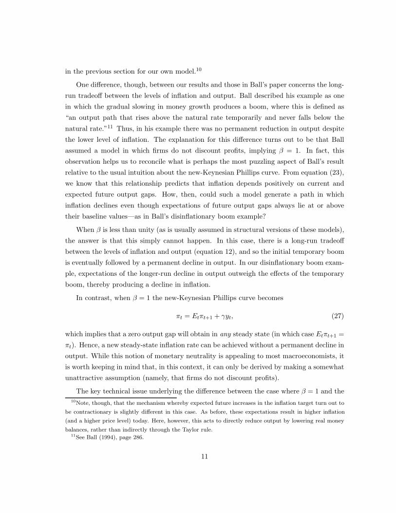
As a concrete example, consider the following simple experiment in which the central

bank’s inflation target drops by two percentage points. Assume that this is not fully

perceived or believed by the public; instead, the public updates its beliefs about the target

gradually by reducing its estimate of the inflation target by 0.2 percentage point each

quarter for ten quarters (each time believing that this is the new, permanent target).

Figure 4 gives the subsequent responses of output and inflation for the cases σ = 0.4 and

σ = 1.0, with all other parameter values set as before. The upper panel shows that while the

misperceived reduction in the inflation target produces a recession in both cases, the exact

path of this contraction depends upon the sensitivity of output growth to real interest rates:

In the case where σ = 1, output contracts more sharply at first, overshooting its long-run

level. In contrast, the path of inflation is essentially independent of σ and closely follows

the private-sector’s perceived value of the inflation target, Etπ∗t .

An aspect of this example that one might wish to specify more explicitly is the exact

process by which the public updates its beliefs about the central bank’s inflation target.

One paper that takes steps in this direction is Erceg and Levin (2001). This paper presents

numerical simulations of a model with sticky prices and wages in which the central bank

14

has an inflation target that is the sum of two components, one being a highly persistent

AR(1) process and the other being white noise. In an exercise that is intended to capture

the Volcker disinflation, Erceg and Levin consider the effects of a six percentage point

reduction in the inflation target’s persistent component under the assumption that agents

can observe the target, but do not know whether its movements reflect shocks to the

persistent or transitory component. In their model, agents solve a Kalman-filtering problem

to gradually “learn” about the shock that has occurred. As in our example, the result is a

gradual reduction in inflation and an immediate loss in output.

While a Kalman learning approach represents one way of formalizing the misperceptions

problem, it is not clear that it provides a particularly suitable method for modelling the

sort of credibility problem that is related to a change in a monetary policy regime. For

example, in Erceg and Levin’s exercise, the six percentage point jump in the permanent

component of the inflation target is hard to reconcile with the underlying process that is

assumed by the agents who perform the Kalman filtering: If such jumps were possible under

the assumed process, then the perceived inflation target would be incredibly volatile. More

generally, the idea that the inflation target can be described as the sum of a persistent (but

mean-reverting) component and a transitory component is somewhat difficult to defend on

common-sense grounds: A priori, a more reasonable description of reality is one in which

there are infrequent discrete changes in the policy regime. Ultimately, these problems illus-

trate the inherent difficulty in formally modelling how agents learn about what is essentially

a once-off event. However, as our own analysis has shown, the role of policy mispercep-

tions in the sticky-price framework can be examined quite generally without reference to a

specific learning model.

5 Consistency with VAR Evidence

In this section, we review a critique of the new-Keynesian Phillips curve that has been

recently advanced by Gregory Mankiw (2001). Central to this critique is an example in

which a sticky-price economy—with inflation characterized by a new-Keynesian Phillips

curve—responds to a monetary policy shock with a decline in inflation and an increase in

output, a response that Mankiw notes is completely at odds with the stylized facts from the

VAR literature. We show that Mankiw’s example is easily understood using the framework

developed in this paper, and argue that his example actually pertains to the effect of a

change in the inflation target, rather than to a VAR-type monetary policy shock. The

15

section concludes with a discussion of whether sticky-price models are actually capable of

matching the VAR evidence.

5.1 Mankiw’s Critique

Mankiw uses a simple numerical example to criticize the realism of the new-Keynesian

Phillips curve, beginning with the observation that papers from the VAR literature (such

as Bernanke and Gertler, 1995) find a “delayed and gradual” response of inflation following

a monetary policy shock. He then considers the following calibrated version of the new-

Keynesian Phillips curve:

πt = Etπt+1 +18yt, (36)

and specifies a path for inflation based on his reading of the evidence from the VAR literature

as to how inflation responds to monetary policy shocks. Given this path of inflation, a path

for output is backed out using equation (36) that is consistent with both the new-Keynesian

Phillips curve and the assumed inflation path.

Mankiw’s calculations for inflation and output are presented in the second and third

columns of Table 1.13 They show a decline in inflation to a new, permanently lower level

that is accompanied by a period of positive output gaps. Mankiw argues that this example

demonstrates that the logic of Ball’s critique of sticky-price models carries over to impulse

response functions. Specifically, he notes that: “Ball showed that in this kind of model,

a fully credible announced disinflation should cause an economic boom . . . [I]n essence we

experience a credible announced disinflation every time we get a contractionary shock. Yet

we do not get the boom that the model says should accompany it.”14

What we wish to stress here is that Mankiw’s example does not describe the new-

Keynesian Phillips curve’s prediction regarding the impulse responses that obtain following

the sort of monetary policy shock actually studied in the VAR literature (i.e., the ε-style

shocks of our model). Moreover, one cannot draw a simple analogy between these two types

of shocks (changes in the inflation target and ε-style policy shocks), as Mankiw does when

interpreting these calculations; rather, this example only provides a further illustration of

what the model predicts will occur following a permanent change in the inflation target. We

have therefore labelled the column in Table 1 that gives Mankiw’s inflation figures as “Path13Mankiw’s original example was actually in terms of the unemployment rate; to maintain consistency

with our examples, we describe his result in terms of the output gap.14Mankiw (2001), pages C57-C58.

16

of inflation under target change,” in order to highlight that these calculations can only

represent the joint path of inflation and output under the new-Keynesian Phillips curve if

they are describing a case in which the target inflation rate changes in period 1 from zero

to minus two percent.

To explicitly demonstrate this point, note that Mankiw’s version of the new-Keynesian

Phillips curve sets the discount rate β equal to one, so the solution for inflation is given by

equation (28). This implies that the change in inflation can be described as

∆πt = ∆π∗t + γ

∞∑

k=0

Etyt+k −∞∑

k=−1

Et−1yt+k

, (37)

that is, the change in inflation each period reflects changes in the inflation target and

updated expectations as to the future path of the output gap.

To see that the thought experiment considered here must involve a change in the inflation

target, compare columns three and four of Table 1. The fourth column (labelled “No target

change”) displays only the second term in equation (37); i.e., it displays the effect on

inflation from the change in the expected path of the output gap. These calculations show

that, absent any change in the inflation target, a shock that results in expectations of higher

output produces a jump in inflation. Mankiw’s calculations, by contrast, show no change in

inflation during this first period, implying that the inflation target must have changed in a

manner that exactly offsets the surprise positive news about output (that is, π∗t must have

declined by two percentage points at t = 1).15 That the target must indeed have changed

should also be evident from the observation that inflation settles down at −2 percent in

this case even after the output gap has returned to zero. Thus, the economic intuition

behind Mankiw’s calculations is quite simple. The new-Keynesian Phillips curve implies

that, ceteris paribus, the credible announcement of a reduction in the target inflation rate

will reduce the actual inflation rate immediately. And to fit the imposed pattern of a

gradual reduction in inflation, it is necessary to assume a positive sequence of output gaps.

However, this example carries no implications for how well the new-Keynesian Phillips curve

captures the effects of the ε-style shocks studied in the empirical VAR literature.

In this sense, then, we would argue that Mankiw’s critique of the new-Keynesian Phillips15One other possible interpretation of Mankiw’s figures is that they do not relate to an unexpected shock at

all, but are rather a representation of a perfect-foresight path, i.e., one in which πt+1 = Etπt+1 in all periods.

One can easily verify that this assumption produces the same path for output and inflation. However, it is

clear from Mankiw’s discussion that his example is intended to capture the effect of an unexpected shock.

17

curve falls short of its mark. The calibrated output and inflation series in Mankiw’s example

do indeed fail to match the empirical impulse responses of these variables following a VAR-

style shock, but because his example relates to a completely different type of shock, it

is unclear as to why they are supposed to match in the first place: Our calculations in

sections 2 and 3 reveal that these two types of shocks (changes in the inflation target and

ε-style policy shocks) cannot be interpreted as having similar effects on output. Moreover,

by equating the two types of shocks, Mankiw’s discussion suggests that the baseline sticky-

price model cannot predict simultaneous declines in inflation and output in response to

an ε-type policy shock. However, our calculations in section 2 (and those presented in

Woodford, 2003, and elsewhere) demonstrate that this is not the case: The announcement

of a sequence of ε-type shocks that imply a period of tighter monetary policy will result in

simultaneous declines in output and inflation.

5.2 Credibility and Persistence

Of course, the requirement that a sticky-price model generate the correct sign of a response

to an ε-type shock serves as only a minimum objective for a model that is intended to be used

for policy analysis. When one looks a little deeper, it is clear that the baseline sticky-price

model still has serious difficulties in matching the empirical responses of output and inflation

following a monetary policy shock. In particular, the completely forward-looking nature

of output and inflation determination—which is exemplified by equations (18) and (19)—

results in the prediction of an overly rapid response of these variables to a shock. For

example, suppose that the policy shock εt were characterized by an AR(1) process with

an autoregressive coefficient of 0.9. Figure 5 illustrates the impulse response of inflation

following a one percentage point increase in εt; as can be seen from the figure, inflation

immediately jumps (attaining its maximum response in the period that the shock hits),

before gradually returning to its initial level. It is this prediction of the model—namely,

the immediate and front-loaded nature of the inflation response—that is at variance with

the gradual and delayed response of inflation that is observed in VAR models following a

monetary policy shock.

Ultimately, the model’s failings along this dimension are connected to a well-known

“persistence problem” that has been extensively discussed in the literature: The prediction

that inflation should jump in response to an ε-style policy shock appears to contradict the

fact that empirical inflation regressions find a strong dependence of inflation on its own lags.

18

One obvious question that arises at this point—especially in light of the results presented in

the previous section—is whether allowing for misperceptions of the inflation target can help

explain the observed persistence of inflation in postwar U.S. data (as well as providing a way

for the sticky-price framework to capture the observed costs of disinflation). This position

has been forcefully advocated by Erceg and Levin (2001), who conclude from the type of

exercise discussed in the previous section—in which inflation adjusts slowly to a change in

policy regime because of lack of credibility—that “. . . inflation persistence is not an inherent

characteristic of the economy, but rather varies with the stability and transparency of the

monetary policy regime.” Under this view, then, inflation persistence is actually relatively

low except during periods like the early 1980s, when large, permanent shifts in the inflation

target were only slowly apprehended by individuals and firms.

In our opinion, this position overstates the extent to which imperfect central bank

credibility serves to explain the empirical evidence on inflation persistence. Specifically,

because large changes in the central bank’s inflation target are probably quite infrequent,

this mechanism would appear incapable of explaining inflation persistence in more than

a small handful of episodes. Consider, for instance, Erceg and Levin’s example of the

Volcker disinflation. If one wishes to model this as a once-off change from a high-inflation

regime to a low-inflation regime, then misperceptions can only explain inflation persistence

during the adjustment period immediately following the regime change.16 But this cannot

then explain the large degree of inflation persistence that prevailed prior to the regime

change, or after the regime change was completely understood by the public. This is

particularly problematic given that Stock (2001) and Pivetta and Reis (2003) document a

high (and relatively stable) degree of inflation persistence both before and after the Volcker

disinflation.

On balance, therefore, we do not view the imperfect credibility mechanism as providing

a viable explanation for the degree of inflation persistence that is actually observed in U.S.

data. Rather, we suspect that inflation persistence may more plausibly be modelled as

resulting from a process in which agents use a rule of thumb based on the recent behavior

of inflation in order to formulate their expectations of future inflation. While not consistent

with the strict rational expectations assumption of the canonical sticky-price framework,

such an approach could still be consistent with rational behavior in a world where monetary16Worth noting, of course, is that others have viewed the regime change that occurred with Volcker’s

chairmanship as relating to a change in the aggressiveness with which the Fed pursued its inflation target,

rather than to a change in the target itself. See Clarida, Galı, and Gertler (1999) for a discussion.

19

policy is not perfectly credible and agents lack widespread agreement as to what constitutes

a good forecasting model for inflation.

6 Conclusions

We have presented a version of the canonical sticky-price monetary business cycle model

that has been extended to account for variations over time in the central bank’s inflation

target, as well as for imperfect perceptions of that target by the public. We believe that the

model provides a useful unifying framework for considering a number of issues that have

been discussed elsewhere using a variety of different approaches.

First, the model has been used to show that Ball’s (1994) well-known disinflationary

boom result (which was derived from a model in which output is determined by real money

balances and monetary policy is implemented by specifying a path for the money stock)

can—under most reasonable parameterizations—be carried over to the canonical sticky-

price model (in which velocity can vary and policy is implemented via an interest rate

rule) once one accounts for variations over time in the central bank’s inflation target.

However, we also show that an important feature of Ball’s results—that inflation can be

reduced without output’s ever declining below its baseline level—hinges upon the somewhat

unattractive assumption that firms do not discount future profits.

Second, we demonstrate how the idea that imperfect central bank credibility influences

the costs of disinflation can be neatly integrated into the canonical sticky-price framework.

That said, it seems unlikely that this mechanism can provide a realistic explanation for

the framework’s failure to generate the degree of inflation persistence that is found in most

empirical studies.

Finally, by illustrating the differing responses of inflation and output to standard mon-

etary policy shocks (“ε-style” deviations of interest rates from the path consistent with a

fixed inflation target) as opposed to changes in the inflation target, we believe the model

provides a useful clarification of Mankiw’s (2001) recent critique of the new-Keynesian

Phillips curve. In particular, we reconcile Mankiw’s example of declining inflation and pos-

itive output gaps following a policy tightening with more standard results in which policy

shocks cause output and inflation to move in the same direction.

20

References

[1] Ball, Laurence (1994). “Credible Disinflation with Staggered Price Setting,” American

Economic Review, 84, 282-289.

[2] Ball, Laurence (1995). “Disinflation with Imperfect Credibility,” Journal of Monetary

Economics, 35, 5-23.

[3] Bernanke, Ben and Mark Gertler (1995). “Inside the Black Box: The Credit Channel

of Monetary Policy Transmission,” Journal of Economic Perspectives, 9, 27-48.

[4] Clarida, Richard, Jordi Galı, and Mark Gertler (1999). “The Science of Monetary

Policy: A New Keynesian Perspective,” Journal of Economic Literature, 37, 1661-

1707.

[5] Devereux, Michael and James Yetman (2003). “Predetermined Prices and the Per-

sistent Effects of Money on Output” (forthcoming, Journal of Money, Credit, and

Banking).

[6] Erceg, Christopher and Andrew Levin (2001). “Imperfect Credibility and Inflation

Persistence,” Federal Reserve Board Finance and Economics Discussion Series, 2001-

45 (forthcoming, Journal of Monetary Economics.)

[7] Mankiw, N. Gregory (2001). “The Inexorable and Mysterious Tradeoff Between Infla-

tion and Unemployment,” Economic Journal, 111, 45-61.

[8] McCallum, Bennett (2001). “Should Monetary Policy Respond Strongly to Output

Gaps?” American Economic Review, 91, 258-262.

[9] Pivetta, Frederic, and Ricardo Reis (2003). “The Persistence of Inflation in the United

States,” mimeo, Harvard University (March).

[10] Stock, James (2001). “Comment” on Cogley and Sargent, NBER Macroeconomics

Annual 2001, 379-387.

[11] Walsh, Carl (1998). Monetary Theory and Policy, Cambridge: MIT Press.

[12] Whelan, Karl (2002). “A Guide to U.S. Chain Aggregated NIPA Data,” Review of

Income and Wealth, 48, 217-233.

[13] Woodford, Michael (2003). Interest and Prices, Princeton: Princeton University Press.

21

A Miscellaneous Results

This Appendix provides complete demonstrations of several results that are discussed in

the main text.

A.1 Derivation of the New-Keynesian Phillips Curve

Writing equation (3) in quasi-differenced form yields

zt = θβEtzt+1 + (1− θβ) (pt +mct + µ) .

From the definition of the price level, the reset price can also be written as

zt =1

1− θ (pt − θpt−1) .

Inserting this into the previous equation, we obtain

11− θ (pt − θpt−1) =

θβ

1− θ (Etpt+1 − θpt) + (1− θβ) (pt +mct + µ) .

Multiplying across by (1− θ) leaves us with

pt − θpt−1 = θβEtpt+1 − θ2βpt + (1− θ) (1− θβ) (pt +mct + µ) .

Finally, collecting terms yields a new-Keynesian Phillips curve:

πt = βEtπt+1 +(1− θ) (1− θβ)

θ(mct + µ) .

A.2 Average Markups under Positive Inflation

This section demonstrates that the average economy-wide markup will lie below the fric-

tionless optimal markup µ in a positive-inflation steady-state so long as β < 1 (i.e. firms

discount future profits), and that this gap will widen as inflation increases.

In a steady-state equilibrium the cross-sectional pattern of steady-state actual markups

µ∗i,j is fixed, with µ∗t+j,t = µ∗t,t−j for all j. Thus, by the pricing equation (5), we have that

the frictionless optimal markup µ is given by

µ = (1− θβ)∞∑

j=0

(θβ)j µ∗t+j,t = (1− θβ)∞∑

j=0

(θβ)j µ∗t,t−j . (38)

Similarly, the economy-wide average steady-state markup µ∗ is given by

µ∗ = (1− θ)∞∑

j=0

θjµ∗t,t−j . (39)

22

Our claim is that µ∗ ≤ µ (where the inequality is strict if β < 1), implying that

µ− µ∗ = (1− θβ)∞∑

j=0

(θβ)j µ∗t,t−j − (1− θ)∞∑

j=0

θjµ∗t,t−j ≥ 0. (40)

This claim is proved as follows. By expanding the sums in (40) and regrouping common

terms, it is straightforward to demonstrate that µ− µ∗ equals∞∑

j=0

[θj+1 − (θβ)j+1] (µ∗t,t−j − µ∗t,t−j−1). (41)

Now, in a positive inflation steady-state, µ∗t,t−j declines with j: The longer a firm’s price

has been set, the lower is the firm’s markup. Hence the terms (µ∗t,t−j − µ∗t,t−j−1) will each

be positive. Furthermore, when β < 1, θj − (θβ)j will be positive for all j ≥ 1. Thus,

when firms discount future profits, the expression in (41) will be greater than zero in a

positive-inflation steady state, which in turn implies that the average markup will lie below

its frictionless optimum.

Intuitively, the reason this occurs is that discounting drives a wedge between the “pop-

ulation weights” that are used to compute the economy-wide average markup and the

weights in the optimal pricing formula. In effect, what this does is to place a larger weight

on the markups of firms who have reset prices more recently (which are higher). Moreover,

as steady-state inflation rises, the cross-sectional distribution of actual markups becomes

steeper, thereby driving an even wider wedge between the average markup and its fric-

tionless optimal level (this is directly evident from equation 41, since a higher steady-state

inflation rate increases the difference between µ∗t,t−j and µ∗t,t−j−1).

Hence, higher steady-state inflation causes the economy-wide average markup µ∗ to lie

even further below the optimal markup µ that obtains when pricing frictions are absent.

In addition, when the average economy-wide markup lies below its frictionless level, then

the average level of real marginal cost in the economy will be greater than the level of real

marginal cost that prevails in the frictionless optimum—implying as well that real output

will lie above its flexible-price level. This, then, is the source of the long-run level tradeoff

between inflation and real activity in the model.

A.3 Parameterization of the Model’s Closed-Form Solution

Recall that the closed-form solution to the model of section 2 is given by

xt = −A−1∞∑

k=0

A−kBEtet+k.

23

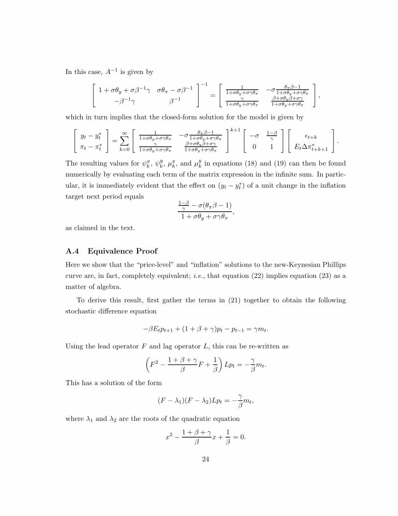
In this case, A−1 is given by 1 + σθy + σβ−1γ σθπ − σβ−1

−β−1γ β−1

−1

=

1

1+σθy+σγθπ−σ θπβ−1

1+σθy+σγθπ

γ1+σθy+σγθπ

β+σθyβ+σγ1+σθy+σγθπ

,

which in turn implies that the closed-form solution for the model is given by yt − y∗tπt − π∗t

=

∞∑k=0

1

1+σθy+σγθπ−σ θπβ−1

1+σθy+σγθπ

γ1+σθy+σγθπ

β+σθyβ+σγ1+σθy+σγθπ

k+1 −σ 1−β

γ

0 1

εt+k

Et∆π∗t+k+1

.

The resulting values for ψπk , ψy

k , µπk , and µy

k in equations (18) and (19) can then be found

numerically by evaluating each term of the matrix expression in the infinite sum. In partic-

ular, it is immediately evident that the effect on (yt − y∗t ) of a unit change in the inflation

target next period equals1−β

γ − σ(θπβ − 1)

1 + σθy + σγθπ,

as claimed in the text.

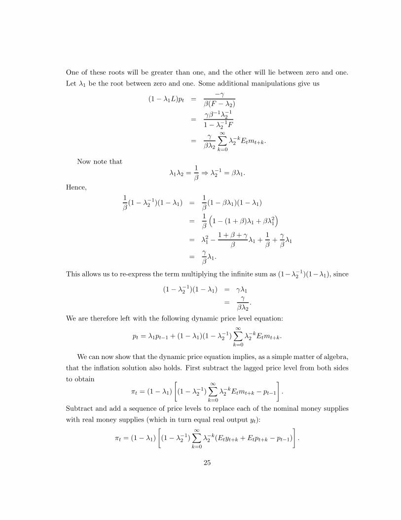
A.4 Equivalence Proof

Here we show that the “price-level” and “inflation” solutions to the new-Keynesian Phillips

curve are, in fact, completely equivalent; i.e., that equation (22) implies equation (23) as a

matter of algebra.

To derive this result, first gather the terms in (21) together to obtain the following

stochastic difference equation

−βEtpt+1 + (1 + β + γ)pt − pt−1 = γmt.

Using the lead operator F and lag operator L, this can be re-written as(F 2 − 1 + β + γ

βF +

1β

)Lpt = −γ

βmt.

This has a solution of the form

(F − λ1)(F − λ2)Lpt = −γβmt,

where λ1 and λ2 are the roots of the quadratic equation

x2 − 1 + β + γ

βx+

1β

= 0.

24

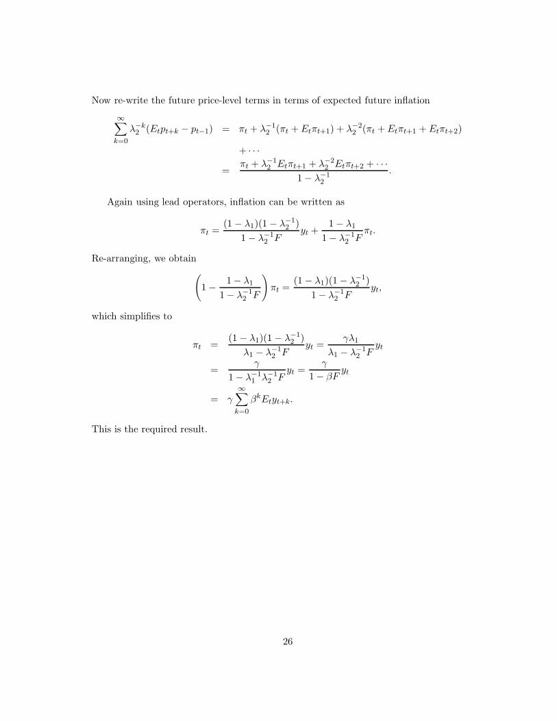
One of these roots will be greater than one, and the other will lie between zero and one.

Let λ1 be the root between zero and one. Some additional manipulations give us

(1− λ1L)pt =−γ

β(F − λ2)

=γβ−1λ−1

2

1− λ−12 F

=γ

βλ2

∞∑k=0

λ−k2 Etmt+k.

Now note that

λ1λ2 =1β⇒ λ−1

2 = βλ1.

Hence,1β

(1− λ−12 )(1− λ1) =

1β

(1− βλ1)(1− λ1)

=1β

(1− (1 + β)λ1 + βλ2

1

)

= λ21 −

1 + β + γ

βλ1 +

1β

+γ

βλ1

=γ

βλ1.

This allows us to re-express the term multiplying the infinite sum as (1−λ−12 )(1−λ1), since

(1− λ−12 )(1 − λ1) = γλ1

=γ

βλ2.

We are therefore left with the following dynamic price level equation:

pt = λ1pt−1 + (1− λ1)(1− λ−12 )

∞∑k=0

λ−k2 Etmt+k.

We can now show that the dynamic price equation implies, as a simple matter of algebra,

that the inflation solution also holds. First subtract the lagged price level from both sides

to obtain

πt = (1− λ1)

[(1− λ−1

2 )∞∑

k=0

λ−k2 Etmt+k − pt−1

].

Subtract and add a sequence of price levels to replace each of the nominal money supplies

with real money supplies (which in turn equal real output yt):

πt = (1− λ1)

[(1− λ−1

2 )∞∑

k=0

λ−k2 (Etyt+k + Etpt+k − pt−1)

].

25

Now re-write the future price-level terms in terms of expected future inflation

∞∑k=0

λ−k2 (Etpt+k − pt−1) = πt + λ−1

2 (πt + Etπt+1) + λ−22 (πt + Etπt+1 + Etπt+2)

+ · · ·=

πt + λ−12 Etπt+1 + λ−2

2 Etπt+2 + · · ·1− λ−1

2

.

Again using lead operators, inflation can be written as

πt =(1− λ1)(1− λ−1

2 )1− λ−1

2 Fyt +

1− λ1

1− λ−12 F

πt.

Re-arranging, we obtain(1− 1− λ1

1− λ−12 F

)πt =

(1− λ1)(1− λ−12 )

1− λ−12 F

yt,

which simplifies to

πt =(1− λ1)(1 − λ−1

2 )λ1 − λ−1

2 Fyt =

γλ1

λ1 − λ−12 F

yt

=γ

1− λ−11 λ−1

2 Fyt =

γ

1− βF yt

= γ∞∑

k=0

βkEtyt+k.

This is the required result.

26

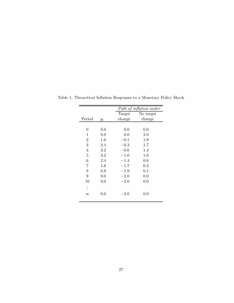
Table 1: Theoretical Inflation Responses to a Monetary Policy Shock

Path of inflation underTarget No target

Period yt change change

0 0.0 0.0 0.01 0.8 0.0 2.02 1.6 −0.1 1.93 2.4 −0.3 1.74 3.2 −0.6 1.45 3.2 −1.0 1.06 2.4 −1.4 0.67 1.6 −1.7 0.38 0.8 −1.9 0.19 0.0 −2.0 0.010 0.0 −2.0 0.0...∞ 0.0 −2.0 0.0

27

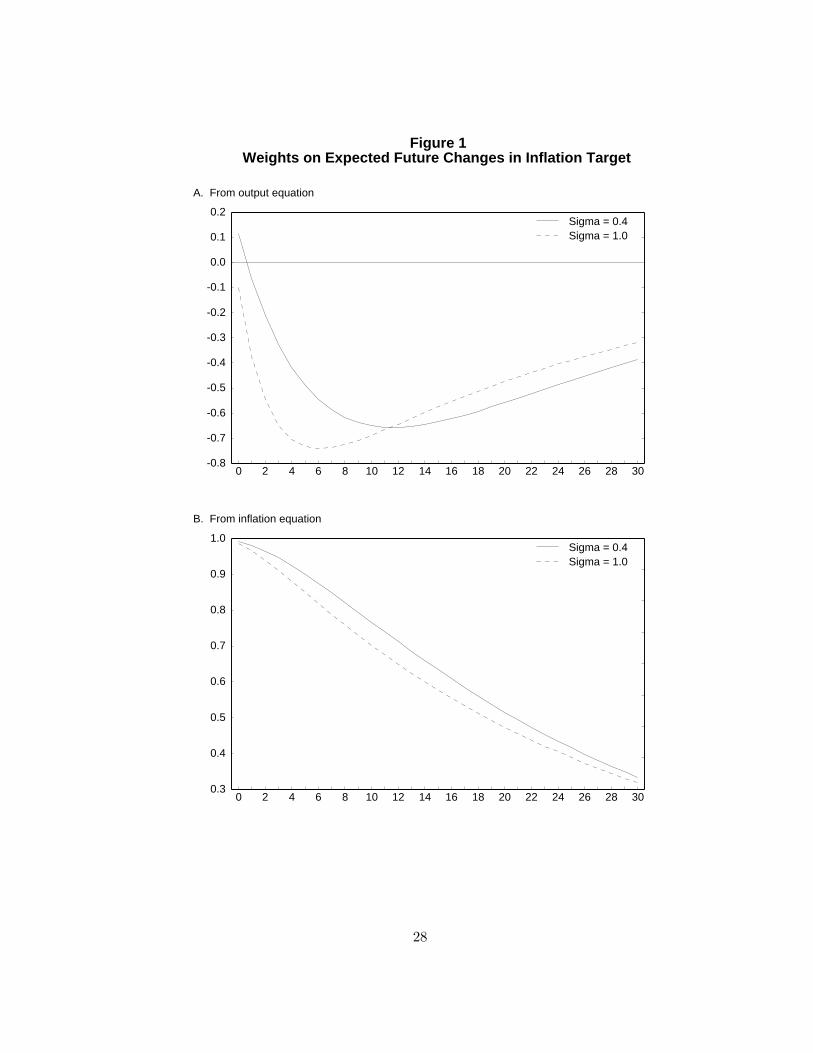
Figure 1Weights on Expected Future Changes in Inflation Target

0 2 4 6 8 10 12 14 16 18 20 22 24 26 28 30-0.8

-0.7

-0.6

-0.5

-0.4

-0.3

-0.2

-0.1

0.0

0.1

0.2Sigma = 0.4Sigma = 1.0

A. From output equation

0 2 4 6 8 10 12 14 16 18 20 22 24 26 28 300.3

0.4

0.5

0.6

0.7

0.8

0.9

1.0Sigma = 0.4Sigma = 1.0

B. From inflation equation

28

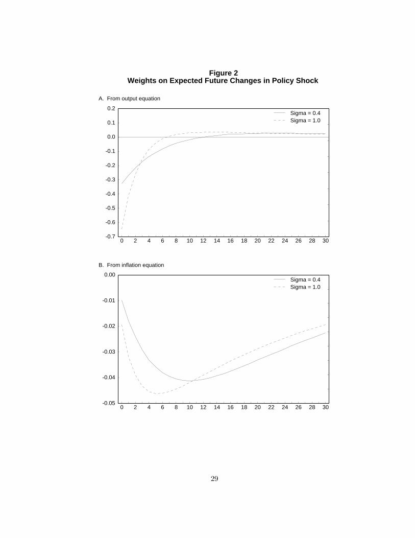
Figure 2Weights on Expected Future Changes in Policy Shock

0 2 4 6 8 10 12 14 16 18 20 22 24 26 28 30-0.7

-0.6

-0.5

-0.4

-0.3

-0.2

-0.1

0.0

0.1

0.2Sigma = 0.4Sigma = 1.0

A. From output equation

0 2 4 6 8 10 12 14 16 18 20 22 24 26 28 30-0.05

-0.04

-0.03

-0.02

-0.01

0.00Sigma = 0.4Sigma = 1.0

B. From inflation equation

29

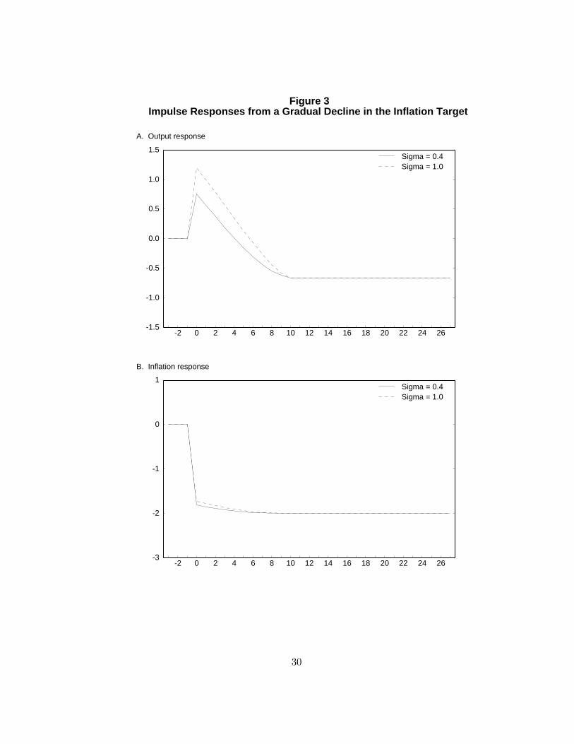
Figure 3Impulse Responses from a Gradual Decline in the Inflation Target

-2 0 2 4 6 8 10 12 14 16 18 20 22 24 26-1.5

-1.0

-0.5

0.0

0.5

1.0

1.5Sigma = 0.4Sigma = 1.0

A. Output response

-2 0 2 4 6 8 10 12 14 16 18 20 22 24 26-3

-2

-1

0

1Sigma = 0.4Sigma = 1.0

B. Inflation response

30

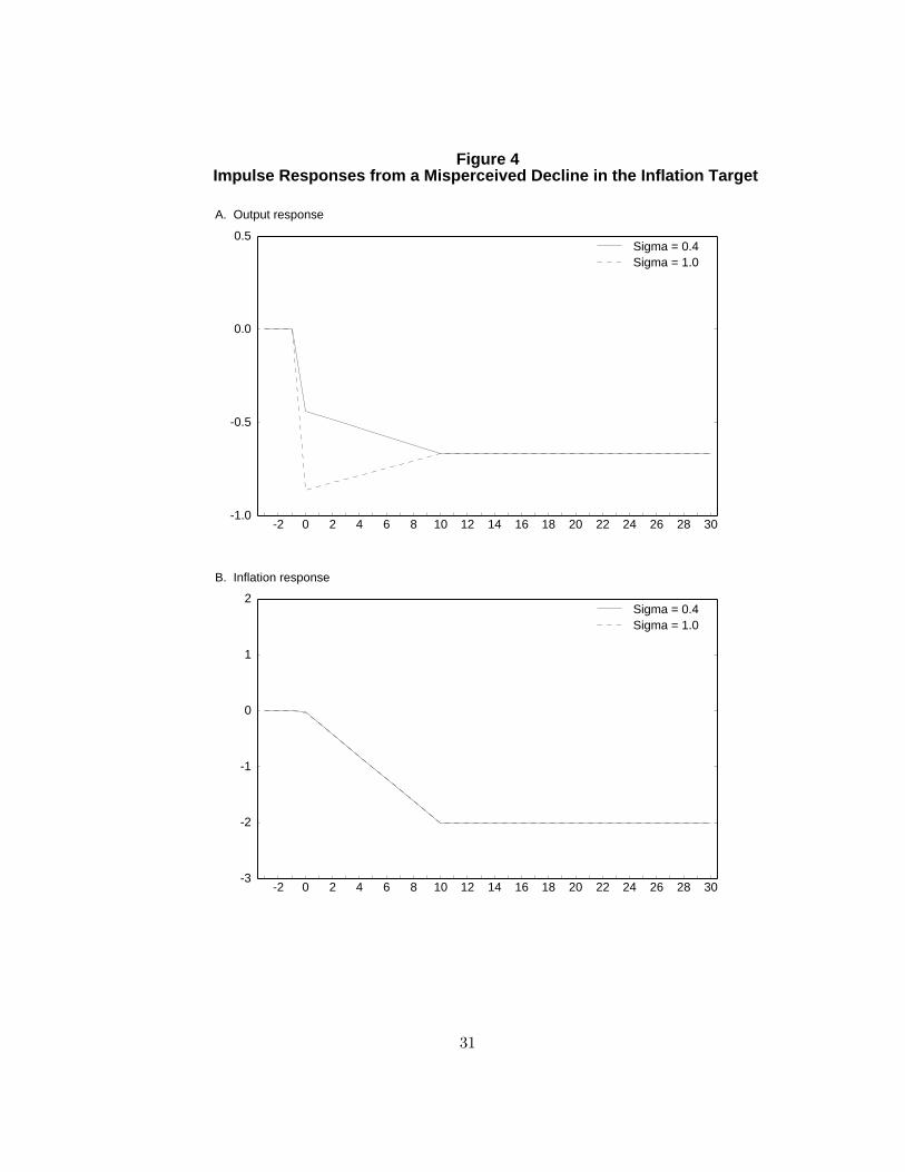
Figure 4Impulse Responses from a Misperceived Decline in the Inflation Target

-2 0 2 4 6 8 10 12 14 16 18 20 22 24 26 28 30-1.0

-0.5

0.0

0.5Sigma = 0.4Sigma = 1.0

A. Output response

-2 0 2 4 6 8 10 12 14 16 18 20 22 24 26 28 30-3

-2

-1

0

1

2Sigma = 0.4Sigma = 1.0

B. Inflation response

31

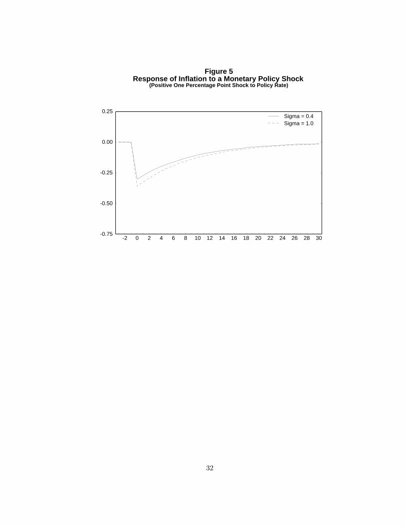
Figure 5Response of Inflation to a Monetary Policy Shock

(Positive One Percentage Point Shock to Policy Rate)

-2 0 2 4 6 8 10 12 14 16 18 20 22 24 26 28 30-0.75

-0.50

-0.25

0.00

0.25Sigma = 0.4Sigma = 1.0

32