Inflation and the Price of Real Assets∗

Monika Piazzesi

Stanford & NBER

Martin Schneider

Stanford & NBER

March 2012

Abstract

In the 1970s, U.S. asset markets witnessed () a 25% dip in the ratio of aggregate

household wealth relative to GDP and () negative comovement of house and stock

prices that drove a 20% portfolio shift out of equity into real estate. This study uses

an overlapping generations model with uninsurable nominal risk to quantify the role of

structural change in these events. We attribute the dip in wealth to the entry of baby

boomers into asset markets, and to the erosion of bond portfolios by surprise inflation,

both of which lowered the overall propensity to save. We also show that the Great

Inflation led to a portfolio shift by making housing more attractive than equity. Apart

from tax effects, a new channel is that disagreement about inflation across age groups

drives up collateral prices when credit is nominal.

∗Email addresses: piazzesi@stanford.edu, schneidr@stanford.edu. For comments and suggestions, we

thank Joao Cocco, Jesus Fernandez-Villaverde, John Heaton, Susan Hume McIntosh, Larry Jones, Patrick

Kehoe, Per Krusell, Ricardo Lagos, Ellen McGrattan, Toby Moskowitz, Neng Wang, seminar participants

at Berkeley, BU, Chicago, Columbia, FRB Minneapolis, Indiana University, LSE, Michigan, NYU, Penn,

UCLA, USC, Universities of Illinois, Texas, and Toronto, as well as conference participants at the Federal

Reserve Banks of Atlanta, Chicago, and Cleveland, the Deutsche Bundesbank/Humboldt University, the

Bank of Portugal Monetary Economics Conference, and the NBER Real Estate and Monetary Economics

Group.

1

1 Introduction

The 1970s brought dramatic changes in the size and composition of US household sector

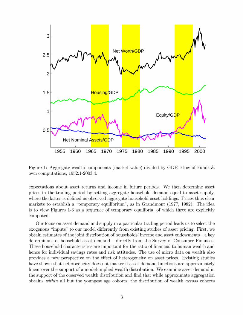
wealth. Figure 1 shows that aggregate household net worth as a fraction of GDP fell by

25% during the 1970s, before recovering again to its late 1960s value. Figure 2 shows that

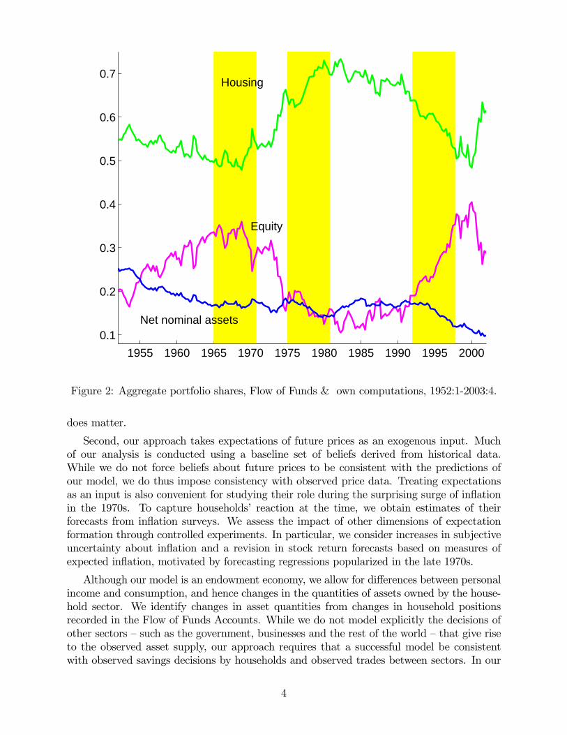
the aggregate household portfolio saw a 20% shift away from equity and into real estate

during the 1970s. This portfolio adjustment was largely driven by negative comovement of

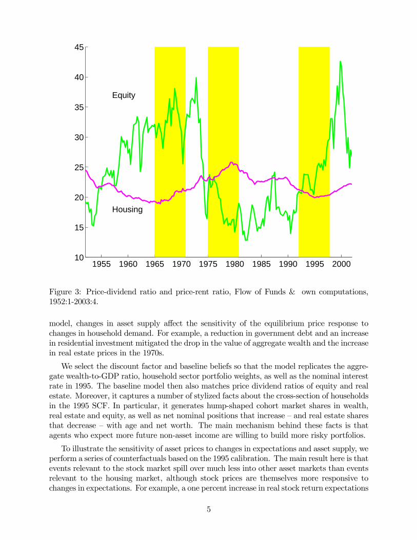
asset prices — house prices rose while equity prices fell, as shown in Figure 3. Compared to

the big swings in the major real asset positions, households’ net position in nominal credit

instruments was relatively stable. As documented below, the stability of net positions masks

substantial increases in gross borrowing and lending within the household sector.

This paper develops an asset pricing model with heterogeneous agents and incomplete

markets to study the 1970s. The key elements of the model are that households differ by

age and wealth and that all credit is nominal, so that inflation matters for bond returns

and the cost of borrowing. Our empirical strategy is based on the idea that micro data on

household characteristics can be used to directly parametrize household sector asset demand.

In particular, the first step of our analysis is to estimate, for each trading period, () the

distribution of income and initial asset endowments across households and () household

expectations about future prices and income. We then determine optimal household policies

given endowments and expectations. Equilibrium prices equate household asset demand to

the supply of assets provided by other sectors. We use this framework to evaluate different

candidate explanations for the price and portfolio movements in Figures 1-3.

Our analysis attributes the dip in household wealth to two events unique to the 1970s

that reduced the propensity to save in the household sector. First, entry of the young baby

boomers into asset markets directly lowered the average savings rate. Second, the erosion of

bond portfolios by surprise inflation reduced the ratio of financial wealth to human wealth,

which also gives rise to lower savings. Since there was only a small reduction in asset supply

in the 1970s, the lower average savings rate reduced the value of outstanding assets. We

also show that the Great Inflation induced a portfolio shift towards real estate. One effect is

that various nominal rigidities in the tax code make housing more attractive when expected

inflation is high. Another effect we stress is that heterogenous inflation expectations in a

nominal credit market increase the volume of credit and drive up the price of collateral.

Our model describes a sequence of trading periods. Households of different ages enter

the period with different initial endowments. They trade goods, as well as three risky assets:

equity, real estate and nominal bonds. In the credit market, households face collateral

constraints — all borrowing must be backed by real estate — as well as a spread between

borrowing and lending rates. Moreover, lending and borrowing is required to be in nominal

terms — there is no riskfree asset. Households experience idiosyncratic shocks to labor income

as well as to the value of their real estate holdings. Neither idiosyncratic risk nor inflation

risk are insurable given the available assets.

We implement the model for three 6-year trading periods, highlighted in yellow in Fig-

ures 1-3. For each period, we derive household sector asset demand by solving households’

consumption-savings problems, given endowments of assets and non-asset income as well as

2

1955 1960 1965 1970 1975 1980 1985 1990 1995 2000

0.5

1

1.5

2

2.5

3

Net Worth/GDP

Housing/GDP

Equity/GDP

Net Nominal Assets/GDP

Figure 1: Aggregate wealth components (market value) divided by GDP, Flow of Funds &

own computations, 1952:1-2003:4.

expectations about asset returns and income in future periods. We then determine asset

prices in the trading period by setting aggregate household demand equal to asset supply,

where the latter is defined as observed aggregate household asset holdings. Prices thus clear

markets to establish a “temporary equilibrium”, as in Grandmont (1977, 1982). The idea

is to view Figures 1-3 as a sequence of temporary equilibria, of which three are explicitly

computed.

Our focus on asset demand and supply in a particular trading period leads us to select the

exogenous “inputs” to our model differently from existing studies of asset pricing. First, we

obtain estimates of the joint distribution of households’ income and asset endowments — a key

determinant of household asset demand — directly from the Survey of Consumer Finances.

These household characteristics are important for the ratio of financial to human wealth and

hence for individual savings rates and risk attitudes. The use of micro data on wealth also

provides a new perspective on the effect of heterogeneity on asset prices. Existing studies

have shown that heterogeneity does not matter if asset demand functions are approximately

linear over the support of a model-implied wealth distribution. We examine asset demand in

the support of the observed wealth distribution and find that while approximate aggregation

obtains within all but the youngest age cohorts, the distribution of wealth across cohorts

3

1955 1960 1965 1970 1975 1980 1985 1990 1995 2000

0.1

0.2

0.3

0.4

0.5

0.6

0.7Housing

Equity

Net nominal assets

Figure 2: Aggregate portfolio shares, Flow of Funds & own computations, 1952:1-2003:4.

does matter.

Second, our approach takes expectations of future prices as an exogenous input. Much

of our analysis is conducted using a baseline set of beliefs derived from historical data.

While we do not force beliefs about future prices to be consistent with the predictions of

our model, we do thus impose consistency with observed price data. Treating expectations

as an input is also convenient for studying their role during the surprising surge of inflation

in the 1970s. To capture households’ reaction at the time, we obtain estimates of their

forecasts from inflation surveys. We assess the impact of other dimensions of expectation

formation through controlled experiments. In particular, we consider increases in subjective

uncertainty about inflation and a revision in stock return forecasts based on measures of

expected inflation, motivated by forecasting regressions popularized in the late 1970s.

Although our model is an endowment economy, we allow for differences between personal

income and consumption, and hence changes in the quantities of assets owned by the house-

hold sector. We identify changes in asset quantities from changes in household positions

recorded in the Flow of Funds Accounts. While we do not model explicitly the decisions of

other sectors — such as the government, businesses and the rest of the world — that give rise

to the observed asset supply, our approach requires that a successful model be consistent

with observed savings decisions by households and observed trades between sectors. In our

4

1955 1960 1965 1970 1975 1980 1985 1990 1995 200010

15

20

25

30

35

40

45

Equity

Housing

Figure 3: Price-dividend ratio and price-rent ratio, Flow of Funds & own computations,

1952:1-2003:4.

model, changes in asset supply affect the sensitivity of the equilibrium price response to

changes in household demand. For example, a reduction in government debt and an increase

in residential investment mitigated the drop in the value of aggregate wealth and the increase

in real estate prices in the 1970s.

We select the discount factor and baseline beliefs so that the model replicates the aggre-

gate wealth-to-GDP ratio, household sector portfolio weights, as well as the nominal interest

rate in 1995. The baseline model then also matches price dividend ratios of equity and real

estate. Moreover, it captures a number of stylized facts about the cross-section of households

in the 1995 SCF. In particular, it generates hump-shaped cohort market shares in wealth,

real estate and equity, as well as net nominal positions that increase — and real estate shares

that decrease — with age and net worth. The main mechanism behind these facts is that

agents who expect more future non-asset income are willing to build more risky portfolios.

To illustrate the sensitivity of asset prices to changes in expectations and asset supply, we

perform a series of counterfactuals based on the 1995 calibration. The main result here is that

events relevant to the stock market spill over much less into other asset markets than events

relevant to the housing market, although stock prices are themselves more responsive to

changes in expectations. For example, a one percent increase in real stock return expectations

5

over the next six years raises the price dividend ratio of stocks by 15%, but raises the nominal

interest rate by only 10 basis points; it lowers the price-dividend ratio on housing by 3.5%.

In contrast, a one percent increase in the expected return on real estate raises the house price

by 7%, increases the nominal interest rate by 80 basis points, and also lowers stock prices

by 13%. The reason for these results is that households can borrow against real estate, so

that events in the housing market feed back more strongly to the credit market than news

about stocks.

We then use the model to examine the 1970s. We show that the model produces a drop

in aggregate wealth between 1968 and 1978 for a wide range of expectations scenarios. It

attributes the dip in the wealth-GDP ratio to two effects. First, the entry of baby boomers

into asset markets lowered the average saving rate. Second, capital losses from realized

inflation lowered wealth and hence savings, especially for older households. At the same

time, lower savings were not counteracted by a large increase in interest rates, because the

outside supply of bonds to the household sector also fell. If we assume that the spread

between borrowing and lending rate was 75 basis points higher in 1968 than in 1995, the

model also generates the increase in gross borrowing and lending between these two years.

We explore three different channels through which inflation expectations can induce neg-

ative comovement of stock and house prices. First, households disagreed about inflation in

the late 1970s. We use the Michigan Survey of Consumers to document that old households

expected lower inflation than young households. When credit is nominal, disagreement about

inflation implies disagreement about real interest rates. As a result, there is more borrowing

and lending among households and an increase in the price of collateral, namely housing. Sec-

ond, nominal rigidities in the taxes code favor housing over equity in times of high expected

inflation. Third, expected inflation is a predictor of low stock returns (for example, because

inflation lowers depreciation allowances based on historical cost accounting and hence real

cash flows), as shown by a number of studies that appeared in the 1970s, such as Fama and

Schwert (1977).

Our quantitative analysis suggests that both inflation and growth expectations were rel-

evant for asset prices and household positions in the 1970s, while neither can account for the

data by itself. Our model attributes the portfolio shift to changes in inflation expectations.

A little more than half of the shift is due to lower stock returns predicted by higher expected

inflation, while about one quarter each is due to disagreement about real interest rates and

nominal rigidities in the tax code. Disagreement also accounts for the increase in credit

volume, which is however mitigated by an increase in inflation uncertainty. Pessimism about

growth, which affects both labor income and dividends, increases the demand for savings

and partly offsets the effects of pessimism about stock returns on the wealth-GDP ratio. At

the same time, pessimism about asset returns puts downward pressure on interest rates, thus

partly offsetting the effects of expected inflation.

The rest of the paper is organized as follows. Section 2 discusses related literature.

Section 3 presents the model. Section 4 describes the quantitative implementation and doc-

uments properties of the model inputs, that is, the joint distribution of asset endowments and

income as well as asset supply. Section 5 derives predictions for optimal household behavior

and compares them to the data. Section 6 illustrates price determination in temporary equi-

6

librium using counterfactuals. Section 7 derives predictions under baseline expectations and

shows that they help understand the evolution of the wealth-GDP ratio. Section 8 considers

the effect of inflation on portfolio composition in the 1970s. Section 9 concludes.

2 Related Literature

Some of the effects of inflation that arise in our model have been discussed before. Feldstein

(1980), Summers (1981) and Poterba (1991) have examined various ways in which the inter-

action of taxes and inflation can affect asset prices. One argument is that inflation lowers

after tax returns on bonds and stocks more than those on real estate and hence might be

responsible for the portfolio shift of the 1970s. We show that this effect contributes to the

portfolio shift, although it cannot quantitatively generate all of it. These authors have also

argued that inflation has effects on real cash flows because of depreciation allowances. These

effects are captured in our pessimism experiments.

Previous literature has shown that demographics cannot account fully for changes in

stock prices, if equity is the only long-lived asset in the model (Abel 2003, Geanakoplos

et al. 2004). The effect of demographics on house prices in isolation has been considered

by Mankiw and Weil (1989) and Ortalo-Magne and Rady (2005). In our model, with both

equity and real estate present in nonzero net supply, demographics impact aggregate savings

and hence the wealth-GDP ratio, but it can also not account for the larger movements in

the individual components of wealth, especially stocks.

There is a large literature on asset pricing models with heterogeneous agents and in-

complete markets and/or borrowing constraints. For example, Constantinides and Duffie

(1996), Heaton and Lucas (1996), Krusell and Smith (1998), Constantinides et al. (2002)

and Storesletten et al. (2004) consider models with equity, riskless bonds and uninsurable

income risk. Alvarez and Jermann (2001) and Lustig and van Nieuwerburgh (2005) consider

models with complete markets, where income risk cannot be insured because of borrowing

constraints or collateral constraints backed by real estate, respectively. The goal of these

papers is to derive a stationary equilibrium of the model that matches empirical moments of

returns such as the equity premium. The input to the model is typically a jointly stationary

process for income and dividends, while the output compared to the data are moments of

returns and macro aggregates, and sometimes also the cross section of consumption (Brav

et al. 2002, Kocherlakota and Pistaferri 2005).

Our paper differs from these studies because of our focus on nominal risk, observed

household asset positions, and structural change. Our empirical implementation uses the

cross section of household asset positions both as an input to the model and as a target of

the analysis. To accommodate structural change, we do not derive a stationary equilibrium

that is compared to empirical moments, but consider instead asset prices and holdings at

specific dates. In this respect, our approach is similar to that of Barsky (1989) who considers

the effect of lower and more volatile economic growth, McGrattan and Prescott (2005) who

look at the effect of taxes on stock prices, Nakajima (2005) who considers the effect of

precautionary savings on house prices and Campbell and Hercowitz (2005) who study the

7

effect of credit market deregulation on debt levels. However, existing studies that focus

on low frequency movements in the economy typically compare steady states or stationary

equilibria at different parameter values, while we use the temporary equilibrium concept of

Grandmont (1977, 1982).

Portfolio choice with housing has been considered by Flavin and Yamashita (2002), Camp-

bell and Cocco (2003), and Fernandez-Villaverde and Krueger (2005). Cocco (2005) and

Yao and Zhang (2005) study intertemporal problems with three assets that are similar to

the problem solved by our households. General equilibrium OLG models with housing have

been considered by Chambers et al. (2006) and Yang (2006). These papers are also inter-

ested in the cross section of house ownership. While they consider a shorter period length

and thus study the cross section in more detail than we do, they abstract from aggregate

risk which is important for our application.

3 Model

The model describes the household sector’s planning and asset trading in a single period .

3.1 Households

Households enter the period with assets and debt accumulated earlier. During the period,

they earn labor income, pay taxes, consume and buy assets. Labor income is affected by

idiosyncratic income shocks. Households can invest in three types of assets: long-lived equity

and real estate as well as short lived nominal bonds. Households face two types of aggregate

risk. They face aggregate growth risk through stock dividends and aggregate components

of their housing dividends and labor income. They also face aggregate inflation risk when

borrowing or lending because there is no riskfree asset. Households also face idiosyncratic

risk which affects the return on individual houses and labor income streams. There are only

three assets, so markets are incomplete.

Planning Horizon

Consumers alive at time differ by endowment of assets and numeraire good as well as by

age. Differences in age are represented by age-specific planning horizons and age-specific

survival probabilities for the next period. We now describe the problem of a typical consumer

with a planning horizon 0.

Preferences

Consumers care about two goods, housing services and other (non-housing) consumption

which serves as the numeraire. A consumption bundle of units of housing services and units of numeraire yields utility

= 1− (1)

Preferences over (random) streams of consumption bundles {} are represented by the

8

recursive utility specification of Epstein and Zin (1989). Utility at time is defined as

=

µ1−1 +

£1−+1

¤ 1−11−

¶ 11−1

(2)

where + = + Here determines the intertemporal elasticity of substitution for de-

terministic consumption paths, is the coefficient of relative risk aversion towards timeless

gambles, and is the discount factor. The expectation operator takes into account that the

agent will reach the next period only with an age-specific survival probability.

Equity

Shares of equity can be thought of as trees that yield some quantity of numeraire good

as dividend. A consumer enters period with an endowment of

≥ 0 units of trees. Treestrade in the equity market at the ex-dividend price ; they cannot be sold short. A tree

pays units of dividend at date . We summarize consumers’ expectations about prices and

dividends beyond period by specifying expectations about returns. In particular, we assume

that consumers expect to earn a (random) real return +1 by holding equity between any

two periods and + 1, where ≥ .

Real Estate

Real estate — or houses — may be thought of as trees that yield housing services. A

consumer enters period with an endowment of

≥ 0 units of houses. Houses trade at theex-dividend price ; they cannot be sold short. To fix units, we assume that one unit of real

estate (also referred to as one house) yields one unit of housing services at date . There is a

perfect rental market, where housing services can be rented at the price . Moreover, every

house requires a maintenance cost of units of numeraire. If a consumer buys units of

real estate, he obtains a dividend ( −) =:

Consumers form expectations about

future returns on housing and rental prices©

ª.

Borrowing and Lending

Consumers can borrow or lend by buying or selling one period discount nominal bonds.

A consumer enters period with an endowment of units of numeraire that is due to past

borrowing and lending in the credit market. In particular, is negative if the consumers

has been a net borrower in the past. In period , consumers can buy or sell bonds at a price

A consumer expects every bond bought to pay 1+1 units of numeraire in period +1.

Here +1 is random and may be thought of as the expected change in the dollar price of

numeraire. This is a simple way to capture that debt is typically denominated in dollars.1

For every bond sold, the consumer expects to repay (1+)+1 units of numeraire in period

+1, where 0 is an exogenous credit spread.2 Bond sellers — borrowers — face a collateral

constraint: the value of bonds sold may not exceed a fraction of the ex-dividend value

1To see why, consider a nominal bond which costs dollars today and pays of $1 tomorrow, or 1+1

units of numeraire consumption. Now consider a portfolio of nominal bonds. The price of the portfolio

is units of numeraire and its payoff is

+1 = 1+1 units of numeraire tomorrow. The model thus

determines the price of a nominal bond in $.2One way to think about the organization of the credit market is that there is a financial intermediary

that matches buyers and sellers in period . In period +1 the intermediary will collect (1 + ) +1 units

of numeraire from every borrower (bond seller), but pay only 1+1 to every lender (bond buyer), keeping

9

of all real estate owned by the consumer. For periods , consumers form expectations

about the (random) real return on bonds©

ª They believe that

= 1−1 is the (expost) real lending rate, and that

(1 + ) is the (ex post) real borrowing rate.

Non-Asset Income

Consumers are endowed with an age-dependent stream of numeraire good {}+= . Here

income should be interpreted as the sum of labor income, transfer income, and income on

illiquid assets such as private businesses.

Budget Set

The consumer enters period with an endowment of houses and equity³

´as well

as an endowment of + from non-asset income and past credit market activity. At period

prices, initial wealth is therefore

= ( + )

+ ( + )

+ + (3)

To allocate this initial wealth to consumption and purchases of assets, the consumer chooses

a plan =©

+

−

ª where + ≥ 0 and − ≥ 0 denote the amount of bonds

bought and sold, respectively. It never makes sense for a consumer to borrow and lend

simultaneously, that is, + ≥ 0 implies − = 0 and vice versa.The plan must satisfy the collateral constraint

− ≤

. The plan must also

satisfy the budget constraint

+ + = , (4)

where terminal wealth is defined as

= +

+

+ −

−

To formulate the budget constraint for periods beyond , it is helpful to define the

ex-dividend value of the consumer’s stock portfolio in by =

the consumer’s

real estate portfolio by =

as well as the values of a (positive or negative) bond

portfolio, + =

+ and −

= − For periods , the consumer chooses plans

= {

+ −

} subject to the collateral constraint − ≤

and the bud-

get constraint

+ + +

+ + − −

=

−1 +

−1 +

+−1 −

(1 + )−−1 + (5)

We denote the consumer’s overall plan by =³ {}+=+1

´ This plan is selected to

maximize utility (2) subject to the budget constraints (3)-(5) and the collateral constraints.

Taxes

In some of our examples below, we will assume proportional income taxes as well as

capital gains and dividend taxes. This will not change the structure consumer’s problem,

+1 for itself. We do not model the financial intermediary explicitly since we only clear markets in period

.

10

just the interpretation of the symbols. In particular, labor income, dividends and returns

will have to be interpreted as their after-tax counterparts. Their precise form will be discuss

in the calibration section below.

Terminal Consumers

The consumers described so far have planning horizons 0. We also allow consumers

with planning horizon = 0 These consumers also enter period with asset and numeraire

endowments that provide them with initial wealth , as in (3). However, they do not make

any savings or portfolio decisions. Instead, they simply purchase numeraire and housing

services in the period goods markets to maximize (1) subject to the budget constraint

+ =

3.2 Equilibrium

To capture consumer heterogeneity, we assume a finite number of consumer types, indexed by

, with different initial endowment vectors (

()

() ()+ ()) and planning horizons

()

The Rest of the Economy

To close the model and regulate the supply of assets exogenous to the household sector,

we introduce a rest-of-the-economy (ROE) sector. It may be thought of as a consolidation of

the business sector, the government and the rest of the world. The ROE sector is endowed

with trees and houses in period . Here could be negative to represent repurchases

of shares by the corporate sector. In addition, the ROE enters period with an outstanding

debt of units of numeraire, and it raises units of numeraire by borrowing in period .

The surplus from these activities is

= (

+ ) + (

+ ) + −

If is positive, it is consumed by the ROE sector. More generally, the ROE is assumed

to have “deep pockets” out of which it pays for any deficit if 0.

Aggregate Asset Supply

We normalize initial endowments of equity and real estate such that there is a single tree

and a single house outstanding: P

() =P

() = 1

In addition, we assume that initial endowments from past credit market activity are con-

sistent, in the sense that every position corresponds to some offsetting position, either by a

household or by the ROE sector: P () =

Equilibrium

An equilibrium consists of a vector of prices for period ,¡

¢ a surplus for

the ROE sector , as well as a collection of consumer plans for period , { ()} =

{ () (), () () + () − ()} such that

11

(1) for every consumer, the plan () is part of an optimal plan () =³ () { ()}+ ()=+1

´given consumer 0 endowment, planning horizon, and expectations about future pricesand returns;

(2) markets for all assets and goods clear:P

() = 1 + P

() = 1 +

P

+ () = +

P − () P

() + () + =

P () + (1 + ) P

() =P

()

In addition to market clearing conditions for stocks, bonds and numeraire, there are two

market clearing conditions for housing: one for the asset “real estate” and one for the good

“housing services”. The first equation ensures that the total demand for houses equals their

total supply. The fifth equation ensures that the fraction of houses that owners set aside as

investment real estate — that is, selling services in the rental market — is the same as the

fraction of housing services demanded in the rental market. As is common in competitive

models, one of the five market clearing conditions is redundant, as it is implied by the sum

of consumers’ budget constraints, the definition of and the other four market clearing

conditions. Solving for equilibrium prices thus amounts to solving a system of four equation

in the four prices , , and .

3.3 Discussion of the Assumptions

Connection to National Income Accounting

Introducing the ROE sector allows us to accommodate deviations between consumption

and household sector income that are usually ignored in endowment economy models. To

clarify the connection to the FFA/NIPA framework, we sum up the last three market clearing

conditions and rearrange to obtainP () + ()| {z }+

+

+ − −1| {z } =

P () + + + (1− −1) | {z }

personal consumption personal savings personal income

The first term on the left-hand side of this equation is personal consumption, including

housing services. The right-hand side of this equation represents personal income. While

our definition of income differs from the NIPAs in some details, as discussed in the next

section, the basic components are the same: non-asset income, dividends on the two long-

lived assets, and net interest. The difference between personal consumption and income is

the second term on the left-hand side, which represents personal savings. It consists of the

same components as in the FFA: net acquisition of real estate and net acquisition of financial

12

assets, here equity and bonds.3 The supply of assets provided by the ROE thus allows for

positive or negative personal savings in equilibrium.

Asset Supply and Savings

The possibility of nonzero savings makes our model compatible with richer models that

explicitly consider production, fiscal policy, and the fact that the US is not a closed economy.

A richer model would give rise to well-founded policy functions for the business, government,

and foreign sectors that link those sectors’ net asset supplies to market prices. At the same

time, if the richer model accounts for observed supply by the ROE sector to the household

sector, evaluating the policy functions at observed prices should deliver observed quantities.

In our empirical implementation below, we thus set the net supply by the ROE equal to

observed quantities.

We thus determine asset prices such that households are willing to hold observed quan-

tities, which would also be provided by the ROE in a well-working richer model. In a model

where the other side of the market is also derived from optimal policies, the household sector

could be modelled in exactly the same way as in our model.4 Hereby, we avoid a common

criticism of asset pricing models based on endowment economies: model features that help

explain prices in an endowment economy — for example, certain preference specifications —

may entail undesirable outcomes once savings are allowed. Our strategy matches simultane-

ously prices and observed household savings.

Prices vs. Quantities

It is not common in endowment economymodels to distinguish asset prices and quantities.

Indeed, if the dividend from a single “tree” provides all consumption, there is no meaningful

concept of quantity — doubling the quantity of trees is the same as doubling the dividend on

the single tree. In our model, asset quantity is identified because we allow trades between

the household sector and the ROE. Households increase or decrease the quantity of trees

they own only through such trades. The change in quantity is determined by comparing the

change in market capitalization with the capital gain on pre-existing trees. While a capital

gain is enjoyed by households who enter the periods owning trees, a change in capitalization

requires households to pay for new trees.

Temporary Equilibrium

Temporary equilibrium does not place restrictions on prices beyond date itself. In

particular, it does not require that agents agree on a common model structure that links

3FFA savings is larger than our concept of savings because FFA investment contains investment in noncor-

porate business, as well as purchases of consumer durables. In our empirical implementation, noncorporate

business is treated as illiquid and investment in it is subtracted from income. In addition, we follow the

NIPA convention of treating expenditure on durables as consumption. This seems appropriate given the

6-year length of each period in our model.4Our modelling strategy requires some care in interpretating counterfactuals. For example, computing the

response to a change in tax rates cannot tell us what would have happened to the economy as a whole, since

we do not model supply responses to tax changes. Instead, the counterfactual tells us what the household

sector would have done if taxes changed, and what the effect on prices would have been had supply remained

unchanged. The reason the exercise is still useful is that it allows us to see whether tax changes can play a

first order role in accounting for asset prices over time, given the actual movements in equilibrium quantities.

13

future fundamentals and prices. As far as household behavior is concerned, our empirical

implementation instead follows the literature on portfolio choice, where exogenous processes

for returns and income are standard. However, we go beyond portfolio choice models in

that we explore how equilibrium prices change when investors’ expectations about returns

vary in a controlled way. This is particularly useful if expectations are matched to inflation

surveys, as we do in Section 8, since expected inflation directly affects returns.

Our model does not link price expectations to future model-implied prices. Such a con-

nection is imposed in rational expectations models, and more generally whenever agents

have “structural knowledge” of the price function, such as in many models with Bayesian

learning. Assuming structural knowledge has appeal when agents understand well how the

economy works, for example because there are stable recurrent patterns in the data. Indeed,

in a stationary environment, “knowing the price function” can be justified by learning from

past data, and appears no more restrictive than “knowing the distribution of fundamentals”.

However, our interest in this paper is in low frequency asset-price movements during

times of structural change. In this context, it is not clear why agent beliefs should be based

on the particular model structure that we consider today with the benefit of hindsight. For

example, it is not clear whether household expectations should be required to anticipate

structural change that we only now know to have taken place. Since the usual justifications

for narrowing down the set of expectations by imposing rational expectations or structural

knowledge is not compelling, we turn to flexible modelling of exogenous expectations.

Connection to consumption-based asset-pricing

Many studies that examine asset prices jointly with real variables focus on consumption,

in particular the connection between consumption and asset prices implied by intertemporal

Euler equations. Since our model is based on utility maximization, an Euler equation also

holds, at least at the individual household level. Instead of considering temporary equilibria,

thus deriving a map from endowments and supply to prices, one could consider examining

the Euler equation directly. In certain ways this might be easier, since it requires only one

non-price variable, consumption, although serious treatment of heterogeneous agents would

require household-level consumption data.

The main problem with the Euler equation approach in our context is that the Euler

equation relates prices to investors’ planned consumption, and thus makes sense only if

planned consumption can be measured. Imposing rational expectations effectively makes

the (subjective) distribution of planned consumption measurable by setting it equal — by

assumption — to the observed distribution of realized consumption. As discussed above, this

is a strong assumption that is not compelling in the context of structural change. As a result,

the Euler equation approach itself is not appealing for the application we consider in this

paper.

Nonnegative Net Worth

Few households have negative net worth. Table 1 documents that the percentage of

negative net worth households has always been between 4% and 7%. Table 1 also shows

that the net worth of these households is moderate. For example, the average net worth was

-11K Dollars in 2001. These numbers suggest that the most important reason for household

14

borrowing is not consumption smoothing. Instead, young households “borrow to gamble”

– they borrow to be able to buy more risky assets, such as housing.

Table 1: Negative Net Worth Households

1962 SCF 1995 SCF 2001 SCF

avg. 29 53 77 avg. 29 53 77 avg. 29 53 77

% of households 4% 10% 3% 2% 7% 18% 4% 2% 7% 20% 5% 2%

net worth (in $) -.4K -.4K -.8K -1.3K -9K -9K -13K -8K -11K -10K -9K -1K

Note: Row 1 reports the percentage of households with negative net worth inthe U.S. population based on different SCFs. Row 2 reports the average net

worth of these households in dollars.

The Role of Housing

In both our model and in reality, housing plays a dual role: housing can be used for

consumption and investment. In its role as consumption good, housing is different from

other consumption, because it enters the utility function separately and has a different price

In its role as asset, housing is different from other assets, because of its return properties

(which will be discussed later), and because it can serve as collateral. In reality, the two

roles are often connected, because the amount of housing services consumed is equal to the

dividend paid by the amount of housing held in the portfolio. In our model, we abstract from

this issue (at least for now) for several reasons. First, most homeowners not only own their

primary residence, but also some investment real estate (such as time shares, vacation homes,

secondary homes, etc.) Hence, there is no tight link between consumption and investment for

these households. Second, U.S. households are highly mobile. As a consequence, houses are

owned by the same owner on average for only seven years, which is roughly the same length

as a period in our model. Moreover, the decision to move is often more or less exogenous to

households (for example, because of job loss, divorce, death of the spouse, etc.)

4 Quantitative Implementation

The inputs needed for implementing the model are () the joint distribution of asset endow-

ments and income, () aggregate supply of assets to the household sector from other sectors,

() expectations about labor income and asset returns and () parameter values for pref-

erences and the credit market. We describe our choices in detail in the Appendix; here we

provide a brief overview. We start with a description of what a model period corresponds

to in the data.

Timing

The length of a period is six years. Since the model compresses what happens over a six

year span into a single date, prices and holdings are best thought of as period averages. We

15

assume that consumers expect to live for at most 10 such periods, where the first period of

life corresponds roughly to the beginning of working life. In any given period, we consider 11

age groups of households (23, 24-29, 30-35, 36-41, 42-47, 48-53, 54-59, 60-65, 66-71, 72-77,

77) who make portfolio choice decisions. For ease of comparison with other models, we

nevertheless report numbers at annual rates.

In the time series dimension, we focus on three six-year periods, namely 1965-70, 1975-80,

and 1992-97. To construct asset endowment distributions, we use data on asset holdings from

the respective precursor periods 1959-64, 1969-74, and 1986-91. Micro data is not available

at high frequencies. To capture the wealth and income distribution during a period, we have

chosen the above intervals so that every period that contains a Survey of Consumer Finances

contains it in the 4th year of the period; we thus use surveys from 1962, 1989 and 1995. We

use the 4th year survey to infer income and asset holdings where possible.

4.1 Defining Assets and Income

We map the three assets in the model to three broad asset classes in US aggregate and

household statistics. For equity and real estate, we use the Flow of Funds Accounts (FFA)

to derive measures of () aggregate holdings of the household sector, () net purchases by the

household sector and () aggregate dividends received by the household sector. We use the

numbers on value, dividends and new issues to calculate price dividend ratios and holding

returns on equity and real estate. For both assets, we also define corresponding measures at

the individual level using the Survey of Consumer Finances (SCF).

Equity

We identify equity with shares in corporations held and controlled by households. We

include both publicly traded and closely held shares, and both foreign and domestic equity.

We also include shares held indirectly through investment intermediaries if the household

can be assumed to control the asset allocation (into our broad asset classes) himself. We take

this to be true for mutual funds and defined contribution (DC) pensions plans. We do not

include equity in defined benefit (DB) pension plans, since households typically do not control

the asset allocation of such funds. Our concept of dividends thus equals dividends received

by households from the National Income and Product Accounts (NIPA) less dividends on

household holdings in DB plans.

Real estate

Our concept of residential real estate contains owner-occupied housing, directly held

residential investment real estate, as well as residential real estate recorded in the FFA/NIPA

as held indirectly by households through noncorporate businesses. This concept contains

almost all residential real estate holdings, since very few residential properties are owned

by corporations. We take housing dividends to be housing consumption net of maintenance

and property tax from NIPA. For net purchases of new houses, we use aggregate residential

investment from NIPA.

The ROE sector endowment of equity consists of net new equity purchased by the house-

hold sector during the trading period. The factor states this endowment relative to total

16

1955 1960 1965 1970 1975 1980 1985 1990 1995 2000

−10

−5

0

5

New supply of long−lived assets (% market cap)

housesequity

1955 1960 1965 1970 1975 1980 1985 1990 1995 2000

30

40

50

Bond supply (% GDP)

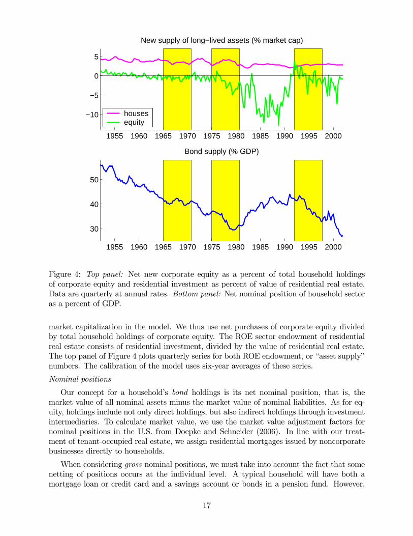
Figure 4: Top panel: Net new corporate equity as a percent of total household holdings

of corporate equity and residential investment as percent of value of residential real estate.

Data are quarterly at annual rates. Bottom panel: Net nominal position of household sector

as a percent of GDP.

market capitalization in the model. We thus use net purchases of corporate equity divided

by total household holdings of corporate equity. The ROE sector endowment of residential

real estate consists of residential investment, divided by the value of residential real estate.

The top panel of Figure 4 plots quarterly series for both ROE endowment, or “asset supply”

numbers. The calibration of the model uses six-year averages of these series.

Nominal positions

Our concept for a household’s bond holdings is its net nominal position, that is, the

market value of all nominal assets minus the market value of nominal liabilities. As for eq-

uity, holdings include not only direct holdings, but also indirect holdings through investment

intermediaries. To calculate market value, we use the market value adjustment factors for

nominal positions in the U.S. from Doepke and Schneider (2006). In line with our treat-

ment of tenant-occupied real estate, we assign residential mortgages issued by noncorporate

businesses directly to households.

When considering gross nominal positions, we must take into account the fact that some

netting of positions occurs at the individual level. A typical household will have both a

mortgage loan or credit card and a savings account or bonds in a pension fund. However,

17

the model has only one type of nominal asset, and a household can be either long or short

that asset. If we were to match the gross aggregates from the FFA or SCF in our model, this

would inevitably lead to net positions that are too large. Instead, we sort SCF households

into borrowers and lenders, according to whether their net nominal position is negative or

not. The numbers for gross borrowing and lending are then calculated as minus the sum

of net nominal positions of borrowers as well as the sum of net positions of all lenders,

respectively.

Table 2 summarizes these gross nominal positions after individual netting from the SCF

and compares them to those in the FFA. Both the FFA numbers and our estimates reflect

a steady increase in borrowing by the household sector. At the same time, both sets of

numbers show a reduction in nominal asset holdings in the 1970s followed by an increase

between 1978 and 1995. Throughout, individual netting reduces gross lending by roughly

one third, while it reduces gross borrowing by slightly more than half.

Table 2: Gross Borrowing and Lending (%GDP)1968 1978 1995

lending borrowing lending borrowing lending borrowing

FFA aggregates 88 47 84 51 107 68

SCF after indiv. netting 61 20 56 23 70 31

The initial nominal position of the ROE sector is taken to be minus the aggregate (up-

dated) net nominal position of the household sector. Finally, the new net nominal position

of the ROE in period — in other words, the “supply of bonds” to the household sector —

is taken to be minus the aggregate net nominal positions from the FFA for period . This

series is reproduced in the bottom panel of Figure 4.

Non-Asset Income

Our concept of non-asset income comprises all income that is available for consumption

or investment, but not received from payoffs of one of our three assets. We construct an

aggregate measure of such income from NIPA and then derive a counterpart at the household

level from the SCF. Of the various components of worker compensation, we include only

wages and salaries, as well as employer contributions to DC pension plans. We do not

include employer contributions to DB pension plans or health insurance, since these funds

are not available for consumption or investment. However, we do include benefits disbursed

from DB plans and health plans. Also included are transfers from the government. Finally,

we subtract personal income tax on non-asset income.

4.2 The joint distribution of asset endowments and income

Consumers in our model are endowed with both assets and non-asset income. To capture

decisions made by the cross-section of households, we thus have to initialize the model

for every period with a joint distribution of asset endowment and income. We derive

18

this distribution from data on terminal asset holdings and income in the precursor period

− 1. To handle multidimensional distributions, we approximate them by a finite number

of household types. Types are selected to retain key moments of the full distribution, in

particular aggregate gross borrowing and lending.

Since the aggregate endowment of long-lived assets is normalized to one, we can read

off the endowment of a household type in period from its market share in period − 1For each long-lived asset = , suppose that

−1 () is the market value of investor ’sposition in − 1 in asset Its initial holdings are given by

() = −1 () =−1 ()P

−1 ()

=−1

−1 ()

−1P

−1 ()

= market share of household in period − 1

For nominal assets, the above approach does not work since these assets are short-term

in our model. Instead, we determine the market value of nominal positions in period − 1and update it to period by multiplying it with a nominal interest rate factor:

() = (1 + −1)−1 ()GDP

= (1 + −1)−1 ()P

−1 ()

P

−1 ()

GDP−1

GDP−1GDP

Letting denote real GDP growth and the aggregate net nominal position as a

fraction of GDP, we have

() ≈

−1 ()−1 (1 + −1 − − )

This equation distinguishes three reasons why () might be small in a given period. The

first is simply that the household’s nominal investment in the previous period was small.

Since all endowments are stated relative to GDP, all current initial nominal positions are

also small if the economy has just undergone a period of rapid growth. Finally, initial nominal

positions are affected by surprise inflation over the last few years. If the nominal interest

rate −1 does not compensate for realized inflation , then

is small (in absolute value).

Surprise inflation thus increases the negative position of a borrower, while it decreases the

positive position of a borrower.

The final step in our construction of the joint income and endowment distribution is to

specify the marginal distribution of non-asset income. Here we make use of the fact that

income is observed in period − 1 in the SCF. We then assume that the transition between − 1 and is determined by a stochastic process for non-asset income. We employ the

same process that agents in the model use to forecast their non-asset income, described in

Appendix B. This approach allows to capture the correlation between income and initial

asset holdings that is implied by the joint distribution of income and wealth.

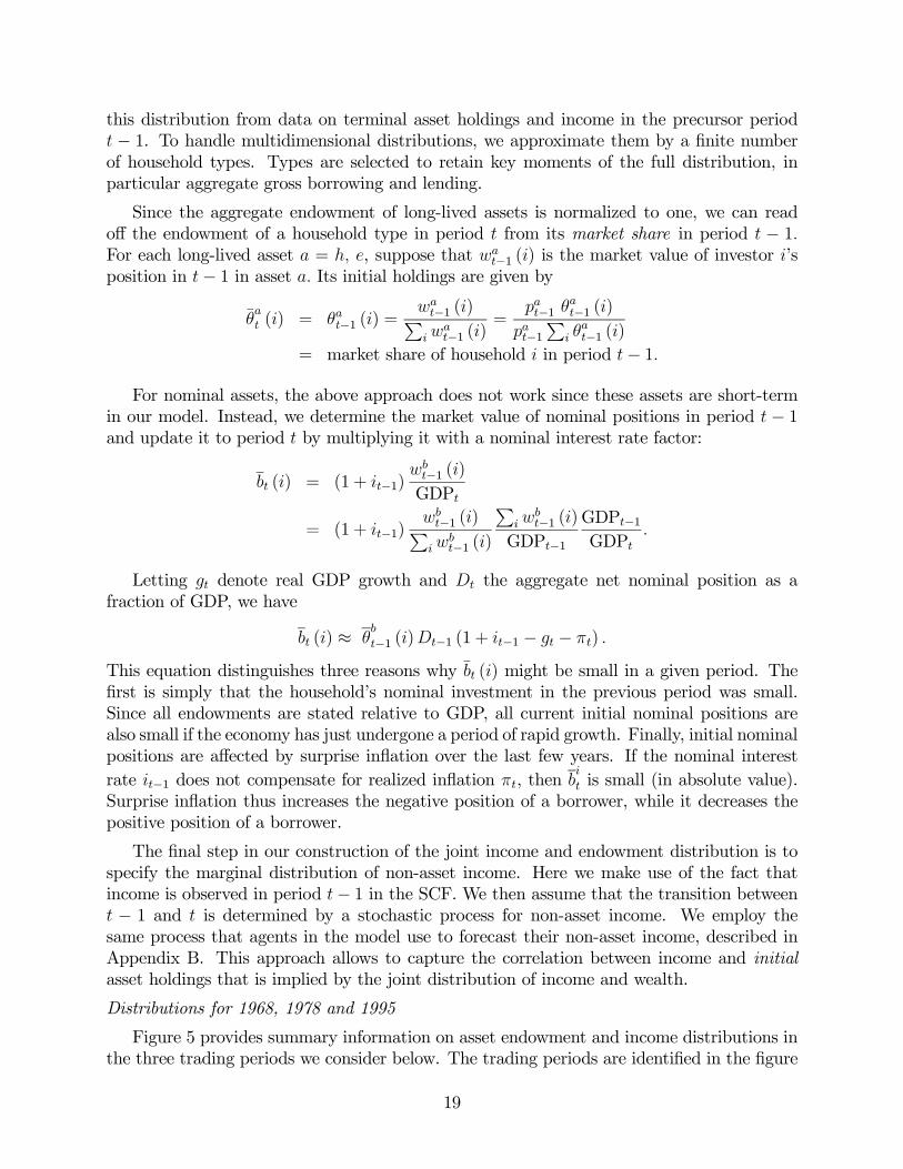
Distributions for 1968, 1978 and 1995

Figure 5 provides summary information on asset endowment and income distributions in

the three trading periods we consider below. The trading periods are identified in the figure

19

by their respective fourth year: 1968, 1978 and 1995. The top left panel provides population

weights by cohort. Cohorts are identified on the horizontal axis by the upper bound of the

age range. In addition, the fraction of households that exit during the period are offset to

the far right.

The different years can be distinguished by the line type: solid with circles for 1968,

dashed with squares for 1978 and dotted with diamonds for 1995. Using the same symbols,

the top right panel shows house endowments (light lines) and stock endowments (dark lines)

by age cohort, while the bottom left panel shows initial net nominal positions as a percent

of GDP. Finally, the bottom right panel shows income distributions. Here we plot not only

non-asset income, but also initial wealth not invested in long-lived assets, in other words,

=

+

+ + (6)

This aggregate will be useful to interpret the results below.

Two demographic changes are apparent from the figure. First, the baby boom makes

the two youngest cohorts relatively larger in the 1978 cross section than in the other two

years. By 1995, the boomers have aged so that the 42-47 year olds are the now strongest

cohort. This shift of population shares is also reflected in the distribution of income in the

bottom right panel. Second, the relative size of the oldest group has become larger over time.

Recently, a lot of retirement income comes from assets, so that the share of of the elderly

groups has also increased a lot. A key difference between the 1968 and 1978 distributions

is thus that the latter places more weight on households who tend to save little: the oldest

and, especially, the youngest. While the 1995 distribution also has relatively more weight

on the elderly, it emphasizes more the middle-aged rather than the young.

The comparison of stock and house endowments in the top right panel reveals that housing

is more of an asset for younger people. For all years, the market shares of cohorts in their

thirties and forties are larger for houses than for stocks, while the opposite is true for older

cohorts. By and large, the market shares are however quite similar across years. In contrast,

the behavior of net nominal positions relative to GDP (bottom right hand panel) has changed

markedly over time. In particular, the amount of intergenerational borrowing and lending

has increased: young households today borrow relatively more, while old households hold

relatively more bonds.

4.3 Expectations and Preference Parameters

A baseline set of beliefs for returns and non-asset income is derived in Appendix B. We

assume that consumers believe real asset returns and aggregate growth to be serially in-

dependent over successive six year periods. Moreover, consumers believe that returns and

growth are identically distributed for periods beyond + 1.5 To pick numbers, we start

from empirical moments of six-year ex-post pre-tax real returns on fixed income securities,

residential real estate and equity, as well as inflation and growth. Since returns on indi-

5In most of the exercises below, we allow beliefs for returns between and + 1 to differ from baseline

beliefs, so that returns are not iid. We discuss the latter aspect of beliefs below when we present our results.

20

29 35 41 47 53 59 65 72 77 83

0.04

0.05

0.06

0.07

0.08

0.09

0.1

0.11

0.12

0.13

Population Weights

196819781995

29 35 41 47 53 59 65 72 77 830

0.02

0.04

0.06

0.08

0.1

0.12

0.14

0.16

0.18

0.2

Endowments of houses (light), stocks (dark)

29 35 41 47 53 59 65 72 77 83

−1

−0.5

0

0.5

1

1.5

2

Bond endowments (% GDP)

29 35 41 47 53 59 65 72 77 830

2

4

6

8

10

12

Income (dark) and E (light) (% GDP)

Figure 5: Asset endowment and income distributions in 1968, 1978 and 1995. Top left panel :

Population weights by cohort, identified on the horizontal axis by the upper bound of the

age range. Exiting households during the period are on the far right. Top right panel :

House endowments (light lines) and stock endowments (dark lines) by age cohort. Bottom

left panel : initial net nominal positions as a percent of GDP. Bottom right panel : Income

distributions.

vidual properties are more volatile than those on a nationwide housing index, we add an

idiosyncratic shock to the house return faced by an individual household.

We also specify a stochastic process for after-tax income. Briefly, the functional form for

this process is motivated by existing specifications for labor income that employ a determin-

istic trend to capture age-specific changes in income, as well as permanent and transitory

components. We also use estimates from the literature to account for changes in the volatility

of the different components over time.

As for preference parameters, the intertemporal elasticity of substitution is = 5 the

coefficient of relative risk aversion is = 5 and the discount factor is = exp (−0025× 6).

21

Since is low, agents do not want to hold bonds when faced with historical Sharpe ratios on

stocks and housing. To avoid this counterfactual implication, we assume that agents view

long-lived assets as riskier than indicated by their historical moments. This idea of “low

aversion against high perceived risk” can be captured by scaling the historical return vari-

ances from Table B.2 with a fixed number. This scaling can be interpreted as a consequence

of Bayesian learning about the premium on equity and housing. We select a factor of 3,

which leads to match the aggregate portfolio weights for 1995 reported in Table 3 almost

exactly.

Table 3: 1995 Data and Baseline Beliefs

experiment wealth/ portfolio weights lend./ borr/ PD ratios interest rate

GDP bonds housing stocks GDP GDP housing stocks nominal

(1) –1995 data – 2.51 .15 .59 .26 .70 .31 20.4 23.9 .061

(2) baseline 2.51 .15 .60 .25 .70 .31 20.8 22.7 .061

Note: The first row reports the aggregate portfolio weights on bonds, housing and

stocks from Figure 2; the gross borrowing and lending numbers from Section A.1, the

wealth-to-GDP ratio from Figure 1; the price-dividend ratios for housing and stocks

together with the nominal 6-year interest rate. The second row report the results

computed from the model for 1995 with baseline beliefs.

An alternative strategy would be to work with agents who have “high aversion against

low perceived risk.” In this case, agents base their portfolio choice on the historical variances

from Table B.2, but are characterized by high risk aversion, = 25, and high discounting,

= exp (−007× 6). The high is needed to lower the portfolio weight on bonds, while thelow is needed to reduce the precautionary savings motive in the presence of uninsurable

income shocks. While the tables below report results based on agents with “low aversion

against high perceived risk,” we would get results comparable to those in Table 3 based on

this alternative parametrization.6

4.4 Taxes and the Credit Market

It remains to select parameters to capture taxes on investment as well as consumers’ op-

portunities for borrowing. For the year 1995, we assume a 2% per year spread between

borrowing and lending interest rates. Early on, credit markets were less developed and gross

credit was thus smaller. To capture this, we set the spread to 2.75% for the earlier years.

6Yet another way to obtain realistic aggregate portfolio weights is to combine low risk aversion with

first-time participation costs, as shown by Gomes and Michaelides (2005).

22

In addition, we select the borrowing constraint parameter = 8 This implies a maximal

loan-to-value ratio of 80%, where “value” is the ex-dividend value of the house.

Investors care about after-tax real returns. In particular, taxes affect the relative attrac-

tiveness of equity and real estate. On the one hand, dividends on owner-occupied housing

are directly consumed and hence not taxed, while dividends on stocks are subject to income

tax. On the other hand, capital gains on housing are more easily sheltered from taxes than

capital gains on stocks. This is because many consumers simply live in their house for a long

period of time and never realize the capital gains. Capital gains tax matters especially in

inflationary times, because the nominal gain is taxed: the effective real after tax return on

an asset subject to capital gains tax is therefore lower when inflation occurs.

To measure the effect of capital gains taxes, one would ideally like to explicitly distin-

guish realized and unrealized capital gains. However, this would involve introducing state

variables to keep track of past individual asset purchase decisions. To keep the problem

manageable, we adopt a simpler approach: we adjust our benchmark returns to capture the

effects described above. For our baseline set of results, we assume proportional taxes, and

we set both the capital gains tax rate and the income tax rate to 20%. We define after tax

real stock returns by subtracting 20% from realized net real stock returns and then further

subtracting 20% times the realized rate of inflation to capture the fact that nominal capital

gains are taxed. In contrast, we assume that returns on real estate are not taxed.

5 Household Behavior

In this section, we consider savings and portfolio choice in the cross section of households.

We focus on baseline beliefs for 1995, the year we have used to calibrate beliefs. The initial

distribution of asset endowments and income is derived from the 1989 SCF, as discussed in

Section 4. We first present optimal policies as functions of wealth and income. We then

compare the predictions of the model for the cross-section of households in 1995 to actual

observations from the 1995 SCF.

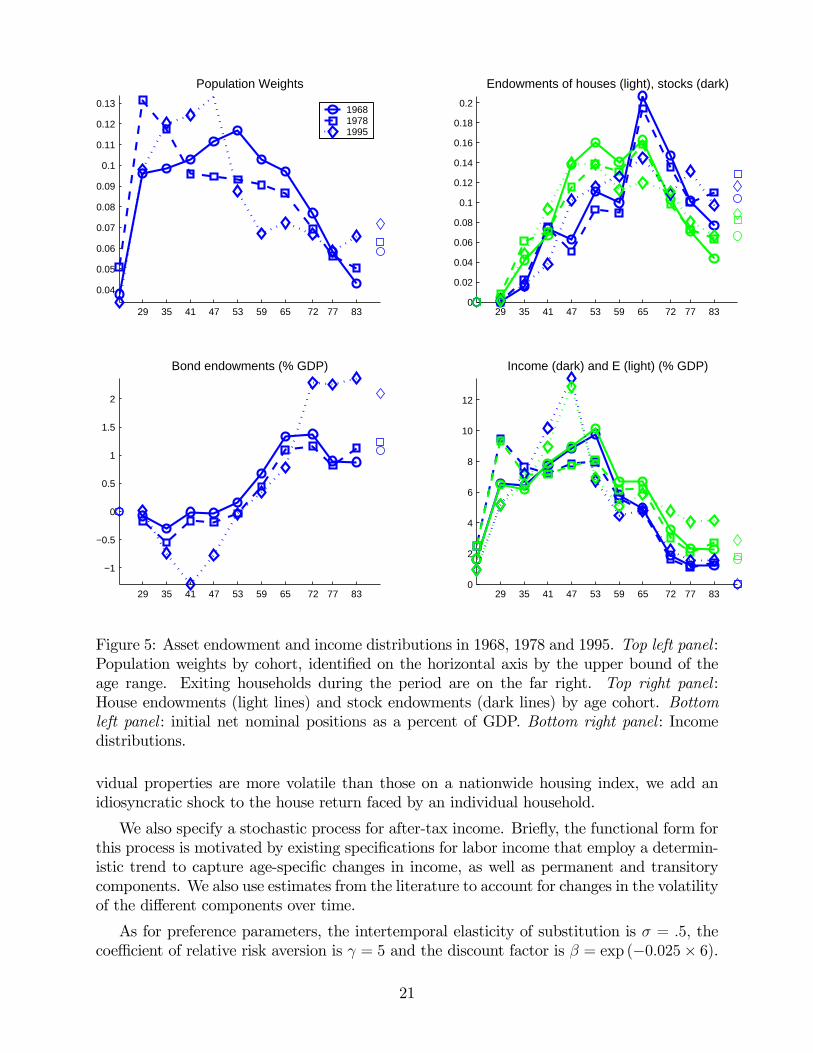
5.1 Lifecycle Savings and Portfolios

Since preferences are homothetic and all constraints are linear, the optimal savings rate and

portfolio weights depend only on age and the ratio of initial wealth — defined in (3) above

as asset wealth plus non-asset income — to the permanent component of non-asset income,

say . For simplicity, we refer to as the wealth-to-income ratio. Figure 6 plots agent

decisions as a function of this wealth-to-income ratio.

Savings

The bottom right panel shows the ratio of terminal wealth to initial wealth, that

is, the savings rate out of initial wealth. Savings are always positive, since the borrowing

constraint precludes strategies that involve negative net worth. Investors who have more

income in later periods than in the current period thus cannot shift that income forward by

23

0 1 2 3 4 50

0.1

0.2

0.3

0.4Houses / Initial Wealth

72 year old47 year old35 year old

0 1 2 3 4 50

0.1

0.2

0.3

0.4Equity / Initial Wealth

0 1 2 3 4 5

−0.2

−0.1

0

0.1

0.2

0.3

Bonds / Initial Wealth

0 1 2 3 4 50

0.2

0.4

0.6

0.8Terminal Wealth / Initial Wealth

Figure 6: Asset holdings and terminal wealth, both as fractions of initial wealth, plotted

against the initial wealth-to-income ratio. Age groups are identified by maximum age in the

cohort.

borrowing. In this sense, there is no borrowing for “consumption smoothing” purposes: all

current consumption must instead come out of current income or from selling initial asset

wealth.

If initial wealth is very low relative to income, all assets will be sold and all income

consumed, so that the investor enters the next period with zero asset wealth. As initial

wealth increases, a greater fraction of it is saved for future consumption. In the absence

of labor income, our assumption of serially independent returns implies a constant optimal

savings rate. As wealth becomes large relative to the permanent component of income, the

savings rate converges to this constant.

The bottom right panel also illustrates how the savings rate changes with age. There are

two relevant effects. On the one hand, younger investors have a longer planning horizon and

therefore tend to spread any wealth they have over more remaining periods. This effect by

itself tends to make younger investors save more. On the other hand, the non-asset income

profile is hump-shaped, so that middle-aged investors can rely more on labor income for

consumption than either young or old investors. This tends to make middle-aged investors

save relatively more than other investors.

The first effect dominates when labor income is not very important, that is, when the

24

wealth-to-income ratio is high. The figure shows that at high wealth-to-income ratios, the

savings rate of the 29-35 year old group climbs beyond that of the oldest investor group.

It eventually also climbs below the savings rate of the 48-53 year old group. The second

effect is important for lower wealth-to-income ratios, especially in the empirically relevant

range around 1-2, where most ratios lie in the data. In this region, the savings rate of the

middle-aged is highest, whereas both the young and the old save less. Among the latter two

groups, the young save the least when their wealth-to-income ratio is low.

Borrowing and Leverage

Rather than enable consumption smoothing, the role of borrowing in our model is to

help households construct leveraged portfolios. The bottom left panel of Figure 6 shows

that investors who are younger and have lower wealth-to-income ratios tend to go short in

bonds. The top panels show that the borrowed funds are used to build leveraged positions

of houses and also stocks. In contrast, investors who are older and have higher wealth-to-

income ratios tend to go long in all three assets. Along the wealth-to-income axis, there is

also an intermediate region where investors hold zero bonds. This region is due to the credit

spread: there exist ratios where it is too costly to leverage at the high borrowing rate, while

it is not profitable to invest at the lower lending rate.

The reason why “gambling” with leverage decreases with age and the wealth-to-income

ratio is the presence of labor income. Effectively, an investor’s portfolio consists of both asset

wealth and human wealth. Younger and lower wealth-to-income households have relatively

more human wealth. Moreover, the correlation of human wealth and asset wealth is small.

As a result, households with a lot of labor income hold riskier strategies in the asset part

of their portfolios. This effect has also been observed by Jagannathan and Kocherlakota

(1996), Heaton and Lucas (2000), and Cocco (2005).

Stock v. House Ownership

For most age groups and wealth-to-income ratios, investment in houses is larger than

investment in stocks. This reflects the higher Sharpe ratio of houses as well as the fact that

houses serve as collateral while stocks do not. The latter feature also explains why the ratio

of house to stock ownership is decreasing with both age and wealth-to-income ratio: for

richer and older households, leverage is less important, and so the collateral value of a house

is smaller.

The model can currently not capture the fact that the portfolio weight on stocks tends

to increase with the wealth-to-income ratio. While it is true in the model that people with

higher wealth-to-income own more stocks relative to housing, they also hold much more

bonds relative to both of the other assets. As a result, their overall portfolio weight on stocks

actually falls with the wealth-to-income ratio. The behavior of the portfolio weight on stocks

implies that the model produces typically too little concentration of stock ownership.

5.2 The Cross Section of Asset Holdings

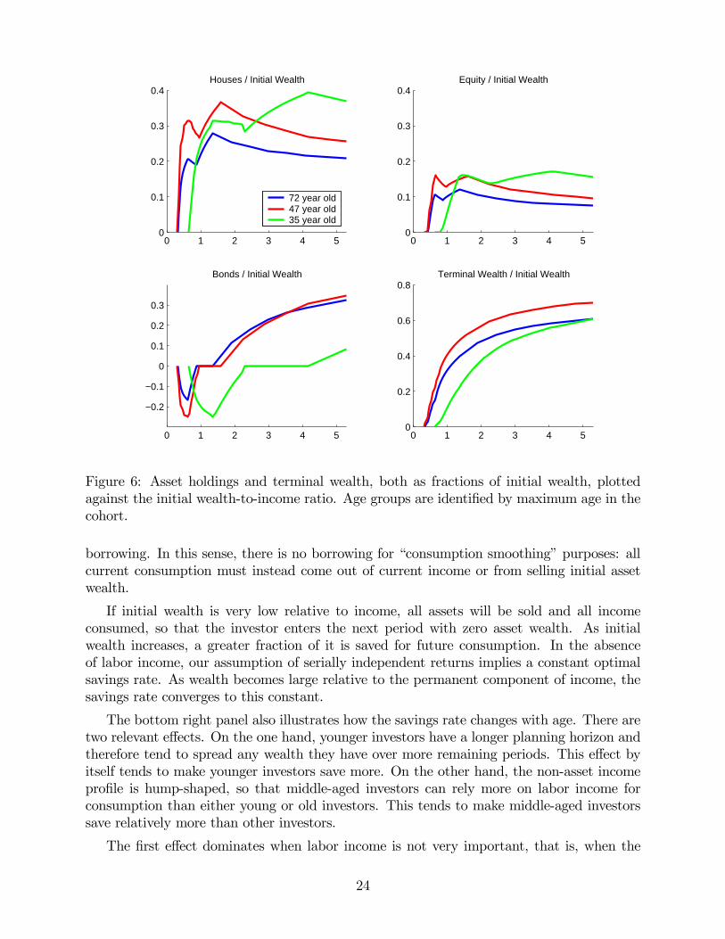
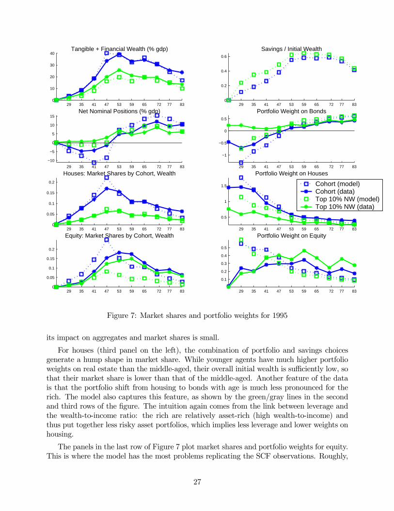
Figure 7 plots predicted portfolio weights and market shares for various groups of households

for 1995, given baseline beliefs. The panels also contain actual weights and market shares for

25

the respective groups from the 1995 SCF. It is useful to compare both portfolio weights and

market shares, since the latter also require the model to do a good job on savings behavior.

Indeed, defining aggregate initial wealth =P

(), the market share of asset =

for a household can be written as

() = () ()P

() ()=

()P

()()

()

=

()

()

where () is household ’s portfolio weight and is the aggregate portfolio weight on

asset . A model that correctly predicts the cross section of portfolio shares will therefore

only correctly predict the cross section of market shares if it also captures the cross section

of terminal wealth. The latter in turn depends on the savings rate of different groups of

agents.

The first row of Figure 7 documents savings behavior by cohort and wealth level. The

top left panel plots terminal wealth as a fraction of GDP at the cohort level (blue/black

lines) for the model (dotted line) and the data (solid line). It also shows separately terminal

wealth of the top decile by net worth (green/light gray lines), again for the model and the

data. This color coding of plots is maintained throughout the figure, so that a “good fit”

means that the lines of the same color are close to each other.

The top left panel shows that model does a fairly good job at matching terminal wealth.

The model also captures skewness of the distribution of terminal wealth and how this skew-

ness changes with age. The top 10% by net worth own more than half of total terminal

wealth, their share increasing with age. In the model, these properties are inherited in part

from the distributions of endowment and labor income. However, it is also the case that

richer agents save more out of initial wealth. This feature is apparent from the top right

panel of Figure 7 which reports savings rates by cohort and net worth. It obtains because

() the rich have higher ratios of initial wealth relative to current labor income, and ()

the savings rate is increase with the wealth-to-income ratio, as explained in the previous

subsection.

In the data, the main difference in portfolio weights by age is the shift from houses into

bonds over the course of the life cycle. This is documented in the right column of Figure 7.

Young agents borrow in order to build leveraged positions in houses. In the second panel,

their portfolio weights become positive with age as they switch to being net lenders. The

accumulation of bond portfolios makes houses — shown in the third panel on the right —

relatively less important for older households. The model captures this portfolio shift fairly

well. Intuitively, younger households “gamble” more, because the presence of future labor

income makes them act in a more risk tolerant fashion in asset markets.

The left column shows the corresponding cohort aggregates. Nominal positions relative to

GDP (second panel on the left) are first negative and decreasing with age, but subsequently

turn around and increase with age so that they eventually become positive. These properties

are present both in the model and the data. On the negative side, the model somewhat

overstates heterogeneity in positions by age: there is too much borrowing — and too much

investment in housing — by young agents. In particular, the portfolio weights for the very

youngest cohort are too extreme. However, since the wealth of this cohort is not very large,

26

29 35 41 47 53 59 65 72 77 830

0.05

0.1

0.15

0.2

Houses: Market Shares by Cohort, Wealth

29 35 41 47 53 59 65 72 77 830

0.05

0.1

0.15

0.2

Equity: Market Shares by Cohort, Wealth

29 35 41 47 53 59 65 72 77 83

−10

−5

0

5

10

15Net Nominal Positions (% gdp)

29 35 41 47 53 59 65 72 77 830

10

20

30

40Tangible + Financial Wealth (% gdp)

29 35 41 47 53 59 65 72 77 83

0.5

1

1.5

Portfolio Weight on Houses

Cohort (model)Cohort (data)Top 10% NW (model)Top 10% NW (data)

29 35 41 47 53 59 65 72 77 83

0.1

0.2

0.3

0.4

0.5

Portfolio Weight on Equity

29 35 41 47 53 59 65 72 77 83

−1

−0.5

0

0.5

Portfolio Weight on Bonds29 35 41 47 53 59 65 72 77 83

0

0.2

0.4

0.6

Savings / Initial Wealth

Figure 7: Market shares and portfolio weights for 1995

its impact on aggregates and market shares is small.

For houses (third panel on the left), the combination of portfolio and savings choices

generate a hump shape in market share. While younger agents have much higher portfolio

weights on real estate than the middle-aged, their overall initial wealth is sufficiently low, so

that their market share is lower than that of the middle-aged. Another feature of the data

is that the portfolio shift from housing to bonds with age is much less pronounced for the

rich. The model also captures this feature, as shown by the green/gray lines in the second

and third rows of the figure. The intuition again comes from the link between leverage and

the wealth-to-income ratio: the rich are relatively asset-rich (high wealth-to-income) and

thus put together less risky asset portfolios, which implies less leverage and lower weights on

housing.

The panels in the last row of Figure 7 plot market shares and portfolio weights for equity.

This is where the model has the most problems replicating the SCF observations. Roughly,

27

investment in stocks in the model behaves “too much” like investment in housing. Indeed,

the portfolio weight is not only decreasing with age after age 53, as in the data, but it is

also decreasing with age for younger households. As a result, while the model does produce

a hump-shaped market share, the hump is too pronounced and occurs at too young an age.

In addition, the model cannot capture the concentration of equity ownership in the data:

the rich hold relatively too few stocks.

6 Asset Prices in Temporary Equilibrium

In this section, we consider the temporary equilibrium map from model inputs — the distri-

bution of endowments and income, asset supply, and expectations — into equilibrium prices.

We report counterfactual experiments, based on the 1995 distribution, to illustrate the me-

chanics of the model and the relative magnitude of key effects.

Price Determination

To organize the discussion, we use the following equations, derived from the market clear-

ing conditions and the household budget constraints. Dropping time subscripts to simplify

notation, we have

(1 + ) =P

( () () ; ) () ; =

(1 + ) + (1 + ) + =P

( () () ; ) () (7)

The aggregate value of long-lived asset (where = or ) must equal, in equilibrium,

the value of household demand for the asset. At the level of the individual household, asset

demand can be written as the product of initial wealth () and the asset weight . The

latter was shown in Figure 6 as a function of the wealth-to-income ratio () (). It also

depends on other household characteristics such as age and expectations, as well as on the

market interest rate, or equivalently the bond price .7 The second equation says that the

value of all assets held by households — in our empirical framework, the numerator of the

wealth-GDP ratio — must equal total household savings, where the savings rate, shown in

the bottom right panel of Figure 6, is denoted .

Equations (7) implicitly determine the three asset prices , and as a function of

supply, endowments and expectations, where the latter enter through the portfolio weight

functions and the savings rate function . The second equation can be written as

(1 + ) + (1 + ) + =P

()P ()

( () () ; )P

()

= ¡ + +

¢

where is the initial-wealth-weighted average savings rate and is aggregate initial wealth

not invested in long-lived assets, as defined in (6).

7Asset demand depends on the prices of long-lived assets only through the effects of those prices on initial

wealth. The reason is that return expectations are exogenous, execpt for bonds where they depend on the

market interest rate and expected inflation.

28

Suppose for the moment that new asset supply is the same for equity and houses, that

is, = = . The intuition generated by this case is helpful for interpreting our results

more generally. The aggregate value of these assets now becomes

+ = −

1 + − (8)

Other things — including expectations — equal, the value of long-lived assets decreases when

the ROE supplies more of these assets. It also decreases when the ROE raises more funds

in the bond market. Here it matters that our calibration strategy takes the market value of

bond supply as given (rather than, say, the face value). Higher bond supply in our exercises

always subtracts a fixed amount from the demand for other savings vehicles, such as houses

and equity and thus lowers the value of those vehicles. Finally, the value of long-lived assets

increases with any event that increased the average savings rate in the household sector. In

particular, it depends on household expectations only through their effect on the average

savings rate.

An important implication of equation (8) is that the total value of long-lived assets is

determined by consumption-savings considerations, not by portfolio choice considerations.

Indeed, at the household level, the optimal savings rate is chosen to smooth consumption over

time, given the total return on wealth. In contrast, the weights on the individual assets are

chosen to generate the highest possible total return on wealth, trading off risk and return.

The total value of long-lived assets depends strongly on aspects of the household problem

that affect the savings decision, such as the discount factor, the intertemporal elasticity of

substitution, the age distribution and expectations of labor income growth. It is less sensitive

to factors that matter for portfolio choice, such as the relative returns on different assets.

The latter factors are instead important for the individual asset prices, as well as the bond

price, which must adjust to ensure that all three equations in (7) hold.

Counterfactuals from the 1995 baseline

Table 3A illustrates the sensitivity of asset prices to changes in expectations and asset

supply. The main result is that events relevant to the stock market spill over much less into

other asset markets than events relevant to the housing market, although stock prices are

themselves more responsive to changes in expectations. Rows 2 and 3 compare one percent

increases in the expected return on stocks and houses, respectively. Since these changes

affect the relative attractiveness of assets, they have only a small (positive) effect on savings

and hence the wealth-GDP ratio. However, they do give rise to significant portfolio shifts

and price changes.

Row 2 shows that a one percent increase in real stock return expectations over the next

six years raises the price dividend ratio of stocks by 15%, but raises the nominal interest rate

by only 10 basis points; it lowers the price-dividend ratio on housing by 3.5%. In contrast,

row 3 shows that a one percent increase in the expected return on real estate raises the house

price by 7%, increases the nominal interest rate by 80 basis points, and lowers stock prices

by 13%. The response of stock prices is therefore larger in both experiments. At the same

time, the spillover effect to interest rates and to the other long-lived asset price is larger in

response to a change in the expected housing return.

29

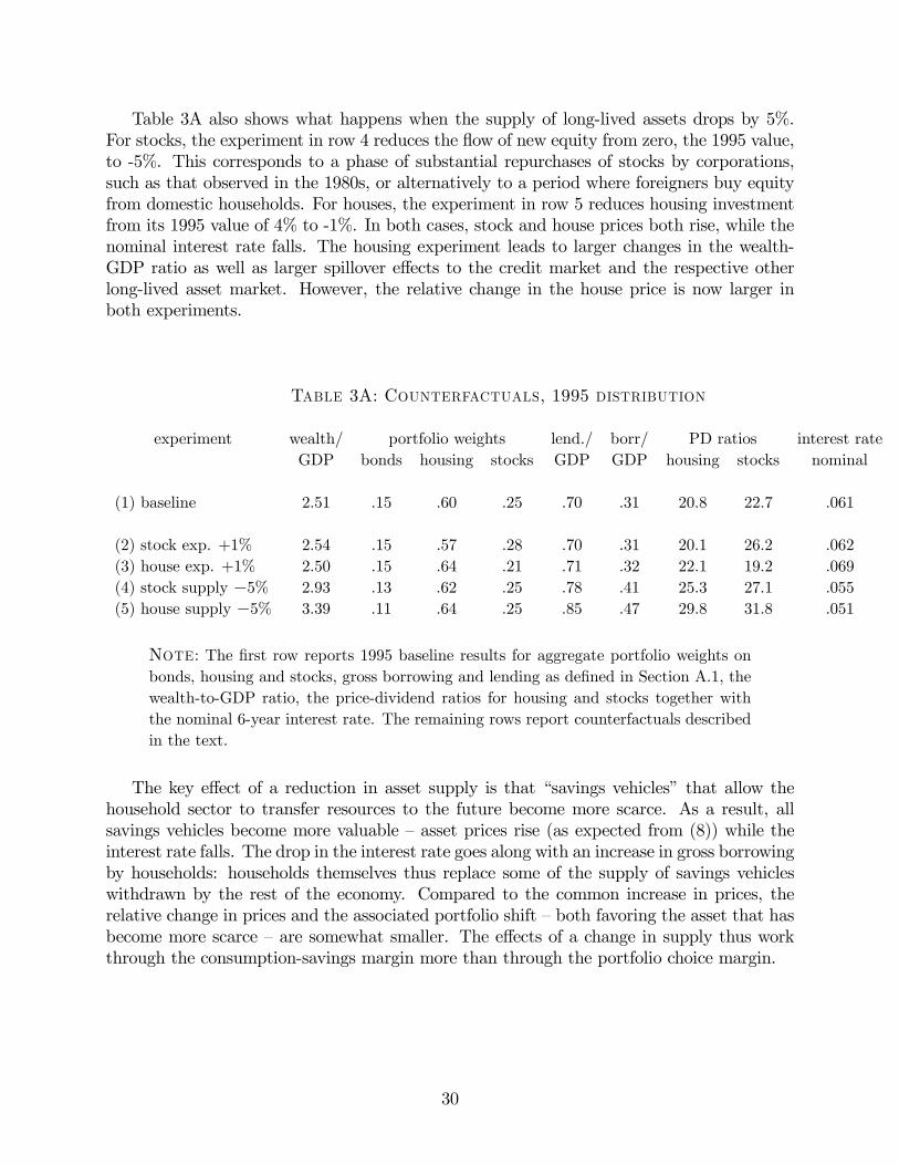
Table 3A also shows what happens when the supply of long-lived assets drops by 5%.

For stocks, the experiment in row 4 reduces the flow of new equity from zero, the 1995 value,

to -5%. This corresponds to a phase of substantial repurchases of stocks by corporations,

such as that observed in the 1980s, or alternatively to a period where foreigners buy equity

from domestic households. For houses, the experiment in row 5 reduces housing investment

from its 1995 value of 4% to -1%. In both cases, stock and house prices both rise, while the

nominal interest rate falls. The housing experiment leads to larger changes in the wealth-

GDP ratio as well as larger spillover effects to the credit market and the respective other

long-lived asset market. However, the relative change in the house price is now larger in

both experiments.

Table 3A: Counterfactuals, 1995 distribution

experiment wealth/ portfolio weights lend./ borr/ PD ratios interest rate

GDP bonds housing stocks GDP GDP housing stocks nominal

(1) baseline 2.51 .15 .60 .25 .70 .31 20.8 22.7 .061

(2) stock exp. +1% 2.54 .15 .57 .28 .70 .31 20.1 26.2 .062

(3) house exp. +1% 2.50 .15 .64 .21 .71 .32 22.1 19.2 .069

(4) stock supply −5% 2.93 .13 .62 .25 .78 .41 25.3 27.1 .055

(5) house supply −5% 3.39 .11 .64 .25 .85 .47 29.8 31.8 .051

Note: The first row reports 1995 baseline results for aggregate portfolio weights onbonds, housing and stocks, gross borrowing and lending as defined in Section A.1, the

wealth-to-GDP ratio, the price-dividend ratios for housing and stocks together with

the nominal 6-year interest rate. The remaining rows report counterfactuals described

in the text.

The key effect of a reduction in asset supply is that “savings vehicles” that allow the

household sector to transfer resources to the future become more scarce. As a result, all

savings vehicles become more valuable — asset prices rise (as expected from (8)) while the

interest rate falls. The drop in the interest rate goes along with an increase in gross borrowing

by households: households themselves thus replace some of the supply of savings vehicles

withdrawn by the rest of the economy. Compared to the common increase in prices, the

relative change in prices and the associated portfolio shift — both favoring the asset that has

become more scarce — are somewhat smaller. The effects of a change in supply thus work

through the consumption-savings margin more than through the portfolio choice margin.

30

Comparing equity and real estate

We now consider the different responses of housing and equity markets to the above

experiments. In our model, housing differs from equity because the overall scale of the

housing market is bigger, its endowment distribution is less concentrated, the mean and

volatility of its return are lower and it can be used as collateral. To isolate the role of

housing as collateral, Table 3B repeats the counterfactuals of Table 3A with artificial data.

In particular, the asset “equity” is now an artificial asset that has all the properties of housing

in the data (that is, the same dividend, endowment distribution and return moments), but

that cannot be used as collateral.

The baseline results in row 1 isolate the value of the collateral property: the true housing

asset is about 10% more valuable than the artificial non-collateralizable housing asset. While

this number comes from a different economy than the results in Table 3A and hence does

not capture the actual value of the collateral property of the US housing stock, we can

conclude from this exercise that the collateral property is not a negligible component of

the value of housing. The expected return experiments in rows 2 and 3 now give rise to

essentially symmetric portfolio shifts and percentage price changes. Collateral is therefore

not responsible for the stronger price response of equity discussed above. However, the

interest rate effects are of a similar magnitude as in Table 3A.

The role of housing as collateral is thus at least in part responsible for the stronger

spillover effects from housing to the credit market. Intuitively, if the expected return on

either long-lived asset increases, the interest rate must also increase, so that the aggregate

household sector — which is a net lender — continues to hold the outstanding bond supply.

An increase in the expected housing return is special because it not only lowers the demand

for bonds by net lenders, but also increases the supply of bonds (that is, mortgages) by net

borrowers, as the collateral constraint permits more borrowing. Since the interest rate must

rise not only to stimulate bond demand, but also to curb supply, it rises by more than when

the expected stock return rises.

The stronger response of stock prices to expected return changes in Table 3A is due to

two properties of the model. The first, discussed above, is that a change in the return on

one of the assets works mostly through the portfolio choice margin, and leaves total savings

almost unchanged. Since the resources raised by the ROE in the credit market are given, this

means that the equilibrium portfolio weight on bonds must also remain almost unchanged,

and any increase in the weight on stocks, say, must be almost exactly offset by a decrease

in the weight on houses. The second property is that the stock market is smaller than the

housing market. It follows that an equal shift in weights must entail a proportionately larger

change than in the value of stocks, and hence in the price-dividend ratio on stocks. In the

artificial economy, where the scale of the two markets is the same, this effect vanishes.

31

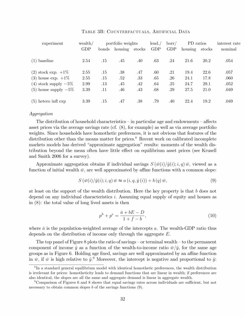
Table 3B: Counterfactuals, Artificial Data

experiment wealth/ portfolio weights lend./ borr/ PD ratios interest rate

GDP bonds housing stocks GDP GDP housing stocks nominal

(1) baseline 2.54 .15 .45 .40 .63 .24 21.6 20.2 .054

(2) stock exp. +1% 2.55 .15 .38 .47 .60 .21 19.4 22.6 .057

(3) house exp. +1% 2.55 .15 .52 .33 .65 .26 24.1 17.8 .060

(4) stock supply −5% 2.99 .13 .45 .42 .64 .25 24.7 29.1 .052

(5) house supply −5% 3.39 .11 .46 .43 .68 .29 27.5 21.0 .049

(5) hetero infl exp 3.39 .15 .47 .38 .79 .40 22.4 19.2 .049

Aggregation

The distribution of household characteristics — in particular age and endowments — affects

asset prices via the average savings rate (cf. (8), for example) as well as via average portfolio

weights. Since households have homothetic preferences, it is not obvious that features of the

distribution other than the means matter for prices.8 Recent work on calibrated incomplete

markets models has derived “approximate aggregation” results: moments of the wealth dis-

tribution beyond the mean often have little effect on equilibrium asset prices (see Krusell

and Smith 2006 for a survey).

Approximate aggregation obtains if individual savings (()(); ) viewed as a

function of initial wealth are well approximated by affine functions with a common slope:

(()(); ) ≈ ( ()) + () (9)

at least on the support of the wealth distribution. Here the key property is that does not

depend on any individual characteristics Assuming equal supply of equity and houses as

in (8): the total value of long lived assets is then

+ =+ −

1 + − (10)

where is the population-weighted average of the intercepts . The wealth-GDP ratio thus

depends on the distribution of income only through the aggregate .

The top panel of Figure 8 plots the ratio of savings — or terminal wealth — to the permanent

component of income as a function of the wealth-to-income ratio , for the same age

groups as in Figure 6. Holding age fixed, savings are well approximated by an affine function

in if is high relative to 9 Moreover, the intercept is negative and proportional to :

8In a standard general equilibrium model with identical homothetic preferences, the wealth distribution

is irrelevant for prices: homotheticity leads to demand functions that are linear in wealth; if preferences are

also identical, the slopes are all the same and aggregate demand is linear in aggregate wealth.9Comparison of Figures 6 and 8 shows that equal savings rates across individuals are sufficient, but not

necessary to obtain common slopes of the savings functions (9).

32

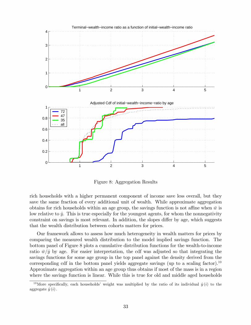
1 2 3 4 50

1

2

3

4Terminal−wealth−income ratio as a function of initial−wealth−income ratio

1 2 3 4 50

0.2

0.4

0.6

0.8

1Adjusted Cdf of initial−wealth−income−ratio by age

724735all

Figure 8: Aggregation Results

rich households with a higher permanent component of income save less overall, but they

save the same fraction of every additional unit of wealth. While approximate aggregation

obtains for rich households within an age group, the savings function is not affine when is

low relative to . This is true especially for the youngest agents, for whom the nonnegativity

constraint on savings is most relevant. In addition, the slopes differ by age, which suggests

that the wealth distribution between cohorts matters for prices.

Our framework allows to assess how much heterogeneity in wealth matters for prices by

comparing the measured wealth distribution to the model implied savings function. The

bottom panel of Figure 8 plots a cumulative distribution functions for the wealth-to-income

ratio by age. For easier interpretation, the cdf was adjusted so that integrating the

savings functions for some age group in the top panel against the density derived from the

corresponding cdf in the bottom panel yields aggregate savings (up to a scaling factor).10

Approximate aggregation within an age group thus obtains if most of the mass is in a region

where the savings function is linear. While this is true for old and middle aged households

10More specifically, each households’ weight was multiplied by the ratio of its individual () to the

aggregate ()

33

who tend to have a lot of wealth relative to income, the majority of young agents (29-35) is

in a region where the savings function is still convex.

7 Supply, Demographics and Asset Prices 1968-95

Panels A and B of Table 4 compare the baseline model to the data not only for 1995, but

also for 1968 and 1978. For 1968, the baseline model captures the fact that the wealth-GDP

ratio as well as the nominal interest rate were both slightly lower than their counterparts in

1995. It accounts for most of the difference because the variance of income shocks was lower

in 1968, which implies that less precautionary savings lowers wealth and interest rates. The

model captures only a small fraction of the portfolio shift towards housing that took place

between 1968 and 1995. As a result, it cannot explain the observed increase in house prices,

although it does produce a drop in the price dividend ratio on stocks.

With a spread of 2.75% between borrowing and lending rates, the model matches gross

borrowing and lending in 1968. A fairly small drop in the spread — 75 basis points — is

thus sufficient to account for the increase in the volume of credit. Changing the spread has

otherwise little effect on the equilibrium. This is illustrated in Table 5, where we collect a

set of counterfactuals designed to provide intuition for the baseline results in Table 4. The

second row of Table 5 recomputes the equilibrium for 1968 with a spread of 2%.

Household portfolios in 1978 were very different from those in 1968 or 1978: wealth as

a percent of GDP was much smaller, and there was a strong portfolio shift from stocks into

houses. The model with baseline expectations held fixed delivers the first fact, but not the

second. The wealth to GDP ratio drops to about twice GDP in both the model and the

data. However, the portfolio allocation in the model remains essentially the same as in 1995.

As a result, the price dividend ratios of houses falls and that of houses rises, in contrast to

what happened in the data.

Three changes in fundamentals are important for the drop in the wealth-to-GDP ratio

in 1978. The first is the change in the distribution of endowments illustrated in Figure 5.

The special feature of the 1978 endowment distribution is that a larger fraction of the funds

available for investment resides with the very youngest and oldest cohorts. As shown in the

last section, the model predicts that these cohorts have small savings rates, which leads to

lower wealth-to-income ratios and pushes interest rates up. This effect is reinforced by the

effects of low ex post real interest rates, which also reduce the ratio of initial wealth to income

and hence savings. A counteracting force is the reduction in bond supply documented in

Figure 4 which tends to lower interest rates and slightly raises the wealth-GDP ratio. Taken

together, these effects produce relatively stable interest rates and a low wealth-GDP ratio.

Table 5 reports experiments that consider the role of each of these three factors in iso-

lation, leaving the others fixed at their 1968 values. The experiment in row 3 (1978 bond

supply) retains the whole 1968 distribution of households, and changes only the supply of

new bonds to the 1978 value, a reduction of 25%. Since the supply of bonds drops, this

experiment is similar to the counterfactual experiments that reduce the house and stock

supplies in Table 3A above.

34

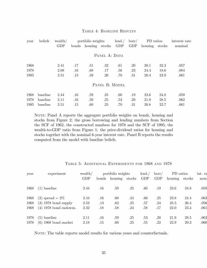
Table 4: Baseline Results

year beliefs wealth/ portfolio weights lend./ borr/ PD ratios interest rate

GDP bonds housing stocks GDP GDP housing stocks nominal

Panel A: Data

1968 2.41 .17 .51 .32 .61 .20 20.1 32.3 .057

1978 2.08 .16 .68 .17 .56 .23 24.4 18.6 .084

1995 2.51 .15 .59 .26 .70 .31 20.4 23.9 .061

Panel B: Model

1968 baseline 2.44 .16 .59 .25 .60 .19 23.6 24.8 .059

1978 baseline 2.11 .16 .59 .25 .53 .20 21.9 28.5 .062

1995 baseline 2.51 .15 .60 .25 .70 .31 20.8 22.7 .061

Note: Panel A reports the aggregate portfolio weights on bonds, housing andstocks from Figure 2; the gross borrowing and lending numbers from Section

the SCF of 1962, the constructed numbers for 1978 and the SCF of 1995; the

wealth-to-GDP ratio from Figure 1; the price-dividend ratios for housing and

stocks together with the nominal 6-year interest rate. Panel B reports the results

computed from the model with baseline beliefs.

Table 5: Additional Experiments for 1968 and 1978

year experiment wealth/ portfolio weights lend./ borr/ PD ratios int. ra

GDP bonds housing stocks GDP GDP housing stocks nom.

1968 (1) baseline 2.44 .16 .59 .25 .60 .19 23.6 24.8 .059

1968 (2) spread = 2% 2.44 .16 .60 .24 .66 .25 23.8 24.4 .063

1968 (3) 1978 bond supply 2.52 .13 .62 .25 .57 .24 25.5 26.4 .056

1968 (4) 1978 bond endowm. 2.32 .18 .58 .24 .58 .17 22.0 23.4 .061

1978 (5) baseline 2.11 .16 .59 .25 .53 .20 21.9 28.5 .062

1978 (6) 1968 bond market 2.18 .15 .60 .25 .55 .22 22.9 29.3 .060

Note: The table reports model results for various years and counterfactuals.

35

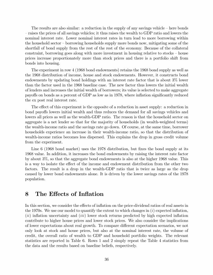
The results are also similar: a reduction in the supply of any savings vehicle — here bonds

— raises the prices of all savings vehicles; it thus raises the wealth to GDP ratio and lowers the

nominal interest rate. Lower nominal interest rates in turn lead to more borrowing within

the household sector — borrowing households supply more bonds now, mitigating some of the

shortfall of bond supply from the rest of the rest of the economy. Because of the collateral

constraint, borrowing goes along with more investment in housing relative to stocks — house

prices increase proportionately more than stock prices and there is a portfolio shift from

bonds into housing.

The experiment in row 4 (1968 bond endowments) retains the 1968 bond supply as well as

the 1968 distribution of income, house and stock endowments. However, it constructs bond

endowments by updating bond holdings with an interest rate factor that is about 3% lower

than the factor used in the 1968 baseline case. The new factor thus lowers the initial wealth

of lenders and increases the initial wealth of borrowers; its value is selected to make aggregate

payoffs on bonds as a percent of GDP as low as in 1978, where inflation significantly reduced

the ex post real interest rate.

The effect of this experiment is the opposite of a reduction in asset supply: a reduction in

bond payoffs lowers initial wealth and thus reduces the demand for all savings vehicles and

lowers all prices as well as the wealth-GDP ratio. The reason is that the household sector on

aggregate is a net lender so that for the majority of households (in wealth-weighted terms)

the wealth-income ratio and the savings rate go down. Of course, at the same time, borrower

households experience an increase in their wealth-income ratio, so that the distribution of

wealth-income ratios becomes less dispersed. This explains the drop in gross credit volume

from the experiment.

Line 6 (1968 bond market) uses the 1978 distribution, but fixes the bond supply at its

1968 value. In addition, it increases the bond endowments by raising the interest rate factor

by about 3%, so that the aggregate bond endowments is also at the higher 1968 value. This

is a way to isolate the effect of the income and endowment distribution from the other two

factors. The result is a drop in the wealth-GDP ratio that is twice as large as the drop

caused by lower bond endowments alone. It is driven by the lower savings rates of the 1978

population.

8 The Effects of Inflation

In this section, we consider the effects of inflation on the price-dividend ratios of real assets in

the 1970s. We use our model to quantify the extent to which changes in () expected inflation,

() inflation uncertainty and () lower stock returns predicted by high expected inflation

contribute to higher house prices and lower stock prices. We also consider the implications

of lower expectations about real growth. To compare different expectation scenarios, we not

only look at stock and house prices, but also at the nominal interest rate, the volume of

credit, the overall ratio of wealth to GDP and household portfolio weights. The relevant

statistics are reported in Table 6. Rows 1 and 2 simply repeat the Table 4 statistics from

the data and the results based on baseline beliefs, respectively.

36

Expected Inflation and Taxes

Row 3 of Table 6 focus on the effects of higher expected inflation. Row 3, labelled

“hi inflation expectations” increases expected inflation for all households from the baseline

number of 4% to the median 5-year inflation forecast from the Michigan survey, averaged

over the trading period, which is 6.3%. In this experiment, all effects of expected inflation are

due to nominal rigidities in the tax system. In particular, taxation of nominal returns makes

housing more attractive as an investment relative to stocks and bonds, and it encourages

mortgage borrowing.

To see the effect of expected inflation on real after tax returns, let denote the pretax

real return on equity and let denote the inflation rate. Under our assumption of a single

effective tax rate on nominal equity returns, the after-tax real return on equity is (1− ) − The expected after-tax real return on equity is thus decreasing in expected inflation.

In contrast, we have assumed that housing returns are not taxed, so that the expected real

return on housing does not depend on expected inflation. As expected inflation increases,

real estate thus become more attractive relative to equity. The return on nominal bonds is

(1− ) − = (1− ) − where is the nominal interest rate and = − is the

pretax real return. Given a nominal rate, holding bonds thus also becomes less attractive as

expected inflation increases, whereas mortgage borrowing becomes more attractive because

interest is tax deductible.

Compared to the baseline, higher expected inflation leads to a drop in the price-dividend

ratio on stocks and an increase in the price-dividend ratio on houses. At the same time,

the nominal interest rate increases by more than the increase in expected inflation. Both

results follow directly from the increased tax burdens on stocks and bonds. On the one

hand, the taxation of nominal equity returns works like a change in expected stock returns,

already discussed in Section 6: a drop in the expected return on stocks does not change the

wealth-GDP ratio or interest rate much, but lowers the price of stocks. On the other hand,

the taxation of nominal interest induces an inflation premium on top of the increase in the

nominal rate warranted by the Fisher equation.

Quantitatively, the changes in household portfolios shown in row 3 do not come close to

matching the portfolio shift of the 1970s shown in row 1. At the same time, the resulting

nominal interest rate of 9% is more than half a percentage point higher than the observed

rate of 8.4%. Our calculations are based on a tax rate of 20%, which is consistent with the

numbers reported by Sialm (2006) for average effective tax rates on equity returns as well

as capital gains tax rates in the 1970s. It is still interesting to ask what happens for higher

tax rates. To match the portfolio weights exactly requires a tax rate of 45%. However, the

resulting increase in the inflation premium pushes the nominal interest rate up to 10.7%,

and the overall lower after tax return on wealth lowers the wealth-GDP ratio to 2.02. This

reveals a basic tension between tax effects on long-lived assets and the credit market. We

conclude that the effects of expected inflation through taxes cannot be the only factor behind

the 1970s portfolio shift.

Expected Inflation and Disagreement

According to the Michigan Survey, households disagreed about expected inflation in the

37

1970s. Interestingly, disagreement is related to age in a systematic way. Figure 9 plots

population median forecasts since 1979 together with median forecasts for the youngest and

oldest cohorts in the Michigan survey. During the high inflation years in the late 1970s

and early 1980s, older households expected much lower inflation than younger households;

the discrepancy vanished as inflation subsided in the 1990s. Our model offers a natural

laboratory for studying the impact of heterogeneity in expectations by age. The exercise in

row 4 of Table 6, labelled “heterogeneous inflation expectations”, assumes that the inflation

rate expected by an age cohort in the model is equal to the corresponding cohort median in

the Michigan Survey.

Heterogeneity in inflation expectations introduces disagreement about real rates – a

second mechanism that pushes house prices up and stock prices down. This disagreement

stimulates borrowing and lending among households and drives up the (relative) price of

collateral, that is, houses. Indeed, given a nominal interest rate quoted in the credit market,

young households (who expect high inflation) perceive a lower real interest rate than old

households (who expect low inflation). This generates gains from trade: young households

believe that borrowing is a bargain and borrow from old households, who are happy to lend.

Since any borrowing requires collateral, more credit created within the household sector leads

to a stronger demand for housing, which drives up house prices. At the same time, both

borrowers and lenders lower their demand for stocks: the former prefer houses, while the

latter prefer bonds. As a result, the stock price falls.

Quantitatively, a switch from the baseline to survey expectations explains half the ob-

served portfolio shift from the baseline 59% portfolio weight on housing to the observed 68%.

Compared with (homogeneous) “hi inflation expectations”, the (heterogeneous) survey ex-

pectations generate double the portfolio shift, without changing our previous conclusions

about the nominal interest rate and wealth-GDP ratio. The survey expectations also lead

to an increase in borrowing and lending. While any disagreement about real rates leads to

gains from trade, the basic effect is reinforced in our context because inflation expectations

are correlated with households’ propensity to borrow: as discussed in Section 7, younger

households tend to have lower wealth relative to permanent income and leverage up more.

Inflation Uncertainty

The “hi inflation volatility” experiment reported in row 5 of Table 6 doubles the condi-

tional volatility of inflation, from 3% to 6% p.a. It is motivated by the increase in uncertainty

about inflation. In our model, higher conditional volatility of inflation increases the condi-

tional volatility of real bond returns and the ex post real cost of mortgage financing. The

main difference to the baseline results is that there is now less nominal borrowing and lending

within the household sector and a higher nominal interest rate. The lower volume of credit is

natural as nominal instruments have become less attractive to both borrowers and lenders.

The nominal interest rate increases because the household sector as a whole is a net lender

and must be compensated if it is to hold the nominal debt of the rest of the economy.

Increasing inflation volatility has little effect on the overall wealth-GDP ratio. Indeed,

it is a comparative static that affects the returns on one asset, leaving those on other assets

unchanged. As is the case for other experiments of this type, the overall return on wealth

and the savings decision are not affected much and the equilibrium wealth-GDP ratio stays

38

1975 1980 1985 1990 1995 20002

3

4

5

6

7

8

9

10

old households

median

young households

Figure 9: Median inflation expectations over the next 5 years, Michigan Survey of Con-

sumers. The lines with “young households” and “old households” represent expecations by

the youngest (18-34 years) and oldest (above 65 years) cohorts in the Michigan survey. These

lines provide bounds for the expectations by other cohorts (not shown in the picture), which

are monotonic in age.

essentially the same. Aggregate portfolio weights also remain unchanged. On the one hand,

households are required to hold the same value of bonds issued by the rest of the economy

in equilibrium, so that the portfolio weight on bonds remains unchanged if the wealth-GDP

does not change. On the other hand, the effect of a change in the relative volatility of after

tax returns on stocks and houses is quantitatively small so that the weights on stocks and

houses also move little.

Lower Stock Return and Growth Expectations

In rows 6-8 of Table 6, we consider experiments that increase pessimism about various

parts of the U.S. economy. Row 6 considers lower expected stock returns, row 7 assumes

lower growth in the aggregate component of non-asset income, and row 8 assumes lower

returns on both long-lived assets together with low non-asset income growth. The latter

case can be viewed as capturing pessimism about the economy as a whole, which shows

up in lower expectations of both dividends and non-asset income. Within our framework,

it does not matter where lower return expectations come from. One source of pessimism

in the 1970s was an expected slowdown in productivity. Another was low projections of

corporate profits due to higher inflation. Inflation thus motivates an experiment in which

39

stock return expectations are lower, while expected payoffs on human capital and housing

remain unchanged.

To get an idea about the plausible order of magnitude for pessimism induced by inflation,

we use the study of Fama and Schwert (1977), who document that measures of expected

inflation are significant predictors of stock returns. The regression results in their Table 6

represent real-time forecasts of returns on a variety of assets — stocks, housing, and bonds

— based on data available at that time. Their results indicate that a one percentage-point

increase in expected inflation lowers the forecast of real stock returns by roughly 6 percentage

points over the following year, but leaves the forecasts of real housing returns unchanged.

Assuming that today’s inflation forecasts do not predict stock returns beyond the next year,

the 1.5 percentage point increase in expected inflation measured by the Michigan Survey

would lower expected real stock returns over the next 6 years by roughly 1.5 percentage

points.

Row 6 of Table 6 reports results for stock return expectations that are 1.5 percentage

points lower than the historical mean. Since this experiment also changes the returns on

only one asset, it does not affect strongly the savings decision and the wealth-GDP ratio

moves little. However, as households lower their return expectations for stocks, other assets

become relatively more attractive and thus valuable. As in the counterfactual experiments in

Table 3A, the price-dividend ratios of stocks and housing are highly sensitive to households’

subjective equity return; in particular, the stock market falls by 25%. The interest rate falls,

although the effect is not large. This scenario is able to generate large movements in the

price of real assets together with a drop in the interest rate.

Row 8 of Table 6 shows that the situation is different if pessimism affects not only the

corporate sector, but also labor income and the dividends on housing. Relative to the

baseline, a 1% drop in expected growth induces a significant increase in the wealth-GDP

ratio (about 10%) together with a large drop in the interest rate, by 1.3 percentage points.

Two effects combine to generate this result. First, a drop in expected non-asset income

lowers the permanent component of non-asset income which increases the savings rates of

all households and drives up the prices of the long-lived assets. This effect is also relevant

when dividends are not affected at all: row 7 shows an increase in the wealth-GDP ratio

when only non-asset income growth is expected to be lower. Second, the interest rate must

fall to lower the return on bonds and bring it back in line with the lower expected return on

stocks and houses. In equilibrium, the portfolio weights then remain unchanged, since the

experiment has not changed the relative returns on stocks and houses much.

40

Table 6: The Effects of Inflation

wealth/ portfolio weights lend./ borr./ PD ratios nominal

beliefs GDP bonds housing stocks GDP GDP housing stocks int. rate

(1) –1978 data – 2.08 .16 .68 .16 .56 .23 24.4 18.6 .084

(2) baseline 2.11 .16 .59 .25 .53 .20 21.9 28.5 .062

(3) hi infl exp 2.09 .16 .61 .23 .53 .20 22.2 25.8 .090

(4) hetero infl exp 2.09 .16 .63 .21 .68 .35 22.8 24.3 .089

(5) hi infl volatility 2.11 .16 .59 .25 .51 .18 21.9 27.9 .066

(6) stock exp — 1.5% 2.05 .16 .64 .20 .54 .21 23.0 21.6 .060

Lower expected growth

(7) labor -1% 2.27 .15 .60 .25 .57 .24 23.9 30.8 .060

(8) ...& returns -1% 2.25 .15 .59 .26 .56 .23 23.1 31.6 .049

Combination

(9) 2.13 .16 .68 .16 .56 .23 24.9 19.0 .084

Note: Rows 1 and 2 repeat the results with baseline expectations from Table

3. The other scenarios change expectations over the next six years away from

the baseline. Row 3 (“hi inflation expectations”) increases households’ expected

inflation from the baseline 4% to the median 6.3% in the Michigan Survey of

Consumers, averaged over 1975-1980. Row 4 (“heterogeneous inflation expec-

tations”) sets every age cohort’s expected inflation in the model equal to the

cohort median in the Michigan Survey, averaged over 1975-80. Row 5 (“high

inflation volatility”) doubles the conditional volatility of inflation. Row 6 lowers

expected pretax stock returns by 1.5%. Row 7 lowers the expected growth rate

of non-asset income by 1%. Row 8 lowers the expected growth rate of non-asset

income as well as expected pretax house and stock returns by 1%. Row 9 com-

bines expected cohort inflation rates (as in row 4), lower expected growth rates

of non-asset income and expected house returns by .88%, lower pretax expected

stock returns by 2.6%, and multiplies the conditional volatility of inflation by a

factor of 4.

Combining Expectations of High Inflation and Low Growth

The discussion so far suggests that neither higher and more uncertain inflation expec-

tations nor lower growth expectations can by themselves account for the experience of the

1970s. Under survey inflation expectations and baseline inflation uncertainty, there is some

portfolio shift towards housing, but the volume of credit and the interest rate are higher than

41

in the data. Inflation uncertainty reduces the volume of credit, but pushes the interest rate

even higher. Lower expected growth only leads to a portfolio shift if pessimism is restricted

to the corporate sector. Otherwise its main effect is to offset the wealth dip that the model

generates at baseline beliefs and to lower the interest rate.

It is natural to ask whether a combination of the above effects can provide a plausible

account of the 1970s. This question is addressed by the experiment in row 9 of Table 6. It

assumes that expected inflation comes from the Michigan survey cohort medians, but also

that the conditional volatility of inflation is multiplied by 4, that expected income growth

and house returns drop by 9% (relative to the baseline) and stock returns drop by 2.6%.

In other words, overall growth is expected to drop by close to 1%, while stock returns are

expected to drop by an additional 1.7%, about the amount motivated above by the role of

expected inflation as a predictor of returns. The results show that all portfolio moments and

the interest rate are matched exactly, while the wealth-GDP ratio is still very close to the

benchmark and hence also to its value in the data.

Our combination experiment suggests a story according to which asset prices and house-

hold positions in the 1970s were driven by two forces. First, there were three channels

through which changes in inflation expectations drove the portfolio shift: a little more than

half of the shift was due to the fact that higher expected inflation predicts lower stock re-

turns, while about one quarter each was due to disagreement about real interest rates and

nominal rigidities in the tax code. Disagreement also accounted for the increase in credit

volume, which would have been even stronger without the increase in inflation uncertainty.

The second important force was lower expected growth. Here pessimism about labor income

and pessimism about asset returns had offsetting effects on the wealth-GDP ratio, which

was mostly driven by demographics and the effects of surprise inflation (cf Section 7). At

the same time, pessimism about asset returns put downward pressure on interest rates that

partly offset the effects of expected inflation.

9 Conclusion

In this paper, we have combined aggregate data from the Flow of Funds with household-

level data from successive SCF cross sections. This approach allows us to measure the

income and asset endowment distribution across households at the beginning of each trading

period. To capture structural change, we consider a sequence of temporary equilibria of this

heterogeneous agent economy. There are three assets — housing, stocks and nominal bonds.

There is no riskless asset, so that market are incomplete. During the 1970s, households

anticipate higher inflation and view inflation as more uncertain. In particular, we document

that young households adjusted their inflation forecasts more than old agents. These changes

in inflation expectations make housing more attractive, because of capital gains taxes on

stocks and mortgage deductibility. Moreover, agents interpret higher inflation expectations

as bad news for future stock returns. Taken together, these effects can then explain the

opposite movements of house and stock prices in the 1970s.

42

References

Abel, Andrew B. 2003. “The Effects of a Baby Boom on Stock Price and Capital Accumu-

lation in the Presence of Social Security.” Econometrica 71(2), pp. 551-578.

Alvarez, Fernando and Urban Jermann 2001. “Quantitative Asset Pricing Implications of

Endogenous Solvency Constraints.”Review of Financial Studies 14(4), pp. 117-151.

Antoniewicz, Rochelle 2004. “A Comparison of the Household Sector from the Flow of

Funds Accounts and the Survey of Consumer Finances.” Working Paper, Federal Re-

serve Board of Governors.

Barsky, Robert B. 1989. “Why don’t the Prices of Stocks and Bonds Move Together?”

American Economic Review 79(5), pp. 1132-1145.

Brav, Alon, George M. Constantinides and Christopher C. Geczy 2002. “Asset Pricing with

Heterogeneous Consumers and Limited Participation: Empirical Evidence.” Journal of

Political Economy 110, pp. 793-824.

Campbell, Jeffrey R. and Zvi Hercowitz 2005. “The Role of Collateralized Household Debt

in Macroeconomic Stability.” NBER Working paper 11330.

Campbell, John Y. and Joao F. Cocco 2003. “Household Risk Management and Optimal

Mortgage Choice.” Quarterly Journal of Economics 118, pp. 1449-1494.

Caplin, Andrew, Sewin Chan, Charles Freeman, and Joseph Tracy 1997. “Housing Part-

nerships.” Cambridge and London: MIT Press.

Case, Karl E. and Robert J. Shiller 2003. “Is there a Bubble in the Housing Market?”

Brookings Papers on Economic Activity 2, pp. 329-362.

Chambers, Matthew, Carlos Garriga and Don E. Schlagenhauf 2006. “Accounting for

Changes in the Homeownership Rate.” Working paper, University of Florida.

Cocco, Joao F. 2005 “Portfolio Choice in the Presence of Housing.” Review of Financial

Studies 18, pp. 535-567

Cocco, Joao F., Francisco Gomes and Pascal Maenhout 2005. “Consumption and Portfolio

Choice over the Lifecyle.” Review of Financial Studies 18, pp. 431-533.

Constantinides, George M., John B. Donaldson and Rajnish Mehra 2002. “Junior Can’t

Borrow: A New Perspective on the Equity Premium Puzzle.” Quarterly Journal of

Economics 117, pp. 269-296.

Constantinides, George M. and Darrell Duffie 1996. “Asset Pricing with Heterogeneous

Consumers.” Journal of Political Economy 104(2), pp. 219-40.

Curcuru, Stephanie, John Heaton, Deborah J. Lucas and Damien Moore 2004. “Hetero-

geneity and Portfolio Choice: Theory and Evidence.” Forthcoming in the Handbook of

Financial Econometrics.

43

DeNardi Mariacristina 2004. “Wealth Inequality and Intergenerational Links.” Review of

Economic Studies 71, pp. 743-768.

Doepke, Matthias and Martin Schneider 2006. “The Real Effects of Inflation through the

Redistribution of Nominal Wealth.” Working paper, UCLA & NYU.

Feldstein, Martin 1980. “Inflation and the Stock Market.” American Economic Review

70(5) pp. 839-847.

Fernandez-Villaverde, Jesus and Dirk Krueger 2005. “Consumption and Saving over the

Life Cycle: How Important are Consumer Durables?” Working Paper, Penn.

Flavin, Marjorie and Takashi Yamashita 2002. “Owner-Occupied Housing and the Compo-

sition of the Household Portfolio.” American Economic Review, pp. 345-62.

Geanakoplos, John, Michael Magill, and Martine Quinzii 2004. “Demography and the

Long-run Predictability of the Stock Market.” Brookings Papers on Economic Activity

1, pp. 241-307.

Glaeser, Edwards, Joseph Gyourko, and Raven E. Saks 2005. “Why have House Prices

Gone Up?" Working paper, Harvard University and Wharton.

Gomes, Francisco and Alex Michaelides 2005. “Optimal Life-Cycle Asset Allocation: Un-

derstanding the Empirical Evidence.” Journal of Finance 60 (2), pp. 869-904.

Gourinchas, Pierre-Olivier and Jonathan Parker 2002.“Consumption over the Life Cycle.”

Econometrica 70, pp. 47-89.

Grandmont, Jean-Michel 1977. “Temporary General Equilibrium.” Econometrica 45, pp.

535-572.

Grandmont, Jean-Michel 1982. “Temporary General Equilibrium Theory.” Chapter 19 in

K.J. Arrow and M.D. Intriligator, Eds, Handbook of Mathematical Economics, North

Holland, Amsterdam.

Greenwood, Jeremy and Boyan Jovanovic 1999. “The Information-Technology Revolution

and teh Stock Market.” American Economic Review 89, pp. 116-122.

Heathcote, Jonathan, Kjetil Storesletten and Giovanni L. Violante 2004. “The Macroeco-

nomic Implications of Rising Wage Inequality in the United States.” Working paper,

NYU.

Heaton, John and Deborah J. Lucas 1996. “Evaluating the Effects of Incomplete Markets

on Risk Sharing and Asset Pricing.” Journal of Political Economy 104, pp. 443-487.

Heaton, John and Deborah J. Lucas 2000. “Portfolio Choice and Asset Prices: The Impor-

tance of Entrepreneurial Risk.” Journal of Finance 55, pp. 1163-1198.

44

Hubbard, R. Glenn, Jonathan Skinner, and Stephen P. Zeldes 1994. “The importance

of precautionary motives in explaining individual and aggregate saving.” Carnegie-

Rochester Conference Series on Public Policy, Elsevier 40, pp. 59-125.

Hurst, Erik, Ming-Ching Luoh and Frank Stafford 1998. “Wealth Dynamics of American

Families: 1984-1994. Brookings Papers on Economic Activity 1.

Jagannathan, Ravi and Narayana Kocherlakota 1996. “Why Should Older People Invest

Less in Stocks Than Younger People?” Quarterly Review Federal Reserve Bank of

Minneapolis 20(3), pp. 11-23

Kocherlakota, Narayana and Luigi Pistaferri 2005. “Asset Pricing Implications of Pareto

Optimality with Private Information.” Working paper, University of Minnesota and

Stanford.

Krusell, Per and Anthony Smith 1998. “Income and Wealth Heterogeneity in the Macro-

economy.” Journal of Political Economy 106(5). pp. 867-896.

Krusell, Per and Anthony Smith 2006. “Quantitative Macroeconomic Models with Hetero-

geneous Agents.” Working paper, Princeton and Yale.

Lustig, Hanno and Stijn van Niewenburgh 2005. “Housing Collateral, Consumption Insur-

ance and Risk Premia.” Working paper, UCLA and NYU.

Mankiw, Gregory N., Ricardo Reis and Justin Wolfers 2003. “Disagreement about Inflation

Expectations” NBER Working paper 9796.

Mankiw, Gregory N. and David Weil 1989. “The Baby Boom, the Baby Bust and the

Housing Market” Regional Science and Urban Economics 19, pp. 235-258.

McGrattan, Ellen R. and Edward C. Prescott 2005. “Taxes, Regulations, and the Value of

U.S. and U.K. Corporations.” Review of Economic Studies 72(3) pp. 767-797.

Nakajima, Makoto 2005. “Rising Earnings Instability, Portfolio Choice, and Housing

Prices.” Working paper, University of Illinois.

Ortalo-Magne, Francois and Sven Rady 2005. “Housing Market Dynamics: On the Contri-

bution of Income Shocks and Credit Constraints.” Forthcoming Review of Economic

Studies.

Piazzesi, Monika, Martin Schneider and Selale Tuzel 2006. “Housing, Consumption and

Asset Pricing.” Forthcoming Journal of Financial Economics.

Poterba, James 1991. “House Price Dynamics: The Role of Tax Policy and Demographics.”

Brookings Papers on Economic Activity 2, pp. 143-203.

Sialm, Clemens 2006. “Tax Changes and Asset Pricing: Time-Series Evidence.” Working

Paper, University of Michigan.

45

Storesletten, Kjetil, Chris I. Telmer, and Amir Yaron 2004. “Cyclical Dynamics in Idiosyn-

cratic Labor-Market Risk.” Journal of Political Economy 112, pp. 695-717.

Summers, Lawrence H. 1981. “Inflation, the Stock Market, and Owner-Occupied Housing.”

American Economic Review 71, pp. 429-434.

Yang, Fang 2006. “Consumption along the Life Cycle: How different is Housing?" Working

paper, University of Minnesota.

Yao, Rui and Harold Zhang 2005. “Optimal Portfolio Choice with Risky Housing and

Borrowing Constraints.” Review of Financial Studies 18, pp. 197-239.

Zeldes, Stephen P. (1989). “Optimal Consumption with Stochastic Income: Deviations from

Certainty Equivalence.” Quarterly Journal of Economics 104, pp. 275-298.

46

Appendix

A Assets and Income

This appendix describes how we map observed asset classes into the three assets present in

the model, and how we measure aggregate and household level asset holdings, as well as

non-asset income.

A.1 Data and Definitions

We map the three assets in the model to three broad asset classes in US aggregate and house-

hold statistics. Our main data sources are the Flow of Funds Accounts (FFA) for aggregates

and the Survey of Consumer Finances (SCF) for individual positions. To make these data

sets comparable, we must ensure that aggregates match. As shown by Antoniewicz (2004),

the match is good for most asset classes in both 1989 and 1995, after a few adjustments.

However, our own computations show that the match for nominal assets is bad for the 1962

SCF. For some classes of assets, especially short-term deposits, the SCF aggregates are only

about 50% of the FFA aggregates. Apparent underreporting of short-term nominal assets

is also present in later SCFs, but is less severe. To achieve a comparable time series of

positions, we assume throughout that the FFA aggregates are correct and that individual

positions in the SCF suffer from proportional measurement error. We then multiply each

individual position by the ratio of the FFA aggregate and the SCF aggregate for the same

asset class.

Asset classes

We identify equity with shares in corporations held and controlled by households, includ-

ing both publicly traded and closely held shares, and both foreign and domestic equity. We

also include shares held indirectly through investment intermediaries if the household can be

assumed to control the asset allocation (into our broad asset classes). We take this to be true

for mutual funds and defined contribution (DC) pensions plans. For these intermediaries,

while the fund manager determines the precise composition of the portfolio, the household

typically makes the decision about equity versus bonds by selecting the type of fund.

We thus consolidate mutual funds and DC pension funds. For example, when households

own a mutual fund, an estimate of the part of the fund invested in stocks is added to stock

holdings. In contrast, we do not include equity held in defined benefit (DB) pension plans,

since the portfolios of these plans are not controlled by households themselves. Instead, DB

plans are treated as a tax-transfer system sponsored by the rest of the economy (in practice,

the corporate sector or the government). We also do not include noncorporate business,

which is treated partly as real estate and partly as labor income, as described below.

We construct an annual series for the aggregate value of household sector equity holdings.

Our starting point is the published series in the FFA. We cannot use that series directly,

since it contains () the market value of the equity component of foreign direct investment

(that is, equity positions by foreigners in excess of 10% of shares in a US corporation) and

47

() the market value of equity held by DB pension funds. We estimate the equity component

of FDI using data on the International Investment Position from the Bureau of Economic

Analysis. Shares held by defined benefit pension funds are available from the FFA. Our series

is obtained by subtracting () and () from the FFA series on household equity holdings.

We derive estimates of net new equity purchased by households using a similar correction

of FFA numbers. Finally, our concept of dividends equals dividends received by households

from the National Income and Product Accounts (NIPA) less dividends on their holdings

in DB pension plans. We use the numbers on value, dividends and new issues to calculate

price dividend ratios and holding returns on equity. The properties of the return series

are discussed in Appendix B below. For household-level positions, we use the Survey of

Consumer Finances, which also contains direct holdings of publicly-traded and closely-held

shares, as well as an estimate of equity held indirectly through investment intermediaries.

Our concept of residential real estate contains owner-occupied housing, directly held

residential investment real estate, as well as residential real estate recorded in the FFA/NIPA

as held indirectly by households through noncorporate businesses. This concept contains

almost all residential real estate holdings, since very few residential properties are owned

by corporations. To construct holdings of tenant-occupied residential real-estate at the

individual level, we start from the SCF numbers and then add a proportional share of the

household’s noncorporate business position. This share is selected so that our aggregate

of tenant-occupied real estate over all households matches the corresponding value from the

FFA. We take housing dividends to be housing consumption net of maintenance and property

tax from NIPA. For net purchases of new houses, we use aggregate residential investment

from NIPA. As with equity, the annual series for holdings, dividends and new issues give rise

to a return series, discussed below.

Household bond holdings are set equal to the net nominal position, that is, the market

value of all nominal assets minus the market value of nominal liabilities. Nominal assets again

include indirect holdings through investment intermediaries. To calculate market value, we

use the market value adjustment factors for nominal positions in the U.S. from Doepke

and Schneider (2006). In line with our treatment of tenant-occupied real estate, we assign

residential mortgages issued by noncorporate businesses directly to households. At the in-

dividual level, we assign a household mortgages in proportion to his noncorporate business

position, again with a share selected to match the aggregate value of residential mortgages

from the FFA.

Non-Asset Income

Our concept of non-asset income comprises all income that is available for consumption or

investment, but not received from payoffs of one of our three assets. We start by constructing

an aggregate measure of such income from NIPA. Of the various components of worker

compensation, we include only wages and salaries, as well as employer contributions to DC

pension plans. We do not include employer contributions to DB pension plans or health

insurance, since these funds are not available for consumption or investment. However, we

do include benefits disbursed from DB plans and health plans. Also included are transfers

from the government. Finally, we subtract personal income tax on non-asset income.

48

Non-asset income also includes dividends from noncorporate business except those at-

tributable to residential real estate. To construct the latter concept of noncorporate divi-

dends, we use the aggregate price-dividend ratio of housing to estimate the housing dividend

provided by an individual’s private business. Our approach essentially splits up the noncor-

porate sector into a real estate component that is very capital intensive and relies heavily on

debt finance, and a rest that is much more labor intensive. Indeed, the capital stock of the

noncorporate nonfinancial sector in 1995 was $3.6trn, of which $2.4trn was residential real

estate.

Given the aggregate series of income, we apply the same conventions to individual income

in the SCF to the extent possible. A problem is that the SCF does not report employer

contributions to DC plans and only reports pretax income for all items. To address this

issue, we apply a proportional tax rate to pretax non-asset income reported in the SCF,

where the tax rate is chosen such that aggregate non-asset income is equal to its counterpart

from NIPA. The outcome is an income distribution that matches with NIPA at the aggregate

level.

A.2 Measuring the Distribution of Endowments

Consumers in our model are endowed with both assets and non-asset income. To capture

decisions made by the cross-section of households, we thus have to initialize the model for

every period with a joint distribution of asset endowment and income. We derive this

distribution from asset holdings and income observed in the previous period −1. Limits ondata availability imply that we have to resort to different approaches for the different years.

For 1995, the data situation is best, since we can use the SCF in the 4th year of period

together with the SCF from the 4th year of period − 1. We describe our strategy first forthis case. We then explain how it is modified for earlier years where less data are available.

Approximating the distribution of households

In principle, one could use all the households in SCF and update them individually. This

would lead to a large number of agents and consequently a large number of portfolio problems

would have to be solved. We simplify by approximating the distribution of endowments and

income with a small number of household types. First, we sort households into the same

nine age groups described at the beginning of this section. Within each age group, we then

select 6 subclasses of SCF households. We start by extracting the top 10% of households by

net worth. Among the bottom 90% net worth, we divide by homeowner and renter. We then

divide homeowners further into “borrowers” and “lenders.” Here a household is a borrower if

his net nominal position — nominal asset minus nominal liabilities — is negative. We further

subdivide each homeowner category into high/low wealth-to-income ratios.

The above procedure splits up households into 9 × 6 = 54 different cells. We assume thatall households that fall into the same cell are identical and compute asset positions at the

cell level. The SCF survey weights determine the cell population. Naturally, the procedure

loses some features of the true distribution due to aggregation. However, it ensures that key

properties of the distribution that we are interested in are retained. In particular, because

very few among the top 10% are net nominal borrowers, gross borrowing and lending are

49

very close in the true and the approximating distributions. In addition, the approximating

distributions retains asset positions conditional on age as well as conditional on wealth when

net worth is split as top 10% and the rest, our key measures of concentration described.

Asset endowments for a transiting individual household

Consider the transition of an individual household’s asset position from period − 1 intoperiod . We have treated both stocks and houses as long-lived trees and we normalize the

number of trees carried into the period by consumers to one. We can thus measure the

household’s endowment of a long-lived asset from its share in total market capitalization of

the asset in period − 1. The SCF does not contain consumption data. Using the languageintroduced in the discussion of the budget constraint (4), we can thus measure either initial

or terminal wealth in a given period, but not both. We assume that terminal wealth can be

directly taken from the survey. The initial supply of assets is normalized to one, so that the

initial holdings of housing

and stocks

are the agent’s market shares in period − 1.For each long-lived asset = , suppose that

−1 () is the market value of investor ’sposition in − 1 in asset Now we can measure household ’s initial holdings as

() = −1 () =−1 ()P

−1 ()

=−1

−1 ()

−1P

−1 ()

= market share of household in period − 1

Updating Nominal Positions

For the nominal assets, the above approach does not work since these assets are short-

term in our model. Instead, we determine the market value of nominal positions in period

− 1 and update it to period by multiplying it with a nominal interest rate factor. In

particular, suppose that −1 () is the market value of investor ’s net nominal positions in

− 1 and that

−1 () =−1 ()P

−1 ()

= market share of household in period − 1We define the initial holdings of bonds for household as

() = (1 + −1)−1 ()GDP

= (1 + −1)−1 ()P

−1 ()

P

−1 ()

GDP−1

GDP−1GDP

As an interest factor for a positive (lending) position, we use an average of 6-year bond rates

between the 4th year of period and the 4th year of period − 1. We add a spread forthe borrowing rate. The spread is 2% for 1995 and 2.75% for 1968 and 1978, for reasons

described in the calibration section 5.

50

Forecasting Income

The final step in our construction of the joint income and endowment distribution is to

specify the marginal distribution of non-asset income. Here we make use of the fact that

income is observed in period − 1 in the SCF. We then assume that the transition between− 1 and is determined by a stochastic process for non-asset income. We employ the sameprocess that agents in the model use to forecast their non-asset income, described in the

next subsection. If the assumption were true, and if there were a large number of identical

individuals in every cell, then our discretization implies that households in a cell should split

up into nine different cells in the following period, with fractions provided by the probabilities

of the income process. This is what we assume. As a result, the distribution of agents in

period is approximated by 9 × 6 × 9 = 486 different cells. For each cell, we know the

endowment of assets as well as income, and we have a set of population weights that sums

to the total population.

Non-transiting households

The previous discussion has covered only households who transit from period into period

+1. We also need to take into account the creation and destruction of households between

− 1 and . In years where successive SCFs are available, we calculate “birthrates” and

“deathrates” for households directly by comparing these surveys. We assume that exiting

households receive no labor income, but sell their assets and consume the proceeds, while

entering households start with zero assets and the average labor income of their cohort. This

is a simplified view that does not do justice to the many different reasons why households

form and dissolve, and how wealth is passed along among households. However, we view it

as a useful benchmark.

Time periods without two successive SCFs

For periods before 1980, the above strategy cannot be executed as is, because we do not

have two consecutive SCFs. For the period 1965-70, the 1962 SCF is used to determine the

initial endowment and income distribution. The only difficulty here is the adjustment of

exiting and entering households. We use data from the Census Bureau on the evolution of

household populations to gauge the size of exiters and entrants. The average labor income

of the entering cohort is then estimated by multiplying per capita income of the young in

the 1962 SCF by the growth rate of aggregate per capita labor income.

For the period 1975-80, we do not have SCF information for period − 1. As for the1960s, the updating of population weights is performed using Census data. To estimate the

cross sectional distribution of endowments and income, we start from the 1962 distribution

and its division of households into cells and modify cell holdings to obtain a new distribution.

In particular, we calculate the unique distribution such that, for stocks, real estate, nominal

assets, nominal debt and income, () aggregates match the aggregates from the FFA for the

period 1969-74, () the ratio of holdings between individual members of any two cells is the

same as in the 1962 SCF and () the relative size of a cell within its age cohort is the same

as in the 1962 SCF.

Condition () and () imply that per capita holdings or income within a cohort changes in

order to account for differences in demographics while simultaneously matching aggregates.

51

Conditions () and () imply that the cross section conditional on age is the same in the

two years. The reason for using the 1962 distribution as the starting point rather than,

say the 1989 distribution, is that the early 1970s aggregates — especially gross nominal

assets — appear more similar to 1962 than to aggregates from the 1980s. Once we have a

distribution of positions at the cell level for 1969-74, we proceed as above to generate an

updated distribution for 1975-80.

A.3 Asset Supply

The endowment of the ROE sector consists of new equity issued during the trading period.

The factor states this endowment relative to total market capitalization in the model. We

thus use net new corporate equity divided by total household holdings of corporate equity.

We obtain the corresponding measure for housing by dividing residential investment by the

value of residential real estate. The calibration of the model uses six-year aggregates. The

initial nominal position of the ROE is taken to be minus the aggregate (updated) net nominal

position of the household sector. Finally, the new net nominal position of the ROE sector

in period — in other words, the “supply of bonds” to the household sector — is taken to be

minus the aggregate net nominal positions from the FFA for period .

B Baseline Expectations

This appendix describes agents’ expectations about returns and income in the future under

the baseline scenario.

Non-Asset Income

We specify a stochastic process to describe consumer expectations about after-tax income.

The functional form for this process is motivated by existing specifications for labor income

that employ a deterministic trend to capture age-specific changes in income, as well as

permanent and transitory components. In particular, following Zeldes (1989) and Gourinchas

and Parker (2001), we assume that individual income is

=

which has a common component an age profile , a permanent idiosyncratic component

and a transitory idiosyncratic component

.

The growth rate of the common component is equal to the growth rate of aggregates,

such as GDP and aggregate income, in the economy. It is common to specify the transitory

idiosyncratic component as lognormally distributed

ln =

µ−122

2

¶

so that is i.i.d with mean one. The permanent component

follows a random walk with

52

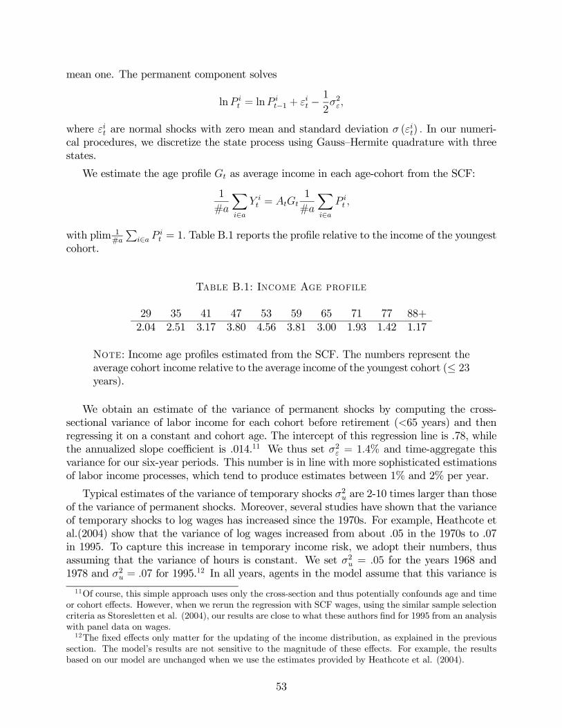
mean one. The permanent component solves

ln = ln

−1 + −

1

22

where are normal shocks with zero mean and standard deviation () In our numeri-

cal procedures, we discretize the state process using Gauss—Hermite quadrature with three

states.

We estimate the age profile as average income in each age-cohort from the SCF:

1

#

X∈

=

1

#

X∈

with plim 1#

P∈

= 1 Table B.1 reports the profile relative to the income of the youngest

cohort.

Table B.1: Income Age profile

29 35 41 47 53 59 65 71 77 88+

2.04 2.51 3.17 3.80 4.56 3.81 3.00 1.93 1.42 1.17

Note: Income age profiles estimated from the SCF. The numbers represent the

average cohort income relative to the average income of the youngest cohort (≤ 23years).

We obtain an estimate of the variance of permanent shocks by computing the cross-

sectional variance of labor income for each cohort before retirement (65 years) and then

regressing it on a constant and cohort age. The intercept of this regression line is .78, while

the annualized slope coefficient is .014.11 We thus set 2 = 14% and time-aggregate this

variance for our six-year periods. This number is in line with more sophisticated estimations

of labor income processes, which tend to produce estimates between 1% and 2% per year.

Typical estimates of the variance of temporary shocks 2 are 2-10 times larger than those

of the variance of permanent shocks. Moreover, several studies have shown that the variance

of temporary shocks to log wages has increased since the 1970s. For example, Heathcote et

al.(2004) show that the variance of log wages increased from about .05 in the 1970s to .07

in 1995. To capture this increase in temporary income risk, we adopt their numbers, thus

assuming that the variance of hours is constant. We set 2 = 05 for the years 1968 and

1978 and 2 = 07 for 1995.12 In all years, agents in the model assume that this variance is

11Of course, this simple approach uses only the cross-section and thus potentially confounds age and time

or cohort effects. However, when we rerun the regression with SCF wages, using the similar sample selection

criteria as Storesletten et al. (2004), our results are close to what these authors find for 1995 from an analysis

with panel data on wages.12The fixed effects only matter for the updating of the income distribution, as explained in the previous

section. The model’s results are not sensitive to the magnitude of these effects. For example, the results

based on our model are unchanged when we use the estimates provided by Heathcote et al. (2004).

53

fixed forever. Finally, we determine the variance of the first draw of permanent income from

the intercept of our regression line. For the earlier years, we scale down this initial variance

by the relative change in the permanent component of income for the youngest agents in

Heathcote et al. This is a simple way to accommodate changes in income due to education

over time. Sensitivity checks have shown that the initial draw of permanent income does not

matter much for the results, since it does not directly affect the portfolio problem.

Most labor income studies focus on pre-retirement income. There are major challenges

to obtaining variance estimates for retirement income. For example, older households tend

to experience large shocks to health expenditures, which are included as NIPA income if

they are disbursed by health plans. These shocks contain both transitory and permanent

components (see the estimates reported in Appendix A, Skinner, Hubbard and Zeldes 1994).

Since these shocks are hard to measure at the household level, we could try to ignore their

variances and assume that household receive a safe stream of income during retirement.

However, this implies that precautionary savings drop dramatically as soon as the household

enters retirement in the absence of such shocks. This prediction is not consistent with the

household savings data from the SCF. For this reason, we apply the above shocks to income

at any age, including retirement.

Returns and aggregate growth

We assume that consumers believe real asset returns and aggregate growth to be serially

independent over successive six year periods. Moreover, when computing an equilibrium for

a given period , we assume that returns are identically distributed for periods beyond +1

We will refer to this set of beliefs — to be described below — as baseline beliefs. However, in

our exercises we will allow beliefs for returns between and + 1 to differ. For example, we

will explore what happens when expected inflation is higher over the next six year period.

We discuss the latter aspect of beliefs below when we present our results. Here we focus on

how we fix the baseline.

To pick numbers for baseline beliefs, we start from empirical moments. Table B.2 reports

summary statistics on ex-post realized pre-tax real returns on fixed income securities, resi-

dential real estate and equity, as well as inflation and growth. These returns are measured

over six year periods, but reported at annualized rates. Since we work with aggregate port-

folio data from the FFA, we construct returns on corporate equity and residential real estate

directly from FFA aggregates.

54

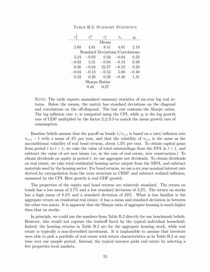
Table B.2: Summary Statistics

Means

268 481 851 401 219

Standard Deviations/Correlations

324 −002 056 −004 033

−002 331 −004 −013 038

056 −004 2287 −052 020

−004 −013 −052 560 −040033 038 020 −040 131

Sharpe Ratios

0.45 0.27

Note: The table reports annualized summary statistics of six-year log real re-turns. Below the means, the matrix has standard deviations on the diagonal

and correlations on the off-diagonal. The last row contains the Sharpe ratios.

The log inflation rate is computed using the CPI, while is the log growth

rate of GDP multiplied by the factor 2.2/3.3 to match the mean growth rate of

consumption.

Baseline beliefs assume that the payoff on bonds 1+1 is based on a (net) inflation rate

+1 − 1 with a mean of 4% per year, and that the volatility of +1 is the same as the

unconditional volatility of real bond returns, about 1.3% per year. To obtain capital gains

from period to + 1, we take the value of total outstandings from the FFA in + 1, and

subtract the value of net new issues (or, in the case of real estate, new construction.) To

obtain dividends on equity in period , we use aggregate net dividends. To obtain dividends

on real estate, we take total residential housing sector output from the NIPA, and subtract

materials used by the housing sector. For bond returns, we use a six year nominal interest rate

derived by extrapolation from the term structure in CRSP, and subtract realized inflation,

measured by the CPI. Here growth is real GDP growth.

The properties of the equity and bond returns are relatively standard. The return on

bonds has a low mean of 2.7% and a low standard deviation of 3.2%. The return on stocks

has a high mean of 8.5% and a standard deviation of 23%. What is less familiar is the

aggregate return on residential real estate: it has a mean and standard deviation in between

the other two assets. It is apparent that the Sharpe ratio of aggregate housing is much higher

than that on stocks.

In principle, we could use the numbers from Table B.2 directly for our benchmark beliefs.

However, this would not capture the tradeoff faced by the typical individual household.

Indeed, the housing returns in Table B.2 are for the aggregate housing stock, while real

estate is typically a non-diversified investment. It is implausible to assume that investors

were able to pick a portfolio of real estate with return characteristics as in Table B.2 at any

time over our sample period. Instead, the typical investor picks real estate by selecting a

few properties local markets.

55

Existing evidence suggests that the volatility of house returns at the metro area, and even

at the neighborhood or property level are significantly higher than returns at the national

aggregate. For example, Caplin et al. (1997) argue that 1/4 of the overall volatility is

aggregate, 1/4 is city-component, and 1/2 is idiosyncratic. Tables 1A and 1B in Flavin and

Yamashita (2002) together with Appendix C in Piazzesi, Schneider, and Tuzel (2006) confirm

this decomposition of housing returns. As a simple way to capture this higher property-level

volatility, we add idiosyncratic shocks to the variance of housing returns that have volatility

equal to 3.5 times aggregate volatility.13 Finally, we assume that expected future real rents

are constant. This ignores the volatility of real rent growth, which is small, at around 2%

per year.

Taxes on investment

Investors care about after-tax real returns. In particular, taxes affect the relative attrac-

tiveness of equity and real estate. On the one hand, dividends on owner-occupied housing

are directly consumed and hence not taxed, while dividends on stocks are subject to income

tax. On the other hand, capital gains on housing are more easily sheltered from taxes than

capital gains on stocks. This is because many consumers simply live in their house for a long

period of time and never realize the capital gains. Capital gains tax matters especially in

inflationary times, because the nominal gain is taxed: the effective real after tax return on

an asset subject to capital gains tax is therefore lower when inflation occurs.

To measure the effect of capital gains taxes, one would ideally like to explicitly distin-

guish realized and unrealized capital gains. However, this would involve introducing state

variables to keep track of past individual asset purchase decisions. To keep the problem

manageable, we adopt a simpler approach: we adjust our benchmark returns to capture the

effects described above. For our baseline set of results, we assume proportional taxes, and

we set both the capital gains tax rate and the income tax rate to 20%. We define after tax

real stock returns by subtracting 20% from realized net real stock returns and then further

subtracting 20% times the realized rate of inflation to capture the fact that nominal capital

gains are taxed. In contrast, we assume that returns on real estate are not taxed.

13Since the volatility of housing is measured imprecisely, we chose the precise number for the multiplicative

factor such that the aggregate share of housing in the model roughly matches the FFA data. The resulting

factor is 3.5, close to the rule-of-thumb factor of 4.

56