Embed Size (px)
Citation preview
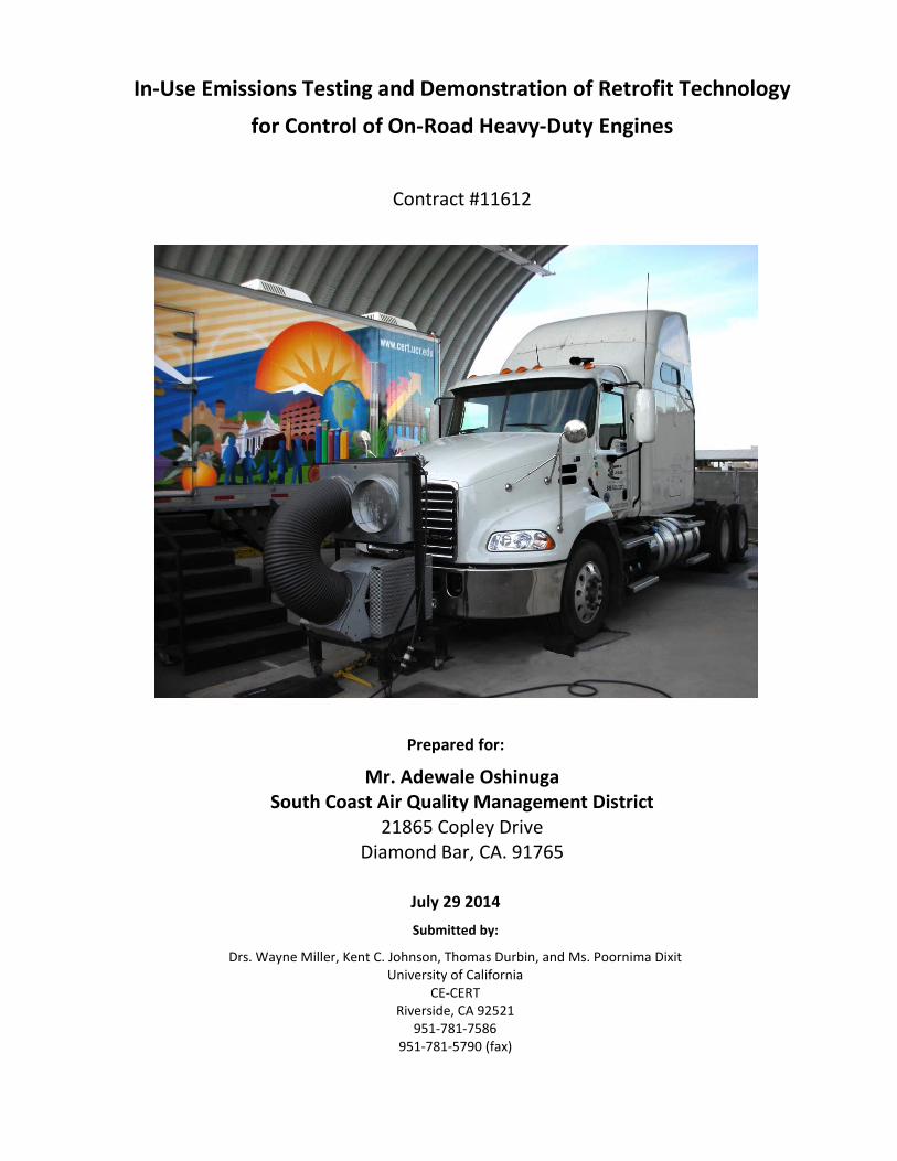
In-Use Emissions Testing and Demonstration of Retrofit Technology
for Control of On-Road Heavy-Duty Engines
Contract #11612
Prepared for:
Mr. Adewale Oshinuga South Coast Air Quality Management District
21865 Copley Drive Diamond Bar, CA. 91765
July 29 2014
Submitted by:
Drs. Wayne Miller, Kent C. Johnson, Thomas Durbin, and Ms. Poornima Dixit University of California
CE-CERT Riverside, CA 92521
951-781-7586 951-781-5790 (fax)
ii
Disclaimer
The statements and conclusions in this report are those of the contractor and not necessarily those of the South Coast Air Quality Management District or other participating organizations and their employees. The mention of commercial products, their source, or their use in connection with material reported herein is not to be construed as actual or implied endorsement of such products.
Acknowledgments
This report was prepared at the University of California, Riverside, and Bourns College of Engineering-Center for Environmental Research and Technology (CE-CERT). The primary contributors to this report include Drs. Wayne Miller, Kent C. Johnson, Thomas D. Durbin, and Ms. Poornima Dixit. The authors thank the following organizations and individuals for their valuable contributions to this project. We acknowledge Messrs. Don Pacocha, Edward O’Neil, and Joe Valdez of CE-CERT for their assistance in carrying out the experimental program.
Also, we would like to thank the following: Mr. Scott Monday, Alfredo Ortiz, and the rest of the support team at the Air Resources Board for N2O analysis and technical guidance. Scott was very helpful in coordinating samples and Alfredo was patient in performing the analysis with short notice.
Also, we would like to thank the following: T. J. Rafel at Western Truck Center and Steve South at EDCO disposal for the use of their SCR equipped diesel refuse haulers. Patrick McGuruk at Container Freight/EIT., LLC for the use of two class 8 diesel powered vehicles. John Vondriska at Moreno Valley Unified School District for the use of a propane powered school bus. David Chiu at Krisda Inc for the use of a Class 8 LPG vehicle. Doug Kollmyer from A to Z Bus Sales for the use of a DPF equipped diesel school bus. Ed Hardiman, Rudy Raya and their support team at Caltrans for the use of two diesel Navistar refuse haulers. Jonathan Evans and Mark Yragui at Cummins Cal Pacific for their assistance in locating SCR equipped diesel refuse haulers in California. Bennie Anselmo for his assistance in locating an SCR equipped diesel refuse hauler in Northern California.
iii
Table of Contents
Disclaimer ............................................................................................................................. ii Acknowledgments ................................................................................................................. ii Table of Contents ................................................................................................................. iii List of Figures ...................................................................................................................... vii List of Tables ........................................................................................................................ xi Acronyms and Abbreviations ............................................................................................... xiv Executive Summary ............................................................................................................. xvi 1 Introduction ................................................................................................................... 1
1.1 Background ............................................................................................................................. 1
1.2 Objectives ............................................................................................................................... 1
1.3 Technology Used for Meeting Low-Emission Limits .............................................................. 2
1.4 Vehicle/Engine ....................................................................................................................... 2
1.5 Test Cycles .............................................................................................................................. 5
1.5.1 EPA Urban Dynamometer Driving Schedule (UDDS) ....................................................... 6 1.5.2 Port Drayage Cycles ........................................................................................................ 7 1.5.3 AQMD refuse truck cycle (AQMD-RTC) ........................................................................... 7 1.5.4 Buses: Central Business District and Orange County Cycles ........................................... 7
1.6 Fuel Selection ......................................................................................................................... 8
1.7 Emission Measurements ........................................................................................................ 8
1.8 Engine Power Measurement .................................................................................................. 8
2 Vehicle and Chassis Testing Procedures......................................................................... 10
2.1 Vehicle Selection .................................................................................................................. 10
2.1.1 Safety inspection ........................................................................................................... 10 2.1.2 Maintenance and usage history ................................................................................... 10 2.1.3 On-site emissions inspection ......................................................................................... 10 2.1.4 Fault codes .................................................................................................................... 10
2.2 Chassis Dynamometer .......................................................................................................... 11
2.3 Chassis Test Procedures ....................................................................................................... 11
2.3.1 Setting up the dynamometer ........................................................................................ 11 2.3.2 Vehicle and dynamometer preconditioning .................................................................. 11 2.3.3 After treatment system (ATS) preconditioning (regenerations) ................................... 12 2.3.4 Soak time between tests ............................................................................................... 12
3 Emissions Laboratory Setup and Checks ........................................................................ 13
3.1 Emissions Measurement Laboratory ................................................................................... 13
3.2 Laboratory Setup for the Emissions Bench (MEL) ................................................................ 15
3.2.1 MEL dilution tunnel cleaning ........................................................................................ 15 3.2.2 MEL laboratory steps prior to test ................................................................................ 15
3.3 Laboratory Setup for the Off-line Analyses .......................................................................... 16
3.3.1 Filter weighting for PM mass ........................................................................................ 16 3.3.2 Measurement of Elemental and Organic Carbon (EC-OC) ............................................ 16
iv
3.3.3 Measuring Carbonyls .................................................................................................... 16 3.3.4 Measuring volatile toxic compounds ............................................................................ 16 3.3.5 Measuring nitrous oxide (N2O) ..................................................................................... 17
4 Quality Control/Quality Assurance ................................................................................ 18
4.1 Cross-laboratory Correlation ................................................................................................ 18
4.1.1 Port vehicle #1 (Mack MP8445C 2011) ......................................................................... 23 4.1.2 Port vehicle #2 (Navistar MAXX-FORCE13 2009) .......................................................... 23 4.1.3 Port vehicle #3 (Navistar MAXX-FORCE12 2011) .......................................................... 24 4.1.4 Refuse vehicle #4 (Navistar A260 2011) ....................................................................... 24 4.1.5 Refuse vehicle #5 (Cummins ISC 8.3 2012) .................................................................... 25
4.2 Post-test QC Procedures ...................................................................................................... 25
4.2.1 MEL carbon balance ...................................................................................................... 25
4.3 MEL quality control NTE ....................................................................................................... 27
4.4 MEL quality control checks .................................................................................................. 30
5 Results and Discussion for Goods Movement Vehicles .................................................. 32
5.1 Test Trucks ............................................................................................................................ 32
5.2 Test Conditions ..................................................................................................................... 32
5.3 Emissions from the UDDS Cycle ........................................................................................... 32
5.3.1 Brake-specific emissions from Hot UDDS Cycle ............................................................ 33 5.3.2 Brake-specific emissions from Cold UDDS Cycle ........................................................... 33 5.3.3 Emissions in g/mile for the UDDS cycle ......................................................................... 34
5.4 Regulated Emissions from Port Cycles in grams/mile .......................................................... 36
5.4.1 NOx emissions ................................................................................................................ 37 5.4.2 Percentage of NOx emissions as NO2 ............................................................................ 39 5.4.3 PM emissions ................................................................................................................ 40 5.4.4 THC/NMHC/CH4 and CO emissions—UDDS cycle ......................................................... 42 5.4.5 THC/NMHC/CH4 and CO emissions—In-use port cycles ................................................ 43
5.5 Non-regulated Gaseous Emissions ....................................................................................... 44
5.5.1 NH3 emissions................................................................................................................ 44 5.5.2 Selected Toxic Emissions (1,3-butadiene and BTEX) ..................................................... 47 5.5.3 Selected Toxic Emissions (carbonyls) ............................................................................ 49
5.6 Non-regulated PM Emission Data ........................................................................................ 51
5.6.1 Fractionation of the PM mass into OC and EC .............................................................. 51 5.6.2 Measurement of the real-time and ultrafine PM emissions ......................................... 54
5.7 Greenhouse Gas (N2O, CH4 & CO2) Emissions and Fuel Economy ....................................... 60
5.7.1 Emissions of nitrous oxide (N2O) ................................................................................... 60 5.7.2 Emissions of methane (CH4) .......................................................................................... 61 5.7.3 CO2 and Fuel Economy emissions.................................................................................. 61
6 Results and Discussion for Refuse Haulers ..................................................................... 65
6.1 Test Trucks ............................................................................................................................ 65
6.2 Test Conditions ..................................................................................................................... 65
v
6.3 NOx Emissions from the UDDS Cycle ................................................................................... 65
6.3.1 Brake-specific emissions for the UDDS Cycle ................................................................ 65 6.3.2 Emissions in g/mile for the UDDS cycle ......................................................................... 66 6.3.3 Percentage of NOx emissions as NO2 ............................................................................ 67
6.4 Regulated Emissions from the AQMD Cycle in g/mile ......................................................... 67
6.4.1 NOx emissions for the UDDS (grams/mile) .................................................................... 67 6.4.2 PM emissions ................................................................................................................ 68 6.4.3 THC/NMHC/CH4 and CO emissions ............................................................................... 69
6.5 Non-regulated Gaseous Emissions ....................................................................................... 70
6.5.1 NH3 emissions................................................................................................................ 70 6.5.2 Selected Toxic Emissions (1,3butadience & BTEX) ........................................................ 71 6.5.3 Selected Toxic Emissions (carbonyls & ketones) ........................................................... 72
6.6 Non-regulated PM Emissions ............................................................................................... 73
6.6.1 Fractionation of the PM mass into OC and EC .............................................................. 73 6.6.2 Measurement of the real-time and ultrafine PM emissions ......................................... 74
6.7 Greenhouse Gas (N2O, CH4 & CO2) Emissions and Fuel Economy ....................................... 77
6.7.1 Emissions of nitrous oxide (N2O) ................................................................................... 77 6.7.2 Emissions of methane (CH4) .......................................................................................... 78 6.7.3 CO2 and Fuel Economy emissions.................................................................................. 78
7 Results and Discussion for School Buses ........................................................................ 80
7.1 Test Buses ............................................................................................................................. 80
7.2 Test Conditions ..................................................................................................................... 80
7.3 Regulated emissions ............................................................................................................. 80
7.3.1 NOx emissions ................................................................................................................ 80 7.3.2 Percentage of NOx emissions as NO2 ............................................................................ 81 7.3.3 PM emissions ................................................................................................................ 81 7.3.4 THC/NMHC/CH4 and CO emissions ............................................................................... 81
7.4 Non-regulated Gaseous Emissions ....................................................................................... 82
7.4.1 NH3 Emissions in g/mile ................................................................................................ 82 7.4.2 Selected toxic emissions (1,3-butadiene & BTEX) ......................................................... 83 7.4.3 Selected toxic emissions (aldehydes & ketones) ........................................................... 83
7.5 Non-regulated PM emissions ............................................................................................... 84
7.5.1 Fractionation of PM mass into OC and EC .................................................................... 84 7.5.2 Measurement of real-time and ultrafine PM ................................................................ 85
7.6 Greenhouse Gas (N2O, CH4 & CO2) Emissions and Fuel Economy ....................................... 85
7.6.1 Emissions of nitrous oxide (N2O) ................................................................................... 85 7.6.2 Emissions of methane (CH4) .......................................................................................... 86 7.6.3 CO2 and Fuel Economy emissions.................................................................................. 86
8 Deeper Analysis of the NOx, NH3, Toxic Emissions, and N2O .......................................... 88
8.1 NOx Emissions Control Technology & Results ..................................................................... 88
8.1.1 Cooled exhaust gas recirculation (EGR) ........................................................................ 88
vi
8.1.2 Three way catalysts (TWC) ............................................................................................ 88 8.1.3 Selective Catalytic reduction (SCR)................................................................................ 88
8.2 NOx from Goods Movement Vehicles .................................................................................. 90
8.3 NOx from Refuse Haulers ..................................................................................................... 92
8.4 Discussion of detection limits .............................................................................................. 96
8.4.1 Discussion of 1,3-butadiene & BTEX ............................................................................. 96 8.4.2 Discussion of Carbonyls & Ketones ............................................................................. 100 8.4.3 Discussion of N2O limits .............................................................................................. 107 8.4.4 Discussion of NH3 limits .............................................................................................. 111 8.4.5 Discussion of EC/OC limits ........................................................................................... 112
9 Summary .................................................................................................................... 117 Attachment A. Test Cycles ................................................................................................. 122 Attachment B: Brake Specific Emissions ............................................................................. 128 Attachment C: ECM Download and Inspection Summary .................................................... 136 Attachment D: Vehicle Inspection Report .......................................................................... 144 Attachment E. Detailed Test Schedule ............................................................................... 146 Attachment F: Quality Control Checks ................................................................................ 149
vii
List of Figures
Figure 3-1 UCR's Mobile Emissions Lab (MEL) .................................................................................... 13
Figure 3-2 Comparison of FTIR & TDL Measurements of Ammonia Concentrations ......................... 15
Figure 4-1 Refuse hauler shared vehicle #4 (Navistar A260 2011) ..................................................... 21
Figure 4-2 Pre and Post DPF NOx concentration for a non-regeneration vehicle operation ............. 22
Figure 4-3 Pre and Post DPF NOx during partial active regeneration during refuse truck cycle ........ 22
Figure 4-4: Real time second by second ECM and carbon balance fuel rate (port cycle) .................. 25
Figure 4-5: Parity Plot of Data from ECM and Exhaust Measurements (port cycle) .......................... 26
Figure 4-6: Carbon balance for all three port cycles and the UDDS cycle .......................................... 27
Figure 4-7 Carbon Balance Correlation on a test cycle basis .............................................................. 27
Figure 4-8: NOx NTE standard 1.8 g/bhp-hr Navistar 2009 MaxForce M131,2 ................................... 28
Figure 4-9: NOx NTE standard 0.75 g/bhp-hr Navistar 2011 MaxForce M131,2 ................................. 29
Figure 4-10: NOx NTE Standard 0.45 g/bhp-hr for the 2010 Cummins ISC 8.3 vehicle 1,2 ................. 29
Figure 4-11: Navistar (12WZJ-B) real-time PM, vehicle speed, and DPF temp for local port cycle ... 30
Figure 4-12: Navistar (12WZJ-B) engine speed repeatability while following the port cycle. ........... 31
Figure 5-1 Brake Specific NOx Emissions for UDDS Cycle ................................................................... 33
Figure 5-2 Brake Specific NOx Emissions for a Cold Start UDDS Cycle ............................................... 34
Figure 5-3: NOx Emission Factors for hot UDDS cycle (g/mile) ........................................................... 34
Figure 5-4: NOx Emission factors for Cold Start UDDS Cycle (g/mile) ................................................. 35
Figure 5-5 NOx emissions compared between cold and hot start UDDS cycles ................................ 36
Figure 5-6: NOx Emission factors for Near Dock Cycle (g/mile) .......................................................... 38
Figure 5-7: NOx Emission factors for Local Cycle (g/mile) .................................................................. 38
Figure 5-8: NOx Emission factors for Regional cycle (g/mile) ............................................................. 39
Figure 5-9: PM Emission factors for Near Dock cycle (g/mile) ........................................................... 40
Figure 5-10: PM Emission factors for Local cycle (g/mile) .................................................................. 41
Figure 5-11: PM Emission factors for Regional cycle (g/mile) ............................................................ 41
Figure 5-12 PM emissions for the cold and hot start UDDS cycles (port vehicles) ............................ 42
Figure 5-13: NH3 Emission Factors for UDDS cycle (g/mile)1 .............................................................. 45
Figure 5-14: NH3 Emission Factors for Cold Start UDDS cycle (g/mile)1 ............................................. 45
Figure 5-15: NH3 Emission factors for Near Dock Cycle (g/mile) ........................................................ 46
Figure 5-16: NH3 Emission factors for Local Cycle (g/mile) ................................................................. 46
Figure 5-17: NH3 Emission factors for Regional Cycle (g/mile)1 .......................................................... 47
viii
Figure 5-18 Emissions in mg/mile for Butadiene & BTEX for the UDDS Cycle ................................... 48
Figure 5-19 Emissions in mg/mile for Butadiene & BTEX for the Near Port Cycle ............................. 48
Figure 5-20 Emissions in mg/mile for Butadiene & BTEX for the Local Port Cycle ............................. 48
Figure 5-21 Emissions in mg/mile for Butadiene & BTEX for the Regional Port Cycle ....................... 49
Figure 5-22 Emissions in mg/mile for Carbonyls & Ketones for the UDDS Cycle ............................... 50
Figure 5-23 Emissions in mg/mile for Carbonyls & Ketones for cold- UDDS Cycle ............................ 50
Figure 5-24 Emissions in mg/mile for Carbonyls & Ketones for the Near Port Cycle ......................... 50
Figure 5-25 Emissions in mg/mile for Carbonyls & Ketones for the Local Port Cycle ........................ 51
Figure 5-26 Emissions in mg/mile for Carbonyls & Ketones for the Regional Port Cycle .................. 51
Figure 5-27 Emissions in grams/mile for the PM as OC & EC for the UDDS Cycle ............................. 52
Figure 5-28 Emissions in grams/mile for the PM as OC & EC for cold- UDDS Cycle ........................... 52
Figure 5-29 Emissions in grams/mile for the PM as OC & EC for the Near Port Cycle ....................... 53
Figure 5-30 Emissions in grams/mile for the PM as OC & EC for the Local Port Cycle ....................... 53
Figure 5-31 Emissions in grams/mile for the PM as OC & EC for the Regional Port Cycle ................. 53
Figure 5-32: Navistar (12WZJ-B) real-time PM, vehicle speed, and DPF temp for local port cycle ... 55
Figure 5-33Average size distributions for the V12.8 SCR equipped vehicle ....................................... 56
Figure 5-34 Average size distributions for the V12.8 SCR equipped vehicle selected times ............. 57
Figure 5-35 Real time scan at 60nm for the V12.8 SCR equipped vehicle ......................................... 57
Figure 5-36 Average size distributions for the N12.3 non-SCR vehicle .............................................. 58
Figure 5-37 Average size distributions for the V12.8 SCR equipped vehicle by cycle ........................ 58
Figure 5-38 Average size distributions for the N12.3 non-SCR vehicle by cycle ................................ 59
Figure 5-39 Average size distributions for various vehicles: UDDS cycle ........................................... 59
Figure 5-40: Fuel Economy in miles/gallon of Fuel for the UDDS Cycle. ............................................ 62
Figure 5-41: Fuel Economy in miles/gallon of Fuel for Cold start UDDS cycle. .................................. 62
Figure 5-42: Fuel Economy in miles/gallon of Fuel for the Near Port Cycle ....................................... 63
Figure 5-43: Fuel Economy in miles/gallon of Fuel for the Local Port Cycle ...................................... 63
Figure 5-44: Fuel Economy in miles/gallon of Fuel for the Regional Port Cycle ................................. 64
Figure 6-1 Brake Specific NOx Emissions for Hot & Cold UDDS Cycles ............................................... 66
Figure 6-2: NOx Emission Factors for Hot & Cold UDDS Cycles (g/mile) ............................................. 66
Figure 6-3: NOx Emission Factors in g/mile for AQMD Refuse Truck Cycle ....................................... 68
Figure 6-4 Emission factors for PM UDDS and cold start UDDS cycles (mg/mile) .............................. 68
Figure 6-5: Emission factors for PM AQMD Refuse Truck Cycle (g/mile) ........................................... 69
ix
Figure 6-6: Emission of NH3 in the cold/hot UDDS Cycle (g/mile)1 .................................................... 70
Figure 6-7: Emission of NH3 in the AQMD Refuse Truck Cycle (g/mile)1 ............................................ 71
Figure 6-8 Emissions of Selected Toxics in mg/mile for UDDS Cycle .................................................. 71
Figure 6-9 Emissions of Selected Toxics in mg/mile for AQMD Refuse Cycle .................................... 72
Figure 6-10 Emissions of Carbonyls & Ketones in mg/mile for UDDS Cycle ....................................... 72
Figure 6-11 Emissions of Carbonyls & Ketones in mg/mile for AQMD Refuse Cycle ......................... 73
Figure 6-12 Emissions in grams/mile for the PM as OC & EC for the UDDS Cycle ............................. 73
Figure 6-13 Emissions in grams/mile for the PM as OC & EC for the Refuse Cycle ............................ 74
Figure 6-14 Refuse vehicle real-time PM emissions for the cold start UDDS cycle ............................ 75
Figure 6-15 Average size distributions for the an SCR equipped refuse vehicle: UDDS ..................... 76
Figure 6-16 Selected scan particle size (60 nm) for the an SCR equipped refuse vehicle .................. 76
Figure 6-17 Average size distributions for an SCR equipped refuse vehicle: by cycle ....................... 77
Figure 6-18: Fuel economy in miles/gallon of fuel for the UDDS cycle on the Refuse haulers. ......... 79
Figure 6-19: Fuel economy in miles/gallon of fuel for the AQMD Refuse Truck Cycle. ..................... 79
Figure 7-1: Emission factors for NOx CBD and cold start CBD cycles (g/mile) ................................... 80
Figure 7-2: PM Emission factors for hot/cold CBD cycles (mg/mile) .................................................. 81
Figure 7-3: Emission factors for NH3 CBD cycle (g/mile)1 ................................................................... 82
Figure 7-4 Emissions of Selected Toxic in mg/mile ............................................................................ 83
Figure 7-5 Emissions of Carbonyls & Ketones in mg/mile .................................................................. 84
Figure 7-6 Fractionation of PM mass into OC and EC (mg/mile) ........................................................ 84
Figure 7-7 Average size distributions for the two school bus vehicles: CBD ...................................... 85
Figure 8-1: Figure of diesel DOC, DPF, and SCR after treatment system arrangement ..................... 89
Figure 8-2: Typical engine catalyst temperatures as measured during this project .......................... 89
Figure 8-3: Brake specific NOx Emissions for Regional Port Cycle versus Time .................................. 90
Figure 8-4: Brake specific NOx emissions for the Regional port cycle as a function of work ............. 91
Figure 8-5: NOx emissions in g/bhp-hr for the whole port cycle ........................................................ 92
Figure 8-6: Accumulated NOx emissions for the C11.9 during hot and cold start UDDS ................... 92
Figure 8-7: NOx emissions in g/bhp-hr for the whole AQMD Refuse Truck Cycle ............................. 93
Figure 8-8: Example of SCR equipped refuse hauler exhaust temperatures ..................................... 94
Figure 8-9: Brake specific NOx emissions for the Refuse Truck Cycle as a function of time .............. 95
Figure 8-10: Brake specific NOx emissions for the Refuse Truck Cycle as a function of work ............ 95
Figure 8-11: Accumulated NOx emissions for the C11.9 during hot and cold start UDDS ................. 96
x
Figure 8-12 FTIR compared to laboratory CO2 measurement for selected vehicle sources ............ 107
Figure 8-13 FTIR compared to laboratory CO2 measurement for selected ambient bags ............... 108
xi
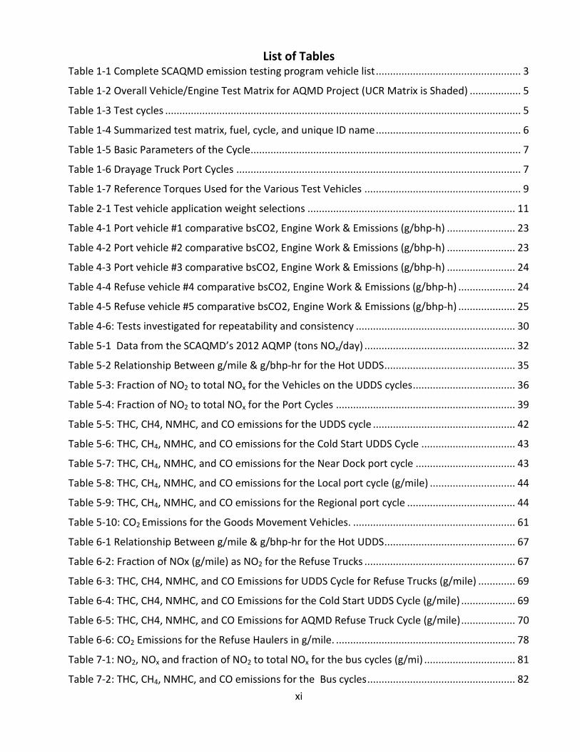
List of Tables Table 1-1 Complete SCAQMD emission testing program vehicle list ................................................... 3
Table 1-2 Overall Vehicle/Engine Test Matrix for AQMD Project (UCR Matrix is Shaded) .................. 5
Table 1-3 Test cycles ............................................................................................................................. 5
Table 1-4 Summarized test matrix, fuel, cycle, and unique ID name ................................................... 6
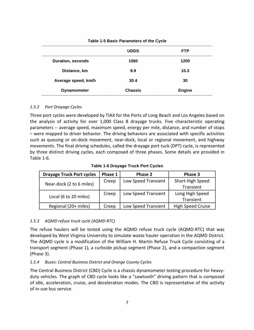
Table 1-5 Basic Parameters of the Cycle ............................................................................................... 7
Table 1-6 Drayage Truck Port Cycles .................................................................................................... 7
Table 1-7 Reference Torques Used for the Various Test Vehicles ....................................................... 9
Table 2-1 Test vehicle application weight selections ......................................................................... 11
Table 4-1 Port vehicle #1 comparative bsCO2, Engine Work & Emissions (g/bhp-h) ........................ 23
Table 4-2 Port vehicle #2 comparative bsCO2, Engine Work & Emissions (g/bhp-h) ........................ 23
Table 4-3 Port vehicle #3 comparative bsCO2, Engine Work & Emissions (g/bhp-h) ........................ 24
Table 4-4 Refuse vehicle #4 comparative bsCO2, Engine Work & Emissions (g/bhp-h) .................... 24
Table 4-5 Refuse vehicle #5 comparative bsCO2, Engine Work & Emissions (g/bhp-h) .................... 25
Table 4-6: Tests investigated for repeatability and consistency ........................................................ 30
Table 5-1 Data from the SCAQMD’s 2012 AQMP (tons NOx/day) ..................................................... 32
Table 5-2 Relationship Between g/mile & g/bhp-hr for the Hot UDDS .............................................. 35
Table 5-3: Fraction of NO2 to total NOx for the Vehicles on the UDDS cycles .................................... 36
Table 5-4: Fraction of NO2 to total NOx for the Port Cycles ............................................................... 39
Table 5-5: THC, CH4, NMHC, and CO emissions for the UDDS cycle .................................................. 42
Table 5-6: THC, CH4, NMHC, and CO emissions for the Cold Start UDDS Cycle ................................. 43
Table 5-7: THC, CH4, NMHC, and CO emissions for the Near Dock port cycle ................................... 43
Table 5-8: THC, CH4, NMHC, and CO emissions for the Local port cycle (g/mile) .............................. 44
Table 5-9: THC, CH4, NMHC, and CO emissions for the Regional port cycle ...................................... 44
Table 5-10: CO2 Emissions for the Goods Movement Vehicles. ......................................................... 61
Table 6-1 Relationship Between g/mile & g/bhp-hr for the Hot UDDS .............................................. 67
Table 6-2: Fraction of NOx (g/mile) as NO2 for the Refuse Trucks ..................................................... 67
Table 6-3: THC, CH4, NMHC, and CO Emissions for UDDS Cycle for Refuse Trucks (g/mile) ............. 69
Table 6-4: THC, CH4, NMHC, and CO Emissions for the Cold Start UDDS Cycle (g/mile) ................... 69
Table 6-5: THC, CH4, NMHC, and CO Emissions for AQMD Refuse Truck Cycle (g/mile) ................... 70
Table 6-6: CO2 Emissions for the Refuse Haulers in g/mile. ............................................................... 78
Table 7-1: NO2, NOx and fraction of NO2 to total NOx for the bus cycles (g/mi) ................................ 81
Table 7-2: THC, CH4, NMHC, and CO emissions for the Bus cycles .................................................... 82
xii
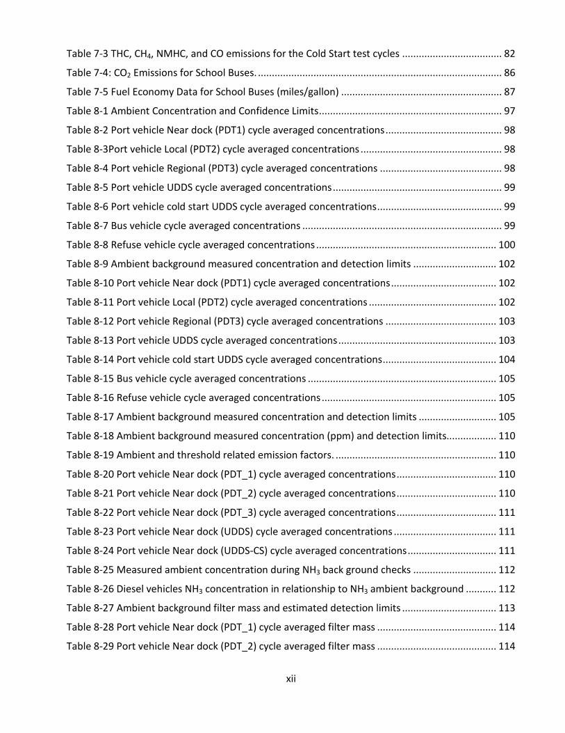
Table 7-3 THC, CH4, NMHC, and CO emissions for the Cold Start test cycles .................................... 82
Table 7-4: CO2 Emissions for School Buses. ........................................................................................ 86
Table 7-5 Fuel Economy Data for School Buses (miles/gallon) .......................................................... 87
Table 8-1 Ambient Concentration and Confidence Limits .................................................................. 97
Table 8-2 Port vehicle Near dock (PDT1) cycle averaged concentrations .......................................... 98
Table 8-3Port vehicle Local (PDT2) cycle averaged concentrations ................................................... 98
Table 8-4 Port vehicle Regional (PDT3) cycle averaged concentrations ............................................ 98
Table 8-5 Port vehicle UDDS cycle averaged concentrations ............................................................. 99
Table 8-6 Port vehicle cold start UDDS cycle averaged concentrations ............................................. 99
Table 8-7 Bus vehicle cycle averaged concentrations ........................................................................ 99
Table 8-8 Refuse vehicle cycle averaged concentrations ................................................................. 100
Table 8-9 Ambient background measured concentration and detection limits .............................. 102
Table 8-10 Port vehicle Near dock (PDT1) cycle averaged concentrations ...................................... 102
Table 8-11 Port vehicle Local (PDT2) cycle averaged concentrations .............................................. 102
Table 8-12 Port vehicle Regional (PDT3) cycle averaged concentrations ........................................ 103
Table 8-13 Port vehicle UDDS cycle averaged concentrations ......................................................... 103
Table 8-14 Port vehicle cold start UDDS cycle averaged concentrations ......................................... 104
Table 8-15 Bus vehicle cycle averaged concentrations .................................................................... 105
Table 8-16 Refuse vehicle cycle averaged concentrations ............................................................... 105
Table 8-17 Ambient background measured concentration and detection limits ............................ 105
Table 8-18 Ambient background measured concentration (ppm) and detection limits .................. 110
Table 8-19 Ambient and threshold related emission factors. .......................................................... 110
Table 8-20 Port vehicle Near dock (PDT_1) cycle averaged concentrations .................................... 110
Table 8-21 Port vehicle Near dock (PDT_2) cycle averaged concentrations .................................... 110
Table 8-22 Port vehicle Near dock (PDT_3) cycle averaged concentrations .................................... 111
Table 8-23 Port vehicle Near dock (UDDS) cycle averaged concentrations ..................................... 111
Table 8-24 Port vehicle Near dock (UDDS-CS) cycle averaged concentrations ................................ 111
Table 8-25 Measured ambient concentration during NH3 back ground checks .............................. 112
Table 8-26 Diesel vehicles NH3 concentration in relationship to NH3 ambient background ........... 112
Table 8-27 Ambient background filter mass and estimated detection limits .................................. 113
Table 8-28 Port vehicle Near dock (PDT_1) cycle averaged filter mass ........................................... 114
Table 8-29 Port vehicle Near dock (PDT_2) cycle averaged filter mass ........................................... 114
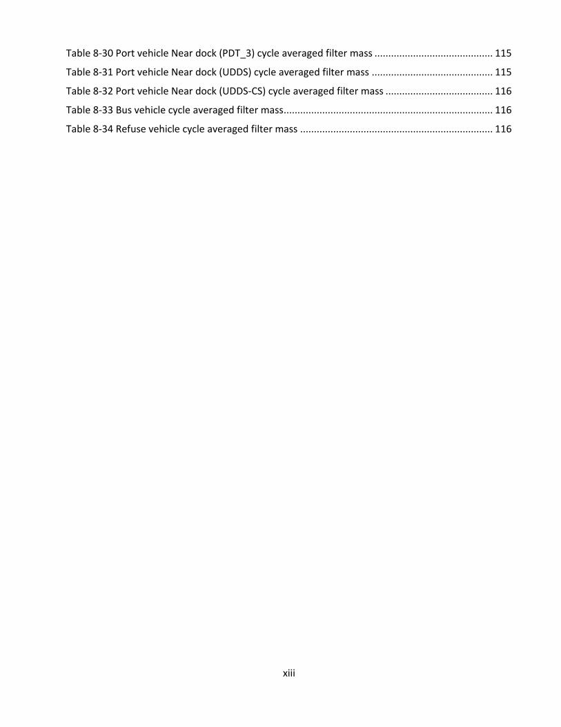
xiii
Table 8-30 Port vehicle Near dock (PDT_3) cycle averaged filter mass ........................................... 115
Table 8-31 Port vehicle Near dock (UDDS) cycle averaged filter mass ............................................ 115
Table 8-32 Port vehicle Near dock (UDDS-CS) cycle averaged filter mass ....................................... 116
Table 8-33 Bus vehicle cycle averaged filter mass ............................................................................ 116
Table 8-34 Refuse vehicle cycle averaged filter mass ...................................................................... 116
xiv
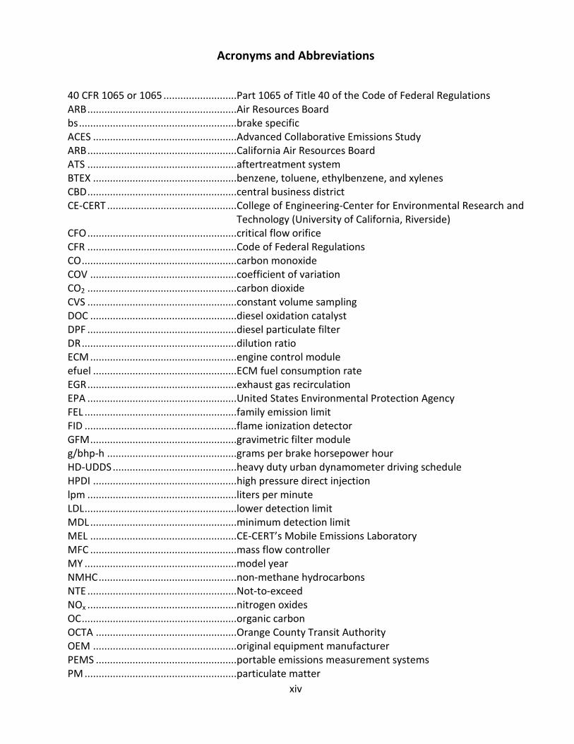
Acronyms and Abbreviations
40 CFR 1065 or 1065 ..........................Part 1065 of Title 40 of the Code of Federal Regulations ARB .....................................................Air Resources Board bs ........................................................brake specific ACES ...................................................Advanced Collaborative Emissions Study ARB .....................................................California Air Resources Board ATS .....................................................aftertreatment system BTEX ...................................................benzene, toluene, ethylbenzene, and xylenes CBD .....................................................central business district CE-CERT ..............................................College of Engineering-Center for Environmental Research and
Technology (University of California, Riverside) CFO .....................................................critical flow orifice CFR .....................................................Code of Federal Regulations CO .......................................................carbon monoxide COV ....................................................coefficient of variation CO2 .....................................................carbon dioxide CVS .....................................................constant volume sampling DOC ....................................................diesel oxidation catalyst DPF .....................................................diesel particulate filter DR .......................................................dilution ratio ECM ....................................................engine control module efuel ...................................................ECM fuel consumption rate EGR .....................................................exhaust gas recirculation EPA .....................................................United States Environmental Protection Agency FEL ......................................................family emission limit FID ......................................................flame ionization detector GFM ....................................................gravimetric filter module g/bhp-h ..............................................grams per brake horsepower hour HD-UDDS ............................................heavy duty urban dynamometer driving schedule HPDI ...................................................high pressure direct injection lpm .....................................................liters per minute LDL ......................................................lower detection limit MDL ....................................................minimum detection limit MEL ....................................................CE-CERT’s Mobile Emissions Laboratory MFC ....................................................mass flow controller MY ......................................................model year NMHC .................................................non-methane hydrocarbons NTE .....................................................Not-to-exceed NOx .....................................................nitrogen oxides OC .......................................................organic carbon OCTA ..................................................Orange County Transit Authority OEM ...................................................original equipment manufacturer PEMS ..................................................portable emissions measurement systems PM ......................................................particulate matter
xv
RPM ....................................................revolutions per minute SCAQMD .............................................South Coast Air Quality Management District SCR .....................................................selective catalytic reduction scfm ....................................................standard cubic feet per minute Tier 2, 3, or 4 ......................................federal emissions standards levels for off-road diesel engines THC .....................................................total hydrocarbons TWC ....................................................three way catalyst UCR .....................................................University of California at Riverside ULSD ...................................................ultralow sulfur diesel WVU ...................................................West Virginia University
xvi
Executive Summary
Heavy-duty diesel vehicles are a major contributor to diesel emissions in the South Coast Air Basin. While emission measurements of these vehicles in engine dynamometer certification laboratories are showing nitrogen oxides (NOx) and particulate matter (PM) emissions meeting the U.S. Environmental Protection Agency’s (EPA’s) and California Air Resources Board’s (CARB’s) emissions standards, some values from in-use conditions are showing increased emissions of ammonia from liquefied natural gas (LNG) trucks and of NOx from diesel trucks. As such, additional studies are required to assess the impact of technology on emissions from heavy-duty engines used in variety of heavy-duty applications. The objective of this study was to carry out chassis dynamometer testing of heavy-duty natural gas and diesel vehicles using near-certification and in-use driving cycles while measuring: 1) regulated emissions; 2) unregulated emissions such as ammonia and formaldehyde; 3) greenhouse gas levels of carbon dioxide (CO2) and nitrous oxide (N2O); and 4) ultrafine PM emissions.
In December 2010 and October 2011, the SCAQMD Board awarded contracts to University of California, Riverside (UCR) and West Virginia University (WVU) to conduct chassis dynamometer testing of twenty-four model year (MY) 2007-2012 heavy-duty vehicles from different vocations and fueling technologies, and if necessary, to evaluate emission-reduction potential of retrofit technology for ammonia emissions from a natural gas heavy-duty engine. The test vehicle vocations included goods movement, refuse, transit and school bus applications, and the test cycles used for the specific vocations were port drayage truck cycles for goods movement, SCAQMD refuse truck cycles for the refuse applications, and Orange County Transportation Authority (OCTA) and Central Business District (CBD) cycles for transit applications. The Heavy Duty Urban Dynamometer Driving Schedule (HD-UDDS) was a common cycle for all vocations. The test matrix involved five natural gas and four dual-fuel vehicles to be tested on a chassis dynamometer by WVU, eight diesel and two propane vehicles tested by UCR, and five diesel vehicles tested by both WVU and UCR for inter-laboratory comparison. The heavy-duty natural gas engines were both stoichiometric fueled and three-way catalytic converter (TWC) equipped; lean burn high-pressure direct injection (HPDI) engines were equipped with diesel particulate filters DPFs and selective catalytic reduction (SCR) technology. Diesel engines tested in were either U.S. EPA 2007 emissions compliant or U.S. EPA 2010 emissions compliant. The U.S. EPA 2007 emissions compliant engines were equipped with exhaust gas recirculation (EGR) technology and DPFs, while the U.S. EPA 2010 emissions compliant engines were of two types: a) with EGR and DPF only b) with DPF and SCR.
The emission results for PM and NOx are summarized below:
• PM emissions from the diesel test vehicles were below 0.01 grams per brake horsepower-hour (g/bhp-h) measured over port drayage, CBD, and UDDS drive cycles. Cold start PM emissions were relatively high for two diesel vehicles; one was a port SCR equipped vehicle and the other was a refuse SCR equipped vehicle. The port vehicle was 17 times higher (22.9 mg/mi vs 1.33 mg/mi) and the refuse vehicle was 8 times higher (18.4 mg/mi vs 2.75 mg/mi). In both cases the high cold start emission factors were below the certification standard. PM emissions were well below the certification for all diesel tests, thus suggesting DPF-based solutions are robust and reliable in meeting targeted standards. In addition, PM emissions from a liquefied petroleum gas (LPG) test vehicle was approximately 0.14 g/bhp-hr measured over the UDDS cycle, which is above the certification standard.
xvii
• NOx results covered a wide range of emission factors, where the emissions depended on the certification standard, vehicle application, driving cycle, and manufacturer. For example, NOx emissions were lowest for goods movement vehicles powered by diesel engines equipped with SCR technology; however, increases from 0.112 g/mi (0.028 g/bhp-h) during high speed cruise operation to 5.36 g/mi (1.34 g/bhp-h) for low speed transient operation were measured. Unique to the high NOx emissions was a condition in which the temperature of the SCR was less than 250ᵒC. Advanced EGR 2010 certified engines showed higher NOx emissions compared to SCR equipped engines, and pre-2010 certified engines were higher than the 2010 certified engines.
• The NOx impact of SCR equipped diesel engines depends on the vehicles’ duty cycles and manufacturers’ implementation for low temperature SCR performance. For the near dock port cycle, the SCR was below 250ᵒC approximately 80% of the time, 65% of the time for the local port cycle, and approximately 45% of the time for the regional port cycle. The percentage of time below 250ᵒC varied significantly between manufacturers, from 8% to 30% for the near dock cycle, and from 41% to 64% for the regional cycle. The difference in time below 250ᵒC suggests some manufacturers have better strategies for maintaining high exhaust temperatures than others.
• The SCR equipped engines were within their certification standards and were typically below 0.2 g/bhp-h. Only during low SCR temperature were the emissions found to be higher than the certification standard. In-use compliance testing does not enforce the emissions standards when the SCR is below 250 ᵒC, thus the SCR equipped vehicles were typically compliant based on the results presented in this report.
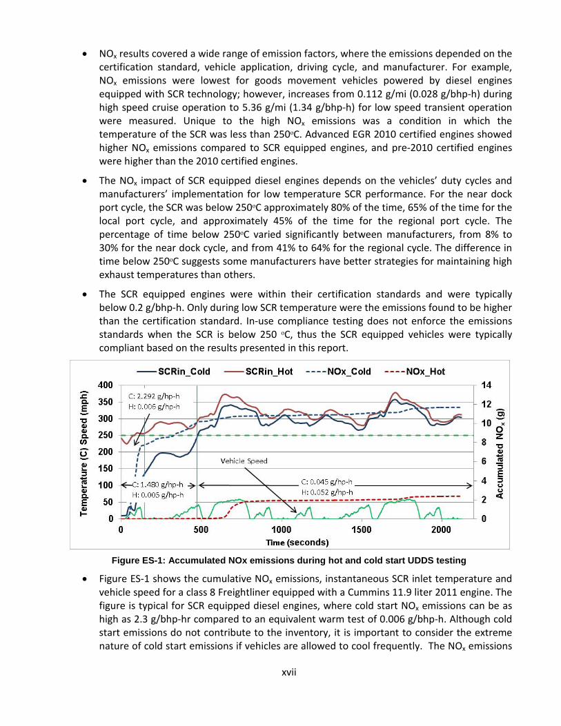
Figure ES-1: Accumulated NOx emissions during hot and cold start UDDS testing
• Figure ES-1 shows the cumulative NOx emissions, instantaneous SCR inlet temperature and vehicle speed for a class 8 Freightliner equipped with a Cummins 11.9 liter 2011 engine. The figure is typical for SCR equipped diesel engines, where cold start NOx emissions can be as high as 2.3 g/bhp-hr compared to an equivalent warm test of 0.006 g/bhp-h. Although cold start emissions do not contribute to the inventory, it is important to consider the extreme nature of cold start emissions if vehicles are allowed to cool frequently. The NOx emissions
xviii
accumulated in 1 mile after a cold start were equivalent to emissions accumulated during 32 miles of running hot.
• The 2010 certified diesel engines with advanced cooled EGR and no SCR were tested. These vehicles operated utilizing a lug curve with peak torque starting as low as 1000 revolutions per minute (RPM), where the driver was instructed to operate the vehicle down to 900 RPM before shifting. The truck behavior was unusual, and both UCR and WVU trained drivers commented on the strange operation. Additionally, the certified emissions had a family emission limit (FEL) of 0.5 g/bhp-hr for 2010 MY, but the measured NOx emissions were around 1 g/bhp-hr (0.25 g/mi) for the UDDS cycle, which represents a certification-like cycle. Even the port cycles showed brake specific emissions higher than 1 g/bhp-hr and as high as 2 g/bhp-hr for the near dock cycle.
• Pre-2010 certified diesel engines exhibited regulated emissions that were very close to the standard and were found to be repeatable for randomly selected models tested. This suggests that pre-2010 emissions inventories may be more reliable than SCR-equipped diesel engines due to SCR performance variability.
• Most NOx emissions from SCR equipped diesel refuse vehicles were produced during the compaction portion of the in-use test cycle. The high NOx emissions corresponded with a low SCR exhaust temperature, where the emissions increased from 0.27 g/bhp-hr NOx for the transient and curbside cycles to 3.8 g/bhp-hr NOx for the compaction cycle.
• The percentage of NOx as NO2 ranged from 10% to near 90%, with the highest levels of NO2
emissions from non-SCR-equipped diesel vehicles. NO2 was highest for the pre-2010 certified engines (averaging 1.15 ± 0.48 g/mi for the UDDS cycle). In general NO2 ratios were similar for all tests at around 45%±8%, except for the SCR equipped diesel vehicles, which showed high variability with a NO2 ratio of 47%±36%.
The emission results for ammonia, hydrocarbons, toxics, and fine particles are summarized below:
• Ammonia (NH3) emissions from the vehicles tested ranged from about 0.01 to 0.1 g/mi. The diesel vehicles’ NH3 emissions averaged 0.04±0.03 g/mi (0.01±0.01 g/hp-h), where the port vehicle emissions were similar (0.03±0.02 g/mi), but the propane school bus had relatively higher NH3 emissions (0.48±0.04 g/mi) over the CBD test cycle. All the diesel vehicles showed cycle averaged raw NH3 emission concentrations less than 10ppm. Of the 54 diesel tests conducted, only 2 vehicles had NH3 emissions over 5 parts per million (ppm). Half of the tests were below 2 ppm. Five of seven propane vehicle tests had NH3 emissions greater than 5 ppm and two were over 50 ppm, suggesting that relatively higher NH3 emissions exist for the propane vehicles compared to the diesel vehicles.
• The emission factors for total hydrocarbon (THC), methane (CH4), non-methane hydrocarbon (NMHC) and toxics were very low for all diesel vehicles tested. This agrees with other research from the Advanced Collaborative Emissions Study (ACES) project that showed a 98% reduction from diesel engines with catalytic exhaust systems. THC, NMHC, and CH4 emissions were at or below 0.09 g/mi, 0.06 g/mi, and 0.04 g/mi, respectively, for all vehicles (except the LPG vehicle) for both the UDDS and port regional cycles. Slightly higher THC, CH4, and NMHC emissions were found for the lower power near dock port cycle (0.36 g/mi, 0.10 g/mi, and 0.29 g/mi, respectively). Toxic emissions were low and near the
xix
detection limits of the method where 75% of the measured carcinogenetic species (benzene, toluene, ethylbenzene, and xylenes - BTEX) were below the average ambient background concentration pulse one standard deviation (< 10 mg/mi and typically < 2 mg/mi background corrected). Carbonyl emissions were also low relative to the measurement method, where more than 75% of the measured species were below the same threshold except for formaldehyde. Formaldehyde showed a relatively higher emission concentration, with 75% of the measurements above the threshold. Even though the formaldehyde samples were relatively high, their absolute contribution were below 72 mg/mi, with an average of 18±19 mg/mi. Acetaldehyde was the next largest carbonyl with maximum emissions of 18 mg/mi and an average of 1.5±4 mg/mi. The rest of the carbonyls were below 2 mg/mi. Cold start UDDS emissions were similar to the hot start UDDS emissions for THC, CH4, NMHC, and toxics (note the UDDS was performed as a 2xUDDS cycle, which may have minimized the cold start effect for the HCs and toxics).
• The LPG goods movement vehicle showed higher THC, NMHC, CH4, and toxic emissions than the diesel vehicles tested. THC, NMHC and CH4 were 22.4 g/mi, 1.43 g/mi, and 21.4 g/mi respectively for the UDDS hot cycle. BTEX and formaldehyde samples were more than 10 times the average ambient background concentration plus one standard deviation. The propane vehicle averaged 6.5±9.3 mg/mi, 9.7±12 mg/mi, and 22.4±19 mg/mi for 1,3-butadiene, n-butane, and benzene respectively for the BTEX sample. The Carbonyls were high for formaldehyde and acetaldehyde (241±253 mg/mi and 42±48 mg/mi respectively) with the remaining aldehydes below 2 mg/mi. These results should be confirmed with additional testing on LPG port vehicles.
• Real-time PM measurements suggest the reported reference PM emission rate may be lower due to low filter weights for DPF equipped vehicles. The PM mass of the gravimetric method averaged 0.78±1.57 mg/bhp-hr for selected diesel vehicles. The average PM mass from the real-time measurement method averaged 0.05±0.09 mg/bhp-hr for the same vehicles. The average filter weight for these selected vehicles ranged from 10-20 µg, where UCR’s CVS tunnel blank averages were 5µg with a 5µg single standard deviation. Thus, there is speculation that some of the uncertainty may be artifacts on the filter. As such, real-time PM measurements are useful for identifying low level PM mass in addition to real-time analysis.
• Elemental carbon (EC) and organic carbon (OC) PM was very low for all the vehicles tested and was typically below 0.2 mg/mi and 2.2 mg/mi respectively. More than half (69%) of the measured EC and OC emissions were below the average ambient background concentration plus one standard deviation. The propane vehicles had the highest organic PM contribution (>10 mg/mi for the near dock port cycle).
• Fine-particle emissions were typically higher during the first 200 seconds of the cold start UDDS cycle compared to the hot stabilized UDDS cycle (5x10⁵ #/cc vs 1x10³ #/cc, respectively). The fine particle emissions appear to be higher for the regional port cycle compared to the near dock, local, and UDDS cycles (8x10⁴ #/cc vs 1x10³ #/cc, respectively). The higher concentration of the regional port cycle may be a result of higher ATS temperatures and possible passive regenerations.
The results for greenhouse gas emissions and fuel economy are summarized below:
xx
• The greenhouse gases (GHG) and fuel economy are characterized by CO2 emissions for the diesel vehicle, but with the LPG truck, methane emissions represented approximately 8% of the GHG. The diesel fuel economy averaged 3.5 mi/gal (Port 1, 2 and UDDS) to 5.06 mi/gal (Port 3) for the port vehicles, 7.0 mi/gal for the school buses, and 4.2 mi/gal (UDDS) to 2.0 mi/gal (RTC) for the refuse haulers. The regional cycle (Port 3) showed 20% higher fuel economy than the more transient Port 1, 2, and UDDS cycles. The fuel economy from the refuse trash cycle (with integrated compaction phase) was about 50% lower than the transient UDDS cycle. The propane port vehicle showed 19% lower fuel economy than the diesel vehicles (3.3 mi/gal).
• The project measured N2O greenhouse gases on selected tests. For those vehicles measured more than half (64%) of the N2O emissions were below 0.4 ppm, which is the average ambient background concentration plus one standard deviation. The emission factors averaged 3.6±1.9 mg/mi with a maximum of 18 mg/mi (Cum_11.9 near dock port cycle).
The results for cross laboratory check are summarized below:
• The work comparison averaged around 3% negative bias (-3%), where UCR’s laboratory was slightly lower than WVU’s, with a spread of -9% to +4% on average. Both WVU and UCR show very low test-to-test variability, with a coefficient of variation (COV) less than 2% for all tests.
• The bsCO2 was close and averaged around 5% positive bias, where UCR’s laboratory was slightly higher than WVU’s with a spread of 0% to 10% overall. Both WVU and UCR show very low test-to-test variability, with a COV less than 3% for all tests.
• The bsNOx correlation was also good, but the comparison varied for the SCR equipped vehicles due to the low emission levels and the variable conditions of the SCR. For the non-SCR equipped vehicles, the deviation averaged about 3% positive bias, where UCR’s laboratory was slightly higher than WVU’s, with an average of -2% to 8%. The NOx
correlation was poor for the cold start SCR equipped vehicles and for two refuse haulers due to variability in the aftertreatment systems.
In summary, the data from this study suggests that 2010 compliant SCR-equipped HDD vehicles are exhibiting high in-use NOx emissions that can be as high as 2 g/hp-h under low load conditions represented by short trips or frequent stops. The cause of the high NOx emissions appears to be low load exhaust temperatures and, thus, low SCR aftertreatment temperatures. For SCR-equipped diesel engines, some accounting of vehicle duty cycle and SCR exhaust temperature is needed to properly characterize NOx inventories. Additionally, there were differences in SCR performance that varied between manufacturers, suggesting future performance will continue to vary. The ratio of NO2 in the NOx has been demonstrated to be about 45% for all diesel vehicles tested, where there is more variability with the SCR equipped diesels. Both NOx emission factors and NO2 ratios suggest NOx emissions are more variable for SCR equipped diesels compared to non-SCR equipped diesel vehicles. This also suggests activity studies are needed to assess the impact of SCR performance on NOx inventories. Other results showed the diesel PM, CO, THC, and selected toxics were all very low, well below certification limits, and near the limits of the measurement method for all the tests performed. The low PM, CO, THC, and selected toxics for all the diesel vehicles tested suggest these emissions are well controlled. Looking ahead, the overall results suggest NOx emissions are still a concern for selected activities, and SCR performance needs to be investigated during wide in-use, on-road operation to characterize its impact on local inventories.
1
1 Introduction
1.1 Background
Emissions from heavy-duty trucks and buses accounted for about one-third of NOx emissions and one-quarter of PM emissions from mobile sources when stringent emission standards were introduced by the EPA on December 21, 2000 and by CARB in October 2001. The new standards, shown below, further reduced PM by 90% and NOx by 95% from existing standards.
• PM—0.01 g/bhp-hr • NOx—0.20 g/bhp-hr • NMHC—0.14 g/bhp-hr
The PM emission standard took effect in the 2007. However, the NOx and NMHC standards were phased in for diesel engines between 2007 and 2010 based on the percent-of-sales basis: 50% from 2007 to 2009 and 100% in 2010. The regulation contained other provisions for meeting the NOx requirement so very few engines actually met the stringent standard of 0.20 g/bhp-hr before 2010. In addition to transient Federal Test Procedure (FTP) testing, the emission certification requirements included: 1) the 13-mode steady-state engine dynamometer test Supplemental Emissions Test (SET) test, with limits equal to the FTP standards, and 2) the not-to-exceed (NTE) emission testing with limits of 1.5 × FTP standards for engines meeting a NOx FEL of 1.5 g/bhp-hr or less and 1.25 × FTP standards for engines with a NOx FEL higher than 1.5 g/bhp-hr.
The implementation of the more stringent standards for heavy-duty highway engines was a key strategic element of the plan for improving air quality in the South Coast Air Quality Management District (AQMD). While measurements in laboratories were showing NOx and PM emissions meeting the stringent certification standards, some values from in-use conditions were showing increased emissions of ammonia from LNG trucks and of NOx from diesel trucks. Since there was a question about whether the in-use engines were meeting the stringent emission standards the AQMD Board authorized issuance of RFP #P2011-06 to assess the in-use emissions.
The RFP’s objectives were to carry out chassis dynamometer testing of heavy-duty natural gas and diesel vehicles using near-certification and in-use driving cycles while measuring: 1) regulated emissions; 2) unregulated emissions such as ammonia and formaldehyde; 3) greenhouse gas levels of CO2 and N2O and 4) ultrafine PM emissions. The study would test about twenty-five heavy-duty vehicles used for transit, refuse and goods movement applications with engines fueled with natural gas, propane, diesel, and a combination of diesel and natural gas fuels. The engine fleet was sub-divided by emission standards and technology.
1.2 Objectives
The University of California, Riverside (UCR) was contracted to test 16 heavy-duty vehicles, mainly diesel fueled engines, used for goods movement, refuse and for transient applications. The testing protocol involved measuring the emissions identified in the RFP while the vehicles operated following driving cycles that better represented the in-use conditions rather than just certification conditions. For example, the trucks used in goods movement were tested on three port driving cycles; refuse haulers tested on the AQMD refuse hauler cycle and buses were tested on the central business district cycle. The contract involved cross-laboratory testing of some common vehicles with West Virginia University as part of the quality assurance program.
2
1.3 Technology Used for Meeting Low-Emission Limits
Meeting the very strict emission standards was a challenge for engine manufacturers and required them to develop technology solutions that looked at the integrated system of engine and after treatment. Furthermore the solutions for a diesel engine were not the same for an engine fueled by natural gas.
For control of PM from diesel engines, the engine manufacturers relied on Diesel Particulate Filters (DPF). In general, DPF control system consists of four sections: 1) an inlet, 2) a Diesel Oxidation Catalyst (DOC), 3) a DPF and 4) an outlet. Exhaust flows out of the engine and through a DOC before entering the DPF where PM is collected on the walls of the DPF. The collected carbon is oxidized to remove it from the DPF during the regeneration process. When operating conditions maintain high exhaust temperatures, the DPF is self-regenerating. Otherwise, an active regeneration is required to remove a build-up of PM and pressure drop in the DPF by adding diesel fuel upstream of the DOC. The chemical reaction over the DOC raises the exhaust gas temperature high enough to oxidize the carbon from the filter.
The control of NOx from diesel engines from 2007 to 2009 was met with the use of cooled exhaust gas recirculation (EGR) and a redesign of engine operating conditions. For the 2010 engines, EGR was continued for all manufacturers and all but one manufacturer, Navistar, adopted the use of Selective Catalytic Reduction (SCR)1
Another path for meeting the stringent 2010 emissions limits was to design engines based on either natural gas or liquefied propane gas (LPG). Gaseous fueled engines meet the strict PM limits without a DPF. However, gaseous-fueled engines require technology for control of NOx. When designed and operated at stoichiometric conditions, then the engine can use three-way catalyst (TWC) technology, like that on gasoline vehicles. However, many engines operate as lean burn so NOx is higher than the 2010 limit and must be controlled with EGR and SCR technologies as used in the diesel engines.
. In the SCR process NOx is converted into nitrogen by the reaction with ammonia over a special catalyst. When operating temperatures are >250°C, an aqueous solution of urea is injected into the exhaust upstream of the SCR catalyst. The heat converts the urea into ammonia and water, which is the reactant to convert NOx to nitrogen. At temperatures <250°C, urea is not injected so the full engine out NOx emissions are emitted. SCR technology has a long history of successful operation in stationary sources.
1.4 Vehicle/Engine
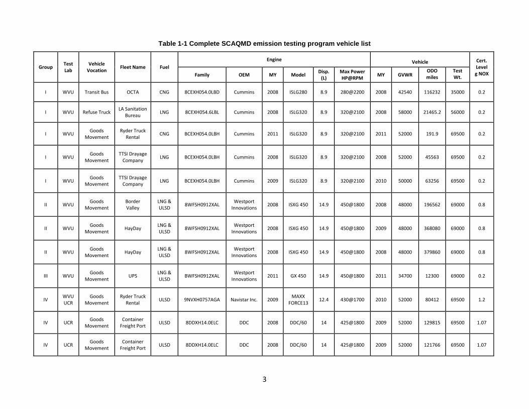
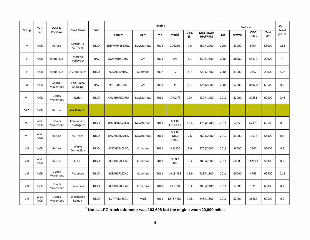
The overall project included twenty-five on-road heavy-duty vehicles (test vehicles) used in the goods movement, refuse, and transit applications. Some are powered by diesel fuel and others by gaseous fuels. Some vehicles were added later to the matrix. The complete vehicle matrix is shown in Table 1-1 with a summarized view by technology in Table 1-2. The “Test Lab” column in Table 1-1 and the shaded portion of the matrix of Table 1-2 identify the vehicles contracted to UCR. The total vehicles contracted to UCR were 16 vehicles, nine port vehicles, five refuse haulers, and two school busses.
1 On October 23, 2012 Navistar and Cummins announced deal on SCR emissions technology.
3
Table 1-1 Complete SCAQMD emission testing program vehicle list
Group Test Lab
Vehicle Vocation
Fleet Name Fuel Engine
Vehicle Cert.
Level g NOX Family OEM MY Model
Disp. (L)
Max Power HP@RPM
MY GVWR ODO miles
Test Wt.
I WVU Transit Bus OCTA CNG 8CEXH054.0LBD Cummins 2008 ISLG280 8.9 280@2200 2008 42540 116232 35000 0.2
I WVU Refuse Truck LA Sanitation
Bureau LNG 8CEXH054.6LBL Cummins 2008 ISLG320 8.9 320@2100 2008 58000 21465.2 56000 0.2
I WVU Goods
Movement Ryder Truck
Rental CNG BCEXH054.0LBH Cummins 2011 ISLG320 8.9 320@2100 2011 52000 191.9 69500 0.2
I WVU Goods
Movement TTSI Drayage
Company LNG BCEXH054.0LBH Cummins 2008 ISLG320 8.9 320@2100 2008 52000 45563 69500 0.2
I WVU Goods
Movement TTSI Drayage
Company LNG BCEXH054.0LBH Cummins 2009 ISLG320 8.9 320@2100 2010 50000 63256 69500 0.2
II WVU Goods
Movement Border Valley
LNG & ULSD
8WFSH0912XAL Westport
Innovations 2008 ISXG 450 14.9 450@1800 2008 48000 196562 69000 0.8
II WVU Goods
Movement HayDay
LNG & ULSD
8WFSH0912XAL Westport
Innovations 2008 ISXG 450 14.9 450@1800 2009 48000 368080 69000 0.8
II WVU Goods
Movement HayDay
LNG & ULSD
8WFSH0912XAL Westport
Innovations 2008 ISXG 450 14.9 450@1800 2008 48000 379860 69000 0.8
III WVU Goods
Movement UPS
LNG & ULSD
BWFSH0912XAL Westport
Innovations 2011 GX 450 14.9 450@1800 2011 34700 12300 69000 0.2
IV WVU UCR
Goods Movement
Ryder Truck Rental
ULSD 9NVXH0757AGA Navistar Inc. 2009 MAXX
FORCE13 12.4 430@1700 2010 52000 80412 69500 1.2
IV UCR Goods
Movement Container
Freight Port ULSD 8DDXH14.0ELC DDC 2008 DDC/60 14 425@1800 2009 52000 129815 69500 1.07
IV UCR Goods
Movement Container
Freight Port ULSD 8DDXH14.0ELC DDC 2008 DDC/60 14 425@1800 2009 52000 121766 69500 1.07
4
Group Test Lab
Vehicle Vocation
Fleet Name Fuel Engine
Vehicle Cert.
Level g NOX Family OEM MY Model
Disp. (L)
Max Power HP@RPM
MY GVWR ODO miles
Test Wt.
IV UCR Refuse District 11 CalTrans
ULSD BNVXH04666AGC Navistar Inc. 2008 GDT260 7.6 260@2200 2009 33000 9754 56000 0.82
V UCR School Bus Moreno
Valley SD LPG 8GMXH08.1502 GM 2008 LPI 8.1 330@1800 2009 30280 55570 20000 *
V UCR School Bus A-Z Bus Sales ULSD 7CEXH0408BAC Cummins 2007 IS 6.7 220@1800 2008 31000 3357 20000 2.0*
VI UCR Goods 1
Movement Port/China
Shipping LPG 9BPTE08.1601 GM 2009 P 8.1 325@4000 2005 52000 103608 69500 0.2
VII UCR Goods
Movement Ryder ULSD ANVXH0757AGA Navistar Inc. 2010 12WZJ/B 12.4 430@1700 2011 52000 80651 69500 0.46
VII* UCR Refuse Not Tested-
VII WVU UCR
Goods Movement
Idealease of Los Angeles
ULSD BNVXH07570GB Navistar Inc. 2011 MAXX
FORCE13 12.4 475@1700 2011 52350 67373 69500 0.5
VII WVU UCR
Refuse CalTrans ULSD BNVZH0466AGA Navistar Inc. 2011 MAXX FORCE A260
7.6 260@2200 2012 33000 10014 56000 0.5
VIII UCR Refuse Waste
Connection ULSD BCEXH0540LAQ Cummins 2011 ISL9 370 8.9 370@2100 2012 36000 2500 56000 0.2
VIII WVU UCR
Refuse EDCO ULSD BCEXH0505CAC Cummins 2011 ISC 8.3
300 8.3 300@2000 2011 60000 14269.4 56000 0.2
VIII UCR Goods
Movement Pac Lease ULSD BCEXH0729XAC Cummins 2011 ISX15-485 11.9 425@1800 2011 80000 4769 69500 0.12
VIII UCR Goods
Movement Coca Cola ULSD ACEXH0505CAC Cummins 2010 ISC-300 8.3 300@2100 2011 52000 13918 65000 0.2
VIII WVU UCR
Goods Movement
Worldwide Rentals
ULSD BVPTH12.8S01 Mack 2011 MP8-445C 12.8 445@1500 2011 52000 36982 69500 0.2
1 Note…LPG truck odometer was 103,608 but the engine was <20,000 miles
5
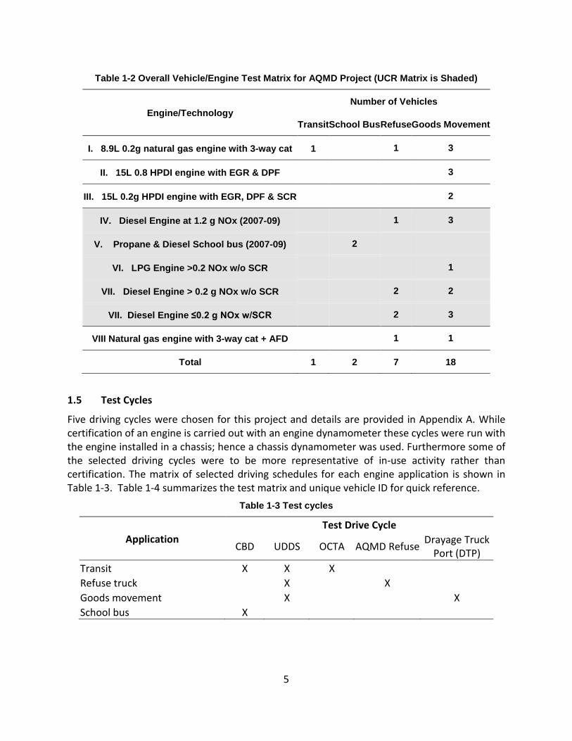
Table 1-2 Overall Vehicle/Engine Test Matrix for AQMD Project (UCR Matrix is Shaded)
Engine/Technology Number of Vehicles
Transit School Bus Refuse Goods Movement
I. 8.9L 0.2g natural gas engine with 3-way cat 1 1 3
II. 15L 0.8 HPDI engine with EGR & DPF 3
III. 15L 0.2g HPDI engine with EGR, DPF & SCR 2
IV. Diesel Engine at 1.2 g NOx (2007-09) 1 3
V. Propane & Diesel School bus (2007-09) 2
VI. LPG Engine >0.2 NOx w/o SCR 1
VII. Diesel Engine > 0.2 g NOx w/o SCR 2 2
VII. Diesel Engine ≤0.2 g NOx w/SCR 2 3
VIII Natural gas engine with 3-way cat + AFD 1 1
Total 1 2 7 18
1.5 Test Cycles
Five driving cycles were chosen for this project and details are provided in Appendix A. While certification of an engine is carried out with an engine dynamometer these cycles were run with the engine installed in a chassis; hence a chassis dynamometer was used. Furthermore some of the selected driving cycles were to be more representative of in-use activity rather than certification. The matrix of selected driving schedules for each engine application is shown in Table 1-3. Table 1-4 summarizes the test matrix and unique vehicle ID for quick reference.
Table 1-3 Test cycles
Application Test Drive Cycle
CBD UDDS OCTA AQMD Refuse Drayage Truck
Port (DTP) Transit X X X Refuse truck X X Goods movement X X School bus X
6
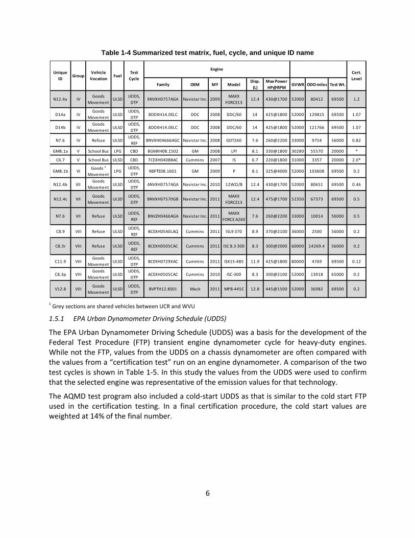
Table 1-4 Summarized test matrix, fuel, cycle, and unique ID name
1 Grey sections are shared vehicles between UCR and WVU
1.5.1 EPA Urban Dynamometer Driving Schedule (UDDS)
The EPA Urban Dynamometer Driving Schedule (UDDS) was a basis for the development of the Federal Test Procedure (FTP) transient engine dynamometer cycle for heavy-duty engines. While not the FTP, values from the UDDS on a chassis dynamometer are often compared with the values from a “certification test” run on an engine dynamometer. A comparison of the two test cycles is shown in Table 1-5. In this study the values from the UDDS were used to confirm that the selected engine was representative of the emission values for that technology.
The AQMD test program also included a cold-start UDDS as that is similar to the cold start FTP used in the certification testing. In a final certification procedure, the cold start values are weighted at 14% of the final number.
Family OEM MY ModelDisp.
(L)Max Power HP@RPM
GVWR ODO miles Test Wt.
D14a IVGoods
MovementULSD
UDDS, DTP
8DDXH14.0ELC DDC 2008 DDC/60 14 425@1800 52000 129815 69500 1.07
D14b IVGoods
MovementULSD
UDDS, DTP
8DDXH14.0ELC DDC 2008 DDC/60 14 425@1800 52000 121766 69500 1.07
N7.6 IV Refuse ULSDUDDS,
REFBNVXH04666AGC Navistar Inc. 2008 GDT260 7.6 260@2200 33000 9754 56000 0.82
GM8.1a V School Bus LPG CBD 8GMXH08.1502 GM 2008 LPI 8.1 330@1800 30280 55570 20000 *
C6.7 V School Bus ULSD CBD 7CEXH0408BAC Cummins 2007 IS 6.7 220@1800 31000 3357 20000 2.0*
GM8.1b VIGoods 1
MovementLPG
UDDS, DTP
9BPTE08.1601 GM 2009 P 8.1 325@4000 52000 103608 69500 0.2
N12.4b VIIGoods
MovementULSD
UDDS, DTP
ANVXH0757AGA Navistar Inc. 2010 12WZJ/B 12.4 430@1700 52000 80651 69500 0.46
C8.9 VIII Refuse ULSDUDDS,
REFBCEXH0540LAQ Cummins 2011 ISL9 370 8.9 370@2100 36000 2500 56000 0.2
C11.9 VIIIGoods
MovementULSD
UDDS, DTP
BCEXH0729XAC Cummins 2011 ISX15-485 11.9 425@1800 80000 4769 69500 0.12
C8.3p VIIIGoods
MovementULSD
UDDS, DTP
ACEXH0505CAC Cummins 2010 ISC-300 8.3 300@2100 52000 13918 65000 0.2
N7.6
N12.4c
V12.8
C8.3r
Cert. Level
0.2
Test Cycle
Unique ID
UDDS, DTP
N12.4a
UDDS, DTP
UDDS, DTP
UDDS, REF
UDDS, REF
12.8 445@1500 52000 36982 69500
56000 0.2
VIIIGoods
MovementULSD BVPTH12.8S01 Mack 2011 MP8-445C
ISC 8.3 300 8.3 300@2000 60000 14269.4
10014 56000 0.5
VIII Refuse ULSD BCEXH0505CAC Cummins 2011
2011MAXX
FORCE A2607.6 260@2200 33000VII Refuse ULSD BNVZH0466AGA Navistar Inc.
475@1700 52350 67373 69500 0.5
1.2
VIIGoods
MovementULSD BNVXH07570GB Navistar Inc. 2011
MAXX FORCE13
12.4
12.4 430@1700 52000 80412 69500IVGoods
MovementULSD 9NVXH0757AGA Navistar Inc. 2009
MAXX FORCE13
GroupVehicle
VocationFuel
Engine
7
Table 1-5 Basic Parameters of the Cycle
UDDS FTP
Duration, seconds 1060 1200
Distance, km 8.9 10.3
Average speed, km/h 30.4 30
Dynamometer Chassis Engine
1.5.2 Port Drayage Cycles
Three port cycles were developed by TIAX for the Ports of Long Beach and Los Angeles based on the analysis of activity for over 1,000 Class 8 drayage trucks. Five characteristic operating parameters -- average speed, maximum speed, energy per mile, distance, and number of stops – were mapped to driver behavior. The driving behaviors are associated with specific activities such as queuing or on-dock movement, near-dock, local or regional movement, and highway movements. The final driving schedules, called the drayage port tuck (DPT) cycle, is represented by three distinct driving cycles, each composed of three phases. Some details are provided in Table 1-6.
Table 1-6 Drayage Truck Port Cycles
Drayage Truck Port cycles Phase 1 Phase 2 Phase 3
Near-dock (2 to 6 miles) Creep Low Speed Transient Short High Speed
Transient
Local (6 to 20 miles) Creep Low Speed Transient Long High Speed
Transient Regional (20+ miles) Creep Low Speed Transient High Speed Cruise
1.5.3 AQMD refuse truck cycle (AQMD-RTC)
The refuse haulers will be tested using the AQMD refuse truck cycle (AQMD-RTC) that was developed by West Virginia University to simulate waste hauler operation in the AQMD District. The AQMD cycle is a modification of the William H. Martin Refuse Truck Cycle consisting of a transport segment (Phase 1), a curbside pickup segment (Phase 2), and a compaction segment (Phase 3).
1.5.4 Buses: Central Business District and Orange County Cycles
The Central Business District (CBD) Cycle is a chassis dynamometer testing procedure for heavy-duty vehicles. The graph of CBD cycle looks like a “sawtooth” driving pattern that is composed of idle, acceleration, cruise, and deceleration modes. The CBD is representative of the activity of in-use bus service.
8
The Orange County Bus Cycle (OCTA) is a chassis dynamometer test for heavy-duty vehicles developed by the West Virginia University (WVU) based on the driving patterns of urban transit buses in the Los Angeles, California area.
1.6 Fuel Selection
Commercial grade #2, ultra-low sulfur diesel fuel was used for the testing rather than fuel used for certification. Street fuel was more representative of what in-use vehicles would be using. Similarly, for the propane vehicles, locally supplied propane fuel was used in the testing as this was more representative of an in-use fuel.
For automotive propane usage Autogas is used for propane, Autogas is a mixture of propane with various contributions from other gasses. As such, locally supplied propane fuel meets the HD-5 specification for propane. As such it consist of at least 90% propane, no more than 5% propylene, and 5% other gases, primarily butane and butylene2
1.7 Emission Measurements
.
The contract specified the measurements of certain properties of the exhaust stream. These included:
• Regulated emissions: nitric oxides (NOx), particulate mass (PM), carbon monoxide (CO) and non-methane hydrocarbons (NMHC).
• Non-regulated emissions: ammonia (NH3), benzene, toluene, butadiene, carbonyls (like formaldehyde).
• Greenhouse gases: nitrous oxide (N2O), methane (CH4), and carbon dioxide (CO2) • Ultrafine PM concentration and particle size distribution.
1.8 Engine Power Measurement
Engine break power was calculated using ECM broadcast J1939 standardized information. These signals are the same signals used for in-use compliance testing for the not-to-exceed standards in the 40 CFR Part 1065. A brief description is provided to describe the calculation and the results from the calculation. Equation 1 below shows the formula to calculate brake power:
𝑏ℎ𝑝 =𝑅𝑃𝑀∗�𝑇𝑎𝑐𝑡𝑢𝑎𝑙−𝑇𝑓𝑟𝑖𝑐𝑡𝑖𝑜𝑛�∗𝑇𝑟𝑒𝑓𝑒𝑟𝑒𝑛𝑐𝑒
5252
Where:
bhp – is the brake power in units of (hp)
RPM – engine speed in revolutions per minute (rpm)
Tactual – ECM broadcast actual torque in (%)
2 Alternative Fuels Data Center, US Department of Energy “Propane Fuel Basics, Office of Energy Efficiency and Renewable Energy, http://www.afdc.energy.gov/fuels/propane_basics.html
Eq 1
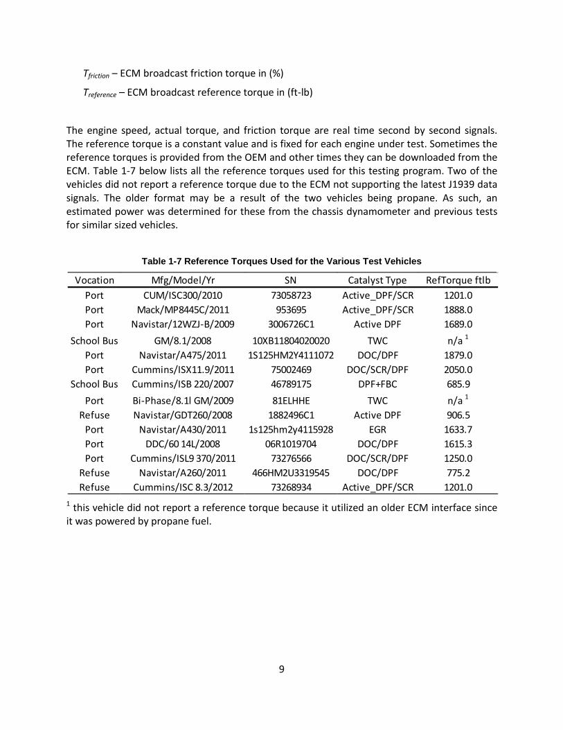
9
Tfriction – ECM broadcast friction torque in (%)
Treference – ECM broadcast reference torque in (ft-lb)
The engine speed, actual torque, and friction torque are real time second by second signals. The reference torque is a constant value and is fixed for each engine under test. Sometimes the reference torques is provided from the OEM and other times they can be downloaded from the ECM. Table 1-7 below lists all the reference torques used for this testing program. Two of the vehicles did not report a reference torque due to the ECM not supporting the latest J1939 data signals. The older format may be a result of the two vehicles being propane. As such, an estimated power was determined for these from the chassis dynamometer and previous tests for similar sized vehicles.
Table 1-7 Reference Torques Used for the Various Test Vehicles
1 this vehicle did not report a reference torque because it utilized an older ECM interface since it was powered by propane fuel.
Vocation Mfg/Model/Yr SN Catalyst Type RefTorque ftlbPort CUM/ISC300/2010 73058723 Active_DPF/SCR 1201.0Port Mack/MP8445C/2011 953695 Active_DPF/SCR 1888.0Port Navistar/12WZJ-B/2009 3006726C1 Active DPF 1689.0
School Bus GM/8.1/2008 10XB11804020020 TWC n/a 1
Port Navistar/A475/2011 1S125HM2Y4111072 DOC/DPF 1879.0Port Cummins/ISX11.9/2011 75002469 DOC/SCR/DPF 2050.0
School Bus Cummins/ISB 220/2007 46789175 DPF+FBC 685.9
Port Bi-Phase/8.1l GM/2009 81ELHHE TWC n/a 1
Refuse Navistar/GDT260/2008 1882496C1 Active DPF 906.5Port Navistar/A430/2011 1s125hm2y4115928 EGR 1633.7Port DDC/60 14L/2008 06R1019704 DOC/DPF 1615.3Port Cummins/ISL9 370/2011 73276566 DOC/SCR/DPF 1250.0
Refuse Navistar/A260/2011 466HM2U3319545 DOC/DPF 775.2Refuse Cummins/ISC 8.3/2012 73268934 Active_DPF/SCR 1201.0
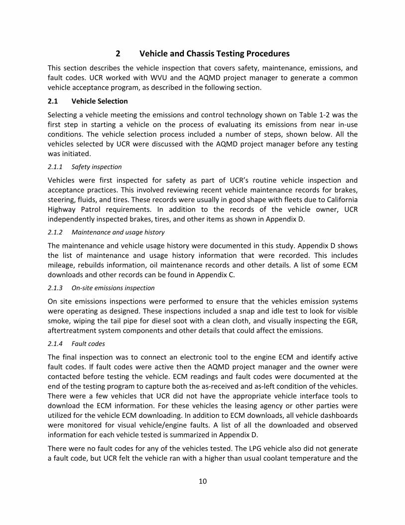
10
2 Vehicle and Chassis Testing Procedures
This section describes the vehicle inspection that covers safety, maintenance, emissions, and fault codes. UCR worked with WVU and the AQMD project manager to generate a common vehicle acceptance program, as described in the following section.
2.1 Vehicle Selection
Selecting a vehicle meeting the emissions and control technology shown on Table 1-2 was the first step in starting a vehicle on the process of evaluating its emissions from near in-use conditions. The vehicle selection process included a number of steps, shown below. All the vehicles selected by UCR were discussed with the AQMD project manager before any testing was initiated.
2.1.1 Safety inspection
Vehicles were first inspected for safety as part of UCR’s routine vehicle inspection and acceptance practices. This involved reviewing recent vehicle maintenance records for brakes, steering, fluids, and tires. These records were usually in good shape with fleets due to California Highway Patrol requirements. In addition to the records of the vehicle owner, UCR independently inspected brakes, tires, and other items as shown in Appendix D.
2.1.2 Maintenance and usage history
The maintenance and vehicle usage history were documented in this study. Appendix D shows the list of maintenance and usage history information that were recorded. This includes mileage, rebuilds information, oil maintenance records and other details. A list of some ECM downloads and other records can be found in Appendix C.
2.1.3 On-site emissions inspection
On site emissions inspections were performed to ensure that the vehicles emission systems were operating as designed. These inspections included a snap and idle test to look for visible smoke, wiping the tail pipe for diesel soot with a clean cloth, and visually inspecting the EGR, aftertreatment system components and other details that could affect the emissions.
2.1.4 Fault codes
The final inspection was to connect an electronic tool to the engine ECM and identify active fault codes. If fault codes were active then the AQMD project manager and the owner were contacted before testing the vehicle. ECM readings and fault codes were documented at the end of the testing program to capture both the as-received and as-left condition of the vehicles. There were a few vehicles that UCR did not have the appropriate vehicle interface tools to download the ECM information. For these vehicles the leasing agency or other parties were utilized for the vehicle ECM downloading. In addition to ECM downloads, all vehicle dashboards were monitored for visual vehicle/engine faults. A list of all the downloaded and observed information for each vehicle tested is summarized in Appendix D.
There were no fault codes for any of the vehicles tested. The LPG vehicle also did not generate a fault code, but UCR felt the vehicle ran with a higher than usual coolant temperature and the
11
engine size seemed small relative to the chassis application. Unfortunately there was only one LPG port vehicle identified and available at the time of the study.
2.2 Chassis Dynamometer
In 2010, UCR installed a state-of-art heavy-duty chassis dynamometer that is capable of performing all of the cycles listed in the RFP. The new dynamometer handles buses and trucks at on-road driving conditions. The dynamometer includes a 48” Electric AC Chassis Dynamometer with dual, direct connected, 300 horsepower motors attached to each roll set. The dynamometer applies appropriate loads to a vehicle to simulate factors such as the friction of the roadway and wind resistance, as would be experienced under typical in-use driving conditions. A driver accelerates and decelerates following a driving trace while on the dynamometer. As the on-road driving conditions are simulated, emissions measurements will be collected with UCR’s Center for Environmental College of Engineering Research and Technology’s (CE-CERT’s) Mobile Emissions Laboratory (MEL) that is described in subsequent sections.
2.3 Chassis Test Procedures
Testing on a chassis dynamometer was ideal for evaluating the effect of the in-use driving cycle on tail pipe emissions. To improve measurement accuracy, a repeatable test procedure was developed to reduce variability in the data due to: 1) the engine, 2) aftertreatment system (ATS), 3) the Mobile Emissions Laboratory (MEL) and 4) dynamometer conditions. For example, it was important to define an amount of time between tests, the so-called soak time. This section describes UCR’s approach to pre-test conditioning to minimize variability and to maximize the quality of the comparison test data.
2.3.1 Setting up the dynamometer
The first activity with the dynamometer was adjustments for the coast down coefficients and for the load. The road load coefficients were calculated based on parameters; for example, the frontal area of the vehicle and a factor accounting for is general shape. The road load and associated coast down coefficients were verified with chassis dynamometer coast downs prior to testing. The targeted vehicle weights for each application varied for each application, as listed in Table 2-1.
Table 2-1 Test vehicle application weight selections
Vehicle Weights (lb) Transit School Bus Refuse Goods Movement
34,500 1 20,000 2 56,000 3 69,500 1 Typical weight of an average transit bus with passengers of 150 lb 2 A school bus with a capacity of 64 passengers at 100 lb. The weight accounted here is the sum of the vehicle weight with school kids. 3 Typically loaded refuse hauler in the SC AQMD district
2.3.2 Vehicle and dynamometer preconditioning
After adjusting the loads on the dynamometer, it was ready for the warm-up cycle. For test days with cold starts of either the UDDS or CBD tests, the cold start test was used as the
12
conditioning and warm-up cycle for the dyno. For test days without planned cold starts; for example the port and refuse cycles, the vehicle was warmed up using a preconditioning drive cycle representative of the application. Thus the preconditioning cycle was the AQMD Refuse for the refuse truck cycle, the OCTA for the OCTA cycle, and a modified version of the DTP cycle for the DTP cycle. Due to the length of the DTP cycles only the final phase of the DTP cycles was used and this is about 30 minutes.
The preconditioning cycles warm up both the vehicle and dynamometer to the conditions of the test configuration, thus reducing emissions variability between tests. This approach is commonly used for certification testing, fuels evaluations, and other repeatable test evaluations.
2.3.3 After treatment system (ATS) preconditioning (regenerations)
There were several discussions with committee members about whether or not to control regenerations from the DPF equipped test vehicles. Regenerations are known to cause variability in measured emission levels due to systems that are statistically not under control; for example, back pressure on the DPF, after treatment catalyst temperature, and DPF cleaning that involved adding and combusting raw diesel fuel in the exhaust line. If uncontrolled, each of these parameters will significantly affect the measured emissions so in this work regenerations were performed on a regular basis prior to or in between test to improve the repeatability of the test data.
Given that the nature of this study is targeting in-use emissions, it was decided to allow regenerations to occur while testing following the in-use cycles. If DPF cleaning/regeneration occurred during the test, that test was repeated and the data were treated as a unique sample and not averaged with the other non-regeneration data. The regeneration data were analyzed and reported separately to characterize emissions with regeneration. Several regenerations occurred during the test project. In the case of one refuse hauler, regeneration occurred on every test cycle so those emission results include regeneration since that was the norm.
2.3.4 Soak time between tests
Soak time or the time between tests is known as an important factor that needs to be standardized to ensure test repeatability. Practically speaking, time is needed between each test to load new filter and sorption media, check instrument calibrations, and give the driver a break. For reference, EPA protocol certification tests use a 20 minute engine off soak period to return the engine to stabile operating condition prior to the next test. As the EPA’s recommended 20 minute interval proved sufficient to prepare all media and checks before subsequent tests, UCR used 20 minutes as the standard soak period for all cycles during this project.
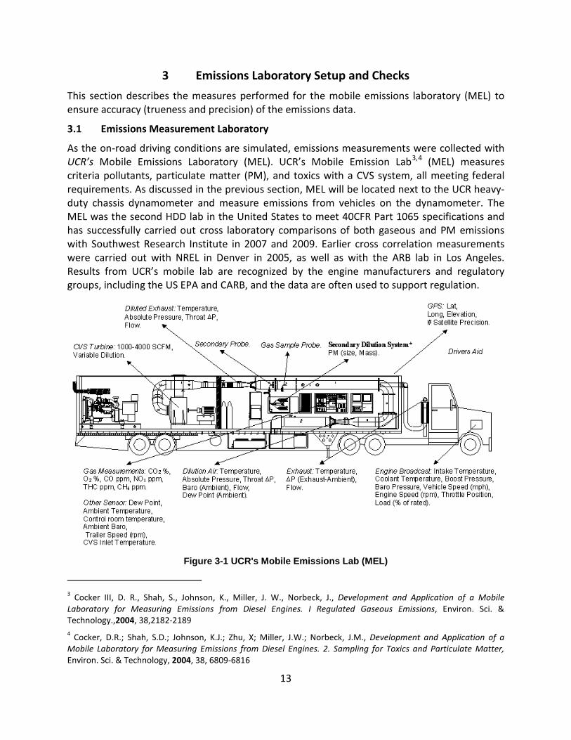
13
3 Emissions Laboratory Setup and Checks
This section describes the measures performed for the mobile emissions laboratory (MEL) to ensure accuracy (trueness and precision) of the emissions data.
3.1 Emissions Measurement Laboratory
As the on-road driving conditions are simulated, emissions measurements were collected with UCR’s Mobile Emissions Laboratory (MEL). UCR’s Mobile Emission Lab3,4
(MEL) measures criteria pollutants, particulate matter (PM), and toxics with a CVS system, all meeting federal requirements. As discussed in the previous section, MEL will be located next to the UCR heavy-duty chassis dynamometer and measure emissions from vehicles on the dynamometer. The MEL was the second HDD lab in the United States to meet 40CFR Part 1065 specifications and has successfully carried out cross laboratory comparisons of both gaseous and PM emissions with Southwest Research Institute in 2007 and 2009. Earlier cross correlation measurements were carried out with NREL in Denver in 2005, as well as with the ARB lab in Los Angeles. Results from UCR’s mobile lab are recognized by the engine manufacturers and regulatory groups, including the US EPA and CARB, and the data are often used to support regulation.
Figure 3-1 UCR's Mobile Emissions Lab (MEL)
3 Cocker III, D. R., Shah, S., Johnson, K., Miller, J. W., Norbeck, J., Development and Application of a Mobile Laboratory for Measuring Emissions from Diesel Engines. I Regulated Gaseous Emissions, Environ. Sci. & Technology.,2004, 38,2182-2189 4 Cocker, D.R.; Shah, S.D.; Johnson, K.J.; Zhu, X; Miller, J.W.; Norbeck, J.M., Development and Application of a Mobile Laboratory for Measuring Emissions from Diesel Engines. 2. Sampling for Toxics and Particulate Matter, Environ. Sci. & Technology, 2004, 38, 6809-6816
14
The first research carried out in the new combined HDD chassis-MEL facility involved a comparison of emissions from federally mandated diesel fuel with those from the stricter California formulation. The project successfully tested 15 heavy-duty trucks over a 75-day period, and so can easily handle the 22 vehicles within the time period specified for this RFP.
Instruments within MEL continuously measure emissions of NOx, CO, CO2, NMHC, and PM2.5 with one-second resolution. The Dekati Mass Monitor (DMM) was used for real-time PM sampling. Ultrafines were monitored using UCR’s unique fast-Scanning Mobility Particle Spectrometer (f-SMPS) analyzer5
The DMM measures PM mass concentrations through a combination of an electrical mobility diameter via particle charging and an aerodynamic diameter via inertial impaction over six stages of electrometers
, which is specifically designed for ultrafines. Integrated PM samples, such as PM mass and speciated PM, were collected on Teflo® and Quartz filters respectively.
6
The f-SMPS is a key tool for measuring particle size distribution; however, use for transient cycles was limited to gathering data from steady state cycles as use was limited by the time resolution of the SMPS. For this study a unique instrument designed at UCR
. The combination of mobility diameter and number averaged aerodynamic particle diameter allows estimation of particle mass with the assumption of a log normal distribution. The aerodynamic diameters are estimated from six impactor electrometers that range from 0.030 um to 0.532 µm. The mobility diameter estimates the sub 30 nm particle diameters. If the distribution is bimodal, the DMM assumes an average density of 1 g/cm3. The DMM also has an inlet precut classifier set around 1.32 µm. The DMM was operated on the faster response option, as opposed to the lower detection option. The faster response setting is more typical for transient emission testing.
7
Ammonia (NH3) concentration was continuously measured using a Tunable Diode Laser (TDL) unit that is part of MEL. Data in
was used to measure the near real time particle size distribution (PSD) with an emphasis on the ultrafine (<100nm) mass. The f-SMPS instrument utilizes a Radial Differential Mobility Analyzer (rDMA) and a Mixing Condensation Particle Counter (mCPC). The combination of these two components allowed the acquisition of particle size distributions range of 5–98 nm at rates of up to 0.4 Hz. For this research program the f-SMPS was setup for a 9 second scan time where typical SMPS’s utilize a 90 second scan time.
Figure 3-2 show the very rapid release of NH3 on acceleration and the quick response of the TDL used in UCR’s earlier research. Other measurement
5 S.D. Shah, D.R. Cocker*, ''A Fast Scanning Mobility Particle Spectrometer for Monitoring Particle Size Distributions From Vehicles,'' Aerosol Science and Technology, 39, 519-526, 2005. 6 Lehmann, U, V. Niemela, and Mohr, (2004) New Method for time-Resolved Diesel Engine Exhaust Particle Mass Measurement, Environ. Sci. Technol. 38 (21), 5704-5711, 2004
7 Sandip D. Shah and David R. Cocker III, A Fast Scanning Mobility Particle Spectrometer for Monitoring Transient Particle Size Distributions, Aerosol Science and Technology, 39:519–526, (2005)
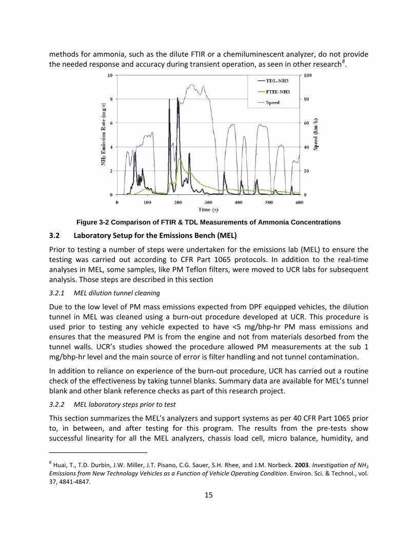
15
methods for ammonia, such as the dilute FTIR or a chemiluminescent analyzer, do not provide the needed response and accuracy during transient operation, as seen in other research8
.
Figure 3-2 Comparison of FTIR & TDL Measurements of Ammonia Concentrations
3.2 Laboratory Setup for the Emissions Bench (MEL)
Prior to testing a number of steps were undertaken for the emissions lab (MEL) to ensure the testing was carried out according to CFR Part 1065 protocols. In addition to the real-time analyses in MEL, some samples, like PM Teflon filters, were moved to UCR labs for subsequent analysis. Those steps are described in this section
3.2.1 MEL dilution tunnel cleaning
Due to the low level of PM mass emissions expected from DPF equipped vehicles, the dilution tunnel in MEL was cleaned using a burn-out procedure developed at UCR. This procedure is used prior to testing any vehicle expected to have <5 mg/bhp-hr PM mass emissions and ensures that the measured PM is from the engine and not from materials desorbed from the tunnel walls. UCR’s studies showed the procedure allowed PM measurements at the sub 1 mg/bhp-hr level and the main source of error is filter handling and not tunnel contamination.
In addition to reliance on experience of the burn-out procedure, UCR has carried out a routine check of the effectiveness by taking tunnel blanks. Summary data are available for MEL’s tunnel blank and other blank reference checks as part of this research project.
3.2.2 MEL laboratory steps prior to test
This section summarizes the MEL’s analyzers and support systems as per 40 CFR Part 1065 prior to, in between, and after testing for this program. The results from the pre-tests show successful linearity for all the MEL analyzers, chassis load cell, micro balance, humidity, and
8 Huai, T., T.D. Durbin, J.W. Miller, J.T. Pisano, C.G. Sauer, S.H. Rhee, and J.M. Norbeck. 2003. Investigation of NH3 Emissions from New Technology Vehicles as a Function of Vehicle Operating Condition. Environ. Sci. & Technol., vol. 37, 4841-4847.
16
other integrated systems. Steps prior to test and startup are included in a checklist as part of the SOP for MEL.
3.3 Laboratory Setup for the Off-line Analyses
This section provides information about the various analyses that were carried out in the UCR labs after the chassis test. Each of these test methods follows a Standing Operating Procedure created according to the EPA protocol guidance document9
3.3.1 Filter weighting for PM mass
.
The mass concentrations of PM2.5, metals and ions were acquired by analysis of particulates collected on 47mm diameter 2μm pore Teflo filters (Whatman brand). The filters were measured for net gains using a UMX2 ultra precision microbalance with buoyancy correction following the weighing procedure guidelines of the Code of Federal Regulations (CFR) (2). Before and after collection, the filters were conditioned for 24 hours in an environmentally controlled room (Tdry = 22 C and Tdew = 9.5C or 45%RH at Tdry 22C) and weighed daily until two consecutive weight measurements were within 3μg.
3.3.2 Measurement of Elemental and Organic Carbon (EC-OC)
OC/EC analysis was performed on samples collected on 2500 QAT-UP Tissuquartz Pall (Ann Arbor, MI) 47 mm filters that were preconditioned at 600°C for 5 h. A 1.5 cm2 punch is cut out from the quartz filter and analyzed with a Sunset Laboratory (Forest Grove, OR) Thermal/Optical Carbon Aerosol Analyzer according to the NIOSH 5040 reference method.
3.3.3 Measuring Carbonyls
Carbonyls are collected on 2,4-dinitrophenylhydrazine (DNPH) coated silica cartridges (Waters Corp., Milford, MA) after a Teflon filter. A critical flow orifice controls the flow to 1.0 LPM through the cartridge and the sample time is adjusted to draw a known volume of exhaust sample through the DNPH cartridge so that the amount of formaldehyde on the cartridge is at the mass level recommended by Waters. Sampled cartridges are extracted using 5 mL of acetonitrile and injected into an Agilent 1100 series high performance liquid chromatograph (HPLC) equipped with a diode array detector. The column is a 5μm Deltabond AK resolution (200cm x 4.6mm ID) with upstream guard column. The HPLC sample injection and operating conditions are set up according to the specifications of the SAE 930142HP protocol. Samples from the dilution air are collected for background correction.
3.3.4 Measuring volatile toxic compounds
Traditional air monitoring methods for direct measurement of very-volatile and volatile organic compounds (VVOC/VOC) are insensitive at the low levels found in exhaust from lean burn engines. Accordingly, UCR uses selective adsorbents for concentrating the molecules of interest after diluted exhaust gas passes through a Teflon filter. After collection, adsorbents are returned to the laboratory where the adsorbed molecules are flashed into a
9 United States Office of Environmental Protection Agency Information Bulleting EPA/600/B-07/001 Guidance for Preparing Standard Operating Procedures (SOPs) EPA QA/G-6, April 2007
17
concentrator/reservoir at low temperature, and then controllably vaporized into a gas chromatograph with a field ionization detector (GC/FID).
Molecules starting at approximately C4 (butadiene) to C6 (benzene) to C12 are effectively collected and concentrated on an adsorbent column composed with a multi-bed carbon bed including molecular sieve, activated charcoal, and carbotrap resin; each adsorbent has a specific selectivity towards certain boiling ranges or polarity. The adsorbent material first contacted in the column adsorbs the most volatile compounds, while the remaining compounds adsorb sequentially in relation to their volatility. The GC sample injection, columns, and operating conditions are set up according to the specifications of SAE 930142HP Method-2 for C4-C12 hydrocarbons. Samples from the dilution air are collected for background correction
3.3.5 Measuring nitrous oxide (N2O)
N2O emissions were collected in a Tedlar bags and analyzed using an outside laboratory equipped with a MKS Fourier Transform Infrared (FTIR) system. The absorption cell for the FTIR has a volume of 5 liters, and the residence time in the cell is approximately 10 seconds. UCR’s N2O FTIR was not available at the time of testing, thus, off-site analyses were carried out by the California Air resources Board and West Virginia University. Since the analysis of N2O was performed off-site UCR did not measure all vehicles in the test program due to logistics. Thus the analysis of N20 only reflects those vehicles sampled.
18
4 Quality Control/Quality Assurance
This section covers some of the quality control/assurance planning that was taken to assure the accuracy of the data.
4.1 Cross-laboratory Correlation
Five diesel vehicles were tested at both UCR and WVU. Although six laboratories are required for a statistically significant comparison, the data obtained from this study still allow a comparison of values from two independent laboratories and create a measure of the confidence in the accuracy of the data since the two laboratories would presumably not have the same bias in the data sets. Three port vehicles and two refuse haulers were jointly tested and comparative data for engine work and brake specific emissions are presented. The vehicles tested represent three different emission level categories from less than 0.2 g/bhp-hr to 1.2 g/bhp-hr NOx emission levels.
This cross-laboratory correlation task serves as a quality check for the emissions data that were collected independently by each laboratory. This correlation attempts to compare the emissions testing procedure of both laboratories that will include both the chassis dynamometer loading of the vehicle and the associated emissions measurement system. Although both WVU and UCR may adopt different procedures to conduct an emissions measurement campaign, the resulting data should be within an acceptable tolerance for real-world representativeness in each laboratory. Both UCR and WVU conducted the emissions measurement within immediate succession to prevent test vehicles going back into service. This procedure ensured the vehicle condition remained the same between WVU and UCR with no engine faults or maintenance conducted between the test intervals. Both laboratories tested the vehicle during day time conditions in Riverside Ca (as WVU was located only 5 miles away from UCR with their mobile laboratory setup)
Table 4-1 through Table 4-5 show the UCR and WVU engine work and selected emissions for five different shared vehicles including the cycle to cycle averaged coefficient of variation (COV). The emissions comparison is on a brake specific basis and includes bsCO2, bsNOx, bsPM, and bsNH3 with units of g/bhp-hr for all species. Chassis dynamometer data is traditionally reported as distance-specific. However, for laboratory comparison purposes, changes in vehicle loading procedure and dynamometer setup can result in differences in distance-specific emissions. Therefore, brake-specific emissions were chosen as metric for comparison as components such as CO2 are linear with work done by the engine.
Engine Work: Five diesel vehicles were tested by both UCR and WVU for cross-laboratory comparison. Although six laboratories are required for a statistically significant comparison, the data obtained from this study still allow a comparison of values from two independent laboratories and create a measure of confidence in the accuracy of the data since the two laboratories would presumably not have the same bias in the data sets. Three port vehicles and two refuse haulers were jointly tested and comparative data for engine work and brake specific emissions are presented. The vehicles tested represent three different emission level categories from less than 0.2 g/bhp-hr to 1.2 g/bhp-hr NOx emission levels.
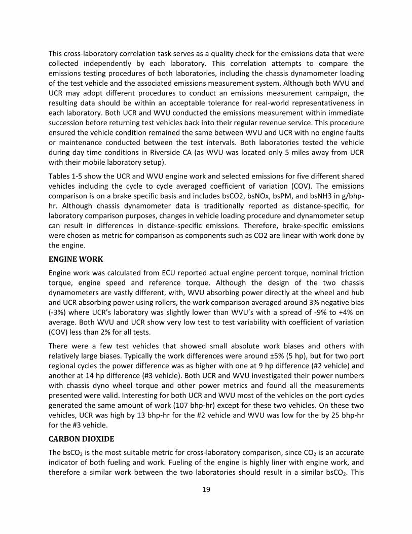
19
This cross-laboratory correlation task serves as a quality check for the emissions data that were collected independently by each laboratory. This correlation attempts to compare the emissions testing procedures of both laboratories, including the chassis dynamometer loading of the test vehicle and the associated emissions measurement system. Although both WVU and UCR may adopt different procedures to conduct an emissions measurement campaign, the resulting data should be within an acceptable tolerance for real-world representativeness in each laboratory. Both UCR and WVU conducted the emissions measurement within immediate succession before returning test vehicles back into their regular revenue service. This procedure ensured the vehicle condition remained the same between WVU and UCR with no engine faults or maintenance conducted between the test intervals. Both laboratories tested the vehicle during day time conditions in Riverside CA (as WVU was located only 5 miles away from UCR with their mobile laboratory setup).
Tables 1-5 show the UCR and WVU engine work and selected emissions for five different shared vehicles including the cycle to cycle averaged coefficient of variation (COV). The emissions comparison is on a brake specific basis and includes bsCO2, bsNOx, bsPM, and bsNH3 in g/bhp-hr. Although chassis dynamometer data is traditionally reported as distance-specific, for laboratory comparison purposes, changes in vehicle loading procedure and dynamometer setup can result in differences in distance-specific emissions. Therefore, brake-specific emissions were chosen as metric for comparison as components such as CO2 are linear with work done by the engine.
ENGINE WORK
Engine work was calculated from ECU reported actual engine percent torque, nominal friction torque, engine speed and reference torque. Although the design of the two chassis dynamometers are vastly different, with, WVU absorbing power directly at the wheel and hub and UCR absorbing power using rollers, the work comparison averaged around 3% negative bias (-3%) where UCR’s laboratory was slightly lower than WVU’s with a spread of -9% to +4% on average. Both WVU and UCR show very low test to test variability with coefficient of variation (COV) less than 2% for all tests.
There were a few test vehicles that showed small absolute work biases and others with relatively large biases. Typically the work differences were around ±5% (5 hp), but for two port regional cycles the power difference was as higher with one at 9 hp difference (#2 vehicle) and another at 14 hp difference (#3 vehicle). Both UCR and WVU investigated their power numbers with chassis dyno wheel torque and other power metrics and found all the measurements presented were valid. Interesting for both UCR and WVU most of the vehicles on the port cycles generated the same amount of work (107 bhp-hr) except for these two vehicles. On these two vehicles, UCR was high by 13 bhp-hr for the #2 vehicle and WVU was low for the by 25 bhp-hr for the #3 vehicle.
CARBON DIOXIDE
The bsCO2 is the most suitable metric for cross-laboratory comparison, since CO2 is an accurate indicator of both fueling and work. Fueling of the engine is highly liner with engine work, and therefore a similar work between the two laboratories should result in a similar bsCO2. This
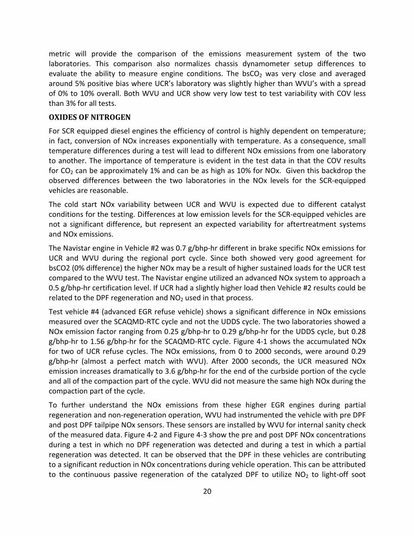
20
metric will provide the comparison of the emissions measurement system of the two laboratories. This comparison also normalizes chassis dynamometer setup differences to evaluate the ability to measure engine conditions. The bsCO2 was very close and averaged around 5% positive bias where UCR’s laboratory was slightly higher than WVU’s with a spread of 0% to 10% overall. Both WVU and UCR show very low test to test variability with COV less than 3% for all tests.
OXIDES OF NITROGEN
For SCR equipped diesel engines the efficiency of control is highly dependent on temperature; in fact, conversion of NOx increases exponentially with temperature. As a consequence, small temperature differences during a test will lead to different NOx emissions from one laboratory to another. The importance of temperature is evident in the test data in that the COV results for CO2 can be approximately 1% and can be as high as 10% for NOx. Given this backdrop the observed differences between the two laboratories in the NOx levels for the SCR-equipped vehicles are reasonable.
The cold start NOx variability between UCR and WVU is expected due to different catalyst conditions for the testing. Differences at low emission levels for the SCR-equipped vehicles are not a significant difference, but represent an expected variability for aftertreatment systems and NOx emissions.
The Navistar engine in Vehicle #2 was 0.7 g/bhp-hr different in brake specific NOx emissions for UCR and WVU during the regional port cycle. Since both showed very good agreement for bsCO2 (0% difference) the higher NOx may be a result of higher sustained loads for the UCR test compared to the WVU test. The Navistar engine utilized an advanced NOx system to approach a 0.5 g/bhp-hr certification level. If UCR had a slightly higher load then Vehicle #2 results could be related to the DPF regeneration and NO2 used in that process.
Test vehicle #4 (advanced EGR refuse vehicle) shows a significant difference in NOx emissions measured over the SCAQMD-RTC cycle and not the UDDS cycle. The two laboratories showed a NOx emission factor ranging from 0.25 g/bhp-hr to 0.29 g/bhp-hr for the UDDS cycle, but 0.28 g/bhp-hr to 1.56 g/bhp-hr for the SCAQMD-RTC cycle. Figure 4-1 shows the accumulated NOx for two of UCR refuse cycles. The NOx emissions, from 0 to 2000 seconds, were around 0.29 g/bhp-hr (almost a perfect match with WVU). After 2000 seconds, the UCR measured NOx emission increases dramatically to 3.6 g/bhp-hr for the end of the curbside portion of the cycle and all of the compaction part of the cycle. WVU did not measure the same high NOx during the compaction part of the cycle.
To further understand the NOx emissions from these higher EGR engines during partial regeneration and non-regeneration operation, WVU had instrumented the vehicle with pre DPF and post DPF tailpipe NOx sensors. These sensors are installed by WVU for internal sanity check of the measured data. Figure 4-2 and Figure 4-3 show the pre and post DPF NOx concentrations during a test in which no DPF regeneration was detected and during a test in which a partial regeneration was detected. It can be observed that the DPF in these vehicles are contributing to a significant reduction in NOx concentrations during vehicle operation. This can be attributed to the continuous passive regeneration of the catalyzed DPF to utilize NO2 to light-off soot
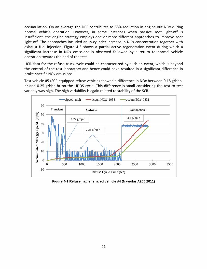
21
accumulation. On an average the DPF contributes to 68% reduction in engine-out NOx during normal vehicle operation. However, in some instances when passive soot light-off is insufficient, the engine strategy employs one or more different approaches to improve soot light off. The approaches included an in-cylinder increase in NOx concentration together with exhaust fuel injection. Figure 4-3 shows a partial active regeneration event during which a significant increase in NOx emissions is observed followed by a return to normal vehicle operation towards the end of the test.
UCR data for the refuse truck cycle could be characterized by such an event, which is beyond the control of the test laboratory and hence could have resulted in a significant difference in brake-specific NOx emissions.
Test vehicle #5 (SCR equipped refuse vehicle) showed a difference in NOx between 0.18 g/bhp-hr and 0.25 g/bhp-hr on the UDDS cycle. This difference is small considering the test to test variably was high. The high variability is again related to stability of the SCR.
Figure 4-1 Refuse hauler shared vehicle #4 (Navistar A260 2011)
-10
0
10
20
30
40
50
60
0 500 1000 1500 2000 2500 3000 3500Acc
umul
ated
NO
x (g
), Sp
eed
(mph
)
Refuse Cycle Time (sec)
Speed_mph accumNOx_1058 accumNOx_0831
Transient Curbside Compaction
3.8 g/hp-h0.27 g/hp-h
0.28 g/hp-h
22
Figure 4-2 Pre and Post DPF NOx concentration for a non-regeneration vehicle operation
Figure 4-3 Pre and Post DPF NOx during partial active regeneration during refuse truck cycle
Particulate Matter: The bsPM emission levels were low for both UCR and WVU and were below the PM certification value for all tests and typically around 10% of the standard (< 1 mg/bhp-h) as expected for a properly functioning DPF. The PM emissions were thus similar between both laboratories and no significant outliers were identified.
0
20
40
60
80
100
120
140
160
180
200
0 500 1000 1500 2000
NO
x Co
ncen
trat
ion
(ppm
)
Time (sec)
Post DPF NOx Concentration
Pre DPF NOx Concentration
0
200
400
600
800
1000
1200
0 500 1000 1500 2000
NO
x Co
ncen
trat
ion
(ppm
)
Time (sec)
Post DPF NOx Concentration
Pre DPF NOx Concentration
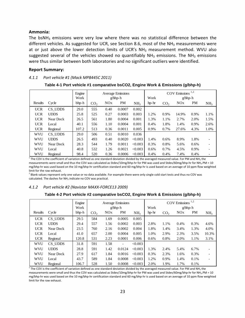
23
Ammonia: The bsNH3 emissions were very low where there was no statistical difference between the different vehicles. As suggested for UCR, see Section 8.6, most of the NH3 measurements were at or just above the lower detection limits of UCR’s NH3 measurement method. WVU also suggested several of the vehicles showed no quantifiably NH3 emissions. The NH3 emissions were thus similar between both laboratories and no significant outliers were identified.
Report Summary:
4.1.1 Port vehicle #1 (Mack MP8445C 2011)
Table 4-1 Port vehicle #1 comparative bsCO2, Engine Work & Emissions (g/bhp-h)
1 The COV is the coefficient of variation defined as one standard deviation divided by the averaged measured value. For PM and NH3 the measurements were small and thus the COV was calculated as Stdev/10mg/bhp-hr for PM was used and Stdev/60mg/bhp-hr for NH3.PM = 10 mg/bhp-hr was used based on the 10 mg/bhp-hr certification standard and 60 mg/bhp-hr is used based on an average of 10 ppm flow weighted limit for the raw exhaust. 2 Blank values represent only one value or no data available. For example there were only single cold start tests and thus no COV was calculated. The dashes for NH3 indicate no COV was practical.
4.1.2 Port vehicle #2 (Navistar MAXX-FORCE13 2009)
Table 4-2 Port vehicle #2 comparative bsCO2, Engine Work & Emissions (g/bhp-h)
1 The COV is the coefficient of variation defined as one standard deviation divided by the averaged measured value. For PM and NH3 the measurements were small and thus the COV was calculated as Stdev/10mg/bhp-hr for PM was used and Stdev/60mg/bhp-hr for NH3.PM = 10 mg/bhp-hr was used based on the 10 mg/bhp-hr certification standard and 60 mg/bhp-hr is used based on an average of 10 ppm flow weighted limit for the raw exhaust.
EngineWork Work
Results Cycle bhp-h CO2 NOx PM NH3 hp-hr CO2 NOx PM NH3
UCR CS_UDDS 29.0 555 0.40 0.0007 0.002UCR UDDS 25.8 525 0.27 0.0003 0.003 1.2% 0.9% 14.9% 0.9% 1.1%UCR Near Dock 26.5 561 1.80 0.0004 0.001 1.3% 1.1% 2.7% 2.0% 1.5%UCR Local 40.1 556 1.10 0.0004 0.001 0.4% 1.8% 1.4% 0.9% 2.6%UCR Regional 107.2 513 0.36 0.0011 0.005 0.9% 0.7% 27.6% 4.3% 1.0%WVU CS_UDDS 29.0 506 0.51 0.0010 0.036WVU UDDS 26.5 493 0.40 0.0020 <0.003 1.4% 0.6% 8.9% 1.8% -WVU Near Dock 28.3 544 1.79 0.0011 <0.003 0.3% 0.8% 5.6% 0.6% -WVU Local 40.8 532 1.26 0.0021 <0.003 0.6% 0.7% 4.5% 0.9% -WVU Regional 98.4 520 0.36 0.0006 <0.003 0.4% 0.4% 7.4% 0.4% -
g/bhp-hAverage Emissions COV Emissions 1,2
g/bhp-h
EngineWork Work
Results Cycle bhp-h CO2 NOx PM NH3 hp-hr CO2 NOx PM NH3
UCR CS_UDDS 29.5 584 1.69 0.0005 0.005UCR UDDS 29.4 557 1.56 0.0002 0.003 2.8% 1.1% 0.4% 0.3% 4.6%UCR Near Dock 23.5 760 2.16 0.0002 0.004 1.8% 1.4% 3.4% 1.3% 4.0%UCR Local 41.0 657 2.00 0.0004 0.005 1.0% 2.9% 2.3% 3.5% 10.3%UCR Regional 120.8 531 2.23 0.0001 0.006 0.6% 0.8% 2.0% 1.1% 3.1%WVU CS_UDDS 31.8 591 1.58 - <0.003WVU UDDS 28.8 591 1.42 0.0124 <0.003 1.3% 2.4% 5.4% 6.7% -WVU Near Dock 27.9 617 1.84 0.0016 <0.003 0.3% 2.3% 1.6% 0.3% -WVU Local 43.7 589 1.84 0.0008 <0.003 1.2% 0.9% 1.4% 0.1% -WVU Regional 106.7 528 1.50 0.0008 <0.003 2.0% 1.9% 1.7% 0.1%
g/bhp-h g/bhp-hAverage Emissions COV Emissions 1,2
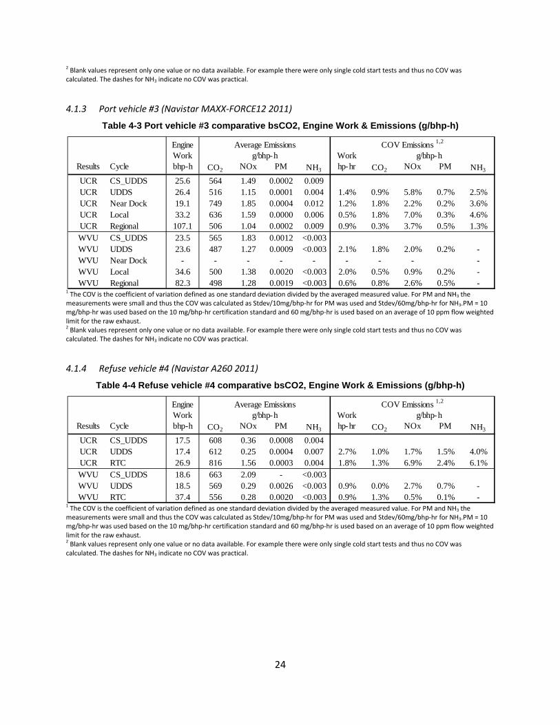
24
2 Blank values represent only one value or no data available. For example there were only single cold start tests and thus no COV was calculated. The dashes for NH3 indicate no COV was practical.
4.1.3 Port vehicle #3 (Navistar MAXX-FORCE12 2011)
Table 4-3 Port vehicle #3 comparative bsCO2, Engine Work & Emissions (g/bhp-h)
1 The COV is the coefficient of variation defined as one standard deviation divided by the averaged measured value. For PM and NH3 the measurements were small and thus the COV was calculated as Stdev/10mg/bhp-hr for PM was used and Stdev/60mg/bhp-hr for NH3.PM = 10 mg/bhp-hr was used based on the 10 mg/bhp-hr certification standard and 60 mg/bhp-hr is used based on an average of 10 ppm flow weighted limit for the raw exhaust. 2 Blank values represent only one value or no data available. For example there were only single cold start tests and thus no COV was calculated. The dashes for NH3 indicate no COV was practical.
4.1.4 Refuse vehicle #4 (Navistar A260 2011)
Table 4-4 Refuse vehicle #4 comparative bsCO2, Engine Work & Emissions (g/bhp-h)
1 The COV is the coefficient of variation defined as one standard deviation divided by the averaged measured value. For PM and NH3 the measurements were small and thus the COV was calculated as Stdev/10mg/bhp-hr for PM was used and Stdev/60mg/bhp-hr for NH3.PM = 10 mg/bhp-hr was used based on the 10 mg/bhp-hr certification standard and 60 mg/bhp-hr is used based on an average of 10 ppm flow weighted limit for the raw exhaust. 2 Blank values represent only one value or no data available. For example there were only single cold start tests and thus no COV was calculated. The dashes for NH3 indicate no COV was practical.
EngineWork Work
Results Cycle bhp-h CO2 NOx PM NH3 hp-hr CO2 NOx PM NH3
UCR CS_UDDS 25.6 564 1.49 0.0002 0.009UCR UDDS 26.4 516 1.15 0.0001 0.004 1.4% 0.9% 5.8% 0.7% 2.5%UCR Near Dock 19.1 749 1.85 0.0004 0.012 1.2% 1.8% 2.2% 0.2% 3.6%UCR Local 33.2 636 1.59 0.0000 0.006 0.5% 1.8% 7.0% 0.3% 4.6%UCR Regional 107.1 506 1.04 0.0002 0.009 0.9% 0.3% 3.7% 0.5% 1.3%WVU CS_UDDS 23.5 565 1.83 0.0012 <0.003WVU UDDS 23.6 487 1.27 0.0009 <0.003 2.1% 1.8% 2.0% 0.2% -WVU Near Dock - - - - - - - - -WVU Local 34.6 500 1.38 0.0020 <0.003 2.0% 0.5% 0.9% 0.2% -WVU Regional 82.3 498 1.28 0.0019 <0.003 0.6% 0.8% 2.6% 0.5% -
g/bhp-h g/bhp-hAverage Emissions COV Emissions 1,2
EngineWork Work
Results Cycle bhp-h CO2 NOx PM NH3 hp-hr CO2 NOx PM NH3
UCR CS_UDDS 17.5 608 0.36 0.0008 0.004UCR UDDS 17.4 612 0.25 0.0004 0.007 2.7% 1.0% 1.7% 1.5% 4.0%UCR RTC 26.9 816 1.56 0.0003 0.004 1.8% 1.3% 6.9% 2.4% 6.1%WVU CS_UDDS 18.6 663 2.09 - <0.003WVU UDDS 18.5 569 0.29 0.0026 <0.003 0.9% 0.0% 2.7% 0.7% -WVU RTC 37.4 556 0.28 0.0020 <0.003 0.9% 1.3% 0.5% 0.1% -
COV Emissions 1,2 Average Emissionsg/bhp-h g/bhp-h
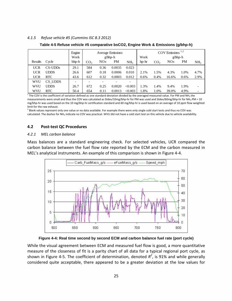
25
4.1.5 Refuse vehicle #5 (Cummins ISC 8.3 2012)
Table 4-5 Refuse vehicle #5 comparative bsCO2, Engine Work & Emissions (g/bhp-h)
1 The COV is the coefficient of variation defined as one standard deviation divided by the averaged measured value. For PM and NH3 the measurements were small and thus the COV was calculated as Stdev/10mg/bhp-hr for PM was used and Stdev/60mg/bhp-hr for NH3.PM = 10 mg/bhp-hr was used based on the 10 mg/bhp-hr certification standard and 60 mg/bhp-hr is used based on an average of 10 ppm flow weighted limit for the raw exhaust. 2 Blank values represent only one value or no data available. For example there were only single cold start tests and thus no COV was calculated. The dashes for NH3 indicate no COV was practical. WVU did not have a cold start test on this vehicle due to vehicle availability.
4.2 Post-test QC Procedures
4.2.1 MEL carbon balance
Mass balances are a standard engineering check. For selected vehicles, UCR compared the carbon balance between the fuel flow rate reported by the ECM and the carbon measured in MEL’s analytical instruments. An example of this comparison is shown in Figure 4-4.
Figure 4-4: Real time second by second ECM and carbon balance fuel rate (port cycle)
While the visual agreement between ECM and measured fuel flow is good, a more quantitative measure of the closeness of fit is a parity chart of all data for a typical regional port cycle, as shown in Figure 4-5. The coefficient of determination, denoted R2, is 91% and while generally considered quite acceptable, there appeared to be a greater deviation at the low values for
EngineWork Work
Results Cycle bhp-h CO2 NOx PM NH3 hp-hr CO2 NOx PM NH3
UCR CS-UDDs 29.1 584 0.36 0.0035 0.023UCR UDDS 26.6 607 0.18 0.0006 0.010 2.1% 1.5% 4.3% 1.0% 4.7%UCR RTC 43.6 612 0.32 0.0003 0.012 0.6% 0.4% 16.6% 0.6% 2.9%WVU CS_UDDS - - - - -WVU UDDS 26.7 672 0.25 0.0020 <0.003 1.3% 1.4% 9.4% 1.9% -WVU RTC 50.4 654 0.11 0.0013 <0.003 1.8% 1.0% 39.0% 4.9% -
COV Emissions 1,2 Average Emissionsg/bhp-h g/bhp-h
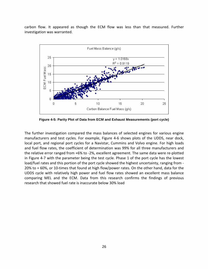
26
carbon flow. It appeared as though the ECM flow was less than that measured. Further investigation was warranted.
Figure 4-5: Parity Plot of Data from ECM and Exhaust Measurements (port cycle)
The further investigation compared the mass balances of selected engines for various engine manufacturers and test cycles. For example, Figure 4-6 shows plots of the UDDS, near dock, local port, and regional port cycles for a Navistar, Cummins and Volvo engine. For high loads and fuel flow rates, the coefficient of determination was 99% for all three manufacturers and the relative error ranged from +6% to -2%, excellent agreement. The same data were re-plotted in Figure 4-7 with the parameter being the test cycle. Phase 1 of the port cycle has the lowest load/fuel rates and this portion of the port cycle showed the highest uncertainty, ranging from -20% to + 60%, or 10-times that found at high flow/power rates. On the other hand, data for the UDDS cycle with relatively high power and fuel flow rates showed an excellent mass balance comparing MEL and the ECM. Data from this research confirms the findings of previous research that showed fuel rate is inaccurate below 30% load
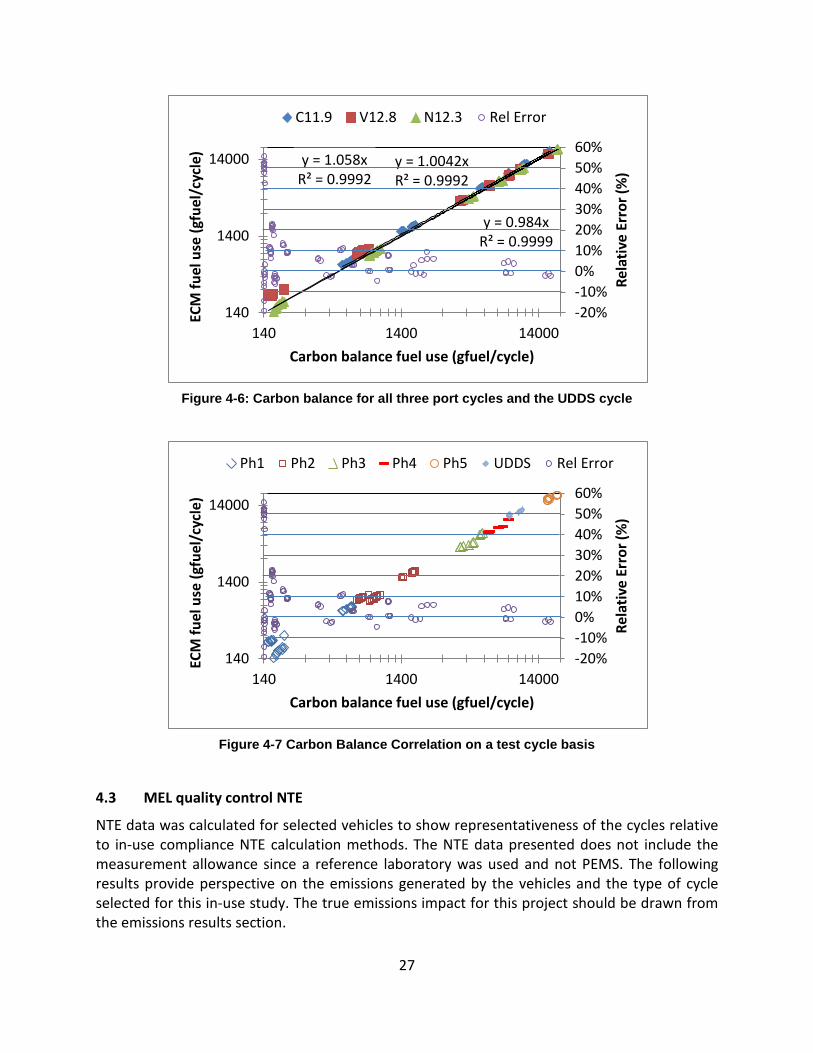
27
Figure 4-6: Carbon balance for all three port cycles and the UDDS cycle
Figure 4-7 Carbon Balance Correlation on a test cycle basis
4.3 MEL quality control NTE
NTE data was calculated for selected vehicles to show representativeness of the cycles relative to in-use compliance NTE calculation methods. The NTE data presented does not include the measurement allowance since a reference laboratory was used and not PEMS. The following results provide perspective on the emissions generated by the vehicles and the type of cycle selected for this in-use study. The true emissions impact for this project should be drawn from the emissions results section.
y = 1.058xR² = 0.9992
y = 1.0042xR² = 0.9992
y = 0.984xR² = 0.9999
-20%-10%0%10%20%30%40%50%60%
140
1400
14000
140 1400 14000
Rela
tive
Err
or (%
)
ECM
fuel
use
(gfu
el/c
ycle
)
Carbon balance fuel use (gfuel/cycle)
C11.9 V12.8 N12.3 Rel Error
-20%-10%0%10%20%30%40%50%60%
140
1400
14000
140 1400 14000
Rela
tive
Err
or (%
)
ECM
fuel
use
(gfu
el/c
ycle
)
Carbon balance fuel use (gfuel/cycle)
Ph1 Ph2 Ph3 Ph4 Ph5 UDDS Rel Error
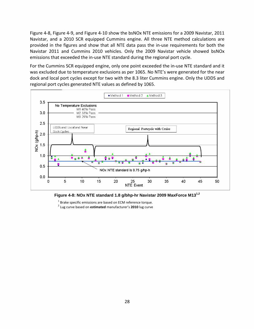
28
Figure 4-8, Figure 4-9, and Figure 4-10 show the bsNOx NTE emissions for a 2009 Navistar, 2011 Navistar, and a 2010 SCR equipped Cummins engine. All three NTE method calculations are provided in the figures and show that all NTE data pass the in-use requirements for both the Navistar 2011 and Cummins 2010 vehicles. Only the 2009 Navistar vehicle showed bsNOx emissions that exceeded the in-use NTE standard during the regional port cycle.
For the Cummins SCR equipped engine, only one point exceeded the in-use NTE standard and it was excluded due to temperature exclusions as per 1065. No NTE’s were generated for the near dock and local port cycles except for two with the 8.3 liter Cummins engine. Only the UDDS and regional port cycles generated NTE values as defined by 1065.
Figure 4-8: NOx NTE standard 1.8 g/bhp-hr Navistar 2009 MaxForce M131,2
1 Brake specific emissions are based on ECM reference torque. 2 Lug curve based on estimated manufacturer’s 2010 lug curve
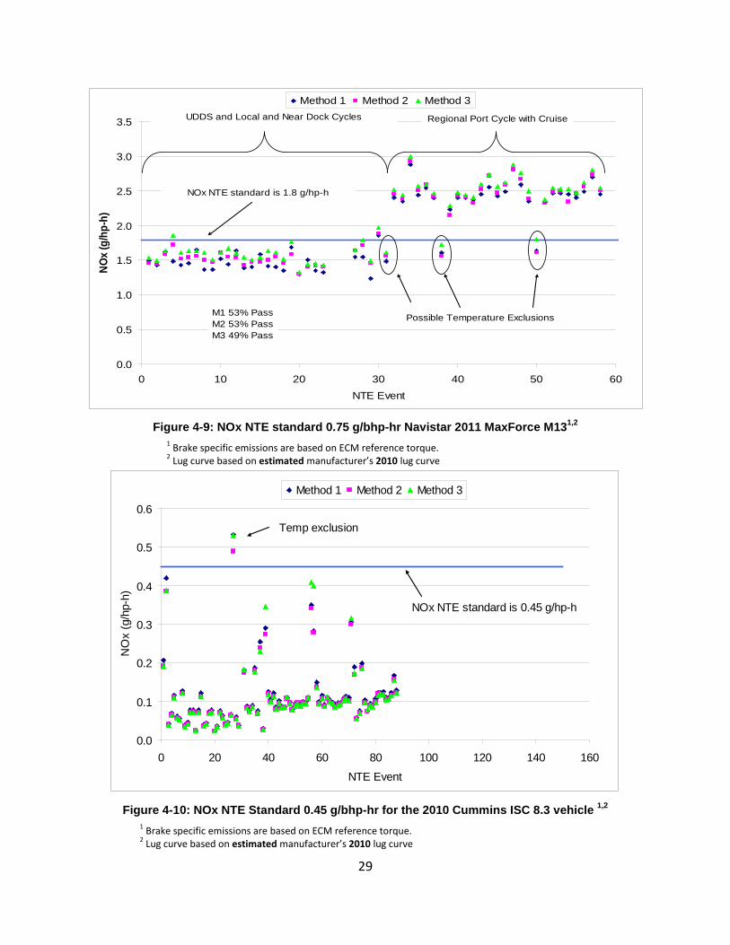
29
Figure 4-9: NOx NTE standard 0.75 g/bhp-hr Navistar 2011 MaxForce M131,2
1 Brake specific emissions are based on ECM reference torque. 2 Lug curve based on estimated manufacturer’s 2010 lug curve
Figure 4-10: NOx NTE Standard 0.45 g/bhp-hr for the 2010 Cummins ISC 8.3 vehicle 1,2
1 Brake specific emissions are based on ECM reference torque. 2 Lug curve based on estimated manufacturer’s 2010 lug curve
0.0
0.5
1.0
1.5
2.0
2.5
3.0
3.5
0 10 20 30 40 50 60NTE Event
NOx
(g/h
p-h)
Method 1 Method 2 Method 3
NOx NTE standard is 1.8 g/hp-h
M1 53% PassM2 53% PassM3 49% Pass
Possible Temperature Exclusions
Regional Port Cycle with CruiseUDDS and Local and Near Dock Cycles
0.0
0.1
0.2
0.3
0.4
0.5
0.6
0 20 40 60 80 100 120 140 160
NTE Event
NO
x (g
/hp-
h)
Method 1 Method 2 Method 3
NOx NTE standard is 0.45 g/hp-h
Temp exclusion
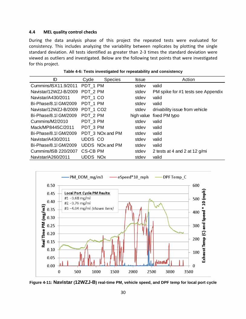
30
4.4 MEL quality control checks
During the data analysis phase of this project the repeated tests were evaluated for consistency. This includes analyzing the variability between replicates by plotting the single standard deviation. All tests identified as greater than 2-3 times the standard deviation were viewed as outliers and investigated. Below are the following test points that were investigated for this project.
Table 4-6: Tests investigated for repeatability and consistency
Figure 4-11: Navistar (12WZJ-B) real-time PM, vehicle speed, and DPF temp for local port cycle
ID Cycle Species Issue ActionCummins/ISX11.9/2011 PDT_1 PM stdev validNavistar/12WZJ-B/2009 PDT_2 PM stdev PM spike for #1 tests see AppendixNavistar/A430/2011 PDT_1 CO stdev validBi-Phase/8.1l GM/2009 PDT_1 PM stdev validNavistar/12WZJ-B/2009 PDT_1 CO2 stdev drivability issue from vehicleBi-Phase/8.1l GM/2009 PDT_2 PM high value fixed PM typoCummins/M2/2010 PDT_3 PM stdev validMack/MP8445C/2011 PDT_3 PM stdev validBi-Phase/8.1l GM/2009 PDT_3 NOx and PM stdev validNavistar/A430/2011 UDDS CO stdev validBi-Phase/8.1l GM/2009 UDDS NOx and PM stdev validCummins/ISB 220/2007 CS-CB PM stdev 2 tests at 4 and 2 at 12 g/miNavistar/A260/2011 UDDS NOx stdev valid
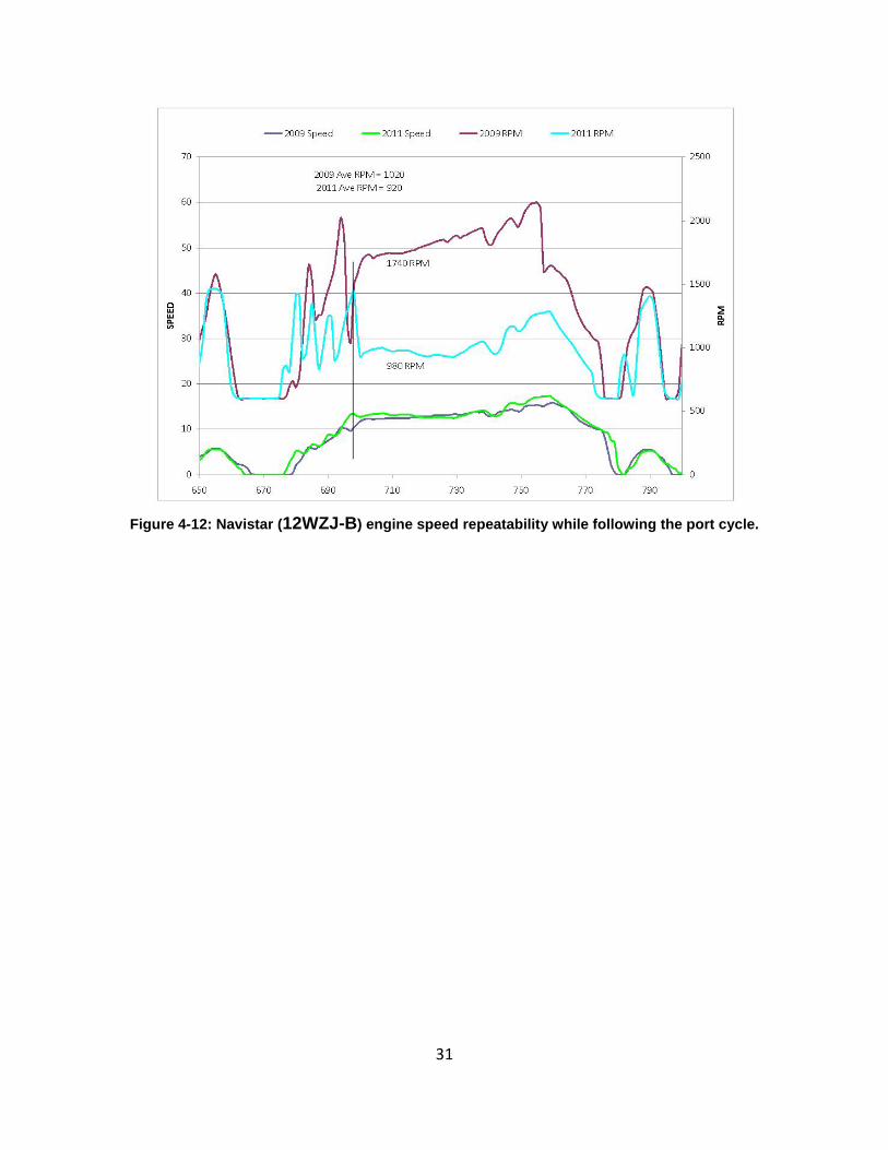
31
Figure 4-12: Navistar (12WZJ-B) engine speed repeatability while following the port cycle.
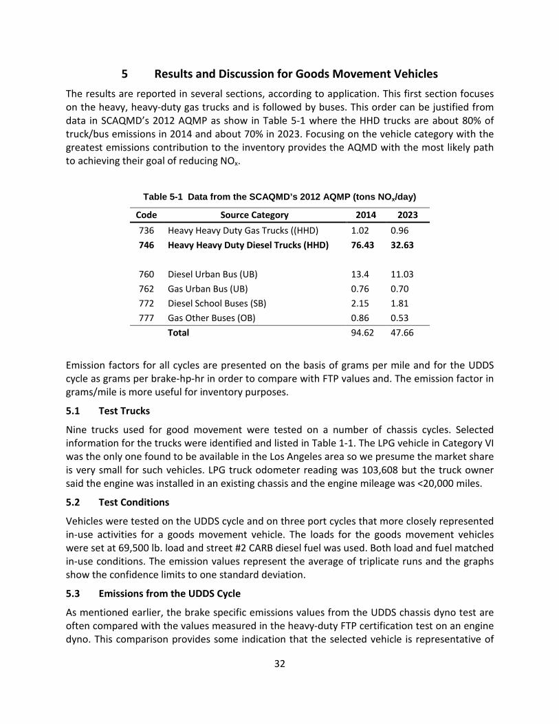
32
5 Results and Discussion for Goods Movement Vehicles
The results are reported in several sections, according to application. This first section focuses on the heavy, heavy-duty gas trucks and is followed by buses. This order can be justified from data in SCAQMD’s 2012 AQMP as show in Table 5-1 where the HHD trucks are about 80% of truck/bus emissions in 2014 and about 70% in 2023. Focusing on the vehicle category with the greatest emissions contribution to the inventory provides the AQMD with the most likely path to achieving their goal of reducing NOx.
Table 5-1 Data from the SCAQMD’s 2012 AQMP (tons NOx/day)
Code Source Category 2014 2023
736 Heavy Heavy Duty Gas Trucks ((HHD) 1.02 0.96
746 Heavy Heavy Duty Diesel Trucks (HHD) 76.43 32.63
760 Diesel Urban Bus (UB) 13.4 11.03
762 Gas Urban Bus (UB) 0.76 0.70
772 Diesel School Buses (SB) 2.15 1.81
777 Gas Other Buses (OB) 0.86 0.53
Total 94.62 47.66
Emission factors for all cycles are presented on the basis of grams per mile and for the UDDS cycle as grams per brake-hp-hr in order to compare with FTP values and. The emission factor in grams/mile is more useful for inventory purposes.
5.1 Test Trucks
Nine trucks used for good movement were tested on a number of chassis cycles. Selected information for the trucks were identified and listed in Table 1-1. The LPG vehicle in Category VI was the only one found to be available in the Los Angeles area so we presume the market share is very small for such vehicles. LPG truck odometer reading was 103,608 but the truck owner said the engine was installed in an existing chassis and the engine mileage was <20,000 miles.
5.2 Test Conditions
Vehicles were tested on the UDDS cycle and on three port cycles that more closely represented in-use activities for a goods movement vehicle. The loads for the goods movement vehicles were set at 69,500 lb. load and street #2 CARB diesel fuel was used. Both load and fuel matched in-use conditions. The emission values represent the average of triplicate runs and the graphs show the confidence limits to one standard deviation.
5.3 Emissions from the UDDS Cycle
As mentioned earlier, the brake specific emissions values from the UDDS chassis dyno test are often compared with the values measured in the heavy-duty FTP certification test on an engine dyno. This comparison provides some indication that the selected vehicle is representative of
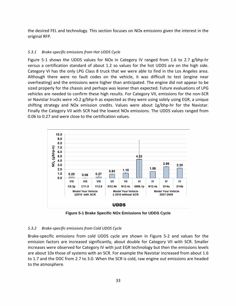
33
the desired FEL and technology. This section focuses on NOx emissions given the interest in the original RFP.
5.3.1 Brake-specific emissions from Hot UDDS Cycle
Figure 5-1 shows the UDDS values for NOx in Category IV ranged from 1.6 to 2.7 g/bhp-hr versus a certification standard of about 1.2 so values for the hot UDDS are on the high side. Category VI has the only LPG Class 8 truck that we were able to find in the Los Angeles area. Although there were no fault codes on the vehicle, it was difficult to test (engine near overheating) and the emissions were higher than anticipated. The engine did not appear to be sized properly for the chassis and perhaps was leaner than expected. Future evaluations of LPG vehicles are needed to confirm these high results. For Category VII, emissions for the non-SCR or Navistar trucks were >0.2 g/bhp-h as expected as they were using solely using EGR, a unique shifting strategy and NOx emission credits. Values were about 1g/bhp-hr for the Navistar. Finally the Category VII with SCR had the lowest NOx emissions. The UDDS values ranged from 0.06 to 0.27 and were close to the certification values.
Figure 5-1 Brake Specific NOx Emissions for UDDS Cycle
5.3.2 Brake-specific emissions from Cold UDDS Cycle
Brake-specific emissions from cold UDDS cycle are shown in Figure 5-2 and values for the emission factors are increased significantly, about double for Category VII with SCR. Smaller increases were observed for Category IV with just EGR technology but then the emissions levels are about 10x those of systems with an SCR. For example the Navistar increased from about 1.6 to 1.7 and the DDC from 2.7 to 3.0. When the SCR is cold, raw engine out emissions are headed to the atmosphere.
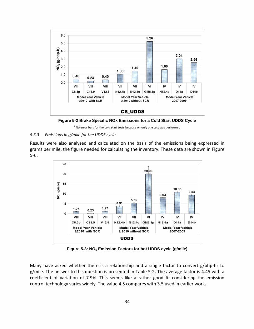
34
Figure 5-2 Brake Specific NOx Emissions for a Cold Start UDDS Cycle
1 No error bars for the cold start tests because on only one test was performed
5.3.3 Emissions in g/mile for the UDDS cycle
Results were also analyzed and calculated on the basis of the emissions being expressed in grams per mile, the figure needed for calculating the inventory. These data are shown in Figure 5-6.
Figure 5-3: NOx Emission Factors for hot UDDS cycle (g/mile)
Many have asked whether there is a relationship and a single factor to convert g/bhp-hr to g/mile. The answer to this question is presented in Table 5-2. The average factor is 4.45 with a coefficient of variation of 7.9%. This seems like a rather good fit considering the emission control technology varies widely. The value 4.5 compares with 3.5 used in earlier work.
35
Table 5-2 Relationship Between g/mile & g/bhp-hr for the Hot UDDS
NOx emissions in g/mile for a cold UDDS cycle are presented in Figure 5-4. Values were a multiple of the values for the hot UDDS cycle, as expected. Note that NOx emissions 1 mile after cold start equal 2 miles after hot start.
Figure 5-4: NOx Emission factors for Cold Start UDDS Cycle (g/mile)
1 No error bars for the cold start tests because on only one test was performed
Apportioning the NOx emissions into NO and NO2 was part of the analysis. These data are shown in Table 5-3. Excluding the LPG truck, the percentage of NO2 ranges from 24% to 59% and most values are >50%. These values are reminiscent of the early retrofit data and the subsequent rule that limited the increase above baseline to a 20% increase. Thus if the baseline was 10%, then the control technology was limited to 30%,
36
Table 5-3: Fraction of NO2 to total NOx for the Vehicles on the UDDS cycles
Figure 5-5 shows the NOx emissions for the cold and hot start UDDS cycles for the port vehicles. In general NOx increased for the cold start and varied by a factor of 3 higher for the Cummins 11.9 SCR equipped vehicle (C11.9) to only a 6% increase for the Navistar 12.4 liter non SCR equipped vehicle (N12.4b). The cold start NOx emissions were much higher (160%) for the SCR equipped vehicles compared to the non-SCR equipped vehicles (only 15% higher). This shows that non-SCR cold start NOx emissions are not as big an impact as SCR equipped engines.
Figure 5-5 NOx emissions compared between cold and hot start UDDS cycles
5.4 Regulated Emissions from Port Cycles in grams/mile
Goods leaving the ports on HDD trucks travel over many routes and distances, few of which resemble the federal FTP driving schedule. Accordingly, the ports contracted TIAX to data log
CategoryEngine MY NO2 NOx %NO2 NO2 NOx %NO2
VIII C8.3p 2010 0.54 1.07 50% 0.51 2.01 25%VIII C11.9 2011 0.15 0.25 58% 0.24 1.04 23%VIII V12.8 2011 0.30 1.27 24% 0.17 2.16 8%VII N12.4b 2011 2.19 3.91 56% 1.82 4.13 44%VII N12.4c 2011 2.18 5.35 41% 2.16 6.89 31%VI GM8.1p 2009 0.05 20.08 0% 0.07 24.32 0%IV N12.4a 2009 3.08 8.04 38% 2.83 8.75 32%IV D14a 2008 6.13 10.95 56% 6.25 12.61 50%IV D14b 2008 5.60 9.54 59% 5.33 10.84 49%
Port UDDS Port UDDS_CSVehicle
37
and create driving schedules that better represented the in-use activity of trucks entering and leaving the ports. Based on travel distance, TIAX developed three driving schedules: 1) near dock; 2) local and 3) regional. Data are presented for each of the driving schedules.
5.4.1 NOx emissions
The NOx emission results in g/mile for the different port cycles are presented in Figure 5-6, Figure 5-7 and Figure 5-8. Clearly the single LPG truck remains an outlier and data suggest the engine is running lean or not properly configured for the chassis. Additional LPG vehicle testing is needed to confirm these results. That truck is not further discussed.
Trucks with SCR and EGR technology had the lowest NOx emissions with the observation that the longer the truck drove; that is the regional cycle, the lower the overall emissions. Presumably longer distances raise average catalyst temperature resulting in lower overall emissions.
Trucks with EGR and an active DPF showed a similar pattern with longest driving times resulting in the lowest emissions. Since nitrogen and oxygen in air react to form NOx, one suspects that the concentration of oxygen is higher for the near dock cycle. This hypothesis is being confirmed. In-use data did show excellent repeatability of the DDC product in the field.
38
Figure 5-6: NOx Emission factors for Near Dock Cycle (g/mile)
Figure 5-7: NOx Emission factors for Local Cycle (g/mile)
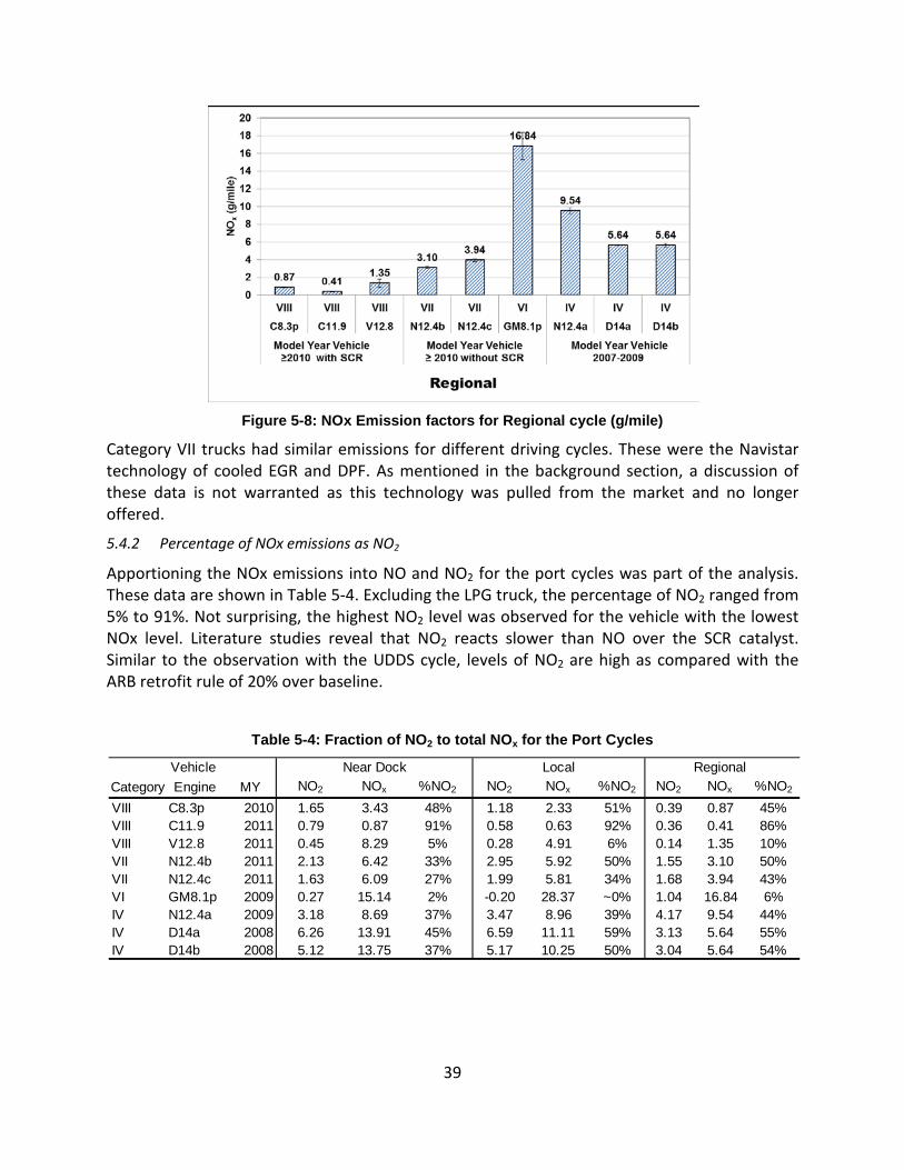
39
Figure 5-8: NOx Emission factors for Regional cycle (g/mile)
Category VII trucks had similar emissions for different driving cycles. These were the Navistar technology of cooled EGR and DPF. As mentioned in the background section, a discussion of these data is not warranted as this technology was pulled from the market and no longer offered.
5.4.2 Percentage of NOx emissions as NO2
Apportioning the NOx emissions into NO and NO2 for the port cycles was part of the analysis. These data are shown in Table 5-4. Excluding the LPG truck, the percentage of NO2 ranged from 5% to 91%. Not surprising, the highest NO2 level was observed for the vehicle with the lowest NOx level. Literature studies reveal that NO2 reacts slower than NO over the SCR catalyst. Similar to the observation with the UDDS cycle, levels of NO2 are high as compared with the ARB retrofit rule of 20% over baseline.
Table 5-4: Fraction of NO2 to total NOx for the Port Cycles
Category Engine MY NO2 NOx %NO2 NO2 NOx %NO2 NO2 NOx %NO2
VIII C8.3p 2010 1.65 3.43 48% 1.18 2.33 51% 0.39 0.87 45%VIII C11.9 2011 0.79 0.87 91% 0.58 0.63 92% 0.36 0.41 86%VIII V12.8 2011 0.45 8.29 5% 0.28 4.91 6% 0.14 1.35 10%VII N12.4b 2011 2.13 6.42 33% 2.95 5.92 50% 1.55 3.10 50%VII N12.4c 2011 1.63 6.09 27% 1.99 5.81 34% 1.68 3.94 43%VI GM8.1p 2009 0.27 15.14 2% -0.20 28.37 ~0% 1.04 16.84 6%IV N12.4a 2009 3.18 8.69 37% 3.47 8.96 39% 4.17 9.54 44%IV D14a 2008 6.26 13.91 45% 6.59 11.11 59% 3.13 5.64 55%IV D14b 2008 5.12 13.75 37% 5.17 10.25 50% 3.04 5.64 54%
Vehicle Near Dock Local Regional
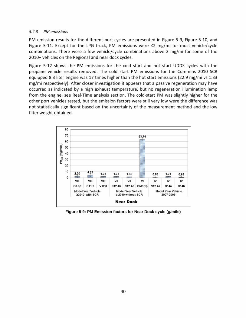
40
5.4.3 PM emissions
PM emission results for the different port cycles are presented in Figure 5-9, Figure 5-10, and Figure 5-11. Except for the LPG truck, PM emissions were ≤2 mg/mi for most vehicle/cycle combinations. There were a few vehicle/cycle combinations above 2 mg/mi for some of the 2010+ vehicles on the Regional and near dock cycles.
Figure 5-12 shows the PM emissions for the cold start and hot start UDDS cycles with the propane vehicle results removed. The cold start PM emissions for the Cummins 2010 SCR equipped 8.3 liter engine was 17 times higher than the hot start emissions (22.9 mg/mi vs 1.33 mg/mi respectively). After closer investigation it appears that a passive regeneration may have occurred as indicated by a high exhaust temperature, but no regeneration illumination lamp from the engine, see Real-Time analysis section. The cold-start PM was slightly higher for the other port vehicles tested, but the emission factors were still very low were the difference was not statistically significant based on the uncertainty of the measurement method and the low filter weight obtained.
Figure 5-9: PM Emission factors for Near Dock cycle (g/mile)
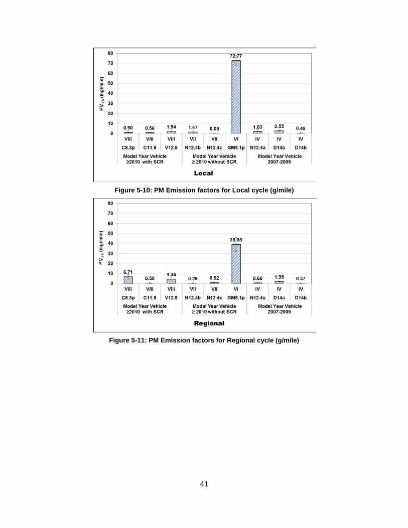
41
Figure 5-10: PM Emission factors for Local cycle (g/mile)
Figure 5-11: PM Emission factors for Regional cycle (g/mile)
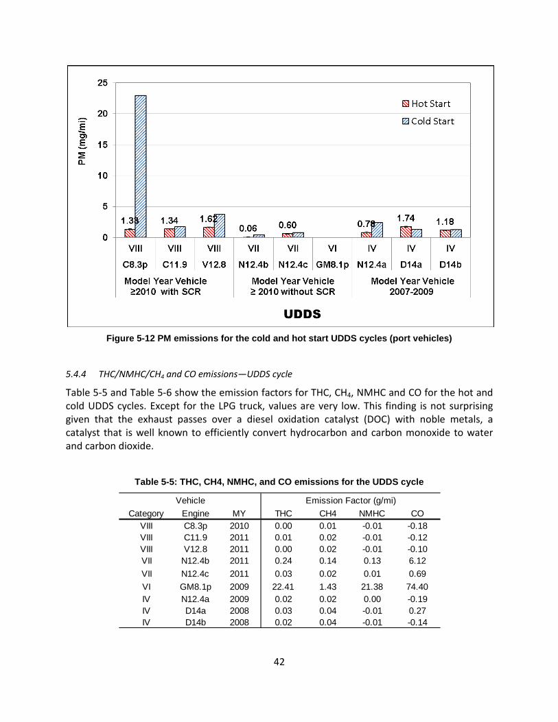
42
Figure 5-12 PM emissions for the cold and hot start UDDS cycles (port vehicles)
5.4.4 THC/NMHC/CH4 and CO emissions—UDDS cycle
Table 5-5 and Table 5-6 show the emission factors for THC, CH4, NMHC and CO for the hot and cold UDDS cycles. Except for the LPG truck, values are very low. This finding is not surprising given that the exhaust passes over a diesel oxidation catalyst (DOC) with noble metals, a catalyst that is well known to efficiently convert hydrocarbon and carbon monoxide to water and carbon dioxide.
Table 5-5: THC, CH4, NMHC, and CO emissions for the UDDS cycle
Category Engine MY THC CH4 NMHC COVIII C8.3p 2010 0.00 0.01 -0.01 -0.18VIII C11.9 2011 0.01 0.02 -0.01 -0.12VIII V12.8 2011 0.00 0.02 -0.01 -0.10VII N12.4b 2011 0.24 0.14 0.13 6.12VII N12.4c 2011 0.03 0.02 0.01 0.69VI GM8.1p 2009 22.41 1.43 21.38 74.40IV N12.4a 2009 0.02 0.02 0.00 -0.19IV D14a 2008 0.03 0.04 -0.01 0.27IV D14b 2008 0.02 0.04 -0.01 -0.14
Vehicle Emission Factor (g/mi)
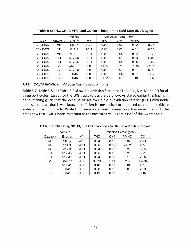
43
Table 5-6: THC, CH4, NMHC, and CO emissions for the Cold Start UDDS Cycle
5.4.5 THC/NMHC/CH4 and CO emissions—In-use port cycles
Table 5-7, Table 5-8 and Table 5-9 show the emission factors for THC, CH4, NMHC and CO for all three port cycles. Except for the LPG truck, values are very low. As stated earlier this finding is not surprising given that the exhaust passes over a diesel oxidation catalyst (DOC) with noble metals, a catalyst that is well known to efficiently convert hydrocarbon and carbon monoxide to water and carbon dioxide. While truck emissions need to meet a carbon monoxide limit, the data show that NOx is more important as the measured values are <10% of the CO standard.
Table 5-7: THC, CH4, NMHC, and CO emissions for the Near Dock port cycle
Category Engine MY THC CH4 NMHCCS-UDDS VIII C8.3p 2010 0.02 0.01 0.02 -0.07CS-UDDS VIII C11.9 2011 0.03 0.03 0.01 -0.03CS-UDDS VIII V12.8 2011 0.06 0.04 0.02 0.27CS-UDDS VII N12.4b 2011 0.08 0.05 0.04 1.44CS-UDDS VII N12.4c 2011 0.08 0.04 0.05 0.46CS-UDDS VI GM8.1p 2009 14.89 0.76 14.38 77.16CS-UDDS IV N12.4a 2009 0.03 0.02 0.01 -0.10CS-UDDS IV D14a 2008 0.05 0.04 0.01 0.85CS-UDDS IV D14b 2008 -0.02 0.03 -0.04 0.54
Vehicle Emission Factor (g/mi)Cycle
Category Engine MY THC CH4 NMHC COVIII C8.3p 2010 0.04 0.03 0.02 -0.41VIII C11.9 2011 0.06 0.09 -0.02 -0.50VIII V12.8 2011 0.34 0.06 0.29 0.65VII N12.4b 2011 0.36 0.10 0.28 3.21VII N12.4c 2011 0.24 0.07 0.18 2.06VI GM8.1p 2009 33.79 1.61 32.73 157.34IV N12.4a 2009 0.10 0.07 0.04 -0.15IV D14a 2008 0.08 0.09 0.00 2.83IV D14b 2008 0.19 0.07 0.13 0.16
Emission Factor (g/mi)Vehicle
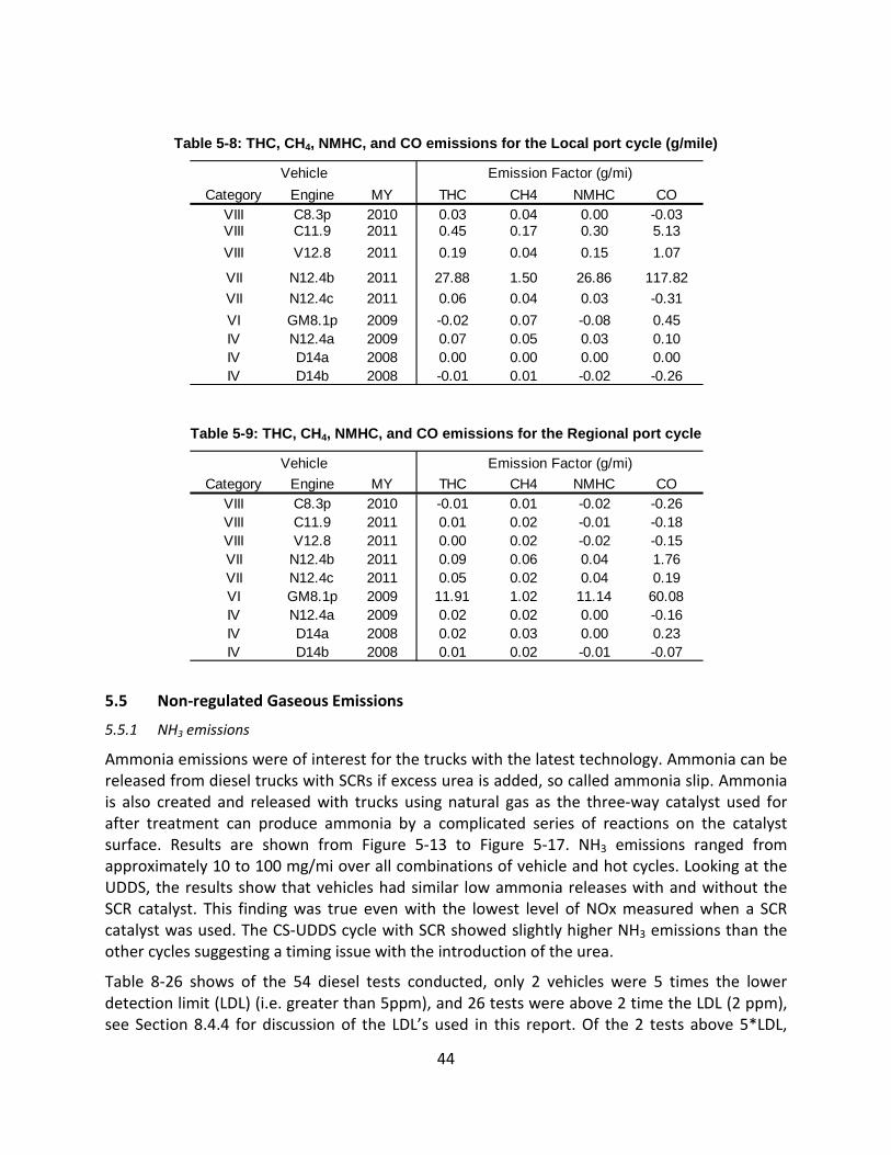
44
Table 5-8: THC, CH4, NMHC, and CO emissions for the Local port cycle (g/mile)
Table 5-9: THC, CH4, NMHC, and CO emissions for the Regional port cycle
5.5 Non-regulated Gaseous Emissions
5.5.1 NH3 emissions
Ammonia emissions were of interest for the trucks with the latest technology. Ammonia can be released from diesel trucks with SCRs if excess urea is added, so called ammonia slip. Ammonia is also created and released with trucks using natural gas as the three-way catalyst used for after treatment can produce ammonia by a complicated series of reactions on the catalyst surface. Results are shown from Figure 5-13 to Figure 5-17. NH3 emissions ranged from approximately 10 to 100 mg/mi over all combinations of vehicle and hot cycles. Looking at the UDDS, the results show that vehicles had similar low ammonia releases with and without the SCR catalyst. This finding was true even with the lowest level of NOx measured when a SCR catalyst was used. The CS-UDDS cycle with SCR showed slightly higher NH3 emissions than the other cycles suggesting a timing issue with the introduction of the urea.
Table 8-26 shows of the 54 diesel tests conducted, only 2 vehicles were 5 times the lower detection limit (LDL) (i.e. greater than 5ppm), and 26 tests were above 2 time the LDL (2 ppm), see Section 8.4.4 for discussion of the LDL’s used in this report. Of the 2 tests above 5*LDL,
Category Engine MY THC CH4 NMHC COVIII C8.3p 2010 0.03 0.04 0.00 -0.03VIII C11.9 2011 0.45 0.17 0.30 5.13VIII V12.8 2011 0.19 0.04 0.15 1.07
VII N12.4b 2011 27.88 1.50 26.86 117.82VII N12.4c 2011 0.06 0.04 0.03 -0.31VI GM8.1p 2009 -0.02 0.07 -0.08 0.45IV N12.4a 2009 0.07 0.05 0.03 0.10IV D14a 2008 0.00 0.00 0.00 0.00IV D14b 2008 -0.01 0.01 -0.02 -0.26
Vehicle Emission Factor (g/mi)
Category Engine MY THC CH4 NMHC COVIII C8.3p 2010 -0.01 0.01 -0.02 -0.26VIII C11.9 2011 0.01 0.02 -0.01 -0.18VIII V12.8 2011 0.00 0.02 -0.02 -0.15VII N12.4b 2011 0.09 0.06 0.04 1.76VII N12.4c 2011 0.05 0.02 0.04 0.19VI GM8.1p 2009 11.91 1.02 11.14 60.08IV N12.4a 2009 0.02 0.02 0.00 -0.16IV D14a 2008 0.02 0.03 0.00 0.23IV D14b 2008 0.01 0.02 -0.01 -0.07
Vehicle Emission Factor (g/mi)
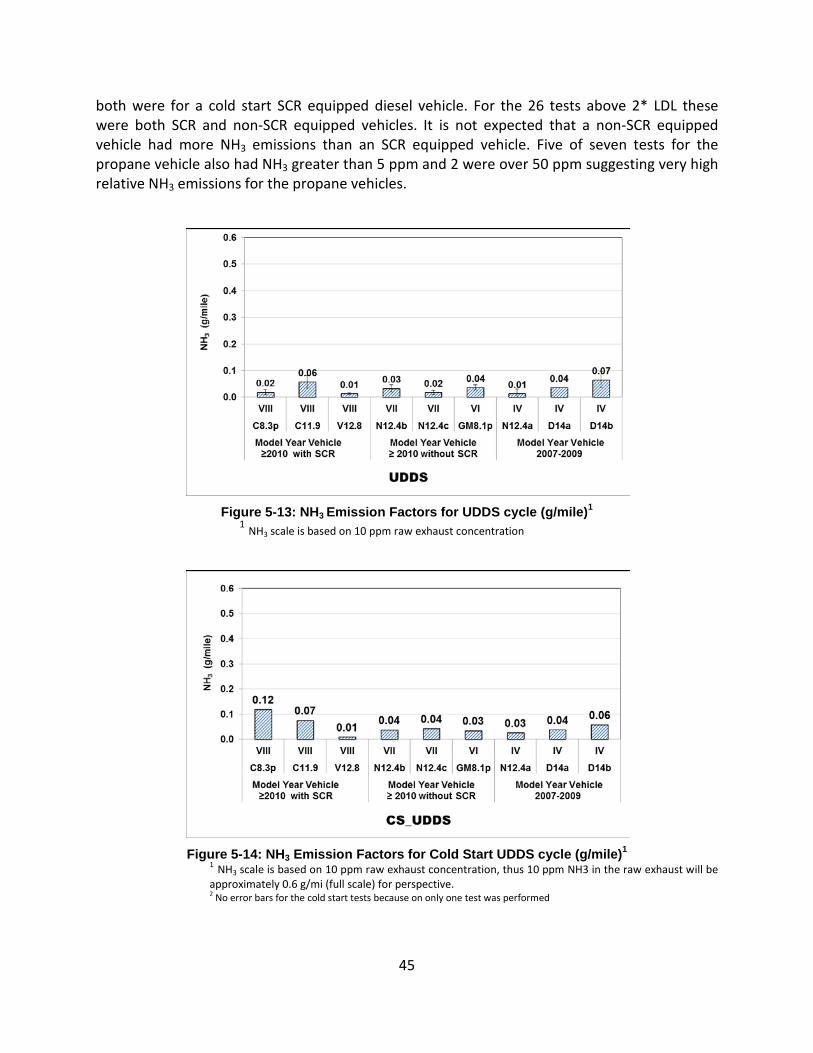
45
both were for a cold start SCR equipped diesel vehicle. For the 26 tests above 2* LDL these were both SCR and non-SCR equipped vehicles. It is not expected that a non-SCR equipped vehicle had more NH3 emissions than an SCR equipped vehicle. Five of seven tests for the propane vehicle also had NH3 greater than 5 ppm and 2 were over 50 ppm suggesting very high relative NH3 emissions for the propane vehicles.
Figure 5-13: NH3 Emission Factors for UDDS cycle (g/mile)1
1 NH3 scale is based on 10 ppm raw exhaust concentration
Figure 5-14: NH3 Emission Factors for Cold Start UDDS cycle (g/mile)1
1 NH3 scale is based on 10 ppm raw exhaust concentration, thus 10 ppm NH3 in the raw exhaust will be approximately 0.6 g/mi (full scale) for perspective. 2 No error bars for the cold start tests because on only one test was performed
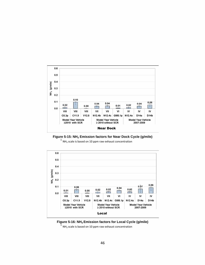
46
Figure 5-15: NH3 Emission factors for Near Dock Cycle (g/mile)
1 NH3 scale is based on 10 ppm raw exhaust concentration
Figure 5-16: NH3 Emission factors for Local Cycle (g/mile)
1 NH3 scale is based on 10 ppm raw exhaust concentration
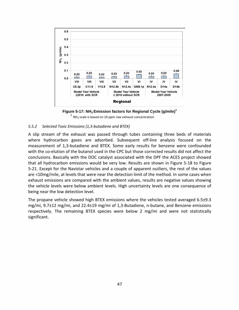
47
Figure 5-17: NH3 Emission factors for Regional Cycle (g/mile)1
1 NH3 scale is based on 10 ppm raw exhaust concentration
5.5.2 Selected Toxic Emissions (1,3-butadiene and BTEX)
A slip stream of the exhaust was passed through tubes containing three beds of materials where hydrocarbon gases are adsorbed. Subsequent off-line analysis focused on the measurement of 1,3-butadiene and BTEX. Some early results for benzene were confounded with the co-elution of the butanol used in the CPC but those corrected results did not affect the conclusions. Basically with the DOC catalyst associated with the DPF the ACES project showed that all hydrocarbon emissions would be very low. Results are shown in Figure 5-18 to Figure 5-21. Except for the Navistar vehicles and a couple of apparent outliers, the rest of the values are <10mg/mile, at levels that were near the detection limit of the method. In some cases when exhaust emissions are compared with the ambient values, results are negative values showing the vehicle levels were below ambient levels. High uncertainty levels are one consequence of being near the low detection level.
The propane vehicle showed high BTEX emissions where the vehicles tested averaged 6.5±9.3 mg/mi, 9.7±12 mg/mi, and 22.4±19 mg/mi of 1,3-Butadiene, n-butane, and Benzene emissions respectively. The remaining BTEX species were below 2 mg/mi and were not statistically significant.

48
Figure 5-18 Emissions in mg/mile for Butadiene & BTEX for the UDDS Cycle
Figure 5-19 Emissions in mg/mile for Butadiene & BTEX for the Near Port Cycle
Figure 5-20 Emissions in mg/mile for Butadiene & BTEX for the Local Port Cycle
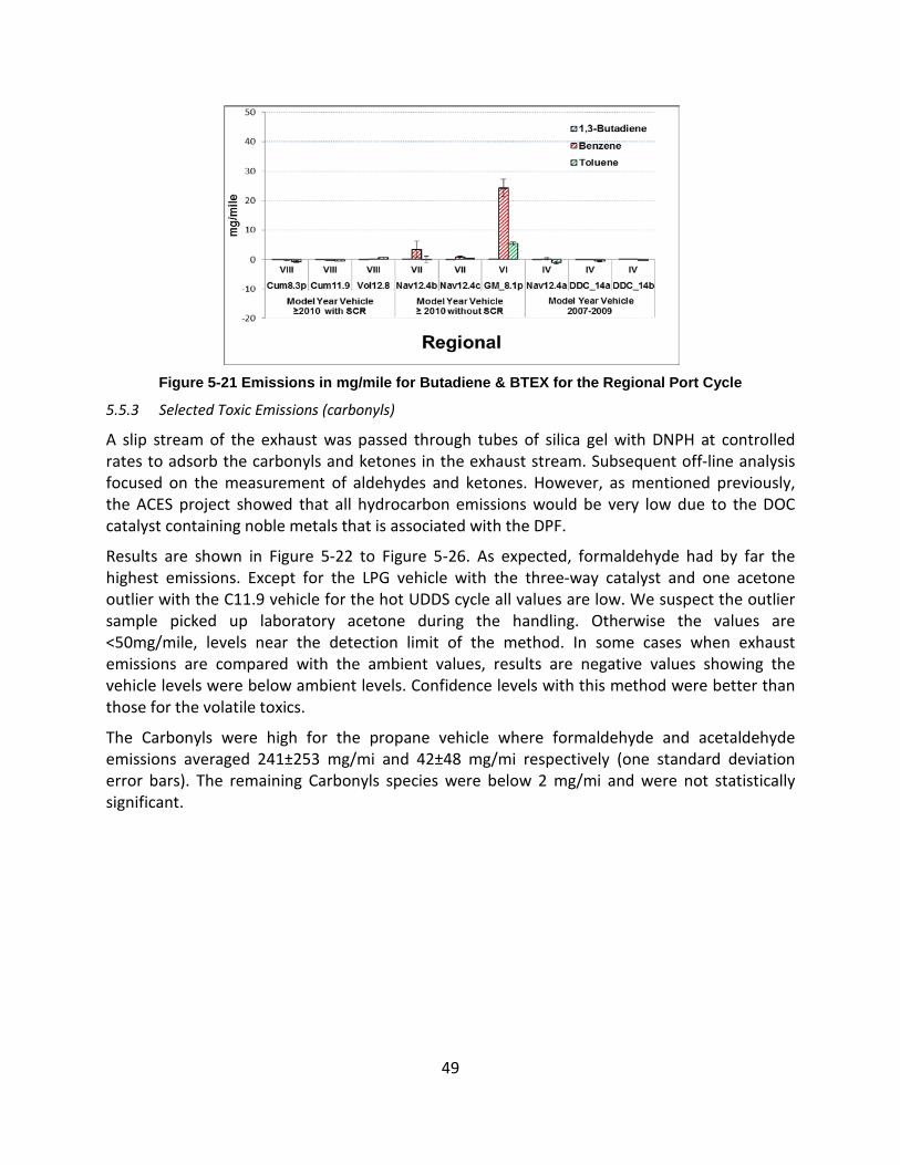
49
Figure 5-21 Emissions in mg/mile for Butadiene & BTEX for the Regional Port Cycle
5.5.3 Selected Toxic Emissions (carbonyls)
A slip stream of the exhaust was passed through tubes of silica gel with DNPH at controlled rates to adsorb the carbonyls and ketones in the exhaust stream. Subsequent off-line analysis focused on the measurement of aldehydes and ketones. However, as mentioned previously, the ACES project showed that all hydrocarbon emissions would be very low due to the DOC catalyst containing noble metals that is associated with the DPF.
Results are shown in Figure 5-22 to Figure 5-26. As expected, formaldehyde had by far the highest emissions. Except for the LPG vehicle with the three-way catalyst and one acetone outlier with the C11.9 vehicle for the hot UDDS cycle all values are low. We suspect the outlier sample picked up laboratory acetone during the handling. Otherwise the values are <50mg/mile, levels near the detection limit of the method. In some cases when exhaust emissions are compared with the ambient values, results are negative values showing the vehicle levels were below ambient levels. Confidence levels with this method were better than those for the volatile toxics.
The Carbonyls were high for the propane vehicle where formaldehyde and acetaldehyde emissions averaged 241±253 mg/mi and 42±48 mg/mi respectively (one standard deviation error bars). The remaining Carbonyls species were below 2 mg/mi and were not statistically significant.
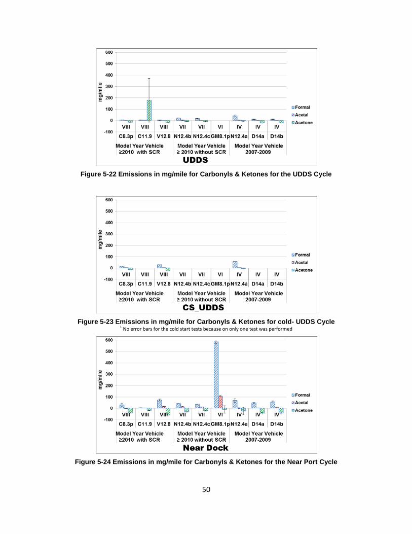
50
Figure 5-22 Emissions in mg/mile for Carbonyls & Ketones for the UDDS Cycle
Figure 5-23 Emissions in mg/mile for Carbonyls & Ketones for cold- UDDS Cycle
1 No error bars for the cold start tests because on only one test was performed
Figure 5-24 Emissions in mg/mile for Carbonyls & Ketones for the Near Port Cycle
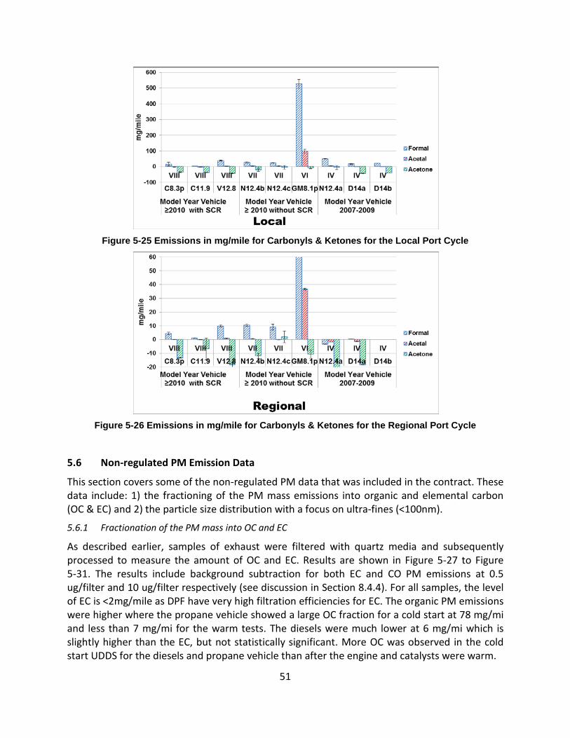
51
Figure 5-25 Emissions in mg/mile for Carbonyls & Ketones for the Local Port Cycle
Figure 5-26 Emissions in mg/mile for Carbonyls & Ketones for the Regional Port Cycle
5.6 Non-regulated PM Emission Data
This section covers some of the non-regulated PM data that was included in the contract. These data include: 1) the fractioning of the PM mass emissions into organic and elemental carbon (OC & EC) and 2) the particle size distribution with a focus on ultra-fines (<100nm).
5.6.1 Fractionation of the PM mass into OC and EC
As described earlier, samples of exhaust were filtered with quartz media and subsequently processed to measure the amount of OC and EC. Results are shown in Figure 5-27 to Figure 5-31. The results include background subtraction for both EC and CO PM emissions at 0.5 ug/filter and 10 ug/filter respectively (see discussion in Section 8.4.4). For all samples, the level of EC is <2mg/mile as DPF have very high filtration efficiencies for EC. The organic PM emissions were higher where the propane vehicle showed a large OC fraction for a cold start at 78 mg/mi and less than 7 mg/mi for the warm tests. The diesels were much lower at 6 mg/mi which is slightly higher than the EC, but not statistically significant. More OC was observed in the cold start UDDS for the diesels and propane vehicle than after the engine and catalysts were warm.
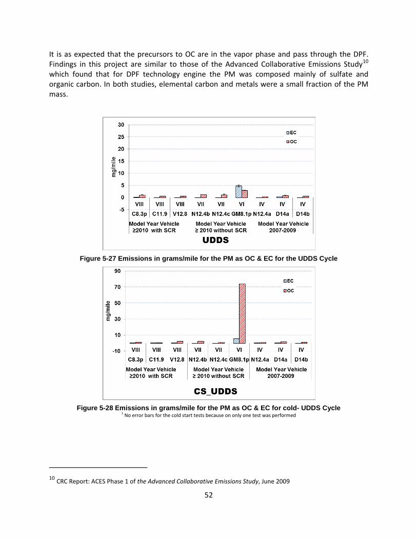
52
It is as expected that the precursors to OC are in the vapor phase and pass through the DPF. Findings in this project are similar to those of the Advanced Collaborative Emissions Study10
which found that for DPF technology engine the PM was composed mainly of sulfate and organic carbon. In both studies, elemental carbon and metals were a small fraction of the PM mass.
Figure 5-27 Emissions in grams/mile for the PM as OC & EC for the UDDS Cycle
Figure 5-28 Emissions in grams/mile for the PM as OC & EC for cold- UDDS Cycle
1 No error bars for the cold start tests because on only one test was performed
10 CRC Report: ACES Phase 1 of the Advanced Collaborative Emissions Study, June 2009
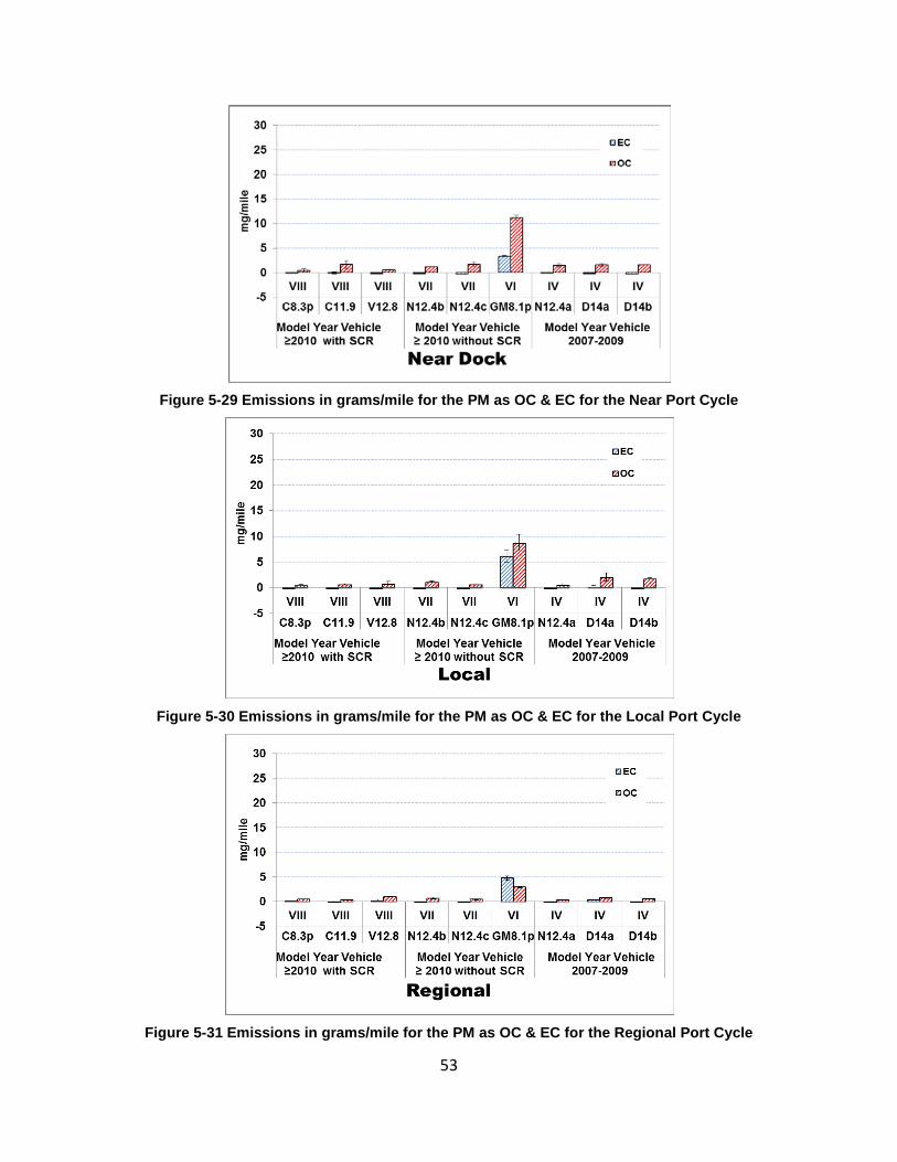
53
Figure 5-29 Emissions in grams/mile for the PM as OC & EC for the Near Port Cycle
Figure 5-30 Emissions in grams/mile for the PM as OC & EC for the Local Port Cycle
Figure 5-31 Emissions in grams/mile for the PM as OC & EC for the Regional Port Cycle
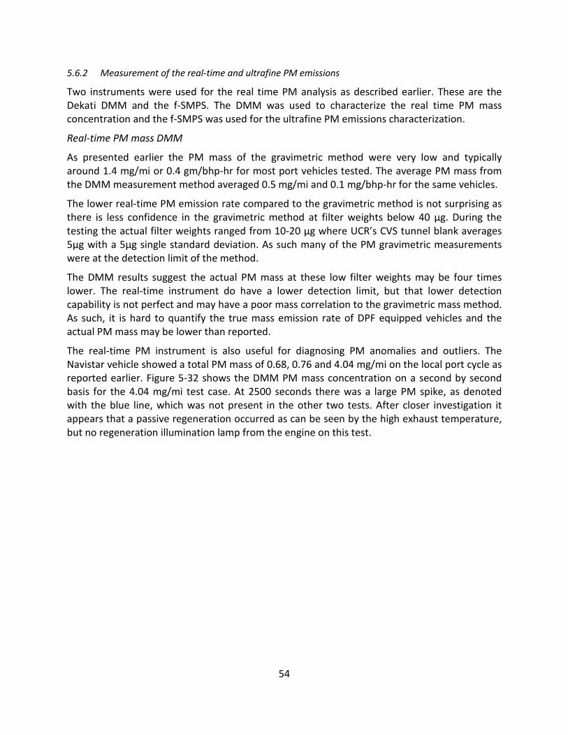
54
5.6.2 Measurement of the real-time and ultrafine PM emissions
Two instruments were used for the real time PM analysis as described earlier. These are the Dekati DMM and the f-SMPS. The DMM was used to characterize the real time PM mass concentration and the f-SMPS was used for the ultrafine PM emissions characterization.
Real-time PM mass DMM
As presented earlier the PM mass of the gravimetric method were very low and typically around 1.4 mg/mi or 0.4 gm/bhp-hr for most port vehicles tested. The average PM mass from the DMM measurement method averaged 0.5 mg/mi and 0.1 mg/bhp-hr for the same vehicles.
The lower real-time PM emission rate compared to the gravimetric method is not surprising as there is less confidence in the gravimetric method at filter weights below 40 µg. During the testing the actual filter weights ranged from 10-20 µg where UCR’s CVS tunnel blank averages 5µg with a 5µg single standard deviation. As such many of the PM gravimetric measurements were at the detection limit of the method.
The DMM results suggest the actual PM mass at these low filter weights may be four times lower. The real-time instrument do have a lower detection limit, but that lower detection capability is not perfect and may have a poor mass correlation to the gravimetric mass method. As such, it is hard to quantify the true mass emission rate of DPF equipped vehicles and the actual PM mass may be lower than reported.
The real-time PM instrument is also useful for diagnosing PM anomalies and outliers. The Navistar vehicle showed a total PM mass of 0.68, 0.76 and 4.04 mg/mi on the local port cycle as reported earlier. Figure 5-32 shows the DMM PM mass concentration on a second by second basis for the 4.04 mg/mi test case. At 2500 seconds there was a large PM spike, as denoted with the blue line, which was not present in the other two tests. After closer investigation it appears that a passive regeneration occurred as can be seen by the high exhaust temperature, but no regeneration illumination lamp from the engine on this test.
55
Figure 5-32: Navistar (12WZJ-B) real-time PM, vehicle speed, and DPF temp for local port cycle
In summary the low reading for the DMM suggests the actual PM mass is lower than reported by the filter mass method. Additionally, the real-time PM mass measurement method is useful for identifying test outliers and anomalies. Real-time PM is recommended with most source emissions research studies.
Ultra-fine PM emissions
In this sub section we investigate the size distribution nature of the particles. This analysis looks at particle diameters ranging from 7 nm to 200 nm, as described previously. High particle concentration at low particle diameters does not imply, necessarily, high PM mass. The calculation from particle size to mass is based on the particle diameter to the 3rd power and assumptions on density which is a strong function of particle size.
The ultra-fine PM emissions showed three unique cases, 1) the effect of cold start conditions, 2) the effect of the cycle, and 3) the difference between after treatment technologies. This section is broken down into those three categories.
Impact of cold start conditions
The cold start conditions are creating higher ultra-fine PM emissions compared to equivalent hot tests. Figure 5-33 - Figure 5-36 show the size distribution data for the UDDS hot and cold start test cycles. Figure 5-33 shows the average triplicate scans and single standard deviation error bars for the hot UDDS with the cold start UDDS from 0-200 seconds and from 200 seconds to the end of the cycle. The 0-200 seconds represents the average concentration for the first 200 seconds or the first 23 scans. Figure 5-33 is showing a very large concentration spike for the full size range from 7 to 200 nm compared to the hot UDDS. Figure 5-34 shows additional details with scan averaging from 0-100 seconds, 100-200 seconds, 0-end, and 200 – to the end.
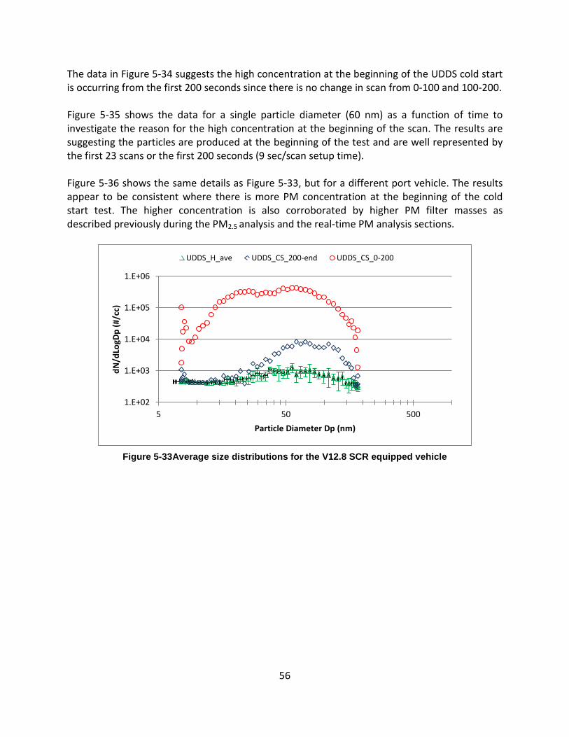
56
The data in Figure 5-34 suggests the high concentration at the beginning of the UDDS cold start is occurring from the first 200 seconds since there is no change in scan from 0-100 and 100-200. Figure 5-35 shows the data for a single particle diameter (60 nm) as a function of time to investigate the reason for the high concentration at the beginning of the scan. The results are suggesting the particles are produced at the beginning of the test and are well represented by the first 23 scans or the first 200 seconds (9 sec/scan setup time). Figure 5-36 shows the same details as Figure 5-33, but for a different port vehicle. The results appear to be consistent where there is more PM concentration at the beginning of the cold start test. The higher concentration is also corroborated by higher PM filter masses as described previously during the PM2.5 analysis and the real-time PM analysis sections.
Figure 5-33Average size distributions for the V12.8 SCR equipped vehicle
1.E+02
1.E+03
1.E+04
1.E+05
1.E+06
5 50 500
dN/d
LogD
p (#
/cc)
Particle Diameter Dp (nm)
UDDS_H_ave UDDS_CS_200-end UDDS_CS_0-200
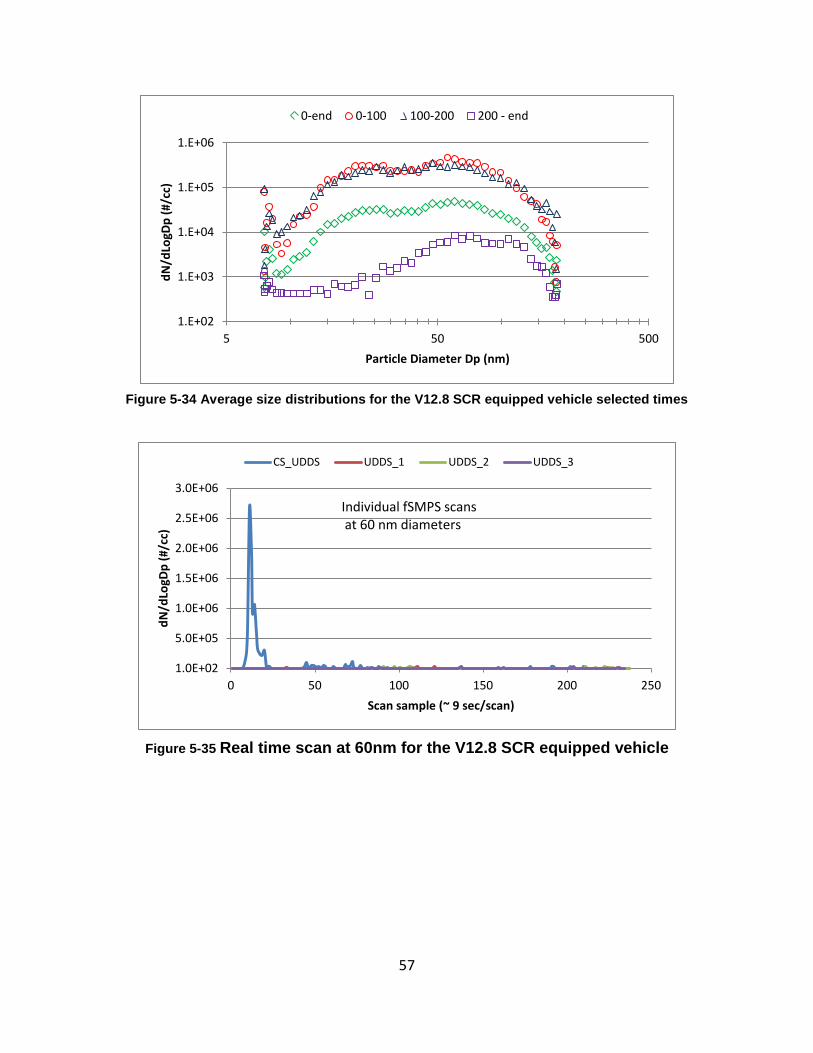
57
Figure 5-34 Average size distributions for the V12.8 SCR equipped vehicle selected times
Figure 5-35 Real time scan at 60nm for the V12.8 SCR equipped vehicle
1.E+02
1.E+03
1.E+04
1.E+05
1.E+06
5 50 500
dN/d
LogD
p (#
/cc)
Particle Diameter Dp (nm)
0-end 0-100 100-200 200 - end
1.0E+02
5.0E+05
1.0E+06
1.5E+06
2.0E+06
2.5E+06
3.0E+06
0 50 100 150 200 250
dN/d
LogD
p (#
/cc)
Scan sample (~ 9 sec/scan)
CS_UDDS UDDS_1 UDDS_2 UDDS_3
Individual fSMPS scans at 60 nm diameters
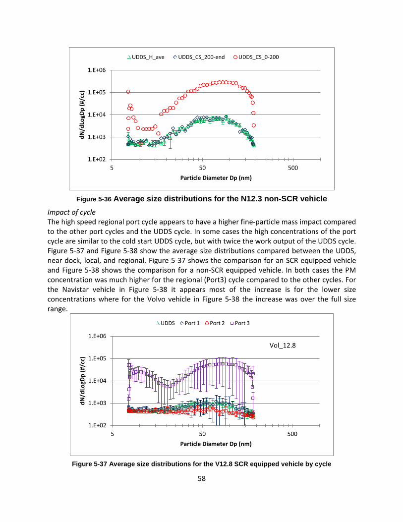
58
Figure 5-36 Average size distributions for the N12.3 non-SCR vehicle
Impact of cycle The high speed regional port cycle appears to have a higher fine-particle mass impact compared to the other port cycles and the UDDS cycle. In some cases the high concentrations of the port cycle are similar to the cold start UDDS cycle, but with twice the work output of the UDDS cycle. Figure 5-37 and Figure 5-38 show the average size distributions compared between the UDDS, near dock, local, and regional. Figure 5-37 shows the comparison for an SCR equipped vehicle and Figure 5-38 shows the comparison for a non-SCR equipped vehicle. In both cases the PM concentration was much higher for the regional (Port3) cycle compared to the other cycles. For the Navistar vehicle in Figure 5-38 it appears most of the increase is for the lower size concentrations where for the Volvo vehicle in Figure 5-38 the increase was over the full size range.
Figure 5-37 Average size distributions for the V12.8 SCR equipped vehicle by cycle
1.E+02
1.E+03
1.E+04
1.E+05
1.E+06
5 50 500
dN/d
LogD
p (#
/cc)
Particle Diameter Dp (nm)
UDDS_H_ave UDDS_CS_200-end UDDS_CS_0-200
1.E+02
1.E+03
1.E+04
1.E+05
1.E+06
5 50 500
dN/d
LogD
p (#
/cc)
Particle Diameter Dp (nm)
UDDS Port 1 Port 2 Port 3
Vol_12.8
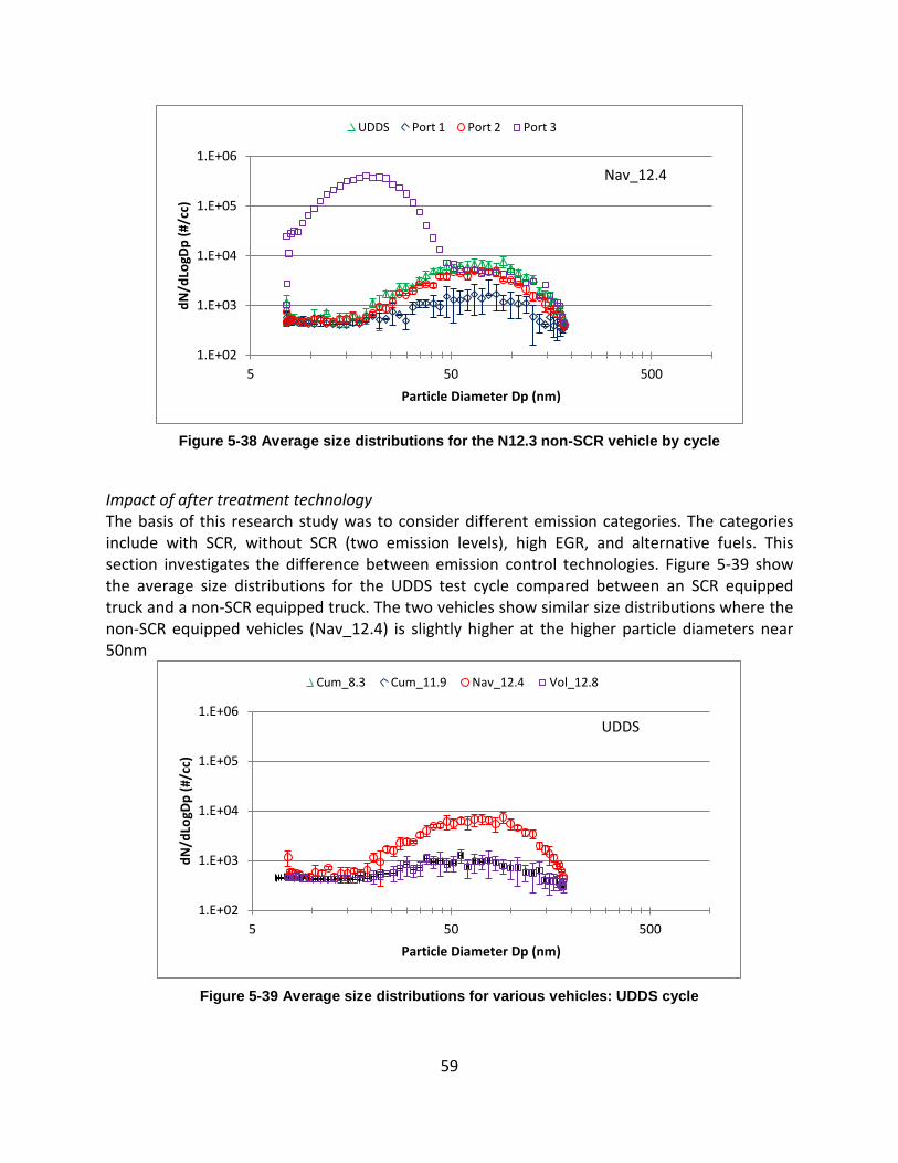
59
Figure 5-38 Average size distributions for the N12.3 non-SCR vehicle by cycle
Impact of after treatment technology The basis of this research study was to consider different emission categories. The categories include with SCR, without SCR (two emission levels), high EGR, and alternative fuels. This section investigates the difference between emission control technologies. Figure 5-39 show the average size distributions for the UDDS test cycle compared between an SCR equipped truck and a non-SCR equipped truck. The two vehicles show similar size distributions where the non-SCR equipped vehicles (Nav_12.4) is slightly higher at the higher particle diameters near 50nm
Figure 5-39 Average size distributions for various vehicles: UDDS cycle
1.E+02
1.E+03
1.E+04
1.E+05
1.E+06
5 50 500
dN/d
LogD
p (#
/cc)
Particle Diameter Dp (nm)
UDDS Port 1 Port 2 Port 3
Nav_12.4
1.E+02
1.E+03
1.E+04
1.E+05
1.E+06
5 50 500
dN/d
LogD
p (#
/cc)
Particle Diameter Dp (nm)
Cum_8.3 Cum_11.9 Nav_12.4 Vol_12.8
UDDS
60
5.7 Greenhouse Gas (N2O, CH4 & CO2) Emissions and Fuel Economy
For greenhouse gases, UCR measured emissions factors of methane and carbon dioxide in real-time for all vehicles and N2O with off-site analyses for selected vehicles. The off-site analyses were carried out by the California Air resources Board and West Virginia University. Results showed the measured values were close to ambient levels, as expected for diesel vehicles. Literature indicates N2O is observed when vehicles rely on three way catalyst and UCR did not have any included in their fleet of test vehicles.
5.7.1 Emissions of nitrous oxide (N2O)
N2O emissions were measured by the IR methods described earlier and found to be near the detection limits. A literature review showed that Huai et alia11
The N2O measurements were very close to the ambient concentrations were negative numbers were reported. The reason for negative numbers is based on the correction of the ambient measured concentration exceeding the sample measurement, as described in a later section. It is expected that many of the measurements are near the detection limits of the N2O measuring method. See Section
only found nitrous oxide when a three way catalyst was warming. Thus we only expected N2O for the LPG truck with the three way catalyst. Unfortunately the LPG port vehicle equipped with a TWC did not have N20 analysis available at the time of testing so no results for vehicles with TWC are reported in this section.
8.4.3 for analysis and summary of N20 measurements and detection limits. The general observations of the N2O emissions from the vehicles tested can be summarized as:
• N2O Analysis was done offsite when facilities were available. As such, not all vehicles or cycles were tested for N2O. Only selected vehicles were tested for N2O analysis.
• During the refuse and school bus testing there were no facilities for N2O analysis thus they were not performed. Similar results are expected for all the vehicle categories.
• More than half (64%) of the measured toxic emissions were below the defined threshold (0.4 ppm), the average ambient background concentration plus one standard deviation.
• Only the SCR equipped vehicles showed signs of N2O emissions not the non-SCR equipped vehicles.
• The cold start UDDS did not show higher integrated N2O emissions compared with hot start UDDS tests (with or with/out SCR). It is not clear from the testing if higher N20 emissions were created for a short duration at the cold start of the cold test cycles. Additional real time N2O data would be necessary to evaluate the first 100 seconds of the cold start UDDS N2O emissions.
• Of the values greater than the threshold, the average vehicle sample concentration was 1.06 ppm (only 2.6 times the threshold) and the single standard deviation was 0.44 ppm.
11 T. Huai, Durbin, T.D., J.W. Miller, and J.M. Norbeck, Estimates of the Emission Rates of Nitrous Oxide from Light-Duty Vehicles using Different Chassis Dynamometer Test Cycles. Atmospheric Environment, vol. 38, 6621-6629 (2004)
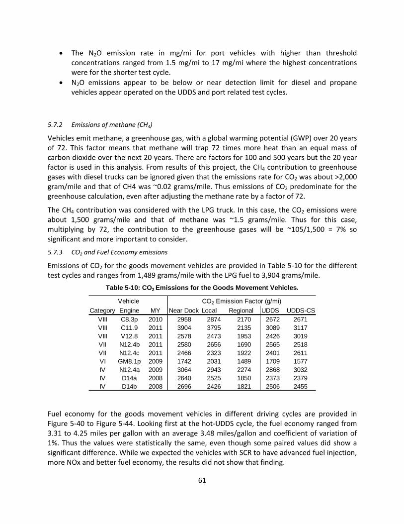
61
• The N2O emission rate in mg/mi for port vehicles with higher than threshold concentrations ranged from 1.5 mg/mi to 17 mg/mi where the highest concentrations were for the shorter test cycle.
• N2O emissions appear to be below or near detection limit for diesel and propane vehicles appear operated on the UDDS and port related test cycles.
5.7.2 Emissions of methane (CH4)
Vehicles emit methane, a greenhouse gas, with a global warming potential (GWP) over 20 years of 72. This factor means that methane will trap 72 times more heat than an equal mass of carbon dioxide over the next 20 years. There are factors for 100 and 500 years but the 20 year factor is used in this analysis. From results of this project, the CH4 contribution to greenhouse gases with diesel trucks can be ignored given that the emissions rate for CO2 was about >2,000 gram/mile and that of CH4 was ~0.02 grams/mile. Thus emissions of CO2 predominate for the greenhouse calculation, even after adjusting the methane rate by a factor of 72.
The CH4 contribution was considered with the LPG truck. In this case, the CO2 emissions were about 1,500 grams/mile and that of methane was ~1.5 grams/mile. Thus for this case, multiplying by 72, the contribution to the greenhouse gases will be ~105/1,500 = 7% so significant and more important to consider.
5.7.3 CO2 and Fuel Economy emissions
Emissions of CO2 for the goods movement vehicles are provided in Table 5-10 for the different test cycles and ranges from 1,489 grams/mile with the LPG fuel to 3,904 grams/mile.
Table 5-10: CO2 Emissions for the Goods Movement Vehicles.
Fuel economy for the goods movement vehicles in different driving cycles are provided in Figure 5-40 to Figure 5-44. Looking first at the hot-UDDS cycle, the fuel economy ranged from 3.31 to 4.25 miles per gallon with an average 3.48 miles/gallon and coefficient of variation of 1%. Thus the values were statistically the same, even though some paired values did show a significant difference. While we expected the vehicles with SCR to have advanced fuel injection, more NOx and better fuel economy, the results did not show that finding.
Category Engine MY Near Dock Local Regional UDDS UDDS-CSVIII C8.3p 2010 2958 2874 2170 2672 2671VIII C11.9 2011 3904 3795 2135 3089 3117VIII V12.8 2011 2578 2473 1953 2426 3019VII N12.4b 2011 2580 2656 1690 2565 2518VII N12.4c 2011 2466 2323 1922 2401 2611VI GM8.1p 2009 1742 2031 1489 1709 1577IV N12.4a 2009 3064 2943 2274 2868 3032IV D14a 2008 2640 2525 1850 2373 2379IV D14b 2008 2696 2426 1821 2506 2455
Vehicle CO2 Emission Factor (g/mi)
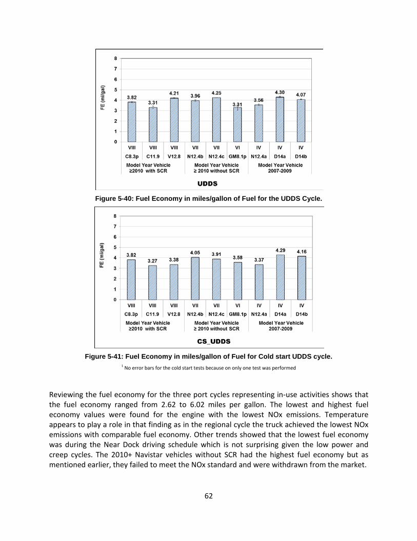
62
Figure 5-40: Fuel Economy in miles/gallon of Fuel for the UDDS Cycle.
Figure 5-41: Fuel Economy in miles/gallon of Fuel for Cold start UDDS cycle.
1 No error bars for the cold start tests because on only one test was performed
Reviewing the fuel economy for the three port cycles representing in-use activities shows that the fuel economy ranged from 2.62 to 6.02 miles per gallon. The lowest and highest fuel economy values were found for the engine with the lowest NOx emissions. Temperature appears to play a role in that finding as in the regional cycle the truck achieved the lowest NOx emissions with comparable fuel economy. Other trends showed that the lowest fuel economy was during the Near Dock driving schedule which is not surprising given the low power and creep cycles. The 2010+ Navistar vehicles without SCR had the highest fuel economy but as mentioned earlier, they failed to meet the NOx standard and were withdrawn from the market.
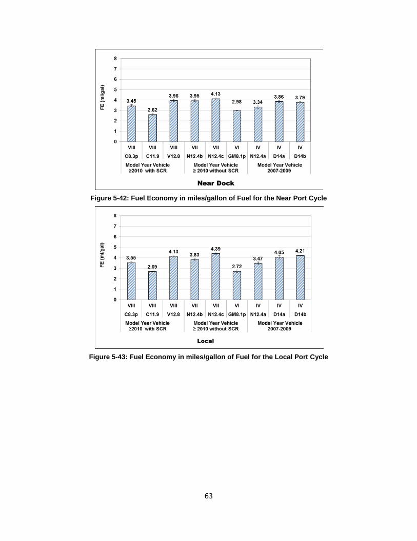
63
Figure 5-42: Fuel Economy in miles/gallon of Fuel for the Near Port Cycle
Figure 5-43: Fuel Economy in miles/gallon of Fuel for the Local Port Cycle
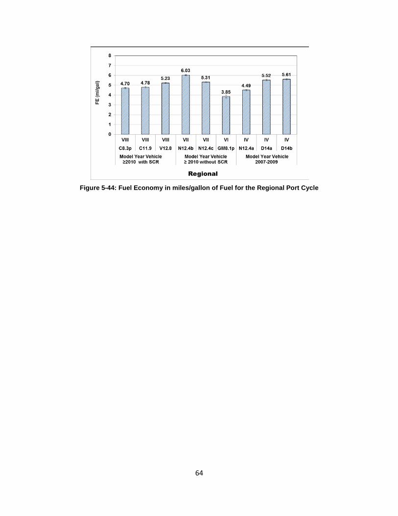
64
Figure 5-44: Fuel Economy in miles/gallon of Fuel for the Regional Port Cycle
65
6 Results and Discussion for Refuse Haulers
This section covers the emissions for refuse vehicles that were tested on the UDDS and the AQMD refuse truck cycles. Most emissions are based on grams per mile for inventory purposes and the UDDS cycle values are in grams/bhp-hr so as to compare with the certification values.
6.1 Test Trucks
Four trucks used as refuse haulers were tested on a number of chassis cycles. Selected information for the trucks is identified in Table 1-1. All of these vehicles were a challenge to find within the AQMD District as most trucks in the District use natural gas. Some were shipped in from Northern California where the air conforms to federal standards and diesel vehicles are still used.
6.2 Test Conditions
Vehicles were tested on the UDDS cycle and on the AQMD refuse hauler cycle as that cycle more closely represented in-use activities for a refuse hauler. The load for the refuse haulers was set at 56,000 lb. load as that value represents the typical load of a refuse hauler in the SCAQMD District. Commercially available CARB #2 diesel fuel was used rather than a certification fuel. Both load and fuel matched in-use conditions. The emission values represent the average of triplicate runs and the graphs show the confidence limits to one standard deviation.
6.3 NOx Emissions from the UDDS Cycle
As mentioned earlier, the brake specific emissions values from the UDDS chassis dyno test are often compared with the values measured in the heavy-duty FTP certification test on an engine dyno. This comparison provides some indication that the selected vehicle is representative of the desired FEL and technology. This section focuses on NOx emissions given the interest in the original RFP.
6.3.1 Brake-specific emissions for the UDDS Cycle
Figure 6-1 shows the UDDS values for NOx ranged from 0.13 to 2.0 g/bhp-hr versus certification standards of 0.2 and 1.2 g/bhp-h. The Value for one vehicle is on the high side; perhaps the manufacturer was using credits for that family of engines, but we do not know. Category VII with SCR had the lowest NOx emissions. The UDDS values ranged from 0.13 to 0.17 and were close to the certification values.
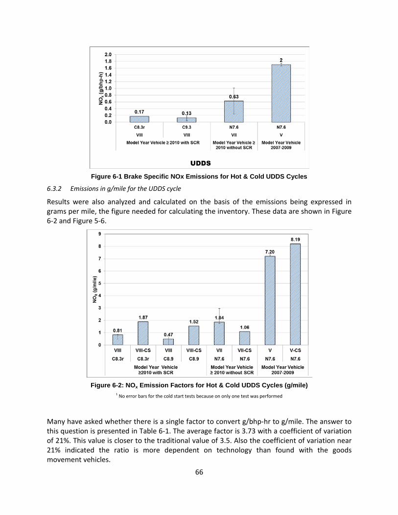
66
Figure 6-1 Brake Specific NOx Emissions for Hot & Cold UDDS Cycles
6.3.2 Emissions in g/mile for the UDDS cycle
Results were also analyzed and calculated on the basis of the emissions being expressed in grams per mile, the figure needed for calculating the inventory. These data are shown in Figure 6-2 and Figure 5-6.
Figure 6-2: NOx Emission Factors for Hot & Cold UDDS Cycles (g/mile)
1 No error bars for the cold start tests because on only one test was performed
Many have asked whether there is a single factor to convert g/bhp-hr to g/mile. The answer to this question is presented in Table 6-1. The average factor is 3.73 with a coefficient of variation of 21%. This value is closer to the traditional value of 3.5. Also the coefficient of variation near 21% indicated the ratio is more dependent on technology than found with the goods movement vehicles.
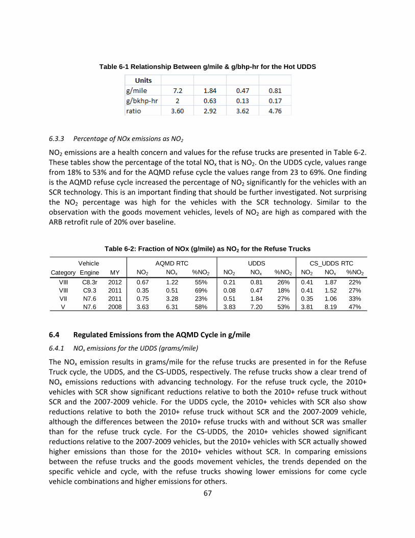
67
Table 6-1 Relationship Between g/mile & g/bhp-hr for the Hot UDDS
6.3.3 Percentage of NOx emissions as NO2
NO2 emissions are a health concern and values for the refuse trucks are presented in Table 6-2. These tables show the percentage of the total NOx that is NO2. On the UDDS cycle, values range from 18% to 53% and for the AQMD refuse cycle the values range from 23 to 69%. One finding is the AQMD refuse cycle increased the percentage of NO2 significantly for the vehicles with an SCR technology. This is an important finding that should be further investigated. Not surprising the NO2 percentage was high for the vehicles with the SCR technology. Similar to the observation with the goods movement vehicles, levels of NO2 are high as compared with the ARB retrofit rule of 20% over baseline.
Table 6-2: Fraction of NOx (g/mile) as NO2 for the Refuse Trucks
6.4 Regulated Emissions from the AQMD Cycle in g/mile
6.4.1 NOx emissions for the UDDS (grams/mile)
The NOx emission results in grams/mile for the refuse trucks are presented in for the Refuse Truck cycle, the UDDS, and the CS-UDDS, respectively. The refuse trucks show a clear trend of NOx emissions reductions with advancing technology. For the refuse truck cycle, the 2010+ vehicles with SCR show significant reductions relative to both the 2010+ refuse truck without SCR and the 2007-2009 vehicle. For the UDDS cycle, the 2010+ vehicles with SCR also show reductions relative to both the 2010+ refuse truck without SCR and the 2007-2009 vehicle, although the differences between the 2010+ refuse trucks with and without SCR was smaller than for the refuse truck cycle. For the CS-UDDS, the 2010+ vehicles showed significant reductions relative to the 2007-2009 vehicles, but the 2010+ vehicles with SCR actually showed higher emissions than those for the 2010+ vehicles without SCR. In comparing emissions between the refuse trucks and the goods movement vehicles, the trends depended on the specific vehicle and cycle, with the refuse trucks showing lower emissions for come cycle vehicle combinations and higher emissions for others.
Category Engine MY NO2 NOx %NO2 NO2 NOx %NO2 NO2 NOx %NO2
VIII C8.3r 2012 0.67 1.22 55% 0.21 0.81 26% 0.41 1.87 22%VIII C9.3 2011 0.35 0.51 69% 0.08 0.47 18% 0.41 1.52 27%VII N7.6 2011 0.75 3.28 23% 0.51 1.84 27% 0.35 1.06 33%V N7.6 2008 3.63 6.31 58% 3.83 7.20 53% 3.81 8.19 47%
Vehicle AQMD RTC UDDS CS_UDDS RTC
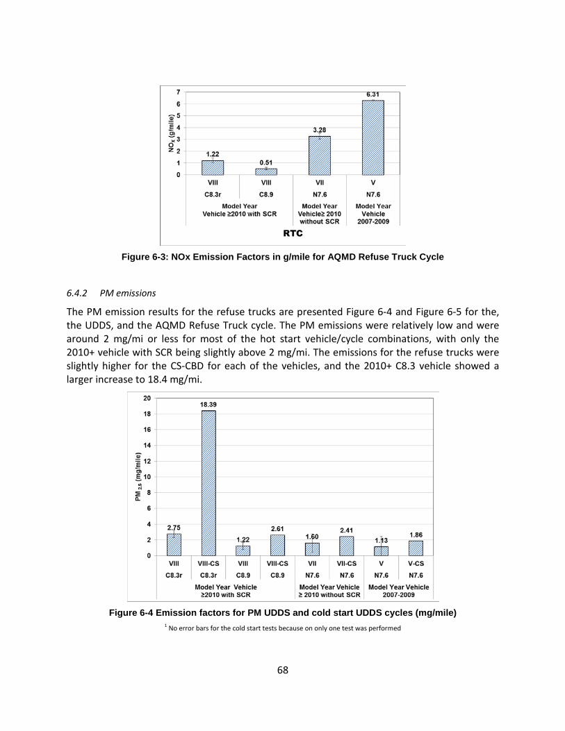
68
Figure 6-3: NOx Emission Factors in g/mile for AQMD Refuse Truck Cycle
6.4.2 PM emissions
The PM emission results for the refuse trucks are presented Figure 6-4 and Figure 6-5 for the, the UDDS, and the AQMD Refuse Truck cycle. The PM emissions were relatively low and were around 2 mg/mi or less for most of the hot start vehicle/cycle combinations, with only the 2010+ vehicle with SCR being slightly above 2 mg/mi. The emissions for the refuse trucks were slightly higher for the CS-CBD for each of the vehicles, and the 2010+ C8.3 vehicle showed a larger increase to 18.4 mg/mi.
Figure 6-4 Emission factors for PM UDDS and cold start UDDS cycles (mg/mile)
1 No error bars for the cold start tests because on only one test was performed
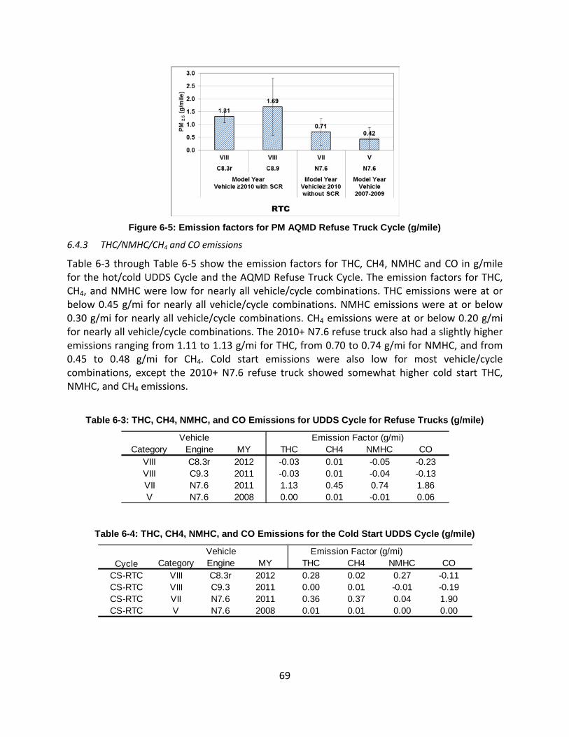
69
Figure 6-5: Emission factors for PM AQMD Refuse Truck Cycle (g/mile)
6.4.3 THC/NMHC/CH4 and CO emissions
Table 6-3 through Table 6-5 show the emission factors for THC, CH4, NMHC and CO in g/mile for the hot/cold UDDS Cycle and the AQMD Refuse Truck Cycle. The emission factors for THC, CH4, and NMHC were low for nearly all vehicle/cycle combinations. THC emissions were at or below 0.45 g/mi for nearly all vehicle/cycle combinations. NMHC emissions were at or below 0.30 g/mi for nearly all vehicle/cycle combinations. CH4 emissions were at or below 0.20 g/mi for nearly all vehicle/cycle combinations. The 2010+ N7.6 refuse truck also had a slightly higher emissions ranging from 1.11 to 1.13 g/mi for THC, from 0.70 to 0.74 g/mi for NMHC, and from 0.45 to 0.48 g/mi for CH4. Cold start emissions were also low for most vehicle/cycle combinations, except the 2010+ N7.6 refuse truck showed somewhat higher cold start THC, NMHC, and CH4 emissions.
Table 6-3: THC, CH4, NMHC, and CO Emissions for UDDS Cycle for Refuse Trucks (g/mile)
Table 6-4: THC, CH4, NMHC, and CO Emissions for the Cold Start UDDS Cycle (g/mile)
Category Engine MY THC CH4 NMHC COVIII C8.3r 2012 -0.03 0.01 -0.05 -0.23VIII C9.3 2011 -0.03 0.01 -0.04 -0.13VII N7.6 2011 1.13 0.45 0.74 1.86V N7.6 2008 0.00 0.01 -0.01 0.06
Vehicle Emission Factor (g/mi)
Category Engine MY THC CH4 NMHC COCS-RTC VIII C8.3r 2012 0.28 0.02 0.27 -0.11CS-RTC VIII C9.3 2011 0.00 0.01 -0.01 -0.19CS-RTC VII N7.6 2011 0.36 0.37 0.04 1.90CS-RTC V N7.6 2008 0.01 0.01 0.00 0.00
CycleVehicle Emission Factor (g/mi)
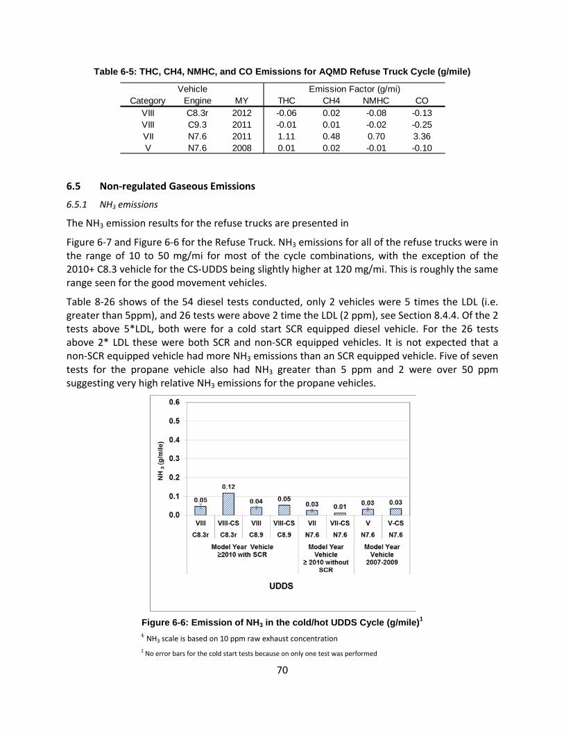
70
Table 6-5: THC, CH4, NMHC, and CO Emissions for AQMD Refuse Truck Cycle (g/mile)
6.5 Non-regulated Gaseous Emissions
6.5.1 NH3 emissions
The NH3 emission results for the refuse trucks are presented in
Figure 6-7 and Figure 6-6 for the Refuse Truck. NH3 emissions for all of the refuse trucks were in the range of 10 to 50 mg/mi for most of the cycle combinations, with the exception of the 2010+ C8.3 vehicle for the CS-UDDS being slightly higher at 120 mg/mi. This is roughly the same range seen for the good movement vehicles.
Table 8-26 shows of the 54 diesel tests conducted, only 2 vehicles were 5 times the LDL (i.e. greater than 5ppm), and 26 tests were above 2 time the LDL (2 ppm), see Section 8.4.4. Of the 2 tests above 5*LDL, both were for a cold start SCR equipped diesel vehicle. For the 26 tests above 2* LDL these were both SCR and non-SCR equipped vehicles. It is not expected that a non-SCR equipped vehicle had more NH3 emissions than an SCR equipped vehicle. Five of seven tests for the propane vehicle also had NH3 greater than 5 ppm and 2 were over 50 ppm suggesting very high relative NH3 emissions for the propane vehicles.
Figure 6-6: Emission of NH3 in the cold/hot UDDS Cycle (g/mile)1 1 NH3 scale is based on 10 ppm raw exhaust concentration 2 No error bars for the cold start tests because on only one test was performed
Category Engine MY THC CH4 NMHC COVIII C8.3r 2012 -0.06 0.02 -0.08 -0.13VIII C9.3 2011 -0.01 0.01 -0.02 -0.25VII N7.6 2011 1.11 0.48 0.70 3.36V N7.6 2008 0.01 0.02 -0.01 -0.10
Vehicle Emission Factor (g/mi)
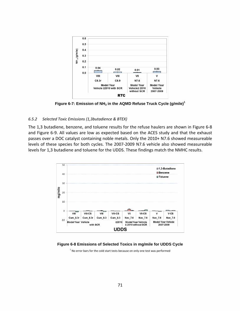
71
Figure 6-7: Emission of NH3 in the AQMD Refuse Truck Cycle (g/mile)1
6.5.2 Selected Toxic Emissions (1,3butadience & BTEX)
The 1,3 butadiene, benzene, and toluene results for the refuse haulers are shown in Figure 6-8 and Figure 6-9. All values are low as expected based on the ACES study and that the exhaust passes over a DOC catalyst containing noble metals. Only the 2010+ N7.6 showed measureable levels of these species for both cycles. The 2007-2009 N7.6 vehicle also showed measureable levels for 1,3 butadiene and toluene for the UDDS. These findings match the NMHC results.
Figure 6-8 Emissions of Selected Toxics in mg/mile for UDDS Cycle 1 No error bars for the cold start tests because on only one test was performed
72
Figure 6-9 Emissions of Selected Toxics in mg/mile for AQMD Refuse Cycle
6.5.3 Selected Toxic Emissions (carbonyls & ketones)
The formaldehyde, acetaldehyde, and acetone carbonyl results for the refuse haulers are shown in Figure 6-10 and Figure 6-11. Emissions are very low, as expected. Formaldehyde emissions were the highest of the carbonyl species, which were measureable for most vehicles on both cycles. The highest formaldehyde emissions were seen for the 2007-2009 N7.6 for both cycles. Acetaldehyde emissions were measureable for several vehicles for both cycles. Acetone emissions were not measureable for any of the vehicle/cycle combinations.
Figure 6-10 Emissions of Carbonyls & Ketones in mg/mile for UDDS Cycle 1 No error bars for the cold start tests because on only one test was performed
73
Figure 6-11 Emissions of Carbonyls & Ketones in mg/mile for AQMD Refuse Cycle
6.6 Non-regulated PM Emissions
6.6.1 Fractionation of the PM mass into OC and EC
Fractioning the PM into elemental and organic carbon was carried out by analysis of the quartz filter media collected at the test site. Results for the refuse haulers are shown in Figure 6-12 and Figure 6-13. For the Refuse Truck Cycle, the elemental and organic carbon emissions were essentially at the background levels. See Section 8.4.4 for a discussion on EC and OC detection limits. For the UDDS only the cold start emissions for the C8.3 showed organic carbon emissions measurably above the background levels, consistent with the higher PM2.5 emissions for that vehicle/cycle combination. Elemental carbon emissions were not measurably above the background levels for the UDDS, as expected due to the high filter efficiency of the DPF.
Figure 6-12 Emissions in grams/mile for the PM as OC & EC for the UDDS Cycle
1 Error bars for the cold start tests were available for this vehicle because multiple tests were performed
74
Figure 6-13 Emissions in grams/mile for the PM as OC & EC for the Refuse Cycle
6.6.2 Measurement of the real-time and ultrafine PM emissions
As described previously, The DMM was used to characterize the real time PM mass concentration and the f-SMPS was used for the ultrafine PM emissions characterization.
Real-time PM mass DMM
As presented earlier the PM mass of the gravimetric method were very low and typically around 2.1 mg/mi or 0.5 gm/bhp-hr for all the refuse vehicles tested. The average PM mass from the DMM measurement method averaged 0.3 mg/mi and 0.1 mg/bhp-hr for the same vehicles. The low PM mass emission factors were near the detection limits of the measurement method as discussed previously in Section 5.6.2.
Figure 6-14 shows the DMM PM mass concentration on a second by second basis for the Cummins 8.3 liter SCR equipped refuse hauler on the cold start UDDS cycle. At 600 seconds, the beginning of the large hill, there was a large PM spike, as denoted with the blue line, which was not present in the hot UDDS tests. The total PM from the gravimetric method was 18.4 mg/mi for the CS UDDS and between 3.2 to 2.2 mg/mi for the hot UDDS’s. The cold start UDDS PM was 6 times higher than the hot UDDS cycles. ThisAfter closer investigation it appears that a passive regeneration occurred as can be seen by the high exhaust temperature, but no regeneration illumination lamp from the engine on this test.
Figure 5-32 shows the DMM PM mass concentration on a second by second basis for the 4.04 mg/mi test case. At 2500 seconds there was a large PM spike, as denoted with the blue line, which was not present in the other two tests. After closer investigation it appears that a passive regeneration occurred as can be seen by the high exhaust temperature, but no regeneration illumination lamp from the engine on this test.
75
Figure 6-14 Refuse vehicle real-time PM emissions for the cold start UDDS cycle
Ultra-fine PM emissions
The cold start UDDS fine particles was also high for the refuse vehicle as compared to the port vehicles. Figure 6-15 through Figure 6-17 show the size distribution results for a selected SCR equipped refuse hauler. The results show a higher fine particle concentration for the first 200 seconds that cover most of the size range sampled. Figure 6-16 shows the real time scan at 60 nm which supports the idea that there is a burst of fine particles at the cold start then after about 200 seconds (23 scans) the high concentration is gone. The size distribution continues to drop as time progresses for the refuse vehicle as seen by the still high concentration at 200 seconds to the end, see Figure 6-15.
Figure 6-17 shows the comparison between the UDDS (hot and cold) compared to the AQMD refuse cycle. The UDDS and refuse cycle show similar fine particles were the small peak at 7-30 nm may be measurement error for the SMPS. Additional data is needed to confirm this response.
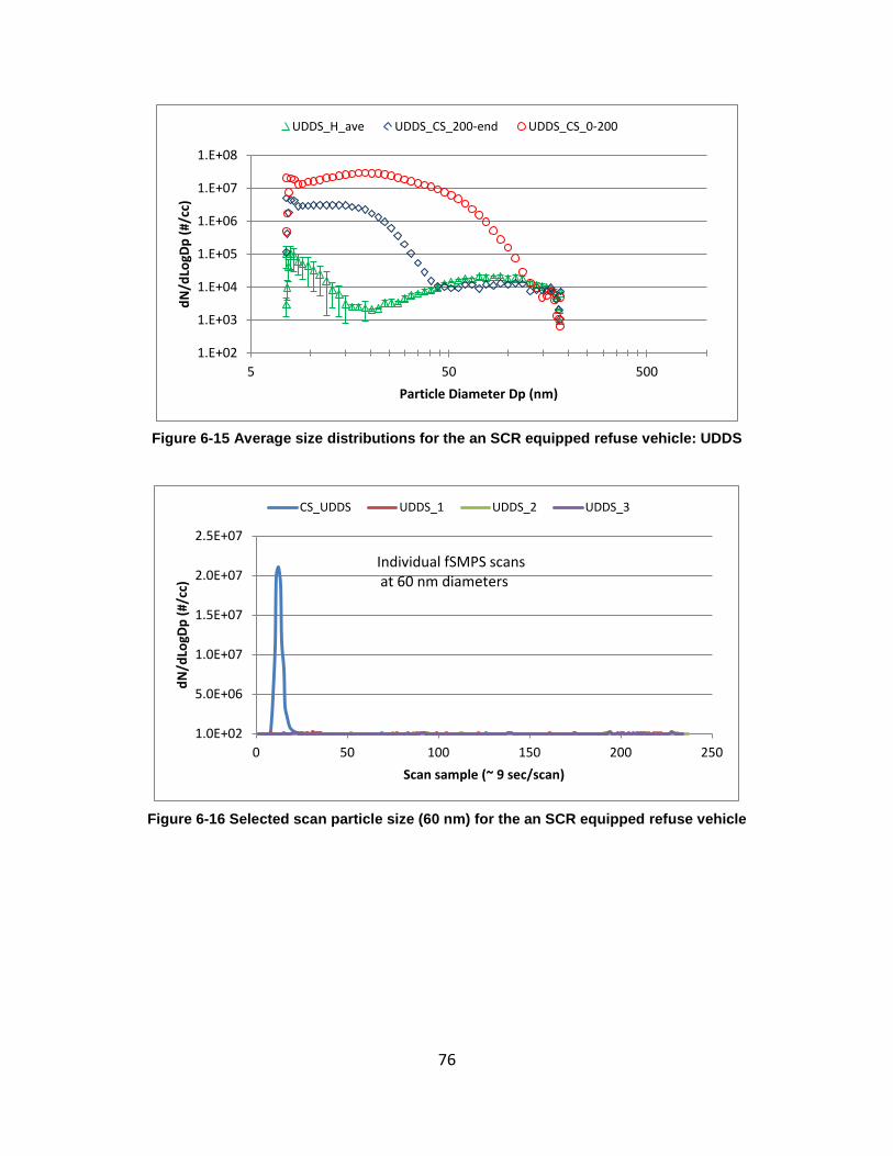
76
Figure 6-15 Average size distributions for the an SCR equipped refuse vehicle: UDDS
Figure 6-16 Selected scan particle size (60 nm) for the an SCR equipped refuse vehicle
1.E+02
1.E+03
1.E+04
1.E+05
1.E+06
1.E+07
1.E+08
5 50 500
dN/d
LogD
p (#
/cc)
Particle Diameter Dp (nm)
UDDS_H_ave UDDS_CS_200-end UDDS_CS_0-200
1.0E+02
5.0E+06
1.0E+07
1.5E+07
2.0E+07
2.5E+07
0 50 100 150 200 250
dN/d
LogD
p (#
/cc)
Scan sample (~ 9 sec/scan)
CS_UDDS UDDS_1 UDDS_2 UDDS_3
Individual fSMPS scans at 60 nm diameters
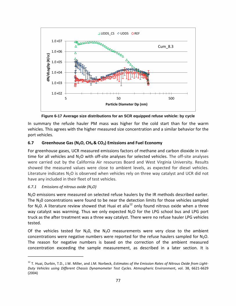
77
Figure 6-17 Average size distributions for an SCR equipped refuse vehicle: by cycle
In summary the refusle hauler PM mass was higher for the cold start than for the warm vehicles. This agrees with the higher measured size concentration and a similar behavior for the port vehicles.
6.7 Greenhouse Gas (N2O, CH4 & CO2) Emissions and Fuel Economy
For greenhouse gases, UCR measured emissions factors of methane and carbon dioxide in real-time for all vehicles and N2O with off-site analyses for selected vehicles. The off-site analyses were carried out by the California Air resources Board and West Virginia University. Results showed the measured values were close to ambient levels, as expected for diesel vehicles. Literature indicates N2O is observed when vehicles rely on three way catalyst and UCR did not have any included in their fleet of test vehicles.
6.7.1 Emissions of nitrous oxide (N2O)
N2O emissions were measured on selected refuse haulers by the IR methods described earlier. The N20 concentrations were found to be near the detection limits for those vehicles sampled for N20. A literature review showed that Huai et alia12
Of the vehicles tested for N20, the N2O measurements were very close to the ambient concentrations were negative numbers were reported for the refuse haulers sampled for N2O. The reason for negative numbers is based on the correction of the ambient measured concentration exceeding the sample measurement, as described in a later section. It is
only found nitrous oxide when a three way catalyst was warming. Thus we only expected N2O for the LPG school bus and LPG port truck as the after treatment was a three way catalyst. There were no refuse hauler LPG vehicles tested.
12 T. Huai, Durbin, T.D., J.W. Miller, and J.M. Norbeck, Estimates of the Emission Rates of Nitrous Oxide from Light-Duty Vehicles using Different Chassis Dynamometer Test Cycles. Atmospheric Environment, vol. 38, 6621-6629 (2004)
1.E+02
1.E+03
1.E+04
1.E+05
1.E+06
1.E+07
5 50 500
dN/d
LogD
p (#
/cc)
Particle Diameter Dp (nm)
UDDS_CS UDDS REF
Cum_8.3
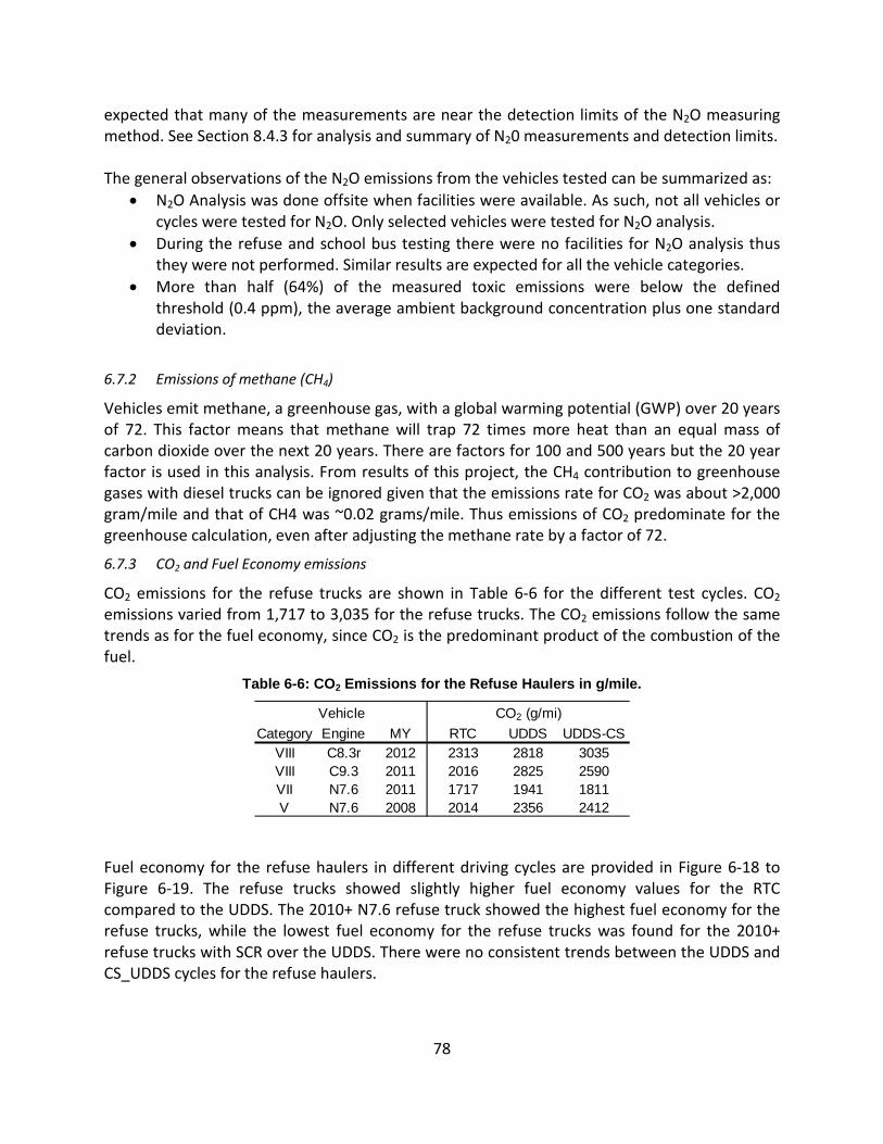
78
expected that many of the measurements are near the detection limits of the N2O measuring method. See Section 8.4.3 for analysis and summary of N20 measurements and detection limits. The general observations of the N2O emissions from the vehicles tested can be summarized as:
• N2O Analysis was done offsite when facilities were available. As such, not all vehicles or cycles were tested for N2O. Only selected vehicles were tested for N2O analysis.
• During the refuse and school bus testing there were no facilities for N2O analysis thus they were not performed. Similar results are expected for all the vehicle categories.
• More than half (64%) of the measured toxic emissions were below the defined threshold (0.4 ppm), the average ambient background concentration plus one standard deviation.
6.7.2 Emissions of methane (CH4)
Vehicles emit methane, a greenhouse gas, with a global warming potential (GWP) over 20 years of 72. This factor means that methane will trap 72 times more heat than an equal mass of carbon dioxide over the next 20 years. There are factors for 100 and 500 years but the 20 year factor is used in this analysis. From results of this project, the CH4 contribution to greenhouse gases with diesel trucks can be ignored given that the emissions rate for CO2 was about >2,000 gram/mile and that of CH4 was ~0.02 grams/mile. Thus emissions of CO2 predominate for the greenhouse calculation, even after adjusting the methane rate by a factor of 72.
6.7.3 CO2 and Fuel Economy emissions
CO2 emissions for the refuse trucks are shown in Table 6-6 for the different test cycles. CO2 emissions varied from 1,717 to 3,035 for the refuse trucks. The CO2 emissions follow the same trends as for the fuel economy, since CO2 is the predominant product of the combustion of the fuel.
Table 6-6: CO2 Emissions for the Refuse Haulers in g/mile.
Fuel economy for the refuse haulers in different driving cycles are provided in Figure 6-18 to Figure 6-19. The refuse trucks showed slightly higher fuel economy values for the RTC compared to the UDDS. The 2010+ N7.6 refuse truck showed the highest fuel economy for the refuse trucks, while the lowest fuel economy for the refuse trucks was found for the 2010+ refuse trucks with SCR over the UDDS. There were no consistent trends between the UDDS and CS_UDDS cycles for the refuse haulers.
Category Engine MY RTC UDDS UDDS-CSVIII C8.3r 2012 2313 2818 3035VIII C9.3 2011 2016 2825 2590VII N7.6 2011 1717 1941 1811V N7.6 2008 2014 2356 2412
Vehicle CO2 (g/mi)
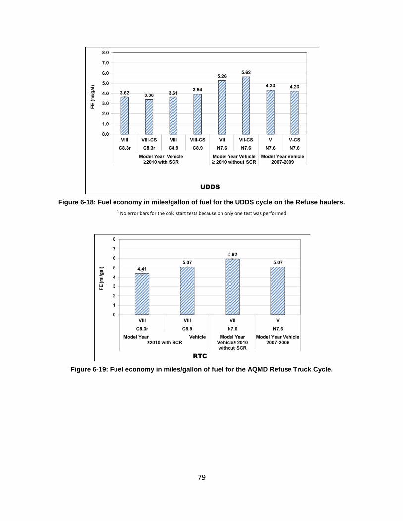
79
Figure 6-18: Fuel economy in miles/gallon of fuel for the UDDS cycle on the Refuse haulers.
1 No error bars for the cold start tests because on only one test was performed
Figure 6-19: Fuel economy in miles/gallon of fuel for the AQMD Refuse Truck Cycle.
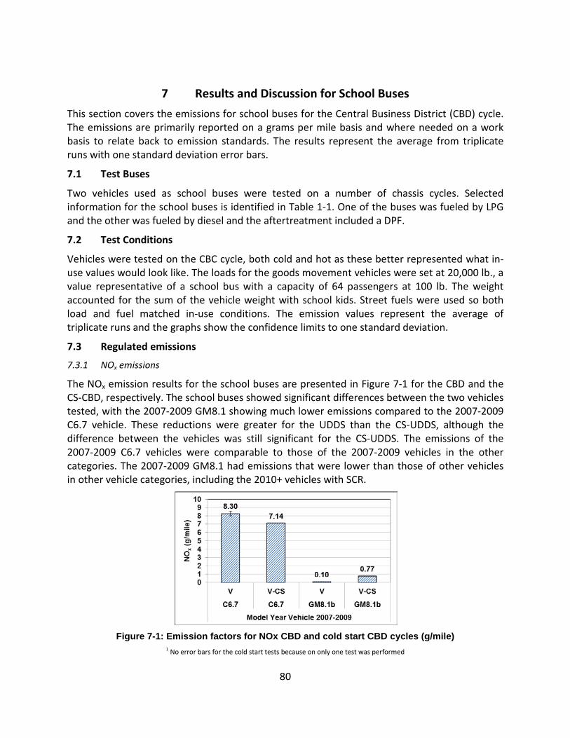
80
7 Results and Discussion for School Buses
This section covers the emissions for school buses for the Central Business District (CBD) cycle. The emissions are primarily reported on a grams per mile basis and where needed on a work basis to relate back to emission standards. The results represent the average from triplicate runs with one standard deviation error bars.
7.1 Test Buses
Two vehicles used as school buses were tested on a number of chassis cycles. Selected information for the school buses is identified in Table 1-1. One of the buses was fueled by LPG and the other was fueled by diesel and the aftertreatment included a DPF.
7.2 Test Conditions
Vehicles were tested on the CBC cycle, both cold and hot as these better represented what in-use values would look like. The loads for the goods movement vehicles were set at 20,000 lb., a value representative of a school bus with a capacity of 64 passengers at 100 lb. The weight accounted for the sum of the vehicle weight with school kids. Street fuels were used so both load and fuel matched in-use conditions. The emission values represent the average of triplicate runs and the graphs show the confidence limits to one standard deviation.
7.3 Regulated emissions
7.3.1 NOx emissions
The NOx emission results for the school buses are presented in Figure 7-1 for the CBD and the CS-CBD, respectively. The school buses showed significant differences between the two vehicles tested, with the 2007-2009 GM8.1 showing much lower emissions compared to the 2007-2009 C6.7 vehicle. These reductions were greater for the UDDS than the CS-UDDS, although the difference between the vehicles was still significant for the CS-UDDS. The emissions of the 2007-2009 C6.7 vehicles were comparable to those of the 2007-2009 vehicles in the other categories. The 2007-2009 GM8.1 had emissions that were lower than those of other vehicles in other vehicle categories, including the 2010+ vehicles with SCR.
Figure 7-1: Emission factors for NOx CBD and cold start CBD cycles (g/mile)
1 No error bars for the cold start tests because on only one test was performed
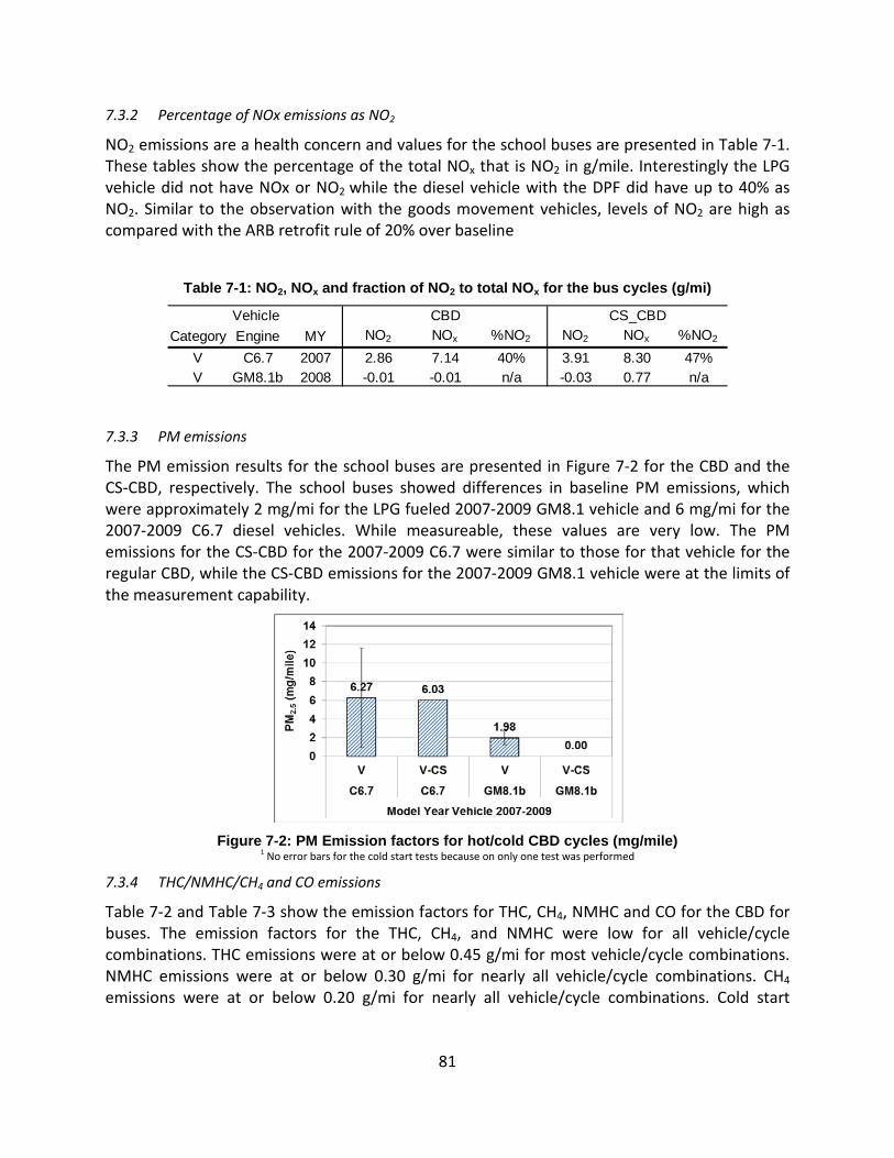
81
7.3.2 Percentage of NOx emissions as NO2
NO2 emissions are a health concern and values for the school buses are presented in Table 7-1. These tables show the percentage of the total NOx that is NO2 in g/mile. Interestingly the LPG vehicle did not have NOx or NO2 while the diesel vehicle with the DPF did have up to 40% as NO2. Similar to the observation with the goods movement vehicles, levels of NO2 are high as compared with the ARB retrofit rule of 20% over baseline
Table 7-1: NO2, NOx and fraction of NO2 to total NOx for the bus cycles (g/mi)
7.3.3 PM emissions
The PM emission results for the school buses are presented in Figure 7-2 for the CBD and the CS-CBD, respectively. The school buses showed differences in baseline PM emissions, which were approximately 2 mg/mi for the LPG fueled 2007-2009 GM8.1 vehicle and 6 mg/mi for the 2007-2009 C6.7 diesel vehicles. While measureable, these values are very low. The PM emissions for the CS-CBD for the 2007-2009 C6.7 were similar to those for that vehicle for the regular CBD, while the CS-CBD emissions for the 2007-2009 GM8.1 vehicle were at the limits of the measurement capability.
Figure 7-2: PM Emission factors for hot/cold CBD cycles (mg/mile)
1 No error bars for the cold start tests because on only one test was performed
7.3.4 THC/NMHC/CH4 and CO emissions
Table 7-2 and Table 7-3 show the emission factors for THC, CH4, NMHC and CO for the CBD for buses. The emission factors for the THC, CH4, and NMHC were low for all vehicle/cycle combinations. THC emissions were at or below 0.45 g/mi for most vehicle/cycle combinations. NMHC emissions were at or below 0.30 g/mi for nearly all vehicle/cycle combinations. CH4 emissions were at or below 0.20 g/mi for nearly all vehicle/cycle combinations. Cold start
Category Engine MY NO2 NOx %NO2 NO2 NOx %NO2
V C6.7 2007 2.86 7.14 40% 3.91 8.30 47%V GM8.1b 2008 -0.01 -0.01 n/a -0.03 0.77 n/a
Vehicle CBD CS_CBD
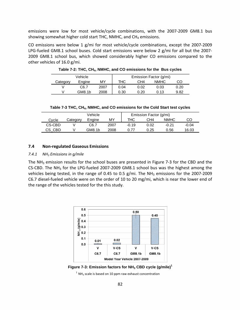
82
emissions were low for most vehicle/cycle combinations, with the 2007-2009 GM8.1 bus showing somewhat higher cold start THC, NMHC, and CH4 emissions.
CO emissions were below 1 g/mi for most vehicle/cycle combinations, except the 2007-2009 LPG-fueled GM8.1 school buses. Cold start emissions were below 2 g/mi for all but the 2007-2009 GM8.1 school bus, which showed considerably higher CO emissions compared to the other vehicles of 16.0 g/mi.
Table 7-2: THC, CH4, NMHC, and CO emissions for the Bus cycles
Table 7-3 THC, CH4, NMHC, and CO emissions for the Cold Start test cycles
7.4 Non-regulated Gaseous Emissions
7.4.1 NH3 Emissions in g/mile
The NH3 emission results for the school buses are presented in Figure 7-3 for the CBD and the CS-CBD. The NH3 for the LPG-fueled 2007-2009 GM8.1 school bus was the highest among the vehicles being tested, in the range of 0.45 to 0.5 g/mi. The NH3 emissions for the 2007-2009 C6.7 diesel-fueled vehicle were on the order of 10 to 20 mg/mi, which is near the lower end of the range of the vehicles tested for the this study.
Figure 7-3: Emission factors for NH3 CBD cycle (g/mile)1
1 NH3 scale is based on 10 ppm raw exhaust concentration
Category Engine MY THC CH4 NMHC COV C6.7 2007 0.04 0.02 0.03 0.20V GM8.1b 2008 0.30 0.20 0.13 9.82
Vehicle Emission Factor (g/mi)
Category Engine MY THC CH4 NMHC COCS-CBD V C6.7 2007 -0.19 0.02 -0.21 -0.04CS_CBD V GM8.1b 2008 0.77 0.25 0.56 16.03
CycleVehicle Emission Factor (g/mi)
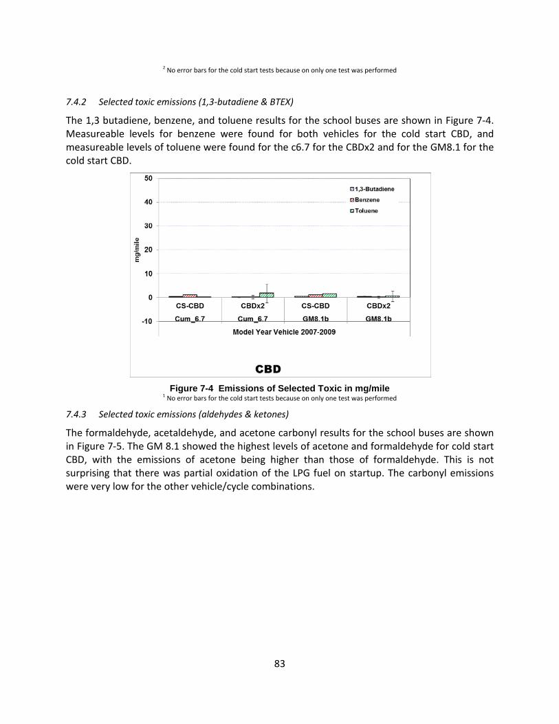
83
2 No error bars for the cold start tests because on only one test was performed
7.4.2 Selected toxic emissions (1,3-butadiene & BTEX)
The 1,3 butadiene, benzene, and toluene results for the school buses are shown in Figure 7-4. Measureable levels for benzene were found for both vehicles for the cold start CBD, and measureable levels of toluene were found for the c6.7 for the CBDx2 and for the GM8.1 for the cold start CBD.
Figure 7-4 Emissions of Selected Toxic in mg/mile
1 No error bars for the cold start tests because on only one test was performed
7.4.3 Selected toxic emissions (aldehydes & ketones)
The formaldehyde, acetaldehyde, and acetone carbonyl results for the school buses are shown in Figure 7-5. The GM 8.1 showed the highest levels of acetone and formaldehyde for cold start CBD, with the emissions of acetone being higher than those of formaldehyde. This is not surprising that there was partial oxidation of the LPG fuel on startup. The carbonyl emissions were very low for the other vehicle/cycle combinations.
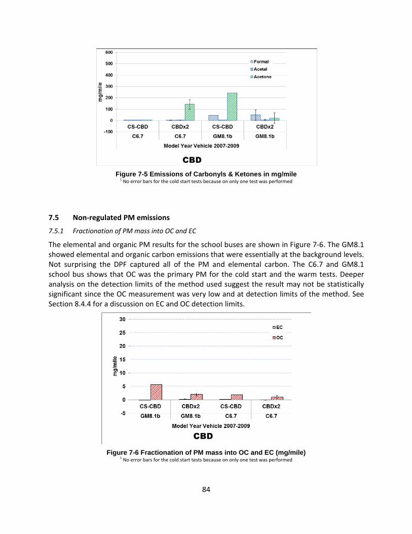
84
Figure 7-5 Emissions of Carbonyls & Ketones in mg/mile
1 No error bars for the cold start tests because on only one test was performed
7.5 Non-regulated PM emissions
7.5.1 Fractionation of PM mass into OC and EC
The elemental and organic PM results for the school buses are shown in Figure 7-6. The GM8.1 showed elemental and organic carbon emissions that were essentially at the background levels. Not surprising the DPF captured all of the PM and elemental carbon. The C6.7 and GM8.1 school bus shows that OC was the primary PM for the cold start and the warm tests. Deeper analysis on the detection limits of the method used suggest the result may not be statistically significant since the OC measurement was very low and at detection limits of the method. See Section 8.4.4 for a discussion on EC and OC detection limits.
Figure 7-6 Fractionation of PM mass into OC and EC (mg/mile)
1 No error bars for the cold start tests because on only one test was performed
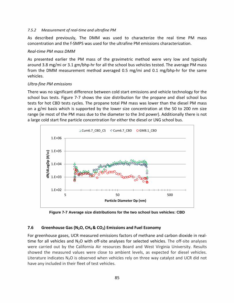
85
7.5.2 Measurement of real-time and ultrafine PM
As described previously, The DMM was used to characterize the real time PM mass concentration and the f-SMPS was used for the ultrafine PM emissions characterization.
Real-time PM mass DMM
As presented earlier the PM mass of the gravimetric method were very low and typically around 3.8 mg/mi or 3.1 gm/bhp-hr for all the school bus vehicles tested. The average PM mass from the DMM measurement method averaged 0.5 mg/mi and 0.1 mg/bhp-hr for the same vehicles.
Ultra-fine PM emissions
There was no significant difference between cold start emissions and vehicle technology for the school bus tests. Figure 7-7 shows the size distribution for the propane and disel school bus tests for hot CBD tests cycles. The propane total PM mass was lower than the diesel PM mass on a g/mi basis which is supported by the lower size concentration at the 50 to 200 nm size range (ie most of the PM mass due to the diameter to the 3rd power). Additionally there is not a large cold start fine particle concentration for either the diesel or LNG school bus.
Figure 7-7 Average size distributions for the two school bus vehicles: CBD
7.6 Greenhouse Gas (N2O, CH4 & CO2) Emissions and Fuel Economy
For greenhouse gases, UCR measured emissions factors of methane and carbon dioxide in real-time for all vehicles and N2O with off-site analyses for selected vehicles. The off-site analyses were carried out by the California Air resources Board and West Virginia University. Results showed the measured values were close to ambient levels, as expected for diesel vehicles. Literature indicates N2O is observed when vehicles rely on three way catalyst and UCR did not have any included in their fleet of test vehicles.
1.E+02
1.E+03
1.E+04
1.E+05
1.E+06
5 50 500
dN/d
LogD
p (#
/cc)
Particle Diameter Dp (nm)
Cum6.7_CBD_CS Cum6.7_CBD GM8.1_CBD
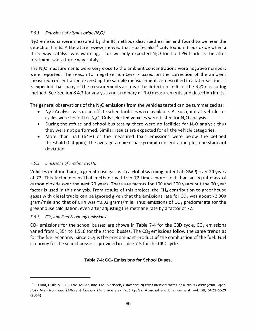
86
7.6.1 Emissions of nitrous oxide (N2O)
N2O emissions were measured by the IR methods described earlier and found to be near the detection limits. A literature review showed that Huai et alia13
The N2O measurements were very close to the ambient concentrations were negative numbers were reported. The reason for negative numbers is based on the correction of the ambient measured concentration exceeding the sample measurement, as described in a later section. It is expected that many of the measurements are near the detection limits of the N2O measuring method. See Section
only found nitrous oxide when a three way catalyst was warming. Thus we only expected N2O for the LPG truck as the after treatment was a three way catalyst.
8.4.3 for analysis and summary of N20 measurements and detection limits. The general observations of the N2O emissions from the vehicles tested can be summarized as:
• N2O Analysis was done offsite when facilities were available. As such, not all vehicles or cycles were tested for N2O. Only selected vehicles were tested for N2O analysis.
• During the refuse and school bus testing there were no facilities for N2O analysis thus they were not performed. Similar results are expected for all the vehicle categories.
• More than half (64%) of the measured toxic emissions were below the defined threshold (0.4 ppm), the average ambient background concentration plus one standard deviation.
7.6.2 Emissions of methane (CH4)
Vehicles emit methane, a greenhouse gas, with a global warming potential (GWP) over 20 years of 72. This factor means that methane will trap 72 times more heat than an equal mass of carbon dioxide over the next 20 years. There are factors for 100 and 500 years but the 20 year factor is used in this analysis. From results of this project, the CH4 contribution to greenhouse gases with diesel trucks can be ignored given that the emissions rate for CO2 was about >2,000 gram/mile and that of CH4 was ~0.02 grams/mile. Thus emissions of CO2 predominate for the greenhouse calculation, even after adjusting the methane rate by a factor of 72.
7.6.3 CO2 and Fuel Economy emissions
CO2 emissions for the school busses are shown in Table 7-4 for the CBD cycle. CO2 emissions varied from 1,354 to 1,516 for the school busses. The CO2 emissions follow the same trends as for the fuel economy, since CO2 is the predominant product of the combustion of the fuel. Fuel economy for the school busses is provided in Table 7-5 for the CBD cycle.
Table 7-4: CO2 Emissions for School Buses.
13 T. Huai, Durbin, T.D., J.W. Miller, and J.M. Norbeck, Estimates of the Emission Rates of Nitrous Oxide from Light-Duty Vehicles using Different Chassis Dynamometer Test Cycles. Atmospheric Environment, vol. 38, 6621-6629 (2004)
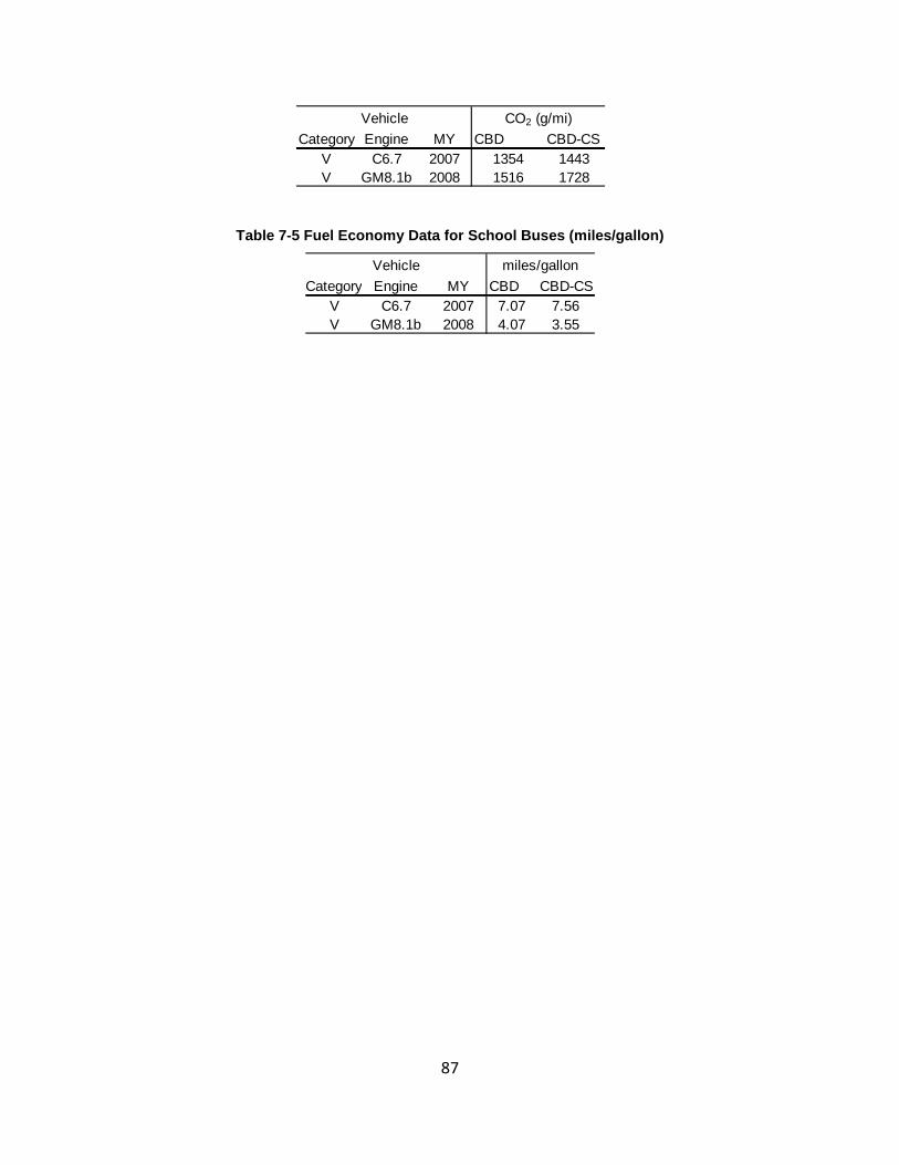
87
Table 7-5 Fuel Economy Data for School Buses (miles/gallon)
Category Engine MY CBD CBD-CSV C6.7 2007 1354 1443V GM8.1b 2008 1516 1728
Vehicle CO2 (g/mi)
Category Engine MY CBD CBD-CSV C6.7 2007 7.07 7.56V GM8.1b 2008 4.07 3.55
Vehicle miles/gallon
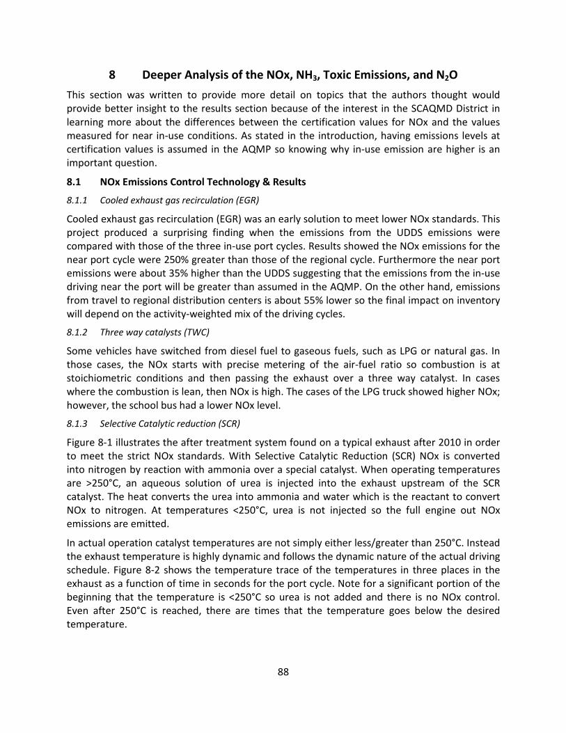
88
8 Deeper Analysis of the NOx, NH3, Toxic Emissions, and N2O
This section was written to provide more detail on topics that the authors thought would provide better insight to the results section because of the interest in the SCAQMD District in learning more about the differences between the certification values for NOx and the values measured for near in-use conditions. As stated in the introduction, having emissions levels at certification values is assumed in the AQMP so knowing why in-use emission are higher is an important question.
8.1 NOx Emissions Control Technology & Results
8.1.1 Cooled exhaust gas recirculation (EGR)
Cooled exhaust gas recirculation (EGR) was an early solution to meet lower NOx standards. This project produced a surprising finding when the emissions from the UDDS emissions were compared with those of the three in-use port cycles. Results showed the NOx emissions for the near port cycle were 250% greater than those of the regional cycle. Furthermore the near port emissions were about 35% higher than the UDDS suggesting that the emissions from the in-use driving near the port will be greater than assumed in the AQMP. On the other hand, emissions from travel to regional distribution centers is about 55% lower so the final impact on inventory will depend on the activity-weighted mix of the driving cycles.
8.1.2 Three way catalysts (TWC)
Some vehicles have switched from diesel fuel to gaseous fuels, such as LPG or natural gas. In those cases, the NOx starts with precise metering of the air-fuel ratio so combustion is at stoichiometric conditions and then passing the exhaust over a three way catalyst. In cases where the combustion is lean, then NOx is high. The cases of the LPG truck showed higher NOx; however, the school bus had a lower NOx level.
8.1.3 Selective Catalytic reduction (SCR)
Figure 8-1 illustrates the after treatment system found on a typical exhaust after 2010 in order to meet the strict NOx standards. With Selective Catalytic Reduction (SCR) NOx is converted into nitrogen by reaction with ammonia over a special catalyst. When operating temperatures are >250°C, an aqueous solution of urea is injected into the exhaust upstream of the SCR catalyst. The heat converts the urea into ammonia and water which is the reactant to convert NOx to nitrogen. At temperatures <250°C, urea is not injected so the full engine out NOx emissions are emitted.
In actual operation catalyst temperatures are not simply either less/greater than 250°C. Instead the exhaust temperature is highly dynamic and follows the dynamic nature of the actual driving schedule. Figure 8-2 shows the temperature trace of the temperatures in three places in the exhaust as a function of time in seconds for the port cycle. Note for a significant portion of the beginning that the temperature is <250°C so urea is not added and there is no NOx control. Even after 250°C is reached, there are times that the temperature goes below the desired temperature.
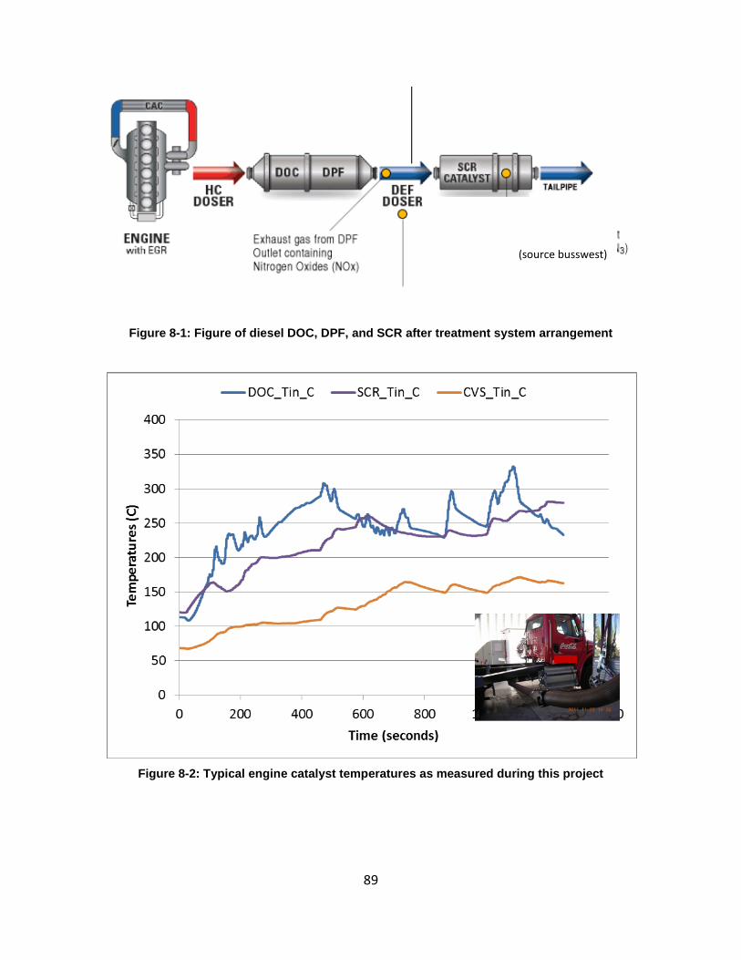
89
Figure 8-1: Figure of diesel DOC, DPF, and SCR after treatment system arrangement
Figure 8-2: Typical engine catalyst temperatures as measured during this project
(source busswest)
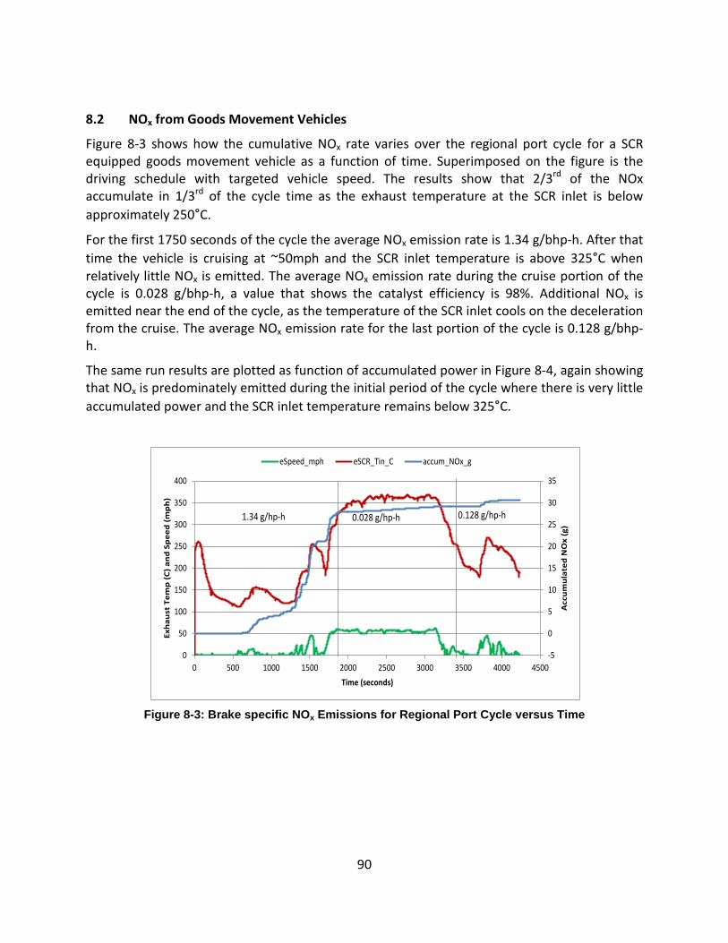
90
8.2 NOx from Goods Movement Vehicles
Figure 8-3 shows how the cumulative NOx rate varies over the regional port cycle for a SCR equipped goods movement vehicle as a function of time. Superimposed on the figure is the driving schedule with targeted vehicle speed. The results show that 2/3rd of the NOx accumulate in 1/3rd of the cycle time as the exhaust temperature at the SCR inlet is below approximately 250°C.
For the first 1750 seconds of the cycle the average NOx emission rate is 1.34 g/bhp-h. After that time the vehicle is cruising at ~50mph and the SCR inlet temperature is above 325°C when relatively little NOx is emitted. The average NOx emission rate during the cruise portion of the cycle is 0.028 g/bhp-h, a value that shows the catalyst efficiency is 98%. Additional NOx is emitted near the end of the cycle, as the temperature of the SCR inlet cools on the deceleration from the cruise. The average NOx emission rate for the last portion of the cycle is 0.128 g/bhp-h.
The same run results are plotted as function of accumulated power in Figure 8-4, again showing that NOx is predominately emitted during the initial period of the cycle where there is very little accumulated power and the SCR inlet temperature remains below 325°C.
Figure 8-3: Brake specific NOx Emissions for Regional Port Cycle versus Time
-5
0
5
10
15
20
25
30
35
0
50
100
150
200
250
300
350
400
0 500 1000 1500 2000 2500 3000 3500 4000 4500
Acc
um
ula
ted
NO
x (g
)
Exh
au
st T
em
p (
C)
an
d S
pe
ed
(m
ph
)
Time (seconds)
eSpeed_mph eSCR_Tin_C accum_NOx_g
1.34 g/hp-h 0.028 g/hp-h 0.128 g/hp-h
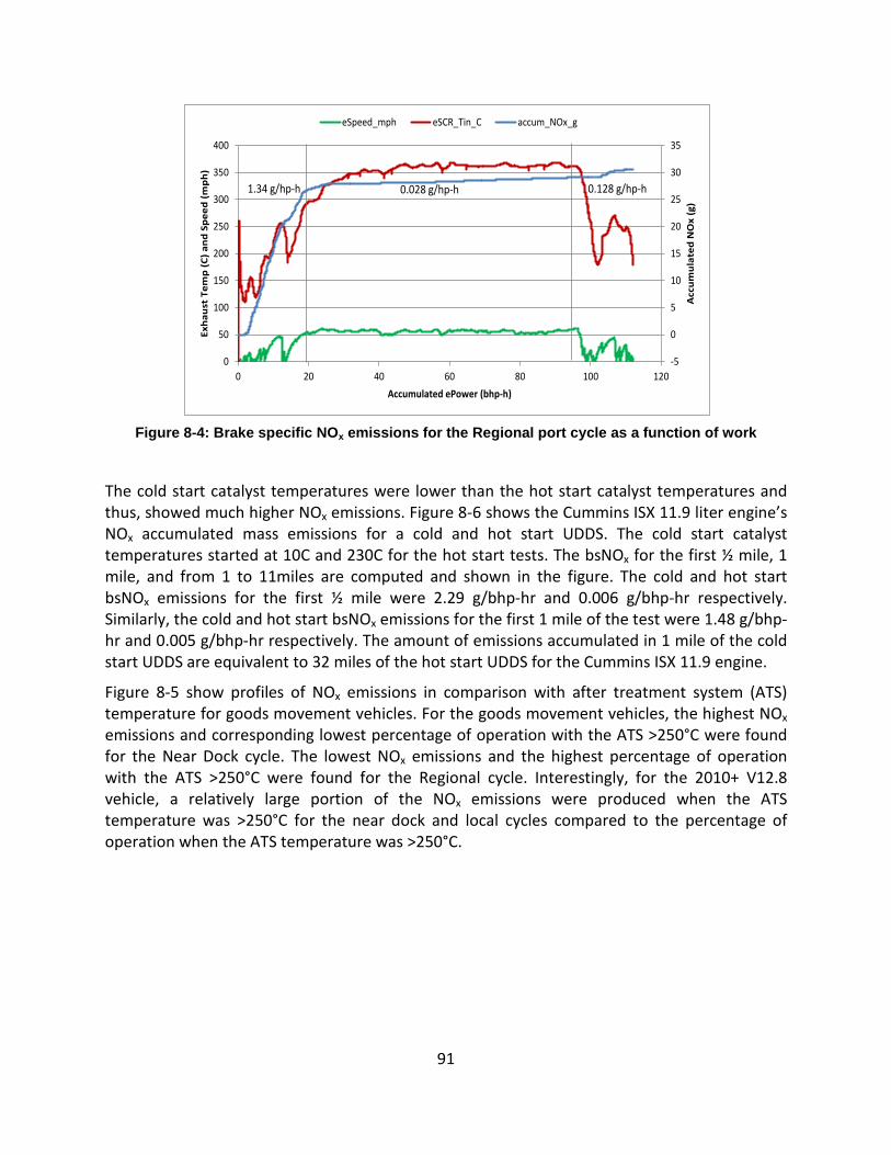
91
Figure 8-4: Brake specific NOx emissions for the Regional port cycle as a function of work
The cold start catalyst temperatures were lower than the hot start catalyst temperatures and thus, showed much higher NOx emissions. Figure 8-6 shows the Cummins ISX 11.9 liter engine’s NOx accumulated mass emissions for a cold and hot start UDDS. The cold start catalyst temperatures started at 10C and 230C for the hot start tests. The bsNOx for the first ½ mile, 1 mile, and from 1 to 11miles are computed and shown in the figure. The cold and hot start bsNOx emissions for the first ½ mile were 2.29 g/bhp-hr and 0.006 g/bhp-hr respectively. Similarly, the cold and hot start bsNOx emissions for the first 1 mile of the test were 1.48 g/bhp-hr and 0.005 g/bhp-hr respectively. The amount of emissions accumulated in 1 mile of the cold start UDDS are equivalent to 32 miles of the hot start UDDS for the Cummins ISX 11.9 engine.
Figure 8-5 show profiles of NOx emissions in comparison with after treatment system (ATS) temperature for goods movement vehicles. For the goods movement vehicles, the highest NOx emissions and corresponding lowest percentage of operation with the ATS >250°C were found for the Near Dock cycle. The lowest NOx emissions and the highest percentage of operation with the ATS >250°C were found for the Regional cycle. Interestingly, for the 2010+ V12.8 vehicle, a relatively large portion of the NOx emissions were produced when the ATS temperature was >250°C for the near dock and local cycles compared to the percentage of operation when the ATS temperature was >250°C.
-5
0
5
10
15
20
25
30
35
0
50
100
150
200
250
300
350
400
0 20 40 60 80 100 120
Acc
um
ula
ted
NO
x (g
)
Exh
aust
Tem
p (
C)
and
Sp
eed
(m
ph
)
Accumulated ePower (bhp-h)
eSpeed_mph eSCR_Tin_C accum_NOx_g
1.34 g/hp-h 0.028 g/hp-h 0.128 g/hp-h
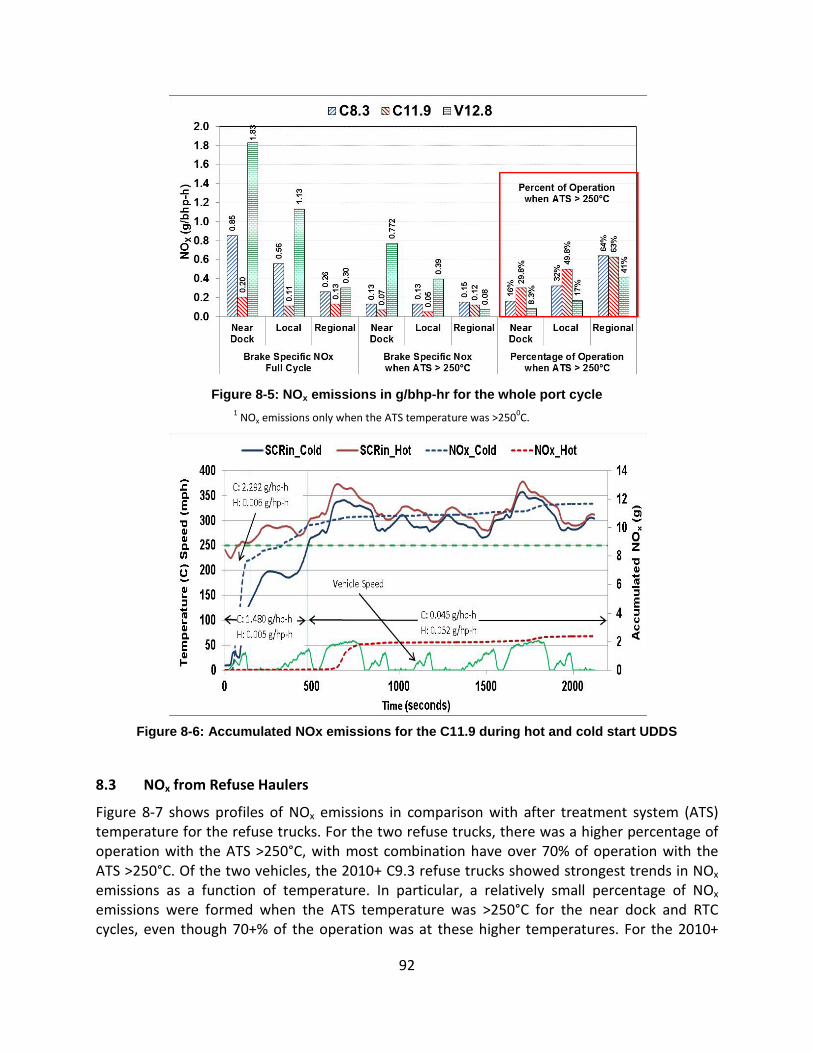
92
Figure 8-5: NOx emissions in g/bhp-hr for the whole port cycle
1 NOx emissions only when the ATS temperature was >2500C.
Figure 8-6: Accumulated NOx emissions for the C11.9 during hot and cold start UDDS
8.3 NOx from Refuse Haulers
Figure 8-7 shows profiles of NOx emissions in comparison with after treatment system (ATS) temperature for the refuse trucks. For the two refuse trucks, there was a higher percentage of operation with the ATS >250°C, with most combination have over 70% of operation with the ATS >250°C. Of the two vehicles, the 2010+ C9.3 refuse trucks showed strongest trends in NOx emissions as a function of temperature. In particular, a relatively small percentage of NOx emissions were formed when the ATS temperature was >250°C for the near dock and RTC cycles, even though 70+% of the operation was at these higher temperatures. For the 2010+
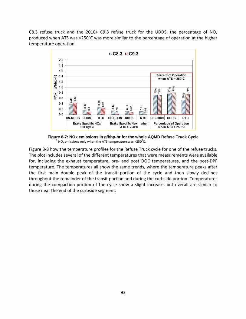
93
C8.3 refuse truck and the 2010+ C9.3 refuse truck for the UDDS, the percentage of NOx produced when ATS was >250°C was more similar to the percentage of operation at the higher temperature operation.
Figure 8-7: NOx emissions in g/bhp-hr for the whole AQMD Refuse Truck Cycle
1 NOx emissions only when the ATS temperature was >2500C.
Figure 8-8 how the temperature profiles for the Refuse Truck cycle for one of the refuse trucks. The plot includes several of the different temperatures that were measurements were available for, including the exhaust temperature, pre- and post DOC temperatures, and the post-DPF temperature. The temperatures all show the same trends, where the temperature peaks after the first main double peak of the transit portion of the cycle and then slowly declines throughout the remainder of the transit portion and during the curbside portion. Temperatures during the compaction portion of the cycle show a slight increase, but overall are similar to those near the end of the curbside segment.
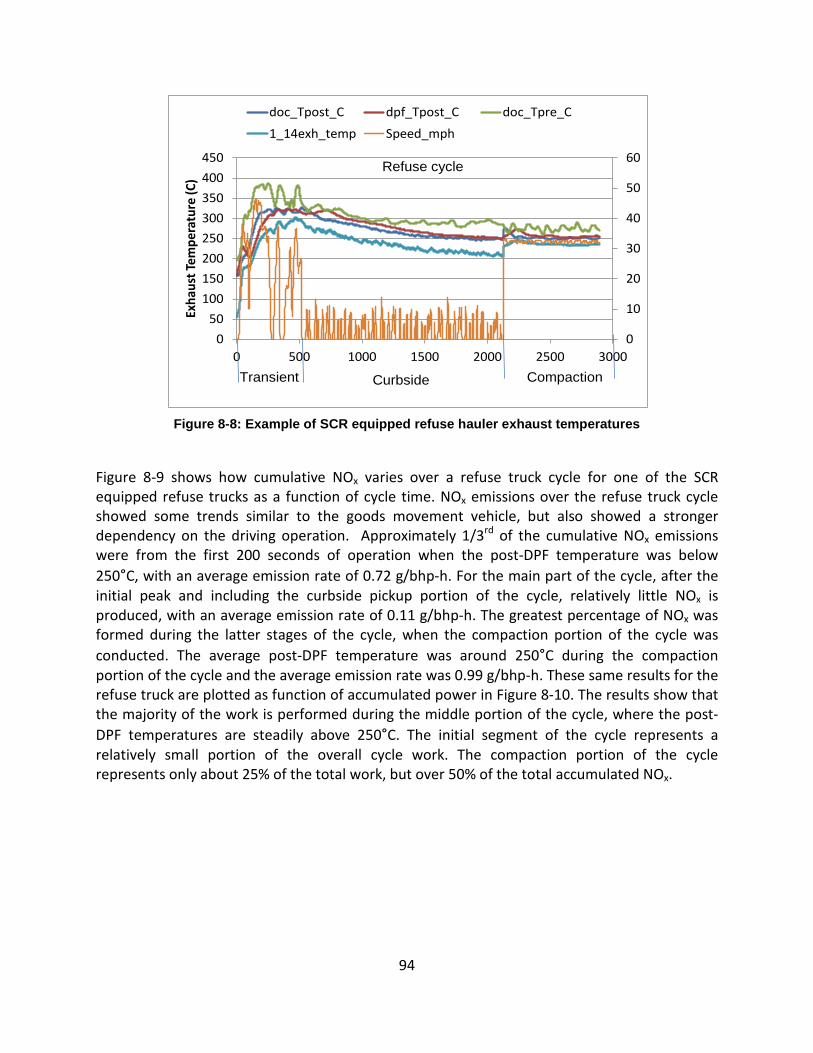
94
Figure 8-8: Example of SCR equipped refuse hauler exhaust temperatures
Figure 8-9 shows how cumulative NOx varies over a refuse truck cycle for one of the SCR equipped refuse trucks as a function of cycle time. NOx emissions over the refuse truck cycle showed some trends similar to the goods movement vehicle, but also showed a stronger dependency on the driving operation. Approximately 1/3rd of the cumulative NOx emissions were from the first 200 seconds of operation when the post-DPF temperature was below 250°C, with an average emission rate of 0.72 g/bhp-h. For the main part of the cycle, after the initial peak and including the curbside pickup portion of the cycle, relatively little NOx is produced, with an average emission rate of 0.11 g/bhp-h. The greatest percentage of NOx was formed during the latter stages of the cycle, when the compaction portion of the cycle was conducted. The average post-DPF temperature was around 250°C during the compaction portion of the cycle and the average emission rate was 0.99 g/bhp-h. These same results for the refuse truck are plotted as function of accumulated power in Figure 8-10. The results show that the majority of the work is performed during the middle portion of the cycle, where the post-DPF temperatures are steadily above 250°C. The initial segment of the cycle represents a relatively small portion of the overall cycle work. The compaction portion of the cycle represents only about 25% of the total work, but over 50% of the total accumulated NOx.
0
10
20
30
40
50
60
0
50
100
150
200
250
300
350
400
450
0 500 1000 1500 2000 2500 3000
Exha
ust T
empe
ratu
re (C
)
doc_Tpost_C dpf_Tpost_C doc_Tpre_C
1_14exh_temp Speed_mph
Refuse cycle
Transient CompactionCurbside
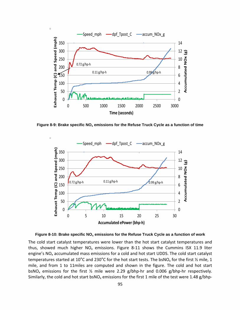
95
Figure 8-9: Brake specific NOx emissions for the Refuse Truck Cycle as a function of time
Figure 8-10: Brake specific NOx emissions for the Refuse Truck Cycle as a function of work
The cold start catalyst temperatures were lower than the hot start catalyst temperatures and thus, showed much higher NOx emissions. Figure 8-11 shows the Cummins ISX 11.9 liter engine’s NOx accumulated mass emissions for a cold and hot start UDDS. The cold start catalyst temperatures started at 10°C and 230°C for the hot start tests. The bsNOx for the first ½ mile, 1 mile, and from 1 to 11miles are computed and shown in the figure. The cold and hot start bsNOx emissions for the first ½ mile were 2.29 g/bhp-hr and 0.006 g/bhp-hr respectively. Similarly, the cold and hot start bsNOx emissions for the first 1 mile of the test were 1.48 g/bhp-
0
2
4
6
8
10
12
14
0
50
100
150
200
250
300
350
0 500 1000 1500 2000 2500 3000
Acc
um
ula
ted
NO
x (
g)
Ex
ha
ust
Te
mp
(C
) a
nd
Sp
ee
d (
mp
h)
Time (seconds)
Speed_mph dpf_Tpost_C accum_NOx_g
0.72 g/hp-h
0.11 g/hp-h 0.99 g/hp-h
0
2
4
6
8
10
12
14
0
50
100
150
200
250
300
350
0 5 10 15 20 25 30
Acc
um
ula
ted
NO
x (
g)
Ex
ha
ust
Te
mp
(C
) a
nd
Sp
ee
d (
mp
h)
Accumulated ePower (bhp-h)
Speed_mph dpf_Tpost_C accum_NOx_g
0.72 g/hp-h 0.11 g/hp-h 0.99 g/hp-h
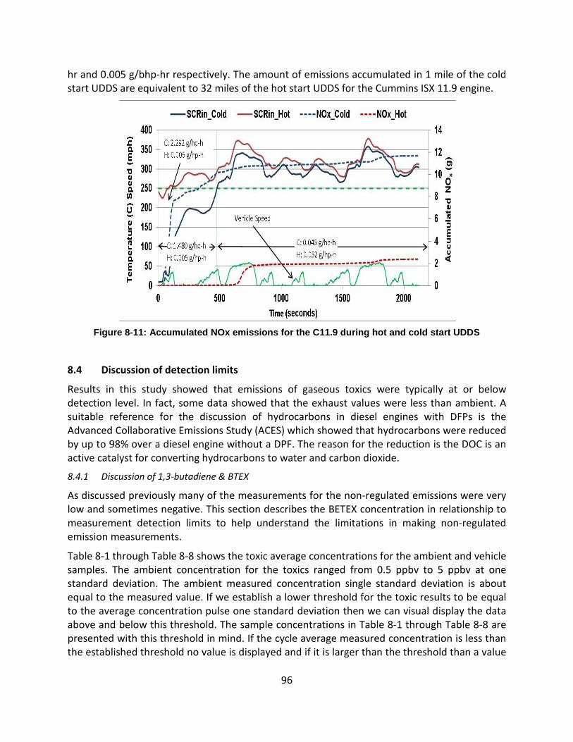
96
hr and 0.005 g/bhp-hr respectively. The amount of emissions accumulated in 1 mile of the cold start UDDS are equivalent to 32 miles of the hot start UDDS for the Cummins ISX 11.9 engine.
Figure 8-11: Accumulated NOx emissions for the C11.9 during hot and cold start UDDS
8.4 Discussion of detection limits
Results in this study showed that emissions of gaseous toxics were typically at or below detection level. In fact, some data showed that the exhaust values were less than ambient. A suitable reference for the discussion of hydrocarbons in diesel engines with DFPs is the Advanced Collaborative Emissions Study (ACES) which showed that hydrocarbons were reduced by up to 98% over a diesel engine without a DPF. The reason for the reduction is the DOC is an active catalyst for converting hydrocarbons to water and carbon dioxide.
8.4.1 Discussion of 1,3-butadiene & BTEX
As discussed previously many of the measurements for the non-regulated emissions were very low and sometimes negative. This section describes the BETEX concentration in relationship to measurement detection limits to help understand the limitations in making non-regulated emission measurements.
Table 8-1 through Table 8-8 shows the toxic average concentrations for the ambient and vehicle samples. The ambient concentration for the toxics ranged from 0.5 ppbv to 5 ppbv at one standard deviation. The ambient measured concentration single standard deviation is about equal to the measured value. If we establish a lower threshold for the toxic results to be equal to the average concentration pulse one standard deviation then we can visual display the data above and below this threshold. The sample concentrations in Table 8-1 through Table 8-8 are presented with this threshold in mind. If the cycle average measured concentration is less than the established threshold no value is displayed and if it is larger than the threshold than a value
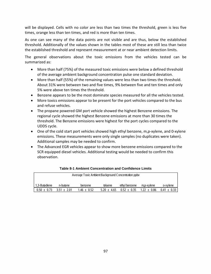
97
will be displayed. Cells with no color are less than two times the threshold, green is less five times, orange less than ten times, and red is more than ten times.
As one can see many of the data points are not visible and are thus, below the established threshold. Additionally of the values shown in the tables most of these are still less than twice the established threshold and represent measurement at or near ambient detection limits.
The general observations about the toxic emissions from the vehicles tested can be summarized as:
• More than half (75%) of the measured toxic emissions were below a defined threshold of the average ambient background concentration pulse one standard deviation.
• More than half (55%) of the remaining values were less than two times the threshold. About 31% were between two and five times, 9% between five and ten times and only 5% were above ten times the threshold.
• Benzene appears to be the most dominate species measured for all the vehicles tested. • More toxics emissions appear to be present for the port vehicles compared to the bus
and refuse vehicles. • The propane powered GM port vehicle showed the highest Benzene emissions. The
regional cycle showed the highest Benzene emissions at more than 30 times the threshold. The Benzene emissions were highest for the port cycles compared to the UDDS cycle.
• One of the cold start port vehicles showed high ethyl benzene, m,p-xylene, and 0-xylene emissions. These measurements were only single samples (no duplicates were taken). Additional samples may be needed to confirm.
• The Advanced EGR vehicles appear to show more benzene emissions compared to the SCR equipped diesel vehicles. Additional testing would be needed to confirm this observation.
Table 8-1 Ambient Concentration and Confidence Limits
0.50 ± 0.73 3.51 ± 2.01 1.46 ± 0.52 5.20 ± 4.65 0.52 ± 0.35 1.22 ± 0.86 0.41 ± 0.33
Average Toxic Ambient Background Concentration ppbv
1,3-Butadiene n-butane benzene toluene ethyl benzene m,p-xylene o-xylene
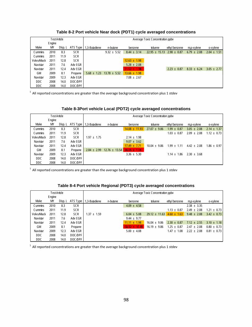
98
Table 8-2 Port vehicle Near dock (PDT1) cycle averaged concentrations
1 All reported concentrations are greater than the average background concentration plus 1 stdev
Table 8-3Port vehicle Local (PDT2) cycle averaged concentrations
1 All reported concentrations are greater than the average background concentration plus 1 stdev
Table 8-4 Port vehicle Regional (PDT3) cycle averaged concentrations
1 All reported concentrations are greater than the average background concentration plus 1 stdev
MakeEngine
MY Disp. L ATS TypeCummins 2010 8.3 SCR 9.32 ± 5.52 8.44 ± 3.14 22.95 ± 15.13 2.98 ± 0.87 6.79 ± 2.08 2.04 ± 1.51Cummins 2011 11.9 SCR
Volvo/Mack 2011 12.8 SCR 12.63 ± 1.98Navistar 2011 7.6 Adv EGR 5.28 ± 2.08Navistar 2011 12.4 Adv EGR 21.62 ± 1.98 2.23 ± 0.87 8.33 ± 6.24 3.05 ± 2.77
GM 2009 8.1 Propane 5.68 ± 1.23 13.78 ± 5.52 13.66 ± 1.98Navistar 2009 12.3 Adv EGR 7.08 ± 2.67
DDC 2008 14.0 DOC/DPFDDC 2008 14.0 DOC/DPF
ethyl benzene m,p-xylene o-xylene
Average Toxic Concentration ppbvTest Article
1,3-Butadiene n-butane benzene toluene
MakeEngine
MY Disp. L ATS TypeCummins 2010 8.3 SCR 14.08 ± 11.93 27.07 ± 9.86 1.99 ± 0.87 3.05 ± 2.08 2.14 ± 1.37Cummins 2011 11.9 SCR 1.03 ± 0.87 2.09 ± 2.08 1.12 ± 0.73
Volvo/Mack 2011 12.8 SCR 1.97 ± 1.75 2.14 ± 1.98Navistar 2011 7.6 Adv EGR 9.07 ± 3.62Navistar 2011 12.4 Adv EGR 17.49 ± 7.71 10.04 ± 9.86 1.99 ± 1.11 4.42 ± 2.08 1.86 ± 0.97
GM 2009 8.1 Propane 2.84 ± 2.99 12.76 ± 13.54 36.05 ± 1.98Navistar 2009 12.3 Adv EGR 3.36 ± 5.30 1.14 ± 1.86 2.30 ± 3.68
DDC 2008 14.0 DOC/DPFDDC 2008 14.0 DOC/DPF
ethyl benzene m,p-xylene o-xylene
Average Toxic Concentration ppbvTest Article
1,3-Butadiene n-butane benzene toluene
MakeEngine
MY Disp. L ATS TypeCummins 2010 8.3 SCR 4.09 ± 4.58 2.38 ± 3.35Cummins 2011 11.9 SCR 1.13 ± 0.87 2.49 ± 2.08 1.21 ± 0.73
Volvo/Mack 2011 12.8 SCR 1.37 ± 1.59 6.04 ± 5.08 29.12 ± 11.63 4.60 ± 1.63 9.48 ± 2.08 3.42 ± 0.73Navistar 2011 7.6 Adv EGR 9.44 ± 9.77Navistar 2011 12.4 Adv EGR 11.11 ± 1.98 16.04 ± 9.86 2.30 ± 0.87 7.12 ± 2.55 3.10 ± 1.18
GM 2009 8.1 Propane 60.82 ± 10.49 16.19 ± 9.86 1.25 ± 0.87 2.47 ± 2.08 0.80 ± 0.73Navistar 2009 12.3 Adv EGR 5.00 ± 4.08 1.47 ± 1.08 2.22 ± 2.08 0.81 ± 0.73
DDC 2008 14.0 DOC/DPFDDC 2008 14.0 DOC/DPF
ethyl benzene m,p-xylene o-xylene
Average Toxic Concentration ppbvTest Article
1,3-Butadiene n-butane benzene toluene
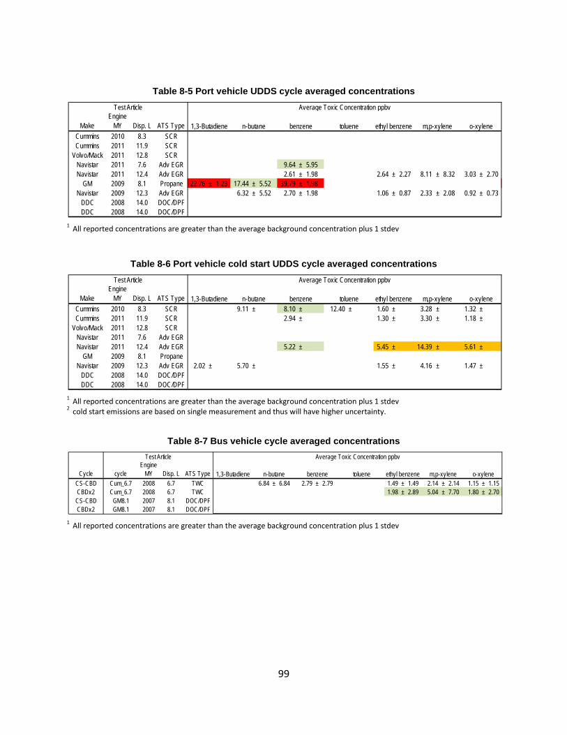
99
Table 8-5 Port vehicle UDDS cycle averaged concentrations
1 All reported concentrations are greater than the average background concentration plus 1 stdev
Table 8-6 Port vehicle cold start UDDS cycle averaged concentrations
1 All reported concentrations are greater than the average background concentration plus 1 stdev 2 cold start emissions are based on single measurement and thus will have higher uncertainty.
Table 8-7 Bus vehicle cycle averaged concentrations
1 All reported concentrations are greater than the average background concentration plus 1 stdev
MakeEngine
MY Disp. L ATS TypeCummins 2010 8.3 SCRCummins 2011 11.9 SCR
Volvo/Mack 2011 12.8 SCRNavistar 2011 7.6 Adv EGR 9.64 ± 5.95Navistar 2011 12.4 Adv EGR 2.61 ± 1.98 2.64 ± 2.27 8.11 ± 8.32 3.03 ± 2.70
GM 2009 8.1 Propane 22.76 ± 1.23 17.44 ± 5.52 39.79 ± 1.98Navistar 2009 12.3 Adv EGR 6.32 ± 5.52 2.70 ± 1.98 1.06 ± 0.87 2.33 ± 2.08 0.92 ± 0.73
DDC 2008 14.0 DOC/DPFDDC 2008 14.0 DOC/DPF
ethyl benzene m,p-xylene o-xylene
Average Toxic Concentration ppbvTest Article
1,3-Butadiene n-butane benzene toluene
MakeEngine
MY Disp. L ATS TypeCummins 2010 8.3 SCR 9.11 ± 8.10 ± 12.40 ± 1.60 ± 3.28 ± 1.32 ±Cummins 2011 11.9 SCR 2.94 ± 1.30 ± 3.30 ± 1.18 ±
Volvo/Mack 2011 12.8 SCRNavistar 2011 7.6 Adv EGRNavistar 2011 12.4 Adv EGR 5.22 ± 5.45 ± 14.39 ± 5.61 ±
GM 2009 8.1 PropaneNavistar 2009 12.3 Adv EGR 2.02 ± 5.70 ± 1.55 ± 4.16 ± 1.47 ±
DDC 2008 14.0 DOC/DPFDDC 2008 14.0 DOC/DPF
ethyl benzene m,p-xylene o-xylene
Average Toxic Concentration ppbvTest Article
1,3-Butadiene n-butane benzene toluene
Cycle cycleEngine
MY Disp. L ATS TypeCS-CBD Cum_6.7 2008 6.7 TWC 6.84 ± 6.84 2.79 ± 2.79 1.49 ± 1.49 2.14 ± 2.14 1.15 ± 1.15CBDx2 Cum_6.7 2008 6.7 TWC 1.98 ± 2.89 5.04 ± 7.70 1.80 ± 2.70
CS-CBD GM8.1 2007 8.1 DOC/DPFCBDx2 GM8.1 2007 8.1 DOC/DPF
Test Article Average Toxic Concentration ppbv
1,3-Butadiene n-butane benzene toluene ethyl benzene m,p-xylene o-xylene
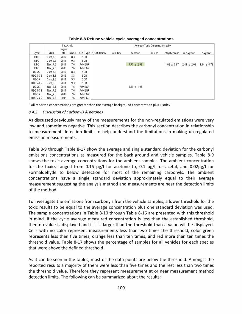
100
Table 8-8 Refuse vehicle cycle averaged concentrations
1 All reported concentrations are greater than the average background concentration plus 1 stdev
8.4.2 Discussion of Carbonyls & Ketones
As discussed previously many of the measurements for the non-regulated emissions were very low and sometimes negative. This section describes the carbonyl concentration in relationship to measurement detection limits to help understand the limitations in making un-regulated emission measurements. Table 8-9 through Table 8-17 show the average and single standard deviation for the carbonyl emissions concentrations as measured for the back ground and vehicle samples. Table 8-9 shows the toxic average concentrations for the ambient samples. The ambient concentration for the toxics ranged from 0.15 µg/l for acetone to, 0.1 µg/l for acetal, and 0.02µg/l for Formaldehyde to below detection for most of the remaining carbonyls. The ambient concentrations have a single standard deviation approximately equal to their average measurement suggesting the analysis method and measurements are near the detection limits of the method. To investigate the emissions from carbonyls from the vehicle samples, a lower threshold for the toxic results to be equal to the average concentration plus one standard deviation was used. The sample concentrations in Table 8-10 through Table 8-16 are presented with this threshold in mind. If the cycle average measured concentration is less than the established threshold, then no value is displayed and if it is larger than the threshold than a value will be displayed. Cells with no color represent measurements less than two times the threshold, color green represents less than five times, orange less than ten times, and red more than ten times the threshold value. Table 8-17 shows the percentage of samples for all vehicles for each species that were above the defined threshold. As it can be seen in the tables, most of the data points are below the threshold. Amongst the reported results a majority of them were less than five times and the rest less than two times the threshold value. Therefore they represent measurement at or near measurement method detection limits. The following can be summarized about the results:
Cycle MakeEngine
MY Disp. L ATS TypeRTC Cum_8.3 2012 8.3 SCRRTC Cum_9.3 2011 9.3 SCRRTC Nav_7.6 2011 7.6 Adv EGR 7.77 ± 2.99 1.02 ± 0.87 2.41 ± 2.08 1.14 ± 0.73RTC Nav_7.6 2008 7.6 Adv EGR
UDDS Cum_8.3 2012 8.3 SCRUDDS-CS Cum_8.3 2012 8.3 SCR
UDDS Cum_9.3 2011 9.3 SCRUDDS-CS Cum_9.3 2011 9.3 SCR
UDDS Nav_7.6 2011 7.6 Adv EGR 2.59 ± 1.98UDDS-CS Nav_7.6 2011 7.6 Adv EGR
UDDS Nav_7.6 2008 7.6 Adv EGRUDDS-CS Nav_7.6 2008 7.6 Adv EGR
ethyl benzene m,p-xylene o-xylene
Test Article Average Toxic Concentration ppbv
1,3-Butadiene n-butane benzene toluene
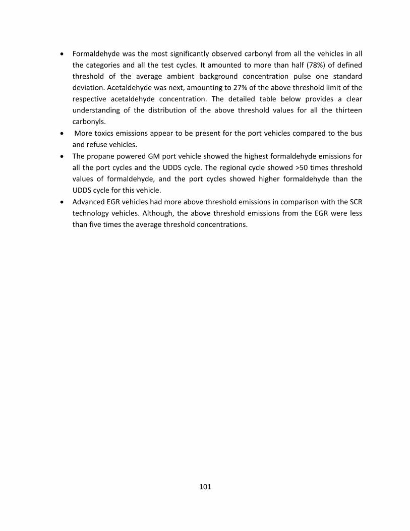
101
• Formaldehyde was the most significantly observed carbonyl from all the vehicles in all the categories and all the test cycles. It amounted to more than half (78%) of defined threshold of the average ambient background concentration pulse one standard deviation. Acetaldehyde was next, amounting to 27% of the above threshold limit of the respective acetaldehyde concentration. The detailed table below provides a clear understanding of the distribution of the above threshold values for all the thirteen carbonyls.
• More toxics emissions appear to be present for the port vehicles compared to the bus and refuse vehicles.
• The propane powered GM port vehicle showed the highest formaldehyde emissions for all the port cycles and the UDDS cycle. The regional cycle showed >50 times threshold values of formaldehyde, and the port cycles showed higher formaldehyde than the UDDS cycle for this vehicle.
• Advanced EGR vehicles had more above threshold emissions in comparison with the SCR technology vehicles. Although, the above threshold emissions from the EGR were less than five times the average threshold concentrations.
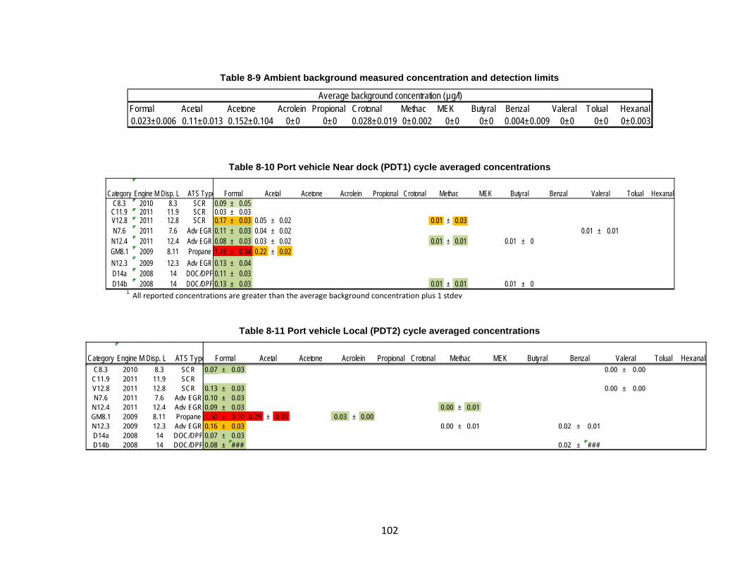
102
Table 8-9 Ambient background measured concentration and detection limits
Table 8-10 Port vehicle Near dock (PDT1) cycle averaged concentrations
1 All reported concentrations are greater than the average background concentration plus 1 stdev
Table 8-11 Port vehicle Local (PDT2) cycle averaged concentrations
Formal Acetal Acetone Acrolein Propional Crotonal Methac MEK Butyral Benzal Valeral Tolual Hexanal0.023±0.006 0.11±0.013 0.152±0.104 0±0 0±0 0.028±0.019 0±0.002 0±0 0±0 0.004±0.009 0±0 0±0 0±0.003
Average background concentration (µg/l)
Category Engine M Disp. L ATS TypeC8.3 2010 8.3 SCR 0.09 ± 0.05
C11.9 2011 11.9 SCR 0.03 ± 0.03V12.8 2011 12.8 SCR 0.17 ± 0.03 0.05 ± 0.02 0.01 ± 0.03N7.6 2011 7.6 Adv EGR 0.11 ± 0.03 0.04 ± 0.02 0.01 ± 0.01
N12.4 2011 12.4 Adv EGR 0.08 ± 0.03 0.03 ± 0.02 0.01 ± 0.01 0.01 ± 0GM8.1 2009 8.11 Propane 1.18 ± 0.04 0.22 ± 0.02N12.3 2009 12.3 Adv EGR 0.13 ± 0.04D14a 2008 14 DOC/DPF 0.11 ± 0.03D14b 2008 14 DOC/DPF 0.13 ± 0.03 0.01 ± 0.01 0.01 ± 0
Crotonal Tolual HexanalMethac MEK Butyral Benzal ValeralFormal Acetal Acetone Acrolein Propional
Category Engine M Disp. L ATS Type Crotonal Tolual HexanalMethac MEK Butyral Benzal ValeralFormal Acetal Acetone Acrolein PropionalC8.3 2010 8.3 SCR 0.07 ± 0.03 0.00 ± 0.00
C11.9 2011 11.9 SCRV12.8 2011 12.8 SCR 0.13 ± 0.03 0.00 ± 0.00N7.6 2011 7.6 Adv EGR 0.10 ± 0.03
N12.4 2011 12.4 Adv EGR 0.09 ± 0.03 0.00 ± 0.01GM8.1 2009 8.11 Propane 1.50 ± 0.10 0.29 ± 0.05 0.03 ± 0.00N12.3 2009 12.3 Adv EGR 0.16 ± 0.03 0.00 ± 0.01 0.02 ± 0.01D14a 2008 14 DOC/DPF 0.07 ± 0.03D14b 2008 14 DOC/DPF 0.08 ± ### 0.02 ± ###
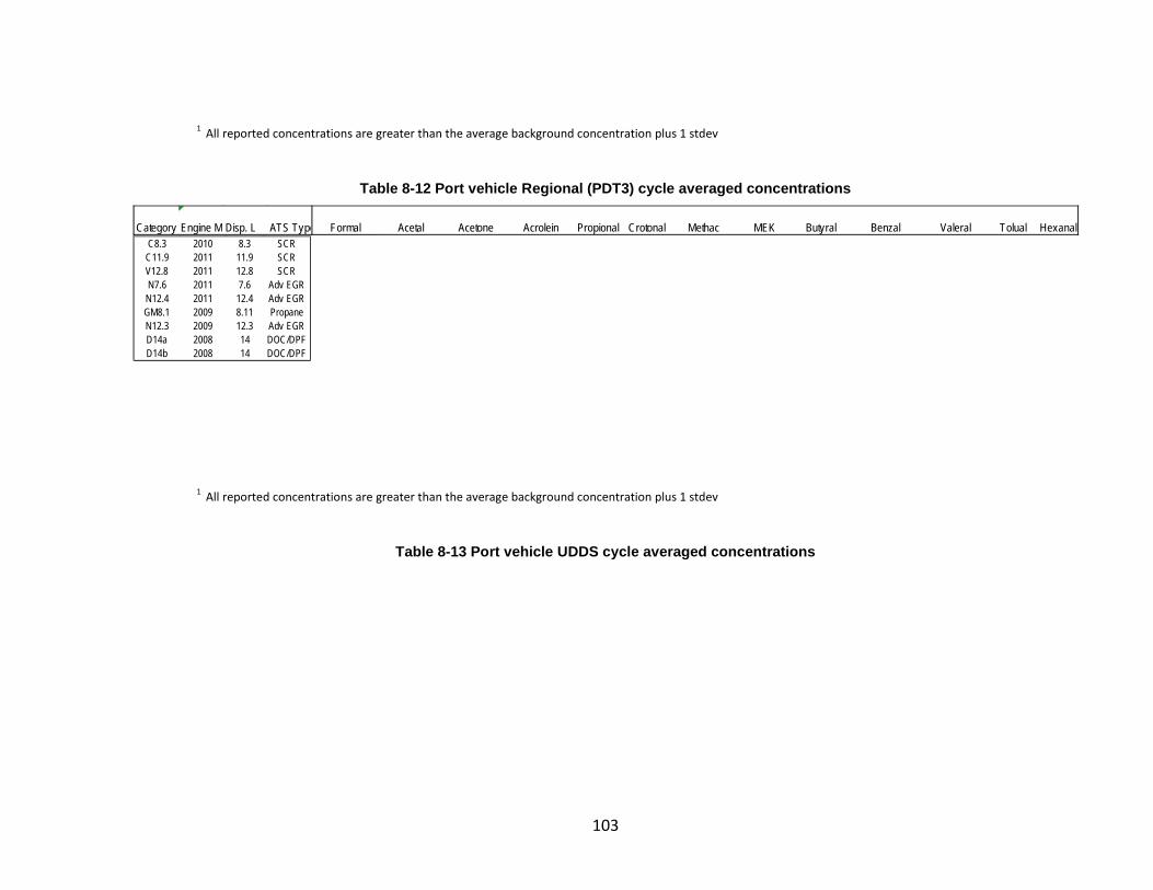
103
1 All reported concentrations are greater than the average background concentration plus 1 stdev
Table 8-12 Port vehicle Regional (PDT3) cycle averaged concentrations
1 All reported concentrations are greater than the average background concentration plus 1 stdev
Table 8-13 Port vehicle UDDS cycle averaged concentrations
Category Engine MYDisp. L ATS Type Crotonal Tolual HexanalMethac MEK Butyral Benzal ValeralFormal Acetal Acetone Acrolein PropionalC8.3 2010 8.3 SCR
C11.9 2011 11.9 SCRV12.8 2011 12.8 SCRN7.6 2011 7.6 Adv EGR
N12.4 2011 12.4 Adv EGRGM8.1 2009 8.11 PropaneN12.3 2009 12.3 Adv EGRD14a 2008 14 DOC/DPFD14b 2008 14 DOC/DPF
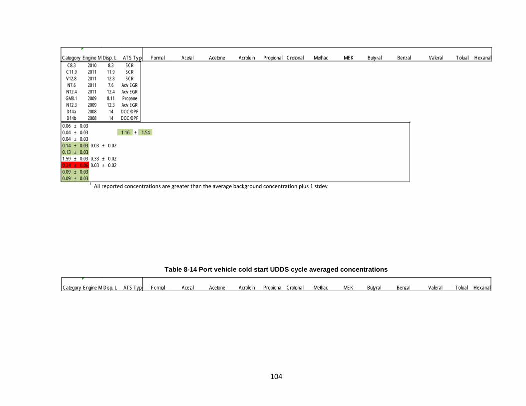
104
1 All reported concentrations are greater than the average background concentration plus 1 stdev
Table 8-14 Port vehicle cold start UDDS cycle averaged concentrations
Category Engine MYDisp. L ATS Type Crotonal Tolual HexanalMethac MEK Butyral Benzal ValeralFormal Acetal Acetone Acrolein PropionalC8.3 2010 8.3 SCR
C11.9 2011 11.9 SCRV12.8 2011 12.8 SCRN7.6 2011 7.6 Adv EGR
N12.4 2011 12.4 Adv EGRGM8.1 2009 8.11 PropaneN12.3 2009 12.3 Adv EGRD14a 2008 14 DOC/DPFD14b 2008 14 DOC/DPF
0.06 ± 0.030.04 ± 0.03 1.16 ± 1.540.04 ± 0.030.14 ± 0.03 0.03 ± 0.020.13 ± 0.031.59 ± 0.03 0.33 ± 0.020.24 ± 0.06 0.03 ± 0.020.09 ± 0.030.09 ± 0.03
Category Engine M Disp. L ATS Type Crotonal Tolual HexanalMethac MEK Butyral Benzal ValeralFormal Acetal Acetone Acrolein Propional
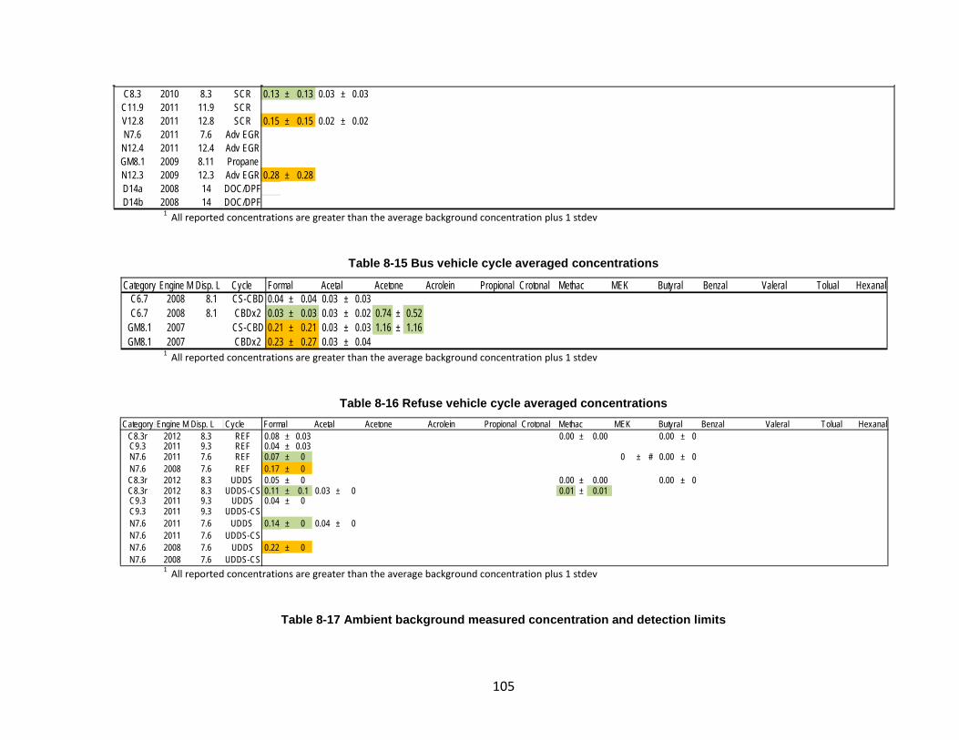
105
1 All reported concentrations are greater than the average background concentration plus 1 stdev
Table 8-15 Bus vehicle cycle averaged concentrations
1 All reported concentrations are greater than the average background concentration plus 1 stdev
Table 8-16 Refuse vehicle cycle averaged concentrations
1 All reported concentrations are greater than the average background concentration plus 1 stdev
Table 8-17 Ambient background measured concentration and detection limits
C8.3 2010 8.3 SCR 0.13 ± 0.13 0.03 ± 0.03C11.9 2011 11.9 SCRV12.8 2011 12.8 SCR 0.15 ± 0.15 0.02 ± 0.02N7.6 2011 7.6 Adv EGR
N12.4 2011 12.4 Adv EGRGM8.1 2009 8.11 PropaneN12.3 2009 12.3 Adv EGR 0.28 ± 0.28D14a 2008 14 DOC/DPFD14b 2008 14 DOC/DPF
Category Engine MYDisp. L Cycle Formal Acetal Acetone Acrolein Propional Crotonal Methac MEK Butyral Benzal Valeral Tolual HexanalC6.7 2008 8.1 CS-CBD 0.04 ± 0.04 0.03 ± 0.03C6.7 2008 8.1 CBDx2 0.03 ± 0.03 0.03 ± 0.02 0.74 ± 0.52
GM8.1 2007 CS-CBD 0.21 ± 0.21 0.03 ± 0.03 1.16 ± 1.16GM8.1 2007 CBDx2 0.23 ± 0.27 0.03 ± 0.04
Category Engine M Disp. L Cycle Formal Acetal Acetone Acrolein Propional Crotonal Methac MEK Butyral Benzal Valeral Tolual HexanalC8.3r 2012 8.3 REF 0.08 ± 0.03 0.00 ± 0.00 0.00 ± 0C9.3 2011 9.3 REF 0.04 ± 0.03N7.6 2011 7.6 REF 0.07 ± 0 0 ± # 0.00 ± 0N7.6 2008 7.6 REF 0.17 ± 0C8.3r 2012 8.3 UDDS 0.05 ± 0 0.00 ± 0.00 0.00 ± 0C8.3r 2012 8.3 UDDS-CS 0.11 ± 0.1 0.03 ± 0 0.01 ± 0.01C9.3 2011 9.3 UDDS 0.04 ± 0C9.3 2011 9.3 UDDS-CSN7.6 2011 7.6 UDDS 0.14 ± 0 0.04 ± 0N7.6 2011 7.6 UDDS-CSN7.6 2008 7.6 UDDS 0.22 ± 0N7.6 2008 7.6 UDDS-CS
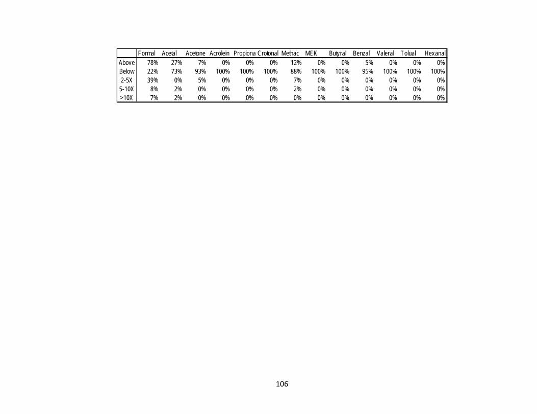
106
Formal Acetal Acetone Acrolein Propiona Crotonal Methac MEK Butyral Benzal Valeral Tolual HexanalAbove 78% 27% 7% 0% 0% 0% 12% 0% 0% 5% 0% 0% 0%Below 22% 73% 93% 100% 100% 100% 88% 100% 100% 95% 100% 100% 100%2-5X 39% 0% 5% 0% 0% 0% 7% 0% 0% 0% 0% 0% 0%
5-10X 8% 2% 0% 0% 0% 0% 2% 0% 0% 0% 0% 0% 0%>10X 7% 2% 0% 0% 0% 0% 0% 0% 0% 0% 0% 0% 0%
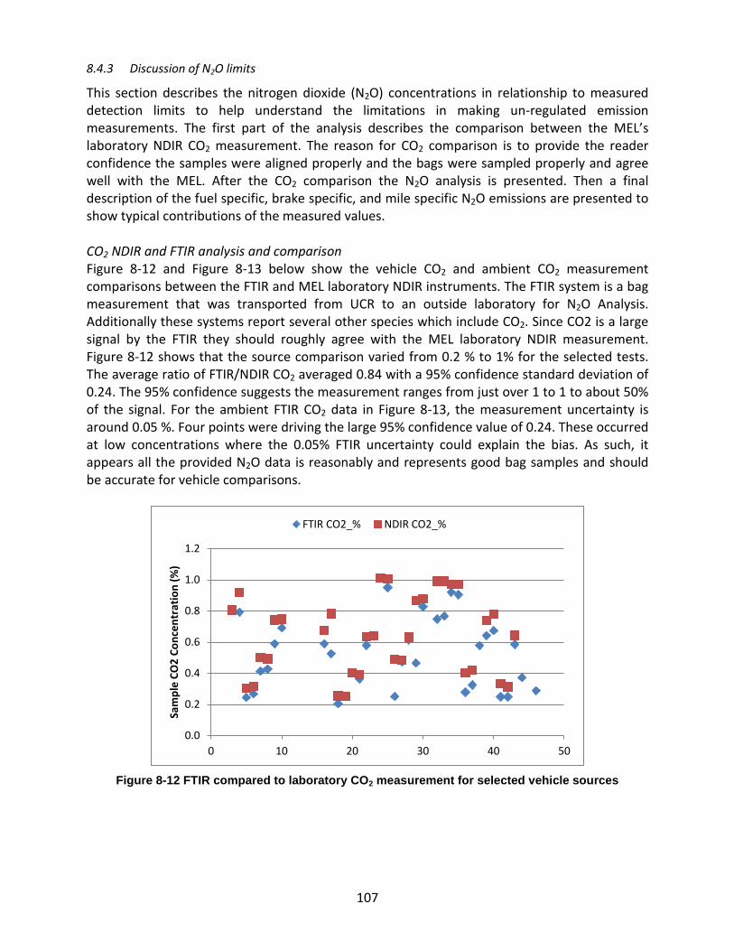
107
8.4.3 Discussion of N2O limits
This section describes the nitrogen dioxide (N2O) concentrations in relationship to measured detection limits to help understand the limitations in making un-regulated emission measurements. The first part of the analysis describes the comparison between the MEL’s laboratory NDIR CO2 measurement. The reason for CO2 comparison is to provide the reader confidence the samples were aligned properly and the bags were sampled properly and agree well with the MEL. After the CO2 comparison the N2O analysis is presented. Then a final description of the fuel specific, brake specific, and mile specific N2O emissions are presented to show typical contributions of the measured values. CO2 NDIR and FTIR analysis and comparison Figure 8-12 and Figure 8-13 below show the vehicle CO2 and ambient CO2 measurement comparisons between the FTIR and MEL laboratory NDIR instruments. The FTIR system is a bag measurement that was transported from UCR to an outside laboratory for N2O Analysis. Additionally these systems report several other species which include CO2. Since CO2 is a large signal by the FTIR they should roughly agree with the MEL laboratory NDIR measurement. Figure 8-12 shows that the source comparison varied from 0.2 % to 1% for the selected tests. The average ratio of FTIR/NDIR CO2 averaged 0.84 with a 95% confidence standard deviation of 0.24. The 95% confidence suggests the measurement ranges from just over 1 to 1 to about 50% of the signal. For the ambient FTIR CO2 data in Figure 8-13, the measurement uncertainty is around 0.05 %. Four points were driving the large 95% confidence value of 0.24. These occurred at low concentrations where the 0.05% FTIR uncertainty could explain the bias. As such, it appears all the provided N2O data is reasonably and represents good bag samples and should be accurate for vehicle comparisons.
Figure 8-12 FTIR compared to laboratory CO2 measurement for selected vehicle sources
0.0
0.2
0.4
0.6
0.8
1.0
1.2
0 10 20 30 40 50
Sam
ple
CO2
Conc
entr
atio
n (%
)
FTIR CO2_% NDIR CO2_%
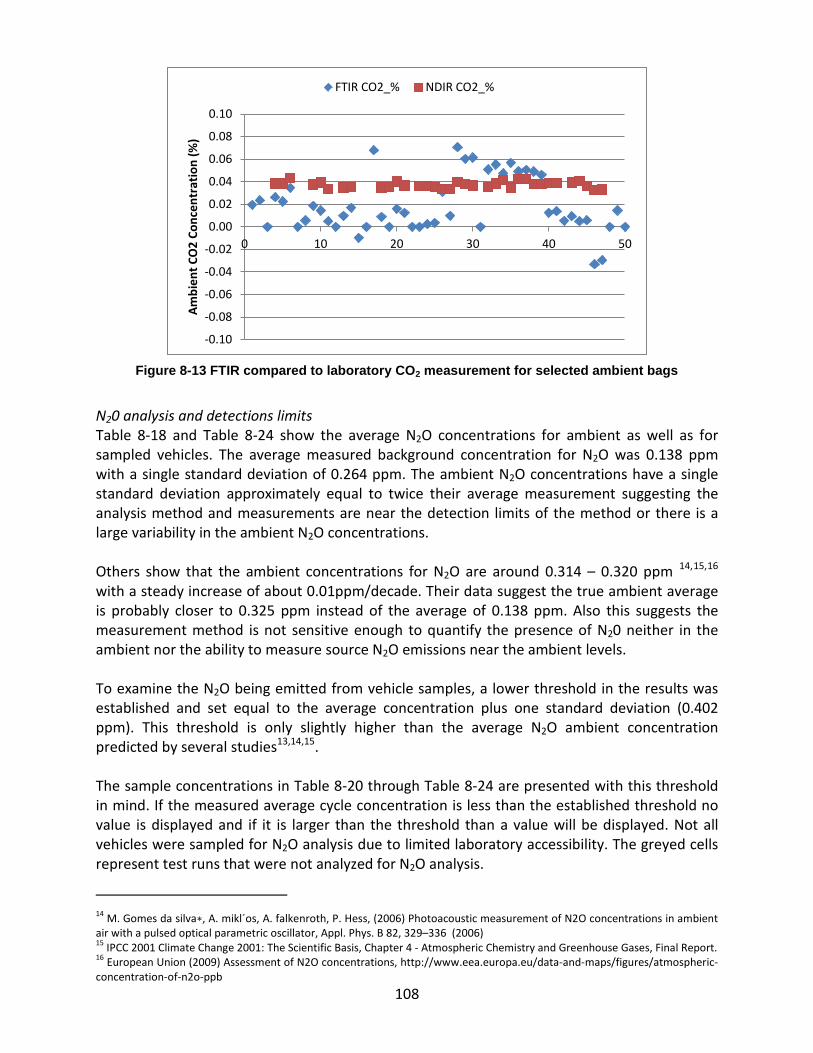
108
Figure 8-13 FTIR compared to laboratory CO2 measurement for selected ambient bags
N20 analysis and detections limits Table 8-18 and Table 8-24 show the average N2O concentrations for ambient as well as for sampled vehicles. The average measured background concentration for N2O was 0.138 ppm with a single standard deviation of 0.264 ppm. The ambient N2O concentrations have a single standard deviation approximately equal to twice their average measurement suggesting the analysis method and measurements are near the detection limits of the method or there is a large variability in the ambient N2O concentrations. Others show that the ambient concentrations for N2O are around 0.314 – 0.320 ppm 14,15,16
with a steady increase of about 0.01ppm/decade. Their data suggest the true ambient average is probably closer to 0.325 ppm instead of the average of 0.138 ppm. Also this suggests the measurement method is not sensitive enough to quantify the presence of N20 neither in the ambient nor the ability to measure source N2O emissions near the ambient levels.
To examine the N2O being emitted from vehicle samples, a lower threshold in the results was established and set equal to the average concentration plus one standard deviation (0.402 ppm). This threshold is only slightly higher than the average N2O ambient concentration predicted by several studies13,14,15. The sample concentrations in Table 8-20 through Table 8-24 are presented with this threshold in mind. If the measured average cycle concentration is less than the established threshold no value is displayed and if it is larger than the threshold than a value will be displayed. Not all vehicles were sampled for N2O analysis due to limited laboratory accessibility. The greyed cells represent test runs that were not analyzed for N2O analysis.
14 M. Gomes da silva∗, A. mikl´os, A. falkenroth, P. Hess, (2006) Photoacoustic measurement of N2O concentrations in ambient air with a pulsed optical parametric oscillator, Appl. Phys. B 82, 329–336 (2006) 15 IPCC 2001 Climate Change 2001: The Scientific Basis, Chapter 4 - Atmospheric Chemistry and Greenhouse Gases, Final Report. 16 European Union (2009) Assessment of N2O concentrations, http://www.eea.europa.eu/data-and-maps/figures/atmospheric-concentration-of-n2o-ppb
-0.10
-0.08
-0.06
-0.04
-0.02
0.00
0.02
0.04
0.06
0.08
0.10
0 10 20 30 40 50
Am
bien
t CO
2 Co
ncen
trat
ion
(%)
FTIR CO2_% NDIR CO2_%
109
N2O emission factors (g/mi) The previous tables showed the N2O concentrations relative to the ambient measured concentration and standard deviation of those values. Additionally the tables showed the calculated N2O emission rates on a grams per mile basis. The N2O emissions rates were calculated by correcting for ambient concentrations as shown by equation 2 below:
Equation 2
𝐸𝐹 =∗𝑉𝑚𝑖𝑥 ∗ 𝜌𝑁20 ∗ �𝐶𝑖 − 𝐶𝑏𝑘 ∗ �1 − 1
𝐷𝐹��
𝑀𝑖𝑙𝑒𝑠
Where: EF is the emission factor in g/mi Vmix volume through the CVS in m3
𝜌N20 density of N20 from ideal gas law at 1 atm and 20C and molar mass N2O Ci sample concentration Cbk background concentration DF dilution ratio from CVS sampling system Miles distance traveled in miles
The N2O measurements were very close to the ambient concentrations were negative numbers were reported. The reason for negative numbers is based on the correction of the ambient measured concentration exceeding the sample measurement. It is expected that many of the measurements are near the detection limits of the measuring method. The general observations of the N2O emissions from the vehicles tested can be summarized as:
• N2O Analysis was done offsite when facilities were available. As such, not all vehicles or cycles were tested for N2O. Only selected vehicles were tested for N2O analysis.
• During the refuse and school bus testing there were no facilities for N2O analysis thus they were not performed.
• More than half (64%) of the measured toxic emissions were below the defined threshold (0.4 ppm), the average ambient background concentration plus one standard deviation.
• Only the SCR equipped vehicles showed signs of N2O emissions not the non-SCR equipped vehicles.
• The cold start UDDS did not show higher integrated N2O emissions compared with hot start UDDS tests (with or with/out SCR). It is not clear from the testing if higher N20 emissions were created for a short duration at the cold start of the cold test cycles. Additional real time N2O data would be necessary to evaluate the first 100 seconds of the cold start UDDS N2O emissions.
• Of the values greater than the threshold, the average vehicle sample concentration was 1.06 ppm (only 2.6 times the threshold) and the single standard deviation was 0.44 ppm.
• The N2O emission rate in mg/mi for port vehicles with higher than threshold concentrations ranged from 1.5 mg/mi to 17 mg/mi where the highest concentrations was
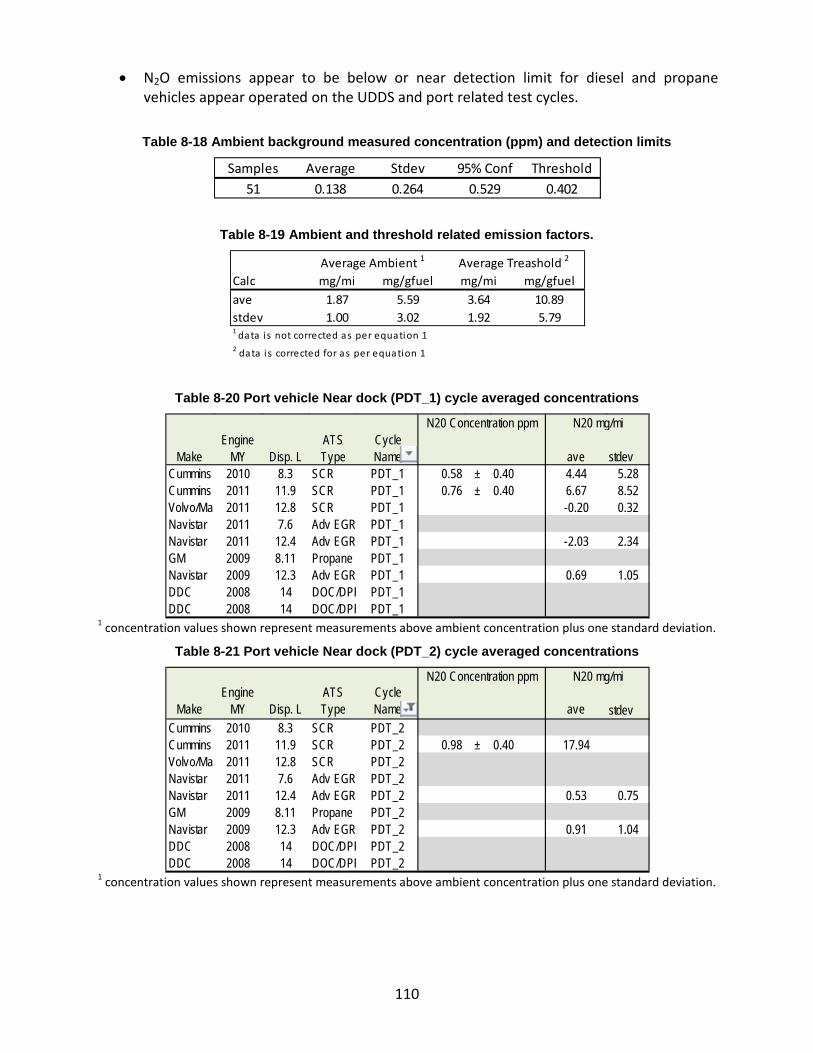
110
• N2O emissions appear to be below or near detection limit for diesel and propane vehicles appear operated on the UDDS and port related test cycles.
Table 8-18 Ambient background measured concentration (ppm) and detection limits
Table 8-19 Ambient and threshold related emission factors.
Table 8-20 Port vehicle Near dock (PDT_1) cycle averaged concentrations
1 concentration values shown represent measurements above ambient concentration plus one standard deviation.
Table 8-21 Port vehicle Near dock (PDT_2) cycle averaged concentrations
1 concentration values shown represent measurements above ambient concentration plus one standard deviation.
Samples Average Stdev 95% Conf Threshold51 0.138 0.264 0.529 0.402
Calc mg/mi mg/gfuel mg/mi mg/gfuelave 1.87 5.59 3.64 10.89stdev 1.00 3.02 1.92 5.791 data i s not corrected as per equation 12 data i s corrected for as per equation 1
Average Ambient 1 Average Treashold 2
MakeEngine
MY Disp. LATS Type
Cycle Name ave stdev
Cummins 2010 8.3 SCR PDT_1 0.58 ± 0.40 4.44 5.28Cummins 2011 11.9 SCR PDT_1 0.76 ± 0.40 6.67 8.52Volvo/Ma 2011 12.8 SCR PDT_1 -0.20 0.32Navistar 2011 7.6 Adv EGR PDT_1Navistar 2011 12.4 Adv EGR PDT_1 -2.03 2.34GM 2009 8.11 Propane PDT_1Navistar 2009 12.3 Adv EGR PDT_1 0.69 1.05DDC 2008 14 DOC/DPF PDT_1DDC 2008 14 DOC/DPF PDT_1
N20 mg/miN20 Concentration ppm
MakeEngine
MY Disp. LATS Type
Cycle Name ave stdev
Cummins 2010 8.3 SCR PDT_2Cummins 2011 11.9 SCR PDT_2 0.98 ± 0.40 17.94Volvo/Ma 2011 12.8 SCR PDT_2Navistar 2011 7.6 Adv EGR PDT_2Navistar 2011 12.4 Adv EGR PDT_2 0.53 0.75GM 2009 8.11 Propane PDT_2Navistar 2009 12.3 Adv EGR PDT_2 0.91 1.04DDC 2008 14 DOC/DPF PDT_2DDC 2008 14 DOC/DPF PDT_2
N20 mg/miN20 Concentration ppm
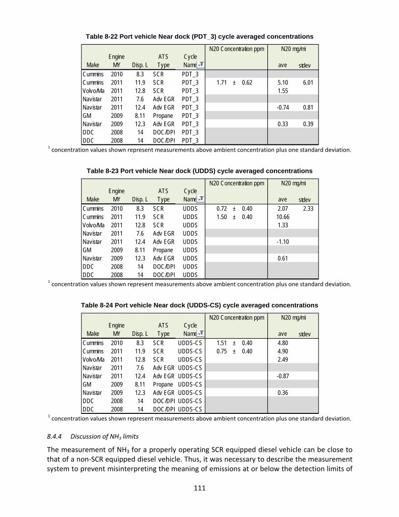
111
Table 8-22 Port vehicle Near dock (PDT_3) cycle averaged concentrations
1 concentration values shown represent measurements above ambient concentration plus one standard deviation.
Table 8-23 Port vehicle Near dock (UDDS) cycle averaged concentrations
1 concentration values shown represent measurements above ambient concentration plus one standard deviation.
Table 8-24 Port vehicle Near dock (UDDS-CS) cycle averaged concentrations
1 concentration values shown represent measurements above ambient concentration plus one standard deviation.
8.4.4 Discussion of NH3 limits
The measurement of NH3 for a properly operating SCR equipped diesel vehicle can be close to that of a non-SCR equipped diesel vehicle. Thus, it was necessary to describe the measurement system to prevent misinterpreting the meaning of emissions at or below the detection limits of
MakeEngine
MY Disp. LATS Type
Cycle Name ave stdev
Cummins 2010 8.3 SCR PDT_3Cummins 2011 11.9 SCR PDT_3 1.71 ± 0.62 5.10 6.01Volvo/Ma 2011 12.8 SCR PDT_3 1.55Navistar 2011 7.6 Adv EGR PDT_3Navistar 2011 12.4 Adv EGR PDT_3 -0.74 0.81GM 2009 8.11 Propane PDT_3Navistar 2009 12.3 Adv EGR PDT_3 0.33 0.39DDC 2008 14 DOC/DPF PDT_3DDC 2008 14 DOC/DPF PDT_3
N20 mg/miN20 Concentration ppm
MakeEngine
MY Disp. LATS Type
Cycle Name ave stdev
Cummins 2010 8.3 SCR UDDS 0.72 ± 0.40 2.07 2.33Cummins 2011 11.9 SCR UDDS 1.50 ± 0.40 10.66Volvo/Ma 2011 12.8 SCR UDDS 1.33Navistar 2011 7.6 Adv EGR UDDSNavistar 2011 12.4 Adv EGR UDDS -1.10GM 2009 8.11 Propane UDDSNavistar 2009 12.3 Adv EGR UDDS 0.61DDC 2008 14 DOC/DPF UDDSDDC 2008 14 DOC/DPF UDDS
N20 mg/miN20 Concentration ppm
MakeEngine
MY Disp. LATS Type
Cycle Name ave stdev
Cummins 2010 8.3 SCR UDDS-CS 1.51 ± 0.40 4.80Cummins 2011 11.9 SCR UDDS-CS 0.75 ± 0.40 4.90Volvo/Ma 2011 12.8 SCR UDDS-CS 2.49Navistar 2011 7.6 Adv EGR UDDS-CSNavistar 2011 12.4 Adv EGR UDDS-CS -0.87GM 2009 8.11 Propane UDDS-CSNavistar 2009 12.3 Adv EGR UDDS-CS 0.36DDC 2008 14 DOC/DPF UDDS-CSDDC 2008 14 DOC/DPF UDDS-CS
N20 mg/miN20 Concentration ppm
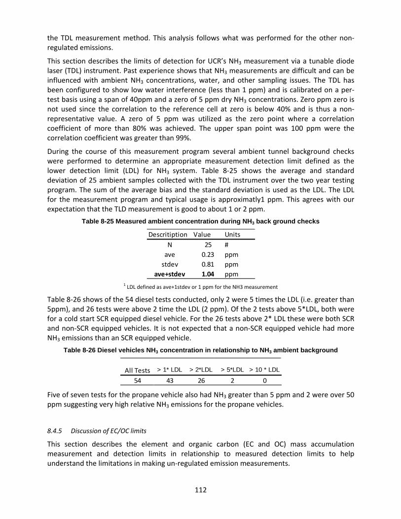
112
the TDL measurement method. This analysis follows what was performed for the other non-regulated emissions.
This section describes the limits of detection for UCR’s NH3 measurement via a tunable diode laser (TDL) instrument. Past experience shows that NH3 measurements are difficult and can be influenced with ambient NH3 concentrations, water, and other sampling issues. The TDL has been configured to show low water interference (less than 1 ppm) and is calibrated on a per-test basis using a span of 40ppm and a zero of 5 ppm dry NH3 concentrations. Zero ppm zero is not used since the correlation to the reference cell at zero is below 40% and is thus a non-representative value. A zero of 5 ppm was utilized as the zero point where a correlation coefficient of more than 80% was achieved. The upper span point was 100 ppm were the correlation coefficient was greater than 99%.
During the course of this measurement program several ambient tunnel background checks were performed to determine an appropriate measurement detection limit defined as the lower detection limit (LDL) for NH3 system. Table 8-25 shows the average and standard deviation of 25 ambient samples collected with the TDL instrument over the two year testing program. The sum of the average bias and the standard deviation is used as the LDL. The LDL for the measurement program and typical usage is approximatly1 ppm. This agrees with our expectation that the TLD measurement is good to about 1 or 2 ppm.
Table 8-25 Measured ambient concentration during NH3 back ground checks
1 LDL defined as ave+1stdev or 1 ppm for the NH3 measurement
Table 8-26 shows of the 54 diesel tests conducted, only 2 were 5 times the LDL (i.e. greater than 5ppm), and 26 tests were above 2 time the LDL (2 ppm). Of the 2 tests above 5*LDL, both were for a cold start SCR equipped diesel vehicle. For the 26 tests above 2* LDL these were both SCR and non-SCR equipped vehicles. It is not expected that a non-SCR equipped vehicle had more NH3 emissions than an SCR equipped vehicle.
Table 8-26 Diesel vehicles NH3 concentration in relationship to NH3 ambient background
Five of seven tests for the propane vehicle also had NH3 greater than 5 ppm and 2 were over 50 ppm suggesting very high relative NH3 emissions for the propane vehicles.
8.4.5 Discussion of EC/OC limits
This section describes the element and organic carbon (EC and OC) mass accumulation measurement and detection limits in relationship to measured detection limits to help understand the limitations in making un-regulated emission measurements.
Descritiption Value UnitsN 25 #
ave 0.23 ppmstdev 0.81 ppm
ave+stdev 1.04 ppm
All Tests > 1* LDL > 2*LDL > 5*LDL > 10 * LDL
54 43 26 2 0
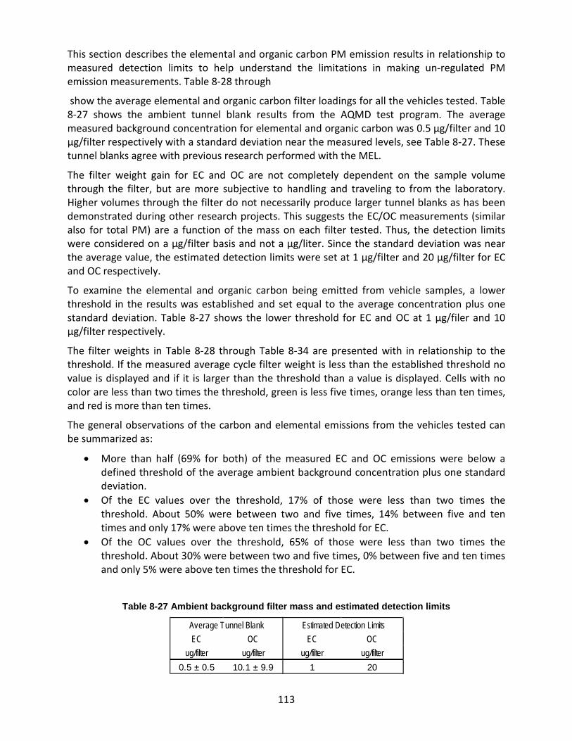
113
This section describes the elemental and organic carbon PM emission results in relationship to measured detection limits to help understand the limitations in making un-regulated PM emission measurements. Table 8-28 through
show the average elemental and organic carbon filter loadings for all the vehicles tested. Table 8-27 shows the ambient tunnel blank results from the AQMD test program. The average measured background concentration for elemental and organic carbon was 0.5 µg/filter and 10 µg/filter respectively with a standard deviation near the measured levels, see Table 8-27. These tunnel blanks agree with previous research performed with the MEL.
The filter weight gain for EC and OC are not completely dependent on the sample volume through the filter, but are more subjective to handling and traveling to from the laboratory. Higher volumes through the filter do not necessarily produce larger tunnel blanks as has been demonstrated during other research projects. This suggests the EC/OC measurements (similar also for total PM) are a function of the mass on each filter tested. Thus, the detection limits were considered on a µg/filter basis and not a µg/liter. Since the standard deviation was near the average value, the estimated detection limits were set at 1 µg/filter and 20 µg/filter for EC and OC respectively.
To examine the elemental and organic carbon being emitted from vehicle samples, a lower threshold in the results was established and set equal to the average concentration plus one standard deviation. Table 8-27 shows the lower threshold for EC and OC at 1 µg/filer and 10 µg/filter respectively.
The filter weights in Table 8-28 through Table 8-34 are presented with in relationship to the threshold. If the measured average cycle filter weight is less than the established threshold no value is displayed and if it is larger than the threshold than a value is displayed. Cells with no color are less than two times the threshold, green is less five times, orange less than ten times, and red is more than ten times.
The general observations of the carbon and elemental emissions from the vehicles tested can be summarized as:
• More than half (69% for both) of the measured EC and OC emissions were below a defined threshold of the average ambient background concentration plus one standard deviation.
• Of the EC values over the threshold, 17% of those were less than two times the threshold. About 50% were between two and five times, 14% between five and ten times and only 17% were above ten times the threshold for EC.
• Of the OC values over the threshold, 65% of those were less than two times the threshold. About 30% were between two and five times, 0% between five and ten times and only 5% were above ten times the threshold for EC.
Table 8-27 Ambient background filter mass and estimated detection limits
EC OC EC OCug/filter ug/filter ug/filter ug/filter
0.5 ± 0.5 10.1 ± 9.9 1 20
Average Tunnel Blank Estimated Detection Limits
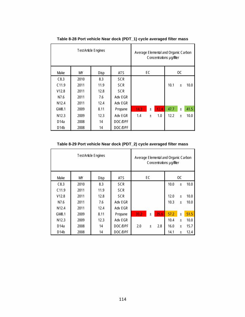
114
Table 8-28 Port vehicle Near dock (PDT_1) cycle averaged filter mass
Table 8-29 Port vehicle Near dock (PDT_2) cycle averaged filter mass
Make MY Disp ATSC8.3 2010 8.3 SCR
C11.9 2011 11.9 SCR 10.1 ± 10.0V12.8 2011 12.8 SCRN7.6 2011 7.6 Adv EGR
N12.4 2011 12.4 Adv EGRGM8.1 2009 8.11 Propane 14.3 ± 12.4 47.7 ± 41.5N12.3 2009 12.3 Adv EGR 1.4 ± 1.0 12.2 ± 10.0D14a 2008 14 DOC/DPFD14b 2008 14 DOC/DPF
Test Article Engines Average Elemental and Organic Carbon Concentrations µg/filter
EC OC
Make MY Disp ATSC8.3 2010 8.3 SCR 10.0 ± 10.0
C11.9 2011 11.9 SCRV12.8 2011 12.8 SCR 12.0 ± 10.0N7.6 2011 7.6 Adv EGR 10.3 ± 10.0
N12.4 2011 12.4 Adv EGRGM8.1 2009 8.11 Propane 39.2 ± 35.6 57.2 ± 51.5N12.3 2009 12.3 Adv EGR 10.4 ± 10.0D14a 2008 14 DOC/DPF 2.0 ± 2.8 16.0 ± 15.7D14b 2008 14 DOC/DPF 14.1 ± 12.4
Test Article Engines Average Elemental and Organic Carbon Concentrations µg/filter
EC OC
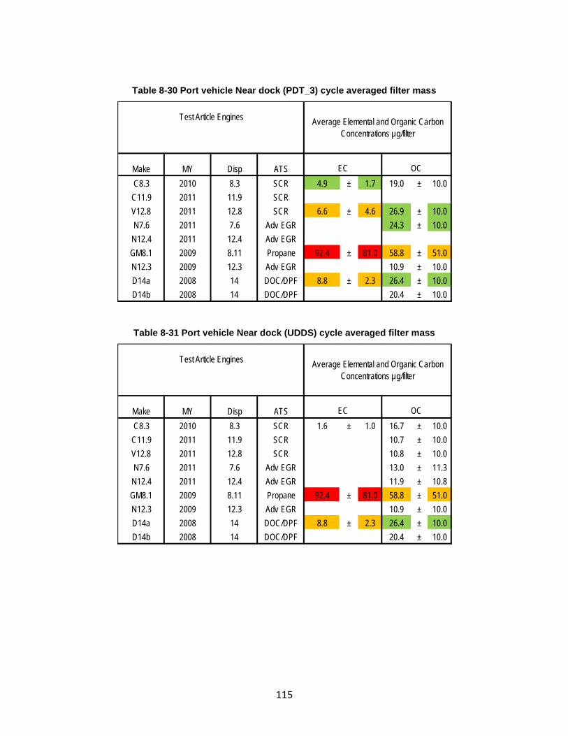
115
Table 8-30 Port vehicle Near dock (PDT_3) cycle averaged filter mass
Table 8-31 Port vehicle Near dock (UDDS) cycle averaged filter mass
Make MY Disp ATSC8.3 2010 8.3 SCR 4.9 ± 1.7 19.0 ± 10.0
C11.9 2011 11.9 SCRV12.8 2011 12.8 SCR 6.6 ± 4.6 26.9 ± 10.0N7.6 2011 7.6 Adv EGR 24.3 ± 10.0
N12.4 2011 12.4 Adv EGRGM8.1 2009 8.11 Propane 92.4 ± 81.0 58.8 ± 51.0N12.3 2009 12.3 Adv EGR 10.9 ± 10.0D14a 2008 14 DOC/DPF 8.8 ± 2.3 26.4 ± 10.0D14b 2008 14 DOC/DPF 20.4 ± 10.0
Test Article Engines Average Elemental and Organic Carbon Concentrations µg/filter
EC OC
Make MY Disp ATSC8.3 2010 8.3 SCR 1.6 ± 1.0 16.7 ± 10.0
C11.9 2011 11.9 SCR 10.7 ± 10.0V12.8 2011 12.8 SCR 10.8 ± 10.0N7.6 2011 7.6 Adv EGR 13.0 ± 11.3
N12.4 2011 12.4 Adv EGR 11.9 ± 10.8GM8.1 2009 8.11 Propane 92.4 ± 81.0 58.8 ± 51.0N12.3 2009 12.3 Adv EGR 10.9 ± 10.0D14a 2008 14 DOC/DPF 8.8 ± 2.3 26.4 ± 10.0D14b 2008 14 DOC/DPF 20.4 ± 10.0
Test Article Engines Average Elemental and Organic Carbon Concentrations µg/filter
EC OC
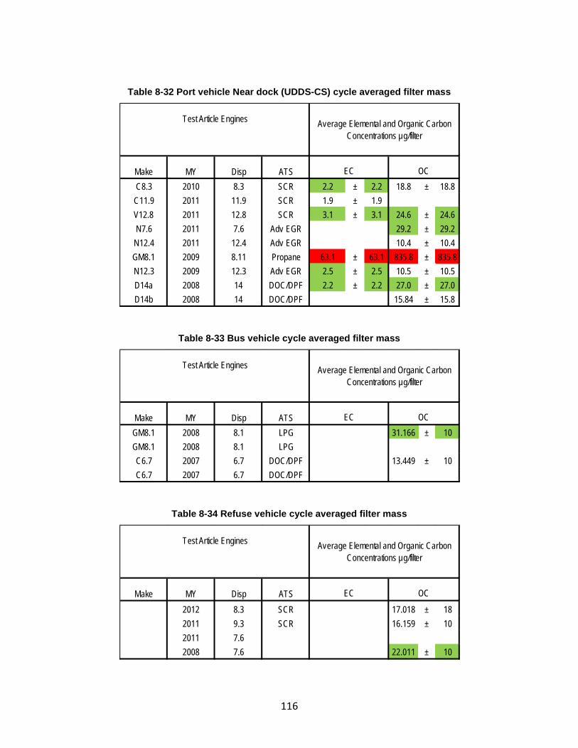
116
Table 8-32 Port vehicle Near dock (UDDS-CS) cycle averaged filter mass
Table 8-33 Bus vehicle cycle averaged filter mass
Table 8-34 Refuse vehicle cycle averaged filter mass
Make MY Disp ATSC8.3 2010 8.3 SCR 2.2 ± 2.2 18.8 ± 18.8
C11.9 2011 11.9 SCR 1.9 ± 1.9V12.8 2011 12.8 SCR 3.1 ± 3.1 24.6 ± 24.6N7.6 2011 7.6 Adv EGR 29.2 ± 29.2
N12.4 2011 12.4 Adv EGR 10.4 ± 10.4GM8.1 2009 8.11 Propane 63.1 ± 63.1 835.8 ± 835.8N12.3 2009 12.3 Adv EGR 2.5 ± 2.5 10.5 ± 10.5D14a 2008 14 DOC/DPF 2.2 ± 2.2 27.0 ± 27.0D14b 2008 14 DOC/DPF 15.84 ± 15.8
Test Article Engines Average Elemental and Organic Carbon Concentrations µg/filter
EC OC
Make MY Disp ATSGM8.1 2008 8.1 LPG 31.166 ± 10GM8.1 2008 8.1 LPGC6.7 2007 6.7 DOC/DPF 13.449 ± 10C6.7 2007 6.7 DOC/DPF
Test Article Engines Average Elemental and Organic Carbon Concentrations µg/filter
EC OC
Make MY Disp ATS2012 8.3 SCR 17.018 ± 182011 9.3 SCR 16.159 ± 102011 7.62008 7.6 22.011 ± 10
Test Article Engines Average Elemental and Organic Carbon Concentrations µg/filter
EC OC
117
9 Summary
The SC AQMD path to cleaner air depends on achieving the strictest NOx standards for heavy-duty vehicles. Recently, the District saw data that indicated the in-use emissions exceeded the certification values. The University of California, Riverside (UCR) was contracted to test 16 heavy-duty vehicles, mainly diesel fueled engines, used for goods movement, refuse hauling and transit applications. The testing protocol involved measuring the emissions identified in the RFP while the vehicles operated following driving cycles that better represented the in-use conditions as well as certification conditions. The testing measured: 1) regulated emissions; 2) unregulated emissions such as ammonia and formaldehyde; 3) greenhouse gas levels of CO2 and N2O and 4) ultrafine PM emissions. A number of vehicles and engines were tested based on the population, emission standards and technology.
The emission results for PM and NOx are summarized below:
• PM emissions from the diesel test vehicles were below 0.01 grams per brake horsepower-hour (g/bhp-h) measured over port drayage, CBD, and UDDS drive cycles. Cold start PM emissions were relatively high for two diesel vehicles; one was a port SCR equipped vehicle and the other was a refuse SCR equipped vehicle. The port vehicle was 17 times higher (22.9 mg/mi vs 1.33 mg/mi) and the refuse vehicle was 8 times higher (18.4 mg/mi vs 2.75 mg/mi). In both cases the high cold start emission factors were below the certification standard. PM emissions were well below the certification for all diesel tests, thus suggesting DPF-based solutions are robust and reliable in meeting targeted standards. In addition, PM emissions from a liquefied petroleum gas (LPG) test vehicle was approximately 0.14 g/bhp-hr measured over the UDDS cycle, which is above the certification standard.
• NOx results covered a wide range of emission factors, where the emissions depended on the certification standard, vehicle application, driving cycle, and manufacturer. For example, NOx emissions were lowest for goods movement vehicles powered by diesel engines equipped with SCR technology; however, increases from 0.112 g/mi (0.028 g/bhp-h) during high speed cruise operation to 5.36 g/mi (1.34 g/bhp-h) for low speed transient operation were measured. Unique to the high NOx emissions was a condition in which the temperature of the SCR was less than 250ᵒC. Advanced EGR 2010 certified engines showed higher NOx emissions compared to SCR equipped engines, and pre-2010 certified engines were higher than the 2010 certified engines.
• The NOx impact of SCR equipped diesel engines depends on the vehicles’ duty cycles and manufacturers’ implementation for low temperature SCR performance. For the near dock port cycle, the SCR was below 250ᵒC approximately 80% of the time, 65% of the time for the local port cycle, and approximately 45% of the time for the regional port cycle. The percentage of time below 250ᵒC varied significantly between manufacturers, from 8% to 30% for the near dock cycle, and from 41% to 64% for the regional cycle. The difference in time below 250ᵒC suggests some manufacturers have better strategies for maintaining high exhaust temperatures than others.
• The SCR equipped engines were within their certification standards and were typically below 0.2 g/bhp-h. Only during low SCR temperature were the emissions found to be higher than the certification standard. In-use compliance testing does not enforce the
118
emissions standards when the SCR is below 250 ᵒC, thus the SCR equipped vehicles were typically compliant based on the results presented in this report.
• Cold start NOx emissions can be as high as 2.3 g/bhp-hr compared to an equivalent warm test of 0.006 g/bhp-h. Although cold start emissions do not contribute to the inventory, it is important to consider the extreme nature of cold start emissions if vehicles are allowed to cool frequently. The NOx emissions accumulated in 1 mile after a cold start were equivalent to emissions accumulated during 32 miles of running hot.
• The 2010 certified diesel engines with advanced cooled EGR and no SCR were tested. These vehicles operated utilizing a lug curve with peak torque starting as low as 1000 revolutions per minute (RPM), where the driver was instructed to operate the vehicle down to 900 RPM before shifting. The truck behavior was unusual, and both UCR and WVU trained drivers commented on the strange operation. Additionally, the certified emissions had a family emission limit (FEL) of 0.5 g/bhp-hr for 2010 MY, but the measured NOx emissions were around 1 g/bhp-hr (0.25 g/mi) for the UDDS cycle, which represents a certification-like cycle. Even the port cycles showed brake specific emissions higher than 1 g/bhp-hr and as high as 2 g/bhp-hr for the near dock cycle.
• Pre-2010 certified diesel engines exhibited regulated emissions that were very close to the standard and were found to be repeatable for randomly selected models tested. This suggests that pre-2010 emissions inventories may be more reliable than SCR-equipped diesel engines due to SCR performance variability.
• Most NOx emissions from SCR equipped diesel refuse vehicles were produced during the compaction portion of the in-use test cycle. The high NOx emissions corresponded with a low SCR exhaust temperature, where the emissions increased from 0.27 g/bhp-hr NOx for the transient and curbside cycles to 3.8 g/bhp-hr NOx for the compaction cycle.
• The percentage of NOx as NO2 ranged from 10% to near 90%, with the highest levels of NO2 emissions from non-SCR-equipped diesel vehicles. NO2 was highest for the pre-2010 certified engines (averaging 1.15 ± 0.48 g/mi for the UDDS cycle). In general NO2 ratios were similar for all tests at around 45%±8%, except for the SCR equipped diesel vehicles, which showed high variability with a NO2 ratio of 47%±36%.
The emission results for ammonia, hydrocarbons, toxics, and fine particles are summarized below:
• Ammonia (NH3) emissions from the vehicles tested ranged from about 0.01 to 0.1 g/mi. The diesel vehicles’ NH3 emissions averaged 0.04±0.03 g/mi (0.01±0.01 g/hp-h), where the port vehicle emissions were similar (0.03±0.02 g/mi), but the propane school bus had relatively higher NH3 emissions (0.48±0.04 g/mi) over the CBD test cycle. All the diesel vehicles showed cycle averaged raw NH3 emission concentrations less than 10ppm. Of the 54 diesel tests conducted, only 2 vehicles had NH3 emissions over 5 parts per million (ppm). Half of the tests were below 2 ppm. Five of seven propane vehicle tests had NH3 emissions greater than 5 ppm and two were over 50 ppm, suggesting that relatively higher NH3 emissions exist for the propane vehicles compared to the diesel vehicles.
• The emission factors for total hydrocarbon (THC), methane (CH4), non-methane hydrocarbon (NMHC) and toxics were very low for all diesel vehicles tested. This agrees
119
with other research from the Advanced Collaborative Emissions Study (ACES) project that showed a 98% reduction from diesel engines with catalytic exhaust systems. THC, NMHC, and CH4 emissions were at or below 0.09 g/mi, 0.06 g/mi, and 0.04 g/mi, respectively, for all vehicles (except the LPG vehicle) for both the UDDS and port regional cycles. Slightly higher THC, CH4, and NMHC emissions were found for the lower power near dock port cycle (0.36 g/mi, 0.10 g/mi, and 0.29 g/mi, respectively). Toxic emissions were low and near the detection limits of the method where 75% of the measured carcinogenetic species (benzene, toluene, ethylbenzene, and xylenes - BTEX) were below the average ambient background concentration pulse one standard deviation (< 10 mg/mi and typically < 2 mg/mi background corrected). Carbonyl emissions were also low relative to the measurement method, where more than 75% of the measured species were below the same threshold except for formaldehyde. Formaldehyde showed a relatively higher emission concentration, with 75% of the measurements above the threshold. Even though the formaldehyde samples were relatively high, their absolute contribution were below 72 mg/mi, with an average of 18±19 mg/mi. Acetaldehyde was the next largest carbonyl with maximum emissions of 18 mg/mi and an average of 1.5±4 mg/mi. The rest of the carbonyls were below 2 mg/mi. Cold start UDDS emissions were similar to the hot start UDDS emissions for THC, CH4, NMHC, and toxics (note the UDDS was performed as a 2xUDDS cycle, which may have minimized the cold start effect for the HCs and toxics).
• The LPG goods movement vehicle showed higher THC, NMHC, CH4, and toxic emissions than the diesel vehicles tested. THC, NMHC and CH4 were 22.4 g/mi, 1.43 g/mi, and 21.4 g/mi respectively for the UDDS hot cycle. BTEX and formaldehyde samples were more than 10 times the average ambient background concentration plus one standard deviation. The propane vehicle averaged 6.5±9.3 mg/mi, 9.7±12 mg/mi, and 22.4±19 mg/mi for 1,3-butadiene, n-butane, and benzene respectively for the BTEX sample. The Carbonyls were high for formaldehyde and acetaldehyde (241±253 mg/mi and 42±48 mg/mi respectively) with the remaining aldehydes below 2 mg/mi. These results should be confirmed with additional testing on LPG port vehicles.
• Real-time PM measurements suggest the reported reference PM emission rate may be lower due to low filter weights for DPF equipped vehicles. The PM mass of the gravimetric method averaged 0.78±1.57 mg/bhp-hr for selected diesel vehicles. The average PM mass from the real-time measurement method averaged 0.05±0.09 mg/bhp-hr for the same vehicles. The average filter weight for these selected vehicles ranged from 10-20 µg, where UCR’s CVS tunnel blank averages were 5µg with a 5µg single standard deviation. Thus, there is speculation that some of the uncertainty may be artifacts on the filter. As such, real-time PM measurements are useful for identifying low level PM mass in addition to real-time analysis.
• Elemental carbon (EC) and organic carbon (OC) PM was very low for all the vehicles tested and was typically below 0.2 mg/mi and 2.2 mg/mi respectively. More than half (69%) of the measured EC and OC emissions were below the average ambient background concentration plus one standard deviation. The propane vehicles had the highest organic PM contribution (>10 mg/mi for the near dock port cycle).
• Fine-particle emissions were typically higher during the first 200 seconds of the cold start UDDS cycle compared to the hot stabilized UDDS cycle (5x10⁵ #/cc vs 1x10³ #/cc,
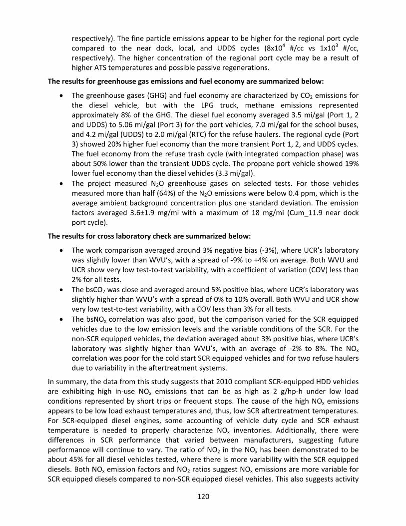
120
respectively). The fine particle emissions appear to be higher for the regional port cycle compared to the near dock, local, and UDDS cycles (8x10⁴ #/cc vs 1x10³ #/cc, respectively). The higher concentration of the regional port cycle may be a result of higher ATS temperatures and possible passive regenerations.
The results for greenhouse gas emissions and fuel economy are summarized below:
• The greenhouse gases (GHG) and fuel economy are characterized by CO2 emissions for the diesel vehicle, but with the LPG truck, methane emissions represented approximately 8% of the GHG. The diesel fuel economy averaged 3.5 mi/gal (Port 1, 2 and UDDS) to 5.06 mi/gal (Port 3) for the port vehicles, 7.0 mi/gal for the school buses, and 4.2 mi/gal (UDDS) to 2.0 mi/gal (RTC) for the refuse haulers. The regional cycle (Port 3) showed 20% higher fuel economy than the more transient Port 1, 2, and UDDS cycles. The fuel economy from the refuse trash cycle (with integrated compaction phase) was about 50% lower than the transient UDDS cycle. The propane port vehicle showed 19% lower fuel economy than the diesel vehicles (3.3 mi/gal).
• The project measured N2O greenhouse gases on selected tests. For those vehicles measured more than half (64%) of the N2O emissions were below 0.4 ppm, which is the average ambient background concentration plus one standard deviation. The emission factors averaged 3.6±1.9 mg/mi with a maximum of 18 mg/mi (Cum_11.9 near dock port cycle).
The results for cross laboratory check are summarized below:
• The work comparison averaged around 3% negative bias (-3%), where UCR’s laboratory was slightly lower than WVU’s, with a spread of -9% to +4% on average. Both WVU and UCR show very low test-to-test variability, with a coefficient of variation (COV) less than 2% for all tests.
• The bsCO2 was close and averaged around 5% positive bias, where UCR’s laboratory was slightly higher than WVU’s with a spread of 0% to 10% overall. Both WVU and UCR show very low test-to-test variability, with a COV less than 3% for all tests.
• The bsNOx correlation was also good, but the comparison varied for the SCR equipped vehicles due to the low emission levels and the variable conditions of the SCR. For the non-SCR equipped vehicles, the deviation averaged about 3% positive bias, where UCR’s laboratory was slightly higher than WVU’s, with an average of -2% to 8%. The NOx
correlation was poor for the cold start SCR equipped vehicles and for two refuse haulers due to variability in the aftertreatment systems.
In summary, the data from this study suggests that 2010 compliant SCR-equipped HDD vehicles are exhibiting high in-use NOx emissions that can be as high as 2 g/hp-h under low load conditions represented by short trips or frequent stops. The cause of the high NOx emissions appears to be low load exhaust temperatures and, thus, low SCR aftertreatment temperatures. For SCR-equipped diesel engines, some accounting of vehicle duty cycle and SCR exhaust temperature is needed to properly characterize NOx inventories. Additionally, there were differences in SCR performance that varied between manufacturers, suggesting future performance will continue to vary. The ratio of NO2 in the NOx has been demonstrated to be about 45% for all diesel vehicles tested, where there is more variability with the SCR equipped diesels. Both NOx emission factors and NO2 ratios suggest NOx emissions are more variable for SCR equipped diesels compared to non-SCR equipped diesel vehicles. This also suggests activity
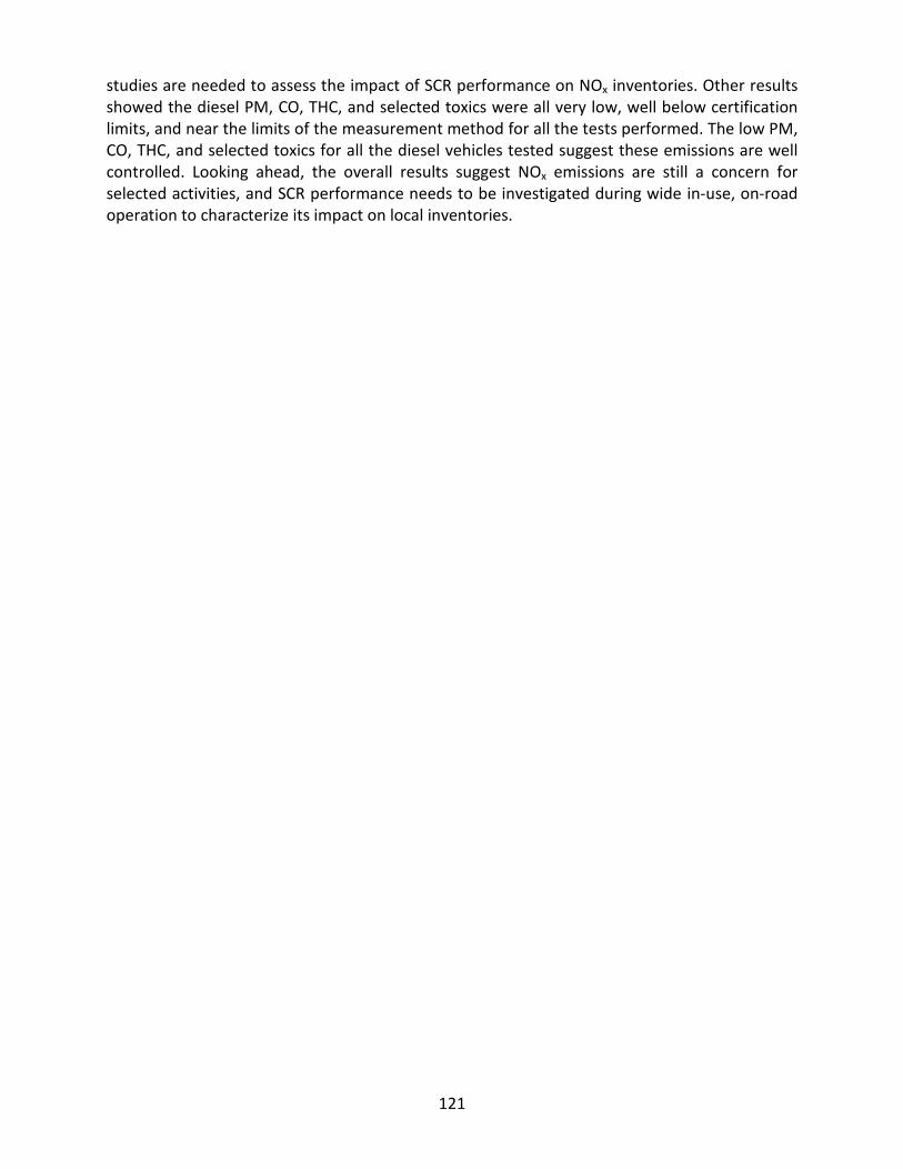
121
studies are needed to assess the impact of SCR performance on NOx inventories. Other results showed the diesel PM, CO, THC, and selected toxics were all very low, well below certification limits, and near the limits of the measurement method for all the tests performed. The low PM, CO, THC, and selected toxics for all the diesel vehicles tested suggest these emissions are well controlled. Looking ahead, the overall results suggest NOx emissions are still a concern for selected activities, and SCR performance needs to be investigated during wide in-use, on-road operation to characterize its impact on local inventories.
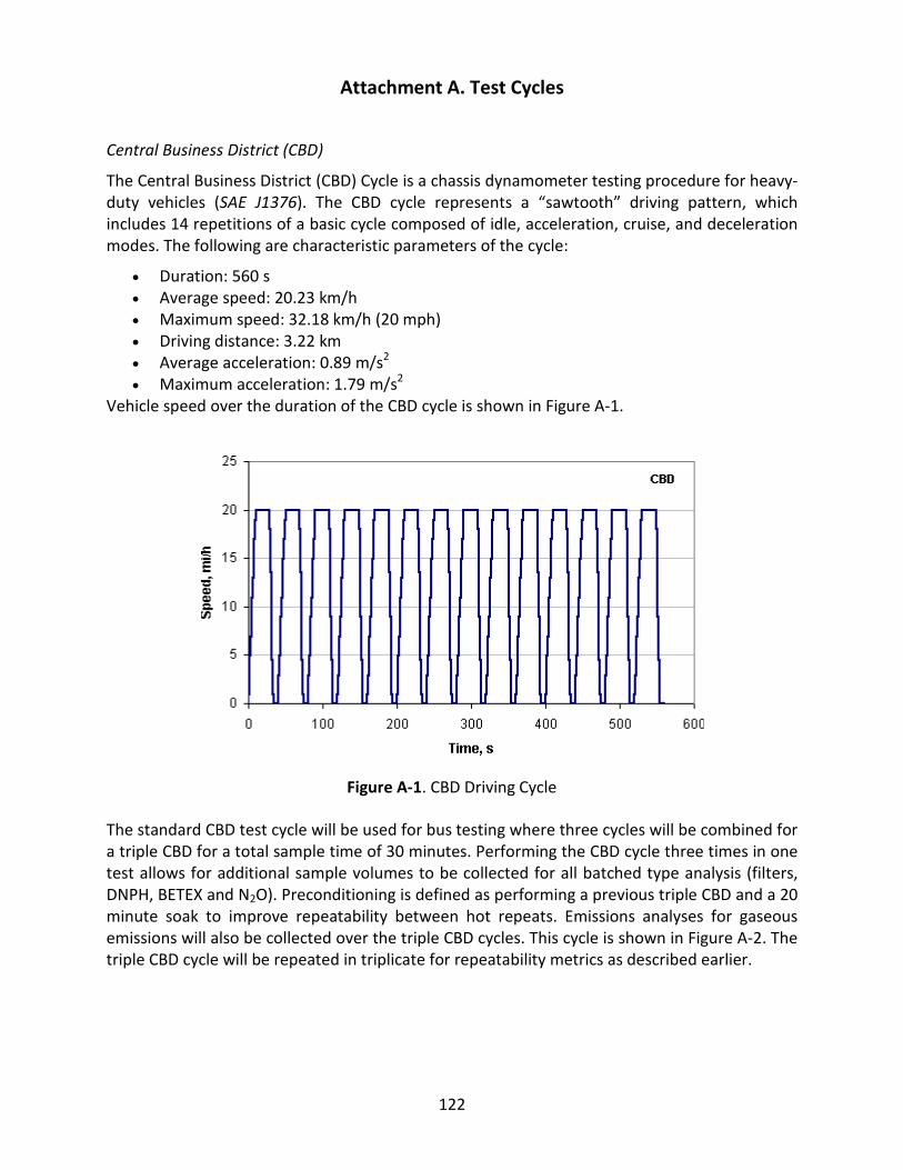
122
Attachment A. Test Cycles
Central Business District (CBD)
The Central Business District (CBD) Cycle is a chassis dynamometer testing procedure for heavy-duty vehicles (SAE J1376). The CBD cycle represents a “sawtooth” driving pattern, which includes 14 repetitions of a basic cycle composed of idle, acceleration, cruise, and deceleration modes. The following are characteristic parameters of the cycle:
• Duration: 560 s • Average speed: 20.23 km/h • Maximum speed: 32.18 km/h (20 mph) • Driving distance: 3.22 km • Average acceleration: 0.89 m/s2 • Maximum acceleration: 1.79 m/s2
Vehicle speed over the duration of the CBD cycle is shown in Figure A-1.
Figure A-1. CBD Driving Cycle
The standard CBD test cycle will be used for bus testing where three cycles will be combined for a triple CBD for a total sample time of 30 minutes. Performing the CBD cycle three times in one test allows for additional sample volumes to be collected for all batched type analysis (filters, DNPH, BETEX and N2O). Preconditioning is defined as performing a previous triple CBD and a 20 minute soak to improve repeatability between hot repeats. Emissions analyses for gaseous emissions will also be collected over the triple CBD cycles. This cycle is shown in Figure A-2. The triple CBD cycle will be repeated in triplicate for repeatability metrics as described earlier.
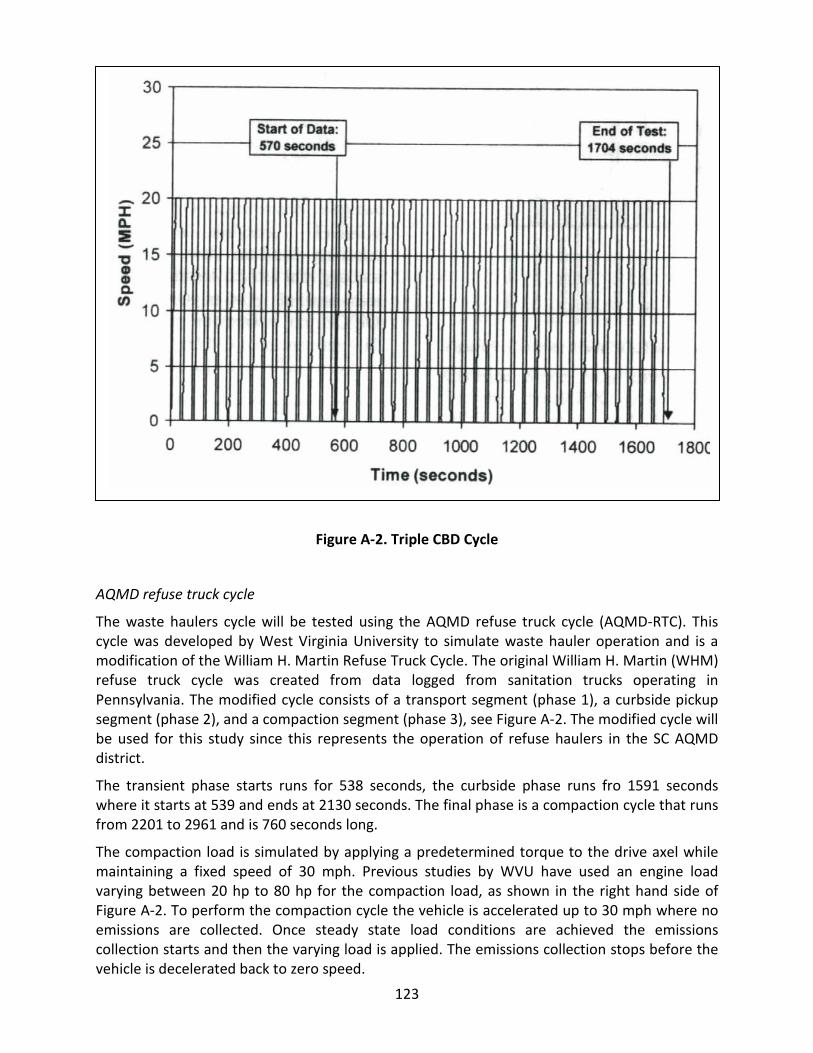
123
Figure A-2. Triple CBD Cycle
AQMD refuse truck cycle
The waste haulers cycle will be tested using the AQMD refuse truck cycle (AQMD-RTC). This cycle was developed by West Virginia University to simulate waste hauler operation and is a modification of the William H. Martin Refuse Truck Cycle. The original William H. Martin (WHM) refuse truck cycle was created from data logged from sanitation trucks operating in Pennsylvania. The modified cycle consists of a transport segment (phase 1), a curbside pickup segment (phase 2), and a compaction segment (phase 3), see Figure A-2. The modified cycle will be used for this study since this represents the operation of refuse haulers in the SC AQMD district.
The transient phase starts runs for 538 seconds, the curbside phase runs fro 1591 seconds where it starts at 539 and ends at 2130 seconds. The final phase is a compaction cycle that runs from 2201 to 2961 and is 760 seconds long.
The compaction load is simulated by applying a predetermined torque to the drive axel while maintaining a fixed speed of 30 mph. Previous studies by WVU have used an engine load varying between 20 hp to 80 hp for the compaction load, as shown in the right hand side of Figure A-2. To perform the compaction cycle the vehicle is accelerated up to 30 mph where no emissions are collected. Once steady state load conditions are achieved the emissions collection starts and then the varying load is applied. The emissions collection stops before the vehicle is decelerated back to zero speed.
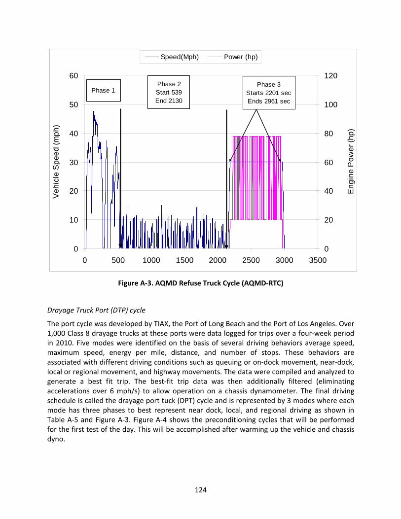
124
Figure A-3. AQMD Refuse Truck Cycle (AQMD-RTC)
Drayage Truck Port (DTP) cycle
The port cycle was developed by TIAX, the Port of Long Beach and the Port of Los Angeles. Over 1,000 Class 8 drayage trucks at these ports were data logged for trips over a four-week period in 2010. Five modes were identified on the basis of several driving behaviors average speed, maximum speed, energy per mile, distance, and number of stops. These behaviors are associated with different driving conditions such as queuing or on-dock movement, near-dock, local or regional movement, and highway movements. The data were compiled and analyzed to generate a best fit trip. The best-fit trip data was then additionally filtered (eliminating accelerations over 6 mph/s) to allow operation on a chassis dynamometer. The final driving schedule is called the drayage port tuck (DPT) cycle and is represented by 3 modes where each mode has three phases to best represent near dock, local, and regional driving as shown in Table A-5 and Figure A-3. Figure A-4 shows the preconditioning cycles that will be performed for the first test of the day. This will be accomplished after warming up the vehicle and chassis dyno.
0
10
20
30
40
50
60
0 500 1000 1500 2000 2500 3000 3500
Veh
icle
Spe
ed (m
ph)
0
20
40
60
80
100
120
Eng
ine
Pow
er (h
p)
Speed(Mph) Power (hp)
Phase 1Phase 2Start 539 End 2130
Phase 3Starts 2201 secEnds 2961 sec
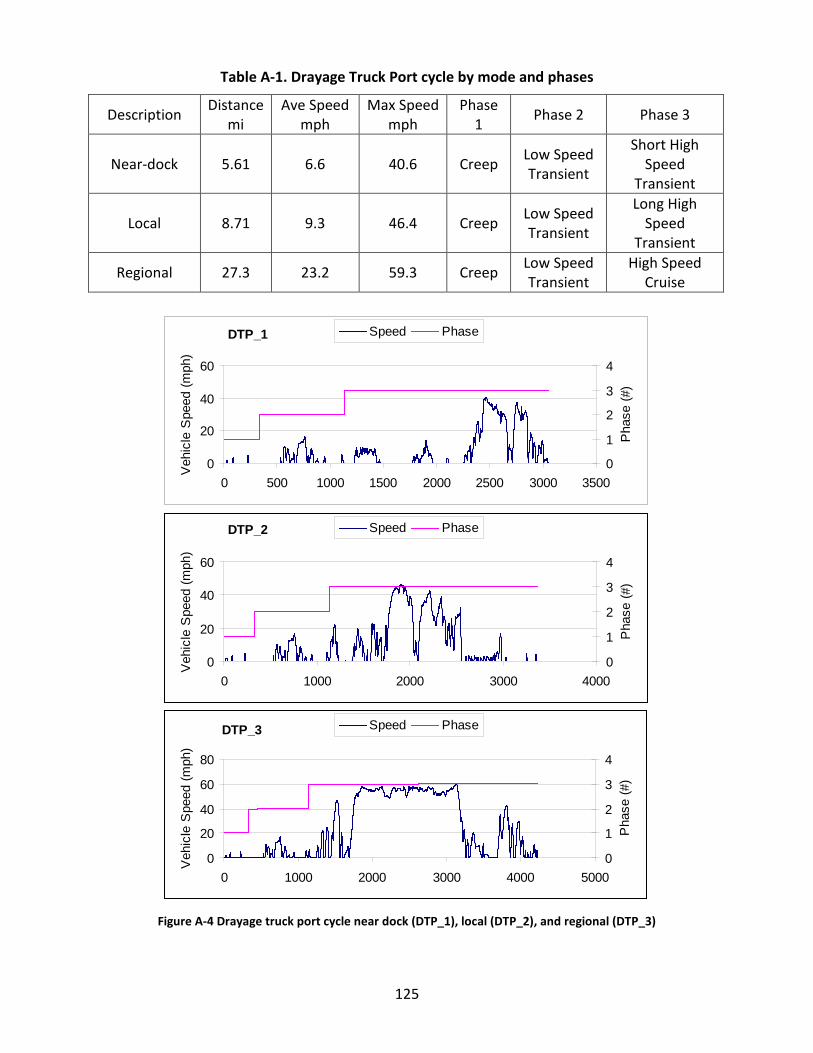
125
Table A-1. Drayage Truck Port cycle by mode and phases
Description Distance
mi Ave Speed
mph Max Speed
mph Phase
1 Phase 2 Phase 3
Near-dock 5.61 6.6 40.6 Creep Low Speed Transient
Short High Speed
Transient
Local 8.71 9.3 46.4 Creep Low Speed Transient
Long High Speed
Transient
Regional 27.3 23.2 59.3 Creep Low Speed Transient
High Speed Cruise
Figure A-4 Drayage truck port cycle near dock (DTP_1), local (DTP_2), and regional (DTP_3)
0
20
40
60
0 500 1000 1500 2000 2500 3000 3500
Veh
icle
Spe
ed (m
ph)
0
1
2
3
4
Pha
se (#
)
Speed PhaseDTP_1
0
20
40
60
0 1000 2000 3000 4000
Veh
icle
Spe
ed (m
ph)
0
1
2
3
4
Pha
se (#
)
Speed PhaseDTP_2
0
20
40
60
80
0 1000 2000 3000 4000 5000
Veh
icle
Spe
ed (m
ph)
0
1
2
3
4
Pha
se (#
)
Speed PhaseDTP_3
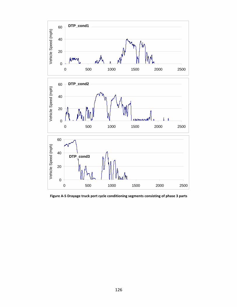
126
Figure A-5 Drayage truck port cycle conditioning segments consisting of phase 3 parts
0
20
40
60
0 500 1000 1500 2000 2500
Veh
icle
Spe
ed (m
ph)
DTP_cond1
0
20
40
60
0 500 1000 1500 2000 2500
Veh
icle
Spe
ed (m
ph) DTP_cond2
0
20
40
60
0 500 1000 1500 2000 2500
Veh
icle
Spe
ed (m
ph)
DTP_cond3
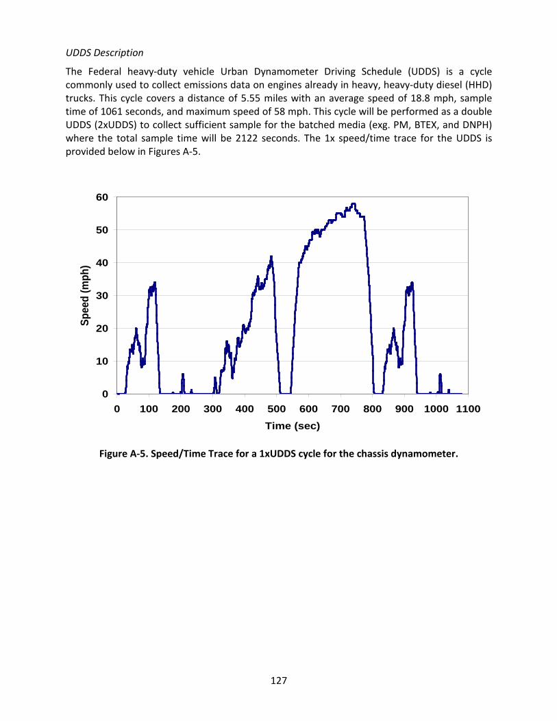
127
UDDS Description
The Federal heavy-duty vehicle Urban Dynamometer Driving Schedule (UDDS) is a cycle commonly used to collect emissions data on engines already in heavy, heavy-duty diesel (HHD) trucks. This cycle covers a distance of 5.55 miles with an average speed of 18.8 mph, sample time of 1061 seconds, and maximum speed of 58 mph. This cycle will be performed as a double UDDS (2xUDDS) to collect sufficient sample for the batched media (exg. PM, BTEX, and DNPH) where the total sample time will be 2122 seconds. The 1x speed/time trace for the UDDS is provided below in Figures A-5.
Figure A-5. Speed/Time Trace for a 1xUDDS cycle for the chassis dynamometer.
0
10
20
30
40
50
60
0 100 200 300 400 500 600 700 800 900 1000 1100Time (sec)
Spee
d (m
ph)
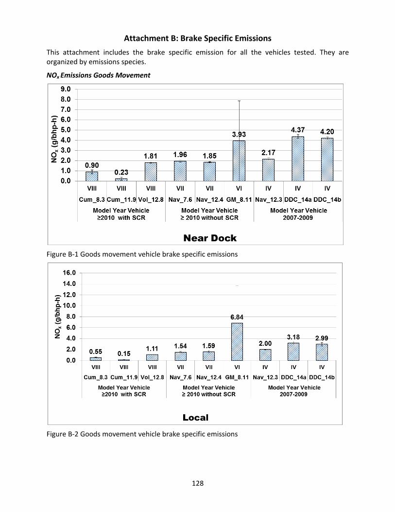
128
Attachment B: Brake Specific Emissions
This attachment includes the brake specific emission for all the vehicles tested. They are organized by emissions species.
NOx Emissions Goods Movement
Figure B-1 Goods movement vehicle brake specific emissions
Figure B-2 Goods movement vehicle brake specific emissions
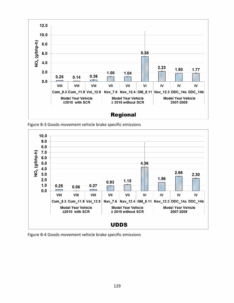
129
Figure B-3 Goods movement vehicle brake specific emissions
Figure B-4 Goods movement vehicle brake specific emissions
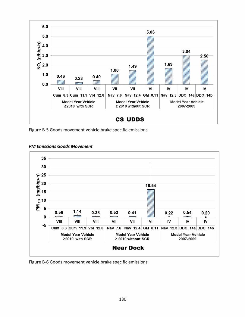
130
Figure B-5 Goods movement vehicle brake specific emissions
PM Emissions Goods Movement
Figure B-6 Goods movement vehicle brake specific emissions
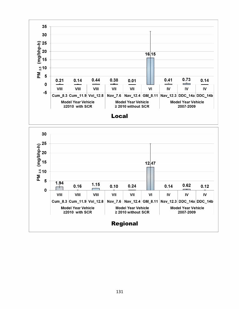
131
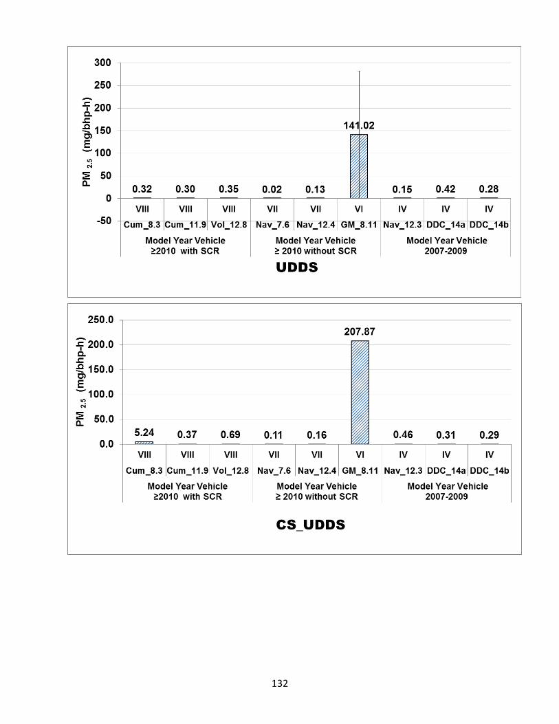
132
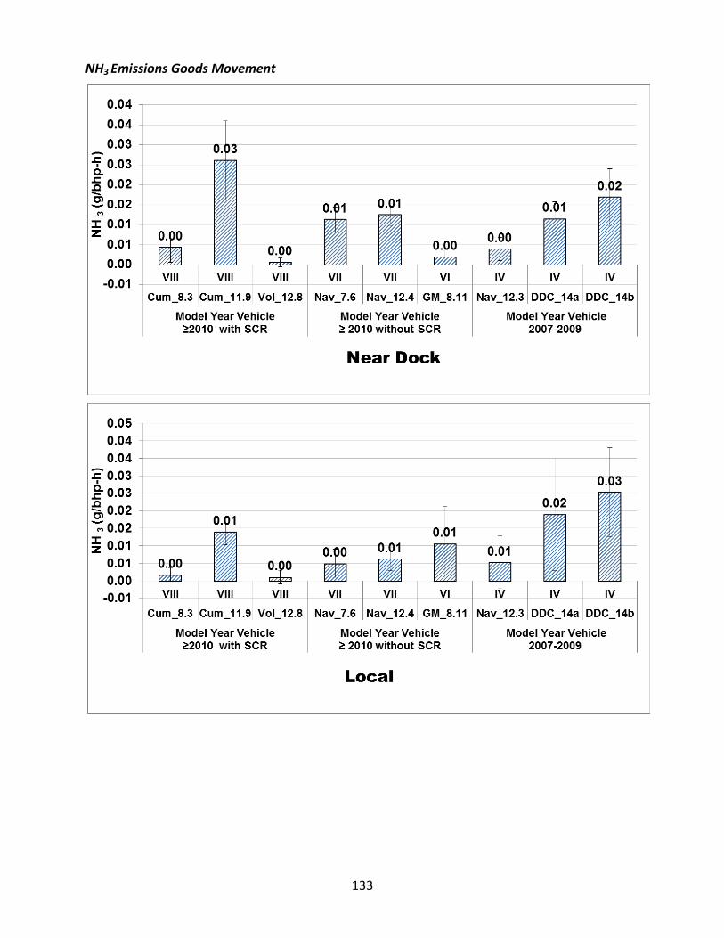
133
NH3 Emissions Goods Movement
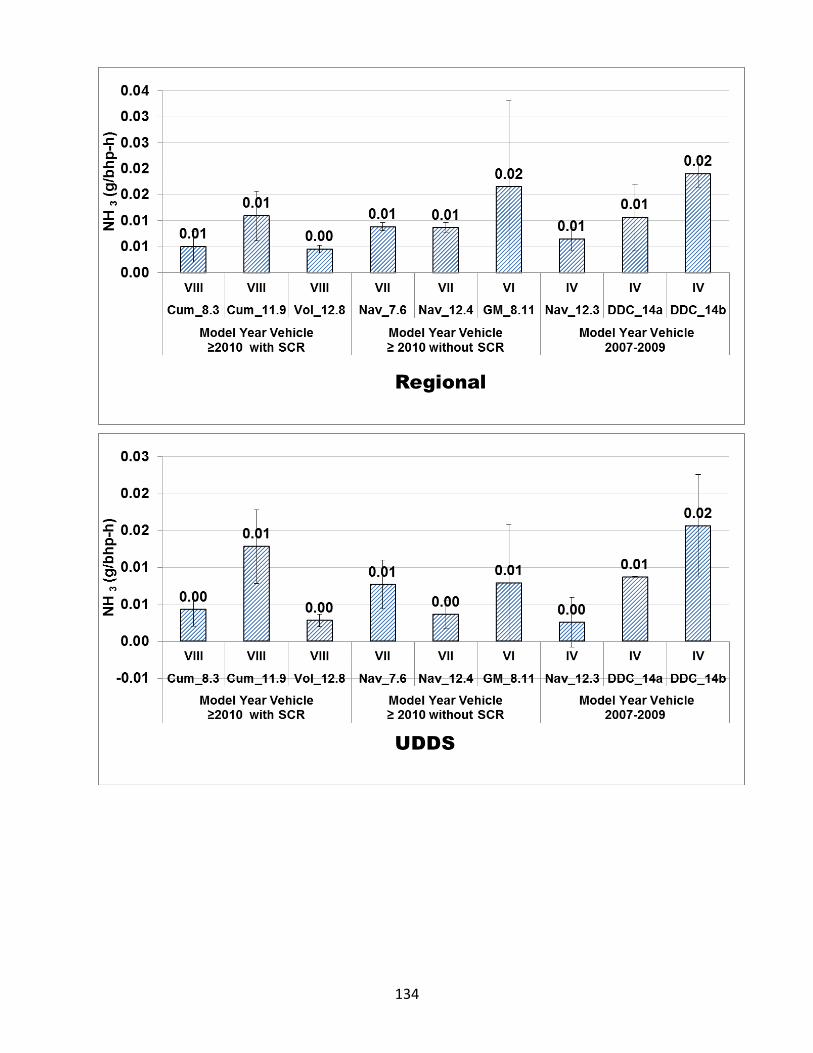
134
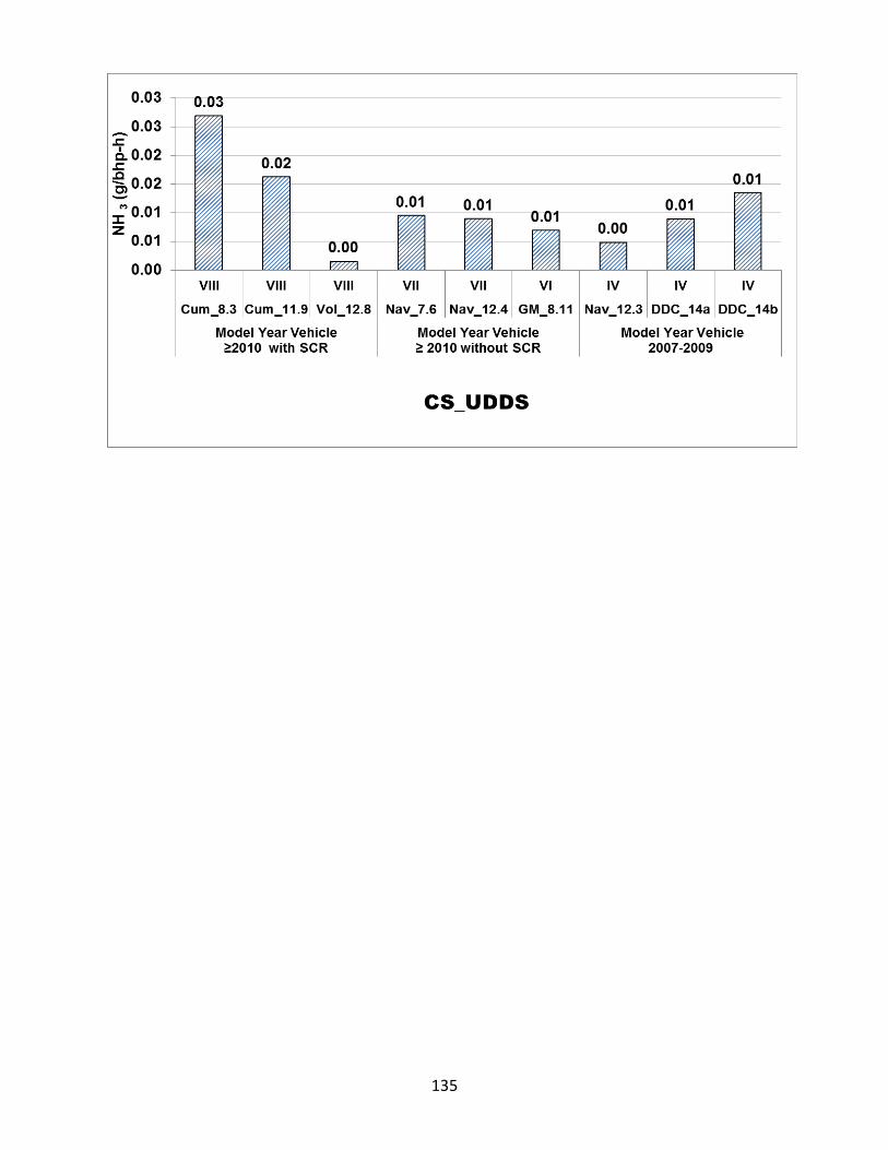
135
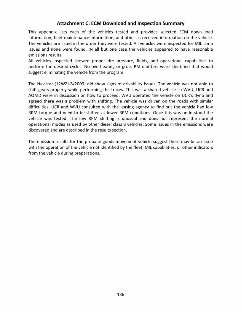
136
Attachment C: ECM Download and Inspection Summary
This appendix lists each of the vehicles tested and provides selected ECM down load information, fleet maintenance information, and other as-received information on the vehicle. The vehicles are listed in the order they were tested. All vehicles were inspected for MIL lamp issues and none were found. IN all but one case the vehicles appeared to have reasonable emissions results. All vehicles inspected showed proper tire pressure, fluids, and operational capabilities to perform the desired cycles. No overheating or gross PM emitters were identified that would suggest eliminating the vehicle from the program. The Navistar (12WZJ-B/2009) did show signs of drivability issues. The vehicle was not able to shift gears properly while performing the traces. This was a shared vehicle so WVU, UCR and AQMD were in discussion on how to proceed. WVU operated the vehicle on UCR’s dyno and agreed there was a problem with shifting. The vehicle was driven on the roads with similar difficulties. UCR and WVU consulted with the leasing agency to find out the vehicle had low RPM torque and need to be shifted at lower RPM conditions. Once this was understood the vehicle was tested. The low RPM shifting is unusual and does not represent the normal operational modes as used by other diesel class 8 vehicles. Some issues in the emissions were discovered and are described in the results section. The emission results for the propane goods movement vehicle suggest there may be an issue with the operation of the vehicle not identified by the fleet, MIL capabilities, or other indicators from the vehicle during preparations.
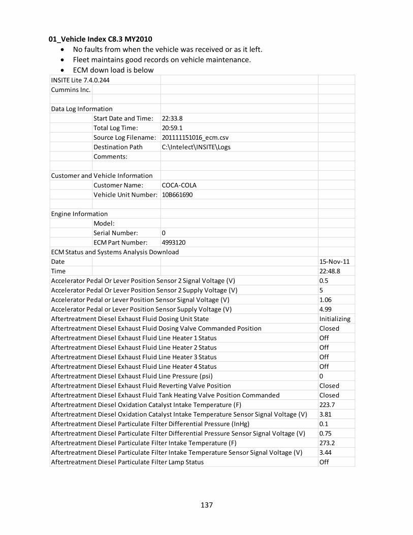
137
01_Vehicle Index C8.3 MY2010 • No faults from when the vehicle was received or as it left. • Fleet maintains good records on vehicle maintenance. • ECM down load is below
INSITE Lite 7.4.0.244Cummins Inc.
Data Log InformationStart Date and Time: 22:33.8Total Log Time: 20:59.1Source Log Filename: 201111151016_ecm.csvDestination Path C:\Intelect\INSITE\LogsComments:
Customer and Vehicle InformationCustomer Name: COCA-COLAVehicle Unit Number: 10B661690
Engine InformationModel:Serial Number: 0ECM Part Number: 4993120
ECM Status and Systems Analysis DownloadDate 15-Nov-11Time 22:48.8Accelerator Pedal Or Lever Position Sensor 2 Signal Voltage (V) 0.5Accelerator Pedal Or Lever Position Sensor 2 Supply Voltage (V) 5Accelerator Pedal or Lever Position Sensor Signal Voltage (V) 1.06Accelerator Pedal or Lever Position Sensor Supply Voltage (V) 4.99Aftertreatment Diesel Exhaust Fluid Dosing Unit State InitializingAftertreatment Diesel Exhaust Fluid Dosing Valve Commanded Position ClosedAftertreatment Diesel Exhaust Fluid Line Heater 1 Status OffAftertreatment Diesel Exhaust Fluid Line Heater 2 Status OffAftertreatment Diesel Exhaust Fluid Line Heater 3 Status OffAftertreatment Diesel Exhaust Fluid Line Heater 4 Status OffAftertreatment Diesel Exhaust Fluid Line Pressure (psi) 0Aftertreatment Diesel Exhaust Fluid Reverting Valve Position ClosedAftertreatment Diesel Exhaust Fluid Tank Heating Valve Position Commanded ClosedAftertreatment Diesel Oxidation Catalyst Intake Temperature (F) 223.7Aftertreatment Diesel Oxidation Catalyst Intake Temperature Sensor Signal Voltage (V) 3.81Aftertreatment Diesel Particulate Filter Differential Pressure (InHg) 0.1Aftertreatment Diesel Particulate Filter Differential Pressure Sensor Signal Voltage (V) 0.75Aftertreatment Diesel Particulate Filter Intake Temperature (F) 273.2Aftertreatment Diesel Particulate Filter Intake Temperature Sensor Signal Voltage (V) 3.44Aftertreatment Diesel Particulate Filter Lamp Status Off
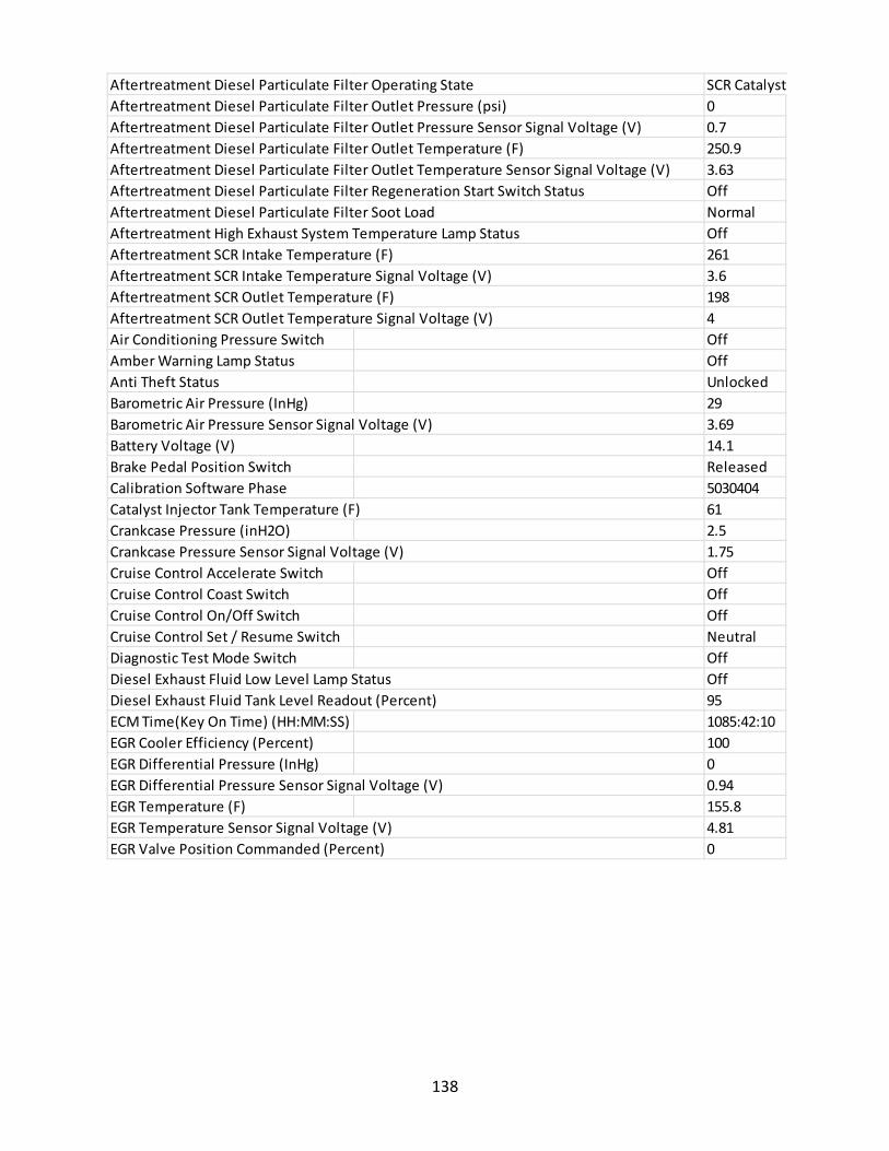
138
Aftertreatment Diesel Particulate Filter Operating State SCR Catalyst Aftertreatment Diesel Particulate Filter Outlet Pressure (psi) 0Aftertreatment Diesel Particulate Filter Outlet Pressure Sensor Signal Voltage (V) 0.7Aftertreatment Diesel Particulate Filter Outlet Temperature (F) 250.9Aftertreatment Diesel Particulate Filter Outlet Temperature Sensor Signal Voltage (V) 3.63Aftertreatment Diesel Particulate Filter Regeneration Start Switch Status OffAftertreatment Diesel Particulate Filter Soot Load NormalAftertreatment High Exhaust System Temperature Lamp Status OffAftertreatment SCR Intake Temperature (F) 261Aftertreatment SCR Intake Temperature Signal Voltage (V) 3.6Aftertreatment SCR Outlet Temperature (F) 198Aftertreatment SCR Outlet Temperature Signal Voltage (V) 4Air Conditioning Pressure Switch OffAmber Warning Lamp Status OffAnti Theft Status UnlockedBarometric Air Pressure (InHg) 29Barometric Air Pressure Sensor Signal Voltage (V) 3.69Battery Voltage (V) 14.1Brake Pedal Position Switch ReleasedCalibration Software Phase 5030404Catalyst Injector Tank Temperature (F) 61Crankcase Pressure (inH2O) 2.5Crankcase Pressure Sensor Signal Voltage (V) 1.75Cruise Control Accelerate Switch OffCruise Control Coast Switch OffCruise Control On/Off Switch OffCruise Control Set / Resume Switch NeutralDiagnostic Test Mode Switch OffDiesel Exhaust Fluid Low Level Lamp Status OffDiesel Exhaust Fluid Tank Level Readout (Percent) 95ECM Time(Key On Time) (HH:MM:SS) 1085:42:10EGR Cooler Efficiency (Percent) 100EGR Differential Pressure (InHg) 0EGR Differential Pressure Sensor Signal Voltage (V) 0.94EGR Temperature (F) 155.8EGR Temperature Sensor Signal Voltage (V) 4.81EGR Valve Position Commanded (Percent) 0
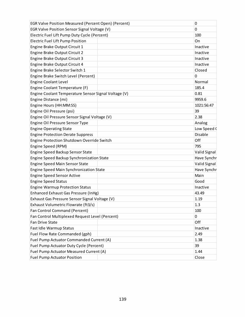
139
EGR Valve Position Measured (Percent Open) (Percent) 0EGR Valve Position Sensor Signal Voltage (V) 0Electric Fuel Lift Pump Duty Cycle (Percent) 100Electric Fuel Lift Pump Position OnEngine Brake Output Circuit 1 InactiveEngine Brake Output Circuit 2 InactiveEngine Brake Output Circuit 3 InactiveEngine Brake Output Circuit 4 InactiveEngine Brake Selector Switch 1 ClosedEngine Brake Switch Level (Percent) 0Engine Coolant Level NormalEngine Coolant Temperature (F) 185.4Engine Coolant Temperature Sensor Signal Voltage (V) 0.81Engine Distance (mi) 9959.6Engine Hours (HH:MM:SS) 1021:56:47Engine Oil Pressure (psi) 39Engine Oil Pressure Sensor Signal Voltage (V) 2.38Engine Oil Pressure Sensor Type AnalogEngine Operating State Low Speed G Engine Protection Derate Suppress DisableEngine Protection Shutdown Override Switch OffEngine Speed (RPM) 795Engine Speed Backup Sensor State Valid SignalEngine Speed Backup Synchronization State Have SynchrEngine Speed Main Sensor State Valid SignalEngine Speed Main Synchronization State Have SynchrEngine Speed Sensor Active MainEngine Speed Status GoodEngine Warmup Protection Status InactiveEnhanced Exhaust Gas Pressure (InHg) 43.49Exhaust Gas Pressure Sensor Signal Voltage (V) 1.19Exhaust Volumetric Flowrate (ft3/s) 1.3Fan Control Command (Percent) 100Fan Control Multiplexed Request Level (Percent) 0Fan Drive State OffFast Idle Warmup Status InactiveFuel Flow Rate Commanded (gph) 2.49Fuel Pump Actuator Commanded Current (A) 1.38Fuel Pump Actuator Duty Cycle (Percent) 39Fuel Pump Actuator Measured Current (A) 1.44Fuel Pump Actuator Position Close
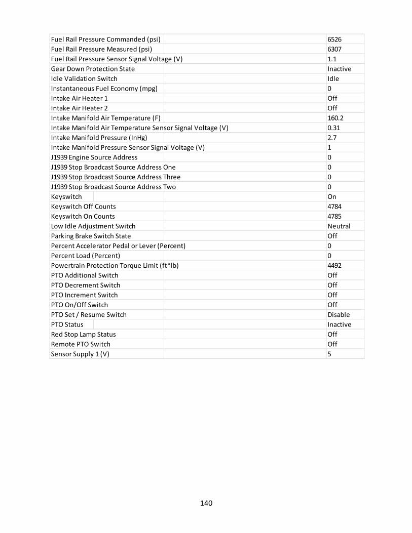
140
Fuel Rail Pressure Commanded (psi) 6526Fuel Rail Pressure Measured (psi) 6307Fuel Rail Pressure Sensor Signal Voltage (V) 1.1Gear Down Protection State InactiveIdle Validation Switch IdleInstantaneous Fuel Economy (mpg) 0Intake Air Heater 1 OffIntake Air Heater 2 OffIntake Manifold Air Temperature (F) 160.2Intake Manifold Air Temperature Sensor Signal Voltage (V) 0.31Intake Manifold Pressure (InHg) 2.7Intake Manifold Pressure Sensor Signal Voltage (V) 1J1939 Engine Source Address 0J1939 Stop Broadcast Source Address One 0J1939 Stop Broadcast Source Address Three 0J1939 Stop Broadcast Source Address Two 0Keyswitch OnKeyswitch Off Counts 4784Keyswitch On Counts 4785Low Idle Adjustment Switch NeutralParking Brake Switch State OffPercent Accelerator Pedal or Lever (Percent) 0Percent Load (Percent) 0Powertrain Protection Torque Limit (ft*lb) 4492PTO Additional Switch OffPTO Decrement Switch OffPTO Increment Switch OffPTO On/Off Switch OffPTO Set / Resume Switch DisablePTO Status InactiveRed Stop Lamp Status OffRemote PTO Switch OffSensor Supply 1 (V) 5
141
02_Vehicle Index Vol_12.8 MY 2011 Mack/MP8445C
• No faults from when the vehicle was received or as it left. • Leased vehicle by WVU and thus all pre inspection of vehicle records were done by
WVU. • WVU has ECM down load in their records
03_Vehicle Index Navistar/12WZJ-B/2009 • No faults from when the vehicle was received or as it left. • Leased vehicle by UCR and thus all pre inspection of vehicle records were done by
leasing company and met DOT inspection requirements. 04_Vehicle Index GM/8.1/2008
• No faults from when the vehicle was received or as it left. • Loaded vehicle by UCR and thus all pre inspection of vehicle records were done by fleet
company and met DOT inspection requirements. 05_Vehicle Index Navistar/A475/2011
• No faults from when the vehicle was received or as it left. • Leased vehicle by UCR and thus all pre inspection of vehicle records were done by
leasing company and met DOT inspection requirements. 06_Vehicle Index Cummins/ISX11.9/2011
• No faults from when the vehicle was received or as it left. • Leased vehicle by UCR and thus all pre inspection of vehicle records were done by
leasing company and met DOT inspection requirements. 07_Vehicle Index Cummins/ISB 220/2007
• No faults from when the vehicle was received or as it left.
Sensor Supply 2 (V) 5Sensor Supply 3 (V) 5Sensor Supply 5 (V) 5Sensor Supply 6 (V) 5Transmission Gear Ratio 16Transmission Status Out of GearTrip Information Aftertreatment Diesel Exhaust Fluid Used (gal) 25.2Trip Information Total Diesel Exhaust Fluid Used (gal) 36.6Turbocharger Actuator Position Commanded (Percent Closed) (Percent) 89Turbocharger Actuator Position Measured (Percent Closed) (Percent) 89Turbocharger Actuator Position Sensor Signal Voltage (V) 0Turbocharger Actuator Type ElectricTurbocharger Compressor Intake Air Temperature (F) 115.6Turbocharger Compressor Intake Air Temperature Sensor Signal Voltage (V) 0.69Turbocharger Compressor Outlet Air Temperature (Calculated) (F) 134.6Turbocharger Speed (RPM) 29633Vehicle Speed (mph) 0Wait To Start Lamp Status OffWater In Fuel Detected Total Accumulated Time (HH:MM:SS) 0:00:00Water in Fuel Sensor Signal Voltage (V) 4.1Water In Fuel State No Water De
142
• Leased vehicle by UCR and thus all pre inspection of vehicle records were done by leasing company and met DOT inspection requirements.
08_Vehicle Index Bi-Phase/8.1l GM/2009 • No faults from when the vehicle was received or as it left. • Loaned vehicle by UCR • No ECM interface was possible thus, utilized fleet records and dash MIL lights for
maintenance information. • The vehicle did appear to run hot. No over temperature issues were identified. Fleet
owner was asked about maintained records and no issues were identified. • Vehicle had in excess of 1,000,000 miles. The engine was repowered to propane about
60,000 miles ago and sees 3,000 to 4,000 miles per year • All fluids and tire pressures were suitable.
09_Vehicle Index Navistar/GDT260/2008 • No faults from when the vehicle was received or as it left. • Fluids, tire pressure and other details all met UCR’s inspection report logs • Leased vehicle by UCR and thus all pre inspection of vehicle records were done by
leasing company and met DOT inspection requirements. 10_Vehicle Index Navistar/A430/2011
• No faults from when the vehicle was received or as it left. • Fluids, tire pressure and other details all met UCR’s inspection report logs • Leased vehicle by UCR and thus all pre inspection of vehicle records were done by
leasing company and met DOT inspection requirements. 11_Vehicle Index DDC/60 14L/2008 SN = 06R1019569
• No faults from when the vehicle was received or as it left. • Loaned vehicle to UCR where fleet owner maintained good vehicle records
12_Vehicle Index DDC/60 14L/2008 SN = 06R1019704 • No faults from when the vehicle was received or as it left. • Loaned vehicle to UCR where fleet owner maintained good vehicle records
13 Refuse hauler Cummins/ISL9 370/2011 • No faults from when the vehicle was received or as it left. • Leased vehicle by UCR and thus all pre inspection of vehicle records were done by
leasing company and met DOT inspection requirements. • ECM down load is below
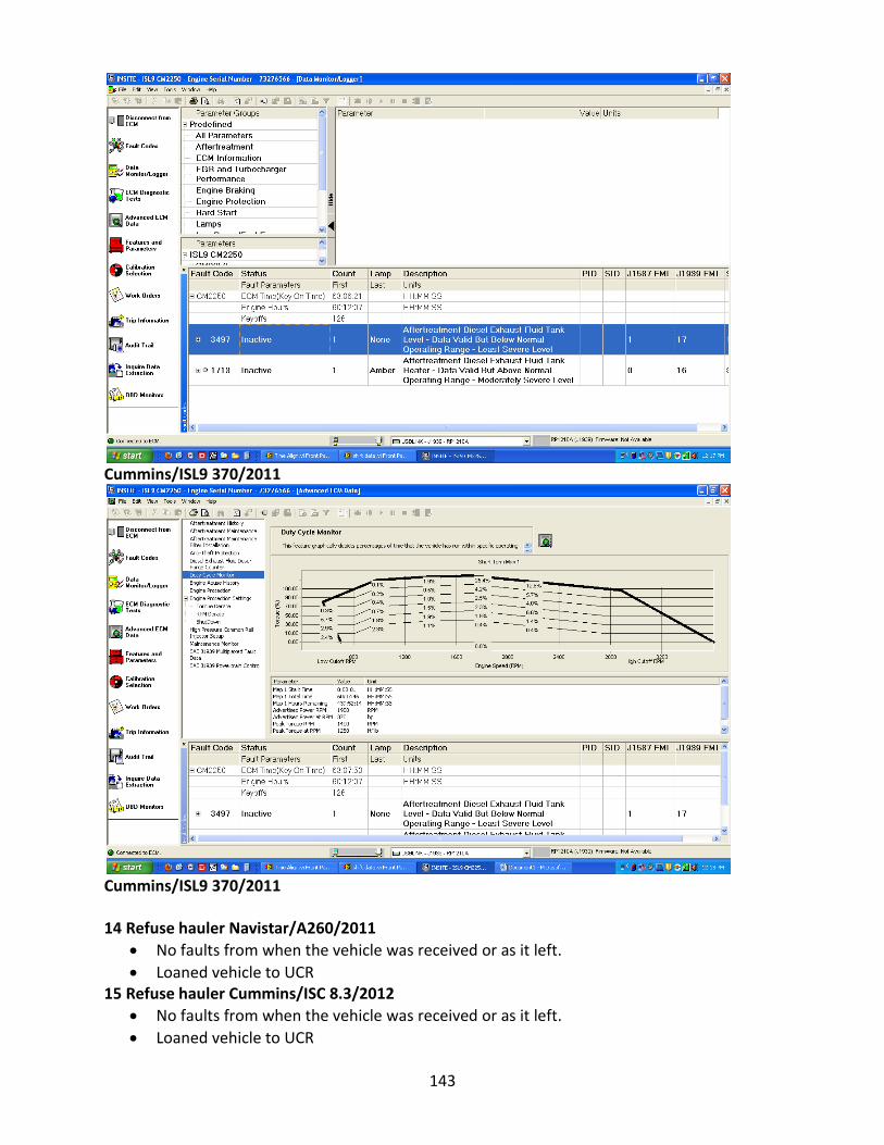
143
Cummins/ISL9 370/2011
Cummins/ISL9 370/2011
14 Refuse hauler Navistar/A260/2011
• No faults from when the vehicle was received or as it left. • Loaned vehicle to UCR
15 Refuse hauler Cummins/ISC 8.3/2012 • No faults from when the vehicle was received or as it left. • Loaned vehicle to UCR
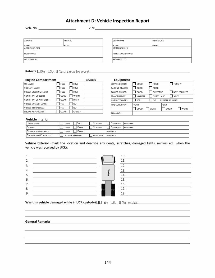
144
Attachment D: Vehicle Inspection Report Veh. No.: VIN:
ARRIVAL
DATE:
ARRIVAL
TIME: AGENCY RELEASE
SIGNATURE:
DELIVERED BY:
DEPARTURE
DATE:
DEPARTURE
TIME: UCR ENGINEER
RELEASE SIGNATURE:
RETURNED TO:
Retest? Yes No. If Yes, reason for retest: Engine Compartment REMARKS
OIL LEVEL: FULL LOW COOLANT LEVEL: FULL LOW POWER STEERING FLUID: FULL LOW CONDITION OF BELTS: GOOD WORN CONDITION OF AIR FILTER: CLEAN DIRTY VISIBLE EXHAUST LEAKS: YES NO VISIBLE FLUID LEAKS: YES NO ENGINE APPEARANCE: CLEAN GREASY
Equipment SERVICE BRAKES: GOOD POOR TOUCHY PARKING BRAKES: GOOD POOR POWER DIVIDER: GOOD DEFECTIVE NOT EQUIPPED TRANSMISSION: NORMAL SHIFTS HARD NOISY LUG NUT COVERS: YES NO NUMBER MISSING: TIRE CONDITION: FRONT REAR
GOOD WORN GOOD WORN
REMARKS:
Vehicle Interior UPHOLSTERY: CLEAN DIRTY STAINED DAMAGED REMARKS: CARPET: CLEAN DIRTY STAINED DAMAGED REMARKS: GENERAL APPEARANCE: CLEAN DIRTY REMARKS: GAUGES AND CONTROLS: OPERATE PROPERLY DEFECTIVE REMARKS:
Vehicle Exterior (mark the location and describe any dents, scratches, damaged lights, mirrors etc. when the vehicle was received by UCR): 1. 10. 2. 11.
3. 12. 4. 13. 5. 14. 6. 15. 7. 16. 8. 17. 9. 18. Was this vehicle damaged while in UCR custody? Yes No. If Yes, explain:
General Remarks
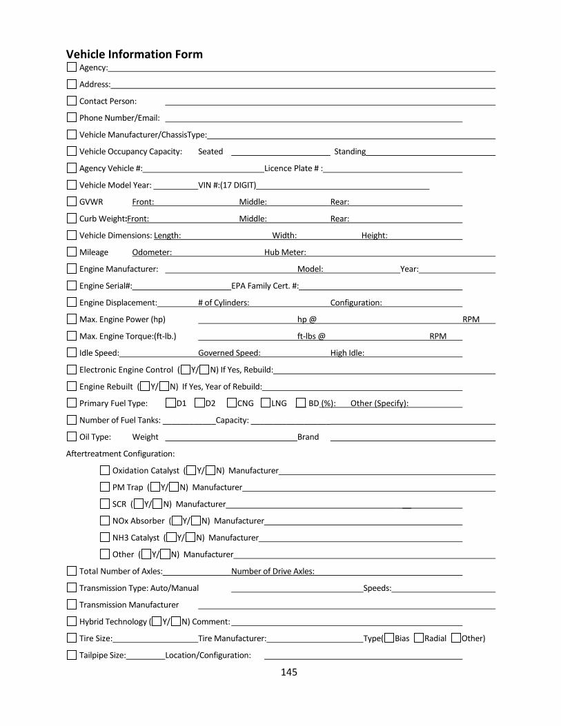
145
Vehicle Information Form Agency:
Address:
Contact Person:
Phone Number/Email:
Vehicle Manufacturer/ChassisType:
Vehicle Occupancy Capacity: Seated Standing
Agency Vehicle #: Licence Plate # :
Vehicle Model Year: VIN #:(17 DIGIT)
GVWR
Curb Weight:
Front: Middle: Rear:
Vehicle Dimensions:
Front: Middle: Rear:
Mileage
Length: Width: Height:
Engine Manufacturer:
Odometer: Hub Meter:
Model:
Engine Serial#: EPA Family Cert. #:
Year:
Engine Displacement:
Max. Engine Power (hp)
# of Cylinders: Configuration:
Max. Engine Torque:(ft-lb.)
hp @ RPM
Idle Speed:
ft-lbs @ RPM
Electronic Engine Control ( Y/ N) If Yes, Rebuild:
Governed Speed: High Idle:
Engine Rebuilt ( Y/ N) If Yes, Year of Rebuild:
Primary Fuel Type: D1 D2 CNG LNG BD
Number of Fuel Tanks: ____________Capacity: __________________
(%): Other (Specify):
Oil Type: Weight Brand
Aftertreatment Configuration:
Oxidation Catalyst ( Y/ N) Manufacturer
PM Trap ( Y/ N) Manufacturer
SCR ( Y/ N) Manufacturer
NOx Absorber ( Y/ N) Manufacturer
__
NH3 Catalyst ( Y/ N) Manufacturer
Other ( Y/ N) Manufacturer
Total Number of Axles:
Transmission Type: Auto/Manual Speeds:
Number of Drive Axles:
Transmission Manufacturer
Hybrid Technology ( Y/ N) Comment:
Tire Size: Tire Manufacturer: Type( Bias Radial Other)
Tailpipe Size: Location/Configuration:
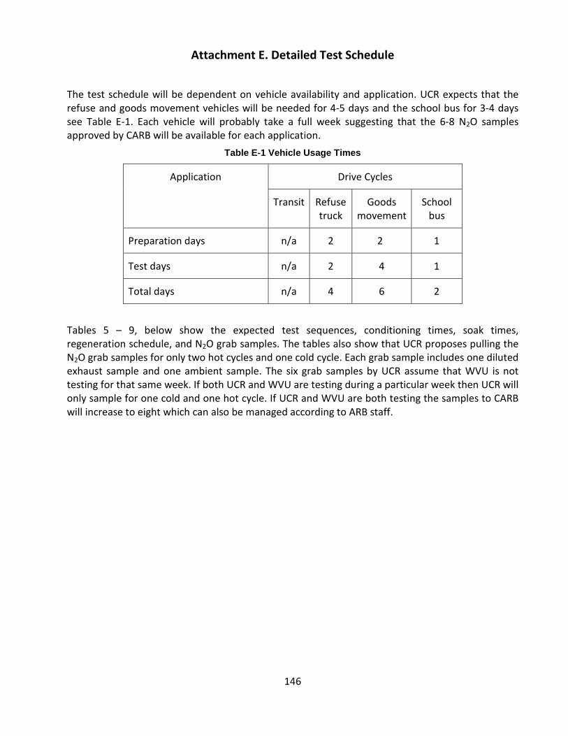
146
Attachment E. Detailed Test Schedule
The test schedule will be dependent on vehicle availability and application. UCR expects that the refuse and goods movement vehicles will be needed for 4-5 days and the school bus for 3-4 days see Table E-1. Each vehicle will probably take a full week suggesting that the 6-8 N2O samples approved by CARB will be available for each application.
Table E-1 Vehicle Usage Times
Application Drive Cycles
Transit Refuse truck
Goods movement
School bus
Preparation days n/a 2 2 1
Test days n/a 2 4 1
Total days n/a 4 6 2
Tables 5 – 9, below show the expected test sequences, conditioning times, soak times, regeneration schedule, and N2O grab samples. The tables also show that UCR proposes pulling the N2O grab samples for only two hot cycles and one cold cycle. Each grab sample includes one diluted exhaust sample and one ambient sample. The six grab samples by UCR assume that WVU is not testing for that same week. If both UCR and WVU are testing during a particular week then UCR will only sample for one cold and one hot cycle. If UCR and WVU are both testing the samples to CARB will increase to eight which can also be managed according to ARB staff.
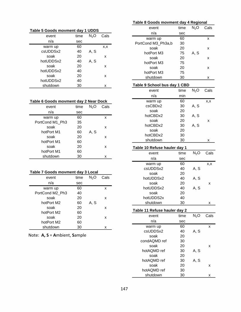
147
Note: A, S = Ambient, Sample
Table 5 Goods movment day 1 UDDSevent time N2O Calsn/a sec
warm up 60 x,xcsUDDSx2 40 A, S
soak 20 xhotUDDSx2 40 A, S
soak 20 xhotUDDSx2 40
soak 20 xhotUDDSx2 40shutdown 30 x
Table 6 Goods movment day 2 Near Dockevent time N2O Calsn/a sec
warm up 60 xPortCond M1_Ph3 35
soak 20 xhotPort M1 60 A, S
soak 20 xhotPort M1 60
soak 20 xhotPort M1 60shutdown 30 x
Table 7 Goods movment day 3 Localevent time N2O Calsn/a sec
warm up 60 xPortCond M2_Ph3 40
soak 20 xhotPort M2 60 A, S
soak 20 xhotPort M2 60
soak 20 xhotPort M2 60shutdown 30 x
Table 8 Goods movment day 4 Regionalevent time N2O Calsn/a sec
warm up 60 xPortCond M3_Ph3a,b 30
soak 20 xhotPort M3 75 A, S
soak 20 xhotPort M3 75
soak 20 xhotPort M3 75shutdown 30 x
Table 9 School bus day 1 CBDevent time N2O Calsn/a min
warm up 60 x,xcsCBDx2 30 A, S
soak 20hotCBDx2 30 A, S
soak 20 xhotCBDx2 30 A, S
soak 20hotCBDx2 30shutdown 30 x
Table 10 Refuse hauler day 1event time N2O Calsn/a sec
warm up 60 x,xcsUDDSx2 40 A, S
soak 20hotUDDSx2 40 A, S
soak 20 xhotUDDSx2 40 A, S
soak 20hotUDDS2x 40shutdown 30 x
Table 11 Refuse hauler day 2event time N2O Calsn/a sec
warm up 60 xcsUDDSx2 40 A, S
soak 20condAQMD ref 30
soak 20 xhotAQMD ref 30 A, S
soak 20hotAQMD ref 30 A, S
soak 20 xhotAQMD ref 30
shutdown 30 x

148
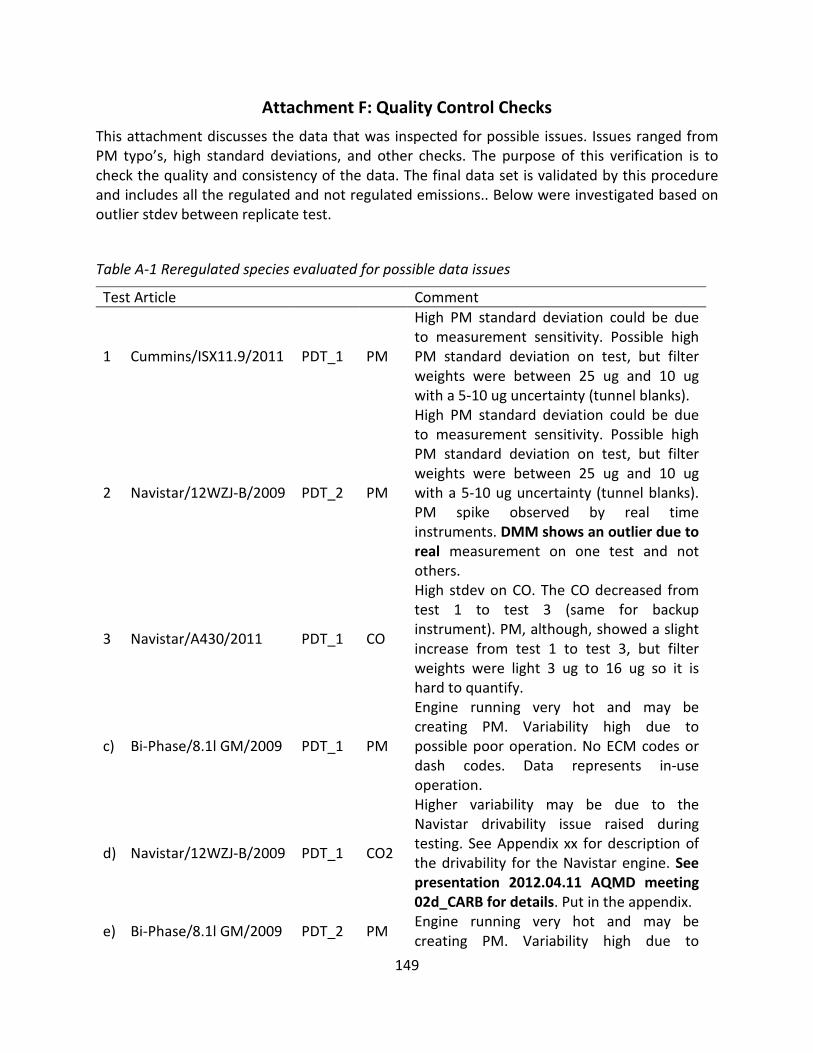
149
Attachment F: Quality Control Checks
This attachment discusses the data that was inspected for possible issues. Issues ranged from PM typo’s, high standard deviations, and other checks. The purpose of this verification is to check the quality and consistency of the data. The final data set is validated by this procedure and includes all the regulated and not regulated emissions.. Below were investigated based on outlier stdev between replicate test.
Table A-1 Reregulated species evaluated for possible data issues
Test Article Comment
1 Cummins/ISX11.9/2011 PDT_1 PM
High PM standard deviation could be due to measurement sensitivity. Possible high PM standard deviation on test, but filter weights were between 25 ug and 10 ug with a 5-10 ug uncertainty (tunnel blanks).
2 Navistar/12WZJ-B/2009 PDT_2 PM
High PM standard deviation could be due to measurement sensitivity. Possible high PM standard deviation on test, but filter weights were between 25 ug and 10 ug with a 5-10 ug uncertainty (tunnel blanks). PM spike observed by real time instruments. DMM shows an outlier due to real measurement on one test and not others.
3 Navistar/A430/2011 PDT_1 CO
High stdev on CO. The CO decreased from test 1 to test 3 (same for backup instrument). PM, although, showed a slight increase from test 1 to test 3, but filter weights were light 3 ug to 16 ug so it is hard to quantify.
c) Bi-Phase/8.1l GM/2009 PDT_1 PM
Engine running very hot and may be creating PM. Variability high due to possible poor operation. No ECM codes or dash codes. Data represents in-use operation.
d) Navistar/12WZJ-B/2009 PDT_1 CO2
Higher variability may be due to the Navistar drivability issue raised during testing. See Appendix xx for description of the drivability for the Navistar engine. See presentation 2012.04.11 AQMD meeting 02d_CARB for details. Put in the appendix.
e) Bi-Phase/8.1l GM/2009 PDT_2 PM Engine running very hot and may be creating PM. Variability high due to
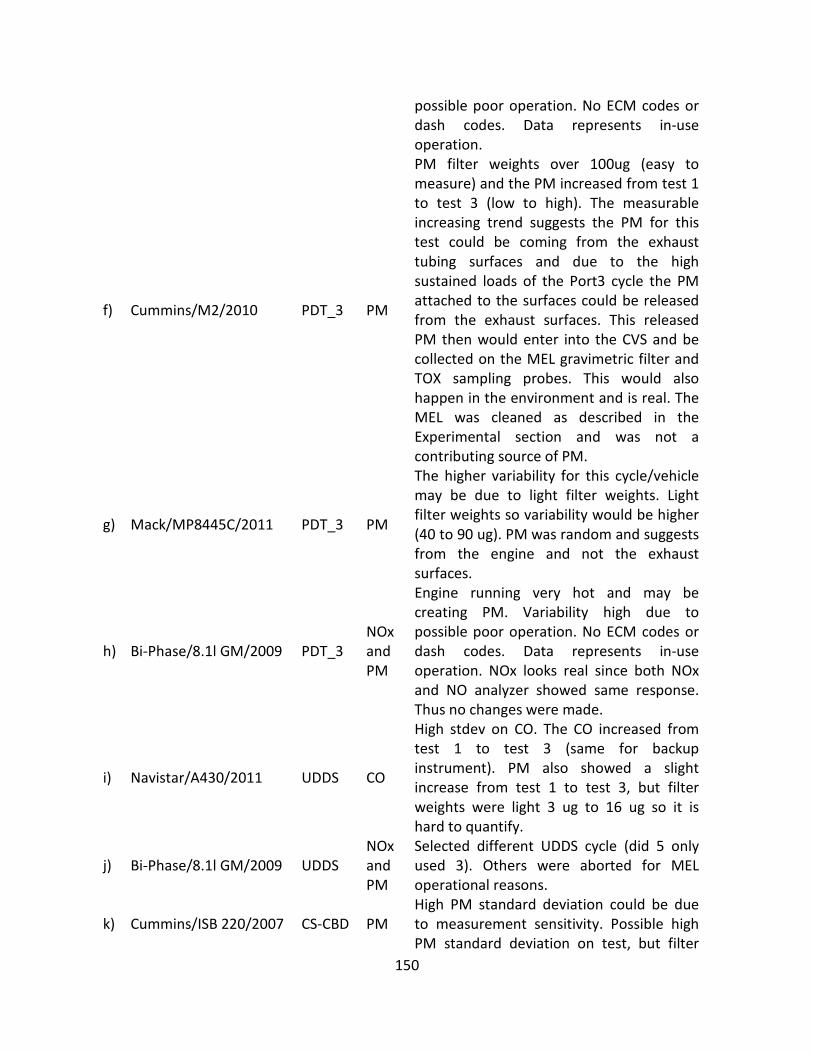
150
possible poor operation. No ECM codes or dash codes. Data represents in-use operation.
f) Cummins/M2/2010 PDT_3 PM
PM filter weights over 100ug (easy to measure) and the PM increased from test 1 to test 3 (low to high). The measurable increasing trend suggests the PM for this test could be coming from the exhaust tubing surfaces and due to the high sustained loads of the Port3 cycle the PM attached to the surfaces could be released from the exhaust surfaces. This released PM then would enter into the CVS and be collected on the MEL gravimetric filter and TOX sampling probes. This would also happen in the environment and is real. The MEL was cleaned as described in the Experimental section and was not a contributing source of PM.
g) Mack/MP8445C/2011 PDT_3 PM
The higher variability for this cycle/vehicle may be due to light filter weights. Light filter weights so variability would be higher (40 to 90 ug). PM was random and suggests from the engine and not the exhaust surfaces.
h) Bi-Phase/8.1l GM/2009 PDT_3 NOx and PM
Engine running very hot and may be creating PM. Variability high due to possible poor operation. No ECM codes or dash codes. Data represents in-use operation. NOx looks real since both NOx and NO analyzer showed same response. Thus no changes were made.
i) Navistar/A430/2011 UDDS CO
High stdev on CO. The CO increased from test 1 to test 3 (same for backup instrument). PM also showed a slight increase from test 1 to test 3, but filter weights were light 3 ug to 16 ug so it is hard to quantify.
j) Bi-Phase/8.1l GM/2009 UDDS NOx and PM
Selected different UDDS cycle (did 5 only used 3). Others were aborted for MEL operational reasons.
k) Cummins/ISB 220/2007 CS-CBD PM High PM standard deviation could be due to measurement sensitivity. Possible high PM standard deviation on test, but filter
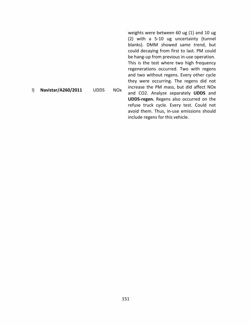
151
weights were between 60 ug (1) and 10 ug (2) with a 5-10 ug uncertainty (tunnel blanks). DMM showed same trend, but could decaying from first to last. PM could be hang-up from previous in-use operation.
l) Navistar/A260/2011 UDDS NOx
This is the test where two high frequency regenerations occurred. Two with regens and two without regens. Every other cycle they were occurring. The regens did not increase the PM mass, but did affect NOx and CO2. Analyze separately UDDS and UDDS-regen. Regens also occurred on the refuse truck cycle. Every test. Could not avoid them. Thus, in-use emissions should include regens for this vehicle.