in to - Oregon State University in storm... · Changes in Storm Hydrographs due to Clearcut Logging of Coastal Watersheds By Warren Charles Harper A THESIS submitted to Oregon State

Changes in Storm Hydrographs due to Clearcut Logging of Coastal Watersheds

By

Warren Charles Harper

A THESIS

submitted to

Oregon State University

in partial fulfillxnentof

the requirements for the

degree of

Master of Science

June 1969

APPROVED:

Professor of Forest Management in charge of major

Head of Department of Forest Management

Dean of Graduate School

Date thesis is presented: May 9, 1969

Typed by Janet J. Harper for Warren Charles Harper

AN ABSTRACT OF THE THESIS OF

WARREN CHARLES HARPER for the (Name of student)

LOGGING OF COASTAL WATERSHEDS

Abstract approved: James T. Krygier

The purpose of this study was to determime the

effect of clearcut logging on stormf low by analysis of

characteristic parameters of individual storm hydrographs.

Parameters considered included height-of-rise, peak

discharge, volume and time-to-peak. The hydrologic

data were derived from experimental watersheds of the

Alsea Study located in the Oregon Coast Range.

Three clearcut watersheds were selected for study;

Deer Creek IV (39 acres) was clearcut, and Needle Branch

(175 acres) was clearcut and burned. Both watersheds

were compared to Flynn Creek (502 acres), an untreated

control, before and after treatment.

Change in hydrologic parameters was determined

from differences between pre- and post-logging linear

M.S. (Degree)

In FOREST MANAGEMENT presented on May 9, 1969 (Major) (Date)

TITLE: CHANGES IN STORM HYDROGRAPHS DUE TO CLEARCUT

regressions. Statistical techniques were utilized to

test for difference in slope or vertical position.

Significant increases were found in peak discharge

from both Needle Branch and Deer Creek IV following

clearcut logging. Larger increases were noted during

the fall period than during the winter period. Volume para-

meters of quick flow, delayed flow, and total flow were

increased for Needle Branch. Volume of flow was not shown

to increase from Deer Creek IV. This may have been due

to a lack of usable storm events for analysis from this

watershed. Time-to-peak was not altered in Needle Branch

but was decreased for low flows and increased for high

flows on Deer Creek IV. The height-of-rise parameter

did not prove to be of value for detecting change in

this study. Comparison of the burned watershed (Needle

Branch) to the unburned watershed (Deer Creek IV) did

not produce a noticable difference in any of the

parameters.

The observed changes in stormf low were related

to clearcut logging and the effect of vegetative re-

moval on watershed response.

ACKNOWLEDGMENT S

Gratitude is expressed to the Water Resources

Research Institute at Oregon State University for

providing the financial aid necessary for this study.

My appreciation is extended to Professors James

T. Krygier, George W. Brown III, and Peter C. Klingeman

for their advice, guidance and assistance both during

the research and during the preparation of this thesis.

Appreciation is extended to my fellow graduate

students for their help and assistance, especially to

Kenneth R. Holtje, Jr. for his assistance in design

of the computer programs used in this study.

Deep appreciation is extended to my wife who not

only provided assistance in the preparation of this

thesis but more importantly provided the support and

encouragement necessary for its completion.

TABLE OF CONTENTS

Page

INTRODUCTION 1

Objectives 2 Scope 3

DESCRIPTION OF FLYNN CREEK, DEER CREEK IV, AND NEEDLE BRANCH 6

Climate 6 Soils and Geology 7

Topography 8

Vegetation 9

LITERATURE REVIEW 11 Clearcut Logging and Water Yield 11 Clearcut Logging and Hydrograph Parameters 18

EvapotranspiratiOn 19 Infiltration and Soil Water Movement 21

Evidence of Change from Watershed Studies 22 Hydrograph Separation 25

Methods to Detect Change 31

Low Flow Analysis 33

DESIGN OF EXPERIMENT 36 Treatments 36

InstrumentatiOn 37

DATA ANALYSIS 39 Definition of Parameters 39 Peak Discharge 39

Height-Of-Rise 40 Volume 40

Time-To-Peak 41 Recession 41

Selection of Events 41 Data Reduction 45

Statistical Techniques 51 Determination of Regression Relations 51

Tests for Change 53 Change in Slope 54 Change in Vertical Position 55

Seasonal Variation 56

Page

RESULTS 59 Peak Discharge 60

Needle Branch 60 Deer Creek IV 62

Height-Of-Rise 65 Needle Branch 65

Deer Creek IV 69 Quick Flow 69


Delayed Flow 71 Needle Branch. 71

Deer Creek IV 73 Total Flow 73


Time-To-Peak 76 Needle Branch 76

Deer Creek IV 79 Recession 79

DISCUSSION 82 Peak Discharge 82

Height-Of-Rise 85 Volume 85

Time-To-Peak 88 Hydrograph Shape 89

CONCLUSIONS 94

BIBLIOGRAPHY .

96

APPENDIX I 102

APPENDIX II 106

APPENDIX III 109

LIST OF TABLES

Table Page

1. Summary of absolute and percentage change in significant parameters for minimum, average

and maximum values for Needle Branch and Deer Creek IV.

I Summary of statistics for Needle Branch including number of observations (n), r2, t

for slope Ct5), t for vertical position (tm), and variance, for years 1957-68.

II. Summary of statistics for Deer Creek IV including number of observations (n)

, r2, t

for slope Ct5), t for vertical position (tm), and variance, for years 1965-68.

III.Sumnmary of statistical results for test to determine difference between fall and winter

data, including nuniber of observations (n), r2, t for slope Ct ), and t for vertical position

(tm) as tested against the control. 104

Data for Flynn Creek used in statistical analyses.

Data for Deer Creek IV used in analyses.

Data for Needle Branch used in analyses.

statistical

statistical

61

102

103

LIST OF FIGURES

Figure Page

Planimetric map of watersheds in the Alsea Watershed study. 4

Method of hydrograph separation. 27

Quick flow-delayed flow hydrograph separation. 30

Hydrograph illustrating quick flow separation of a small event for storm of October 28,

1960, on Needle Branch. 48

Hydrograph illustrating quick flow separation of a median event for storm of November 23,

1959, on needle Branch. 49

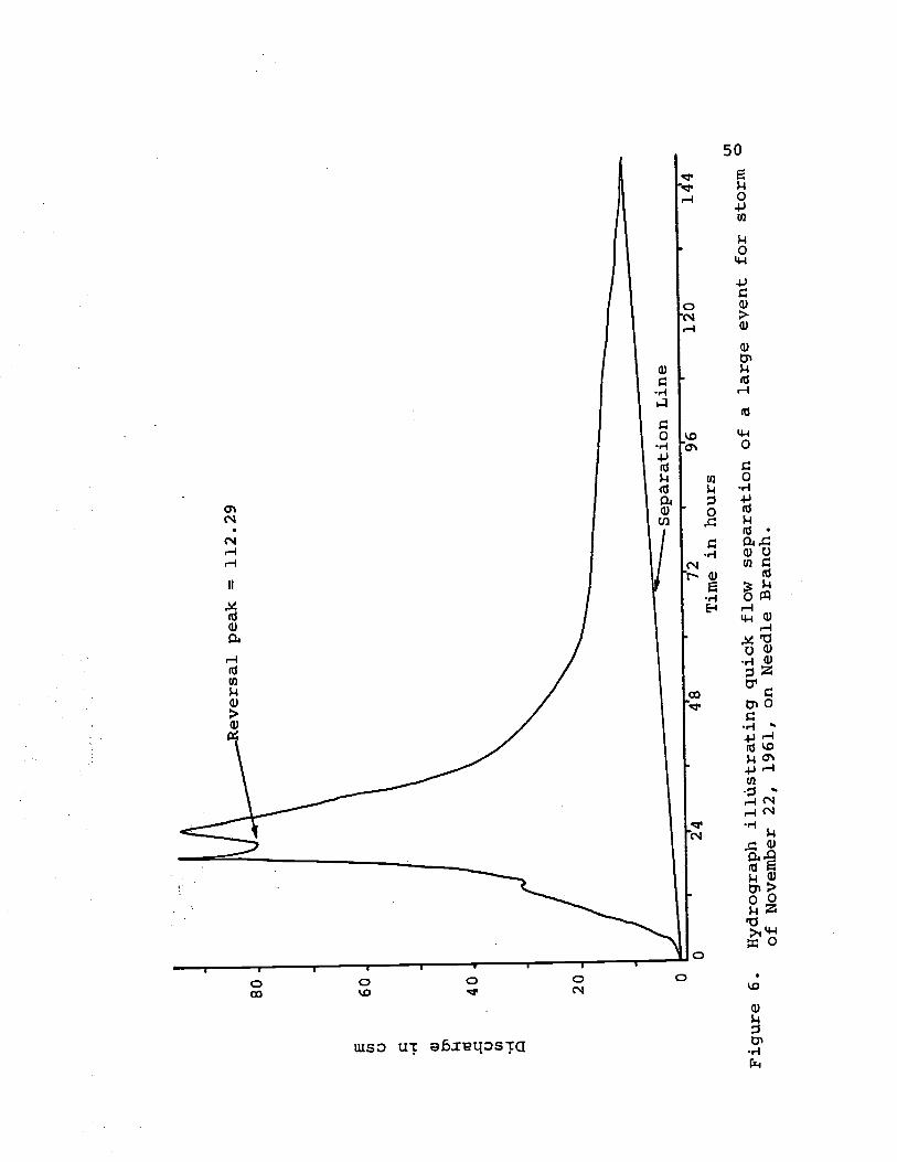
Hydrograph illustrating quick flow separation of a large event for storm of November 22,

1961, on Needle Branch. 50

Peak discharge from Needle Branch regressed on Flynn Creek for full period, pre- and post-

logging. 63

Peak discharge from Needle Branch regressed on Flynn Creek for fall period, pre- and post-

logging. 63

Peak discharge from Needle Branch regressed on Flynn Creek for winter period, pre- and

post-logging. 64

Peak discharge from Deer CreekIV regressed on Flynn Creek for full period, pre- and post-

logging. .

64

Peak: discharge from Deer Creek.IV regressed on Flynn Creek for fall period, pre- and post-

logging. 66

Peak discharge, from Deer Creek IV regressed on Flynn Creek for winter period, pre- and

post-logging. 66

Height-of-rise for Needle Branch regressed on

Figure

Flynn Creek for full period, pre- and post- logging.

Height-of-rise for Needle Branch regressed on Flynn Creek for fall period, pre- and post-

logging. 67

Height-of-rise for Needle Branch regressed on Flynn Creek for winter period, pre- and

post-logging 68

Height-of-rise for Deer Creek IV regressed on Flynn Creek for full period, pre- and post

logging. 68

Quick flow volume from Needle Branch regressed on Flynn Creek for full period,

pre- and post-logging. 70

Quick flow volume from Needle Branch regressed on Flynn Creek for fall period,


Quick flow volume from Needle Branch regr.essed on Flynn Creek for winter period,


Quick flow volume from Deer Creek IV regressed on Flynn Creek for full period, pre-

and post-logging. 72

Delayed flow volume from Needle Branch regressed on Flynn Creek for full period,


Delayed flow volume from Needle Branch regressed on Flynn Creek for fall period,

pre- aPd post-logging. 74

Delayed flow volume from Needle Bratich regressed on Flynn Creek for winter period,

pre- and post-logging.

Delayed flow volume from Deer Creek IV regressed on Flynn Creek for full period,

pre- and post-logging.

Page

67

75

75

Figure Page

Total flow volume from Needle Branch regressed on Flynn Creek for full period,

pre- and post-logging 77

Total flow volume from Needle Branch regressed on Flynn Creek for fall period,


Total flow volume from Needle Branch regressed on Flynn Creek for winter period,


Total flow volume from Deer Creek IV regressed on Flynn Creek for full period,


Time-to-peak on Needle Branch regressed on Flynn Creek for full period, pre- and post-

logging. 80

Time-to-peak on Needle Branch regressed on Flynn Creek for fall period, pre- and post-

logging. 80

Time-to-peak on Needle Branch regressed on Flynn Creek for winter period, pre- and post-

logging. 81

Time-to-peak on Deer Creek IV regressed on Flynn Creek for full period, pre- and. post-

logging. 81

Hydrographs for Nov. 24, 1964 and Oct. 27, 1967 for Needle Branch and Flynn Creek

illustrating pre- logging and post-logging relationships for the fall period. 90

Hydrographs for Jan. 6, 1964 and Dec. 4,

1966 for Needle Branch and Flynn Creek illustrating pre-logging and post-logging relationships for the winter period. 91

Hydrographs for Jan. 15, 1966 and Oct. 27, 1967 for Deer Creek IV and Flynn Creek

illustrating pre-logging and post-logging relationships for the fall period. 92

Page Figure

105

105

Double-mass-analysis of precipitation for Needle Branch and Flynn Creek, years 1960

through 1967.

Double-mass-analysis of precipitation for Deer Creek and Flynn Creek, years 1960

through 1967.

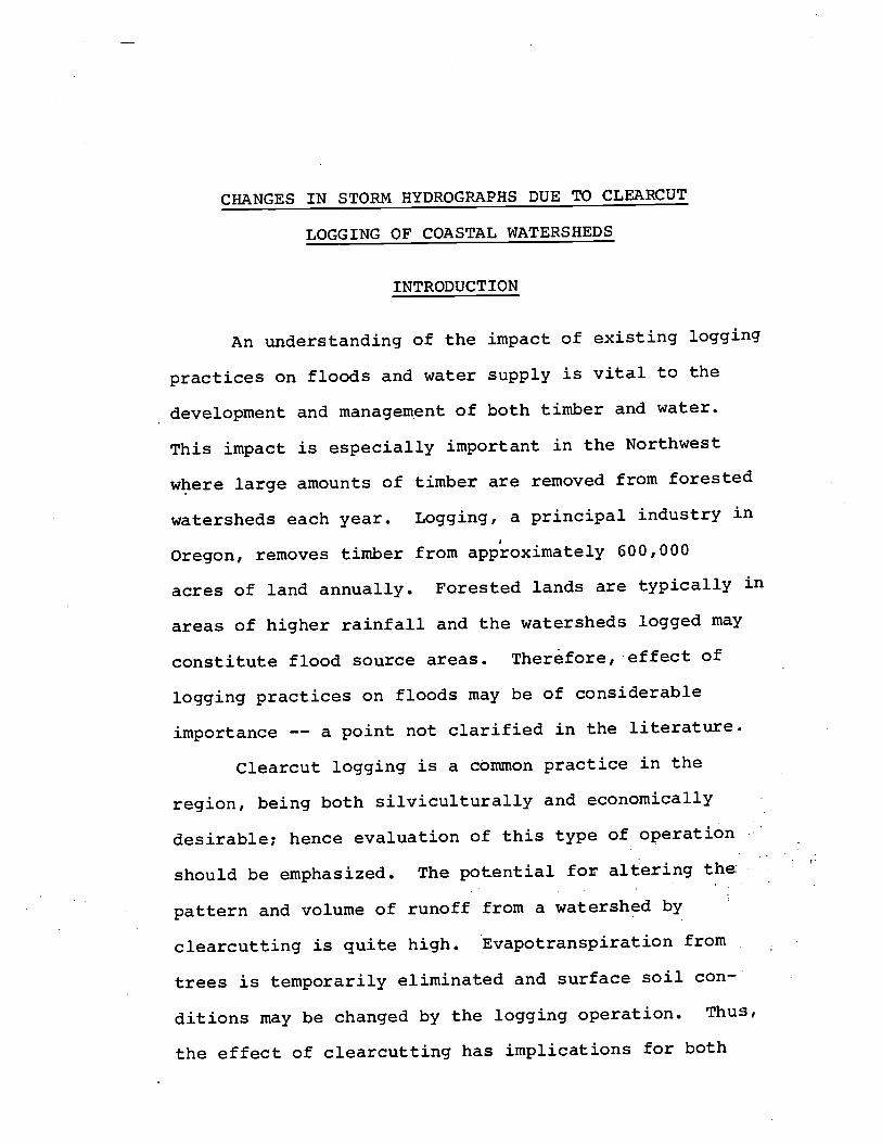
CHANGES IN STORM HYDROGPAPHS DUE TO CLEARCUT

LOGGING OF COASTAL WATERSHEDS

INTRODUCT ION

An understanding of the impact of existing logging

practices on floods and water supply is vital to the

development and management of both timber and water.

This impact is especially important in the Northwest

where large amounts of timber are removed from forested

watersheds each year. Logging, a principal industry in

Oregon, removes timber from app'roximately 600,000

acres of land annually. Forested lands are typically in

areas of higher rainfall and the watersheds logged may

constitute flood source areas. Therefore, effect of

logging practices on floods may be of considerable

importance -- a point not clarified in the literature.

Clearcut logging is a common practice in the

region, being both silviculturally and economically

desirable; hence evaluation of this type of operation

should be emphasized. The potential for altering the

pattern and volume of runoff from a watershed by

clearcutting is quite high. EvapotranspiratiOn from

trees is temporarily eliminated and surface soil con-

ditions may be changed by the logging operation. Thus,

the effect of clearcutting has implications for both

2

water supply augmentation and structural design criteria.

These same flow parameters may alter fish habitat and

the magnitude of sediment transport. The effect of

clearcutting on storm hydrograph characteristics has

not been satisfactorily determined. For these reasons

a study of the impact of clearcut logging on individual

hydrograph parameters should lend insight into changes

of hydrologic significance.

The experimental watersheds of the Alsea Study in

the coast range provided a basis for determining possible

changes on individual hydrograph factors.

Objectives

The primary objective of this research is to

determine the effect of clearcut logging on individual

runoff events from two watersheds in Oregon's Coast

Range. Detection of change is sought by examining

several parameters defining principal components of

storm hydrographs. Parameters considered are peak

discharge, height-of-rise, storm volume,.and time-to-

peak.

Secondary objectives are to:

Explain any hydrologic changes in terms of

possible physical processes involved.

Evaluate the method used to determine its

ability to detect hydrologic changes.

Scope

Concern about the possible influence of logging on

aquatic resources in the state of Oregon led to the

initiation of the Alsea Watershed Study in 1958. The

present study was formulated to evaluate hydrologic

data being collected on a number of experimental water-

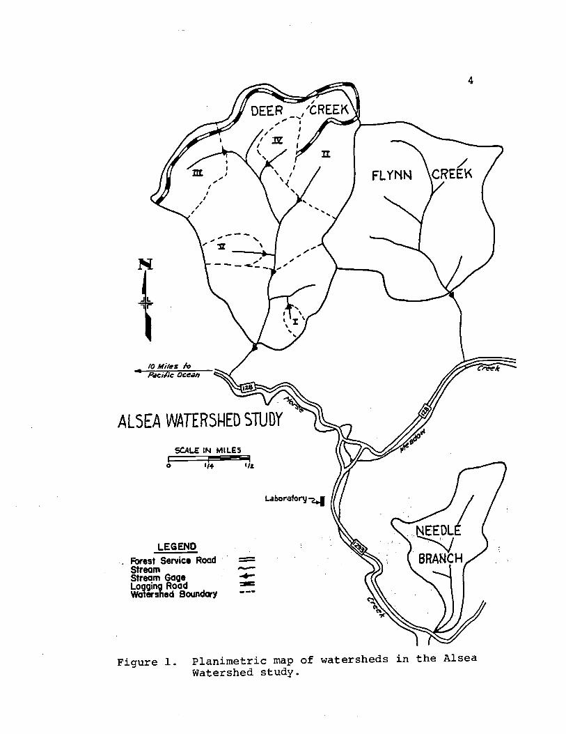
sheds. As illustrated in Figure 1, the experimental

watersheds are within the Alsea Basin of the Oregon Coast

Range, about 12 miles south of Toledo, Oregon, and

approximately 10 miles from the Pacific Ocean.

The Alsea Watershed Study includes a number of

gaged watersheds. The stream gages at the outlet of

the three major watersheds were installed in 1958 by

Oregon State University in cooperation with the U. S.

Geological Survey and have been in continuous operation.

Deer Creek, one of the major watersheds, was subidivided

in 1964 by Oregon State University to gain a more precise

evaluation of the effect of logging on stream hydrology.

Two of these watersheds were selected for a

complete clearcut treatment: Deer Creek IV (39 acres),

a subdrainage of the Deer Creek basin delineated in Figure

1, is the smaller of the two treated watersheds and

Needle Branch (175 acres) is the larger. The watershed

3

IAL5EIA WATER5ED STUDY

0

LEGEND

Forest Service Road Stream Stream Gage Logging Road

Watshed Boundary

4

Figure 1. Planiinetric map of watersheds in the Alsea Watershed study.

5

used as a Icontroll is Flynn Creek (502 acres).

The effect of logging practices on streamf low is

evaluated by considering individual hydrograph paranteters

as obtained from individual storm events. This study

has been restricted to the effect of logging on stream

flow parameters which should yield insight into the

hydrologic changes that occurred on the streams under

study.

DESCRIPTION OF FLYNN CREEK, DEER CREEK IV,

AND NEEDLE BRANCH

frontal systems moving in from the Pacific

pecially during the winter period.

Temperatures are generally mild with

monthly averages of 350 F during the colder

months and 500 F during the summer months.

6

Ocean, es-

approximate

winter

During the

The experimental watersheds are within the Alsea

Basin of the Oregon Coast Range. Needle Branch, Deer

Creek, and Flynn Creek, the three streams included in

this study are tributary to Drift Creek, a stream which

enters Alsea Bay near Waldport.

Climate

These watersheds are subjected to a marine climate,

typical of the Oregon coastal regions. This type of

climate produces cool wet winters and warm dry summers.

Rainfall is the principal precipitation type with at

least 90 per cent occurring during the winter months of

October through May. Snow is uncommon. Average annual

precipitation from 1959 to 1968 for the area is 95 inches.

Storm intensities are low and aerial extent is generally

quite wide, especially during the winter period. This

type of climate is the result of a large nuither cf

7

winter period average daily maximum is 45° F and

average daily minimum is 300 F. For the sunimer period

average maximum and minimum is 75° F and 45° F respec-

tively.

Soils and Geology

Soils were developed from the Tyee formation, a

formation consisting of arkosic sandstone and silt-

stone. Both of these rock types are sedimentary rocks

having an estuarine and marine origin. The two dominant

soil types resulting from these rock types and making

up the soil complex for the study watersheds are:

Bohannon and Slickrock. These two types are generally

found in association, with Bohannon on the steeper

slopes and Slickrock on the more moderate slopes

(U. S. Soil Conservation Service, 1964).

Slickrock makes up 75 to 80 per cent of the soils

on Flynn Creek. Needle Branch is primarily Bohannon with

65 to 75 per cent of the area occupied by this soil

type. Ninety per cent of Deer Creek IV is made up of

the Bohannon soil type. .Bohannon soils are well-drained,

medium-textured, shallow, gravelly and stony, and are

found on moderate to steep slopes. The A and B horizons

are typically 11 and 13 inches thick respectively, and

8

total soil depth to bedrock is about 24 inches. Per-

colation rate is moderately rapid and storage capacity

is low.

Slickrock soils occupy gentle undulating slopes,

and are moderately well-drained, deep, moderately

gravelly and cobbly, and are moderately fine textured.

The A and B horizons are often seven inches and 40 inches

respectively with a total soil depth near 55 inches.

Percolation rate is moderately rapid and water storage

capacity is high.

Topography

Relative shape of each of the three watersheds

may be noted by reference to Figure 1. Deer Creek IV

and Flynn Creek are essentially circular while Needle

Branch is elongate in shape. Average slope on Needle

Branch, Flynn Creek, and Deer Creek IV is 37 per cent,

34 per cent and 30 per cent respectively. Valleys on

Needle Branch are narrow and steep sided with some

slopes approaching 70 per cent. Hillsides are less

steep on Flynn Creek and Deer Creek with a large portion

of the area between 35 and 40 per cent.

Stream pattern is dendritic for each watershed,

with the major streams of Needle Branch and Flynn Creek

flowing in a southerly direction. Deer Creek IV,

9

however, flows in a westerly direction.

Drainage density for Needle Branch is 5.26 miles

of stream channel per square mile of area, Flynn Creek,

3.03 miles per square mile, and Deer Creek IV, 3.07

miles per square mile. Channel length was obtained from

maps prepared from aerial photographs by P. E. Black for

the Forest Management Department. These maps included

ephemeral portions of many stream channels and therefore

the drainage figures given do not necessarily reflect

the length of perennial channel. If only perennial

stream length is used, the drainage density for Needle

Branch, where the upper portion of both channels become

dry during the summer period, would be much lower than

shown above. Drainage density for Deer Creek IV,

where the channel becomes completely dry for its entire

length, would be zero. The length of channel used on

Flynn Creek is probably near the length of perennial

channel.

Vegetation

In the pre-logging condition, overstory vegetation

approached 90 per cent for the whole study area. The

overstory consisted principally of varying combinations

of two species; Douglas-fir and red alder. Douglas-fir

stands were approximately 120 year old second growth

10

timber and the stands of alder were uneven aged. Thirty

per cent of Deer Creek IV was covered by pure stands of

alder and the remainder of the watershed was covered by

mixed stands of Douglas-fir and alder. Flynn Creek is

covered by similar vegetation to that found on Deer

Creek IV prior to logging. Thirty-nine per cent of the

area is covered by pure stands of alder and the remainder

is covered by mixed stands of alder and Douglas-fir.

Needle Branch had two per cent of the area in pure

stands of alder, and 76 per cent in pure stands of

Douglas-fir. The remainder was covered by mixed stands

of both species.

The understory, prior to treatment on all

watersheds, consisted of communities dominated by

species of vinernaple, sword fern, and salrnonberry.

These three species, in varying proportions, make up the

understory over the whole area.

Following treatment in 1966, the deep rooted

vegetation on Needle Branch and Deer Creek IV was

removed and the area was almost devoid of vegetation.

In time the cleared watershed was revegetated by shallow

rooted species including Senecio and other forbs,

grasses, and shrubs. Rooting depth of these species

will increase and they will again be replaced by trees.

LITERATURE REVIEW

11

Water yield studies under almost all environmental

conditions have indicated that vegetative manipulation

will result in alteration of streamf low response.

Hibbert (1967) reported results of 39 studies dealing

with effect of forest cover alteration on annual water

yield. He concluded that these studies, when taken

collectively, indicate that forest reduction increases

water yield and reforestation decreases water yield. He

found results of individual treatments to vary widely

and for the most part they were not simply predictable

from the treatments applied to watersheds.

The effect on individual hydrograph parameters in

most water yield studies has not been considered. It

is these parameters, such as peak discharge, time-to-

peak,. and volume which allow determination of actual

change in the hydrology of a stream. However, water yield

studies do give an indication as to effect of vege-

tative removal on yearly quantity of flow, which in

turn yields information as to direction of response

which might be expected of individual storm parameters.

Clearcut Logging and Water Yield

The largest increases of water yield resulting

12

from forest removal have been found in humid climates.

This includes studies located at Coweeta, North

Carolina, Fernow, West Virginia, H. J. Andrews Experi-

mental Forest in Oregon, and Kenya, East Africa

(Krygier, 1969). On Watershed 13 at Coweeta, Kovner

(1956) found an increase of 46.7 per cent in yearly flow

the first year following treatment. The mixed hardwood

on this watershed was clearcut in 1940 and the vegetation

was allowed to return. The increase in flow declined

in succeeding years to 25.7 per cent in 1944, the fifth

year following treatment. In 1962 the treatment was

repeated producing a 46.8 per cent increase, a result

very similar to the response in 1940 (Hibbert, 1967).

Watershed .17 at Coweeta was clearcut in 1941 and

the regrowth cut back annually. Hoover (1944) found an

increase in annual water yield of 52 per cent the first

year following treatment. He was able to show that the

largest increases occurred in the late sunimer and fall,

during periods of: low flow. He concluded that this

response could.be the result of reduced drain on soil

moisture, produced by reduced transpiration on the clear-

cut watershed. Hoover indicates that because of this

lower drain on soil moisture, the precipitation occurring

during the summer and fall periods result in runoff

rather than going to satisfy depleted storage. This

13

effect was found to decrease with time as the vegetation

grew back.

A similar study was conducted at the Fernow

Experimental Forest in West Virginia. One watershed was

clearcut and four others were subjected to various

percentages of total watershed area treated. Forest

cutting was found to produce an increase in streamf low,

the increase generally in proportion to the severity

of cutting (Reinhart, Eschner and Trimble, 1963). Most

of the increase cwne during the May to October period.

Reinhart states that the July to September increases

could be explained by a decrease in transpiration during

these months. The October increase can also be

explained by a decrease in transpiration during the

July to September months. Transpiration was reduced

during the growing season thus resulting in the

requirement of less water to replace depleted storage.

Increases in streamf low due to decreased summer trans-

piration often occurred in November and sometimes in

December. The study indidates a large positive effect

on low flows with the more heavily äut watersheds producing

the greater effect. Presumably this was the result of

reduced transpiratiOn and the resulting reduction of

soil moisture depletion, thus contributing more water to

low flow.

14

At the H. J. Andrews Experimental Forest in

Oregon, Rothacher (1965) reported an increase of 12 to

28 per cent in low flows from a clearcut watershed.

Low flows in this area occur during the summer growing

season. With respect to the low flow increases,

Rothacher states that the removal of vegetation and the

subsequent decrease in transpiration should produce

higher soil moisture levels. More water would be

available during these months, thus increasing sunimer

low flows.

Following clearing of bamboo over 34 per cent of

a watershed in Kenya, East Africa, Pereira (1962) found

an increase in streamflow of 80 per cent. The area was

cleared for a tea plantation and therefore only one

year of record following treatment was available.

Several studies have been cond.ucted in the dryer

climates and the snow influenced climates of the western

United States. They are not as directly related to the

present study as are the studies given previously for

moist areas. However, they:are of!importance in showing

trends that might be expected when timber is removed

from a watershed.

Forest cover was removed and replaced by grass on

the Workman Creek Watershed near Globe, Arizona, pro-

ducing an increase in annual yield (Rich, 1960; Rich and

burned over

redesigned.

increase in

was observed

calibration,

15

Reynolds, 1961). Approximately 46 per cent of the

merchantable timber was removed on the treated watershed.

The first year indicated a small positive change.

However, the change was not as large as would be

expected considering the results of previous studies.

The second year following treatment an increase of

almost 50 per cent was indicated. The results of this

study are inconclusive and as was noted by Rich, the

two years of available record is not really sufficient

to determine if a change did or did not occur. However,

the largest change should be noted in the first year

following treatment, due primarily to vegetative

regrowth that tends to reduce increases in water yield

with succeeding years.

Following removal of chaparral from the 3-Bar

watersheds in Arizona by wild fire, an increase in total

runoff was experienced (Glendening, 1959). These

watersheds were established for the purpose of applying

and evaluating various management techniques. After

only three years of calibration, however, a wild fire

the area and the experiment had to be

During the year following the fire, an

total yield from nine per cent to 38 per cent

These data represent only three years of

as mentioned above, and includes only one

16

year of post-treatment data. Even under these conditions

it appears that an increase was experienced.

Numerous experiments in forest hydrology have been

conducted in the snow influenced climates of the western

states. The earliest study was conducted at Wagon Wheel

Gap in Colorado (Bates and Henry, 1928). Bates found an

increase in water yield of almost 22 per cent the first

year following treatment. The greater part of the in-

crease occurred during the spring freshet following snow

melt. Bates suggested that the increased flow was a

result of the effect of forest removal on the winter

snow accumulation. He states that "there is no evidence

in this study that the summer demand for moisture was

appreciably affected by the removal of the forest cover"

and that drying of the soil was the same for both forest

and herbaceous cover. However it seems probable that

reduced transpiration should result in less drain on

storage during summer months, thus making more water

available both to the spring peak and to lowflow:later

in the growing season.

At Fraser, Colorado, a study area affected by

similar climatic conditions, Goodell (1958) and

Martinelli (1964) found an increase of 30 per cent

following application of a treatment which clearcut in

strips 40 per cent of the watershed area. Love and

17

Goodell (1960) and Wilm and Dunford (1948) attempted to

determine effects of timber harvest on snow accumulation

and yield. Love states that although the accumulation

of snow was greater on the clearcut plots, the snow

disappeared just as rapidly from the uncut plot. This

would indicate increased snow melt rate and increased

volume for streamf low.

Following an attack of Englemann spruce beetle, an

increase of 15 per cent was indicated when flows from the

White River watershed above Meeker, Colorado, were

averaged over a five year period. The attack of

Englemann Spruce Beetle reduced the forest stand by

80 per cent, on 30 per cent of the area (Love, 1955).

The White River watershed is similar to the Fraser

Experimental Forest in soil type, precipitation amount

and distribution, elevation, and in vegetative type.

No analysis was given for the seasonal distribution of

runoff. Due to precipitation occurring primarily as snow,

it would be logical to assume that the increase was

during the spring snow melt period. Reduced inter-:

ception and transpiration are given as the reasons for

observed streamf low increase.

Many studies have been conducted to determine the

effect of reforestation, afforestation, or stand improve-

ment on water yield. Notable examples include Pine Tree

18

Branch in western Tennessee (Tennessee Valley Authority,

1955), White Hollow in eastern Tennessee (Tennessee

Valley Authority, 1961), Central New York study

(Schneider and Ayer, 1961), and CoshoctOn in Ohio

(Harrold et al, 1962). As might be expected, the change

following treatment was in the opposite direction as

that experienced on areas that were logged; i.e., annual

water yield was reduced. An exception is White Hollow

where no effect on total water yield was noted

(Rothacher, 1953).

All the preceding studies indicate that an increase

in quantity might be expected following logging. How-

ever in many of the studies no indication was given as

to how the increase was distributed in time, or how

individual hydrographs were effected. Hypotheses

with respect to change in hydrograPh parameters, such as

peak discharge, time-to-peak, volume, and height-Ofrise,

must largely be formulated from theoretical considerations.

An exception is peak discharge. Some indication of

change is found in the literature.

Clearcut Logging and HydrograPh Parameters

Vegetation plays an important role in the

hydrologic cycle by preventing water from reaching the

soil, by removing water stored in the soil profile, and

19

by affecting the, rate of travel over and through the

soil. Therefore, physical and vegetative factors which

might cause changes in individual hydrograPh parameters

include interception, evapotranspiration and infil-

tration.

Evapotranspiration

Interception loss is a part of evapotransPiration

and is made up of storage capacity and water evaporated

from storage during the storm (Leonard, 1967). Thus it

is an abstraction fron storm yield. After storage

capacity is satisfied, interception is dependent only

on evaporation rate, and for increasing storm duration

interception becomes a decreasing percentage of total

rainfall. Interception may account for a large per-

centage of the total precipitation during row-intensity,

short-duration events, but niay be a small percentage

during long-duration storms. Interception storage for

rainfall ha's been found to range in magnitude from

0.01 to O.36:iñches, with an average of 0.05 inches for

most grasses, shrubs and trees (Zinke, 1967).

Rainfall interception for Douglas-fir has been

found to range from 19 to 100 per cent depending on

storm size. Rothacher (1963) found a storm of 0 to

0.5 inches to intercept 100 per cent while a storm 1.5

20

to 2.0 inches intercepted 19 per cent of incoming rainfall.

Transpiration is probably the more significant

aspect of well-stocked vegetative communities with

respect to influence on individual hydrograPh parameters.

This mechanism of a plant system extracts water from

soil at depths below that affected by surface evapora-

tion, and releases it to the atmosphere through the

stomates. In a study to determine effect of trees on

soil moisture removal, Ziemer (1964) found that

forested areas lost water more rapidly than adjacent

areas cleared of trees. The rate of moisture loss was

greater in early summer and then decreased as water

became limiting. Maximum depletion occurred in early

September with nearly all available moisture removed

from the forest. The openings, however, still main-

tained soil moisture levels considerably above those

found in the forest.

It has been shown that evaporation from bare

soil extracts water from relatively shallow depths, four

inches for clays and about eight inches for sands

(Veihmeyer, 1964) Therefore, water loss from a

vegetated site will generally be much greater than from

a bare soil. Even if potential evapotransPiration is

the same for all vegetative types, as has been

suggested (Penman, 1963), the actual water use for a

21

site will be dependent on rooting depth and available

moisture when water becomes limiting, potential eva-

potranspiratiOn is defined as that amount of water lost

by a plant when water is continuously supplied to the

root system (Penman, 1963). In nature the soil

surrounding the root system is seldom held at saturation.

Following a rainfall event the ground is saturated only

until drainage through the profile is completed.

potential evapotransPiration is a process that occurs

for a period following recharge until water becomes

limiting in the root zone. Because a deep rooted

species extracts water from a greater depth, it will

remove more water under limiting conditions than a

shallow rooted species. This would lend support to the

hypothesis that removal of a forest and replacement with

a shallower rooted species will result in an increased

quantity of water available for streamf low.

Infiltration and Soil Water Movement

Logging may cause soil compaction which can lead

to reduced infiltration and percolation. Overland flow

will result when precipitation intensity is greater than

the infiltration rate of the soil (Chow, 1964). When

this situation occurs on a mountain watershed as a

result of road building or logging, increased peak flows

22

and storm volumes may be expected.

On forested watersheds however, there is evidence

that when the forest floor is in its natural state, or

when logged with little or no disturbance to the forest

floor, infiltration is not reduced (Dils, 1957; Rothacher,

1965). The lack of overland flow suggests that quick

flow is a result of subsurface flow (Whipkey, 1965;

Hewlett and Hibbert, 1967). The rapid response of a

watershed to precipitation, when assuming no overland

flow, may be explained by the variable source concept

presented by Hewlett and Hibbert (1967). As rainfall

continues, the "saturated" area is extended further up

the watershed. Due to these saturated zones, or zones

that are above field capacity, water is contributed to

the stream channel by a pulse action. The outflow to

the stream is from pressure displacement, rather than

from percolation.

A temporary water table may also develop at a less

permeable layer, or along the wetting front in a dry

soil, permitting water to flow. front a watershed prior to

saturation (Whipkey, 1965).

Evidence of Change from Watershed Studies

Changes in individual hydrograph parameters may be

a result of reduced infiltration and interception.

23

However, a major factor appears to be the reduction in

transpiration with the resulting reduction in soil

moisture depletion.

The increase in amount of water in storage due to

reduced evapotranspiration following forest removal will

alter timing and magnitude of peak flow as well as

quantity of flow. This is substantiated by Reinhart

(1963) at Fernow, West Virginia. He found peak

discharge increased 21 per cent during the growing

season following a clearcutting operation. It was felt

that increases were a direct result of reduced

evapotranspiration. Less water was required to replenish

that removed by vegetation following logging, making

more available for streamf low.

Two studies in Japan indicated increases in

peak discharge following logging. Maruyama (1952)

found average instantaneous peaks increased nore than

20 per cent following clearcutting. Nakano (1967) found.

an increase in peak flow of 69 to 114 per cent following

logging. He states that the cause might bethat vege-

tation removal reduced transpiration onthe watersheds.

When snow irielt was a significant factor, peaks were

increased following logging; however, this increase

occurred printarily during the spring freshet. Snow is

the predominant form of precipitation in nany western

24

watersheds. Any increase in peak flow or yield must be

attributed to reduced interception, decreased trans-

piration especially during the growing season, and also

changes in deposition of snow and shading affects.

The experiments at Wagon Wheel Gap (Bates and

Henry, 1928) and Fraser, Colorado (Goodell, 1958) both

indicate increased peak flow in the spring following

logging. At Fraser, Goodell found the rise during the

spring freshet more rapid than formally and the spring

peak higher. Peak flows were similarly increased on

the White River experiment where the timber was killed

by the Englemann Spruce Beetle.

After considering both reforestation and forest

removal it must be concluded, as did Hewlett and Hibbert

(1961), that in most well-watered lands, conversion of

mature forest to low-growing vegetation will increase

streairif low. Reinhart et al (1963) further stated that

the results are more pronounced in areas of abundant

moisture such as Coweeta, Fernow, and Kamabuti, while

areas of low precipitaiton will show less response, such

as Wagon Wheel Gap and Workman Creek.

The timing of increases depends on form and amount

of precipitation. When the precipitation comes mostly

in the form of winter snow the increases will most likely

occur during the spring freshet or snow melt period. This

25

could be a response to changing snow accumulation and melt

conditions or could be attributed to lower water use

during the growing season. This would result in a

lower recharge requirement before runoff could result.

Observed increases, in most cases, are probably due to

a combination of both conditions. Summer, or growing

season, increases would not be expected except where

rainfall is sufficient to replace the small amount of

soil moisture depleted by evapotranspiration due to the

shallow rooted vegetation. Sustained flow, or low

flow has been shown to increase on the H. J. Andrews

Experimental Forest following logging as a result of

less water use (Rothacher, 1965).

There has been a fairly large accumulation of

information regarding the response of a watershed to

treatment but it remains doubtful that this information

can be transposed to other watersheds. As Hewlett and

Hibbert (1961) states, it will not be possible to

predict the response of a watershed to a particular

treatment until we can identify and isolate the parameters

which contribute to that change.

Hydrograph Separation

In a study such as this one, where the expressed

purpose is not only to determine change but to explain

26

why this change occurred, it is essential to estimate the

souxce of flow. The sources of flow consist of pre-

cipitation directly on the surface of the contributing

waters, surface runoff, subsurface flow, and ground

water flow (Wisler and Brater, 1959). Thus with a

knowledge of the change and a knowledge of the source of

that change it is possible to describe cause and effect

relations. Unfortunately it is difficult in a real

situation to divide a hydrograph into its component

parts of surface, subsurface and ground water flow or

into direct runoff and base flow. Therefore, any method

of separation must be based on arbitrary decisions as

to rates or amounts of flow to be included in each

catagory.

Three methods (Chow, 1964) are traditionally used

to separate direct runoff (surface and subsurface) from

base (ground water) flow. In each method, flood flow is

terminated at that point where the base flow line inter-

sects the recession of the hydrograph (Figure 2). The

area above the separation lines is considered direct

runoff or flood flow and that area below the line is

considered base flow. The time when direct recession

ceases may be estimated by relationships such as:

N = A02

27

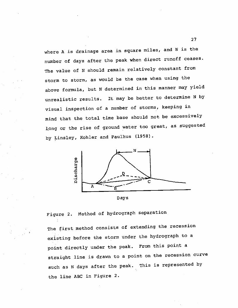
where A is drainage area in square miles, and N is the

number of days after the peak when direct runoff ceases.

The value of N should remain relatively constant from

storm to storm, as would be the case when using the

above formula, but N determined in this manner may yield

unrealistic results. It may be better to determine N by

visual inspection of a number of storms, keeping in

mind that the total time base should not be excessively

l.ong or the rise of ground water too great, as suggested

by Linsley, Kohler and Paulhus (1958).

B

Days

Figure 2. Method of hydrograPh separation

The first method consists of extending the recession

exIsting before the storm under the hydrograPh to a

point directly under the peak. From this point a

straight line is drawn to a point on the recession curve

such as N days after the peak. This is represented by

the line ABC in Figure 2.

28

Support is given this method by considering that

flow should be into the bank as long as the stream is

rising and base flow should therefore decrease until the

peak passes. There is no real reason, however, that

the decrease in base flow should conform to the

original recession (Linsley et al, 1958).

A second method uses a straight line from the point

of initial rise to a point N days after the peak. This

is illustrated by the line AC in Figure 2.

The above methods do not differ appreciably in

volume of direct runoff. The difference is probably

unimportant as long as one method is used consistently.

The third method involves projection of the ground

water recession back under the hydrograPh to a point

below the "point of inflection" of the recession. The

"point of inflection't is defined as that point on the

recession where the change in slope is zero, i.e. where

dt2

An arbitrary curve is then drawn to the point of rise.

This method, as illustrated by line ADC in Figure 2, would

probably be used in an area where ground water reached

the stream rather quickly.

Another method has been proposed by Hewlett and

29

Hibbert (1967) and by Hibbert and cunningham (1967).

This method is an application of the straight line

method given earlier, but has some distinct advantages.

HydrograPh separation as described above has been

developed with the idea that direct flow exists for a

period of time during the storm event, and that this

flow can be separated on the hydrograPh.

In reality it is almost impossible to separate

direct flow from base flow on a physical basis. It is

necessary, however, for purposes of hydrOgraPh analysis

to separate flow that runs quickly from a watershed

from that which is delayed, or is well controlled. As

pointed out by Hewlett and Hibbert (1967), the problem

with elaborate separation methods is that an arbitrary

classification for rate of flow is added to an arbitrary

classification for source of flow. A decision is made

as to what rates are considered storm flows and these

rates are arbitrarily divided into direct runoff and

base -flow. Because the decision is arbitrary in any

case, it wduld seem làgical to base the separation on

one arbitrary decision rather than two and base the

classification on a fixed, universal method applicable

to all hydrOgraPhs on small watersheds.

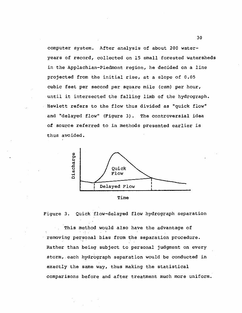
Based on the above ideas, Hewlett suggests a line

of constant slope that could be readily adapted to a

30

computer system. After analysis of about 200 water

years of record, collected on 15 small forested watersheds

in the ApplaChian_ edmont region, he decided on a line

projected from the initial rise, at a slope of 0.05

cubic feet per second per square mile (csm) per hour,

until it intersected the falling limb of the hydrOgraPI

Hewlett refers to the flow thus divided as "quick flow"

and "delayed flow" (Figure 3). The controversial idea

of source referred to in methods presented earlier i5

thus avoided.

Quick Flow

Delayed Flow

Tune

Figure 3. Quick f0w_delayed flow hydrOgraPh separation

This method would also have the advantage of

removing personal bias front the separation procedure.

Rather than being subject to personal judgitient on every

storm, each hydrOgraPh separation would be conducted in

exactly the same way, thus making the statistical

comparisons before and after treatment much more uniform.

Methods to Detect Change

A common denominator running through past studies

is the use of average annual flow for comparisons to

detect change (Kovner, 1956; Hoover, 1944; Reinhart, et

al, 1963). A coniparison utilizing regression analysis

for annual flow does not give the actual flow to be

expected at some point in time but rather an expected

yearly total as related to the control watershed.

- Comparisons using individual storm events could be

used instead, producing several distinct advantages.

By study of individual hydrograPh parameters it is

possible to gain insight as to actual change of the

streamf low hydrology, and it is possible to hypothesize

where and why this change occurred. Important para-

meters such as time-to-peak, peak discharge, and storm

volume cannot be determined in an annual yield study.

However these are major parameters which show actual

change in the flow regime.

A further. advantage. is a decrease in the time

required for detection of a change. Instatistics, the

greater the number of points, the greater the re-

liability of the relation5hiP.e5tabli5hL With this

in mind, it is readily apparent that if a comparison of

individual storm events, rather than annual values is

31

32

used, enough points may be obtained in only a few years

to make statistically significant comparisons between

two watersheds. Wilm (1949) developed a method for

determining the length of watershed calibration. Kovner

and Evans (1954) developed a relation for determining

duration for watershed experiments using this method.

These methods indicate that a sufficient nuniber of

observations can be obtained in one or two years by

utilizing individual storm events.

BethlahlrLy (1963) developed a method of rapid

calibration of watersheds utilizing this idea. An

important advantage to the shorter time interval is the

increased probability that an experiment will proceed to

completion without disruption from unforseen catas

trophies. Bethlahmy compared the change in stage in

the rising linib and the elapsed time for the period of

rise. An important reason for using the rising limb is

because discrete values are involved. This eliminates

the need for additional computations that might:lead to

additional error. The, method consists of four steps:

TabulatiOn the jse_in-5tage and time-t0

peak of both control and treated watersheds.

Computation of a regression line for the pre-

treatment years.

Computation of a regression line for the post-

33

treatment years.

4. Comparison of the two regression lines in

magnitude and slope.

Gilleran (1968) applied this method to determine

the effects of road building on small coastal streams.

He was able to show statistically significant change

with only 2.5 years of calibration and only one year of

data following treatment.

Low Flow Analysis

Three methods of recession analysis are presented

by Linsley et al (1958). The first method uses a semi-

logarithmic plot of the recession or depletion curve to

determine values of Kr where Kr i-s a characteristic

slope constant. Using graphical methods, the ground

water recession is projected back under the hydrograph.

Again using graphical techniques the interf low and surface

runoff recessions are determined, and from these the

values of Kr are determined. This method represents a

degree of refinement rarely necessay for engineering

problems but which may be needed to detect the effect of

minor treatments.

Two other methods given by Linsley et al involve

the development of base-flow recession curves. One

method pieces together sections of recession from various

34

storms until a composite curve is obtained. The second

method for developing the curve is to plot values of

q0 against some fixed time t later. The plotted data

should form a straight line on logarithmic paper if the

relation = q0Krt is strictly correct, but generally a

gradual change in Kr results. Lines could be developed in

this manner for both the pre- and post_treatment periods

and comparisons made tO determine effect of treatment. The

technique does not compare treated and control watersheds

but rather the pre_treatment and post_treatment periods

are compared on the same watershed.

A method valuable in demonstrating the change in

peak discharge and recession flow is the use of flow

duration curves. Again a comparison is established

between the treated watershed and the control. These

curves could produce a meaningful estimate of the amount

of flow that could be expected a given percentage of

time. If extended to a long term flow duration curve a

good estimate of yearly mean, both before and after

treatment could be obtained. Also use of double.maS5

analysis has been found useful in escribing percentage

change in flow (Chow, 1964). A prerequisite to these two

methods is a continuous record over all ranges of flow.

A method showing change in individual hydrOgraPh

parameters would be of as much value as a comparison of

35

yearly flows in showing effects of watershed treatments.

Regression analysis of yearly flows indicate relative

change of average flows, but analysis of individual

storm events has the added advantage of demonstrating

actual changes in hydrograph shape. Either method will

give the same trends but study of individual parameters

yields the added advantage of producing insight to

causes by defining changes in hydrograph shape.

DESIGN OF EXPERIMENT

Treatments

36

Following a calibration period of approXimatelY

two years (January 1964 through March 1966) on Deer

Creek IV and a calibration period of eight years

(October 1958 through March 1966) on Needle Branch,

both watersheds were subjected to a clearcut logging

operation. Needle Branch,but not Deer Creek IV, was

burned following timber removal in 1966. The calibration

period provided a period of time when both watersheds

to be treated were compared to Flynn Creek, the control

watershed. This provided the pre-logging relation

necessary in a paired watershed analysis to determine

effect of treatment. During the spring of 1965, one

year prior to logging, roads were constructed along

watershed boundaries on both Needle Branch and Deer

Creek IV.

Needle Branch, with a longer period of record and

a watershed area more nearly equal in size to the control.

was selected as the principal study watershed. The

effects of clearcutting the smaller Deer Creek IV

watershed were used for supplementing the results

obtained on Needle Branch.

Instrumentat ion

37

The gaging station on Deer Creek IV has a Belfort

FW-1 (Belfort Instrument Co., n.d.) water level re-

corder and an H-type flume (U. S. Dept. of Agriculture,

1962) is used for the control section. The 2.0 foot

deep H-type flume is designed to measure runoff from

small watersheds where flow does not exceed 11 cubic

feet per second. This is equivalent on this watershed

to 180 csm. Measured values of discharge through the

flume were found to differ slightly from theoretical

values given by the U. S. Dept. of Agriculture (1962).

Therefore a rating curve based on these measured

values was constructed.

Instrumentation on Needle Branch includes both a

Leupold and Stevens A-35 (Leupold and Stevens Instrument

Company, n.d.) and a series 1540 Fisher and Porter (Fisher

and Porter Company, n.d.) water level recorder. The

control section consists of a v-notch weir with a

rounded concrete surface and a stilling pond upstream

of the weir. The control section was not constructed

to any theoretical model and it was therefore necessary

to develop the rating curve by measurement over the

full range of stage. In order to adequately define the

rating, measurements have been obtained monthly and during

38

storm periods through the period of record by the U. S.

Geological Survey. The rating has been adjusted when

needed.

The gaging station on Flynn Creek is very similar

to that given above for Needle Branch. The primary

difference lies in the size and shape of the control

section weir. The weir for Flynn Creek is larger and

continues in a v-shape for the entire range in stage,

while the higher stages on Needle Branch are controlled

by a rectangular-shaped section.

DATA ANALY

Definition of Parameters

In this study, each streamf low rise was considered

an independent event. In order to determine hydrologic

changes it was necessary to select parameters that would

define the hydrOgraPh shape as completely as possible.

Recession, time-to-peak and height_of-rise were selected

for this purpose. These three parameters were discrete

values easily obtained directly from the jme-5tage

record. Voluirte and peak discharge were two additional

parameters selected to define shape. These parameters

were not obtained directly but were computed using time-

stage records and rating curves.

Peak Discharg

Peak jscharge defines the maximum flow attained

during a given storm event. It may be converted from the

time-stage trace using the appropriate rating curve.

discharge was selected both to help define hydrOgraPh

shape and because it has practical significance..

Significance is related to its importance in design

considerations for structures influenced by flood events.

39

Height-Of-Rise

Height-of-rise indicates the fluctuation in

elevation of the water surface from the beginning of

the storm event until it reaches a peak. It does not

include stage of base flow at initiation of the event

nor is it dependent upon rating curves. Therefore this

parameter eliminates antecedent flow conditions from

the analysis of stream response to a particular storm

event. In addition, it does not contain errors due to

incorrect construction of the rating curve.

Volume

Volume was selected to help define hydrograph

shape and also to quantitatively define the effect of

logging. For instance, an increase in peak discharge

does not necessarily indicate an increase in quantity

of flow for a given storm event. An increase in peak

discharge could reflect faster runoff of the same

quantity. By utilizing the volume parameter it is possible

to quantify changes in watershed yield for a particular

storm event, by comparison to a control watershed for a

particular treatment.

40

Time-To-Peak

41

The time-to-peak parameter is defined as the time

required to reach a peak, starting with an initial time

when the stream first responds to a storm event. This

parameter gives an indication of possible changes in

travel time due to watershed treatment. A shorter time

interval from initial rise to the peak would indicate a

reduction in detention storage and less resistance to

flow. The increase in velocities that may result

could produce channel changes by increased scour and

filling.

Recession

Three points were selected on the recession to

define changes in storage flow following removal of

vegetation. These points were located on the hydrograph

24, 48 and 72 hours after occurrance of the peak. This

parameter gives an indication of change in the storage

relation on the watershed and also helps define

hydrograph shape.

Selection of Events

The primary consideration for including the peak

discharge of a particular storm event in the sample, was

42

that the same streainf low rise could be detected on both

control and treated watersheds. Hydrographs did not have

to possess a sharp initial rise or peak to be considered

for the peak discharge parameter.

These same considerations were used in selecting

samples for the height-of-rise parameter. An additional

requirement for the latter, however, was that the

initial rise had to be distinct on the streamf low trace.

Any well-defined hydrograph that could be detected

on both watersheds could be considered for the volume

parameter. Due to the labor and time involved it was

not possible to analyze all storms. Instead storms were

selected which would cover the full range in storm flows.

Multiple peaks were not considered a problem since storm

flow ceased when the delayed flow line intersected the

recession of the hydrograph. It was assumed (and

justified by experimental data) that what happened in

terms of number of peaks on one watershed was repeated

on the other. When two peaks occurred on the treated

watershed before the base flow line intersected the

recession, two peaks also occurred on the control. This

would be expected if the control and treated watersheds

were in fact correlated.

Before a storm was considered for the time-to-

peak parameter, it had to have both a well-defined

43

initial rise and a well_defined peak. This precluded

use of any storm flow which did not possess a sharp

peak. Therefore, many of the storm flows with broad

peaks used for peak jscharge, height_of_rise and volume

parameters could not be used for time_to-peak con-

siderations.

W1-ien selecting storms for recession considerations

it was necessary that the hydrograPh possess a definite

peak and well_defined recession, a recession that

continued to base flow uninterrupted (for at least 72

hours) by any succeeding storm flows. In practices

storms already selected for the other parameters

were utilized for this parameters provided they fit the

selection criteria given above.

In preliminary data analysis, a problem was

detected with regard to multiple peaks. As noted above,

multiple peaks were not a problem with regard to the

volume parameter. However, they were an important con-

sideration for all other paralTteters. When several

peaks were encountered atiflie interval of two or

three dáys, and when each was treated as an independent

event, very poor correlations were obtained between

treated and control watersheds. This correlation was

improved considerably by treating each multiple_peaked

storm as one complex hydrograPh. it was therefore

44

necessary to develop criteria to determine when a peak

was an independent event and when it could be considered

a part of a complex storm hydrograph. When multiple

peaks were encountered, criteria developed by the U. S.

Geological Survey were used to determine whether these

peaks were independent (U. S. Geological Survey, 1951).

Only the highest peak was used when two or more occurred

within 48 hours, unless it was probable that the peaks

were independent. It was considered probable for

these peaks to be independent if the hydrograPh receded

to base flow during the tune interval between peaks.

An additional problem was encountered with data

from Deer Creek IV. Leakage flow occurs through the

very deep alluvial -deposits under the flume. When flow

did not exist prior to initial rise it was impossible to

determine the time or volume of runoff necessary to

produce surface flow in the channel. Therefore,

events were not considered unless flow existed prior to

the initial streamf low rise, i.e., events starting at

zero flow were not considered.

A double-mass analysis was performed on the

precipitation data with the purpose of detecting any

change in precipitation pattern during the experimental

period. Monthly precipitation totals were accumulated

for the rain gage on Needle Branch and plotted against

45

values for the rain gage on Flynn Creek. PreciPitatio

data from Deer Creek was also plotted against Flynn

Creek. Any break in slope of these lines would indicate

a change in the precipitation pattern over the

watersheds. If such a change is indicated, this change

must be considered when analyzing results of the stream-

f low parameters.

Data Reducti

The height_ofse time_to-peak, and recession

parameters were obtained directly from the gage height

traces for the respective gaging station. For these

parameters height was recorded to the nearest o.Ol foot

and time in hours was recorded to the nearest 0.5 hour.

Peak discharge and volume were converted from a simple

time-stage function to discharge and volume in terms of

csm and csm-hOur respectively.

Gage height data on Deer Creek IV was reduced

using the rating formula developed by the Forest

Management Department. This formula was develOPed from

field measurements and 15 similar to the one provid by

the Agricultural Research service (U. s. Department of

Agriculture, 1962). The formula as developed is:

Q = 1.459112

+ O.854H3

46

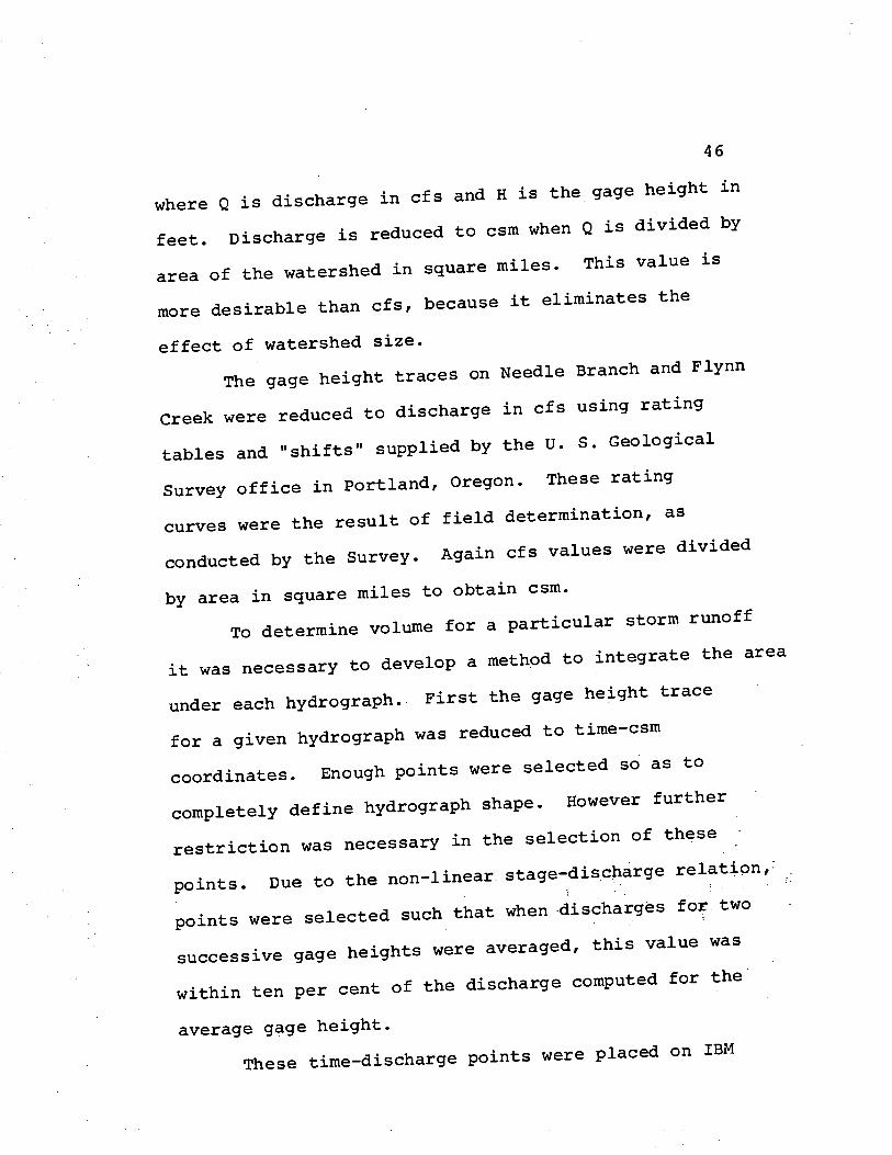
where Q is discharge in cfs and H is the gage height in

feet. Discharge is reduced to csm when Q is divided by

area of the watershed in square miles. This value is

more desirable than cfs, because it eliirLinates the

effect of watershed size.

The gage height traces on Needle Branch and Flynn

Creek were reduced to discharge in cfs using rating

tables and. "shifts" supplied by the u. s. Geological

Survey office in portland, Oregon. These rating

curves were the result of field determination, as

conducted by the Survey. Again cfs values were divided

by area in square miles to obtain csm.

To determine volume for a particular storm runoff

it was necessary to develop a method to integrate the area

under each hydrograph. First the gage height trace

for a given hydrograPh was reduced to time-csIfl

coordinates. Enough points were selected so as to

completely define hydrograPh shape. However further

restriction was necessary in the selection of these

points. Due to the non-linear stage_discharge relation,

points were selected such that when discharges for two

successive gage heights were averaged, this value was

within ten per cent of the discharge computed for the

average gage height.

These jme_discharge points were placed on IBM

47

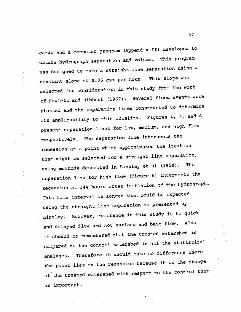
cards and a computer program (Appendix II) developed to

obtain hydrograph separation and volume. This program

was designed to make a straight line separation using a

constant slope of 0.05 csm per hour. This slope was

selected for consideration in this study from the work

of Hewlett and Hibbert (1967). Several flood events were

plotted and the separation lines constructed to determine

its applicability to this locality. Figures 4, 5, and 6

present separation lines for low, medium, and high flow

respectively. The separation line intersects the

recession at a point which approximates the location

that might be selected for a straight line separation,

using methods described in Linsley et al (1958). The

separation line for high flow (Figure 6) intersects the

recession at 144 hours after initiation of the hydrOgraPh.

This time interval is longer than would be expected

using the straight line separation as presented by

Linsley. However, reference in this study is to quick

and delayed flow and not surface and base flow. Also

it should be remeiribered that the treated watershed 15

compared to the control watershed in all the statistical

analyses. Therefore it should make no difference where

the point lies on the recession because it is the change

of the treated watershed with respect to the control that

is important.

10 5-

eparation Line

Time in Hours

48

72

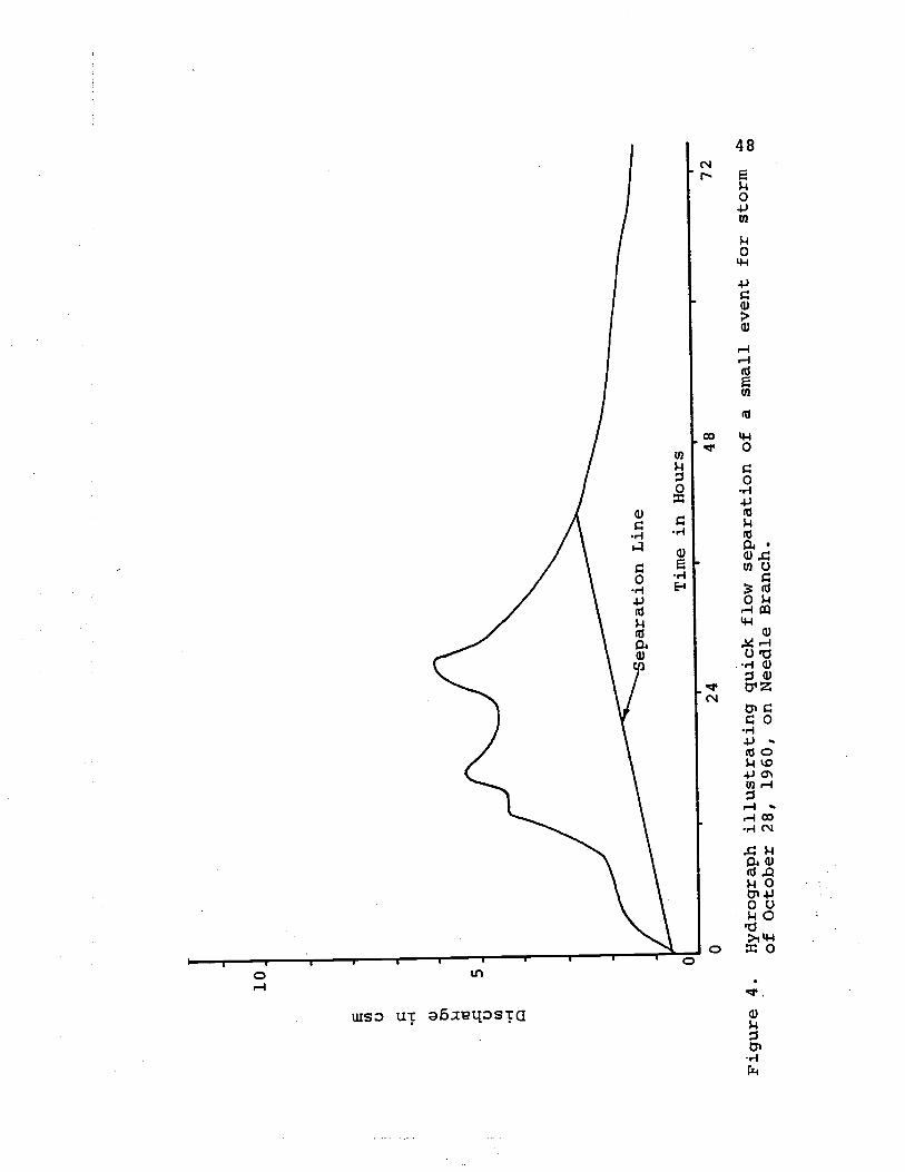
Figure 4.

Hydrograph illustrating quick flow separation of

a small event for storm

of October 28, 1960, on Needle Branch.

24

0

20

10 0

0

'-SeparatiOfl Line

2'4

418

Time in hours

/2

10

144

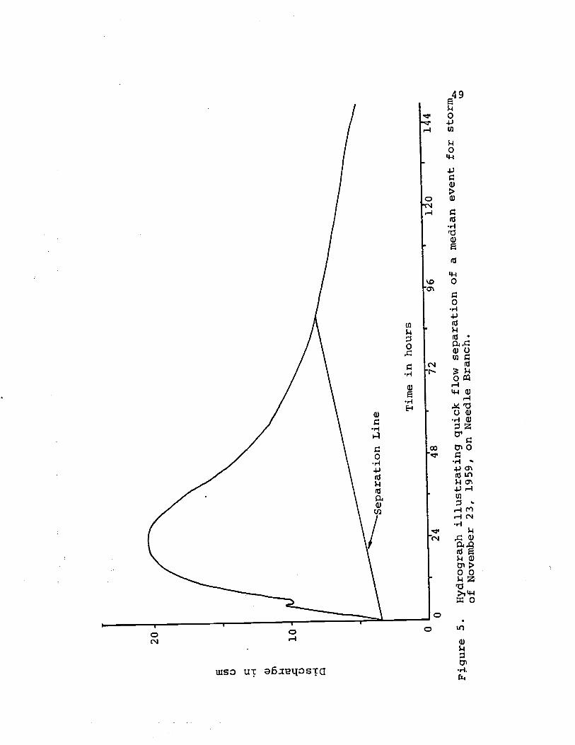
Figure 5.

HydrograPh illustrating quick flow separation of a median event for storm

of November 23, 1959, on Needle Branch.

80 -

60

40 20

-

eversal peak = 112.29

Separation Line

2'4

4'8

12

96

120

144

Time in hours

Figure 6.

Hydrograph illustrating quick flow separation of a large event for storm

of November 22, 1961, on Needle Branch.

51

Following separation, three values were computed --

quick flow, delayed flow, and total flow. All three

values included a time base equal to the interval

between initial stream rise and the time at which the

separation line intersected the recession. Quick flow

consisted of that area above the line and enclosed by the

hydrograph, while delayed flow consisted of that area

below the separation line. Total flow is the sum of

these two. No attempt was made to distinguish origin

of the water with regard to direct flow or base flow.

A change in any one of these values would yield

information regarding change in stream hydrology, both

as to timing and quantity of flow. An increase in

quick flow and a decrease in delayed flow would indicate

less water held in storage while an increase in total

flow would indicate less consumptive use of water on the

watershed.

Statistical Techniques

Determination of Regression Relations

All the parameters values for peak discharge, height-

of-rise, volume, time-to-peak, and the three points on

the recession were placed on IBM cards so statistical

analysis could be accomplished with the aid of a CDC 3300

52

computer.

A computer program was developed to make the

necessary computations for a linear regression analysis.

This program was designed to give a prediction equation

for each parameter on the treated watersheds, as compared

to the control watershed. A line of prediction was

computed for both the pre- and post-logging periods.

Values of the coefficient of determination, r2,

defined as:

r2 = (Sum of Squares due to Regression) (Total Sum of Squares, corrected for the mean)

after Draper and Smith (1968), were then examined to

determine the value of the regression lines as predictor5

It was necessary to examine r2 because a paired water-

shed study requires a high degree of correlation between

the test watershed and the control during the calibration

period. The value of a regression equation as a

predictor increases as r2 approaches unity or 100 per cent.

An r2 value of 100 per cent indicates that all points

lje on the regression line and the line is a perfect

predictor. The basic assumption in the use of r2 is

that two variables are related, with one variable

independent and one dependent. This assumption makes

it possible to use the line of regression as a predictor,

using the independent variable X to determine the depen-

53

dent variable Y. This is the essence of the data analysis

for this study. A prediction line is developed for the

pre-logging (calibration) period between the control

watershed and the treated watershed for each of the

parameters -- peak discharge, height-of-rise, volume,

time-to-peak, and recession. This is followed by

development of a prediction line between the same two

watersheds for the post-logging period. An analysis of

the difference between these two prediction lines gives

an indication of the change that has occurred and the

significance of that change.

Tests for Change

Further statistical tests were used to determine

the statistical equality of the pre- and post-logging

relationships, i.e., tests were used to determine whether

these two lines were actually different, or whether the

difference that occurred could have happened by chance.

In any statistical test of this type the level of

significance must be chosen. In this study two levels

were considered. The first was the 95 per cent level

and the second was the 99 per cent level. These two are.

designated as "significant" and "highly significant",

respectively. The level of significance gives the

54

probability of obtaining the same results in repeated

sampling. For example, the 99 per cent level indicates

a hypothesis of equality between two equal regression

parameters will be rejected only one per cent of the

time.

Any indicated change in the regression for a

particular parameter as a result of treatment was

subjected to two tests; a test for change in slope and

a test for change in vertical position. A distinction

should be made between change in slope and change in

vertical position of the prediction lines. Both

indicate a change as a result of the treatment, but

each has a different physical meaning. A change in slope

would imply that the effect of the treatment varied

with increasing values, of the parameter while a change

in vertical position implies that the effect is the same

over the full range of values.

Change in Slope

This test compared differences in slope between

pre- and'post-logging regressibn5 for each parameter.

The coefficient under consideration is b1 as in the

expression:

y = b0 + b1x.

55

This test, as given by Lee (1957), may be noted by

reference to Appendix iii. The hypothesis tested is

that b11 = l2' i.e., the slope prior to logging is

equal to the slope following logging. The second

subscript (1 or 2) designates pre-logging (1) or post-

logging (2) period.

The test for change in slope yields a computed

value of "t" which must be compared with the critical

value of t. The critical value of t is dependent on the

level of significance selected and the degrees of freedom

involved. If the computed value of t is greater than

the critical value of t, the hypothesis is rejected in

favor of the alternate hypothesis that the slopes are

in fact different. If the slopes were found to be

different, no further testing was required.

Change in vertical Position

If slopes were not found to be atjstically

different, a test for change in vertical position was

required. For is analysis. it was: necessary to make

the assumption that slopes not statistically different

are equal.

The test for change in vertical position, which is

given the name "mean of means", is a modification of the

test for change in intercept given by Draper and Smith

56

(1968), i.e., the change in b, as in the expression:

y = b0 + b1x.

The development of this test and its final form may be

found by reference to Appendix III.

In many studies, covariance techniques have been

used to test for change in vertical position. In the

test of homogenity of adjusted means, as well as other

covariance tests, an assumption that variances before and

after treatment are equal must be accepted. This does

not seem probable for this study. The whole regime

of water production has been changed as a result of

the drastic treatment applied. It seems unlikely that

variance has remained unchanged following clearcut

logging.

If a change was indicated using the statistical

techniques, this change was further defined in terms of

percentage in order to define the change in quantitative

terms. Such information is valuable for comparative

purposes.

Seasonal Variation

Following analysis using all available data, the

data were then divided to determine change as related

to a particular season. A seasonal segregation of the

57

data was made because it has been indicated that the

largest effect of vegetation removal on streainf low often

occurs during the fall recharge period (Reinhart, 1963).

The fall months of September, October and November were

analyzed using the same analytical techniques described

above. December, January, February and March were

analyzed separately as the winter period. Thus, the pre- logging regression of a given parameter for a given

season was compared with the post-logging regression

of the same parameter for the same season. Statistical justification for this separation

based on physical theory was obtained by comparing fall and winter regressions in the pre-logging period. A

regression was developed between the fall period of

record on each treated watershed and the fall period

of record on the control for the pre-logging period.

A second series of regressions was developed using only

the winter pre-logging period of record. These two

regressions were then contpared statistically to determine

whether a seasonal difference actually existed. The

same technique was applied to the post-logging data to

test for seasonal variations in the data. This analysis

was used for statistical justification of the seasonal

separation already assumed, using previous studies for justification. It was applied to all paranteters which

58

indicated a statistically significant change as a result

of treatment when analyzed on a seasonal basis, both on

Deer Creek IV and Needle Branch.

RESULTS

59

Roads were constructed along the ridges on both

Deer Creek IV and Needle Branch watersheds in 1965. A

statistical comparison of the data for this year with

the previous non-treatment years indicated road building

had no effect on streamf low. These data were then

included in the pre-logging period in all subsequent

tests to detect change in peak discharge, height-of

rise, volume, and time-to-peak.

Comparative watershed studies have an underlying

assumption of homogeneous precipitation patterns over both

watersheds. For this reason a double-mass analysis of

precipitation data for years 1960 to 1967 was conducted

(Appendix I, Figures I and II). The cumulative relation

was established between rain gages at Deer Creek and

Flynn Creek and between Needle Branch and Flynn Creek.

A change in slope occurred during 1965 and 1966 for

Needle Branch but the relation came back to the original

slope by 1967. A check of the records indicated the

data were of good quality through this period. The change

resulted in less precipitation over the Needle Branch

watershed and hence will qualify conclusions. An in-

crease in any given parameter may be conservative, while

a change found non-significant might be significant if

60

the precipitation change was included as a parameter in

the prediction equation.

The variables are presented in sequence of peak

discharge, height-of-rise, quick flow, delayed flow, total

flow, and time-to-peak. A summary of the statistical

analysis for each parameter is given in Appendix I,

Table I, II, and III.

In order to assess the practical significance of

changes shown statistically, percentage differences

between regression lines at the pre-logging mean,

maximum and minimum levels of the control are presented

in Table 1 for each parameter changed by clearcut logging.

Peak Discharge

Needle Branch

Variation between fall and winter peak discharge

data occurred following logging. This was reflected in

a statistical difference between the two periods

significant at the 95 per cent level (Appendix I, Table

III) Seasonal difference was also indicated by the

increase in r2 from 0.80 for the full year data to 0.98

for the fall period and 0.83 for the winter (Appendix I,

Table I). Flows during the fall period were consistently

greater than during the winter period.

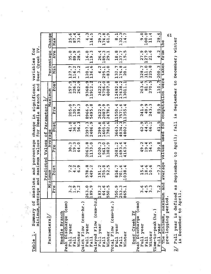
Table 1.

Summary of absolute and percentage change in significant

variables for

miniinuxn,average and maximum values for Needle

Branch and Deer Creek IV.

1/ The minimum, maximum and average values used for computation

were taken from the

pre-logging period.

2/ Full year is defined as September to April; fall is Septentherto December; winter

is December to April.

parametersa/

Predicted Values of Parameters

1/Percentage Change

Minimum

Average

Maximum

Pre

Post

Pre

Post

Pre

Post

Mm

Ave

Max

Needle Branch

Peak Discharge (csm)

Full year

3.2

7.2

30.3

41.0

205.0

257.9 127.7

35.0

25.6

Fall

1.9

4.2

19.3

36.6

120.7

226.2 116.2

89.9

87.4

Winter

7.2

6.9

44.0

56.3

198.3

262.9 - 3.2

28.5

33.4

Quick Flow (csm-hr.)

Full year

263.0

578.8

2063.8

2397.3 8966.9

9368.9 120.1

16.0

4.3

Fall

189.9

449.2

1133.0

2486.9 5495.8

11912.2 136.6 119.3

116.5

Delayed Flow (csm-hr.)

Full year

183.2

191.2

1020.3

1299.8 2622.9

3422.2

4.2

26.4

29.3

Fall

64.6

255.8

561.0

1605.0 2087.9

5756.0 295.1 185.3

174.8

Winter

550.5

92.5

1382.9

1782.6 2478.9

4007.8 -83.0

29.1

61.9

Total Flow (csm-hr.)

Full year

350.9

816.7

3081.2

3663.111550.4

12492.8 132.7

18.8

8.1

Fall

253.3

701.6

1693.4

4034.3 7571.6

17638.2 176.8 137.7

132.3

Winter

865.1

1038.4

4163.4

4802.711355.4

13011.1

20.1

15.5

14.7

Deer Creek IV

Peak Discharge (csn)

Full year

3.6

15.4

49.2

62.9

241.9

263.6 328.7

27.9

9.0

Fall

4.5

18.6

19.4

44.5

40.9

81.7 311.0 127.9

100.0

Winter

3.3

10.6

54.5

66.1

243.3

270.5 225.8

21.6

11.4

Time-to-peak (hr.)

Full year

7.2

-7.3

39.8

41.5

85.9

110.7-200.3

4.2

28.6

62

Since a seasonal analysis was indicated, fall and

winter peaks were compared separately before and after

logging. The effect of logging using the full year

(September to March) is given for comparative purposes

(Figure 7). Fall peak discharges were found significantly

greater at the 95 per cent level following treatment.

Scatter diagrams and regressions before and after

clearcutting for the fall period are presented in

Figure 8.

Increases in winter peak discharge was also found

significant at the 95 per cent level (Figure 9).

However, the percentage increase was not as great as

for the fall period (Table 1).

Deer Creek IV

Seasonal variation was found in the peak discharge

data on Deer Creek IV following logging. Difference

between fall and winter data for the post_logging period

was found statistically significant at the 95 per cent

level (Appendix I, Table III). Seasonal differences in

the data were also suggested by the change in r2 values

following seasonal separation. The r2 value was increased

from 0.80 for the full year data to 0.97 for the fall

data (Appendix I, Table I). As was found on Needle Branch,

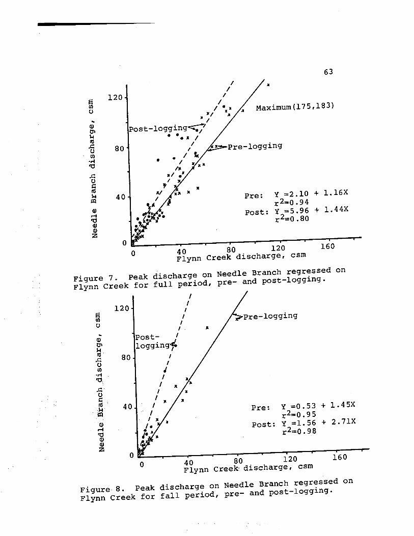
1) r1

ci)

1) z

E

0

post-loggingz7

/ / 80

r4

o

40 /

z

120

0

120

*

, I

/ 0

- Post- /

ioggingi.

80 /

o /

I

/

/

0

/ "I

$1

0 40 80 120 160 Flynn Creek discharge, csm

Figure 7. peak discharge on Needle Branch regressed on Flynn Creek for full period, pre- and post_logging.

/

/

/

/

Pre- logging

Pre: Y =2.10 + l.16X r20.94

Post: Y =5.96 + l.44X r20.80

63

Maxilflum(175483)

Pre- logging

Pre: Y =0.53 + l.45X r20.95

Post: Y =1.56 + 2.71X r20.98

40 80 120 160 Flynn Creek discharge, csjn

Figure 8. Peak discharge on Needle Branch regressed on Flynn Creek for fall period, pre- and post_logging.

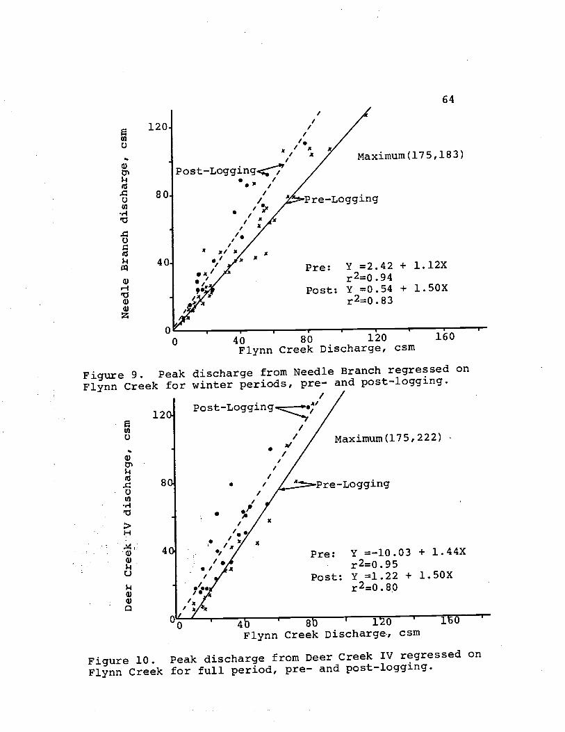
In C.)

a)

80-

.1-f TO

.c: C.)

40-

a) r1 V a) a) z

In C.)

a)

.c: C.)

In

V

H

a) a)

U

a) a)

120.

12

Post-Logging<' I /

/

.

/ I /.

/

x

N

I

/ /.

Pre-Logging

Pre: Y =2.42 + 1.12X r20.94

Post: Y =0.54 + l.50X r2=0.83

64

Maximum(175,l83)

V 0 40 80 120 160

Flynn Creek Discharge, csm

Figure 9. Peak discharge from Needle Branch regressed on Flynn Creek for winter periods, pre- and post-logging.

/ Post-Logging.-,.7

Maximum(175,222)

p re-Logging

Pre: Y =-l0.03 + l.44X r2=0.95

Post: Y =1.22 + l.50X r2=O.80

4' 8' 1 0 1.0 Flynn Creek Discharge-, csm

Figure 10. Peak discharge from Deer Creek IV regressed on Flynn Creek for full period, pre- and post-logging.

65

the r2 value was not increased as much for the winter

period. The r2 value for the winter data was 0.90

as compared to the full year value of 0.80. The

scatter diagrams for the full year data may be noted

by reference to Figure 10.

Fall period analysis indicated a significant

increase after clearcutting at the 99 per cent level

(Appendix I, Table II). Scatter diagrams and regression

before and after are presented in Figure 11.

Winter period analysis indicated a statistically

significant increase at the 99 per cent level (Figure

12). The percentage increases for the winter period

were not as great as for the fall period (Table 1).

Height-of-Rise

Needle Branch

Analysis of the height-of-rise parameter on

Needle Branch did not indicate a change as a result of

the treatment. A change was not found when the data was

analyzed using the fill year (Figure 13) nor was a

change indicated when analyzed by season, i.e., fall

(Figure 14) and winter (Figure 15).

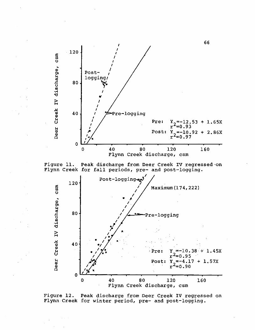
40

C)

w w Q

/

I - Pre-logging

I',

t . / $x / 'S.

I.

I / 120

U) o I

/ a) Post-

logging,' 80 k

U)

'a

H

/ / .7 I.

66

logging

Pre: Y -lO.38-i- i.45X r

2=0 .

95 Post: Y -4.17 + l.57X

r2=0.90

Pre: Y -12.53 + l.65x r20.93 Post: Y =-l0.92 + 2..86X

r2=0.97

0 40 80 120 160 Flynn Creek discharge, csm

Figure 11. Peak discharge from Deer Creek IV regressed on Flynn Creek for fall periods, pre- and post-logging.

Post-logging.e'

120 / / Maximum(l74,222)

40 80 120 160 Flynn Creek discharge, csm

Figure 12. Peak discharge from Deer Creek IV regressed on Flynn. Creek for winter period, pre- and post-logging.

/

Sf

/

U) 0

w bs

80 0 U)

'a

H

w 40 w

C)

a)

w Q

0

.1-) a) a) 4-I

.1-)

a)

0 (U '-I

a) '-I a) a) z

.1-)

a) a) 4-I

.1-)

a)

0 (U

co. a) '-I a) a) z

1.2

Maximum(1.78,1.65)

0.4 0.8 1.2 1.6 Flynn Creek height, feet

Figure 13. Height-of-rise for Needle Branch regressed on Flynn Creek for full period, pre- and post-logaing.

Post-logging!,,

Post-logging.

"jx

x ,

N

'S.

Pre-logging

Pre-logging

67

Pre: Y =0.08 + 0.79X * r2=O.93

Post: Y =0.05 + 0.88X r2=O.88


Figure 14. Height-of-rise for Needle Branch regressed on Flynn Creek for fall period, pre- and post-logging.

Pre: Y =0.08 + 0.78X r20.93

Post: Y =0.04 + 0.86X r2=0.85

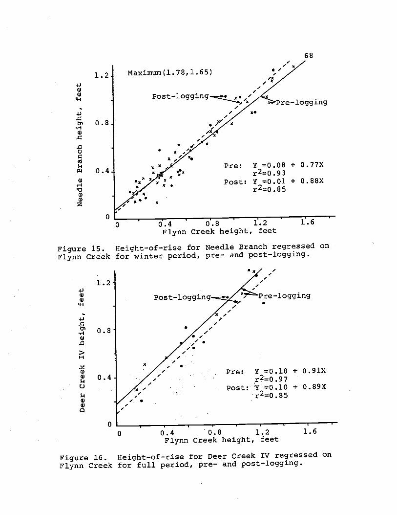
4.) U) U) 4-I

4.)

..-4 U)

H

U) U)

C-)

U) U)

1.2

4.) U) U) 4-I

4.)

0.8 .1-I U)

U

0.4

U) I-s

U) U) z

0.8

Maximum(1.78,l.6S)

Post-1ogging-.z,'

Post-logging

68

Pre -10 gging

x.

Pre: Y =0.08 + 0.77X r2=O .93

Post: Y =0.01 + O.88X r2=0 .85


Figure 15. Height-of-rise for Needle Branch regressed on Flynn Creek for winter period, pre- and post-logging.

1.2

Pre-logging

/

S

, ._.

x

0.4 Pre: Y =0.18 + 0.91X r2=0.97

I

Post: Y =0.10 + O.89X r20.85

1.6 0 0.4 0.8 1.2 Flynn Creek height, feet

Figure 16. Height-of-rise for Deer Creek IV regressed on Flynn Creek for full period, pre- and post-logging.

Deer Creek IV

Analysis of data for Deer Creek IV failed to

indicate any effect of learcUttjng on height_of-rise.

The small change in regression lines between pre_lOggi

and post_logging periods was not found to be significant

for the full year analysis (Figure 16). There was not

sufficient data for this parameter to permit seasonal

separation.

Quick Flow

Needle Branch

Quick flow analysis for Needle Branch did not

indicate a 5atjstically significant difference between

fall and winterperi0d5 (Appendix I, Table III). How

ever, the scatter of data at the low end of the regression

indicated the 055ibility of some difference in seasonal

response. The data were therefore divided and analyzed

by season. The full year analysis 5:

presented in

Figure 17. increases:for the full- year were found

significant at the 95 per cent level.

Seasonal variation in the data was also suggested

by the increase in r2 from 0.87 to 0.91 following data

separation for the fall period as compared to the full

69

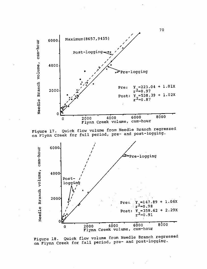
6000 0

U) C.)

4000

200:

6000

4000

200

Maxiinuln(86S7 19455)

/ /

/ / / / Post- /

lo gg in4 a, /

post-logging- /

I

*

,

/ / / / / /

/ /

>Pre-l0gging

70

Pre: Y =223.04 + l.O1X r20.97 Post: Y =538.39 + l.02X

r2=0 .87

0 2000 4000 6000 8000 Flynn Creek volume, csm-hour

Figure 17. Quick flow volume from Needle Branch regressed on Flynn Creek for full period, pre- and post-logging.

Pre-logging

Pre:. Y .147.89 + l.06X r2=O.98

Post: Y =358.62 + 2.29X r20 .91 0

2000 4000 6000 8000 Flynn Creek volume, csrn-hour

Figure 18. Quick flow voluirie from Needle Branch regressed on Flynn Creek for fall period, pre- and post-logging.

71

year (Appendix i, Table I).

Following separation of the data by season, an

increase in quick flow volume was indicated for the

fall period (Figure 18). This increase was found

significant at the 99 per cent level. No changes

were discernable for the winter period (Figure 19).

percentage increases were much larger for the fall

period than for the winter period (Table 1).

Deer Creek IV

A change in quick flow was not found for Deer

Creek IV when the full period of record was analyzed.

This relation is presented in Figure 20. Due to a lack

of usable storm events during the fall period, it was

not possible to consider the effect of seasonal

separation.

Delayed Flow

Needle Branch

A difference in delayed flow between the fall and

winter seasons was observed during the pre_logging

period. This was reflected in a statistical difference

between the two periods significant at the 95 per cent

level. Seasonal differences were also indicated by the

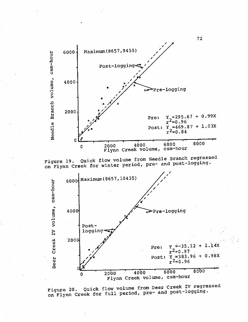
0

Post- logging

I. /

/

Figure 19. Quick flow volume from Needle Branch regressed

on Flynn Creek for winter period, pre- and post_logging.

'4 6000Maxjml(8657,1O435)

U) C)

/

Pre: Y -35.12 + l.14X // r20.97 ' Post: Y =383.96 + 0.98X

r20.96

2000 4000 6000 8000 Flynn Creek volume, csm-hOur

Figure 20. Quick flow volume from Deer Creek IV regressed on Flynn Creek for full period, pre- and post_logging.

, /

,

Pre-logging

72

0

C)

H 0

C)

U) H U) U) z

6000-

4000-

2000.

-

/ MaximUm(8657,9455) / / /

/ Post- logging,

/

x / Pre- logging /

Pre: Y =295.67 / r2=0.96

Post: Y =469.87 ,. r20.84

+ 0.99X

+ l.03X

I 0

I I I I I 2000 4000 6000 Flynn Creek volume, csm-hour

8000

A change in delayed flow was not indicated on Deer

Creek IV when the full year data were analyzed. Re-

gressions for these data are presented in Figure 24.

Due to a lack of usable storm events during the fall

period, it was not possible to consider the effect of

seasonal separation.

Total Flow

Needle Branch

73

increase in r2 from 0.85 for the full year to 0.90 for

the fall period. The winter period however remained at

0.85.

Effect of logging over the full year is given for

comparative purposes (Figure 21). The fall period

analysis indicated an increase significant at the

99 per cent level (Appendix I, Table I, Figure 22).

Increases in winter delayed flow volume was found

significant at the 95 per cent level (Figure 23)

Percentage increases were smaller during the winter period

than during the fall period (Table 1).

Deer Creek IV

A seasonal difference in the total flow data is

indicated by the increase in r2 from 0.87 for the

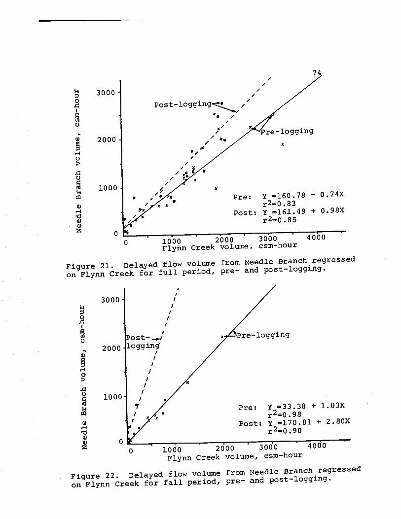
3000 0

0

a 2000

1000

G)

H '0 a) G)

14

a 0

G) I

3000

2000

1000

/

,

. ,_. x I / xx

/ / / / I Post- _.I logging /

/

I /

Post-1Ogging,,'

x

S

I I

x

'C, ,

x

,

Pre-logging

re-logging

74

Pre: Y =160.78 + 0.74X r2=0.83

Post: Y =161.49 + 0.98X r2=0 .85

1000 2000 3000 4000 Flynn Creek volume, csm-hour

Figure 21. Delayed flow volume from Needle Branch regressed

on Flynn Creek for full period, pre- and post_logging.

Pre: Y =33.38 + l.03X r20.98

Post: Y =170.81 + 2.80X r20.90

0 .1000 2000 3000 4000 Flynn Creek volume, csm-hOUr

Figure 22. Delayed flow volume from Needle Branch regressed on Flynn Creek for fall period, pre- and post_logging.

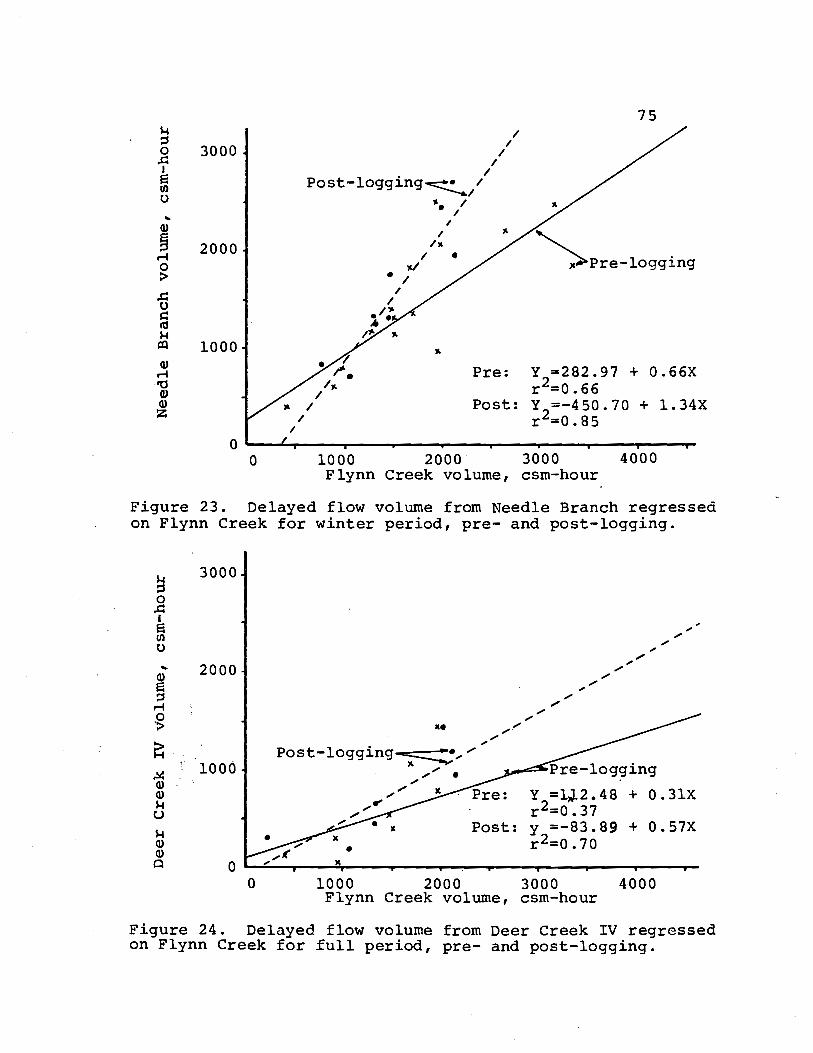
0

U) 0

a) E

H 0

3000

2000

0


Figure 23. Delayed flow volume from Needle Branch regressed on Flynn Creek for winter period, pre- and Post-logging.

Post-logging...---- 1000

a) a)

C-)

. a) Q

Pre-logging - I

Pre: y =l,2.48 0.31x r2=0.37

* Post: y =-83.89 0.57X r2=0.70


Figure 24. Delayed flow volume from Deer Creek IV regressed on Flynn Creek for full period, pre- and post-logging.

4000

75

a) H rc a,

a) z / / /

j3' . 1% Pre:

Post:

Y =282.97 r2=0.66

Y2=-450.70

0.66X

l.34X

/ r =0.85

/ 3000 / / /

U)

/ Post-logging..o, 0 %. / /

/ / 2000. Ix / ii .

Pre-logging / / / , . 4 ,' 1.

1000-

76

full year analysis to 0.90 for the fall period. The

r2 value dropped to 0.83 for the winter period (Figures

25, 26, and 27). The full year analysis (Figure 25)

is presented for comparative purposes.

When the data were separated and analyzed

according to fall and winter periods ,

a change in total

flow had occurred as a result of logging. The fall

period increase was signficant at the 99 per cent level

and the winter period at the 95 per cent level

(Appendix I, Table I). percentage increases however

were found greater for the fall period (Table 1).

Deer Creek IV

A change in total flow was not found for Deer

Creek IV when the full-year record was analyzed (Figure

28). Due to a lack of usable storm events during the fall

period, it was not possible to consider the effect of

seasonal separation.

Time-To - Peak

Needle Branch

result of There was no notable change as a

treatment in the time_to-Peak relation on Needle Branch.

A change was not found when the data was analyzed by

12000 0

Cl)

U

8000

4000 ./ 'z

a)

It, a)

z

Post- logginp

/

.1 /

I

/

/

, ,

/ ,

/

/

" -Pre-logging

77

Pre: Y2=284.96 + 0.94X r =0.98

Post: Y =747.94 + 0.98X r2=0

. 87


Figure 25. Total flow volume from Needle Branch regressed

on Flynn Creek for full period, pre- and post_logging.

12000

Post- //

logging"

8000 1

/ -s.-Pre-logging

0

0

4000 1

I .Pre: Y =179.64+ l.05X

r20.99 I' Post: Y =531.17 + 2.43X

r20.90

0 4000 8000 12000 16000 Flynn Creek volume, csm-hOur

Figure 26. Total flow volume from Needle Branch regressed

on Flynn Creek for fall period, pre- and post_logging.

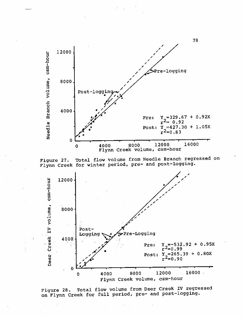
8000.

4000.

0

x

/ ,


Figure 27. Total flow volume from Needle Branch regressed on Flynn Creek for winter period, pre- and post-logging.

12000 0 f C')

U

8000

Post- Loggi,ng

400a

, ,

, , , , ,

0 4000 8000 12000 16000

Flynn Creek volume, csm-hour

Figure 28. Total flow volume from Deer Creek IV regressed on Flynn Creek for full period, pre- and post-logging.

Pre: y =329.67 + 0.92X r2= 0.92

Post: Y =427.30 + l.05X r2=0 .83

'Pre-Logging

Pre: Y =-532.92 + 0.95X r20.99 Post: Y =265.39 + 0.8OX r20 .90

Post-loggin',-. /

x

, . ,

78

, / / /

/ ,' Pre-logging

1-4

ci)

C)

ci)

ci)

79

season nor was a change indicated when analyzed for the

full year (Figures 29, 30, 31).

Deer Creek IV

A change in time-to-Peak was indicated on Deer

Creek IV when the data was analyzed for the full year

record (Figure 32). This change was found significant

at the 95 per cent level (Appendix i, Table II).

Average time-to-peak increased, minimum time-.toPeak

decreased, and maximum time-to-peak increased following

treatment (Table I).

Due to an insufficient number of storms during

the fall period, it was not possible to divide the data

into fall and winter periods.

Recess ion

Analysis of recession flow using 24, 48 and 72

hours following the peak of each event showed very low

correlations between the treated watersheds and the

control. The r2 values -ranged from 0.2 to 0.8. Be-

cause of this wide range in correlation coefficients, the

recession parameter has not been included in the graphical

or tabular presentations.

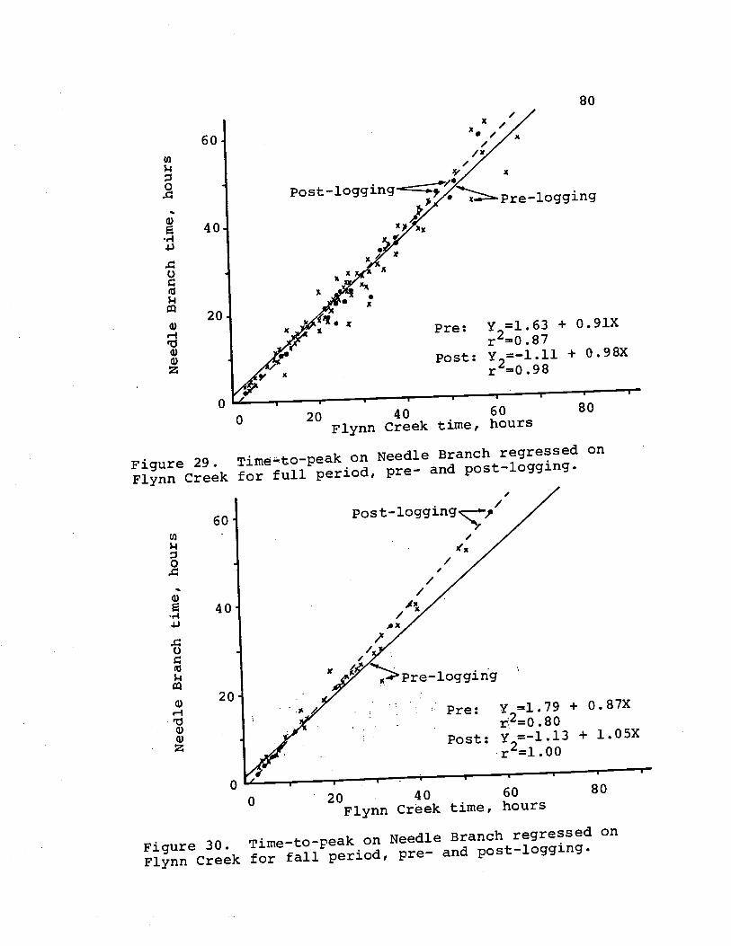
60

(a

0

a) 40

0 (j

20 a)

r4

a)

a)

z

0

a)

40

U

(j

20

60

a.

x

S x

A

/ / / /

80

post-logging 'pre-logging

Pre: Y =1.63 + 0.91X r2=O.87

Post: y2=-l.11 + O.98X r =0.98

20 40 60 Flynn Creek time, hours

80

Figure 29. Time-to-Peak on Needle Branch regressed on Flynn Creek for full periods pre- and post_logging.

/ / Post- loin.ç/

Pre-loggiflg

Pre: Y =1.79 + 0.87X r2=0 .80

Post: Y -l.13 + l.05X r2l.00

80 0 20 40 60 Flynn Creek time, hours

Figure 30. Time-tO-Peak on Needle Branch regressed on Flynn Creek for fall periods pre- and post_logging.

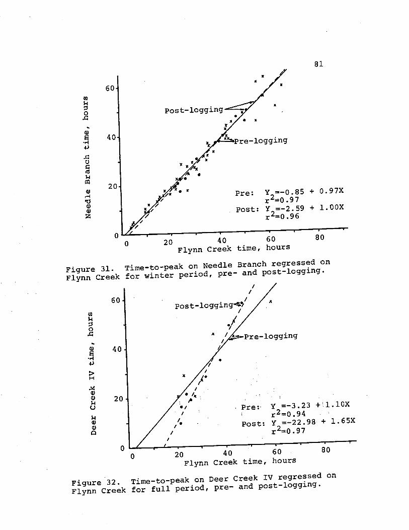
U) $4

0

U)

0

60

a)

E 40

4-)

U

('j $4

20 a)

r1

a)

a)

z

post-logging

40 /

/

60 . Post logging

/

/

g

x

Pre-logging

x

81

Pre: Y =-0.85 + O.97X r2=0 .97

Post: Y =-2.59 + l.00X r2=0.96

0 20 40 60 Flynn Creek time, hours

Figure 31. Time-to-peak on Needle Branch regressed on Flynn Creek for winter period, pre- and post_logging.

/ /

Pre- logging

80

a) /

0) 20 $4 ft 0

Pre: Y =:-3.23 +l.lOX // r2=0.94 I. Post: Y =-22.98 + l..65X

// r20.97

80 20 40 60 Flynn Creek time, hours

Figure 32. Time-to-peak on Deer Creek iv regressed on Flynn Creek for full period, pre- and post_logging.

DISCUSSIO!

Past studies concerned with forest removal have

indicated that changes in runoff relations should be

manifested by changes of hydrograPh shape. In this

study increases of peak discharge were found on both

Needle Branch and Deer Creek iv following clearcut

logging. Volume parameters of quick flow, delayed flow,

and total flow were increased for Needle Branch but not

for Deer Creek IV. Time_to-peak relations were decreased

for low flows and increased for high flows on Deer Creek

iv only. These changes in stream hydrolOgy as reflected

by hydrograPh changes, demonstrate a change in runoff

relations has occurred as a result of forest removal and

burning.

Peak Dischar9

Seasonal variation in peak discharge can be

accounted for by the role of evapotran5Piratio on soil

moisture storage, as reported by Reinhart (1963), Ziemer

(1964) and others. They indicated that the larger in-

creases in flow from a clearcut watershed should occur

during the fall recharge period because reduced evapO

transpiration should cause the moisture level in the

soil to remain at a higher level than on a similar

82

fall period (Table

Increases in

evapotraflsPiratiofl

transpiration does

the winter period,

83

forested area. This would result in a reduction of

water required to satisfy depleted storage on the clearcut

area. The findings of this study substantiate the

results and conclusions of the previous studies. Peak

discharges were increased in both fall and winter;

however, much larger increases were indicated during the

1)

winter peaks can be explained by the

process presented above. Evapo-

occur from a forested watershed during

however the rate is less as compared

to the summer growing season. Because of evapotran5Pirat]0

and subsurface drainage the watershed does not remain

at the same level of wetness for the full winter period.

The "winter period" in this study included the months of

December through March. During this period, cutover

watersheds may cycle less water than unforested watersheds

to evapotransPiration between storms. Therefore, peak

flows should be larger from the clearcut watershed.. The

effect would not be as great for the winter period as

during the fall because the intervals between storms1 are

insufficient to produce a major effect on storage.

Interception has a role as part of total evapOtrans

piration both for the fall and winter periods, Storage

on leaf surfaces must be satisfied before appreciable

84

amounts of water will reach the ground. This effect

however diminishes with increasing storm duration.

Increase from reduced interception can be expected but

the effect on the total increase is probably minor even

for short duration storms.

Another ntributing factor, other than vegetative

changes, that might result in increased flow following

forest removal is a change in infiltration and percolation

characteristics of the soil. Soil compaction may result

from road constructi0n, tree felling and tree removal.

As compaction occurs infiltration tends to decrease and

surface runoff tends to increase. Decreased infiltration

may also be due to rain drop impact on exposed soils

which can cause clogging of pores of surface soil.

Infiltration has also been shown to decrease following

burning due to the formation of a hydrophobic surface

layer on some soils in southern California (DeBanO, Osborn,

Krammes andLetey, 1967).

Differences between Needle Branch and Deer Creek

IV with respect to peak discharge were not di5cernabl

Increases of peak discharge in terms of csm, were of :the

same magnitude for both streams. The fact that burning

was a part of the treatment on Needle Branch did not seem

to make an appreciable difference.

The large increase in average flows is significant

85

because these flows recur with the greatest frequency.

This would be of greater importance to total quantity of

flow over a given time interval than it would be to

structural design. With respect to design, the maximum

peak flows expected would be of greater importance. As

noted in the scatter diagrams (Figures 7 through 12),

however, this is where observations tend to be more

widely scattered and interpretation should be made with

caution.

Height-Of-Rise

Height-of-rise of the flood hydrograph did not

increase as a result of clearcut logging as would be

expected considering the results of the peak discharge

analysis. This variable should offer a means of comparison

free from error due to rating table construction.

However, there are too many factors involved in this

study to make it of value for detection of change.

Differences in control sections between watersheds, as

well as changes over time of one or both sections,

rendered this variable valueless.

Volume

There is evidence to suggest that fall quick flow

volumes were increased more than winter volumes, even

86

though a statistically significant difference between fall

and winter data was not indicated. The points in the

regression analysis for three fall storms following

logging (Figure 18) indicate a much greater response

than either the winter relation or the fall relation

before treatment. unfortunately these points all lie at

the low end of the relation and therefore do not carry

enough weight to show a significant difference from the

full range of winter data. There is a strong possibility

that if the data had included points at the upper end of

the regression relation a difference would have been

noted.

The Deer Creek IV analysis did not indicate a

change in any of the volume parameters. It cannot be

stated with certainty that this is a true response of the

watershed because there may have been insufficient data

to detect a change.

The fall period for Needle Branch indicated much

larger increases than the winter period for all three

volume parameters; quick flow, delayed flow, and total

flow. A possible explanation for increases in these.

volume parameters is related to reduced evapotran5Pirat0

and the resulting reduction in soil moisture depletion

following logging. The effect would not be as great

during the winter as during the fall however, due to less

87

soil moisture depletion between storms during the winter

period.

Factors other than vegetative considerations which

may have caused a part of the increases in volume are

the alterations in the infiltration and percolation

relations. As discussed under peak discharge, both

infiltration and percolation rates may have been decreased

as a result of soil compaction during the logging

operation. This is not thought to be a large factor,

however, due to the high infiltration rates characteristic

of the area, even following logging.

The higher variation of data during the winter period

reflects the effect of antecedent conditions on watershed

response. Variation in antecedent conditions is at a

maximum during the winter period when the watershed

may reach varying degrees of dryness between subsequent

storms. This variation in response due to antecedent

conditions indicates that for future studies a data

separation procedure based on antecedent conditions

would be better than one based only on a seasonal

separation as used in this study. A more 5tisfactOry

separation might be based on antecedent moisture

conditions, such as time since last rainfall, soil

moisture stress or base flow-.

Time-To -Peak

88

Following logging on Deer Creek IV, the time

required to reach a flood peak following the initial rise

was decreased for low flows and increased for high flows.

Any change in time-to-peak must reflect changes in travel

time of the runoff from the watershed in question. This

would indicate changes in detention storage. The

observed phenomenon may be explained by changes in

infiltration and hydraulic conductivity of the soil.

Initially, infiltration and hydraulic conductivity on the

clearcut area are both lower than those on similar

forested areas due to compaction resulting from the

logging operation. As rainfall continues, storage in the

soil is filled more readily on the uncut area and a

point in time is reached when infiltration on the logged

area is greater. This is because reduced infiltration

and conductivity increases the time required to fill soil

moisture storage. This process could result in the

availability of niora water for runoff in a shorter time,

and therefore a shorter time of concentration for small

events. For large events, however, the time of con-

centration is increased. The result from this study with

respect to this parameter agree with the results found by

Gilleran (1968) in a study of the effect of road building

89

on these same experimental watersheds.

Time-to-peak was not altered on Needle Branch. The

reason is not readily apparent but it may be related

to watershed size and soil characteristics that differ

from Deer Creek IV.

HydrograPh Shape

It has been demonstrated by the analysis of

individual variables that peak discharge, quick flow,

delayed flow, and total flow have all increased

following clearcut logging on Needle Branch. These changes

can be illustrated by comparison of hydrograPhs prior to

logging with hydrograPhs following logging. For

example, a fall storm and a winter storm in the pre-

logging period were compared with a fall and winter

storm during the post-logging period for each basin

(Figures 33 through 35). Storms were selected that

produced equal peaks on Flynn Creek, the control. The

hydrograPhs of Flynn Creek and Needle Branch produced by

these storms are compared in Figure 33 (fall storms) and

Figure 34(winter storms). The greater response of the

fall periOd storms may be noted by comparing Figures 33

and 34. The difference in response of Needle Branch in

both figures is indicative of clearcut logging effect.

The change in response for actual storms occurring

8ct

6O

40-

2O

I I' It

I :

I,-

S,

II I I

SI

Ij II II II

eedle Branch

lynn Creek

Pre-logging

I2

45

6

Time in days

Figure 33.

HydrOgraPhS of Nov. 24, 1964 and

Oct. 27, 1967 for Needle

Branch and

Flynn Creek illustrating

pre-logging and post-logging

relationships for

the fall period.

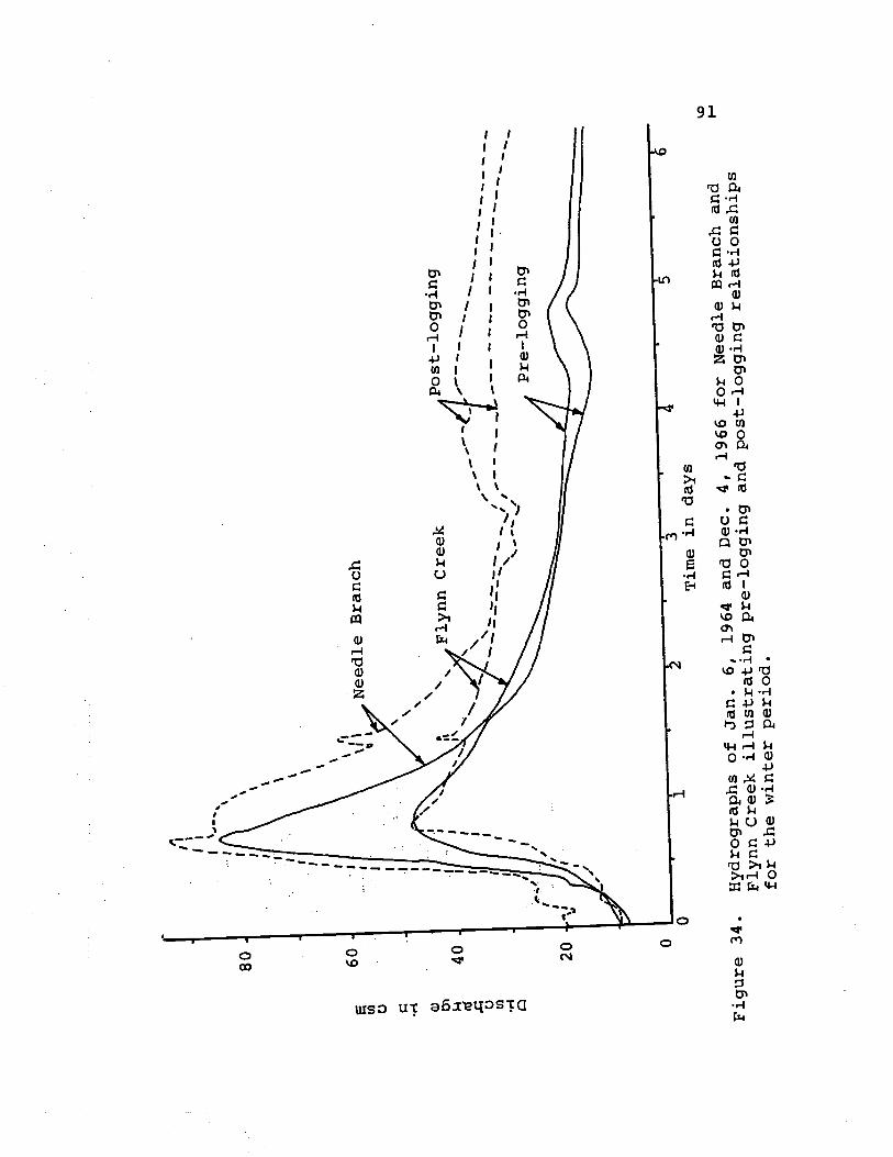
I-

'4

80

I

60

'i

Needle Branch

I

"It'

40

20

7

p.

i'I, I'

post-logging

'S-

-I-

--

- -

- -. -

. -- .-

-I-

-S

--

'.-

I--

-

14

Pre-logging

Time in days

Figure 34.

IiydrograPhs of Jan. 6, 1964 and Dec. 4, 1966 for Needle Branch and

Flynn Creek illustrating pre-logging and post-logging relationships

for the winter period.

80

I'

60

I

20

0

Flynn Creek

Pre-logging

1

Time in days

46

Figure 35.

HydrograPhs of Jan. 15, 1966 and Oct. 27, 1967 for Deer creek IV and

Flynn Creek illustrating pre_logging and post_logging relationships

for the fall period.

40

Deer Creek IV

93

on Deer Creek IV during the fall period is presented in

Figure 35. peak discharge and volume are both shown to

increase significantlY. The change in the time_to-Peak

parameter may also be noted in this figure. For the

storm representing the pre_logging period1 the storm

peak occurs at very nearly the same point in time.

Following logging, illustrated by the two dashed lines,

the time-to-peak is much shorter on Deer Creek IV. This

is the sante result as found in the preceding parameter

analysis where time_to-peak decreased by 200 per cent

for the shorter duration storms.

Base flow recession also appears to have increased

as a result of logging. This statement is based on

Figures 33 and 34. In both figures the base flow

recession for Needle Branch prior to logging is below or

almost coincident with that on Flynn Creek. following

logging however, the base flow recession remains above

that of Flynn Creek for almost the whole period of six

days shown in the figures.

CONCLUSIONS

94

This study has indicated a change in the hydrology

of small coastal streams in Oregon as a result of

clearcut logging. These changes are reflected in

alteration of hydrograph shape as defined by peak

discharge, volume, and time-to-peak. Conclusions drawn

from these changes are:

Peak discharge was increased from both Needle

Branch and Deer Creek IV, the largest increases occurring

during the fall period. Increases were of similar

magnitude for both watersheds.

Burning on Needle Branch did not produce a

noticable difference when compared to Deer Creek IV, the

unburned watershed.

Volume of flow was increased from Needle Branch.

This was reflected in changes in quick flow, delayed flow,

and total flow, with the largest increases occurring

during the fall period.

Volume of flow was not shown to. increase from

Deer Creek IV. This may have been due toa lack of usable

storm events for analysis from this watershed.

Time-to-peak was altered on Deer Creek IV but

not on Needle Branch. Time-to-peak was decreased for

minimum flows and increased for high flows.

95

The use of the height-of-rise parameter for

detecting change may be questionable if channel controls

lacking a constant stage discharge relation with time are

involved.

In future studies of this type there is need

for a data separation procedure based on antecedent

conditions rather than on time of year.

The method of analysis used in this study has

demonstrated its ability to detect hydrologically

significant change.

B IBL IOGRAPHY

Bates, C. G. and A. J. Henry. 1928. Forest and streamfioW experiment at Wagon Wheel Gap, Colorado. Washington, D. C. 79 p. (Monthly Westher Supplement 30)

Belfort Instrument Company. n.d. Instrument book for portable liquid level recorder. Baltimore, Maryland, 9 p.

Bethlahmy, Nedavia. 1963. Rapid calibration of watersheds for hydrologic studies. Bulletin of

the International Association of Scientific Hydrology 8(3): 38-42.

Chow, Ven-Te. 1964. Handbook of applied hydrology. New York, McGraw-Hill. Various paging.

DeBanO, L. F., J. F. Osborn, J. S. Kraxnlnes and John Letey, Jr. 1967. Soil wettability and wetting

agents: Our current knowledge of the problem. Berkeley. 13 p. (U. S. Forest Service. Pacific Southwest Forest and Range Experiment Station. Research Paper PSW-43)

Dils, Robert E. 1957. A guide to the Coweeta Hydrologic Laboratory. Asheville, N. C. U. S. Forest

Service, Southeastern Forest Experiment Station. 40 p.

Draper, N. R. and H. Smith. 1968. Applied regression analysis.- New York, John Wiley. 407 p.

Fisher and Porter Company. n.d. Instruction bulletin for model 1542 punched tape level recorder.

Warminster, Pennsylvania. 6 p.

Gilleran, Dennis J. 1968. Rapid calibration of coastal streams to detect effects of oadbuilding. Master's thesis. Corvallis, Oregon State

University. 51 nunth. leaves.

Glendening, C. E. 1959. Research in the chaparral type. In: Watershed management research in Arizona. Ft. Collins, Colorado. p. 13-16. (U. S. Forest

Service. Rocky Mountain Forest and Range Experiment Station. 1959 Annual Report)

96

97

Goodell, Bertram C. 1958. A preliminary report on the first years effect of timber harvest on water yield from a Colorado watershed. Ft. Collins,

Colorado. 12 p. (U. S. Forest Service. Rocky Mountain Forest and Range Experiment Station. Station Paper No. 36)

Harrold, L. L. et al. 1962. Influence of land use and treatment on the hydrology of small watershed at Coshocton, Ohio. Washington, D. C. 194 p. (U.

S. Dept. of Agriculture. Technical Bulletin 1256)

Hewlett, John D. and Alden R. Hibbert. 1961. Increases in water yield after several types of forest cutting.

Bulletin of the International Association of Scientific Hydrology 6(3):l-17.

1967. Factors affecting the response of small watersheds to precipitation in humid

areas. In: Forest hydrology, ed. by William E. Sopper and Howard W. Lull. proceedings of a

National Science Foundation advanced science seminar, University Park, Pennsylvania, Sept.

1965. New York, Pergamon. p. 275-290.

Hibbert, Alden R. 1967. Forest treatment effects on water yield. In: Forest hydrology, ed. by

William E. Sopper and Howard W. Lull. proceedings of a National Science Foundation advanced science

seminar, University Park, Pennsylvania, Sept. 1965. New York, Pergamon. p. 527-543.

Hibbert, A. R. and B. G. Cunningham. 1967. Streamf low data processing opportunities and application. In: Forest hydrology, ed. by William E. Sopper and Howard W. Lull. Proceedings of a National

Science Foundation advanced science seminar, University Park, Pennsylvania, Sept. 1965.

New York, Pergamon. p. 725-736.

Hoover, M. D. 1944. Effect of removal of forest vegetation upon water-yields. Transaction of the

merican Geophysical Union 25:969-975 p.

Kovner, J. L. 1956. EvapotranspiratiOn and water yields following forest cutting and natural regrowth.

Proceedings. of the Society of American Foresters, 1956, p. 106-110.

98

Kovner, J. L. and T. c. Evens. 1954. A method for determining the minimum duration of watershed experiments. Transactions of the xnerican Geophysical Union 35:608-612.

Krygier, J. T. 1969. changes in water yield and peak flows from land management. Unpublished manuscript.

corvallis, Oregon, Oregon State university, Dept. of Forest Management. 17 p.

Leonard, Raymond E. 1967. Mathematical theory of interception. In: Forest hydrologY ed. by


seminar, University park, Pennsylvania, Sept. 1965. New York, Pergamon., p. 131-136.

LeupOld and Stevens Instrunient company. n.d. Stevens water level recorder, type A35. portland,

Oregon. 8 p.

Li, Jerome c. R. 1964. Statistical inference. Ann Arbor, Michigan, Edwards. 658 p.

Linsley, Ray K., Max A. Kohler and Joseph L. H. Paulhus. 1958. Hydrology for engineers. New York,

McGraw-Hill. 340 p.

Love, L. D. 1955. The.effect killing of spruce & pine Beetle. Transactions of Union 36:113-118.

Love, L. D. and B. c. Goodell. 1960. Watershed research on the Fraser Experimental Forest. Journal of Forestry 58:272-275.

Watershed management in the and subalpine zones. Ft. p. (U. S. Forest Service.

Experiment Station. Note

Martinelli, M., Jr. 1964. Rocky Mountain alpine

collins, colorado. 7 Rocky Mountain Forest P14-36)

on streamf low on the by the Englemann Spruce the American Geophysical

Maruyama, I. and T. Inose. 1952. Experiment of forest influences upon streamf low at Kamabuti. MegUrO,

Japan. 44 p. (Government Forest Experiment Station. Bulletin 53)

NakamO, H. 1967. Effects of changes of forest conditions

99

on water yield, peak flow, and direct runoff of small watersheds in Japan. In: Forest hydrology

ed. by William E. Sopper and Howard W. Lull. proceedings of a National Science Foundation

advanced science seminar, university Park, Pennsylvania, Sept. 1965. New York, Pergalflon.

p. 551-564.

Penman, H. J. 1963. vegetation and hydrology. Reading, England, LampOrt Gilbert. 124 p.

Pereira, H. C. 1962. Hydrologic effects of changes in land use in South African catchment areas. East

African Agricultural and Forestry Journal. vol. 27. 131 p. (Special issue)

Reinhart, K. G. 1958. Calibration of five small forested watersheds. Transactions of the American

Geophysical Union 39:933-936.

Reinhart, K. G., A. R. Eschner and G. R. Trimble, Jr. 1963. Effect on streamflow of four forest

practices in the mountains of West virginia. Upper Darby, Pennsylvania. 79 p. (U. S. Forest Service. Northeastern Forest Experiment

Station. Research Paper NE-l)

Rich, Lowell. 1960. preliminary effects of forest tree removal on water yields and sedimentation. In:

watershed and related water mangement problems proceedings of the Fourth Annual Arizona Watershed Symposium, Sept. 1960. [TucsOnl State Land

Department. p. 12-15.

Rich, Lowell R. and H. G. Reynolds. 1961. The Workman Creek experimental watershed. Ft. Collins,

Colorado. 18 p. (U. S. Forest Service. Rocky Mountain Forest and Range Experiment Station.

Paper 65)

Rothacher, Jack. 1953. White Hollow watershed management: 15 years of progress in character

of forest, runoff & streamf low. Journal of Forestry 51:731-738.

1963. Net precipitation under a Douglas-fir forest. Forest science 9:423-429.

100

Rothacher, Jack. 1965. Streamf low from small watersheds on the western slope of the Cascade Range

of Oregon. Water Resources Research 1:124-34.

Schneider, W. J. and G. R. Ayer. 1961. Effect of reforestation on streaimf low in Central New York.

Washington, D. C. 61 p. (U. S. Geological Survey. Water-Supply Paper 1602)

Tennessee valley Authority. Division Water Control Planning, Hydrologic Data Branch. 1955.

Influences of reforestation and erosion control upon the hydrology of the Pine Tree branch

watershed. Knoxville, Tennessee. 95 p. (Technology Monograph 86)

Tennessee valley Authority. Division Water Control Planning, Hydraulics Data Branch. 1961.

Forest cover improvement influences upon hydrologic characters of White Hollow Watershed, 1935-58. Knoxville, Tennessee. 104 p.

U. S. Dept. of Agriculture. Agricultural Research Service. 1962. Field manual for research in

agricultural hydrology. Washington, D. C. 214 p. (Agriculture Handbook 224)

U. S. Geological Survey. 1951. Water Resource Division. Instructions for preparation of manuscript for

annual reports of surface water supply. Washington, D. C. 70 p.

U. S. Soil Conservation Service. 1964. Soil and vegetation survey, Alsea area Oregon. prepared

in cooperation with Oregon State University, U. 5. Bureau of Soil Management and U. S. Forest

Service. 2nd draft. Corvallis, Oregon. 730 nunth.

leaves.

veihméyer, Frank J. 1964. EvapotransPiration. In: Handbook of applied hydrology, ed. by yen Te Chow.

New York, McGraw-Hill. 1-11 to 11-33.

Whipkey, R. Z. 1965. Subsurface stormf low from forested slopes. Bulletin of the International Association

of Scientific Hydrology l0(2):74-85.

101

Wilm, H. C. 1949. How long should experimental watersheds be calibrated. Transactions of the American

Geophysical Union 30:272-278.

Wilm, H. G. and E. G. Dunford. 1948. Effect of timber cutting on water available for streamf low from

a Lodgepole Pine forest. Washington, D. C. 43 p. (U. S. Dept. of Agriculture. Technical Bulletin

968)

Wisler, C. 0. and E. F. Brater. 1959. Hydrology. 2d ed. New York, John Wiley. 408 p.

Ziemer, R. R. 1964. SunIner evapotransPiration trends as related to time after logging of forests in

Sierra Nevada. Journal of Geophysical Research, part 1, 69:615-620.

Zinke, Paul J. 1967. Forest interception studies in the United States. In: Forest hydrology, ed. by


seminar, University Park, Pennsylvania, Sept. 1965. New York, Pergamon. p. 137-160.

I XIaN2ddV

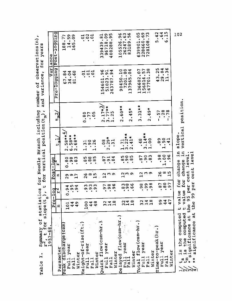
Table I.

Summary of statistics for Needle Branch including

r2, t fOr slope(t ),, t for vertical position(t

),,

m

1/ t5 is the computed t value for change in slope.

/ tm is the computed t value for change in vertical position.

3/ * significance at the 95 per cent level.

4/ ** significance at the 99 per cent level

number of observations(n),

and variance, for years

0 t)

1957-68.

Pre -10

Pos t-1q

tVar i ance

Post-logging

Parameter

nr

nr

tm2/

Pre-logging

Peak discharge (csm)

Full year

Fall

Winter

1014449

0.94

.95

.94

29 9

17

0.80

.98

.83

6.58**

2.68**

67.84

34.04

81.68

188.77

14.59

165.09

Height-of-riSe (ft .)

Full year

Fall

Winter

100

4448

.93

.93

.93

26 8

15

.85

.88

.85

1.31

.90

1.26

0.80

.77

.05

.01

.01

.01

.01

.02

.01

Quick flow(csm-hr. )

Full year

Fall

Winter

32

1418

.97

.98

.96

12 3 9

87

.91

.84

.08

2.29*

.31

2.17*1"

377**

1.25

154601.96

51023.91

243787.94

339439.81

96718.09

408288.95

Delayed flow(csm-hr.)

Full year

Fall

Winter

32

1418

.83

.98

.66

12 3 9

.85

.90

.85

1.71

3.22**

2.41*

2.60**

2.45*

90450.10

7201.80

137965.04

105526.96

26247.63

83189.56

Total flow (csm-hr.)

Full year

Fall

Winter

32

1418

.98

.99

.98

12 3 9

87

.90

.83

.48

3.14**

1.00

3.31**

2.49*

136602.07

156814 .57

167701.38

639901.05

228660.69

728108.73

Time-to-peak (hr. )

Full year

Fall

Winter

9944

47

87

.80

.97

26 8

15

.98

1.00

.96

.89

1.50

.41

-.57

.28

-.78

43.25

29.84

11.36

5.42

.64

6.15

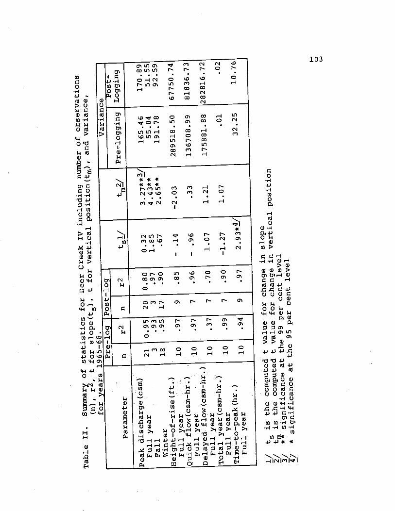
Table II.

Suiniflar

of statistics for Deer Creek IV including number of observations

(n), r2, t for slope(t5), t for vertical position(t)i and variance,

for years 1965-68.

Pre-log

Post-log

VariancePost -

1/

t5 is the computed t value for change in slope

2/

tm is the computed t value for change in vertical position

3/

** significance at the 99

per cent level

47

* significance at the 95 per cent level

0

Parameter

nr2

nr2

tsi/

tm2/

Pre-logging

Logging

Peak discharge(csm)

Full year

Fall

Winter

21 3

18

0.95

.93

.95

20 3

17

0.80

.97

.90

0.32

1.85

.67

3. 27**/

443**

2. 65* *

165.46

55.04

191.78

170.89

51.55

92.59

Height-of-rise (ft..)

Full year

10

.97

9.85

- .14

-2.03

289518.50

67750.74

Quick flow(csm-hr.)

Full year

10

.97

7.96

- .96

.33

136708.99

81836.73

Delayed flow (csm-l.)

Full year

10

.37

7.70

1.07

1 . 21

175881.88

282816.72

Total year (csm-hr.

Full year

10

.99

7.90

-1.27

1.07

.01

.02

Time-to-peak (hr.)

Full year

10

.94

9.97

2.93*Y

32.25

10.76

Table III.

Summary of statistical results for test to determine

difference between

fall and winter data, including number

of observations(n), r2, t for

slope(t5), and t for vertical

position(tm), as tested against the control.

1/

t5 is the computed t value for change in slope

2/

tis the computed t value for change in vertical

position

3/

*significance at the 99 per cent level

4/

* significance at the 95

per cent level

Watershed

Variable

Period

nr2

t/

tmi/

Winter/Fall Winter/Fall

Needle Branch

Peak Discharge

Pre

49/44

0.87/0.95 4.88**Y

Post

17/9

0.83/0.98

3.lO**

Needle Branch

Quick Flow

Pre

18/14

0.96/0.98

0.81

-0.13

Post

9/3

0.84/0.91

0.89

0.97

Needle Branch

Delayed Flow

Pre

18/14

0.66/0.98

2.21*!!

Post

9/3

0.85/0.90

0.89

1.51

Needle Branch

.Total Flow

Pre

18/14

0.98/0.99

2.30*

Post

9/3

0.83/0.90

1.01

1.21

Deer Cresk IV

Peak Discharge

Pre

17/3

0.95/0.93

0.24

0.33

Post

16/3

0.93/0.97

2.22*

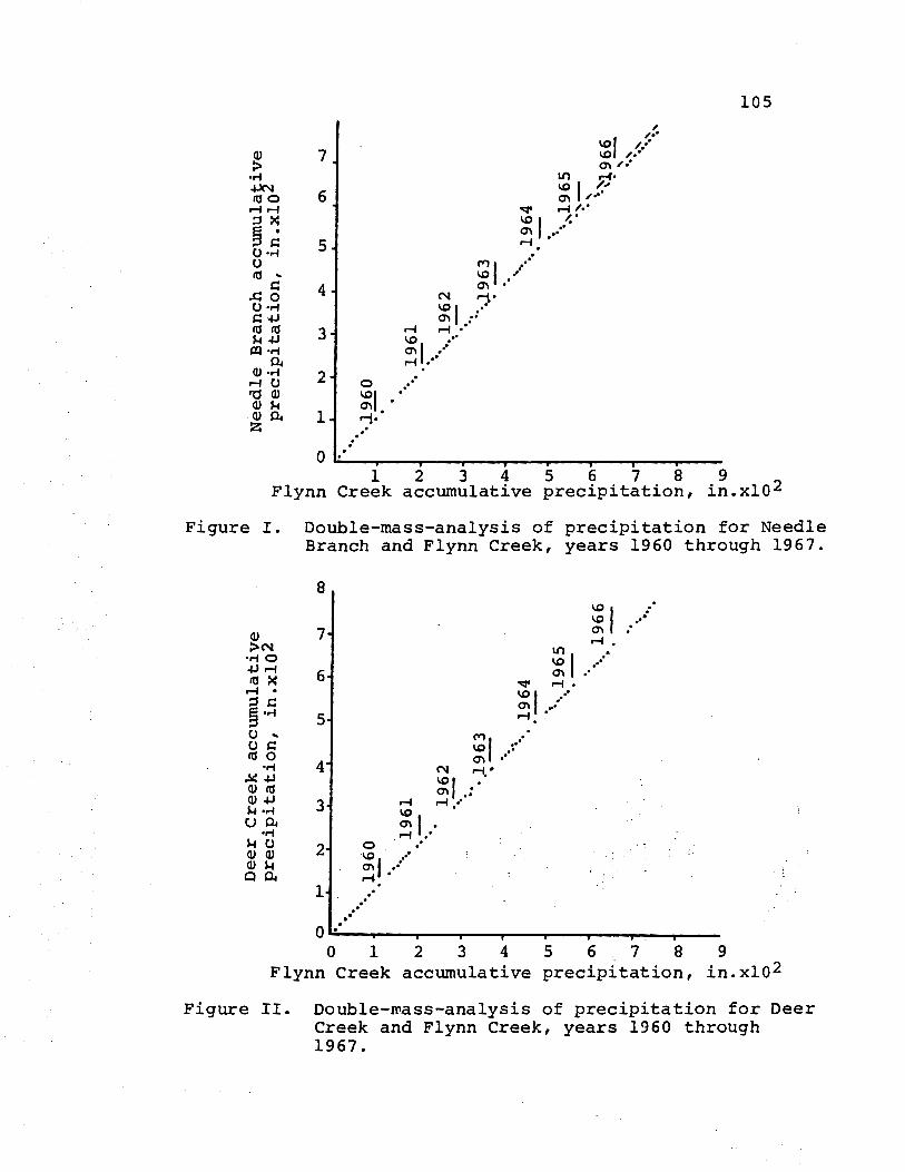
/ /.. ,.' 7

Lfl -4. 4X4 tot ' o 6 r4r4 i>4 'i c'I.f

5 -

0 mi A

CS1 rt 4)

( r4 r4' 44) -,

r4/ r40 ' 0 rdQ)

1-

O__. 1 2 3 4 5 6 7 8 9

Flynn Creek accumulative precipitation? in.x102

Figure I. of precipitation for Needle Branch and Flynn Creek, years 1960 through 1967.

U) Cs1 rl 0 4)r4 ('ix

(o rl

-i op rl .10 U)U) U)Ii

m '0 C.'

4 r '0 r-4 r4/ '0 C.'

0 / C.' r4

'0 '0 C.' r4.

u . to C.'

. r4. to C.'-

105

0 1 2 3 4 5 67 8 9

Flynn Creek accuxnulat1e preciPitat]0n? in.x102

Figure II. of precipitation for Deer Creek and Flynn Creek, years 1960 through 1967.

II XIQcH

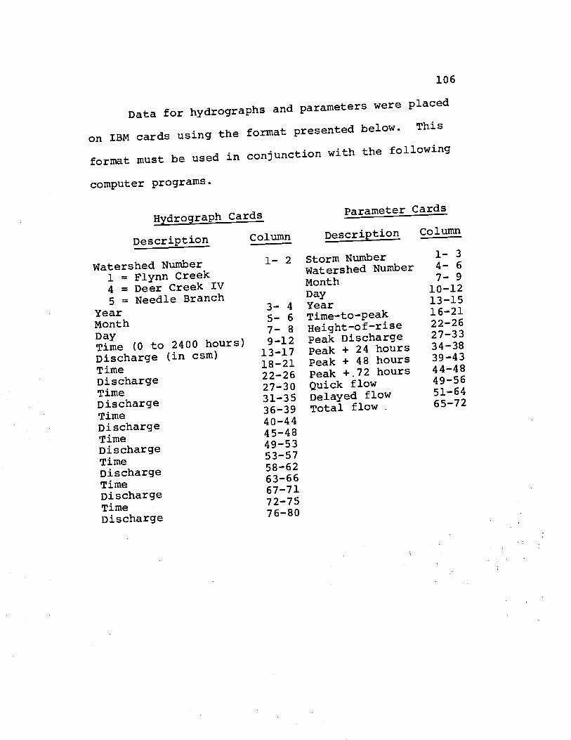
106

Data for hydrograPhs and parameters were placed

on IBM cards using the format presented below. This

format must be used in conjunction with the following

computer programs.

Hydrograph Cards

Description Column

Parameter Cards

Descriptio Column

Watershed Number 1 = Flynn Creek 4 = Deer Creek IV 5 = Needle Branch Year Month Day Time (0 to 2400 hours)

Discharge (in csm) Time

Discharge Time

Discharge Time

Discharge Time

Discharge Time

Discharge Time

Discharge Time

Discharge

1- 2

3- 4

5- 6

7- 8 9-12 13-17 18-21 22-26 27-30 31-35 36-39 40-4 4

4 5-48 49-53 53-57 58-62

6 3-66 67-71 72-7 5

7 6-80

Storm Number watershed Number

Month Day

Year Time-to-peak

Height-Ofrise Peak Discharge Peak + 24 hours Peak + 48 hours Peak +.72 hours

Quick flow Delayed flow

Total flow

1- 3

4- 6

7- 9 10-12 13-15 16-21 22-26 27-33 34-38 39-4 3

44-48 49-56 51-64 65-72

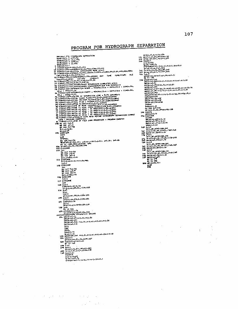
0.3LS

0(50Oct IL00OIL

ll0ilu000100it00dLl9ilil0)il 1S1

ibi00I1.1.1 Cal111)01011 141155 051

ist(5ui i0(.ilitPllil l.Il VOllI.il,tI(.t,h405 iiIL

111l101 10131i5 I 141I.t.t DLI

501101

Iot.001 lUIJli5It 1.151 VOlIblIlOdL

lb. 1.1)01 11.1..ljLiSOI,. 1)0 t01 11iLu15it101 iS ISO

00.110:3 OIlI11101005

i.b,.i Ill1l111 l50110L0 II.Ll,Iil 00051 III lU

i1 iIVl'. 15wI

SO,.ivelliLi'5 1L5 V1 iLlSO500 II10151155

I.5,l$L.11C3l1011110t.,il,.bDi 115 LVI 51 iSO10 Il' iiI

i)0liLid01t311).10141 IS.

11 IV) 41110

111IV 10110l)o 11III. i(t 101 I0l.tOtiLiSO OIl'SI -1

i1 110110 II,101t0)iLlS101

101IIIIl1)41 501lit

b,11'I b101i151(51 i( t.II,.1111,) IlS

bL lb. 110

b5t%IIlIl0j)u1 51*ill.l.I1).41 11%

11111 I,.bt11I

LOT

jitiiII0ç1.0.j. *% lb11

l0Oh1I SI t*t

005ib*.('J ii. II,. Iii l.I500%1.11 eu

VI .1 ISLit

gii.St 1,,03 IV. i..li OiliC1l0 lVt 1,151105 041

Iiii.0001

1.31i

I(1l0 lV)1V1)0 1I1).. Ipl tVliLlSO

(V I)1I 1lIbl(t ;0I SOIlS11l0151155 SI

$01050 ..I1',4i5hI :s I, let Sil

5li.5Zll03IlIbJhii i.t.t t1ll'5"lit151011 1004 l0ll04110t051003 i.tI0Iil 1.101

I..Il51l OIl

itIt)003 i,.It,lil('1.01.11 SIt

11.100.11013 itt

1.1.100.ILb) Oil

i..rla.1rl)N ..t.r Oil 30etl LIt 00 01tO &It too

tl il0.ILb.) illt.ll Oid'Il0 111)0 10110 00.LLb111

1.1.r Ill LOll ill00

itt .1)1.1 ill

0&ih) aOlOØl.Otlib0l11 001

1001 5i3 iiOl100b)L IS

1S.l.l'I1 l4r*tIOlIIVt1 i..v.Ilo0V00 out 00

0.10001

0..IL)l:1111

o.i,.r.Ile DS.l0 101 toO101itO

e'li 1151 10 0(51

i.u3003 NOSO00S - 0311330050113 3115 iIk3$ll11101.4 15000 .0)0155 - 0.11

31.113 0111.55131dlS000Ui501435 0545 15S13 i1l,lj..tlL101:iDO

000030 101i.50l'i 01ii00iLpi.0lIL0).5'C

0035 LI1j,10l1L10004 11

l.l310Vi1115LI1i,.l01)L'005i dl0154) 55idL 35iL.0utl0SIt

Slid 4: S.,Ij..lOI)L101.i Oh4lb13l)Sihu1.0IiLIll1i bi

0114LL*.0Otl14 050310)5001)1.00.4 Li

.31)11 101,..0llL0li Siie4.lS3 lifeNliL151d3I iIs

-

,40351L.1l.1001l110L500 - (55)50411dlIL00.i VS-

- l.hl1VU - .LI.Lfl- 00945 )1Q1I1I).jj Ci111 514j,5,30dISV550I501CL

tLV (51315513 011115154105II

i5.01i.z.oi.e.i.LI.LIVQIILVS.i 'I11P,,0IIO,li

45113511IVO u1a:.'o:10140)OSILISS_i II

ous,.sen:,500uh3',0105.tjS,oi.,Th10lli5lLVb5tJ dl

11111 3015 MII0I?flUAKl,ILI.,I,flhILIhUl4 UUI

il..1111.S1i I100V1: IlISIhSUIlO

wS 011155510

i%0tJ51 I,.Ii'n,d3S 041rJ10UA, V..i.051.5*

ijxvdaS HdIDOUAHiO WVDOd

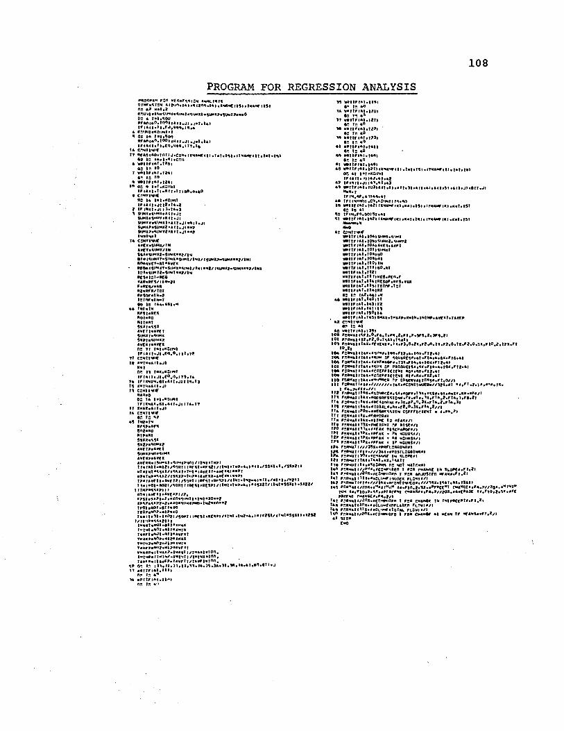
UI)

IIzsacIv4L IVII jINV') UL IQj3/L111..4 uII/JIM:,. lwLtnIp.n:ns'I%.ILvne..i

InI,IIlI4I4IL'.b.j 11%

Z'14ILd))MJIII WII.VJMj I Ii

4II/bjJ3WW'.J 1.J1)L

)I.OIjMI lUll).01//I4'IaU77M L4'0Ij'Jl..nI

Qz//W.11'.V..Lh),64d.'IIruJli"lIlflI')I'Il(.ll0(.(s'.L

..j 111

Il.IM:J MI(U.I ,..':.,..l(,Lli jlj(UL1IJ'.V

ullUnru? ILl £JUU/IL7Mg elIL4101IS III 1*1711/ di I

*14113.£7111.4 uvi

**I*I7I40*. 01117*1.4 I.(*1711'*17WII&l11M.i Lfl

i.a:iIll I .v..3.'*(ue11l;j7

I.W.l397:ucL..'.lL,'.l.Il7.I0. II ,e;c,,,uv'.:a 'LII/III IL4*1J11)4l*.l.i e%1/eUIOLM IMVH,.1*4*1*1.4 4fl

LII W,*LLILVIIM4 IIII,.17,13111 )8Jl.l*LUY*.l0i 011(,.4IIMIl*E1IIYllI-i II

LI IIIIII,07(Ia7'.M.j Ifl

4)111,4:3 NLII*.4d7j..l110IIV11Mj.11

I#lij!(0i4'*1I7I11171*1.4 III

IUnj'z'.I4l,.'e'.illUu IvlbII

UVMI.1II

IlJjJlll1lI!b1laXtl1$iUP1tS'e33Illbl11l1ILVeI.4j

'II '..,.I'lL4'I.,,.aIrw.Ie:..'lI. 141*1.llI7..WL1 III114*1u11 IIii).l.l07IILV1*W..i 141

(lI's0l IllI41)1..*,11171404 101IiIiO,l4'1*.17L30014 IL Ifl*1'11171*104 LII

IWlIj'IOI'l7Ij'7(I'jIuV*11711171*l04701

I,1111097,Ij407700 IL 100011IL7014

141'UI

'i'llIll100I4*!1b0141J1*01i'111'1i141I1'1i17*

'1711Li 10*I*7'I,1*lOlj.UllLUII1 101

(U1,11II'9'io 10*177101 *10* 111197111110 07Iv 01 1(11*0*1*11.4 lv

IO2M'mIIM Wl11*dlY.11*7,ll(117%' ;,*11Iul

71 *011*' 17141110111171971i1110ii It'I IIi1.I10 I071*.I 11110 17N' 170*jlI .1 LI101v11I7)i1I10

£011*1LL1 *11*11 %VI4jlI0*I7*1*IilhjUSIlIl*l' *7*41(10

A'9)11*1 I)71Ill I

I.1061I11 17141110WL*OI%9711L110111 I.019*IILISO011IVOl1I74L1I0

L0*111111011 17144100-IIQ%1%7IiLlR

NP,*161110I *71411101111*IUIIUI III £1110

4*1*111103 1700W

ISI'l.0(NIlM*IlIIIMlI111*.Th.IIZ,19,IILIIA II

l,.111111ej11)jI Pb(7 0401

(cI'l.7I.'p,e4IIcII.11 IIIIi..7N01I19.181(10 04

1*111*1* I4I.l,'IIV *1.11.11*111II

1r910. ((117119,,(EUI.IIIILISM IvU,'!,.111'*11,1 lvlv'I,'E.Itr' 11.110711.1 17 00

(11I'I.1111I11*I.IIl4,7h7II44I1I7Iil10 (*7I11,I'I,11L110 IS

47L LIL117(171j1110 Ill

0' 0141.1971i1110 LI

.1 IIICLI'I,141110 IL

ov -1 01Il'%v1j1110 II -I LIII1(I41110 LI

-s .l1741'IvIiLI.I VI

l .1 .1161197)41101 11

801

I...&

IvlIIV)iIld'Pb

.1 .1Ij,i'IlIiIIOP It

r.'e09711',U*SC,(tLII'LUII'ItI ..L

.1) 41

L171*111h/ I %).$*.1J71174Ia#.I.10q1.117..h/111Ih11171.41 I. 4*1.1 t*..Z,,

,*IhI.CI#11011fl1111 1

IOiJV.I 111.1711.1.1 (I.I41*1'.IOL77111.1 ,V.IL.01r7*.L

III1.11/I

DlilI*4OIM40*L 41.111. 101 IOtA

10*14

ZOO.1114.1Z/ (1141y 113*111.00

IIIII

,aus.IIs.I'.,I.)11IM/lbbdb011U lIZ.,.I,lO,9),I,_Z*I1_II/b4I1i0IILShl7I41 II.111u1I,jIbb.I*.L.L0Ij..I.IIi*vI.I..L.IIb)/I1SS.Ihl1t1

I(Pb,.%.I.7%,_II.l,1IP*.&I4IUSiIlZIII04I4*.1.III.lIlIUh4Ml.I1*. 141110*1011*7 1307.11341

4110*11*4*1116

iISLll* .1*16611.41101.111

S41 LI LIj.16Lu103 VI

((11701701 LILI 7L I IC l)V&10411111

IL LU0.07.

MlC) 1.1Ir'Il7'U110 IL

£LeLlIrp),L9..1..IIII ILL*4101'$OI IL LU

I.) If'3)VPbI,.l IL410111103 II

1L IL (003 IN1171414,.*:NI.I IL LU

1.41111*0.1161141*5*341.1131.7

.00.10011IlIIV 01.101

031.111111*111111 II

II.'IIvv,) LI 011.*I1.i(ISIU404/510411

l341LLIflS3INL/l..111541*ldIIlLLI

l*016117111I0) /011INLIII.-LOIoIOI 19111131.7. IV.A30l,j5

(N1/Z..110*4141)S) / *11*4*0 0.0*1*1*101 III

111/111,4113*1111/11114113*!

410111103 VI

I.. ir. I S 5*15 11411*1*1154.1 Ir.l ,,.ow,41d..mc

IN Ill Ir.l*,.o1*14111..I,sIt1)ipL,.oS.LMI15IC'II.UI(r'LSII4I 1 *57*1111110)01.1 II 01

IOI**uII*PI...IIllIvliI 1*I)103I.I S 01

I9ZI'I,IlLIIN I 04 LI(Ill' (II 01 LI 01I511 III

1*431*1LI 09

(0I(.(II)3117)'IIII..,01I.I*43.r)I7(.O,IIjvluLI

4101L7L3 III 'LI I*b.*03 I I' 111131

III.1001t.')U!aWLOS' IllII 01 1*1.1I.*10l.1*d*4. I

'S*6'pI (*1171,1*'l.1' IN(-(,Jle7il

nob_Ill I 00

0lNlCA10ItONflSs*IpWlflAflI01.a,'..WIeltflL. 4V LU

lI)j07I*'ISlI).*VNI'I7%l.'.UII.l,IlL(,1I7I*4(0eP.IL

:100141), 10*1

SISA'IVMVMOISS UXU0d WVIOtd

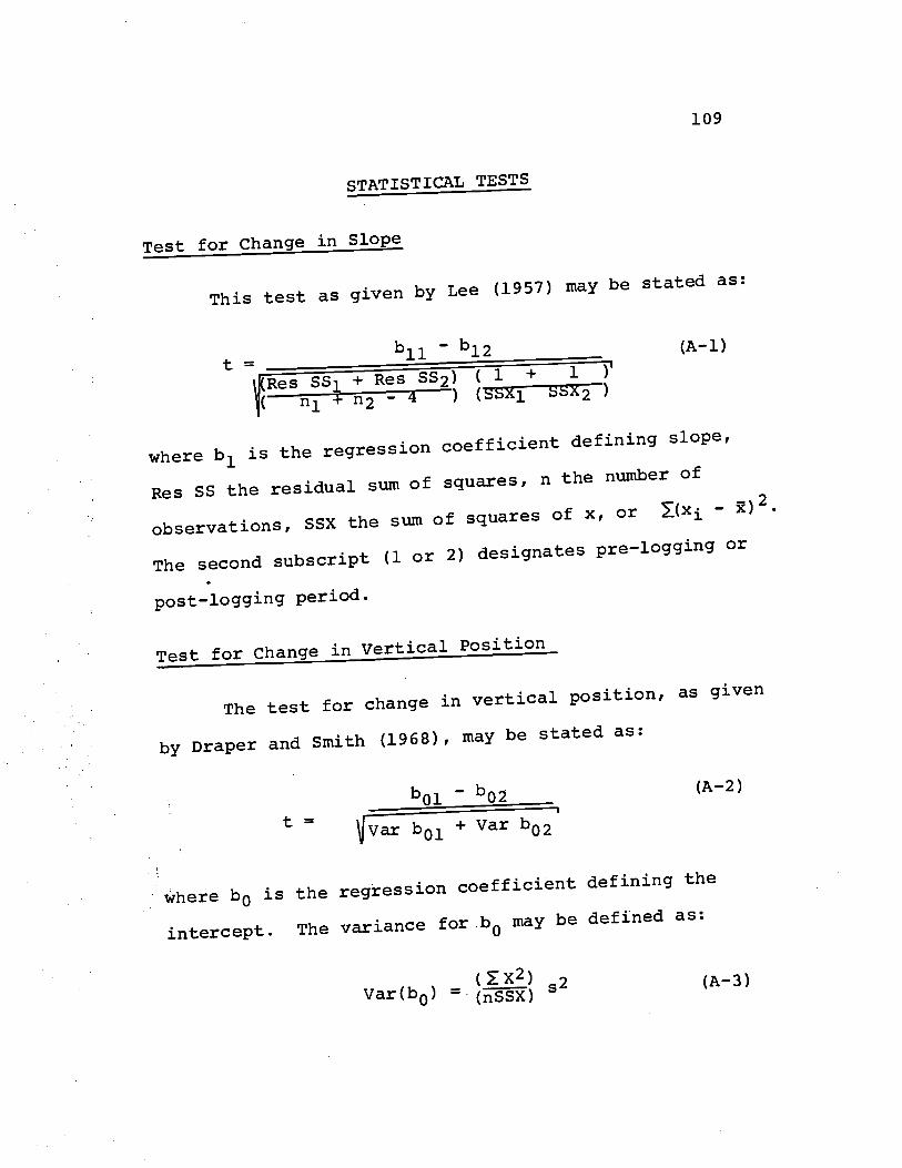
t=

109

STATISTICAL TESTS

Test for Change in Slope

This test as given by Lee (1957) may be stated as:

b11b12

Res SSi + Res SS2) (1 + 1

+ n2 - 4 ) (SSX ssx2)

where b1 is the regression coefficient defining slope,

Res SS the residual sum of squares, n the number of

observations, SSX the sum of squares of x, or (x

The second subscript (1 or 2) designates pre_lOgging or

post_logging period.

Test for Change in Vertical position

The test for change in vertical positiOns as given

by Draper and Smith (1968), may be stated as:

b01 - b02 (A-2)

t= Var b01 + Var b

where b0 is the regression coefficient defining the

intercept. The variance for b0 may be defined as:

(X2) 2 Var(b0) = (nSSX)

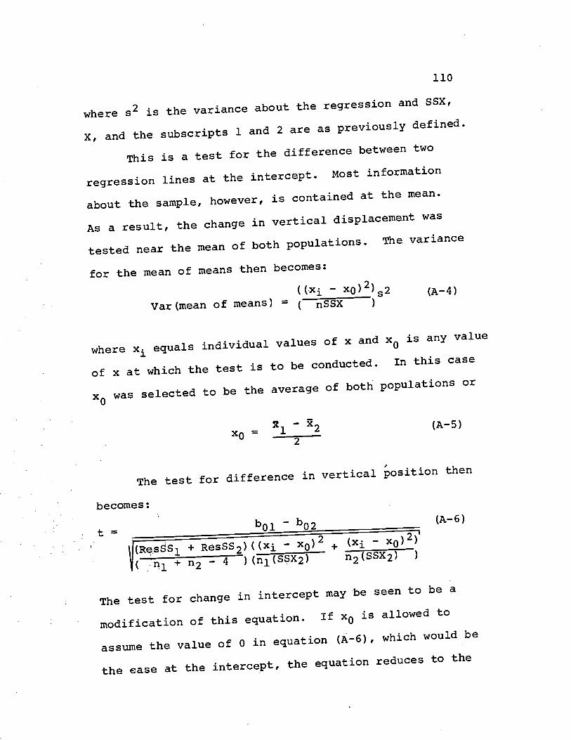
t=

2 - Xn 1 (A-5)

The test for difference in vertical position then

becomes:

b 1-b 0 022

2 (Re5SS1 + Re5SS2)((Xj - x0) + (x - x0)

(.'l + n2 - 4) (n1(SSX2) j(sSX2) )

The test for change in intercept may be seen to be a

modification of this equation. If x0 is allowed to

assuitLe the value of 0 in equation (A-6), which would be

the ase at the intercept, the equation reduces to the

(A- 6)

110

where 2 is the variance about the regression and SSX,

x, and the subscripts 1 and 2 are as previouslY defined.

This is a test for the difference between two

regression lines at the intercept. Most information

about the sample, however, is contained at the mean.

As a result, the change in vertical displacement was

tested near the mean of both populations. The variance

for the mean of means then becomes:

- xo)2)52

(A- 4) Var (mean of means) = (nSSX )

where x1 equals individual values of x and x0 is any value

of x at which the test is to be conducted. In this case

x0 was selected to be the average of both populations or

original form of equation (A-2).

Data Used in Study

A complete listing of all data used for all analysis

is presented in Tables IV, V and VI. Table IV gives

data for Flynn Creek, Table V data for Deer Creek IV, and

Table VI the data for Needle Branch. In all three

tables, column one is the event number. This number is

the same for a given event on all three watersheds.

Column two gives the date of the event, and columns

three through

in the study.

and eight are

to the volume

is defined as

111

point the separation line intersects the recession.

A blank for a given parameter for any given storm event

does not indicate the lack of a value. Instead, it

indicates that the quality of that value for that

particular event was not satisfactory for use in the

analysis.

eight give the values of the parameters used

The values of volume in colunn5 six, seven

expressed in csm-hr. This corresponds

of runoff for each storm event where time

the interval from the initial rise to the

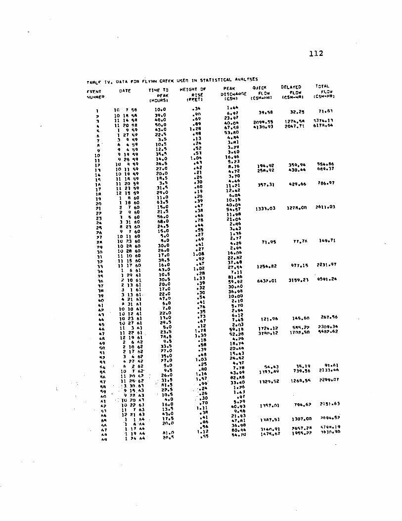
112

TAPL TV. DATA FOP FLYNN CREFK USEO TN STATISTICAL. ANALYSES

FVF.NT DATE TIME TO

PFAK (HOURSI

HEIGHT OF RISE (FWET)

PEAK DISCMAP6E

(CSM)

QUICK FLOW (CSMHWI

DELAYED

(CSM-MR)

TOTAL

FLOW CSu-HRI

I IC 1 38 10 18 88

10.0

39.0 .34 I.4

6,qr 39.38 32.25 71.81 3 4

II 14 58 11 20 38 1 9 59

40.0 50.0 43,0

.69

.89 1.28

23.91 40.04 67.88

209Q.55 4130.93

1274.S 2047.71

1374.11 6178.64

6 1 27 39 22.5 .88 53.80 7 3 9 59 3.5 .13 A 6 4 59 10.5 .24 3.81

9 4 59 12.5 .52 3.29 10 9 19 89

9 26 9

35,3 14.0

.53 1.04

3,40 16.96

12 i

14 c

10 8 39 10 II 39 10 19 9 11 18 s9

26.5 27.0 20.0 18.5

.4

.42 .21 .26

5.73 8.76 4.72 3.70 4,46

194.92 758.92

35994 430.44

554.86 689.37

IA i

II 20 59 11 23 59

3.5 31.S

.30

.60 11.21 357.31 429.66 786.97

q 12 15 59 29.0 19 12.42 6.04 19 1 8 60 11.0 .26 10.15 20 1 18 60 63.5 .39 40.04 21

22

2 7 60 2 9 60

13.0 21.5

.47

.38 54,51 11.98

1333.03 1278.00 2611.03

23 '4

3 5 60 3 31 60

36.0 68.0

46 .78 21.04

2.36 25 26 7

8 23 60 9 7 60 10 11 60

24.5 15.0 5.0

.44

.55

.27 3.43 1.36 2.7 28

q

10 23 60 10 28 60

8.0 30.0

.49

.41 4.26 2.94

71.95 77.78 149.71

3n 10 28 60 26.0 .27

31 32 li

II 10 60 II 15 60 II 17 60 1 6 61

17.0 33.5 16.0 43.0

1.08 .92 .47 1.02

22.82 31.48 27.54 1254.82 977.15 2231.97

1 29 41 10.5 .28 7.11

38 2 10 61 2 13 61

30.5 20.0

1.33 81.86 59.92 6432.01 3159.23 9591.24

3 1 61 17.0 .32 30.80 3 13 61 22.0 .30 36,98

10.00 40 41

4 21 61 8 31 81 10 10 61

47.0 6.0 7.0

.54

.41

.76 2.10 5.70 2.94 41

44 10 12 61 10 23 61 10 27 81

22.0 13.0 79.5

35 .73 .67

6.12 7.45 2.03

121.96 145.60 267.56

48 7

48

11 3 81 11 2? 61 12 19 61 2 6 82

5.0 23.5 78.5 9.5

.12 1.78 1.30

59.1 52.28 4,74

1724.12 3780.12

585.22 1702.50

2309.34 5482.62

2 10 62 33.5 .58 18.74

51 87 83

2 17 62 3 4 62 4 27- 82

27.0 35.0 27.0

.39

.48 1.03

15.63 26.32 437 84

sc 58 ci SR 59 80

- 6 2 62 10- 7 62- 11 70 6? II 23-67

-

:3- 30 61

-

9 15.83 -

22 63

5.0 9.5

: 26.0

-. 31.5 81.5 22.5 10.5

.25

.80 1.16 1.57.

.24

.26

7.78 43.99 82.88 33.40 l.2 1.4)

38.43 1191.89

1121.32

35.19 739.56

1269.58

91.61 2133.46

2299.07

1

82 61 84

68 87

89

10 20 83 10 2? 63 11 7 63 12 21 63 I I 64 1 F,E.4 1 11 84 I 19 84 1 74 84

4.0 16.0 13.5 41.0 17.5 20.0

81.0 20.5

.30

.70 1.11 .38 .41 .84 .36 1.12

5.9 40.93 9.56 21.93 47.81 36.98 80.84 54.70

1387.01

1387.51

3140.91 1878.67

794.62

1307.00

2657.28 1935.72

2151.63

b94.5

8798.19 1430.90

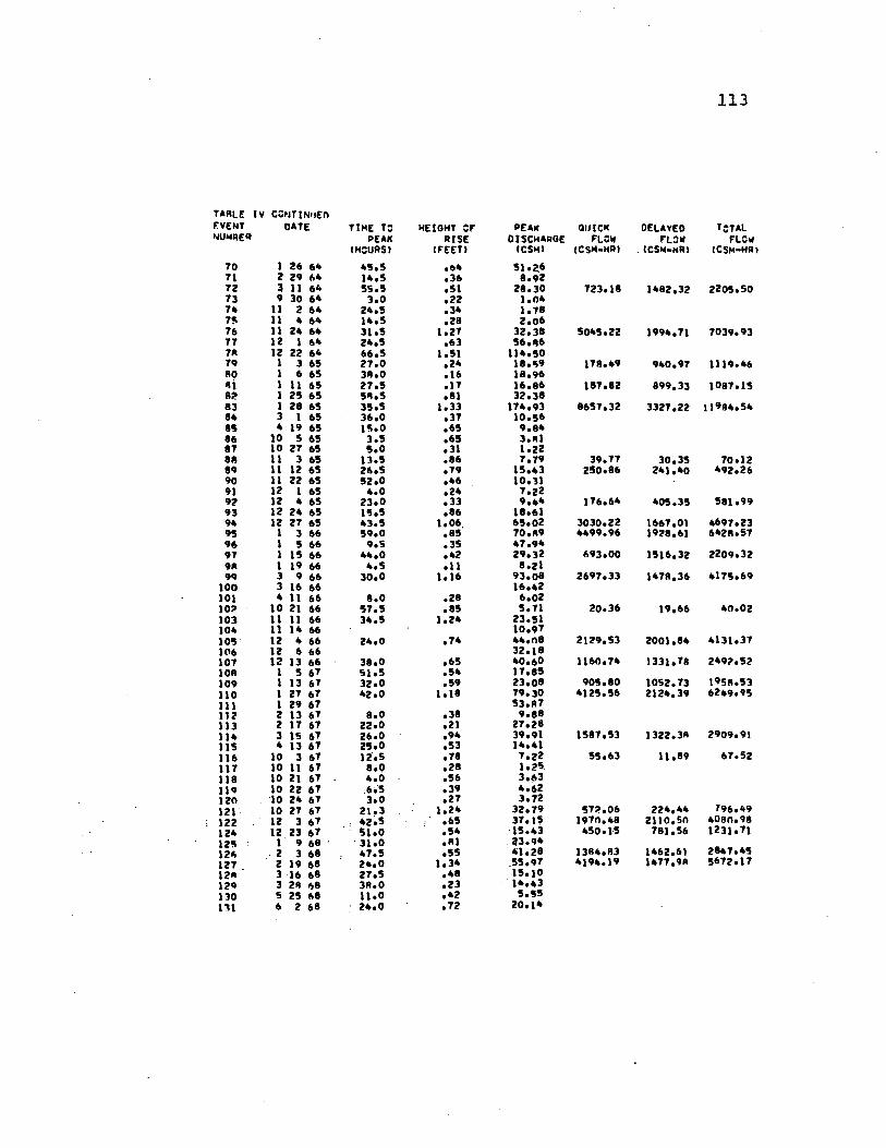
'02S

otc%

L%195pi6LL9%6%6%9lbSS

,'L992t9'299%9q9E%g2%9ipbt

95%9Lçl'059

96U80'Q0%9qULb%ç11E

64,96Lq9U90L56L2EEL E

9

25L969'%%£955

16b062WE22t%t5L951%6'bE92 1299 6lCS

5669296E92%Z9552%9OE6L

CSS6tE1250%O906gOtZ59

2sb9Z81'%ECt9L'09%%0909g%ZE

IC%C%91002£SbZ9U991601SCZ

20099CO2115

20 9

69'5Lt9EtIl£t'169290t6

ZE6OZZ2E9%S%00E6926Z

L592991996%96666W.01

£VL69't0L99lZVOE0E20S9

66' 1955C50999l%22 I1L01

922690%9Z99052

Z%OLSCOEII6C6LL2ZI

60%

9ç.qU ZELZCC2E1599£6L%gt2C

St'L90%£t66929L9%96 91

996%1%L6'09661P91%OS'91 I9b 9S

C66C0L%L,66%2Z'59059E2C9091' 11p0%

OSS0ZE2E299%9%'CEL0C9226 99? 15

IbHS3tdHW53tbS3)1133i)tSdflH)

M1i39VH3SlO3Slbb3UMflN

11LL03A%30s3lFlD)193dLHDl34L 34lI31901N3AU3IINlLt3 Al1iL

ZL092g9 29

oU99 52OU

£2.0E99 92 C*2%

99 91 C99 61 212%

5L99E292%

O%E.99 6%52%

o%519 CE 2%92%

ç2919 C2%22%

19 12 0112%

LVOE19 92 01.

6Eç919 22 01*11

95'.o19 12 0%

O'919 1% 0%11%

19 £01911

CS'O5219 Cl 9

09Z19 SI C

OU19 1% 2£11

o'919 Cl 219 62 1

02919 12%011

02E19 £1%60%

p5%S19 5%80%

o9C99 Cl 2%101

99921

91'092921.50%

99%90%

1p2159C99 1% 1%£01

99 12 010%

920999101

999%t00%

00E99 6C*6

99 6%186

09 51 199S196

0659Sb

S9 12 2%96

92 21

OEES9 92126

9 12116

o259 22 U06

61'5929 21 1%69

9959 C11

9 12 0119

5'tç9 cot

O159 61 9

09E59 1C

tt'%çSC59 92 1£9

s95S9 52 1

5L259 111

91OWE59 9108

O'LZ59 C161

5999 U 2181

E9592912%LI

LVIç%C99 92 1%1

91

5929 21%91

ZZ0C9 DC 6£1

9EL

9E59%99 62 2IL

9 92 101

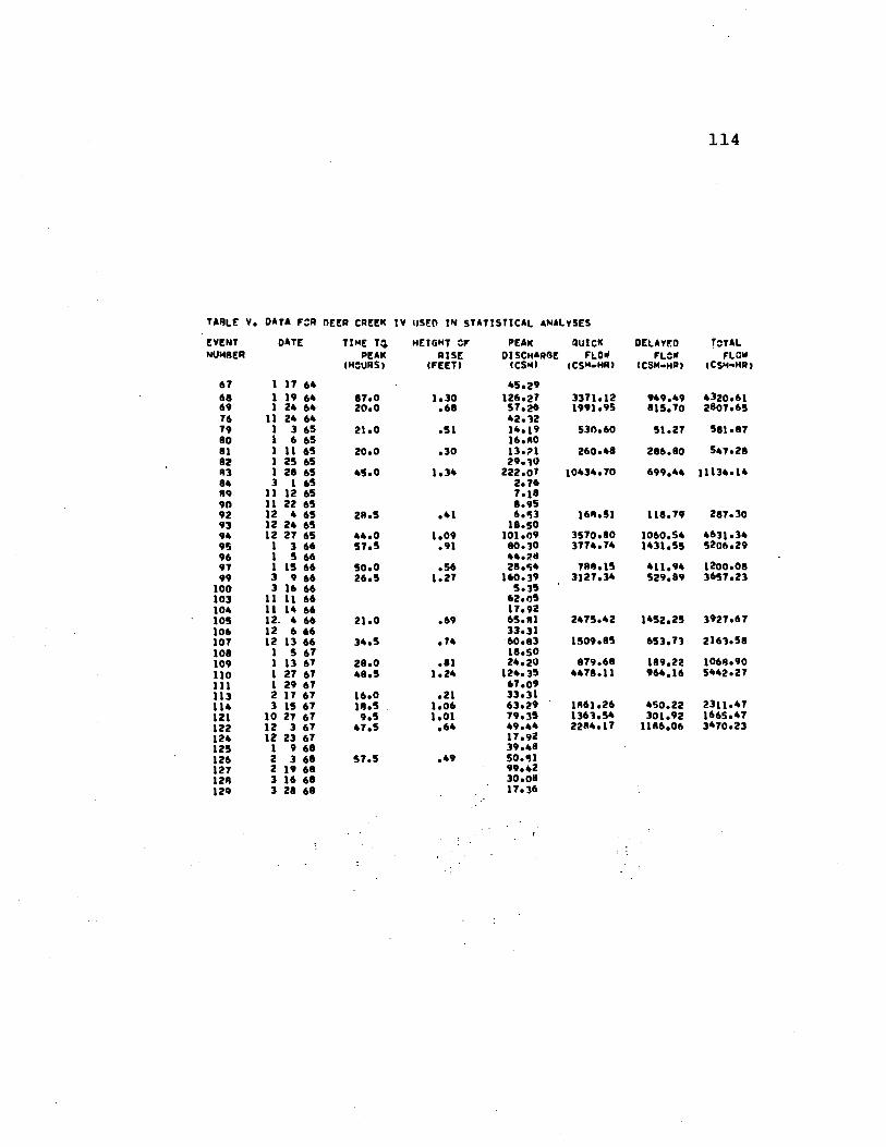
114

TABLE V. DATA FR DEER CREEK TV USED TN STATISTICAL ANALYSES

EVENT NUMBER

67

DATE

1 17 64

TIME T PEAK (HCURS)

HEIGHT F RISE (FEET)

PEAK DISCHARGE

(CSM)

45.29

GUICK FLC

(CSH.HR)

DELAYED FLDW

(CSM-HB)

TCTAL FLCW (CSHHR)

68 1 19 64 87.0 1.30 12A.27 3371.12 949.49 4320.61 69 1 24 64 20.0 .68 57.26 1991.95 815.10 2807.65 76 11 24 64 42.12 79 1 3 65 21.0 .51 14.19 530.60 51,27 581.87 80 1 6 65 16.80 81 1 11 65 20.0 .30 13.?1 260.48 286.80 547.28 82 1 2S 65 29.10 83 1 28 65 45.0 1.34 222.07 10434.70 699.44 11134.14 84 3 1 65 2.76 8 11 12 65 7,18

90 11 22 65 8.95 92 12 4 65 28.5 .41 6.53 168.51 118,7w 287.30 93 12 24 65 18.50 94 12 27 65 44.0 1.09 101.09 3570.80 1060.54 4631.34 95 1 3 66 S7.S .91 80.30 3774,14 1431.55 5204.29 96 1 5 66 44.2 97 1 15 66 SO,0 .56 28.54 788,15 411.94 1200,08 99 3 9 66 26.S 1.27 160,39 3127.34 529.89 3657.23 100 3 16 66 5.35 103 11 11 66 62.05 104 11 14 66 17.92 105 12- 4 66 21.0 .69 65.81 2475,42 1452,25 3927.67 106 12 6 66 33,31 107 12 13 66 34,5 .74 60,83 1509.85 6S3,71 2161.58

108 1 S 67 18,50 109 1 13 67 28.0 .81 24.20 879.68 189.22 1068.90

110 1 27 67 48,S 1,24 124.35 4418,11 964.16 5442,27 111 1 29 67 67.09 113 2 17 67 16.0 .21 33.31 114 3 15 67 18,5 1,06 63.29 1861.26 450.22 2311.47 121 10 27 7 9,5 1.01 79.35 1361.54 301.92 1665.47

122 12 3 67 47.5 .64 49.44 2284.17 1186.06 3470.23

124 12 23 67 17.92 12S 1 9 68 39.48 126 2 3 68 57.5 .49 50.51 127 2 19 68 99.42 128 3 16 68 30.08 12q 3 28 68 - 17.36

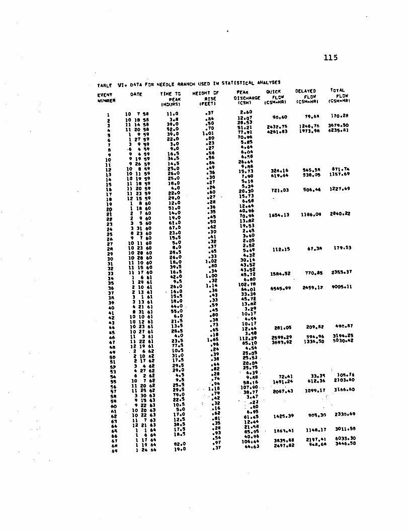
115

NEEDLE RRANCM USED IN STATISTICAL ANALYSES TARL!

EVENT NUNRER

VI. DATA R

DATE TIME TD HEIGHT CF PEAK QUICK

PEAK RISE DISCHARGE FLCW (HCURS) LFEET) (CSM) (CSM.HR)

DELAYED FLCW (CSM.HR

TCTAL FLCW (CSMHR

10 7 38 11.0 .37 2.60 170.28 2 10 1$ 58 3.8 .84 12.01 90,60 79,68

3 4 3

11 14 58 11 20 58 1 9 59

39.0 52.0 39.0

.30

.70 1.01

51.21 77.91

2432.15 4261.83

1246.76 1973.98

3619.50 6235.81

6 1 27 59 22.0 .80 70.96 7 3 9 59 3,0 .23 5.85 8 .6 439 9,0 .27 4.64 9 9 439 16.3 .56 6.04 10 9 19 59

9 26 59 34.5 14.5

.56

.84 6.58 26.44

12 13 14

10 S 39 10 11 59 10 19 59

23.0 26.0 25.0

49 .36 .30

9,8 13.73 7.90

326.16 619.64

54558 538.05

871.14 1157.69

15 11 18 59 18.0 .27 5.16 16 17

11 20 39 11 23 59

4.0 22.0

.24

.60 5,34 20.30 721.03 506,46 1221.49

is 12 15 59 29.0 .27 -

15.73 19 1 $ 60 12.0 .28 6.58 20 1 1$ 60 51.0 .36 12.44

40.96 21 22 23

2 7 60 2 9 60 3 5 60

14.0 19.0 61.0

.35

.45

.50 10,96 13.82 19.53

1654.13 1186.09 2840.22

24 3 31 60 67.0 .62 25 26 27

$ 23 60 9 7 60 10 11 60

23.0 15.5 5.0

.30

.41

.32

2.45 3,40 2.05 2.52 28

29

10 23 60 10 2$ 60

8.0 28.5

.37

.45 5,49 4,32

112.15 67.38 119.53

30 31

32 33

10 2$ 60 11 10 60 11 15 60 11 17 60 1 6 61

26,0 18.0 39.5 16.5 42.0

.33 1.02 .80 34 1.00

30.14 43,52 43,52 45,72 1584.52 170,85 2353.37

35 36 37 38 39 40

1 29 61 2 10 61 2 13 61 3 1 61 3 13 61 4 21 61

9.5 26.0 16.0 15.5 18.0 44.0

.32 1.14 .36 ,43 .33 .59

6.80 102.7$ 64.01 33,36 45.1Z 13.82 3.29

6545.99 2459.1? 9005.11

41 42

$ 31 61 10 10 61

55.0 6.0

.45

.80 10.17 4,54 43

44 45

10 12 61 10 23 61 10 27 61

21.5 13.5 28.5

,3$ .13 ,63

10.11 12.44 2$l.05 209.8? 490.87

4 47 48 49 so

11 3 61 11 22 61 12 19 61 .2 662 2 10 62 2 11 62

4.0 z3,5 71.5 10.5 31.0 17.5

.18 1,65 .96 .24 .39 38

112.29 63.10 4,54 25.05 25.53

2599.29 3693.92

594,9 1336.50

3194.25 5030.42

5; 3 4 62 4 27 62

29.5 29.0

.44

.82 20.04 25.15

53 36 57

6 262 10 1 62 11 20 62 11 25 62 3 30 63

91563

4.5 9.5 25.5 29.5 19.0 22.5

.2$

.14

. .

1,18 ,9 .42

4,39 9.88 5$.16 107.90. 3$,71 3,41 .23

12.41 1491.24

2061.43

33.35 612.36

1099.17

103.16 2103.60

3166.60

60 92263 10 20 63

iO.5 5.0

32 16 0

6.95 62 61 64

10 22 63 11 7 63 12 21 63

17.0 12.5 38,5

.62

.3S 61,45 12.44

1423.39 905.30 2330.69

65 66 67 68 69

1 1 64 1 6 64 1 11 64 1 19 64 1 24 64

11.5 i.5

82,0 19.0

.28

.93

.54

.91

.31

85.95 40.96 106.44 44.63

1861.41

3833.88 2491.82

1148.11

2197.41 948,68

3011.58

6033.30 3446.50

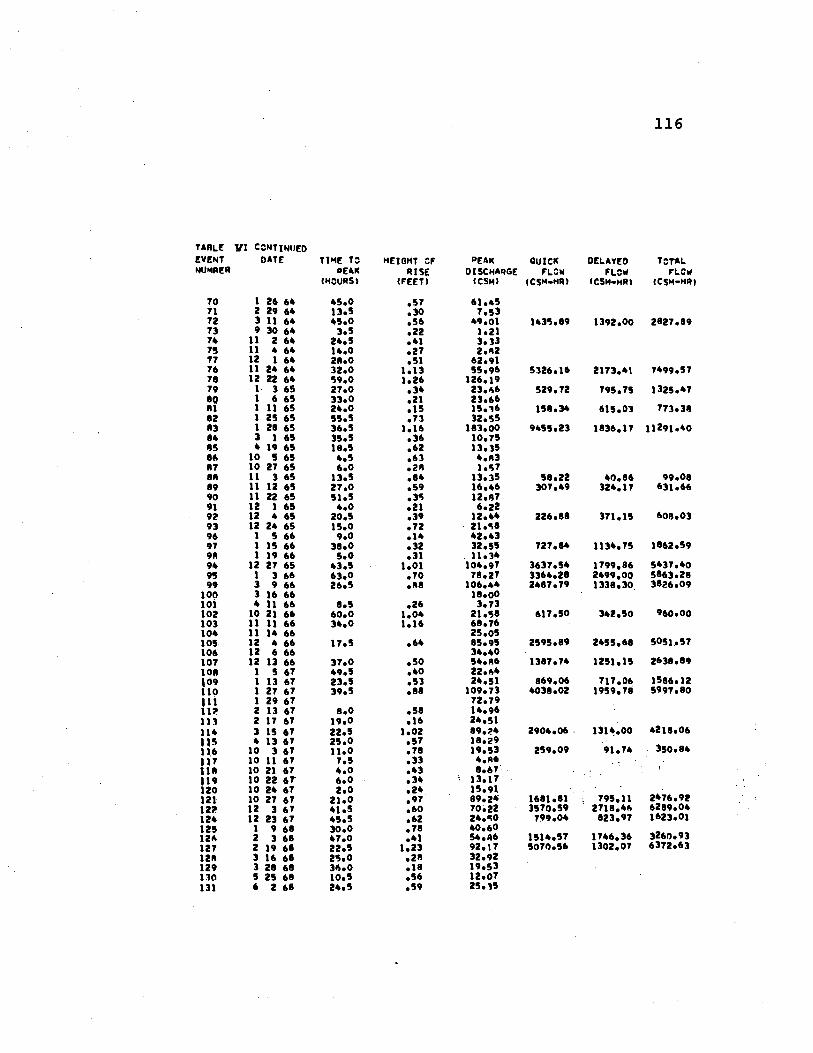
116

TARLE tf! CCNTINII(D

EVENT DATE NUMPER

To 1 26 64

TIME T

PEAK (HOURS)

43.0

HEIGHT RISE (FEET)

,57

PEAK DISCHARGE

(CSHI

61.S

QUICK LCW (CSM-HR)

DELAYED LCW (CSH-HR

TCT*L FLOW (C5M-P$R)

71 2 29 64 13.5 .30 7,3 72 3 11 64 43.0 .56 49.01 1435.89 1392.00 2827.89 73 9 30 64 3.5 22 1.21 74 11 2 64 24.3 .41 3.33 75 11 4 64 14.0 .27 2.62 77 12 1 64 28.0 .31 62.91 76 11 24 64 32.0 1.13 55.96 5326.16 2173,41 7499.57 78 12 22 64 39.0 1.26 126.19 79 1 3 65 27.0 .34 23.66 529.72 795,75 1325.47 80 1 6 65 33.0 .21 23.66 81 1 11 65 24.0 .13 13.16 158.34 615,03 773.38 82 1 25 65 33.3 .73 32.53 83 1 28 65 36.5 1.16 183.00 9455.23 1836.17 11291.40 84 3 1 65 33.5 .36 10.73 83 4 19 63 18.5 62 13.35 86 10 5 65 4,5 .63 4.R3 87 10 27 63 6.0 .28 1.57 88 11 3 65 13.5 .84 13.35 58.22 40.86 99.08 89 11 12 65 27.0 .59 16.46 307.49 324,17 631.66 90 11 22 65 31.5 .33 12.87 91 12 1 65 4.0 .21 6,22 92 12 4 65 20,5 .39 12.44 226.88 371.15 608,03 93 12 24 65 13.0 .72 21.38 96 1 5 66 9,0 .14 42.43 97 1 15 66 38.0 32 32.55 727.84 1134.75 1862.59 98 1 19 66 3.0 .31 11.34 94 12 27 65 43.5 1.01 104.97 3637.54 1799,86 5437,40 95 1 3 66 63.0 .70 78.27 3364.28 2499,00 3863.28 99 3 9 66 26.3 .88 106.44 2487.79 1338.30. 3826.09 100 3 16 66 18.00 101 4 11 66 8,5 .26 3.73 102 10 21 66 60.0 1.04 21.58 617.30 342,50 960.00 103 11 11 66 34.0 1.16 68.76 104 11 14 66 25.05 105 12 4 66 17,3 .64 83.95 2595.89 2455,68 5031.37 106 12 6 66 34.40 107 12 13 66 37.0 .50 54.R6 1387.74 1231.15 2638.89 108 1 5 67 49.5 .40 22.A4 09 1 13 67 23.5 .53 24.31 869.06 717.06 1386.12 110 1 27 67 39,3 .88 109.73 4038.02 1959.78 5997.80 ll 1 29 67 72.79 112 2 13 67 8.0 .38 14.96 113 2 17 67 19.0 .16 24.51 114 3 15 67 22,5 1.02 89,24 2904,06

.

1314,00 4218.06 I1 4 13 67 23.0 .57 18.29

116 10 3 67 11,0 .78 19.53 239.09 91.74 .

350,84 17 10 11 67 7.5 ,33 4,R6

. 118 10 21 67 4.0 .43 8.67

. . 19 10 22 67 6.0 .34 13.17 120 10 24 67 2.0 ,24 13.91 .

121 10 27 67 21.0 .97 89.26 1681.81 793.11 2476.92 122 12 3 67 41.5 .60 70.22 3370.39 2718.46 6289.04 124 12 23 67 43.5 .62 24.50 799.04 823.97 1623.01 125 1 9 68 30.0 .78 40,60 126 2 3 68 47.0 .41 34.66 1314.37 1746.36 3260.93 127 2 19 68 22.5 1.23 92.17 3070.56 1302.07 6372.63 128 3 16 68 23.0 .28 32.92 129 3 28 68 36.0 .18 19.53 110 3 23 68 10,3 .56 12.07 131 6 2 68 24,5 .39 25.iS

Documents

in to - Oregon State University in storm... · Changes in Storm Hydrographs due to Clearcut Logging of Coastal Watersheds By Warren Charles Harper A THESIS submitted to Oregon State