BREADibread.org/bread/system/files/bread_wpapers/239.pdfIn this context voter education and informational campaigns are becom-ing popular with donors. We followed a large-scale randomized

POLITICAL VIOLENCE AND SOCIAL NETWORKS:

EXPERIMENTAL EVIDENCE FROM A NIGERIAN ELECTION

MARCEL FAFCHAMPS

PEDRO C. VICENTE

BREAD WORKING PAPER No. 239 JULY, 2009

BREAD Working Paper

Bureau for Research and Economic Analysis of Development

© Copyright 2009 Marcel Fafchamps and Pedro C. Vicente

Political Violence and Social Networks:

Experimental Evidence from a Nigerian Election�

Marcel Fafchamps

University of Oxfordy

Pedro C. Vicente

Trinity College Dublinzand CSAE

July 2009

Abstract

Political accountability and participation are taken as key ingredients for devel-

opment. In this context voter education and informational campaigns are becom-

ing popular with donors. We followed a large-scale randomized campaign against

electoral violence sponsored by an international NGO during the 2007 Nigerian

elections. Substantial direct e¤ects on perceptions about violence and voting be-

havior are reported for this campaign. This paper is devoted to the assessment of

�We thank Oriana Bandiera, Paul Collier, Donald Green, Macartan Humphreys, Craig McIntosh, Bi-lal Siddiqi, and seminar participants at CERDI, CSAE-Oxford, and EGAP-Yale for helpful suggestions.Sarah Voitchovsky provided superb research assistance. We are particularly grateful to Ojobo Atukulu,Otive Igbuzor, and Olutayo Olujide at ActionAid International Nigeria, Austin Emeanua, campaignersNwakaudu Chijoke Mark, Gbolahan Olubowale, George-Hill Anthony, Monday Itoghor, Umar Farouk,Emmanuel Nehemiah, Henry Mang and their �eld teams, and to the surveyors headed by Taofeeq Akin-remi, Gbenga Adewunmi, Oluwasegun Olaniyan, and Moses Olusola. We also want to acknowledge thekind institutional collaboration of the Afrobarometer. We wish to acknowledge �nancial support fromthe iiG Consortium - �Improving Institutions for Pro-Poor Growth�. All errors are our responsibility.

yDepartment of Economics, University of Oxford, Manor Road, Oxford OX1 3UQ, UK. Email:marcel:fafchamps@economics:ox:ac:uk. Fax: +44(0)1865-281447. Tel: +44(0)1865-281446.

zDepartment of Economics, Trinity College, Arts Building, Dublin 2, Ireland. Email:vicentep@tcd:ie. Fax: +353(0)1-6772503. Tel: +353(0)1-8963478.

the network e¤ects of this intervention. Comprehensive measurement of the links

between households allows us to estimate reinforcement e¤ects on the treated sub-

jects in campaign locations, and di¤usion e¤ects on untreated subjects in campaign

locations. These e¤ects are derived with reference to suitable comparison groups

in untreated locations. We �nd evidence for both network e¤ects using di¤erent

estimation techniques. Namely, we document the importance of kinship and geo-

graphical distance in spreading perceptions associated with the campaign. We do

not �nd clear network e¤ects on behavior.

1. Introduction

Democracy is notoriously di¢ cult to implement in Africa. For it to deliver politicians

that seek to improve the welfare of the masses, it is central that citizens are better

informed and vote according to policy-accountability. Yet it is only too easy for politicians

to seek votes by stirring up greed, rivalry, or fear. Using �eld experiments in Benin

and Sao Tome and Principe respectively, Wantchekon (2003) and Vicente (2007) study

greed: they show that politicians attract more votes by using clientelistic and vote-buying

platforms. The study of rivalry has been centered on the use of ethnic divisions in politics.

Posner (2004) uses a natural experiment in the border of Malawi and Zambia to prove

that ethnic identi�cation is endogenous to political conditions. This �nding is reinforced

by Habyarimana, Humphreys, Posner, and Weinstein (2007) using lab experiments in

Uganda, and by Eifert, Miguel, and Posner (2009) using Afrobarometer data across ten

African countries. In this paper we focus our attention on the use of fear in elections.

In this context, the fundamental question we face is: what can be done to reduce

2

the role of malfeasant electoral strategies like vote-buying, ethnic polarization, or violent

intimidation? Vicente (2007) shows that a campaign against vote-buying is e¤ective in

reducing the e¤ect the practice has on voting behavior. In a similar vein, Collier and

Vicente (2009) use a �eld experiment and show that an awareness campaign encouraging

Nigerian voters to oppose electoral violence was successful in reducing perceptions of local

violence and margins of related behavior.1 The campaign also a¤ected voting behavior

by increasing turnout and reducing the electoral score of non-incumbent candidates.

If awareness campaigns can successfully reduce the role of malfeasance in voting be-

havior, this raises other questions, such as what proportion of the population must be

reached for a campaign to be successful. It is indeed onerous and, in many cases, infea-

sible for an awareness campaign to target everyone. One would therefore like to know

whether individuals not directly exposed to an awareness campaign nevertheless report

perception and behavioral changes similar to those of exposed individuals as the message

di¤uses through social networks. We call this a di¤usion e¤ect. It is also possible that

community members directly exposed to the message of a campaign may have the impact

of that campaign reinforced by interaction with their peers. We call this a reinforcement

e¤ect.

This paper provides a partial answer to these two questions using a �eld experiment

speci�cally designed to evaluate the di¤usion and reinforcement of an anti-violence mes-

sage among voters. We study the e¤ects of an informational campaign against political

1Perception and behavioral e¤ects of broadcasting information on violence and crime are studied byDellavigna and Kaplan (2007) and Dahl and Dellavigna (2009). The �rst reports on paranoia e¤ects ofstressing information related to terrorism. Perhaps due to the nature of an anti-violence campaign, theNigerian campaign this not induce the same kind of impact.

3

violence, undertaken nationwide in Nigeria before the 2007 elections. It worked primar-

ily through town meetings and popular theatres, as a way to decrease collective action

costs for counteracting violence. For the estimation of our e¤ects of interest, we collected

information about social network links and geographical distance between households in

targeted and control groups within treatment villages, and in groups within control vil-

lages. To test for the presence of a reinforcement e¤ect, we examine whether the e¤ect

of the message on the perceptions and behavior of targeted households is reinforced by

proximity to other exposed households. To investigate di¤usion within a village, we test

whether households not directly exposed to the campaign show e¤ects similar to exposed

households with whom they have close social ties.

Results provide some evidence of both reinforcement e¤ects. Findings suggest that

the impact of the campaign on perceptions of community violence and feelings of intim-

idation is reinforced by social and geographical proximity to other exposed households.

What seems to matter most is kinship �i.e. family relationships �although geographi-

cal proximity is also signi�cant. We however �nd little reinforcement e¤ect on behavior

�either in terms of voting behavior or in terms of willingness to express opposition to

electoral violence.

We also �nd evidence of di¤usion to unexposed households. For perceptions of commu-

nity violence and intimidation, the di¤usion e¤ect nearly perfectly mimics the reinforce-

ment e¤ect: the sign, signi�cance, and magnitude of the coe¢ cients are similar. We �nd

a signi�cant externality of the campaign on households�willingness to express disapproval

of electoral violence, but unclear e¤ects on voting behavior per se. Because self-reported

exposure to the anti-violence campaign may be subject to self-selection, we investigate

4

the robustness of our results with respect to selection on observables or unobservables.

Similar �ndings obtain.

Our estimation of network e¤ects in the context of a randomized �eld experiment

relates to a recent body of literature on the role of networks in aid interventions. Kremer

and Miguel (2004) launched this literature by estimating externalities of a deworming

school-based programme in Kenya. They estimated the impact of the treatment on control

populations. Because their design featured programme randomization at the school level,

this did not allow for an experimental estimation of individual externalities within treated

schools. More recently, Angelucci, DiGiorgi, Rangel, and Rasul (2009) extend the study

of externalities to a conditional cash transfer programme. By exploring a rich set of

outcomes at the household level they are able to draw light into speci�c mechanisms of

in�uence of unexposed households. These authors do not use explicit network variables,

however. Still in the context of a conditional cash transfer programme, Macours and Vakis

(2008) extend the literature by introducing explicit interaction among households. But

they only estimate reinforcement e¤ects and do not have individual variation in networks.

The work by Nickerson (2008) relates most closely to our study: his focus is on using door-

to-door randomized get-out-to-vote campaigning to identify peer-e¤ects in two-member

households. Our result that kinship proximity is more important than other measures

of social interaction is similar to the results of Bandiera and Rasul (2006) who study

technology adoption in Mozambique in a non-experimental setting.

The paper is organized as follows. In Section 2 we begin by providing a rapid de-

scription of the context in which our study takes place. The �eld experiment and testing

strategy are presented in detail in Section 3. The data and descriptive statistics are dis-

5

cussed in Section 4. Subsequently, in Section 5, empirical results are presented, with

corresponding robustness tests. Section 6 concludes.

2. Context

Nigeria, the most populous country in Africa with estimated 146 million inhabitants2, has

been challenged by persistent development problems. Despite holding the largest proven

oil reserves in Sub-Saharan Africa (10th largest in the world3), Nigeria ranks 201 in 233

countries in terms of GDP per capita (1400 USD PPP in 20054). Moreover, it has been

seen as a textbook-example of bad governance: Nigeria has continuously featured among

the most corrupt countries in the world (see Transparency International). Clearly, one

can only understand this state of a¤airs if one deepens the study of politics in Nigeria:

in the words of Chinua Achebe (1983), �the trouble with Nigeria is simply and squarely

a failure of leadership�. From independence in 1960, Nigeria faced enormous political

instability and, for most of the time, military rule. However, in 1999, a new constitution

was passed and civilian rule was adopted. Elections were run in 1999, 2003, and 2007.

Despite formally marking the transfer of political power, these elections were in�uenced

by widespread vote-buying, ballot-fraud, and violent intimidation. Most observers have

seen these elections as being far from �free and fair�.

The focus of our attention is the 2007 su¤rage. In April of that year, elections were run

for all the federal and state-level political bodies (president, federal house of representa-

2CIA World Factbook 2009.3Oil & Gas Journal, 103(47), December 19th, 2005.4World Development Indicators.

6

tives, and senate; state governors, and assemblies).5 The election was highly anticipated

because it marked the �rst transfer of presidential power from one civilian to another:

Olesegun Obasanjo was stepping down as president due to a two-term limit, and the

main contestants were Umaru Yar�Adua from PDP, Muhammadu Buhari from ANPP,

and Atiku Abubakar from AC. Yar�Adua was seen as a protégé of Obasanjo, clearly the

front-runner due to the overwhelming in�uence of the ruling party PDP. Buhari had been

the main challenger in 2003, was strongly associated to the Muslim North, and had an

anti-corruption track-record. Finally, Abubakar, the vice-president of Obasanjo, and a

former customs o¢ cial with controversial sources of wealth, was very much on the news

because of corruption accusations that almost impeded him from running; he was led to

switch to AC due to a con�ict with Obasanjo.

PDP easily won the 2007 elections: Yar�Adua secured 70% of votes, and PDP candi-

dates were able to sweep 28 out of the 36 gubernatorial races. The elections were seriously

marred by ballot-fraud and violence. Electoral observers, most notably the European

Union mission, and Transition Monitoring Group (which deployed 50,000 observers) were

unanimous in underlining numerous irregularities in the conduction of the su¤rage. Both

were clear in stating that the elections were not credible and fell far short of basic in-

ternational standards. Human Rights Watch, in a report released in May 20076, writes

�[ ... ] violence and intimidation were so pervasive and on such naked display that they

made a mockery of the electoral process. [ ... ] Where voting did take place, many voters

stayed away from the polls. [ ... ] By the time voting ended [on the election days], the

5Elections at the state and federal levels took place on two separate su¤rage days.6Human Rights Watch, �Nigerian Debacle a Threat to Africa�, May 2007.

7

body count had surpassed 300�. This violence was identi�ed by Human Rights Watch

to be originated from marginalized political groups, many of which dissidents formerly

associated to PDP7. On the ground, this hostility emerged in the form of assassinations

of known politicians, but mainly as locally-widespread intimidation, usually conducted by

armed gangs, recruited among the young and unemployed. This is the context in which

we ran our �eld experiment to which we now turn.

3. Experimental design

In anticipation for the 2007 elections ActionAid International Nigeria (AAIN) launched a

nationwide campaign against electoral violence in February 2007. AAIN is the local chap-

ter of a major international NGO specializing in community participatory development,

with a wide and experienced �eld-infrastructure in the country. AAIN�s campaign encour-

aged voters to resist intimidation and to participate in the elections. It also intended to

persuade voters to punish violent candidates by voting against them. The main theoreti-

cal rationale of the campaign was to improve collective action in counteracting electoral

violence at the local level. The analytic foundation for this aspect of the campaign is the

model of political protest of Kuran (1989), where a public call to a common protest lowers

its costs and makes it easier to resist intimidation. The campaign also worked through

the provision of information about ways to counteract violence: by calling voters to deny

their vote to perpetrators of violence, the campaign incited the population to reconsider

the meaning of their vote and the value of the di¤erent candidates.

7Human Rights Watch, �Criminal Politics: Violence, �Godfathers�, and Corruption in Nigeria�, October2007.

8

Campaign sta¤toured villages and urban neighborhoods organizing town meetings and

street theatres to sensitize voters to the campaign message. They also distributed lea�ets,

posters, and items of clothing bearing an anti-violence message, the purpose of which was

to reinforce and disseminate the message further.8 A poster from the campaign is shown

in Figure 1. Our survey shows that 89% of the households approached by campaigners

received at least one item of clothing (e.g., t-shirt, cap, hijab), 83% received at least one

written material (e.g., lea�et, sticker, poster), and 71% attended a public event orga-

nized by the campaign (e.g., community meeting, popular theatre, roadshow). To avoid

possible self-selection bias, data on compliance are not used in the analysis. Households

that were approached by campaigners are regarded as �treated�, irrespective of whether

they accepted campaign materials or participated to campaign events. Consequently, our

analysis is probably best construed as measuring �intent-to-treat�e¤ects.

We conducted a �eld experiment in collaboration with AAIN, the campaign organizer,

who agreed to randomize their campaign across locations. The campaign was conducted

in six states covering the three main socioeconomic regions of Nigeria: Lagos and Oyo in

the Southwest; Kaduna and Plateau in the Middle-Belt/North; and Delta and Rivers in

the Niger Delta. These states were chosen because they have a history of recent political

violence.9 Within each of the selected states, two pairs of nearby enumeration areas (EA)

were selected randomly from a large and representative sample assembled for the 2007

Afrobarometer survey of Nigeria.10 We started by selecting twelve villages and urban

8For details on this campaign, see http://www.iig.ox.ac.uk/research/08-political-violence-nigeria/default.htm.

9Selection is based on reports from earlier elections, such as Human Rights Watch, �Testing Democracy:Political Violence in Nigeria�, April 2003.10The Afrobarometer sample is itself drawn from census data.

9

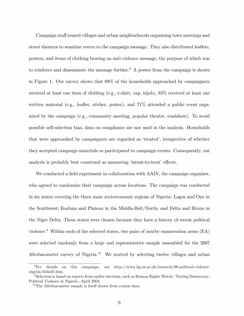
neighborhoods for treatment. We then identi�ed twelve control EA�s that are located

nearby and have the same o¢ cial urban-rural classi�cation. By design, treatment and

control EA�s are broadly comparable. Their approximate location is shown in Figure 2.

In both treatment and control EA�s, 50 randomly selected households were interviewed

for the baseline survey in January 2007 �immediately before the campaign. The total

number of respondents is 1200. The same respondents were resurveyed in May 2007,

shortly after the elections. We refer to these households as panel respondents. To facilitate

the evaluation of the direct impact of the campaign, all panel respondents in treated EA�s

were individually targeted by campaigners, i.e., they were o¤ered campaign materials and

were invited to town meetings and popular theatres organized by the campaign.

To study di¤usion, in each treated location we interviewed an oversample of 25 house-

holds not directly exposed to the anti-violence campaign.11 These were only interviewed

in the second survey round. The total number of oversample respondents is 300. They are

representative of the population that was not approached by campaigners. Both surveys

were designed and supervised in the �eld by the authors, using original questionnaires

pre-tested for the purpose of the experiment. Data collection was undertaken in direct

collaboration with Afrobarometer and its Nigerian partner (Practical Sampling Interna-

tional).

Since, by design, the experiment is meant to in�uence voting behavior primarily by

reducing the perceived threat of violence, the surveys were designed to gather information

about perceptions and voting behavior. Questions on perceived violence were asked in the

11In May 2007 randomly selected respondents were �rst asked if they had been approached by AAINcampaigners. Only those who answered no to this question were included in the oversample survey.

10

baseline prior to the campaign, focusing on a reference period (�the last year�). Similar

questions were again asked in the second survey, focusing on what had happened just

before and during the elections. In the baseline, questions on voting focus on intentions;

in the ex post survey, questions refer to actual voting behavior at the April 2007 elec-

tions, as reported by respondents. In addition, all respondents to the May 2007 survey

�panel and oversample �were asked about their social links to each of the 50 baseline

households. An approximate map of each surveyed EA was also draw with the location

of each respondent�s residence.

3.1. Testing strategy

We are interested in estimating the reinforcement and di¤usion e¤ects of the anti-violence

campaign. We proceed as follows. Let yivt denote a relevant outcome variable for indi-

vidual i in location/village v at time t = f0; 1g where 0 stands for baseline and 1 for

the post-election survey. Further let wiv = 1 if village v was selected for treatment and

let Tivt = 1 at t = 1 and 0 otherwise. The average treatment e¤ect of the campaign is

coe¢ cient � in the following regression:

yiv1 = � + �wiv + eiv1; (3.1)

or, equivalently:

yivt = � + �wivTivt + �wiv + Tivt + eivt; (3.2)

if we include baseline data. Given randomization, � in either of these equations provides

a consistent estimate of the average treatment e¤ect. Because of the small sample size,

11

however, it may be preferable to include individual �xed e¤ects uiv, which also control for

time-invariant village unobservables:

yivt = �wivTivt + Tivt + uiv + eivt (3.3)

Note that time-invariant regressors drop out of equation (3.3) after inclusion of the �xed

e¤ects. Estimating equation (3.3) by ordinary least squares yields the standard di¤erence-

in-di¤erences estimator. Equivalently, (3.3) can be estimated in �rst-di¤erence:

�yivt = �wiv + +�eivt (3.4)

In this paper we are not primarily interested in the average treatment e¤ect, which

is discussed in detail in Collier and Vicente (2009). Our focus is on reinforcement and

di¤usion through social networks. Let g denote a social network matrix where gij = 1

if i is linked to baseline household j in a way deemed relevant for our purpose. It is

important that gij be exogenous to the campaign itself. Remember that, by design,

all baseline households were visited by the campaign. We therefore postulate that the

in�uence of the campaign increases with the number of links respondents have to baseline

respondents.12 Formally, let eni = 150

P50j=1 gij. Following Wooldridge (2002) regarding

the estimation of heterogeneous treatment e¤ect models, we calculate the de-meaned

equivalent ni = eni � 1N

PNj=1 enj where N is total sample size.

12Given that all respondents in one EA are asked about the same 50 treated households, we are unableto distinguish whether in�uence comes from the number or the proportion of treated neighbors.

12

If we use only second round data, the estimated model takes the simple form:

yiv1 = � + �wiv + �wivni + �eni + eiv1 (3.5)

The parameter of interest is �, which measures the indirect in�uence on yiv1 of the social

proximity of individual i to individuals exposed to the anti-violence campaign. Given the

experimental design, these individuals can be seen as having been randomly exposed to

a speci�c message.

If we include time 0 information, the estimated model takes the form:

yivt = � + �wivTivt + �wivTivtni + �niTivt

+�niwiv + 'eni + �wiv + Tivt + eivt (3.6)

Expressing the equation in �rst di¤erence to get rid of individual �xed e¤ects, we obtain:

�yivt = �wiv + �wivni + �eni + +�eivt (3.7)

We also seek to test whether in�uence depends on geographical distance edij betweeni and j. Distance can be seen as de�ning a valued network. In�uence now depends on

how close respondent i is to other villagers, namely those exposed to the anti-violence

campaign. Let edi = 1K

PKj=1

edij, where K is the number of respondents in the same

location. Like before, the variable we use is the demeaned equivalent di = edi� 1N

PNj=1

edjwhere N is total sample size. We reestimate models (3.5), (3.6) and (3.7) with di and ediin lieu of ni and eni.

13

We conduct two di¤erent sets of comparisons. To test for the presence of a reinforce-

ment e¤ect associated with social or geographical proximity, we compare panel respon-

dents from control and treatment villages using models (3.5), (3.6) and (3.7). In these

regressions, the coe¢ cient � of the heterogeneous network e¤ect measures the extent to

which the e¤ect of the treatment wiv on the outcome variable yivt is magni�ed by proximity

with other individuals who have also been exposed to the anti-violence campaign. This re-

inforcement e¤ect can be viewed as a kind of social multiplier e¤ect by which the message

e¤ects are strengthened for the primary targets of campaigning through communication

with their networked individuals.

We also test whether the campaign message communicated directly to panel respon-

dents a¤ects residents of the same village who did not receive the campaign message di-

rectly. To this e¤ect we compare respondents in control villages �who were not a¤ected,

either directly or indirectly, by the campaign � to oversample respondents in treated

villages �who were not directly exposed to the campaign but were exposed indirectly

through other villagers. In this case, coe¢ cient � captures the externality that indirect

exposure to the campaign generates for all unexposed individuals in treated villages while

� can be regarded as measuring di¤usion of the e¤ect of the campaign through social

networks.

The comparison between panel respondents in control and treated villages poses no

particular problem, given that treatment was allocated randomly to matched pairs of vil-

lages. The comparison between oversample and control respondents is potentially prob-

lematic given that (non-)exposure to the campaign message within a treated village may

be correlated with respondent characteristics that also a¤ect the outcome variable yivt.

14

This is more a source of concern for � �the average treatment e¤ect �than for � �the

heterogeneous treatment e¤ect. Furthermore, it a¤ects models (3.5) and (3.6) more than

model (3.7) where the addition of respondent �xed e¤ects hopefully takes care of most of

the problem.13 In the next sections we deal with this issue the best we can given data

constraints. We begin by testing balancedness of the di¤erent sub-samples. Whenever

necessary, we introduce individual controls in models (3.5) and (3.6) to control for selec-

tion on observables. We also investigate the sensitivity of our results to the possibility of

selection on unobservables.

4. Data

Balancedness is investigated in Table 1 where we report baseline values for a wide range

of respondent characteristics. There is no noticeable di¤erence between panel households

in control and treated villages: only one variable is signi�cantly di¤erent at the 10% level,

a normal �nding given the number of variables considered. Attrition is not a serious

concern: 97% of control baseline respondents also answered the post-election survey; the

corresponding percentage for treated villages is 95%.

We also compare panel households in control villages with oversample households in

treated villages. Most characteristics are not signi�cantly di¤erent between oversample

and control households. There is, however, a small subset of variables for which bal-

ancedness does not hold: namely, schooling, religious intensity, and ownership of radios

(all higher in the oversample). We control for these variables in the subsequent analysis.

13Because oversample respondents could only be identi�ed ex-post, that is, after the campaign hadtaken place, another possible source of bias is recall bias. This issue is discussed in detail in the empiricalsection.

15

There is thus some evidence of selection into the oversample (respondents stating up-front

that they were not approached by AAIN campaigners). A possibility is that �more aver-

age�(e.g. less schooled) respondents over-reported campaign reach and this resulted in

them being left out of the oversample.

Two measures of social distance are used in the analysis. For the �rst one, a link

from i to j is assumed to exist if i could identify the name of j when prompted, and i

stated that he/she talks to j on a regular basis.14 We call this variable chatting. We also

construct another measure of social proximity, whereby a link from i to j exists if i can

identify j by name and reports being related to j.15 We call this variable kinship.

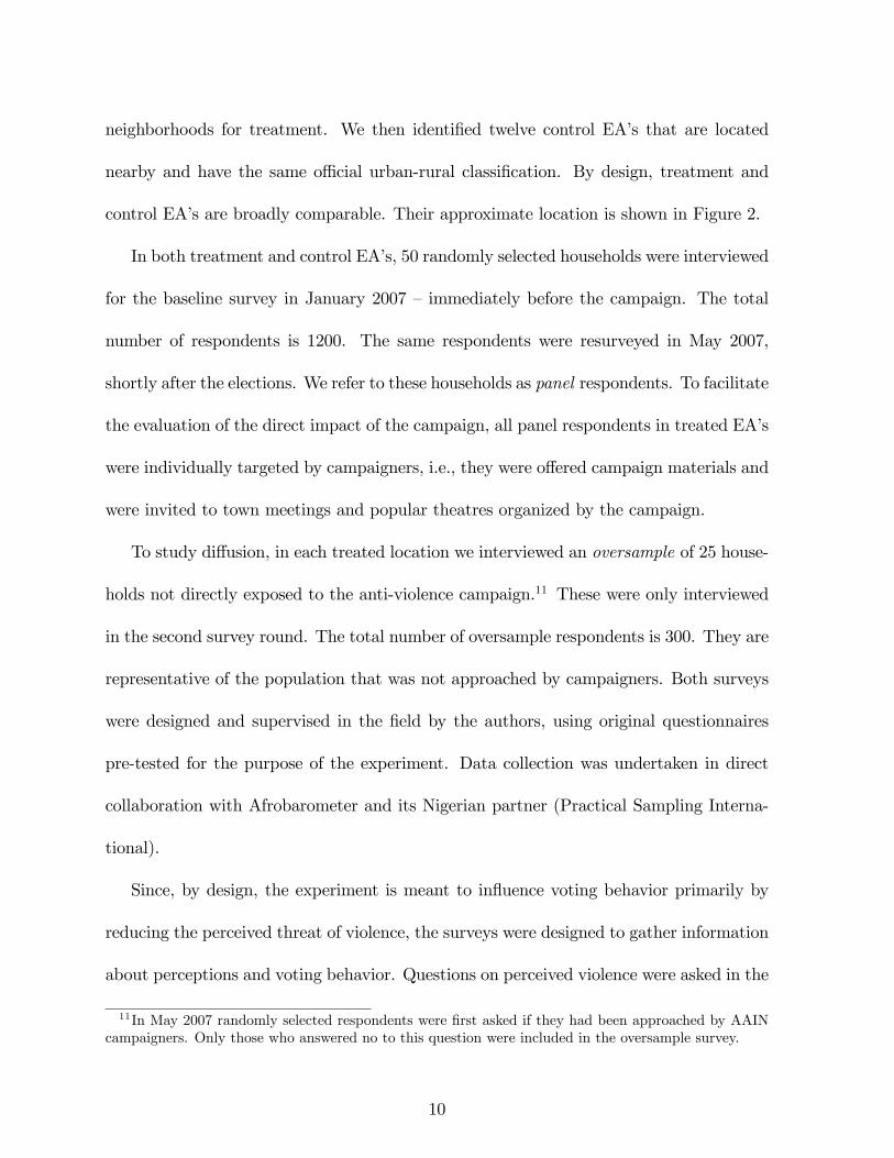
We also investigate the e¤ect of geographical distance between i and j, what we call

distance. Each enumerator was asked to locate each respondent and his/her itinerary on

an approximate EA map, and to calculate the distance between interviews. See Figure 3

for an example. To evaluate the position of each respondent on the map, we construct

up-down and left-right coordinates for each of them. The distance between each ij pair

is then calculated from these coordinates. Because maps di¤er in scale, distances are re-

scaled to make them comparable across all locations.16 The result of these calculations is

our variable edij, which is then used to compute edi, the average distance to all respondentsin the same location. As shown in Table 2 all network measures are balanced across

treatment and control groups.

In this paper, we focus our attention on �ve outcome variables. This concise set is

14The question asked was �How frequently do you calmly chat about the day events with the followingindividuals or members of their households? Not at all-Sometimes-Frequently�.15The exact question used was �Are the following individuals relatives of yours, i.e. members of your

family? Yes-No�.16This is accomplished by using the subset of pairwise distances reported by enumerators.

16

chosen because it captures the range of information collected in the survey �see Collier

and Vicente (2009) for details. The �rst two variables focus on respondents�perceptions

regarding violence. The �rst of these two, which we call violence, is the answer to the

question �In your experience, how often did violent con�icts arise between people within

the community where you live? Never-Always on a 0-4 scale�. Given the timing of the

surveys, it proxies for respondents� opinion of the severity of political violence within

the community. The second of the two, which we dub intimidation, is the answer to the

question �How often, if ever, have you or anyone in your family been physically threatened?

Never-Many times on a 1-4 scale�. Given its more precise wording, it can be regarded

as a proxy for the level of political intimidation experienced by respondents. Variables

violence and intimidation are scaled so that higher values correspond to worse outcomes.

The other three outcome variables of interest capture electoral behavior. The �rst,

which we name postcard, is an experimentally generated measure of political empower-

ment. Each respondent in the post-election survey was given a stamped postcard with

an anti-violence message, and encouraged to mail it to AAIN as manifestation of their

disapproval towards electoral violence. If the respondent mailed the postcard, the vari-

able postcard takes value 1. It was promised that if enough postcards were received from

the respondent�s state, AAIN would �ag that state in the media as facing electoral vio-

lence problems. This process mimicked petitioning, except that it was likely perceived as

anonymous. Even though it incurred no �nancial outlay for the respondent, sending the

postcard requires some e¤ort. This empowerment measure can therefore be regarded as

incentive-compatible.

The second behavior variable, which we call voting, takes value 1 if the respondent

17

voted for Atiku Abubakar, AC�s presidential candidate. This candidate was generally

associated with political instability. The third variable is voter turnout at the gubernato-

rial elections, which we name turnout. We focus on state-level elections because they are

arguably the most associated with political violence at the local level.

In Table 2 we present average perceptions of violence reported by treatment and

control households. For panel households, the data come from the baseline survey; for

oversample households, the data come from retrospective questins. We �nd no statistically

signi�cant di¤erence between treatment and control panel households. We do however

�nd a signi�cant di¤erence in the level of violence reported by oversample households, who

report a lower level of political violence at the time of the baseline. This may re�ect recall

bias �respondents underestimate their own perception of violence prior to treatment. We

do not, however, �nd evidence of a similar recall bias for other retrospective questions,

suggesting that recall bias may not be the reason. Alternatively, it may re�ect self-

selection out of treatment: households who perceived less violence avoided campaigners.

To address the possibility of recall bias, in the next Section we present regression results

based on second-round data only. Possible self-selection out of treatment among the

oversample households is addressed in the usual way, e.g., by including control variables

in the analysis to control for selection on observables, and by instrumenting selection into

the oversample to control for selection on unobservables. For comparison purposes, we

also include a measure of actual violence compiled by independent journalists.17 This

17These measures were gathered through the deployment of an independent journalist in each exper-imental location. These observers compiled diaries of violent events through the period covered by theexperiment (from the second semester of 2006 to the election aftermath in May 2007). See Collier andVicente (2009) for details.

18

shows no signi�cant di¤erence in political violence between treatment and control EA�s

prior to the campaign.

At the bottom of Table 2 we compare underlying electoral preferences across treatment

and control. The �rst four variables report electoral behavior at the 2003 elections. We

see no signi�cant di¤erence between control households and either panel or oversample

households. Baseline interest in politics also appears similar across both comparison

groups.

5. Empirical results

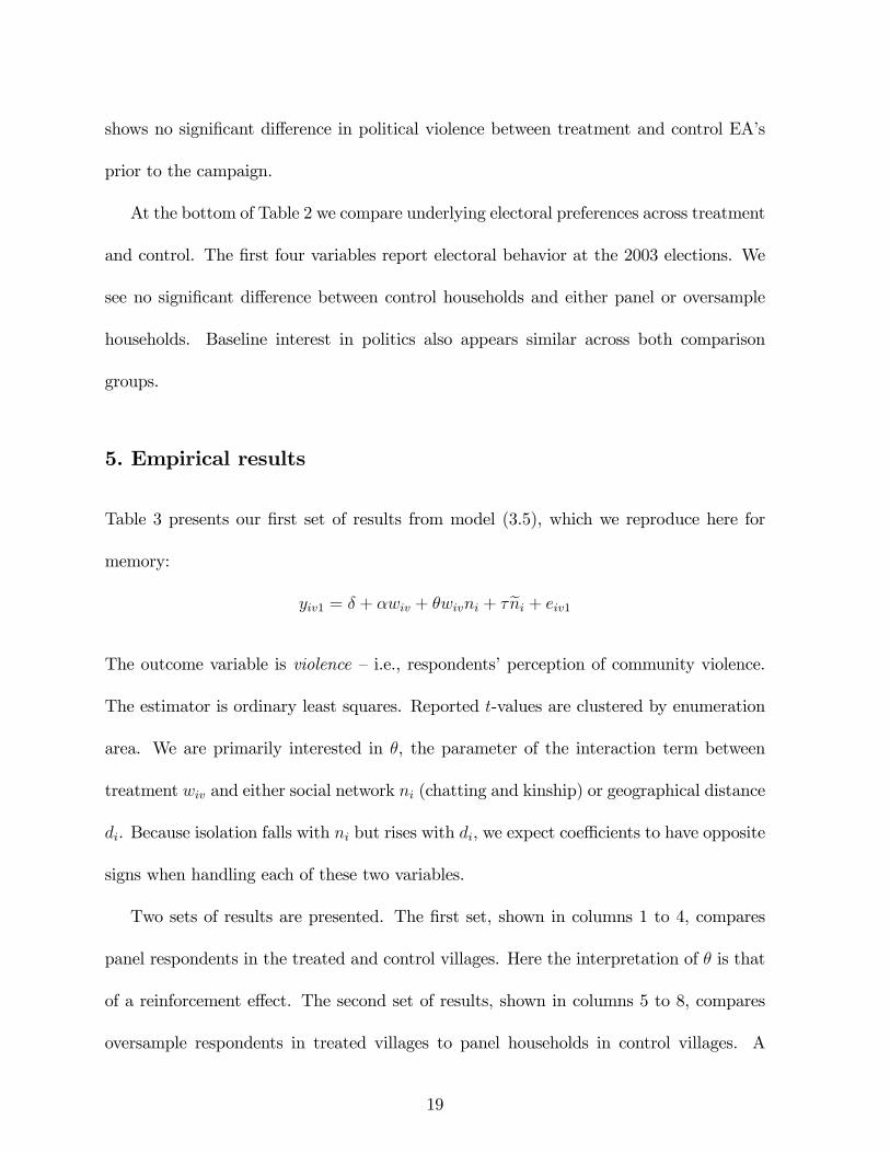
Table 3 presents our �rst set of results from model (3.5), which we reproduce here for

memory:

yiv1 = � + �wiv + �wivni + �eni + eiv1The outcome variable is violence �i.e., respondents�perception of community violence.

The estimator is ordinary least squares. Reported t-values are clustered by enumeration

area. We are primarily interested in �, the parameter of the interaction term between

treatment wiv and either social network ni (chatting and kinship) or geographical distance

di. Because isolation falls with ni but rises with di, we expect coe¢ cients to have opposite

signs when handling each of these two variables.

Two sets of results are presented. The �rst set, shown in columns 1 to 4, compares

panel respondents in the treated and control villages. Here the interpretation of � is that

of a reinforcement e¤ect. The second set of results, shown in columns 5 to 8, compares

oversample respondents in treated villages to panel households in control villages. A

19

signi�cant � is evidence of di¤usion e¤ect. The campaign may also a¤ect unexposed

villagers in ways other than di¤usion through social networks.18 This is captured by the

coe¢ cient � of the treatment village dummy wiv which measures the total indirect e¤ects

of the campaign on individuals who were not directly exposed to it. Individual controls

are included in all regressions.19

Results show that the perception of community violence is signi�cantly lower in treated

villages. Coe¢ cient � is negative and signi�cant whether the question was answered by

individuals directly exposed to the campaign, or individuals who were not directly a¤ected

by it. This is consistent with the campaign having bene�cial externalities on individuals

not directly exposed to it. Turning to �, we �nd no evidence of bene�cial social network

e¤ects from chatting or kinship, either in the sense of reinforcement (columns 2 and 3)

or in the sense of di¤usion (columns 6 and 7). Coe¢ cient � is signi�cant for chatting

when comparing oversample to control, but with a sign contrary to soothing e¤ects of the

campaign.

In contrast, geographical distance is strongly signi�cant for both the reinforcement and

di¤usion models (columns 4 and 8): the coe¢ cient � of the distance-treatment interaction

term is strongly positive, while � , the coe¢ cient of distance alone, is strongly negative.

We also see that � is now no longer signi�cant. Coe¢ cient estimates are basically identical

whenever we compare control respondents either to panel respondents or to oversample

respondents.

18Or via di¤usion through social networks that we do not observe.19These controls are selected from the variables displayed in Table 1 (demographics) and the bottom

part (baseline political preferences) of Table 2. The exact same control variables are used in all regressionswhere individual controls are reported to be included.

20

Coe¢ cient � captures the way in which perceptions of community violence vary sys-

tematically with distance from same-location respondents. Since respondents were ran-

domly selected, distance from other households basically measures the �peripherality�of

each household: more centrally located households have a smaller distance, while those

located at the periphery of the village have a larger distance di. The signi�cantly negative

� coe¢ cient we observe in the results implies that households that live at the periphery of

control villages have lower perception of community violence. Conversely, those living in

the center of those villages perceive higher community violence. This negative relationship

between distance and perceptions of violence disappears in treated villages. This means

that perceptions of violence fall among centrally located households but they increase for

those at the periphery. Since most people live close to center, the perception of violence

falls on average, as shown in columns 1 and 5.20

Next we examine the impact of the campaign on feelings of intimidation. Results

from model (3.5) are shown in Table 4. Judging from the average treatment e¤ects on

the exposed (column 1) and unexposed (column 5), the campaign seems to have no ben-

e�cial e¤ect on intimidation: the treatment dummy has the anticipated sign but is not

signi�cant. Network e¤ects, however, are signi�cant with the expected sign for reinforce-

ment e¤ects (columns 3 and 4). In control villages, panel respondents with more relatives

among panel households on average feel more intimidated. But this di¤erence vanishes

20Perpetrators of electoral violence may be recruited among socially isolated individuals. By makingthe community more assertive in its resistance towards violence, the campaign makes perpetrators ofviolence feel less secure. Indeed, we have some evidence of that: we ran regressions of survey measuresof sympathy for unlawfulness on our measures of networks; we �nd a clear positive e¤ect of geographicaldistance (regressions available upon request). Another possibility is that most respondents believe thatsympathizers of electoral violence are found among individuals who are socially isolated. By strength-ening the resolve of the majority, the anti-violence campaign may have made isolated individuals feelthreathened, whether or not they personally condone violence.

21

in treated villages. A similar pattern is observed for distance with, as expected, the sign

reversed. Coe¢ cients of a similar sign and magnitude are estimated for di¤usion (columns

7 and 8), but the interaction coe¢ cient � is never statistically signi�cant. As in Table 3,

the di¤usion interaction term with chatting is signi�cant but with the unanticipated sign.

In Table 5 we show similar results for the postcard. Here yivt takes value 1 if the

respondent household sent the postcard provided by the enumerators, and 0 otherwise.

The estimator is logit. The campaign by itself appears to have a positive e¤ect on the

likelihood that respondents households return the postcard - even though statistical sig-

ni�cance is not achieved in the shown table of results. But interaction terms with both

social proximity variables, when estimating di¤usion e¤ects, are positive and signi�cant

at the 10% level (columns 6 and 7). We observe coe¢ cients of a similar magnitude for

reinforcement (columns 2 and 3) but the e¤ect is not signi�cant.

Results for voting behavior are presented in Tables 6 and 7. In Table 6 the dependent

variable takes value 1 if the respondent declared voting for AC as presidential candidate,

and 0 otherwise. In general the campaign had a negative e¤ect on this variable; how-

ever, the average treatment e¤ect is not signi�cant either on respondents exposed to the

campaign (column 1) or on their unexposed co-villagers (column 5). Distance, however,

matters. In treated villages, respondents who live further away from other respondents �

i.e., those who live at the outskirts of the village �are more likely to vote for the oppo-

sition. This is true for both the reinforcement and the di¤usion e¤ect which, once again,

are seen to operate in similar fashion. In Table 7 the binary dependent variable takes

value 1 for respondents who reported voting in the gubernatorial elections. We do not

�nd signi�cant network e¤ects on turnout either in terms of reinforcement or in terms of

22

di¤usion.

Taken together, these results o¤er some evidence in favor of both reinforcement and

di¤usion e¤ects. What is most reassuring is that, in many cases, results for reinforcement

and di¤usion are similar: they nearly always have the same sign and often are signi�cant

at the same time. Physical distance from the center of the village �measured by the total

distance to panel respondents �seems to play a more important role than chatting with

friends, which is hardly ever signi�cant, and at times appears with an unexpected sign.

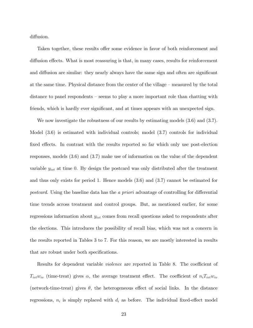
We now investigate the robustness of our results by estimating models (3.6) and (3.7).

Model (3.6) is estimated with individual controls; model (3.7) controls for individual

�xed e¤ects. In contrast with the results reported so far which only use post-election

responses, models (3.6) and (3.7) make use of information on the value of the dependent

variable yivt at time 0. By design the postcard was only distributed after the treatment

and thus only exists for period 1. Hence models (3.6) and (3.7) cannot be estimated for

postcard. Using the baseline data has the a priori advantage of controlling for di¤erential

time trends across treatment and control groups. But, as mentioned earlier, for some

regressions information about yivt comes from recall questions asked to respondents after

the elections. This introduces the possibility of recall bias, which was not a concern in

the results reported in Tables 3 to 7. For this reason, we are mostly interested in results

that are robust under both speci�cations.

Results for dependent variable violence are reported in Table 8. The coe¢ cient of

Tivtwiv (time-treat) gives �, the average treatment e¤ect. The coe¢ cient of niTivtwiv

(network-time-treat) gives �, the heterogeneous e¤ect of social links. In the distance

regressions, ni is simply replaced with di as before. The individual �xed-e¤ect model

23

(3.7) is estimated in �rst di¤erences.21 The estimator is ordinary least squares with errors

clustered by village.

We �nd strong evidence of both reinforcement and di¤usion e¤ects with respect to

kinship links and geographical distance: estimated coe¢ cients for the triple interaction

term niTivtwiv (network-time-treat) are negative and signi�cant for kinship, and positive

and signi�cant for distance. The magnitude of estimated coe¢ cients is in general very

similar between models (3.6) and (3.7), a �nding that is consistent with the fact that

the data come from a randomized experiment so that individual characteristics �whether

observable or not �should not matter. Note that, even though chatting-network e¤ects

remain positive, they lose statistical signi�cance. These �ndings reinforce and broaden

earlier �ndings from Table 3.

Next we look at perceptions of intimidation. Estimation results, reported in Table 9,

are very similar to those shown in Table 8: coe¢ cients for the triple interaction terms are

signi�cant with the anticipated sign in the kinship and distance regressions. This con�rms

the presence of both reinforcement and di¤usion e¤ects of the campaign on respondents�

perceptions.

We �nd no evidence of an impact of the campaign on behavior, however. Results for

voting (for AC) and turnout are reported in Tables 10 and 11. Model (3.7) is estimated

using �xed-e¤ects logit. None of the triple interaction terms is signi�cant, and some take

unlikely �albeit non-signi�cant �values. This may be because the dependent variables

are dichotomous and hence contains little information: indeed, when estimating (3.7) all

observations with identical values of yivt over time are dropped, dramatically reducing

21To facilitate comparison, we have aligned coe¢ cients according to their meaning in model (3.6).

24

sample size.

To summarize, results suggest the presence of reinforcement and di¤usion e¤ects for

kinship and distance, in particular when we consider perception outcomes. The two

network measures may be correlated, however. This raises the question of which of the

two matters. To investigate this issue, we reestimate model (3.7) with both interaction

terms combined:

�yivt = �wiv + �1wivni + � 1ni + �2wivdi + � 2di + +�eivt (5.1)

Results are shown in Table 12. For the postcard regression, we report results for a one-

period version of (5.1). For violence and intimidation, the model is estimated in �rst

di¤erence. For voting (for AC) and turnout, estimates are obtained using �xed-e¤ects

logit. We �nd that the strongest and most consistent results are obtained for kinship:

it is signi�cant in 5 of the 8 regressions reported in Table 10. This con�rms earlier

�ndings. When we control for kinship, physical distance to panel respondents no longer

matters �except for the reinforcement regression for the violence outcome where it remains

signi�cant.

5.1. Robustness

Collier and Vicente (2009) run a variety of robustness checks on the average treatment

e¤ect of the campaign using the same data as this paper. They look for evidence of con-

formity bias that would stem from respondents answering survey questions in a way that

arti�cially adapts to expected e¤ects of the treatment. However no such evidence is found.

25

Changes in perceptions of violence in the respondent�s location do not di¤er signi�cantly

when comparing subjects who were confronted with the whole experimental activities and

those who only responded to the post-election questionnaire and are therefore less prone to

conformity. Furthermore, the intensity of violence measured by independent journalists in

each EA is also reported to have decreased. Finally, in the spirit of Nickerson (2008) who

�nds that voting behavior is �contagious�, network-correlated individual voting behavior

(i.e. voting behavior explained by that of each individual�s closest subjects) is regressed

on the treatment. This exercise assumes that any voting mismeasurement (conformity)

is not correlated within networks. Average treatment e¤ects are found to be maintained.

Collier and Vicente (2009) also test whether control locations were contaminated by

the AAIN�s campaign. To this e¤ect, they regress outcome variables in control EA�s on

the distance to the nearest treatment EA. They �nd no clear e¤ects and conclude that

contamination is not of overall concern. They also point out that, if present, contamina-

tion would result in underestimated average treatment e¤ects. Please refer to Collier and

Vicente (2009) for details.

Turning to the main focus of this paper on network e¤ects, we subjected our results

to various robustness checks for the di¤usion e¤ect. As explained earlier, oversample

respondents were identi�ed after the campaign among households that had not been

directly exposed to it. Comparing oversample and control households in Table 2 led us

to consider the possibility of selection bias. So far we have dealt with this possibility by

including additional controls �i.e., individual characteristics or �xed e¤ects. But there

remain other sources of concern.

One is that, in the presence of heterogeneous e¤ects, the average treatment e¤ect is

26

mismeasured. To investigate this possibility, we reestimate the average di¤usion e¤ect us-

ing a matching method. This approach ensures that control households are only compared

to oversample households that are su¢ ciently similar to them in terms of observables. We

use the nearest-neighbor matching procedure proposed by Abadie and Imbens (2006).22

This non-parametric approach bypasses the di¢ culties associated with propensity score

matching �especially issues regarding balancedness of an a priori set of observables. Re-

sults shown in Table 13 con�rm the presence of a di¤usion impact on households not

directly exposed to the anti-violence campaign: the impact is positive and signi�cant for

perceptions of community violence and for the postcard. The campaign also has reduced

voting for the opposition and increased voter turnout. These �ndings lend clear credibility

to the homogeneous e¤ects we estimated before.

Our last set of robustness checks seeks to instrument (the absence of) treatment for

oversample households. Our main concern is the possibility that oversample households

di¤er in meaningful but unobserved ways from control households, and that this causes

spurious estimates of heterogeneous di¤usion e¤ects. Our ability to deal with this concern

is limited by the available data. We use two instruments for oversample households: an

average of questions about membership in village institutions23 and a measure of physical

isolation (distance to the mean coordinates of the panel respondents). The rationale for

this choice of instruments is that oversample households may have avoided exposure to the

campaign because they are socially and geographically isolated. These instruments satisfy

22This estimator is implemented in Stata using the nnmatch command.23The speci�c question used was: �I am going to read out a list of groups that people join or attend.

For each one, could you tell me whether in January you were an o¢ cial leader, an active member, aninactive member, or not a member? A religious group (e.g., church, mosque); a trade union or farmersassociation; a professional or business association; a community development or self-help association; aneighbourhood watch (�vigilante�) committee.�.

27

the inclusion restriction: they are jointly signi�cant in the instrumenting regression with

an F -statistic well in excess of 10. As recommended by Wooldridge (2002), Chapter 18,

estimated propensity scores bwiv from the instrumenting regression are used as instrumentsfor wiv in (5.1), while bwivni is used as instrument for wivni and bwivdi is used as instrumentfor wivdi. Results are presented in Table 14. We �nd signi�cant interaction e¤ects for

distance in the violence and intimidation regressions, which con�rm the existence of

di¤usion e¤ects. But the interaction term with kinship is no longer signi�cant. We also

con�rm a signi�cant kinship interaction e¤ect in the postcard regression while a positive

kinship e¤ect on turnout emerges for the �rst time. While they should be taken with

a grain of salt, these results nevertheless constitute additional evidence in support of

di¤usion e¤ects.

6. Conclusion

In this paper we have reported results from a �eld experiment designed to evaluate the

reinforcement and di¤usion e¤ects of a campaign to discourage electoral violence. Infor-

mation was collected on social networks and geographical distance between households

targeted by an awareness campaign. To test for the presence of a reinforcement e¤ect,

we examined whether the impact of the campaign on perceptions and behavior among

treated households is reinforced by proximity to other treated households. To investigate

di¤usion to unexposed households, we test whether households not directly exposed to

the campaign show e¤ects that are similar to exposed households and whether the impact

is stronger when they are closer �in a social or spatial sense �to other households.

28

Results provide evidence of both di¤usion and reinforcement e¤ects. Findings suggest

that the impact of the campaign on perceptions of violence is reinforced by social (kinship)

and geographical proximity to other households. We however �nd little reinforcement ef-

fect on behavior. For perceptions of violence, the di¤usion e¤ect nearly perfectly mimics

the reinforcement e¤ect. We �nd a signi�cant externality of the campaign on households�

willingness to express disapproval of electoral violence, but unclear e¤ects on voting be-

havior per se.

The �ndings presented in this paper together with those reported by Collier and Vi-

cente (2009) suggest that an anti-violence campaign of the kind implemented prior to

the 2007 Nigerian elections by AAIN was e¤ective in reducing perceptions of community

violence and intimidation. It also a¤ected respondents�willingness to express their disap-

proval of electoral violence. Part of the e¤ect of the campaign (in particular for percep-

tions) can be attributed to reinforcement and di¤usion e¤ects among kin and neighbors.

This is reassuring as it indicates that a campaign such as this one reaches more people

than those directly exposed to it, and that those exposed to it probably discuss it among

themselves in ways that reinforce its impact. For these same reasons, awareness cam-

paign such as the one studied here can be expected to have less impact on socially and

geographically isolated individuals. Yet these less well integrated individual �who are

more likely to be disenfranchised �may themselves be a source of electoral violence, either

directly or because they are manipulated by cynical politicians. A campaign directed at

them may reduce the risk of electoral violence directly.

In the results reported here, social and geographical proximity between households

is taken as given and remains outside the control of the researcher. Yet if proximity

29

reinforces the impact of the campaign and di¤uses its e¤ect more widely, it may be

possible to magnify campaign impact by fostering the formation of links among exposed

people, as well as between exposed and non-exposed people. How this could be achieved

is unclear, but one idea worth investigating is the possibility of identifying local relays

for the campaign message � churches, civil society � that could magnify its e¤ect by

canvassing their neighborhood. This deserves further investigation.

References

Abadie, A., and G. Imbens (2006): �Large Sample Properties of Matching Estimators

for Average Treatment E¤ects,�Econometrica, 74(1), 235�267.

Achebe, C. (1983): The Trouble with Nigeria. Heinemann Educational Publishers.

Angelucci, M., G. DiGiorgi, M. Rangel, and I. Rasul (2009): �Insurance and

Investment in Family Networks��(mimeograph).

Bandiera, O., and I. Rasul (2006): �Social Networks and Technology Adoption in

Northern Mozambique,�Economic Journal, 116(514), 862�902.

Collier, P., and P. C. Vicente (2009): �Votes and Violence: Evidence from a Field

Experiment in Nigeria,� Discussion paper, Oxford University and BREAD, Working

Paper.

Dahl, G., and S. Dellavigna (2009): �Does Movie Violence Increase Violent Crime?,�

Quarterly Journal of Economics, 124, 677�734.

30

Dellavigna, S., and E. Kaplan (2007): �The Fox News E¤ect: Media Bias and

Voting,�Quarterly Journal of Economics, 122, 1187�1234.

Eifert, B., E. Miguel, and D. Posner (2009): �Political Competition and Ethnic

Identi�cation in Africa,�American Journal of Political Science, (forthcoming).

Habyarimana, J., M. Humphreys, D. N. Posner, and J. M. Weinstein (2007):

�Why Does Ethnic Diversity Undermine Public Goods Provision?,�American Political

Science Review, 101(4), 709�725.

Kremer, M., and E. Miguel (2004): �Worms: Identifying Impacts on Education and

Health in the Presence of Treatment Externalities,�Econometrica, 72(1), 159�217.

Kuran, T. (1989): �Sparks and Prairie Fires: A Theory of Unanticipated Political

Revolution,�Public Choice, 61, 41�74.

Macours, K., and R. Vakis (2008): Changing Households�Investments and Aspirations

through Social Interactions: Evidence from a Randomized Transfer Program in a Low-

Income Country. World Bank, (Working Paper).

Nickerson, D. W. (2008): �Is Voting Contagious? Evidence from Two Field Experi-

ments,�American Political Science Review, 102(1), 49�57.

Posner, D. N. (2004): �The Political Salience of Cultural Di¤erence: Why Chewas and

Tumbukas are Allies in Zambia and Adversaries in Malawi,�American Political Science

Review, 98(4), 529�545.

31

Vicente, P. C. (2007): Is Vote Buying E¤ective? Evidence from a Field Experiment in

West Africa. Oxford University and BREAD, (Working Paper).

Wantchekon, L. (2003): �Clientelism and Voting Behavior: Evidence from a Field

Experiment in Benin,�World Politics, 55, 399�422.

Wooldridge, J. M. (2002): Econometric Analysis of Cross Section and Panel Data.

MIT Press, Cambridge, Mass.

32

Figure 1: A Poster Distributed during the Anti-violence Campaign

Figure 2: Map of Experimental Locations

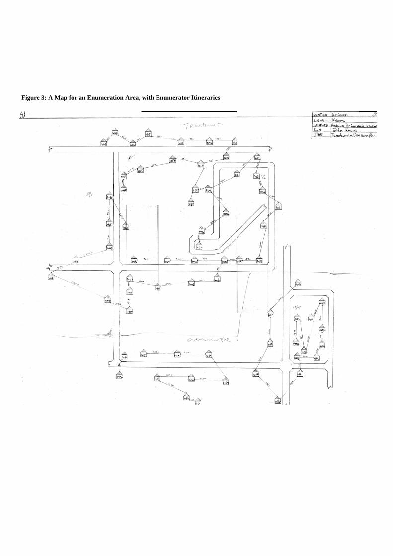
Figure 3: A Map for an Enumeration Area, with Enumerator Itineraries

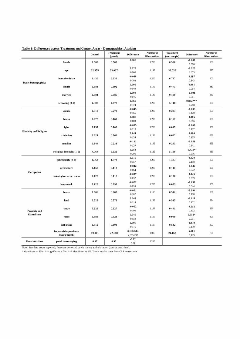
Table 1: Differences across Treatment and Control Areas - Demographics, Attrition

ControlTreatment

(panel)Difference

Number of Observations

Treatment (oversample)

DifferenceNumber of

Observations

0.000 -0.000

0.006

0.072 -0.925

0.960 1.373

-0.098 0.297

0.708 0.843

0.009 0.091

0.049 0.064

0.004 -0.091

0.046 0.061

0.365 0.832***

0.374 0.288

-0.045 -0.035

0.166 0.170

0.088 0.085

0.089 0.086

-0.055 -0.060

0.113 0.117

0.141 0.066

0.124 0.135

-0.111 -0.051

0.129 0.141

0.258 0.426*

0.206 0.236

0.015 0.120

0.157 0.198

-0.042 -0.042

0.064 0.072

-0.007 0.045

0.032 0.039

-0.022 -0.037

0.033 0.044

-0.001 -0.094

0.107 0.118

0.047 -0.011

0.114 0.122

-0.002 0.112

0.100 0.102

0.040 0.052*

0.033 0.031

0.096 0.030

0.116 0.130

3,186.514 5,161

4,655.297 5,119

-0.02

0.01

Note: Standard errors reported; these are corrected by clustering at the location (census area) level.

* significant at 10%; ** significant at 5%; *** significant at 1%. These results come from OLS regressions.

Panel Attrition panel re-surveying 0.97 0.95 1200

household expenditure (naira/month)

19,001 22,188 1,003 24,162 770

cell phone 0.512 0.608 1,197 0.542 897

0.441 896

radio 0.888 0.928 1,199 0.940 899

896

land 0.526 0.573 1,199 0.515 894

Property and Expenditure

house 0.606 0.605 1,199 0.512

cattle 0.329 0.327 1,198

housework 0.120 0.098 1,200 0.083 900

industry/services: trader 0.125 0.118 1,200 0.170 900

0.158 0.117 1,200 0.117 900

Occupation

job stability (0-3) 1.363 1.378 1,200 1.483 900

agriculture

religious intensity (1-6) 4.764 5.022 1,185 5.190 889

muslim 0.344 0.233 1,199 0.293 899

0.097 900

christian 0.621 0.762 1,199 0.687 899

900

hausa 0.072 0.160 1,200 0.157 900

Ethnicity and Religion

yoruba 0.318 0.273 1,200 0.283

igbo 0.157 0.102 1,200

schooling (0-9) 4.308 4.673 1,200 5.140 900

married 0.581 0.585 1,149 0.490 880

6.727 900

single 0.383 0.392 1,149 0.473 880

900

age 32.955 33.027 1,198 32.030 897

Basic Demographics

female 0.500 0.500 1,200 0.500

household size 6.430 6.332 1,200

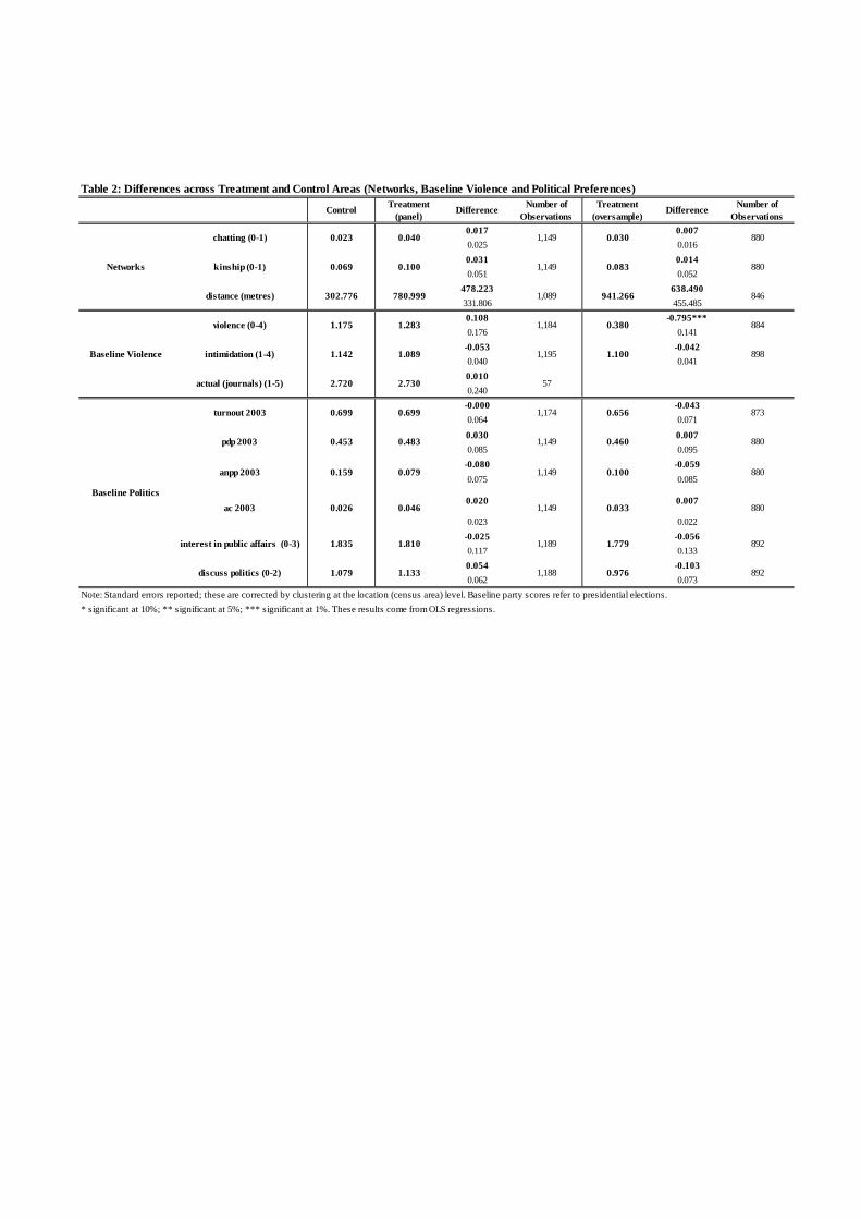
Table 2: Differences across Treatment and Control Areas (Networks, Baseline Violence and Political Preferences)

ControlTreatment

(panel)Difference


Treatment (oversample)

DifferenceNumber of

Observations

0.017 0.007

0.025 0.016

0.031 0.014

0.051 0.052

478.223 638.490

331.806 455.485

0.108 -0.795***

0.176 0.141

-0.053 -0.042

0.040 0.041

0.010

0.240

-0.000 -0.043

0.064 0.071

0.030 0.007

0.085 0.095

-0.080 -0.059

0.075 0.085

0.020 0.007

0.023 0.022

-0.025 -0.056

0.117 0.133

0.054 -0.103

0.062 0.073

Note: Standard errors reported; these are corrected by clustering at the location (census area) level. Baseline party scores refer to presidential elections.

* significant at 10%; ** significant at 5%; *** significant at 1%. These results come from OLS regressions.

discuss politics (0-2) 1.079 1.133 1,188 0.976 892

interest in public affairs (0-3) 1.835 1.810 1,189 1.779 892

880

ac 2003 0.026 0.046 1,149 0.033 880

0.483 1,149 0.460 880

anpp 2003 0.159 0.079 1,149 0.100

Baseline Politics

turnout 2003 0.699 0.699 1,174 0.656 873

pdp 2003 0.453

1.142 1.089 1,195 1.100 898

actual (journals) (1-5) 2.720 2.730 57

941.266 846

Baseline Violence

violence (0-4) 1.175 1.283 1,184 0.380 884

intimidation (1-4)

880

kinship (0-1) 0.069 0.100 1,149 0.083 880Networks

chatting (0-1) 0.023 0.040 1,149 0.030

distance (metres) 302.776 780.999 1,089

Table 3: Regressions of 'Conflict within Community'

Chatting Kinship Distance Chatting Kinship Distance

-0.325*** -0.320*** -0.334*** -0.032 -0.414*** -0.409*** -0.423*** -0.133

(-2.912) (-2.847) (-2.942) (-0.245) (-3.743) (-3.852) (-3.825) (-1.073)

-0.735 0.526 -0.900*** -0.602 0.591 -0.904***

(-1.015) (0.571) (-2.747) (-0.798) (0.635) (-3.235)

1.080 -0.356 0.943*** 2.069** -0.136 0.958***

(1.423) (-0.388) (2.868) (2.466) (-0.149) (3.362)

Yes Yes Yes Yes Yes Yes Yes Yes

0.099 0.099 0.099 0.131 0.122 0.127 0.125 0.160

971 971 971 900 744 744 744 708

Note: t-stats reported; these are corrected by clustering at the location (enumeration area) level. * significant at 10%; ** significant at 5%; *** significant at 1%.

network*treat

Demographic/Political Controls

Adjusted R-squared


OLS

Main Explanatory Variables

treated village

network

Homogeneous Effect (Oversample vs. Control)

Diffusion Effect (Oversample vs. Control)Dependent Variable ------>

Conflict within Community

Homogeneous Effect (Panel vs. Control)

Reinforcement Effect (Panel vs. Control)

Table 4: Regressions of 'Physical Intimidation'


-0.019 -0.019 -0.025 0.028 -0.047 -0.045 -0.055* -0.002

(-0.658) (-0.655) (-0.831) (0.722) (-1.535) (-1.508) (-1.763) (-0.050)

0.026 0.442** -0.139* -0.162 0.531*** -0.134*

(0.073) (2.236) (-1.807) (-0.403) (2.918) (-1.682)

-0.005 -0.435** 0.152* 0.929** -0.245 0.132

(-0.013) (-2.065) (1.915) (2.339) (-1.284) (1.558)


-0.007 -0.009 -0.005 -0.006 0.010 0.017 0.023 0.008

978 978 978 906 747 747 747 711



network

network*treat


Adjusted R-squared

OLS


treated village

Physical Intimidation


Reinforcement Effect (Panel vs. Control) Homogeneous Effect (Oversample vs. Control)


Table 5: Regressions of 'Postcard'


0.366 0.335 0.380 0.307 0.055 0.030 0.079 0.149

(0.902) (0.844) (0.942) (0.755) (0.129) (0.073) (0.200) (0.334)

0.727 -2.265 0.240 2.074 -0.696 0.041

(0.453) (-0.680) (0.295) (1.419) (-0.264) (0.054)

2.080 3.939 -0.330 4.365* 4.461* -0.255

(1.181) (1.177) (-0.396) (1.926) (1.719) (-0.328)


0.038 0.047 0.051 0.040 0.072 0.087 0.096 0.077

980 980 980 908 748 748 748 712



Adjusted R-squared


Logit


treated village

network

network*treat

Dependent Variable ------>

Postcard



Diffusion Effect (Oversample vs. Control)

Table 6: Regressions of 'Voting for AC (Opposition) in Presidential Elections'


-0.048 -0.016 -0.107 -0.237 -0.264 -0.164 -0.277 -0.980**

(-0.117) (-0.038) (-0.237) (-0.748) (-0.359) (-0.247) (-0.370) (-2.083)

-0.934 1.528 -0.348 -0.542 1.642 -0.336

(-0.808) (1.080) (-1.005) (-0.458) (1.053) (-1.104)

1.242 -2.258 0.914** 3.633** -0.259 1.170***

(0.760) (-1.148) (2.442) (2.155) (-0.180) (3.538)


0.257 0.258 0.259 0.298 0.211 0.222 0.215 0.301

980 980 980 908 748 748 748 712



network

network*treat


Adjusted R-squared

Logit


treated village

Voting for AC (Opposition) in Presidential Elections




Table 7: Regressions of 'Turnout in Gubernatorial Elections'


-0.104 -0.220 -0.165 -0.518** -0.625** -0.730** -0.689** -0.855***

(-0.414) (-0.819) (-0.650) (-2.541) (-2.116) (-2.368) (-2.354) (-3.581)

6.876 2.172 0.828* 8.531 3.188 0.609

(1.226) (1.000) (1.661) (1.365) (1.595) (1.207)

-6.698 -1.838 -0.585 -6.006 -1.998 0.758

(-1.197) (-0.839) (-1.162) (-0.927) (-0.984) (0.667)


0.139 0.142 0.141 0.162 0.169 0.176 0.174 0.205

974 974 974 903 744 744 744 709



network

network*treat


Adjusted R-squared

Logit


treated village

Turnout in Gubernatorial Elections




Table 8: Regressions of 'Conflict within Community' (with two periods)

1.489*** 1.509*** 1.450*** 1.335*** 1.443*** 1.458*** 1.414*** 1.222***

(5.373) (5.683) (5.182) (7.084) (4.476) (4.640) (4.479) (6.486)

-0.335** -0.433*** -0.345** -0.446*** -0.311** -0.387*** -0.690*** -0.813*** -0.335** -0.433*** -0.345** -0.446*** -0.311** -0.387*** -0.690*** -0.813***

(-2.405) (-2.679) (-2.400) (-2.734) (-2.449) (-2.889) (-3.073) (-2.962) (-2.399) (-2.679) (-2.393) (-2.733) (-2.442) (-2.888) (-3.065) (-2.961)

0.137 0.138 0.160 0.148 -0.730*** -0.734*** -0.708*** -0.766***

(0.919) (0.920) (1.114) (0.849) (-5.274) (-5.236) (-5.581) (-4.445)

-0.502** -0.432** -0.500** -0.427** -0.535*** -0.488** -0.182 -0.074 0.274* 0.382** 0.282* 0.397** 0.248* 0.337** 0.621*** 0.760***

(-2.407) (-1.965) (-2.390) (-1.971) (-2.687) (-2.498) (-0.682) (-0.241) (1.819) (2.254) (1.862) (2.349) (1.817) (2.389) (2.666) (2.714)

0.327 -1.676*** -0.023 0.506 -1.814*** 0.010

(0.279) (-2.726) (-0.080) (0.437) (-2.870) (0.033)

-1.137 -1.637 2.442*** 3.087*** -0.943** -1.051* -1.137 -1.637 2.442*** 3.087*** -0.943** -1.051*

(-0.545) (-0.800) (2.862) (3.065) (-2.009) (-1.834) (-0.544) (-0.800) (2.854) (3.063) (-2.004) (-1.833)

-0.718 1.330** -0.063 -0.412 1.763*** 0.018

(-0.586) (2.105) (-0.221) (-0.329) (2.880) (0.059)

2.083 2.636 -1.847** -2.405** 1.081** 1.195** 2.494 3.022 -2.000** -2.625*** 0.965** 1.060*

(0.985) (1.270) (-2.047) (-2.305) (2.300) (2.083) (1.181) (1.460) (-2.323) (-2.595) (2.051) (1.849)

Yes No Yes No Yes No Yes No Yes No Yes No Yes No Yes No

No Yes No Yes No Yes No Yes No Yes No Yes No Yes No Yes

0.159 0.027 0.159 0.033 0.167 0.057 0.180 0.057 0.150 0.022 0.152 0.027 0.161 0.060 0.173 0.065

1,912 1,114 1,912 1,114 1,912 1,114 1,772 1,036 1,462 856 1,462 856 1,462 856 1,392 819



network*time

network*treat

network*time*treat


Individual Fixed Effects

Adjusted R-squared

treated village

time*treat

network

OLS


constant

time



Conflict within Community


Reinforcement Effect (Panel vs. Control)Homogeneous Effect

(Oversample vs. Control)


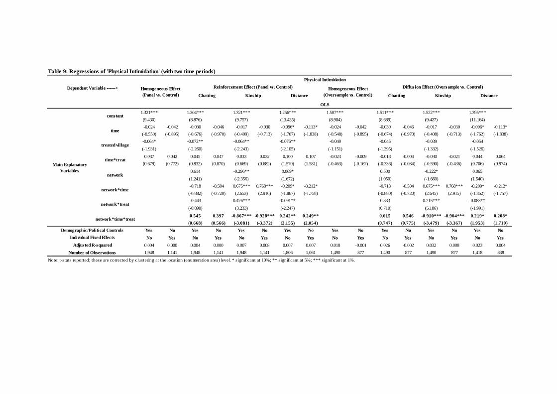
Table 9: Regressions of 'Physical Intimidation' (with two time periods)

1.321*** 1.304*** 1.321*** 1.256*** 1.507*** 1.511*** 1.522*** 1.395***

(9.430) (8.876) (9.757) (13.435) (8.984) (8.689) (9.427) (11.164)

-0.024 -0.042 -0.030 -0.046 -0.017 -0.030 -0.096* -0.113* -0.024 -0.042 -0.030 -0.046 -0.017 -0.030 -0.096* -0.113*

(-0.550) (-0.895) (-0.676) (-0.970) (-0.409) (-0.713) (-1.767) (-1.838) (-0.548) (-0.895) (-0.674) (-0.970) (-0.408) (-0.713) (-1.762) (-1.838)

-0.064* -0.072** -0.064** -0.076** -0.040 -0.045 -0.039 -0.054

(-1.931) (-2.260) (-2.243) (-2.105) (-1.151) (-1.395) (-1.332) (-1.526)

0.037 0.042 0.045 0.047 0.033 0.032 0.100 0.107 -0.024 -0.009 -0.018 -0.004 -0.030 -0.021 0.044 0.064

(0.679) (0.772) (0.832) (0.870) (0.669) (0.682) (1.570) (1.581) (-0.463) (-0.167) (-0.336) (-0.084) (-0.590) (-0.436) (0.706) (0.974)

0.614 -0.296** 0.069* 0.500 -0.222* 0.065

(1.241) (-2.356) (1.672) (1.050) (-1.660) (1.540)

-0.718 -0.504 0.675*** 0.768*** -0.209* -0.212* -0.718 -0.504 0.675*** 0.768*** -0.209* -0.212*

(-0.882) (-0.720) (2.653) (2.916) (-1.867) (-1.758) (-0.880) (-0.720) (2.645) (2.915) (-1.862) (-1.757)

-0.443 0.476*** -0.091** 0.333 0.715*** -0.083**

(-0.890) (3.233) (-2.247) (0.710) (5.186) (-1.991)

0.545 0.397 -0.867*** -0.928*** 0.242** 0.249** 0.615 0.546 -0.910*** -0.904*** 0.219* 0.208*

(0.668) (0.566) (-3.081) (-3.372) (2.155) (2.054) (0.747) (0.775) (-3.479) (-3.367) (1.953) (1.719)



0.004 0.000 0.004 0.000 0.007 0.008 0.007 0.007 0.018 -0.001 0.026 -0.002 0.032 0.008 0.023 0.004

1,948 1,141 1,948 1,141 1,948 1,141 1,806 1,061 1,490 877 1,490 877 1,490 877 1,418 838



Adjusted R-squared


network

network*time

network*treat

network*time*treat


treated village

time*treat

Distance

OLS


constant

time




Chatting


Physical Intimidation

Kinship Distance Chatting Kinship

Table 10: Regressions of 'Voting for AC (Opposition) in Presidential Elections' (with two time periods)

-2.796*** -2.721*** -2.656*** -3.560*** -3.239*** -3.173*** -3.099*** -3.407***

(-3.512) (-3.563) (-3.426) (-4.305) (-4.784) (-4.718) (-4.623) (-4.032)

0.701** 1.145*** 0.685** 1.245*** 0.672** 1.124*** 0.769 1.402*** 0.682** 1.145*** 0.674** 1.245*** 0.661** 1.124*** 0.794 1.402***

(2.199) (3.732) (2.151) (2.888) (2.096) (3.068) (1.490) (2.648) (2.243) (3.732) (2.194) (2.888) (2.144) (3.068) (1.575) (2.648)

0.746** 0.768** 0.688* 0.719 0.639 0.719 0.614 0.104

(2.073) (2.094) (1.874) (1.516) (1.059) (1.294) (1.001) (0.294)

-0.746* -1.361*** -0.732* -1.460*** -0.737* -1.348*** -0.925 -1.913*** -0.829** -1.551 -0.821** 1.639 -0.806** 1.105 -1.028* -1.422

(-1.854) (-3.442) (-1.798) (-2.928) (-1.770) (-3.037) (-1.619) (-3.180) (-2.523) (-1.610) (-2.496) (0.184) (-2.432) (0.154) (-1.924) (-1.172)

-0.463 2.633* -0.363 0.272 2.607 -0.400

(-0.352) (1.800) (-0.443) (0.200) (1.559) (-0.657)

-0.659 2.029 -1.463 -0.595 0.184 0.828 -0.691 2.029 -1.389 -0.595 0.167 0.828

(-0.728) (0.342) (-0.879) (-0.105) (0.232) (0.681) (-0.720) (0.342) (-0.913) (-0.105) (0.223) (0.681)

0.770 -2.577 0.589 2.178 -1.669 1.183*

(0.533) (-1.645) (0.709) (1.278) (-1.078) (1.906)

0.554 -1.920 0.579 -0.205 0.071 -0.411 1.000 32.628 1.624 35.252 -0.122 1.082

(0.349) (-0.316) (0.251) (-0.035) (0.089) (-0.334) (1.009) (0.348) (1.059) (0.376) (-0.162) (0.361)



0.207 0.100 0.208 0.101 0.209 0.102 0.227 0.141 0.196 0.189 0.204 0.192 0.199 0.191 0.287 0.194

1,960 246 1,960 246 1,960 246 1,816 240 1,496 126 1,496 126 1,496 126 1,424 124



Adjusted R-squared


network

network*time

network*treat

network*time*treat


treated village

time*treat

Distance

Logit


constant

time




Chatting


Voting for AC (Opposition) in Presidential Elections


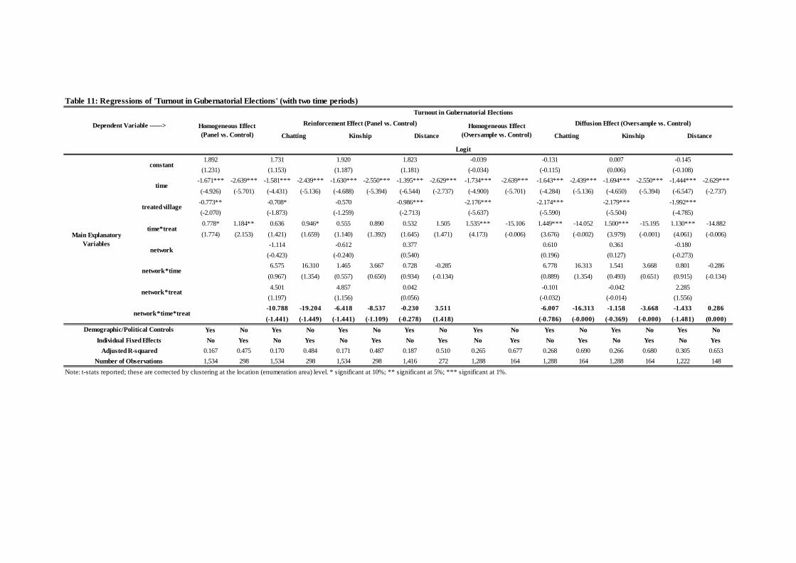
Table 11: Regressions of 'Turnout in Gubernatorial Elections' (with two time periods)

1.892 1.731 1.920 1.823 -0.039 -0.131 0.007 -0.145

(1.231) (1.153) (1.187) (1.181) (-0.034) (-0.115) (0.006) (-0.108)

-1.671*** -2.639*** -1.581*** -2.439*** -1.630*** -2.550*** -1.395*** -2.629*** -1.734*** -2.639*** -1.643*** -2.439*** -1.694*** -2.550*** -1.444*** -2.629***

(-4.926) (-5.701) (-4.431) (-5.136) (-4.688) (-5.394) (-6.544) (-2.737) (-4.900) (-5.701) (-4.284) (-5.136) (-4.650) (-5.394) (-6.547) (-2.737)

-0.773** -0.708* -0.570 -0.986*** -2.176*** -2.174*** -2.179*** -1.992***

(-2.070) (-1.873) (-1.259) (-2.713) (-5.637) (-5.590) (-5.504) (-4.785)

0.778* 1.184** 0.636 0.946* 0.555 0.890 0.532 1.505 1.535*** -15.106 1.449*** -14.052 1.500*** -15.195 1.130*** -14.882

(1.774) (2.153) (1.421) (1.659) (1.140) (1.392) (1.645) (1.471) (4.173) (-0.006) (3.676) (-0.002) (3.979) (-0.001) (4.061) (-0.006)

-1.114 -0.612 0.377 0.610 0.361 -0.180

(-0.423) (-0.240) (0.540) (0.196) (0.127) (-0.273)

6.575 16.310 1.465 3.667 0.728 -0.285 6.778 16.313 1.541 3.668 0.801 -0.286

(0.967) (1.354) (0.557) (0.650) (0.934) (-0.134) (0.889) (1.354) (0.493) (0.651) (0.915) (-0.134)

4.501 4.857 0.042 -0.101 -0.042 2.285

(1.197) (1.156) (0.056) (-0.032) (-0.014) (1.556)

-10.788 -19.204 -6.418 -8.537 -0.230 3.511 -6.007 -16.313 -1.158 -3.668 -1.433 0.286

(-1.441) (-1.449) (-1.441) (-1.109) (-0.278) (1.418) (-0.786) (-0.000) (-0.369) (-0.000) (-1.481) (0.000)



0.167 0.475 0.170 0.484 0.171 0.487 0.187 0.510 0.265 0.677 0.268 0.690 0.266 0.680 0.305 0.653

1,534 298 1,534 298 1,534 298 1,416 272 1,288 164 1,288 164 1,288 164 1,222 148



Adjusted R-squared


network

network*time

network*treat

network*time*treat


treated village

time*treat

Distance

Logit


constant

time




Chatting


Turnout in Gubernatorial Elections


Table 12: Regressions using Kinship and Distance

Reinforcement Diffusion Reinforcement Diffusion Reinforcement Diffusion Reinforcement Diffusion Reinforcement Diffusion

-0.711*** -0.711*** -0.087 -0.087 -1.753** -2.736** 1.405** 1.405** -2.454** -2.454**

(-2.848) (-2.846) (-1.535) (-1.534) (-2.136) (-2.461) (2.447) (2.447) (-2.510) (-2.510)

-0.190 0.657*** 0.085 0.038 0.366 0.202 -2.045*** 0.166 1.204 -15.416

(-0.670) (2.586) (1.381) (0.631) (0.851) (0.457) (-3.068) (0.022) (1.139) (-0.001)

2.432*** 2.432*** 0.613** 0.613** -2.362 -1.141 0.069 0.069 4.481 4.480

(2.642) (2.640) (2.040) (2.039) (-0.681) (-0.385) (0.012) (0.012) (0.787) (0.787)

-0.848 -0.848 -0.161 -0.161 0.068 -0.057 0.829 0.829 -0.146 -0.146

(-1.482) (-1.481) (-1.210) (-1.209) (0.089) (-0.077) (0.681) (0.681) (-0.068) (-0.068)

-1.760* -1.964** -0.776** -0.751** 4.037 4.848* -3.158 21.127 -8.203 -4.480

(-1.831) (-2.123) (-2.518) (-2.459) (1.161) (1.684) (-0.483) (0.211) (-1.231) (-0.000)

0.994* 0.861 0.197 0.155 -0.139 -0.106 -0.320 0.953 3.667 0.146

(1.735) (1.503) (1.479) (1.168) (-0.180) (-0.141) (-0.259) (0.312) (1.443) (0.000)

No No No No Yes Yes No No No No

Yes Yes Yes Yes No No Yes Yes Yes Yes

0.077 0.087 0.011 0.009 0.053 0.101 0.151 0.195 0.524 0.659

1,036 819 1,061 838 908 712 240 124 272 148




Adjusted R-squared



constant

treated village

kinship

distance

kinship*treat

distance*treat

OLS OLS Logit Logit Logit

Dependent Variable ------>Violence Intimidation Postcard Voting (for AC) Turnout

Table 13: Nearest-neighbor MatchingViolence Intimidation Postcard Voting (for AC) Turnout

0.372*** 0.044 0.119** -0.087** 0.111***

0.126 0.061 0.057 0.035 0.035

801 820 823 823 709

Note: st. errors reported. * significant at 10%; ** significant at 5%; *** significant at 1%.

Matching was performed on statistically significant different demographics (across oversample and control), together with the instruments used in this paper.



treated village

Table 14: IV EstimatesViolence Intimidation Postcard Voting (for AC) Turnout

Heterogeneous Effect





IV IV IV IV IV

-0.844*** -0.177* 0.051 -0.074**

(-2.802) (-1.652) (0.984) (-2.453)

0.838** 0.141 -0.127 -0.047 0.024

(2.518) (1.148) (-0.761) (-0.823) (0.554)

1.955* 0.308 -0.298 -0.090 -0.357*

(1.868) (0.685) (-0.610) (-0.685) (-1.693)

-1.149* -0.414 0.172 0.007 -0.102

(-1.701) (-1.634) (0.562) (0.083) (-1.264)

-1.400 -0.395 1.047** 0.081 0.432**

(-1.268) (-0.823) (2.322) (0.562) (2.148)

1.164* 0.417* -0.195 -0.007 0.110

(1.725) (1.654) (-0.641) (-0.078) (1.365)

No No Yes No No

Yes Yes No Yes Yes

28.288 27.249 23.651 27.206 31.954

0.082 -0.000 -0.031 0.005 0.032

812 831 709 834 716

Note: t-stats reported (corrected by clustering at the location level). * significant at 10%; ** significant at 5%; *** significant at 1%.

Instruments are distance to mean panel coordinates and an average of membership of local organizations (social capital).

distance*treat



F-stat on Excluded Instruments

Adjusted R-squared




constant

treated village

kinship

distance

kinship*treat

Documents

BREADibread.org/bread/system/files/bread_wpapers/239.pdfIn this context voter education and informational campaigns are becom-ing popular with donors. We followed a large-scale randomized