Embed Size (px)
Citation preview

In the format provided by the authors and unedited.
(Supplementary Information)A spatially localised architecture for fast and modular DNA
computing
Gourab Chatterjee, Neil Dalchau, Richard Muscat, Andrew Phillips, Georg Seelig
ContentsS1 Methods 3
S1.1 Circuit layouts on origami . . . . . . . . . . . . . . . . . . . . . . . . . . . . . . . . . . . . . . . . . . 3S1.2 Origami purification . . . . . . . . . . . . . . . . . . . . . . . . . . . . . . . . . . . . . . . . . . . . . . 4S1.3 Fluorescence data representation . . . . . . . . . . . . . . . . . . . . . . . . . . . . . . . . . . . . . . 5
S2 Spacing between hairpins on origami 7
S3 Effect of origami concentration on localised circuit dynamics 8
S4 Computational modelling 10S4.1 Introduction to Visual DSD . . . . . . . . . . . . . . . . . . . . . . . . . . . . . . . . . . . . . . . . . . 10S4.2 Two hairpin wire . . . . . . . . . . . . . . . . . . . . . . . . . . . . . . . . . . . . . . . . . . . . . . . . 10S4.3 Varying the concentration of input and fuel molecules . . . . . . . . . . . . . . . . . . . . . . . . . . 14S4.4 Reporters . . . . . . . . . . . . . . . . . . . . . . . . . . . . . . . . . . . . . . . . . . . . . . . . . . . . 15S4.5 One hairpin circuits . . . . . . . . . . . . . . . . . . . . . . . . . . . . . . . . . . . . . . . . . . . . . . 16S4.6 Three to eight hairpin wires . . . . . . . . . . . . . . . . . . . . . . . . . . . . . . . . . . . . . . . . . 17S4.7 Simple logic circuits . . . . . . . . . . . . . . . . . . . . . . . . . . . . . . . . . . . . . . . . . . . . . . 19S4.8 Parameters extracted from measurement data . . . . . . . . . . . . . . . . . . . . . . . . . . . . . . . 22S4.9 Parameterising and simulating models of localised circuits . . . . . . . . . . . . . . . . . . . . . . . 23S4.10 Model with hairpin closing . . . . . . . . . . . . . . . . . . . . . . . . . . . . . . . . . . . . . . . . . . 29S4.11 Calibrating the parameters of the wire crossover circuit . . . . . . . . . . . . . . . . . . . . . . . . . 30
S5 Allowable turning angles between successive hairpins 32
S6 A three hairpin domino wire 33
S7 Predictable localised interactions between adjacent hairpins 34
S8 Signal loss 35S8.1 A simple model of hairpin incorporation efficiency . . . . . . . . . . . . . . . . . . . . . . . . . . . . 36
S9 Positional dependence of signal transfer 39
S10 Interorigami interactions with multi-hairpin wires 40S10.1 Wires with multiple Output hairpins . . . . . . . . . . . . . . . . . . . . . . . . . . . . . . . . . . . . 40S10.2 Eight hairpin wire: Different cases of interorigami interactions . . . . . . . . . . . . . . . . . . . . . 41
S11 Mechanism of thresholding 42
S12 Predicting the dynamics of complex logic circuits with the parameterised model 43S12.1 Three-input AND circuit . . . . . . . . . . . . . . . . . . . . . . . . . . . . . . . . . . . . . . . . . . . 43
1
A spatially localized architecture for fast and modular DNA computing
© 2017 Macmillan Publishers Limited, part of Springer Nature. All rights reserved.
SUPPLEMENTARY INFORMATIONDOI: 10.1038/NNANO.2017.127
NATURE NANOTECHNOLOGY | www.nature.com/naturenanotechnology 1

S12.2 Two three-input AND circuits in parallel . . . . . . . . . . . . . . . . . . . . . . . . . . . . . . . . . . 44S12.3 Six-input AND circuit . . . . . . . . . . . . . . . . . . . . . . . . . . . . . . . . . . . . . . . . . . . . . 44S12.4 XNOR circuit . . . . . . . . . . . . . . . . . . . . . . . . . . . . . . . . . . . . . . . . . . . . . . . . . . 45
S13 Alternative architecture for circuits with more inputs 47
S14 Performance comparison 48
S15 Energy calculations 49
S16 Sequences 50S16.1 M13mp18 template DNA . . . . . . . . . . . . . . . . . . . . . . . . . . . . . . . . . . . . . . . . . . . 50S16.2 Sequences of staples and domino circuit components . . . . . . . . . . . . . . . . . . . . . . . . . . . 52
S17 Program Code 64
2
© 2017 Macmillan Publishers Limited, part of Springer Nature. All rights reserved.
NATURE NANOTECHNOLOGY | www.nature.com/naturenanotechnology 2
SUPPLEMENTARY INFORMATIONDOI: 10.1038/NNANO.2017.127
S1 Methods
S1.1 Circuit layouts on origami
-8 -7 -6 -5 -4 -3 -2 -1 1 2 3 4 5 6 7 80123456789
1011121314151617181920212223
b. Layout 2
-8 -7 -6 -5 -4 -3 -2 -1 1 2 3 4 5 6 7 80123456789
1011121314151617181920212223
c. Layout 3
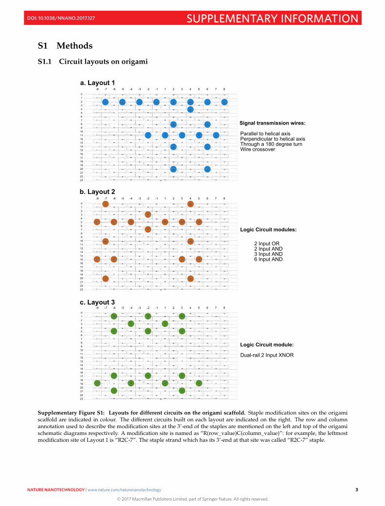
Signal transmission wires:
Logic Circuit modules:
Logic Circuit module:
Dual-rail 2 Input XNOR
2 Input OR2 Input AND3 Input AND6 Input AND
Parallel to helical axisPerpendicular to helical axisThrough a 180 degree turnWire crossover
-8 -7 -6 -5 -4 -3 -2 -1 1 2 3 4 5 6 7 80123456789
1011121314151617181920212223
a. Layout 1
Supplementary Figure S1: Layouts for different circuits on the origami scaffold. Staple modification sites on the origamiscaffold are indicated in colour. The different circuits built on each layout are indicated on the right. The row and columnannotation used to describe the modification sites at the 3’-end of the staples are mentioned on the left and top of the origamischematic diagrams respectively. A modification site is named as “R(row_value)C(column_value)”: for example, the leftmostmodification site of Layout 1 is “R2C-7”. The staple strand which has its 3’-end at that site was called “R2C-7” staple.
3
© 2017 Macmillan Publishers Limited, part of Springer Nature. All rights reserved.
NATURE NANOTECHNOLOGY | www.nature.com/naturenanotechnology 3
SUPPLEMENTARY INFORMATIONDOI: 10.1038/NNANO.2017.127
S1.2 Origami purification
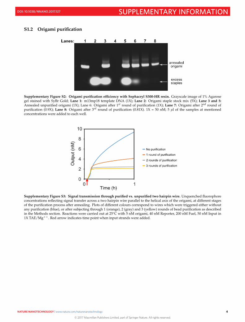
Supplementary Figure S2: Origami purification efficiency with Sephacryl S300-HR resin. Grayscale image of 1% Agarosegel stained with SyBr Gold; Lane 1: m13mp18 template DNA (1X); Lane 2: Origami staple stock mix (5X); Lane 3 and 5:Annealed unpurified origami (1X); Lane 6: Origami after 1st round of purification (1X); Lane 7: Origami after 2nd round ofpurification (0.9X); Lane 8: Origami after 3rd round of purification (0.81X). 1X = 50 nM; 5 µl of the samples at mentionedconcentrations were added to each well.
Supplementary Figure S3: Signal transmission through purified vs. unpurified two hairpin wire. Unquenched fluorophoreconcentrations reflecting signal transfer across a two hairpin wire parallel to the helical axis of the origami, at different stagesof the purification process after annealing. Plots of different colours correspond to wires which were triggered either withoutany purification (blue), or after subjecting through 1 (orange), 2 (gray) and 3 (yellow) rounds of bead purification as describedin the Methods section. Reactions were carried out at 25°C with 5 nM origami, 40 nM Reporter, 200 nM Fuel, 50 nM Input in1X TAE/Mg++. Red arrow indicates time point when input strands were added.
4
© 2017 Macmillan Publishers Limited, part of Springer Nature. All rights reserved.
NATURE NANOTECHNOLOGY | www.nature.com/naturenanotechnology 4
SUPPLEMENTARY INFORMATIONDOI: 10.1038/NNANO.2017.127
S1.3 Fluorescence data representation
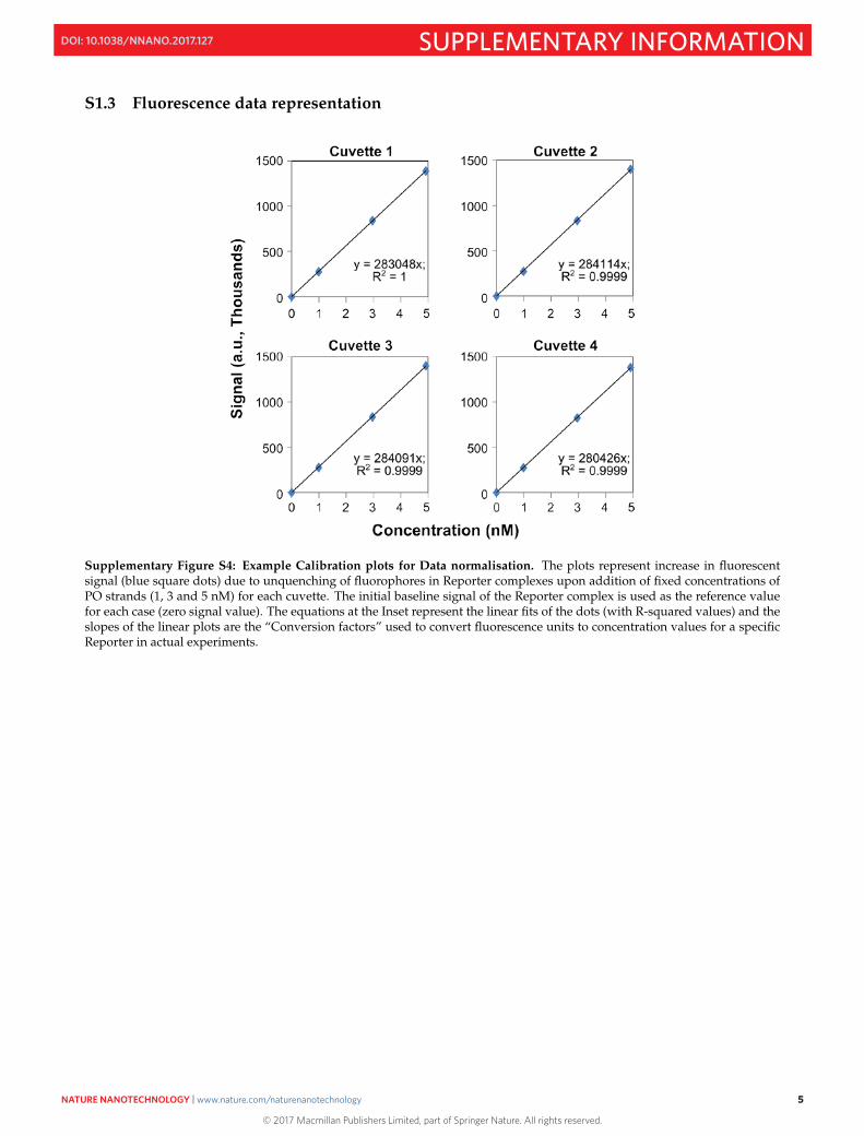
Supplementary Figure S4: Example Calibration plots for Data normalisation. The plots represent increase in fluorescentsignal (blue square dots) due to unquenching of fluorophores in Reporter complexes upon addition of fixed concentrations ofPO strands (1, 3 and 5 nM) for each cuvette. The initial baseline signal of the Reporter complex is used as the reference valuefor each case (zero signal value). The equations at the Inset represent the linear fits of the dots (with R-squared values) and theslopes of the linear plots are the “Conversion factors” used to convert fluorescence units to concentration values for a specificReporter in actual experiments.
5
© 2017 Macmillan Publishers Limited, part of Springer Nature. All rights reserved.
NATURE NANOTECHNOLOGY | www.nature.com/naturenanotechnology 5
SUPPLEMENTARY INFORMATIONDOI: 10.1038/NNANO.2017.127
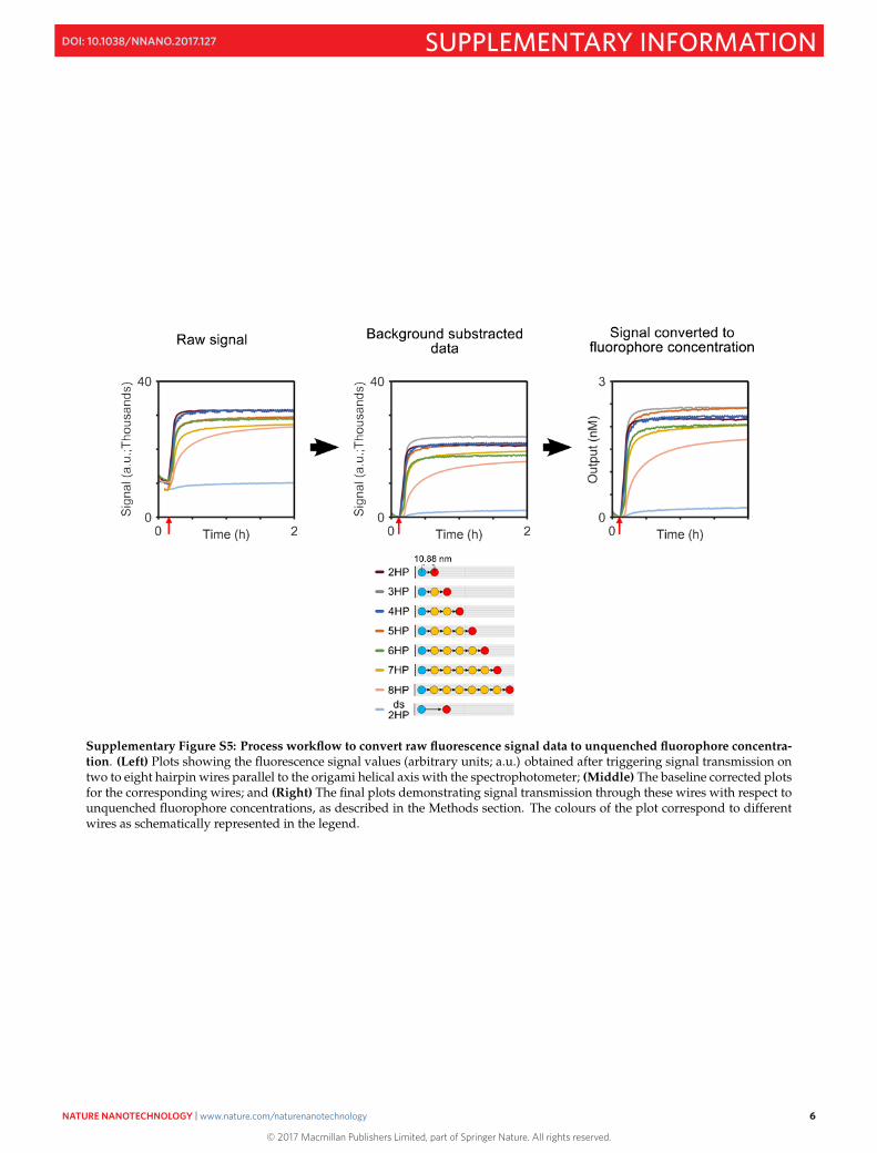
Supplementary Figure S5: Process workflow to convert raw fluorescence signal data to unquenched fluorophore concentra-tion. (Left) Plots showing the fluorescence signal values (arbitrary units; a.u.) obtained after triggering signal transmission ontwo to eight hairpin wires parallel to the origami helical axis with the spectrophotometer; (Middle) The baseline corrected plotsfor the corresponding wires; and (Right) The final plots demonstrating signal transmission through these wires with respect tounquenched fluorophore concentrations, as described in the Methods section. The colours of the plot correspond to differentwires as schematically represented in the legend.
6
© 2017 Macmillan Publishers Limited, part of Springer Nature. All rights reserved.
NATURE NANOTECHNOLOGY | www.nature.com/naturenanotechnology 6
SUPPLEMENTARY INFORMATIONDOI: 10.1038/NNANO.2017.127
S2 Spacing between hairpins on origami
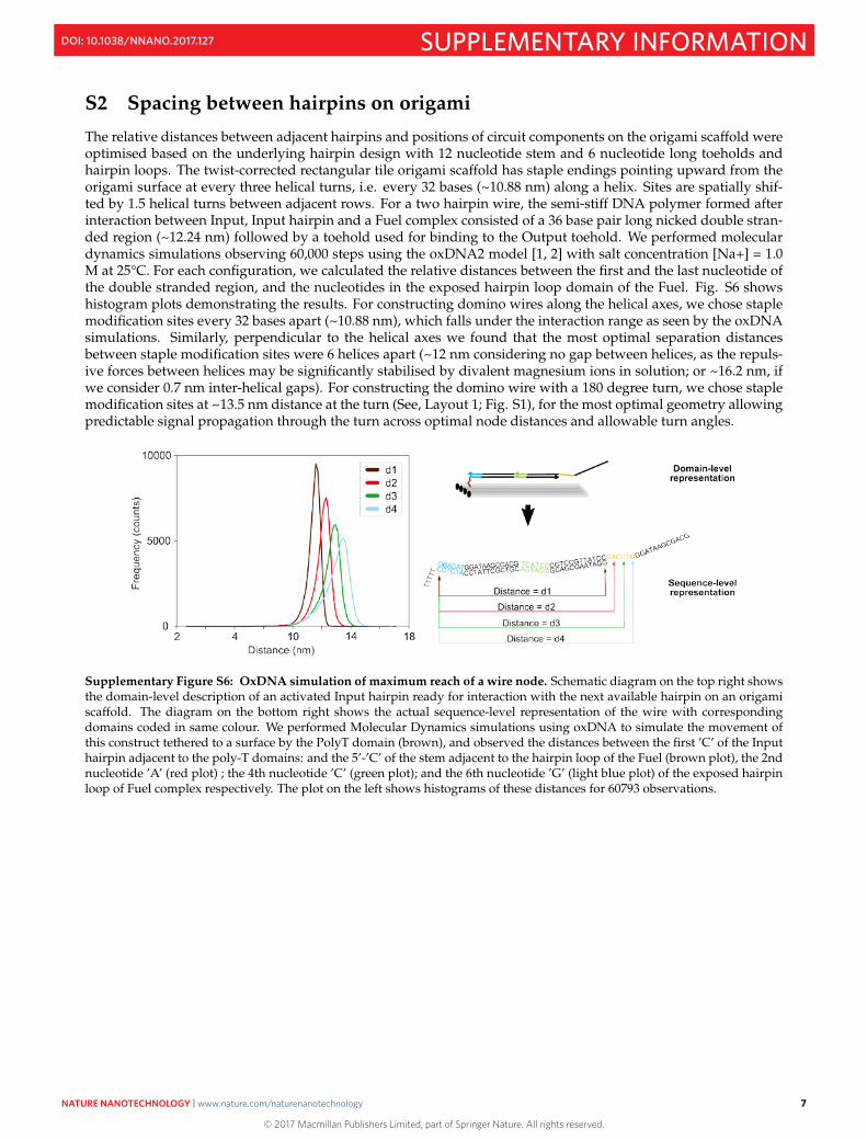
The relative distances between adjacent hairpins and positions of circuit components on the origami scaffold wereoptimised based on the underlying hairpin design with 12 nucleotide stem and 6 nucleotide long toeholds andhairpin loops. The twist-corrected rectangular tile origami scaffold has staple endings pointing upward from theorigami surface at every three helical turns, i.e. every 32 bases (~10.88 nm) along a helix. Sites are spatially shif-ted by 1.5 helical turns between adjacent rows. For a two hairpin wire, the semi-stiff DNA polymer formed afterinteraction between Input, Input hairpin and a Fuel complex consisted of a 36 base pair long nicked double stran-ded region (~12.24 nm) followed by a toehold used for binding to the Output toehold. We performed moleculardynamics simulations observing 60,000 steps using the oxDNA2 model [1, 2] with salt concentration [Na+] = 1.0M at 25°C. For each configuration, we calculated the relative distances between the first and the last nucleotide ofthe double stranded region, and the nucleotides in the exposed hairpin loop domain of the Fuel. Fig. S6 showshistogram plots demonstrating the results. For constructing domino wires along the helical axes, we chose staplemodification sites every 32 bases apart (~10.88 nm), which falls under the interaction range as seen by the oxDNAsimulations. Similarly, perpendicular to the helical axes we found that the most optimal separation distancesbetween staple modification sites were 6 helices apart (~12 nm considering no gap between helices, as the repuls-ive forces between helices may be significantly stabilised by divalent magnesium ions in solution; or ~16.2 nm, ifwe consider 0.7 nm inter-helical gaps). For constructing the domino wire with a 180 degree turn, we chose staplemodification sites at ~13.5 nm distance at the turn (See, Layout 1; Fig. S1), for the most optimal geometry allowingpredictable signal propagation through the turn across optimal node distances and allowable turn angles.
Supplementary Figure S6: OxDNA simulation of maximum reach of a wire node. Schematic diagram on the top right showsthe domain-level description of an activated Input hairpin ready for interaction with the next available hairpin on an origamiscaffold. The diagram on the bottom right shows the actual sequence-level representation of the wire with correspondingdomains coded in same colour. We performed Molecular Dynamics simulations using oxDNA to simulate the movement ofthis construct tethered to a surface by the PolyT domain (brown), and observed the distances between the first ’C’ of the Inputhairpin adjacent to the poly-T domains: and the 5’-’C’ of the stem adjacent to the hairpin loop of the Fuel (brown plot), the 2ndnucleotide ’A’ (red plot) ; the 4th nucleotide ’C’ (green plot); and the 6th nucleotide ’G’ (light blue plot) of the exposed hairpinloop of Fuel complex respectively. The plot on the left shows histograms of these distances for 60793 observations.
7
© 2017 Macmillan Publishers Limited, part of Springer Nature. All rights reserved.
NATURE NANOTECHNOLOGY | www.nature.com/naturenanotechnology 7
SUPPLEMENTARY INFORMATIONDOI: 10.1038/NNANO.2017.127
S3 Effect of origami concentration on localised circuit dynamics
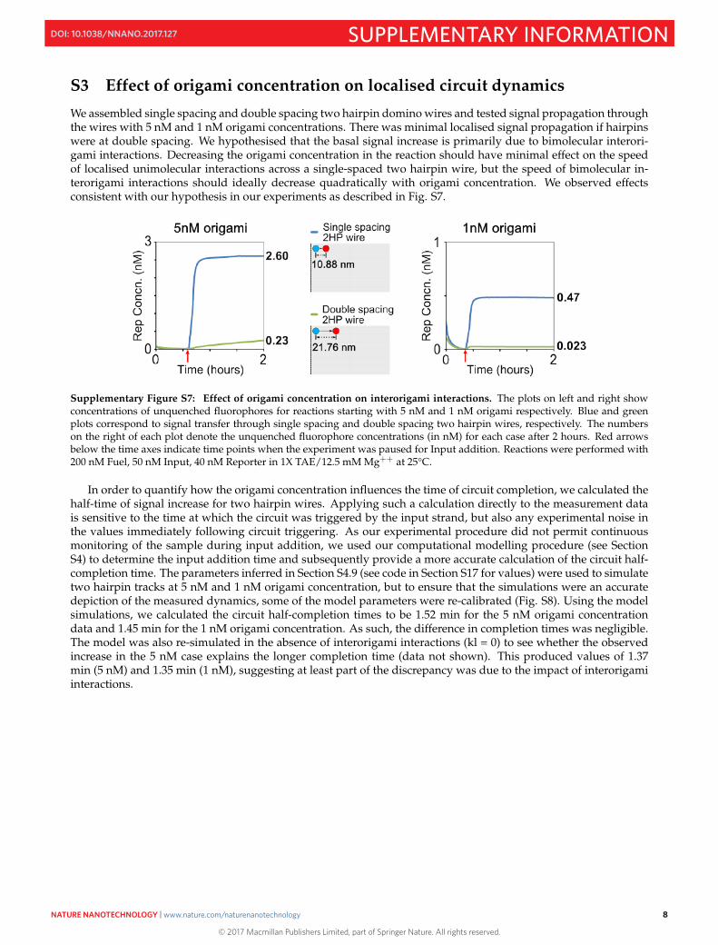
We assembled single spacing and double spacing two hairpin domino wires and tested signal propagation throughthe wires with 5 nM and 1 nM origami concentrations. There was minimal localised signal propagation if hairpinswere at double spacing. We hypothesised that the basal signal increase is primarily due to bimolecular interori-gami interactions. Decreasing the origami concentration in the reaction should have minimal effect on the speedof localised unimolecular interactions across a single-spaced two hairpin wire, but the speed of bimolecular in-terorigami interactions should ideally decrease quadratically with origami concentration. We observed effectsconsistent with our hypothesis in our experiments as described in Fig. S7.
Supplementary Figure S7: Effect of origami concentration on interorigami interactions. The plots on left and right showconcentrations of unquenched fluorophores for reactions starting with 5 nM and 1 nM origami respectively. Blue and greenplots correspond to signal transfer through single spacing and double spacing two hairpin wires, respectively. The numberson the right of each plot denote the unquenched fluorophore concentrations (in nM) for each case after 2 hours. Red arrowsbelow the time axes indicate time points when the experiment was paused for Input addition. Reactions were performed with200 nM Fuel, 50 nM Input, 40 nM Reporter in 1X TAE/12.5 mM Mg++ at 25°C.
In order to quantify how the origami concentration influences the time of circuit completion, we calculated thehalf-time of signal increase for two hairpin wires. Applying such a calculation directly to the measurement datais sensitive to the time at which the circuit was triggered by the input strand, but also any experimental noise inthe values immediately following circuit triggering. As our experimental procedure did not permit continuousmonitoring of the sample during input addition, we used our computational modelling procedure (see SectionS4) to determine the input addition time and subsequently provide a more accurate calculation of the circuit half-completion time. The parameters inferred in Section S4.9 (see code in Section S17 for values) were used to simulatetwo hairpin tracks at 5 nM and 1 nM origami concentration, but to ensure that the simulations were an accuratedepiction of the measured dynamics, some of the model parameters were re-calibrated (Fig. S8). Using the modelsimulations, we calculated the circuit half-completion times to be 1.52 min for the 5 nM origami concentrationdata and 1.45 min for the 1 nM origami concentration. As such, the difference in completion times was negligible.The model was also re-simulated in the absence of interorigami interactions (kl = 0) to see whether the observedincrease in the 5 nM case explains the longer completion time (data not shown). This produced values of 1.37min (5 nM) and 1.35 min (1 nM), suggesting at least part of the discrepancy was due to the impact of interorigamiinteractions.
8
© 2017 Macmillan Publishers Limited, part of Springer Nature. All rights reserved.
NATURE NANOTECHNOLOGY | www.nature.com/naturenanotechnology 8
SUPPLEMENTARY INFORMATIONDOI: 10.1038/NNANO.2017.127
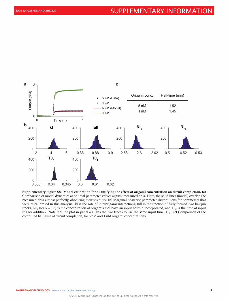
Supplementary Figure S8: Model calibration for quantifying the effect of origami concentration on circuit completion. (a)Comparison of model dynamics at optimal parameter values against measured data. Here, the solid lines (model) overlap themeasured data almost perfectly, obscuring their visibility. (b) Marginal posterior parameter distributions for parameters thatwere re-calibrated in this analysis. kl is the rate of interorigami interactions, full is the fraction of fully formed two hairpintracks, NIk (for k = 1,5) is the concentration of origamis that have an input hairpin incorporated, and T0k is the time of inputtrigger addition. Note that the plot in panel a aligns the two traces to use the same input time, T05. (c) Comparison of thecomputed half-time of circuit completion, for 5 nM and 1 nM origami concentrations.
9
© 2017 Macmillan Publishers Limited, part of Springer Nature. All rights reserved.
NATURE NANOTECHNOLOGY | www.nature.com/naturenanotechnology 9
SUPPLEMENTARY INFORMATIONDOI: 10.1038/NNANO.2017.127
S4 Computational modelling
S4.1 Introduction to Visual DSD
Computational models of all localised molecular circuits presented in the main text were constructed using VisualDSD [3], a software tool for the design and analysis of DNA strand displacement devices. Visual DSD features aprogramming language for expressing device designs, a compiler for automatically compiling programs to chem-ical reaction networks, and a range of analysis and simulation methods. The DSD language supports modules andlocal parameters to allow for abstraction and code-reuse, and includes recently added features for describing DNAcomplexes tethered to tiles [4]. The full definition of the DSD language used in this paper is provided in [4], andthe Visual DSD software is freely available from . A DSD program definesan initial collection of DNA species, where a species can be either a single complex in solution or a collection ofcomplexes tethered to a tile. The DSD compiler computes the set of all DNA strand displacement reactions thatcan be generated from a given set of initial species. The generated reactions can then be simulated using stochasticor deterministic methods.
We briefly summarise the textual syntax of the DSD programming language used in this paper, defined interms of elementary sequences and species. A sequence S comprises one or more domains, which can be long do-mains x or short domains xˆ, where a short domain is also referred to as a toehold. We write S∗ to denote a sequencecomplementary to S, according to Watson-Crick base pairing, and similarly write x∗ to denote a domain comple-mentary to x. A species I can be a single complex consisting of one or more strands, or a tile containing one ormore complexes tethered to its surface. A complex X can be an upper strand <S>, which denotes a sequence Soriented from left to right; a lower strand {S}, which denotes a sequence S oriented from right to left; or a gateG composed of segments M1, M2, ..., MN concatenated together. A segment M is of the form {L′}<L>[S]<R>{R′},which represents an upper strand <LSR> bound to a lower strand {L′S∗R′} along the double-stranded region [S].The overhanging sequences L, L′ and R, R′ can potentially be empty, in which case we simply omit them. In par-ticular, a segment with no overhangs is represented simply as [S], which denotes an upper strand <S> bound to acomplementary lower strand {S∗}. A segment can also be of the form <S′}[S]<R>{R′}, which denotes a hairpin loopon the left, or {L′}<L>[S]{S′>, which denotes a hairpin loop on the right. A gate is built up by concatenating seg-ments M1, M2, ..., MN using the concatenation operator (∼), written M1 ∼ M2 ∼ ... ∼ MN , where concatenation oftwo segments Mi ∼ Mj can take place along a common lower strand, written Mi : Mj, or along a common upperstrand, written Mi :: Mj. Concatenation is defined such that hairpins can only occur at the ends of the gate. A tileT contains a collection of complexes X1, ..., XN tethered to its surface, represented by enclosing the set of tetheredcomplexes in brackets [[X1|...|XN]]. Each complex tethered to a tile contains at least one tether, denoted by thekeyword tether, where each tether is annotated with one or more location tags l1, ..., lN , written tether(l1, ..., lN). Weassume that all of the complexes that share a particular tag are tethered sufficiently close to each other to interact,and that two tethered complexes can only interact if they have at least one tag in common. We also associate eachtag with a local concentration, which denotes the fact that tethered complexes may interact at a faster rate comparedto complexes in solution. We let D range over systems, where a system denotes a collection of initial species. Mul-tiple systems D1, ..., DN can be present in parallel, written D1|...|DN . We also allow module definitions of the formdef E(n) = D, where n is a list of module parameters and E(m) is an instance of the module D with parameters nreplaced by m. We assume a fixed set of module definitions, which are declared at the start of the program.
S4.2 Two hairpin wire
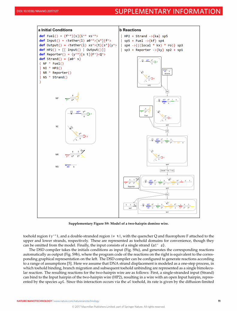
We first present a DSD model of the simple two-hairpin domino wire described in Fig. 1 of the main text, whichincorporates the main modelling concepts used in this paper (Fig. S9). The DSD code defines the initial conditionsof the system (Fig. S9a), represented as a set of species and their corresponding concentrations, where the programcode on the right is equivalent to the corresponding graphical representation on the left. The Fuel species is asingle hairpin consisting of a toehold domain ∗ , a double-stranded stem region and a hairpin loop ∗
∗ . The sequence of two domains ∗ ∗ together forms the longer domain ∗ shown in Fig. 1b of themain text. Here we represent the sub-domains explicitly, to model the case where only the ∗ region of the Fuelhairpin loop interacts with the toehold of the Output hairpin. The two-hairpin wire consists of a tile containingan Input and Output hairpin, written . The Input hairpin consists of a toehold ∗ ,stem region ∗ and hairpin loop , with a tether extending from the toehold. Similarly, the Output hairpinconsists of a toehold , stem ∗ and hairpin loop , with a tether extending from the toehold and anadditional domain overhanging the toehold. Both the Input and Output hairpin share the location tag ,which indicates that they are tethered close enough to interact with each other. The Reporter complex consists of a
10
© 2017 Macmillan Publishers Limited, part of Springer Nature. All rights reserved.
NATURE NANOTECHNOLOGY | www.nature.com/naturenanotechnology 10
SUPPLEMENTARY INFORMATIONDOI: 10.1038/NNANO.2017.127
b Reactionsa Initial Conditions
sa0NS
s t Q
y* t*s* FNR
t
s*y
s
(l)
xs
s*f
s
(l) a0*
NI
f*
s xs*
i*s*NF
f*
s xs*
i*s*
Fuel
t
s*y
s
(l)
xs
s*f
s
(l) a0*
HP2
s t Q
y* t*s* F
Reporter
sa0Strand
t
s*y
s
(l)
xs
(l) a0* s* f s
sa0
sp5
ts*
ys
(l)
xs
(l) a0* s* f s
s*f* sxs*i*sa0
sp4
(l)xs s* y s t
sxs*i*s*f*
(l) a0* s* f s
sa0
sp3
s t Q
sp2
(l)xs s* y s t
t*s*y* Fsxs*i*s*f*
(l) a0* s* f s
sa0
sp1
ka
kf
(local * kx * ro)
ky
Supplementary Figure S9: Model of a two-hairpin domino wire.
toehold region ∗ , and a double-stranded region , with the quencher Q and fluorophore F attached to theupper and lower strands, respectively. These are represented as toehold domains for convenience, though theycan be omitted from the model. Finally, the input consists of a single strand .
The DSD compiler takes the initials conditions as input (Fig. S9a), and generates the corresponding reactionsautomatically as output (Fig. S9b), where the program code of the reactions on the right is equivalent to the corres-ponding graphical representation on the left. The DSD compiler can be configured to generate reactions accordingto a range of assumptions [5]. Here we assume that DNA strand displacement is modeled as a one-step process, inwhich toehold binding, branch migration and subsequent toehold unbinding are represented as a single bimolecu-lar reaction. The resulting reactions for the two-hairpin wire are as follows: First, a single-stranded input (Strand)can bind to the Input hairpin of the two-hairpin wire (HP2), resulting in a wire with an open Input hairpin, repres-ented by the species . Since this interaction occurs via the toehold, its rate is given by the diffusion-limited
11
© 2017 Macmillan Publishers Limited, part of Springer Nature. All rights reserved.
NATURE NANOTECHNOLOGY | www.nature.com/naturenanotechnology 11
SUPPLEMENTARY INFORMATIONDOI: 10.1038/NNANO.2017.127
bimolecular rate constant ka. A Fuel hairpin can then bind to the exposed domain of the open Input hairpinat rate k f , and itself become opened. The resulting complex can then undergo a localised reaction, in whichthe opened Fuel hairpin interacts with the nearby Output hairpin. This interaction happens at the unimolecularrate local · kx · ro, where the factor local denotes the local concentration, which captures the effect of localisation.Crucially, the rate of the reaction is unimolecular, since it involves two components tethered to the same origamiat fixed locations and therefore at fixed concentrations relative to each other. Essentially, the local concentrationmodels the fact that the Input and Output hairpins of the two-hairpin wire are tethered in close proximity, andtherefore not limited by diffusion in solution. Since this local concentration is difficult to compute in the generalcase [6], we take the approach of inferring the local concentration associated with each local interaction directlyfrom experimental data (Fig. S18). The factor ro models the fact that the shorter toehold binds at a lower ratethan the longer domain. Finally, a Reporter complex can bind to the opened Output hairpin of the completedtwo-hairpin wire on the exposed domain, at rate ky .
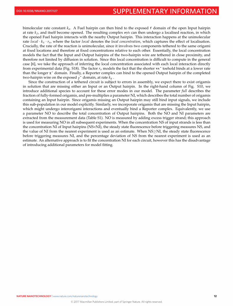
Since the construction of a tethered circuit is subject to errors in assembly, we expect there to exist origamisin solution that are missing either an Input or an Output hairpin. In the right-hand column of Fig. S10, weintroduce additional species to account for these error modes in our model. The parameter full describes thefraction of fully-formed origamis, and pre-multiplies a parameter NI, which describes the total number of origamiscontaining an Input hairpin. Since origamis missing an Output hairpin may still bind input signals, we includethis sub-population in our model explicitly. Similarly, we incorporate origamis that are missing the Input hairpin,which might undergo interorigami interactions and eventually bind a Reporter complex. Equivalently, we usea parameter NO to describe the total concentration of Output hairpins. Both the NO and NI parameters areextracted from the measurement data (Table S1). NO is measured by adding excess trigger strand; this approachis used for measuring NO in all subsequent experiments. When the concentration NS of input strands is less thanthe concentration NI of Input hairpins (NS<NI), the steady state fluorescence before triggering measures NS, andthe value of NI from the nearest experiment is used as an estimate. When NS≥NI, the steady state fluorescencebefore triggering measures NI, and the percentage deviation of NS from the nearest experiment is used as anestimate. An alternative approach is to fit the concentration NI for each circuit, however this has the disadvantageof introducing additional parameters for model fitting.
12
© 2017 Macmillan Publishers Limited, part of Springer Nature. All rights reserved.
NATURE NANOTECHNOLOGY | www.nature.com/naturenanotechnology 12
SUPPLEMENTARY INFORMATIONDOI: 10.1038/NNANO.2017.127
b Reactionsa Initial Conditions
(l)xs s* y s t
TOP
sxs*
(l) a0* s* f s
s*f* sxs*i*sa0
t
s*y
s
(l)
xs
s*f
s
(l) a0*
f*
s xs*
i*s*
t
s*y
s
(l)
xs
s*f
s
(l) a0*
sa0
s t Q
y* t*s* F
t
s*y
s
(l)
xs
(l) a0* s* f s
sa0
(l) a0* s* f s
sa0
s t Q
(l)xs s* y s t
t*s*y* F
TOP
sxs*
t
s*y
s
(l)
xs
(l) a0* s* f s
s*f* sxs*i*sa0
(l)xs s* y s t
sxs*i*s*f*
(l) a0* s* f s
sa0
(l)xs s* y s t
t*s*y* Fsxs*i*s*f*
(l) a0* s* f s
sa0
ka ka
ky
kfkf
(local * kx * ro)
ky
(kl * ro)
s t Q
y* t*s* FNR
sa0NS
t
s*y
s
(l)
xs
s*f
s
(l) a0*
(NI * full)
f*
s xs*
i*s*NF
s*f
s
(l) a0*(NI * (1 - full))
t
s*y
s
(l)
xs(NO - (NI * full))
Supplementary Figure S10: Model of interorigami reactions in a two hairpin wire. There are three main types of interorigamireactions for this circuit. (1) The opened Fuel hairpin on a fully-formed circuit can interact with the Output hairpin on anothercircuit; this is unlikely, since the opened Fuel hairpin has a much higher probability of interacting locally with an adjacentOutput hairpin on the same origami. Therefore, we do not model this interaction explicitly. (2) The opened Fuel hairpin ona circuit with no Output hairpin can interact with the Output hairpin on another fully-formed circuit. In this case the overallfluorescence is not significantly affected, so we do not model this interaction explicitly. (3) The opened Fuel hairpin on acircuit with no Output hairpin can interact with the Output hairpin on another circuit with no Input hairpin. In this case theinteraction is significant, since it produces additional fluorescence that would not have been produced otherwise. We modelthis interaction explicitly in the figure, where the domain represents a second circuit attached to the opened Fuel hairpin.
13
© 2017 Macmillan Publishers Limited, part of Springer Nature. All rights reserved.
NATURE NANOTECHNOLOGY | www.nature.com/naturenanotechnology 13
SUPPLEMENTARY INFORMATIONDOI: 10.1038/NNANO.2017.127
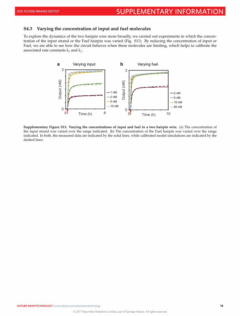
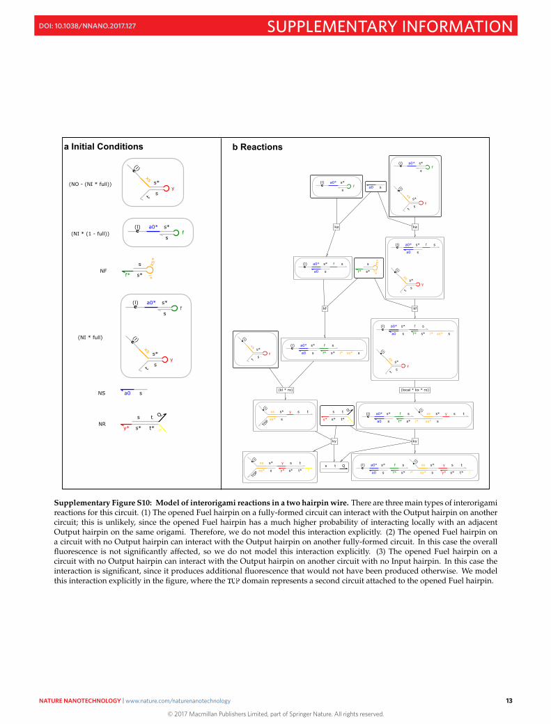
S4.3 Varying the concentration of input and fuel molecules
To explore the dynamics of the two hairpin wire more broadly, we carried out experiments in which the concen-tration of the input strand or the Fuel hairpin was varied (Fig. S11). By reducing the concentration of input orFuel, we are able to see how the circuit behaves when these molecules are limiting, which helps to calibrate theassociated rate constants ka and k f .
0 8Time (h)0
3
Out
put (
nM)
1 nM2 nM5 nM10 nM
0 10Time (h)0
3
Out
put (
nM)
2 nM5 nM10 nM50 nM
a b Varying fuelVarying input
Supplementary Figure S11: Varying the concentrations of input and fuel in a two hairpin wire. (a) The concentration ofthe input strand was varied over the range indicated. (b) The concentration of the Fuel hairpin was varied over the rangeindicated. In both, the measured data are indicated by the solid lines, while calibrated model simulations are indicated by thedashed lines.
14
© 2017 Macmillan Publishers Limited, part of Springer Nature. All rights reserved.
NATURE NANOTECHNOLOGY | www.nature.com/naturenanotechnology 14
SUPPLEMENTARY INFORMATIONDOI: 10.1038/NNANO.2017.127
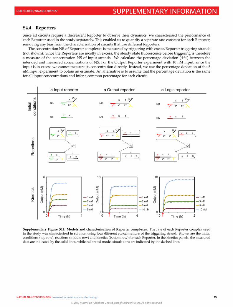
S4.4 Reporters
Since all circuits require a fluorescent Reporter to observe their dynamics, we characterised the performance ofeach Reporter used in the study separately. This enabled us to quantify a separate rate constant for each Reporter,removing any bias from the characterisation of circuits that use different Reporters.
The concentration NR of Reporter complexes is measured by triggering with excess Reporter triggering strands(not shown). Since the Reporters are mostly in excess, the steady state fluorescence before triggering is thereforea measure of the concentration NS of input strands. We calculate the percentage deviation (±%) between theintended and measured concentrations of NS. For the Output Reporter experiment with 10 nM input, since theinput is in excess we cannot measure its concentration directly. Instead, we use the percentage deviation of the 5nM input experiment to obtain an estimate. An alternative is to assume that the percentage deviation is the samefor all input concentrations and infer a common percentage for each circuit.
a Input reporter b Output reporter c Logic reporter
Initi
al
cond
ition
sR
eact
ions
Kine
tics
0 1Time (h)0
6
Out
put (
nM)
1 nM2 nM3 nM5 nM
0 4Time (h)0
10
Out
put (
nM)
1 nM2 nM5 nM10 nM
0 2Time (h)0
10
Out
put (
nM)
1 nM3 nM5 nM10 nM
f sNS
s Q
f* s* FNR
s Qf s
s*f* F
s Q
f* s* Ff s
kfr
s t Q
y* t*s* F
y s t
t*s*y* Fs t Q
y s t
ky
y s tNS
s t Q
y* t*s* FNR
s t Q
y* t*s* Fy s t
y s t
t*s*y* Fs t Q
kyl
y s tNS
s t Q
y* t*s* FNR
Supplementary Figure S12: Models and characterisation of Reporter complexes. The rate of each Reporter complex usedin the study was characterised in solution using four different concentrations of the triggering strand. Shown are the initialconditions (top row), reactions (middle row) and kinetics (bottom row) for each Reporter. In the kinetics panels, the measureddata are indicated by the solid lines, while calibrated model simulations are indicated by the dashed lines.
15
© 2017 Macmillan Publishers Limited, part of Springer Nature. All rights reserved.
NATURE NANOTECHNOLOGY | www.nature.com/naturenanotechnology 15
SUPPLEMENTARY INFORMATIONDOI: 10.1038/NNANO.2017.127
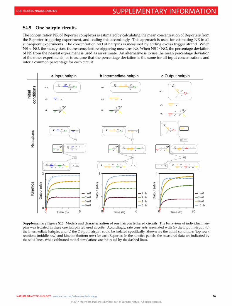
S4.5 One hairpin circuits
The concentration NR of Reporter complexes is estimated by calculating the mean concentration of Reporters fromthe Reporter triggering experiment, and scaling this accordingly. This approach is used for estimating NR in allsubsequent experiments. The concentration NO of hairpins is measured by adding excess trigger strand. WhenNS < NO, the steady state fluorescence before triggering measures NS. When NS ≥ NO, the percentage deviationof NS from the nearest experiment is used as an estimate. An alternative is to use the mean percentage deviationof the other experiments, or to assume that the percentage deviation is the same for all input concentrations andinfer a common percentage for each circuit.
a Input hairpin b Intermediate hairpin c Output hairpin
Initi
al
cond
ition
sR
eact
ions
Kine
tics
0 6Time (h)0
3
Out
put (
nM)
1 nM2 nM3 nM5 nM
0 6Time (h)0
3
Out
put (
nM)
1 nM2 nM3 nM5 nM
0 20Time (h)0
4
Out
put (
nM)
1 nM2 nM5 nM10 nM
s Q
f* s* FNR
sa0NS
s*f
s
(l) a0*NO
s Q(l) a0* s* f s
s*f* Fsa0
(l) a0* s* f s
sa0
s*f
s
(l) a0*
s Q
f* s* F
sa0
ka
kfr
s Q(l) i xs s* f s
s*f* Fsxs*i*
(l) i xs s* f s
sxs*i*
s*f
s
(l) i xs
s Q
f* s* F
sxs*i*
kx
kfr
s Q
f* s* FNR
sxs*i*NS
s*f
s
(l) i xsNO
t
s*y
s
(l)
xs
s t Q
y* t*s* F
(l) xs s* y s t
sxs*
s t Q(l) xs s* y s t
t*s*y* Fsxs*
sxs*
(kx * ro)
ky
s t Q
y* t*s* FNR
sxs*NS
t
s*y
s
(l)
xsNO
Supplementary Figure S13: Models and characterisation of one hairpin tethered circuits. The behaviour of individual hair-pins was isolated in these one hairpin tethered circuits. Accordingly, rate constants associated with (a) the Input hairpin, (b)the Intermediate hairpin, and (c) the Output hairpin, could be isolated specifically. Shown are the initial conditions (top row),reactions (middle row) and kinetics (bottom row) for each Reporter. In the kinetics panels, the measured data are indicated bythe solid lines, while calibrated model simulations are indicated by the dashed lines.
16
© 2017 Macmillan Publishers Limited, part of Springer Nature. All rights reserved.
NATURE NANOTECHNOLOGY | www.nature.com/naturenanotechnology 16
SUPPLEMENTARY INFORMATIONDOI: 10.1038/NNANO.2017.127
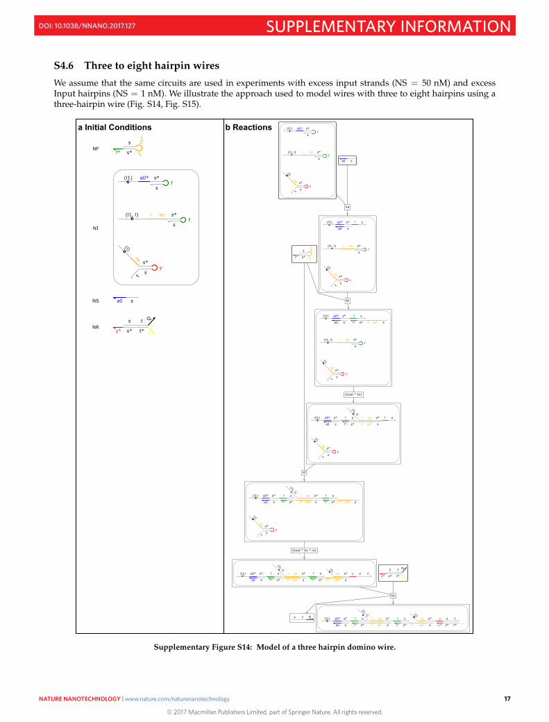
S4.6 Three to eight hairpin wires
We assume that the same circuits are used in experiments with excess input strands (NS = 50 nM) and excessInput hairpins (NS = 1 nM). We illustrate the approach used to model wires with three to eight hairpins using athree-hairpin wire (Fig. S14, Fig. S15).
b Reactionsa Initial Conditions
f*
s xs*
i*s*
t
s*y
s
(l)
xs
s*f
s
(l1, l) i xs
s*f
s
(l1) a0*
sa0
s t Q
y* t*s* F
t
s*y
s
(l)
xs
s*f
s
(l1, l) i xs
(l1) a0* s* f s
sa0
t
s*y
s
(l)
xs
s*f
s
(l1, l) i xs
(l1) a0* s* f s
s*f* sxs*i*sa0t
s*y
s
(l)
xs
(l1, l)i xs s* f s
sxs*i*s*f*
(l1) a0* s* f s
sa0
t
s*y
s
(l)
xs
(l1, l)i xs s* f s
s*f* sxs*i*sxs*i*s*f*
(l1) a0* s* f s
sa0
(l)xs s* y s t
sxs*i*s*f*
(l1, l)i xs s* f s
sxs*i*s*f*
(l1) a0* s* f s
sa0
s t Q(l)
xs s* y s t
t*s*y* Fsxs*i*s*f*
(l1, l)i xs s* f s
sxs*i*s*f*
(l1) a0* s* f s
sa0
ka
kf
(local * kx)
kf
(local * kx * ro)
ky
s t Q
y* t*s* FNR
sa0NS
t
s*y
s
(l)
xs
s*f
s
(l1, l) i xs
s*f
s
(l1) a0*
NI
f*
s xs*
i*s*NF
Supplementary Figure S14: Model of a three hairpin domino wire.
17
© 2017 Macmillan Publishers Limited, part of Springer Nature. All rights reserved.
NATURE NANOTECHNOLOGY | www.nature.com/naturenanotechnology 17
SUPPLEMENTARY INFORMATIONDOI: 10.1038/NNANO.2017.127
b Reactionsa Initial Conditions
(l)xs s* y s t
TOP
sxs*
(l) a0* s* f s
s*f* sxs*i*sa0
t
s*y
s
(l)
xs
s*f
s
(l2, l) i xs
s*f
s
(l) a0*
f*
s xs*
i*s*
t
s*y
s
(l)
xs
s*f
s
(l1, l) i xs
s*f
s
(l1) a0*
sa0
s t Q
y* t*s* F
t
s*y
s
(l)
xs
s*f
s
(l1, l) i xs
(l1) a0* s* f s
sa0
(l) a0* s* f s
sa0
s t Q
(l)xs s* y s t
t*s*y* F
TOP
sxs*
t
s*y
s
(l)
xs
s*f
s
(l1, l) i xs
(l1) a0* s* f s
s*f* sxs*i*sa0
t
s*y
s
(l)
xs
(l1, l)i xs s* f s
sxs*i*s*f*
(l1) a0* s* f s
sa0
t
s*y
s
(l)
xs
(l1, l)i xs s* f s
s*f* sxs*i*sxs*i*s*f*
(l1) a0* s* f s
sa0
(l)xs s* y s t
sxs*i*s*f*
(l1, l)i xs s* f s
sxs*i*s*f*
(l1) a0* s* f s
sa0
(l)xs s* y s t
t*s*y* Fsxs*i*s*f*
(l1, l)i xs s* f s
sxs*i*s*f*
(l1) a0* s* f s
sa0
ka ka
ky
kfkf
(local * kx)
kf
(local * kx * ro)
ky
((kl * ro) + kl)
s t Q
y* t*s* FNR
sa0NS
t
s*y
s
(l)
xs
s*f
s
(l1, l) i xs
s*f
s
(l1) a0*
(NI * full)
f*
s xs*
i*s*NF
s*f
s
(l) a0*(NI * (1 - full))
t
s*y
s
(l)
xs
s*f
s
(l2, l) i xs
(NO - (NI * full))
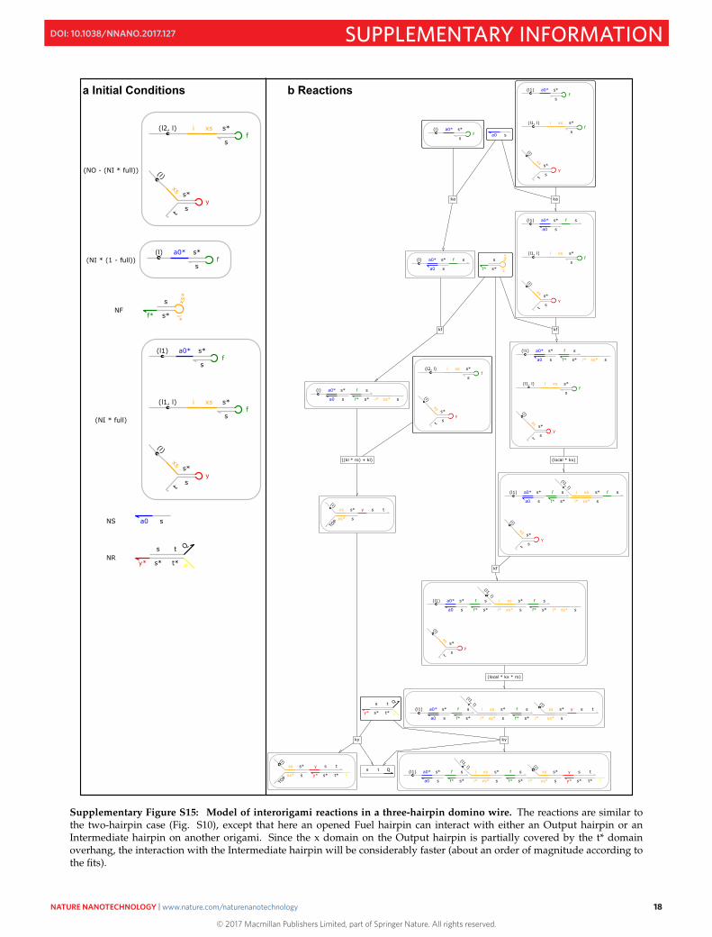
Supplementary Figure S15: Model of interorigami reactions in a three-hairpin domino wire. The reactions are similar tothe two-hairpin case (Fig. S10), except that here an opened Fuel hairpin can interact with either an Output hairpin or anIntermediate hairpin on another origami. Since the x domain on the Output hairpin is partially covered by the t* domainoverhang, the interaction with the Intermediate hairpin will be considerably faster (about an order of magnitude according tothe fits).
18
© 2017 Macmillan Publishers Limited, part of Springer Nature. All rights reserved.
NATURE NANOTECHNOLOGY | www.nature.com/naturenanotechnology 18
SUPPLEMENTARY INFORMATIONDOI: 10.1038/NNANO.2017.127
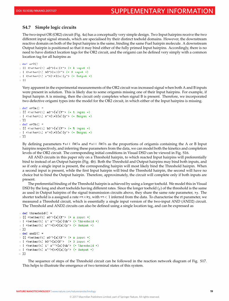
S4.7 Simple logic circuits
The two-input OR (OR2) circuit (Fig. 4a) has a conceptually very simple design. Two Input hairpins receive the twodifferent input signal strands, which are specialised by their distinct toehold domains. However, the downstreamreactive domain on both of the Input hairpins is the same, binding the same Fuel hairpin molecule. A downstreamOutput hairpin is positioned so that it may bind either of the fully primed Input hairpins. Accordingly, there is noneed to have distinct location tags for the OR2 circuit, and the origami can be defined very simply with a commonlocation tag for all hairpins as
1
2
3
4
5
Very apparent in the experimental measurements of the OR2 circuit was increased signal when both A and B inputswere present in solution. This is likely due to some origamis missing one of their Input hairpins. For example, ifInput hairpin A is missing, then the circuit only completes when signal B is present. Therefore, we incorporatedtwo defective origami types into the model for the OR2 circuit, in which either of the Input hairpins is missing.
1
2
3
4
5
6
7
8
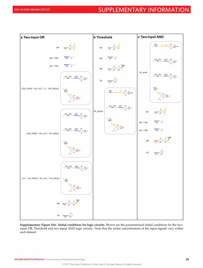
By defining parameters and as the proportions of origamis containing the A or B Inputhairpins respectively, and inferring these parameters from the data, we can model both the kinetics and completionlevels of the OR2 circuit. The corresponding initial conditions in Visual DSD can be viewed in Fig. S16.
All AND circuits in this paper rely on a Threshold hairpin, to which reacted Input hairpins will preferentiallybind to instead of an Output hairpin (Fig. 4b). Both the Threshold and Output hairpins may bind both inputs, andso if only a single input is present, the corresponding hairpin will most likely bind the Threshold hairpin. Whena second input is present, while the first Input hairpin will bind the Threshold hairpin, the second will have nochoice but to bind the Output hairpin. Therefore, approximately, the circuit will complete only if both inputs arepresent.
The preferential binding of the Threshold hairpin is achieved by using a longer toehold. We model this in VisualDSD by the long and short toeholds having different rates. Since the longer toehold ( ) of the threshold is the sameas used in Output hairpins of the signal transmission circuits above, they share the same rate parameter, . Theshorter toehold is a assigned a rate × , with < 1 inferred from the data. To characterise the rt parameter, wemeasured a Threshold circuit, which is essentially a single input version of the two-input AND (AND2) circuit.The Threshold and AND2 circuits can also be defined using a single location tag, and can be expressed as
1
2
3
4
5
6
7
8
9
10
11
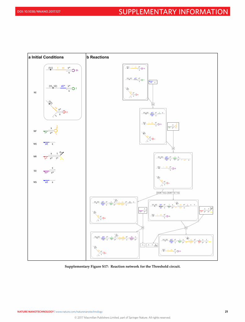
The sequence of steps of the Threshold circuit can be followed in the reaction network diagram of Fig. S17.This helps to illustrate the emergence of two terminal states of this system.
19
© 2017 Macmillan Publishers Limited, part of Springer Nature. All rights reserved.
NATURE NANOTECHNOLOGY | www.nature.com/naturenanotechnology 19
SUPPLEMENTARY INFORMATIONDOI: 10.1038/NNANO.2017.127
b Thresholda Two-input OR
s
th* s*50
s t Q
y* t*s* FNR
t
s*y
s
(t2)
xs
s*f
s
(t1, t2) b0*
(((1 - full_OR2b) * NI_or2) * full_OR2a)
t
s*y
s
(t2)
xs
s*f
s
(t1, t2) b0*
s*f
s
(t1, t2) a0*
((full_OR2b * NI_or2) * full_OR2a)
t
s*y
s
(t2)
xs
s*f
s
(t1, t2) a0*
((full_OR2b * NI_or2) * (1 - full_OR2a))
sa0(Ao * NS)
sb0(Bo * NS)
f*
s xs*
i*s*NF
c Two-input AND
t
s*y
s
(t2)
xs
s*f
s
(t1, t2) a0*
s*th
s
(t1) i xs
NI_thresh
s
th* s*50
s t Q
y* t*s* FNR
sa0NS
f*
s xs*
i*s*NF
s
th* s*50
s t Q
y* t*s* FNR
sa0(Ao * NS)
sb0(Bo * NS)
f*
s xs*
i*s*NF
t
s*y
s
(t2)
xs
s*f
s
(t1, t2) b0*
s*f
s
(t1, t2) a0*
s*th
s
(t1) i xs
NI_and2
Supplementary Figure S16: Initial conditions for logic circuits. Shown are the parameterised initial conditions for the two-input OR, Threshold and two-input AND logic circuits. Note that the initial concentrations of the input signals vary withineach dataset.
20
© 2017 Macmillan Publishers Limited, part of Springer Nature. All rights reserved.
NATURE NANOTECHNOLOGY | www.nature.com/naturenanotechnology 20
SUPPLEMENTARY INFORMATIONDOI: 10.1038/NNANO.2017.127
b Reactionsa Initial Conditions
sa0NS
s
th* s*50
s t Q
y* t*s* FNR
sa0NS
f*
s xs*
i*s*NF
t
s*y
s
(t2)
xs
s*f
s
(t1, t2) a0*
s*th
s
(t1) i xs
NI
t
s*y
s
(t2)
xs
s*f
s
(t1, t2) a0*
s*th
s
(t1) i xs
f*
s xs*
i*s*
s t Q
y* t*s* F
s
th* s*
t
s*y
s
(t2)
xs
s*th
s
(t1) i xs
(t1, t2) a0* s* f s
sa0
t
s*y
s
(t2)
xs
s*th
s
(t1) i xs
(t1, t2) a0* s* f s
s*f* sxs*i*sa0
s*th
s
(t1) i xs
(t2)xs s* y s t
sxs*i*s*f*
(t1, t2) a0* s* f s
sa0
t
s*y
s
(t2)
xs
(t1)i xs s* th s
sxs*i*s*f*
(t1, t2) a0* s* f s
sa0
s t Q
s*th
s
(t1) i xs
(t2)xs s* y s t
t*s*y* Fsxs*i*s*f*
(t1, t2) a0* s* f s
sa0s
t
s*y
s
(t2)
xs
(t1)i xs s* th s
s*th*sxs*i*s*f*
(t1, t2) a0* s* f s
sa0
sa0
ka
kf
(localt * kx) (localt * kx * ro)
kykt
Supplementary Figure S17: Reaction network for the Threshold circuit.
21
© 2017 Macmillan Publishers Limited, part of Springer Nature. All rights reserved.
NATURE NANOTECHNOLOGY | www.nature.com/naturenanotechnology 21
SUPPLEMENTARY INFORMATIONDOI: 10.1038/NNANO.2017.127
S4.8 Parameters extracted from measurement data
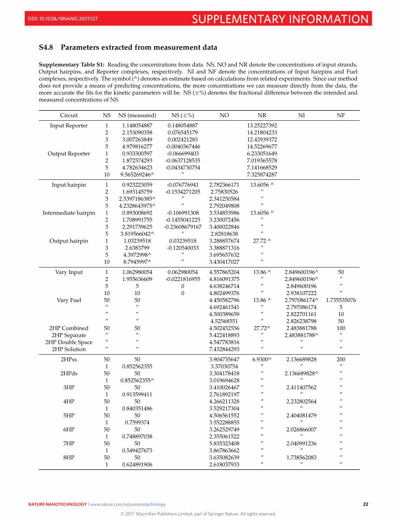
Supplementary Table S1: Reading the concentrations from data. NS, NO and NR denote the concentrations of input strands,Output hairpins, and Reporter complexes, respectively. NI and NF denote the concentrations of Input hairpins and Fuelcomplexes, respectively. The symbol (^) denotes an estimate based on calculations from related experiments. Since our methoddoes not provide a means of predicting concentrations, the more concentrations we can measure directly from the data, themore accurate the fits for the kinetic parameters will be. NS (±%) denotes the fractional difference between the intended andmeasured concentrations of NS.
Circuit NS NS (measured) NS (±%) NO NR NI NF
Input Reporter 1 1.148054887 0.148054887 13.252273922 2.153090358 0.076545179 14.218042333 3.007263849 0.002421283 12.429393725 4.979816277 -0.0040367446 14.52269677
Output Reporter 1 0.933300597 -0.066699403 6.2330516492 1.872574293 -0.0637128535 7.0193655785 4.782634623 -0.0434730754 7.14166852910 9.565269246^ ” 7.325874287
Input hairpin 1 0.923223059 -0.076776941 2.782366171 13.6056 ^2 1.693145759 -0.1534271205 2.75830526 ”3 2.5397186385^ ” 2.341250584 ”5 4.2328643975^ ” 2.792049808 ”
Intermediate hairpin 1 0.893008692 -0.106991308 3.534853986 13.6056 ^2 1.708991755 -0.1455041225 3.230072456 ”3 2.291739625 -0.23608679167 3.400022846 ”5 3.819566042^ ” 2.82818638 ”
Output hairpin 1 1.03239518 0.03239518 3.288857674 27.72 ^3 2.6383799 -0.120540033 3.388871316 ”5 4.3972998^ ” 3.695657632 ”
10 8.7945997^ ” 3.430417027 ”
Vary Input 1 1.062980054 0.062980054 4.557865204 13.86 ^ 2.849600196^ 502 1.955636609 -0.0221816955 4.816091375 ” 2.849600196^ ”5 5 0 4.638246714 ” 2.849600196 ”
10 10 0 4.802499376 ” 2.938107222 ”Vary Fuel 50 50 4.450582796 13.86 ^ 2.797086174^ 1.735535076
” ” 4.692461541 ” 2.797086174 5” ” 4.500389659 ” 2.822701161 10” ” 4.52568551 ” 2.826238798 50
2HP Combined 50 50 4.502452556 27.72^ 2.483881788 1002HP Separate ” ” 5.422418893 ” 2.483881788^ ”
2HP Double Space ” ” 4.547783816 ” ” ”2HP Solution ” ” 7.432844293 ” ” ”
2HPss 50 50 3.904735647 6.9300^ 2.136689828 2001 0.852562355 3.37030754 ” ” ”
2HPds 50 50 3.304178418 ” 2.136689828^ ”1 0.852562355^ 3.019694628 ” ” ”
3HP 50 50 3.410026467 ” 2.411407562 ”1 0.913599411 2.761892197 ” ” ”
4HP 50 50 4.266211328 ” 2.232802564 ”1 0.840351486 3.529217304 ” ” ”
5HP 50 50 4.506561552 ” 2.404081479 ”1 0.7599374 3.552288855 ” ” ”
6HP 50 50 3.262529749 ” 2.026866007 ”1 0.748897038 2.355061522 ” ” ”
7HP 50 50 5.835323408 ” 2.040991236 ”1 0.549427673 3.867863662 ” ” ”
8HP 50 50 3.635082639 ” 1.738562083 ”1 0.624891906 2.618037933 ” ” ”
22
© 2017 Macmillan Publishers Limited, part of Springer Nature. All rights reserved.
NATURE NANOTECHNOLOGY | www.nature.com/naturenanotechnology 22
SUPPLEMENTARY INFORMATIONDOI: 10.1038/NNANO.2017.127
S4.9 Parameterising and simulating models of localised circuits
To estimate the rate constants associated with the localised circuits described above, we used Bayesian parameterinference techniques. Specifically, we took an equivalent approach to that described in [7]. However, this approachis now embedded directly in Visual DSD. Briefly, we use Markov chain Monte Carlo (MCMC) to estimate the pos-terior probability density of each unknown parameter, given the experimental measurements for the circuits de-scribed above. i.e. we seek Pr(θ|data), where θ is a vector of parameters (see [8] for an overview). The Metropolis-Hastings algorithm performs MCMC by sampling proposal parameter sets from a prior distribution, and evaluat-ing a likelihood function that describes how close the model reproduces observations from the current parameters.Iteratively, neighbouring parameter sets are sampled, and accepted with probability 1 if the likelihood is improved,or with some probability if the likelihood decreases. In this way, a Markov chain of parameters is formed, whichshould converge to regions of the parameter space with high likelihood scores. This produces a sample of thejoint posterior distribution, from which marginal posterior distributions can be obtained. The marginals thereforeencode the values of the parameters that are most supported by the data. We used the implementation of theMetropolis-Hastings algorithm in the Filzbach software ( ).The software stores a user-specified number of joint posterior samples after a so-called burn-in phase, whichcomprises a user-specified number of iterations. Beyond this, Filzbach requires only the specification of a log-likelihood function, and the parameter prior distributions.
Filzbach operates with the natural logarithm of the likelihood function, to convert a product of probabilitiesinto a numerically more favorable sum of log-probabilities. We consider the probability density of each data-pointto be Gaussian distributed, with mean equal to the model-simulated value, and an unknown variance. We canwrite this as:
log L(θ) = log
{Nd
∏k=1
P(yk|θ)}
=Nd
∑k=1
log P(yk|θ) (1)
whereyk ∼ N (xk, σ2)
Here, the xk are simulations of the model and σ2 is the measurement variance in a particular dataset. Accordingly,a separate σ2 is inferred for each dataset. These variance parameters are inferred at the same time as the modelparameters, by appending them to the vector θ in Filzbach.
The simulated values are obtained using a deterministic simulation option in Visual DSD. This converts thereaction system to ordinary differential equations, evaluating the concentration of each species over time. Byusing the command-line version of Visual DSD, it is possible to use the fast SUNDIALs solvers [9]. These areselected by using either or in the DSDcode. The latter uses SUNDIALs options that are recommended by stiff ODE systems: the BDF variant of CVODE[9].
For all parameters, uniform priors were used. However, some priors were uniform on a logarithmic scale.The priors that were used for the presented model are detailed in the DSD code in Section S17, as defined by the
code block. The DSD syntax for parameters is
1
2
3
where can be any string, , and are floats, may be or ,and may be or (to be inferred). In our DSD code, multiple parameters are specified usinglist syntax, where multiple entries are separated by semicolons and the whole list is enclosed by square brackets.
A relationship between a data-file and a model simulation is specified using , which takes threearguments.
1
The first argument specifies a parameter sweep, which instantiates model parameter values (e.g. input and fuelconcentrations) that correspond to a specific column of data. The second argument specifies a data file, while thethird argument specifies the DSD species that should be compared with the data column. For example,
1
2
23
© 2017 Macmillan Publishers Limited, part of Springer Nature. All rights reserved.
NATURE NANOTECHNOLOGY | www.nature.com/naturenanotechnology 23
SUPPLEMENTARY INFORMATIONDOI: 10.1038/NNANO.2017.127

In this example, the data-file must contain precisely five columns, where the first column has the time-points, andsubsequent columns correspond to measurements for which the input species is at the indicated values. If morethan one is specified, e.g. , then the columns of the data-file are grouped by sweepitem, and have the following structure:
Time Fluor. 1 (input = 0.0) Fluor. 2 (input = 0.0) Fluor. 1 (input = 0.1) Fluor. 2 (input = 0.1) . . .
0.0 4829 429 4802 924 . . ....
......
...... . . .
The following figures present the results of running inference in Visual DSD for 100,000 burn-in iterations and100,000 samples, but retaining only one-tenth of the samples for further analysis. Such thinning is commonlydone to reduce the effects of autocorrelation in the sample set. The number of samples and extent of thinning isspecified in Visual DSD using (see Section S17). In Fig. S18, the marginal parameter posteriordistributions are shown, in Fig. S20 we show the pairwise correlations between each parameter, and in Fig. S21we show the evolution of chain through successive iterations.
24
© 2017 Macmillan Publishers Limited, part of Springer Nature. All rights reserved.
NATURE NANOTECHNOLOGY | www.nature.com/naturenanotechnology 24
SUPPLEMENTARY INFORMATIONDOI: 10.1038/NNANO.2017.127
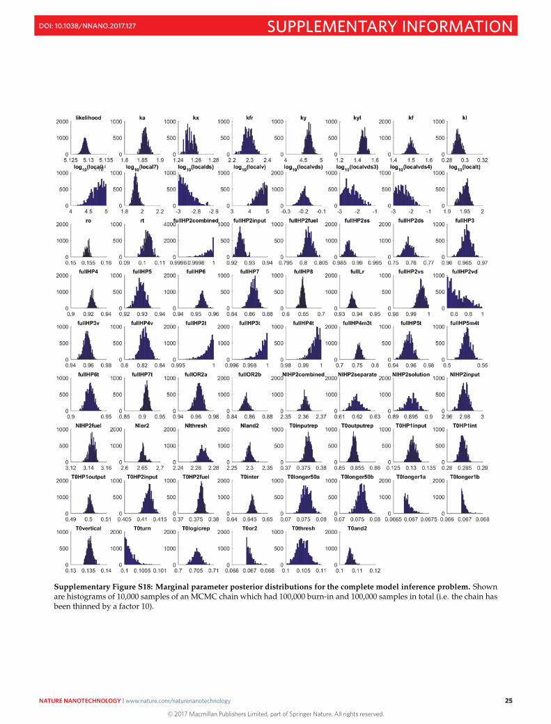
Supplementary Figure S18: Marginal parameter posterior distributions for the complete model inference problem. Shownare histograms of 10,000 samples of an MCMC chain which had 100,000 burn-in and 100,000 samples in total (i.e. the chain hasbeen thinned by a factor 10).
25
© 2017 Macmillan Publishers Limited, part of Springer Nature. All rights reserved.
NATURE NANOTECHNOLOGY | www.nature.com/naturenanotechnology 25
SUPPLEMENTARY INFORMATIONDOI: 10.1038/NNANO.2017.127
Input reporter Output reporter
Logic reporter
Input hairpin
Intermediate hairpin
Output hairpin
2 hairpin track 2HP varying input 2HP varying fuel
Horizontal track (1 nM input)Horizontal track Vertical track Track with turn
2 input OR Threshold 2 input AND
0 6Time (h)0
3
Out
put (
nM)
1 nM2 nM3 nM5 nM
0 1Time (h)0
6
Out
put (
nM)
1 nM2 nM3 nM5 nM
0 6Time (h)0
3
Out
put (
nM)
1 nM2 nM3 nM5 nM
0 1Time (h)0
3
Out
put (
nM)
2HP track
Separate origamis
Output HP in solution
No input
0 10Time (h)0
1
Out
put (
nM)
2HP3HP4HP5HP6HP7HP8HP2HP ds
0 2Time (h)0
3
Out
put (
nM)
2HP3HP4HP5HP6HP7HP8HP2HP ds
0 20Time (h)0
4
Out
put (
nM)
1 nM2 nM5 nM10 nM
0 4Time (h)0
10
Out
put (
nM)
1 nM2 nM5 nM10 nM
0 2Time (h)0
10
Out
put (
nM)
1 nM3 nM5 nM10 nM
0 1Time (h)0
3
Out
put (
FAM
; nM
)
A+BNoneAB
0 1Time (h)0
3
Out
put (
FAM
; nM
)
A+BNoneAB
0 1Time (h)0
3
Out
put (
FAM
; nM
)
-Thr+Thr
0 2Time (h)0
3
Out
put (
nM)
2HP3HP4HP4HP (-3)5HP (-4)5HP6HP7HP
0 10Time (h)0
3
Out
put (
nM)
2 nM5 nM10 nM50 nM
0 8Time (h)0
3
Out
put (
nM)
1 nM2 nM5 nM10 nM
0 2Time (h)0
3
Out
put (
nM)
2HP3HP4HP2HP ds
a b c d
e f g h
i j k l
m n o p
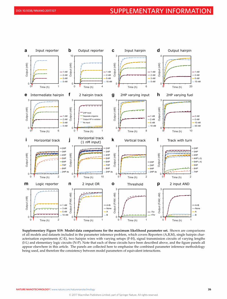
Supplementary Figure S19: Model-data comparisons for the maximum likelihood parameter set. Shown are comparisonsof all models and datasets included in the parameter inference problem, which covers Reporters (A,B,M), single hairpin char-acterisation experiments (C-E), two hairpin wires with varying setups (F-H), signal transmission circuits of varying lengths(I-L) and elementary logic circuits (N-P). Note that each of these circuits have been described above, and the figure panels allappear elsewhere in this article. The panels are collected here to emphasise the combined parameter inference methodologybeing used, and therefore the consistency between model parameters of equivalent interactions.
26
© 2017 Macmillan Publishers Limited, part of Springer Nature. All rights reserved.
NATURE NANOTECHNOLOGY | www.nature.com/naturenanotechnology 26
SUPPLEMENTARY INFORMATIONDOI: 10.1038/NNANO.2017.127
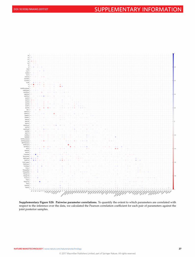
Supplementary Figure S20: Pairwise parameter correlations. To quantify the extent to which parameters are correlated withrespect to the inference over the data, we calculated the Pearson correlation coefficient for each pair of parameters against thejoint posterior samples.
27
© 2017 Macmillan Publishers Limited, part of Springer Nature. All rights reserved.
NATURE NANOTECHNOLOGY | www.nature.com/naturenanotechnology 27
SUPPLEMENTARY INFORMATIONDOI: 10.1038/NNANO.2017.127
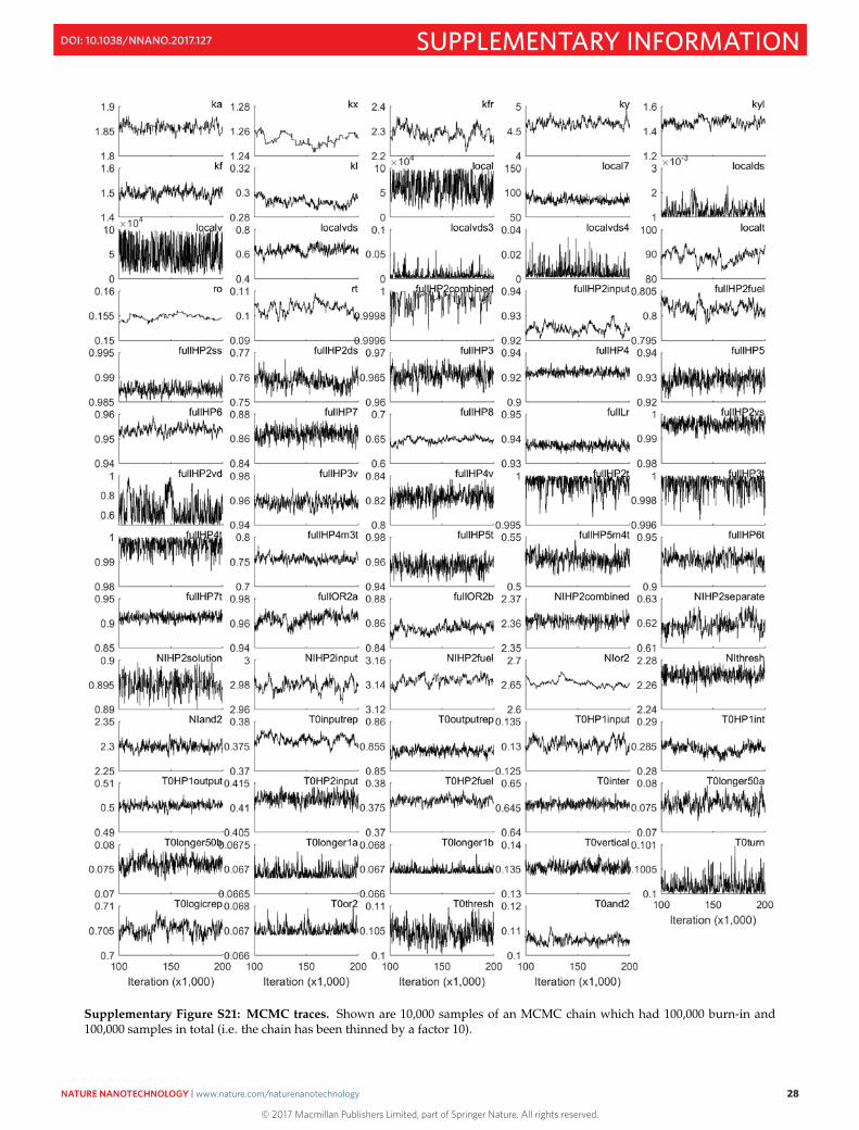
Supplementary Figure S21: MCMC traces. Shown are 10,000 samples of an MCMC chain which had 100,000 burn-in and100,000 samples in total (i.e. the chain has been thinned by a factor 10).
28
© 2017 Macmillan Publishers Limited, part of Springer Nature. All rights reserved.
NATURE NANOTECHNOLOGY | www.nature.com/naturenanotechnology 28
SUPPLEMENTARY INFORMATIONDOI: 10.1038/NNANO.2017.127
S4.10 Model with hairpin closing
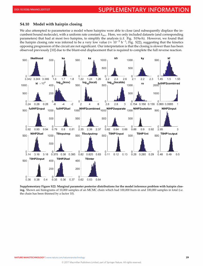
We also attempted to parameterise a model where hairpins were able to close (and subsequently displace the in-cumbent bound molecule), with a uniform rate constant krev. Here, we only included datasets (and correspondingparameters) that had at most two hairpins, to simplify the analysis (c.f. Fig. S19a-h). However, we found thatthe hairpin closing rate was inferred to be a very low value (≈ 10−5 h−1; Fig. S22), suggesting that the kineticsopposing progression of the circuit are not significant. Our interpretation is that the closing is slower than has beenobserved previously [10] due to the blunt-end displacement that is required to complete the full reverse reaction.
Supplementary Figure S22: Marginal parameter posterior distributions for the model inference problem with hairpin clos-ing. Shown are histograms of 10,000 samples of an MCMC chain which had 100,000 burn-in and 100,000 samples in total (i.e.the chain has been thinned by a factor 10).
29
© 2017 Macmillan Publishers Limited, part of Springer Nature. All rights reserved.
NATURE NANOTECHNOLOGY | www.nature.com/naturenanotechnology 29
SUPPLEMENTARY INFORMATIONDOI: 10.1038/NNANO.2017.127
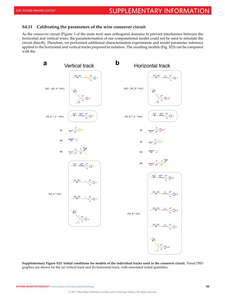
S4.11 Calibrating the parameters of the wire crossover circuit
As the crossover circuit (Figure 3 of the main text) uses orthogonal domains to prevent interference between thehorizontal and vertical wires, the parameterisation of our computational model could not be used to simulate thecircuit directly. Therefore, we performed additional characterisation experiments and model parameter inferenceapplied to the horizontal and vertical tracks prepared in isolation. The resulting models (Fig. S23) can be comparedwith the
Vertical track Horizontal tracka b
t
s*y2
s
(l4)
x
s*f
s
(l3, l4) xc
s*fc
s
(l2, l3) xc
s*fc
s
(l1, l2) xc
s*fc
s
(l1) b0*
(NI_B * full)
s t Q
y2* t*s* FNR
sb0NS
f*
sx*
s*NF
fc*
sxc*
s*NF
s*f
s
(l1) b0*(NI_B * (1 - full))
t2
s*y2
s
(l4)
x
s*f
s
(l3, l4) xc
(NO - (NI_B * full))
t
s*y
s
(l3)
x
s*f
s
(l2, l3) x
s*f
s
(l1, l2) x
s*f
s
(l1) a0*
(NI_A * full)
s t Q
y* t*s* FNR
sa0NS
f*
sx*
s*NF
s*f
s
(l1) a0*(NI_A * (1 - full))
t2
s*y
s
(l3)
x
s*f
s
(l2, l3) x
(NO - (NI_A * full))
Supplementary Figure S23: Initial conditions for models of the individual tracks used in the crossover circuit. Visual DSDgraphics are shown for the (a) vertical track and (b) horizontal track, with associated initial quantities.
30
© 2017 Macmillan Publishers Limited, part of Springer Nature. All rights reserved.
NATURE NANOTECHNOLOGY | www.nature.com/naturenanotechnology 30
SUPPLEMENTARY INFORMATIONDOI: 10.1038/NNANO.2017.127
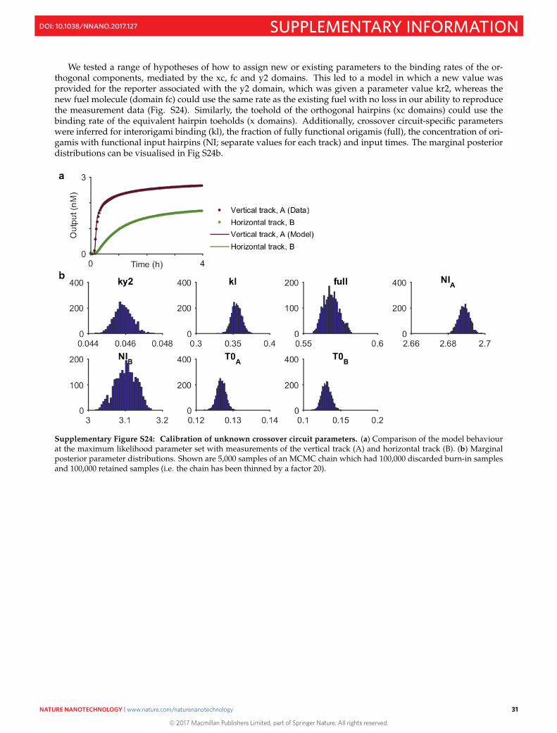
We tested a range of hypotheses of how to assign new or existing parameters to the binding rates of the or-thogonal components, mediated by the xc, fc and y2 domains. This led to a model in which a new value wasprovided for the reporter associated with the y2 domain, which was given a parameter value kr2, whereas thenew fuel molecule (domain fc) could use the same rate as the existing fuel with no loss in our ability to reproducethe measurement data (Fig. S24). Similarly, the toehold of the orthogonal hairpins (xc domains) could use thebinding rate of the equivalent hairpin toeholds (x domains). Additionally, crossover circuit-specific parameterswere inferred for interorigami binding (kl), the fraction of fully functional origamis (full), the concentration of ori-gamis with functional input hairpins (NI; separate values for each track) and input times. The marginal posteriordistributions can be visualised in Fig S24b.
Supplementary Figure S24: Calibration of unknown crossover circuit parameters. (a) Comparison of the model behaviourat the maximum likelihood parameter set with measurements of the vertical track (A) and horizontal track (B). (b) Marginalposterior parameter distributions. Shown are 5,000 samples of an MCMC chain which had 100,000 discarded burn-in samplesand 100,000 retained samples (i.e. the chain has been thinned by a factor 20).
31
© 2017 Macmillan Publishers Limited, part of Springer Nature. All rights reserved.
NATURE NANOTECHNOLOGY | www.nature.com/naturenanotechnology 31
SUPPLEMENTARY INFORMATIONDOI: 10.1038/NNANO.2017.127
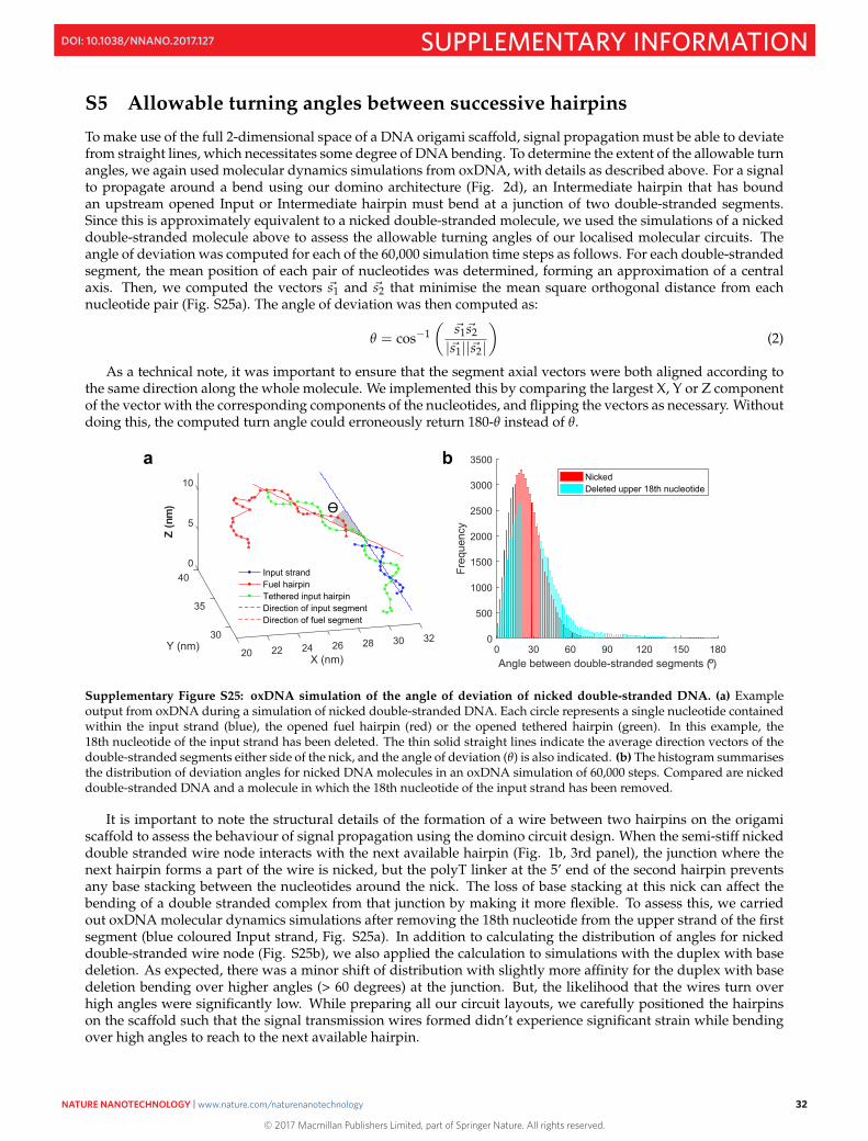
S5 Allowable turning angles between successive hairpins
To make use of the full 2-dimensional space of a DNA origami scaffold, signal propagation must be able to deviatefrom straight lines, which necessitates some degree of DNA bending. To determine the extent of the allowable turnangles, we again used molecular dynamics simulations from oxDNA, with details as described above. For a signalto propagate around a bend using our domino architecture (Fig. 2d), an Intermediate hairpin that has boundan upstream opened Input or Intermediate hairpin must bend at a junction of two double-stranded segments.Since this is approximately equivalent to a nicked double-stranded molecule, we used the simulations of a nickeddouble-stranded molecule above to assess the allowable turning angles of our localised molecular circuits. Theangle of deviation was computed for each of the 60,000 simulation time steps as follows. For each double-strandedsegment, the mean position of each pair of nucleotides was determined, forming an approximation of a centralaxis. Then, we computed the vectors �s1 and �s2 that minimise the mean square orthogonal distance from eachnucleotide pair (Fig. S25a). The angle of deviation was then computed as:
θ = cos−1(
�s1�s2
|�s1||�s2|
)(2)
As a technical note, it was important to ensure that the segment axial vectors were both aligned according tothe same direction along the whole molecule. We implemented this by comparing the largest X, Y or Z componentof the vector with the corresponding components of the nucleotides, and flipping the vectors as necessary. Withoutdoing this, the computed turn angle could erroneously return 180-θ instead of θ.
040
5
Z (n
m)
35
Y (nm)
10
30
X (nm)
32302826242220
Input strandFuel hairpinTethered input hairpinDirection of input segmentDirection of fuel segment
0 30 60 90 120 150 180Angle between double-stranded segments (°)
0
500
1000
1500
2000
2500
3000
3500Fr
eque
ncy
NickedDeleted upper 18th nucleotide
a b
Ɵ
Supplementary Figure S25: oxDNA simulation of the angle of deviation of nicked double-stranded DNA. (a) Exampleoutput from oxDNA during a simulation of nicked double-stranded DNA. Each circle represents a single nucleotide containedwithin the input strand (blue), the opened fuel hairpin (red) or the opened tethered hairpin (green). In this example, the18th nucleotide of the input strand has been deleted. The thin solid straight lines indicate the average direction vectors of thedouble-stranded segments either side of the nick, and the angle of deviation (θ) is also indicated. (b) The histogram summarisesthe distribution of deviation angles for nicked DNA molecules in an oxDNA simulation of 60,000 steps. Compared are nickeddouble-stranded DNA and a molecule in which the 18th nucleotide of the input strand has been removed.
It is important to note the structural details of the formation of a wire between two hairpins on the origamiscaffold to assess the behaviour of signal propagation using the domino circuit design. When the semi-stiff nickeddouble stranded wire node interacts with the next available hairpin (Fig. 1b, 3rd panel), the junction where thenext hairpin forms a part of the wire is nicked, but the polyT linker at the 5’ end of the second hairpin preventsany base stacking between the nucleotides around the nick. The loss of base stacking at this nick can affect thebending of a double stranded complex from that junction by making it more flexible. To assess this, we carriedout oxDNA molecular dynamics simulations after removing the 18th nucleotide from the upper strand of the firstsegment (blue coloured Input strand, Fig. S25a). In addition to calculating the distribution of angles for nickeddouble-stranded wire node (Fig. S25b), we also applied the calculation to simulations with the duplex with basedeletion. As expected, there was a minor shift of distribution with slightly more affinity for the duplex with basedeletion bending over higher angles (> 60 degrees) at the junction. But, the likelihood that the wires turn overhigh angles were significantly low. While preparing all our circuit layouts, we carefully positioned the hairpinson the scaffold such that the signal transmission wires formed didn’t experience significant strain while bendingover high angles to reach to the next available hairpin.
32
© 2017 Macmillan Publishers Limited, part of Springer Nature. All rights reserved.
NATURE NANOTECHNOLOGY | www.nature.com/naturenanotechnology 32
SUPPLEMENTARY INFORMATIONDOI: 10.1038/NNANO.2017.127
S6 A three hairpin domino wire
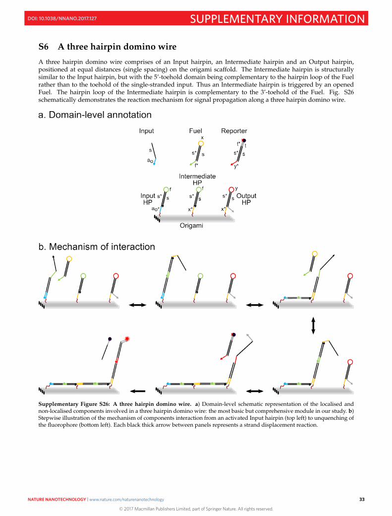
A three hairpin domino wire comprises of an Input hairpin, an Intermediate hairpin and an Output hairpin,positioned at equal distances (single spacing) on the origami scaffold. The Intermediate hairpin is structurallysimilar to the Input hairpin, but with the 5’-toehold domain being complementary to the hairpin loop of the Fuelrather than to the toehold of the single-stranded input. Thus an Intermediate hairpin is triggered by an openedFuel. The hairpin loop of the Intermediate hairpin is complementary to the 3’-toehold of the Fuel. Fig. S26schematically demonstrates the reaction mechanism for signal propagation along a three hairpin domino wire.
Supplementary Figure S26: A three hairpin domino wire. a) Domain-level schematic representation of the localised andnon-localised components involved in a three hairpin domino wire: the most basic but comprehensive module in our study. b)Stepwise illustration of the mechanism of components interaction from an activated Input hairpin (top left) to unquenching ofthe fluorophore (bottom left). Each black thick arrow between panels represents a strand displacement reaction.
33
© 2017 Macmillan Publishers Limited, part of Springer Nature. All rights reserved.
NATURE NANOTECHNOLOGY | www.nature.com/naturenanotechnology 33
SUPPLEMENTARY INFORMATIONDOI: 10.1038/NNANO.2017.127
S7 Predictable localised interactions between adjacent hairpins
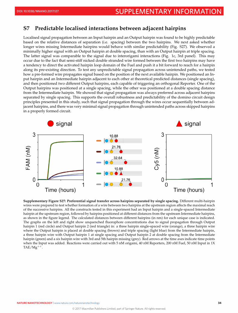
Localised signal propagation between an Input hairpin and an Output hairpin was found to be highly predictablebased on the relative distances of separation (i.e. spacing) between the two hairpins. We next asked whetherlonger wires missing Intermediate hairpins would behave with similar predictability (Fig. S27). We observed aminimally higher signal with an Output hairpin at double spacing, than with an Output hairpin at triple spacing.The latter signal was comparable to the signal due to interorigami interactions (Fig. 1c, 3rd panel). This mayoccur due to the fact that semi-stiff nicked double stranded wire formed between the first two hairpins may havea tendency to direct the activated hairpin loop domain of the Fuel and push it a bit forward to reach for a hairpinalong its pre-existing direction. To test any unpredictable signal propagation across unintended paths, we testedhow a pre-formed wire propagates signal based on the position of the next available hairpin. We positioned an In-put hairpin and an Intermediate hairpin adjacent to each other at theoretical predicted distances (single spacing),and then positioned two different Output hairpins, each capable of triggering an orthogonal Reporter. One of theOutput hairpins was positioned at a single spacing, while the other was positioned at a double spacing distancefrom the Intermediate hairpin. We showed that signal propagation was always preferred across adjacent hairpinsseparated by single spacing. This supports the overall robustness and predictability of the domino circuit designprinciples presented in this study, such that signal propagation through the wires occur sequentially between ad-jacent hairpins, and there was very minimal signal propagation through unintended paths across skipped hairpinsin a properly formed circuit.
Supplementary Figure S27: Preferential signal transfer across hairpins separated by single spacing. Different multi-hairpinwires were prepared to test whether formation of a wire between two hairpins at the upstream region affects the maximal reachof the successive hairpins. All the constructs tested in this experiment had an Input hairpin and a single-spaced Intermediatehairpin at the upstream region, followed by hairpins positioned at different distances from the upstream Intermediate hairpins,as shown in the figure legend. The calculated distances between different hairpins (in nm) for each unique case is indicated.The graphs on the left and right show unquenched fluorophore concentrations due to signal propagation through Outputhairpin 1 (red circle) and Output hairpin 2 (red triangle) in: a three hairpin single-spaced wire (orange), a three hairpin wirewhere the Output hairpin is placed at double spacing (brown) and triple spacing (light blue) from the Intermediate hairpin,a three hairpin wire with Output hairpin 1 at single spacing and Output hairpin 2 at double spacing from the Intermediatehairpin (green) and a six hairpin wire with 3rd and 5th hairpin missing (grey). Red arrows at the time axes indicate time pointswhen the Input was added. Reactions were carried out with 5 nM origami, 40 nM Reporters, 200 nM Fuel, 50 nM Input in 1XTAE/Mg++.
34
© 2017 Macmillan Publishers Limited, part of Springer Nature. All rights reserved.
NATURE NANOTECHNOLOGY | www.nature.com/naturenanotechnology 34
SUPPLEMENTARY INFORMATIONDOI: 10.1038/NNANO.2017.127
S8 Signal loss
The efficiency of incorporation of individual staples may vary depending on the annealing protocol, staple se-quences, position of the staple in the scaffold, and/or structural and conformational intermediate states that theorigami attains during annealing [11, 12]. Imperfect incorporation of staples that are modified with hairpins willdirectly and negatively affect domino circuit performance.
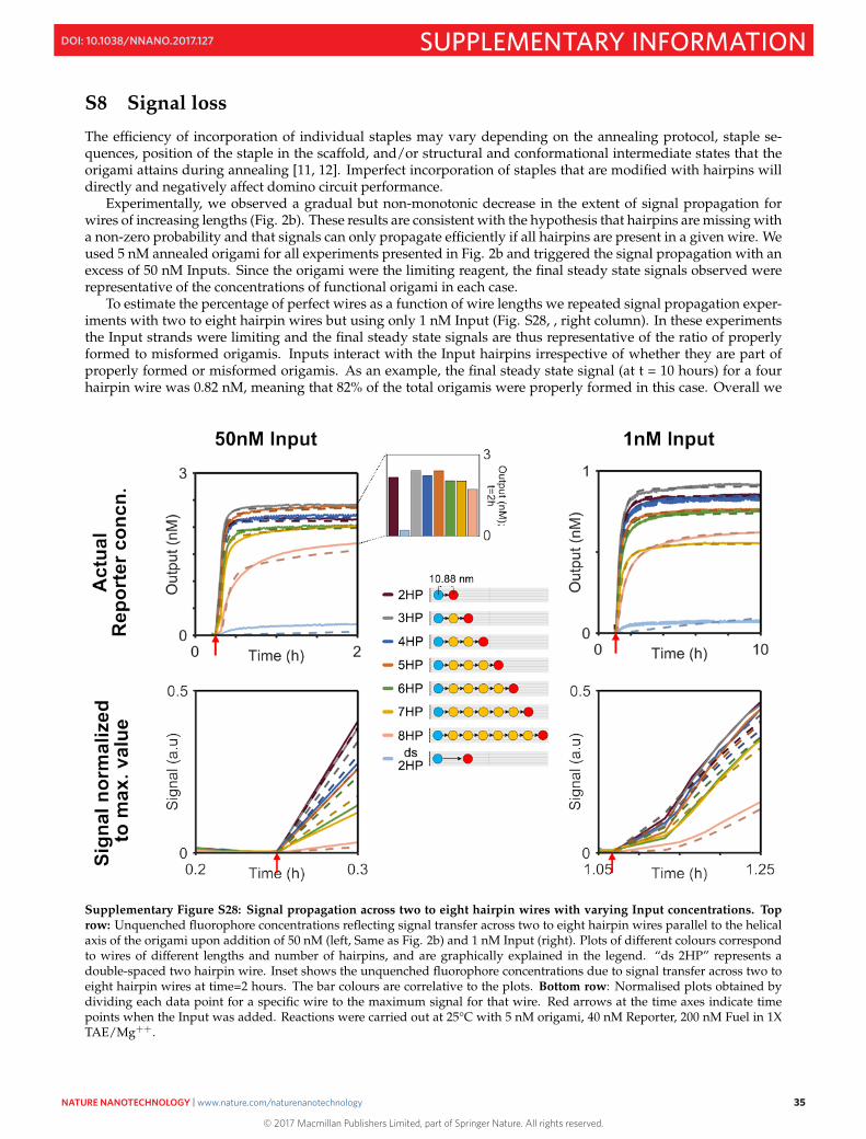
Experimentally, we observed a gradual but non-monotonic decrease in the extent of signal propagation forwires of increasing lengths (Fig. 2b). These results are consistent with the hypothesis that hairpins are missing witha non-zero probability and that signals can only propagate efficiently if all hairpins are present in a given wire. Weused 5 nM annealed origami for all experiments presented in Fig. 2b and triggered the signal propagation with anexcess of 50 nM Inputs. Since the origami were the limiting reagent, the final steady state signals observed wererepresentative of the concentrations of functional origami in each case.
To estimate the percentage of perfect wires as a function of wire lengths we repeated signal propagation exper-iments with two to eight hairpin wires but using only 1 nM Input (Fig. S28, , right column). In these experimentsthe Input strands were limiting and the final steady state signals are thus representative of the ratio of properlyformed to misformed origamis. Inputs interact with the Input hairpins irrespective of whether they are part ofproperly formed or misformed origamis. As an example, the final steady state signal (at t = 10 hours) for a fourhairpin wire was 0.82 nM, meaning that 82% of the total origamis were properly formed in this case. Overall we
Supplementary Figure S28: Signal propagation across two to eight hairpin wires with varying Input concentrations. Toprow: Unquenched fluorophore concentrations reflecting signal transfer across two to eight hairpin wires parallel to the helicalaxis of the origami upon addition of 50 nM (left, Same as Fig. 2b) and 1 nM Input (right). Plots of different colours correspondto wires of different lengths and number of hairpins, and are graphically explained in the legend. “ds 2HP” represents adouble-spaced two hairpin wire. Inset shows the unquenched fluorophore concentrations due to signal transfer across two toeight hairpin wires at time=2 hours. The bar colours are correlative to the plots. Bottom row: Normalised plots obtained bydividing each data point for a specific wire to the maximum signal for that wire. Red arrows at the time axes indicate timepoints when the Input was added. Reactions were carried out at 25°C with 5 nM origami, 40 nM Reporter, 200 nM Fuel in 1XTAE/Mg++.
35
© 2017 Macmillan Publishers Limited, part of Springer Nature. All rights reserved.
NATURE NANOTECHNOLOGY | www.nature.com/naturenanotechnology 35
SUPPLEMENTARY INFORMATIONDOI: 10.1038/NNANO.2017.127
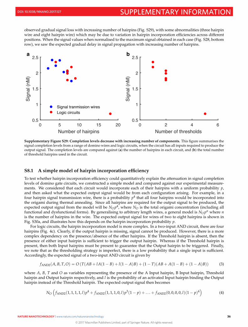
observed gradual signal loss with increasing number of hairpins (Fig. S29), with some abnormalities (three hairpinwire and eight hairpin wire) which may be due to variation in hairpin incorporation efficiencies across differentpositions. When the signal values when normalised to the maximum signal obtained in each case (Fig. S28, bottomrow), we saw the expected gradual delay in signal propagation with increasing number of hairpins.
0 5 10 15 20Number of hairpins
0.5
1
1.5
2
2.5
Sign
al (n
M)
Signal tranmission wiresLogic circuits
0 2 4 6Number of thresholds
0.5
1
1.5
2
2.5
Sign
al (n
M)
a b
Supplementary Figure S29: Completion levels decrease with increasing number of components. This figure summarises thesignal completion levels from a range of domino wires and logic circuits, when the circuit has all inputs required to produce theoutput signal. The completion levels are compared against (a) the number of hairpins in each circuit, and (b) the total numberof threshold hairpins used in the circuit.
S8.1 A simple model of hairpin incorporation efficiency
To test whether hairpin incorporation efficiency could quantitatively explain the attenuation in signal completionlevels of domino gate circuits, we constructed a simple model and compared against our experimental measure-ments. We considered that each circuit would incorporate each of their hairpins with a uniform probability p,and then asked what the expected output signal would be from each configuration arising. For example, in afour hairpin signal transmission wire, there is a probability p4 that all four hairpins would be incorporated intothe origami during thermal annealing. Since all hairpins are required for the output signal to be produced, theexpected output signal from the model will be NO p4, where NO is the total origami concentration (including allfunctional and dysfunctional forms). By generalising to arbitrary length wires, a general model is NO pn where nis the number of hairpins in the wire. The expected output signal for wires of two to eight hairpins is shown inFig. S30a, and illustrates how this depends on the hairpin incorporation probability p.
For logic circuits, the hairpin incorporation model is more complex. In a two-input AND circuit, there are fourhairpins (Fig. 4c). Clearly, if the output hairpin is missing, signal cannot be produced. However, there is a morecomplex dependency on the presence/absence of the other hairpins. If the Threshold hairpin is absent, then thepresence of either input hairpin is sufficient to trigger the output hairpin. Whereas if the Threshold hairpin ispresent, then both Input hairpins must be present to guarantee that the Output hairpin to be triggered. Finally,we note that as the thresholding strategy is imperfect, there is a low probability that a single input is sufficient.Accordingly, the expected signal of a two-input AND circuit is given by
fAND2(A, B, T, O) = O (T(AB + lA(1 − B) + l(1 − A)B) + (1 − T)(AB + A(1 − B) + (1 − A)B)) (3)
where A, B, T and O as variables representing the presence of the A Input hairpin, B Input hairpin, Thresholdhairpin and Output hairpin respectively, and l is the probability of an activated Input hairpin binding the Outputhairpin instead of the Threshold hairpin. The expected output signal then becomes
NO
(fAND2(1, 1, 1, 1, l)p4 + fAND2(1, 1, 1, 0, l)p3(1 − p) + . . . + fAND2(0, 0, 0, 0, l)(1 − p)4
)(4)
36
© 2017 Macmillan Publishers Limited, part of Springer Nature. All rights reserved.
NATURE NANOTECHNOLOGY | www.nature.com/naturenanotechnology 36
SUPPLEMENTARY INFORMATIONDOI: 10.1038/NNANO.2017.127
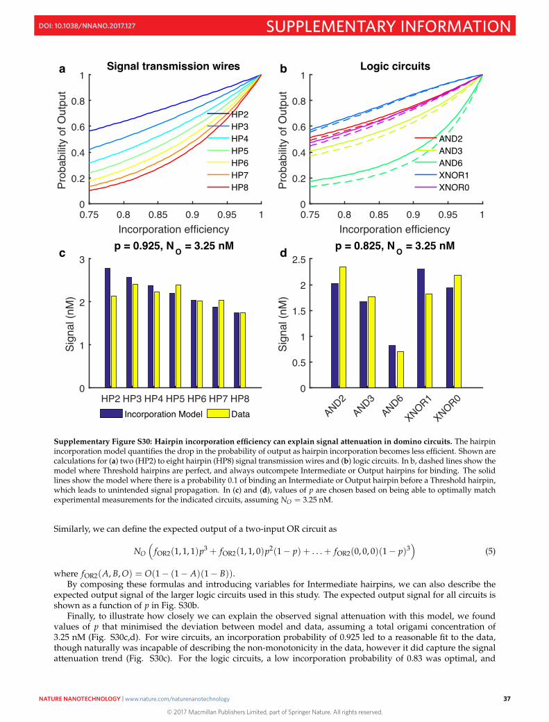
0.75 0.8 0.85 0.9 0.95 1Incorporation efficiency
0
0.2
0.4
0.6
0.8
1Pr
obab
ility
of O
utpu
tSignal transmission wires
HP2HP3HP4HP5HP6HP7HP8
0.75 0.8 0.85 0.9 0.95 1Incorporation efficiency
0
0.2
0.4
0.6
0.8
1
Prob
abilit
y of
Out
put
Logic circuits
AND2AND3AND6XNOR1XNOR0
HP2 HP3 HP4 HP5 HP6 HP7 HP80
1
2
3
Sign
al (n
M)
p = 0.925, N O = 3.25 nM
Incorporation Model Data AND2AND3
AND6
XNOR1
XNOR00
0.5
1
1.5
2
2.5
Sign
al (n
M)
p = 0.825, N O = 3.25 nM
a b
c d
Supplementary Figure S30: Hairpin incorporation efficiency can explain signal attenuation in domino circuits. The hairpinincorporation model quantifies the drop in the probability of output as hairpin incorporation becomes less efficient. Shown arecalculations for (a) two (HP2) to eight hairpin (HP8) signal transmission wires and (b) logic circuits. In b, dashed lines show themodel where Threshold hairpins are perfect, and always outcompete Intermediate or Output hairpins for binding. The solidlines show the model where there is a probability 0.1 of binding an Intermediate or Output hairpin before a Threshold hairpin,which leads to unintended signal propagation. In (c) and (d), values of p are chosen based on being able to optimally matchexperimental measurements for the indicated circuits, assuming NO = 3.25 nM.
Similarly, we can define the expected output of a two-input OR circuit as
NO
(fOR2(1, 1, 1)p3 + fOR2(1, 1, 0)p2(1 − p) + . . . + fOR2(0, 0, 0)(1 − p)3
)(5)
where fOR2(A, B, O) = O(1 − (1 − A)(1 − B)).By composing these formulas and introducing variables for Intermediate hairpins, we can also describe the
expected output signal of the larger logic circuits used in this study. The expected output signal for all circuits isshown as a function of p in Fig. S30b.
Finally, to illustrate how closely we can explain the observed signal attenuation with this model, we foundvalues of p that minimised the deviation between model and data, assuming a total origami concentration of3.25 nM (Fig. S30c,d). For wire circuits, an incorporation probability of 0.925 led to a reasonable fit to the data,though naturally was incapable of describing the non-monotonicity in the data, however it did capture the signalattenuation trend (Fig. S30c). For the logic circuits, a low incorporation probability of 0.83 was optimal, and
37
© 2017 Macmillan Publishers Limited, part of Springer Nature. All rights reserved.
NATURE NANOTECHNOLOGY | www.nature.com/naturenanotechnology 37
SUPPLEMENTARY INFORMATIONDOI: 10.1038/NNANO.2017.127

could account for much of the drop in signal from a two input to a six input AND circuit (Fig. S30d). While acloser match could be obtained with non-uniform hairpin incorporation parameters, these parameters would beunderconstrained by the observations. These findings are consistent with previous studies on staple incorporationefficiency in a single-layered origami[13].
38
© 2017 Macmillan Publishers Limited, part of Springer Nature. All rights reserved.
NATURE NANOTECHNOLOGY | www.nature.com/naturenanotechnology 38
SUPPLEMENTARY INFORMATIONDOI: 10.1038/NNANO.2017.127
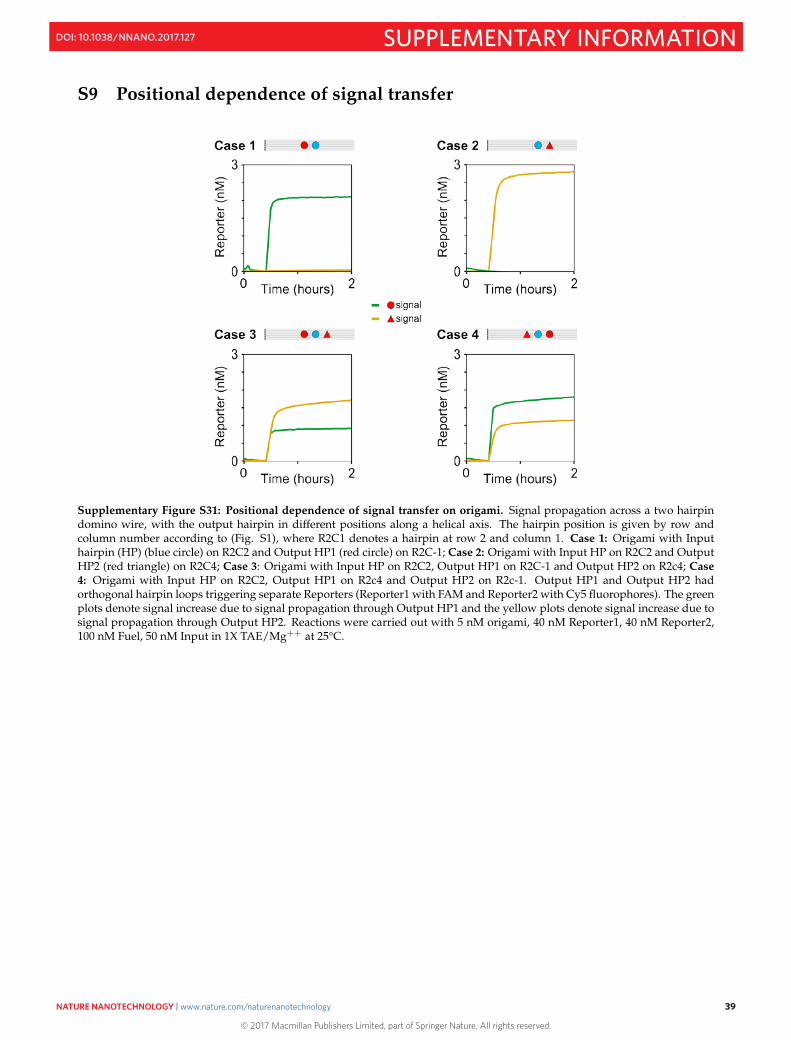
S9 Positional dependence of signal transfer
Supplementary Figure S31: Positional dependence of signal transfer on origami. Signal propagation across a two hairpindomino wire, with the output hairpin in different positions along a helical axis. The hairpin position is given by row andcolumn number according to (Fig. S1), where R2C1 denotes a hairpin at row 2 and column 1. Case 1: Origami with Inputhairpin (HP) (blue circle) on R2C2 and Output HP1 (red circle) on R2C-1; Case 2: Origami with Input HP on R2C2 and OutputHP2 (red triangle) on R2C4; Case 3: Origami with Input HP on R2C2, Output HP1 on R2C-1 and Output HP2 on R2c4; Case4: Origami with Input HP on R2C2, Output HP1 on R2c4 and Output HP2 on R2c-1. Output HP1 and Output HP2 hadorthogonal hairpin loops triggering separate Reporters (Reporter1 with FAM and Reporter2 with Cy5 fluorophores). The greenplots denote signal increase due to signal propagation through Output HP1 and the yellow plots denote signal increase due tosignal propagation through Output HP2. Reactions were carried out with 5 nM origami, 40 nM Reporter1, 40 nM Reporter2,100 nM Fuel, 50 nM Input in 1X TAE/Mg++ at 25°C.
39
© 2017 Macmillan Publishers Limited, part of Springer Nature. All rights reserved.
NATURE NANOTECHNOLOGY | www.nature.com/naturenanotechnology 39
SUPPLEMENTARY INFORMATIONDOI: 10.1038/NNANO.2017.127
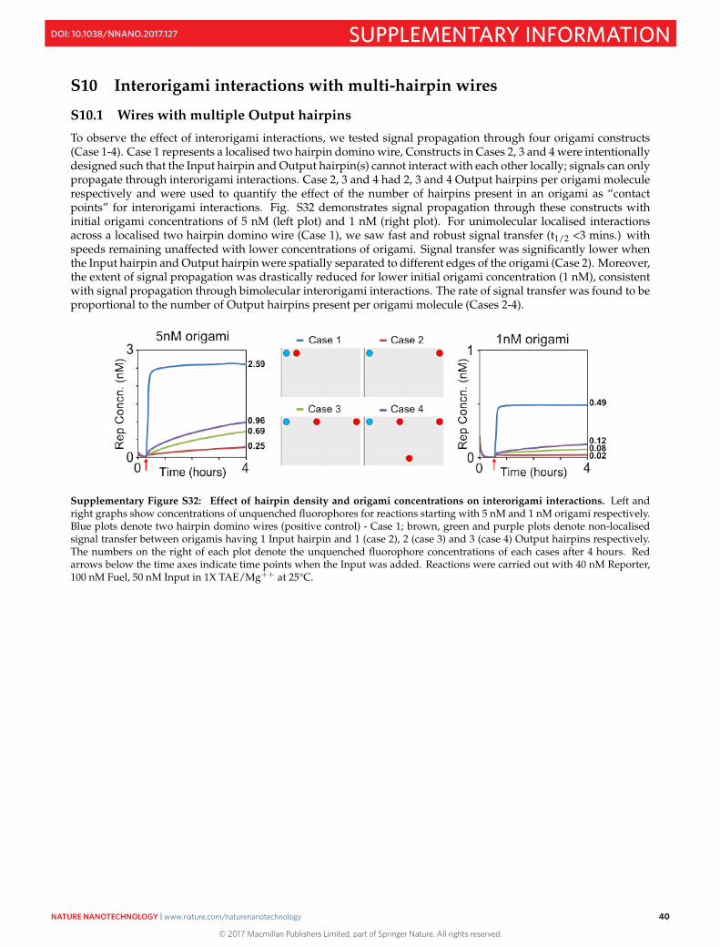
S10 Interorigami interactions with multi-hairpin wires
S10.1 Wires with multiple Output hairpins
To observe the effect of interorigami interactions, we tested signal propagation through four origami constructs(Case 1-4). Case 1 represents a localised two hairpin domino wire, Constructs in Cases 2, 3 and 4 were intentionallydesigned such that the Input hairpin and Output hairpin(s) cannot interact with each other locally; signals can onlypropagate through interorigami interactions. Case 2, 3 and 4 had 2, 3 and 4 Output hairpins per origami moleculerespectively and were used to quantify the effect of the number of hairpins present in an origami as “contactpoints” for interorigami interactions. Fig. S32 demonstrates signal propagation through these constructs withinitial origami concentrations of 5 nM (left plot) and 1 nM (right plot). For unimolecular localised interactionsacross a localised two hairpin domino wire (Case 1), we saw fast and robust signal transfer (t1/2 <3 mins.) withspeeds remaining unaffected with lower concentrations of origami. Signal transfer was significantly lower whenthe Input hairpin and Output hairpin were spatially separated to different edges of the origami (Case 2). Moreover,the extent of signal propagation was drastically reduced for lower initial origami concentration (1 nM), consistentwith signal propagation through bimolecular interorigami interactions. The rate of signal transfer was found to beproportional to the number of Output hairpins present per origami molecule (Cases 2-4).
Supplementary Figure S32: Effect of hairpin density and origami concentrations on interorigami interactions. Left andright graphs show concentrations of unquenched fluorophores for reactions starting with 5 nM and 1 nM origami respectively.Blue plots denote two hairpin domino wires (positive control) - Case 1; brown, green and purple plots denote non-localisedsignal transfer between origamis having 1 Input hairpin and 1 (case 2), 2 (case 3) and 3 (case 4) Output hairpins respectively.The numbers on the right of each plot denote the unquenched fluorophore concentrations of each cases after 4 hours. Redarrows below the time axes indicate time points when the Input was added. Reactions were carried out with 40 nM Reporter,100 nM Fuel, 50 nM Input in 1X TAE/Mg++ at 25°C.
40
© 2017 Macmillan Publishers Limited, part of Springer Nature. All rights reserved.
NATURE NANOTECHNOLOGY | www.nature.com/naturenanotechnology 40
SUPPLEMENTARY INFORMATIONDOI: 10.1038/NNANO.2017.127
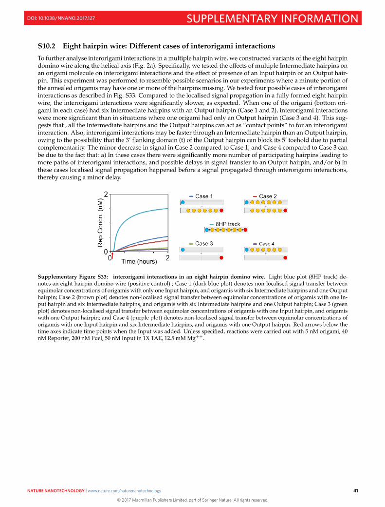
S10.2 Eight hairpin wire: Different cases of interorigami interactions
To further analyse interorigami interactions in a multiple hairpin wire, we constructed variants of the eight hairpindomino wire along the helical axis (Fig. 2a). Specifically, we tested the effects of multiple Intermediate hairpins onan origami molecule on interorigami interactions and the effect of presence of an Input hairpin or an Output hair-pin. This experiment was performed to resemble possible scenarios in our experiments where a minute portion ofthe annealed origamis may have one or more of the hairpins missing. We tested four possible cases of interorigamiinteractions as described in Fig. S33. Compared to the localised signal propagation in a fully formed eight hairpinwire, the interorigami interactions were significantly slower, as expected. When one of the origami (bottom ori-gami in each case) had six Intermediate hairpins with an Output hairpin (Case 1 and 2), interorigami interactionswere more significant than in situations where one origami had only an Output hairpin (Case 3 and 4). This sug-gests that , all the Intermediate hairpins and the Output hairpins can act as “contact points” to for an interorigamiinteraction. Also, interorigami interactions may be faster through an Intermediate hairpin than an Output hairpin,owing to the possibility that the 3’ flanking domain (t) of the Output hairpin can block its 5’ toehold due to partialcomplementarity. The minor decrease in signal in Case 2 compared to Case 1, and Case 4 compared to Case 3 canbe due to the fact that: a) In these cases there were significantly more number of participating hairpins leading tomore paths of interorigami interactions, and possible delays in signal transfer to an Output hairpin, and/or b) Inthese cases localised signal propagation happened before a signal propagated through interorigami interactions,thereby causing a minor delay.
Supplementary Figure S33: interorigami interactions in an eight hairpin domino wire. Light blue plot (8HP track) de-notes an eight hairpin domino wire (positive control) ; Case 1 (dark blue plot) denotes non-localised signal transfer betweenequimolar concentrations of origamis with only one Input hairpin, and origamis with six Intermediate hairpins and one Outputhairpin; Case 2 (brown plot) denotes non-localised signal transfer between equimolar concentrations of origamis with one In-put hairpin and six Intermediate hairpins, and origamis with six Intermediate hairpins and one Output hairpin; Case 3 (greenplot) denotes non-localised signal transfer between equimolar concentrations of origamis with one Input hairpin, and origamiswith one Output hairpin; and Case 4 (purple plot) denotes non-localised signal transfer between equimolar concentrations oforigamis with one Input hairpin and six Intermediate hairpins, and origamis with one Output hairpin. Red arrows below thetime axes indicate time points when the Input was added. Unless specified, reactions were carried out with 5 nM origami, 40nM Reporter, 200 nM Fuel, 50 nM Input in 1X TAE, 12.5 mM Mg++.
41
© 2017 Macmillan Publishers Limited, part of Springer Nature. All rights reserved.
NATURE NANOTECHNOLOGY | www.nature.com/naturenanotechnology 41
SUPPLEMENTARY INFORMATIONDOI: 10.1038/NNANO.2017.127
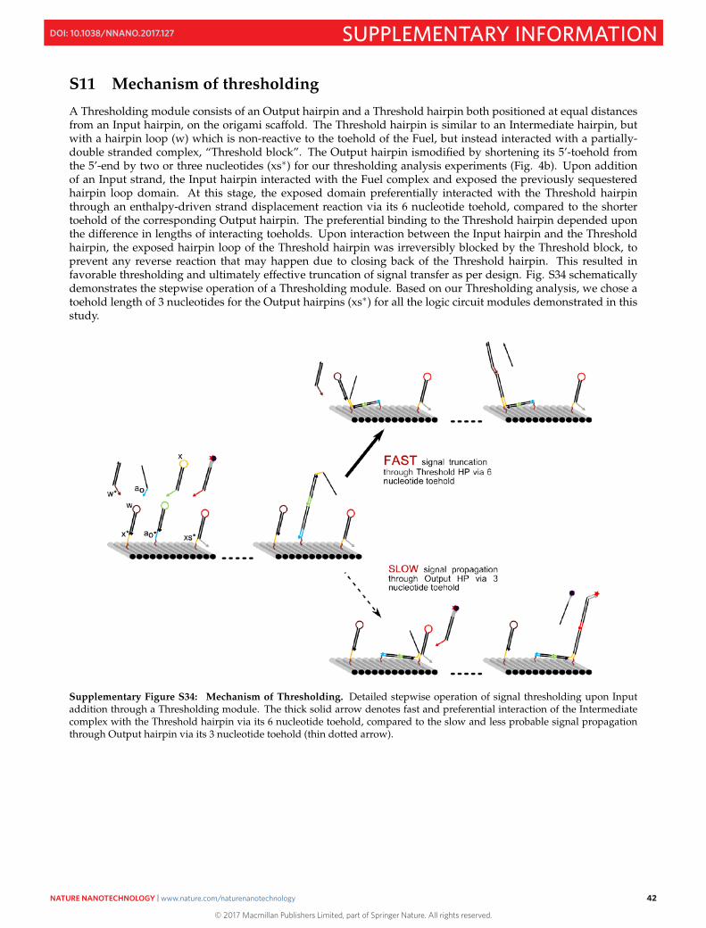
S11 Mechanism of thresholding
A Thresholding module consists of an Output hairpin and a Threshold hairpin both positioned at equal distancesfrom an Input hairpin, on the origami scaffold. The Threshold hairpin is similar to an Intermediate hairpin, butwith a hairpin loop (w) which is non-reactive to the toehold of the Fuel, but instead interacted with a partially-double stranded complex, “Threshold block”. The Output hairpin ismodified by shortening its 5’-toehold fromthe 5’-end by two or three nucleotides (xs∗) for our thresholding analysis experiments (Fig. 4b). Upon additionof an Input strand, the Input hairpin interacted with the Fuel complex and exposed the previously sequesteredhairpin loop domain. At this stage, the exposed domain preferentially interacted with the Threshold hairpinthrough an enthalpy-driven strand displacement reaction via its 6 nucleotide toehold, compared to the shortertoehold of the corresponding Output hairpin. The preferential binding to the Threshold hairpin depended uponthe difference in lengths of interacting toeholds. Upon interaction between the Input hairpin and the Thresholdhairpin, the exposed hairpin loop of the Threshold hairpin was irreversibly blocked by the Threshold block, toprevent any reverse reaction that may happen due to closing back of the Threshold hairpin. This resulted infavorable thresholding and ultimately effective truncation of signal transfer as per design. Fig. S34 schematicallydemonstrates the stepwise operation of a Thresholding module. Based on our Thresholding analysis, we chose atoehold length of 3 nucleotides for the Output hairpins (xs∗) for all the logic circuit modules demonstrated in thisstudy.
Supplementary Figure S34: Mechanism of Thresholding. Detailed stepwise operation of signal thresholding upon Inputaddition through a Thresholding module. The thick solid arrow denotes fast and preferential interaction of the Intermediatecomplex with the Threshold hairpin via its 6 nucleotide toehold, compared to the slow and less probable signal propagationthrough Output hairpin via its 3 nucleotide toehold (thin dotted arrow).
42
© 2017 Macmillan Publishers Limited, part of Springer Nature. All rights reserved.
NATURE NANOTECHNOLOGY | www.nature.com/naturenanotechnology 42
SUPPLEMENTARY INFORMATIONDOI: 10.1038/NNANO.2017.127
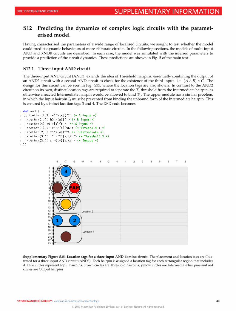
S12 Predicting the dynamics of complex logic circuits with the paramet-erised model
Having characterised the parameters of a wide range of localised circuits, we sought to test whether the modelcould predict dynamic behaviours of more elaborate circuits. In the following sections, the models of multi-inputAND and XNOR circuits are described. In each case, the model was simulated with the inferred parameters toprovide a prediction of the circuit dynamics. These predictions are shown in Fig. 5 of the main text.
S12.1 Three-input AND circuit
The three-input AND circuit (AND3) extends the idea of Threshold hairpins, essentially combining the output ofan AND2 circuit with a second AND circuit to check for the existence of the third input. i.e. (A ∧ B) ∧ C. Thedesign for this circuit can be seen in Fig. S35, where the location tags are also shown. In contrast to the AND2circuit on its own, distinct location tags are required to separate the T1 threshold from the Intermediate hairpin, asotherwise a reacted Intermediate hairpin would be allowed to bind T1. The upper module has a similar problem,in which the Input hairpin I3 must be prevented from binding the unbound form of the Intermediate hairpin. Thisis ensured by distinct location tags 3 and 4. The DSD code becomes:
1
2
3
4
5
6
7
8
9
01234
765
9101112131415161718
8
1920212223
-8 -6 -4-7 -5 -3 -2 -1 1 2 3 4 5 6 7 8
3
21
FAM
Loca
tion
4
Location 6
Loca
tion
5
Location 1
Location 2
Location 3
Supplementary Figure S35: Location tags for a three-input AND domino circuit. The placement and location tags are illus-trated for a three-input AND circuit (AND3). Each hairpin is assigned a location tag for each rectangular region that includesit. Blue circles represent Input hairpins, brown circles are Threshold hairpins, yellow circles are Intermediate hairpins and redcircles are Output hairpins.
43
© 2017 Macmillan Publishers Limited, part of Springer Nature. All rights reserved.
NATURE NANOTECHNOLOGY | www.nature.com/naturenanotechnology 43
SUPPLEMENTARY INFORMATIONDOI: 10.1038/NNANO.2017.127
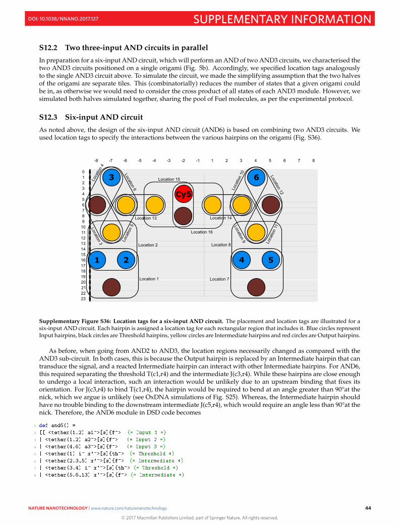
S12.2 Two three-input AND circuits in parallel
In preparation for a six-input AND circuit, which will perform an AND of two AND3 circuits, we characterised thetwo AND3 circuits positioned on a single origami (Fig. 5b). Accordingly, we specified location tags analogouslyto the single AND3 circuit above. To simulate the circuit, we made the simplifying assumption that the two halvesof the origami are separate tiles. This (combinatorially) reduces the number of states that a given origami couldbe in, as otherwise we would need to consider the cross product of all states of each AND3 module. However, wesimulated both halves simulated together, sharing the pool of Fuel molecules, as per the experimental protocol.
S12.3 Six-input AND circuit
As noted above, the design of the six-input AND circuit (AND6) is based on combining two AND3 circuits. Weused location tags to specify the interactions between the various hairpins on the origami (Fig. S36).
01234
765
9101112131415161718
8
1920212223
-8 -6 -4-7 -5 -3 -2 -1 1 2 3 4 5 6 7 8
3
21
6
4 5
Cy5
Loca
tion
4
Location 6
Loca
tion
5
Location 1
Location 2
Location 3
Location 15
Location 16
Location 13 Location 14
Location 7
Location 8
Location 12Loca
tion
10
Location 9 Loca
tion
11
Supplementary Figure S36: Location tags for a six-input AND circuit. The placement and location tags are illustrated for asix-input AND circuit. Each hairpin is assigned a location tag for each rectangular region that includes it. Blue circles representInput hairpins, black circles are Threshold hairpins, yellow circles are Intermediate hairpins and red circles are Output hairpins.
As before, when going from AND2 to AND3, the location regions necessarily changed as compared with theAND3 sub-circuit. In both cases, this is because the Output hairpin is replaced by an Intermediate hairpin that cantransduce the signal, and a reacted Intermediate hairpin can interact with other Intermediate hairpins. For AND6,this required separating the threshold T(c1,r4) and the intermediate J(c3,r4). While these hairpins are close enoughto undergo a local interaction, such an interaction would be unlikely due to an upstream binding that fixes itsorientation. For J(c3,r4) to bind T(c1,r4), the hairpin would be required to bend at an angle greater than 90°at thenick, which we argue is unlikely (see OxDNA simulations of Fig. S25). Whereas, the Intermediate hairpin shouldhave no trouble binding to the downstream intermediate J(c5,r4), which would require an angle less than 90°at thenick. Therefore, the AND6 module in DSD code becomes
1
2
3
4
5
6
7
8
44
© 2017 Macmillan Publishers Limited, part of Springer Nature. All rights reserved.
NATURE NANOTECHNOLOGY | www.nature.com/naturenanotechnology 44
SUPPLEMENTARY INFORMATIONDOI: 10.1038/NNANO.2017.127
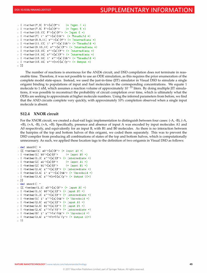
9
10
11
12
13
14
15
16
17
18
19
20
The number of reactions is enormous for the AND6 circuit, and DSD compilation does not terminate in reas-onable time. Therefore, it was not possible to use an ODE simulation, as this requires the prior enumeration of thecomplete model state-space. Instead, we used the just-in-time (JIT) simulator in Visual DSD to simulate a singleorigami binding to populations of input and fuel molecules in the corresponding concentrations. We equate 1molecule to 1 nM, which assumes a reaction volume of approximately 10−15 liters. By doing multiple JIT simula-tions, it was possible to reconstruct the probability of circuit completion over time, which is ultimately what theODEs are seeking to approximate at higher molecule numbers. Using the inferred parameters from before, we findthat the AND circuits complete very quickly, with approximately 10% completion observed when a single inputmolecule is absent.
S12.4 XNOR circuit
For the XNOR circuit, we created a dual-rail logic implementation to distinguish between four cases: (-A, -B), (-A,+B), (+A, -B), (+A, +B). Specifically, presence and absence of input A was encoded by input molecules A1 andA0 respectively, and equivalently for an input B, with B1 and B0 molecules. As there is no interaction betweenthe hairpins of the top and bottom halves of this origami, we coded them separately. This was to prevent theDSD compiler from producing all combinations of states of the top and bottom halves, which is computationallyunnecessary. As such, we applied these location tags to the definition of two origamis in Visual DSD as follows:
1
2
3
4
5
6
7
8
9
10
11
12
13
14
15
16
17
18
19
20
21
45
© 2017 Macmillan Publishers Limited, part of Springer Nature. All rights reserved.
NATURE NANOTECHNOLOGY | www.nature.com/naturenanotechnology 45
SUPPLEMENTARY INFORMATIONDOI: 10.1038/NNANO.2017.127
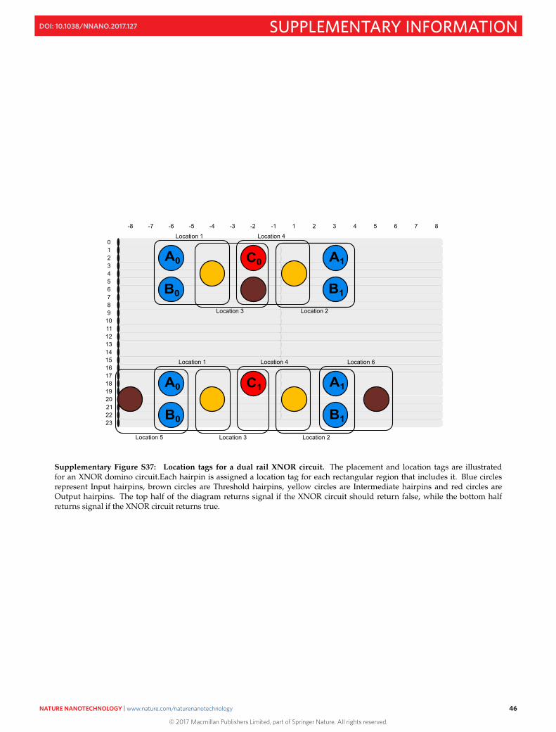
A0
B0
A1
B1
A0
B0
A1
B1
C1
C0
Location 1
Location 3
Location 4
Location 2
Location 1
Location 3
Location 4
Location 2
Location 6
Location 5
01234
765
9101112131415161718
8
1920212223
-8 -6 -4-7 -5 -3 -2 -1 1 2 3 4 5 6 7 8
Supplementary Figure S37: Location tags for a dual rail XNOR circuit. The placement and location tags are illustratedfor an XNOR domino circuit.Each hairpin is assigned a location tag for each rectangular region that includes it. Blue circlesrepresent Input hairpins, brown circles are Threshold hairpins, yellow circles are Intermediate hairpins and red circles areOutput hairpins. The top half of the diagram returns signal if the XNOR circuit should return false, while the bottom halfreturns signal if the XNOR circuit returns true.
46
© 2017 Macmillan Publishers Limited, part of Springer Nature. All rights reserved.
NATURE NANOTECHNOLOGY | www.nature.com/naturenanotechnology 46
SUPPLEMENTARY INFORMATIONDOI: 10.1038/NNANO.2017.127
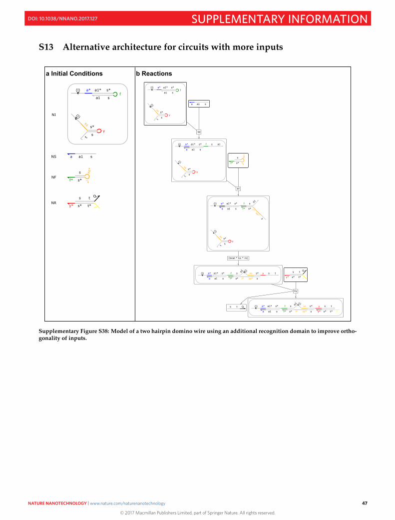
S13 Alternative architecture for circuits with more inputs
b Reactionsa Initial Conditions
t
s*y
s
(l)
xs
a1* s*f
sa1
(l) a*
sa1a
f*
s xs*
i*s*
s t Q
y* t*s* F
t
s*y
s
(l)
xs
(l) a* a1* s* f s a1
sa1a
t
s*y
s
(l)
xs
(l) a* a1* s* f s a1
s*f*
s
xs*
i*sa1a
(l)xs s* y s t
sxs*i*s*f*
(l) a* a1* s* f s a1
sa1a
s t Q
(l)xs s* y s t
t*s*y* Fsxs*i*s*f*
(l) a* a1* s* f s a1
sa1a
ka
kf
(local * kx * ro)
ky
s t Q
y* t*s* FNR
f*
s xs*
i*s*NF
sa1aNS
t
s*y
s
(l)
xs
a1* s*f
sa1
(l) a*
NI
Supplementary Figure S38: Model of a two hairpin domino wire using an additional recognition domain to improve ortho-gonality of inputs.
47
© 2017 Macmillan Publishers Limited, part of Springer Nature. All rights reserved.
NATURE NANOTECHNOLOGY | www.nature.com/naturenanotechnology 47
SUPPLEMENTARY INFORMATIONDOI: 10.1038/NNANO.2017.127

S14 Performance comparison
The previous study by Qian et al.[14] with diffusible components, demonstrates the state-of-the-art in the field ofcomplex DNA logic circuits. This section highlights some advantages of the DNA domino architecture over thecurrent state-of-the-art system by comparing some key features.
Key differences between systems: 5 nt. toehold sequences, non-hairpin constructs (Qian et al.) vs. 6/3 nt.toehold sequences, hairpin constructs (our study); 20°C experiments (Qian et al.) vs. 25°C experiments (our study);150 nM Reporter (Qian et al.) vs. 40 nM Reporter (our study); 100 nM Input (Qian et al.) vs. 50 nM Input (ourstudy).
Supplementary Table S2: Domino Circuits vs. Current state-of-the-art
Category Qian et al. (2011) This study
Operating concentration of Gate compon-ent
100 nM ~2 nM
3 Input AND GATE (2 AND Gates inseries): T1/2
>4 hours (Fig. S5B) <7 minutes (Fig. 5a)
4 layered gate (4-layered OR Gate withone input (x2) vs. 4 hairpin domino wire):T1/2
>2 hours (Fig. S6) <5 minutes (Fig. 2a)
Number of unique domains required for a2 Gate circuit (3 Input AND GATE)
11 [3*(no. of Gates) + (no. ofinputs) + (no. of outputs) + 1]
9 [(no. of inputs) + (no. of out-puts) + 5]
Number of unique domains required for a4 Gate circuit ( 4 Input OR GATE)
19 10 (4 + 1 + 5)
48
© 2017 Macmillan Publishers Limited, part of Springer Nature. All rights reserved.
NATURE NANOTECHNOLOGY | www.nature.com/naturenanotechnology 48
SUPPLEMENTARY INFORMATIONDOI: 10.1038/NNANO.2017.127
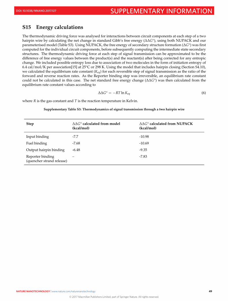
S15 Energy calculations
The thermodynamic driving force was analysed for interactions between circuit components at each step of a twohairpin wire by calculating the net change in standard Gibb’s free energy (∆∆G°), using both NUPACK and ourparameterised model (Table S3). Using NUPACK, the free energy of secondary structure formation (∆G°) was firstcomputed for the individual circuit components, before subsequently computing the intermediate state secondarystructures. The thermodynamic driving force at each step of signal transmission can be approximated to be thedifference of free energy values between the product(s) and the reactant(s) after being corrected for any entropicchange. We included possible entropy loss due to association of two molecules in the form of initiation entropy of6.4 cal/mol/K per association[15] at 25°C or 298 K. Using the model that includes hairpin closing (Section S4.10),we calculated the equilibrium rate constant (Keq) for each reversible step of signal transmission as the ratio of theforward and reverse reaction rates. As the Reporter binding step was irreversible, an equilibrium rate constantcould not be calculated in this case. The net standard free energy change (∆∆G°) was then calculated from theequilibrium rate constant values according to
∆∆G° = −RT ln Keq (6)
where R is the gas constant and T is the reaction temperature in Kelvin.
Supplementary Table S3: Thermodynamics of signal transmission through a two hairpin wire
Step ∆∆G° calculated from model(kcal/mol)
∆∆G° calculated from NUPACK(kcal/mol)
Input binding -7.7 -10.98
Fuel binding -7.68 -10.69
Output hairpin binding -6.48 -9.35
Reporter binding(quencher strand release)
– -7.83
49
© 2017 Macmillan Publishers Limited, part of Springer Nature. All rights reserved.
NATURE NANOTECHNOLOGY | www.nature.com/naturenanotechnology 49
SUPPLEMENTARY INFORMATIONDOI: 10.1038/NNANO.2017.127

S16 Sequences
S16.1 M13mp18 template DNA
Bayou Biolabs m13mp18 DNA sequence: Source: http://www.bayoubiolabs.com/biochemicat/vectors/pUCM13/
AATGCTACTACTATTAGTAGAATTGATGCCACCTTTTCAGCTCGCGCCCCAAATGAAAATATAGCTAAACAGGTTATTGACCATTTGCGAAATGTATCTAATGGTCAAACTAAATCTACTCGTTCGCAGAATTGGGAATCAACTGTTATATGGAATGAAACTTCCAGACACCGTACTTTAGTTGCATATTTAAAACATGTTGAGCTACAGCATTATATTCAGCAATTAAGCTCTAAGCCATCCGCAAAAATGACCTCTTATCAAAAGGAGCAATTAAAGGTACTCTCTAATCCTGACCTGTTGGAGTTTGCTTCCGGTCTGGTTCGCTTTGAAGCTCGAATTAAAACGCGATATTTGAAGTCTTTCGGGCTTCCTCTTAATCTTTTTGATGCAATCCGCTTTGCTTCTGACTATAATAGTCAGGGTAAAGACCTGATTTTTGATTTATGGTCATTCTCGTTTTCTGAACTGTTTAAAGCATTTGAGGGGGATTCAATGAATATTTATGACGATTCCGCAGTATTGGACGCTATCCAGTCTAAACATTTTACTATTACCCCCTCTGGCAAAACTTCTTTTGCAAAAGCCTCTCGCTATTTTGGTTTTTATCGTCGTCTGGTAAACGAGGGTTATGATAGTGTTGCTCTTACTATGCCTCGTAATTCCTTTTGGCGTTATGTATCTGCATTAGTTGAATGTGGTATTCCTAAATCTCAACTGATGAATCTTTCTACCTGTAATAATGTTGTTCCGTTAGTTCGTTTTATTAACGTAGATTTTTCTTCCCAACGTCCTGACTGGTATAATGAGCCAGTTCTTAAAATCGCATAAGGTAATTCACAATGATTAAAGTTGAAATTAAACCATCTCAAGCCCAATTTACTACTCGTTCTGGTGTTTCTCGTCAGGGCAAGCCTTATTCACTGAATGAGCAGCTTTGTTACGTTGATTTGGGTAATGAATATCCGGTTCTTGTCAAGATTACTCTTGATGAAGGTCAGCCAGCCTATGCGCCTGGTCTGTACACCGTTCATCTGTCCTCTTTCAAAGTTGGTCAGTTCGGTTCCCTTATGATTGACCGTCTGCGCCTCGTTCCGGCTAAGTAACATGGAGCAGGTCGCGGATTTCGACACAATTTATCAGGCGATGATACAAATCTCCGTTGTACTTTGTTTCGCGCTTGGTATAATCGCTGGGGGTCAAAGATGAGTGTTTTAGTGTATTCTTTTGCCTCTTTCGTTTTAGGTTGGTGCCTTCGTAGTGGCATTACGTATTTTACCCGTTTAATGGAAACTTCCTCATGAAAAAGTCTTTAGTCCTCAAAGCCTCTGTAGCCGTTGCTACCCTCGTTCCGATGCTGTCTTTCGCTGCTGAGGGTGACGATCCCGCAAAAGCGGCCTTTAACTCCCTGCAAGCCTCAGCGACCGAATATATCGGTTATGCGTGGGCGATGGTTGTTGTCATTGTCGGCGCAACTATCGGTATCAAGCTGTTTAAGAAATTCACCTCGAAAGCAAGCTGATAAACCGATACAATTAAAGGCTCCTTTTGGAGCCTTTTTTTTGGAGATTTTCAACGTGAAAAAATTATTATTCGCAATTCCTTTAGTTGTTCCTTTCTATTCTCACTCCGCTGAAACTGTTGAAAGTTGTTTAGCAAAATCCCATACAGAAAATTCATTTACTAACGTCTGGAAAGACGACAAAACTTTAGATCGTTACGCTAACTATGAGGGCTGTCTGTGGAATGCTACAGGCGTTGTAGTTTGTACTGGTGACGAAACTCAGTGTTACGGTACATGGGTTCCTATTGGGCTTGCTATCCCTGAAAATGAGGGTGGTGGCTCTGAGGGTGGCGGTTCTGAGGGTGGCGGTTCTGAGGGTGGCGGTACTAAACCTCCTGAGTACGGTGATACACCTATTCCGGGCTATACTTATATCAACCCTCTCGACGGCACTTATCCGCCTGGTACTGAGCAAAACCCCGCTAATCCTAATCCTTCTCTTGAGGAGTCTCAGCCTCTTAATACTTTCATGTTTCAGAATAATAGGTTCCGAAATAGGCAGGGGGCATTAACTGTTTATACGGGCACTGTTACTCAAGGCACTGACCCCGTTAAAACTTATTACCAGTACACTCCTGTATCATCAAAAGCCATGTATGACGCTTACTGGAACGGTAAATTCAGAGACTGCGCTTTCCATTCTGGCTTTAATGAGGATTTATTTGTTTGTGAATATCAAGGCCAATCGTCTGACCTGCCTCAACCTCCTGTCAATGCTGGCGGCGGCTCTGGTGGTGGTTCTGGTGGCGGCTCTGAGGGTGGTGGCTCTGAGGGTGGCGGTTCTGAGGGTGGCGGCTCTGAGGGAGGCGGTTCCGGTGGTGGCTCTGGTTCCGGTGATTTTGATTATGAAAAGATGGCAAACGCTAATAAGGGGGCTATGACCGAAAATGCCGATGAAAACGCGCTACAGTCTGACGCTAAAGGCAAACTTGATTCTGTCGCTACTGATTACGGTGCTGCTATCGATGGTTTCATTGGTGACGTTTCCGGCCTTGCTAATGGTAATGGTGCTACTGGTGATTTTGCTGGCTCTAATTCCCAAATGGCTCAAGTCGGTGACGGTGATAATTCACCTTTAATGAATAATTTCCGTCAATATTTACCTTCCCTCCCTCAATCGGTTGAATGTCGCCCTTTTGTCTTTGGCGCTGGTAAACCATATGAATTTTCTATTGATTGTGACAAAATAAACTTATTCCGTGGTGTCTTTGCGTTTCTTTTATATGTTGCCACCTTTATGTATGTATTTTCTACGTTTGCTAACATACTGCGTAATAAGGAGTCTTAATCATGCCAGTTCTTTTGGGTATTCCGTTATTATTGCGTTTCCTCGGTTTCCTTCTGGTAACTTTGTTCGGCTATCTGCTTACTTTTCTTAAAAAGGGCTTCGGTAAGATAGCTATTGCTATTTCATTGTTTCTTGCTCTTATTATTGGGCTTAACTCAATTCTTGTGGGTTATCTCTCTGATATTAGCGCTCAATTACCCTCTGACTTTGTTCAGGGTGTTCAGTTAATTCTCCCGTCTAATGCGCTTCCCTGTTTTTATGTTATTCTCTCTGTAAAGGCTGCTATTTTCATTTTTGACGTTAAACAAAAAATCGTTTCTTATTTGGATTGGGATAAATAATATGGCTGTTTATTTTGTAACTGGCAAATTAGGCTCTGGAAAGACGCTCGTTAGCGTTGGTAAGATTCAGGATAAAATTGTAGCTGGGTGCAAAATAGCAACTAATCTTGATTTAAGGCTTCAAAACCTCCCGCAAGTCGGGAGGTTCGCTAAAACGCCTCGCGTTCTTAGAATACCGGATAAGCCTTCTATATCTGATTTGCTTGCTATTGGGCGCGGTAATGATTCCTACGATGAAAATAAAAACGGCTTGCTTGTTCTCGATGAGTGCGGTACTTGGTTTAATACCCGTTCTTGGAATGATAAGGAAAGACAGCCGATTATTGATTGGTTTCTACATGCTCGTAAATTAGGATGGGATATTATTTTTCTTGTTCAGGACTTATCTATTGTTGATAAAC
50
© 2017 Macmillan Publishers Limited, part of Springer Nature. All rights reserved.
NATURE NANOTECHNOLOGY | www.nature.com/naturenanotechnology 50
SUPPLEMENTARY INFORMATIONDOI: 10.1038/NNANO.2017.127

AGGCGCGTTCTGCATTAGCTGAACATGTTGTTTATTGTCGTCGTCTGGACAGAATTACTTTACCTTTTGTCGGTACTTTATATTCTCTTATTACTGGCTCGAAAATGCCTCTGCCTAAATTACATGTTGGCGTTGTTAAATATGGCGATTCTCAATTAAGCCCTACTGTTGAGCGTTGGCTTTATACTGGTAAGAATTTGTATAACGCATATGATACTAAACAGGCTTTTTCTAGTAATTATGATTCCGGTGTTTATTCTTATTTAACGCCTTATTTATCACACGGTCGGTATTTCAAACCATTAAATTTAGGTCAGAAGATGAAATTAACTAAAATATATTTGAAAAAGTTTTCTCGCGTTCTTTGTCTTGCGATTGGATTTGCATCAGCATTTACATATAGTTATATAACCCAACCTAAGCCGGAGGTTAAAAAGGTAGTCTCTCAGACCTATGATTTTGATAAATTCACTATTGACTCTTCTCAGCGTCTTAATCTAAGCTATCGCTATGTTTTCAAGGATTCTAAGGGAAAATTAATTAATAGCGACGATTTACAGAAGCAAGGTTATTCACTCACATATATTGATTTATGTACTGTTTCCATTAAAAAAGGTAATTCAAATGAAATTGTTAAATGTAATTAATTTTGTTTTCTTGATGTTTGTTTCATCATCTTCTTTTGCTCAGGTAATTGAAATGAATAATTCGCCTCTGCGCGATTTTGTAACTTGGTATTCAAAGCAATCAGGCGAATCCGTTATTGTTTCTCCCGATGTAAAAGGTACTGTTACTGTATATTCATCTGACGTTAAACCTGAAAATCTACGCAATTTCTTTATTTCTGTTTTACGTGCAAATAATTTTGATATGGTAGGTTCTAACCCTTCCATTATTCAGAAGTATAATCCAAACAATCAGGATTATATTGATGAATTGCCATCATCTGATAATCAGGAATATGATGATAATTCCGCTCCTTCTGGTGGTTTCTTTGTTCCGCAAAATGATAATGTTACTCAAACTTTTAAAATTAATAACGTTCGGGCAAAGGATTTAATACGAGTTGTCGAATTGTTTGTAAAGTCTAATACTTCTAAATCCTCAAATGTATTATCTATTGACGGCTCTAATCTATTAGTTGTTAGTGCTCCTAAAGATATTTTAGATAACCTTCCTCAATTCCTTTCAACTGTTGATTTGCCAACTGACCAGATATTGATTGAGGGTTTGATATTTGAGGTTCAGCAAGGTGATGCTTTAGATTTTTCATTTGCTGCTGGCTCTCAGCGTGGCACTGTTGCAGGCGGTGTTAATACTGACCGCCTCACCTCTGTTTTATCTTCTGCTGGTGGTTCGTTCGGTATTTTTAATGGCGATGTTTTAGGGCTATCAGTTCGCGCATTAAAGACTAATAGCCATTCAAAAATATTGTCTGTGCCACGTATTCTTACGCTTTCAGGTCAGAAGGGTTCTATCTCTGTTGGCCAGAATGTCCCTTTTATTACTGGTCGTGTGACTGGTGAATCTGCCAATGTAAATAATCCATTTCAGACGATTGAGCGTCAAAATGTAGGTATTTCCATGAGCGTTTTTCCTGTTGCAATGGCTGGCGGTAATATTGTTCTGGATATTACCAGCAAGGCCGATAGTTTGAGTTCTTCTACTCAGGCAAGTGATGTTATTACTAATCAAAGAAGTATTGCTACAACGGTTAATTTGCGTGATGGACAGACTCTTTTACTCGGTGGCCTCACTGATTATAAAAACACTTCTCAGGATTCTGGCGTACCGTTCCTGTCTAAAATCCCTTTAATCGGCCTCCTGTTTAGCTCCCGCTCTGATTCTAACGAGGAAAGCACGTTATACGTGCTCGTCAAAGCAACCATAGTACGCGCCCTGTAGCGGCGCATTAAGCGCGGCGGGTGTGGTGGTTACGCGCAGCGTGACCGCTACACTTGCCAGCGCCCTAGCGCCCGCTCCTTTCGCTTTCTTCCCTTCCTTTCTCGCCACGTTCGCCGGCTTTCCCCGTCAAGCTCTAAATCGGGGGCTCCCTTTAGGGTTCCGATTTAGTGCTTTACGGCACCTCGACCCCAAAAAACTTGATTTGGGTGATGGTTCACGTAGTGGGCCATCGCCCTGATAGACGGTTTTTCGCCCTTTGACGTTGGAGTCCACGTTCTTTAATAGTGGACTCTTGTTCCAAACTGGAACAACACTCAACCCTATCTCGGGCTATTCTTTTGATTTATAAGGGATTTTGCCGATTTCGGAACCACCATCAAACAGGATTTTCGCCTGCTGGGGCAAACCAGCGTGGACCGCTTGCTGCAACTCTCTCAGGGCCAGGCGGTGAAGGGCAATCAGCTGTTGCCCGTCTCACTGGTGAAAAGAAAAACCACCCTGGCGCCCAATACGCAAACCGCCTCTCCCCGCGCGTTGGCCGATTCATTAATGCAGCTGGCACGACAGGTTTCCCGACTGGAAAGCGGGCAGTGAGCGCAACGCAATTAATGTGAGTTAGCTCACTCATTAGGCACCCCAGGCTTTACACTTTATGCTTCCGGCTCGTATGTTGTGTGGAATTGTGAGCGGATAACAATTTCACACAGGAAACAGCTATGACCATGATTACGAATTCGAGCTCGGTACCCGGGGATCCTCTAGAGTCGACCTGCAGGCATGCAAGCTTGGCACTGGCCGTCGTTTTACAACGTCGTGACTGGGAAAACCCTGGCGTTACCCAACTTAATCGCCTTGCAGCACATCCCCCTTTCGCCAGCTGGCGTAATAGCGAAGAGGCCCGCACCGATCGCCCTTCCCAACAGTTGCGCAGCCTGAATGGCGAATGGCGCTTTGCCTGGTTTCCGGCACCAGAAGCGGTGCCGGAAAGCTGGCTGGAGTGCGATCTTCCTGAGGCCGATACTGTCGTCGTCCCCTCAAACTGGCAGATGCACGGTTACGATGCGCCCATCTACACCAACGTGACCTATCCCATTACGGTCAATCCGCCGTTTGTTCCCACGGAGAATCCGACGGGTTGTTACTCGCTCACATTTAATGTTGATGAAAGCTGGCTACAGGAAGGCCAGACGCGAATTATTTTTGATGGCGTTCCTATTGGTTAAAAAATGAGCTGATTTAACAAAAATTTAATGCGAATTTTAACAAAATATTAACGTTTACAATTTAAATATTTGCTTATACAATCTTCCTGTTTTTGGGGCTTTTCTGATTATCAACCGGGGTACATATGATTGACATGCTAGTTTTACGATTACCGTTCATCGATTCTCTTGTTTGCTCCAGACTCTCAGGCAATGACCTGATAGCCTTTGTAGATCTCTCAAAAATAGCTACCCTCTCCGGCATTAATTTATCAGCTAGAACGGTTGAATATCATATTGATGGTGATTTGACTGTCTCCGGCCTTTCTCACCCTTTTGAATCTTTACCTACACATTACTCAGGCATTGCATTTAAAATATATGAGGGTTCTAAAAATTTTTATCCTTGCGTTGAAATAAAGGCTTCTCCCGCAAAAGTATTACAGGGTCATAATGTTTTTGGTACAACCGATTTAGCTTTATGCTCTGAGGCTTTATTGCTTAATTTTGCTAATTCTTTGCCTTGCCTGTATGATTTATTGGATGTT
51
© 2017 Macmillan Publishers Limited, part of Springer Nature. All rights reserved.
NATURE NANOTECHNOLOGY | www.nature.com/naturenanotechnology 51
SUPPLEMENTARY INFORMATIONDOI: 10.1038/NNANO.2017.127
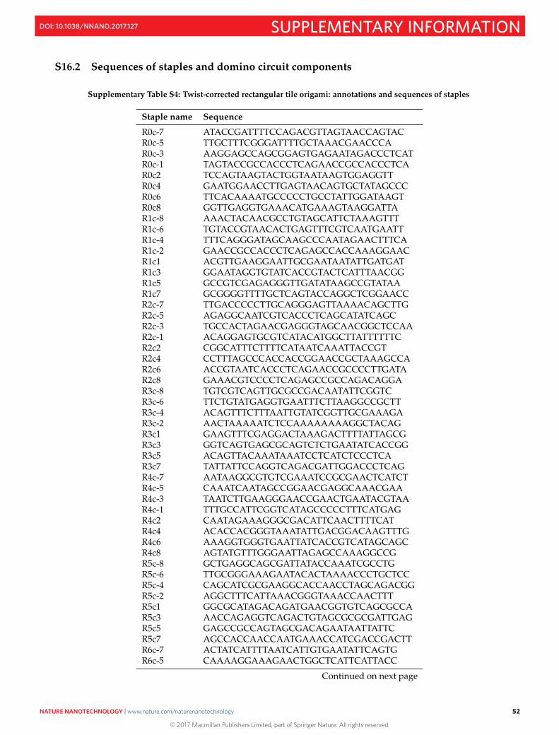
S16.2 Sequences of staples and domino circuit components
Supplementary Table S4: Twist-corrected rectangular tile origami: annotations and sequences of staples
Staple name Sequence
R0c-7 ATACCGATTTTCCAGACGTTAGTAACCAGTACR0c-5 TTGCTTTCGGGATTTTGCTAAACGAACCCAR0c-3 AAGGAGCCAGCGGAGTGAGAATAGACCCTCATR0c-1 TAGTACCGCCACCCTCAGAACCGCCACCCTCAR0c2 TCCAGTAAGTACTGGTAATAAGTGGAGGTTR0c4 GAATGGAACCTTGAGTAACAGTGCTATAGCCCR0c6 TTCACAAAATGCCCCCTGCCTATTGGATAAGTR0c8 GGTTGAGGTGAAACATGAAAGTAAGGATTAR1c-8 AAACTACAACGCCTGTAGCATTCTAAAGTTTR1c-6 TGTACCGTAACACTGAGTTTCGTCAATGAATTR1c-4 TTTCAGGGATAGCAAGCCCAATAGAACTTTCAR1c-2 GAACCGCCACCCTCAGAGCCACCAAAGGAACR1c1 ACGTTGAAGGAATTGCGAATAATATTGATGATR1c3 GGAATAGGTGTATCACCGTACTCATTTAACGGR1c5 GCCGTCGAGAGGGTTGATATAAGCCGTATAAR1c7 GCGGGGTTTTGCTCAGTACCAGGCTCGGAACCR2c-7 TTGACCCCCTTGCAGGGAGTTAAAACAGCTTGR2c-5 AGAGGCAATCGTCACCCTCAGCATATCAGCR2c-3 TGCCACTAGAACGAGGGTAGCAACGGCTCCAAR2c-1 ACAGGAGTGCGTCATACATGGCTTATTTTTTCR2c2 CGGCATTTCTTTTCATAATCAAATTACCGTR2c4 CCTTTAGCCCACCACCGGAACCGCTAAAGCCAR2c6 ACCGTAATCACCCTCAGAACCGCCCCTTGATAR2c8 GAAACGTCCCCTCAGAGCCGCCAGACAGGAR3c-8 TGTCGTCAGTTGCGCCGACAATATTCGGTCR3c-6 TTCTGTATGAGGTGAATTTCTTAAGGCCGCTTR3c-4 ACAGTTTCTTTAATTGTATCGGTTGCGAAAGAR3c-2 AACTAAAAATCTCCAAAAAAAAGGCTACAGR3c1 GAAGTTTCGAGGACTAAAGACTTTTATTAGCGR3c3 GGTCAGTGAGCGCAGTCTCTGAATATCACCGGR3c5 ACAGTTACAAATAAATCCTCATCTCCCTCAR3c7 TATTATTCCAGGTCAGACGATTGGACCCTCAGR4c-7 AATAAGGCGTGTCGAAATCCGCGAACTCATCTR4c-5 CAAATCAATAGCCGGAACGAGGCAAACGAAR4c-3 TAATCTTGAAGGGAACCGAACTGAATACGTAAR4c-1 TTTGCCATTCGGTCATAGCCCCCTTTCATGAGR4c2 CAATAGAAAGGGCGACATTCAACTTTTCATR4c4 ACACCACGGGTAAATATTGACGGACAAGTTTGR4c6 AAAGGTGGGTGAATTATCACCGTCATAGCAGCR4c8 AGTATGTTTGGGAATTAGAGCCAAAGGCCGR5c-8 GCTGAGGCAGCGATTATACCAAATCGCCTGR5c-6 TTGCGGGAAAGAATACACTAAAACCCTGCTCCR5c-4 CAGCATCGCGAAGGCACCAACCTAGCAGACGGR5c-2 AGGCTTTCATTAAACGGGTAAACCAACTTTR5c1 GGCGCATAGACAGATGAACGGTGTCAGCGCCAR5c3 AACCAGAGGTCAGACTGTAGCGCGCGATTGAGR5c5 GAGCCGCCAGTAGCGACAGAATAATTATTCR5c7 AGCCACCAACCAATGAAACCATCGACCGACTTR6c-7 ACTATCATTTTAATCATTGTGAATATTCAGTGR6c-5 CAAAAGGAAAGAACTGGCTCATTCATTACC
Continued on next page
52
© 2017 Macmillan Publishers Limited, part of Springer Nature. All rights reserved.
NATURE NANOTECHNOLOGY | www.nature.com/naturenanotechnology 52
SUPPLEMENTARY INFORMATIONDOI: 10.1038/NNANO.2017.127
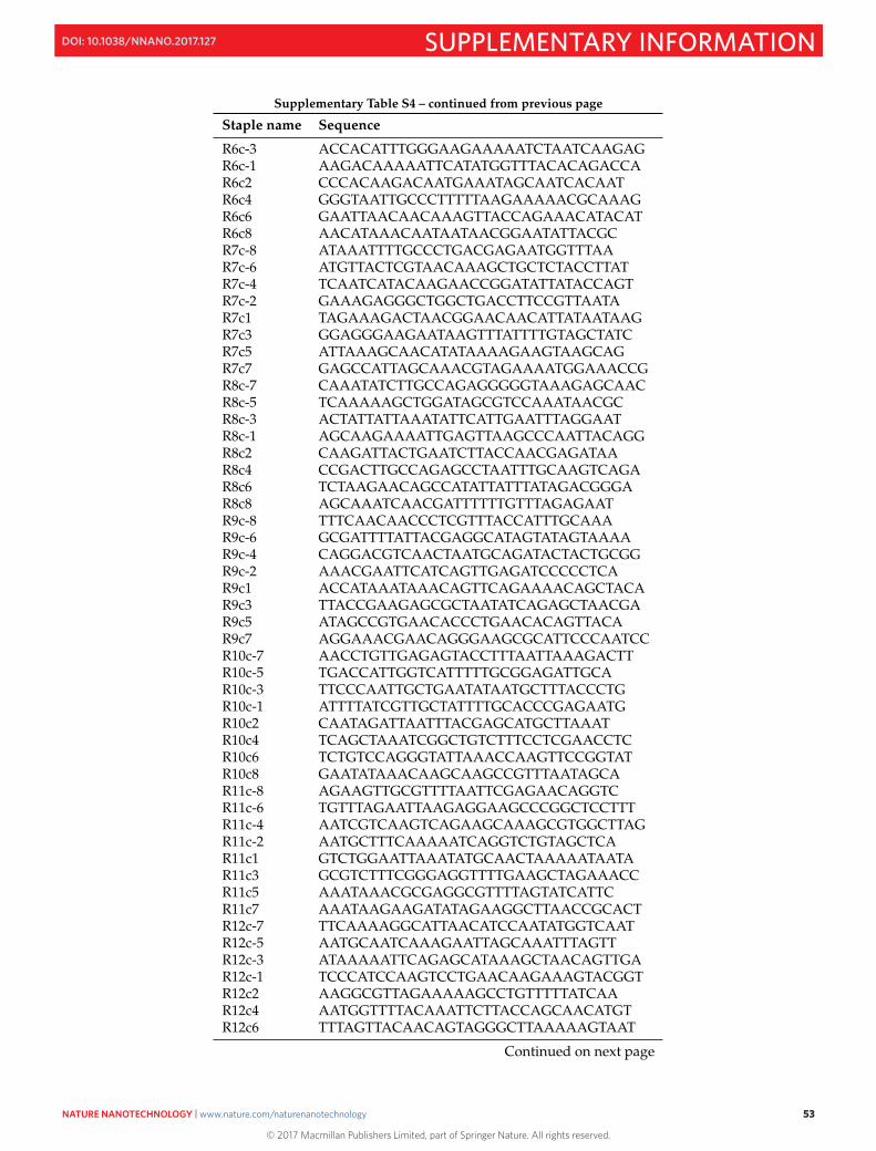
Supplementary Table S4 – continued from previous page
Staple name Sequence
R6c-3 ACCACATTTGGGAAGAAAAATCTAATCAAGAGR6c-1 AAGACAAAAATTCATATGGTTTACACAGACCAR6c2 CCCACAAGACAATGAAATAGCAATCACAATR6c4 GGGTAATTGCCCTTTTTAAGAAAAACGCAAAGR6c6 GAATTAACAACAAAGTTACCAGAAACATACATR6c8 AACATAAACAATAATAACGGAATATTACGCR7c-8 ATAAATTTTGCCCTGACGAGAATGGTTTAAR7c-6 ATGTTACTCGTAACAAAGCTGCTCTACCTTATR7c-4 TCAATCATACAAGAACCGGATATTATACCAGTR7c-2 GAAAGAGGGCTGGCTGACCTTCCGTTAATAR7c1 TAGAAAGACTAACGGAACAACATTATAATAAGR7c3 GGAGGGAAGAATAAGTTTATTTTGTAGCTATCR7c5 ATTAAAGCAACATATAAAAGAAGTAAGCAGR7c7 GAGCCATTAGCAAACGTAGAAAATGGAAACCGR8c-7 CAAATATCTTGCCAGAGGGGGTAAAGAGCAACR8c-5 TCAAAAAGCTGGATAGCGTCCAAATAACGCR8c-3 ACTATTATTAAATATTCATTGAATTTAGGAATR8c-1 AGCAAGAAAATTGAGTTAAGCCCAATTACAGGR8c2 CAAGATTACTGAATCTTACCAACGAGATAAR8c4 CCGACTTGCCAGAGCCTAATTTGCAAGTCAGAR8c6 TCTAAGAACAGCCATATTATTTATAGACGGGAR8c8 AGCAAATCAACGATTTTTTGTTTAGAGAATR9c-8 TTTCAACAACCCTCGTTTACCATTTGCAAAR9c-6 GCGATTTTATTACGAGGCATAGTATAGTAAAAR9c-4 CAGGACGTCAACTAATGCAGATACTACTGCGGR9c-2 AAACGAATTCATCAGTTGAGATCCCCCTCAR9c1 ACCATAAATAAACAGTTCAGAAAACAGCTACAR9c3 TTACCGAAGAGCGCTAATATCAGAGCTAACGAR9c5 ATAGCCGTGAACACCCTGAACACAGTTACAR9c7 AGGAAACGAACAGGGAAGCGCATTCCCAATCCR10c-7 AACCTGTTGAGAGTACCTTTAATTAAAGACTTR10c-5 TGACCATTGGTCATTTTTGCGGAGATTGCAR10c-3 TTCCCAATTGCTGAATATAATGCTTTACCCTGR10c-1 ATTTTATCGTTGCTATTTTGCACCCGAGAATGR10c2 CAATAGATTAATTTACGAGCATGCTTAAATR10c4 TCAGCTAAATCGGCTGTCTTTCCTCGAACCTCR10c6 TCTGTCCAGGGTATTAAACCAAGTTCCGGTATR10c8 GAATATAAACAAGCAAGCCGTTTAATAGCAR11c-8 AGAAGTTGCGTTTTAATTCGAGAACAGGTCR11c-6 TGTTTAGAATTAAGAGGAAGCCCGGCTCCTTTR11c-4 AATCGTCAAGTCAGAAGCAAAGCGTGGCTTAGR11c-2 AATGCTTTCAAAAATCAGGTCTGTAGCTCAR11c1 GTCTGGAATTAAATATGCAACTAAAAATAATAR11c3 GCGTCTTTCGGGAGGTTTTGAAGCTAGAAACCR11c5 AAATAAACGCGAGGCGTTTTAGTATCATTCR11c7 AAATAAGAAGATATAGAAGGCTTAACCGCACTR12c-7 TTCAAAAGGCATTAACATCCAATATGGTCAATR12c-5 AATGCAATCAAAGAATTAGCAAATTTAGTTR12c-3 ATAAAAATTCAGAGCATAAAGCTAACAGTTGAR12c-1 TCCCATCCAAGTCCTGAACAAGAAAGTACGGTR12c2 AAGGCGTTAGAAAAAGCCTGTTTTTATCAAR12c4 AATGGTTTTACAAATTCTTACCAGCAACATGTR12c6 TTTAGTTACAACAGTAGGGCTTAAAAAGTAAT
Continued on next page
53
© 2017 Macmillan Publishers Limited, part of Springer Nature. All rights reserved.
NATURE NANOTECHNOLOGY | www.nature.com/naturenanotechnology 53
SUPPLEMENTARY INFORMATIONDOI: 10.1038/NNANO.2017.127
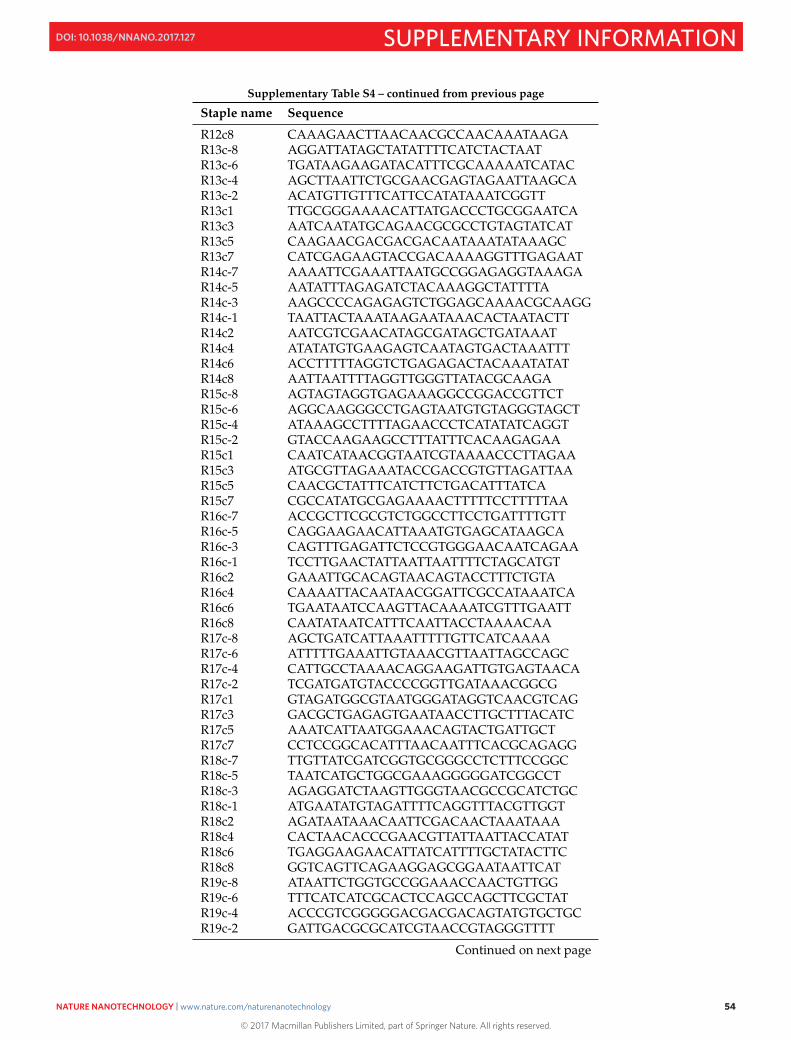
Supplementary Table S4 – continued from previous page
Staple name Sequence
R12c8 CAAAGAACTTAACAACGCCAACAAATAAGAR13c-8 AGGATTATAGCTATATTTTCATCTACTAATR13c-6 TGATAAGAAGATACATTTCGCAAAAATCATACR13c-4 AGCTTAATTCTGCGAACGAGTAGAATTAAGCAR13c-2 ACATGTTGTTTCATTCCATATAAATCGGTTR13c1 TTGCGGGAAAACATTATGACCCTGCGGAATCAR13c3 AATCAATATGCAGAACGCGCCTGTAGTATCATR13c5 CAAGAACGACGACGACAATAAATATAAAGCR13c7 CATCGAGAAGTACCGACAAAAGGTTTGAGAATR14c-7 AAAATTCGAAATTAATGCCGGAGAGGTAAAGAR14c-5 AATATTTAGAGATCTACAAAGGCTATTTTAR14c-3 AAGCCCCAGAGAGTCTGGAGCAAAACGCAAGGR14c-1 TAATTACTAAATAAGAATAAACACTAATACTTR14c2 AATCGTCGAACATAGCGATAGCTGATAAATR14c4 ATATATGTGAAGAGTCAATAGTGACTAAATTTR14c6 ACCTTTTTAGGTCTGAGAGACTACAAATATATR14c8 AATTAATTTTAGGTTGGGTTATACGCAAGAR15c-8 AGTAGTAGGTGAGAAAGGCCGGACCGTTCTR15c-6 AGGCAAGGGCCTGAGTAATGTGTAGGGTAGCTR15c-4 ATAAAGCCTTTTAGAACCCTCATATATCAGGTR15c-2 GTACCAAGAAGCCTTTATTTCACAAGAGAAR15c1 CAATCATAACGGTAATCGTAAAACCCTTAGAAR15c3 ATGCGTTAGAAATACCGACCGTGTTAGATTAAR15c5 CAACGCTATTTCATCTTCTGACATTTATCAR15c7 CGCCATATGCGAGAAAACTTTTTCCTTTTTAAR16c-7 ACCGCTTCGCGTCTGGCCTTCCTGATTTTGTTR16c-5 CAGGAAGAACATTAAATGTGAGCATAAGCAR16c-3 CAGTTTGAGATTCTCCGTGGGAACAATCAGAAR16c-1 TCCTTGAACTATTAATTAATTTTCTAGCATGTR16c2 GAAATTGCACAGTAACAGTACCTTTCTGTAR16c4 CAAAATTACAATAACGGATTCGCCATAAATCAR16c6 TGAATAATCCAAGTTACAAAATCGTTTGAATTR16c8 CAATATAATCATTTCAATTACCTAAAACAAR17c-8 AGCTGATCATTAAATTTTTGTTCATCAAAAR17c-6 ATTTTTGAAATTGTAAACGTTAATTAGCCAGCR17c-4 CATTGCCTAAAACAGGAAGATTGTGAGTAACAR17c-2 TCGATGATGTACCCCGGTTGATAAACGGCGR17c1 GTAGATGGCGTAATGGGATAGGTCAACGTCAGR17c3 GACGCTGAGAGTGAATAACCTTGCTTTACATCR17c5 AAATCATTAATGGAAACAGTACTGATTGCTR17c7 CCTCCGGCACATTTAACAATTTCACGCAGAGGR18c-7 TTGTTATCGATCGGTGCGGGCCTCTTTCCGGCR18c-5 TAATCATGCTGGCGAAAGGGGGATCGGCCTR18c-3 AGAGGATCTAAGTTGGGTAACGCCGCATCTGCR18c-1 ATGAATATGTAGATTTTCAGGTTTACGTTGGTR18c2 AGATAATAAACAATTCGACAACTAAATAAAR18c4 CACTAACACCCGAACGTTATTAATTACCATATR18c6 TGAGGAAGAACATTATCATTTTGCTATACTTCR18c8 GGTCAGTTCAGAAGGAGCGGAATAATTCATR19c-8 ATAATTCTGGTGCCGGAAACCAACTGTTGGR19c-6 TTTCATCATCGCACTCCAGCCAGCTTCGCTATR19c-4 ACCCGTCGGGGGACGACGACAGTATGTGCTGCR19c-2 GATTGACGCGCATCGTAACCGTAGGGTTTT
Continued on next page
54
© 2017 Macmillan Publishers Limited, part of Springer Nature. All rights reserved.
NATURE NANOTECHNOLOGY | www.nature.com/naturenanotechnology 54
SUPPLEMENTARY INFORMATIONDOI: 10.1038/NNANO.2017.127
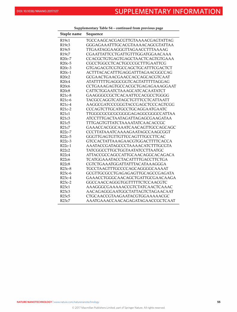
Supplementary Table S4 – continued from previous page
Staple name Sequence
R19c1 TGCCAAGCACGACGTTGTAAAACGAGTATTAGR19c3 GGGAGAAATTTGCACGTAAAACAGCGTATTAAR19c5 TTGAATAGGAAGGGTTAGAACCTTTAAAAGR19c7 CGAATTATTCCTGATTGTTTGGATGGAACAAAR20c-7 CCACGCTGTGAGTGAGCTAACTCAGTGTGAAAR20c-5 CGCCTGGCCTCACTGCCCGCTTTGAATTCGR20c-3 GTGAGACGTCGTGCCAGCTGCATTTCGACTCTR20c-1 ACTTTACACATTTGAGGATTTAGAACGGCCAGR20c2 GCGAACTGAACGAACCACCAGCACGTCAATR20c4 ATATTTTTTGAGGCGGTCAGTATTTTTAGGAGR20c6 CCTGAAAGAGTGCCACGCTGAGAGAAAGGAATR20c8 CATTCTGGAATCTAAAGCATCACAATATCTR21c-8 GAAGGGCCGCTCACAATTCCACGCCTGGGGR21c-6 TACGCCAGGTCATAGCTGTTTCCTCATTAATTR21c-4 AAGGCGATCCCGGGTACCGAGCTCCCAGTCGGR21c-2 CCCAGTCTTGCATGCCTGCAGGAATGAATCR21c1 TTGGGCGCGCGCGGGGAGAGGCGGGCCATTAAR21c3 ATCCTTTGACTAATAGATTAGAGCGAAGATAAR21c5 TTTGAGTGTTATCTAAAATATCAACACCGCR21c7 GAAACCACGGCAAATCAACAGTTGCCAGCAGCR22c-7 CCCTTATAAATCAAAAGAATAGCCAAGCGGTR22c-5 GGGTTGAGTGTTGTTCCAGTTTGCCTTCACR22c-3 GTCCACTATTAAAGAACGTGGACTTTTCACCAR22c-1 AAATACCGATAGCCCTAAAACATCTTTGCGTAR22c2 TATCGGCCTTGCTGGTAATATCCTTAATGCR22c4 ATTACCGCCAGCCATTGCAACAGGCACAGACAR22c6 TCATGGAAATACCTACATTTTGACCTTCTGAR22c8 CGTCTGAAATGGATTATTTACATAAAGGGAR23c-8 TGCCTAAGTTTGCCCCAGCAGGGGCAAAATR23c-6 GCGTTGCGCCTGAGAGAGTTGCAGCCGAGATAR23c-4 GAAACCTGGGCAACAGCTGATTGCGAACAAGAR23c-2 GGCCAACCAGGGTGGTTTTTCTCCAACGTCR23c1 AAAGGGCGAAAAACCGTCTATCAACTCAAACR23c3 AACAGAGGGAATGGCTATTAGTCTAGAACAATR23c5 CTGCAACCGTAAGAATACGTGGAAAAACGCR23c7 AAATGAAACCAACAGAGATAGAACCGCTCAAT
55
© 2017 Macmillan Publishers Limited, part of Springer Nature. All rights reserved.
NATURE NANOTECHNOLOGY | www.nature.com/naturenanotechnology 55
SUPPLEMENTARY INFORMATIONDOI: 10.1038/NNANO.2017.127

Supplementary Table S5: Staples modified for domino wires: Fig. S1a
Direction of wires Staples Sequences of staples
Parallel to helical axis (Fig. 2b)
R2c-7 TTGACCCCCTTGCAGGGAGTTAAAACAGCTTGR2c-5 AGAGGCAATCGTCACCCTCAGCATATCAGCR2c-3 TGCCACTAGAACGAGGGTAGCAACGGCTCCAAR2c-1 ACAGGAGTGCGTCATACATGGCTTATTTTTTCR2c2 CGGCATTTCTTTTCATAATCAAATTACCGTR2c4 CCTTTAGCCCACCACCGGAACCGCTAAAGCCAR2c6 ACCGTAATCACCCTCAGAACCGCCCCTTGATAR2c8 GAAACGTCCCCTCAGAGCCGCCAGACAGGA
Perpendicular to helical axis (Fig. 2c)
R2c2 CGGCATTTCTTTTCATAATCAAATTACCGTR8c2 CAAGATTACTGAATCTTACCAACGAGATAAR14c2 AATCGTCGAACATAGCGATAGCTGATAAATR20c2 GCGAACTGAACGAACCACCAGCACGTCAAT
Through a 180 degree turn (Fig. 2d)
R20c6 CCTGAAAGAGTGCCACGCTGAGAGAAAGGAATR14c6 ACCTTTTTAGGTCTGAGAGACTACAAATATATR8c6 TCTAAGAACAGCCATATTATTTATAGACGGGAR2c6 ACCGTAATCACCCTCAGAACCGCCCCTTGATAR4c4 ACACCACGGGTAAATATTGACGGACAAGTTTGR8c2 CAAGATTACTGAATCTTACCAACGAGATAAR14c2 AATCGTCGAACATAGCGATAGCTGATAAATR20c2 GCGAACTGAACGAACCACCAGCACGTCAAT
Wire crossover (Fig. 3)
R20c2 GCGAACTGAACGAACCACCAGCACGTCAATR14c2 AATCGTCGAACATAGCGATAGCTGATAAATR8c2 CAAGATTACTGAATCTTACCAACGAGATAAR2c2 CGGCATTTCTTTTCATAATCAAATTACCGTR11c-2 AATGCTTTCAAAAATCAGGTCTGTAGCTCAR11c1 GTCTGGAATTAAATATGCAACTAAAAATAATAR11c3 GCGTCTTTCGGGAGGTTTTGAAGCTAGAAACCR11c5 AAATAAACGCGAGGCGTTTTAGTATCATTCR11c7 AAATAAGAAGATATAGAAGGCTTAACCGCACT
56
© 2017 Macmillan Publishers Limited, part of Springer Nature. All rights reserved.
NATURE NANOTECHNOLOGY | www.nature.com/naturenanotechnology 56
SUPPLEMENTARY INFORMATIONDOI: 10.1038/NNANO.2017.127

Supplementary Table S6: Circuit components for domino wires: Fig. S1a
Component Domains (5’-3’) Sequence (5’-3’)
Input hairpin (blue circle,Fig. 2a)
polyT ao* s* f s TTTTT CCTCTA CCTATTCGCTGC AGTAGGGCAGCGAATAGG
Intermediate hairpin (yellowcircle, Fig. 2a)
polyT x* s* f s TTTTT CTGGAC CCTATTCGCTGC AGTAGGGCAGCGAATAGG
Output hairpin 1 (red circle,Fig. 2a)
polyT x* s* y s t TTTTT CTGGAC CCTATTCGCTGC CAATCAGCAGCGAATAGG ACCAAG
Output hairpin 2 (red tri-angle, Fig. S31, S27)
polyT x* s* y2 s t TTTTT CTGGAC CCTATTCGCTGC CTCATTGCAGCGAATAGG ACCAAG
Fuel s x s* f* GCAGCGAATAGG GTCCAG CCTATTCGCTGCCCTACT
Input-A s ao GCAGCGAATAGG TAGAGG
Reporter 1 fluorophorestrand
FAM t* s* y* /56-FAM/ CTTGGT CCTATTCGCTGC TGATTG
Reporter 1 quencher strand s t FQ GCAGCGAATAGG ACCAAG /3IABkFQ/
Reporter 2 fluorophorestrand
Cy5 t* s* y2* /5Cy5/ CTTGGT CCTATTCGCTGC AATGAG
Reporter 2 quencher strand s t RQ GCAGCGAATAGG ACCAAG /3IAbRQSp/
57
© 2017 Macmillan Publishers Limited, part of Springer Nature. All rights reserved.
NATURE NANOTECHNOLOGY | www.nature.com/naturenanotechnology 57
SUPPLEMENTARY INFORMATIONDOI: 10.1038/NNANO.2017.127

Supplementary Table S7: Circuit components for wire crossover module: Fig. S1a
Component Domains (5’-3’) Sequence (5’-3’)
Input hairpin A (blue circle:A, Fig. 3)
polyT ao* s* f s TTTTT CCTCTA CCTATTCGCTGC AGTAGGGCAGCGAATAGG
Input hairpin B (blue circle:B, Fig. 3)
polyT bo* s* fc s TTTTT AGTGCT CCTATTCGCTGC TGACGTGCAGCGAATAGG
Intermediate hairpin x:f (yel-low circle in A track, Fig. 3)
polyT x* s* f s TTTTT CTGGAC CCTATTCGCTGC AGTAGGGCAGCGAATAGG
Intermediate hairpin xc:fc(purple circle in B track, Fig.3)
polyT xc* s* fc s TTTTT TTAGCG CCTATTCGCTGC TGACGTGCAGCGAATAGG
Intermediate hairpin xc:f(yellow circle in B track, Fig.3)
polyT xc* s* f s TTTTT TTAGCG CCTATTCGCTGC AGTAGGGCAGCGAATAGG
Output hairpin FAM (redcircle: FAM, Fig. 3)
polyT x* s* y s t2 TTTTT CTGGAC CCTATTCGCTGC CAATCAGCAGCGAATAGG ACTTTG
Output hairpin Cy5 (redcircle: Cy5, Fig. 3)
polyT x* s* y2 s t2 TTTTT CTGGAC CCTATTCGCTGC CTCATTGCAGCGAATAGG ACTTTG
Fuel1 s x s* f* GCAGCGAATAGG GTCCAG CCTATTCGCTGCCCTACT
Fuel2 s xc s* fc* GCAGCGAATAGG CGCTAA CCTATTCGCTGCACGTCA
InputA s ao GCAGCGAATAGG TAGAGG
InputB s bo GCAGCGAATAGG AGCACT
ReporterFAM fluorophorestrand
FAM t2* s* y* /56-FAM/ CAAAGT CCTATTCGCTGC TGATTG
ReporterFAM quencherstrand
s t2 FQ GCAGCGAATAGG ACTTTG /3IABkFQ/
ReporterCy5 fluorophorestrand
Cy5 t2* s* y2* /5Cy5/ CAAAGT CCTATTCGCTGC AATGAG
ReporterCy5 quencherstrand
s t2 RQ GCAGCGAATAGG ACTTTG /3IAbRQSp/
58
© 2017 Macmillan Publishers Limited, part of Springer Nature. All rights reserved.
NATURE NANOTECHNOLOGY | www.nature.com/naturenanotechnology 58
SUPPLEMENTARY INFORMATIONDOI: 10.1038/NNANO.2017.127
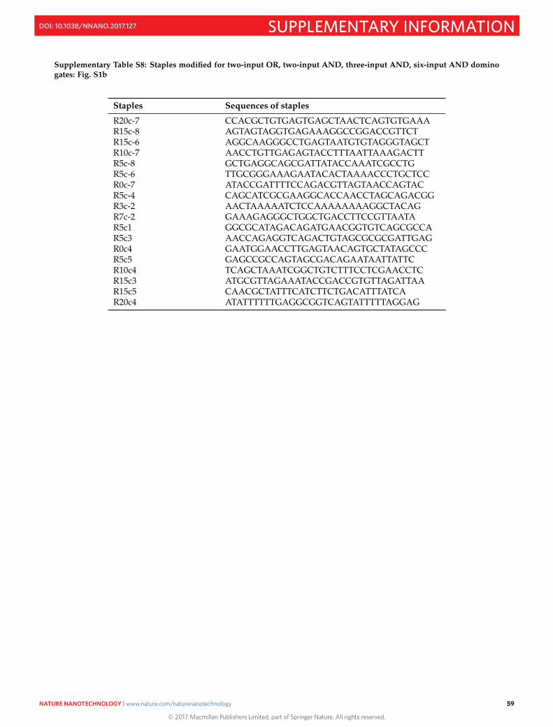
Supplementary Table S8: Staples modified for two-input OR, two-input AND, three-input AND, six-input AND dominogates: Fig. S1b
Staples Sequences of staples
R20c-7 CCACGCTGTGAGTGAGCTAACTCAGTGTGAAAR15c-8 AGTAGTAGGTGAGAAAGGCCGGACCGTTCTR15c-6 AGGCAAGGGCCTGAGTAATGTGTAGGGTAGCTR10c-7 AACCTGTTGAGAGTACCTTTAATTAAAGACTTR5c-8 GCTGAGGCAGCGATTATACCAAATCGCCTGR5c-6 TTGCGGGAAAGAATACACTAAAACCCTGCTCCR0c-7 ATACCGATTTTCCAGACGTTAGTAACCAGTACR5c-4 CAGCATCGCGAAGGCACCAACCTAGCAGACGGR3c-2 AACTAAAAATCTCCAAAAAAAAGGCTACAGR7c-2 GAAAGAGGGCTGGCTGACCTTCCGTTAATAR5c1 GGCGCATAGACAGATGAACGGTGTCAGCGCCAR5c3 AACCAGAGGTCAGACTGTAGCGCGCGATTGAGR0c4 GAATGGAACCTTGAGTAACAGTGCTATAGCCCR5c5 GAGCCGCCAGTAGCGACAGAATAATTATTCR10c4 TCAGCTAAATCGGCTGTCTTTCCTCGAACCTCR15c3 ATGCGTTAGAAATACCGACCGTGTTAGATTAAR15c5 CAACGCTATTTCATCTTCTGACATTTATCAR20c4 ATATTTTTTGAGGCGGTCAGTATTTTTAGGAG
59
© 2017 Macmillan Publishers Limited, part of Springer Nature. All rights reserved.
NATURE NANOTECHNOLOGY | www.nature.com/naturenanotechnology 59
SUPPLEMENTARY INFORMATIONDOI: 10.1038/NNANO.2017.127
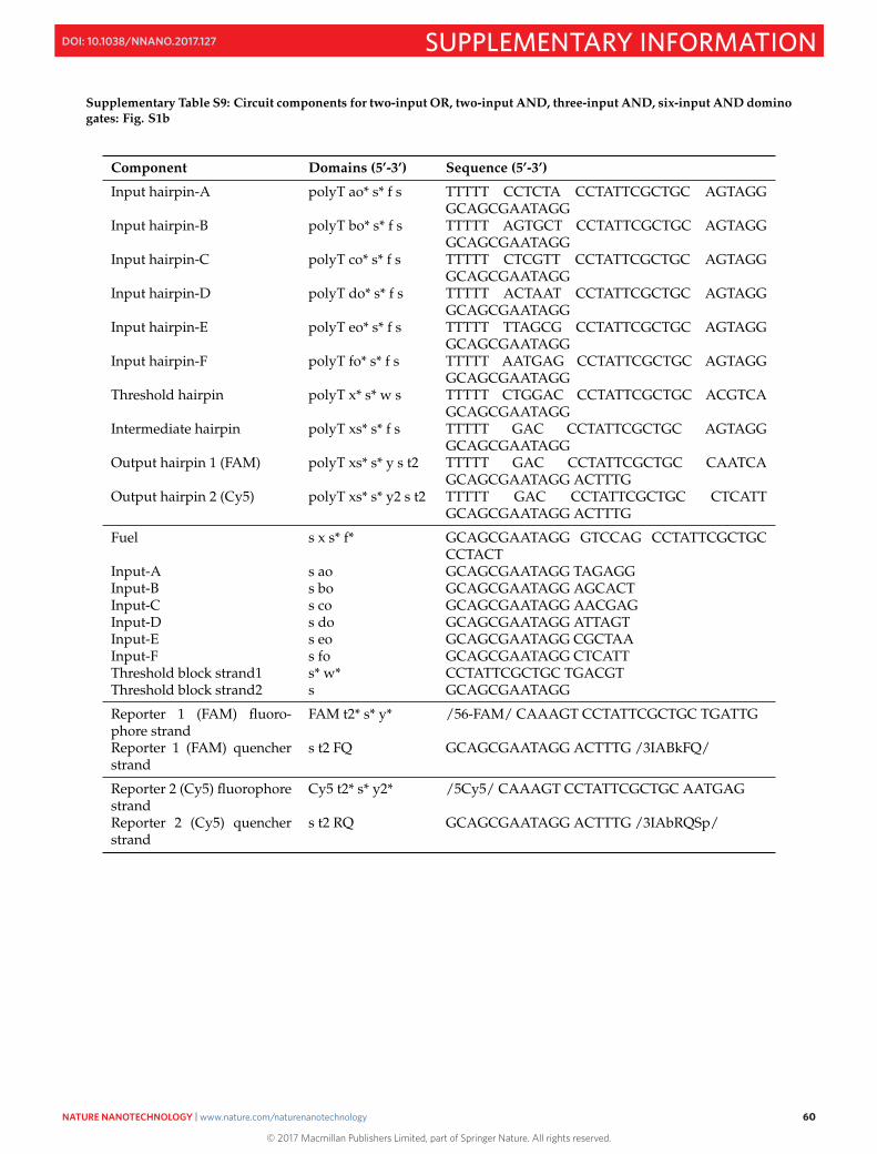
Supplementary Table S9: Circuit components for two-input OR, two-input AND, three-input AND, six-input AND dominogates: Fig. S1b
Component Domains (5’-3’) Sequence (5’-3’)
Input hairpin-A polyT ao* s* f s TTTTT CCTCTA CCTATTCGCTGC AGTAGGGCAGCGAATAGG
Input hairpin-B polyT bo* s* f s TTTTT AGTGCT CCTATTCGCTGC AGTAGGGCAGCGAATAGG
Input hairpin-C polyT co* s* f s TTTTT CTCGTT CCTATTCGCTGC AGTAGGGCAGCGAATAGG
Input hairpin-D polyT do* s* f s TTTTT ACTAAT CCTATTCGCTGC AGTAGGGCAGCGAATAGG
Input hairpin-E polyT eo* s* f s TTTTT TTAGCG CCTATTCGCTGC AGTAGGGCAGCGAATAGG
Input hairpin-F polyT fo* s* f s TTTTT AATGAG CCTATTCGCTGC AGTAGGGCAGCGAATAGG
Threshold hairpin polyT x* s* w s TTTTT CTGGAC CCTATTCGCTGC ACGTCAGCAGCGAATAGG
Intermediate hairpin polyT xs* s* f s TTTTT GAC CCTATTCGCTGC AGTAGGGCAGCGAATAGG
Output hairpin 1 (FAM) polyT xs* s* y s t2 TTTTT GAC CCTATTCGCTGC CAATCAGCAGCGAATAGG ACTTTG
Output hairpin 2 (Cy5) polyT xs* s* y2 s t2 TTTTT GAC CCTATTCGCTGC CTCATTGCAGCGAATAGG ACTTTG
Fuel s x s* f* GCAGCGAATAGG GTCCAG CCTATTCGCTGCCCTACT
Input-A s ao GCAGCGAATAGG TAGAGGInput-B s bo GCAGCGAATAGG AGCACTInput-C s co GCAGCGAATAGG AACGAGInput-D s do GCAGCGAATAGG ATTAGTInput-E s eo GCAGCGAATAGG CGCTAAInput-F s fo GCAGCGAATAGG CTCATTThreshold block strand1 s* w* CCTATTCGCTGC TGACGTThreshold block strand2 s GCAGCGAATAGG
Reporter 1 (FAM) fluoro-phore strand
FAM t2* s* y* /56-FAM/ CAAAGT CCTATTCGCTGC TGATTG
Reporter 1 (FAM) quencherstrand
s t2 FQ GCAGCGAATAGG ACTTTG /3IABkFQ/
Reporter 2 (Cy5) fluorophorestrand
Cy5 t2* s* y2* /5Cy5/ CAAAGT CCTATTCGCTGC AATGAG
Reporter 2 (Cy5) quencherstrand
s t2 RQ GCAGCGAATAGG ACTTTG /3IAbRQSp/
60
© 2017 Macmillan Publishers Limited, part of Springer Nature. All rights reserved.
NATURE NANOTECHNOLOGY | www.nature.com/naturenanotechnology 60
SUPPLEMENTARY INFORMATIONDOI: 10.1038/NNANO.2017.127

Supplementary Table S10: Staples modified for dual rail two-input XNOR domino gate: Fig. S1c
Staples Sequences of staples
R1c-6 TGTACCGTAACACTGAGTTTCGTCAATGAATTR1c-2 GAACCGCCACCCTCAGAGCCACCAAAGGAACR1c3 GGAATAGGTGTATCACCGTACTCATTTAACGGR3c-4 ACAGTTTCTTTAATTGTATCGGTTGCGAAAGAR3c1 GAAGTTTCGAGGACTAAAGACTTTTATTAGCGR5c-6 TTGCGGGAAAGAATACACTAAAACCCTGCTCCR5c-2 AGGCTTTCATTAAACGGGTAAACCAACTTTR5c3 AACCAGAGGTCAGACTGTAGCGCGCGATTGAGR17c-6 ATTTTTGAAATTGTAAACGTTAATTAGCCAGCR17c-2 TCGATGATGTACCCCGGTTGATAAACGGCGR17c3 GACGCTGAGAGTGAATAACCTTGCTTTACATCR19c-8 ATAATTCTGGTGCCGGAAACCAACTGTTGGR19c-4 ACCCGTCGGGGGACGACGACAGTATGTGCTGCR19c1 TGCCAAGCACGACGTTGTAAAACGAGTATTAGR19c5 TTGAATAGGAAGGGTTAGAACCTTTAAAAGR21c-6 TACGCCAGGTCATAGCTGTTTCCTCATTAATTR21c3 ATCCTTTGACTAATAGATTAGAGCGAAGATAA
61
© 2017 Macmillan Publishers Limited, part of Springer Nature. All rights reserved.
NATURE NANOTECHNOLOGY | www.nature.com/naturenanotechnology 61
SUPPLEMENTARY INFORMATIONDOI: 10.1038/NNANO.2017.127
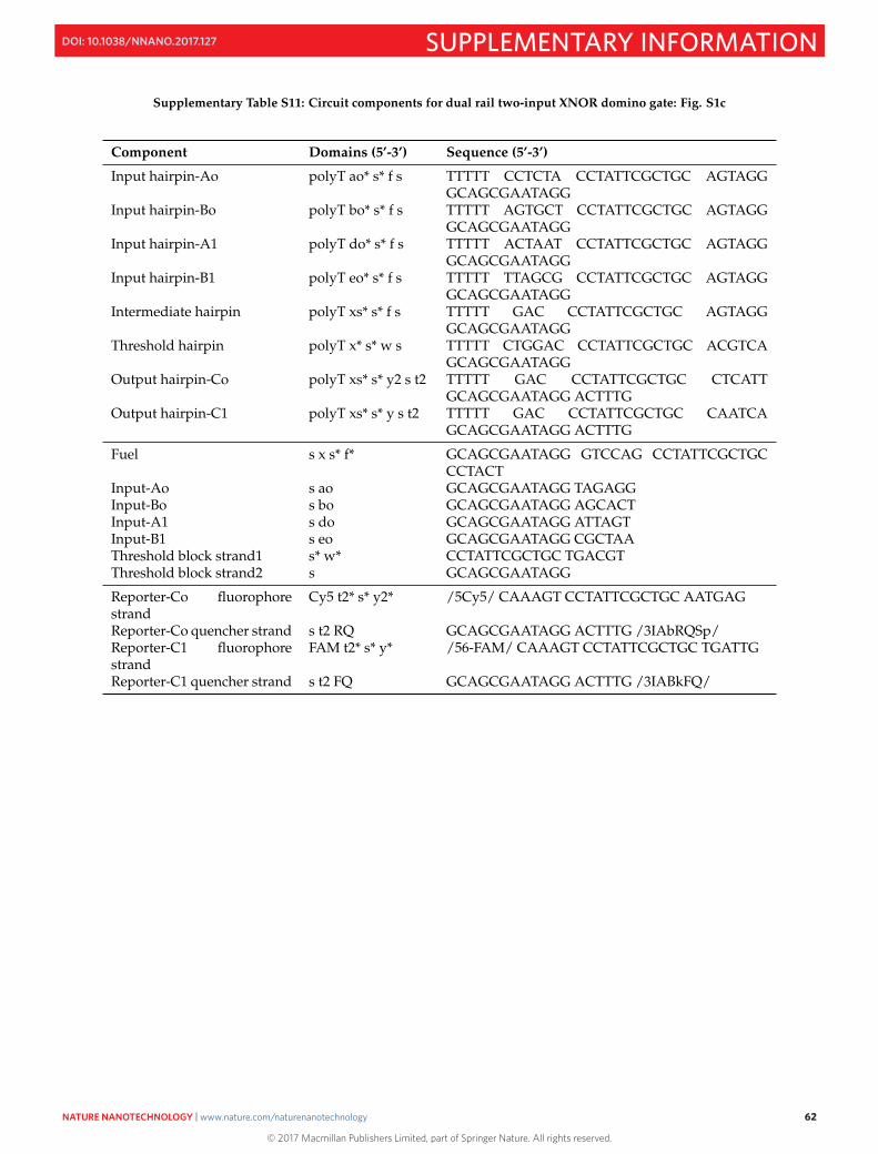
Supplementary Table S11: Circuit components for dual rail two-input XNOR domino gate: Fig. S1c
Component Domains (5’-3’) Sequence (5’-3’)
Input hairpin-Ao polyT ao* s* f s TTTTT CCTCTA CCTATTCGCTGC AGTAGGGCAGCGAATAGG
Input hairpin-Bo polyT bo* s* f s TTTTT AGTGCT CCTATTCGCTGC AGTAGGGCAGCGAATAGG
Input hairpin-A1 polyT do* s* f s TTTTT ACTAAT CCTATTCGCTGC AGTAGGGCAGCGAATAGG
Input hairpin-B1 polyT eo* s* f s TTTTT TTAGCG CCTATTCGCTGC AGTAGGGCAGCGAATAGG
Intermediate hairpin polyT xs* s* f s TTTTT GAC CCTATTCGCTGC AGTAGGGCAGCGAATAGG
Threshold hairpin polyT x* s* w s TTTTT CTGGAC CCTATTCGCTGC ACGTCAGCAGCGAATAGG
Output hairpin-Co polyT xs* s* y2 s t2 TTTTT GAC CCTATTCGCTGC CTCATTGCAGCGAATAGG ACTTTG
Output hairpin-C1 polyT xs* s* y s t2 TTTTT GAC CCTATTCGCTGC CAATCAGCAGCGAATAGG ACTTTG
Fuel s x s* f* GCAGCGAATAGG GTCCAG CCTATTCGCTGCCCTACT
Input-Ao s ao GCAGCGAATAGG TAGAGGInput-Bo s bo GCAGCGAATAGG AGCACTInput-A1 s do GCAGCGAATAGG ATTAGTInput-B1 s eo GCAGCGAATAGG CGCTAAThreshold block strand1 s* w* CCTATTCGCTGC TGACGTThreshold block strand2 s GCAGCGAATAGG
Reporter-Co fluorophorestrand
Cy5 t2* s* y2* /5Cy5/ CAAAGT CCTATTCGCTGC AATGAG
Reporter-Co quencher strand s t2 RQ GCAGCGAATAGG ACTTTG /3IAbRQSp/Reporter-C1 fluorophorestrand
FAM t2* s* y* /56-FAM/ CAAAGT CCTATTCGCTGC TGATTG
Reporter-C1 quencher strand s t2 FQ GCAGCGAATAGG ACTTTG /3IABkFQ/
62
© 2017 Macmillan Publishers Limited, part of Springer Nature. All rights reserved.
NATURE NANOTECHNOLOGY | www.nature.com/naturenanotechnology 62
SUPPLEMENTARY INFORMATIONDOI: 10.1038/NNANO.2017.127
References
[1] Thomas E Ouldridge, Ard A Louis, and Jonathan P Doye. Structural, mechanical, and thermodynamic prop-erties of a coarse-grained DNA model. The Journal of chemical physics, 134(8):085101, Feb 2011.
[2] Benedict Snodin, Ferdinando Randisi, Majid Mosayebi, Petr Šulc, John Schreck, Flavio Romano, ThomasOuldridge, Roman Tsukanov, Eyal Nir, Ard Louis, and et al. Introducing improved structural properties andsalt dependence into a coarse-grained model of DNA. The Journal of Chemical Physics, 142(23):234901, 2015.
[3] Matthew R. Lakin, Simon Youssef, Filippo Polo, Stephen Emmott, and Andrew Phillips. Visual DSD: A designand analysis tool for DNA strand displacement systems. Bioinformatics, 27(22):3211–3213, 2011.
[4] Matthew R Lakin, Rasmus Petersen, Kathryn E Gray, and Andrew Phillips. Abstract Modelling of TetheredDNA Circuits. In Satoshi Murata and Satoshi Kobayashi, editors, DNA Computing and Molecular Programming:20th International Conference, DNA 20, Kyoto, Japan, September 22-26, 2014. Proceedings, pages 132–147. SpringerInternational Publishing, Cham, 2014.
[5] M. R. Lakin, S. Youssef, L. Cardelli, and a. Phillips. Abstractions for DNA circuit design. Journal of The RoyalSociety Interface, 9(68):470–486, 2012.
[6] Anthony J Genot, David Yu Zhang, Jonathan Bath, and Andrew J. Turberfield. Remote toehold: A mechanismfor flexible control of DNA hybridization kinetics. Journal of the American Chemical Society, 133(7):2177–2182,2011.
[7] Yuan-Jyue Chen, Neil Dalchau, Niranjan Srinivas, Andrew Phillips, Luca Cardelli, David Soloveichik, andGeorg Seelig. Programmable chemical controllers made from DNA. Nature nanotechnology, 8(10):755–62,2013.
[8] Christian P Robert and George Casella. Monte Carlo Statistical Methods, volume 95. 2004.
[9] Alan C. Hindmarsh, Peter N. Brown, Keith E. Grant, Steven L. Lee, Radu Serban, Dan E. Shumaker, andCarol S. Woodward. SUNDIALS: Suite of Nonlinear and Differential/Algebraic Equation Solvers. ACMTransactions on Mathematical Software, 31(3):363–396, 2005.
[10] Grégoire Bonnet, Oleg Krichevsky, and Albert Libchaber. Kinetics of conformational fluctuations in dnahairpin-loops. Proceedings of the National Academy of Sciences, 95(15):8602–8606, 1998.
[11] Xixi Wei, Jeanette Nangreave, Shuoxing Jiang, Hao Yan, and Yan Liu. Mapping the thermal behavior of DNAorigami nanostructures. Journal of the American Chemical Society, 135(16):6165–6176, 2013.
[12] Katherine E. Dunn, Frits Dannenberg, Thomas E. Ouldridge, Marta Kwiatkowska, Andrew J. Turberfield, andJonathan Bath. Guiding the folding pathway of DNA origami. Nature, 525(7567):82–86, 2015.
[13] R Jungmann, MS Avendaño, M Dai, and JB Woehrstein. Quantitative super-resolution imaging with qPAINT.Nature âAe, 2016.
[14] Lulu Qian and Erik Winfree. Scaling up digital circuit computation with DNA strand displacement cascades.Science (New York, N.Y.), 332(6034):1196–201, Jun 2011.
[15] David Zhang, Andrew J Turberfield, Bernard Yurke, and Erik Winfree. Engineering Entropy-Driven reactionsand networks catalyzed by DNA. Science, 318(5853):1121–1125, 2007.
63
© 2017 Macmillan Publishers Limited, part of Springer Nature. All rights reserved.
NATURE NANOTECHNOLOGY | www.nature.com/naturenanotechnology 63
SUPPLEMENTARY INFORMATIONDOI: 10.1038/NNANO.2017.127
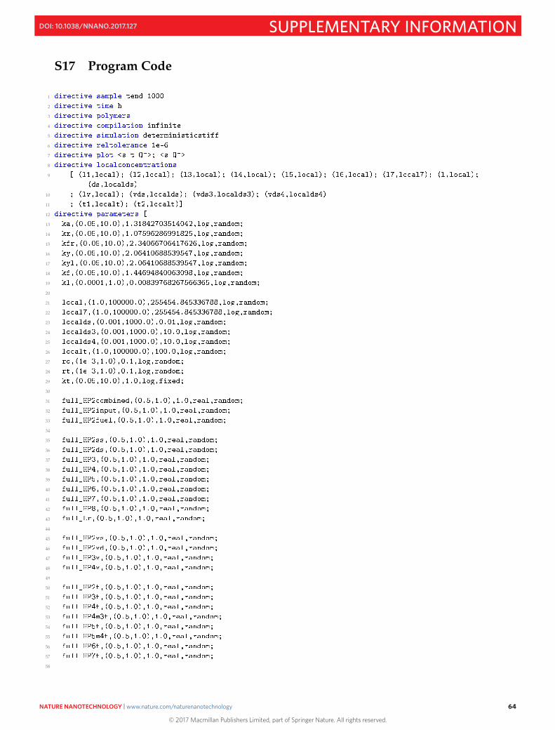
S17 Program Code
1
2
3
4
5
6
7
8
9
10
11
12
13
14
15
16
17
18
19
20
21
22
23
24
25
26
27
28
29
30
31
32
33
34
35
36
37
38
39
40
41
42
43
44
45
46
47
48
49
50
51
52
53
54
55
56
57
58
64
© 2017 Macmillan Publishers Limited, part of Springer Nature. All rights reserved.
NATURE NANOTECHNOLOGY | www.nature.com/naturenanotechnology 64
SUPPLEMENTARY INFORMATIONDOI: 10.1038/NNANO.2017.127
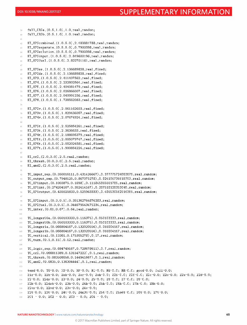
59
60
61
62
63
64
65
66
67
68
69
70
71
72
73
74
75
76
77
78
79
80
81
82
83
84
85
86
87
88
89
90
91
92
93
94
95
96
97
98
99
100
101
102
103
104
105
106
107
108
109
110
111
112
113
114
115
116
117
118
119
120
65
© 2017 Macmillan Publishers Limited, part of Springer Nature. All rights reserved.
NATURE NANOTECHNOLOGY | www.nature.com/naturenanotechnology 65
SUPPLEMENTARY INFORMATIONDOI: 10.1038/NNANO.2017.127
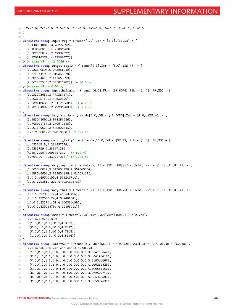
121
122
123
124
125
126
127
128
129
130
131
132
133
134
135
136
137
138
139
140
141
142
143
144
145
146
147
148
149
150
151
152
153
154
155
156
157
158
159
160
161
162
163
164
165
166
167
168
169
170
171
172
173
174
175
176
177
178
179
180
181
182
66
© 2017 Macmillan Publishers Limited, part of Springer Nature. All rights reserved.
NATURE NANOTECHNOLOGY | www.nature.com/naturenanotechnology 66
SUPPLEMENTARY INFORMATIONDOI: 10.1038/NNANO.2017.127
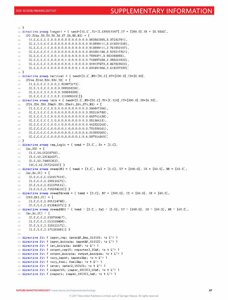
183
184
185
186
187
188
189
190
191
192
193
194
195
196
197
198
199
200
201
202
203
204
205
206
207
208
209
210
211
212
213
214
215
216
217
218
219
220
221
222
223
224
225
226
227
228
229
230
231
232
233
234
235
236
237
238
239
240
241
242
243
244
67
© 2017 Macmillan Publishers Limited, part of Springer Nature. All rights reserved.
NATURE NANOTECHNOLOGY | www.nature.com/naturenanotechnology 67
SUPPLEMENTARY INFORMATIONDOI: 10.1038/NNANO.2017.127
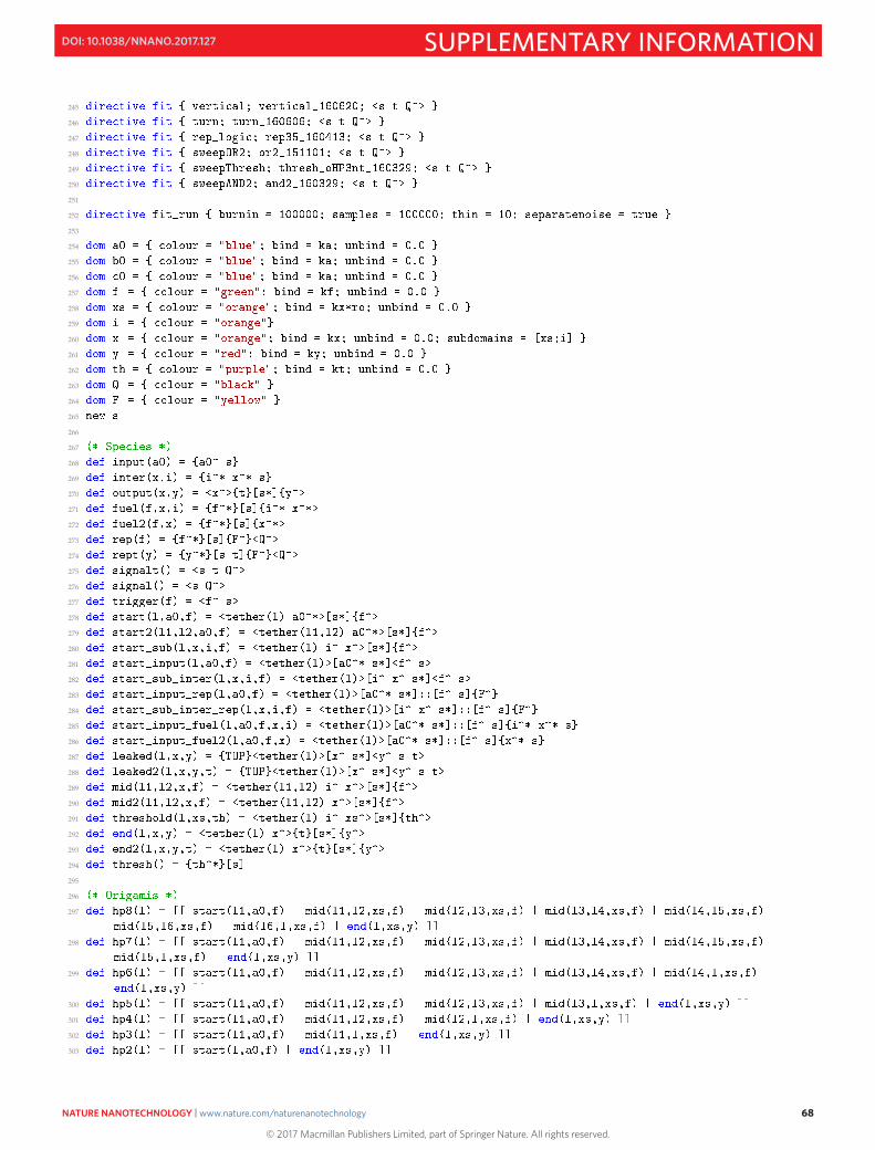
245
246
247
248
249
250
251
252
253
254
255
256
257
258
259
260
261
262
263
264
265
266
267
268
269
270
271
272
273
274
275
276
277
278
279
280
281
282
283
284
285
286
287
288
289
290
291
292
293
294
295
296
297
298
299
300
301
302
303
68
© 2017 Macmillan Publishers Limited, part of Springer Nature. All rights reserved.
NATURE NANOTECHNOLOGY | www.nature.com/naturenanotechnology 68
SUPPLEMENTARY INFORMATIONDOI: 10.1038/NNANO.2017.127
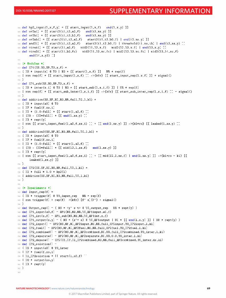
304
305
306
307
308
309
310
311
312
313
314
315
316
317
318
319
320
321
322
323
324
325
326
327
328
329
330
331
332
333
334
335
336
337
338
339
340
341
342
343
344
345
346
347
348
349
350
351
352
353
354
355
356
357
358
359
360
361
362
363
69
© 2017 Macmillan Publishers Limited, part of Springer Nature. All rights reserved.
NATURE NANOTECHNOLOGY | www.nature.com/naturenanotechnology 69
SUPPLEMENTARY INFORMATIONDOI: 10.1038/NNANO.2017.127
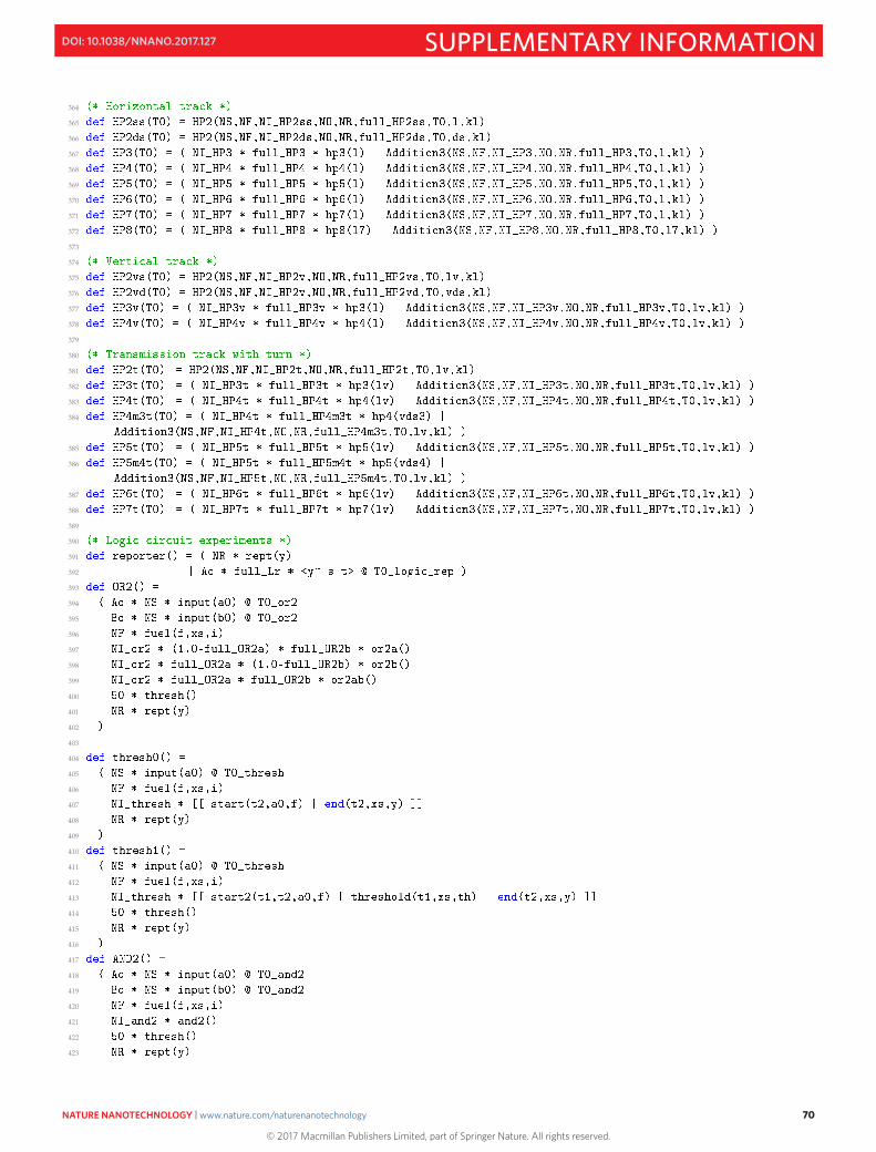
364
365
366
367
368
369
370
371
372
373
374
375
376
377
378
379
380
381
382
383
384
385
386
387
388
389
390
391
392
393
394
395
396
397
398
399
400
401
402
403
404
405
406
407
408
409
410
411
412
413
414
415
416
417
418
419
420
421
422
423
70
© 2017 Macmillan Publishers Limited, part of Springer Nature. All rights reserved.
NATURE NANOTECHNOLOGY | www.nature.com/naturenanotechnology 70
SUPPLEMENTARY INFORMATIONDOI: 10.1038/NNANO.2017.127

424
425
426
427
428
429
430
431
432
433
434
435
436
437
438
71
© 2017 Macmillan Publishers Limited, part of Springer Nature. All rights reserved.
NATURE NANOTECHNOLOGY | www.nature.com/naturenanotechnology 71
SUPPLEMENTARY INFORMATIONDOI: 10.1038/NNANO.2017.127