In summary

In summary

If x[n] is a finite-length sequence (n0 only when |n|<N) , its DTFT X(ejw) shall be a periodic continuous function with period 2.

The DFT of x[n], denoted by X(k), is also of length N.

where , and Wn are the the roots of Wn = 1. Relationship: X(k) is the uniform samples of X(ejw) at the discrete frequency wk = (2/N)k, when the frequency range [0, 2] is divided into N equally spaced points.

nNjeW /2

The Concept of ‘System’ (oppenheim et al. 1999)

• Discrete-time Systems– A transformation or operator that maps an input sequen

ce with values x[n] into an output sequence with value y[n] .

y[n] = T{x[n]}

x[n] T{}

y[n]

System Examples

• Ideal Delay– y[n] = x[nnd], where nd is a fixed positive integer called th

e delay of the system.

• Moving Average

• Memoryless Systems– The output y[n] at every value of n depends only on the i

nput x[n], at the same value of n.– Eg. y[n] = (x[n])2, for each value of n.

2

11

1

21

M

Mk

knxMM

ny

System Examples (continue)

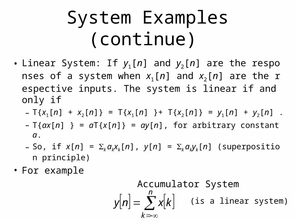
• Linear System: If y1[n] and y2[n] are the responses of a system when x1[n] and x2[n] are the respective inputs. The system is linear if and only if– T{x1[n] + x2[n]} = T{x1[n] }+ T{x2[n]} = y1[n] + y2[n] .

– T{ax[n] } = aT{x[n]} = ay[n], for arbitrary constant a.

– So, if x[n] = k akxk[n], y[n] = k akyk[n] (superposition principle)

• For example

Accumulator System

n

k

kxny (is a linear system)


• Nonlinear System. – Eg. w[n] = log10(|x[n]|) is not linear.

• Time-invariant System:– If y[n] = T{x[n]}, then y[nn0] = T{x[n n0]}

– The accumulator is a time-invariant system.

• The compressor system (not time-invariant)– y[n] = x[Mn], < n < .


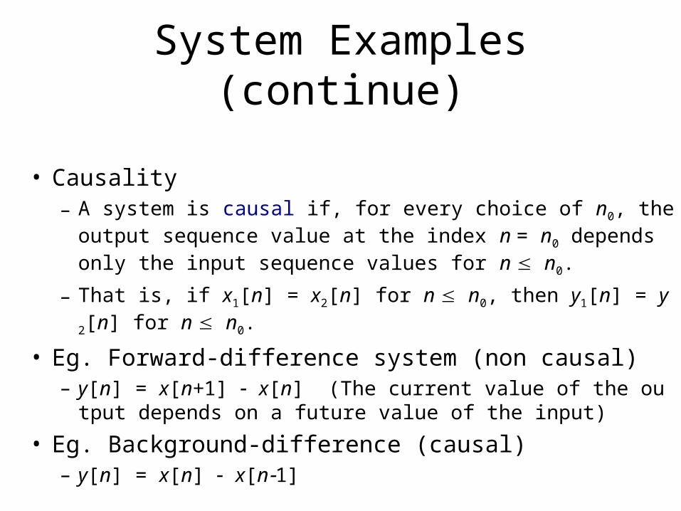
• Causality– A system is causal if, for every choice of n0, the output seq

uence value at the index n = n0 depends only the input sequence values for n n0.

– That is, if x1[n] = x2[n] for n n0, then y1[n] = y2[n] for n n0.

• Eg. Forward-difference system (non causal)– y[n] = x[n+1] x[n] (The current value of the output depen

ds on a future value of the input)

• Eg. Background-difference (causal)– y[n] = x[n] x[n1]


• Stability– Bounded input, bounded output (BIBO): If the input

is bounded, |x[n]| Bx < for all n, then the output is also bounded, i.e., there exists a positive value By s.t. |y[n]| By < for all n.

• Eg., the system y[n] = (x[n])2 is stable.• Eg., the accumulated system is unstable, whic

h can be easily verified by setting x[n] = u[n], the unit step signal.

Linear Time Invariant Systems

• A system that is both linear and time invariant is called a linear time invariant (LTI) system.

• By setting the input x[n] as [n], the impulse function, the output h[n] of an LTI system is called the impulse response of this system.– Time invariant: when the input is [n-k], the output i

s h[n-k].– Remember that the x[n] can be represented as a lin

ear combination of delayed impulses

k

knkxnx

• Hence

• Therefore, a LTI system is completely characterized by its impulse response h[n].

Linear Time Invariant Systems (continue)

k

knhkx

kk

knTkxknkxTny

– Note that the above operation is convolution, and can be written in short by y[n] = x[n] h[n].

– The output of an LTI system is equivalent to the convolution of the input and the impulse response.

• In a LTI system, the input sample at n = k, represented as x[k][n-k], is transformed by the system into an output sequence x[k]h[n-k] for < n < .

Linear Time Invariant Systems (continue)

k

knhkxny

• Communitive– x[n] h[n] = h[n] x[n].

• Distributive over addition– x[n] (h1[n] + h2[n]) = x[n] h1[n] + x[n] h2[n].

• Cascade connection

Property of LTI System and Convolution

x[n]h1[n] h2[n]

y[n]

x[n]h2[n] h1[n]

y[n]x[n]

h1[n] h2[n]y[n]

Property of LTI System and Convolution (continue)

• Parallel combination of LTI systems and its equivalent system.

• Stability: A LTI system is stable if and only if

Since

when |x[n]| Bx.

• This is a sufficient condition proof.


k

khS

kk

knxkhknxkhny

• Causality– those systems for which the output depends only o

n the input samples y[n0] depends only the input sequence values for n n0.

– Follow this property, an LTI system is causal iff

h[n] = 0 for all n < 0.

– Causal sequence: a sequence that is zero for n<0. A causal sequence could be the impulse response of a causal system.


• Ideal delay: h[n] = [n-nd]

• Moving average

• Accumulator

• Forward difference: h[n] = [n+1][n] • Backward difference: h[n] = [n][n1]

Impulse Responses of Some LTI Systems

otherwise0

1

121

21

MnMMMnh

otherwise0

01 nnh

• In the above, moving average, forward difference and backward difference are stable systems, since the impulse response has only a finite number of terms.– Such systems are called finite-duration impulse

response (FIR) systems.– FIR is equivalent to a weighted average of a sliding

window.– FIR systems will always be stable.

• The accumulator is unstable since

Examples of Stable/Unstable Systems

0n

nuS

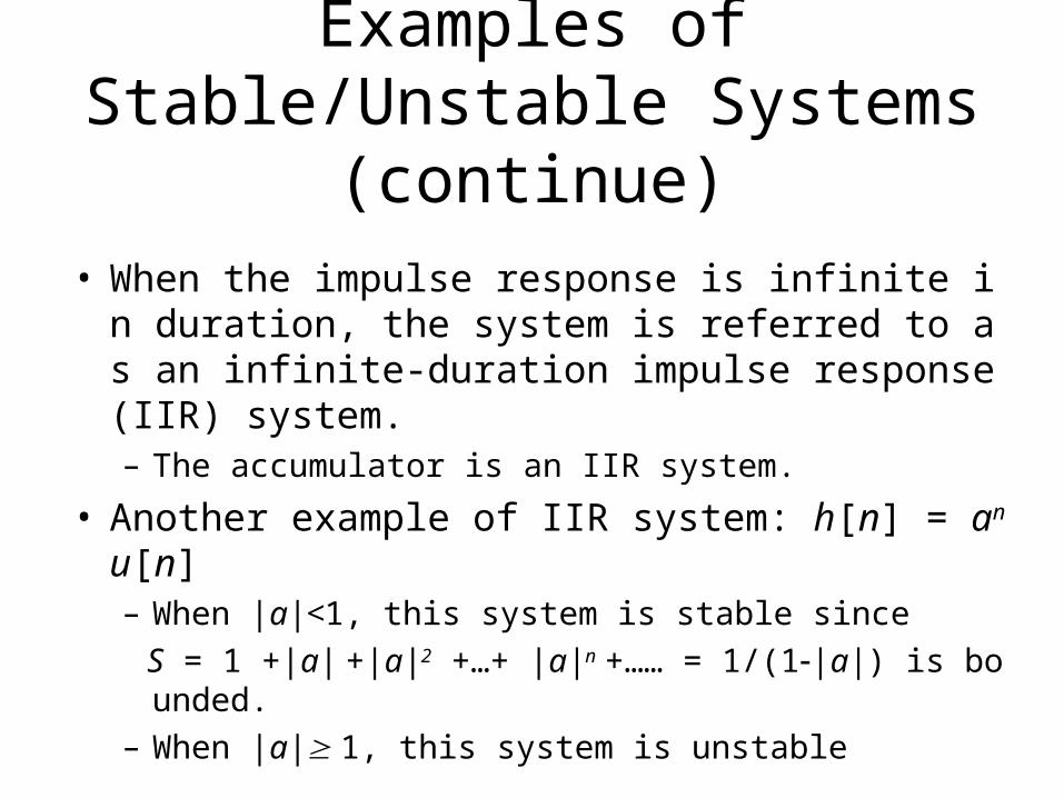
• When the impulse response is infinite in duration, the system is referred to as an infinite-duration impulse response (IIR) system.– The accumulator is an IIR system.

• Another example of IIR system: h[n] = anu[n]– When |a|<1, this system is stable since

S = 1 +|a| +|a|2 +…+ |a|n +…… = 1/(1|a|) is bounded.– When |a| 1, this system is unstable

Examples of Stable/Unstable Systems (continue)

• The ideal delay, accumulator, and backward difference systems are causal.

• The forward difference system is noncausal.• The moving average system is causal requires

M10 and M20.

Examples of Causal Systems

• A LTI system can be realized in different ways by separating it into different subsystems.

Equivalent Systems

1

11

11

nn

nnn

nnnnh

• Another example of cascade systems – inverse system.

Equivalent Systems (continue)

nnununnnunh 11

Linear Constant-coefficient Difference Equations

M

mm

N

kk mnxbknya

00

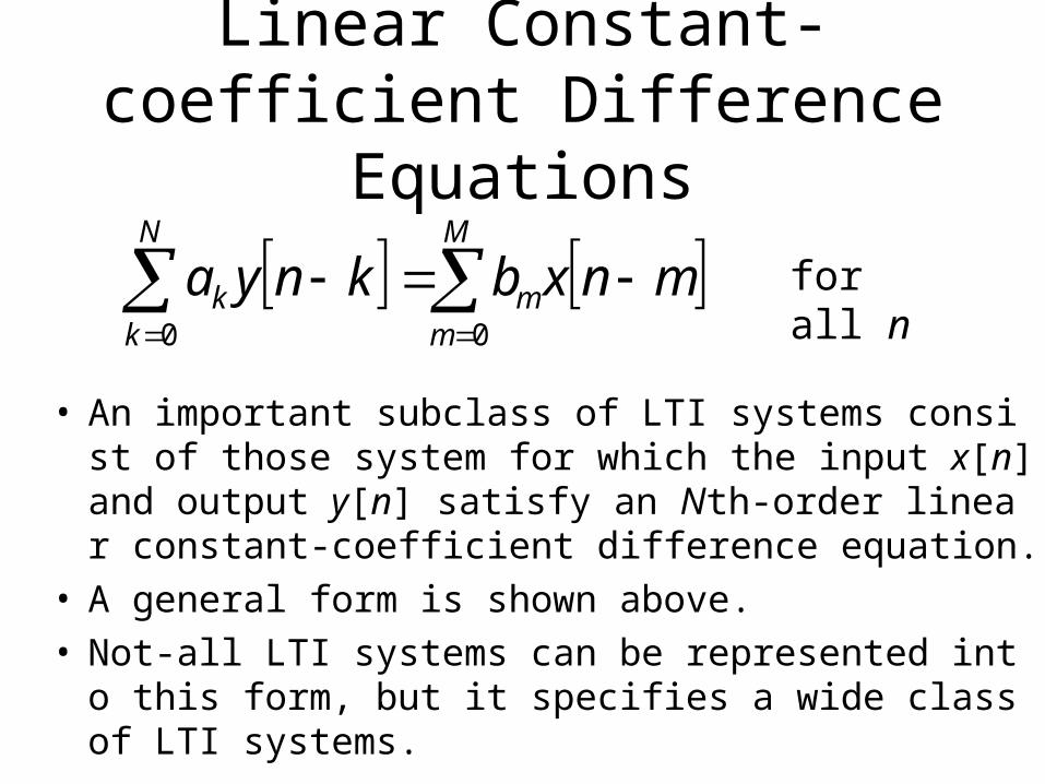
• An important subclass of LTI systems consist of those system for which the input x[n] and output y[n] satisfy an Nth-order linear constant-coefficient difference equation.

• A general form is shown above.• Not-all LTI systems can be represented into this for

m, but it specifies a wide class of LTI systems.

for all n

Block Diagram of the Difference Equation

x[n]

TD

TD

TD

x[n-2]

x[n-1]

x[n-M]

+

+

+

+

b1

b0

b2

bM

+

+

+

+

y[n]

TD

TD

TD

a1

a2

aN y[n-N]

y[n-2]

y[n-1]

• Assume that a0 = 1. Let TD denote one-sample delay.

Difference Equation: FIR system

• The assumption a0 = 1 can be always achieved by dividing all the coefficients by a0 if a00.

• The difference equation characterizes a recursive way of obtaining the output y[n] from the input x[n].

• When ak = 0 for k = 1 … N, the difference equation degenerates to a FIR (finite impulse response) system - the impulse response is of finite length.– The output consists of a linear combination of finite inpu

ts.

M

mm mnxbny

0

Difference equation: IIR System

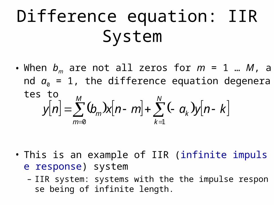
• When bm are not all zeros for m = 1 … M, and a0 = 1, the difference equation degenerates to

• This is an example of IIR (infinite impulse response) system– IIR system: systems with the the impulse response being

of infinite length.

N

kk

M

mm knyamnxbny

10

Example

• Accumulator

11

nynxkxnx

kxny

n

k

n

k

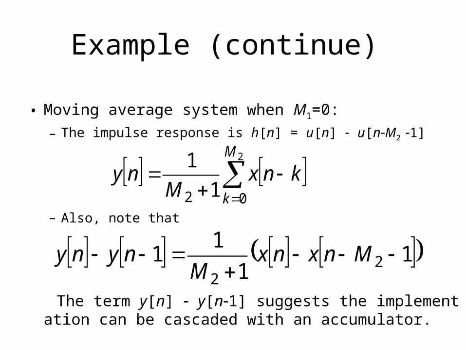
• Moving average system when M1=0:

– The impulse response is h[n] = u[n] u[nM2 1]

– Also, note that

The term y[n] y[n1] suggests the implementation can be cascaded with an accumulator.

Example (continue)

2

02 1

1 M

k

knxM

ny

11

11 2

2

MnxnxM

nyny

Moving Average System

– Hence, there are at least two difference equation representations of the moving average system. First,

x[n]

TD

TD

TD

x[n-2]

x[n-1]

x[n-M]

+

+

+

+

b

b

b

b

y[n]

where b = 1/ (M2+1) and TD denotes one-sample delay

Moving Average System (continue)

– Second,

• The first representation is FIR, and the second is IIR.

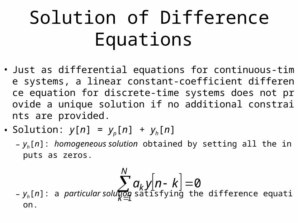
Solution of Difference Equations

• Just as differential equations for continuous-time systems, a linear constant-coefficient difference equation for discrete-time systems does not provide a unique solution if no additional constraints are provided.

• Solution: y[n] = yp[n] + yh[n]

– yh[n]: homogeneous solution obtained by setting all the inputs as zeros.

– yh[n]: a particular solution satisfying the difference equation.

01

N

kk knya

• Additional constraints: consider the N auxiliary conditions that y[1], y[2], …, y[N] are given.– The other values of y[n] (n0) can be generated by

when x[n] is available, y[1], y[2], … y[n], … can be computed recursively.

– To generate values of y[n] for n<N recursively,

Solution of Difference Equations (continue)

M

m

mN

k

k mnxa

bkny

a

any

0 01 0

M

m N

kN

k N

k mnxa

bkny

a

aNny

0

1

1

• Consider the difference equation

y[n] = ay[n-1] + x[n].– Assume the input is x[n] =K [n], and the auxiliary conditi

on is y[1] = c.

– Hence, y[0] = ac+K, y[1] = a y[0]+0 = a2c+aK, …– Recursively, we found that y[n] = an+1c+anK, for n0.

– For n<1, y[-2] = a1(y[1] x[1] ) = a1c,

y[2] = a1 y[1] = a2 c, …, and y[n] = an+1c for n<1.

– Hence, the solution is

y[n] = an+1c+Kanu[n],

Example of the Solutions

• The solution system is non-linear:– When K=0, i.e., the input is zero, the solution (system resp

onse) y[n] = an+1c.

– Since a linear system requires that the output is zero for all time when the input is zero for all time.

• The solution system is not shift invariant:– when input were shifted by n0 samples, x1[n] =K [n - n0], t

he output is y1[n] = an+1c+Kann0 u[n - n0].

• The recursively-implemented system for finding the solution is non-causal.

Example of the Solutions (continue)

• Our principal interest in the text is in systems that are linear and time invariant.

• How to make the recursively-implemented solution system be LTI?

• Initial-rest condition:– If the input x[n] is zero for n less than some time n0, the out

put y[n] is also zero for n less than n0.• The previous example does not satisfy this condition since x[n] = 0 f

or n<0 but y[1] = c.

• Property: If the initial-rest condition is satisfied, then the system will be LTI and causal.

LTI solution of difference equations

Frequency-Domain Representation of Discrete-time Signals and Systems

• Eigen function of a LTI system– When applying an eigenfunction as input, the output is the

same function multiplied by a constant.

• x[n] = ejwn is the eigenfunction of all LTI systems.– Let h[n] be the impulse response of an LTI system, when ej

wn is applied as the input,

k

jwkjwn

k

knjw ekheekhny

• Let

we have • Consequently, ejwn is the eigenfunction of the sys

tem, and the associated eigenvalue is H(ejw).

• Remember that H(ejw) is the DTFT of h[n] .

• We call H(ejw) the LTI system’s frequency response – consisting of the real and imaginary parts, H(ejw) = HR

(ejw) + jHI(ejw), or in terms of magnitude and phase.

Eigenfunction of LTI

jwnjw eeHny

k

jwkjw ekheH

• Frequency response of the ideal delay system,

y[n] =x[n nd],

• If we consider x[n] = ejwn as input, then

Hence, the frequency response is

• The magnitude and phase are

Example of Frequency Response

djwnjw eeH

jwnjwnnnjw eeeny dd

djwjw wneHeH 1,

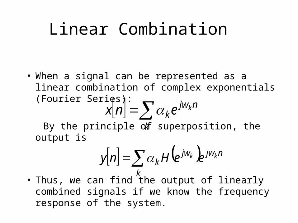
• When a signal can be represented as a linear combination of complex exponentials (Fourier Series):

By the principle of superposition, the output is

• Thus, we can find the output of linearly combined signals if we know the frequency response of the system.

Linear Combination

njwjw

kk

kk eeHny

k

njwk

kenx

• Sinusoidal responses of LTI systems:

– The response of x1[n] and x2[n] are

– If h[n] is real, by the DTFT property that H(ejw0) = H*(ejw0), the total response y[n] = y1[n] + y2[n] is

Example of Linear Combination

njwjjw eeAeHny 00 22 /

nxnxeeA

eeA

nwAnx njwjnjwj210

00

22 cos

njwjjw eeAeHny 00 21/

00 where0jwjw eHnweHAny ,cos

• For a continuous-time system, the frequency response applied is the continuous Fourier transform, which is not necessarily to be periodic.

• However, for a discrete-time system, the frequency response is always periodic with period 2, since

– Because H(ejw) is periodic with period 2, we need only specify

H(ejw) over an interval of length 2, eg., [0, 2] or [, ]. For consistency, we choose the interval [, ].

– The inherent periodicity defines the frequency response everywhere outside the chosen interval.

Difference to Continuous-time System Response

22

wj

k

kwj

k

jwkjw eHekhekheH

Convolution vs. Multiplication • For DTFT, when performing convolution in time do

main, it is equivalent to perform multiplication in the frequency domain.

• Hence, for an LTI system with the impulse response being h[n], when the input is x[n]– We know that y[n] = h[n]x[n].– The spectrum of y[n] shall be Y(ejw) = H(ejw)X(ejw).– i.e., the spectrum of y[n] can be obtained by multiplying th

e spectrum of x[n] with the frequency response.

• The “low frequencies” are frequencies close to zero, while the “high frequencies” are those close to .– Since that the frequencies differing by an integer multiple of

2 are indistinguishable, the “low frequency” are those that are close to an even multiple of , while the “high frequencies” are those close to an odd multiple of .

• Ideal frequency-selective filters:– An important class of linear-invariant systems includes

those systems for which the frequency response is unity over a certain range of frequencies and is zero at the remaining frequencies.

Ideal Frequency-selective Filters

Frequency Response of Ideal Low-pass Filter

Frequency Response of Ideal High-pass Filter

Frequency Response of Ideal Band-stop Filter

Frequency Response of Ideal Band-pass Filter

• The impulse response of the moving-average system is

– Therefore, the frequency response is

– By noting that the following formula holds:

Frequency Response of the Moving-average System

nmmnm

nk

k

1

1

,

otherwise0

1

121

21

MnMMMnh

2

11

1

21

M

Mn

jwnjw eMM

eH

Frequency Response of the Moving-

average System (continue)

jweHjjw

MMjw

MMjwjwjw

MMjwMMjw

MMjwjw

MMjwMMjw

jw

MjwjwMjw

eH

ew

MMjw

MM

eee

ee

MM

ee

ee

MM

e

ee

MMeH

exp

/sin

/sin /

///

//

///

221

21

222

2121

21

212121

21

1

21

12

122121

122121

21

2

21

1

1

1

1

11

1

11

1

(magnitude and phase)

Frequency Response of the Moving-

average System (continue)

M1 = 0 and M2 = 4

Amplitude response

Phase response2w

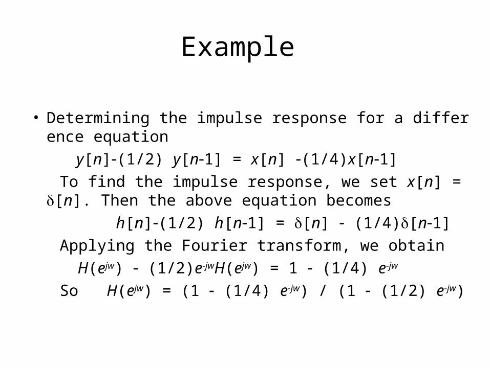
Example

• Determining the impulse response for a difference equation

y[n](1/2) y[n1] = x[n] (1/4)x[n1]

To find the impulse response, we set x[n] = [n]. Then the above equation becomes

h[n](1/2) h[n1] = [n] (1/4)[n1]

Applying the Fourier transform, we obtain

H(ejw) (1/2)e-jwH(ejw) = 1 (1/4) e-jw

So H(ejw) = (1 (1/4) e-jw) / (1 (1/2) e-jw)

Example (continue)

• To obtain the impulse response h[n]• From the DTFT pair-wise table, we know that

thus, (1/2)nu[n] 1 / (1 (1/2) e-jw)

By the shifting property,

(1/4)(1/2)n1u[n1] (1/4) e-jw / (1 (1/2) e-jw)

Thus,

h[n] = (1/2)nu[n] (1/4)(1/2)n1u[n1]

jw

n

aeanua

1

11)(

Suddenly Applied Complex Exponential Inputs

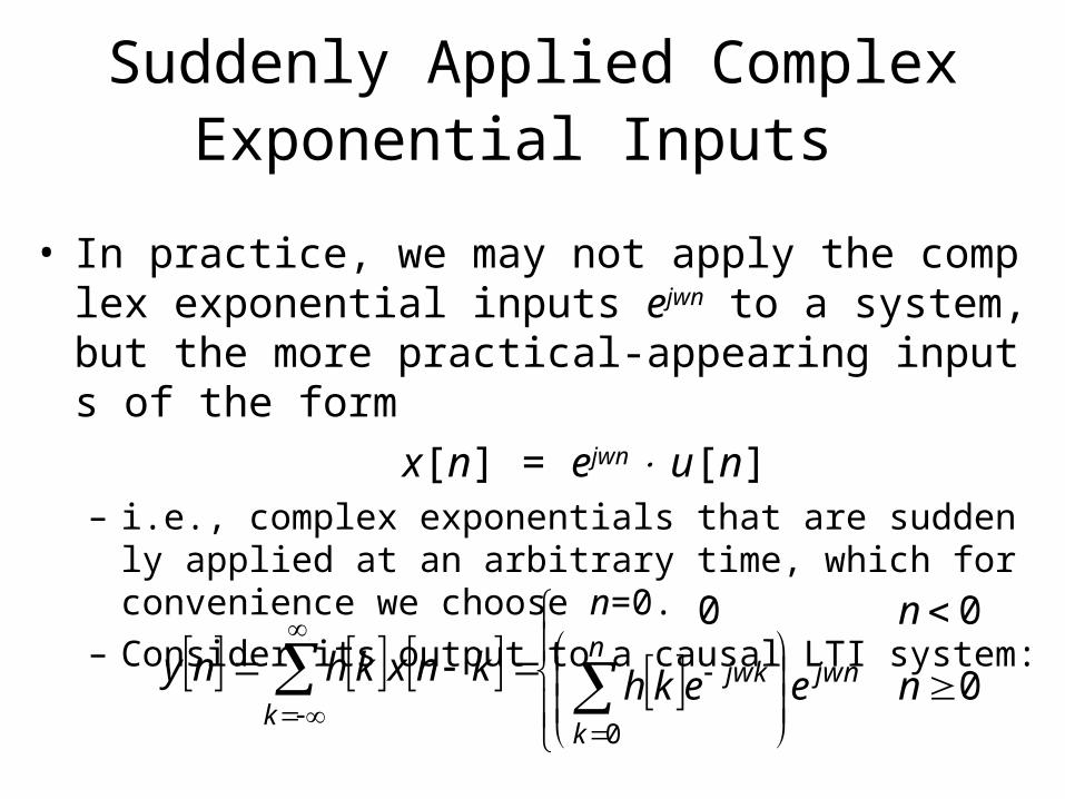
• In practice, we may not apply the complex exponential inputs ejwn to a system, but the more practical-appearing inputs of the form

x[n] = ejwn u[n]– i.e., complex exponentials that are suddenly applied at an

arbitrary time, which for convenience we choose n=0.– Consider its output to a causal LTI system:

0

00

0

neekh

n

knxkhny jwnn

k

jwk

k

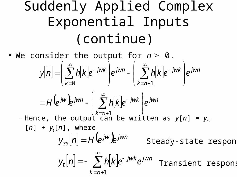
• We consider the output for n 0.

– Hence, the output can be written as y[n] = yss[n] + yt[n], where

Suddenly Applied Complex Exponential Inputs (continue)

jwn

nk

jwkjwnjw

jwn

nk

jwkjwn

k

jwk

eekheeH

eekheekhny

1

10

jwn

nk

jwkt

jwnjwss

eekhny

eeHny

1

Steady-state response

Transient response

• If h[n] = 0 except for 0 n M (i.e., a FIR system), then the transient response yt[n] = 0 for n+1 > M. That is, the transient response becomes zero since the time n = M. For n M, only the steady-state response exists.

• For infinite-duration impulse response (i.e., IIR)

– For stable system, Qn must become increasingly smaller as n , and so is the transient response.


nnknk

jwnjwkt Qkheekhny

11


Illustration for the FIR case by convolution


Illustration for the IIR case by convolution

Documents

In summary