Preprint typeset in JINST style - HYPER VERSION1

In-situ calibration of the single-photoelectron2

charge response of the IceCube photomultipliers3

IceCube author list to be inserted... E-mail: analyses@icecube.wisc.edu

ABSTRACT: This article outlines the in-situ calibration of the single-photoelectron charge distri-butions for each of the Hamamatsu Photonics R7081-02 photomultipliers in the IceCube NeutrinoObservatory. The accurate characterization of the individual PMT charge distributions is importantfor event reconstruction and calibration. We discuss the single photoelectron identification pro-cedure and how we extract the single-photoelectron charge distribution using a deconvolution ofthe multiple photoelectron charge distribution, and we examine various correlations between theshape of the single-photoelectron charge distribution and various hardware components. The timedependence of the charge distributions is also investigated.Definitions (this will be removed in the final draft):

1. Charge: WaveDeform fits the waveform with an SPE pulses template. The integral of thefitted pulse, divided by the load resistance, divided by the gain, is the reported measuredcharge of the pulse. It is reported in units of a single electron.

2. PE: The unit of charge. This represents the charge relative to one electron.

3. 1 PE: The HV on each DOM is set such that the gain on the PMT is 107. It is determinedto be at the proper gain (107), when the Gaussian mean of the fitted charge distribution is at1 PE.

4. Photoelectron: The physical electron emitted from the photocathode.

5. SPE: (Single Photoelectron) A single physical electron emitted from the photocathode.

6. MPE: Multiple electrons emitted from the photocathode, charges may have been combined.

7. Charge distribution: The distribution of the measured charges. This will include both SPEand MPE events.

8. Single Photoelectron Charge distribution: The hypothetical charge distribution generated byobserving a pure sample of single photoelectron.

9. SPE Template: The functional form that is used to fit the charge distribution.

4

KEYWORDS: IceCube, single photoelectron, charge distribution, PMT.5

6

Contents7

1. Introduction 18

1.1 Single-photoelectron charge distributions 39

1.2 IceCube datasets and software definitions 510

2. Extracting the SPE templates 611

2.1 Single photoelectron pulse selection 612

2.2 Characterizing the low-charge region 813

2.3 Fitting procedure 814

2.4 SPE template fit results 915

3. Discussion 1116

3.1 Correlations between fit parameters and DOM hardware differences 1117

3.2 Quantifying observable changes when modifying the PMT charge distributions 1318

3.2.1 Model comparison 1419

3.3 SPE templates in simulation 1420

3.4 SPE templates for calibration 1521

4. Conclusion 1622

23

1. Introduction24

The IceCube Neutrino Observatory [1,2] is a cubic-kilometer-sized array of 5,160 photomultiplier25

tubes (PMTs) buried in the Antarctic ice sheet designed to observe high-energy neutrinos interact-26

ing with the ice [3]. In 2011, the IceCube Collaboration completed the installation of 86 vertical27

strings of PMT modules, eight of which were arranged in a denser array for the DeepCore detec-28

tor [4] and the remaining for the main IceCube detector. Each string in the detector contains 6029

digital optical modules (DOMs), which contain a single PMT each, as well as all required elec-30

tronics [5]. The DOMs extend from 1450 m to 2450 m below the surface of the ice sheet and are31

spaced 17 m apart in the IceCube detector, and 7 m apart in the DeepCore detector.32

Each DOM consists of a 0.5" thick spherical glass pressure vessel that houses a single down-33

facing 10" R7081-02 PMT from Hamamatsu Photonics [6]. The PMT is specified for wavelengths34

ranging from 300 nm to 650 nm, with peak quantum efficiency of 25% near 390 nm, classified as35

normal quantum efficiency (NQE) DOMs. Each PMT is coupled to the glass housing with optical36

gel and is surrounded by a wire mesh of µ metal to reduce the effect of the Earth’s ambient magnetic37

field. The glass housing is transparent to wavelengths 350 nm and above [7].38

IceCube has also deployed 399 DOMs with Hamamatsu R7081-02MOD PMTs, which, having39

a peak quantum efficiency of 34% near 390 nm (36% higher efficiency than the standard DOMs),40

– 1 –

0 10 20 30 40 50 60 70 80String

0

10

20

30

40

50

60

Op

tica

lM

odu

le

Dead

NQE

HQE

Qu

antu

mE

ffici

ency

0 10 20 30 40 50 60 70 80String

0

10

20

30

40

50

60

Op

tica

lM

odu

le

Dead

New

Old

AC

Cou

plin

gM

eth

od

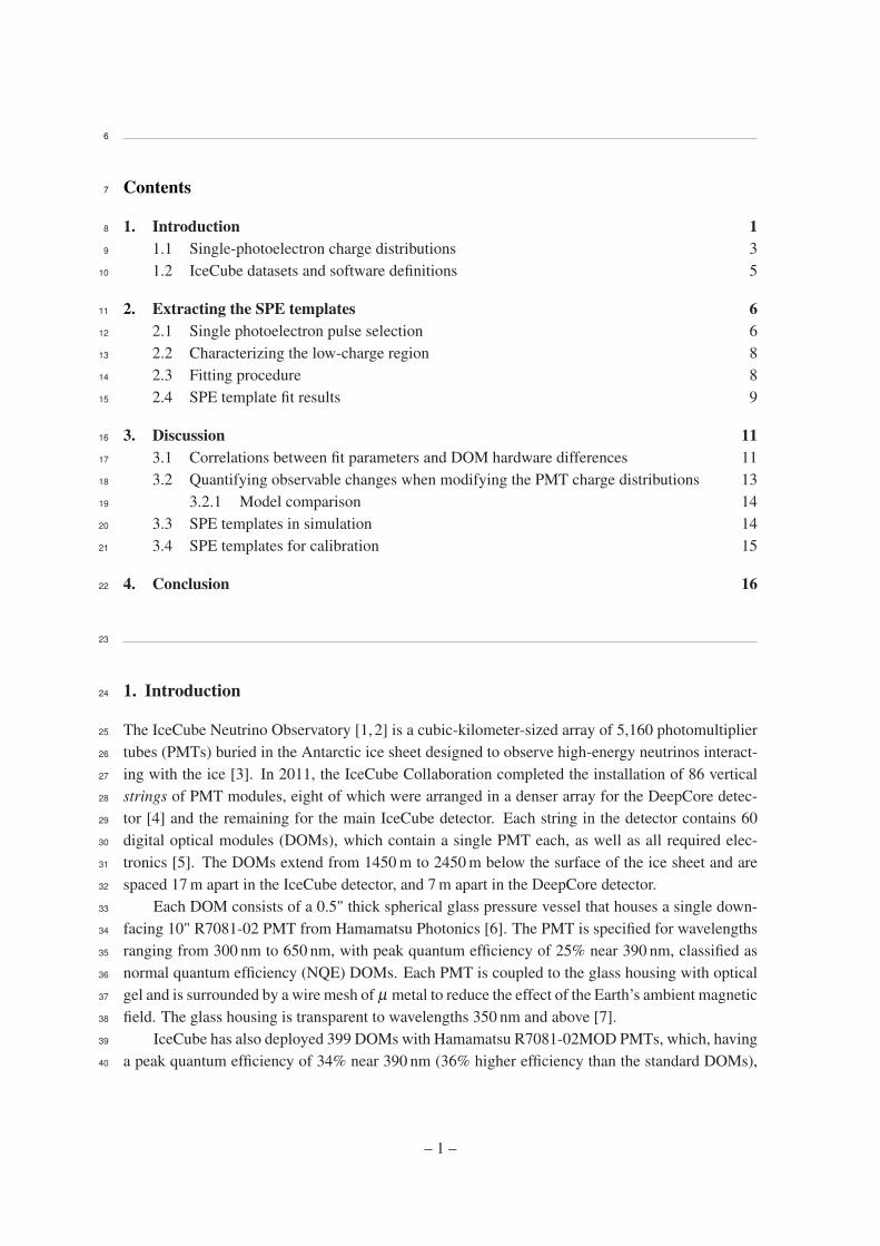
Figure 1. Left: A mapping of the HQE DOMs (black) and standard NQE DOMs (gray). Right: The versionof AC coupling, old toroids (black) and new toroids (gray). DOMs that have been removed from service areshown in white.

are classified as high quantum efficiency (HQE) DOMs [4]. These DOMs are primarily located in41

DeepCore and on strings 36 and 43, as shown in the left side of Fig. 1.42

The R7081-02 and R7081-02MOD PMTs have 10 dynode stages and are operated with a gain43

of 107 and high voltage around 1200 V (a typical amplified single photoelectron will generate a44

≈6 mV peak voltage at the input to the front-end amplifiers). The PMTs operate with the anodes45

at high voltage and the signal is AC coupled to the front-end amplifiers. There are two versions46

of AC coupling in the detectors, both of which use custom-designed wideband bifilar wound 1:147

toroidal transformers1 (the DOM-specific AC-coupling versions, new and old toroids, are shown48

on the right side of Fig. 1). The DOMs with the old toroids were designed with an impedance of49

43Ω, while the new toroids are 50Ω [8].50

IceCube relies on two observables per DOM to reconstruct events: the total number of detected51

photons and their timing distribution. Both the timing and the number of photons are extracted from52

the on-board digitized waveforms in software. The waveforms are deconvolved into a series of53

scaled single photoelectron pulses (so-called pulse series) and the integral of the individual pulses54

(divided by the load resistance) defines the observed charge. It will often be expressed in units of55

PE, or photoelectrons, which further divides the measured charge by the charge of a single electron56

times the nominal gain (107). Accurate characterization of the individual PMT charge distributions57

is crucial for calibration and event reconstructions relying on charge information. The charge58

distribution can also be used to assess long-term detector performance and identify discrepancies59

between data and Monte Carlo. It is therefore critically important to accurately measure the single-60

photoelectron (SPE) charge distribution in order to understand the IceCube detector behavior.61

When one or more photons produce a voltage at the anode sufficient to trigger the onboard62

discriminator (set via a DAC to approximately 1.3 mV, or equivalently to 0.25PE), the signal ac-63

quisition process is triggered. The signal is fed into four parallel input channels. Three of the64

1Conventional AC-coupling high-voltage ceramic capacitors can produce noise from leakage currents and impracticalrequirements on the capacitors in order to meet the signal droop and undershoot requirements. The toroidal transformereffectively acts as a high-pass filter with good signal fidelity at high frequencies. It also provides higher reliability thancapacitive coupling and reduces the stored energy, which might cause damage if there is HV discharge in the system [7].However, the toroidal-transformer AC coupling also introduces signal droop and undershoot.

– 2 –

channels pass first through a 75 ns delay loop in order to capture the leading edge of the pulse65

and then into three high-speed (300 MSPS for 128 samples) 10-bit waveform digitizers (Analog66

Transient Waveform Digitizer, ATWD), each of which has a different level of amplification (15.767

± 0.6, 1.79 ± 0.06, and 0.21 ± 0.01 [8]). There are also three extra ATWDs on board each DOM:68

one is used for calibration and the other two operate in a ping-pong fashion to remove dead time69

associated with the readout. The signal to the fourth channel is first shaped and amplified and then70

fed into a 10-bit fast analog-to-digital converter (fADC) operating at a sampling speed of 40 MSPS.71

Further detail regarding the description of the DOM electronics can be found in Refs. [5, 9].72

This article discusses the accurate determination of how individual DOMs collect charge in73

order to improve calibration and the detector description as used in the IceCube Monte Carlo simu-74

lation. It describes the procedure for determining the PMT’s gain characteristics as seen in the SPE75

charge distributions using in-situ data from the IceCube and DeepCore detectors. The SPE charge76

distribution refers to the measured charge probability density function of the individual DOMs gen-77

erated by the amplification of a pure sample of single photoelectrons. The extraction of the SPE78

charge distribution was recently made possible from the development of two pieces of software:79

1. A specially-designed unbiased pulse selection was developed to reduce the multiple photo-80

electron (MPE) contamination while accounting for physical phenomena (e.g., late pulses,81

afterpulses, pre-pulses, and baseline shifts) and software-related effects (e.g., pulse splitting).82

This is further described in Sec. 2.1.83

2. A fitting procedure was developed that separates the remaining MPE contamination from the84

SPE charge distribution by deconvolving the measured charged distribution. This is further85

described in Sec. 2.3.86

By using in-situ data to determine the SPE charge distributions, we accurately represent the87

individual PMT response as a function of time, environmental conditions, software version, and88

hardware differences, and we sample photons uniformly over the surface of the photocathode. This89

is beneficial since it also allows us to inspect the stability and long-term behavior of the individual90

DOMs, verify previous calibration, and correlate features and environment to DOM behavior.91

1.1 Single-photoelectron charge distributions92

In an idealized scenario, a single photon produces a single photoelectron, which is then amplified by93

a known amount and the measured charge corresponds to 1 PE. However, there are many physical94

processes that create structure in the measured charge distributions. For example:95

• Statistical fluctuation due to cascade multiplication [10]. At every stage of dynode am-96

plification, there is a stochastic spread in the number of emitted electrons that make it to the97

next dynode. This in turn causes a spread in the measured charge after the gain stage of the98

PMT.99

• Photoelectron trajectory. Some electrons may deviate from the favorable trajectory, reduc-100

ing the number of secondaries produced at a dynode or the efficiency to collect them on the101

following dynode. This can occur at any stage, but it has the largest effect on the multipli-102

cation at the first dynode [11]. The trajectory of a photoelectron striking the first dynode103

– 3 –

will depend on many things, including where on the photocathode it was emitted, the unifor-104

mity of the electric field, the size and shape of the dynodes [10], and the ambient magnetic105

field [12, 13].106

• Late or delayed pulses. A photoelectron can elastically or inelastically scatter off the first107

dynode. The scattered electron can then be re-accelerated to the dynode, creating a second108

pulse. The difference in time between the initial pulse and the re-accelerated pulse in the109

R7081-02 PMT was previously measured to be up to 70 ns [7, 14]. The two sub-pulses have110

lower charges, but the sum of the two tends to add up to the original charge. Collecting either111

the initial pulse or the late pulse will result in the charge being reconstructed in the low-PE112

region [15].113

• Afterpulses. When a photoelectron or the secondary electrons produced during the electron114

cascade gain sufficient energy to ionize residual gas in the PMT, the positively charged ion-115

ized gas will be accelerated in the electric field towards the photocathode. Upon impact with116

the photocathode, electrons can be again released from the photocathode, creating what is117

called an afterpulse. For the R7081-02 PMTs, the timescale for afterpulses was measured118

to occur from 0.3 to 11 µs after the initial pulse, with the first prominent afterpulse peak119

occurring at approximately 600 ns [7]. The spread in the afterpulse time is dependent on120

the position of photocathode, the charge-to-mass ratio of the ion produced, and the electric121

potential distribution [16], whereas the size of the afterpulse is related to the momentum and122

species of the ionized gas and composition of the photocathode [17].123

• Pre-pulses. If an incident photon passes through the photocathode without interaction and124

strikes one of the dynodes, it can eject an electron that is only amplified by the subsequent125

stages, resulting in a lower measured charge (lower by a factor of approximately 25). For126

the IceCube PMTs, the prepulses have been found to arrive approximately 30 ns before the127

signal from other photoelectrons from the photocathode [7].128

• MPE contamination. When multiple photoelectrons arrive at the first dynodes within sev-129

eral nanoseconds of each other, they can be reconstructed by the software as a single, MPE130

pulse.131

• Electronic noise. This refers to the fluctuations in the analog-to-digital converters (ATWDs132

and FADC) and ringing that arises from the electronics.133

Beyond the physical phenomena above that modify the measured charge distribution, there is134

also a lower limit on the smallest charge that can be extracted. For IceCube, the discriminator limits135

the trigger pulse to be above approximately 0.25PE, and subsequent pulses in the readout time136

window are subject to a software-defined threshold. The software threshold was set conservatively137

to avoid extracting pulses that originated from electronic noise. This threshold can be modified to138

gain access to lower charge pulses and will be discussed in Sec. 2.2.139

The standard charge distribution model used by the IceCube Collaboration (known as the140

TA0003 distribution [7]) represented the above effects as the sum of an exponential plus a Gaussian,141

where the exponential represented charge of poorly amplified pulses and the Gaussian represented142

– 4 –

the spread in statistical fluctuations due to the cascade multiplication. The TA0003 distribution was143

previously used to describe all the PMTs in the IceCube and DeepCore detectors.144

Recently, IceCube has performed several lab measurements using the R7081-02 PMTs with in-145

time laser pulses, demonstrating that the in-time charge distribution includes a steeply falling low-146

charge component below the discriminator threshold. To account for this, a new functional form147

including a second exponential was introduced. This form of the charge distribution, f (q)SPE =148

Exp1 +Exp2+ Gaussian, is referred to as the SPE template in this article. Explicitly, it is:149

f (q)SPE = E1e−q/w1 +E2e−q/w2 +Ne−(q−µ)2

2σ2 , (1.1)

where q represents the measured charge; E1, E2, and N represent normalization factors of each150

components; w1 and w2 are the exponential decay widths; and µ , σ are the Gaussian mean and151

width, respectively. This is the assumed functional shape of the SPE charge distributions and the152

components of Eq. 1.1 are determined in this article for all in-ice DOMs. IceCube defines 1 PE as153

the location of the Gaussian mean (µ) and calibrates the gain on the individual PMTs during the154

start of each season to meet this definition. The choice of where we define 1 PE is arbitrary, since155

linearity between the total charge collected and the number of incident photons is guaranteed. This156

is because the average of the distribution is a set fraction of the Gaussian mean and the mean of157

a N-fold convolution is the sum of means (central limit theorem). Any bias in the total observed158

charge can be absorbed into an efficiency term, such as the quantum efficiency.159

1.2 IceCube datasets and software definitions160

The largest contribution to the IceCube trigger rate comes from downgoing muons produced in161

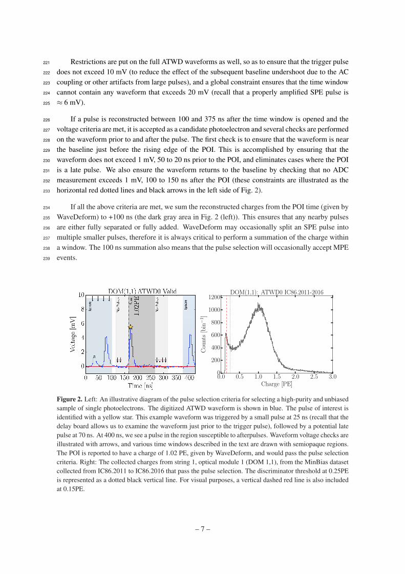
cosmic ray induced showers [18]. Cosmic ray muons stopping in the detector cause the individual162

trigger rate to decrease at lower depths. Further, during the formation of this ice sheet, there have163

been several periods of colder climate that have caused the optical properties of the ice to differ164

at various depths. The optical properties also affect the trigger rate; in particular, the “dust layer"165

from 2100 to 2200 m below the surface (optical modules 32 to 38 in the IceCube detector) is a166

region in the ice with relatively large scattering and absorption coefficients [19].167

An induced signal in the PMT that passes through the AC coupling toroid located on the base168

of the PMT is compared to a discriminator threshold. If two DOMs within two DOM distances of169

each other observe a passing of the discriminator, a hard local coincidence (HLC) is initiated and170

the corresponding waveforms are sampled 128 times and read out on the three ATWDs.171

After waveform digitization, there is a correction applied to remove the measured DC baseline172

offset. The signal droop and undershoot introduced by the toroidal transformer AC coupling is173

compensated for in software (during waveform calibration) by adding the expected temperature-174

dependent reaction voltage of the undershoot to the calibrated waveform. If the undershoot voltage175

drops below 0 ADC counts, the ADC values are zeroed and then compensated for once the wave-176

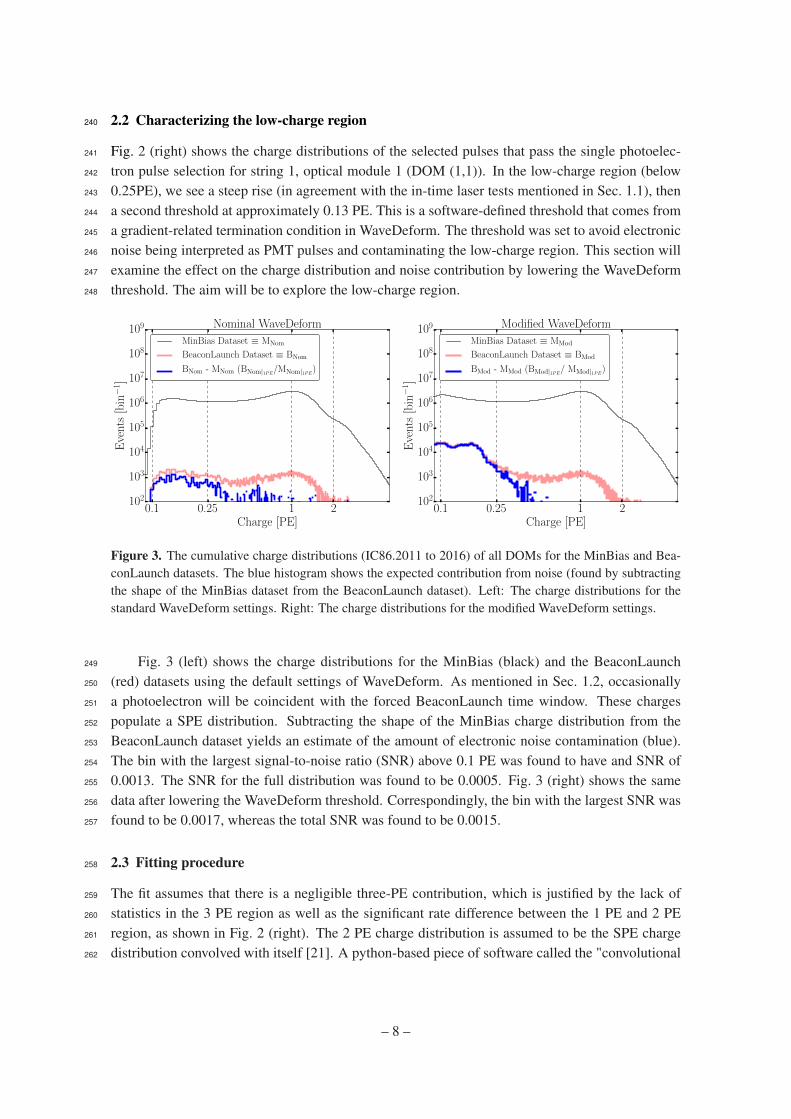
form is above the minimum ADC input. Scaled single photoelectron pulse shapes (that take into177

account the version of the AC coupling) are then fit to the waveforms using software referred to178

as WaveDeform (waveform unfolding process), which determines the individual pulse time stamps179

and charges and populates a pulse series [20].180

The pulse series used in this analysis come from two datasets provided by IceCube:181

– 5 –

1. The MinBias dataset. This dataset records the full waveform readout of randomly-triggered182

HLC events at a rate that corresponds on average to 1/1000 events. The largest contribution183

to the IceCube trigger rate comes from downgoing muons produced in cosmic-ray-induced184

showers [18] and therefore is the largest signal component in this dataset. These muons tend185

to have small energies when they reach the detector, thus they produce minimal MPE con-186

tamination. The full waveform of these events allows us to extract the raw information about187

the individual pulses. This will be used to measure the individual PMT charge distributions.188

2. The BeaconLaunch dataset. This is a forced trigger (not triggered by the discriminator)189

filter that is typically used to monitor the individual DOM baseline. It includes the full190

ATWD-window waveform readout. Since this dataset is forced-triggered, the majority of191

these waveforms represent baseline fluctuations with minimal contamination from the occa-192

sional coincidental pulse that makes it into the readout window. This dataset will be used193

to examine the noise contribution to the charge distributions. Note: when using this dataset,194

the weight of every pulse is multiplied by a factor of 28.4 to account for the livetime differ-195

ence between the MinBias dataset and the BeaconLaunch dataset. Weight, in this context,196

refers to the number of photons in the MinBias dataset proportional to one photon in the197

BeaconLaunch dataset for which both datasets have the same equivalent livetime.198

This analysis uses the full MinBias and BeaconLaunch datasets from IceCube seasons 2011199

to 2016 (subsequently referred to as IC86.2011 to IC86.2016). Seasons in IceCube typically start200

in June of the labeled year and end approximately one year later. Calibration is performed at the201

beginning of each season.202

2. Extracting the SPE templates203

2.1 Single photoelectron pulse selection204

The pulse selection is the method used to extract candidate, unbiased, single photoelectron pulses205

from data while minimizing the MPE contamination. It avoids collecting afterpulses, rejects late206

pulses from the trigger, reassembles late pulses, accounts for the discriminator threshold, reduces207

the effect of droop and baseline undershoot, and gives sufficient statistics to perform a season-to-208

season measurement. An illustrative diagram of the pulse selection is shown in the left side of209

Fig. 2, while a description of the procedure is detailed below.210

In order to trigger a DOM, the input to the front-end amplifiers must exceed the discriminator211

threshold. To avoid the selection bias of the discriminator trigger, we ignore the trigger pulse as212

well as the entire first 100 ns of the time window. Ignoring the first 100 ns has the added benefit213

of also removing late pulses that could be attributed to the triggering pulse. To ensure we are not214

accepting afterpulses into the selection, we also enforce the constraint that the pulse of interest215

(POI) is within the first 375 ns of the ATWD time window. This also allows us to examine the216

waveform up to 50 ns after the POI (the ATWD time window is ≈425 ns). In the vicinity of the217

POI, we check that WaveDeform did not reconstruct any pulses up to 50 ns prior to the POI, or 100218

to 150 ns after the POI (the light gray region of Fig. 2 (left)). This latter constraint is to reduce the219

probability of accidentally splitting a late pulse in the summation window.220

– 6 –

Restrictions are put on the full ATWD waveforms as well, so as to ensure that the trigger pulse221

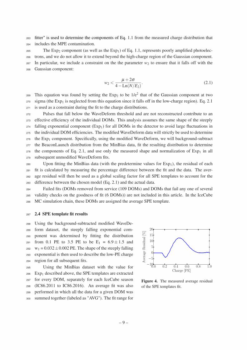
does not exceed 10 mV (to reduce the effect of the subsequent baseline undershoot due to the AC222

coupling or other artifacts from large pulses), and a global constraint ensures that the time window223

cannot contain any waveform that exceeds 20 mV (recall that a properly amplified SPE pulse is224

≈ 6 mV).225

If a pulse is reconstructed between 100 and 375 ns after the time window is opened and the226

voltage criteria are met, it is accepted as a candidate photoelectron and several checks are performed227

on the waveform prior to and after the pulse. The first check is to ensure that the waveform is near228

the baseline just before the rising edge of the POI. This is accomplished by ensuring that the229

waveform does not exceed 1 mV, 50 to 20 ns prior to the POI, and eliminates cases where the POI230

is a late pulse. We also ensure the waveform returns to the baseline by checking that no ADC231

measurement exceeds 1 mV, 100 to 150 ns after the POI (these constraints are illustrated as the232

horizontal red dotted lines and black arrows in the left side of Fig. 2).233

If all the above criteria are met, we sum the reconstructed charges from the POI time (given by234

WaveDeform) to +100 ns (the dark gray area in Fig. 2 (left)). This ensures that any nearby pulses235

are either fully separated or fully added. WaveDeform may occasionally split an SPE pulse into236

multiple smaller pulses, therefore it is always critical to perform a summation of the charge within237

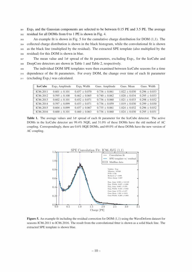
a window. The 100 ns summation also means that the pulse selection will occasionally accept MPE238

events.239

0.0 0.5 1.0 1.5 2.0 2.5 3.0Charge [PE]

0

200

400

600

800

1000

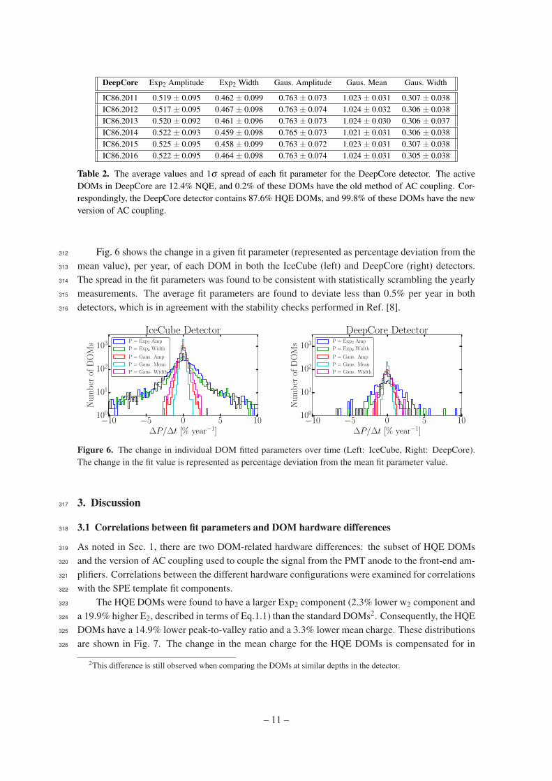
1200

Cou

nts

[bin−

1]

DOM(1,1): ATWD0 IC86.2011-2016

Figure 2. Left: An illustrative diagram of the pulse selection criteria for selecting a high-purity and unbiasedsample of single photoelectrons. The digitized ATWD waveform is shown in blue. The pulse of interest isidentified with a yellow star. This example waveform was triggered by a small pulse at 25 ns (recall that thedelay board allows us to examine the waveform just prior to the trigger pulse), followed by a potential latepulse at 70 ns. At 400 ns, we see a pulse in the region susceptible to afterpulses. Waveform voltage checks areillustrated with arrows, and various time windows described in the text are drawn with semiopaque regions.The POI is reported to have a charge of 1.02 PE, given by WaveDeform, and would pass the pulse selectioncriteria. Right: The collected charges from string 1, optical module 1 (DOM 1,1), from the MinBias datasetcollected from IC86.2011 to IC86.2016 that pass the pulse selection. The discriminator threshold at 0.25PEis represented as a dotted black vertical line. For visual purposes, a vertical dashed red line is also includedat 0.15PE.

– 7 –

2.2 Characterizing the low-charge region240

Fig. 2 (right) shows the charge distributions of the selected pulses that pass the single photoelec-241

tron pulse selection for string 1, optical module 1 (DOM (1,1)). In the low-charge region (below242

0.25PE), we see a steep rise (in agreement with the in-time laser tests mentioned in Sec. 1.1), then243

a second threshold at approximately 0.13 PE. This is a software-defined threshold that comes from244

a gradient-related termination condition in WaveDeform. The threshold was set to avoid electronic245

noise being interpreted as PMT pulses and contaminating the low-charge region. This section will246

examine the effect on the charge distribution and noise contribution by lowering the WaveDeform247

threshold. The aim will be to explore the low-charge region.248

0.1 0.25 1 2Charge [PE]

102

103

104

105

106

107

108

109

Eve

nts

[bin−

1 ]

Nominal WaveDeform

MinBias Dataset ≡ MNom

BeaconLaunch Dataset ≡ BNom

BNom - MNom (BNom|1PE/MNom|1PE)

0.1 0.25 1 2Charge [PE]

102

103

104

105

106

107

108

109

Eve

nts

[bin−

1 ]

Modified WaveDeform

MinBias Dataset ≡ MMod

BeaconLaunch Dataset ≡ BMod

BMod - MMod (BMod|1PE/ MMod|1PE)

Figure 3. The cumulative charge distributions (IC86.2011 to 2016) of all DOMs for the MinBias and Bea-conLaunch datasets. The blue histogram shows the expected contribution from noise (found by subtractingthe shape of the MinBias dataset from the BeaconLaunch dataset). Left: The charge distributions for thestandard WaveDeform settings. Right: The charge distributions for the modified WaveDeform settings.

Fig. 3 (left) shows the charge distributions for the MinBias (black) and the BeaconLaunch249

(red) datasets using the default settings of WaveDeform. As mentioned in Sec. 1.2, occasionally250

a photoelectron will be coincident with the forced BeaconLaunch time window. These charges251

populate a SPE distribution. Subtracting the shape of the MinBias charge distribution from the252

BeaconLaunch dataset yields an estimate of the amount of electronic noise contamination (blue).253

The bin with the largest signal-to-noise ratio (SNR) above 0.1 PE was found to have and SNR of254

0.0013. The SNR for the full distribution was found to be 0.0005. Fig. 3 (right) shows the same255

data after lowering the WaveDeform threshold. Correspondingly, the bin with the largest SNR was256

found to be 0.0017, whereas the total SNR was found to be 0.0015.257

2.3 Fitting procedure258

The fit assumes that there is a negligible three-PE contribution, which is justified by the lack of259

statistics in the 3 PE region as well as the significant rate difference between the 1 PE and 2 PE260

region, as shown in Fig. 2 (right). The 2 PE charge distribution is assumed to be the SPE charge261

distribution convolved with itself [21]. A python-based piece of software called the "convolutional262

– 8 –

fitter" is used to determine the components of Eq. 1.1 from the measured charge distribution that263

includes the MPE contamination.264

The Exp2 component (as well as the Exp1) of Eq. 1.1, represents poorly amplified photoelec-265

trons, and we do not allow it to extend beyond the high-charge region of the Gaussian component.266

In particular, we include a constraint on the the parameter w2 to ensure that it falls off with the267

Gaussian component:268

w2 <µ +2σ

4−Ln(N/E2). (2.1)

This equation was found by setting the Exp2 to be 1/e2 that of the Gaussian component at two269

sigma (the Exp1 is neglected from this equation since it falls off in the low-charge region). Eq. 2.1270

is used as a constraint during the fit to the charge distributions.271

Pulses that fall below the WaveDeform threshold and are not reconstructed contribute to an272

effective efficiency of the individual DOMs. This analysis assumes the same shape of the steeply273

falling exponential component (Exp1) for all DOMs in the detector to avoid large fluctuations in274

the individual DOM efficiencies. The modified WaveDeform data will strictly be used to determine275

the Exp1 component. Specifically, using the modified WaveDeform, we will background-subtract276

the BeaconLaunch distribution from the MinBias data, fit the resulting distribution to determine277

the components of Eq. 2.1, and use only the measured shape and normalization of Exp1 in all278

subsequent unmodified WaveDeform fits.279

Upon fitting the MinBias data (with the predetermine values for Exp1), the residual of each280

fit is calculated by measuring the percentage difference between the fit and the data. The aver-281

age residual will then be used as a global scaling factor for all SPE templates to account for the282

difference between the chosen model (Eq. 2.1) and the actual data.283

Failed fits (DOMs removed from service (109 DOMs) and DOMs that fail any one of several284

validity checks on the goodness of fit (6 DOMs)) are not included in this article. In the IceCube285

MC simulation chain, these DOMs are assigned the average SPE template.286

2.4 SPE template fit results287

0.0 0.2 0.4 0.6 0.8 1.0Charge [PE]

−10

−5

0

5

10

15

20

Ave

rage

Res

idu

al[%

]

Figure 4. The measured average residualof the SPE templates fit.

Using the background-subtracted modified WaveDe-288

form dataset, the steeply falling exponential com-289

ponent was determined by fitting the distribution290

from 0.1 PE to 3.5 PE to be E1 = 6.9± 1.5 and291

w1 = 0.032±0.002 PE. The shape of the steeply falling292

exponential is then used to describe the low-PE charge293

region for all subsequent fits.294

Using the MinBias dataset with the value for295

Exp1 described above, the SPE templates are extracted296

for every DOM, separately for each IceCube season297

(IC86.2011 to IC86.2016). An average fit was also298

performed in which all the data for a given DOM was299

summed together (labeled as "AVG"). The fit range for300

– 9 –

Exp2 and the Gaussian components are selected to be between 0.15 PE and 3.5 PE. The average301

residual for all DOMs from 0 to 1 PE is shown in Fig. 4.302

An example fit is shown in Fig. 5 for the cumulative charge distribution for DOM (1,1). The303

collected charge distribution is shown in the black histogram, while the convolutional fit is shown304

as the black line (multiplied by the residual). The extracted SPE template (also multiplied by the305

residual) for this DOM is shown in blue.306

The mean value and 1σ spread of the fit parameters, excluding Exp1, for the IceCube and307

DeepCore detectors are shown in Table 1 and Table 2, respectively.308

The individual DOM SPE templates were then examined between IceCube seasons for a time309

dependence of the fit parameters. For every DOM, the change over time of each fit parameter310

(excluding Exp1) was calculated.311

IceCube Exp2 Amplitude Exp2 Width Gaus. Amplitude Gaus. Mean Gaus. Width

IC86.2011 0.601 ± 0.101 0.457 ± 0.070 0.736 ± 0.061 1.022 ± 0.030 0.296 ± 0.033IC86.2012 0.595 ± 0.100 0.462 ± 0.065 0.740 ± 0.062 1.020 ± 0.034 0.295 ± 0.033IC86.2013 0.602 ± 0.101 0.452 ± 0.071 0.736 ± 0.060 1.021 ± 0.033 0.298 ± 0.032IC86.2014 0.597 ± 0.099 0.453 ± 0.071 0.736 ± 0.059 1.019 ± 0.030 0.299 ± 0.030IC86.2015 0.604 ± 0.099 0.457 ± 0.067 0.735 ± 0.061 1.024 ± 0.032 0.296 ± 0.032IC86.2016 0.600 ± 0.101 0.460 ± 0.063 0.736 ± 0.060 1.024 ± 0.030 0.295 ± 0.031

Table 1. The average values and 1σ spread of each fit parameter for the IceCube detector. The activeDOMs in the IceCube detector are 99.4% NQE, and 31.0% of these DOMs have the old method of ACcoupling. Correspondingly, there are 0.6% HQE DOMs, and 69.0% of these DOMs have the new version ofAC coupling.

0.0 0.5 1.0 1.5 2.0 2.5 3.0 3.5

Charge [PE]

0.0

0.2

0.4

0.6

0.8

1.0

1.2

Validity: True

NEntries: 197368

PVR: 2.739

Reduced χ2: 0.899

Mean charge: 0.687

Exp1 Amp: 6.900 ± 144.519

Exp1 Width: 0.027 ± 0.098

Exp2 Amp: 0.602 ± 0.378

Exp2 Width: 0.445 ± 0.022

Gaus Amp: 0.778 ± 0.477

Gaus Mean: 1.031 ± 0.011

Gaus Width: 0.280 ± 0.003

SPE Convolution Fit: IC86.AVG (1,1)

Convolution fit

SPE template w/ residual

MinBias data

Figure 5. An example fit including the residual correction for DOM (1,1) using the WaveDeform dataset forseasons IC86.2011 to IC86.2016. The result from the convolutional fitter is shown as a solid black line. Theextracted SPE template is shown blue.

– 10 –

DeepCore Exp2 Amplitude Exp2 Width Gaus. Amplitude Gaus. Mean Gaus. Width

IC86.2011 0.519 ± 0.095 0.462 ± 0.099 0.763 ± 0.073 1.023 ± 0.031 0.307 ± 0.038IC86.2012 0.517 ± 0.095 0.467 ± 0.098 0.763 ± 0.074 1.024 ± 0.032 0.306 ± 0.038IC86.2013 0.520 ± 0.092 0.461 ± 0.096 0.763 ± 0.073 1.024 ± 0.030 0.306 ± 0.037IC86.2014 0.522 ± 0.093 0.459 ± 0.098 0.765 ± 0.073 1.021 ± 0.031 0.306 ± 0.038IC86.2015 0.525 ± 0.095 0.458 ± 0.099 0.763 ± 0.072 1.023 ± 0.031 0.307 ± 0.038IC86.2016 0.522 ± 0.095 0.464 ± 0.098 0.763 ± 0.074 1.024 ± 0.031 0.305 ± 0.038

Table 2. The average values and 1σ spread of each fit parameter for the DeepCore detector. The activeDOMs in DeepCore are 12.4% NQE, and 0.2% of these DOMs have the old method of AC coupling. Cor-respondingly, the DeepCore detector contains 87.6% HQE DOMs, and 99.8% of these DOMs have the newversion of AC coupling.

Fig. 6 shows the change in a given fit parameter (represented as percentage deviation from the312

mean value), per year, of each DOM in both the IceCube (left) and DeepCore (right) detectors.313

The spread in the fit parameters was found to be consistent with statistically scrambling the yearly314

measurements. The average fit parameters are found to deviate less than 0.5% per year in both315

detectors, which is in agreement with the stability checks performed in Ref. [8].316

−10 −5 0 5 10∆P/∆t [% year−1]

100

101

102

103

Nu

mb

erof

DO

Ms

IceCube DetectorP = Exp2 Amp

P = Exp2 Width

P = Gaus. Amp

P = Gaus. Mean

P = Gaus. Width

−10 −5 0 5 10∆P/∆t [% year−1]

100

101

102

103

Nu

mb

erof

DO

Ms

DeepCore DetectorP = Exp2 Amp

P = Exp2 Width

P = Gaus. Amp

P = Gaus. Mean

P = Gaus. Width

Figure 6. The change in individual DOM fitted parameters over time (Left: IceCube, Right: DeepCore).The change in the fit value is represented as percentage deviation from the mean fit parameter value.

3. Discussion317

3.1 Correlations between fit parameters and DOM hardware differences318

As noted in Sec. 1, there are two DOM-related hardware differences: the subset of HQE DOMs319

and the version of AC coupling used to couple the signal from the PMT anode to the front-end am-320

plifiers. Correlations between the different hardware configurations were examined for correlations321

with the SPE template fit components.322

The HQE DOMs were found to have a larger Exp2 component (2.3% lower w2 component and323

a 19.9% higher E2, described in terms of Eq.1.1) than the standard DOMs2. Consequently, the HQE324

DOMs have a 14.9% lower peak-to-valley ratio and a 3.3% lower mean charge. These distributions325

are shown in Fig. 7. The change in the mean charge for the HQE DOMs is compensated for in326

2This difference is still observed when comparing the DOMs at similar depths in the detector.

– 11 –

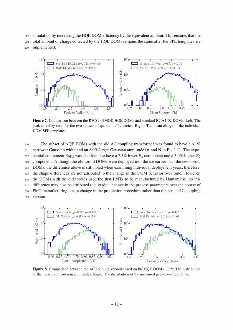
simulation by increasing the HQE DOM efficiency by the equivalent amount. This ensures that the327

total amount of charge collected by the HQE DOMs remains the same after the SPE templates are328

implemented.329

1.5 2.0 2.5 3.0 3.5 4.0Peak-to-Valley Ratio

100

101

102

103

Nu

mb

erof

DO

Ms

Standard DOMs: µ=2.729, σ=0.469

HQE DOMs: µ=2.322, σ=0.263

0.62 0.64 0.66 0.68 0.70 0.72 0.74Mean Charge [PE]

100

101

102

103

Nu

mb

erof

DO

Ms

Standard DOMs: µ=0.7, σ=0.019

HQE DOMs: µ=0.677, σ=0.015

Figure 7. Comparison between the R7081-02MOD HQE DOMs and standard R7081-02 DOMs. Left: Thepeak-to-valley ratio for the two subsets of quantum efficiencies. Right: The mean charge of the individualDOM SPE templates.

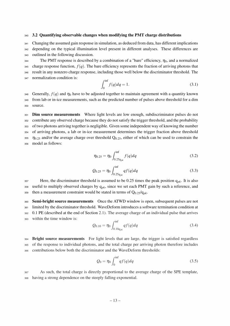
The subset of NQE DOMs with the old AC coupling transformer was found to have a 6.1%330

narrower Gaussian width and an 8.0% larger Gaussian amplitude (σ and N in Eq. 1.1). The expo-331

nential component Exp2 was also found to have a 7.5% lower E2 component and a 3.0% higher E2332

component. Although the old toroid DOMs were deployed into the ice earlier than the new toroid333

DOMs, the difference above is still noted when examining individual deployment years; therefore,334

the shape differences are not attributed to the change in the DOM behavior over time. However,335

the DOMs with the old toroids used the first PMTs to be manufactured by Hamamatsu, so this336

difference may also be attributed to a gradual change in the process parameters over the course of337

PMT manufacturing, i.e., a change in the production procedure rather than the actual AC coupling338

version.339

0.60 0.65 0.70 0.75 0.80 0.85 0.90 0.95Gaus. Amplitude [A.U]

100

101

102

103

Nu

mb

erof

DO

Ms

New Toroids: µ=0.747, σ=0.063

Old Toroids: µ=0.813, σ=0.058

1.5 2.0 2.5 3.0 3.5 4.0Peak-to-Valley Ratio

100

101

102

103

Nu

mb

erof

DO

Ms

New Toroids: µ=2.61, σ=0.447

Old Toroids: µ=3.011, σ=0.408

Figure 8. Comparison between the AC coupling versions used on the NQE DOMs. Left: The distributionof the measured Gaussian amplitudes. Right: The distribution of the measured peak-to-valley ratios.

– 12 –

3.2 Quantifying observable changes when modifying the PMT charge distributions340

Changing the assumed gain response in simulation, as deduced from data, has different implications341

depending on the typical illumination level present in different analyses. These differences are342

outlined in the following discussion.343

The PMT response is described by a combination of a "bare" efficiency, η0, and a normalized344

charge response function, f (q). The bare efficiency represents the fraction of arriving photons that345

result in any nonzero charge response, including those well below the discriminator threshold. The346

normalization condition is:347 ∫ inf

0f (q)dq = 1. (3.1)

Generally, f (q) and η0 have to be adjusted together to maintain agreement with a quantity known348

from lab or in-ice measurements, such as the predicted number of pulses above threshold for a dim349

source.350

Dim source measurements Where light levels are low enough, subdiscriminator pulses do not351

contribute any observed charge because they do not satisfy the trigger threshold, and the probability352

of two photons arriving together is negligible. Given some independent way of knowing the number353

of arriving photons, a lab or in-ice measurement determines the trigger fraction above threshold354

η0.25 and/or the average charge over threshold Q0.25, either of which can be used to constrain the355

model as follows:356

η0.25 = η0

∫ inf

0.25qpk

f (q)dq (3.2)

Q0.25 = η0

∫ inf

0.25qpk

q f (q)dq (3.3)

Here, the discriminator threshold is assumed to be 0.25 times the peak position qpk. It is also357

useful to multiply observed charges by qpk, since we set each PMT gain by such a reference, and358

then a measurement constraint would be stated in terms of Q0.25/qpk.359

Semi-bright source measurements Once the ATWD window is open, subsequent pulses are not360

limited by the discriminator threshold. WaveDeform introduces a software termination condition at361

0.1 PE (described at the end of Section 2.1). The average charge of an individual pulse that arrives362

within the time window is:363

Q0.10 = η0

∫ inf

0.10qpk

q f (q)dq (3.4)

Bright source measurements For light levels that are large, the trigger is satisfied regardless364

of the response to individual photons, and the total charge per arriving photon therefore includes365

contributions below both the discriminator and the WaveDeform thresholds:366

Q0 = η0

∫ inf

0q f (q)dq (3.5)

As such, the total charge is directly proportional to the average charge of the SPE template,367

having a strong dependence on the steeply falling exponential.368

– 13 –

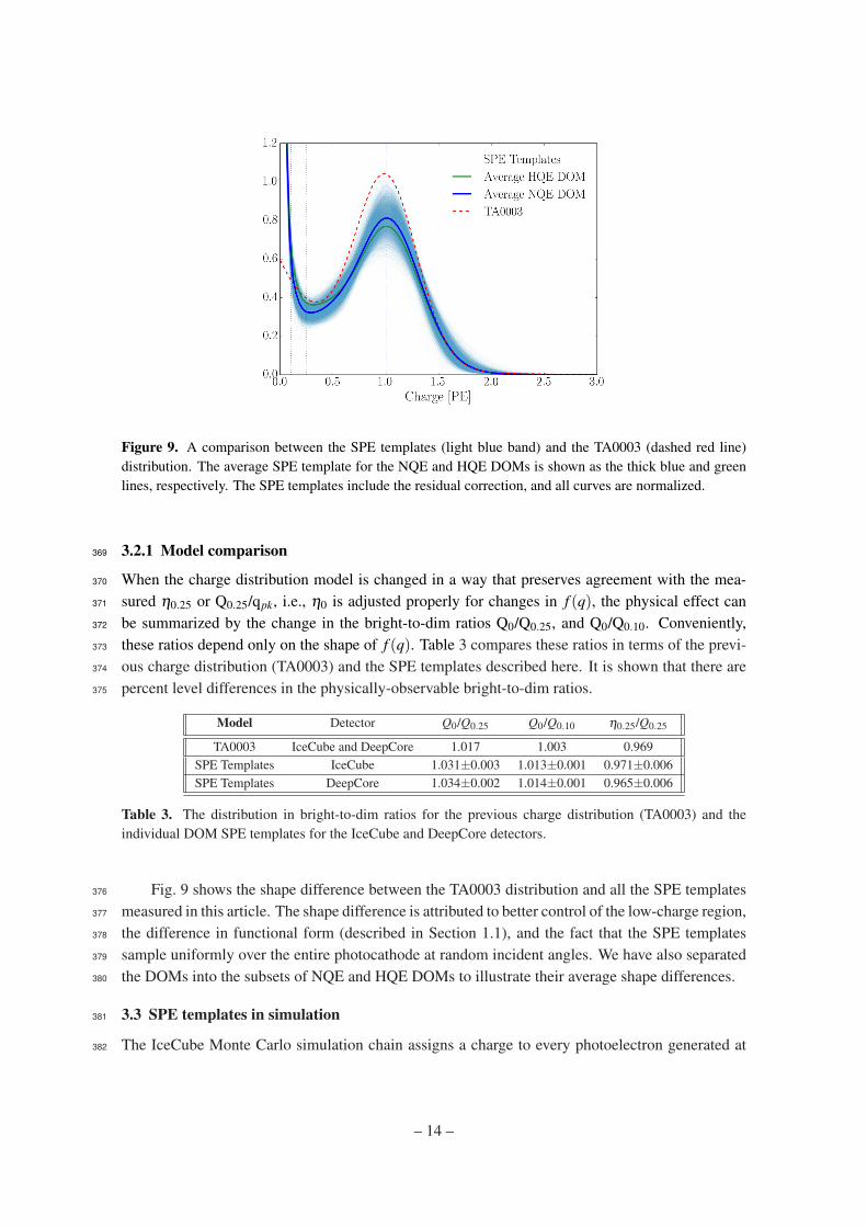
Figure 9. A comparison between the SPE templates (light blue band) and the TA0003 (dashed red line)distribution. The average SPE template for the NQE and HQE DOMs is shown as the thick blue and greenlines, respectively. The SPE templates include the residual correction, and all curves are normalized.

3.2.1 Model comparison369

When the charge distribution model is changed in a way that preserves agreement with the mea-370

sured η0.25 or Q0.25/qpk, i.e., η0 is adjusted properly for changes in f (q), the physical effect can371

be summarized by the change in the bright-to-dim ratios Q0/Q0.25, and Q0/Q0.10. Conveniently,372

these ratios depend only on the shape of f (q). Table 3 compares these ratios in terms of the previ-373

ous charge distribution (TA0003) and the SPE templates described here. It is shown that there are374

percent level differences in the physically-observable bright-to-dim ratios.375

Model Detector Q0/Q0.25 Q0/Q0.10 η0.25/Q0.25

TA0003 IceCube and DeepCore 1.017 1.003 0.969SPE Templates IceCube 1.031±0.003 1.013±0.001 0.971±0.006SPE Templates DeepCore 1.034±0.002 1.014±0.001 0.965±0.006

Table 3. The distribution in bright-to-dim ratios for the previous charge distribution (TA0003) and theindividual DOM SPE templates for the IceCube and DeepCore detectors.

Fig. 9 shows the shape difference between the TA0003 distribution and all the SPE templates376

measured in this article. The shape difference is attributed to better control of the low-charge region,377

the difference in functional form (described in Section 1.1), and the fact that the SPE templates378

sample uniformly over the entire photocathode at random incident angles. We have also separated379

the DOMs into the subsets of NQE and HQE DOMs to illustrate their average shape differences.380

3.3 SPE templates in simulation381

The IceCube Monte Carlo simulation chain assigns a charge to every photoelectron generated at382

– 14 –

the surface of the photocathode. The charge is determined by sampling from a normalized charge383

distribution probability density function. A comparison between describing the charge distribution384

using the SPE templates and the TA0003 distribution follows.385

Two simulation sets consisting of the same events were processed through the IceCube Monte386

Carlo simulation chain to the final level of the multiyear high-energy sterile analysis. At analysis387

level, the events that pass the cuts are >99.9% pure upgoing (directed upwards relative to the388

horizon) secondary muons produced by charged current muon neutrino/antineutrino interactions.389

The muon energy range of this event selection is between 500 GeV and 10 TeV (reconstructed390

quantities).391

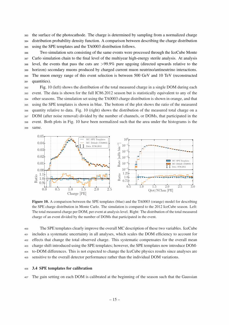
Fig. 10 (left) shows the distribution of the total measured charge in a single DOM during each392

event. The data is shown for the full IC86.2012 season but is statistically equivalent to any of the393

other seasons. The simulation set using the TA0003 charge distribution is shown in orange, and that394

using the SPE templates is shown in blue. The bottom of the plot shows the ratio of the measured395

quantity relative to data. Fig. 10 (right) shows the distribution of the measured total charge on a396

DOM (after noise removal) divided by the number of channels, or DOMs, that participated in the397

event. Both plots in Fig. 10 have been normalized such that the area under the histograms is the398

same.399

0.00

0.01

0.02

0.03

0.04

0.05MC: SPE Templates

MC: Default (TA0003)

Data: IC86.2012

0.0 0.5 1.0 1.5 2.0 2.5Charge [PE]

0.91.01.1

Rat

io

10−5

10−4

10−3

10−2

10−1

100

Rat

e[m

Hz

bin−

1 ]

MC: SPE Templates

MC: Default (TA0003)

Data: IC86.2012

0.5 1.0 1.5 2.0 2.5 3.0Qtot/NChan [PE]

0.751.0

1.25

Rat

io

Figure 10. A comparison between the SPE templates (blue) and the TA0003 (orange) model for describingthe SPE charge distribution in Monte Carlo. The simulation is compared to the 2012 IceCube season. Left:The total measured charge per DOM, per event at analysis level. Right: The distribution of the total measuredcharge of an event divided by the number of DOMs that participated in the event.

The SPE templates clearly improve the overall MC description of these two variables. IceCube400

includes a systematic uncertainty in all analyses, which scales the DOM efficiency to account for401

effects that change the total observed charge. This systematic compensates for the overall mean402

charge shift introduced using the SPE templates; however, the SPE templates now introduce DOM-403

to-DOM differences. This is not expected to change the IceCube physics results since analyses are404

sensitive to the overall detector performance rather than the individual DOM variations.405

3.4 SPE templates for calibration406

The gain setting on each DOM is calibrated at the beginning of the season such that the Gaussian407

– 15 –

mean charge distribution corresponds to a gain of 107 (equivalently labelled as 1 PE). Since the408

method used to extract the Gaussian mean described in this article is different from the previous409

method used for calibration of the DOMs, the total measured charge from a DOM is expected to410

change with the updated calibration.411

As shown in Tables 1 and 2, the Gaussian mean component of the fit of every year is found to412

be on average 2.2% higher than unity, corresponding to a systematic overestimation of the measured413

charge in the detector. This correction to the measured charge can be implemented retroactively by414

dividing the reported charge from WaveDeform by the corresponding Gaussian mean for a given415

DOM. Alternatively, the MC can account for this difference by simply inserting the SPE templates416

with Gaussian mean matching the values found in the data. Both of these solutions will be used in417

future IceCube data/MC production.418

4. Conclusion419

This article outlines the procedure used for collecting a relatively pure sample of single photoelec-420

tron charges for each of the in-ice DOMs in IceCube. MPE contamination was removed under the421

assumption that it is the convolution of the SPE distribution from multiple times.422

The SPE templates were extracted for each DOM and each season in the IceCube and Deep-423

Core detectors and investigated for correlations with hardware-related features. Neither detector424

shows more than a 0.5% deviation in any of the fitted parameters over the investigated seasons, in425

agreement with Ref. [8]. Yearly variations in the fit parameters are consistent with statistical fluc-426

tuations. The HQE DOMs located in the IceCube and DeepCore detectors were found to have an427

Exp2 component distinguishable from the standard DOMs. Similarly, DOMs with the old method428

of AC coupling were found to have a narrower and larger Gaussian component. This was not found429

to be due to a manufacturing process and is still under investigation.430

The SPE templates were introduced into the MC simulation production and the result was431

compared to the default charge distribution. A significant improvement in the description of the432

low-level variables, total charge per DOM, and total charge per event over the number of channels433

was shown. IceCube includes a systematic that scales the bare efficiency of the DOMs to maintain434

agreement with a quantity known from lab or in-ice measurements. After accounting for this shift,435

the effect on physics analysis, as shown by the bright-to-dim ratios, is expected to be minimal436

(percent level changes in the measured charge).437

The new method for extracting the calibration constant that determines the gain setting on each438

of the PMTs (the Gaussian mean of the fit) has been revised and shows that the average gain was439

approximately 2.2%±3.1% higher than expected. This will be implemented in future IceCube data440

reprocessing.441

442

Acknowledgments443

We acknowledge the support from the following agencies: U.S. National Science Foundation - Of-444

fice of Polar Programs, U.S. National Science Foundation - Physics Division, University of Wiscon-445

sin Alumni Research Foundation, the Grid Laboratory Of Wisconsin (GLOW) grid infrastructure446

– 16 –

at the University of Wisconsin - Madison, the Open Science Grid (OSG) grid infrastructure; U.S.447

Department of Energy, and National Energy Research Scientific Computing Center, the Louisiana448

Optical Network Initiative (LONI) grid computing resources; Natural Sciences and Engineering449

Research Council of Canada, WestGrid and Compute/Calcul Canada; Swedish Research Coun-450

cil, Swedish Polar Research Secretariat, Swedish National Infrastructure for Computing (SNIC),451

and Knut and Alice Wallenberg Foundation, Sweden; German Ministry for Education and Re-452

search (BMBF), Deutsche Forschungsgemeinschaft (DFG), Helmholtz Alliance for Astroparticle453

Physics (HAP), Research Department of Plasmas with Complex Interactions (Bochum), Germany;454

Fund for Scientific Research (FNRS-FWO), FWO Odysseus programme, Flanders Institute to en-455

courage scientific and technological research in industry (IWT), Belgian Federal Science Policy456

Office (Belspo); University of Oxford, United Kingdom; Marsden Fund, New Zealand; Australian457

Research Council; Japan Society for Promotion of Science (JSPS); the Swiss National Science458

Foundation (SNSF), Switzerland; National Research Foundation of Korea (NRF); Villum Fonden,459

Danish National Research Foundation (DNRF), Denmark.460

– 17 –

References461

[1] J. Ahrens et al., “Icecube preliminary design document,” URL: http://www. icecube. wisc.462

edu/science/publications/pdd, 2001.463

[2] A. Achterberg, M. Ackermann, J. Adams, J. Ahrens, K. Andeen, D. Atlee, J. Baccus, J. Bahcall,464

X. Bai, B. Baret, et al., “First year performance of the icecube neutrino telescope,” Astroparticle465

Physics, vol. 26, no. 3, pp. 155–173, 2006.466

[3] I. Collaboration et al., “Evidence for high-energy extraterrestrial neutrinos at the icecube detector,”467

Science, vol. 342, no. 6161, p. 1242856, 2013.468

[4] R. Abbasi, Y. Abdou, T. Abu-Zayyad, M. Ackermann, J. Adams, J. Aguilar, M. Ahlers, M. Allen,469

D. Altmann, K. Andeen, et al., “The design and performance of icecube deepcore,” Astroparticle470

physics, vol. 35, no. 10, pp. 615–624, 2012.471

[5] R. Abbasi, M. Ackermann, J. Adams, M. Ahlers, J. Ahrens, K. Andeen, J. Auffenberg, X. Bai,472

M. Baker, S. Barwick, et al., “The icecube data acquisition system: Signal capture, digitization, and473

timestamping,” Nuclear Instruments and Methods in Physics Research Section A: Accelerators,474

Spectrometers, Detectors and Associated Equipment, vol. 601, no. 3, pp. 294–316, 2009.475

[6] Hamamatsu, “Datasheet,” URL: https://www.hamamatsu.com/, 2018.476

[7] R. Abbasi, Y. Abdou, T. Abu-Zayyad, J. Adams, J. Aguilar, M. Ahlers, K. Andeen, J. Auffenberg,477

X. Bai, M. Baker, et al., “Calibration and characterization of the icecube photomultiplier tube,”478

Nuclear Instruments and Methods in Physics Research Section A: Accelerators, Spectrometers,479

Detectors and Associated Equipment, vol. 618, no. 1-3, pp. 139–152, 2010.480

[8] M. Aartsen et al., “The icecube neutrino observatory: Instrumentation and online systems, jinst 12481

(03)(2017) p03012,” arXiv preprint arXiv:1612.05093, pp. 1748–0221.482

[9] R. Stokstad, “Design and performance of the icecube electronics,” 2005.483

[10] Hamamatsu, “Resources: Basics and applications,” URL:484

https://www.hamamatsu.com/resources/pdf/etd/PMT_handbook_v3aE.pdf, 2018.485

[11] Hamamatsu, “Handbook resources, chapter 4,” URL:486

https://www.hamamatsu.com/resources/pdf/etd/PMT_handbook_v3aE-Chapter4.pdf, 2018.487

[12] J. Brack, B. Delgado, J. Dhooghe, J. Felde, B. Gookin, S. Grullon, J. Klein, R. Knapik, A. LaTorre,488

S. Seibert, et al., “Characterization of the hamamatsu r11780 12 in. photomultiplier tube,” Nuclear489

Instruments and Methods in Physics Research Section A: Accelerators, Spectrometers, Detectors and490

Associated Equipment, vol. 712, pp. 162–173, 2013.491

[13] E. Calvo, M. Cerrada, C. Fernández-Bedoya, I. Gil-Botella, C. Palomares, I. Rodríguez, F. Toral, and492

A. Verdugo, “Characterization of large-area photomultipliers under low magnetic fields: Design and493

performance of the magnetic shielding for the double chooz neutrino experiment,” Nuclear494

Instruments and Methods in Physics Research Section A: Accelerators, Spectrometers, Detectors and495

Associated Equipment, vol. 621, no. 1-3, pp. 222–230, 2010.496

[14] F. Kaether and C. Langbrandtner, “Transit time and charge correlations of single photoelectron events497

in r7081 photomultiplier tubes,” Journal of Instrumentation, vol. 7, no. 09, p. P09002, 2012.498

[15] B. Lubsandorzhiev, P. Pokhil, R. Vasiljev, and A. Wright, “Studies of prepulses and late pulses in the499

8" electron tubes series of photomultipliers,” Nuclear Instruments and Methods in Physics Research500

Section A: Accelerators, Spectrometers, Detectors and Associated Equipment, vol. 442, no. 1-3,501

pp. 452–458, 2000.502

– 18 –

[16] K. Ma, W. Kang, J. Ahn, S. Choi, Y. Choi, M. Hwang, J. Jang, E. Jeon, K. Joo, H. Kim, et al., “Time503

and amplitude of afterpulse measured with a large size photomultiplier tube,” Nuclear Instruments504

and Methods in Physics Research Section A: Accelerators, Spectrometers, Detectors and Associated505

Equipment, vol. 629, no. 1, pp. 93–100, 2011.506

[17] S. Torre, T. Antonioli, and P. Benetti, “Study of afterpulse effects in photomultipliers,” Review of507

scientific instruments, vol. 54, no. 12, pp. 1777–1780, 1983.508

[18] M. Aartsen, K. Abraham, M. Ackermann, J. Adams, J. Aguilar, M. Ahlers, M. Ahrens, D. Altmann,509

T. Anderson, M. Archinger, et al., “Characterization of the atmospheric muon flux in icecube,”510

Astroparticle physics, vol. 78, pp. 1–27, 2016.511

[19] M. Aartsen, R. Abbasi, Y. Abdou, M. Ackermann, J. Adams, J. Aguilar, M. Ahlers, D. Altmann,512

J. Auffenberg, X. Bai, et al., “Measurement of south pole ice transparency with the icecube led513

calibration system,” Nuclear Instruments and Methods in Physics Research Section A: Accelerators,514

Spectrometers, Detectors and Associated Equipment, vol. 711, pp. 73–89, 2013.515

[20] M. Aartsen, R. Abbasi, M. Ackermann, J. Adams, J. Aguilar, M. Ahlers, D. Altmann, C. Arguelles,516

J. Auffenberg, X. Bai, et al., “Energy reconstruction methods in the icecube neutrino telescope,”517

Journal of Instrumentation, vol. 9, no. 03, p. P03009, 2014.518

[21] R. Dossi, A. Ianni, G. Ranucci, and O. J. Smirnov, “Methods for precise photoelectron counting with519

photomultipliers,” Nuclear Instruments and Methods in Physics Research Section A: Accelerators,520

Spectrometers, Detectors and Associated Equipment, vol. 451, no. 3, pp. 623–637, 2000.521

– 19 –