In Search of Systematic Risk and the Idiosyncratic VolatilityPuzzle in the Corporate Bond Market∗

Jennie Bai† Turan G. Bali‡ Quan Wen§

Abstract

We propose a comprehensive measure of systematic risk for corporate bonds as a nonlin-ear function of robust risk factors and find a significantly positive link between systematicrisk and the time-series and cross-section of future bond returns. We also find a positivebut insignificant relation between idiosyncratic risk and future bond returns, suggestingthat institutional investors dominating the bond market hold well-diversified portfolioswith a negligible exposure to bond-specific risk. The composite measure of systematicrisk also predicts the distribution of future market returns, and the systematic risk factorearns a positive price of risk, consistent with Merton’s (1973) ICAPM.

This Version: June 2019

JEL Classification: G10, G11, C13.Keywords: Corporate bonds, systematic risk, idiosyncratic volatility, risk factors.

∗We thank Andreas Barth, Marc Crummenerl, Kris Jacobs, Yigitcan Karabulut, Francesco Sangiorgi,Christian Schlag, Grigory Vilkov, and seminar participants at Bloomberg, the Frankfurt School of Financeand Management, Goethe University, the University of Houston, and the 2019 Q-group annual conference fortheir helpful comments and suggestions. We also thank Kenneth French, Kewei Hou, Lubos Pastor, RobertStambaugh, Chen Xue, and Lu Zhang for making a large amount of historical data publicly available. Allerrors remain our responsibility.†Associate Professor of Finance, McDonough School of Business, Georgetown University, and NBER Faculty

Research Fellow, Phone: (202) 687-5695, Email: Jennie.Bai@georgetown.edu.‡Corresponding author: Robert S. Parker Chair Professor of Finance, McDonough School of Business,

Georgetown University, Washington, D.C. 20057. Phone: (202) 687-5388, Email: Turan.Bali@georgetown.edu.§Assistant Professor of Finance, McDonough School of Business, Georgetown University, Washington, D.C.

20057. Phone: (202) 687-6530, Email: Quan.Wen@georgetown.edu.

1 Introduction

According to the Capital Asset Pricing Model (CAPM) of Sharpe (1964), Lintner (1965), and

Mossin (1966), the cross-sectional variation in expected returns of different securities is driven

only by the cross-sectional variation in their market betas. This hypothesis is perhaps the

most studied, and also one of the most strongly refuted hypotheses in empirical asset pricing.1

Despite the vast literature investigating the role of systematic risk in the cross-sectional pricing

of individual stocks, far less effort has been devoted to explaining the cross-sectional dispersion

in corporate bond returns. This paper is the first to propose a novel measure of systematic

risk for corporate bonds and examine its relationship with expected bond returns.

Bai, Bali, and Wen (2019, hereafter BBW) introduce common risk factors based on the

downside risk, credit risk, and liquidity risk of corporate bonds. They show that these novel

bond factors have significant risk premia and outperform all other models considered in the

literature in explaining the returns of the industry- and size/maturity-sorted portfolios of

corporate bonds. Extending the original work of BBW, this paper introduces a composite

measure of systematic risk for individual corporate bonds, defined as a nonlinear function of

the aggregate bond market portfolio (MKT), downside risk factor (DRF), credit risk factor

(CRF), and liquidity risk factor (LRF). Specifically, the composite measure of systematic

risk synthesizes the variance of the MKT, DRF, CRF, and LRF factors, these factors’ cross-

covariances, and the exposures of corporate bond returns to these factors.

We contribute to the literature by analyzing corporate bonds’ aggregate exposure to the

new bond factors (DRF, CRF, LRF) and by investigating the performance of this broad mea-

sure of systematic risk in predicting both time-series and cross-sectional bond returns. We

assemble a comprehensive dataset of corporate bonds from January 1997 to December 2017,

including over 1.2 million monthly bond return observations for a total of 22,231 bonds issued

by 7,915 firms. Then, we test the significance of a cross-sectional relation between systematic

1Over the past four decades, a number of studies provide evidence that firm characteristics such as firmsize, value-to-price ratios, investment, profitability, and past returns do have significant explanatory power foraverage stock returns, while market beta has no power.

1

risk and future returns using portfolio-level analysis, and find that bonds in the highest system-

atic risk quintile generate 6.24% to 9.36% more annualized raw and risk-adjusted returns than

bonds in the lowest systematic risk quintile, with the systematic risk premium stemming from

the outperformance of bonds with high systematic risk (long leg of the arbitrage portfolio).

Such results remain robust after controlling for various bond characteristics simultaneously in

Fama-MacBeth (1973) regressions.

Once we establish the fact that systematic risk plays a significant role in the cross-sectional

pricing of corporate bonds, we examine the time-series predictive power of aggregate systematic

risk in forecasting bond market returns and volatility. Maio and Santa-Clara (2012) investi-

gate the restrictions of the cross-sectional and time-series predictability in the intertemporal

capital asset pricing model (ICAPM, Merton, 1973), and show that a cross-sectional variable,

when aggregated, should predict future market return and market volatility, if the variable is

interpreted as a state variable that affects investment opportunity set in the ICAPM. Aggre-

gating systematic risk across bonds, either equal-weighted, value-weighted, or rating-weighted,

we find that the aggregate measure of systematic risk significantly predicts future bond mar-

ket returns and bond market volatility, even after controlling for a large set of macroeconomic

variables capturing business cycle fluctuations. We also construct a new systematic risk factor

based on the independently sorted bivariate portfolios of credit rating and systematic risk,

and show that the systematic risk factor earns a positive price of risk in the cross-section of

corporate bonds. Moreover, the price of systematic risk estimated from the cross-sectional

regressions yields an economically sensible estimate of the relative risk aversion of bond mar-

ket investors. Since the composite measure of systematic risk satisfies all restrictions of the

ICAPM on the time-series and cross-sectional predictability, we conclude that Merton’s model

provides a theoretical background for the systematic risk factor in the corporate bond market.

Dynamic asset pricing models starting with Merton’s (1973) ICAPM provide a theoretical

framework that gives a positive equilibrium relation between the conditional first and second

moments of excess returns on the market portfolio. Despite the importance of the positive

2

risk-return tradeoff and the theoretical appeal of Merton’s result, empirical studies are not

in agreement on the direction of an intertemporal relation between expected return and risk

in the equity market. Many studies fail to identify a robust and significant intertemporal

relation between risk and return on the equity market portfolio. Several studies even find

that the intertemporal relation between risk and return is negative. Some recent work does

document a positive and significant time-series relation between expected return and risk in

the equity market.2 It is important to note that we find a significantly positive time-series

relation between systematic risk and expected returns on the aggregate bond market portfolio,

indicating a positive intertemporal risk-return tradeoff in the corporate bond market, while

the equity literature has not yet reached an agreement on the existence of such a positive

risk-return tradeoff in the equity market.

In addition to proposing a new measure of systematic risk and testing its cross-sectional and

time-series predictive power, this paper further contributes to the literature by investigating

the idiosyncratic volatility puzzle in the corporate bond market. Assuming that assets are

perfectly liquid (frictionless) and that investors have complete information, firm-specific risk

does not command a risk premium because investors can create well-diversified portfolios

that have zero exposure to firm-specific risk. The corresponding empirical implication is that

measures of firm-specific risk, or risk that is not related to a systematic risk factor, should

exhibit no relation with future returns. Theoretically, however, Levy (1978) shows that if

investors do not hold a large number of assets in their portfolios, and are hence unable to

diversify firm-specific risk, idiosyncratic risk affects equilibrium asset prices. Merton (1987)

indicates that if investors cannot hold the market portfolio, then they care about total risk,

not simply market risk. Therefore, firms with larger total or idiosyncratic risk require higher

returns to compensate for imperfect diversification.

The most widely-cited study on idiosyncratic risk and expected returns is Ang, Hodrick,

2See, e.g., French, Schwert, and Stambaugh (1987), Bollerslev, Engle, and Wooldridge (1988), Nelson(1991), Campbell and Hentchel (1992), Glosten, Jagannathan, and Runkle (1993), Whitelaw (1994), Harrisonand Zhang (1999), Harvey (2001), Brandt and Kang (2004), Ghysels, Santa-Clara, and Valkanov (2005),Bollerslev and Zhou (2006), Guo and Whitelaw (2006), Bali (2008), and Bali and Engle (2010).

3

Xing, and Zhang (2006), which demonstrates a strong negative cross-sectional relation between

idiosyncratic volatility and future stock returns. This result is highly inconsistent with theo-

retical predictions and thus considered as a puzzle. Several subsequent papers have proposed

explanations for the idiosyncratic volatility puzzle based on liquidity (Bali and Cakici, 2008;

Han and Lesmond, 2011), lottery demand (Bali, Cakici, and Whitelaw, 2011), short-term re-

versal (Fu, 2009; Huang et al., 2010), average variance beta (Chen and Petkova, 2012), and

retail trading proportion (Han and Kumar, 2013).3

We re-examine the idiosyncratic volatility puzzle in the corporate bond market by testing

the direction and significance of a cross-sectional relation between idiosyncratic volatility and

future bond returns. Idiosyncratic volatility is measured by the variance of the residuals from

the monthly time-series regressions of bond excess returns on the MKT, DRF, CRF, and LRF

factors of BBW. We form value-weighted univariate portfolios by sorting corporate bonds into

quintiles based on their idiosyncratic volatility and find that the risk-adjusted return (alpha)

spread between the highest and lowest idiosyncratic volatility quintiles is positive but economi-

cally and statistically insignificant: 0.25% per month (t-stat = 1.54). This result suggests that

institutional investors that dominate the corporate bond market hold well-diversified portfo-

lios with a negligible exposure to bond-specific risk so that idiosyncratic volatility does not

command a significant risk premium in the corporate bond market. Furthermore, idiosyncratic

risk becomes even weaker, both economically and statistically, after controlling for systematic

risk, whereas systematic risk remains a significant determinant of the cross-sectional dispersion

in bond returns after controlling for idiosyncratic risk.

To assess the relative performance of our composite measure of risk, we consider three

benchmark models in the literature and construct alternative measures of systematic and

idiosyncratic risk. The first benchmark is the one-factor model of Elton, Gruber, and Blake

(1995) that relies on the aggregate corporate bond market portfolio (MKT ). Second, we

3Hou and Loh (2016) find that many existing explanations resolve less than 10% of the puzzle. On theother hand, explanations based on investors’ lottery preferences and market frictions show some promise insolving the idiosyncratic volatility puzzle. Together, all existing explanations account for 29-54% of the puzzlein individual stocks and 78-84% of the puzzle in idiosyncratic volatility-sorted portfolios.

4

extend the one-factor model by including the term and default factors (TERM,DEF ) used by

Fama and French (1993) and Bessembinder et al. (2009). The third benchmark, also the most

comprehensive one, is the six-factor model in Chung, Wang, and Wu (2019), which extends

the second benchmark (three-factor model) by adding the size, book-to-market, and market

volatility factors (SMB,HML,∆V IX). We find that proxies of systematic risk generated

by these alternative factor models do not predict the cross-sectional variation in future bond

returns, whereas proxies of idiosyncratic risk from these models positively predict future bond

returns. However, after accounting for bond exposures to the downside, credit, and liquidity

risk factors of BBW, there is no significant link between idiosyncratic volatility and future

bond returns.4 These results indicate that the risk factors of BBW provide an accurate

characterization of systematic risk in the corporate bond market, and hence the BBW-based

composite measure of systematic variance is a priced risk factor.

Lastly, we examine the differences between the roles of systematic and firm-specific risk

measures in the cross-sectional pricing of equities versus bonds. To make a fair comparison,

we employ the same composite methodology to construct systematic and idiosyncratic risk

measures of individual stocks using the five-factor model of Fama and French (2015) and

the four-factor model of Hou, Xue, and Zhang (2015). We find no evidence of a significant

relation between systematic risk and future stock returns, but a strong negative link exists

between idiosyncratic volatility and future equity returns, consistent with Ang et al. (2006).

These findings are in sharp contrast to those in the corporate bond market. We provide

an explanation for these contradictory findings based on differing investor preferences and

clienteles in the bond and equity markets.

According to the Flow of Funds report released by the Federal Reserve Board, corporate

bonds are primarily held by institutional investors such as insurance companies, mutual funds,

and pension funds, while a significant amount of equities is held by retail investors. As of

4Chung, Wang, and Wu (2019) find a significantly positive relation between idiosyncratic volatility andrisk-adjusted returns since they use the Fama-French (2015) five-factor model to estimate the risk-adjustedreturns (alphas) of corporate bonds. We are able to replicate their findings reported in their Table 6. However,when we use the risk factors of BBW, the alpha spread disappears in idiosyncratic volatility-sorted portfolios.

5

2018, retail investors own about 6% in the corporate bond market versus 37% in the equity

market. Clearly, equities and bonds are mainly traded (or held) by a markedly different

group of investors: retail vs. institutional investors with distinct risk appetites, preferences,

and investment objectives. Thus, investor clientele can be a plausible cause of the different

(systematic/idiosyncratic) risk-return relations in the bond and equity markets.

Indeed, we find that in the equity market, the idiosyncratic volatility puzzle is more pro-

nounced for stocks largely held by retail investors, whereas there is no significant relation

between idiosyncratic volatility and future returns for stocks largely held by institutional in-

vestors. In the corporate bond market, the systematic risk premium is stronger for corporate

bonds largely held by active institutional investors. We explain these results by showing that

institutional investors with higher exposures to common risk factors tend to have stronger

timing abilities and higher future returns. That is, institutional investors with stronger timing

abilities willingly take direct exposures to the systematic risk factors, relying on their market-

and volatility-timing abilities to generate superior returns. Since these are active institutions

with dynamic investment strategies that are highly exposed to systematic risk, timing the

switch in economic trends is essential to their success. Accordingly, the systematic risk pre-

mium is stronger (weaker) for corporate bonds largely held by active (passive) institutional

investors. Thus, our findings offer a plausible explanation for the significance of systematic

risk (idiosyncratic risk) in the bond (equity) market based on differing investor preferences

and clienteles.

In the remainder of this paper, we introduce the data and variables in Section 2, examine

the cross-sectional relation between systematic risk, idiosyncratic risk and future bond returns

in Section 3, and test alternative measures of systematic risk in Section 4. Section 5 inves-

tigates whether the newly proposed measure of systematic risk is consistent with Merton’s

(1973) theoretical model. Section 6 provides an explanation for the contradictory role of sys-

tematic and idiosyncratic risk in the cross-sectional pricing of equities versus bonds. Section 7

concludes the paper.

6

2 Data

2.1 Corporate bond returns

We compile corporate bond pricing data from the National Association of Insurance Com-

missioners database (NAIC) and the enhanced version of the Trade Reporting and Compli-

ance Engine (TRACE) for the sample period from January 1994 to December 2017, with

the TRACE data starting from July 2002. We then merge corporate bond pricing data with

the Mergent fixed income securities database to obtain bond characteristics such as offering

amount, offering date, maturity date, coupon rate, coupon type, interest payment frequency,

bond type, bond rating, bond option features, and issuer information.

For bond pricing data, we adopt the filtering criteria proposed by Bai, Bali, and Wen (2019).

Specifically, we remove bonds that (i) are not listed or traded in the U.S. public market, or not

issued by U.S. companies; (ii) are structured notes, mortgage-backed, asset-backed, agency-

backed, or equity-linked; (iii) are convertible; (iv) trade under $5 or above $1,000; (v) have

floating coupon rates; and (vi) have less than one year to maturity. For intraday data, we also

eliminate bond transactions that (vii) are labeled as when-issued, locked-in, or have special

sales conditions; (viii) are canceled, and (ix) have a trading volume smaller than $10,000.

From the original intraday transaction records, we first calculate the daily clean price as the

trading volume-weighted average of intraday prices to minimize the effect of bid-ask spreads

in prices, following Bessembinder et al. (2009).

The corporate bond return in month-t is computed as

ri,t =Pi,t + AIi,t + Couponi,t

Pi,t−1 + AIi,t−1

− 1, (1)

where Pi,t is the end-of-month transaction price, AIi,t is accrued interest on the same day of

bond prices, and Couponi,t is the coupon payment in month t, if any. The end-of-month price

refers to the last daily observation if there are multiple trading records in the last five days

of a given month. We denote Ri,t as bond i’s excess return, Ri,t = ri,t − rf,t, where rf,t is the

7

risk-free rate proxied by the one-month Treasury bill rate.

2.2 Corporate bond and equity holdings data

To investigate the clientele effect in the equity and bond markets, we also collect asset hold-

ings data. For equities holdings, we use the Thomson-Reuters’ institutional holdings (13F)

database that covers all investment companies, including banks, insurance companies, par-

ents of mutual funds, pension funds, university endowments, and numerous other types of

professional investment advisors for the sample period of 1980-2017. For bond holdings, we

use eMaxx data from Thomson-Reuters that cover investment companies, including insurance

companies, mutual funds, and pension funds for the sample period of 2001-2017 (the earliest

bond holdings data start from 2001). For each asset, equity or corporate bond, we aggregate

the shares held by all investors provided in the data and label it as institutional ownership,

INST.

It is worth noting that indicators for institutional ownership have different interpretations

for equities and bonds. For example, when we sort the entire equity (bond) sample into

five quintiles by institutional ownership, the first quintile with the lowest institutional owner-

ship (INST ,1) for equity portfolios refers to equities largely held by retail investors, whereas

(INST ,1) for bond portfolios refers to bonds still held by institutional investors even in the

lowest institutional ownership quintile. This is due to the different sources of equity and bond

holdings data, with the bond holdings data compiled solely from institutional investors and

also from a partial list of institutional investors (hedge funds are not included).

2.3 A composite measure of systematic risk in the bond market

For each month, we use a 36-month rolling window to estimate the monthly variance (total

risk) of corporate bonds:

σ2i,t =

1

n− 1

n∑t=1

(Ri,t −Ri)2, (2)

8

where Ri,t = ri,t − rf,t is the excess return on bond i in month t, R̄i =∑n

t=1Ri,t

nis the sample

mean of excess returns over the past 36 months (n = 36), and σ2i,t is the sample variance of

monthly excess returns over the past 36 months.

After computing the total risk of each bond, we divide the total variance (σ2i ) into its

systematic and unsystematic components. Our objective is to investigate whether the system-

atic or unsystematic component has any predictive power on future corporate bond returns.

We use the factor model of Bai, Bali, and Wen (2019) that introduces the downside risk,

credit risk, and liquidity risk factors based on the independently sorted bivariate portfolios of

bond-level credit rating, value-at-risk, and bond-level illiquidity:5

Ri,t = αi + β1,i ·MKTt + β2,i ·DRFt + β3,i · CRFt + β4,i · LRFt + εi,t, (3)

where Ri,t is the excess return on bond i in month t. Total risk of bond i is measured by the

variance of Ri,t, denoted by σ2i . The unsystematic (or residual) risk of bond i is proxied by

the variance of εi,t in Eq. (3), denoted by σ2ε,i. The systematic risk of bond i is defined as the

difference between total and unsystematic variance, SR = σ2i − σ2

ε,i, and it is a function of

the variance of the MKT , DRF , CRF , and LRF factors, the cross-covariances of the MKT ,

DRF , CRF , and LRF factors, and the exposures of the bond’s excess returns to the MKT ,

DRF , CRF , and LRF factors (i.e., factor loadings). That is, the systematic risk of bond i is

measured by the bond’s systematic variance attributable to the overall volatility of the four

factors as well as the factors’ cross-covariances.

5DRF is the downside risk factor, defined as the value-weighted average return difference between thehighest-VaR portfolio minus the lowest-VaR portfolio within each rating portfolio. CRF is the credit riskfactor, defined as the value-weighted average return difference between the highest credit risk portfolio minusthe lowest credit risk portfolio within each illiquidity portfolio. LRF is the liquidity risk factor, defined as thevalue-weighted average return difference between the highest illiquidity portfolio minus the lowest illiquidityportfolio within each rating portfolio.

9

2.4 Alternative factor models

We consider three different factor models to estimate the risk-adjusted returns (alphas) of

corporate bond portfolios sorted by total risk, systematic risk, and idiosyncratic risk, respec-

tively.

The first one is the 5-factor model with equity market factors, including the excess return

on the market portfolio proxied by the value-weighted stock market index (MKTStock) in the

Center for Research in Security Prices (CRSP), the size factor (SMB), the book-to-market

factor (HML), the momentum factor (MOMStock), and the liquidity risk factor (LIQStock),

following Fama and French (1993), Carhart (1997), and Pastor and Stambaugh (2003).6

The second one is the 5-factor model with bond market factors, including the aggregate cor-

porate bond market (MKT), the default spread factor (DEF), the term spread factor (TERM),

the bond liquidity factor (LIQBond), and the bond momentum factor (MOMBond), following

Fama and French (1993), Elton, Gruber, and Blake (1995), Lin, Wang, and Wu (2011), and

Jostova et al. (2013). The excess bond market return (MKT) is proxied by the return of the

Merrill Lynch Aggregate Bond Market Index in excess of the one-month T-bill rate.7 Follow-

ing Fama and French (1993), we define the default factor (DEF) as the difference between

the return on a market portfolio of long-term corporate bonds (the composite portfolio on

the corporate bond module from Ibbotson Associates) and the long-term government bond

return, and we define the term factor (TERM) as the difference between the monthly long-

term government bond return (from Ibbotson Associates) and the one-month Treasury bill

rate. The bond momentum factor (MOMBond) is constructed from 5×5 bivariate portfolios of

credit rating and bond momentum, defined as the cumulative returns over months from t− 7

to t− 2 (formation period). We construct the liquidity risk factor (LIQBond) in line with Lin,

6The factors MKTStock (excess market return), SMB (small minus big), HML (high minus low), MOM(winner minus loser), and LIQ (liquidity risk) are described in and obtained from Kenneth French’sand Lubos Pastor’s online data libraries: http://mba.tuck.dartmouth.edu/pages/faculty/ken.french/ andhttp://faculty.chicagobooth.edu/lubos.pastor/research/.

7We also consider alternative bond market proxies such as the Barclays Aggregate Bond Index and thevalue-weighted average returns of all corporate bonds in our sample. The results from these alternative bondmarket proxies are similar to those reported in our tables.

10

Wang, and Wu (2011).

The third one is the 10-factor model combining the five equity market factors and the five

bond market factors described above.

2.5 Summary statistics

After applying the data filtering criteria in Section 2.1, our sample includes 22,231 bonds

issued by 7,915 unique firms, for a total of 1,226,357 bond-month return observations covering

the sample period from January 1997 to December 2017.8 Panel A of Table 1 reports the

time-series average of the cross-sectional bond return distribution and bond characteristics.

Bonds in our sample have an average monthly return of 0.59%, an average rating of 8 (i.e.,

BBB+), an average issue size of 419 million dollars, and an average time-to-maturity of 9.14

years. The sample consists of 75% investment-grade bonds and 25% high-yield bonds.9

Panel B of Table 1 presents the correlation matrix for the bond-level characteristics. Fol-

lowing Bai, Bali, and Wen (2019), our proxy for downside risk is the 5% Value-at-Risk (VaR),

the second lowest monthly return observation over the past 36 months.10 Following Bao, Pan,

and Wang (2011), bond-level illiquidity is proxied by the autocovariance of daily bond price

changes within each month. As shown in Panel B, systematic risk is positively associated with

rating, maturity, downside risk, and bond-level illiquidity, with respective correlations of 0.334,

0.098, 0.545, and 0.084. These numbers indicate that bonds with higher credit risk, longer

maturity (proxying for higher interest rate risk), higher downside risk, and lower liquidity have

higher systematic risk. Bond size is negatively correlated with systematic risk, implying that

8Our key variables of interest – total, systematic, and idiosyncratic risk – are estimated using monthlyreturns over the past 36 months. A bond is included in the risk calculations if it has at least 24 monthly returnobservations in the 36-month rolling window before the test month. Thus, the final sample size reduces from1,226,357 to 715,612 bond-month return observations for the period January 1997 – December 2017.

9We collect bond-level rating information from Mergent FISD historical ratings and assign a number tofacilitate the analysis. Specifically, 1 refers to a AAA rating, 2 refers to AA+, ..., and 21 refers to CCC.Investment-grade bonds have ratings from 1 (AAA) to 10 (BBB-). Non-investment-grade bonds have ratingsabove 10. A larger number indicates higher credit risk or lower credit quality. We determine a bond’s ratingas the average of ratings provided by S&P and Moody’s when both are available, or as the rating provided byone of the two rating agencies when only one rating is available.

10Following BBW, we multiply the original VaR measure by −1 so that a higher value is associated withhigher downside risk for convenience of interpretation.

11

smaller and illiquid bonds have higher systematic risk.

3 Systematic Risk vs. Idiosyncratic Risk in the Cross-

Section of Corporate Bonds

3.1 The predictive power of total risk

We first test the significance of a cross-sectional relation between volatility and future returns

on corporate bonds using portfolio-level analysis. For each month from January 1997 to

December 2017, we form value-weighted univariate portfolios by sorting corporate bonds into

quintiles based on their total variance (VOL), where quintile 1 contains bonds with the lowest

volatility and quintile 5 contains bonds with the highest volatility. Table 2 shows, for each

quintile, the average volatility of bonds, the next month average excess return, the 5-factor

alpha from stock market factors, the 5-factor alpha from bond market factors, and the 10-factor

alpha from both stock and bond market factors. The last six columns report the average bond

characteristics for each quintile, including the bond market beta (βMKT ), illiquidity (ILLIQ),

downside risk (VaR), credit rating, time-to-maturity, and bond size. The last row displays

the differences in the average returns and the alphas between quintile 5 and quintile 1. The

average excess returns and alphas are defined in terms of monthly percentages. Newey-West

(1987) adjusted t-statistics with six lags are reported in parentheses.

Moving from quintile 1 to quintile 5, the average excess return on the volatility-sorted

portfolios increases monotonically from 0.09% to 1.03% per month. This indicates a monthly

average return difference of 0.94% between quintiles 5 and 1 with a Newey-West t-statistic of

2.75, implying that this positive return difference is economically and statistically significant.

This result shows that corporate bonds in the highest VOL quintile generate 11.28% per annum

higher average return than bonds in the lowest VOL quintile do.

In addition to the average excess returns, Table 2 presents the intercepts (alphas) from the

regression of the quintile excess portfolio returns on a constant, the excess stock market return

12

(MKTStock), the size factor (SMB), the book-to-market factor (HML), the momentum factor

(MOM), and the liquidity factor (LIQ) described in Section 2.4. The third column of Table 2

shows that, similar to the average excess returns, the 5-factor alpha from stock market factors

also increases monotonically from 0.08% to 0.81% per month, moving from the Low-VOL to

the High-VOL quintile, indicating a positive and significant alpha spread of 0.73% per month

(t-stat.=2.81).

Beyond the well-known stock market factors (size, book-to-market, momentum, and liq-

uidity), we also test whether the significant return difference between High-VOL bonds and

Low-VOL bonds is explained by prominent bond market factors. Similar to our earlier find-

ings from the average excess returns and the 5-factor alphas from stock market factors, the

fourth column of Table 2 shows that, moving from the Low-VOL to the High-VOL quintile,

the 5-factor alpha from bond market factors increases almost monotonically from -0.01% to

0.82% per month. The corresponding 5-factor alpha spread between quintiles 5 and 1 is pos-

itive and highly significant: 0.83% per month with a t-statistic of 3.27. The fifth column of

Table 2 presents the 10-factor alpha for each quintile from the combined five stock and five

bond market factors. Consistent with our earlier results, moving from the Low-VOL to the

High-VOL quintile, the 10-factor alpha increases almost monotonically from −0.00% to 0.71%

per month, generating a positive and highly significant risk-adjusted return spread of 0.72%

per month with a t-statistic of 2.75.

Next, we investigate the source of the significant risk-adjusted return (alpha) spread be-

tween the high- and low-volatility bonds. As reported in Table 2, the 10-factor alpha in quintile

1 (low-volatility bonds) is insignificant, whereas the 10-factor alpha in quintile 5 (high-volatility

bonds) is positive and highly significant. Hence, we conclude that the significantly positive al-

pha spread between the high- and low-volatility bonds is due to outperformance by High-VOL

bonds, but not to underperformance by Low-VOL bonds.

Finally, we examine the average bond characteristics of volatility-sorted portfolios. As

shown in the last six columns of Table 2, high-volatility bonds have higher bond market beta

13

(βMKT ), higher illiquidity (or lower liquidity), higher downside risk, higher credit rating (or

lower credit quality), longer maturity, and smaller size. These results suggest a risk-based

explanation for the outperformance of bonds with higher volatility.

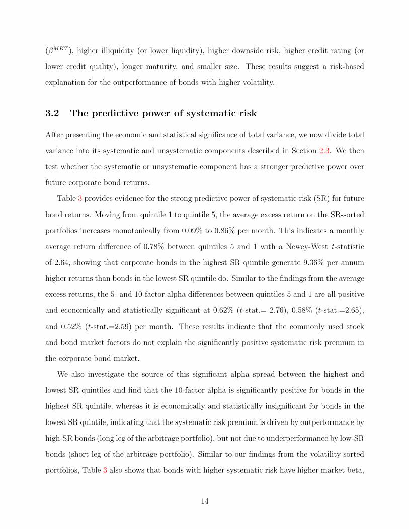
3.2 The predictive power of systematic risk

After presenting the economic and statistical significance of total variance, we now divide total

variance into its systematic and unsystematic components described in Section 2.3. We then

test whether the systematic or unsystematic component has a stronger predictive power over

future corporate bond returns.

Table 3 provides evidence for the strong predictive power of systematic risk (SR) for future

bond returns. Moving from quintile 1 to quintile 5, the average excess return on the SR-sorted

portfolios increases monotonically from 0.09% to 0.86% per month. This indicates a monthly

average return difference of 0.78% between quintiles 5 and 1 with a Newey-West t-statistic

of 2.64, showing that corporate bonds in the highest SR quintile generate 9.36% per annum

higher returns than bonds in the lowest SR quintile do. Similar to the findings from the average

excess returns, the 5- and 10-factor alpha differences between quintiles 5 and 1 are all positive

and economically and statistically significant at 0.62% (t-stat.= 2.76), 0.58% (t-stat.=2.65),

and 0.52% (t-stat.=2.59) per month. These results indicate that the commonly used stock

and bond market factors do not explain the significantly positive systematic risk premium in

the corporate bond market.

We also investigate the source of this significant alpha spread between the highest and

lowest SR quintiles and find that the 10-factor alpha is significantly positive for bonds in the

highest SR quintile, whereas it is economically and statistically insignificant for bonds in the

lowest SR quintile, indicating that the systematic risk premium is driven by outperformance by

high-SR bonds (long leg of the arbitrage portfolio), but not due to underperformance by low-SR

bonds (short leg of the arbitrage portfolio). Similar to our findings from the volatility-sorted

portfolios, Table 3 also shows that bonds with higher systematic risk have higher market beta,

14

lower liquidity, higher downside risk, lower credit quality, longer maturity, and smaller size,

supporting a risk-based explanation for the outperformance of bonds with higher systematic

risk.

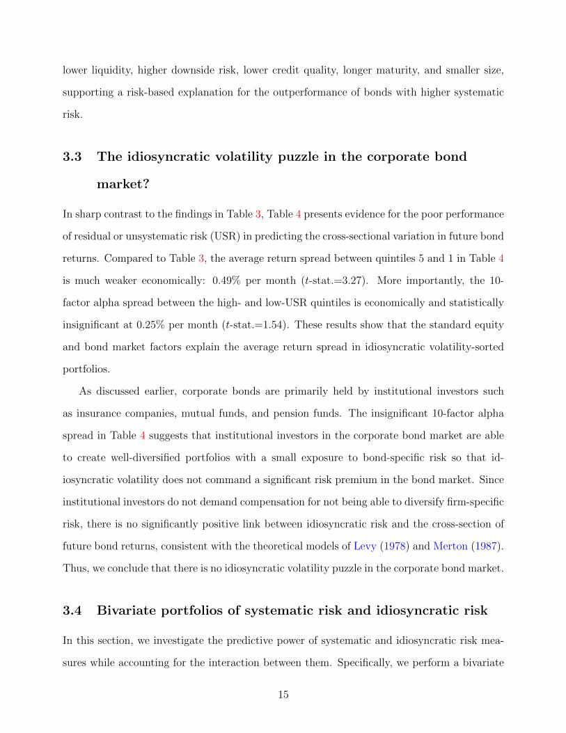
3.3 The idiosyncratic volatility puzzle in the corporate bond

market?

In sharp contrast to the findings in Table 3, Table 4 presents evidence for the poor performance

of residual or unsystematic risk (USR) in predicting the cross-sectional variation in future bond

returns. Compared to Table 3, the average return spread between quintiles 5 and 1 in Table 4

is much weaker economically: 0.49% per month (t-stat.=3.27). More importantly, the 10-

factor alpha spread between the high- and low-USR quintiles is economically and statistically

insignificant at 0.25% per month (t-stat.=1.54). These results show that the standard equity

and bond market factors explain the average return spread in idiosyncratic volatility-sorted

portfolios.

As discussed earlier, corporate bonds are primarily held by institutional investors such

as insurance companies, mutual funds, and pension funds. The insignificant 10-factor alpha

spread in Table 4 suggests that institutional investors in the corporate bond market are able

to create well-diversified portfolios with a small exposure to bond-specific risk so that id-

iosyncratic volatility does not command a significant risk premium in the bond market. Since

institutional investors do not demand compensation for not being able to diversify firm-specific

risk, there is no significantly positive link between idiosyncratic risk and the cross-section of

future bond returns, consistent with the theoretical models of Levy (1978) and Merton (1987).

Thus, we conclude that there is no idiosyncratic volatility puzzle in the corporate bond market.

3.4 Bivariate portfolios of systematic risk and idiosyncratic risk

In this section, we investigate the predictive power of systematic and idiosyncratic risk mea-

sures while accounting for the interaction between them. Specifically, we perform a bivariate

15

portfolio analysis for systematic risk by controlling for idiosyncratic risk, and then we conduct

the same test for idiosyncratic risk while controlling for systematic risk.

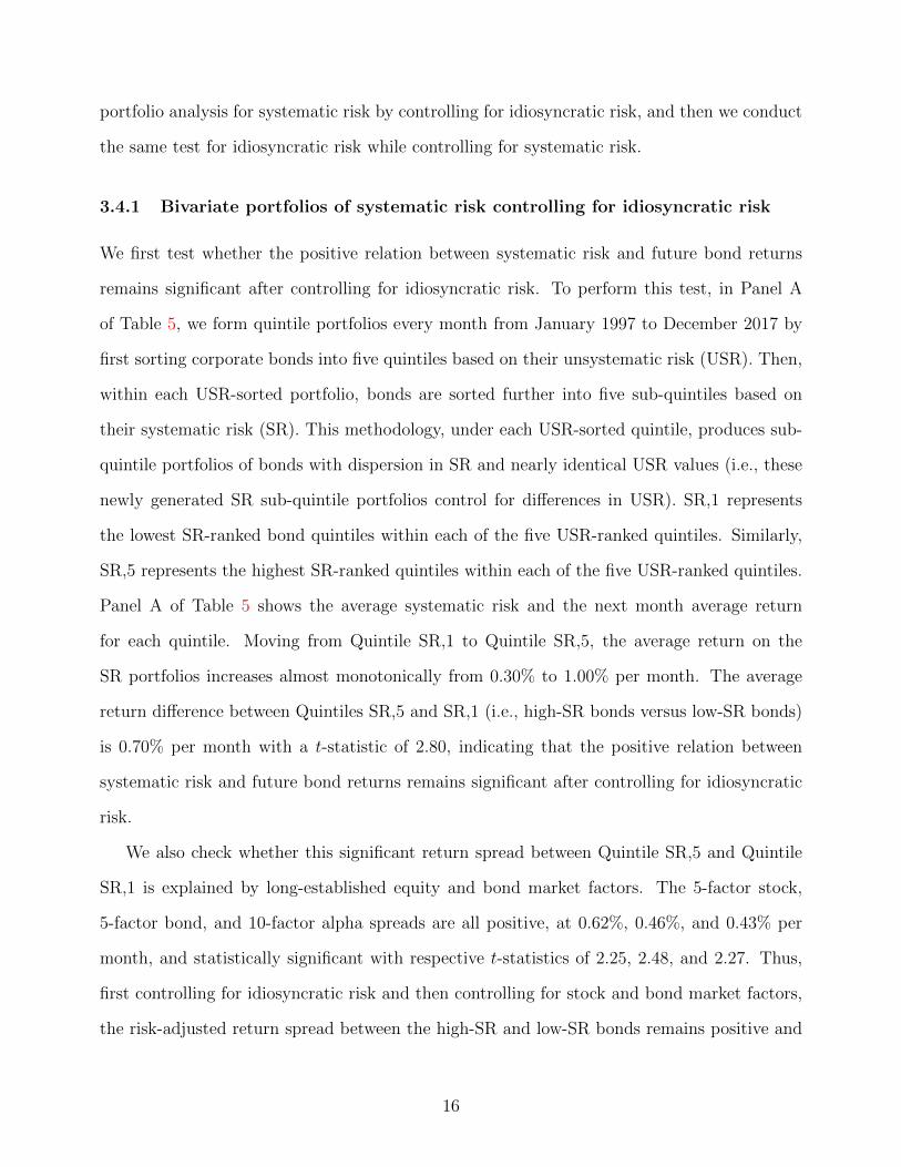
3.4.1 Bivariate portfolios of systematic risk controlling for idiosyncratic risk

We first test whether the positive relation between systematic risk and future bond returns

remains significant after controlling for idiosyncratic risk. To perform this test, in Panel A

of Table 5, we form quintile portfolios every month from January 1997 to December 2017 by

first sorting corporate bonds into five quintiles based on their unsystematic risk (USR). Then,

within each USR-sorted portfolio, bonds are sorted further into five sub-quintiles based on

their systematic risk (SR). This methodology, under each USR-sorted quintile, produces sub-

quintile portfolios of bonds with dispersion in SR and nearly identical USR values (i.e., these

newly generated SR sub-quintile portfolios control for differences in USR). SR,1 represents

the lowest SR-ranked bond quintiles within each of the five USR-ranked quintiles. Similarly,

SR,5 represents the highest SR-ranked quintiles within each of the five USR-ranked quintiles.

Panel A of Table 5 shows the average systematic risk and the next month average return

for each quintile. Moving from Quintile SR,1 to Quintile SR,5, the average return on the

SR portfolios increases almost monotonically from 0.30% to 1.00% per month. The average

return difference between Quintiles SR,5 and SR,1 (i.e., high-SR bonds versus low-SR bonds)

is 0.70% per month with a t-statistic of 2.80, indicating that the positive relation between

systematic risk and future bond returns remains significant after controlling for idiosyncratic

risk.

We also check whether this significant return spread between Quintile SR,5 and Quintile

SR,1 is explained by long-established equity and bond market factors. The 5-factor stock,

5-factor bond, and 10-factor alpha spreads are all positive, at 0.62%, 0.46%, and 0.43% per

month, and statistically significant with respective t-statistics of 2.25, 2.48, and 2.27. Thus,

first controlling for idiosyncratic risk and then controlling for stock and bond market factors,

the risk-adjusted return spread between the high-SR and low-SR bonds remains positive and

16

statistically significant.

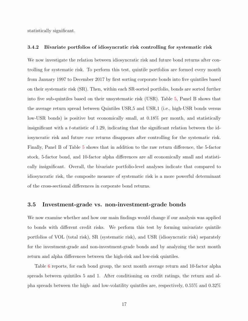
3.4.2 Bivariate portfolios of idiosyncratic risk controlling for systematic risk

We now investigate the relation between idiosyncratic risk and future bond returns after con-

trolling for systematic risk. To perform this test, quintile portfolios are formed every month

from January 1997 to December 2017 by first sorting corporate bonds into five quintiles based

on their systematic risk (SR). Then, within each SR-sorted portfolio, bonds are sorted further

into five sub-quintiles based on their unsystematic risk (USR). Table 5, Panel B shows that

the average return spread between Quintiles USR,5 and USR,1 (i.e., high-USR bonds versus

low-USR bonds) is positive but economically small, at 0.18% per month, and statistically

insignificant with a t-statistic of 1.29, indicating that the significant relation between the id-

iosyncratic risk and future raw returns disappears after controlling for the systematic risk.

Finally, Panel B of Table 5 shows that in addition to the raw return difference, the 5-factor

stock, 5-factor bond, and 10-factor alpha differences are all economically small and statisti-

cally insignificant. Overall, the bivariate portfolio-level analyses indicate that compared to

idiosyncratic risk, the composite measure of systematic risk is a more powerful determinant

of the cross-sectional differences in corporate bond returns.

3.5 Investment-grade vs. non-investment-grade bonds

We now examine whether and how our main findings would change if our analysis was applied

to bonds with different credit risks. We perform this test by forming univariate quintile

portfolios of VOL (total risk), SR (systematic risk), and USR (idiosyncratic risk) separately

for the investment-grade and non-investment-grade bonds and by analyzing the next month

return and alpha differences between the high-risk and low-risk quintiles.

Table 6 reports, for each bond group, the next month average return and 10-factor alpha

spreads between quintiles 5 and 1. After conditioning on credit ratings, the return and al-

pha spreads between the high- and low-volatility quintiles are, respectively, 0.55% and 0.32%

17

per month, and are statistically significant for investment-grade bonds. The corresponding

return and alpha spreads are much higher and highly significant for non-investment-grade

bonds: 1.21% and 0.90% per month, respectively. Similarly, the return and alpha spreads

between the high- and low-SR quintiles are positive, at 0.42% and 0.27% per month, and

statistically significant for investment-grade bonds. As expected, the systematic risk premia

are economically larger for non-investment-grade bonds: 0.88% and 0.96% per month. In

contrast to the findings on systematic risk, the alpha spreads between the high- and low-USR

quintiles are economically small and statistically insignificant for both investment-grade bonds

(−0.08% per month with t-stat.=-0.85) and non-investment grade bonds (0.20% per month

with t-stat.=0.57).

These results indicate that on one hand, idiosyncratic volatility does not command a

significant risk premium in the sample of investment- or non-investment-grade bonds. On the

other hand, there is a strong, positive relation between systematic risk and future returns

conditioned on the credit quality of corporate bonds. Specifically, the cross-sectional relation

between systematic risk and expected returns is stronger for non-investment-grade bonds, but

the positive link between systematic risk and future returns remains significant for investment-

grade bonds as well.

3.6 Fama-MacBeth cross-sectional regressions

We have so far tested the significance of systematic and idiosyncratic risk measures as deter-

minants of the cross-section of future bond returns at the portfolio level. We now examine the

cross-sectional relation between systematic risk, idiosyncratic risk, and expected returns at

the bond level using Fama and MacBeth (1973) regressions. We present the time-series aver-

ages of the slope coefficients from the regressions of one-month-ahead excess bond returns on

systematic risk (SR), unsystematic risk (USR), and the control variables, including the bond

market beta (βMKT ), default beta (βDEF ), term beta (βTERM), bond-level illiquidity (ILLIQ),

credit rating, year-to-maturity (MAT), bond amount outstanding (SIZE), and previous month

18

bond return (REV).11 The average slopes provide standard Fama-MacBeth tests for determin-

ing which explanatory variables on average have non-zero premium. Monthly cross-sectional

regressions are run for the following specification and nested versions thereof:

Ri,t+1 = λ0,t + λ1,t · SRi,t + λ2,t · USRi,t +K∑k=1

λk,t · Controlk,t + εi,t+1, (4)

where Ri,t+1 is the excess return on bond i in month t + 1. The predictive cross-sectional

regressions are run on the one-month lagged measures of systematic risk (SR), unsystematic

risk (USR), and the lagged control variables.

Table 7 reports the time series average of the intercept, slope coefficients (λ’s), and the

adjusted R2 values over the 252 months from January 1997 to December 2017. The Newey-

West adjusted t-statistics are reported in parentheses. The univariate regression results show

a positive and significant relation between systematic risk (SR) and the cross-section of future

bond returns. In Regression (1), the average slope, λ1,t, from the monthly regressions of

excess returns on SR alone is 2.166 with a t-statistic of 4.61. The economic magnitude of the

associated effect is similar to that documented in Table 3 for the univariate quintile portfolios

of SR. The spread in average SR between quintiles 5 and 1 is approximately 0.43%, and

multiplying this spread by the average slope of 2.166 produces an estimated monthly return

difference of 93 basis points.12

Regression specification (2) in Table 7 shows that after we control for βMKT , βDEF , βTERM ,

illiquidity, credit rating, maturity, size, and the previous month return, the average slope

coefficient of SR remains positive and highly significant. In other words, controlling for bond

characteristics does not affect the significance of systematic risk in the corporate bond market.

11The bond market beta (βMKT ), default beta (βDEF ), and term beta (βTERM ) are the bond exposuresto the aggregate bond market factor, the default factor, and the term factor obtained from a 36-month rollingwindow estimation.

12Note that the ordinary least squares (OLS) methodology used in the Fama-MacBeth regressions gives anequal weight to each cross-sectional observation so that the regression results are more aligned with the equal-weighted portfolios. That is why the economic significance of SR obtained from Fama-MacBeth regressions,0.93% per month, is somewhat higher than the 0.78% per month obtained from the value-weighted portfolios(see Table 3).

19

Regression (3) tests the cross-sectional predictive power of unsystematic risk (USR) for fu-

ture bond returns. The average slope, λ2,t, is positive and significant in univariate regressions,

consistent with the significantly positive raw return spread reported in Table 4. However, in

Regression (4), the predictive power of USR disappears when controlling for the bond charac-

teristics simultaneously. The coefficient on USR is economically and statistically insignificant:

−0.006 with a t-statistic of −0.03, consistent with the insignificant 10-factor alpha spread

presented in Table 4.

Regression (5) tests the cross-sectional predictive power of SR while controlling for USR.

Importantly, the average slope coefficient on SR remains positive and highly significant, 0.921

(t-stat. = 4.56), indicating that the predictive power of SR is not subsumed by the idiosyncratic

risk. Whereas, the predictive power of USR disappears in the bivariate regression specification

(5) controlling for SR, consistent with the bivariate portfolio results reported in Table 5.

The last specification, Regression (6), presents results from the multivariate regressions

with both systematic and idiosyncratic risk measures while simultaneously controlling for

βMKT , βDEF , βTERM , illiquidity, credit rating, maturity, size, and the one-month lagged re-

turn. Similar to our findings in Regressions (2) and (4), the systematic risk premium is positive

and highly significant, whereas idiosyncratic volatility does not command a risk premium af-

ter controlling for the bond characteristics. These results show that the composite measure

of systematic risk has distinct, significant information beyond bond size, maturity, rating,

liquidity, market risk, and default risk, and that it is a strong and robust predictor of future

bond returns.

3.7 Are corporate bond exposures to the risk factors priced?

We attribute our theoretically consistent finding on the positive relation between systematic

risk and future bond returns primarily to the fact that we construct an economically sensible

measure of systematic risk, not only because we choose the robust risk factors that capture

common variation in corporate bond returns, but also because of the way we synthesize in-

20

formation over these factors. Our systematic risk measure is a function of the variance of

the underlying factors, the cross-covariances of the factors, and the exposures of bond excess

returns to the factors. Motivated by the fact that downside risk, credit risk, and liquidity risk

jointly play an important role in determining expected bond returns, we think that one needs

a comprehensive measure that can integrate the covariances of these risk factors as well as

their own variances. Thus, the conventional measure, such as the market beta, is not sufficient

to capture the broad systematic risk in the corporate bond market. That being said, we now

investigate the source of systematic risk by testing whether exposures of corporate bonds to

the DRF, CRF, and LRF factors can predict the cross-sectional variations in future bond

returns. Motivated by Daniel and Titman (1997) and Brennan, Chordia, and Subrahmanyam

(1998), we investigate this issue using bond-level cross-sectional regressions. Specifically, for

each bond and each month in our sample, we estimate the factor betas from the monthly

rolling regressions of excess bond returns on the DRF, CRF, and LRF factors over a 36-month

rolling window after controlling for the bond market factor (MKT ):

Ri,t = αi,t + βMKTi,t ·MKTt + βFactori,t · Factort + εi,t, (5)

where Factort is one of the three value-weighted bond risk factors (DRF, CRF, and LRF),

and βFactori,t refers to βDRFi,t , βCRFi,t , or βLRFi,t .

We examine the cross-sectional relation between βDRF , βCRF , and βLRF and expected

returns at the bond level using Fama and MacBeth (1973) regressions. Regression (1) in Table 8

presents positive and significant relations between all three factor betas (βDRF , βCRF , βLRF )

and the cross-section of future bond returns. Then, regressions (2) to (6) sequentially control

for the risk and non-risk features of corporate bonds, that is, rating, illiquidity, maturity, size,

and lagged return. Finally, Regression (7) simultaneously controls for all characteristics. All

regressions present similar results: the cross-sectional relations between future bond returns

and three factor betas (βDRF , βCRF , βLRF ) are positive and highly significant. Thus, we

conclude that not just the variances and cross-covariances of the factors, but the significant

21

factor loadings also contribute to the predictive power of systematic risk in explaining the

cross-sectional dispersion in future bond returns.

4 Alternative Measures of Systematic Risk

In this section, we utilize alternative factor models to generate systematic and idiosyncratic risk

of individual corporate bonds. We show that measures of systematic risk estimated with these

alternative factor models do not predict the cross-sectional bond returns, whereas measures of

unsystematic risk from these models positively and significantly predict future bond returns,

though this positive relation is fully explained by the DRF, CRF, and LRF factors of Bai,

Bali, and Wen (2019). That is, after accounting for bond exposures to the downside, credit,

and liquidity risk factors, there is no significant link between idiosyncratic volatility and future

bond returns.

We construct risk measures based on three benchmark factor models in comparison to our

measures described in Section 2.3:

1. One-factor model of Elton, Gruber, and Blake (1995):

Ri,t = αi + β1,iMKTt + εi,t. (6)

2. Three-factor model of Fama and French (1993), Elton, Gruber, and Blake (1995), and

Bessembinder et al. (2009):

Ri,t = αi + β1,iMKTt + β2,iDEFt + β3,iTERMt + εi,t. (7)

3. Six-factor model of Chung, Wang, and Wu (2019):

Ri,t = αi+β1,iMKTt+β2,iSMBt+β3,iHMLt+β4,iDEFt+β5,iTERMt+β6,i∆V IXt+εi,t.

(8)

22

In the above factor models, Ri,t is the excess return of bond i in month t, MKTt, SMBt,

HMLt, DEFt, TERMt, and ∆V IXt denote the aggregate corporate bond market excess

return, the size factor, the book-to-market factor, the default factor, the term factor, and the

market volatility factor, respectively.13 The total risk of bond i is measured by the variance

of Ri,t, denoted by σ2i . The unsystematic (or residual) risk of bond i is proxied with the

variance of εi,t, denoted by σ2ε,i. Consistent with our original measure of systematic risk, we

define the systematic risk of bond i as the difference between total and unsystematic variance,

SR = σ2i − σ2

ε,i, which is a function of the variance of the factors, their cross-covariances, and

the exposures of the bond’s excess returns to the factors.

Table 9 presents the portfolio-level results of systematic and unsystematic risk based on

the above three factor models. For each month from January 1997 to December 2017, we

form value-weighted univariate portfolios by sorting corporate bonds into quintiles based on

different measures of systematic risk (in Panel A) or unsystematic risk (in Panel B), where

quintile 1 contains bonds with the lowest SR (or USR) and quintile 5 contains bonds with the

highest SR (or USR).

Panel A shows that, for all alternative measures of systematic risk, there is no significant

relation between systematic risk and the cross-section of future bond returns. Specifically, the

average return spreads between the high- and low-SR quintiles are positive but insignificant.

Similarly, the 10-factor and the BBW alpha spreads between quintiles 5 and 1 are economically

small and statistically insignificant, ranging from −0.24% to 0.21% per month. These results

are in sharp contrast to the findings in Table 3, which demonstrates a significantly positive

link between SR and future bond returns using the BBW-factor-generated SR measure.

The findings for USR-sorted portfolios are the opposite. Panel B shows that the average

return spreads between the high- and low-USR quintiles are economically and statistically

significant, ranging from 0.70% to 0.79% per month. Also, the 10-factor alpha spreads for

the USR-sorted portfolios are economically and statistically significant for all three USR mea-

13Chung, Wang, and Wu (2019) show that market volatility risk is priced in the cross-section of corporatebond returns. Based on a similar specification in Eq.(8), they also document a positive relation betweenidiosyncratic volatility and future bond returns.

23

sures based on Eqs.(6)−(8). However, the positive return spreads are fully explained by the

BBW 4-factor model. Specifically, the BBW alpha spreads between the high- and low-USR

portfolios are small and insignificant, ranging from 0.08% (t-stat=0.45) to 0.14% (t-stat=0.77)

per month. Overall, Table 9 highlights the importance of the downside risk, credit risk, and

liquidity risk factors of BBW in defining systematic risk of corporate bonds.

5 Testing the Consistency of Systematic Risk with the ICAPM

Although the aggregate market portfolio is the only systematic risk factor in a simple CAPM

world, follow-up studies consider additional sources of systematic risk. For example, Fama

(1970) points out that, in a multi-period economy, investors have an incentive to hedge against

future stochastic shifts in the investment opportunity set. Merton (1973) indicates that state

variables that are correlated with changes in consumption and investment opportunities are

priced in capital markets in the sense that an asset’s covariance with those state variables

affects its expected returns. Thus, any variables that affect future consumption and investment

decisions could be a priced risk factor in equilibrium. Ross (1976) further documents that

securities affected by such systematic risk factors should earn risk premia in a risk-averse

economy.

Over the past four decades, the empirical asset pricing literature has produced a large

number of variables related to the cross-section of equity returns, and many of the documented

predictors of stock returns capture the same (or similar) underlying economic phenomena.

Some of these cross-sectional return predictors have been justified as empirical applications

of Merton’s ICAPM, leading Fama (1991) to view the ICAPM as a safe harbor to facilitate

data mining exercise, especially for authors claiming that the ICAPM provides a theoretical

support for relatively unscripted risk factors in their models. Maio and Santa-Clara (2012)

show that although the ICAPM does not directly identify the “state variables” underlying the

risk factors, there are some restrictions that these state variables must satisfy. According to

Merton’s (1973) ICAPM, the state variables related to changes in the investment opportunity

24

set are supposed to predict the distribution of future market returns. Moreover, the innovations

in these state variables should be priced factors in the cross-section.

Maio and Santa-Clara (2012) focus on three restrictions of the ICAPM. First, the candi-

dates for ICAPM state variables must forecast the first or second moment of market returns. As

will be discussed in Section 5.1, the aggregate measure of systematic risk significantly predicts

future bond market returns and bond market volatility, satisfying the first ICAPM restriction.

Second, if a given state variable predicts positive (negative) expected market returns, the cor-

responding risk factor should earn a positive (negative) price of risk in cross-sectional tests.

Since our state variable, the composite measure of systematic risk, predicts positive expected

bond market returns, the corresponding systematic risk factor is expected to earn a positive

price of risk in the cross-section of corporate bonds. Section 5.2 shows that bond exposure

to the systematic risk factor predicts higher returns in the cross-section of corporate bonds,

satisfying the second ICAPM restriction. The third restriction associated with the ICAPM is

that the price of systematic risk estimated from the cross-sectional regressions must generate

an economically sensible estimate of the coefficient of relative risk aversion of the representa-

tive investor. Section 5.2 provides empirical evidence satisfying the third ICAPM restriction

as well.

5.1 The Time-Series Predictive Power of Aggregate SystematicRisk

We have so far shown that the composite measure of systematic risk estimated with the

aggregate bond market, downside risk, credit risk, and liquidity risk factors of BBW is a

strong predictor of the cross-sectional differences in future bond returns. In this section, we test

whether the composite measure of systematic risk predicts the first and second moments of the

return distribution of the aggregate bond market portfolio. Specifically, we construct aggregate

systematic risk using the cross-sectional average of bond-level systematic risk measures and

investigate its predictive power for the future returns and volatility of the aggregate bond

25

market portfolio.

The intertemporal relation between expected return and risk in the equity market has been

one of the most extensively studied topics in financial economics. Most asset pricing models

postulate a positive intertemporal relation between the market portfolio’s expected return and

risk, which is often defined by the variance or standard deviation of market returns. However,

the literature has not yet reached an agreement on the existence of such a positive risk-return

tradeoff for stock market indices.14 Many studies fail to identify a robust and significant

intertemporal relation between risk and return on the aggregate stock market portfolio.

French, Schwert, and Stambaugh (1987) find that the risk-return coefficient is not signif-

icantly different from zero when they use past daily returns to estimate the monthly condi-

tional variance. Follow-up studies by Campbell and Hentchel (1992), Glosten, Jagannathan,

and Runkle (1993), Harrison and Zhang (1999), and Bollerslev and Zhou (2006) rely on the

GARCH-in-mean and realized volatility models that provide no evidence of a robust, signifi-

cant link between risk and return on the equity market portfolio. Several studies even find that

the intertemporal relation between risk and return is negative. Examples include Campbell

(1987), Nelson (1991), Glosten et al. (1993), Whitelaw (1994), Harvey (2001), and Brandt

and Kang (2004). Some studies do provide evidence supporting a positive and significant link

between expected return and risk in the equity market (e.g., Bollerslev et al., 1988; Ghysels

et al., 2005; Guo and Whitelaw, 2006; Bali, 2008; and Bali and Engle, 2010).

For the first time in the literature, we examine the intertemporal relation between expected

return and systematic risk for the aggregate bond market portfolio. We consider three new

aggregate measures of systematic risk using different weighting schemes: the equal-weighted,

value-weighted, and rating-weighted average systematic risk. Figure 1 plots the time-series of

the aggregate systematic risk over the sample period from January 1997 to December 2017.

The three measures of aggregate SR are highly correlated with an average correlation coefficient

14Due to the fact that the conditional volatility of stock market returns is not observable, different ap-proaches and specifications used by previous studies in estimating the conditional volatility are largely respon-sible for the conflicting empirical evidence.

26

of 0.95, and all spike during the Great Recession.15 To test the time-series predictive power

of aggregate systematic risk, we control for a large set of macroeconomic variables proxying

for business cycle fluctuations:

Yt+τ = α + γ1 · SRt + γ2 ·Xkt + εt+1, k = 1, ..., 6; τ = 1, 2, ..., 12 (9)

where Yt+τ is one of the two dependent variables, the monthly bond market excess return

(MKT ) and the monthly bond market variance (MKTV OL), calculated as the sum of squared

daily bond market returns in a month. Xkt is a vector of control variables. Following Goyal

and Welch (2008), we control for variables related to macro fundamentals including the log

earnings-to-price ratio (EP), the log dividend-to-price ratio (DP), the book-to-market ra-

tio (BM), the difference between long-term yield on government bonds and the one-month

Treasury-bill (TERM), the difference between BAA- and AAA-rated corporate bond yields

(DEF), and the equity market variance (SVAR).

Table 10 presents the performance of the aggregate systematic risk in predicting τ -month

ahead aggregate bond market returns and bond market volatility for different horizons (τ =

1, 2, ..., 12). Panel A shows that the estimated slope coefficients (γ1) in Eq. (9) are significantly

positive, indicating the strong predictive power of aggregate systematic risk on future bond

market returns up to 10 months, even after controlling for a number of time-series return

predictors. Further, the adjusted R2 in the multivariate regression declines from 9.53% for

one-month-ahead predictability to 0.66% for 12-month-ahead predictability, suggesting that

the aggregate measure of systematic risk has the best performance in predicting the one-

month-ahead returns on the bond market portfolio.

Panel B of Table 10 reports the forecasting performance of the aggregate systematic risk in

predicting future bond market volatility (MKTV OL). Maio and Santa-Clara (2012) investigate

the ICAPM restrictions in the time-series and cross-sectional predictability, and show that the

cross-sectional variable (when aggregated) should predict future market return and market

15As a result, we use the equal-weighted average SR (SREW ) in our time-series predictive regressions, andthe results are similar when we use the other two measures of aggregate SR.

27

volatility, if the variable is interpreted as a state variable that affects investment opportunity

set in the ICAPM. Panel B provides evidence consistent with this interpretation. Specifically,

the aggregate systematic risk positively predicts future bond market volatility up to seven

months into the future, indicating that the composite measure of systematic risk satisfies the

first ICAPM restriction. The results also show that high systematic risk in the corporate

bond market robustly predicts high future returns on the bond market portfolio, indicating

a positive intertemporal risk-return tradeoff in the corporate bond market, while the equity

literature is still not in agreement on the direction of a time-series relation between expected

return and risk in the equity market.

5.2 The positive price of systematic risk in the cross-section ofcorporate bonds

In this section, we test whether systematic risk is consistent with Merton’ theoretical model

based on the second and third restrictions of the ICAPM. Specifically, we form a systematic

risk factor and investigate whether the systematic risk factor earns a positive price of risk

in the cross-section of corporate bond returns (second restriction). Then, we examine if the

price of the systematic risk factor estimated from the cross-sectional regressions generates an

economically plausible magnitude of the relative risk aversion coefficient (third restriction).

We build a systematic risk factor of corporate bonds following the factor construction

methodology of Bai, Bali, and Wen (2019). That is, for each month from January 1997 to

December 2017, we form bivariate portfolios by independently sorting bonds into five quintiles

based on their credit rating and five quintiles based on their systematic risk. The systematic

risk factor, SRF, is the value-weighted average return difference between the highest-SR port-

folio and the lowest-SR portfolio across the rating portfolios. The average return on the newly

proposed systematic risk factor is positive and highly significant, at 0.54% per month (t-stat.

= 3.47), which is consistent with our earlier findings on the significantly positive systematic

risk premium in the cross-section of both IG and NIG bonds.

Next, for each bond and each month in our sample, we estimate corporate bond exposure to

28

the systematic risk factor (βSRF ) from the monthly rolling regressions of excess bond returns

on the SRF factor over a 36-month rolling window while controlling for the bond market factor

(MKT):

Ri,t = αi,t + βMKTi,t ·MKTt + βSRFi,t · SRF + εi,t, (10)

where Ri,t is the excess return on bond i in month t, and MKTt and SRFt are the excess

returns on the bond market and systematic risk factors in month t, respectively. βMKTi,t and

βSRFi,t are the bond exposures to the market and systematic risk factors, respectively. Once

we estimate βMKTi,t and βSRFi,t for each bond and each month in our sample, we test whether

the systematic risk factor (SRF) earns a positive price of risk in the cross-section of corporate

bond returns. Specifically, we examine the cross-sectional relation between βSRF and expected

returns at the bond level using Fama and MacBeth (1973) regressions:

Ri,t+1 = λ0,t + λ1,t · βMKTi,t + λ2,t · βSRFi,t + εi,t+1. (11)

The average slope coefficient (λ2) from the cross-sectional regressions of one-month-ahead

bond excess returns on βSRF turns out to be positive and statistically significant: 0.43 (t-stat.

= 4.75). Whereas, the average slope (λ1) on βMKT is positive but statistically insignificant:

0.14 (t-stat.= 0.80). Thus, our results indicate that the composite measure of systematic

risk predicts positive expected bond market returns and that the systematic risk factor earns

a positive price of risk in the cross-section of corporate bonds, consistent with the second

ICAPM restriction. The intuition for this result is simple. An asset that covaries positively

with the risk factor also covaries positively with future expected returns. It does not provide

a hedge for reinvestment risk because it offers lower returns when market returns are expected

to be lower. Hence, a risk-averse investor does require a positive risk premium to invest in

such an asset, implying a positive price of risk for the factor.

Finally, we investigate whether the price of the systematic risk factor estimated from the

cross-sectional regressions produces an economically sensible estimate of expected excess return

29

on the bond market. Bali and Engle (2010) show that Merton’s (1973) ICAPM implies the

following conditional intertemporal relation:

Et(Rt+1) = A · Covt(Ri,t+1,MKTt+1) +B · Covt(Ri,t+1, SRFt+1), (12)

where Ri,t+1 is the excess return on bond i at time t + 1, and MKTt+1 and SRFt+1 are the

excess returns on the market and systematic risk factors at time t+ 1, respectively. Et(Ri,t+1)

is the time-t expected excess return of bond i at time t+1, Covt(Ri,t+1,MKTt+1) is the time-t

expected conditional covariance between Ri,t+1 and MKTt+1, and Covt(Ri,t+1, SRFt+1) is the

time-t expected conditional covariance between Ri,t+1 and SRFt+1. The parameter A in Eq.

(12) is the relative risk aversion of market investors, and B measures the market’s aggregate

reaction to shifts in a state variable that governs the stochastic investment opportunity set.

Thus, Eq. (12) indicates that in equilibrium, investors are compensated in terms of expected

return for bearing market risk and for bearing the risk of unfavorable shifts in the investment

opportunity set.16

Following Bali and Engle (2010), we aggregate Eq. (12) and write the static (unconditional)

version of the conditional ICAPM to determine the economic significance of A and B:

E(MKT ) = A · σ2MKT +B · σMKT,SRF , (13)

where E(MKT ) is the unconditional expected excess return on the bond market portfo-

lio, σ2MKT is the unconditional variance of excess returns on the bond market portfolio, and

σMKT,SRF is the unconditional covariance between excess returns on the market and systematic

risk factors.

We use the price of market risk (λ1) and the price of systematic risk factor (λ2) estimated

from the cross-sectional regressions in Eq. (11) to proxy for A and B in Eq. (13), respectively.

Substituting the sample estimates of σ2MKT = 0.023 and σMKT,SRF = 0.021 along with (A =

16Since the conditional variances of MKTt+1 and SRFt+1 are identical across bonds, Eq. (12) can bewritten in terms of the conditional betas (βMKT

i,t , βSRFi,t ) as in Eq. (11).

30

λ1/σ2MKT = 6.09) and (B = λ2/σ

2SRF = 6.94) into Eq. (13) gives 0.29% per month, which

is very close to the average excess return on the bond market portfolio in our sample, 0.33%

per month. These results indicate that the price of the systematic risk factor generates an

economically sensible estimate of expected excess return on the bond market, and hence the

implied relative risk aversion of bond market investors, satisfying the third ICAPM restriction.

Since the composite measure of systematic risk satisfies all three restrictions of the ICAPM,

we conclude that Merton’s (1973) model provides a theoretical support for the systematic risk

factor in the corporate bond market.

6 Investigating the Role of Systematic and Idiosyncratic

Risk in the Bond and Equity Markets

In this section, we examine the different roles played by systematic and firm-specific risk

in the cross-sectional pricing of equities versus bonds. First, we propose a similar measure

of systematic risk for individual stocks and test whether this measure predicts the cross-

section of expected stock returns. Second, we revisit the idiosyncratic volatility puzzle in the

equity market. Third, we explore the impact of investor clientele on the predictive power of

idiosyncratic risk for future stock returns and on the predictive power of systematic risk for

future bond returns.

6.1 A composite measure of systematic risk in the equity market

Our composite measure of systematic risk for corporate bonds is a function of the variance of

the underlying bond factors, the cross-covariances of the factors, and the bond exposures to

these factors. Thus, the key input to construct a sound measure of systematic risk is to use

economically sensible risk factors that capture common return variation in corporate bonds

and that provide an accurate characterization of firm fundamentals.

In this section, we propose a similar, comprehensive measure of systematic risk for individ-

ual stocks using the powerful equity factor models proposed by Fama and French (2015) and

Hou, Xue, and Zhang (2015). Specifically, we construct a composite measure of systematic

31

risk for individual stocks based on the five-factor model of Fama and French (2015) in Eq. (14)

and the four-factor model of Hou, Xue, and Zhang (2015) in Eq. (15):

Ri,d = αi+β1,i ·MKT Stockd +β2,i ·SMBd+β3,i ·HMLd+β4,i ·RMWd+β5,i ·CMAd+εi,d, (14)

Ri,d = αi + β1,i ·MKT Stockd + β2,i ·MEQ,d + β3,i ·ROEQ,d + β4,i · IAQ,d + εi,d. (15)

where Ri,d is the excess return of stock i on day d, and MKT Stockd , SMBd, HMLd, RMWd,

and CMAd in Eq. (14) are the daily equity market, size, book-to-market, profitability, and

investment factors of Fama and French (2015), respectively. In Eq. (15), MEQ,d, ROEQ,d,

and IAQ,d are the daily size, profitability, and investment Q factors of Hou, Xue, and Zhang

(2015), respectively.17

The total risk of stock i is measured by the variance of Ri,d (σ2i ), calculated as the sum

of squared daily returns in a month. The unsystematic (or idiosyncratic) risk of stock i is

measured by the variance of εi,d, denoted by σ2ε,i. The systematic risk of stock i is defined as

the difference between the total and unsystematic variance, SR = σ2i − σ2

ε,i. Following Ang

et al. (2006) and subsequent work on idiosyncratic volatility in the equity market, Eqs. (14)

and (15) are estimated using daily returns over the past one month, requiring at least 15 daily

return observations in a month. Eqs. (14) and (15) also generate two different measures of

systematic and idiosyncratic risk for individual equities; one based on the five-factor model of

Fama and French (2015) and the other building on the four-factor model of Hou, Xue, and

Zhang (2015).

Table 11 presents results from the value-weighted univariate portfolios of stocks sorted by

total risk, systematic risk, and idiosyncratic risk. We use both the five-factor model of Fama

and French (2015) and the four-factor model of Hou, Xue, and Zhang (2015) to estimate the

17The MKT , SMB, HML, RMW , and CMA factors of Fama-French (2015) are obtained from thedata library of Ken French (http://mba.tuck.dartmouth.edu/pages/faculty/ken.french/) for the longest sampleperiod from July 1963 to December 2017. The Q factors (MEQ, ROEQ, and IAQ) are obtained from theauthors of Hou, Xue, and Zhang (2015) for the longest sample period from January 1967 to December 2017.

32

one-month-ahead risk-adjusted returns (alphas) of total risk, systematic risk, and idiosyncratic

risk sorted portfolios. Consistent with the idiosyncratic volatility puzzle in the equity litera-

ture, Panel A of Table 11 reports a strong negative relation between total risk and future stock

returns. As shown in the first four columns of Panel A, the average return and alpha spreads

range from −0.80% to −0.89% per month and are statistically significant for the sample period

1963-2017, indicating that stocks in the highest total risk quintile underperform those in the

lowest quintile by about 9.6% per annum. The last four columns of Panel A present similar

results in terms of the economic and statistical significance of the low volatility effect for the

sample period 1967-2017. In contrast to our findings for corporate bonds, Panels B and C

show that the low volatility effect in Panel A is driven by the negative relation between id-

iosyncratic volatility and future stock returns, but not due to the systematic risk of individual

stocks.

As presented in the first four columns of Panels B and C, when systematic and idiosyn-

cratic risk measures are estimated with the five-factor model of Fama and French (2015), the

monthly return and alpha spreads between the highest and lowest systematic risk quintiles

are insignificant, ranging from −0.36% (t-stat.= −1.26) to −0.49% (t-stat.= −1.36), whereas

the return and alpha spreads between the highest and lowest idiosyncratic volatility quin-

tiles are economically large and highly significant, ranging from −0.77% (t-stat. = −2.72) to

−0.86% (t-stat. = −2.37). Finally, the last four columns of Panels B and C present similar

results when SR and USR measures are estimated using the four-factor model of Hou, Xue,

and Zhang (2015), confirming the insignificant (significant) cross-sectional relation between

SR (USR) and future equity returns.18

Overall, these results indicate that systematic risk does not predict the cross-sectional

variation in equity returns, whereas the idiosyncratic volatility puzzle remains significant in

the equity market even when we use the composite measures of systematic and idiosyncratic

18In untabulated results, we estimate SR and USR measures using the extended factor models of Fama andFrench (2015) and Hou, Xue, and Zhang (2015) with an additional momentum factor of Carhart (1997). Theresults are similar to those reported in Table 11, validating the insignificance (significance) of SR (USR) inpredicting the cross-sectional differences in stock returns.

33

variance, estimated with the new methodology proposed in this paper. One potential expla-

nation of the idiosyncratic volatility puzzle is that investors hold concave preferences and like

positive skewness. If positive skewness is a desirable characteristic of a return distribution,

then the fact that the simple act of diversification destroys portfolio skewness (or eliminates

idiosyncratic skewness) is a likely explanation of observed behavior. That is, investors who

care about the third-moment of the return distribution would be willing to hold a limited

number of stocks in their portfolios, the exact number being a function of each individual’s

skewness/variance awareness. Those who are most concerned with skewness (variance) will

hold a relatively small (large) number of stocks in their portfolios. Since the idiosyncratic

volatility puzzle is known to be significant only in the sample of stocks largely held by in-

dividual investors (which will be confirmed in the next section), we can conclude that retail

investors’ demand for positive skewness dominates their aversion to volatility so that retail

investors prefer to hold a small number of lottery-like stocks with large positive skewness, and

lottery stocks happen to have high idiosyncratic volatility and low future returns.

Although diversification is critical in eliminating idiosyncratic risk, a closer examination

of the portfolios of individual investors suggests that these investors are, in general, not well-

diversified. For example, Polkovnichenko (2005) examines a survey of 14 million households

and shows that the median number of stocks in household portfolios is two in 1989, 1992, 1995,

and 1998. The median increases to three stocks in 2001. Based on 40,000 stock accounts at

a brokerage firm, Goetzmann and Kumar (2008) find that the median number of stocks in a

portfolio of individual investors is three in the 1991-1996 period. These results are similar to

the findings of earlier studies. For example, Blume and Friend (1975) and Blume, Crockett,

and Friend (1974) provide evidence that the average number of stocks in household portfolios

is about 3.41 in 1967. Odean (1999) and Barber and Odean (2001) also report the median

number of stocks in individual investors’ portfolios as two to three. In more recent work,

Dorn and Huberman (2005, 2010) use trading records between 1995 and 2000 of over 20,000

customers of a German discount brokerage and find that the typical portfolio consists of little

34

more than three stocks.

Since individual investors do not hold a large number of stocks in their portfolios, they

are unable to diversify firm-specific risk. Thus, according to the theoretical models of Levy

(1978) and Merton (1987), stocks with higher idiosyncratic risk require higher returns to

compensate for imperfect diversification, justifying a positive (not negative) cross-sectional

relation between idiosyncratic risk and future equity returns. Since retail investors are known

to hold a small number of positively skewed, high-volatility stocks, explanations based on retail

investors’ preferences for lottery-like securities show some promise in solving the idiosyncratic

volatility puzzle in the equity market (e.g., Kumar (2009), Bali et al. (2011), and Hou and

Loh (2016)).

6.2 The investor clientele effect in the equity and bond markets

The Flow of Funds report released by the Federal Reserve Board shows the composition of

investors in the U.S. equity and corporate bond markets. Over the period of 1986 to 2017, the

primary holders of corporate bonds are institutional investors (78% on average), in particular,

insurance companies, mutual funds, and pension funds, whereas the main holders of equities

are retail investors (household sector, 43%), then mutual funds (33%) and pension funds

(15%). Since equities and bonds are mainly held by different groups of investors (retail vs.

institutional investors), the difference in investor preferences and clienteles can be a plausible

cause for the significance of systematic risk (idiosyncratic risk) in the bond (equity) market.

We first investigate the effect of investor clientele on the predictive power of idiosyncratic

risk for future stock returns. To perform this task, we form quintile portfolios every month

from January 1980 to December 2017 by sorting individual stocks into quintiles based on

institutional ownership, then within each ownership quintile, we further sort stocks into sub-

quintiles based on their unsystematic risk (USR). Table 12 shows that the negative cross-

sectional relation between idiosyncratic risk and future returns is more pronounced among

stocks with low institutional ownership (i.e., stocks largely held by retail investors). More

35

importantly, the idiosyncratic volatility puzzle disappears among stocks with high institutional

ownership. This result is consistent with the direct or indirect evidence provided by Kumar

(2009), Han and Kumar (2013), and Bali, Brown, Murray, and Tang (2017) that retail investors

tend to be more attracted to high volatility stocks because of their lottery-like features, and

such behavior leads to the negative cross-sectional relation between idiosyncratic volatility and

future stock returns.

We conduct a similar analysis for corporate bonds to investigate the interaction between

the clientele effect and systematic risk in the corporate bond market. Table 13 shows that

within all institutional ownership quintiles, there is a monotonically increasing pattern in the

average returns on SR-sorted portfolios moving from the low-SR to high-SR quintile, producing

a significantly positive link between systematic risk and average returns of corporate bonds.

However, the last three columns in Panel A provide evidence that the positive relation between

the composite measure of systematic risk and risk-adjusted return is more pronounced among

bonds with relatively low institutional ownership. That being said, it is difficult to identify

retail ownership in corporate bond holdings data because the bond market is dominated by

instiutional investors.

Thus, we try to gain a better understanding of the driving force of the significant relation

between systematic risk and future bond returns by examining the key characteristics of the

5×5 bivariate portfolios of corporate bonds sorted by systematic risk and institutional owner-

ship. Panel B of Table 13 presents the average systematic risk (SR) and the average exposures

to the downside risk, credit risk, and liquidity risk factors (βDRF , βCRF , and βLRF ) in the 25

portfolios. We observe strong evidence that institutions in the low-INST quintile hold bonds

with higher systematic risk and higher exposures to the DRF, CRF, and LRF factors. This

explains why the systematic risk premium is strongest for bonds in low-institutional-ownership

quintile.

Lastly, we investigate whether institutional investors holding bonds with high systematic

risk actively adjust their exposures to the systematic risk factor in the corporate bond market.

36

Following the market-timing model of Treynor and Mazuy (1966), we run time-series regres-

sions of the 25 SR&INST-sorted portfolios’ excess returns (Rpi,t) on the bond market excess

returns (MKTt) and the squared excess market returns (MKT 2t ):

Rpi,t = αi + β1,iMKTt + β2,iMKT 2

t + εi,t, (16)

where β2,i captures the market-timing ability of institutions in each of the 25 SR&INST-sorted

portfolios.

Panel C of Table 13 shows that institutions in the low-INST quintile have positive and

much higher market-timing coefficients (β2,i) compared to those in the remaining four INST

quintiles. Combining this particular finding with the results in Panel B of Table 13 indicates

that institutions in INST,1 have stronger market-timing ability, and they have higher system-

atic risk and higher future returns. Consistent with the market-timing ability of institutions,

these results suggest that by predicting fluctuations in the systematic risk factors, institutional

investors can adjust their bond portfolio exposures up or down in a timely fashion to generate

superior returns. Indeed, we find that institutional investors, particularly those with higher

systematic risk and higher exposures to the DRF, CRF, and LRF factors, correctly adjust

their aggregate exposure to the common risk factors, and hence there exists a positive and

stronger link between their systematic risk and future returns.

7 Conclusion

In this paper, we propose a novel measure of systematic risk for individual corporate bonds

and test its significance in both the time-series and cross-sectional pricing of corporate bonds.

We find that the newly proposed measure of systematic risk has a strong predictive power on

the cross-sectional dispersion in future bond returns, and the positive systematic risk premium

is driven by the outperformance of bonds with high systematic risk. Moreover, the aggregate

measure of systematic risk significantly predicts positive expected bond market returns, and

the corresponding systematic risk factor earns a positive price of risk in the cross-section

37

of corporate bonds. The price of systematic risk estimated from the cross-sectional tests

also generates an economically sensible estimate of the relative risk aversion of bond market

investors. Since the composite measure of systematic risk satisfies all restrictions of Merton’s

(1973) ICAPM on the time-series and cross-sectional predictability, we conclude that Merton’s

model provides a theoretical support for the systematic risk factor in the corporate bond

market.

Given the powerful presence of systematic risk in the time-series and cross-sectional pric-

ing of corporate bonds, the idiosyncratic volatility puzzle that is well-documented in the stock

market no longer exists in the bond market. This finding suggests that the institutional

investors dominating the bond market hold well-diversified portfolios with a negligible expo-

sure to bond-specific risk so that idiosyncratic volatility does not command a significant risk

premium in the bond market.

To gain a better understanding of the different roles played by systematic and firm-specific

risk measures in the pricing of equities versus bonds, we investigate the interaction between in-

vestor clientele and these risk measures. Clearly, equities and bonds are disintegrated in terms

of primary players in these two markets. We find that retail investors with a strong prefer-

ence for small, illiquid, and high-volatility stocks play an important role in the equity market.

Specifically, the negative relationship between idiosyncratic volatility and future stock returns

is more pronounced among stocks largely held by retail investors, but the idiosyncratic volatil-

ity puzzle disappears among stocks with high institutional ownership. On the contrary, the

systematic risk premium is stronger for corporate bonds largely held by institutional investors

with market- and volatility-timing abilities due to their talent in taking direct exposures to

the systematic risk factors in the bond market and hence generating superior bond returns.

Overall, our results provide a plausible explanation for the significance of systematic risk (id-

iosyncratic risk) based on differing investor preferences and clienteles in the bond (equity)

market.

38

References

Ang, A., Hodrick, R. J., Xing, Y., Zhang, X., 2006. The cross-section of volatility and expectedreturns. Journal of Finance 61, 259–299.

Bai, J., Bali, T. G., Wen, Q., 2019. Common risk factors in the cross-section of corporate bondreturns. Journal of Financial Economics 131, 619–642.

Bali, T. G., 2008. The intertemporal relation between expected returns and risk. Journal of FinancialEconomics 87, 101–131.

Bali, T. G., Brown, S., Murray, S., Tang, Y., 2017. A lottery demand-based explanation of the betaanomaly. Journal of Financial and Quantitative Analysis 52, 2369–2397.

Bali, T. G., Cakici, N., 2008. Idiosyncratic volatility and the cross-section of expected returns. Journalof Financial and Quantitative Analysis 43, 29–58.

Bali, T. G., Cakici, N., Whitelaw, R. F., 2011. Maxing out: Stocks as lotteries and the cross-sectionof expected returns. Journal of Financial Economics 99, 427–446.

Bali, T. G., Engle, R. F., 2010. The intertemporal capital asset pricing model with dynamic condi-tional correlations. Journal of Monetary Economics 57, 377–390.

Bao, J., Pan, J., Wang, J., 2011. The illiquidity of corporate bonds. Journal of Finance 66, 911–946.

Barber, B., Odean, T., 2001. Boys will be boys: Gender, overconfidence, and common stock invest-ment. Quarterly Journal of Economics 116, 261–292.

Bessembinder, H., Kahle, K. M., Maxwell, W. F., Xu, D., 2009. Measuring abnormal bond perfor-mance. Review of Financial Studies 22, 4219–4258.

Blume, M., Friend, I., 1975. The asset structure of individual portfolios and some implications forutility functions. Journal of Finance 30, 585–603.

Blume, M. E., Crockett, J., Friend, I., 1974. Stock ownership in the united states: Characteristicsand trends. Survey of Current Business 54, 16–40.

Bollerslev, T., Engle, R. F., Wooldridge, J., 1988. A capital asset pricing model with time-varyingcovariances. Journal of Political Economy 96, 116–131.

Bollerslev, T., Zhou, H., 2006. Volatility puzzles: a simple framework for gauging return-volatilityregressions. Journal of Econometrics 131, 123–150.

Brandt, M., Kang, Q., 2004. On the relationship between the conditional mean and volatility of stockreturns: a latent var approach. Journal of Financial Economics 72, 217–257.

Brennan, M., Chordia, T., Subrahmanyam, A., 1998. Alternative factor specifications, security char-acteristics, and the cross-section of expected stock returns. Journal of Financial Economics 49,345–373.

Campbell, J. Y., 1987. Stock returns and the term structure. Journal of Financial Economics 18,373–399.

39

Campbell, J. Y., Hentchel, L., 1992. No news is good news: an asymmetric model of changingvolatility in stock returns. Journal of Financial Economics 31, 281–318.

Carhart, M. M., 1997. On persistence in mutual fund performance. Journal of Finance 52, 57–82.

Chen, Z., Petkova, R., 2012. Does idiosyncratic volatility proxy for risk exposure? Review of FinancialStudies 25, 2745–2787.

Chung, K., Wang, J., Wu, C., 2019. Volatility and the cross-section of corporate bond returns. Journalof Financial Economics, forthcoming.

Daniel, K., Titman, S., 1997. Evidence on the characteristics of cross sectional variation in stockreturns. Journal of Finance 52, 1–33.

Dorn, D., Huberman, G., 2005. Talk and action: What individual investors say and what they do.Review of Finance 9, 437–481.

Dorn, D., Huberman, G., 2010. Preferred risk habitat of individual investors. Journal of FinancialEconomics 97, 155–173.

Elton, E. J., Gruber, M. J., Blake, C., 1995. Fundamental economic variables, expected returns, andbond fund performance. Journal of Finance 50, 1229–1256.

Fama, E. F., 1970. Efficient capital markets: A review of theory and empirical work. Journal ofFinance 25, 383–417.

Fama, E. F., 1991. Efficient capital markets: Ii. Journal of Finance 46, 1575–1617.

Fama, E. F., French, K. R., 1993. Common risk factors in the returns on stocks and bonds. Journalof Financial Economics 33, 3–56.

Fama, E. F., French, K. R., 2015. A five-factor asset pricing model. Journal of Financial Economics116, 1–22.

Fama, E. F., MacBeth, J. D., 1973. Risk, return, and equilibrium: Empirical tests. Journal of PoliticalEconomy 81, 607–636.

French, K. R., Schwert, G., Stambaugh, R., 1987. Expected stock returns and volatility. Journal ofFinancial Economics 19, 3–29.

Fu, F., 2009. Idiosyncratic risk and the cross-section of expected stock returns. Journal of FinancialEconomics 91, 24–37.

Ghysels, E., Santa-Clara, P., Valkanov, R., 2005. There is a risk-return trade-off after all. Journal ofFinancial Economics 76, 509–548.

Glosten, L., Jagannathan, R., Runkle, D., 1993. On the relation between the expected value and thevolatility of the nominal excess returns on stocks. Journal of Finance 48, 1779–1801.

Goetzmann, W. N., Kumar, A., 2008. Equity portfolio diversification. Review of Finance 12, 433–463.

Goyal, A., Welch, I., 2008. A comprehensive look at the empirical performance of equity premiumprediction. Review of Financial Studies 21, 1455–1508.

40

Guo, H., Whitelaw, R., 2006. Uncovering the risk-return relation in the stock market. Journal ofFinance 61, 1433–1463.

Han, B., Kumar, A., 2013. Speculative retail trading and asset prices. Journal of Financial andQuantitative Analysis 48, 377–404.

Han, Y., Lesmond, D., 2011. Liquidity biases and the pricing of cross-sectional idiosyncratic volatility.Review of Financial Studies 24, 1590–1629.

Harrison, P., Zhang, H., 1999. An investigation of the risk and return relation at long horizons.Review of Economics and Statistics 81, 399–408.

Harvey, C. R., 2001. The specification of conditional expectations. Journal of Empirical Finance 8,573–637.

Hou, K., Loh, R., 2016. Have we solved the idiosyncratic volatility puzzle? Journal of FinancialEconomics 121, 167–194.

Hou, K., Xue, C., Zhang, L., 2015. Digesting anomalies: an investment approach. Review of FinancialStudies 28, 650–705.

Huang, W., Liu, Q., Rhee, S. G., Zhang, L., 2010. Return reversals, idiosyncratic risk, and expectedreturns. Review of Financial Studies 23, 147–168.

Jostova, G., Nikolova, S., Philipov, A., Stahel, C., 2013. Momentum in corporate bond returns.Review of Financial Studies 26, 1649–1693.

Kumar, A., 2009. Who gambles in the stock market? Journal of Finance 64, 1889–1933.

Levy, H., 1978. Equilibrium in an imperfect market: a constraint on the number of securities in theportfolio. American Economic Review 68, 643–658.

Lin, H., Wang, J., Wu, C., 2011. Liquidity risk and the cross-section of expected corporate bondreturns. Journal of Financial Economics 99, 628–650.

Lintner, J., 1965. The valuation of risky assets and the selection of risky investments in stock portfoliosand capital budgets. Review of Economics and Statistics 47, 13–37.

Maio, P., Santa-Clara, P., 2012. Multifactor models and their consistency with the icapm. Journal ofFinancial Economics 106, 586–613.

Merton, R. C., 1973. An intertemporal capital asset pricing model. Econometrica 41, 867–887.

Merton, R. C., 1987. A simple model of capital market equilibrium with incomplete information.Journal of Finance 42, 483–510.

Mossin, J., 1966. Equilibrium in a capital asset market. Econometrica 34, 768–783.

Nelson, D., 1991. Conditional heteroskedasticity in asset returns: a new approach. Econometrica 59,347–370.

Newey, W. K., West, K. D., 1987. A simple, positive semi-definite, heteroskedasticity and autocorre-lation consistent covariance matrix. Econometrica 55, 703–708.

41

Odean, T., 1999. Do investors trade too much? American Economic Review 89, 1279–1298.

Pastor, L., Stambaugh, R. F., 2003. Liquidity risk and expected stock returns. Journal of PoliticalEconomy 111, 642–685.

Polkovnichenko, V., 2005. Household portfolio diversification: A case for rank-dependent preferences.Review of Financial Studies 18, 1467–1502.

Ross, S. A., 1976. The arbitrage theory of capital asset pricing model (capm). Journal of EconomicTheory 13, 341–360.

Sharpe, W. F., 1964. Capital asset prices: A theory of market equilibrium under conditions of risk.Journal of Finance 19, 425–442.

Treynor, J., Mazuy, K., 1966. Can mutual funds outguess the market? Harvard Business Review 44,131–136.

Whitelaw, R. F., 1994. Time variations and covariations in the expectation and volatility of stockmarket returns. Journal of Finance 49, 515–541.

42

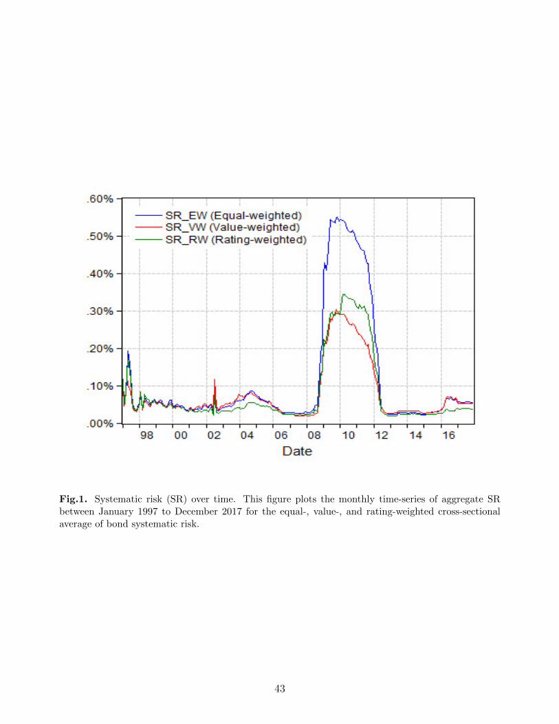
Fig.1. Systematic risk (SR) over time. This figure plots the monthly time-series of aggregate SRbetween January 1997 to December 2017 for the equal-, value-, and rating-weighted cross-sectionalaverage of bond systematic risk.

43

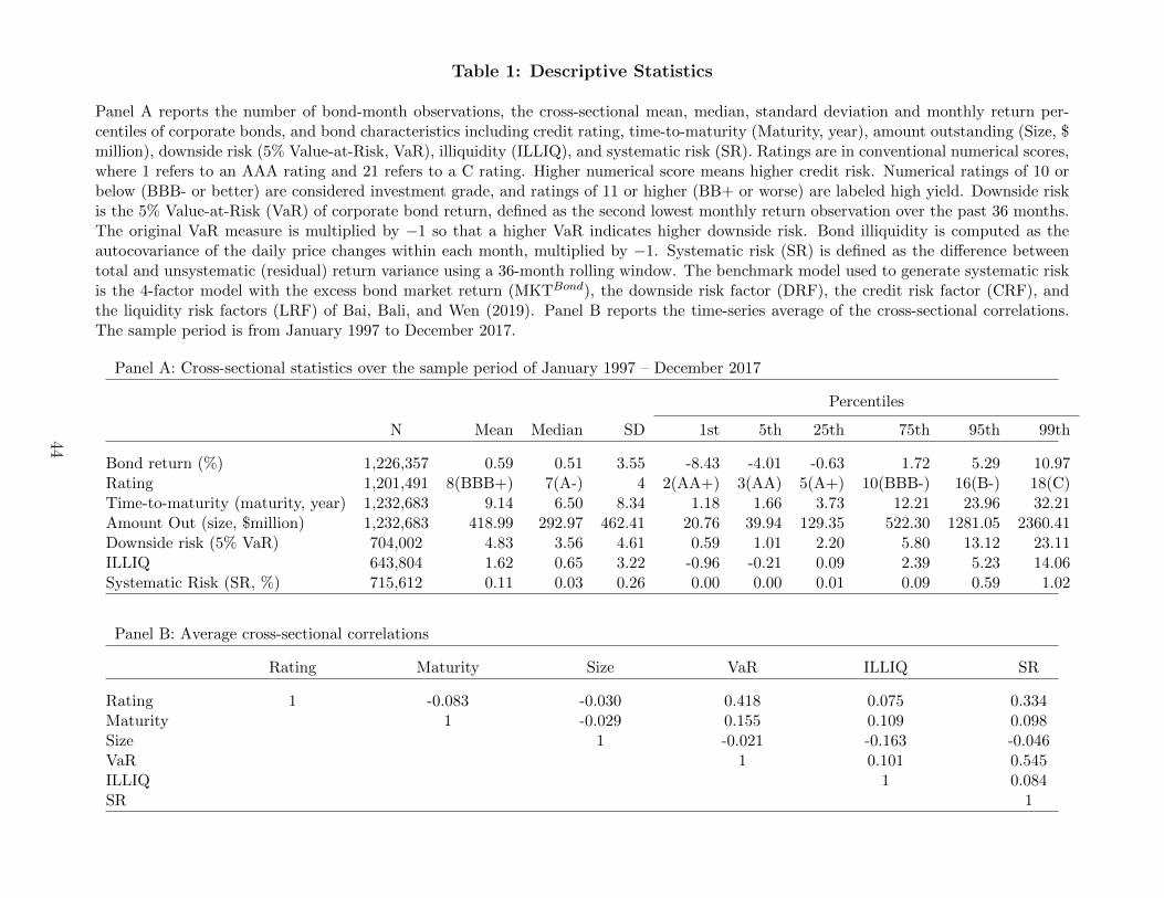
Table 1: Descriptive Statistics

Panel A reports the number of bond-month observations, the cross-sectional mean, median, standard deviation and monthly return per-centiles of corporate bonds, and bond characteristics including credit rating, time-to-maturity (Maturity, year), amount outstanding (Size, $million), downside risk (5% Value-at-Risk, VaR), illiquidity (ILLIQ), and systematic risk (SR). Ratings are in conventional numerical scores,where 1 refers to an AAA rating and 21 refers to a C rating. Higher numerical score means higher credit risk. Numerical ratings of 10 orbelow (BBB- or better) are considered investment grade, and ratings of 11 or higher (BB+ or worse) are labeled high yield. Downside riskis the 5% Value-at-Risk (VaR) of corporate bond return, defined as the second lowest monthly return observation over the past 36 months.The original VaR measure is multiplied by −1 so that a higher VaR indicates higher downside risk. Bond illiquidity is computed as theautocovariance of the daily price changes within each month, multiplied by −1. Systematic risk (SR) is defined as the difference betweentotal and unsystematic (residual) return variance using a 36-month rolling window. The benchmark model used to generate systematic riskis the 4-factor model with the excess bond market return (MKTBond), the downside risk factor (DRF), the credit risk factor (CRF), andthe liquidity risk factors (LRF) of Bai, Bali, and Wen (2019). Panel B reports the time-series average of the cross-sectional correlations.The sample period is from January 1997 to December 2017.

Panel A: Cross-sectional statistics over the sample period of January 1997 – December 2017

Percentiles

N Mean Median SD 1st 5th 25th 75th 95th 99th

Bond return (%) 1,226,357 0.59 0.51 3.55 -8.43 -4.01 -0.63 1.72 5.29 10.97Rating 1,201,491 8(BBB+) 7(A-) 4 2(AA+) 3(AA) 5(A+) 10(BBB-) 16(B-) 18(C)Time-to-maturity (maturity, year) 1,232,683 9.14 6.50 8.34 1.18 1.66 3.73 12.21 23.96 32.21Amount Out (size, $million) 1,232,683 418.99 292.97 462.41 20.76 39.94 129.35 522.30 1281.05 2360.41Downside risk (5% VaR) 704,002 4.83 3.56 4.61 0.59 1.01 2.20 5.80 13.12 23.11ILLIQ 643,804 1.62 0.65 3.22 -0.96 -0.21 0.09 2.39 5.23 14.06Systematic Risk (SR, %) 715,612 0.11 0.03 0.26 0.00 0.00 0.01 0.09 0.59 1.02

Panel B: Average cross-sectional correlations

Rating Maturity Size VaR ILLIQ SR

Rating 1 -0.083 -0.030 0.418 0.075 0.334Maturity 1 -0.029 0.155 0.109 0.098Size 1 -0.021 -0.163 -0.046VaR 1 0.101 0.545ILLIQ 1 0.084SR 1

44

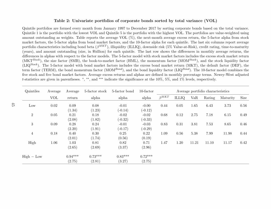
Table 2: Univariate portfolios of corporate bonds sorted by total variance (VOL)

Quintile portfolios are formed every month from January 1997 to December 2017 by sorting corporate bonds based on the total variance.Quintile 1 is the portfolio with the lowest VOL and Quintile 5 is the portfolio with the highest VOL. The portfolios are value-weighted usingamount outstanding as weights. Table reports the average VOL (%), the next-month average excess return, the 5-factor alpha from stockmarket factors, the 5-factor alpha from bond market factors, and the 10-factor alpha for each quintile. The last six columns report averageportfolio characteristics including bond beta (βMKT ), illiquidity (ILLIQ), downside risk (5% Value-at-Risk), credit rating, time-to-maturity(years), and amount outstanding (size, in $billion) for each quintile. The last row shows the differences in monthly average returns, thedifferences in alphas with respect to the factor models. The 5-factor model with stock market factors includes the excess stock market return(MKTStock), the size factor (SMB), the book-to-market factor (HML), the momentum factor (MOMStock), and the stock liquidity factor(LIQStock). The 5-factor model with bond market factors includes the excess bond market return (MKT), the default factor (DEF), theterm factor (TERM), the bond momentum factor (MOMBond), and the bond liquidity factor (LIQBond). The 10-factor model combines thefive stock and five bond market factors. Average excess returns and alphas are defined in monthly percentage terms. Newey-West adjustedt-statistics are given in parentheses. ∗, ∗∗, and ∗∗∗ indicate the significance at the 10%, 5%, and 1% levels, respectively.

Quintiles Average Average 5-factor stock 5-factor bond 10-factor Average portfolio characteristics

VOL return alpha alpha alpha βMKT ILLIQ VaR Rating Maturity Size

Low 0.02 0.09 0.08 -0.01 -0.00 0.44 0.05 1.65 6.43 3.73 0.56(1.34) (1.23) (-0.14) (-0.12)

2 0.05 0.21 0.18 -0.02 -0.02 0.68 0.12 2.75 7.18 6.15 0.49(2.08) (1.82) (-0.32) (-0.33)

3 0.09 0.28 0.24 -0.01 -0.03 0.83 0.31 3.81 7.53 8.65 0.46(2.20) (1.91) (-0.17) (-0.29)

4 0.18 0.40 0.30 0.25 0.22 1.09 0.56 5.38 7.99 11.98 0.44(2.01) (1.74) (0.56) (0.19)

High 1.06 1.03 0.81 0.82 0.71 1.47 1.20 11.21 11.10 11.17 0.42(2.65) (2.69) (3.37) (2.96)

High − Low 0.94*** 0.73*** 0.83*** 0.72***(2.75) (2.81) (3.27) (2.75)

45

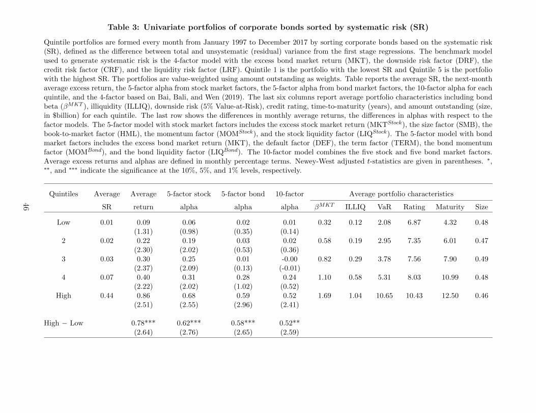
Table 3: Univariate portfolios of corporate bonds sorted by systematic risk (SR)

Quintile portfolios are formed every month from January 1997 to December 2017 by sorting corporate bonds based on the systematic risk(SR), defined as the difference between total and unsystematic (residual) variance from the first stage regressions. The benchmark modelused to generate systematic risk is the 4-factor model with the excess bond market return (MKT), the downside risk factor (DRF), thecredit risk factor (CRF), and the liquidity risk factor (LRF). Quintile 1 is the portfolio with the lowest SR and Quintile 5 is the portfoliowith the highest SR. The portfolios are value-weighted using amount outstanding as weights. Table reports the average SR, the next-monthaverage excess return, the 5-factor alpha from stock market factors, the 5-factor alpha from bond market factors, the 10-factor alpha for eachquintile, and the 4-factor based on Bai, Bali, and Wen (2019). The last six columns report average portfolio characteristics including bondbeta (βMKT ), illiquidity (ILLIQ), downside risk (5% Value-at-Risk), credit rating, time-to-maturity (years), and amount outstanding (size,in $billion) for each quintile. The last row shows the differences in monthly average returns, the differences in alphas with respect to thefactor models. The 5-factor model with stock market factors includes the excess stock market return (MKTStock), the size factor (SMB), thebook-to-market factor (HML), the momentum factor (MOMStock), and the stock liquidity factor (LIQStock). The 5-factor model with bondmarket factors includes the excess bond market return (MKT), the default factor (DEF), the term factor (TERM), the bond momentumfactor (MOMBond), and the bond liquidity factor (LIQBond). The 10-factor model combines the five stock and five bond market factors.Average excess returns and alphas are defined in monthly percentage terms. Newey-West adjusted t-statistics are given in parentheses. ∗,∗∗, and ∗∗∗ indicate the significance at the 10%, 5%, and 1% levels, respectively.

Quintiles Average Average 5-factor stock 5-factor bond 10-factor Average portfolio characteristics

SR return alpha alpha alpha βMKT ILLIQ VaR Rating Maturity Size

Low 0.01 0.09 0.06 0.02 0.01 0.32 0.12 2.08 6.87 4.32 0.48(1.31) (0.98) (0.35) (0.14)

2 0.02 0.22 0.19 0.03 0.02 0.58 0.19 2.95 7.35 6.01 0.47(2.30) (2.02) (0.53) (0.36)

3 0.03 0.30 0.25 0.01 -0.00 0.82 0.29 3.78 7.56 7.90 0.49(2.37) (2.09) (0.13) (-0.01)

4 0.07 0.40 0.31 0.28 0.24 1.10 0.58 5.31 8.03 10.99 0.48(2.22) (2.02) (1.02) (0.52)

High 0.44 0.86 0.68 0.59 0.52 1.69 1.04 10.65 10.43 12.50 0.46(2.51) (2.55) (2.96) (2.41)

High − Low 0.78*** 0.62*** 0.58*** 0.52**(2.64) (2.76) (2.65) (2.59)

46

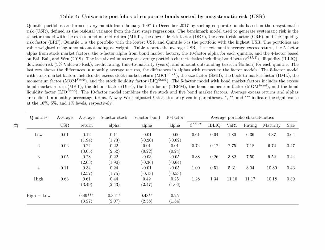
Table 4: Univariate portfolios of corporate bonds sorted by unsystematic risk (USR)

Quintile portfolios are formed every month from January 1997 to December 2017 by sorting corporate bonds based on the unsystematicrisk (USR), defined as the residual variance from the first stage regressions. The benchmark model used to generate systematic risk is the4-factor model with the excess bond market return (MKT), the downside risk factor (DRF), the credit risk factor (CRF), and the liquidityrisk factor (LRF). Quintile 1 is the portfolio with the lowest USR and Quintile 5 is the portfolio with the highest USR. The portfolios arevalue-weighted using amount outstanding as weights. Table reports the average USR, the next-month average excess return, the 5-factoralpha from stock market factors, the 5-factor alpha from bond market factors, the 10-factor alpha for each quintile, and the 4-factor basedon Bai, Bali, and Wen (2019). The last six columns report average portfolio characteristics including bond beta (βMKT ), illiquidity (ILLIQ),downside risk (5% Value-at-Risk), credit rating, time-to-maturity (years), and amount outstanding (size, in $billion) for each quintile. Thelast row shows the differences in monthly average returns, the differences in alphas with respect to the factor models. The 5-factor modelwith stock market factors includes the excess stock market return (MKTStock), the size factor (SMB), the book-to-market factor (HML), themomentum factor (MOMStock), and the stock liquidity factor (LIQStock). The 5-factor model with bond market factors includes the excessbond market return (MKT), the default factor (DEF), the term factor (TERM), the bond momentum factor (MOMBond), and the bondliquidity factor (LIQBond). The 10-factor model combines the five stock and five bond market factors. Average excess returns and alphasare defined in monthly percentage terms. Newey-West adjusted t-statistics are given in parentheses. ∗, ∗∗, and ∗∗∗ indicate the significanceat the 10%, 5%, and 1% levels, respectively.

Quintiles Average Average 5-factor stock 5-factor bond 10-factor Average portfolio characteristics

USR return alpha alpha alpha βMKT ILLIQ VaR5 Rating Maturity Size

Low 0.01 0.12 0.11 -0.01 -0.00 0.61 0.04 1.80 6.36 4.37 0.64(1.94) (1.73) (-0.20) (-0.02)

2 0.02 0.24 0.22 0.01 0.01 0.74 0.12 2.75 7.18 6.72 0.47(3.05) (2.52) (0.22) (0.24)

3 0.05 0.28 0.22 -0.03 -0.05 0.88 0.26 3.82 7.50 9.52 0.44(2.63) (1.90) (-0.36) (-0.64)

4 0.11 0.34 0.24 -0.01 -0.05 1.00 0.51 5.31 8.04 10.89 0.43(2.57) (1.75) (-0.13) (-0.53)

High 0.63 0.61 0.44 0.42 0.25 1.28 1.34 11.10 11.17 10.18 0.39(3.49) (2.43) (2.47) (1.66)

High − Low 0.49*** 0.34** 0.43** 0.25(3.27) (2.07) (2.38) (1.54)

47

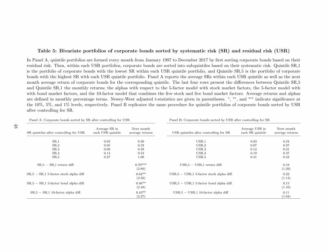
Table 5: Bivariate portfolios of corporate bonds sorted by systematic risk (SR) and residual risk (USR)

In Panel A, quintile portfolios are formed every month from January 1997 to December 2017 by first sorting corporate bonds based on theirresidual risk. Then, within each USR portfolios, corporate bonds are sorted into subquintiles based on their systematic risk. Quintile SR,1is the portfolio of corporate bonds with the lowest SR within each USR quintile portfolio, and Quintile SR,5 is the portfolio of corporatebonds with the highest SR with each USR quintile portfolio. Panel A reports the average SRs within each USR quintile as well as the nextmonth average return of corporate bonds for the corresponding quintile. The last four rows present the differences between Quintile SR,5and Quintile SR,1 the monthly returns; the alphas with respect to the 5-factor model with stock market factors, the 5-factor model withwith bond market factors, and the 10-factor model that combines the five stock and five bond market factors. Average returns and alphasare defined in monthly percentage terms. Newey-West adjusted t-statistics are given in parentheses. ∗, ∗∗, and ∗∗∗ indicate significance atthe 10%, 5%, and 1% levels, respectively. Panel B replicates the same procedure for quintile portfolios of corporate bonds sorted by USRafter controlling for SR.

Panel A: Corporate bonds sorted by SR after controlling for USR Panel B: Corporate bonds sorted by USR after controlling for SR

Average SR in Next month Average USR in Next monthSR quintiles after controlling for USR each USR quintile average returns USR quintiles after controlling for SR each SR quintile average returns

SR,1 0.02 0.30 USR,1 0.03 0.24SR,2 0.05 0.33 USR,2 0.07 0.27SR,3 0.09 0.39 USR,3 0.12 0.31SR,4 0.14 0.53 USR,4 0.19 0.37SR,5 0.27 1.00 USR,5 0.41 0.42

SR,5 − SR,1 return diff. 0.70*** USR,5 − USR,1 return diff. 0.18(2.80) (1.29)

SR,5 − SR,1 5-factor stock alpha diff. 0.62** USR,5 − USR,1 5-factor stock alpha diff. 0.22(2.56) (1.14)

SR,5 − SR,1 5-factor bond alpha diff. 0.46** USR,5 − USR,1 5-factor bond alpha diff. 0.15(2.48) (1.10)

SR,5 − SR,1 10-factor alpha diff. 0.43** USR,5 − USR,1 10-factor alpha diff. 0.11(2.27) (1.04)

48

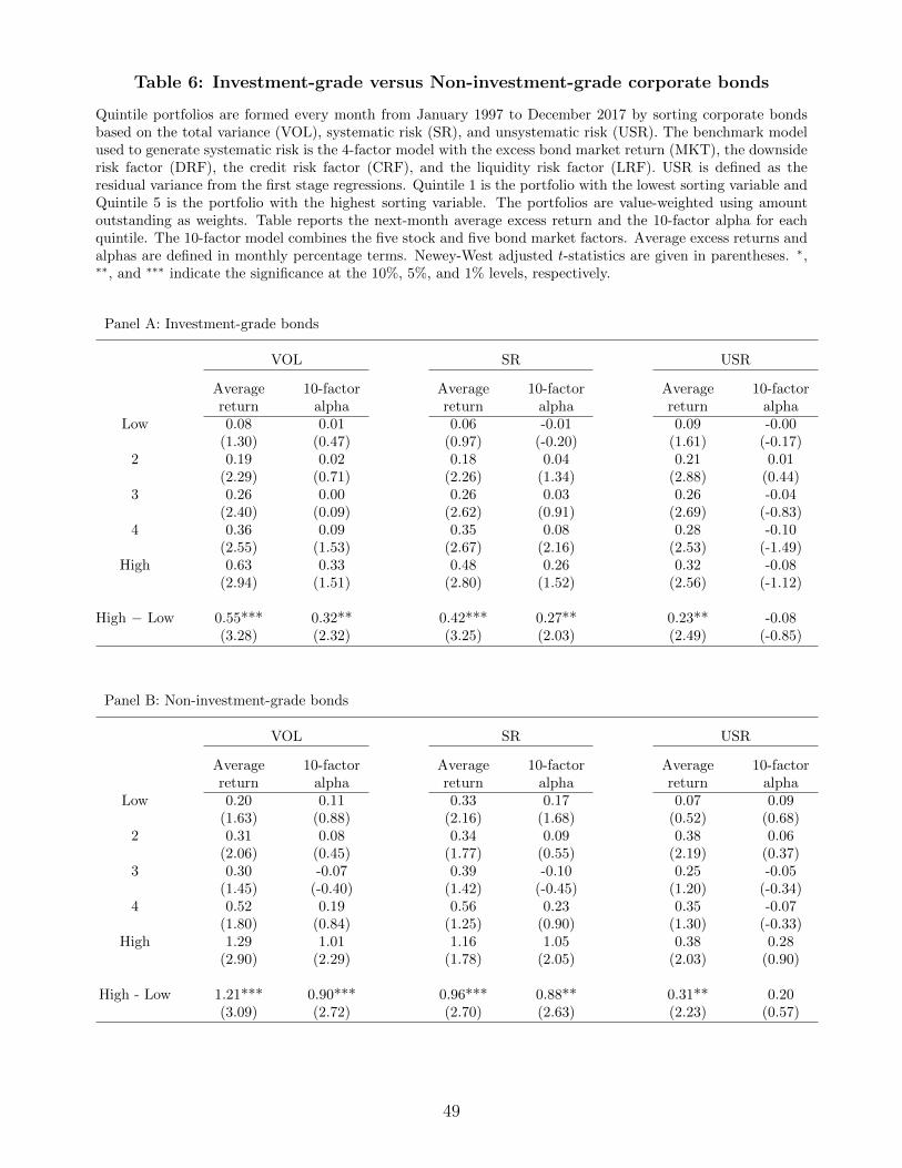
Table 6: Investment-grade versus Non-investment-grade corporate bonds

Quintile portfolios are formed every month from January 1997 to December 2017 by sorting corporate bondsbased on the total variance (VOL), systematic risk (SR), and unsystematic risk (USR). The benchmark modelused to generate systematic risk is the 4-factor model with the excess bond market return (MKT), the downsiderisk factor (DRF), the credit risk factor (CRF), and the liquidity risk factor (LRF). USR is defined as theresidual variance from the first stage regressions. Quintile 1 is the portfolio with the lowest sorting variable andQuintile 5 is the portfolio with the highest sorting variable. The portfolios are value-weighted using amountoutstanding as weights. Table reports the next-month average excess return and the 10-factor alpha for eachquintile. The 10-factor model combines the five stock and five bond market factors. Average excess returns andalphas are defined in monthly percentage terms. Newey-West adjusted t-statistics are given in parentheses. ∗,∗∗, and ∗∗∗ indicate the significance at the 10%, 5%, and 1% levels, respectively.

Panel A: Investment-grade bonds

VOL SR USR

Average 10-factor Average 10-factor Average 10-factorreturn alpha return alpha return alpha

Low 0.08 0.01 0.06 -0.01 0.09 -0.00(1.30) (0.47) (0.97) (-0.20) (1.61) (-0.17)

2 0.19 0.02 0.18 0.04 0.21 0.01(2.29) (0.71) (2.26) (1.34) (2.88) (0.44)

3 0.26 0.00 0.26 0.03 0.26 -0.04(2.40) (0.09) (2.62) (0.91) (2.69) (-0.83)

4 0.36 0.09 0.35 0.08 0.28 -0.10(2.55) (1.53) (2.67) (2.16) (2.53) (-1.49)

High 0.63 0.33 0.48 0.26 0.32 -0.08(2.94) (1.51) (2.80) (1.52) (2.56) (-1.12)

High − Low 0.55*** 0.32** 0.42*** 0.27** 0.23** -0.08(3.28) (2.32) (3.25) (2.03) (2.49) (-0.85)

Panel B: Non-investment-grade bonds

VOL SR USR

Average 10-factor Average 10-factor Average 10-factorreturn alpha return alpha return alpha

Low 0.20 0.11 0.33 0.17 0.07 0.09(1.63) (0.88) (2.16) (1.68) (0.52) (0.68)

2 0.31 0.08 0.34 0.09 0.38 0.06(2.06) (0.45) (1.77) (0.55) (2.19) (0.37)

3 0.30 -0.07 0.39 -0.10 0.25 -0.05(1.45) (-0.40) (1.42) (-0.45) (1.20) (-0.34)

4 0.52 0.19 0.56 0.23 0.35 -0.07(1.80) (0.84) (1.25) (0.90) (1.30) (-0.33)

High 1.29 1.01 1.16 1.05 0.38 0.28(2.90) (2.29) (1.78) (2.05) (2.03) (0.90)

High - Low 1.21*** 0.90*** 0.96*** 0.88** 0.31** 0.20(3.09) (2.72) (2.70) (2.63) (2.23) (0.57)

49

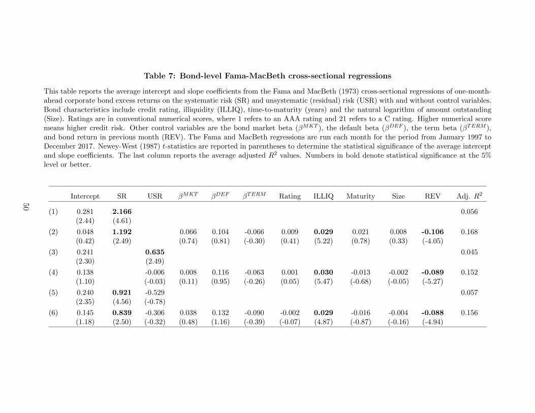
Table 7: Bond-level Fama-MacBeth cross-sectional regressions

This table reports the average intercept and slope coefficients from the Fama and MacBeth (1973) cross-sectional regressions of one-month-ahead corporate bond excess returns on the systematic risk (SR) and unsystematic (residual) risk (USR) with and without control variables.Bond characteristics include credit rating, illiquidity (ILLIQ), time-to-maturity (years) and the natural logarithm of amount outstanding(Size). Ratings are in conventional numerical scores, where 1 refers to an AAA rating and 21 refers to a C rating. Higher numerical scoremeans higher credit risk. Other control variables are the bond market beta (βMKT ), the default beta (βDEF ), the term beta (βTERM ),and bond return in previous month (REV). The Fama and MacBeth regressions are run each month for the period from January 1997 toDecember 2017. Newey-West (1987) t-statistics are reported in parentheses to determine the statistical significance of the average interceptand slope coefficients. The last column reports the average adjusted R2 values. Numbers in bold denote statistical significance at the 5%level or better.

Intercept SR USR βMKT βDEF βTERM Rating ILLIQ Maturity Size REV Adj. R2

(1) 0.281 2.166 0.056(2.44) (4.61)

(2) 0.048 1.192 0.066 0.104 -0.066 0.009 0.029 0.021 0.008 -0.106 0.168(0.42) (2.49) (0.74) (0.81) (-0.30) (0.41) (5.22) (0.78) (0.33) (-4.05)

(3) 0.241 0.635 0.045(2.30) (2.49)

(4) 0.138 -0.006 0.008 0.116 -0.063 0.001 0.030 -0.013 -0.002 -0.089 0.152(1.10) (-0.03) (0.11) (0.95) (-0.26) (0.05) (5.47) (-0.68) (-0.05) (-5.27)

(5) 0.240 0.921 -0.529 0.057(2.35) (4.56) (-0.78)

(6) 0.145 0.839 -0.306 0.038 0.132 -0.090 -0.002 0.029 -0.016 -0.004 -0.088 0.156(1.18) (2.50) (-0.32) (0.48) (1.16) (-0.39) (-0.07) (4.87) (-0.87) (-0.16) (-4.94)

50

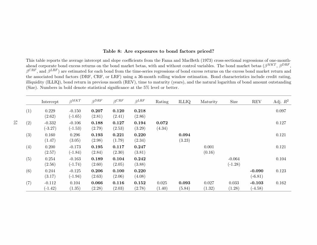
Table 8: Are exposures to bond factors priced?

This table reports the average intercept and slope coefficients from the Fama and MacBeth (1973) cross-sectional regressions of one-month-ahead corporate bond excess returns on the bond market betas, with and without control variables. The bond market betas (βMKT , βDRF ,βCRF , and βLRF ) are estimated for each bond from the time-series regressions of bond excess returns on the excess bond market return andthe associated bond factors (DRF, CRF, or LRF) using a 36-month rolling window estimation. Bond characteristics include credit rating,illiquidity (ILLIQ), bond return in previous month (REV), time to maturity (years), and the natural logarithm of bond amount outstanding(Size). Numbers in bold denote statistical significance at the 5% level or better.

Intercept βMKT βDRF βCRF βLRF Rating ILLIQ Maturity Size REV Adj. R2

(1) 0.229 -0.150 0.207 0.120 0.218 0.097(2.62) (-1.65) (2.81) (2.41) (2.86)

(2) -0.332 -0.106 0.188 0.127 0.194 0.072 0.127(-3.27) (-1.53) (2.79) (2.53) (3.29) (4.34)

(3) 0.160 0.296 0.193 0.221 0.220 0.094 0.121(1.47) (3.05) (2.98) (1.79) (2.34) (3.23)

(4) 0.200 -0.173 0.195 0.117 0.247 0.001 0.121(2.57) (-1.84) (2.84) (2.30) (3.81) (0.16)

(5) 0.254 -0.163 0.189 0.104 0.242 -0.064 0.104(2.56) (-1.74) (2.60) (2.05) (3.88) (-1.28)

(6) 0.244 -0.125 0.206 0.100 0.220 -0.090 0.123(3.17) (-1.94) (2.63) (2.06) (4.08) (-6.81)

(7) -0.112 0.104 0.066 0.116 0.152 0.025 0.093 0.027 0.033 -0.103 0.162(-1.42) (1.35) (2.28) (2.03) (2.78) (1.40) (5.84) (1.32) (1.28) (-4.58)

51

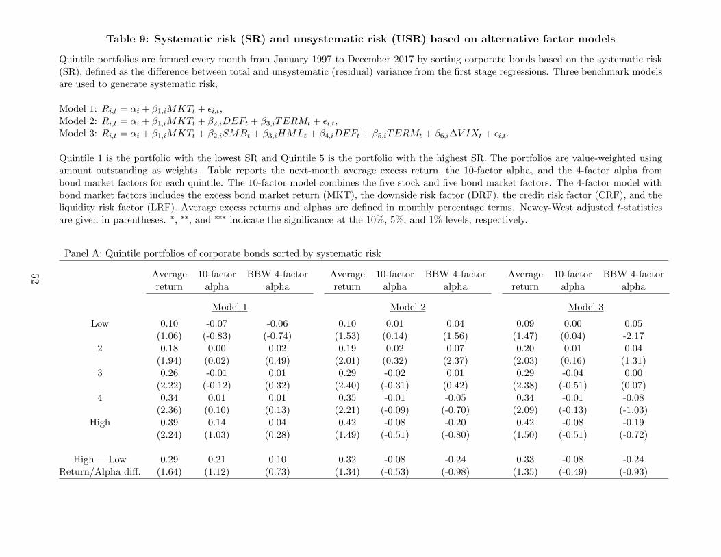
Table 9: Systematic risk (SR) and unsystematic risk (USR) based on alternative factor models

Quintile portfolios are formed every month from January 1997 to December 2017 by sorting corporate bonds based on the systematic risk(SR), defined as the difference between total and unsystematic (residual) variance from the first stage regressions. Three benchmark modelsare used to generate systematic risk,

Model 1: Ri,t = αi + β1,iMKTt + εi,t,Model 2: Ri,t = αi + β1,iMKTt + β2,iDEFt + β3,iTERMt + εi,t,Model 3: Ri,t = αi + β1,iMKTt + β2,iSMBt + β3,iHMLt + β4,iDEFt + β5,iTERMt + β6,i∆V IXt + εi,t.

Quintile 1 is the portfolio with the lowest SR and Quintile 5 is the portfolio with the highest SR. The portfolios are value-weighted usingamount outstanding as weights. Table reports the next-month average excess return, the 10-factor alpha, and the 4-factor alpha frombond market factors for each quintile. The 10-factor model combines the five stock and five bond market factors. The 4-factor model withbond market factors includes the excess bond market return (MKT), the downside risk factor (DRF), the credit risk factor (CRF), and theliquidity risk factor (LRF). Average excess returns and alphas are defined in monthly percentage terms. Newey-West adjusted t-statisticsare given in parentheses. ∗, ∗∗, and ∗∗∗ indicate the significance at the 10%, 5%, and 1% levels, respectively.

Panel A: Quintile portfolios of corporate bonds sorted by systematic risk

Average 10-factor BBW 4-factor Average 10-factor BBW 4-factor Average 10-factor BBW 4-factorreturn alpha alpha return alpha alpha return alpha alpha

Model 1 Model 2 Model 3

Low 0.10 -0.07 -0.06 0.10 0.01 0.04 0.09 0.00 0.05(1.06) (-0.83) (-0.74) (1.53) (0.14) (1.56) (1.47) (0.04) -2.17

2 0.18 0.00 0.02 0.19 0.02 0.07 0.20 0.01 0.04(1.94) (0.02) (0.49) (2.01) (0.32) (2.37) (2.03) (0.16) (1.31)

3 0.26 -0.01 0.01 0.29 -0.02 0.01 0.29 -0.04 0.00(2.22) (-0.12) (0.32) (2.40) (-0.31) (0.42) (2.38) (-0.51) (0.07)

4 0.34 0.01 0.01 0.35 -0.01 -0.05 0.34 -0.01 -0.08(2.36) (0.10) (0.13) (2.21) (-0.09) (-0.70) (2.09) (-0.13) (-1.03)

High 0.39 0.14 0.04 0.42 -0.08 -0.20 0.42 -0.08 -0.19(2.24) (1.03) (0.28) (1.49) (-0.51) (-0.80) (1.50) (-0.51) (-0.72)

High − Low 0.29 0.21 0.10 0.32 -0.08 -0.24 0.33 -0.08 -0.24Return/Alpha diff. (1.64) (1.12) (0.73) (1.34) (-0.53) (-0.98) (1.35) (-0.49) (-0.93)

52

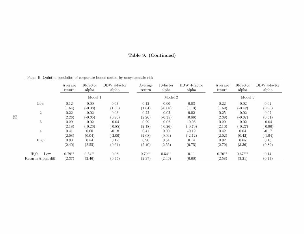
Table 9. (Continued)

Panel B: Quintile portfolios of corporate bonds sorted by unsystematic risk

Average 10-factor BBW 4-factor Average 10-factor BBW 4-factor Average 10-factor BBW 4-factorreturn alpha alpha return alpha alpha return alpha alpha

Model 1 Model 2 Model 3

Low 0.12 -0.00 0.03 0.12 -0.00 0.03 0.22 -0.02 0.02(1.64) (-0.08) (1.36) (1.64) (-0.08) (1.13) (1.69) (-0.42) (0.86)

2 0.22 -0.02 0.03 0.22 -0.02 0.02 0.25 -0.02 0.02(2.26) (-0.35) (0.96) (2.26) (-0.35) (0.86) (2.39) (-0.37) (0.51)

3 0.29 -0.02 -0.04 0.29 -0.02 -0.03 0.29 -0.02 -0.04(2.18) (-0.26) (-0.85) (2.18) (-0.26) (-0.70) (2.10) (-0.27) (-0.90)

4 0.41 0.00 -0.18 0.41 0.00 -0.19 0.42 0.04 -0.17(2.08) (0.04) (-2.00) (2.08) (0.04) (-2.12) (2.02) (0.42) (-1.94)

High 0.90 0.54 0.12 0.90 0.54 0.14 0.92 0.65 0.16(2.40) (2.55) (0.64) (2.40) (2.55) (0.75) (2.79) (3.36) (0.89)

High − Low 0.79∗∗ 0.54∗∗ 0.08 0.79∗∗ 0.54∗∗ 0.11 0.70∗∗ 0.67∗∗∗ 0.14Return/Alpha diff. (2.37) (2.46) (0.45) (2.37) (2.46) (0.60) (2.58) (3.21) (0.77)

53

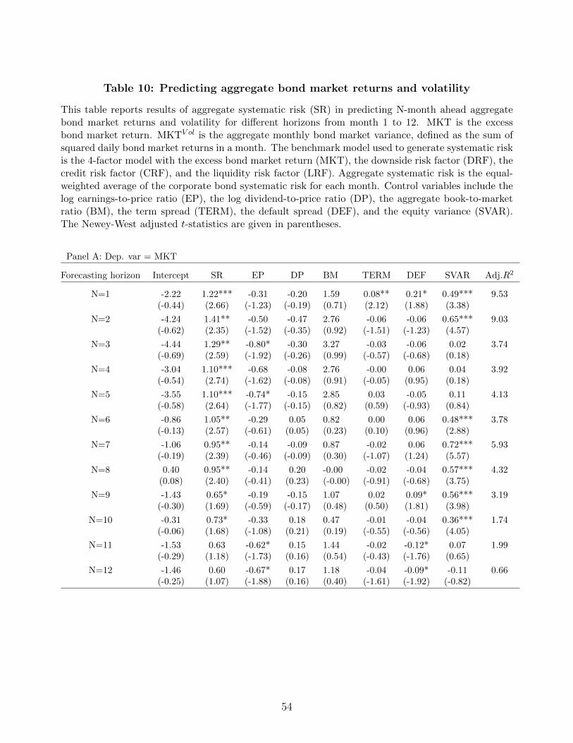
Table 10: Predicting aggregate bond market returns and volatility

This table reports results of aggregate systematic risk (SR) in predicting N-month ahead aggregatebond market returns and volatility for different horizons from month 1 to 12. MKT is the excessbond market return. MKTV ol is the aggregate monthly bond market variance, defined as the sum ofsquared daily bond market returns in a month. The benchmark model used to generate systematic riskis the 4-factor model with the excess bond market return (MKT), the downside risk factor (DRF), thecredit risk factor (CRF), and the liquidity risk factor (LRF). Aggregate systematic risk is the equal-weighted average of the corporate bond systematic risk for each month. Control variables include thelog earnings-to-price ratio (EP), the log dividend-to-price ratio (DP), the aggregate book-to-marketratio (BM), the term spread (TERM), the default spread (DEF), and the equity variance (SVAR).The Newey-West adjusted t-statistics are given in parentheses.

Panel A: Dep. var = MKT

Forecasting horizon Intercept SR EP DP BM TERM DEF SVAR Adj.R2

N=1 -2.22 1.22*** -0.31 -0.20 1.59 0.08** 0.21* 0.49*** 9.53(-0.44) (2.66) (-1.23) (-0.19) (0.71) (2.12) (1.88) (3.38)

N=2 -4.24 1.41** -0.50 -0.47 2.76 -0.06 -0.06 0.65*** 9.03(-0.62) (2.35) (-1.52) (-0.35) (0.92) (-1.51) (-1.23) (4.57)

N=3 -4.44 1.29** -0.80* -0.30 3.27 -0.03 -0.06 0.02 3.74(-0.69) (2.59) (-1.92) (-0.26) (0.99) (-0.57) (-0.68) (0.18)

N=4 -3.04 1.10*** -0.68 -0.08 2.76 -0.00 0.06 0.04 3.92(-0.54) (2.74) (-1.62) (-0.08) (0.91) (-0.05) (0.95) (0.18)

N=5 -3.55 1.10*** -0.74* -0.15 2.85 0.03 -0.05 0.11 4.13(-0.58) (2.64) (-1.77) (-0.15) (0.82) (0.59) (-0.93) (0.84)

N=6 -0.86 1.05** -0.29 0.05 0.82 0.00 0.06 0.48*** 3.78(-0.13) (2.57) (-0.61) (0.05) (0.23) (0.10) (0.96) (2.88)

N=7 -1.06 0.95** -0.14 -0.09 0.87 -0.02 0.06 0.72*** 5.93(-0.19) (2.39) (-0.46) (-0.09) (0.30) (-1.07) (1.24) (5.57)

N=8 0.40 0.95** -0.14 0.20 -0.00 -0.02 -0.04 0.57*** 4.32(0.08) (2.40) (-0.41) (0.23) (-0.00) (-0.91) (-0.68) (3.75)

N=9 -1.43 0.65* -0.19 -0.15 1.07 0.02 0.09* 0.56*** 3.19(-0.30) (1.69) (-0.59) (-0.17) (0.48) (0.50) (1.81) (3.98)

N=10 -0.31 0.73* -0.33 0.18 0.47 -0.01 -0.04 0.36*** 1.74(-0.06) (1.68) (-1.08) (0.21) (0.19) (-0.55) (-0.56) (4.05)

N=11 -1.53 0.63 -0.62* 0.15 1.44 -0.02 -0.12* 0.07 1.99(-0.29) (1.18) (-1.73) (0.16) (0.54) (-0.43) (-1.76) (0.65)

N=12 -1.46 0.60 -0.67* 0.17 1.18 -0.04 -0.09* -0.11 0.66(-0.25) (1.07) (-1.88) (0.16) (0.40) (-1.61) (-1.92) (-0.82)

54

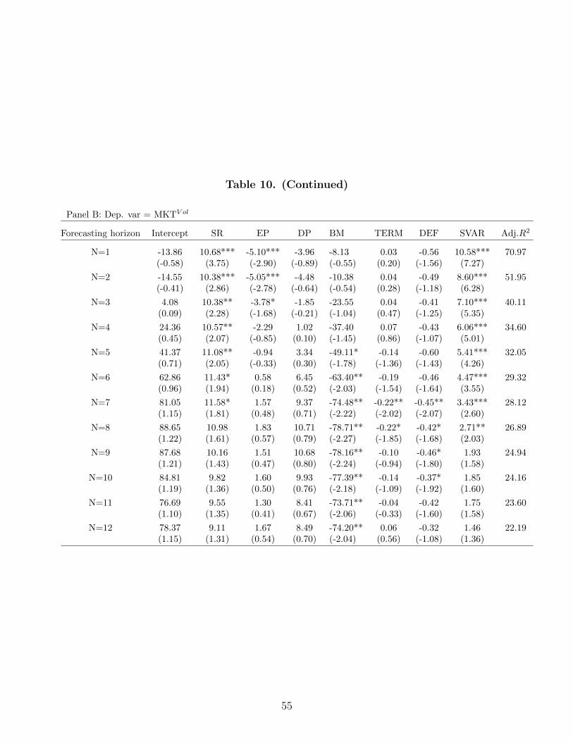
Table 10. (Continued)

Panel B: Dep. var = MKTV ol

Forecasting horizon Intercept SR EP DP BM TERM DEF SVAR Adj.R2

N=1 -13.86 10.68*** -5.10*** -3.96 -8.13 0.03 -0.56 10.58*** 70.97(-0.58) (3.75) (-2.90) (-0.89) (-0.55) (0.20) (-1.56) (7.27)

N=2 -14.55 10.38*** -5.05*** -4.48 -10.38 0.04 -0.49 8.60*** 51.95(-0.41) (2.86) (-2.78) (-0.64) (-0.54) (0.28) (-1.18) (6.28)

N=3 4.08 10.38** -3.78* -1.85 -23.55 0.04 -0.41 7.10*** 40.11(0.09) (2.28) (-1.68) (-0.21) (-1.04) (0.47) (-1.25) (5.35)

N=4 24.36 10.57** -2.29 1.02 -37.40 0.07 -0.43 6.06*** 34.60(0.45) (2.07) (-0.85) (0.10) (-1.45) (0.86) (-1.07) (5.01)

N=5 41.37 11.08** -0.94 3.34 -49.11* -0.14 -0.60 5.41*** 32.05(0.71) (2.05) (-0.33) (0.30) (-1.78) (-1.36) (-1.43) (4.26)

N=6 62.86 11.43* 0.58 6.45 -63.40** -0.19 -0.46 4.47*** 29.32(0.96) (1.94) (0.18) (0.52) (-2.03) (-1.54) (-1.64) (3.55)

N=7 81.05 11.58* 1.57 9.37 -74.48** -0.22** -0.45** 3.43*** 28.12(1.15) (1.81) (0.48) (0.71) (-2.22) (-2.02) (-2.07) (2.60)

N=8 88.65 10.98 1.83 10.71 -78.71** -0.22* -0.42* 2.71** 26.89(1.22) (1.61) (0.57) (0.79) (-2.27) (-1.85) (-1.68) (2.03)

N=9 87.68 10.16 1.51 10.68 -78.16** -0.10 -0.46* 1.93 24.94(1.21) (1.43) (0.47) (0.80) (-2.24) (-0.94) (-1.80) (1.58)

N=10 84.81 9.82 1.60 9.93 -77.39** -0.14 -0.37* 1.85 24.16(1.19) (1.36) (0.50) (0.76) (-2.18) (-1.09) (-1.92) (1.60)

N=11 76.69 9.55 1.30 8.41 -73.71** -0.04 -0.42 1.75 23.60(1.10) (1.35) (0.41) (0.67) (-2.06) (-0.33) (-1.60) (1.58)

N=12 78.37 9.11 1.67 8.49 -74.20** 0.06 -0.32 1.46 22.19(1.15) (1.31) (0.54) (0.70) (-2.04) (0.56) (-1.08) (1.36)

55

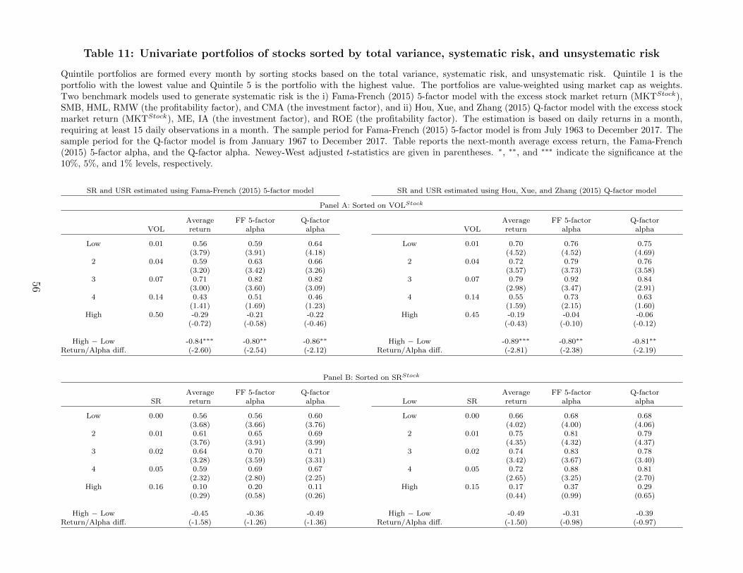
Table 11: Univariate portfolios of stocks sorted by total variance, systematic risk, and unsystematic risk

Quintile portfolios are formed every month by sorting stocks based on the total variance, systematic risk, and unsystematic risk. Quintile 1 is theportfolio with the lowest value and Quintile 5 is the portfolio with the highest value. The portfolios are value-weighted using market cap as weights.Two benchmark models used to generate systematic risk is the i) Fama-French (2015) 5-factor model with the excess stock market return (MKTStock),SMB, HML, RMW (the profitability factor), and CMA (the investment factor), and ii) Hou, Xue, and Zhang (2015) Q-factor model with the excess stockmarket return (MKTStock), ME, IA (the investment factor), and ROE (the profitability factor). The estimation is based on daily returns in a month,requiring at least 15 daily observations in a month. The sample period for Fama-French (2015) 5-factor model is from July 1963 to December 2017. Thesample period for the Q-factor model is from January 1967 to December 2017. Table reports the next-month average excess return, the Fama-French(2015) 5-factor alpha, and the Q-factor alpha. Newey-West adjusted t-statistics are given in parentheses. ∗, ∗∗, and ∗∗∗ indicate the significance at the10%, 5%, and 1% levels, respectively.

SR and USR estimated using Fama-French (2015) 5-factor model SR and USR estimated using Hou, Xue, and Zhang (2015) Q-factor model

Panel A: Sorted on VOLStock

Average FF 5-factor Q-factor Average FF 5-factor Q-factorVOL return alpha alpha VOL return alpha alpha

Low 0.01 0.56 0.59 0.64 Low 0.01 0.70 0.76 0.75(3.79) (3.91) (4.18) (4.52) (4.52) (4.69)

2 0.04 0.59 0.63 0.66 2 0.04 0.72 0.79 0.76(3.20) (3.42) (3.26) (3.57) (3.73) (3.58)

3 0.07 0.71 0.82 0.82 3 0.07 0.79 0.92 0.84(3.00) (3.60) (3.09) (2.98) (3.47) (2.91)

4 0.14 0.43 0.51 0.46 4 0.14 0.55 0.73 0.63(1.41) (1.69) (1.23) (1.59) (2.15) (1.60)

High 0.50 -0.29 -0.21 -0.22 High 0.45 -0.19 -0.04 -0.06(-0.72) (-0.58) (-0.46) (-0.43) (-0.10) (-0.12)

High − Low -0.84∗∗∗ -0.80∗∗ -0.86∗∗ High − Low -0.89∗∗∗ -0.80∗∗ -0.81∗∗

Return/Alpha diff. (-2.60) (-2.54) (-2.12) Return/Alpha diff. (-2.81) (-2.38) (-2.19)

Panel B: Sorted on SRStock

Average FF 5-factor Q-factor Average FF 5-factor Q-factorSR return alpha alpha Low SR return alpha alpha

Low 0.00 0.56 0.56 0.60 Low 0.00 0.66 0.68 0.68(3.68) (3.66) (3.76) (4.02) (4.00) (4.06)

2 0.01 0.61 0.65 0.69 2 0.01 0.75 0.81 0.79(3.76) (3.91) (3.99) (4.35) (4.32) (4.37)

3 0.02 0.64 0.70 0.71 3 0.02 0.74 0.83 0.78(3.28) (3.59) (3.31) (3.42) (3.67) (3.40)

4 0.05 0.59 0.69 0.67 4 0.05 0.72 0.88 0.81(2.32) (2.80) (2.25) (2.65) (3.25) (2.70)

High 0.16 0.10 0.20 0.11 High 0.15 0.17 0.37 0.29(0.29) (0.58) (0.26) (0.44) (0.99) (0.65)

High − Low -0.45 -0.36 -0.49 High − Low -0.49 -0.31 -0.39Return/Alpha diff. (-1.58) (-1.26) (-1.36) Return/Alpha diff. (-1.50) (-0.98) (-0.97)

56

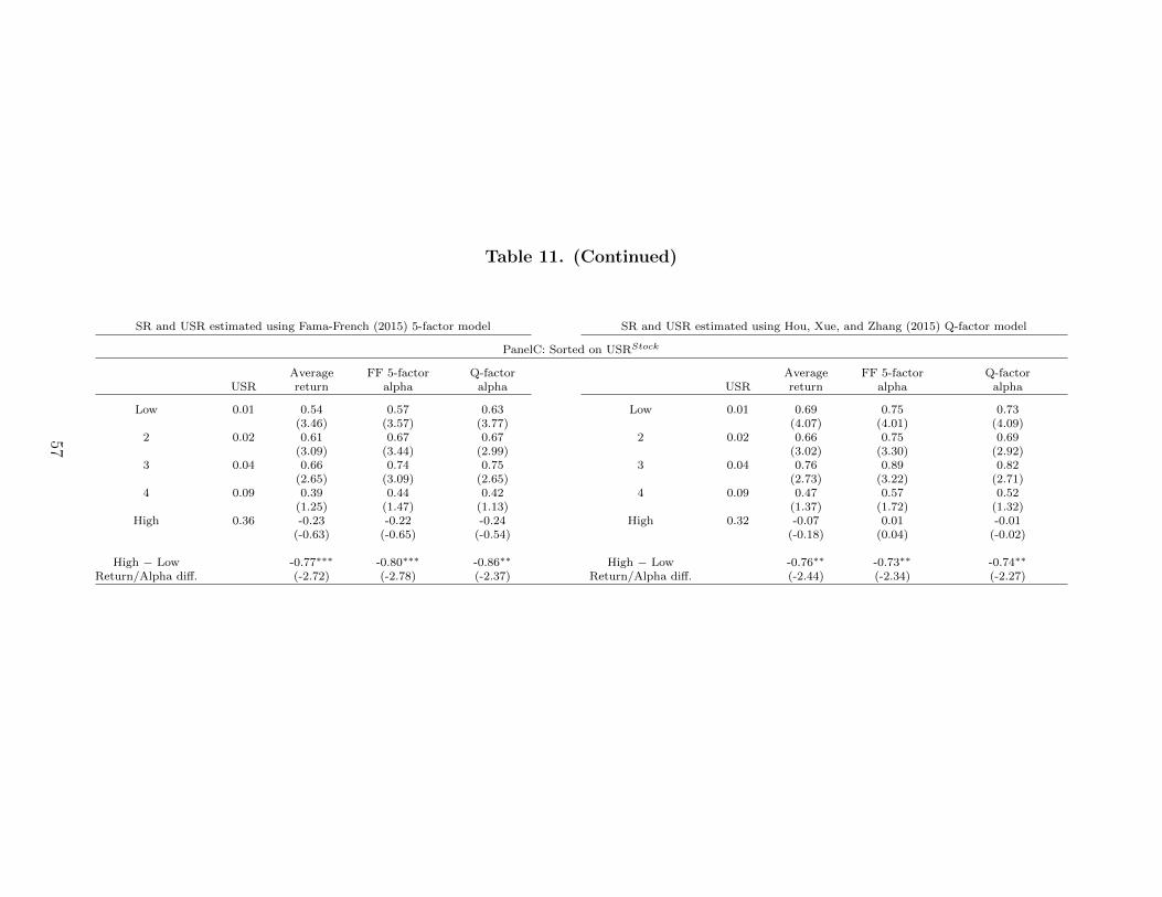
Table 11. (Continued)

SR and USR estimated using Fama-French (2015) 5-factor model SR and USR estimated using Hou, Xue, and Zhang (2015) Q-factor model

PanelC: Sorted on USRStock

Average FF 5-factor Q-factor Average FF 5-factor Q-factorUSR return alpha alpha USR return alpha alpha

Low 0.01 0.54 0.57 0.63 Low 0.01 0.69 0.75 0.73(3.46) (3.57) (3.77) (4.07) (4.01) (4.09)

2 0.02 0.61 0.67 0.67 2 0.02 0.66 0.75 0.69(3.09) (3.44) (2.99) (3.02) (3.30) (2.92)

3 0.04 0.66 0.74 0.75 3 0.04 0.76 0.89 0.82(2.65) (3.09) (2.65) (2.73) (3.22) (2.71)

4 0.09 0.39 0.44 0.42 4 0.09 0.47 0.57 0.52(1.25) (1.47) (1.13) (1.37) (1.72) (1.32)

High 0.36 -0.23 -0.22 -0.24 High 0.32 -0.07 0.01 -0.01(-0.63) (-0.65) (-0.54) (-0.18) (0.04) (-0.02)

High − Low -0.77∗∗∗ -0.80∗∗∗ -0.86∗∗ High − Low -0.76∗∗ -0.73∗∗ -0.74∗∗

Return/Alpha diff. (-2.72) (-2.78) (-2.37) Return/Alpha diff. (-2.44) (-2.34) (-2.27)

57

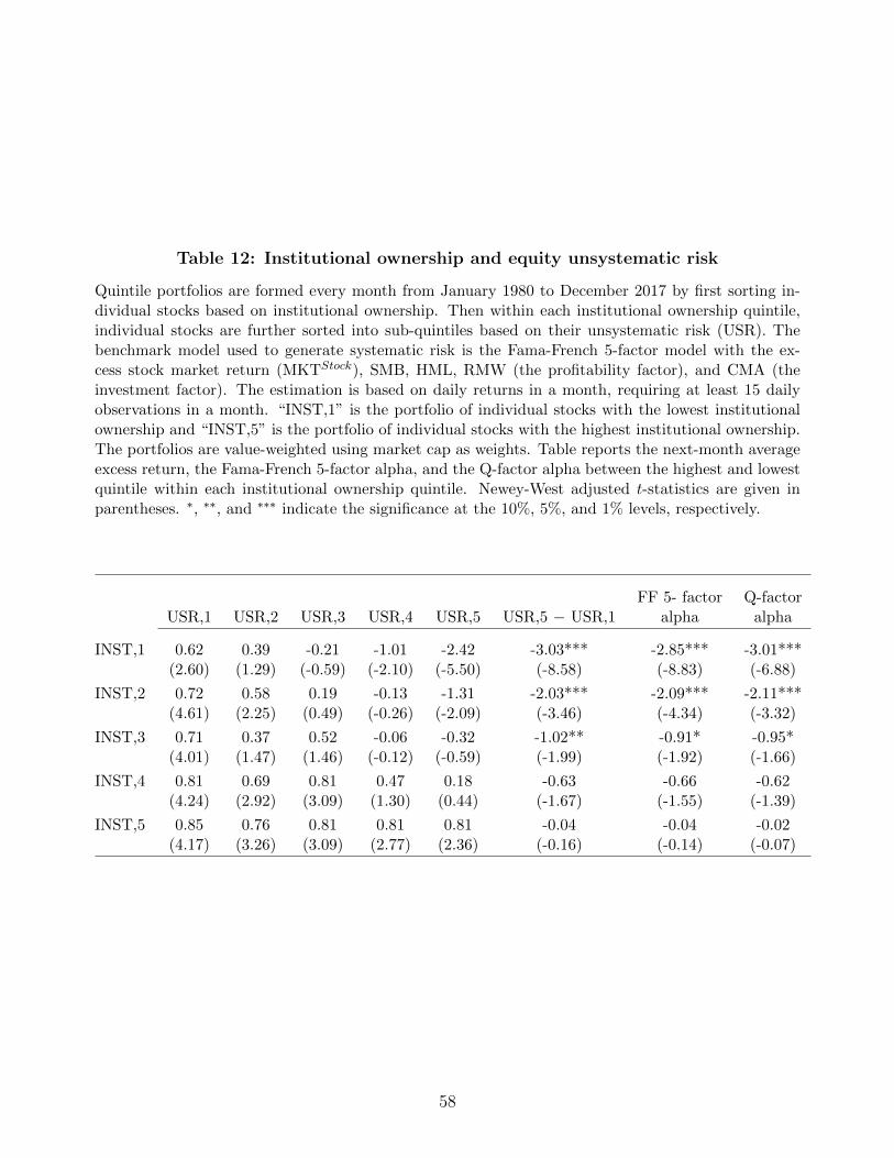
Table 12: Institutional ownership and equity unsystematic risk

Quintile portfolios are formed every month from January 1980 to December 2017 by first sorting in-dividual stocks based on institutional ownership. Then within each institutional ownership quintile,individual stocks are further sorted into sub-quintiles based on their unsystematic risk (USR). Thebenchmark model used to generate systematic risk is the Fama-French 5-factor model with the ex-cess stock market return (MKTStock), SMB, HML, RMW (the profitability factor), and CMA (theinvestment factor). The estimation is based on daily returns in a month, requiring at least 15 dailyobservations in a month. “INST,1” is the portfolio of individual stocks with the lowest institutionalownership and “INST,5” is the portfolio of individual stocks with the highest institutional ownership.The portfolios are value-weighted using market cap as weights. Table reports the next-month averageexcess return, the Fama-French 5-factor alpha, and the Q-factor alpha between the highest and lowestquintile within each institutional ownership quintile. Newey-West adjusted t-statistics are given inparentheses. ∗, ∗∗, and ∗∗∗ indicate the significance at the 10%, 5%, and 1% levels, respectively.

FF 5- factor Q-factorUSR,1 USR,2 USR,3 USR,4 USR,5 USR,5 − USR,1 alpha alpha

INST,1 0.62 0.39 -0.21 -1.01 -2.42 -3.03*** -2.85*** -3.01***(2.60) (1.29) (-0.59) (-2.10) (-5.50) (-8.58) (-8.83) (-6.88)

INST,2 0.72 0.58 0.19 -0.13 -1.31 -2.03*** -2.09*** -2.11***(4.61) (2.25) (0.49) (-0.26) (-2.09) (-3.46) (-4.34) (-3.32)

INST,3 0.71 0.37 0.52 -0.06 -0.32 -1.02** -0.91* -0.95*(4.01) (1.47) (1.46) (-0.12) (-0.59) (-1.99) (-1.92) (-1.66)

INST,4 0.81 0.69 0.81 0.47 0.18 -0.63 -0.66 -0.62(4.24) (2.92) (3.09) (1.30) (0.44) (-1.67) (-1.55) (-1.39)

INST,5 0.85 0.76 0.81 0.81 0.81 -0.04 -0.04 -0.02(4.17) (3.26) (3.09) (2.77) (2.36) (-0.16) (-0.14) (-0.07)

58

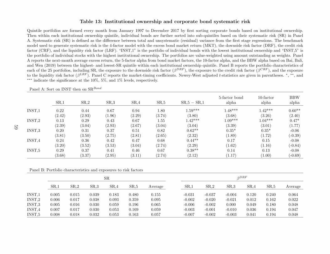
Table 13: Institutional ownership and corporate bond systematic risk

Quintile portfolios are formed every month from January 1997 to December 2017 by first sorting corporate bonds based on institutional ownership.Then within each institutional ownership quintile, individual bonds are further sorted into sub-quintiles based on their systematic risk (SR) in PanelA. Systematic risk (SR) is defined as the difference between total and unsystematic (residual) variance from the first stage regressions. The benchmarkmodel used to generate systematic risk is the 4-factor model with the excess bond market return (MKT), the downside risk factor (DRF), the credit riskfactor (CRF), and the liquidity risk factor (LRF). “INST,1” is the portfolio of individual bonds with the lowest institutional ownership and “INST,5” isthe portfolio of individual stocks with the highest institutional ownership. The portfolios are value-weighted using amount outstanding as weights. PanelA reports the next-month average excess return, the 5-factor alpha from bond market factors, the 10-factor alpha, and the BBW alpha based on Bai, Bali,and Wen (2019) between the highest- and lowest-SR quintile within each institutional ownership quintile. Panel B reports the portfolio characteristics ofeach of the 25 portfolios, including SR, the exposure to the downside risk factor (βDRF ), the exposure to the credit risk factor (βCRF ), and the exposureto the liquidity risk factor (βLRF ). Panel C reports the market-timing coefficients. Newey-West adjusted t-statistics are given in parentheses. ∗, ∗∗, and∗∗∗ indicate the significance at the 10%, 5%, and 1% levels, respectively.

Panel A: Sort on INST then on SRBond

5-factor bond 10-factor BBWSR,1 SR,2 SR,3 SR,4 SR,5 SR,5 − SR,1 alpha alpha alpha

INST,1 0.22 0.44 0.67 0.94 1.80 1.59*** 1.48*** 1.42*** 0.60**(2.42) (2.93) (1.96) (2.29) (3.74) (3.80) (3.68) (3.26) (2.40)

INST,2 0.13 0.29 0.43 0.67 1.55 1.42*** 1.09*** 1.04*** 0.47*(2.39) (3.04) (2.93) (2.67) (3.04) (3.04) (3.39) (3.01) (1.77)

INST,3 0.20 0.31 0.37 0.51 0.82 0.62** 0.35* 0.35* -0.06(3.81) (3.50) (2.75) (2.81) (2.65) (2.32) (1.89) (1.72) (-0.39)

INST,4 0.24 0.36 0.42 0.47 0.68 0.44** 0.17 0.15 -0.08(3.20) (3.52) (3.53) (3.04) (2.74) (2.29) (1.62) (1.16) (-0.84)

INST,5 0.29 0.37 0.41 0.46 0.67 0.38** 0.14 0.13 -0.08(3.68) (3.37) (2.95) (3.11) (2.74) (2.12) (1.17) (1.00) (-0.69)

Panel B: Portfolio characteristics and exposures to risk factors

SR βDRF

SR,1 SR,2 SR,3 SR,4 SR,5 Average SR,1 SR,2 SR,3 SR,4 SR,5 Average

INST,1 0.005 0.015 0.039 0.183 0.480 0.155 -0.031 -0.037 -0.004 0.120 0.240 0.064INST,2 0.006 0.017 0.038 0.093 0.359 0.095 -0.002 -0.020 -0.021 0.012 0.162 0.022INST,3 0.005 0.016 0.030 0.059 0.196 0.065 -0.006 -0.002 0.000 0.049 0.180 0.048INST,4 0.007 0.017 0.030 0.053 0.169 0.059 -0.003 -0.001 -0.010 0.036 0.194 0.047INST,5 0.008 0.018 0.032 0.053 0.163 0.057 -0.007 -0.002 -0.003 0.041 0.194 0.048

59

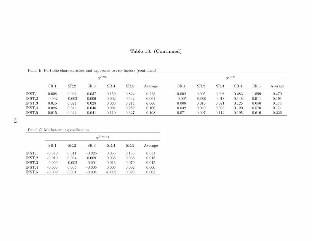
Table 13. (Continued)

Panel B: Portfolio characteristics and exposures to risk factors (continued)

βCRF βLRF

SR,1 SR,2 SR,3 SR,4 SR,5 Average SR,1 SR,2 SR,3 SR,4 SR,5 Average

INST,1 0.008 0.032 0.037 0.159 0.824 0.228 0.002 0.005 0.098 0.483 1.599 0.470INST,2 -0.002 -0.002 0.006 0.002 0.342 0.061 -0.005 -0.009 0.018 0.148 0.911 0.191INST,3 0.015 0.024 0.028 0.033 0.214 0.066 0.008 0.010 0.021 0.125 0.650 0.174INST,4 0.026 0.045 0.046 0.094 0.289 0.106 0.032 0.040 0.035 0.120 0.570 0.171INST,5 0.015 0.024 0.041 0.110 0.327 0.108 0.071 0.097 0.112 0.195 0.616 0.226

Panel C: Market-timing coefficients

βTiming

SR,1 SR,2 SR,3 SR,4 SR,5 Average

INST,1 -0.040 0.011 -0.026 0.055 0.155 0.031INST,2 -0.010 0.004 0.009 0.035 0.036 0.015INST,3 -0.009 -0.002 -0.004 0.013 0.079 0.015INST,4 -0.006 0.005 -0.005 0.003 0.002 0.000INST,5 -0.009 0.001 -0.004 -0.002 0.028 0.003

60