Embed Size (px)
Citation preview

1
On the Cooling of a Buoyant Boundary Current∗∗∗∗
HSIEN-WANG OU
Lamont-Doherty Earth Observatory
Columbia University, Palisades, New York
January 27, 2003
In press, J. Phys. Oceanogr.
∗ Lamont-Doherty Earth Observatory Contribution Number xxxx. Corresponding author’s address: Dr. Hsien-Wang Ou, Lamont-Doherty Earth Observatory, Columbia Uni-versity, Route 9W, Palisades, NY 10964 E-mail: [email protected]

2
ABSTRACT
Through a steady-state reduced-gravity model, we examine the downstream evo-
lution of a buoyant boundary current as it is subjected to surface cooling. It is found that
the adverse pressure gradient associated with the diminishing buoyancy is countered by
falling pressure head, so the overall strength of the current --- as measured by the (trans-
port-weighted) mean square velocity --- remains unchanged. This constancy also applies
to the cross-stream difference of the square velocity because of the vorticity constraint,
which leads to the general deduction that the net current shear is enhanced regardless of
its upstream sign. As a consequence, if the upstream flow contains comparable near-
shore and offshore branches, this parity would persist downstream; but if the near-shore
branch is weaker to begin with, it may be stagnated by cooling, with the ensuing genera-
tion of anti-cyclonic eddies. On account of the geostrophic balance, the buoyant layer
narrows as the square root of the buoyancy --- the same rate as the falling pressure head,
but more rapid than that of the local deformation radius. Some of the model predictions
are compared with observations from the Tsushima Current in the Japan/East Sea.

3
1. Introduction
In the ocean, a warm buoyant current may move poleward along the eastern
boundary, being confined there by the Coriolis force. Examples of such boundary cur-
rents abound, including the Tsushima Current in the Japan/East Sea. As such currents are
separated from the ambient water by a sharpened density gradient across which property
exchanges are curtailed, their buoyancy is more susceptible to depletion by the atmos-
pheric cooling. For the case of the Tsushima Current, for example, frequent cold-air out-
breaks in winter may extract a heat of several hundred 2−⋅ mW from the surface, rapidly
eroding its buoyancy as the current moves north. Because of the heat capacity of the wa-
ter, such poleward decrease of the buoyancy persists into summer even when the surface
is heated.
Questions of obvious dynamical interest include: how does the current respond to
such buoyancy decrease? What might be its eventual fate? The addressing of these ques-
tions is also of practical importance since it may aid our understanding of how the heat
and salt carried by the current may be dispersed.
Surprisingly, there does not seem to be dynamical studies of the problem in the
literature; the closest is perhaps that of Nof (1983), who considered the cooling effect on
the path of a free jet. His study however has little relevance to the present problem since
the path of our buoyant current is affixed to the boundary by the Coriolis force. On the
other hand, also in contrast to a mid-ocean jet, there is a well-defined boundary separat-

4
ing our buoyant current from the ambient, so the conservation laws impose a stronger
constraint on flow properties. As we shall see, such dynamical constraints lead to current
behaviors that are not obvious at the outset, which nonetheless are robust and possibly
testable by observations.
One recognizes of course that other external changes, such as that of the Coriolis
parameter, boundary curvature or bottom topography, may all elicit a response from the
current. Some these responses have been discussed in the literature, and need to be taken
into account when assessing the total behavior of the flow (see discussion in section 5).
The intention here however is to examine the narrow effect of cooling of which our dy-
namical understanding is particularly lacking. To facilitate such understanding, we con-
struct a highly idealized model by removing all non-essential elements, including the
complications mentioned above.
The model is formulated in section 2, which reveals some strong constraints im-
posed by conservation laws. In section 3, the general behavior of the solution is dis-
cussed based on its non-dimensional form. Some model predictions are compared in sec-
tion 4 with observations from the Tsushima Current, and the paper is concluded in sec-
tion 5 by a summary of the main findings and additional discussion.
2. Model

5
Let us consider a model configuration sketched in Fig. 1, which is placed in the
northern hemisphere for convenience. The coastal boundary is taken to be straight and
vertical, so that a right-handed Cartesian coordinate system can be used with x, y and z di-
rected to the east, north and upwards, respectively. On account of the Coriolis force, the
buoyant current is pressed against the eastern boundary and separated from the ambient
by a density interface. The origin of the coordinate system is set at the eastern boundary
at some upstream point where the flow conditions are specified, and z=0 is aligned with
the unperturbed ocean surface outside the buoyant layer. The Coriolis parameter is taken
to be a positive constant for simplicity.
We assume that the vertical mixing has erased the vertical shear within the layer,
which exchanges no mass with the ambient. In accordance, the continuity equation for
the time-mean fields can be integrated vertically through the layer depth h to yield
( ) 0=⋅∇ vh � , (2.1)
which allows the definition of a transport streamfunction ψ as
ψ∇×= kvh ˆ� . (2.2)
The y-component of (2.2) may be integrated in x to yield
∫−=x
ldxhvψ , (2.3)
where l is the width of the buoyant layer, an unknown function of the downstream dis-
tance. This streamfunction spans a constant range [0,Q] across the buoyant layer, with Q
being the volume transport, an external parameter. As seen later, this streamfunction
provides a more convenient independent variable than the cross-stream distance in the
derivation of the model solution.

6
We assume the ambient water outside the buoyant layer to be homogeneous and
motionless, and denoting its variables by the subscript “r” (as in “reference”), the buoy-
ancy b of the moving layer is then defined as
)( ρρρ
−= rr
gb , (2.4)
where g is the gravitational acceleration and ρ , the density. For simplicity, we assume
this buoyancy to be uniform crossing the layer (that is, in both z and x), which can be jus-
tified by its upstream source and/or cooling-induced convection and mixing. It dimin-
ishes however over the longer downstream distance due to surface cooling, and the object
of the study is to examine the change of the flow structure in response. Given the cross-
stream homogenization of the buoyancy, it is coupled to the dynamics only through the
volume transport, independent of the current structure. Combined with the fact that it is
not our intention to explain the buoyancy field, the latter thus may be regarded as external
to the model. Moreover, as it turns out, the buoyancy enters the solution only parametri-
cally, which thus can be used as an independent variable, in place of the downstream dis-
tance. This direct linkage of the flow field to the local buoyancy without reference to the
downstream coordinate allows a broader application of the model --- for example, even in
summer when the ocean is heated so long as the other model approximations remain
valid.
To derive the pressure-gradient force in the presence of a varying density (see
also Nof 1983), one first notes that hydrostatic balance implies that the lower layer has a
pressure of

7
)( hzghgp rr −−+= ηρρ , (2.5)
where η is the surface displacement, and hence is subjected to a pressure gradient force
of
)()(1 hghgpr
rr
ρρ
ηρ
∇−−∇−=∇− . (2.6)
As the lower layer is motionless, one sets this force to zero to derive, using the definition
(2.4),
)(bhg ∇=∇ η , (2.7)
which can be integrated once to yield
bhg =η , (2.8)
since both variables vanish outside the buoyant layer. The surface height thus is propor-
tional to the layer depth --- albeit with a decreasing proportion constant, and (2.8) will be
referred as the pressure head. Similarly, the pressure in the upper layer is given by
)( zgp −= ηρ , (2.9)
which, using (2.8) and the Boussinesq approximation, exerts a force of
)()(1 bhbzp ∇−∇−=∇− ηρ
. (2.10)
Although this force varies vertically, only its vertical average enters the momentum equa-
tion since the velocity is vertically uniform within the layer. Averaging (2.10) vertically,
one derives
∫ −∇−∇=∇−
η
η ρhbhbhpdz
h)(
211 , (2.11)
so the momentum equation is given by

8
)(2
ˆ bhbhvkfdtvd ∇−∇=×+ �
�
, (2.12)
with f being the Coriolis parameter, a constant. It is seen that the spatial variations of
both buoyancy and surface displacement (the two terms on the rhs) may exert a pressure
gradient force. The former in particular has a definite sign --- adverse to the flow --- as
the buoyancy decreases downstream, but since it can be countered by the falling surface,
the flow need not slow down.
Since the buoyancy is constant in x, the x-component of (2.12) states simply that
the time-mean flow satisfies the geostrophic balance
xbhfv = , (2.13)
where the derivative has been short-handed by a subscript. Substituting (2.13) into (2.3),
one derives
2
21
bhf
=ψ , (2.14)
which can be evaluated at the eastern boundary (denoted by the index “0”) to yield
2/10 )/2( bfQh = . (2.15)
It is seen that as a direct consequence of the mass conservation and geostrophy, the layer
depth along the eastern boundary increases downstream. But since this increase is slower
than the inverse of buoyancy, the surface height (2.8) still decreases downstream --- at a
rate of 2/1b . This stretching of the layer would induce a positive shear in the current, a
tendency that is seen later however to be countered by other effects on the vorticity.

9
Taking the curl of the momentum equation (2.12), one derives the vorticity equa-
tion
bhkdtdqh ∇×∇⋅= ˆ
21 , (2.16)
where
)ˆ(1 vkfhq �×∇⋅+= − (2.17)
is the potential vorticity (PV). It is seen that, since the buoyant layer thickens toward the
coastal boundary and the buoyancy decreases downstream, the solenoidal term (rhs in
[2.16]) acts to reduce PV. Physically, this is because the adverse pressure gradient in
(2.12) is greater over the thicker part of the layer, thus tending to induce a negative shear.
Drawing the similar conservation --- and hence mixing --- of PV by the turbulent motion
as the buoyancy, we assume the time-mean PV to be homogenized across the moving
layer, just like the buoyancy. With this approximation, the time-mean of (2.16) can be
integrated cross-stream to yield
yy bhQq 021)( = , (2.18)
where q is henceforth understood to represent the time-mean, and hence given by (from
[2.17])
)(1xvfhq += − . (2.19)
Substituting (2.15) into (2.18), the latter can be integrated in y to yield
)()/2( 2/12/12/1 bbQfqq uu −−= , (2.20)
where the subscript “u” is used hereafter to indicate upstream values --- external parame-
ters of the model. As expected from earlier discussion, the downstream erosion of the

10
buoyancy causes a reduction of PV, which thus may counter the stretching of the layer in
affecting the current shear, as seen later.
The Bernoulli function of course is not conserved with the turbulent motion,
hence its time-mean not mixed as PV. There however is a well-known relation linking
the two on account of the geostrophic balance. With B denoting the (time-mean) Ber-
noulli function
bhvB += 2
21 , (2.21)
it is readily seen from (2.3) and (2.13) that
qddB =ψ
, (2.22)
so its span-wise distribution is known. In particular, with q being uniform cross-stream,
one has then
)2/( QqBB −+= ψ , (2.23)
where overbar is used henceforth to denote the transport-weighted mean so that, for ex-
ample,
∫−≡
QdBQB
0
1 ψ . (2.24)
Since we deal only with time-mean rather than turbulent variables from this point on, this
transport-weighted mean will sometimes be referred simply as “mean” without causing
undue confusion. To examine the downstream variation of B, one takes the dot product
of v� with the time-mean of (2.12) and uses the continuity equation (2.1) to derive the
Bernoulli equation

11
bvhBvh ∇⋅−=⋅∇ �� 2
21)( . (2.25)
As an extension of the previous discussion, the adverse pressure gradient associated with
the decreasing buoyancy acts to diminish the flux of Bernoulli function. As remarked
earlier, this does not necessarily slow down the flow since the decrease can be fully ac-
commodated by a falling surface. Integrating (2.25) in x, we have
∫−=0 2
21)(
lyy dxvhbBQ , (2.26)
or, using (2.13) and (2.15),
yy bbfQB 2/1)/2(31= . (2.27)
Integrating this equation in y, one derives
)()2(32 2/12/12/1 bbfQBB uu −−= , (2.28)
where the upstream value uB is an external parameter. With this, B is now fully deter-
mined as a function of ψ (2.23), so is the velocity from (2.21) given the layer depth.
To translate this dependence on ψ to x, one rewrites the geostrophic balance
(2.13) as
v
dhfbdx = . (2.29)
Expressing v in terms of ψ (through [2.21] and [2.23]) and using (2.14) that relates ψ to
h, (2.29) can be integrated once to yield
−+Γ−+Γ
=
qfhqfh
qfbx
//ln
02/1
0
2/12/1
, (2.30)

12
with
( )qQBqbfh
qfh −+−≡Γ 222 . (2.31)
It is seen that given the values of Q, ub , uq and uB , one now has a full determination of
the flow as a function of the downstream buoyancy b, which will be discussed next.
3. Solution
For a more general discussion of the solution, we non-dimensionalize the vari-
ables according to the following scaling rules (indicated by brackets): ubb =][ , Q=][ψ ,
2/1)/(][ ubfQh = , CRx =][ (Rossby deformation radius) 12/1])[]([ −≡ fhb ,
2/1])][([][ hbv = , ]/[][ hfq = , and ][][][ hbB = . With the non-dimensionalization, (2.20)
and (2.28) become
( )bqq u −−= 12 , (3.1)
and
( )bBB u −−= 1232 , (3.2)
which determine PV and the mean Bernoulli function as functions of the local buoyancy
b. With these variables known, the cross-stream structure of the flow can be expressed as
functions of the streamfunction (from [2.14], [2.23] and [2.21])
2/1)2( ψbbh = , (3.3)
)2/1( −+= ψqBB , (3.4)

13
( )[ ] 2/12 bhBv −= , (3.5)
and the streamfunction is linked to the x-coordinate by (from [2.30])
−+Γ−+Γ
=qh
qhqbx
/1/1ln
02/1
0
2/12/1
, (3.6)
with
( )qBqb
hq
h −+−≡Γ 2122 . (3.7)
As an example of the solution, we have plotted B and bh in Fig. 2a as functions of
the streamfunction at the upstream point (that is, b=1) for the case of =uB 1.061 and
2=uq . For these parameter values, the minimum velocity is nearly zero, which would
accentuate some solution behavior discussed later. Since the square velocity is propor-
tional to the difference of the two curves ([3.5], shaded in the figure), it thus contains
double maxima --- one at the outcrop and the other at the coastal boundary. The former
always exists since the slope of the bh curve there is infinite while that of the Bernoulli
function is finite (given by PV). The maximum at the coastal boundary on the other
hands can be seen to require the inequality 71.02 2/1 ≈> −uq , a condition met by the
above choice of PV. One possible upstream process that may enhance PV --- thus brings
about this branching of the flow --- has been proposed by Ou (2001). As discussed
therein, if the flow has gone through a shallow strait, the frictional torque exerted by the
sill may cause the needed enhancement in PV. The flow structure in the physical space is
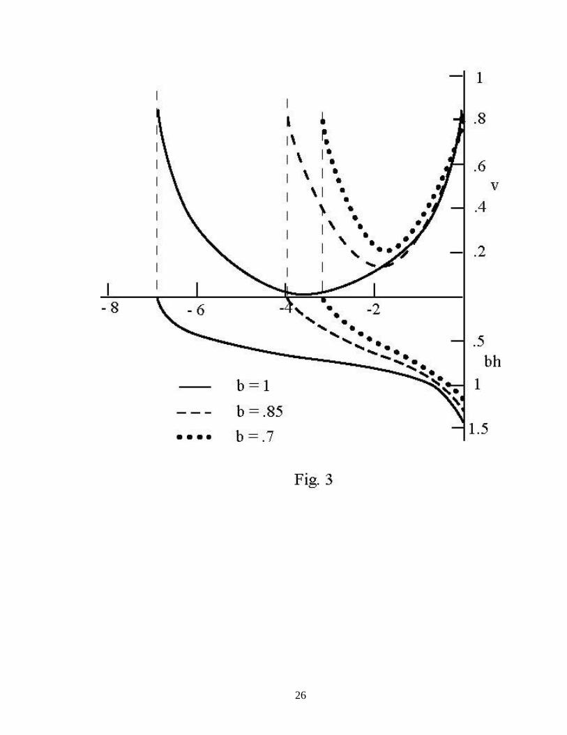
plotted in Fig. 3 (the solid lines). The double cores in the velocity are reflected in the

14
layer depth that contains an inflection point where the velocity is the weakest. Since the
surface height is proportional to the layer depth (2.8), it exhibits the same structure.
To assess how the flow evolves downstream in response to the decreasing buoy-
ancy, we have plotted in Fig. 2 and 3 additional curves for buoyancy that has been re-
duced by 15 and 30 % of its upstream value (i.e. b = 0.85 and 0.7). One notes that al-
though the pressure head is diminished by cooling, as expected from (3.3), the current
strength does not seem to be strongly affected. For a more precise derivation concerning
this feature, let us consider the transport-weighted mean of the pressure head, which is
given by (from the non-dimensionalized version of [2.14] and [2.15])
∫=1
0ψdhbhb
( )b−−= 12322
32 . (3.8)
As this pressure head decreases at the same rate as the mean Bernoulli function (3.2), the
mean square velocity
)(22 hbBv −= (3.9)
is thus unchanged, as can be seen in Fig. 4 by the constant interval of the shaded area
where the mean properties are plotted against buoyancy. In other words, the reduction of
the Bernoulli function by cooling is wholly absorbed by the falling pressure head, so the
mean square velocity maintains its upstream value. As we shall see next, this conserva-
tion also applies to the cross-stream difference (indicated by ∆ ) of the square velocity.
Based on (3.4), (3.1) and (3.3), one notes that
qB =∆
15
( )bqu −−= 12 , (3.10)
and
( )bbh −−=∆ 122)( , (3.11)
so that, from (3.5),
)(22)( 2 bhBv ∆−∆=∆
)2(2 −= uq , (3.12)
independent of the buoyancy.
The current profile of course may change since it is seen from (3.3) through (3.5)
that
( ) ( )bvv u −+−−= 166123122 ψψ , (3.13)
so the flow actually strengthens within the range ]79.0,21.0[∈ψ , while weakening out-
side. This weakening leads to a general result concerning the net current shear, as seen
next. Let the velocity at the offshore edge be denoted by 1v , one has
vvvv ∆+=∆ )()( 102 . (3.14)
Since the lhs is unchanged (3.12) and the velocity at both edges weakens (3.13), the net
shear v∆ thus increases downstream unless it is zero to begin with, in which case it re-
mains zero. Of relevance to the branching feature discussed above, if the upstream flow
contains comparable double cores, this parity would persist downstream --- unaffected by
cooling. The branching feature would become less distinct however since the flow in the
mid-section is strengthened (3.13), thus smoothing the flow. If the upstream flow has a
weak coastal branch, on the other hand, the above enhancement of the current shear may

16
cause the coastal velocity to vanish, beyond which point it becomes imaginary, clearly an
unphysical situation. One logical inference is that eddies would be generated and con-
tinuously shed to accommodate the upstream transport. It is seen therefore that the dy-
namical response to cooling differs qualitatively, depending on the upstream flow struc-
ture, particularly the relative strength of the coastal and frontal branches.
Now that the y-velocity is geostrophic, the deduction that its overall strength is
unchanged implies the same for the overall cross-stream pressure gradient. As a conse-
quence, one expects the layer to narrow at the same rate as the decreasing pressure head,
or 2/1b , consistent with the solutions shown in Figs. 2 and 3. One notes that this narrow-
ing is more rapid than the local deformation radius, which varies as ( ) 4/12/10 bbh ∝ . In
this context, it should also be pointed out that although the y-velocity varies cross-stream
on the scale of the deformation radius, the total layer width can be much greater since
there can be extensive region of negligible velocity. For the upstream flow shown in
Fig. 3 with a near-zero minimum velocity, the buoyant layer is seen to span many defor-
mation radii. The evening out of the velocity profile is consistent with the more rapid
narrowing of the layer than the deformation radius.
4. Application
It is seen that, given the model idealization, a simple application of the conserva-
tion laws leads to strong constraints on the flow behavior, and one wonders if some
model predictions can be discerned from observations. For this purpose, we turn to the

17
Tsushima Current, which motivates the present study and is among the most extensively
surveyed boundary currents. Of particular relevance, Katoh (1994) has obtained direct
current measurements across several transects of the current after it leaves the Tsushima
Strait (see his Fig. 5). His data have provided the strongest confirmation yet of the exis-
tence of two branches: a near-shore branch along the 100 m isobath (approximately
where the thermocline intersects the bottom) and an offshore branch along the thermal
front (see his Fig. 3) --- a feature that in fact motivates the solution shown in Fig. 3. It is
recognized that the area contains considerable topographic irregularity, causing large ex-
cursion of the current. For example, the cyclonic loop as the current approaches Mishima
may induce negative shear, possibly accounting for the disappearance of the near-shore
branch along transect E. But downstream of the island where the isobaths are relatively
straight, there appears to be narrowing of the current (from sections F to H in his Fig. 5),
as also reflected in the width of the buoyant layer (his Fig. 3). One is tempted to correlate
this feature with the variation of the 200 m isobath, but, as noted above, the buoyant layer
is anchored at about 100 m, so the offshore branch is not likely strongly tied to the deeper
isobaths. Despite the narrowing, one also notes that parity in the two branches is main-
tained, with a strengthening of the in-between flow, resembling the solution shown in
Fig. 3.
Based on his Figs. 10 and 3 (the June data), one may set the temperature below
the buoyant layer to be 10 Co and a temperature change of the buoyant layer from 16 to
14 Co between transects F and H, which corresponds to a buoyancy reduction of about
30 %, incidentally the range covered in Fig. 3. The Rossby deformation radius at section

18
F is estimated to be 15 km, so the current width shown in Fig. 3 narrows from about 100
to 50 km, not inconsistent with that observed. As noted earlier, the wide upstream layer
is the consequence of near-zero minimum velocity, which nonetheless can be representa-
tive of the observed current at section F (see his Fig. 6). Given the uncertainty in obser-
vation and idealization of the model, the above comparison is only suggestive of the rele-
vance of the model and cannot be viewed as its confirmation.
As the current structure is linked to the pressure head via geostrophy, which in
turn is reflected in the surface height, one naturally thought the altimeter data may pro-
vide a useful test of model predictions. Unfortunately, the near-shore branch is anchored
over the shelf, so one may not determine the geoid from an assumed level of no motion.
5. Summary and discussion
To examine the evolution of a buoyant boundary current when subjected to sur-
face cooling, we have considered a reduced-gravity model in which buoyancy and PV are
homogenized across the moving layer, which exchanges no mass or momentum with the
ambient water. Application of conservation laws of mass, PV and Bernoulli function is
found to lead to strong constraints on the flow behavior in response to diminishing buoy-
ancy, as summarized below:
• The adverse pressure-gradient is countered by falling pressure head, so the overall
strength of the current as measured by the (transport-weighted) mean square ve-
locity remains unchanged.

19
• The stretching of the layer along the coastal boundary is countered by the sole-
noidal term in the vorticity balance, so the cross-stream difference of the square
velocity is also unchanged.
• Regardless of the upstream sign of the net current shear, it is enhanced down-
stream, which may cause stagnation of the coastal flow if it is relatively weak to
begin with, leading possibly to the generation of anti-cyclonic eddies.
• If the upstream flow contains comparable coastal and frontal branches, the parity
would persist downstream, although the branching feature is rendered less distinct
as the current is smoothed.
• The buoyant layer narrows downstream at the same rate as the falling pressure
head, which is more rapid than that of the local deformation radius.
It is seen that the buoyancy current may evolve differently, depending particularly
on the relative strength of the coastal and offshore branches. If the coastal flow equals or
exceeds the frontal jet, the current eventually barotropicizes as its buoyancy is depleted;
if, on the other hand, the coastal branch is weaker, the current may degenerate into anti-
cyclonic eddies, which, through self-propagation, may cause a wider dispersal of its salt
and heat content.
While some model predictions are consistent with observations from the Tsu-
shima Current, a more definitive interpretation of the observation clearly lies beyond the
narrow scope of the present model that considers only the cooling effect. A curvature in
the coastal boundary, for example, may induce current shear via PV conservation --- the

20
reason that the above comparison is made over a relatively straight stretch of the coast.
The effect of a shelf topography can be quite subtle. The compression of the layer as it
intrudes onto the shelf would induce negative vorticity, which however is countered by
the frictional torque acting on the flow. As the bottom friction dissipates the barotropic
flow, it expels the transport offshore on account of the mass conservation, which would
stretch the layer and enhance the coastal branch. While a dynamical study is needed to
sort out these interplays, so long as the bottom slope is large compared with that of the in-
terface, it may be approximation by a vertical wall.
Acknowledgments. This research is supported by the Office of Naval Research
under the Japan/East Sea initiative (Grant N00014-99-1-0092).

21
REFERENCES
Katoh, O., 1994: Structure of the Tsushima Current in the Southwestern Japan Sea. J.
Oceanogr., 50, 317-338.
Nof, D., 1983: On the response of ocean currents to atmospheric cooling. Tellus, 35A,
60-72.
Ou, H. W., 2001: A model of buoyant throughflow: With application to branching of the
Tsushima Current. J. Phys. Oceanogr., 31, 115-126.

22
FIGURE CAPTIONS
FIG. 1. The model configuration showing a buoyant current moving poleward along an
eastern boundary (positioned in the northern hemisphere). The buoyant layer is
separated from the motionless ambient by a density interface, across which there
is no exchange of mass or momentum. The buoyancy is homogenized across the
moving layer, which decreases downstream due to surface cooling, and the object
of the model is to determine the evolution of the current structure in response to
such buoyancy change.
FIG. 2. (a) Bernoulli function and pressure head as functions of the streamfunction at the
upstream point (i.e. b=1) for the parameter values of uB =1.061 and 2=uq .
The dashed line marks the (transport-weighted) mean Bernoulli function, and the
shaded area is proportional to the square velocity. For this choice of parameters,
the upstream flow contains double maxima at the front and the coastal boundary
with equal strengths; (b) same as (a), but for the downstream point of b=0.85.
The transport-weighted square velocity is unaltered and the parity of the two
branches is maintained; (c) same as (a) but farther downstream at b=0.7. The
above trend continues and the branching becomes less distinct with smoothing of
the flow.
FIG. 3. The stream-wise velocity and the pressure head (or equivalently the surface
height) for the three transects shown in Fig. 2, but plotted against the span-wise

23
distance. It is seen that the current profile is smoothed downstream, but its over-
all strength is unchanged. The buoyant layer is narrowed in proportion to the de-
creasing pressure head, which is more rapid than the local deformation radius.
FIG. 4. The layer width, PV, the transport-weighted mean values of the Bernoulli func-
tion and pressure head plotted against the buoyancy. The last two decrease at the
same rate, so the mean square velocity (proportional to the shaded interval) re-
mains unchanged. The current narrows with decreasing buoyancy, at a more
rapid rate than the local deformation radius. The dashed lines mark the buoyancy
of the solutions shown in Figs. 2 and 3.

24

25
26

27