QTATIONARY SOLUTIONS OF ABSTRACT KINETIC EQUATIONS/

. by

Wlodzimierz Ignacy\}Valus

Dissertation submitted to the Faculty of the

Virginia Polytechnic Institute and State University

in partial fulfillment of the requirements for the degree of

DOCTOR OF PHILOSOPHY

in

Mathematics

APPROVED:

- /„ /) p .Ä;

,//„

· v,M«¢6ߧ l' i ( V;-jqg

W. Greenberg, Chair n 4 J. Arnold

G. Hagedorn _ .... .1, J.4Slaäny

·"w„ I

/7

x- ‘ 4/‘“ "/JF,-J-Fix

M. Williams P.F. Zweifel

August 1985

Blacksburg, Virginia

(Y STATIONARY SOLUTIONS OF ABSTRACT KINETIC EQUATIONS

by\¤

ä Wlodzimierz Ignacy \«Valus ·

%Committee Chairman: William Greenberg

i

Mathematics

(ABSTRACT)A

The abstract kinetic equation T¢•’=-Agb is studied with partial range

boundary conditions in two geometries, in the half space x20 and on a finite

interval [0,1*]. T and A are abstract self-adjoint operators in a complex Hilbert

space. In the case of the half space problem it is assumed that T is a (possibly)

unbounded injection and A is a positive compact perturbation of the identity

satisfying a regularity condition, while in the case of slab geometry T is a bounded _

Ainjection and A is a bounded Fredholm operator with a finite dimensional negative

part. Existence and uniqueness theory is developed for both models. Results are

illustrated on relevant physical examples.

ACKNOWLEDGMENTS

First, I would like to thank Dr. William Greenberg, my advisor and mentor.I

He introduced me to the subject of abstract kinetic theory and openly shared his

ideas with me. His advice and encouragement have helped me to achieve my

academic goals. To him I owe many suggestions and improvements which haveI

influenced the final version of this dissertation. Moreover, his warm friendsliip and

assistance in every day life situations have helped me very much during the years

I have spent in Blacksburg. I will always feel indebted to him.

I would like to express my gratitude to allithe members of The Center for

Transport Theory and Mathematical Physics for creation of the atmosphere which

stimulated my growth as a mathematical physicist. I also thank Profs. William

Greenberg and Paul F. Zweifel for providing financial support during summer months

of my stay at Virginia Tech.

I would also like to mention here the Polish community in Blacksburg. In

the course of time, this small group of people, once strange to me, has become

"the other family°' for me. With them I shared my doubts, sorrow as well as

expectations and happiness. I thank all of them for this.

Finally, I would like to thank my wife . I realize that without her love,

constant encouragement and sacrifices I would not have been able to

complete my studies. I dedicate this work to her.

‘l‘l'l

TABLE OF CONTENTS

Chapter I Introduction 1

Chapter II Dissipative models: Strictly positive collision operators 8

1. Definitions and preliminaries 8

2. The boundary value problem · 10

3. Properties of the operator V 14

Chapter III Conservative models: Collision operators with nontrival kernel 24

1. Decompositions and reductionS

24

2. Existence and uniqueness theory for half space problems 31

Chapter IV Nondissipative models: Collision operators with negative part 39

1. Preliminaries and decompositions 39

2. Solution of the boundary value problem 45

Chapter V Applications 55

1. The scalar BGK equation 56

2. The one dimensional BGK equation 57

3. The BGK equation for the heat transfer 58

4. The isotropic neutron transport equation 59

5. The symmetric multigroup transport equation 60

References 62

iv

CHAPTER I .

INTRODUCTION[

Over the past three decades, a variety of functional analytic techniques

have been developed for the study of properties of many transport equations which

occur in physical models, including neutron transport in nuclear reactors, polarized

light transfer through planetary atmosphers, electron scattering in metals, and

kinetics in rarefied gases. The most popular of these techniques (from early in the

1960’s and until the present in many engineering and physics circles) has been the

eigenfunction expansion method first introduced by Case in 1959 [7,8], based in part

on an earlier work of van Kampen [26].

In 1973, Hangelbroek [18,19] introduced a Hilbert space technique based on

a detailed analysis of certain noncormnuting projections, which he applied to a

one—speed neutron transport equation. Although in these articles explicit use was

made of the Wiener-Hopf factorization of a dispersion function (symbol of the

equation), it was later shown, in joint work with Lekkerkerker [23], that the

required factorization was a corollary of some operator constructions carried out in

the analysis. Because this Hilbert space technique leads to the study of abstract

versions of transport equations, and because it avoids the difficulties of

\Viener-Hopf factorizations (or Riemann matrix problems), it has been intensively

l

2

studied in the last few years.

The common feature of stationary linear transport processes in plane

parallel geometry is! that each of them is described by a linear

Uintegro—differential equation which can be written

T·J»'(><) = —A¢(><). (1)

where T and A are certain self—adjoint operators on a Hilbert space, with A

representing the collision process for the particular physical model. The specific

form of the operators T and A depends on the nature of the problem, but several

properties of these operators are shared by almost all models, such as

self—adjointness of T and A, injectivity of T, and in many important cases

positivity of A and compactness of I—A. Therefore it is natural to develop a

unified theory for all of these physical models. iThis approach has led to the

foundation of so called abstract kinetic theory, where Eq.(1), referred to as an

abstract kinetic equation, is the central object of study. I

In this dissertation we present an existence and uniqueness theory for a

class of problems in abstract kinetic theory relevant to rarefied gas dynamics and

neutron transport in multiplying media. First we describe briefly the type of

physical problems we have in mind and which we wish to study in abstract

generalization.

In rarefied gas dynamics, the BGK approximation of the Boltzmann equation

leads to the kinetic equation

8 4gl? + V-V¢1=O

where 1ß(t,x,v) represents the molecular density of particles having velocity v at a

point x at time t, 1bi, i=0,l,2,3,4 are the collision invariants of mass, the three

momenta and energy, and l/(V) is the collision frequency. We assume that the

3

collision invariants are normalized such that (1/2i,z/2j)=6ij. Under the assumption of

constant collision frequency the stationary version of this equation in plane parallel

geometry is futher reduced to

gp? 4Vx dx = —¢ (2)

The above equation and its various modifications have been studied in many

contexts (cf. [1,5,6,1l,13,27,42]). An excellent introduction to the Boltzmann

equation and related model equations can be found in Cercignani’s monograph [10],

to which we refer the reader for additional details and physical background.

Equation (2) takes the form of Eq.(1) if we define

(T~/»)(v) = vX¢(v)

andi

4

In this example the operator T is unbounded, injective and self—adjoint on the

Hilbert space H=L2(lR3,(rr3)_%e_v2dv), while A is a positive compact perturbation

of the identity. These properties of T and A will be the assumptions under which

we will study Eq.(1) in the half space x20. Equation (2) will serve then as an

example of our study.

In the one—speed approximation, stationary neutron transport in a plane

parallel homogeneous medium is described by the following equation

(3)

Here the unknown function zb represents the angular density of neutrons,

;46[—1,1] is the cosine of the angle describing the direction of propagation and

x is the position coordinate. The scattering kernel has the form

4

211*f(p,u) = (211*)-1].0 p(p1/+(p2-1)%(u2—1)%cosa)da.

The function p is determined by properties of the host medium. The value

cf(;1,u) gives the probability that the collision of a particle having velocity "in , „

the direction 1/" with the host medium results in a secondary particle with

velocity direction p. Therefore we assume that p is nonnegative and satisfies

the normalization condition

1 15] p(1)d1=1.

-1

Then c is the mean number of secondaries per collision. If 0<c<1 the host

medium is absorbing, c=1 corresponds to a conservative medium and c>1 to a

multiplying medium. For additional details we refer the reader to the classic text

by Case and Zweifel Equation (3) has been analyzed extensively in the case of

absorbing and conservative media (cf. [3,18—23,33,36]) but very few studies have

dealt with the case of a multiplying medium (cf. [2,37,38]).

If we define

(T1/»)(#) = #1/»(u)

and

1

then Eq.(3) can be rewritten in the form In this example T and A are bounded

self—adjoint on the Hilbert space H=L2[-1,1]. If 0<c<1, A is strictly positive; if

c=1, A is positive but has a nontrival kernel; and if c>1, A is no longer positive.

Indeed in this latter case the spectrum of A contains strictly negative eigenvalues.

We will study Eq.(1) on a finite spatial domain [0,1] for bounded self—adjoint

Fredholm operators A which have "a -finite negative part". Since relevant physical

applications come from neutron transport theory, we assume for the sake of

5

simplicity that T is bounded.

The abstract kinetic equation as well as concrete kinetic models have been

studied mostly for positive collision operators A. An important exception is the

recent work of Greenberg and van der Mee [16], where the half space problem for

Eq.(1) with A having a finite negative part has been solved. \Ve also note an

earlier paper by Ball and Greenberg [2], where the use of I”IK—space

(Pontryagin space) theory has led to spectral analysis of the one—speed isotropic

neutron transport equation in a multiplying medium. Our treatment of Eq.(1) on

finite intervals [0,1*] with A having a finite negative part is new.

l

The theory for positive A so far developed either assumes that the operator

T is bounded or seeks solutions in an "enlarged" space HTDD(T) (weak solutions).

For T bounded, the existence and uniqueness theory for H—valued functions

(strong solutions) has been developed by Hangelbroek for A a concrete rank one

perturbation of the identity [18,19] and for I—A a trace class operator from neutron

transport [20]. In both these studies the collision operator A was assumed

invertible. The critical case (conservative medium) for the one—speed neutron

transport equation, in which A has a nontrivial kernel, has been solved by

Lekkerkerker [33]. Equation (1) for I—A an abstract compact operator satisfying a

"regularity condition" and T bounded has been studied extensively by van der Mee

[34], who obtained a complete existence and uniqueness theory for the half space

and slab problems with partial range boundary conditions. In this dissertation we

extend the existence and uniqueness results of van der Mee [34] to the case of T

unbounded.

Existence and uniqueness theory for weak solutions was developed initially

by Beals In his innovative work both half space and slab problems have been

analyzed. The approach he initiated has since been applied to more general

6 .

abstract kinetic equations. We_note the work of Greenberg, van der Mee and

Zweifel [17], where the case of positive self—adjoint Fredholm collision operator A

with nontrivial kernel has been studied.

Now 'let us review the aim of this dissertation. \Ve consider an abstract

kinetic equation

T¢'(><) = —A«l»(><) _ (1)in two geometries, in the half space x20 and on a finite interval [0,1*].

In'the first case we assume that T is a self—adjoint, possibly unbounded,

injective operator on a complex Hilbert space H and A is a positive compact

perturbation of the identity. We study Eq.(l) together with the partial range

boundary condition at x=0

Q+¢(0) = $9+, (4)

where Q+ is the orthogonal projection onto the maximal T—positive T—invariant

subspace of H, and with a condition at infinity, namely one of

||1!»(x)l| = 0, (5a)

||¤/»(x)l| < <>¤, (5b)

II¢(x)II = O(x) as x—»oo. (5c)

We prove theorems describing the measure of noncompleteness (which we define as

the codimension in Ran Q+ of the subspace of boundary values $O+€R&H Q+ for

which the problem is solvable) and the measure of nonuniqueness (the dimension of

the solution space of the corresponding homogeneous problem) for the boundary

value problems (1)-·(4)—(5).

In the second case, T is bounded, self—adjoint and injective but A is no

longer required to be positive. \Ve assume that A is a bounded self-—adjoint

Fredholm operator with a finite negative part. Now Eq.(l) is studied together with

the partial range boundary conditions

7

Q+¢(6) = <P+, (4)

Q;/»(r) = <P_, (6)

where Q_=I—Q+ is the orthogonal projection onto the maximal T—negative

T-invariant subspace of H and <p+, <,o_ are given vectors in the ranges of Q+,

Q_ respectively. We prove that for any incoming fluxes <p+, <p_ the

boundary value problem (l)—(4)—(6) is uniquely solvable for values of r less then a

certain critical value.A

The·presentation of the dissertation is organized as follows. In Chapter II

we study the half space problem for strictly positive collision operators A. There

we introduce the albedo operator and study its properties. The existence and

uniqueness theorem is shown to be a consequence of the bounded invertibility of

Mthe albedo operator. In Chapter III we generalize the results of the previous

chapter to positive collision operators A. This generalization is possible due to a

decomposition of the Hilbert space which reduces the relevant transport operator.

In the first part of Chapter III we show that such decomposition exists. Then in

the second part we construct solutions of the half space problems (1)—(4)—(5)

and prove the corresponding solvability theorems. Chapter IV is devoted to the

study of the abstract slab problem (1)-(4)—(6) for collision operators having a finite

negative part. First we introduce another useful decomposition of the Hilbert

space, which is in fact a generalization of the one used in Chapter III. \«Vith the

help of this decomposition we prove the existence and uniqueness theorems for

weak and strong solutions of the slab problem. In Chapter V we demonstrate

applications of our results to several physical problems. The first three examples,

which come from rarefied gas dynamics, illustrate the results of Chapter III. The

other two examples, both from neutron transport, illustrate the results of Chapter

IV.

. CHAPTER II

DISSIPATIVE·MODELS: STRICTLY POSITIVE COLLISION OPERATORS

We study the abstract kinetic equation

(Ti/¤)’(><) = —A¤/»(><)» 0<><<<=¤, (1)

, along with the partial range boundary condition at x=0

Q+¢(0) = s¤+ (2)

and the growth condition at infinity

lim II1/¤(x)II < ¤¤. (3)_ X-mo

We assume that A is a strictly positive compact perturbation of the identity and

satisfies a regularity condition.

L DEFINITIONS AND PRELIMINARIES

Let H be a complex Hilbert space with an inner product and T an

injective self—adjoint operator on H. We define Qi as the complementary

orthogonal projections onto the maximal T—positive/negative T invariant subspaces

of H. Throughout this chapter A will be a strictly positive operator on H such

that B=I—A is compact. Then KerA = {0} and A—1=I+C, where C=BA·-1 is

obviously compact. Since A andA_l

are bounded, the inner product (·,·)A on

8

9

H defined by

(f.s)A = (Als)- (4)

is equivalent to the original inner product on H. We will denote by HA the Hilbert

space H endowed with the inner product (·,·)A.

LEMMA M. The operator S=A—1T is injective and self—adjoint with

respect to the HA-innerproduct_P_1_p_ci:

Clearly D(S)=D(T). Let f,g6D(S). Since T and A are self—adjoint

(Sf,g)A=(Tf,g)=(f,Tg)=(f,Sg)A which shows that S is symmetric, i.e. ScS*. Now let

f6D(S*). Then the functional D(S)ag—»(f,Sg)A=(f,Tg) is continuous on D(S)=D(T).

Since T is self—adjoint this implies that f6D(T)5=D(S). Hence D(S*)cD(S) and

s=sL¤

ASince S is self—adjoint and injective we can define Pi as the

complementary (·,·)A— orthogonal projections of H onto the maximal

S—positive/negative S—invariant subspaces of H. Moreover Pi, as well as Qi,

are invariant on D(T) and are bounded complementary projections on the complete

inner product space D(T) with the graph inner product defined by

. (f.s)GT = (Rs) + (TCTS)- (5)

The self·—adjointness of S with respect to the inner product (4) allows the

machinery of the Spectral Theorem to be introduced. If is the resolution of

the identity associated with S, we can define the operator valued functions

exp{$zT_1A}Pih = x Iäcoen/t'dF(t)h, h6H, (6)

for Rez>0. Then the restrictions of exp{¢zT_1A}Pt to Ran Pi are bounded

analytic semigroups on Ran Pi whose infinitesimal generators are the restrictions

IO

of 1T—1A to Ran Pi. From the injectivity of A and the dominated

convergence theorem, we have lim IIexp{¢xT_1A}PihIl = 0 for hEH.X—>oo

Moreover, the strong (and even uniform) derivative of the expression (6) exists for

xE(0,¤¤), belongs to D(T) and satisfies the differentialequationL

E BOUNDARY PROBLEM

In this section we shall prove the existence and uniqueness theorem for the

right (left) half space problem

(Tab)'(x) = —Aab(x), O<xx<¤¤, (1)

Qi¢(0) = <Pi„ (2)

lim IIab(x)II < ¤¤.l

(3)x—>:¤¤

( We define a solution of the boundary value problem (1)-·(3) for any

to be a continuous function abt[0,<><>)—·D(T) (1/¤I(—¤<>,O]—>D(T))

such that Tab is strongly differentiable on (0,¤o) ((—¤¤,0)) and Eqs. (1)—(3) are

satisfied.

LEMMA Q. ab(x) is a solution of the boundary value problem (1)—(3) if

and only if

ab(x) = e_xT-lAhi, 0<:x<¤¤, V (7) I

for some htERan PiV1D(T) with Qih=api. Such solutions are strongly

differentiable on (O,¤¤) ((—¤¤,0)) and vanish at infinity with respect to the original

norm on H as well as the graph norm on D(T),

: We will consider the right half space (1)-(3) only. The proof for

the left half space problem goes along the same lines. Suppose that

ll

wb:[0,«>)—>D(T) is a solution of the boundary value problem. Using the facts that

wb:[0,¤¤)—•H is continuous, A is bounded and (Twb)'(x)=—Awb(x), we have that the

function (Tw,/;)' is bounded and continuous on (0,oo). Since, for Ü<€,X<00,

x _ xTwb(x) — Twb(6)·= (Twb’)’(x)dx = —A)~ wb(x)dx (8)

6 6it follows that Twb is continuous on (0,¤¤) and IITwb(x)II=O(x) as x—>oo. For all

m xxxRe)\<0 and m>0, we have e wb(x)dx€D(T) and6

m m _TI ex/>‘wb(x)dx = ex/>‘Twb(x)dx,

6 6whence

m x/>„0 = xl e [(Twb)’(x)+Awb(x)]dx =

6

X/>. x=m m xxx= [ke Twb(x)]x=€ — (T—)«A))‘ e wb(x)dx. (9)6

Notice that from (8) it follows that Twb(x) has a strong limit as x—»0. Using the

fact that wb is continuous on [0,¤¤) and T is a closed operator, the limit is, in

fact, Twb(0). Thus one can conclude that (9) is valid for 6=0. Noting also that

Äex/>‘Twb(x) vanishes as x—•¤o, we have

jzex/M;„(x)dx = >\().—A_1T)_1A_1Twb(0)for all nonreal X in the left half plane. The left hand side of this expression

has an analytic continuation to the left half plane and so does the right hand side.

But this forces wb(0)€ Ran P+F1D(T) and thus Eqs. (4)—(5) specify an initial

value problem on Ran P+ whose solution must have the form The identity

Q+h=<p+ is immediate, as is the proof of the converse argument.!

Lemma II.2 provides a solution of the boundary value problems (1)—(3) if

one is able to find vectors hi such that the conditions Q+h=<,o+ are satisfied.

Since hi€Ran Pi¤D(T) one can combine these two conditions into the

l2

following single equation

(Q_,_P+ + Q_P_)h = <P

where h=h++h__ and <p=<p++<p_. Let V=Q+P++Q_P_. Clearly V maps

Ran Pi into Ran Qi. Therefore if we show that V is invertible,E=V_1

isboundedthe choice of the vectors hi will be possible. One can simply take

ht=E<pi. To secure that hi belong to D(T) whenever ¢i€D(T) we will

also have to prove that V maps D(T) onto D(T). lt is clear that the above choice

will be unique and consequently the boundary value problem (1)—(3) will be °

[uniquely solvable.

The operator V was first introduced by Hangelbroek [18,19] in the context

of isotropic one—speed neutron transport. In that study a Wiener—Hopf

factorization was assumed to exist for the dispersion function associated with the

integral equation, and the invertibility of V was a consequence of the known

factorization. It was not until 1977, in joint work with Lekkerkerker [23], that the

invertibility of V was shown to be equivalent to the Wiener—Hopf factorization.

The operatorE=V_1

is sometimes refered to as the albedo operator. One

can give simple physical interpretation for the action of the albedo operator.

Namely, in transport theory language, if <pi6Ran Qi is an incoming flux at the

boundary x=0 for the right (left) half space problem then E<pi will be the

corresponding total (i.e. incoming and reflected ) flux at x=0.

The properties of the operator V are collected in the next lemma. The

proof of this lemma requires a regularity condition for the collision operator A.

Since the proof is rather lengthy and technical, we will postpone it as well as the

formulation of the regularity condition to Section 3. Here we limit ourselves to

the statement of the lemma.

. 13

LEMMA The operator V is invertible andE=V_1

is bounded on H

and V maps D(T) onto D(T).

Now Lemmas II.2 and II.3 give us the principal result of this section.

THEOREM lg. The right (left) half space problem

(T1ß)’(x) = —A1/2(x), 0<:x<o¤,

Qi¢(0) = sei, ‘

11m I|¢(><)II < ¤<>,X—>1oo

is uniquely solvable for each <piEQi[D(T)], and the solution is

-11b(x) = e_XT AE<pi, 0S:x<¤o. —

It is possible to seek solutions of the boundary value problem for all

<pi€Qt[H] rather then just <pi€Qi[D(T)]. However, in this case it seems

necessary to reformulate the problem slightly. The differential equation (1) is

replaced by

T1ß’(x) = —A1b(x), 0<::x<¤¤, (10)

and a solution is defined to be a continuous function 1/;:[0,¤¤)-H (1/1:(—¤¤,0]—>H)

which is continuously differentiable on (0,¤o) ((-¤¤,0)) such that 1l:'(x)€D(T) for

x€(0,«>) (x€(—¤o,0)), and which satisfies (10)-(2)—(3). Then one can prove

the following analog of Theorem II.4.

THEOREM The right (left) half space problem

Ti,/2’(x) = -A¢(x), 0<1x<¤o,

Q;/>(0) = wi.

141

lim ||¢(x)|| < ¤<>,X—>;too

is uniquely solvable for each <pi€Qi[H], and the solution isI

-1 .1/2(x) = e_XT AE<pi, 0$:x<¤¤.

Q; PROPERTIES Q THE OPERATOR Y

We prove here Lemma II.3 stated in the previous section. We shall

establish the injectivity of V on H and the compactness of I—V on H and on D(T)

equipped with the graph norm Once these are proved, the Fredholm alternative

gives the boundedness ofV—1

and shows that V[D(T)]=D(T).

We present four technical lemmas which will be used in the subsequent

analysis. The first is a result on Bochner integrable functions. The proof of this

result as well as the exposition of Bochner integral theory can be found in the

monograph by Hille and Phillips [24].

LEMMA Let T be a closed linear operator on H. If f is a Bochner

integrable H-valued function on Q such that Tf is also Bochner integrable on Q,

then

D(T)(2

and1

T( f()„)d>„) = Tf(>„)d>„.

The next lernma is a consequence of the norm closedness of the ideal of

compact operators in thealgebraLEMMA

The integral of a (norm) continuous compact operator valued

15

function with integrable norm is a compact operator.

The following two lemmas involving fractional powers of positive operators

are, standard. For compeletenees we will present proofs, which have been taken

from Krasnoselskii et al. [28]. The first lemma is a consequence of the Hölder

inequality, while the second one was originally proved by Krein and Sobolevskii

[30].

LEMMA Let A be a positive self—adjoint operator. Then for any

1*€(0,1) and any h€D(A) we have IIAThIlSIIAhIITIIhIl1_T.

Proof: Let E be the resolution of the identity for the operator A. Then if

1*6(0,1) and hED(A), it follows from the Hölder inequality that

1* 2 °° 1*IIA hll = ] x d(E(x)h,h) S0

0 0

LEMMA Let A be a strictly positive self—adjoint operator and B a

closed operator satisfying HBhIISkIIAhIITIIhII1_T for any D(A) and some

1*€(O,1). Then for all 1*<6<1, D(Aö)cD(B) and for any h€D(A6),

|IBh||sk0l|A6hII.

Proof: First of all note that since 0(A)C[a,¤o) for same a>O and D(A)CD(B),

the vector valued function

t—»t_TB(tI+A)_1h = BA-1t_TA(tI+A)_1h

is well defined and continuous on (0,¤¤) for any h6H.

Now using the hypothesis of the lemma and the following estimates

l6

ll (tI+A)"1 Il $(a+t)—1,

IIA(tI+A)II$1 for any t20 ,

we show that for r<5<1

°° 6 1I F ||B(tI+A)” hlldts

0

kvlwföIIA(tI+A)—1hII T |l(tI+A)'1hIl1'Tdt$

0

k)-0t—6(a+t)T_1dtIIhII =k1IIhII.

°° 6 1This means that It- (tI+A)_ hdt 6 D(B) and

O

B‘|i°°t"6(tI+A)”1hdu = V°t—6B(tI+A)'-lhdt 1O O

(cf. Lemma II.6). Therefore, since for any o16(O,1)A_a

= 1r—1sina1r)‘°°t_CY(tI+A)—ldt0

we have the estimate IIBA—6hIISk0HhII for any h€H, where k0=k11r—1sina11·.

Now this implies that DA5 CDB and IIBhlI$k IIA6hII for any h6D A5 .¤0

In addition to the compactness of I—A, we shall assume throughout the

regularity condition:

3a€(0,1) and w>max{%)i,l§£}: Ran(I-A)CRan(ITIa)f'1D(ITI1+w). (10)

LEl\/IMA II.10. The operators P —Q are compact on H and the restrictions——-—— 1- 1 1

of Pi—Qi to D(T) are compact on D(T) endowed with the graph inner product

(5). Moreover

17

Proof: Since P+—Q+=-(P_-Q_) we will give the proof for P+—Q+ only.

We will prove first that P+·-Q+ is compact on H and (P+-Q+)[H]cD(T). Let

A1=A(6,M) denote the oriented curve composed of the straight lines from -i6

to —i, from -i to M—i, from M+i to i, and from +i to +i+6. Let A2=A(M)

denote the oriented curve composed of the straight lines from M—i to +¤¤-i

and from +¤¤+i to M+i. Denote A=A1UA2 with the orientation inherited from

A1 and A2. We recall that the projections P+ and Q+ are bounded on H and

on D(T) endowed with the graph inner product We have the integral

representations

P = lim—L·— (x-s)‘1d>.,

- 1 -1„ Q+ = dx, »where the limits are in the strong topology. Let

(1)_.1)‘_-1 (2)_1 _—1

and

Qfrl) = nmyjx)6->0 A1 A2

Then one has

- - (1)_ (1) (2)_ (2)P+ ($2+ — (P+ Q+ ) + (P+ Q., )- (11)

We will show that P$_l)—Q$_1) and P_$_2)—Q$_2) are compact on H, and

(P_$_1)—Q$_1))[H]CD(T) as weil as (Piz)-og ))(H}cD(r).Consider first

(12)6-*Ü A1

We shall see that this limit can be taken in the norm topology. We exploit the

regularity condition (10) and obtain from the Clos·ed Graph Theorem the existence

of a bounrl•·-I operator D such that B= ITIQD. Then for nonreal >«

18

- - -1 -<x—S> 1-0-1*) 1 = <S—T><x—S> 1 == ()\—T)_1BS(>«—S)—1 = ()«—T)_1ITIaD S(>‘—S)'1,

which shows that (X-S)_1-(}«—T)_1 is a compact operator on H. Next, since S

is self-adjoint on H with respect to the inner product (4), we may use the

Spectral Theorem to show the norm estimate

‘ S ’1 i-.L <IlS(1p S) III-(HA) S 1.

But the inner products on H and HA are equivalent, and thus also are the L(H)

and L (HA) norms, so there is a constant co such that. -1 ·

L

Likewise, from the Spectral Theorem,

oz · -1 te 0:-1"T -. *

— „IIITI (1;: ) IIL(H) <iälgll/Ä_tI

< calpl

Thus

¤¤< - >i<>—S>‘1—<x—T>‘11«m¤ SiA<6.M> iA(·1.M> 1(H),7

a—1S dp

which shows that the limit (12) exists in the operator norm topology, and

consequently proves the compactness ofP_S_1)—Q_$_1Let

hEH. Since [(>„-S)'1—-(>„—T)”1]h and T[()\-—S)—1—-(X-T)_1]h

= T()\—T)-1BS()\—S)—lh are bounded and continuous functions on A1,

-2-fn-(A [(x-s)‘1-(x-T)‘1]hd>t6D(T) and

T<e,—%—;f l(>~—$)_1—(>—T)”11hd>~) =

= T[(x-s)‘1-(x-T)‘1]hd>„.

Now, note that

II — T x-s‘1- x-T‘1dxII Sl( ) ( ) l [_(H)

19 .

implies the existence of the limit

1 im L r[(x-s)"-(x—r)'1]dx6—>0in

the operator norm topology. Therefore, by the closedness of T,

(1)- (1) - · .;. - -1- _ -1(P+ Q+ )h —

2n_i]‘A1[(>« S) (X T) ]hd>\€D(T),

which proves the inclusion (P_]_1)—Q_]_1 C D(T).

Next let us consider

P_]_2)—Q_]_2) = [(1-s)-1-(1-T)-11111. (13)A2

Since, for nonreal X, (>„—S)”1—(>«—T)—1 = (>„—T)_1BS(>„—S)—1 is compact, it

is enough to show the integrability of this operator. We can rewrite the operator

in the following form:

-1 -1 -= (>„—T) CT(>(—T) [(>„—T)(>\—S) 1].

Evidently Ran (X-S)_1=D()«—T) and by the Closed Graph Theorem

(>\—T)(>1—S)—1 is a bounded operator on H. In fact we will show that the

norm of this operator is uniformly bounded for)(€A,,.

We have the identity

(X-T)()\—S)_1 = I+BS(>\—S)—1 = l+CT()«—S)_l. By virtue of the estimate

]I(>\—S)—1IIL(H)$c0 for XEAQ, it is enough to show that CT is bounded on

D(T)=D(S). But by the regularity condition (10), Ran C = Ran B C

D(ITI1-HM) C D(T) and then by the Closed Graph Theorem, the operator TC is

bounded on H, thus CT C is bounded on D(T). Finally, for any XEA2

we have Il(>(—T)(>(—S)_1I|L(H)$ 1+Il(TC)*IIL(H)c0, which provides a

>\—uniform bound, as claimed.

Thvrcfore it is sufficient to show the integrability of F(k) =

20

(>\—T)—1CT(>«—T)-1. Let Q0 be a spectral projection belonging to the

spectral decomposition of the self—adjoint operator T such that the resolvent set

of Q1=I-Q0 contains a real neighborhood of zero. \IVe can decompose F()\) as

follows:

F(>„) =

I TI’“Q1

IT I °“cT(x-T)"Q0+

where 1/=% and 2w>max{1+oz,2-oz}, and we may choose w<l+%. Note that

u+w>1. For )\€[M;I:i, wxi) we have the following estimates:

II(>:—T)-1 IT I ”°“Q1IIL(H) S const.(Re>„)""’,I

(14)

II IT I -1-1/T()«—T)_1Q1IIL(H) S const.(Re)\)_V, (15)

S (16)

IIT(>„-T)"1Q0IIL(H) S const.(Re>„)"1. (17)

Moreover, since Ran C = Ran B C D(ITI1+w) C D(ITI1+a) C

D(ITI1+") c D(lTI°J), both ITIwC and (cITI‘+”)*=ITI1+”o am

bounded, thus also CITI1+V (on D(ITI1+V)). So we must consider

|TI°‘)CITI1+”.Choose o•€(0,1). Clearly it is enough to consider ITI on Ran Q1.

As C I T I 1+w is bounded on D( I T I 1+w), we have I

IIChIISkII ITI-1_°’)hII for all h€D(ITI_1—°J)=Ran(|TI1+w). Then, by

Lemma II.8, for h€D( I T I -1-w) we- have

II ICI "hIISk”II ITI—1—whIIUIIhII1_0. Hence, by Lemma II.9,

II IC I °hIISk0II IT I "ö(l+°“lhII for all h€D(IT I —5(1+°’)) and any

d<6<1. Tlmnrdnn ITI ö(l+°J)ICIU and ICIUITI äI1+°“I are bnnnded.

42] ·

For 6 =ä and 6 =ä-, respectively, and 0=% we recoverIT|°°|C|1/2 and ICII/2lT|1+V as bounded operators. Then, using the

polar decomposition C=LlICI, we can represent lTl°JCIT|1+V as a

composition of bounded operators; one hasI

¤T¤“’cu1‘¤1+" =uTu“¤cu1/2u1c1l/2¤T1‘+”.Now we can estimate the norm of F(X):

i

Swherec is a constant and s=min{u+w,1+w,1+1/,2}. This estimate, along with the

uniform boundedness of (X—T)(X-5)-1 for XGA2, shows the integrability of

(X—S)—1-(X-T)—1 on A2 and completes the proof of the compactness of

Pi2’—Q£?)—I

Let hGH. Note that [(X—S)_1-(X-T)_1]hGD(T) for any XGA,2. In

order to prove that (P£_2)—Q_$_2))h€D(T) it is enough to show that

lT[(X—S)_1—(X—T)-1]h is Bochner integrable on A2 (cf. Lemma II.6).

Since

lIT[(X—S)”1-(X-T)”1]hII = lIT(X—T)”1BS(X-S)”1hII =

= I|T(X-T)'1CT(X—T)'1[(X—T)(X—S)”1h]II S

S

= (1+I|(TC)*I|L(H)c0)lITF(X)IIL(H)Ilh|I,

it is sufficient to prove the integrability of IITF(X)IIL(H) on This can be

done in the same way as in the case of IIF(X)IIL(H), the only change being that

one must use ITI_1—/7!TI1+P’ with max{%g-,2—§l}<^;<w instead of

lTI—wlTIw in the decomposition of TF(X). Namely, we decompose

TF(X) as follows: TF(X) =

22

I T I‘+"

I

TIanduse the estimates (15)—(17) and

IIT()„—T)_1 I T I _1_i7Q1IIL(H) S const.(Re>«)—7

along with the boundedness of IT I 1+7C , C I T I 1+-U and

ITI1+7CITI1+V which are proved in the same way as before. This ends

the proof of the inclusion (Pi?)-Q£2))[H] C D(T).

Now (11) implies that P+—Q+is compact on H and (P+—Q+)[H]cD(T).

It remains to prove that the restriction ofP+—Q+

to D(T) is compact

with respect to the graph norm If P:_=AP+A—1, then

P:_—Q+=P+—Q++P+C·BP+—BP+C is compact in H and

(Pl-Q+)Th=T(P+—Q+)h for .h6D(T). Let {hn} be a II · IIGT—bounded

sequence in D(T). Then the squences {hn} and {Thn} are bounded in H-norm.

SinceP+—Q+

and Pl-Q+ are compact on H, we can choose a subsequence {hum}

C {hn} such that both sequences {(P+—Q+)hnm} and {(P:_—Q+)Thnm} are Cauchy in

H. Now since

2 _ 2 2 _II(P+—Q+)h?mIIGT — II(P+—Q+)hnmII + IIT(P+—Q+)hnmII —

2 + 2= II(P+—Q+)h¤mII + ||(P+—Q+)Thnm|l ,

it is clear that {(P+-Q+)hn } is a Cauchy sequence in the graph norm . Thism

proves that P+—Q+ is is compact on D(T) endowed with the graph norm and

completes the proof of the lemma.¤

From the identity I-V=(Q__—Q+)(P+—Q+) and Lemma II.l0, we have the

23

following corollary.

COROLLARY. I—V is compact (in both topologies under consideration).

The injectivity of V remains to be demonstrated. VVe have

LEMMA II.11. The operator V has zero null space.

Proof: Suppose Vh=0 for some h€H. Then Q+P+h=—Q_P_h=0 yields

that (cf. the previous lemma)

P+h = (P+—Q+)P+h€D(T),

P_h =(P_—Q_)P_h€D(T),whence

h=P+h+P_h€D(T). Thus KerV C D(T). Following [23], we note

P+h€Ran Q_¤Ran P+, so (TP+h,P+h)S0 and

(TP+h,P+h)=(A—1TP+h,P+h)A2O. Thus we conclude that P+h=0. In a similar

way one may derive P_h=0.!

Finally we prove

LEMMA The operator V is invertible andE=V_1

is bounded on H

and V maps D(T) onto D(T).

Proof: Since V is invertible and I—V is compact on H, from the Fredholm

alternative follows that the equation Vg=f has a unique solution for any f6H, i.e.

RanV=H. Then by the Closed Graph TheoremE=V_1

is bounded on H. The

proof that V maps D(T) onto D(T) uses the same argument i.e. the Fredholm

alternative in the space D(T) endowed with the graph norm (S).!

CHAPTER III

CONSERVATIVE MODELS: COLLISION OPERATORS WITH NONTRIVIAL

KERNEL

- In the previous chapter we have assumed that A is a strictly positive

operator. Requiring that KerA={0} excludes from consideration many physically

important problems, in particular linearized gas kinetic equations, where

conservation laws result in the collision operator A having a nontrivial kernel,

consisting of collision invariants (cf. [10]). In this chapter we will generalize the

results of Chapter II to the case where A is positive but has a nontrivial kernel.

As before we will assume that A is a compact perturbation of the identity and

satisfies a regularity condition which is a slightly strengthened version of condition

II.(10). The condition we henceforth impose reads as follows:

El0z€(0,1) and w>max{—L“,$,ä—q-}: Ran(I—A)CRan(|T!a)I"lD(|T|3+w). (1) _

L DECOMPOSITIONS AND REDUCTION

Let L be a linear operator on H. We define the zero root linear manifold

Z0(L) of L by

24

25

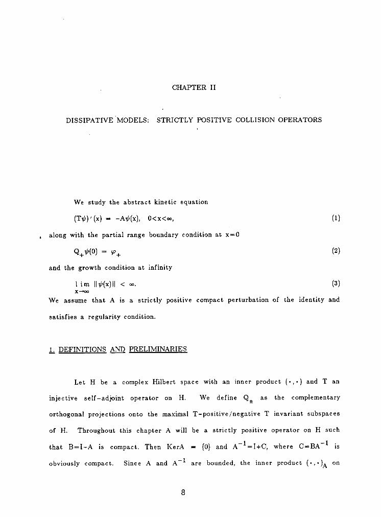
Z0(L) = { f€D(L)If€D(Lu) and Lnf=0 for somenENIn

addition to the regularity condition above we will assume that the zero

root manifold is contained in D(T). The following lemma characterizes

Z0(T—1A) and Z0(AT—1), and yields useful decompositions of H. For isotropic

neutron transport, these results are due to Lekkerkerker [33] and for more general

cases with T bounded to van der Mee [34] and Greenberg et al. [17].

LEl\/IMA The Jordan chains of T_1A at the zero eigenvalue have

at most length two, i.e. if then there exists g€Z0(T_1A) such that

T_1Af=g and T-1Ag=0. Hence Z0(T—1A) = Ker((T—1A)2).

(ii) T[Z0(T—1A)] == ZO(AT—1). (2)

(iii) The following decompositions hold true:

ZO(T_1A) 6 Z0(AT_1)J' = H, (3a)

Z0(AT"1) 44 Z0(T"1A)‘L = H. (3b)

(iv) (4)

Let f€Z0(T_1A) and g=T—1Af. Clearly g€Z0(T—1A). Let

h=T-1Ag. We will show that if T-1Ah=0 then h=0. Assume that T_1Ah=0.

Then (Ag,g)=(Th,g)=(h,Tg)=(h,Af)=(Ah,f)=0. Since A is positive this implies that

Th=Ag=0 and consequently that h=0.

(ii) First we will show the inclusion T[ZO(T”1A)]c:Z0(AT_1). Let f€KerA

then TfED(AT_1) and AT_1(Tf)=O so Tf€T[KerA]CKer(AT—1)CZ0(AT—-1).

Moreover if f€D(T_1A) and T.-1Af€KerA then Tf€D(AT—1) and

Af=T(T_1Af)€Ker(AT—l). Therefore (AT_1)2(Tf)=AT_ 1Af=0 so

Tf€Z0(AT—1). This shows that indeed T[Z0(T—lA)]CZ0(AT_1). Now we will

. Z6

prove that Z0(AT—1)CT[Z0(T—1A)]. Let f€Ker(AT_l). Then T_1f€KerA

implies that f€T[KerA]CT[Z0(T—1A)]. Next assume that f€Ker(AT—1)2 and

AT_1f¢0. Then AT_1f=Tg for some g€KerA. Since Tg€RanA, there exists

h€RanA such that Tg=Ah. Then h€Ker((T—lA)2)CD(T) and T—1f=h which shows

that f€T[Ker(T_1A)2]=T[ZO(T—1A)]. Similary using the induction one shows that

· l Ker((AT—1)n)CT[Ker(T_lA)n]CT[ZO(T_1A)] for any n€lN. Then this implies that

Z0(AT—1)CT[Z0(T—1A)] and ends the proof of (ii).

(iii) First we will show that Z0(T_1A) is nondegenerate, i.e.,

{ f€Z0(T—1A)I(Tf,g)=0 for all g€Z0(T_1A) }

=Letand (Tf,g)=0 for all g€Z0(T_1A). Then

Tf€Z0(T-1A)‘LC(KerA)‘L=RanA. Thus f=T_1Ah for some h€H. But then h

must belong to Z0(T—1A) and (Ah,h)=·=(Tf,h)=(l. Therefore Tf=Ah=0 and __

conseqently f=0.

Now let f€Z0(T_1A)I”1Z0(AT_1)'L. Then (2) implies that (Tf,g)=0 for all

g€Z0(T_1A). Since Z0(T_1A) is nondegenerate, f=0. This shows that

Z0(T—lA)¤Z0(AT_1)J'={0}. Likewise if then f=Th for

some h€Z0(T_1A) and (Th,g)=0 for all g€Z0(T—1A). Hence h=0 and then f=0

showing that ZO(AT_1)I'“lZ0(T-1A)'L={0}. Now we use a simple dimension

argument. We have

codim ZO(AT_1)'L = dim Z0(AT—1) = dim Z0(T_1A)

and similary

eooam Z0(T_1A)‘L = dim z0(T‘lA) = dam zO(AT‘l)

which imply the decompositions (3a) and (3b) respectively.

(iv) Note thot T mooe z0(AT")*nn(T) toto z0(T"A)* and Z0(T—1A)

onto Now using the fact that T has dense range one proves that

7_)(T·1A)¢ = .

27i

Clearly A maps Z0(T'-1A) into Z0(AT_1) and Z0(AT—1)l into Z0(T°1A)i.

Since KerACZ0(T_1A), the codimension of A[Z0(T'-1A)] in the subspace Z0(AT—1)

is equal to dim KerA. But in the first place codim RanA=dim KerA and therefore,

since the restriction of A to the subspace Z0(AT_1)'L has closed range in

ZO(T—1A)l, one must have

^lZ0(AT_1)i] = Z0(T”1A)l,

which ends the proof.!

The decompositions (3) will enable us to reduce a boundary value problem

with given A (having nontrivial kernel) to one with a strictly positive collision

operator. This reduction, in fact, follows immediately from the following

proposition. _

PROPOSITION Let ß be an invertible operator

onsatisfyingl

(Tßh,h) 2 0, h€Z0(T—1A). (5)

Let P be the projection of H onto Z0(AT—1)'L along Z0(T_1A). If A is a

positive, compact perturbation of the identity with nontrivial kernel and satisfies

the regularity condition (1), then Aß defined by

Aß = Tß—1(I—P) + AP _ (6)

is a strictly positive operator satisfying

Ag1T = 6 (1)

Aß is also a compact perturbation of the identity satisfying the condition

Ran(I—Aß) C Ran(nT¤°‘) n 1>(m1+‘”), (6)

with a and w as in

28

§@: The identity (7) follows immediately from the definition of Aß.

Moreover, forg€H

we have

(Aßas) = (APs,Ps) + (Tß_1(I—P)g,(I—P)s) 2 0-

We have usedihere (5) for h=ß_1T(I—P)g. Since o·(A)C{0}U[6,oo) for some

6>0 and Z0(T_1A) has finite dimension, we must have strict positivity for Aßl

from the obvious triviality of its kernel.

Next, since Aß—A=(Aß—A)(I—P) has finite rank, Aß must be a compact

perturbation of the identity. Furthermore,

I—Aß = (I—A)—(Aß—A)(I—P) = (I—A)-T(ß_l—T—1A)(I—P) (9)

and therefore

Ran(I—Aß) C Ran(|TIa). (10)

Also, using that Ran(I—A) C D(|T|3+w) C D(|T!2+°)) we find that for

h€Z0(T—1A) and g=T_1Ah

h = (I—A)h+Tg = (I-A)h+T(I-A)g E D(¤T¤2+°)).

But this and (9) imply that

Ran(I—Aß) C D(|T•1+°°). (11)

Now from (10) and (11) we obtain (8).I

As in Chapter II one can construct the Hilbert space HAß. Due to

boundedness and strict positivity of Aß the HAß—norm is equivalent to the original V

norm on H. The equivalence of these norms also shows that the topology of

HAß does not depend on the choice of the operator ß in Proposition IlI.2. We

may define Pi as the HAß—orthogonal complementary projections of H onto the

maximal A/;1T—positive/negative Aé1T—invariant subspaces. Since the

decomposition (3a) reduces completely the operators T—1A and AÄIT, it clear

29

that PP+, PP_ and I—P form a family of complementary projections commuting

with T_1A. One can also show that they are ß—independent. Moreover using

the results of Section II.1 one shows that the operatorT—1Aß

is densly defined

in H. 1*11115 D(T_1AßrZ0(AT_1)i)=D(T_1ArZ0(AT—1)'L) is d5115a in

Since Z0(T_1A) is finite dimensional,

and tzhß np51a1n1T_1A

is closed and densly defined in H.

The next proposition gives a decomposition of Z0(T—1A) into

T-positive/negative subspaces and a characterization of ß compatible with the

intended boundary value problems. A proof of this proposition can be found in [34]

and [17] for bounded T; the unbounded case introduces some technicalities

connected with

D(T).PROPOSITION E. The subspaces

Mt = {Ran PP;@ Ran (12)

satisfy the condition

:;(Tf,f) > 0, 0¢f€Mt, (13)

while

M+© M_ = ZO(T_1A) (14)

and

{M+f1KerA} aa {M_V1KerA} © = KerA. (15)

Moreover, it is possible to choose the operator ,8 such that

Ran P+ C Ran PP+ ® KerA. (16)

Egg: Let us first distinguishbetweenMi

= (17)

30

and

Ni = {PP;[Hl¤>Qi[Hl}¤Z0(T”1A) (18)

Since MtcNi are finite dimensional and we have the orthogonal complements

(PPilD(T)l)l = (PPi[Hl)i„

(Qi(D(T)l)i = (Q,„lHl)i,

it is clear that Mi=Ni. Therefore, we shall interpret Mi as in (17), but use

the shorthand notation (12).

Everyf0€M+

can be written as f0=g_+h+, where g_€PP_[D(T)] and

h+€Q+[D(T)]. Thus,

0=

(Tf0,f0)+(A°ß1Tg_,g_)Aß s(Tf0,t'0),where

we have deleted two vanishing terms by using (4). Also, (Tf0,f0)=0 would

imply (Th+,h+)=(A°ß1Tg_,g_)Aß=0, thus h+=g_=0 and fO=0, which settles (13)

for M+. The proof for M_ is analogous.

Next, observe that

(TPP$[D(T)])J'

=(TQilD(T)))l= Q,,,lHl,

= Z0(AT'1)l.

One easily computes that

{[RanNotethat

(I—P)({Ran PPioZ0(T“1A)}nRan Q;] =

{RanPPi®RanThen

we have

(T[Mi])i = (I-P)[{Ran PPioZ0(T“1A)}nRan Q;] +

+ P[{Ran PPioZ0(T—1A)}¤Ran Q;] + Z0(AT”1)J‘ =u

3l

={RanHence,

(14) holds true.

Since (T[KerA])J“f'lZ0(T—1A) = T—1A[Z0(T—1A)], one obtains easily

{T(MiI')KerA]}'Lf'1KerA = {(T[Mi])'L+(T[KerA])J'}V)KerA =

= {M¥+T-1A[Z0(T—1A)]©ZO(AT—1)i}V1KerA =

= {M;I"•KerA}$T—1A[Z0(T—1A)],

where we have used that h€T—1A[Z0(T—1A)]CKerA satisfies (Th,h)=0, in

combination with (13). This then implies (15).

Let us construct ß in such a way thati

V

Ran P+ C Ran PP+ © KerA. (16)

Choose a basis xl,...,xk of the subspace T_1A[Z0(T—1A)]CKerA. Since

(Tx,z)=(Ay,z)=(y,Az)=0 for all z6KerA and X=T;1Ay€T—1A(Z0(T-1A)), we have

(Txi,xj)=0. Next choose a basis z1,...,zm of any complement of T_1A[Z0(T-1A)]

in KerA in such a way that (Tzi,zj)=0 for i¢j and (Tzi,xj)=O for all i$m and

jSk. Since Z0(T_1A) is nondegenerate, we must have (Tzi,zi)E T(zi)¢0 for

iSm. Using an induction argument we then select y1,...,yk satisfying T_1Ayi=xi

as well as (Tyi,zj)=0 for jSm and (Tyi,xj)=(Tyi,yj)=O for jSi—1, and (Tyi,yi)<0

for i=1,...,k. As a result we obtain a special basis {xl,...,xk,y1,...,yk,z1,...zm} of the

zero root linear manifold Z0(T—1A). We now define the invertible matrix ß on

-1 . T( Z ' l _ _ _Z0(T A) by ßxi=xi, ßyi=—yi, and ßzj = zj. The inclusion (16) IS

immediate.¤

L EXISTENCE UNIOUENESS THEORY PROBLEMS

In this section we will analyze the boundary value problems

(T1/»)'(x) = —.x«1»(x), 0<ix<„, (19)

32 .

Qi¢(0) = <Pi, . (20)

along with a condition at infinity, namely, one of

lim Ile/2(x)II = 0, (21)x->:¤¤Il¢(X)|| = 0(1) (X‘**°°): ” (22)

I|¢(X)|l = 0(X) (><·*¢=*°)· (23)

As there is a complete symmetry between left and right half space problems, we

will consider the right half space problem only. By a solution of the various

boundary value problems for <p+€Q'+[D(T)] we shall mean a continuous function 1/1:

[0,oo)—>D(T)CH such that Tal; is strongly differentiable on (0,oo) and Eqs. (19), (20)

and (21) ((22), (23), resp.) are satisfied.

First we outline the procedure which will be used to construct solutions to

these boundary value problems. Let us reduce theihalf space problem (19)-(20) to

two subproblems. Writing ¢1=P1b and 1,/20=(l—P)1/2, Eq.(19) may be decomposed as

follows:

(T·qb1)'(x) = -A1/21(x), 0<x<¤¤, (24)

and

¢0’(x) = 0<x<oo.

The second equation is an evolution equation on the finite dimensional space

ZO(T_1A), and therefore admits an elementary solution of the form

-1¢0(><) = VXT A¢0(0)

=whereLemma III.1 has been used. Next consider Eq.(24). Let us add to this

equation the dummy equation

(T¢0)’(x) = —Aߢ0(x), 0<x<¤o, (25)

on Z0(T—1A), where Aß is given by (6) for some ß. The solution of Eq.(25) is

easy to compute but does not concern us, as it will be projected out shortly.

However, defining d>=d>0+1/>1 we can combine Eqs. (24) and (25) to obtain

33

(T¢)'(x) = —Aߢ(x), 0<x<¤o. (26)

Now since Aß is strictly positive·(and a compact perturbation of the identity

satisfying (8)), we can apply the results of Chapter II to Eq.(26) and obtain its

solution in the form

¢(x) = e_xT—1A,8Eg+, 0Sx<¤¤,

where g+€Q(_[D(T)] and E=(Q+P++Q_P_)-1. Then projecting ¢>(x) onto

Z0(AT—1)i along Z0(T—1A) and adding 1/20(x), we obtain a solution of Eq.(19) in

the form ‘

(27)

Now we have to fit the boundary condition (20). To do this we must find

g+€Q+[D(T)] andi/10(0)€Z0(T-IA) such that

Q+(PEs_,_+¢0(0))_= s¤+-i

(28)

Note that if ¢0(0)=0 (1/20(0)€KerA, ¢•0(0)€Z0(T_1A), resp.) then the right half

space condition at infinity (21) ((22), (23), resp.) is satisfied.

Let us define the measure of noncompleteness for any of the boundary

value problems to be the codimension in Ran Q+ of the subspace of boundary

values <p+6Ran Q+ for which the problem is solvable, and the measure of

nonuniqueness to be the dimension of the solution space of the corresponding

homogeneous problem. The principal results of this chapter are the following

existence and uniqueness theorems:

THEOREM . The boundary value problem

(T1/>)’(x) = —A1/1(x), 0<x<o¤, (19)

Q_,_¢(0) = <P+, (20)

lim II1,b(x)Il = 0, (21)x—•e¤

has at most one solution for every <p+EQ+(D(T)], and the measure of

34

noncompleteness for solutions of this problem coincides with the maximal number of

lineary independent vectors g1,...,gD€KerA satisfying

(Tgi,gj) = 0, 1Si,jSn, i¢j, (29)

‘·°°(Tgi,gi) 2 0, 1SiSn. (30)

The solution, if it exists, is given by

1/2(x) = e-xT_1APEg+ (31)

where g+ is the unique solution of

Q+PEg+= <p+.

i(32)

THEOREM @. The boundary value problem

(T1/»)’(><) = —A¢(><)„ 0<x<„, (19)

Q+¤/¤(0) = s¤+, i (20)

Ih/¤(x)II = 0(1) (x—»„), (22)

has at least one solution for every <p+€Q+[D(T)], and the measure of nonuniqueness

for solutions of this problem coincides with the maximal number of linearly

independent vectors h1,...,hk€KerA satisfying

(Thi,hj) = 0, 1$i,j$k, i¢j, (33)

(Thi,hi) < 0, 1Si$k. (34)

The solutions have the form

1ß(x) = e—XT—lAPEh+ + ho n(35)

where h0€{Ran PP+®Ran Q_}¤KerA and h+ is the unique solution of

Q+PEh+ + Q+h0 = <p+. (36)

THEOREM @1. The boundary value problem

(T¢)'(x) = —A¢(x), 0<x<¤¤, (19)

Q+¤!·(0) = 62+, (20)

35

Ih/»(><)II = 0(>¤) (><—~==>)» . (23)

has at least one solution, and the measure of nonuniqueness for solutions of this

problem coincides with the maximal number of linearly independent vectors

e1,...,em€Z0(T_1A) satisfying '

(Tei,ej) = 0, 1Si,jSm, i¢j, (37)

(Tei,ei) < 0,1$iSm.The

solutions have the form

1/)(X) = e—xT_1APEf++(I—xT_1A)f0,”

(39)

where f0€{Ran PP+®Ran Q_}V)ZO(T—1A) and f+ is the unique solution of

Q+PEf+ + Q+f0 = <p+. (40)

>£ Q Theorems l, E EQ: Consider first the boundary value

problem (19), (20) and (22). A solution of this boundary value problem exists if one

is able to find g+€Ran Q+ and 1ß0(0)€KerA such that the equation

Q+(PEg++1/20(0))=<p+ is fulfilled. Since E<p+€Ran P+CRan PP+®KerA, one

can simply chooseg+=<p+

and 1/1O(0)=(I—P)E<p+. This establishes the existence of

solutions to the boundary value problem. To study uniqueness, let us suppose that 1/1

is a solution of (19), (20) and (22) corresponding to go+=0. Then 1/: has the form

(27) with PEg++1b0(0)€Ran Q_ for some g+€Ran Q+ and 1/10(0)€Ke1·A.

Therefore 1/10(0)€{Ran PP+©Ran Q_}I")KerA = M_I’1KerA. Conversely, if

1ß0(O)€M_¤KerA, then we can find g+€Ran Q+ and h_ERan Q_ such that

1/10(0)=PEg+·h_, i.e., Q+(PEg++¢0(0)) = 0. Hence the measure of

nonuniqueness of solutions of the boundary value problem (19), (20) and (22) is equal

to dim (M_0KerA). Since by Proposition III.3 M_ is a subspace of Z0(T-IA)

maximal with regard to vectors h satisfying (Th,h)<0 for h¢0, M;_¤KerA is also

maximal in this respect as a subspace of KerA. One can show that the dimension

36

of such a maximal subspace does not depend on the specific choice of this

subspace. Therefore, the dimension of M_V)KerA equals the dimension of the

subspace spanned by hi satisfying (33) and (34), which completes the proof of

Theorem III.5.

Consider now the boundary value problem (19), (20) and (23). By virtue of

the above considerations the existence of solutions is clear. To study uniqueness

let us assume that 1/1 is a solution of (19), (20) and (23) with <p+=0. Then 1/2

has the form (39) and ¢0(0)€{Ran PP+©Ran M_. Conversely,

if 1/10(0)€M_, then there exists a vector f+ERan Q+ such that

Q+(PEf++¢0(0))=0 which leads to a solution of Eqs. (19), (20) and (23) with

go+=0. Therefore, the measure of nonuniqueness equals dim M_, which

coincides with the dimension of thedsubspace spanned by vectors ei satisfying (37)

and (38). This ends the proof of Theorem III.6.

It remains to demonstrate the proof of Theorem III.4. The uniqueness of

solutions of the boundary value problem (19), (20) and (21) follows from the

uniqueness of solutions of the problem

(T<p)'(x) = —Aß<p(x), 0<x<o¤, (41)

Q+<p(0) = <p+„ (42)

lim II<p(x)II = 0, (43)x—•e¤

which was proved in Chapter II (cf. Theorem II.4). For, in fact, every solution of

(19), (20) and (21) has its initial value 1/1(O) in Ran PP+ and therefore must be a

solution of Eqs. (41)—(43). To analyze existence for Eqs. (19) (20) and (21), we

consider the possibility of finding g+€Ran Q+ such that

¢+ = Q+PEg+ = PEs+—Q_PEs+„i

or, equivalently, go+€{Ran PP+©Ran Q_}f'1Ran Q+. Therefore the measure of

noncompleteness is equal to the codimension of {Ran PP+oRan Q_}¤Ran Q+ in

37(

Ran Q+. Let us compute:

Ran Q6+=dim -1-———-;——— =dim —IL—-—-.{Ran PP+©Ran Q_}ORan Q+ Ran PP+©Ran Q_

Since RanV=H, V=Q+P++Q_P_=P++Q_(P_—P+), and Ran P+V'IRan Q_={0}, we

conclude that H C Ran P+$Ran Q_ and consequently that

' Ran PP+®Ran Q_+KerA = H (cf. Proposition III.3). Then

Ran PP+©Ran Q_+KerA5+ = dim =

Ran PP+®Ran Q_

dim Ke rA = dim Ke rA ={Ran PP+@Ran Q_}I'“•Ke rA M_0Ke rA

dim [{M+V1KerA}©T—1A[Z0(T_1A)]], ·

where we have used (15). Note that the subspace {M+OKerA}©T_1A[Z0(T_1A)]

has the property (Tf,f)20 for all f contained therein, and any subspace of KerA

containing {M+OKerA}OT_1A(Z0(T_1A)] and having the same property coincides

with the latter. Using standard Pontryagin space theory (cf.[4], Chapter IX), we

conclude that 6+ equals the dimension of a subspace of KerA spanned by vectors

gi satisfying (29) and (30). This completes the proof of Theorem III.4.¤

If the differential equation (19) is replaced by

T1l:’(x) = —A16(x), 0<x<¤¤, (44)

one can seek solutions of the boundary value problems with <p+€Q+[H]. Here by

a solution we mean a continuous function qb:[0,¤¤)-—>H which is continuously

differentiable on (0,¤¤), 1/1'(x)€D(T) for xE(0,¤o) and such that Eq.(44), the boundary

condition Q+1,b(0)=cp+ and an appropriate condition at infinity are satisfied.

Then one can prove the analogs of Theorems III.4, III.5 and III.6, where one has

38

to substitute Eq.(44) for Eq.(19), and <p+ may belong to Q+[H] rather then just to

Q+[D(T)]. In this setting the spaces Mi appearing in the proofs of the analogs of

these theorems must be read as in (18). The equivalence of (17) and (18) causes

the measures of nonuniqueness and noncompleteness to coincide with those for Eqs.

(19)-(20) with appropriate condition at infinity. We note, however, that unlike the

earlier boundary value problem, Eq.(44) may not lead to an equivalent vector valued

convolution equation [35].

CHAPTER IV

NONDISSIPATIVE MODELS: COLLISION OPERATORS WITH NEGATIVE PART

In this chapter we study the abstract kinetic equation

T1b’(x) = —A¢(x), 0<x<r, (1)

relevant to transport in a multiplying medium confined within the slab [0,r]. The

multiplying character of the medium manifests itself mathematically in allowing A to

have a finite dimensional negative part. The equation is studied along with the

partial range boundary conditions

Q+¢(0) = <P+„ (2)

Q_¢(T) = s¤_, (3)

where Qi are the complemetary orthogonal projections onto the maximal

T—positive/negative subspaces of H and <p+, <p_ are given vectors in the ranges

of Q+ and Q__ respectively.

L PRELIMINARIES AND DECOMPOSITIONS

_Let T be a bounded self—adjoint injective operator on a complex Hilbert

space H. Let A be a bounded self—adjoint Fredholm operator on H such that the

spectrum of A in (—¤¤,0] consists of a finite number of eigenvalues of finite

39

40

multiplicity. Let us introduce the (indefinite) inner product on H by

lf„slA = (Af„s)· (4)

We will denote by HA the space H equipped with the [·,·]A—inner product.

Then HA is an indefinite inner product space with the fundamental decomposition

HA=HÄeH/gen; (6)where HÄ is strictly positive/strictly negative subspace of HA while HX is

kneutral. One can take for example HÄ=ii1Ker(ki-A) where kl, . . ., kk are

the strictly negative eigenvalues of A, H2=KerA and H; to be the the

H—orthogonal complement of HÄ If KerA={0}, then HA is a

I”IK—space where :c· is the sum of the multiplicities of the negative

eigenvalues of A (cf. [25,32]). One can easily show that the operator T_1A is

self—adjoint with respect to the indefinite inner product ThenT—1A

has at

most rc nonreal eigenvalues (multiplicities taken into account) occuring in complex

conjugate pairs with pairwise coinciding Jordan structures, while the length of a

Jordan chain for a real eigenvalue ofT—1A

does not exceed ‘2rc+1. Moreovuer

there is a resolution of the identity for the real spectrum of T-IA, possibly with

finitely many critical points at certain eigenvalues (cf. [25,32]). If A has a

nontrivial kernel, then HA is no longer I”IK—space. It is not even a Krein space.

This complicates the spectral analysis of the operator T_1A. However under

certain additional assumptions we will be able to deduce spectral properties ofT_1A

vital for the subsequent analysis.

Let L be a linear operator on H and k be a complex number. We define

the k root linear manifold ZÄ(L) by

Z)\(L) é { h€H I h€D(Ln) and (k—L)nh=0 for some nElN

4l

DEFINITION. The operator A will be called T-regular if

(a) Z0(T_1A) is finite dimensional and nondegenerage with respect to the

indefinite inner product [f,g]T=(Tf,g), i.e.,

{ f€Z0(T_1A)|(Tf,g)=0 for all g€Z0(T—1A) }=(b)

for any real nonzero X Z)\(T_1A) is nondegenerate with respect to the

indefinite inner product [·,·]A.

[Using the condition (a) and a simple dimension argument one finds that

iZ0(T-IA) <¤ (T[ZO(T”1A)l)‘L = H

i(6)

Since the neutral subspace Hg=KerA is contained in Z0(T—1A), the subspace

(T[Z0(T—1A)])‘L is a l”IN—space invariant under T_1A. Now one can formulate a

spectral theorem for the restriction of T-IA to" Condition (b)

guarantees that the critical points in the spectral resolution of

T-1At(T[Z0(T—1A)])‘L are regular (cf. [25,32]).

The assumption on A we have just made allows us to construct a

decomposition of the Hilbert space H intoT_1A

invariant subspaces in such a way

that A can be deformed to a strictly positive operator. Such a decomposition and

the corresponding modification of the collision operator is provided by the following

proposition.

PROPOSITION Let A be T—regular. Then there exists aT—lA

invariant finite dimensional subspace Z(T—1A) of H with the following properties:

6) Z(T'1A) 6 <T)z<T‘1A)))* = H. 6)(ii) The subspace (T[Z(T”1A)])‘L is T_1A—invariant and strictly positive with

respect to [·,·]A,

(iii) The constituent subspaces in the decomposition (7) are

42

[· , · ]A—orthogonal.

Moreover, if P denotes the projection of H onto (Z[T(T—1A)])i along

Z(T-IA) and ,6 is an inveritible [·,·]T—positive operator on Z("|“-IA), then the

‘ bounded operator

Aß = AP + Tß”1(I—P)

is strictly positive with respect to H—inner product, Fredholm and

AÄIT = 6 e (T_1Ar(T[Z(T_1A)])J')—1.

Finally, if I—A is compact and satisfies the regularity condition

Ran(I-A) C R3HITl7 for some ·'1€(0,1), (8)

then I—Aß is also compact and satisfies the same regularity condition.

The proof of this proposition has been given by Greenberg and van der Mee

in [16]. Here we present a new version of this proof and, in fact, a slightly

different Hilbert space decomposition.

: Since Z0(T-IA) is finite dimensional and nondegenerate with respect

to [·,·]T-inner product, we have the following decomposition of the space H

Z0(T_1A) e (T[z0(T‘1A)})* = H.

The space (T[Z0(T_1A)])'L is a I]K—space with respect to [·,·]A—inner

product and the restriction of to this subspace is self—adjoint in

[·,·]A-inner product. Then there is a decomposition of the space

(T[Z0(T_1A)])‘L into the [•,·]A—orthogonal direct sum of the spectral subspaces

of T—1Ar(T[Z0(T_1A)])i

= Him 6 Hm ,

such that a(T_1ArHre) is purely real and the spectrum of T_1ArHim

consists of finite number of nonreal eigenvalues )«i,Xi, i=1,...,mS1ciof finite

mulitiplicity (cf. [39]). In fact we have

_ 43

H = Ü (z (T'”1A)o z (T”1A))im 1=1 *1 X1

and dim Him=2ES21c where E is the sum of the algebraic multiplicities of the

eigenvalues of T_1A in the open upper (lower) half plane. Him is neutral with

respect to [·,·]Äinner product. The space Hm is a HK,—space and

:c’=rc—E (cf. [4,25]). If fi, i=1,...,n are all critical points of the spectral

resolution of T_1A IHN then Hm can be decomposed into the

[·,·]A—orthogonal direct sum of the T_1A-invariant subspaces

H H H z TTIAI.e‘

0whereZ€i(T_1A) are l”IN(€i)—spaces, while H0 is a Hilbert space and

nE 1c(§i)=1c’ (cf. [25,29]). Moreover, since fi are regular critical points , the

i=1

subspaces are nondegenerate and finite dimensional. Now weput1

Z'(T'1A) = H. «>( Ä z (VIA))Im 1=1 $1

Clearly Z'(T_1A) is finite dimensional, T-°1A—invariant,

Z'(T”1A) e H0 = (T[Z0(T”1A)])‘I‘

and the subspaces Z’(T_lA) and H0 are [•,.]A—orthogonal.

Now we will show that by proving that

can be decomposed into [·,·]A—orthogonal direct sum of the

subspaces Z'(T—1A) and (T[Z’(T-1A)])‘L. This decomposition will follow

immediately from a simple dimension argument if we show that

I -1 I

—1Z (T A)¤(TlZ (T A)l)i = {0}·

Since Z’(T-1A)¤(T[Z'(T_1A)])‘L can be written as an intersection of the

44

subspaces Z„(T—1A)f°1[TZ„(T—1A)]‘L, where #7 is a complex eigenvalue or a

critical point of T_lA, it is enuogh to show that at least one of them contains

_ only the zero vector. In fact this holds true for any of these subspaces. Let

f€Z„(T—l”A)ÜlTZ„(T_1A))i. Then for any-g6Z„(T_1A)

° [f»s]A=(Af»s)=(f„T(T_1A)s)=0~

· Since Zn(T—1A) is nondegenerate with respect to [•,•]A—inner product, this

implies that f=0. Therefore

mz„m‘A>1>* = z · <*r‘*A> Q mz » (T”1A)l)l~It remains to show that the constituent subspaces in this decomposition are

[·,•]A-orthogonal. If f€Z’(T_1A) and g€(T[Z’(T_1A)))°L then we have

[f»s]A=(Af,s)=(T(T_1A)f,s)=¤-

Now we define lZ(T—1A) - Z0(T_1A) 6 Z'(T'1A).

Since

(T[Z(T"1A)l)i = mz„<T‘1A>1 Q TlZ’(T”1A)l)i =

mzwehave the follwing decomposition of the space H

Z(T"1A) 6 (T[Z(T"1A)])J' = H.

Clearly the constituent subspaces in (7) have all the properties stated in the first

part of the propostion.

The proof of the remaining part is exactly the same as the proof of

Proposition HI.2.!

Since Aß is strictly positive on H and Agl is bounded, the inner product

(·,-)A defined byß

45

is equivalent to the original inner product on H. We will denote by HA theß

space H endowed with the (•,·)A —inner product. It is clear that the topology onß

HAß does not depend on ,8. Now we can easily show that the operator

Sß=Ag1T is bounded, injective and self-adjoint on HA . Then we defineß

Pi as the (·,·)A —orthogonal complementary projections of HA onto theß ß

maximal (·,•)A —positive/negative AE1T—invariant subspaces of HA .ß ß

Note that Pt depend on ß. However, since the decomposition (7) reduces the

operator AÄIT and AE1Tr(T[Z(T'1A)])J' does not depend on ,8, the operators

PP+, PP_ and I—P form a set of ,ß—independent complementary projections on

H. "

Employing the self—adjointness of T_1Aß with respect to the

· (·,•)A —inner product and the self-adjointness of the restriction of T-IAß

to the subspace (T[Z(T-1A)])l one defines the semigroups exp{¥xT”1Aß}Pi

and exp{¢xT_1A}PPi. Moreover one can show that they can be extended to

contraction analytic semigroups on appropriate subspaces.

2; SOLUTION Q THE BOUNDARY VALUE PROBLEM

In this section we will prove existence and uniqueness theorems for the

boundary value problem

(1)

(2)

Q_¢(¢) = <„¤_, (3)

46

where Qi are the complementary orthogonal projections of H onto the maximal

T-positive /negative T-invariant subspac es of H and the ve c tors

<pt€Ran Qi are given. In the first part of this section we will study

solutions in some extension space HS of H (weak solutions). This approach was

introduced by Beals [3] and then developed further in [14,17]. In the second part

we will strengthen the results in the case when A is a compact perturbation of the

identity satisfying the regularityconditionLet

Hsß be the completion of HAß with respect to the inner product

(f:S)Sß " (lSß'f»$)Aß· (9)

Since Z(T-1A) is finite dimensional, the topology of Hsß does not depend on ß

and all inner products (9) are equivalent. In fact, one can show that Hsß is

topologically isomorphic to HT, the completion of H with respect to the inner

product (f,g)-F = (ITlf,g) (cf. the proof of Lemma IV.3). Therefore we will

suppress the subscript ,8 in Hsß and write HS. Since the extension of T_1Aß

to the space HS is self-adjoint one can define the projections Pi and the

contraction semigroups exp{=¤=xT_1Aß}Pt with the help of the spectral theorem.

Moreover one can extend Qi and P to bounded projections acting in HS. Now P

is the projectin of HS onto the completion of (T[Z(T”1A])J‘ along Z(T_1A). The

problem of extending T_1A to HS is more delicate. Since the decomposition (7)

reduces completely the operators T_1A and T_1Aß and these operators coincide on

the subspace (T[Z(T—1A)])J‘ one can extend the restriction of T_1A to

(T[Z(T_1A)])'l' with respect to the inner product (9) to the self—adjoint operator

on the completion of (T[Z(T_1A)])'L. Since_ Z(T—1A) is finite dimensional, the

restriction of T-IA to Z(T—1A) can be defined in the natural way as the bounded

operator with respect to the norm induced by the inner product We willU

{17

denote by K the resulting extension of T_1A to HS. Now one can define the

complementary projections of P[HS] onto the maximal K—positive/negative

K—invariant subspaces of P[HS]. Since P and Pi commute one can show that

‘ they coiticide with PPi. Further, using the spectral theorem for the restriction

of K to P[HS] one defines the semigroups exp{¥xK}PPi. Clearly exp{¢xK}PPi

= exp{=¤xT-1Aß}PPi.

After this introduction we can precise what we shall mean by a (weak)

solution of the boundary value problem (1)—(3). A icontinuous function

1/::[0,r]—>HS is a weak solution of the boundary value problem (1)—(3) if

(i) for all x€(0,r) e/2(x) belongs to the domain of K,

(ii) 1b is continuously differentiable on (0,r) and 1b' =—K1/1,

(iii) Q+¢(0)=<p+ and Q_~ß(r)=<p_-A

Solving Eq.(1) on the subspaces Ran PP+, Ran PP_ and

Ran(I—P)=Z(T_1A) with the help of standard semigroup theory, we obtain

Putting h=PP+¢(0)+PP_1/2(1')+(I-P)¢(0) one can write

(10)

Hence ¢(x) will solve the boundary value problem (1)—(3), if the vector h is

chosen in such a way that the boundary conditions (2) and (3) are satisfied.

Fitting Eqs. (2) and (3) one sees that h must be a solution of

Vrh = <p

where <p=<p++<p_ and

vr = Q+[1>1>++JKPP_+(1-P)} +

+ Q_[e—TKPP++PP_+e”TT_1A(I—P)]. (11)Therefore the unique solvability of the boundary value problem (1)—(3) is

48

equivalent to the bounded invertibility of the operator VT on HS. We will proof _

that this is in fact the case. We have

THEOREM IV.2. Let A be T—regular. Then there exists Tc>Ü such that

for all 0<1·<rc and every <p+€Q+[HS] and <p_€Q_[HS] the boundary value

problem

T1,b'(x) = -A¢(x), 0<x<1·, (1)

Q+¢(0) = $9+, l (2)

Q_¢(¤*) = s<¤_, (3)

has a unique solution. The solution is given by-1 (12)

where <p=<p++<p_ and VT is the invertible operatorion HS defined by (11).

The proof of Theorem IV.2 employs certain properties of the operator

1'T—1A —rT-IAßP_] + Q_[e ßP++P_]

which are described in the following lernma.

LEMMA IV.3. For any 1‘>0 the operator VT /3 is invertible on HS and

-1ll . ......—""( "(<HS> .1.)r ,ß L(H ) _ -1_

where Vß=Q+P++Q_P_ has a bounded inverse on HS satisfying

-1

Proof: The following proof is adopted from an argument of Beals We

will show first that the Hilbert spaces HS and HT are topologically isomorphic. As

49

the first step in this prove we will demonstrate the equivalence of the uorms

II · IIS and II · IIT on H-

Let h6P+[HAß] and u(x)=exp{—xT—1Aß}P+h for x20. Clearly u is

continuous on [0,¤¤), differentiable on (0,«>) and Tu'(x)=-Aßu(x). Therefore”

= I2Re((Q+—Q_)Tu’(x),u(x))I = I2Re((Q+-Q_)Aßu(x),u(x))| S

S 2CIIu(x)IIä .ß

Here we have used the fact that the norms II•II, II·IIA· and IIAß(·)II areß

equivalent . C denotes a constant. Then, since lIu(x)IIT—>0 as x—>¤¤,

|Ih|I2 = II¤(0)II2 =—Vo d II¤(X)II2dX ST T OH? T '

-u X = exp — X , X.()u2 dx 2c)°°( { 2 T;iA }P hh) d

0 Aß 0 ß + Aß

But from the spectral theorem

2v[°°(exp{—2xT_1A }P hh) dx = (A—1Th h) = IlhlI20 ß +' Aß ß ' Aß S '

hence cmduä .Likewise if héP_[HA ] we prove that Ilhllä S Cllhllä in the very analogous

ßway. Now if h6HA , let hi = Pih. Then

ß

Ilhllä S ‘2(IIh+IIä— + IIh_II·§—) S 2C(IIh+IIä + IIh_IIä) = 2ClIhIIä-

Now, let us suppose that h6HAß. Then

2 _ -lIhIIS =(•Sßnh,h)Aß = (Sßh,(P+-P_)h)Aß — (Th,(P+—P_)h) —

= ((Q+—Q_)h,(P+-P_)h)T S II(Q+—Q_)hIITII(P+—P_)hIIT S

S IIhIIT(IIP+hIIT + IIP_hIIT) S ‘2(C)%IIhIITIIhIIS ,

504 ‘

so llhlIS S 2(C)%IIhlIT. This ends the prove of the equivalence of HS and HT

norms.

In the next step we will show that Vß=Q+P++Q_P_- establishes the

topological isomorphism of HS and HT. Let Wß=I—Vß= Q+P_+Q_P+. Then

for any h€HA we have '6 .

. 2 2IIVßhIIT — IIWßhIIT = (TP+h,P+h) - (TP_,P_h) — (TP_h,P+h) +

(TP+h,P_h) = (T(P+-P__)h,h) = (Sß(P+—P_)h,h)Aß = Ilhllä. (15)

Hence lIhIIS S IIVßhIIT. Now , using a density argument we extend this

inequality to all HS. This shows that Vß is injective. To prove that Vgl exists

as a bounded operator it is enough to show that V;:HT—>HS is also injective.

Recall that Pi are self-adjoint in HS and consider Qi as mapping HS to HT.

Theni

*(Q+s,h)S = (s„Q+b)T = (Q+s,h)T = (SßQ+s„h)Aß = ((P+—P_)Q+s,h)S

implies that Q;=(P+—P_)Q+. Likewise, one proves that Qi=(P_—-P+)Q_.

Then we compute the following identities¤•«

* ¤•¤ ¤«Vß = (Q+P++Q_P_) = P+Q++P_Q_ = P+Q++P_Q_,

»« *•-VWßIß

(P+Q_+P_Q+),

and similary as in (15)

* 2 * 2 _ 2IIVßg|!S - IIWßg||S — IIslIT. (16)

Therefore V; is injective and consequently RanVß=HT. Hence Vß:HS—>HT asrk

well as Vß:HT—>HS are topological isomorphisms.

Now we can proceed to the proof of the inequality (14). Note that ‘

|IV'l—I|I = IIV—1W ll = |lW*(V*)—lII .ß HHS) ß ß L(HS) ß ß L(HS)

Moreover from (16) follows that

* *-1 2 _ 2 *-1 2IlWß(Vß) h||S — Ilhlls — lI(Vß) hIIT. (17)

5]

Since V* is a topological isomorphism, II(V*)_1hII 2 CIIhIl for some,6 ,8 T S

constant C>0. Finally it is clear from (17) that CSI and

* *V-1_ = W V -1 _ _ 2% _

Now we will prove the inequality (13). Using simple algebra and the fact

that exp{¥1·T-1Aß}Pi = Piexp{-1* 1T—1Aß 1} we show

v = v (1+(v"‘-1)e"'T_1^ß‘)1*,ß ß ß’

Then since

-1 -1* 1T_1A 1 -1lI(V/3 I)e ß 1,

the inequality (13) follows by mere computation.l

This completes the proof.!

The analogs of the operators Vß and VT ,8 play important role in the

analysis of the abstract half space and slab problems relevant to subcritcal media,

i.e. for A strictly positive and bounded. The proofs of the statements [contained in

this lemma except the inequality (13) can be found in many sources. In addition to

Beals [3] we cite a recent paper by Hangelbroek [22], where different proofs are

given.

Proof Q Theorem IV.2: We will show that for sufficiently small 1*

II V —V II < —————l————,L

(18)T T,ß V-].1*

,ß L (HS)

which guarantees the bounded invertibility of VT. Simple algebra shows that

vvT-T,ß—Q+l-B l(—)-+Q-l—€ ](-)++

-1 -1

52

Therefore

—V

"VT T,ß"L<HS>‘

-1 -1 -1S const.(eTH'ß "—1)+const.(eTHT ArZ(T A)H—1) E f(1*).

Clearly f(1*)—>0 as 1*—>0. Let

-1 -1 -11* == sup{1* |f(1·)< (1-II V -III )II VIICOO ß 1-(HS) ß L(Hg)

Now using the inequality (13) from Lemma IV.3 one shows that the inequality (18)

holds true for any 1*€(0,1*c).|

In the case where the collision operator A is a compact perturbation of the

identity satisfying the regularity condition

Ran(I-A) C Ran|T|fl for some ·1€(0,1) 1 (8)

one can improve the statement of Theorem IV.2. First of all one does not have to

extend the original Hilbert space H to obtain a solution ¢(x). All operators

involved act on H and the solution ¢v(x) of the boundary value problem (1)-(3) has

the same structure as (12) with K replaced by T-IA. But the crucial observation,

which helps to strengthen the uniqueness and existence theorem, is contained in

the following lemma.

LEMMA IV.4. For all z with Rez>0 the operator VZ-I is compact and

the operator valued function z-• VZ—I is analytic in the open right half plane.

Proof: Let Rez>0. Simple computation yields-1 -1

vz-1 APP_ +

—zT—1A+ Q_(PP+—Q+)C PP+ ·· Q+(PP_—Q_) · Q_(PP+—Q+)- (19)

53

Since PP+—Q+ and PP_—Q_ are compact (cf. Lemma II.10) and the semigroups

exp{$zT_1A}PPi, exp{—zT—1A}(I—P) are bounded and analytic, one can conclude

that z—+ VT—I is an analytic function with values in the ideal of compact

operators onH.!Now

using the analytic version of the Fredholm alternative (cf. Reed and

Simon [40]) one can infer the following result: either VZ is not invertible for any z

with Rez>0 or Vgl exists for all zE{zIRez>0} \ A where A is a discrete subset

of the open right half plane andz€A

if and only if the equation Vzh=0 has a

nontrivial solution. Since by Theorem IV.2 VT as a bounded operator on H has

trivial kernel for any 1·6(0,rc) and VT—I is compact, it follows that for such ·r

the bounded inverse of VT exists. But this excludes the first possibility stated in

the above corollary and yields the following theorem.

THEOREM Let A be T—regular compact perturbation of the identity

satisfying the regularity condition Then there exists a discrete subset A of

the open right half plane such that:

(i) for any r€(0,oo)\ A and every <p+€Q+[H] and <p_€Q_[H] the

boundary value problem (1)—(3) has a unique solution given by the equation (12),

T T where <p=g0++<p_ and VT is the invertible operator on H defined by (11),

(ii) for any real·r€A

the boundary value problem (1)—(3) with <pi=0 has

at least one nontrivial solution, which is given by the formula (10) where h is a

nontrivial solution of VTh=0.

If I-A is a finite rank perturbation of the identity satisfying the

regularity condition we can characterize the set A.

54

THEOREM Let A be a T—regular finite rank perturbation of the

identity satisfying the regularity condition Then

A = { ZEC

IEgg:If we show that Vz—I is a trace class operator, the description of

the set A will follow easily from the Fredholm theory of trace class operators

'(cf.[41], Theorem 3.3.9). It is clear from (19) that one has to prove only that

PPi-Qi are trace class operators. Moreover, since Z(T_1A) is finite

dimensional, it is enough to prove that Pi—Qi are trace class operators. To show

this we mimic the argument given in the first part of the proof of Lemma II.10.

Since a closedness argument is employed in this proof and the ideal of trace class

operators is closed in the II·IIl=trI·I norm, we have to use this norm in

estimating relevant operator valued integrals. However, the estimates carry over

with IIDH1 replacing IIDII where is obviously a finite rank

operator.:

CHAPTER V

APPLICATIONS

This section contains several physical models leading to equations of the

form

T¢'(><) = -A1/¤(><) (1)

All of them involve a time independent one dimensional transport problem in a

semi—infinite medium with spatial variable x€[0,¤o) or in a slab [0,1*]. The

equations are studied with the boundary condition

Q+¢(0) = <P+ (2)

at x=0, and the condition

Q_¢(r) = s¤_ (3)

at x=1‘ in the case of transport in the slab [0,1*], or with a condition at infinity

for transport in the semi—infinite medium x20. For all models we shall specify the

Hilbert space H, operators T and A, and whenever it is relevant the kernel of A

and the zero root linear manifold Z0(T_lA). We shall state the results of the

existence and uniqueness theory using the abstract theorems presented in Chapters

III and IV.

The first three examples come from kinetic theory of rarefied gases

andillustrstethe results of Chapter III.

55

56

L The scalar BGK eguation ([6,10,11,29])

+oo 2vgé(x,v) = -f(x,v) + é I f(x,u)e—u du, v€(—¤¢,+¤¤).

\/7I* -co

The equation is posed in the Hilbert space H=L2(lR,p) where

2dp=1r_1/2e-V dv. We define T and A by

(Tf)(v) = vf(v)

and

1 +oo _v2(Af)(v) = f(v) - tf f(x,v)e dv.

\/1l’ -oo

Then T is unbounded and self—adjoint. Since Af==f—(1,f)1, I—A is compact (in

fact rank one) and A is positive, the last property being a conseqnence of the

Bessel inequality. One checks easily that the regularity condition III.(1) is met.

Further, KerA=span{1} and Z0(T—1A)=span{1,v}. With respect to the sesquilinear

form

1 +oo —— _v2[h,k]T = (Th,k) = -1)- vh(v)k(v)e dv,

\/7l’ —oo

the set {v+1,v—l} is a basis of mutually [·,·]T—orthogonal vectors of Z0(T-IA).

Now we can apply the main theorems of Chapter III. Since [1,1]T=0,

Theorem III.5 guarantees the existence of a unique bounded at infinity solution of

Eqs. (1)—(2), which agrees with the result of Beals On the other hand, by

Theorem III.4, a solution of Eqs. (1)—(2) vanishing at infinity may not exist, the

measure of noncompleteness being 1. Consider now solutions to Eqs. (1)—(2)

which may grow like x at infinity. By Theorem III.6, since [v+1, v+1]T=1 and

[v—1,v—l]T=-1, these solutions are not unique, the measure of nonuniqueness

being 1. Thus, the Kramers or slip—flow problem [11], with <p+=0 in (2), has a

unique nonzero solution, up to a constant factor.

[57

_; dimensional eguation ([1,42])

v%§(x,v) + f(x,v) =ä

]--i:[1+2vu+2(v2—%)(u2—%)]f(x,u)e—u2du. l

The equation is posied in the Hilbert space H=L2(lR,p) where p is the same

measure as in the first example~. We define T and A by

(Tf)(v) = vf(v)

and

(Af)(v) = f(v) — —ä--]—+o°[1+2vu+2(v2-é-)(u2—%)]f(u)e_u2du.\/rr —¤¤

Then T is unbounded and self—adjoint. Sinc e

Af=f-(oz1,f)oz1-(oz2,f)a2—(oz3,f)oz3

andformsan orthonormal sequence in H, it follows from the Bessel inequality that A is

lpositive. Moreover it is clear that I—A is compact. One checks easily that the

regularity condition III.(1) is fulfilled, and that KerA = span {1,v,v2},

Z0(T—1A)=span {1,v,v2,v3}. Now we introduce the sesquilinear form

1 _v2[h,k]T = (Th,k) = —-;—]‘ vh(v)k(v)e dv.

\/rr -¤¤To apply Theorems III.4 and III.5 one has to represent this sesquilinear form as a

diagonal matrix with respect to an appropriate mutually [-,-],1.-orthogonal basis

of KerA. The diagonalization of a synunetric bilinear form is a simple algebraic

procedure and results in a matrix with 1, -1 and 0 on the diagonal. Then, by

Theorem III.4, a solution of Eqs. (1)—(2) vanishing at infinity may not exist; more

precisely, the measure of noncompleteness is 2. This reflects the fact that the

BGK linearized equation under study represents perturbation of the longitudinal

momentum density. Thus, conservation of mass and energy restricts the set of

initial states correspondingly by two dimensions in order to have solutions vanishing

at infinity, or, equivalently, to have physical densities approaching the equilibrium

59

One easily checks that the regularity condition III.(1) is satisfied. Straightforward

computation gives2KerA = span0

1and

2 3Z¤‘T'l^’ = {l‘l·lVl»l” llv ll0 1 1 v

Now we introduce the sesquilinear form

[h,k]T = (Th,k) =

1 +00 _v21 +00 _v2

= il vh1(v)k1(v)e dv + TI vh.,(v)k2(v)e dv.\/1r -oo \/7I’ —e¤ "

Since KerA is degenerate with respect to this sesquilinear form, Theorem III.5

implies that the boundary value problem (1), (2) has a unique bounded at infinity

solution. On the other hand, by Theorem III.4, solutions vanishing at infinity may

not exist, the measure of noncompleteness being 2, which is again a result of the

conservation laws (of mass and energy). To apply Theorem III.6 one has to

represent the sesquilinear form on Z0(T—1A) as a diagonal matrix. One obtains a

matrix with 1, -1, and —% on the diagonal. Thus, solutions to the boundary

value problem of order x at infinity have measure of nonuniqueness 2. The

corresponding Kramers or slip—flow problem has a two dimensional manifold of

solutions.

The next two examples come from neutron transport theory andi illustrate

the results of Chapter IV.

jp The isotropic neutron transport eguation ([2,9))

The isotropic one—speed neutron transport equation is

Ü 1 1ug%(><,u) = —¢(x,u) + gc) li/»(x,¤)d¤ (4)

60 l

where ;1€[-1,1] is the cosine of the angle describing the direction of

propagation and x€(0,r) is the position coordinate. The number c represents the

mean number of secondaries per collision. We will assume that c>1 which is the

case for a multiplyirig medium. The equation is studied in the Hilbert space

H=L2[—1,1]. We define the operators A, T and Qi on H in the following manner:

(Af)(#) = f(#) — éc] ]f(¤)d¤ ,

(Tf)(#) = #f(u),

cqirim = [Ԥ,")

jßiß,One easily verifies that T and A are bounded self—adjoint, injective, I—A

is compact (in fact rank one) and the regularity condition IV.(8) is satisfied with

any ·'1€(0,%). It also has been shown in [16] that A is T-regular. Therefore

we can use Theorem IV.5 to conclude that for sufficiently small diameter the slab

problem for the isotropic neutron transport equation with c>1 has a unique solution

for any incoming fluxes at the boundaries x=0 and x=1‘. Since 1/2 represents

the neutron density, it is clear that only nonnegative solutions are physically

acceptable. Using the integral equation corresponding to Eq.(4) one can easily

show that the solution is in fact nonnegative whenever incoming fluxes are

nonnegative.

5; svmmetric multigroup transyrt eguation ([16,34])·

The symrnetric multigroup approximation with isotropic scattering leads to

the following neutron transport equation:

M1 1 N 1 . .,N (5)

where 116]-1,1] and x€(0,r). Here 1l>i(x,p) is the angular density of neutrons

with speed é (in units of the largest speed). We will assume that1

6]

C=(Cij)1?’ j=1 is a real symmetric matrix. Let E be the diagonal matrix with

diagonal entries 612622. . .26N=1.

Equation (5) is studied in the Hilbert space H=_I;1L2([-1,1],o·id_;4). We

define operators A,T and Qi on H by

(Anm =

rmwheref==(fi)1?=1€H. Let ei€H be the constant vector valued function whose all

entries are zero but the i—th entry which is equal to 1. Then

Af = r - %2‘10_ii (ei,f)ei. ’1=1

Now it is clear that I—A is compact (in fact of finite rank) and A is

self-adjoint in H. We will assume that det(Z—~C)¢0 so that A is invertible. One

verifies easily that the regularity condition IV.(8) is satisfied with any ·7€(0,%).

The operator T is evidently bounded and self-adjoint in H. Moreover it has been

shown in [16] that A is T—regular. Thus, by Theorem IV.5, for sufficiently small

diameter the slab problem for Eq.(5) has a unique solution for any incoming fluxes.

REFERENCES

1. M.D. Arthur and C. Cercignani, Non-existence of a steady rarefied supersonic flow

in a half space, Zeitschr. Angew. Math. Phys. §$ (1980), 634-645.

2. J. A. Ball and W. Greenberg, A Pontryagin space_ analysis of the supercritical

transport equation, Transp. Theory Stat. Phys. $(4) (1975), 143-154.

3. R. Beals, On an abstract treatment of some forward—backward problems of

transport and scattering, J. Funct. Anal. Q1; (1979), 1-20.h

4. J. Bognar: Indefinite Inner Product Spaces, Springer Verlag, Berlin l974.

5. R.L. Bowden and W.L. Cameron, Constructive solution of the linearized Boltzmann

Equation. Vector BGK Model, Transp. Theory Stat. Phys. g (1979),45-62.

6. R.L. Bowden and L. F. Garbanati, Constructive solution of the linearized Boltzmann

equation. Scalar BGK Model Equations, Transp. Theory Stat. Phys. Z

(1978),1-24.

7. K.M. Case, Plasma oscillations, Ann. Phys. (N.Y.)1 (1959), 349-364.

8. K.M. Case, Elementary solutions of the transport equation and their application,

Ann. Phys. g (1960), 1-23.

9. K.M. Case and P.F. Zweifel: Linear Transport Theorv, Addison Wesley Publ. Co.,

Reading, Massachusetts 1967.

10. C. Cercignani: Theory ggg Application gt; Boltzmann Eguation, Elsevier, New

York 1975.

11. C. Cercignani, Elementary solutions of the linearized gas dynamics Boltzmann

equation and their application to the slip—flow problem, Ann. Phys. (N.Y.) gg (1962),

219-233.

12. C. Cercignani and Siewert, On partial indices for a matrix Riemann-Hilbert

problem, Zeitschr. Angew. Math. Phys. gg (1982), 297-299.

13. W. Greenberg and C.V.M. van der Mee, An abstract approach to evaporation models

62

63

in rarefied gas dynamics, Zeitschr. Angew. Math. Phys. Q (1984), 156-165.

14. W. Greenberg and C.V.M. van der Mee: Abstract boundary value problems in from

kinetic theory, Transp. Theory Stat. Phys. Q (1982/83), 155-181.

15. W. Greenberg and C.V.M. van der Mee, An abstract model for radiative transfer in

an atmosphere with reflectin by the planetary surface, SIAM J. Math. Anal., 1_§(4)

(1985), 695-702.'

16. W. Greenberg 'and C.V.M. van der Mee, Abstract kinetic equations relevant to

supercritical media, J. Fuuct. Anal. Q(2) (1984), 111-142.

17. W. Greenberg, C.V.M. van der Mee, P.F. Zweifel, Generalized kinetic equations, Int.

Eqs. Oper. Theory Z (1984), 60-95.

18. R.J. Hangelbroek, A functional analytic approach to the linear transport equation,

Ph.D. thesis, Rijks Universiteit, Groningen, 1973.

19. R.J. Hangelbroek, Linear analysis and solutions of neutron transport problems,

Transp. Theory Stat. Phys. §_ (1976), 1-85.I

20. R.J. Hangelbroek, Time independent neutron transport equation with anisotropic

scattering in absorbing media, Report ANL 80-60, Argonne National Laboratory,

Argonne IL (1980).

21. R.J. Hangelbroek, On the derivation of formulas relevant to neutron transport in

media with anisotropic scattering, Report No. 7720, Univ. of Nijmegen, The

Netherlands, 1978.

22. R.J. Hangelbroek, On the stability of the transport equation, Int. Eqs Oper. Theory

§(1) (1985), 1-12.

23. R.J. Hangelbroek and C.G. Lekkerkerker, Decompositions of a Hilbert space and

factorization of a W—A determinant, SIAM J. Math. Anal. 8 (1977), 458-472.

24. E. Hille and R.S. Phillips: Functional Analysis Q Semigroups, AMS Colloquium

Publications vol. 31, Proyidence R.I. 1957.

25. I.S. Iohvidov, M.G. Krein, H. Langer: Introduction Q Q spectral theorv Q

operators Q spaces with a_n indefinite metric, Mathematical Research , Academie

Verlag, Berlin 1982.

64

26. N.G. van Kampen, On the theory of stationary waves in plasmas, Physica Q (1955),

949-963.

27. H.G. Kaper, A constructive approach to the solution of a class of boundary value

problems of mixed type, J. Math. Anal. Appl. Q (1978), 691-718.

28. M.A. Krasnoselskii, P.P. Zabreiko, E.I. Pustylnik and P.E. Sobolevskii: Integral

Operators Q Spaces Q Summable Functions, Noordhoff, Leiden 1976.

29. M.G. Krein and H. Langer, The spectral function of a self-adjoint operator in a

space with indefinite metric, Soviet Math. Dokl. Q (1963), 1236-1239; Dokl. Acad.

Nauk Q(5) (1963), 39-42 [Russian].

30. M.G. Krein and P.E. Sobolevskii, Differential equations with abstract elliptic

operators in Hilbert space, Dokl. Akad. Nauk SSSR Q (1958), 233-236 [Russian].

31. J.T. Kriese, T.S. Chang and C.E. Siewert, Elementary solutions of coupled model

equations in the kinetic theory of gases, Internat. J. Eng. Sci. Q (1974),

441-470. "

32. H. Langer, Spectral functions of definitizable operators in Krein spaces, in

Functional Analysis (D. Butkovic, H. Kraljevic. and S. Kurepa, Eds.), Lecture Notes

in Mathematics No. 948, Springer—Verlag, Berlin 1982. ~

33. C.G. Lekkerkerker, The linear transport equation. The degenerate case c=1. I.

Full range theory; II. Half range theory, Proc. Royal Soc. Edinburgh 75A (1975/76),

259-282 and 283-295.

34. C.V.M. van der Mee: Semigroups Q Factorization Methods Q Transport Theorv,

Math. Centre Tract No. 146, Amsterdam 1981.

35. C.V.M. van der Mee, Albedo operators and H—equations for generalized kinetic

equations, Transp. Theory Stat. Phys. Q (1984), 341-376.

36. C.V.M. van der Mee, Transport equation on a finite domain II. Reduction to X and

Y functions, Int. Eqs. Oper. Theor. Q (1983), 730-757.

37. C.V.M. van der Mee, Positivity and monotonicity properties of transport equations

with spatially dependent cross sections. Transp. Theory Stat. Phys. Q(3)

(1982-83), 199-215.

38. P. Nel<on, Jr., Subcriticality for transport of multiplying particles in a slab, J.

65

Math. Anal. Appl. Q (1971), 90-104.

39. L.S. Pontryagin, Hermitian operators in spaces with indefinite metric, Izv. Akad.

Nauk SSSR, Ser. Mat. _§ (1944), 243-280 [Russian].

40. M. Reed and B. Simon, Methods Q modern mathematical physics. Functional

analysis, Academic Press, New York, London 1972.

41. J.R. Ringrose, Compact non—self—adjoint operators, Van Nostrand Reinhold

Company, London 1971.

42. C.E. Siewert and .].R. Thomas, Strong evaporation into a half space, Zeitschr.

Angew. Math. Phys. Q (1981), 421-433.