Embed Size (px)
Citation preview
Numerical Recipesin Fortran 90
Second Edition
Volume 2 ofFortran Numerical Recipes

Numerical Recipesin Fortran 90
The Art of Parallel Scientific Computing
Second Edition
Volume 2 ofFortran Numerical Recipes
William H. PressHarvard-Smithsonian Center for Astrophysics
Saul A. TeukolskyDepartment of Physics, Cornell University
William T. VetterlingPolaroid Corporation
Brian P. FlanneryEXXON Research and Engineering Company
Foreword by
Michael MetcalfCERN, Geneva, Switzerland
Published by the Press Syndicate of the University of CambridgeThe Pitt Building, Trumpington Street, Cambridge CB2 1RP40 West 20th Street, New York, NY 10011-4211, USA10 Stamford Road, Oakleigh, Melbourne 3166, Australia
Copyright c© Cambridge University Press 1986, 1996,except for all computer programs and procedures, which areCopyright c© Numerical Recipes Software 1986, 1996,and except for Appendix C1, which is placed into the public domain.All Rights Reserved.
Numerical Recipes in Fortran 90: The Art of Parallel Scientific Computing,Volume 2 of Fortran Numerical Recipes, Second Edition, first published 1996.Reprinted with corrections 1997.The code in this volume is corrected to software version 2.08
Printed in the United States of AmericaTypeset in TEX
Without an additional license to use the contained software, this book is intended asa text and reference book, for reading purposes only. A free license for limited use of thesoftware by the individual owner of a copy of this book who personally types one or moreroutines into a single computer is granted under terms described on p. xviii. See the section“License Information” (pp. xvii–xx) for information on obtaining more general licenses atlow cost.
Machine-readable media containing the software in this book, with included licensesfor use on a single screen, are available from Cambridge University Press. See theorder form at the back of the book, email to “[email protected]” (North America) or“[email protected]” (rest of world), or write to Cambridge University Press, 110Midland Avenue, Port Chester, NY 10573 (USA), for further information.
The software may also be downloaded, with immediate purchase of a licensealso possible, from the Numerical Recipes Software Web site (http://www.nr.com).Unlicensed transfer of Numerical Recipes programs to any other format, or to anycomputer except one that is specifically licensed, is strictly prohibited. Technical questions,corrections, and requests for information should be addressed to Numerical RecipesSoftware, P.O. Box 243, Cambridge, MA 02238 (USA), email “[email protected]”, or fax781 863-1739.
Library of Congress Cataloging-in-Publication Data
Numerical recipes in Fortran 90 : the art of parallel scientific computing / William H. Press. . . [et al.]. – 2nd ed.
p. cm.Includes bibliographical references and index.
ISBN 0-521-57439-0 (hardcover)
1. FORTRAN 90 (Computer program language) 2. Parallel programming (Computerscience) 3. Numerical analysis–Data processing.
I. Press, William H.QA76.73.F25N85 1996519.4′0285′52–dc20 96-5567
CIP
A catalog record for this book is available from the British Library.
ISBN 0 521 57439 0 Volume 2 (this book)ISBN 0 521 43064 X Volume 1ISBN 0 521 43721 0 Example book in FORTRANISBN 0 521 57440 4 FORTRAN diskette (IBM 3.5 ′′)ISBN 0 521 57608 3 CDROM (IBM PC/Macintosh)ISBN 0 521 57607 5 CDROM (UNIX)
Contents
Preface to Volume 2 viii
Foreword by Michael Metcalf x
License Information xvii
21 Introduction to Fortran 90 Language Features 93521.0 Introduction 93521.1 Quick Start: Using the Fortran 90 Numerical Recipes Routines 93621.2 Fortran 90 Language Concepts 93721.3 More on Arrays and Array Sections 94121.4 Fortran 90 Intrinsic Procedures 94521.5 Advanced Fortran 90 Topics 95321.6 And Coming Soon: Fortran 95 959
22 Introduction to Parallel Programming 96222.0 Why Think Parallel? 96222.1 Fortran 90 Data Parallelism: Arrays and Intrinsics 96422.2 Linear Recurrence and Related Calculations 97122.3 Parallel Synthetic Division and Related Algorithms 97722.4 Fast Fourier Transforms 98122.5 Missing Language Features 983
23 Numerical Recipes Utility Functions for Fortran 90 98723.0 Introduction and Summary Listing 98723.1 Routines That Move Data 99023.2 Routines Returning a Location 99223.3 Argument Checking and Error Handling 99423.4 Routines for Polynomials and Recurrences 99623.5 Routines for Outer Operations on Vectors 100023.6 Routines for Scatter with Combine 100223.7 Routines for Skew Operations on Matrices 100423.8 Other Routines 1007
Fortran 90 Code Chapters 1009
B1 Preliminaries 1010
B2 Solution of Linear Algebraic Equations 1014
B3 Interpolation and Extrapolation 1043
v
vi Contents
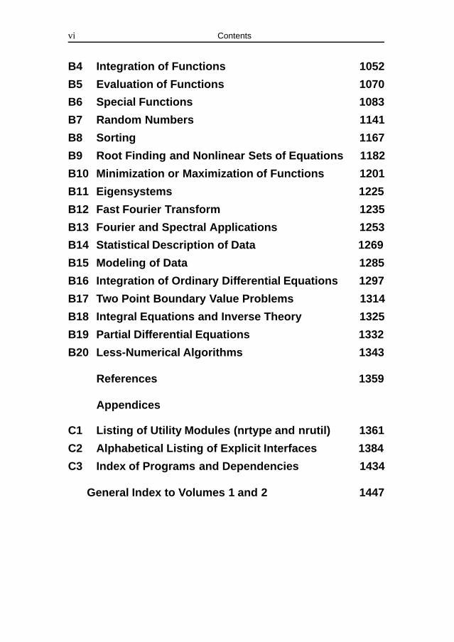
B4 Integration of Functions 1052
B5 Evaluation of Functions 1070
B6 Special Functions 1083
B7 Random Numbers 1141
B8 Sorting 1167
B9 Root Finding and Nonlinear Sets of Equations 1182
B10 Minimization or Maximization of Functions 1201
B11 Eigensystems 1225
B12 Fast Fourier Transform 1235
B13 Fourier and Spectral Applications 1253
B14 Statistical Description of Data 1269
B15 Modeling of Data 1285
B16 Integration of Ordinary Differential Equations 1297
B17 Two Point Boundary Value Problems 1314
B18 Integral Equations and Inverse Theory 1325
B19 Partial Differential Equations 1332
B20 Less-Numerical Algorithms 1343
References 1359
Appendices
C1 Listing of Utility Modules (nrtype and nrutil) 1361
C2 Alphabetical Listing of Explicit Interfaces 1384
C3 Index of Programs and Dependencies 1434
General Index to Volumes 1 and 2 1447
Contents vii
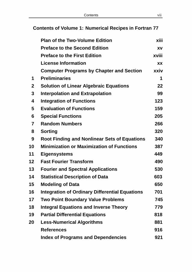
Contents of Volume 1: Numerical Recipes in Fortran 77
Plan of the Two-Volume Edition xiii
Preface to the Second Edition xv
Preface to the First Edition xviii
License Information xx
Computer Programs by Chapter and Section xxiv
1 Preliminaries 1
2 Solution of Linear Algebraic Equations 22
3 Interpolation and Extrapolation 99
4 Integration of Functions 123
5 Evaluation of Functions 159
6 Special Functions 205
7 Random Numbers 266
8 Sorting 320
9 Root Finding and Nonlinear Sets of Equations 340
10 Minimization or Maximization of Functions 387
11 Eigensystems 449
12 Fast Fourier Transform 490
13 Fourier and Spectral Applications 530
14 Statistical Description of Data 603
15 Modeling of Data 650
16 Integration of Ordinary Differential Equations 701
17 Two Point Boundary Value Problems 745
18 Integral Equations and Inverse Theory 779
19 Partial Differential Equations 818
20 Less-Numerical Algorithms 881
References 916
Index of Programs and Dependencies 921
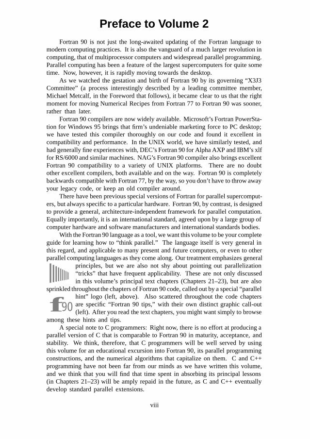
Preface to Volume 2Fortran 90 is not just the long-awaited updating of the Fortran language to
modern computing practices. It is also the vanguard of a much larger revolution incomputing, that of multiprocessor computers and widespread parallel programming.Parallel computing has been a feature of the largest supercomputers for quite sometime. Now, however, it is rapidly moving towards the desktop.
As we watched the gestation and birth of Fortran 90 by its governing “X3J3Committee” (a process interestingly described by a leading committee member,Michael Metcalf, in the Foreword that follows), it became clear to us that the rightmoment for moving Numerical Recipes from Fortran 77 to Fortran 90 was sooner,rather than later.
Fortran 90 compilers are now widely available. Microsoft’s Fortran PowerSta-tion for Windows 95 brings that firm’s undeniable marketing force to PC desktop;we have tested this compiler thoroughly on our code and found it excellent incompatibility and performance. In the UNIX world, we have similarly tested, andhad generally fine experiences with, DEC’s Fortran 90 for Alpha AXP and IBM’s xlffor RS/6000 and similar machines. NAG’s Fortran 90 compiler also brings excellentFortran 90 compatibility to a variety of UNIX platforms. There are no doubtother excellent compilers, both available and on the way. Fortran 90 is completelybackwards compatible with Fortran 77, by the way, so you don’t have to throw awayyour legacy code, or keep an old compiler around.
There have been previous special versions of Fortran for parallel supercomput-ers, but always specific to a particular hardware. Fortran 90, by contrast, is designedto provide a general, architecture-independent framework for parallel computation.Equally importantly, it is an international standard, agreed upon by a large group ofcomputer hardware and software manufacturers and international standards bodies.
With the Fortran 90 language as a tool, we want this volume to be your completeguide for learning how to “think parallel.” The language itself is very general inthis regard, and applicable to many present and future computers, or even to otherparallel computing languages as they come along. Our treatment emphasizes general
principles, but we are also not shy about pointing out parallelization“tricks” that have frequent applicability. These are not only discussedin this volume’s principal text chapters (Chapters 21–23), but are also
sprinkled throughout the chapters of Fortran 90 code, called out by a special “parallel
f90hint” logo (left, above). Also scattered throughout the code chaptersare specific “Fortran 90 tips,” with their own distinct graphic call-out(left). After you read the text chapters, you might want simply to browse
among these hints and tips.A special note to C programmers: Right now, there is no effort at producing a
parallel version of C that is comparable to Fortran 90 in maturity, acceptance, andstability. We think, therefore, that C programmers will be well served by usingthis volume for an educational excursion into Fortran 90, its parallel programmingconstructions, and the numerical algorithms that capitalize on them. C and C++programming have not been far from our minds as we have written this volume,and we think that you will find that time spent in absorbing its principal lessons(in Chapters 21–23) will be amply repaid in the future, as C and C++ eventuallydevelop standard parallel extensions.
viii

Preface to Volume 2 ix
A final word of truth in packaging: Don’t buy this volume unless you alsobuy (or already have) Volume 1 (now retitled Numerical Recipes in Fortran 77).Volume 2 does not repeat any of the discussion of what individual programs actuallydo, or of the mathematical methods they utilize, or how to use them. While ourFortran 90 code is thoroughly commented, and includes a header comment foreach routine that describes its input and output quantities, these comments are notsupposed to be a complete description of the programs; the complete descriptionsare in Volume 1, which we reference frequently. But here’s a money-saving hintto our previous readers: If you already own a Second Edition version whose titleis Numerical Recipes in FORTRAN (which doesn’t indicate either “Volume 1” or“Volume 2” on its title page) then take a marking pen and write in the words “Volume1.” There! (Differences between the previous reprintings and the newest reprinting,the one labeled “Volume 1,” are minor.)
Acknowledgments
We continue to be in the debt of many colleagues who give us the benefit oftheir numerical and computational experience. Many, though not all, of these arelisted by name in the preface to the second edition, in Volume 1. To that list we mustnow certainly add George Marsaglia, whose ideas have greatly influenced our newdiscussion of random numbers in this volume (Chapter B7).
With this volume, we must acknowledge our additional gratitude and debt to anumber of people who generously provided advice, expertise, and time (a great dealof time, in some cases) in the areas of parallel programming and Fortran 90. Theoriginal inspiration for this volume came from Mike Metcalf, whose clear lectures onFortran 90 (in this case, overlooking the beautiful Adriatic at Trieste) convinced usthat Fortran 90 could serve as the vehicle for a book with the larger scope of parallelprogramming generally, and whose continuing advice throughout the project hasbeen indispensable. Gyan Bhanot also played a vital early role in the developmentof this book; his first translations of our Fortran 77 programs taught us a lot aboutparallel programming. We are also grateful to Greg Lindhorst, Charles Van Loan,Amos Yahil, Keith Kimball, Malcolm Cohen, Barry Caplin, Loren Meissner, MitsuSakamoto, and George Schnurer for helpful correspondence and/or discussion ofFortran 90’s subtler aspects.
We once again express in the strongest terms our gratitude to programmingconsultant Seth Finkelstein, whose contribution to both the coding and the thoroughtesting of all the routines in this book (against multiple compilers and in sometimes-buggy, and always challenging, early versions) cannot be overstated.
WHP and SAT acknowledge the continued support of the U.S. National ScienceFoundation for their research on computational methods.
February 1996 William H. PressSaul A. Teukolsky
William T. VetterlingBrian P. Flannery
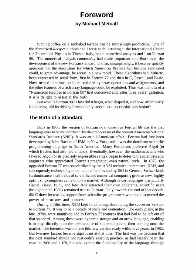
Forewordby Michael Metcalf
Sipping coffee on a sunbaked terrace can be surprisingly productive. One ofthe Numerical Recipes authors and I were each lecturing at the International Centerfor Theoretical Physics in Trieste, Italy, he on numerical analysis and I on Fortran90. The numerical analysis community had made important contributions to thedevelopment of the new Fortran standard, and so, unsurprisingly, it became quicklyapparent that the algorithms for which Numerical Recipes had become renownedcould, to great advantage, be recast in a new mold. These algorithms had, hitherto,been expressed in serial form, first in Fortran 77 and then in C, Pascal, and Basic.Now, nested iterations could be replaced by array operations and assignments, andthe other features of a rich array language could be exploited. Thus was the idea of a“Numerical Recipes in Fortran 90" first conceived and, after three years’ gestation,it is a delight to assist at the birth.
But what is Fortran 90? How did it begin, what shaped it, and how, after nearlyfoundering, did its driving forces finally steer it to a successful conclusion?
The Birth of a Standard
Back in 1966, the version of Fortran now known as Fortran 66 was the firstlanguage ever to be standardized, by the predecessor of the present American NationalStandards Institute (ANSI). It was an all-American affair. Fortran had first beendeveloped by John Backus of IBM in New York, and it was the dominant scientificprogramming language in North America. Many Europeans preferred Algol (inwhich Backus had also had a hand). Eventually, however, the mathematicians whofavored Algol for its precisely expressible syntax began to defer to the scientists andengineers who appreciated Fortran’s pragmatic, even natural, style. In 1978, theupgraded Fortran 77 was standardized by the ANSI technical committee, X3J3, andsubsequently endorsed by other national bodies and by ISO in Geneva, Switzerland.Its dominance in all fields of scientific and numerical computing grew as new, highlyoptimizing compilers came onto the market. Although newer languages, particularlyPascal, Basic, PL/1, and later Ada attracted their own adherents, scientific usersthroughout the 1980s remained true to Fortran. Only towards the end of that decadedid C draw increasing support from scientific programmers who had discovered thepower of structures and pointers.
During all this time, X3J3 kept functioning, developing the successor versionto Fortran 77. It was to be a decade of strife and contention. The early plans, in thelate 1970s, were mainly to add to Fortran 77 features that had had to be left out ofthat standard. Among these were dynamic storage and an array language, enablingit to map directly onto the architecture of supercomputers, then coming onto themarket. The intention was to have this new version ready within five years, in 1982.But two new factors became significant at that time. The first was the decision thatthe next standard should not just codify existing practice, as had largely been thecase in 1966 and 1978, but also extend the functionality of the language through
x
Foreword xi
innovative additions (even though, for the array language, there was significantborrowing from John Iverson’s APL and from DAP Fortran). The second factor wasthat X3J3 no longer operated under only American auspices. In the course of the1980s, the standardization of programming languages came increasingly under theauthority of the international body, ISO. Initially this was in an advisory role, butnow ISO is the body that, through its technical committee WG5 (in full, ISO/IECJTC1/SC22/WG5), is responsible for determining the course of the language. WG5also steers the work of the development body, then as now, the highly skilled andcompetent X3J3. As we shall see, this shift in authority was crucial at the mostdifficult moment of Fortran 90’s development.
The internationalization of the standards effort was reflected in the welcomegiven by X3J3 to six or seven European members; they, and about one-third ofX3J3’s U.S. members, provided the overlapping core of membership of X3J3 andWG5 that was vital in the final years in bringing the work to a successful conclusion.X3J3 membership, which peaked at about 45, is restricted to one voting memberper organization, and significant decisions require a majority of two-thirds of thosevoting. Nationality plays no role, except in determining the U.S. position on aninternational issue. Members, who are drawn mainly from the vendors, largeresearch laboratories, and academia, must be present or represented at two-thirds ofall meetings in order to retain voting rights.
In 1980, X3J3 reported on its plans to the forerunner of WG5 in Amsterdam,Holland. Fortran 8x, as it was dubbed, was to have a basic array language, newlooping constructs, a bit data type, data structures, a free source form, a mechanismto “group” procedures, and another to manage the global name space. Old features,including COMMON, EQUIVALENCE, and the arithmetic-IF, were to be consigned to aso-called obsolete module, destined to disappear in a subsequent revision. This waspart of the “core plus modules” architecture, for adding new features and retiringold ones, an aid to backwards compatibility. Even though Fortran 77 compilerswere barely available, the work seemed well advanced and the mood was optimistic.Publication was intended to take place in 1985. It was not to be.
One problem was the sheer number of new features that were proposed asadditions to the language, most of them worthwhile in themselves but with thetotality being too large. This became a recurrent theme throughout the developmentof the standard. One example was the suggestion of Lawrie Schonfelder (LiverpoolUniversity), at a WG5 meeting in Vienna, Austria, in 1982, that certain featuresalready proposed as additions could be combined to provide a full-blown deriveddata type facility, thus providingFortran with abstract data types. This idea was takenup by X3J3 and has since come to be recognized, along with the array language, asone of the two main advances brought about by what became Fortran 90. However,the ramifications go very deep: all the technical details of how to handle arrays ofobjects of derived types that in turn have array components that have the pointerattribute, and so forth, have to be precisely defined and rigorously specified.
Conflict
The meetings of X3J3 were often full of drama. Most compiler vendors wererepresented as a matter of course but, for many, their main objective appeared tobe to maintain the status quo and to ensure that Fortran 90 never saw the light of
xii Foreword
day. One vendor’s extended (and much-copied) version of Fortran 77 had virtuallybecome an industry standard, and it saw as its mission the maintenance of this lead.A new standard would cost it its perceived precious advantage. Other large vendorshad similar points of view, although those marketing supercomputers were clearlykeen on the array language. Most users, on the other hand, were hardly prepared toinvest large amounts of their employers’ and their own resources in simply settlingfor a trivial set of improvements to the existing standard. However, as long asX3J3 worked under a simple-majority voting rule, at least some apparent progresscould be made, although the underlying differences often surfaced. These were evensometimes between users — those who wanted Fortran to become a truly modernlanguage and those wanting to maintain indefinite backwards compatibility for theirbillions of lines of existing code.
At a watershed meeting, in Scranton, Pennsylvania, in 1986, held in anatmosphere that sometimes verged on despair, a fragile compromise was reachedas a basis for further work. One breakthrough was to weaken the procedures forremoving outdated features from the language, particularly by removing no featureswhatsoever from the next standard and by striking storage association (i.e., COMMONand EQUIVALENCE) from the list of features to be designated as obsolescent (as theyare now known). A series of votes definitively removed from the language all plansto add: arrays of arrays, exception handling, nesting of internal procedures, theFORALL statement (now in Fortran 95), and a means to access skew array sections.There were other features on this list that, although removed, were reinstated atlater meetings: user-defined operators, operator overloading, array and structureconstructors, and vector-valued subscripts. After many more travails, the committeevoted, a year later, by 26 votes to 9, to forward the document for what was to becomethe first of three periods of public comment.
While the document was going through the formal standards bureaucracy andbeing placed before the public, X3J3 polished it further. X3J3 also preparedprocedures for processing the comments it anticipated receiving from the public,and to each of which, under the rules, it would have to reply individually. It wasjust as well. Roughly 400 replies flooded in, many of them very detailed and,disappointingly for those of us wanting a new standard quickly, unquestionablynegative towards our work. For many it was too radical, but many others pleadedfor yet more modern features, such as pointers.
Now the committee was deadlocked. Given that a document had alreadybeen published, any further change required not a simple but a two-thirds majority.The conservatives and the radicals could each block a move to modify the draftstandard, or to accept a revised one for public review — and just that happened,in Champagne-Urbana, Illinois, in 1988. Any change, be it on the one hand tomodify the list of obsolescent features, to add the pointers or bit data type wantedby the public, to add multi-byte characters to support Kanji and other non-Europeanlanguages or, on the other hand, to emasculate the language by removing modules oroperator overloading, and hence abstract data types, to name but some suggestions,none of these could be done individually or collectively in a way that would achieveconsensus. I wrote:
“In my opinion, no standard can now emerge without either a huge concessionby the users to the vendors (MODULE / USE) and/or a major change in the compositionof the committee. I do not see how members who have worked for up to a decade
Foreword xiii
or more, devoting time and intellectual energy far beyond the call of duty, can beexpected to make yet more personal sacrifices if no end to the work is in sight, orif that end is nothing but a travesty of what had been designed and intended as amodern scientific programming language. . . . I think the August meeting will be awatershed — if no progress is achieved there will be dramatic resignations, and ISOcould even remove the work from ANSI, which is failing conspicuously in its task."
(However, the same notes began with a quotation from The Taming of theShrew: “And do as adversaries do in law, / Strive mightily, but eat and drink / asfriend." That we always did, copiously.)
Resolution
The “August meeting” was, unexpectedly, imbued with a spirit of compromisethat had been so sadly lacking at the previous one. Nevertheless, after a week ofdiscussing four separate plans to rescue the standard, no agreement was reached.Now the question seriously arose: Was X3J3 incapable of producing a new Fortranstandard for the international community, doomed to eternal deadlock, a victim ofANSI procedures?
Breakthrough was achieved at a traumatic meeting of WG5 in Paris, France, amonth later. The committee spent several extraordinary days drawing up a detailedlist of what it wanted to be in Fortran 8x. Finally, it set X3J3 an ultimatum that wasunprecedented in the standards world: The ANSI committee was to produce a newdraft document, corresponding to WG5’s wishes, within five months! Failing that,WG5 would assume responsibility and produce the new standard itself.
This decision was backed by the senior U.S. committee, X3, which effectivelydirected X3J3 to carry out WG5’s wishes. And it did! The following November, itimplemented most of the technical changes, adding pointers, bit manipulation intrin-sic procedures, and vector-valued subscripts, and removing user-defined elementalfunctions (now in Fortran 95). The actual list of changes was much longer. X3J3 andWG5, now collaborating closely, often in gruelling six-day meetings, spent the next18 months and two more periods of (positive) public comment putting the finishingtouches to what was now called Fortran 90, and it was finally adopted, after somecliff-hanging votes, for forwarding as a U.S. and international standard on April 11,1991, in Minneapolis, Minnesota.
Among the remaining issues that were decided along the way were whetherpointers should be a data type or be defined in terms of an attribute of a variable,implying strong typing (the latter was chosen), whether the new standard shouldcoexist alongside the old one rather than definitively replace it (it coexisted for awhile in the U.S., but was a replacement elsewhere, under ISO rules), and whether,in the new free source form, blanks should be significant (fortunately, they are).
Fortran 90
The main new features of Fortran 90 are, first and foremost, the array languageand abstract data types. The first is built on whole array operations and assignments,array sections, intrinsic procedures for arrays, and dynamic storage. It was designedwith optimization in mind. The second is built on modules and module procedures,derived data types, operator overloading and generic interfaces, together with
xiv Foreword
pointers. Also important are the new facilities for numerical computation includinga set of numeric inquiry functions, the parametrization of the intrinsic types, newcontrol constructs — SELECT CASE and new forms of DO, internal and recursiveprocedures and optional and keyword arguments, improved I/O facilities, and manynew intrinsic procedures. Last but not least are the new free source form, animproved style of attribute-oriented specifications, the IMPLICIT NONE statement,and a mechanism for identifying redundant features for subsequent removal from thelanguage. The requirement on compilers to be able to identify, for example, syntaxextensions, and to report why a program has been rejected, are also significant. Theresulting language is not only a far more powerful tool than its successor, but a saferand more reliable one too. Storage association, with its attendant dangers, is notabolished, but rendered unnecessary. Indeed, experience shows that compilers detecterrors far more frequently than before, resulting in a faster development cycle. Thearray syntax and recursion also allow quite compact code to be written, a furtheraid to safe programming.
No programming language can succeed if it consists simply of a definition(witness Algol 68). Also required are robust compilers from a wide variety ofvendors, documentation at various levels, and a body of experience. The first Fortran90 compiler appeared surprisingly quickly, in 1991, especially in view of the widelytouted opinion that it would be very difficult to write one. Even more remarkablewas that it was written by one person, Malcolm Cohen of NAG, in Oxford, U.K.There was a gap before other compilers appeared, but now they exist as nativeimplementations for almost all leading computers, from the largest to PCs. For themost part, they produce very efficient object code; where, for certain new features,this is not the case, work is in progress to improve them.
The first book, Fortran 90 Explained, was published by John Reid and meshortly before the standard itself was published. Others followed in quick succession,including excellent texts aimed at the college market. At the time of writing thereare at least 19 books in English and 22 in various other languages: Chinese, Dutch,French, Japanese, Russian, and Swedish. Thus, the documentation condition isfulfilled.
The body of experience, on the other hand, has yet to be built up to a critical size.Teaching of the language at college level has only just begun. However, I am certainthat this present volume will contribute decisively to a significant breakthrough, as itprovides models not only of the numerical algorithms for which previous editions arealready famed, but also of an excellent Fortran 90 style, something that can developonly with time. Redundant features are abjured. It shows that, if we abandon thesefeatures and use new ones in their place, the appearance of code can initially seemunfamiliar, but, in fact, the advantages become rapidly apparent. This new editionof Numerical Recipes stands as a landmark in this regard.
Fortran Evolution
The formal procedures under which languages are standardized require themeither to evolve or to die. A standard that has not been revised for some years musteither be revised and approved anew, or be withdrawn. This matches the technicalpressure on the language developers to accommodate the increasing complexity bothof the problems to be tackled in scientific computation and of the underlyinghardware
Foreword xv
on which programs run. Increasing problem complexity requires more powerfulfeatures and syntax; new hardware needs language features that map onto it well.
Thus it was that X3J3 and WG5, having finished Fortran 90, began a new roundof improvement. They decided very quickly on new procedures that would avoidthe disputes that bedevilled the previous work: WG5 would decide on a plan forfuture standards, and X3J3 would act as the so-called development body that wouldactually produce them. This would be done to a strict timetable, such that any featurethat could not be completed on time would have to wait for the next round. It wasfurther decided that the next major revision should appear a decade after Fortran 90but, given the somewhat discomforting number of requests for interpretation that hadarrived, about 200, that a minor revision should be prepared for mid-term, in 1995.This should contain only “corrections, clarifications and interpretations” and a verylimited number (some thought none) of minor improvements.
At the same time, scientific programmers were becoming increasingly concernedat the variety of methods that were necessary to gain efficient performance from theever-more widely used parallel architectures. Each vendor provided a different setof parallel extensions for Fortran, and some academic researchers had developed yetothers. On the initiative of Ken Kennedy of Rice University, a High-PerformanceFortran Forum was established. A coalition of vendors and users, its aim was toproduce an ad hoc set of extensions to Fortran that would become an informal butwidely accepted standard for portable code. It set itself the daunting task of achievingthat in just one year, and succeeded. Melding existing dialects like Fortran D, CMFortran, and Vienna Fortran, and adopting the new Fortran 90 as a base, becauseof its array syntax, High-Performance Fortran (HPF) was published in 1993 andhas since become widely implemented. However, although HPF was designed fordata parallel codes and mainly implemented in the form of directives that appearto non-HPF processors as comment lines, an adequate functionality could not beachieved without extending the Fortran syntax. This was done in the form of thePURE attribute for functions — an assertion that they contain no side effects — and theFORALL construct — a form of array assignment expressed with the help of indices.
The dangers of having diverging or competing forms of Fortran 90 wereimmediately apparent, and the standards committees wisely decided to incorporatethese two syntactic changes also into Fortran 95. But they didn’t stop there. Twofurther extensions, useful not only for their expressive power but also to accessparallel hardware, were added: elemental functions, ones written in terms of scalarsbut that accept array arguments of any permitted shape or size, and an extension toallow nesting of WHERE constructs, Fortran’s form of masked assignment. To readersof Numerical Recipes, perhaps the most relevant of the minor improvements thatFortran 95 brings are the ability to distinguish between a negative and a positive realzero, automatic deallocation of allocatable arrays, and a means to initialize the valuesof components of objects of derived data types and to initialize pointers to null.
The medium-term objective of a relatively minor upgrade has been achieved onschedule. But what does the future hold? Developments in the underlying principlesof procedural programming languages have not ceased. Early Fortran introduced theconcepts of expression abstraction (X=Y+Z) and later control expression (e.g., the DOloop). Fortran 77 continued this with the if-then-else, and Fortran 90 with theDO and SELECT CASE constructs. Fortran 90 has a still higher level of expressionabstraction (array assignments and expressions) as well as data structures and even
xvi Foreword
full-blown abstract data types. However, during the 1980s the concept of objectscame to the fore, with methods bound to the objects on which they operate. Here,one particular language, C++, has come to dominate the field. Fortran 90 lacksa means to point to functions, but otherwise has most of the necessary features inplace, and the standards committees are now faced with the dilemma of decidingwhether to make the planned Fortran 2000 a fully object-oriented language. Thiscould possibly jeopardize its powerful, and efficient, numerical capabilities by toogreat an increase in language complexity, so should they simply batten down thehatches and not defer to what might be only a passing storm? At the time of writing,this is an open issue. One issue that is not open is Fortran’s lack of in-built exceptionhandling. It is virtually certain that such a facility, much requested by the numericalcommunity, and guided by John Reid, will be part of the next major revision. Thelist of other requirements is long but speculative, but some at the top of the listare conditional compilation, command line argument handling, I/O for objects ofderived type, and asynchronous I/O (which is also planned for the next releaseof HPF). In the meantime, some particularly pressing needs have been identified,for the handling of floating-point exceptions, interoperability with C, and allowingallocatable arrays as structure components, dummy arguments, and function results.These have led WG5 to begin processing these three items using a special form offast track, so that they might become optional but standard extensions well beforeFortran 2000 itself is published in the year 2001.
Conclusion
Writing a book is always something of a gamble. Unlike a novel that standsor falls on its own, a book devoted to a programming language is dependent onthe success of others, and so the risk is greater still. However, this new NumericalRecipes in Fortran 90 volume is no ordinary book, since it comes as the continuationof a highly successful series, and so great is its significance that it can, in fact,influence the outcome in its own favor. I am entirely confident that its publicationwill be seen as an important event in the story of Fortran 90, and congratulate itsauthors on having performed a great service to the field of numerical computing.
Geneva, SwitzerlandJanuary 1996
Michael Metcalf
License Information
Read this section if you want to use the programs in this book on a computer.You’ll need to read the following Disclaimer of Warranty, get the programs onto yourcomputer, and acquire a Numerical Recipes software license. (Without this license,which can be the free “immediate license” under terms described below, the book isintended as a text and reference book, for reading purposes only.)
Disclaimer of Warranty
We make no warranties, express or implied, that the programs containedin this volume are free of error, or are consistent with any particular standardof merchantability, or that they will meet your requirements for any particularapplication. They should not be relied on for solving a problem whose incorrectsolution could result in injury to a person or loss of property. If you do use theprograms in such a manner, it is at your own risk. The authors and publisherdisclaim all liability for direct or consequential damages resulting from youruse of the programs.
How to Get the Code onto Your Computer
Pick one of the following methods:
• You can type the programs from this book directly into your computer. Inthis case, the only kind of license available to you is the free “immediatelicense” (see below). You are not authorized to transfer or distribute amachine-readable copy to any other person, nor to have any other persontype the programs into a computer on your behalf. We do not want to hearbug reports from you if you choose this option, because experience hasshown that virtually all reported bugs in such cases are typing errors!
• You can download the Numerical Recipes programs electronically fromthe Numerical Recipes On-Line Software Store, located at our Web site(http://www.nr.com). They are packaged as a password-protectedfile, and you’ll need to purchase a license to unpack them. You canget a single-screen license and password immediately, on-line, from theOn-Line Store, with fees ranging from $50 (PC, Macintosh, educationalinstitutions’ UNIX) to $140 (general UNIX). Downloading the packagedsoftware from the On-Line Store is also the way to start if you want toacquire a more general (multiscreen, site, or corporate) license.
• You can purchase media containing the programs from Cambridge Uni-versity Press. Diskette versions are available in IBM-compatible formatfor machines running Windows 3.1, 95, or NT. CDROM versions in ISO-9660 format for PC, Macintosh, and UNIX systems are also available;these include both Fortran and C versions (as well as versions in Pascal
xvii
xviii License Information
and BASIC from the first edition) on a single CDROM. Diskettes pur-chased from Cambridge University Press include a single-screen licensefor PC or Macintosh only. The CDROM is available with a single-screen license for PC or Macintosh (order ISBN 0 521 576083), or (at aslightly higher price) with a single-screen license for UNIX workstations(order ISBN 0 521 576075). Orders for media from Cambridge Univer-sity Press can be placed at 800 872-7423 (North America only) or byemail to [email protected] (North America) or [email protected] (restof world). Or, visit the Web sites http://www.cup.org (North America)or http://www.cup.cam.ac.uk (rest of world).
Types of License Offered
Here are the types of licenses that we offer. Note that some types areautomatically acquired with the purchase of media from Cambridge UniversityPress, or of an unlocking password from the Numerical Recipes On-Line SoftwareStore, while other types of licenses require that you communicate specifically withNumerical Recipes Software (email: [email protected] or fax: 781 863-1739). OurWeb site http://www.nr.com has additional information.
• [“Immediate License”] If you are the individual owner of a copy of thisbook and you type one or more of its routines into your computer, weauthorize you to use them on that computer for your own personal andnoncommercial purposes. You are not authorized to transfer or distributemachine-readable copies to any other person, or to use the routines onmore than one machine, or to distribute executable programs containingour routines. This is the only free license.
• [“Single-Screen License”] This is the most common type of low-costlicense, with terms governed by our Single Screen (Shrinkwrap) Licensedocument (complete terms available through our Web site). Basically, thislicense lets you use Numerical Recipes routines on any one screen (PC,workstation, X-terminal, etc.). You may also, under this license, transferpre-compiled, executable programs incorporating our routines to other,unlicensed, screens or computers, providing that (i) your application isnoncommercial (i.e., does not involve the selling of your program for afee), (ii) the programs were first developed, compiled, and successfullyrun on a licensed screen, and (iii) our routines are bound into the programsin such a manner that they cannot be accessed as individual routines andcannot practicably be unbound and used in other programs. That is, underthis license, your program user must not be able to use our programs aspart of a program library or “mix-and-match” workbench. Conditions forother types of commercial or noncommercial distribution may be foundon our Web site (http://www.nr.com).
• [“Multi-Screen, Server, Site, and Corporate Licenses”] The terms ofthe Single Screen License can be extended to designated groups ofmachines, defined by number of screens, number of machines, locations,or ownership. Significant discounts from the corresponding single-screen
License Information xix
prices are available when the estimated number of screens exceeds 40.Contact Numerical Recipes Software (email: [email protected] or fax: 781863-1739) for details.
• [“Course Right-to-Copy License”] Instructors at accredited educationalinstitutions who have adopted this book for a course, and who havealready purchased a Single Screen License (either acquired with thepurchase of media, or from the Numerical Recipes On-Line SoftwareStore), may license the programs for use in that course as follows: Mailyour name, title, and address; the course name, number, dates, andestimated enrollment; and advance payment of $5 per (estimated) studentto Numerical Recipes Software, at this address: P.O. Box 243, Cambridge,MA 02238 (USA). You will receive by return mail a license authorizingyou to make copies of the programs for use by your students, and/or totransfer the programs to a machine accessible to your students (but onlyfor the duration of the course).
About Copyrights on Computer Programs
Like artistic or literary compositions, computer programs are protected bycopyright. Generally it is an infringement for you to copy into your computer aprogram from a copyrighted source. (It is also not a friendly thing to do, since itdeprives the program’s author of compensation for his or her creative effort.) Undercopyright law, all “derivative works” (modified versions, or translations into anothercomputer language) also come under the same copyright as the original work.
Copyright does not protect ideas, but only the expression of those ideas ina particular form. In the case of a computer program, the ideas consist of theprogram’s methodology and algorithm, including the necessary sequence of stepsadopted by the programmer. The expression of those ideas is the program sourcecode (particularly any arbitrary or stylistic choices embodied in it), its derived objectcode, and any other derivative works.
If you analyze the ideas contained in a program, and then express thoseideas in your own completely different implementation, then that new programimplementation belongs to you. That is what we have done for those programs inthis book that are not entirely of our own devising. When programs in this book aresaid to be “based” on programs published in copyright sources, we mean that theideas are the same. The expression of these ideas as source code is our own. Webelieve that no material in this book infringes on an existing copyright.
Trademarks
Several registered trademarks appear within the text of this book: Sun is atrademark of Sun Microsystems, Inc. SPARC and SPARCstation are trademarks ofSPARC International, Inc. Microsoft, Windows 95, Windows NT, PowerStation,and MS are trademarks of Microsoft Corporation. DEC, VMS, Alpha AXP, andULTRIX are trademarks of Digital Equipment Corporation. IBM is a trademark ofInternational Business Machines Corporation. Apple and Macintosh are trademarksof Apple Computer, Inc. UNIX is a trademark licensed exclusively through X/Open
xx License Information
Co. Ltd. IMSL is a trademark of Visual Numerics, Inc. NAG refers to proprietarycomputer software of Numerical Algorithms Group (USA) Inc. PostScript andAdobe Illustrator are trademarks of Adobe Systems Incorporated. Last, and no doubtleast, Numerical Recipes (when identifying products) is a trademark of NumericalRecipes Software.
Attributions
The fact that ideas are legally “free as air” in no way supersedes the ethicalrequirement that ideas be credited to their known originators. When programs inthis book are based on known sources, whether copyrighted or in the public domain,published or “handed-down,” we have attempted to give proper attribution. Unfor-tunately, the lineage of many programs in common circulation is often unclear. Wewould be grateful to readers for new or corrected information regarding attributions,which we will attempt to incorporate in subsequent printings.
Chapter 21. Introductionto Fortran 90Language Features
21.0 Introduction
Fortran 90 is in many respects a backwards-compatible modernization of thelong-used (and much abused) Fortran 77 language, but it is also, in other respects,a new language for parallel programming on present and future multiprocessormachines. These twin design goals of the language sometimes add confusion to theprocess of becoming fluent in Fortran 90 programming.
In a certain trivial sense, Fortran 90 is strictly backwards-compatible withFortran 77. That is, any Fortran 90 compiler is supposed to be able to compile anylegacy Fortran 77 code without error. The reason for terming this compatibilitytrivial, however, is that you have to tell the compiler (usually via a source file nameending in “.f” or “.for”) that it is dealing with a Fortran 77 file. If you insteadtry to pass off Fortran 77 code as native Fortran 90 (e.g., by naming the source filesomething ending in “.f90”) it will not always work correctly!
It is best, therefore, to approach Fortran 90 as a new computer language, albeitone with a lot in common with Fortran 77. Indeed, in such terms, Fortran 90 is afairly big language, with a large number of new constructions and intrinsic functions.Here, in one short chapter, we do not pretend to provide a complete description ofthe language. Luckily, there are good books that do exactly that. Our favorite oneis by Metcalf and Reid [1], cited throughout this chapter as “M&R.” Other goodstarting points include [2] and [3].
Our goal, in the remainder of this chapter, is to give a good, working descriptionof those Fortran 90 language features that are not immediately self-explanatoryto Fortran 77 programmers, with particular emphasis on those that occur mostfrequently in the Fortran 90 versions of the Numerical Recipes routines. Thischapter, by itself, will not teach you to write Fortran 90 code. But it ought to helpyou acquire a reading knowledge of the language, and perhaps provide enough ofa head start that you can rapidly pick up the rest of what you need to know fromM&R or another Fortran 90 reference book.
CITED REFERENCES AND FURTHER READING:
Metcalf, M., and Reid, J. 1996, Fortran 90/95 Explained (Oxford: Oxford University Press). [1]
935
936 Chapter 21. Introduction to Fortran 90 Language Features
Kerrigan, J.F. 1993, Migrating to Fortran 90 (Sebastopol, CA: O’Reilly). [2]
Brainerd, W.S., Goldberg, C.H., and Adams, J.C. 1996, Programmer’s Guide to Fortran 90, 3rded. (New York: Springer-Verlag). [3]
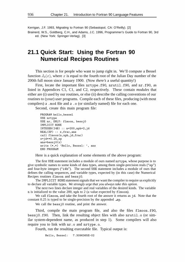
21.1 Quick Start: Using the Fortran 90Numerical Recipes Routines
This section is for people who want to jump right in. We’ll compute a Besselfunction J0(x), where x is equal to the fourth root of the Julian Day number of the200th full moon since January 1900. (Now there’sa useful quantity!)
First, locate the important files nrtype.f90, nrutil.f90, and nr.f90, aslisted in Appendices C1, C1, and C2, respectively. These contain modulesthateither are (i) used by our routines, or else (ii) describe the calling conventions of ourroutines to (your) user programs. Compile each of these files, producing (with mostcompilers) a .mod file and a .o (or similarly named) file for each one.
Second, create this main program file:
PROGRAM hello_besselUSE nrtypeUSE nr, ONLY: flmoon, bessj0IMPLICIT NONEINTEGER(I4B) :: n=200,nph=2,jdREAL(SP) :: x,frac,anscall flmoon(n,nph,jd,frac)x=jd**0.25_spans=bessj0(x)write (*,*) ’Hello, Bessel: ’, ansEND PROGRAM
Here is a quick explanation of some elements of the above program:
The first USE statement includes a module of ours named nrtype, whose purpose is togive symbolic names to some kinds of data types, among them single-precision reals (“sp”)and four-byte integers (“i4b”). The second USE statement includes a module of ours thatdefines the calling sequences, and variable types, expected by (in this case) the NumericalRecipes routines flmoon and bessj0.
The IMPLICIT NONE statement signals that we want the compiler to require us explicitlyto declare all variable types. We strongly urge that you always take this option.
The next two lines declare integer and real variables of the desired kinds. The variablen is initialized to the value 200, nph to 2 (a value expected by flmoon).
We call flmoon, and take the fourth root of the answer it returns as jd. Note that theconstant 0.25 is typed to be single-precision by the appended sp.
We call the bessj0 routine, and print the answer.
Third, compile the main program file, and also the files flmoon.f90,bessj0.f90. Then, link the resulting object files with also nrutil.o (or sim-ilar system-dependent name, as produced in step 1). Some compilers will alsorequire you to link with nr.o and nrtype.o.
Fourth, run the resulting executable file. Typical output is:
Hello, Bessel: 7.3096365E-02
21.2 Fortran 90 Language Concepts 937
21.2 Fortran 90 Language Concepts
The Fortran 90 language standard defines and uses a number of standard termsfor concepts that occur in the language. Here we summarize briefly some of themost important concepts. Standard Fortran 90 terms are shown in italics. While byno means complete, the information in this section should help you get a quick startwith your favorite Fortran 90 reference book or language manual.
A note on capitalization: Outside a character context, Fortran 90 is not case-sensitive, so you can use upper and lower case any way you want, to improvereadability. A variable like SP (see below) is the same variable as the variable sp.We like to capitalize keywords whose use is primarily at compile-time (statementsthat delimit program and subprogram boundaries, declaration statements of variables,fixed parameter values), and use lower case for the bulk of run-time code. You canadopt any convention that you find helpful to your own programming style; but westrongly urge you to adopt and follow someconvention.
Data Types and Kinds
Data types(also called simply types) can be either intrinsic data types(thefamiliar INTEGER, REAL, LOGICAL, and so forth) or else derived data typesthat arebuilt up in the manner of what are called “structures” or “records” in other computerlanguages. (We’ll use derived data types very sparingly in this book.) Intrinsic datatypes are further specified by their kind parameter(or simply kind), which is simplyan integer. Thus, on many machines, REAL(4) (with kind = 4) is a single-precisionreal, while REAL(8) (with kind = 8) is a double-precision real. Literal constants(or simply literals) are specified as to kind by appending an underscore, as 1.5 4
for single precision, or 1.5 8 for double precision. [M&R, §2.5–§2.6]Unfortunately, the specific integer values that define the different kind types
are not specified by the language, but can vary from machine to machine. Forthat reason, one almost never uses literal kind parameters like 4 or 8, but ratherdefines in some central file, and imports into all one’s programs, symbolic namesfor the kinds. For this book, that central file is the modulenamed nrtype, and thechosen symbolic names include SP, DP (for reals); I2B, I4B (for two- and four-byteintegers); and LGT for the default logical type. You will therefore see us consistentlywriting REAL(SP), or 1.5 sp, and so forth.
Here is an example of declaring some variables, including a one-dimensionalarray of length 500, and a two-dimensional array with 100 rows and 200 columns:
USE nrtypeREAL(SP) :: x,y,zINTEGER(I4B) :: i,j,kREAL(SP), DIMENSION(500) :: arrREAL(SP), DIMENSION(100,200) :: barrREAL(SP) :: carr(500)
The last line shows an alternative form for array syntax. And yes, there are defaultkind parameters for each intrinsic type, but these vary from machine to machine andcan get you into trouble when you try to move code. We therefore specify all kindparameters explicitly in almost all situations.
938 Chapter 21. Introduction to Fortran 90 Language Features
Array Shapes and Sizes
The shapeof an array refers to both its dimensionality (called its rank), andalso the lengths along each dimension (called the extents). The shape of an array isspecified by a rank-one array whose elements are the extents along each dimension,and can be queried with the shape intrinsic (see p. 949). Thus, in the above example,shape(barr) returns an array of length 2 containing the values (100, 200).
The sizeof an array is its total number of elements, so the intrinsic size(barr)would return 20000 in the above example. More often one wants to know theextents along each dimension, separately: size(barr,1) returns the value 100,while size(barr,2) returns the value 200. [M&R, §2.10]
Section §21.3, below, discusses additional aspects of arrays in Fortran 90.
Memory Management
Fortran 90 is greatly superior to Fortran 77 in its memory-management capa-bilities, seen by the user as the ability to create, expand, or contract workspace forprograms. Within subprograms(that is, subroutinesand functions), one can haveautomatic arrays(or other automatic data objects) that come into existence eachtime the subprogram is entered, and disappear (returning their memory to the pool)when the subprogram is exited. The size of automatic objects can be specifiedby arbitrary expressions involving values passed as actual argumentsin the callingprogram, and thus received by the subprogram through its corresponding dummyarguments. [M&R, §6.4]
Here is an example that creates some automatic workspace named carr:
SUBROUTINE dosomething(j,k)USE nrtypeREAL(SP), DIMENSION(2*j,k**2) :: carr
Finer control on when workspace is created or destroyed can be achieved bydeclaring allocatable arrays, which exist as names only, without associated memory,until they are allocatedwithin the program or subprogram. When no longer needed,they can be deallocated. The allocation statusof an allocatable array can be testedby the program via the allocated intrinsic function (p. 952). [M&R, §6.5]
Here is an example in outline:
REAL(SP), DIMENSION(:,:), ALLOCATABLE :: darr...allocate(darr(10,20))...deallocate(darr)...allocate(darr(100,200))...deallocate(darr)
Notice that darr is originally declared with only “slots” (colons) for its dimensions,and is then allocated/deallocated twice, with different sizes.
Yet finer control is achieved by the use of pointers. Like an allocatable array,a pointer can be allocated, at will, its own associated memory. However, it hasthe additional flexibility of alternatively being pointer associatedwith a target that
21.2 Fortran 90 Language Concepts 939
already exists under another name. Thus, pointers can be used as redefinable aliasesfor other variables, arrays, or (see §21.3) array sections. [M&R, §6.12]
Here is an example that first associates the pointer parr with the array earr,then later cancels that association and allocates it its own storage of size 50:
REAL(SP), DIMENSION(:), POINTER :: parrREAL(SP), DIMENSION(100), TARGET :: earr...parr => earr...nullify(parr)allocate(parr(50))...deallocate(parr)
Procedure Interfaces
When a procedure is referenced(e.g., called) from within a program orsubprogram (examples of scoping units), the scoping unit must be told, or mustdeduce, the procedure’s interface, that is, its calling sequence, including the typesand kinds of all dummy arguments, returned values, etc. The recommendedprocedure is to specify this interface via an explicit interface, usually an interfaceblock(essentially a declaration statement for subprograms) in the calling subprogramor in some modulethat the calling program includes via a USE statement. In thisbook all interfaces are explicit, and the module named nr contains interface blocksfor all of the Numerical Recipes routines. [M&R, §5.11]
Here is a typical example of an interface block:
INTERFACESUBROUTINE caldat(julian,mm,id,iyyy)USE nrtypeINTEGER(I4B), INTENT(IN) :: julianINTEGER(I4B), INTENT(OUT) :: mm,id,iyyyEND SUBROUTINE caldat
END INTERFACE
Once this interface is made known to a program that you are writing (by eitherexplicit inclusion or a USE statement), then the compiler is able to flag for you avariety of otherwise difficult-to-find bugs. Although interface blocks can sometimesseem overly wordy, they give a big payoff in ultimately minimizing programmertime and frustration.
For compatibility with Fortran 77, the language also allows for implicit inter-faces, where the calling program tries to figure out the interface by the old rules ofFortran 77. These rules are quite limited, and prone to producing devilishly obscureprogram bugs. We strongly recommend that implicit interfaces never be used.
Elemental Procedures and Generic Interfaces
Many intrinsic procedures(those defined by the language standard and thususable without any further definition or specification) are also generic. This meansthat a single procedure name, such as log(x), can be used with a variety of typesand kind parameters for the argument x, and the result returned will have the sametype and kind parameter as the argument. In this example, log(x) allows any realor complex argument type.
940 Chapter 21. Introduction to Fortran 90 Language Features
Better yet, most generic functions are also elemental. The argument of anelemental function can be an array of arbitrary shape! Then, the returned result isan array of the same shape, with each element containing the result of applying thefunction to the corresponding element of the argument. (Hence the name elemental,meaning “applied element by element.”) [M&R, §8.1] For example:
REAL(SP), DIMENSION(100,100) :: a,bb=sin(a)
Fortran 90 has no facility for creating new, user-defined elemental functions.It does have, however, the related facility of overloadingby the use of genericinterfaces. This is invoked by the use of an interface block that attaches a singlegeneric nameto a number of distinct subprograms whose dummy arguments havedifferent types or kinds. Then, when the generic name is referenced (e.g., called),the compiler chooses the specific subprogram that matches the types and kinds of theactual arguments used. [M&R, §5.18] Here is an example of a generic interface block:
INTERFACE myfuncFUNCTION myfunc_single(x)USE nrtypeREAL(SP) :: x,myfunc_singleEND FUNCTION myfunc_single
FUNCTION myfunc_double(x)USE nrtypeREAL(DP) :: x,myfunc_doubleEND FUNCTION myfunc_double
END INTERFACE
A program with knowledge of this interface could then freely use the functionreference myfunc(x) for x’s of both type SP and type DP.
We use overloading quite extensively in this book. A typical use is to provide,under the same name, both scalar and vector versions of a function such as aBessel function, or to provide both single-precision and double-precision versionsof procedures (as in the above example). Then, to the extent that we have providedall the versions that you need, you can pretend that our routine is elemental. Insuch a situation, if you ever call our function with a type or kind that we havenot provided, the compiler will instantly flag the problem, because it is unable toresolve the generic interface.
Modules
Modules, already referred to several times above, are Fortran 90’s generalizationof Fortran 77’s common blocks, INCLUDEd files of parameter statements, and (tosome extent) statement functions. Modules are program units, like main programs orsubprograms (subroutines and functions), that can be separately compiled. A moduleis a convenient place to stash global data, named constants(what in Fortran 77are called “symbolic constants” or “PARAMETERs”), interface blocks to subprogramsand/or actual subprograms themselves (module subprograms). The convenience isthat a module’s information can be incorporated into another program unit via asimple, one-line USE statement. [M&R, §5.5]
Here is an example of a simple module that defines a few parameters, createssome global storage for an array named arr (as might be done with a Fortran 77common block), and defines the interface to a function yourfunc:
21.3 More on Arrays and Array Sections 941
MODULE mymoduleUSE nrtypeREAL(SP), PARAMETER :: con1=7.0_sp/3.0_sp,con2=10.0_spINTEGER(I4B), PARAMETER :: ndim=10,mdim=9REAL(SP), DIMENSION(ndim,mdim) :: arrINTERFACE
FUNCTION yourfunc(x)USE nrtypeREAL(SP) :: x,yourfuncEND FUNCTION yourfunc
END INTERFACEEND MODULE mymodule
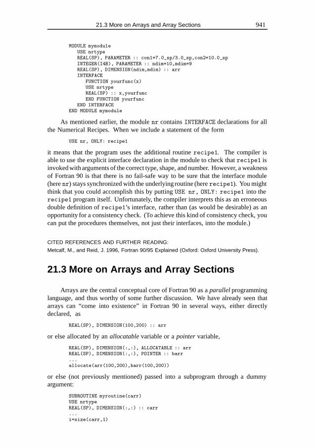
As mentioned earlier, the module nr contains INTERFACE declarations for allthe Numerical Recipes. When we include a statement of the form
USE nr, ONLY: recipe1
it means that the program uses the additional routine recipe1. The compiler isable to use the explicit interface declaration in the module to check that recipe1 isinvoked with arguments of the correct type, shape, and number. However, a weaknessof Fortran 90 is that there is no fail-safe way to be sure that the interface module(here nr) stays synchronized with the underlying routine (here recipe1). You mightthink that you could accomplish this by putting USE nr, ONLY: recipe1 into therecipe1 program itself. Unfortunately, the compiler interprets this as an erroneousdouble definition of recipe1’s interface, rather than (as would be desirable) as anopportunity for a consistency check. (To achieve this kind of consistency check, youcan put the procedures themselves, not just their interfaces, into the module.)
CITED REFERENCES AND FURTHER READING:
Metcalf, M., and Reid, J. 1996, Fortran 90/95 Explained (Oxford: Oxford University Press).
21.3 More on Arrays and Array Sections
Arrays are the central conceptual core of Fortran 90 as a parallel programminglanguage, and thus worthy of some further discussion. We have already seen thatarrays can “come into existence” in Fortran 90 in several ways, either directlydeclared, as
REAL(SP), DIMENSION(100,200) :: arr
or else allocated by an allocatablevariable or a pointervariable,
REAL(SP), DIMENSION(:,:), ALLOCATABLE :: arrREAL(SP), DIMENSION(:,:), POINTER :: barr...allocate(arr(100,200),barr(100,200))
or else (not previously mentioned) passed into a subprogram through a dummyargument:
SUBROUTINE myroutine(carr)USE nrtypeREAL(SP), DIMENSION(:,:) :: carr...i=size(carr,1)
942 Chapter 21. Introduction to Fortran 90 Language Features
j=size(carr,2)
In the above example we also show how the subprogram can find out the size ofthe actual array that is passed, using the size intrinsic. This routine is an exampleof the use of an assumed-shape array, new to Fortran 90. The actual extents alongeach dimension are inherited from the calling routine at run time. A subroutinewith assumed-shape array arguments musthave an explicit interface in the callingroutine, otherwise the compiler doesn’t know about the extra information that mustbe passed. A typical setup for calling myroutine would be:
PROGRAM use_myroutineUSE nrtypeREAL(SP), DIMENSION(10,10) :: arrINTERFACE
SUBROUTINE myroutine(carr)USE nrtypeREAL(SP), DIMENSION(:,:) :: carrEND SUBROUTINE myroutine
END INTERFACE...call myroutine(a)
Of course, for the recipes we have provided all the interface blocks in the file nr.f90,and you need only a USE nr statement in your calling program.
Conformable Arrays
Two arrays are said to be conformableif their shapes are the same. Fortran 90allows practically all operations among conformable arrays and elemental functionsthat are allowed for scalar variables. Thus, if arr, barr, and carr are mutuallyconformable, we can write,
arr=barr+cos(carr)+2.0_sp
and have the indicated operations performed, element by corresponding element,on the entire arrays. The above line also illustrates that a scalar (here the constant2.0 sp, but a scalar variable would also be fine) is deemed conformable with anyarray — it gets “expanded” to the shape of the rest of the expression that it isin. [M&R, §3.11]
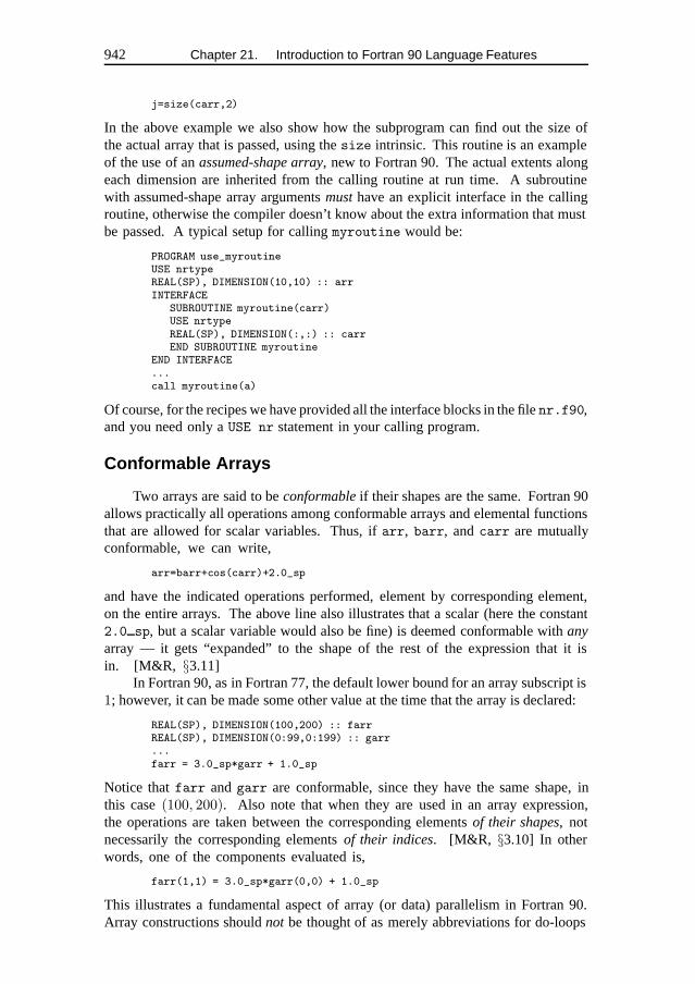
In Fortran 90, as in Fortran 77, the default lower bound for an array subscript is1; however, it can be made some other value at the time that the array is declared:
REAL(SP), DIMENSION(100,200) :: farrREAL(SP), DIMENSION(0:99,0:199) :: garr...farr = 3.0_sp*garr + 1.0_sp
Notice that farr and garr are conformable, since they have the same shape, inthis case (100, 200). Also note that when they are used in an array expression,the operations are taken between the corresponding elements of their shapes, notnecessarily the corresponding elements of their indices. [M&R, §3.10] In otherwords, one of the components evaluated is,
farr(1,1) = 3.0_sp*garr(0,0) + 1.0_sp
This illustrates a fundamental aspect of array (or data) parallelism in Fortran 90.Array constructions should not be thought of as merely abbreviations for do-loops
21.3 More on Arrays and Array Sections 943
over indices, but rather as genuinely parallel operations on same-shaped objects,abstracted of their indices. This is why the standard makes no statement about theorder in which the individual operations in an array expression are executed; theymight in fact be carried out simultaneously, on parallel hardware.
By default, array expressions and assignments are performed for all elementsof the same-shaped arrays referenced. This can be modified, however, by use ofa where construction like this:
where (harr > 0.0_sp)farr = 3.0_sp*garr + 1.0_sp
end where
Here harrmust also be conformable to farrand garr. Analogously with the Fortranif-statement, there is also a one-line form of the where-statement. There is alsoa where ... elsewhere ... end where form of the statement, analogous toif ... else if ... end if. A significant language limitation in Fortran 90is that nested where-statements are not allowed. [M&R, §6.8]
Array Sections
Much of the versatility of Fortran 90’s array facilities stems from the availabilityof array sections. An array section acts like an array, but its memory location, andthus the values of its elements, is actually a subset of the memory location of analready-declared array. Array sections are thus “windows into arrays,” and they canappear on either the left side, or the right side, or both, of a replacement statement.Some examples will clarify these ideas.
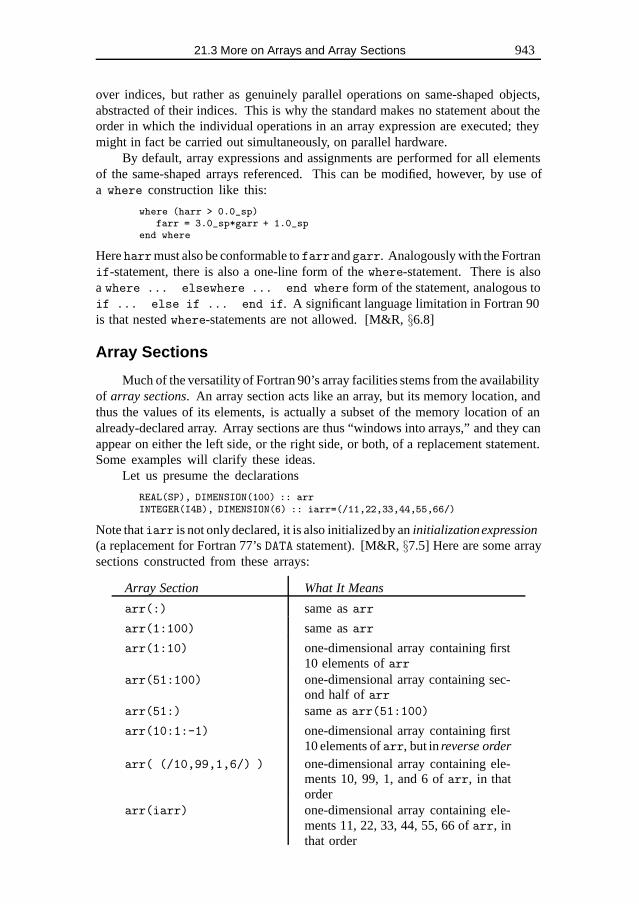
Let us presume the declarations
REAL(SP), DIMENSION(100) :: arrINTEGER(I4B), DIMENSION(6) :: iarr=(/11,22,33,44,55,66/)
Note that iarr is not only declared, it is also initializedby an initializationexpression(a replacement for Fortran 77’s DATA statement). [M&R, §7.5] Here are some arraysections constructed from these arrays:
Array Section What It Means
arr(:) same as arr
arr(1:100) same as arr
arr(1:10) one-dimensional array containing first10 elements of arr
arr(51:100) one-dimensional array containing sec-ond half of arr
arr(51:) same as arr(51:100)
arr(10:1:-1) one-dimensional array containing first10 elements of arr, but in reverse order
arr( (/10,99,1,6/) ) one-dimensional array containing ele-ments 10, 99, 1, and 6 of arr, in thatorder
arr(iarr) one-dimensional array containing ele-ments 11, 22, 33, 44, 55, 66 of arr, inthat order
944 Chapter 21. Introduction to Fortran 90 Language Features
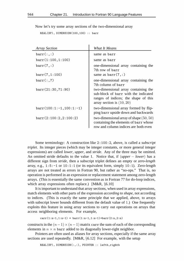
Now let’s try some array sections of the two-dimensional array
REAL(SP), DIMENSION(100,100) :: barr
Array Section What It Means
barr(:,:) same as barr
barr(1:100,1:100) same as barr
barr(7,:) one-dimensional array containing the7th row of barr
barr(7,1:100) same as barr(7,:)
barr(:,7) one-dimensional array containing the7th column of barr
barr(21:30,71:90) two-dimensional array containing thesub-block of barr with the indicatedranges of indices; the shape of thisarray section is (10, 20)
barr(100:1:-1,100:1:-1) two-dimensional array formed by flip-ping barr upside down and backwards
barr(2:100:2,2:100:2) two-dimensional array of shape (50, 50)containing the elements of barr whoserow and column indices are both even
Some terminology: A construction like 2:100:2, above, is called a subscripttriplet. Its integer pieces (which may be integer constants, or more general integerexpressions) are called lower, upper, and stride. Any of the three may be omitted.An omitted stride defaults to the value 1. Notice that, if (upper− lower) has adifferent sign from stride, then a subscript triplet defines an empty or zero-lengtharray, e.g., 1:5:-1 or 10:1:1 (or its equivalent form, simply 10:1). Zero-lengtharrays are not treated as errors in Fortran 90, but rather as “no-ops.” That is, nooperation is performed in an expression or replacement statement among zero-lengtharrays. (This is essentially the same convention as in Fortran 77 for do-loop indices,which array expressions often replace.) [M&R, §6.10]
It is important to understand that array sections, when used in array expressions,match elements with other parts of the expression according to shape, not accordingto indices. (This is exactly the same principle that we applied, above, to arrayswith subscript lower bounds different from the default value of 1.) One frequentlyexploits this feature in using array sections to carry out operations on arrays thataccess neighboring elements. For example,
carr(1:n-1,1:n-1) = barr(1:n-1,1:n-1)+barr(2:n,2:n)
constructs in the (n−1)× (n−1) matrix carr the sum of each of the correspondingelements in n × n barr added to its diagonally lower-right neighbor.
Pointers are often used as aliases for array sections, especially if the same arraysections are used repeatedly. [M&R, §6.12] For example, with the setup
REAL(SP), DIMENSION(:,:), POINTER :: leftb,rightb
21.4 Fortran 90 Intrinsic Procedures 945
leftb=>barr(1:n-1,1:n-1)rightb=>barr(2:n,2:n)
the statement above can be coded as
carr(1:n-1,1:n-1)=leftb+rightb
We should also mention that array sections, while powerful and concise, aresometimes not quite powerful enough. While any row or column of a matrix is easilyaccessible as an array section, there is no good way, in Fortran 90, to access (e.g.)the diagonal of a matrix, even though its elements are related by a linear progressionin the Fortran storage order (by columns). These so-called skew-sectionswere muchdiscussed by the Fortran 90 standards committee, but they were not implemented.We will see examples later in this volume of work-around programming tricks (nonetotally satisfactory) for this omission. (Fortran 95 corrects the omission; see §21.6.)
CITED REFERENCES AND FURTHER READING:
Metcalf, M., and Reid, J. 1996, Fortran 90/95 Explained (Oxford: Oxford University Press).
21.4 Fortran 90 Intrinsic Procedures
Much of Fortran 90’s power, both for parallel programming and for its conciseexpression of algorithmic ideas, comes from its rich set of intrinsicprocedures. Thesehave the effect of making the language “large,” hence harder to learn. However,effort spent on learning to use the intrinsics — particularly some of their moreobscure, and more powerful, optional arguments — is often handsomely repaid.
This section summarizes the intrinsics that we find useful in numerical work.We omit, here, discussion of intrinsics whose exclusive use is for character and stringmanipulation. We intend only a summary, not a complete specification, which canbe found in M&R’s Chapter 8, or other reference books.
If you find the sheer number of new intrinsic procedures daunting, you mightwant to start with our list of the “top 10” (with the number of different NumericalRecipes routines that use each shown in parentheses): size (254), sum (44),dot product (31), merge (27), all (25), maxval (23), matmul (19), pack (18),any (17), and spread (15). (Later, in Chapter 23, you can compare these numberswith our frequency of using the short utility functions that we define in a modulenamed nrutil — several of which we think ought to have been included as Fortran90 intrinsic procedures.)
The type, kind, and shape of the value returned by intrinsic functions willusually be clear from the short description that we give. As an additional hint(though not necessarily a precise description), we adopt the following codes:
946 Chapter 21. Introduction to Fortran 90 Language Features
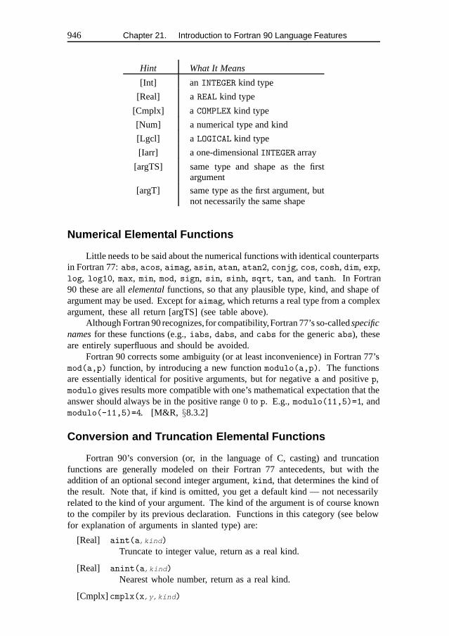
Hint What It Means
[Int] an INTEGER kind type
[Real] a REAL kind type
[Cmplx] a COMPLEX kind type
[Num] a numerical type and kind
[Lgcl] a LOGICAL kind type
[Iarr] a one-dimensional INTEGER array
[argTS] same type and shape as the firstargument
[argT] same type as the first argument, butnot necessarily the same shape
Numerical Elemental Functions
Little needs to be said about the numerical functions with identical counterpartsin Fortran 77: abs, acos, aimag, asin, atan, atan2, conjg, cos, cosh, dim, exp,log, log10, max, min, mod, sign, sin, sinh, sqrt, tan, and tanh. In Fortran90 these are all elementalfunctions, so that any plausible type, kind, and shape ofargument may be used. Except for aimag, which returns a real type from a complexargument, these all return [argTS] (see table above).
Although Fortran 90 recognizes, for compatibility,Fortran 77’s so-called specificnamesfor these functions (e.g., iabs, dabs, and cabs for the generic abs), theseare entirely superfluous and should be avoided.
Fortran 90 corrects some ambiguity (or at least inconvenience) in Fortran 77’smod(a,p) function, by introducing a new function modulo(a,p). The functionsare essentially identical for positive arguments, but for negative a and positive p,modulo gives results more compatible with one’s mathematical expectation that theanswer should always be in the positive range 0 to p. E.g., modulo(11,5)=1, andmodulo(-11,5)=4. [M&R, §8.3.2]
Conversion and Truncation Elemental Functions
Fortran 90’s conversion (or, in the language of C, casting) and truncationfunctions are generally modeled on their Fortran 77 antecedents, but with theaddition of an optional second integer argument, kind, that determines the kind ofthe result. Note that, if kind is omitted, you get a default kind — not necessarilyrelated to the kind of your argument. The kind of the argument is of course knownto the compiler by its previous declaration. Functions in this category (see belowfor explanation of arguments in slanted type) are:
[Real] aint(a,kind)
Truncate to integer value, return as a real kind.
[Real] anint(a,kind)
Nearest whole number, return as a real kind.
[Cmplx] cmplx(x,y,kind)
21.4 Fortran 90 Intrinsic Procedures 947
Convert to complex kind. If y is omitted, it is taken to be 0.
[Int] int(a,kind)
Convert to integer kind, truncating towards zero.
[Int] nint(a,kind)
Convert to integer kind, choosing the nearest whole number.
[Real] real(a,kind)
Convert to real kind.
[Lgcl] logical(a,kind)
Convert one logical kind to another.
We must digress here to explain the use of optional argumentsand keywordsas Fortran 90 language features. [M&R, §5.13] When a routine (either intrinsicor user-defined) has arguments that are declared to be optional, then the dummynames given to them also become keywords that distinguish — independent of theirposition in a calling list — which argument is intended to be passed. (There are someadditional rules about this that we will not try to summarize here.) In this section’stabular listings, we indicate optional arguments in intrinsic routines by printing themin smaller slanted type. For example, the intrinsic function
eoshift(array,shift,boundary,dim)
has two required arguments, array and shift, and two optional arguments,boundary and dim. Suppose we want to call this routine with the actual argumentsmyarray, myshift, and mydim, but omitting the argument in the boundary slot.We do this by the expression
eoshift(myarray,myshift,dim=mydim)
Conversely, if we wanted a boundary argument, but no dim, we might writeeoshift(myarray,myshift,boundary=myboundary)
It is always a good idea to use this kind of keyword construction when invokingoptional arguments, even though the rules allow keywords to be omitted in someunambiguous cases. Now back to the lists of intrinsic routines.
A peculiarity of the real function derives from its use both as a type conversionand for extracting the real part of complex numbers (related, but not identical,usages): If the argument of real is complex, and kind is omitted, then the resultisn’t a default real kind, but rather is (as one generally would want) the real kindtype corresponding to the kind type of the complex argument, that is, single-precisionreal for single-precision complex, double-precision for double-precision, and so on.[M&R, §8.3.1] We recommend neverusing kind when you intend to extract thereal part of a complex, and alwaysusing kind when you intend conversion of areal or integer value to a particular kind of REAL. (Use of the deprecated functiondble is not recommended.)
The last two conversion functions are the exception in that they don’t allowa kind argument, but rather return default integer kinds. (The X3J3 standardscommittee has fixed this in Fortran 95.)
[Int] ceiling(a)
Convert to integer, truncating towards more positive.
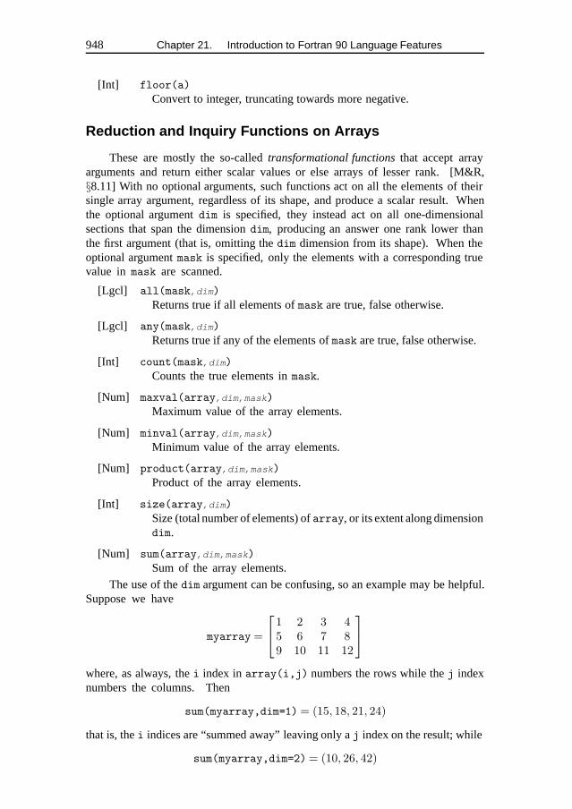
948 Chapter 21. Introduction to Fortran 90 Language Features
[Int] floor(a)
Convert to integer, truncating towards more negative.
Reduction and Inquiry Functions on Arrays
These are mostly the so-called transformational functionsthat accept arrayarguments and return either scalar values or else arrays of lesser rank. [M&R,§8.11] With no optional arguments, such functions act on all the elements of theirsingle array argument, regardless of its shape, and produce a scalar result. Whenthe optional argument dim is specified, they instead act on all one-dimensionalsections that span the dimension dim, producing an answer one rank lower thanthe first argument (that is, omitting the dim dimension from its shape). When theoptional argument mask is specified, only the elements with a corresponding truevalue in mask are scanned.
[Lgcl] all(mask,dim)
Returns true if all elements of mask are true, false otherwise.
[Lgcl] any(mask,dim)
Returns true if any of the elements of mask are true, false otherwise.
[Int] count(mask,dim)
Counts the true elements in mask.
[Num] maxval(array,dim,mask)
Maximum value of the array elements.
[Num] minval(array,dim,mask)
Minimum value of the array elements.
[Num] product(array,dim,mask)
Product of the array elements.
[Int] size(array,dim)
Size (total number of elements) of array, or its extent along dimensiondim.
[Num] sum(array,dim,mask)
Sum of the array elements.
The use of the dim argument can be confusing, so an example may be helpful.Suppose we have
myarray =
1 2 3 45 6 7 89 10 11 12
where, as always, the i index in array(i,j) numbers the rows while the j indexnumbers the columns. Then
sum(myarray,dim=1) = (15, 18, 21, 24)
that is, the i indices are “summed away” leaving only a j index on the result; while
sum(myarray,dim=2) = (10, 26, 42)
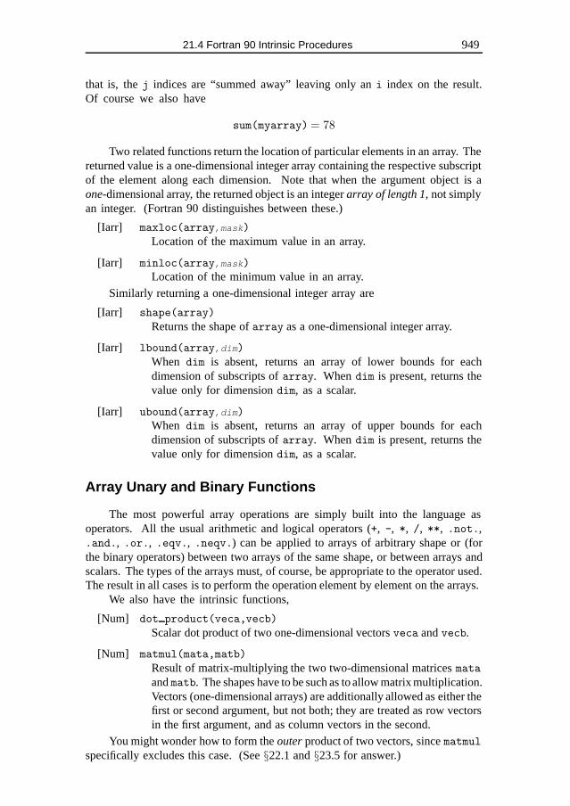
21.4 Fortran 90 Intrinsic Procedures 949
that is, the j indices are “summed away” leaving only an i index on the result.Of course we also have
sum(myarray) = 78
Two related functions return the location of particular elements in an array. Thereturned value is a one-dimensional integer array containing the respective subscriptof the element along each dimension. Note that when the argument object is aone-dimensional array, the returned object is an integer array of length 1, not simplyan integer. (Fortran 90 distinguishes between these.)
[Iarr] maxloc(array,mask)
Location of the maximum value in an array.
[Iarr] minloc(array,mask)
Location of the minimum value in an array.
Similarly returning a one-dimensional integer array are
[Iarr] shape(array)
Returns the shape of array as a one-dimensional integer array.
[Iarr] lbound(array,dim)
When dim is absent, returns an array of lower bounds for eachdimension of subscripts of array. When dim is present, returns thevalue only for dimension dim, as a scalar.
[Iarr] ubound(array,dim)
When dim is absent, returns an array of upper bounds for eachdimension of subscripts of array. When dim is present, returns thevalue only for dimension dim, as a scalar.
Array Unary and Binary Functions
The most powerful array operations are simply built into the language asoperators. All the usual arithmetic and logical operators (+, -, *, /, **, .not.,.and., .or., .eqv., .neqv.) can be applied to arrays of arbitrary shape or (forthe binary operators) between two arrays of the same shape, or between arrays andscalars. The types of the arrays must, of course, be appropriate to the operator used.The result in all cases is to perform the operation element by element on the arrays.
We also have the intrinsic functions,
[Num] dot product(veca,vecb)
Scalar dot product of two one-dimensional vectors veca and vecb.
[Num] matmul(mata,matb)
Result of matrix-multiplying the two two-dimensional matrices mataand matb. The shapes have to be such as to allow matrix multiplication.Vectors (one-dimensional arrays) are additionally allowed as either thefirst or second argument, but not both; they are treated as row vectorsin the first argument, and as column vectors in the second.
You might wonder how to form the outerproduct of two vectors, since matmulspecifically excludes this case. (See §22.1 and §23.5 for answer.)
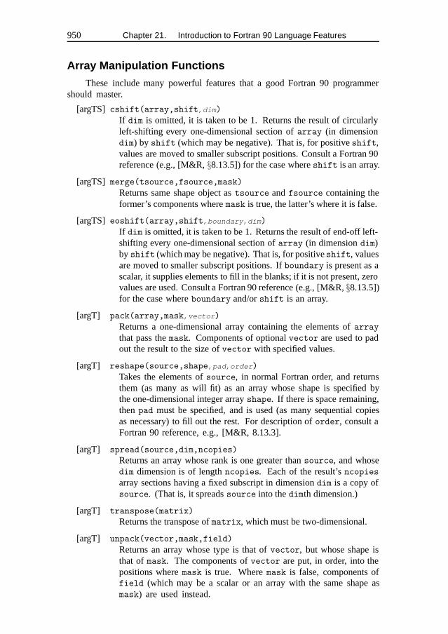
950 Chapter 21. Introduction to Fortran 90 Language Features
Array Manipulation Functions
These include many powerful features that a good Fortran 90 programmershould master.
[argTS] cshift(array,shift,dim)
If dim is omitted, it is taken to be 1. Returns the result of circularlyleft-shifting every one-dimensional section of array (in dimensiondim) by shift (which may be negative). That is, for positive shift,values are moved to smaller subscript positions. Consult a Fortran 90reference (e.g., [M&R, §8.13.5]) for the case where shift is an array.
[argTS] merge(tsource,fsource,mask)
Returns same shape object as tsource and fsource containing theformer’s components where mask is true, the latter’s where it is false.
[argTS] eoshift(array,shift,boundary,dim)
If dim is omitted, it is taken to be 1. Returns the result of end-off left-shifting every one-dimensional section of array (in dimension dim)by shift (which may be negative). That is, for positive shift, valuesare moved to smaller subscript positions. If boundary is present as ascalar, it supplies elements to fill in the blanks; if it is not present, zerovalues are used. Consult a Fortran 90 reference (e.g., [M&R, §8.13.5])for the case where boundary and/or shift is an array.
[argT] pack(array,mask,vector)
Returns a one-dimensional array containing the elements of array
that pass the mask. Components of optional vector are used to padout the result to the size of vector with specified values.
[argT] reshape(source,shape,pad,order)
Takes the elements of source, in normal Fortran order, and returnsthem (as many as will fit) as an array whose shape is specified bythe one-dimensional integer array shape. If there is space remaining,then pad must be specified, and is used (as many sequential copiesas necessary) to fill out the rest. For description of order, consult aFortran 90 reference, e.g., [M&R, 8.13.3].
[argT] spread(source,dim,ncopies)
Returns an array whose rank is one greater than source, and whosedim dimension is of length ncopies. Each of the result’s ncopiesarray sections having a fixed subscript in dimension dim is a copy ofsource. (That is, it spreads source into the dimth dimension.)
[argT] transpose(matrix)
Returns the transpose of matrix, which must be two-dimensional.
[argT] unpack(vector,mask,field)
Returns an array whose type is that of vector, but whose shape isthat of mask. The components of vector are put, in order, into thepositions where mask is true. Where mask is false, components offield (which may be a scalar or an array with the same shape asmask) are used instead.
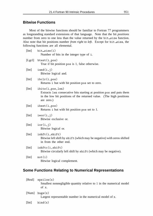
21.4 Fortran 90 Intrinsic Procedures 951
Bitwise Functions
Most of the bitwise functions should be familiar to Fortran 77 programmersas longstanding standard extensions of that language. Note that the bit positionsnumber from zero to one less than the value returned by the bit size function.Also note that bit positions number from right to left. Except for bit size, thefollowing functions are all elemental.
[Int] bit size(i)
Number of bits in the integer type of i.
[Lgcl] btest(i,pos)
True if bit position pos is 1, false otherwise.
[Int] iand(i,j)
Bitwise logical and.
[Int] ibclr(i,pos)
Returns i but with bit position pos set to zero.
[Int] ibits(i,pos,len)
Extracts len consecutive bits starting at position pos and puts themin the low bit positions of the returned value. (The high positionsare zero.)
[Int] ibset(i,pos)
Returns i but with bit position pos set to 1.
[Int] ieor(i,j)
Bitwise exclusive or.
[Int] ior(i,j)
Bitwise logical or.
[Int] ishft(i,shift)
Bitwise left shift by shift (which may be negative) with zeros shiftedin from the other end.
[Int] ishftc(i,shift)
Bitwise circularly left shift by shift (which may be negative).
[Int] not(i)
Bitwise logical complement.
Some Functions Relating to Numerical Representations
[Real] epsilon(x)
Smallest nonnegligible quantity relative to 1 in the numerical modelof x.
[Num] huge(x)
Largest representable number in the numerical model of x.
[Int] kind(x)
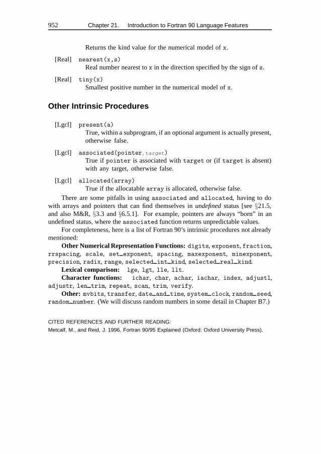
952 Chapter 21. Introduction to Fortran 90 Language Features
Returns the kind value for the numerical model of x.
[Real] nearest(x,s)
Real number nearest to x in the direction specified by the sign of s.
[Real] tiny(x)
Smallest positive number in the numerical model of x.
Other Intrinsic Procedures
[Lgcl] present(a)
True, within a subprogram, if an optional argument is actually present,otherwise false.
[Lgcl] associated(pointer,target)
True if pointer is associated with target or (if target is absent)with any target, otherwise false.
[Lgcl] allocated(array)
True if the allocatable array is allocated, otherwise false.
There are some pitfalls in using associated and allocated, having to dowith arrays and pointers that can find themselves in undefinedstatus [see §21.5,and also M&R, §3.3 and §6.5.1]. For example, pointers are always “born” in anundefined status, where the associated function returns unpredictable values.
For completeness, here is a list of Fortran 90’s intrinsic procedures not alreadymentioned:
Other Numerical Representation Functions: digits, exponent, fraction,rrspacing, scale, set exponent, spacing, maxexponent, minexponent,precision, radix, range, selected int kind, selected real kind.
Lexical comparison: lge, lgt, lle, llt.Character functions: ichar, char, achar, iachar, index, adjustl,
adjustr, len trim, repeat, scan, trim, verify.Other: mvbits, transfer, date and time, system clock, random seed,
random number. (We will discuss random numbers in some detail in Chapter B7.)
CITED REFERENCES AND FURTHER READING:
Metcalf, M., and Reid, J. 1996, Fortran 90/95 Explained (Oxford: Oxford University Press).
21.5 Advanced Fortran 90 Topics 953
21.5 Advanced Fortran 90 Topics
Pointers, Arrays, and Memory Management
One of the biggest improvements in Fortran 90 over Fortran 77 is in thehandling of arrays, which are the cornerstone of many numerical algorithms. In thissubsection we will take a closer look at how to use some of these new array featureseffectively. We will look at how to code certain commonly occurring elements ofprogram design, and we will pay particular attention to avoiding “memory leaks,”where — usually inadvertently — we keep cumulatively allocating new storage foran array, every time some piece of code is invoked.
Let’s first review some of the rules for using allocatable arrays and pointers toarrays. Recall that a pointer is born with an undefined status. Its status changesto “associated” when you make it refer to a target, and to “disassociated” whenyou nullify the pointer. [M&R, §3.3] You can also use nullify on a newlyborn pointer to change its status from undefined to disassociated; this allows you totest the status with the associated inquiry function. [M&R, §6.5.4] (While manycompilers will not produce a run-time error if you test an undefined pointer withassociated, you can’t rely on this laissez-fairein your programming.)
The initial status of an allocatable array is “not currently allocated.” Its statuschanges to “allocated” when you give it storage with allocate, and back to “notcurrently allocated” when you use deallocate. [M&R, §6.5.1] You can test thestatus with the allocated inquiry function. Note that while you can also give apointer fresh storage with allocate, you can’t test this with allocated — onlyassociated is allowed with pointers. Note also that nullifying an allocated pointerleaves its associated storage in limbo. You must instead deallocate, which givesthe pointer a testable “disassociated” status.
While allocating an array that is already allocated gives an error, you are allowedto allocate a pointer that already has a target. This breaks the old association, andcould leave the old target inaccessible if there is no other pointer associated withit. [M&R, §6.5.2] Deallocating an array or pointer that has not been allocated isalways an error.
Allocated arrays that are local to a subprogram acquire the “undefined” statuson exit from the subprogram unless they have the SAVE attribute. (Again, not allcompilers enforce this, but be warned!) Such undefined arrays cannot be referencedin any way, so you should explicitly deallocate all allocated arrays that are notsaved before returning from a subprogram. [M&R, §6.5.1] The same rule appliesto arrays declared in modules that are currently accessed only by the subprogram.While you can reference undefined pointers (e.g., by first nullifying them), it is goodprogramming practice to deallocate explicitly any allocated pointers declared locallybefore leaving a subprogram or module.
Now let’s turn to using these features in programs. The simplest example iswhen we want to implement global storage of an array that needs to be accessed bytwo or more different routines, and we want the size of the array to be determinedat run time. As mentioned earlier, we implement global storage with a MODULE
rather than a COMMON block. (We ignore here the additional possibility of passing
954 Chapter 21. Introduction to Fortran 90 Language Features
global variables by having one routine CONTAINed within the other.) There aretwo good ways of handling the dynamical allocation in a MODULE. Method 1 usesan allocatable array:
MODULE aREAL(SP), DIMENSION(:), ALLOCATABLE :: xEND MODULE a
SUBROUTINE b(y)USE aREAL(SP), DIMENSION(:) :: y...allocate(x(size(y)))... [other routines usingx called here] ...END SUBROUTINE b
Here the global variable x gets assigned storage in subroutine b (in this case,the same as the length of y). The length of y is of course defined in the procedurethat calls b. The array x is made available to any other subroutine called by b byincluding a USE a statement. The status of x can be checked with an allocated
inquiry function on entry into either b or the other subroutine if necessary. Asdiscussed above, you must be sure to deallocate x before returning from subroutineb. If you want x to retain its values between calls to b, you add the SAVE attributeto its declaration in a, and don’t deallocate it on returning from b. (Alternatively,you could put a USE a in your main program, but we consider that bug-prone, sinceforgetting to do so can create all manner of difficult-to-diagnose havoc.) To avoidallocating x more than once, you test it on entry into b:
if (.not. allocated(x)) allocate(x(size(y)))
The second way to implement this type of global storage (Method 2) usesa pointer:
MODULE aREAL(SP), DIMENSION(:), POINTER :: xEND MODULE a
SUBROUTINE b(y)USE aREAL(SP), DIMENSION(:) :: yREAL(SP), DIMENSION(size(y)), TARGET :: xx...x=>xx... [other routines usingx called here] ...END SUBROUTINE b
Here the automatic arrayxx gets its temporary storage automatically on entryinto b, and automatically gets deallocated on exit from b. [M&R, §6.4] The globalpointer x can access this storage in any routine with a USE a that is called by b.You can check that things are in order in such a called routine by testing x withassociated. If you are going to use x for some other purpose as well, you shouldnullify it on leaving b so that it doesn’t have undefined status. Note that thisimplementation does not allow values to be saved between calls: You can’t SAVEautomatic arrays — that’s not what they’re for. You would have to SAVE x inthe module, and allocate it in the subroutine instead of pointing it to a suitableautomatic array. But this is essentially Method 1 with the added complication of usinga pointer, so Method 1 is simpler when you want to save values. When you don’t
21.5 Advanced Fortran 90 Topics 955
need to save values between calls, we lean towards Method 2 over Method 1 becausewe like the automatic allocation and deallocation, but either method works fine.
An example of Method 1 (allocatable array) is in routine rkdumb on page 1297.An example of Method 1 with SAVE is in routine pwtset on p. 1265. Method2 (pointer) shows up in routines newt (p. 1196), broydn (p. 1199), and fitexy
(p. 1286). A variation is shown in routines linmin (p. 1211) and dlinmin (p. 1212):When the array that needs to be shared is an argument of one of the routines,Method 2 is better.
An extension of these ideas occurs if we allocate some storage for an arrayinitially, but then might need to increase the size of the array later without losingthe already-stored values. The function reallocate in our utility module nrutilwill handle this for you, but it expects a pointer argument as in Method 2. Sinceno automatic arrays are used, you are free to SAVE the pointer if necessary. Hereis a simple example of how to use reallocate to create a workspace array thatis local to a subroutine:
SUBROUTINE aUSE nrutil, ONLY : reallocateREAL(SP), DIMENSION(:), POINTER, SAVE :: wkspLOGICAL(LGT), SAVE :: init=.true.if (init) then
init=.false.nullify(wksp)wksp=>reallocate(wksp,100)
end if...if (nterm > size(wksp)) wksp=>reallocate(wksp,2*size(wksp))...END SUBROUTINE a
Here the workspace is initially allocated a size of 100. If the number of elementsused (nterm) ever exceeds the size of the workspace, the workspace is doubled. (Ina realistic example, one would of course check that the doubled size is in fact bigenough.) Fortran 90 experts can note that the SAVE on init is not strictly necessary:Any local variable that is initialized is automatically saved. [M&R, §7.5]
You can find similar examples of reallocate (with some further discussion) ineulsum (p. 1070), hufenc (p. 1348), and arcode (p. 1350). Examples of reallocateused with global variables in modules are in odeint (p. 1300) and ran state
(p. 1144).Another situation where we have to use pointers and not allocatable arrays
is when the storage is required for components of a derived type, which are notallowed to have the allocatable attribute. Examples are in hufmak (p. 1346) andarcmak (p. 1349).
Turning away from issues relating to global variables, we now consider severalother important programming situations that are nicely handled with pointers. Thefirst case is when we want a subroutine to return an array whose size is not knownin advance. Since dummy arguments are not allocatable, we must use a pointer.Here is the basic construction:
SUBROUTINE a(x,nx)REAL(SP), DIMENSION(:), POINTER :: xINTEGER(I4B), INTENT(OUT) :: nxLOGICAL(LGT), SAVE :: init=.true.if (init) then
956 Chapter 21. Introduction to Fortran 90 Language Features
init=.false.nullify(x)
elseif (associated(x)) deallocate(x)
end if...nx=...allocate(x(nx))x(1:nx)=...END SUBROUTINE a
Since the length of x can be found from size(x), it is not absolutely necessaryto pass nx as an argument. Note the use of the initial logic to avoid memoryleaks. If a higher-level subroutine wants to recover the memory associated with x
from the last call to SUBROUTINE a, it can do so by first deallocating it, and thennullifying the pointer. Examples of this structure are in zbrak (p. 1184), period(p. 1258), and fasper (p. 1259). A related situation is where we want a functionto return an array whose size is not predetermined, such as in voltra on (p. 1326).The discussion of voltra also explains the potential pitfalls of functions returningpointers to dynamically allocated arrays.
A final useful pointer construction enables us to set up a data structure that isessentially an array of arrays, independently allocatable on each part. We are notallowed to declare an array of pointers in Fortran 90, but we can do this indirectlyby defining a derived type that consists of a pointer to the appropriate kind of array.[M&R, §6.11] We can then define a variable that is an allocatable array of the newtype. For example,
TYPE ptr_to_arrREAL(SP), DIMENSION(:), POINTER :: arr
END TYPETYPE(ptr_to_arr), DIMENSION(:), ALLOCATABLE :: x...allocate(x(n))...do i=1,n
allocate(x(i)%arr(m))end do
sets up a set x of n arrays of length m. See also the example in mglin (p. 1334).There is a potential problem with dynamical memory allocation that we should
mention. The Fortran 90 standard does not require that the compiler perform“garbage collection,” that is, it is not required to recover deallocated memory intonice contiguous pieces for reuse. If you enter and exit a subroutine many times,and each time a large chunk of memory gets allocated and deallocated, you couldrun out of memory with a “dumb” compiler. You can often alleviate the problemby deallocating variables in the reverse order that you allocated them. This tends tokeep a large contiguous piece of memory free at the top of the heap.
Scope, Visibility, and Data Hiding
An important principle of good programming practice is modularization, theidea that different parts of a program should be insulated from each other as muchas possible. An important subcase of modularization is data hiding, the principlethat actions carried out on variables in one part of the code should not be able to
21.5 Advanced Fortran 90 Topics 957
affect the values of variables in other parts of the code. When it is necessary forone “island” of code to communicate with another, the communication should bethrough a well-defined interface that makes it obvious exactly what communicationis taking place, and prevents any other interchange from occurring. Otherwise,different sections of code should not have access to variables that they don’t need.
The concept of data hiding extends not only to variables, but also to the namesof procedures that manipulate the variables: A program for screen graphics mightgive the user access to a routine for drawing a circle, but it might “hide” thenames (and methods of operation) of the primitive routines used for calculatingthe coordinates of the points on the circumference. Besides producing code thatis easier to understand and to modify, data hiding prevents unintended side effectsfrom producing hard-to-find errors.
In Fortran, the principal language construction that effects data hiding is theuse of subroutines. If all subprograms were restricted to have no more than tenexecutable statements per routine, and to communicate between routines only byan explicit list of arguments, the number of programming errors might be greatlyreduced! Unfortunately few tasks can be easily coded in this style. For this andother reasons, we think that too much procedurization is a bad thing; one wantsto find the right amount. Fortunately Fortran 90 provides several additional toolsto help with data hiding.
Global variables and routine names are important, but potentially dangerous,things. In Fortran 90, global variables are typically encapsulated in modules. Accessis granted only to routines with an appropriate USE statement, and can be restrictedto specific identifiers by the ONLY option. [M&R, §7.10] In addition, variable androutine names within the module can be designated as PUBLIC or PRIVATE (see,e.g., quad3d on p. 1065). [M&R, §7.6]
The other way global variables get communicated is by having one routineCONTAINed within another. [M&R, §5.6] This usage is potentially lethal, however,because all the outer routine’s variables are visible to the inner routine. You cantry to control the problem somewhat by passing some variables back and forth asarguments of the inner routine, but that still doesn’t prevent inadvertent side effects.(The most common, and most stupid, is inadvertent reuse of variables named i or jin the CONTAINed routine.) Also, a long list of arguments reduces the convenienceof using an internal routine in the first place. We advise that internal subprogramsbe used with caution, and only to carry out simple tasks.
There are some good ways to use CONTAINS, however. Several of our recipeshave the following structure: A principal routine is invoked with several arguments.It calls a subsidiary routine, which needs to know some of the principal routine’sarguments, some global variables, and some values communicated directly asarguments to the subsidiary routine. In Fortran 77, we have usually coded this bypassing the global variables in a COMMON block and all other variables as argumentsto the subsidiary routine. If necessary, we copied the arguments of the primaryroutine before passing them to the subsidiary routine. In Fortran 90, there is a moreelegant way of accomplishing this, as follows:
SUBROUTINE recipe(arg)REAL(SP) :: argREAL(SP) :: global_varcall recipe_privateCONTAINS
958 Chapter 21. Introduction to Fortran 90 Language Features
SUBROUTINE recipe_private...call subsidiary(local_arg)...END SUBROUTINE recipe_private
SUBROUTINE subsidiary(local_arg)...END SUBROUTINE subsidiaryEND SUBROUTINE recipe
Notice that the principal routine (recipe) has practically nothing in it — only dec-larations of variables intended to be visible to the subsidiary routine (subsidiary).All the real work of recipe is done in recipe private. This latter routinehas visibility on all of recipe’s variables, while any additional variables thatrecipe private defines are not visible to subsidiary — which is the wholepurpose of this way of organizing things. Obviously arg and global var canbe much more general data types than the example shown here, including functionnames. For examples of this construction, see amoeba (p. 1208), amebsa (p. 1222),mrqmin (p. 1292), and medfit (p. 1294).
Recursion
A subprogram is recursive if it calls itself. While forbidden in Fortran77, recursion is allowed in Fortran 90. [M&R, §5.16–§5.17] You must supply thekeyword RECURSIVE in front of the FUNCTIONor SUBROUTINEkeyword. In addition,if a FUNCTION calls itself directly, as opposed to calling another subprogram that inturn calls it, you must supply a variable to hold the result with the RESULT keyword.Typical syntax for this case is:
RECURSIVE FUNCTION f(x) RESULT(g)REAL(SP) :: x,gif ...
g=...else
g=f(...)end ifEND FUNCTION f
When a function calls itself directly, as in this example, there always has to be a“base case” that does not call the function; otherwise the recursion never terminates.We have indicated this schematically with the if...else...end if structure.
On serial machines we tend to avoid recursive implementations because of theadditional overhead they incur at execution time. Occasionally there are algorithmsfor which the recursion overhead is relatively small, and the recursive implementationis simpler than an iterative version. Examples in this book are quad 3d (p. 1065),miser (p. 1164), and mglin (p. 1334). Recursion is much more important whenparallelization is the goal. We will encounter in Chapter 22 numerous examples ofalgorithms that can be parallelized with recursion.
SAVE Usage Style
A quirk of Fortran 90 is that any variable with initial values acquires theSAVE attribute automatically. [M&R, §7.5 and §7.9] As a help to understanding
21.6 And Coming Soon: Fortran 95 959
an algorithm, we have elected to put an explicit SAVE on all variables that reallydo need to retain their values between calls to a routine. We do this even if it isredundant because the variables are initialized. Note that we generally prefer toassign initial values with initialization expressions rather than with DATA statements.We reserve DATA statements for cases where it is convenient to use the repeat countfeature to set multiple occurrences of a value, or when binary, octal, or hexadecimalconstants are used. [M&R, §2.6.1]
Named Control Structures
Fortran 90 allows control structures such as do loops and if blocks to benamed. [M&R, §4.3–§4.5] Typical syntax is
name:do i=1,n...
end do name
One use of naming control structures is to improve readability of the code,especially when there are many levels of nested loops and if blocks. A moreimportant use is to allow exit and cycle statements, which normally refer to theinnermost do loop in which they are contained, to transfer execution to the endof some outer loop. This is effected by adding the name of the outer loop to thestatement: exit name or cycle name.
There is great potential for misuse with named control structures, since theyshare some features of the much-maligned goto. We recommend that you use themsparingly. For a good example of their use, contrast the Fortran 77 version of simplxwith the Fortran 90 version on p. 1216.
CITED REFERENCES AND FURTHER READING:
Metcalf, M., and Reid, J. 1996, Fortran 90/95 Explained (Oxford: Oxford University Press).
21.6 And Coming Soon: Fortran 95
One of the more positive effects of Fortran 90’s long gestation period has beenthe general recognition, both by the X3J3 committee and by the community at large,that Fortran needs to evolve over time. Indeed, as we write, the process of bringingforth a minor, but by no means insignificant, updating of Fortran 90 — namedFortran 95 — is well under way.
Fortran 95 will differ from Fortran 90 in about a dozen features, only a handfulof which are of any importance to this book. Generally these are extensions thatwill make programming, especially parallel programming, easier. In this section wegive a summary of the anticipated language changes. In §22.1 and §22.5 we willcomment further on the implications of Fortran 95 to some parallel programmingtasks; in §23.7 we comment on what differences Fortran 95 will make to our nrutilutility functions.
No programs in Chapters B1 through B20 of this book edition use any Fortran95 extensions.
960 Chapter 21. Introduction to Fortran 90 Language Features
FORALL Statements and Blocks
Fortran 95 introduces a new forall control structure, somewhat akin to thewhere construct, but allowing for greater flexibility. It is something like a do-loop,but with the proviso that the indices looped over are allowed to be done in any order(ideally, in parallel). The forall construction comes in both single-statement andblock variants. Instead of using the do-loop’s comma-separated triplets of lower-value, upper-value, and increment, it borrows its syntax from the colon-separatedform of array sections. Some examples will give you the idea.
Here is a simple example that could alternatively be done with Fortran 90’sarray sections and transpose intrinsic:
forall (i=1:20, j=1:10:2) x(i,j)=y(j,i)
The block form allows more than one executable statement:
forall (i=1:20, j=1:10:2)x(i,j)=y(j,i)z(i,j)=y(i,j)**2
end forall
Here is an example that cannot be done with Fortran 90 array sections:
forall (i=1:20, j=1:20) a(i,j)=3*i+j**2
forall statements can also take optional masks that restrict their action to asubset of the loop index combinations:
forall (i=1:100, j=1:100, (i>=j .and. x(i,j)/=0.0) ) x(i,j)=1.0/x(i,j)
forall constructions can be nested, or nested inside where blocks, or havewhere constructions inside them. An additional new feature in Fortran 95 is thatwhere blocks can themselves be nested.
PURE Procedures
Because the inside iteration of a forall block can be done in any order, or inparallel, there is a logical difficulty in allowing functions or subroutines inside suchblocks: If the function or subroutine has side effects(that is, if it changes any dataelsewhere in the machine, or in its own saved variables) then the result of a forallcalculation could depend on the order in which the iterations happen to be done.This can’t be tolerated, of course; hence a new PURE attribute for subprograms.
While the exact stipulations are somewhat technical, the basic idea is that if youdeclare a function or subroutine as PURE, with a syntax like,
PURE FUNCTION myfunc(x,y,z)
orPURE SUBROUTINE mysub(x,y,z)
then you are guaranteeing to the compiler (and it will enforce) that the only valueschanged by mysubor myfuncare returned function values, subroutine arguments withthe INTENT(OUT) attribute, and automatic (scratch) variables within the procedure.
You can then use your pure procedures within forall constructions. Purefunctions are also allowed in some specification statements.
21.6 And Coming Soon: Fortran 95 961
ELEMENTAL Procedures
Fortran 95 removes Fortran 90’s nagging restriction that only intrinsic functionsare elemental. The way this works is that you write a pure procedure that operateson scalar values, but include the attribute ELEMENTAL (which automatically impliesPURE). Then, as long as the function has an explicit interface in the referencingprogram, you can call it with any shape of argument, and it will act elementally.Here’s an example:
ELEMENTAL FUNCTION myfunc(x,y,z)REAL :: x,y,z,myfunc...myfunc = ...END
In a program with an explicit interface for myfunc you could now have
REAL, DIMENSION(10,20) :: x,y,z,w...w=myfunc(x,y,z)
Pointer and Allocatable Improvements
Fortran 95, unlike Fortran 90, requires that any allocatable variables (exceptthose with SAVE attributes) that are allocated within a subprogram be automaticallydeallocated by the compiler when the subprogram is exited. This will remove Fortran90’s “undefined allocation status” bugaboo.
Fortran 95 also provides a method for pointer variables to be born withdisassociated association status, instead of the default (and often inconvenient)“undefined” status. The syntax is to add an initializing=> NULL() to the declaration,as:
REAL, DIMENSION(:,:), POINTER :: mypoint => NULL()
This does not, however, eliminate the possibility of undefined association status,because you have to remember to use the null initializer if want your pointer tobe disassociated.
Some Other Fortran 95 Features
In Fortran 95, maxloc and minloc have the additional optional argument DIM,which causes them to act on all one-dimensional sections that span through thenamed dimension. This provides a means for getting the locations of the valuesreturned by the corresponding functions maxval and minval in the case that theirDIM argument is present.
The sign intrinsic can now distinguish a negative from a positive real zerovalue: sign(2.0,-0.0) is −2.0.
There is a new intrinsic subroutine cpu time(time) that returns as a real valuetime a process’s elapsed CPU time.
There are some minor changes in the namelist facility, in defining minimumfield widths for the I, B, O, Z, and F edit descriptors, and in resolving minor conflictswith some other standards.
Chapter 22. Introductionto ParallelProgramming
22.0 Why Think Parallel?
In recent years we Numerical Recipes authors have increasingly becomeconvinced that a certain revolution, cryptically denoted by the words “parallelprogramming,” is about to burst forth from its gestation and adolescence in thecommunity of supercomputer users, and become the mainstream methodology forall computing.
Let’s review the past: Take a screwdriver and open up the computer (workstationor PC) that sits on your desk. (Don’t blame us if this voids your warranty; andbe sure to unplug it first!) Count the integrated circuits — just the bigger ones,with more than a million gates (transistors). As we write, in 1995, even lowlymemory chips have one or four million gates, and this number will increase rapidlyin coming years. You’ll probably count at least dozens, and often hundreds, ofsuch chips in your computer.
Next ask, how many of these chips are CPUs? That is, how many implementvon Neumann processors capable of executing arbitrary, stored program code?For most computers, in 1995, the answer is: about one. A significant numberof computers do have secondary processors that offload input-output and/or videofunctions. So, two or three is often a more accurate answer, but only one is usuallyunder the user’s direct control.
Why do our desktop computers have dozens or hundreds of memory chips, butmost often only one (user-accessible) CPU? Do CPU chips intrinsically cost moreto manufacture? No. Are CPU chips more expensive than memory chips? Yes,primarily because fixed development and design costs must be distributed over asmaller number of units sold. We have been in a kind of economic equilibrium:CPU’s are relatively expensive because there is only one per computer; and there isonly one per computer, because they are relatively expensive.
Stabilizing this equilibrium has been the fact that there has been no standard, orwidely taught, methodology for parallel programming. Except for the special case ofscientific computing on supercomputers (where large problems often have a regularor geometric character), it is not too much of an exaggeration to say that nobodyreally knows how to program multiprocessor machines. Symmetric multiprocessor
962
22.0 Why Think Parallel? 963
operating systems, for example, have been very slow in developing; and efficient,parallel methodologies for query-serving on large databases are even now a subjectof continuing research.
However, things are now changing. We consider it an easy prognostication that,by the first years of the new century, the typical desktop computer will have 4 to 8user-accessible CPUs; ten years after that, the typical number will be between 16 and512. It is not coincidence that these numbers are characteristic of supercomputers(including some quite different architectures) in 1995. The rough rule of ten years’lag from supercomputer to desktop has held firm for quite some time now.
Scientists and engineers have the advantage that techniques for parallel com-putation in their disciplineshave already been developed. With multiprocessorworkstations right around the corner, we think that now is the right time for scientistsand engineers who use computers to startthinking parallel. We don’t mean that youshould put an axe through the screen of your fast serial (single-CPU) workstation.We do mean, however, that you should start programming somewhat differentlyon that workstation, indeed, start thinking a bit differently about the way that youapproach numerical problems in general.
In this volume ofNumerical Recipes in Fortran, our pedagogical goal is toshow you that there are conceptual and practical benefits in parallel thinking, evenif you are using a serial machine today. These benefits include conciseness andclarity of code, reusability of code in wider contexts, and (not insignificantly)increased portability of code to today’s parallel supercomputers. Of course, onparallel machines, either supercomputers today or desktop machines tomorrow, thebenefits of thinking parallel are much more tangible: They translate into significantimprovements in efficiency and computational capability.
Thinking Parallel with Fortran 90
Until very recently, a strong inhibition to thinking parallel was the lack of anystandard, architecture-independent, computer language in which to think. That haschanged with the finalization of the Fortran 90 language standard, and with theavailability of good, optimizing Fortran 90 compilers on a variety of platforms.
There is a significant body of opinion (with which we, however, disagree) thatthere is no such thing as architecture-independent parallel programming. Proponentsof this view, who are generally committed wizards at programming on one or anotherparticular architecture, point to the fact that algorithms that are optimized to onearchitecture can run hundreds of times more slowly on other architectures. And,they are correct!
Our opposing point of view is one of pragmatism. We think that it is nothard to learn, in a general way, what kinds of architectures are in general use, andwhat kinds of parallel constructions work well (or poorly) on each kind. With thisknowledge (much of which we hope to develop in this book) the user can, we think,write good, general-purpose parallel code that works on a variety of architectures— including, importantly, on purely serial machines. Equally important, the userwill be aware of when certain parts of a code can be significantly improved onsome, but not other, architectures.
Fortran 90 is a good test-bench for this point of view. It is not the perfectlanguage for parallel programming. But it isa language, and it is the only
964 Chapter 22. Introduction to Parallel Programming
cross-platformstandard language now available. The committee that developedthe language between 1978 and 1991 (known technically as X3J3) had strongrepresentation from both a traditional “vectorization” viewpoint (e.g., from the CrayXMP and YMP series of computers), and also from the “data parallel” or “SIMD”viewpoints of parallel machines like the CM-2 and CM-5 from Thinking Machines,Inc. Language compromises were made, and a few (in our view) almost essentialfeatures were left out (see§22.5). But, by and large, the necessary tools are there: Ifyou learn to think parallel in Fortran 90, you will easily be able to transfer the skillto future parallel standards, whether they are Fortran-based, C-based, or other.
CITED REFERENCES AND FURTHER READING:
Metcalf, M., and Reid, J. 1996, Fortran 90/95 Explained (Oxford: Oxford University Press).
22.1 Fortran 90 Data Parallelism: Arraysand Intrinsics
The underlying model for parallel computation in Fortran 90 isdata parallelism,implemented by the use of arrays of data, and by the provision of operations andintrinsic functions that act on those arrays in parallel, in a manner optimized bythe compiler for each particular hardware architecture. We will not try to draw afine definitional distinction between “data parallelism” and so-called SIMD (singleinstruction multiple data) programming. For our purposes the two terms mean aboutthe same thing: The programmer writes a single operation, “+” say, and the compilercauses it to be carried out on multiple pieces of data in as parallel a manner as theunderlying hardware allows.
Any kind of parallel computing that is not SIMD is generally called MIMD(multiple instruction multiple data). A parallel programming language with MIMDfeatures might allow, for example, several different subroutines — acting on differentparts of the data — to be called into execution simultaneously. Fortran 90 has few, ifany, MIMD constructions. A Fortran 90 compiler might, on some machines, executeMIMD code in implementing some Fortran 90 intrinsic functions (pack or unpack,e.g.), but this will be hidden from the Fortran 90 user. Some extensions of Fortran90, like HPF, do implement MIMD features explicitly; but we will not consider thesein this book. Fortran 95’sforall andPURE extensions (see§21.6) will allow somesignificantly greater access to MIMD features (see§22.5).
Array Parallel Operations
We have already met the most basic, and most important, parallel facility ofFortran 90, namely, the ability to use whole arrays in expressions and assignments,with the indicated operations being effected in parallel across the array. Suppose,for example, we have the two-dimensional matricesa, b, andc,
REAL, DIMENSION(30,30) :: a,b,c
22.1 Fortran 90 Data Parallelism: Arrays and Intrinsics 965
Then, instead of the serial construction,
do j=1,30do k=1,30
c(j,k)=a(j,k)+b(j,k)end do
end do
which is of course perfectly valid Fortran 90 code, we can simply write
c=a+b
The compiler deduces from the declaration statement thata, b, andc are matrices,and what their bounding dimensions are.
Let us dwell for a moment on the conceptual differences between the serialcode and parallel code for the above matrix addition. Although one is perhapsused to seeing the nested do-loops as simply an idiom for “do-the-enclosed-on-all-components,” it in fact, according to the rules of Fortran, specifies a very particulartime-ordering for the desired operations. The matrix elements are added by rows, inorder (j=1,30), and within each row, by columns, in order (k=1,30).
In fact, the serial code aboveoverspecifies the desired task, since it is guaranteedby the laws of mathematics that the order in which the element operations are doneis of no possible relevance. Over the 50 year lifetime of serial von Neumancomputers, we programmers have been brainwashed to break up all problems intosingle executable streamsin the time dimension only. Indeed, the major designproblem for supercomputer compilers for the last 20 years has been toundo suchserial constructions and recover the underlying “parallel thoughts,” for execution invector or parallel processors. Now, rather than taking this expensive detour into andout of serial-land, we are asked simply to say what we mean in the first place,c=a+b.
The essence of parallel programming is not to force “into the time dimen-sion” (i.e., to serialize) operations that naturally extend across a span of data,that is, “in the space dimension.” If it were not for 50-year-old collective habits,and the languages designed to support them, parallel programming would probablystrike us as more natural than its serial counterpart.
Broadcasts and Dimensional Expansion: SSP vs. MMP
We have previously mentioned the Fortran 90 rule that a scalar variable isconformable with any shape array. Thus, we can implement a calculation such as
yi = xi + s, i = 1, . . . , n (22.1.1)
with code like
y=x+s
where we of course assume previous declarations like
REAL(SP) :: sREAL(SP), DIMENSION(n) :: x,y
with n a compile-time constant or dummy argument. (Hereafter, we will omit thedeclarations in examples that are this simple.)
This seemingly simple construction actually hides an important underlyingparallel capability, namely, that ofbroadcast. The sums iny=x+s are done in parallel
966 Chapter 22. Introduction to Parallel Programming
on different CPUs, each CPU accessing different components ofx andy. Yet, theyall must access the same scalar values. If the hardware has local memory for eachCPU, the value ofs must be replicated and transferred to each CPU’s local memory.On the other hand, if the hardware implements a single, global memory space, it isvital to do something that mitigates the traffic jam potentially caused by all the CPUstrying to access the same memory location at the same time. (We will use the term“broadcast” to refer equally to both cases.) Although hidden from the user, Fortran90’s ability to do broadcasts is an essential feature of it as a parallel language.
Broadcasts can be more complicated than the above simple example. Consider,for example, the calculation
wi =
n∑j=1
|xi + xj|, i = 1, . . . , n (22.1.2)
Here, we are doingn2 operations: For each ofn values ofi there is a sum overn values of j.
Serial code for this calculation might be
do i=1,nw(i)=0.do j=1,n
w(i)=w(i)+abs(x(i)+x(j))end do
end do
The obvious immediate parallelization in Fortran 90 uses thesum intrinsicfunction to eliminate the inner do-loop. This would be a suitable amount ofparallelization for a small-scale parallel machine, with a few processors:
do i=1,nw(i)=sum(abs(x(i)+x))
end do
Notice that the conformability rule implies that a new value ofx(i), a scalar, isbeing broadcast to all the processors involved in theabs andsum, with each iterationof the loop overi.
What about the outer do-loop? Do we need, or want, to eliminate it, too?That depends on the architecture of your computer, and on the tradeoff betweentime and memory in your problem (a common feature of all computing, no lessso parallel computing). Here is an implementation that is free of all do-loops,in principle capable of being executed in a small number (independent ofn) ofparallel operations:
REAL(SP), DIMENSION(n,n) :: a...a = spread(x,dim=2,ncopies=n)+spread(x,dim=1,ncopies=n)w = sum(abs(a),dim=1)
This is an example of what we calldimensional expansion, as implemented bythespread intrinsic. Although the above may strike you initially as quite a crypticconstruction, it is easy to learn to read it. In the first assignment line, a matrix isconstructed with all possible values ofx(i)+x(j). In the second assignment line,this matrix is collapsed back to a vector by applying the sum operation to the absolutevalue of its elements, across one of its dimensions.
22.1 Fortran 90 Data Parallelism: Arrays and Intrinsics 967
More explicitly, the first line creates a matrixa by adding two matrices eachconstructed viaspread. In spread, thedim argument specifies which argumentis duplicated, so that the first termvaries across its first (row) dimension, and viceversa for the second term:
aij = xi + xj
=
x1 x1 x1 . . .x2 x2 x2 . . .x3 x3 x3 . . ....
......
. . .
+
x1 x2 x3 . . .x1 x2 x3 . . .x1 x2 x3 . . ....
......
. . .
(22.1.3)
Since equation (22.1.2) above is symmetric ini andj, it doesn’t really matter whatvalue ofdim we put in thesum construction, but the valuedim=1 corresponds tosumming across the rows, that is, down each column of equation (22.1.3).
Be sure that you understand that thespread construction changed anO(n)memory requirement into anO(n2) one! If your values ofn are large, this is animpossible burden, and the previous implementation with a single do-loop remainsthe only practical one. On the other hand, if you are working on a massively parallelmachine, whose number of processors is comparable ton2 (or at least much largerthann), then thespread construction, and the underlying broadcast capability thatit invokes, leads to a big win: Alln2 operations can be done in parallel. Thisdistinction between small-scale parallel machines — which we will hereafter refer toasSSP machines — and massively multiprocessor machines — which we will referto asMMP machines — is an important one. A main goal of parallelism is to saturatethe available number of processors, and algorithms for doing so are often differentin the SSP and MMP opposite limits. Dimensional expansion is one method forsaturating processors in the MMP case.
Masks and “Index Loss”
An instructive extension of the above example is the following case of a productthat omits one term (the diagonal one):
wi =
n∏j=1j �=i
(xj − xi), i = 1, . . . , n (22.1.4)
Formulas like equation (22.1.4) frequently occur in the context of interpolation,where all thexi’s are known to be distinct, so let us for the moment assume thatthis is the case.
Serial code for equation (22.1.4) could be
do i=1,nw(i)=1.0_spdo j=1,n
if (j /= i) w(i)=w(i)*(x(j)-x(i))end do
end do
Parallel code for SSP machines, or for large enoughn on MMP machines,could be
968 Chapter 22. Introduction to Parallel Programming
do i=1,nw(i)=product( x-x(i), mask=(x/=x(i)) )
end do
Here, themask argument in theproduct intrinsic function causes the diagonal termto be omitted from the product, as we desire. There are some features of this code,however, that bear commenting on.
First, notice that, according to the rules of conformability, the expressionx/=x(i) broadcasts the scalarx(i) and generates a logical array of lengthn,suitable for use as amask in theproduct intrinsic. It is quite common in Fortran90 to generate masks “on the fly” in this way, particularly if the mask is to beused only once.
Second, notice that thej index has disappeared completely. It is now implicitin the two occurrences ofx (equivalent tox(1:n)) on the right-hand side. Withthe disappearance of thej index, we also lose the ability to do the test oni andj,but must use, in essence,x(i) andx(j) instead! That is a very general featurein Fortran 90: when an operation is done in parallel across an array, there isnoassociated index available within the operation. This “index loss,” as we will see inlater discussion, can sometimes be quite an annoyance.
A language construction present in CM [Connection Machine] Fortran, theso-calledforall, which would have allowed access to an associated index in manycases, was eliminated from Fortran 90 by the X3J3 committee, in a controversialdecision. Such a construction will come into the language in Fortran 95.
What about code for an MMP machine, where we are willing to use dimensionalexpansion to achieve greater parallelism? Here, we can write,
a = spread(x,dim=2,ncopies=n)-spread(x,dim=1,ncopies=n)w = product(a,dim=1,mask=(a/=0.))
This time it does matter that the value ofdim in theproduct intrinsic is1 ratherthan2. If you write out the analog of equation (22.1.3) for the present example,you’ll see that the above fragment is the right way around. The problem of indexloss is still with us: we have to construct a mask from the arraya, not from itsindices,both of which are now lost to us!
In most cases, there are workarounds (more, or less, awkward as they may be)for the problem of index loss. In the worst cases, which are quite rare, you have tocreate objects to hold, and thus bring back into play, the lost indices. For example,
INTEGER(I4B), DIMENSION(n) :: jj...jj = (/ (i,i=1,n) /)do i=1,n
w(i)=product( x-x(i), mask=(jj/=i) )end do
Now the arrayjj is filled with the “lost” j index, so that it is available for use inthe mask. A similar technique, involving spreads ofjj, can be used in the aboveMMP code fragment, which used dimensional expansion. (Fortran 95’sforall
construction will make index loss much less of a problem. See§21.6.)Incidentally, the above Fortran 90 construction,(/ (i,i=1,n) /), is called
anarray constructor with implied do list. For reasons to be explained in§22.2, wealmost never use this construction, in most cases substituting a Numerical Recipesutility function for generating arithmetical progressions, which we callarth.
22.1 Fortran 90 Data Parallelism: Arrays and Intrinsics 969
Interprocessor Communication Costs
It is both a blessing and a curse that Fortran 90 completely hides from the userthe underlying machinery of interprocessor communication, that is, the way that datavalues computed by (or stored locally near) one CPU make their way to a differentCPU that might need them next. The blessing is that, by and large, the Fortran 90programmer need not be concerned with how this machinery works. If you write
a(1:10,1:10) = b(1:10,1:10) + c(10:1:-1,10:1:-1)
the required upside-down-and-backwards values of the arrayc are justthere, nomatter that a great deal of routing and switching may have taken place. An ancillaryblessing is that this book, unlike so many other (more highly technical) books onparallel programming (see references below) need not be filled with complex andsubtle discussions of CPU connectivity, topology, routing algorithms, and so on.
The curse is, just as you might expect, that the Fortran 90 programmer can’tcontrol the interprocessor communication, even when it is desirable to do so. Afew regular communication patterns are “known” to the compiler through Fortran90 intrinsic functions, for exampleb=transpose(a). These, presumably, aredone in an optimal way. However, many other regular patterns of communication,which might also allow highly optimized implementations, don’t have correspondingintrinsic functions. (An obvious example is the “butterfly” pattern of communicationthat occurs in fast Fourier transforms.) These, if coded in Fortran 90 by usinggeneral vector subscripts (e.g.,barr=arr(iarr)or barr(jarr)=arr, whereiarrandjarr are integer arrays), lose all possibility of being optimized. The compilercan’t distinguish a communication step with regular structure from one with generalstructure, so it must assume the worst case, potentially resulting in very slowexecution.
About the only thing a Fortran 90 programmer can do is to start with a generalawareness of the kind of apparently parallel constructions thatmight be quite slowon his/her parallel machine, and then to refine that awareness by actual experienceand experiment. Here is our list of constructions most likely to cause interprocessorcommunication bottlenecks:
• vector subscripts, likebarr=arr(iarr) or barr(jarr)=arr (that is,general gather/scatter operations)
• the pack andunpack intrinsic functions• mixing positive strides and negative strides in a single expression (as in
the aboveb(1:10,1:10)+c(10:1:-1,10:1:-1))• thereshape intrinsic when used with theorder argument• possibly, thecshift and eoshift extrinsics, especially for nonsmall
values of the shift.On the other hand, the fact is that these constructionsare parallel, andare there
for you to use. If the alternative to using them is strictly serial code, you shouldalmost always give them a try.
Linear Algebra
You should be alert for opportunities to use combinations of thematmul,spread, anddot product intrinsics to perform complicated linear algebra calcu-lations. One useful intrinsic that is not provided in Fortran 90 is theouter product
970 Chapter 22. Introduction to Parallel Programming
of two vectors,
cij = aibj (22.1.5)
We already know how to implement this (cf. equation 22.1.3):
c = spread(a,dim=2,ncopies=size(b))*spread(b,dim=1,ncopies=size(a))
In fact, this operation occurs frequently enough to justify making it a utility function,outerprod, which we will do in Chapter 23. There we also define other “outer”operations between vectors, where the multiplication in the outer product is replacedby another binary operation, such as addition or division.
Here is an example of using these various functions: Many linear algebraroutines require that a submatrix be updated according to a formula like
ajk = ajk + biaji
m∑p=i
apiapk, j = i, . . . , m, k = l, . . . , n (22.1.6)
where i, m, l, andn are fixed values. Using an array slice likea(:,i) to turnapi into a vector indexed byp, we can code the sum with amatmul, yielding avector indexed byk:
temp(l:n)=b(i)*matmul(a(i:m,i),a(i:m,l:n))
Here we have also included the multiplication byb i, a scalar for fixedi. The vectortemp, along with the vectoraji = a(:,i), is then turned into a matrix by theouterprod utility and used to incrementajk:
a(i:m,l:n)=a(i:m,l:n)+outerprod(a(i:m,i),temp(l:n))
Sometimes the update formula is similar to (22.1.6), but with a slight permutationof the indices. Such cases can be coded as above if you are careful about the orderof the quantities in thematmul and theouterprod.
CITED REFERENCES AND FURTHER READING:
Akl, S.G. 1989, The Design and Analysis of Parallel Algorithms (Englewood Cliffs, NJ: PrenticeHall).
Bertsekas, D.P., and Tsitsiklis, J.N. 1989, Parallel and Distributed Computation: Numerical Meth-ods (Englewood Cliffs, NJ: Prentice Hall).
Carey, G.F. 1989, Parallel Supercomputing: Methods, Algorithms, and Applications (New York:Wiley).
Fountain, T.J. 1994, Parallel Computing: Principles and Practice (New York: Cambridge Univer-sity Press).
Golub, G., and Ortega, J.M. 1993, Scientific Computing: An Introduction with Parallel Computing(San Diego, CA: Academic Press).
Fox, G.C., et al. 1988, Solving Problems on Concurrent Processors, Volume I (Englewood Cliffs,NJ: Prentice Hall).
Hockney, R.W., and Jesshope, C.R. 1988, Parallel Computers 2 (Bristol and Philadelphia: AdamHilger).
Kumar, V., et al. 1994, Introduction to Parallel Computing: Design and Analysis of ParallelAlgorithms (Redwood City, CA: Benjamin/Cummings).
Lewis, T.G., and El-Rewini, H. 1992, Introduction to Parallel Computing (Englewood Cliffs, NJ:Prentice Hall).
22.2 Linear Recurrence and Related Calculations 971
Modi, J.J. 1988, Parallel Algorithms and Matrix Computation (New York: Oxford University Press).
Smith, J.R. 1993, The Design and Analysis of Parallel Algorithms (New York: Oxford UniversityPress).
Van de Velde, E. 1994, Concurrent Scientific Computing (New York: Springer-Verlag).
22.2 Linear Recurrence and RelatedCalculations
We have already seen that Fortran 90’sarray constructor with implied do listcan be used to generate simple series of integers, like(/ (i,i=1,n) /). Slightlymore generally, one might want to generate an arithmetic progression, by the formula
vj = b+ (j − 1)a, j = 1, . . . , n (22.2.1)
This is readily coded as
v(1:n) = (/ (b+(j-1)*a, j=1,n) /)
Although it is concise, and valid,we don’t like this coding. The reason is thatit violates the fundamental rule of “thinking parallel”: it turns a parallel operationacross a data vector into a serial do-loop over the components of that vector. Yes, weknow that the compiler might be smart enough to generate parallel code for implieddo lists; but it also mightnot be smart enough, here or in more complicated examples.
Equation (22.2.1) is also the simplest example of alinear recurrence relation.It can be rewritten as
v1 = b, vj = vj−1 + a, j = 2, . . . , n (22.2.2)
In this form (assuming that, in more complicated cases, one doesn’t know an explicitsolution like equation 22.2.1) one can’t write an explicit array constructor. Code like
v(1) = bv(2:n) = (/ (v(j-1)+a,j=2,n) /) ! wrong
is legal Fortran 90 syntax, but illegal semantics; it doesnot do the desired recurrence!(The rules of Fortran 90 require that all the components ofv on the right-hand sidebe evaluated before any of the components on the left-hand side are set.) Yet, as weshall see, techniques for accomplishing the evaluation in parallel are available.
With this as our starting point, we now survey some particular tricks of the(parallel) trade.
972 Chapter 22. Introduction to Parallel Programming
Subvector Scaling: Arithmetic and Geometric Progressions
For explicit arithmetic progressions like equation (22.2.1), the simplest paralleltechnique issubvector scaling [1]. The idea is to work your way through the desiredvector in larger and larger parallel chunks:
v1 = b
v2 = b+ a
v3...4 = v1...2 + 2a
v5...8 = v1...4 + 4a
v9...16 = v1...8 + 8a (22.2.3)
And so on, until you reach the length of your vector. (The last step will notnecessarily go all the way to the next power of 2, therefore.) The powers of 2,timesa, can of course be obtained by successive doublings, rather than the explicitmultiplications shown above.
You can see that subvector scaling requires aboutlog2 n parallel steps to processa vector of lengthn. Equally important for serial machines, or SSP machines, thescalar operation count for subvector scaling is no worse than entirely serial code:each new componentvi is produced by a single addition.
If addition is replaced by multiplication, the identical algorithm will producegeometric progressions, instead of arithmetic progressions. In Chapter 23, we willuse subvector scaling to implement our utility functionsarth andgeop for thesetwo progressions. (You can then call one of these functions instead of recodingequation 22.2.3 every time you need it.)
Vector Reduction: Evaluation of Polynomials
Logically related to subvector scaling is the case where a calculation can beparallelized across a vector thatshrinks by a factor of 2 in each iteration, until adesiredscalar result is reached. A good example of this is the parallel evaluationof a polynomial[2]
P (x) =N∑j=0
cjxj (22.2.4)
For clarity we take the special case ofN = 5. Start with the vector of coefficients(imagining appended zeros, as shown):
c0, c1, c2, c3, c4, c5, 0, . . .
Now, add the elements by pairs, multiplying the second of each pair byx:
c0 + c1x, c2 + c3x, c4 + c5x, 0, . . .
Now, the same operation, but with the multiplierx2:
(c0 + c1x) + (c2 + c3x)x2, (c4 + c5x) + (0)x2, 0, . . .
22.2 Linear Recurrence and Related Calculations 973
And a final time, with multiplierx4:
[(c0 + c1x) + (c2 + c3x)x2] + [(c4 + c5x) + (0)x2]x4, 0, . . .
We are left with a vector of (active) length 1, whose value is the desired polynomialevaluation. (You can see that the zeros are just a bookkeeping device for takingaccount of the case where the active subvector has odd length.) The key point is thatthe combining by pairs is a parallel operation at each stage.
As in subvector scaling, there are aboutlog2 n parallel stages. Also as insubvector scaling, our total operations count is only negligibly different from purelyscalar code: We do one add and one multiply for each original coefficientcj. Theonly extra operations arelog2 n successive squarings ofx; but this comes withthe extra benefit of better roundoff properties than the standard scalar coding. InChapter 23 we use vector reduction to implement our utility functionpoly forpolynomial evaluation.
Recursive Doubling: Linear Recurrence Relations
Please don’t confuse our use of the word “recurrence” (as in “recurrencerelation,” “linear recurrence,” or equation 22.2.2) with the words “recursion” and“recursive,” which both refer to the idea of a subroutine calling itself to obtain anefficient or concise algorithm. There are ample grounds for confusion, becauserecursive algorithms are in fact a good way of obtaining parallel solutions to linearrecurrence relations, as we shall now see!
Consider the general first order linear recurrence relation
uj = aj + bj−1uj−1, j = 2, 3, . . . , n (22.2.5)
with initial valueu1 = a1. On a serial machine, we evaluate such a recurrence witha simple do-loop. To parallelize the recurrence, we can employ the powerful generalstrategy ofrecursive doubling. Write down equation (22.2.5) for2j and for2j − 1:
u2j = a2j + b2j−1u2j−1 (22.2.6)
u2j−1 = a2j−1 + b2j−2u2j−2 (22.2.7)
Substitute equation (22.2.7) in equation (22.2.6) to eliminateu 2j−1 and get
u2j = (a2j + a2j−1b2j−1) + (b2j−2b2j−1)u2j−2 (22.2.8)
This is a new recurrence of the same form as (22.2.5) but over only the evenuj, andhence involving onlyn/2 terms. Clearly we can continue this process recursively,halving the number of terms in the recurrence at each stage, until we are left with arecurrence of length 1 or 2 that we can do explicitly. Each time we finish a subpart ofthe recursion, we fill in the odd terms in the recurrence, using equation (22.2.7). Inpractice, it’s even easier than it sounds. Turn to Chapter B5 to see a straightforwardimplementation of this algorithm as the reciperecur1.
On a machine with more processors thann, all the arithmetic at each stage ofthe recursion can be done simultaneously. Since there are of orderlogn stages in the
974 Chapter 22. Introduction to Parallel Programming
recursion, the execution time isO(logn). The total number of operations carried outis of ordern+ n/2 + n/4 + · · · = O(n), the same as for the obvious serial do-loop.
In the utility routines of Chapter 23, we will use recursive doubling toimplement the routinespoly term, cumsum, andcumprod. Wecould use recursivedoubling to implement parallel versions ofarth andgeop (arithmetic and geometricprogressions), andzroots unity (complexnth roots of unity), but these can bedone slightly more efficiently by subvector scaling, as discussed above.
Cyclic Reduction: Linear Recurrence Relations
There is a variant of recursive doubling, calledcyclic reduction, that can beimplemented with a straightforward iteration loop, instead of a recursive procedurecall. [3] Here we start by writing down the recurrence (22.2.5) forall adjacent termsuj and uj−1 (not just the even ones, as before). Eliminatinguj−1, just as inequation (22.2.8), gives
uj = (aj + aj−1bj−1) + (bj−2bj−1)uj−2 (22.2.9)
which is a first order recurrence with new coefficientsa′j and b′j. Repeating thisprocess gives successive formulas foruj in terms ofuj−2, uj−4, uj−8. . . . Theprocedure terminates when we reachuj−n (for n a power of 2), which is zero for allj. Thus the last step givesuj equal to the last set ofa′j ’s.
Here is a code fragment that implements cyclic reduction by direct iteration.The quantitiesa′j are stored in the variablerecur1.
recur1=abb=bj=1do
if (j >= n) exitrecur1(j+1:n)=recur1(j+1:n)+bb(j:n-1)*recur1(1:n-j)bb(2*j:n-1)=bb(2*j:n-1)*bb(j:n-j-1)j=2*j
enddo
In cyclic reduction the length of the vectoru j that is updated at each stage doesnot decrease by a factor of 2 at each stage, but rather only decreases from∼ n to∼ n/2 during all log2 n stages. Thus the total number of operations carried out isO(n logn), as opposed toO(n) for recursive doubling. For a serial machine or SSPmachine, therefore, cyclic reduction is rarely superior to recursive doubling whenthe latter can be used. For an MMP machine, however, the issue is less clear cut,because the pattern of communication in cyclic reduction is quite different (and, forsome parallel architectures, possibly more favorable) than that of recursive doubling.
Second Order Recurrence Relations
Consider the second order recurrence relation
yj = aj + bj−2yj−1 + cj−2yj−2, j = 3, 4, . . . , n (22.2.10)
with initial values
y1 = a1, y2 = a2 (22.2.11)
22.2 Linear Recurrence and Related Calculations 975
Our labeling of subscripts is designed to make it easy to enter the coefficients in acomputer program: You need to supplya1, . . . , an, b1, . . . , bn−2, andc1, . . . , cn−2.Rewrite the recurrence relation in the form ([3])(
yjyj+1
)=
(0aj+1
)+
(0 1cj−1 bj−1
)(yj−1
yj
), j = 2, . . . , n− 1
(22.2.12)that is,
uj = aj + bj−1 · uj−1, j = 2, . . . , n− 1 (22.2.13)
where
uj =
(yjyj+1
), aj =
(0aj+1
), bj−1 =
(0 1cj−1 bj−1
), j = 2, . . . , n− 1
(22.2.14)and
u1 = a1 =
(y1y2
)=
(a1a2
)(22.2.15)
This is a first order recurrence relation for the vectorsuj, and can be solved bythe algorithm described above (and implemented in the reciperecur1). The onlydifference is that the multiplicationsare matrix multiplicationswith the2×2 matricesbj . After the first recursive call, the zeros ina andb are lost, so we have to writethe routine for general two-dimensional vectors and matrices.
Note that this algorithm does not avoid the potential instability problemsassociated with second order recurrences that are discussed in§5.5 of Volume1. Also note that the algorithm generalizes in the obvious way to higher-orderrecurrences: Annth order recurrence can be written as a first order recurrenceinvolving n-dimensional vectors and matrices.
Parallel Solution of Tridiagonal Systems
Closely related to recurrence relations, recursive doubling, and cyclic reductionis the parallel solution of tridiagonal systems. Since Fortran 90 vectors “knowtheir own size,” it is most logical to number the components of both the sub- andsuper-diagonals of the tridiagonal matrix from1 to N − 1. Thus equation (2.4.1),here written in the special case ofN = 7, becomes (blank elements denoting zero),
b1 c1a1 b2 c2
a2 b3 c3a3 b4 c4
a4 b5 c5a5 b6 c6
a6 b7
·
u1
u2
u3
u4
u5
u6
u7
=
r1r2r3r4r5r6r7
(22.2.16)
The basic idea for solving equation (22.2.16) on a parallel computer is topartition the problem into even and odd elements, recurse to solve the former, and
976 Chapter 22. Introduction to Parallel Programming
then solve the latter in parallel. Specifically, we first rewrite (22.2.16), by permutingits rows and columns, as
b1 c1b3 a2 c3
b5 a4 c5b7 a6
a1 c2 b2a3 c4 b4
a5 c6 b6
·
u1
u3
u5
u7
u2
u4
u6
=
r1r3r5r7r2r4r6
(22.2.17)
Now observe that, by row operations that subtract multiples of the first fourrows from each of the last three rows, we can eliminate all nonzero elements inthe lower-left quadrant. The price we pay is bringing some new elements into thelower-right quadrant, whose nonzero elements we now callx’s, y’s, andz’s. We callthe modified right-hand sidesq. The transformed problem is now
b1 c1b3 a2 c3
b5 a4 c5b7 a6
y1 z1x1 y2 z2
x2 y3
·
u1
u3
u5
u7
u2
u4
u6
=
r1r3r5r7q1q2q3
(22.2.18)
Notice that the last three rows form a new, smaller, tridiagonal problem, whichwe can solve simply by recursing! Once its solution is known, the first four rows canbe solved by a simple, parallelizable, substitution. This algorithm is implementedin tridag in Chapter B2.
The above method is essentially cyclic reduction, but in the case of thetridiagonal problem, it does not “unwind” into a simple iteration; on the contrary,a recursive subroutine is required. For discussion of this and related methods forparallelizing tridiagonal systems, and references to the literature, see Hockney andJesshope[3].
Recursive doubling can also be used to solve tridiagonal systems, the methodrequiring the parallel solution (as above) of both a first order recurrence and a secondorder recurrence[3,4]. For tridiagonal systems, however, cyclic reduction is usuallymore efficient than recursive doubling.
CITED REFERENCES AND FURTHER READING:
Van Loan, C.F. 1992, Computational Frameworks for the Fast Fourier Transform (Philadelphia:S.I.A.M.) §1.4.2. [1]
Estrin, G. 1960, quoted in Knuth, D.E. 1981, Seminumerical Algorithms, volume 2 of The Art ofComputer Programming (Reading, MA: Addison-Wesley), §4.6.4. [2]
Hockney, R.W., and Jesshope, C.R. 1988, Parallel Computers 2: Architecture, Programming,and Algorithms (Bristol and Philadelphia: Adam Hilger), §5.2.4 (cyclic reduction); §5.4.2(second order recurrences); §5.4 (tridiagonal systems). [3]
Stone, H.S. 1973, Journal of the ACM, vol. 20, pp. 27–38; 1975, ACM Transactions on Mathe-matical Software, vol. 1, pp. 289–307. [4]
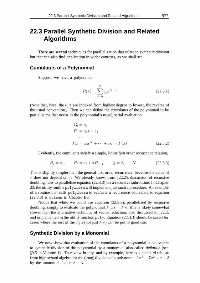
22.3 Parallel Synthetic Division and Related Algorithms 977
22.3 Parallel Synthetic Division and RelatedAlgorithms
There are several techniques for parallelization that relate to synthetic divisionbut that can also find application in wider contexts, as we shall see.
Cumulants of a Polynomial
Suppose we have a polynomial
P (x) =
N∑j=0
cjxN−j (22.3.1)
(Note that, here, thecj ’s are indexed from highest degree to lowest, the reverse ofthe usual convention.) Then we can define thecumulants of the polynomial to bepartial sums that occur in the polynomial’s usual, serial evaluation,
P0 = c0
P1 = c0x+ c1
· · ·PN = c0x
N + · · ·+ cN = P (x) (22.3.2)
Evidently, the cumulants satisfy a simple, linear first order recurrence relation,
P0 = c0, Pj = cj + xPj−1, j = 2, . . . , N (22.3.3)
This is slightly simpler than the general first order recurrence, because the value ofx does not depend onj. We already know, from§22.2’s discussion of recursivedoubling, how to parallelize equation (22.3.3) via a recursive subroutine. In Chapter23, the utility routinepoly termwill implement just such a procedure. An exampleof a routine that callspoly term to evaluate a recurrence equivalent to equation(22.3.3) iseulsum in Chapter B5.
Notice that while we could use equation (22.3.3), parallelized by recursivedoubling, simply to evaluate the polynomialP (x) = PN , this is likely somewhatslower than the alternative technique of vector reduction, also discussed in§22.2,and implemented in the utility functionpoly. Equation (22.3.3) should be saved forcases where the rest of thePj ’s (not justPN ) can be put to good use.
Synthetic Division by a Monomial
We now show that evaluation of the cumulants of a polynomial is equivalentto synthetic division of the polynomial by a monomial, also calleddeflation (see§9.5 in Volume 1). To review briefly, and by example, here is a standard tableaufrom high school algebra for the (long) division of a polynomial2x 3 − 7x2 + x+ 3by the monomial factorx − 3.
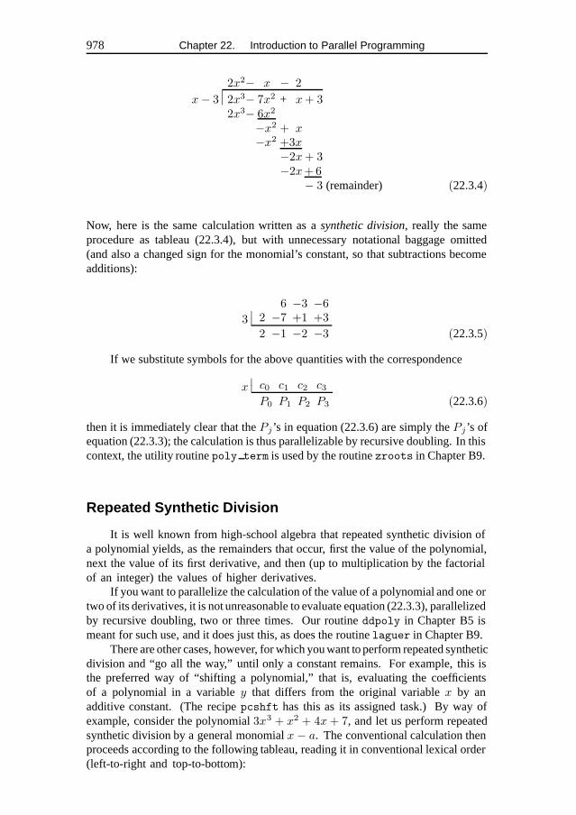
978 Chapter 22. Introduction to Parallel Programming
x− 3
2x2− x − 2∣∣ 2x3− 7x2 + x+ 32x3− 6x2
−x2 + x−x2 +3x
−2x+ 3−2x+6
− 3 (remainder) (22.3.4)
Now, here is the same calculation written as asynthetic division, really the sameprocedure as tableau (22.3.4), but with unnecessary notational baggage omitted(and also a changed sign for the monomial’s constant, so that subtractions becomeadditions):
3
6 −3 −6∣∣ 2 −7 +1 +3
2 −1 −2 −3 (22.3.5)
If we substitute symbols for the above quantities with the correspondence
x∣∣ c0 c1 c2 c3P0 P1 P2 P3 (22.3.6)
then it is immediately clear that thePj ’s in equation (22.3.6) are simply thePj ’s ofequation (22.3.3); the calculation is thus parallelizable by recursive doubling. In thiscontext, the utility routinepoly term is used by the routinezroots in Chapter B9.
Repeated Synthetic Division
It is well known from high-school algebra that repeated synthetic division ofa polynomial yields, as the remainders that occur, first the value of the polynomial,next the value of its first derivative, and then (up to multiplication by the factorialof an integer) the values of higher derivatives.
If you want to parallelize the calculation of the value of a polynomial and one ortwo of its derivatives, it is not unreasonable to evaluate equation (22.3.3), parallelizedby recursive doubling, two or three times. Our routineddpoly in Chapter B5 ismeant for such use, and it does just this, as does the routinelaguer in Chapter B9.
There are other cases, however, for which you want to perform repeated syntheticdivision and “go all the way,” until only a constant remains. For example, this isthe preferred way of “shifting a polynomial,” that is, evaluating the coefficientsof a polynomial in a variabley that differs from the original variablex by anadditive constant. (The recipepcshft has this as its assigned task.) By way ofexample, consider the polynomial3x3 + x2 + 4x+ 7, and let us perform repeatedsynthetic division by a general monomialx − a. The conventional calculation thenproceeds according to the following tableau, reading it in conventional lexical order(left-to-right and top-to-bottom):
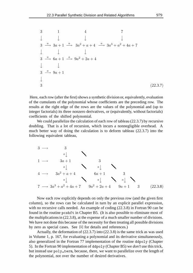
22.3 Parallel Synthetic Division and Related Algorithms 979
3 1 4 7� � � �3
a−→ 3a+ 1a−→ 3a2 + a+ 4
a−→ 3a3 + a2 + 4a+ 7� � �3
a−→ 6a+ 1a−→ 9a2 + 2a+ 4� �
3a−→ 9a+ 1�
3 (22.3.7)
Here, each row (after the first) shows a synthetic division or, equivalently, evaluationof the cumulants of the polynomial whose coefficients are the preceding row. Theresults at the right edge of the rows are the values of the polynomial and (up tointeger factorials) its three nonzero derivatives, or (equivalently, without factorials)coefficients of the shifted polynomial.
We could parallelize the calculation of each row of tableau (22.3.7) by recursivedoubling. That is a lot of recursion, which incurs a nonnegligible overhead. Amuch better way of doing the calculation is to deform tableau (22.3.7) into thefollowing equivalent tableau,
3 −→ 3
a� ↘
1 −→ 3a+ 1 3
a� ↘ a
� ↘4 −→ 3a2 + a+ 4 6a+ 1 3
a� ↘ a
� ↘ a� ↘
7 −→ 3a3 + a2 + 4a+ 7 9a2 + 2a+ 4 9a+ 1 3 (22.3.8)
Now each row explicitly depends on only the previous row (and the given firstcolumn), so the rows can be calculated in turn by an explicit parallel expression,with no recursive calls needed. An example of coding (22.3.8) in Fortran 90 can befound in the routinepcshft in Chapter B5. (It is also possible to eliminate most ofthe multiplications in (22.3.8), at the expense of a much smaller number of divisions.We have not done this because of the necessity for then treating all possible divisionsby zero as special cases. See[1] for details and references.)
Actually, the deformation of (22.3.7) into (22.3.8) is the same trick as was usedin Volume 1, p. 167, for evaluating a polynomial and its derivative simultaneously,also generalized in the Fortran 77 implementation of the routineddpoly (Chapter5). In the Fortran 90 implementation ofddpoly (Chapter B5) wedon’t use this trick,but instead usepoly term, because, there, we want to parallelize over the length ofthe polynomial, not over the number of desired derivatives.
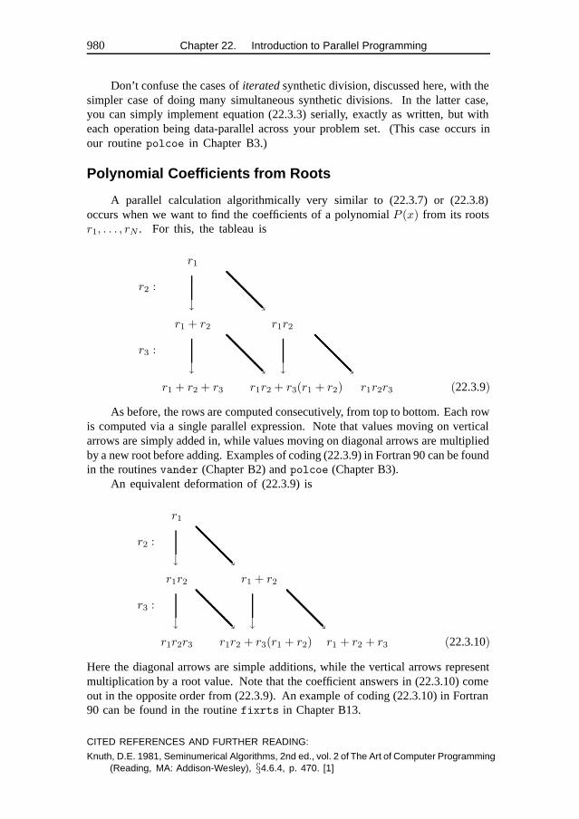
980 Chapter 22. Introduction to Parallel Programming
Don’t confuse the cases ofiterated synthetic division, discussed here, with thesimpler case of doing many simultaneous synthetic divisions. In the latter case,you can simply implement equation (22.3.3) serially, exactly as written, but witheach operation being data-parallel across your problem set. (This case occurs inour routinepolcoe in Chapter B3.)
Polynomial Coefficients from Roots
A parallel calculation algorithmically very similar to (22.3.7) or (22.3.8)occurs when we want to find the coefficients of a polynomialP (x) from its rootsr1, . . . , rN . For this, the tableau is
r1
r2 :
↓ ↘r1 + r2 r1r2
r3 :
↓ ↘ ↓ ↘r1 + r2 + r3 r1r2 + r3(r1 + r2) r1r2r3 (22.3.9)
As before, the rows are computed consecutively, from top to bottom. Each rowis computed via a single parallel expression. Note that values moving on verticalarrows are simply added in, while values moving on diagonal arrows are multipliedby a new root before adding. Examples of coding (22.3.9) in Fortran 90 can be foundin the routinesvander (Chapter B2) andpolcoe (Chapter B3).
An equivalent deformation of (22.3.9) is
r1
r2 :
↓ ↘r1r2 r1 + r2
r3 :
↓ ↘ ↓ ↘r1r2r3 r1r2 + r3(r1 + r2) r1 + r2 + r3 (22.3.10)
Here the diagonal arrows are simple additions, while the vertical arrows representmultiplication by a root value. Note that the coefficient answers in (22.3.10) comeout in the opposite order from (22.3.9). An example of coding (22.3.10) in Fortran90 can be found in the routinefixrts in Chapter B13.
CITED REFERENCES AND FURTHER READING:
Knuth, D.E. 1981, Seminumerical Algorithms, 2nd ed., vol. 2 of The Art of Computer Programming(Reading, MA: Addison-Wesley), §4.6.4, p. 470. [1]
22.4 Fast Fourier Transforms 981
22.4 Fast Fourier Transforms
Fast Fourier transforms are beloved by computer scientists, especially thosewho are interested in parallel algorithms, because the FFT’s hierarchical structuregenerates a complicated, but analyzable, set of requirements for interprocessorcommunication on MMPs. Thus, almost all books on parallel algorithms (e.g.,[1–3]) have a chapter on FFTs.
Unfortunately, the resulting algorithms are highly specific to particular parallelarchitectures, and therefore of little use to us in writing general purpose code in anarchitecture-independent parallel language like Fortran 90.
Luckily there is a good alternative that covers almost all cases of both serialand parallel machines. If, for a one-dimensional FFT of sizeN , one is satisfied withparallelism of order
√N , then there is a good, general way of achieving a parallel FFT
with quite minimal interprocessor communication; and the communication requiredis simply the matrix transpose operation, which Fortran 90 implements as an intrinsic.That is the approach that we discuss in this section, and implement in Chapter B12.
For a machine withM processors, this approach will saturate the processors (thedesirable condition where none are idle) when the size of a one-dimensional Fouriertransform,N , is large enough:N > M 2. SmallerN ’s will not achieve maximumparallelism. But suchN ’s are in fact so small for one-dimensional problems thatthey are unlikely to be the rate-determining step in scientific calculations. If theyare, it is usually because you are doing many such transforms independently, andyou should recover “outer parallelism” by doing them all at once.
For two or more dimensions, the adopted approach will saturateM processorswheneach dimension of the problem is larger thanM .
Column- and Row-Parallel FFTs
The basic building block that we assume (and implement in Chapter B12) is aroutine for simultaneously taking the FFT of eachrow of a two-dimensional matrix.The method is exactly that of Volume 1’sfour1 routine, but with array sectionslike data(:,j) replacing scalars likedata(j). Chapter B12’s implementation ofthis is a routine calledfourrow. If all the data for one column (that is, all thevaluesdata(i,:), for somei) are local to a single processor, then the parallelisminvolves no interprocessor communication at all: The independent FFTs simplyproceed, data parallel and in lockstep. This is architecture-independent parallelismwith a vengeance.
We will also need to take the FFT of eachcolumn of a two-dimensional matrix.One way to do this is to take the transpose (a Fortran 90 intrinsic that hides a lotof interprocessor communication), then take the FFT of the rows usingfourrow,then take the transpose again. An alternative method is to recode thefour1 routinewith array sections in the other dimension (data(j,:)) replacingfour1’s scalars(data(j)). This scheme, in Chapter B12, is a routine calledfourcol. In thiscase, good parallelism will be achieved only if the valuesdata(:,i), for somei,are local to a single processor. Of course, Fortran 90 does not give the user directcontrol over how data are distributed over the machine; but extensions such as HPFare designed to give just such control.
982 Chapter 22. Introduction to Parallel Programming
On a serial machine, you might think thatfourrow andfourcol should haveidentical timings (acting on a square matrix, say). The two routines do exactlythe same operations, after all. Not so! On modern serial computers,fourrow
and fourcol can have timings that differ by a factor of 2 or more, even whentheir detailed arithmetic is made identical (by giving to one a data array that is thetranspose of the data array given to the other). This effect is due to the multilevelcache architecture of most computer memories, and the fact that serial Fortran alwaysstores matrices by columns (first index changing most rapidly). On our workstations,fourrow is significantly faster thanfourcol, and this is likely the generic behavior.However, we do not exclude the possibility that some machines, and some sizes ofmatrices, are the other way around.
One-Dimensional FFTs
Turn now to the problem of how to do a single, one-dimensional, FFT. We aregiven a complex arrayf of lengthN , an integer power of 2. The basic idea is toaddress the input array as if it were a two-dimensional array of sizem×M , wheremandM are each integer powers of 2. Then the components off can be addressed as
f(Jm + j), 0 ≤ j < m, 0 ≤ J < M (22.4.1)
where thej index changes more rapidly, theJ index more slowly, and parenthesesdenote Fortran-style subscripts.
Now, suppose we had some magical (parallel) method to compute the discreteFourier transform
F (kM +K) ≡∑j,J
e2πi(kM+K)(Jm+j)/(Mm)f(Jm + j),
0 ≤ k < m, 0 ≤ K < M (22.4.2)
Then, you can see that the indicesk andK would address the desired result (FFTof the original array), withK varying more rapidly.
Starting with equation (22.4.2) it is easy to verify the following identity,
F (kM +K) =∑j
[e2πijk/m
(e2πijK/(Mm)
[∑J
e2πiJK/M f(Jm+ j)
])]
(22.4.3)But this, reading it from the innermost operation outward, is just the magical methodthat we need:
• Reshape the original array tom ×M in Fortran normal order (storageby columns).
• FFT on the second (column) index for all values of the first (row) index,using the routinefourrow.
• Multiply each component by a phase factorexp[2πijK/(Mm)].• Transpose.
22.5 Missing Language Features 983
• Again FFT on the second (column) index for all values of the first (row)index, using the routinefourrow.
• Reshape the two-dimensional array back into one-dimensional output.The above scheme usesfourrow exclusively, on the assumption that it is faster
than its siblingfourcol. When that is the case (as we typically find), it is likelythat the above method, implemented asfour1 in Chapter B12, is faster, even onscalar machines, than Volume 1’s scalar version offour1 (Chapter 12). The reason,as already mentioned, is thatfourrow’s parallelism is taking better advantage ofcache memory locality.
If fourrow is not faster thanfourcol on your machine, then you should insteadtry the following alternative scheme, usingfourcol only:
• Reshape the original array tom ×M in Fortran normal order (storageby columns).
• Transpose.• FFT on the first (row) index for all values of the second (column) index,
using the routinefourcol.• Multiply each component by a phase factorexp[2πijK/(Mm)].• Transpose.• Again FFT on the first (row) index for all values of the second (column)
index, using the routinefourcol.• Transpose.• Reshape the two-dimensional array back into one-dimensional output.In Chapter B12, this scheme is implemented asfour1 alt. You might
wonder whyfour1 alt has three transpose operations, whilefour1 had only one.Shouldn’t there be a symmetry here? No. Fortran makes the arbitrary, but consistent,choice of storing two-dimensional arrays by columns, and this choice favorsfour1
in terms of transposes. Luckily, at least on our serial workstations,fourrow (usedby four1) is faster thanfourcol (used byfour1 alt), so it is a double win.
For further discussion and references on the ideas behindfour1andfour1 alt
see [4], where these algorithms are called the four-step and six-step frameworks,respectively.
CITED REFERENCES AND FURTHER READING:
Fox, G.C., et al. 1988, Solving Problems on Concurrent Processors, Volume I (Englewood Cliffs,NJ: Prentice Hall), Chapter 11. [1]
Akl, S.G. 1989, The Design and Analysis of Parallel Algorithms (Englewood Cliffs, NJ: PrenticeHall), Chapter 9. [2]
Hockney, R.W., and Jesshope, C.R. 1988, Parallel Computers 2 (Bristol and Philadelphia: AdamHilger), §5.5. [3]
Van Loan, C. 1992, Computational Frameworks for the Fast Fourier Transform (Philadelphia:S.I.A.M.), §3.3. [4]
22.5 Missing Language Features
A few facilities that are fairly important to parallel programming are missingfrom the Fortran 90 language standard. On scalar machines this lack is not a
984 Chapter 22. Introduction to Parallel Programming
problem, since one can readily program the missing features by using do-loops.On parallel machines, both SSP machines and MMP machines, one must hopethat hardware manufacturers provide library routines, callable from Fortran 90, thatprovide access to the necessary facilities, or use extensions of Fortran 90, such asHigh Performance Fortran (HPF).
Scatter-with-Combine Functions
Fortran 90 allows the use ofvector subscripts for so-calledgather andscatteroperations. For example, with the setup
REAL(SP), DIMENSION(6) :: arr,barr,carrINTEGER(I4B), DIMENSION(6) :: iarr,jarr...iarr = (/ 1,3,5,2,4,6 /)jarr = (/ 3,2,3,2,1,1 /)
Fortran 90 allows both theone-to-one gather and theone-to-many gather,
barr=arr(iarr)carr=arr(jarr)
It also allows the one-to-one scatter,
barr(iarr)=carr
where the elements ofcarr are “scattered” intobarr under the direction of thevector subscriptiarr.
Fortran 90 doesnot allow the many-to-one scatter
barr(jarr)=carr ! illegal for this jarr
because the repeated values injarr try to assign different components ofcarr tothe same location inbarr. The result would not be deterministic.
Sometimes, however, one would in fact like a many-to-one construction, wherethe colliding elements get combined by a (commutative and associative) operation,like + or *, or max(). These so-calledscatter-with-combine functions are readilyimplemented on serial machines by a do-loop, for example,
barr=0.do j=1,size(carr)
barr(jarr(j))=barr(jarr(j))+carr(j)end do
Fortran 90 unfortunately provides no means for effecting scatter-with-combinefunctions in parallel. Luckily, almost all parallel machines do provide such a facilityas a library program, as does HPF, where the above facility is calledSUM SCATTER.In Chapter 23 we will define utility routinesscatter add andscatter max forscatter-with-combine functionalities, but the implementation given in Fortran 90 willbe strictly serial, with a do-loop.
22.5 Missing Language Features 985
Skew Sections
Fortran 90 provides no good, parallel way to access the diagonal elements ofa matrix, either to read them or to set them. Do-loops will obviously serve thisneed on serial machines. In principle, a construction like the following bizarrefragment could also be utilized,
REAL(SP), DIMENSION(n,n) :: matREAL(SP), DIMENSION(n*n) :: arrREAL(SP), DIMENSION(n) :: diag...arr = reshape(mat,shape(arr))diag = arr(1:n*n:n+1)
which extracts every(n + 1)st element from a one-dimensional array derived byreshaping the input matrix. However, it is unlikely that any foreseeable parallelcompiler will implement the above fragment without a prohibitive amount ofunnecessary data movement; and code like the above is also exceedingly slow onall serial machines that we have tried.
In Chapter 23 we will define utility routinesget diag, put diag, diagadd,diagmult, andunit matrix to manipulate diagonal elements, but the implemen-tation given in Fortran 90 will again be strictly serial, with do-loops.
Fortran 95 (see§21.6) will essentially fix Fortran 90’s skew sections deficiency.For example, using itsforall construction, the diagonal elements of an array canbe accessed by a statement like
forall (j=1:20) diag(j) = arr(j,j)
SIMD vs. MIMD
Recall that we use “SIMD” (single-instruction,multiple data) and “data parallel”as interchangeable terms, and that “MIMD” (multiple-instruction, multiple data) isa more general programming model. (See§22.1.)
You should not be too quick to jump to the conclusion that Fortran 90’s dataparallel or SIMD model is “bad,” and that MIMD features, absent in Fortran 90, aretherefore “good.” On the contrary, Fortran 90’s basic data-parallel paradigm has alot going for it. As we discussed in§22.1, most scientific problems naturally havea “data dimension” across which the time ordering of the calculation is irrelevant.Parallelism across this dimension, which is by nature most often SIMD, frees themind to think clearly about the computational steps in an algorithm that actually needto be sequential. SIMD code has advantages of clarity and predictability that shouldnot be taken lightly. The general MIMD model of “lots of different things all goingon at the same time and communicating data with each other” is a programmingand debugging nightmare.
Having said this, we must at the same time admit that a few MIMD features— most notably the ability to go through different logical branches for calculatingdifferent data elements in a data-parallel computation — are badly needed in certainprogramming situations. Fortran 90 is quite weak in this area.
Note that thewhere...elsewhere...end where construction isnot a MIMDconstruction. Fortran 90 requires that thewhereclause be executed completely beforetheelsewhere is started. (This allows the results of any calculations in the former
986 Chapter 22. Introduction to Parallel Programming
clause to be available for use in the latter.) So, this construction cannot be used toallow two logical branches to be calculated in parallel.
Special functions, where one would like to calculate function values for anarray of input quantities, are a particularly compelling example of the need forsome MIMD access. Indeed, you will find that Chapter B6 contains a number ofintricate, and in a few cases truly bizarre, workarounds, using allowed combinationsof merge, where, andCONTAINS (the latter, for separating different logical branchesinto formally different subprograms).
Fortran 95’sELEMENTAL and PURE constructions, and to some extent alsoforall (whose body will be able to includePURE function calls), will go a long waytowards providing exactly the kind of MIMD constructions that are most needed.Once Fortran 95 becomes available and widespread, you can expect to see a newversion of this volume, with a much-improved Chapter B6.
Conversely, the number of routines outside of Chapter B6 that can be signif-icantly improved by the use of MIMD features is relatively small; this illustratesthe underlying viability of the basic data-parallel SIMD model, even in a futurelanguage version with useful MIMD features.
Chapter 23. Numerical RecipesUtility Functions forFortran 90
23.0 Introduction and Summary Listing
This chapter describes and summarizes the Numerical Recipes utility routinesthat are used throughout the rest of this volume. A complete implementation of theseroutines in Fortran 90 is listed in Appendix C1.
Why do we need utility routines? Aren’t there already enough of them builtinto the language as Fortran 90 intrinsics? The answers lie in this volume’s dualpurpose: to implement the Numerical Recipes routines in Fortran 90 code that runsefficiently on fast serial machines,and to implement them, wherever possible, withefficient parallel code for multiprocessor machines that will become increasinglycommon in the future. We have found three kinds of situations where additionalutility routines seem desirable:
1. Fortran 90 is a big language, with many high-level constructs — singlestatements that actually result in a lot of computing. We like this; it gives thelanguage the potential for expressing algorithms very readably, getting them “outof the mud” of microscopic coding. In coding the 350+ Recipes for this volume,we kept a systematic watch for bits of microscopic coding that were repeated inmany routines, and that seemed to be at a lower level of coding than that aspiredto by good Fortran 90 style. Once these bits were identified, we pulled them outand substituted calls to new utility routines. These are the utilities that arguablyought to be new language intrinsics, equally useful for serial and parallel machines.(A prime example isswap.)
2. Fortran 90 contains many highly parallelizable language constructions. But,as we have seen in§22.5, it is also missing a few important constructions. Mostparallel machines will provide these missing elements as machine-coded librarysubroutines. Some of our utility routines are provided simply as a standard interfaceto these common, but nonstandard, functionalities. Note that it is the nature ofthese routines that our specific implementation, in Appendix C1, will be serial,and therefore inefficient on parallel machines. If you have a parallel machine,you will need to recode these; this often involves no more than substituting aone-line library function call for the body of our implementation. Utilities in thiscategory will likely become unnecessary over time, either as machine-dependentlibraries converge to standard interfaces, or as the utilities get added to future Fortran
987
988 Chapter 23. Numerical Recipes Utility Functions for Fortran 90
versions. (Indeed, some routines in this category will be unnecessary in Fortran95, once it is available; see§23.7.)
3. Some tasks should just be done differently in serial, versus parallel,implementation. Linear recurrence relations are a good example (§22.2). Theseare trivially coded with a do-loop on serial machines, but require a fairly elaboraterecursive construction for good parallelization. Rather than provide separate serialand parallel versions of the Numerical Recipes, we have chosen to pull out of theRecipes, and into utility routines, some identifiable tasks of this kind. These arecases where some recoding of our implementation in Appendix C1 might resultin improved performance on your particular hardware. Unfortunately, it is not sosimple as providing a single “serial implementation” and another single “parallelimplementation,” because even the seemingly simple word “serial” hides, at thehardware level, a variety of different degrees of pipelining, wide instructions, andso on. Appendix C1 therefore provides only a single implementation, although withsome adjustable parameters that you can customize (by experiment) to maximizeperformance on your hardware.
The above three cases are not really completely distinct, and it is therefore notpossible to assign any single utility routine to exactly one situation. Instead, weorganize the rest of this chapter as follows: first, an alphabetical list, with shortsummary, of all the new utility routines; next, a series of short sections, grouped byfunctionality, that contain the detailed descriptions of the routines.
Alphabetical Listing
The following list gives an abbreviated mnemonic for the type, rank, and/orshape of the returned values (as in§21.4), the routine’s calling sequence (optionalarguments shown in italics), and a brief, often incomplete, description. The completedescription of the routine is given in the later section shown in square brackets.
For each entry, the number shown in parentheses is the approximate number ofdistinct Recipes in this book that make use of that particular utility function, and isthus a rough guide to that utility’s importance. (There may be multiple invocationsof the utility in each such Recipe.) Where this number is small or zero, it is usuallybecause the utility routine is a member of a related family of routines whose totalusage was deemed significant enough to include, and we did not want users to haveto “guess” which family members were instantiated.
call array copy(src,dest,n copied,n not copied)
Copy one-dimensional array (whose size is not necessarily known).[23.1] (9)
[Arr] arth(first,increment,n)
Return an arithmetic progression as an array. [23.4] (55)
call assert(n1,n2,...,string)
Exit with error message if any logical arguments are false. [23.3] (50)
[Int] assert eq(n1,n2,...,string)
Exit with error message if all integer arguments are not equal;otherwisereturn common value. [23.3] (133)
[argTS] cumprod(arr,seed)
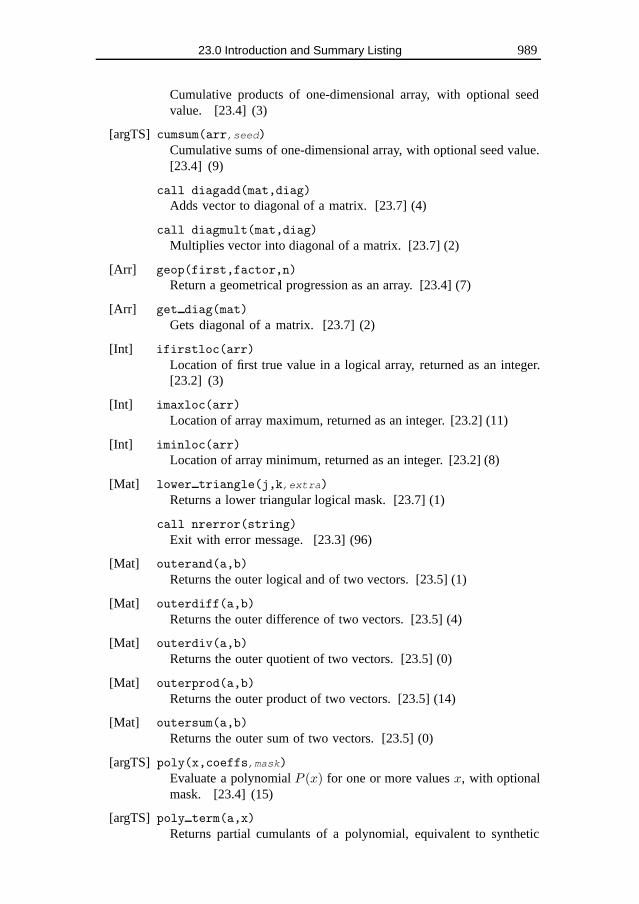
23.0 Introduction and Summary Listing 989
Cumulative products of one-dimensional array, with optional seedvalue. [23.4] (3)
[argTS] cumsum(arr,seed)Cumulative sums of one-dimensional array, with optional seed value.[23.4] (9)
call diagadd(mat,diag)
Adds vector to diagonal of a matrix. [23.7] (4)
call diagmult(mat,diag)
Multiplies vector into diagonal of a matrix. [23.7] (2)
[Arr] geop(first,factor,n)
Return a geometrical progression as an array. [23.4] (7)
[Arr] get diag(mat)
Gets diagonal of a matrix. [23.7] (2)
[Int] ifirstloc(arr)
Location of first true value in a logical array, returned as an integer.[23.2] (3)
[Int] imaxloc(arr)
Location of array maximum, returned as an integer. [23.2] (11)
[Int] iminloc(arr)
Location of array minimum, returned as an integer. [23.2] (8)
[Mat] lower triangle(j,k,extra)
Returns a lower triangular logical mask. [23.7] (1)
call nrerror(string)
Exit with error message. [23.3] (96)
[Mat] outerand(a,b)
Returns the outer logical and of two vectors. [23.5] (1)
[Mat] outerdiff(a,b)
Returns the outer difference of two vectors. [23.5] (4)
[Mat] outerdiv(a,b)
Returns the outer quotient of two vectors. [23.5] (0)
[Mat] outerprod(a,b)
Returns the outer product of two vectors. [23.5] (14)
[Mat] outersum(a,b)
Returns the outer sum of two vectors. [23.5] (0)
[argTS] poly(x,coeffs,mask)Evaluate a polynomialP (x) for one or more valuesx, with optionalmask. [23.4] (15)
[argTS] poly term(a,x)
Returns partial cumulants of a polynomial, equivalent to synthetic
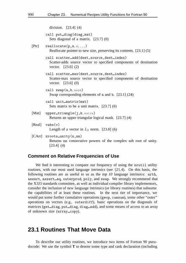
990 Chapter 23. Numerical Recipes Utility Functions for Fortran 90
division. [23.4] (4)
call put diag(diag,mat)
Sets diagonal of a matrix. [23.7] (0)
[Ptr] reallocate(p,n,m,...)
Reallocate pointer to new size, preserving its contents. [23.1] (5)
call scatter add(dest,source,dest index)
Scatter-adds source vector to specified components of destinationvector. [23.6] (2)
call scatter max(dest,source,dest index)
Scatter-max source vector to specified components of destinationvector. [23.6] (0)
call swap(a,b,mask)
Swap corresponding elements ofa andb. [23.1] (24)
call unit matrix(mat)
Sets matrix to be a unit matrix. [23.7] (6)
[Mat] upper triangle(j,k,extra)
Returns an upper triangular logical mask. [23.7] (4)
[Real] vabs(v)
Length of a vector inL2 norm. [23.8] (6)
[CArr] zroots unity(n,nn)
Returnsnn consecutive powers of the complexnth root of unity.[23.4] (4)
Comment on Relative Frequencies of Use
We find it interesting to compare our frequency of using thenrutil utilityroutines, with our most used language intrinsics (see§21.4). On this basis, thefollowing routines are as useful to us as thetop 10 language intrinsics:arth,assert, assert eq, outerprod, poly, andswap. We strongly recommend thatthe X3J3 standards committee, as well as individual compiler library implementors,consider the inclusion of new language intrinsics (or library routines) that subsumethe capabilities of at least these routines. In the next tier of importance, wewould put some further cumulative operations (geop, cumsum), some other “outer”operations on vectors (e.g.,outerdiff), basic operations on the diagonals ofmatrices (get diag, put diag, diag add), and some means of access to an arrayof unknown size (array copy).
23.1 Routines That Move Data
To describe our utility routines, we introduce two items of Fortran 90 pseu-docode: We use the symbolT to denote some type and rank declaration (including
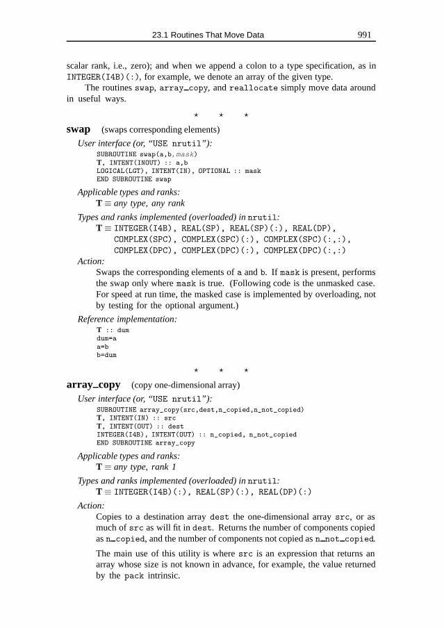
23.1 Routines That Move Data 991
scalar rank, i.e., zero); and when we append a colon to a type specification, as inINTEGER(I4B)(:), for example, we denote an array of the given type.
The routinesswap, array copy, andreallocate simply move data aroundin useful ways.
� � �
swap (swaps corresponding elements)
User interface (or, “USE nrutil”):SUBROUTINE swap(a,b,mask)T, INTENT(INOUT) :: a,bLOGICAL(LGT), INTENT(IN), OPTIONAL :: maskEND SUBROUTINE swap
Applicable types and ranks:T ≡ any type, any rank
Types and ranks implemented (overloaded) innrutil:T ≡ INTEGER(I4B), REAL(SP), REAL(SP)(:), REAL(DP),
COMPLEX(SPC), COMPLEX(SPC)(:), COMPLEX(SPC)(:,:),
COMPLEX(DPC), COMPLEX(DPC)(:), COMPLEX(DPC)(:,:)
Action:Swaps the corresponding elements ofa andb. If mask is present, performsthe swap only wheremask is true. (Following code is the unmasked case.For speed at run time, the masked case is implemented by overloading, notby testing for the optional argument.)
Reference implementation:T :: dumdum=aa=bb=dum
� � �
array copy (copy one-dimensional array)
User interface (or, “USE nrutil”):SUBROUTINE array_copy(src,dest,n_copied,n_not_copied)T, INTENT(IN) :: srcT, INTENT(OUT) :: destINTEGER(I4B), INTENT(OUT) :: n_copied, n_not_copiedEND SUBROUTINE array_copy
Applicable types and ranks:T ≡ any type, rank 1
Types and ranks implemented (overloaded) innrutil:T ≡ INTEGER(I4B)(:), REAL(SP)(:), REAL(DP)(:)
Action:Copies to a destination arraydest the one-dimensional arraysrc, or asmuch ofsrc as will fit in dest. Returns the number of components copiedasn copied, and the number of components not copied asn not copied.
The main use of this utility is wheresrc is an expression that returns anarray whose size is not known in advance, for example, the value returnedby the pack intrinsic.
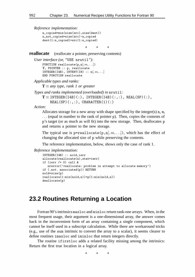
992 Chapter 23. Numerical Recipes Utility Functions for Fortran 90
Reference implementation:n_copied=min(size(src),size(dest))n_not_copied=size(src)-n_copieddest(1:n_copied)=src(1:n_copied)
� � �
reallocate (reallocate a pointer, preserving contents)
User interface (or, “USE nrutil”):FUNCTION reallocate(p,n[,m, . . .])T, POINTER :: p, reallocateINTEGER(I4B), INTENT(IN) :: n[,m, . . .]END FUNCTION reallocate
Applicable types and ranks:T ≡ any type, rank 1 or greater
Types and ranks implemented (overloaded) innrutil:T ≡ INTEGER(I4B)(:), INTEGER(I4B)(:,:), REAL(SP)(:),
REAL(SP)(:,:), CHARACTER(1)(:)
Action:Allocates storage for a new array with shape specified by the integer(s)n, m,. . . (equal in number to the rank of pointerp). Then, copies the contents ofp’s target (or as much as will fit) into the new storage. Then, deallocatesp
and returns a pointer to the new storage.
The typical use isp=reallocate(p,n[, m, . . .]), which has the effect ofchanging the allocated size ofp while preserving the contents.
The reference implementation, below, shows only the case of rank 1.
Reference implementation:INTEGER(I4B) :: nold,ierrallocate(reallocate(n),stat=ierr)if (ierr /= 0) call &
nrerror(’reallocate: problem in attempt to allocate memory’)if (.not. associated(p)) RETURNnold=size(p)reallocate(1:min(nold,n))=p(1:min(nold,n))deallocate(p)
23.2 Routines Returning a Location
Fortran 90’s intrinsicsmaxloc andminloc return rank-one arrays. When, in themost frequent usage, their argument is a one-dimensional array, the answer comesback in the inconvenient form of an array containing a single component, whichcannot be itself used in a subscript calculation. While there are workaround tricks(e.g., use of thesum intrinsic to convert the array to a scalar), it seems clearer todefine routinesimaxloc andiminloc that return integers directly.
The routineifirstloc adds a related facility missing among the intrinsics:Return the first true location in a logical array.
� � �
23.2 Routines Returning a Location 993
imaxloc (location of array maximum as an integer)
User interface (or, “USE nrutil”):FUNCTION imaxloc(arr)T, INTENT(IN) :: arrINTEGER(I4B) :: imaxlocEND FUNCTION imaxloc
Applicable types and ranks:T ≡ any integer or real type, rank 1
Types and ranks implemented (overloaded) innrutil:T ≡ INTEGER(I4B)(:), REAL(SP)(:)
Action:For one-dimensional arrays, identical to themaxloc intrinsic, except returnsits answer as an integer rather than asmaxloc’s somewhat awkward rank-onearray containing a single component.
Reference implementation:INTEGER(I4B), DIMENSION(1) :: imaximax=maxloc(arr(:))imaxloc=imax(1)
� � �
iminloc (location of array minimum as an integer)
User interface (or, “USE nrutil”):FUNCTION iminloc(arr)T, INTENT(IN) :: arrINTEGER(I4B) :: iminlocEND FUNCTION iminloc
Applicable types and ranks:T ≡ any integer or real type, rank 1
Types and ranks implemented (overloaded) innrutil:T ≡ REAL(SP)(:)
Action:For one-dimensional arrays, identical to theminloc intrinsic, except returnsits answer as an integer rather than asminloc’s somewhat awkward rank-onearray containing a single component.
Reference implementation:INTEGER(I4B), DIMENSION(1) :: iminimin=minloc(arr(:))iminloc=imin(1)
� � �
ifirstloc (returns location of first “true” in a logical vector)
User interface (or, “USE nrutil”):FUNCTION ifirstloc(mask)T, INTENT(IN) :: maskINTEGER(I4B) :: ifirstlocEND FUNCTION ifirstloc
994 Chapter 23. Numerical Recipes Utility Functions for Fortran 90
Applicable types and ranks:T ≡ any logical type, rank 1
Types and ranks implemented (overloaded) innrutil:T ≡ LOGICAL(LGT)
Action:Returns the index (subscript value) of the first location, in a one-dimensionallogical mask, that has the value.TRUE., or returnssize(mask)+1 if allcomponents ofmask are .FALSE.
Note that while the reference implementation uses a do-loop, the function isparallelized innrutil by instead using themerge andmaxloc intrinsics.
Reference implementation:INTEGER(I4B) :: ido i=1,size(mask)
if (mask(i)) thenifirstloc=ireturn
end ifend doifirstloc=i
23.3 Argument Checking and Error Handling
It is good programming practice for a routine to check the assumptions(“assertions”) that it makes about the sizes of input arrays, allowed range ofnumerical arguments, and so forth. The routinesassert andassert eq are meantfor this kind of use. The routinenrerror is our default error reporting routine.
� � �
assert (exit with error message if any assertion is false)
User interface (or, “USE nrutil”):SUBROUTINE assert(n1,n2,...,string)CHARACTER(LEN=*), INTENT(IN) :: stringLOGICAL, INTENT(IN) :: n1,n2,...END SUBROUTINE assert
Action:Embedding program dies gracefully with an error message if any of thelogical arguments are false. Typical use is with logical expressions as theactual arguments.nrutil implements and overloads forms with 1, 2, 3, and4 logical arguments, plus a form with a vector logical argument,LOGICAL, DIMENSION(:), INTENT(IN) :: n
that is checked by theall(n) intrinsic.
23.3 Argument Checking and Error Handling 995
Reference implementation:if (.not. (n1.and.n2.and...)) then
write (*,*) ’nrerror: an assertion failed with this tag:’, stringSTOP ’program terminated by assert’
end if
� � �
assert eq (exit with error message if integer arguments not all equal)
User interface (or, “USE nrutil”):FUNCTION assert_eq(n1,n2,n3,...,string)CHARACTER(LEN=*), INTENT(IN) :: stringINTEGER, INTENT(IN) :: n1,n2,n3,...INTEGER :: assert_eqEND FUNCTION assert_eq
Action:Embedding program dies gracefully with an error message if any of theinteger arguments are not equal to the first. Otherwise, return the value ofthe first argument. Typical use is for enforcing equality on the sizes of arrayspassed to a subprogram.nrutil implements and overloads forms with 1, 2,3, and 4 integer arguments, plus a form with a vector integer argument,INTEGER, DIMENSION(:), INTENT(IN) :: n
that is checked by the conditionalif (all(nn(2:)==nn(1))).
Reference implementation:if (n1==n2.and.n2==n3.and...) then
assert_eq=n1else
write (*,*) ’nrerror: an assert_eq failed with this tag:’, stringSTOP ’program terminated by assert_eq’
end if
� � �
nrerror (report error message and stop)
User interface (or, “USE nrutil”):SUBROUTINE nrerror(string)CHARACTER(LEN=*), INTENT(IN) :: stringEND SUBROUTINE nrerror
Action:This is the minimal error handler used in this book. In applications ofany complexity, it is intended only as a placeholder for a user’s morecomplicated error handling strategy.
Reference implementation:write (*,*) ’nrerror: ’,stringSTOP ’program terminated by nrerror’
996 Chapter 23. Numerical Recipes Utility Functions for Fortran 90
23.4 Routines for Polynomials and Recurrences
Apart from programming convenience, these routines are designed to allow fornontrivial parallel implementations, as discussed in§22.2 and§22.3.
� � �
arth (returns arithmetic progression as an array)
User interface (or, “USE nrutil”):FUNCTION arth(first,increment,n)T, INTENT(IN) :: first,incrementINTEGER(I4B), INTENT(IN) :: nT, DIMENSION(n) [or, 1 rank higher thanT]:: arthEND FUNCTION arth
Applicable types and ranks:T ≡ any numerical type, any rank
Types and ranks implemented (overloaded) innrutil:T ≡ INTEGER(I4B), REAL(SP), REAL(DP)
Action:Returns an array of lengthn containing an arithmetic progression whosefirst value isfirst and whose increment isincrement. If first andincrement have rank greater than zero, returns an array of one larger rank,with the last subscript having sizen and indexing the progressions. Note thatthe following reference implementation (for the scalar case) is definitionalonly, and neither parallelized nor optimized for roundoff error. See§22.2and Appendix C1 for implementation by subvector scaling.
Reference implementation:INTEGER(I4B) :: kif (n > 0) arth(1)=firstdo k=2,n
arth(k)=arth(k-1)+incrementend do
� � �
geop (returns geometric progression as an array)
User interface (or, “USE nrutil”):FUNCTION geop(first,factor,n)T, INTENT(IN) :: first,factorINTEGER(I4B), INTENT(IN) :: nT, DIMENSION(n) [or, 1 rank higher thanT]:: geopEND FUNCTION geop
Applicable types and ranks:T ≡ any numerical type, any rank
Types and ranks implemented (overloaded) innrutil:T ≡ INTEGER(I4B), REAL(SP), REAL(DP), REAL(DP)(:),
COMPLEX(SPC)
23.4 Routines for Polynomials and Recurrences 997
Action:Returns an array of lengthn containing a geometric progression whose firstvalue isfirst and whose multiplier isfactor. If first and factor
have rank greater than zero, returns an array of one larger rank, with thelast subscript having sizen and indexing the progression. Note that thefollowing reference implementation (for the scalar case) is definitional only,and neither parallelized nor optimized for roundoff error. See§22.2 andAppendix C1 for implementation by subvector scaling.
Reference implementation:INTEGER(I4B) :: kif (n > 0) geop(1)=firstdo k=2,n
geop(k)=geop(k-1)*factorend do
� � �
cumsum (cumulative sum on an array, with optional additive seed)
User interface (or, “USE nrutil”):FUNCTION cumsum(arr,seed)T, DIMENSION(:), INTENT(IN) :: arrT, OPTIONAL, INTENT(IN) :: seedT, DIMENSION(size(arr)), INTENT(OUT) :: cumsumEND FUNCTION cumsum
Applicable types and ranks:T ≡ any numerical type
Types and ranks implemented (overloaded) innrutil:T ≡ INTEGER(I4B), REAL(SP)
Action:Given the rank 1 arrayarr of typeT, returns an array of identical type andsize containing the cumulative sums ofarr. If the optional argumentseedis present, it is added to the first component (and therefore, by cumulation,all components) of the result. See§22.2 for parallelization ideas.
Reference implementation:INTEGER(I4B) :: n,jT :: sdn=size(arr)if (n == 0) returnsd=0.0if (present(seed)) sd=seedcumsum(1)=arr(1)+sddo j=2,n
cumsum(j)=cumsum(j-1)+arr(j)end do
� � �
cumprod (cumulative prod on an array, with optional multiplicative seed)
User interface (or, “USE nrutil”):FUNCTION cumprod(arr,seed)T, DIMENSION(:), INTENT(IN) :: arrT, OPTIONAL, INTENT(IN) :: seedT, DIMENSION(size(arr)), INTENT(OUT) :: cumprodEND FUNCTION cumprod
998 Chapter 23. Numerical Recipes Utility Functions for Fortran 90
Applicable types and ranks:T ≡ any numerical type
Types and ranks implemented (overloaded) innrutil:T ≡ REAL(SP)
Action:Given the rank 1 arrayarr of typeT, returns an array of identical type andsize containing the cumulative products ofarr. If the optional argumentseed is present, it is multiplied into the first component (and therefore, bycumulation, into all components) of the result. See§22.2 for parallelizationideas.
Reference implementation:INTEGER(I4B) :: n,jT :: sdn=size(arr)if (n == 0) returnsd=1.0if (present(seed)) sd=seedcumprod(1)=arr(1)*sddo j=2,n
cumprod(j)=cumprod(j-1)*arr(j)end do
� � �
poly (polynomial evaluation)
User interface (or, “USE nrutil”):FUNCTION poly(x,coeffs,mask)T,, DIMENSION(:,...), INTENT(IN) :: xT, DIMENSION(:), INTENT(IN) :: coeffsLOGICAL(LGT), DIMENSION(:,...), OPTIONAL, INTENT(IN) :: maskT :: polyEND FUNCTION poly
Applicable types and ranks:T ≡ any numerical type (xmay be scalar or have any rank;x and
coeffs may have different numerical types)Types and ranks implemented (overloaded) innrutil:
T ≡ various combinations ofREAL(SP), REAL(SP)(:), REAL(DP),
REAL(DP)(:), COMPLEX(SPC) (see Appendix C1 for de-tails)
Action:Returns a scalar value or array with the same type and shape asx, containingthe result of evaluating the polynomial with one-dimensional coefficientvectorcoeffs on each component ofx. The optional argumentmask, ifpresent, has the same shape asx, and suppresses evaluation of the polynomialwhere its components are.false.. The following reference code showsthe case wheremask is not present. (The other case can be included byoverloading.)
23.4 Routines for Polynomials and Recurrences 999
Reference implementation:INTEGER(I4B) :: i,nn=size(coeffs)if (n <= 0) then
poly=0.0else
poly=coeffs(n)do i=n-1,1,-1
poly=x*poly+coeffs(i)end do
end if
� � �
poly term (partial cumulants of a polynomial)
User interface (or, “USE nrutil”):FUNCTION poly_term(a,x)T, DIMENSION(:), INTENT(IN) :: aT, INTENT(IN) :: xT, DIMENSION(size(a)) :: poly_termEND FUNCTION poly_term
Applicable types and ranks:T ≡ any numerical type
Types and ranks implemented (overloaded) innrutil:T ≡ REAL(SP), COMPLEX(SPC)
Action:Returns an array of type and size the same as the one-dimensional arraya, containing the partial cumulants of the polynomial with coefficientsa
(arranged from highest-order to lowest-order coefficients, n.b.) evaluatedat x. This is equivalent to synthetic division, and can be parallelized. See§22.3. Note that the order of arguments is reversed inpoly andpoly term
— each routine returns a value with the size and shape of thefirst argument,the usual Fortran 90 convention.
Reference implementation:INTEGER(I4B) :: n,jn=size(a)if (n <= 0) returnpoly_term(1)=a(1)do j=2,n
poly_term(j)=a(j)+x*poly_term(j-1)end do
� � �
zroots unity (returns powers of complexnth root of unity)
User interface (or, “USE nrutil”):FUNCTION zroots_unity(n,nn)INTEGER(I4B), INTENT(IN) :: n,nnCOMPLEX(SPC), DIMENSION(nn) :: zroots_unityEND FUNCTION zroots_unity
1000 Chapter 23. Numerical Recipes Utility Functions for Fortran 90
Action:Returns a complex array containingnn consecutive powers of thenthcomplex root of unity. Note that the following reference implementation isdefinitional only, and neither parallelized nor optimized for roundoff error.See Appendix C1 for implementation by subvector scaling.
Reference implementation:INTEGER(I4B) :: kREAL(SP) :: thetaif (nn==0) returnzroots_unity(1)=1.0if (nn==1) returntheta=TWOPI/nzroots_unity(2)=cmplx(cos(theta),sin(theta))do k=3,nn
zroots_unity(k)=zroots_unity(k-1)*zroots_unity(2)end do
23.5 Routines for Outer Operations on Vectors
Outer operations on vectors take two vectors as input, and return a matrix asoutput. One dimension of the matrix is the size of the first vector, the other is thesize of the second vector. Our convention is always the standard one,
result(i,j) = first operand(i) (op) second operand(j)
where(op) is any of addition, subtraction, multiplication, division, and logicaland.The reason for coding these as utility routines is that Fortran 90’s native construction,with two spreads (cf.§22.1), is difficult to read and thus prone to programmer errors.
� � �
outerprod (outer product)
User interface (or, “USE nrutil”):FUNCTION outerprod(a,b)T, DIMENSION(:), INTENT(IN) :: a,bT, DIMENSION(size(a),size(b)) :: outerprodEND FUNCTION outerprod
Applicable types and ranks:T ≡ any numerical type
Types and ranks implemented (overloaded) innrutil:T ≡ REAL(SP), REAL(DP)
Action:Returns a matrix that is the outer product of two vectors.
Reference implementation:outerprod = spread(a,dim=2,ncopies=size(b)) * &
spread(b,dim=1,ncopies=size(a))
� � �
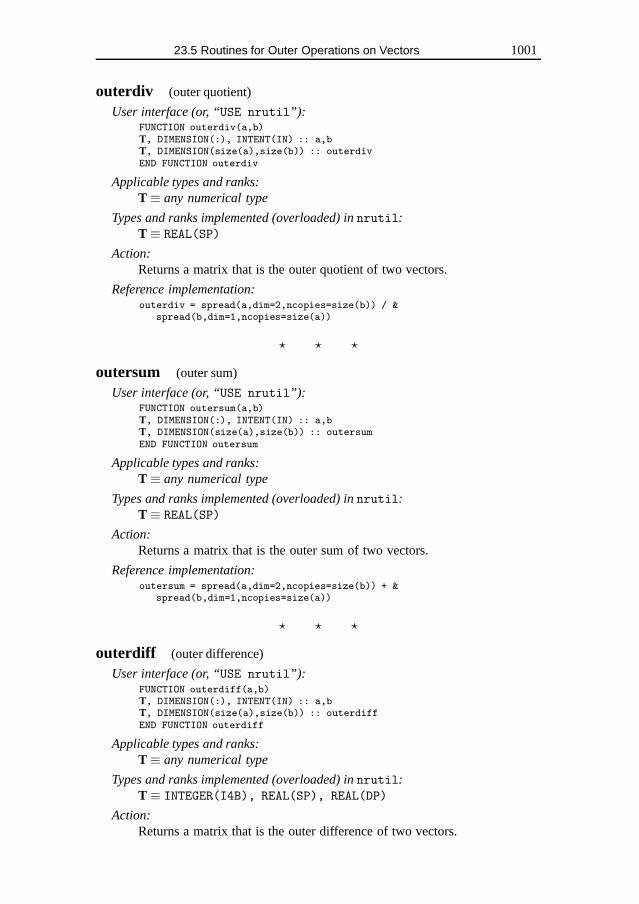
23.5 Routines for Outer Operations on Vectors 1001
outerdiv (outer quotient)
User interface (or, “USE nrutil”):FUNCTION outerdiv(a,b)T, DIMENSION(:), INTENT(IN) :: a,bT, DIMENSION(size(a),size(b)) :: outerdivEND FUNCTION outerdiv
Applicable types and ranks:T ≡ any numerical type
Types and ranks implemented (overloaded) innrutil:T ≡ REAL(SP)
Action:Returns a matrix that is the outer quotient of two vectors.
Reference implementation:outerdiv = spread(a,dim=2,ncopies=size(b)) / &
spread(b,dim=1,ncopies=size(a))
� � �
outersum (outer sum)
User interface (or, “USE nrutil”):FUNCTION outersum(a,b)T, DIMENSION(:), INTENT(IN) :: a,bT, DIMENSION(size(a),size(b)) :: outersumEND FUNCTION outersum
Applicable types and ranks:T ≡ any numerical type
Types and ranks implemented (overloaded) innrutil:T ≡ REAL(SP)
Action:Returns a matrix that is the outer sum of two vectors.
Reference implementation:outersum = spread(a,dim=2,ncopies=size(b)) + &
spread(b,dim=1,ncopies=size(a))
� � �
outerdiff (outer difference)
User interface (or, “USE nrutil”):FUNCTION outerdiff(a,b)T, DIMENSION(:), INTENT(IN) :: a,bT, DIMENSION(size(a),size(b)) :: outerdiffEND FUNCTION outerdiff
Applicable types and ranks:T ≡ any numerical type
Types and ranks implemented (overloaded) innrutil:T ≡ INTEGER(I4B), REAL(SP), REAL(DP)
Action:Returns a matrix that is the outer difference of two vectors.
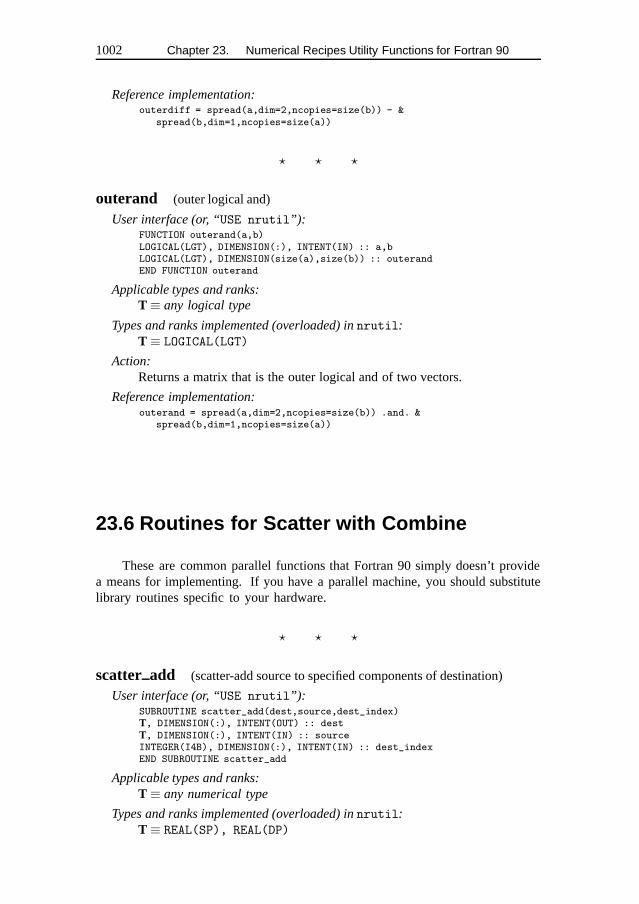
1002 Chapter 23. Numerical Recipes Utility Functions for Fortran 90
Reference implementation:outerdiff = spread(a,dim=2,ncopies=size(b)) - &
spread(b,dim=1,ncopies=size(a))
� � �
outerand (outer logical and)
User interface (or, “USE nrutil”):FUNCTION outerand(a,b)LOGICAL(LGT), DIMENSION(:), INTENT(IN) :: a,bLOGICAL(LGT), DIMENSION(size(a),size(b)) :: outerandEND FUNCTION outerand
Applicable types and ranks:T ≡ any logical type
Types and ranks implemented (overloaded) innrutil:T ≡ LOGICAL(LGT)
Action:Returns a matrix that is the outer logical and of two vectors.
Reference implementation:outerand = spread(a,dim=2,ncopies=size(b)) .and. &
spread(b,dim=1,ncopies=size(a))
23.6 Routines for Scatter with Combine
These are common parallel functions that Fortran 90 simply doesn’t providea means for implementing. If you have a parallel machine, you should substitutelibrary routines specific to your hardware.
� � �
scatter add (scatter-add source to specified components of destination)
User interface (or, “USE nrutil”):SUBROUTINE scatter_add(dest,source,dest_index)T, DIMENSION(:), INTENT(OUT) :: destT, DIMENSION(:), INTENT(IN) :: sourceINTEGER(I4B), DIMENSION(:), INTENT(IN) :: dest_indexEND SUBROUTINE scatter_add
Applicable types and ranks:T ≡ any numerical type
Types and ranks implemented (overloaded) innrutil:T ≡ REAL(SP), REAL(DP)
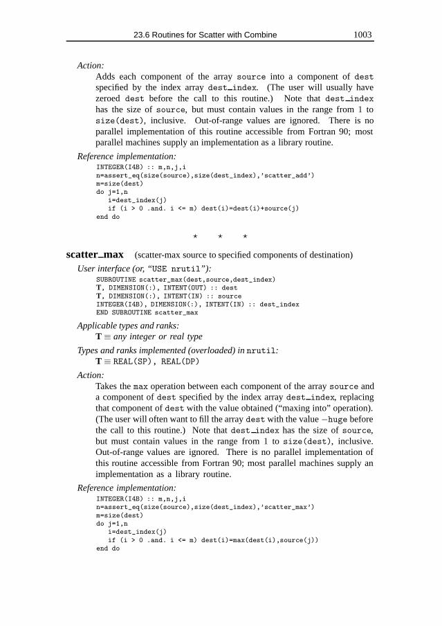
23.6 Routines for Scatter with Combine 1003
Action:Adds each component of the arraysource into a component ofdestspecified by the index arraydest index. (The user will usually havezeroed dest before the call to this routine.) Note thatdest index
has the size ofsource, but must contain values in the range from1 tosize(dest), inclusive. Out-of-range values are ignored. There is noparallel implementation of this routine accessible from Fortran 90; mostparallel machines supply an implementation as a library routine.
Reference implementation:INTEGER(I4B) :: m,n,j,in=assert_eq(size(source),size(dest_index),’scatter_add’)m=size(dest)do j=1,n
i=dest_index(j)if (i > 0 .and. i <= m) dest(i)=dest(i)+source(j)
end do
� � �
scatter max (scatter-max source to specified components of destination)
User interface (or, “USE nrutil”):SUBROUTINE scatter_max(dest,source,dest_index)T, DIMENSION(:), INTENT(OUT) :: destT, DIMENSION(:), INTENT(IN) :: sourceINTEGER(I4B), DIMENSION(:), INTENT(IN) :: dest_indexEND SUBROUTINE scatter_max
Applicable types and ranks:T ≡ any integer or real type
Types and ranks implemented (overloaded) innrutil:T ≡ REAL(SP), REAL(DP)
Action:Takes themax operation between each component of the arraysource anda component ofdest specified by the index arraydest index, replacingthat component ofdest with the value obtained (“maxing into” operation).(The user will often want to fill the arraydest with the value−huge beforethe call to this routine.) Note thatdest index has the size ofsource,but must contain values in the range from1 to size(dest), inclusive.Out-of-range values are ignored. There is no parallel implementation ofthis routine accessible from Fortran 90; most parallel machines supply animplementation as a library routine.
Reference implementation:INTEGER(I4B) :: m,n,j,in=assert_eq(size(source),size(dest_index),’scatter_max’)m=size(dest)do j=1,n
i=dest_index(j)if (i > 0 .and. i <= m) dest(i)=max(dest(i),source(j))
end do
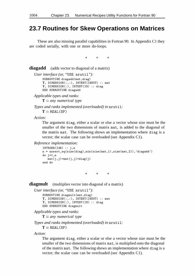
1004 Chapter 23. Numerical Recipes Utility Functions for Fortran 90
23.7 Routines for Skew Operations on Matrices
These are also missing parallel capabilities in Fortran 90. In Appendix C1 theyare coded serially, with one or more do-loops.
� � �
diagadd (adds vector to diagonal of a matrix)
User interface (or, “USE nrutil”):SUBROUTINE diagadd(mat,diag)T, DIMENSION(:,:), INTENT(INOUT) :: matT, DIMENSION(:), INTENT(IN) :: diagEND SUBROUTINE diagadd
Applicable types and ranks:T ≡ any numerical type
Types and ranks implemented (overloaded) innrutil:T ≡ REAL(SP)
Action:The argumentdiag, either a scalar or else a vector whose size must be thesmaller of the two dimensions of matrixmat, is added to the diagonal ofthe matrixmat. The following shows an implementation wherediag is avector; the scalar case can be overloaded (see Appendix C1).
Reference implementation:INTEGER(I4B) :: j,nn = assert_eq(size(diag),min(size(mat,1),size(mat,2)),’diagadd’)do j=1,n
mat(j,j)=mat(j,j)+diag(j)end do
� � �
diagmult (multiplies vector into diagonal of a matrix)
User interface (or, “USE nrutil”):SUBROUTINE diagmult(mat,diag)T, DIMENSION(:,:), INTENT(INOUT) :: matT, DIMENSION(:), INTENT(IN) :: diagEND SUBROUTINE diagmult
Applicable types and ranks:T ≡ any numerical type
Types and ranks implemented (overloaded) innrutil:T ≡ REAL(SP)
Action:The argumentdiag, either a scalar or else a vector whose size must be thesmaller of the two dimensions of matrixmat, is multiplied onto the diagonalof the matrixmat. The following shows an implementation wherediag is avector; the scalar case can be overloaded (see Appendix C1).
23.7 Routines for Skew Operations on Matrices 1005
Reference implementation:INTEGER(I4B) :: j,nn = assert_eq(size(diag),min(size(mat,1),size(mat,2)),’diagmult’)do j=1,n
mat(j,j)=mat(j,j)*diag(j)end do
� � �
get diag (gets diagonal of matrix)
User interface (or, “USE nrutil”):FUNCTION get_diag(mat)T, DIMENSION(:,:), INTENT(IN) :: matT, DIMENSION(min(size(mat,1),size(mat,2))) :: get_diagEND FUNCTION get_diag
Applicable types and ranks:T ≡ any type
Types and ranks implemented (overloaded) innrutil:T ≡ REAL(SP), REAL(DP)
Action:Returns a vector containing the diagonal values of the matrixmat.
Reference implementation:INTEGER(I4B) :: jdo j=1,min(size(mat,1),size(mat,2))
get_diag(j)=mat(j,j)end do
� � �
put diag (sets the diagonal elements of a matrix)
User interface (or, “USE nrutil”):SUBROUTINE put_diag(diag,mat)T, DIMENSION(:), INTENT(IN) :: diagT, DIMENSION(:,:), INTENT(INOUT) :: matEND SUBROUTINE put_diag
Applicable types and ranks:T ≡ any type
Types and ranks implemented (overloaded) innrutil:T ≡ REAL(SP)
Action:Sets the diagonal of matrixmat equal to the argumentdiag, either a scalar orelse a vector whose size must be the smaller of the two dimensions of matrixmat. The following shows an implementation wherediag is a vector; thescalar case can be overloaded (see Appendix C1).
Reference implementation:INTEGER(I4B) :: j,nn=assert_eq(size(diag),min(size(mat,1),size(mat,2)),’put_diag’)do j=1,n
mat(j,j)=diag(j)end do
� � �
1006 Chapter 23. Numerical Recipes Utility Functions for Fortran 90
unit matrix (returns a unit matrix)
User interface (or, “USE nrutil”):SUBROUTINE unit_matrix(mat)T, DIMENSION(:,:), INTENT(OUT) :: matEND SUBROUTINE unit_matrix
Applicable types and ranks:T ≡ any numerical type
Types and ranks implemented (overloaded) innrutil:T ≡ REAL(SP)
Action:Sets the diagonal components ofmat to unity, all other components to zero.Whenmat is square, this will be the unit matrix; otherwise, a unit matrixwith appended rows or columns of zeros.
Reference implementation:INTEGER(I4B) :: i,nn=min(size(mat,1),size(mat,2))mat(:,:)=0.0do i=1,n
mat(i,i)=1.0end do
� � �
upper triangle (returns an upper triangular mask)
User interface (or, “USE nrutil”):FUNCTION upper_triangle(j,k,extra)INTEGER(I4B), INTENT(IN) :: j,kINTEGER(I4B), OPTIONAL, INTENT(IN) :: extraLOGICAL(LGT), DIMENSION(j,k) :: upper_triangleEND FUNCTION upper_triangle
Action:When the optionalargumentextra is zero or absent, returns a logical mask ofshape(j, k) whose values are true above and to the right of the diagonal, falseelsewhere (including on the diagonal). Whenextra is present and positive,a corresponding number of additional (sub-)diagonals are returned as true.(extra = 1 makes the main diagonal return true.) Whenextra is presentand negative, it suppresses a corresponding number of superdiagonals.
Reference implementation:INTEGER(I4B) :: n,jj,kkn=0if (present(extra)) n=extrado jj=1,j
do kk=1,kupper_triangle(jj,kk)= (jj-kk < n)
end doend do
� � �
23.8 Other Routine(s) 1007
lower triangle (returns a lower triangular mask)
User interface (or, “USE nrutil”):FUNCTION lower_triangle(j,k,extra)INTEGER(I4B), INTENT(IN) :: j,kINTEGER(I4B), OPTIONAL, INTENT(IN) :: extraLOGICAL(LGT), DIMENSION(j,k) :: lower_triangleEND FUNCTION lower_triangle
Action:When the optional argumentextra is zero or absent, returns a logical maskof shape(j, k) whose values are true below and to the left of the diagonal,false elsewhere (including on the diagonal). Whenextra is present andpositive, a corresponding number of additional (super-)diagonals are returnedas true. (extra = 1 makes the main diagonal return true.) Whenextra ispresent and negative, it suppresses a corresponding number of subdiagonals.
Reference implementation:INTEGER(I4B) :: n,jj,kkn=0if (present(extra)) n=extrado jj=1,j
do kk=1,klower_triangle(jj,kk)= (kk-jj < n)
end doend do
Fortran 95’sforall construction will make the parallel implementation ofall our skew operations utilities extremely simple. For example, the do-loop indiagadd will collapse to
forall (j=1:n) mat(j,j)=mat(j,j)+diag(j)
In fact, this implementation is so simple as to raise the question of whether a separateutility like diagaddwill be needed at all. There are valid arguments on both sides ofthis question: The “con” argument, against a routine likediagadd, is that it is justanother reserved name that you have to remember (if you want to use it). The “pro”argument is that a separate routine avoids the “index pollution” (the opposite diseasefrom “index loss” discussed in§22.1) of introducinga superfluous variablej, and thata separate utility allows for additional error checking on the sizes and compatibilityof its arguments. We expect that different programmers will have differing tastes.
The argument for keeping a routine likeupper triangleorlower triangle,once Fortran 95’smaskedforall constructions become available, is less persuasive.We recommend that you consider these two routines as placeholders for “rememberto recode this in Fortran 95, someday.”
23.8 Other Routine(s)
You might argue that we don’t really need a routine for the idiom
sqrt(dot product(v,v))
1008 Chapter 23. Numerical Recipes Utility Functions for Fortran 90
You might be right. The ability to overload the complex case, with its additionalcomplex conjugate, is an argument in its favor, however.
� � �
vabs (L2 norm of a vector)
User interface (or, “USE nrutil”):FUNCTION vabs(v)T, DIMENSION(:), INTENT(IN) :: vT :: vabsEND FUNCTION vabs
Applicable types and ranks:T ≡ any real or complex type
Types and ranks implemented (overloaded) innrutil:T ≡ REAL(SP)
Action:Returns the length of a vectorv inL2 norm, that is, the square root of the sumof the squares of the components. (For complex types, thedot product
should be between the vector and its complex conjugate.)
Reference implementation:vabs=sqrt(dot_product(v,v))
Fortran 90 Code Chapters B1–B20
Fortran 90 versions of all the Numerical Recipes routines appear in the followingChapters B1 through B20, numbered in correspondence with Chapters 1 through 20in Volume 1. Within each chapter, the routines appear in the same order as in Volume1, but not broken out separately by section number within Volume 1’s chapters.
There are commentaries accompanying many of the routines, generally follow-ing the printed listing of the routine to which they apply. These are of two kinds:issues related to parallelizing the algorithm in question, and issues related to theFortran 90 implementation. To distinguish between these two, rather different, kindsof discussions, we use the two icons,
f90the left icon (above) indicating a “parallel note,” and the right icon denoting a“Fortran 90 tip.” Specific code segments of the routine that are discussed in thesecommentaries are singled out by reproducing some of the code as an “index line”next to the icon, or at the beginning of subsequent paragraphs if there are severalitems that are commented on.
d=merge(FPMIN,d,abs(d)<FPMIN) This would be the start of a discussion ofcode that begins at the line in the listing containing the indicated code fragment.
� � �
A row of stars, like the above, is used between unrelated routines, or at thebeginning and end of related groups of routines.
Some chapters contain discussions that are more general than commentary onindividual routines, but that were deemed too specific for inclusion in Chapters 21through 23. Here are some highlights of this additional material:
• Approximations to roots of orthogonal polynomials for parallel computa-tion of Gaussian quadrature formulas (Chapter B4)
• Difficulty of, and tricks for, parallel calculation of special function valuesin a SIMD model of computation (Chapter B6)
• Parallel random number generation (Chapter B7)• Fortran 90 tricks for dealing with ties in sorted arrays, counting things in
boxes, etc. (Chapter B14)• Use of recursion in implementing multigrid elliptic PDE solvers (Chapter
B19)
1009
Chapter B1. Preliminaries
SUBROUTINE flmoon(n,nph,jd,frac)USE nrtype; USE nrutil, ONLY : nrerrorIMPLICIT NONEINTEGER(I4B), INTENT(IN) :: n,nphINTEGER(I4B), INTENT(OUT) :: jdREAL(SP), INTENT(OUT) :: frac
Our programs begin with an introductory comment summarizing their purpose and explain-ing their calling sequence. This routine calculates the phases of the moon. Given an integern and a code nph for the phase desired (nph = 0 for new moon, 1 for first quarter, 2 forfull, 3 for last quarter), the routine returns the Julian Day Number jd, and the fractionalpart of a day frac to be added to it, of the nth such phase since January, 1900. GreenwichMean Time is assumed.
REAL(SP), PARAMETER :: RAD=PI/180.0_spINTEGER(I4B) :: iREAL(SP) :: am,as,c,t,t2,xtrac=n+nph/4.0_sp This is how we comment an individual line.t=c/1236.85_spt2=t**2as=359.2242_sp+29.105356_sp*c You aren’t really intended to understand this al-
gorithm, but it does work!am=306.0253_sp+385.816918_sp*c+0.010730_sp*t2jd=2415020+28*n+7*nphxtra=0.75933_sp+1.53058868_sp*c+(1.178e-4_sp-1.55e-7_sp*t)*t2select case(nph)
case(0,2)xtra=xtra+(0.1734_sp-3.93e-4_sp*t)*sin(RAD*as)-0.4068_sp*sin(RAD*am)
case(1,3)xtra=xtra+(0.1721_sp-4.0e-4_sp*t)*sin(RAD*as)-0.6280_sp*sin(RAD*am)
case defaultcall nrerror(’flmoon: nph is unknown’) This is how we will indicate error
conditions.end selecti=int(merge(xtra,xtra-1.0_sp, xtra >= 0.0))jd=jd+ifrac=xtra-iEND SUBROUTINE flmoon
f90select case(nph)...case(0,2)...end select Fortran 90 includes acase construction that executes at most one of several blocks of code,depending on the value of an integer, logical, or character expression.
Ideally, thecase construction will execute more efficiently than a long sequence ofcascadedif...else if...else if... constructions.C programmers should note thatthe Fortran 90 construction, perhaps mercifully, does not haveC’s “drop-through”feature.
merge(xtra,xtra-1.0_sp, xtra >= 0.0) The merge construction in Fortran90, while intended primarily for use with vector arguments, is also a convenient wayof generating conditional scalar expressions, that is, expressions with one value, oranother, depending on the result of a logical test.
1010
Chapter B1. Preliminaries 1011
When the arguments of amerge are vectors, parallelization by thecompiler is straightforward as an array parallel operation (see p. 964).Less obvious is how the scalar case, as above, is handled. For small-scale
parallel (SSP) machines, the natural gain is via speculative evaluation of both of thefirst two arguments simultaneously with evaluation of the test.
A good compiler should not penalize a scalar machine for use of either thescalar or vectormerge construction. The Fortran 90 standard states that “it is notnecessary for a processor to evaluate all of the operands of an expression, or toevaluate entirely each operand, if the value of the expression can be determinedotherwise.” Therefore, for each test on a scalar machine, only one or the other ofthe first two argument components need be evaluated.
� � �
FUNCTION julday(mm,id,iyyy)USE nrtype; USE nrutil, ONLY : nrerrorIMPLICIT NONEINTEGER(I4B), INTENT(IN) :: mm,id,iyyyINTEGER(I4B) :: julday
In this routine julday returns the Julian Day Number that begins at noon of the calendardate specified by month mm, day id, and year iyyy, all integer variables. Positive yearsignifies A.D.; negative, B.C. Remember that the year after 1 B.C. was 1 A.D.
INTEGER(I4B), PARAMETER :: IGREG=15+31*(10+12*1582) Gregorian Calendar adoptedOct. 15, 1582.INTEGER(I4B) :: ja,jm,jy
jy=iyyyif (jy == 0) call nrerror(’julday: there is no year zero’)if (jy < 0) jy=jy+1if (mm > 2) then Here is an example of a block IF-structure.
jm=mm+1else
jy=jy-1jm=mm+13
end ifjulday=int(365.25_sp*jy)+int(30.6001_sp*jm)+id+1720995if (id+31*(mm+12*iyyy) >= IGREG) then Test whether to change to Gregorian Cal-
endar.ja=int(0.01_sp*jy)julday=julday+2-ja+int(0.25_sp*ja)
end ifEND FUNCTION julday
� � �
PROGRAM badlukUSE nrtypeUSE nr, ONLY : flmoon,juldayIMPLICIT NONEINTEGER(I4B) :: ic,icon,idwk,ifrac,im,iyyy,jd,jday,nINTEGER(I4B) :: iybeg=1900,iyend=2000 The range of dates to be searched.REAL(SP) :: fracREAL(SP), PARAMETER :: TIMZON=-5.0_sp/24.0_spTime zone −5 is Eastern Standard Time.
write (*,’(1x,a,i5,a,i5)’) ’Full moons on Friday the 13th from’,&iybeg,’ to’,iyend
do iyyy=iybeg,iyend Loop over each year,do im=1,12 and each month.
jday=julday(im,13,iyyy) Is the 13th a Friday?idwk=mod(jday+1,7)
1012 Chapter B1. Preliminaries
if (idwk == 5) thenn=12.37_sp*(iyyy-1900+(im-0.5_sp)/12.0_sp)This value n is a first approximation to how many full moons have occurredsince 1900. We will feed it into the phase routine and adjust it up or down untilwe determine that our desired 13th was or was not a full moon. The variableicon signals the direction of adjustment.
icon=0do
call flmoon(n,2,jd,frac) Get date of full moon n.ifrac=nint(24.0_sp*(frac+TIMZON)) Convert to hours in correct time
zone.if (ifrac < 0) thenjd=jd-1 Convert from Julian Days beginning at noon
to civil days beginning at midnight.ifrac=ifrac+24end ifif (ifrac > 12) then
jd=jd+1ifrac=ifrac-12
elseifrac=ifrac+12
end ifif (jd == jday) then Did we hit our target day?
write (*,’(/1x,i2,a,i2,a,i4)’) im,’/’,13,’/’,iyyywrite (*,’(1x,a,i2,a)’) ’Full moon ’,ifrac,&
’ hrs after midnight (EST).’Don’t worry if you are unfamiliar with FORTRAN’s esoteric input/outputstatements; very few programs in this book do any input/output.
exit Part of the break-structure, case of a match.else Didn’t hit it.
ic=isign(1,jday-jd)if (ic == -icon) exit Another break, case of no match.icon=icn=n+ic
end ifend do
end ifend do
end doEND PROGRAM badluk
f90...IGREG=15+31*(10+12*1582) (in julday), ...TIMZON=-5.0_sp/24.0_sp
(in badluk) These are two examples of initialization expressions for“named constants” (that is,PARAMETERs). Because the initialization
expressions will generally be evaluated at compile time, Fortran 90 puts somerestrictions on what kinds of intrinsic functions they can contain. Although theevaluation of a real expression like-5.0_sp/24.0_sp ought to give identical resultsat compile time and at execution time, all the way down to the least significantbit, in our opinion the conservative programmer shouldn’t count on strict identity atthe level of floating-point roundoff error. (In the special case ofcross-compilers,such roundoff-level discrepancies between compile time and run time are almostinevitable.)
� � �
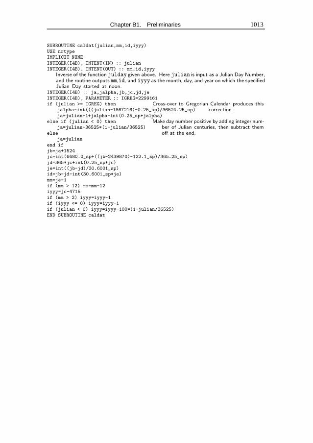
Chapter B1. Preliminaries 1013
SUBROUTINE caldat(julian,mm,id,iyyy)USE nrtypeIMPLICIT NONEINTEGER(I4B), INTENT(IN) :: julianINTEGER(I4B), INTENT(OUT) :: mm,id,iyyy
Inverse of the function julday given above. Here julian is input as a Julian Day Number,and the routine outputs mm,id, and iyyy as the month, day, and year on which the specifiedJulian Day started at noon.
INTEGER(I4B) :: ja,jalpha,jb,jc,jd,jeINTEGER(I4B), PARAMETER :: IGREG=2299161if (julian >= IGREG) then Cross-over to Gregorian Calendar produces this
correction.jalpha=int(((julian-1867216)-0.25_sp)/36524.25_sp)ja=julian+1+jalpha-int(0.25_sp*jalpha)
else if (julian < 0) then Make day number positive by adding integer num-ber of Julian centuries, then subtract themoff at the end.
ja=julian+36525*(1-julian/36525)else
ja=julianend ifjb=ja+1524jc=int(6680.0_sp+((jb-2439870)-122.1_sp)/365.25_sp)jd=365*jc+int(0.25_sp*jc)je=int((jb-jd)/30.6001_sp)id=jb-jd-int(30.6001_sp*je)mm=je-1if (mm > 12) mm=mm-12iyyy=jc-4715if (mm > 2) iyyy=iyyy-1if (iyyy <= 0) iyyy=iyyy-1if (julian < 0) iyyy=iyyy-100*(1-julian/36525)END SUBROUTINE caldat
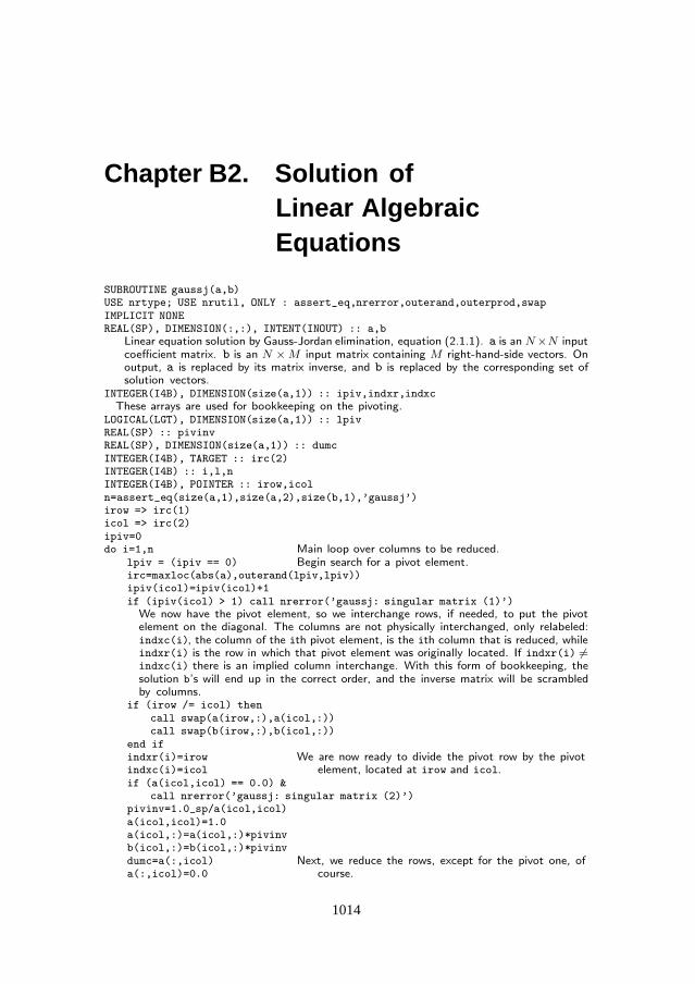
Chapter B2. Solution ofLinear AlgebraicEquations
SUBROUTINE gaussj(a,b)USE nrtype; USE nrutil, ONLY : assert_eq,nrerror,outerand,outerprod,swapIMPLICIT NONEREAL(SP), DIMENSION(:,:), INTENT(INOUT) :: a,b
Linear equation solution by Gauss-Jordan elimination, equation (2.1.1). a is an N×N inputcoefficient matrix. b is an N ×M input matrix containing M right-hand-side vectors. Onoutput, a is replaced by its matrix inverse, and b is replaced by the corresponding set ofsolution vectors.
INTEGER(I4B), DIMENSION(size(a,1)) :: ipiv,indxr,indxcThese arrays are used for bookkeeping on the pivoting.
LOGICAL(LGT), DIMENSION(size(a,1)) :: lpivREAL(SP) :: pivinvREAL(SP), DIMENSION(size(a,1)) :: dumcINTEGER(I4B), TARGET :: irc(2)INTEGER(I4B) :: i,l,nINTEGER(I4B), POINTER :: irow,icoln=assert_eq(size(a,1),size(a,2),size(b,1),’gaussj’)irow => irc(1)icol => irc(2)ipiv=0do i=1,n Main loop over columns to be reduced.
lpiv = (ipiv == 0) Begin search for a pivot element.irc=maxloc(abs(a),outerand(lpiv,lpiv))ipiv(icol)=ipiv(icol)+1if (ipiv(icol) > 1) call nrerror(’gaussj: singular matrix (1)’)
We now have the pivot element, so we interchange rows, if needed, to put the pivotelement on the diagonal. The columns are not physically interchanged, only relabeled:indxc(i), the column of the ith pivot element, is the ith column that is reduced, whileindxr(i) is the row in which that pivot element was originally located. If indxr(i) �=indxc(i) there is an implied column interchange. With this form of bookkeeping, thesolution b’s will end up in the correct order, and the inverse matrix will be scrambledby columns.
if (irow /= icol) thencall swap(a(irow,:),a(icol,:))call swap(b(irow,:),b(icol,:))
end ifindxr(i)=irow We are now ready to divide the pivot row by the pivot
element, located at irow and icol.indxc(i)=icolif (a(icol,icol) == 0.0) &
call nrerror(’gaussj: singular matrix (2)’)pivinv=1.0_sp/a(icol,icol)a(icol,icol)=1.0a(icol,:)=a(icol,:)*pivinvb(icol,:)=b(icol,:)*pivinvdumc=a(:,icol) Next, we reduce the rows, except for the pivot one, of
course.a(:,icol)=0.0
1014
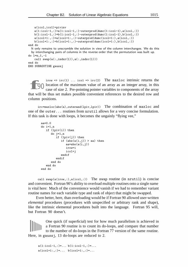
Chapter B2. Solution of Linear Algebraic Equations 1015
a(icol,icol)=pivinva(1:icol-1,:)=a(1:icol-1,:)-outerprod(dumc(1:icol-1),a(icol,:))b(1:icol-1,:)=b(1:icol-1,:)-outerprod(dumc(1:icol-1),b(icol,:))a(icol+1:,:)=a(icol+1:,:)-outerprod(dumc(icol+1:),a(icol,:))b(icol+1:,:)=b(icol+1:,:)-outerprod(dumc(icol+1:),b(icol,:))
end doIt only remains to unscramble the solution in view of the column interchanges. We do thisby interchanging pairs of columns in the reverse order that the permutation was built up.
do l=n,1,-1call swap(a(:,indxr(l)),a(:,indxc(l)))
end doEND SUBROUTINE gaussj
f90irow => irc(1) ... icol => irc(2) The maxloc intrinsic returns thelocation of the maximum value of an array as an integer array, in thiscase of size 2. Pre-pointing pointer variables to components of the array
that will be thus set makes possible convenient references to the desired row andcolumn positions.
irc=maxloc(abs(a),outerand(lpiv,lpiv)) The combination ofmaxloc andone of theouter... routines fromnrutil allows for a very concise formulation.If this task is done with loops, it becomes the ungainly “flying vee,”
aa=0.0do i=1,n
if (lpiv(i)) thendo j=1,n
if (lpiv(j)) thenif (abs(a(i,j)) > aa) then
aa=abs(a(i,j))irow=iicol=j
endifendif
end doend do
end do
call swap(a(irow,:),a(icol,:)) The swap routine (in nrutil) is conciseand convenient. Fortran 90’s ability to overload multiple routines onto a single nameis vital here: Much of the convenience would vanish if we had to remember variantroutine names for each variable type and rank of object that might be swapped.
Even better, here, than overloading would be if Fortran 90 allowed user-writtenelemental procedures (procedures with unspecified or arbitrary rank and shape),like the intrinsic elemental procedures built into the language. Fortran 95 will,but Fortran 90 doesn’t.
One quick (if superficial) test for how much parallelism is achieved ina Fortran 90 routine is to count its do-loops, and compare that numberto the number of do-loops in the Fortran 77 version of the same routine.
Here, ingaussj, 13 do-loops are reduced to 2.
a(1:icol-1,:)=... b(1:icol-1,:)=...
a(icol+1:,:)=... b(icol+1:,:)=...
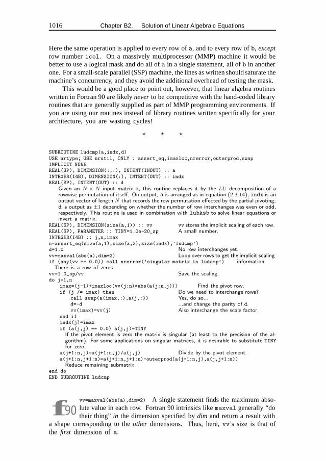
1016 Chapter B2. Solution of Linear Algebraic Equations
Here the same operation is applied to every row ofa, and to every row ofb, exceptrow numbericol. On a massively multiprocessor (MMP) machine it would bebetter to use a logical mask and do all ofa in a single statement, all ofb in anotherone. For a small-scale parallel (SSP) machine, the lines as written should saturate themachine’s concurrency, and they avoid the additional overhead of testing the mask.
This would be a good place to point out, however, that linear algebra routineswritten in Fortran 90 are likelynever to be competitive with the hand-coded libraryroutines that are generally supplied as part of MMP programming environments. Ifyou are using our routines instead of library routines written specifically for yourarchitecture, you are wasting cycles!
� � �
SUBROUTINE ludcmp(a,indx,d)USE nrtype; USE nrutil, ONLY : assert_eq,imaxloc,nrerror,outerprod,swapIMPLICIT NONEREAL(SP), DIMENSION(:,:), INTENT(INOUT) :: aINTEGER(I4B), DIMENSION(:), INTENT(OUT) :: indxREAL(SP), INTENT(OUT) :: d
Given an N × N input matrix a, this routine replaces it by the LU decomposition of arowwise permutation of itself. On output, a is arranged as in equation (2.3.14); indx is anoutput vector of length N that records the row permutation effected by the partial pivoting;d is output as ±1 depending on whether the number of row interchanges was even or odd,respectively. This routine is used in combination with lubksb to solve linear equations orinvert a matrix.
REAL(SP), DIMENSION(size(a,1)) :: vv vv stores the implicit scaling of each row.REAL(SP), PARAMETER :: TINY=1.0e-20_sp A small number.INTEGER(I4B) :: j,n,imaxn=assert_eq(size(a,1),size(a,2),size(indx),’ludcmp’)d=1.0 No row interchanges yet.vv=maxval(abs(a),dim=2) Loop over rows to get the implicit scaling
information.if (any(vv == 0.0)) call nrerror(’singular matrix in ludcmp’)There is a row of zeros.
vv=1.0_sp/vv Save the scaling.do j=1,n
imax=(j-1)+imaxloc(vv(j:n)*abs(a(j:n,j))) Find the pivot row.if (j /= imax) then Do we need to interchange rows?
call swap(a(imax,:),a(j,:)) Yes, do so...d=-d ...and change the parity of d.vv(imax)=vv(j) Also interchange the scale factor.
end ifindx(j)=imaxif (a(j,j) == 0.0) a(j,j)=TINY
If the pivot element is zero the matrix is singular (at least to the precision of the al-gorithm). For some applications on singular matrices, it is desirable to substitute TINYfor zero.
a(j+1:n,j)=a(j+1:n,j)/a(j,j) Divide by the pivot element.a(j+1:n,j+1:n)=a(j+1:n,j+1:n)-outerprod(a(j+1:n,j),a(j,j+1:n))
Reduce remaining submatrix.end doEND SUBROUTINE ludcmp
f90vv=maxval(abs(a),dim=2) A single statement finds the maximum abso-lute value in each row. Fortran 90 intrinsics likemaxval generally “dotheir thing” in the dimension specified bydim and return a result with
a shape corresponding to theother dimensions. Thus, here,vv’s size is that ofthe first dimension ofa.
Chapter B2. Solution of Linear Algebraic Equations 1017
imax=(j-1)+imaxloc(vv(j:n)*abs(a(j:n,j)) Here we see why thenrutilroutine imaxloc is handy: We want the index, in the range1:n of a quantityto be searched for only in the limited rangej:n. Using imaxloc, we just addback the proper offset ofj-1. (Using only Fortran 90 intrinsics, we could writeimax=(j-1)+sum(maxloc(vv(j:n)*abs(a(j:n,j)))), but the use ofsum just to turn anarray of length1 into a scalar seems sufficiently confusing as to be avoided.)
a(j+1:n,j+1:n)=a(j+1:n,j+1:n)-outerprod(a(j+1:n,j),a(j,j+1:n))
The Fortran 77 version ofludcmp, using Crout’s algorithm for thereduction, does not parallelize well: The elements are updated byO(N 2)
separate dot product operations in a particular order. Here we use a slightly differentreduction, termed “outer product Gaussian elimination” by Golub and Van Loan[1],that requires justN steps of matrix-parallel reduction. (See their§3.2.3 and§3.2.9for the algorithm, and their§3.4.1 to understand how the pivoting is performed.)
We usenrutil’s routineouterprod instead of the more cumbersome pureFortran 90 construction:
spread(a(j+1:n,j),dim=2,ncopies=n-j)*spread(a(j,j+1:n),dim=1,ncopies=n-j)
SUBROUTINE lubksb(a,indx,b)USE nrtype; USE nrutil, ONLY : assert_eqIMPLICIT NONEREAL(SP), DIMENSION(:,:), INTENT(IN) :: aINTEGER(I4B), DIMENSION(:), INTENT(IN) :: indxREAL(SP), DIMENSION(:), INTENT(INOUT) :: b
Solves the set of N linear equations A ·X = B. Here the N × N matrix a is input, notas the original matrix A, but rather as its LU decomposition, determined by the routineludcmp. indx is input as the permutation vector of length N returned by ludcmp. b isinput as the right-hand-side vector B, also of length N , and returns with the solution vectorX . a and indx are not modified by this routine and can be left in place for successive callswith different right-hand sides b. This routine takes into account the possibility that b willbegin with many zero elements, so it is efficient for use in matrix inversion.
INTEGER(I4B) :: i,n,ii,llREAL(SP) :: summn=assert_eq(size(a,1),size(a,2),size(indx),’lubksb’)ii=0 When ii is set to a positive value, it will become the in-
dex of the first nonvanishing element of b. We now dothe forward substitution, equation (2.3.6). The only newwrinkle is to unscramble the permutation as we go.
do i=1,nll=indx(i)summ=b(ll)b(ll)=b(i)if (ii /= 0) then
summ=summ-dot_product(a(i,ii:i-1),b(ii:i-1))else if (summ /= 0.0) then
ii=i A nonzero element was encountered, so from now on we willhave to do the dot product above.end if
b(i)=summend dodo i=n,1,-1 Now we do the backsubstitution, equation (2.3.7).
b(i) = (b(i)-dot_product(a(i,i+1:n),b(i+1:n)))/a(i,i)end doEND SUBROUTINE lubksb
Conceptually, the search for the first nonvanishingelement of b (indexii)should be moved out of the first do-loop. However, in practice, the needto unscramble the permutation, and also considerations of performance
1018 Chapter B2. Solution of Linear Algebraic Equations
on scalar machines, cause us to write this very scalar-looking code. The performancepenalty on parallel machines should be minimal.
� � �
Serial and parallel algorithms for tridiagonal problems are quite different.We therefore provide separate routinestridag ser and tridag par. In theMODULE nr interface file, one or the other of these (your choice) is given the genericnametridag. Of course,either version will work correctly on any computer;it is only a question of efficiency. See§22.2 for the numbering of the equationcoefficients, and for a description of the parallel algorithm.
SUBROUTINE tridag_ser(a,b,c,r,u)USE nrtype; USE nrutil, ONLY : assert_eq,nrerrorIMPLICIT NONEREAL(SP), DIMENSION(:), INTENT(IN) :: a,b,c,rREAL(SP), DIMENSION(:), INTENT(OUT) :: u
Solves for a vector u of size N the tridiagonal linear set given by equation (2.4.1) using aserial algorithm. Input vectors b (diagonal elements) and r (right-hand sides) have size N ,while a and c (off-diagonal elements) are size N − 1.
REAL(SP), DIMENSION(size(b)) :: gam One vector of workspace, gam is needed.INTEGER(I4B) :: n,jREAL(SP) :: betn=assert_eq((/size(a)+1,size(b),size(c)+1,size(r),size(u)/),’tridag_ser’)bet=b(1)if (bet == 0.0) call nrerror(’tridag_ser: Error at code stage 1’)
If this happens then you should rewrite your equations as a set of order N − 1, with u2
trivially eliminated.u(1)=r(1)/betdo j=2,n Decomposition and forward substitution.
gam(j)=c(j-1)/betbet=b(j)-a(j-1)*gam(j)if (bet == 0.0) & Algorithm fails; see below routine in Vol. 1.
call nrerror(’tridag_ser: Error at code stage 2’)u(j)=(r(j)-a(j-1)*u(j-1))/bet
end dodo j=n-1,1,-1 Backsubstitution.
u(j)=u(j)-gam(j+1)*u(j+1)end doEND SUBROUTINE tridag_ser
RECURSIVE SUBROUTINE tridag_par(a,b,c,r,u)USE nrtype; USE nrutil, ONLY : assert_eq,nrerrorUSE nr, ONLY : tridag_serIMPLICIT NONEREAL(SP), DIMENSION(:), INTENT(IN) :: a,b,c,rREAL(SP), DIMENSION(:), INTENT(OUT) :: u
Solves for a vector u of size N the tridiagonal linear set given by equation (2.4.1) using aparallel algorithm. Input vectors b (diagonal elements) and r (right-hand sides) have sizeN , while a and c (off-diagonal elements) are size N − 1.
INTEGER(I4B), PARAMETER :: NPAR_TRIDAG=4 Determines when serial algorithm is in-voked.INTEGER(I4B) :: n,n2,nm,nx
REAL(SP), DIMENSION(size(b)/2) :: y,q,pivaREAL(SP), DIMENSION(size(b)/2-1) :: x,zREAL(SP), DIMENSION(size(a)/2) :: pivcn=assert_eq((/size(a)+1,size(b),size(c)+1,size(r),size(u)/),’tridag_par’)if (n < NPAR_TRIDAG) then
call tridag_ser(a,b,c,r,u)else
if (maxval(abs(b(1:n))) == 0.0) & Algorithm fails; see below routine in Vol. 1.
Chapter B2. Solution of Linear Algebraic Equations 1019
call nrerror(’tridag_par: possible singular matrix’)n2=size(y)nm=size(pivc)nx=size(x)piva = a(1:n-1:2)/b(1:n-1:2) Zero the odd a’s and even c’s, giving x,
y, z, q.pivc = c(2:n-1:2)/b(3:n:2)y(1:nm) = b(2:n-1:2)-piva(1:nm)*c(1:n-2:2)-pivc*a(2:n-1:2)q(1:nm) = r(2:n-1:2)-piva(1:nm)*r(1:n-2:2)-pivc*r(3:n:2)if (nm < n2) then
y(n2) = b(n)-piva(n2)*c(n-1)q(n2) = r(n)-piva(n2)*r(n-1)
end ifx = -piva(2:n2)*a(2:n-2:2)z = -pivc(1:nx)*c(3:n-1:2)call tridag_par(x,y,z,q,u(2:n:2)) Recurse and get even u’s.u(1) = (r(1)-c(1)*u(2))/b(1) Substitute and get odd u’s.u(3:n-1:2) = (r(3:n-1:2)-a(2:n-2:2)*u(2:n-2:2) &
-c(3:n-1:2)*u(4:n:2))/b(3:n-1:2)if (nm == n2) u(n)=(r(n)-a(n-1)*u(n-1))/b(n)
end ifEND SUBROUTINE tridag_par
f90The serial versiontridag ser is called when the routine has recursedits way down to sufficiently small subproblems. The point at whichthis occurs is determined by the parameterNPAR TRIDAGwhose optimal
value is likely machine-dependent. Notice thattridag ser must here be calledby its specific name, not by the generictridag (which might itself be overloadedwith either tridag ser or tridag par).
� � �
SUBROUTINE banmul(a,m1,m2,x,b)USE nrtype; USE nrutil, ONLY : assert_eq,arthIMPLICIT NONEREAL(SP), DIMENSION(:,:), INTENT(IN) :: aINTEGER(I4B), INTENT(IN) :: m1,m2REAL(SP), DIMENSION(:), INTENT(IN) :: xREAL(SP), DIMENSION(:), INTENT(OUT) :: b
Matrix multiply b = A · x, where A is band diagonal with m1 rows below the diagonal andm2 rows above. If the input vector x and output vector b are of length N , then the arraya(1:N,1:m1+m2+1) stores A as follows: The diagonal elements are in a(1:N,m1+1).Subdiagonal elements are in a(j:N,1:m1) (with j > 1 appropriate to the number ofelements on each subdiagonal). Superdiagonal elements are in a(1:j,m1+2:m1+m2+1)with j < N appropriate to the number of elements on each superdiagonal.
INTEGER(I4B) :: m,nn=assert_eq(size(a,1),size(b),size(x),’banmul: n’)m=assert_eq(size(a,2),m1+m2+1,’banmul: m’)b=sum(a*eoshift(spread(x,dim=2,ncopies=m), &
dim=1,shift=arth(-m1,1,m)),dim=2)END SUBROUTINE banmul
f90b=sum(a*eoshift(spread(x,dim=2,ncopies=m), &
dim=1,shift=arth(-m1,1,m)),dim=2)
This is a good example of Fortran 90 at both its best and its worst: best,because it allows quite subtle combinations of fully parallel operations to be builtup; worst, because the resulting code is virtually incomprehensible!
1020 Chapter B2. Solution of Linear Algebraic Equations
What is going on becomes clearer if we imagine a temporary arrayy with adeclaration likeREAL(SP), DIMENSION(size(a,1),size(a,2)) :: y. Then, the abovesingle line decomposes intoy=spread(x,dim=2,ncopies=m) [Duplicatex into columns ofy.]y=eoshift(y,dim=1,shift=arth(-m1,1,m)) [Shift columns by a linear progression.]b=sum(a*y,dim=2) [Multiply by the band-diagonal elements,
and sum.]We use here a relatively rare subcase of theeoshift intrinsic, using a vector value fortheshift argument to accomplish the simultaneous shifting of a bunch of columns,by different amounts (here specified by the linear progression returned byarth).
If you still don’t see how this accomplishes the multiplicationof a band diagonalmatrix by a vector, work through a simple example by hand.
SUBROUTINE bandec(a,m1,m2,al,indx,d)USE nrtype; USE nrutil, ONLY : assert_eq,imaxloc,swap,arthIMPLICIT NONEREAL(SP), DIMENSION(:,:), INTENT(INOUT) :: aINTEGER(I4B), INTENT(IN) :: m1,m2REAL(SP), DIMENSION(:,:), INTENT(OUT) :: alINTEGER(I4B), DIMENSION(:), INTENT(OUT) :: indxREAL(SP), INTENT(OUT) :: dREAL(SP), PARAMETER :: TINY=1.0e-20_sp
Given an N × N band diagonal matrix A with m1 subdiagonal rows and m2 superdiagonalrows, compactly stored in the array a(1:N,1:m1+m2+1) as described in the comment forroutine banmul, this routine constructs an LU decomposition of a rowwise permutation ofA. The upper triangular matrix replaces a, while the lower triangular matrix is returned inal(1:N,1:m1). indx is an output vector of length N that records the row permutationeffected by the partial pivoting; d is output as ±1 depending on whether the number ofrow interchanges was even or odd, respectively. This routine is used in combination withbanbks to solve band-diagonal sets of equations.
INTEGER(I4B) :: i,k,l,mdum,mm,nREAL(SP) :: dumn=assert_eq(size(a,1),size(al,1),size(indx),’bandec: n’)mm=assert_eq(size(a,2),m1+m2+1,’bandec: mm’)mdum=assert_eq(size(al,2),m1,’bandec: mdum’)a(1:m1,:)=eoshift(a(1:m1,:),dim=2,shift=arth(m1,-1,m1)) Rearrange the storage a
bit.d=1.0do k=1,n For each row...
l=min(m1+k,n)i=imaxloc(abs(a(k:l,1)))+k-1 Find the pivot element.dum=a(i,1)if (dum == 0.0) a(k,1)=TINY
Matrix is algorithmically singular, but proceed anyway with TINY pivot (desirable in someapplications).
indx(k)=iif (i /= k) then Interchange rows.
d=-dcall swap(a(k,1:mm),a(i,1:mm))
end ifdo i=k+1,l Do the elimination.
dum=a(i,1)/a(k,1)al(k,i-k)=duma(i,1:mm-1)=a(i,2:mm)-dum*a(k,2:mm)a(i,mm)=0.0
end doend doEND SUBROUTINE bandec
Chapter B2. Solution of Linear Algebraic Equations 1021
f90a(1:m1,:)=eoshift(a(1:m1,:),... See similar discussion ofeoshiftfor banmul, just above.
i=imaxloc(abs(a(k:l,1)))+k-1 See discussion ofimaxloc on p. 1017.
Notice that the above isnot well parallelized for MMP machines:the outer do-loop is doneN times, whereN , the diagonal length, ispotentially the largest dimension in the problem. Small-scale parallel
(SSP) machines, and scalar machines, are not disadvantaged, because the parallelismof ordermm=m1+m2+1 in the inner loops can be enough to saturate their concurrency.
We don’t know of anN -parallel algorithm for decomposing band diagonalmatrices, at least one that has any reasonably concise expression in Fortran 90.Conceptually, one can view a band diagonal matrix as ablock tridiagonal matrix,and then apply the same recursive strategy as was used intridag par. However, theimplementation details of this are daunting. (We would welcome a user-contributedroutine, clear, concise, and with parallelism of orderN .)
SUBROUTINE banbks(a,m1,m2,al,indx,b)USE nrtype; USE nrutil, ONLY : assert_eq,swapIMPLICIT NONEREAL(SP), DIMENSION(:,:), INTENT(IN) :: a,alINTEGER(I4B), INTENT(IN) :: m1,m2INTEGER(I4B), DIMENSION(:), INTENT(IN) :: indxREAL(SP), DIMENSION(:), INTENT(INOUT) :: b
Given the arrays a, al, and indx as returned from bandec, and given a right-hand-sidevector b, solves the band diagonal linear equations A·x = b. The solution vector x overwritesb. The other input arrays are not modified, and can be left in place for successive calls withdifferent right-hand sides.
INTEGER(I4B) :: i,k,l,mdum,mm,nn=assert_eq(size(a,1),size(al,1),size(b),size(indx),’banbks: n’)mm=assert_eq(size(a,2),m1+m2+1,’banbks: mm’)mdum=assert_eq(size(al,2),m1,’banbks: mdum’)do k=1,n Forward substitution, unscrambling the permuted rows as we
go.l=min(n,m1+k)i=indx(k)if (i /= k) call swap(b(i),b(k))b(k+1:l)=b(k+1:l)-al(k,1:l-k)*b(k)
end dodo i=n,1,-1 Backsubstitution.
l=min(mm,n-i+1)b(i)=(b(i)-dot_product(a(i,2:l),b(1+i:i+l-1)))/a(i,1)
end doEND SUBROUTINE banbks
As for bandec, the routinebanbks is not parallelized on the largedimensionN , though it does give the compiler the opportunity for amplesmall-scale parallelization inside the loops.
� � �
1022 Chapter B2. Solution of Linear Algebraic Equations
SUBROUTINE mprove(a,alud,indx,b,x)USE nrtype; USE nrutil, ONLY : assert_eqUSE nr, ONLY : lubksbIMPLICIT NONEREAL(SP), DIMENSION(:,:), INTENT(IN) :: a,aludINTEGER(I4B), DIMENSION(:), INTENT(IN) :: indxREAL(SP), DIMENSION(:), INTENT(IN) :: bREAL(SP), DIMENSION(:), INTENT(INOUT) :: x
Improves a solution vector x of the linear set of equations A ·X = B. The N ×N matrix aand the N -dimensional vectors b and x are input. Also input is alud, the LU decompositionof a as returned by ludcmp, and the N -dimensional vector indx also returned by thatroutine. On output, only x is modified, to an improved set of values.
INTEGER(I4B) :: ndumREAL(SP), DIMENSION(size(a,1)) :: rndum=assert_eq((/size(a,1),size(a,2),size(alud,1),size(alud,2),size(b),&
size(x),size(indx)/),’mprove’)r=matmul(real(a,dp),real(x,dp))-real(b,dp)
Calculate the right-hand side, accumulating the residual in double precision.call lubksb(alud,indx,r) Solve for the error term,x=x-r and subtract it from the old solution.END SUBROUTINE mprove
f90assert_eq((/.../),’mprove’) This overloaded version of thenrutilroutineassert eq makes use of a trick for passing a variable numberof scalar arguments to a routine: Put them into an array constructor,
(/.../), and pass the array. The receiving routine can use thesize intrinsic tocount them. The technique has some obvious limitations: All the arguments in thearray must be of the same type; and the arguments are passed, in effect, byvalue,not by address, so they must be, in effect,INTENT(IN).
r=matmul(real(a,dp),real(x,dp))-real(b,dp) Since Fortran 90’s elementalintrinsics operate with the type of their arguments, we can use thereal(...,dp)’sto force thematmul matrix multiplication to be done in double precision, which iswhat we want. In Fortran 77, we would have to do the matrix multiplication withtemporary double precision variables, both inconvenient and (since Fortran 77 hasno dynamic memory allocation) a waste of memory.
� � �
SUBROUTINE svbksb_sp(u,w,v,b,x)USE nrtype; USE nrutil, ONLY : assert_eqREAL(SP), DIMENSION(:,:), INTENT(IN) :: u,vREAL(SP), DIMENSION(:), INTENT(IN) :: w,bREAL(SP), DIMENSION(:), INTENT(OUT) :: x
Solves A · X = B for a vector X , where A is specified by the arrays u, v, w as returnedby svdcmp. Here u is M × N , v is N ×N , and w is of length N . b is the M -dimensionalinput right-hand side. x is the N -dimensional output solution vector. No input quantitiesare destroyed, so the routine may be called sequentially with different b’s.
INTEGER(I4B) :: mdum,ndumREAL(SP), DIMENSION(size(x)) :: tmpmdum=assert_eq(size(u,1),size(b),’svbksb_sp: mdum’)ndum=assert_eq((/size(u,2),size(v,1),size(v,2),size(w),size(x)/),&
’svbksb_sp: ndum’)where (w /= 0.0)
tmp=matmul(b,u)/w Calculate diag(1/wj)UTB,
elsewheretmp=0.0 but replace 1/wj by zero if wj = 0.
end where
Chapter B2. Solution of Linear Algebraic Equations 1023
x=matmul(v,tmp) Matrix multiply by V to get answer.END SUBROUTINE svbksb_sp
f90where (w /= 0.0)...tmp=...elsewhere...tmp= Normally, when awhere...elsewhere construction is used to set a variable (heretmp) to oneor another value, we like to replace it with amerge expression. Here,
however, thewhere is required to guarantee that a division by zero doesn’t occur.The rule is thatwherewill never evaluate expressions that are excluded by the maskin the where line, but other constructions, likemerge, might perform speculativeevaluation of more than one possible outcome before selecting the applicable one.
Because singular value decomposition is something that one often wants to doin double precision, we include a double-precision version. Innr, the single- anddouble-precision versions are overloaded onto the namesvbksb.
SUBROUTINE svbksb_dp(u,w,v,b,x)USE nrtype; USE nrutil, ONLY : assert_eqREAL(DP), DIMENSION(:,:), INTENT(IN) :: u,vREAL(DP), DIMENSION(:), INTENT(IN) :: w,bREAL(DP), DIMENSION(:), INTENT(OUT) :: xINTEGER(I4B) :: mdum,ndumREAL(DP), DIMENSION(size(x)) :: tmpmdum=assert_eq(size(u,1),size(b),’svbksb_dp: mdum’)ndum=assert_eq((/size(u,2),size(v,1),size(v,2),size(w),size(x)/),&
’svbksb_dp: ndum’)where (w /= 0.0)
tmp=matmul(b,u)/welsewhere
tmp=0.0end wherex=matmul(v,tmp)END SUBROUTINE svbksb_dp
SUBROUTINE svdcmp_sp(a,w,v)USE nrtype; USE nrutil, ONLY : assert_eq,nrerror,outerprodUSE nr, ONLY : pythagIMPLICIT NONEREAL(SP), DIMENSION(:,:), INTENT(INOUT) :: aREAL(SP), DIMENSION(:), INTENT(OUT) :: wREAL(SP), DIMENSION(:,:), INTENT(OUT) :: v
Given an M × N matrix a, this routine computes its singular value decomposition, A =U · W · V T . The matrix U replaces a on output. The diagonal matrix of singular valuesW is output as the N -dimensional vector w. The N ×N matrix V (not the transpose V T )is output as v.
INTEGER(I4B) :: i,its,j,k,l,m,n,nmREAL(SP) :: anorm,c,f,g,h,s,scale,x,y,zREAL(SP), DIMENSION(size(a,1)) :: tempmREAL(SP), DIMENSION(size(a,2)) :: rv1,tempnm=size(a,1)n=assert_eq(size(a,2),size(v,1),size(v,2),size(w),’svdcmp_sp’)g=0.0scale=0.0do i=1,n Householder reduction to bidiagonal form.
l=i+1rv1(i)=scale*gg=0.0scale=0.0if (i <= m) then
1024 Chapter B2. Solution of Linear Algebraic Equations
scale=sum(abs(a(i:m,i)))if (scale /= 0.0) then
a(i:m,i)=a(i:m,i)/scales=dot_product(a(i:m,i),a(i:m,i))f=a(i,i)g=-sign(sqrt(s),f)h=f*g-sa(i,i)=f-gtempn(l:n)=matmul(a(i:m,i),a(i:m,l:n))/ha(i:m,l:n)=a(i:m,l:n)+outerprod(a(i:m,i),tempn(l:n))a(i:m,i)=scale*a(i:m,i)
end ifend ifw(i)=scale*gg=0.0scale=0.0if ((i <= m) .and. (i /= n)) then
scale=sum(abs(a(i,l:n)))if (scale /= 0.0) then
a(i,l:n)=a(i,l:n)/scales=dot_product(a(i,l:n),a(i,l:n))f=a(i,l)g=-sign(sqrt(s),f)h=f*g-sa(i,l)=f-grv1(l:n)=a(i,l:n)/htempm(l:m)=matmul(a(l:m,l:n),a(i,l:n))a(l:m,l:n)=a(l:m,l:n)+outerprod(tempm(l:m),rv1(l:n))a(i,l:n)=scale*a(i,l:n)
end ifend if
end doanorm=maxval(abs(w)+abs(rv1))do i=n,1,-1 Accumulation of right-hand transformations.
if (i < n) thenif (g /= 0.0) then
v(l:n,i)=(a(i,l:n)/a(i,l))/g Double division to avoid possible under-flow.tempn(l:n)=matmul(a(i,l:n),v(l:n,l:n))
v(l:n,l:n)=v(l:n,l:n)+outerprod(v(l:n,i),tempn(l:n))end ifv(i,l:n)=0.0v(l:n,i)=0.0
end ifv(i,i)=1.0g=rv1(i)l=i
end dodo i=min(m,n),1,-1 Accumulation of left-hand transformations.
l=i+1g=w(i)a(i,l:n)=0.0if (g /= 0.0) then
g=1.0_sp/gtempn(l:n)=(matmul(a(l:m,i),a(l:m,l:n))/a(i,i))*ga(i:m,l:n)=a(i:m,l:n)+outerprod(a(i:m,i),tempn(l:n))a(i:m,i)=a(i:m,i)*g
elsea(i:m,i)=0.0
end ifa(i,i)=a(i,i)+1.0_sp
end dodo k=n,1,-1 Diagonalization of the bidiagonal form: Loop over
singular values, and over allowed iterations.do its=1,30do l=k,1,-1 Test for splitting.
Chapter B2. Solution of Linear Algebraic Equations 1025
nm=l-1if ((abs(rv1(l))+anorm) == anorm) exit
Note that rv1(1) is always zero, so can never fall through bottom of loop.if ((abs(w(nm))+anorm) == anorm) then
c=0.0 Cancellation of rv1(l), if l > 1.s=1.0do i=l,k
f=s*rv1(i)rv1(i)=c*rv1(i)if ((abs(f)+anorm) == anorm) exitg=w(i)h=pythag(f,g)w(i)=hh=1.0_sp/hc= (g*h)s=-(f*h)tempm(1:m)=a(1:m,nm)a(1:m,nm)=a(1:m,nm)*c+a(1:m,i)*sa(1:m,i)=-tempm(1:m)*s+a(1:m,i)*c
end doexit
end ifend doz=w(k)if (l == k) then Convergence.
if (z < 0.0) then Singular value is made nonnegative.w(k)=-zv(1:n,k)=-v(1:n,k)
end ifexit
end ifif (its == 30) call nrerror(’svdcmp_sp: no convergence in svdcmp’)x=w(l) Shift from bottom 2-by-2 minor.nm=k-1y=w(nm)g=rv1(nm)h=rv1(k)f=((y-z)*(y+z)+(g-h)*(g+h))/(2.0_sp*h*y)g=pythag(f,1.0_sp)f=((x-z)*(x+z)+h*((y/(f+sign(g,f)))-h))/xc=1.0 Next QR transformation:s=1.0do j=l,nm
i=j+1g=rv1(i)y=w(i)h=s*gg=c*gz=pythag(f,h)rv1(j)=zc=f/zs=h/zf= (x*c)+(g*s)g=-(x*s)+(g*c)h=y*sy=y*ctempn(1:n)=v(1:n,j)v(1:n,j)=v(1:n,j)*c+v(1:n,i)*sv(1:n,i)=-tempn(1:n)*s+v(1:n,i)*cz=pythag(f,h)w(j)=z Rotation can be arbitrary if z = 0.if (z /= 0.0) then
z=1.0_sp/zc=f*z
1026 Chapter B2. Solution of Linear Algebraic Equations
s=h*zend iff= (c*g)+(s*y)x=-(s*g)+(c*y)tempm(1:m)=a(1:m,j)a(1:m,j)=a(1:m,j)*c+a(1:m,i)*sa(1:m,i)=-tempm(1:m)*s+a(1:m,i)*c
end dorv1(l)=0.0rv1(k)=fw(k)=x
end doend doEND SUBROUTINE svdcmp_sp
The SVD algorithm implemented above does not parallelize very well.There are two parts to the algorithm. The first, reduction to bidiagonalform, can be parallelized. The second, the iterative diagonalization of
the bidiagonal form, uses QR transformations that are intrinsically serial. Therehave been proposals for parallel SVD algorithms[2], but we do not have sufficientexperience with them yet to recommend them over the well-established serialalgorithm.
tempn(l:n)=matmul...a(i:m,l:n)=...outerprod... Here is an example of anupdate as in equation (22.1.6). In this casebi is independent ofi: It is simply1/h.The lines beginningtempm(l:m)=matmul about 16 lines down are of a similar form,but with the terms in the opposite order in thematmul.
f90As with svbksb, single- and double-precision versions of the routinesare overloaded onto the namesvdcmp in nr.
SUBROUTINE svdcmp_dp(a,w,v)USE nrtype; USE nrutil, ONLY : assert_eq,nrerror,outerprodUSE nr, ONLY : pythagIMPLICIT NONEREAL(DP), DIMENSION(:,:), INTENT(INOUT) :: aREAL(DP), DIMENSION(:), INTENT(OUT) :: wREAL(DP), DIMENSION(:,:), INTENT(OUT) :: vINTEGER(I4B) :: i,its,j,k,l,m,n,nmREAL(DP) :: anorm,c,f,g,h,s,scale,x,y,zREAL(DP), DIMENSION(size(a,1)) :: tempmREAL(DP), DIMENSION(size(a,2)) :: rv1,tempnm=size(a,1)n=assert_eq(size(a,2),size(v,1),size(v,2),size(w),’svdcmp_dp’)g=0.0scale=0.0do i=1,n
l=i+1rv1(i)=scale*gg=0.0scale=0.0if (i <= m) then
scale=sum(abs(a(i:m,i)))if (scale /= 0.0) then
a(i:m,i)=a(i:m,i)/scales=dot_product(a(i:m,i),a(i:m,i))f=a(i,i)g=-sign(sqrt(s),f)
Chapter B2. Solution of Linear Algebraic Equations 1027
h=f*g-sa(i,i)=f-gtempn(l:n)=matmul(a(i:m,i),a(i:m,l:n))/ha(i:m,l:n)=a(i:m,l:n)+outerprod(a(i:m,i),tempn(l:n))a(i:m,i)=scale*a(i:m,i)
end ifend ifw(i)=scale*gg=0.0scale=0.0if ((i <= m) .and. (i /= n)) then
scale=sum(abs(a(i,l:n)))if (scale /= 0.0) then
a(i,l:n)=a(i,l:n)/scales=dot_product(a(i,l:n),a(i,l:n))f=a(i,l)g=-sign(sqrt(s),f)h=f*g-sa(i,l)=f-grv1(l:n)=a(i,l:n)/htempm(l:m)=matmul(a(l:m,l:n),a(i,l:n))a(l:m,l:n)=a(l:m,l:n)+outerprod(tempm(l:m),rv1(l:n))a(i,l:n)=scale*a(i,l:n)
end ifend if
end doanorm=maxval(abs(w)+abs(rv1))do i=n,1,-1
if (i < n) thenif (g /= 0.0) then
v(l:n,i)=(a(i,l:n)/a(i,l))/gtempn(l:n)=matmul(a(i,l:n),v(l:n,l:n))v(l:n,l:n)=v(l:n,l:n)+outerprod(v(l:n,i),tempn(l:n))
end ifv(i,l:n)=0.0v(l:n,i)=0.0
end ifv(i,i)=1.0g=rv1(i)l=i
end dodo i=min(m,n),1,-1
l=i+1g=w(i)a(i,l:n)=0.0if (g /= 0.0) then
g=1.0_dp/gtempn(l:n)=(matmul(a(l:m,i),a(l:m,l:n))/a(i,i))*ga(i:m,l:n)=a(i:m,l:n)+outerprod(a(i:m,i),tempn(l:n))a(i:m,i)=a(i:m,i)*g
elsea(i:m,i)=0.0
end ifa(i,i)=a(i,i)+1.0_dp
end dodo k=n,1,-1
do its=1,30do l=k,1,-1
nm=l-1if ((abs(rv1(l))+anorm) == anorm) exitif ((abs(w(nm))+anorm) == anorm) then
c=0.0s=1.0do i=l,k
1028 Chapter B2. Solution of Linear Algebraic Equations
f=s*rv1(i)rv1(i)=c*rv1(i)if ((abs(f)+anorm) == anorm) exitg=w(i)h=pythag(f,g)w(i)=hh=1.0_dp/hc= (g*h)s=-(f*h)tempm(1:m)=a(1:m,nm)a(1:m,nm)=a(1:m,nm)*c+a(1:m,i)*sa(1:m,i)=-tempm(1:m)*s+a(1:m,i)*c
end doexit
end ifend doz=w(k)if (l == k) then
if (z < 0.0) thenw(k)=-zv(1:n,k)=-v(1:n,k)
end ifexit
end ifif (its == 30) call nrerror(’svdcmp_dp: no convergence in svdcmp’)x=w(l)nm=k-1y=w(nm)g=rv1(nm)h=rv1(k)f=((y-z)*(y+z)+(g-h)*(g+h))/(2.0_dp*h*y)g=pythag(f,1.0_dp)f=((x-z)*(x+z)+h*((y/(f+sign(g,f)))-h))/xc=1.0s=1.0do j=l,nm
i=j+1g=rv1(i)y=w(i)h=s*gg=c*gz=pythag(f,h)rv1(j)=zc=f/zs=h/zf= (x*c)+(g*s)g=-(x*s)+(g*c)h=y*sy=y*ctempn(1:n)=v(1:n,j)v(1:n,j)=v(1:n,j)*c+v(1:n,i)*sv(1:n,i)=-tempn(1:n)*s+v(1:n,i)*cz=pythag(f,h)w(j)=zif (z /= 0.0) then
z=1.0_dp/zc=f*zs=h*z
end iff= (c*g)+(s*y)x=-(s*g)+(c*y)tempm(1:m)=a(1:m,j)a(1:m,j)=a(1:m,j)*c+a(1:m,i)*sa(1:m,i)=-tempm(1:m)*s+a(1:m,i)*c
Chapter B2. Solution of Linear Algebraic Equations 1029
end dorv1(l)=0.0rv1(k)=fw(k)=x
end doend doEND SUBROUTINE svdcmp_dp
FUNCTION pythag_sp(a,b)USE nrtypeIMPLICIT NONEREAL(SP), INTENT(IN) :: a,bREAL(SP) :: pythag_sp
Computes (a2 + b2)1/2 without destructive underflow or overflow.REAL(SP) :: absa,absbabsa=abs(a)absb=abs(b)if (absa > absb) then
pythag_sp=absa*sqrt(1.0_sp+(absb/absa)**2)else
if (absb == 0.0) thenpythag_sp=0.0
elsepythag_sp=absb*sqrt(1.0_sp+(absa/absb)**2)
end ifend ifEND FUNCTION pythag_sp
FUNCTION pythag_dp(a,b)USE nrtypeIMPLICIT NONEREAL(DP), INTENT(IN) :: a,bREAL(DP) :: pythag_dpREAL(DP) :: absa,absbabsa=abs(a)absb=abs(b)if (absa > absb) then
pythag_dp=absa*sqrt(1.0_dp+(absb/absa)**2)else
if (absb == 0.0) thenpythag_dp=0.0
elsepythag_dp=absb*sqrt(1.0_dp+(absa/absb)**2)
end ifend ifEND FUNCTION pythag_dp
� � �
1030 Chapter B2. Solution of Linear Algebraic Equations
SUBROUTINE cyclic(a,b,c,alpha,beta,r,x)USE nrtype; USE nrutil, ONLY : assert,assert_eqUSE nr, ONLY : tridagIMPLICIT NONEREAL(SP), DIMENSION(:), INTENT(IN):: a,b,c,rREAL(SP), INTENT(IN) :: alpha,betaREAL(SP), DIMENSION(:), INTENT(OUT):: x
Solves the “cyclic” set of linear equations given by equation (2.7.9). a, b, c, and r areinput vectors, while x is the output solution vector, all of the same size. alpha and betaare the corner entries in the matrix. The input is not modified.
INTEGER(I4B) :: nREAL(SP) :: fact,gammaREAL(SP), DIMENSION(size(x)) :: bb,u,zn=assert_eq((/size(a),size(b),size(c),size(r),size(x)/),’cyclic’)call assert(n > 2, ’cyclic arg’)gamma=-b(1) Avoid subtraction error in forming bb(1).bb(1)=b(1)-gamma Set up the diagonal of the modified tridiag-
onal system.bb(n)=b(n)-alpha*beta/gammabb(2:n-1)=b(2:n-1)call tridag(a(2:n),bb,c(1:n-1),r,x) Solve A · x = r.u(1)=gamma Set up the vector u.u(n)=alphau(2:n-1)=0.0call tridag(a(2:n),bb,c(1:n-1),u,z) Solve A · z = u.fact=(x(1)+beta*x(n)/gamma)/(1.0_sp+z(1)+beta*z(n)/gamma) Form v·x/(1+v·z).x=x-fact*z Now get the solution vector x.END SUBROUTINE cyclic
The parallelism incyclic is in tridag. Users with multiprocessormachines will want to be sure that, innrutil, they have set the nametridag to be overloaded withtridag par instead oftridag ser.
� � �
The routinessprsin, sprsax, sprstx, sprstp, andsprsdiag give roughlyequivalent functionality to the corresponding Fortran 77 routines, but they arenotplug compatible. Instead, they take advantage of (and illustrate) several Fortran 90features that are not present in Fortran 77.
In the modulenrtypewe define aTYPE sprs2 sp for two-dimensional sparse,square, matrices, in single precision, as follows
TYPE sprs2_spINTEGER(I4B) :: n,lenREAL(SP), DIMENSION(:), POINTER :: valINTEGER(I4B), DIMENSION(:), POINTER :: irowINTEGER(I4B), DIMENSION(:), POINTER :: jcol
END TYPE sprs2_sp
This has much less structure to it than the “row-indexed sparse storage mode” usedin Volume 1. Here, a sparse matrix is just a list of values, and corresponding listsgiving the row and column number that each value is in. Two integersn andlengive, respectively, the underlying size (number of rows or columns) in the full matrix,and the number of stored nonzero values. While the previously used row-indexedscheme can be somewhat more efficient for serial machines, it does not parallelizeconveniently, while this one does (though with some caveats; see below).
Chapter B2. Solution of Linear Algebraic Equations 1031
SUBROUTINE sprsin_sp(a,thresh,sa)USE nrtype; USE nrutil, ONLY : arth,assert_eqIMPLICIT NONEREAL(SP), DIMENSION(:,:), INTENT(IN) :: aREAL(SP), INTENT(IN) :: threshTYPE(sprs2_sp), INTENT(OUT) :: sa
Converts a square matrix a to sparse storage format as sa. Only elements of a with mag-nitude ≥ thresh are retained.
INTEGER(I4B) :: n,lenLOGICAL(LGT), DIMENSION(size(a,1),size(a,2)) :: maskn=assert_eq(size(a,1),size(a,2),’sprsin_sp’)mask=abs(a)>threshlen=count(mask) How many elements to store?allocate(sa%val(len),sa%irow(len),sa%jcol(len))sa%n=nsa%len=lensa%val=pack(a,mask) Grab the values, row, and column numbers.sa%irow=pack(spread(arth(1,1,n),2,n),mask)sa%jcol=pack(spread(arth(1,1,n),1,n),mask)END SUBROUTINE sprsin_sp
SUBROUTINE sprsin_dp(a,thresh,sa)USE nrtype; USE nrutil, ONLY : arth,assert_eqIMPLICIT NONEREAL(DP), DIMENSION(:,:), INTENT(IN) :: aREAL(DP), INTENT(IN) :: threshTYPE(sprs2_dp), INTENT(OUT) :: saINTEGER(I4B) :: n,lenLOGICAL(LGT), DIMENSION(size(a,1),size(a,2)) :: maskn=assert_eq(size(a,1),size(a,2),’sprsin_dp’)mask=abs(a)>threshlen=count(mask)allocate(sa%val(len),sa%irow(len),sa%jcol(len))sa%n=nsa%len=lensa%val=pack(a,mask)sa%irow=pack(spread(arth(1,1,n),2,n),mask)sa%jcol=pack(spread(arth(1,1,n),1,n),mask)END SUBROUTINE sprsin_dp
f90Note that the routinessprsin sp andsprsin dp — single and doubleprecision versions of the same algorithm — are overloaded onto thenamesprsin in modulenr. We supply both forms because the routine
linbcg, below, works in double precision.
sa%irow=pack(spread(arth(1,1,n),2,n),mask) The trick here is to use the samemask,abs(a)>thresh, in three consecutivepack expressions, thus guaranteeingthat the corresponding elements of the array argument get selected for packing.The first time, we get the desired matrix element values. The second time (abovecode fragment), we construct a matrix with each element having the value of itsrow number. The third time, we construct a matrix with each element having thevalue of its column number.
1032 Chapter B2. Solution of Linear Algebraic Equations
SUBROUTINE sprsax_sp(sa,x,b)USE nrtype; USE nrutil, ONLY : assert_eq,scatter_addIMPLICIT NONETYPE(sprs2_sp), INTENT(IN) :: saREAL(SP), DIMENSION (:), INTENT(IN) :: xREAL(SP), DIMENSION (:), INTENT(OUT) :: b
Multiply a matrix sa in sparse matrix format by a vector x, giving a vector b.INTEGER(I4B) :: ndumndum=assert_eq(sa%n,size(x),size(b),’sprsax_sp’)b=0.0_spcall scatter_add(b,sa%val*x(sa%jcol),sa%irow)
Each sparse matrix entry adds a term to some component of b.END SUBROUTINE sprsax_sp
SUBROUTINE sprsax_dp(sa,x,b)USE nrtype; USE nrutil, ONLY : assert_eq,scatter_addIMPLICIT NONETYPE(sprs2_dp), INTENT(IN) :: saREAL(DP), DIMENSION (:), INTENT(IN) :: xREAL(DP), DIMENSION (:), INTENT(OUT) :: bINTEGER(I4B) :: ndumndum=assert_eq(sa%n,size(x),size(b),’sprsax_dp’)b=0.0_dpcall scatter_add(b,sa%val*x(sa%jcol),sa%irow)END SUBROUTINE sprsax_dp
call scatter_add(b,sa%val*x(sa%jcol),sa%irow) Since more than onecomponent of the middle vector argument will, in general, need to beadded into the same component ofb, we must resort to a call to the
nrutil routine scatter add to achieve parallelism.However, this parallelismis achieved only if a parallel version ofscatter add is available! As we havediscussed previously (p. 984), Fortran 90 does not provide any scatter-with-combine(here, scatter-with-add) facility, insisting instead that indexed operations yield non-colliding addresses. Luckily, almost all parallel machines do provide such a facilityas a library program. In HPF, for example, the equivalent ofscatter add isSUM SCATTER.
The call toscatter add above is equivalent to the do-loop
b=0.0do k=1,sa%len
b(sa%irow(k))=b(sa%irow(k))+sa%val(k)*x(sa%jcol(k))end do
SUBROUTINE sprstx_sp(sa,x,b)USE nrtype; USE nrutil, ONLY : assert_eq,scatter_addIMPLICIT NONETYPE(sprs2_sp), INTENT(IN) :: saREAL(SP), DIMENSION (:), INTENT(IN) :: xREAL(SP), DIMENSION (:), INTENT(OUT) :: b
Multiply the transpose of a matrix sa in sparse matrix format by a vector x, giving a vector b.INTEGER(I4B) :: ndumndum=assert_eq(sa%n,size(x),size(b),’sprstx_sp’)b=0.0_spcall scatter_add(b,sa%val*x(sa%irow),sa%jcol)
Each sparse matrix entry adds a term to some component of b.END SUBROUTINE sprstx_sp
Chapter B2. Solution of Linear Algebraic Equations 1033
SUBROUTINE sprstx_dp(sa,x,b)USE nrtype; USE nrutil, ONLY : assert_eq,scatter_addIMPLICIT NONETYPE(sprs2_dp), INTENT(IN) :: saREAL(DP), DIMENSION (:), INTENT(IN) :: xREAL(DP), DIMENSION (:), INTENT(OUT) :: bINTEGER(I4B) :: ndumndum=assert_eq(sa%n,size(x),size(b),’sprstx_dp’)b=0.0_dpcall scatter_add(b,sa%val*x(sa%irow),sa%jcol)END SUBROUTINE sprstx_dp
Precisely the same comments as forsprsax apply tosprstx. The callto scatter add is here equivalent to
b=0.0do k=1,sa%len
b(sa%jcol(k))=b(sa%jcol(k))+sa%val(k)*x(sa%irow(k))end do
SUBROUTINE sprstp(sa)USE nrtypeIMPLICIT NONETYPE(sprs2_sp), INTENT(INOUT) :: sa
Replaces sa, in sparse matrix format, by its transpose.INTEGER(I4B), DIMENSION(:), POINTER :: temptemp=>sa%irow We need only swap the row and column pointers.sa%irow=>sa%jcolsa%jcol=>tempEND SUBROUTINE sprstp
SUBROUTINE sprsdiag_sp(sa,b)USE nrtype; USE nrutil, ONLY : array_copy,assert_eqIMPLICIT NONETYPE(sprs2_sp), INTENT(IN) :: saREAL(SP), DIMENSION(:), INTENT(OUT) :: b
Extracts the diagonal of a matrix sa in sparse matrix format into a vector b.REAL(SP), DIMENSION(size(b)) :: valINTEGER(I4B) :: k,l,ndum,nerrINTEGER(I4B), DIMENSION(size(b)) :: iLOGICAL(LGT), DIMENSION(:), ALLOCATABLE :: maskndum=assert_eq(sa%n,size(b),’sprsdiag_sp’)l=sa%lenallocate(mask(l))mask = (sa%irow(1:l) == sa%jcol(1:l)) Find diagonal elements.call array_copy(pack(sa%val(1:l),mask),val,k,nerr) Grab the values...i(1:k)=pack(sa%irow(1:l),mask) ...and their locations.deallocate(mask)b=0.0 Zero b because zero values not stored in sa.b(i(1:k))=val(1:k) Scatter values into correct slots.END SUBROUTINE sprsdiag_sp
1034 Chapter B2. Solution of Linear Algebraic Equations
SUBROUTINE sprsdiag_dp(sa,b)USE nrtype; USE nrutil, ONLY : array_copy,assert_eqIMPLICIT NONETYPE(sprs2_dp), INTENT(IN) :: saREAL(DP), DIMENSION(:), INTENT(OUT) :: bREAL(DP), DIMENSION(size(b)) :: valINTEGER(I4B) :: k,l,ndum,nerrINTEGER(I4B), DIMENSION(size(b)) :: iLOGICAL(LGT), DIMENSION(:), ALLOCATABLE :: maskndum=assert_eq(sa%n,size(b),’sprsdiag_dp’)l=sa%lenallocate(mask(l))mask = (sa%irow(1:l) == sa%jcol(1:l))call array_copy(pack(sa%val(1:l),mask),val,k,nerr)i(1:k)=pack(sa%irow(1:l),mask)deallocate(mask)b=0.0b(i(1:k))=val(1:k)END SUBROUTINE sprsdiag_dp
f90call array_copy(pack(sa%val(1:l),mask),val,k,nerr) We use thenrutil routinearray copy because we don’t know in advance howmany nonzero diagonal elements will be selected bymask. Of course
we could count them with acount(mask), but this is an extra step, and inefficienton scalar machines.
i(1:k)=pack(sa%irow(1:l),mask) Using the same mask, we pick out the cor-responding locations of the diagonal elements. No need to usearray copy now,since we know the value ofk.
b(i(1:k))=val(1:k) Finally, we can put each element in the right place.Notice that if the sparse matrix is ill-formed, with more than one value stored for thesame diagonal element (which should not happen!) then the vector subscripti(1:k)
is a “many-one section” and its use on the left-hand side is illegal.
� � �
SUBROUTINE linbcg(b,x,itol,tol,itmax,iter,err)USE nrtype; USE nrutil, ONLY : assert_eq,nrerrorUSE nr, ONLY : atimes,asolve,snrmIMPLICIT NONEREAL(DP), DIMENSION(:), INTENT(IN) :: b Double precision is a good idea in this
routine.REAL(DP), DIMENSION(:), INTENT(INOUT) :: xINTEGER(I4B), INTENT(IN) :: itol,itmaxREAL(DP), INTENT(IN) :: tolINTEGER(I4B), INTENT(OUT) :: iterREAL(DP), INTENT(OUT) :: errREAL(DP), PARAMETER :: EPS=1.0e-14_dp
Solves A · x = b for x, given b of the same length, by the iterative biconjugate gradientmethod. On input x should be set to an initial guess of the solution (or all zeros); itol is1,2,3, or 4, specifying which convergence test is applied (see text); itmax is the maximumnumber of allowed iterations; and tol is the desired convergence tolerance. On output, xis reset to the improved solution, iter is the number of iterations actually taken, and erris the estimated error. The matrix A is referenced only through the user-supplied routinesatimes, which computes the product of either A or its transpose on a vector; and asolve,
Chapter B2. Solution of Linear Algebraic Equations 1035
which solves A · x = b or AT · x = b for some preconditioner matrix A (possibly the trivial
diagonal part of A).INTEGER(I4B) :: nREAL(DP) :: ak,akden,bk,bkden,bknum,bnrm,dxnrm,xnrm,zm1nrm,znrmREAL(DP), DIMENSION(size(b)) :: p,pp,r,rr,z,zzn=assert_eq(size(b),size(x),’linbcg’)iter=0call atimes(x,r,0) Calculate initial residual. Input to atimes is
x(1:n), output is r(1:n); the final 0indicates that the matrix (not its trans-pose) is to be used.
r=b-rrr=r
! call atimes(r,rr,0)Uncomment this line to get the “minimum residual” variant of the algorithm.
select case(itol) Calculate norms for use in stopping criterion,and initialize z.case(1)
bnrm=snrm(b,itol)call asolve(r,z,0) Input to asolve is r(1:n), output is z(1:n);
the final 0 indicates that the matrix A(not its transpose) is to be used.
case(2)call asolve(b,z,0)bnrm=snrm(z,itol)call asolve(r,z,0)
case(3:4)call asolve(b,z,0)bnrm=snrm(z,itol)call asolve(r,z,0)znrm=snrm(z,itol)
case defaultcall nrerror(’illegal itol in linbcg’)
end selectdo Main loop.
if (iter > itmax) exititer=iter+1
call asolve(rr,zz,1) Final 1 indicates use of transpose matrix AT.
bknum=dot_product(z,rr) Calculate coefficient bk and direction vectorsp and pp.if (iter == 1) then
p=zpp=zz
elsebk=bknum/bkdenp=bk*p+zpp=bk*pp+zz
end ifbkden=bknum Calculate coefficient ak, new iterate x, and
new residuals r and rr.call atimes(p,z,0)akden=dot_product(z,pp)ak=bknum/akdencall atimes(pp,zz,1)x=x+ak*pr=r-ak*zrr=rr-ak*zzcall asolve(r,z,0) Solve A ·z = r and check stopping criterion.select case(itol)
case(1)err=snrm(r,itol)/bnrm
case(2)err=snrm(z,itol)/bnrm
case(3:4)zm1nrm=znrmznrm=snrm(z,itol)if (abs(zm1nrm-znrm) > EPS*znrm) then
dxnrm=abs(ak)*snrm(p,itol)err=znrm/abs(zm1nrm-znrm)*dxnrm
elseerr=znrm/bnrm Error may not be accurate, so loop again.cycle
1036 Chapter B2. Solution of Linear Algebraic Equations
end ifxnrm=snrm(x,itol)if (err <= 0.5_dp*xnrm) then
err=err/xnrmelse
err=znrm/bnrm Error may not be accurate, so loop again.cycle
end ifend selectwrite (*,*) ’ iter=’,iter,’ err=’,errif (err <= tol) exit
end doEND SUBROUTINE linbcg
f90case default...call nrerror(’illegal itol in linbcg’) It’s always agood idea to trap errors when the value of a case construction is suppliedexternally to the routine, as here.
FUNCTION snrm(sx,itol)USE nrtypeIMPLICIT NONEREAL(DP), DIMENSION(:), INTENT(IN) :: sxINTEGER(I4B), INTENT(IN) :: itolREAL(DP) :: snrm
Compute one of two norms for a vector sx, as signaled by itol. Used by linbcg.if (itol <= 3) then
snrm=sqrt(dot_product(sx,sx)) Vector magnitude norm.else
snrm=maxval(abs(sx)) Largest component norm.end ifEND FUNCTION snrm
SUBROUTINE atimes(x,r,itrnsp)USE nrtype; USE nrutil, ONLY : assert_eqUSE nr, ONLY : sprsax,sprstx DOUBLE PRECISION versions of sprsax and sprstx.USE xlinbcg_data The matrix is accessed through this module.REAL(DP), DIMENSION(:), INTENT(IN) :: xREAL(DP), DIMENSION(:), INTENT(OUT) :: rINTEGER(I4B), INTENT(IN) :: itrnspINTEGER(I4B) :: nn=assert_eq(size(x),size(r),’atimes’)if (itrnsp == 0) then
call sprsax(sa,x,r)else
call sprstx(sa,x,r)end ifEND SUBROUTINE atimes
Chapter B2. Solution of Linear Algebraic Equations 1037
SUBROUTINE asolve(b,x,itrnsp)USE nrtype; USE nrutil, ONLY : assert_eq,nrerrorUSE nr, ONLY : sprsdiag DOUBLE PRECISION version of sprsdiag.USE xlinbcg_data The matrix is accessed through this module.REAL(DP), DIMENSION(:), INTENT(IN) :: bREAL(DP), DIMENSION(:), INTENT(OUT) :: xINTEGER(I4B), INTENT(IN) :: itrnspINTEGER(I4B) :: ndumndum=assert_eq(size(b),size(x),’asolve’)call sprsdiag(sa,x)
The matrix A is taken to be the diagonal part of A. Since the transpose matrix has the samediagonal, the flag itrnsp is not used.
if (any(x == 0.0)) call nrerror(’asolve: singular diagonal matrix’)x=b/xEND SUBROUTINE asolve
f90The routinesatimes andasolve are examples of user-supplied routinesthat interfacelinbcg to a user-supplied method for multiplying theuser’s sparse matrix by a vector, and for solving the preconditioner matrix
equation. Here, we have used these routines to connectlinbcg to the sparse matrixmachinery developed above. If we were instead using the different sparse matrixmachinery of Volume 1, we would modifyatimes andasolve accordingly.
USE xlinbcg_data This user-supplied module is assumed to havesa (thesparse matrix) in it.
� � �
FUNCTION vander(x,q)USE nrtype; USE nrutil, ONLY : assert_eq,outerdiffIMPLICIT NONEREAL(DP), DIMENSION(:), INTENT(IN) :: x,qREAL(DP), DIMENSION(size(x)) :: vander
Solves the Vandermonde linear system∑N
i=1 xk−1i wi = qk (k = 1, . . . ,N). Input consists
of the vectors x and q of length N . The solution w (also of lengthN) is returned in vander.REAL(DP), DIMENSION(size(x)) :: cREAL(DP), DIMENSION(size(x),size(x)) :: aINTEGER(I4B) :: i,nn=assert_eq(size(x),size(q),’vander’)if (n == 1) then
vander(1)=q(1)else
c(:)=0.0 Initialize array.c(n)=-x(1) Coefficients of the master polynomial are found
by recursion.do i=2,nc(n+1-i:n-1)=c(n+1-i:n-1)-x(i)*c(n+2-i:n)c(n)=c(n)-x(i)
end doa(:,:)=outerdiff(x,x) Make vector wj =
∏n�=j(xj − xn).
vander(:)=product(a,dim=2,mask=(a /= 0.0))Now do synthetic division by x− xj . The division for all xj can be done in parallel (ona parallel machine), since the : in the loop below is over j.
a(:,1)=-c(1)/x(:)do i=2,n
a(:,i)=-(c(i)-a(:,i-1))/x(:)end dovander(:)=matmul(a,q)/vander(:) Solve linear system and supply denomina-
tor.end ifEND FUNCTION vander
1038 Chapter B2. Solution of Linear Algebraic Equations
f90a=outerdiff...w=product... Here is an example of the coding of equa-tion (22.1.4). Since in this case the product is over the second index (nin xj − xn), we havedim=2 in the product.
FUNCTION toeplz(r,y)USE nrtype; USE nrutil, ONLY : assert_eq,nrerrorIMPLICIT NONEREAL(SP), DIMENSION(:), INTENT(IN) :: r,yREAL(SP), DIMENSION(size(y)) :: toeplz
Solves the Toeplitz system∑N
j=1 R(N+i−j)xj = yi (i = 1, . . . , N). The Toeplitz matrix
need not be symmetric. y (of length N) and r (of length 2N − 1) are input arrays; thesolution x (of length N) is returned in toeplz.
INTEGER(I4B) :: m,m1,n,ndumREAL(SP) :: sd,sgd,sgn,shn,sxnREAL(SP), DIMENSION(size(y)) :: g,h,tn=size(y)ndum=assert_eq(2*n-1,size(r),’toeplz: ndum’)if (r(n) == 0.0) call nrerror(’toeplz: initial singular minor’)toeplz(1)=y(1)/r(n) Initialize for the recursion.if (n == 1) RETURNg(1)=r(n-1)/r(n)h(1)=r(n+1)/r(n)do m=1,n Main loop over the recursion.
m1=m+1sxn=-y(m1)+dot_product(r(n+1:n+m),toeplz(m:1:-1))
Compute numerator and denominator for x,sd=-r(n)+dot_product(r(n+1:n+m),g(1:m))if (sd == 0.0) exittoeplz(m1)=sxn/sd whence x.toeplz(1:m)=toeplz(1:m)-toeplz(m1)*g(m:1:-1)if (m1 == n) RETURNsgn=-r(n-m1)+dot_product(r(n-m:n-1),g(1:m)) Compute numerator and denom-
inator for G and H ,shn=-r(n+m1)+dot_product(r(n+m:n+1:-1),h(1:m))sgd=-r(n)+dot_product(r(n-m:n-1),h(m:1:-1))if (sd == 0.0 .or. sgd == 0.0) exitg(m1)=sgn/sgd whence G and H .h(m1)=shn/sdt(1:m)=g(1:m)g(1:m)=g(1:m)-g(m1)*h(m:1:-1)h(1:m)=h(1:m)-h(m1)*t(m:1:-1)
end do Back for another recurrence.if (m > n) call nrerror(’toeplz: sanity check failed in routine’)call nrerror(’toeplz: singular principal minor’)END FUNCTION toeplz
� � �
SUBROUTINE choldc(a,p)USE nrtype; USE nrutil, ONLY : assert_eq,nrerrorIMPLICIT NONEREAL(SP), DIMENSION(:,:), INTENT(INOUT) :: aREAL(SP), DIMENSION(:), INTENT(OUT) :: p
Given an N × N positive-definite symmetric matrix a, this routine constructs its Choleskydecomposition, A = L · LT . On input, only the upper triangle of a need be given; it isnot modified. The Cholesky factor L is returned in the lower triangle of a, except for itsdiagonal elements, which are returned in p, a vector of length N .
INTEGER(I4B) :: i,nREAL(SP) :: summn=assert_eq(size(a,1),size(a,2),size(p),’choldc’)do i=1,n
Chapter B2. Solution of Linear Algebraic Equations 1039
summ=a(i,i)-dot_product(a(i,1:i-1),a(i,1:i-1))if (summ <= 0.0) call nrerror(’choldc failed’) a, with rounding errors, is
not positive definite.p(i)=sqrt(summ)a(i+1:n,i)=(a(i,i+1:n)-matmul(a(i+1:n,1:i-1),a(i,1:i-1)))/p(i)
end doEND SUBROUTINE choldc
SUBROUTINE cholsl(a,p,b,x)USE nrtype; USE nrutil, ONLY : assert_eqIMPLICIT NONEREAL(SP), DIMENSION(:,:), INTENT(IN) :: aREAL(SP), DIMENSION(:), INTENT(IN) :: p,bREAL(SP), DIMENSION(:), INTENT(INOUT) :: x
Solves the set of N linear equations A · x = b, where a is a positive-definite symmetricmatrix. a (N × N) and p (of length N) are input as the output of the routine choldc.Only the lower triangle of a is accessed. b is the input right-hand-side vector, of length N .The solution vector, also of length N , is returned in x. a and p are not modified and can beleft in place for successive calls with different right-hand sides b. b is not modified unlessyou identify b and x in the calling sequence, which is allowed.
INTEGER(I4B) :: i,nn=assert_eq((/size(a,1),size(a,2),size(p),size(b),size(x)/),’cholsl’)do i=1,n Solve L · y = b, storing y in x.
x(i)=(b(i)-dot_product(a(i,1:i-1),x(1:i-1)))/p(i)end dodo i=n,1,-1 Solve LT · x = y.
x(i)=(x(i)-dot_product(a(i+1:n,i),x(i+1:n)))/p(i)end doEND SUBROUTINE cholsl
� � �
SUBROUTINE qrdcmp(a,c,d,sing)USE nrtype; USE nrutil, ONLY : assert_eq,outerprod,vabsIMPLICIT NONEREAL(SP), DIMENSION(:,:), INTENT(INOUT) :: aREAL(SP), DIMENSION(:), INTENT(OUT) :: c,dLOGICAL(LGT), INTENT(OUT) :: sing
Constructs the QR decomposition of the n× n matrix a. The upper triangular matrix R isreturned in the upper triangle of a, except for the diagonal elements of R, which are returnedin the n-dimensional vector d. The orthogonal matrix Q is represented as a product of n−1Householder matrices Q1 . . .Qn−1, where Qj = 1− uj ⊗ uj/cj . The ith component of uj
is zero for i = 1, . . . , j − 1 while the nonzero components are returned in a(i,j) fori = j, . . . , n. sing returns as true if singularity is encountered during the decomposition,but the decomposition is still completed in this case.
INTEGER(I4B) :: k,nREAL(SP) :: scale,sigman=assert_eq(size(a,1),size(a,2),size(c),size(d),’qrdcmp’)sing=.false.do k=1,n-1
scale=maxval(abs(a(k:n,k)))if (scale == 0.0) then Singular case.
sing=.true.c(k)=0.0d(k)=0.0
else Form Qk and Qk · A.a(k:n,k)=a(k:n,k)/scalesigma=sign(vabs(a(k:n,k)),a(k,k))a(k,k)=a(k,k)+sigmac(k)=sigma*a(k,k)
1040 Chapter B2. Solution of Linear Algebraic Equations
d(k)=-scale*sigmaa(k:n,k+1:n)=a(k:n,k+1:n)-outerprod(a(k:n,k),&
matmul(a(k:n,k),a(k:n,k+1:n)))/c(k)end if
end dod(n)=a(n,n)if (d(n) == 0.0) sing=.true.END SUBROUTINE qrdcmp
f90a(k:n,k+1:n)=a(k:n,k+1:n)-outerprod...matmul... See discussion of equa-tion (22.1.6).
SUBROUTINE qrsolv(a,c,d,b)USE nrtype; USE nrutil, ONLY : assert_eqUSE nr, ONLY : rsolvIMPLICIT NONEREAL(SP), DIMENSION(:,:), INTENT(IN) :: aREAL(SP), DIMENSION(:), INTENT(IN) :: c,dREAL(SP), DIMENSION(:), INTENT(INOUT) :: b
Solves the set of n linear equations A · x = b. The n × n matrix a and the n-dimensionalvectors c and d are input as the output of the routine qrdcmp and are not modified. b isinput as the right-hand-side vector of length n, and is overwritten with the solution vectoron output.
INTEGER(I4B) :: j,nREAL(SP) :: taun=assert_eq((/size(a,1),size(a,2),size(b),size(c),size(d)/),’qrsolv’)
do j=1,n-1 Form QT · b.tau=dot_product(a(j:n,j),b(j:n))/c(j)b(j:n)=b(j:n)-tau*a(j:n,j)
end docall rsolv(a,d,b) Solve R · x = QT · b.END SUBROUTINE qrsolv
SUBROUTINE rsolv(a,d,b)USE nrtype; USE nrutil, ONLY : assert_eqIMPLICIT NONEREAL(SP), DIMENSION(:,:), INTENT(IN) :: aREAL(SP), DIMENSION(:), INTENT(IN) :: dREAL(SP), DIMENSION(:), INTENT(INOUT) :: b
Solves the set of n linear equations R · x = b, where R is an upper triangular matrix storedin a and d. The n×n matrix a and the vector d of length n are input as the output of theroutine qrdcmp and are not modified. b is input as the right-hand-side vector of length n,and is overwritten with the solution vector on output.
INTEGER(I4B) :: i,nn=assert_eq(size(a,1),size(a,2),size(b),size(d),’rsolv’)b(n)=b(n)/d(n)do i=n-1,1,-1
b(i)=(b(i)-dot_product(a(i,i+1:n),b(i+1:n)))/d(i)end doEND SUBROUTINE rsolv
� � �
Chapter B2. Solution of Linear Algebraic Equations 1041
SUBROUTINE qrupdt(r,qt,u,v)USE nrtype; USE nrutil, ONLY : assert_eq,ifirstlocUSE nr, ONLY : rotate,pythagIMPLICIT NONEREAL(SP), DIMENSION(:,:), INTENT(INOUT) :: r,qtREAL(SP), DIMENSION(:), INTENT(INOUT) :: uREAL(SP), DIMENSION(:), INTENT(IN) :: v
Given the QR decomposition of some n × n matrix, calculates the QR decomposition ofthe matrix Q · (R + u ⊗ v). Here r and qt are n × n matrices, u and v are n-dimensional
vectors. Note that QT is input and returned in qt.INTEGER(I4B) :: i,k,nn=assert_eq((/size(r,1),size(r,2),size(qt,1),size(qt,2),size(u),&
size(v)/),’qrupdt’)k=n+1-ifirstloc(u(n:1:-1) /= 0.0) Find largest k such that u(k) �= 0.if (k < 1) k=1do i=k-1,1,-1 Transform R + u ⊗ v to upper Hessenberg.
call rotate(r,qt,i,u(i),-u(i+1))u(i)=pythag(u(i),u(i+1))
end dor(1,:)=r(1,:)+u(1)*vdo i=1,k-1 Transform upper Hessenberg matrix to upper
triangular.call rotate(r,qt,i,r(i,i),-r(i+1,i))end doEND SUBROUTINE qrupdt
f90k=n+1-ifirstloc(u(n:1:-1) /= 0.0) The function ifirstloc innrutil returns the first occurrence of.true. in a logical vector.See the discussion of the analogous routineimaxloc on p. 1017.
SUBROUTINE rotate(r,qt,i,a,b)USE nrtype; USE nrutil, ONLY : assert_eqIMPLICIT NONEREAL(SP), DIMENSION(:,:), TARGET, INTENT(INOUT) :: r,qtINTEGER(I4B), INTENT(IN) :: iREAL(SP), INTENT(IN) :: a,b
Given n×n matrices r and qt, carry out a Jacobi rotation on rows i and i+1 of each matrix.
a and b are the parameters of the rotation: cos θ = a/√a2 + b2, sin θ = b/
√a2 + b2.
REAL(SP), DIMENSION(size(r,1)) :: tempINTEGER(I4B) :: nREAL(SP) :: c,fact,sn=assert_eq(size(r,1),size(r,2),size(qt,1),size(qt,2),’rotate’)if (a == 0.0) then Avoid unnecessary overflow or underflow.
c=0.0s=sign(1.0_sp,b)
else if (abs(a) > abs(b)) thenfact=b/ac=sign(1.0_sp/sqrt(1.0_sp+fact**2),a)s=fact*c
elsefact=a/bs=sign(1.0_sp/sqrt(1.0_sp+fact**2),b)c=fact*s
end iftemp(i:n)=r(i,i:n) Premultiply r by Jacobi rotation.r(i,i:n)=c*temp(i:n)-s*r(i+1,i:n)r(i+1,i:n)=s*temp(i:n)+c*r(i+1,i:n)temp=qt(i,:) Premultiply qt by Jacobi rotation.qt(i,:)=c*temp-s*qt(i+1,:)qt(i+1,:)=s*temp+c*qt(i+1,:)END SUBROUTINE rotate

1042 Chapter B2. Solution of Linear Algebraic Equations
CITED REFERENCES AND FURTHER READING:
Golub, G.H., and Van Loan, C.F. 1989, Matrix Computations, 2nd ed. (Baltimore: Johns HopkinsUniversity Press). [1]
Gu, M., Demmel, J., and Dhillon, I. 1994, LAPACK Working Note #88 (Computer Science De-partment, University of Tennessee at Knoxville, Preprint UT-CS-94-257; available fromNetlib, or as http://www.cs.utk.edu/∼library/TechReports/1994/ut-cs-94-257.ps.Z). [2] Seealso discussion after tqli in Chapter B11.
Chapter B3. Interpolation andExtrapolation
SUBROUTINE polint(xa,ya,x,y,dy)USE nrtype; USE nrutil, ONLY : assert_eq,iminloc,nrerrorIMPLICIT NONEREAL(SP), DIMENSION(:), INTENT(IN) :: xa,yaREAL(SP), INTENT(IN) :: xREAL(SP), INTENT(OUT) :: y,dy
Given arrays xa and ya of length N , and given a value x, this routine returns a value y,and an error estimate dy. If P (x) is the polynomial of degree N − 1 such that P (xai) =yai, i = 1, . . . , N , then the returned value y = P (x).
INTEGER(I4B) :: m,n,nsREAL(SP), DIMENSION(size(xa)) :: c,d,den,hon=assert_eq(size(xa),size(ya),’polint’)c=ya Initialize the tableau of c’s and d’s.d=yaho=xa-xns=iminloc(abs(x-xa)) Find index ns of closest table entry.y=ya(ns) This is the initial approximation to y.ns=ns-1do m=1,n-1 For each column of the tableau,
den(1:n-m)=ho(1:n-m)-ho(1+m:n) we loop over the current c’s and d’s and up-date them.if (any(den(1:n-m) == 0.0)) &
call nrerror(’polint: calculation failure’)This error can occur only if two input xa’s are (to within roundoff) identical.
den(1:n-m)=(c(2:n-m+1)-d(1:n-m))/den(1:n-m)d(1:n-m)=ho(1+m:n)*den(1:n-m) Here the c’s and d’s are updated.c(1:n-m)=ho(1:n-m)*den(1:n-m)if (2*ns < n-m) then After each column in the tableau is completed, we decide
which correction, c or d, we want to add to our accu-mulating value of y, i.e., which path to take throughthe tableau—forking up or down. We do this in such away as to take the most “straight line” route through thetableau to its apex, updating ns accordingly to keep trackof where we are. This route keeps the partial approxima-tions centered (insofar as possible) on the target x. Thelast dy added is thus the error indication.
dy=c(ns+1)else
dy=d(ns)ns=ns-1
end ify=y+dy
end doEND SUBROUTINE polint
SUBROUTINE ratint(xa,ya,x,y,dy)USE nrtype; USE nrutil, ONLY : assert_eq,iminloc,nrerrorIMPLICIT NONEREAL(SP), DIMENSION(:), INTENT(IN) :: xa,yaREAL(SP), INTENT(IN) :: xREAL(SP), INTENT(OUT) :: y,dy
Given arrays xa and ya of length N , and given a value of x, this routine returns a value of yand an accuracy estimate dy. The value returned is that of the diagonal rational function,evaluated at x, that passes through the N points (xai,yai), i = 1 . . .N .
INTEGER(I4B) :: m,n,nsREAL(SP), DIMENSION(size(xa)) :: c,d,dd,h,t
1043
1044 Chapter B3. Interpolation and Extrapolation
REAL(SP), PARAMETER :: TINY=1.0e-25_sp A small number.n=assert_eq(size(xa),size(ya),’ratint’)h=xa-xns=iminloc(abs(h))y=ya(ns)if (x == xa(ns)) then
dy=0.0RETURN
end ifc=yad=ya+TINY The TINY part is needed to prevent
a rare zero-over-zero condition.ns=ns-1do m=1,n-1
t(1:n-m)=(xa(1:n-m)-x)*d(1:n-m)/h(1+m:n) h will never be zero, since this wastested in the initializing loop.dd(1:n-m)=t(1:n-m)-c(2:n-m+1)
if (any(dd(1:n-m) == 0.0)) &call nrerror(’failure in ratint’) This error condition indicates that
the interpolating function has apole at the requested value ofx.
dd(1:n-m)=(c(2:n-m+1)-d(1:n-m))/dd(1:n-m)d(1:n-m)=c(2:n-m+1)*dd(1:n-m)c(1:n-m)=t(1:n-m)*dd(1:n-m)if (2*ns < n-m) then
dy=c(ns+1)else
dy=d(ns)ns=ns-1
end ify=y+dy
end doEND SUBROUTINE ratint
� � �
SUBROUTINE spline(x,y,yp1,ypn,y2)USE nrtype; USE nrutil, ONLY : assert_eqUSE nr, ONLY : tridagIMPLICIT NONEREAL(SP), DIMENSION(:), INTENT(IN) :: x,yREAL(SP), INTENT(IN) :: yp1,ypnREAL(SP), DIMENSION(:), INTENT(OUT) :: y2
Given arrays x and y of length N containing a tabulated function, i.e., yi = f(xi), with x1 <x2 < . . . < xN , and given values yp1 and ypn for the first derivative of the interpolatingfunction at points 1 and N , respectively, this routine returns an array y2 of length Nthat contains the second derivatives of the interpolating function at the tabulated pointsxi. If yp1 and/or ypn are equal to 1 × 1030 or larger, the routine is signaled to set thecorresponding boundary condition for a natural spline, with zero second derivative on thatboundary.
INTEGER(I4B) :: nREAL(SP), DIMENSION(size(x)) :: a,b,c,rn=assert_eq(size(x),size(y),size(y2),’spline’)c(1:n-1)=x(2:n)-x(1:n-1) Set up the tridiagonal equations.r(1:n-1)=6.0_sp*((y(2:n)-y(1:n-1))/c(1:n-1))r(2:n-1)=r(2:n-1)-r(1:n-2)a(2:n-1)=c(1:n-2)b(2:n-1)=2.0_sp*(c(2:n-1)+a(2:n-1))b(1)=1.0b(n)=1.0if (yp1 > 0.99e30_sp) then The lower boundary condition is set either to be “nat-
ural”r(1)=0.0c(1)=0.0
else or else to have a specified first derivative.r(1)=(3.0_sp/(x(2)-x(1)))*((y(2)-y(1))/(x(2)-x(1))-yp1)
Chapter B3. Interpolation and Extrapolation 1045
c(1)=0.5end if The upper boundary condition is set either to be
“natural”if (ypn > 0.99e30_sp) thenr(n)=0.0a(n)=0.0
else or else to have a specified first derivative.r(n)=(-3.0_sp/(x(n)-x(n-1)))*((y(n)-y(n-1))/(x(n)-x(n-1))-ypn)a(n)=0.5
end ifcall tridag(a(2:n),b(1:n),c(1:n-1),r(1:n),y2(1:n))END SUBROUTINE spline
FUNCTION splint(xa,ya,y2a,x)USE nrtype; USE nrutil, ONLY : assert_eq,nrerrorUSE nr, ONLY: locateIMPLICIT NONEREAL(SP), DIMENSION(:), INTENT(IN) :: xa,ya,y2aREAL(SP), INTENT(IN) :: xREAL(SP) :: splint
Given the arrays xa and ya, which tabulate a function (with the xai’s in increasing ordecreasing order), and given the array y2a, which is the output from spline above, andgiven a value of x, this routine returns a cubic-spline interpolated value. The arrays xa, yaand y2a are all of the same size.
INTEGER(I4B) :: khi,klo,nREAL(SP) :: a,b,hn=assert_eq(size(xa),size(ya),size(y2a),’splint’)klo=max(min(locate(xa,x),n-1),1)
We will find the right place in the table by means of locate’s bisection algorithm. This isoptimal if sequential calls to this routine are at random values of x. If sequential calls are inorder, and closely spaced, one would do better to store previous values of klo and khi andtest if they remain appropriate on the next call.
khi=klo+1 klo and khi now bracket the input value of x.h=xa(khi)-xa(klo)if (h == 0.0) call nrerror(’bad xa input in splint’) The xa’s must be distinct.a=(xa(khi)-x)/h Cubic spline polynomial is now evaluated.b=(x-xa(klo))/hsplint=a*ya(klo)+b*ya(khi)+((a**3-a)*y2a(klo)+(b**3-b)*y2a(khi))*(h**2)/6.0_spEND FUNCTION splint
f90klo=max(min(locate(xa,x),n-1),1) In the Fortran 77 version of splint,there is in-line code to find the location in the table by bisection. Herewe prefer an explicit call to locate, which performs the bisection. On
some massively multiprocessor (MMP) machines, one might substitute a different,more parallel algorithm (see next note).
� � �
FUNCTION locate(xx,x)USE nrtypeIMPLICIT NONEREAL(SP), DIMENSION(:), INTENT(IN) :: xxREAL(SP), INTENT(IN) :: xINTEGER(I4B) :: locate
Given an array xx(1:N), and given a value x, returns a value j such that x is betweenxx(j) and xx(j + 1). xx must be monotonic, either increasing or decreasing. j = 0 orj = N is returned to indicate that x is out of range.
INTEGER(I4B) :: n,jl,jm,juLOGICAL :: ascnd
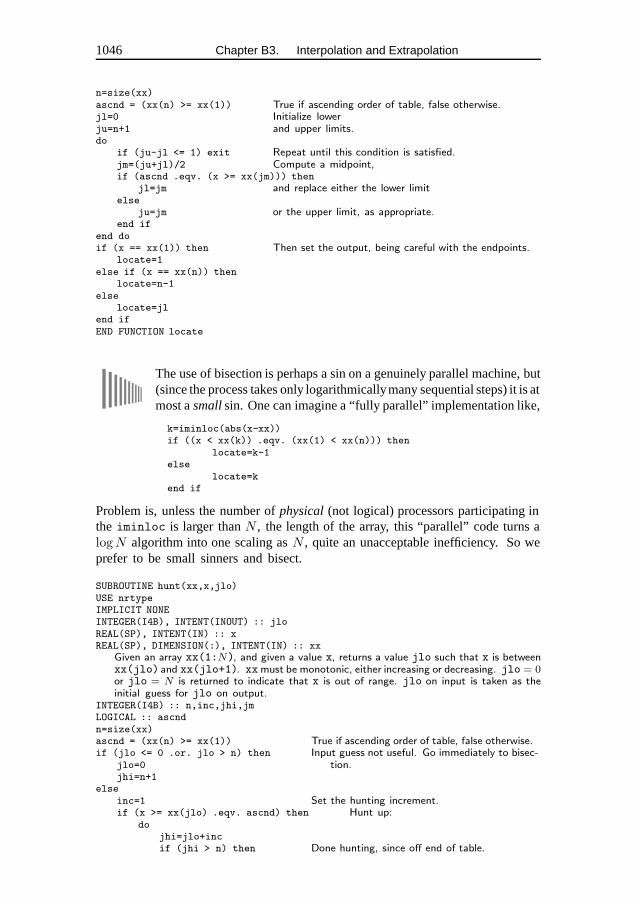
1046 Chapter B3. Interpolation and Extrapolation
n=size(xx)ascnd = (xx(n) >= xx(1)) True if ascending order of table, false otherwise.jl=0 Initialize lowerju=n+1 and upper limits.do
if (ju-jl <= 1) exit Repeat until this condition is satisfied.jm=(ju+jl)/2 Compute a midpoint,if (ascnd .eqv. (x >= xx(jm))) then
jl=jm and replace either the lower limitelse
ju=jm or the upper limit, as appropriate.end if
end doif (x == xx(1)) then Then set the output, being careful with the endpoints.
locate=1else if (x == xx(n)) then
locate=n-1else
locate=jlend ifEND FUNCTION locate
The use of bisection is perhaps a sin on a genuinely parallel machine, but(since the process takes only logarithmicallymany sequential steps) it is atmost a small sin. One can imagine a “fully parallel” implementation like,
k=iminloc(abs(x-xx))if ((x < xx(k)) .eqv. (xx(1) < xx(n))) then
locate=k-1else
locate=kend if
Problem is, unless the number of physical (not logical) processors participating inthe iminloc is larger than N , the length of the array, this “parallel” code turns alogN algorithm into one scaling as N , quite an unacceptable inefficiency. So weprefer to be small sinners and bisect.
SUBROUTINE hunt(xx,x,jlo)USE nrtypeIMPLICIT NONEINTEGER(I4B), INTENT(INOUT) :: jloREAL(SP), INTENT(IN) :: xREAL(SP), DIMENSION(:), INTENT(IN) :: xx
Given an array xx(1:N), and given a value x, returns a value jlo such that x is betweenxx(jlo) and xx(jlo+1). xxmust be monotonic, either increasing or decreasing. jlo = 0or jlo = N is returned to indicate that x is out of range. jlo on input is taken as theinitial guess for jlo on output.
INTEGER(I4B) :: n,inc,jhi,jmLOGICAL :: ascndn=size(xx)ascnd = (xx(n) >= xx(1)) True if ascending order of table, false otherwise.if (jlo <= 0 .or. jlo > n) then Input guess not useful. Go immediately to bisec-
tion.jlo=0jhi=n+1
elseinc=1 Set the hunting increment.if (x >= xx(jlo) .eqv. ascnd) then Hunt up:
dojhi=jlo+incif (jhi > n) then Done hunting, since off end of table.
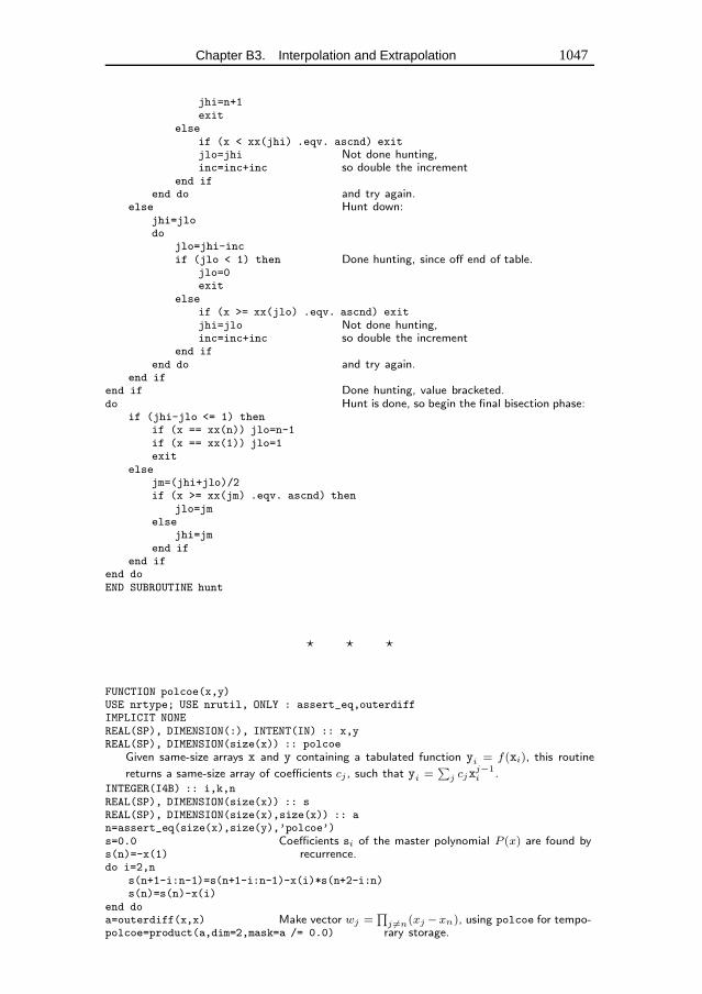
Chapter B3. Interpolation and Extrapolation 1047
jhi=n+1exit
elseif (x < xx(jhi) .eqv. ascnd) exitjlo=jhi Not done hunting,inc=inc+inc so double the increment
end ifend do and try again.
else Hunt down:jhi=jlodo
jlo=jhi-incif (jlo < 1) then Done hunting, since off end of table.
jlo=0exit
elseif (x >= xx(jlo) .eqv. ascnd) exitjhi=jlo Not done hunting,inc=inc+inc so double the increment
end ifend do and try again.
end ifend if Done hunting, value bracketed.do Hunt is done, so begin the final bisection phase:
if (jhi-jlo <= 1) thenif (x == xx(n)) jlo=n-1if (x == xx(1)) jlo=1exit
elsejm=(jhi+jlo)/2if (x >= xx(jm) .eqv. ascnd) then
jlo=jmelse
jhi=jmend if
end ifend doEND SUBROUTINE hunt
� � �
FUNCTION polcoe(x,y)USE nrtype; USE nrutil, ONLY : assert_eq,outerdiffIMPLICIT NONEREAL(SP), DIMENSION(:), INTENT(IN) :: x,yREAL(SP), DIMENSION(size(x)) :: polcoe
Given same-size arrays x and y containing a tabulated function yi = f(xi), this routine
returns a same-size array of coefficients cj , such that yi =∑
j cjxj−1i .
INTEGER(I4B) :: i,k,nREAL(SP), DIMENSION(size(x)) :: sREAL(SP), DIMENSION(size(x),size(x)) :: an=assert_eq(size(x),size(y),’polcoe’)s=0.0 Coefficients si of the master polynomial P (x) are found by
recurrence.s(n)=-x(1)do i=2,n
s(n+1-i:n-1)=s(n+1-i:n-1)-x(i)*s(n+2-i:n)s(n)=s(n)-x(i)
end doa=outerdiff(x,x) Make vector wj =
∏j �=n(xj −xn), using polcoe for tempo-rary storage.polcoe=product(a,dim=2,mask=a /= 0.0)
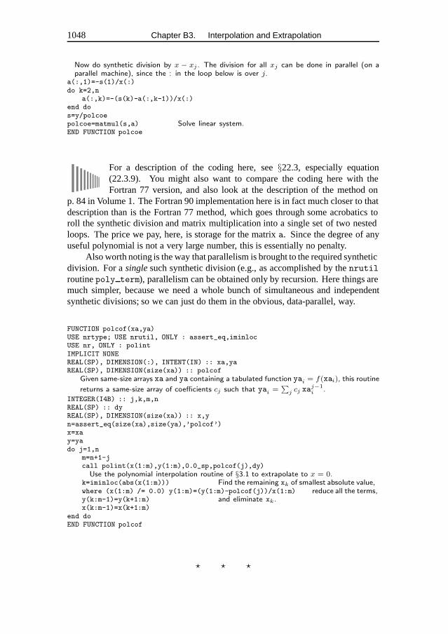
1048 Chapter B3. Interpolation and Extrapolation
Now do synthetic division by x − xj . The division for all xj can be done in parallel (on aparallel machine), since the : in the loop below is over j.
a(:,1)=-s(1)/x(:)do k=2,n
a(:,k)=-(s(k)-a(:,k-1))/x(:)end dos=y/polcoepolcoe=matmul(s,a) Solve linear system.END FUNCTION polcoe
For a description of the coding here, see §22.3, especially equation(22.3.9). You might also want to compare the coding here with theFortran 77 version, and also look at the description of the method on
p. 84 in Volume 1. The Fortran 90 implementation here is in fact much closer to thatdescription than is the Fortran 77 method, which goes through some acrobatics toroll the synthetic division and matrix multiplication into a single set of two nestedloops. The price we pay, here, is storage for the matrix a. Since the degree of anyuseful polynomial is not a very large number, this is essentially no penalty.
Also worth noting is the way that parallelism is brought to the required syntheticdivision. For a single such synthetic division (e.g., as accomplished by the nrutilroutine poly term), parallelism can be obtained only by recursion. Here things aremuch simpler, because we need a whole bunch of simultaneous and independentsynthetic divisions; so we can just do them in the obvious, data-parallel, way.
FUNCTION polcof(xa,ya)USE nrtype; USE nrutil, ONLY : assert_eq,iminlocUSE nr, ONLY : polintIMPLICIT NONEREAL(SP), DIMENSION(:), INTENT(IN) :: xa,yaREAL(SP), DIMENSION(size(xa)) :: polcof
Given same-size arrays xa and ya containing a tabulated function yai = f(xai), this routine
returns a same-size array of coefficients cj such that yai =∑
j cj xaj−1i .
INTEGER(I4B) :: j,k,m,nREAL(SP) :: dyREAL(SP), DIMENSION(size(xa)) :: x,yn=assert_eq(size(xa),size(ya),’polcof’)x=xay=yado j=1,n
m=n+1-jcall polint(x(1:m),y(1:m),0.0_sp,polcof(j),dy)
Use the polynomial interpolation routine of §3.1 to extrapolate to x = 0.k=iminloc(abs(x(1:m))) Find the remaining xk of smallest absolute value,where (x(1:m) /= 0.0) y(1:m)=(y(1:m)-polcof(j))/x(1:m) reduce all the terms,y(k:m-1)=y(k+1:m) and eliminate xk.x(k:m-1)=x(k+1:m)
end doEND FUNCTION polcof
� � �
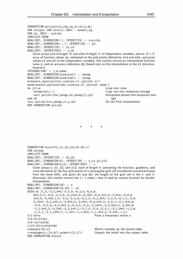
Chapter B3. Interpolation and Extrapolation 1049
SUBROUTINE polin2(x1a,x2a,ya,x1,x2,y,dy)USE nrtype; USE nrutil, ONLY : assert_eqUSE nr, ONLY : polintIMPLICIT NONEREAL(SP), DIMENSION(:), INTENT(IN) :: x1a,x2aREAL(SP), DIMENSION(:,:), INTENT(IN) :: yaREAL(SP), INTENT(IN) :: x1,x2REAL(SP), INTENT(OUT) :: y,dy
Given arrays x1a of length M and x2a of length N of independent variables, and an M×Narray of function values ya, tabulated at the grid points defined by x1a and x2a, and givenvalues x1 and x2 of the independent variables, this routine returns an interpolated functionvalue y, and an accuracy indication dy (based only on the interpolation in the x1 direction,however).
INTEGER(I4B) :: j,m,ndumREAL(SP), DIMENSION(size(x1a)) :: ymtmpREAL(SP), DIMENSION(size(x2a)) :: yntmpm=assert_eq(size(x1a),size(ya,1),’polin2: m’)ndum=assert_eq(size(x2a),size(ya,2),’polin2: ndum’)do j=1,m Loop over rows.
yntmp=ya(j,:) Copy row into temporary storage.call polint(x2a,yntmp,x2,ymtmp(j),dy) Interpolate answer into temporary stor-
age.end docall polint(x1a,ymtmp,x1,y,dy) Do the final interpolation.END SUBROUTINE polin2
� � �
SUBROUTINE bcucof(y,y1,y2,y12,d1,d2,c)USE nrtypeIMPLICIT NONEREAL(SP), INTENT(IN) :: d1,d2REAL(SP), DIMENSION(4), INTENT(IN) :: y,y1,y2,y12REAL(SP), DIMENSION(4,4), INTENT(OUT) :: c
Given arrays y, y1, y2, and y12, each of length 4, containing the function, gradients, andcross derivative at the four grid points of a rectangular grid cell (numbered counterclockwisefrom the lower left), and given d1 and d2, the length of the grid cell in the 1- and 2-directions, this routine returns the 4× 4 table c that is used by routine bcuint for bicubicinterpolation.
REAL(SP), DIMENSION(16) :: xREAL(SP), DIMENSION(16,16) :: wtDATA wt /1,0,-3,2,4*0,-3,0,9,-6,2,0,-6,4,&
8*0,3,0,-9,6,-2,0,6,-4,10*0,9,-6,2*0,-6,4,2*0,3,-2,6*0,-9,6,&2*0,6,-4,4*0,1,0,-3,2,-2,0,6,-4,1,0,-3,2,8*0,-1,0,3,-2,1,0,-3,&2,10*0,-3,2,2*0,3,-2,6*0,3,-2,2*0,-6,4,2*0,3,-2,0,1,-2,1,5*0,&-3,6,-3,0,2,-4,2,9*0,3,-6,3,0,-2,4,-2,10*0,-3,3,2*0,2,-2,2*0,&-1,1,6*0,3,-3,2*0,-2,2,5*0,1,-2,1,0,-2,4,-2,0,1,-2,1,9*0,-1,2,&-1,0,1,-2,1,10*0,1,-1,2*0,-1,1,6*0,-1,1,2*0,2,-2,2*0,-1,1/
x(1:4)=y Pack a temporary vector x.x(5:8)=y1*d1x(9:12)=y2*d2x(13:16)=y12*d1*d2x=matmul(wt,x) Matrix multiply by the stored table.c=reshape(x,(/4,4/),order=(/2,1/)) Unpack the result into the output table.END SUBROUTINE bcucof
1050 Chapter B3. Interpolation and Extrapolation
f90x=matmul(wt,x) ... c=reshape(x,(/4,4/),order=(/2,1/)) It is a power-ful technique to combine the matmul intrinsic with reshape’s of theinput or output. The idea is to use matmul whenever the calculation
can be cast into the form of a linear mapping between input and output objects.Here the order=(/2,1/) parameter specifies that we want the packing to be byrows, not by Fortran’s default of columns. (In this two-dimensional case, it’s theequivalent of applying transpose.)
SUBROUTINE bcuint(y,y1,y2,y12,x1l,x1u,x2l,x2u,x1,x2,ansy,ansy1,ansy2)USE nrtype; USE nrutil, ONLY : nrerrorUSE nr, ONLY : bcucofIMPLICIT NONEREAL(SP), DIMENSION(4), INTENT(IN) :: y,y1,y2,y12REAL(SP), INTENT(IN) :: x1l,x1u,x2l,x2u,x1,x2REAL(SP), INTENT(OUT) :: ansy,ansy1,ansy2
Bicubic interpolation within a grid square. Input quantities are y,y1,y2,y12 (as describedin bcucof); x1l and x1u, the lower and upper coordinates of the grid square in the 1-direction; x2l and x2u likewise for the 2-direction; and x1,x2, the coordinates of thedesired point for the interpolation. The interpolated function value is returned as ansy,and the interpolated gradient values as ansy1 and ansy2. This routine calls bcucof.
INTEGER(I4B) :: iREAL(SP) :: t,uREAL(SP), DIMENSION(4,4) :: ccall bcucof(y,y1,y2,y12,x1u-x1l,x2u-x2l,c) Get the c’s.if (x1u == x1l .or. x2u == x2l) call &
nrerror(’bcuint: problem with input values - boundary pair equal?’)t=(x1-x1l)/(x1u-x1l) Equation (3.6.4).u=(x2-x2l)/(x2u-x2l)ansy=0.0ansy2=0.0ansy1=0.0do i=4,1,-1 Equation (3.6.6).
ansy=t*ansy+((c(i,4)*u+c(i,3))*u+c(i,2))*u+c(i,1)ansy2=t*ansy2+(3.0_sp*c(i,4)*u+2.0_sp*c(i,3))*u+c(i,2)ansy1=u*ansy1+(3.0_sp*c(4,i)*t+2.0_sp*c(3,i))*t+c(2,i)
end doansy1=ansy1/(x1u-x1l)ansy2=ansy2/(x2u-x2l)END SUBROUTINE bcuint
� � �
SUBROUTINE splie2(x1a,x2a,ya,y2a)USE nrtype; USE nrutil, ONLY : assert_eqUSE nr, ONLY : splineIMPLICIT NONEREAL(SP), DIMENSION(:), INTENT(IN) :: x1a,x2aREAL(SP), DIMENSION(:,:), INTENT(IN) :: yaREAL(SP), DIMENSION(:,:), INTENT(OUT) :: y2a
Given an M × N tabulated function ya, and N tabulated independent variables x2a, thisroutine constructs one-dimensional natural cubic splines of the rows of ya and returns thesecond derivatives in the M × N array y2a. (The array x1a is included in the argumentlist merely for consistency with routine splin2.)
INTEGER(I4B) :: j,m,ndumm=assert_eq(size(x1a),size(ya,1),size(y2a,1),’splie2: m’)ndum=assert_eq(size(x2a),size(ya,2),size(y2a,2),’splie2: ndum’)do j=1,m
call spline(x2a,ya(j,:),1.0e30_sp,1.0e30_sp,y2a(j,:))
Chapter B3. Interpolation and Extrapolation 1051
Values 1 × 1030 signal a natural spline.end doEND SUBROUTINE splie2
FUNCTION splin2(x1a,x2a,ya,y2a,x1,x2)USE nrtype; USE nrutil, ONLY : assert_eqUSE nr, ONLY : spline,splintIMPLICIT NONEREAL(SP), DIMENSION(:), INTENT(IN) :: x1a,x2aREAL(SP), DIMENSION(:,:), INTENT(IN) :: ya,y2aREAL(SP), INTENT(IN) :: x1,x2REAL(SP) :: splin2
Given x1a, x2a, ya as described in splie2 and y2a as produced by that routine; and givena desired interpolating point x1,x2; this routine returns an interpolated function value bybicubic spline interpolation.
INTEGER(I4B) :: j,m,ndumREAL(SP), DIMENSION(size(x1a)) :: yytmp,y2tmp2m=assert_eq(size(x1a),size(ya,1),size(y2a,1),’splin2: m’)ndum=assert_eq(size(x2a),size(ya,2),size(y2a,2),’splin2: ndum’)do j=1,m
yytmp(j)=splint(x2a,ya(j,:),y2a(j,:),x2)Perform m evaluations of the row splines constructed by splie2, using the one-dimensionalspline evaluator splint.
end docall spline(x1a,yytmp,1.0e30_sp,1.0e30_sp,y2tmp2)
Construct the one-dimensional column spline and evaluate it.splin2=splint(x1a,yytmp,y2tmp2,x1)END FUNCTION splin2
Chapter B4. Integration of Functions
SUBROUTINE trapzd(func,a,b,s,n)USE nrtype; USE nrutil, ONLY : arthIMPLICIT NONEREAL(SP), INTENT(IN) :: a,bREAL(SP), INTENT(INOUT) :: sINTEGER(I4B), INTENT(IN) :: nINTERFACE
FUNCTION func(x)USE nrtypeREAL(SP), DIMENSION(:), INTENT(IN) :: xREAL(SP), DIMENSION(size(x)) :: funcEND FUNCTION func
END INTERFACEThis routine computes the nth stage of refinement of an extended trapezoidal rule. func isinput as the name of the function to be integrated between limits a and b, also input. When
called with n=1, the routine returns as s the crudest estimate of∫ ba f(x)dx. Subsequent
calls with n=2,3,... (in that sequential order) will improve the accuracy of s by adding 2n-2
additional interior points. s should not be modified between sequential calls.REAL(SP) :: del,fsumINTEGER(I4B) :: itif (n == 1) then
s=0.5_sp*(b-a)*sum(func( (/ a,b /) ))else
it=2**(n-2)del=(b-a)/it This is the spacing of the points to be added.fsum=sum(func(arth(a+0.5_sp*del,del,it)))s=0.5_sp*(s+del*fsum) This replaces s by its refined value.
end ifEND SUBROUTINE trapzd
f90While most of the quadrature routines in this chapter are coded asfunctions,trapzd is a subroutine because the arguments that returns thefunction value must also be supplied as an input parameter. We could
change the subroutine into a function by declarings to be a local variable with theSAVE attribute. However, this would prevent us from being able to use the routinerecursively to do multidimensional quadrature (seequad3d on p. 1065). Whensis left as an argument, a fresh copy is created on each recursive call. As aSAVE’dvariable, by contrast, its value would get overwritten on each call, and the codewould not be properly “re-entrant.”
s=0.5_sp*(b-a)*sum(func( (/ a,b /) )) Note how we use the(/.../) con-struct to supply a set of scalar arguments to a vector function.
� � �
1052
Chapter B4. Integration of Functions 1053
FUNCTION qtrap(func,a,b)USE nrtype; USE nrutil, ONLY : nrerrorUSE nr, ONLY : trapzdIMPLICIT NONEREAL(SP), INTENT(IN) :: a,bREAL(SP) :: qtrapINTERFACE
FUNCTION func(x)USE nrtypeREAL(SP), DIMENSION(:), INTENT(IN) :: xREAL(SP), DIMENSION(size(x)) :: funcEND FUNCTION func
END INTERFACEINTEGER(I4B), PARAMETER :: JMAX=20REAL(SP), PARAMETER :: EPS=1.0e-6_sp, UNLIKELY=-1.0e30_sp
Returns the integral of the function func from a to b. The parameter EPS should be set tothe desired fractional accuracy and JMAX so that 2 to the power JMAX-1 is the maximumallowed number of steps. Integration is performed by the trapezoidal rule.
REAL(SP) :: oldsINTEGER(I4B) :: jolds=UNLIKELY Any number that is unlikely to be the average of the
function at its endpoints will do here.do j=1,JMAXcall trapzd(func,a,b,qtrap,j)if (j > 5) then Avoid spurious early convergence.
if (abs(qtrap-olds) < EPS*abs(olds) .or. &(qtrap == 0.0 .and. olds == 0.0)) RETURN
end ifolds=qtrap
end docall nrerror(’qtrap: too many steps’)END FUNCTION qtrap
� � �
FUNCTION qsimp(func,a,b)USE nrtype; USE nrutil, ONLY : nrerrorUSE nr, ONLY : trapzdIMPLICIT NONEREAL(SP), INTENT(IN) :: a,bREAL(SP) :: qsimpINTERFACE
FUNCTION func(x)USE nrtypeREAL(SP), DIMENSION(:), INTENT(IN) :: xREAL(SP), DIMENSION(size(x)) :: funcEND FUNCTION func
END INTERFACEINTEGER(I4B), PARAMETER :: JMAX=20REAL(SP), PARAMETER :: EPS=1.0e-6_sp, UNLIKELY=-1.0e30_sp
Returns the integral of the function func from a to b. The parameter EPS should be set tothe desired fractional accuracy and JMAX so that 2 to the power JMAX-1 is the maximumallowed number of steps. Integration is performed by Simpson’s rule.
INTEGER(I4B) :: jREAL(SP) :: os,ost,stost=UNLIKELYos= UNLIKELYdo j=1,JMAX
call trapzd(func,a,b,st,j)qsimp=(4.0_sp*st-ost)/3.0_sp Compare equation (4.2.4).if (j > 5) then Avoid spurious early convergence.
if (abs(qsimp-os) < EPS*abs(os) .or. &(qsimp == 0.0 .and. os == 0.0)) RETURN
end ifos=qsimp
1054 Chapter B4. Integration of Functions
ost=stend docall nrerror(’qsimp: too many steps’)END FUNCTION qsimp
� � �
FUNCTION qromb(func,a,b)USE nrtype; USE nrutil, ONLY : nrerrorUSE nr, ONLY : polint,trapzdIMPLICIT NONEREAL(SP), INTENT(IN) :: a,bREAL(SP) :: qrombINTERFACE
FUNCTION func(x)USE nrtypeREAL(SP), DIMENSION(:), INTENT(IN) :: xREAL(SP), DIMENSION(size(x)) :: funcEND FUNCTION func
END INTERFACEINTEGER(I4B), PARAMETER :: JMAX=20,JMAXP=JMAX+1,K=5,KM=K-1REAL(SP), PARAMETER :: EPS=1.0e-6_sp
Returns the integral of the function func from a to b. Integration is performed by Romberg’smethod of order 2K, where, e.g., K=2 is Simpson’s rule.Parameters: EPS is the fractional accuracy desired, as determined by the extrapolation er-ror estimate; JMAX limits the total number of steps; K is the number of points used in theextrapolation.
REAL(SP), DIMENSION(JMAXP) :: h,s These store the successive trapezoidal ap-proximations and their relative stepsizes.REAL(SP) :: dqromb
INTEGER(I4B) :: jh(1)=1.0do j=1,JMAX
call trapzd(func,a,b,s(j),j)if (j >= K) then
call polint(h(j-KM:j),s(j-KM:j),0.0_sp,qromb,dqromb)if (abs(dqromb) <= EPS*abs(qromb)) RETURN
end ifs(j+1)=s(j)h(j+1)=0.25_sp*h(j) This is a key step: The factor is 0.25 even
though the stepsize is decreased by only0.5. This makes the extrapolation a poly-nomial in h2 as allowed by equation (4.2.1),not just a polynomial in h.
end docall nrerror(’qromb: too many steps’)END FUNCTION qromb
� � �
SUBROUTINE midpnt(func,a,b,s,n)USE nrtype; USE nrutil, ONLY : arthIMPLICIT NONEREAL(SP), INTENT(IN) :: a,bREAL(SP), INTENT(INOUT) :: sINTEGER(I4B), INTENT(IN) :: nINTERFACE
FUNCTION func(x)USE nrtypeREAL(SP), DIMENSION(:), INTENT(IN) :: xREAL(SP), DIMENSION(size(x)) :: funcEND FUNCTION func
END INTERFACEThis routine computes the nth stage of refinement of an extended midpoint rule. func isinput as the name of the function to be integrated between limits a and b, also input. When

Chapter B4. Integration of Functions 1055
called with n=1, the routine returns as s the crudest estimate of∫ ba f(x)dx. Subsequent
calls with n=2,3,... (in that sequential order) will improve the accuracy of s by adding
(2/3)× 3n-1 additional interior points. s should not be modified between sequential calls.REAL(SP) :: delINTEGER(I4B) :: itREAL(SP), DIMENSION(2*3**(n-2)) :: xif (n == 1) then
s=(b-a)*sum(func( (/0.5_sp*(a+b)/) ))else
it=3**(n-2)del=(b-a)/(3.0_sp*it) The added points alternate in spacing between
del and 2*del.x(1:2*it-1:2)=arth(a+0.5_sp*del,3.0_sp*del,it)x(2:2*it:2)=x(1:2*it-1:2)+2.0_sp*dels=s/3.0_sp+del*sum(func(x)) The new sum is combined with the old integral
to give a refined integral.end ifEND SUBROUTINE midpnt
f90midpnt is a subroutine and not a function for the same reasons astrapzd.This is also true for the othermid... routines below.
s=(b-a)*sum(func( (/0.5_sp*(a+b)/) )) Here we use(/.../) to pass a singlescalar argument to a vector function.
� � �
FUNCTION qromo(func,a,b,choose)USE nrtype; USE nrutil, ONLY : nrerrorUSE nr, ONLY : polintIMPLICIT NONEREAL(SP), INTENT(IN) :: a,bREAL(SP) :: qromoINTERFACE
FUNCTION func(x)USE nrtypeIMPLICIT NONEREAL(SP), DIMENSION(:), INTENT(IN) :: xREAL(SP), DIMENSION(size(x)) :: funcEND FUNCTION func
SUBROUTINE choose(funk,aa,bb,s,n)USE nrtypeIMPLICIT NONEREAL(SP), INTENT(IN) :: aa,bbREAL(SP), INTENT(INOUT) :: sINTEGER(I4B), INTENT(IN) :: nINTERFACE
FUNCTION funk(x)USE nrtypeIMPLICIT NONEREAL(SP), DIMENSION(:), INTENT(IN) :: xREAL(SP), DIMENSION(size(x)) :: funkEND FUNCTION funk
END INTERFACEEND SUBROUTINE choose
END INTERFACEINTEGER(I4B), PARAMETER :: JMAX=14,JMAXP=JMAX+1,K=5,KM=K-1REAL(SP), PARAMETER :: EPS=1.0e-6
Romberg integration on an open interval. Returns the integral of the function func from ato b, using any specified integrating subroutine choose and Romberg’s method. Normallychoose will be an open formula, not evaluating the function at the endpoints. It is assumedthat choose triples the number of steps on each call, and that its error series contains only
1056 Chapter B4. Integration of Functions
even powers of the number of steps. The routines midpnt, midinf, midsql, midsqu,and midexp are possible choices for choose. The parameters have the same meaning asin qromb.
REAL(SP), DIMENSION(JMAXP) :: h,sREAL(SP) :: dqromoINTEGER(I4B) :: jh(1)=1.0do j=1,JMAX
call choose(func,a,b,s(j),j)if (j >= K) then
call polint(h(j-KM:j),s(j-KM:j),0.0_sp,qromo,dqromo)if (abs(dqromo) <= EPS*abs(qromo)) RETURN
end ifs(j+1)=s(j)h(j+1)=h(j)/9.0_sp This is where the assumption of step tripling and an even
error series is used.end docall nrerror(’qromo: too many steps’)END FUNCTION qromo
� � �
SUBROUTINE midinf(funk,aa,bb,s,n)USE nrtype; USE nrutil, ONLY : arth,assertIMPLICIT NONEREAL(SP), INTENT(IN) :: aa,bbREAL(SP), INTENT(INOUT) :: sINTEGER(I4B), INTENT(IN) :: nINTERFACE
FUNCTION funk(x)USE nrtypeREAL(SP), DIMENSION(:), INTENT(IN) :: xREAL(SP), DIMENSION(size(x)) :: funkEND FUNCTION funk
END INTERFACEThis routine is an exact replacement for midpnt, i.e., returns as s the nth stage of refinementof the integral of funk from aa to bb, except that the function is evaluated at evenly spacedpoints in 1/x rather than in x. This allows the upper limit bb to be as large and positiveas the computer allows, or the lower limit aa to be as large and negative, but not both.aa and bb must have the same sign.
REAL(SP) :: a,b,delINTEGER(I4B) :: itREAL(SP), DIMENSION(2*3**(n-2)) :: xcall assert(aa*bb > 0.0, ’midinf args’)b=1.0_sp/aa These two statements change the limits of integration ac-
cordingly.a=1.0_sp/bbif (n == 1) then From this point on, the routine is exactly identical to midpnt.
s=(b-a)*sum(func( (/0.5_sp*(a+b)/) ))else
it=3**(n-2)del=(b-a)/(3.0_sp*it)x(1:2*it-1:2)=arth(a+0.5_sp*del,3.0_sp*del,it)x(2:2*it:2)=x(1:2*it-1:2)+2.0_sp*dels=s/3.0_sp+del*sum(func(x))
end ifCONTAINS
FUNCTION func(x) This internal function effects the change of variable.REAL(SP), DIMENSION(:), INTENT(IN) :: xREAL(SP), DIMENSION(size(x)) :: funcfunc=funk(1.0_sp/x)/x**2END FUNCTION func
END SUBROUTINE midinf
Chapter B4. Integration of Functions 1057
f90FUNCTION func(x) The change of variable could have been effected by astatement function inmidinf itself. However, the statement function isa Fortran 77 feature that is deprecated in Fortran 90 because it does not
allow the benefits of having an explicit interface, i.e., a complete set of specificationstatements. Statement functions can always be coded as internal subprograms instead.
SUBROUTINE midsql(funk,aa,bb,s,n)USE nrtype; USE nrutil, ONLY : arthIMPLICIT NONEREAL(SP), INTENT(IN) :: aa,bbREAL(SP), INTENT(INOUT) :: sINTEGER(I4B), INTENT(IN) :: nINTERFACE
FUNCTION funk(x)USE nrtypeREAL(SP), DIMENSION(:), INTENT(IN) :: xREAL(SP), DIMENSION(size(x)) :: funkEND FUNCTION funk
END INTERFACEThis routine is an exact replacement for midpnt, i.e., returns as s the nth stage of refinementof the integral of funk from aa to bb, except that it allows for an inverse square-rootsingularity in the integrand at the lower limit aa.
REAL(SP) :: a,b,delINTEGER(I4B) :: itREAL(SP), DIMENSION(2*3**(n-2)) :: xb=sqrt(bb-aa) These two statements change the limits of integration ac-
cordingly.a=0.0if (n == 1) then From this point on, the routine is exactly identical to midpnt.
s=(b-a)*sum(func( (/0.5_sp*(a+b)/) ))else
it=3**(n-2)del=(b-a)/(3.0_sp*it)x(1:2*it-1:2)=arth(a+0.5_sp*del,3.0_sp*del,it)x(2:2*it:2)=x(1:2*it-1:2)+2.0_sp*dels=s/3.0_sp+del*sum(func(x))
end ifCONTAINS
FUNCTION func(x) This internal function effects the change of variable.REAL(SP), DIMENSION(:), INTENT(IN) :: xREAL(SP), DIMENSION(size(x)) :: funcfunc=2.0_sp*x*funk(aa+x**2)END FUNCTION func
END SUBROUTINE midsql
SUBROUTINE midsqu(funk,aa,bb,s,n)USE nrtype; USE nrutil, ONLY : arthIMPLICIT NONEREAL(SP), INTENT(IN) :: aa,bbREAL(SP), INTENT(INOUT) :: sINTEGER(I4B), INTENT(IN) :: nINTERFACE
FUNCTION funk(x)USE nrtypeREAL(SP), DIMENSION(:), INTENT(IN) :: xREAL(SP), DIMENSION(size(x)) :: funkEND FUNCTION funk
END INTERFACEThis routine is an exact replacement for midpnt, i.e., returns as s the nth stage of refinementof the integral of funk from aa to bb, except that it allows for an inverse square-rootsingularity in the integrand at the upper limit bb.
REAL(SP) :: a,b,del
1058 Chapter B4. Integration of Functions
INTEGER(I4B) :: itREAL(SP), DIMENSION(2*3**(n-2)) :: xb=sqrt(bb-aa) These two statements change the limits of integration ac-
cordingly.a=0.0if (n == 1) then From this point on, the routine is exactly identical to midpnt.
s=(b-a)*sum(func( (/0.5_sp*(a+b)/) ))else
it=3**(n-2)del=(b-a)/(3.0_sp*it)x(1:2*it-1:2)=arth(a+0.5_sp*del,3.0_sp*del,it)x(2:2*it:2)=x(1:2*it-1:2)+2.0_sp*dels=s/3.0_sp+del*sum(func(x))
end ifCONTAINS
FUNCTION func(x) This internal function effects the change of variable.REAL(SP), DIMENSION(:), INTENT(IN) :: xREAL(SP), DIMENSION(size(x)) :: funcfunc=2.0_sp*x*funk(bb-x**2)END FUNCTION func
END SUBROUTINE midsqu
SUBROUTINE midexp(funk,aa,bb,s,n)USE nrtype; USE nrutil, ONLY : arthIMPLICIT NONEREAL(SP), INTENT(IN) :: aa,bbREAL(SP), INTENT(INOUT) :: sINTEGER(I4B), INTENT(IN) :: nINTERFACE
FUNCTION funk(x)USE nrtypeREAL(SP), DIMENSION(:), INTENT(IN) :: xREAL(SP), DIMENSION(size(x)) :: funkEND FUNCTION funk
END INTERFACEThis routine is an exact replacement for midpnt, i.e., returns as s the nth stage of refinementof the integral of funk from aa to bb, except that bb is assumed to be infinite (value passednot actually used). It is assumed that the function funk decreases exponentially rapidly atinfinity.
REAL(SP) :: a,b,delINTEGER(I4B) :: itREAL(SP), DIMENSION(2*3**(n-2)) :: xb=exp(-aa) These two statements change the limits of integration ac-
cordingly.a=0.0if (n == 1) then From this point on, the routine is exactly identical to midpnt.
s=(b-a)*sum(func( (/0.5_sp*(a+b)/) ))else
it=3**(n-2)del=(b-a)/(3.0_sp*it)x(1:2*it-1:2)=arth(a+0.5_sp*del,3.0_sp*del,it)x(2:2*it:2)=x(1:2*it-1:2)+2.0_sp*dels=s/3.0_sp+del*sum(func(x))
end ifCONTAINS
FUNCTION func(x) This internal function effects the change of variable.REAL(SP), DIMENSION(:), INTENT(IN) :: xREAL(SP), DIMENSION(size(x)) :: funcfunc=funk(-log(x))/xEND FUNCTION func
END SUBROUTINE midexp
� � �
Chapter B4. Integration of Functions 1059
SUBROUTINE gauleg(x1,x2,x,w)USE nrtype; USE nrutil, ONLY : arth,assert_eq,nrerrorIMPLICIT NONEREAL(SP), INTENT(IN) :: x1,x2REAL(SP), DIMENSION(:), INTENT(OUT) :: x,wREAL(DP), PARAMETER :: EPS=3.0e-14_dp
Given the lower and upper limits of integration x1 and x2, this routine returns arrays x and wof length N containing the abscissas and weights of the Gauss-LegendreN -point quadratureformula. The parameter EPS is the relative precision. Note that internal computations aredone in double precision.
INTEGER(I4B) :: its,j,m,nINTEGER(I4B), PARAMETER :: MAXIT=10REAL(DP) :: xl,xmREAL(DP), DIMENSION((size(x)+1)/2) :: p1,p2,p3,pp,z,z1LOGICAL(LGT), DIMENSION((size(x)+1)/2) :: unfinishedn=assert_eq(size(x),size(w),’gauleg’)m=(n+1)/2 The roots are symmetric in the interval,
so we only have to find half of them.xm=0.5_dp*(x2+x1)xl=0.5_dp*(x2-x1)z=cos(PI_D*(arth(1,1,m)-0.25_dp)/(n+0.5_dp)) Initial approximations to the roots.unfinished=.true.do its=1,MAXIT Newton’s method carried out simultane-
ously on the roots.where (unfinished)p1=1.0p2=0.0
end wheredo j=1,n Loop up the recurrence relation to get
the Legendre polynomials evaluatedat z.
where (unfinished)p3=p2p2=p1p1=((2.0_dp*j-1.0_dp)*z*p2-(j-1.0_dp)*p3)/j
end whereend dop1 now contains the desired Legendre polynomials. We next compute pp, the derivatives,by a standard relation involving also p2, the polynomials of one lower order.
where (unfinished)pp=n*(z*p1-p2)/(z*z-1.0_dp)z1=zz=z1-p1/pp Newton’s method.unfinished=(abs(z-z1) > EPS)
end whereif (.not. any(unfinished)) exit
end doif (its == MAXIT+1) call nrerror(’too many iterations in gauleg’)x(1:m)=xm-xl*z Scale the root to the desired interval,x(n:n-m+1:-1)=xm+xl*z and put in its symmetric counterpart.w(1:m)=2.0_dp*xl/((1.0_dp-z**2)*pp**2) Compute the weightw(n:n-m+1:-1)=w(1:m) and its symmetric counterpart.END SUBROUTINE gauleg
f90Often we have an iterative procedure that has to be applied until allcomponents of a vector have satisfied a convergence criterion. Somecomponents of the vector might converge sooner than others, and it is
inefficient on a small-scale parallel (SSP) machine to continue iterating on thosecomponents. The general structure we use for such an iteration is exemplified bythe following lines fromgauleg:
LOGICAL(LGT), DIMENSION((size(x)+1)/2) :: unfinished...
unfinished=.true.do its=1,MAXIT
1060 Chapter B4. Integration of Functions
where (unfinished)...
unfinished=(abs(z-z1) > EPS)end whereif (.not. any(unfinished)) exit
end doif (its == MAXIT+1) call nrerror(’too many iterations in gauleg’)
We use the logical maskunfinished to control which vector components areprocessed inside thewhere. The mask gets updated on each iteration by testingwhether any further vector components have converged. When all have converged,we exit the iteration loop. Finally, we check the value ofits to see whetherthe maximum allowed number of iterations was exceeded before all componentsconverged.
The logical expression controlling thewhere block (in this caseunfinished)gets evaluated completely on entry into thewhere, and it is then perfectly fineto modify it inside the block. The modification affects only thenext executionof the where.
On a strictlyserial machine, there is of course some penalty associated with theabove scheme: after a vector component converges, its corresponding componentin unfinished is redundantly tested on each further iteration, until the slowest-converging component is done. If the number of iterations required does notvary too greatly from component to component, this is a minor, often negligible,penalty. However, one should be on the alert against algorithms whose worst-caseconvergence could differ from typical convergence by orders of magnitude. Forthese, one would need to implement a more complicated packing-unpacking scheme.(See discussion in Chapter B6, especially introduction, p. 1083, and notes forfactrl, p. 1087.)
SUBROUTINE gaulag(x,w,alf)USE nrtype; USE nrutil, ONLY : arth,assert_eq,nrerrorUSE nr, ONLY : gammlnIMPLICIT NONEREAL(SP), INTENT(IN) :: alfREAL(SP), DIMENSION(:), INTENT(OUT) :: x,wREAL(DP), PARAMETER :: EPS=3.0e-13_dp
Given alf, the parameter α of the Laguerre polynomials, this routine returns arrays x and wof length N containing the abscissas and weights of the N -point Gauss-Laguerre quadratureformula. The abscissas are returned in ascending order. The parameter EPS is the relativeprecision. Note that internal computations are done in double precision.
INTEGER(I4B) :: its,j,nINTEGER(I4B), PARAMETER :: MAXIT=10REAL(SP) :: anuREAL(SP), PARAMETER :: C1=9.084064e-01_sp,C2=5.214976e-02_sp,&
C3=2.579930e-03_sp,C4=3.986126e-03_spREAL(SP), DIMENSION(size(x)) :: rhs,r2,r3,thetaREAL(DP), DIMENSION(size(x)) :: p1,p2,p3,pp,z,z1LOGICAL(LGT), DIMENSION(size(x)) :: unfinishedn=assert_eq(size(x),size(w),’gaulag’)anu=4.0_sp*n+2.0_sp*alf+2.0_sp Initial approximations to the roots go into z.rhs=arth(4*n-1,-4,n)*PI/anur3=rhs**(1.0_sp/3.0_sp)r2=r3**2theta=r3*(C1+r2*(C2+r2*(C3+r2*C4)))z=anu*cos(theta)**2unfinished=.true.do its=1,MAXIT Newton’s method carried out simultaneously on
the roots.where (unfinished)
Chapter B4. Integration of Functions 1061
p1=1.0p2=0.0
end wheredo j=1,n Loop up the recurrence relation to get the La-
guerre polynomials evaluated at z.where (unfinished)p3=p2p2=p1p1=((2.0_dp*j-1.0_dp+alf-z)*p2-(j-1.0_dp+alf)*p3)/j
end whereend dop1 now contains the desired Laguerre polynomials. We next compute pp, the derivatives,by a standard relation involving also p2, the polynomials of one lower order.
where (unfinished)pp=(n*p1-(n+alf)*p2)/zz1=zz=z1-p1/pp Newton’s formula.unfinished=(abs(z-z1) > EPS*z)
end whereif (.not. any(unfinished)) exit
end doif (its == MAXIT+1) call nrerror(’too many iterations in gaulag’)x=z Store the root and the weight.w=-exp(gammln(alf+n)-gammln(real(n,sp)))/(pp*n*p2)END SUBROUTINE gaulag
The key difficulty in parallelizing this routine starting from the Fortran 77version is that the initial guesses for the roots of the Laguerre polynomialswere given in terms of previously determined roots. This prevents one
from finding all the roots simultaneously. The solution is to come up with a newapproximation to the roots that is a simple explicit formula, like the formula weused for the Legendre roots ingauleg.
We start with the approximation toLαn(x) given in equation (10.15.8) of[1]. We
keep only the first term and ask when it is zero. This gives the following prescriptionfor the kth rootxk of Lα
n(x): Solve forθ the equation
2θ− sin 2θ =4n− 4k + 3
4n+ 2α + 2π (B4.1)
Since1 ≤ k ≤ n andα > −1, we can always find a value such that0 < θ < π/2.Then the approximation to the root is
xk = (4n + 2α+ 2) cos2 θ (B4.2)
This typically gives 3-digit accuracy, more than enough for the Newton iteration tobe able to refine the root. Unfortunately equation (B4.1) is not an explicit formulafor θ. (You may recognize it as being of the same form as Kepler’s equation inmechanics.) If we call the right-hand side of (B4.1)y, then we can get an explicitformula by working out the power series fory1/3 nearθ = 0 (using a computeralgebra program). Next invert the series to giveθ as a function ofy1/3. Finally,economize the series (see§5.11). The result is the concise approximation
θ = 0.9084064y1/3 + 5.214976× 10⁻²y + 2.579930× 10⁻³y5/3
+ 3.986126× 10⁻³y7/3 (B4.3)
1062 Chapter B4. Integration of Functions
SUBROUTINE gauher(x,w)USE nrtype; USE nrutil, ONLY : arth,assert_eq,nrerrorIMPLICIT NONEREAL(SP), DIMENSION(:), INTENT(OUT) :: x,wREAL(DP), PARAMETER :: EPS=3.0e-13_dp,PIM4=0.7511255444649425_dp
This routine returns arrays x and w of length N containing the abscissas and weights ofthe N -point Gauss-Hermite quadrature formula. The abscissas are returned in descendingorder. Note that internal computations are done in double precision.Parameters: EPS is the relative precision, PIM4 = 1/π1/4.
INTEGER(I4B) :: its,j,m,nINTEGER(I4B), PARAMETER :: MAXIT=10REAL(SP) :: anuREAL(SP), PARAMETER :: C1=9.084064e-01_sp,C2=5.214976e-02_sp,&
C3=2.579930e-03_sp,C4=3.986126e-03_spREAL(SP), DIMENSION((size(x)+1)/2) :: rhs,r2,r3,thetaREAL(DP), DIMENSION((size(x)+1)/2) :: p1,p2,p3,pp,z,z1LOGICAL(LGT), DIMENSION((size(x)+1)/2) :: unfinishedn=assert_eq(size(x),size(w),’gauher’)m=(n+1)/2 The roots are symmetric about the origin, so we have to
find only half of them.anu=2.0_sp*n+1.0_sprhs=arth(3,4,m)*PI/anur3=rhs**(1.0_sp/3.0_sp)r2=r3**2theta=r3*(C1+r2*(C2+r2*(C3+r2*C4)))z=sqrt(anu)*cos(theta) Initial approximations to the roots.unfinished=.true.do its=1,MAXIT Newton’s method carried out simultaneously on the roots.
where (unfinished)p1=PIM4p2=0.0
end wheredo j=1,n Loop up the recurrence relation to get the Hermite poly-
nomials evaluated at z.where (unfinished)p3=p2p2=p1p1=z*sqrt(2.0_dp/j)*p2-sqrt(real(j-1,dp)/real(j,dp))*p3
end whereend dop1 now contains the desired Hermite polynomials. We next compute pp, the derivatives,by the relation (4.5.21) using p2, the polynomials of one lower order.
where (unfinished)pp=sqrt(2.0_dp*n)*p2z1=zz=z1-p1/pp Newton’s formula.unfinished=(abs(z-z1) > EPS)
end whereif (.not. any(unfinished)) exit
end doif (its == MAXIT+1) call nrerror(’too many iterations in gauher’)x(1:m)=z Store the rootx(n:n-m+1:-1)=-z and its symmetric counterpart.w(1:m)=2.0_dp/pp**2 Compute the weightw(n:n-m+1:-1)=w(1:m) and its symmetric counterpart.END SUBROUTINE gauher
Once again we need an explicit approximation for the polynomial roots,this time forHn(x). We can use the same approximation scheme asfor Lα
n(x), since
H2m(x) ∝ L−1/2m (x2), H2m+1(x) ∝ xL1/2
m (x2) (B4.4)
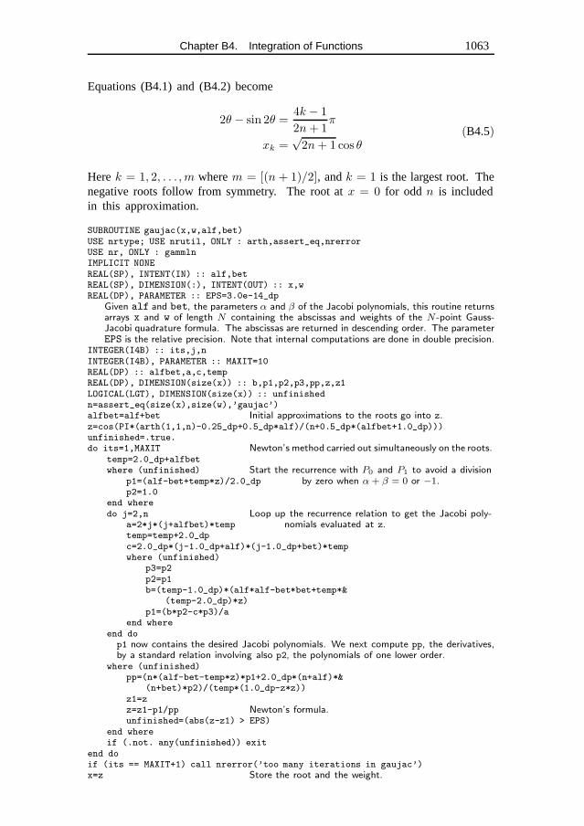
Chapter B4. Integration of Functions 1063
Equations (B4.1) and (B4.2) become
2θ − sin 2θ =4k − 1
2n + 1π
xk =√
2n + 1 cos θ(B4.5)
Herek = 1, 2, . . . , m wherem = [(n + 1)/2], andk = 1 is the largest root. Thenegative roots follow from symmetry. The root atx = 0 for odd n is includedin this approximation.
SUBROUTINE gaujac(x,w,alf,bet)USE nrtype; USE nrutil, ONLY : arth,assert_eq,nrerrorUSE nr, ONLY : gammlnIMPLICIT NONEREAL(SP), INTENT(IN) :: alf,betREAL(SP), DIMENSION(:), INTENT(OUT) :: x,wREAL(DP), PARAMETER :: EPS=3.0e-14_dp
Given alf and bet, the parameters α and β of the Jacobi polynomials, this routine returnsarrays x and w of length N containing the abscissas and weights of the N -point Gauss-Jacobi quadrature formula. The abscissas are returned in descending order. The parameterEPS is the relative precision. Note that internal computations are done in double precision.
INTEGER(I4B) :: its,j,nINTEGER(I4B), PARAMETER :: MAXIT=10REAL(DP) :: alfbet,a,c,tempREAL(DP), DIMENSION(size(x)) :: b,p1,p2,p3,pp,z,z1LOGICAL(LGT), DIMENSION(size(x)) :: unfinishedn=assert_eq(size(x),size(w),’gaujac’)alfbet=alf+bet Initial approximations to the roots go into z.z=cos(PI*(arth(1,1,n)-0.25_dp+0.5_dp*alf)/(n+0.5_dp*(alfbet+1.0_dp)))unfinished=.true.do its=1,MAXIT Newton’s method carried out simultaneously on the roots.
temp=2.0_dp+alfbetwhere (unfinished) Start the recurrence with P0 and P1 to avoid a division
by zero when α + β = 0 or −1.p1=(alf-bet+temp*z)/2.0_dpp2=1.0
end wheredo j=2,n Loop up the recurrence relation to get the Jacobi poly-
nomials evaluated at z.a=2*j*(j+alfbet)*temptemp=temp+2.0_dpc=2.0_dp*(j-1.0_dp+alf)*(j-1.0_dp+bet)*tempwhere (unfinished)
p3=p2p2=p1b=(temp-1.0_dp)*(alf*alf-bet*bet+temp*&
(temp-2.0_dp)*z)p1=(b*p2-c*p3)/a
end whereend dop1 now contains the desired Jacobi polynomials. We next compute pp, the derivatives,by a standard relation involving also p2, the polynomials of one lower order.
where (unfinished)pp=(n*(alf-bet-temp*z)*p1+2.0_dp*(n+alf)*&
(n+bet)*p2)/(temp*(1.0_dp-z*z))z1=zz=z1-p1/pp Newton’s formula.unfinished=(abs(z-z1) > EPS)
end whereif (.not. any(unfinished)) exit
end doif (its == MAXIT+1) call nrerror(’too many iterations in gaujac’)x=z Store the root and the weight.
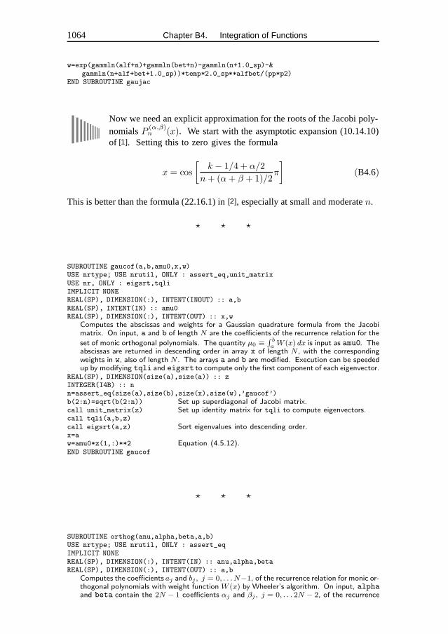
1064 Chapter B4. Integration of Functions
w=exp(gammln(alf+n)+gammln(bet+n)-gammln(n+1.0_sp)-&gammln(n+alf+bet+1.0_sp))*temp*2.0_sp**alfbet/(pp*p2)
END SUBROUTINE gaujac
Now we need an explicit approximation for the roots of the Jacobi poly-nomialsP (α,β)
n (x). We start with the asymptotic expansion (10.14.10)of [1]. Setting this to zero gives the formula
x = cos
[k − 1/4 + α/2
n + (α + β + 1)/2π
](B4.6)
This is better than the formula (22.16.1) in[2], especially at small and moderaten.
� � �
SUBROUTINE gaucof(a,b,amu0,x,w)USE nrtype; USE nrutil, ONLY : assert_eq,unit_matrixUSE nr, ONLY : eigsrt,tqliIMPLICIT NONEREAL(SP), DIMENSION(:), INTENT(INOUT) :: a,bREAL(SP), INTENT(IN) :: amu0REAL(SP), DIMENSION(:), INTENT(OUT) :: x,w
Computes the abscissas and weights for a Gaussian quadrature formula from the Jacobimatrix. On input, a and b of length N are the coefficients of the recurrence relation for the
set of monic orthogonal polynomials. The quantity µ0 ≡∫ ba W (x) dx is input as amu0. The
abscissas are returned in descending order in array x of length N , with the correspondingweights in w, also of length N . The arrays a and b are modified. Execution can be speededup by modifying tqli and eigsrt to compute only the first component of each eigenvector.
REAL(SP), DIMENSION(size(a),size(a)) :: zINTEGER(I4B) :: nn=assert_eq(size(a),size(b),size(x),size(w),’gaucof’)b(2:n)=sqrt(b(2:n)) Set up superdiagonal of Jacobi matrix.call unit_matrix(z) Set up identity matrix for tqli to compute eigenvectors.call tqli(a,b,z)call eigsrt(a,z) Sort eigenvalues into descending order.x=aw=amu0*z(1,:)**2 Equation (4.5.12).END SUBROUTINE gaucof
� � �
SUBROUTINE orthog(anu,alpha,beta,a,b)USE nrtype; USE nrutil, ONLY : assert_eqIMPLICIT NONEREAL(SP), DIMENSION(:), INTENT(IN) :: anu,alpha,betaREAL(SP), DIMENSION(:), INTENT(OUT) :: a,b
Computes the coefficients aj and bj , j = 0, . . .N−1, of the recurrence relation for monic or-thogonal polynomials with weight function W (x) by Wheeler’s algorithm. On input, alphaand beta contain the 2N − 1 coefficients αj and βj , j = 0, . . . 2N − 2, of the recurrence
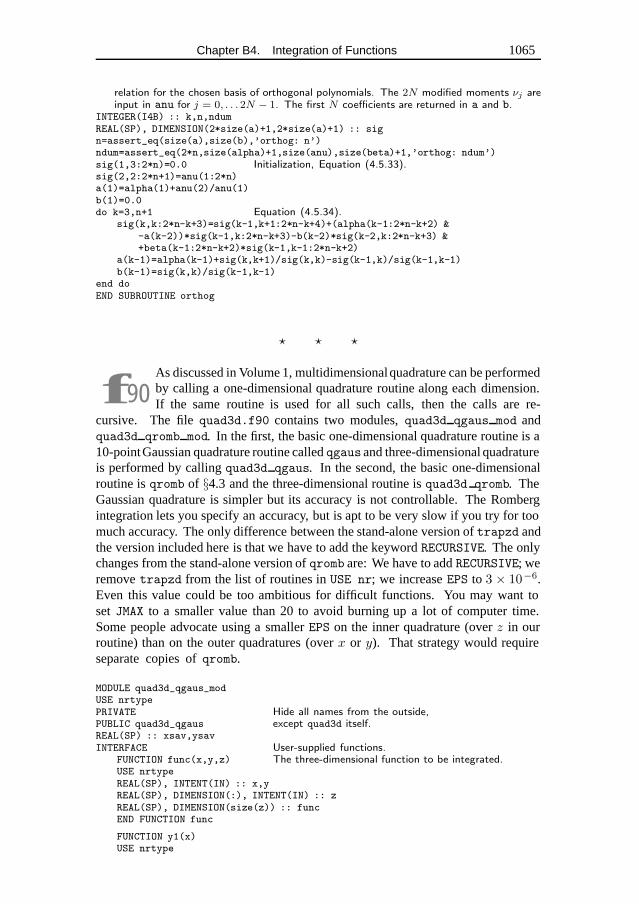
Chapter B4. Integration of Functions 1065
relation for the chosen basis of orthogonal polynomials. The 2N modified moments νj areinput in anu for j = 0, . . .2N − 1. The first N coefficients are returned in a and b.
INTEGER(I4B) :: k,n,ndumREAL(SP), DIMENSION(2*size(a)+1,2*size(a)+1) :: sign=assert_eq(size(a),size(b),’orthog: n’)ndum=assert_eq(2*n,size(alpha)+1,size(anu),size(beta)+1,’orthog: ndum’)sig(1,3:2*n)=0.0 Initialization, Equation (4.5.33).sig(2,2:2*n+1)=anu(1:2*n)a(1)=alpha(1)+anu(2)/anu(1)b(1)=0.0do k=3,n+1 Equation (4.5.34).
sig(k,k:2*n-k+3)=sig(k-1,k+1:2*n-k+4)+(alpha(k-1:2*n-k+2) &-a(k-2))*sig(k-1,k:2*n-k+3)-b(k-2)*sig(k-2,k:2*n-k+3) &+beta(k-1:2*n-k+2)*sig(k-1,k-1:2*n-k+2)
a(k-1)=alpha(k-1)+sig(k,k+1)/sig(k,k)-sig(k-1,k)/sig(k-1,k-1)b(k-1)=sig(k,k)/sig(k-1,k-1)
end doEND SUBROUTINE orthog
� � �
f90As discussed in Volume 1, multidimensionalquadrature can be performedby calling a one-dimensional quadrature routine along each dimension.If the same routine is used for all such calls, then the calls are re-
cursive. The filequad3d.f90 contains two modules,quad3d qgaus mod andquad3d qromb mod. In the first, the basic one-dimensional quadrature routine is a10-pointGaussian quadrature routine calledqgausand three-dimensional quadratureis performed by callingquad3d qgaus. In the second, the basic one-dimensionalroutine isqromb of §4.3 and the three-dimensional routine isquad3d qromb. TheGaussian quadrature is simpler but its accuracy is not controllable. The Rombergintegration lets you specify an accuracy, but is apt to be very slow if you try for toomuch accuracy. The only difference between the stand-alone version oftrapzd andthe version included here is that we have to add the keywordRECURSIVE. The onlychanges from the stand-alone version ofqromb are: We have to addRECURSIVE; weremovetrapzd from the list of routines inUSE nr; we increaseEPS to 3 × 10⁻⁶.Even this value could be too ambitious for difficult functions. You may want toset JMAX to a smaller value than 20 to avoid burning up a lot of computer time.Some people advocate using a smallerEPS on the inner quadrature (overz in ourroutine) than on the outer quadratures (overx or y). That strategy would requireseparate copies ofqromb.
MODULE quad3d_qgaus_modUSE nrtypePRIVATE Hide all names from the outside,PUBLIC quad3d_qgaus except quad3d itself.REAL(SP) :: xsav,ysavINTERFACE User-supplied functions.
FUNCTION func(x,y,z) The three-dimensional function to be integrated.USE nrtypeREAL(SP), INTENT(IN) :: x,yREAL(SP), DIMENSION(:), INTENT(IN) :: zREAL(SP), DIMENSION(size(z)) :: funcEND FUNCTION func
FUNCTION y1(x)USE nrtype
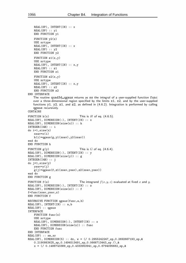
1066 Chapter B4. Integration of Functions
REAL(SP), INTENT(IN) :: xREAL(SP) :: y1END FUNCTION y1
FUNCTION y2(x)USE nrtypeREAL(SP), INTENT(IN) :: xREAL(SP) :: y2END FUNCTION y2
FUNCTION z1(x,y)USE nrtypeREAL(SP), INTENT(IN) :: x,yREAL(SP) :: z1END FUNCTION z1
FUNCTION z2(x,y)USE nrtypeREAL(SP), INTENT(IN) :: x,yREAL(SP) :: z2END FUNCTION z2
END INTERFACEThe routine quad3d qgaus returns as ss the integral of a user-supplied function funcover a three-dimensional region specified by the limits x1, x2, and by the user-suppliedfunctions y1, y2, z1, and z2, as defined in (4.6.2). Integration is performed by callingqgaus recursively.
CONTAINS
FUNCTION h(x) This is H of eq. (4.6.5).REAL(SP), DIMENSION(:), INTENT(IN) :: xREAL(SP), DIMENSION(size(x)) :: hINTEGER(I4B) :: ido i=1,size(x)
xsav=x(i)h(i)=qgaus(g,y1(xsav),y2(xsav))
end doEND FUNCTION h
FUNCTION g(y) This is G of eq. (4.6.4).REAL(SP), DIMENSION(:), INTENT(IN) :: yREAL(SP), DIMENSION(size(y)) :: gINTEGER(I4B) :: jdo j=1,size(y)
ysav=y(j)g(j)=qgaus(f,z1(xsav,ysav),z2(xsav,ysav))
end doEND FUNCTION g
FUNCTION f(z) The integrand f(x, y, z) evaluated at fixed x and y.REAL(SP), DIMENSION(:), INTENT(IN) :: zREAL(SP), DIMENSION(size(z)) :: ff=func(xsav,ysav,z)END FUNCTION f
RECURSIVE FUNCTION qgaus(func,a,b)REAL(SP), INTENT(IN) :: a,bREAL(SP) :: qgausINTERFACE
FUNCTION func(x)USE nrtypeREAL(SP), DIMENSION(:), INTENT(IN) :: xREAL(SP), DIMENSION(size(x)) :: funcEND FUNCTION func
END INTERFACEREAL(SP) :: xm,xrREAL(SP), DIMENSION(5) :: dx, w = (/ 0.2955242247_sp,0.2692667193_sp,&
0.2190863625_sp,0.1494513491_sp,0.0666713443_sp /),&x = (/ 0.1488743389_sp,0.4333953941_sp,0.6794095682_sp,&
Chapter B4. Integration of Functions 1067
0.8650633666_sp,0.9739065285_sp /)xm=0.5_sp*(b+a)xr=0.5_sp*(b-a)dx(:)=xr*x(:)qgaus=xr*sum(w(:)*(func(xm+dx)+func(xm-dx)))END FUNCTION qgaus
SUBROUTINE quad3d_qgaus(x1,x2,ss)REAL(SP), INTENT(IN) :: x1,x2REAL(SP), INTENT(OUT) :: ssss=qgaus(h,x1,x2)END SUBROUTINE quad3d_qgausEND MODULE quad3d_qgaus_mod
f90PRIVATE...PUBLIC quad3d qgaus By default, all module entities are ac-cessible by a routine that uses the module (unless we restrict theUSE
statement withONLY). In this module, the user needs access only to theroutinequad3d qgaus; the variablesxsav, ysav and the proceduresf, g, h, andqgaus are purely internal. It is good programming practice to prevent duplicate nameconflicts or data overwriting by limiting access to only the desired entities. Here thePRIVATE statement with no variable names resets the default fromPUBLIC. Then weinclude in thePUBLIC statement only the function name we want to be accessible.
REAL(SP) :: xsav,ysav In Fortran 90, we generally avoid declaring globalvariables inCOMMON blocks. Instead, we give them complete specifications in amodule. A deficiency of Fortran 90 is that it does not allow pointers to functions. Sohere we have to use the fixed-name functionfunc for the function to be integratedover. If we could have a pointer to a function as a global variable, then we wouldjust set the pointer to point to the user function (of any name) in the calling program.Similarly the functionsy1, y2, z1, andz2 could also have any name.
CONTAINS Here follow the internal subprogramsf, g, h, qgaus, andquad3d qgaus. Note that such internal subprograms are all “visible” to each other,i.e., their interfaces are mutually explicit, and do not requireINTERFACE statements.
RECURSIVE SUBROUTINE qgaus(func,a,b,ss) The RECURSIVE keyword is re-quired for the compiler to process correctly any procedure that is invoked againin its body before the return from the first call has been completed. While somecompilers may let you get away without explicitly informing them that a routineis recursive, don’t count on it!
MODULE quad3d_qromb_modAlternative to quad3d qgaus mod that uses qromb to perform each one-dimensional in-tegration.
USE nrtypePRIVATEPUBLIC quad3d_qrombREAL(SP) :: xsav,ysavINTERFACE
FUNCTION func(x,y,z)USE nrtypeREAL(SP), INTENT(IN) :: x,yREAL(SP), DIMENSION(:), INTENT(IN) :: zREAL(SP), DIMENSION(size(z)) :: funcEND FUNCTION func
FUNCTION y1(x)
1068 Chapter B4. Integration of Functions
USE nrtypeREAL(SP), INTENT(IN) :: xREAL(SP) :: y1END FUNCTION y1
FUNCTION y2(x)USE nrtypeREAL(SP), INTENT(IN) :: xREAL(SP) :: y2END FUNCTION y2
FUNCTION z1(x,y)USE nrtypeREAL(SP), INTENT(IN) :: x,yREAL(SP) :: z1END FUNCTION z1
FUNCTION z2(x,y)USE nrtypeREAL(SP), INTENT(IN) :: x,yREAL(SP) :: z2END FUNCTION z2
END INTERFACECONTAINS
FUNCTION h(x)REAL(SP), DIMENSION(:), INTENT(IN) :: xREAL(SP), DIMENSION(size(x)) :: hINTEGER(I4B) :: ido i=1,size(x)
xsav=x(i)h(i)=qromb(g,y1(xsav),y2(xsav))
end doEND FUNCTION h
FUNCTION g(y)REAL(SP), DIMENSION(:), INTENT(IN) :: yREAL(SP), DIMENSION(size(y)) :: gINTEGER(I4B) :: jdo j=1,size(y)
ysav=y(j)g(j)=qromb(f,z1(xsav,ysav),z2(xsav,ysav))
end doEND FUNCTION g
FUNCTION f(z)REAL(SP), DIMENSION(:), INTENT(IN) :: zREAL(SP), DIMENSION(size(z)) :: ff=func(xsav,ysav,z)END FUNCTION f
RECURSIVE FUNCTION qromb(func,a,b)USE nrtype; USE nrutil, ONLY : nrerrorUSE nr, ONLY : polintIMPLICIT NONEREAL(SP), INTENT(IN) :: a,bREAL(SP) :: qrombINTERFACE
FUNCTION func(x)USE nrtypeREAL(SP), DIMENSION(:), INTENT(IN) :: xREAL(SP), DIMENSION(size(x)) :: funcEND FUNCTION func
END INTERFACEINTEGER(I4B), PARAMETER :: JMAX=20,JMAXP=JMAX+1,K=5,KM=K-1REAL(SP), PARAMETER :: EPS=3.0e-6_spREAL(SP), DIMENSION(JMAXP) :: h,sREAL(SP) :: dqromb
Chapter B4. Integration of Functions 1069
INTEGER(I4B) :: jh(1)=1.0do j=1,JMAX
call trapzd(func,a,b,s(j),j)if (j >= K) then
call polint(h(j-KM:j),s(j-KM:j),0.0_sp,qromb,dqromb)if (abs(dqromb) <= EPS*abs(qromb)) RETURN
end ifs(j+1)=s(j)h(j+1)=0.25_sp*h(j)
end docall nrerror(’qromb: too many steps’)END FUNCTION qromb
RECURSIVE SUBROUTINE trapzd(func,a,b,s,n)USE nrtype; USE nrutil, ONLY : arthIMPLICIT NONEREAL(SP), INTENT(IN) :: a,bREAL(SP), INTENT(INOUT) :: sINTEGER(I4B), INTENT(IN) :: nINTERFACE
FUNCTION func(x)USE nrtypeREAL(SP), DIMENSION(:), INTENT(IN) :: xREAL(SP), DIMENSION(size(x)) :: funcEND FUNCTION func
END INTERFACEREAL(SP) :: del,fsumINTEGER(I4B) :: itif (n == 1) then
s=0.5_sp*(b-a)*sum(func( (/ a,b /) ))else
it=2**(n-2)del=(b-a)/itfsum=sum(func(arth(a+0.5_sp*del,del,it)))s=0.5_sp*(s+del*fsum)
end ifEND SUBROUTINE trapzd
SUBROUTINE quad3d_qromb(x1,x2,ss)REAL(SP), INTENT(IN) :: x1,x2REAL(SP), INTENT(OUT) :: ssss=qromb(h,x1,x2)END SUBROUTINE quad3d_qrombEND MODULE quad3d_qromb_mod
MODULE quad3d qromb_mod The only difference between this module and theprevious one is that all calls toqgaus are replaced by calls toqromb and that theroutineqgaus is replaced byqromb andtrapzd.
CITED REFERENCES AND FURTHER READING:
Erdelyi, A., Magnus, W., Oberhettinger, F., and Tricomi, F.G. 1953, Higher TranscendentalFunctions, Volume II (New York: McGraw-Hill). [1]
Abramowitz, M., and Stegun, I.A. 1964, Handbook of Mathematical Functions, Applied Mathe-matics Series, Volume 55 (Washington: National Bureau of Standards; reprinted 1968 byDover Publications, New York). [2]
Chapter B5. Evaluation of Functions
SUBROUTINE eulsum(sum,term,jterm)USE nrtype; USE nrutil, ONLY : poly_term,reallocateIMPLICIT NONEREAL(SP), INTENT(INOUT) :: sumREAL(SP), INTENT(IN) :: termINTEGER(I4B), INTENT(IN) :: jterm
Incorporates into sum the jterm’th term, with value term, of an alternating series. sumis input as the previous partial sum, and is output as the new partial sum. The first callto this routine, with the first term in the series, should be with jterm=1. On the secondcall, term should be set to the second term of the series, with sign opposite to that of thefirst call, and jterm should be 2. And so on.
REAL(SP), DIMENSION(:), POINTER, SAVE :: wkspINTEGER(I4B), SAVE :: nterm Number of saved differences in wksp.LOGICAL(LGT), SAVE :: init=.true.if (init) then Initialize.
init=.false.nullify(wksp)
end ifif (jterm == 1) then
nterm=1wksp=>reallocate(wksp,100)wksp(1)=termsum=0.5_sp*term Return first estimate.
elseif (nterm+1 > size(wksp)) wksp=>reallocate(wksp,2*size(wksp))wksp(2:nterm+1)=0.5_sp*wksp(1:nterm) Update saved quantities by van Wijn-
gaarden’s algorithm.wksp(1)=termwksp(1:nterm+1)=poly_term(wksp(1:nterm+1),0.5_sp)if (abs(wksp(nterm+1)) <= abs(wksp(nterm))) then Favorable to increase p,
sum=sum+0.5_sp*wksp(nterm+1)nterm=nterm+1 and the table becomes longer.
else Favorable to increase n,sum=sum+wksp(nterm+1) the table doesn’t become longer.
end ifend ifEND SUBROUTINE eulsum
f90This routine uses the function reallocate in nrutil to define atemporary workspace and then, if necessary, enlarge the workspacewithout destroying the earlier contents. The pointer wksp is declared
with the SAVE attribute. Since Fortran 90 pointers are born “in limbo,” wecannot immediately test whether they are associated or not. Hence the codeif (init)...nullify(wksp). Then the line wksp=>reallocate(wksp,100) allocates anarray of length 100 and points wksp to it. On subsequent calls to eulsum, if ntermever gets bigger than the size of wksp, the call to reallocate doubles the size ofwksp and copies the old contents into the new storage.
You could achieve the same effect as the code if (init)...nullify(wksp)...
wksp=>reallocate(wksp,100) with a simple allocate(wksp,100). You would then use
1070
Chapter B5. Evaluation of Functions 1071
reallocate only for increasing the storage if necessary. Don’t! The advantageof the above scheme becomes clear if you consider what happens if eulsum isinvoked twice by the calling program to evaluate two different sums. On the secondinvocation, when jterm = 1 again, you would be allocating an already allocatedpointer. This does not generate an error — it simply leaves the original targetinaccessible. Using reallocate instead not only allocates a new array of length100, but also detects that wksp had already been associated. It dutifully (andwastefully) copies the first 100 elements of the old wksp into the new storage, and,more importantly, deallocates the old wksp, reclaiming its storage. While only twoinvocations of eulsum without intervening deallocation of memory would not causea problem, many such invocations might well. We believe that, as a general rule,the potential for catastrophe from reckless use of allocate is great enough that youshould always deallocate whenever storage is no longer required.
The unnecessary copying of 100 elements when eulsum is invoked a secondtime could be avoided by making init an argument. It hardly seems worth it to us.
For Fortran 90 neophytes, note that unlike in C you have to do nothing special toget the contents of the storage a pointer is addressing. The compiler figures out fromthe context whether you mean the contents, such as wksp(1:nterm), or the address,such as both occurrences of wksp in wksp=>reallocate(wksp,100).
wksp(1:nterm+1)=poly_term(wksp(1:nterm+1),0.5_sp) The poly term func-tion in nrutil tabulates the partial sums of a polynomial, or, equivalently, performsthe synthetic division of a polynomial by a monomial.
Small-scale parallelism in eulsum is achieved straightforwardly by theuse of vector constructions and poly term (which parallelizes recur-sively). The routine is not written to take advantage of data parallelism
in the (infrequent) case of wanting to sum many different series simultaneously; nor,since wksp is a SAVEd variable, can it be used in many simultaneous instances on aMIMD machine. (You can easily recode these generalizations if you need them.)
� � �
SUBROUTINE ddpoly(c,x,pd)USE nrtype; USE nrutil, ONLY : arth,cumprod,poly_termIMPLICIT NONEREAL(SP), INTENT(IN) :: xREAL(SP), DIMENSION(:), INTENT(IN) :: cREAL(SP), DIMENSION(:), INTENT(OUT) :: pd
Given the coefficients of a polynomial of degree Nc − 1 as an array c(1:Nc) with c(1)being the constant term, and given a value x, this routine returns the polynomial evaluatedat x as pd(1) and Nd − 1 derivatives as pd(2:Nd).
INTEGER(I4B) :: i,nc,ndREAL(SP), DIMENSION(size(pd)) :: facREAL(SP), DIMENSION(size(c)) :: dnc=size(c)nd=size(pd)d(nc:1:-1)=poly_term(c(nc:1:-1),x)do i=2,min(nd,nc)
d(nc:i:-1)=poly_term(d(nc:i:-1),x)end dopd=d(1:nd)fac=cumprod(arth(1.0_sp,1.0_sp,nd)) After the first derivative, factorial constants
come in.pd(3:nd)=fac(2:nd-1)*pd(3:nd)END SUBROUTINE ddpoly
1072 Chapter B5. Evaluation of Functions
f90d(nc:1:-1)=poly_term(c(nc:1:-1),x) The poly term function innrutil tabulates the partial sums of a polynomial, or, equivalently,performs synthetic division. See §22.3 for a discussion of why ddpoly
is coded this way.
fac=cumprod(arth(1.0_sp,1.0_sp,nd)) Here the function arth from nrutil
generates the sequence 1, 2, 3. . . . The function cumprod then tabulates the cumu-lative products, thus making a table of factorials.
Notice that ddpoly doesn’t need an argument to pass Nd, the number of outputterms desired by the user: It gets that information from the length of the arraypd that the user provides for it to fill. It is a minor curiosity that pd, declared asINTENT(OUT), can thus be used, on the sly, to pass some INTENT(IN) information.(A Fortran 90 brain teaser could be: A subroutinewith onlyINTENT(OUT) argumentscan be called to print any specified integer. How is this done?)
SUBROUTINE poldiv(u,v,q,r)USE nrtype; USE nrutil, ONLY : assert_eqIMPLICIT NONEREAL(SP), DIMENSION(:), INTENT(IN) :: u,vREAL(SP), DIMENSION(:), INTENT(OUT) :: q,r
Given the N coefficients of a polynomial in u, and the Nv coefficients of another polynomialin v, divide the polynomial u by the polynomial v (“u”/“v”) giving a quotient polynomialwhose coefficients are returned in q, and a remainder polynomial whose coefficients arereturned in r. The arrays q and r are of length N , but only the first N −Nv + 1 elementsof q and the first Nv − 1 elements of r are used. The remaining elements are returnedas zero.
INTEGER(I4B) :: i,n,nvn=assert_eq(size(u),size(q),size(r),’poldiv’)nv=size(v)r(:)=u(:)q(:)=0.0do i=n-nv,0,-1
q(i+1)=r(nv+i)/v(nv)r(i+1:nv+i-1)=r(i+1:nv+i-1)-q(i+1)*v(1:nv-1)
end dor(nv:n)=0.0END SUBROUTINE poldiv
� � �
FUNCTION ratval_s(x,cof,mm,kk)USE nrtype; USE nrutil, ONLY : polyIMPLICIT NONEREAL(DP), INTENT(IN) :: x Note precision! Change to REAL(SP) if desired.INTEGER(I4B), INTENT(IN) :: mm,kkREAL(DP), DIMENSION(mm+kk+1), INTENT(IN) :: cofREAL(DP) :: ratval_s
Given mm, kk, and cof(1:mm+kk+1), evaluate and return the rational function (cof(1)+
cof(2)x+ · · · + cof(mm+1)xmm)/(1 + cof(mm+2)x+ · · · + cof(mm+kk+1)xkk).ratval_s=poly(x,cof(1:mm+1))/(1.0_dp+x*poly(x,cof(mm+2:mm+kk+1)))END FUNCTION ratval_s
f90This simple routine uses the function poly from nrutil to evaluate thenumerator and denominator polynomials. Single- and double-precisionversions, ratval sandratval v, are overloaded onto the nameratval
when the module nr is used.
Chapter B5. Evaluation of Functions 1073
FUNCTION ratval_v(x,cof,mm,kk)USE nrtype; USE nrutil, ONLY : polyIMPLICIT NONEREAL(DP), DIMENSION(:), INTENT(IN) :: xINTEGER(I4B), INTENT(IN) :: mm,kkREAL(DP), DIMENSION(mm+kk+1), INTENT(IN) :: cofREAL(DP), DIMENSION(size(x)) :: ratval_vratval_v=poly(x,cof(1:mm+1))/(1.0_dp+x*poly(x,cof(mm+2:mm+kk+1)))END FUNCTION ratval_v
� � �
The routines recur1 and recur2 are new in this volume, and do not haveFortran 77 counterparts. First- and second-order linear recurrences are implementedas trivial do-loops on strictly serial machines. On parallel machines, however,they pose different, and quite interesting, programming challenges. Since manycalculations can be decomposed into recurrences, it is useful to have general,parallelizable routines available. The algorithms behind recur1 and recur2 arediscussed in §22.2.
RECURSIVE FUNCTION recur1(a,b) RESULT(u)USE nrtype; USE nrutil, ONLY : assert_eqIMPLICIT NONEREAL(SP), DIMENSION(:), INTENT(IN) :: a,bREAL(SP), DIMENSION(size(a)) :: uINTEGER(I4B), PARAMETER :: NPAR_RECUR1=8
Given vectors a of size n and b of size n − 1, returns a vector u that satisfies the firstorder linear recurrence u1 = a1, uj = aj + bj−1uj−1, for j = 2, . . . , n. Parallelization isvia a recursive evaluation.
INTEGER(I4B) :: n,jn=assert_eq(size(a),size(b)+1,’recur1’)u(1)=a(1)if (n < NPAR_RECUR1) then Do short vectors as a loop.
do j=2,nu(j)=a(j)+b(j-1)*u(j-1)
end doelse
Otherwise, combine coefficients and recurse on the even components, then evaluate allthe odd components in parallel.
u(2:n:2)=recur1(a(2:n:2)+a(1:n-1:2)*b(1:n-1:2), &b(3:n-1:2)*b(2:n-2:2))
u(3:n:2)=a(3:n:2)+b(2:n-1:2)*u(2:n-1:2)end ifEND FUNCTION recur1
f90RECURSIVE FUNCTION recur1(a,b) RESULT(u) When a recursive functioninvokes itself only indirectly through a sequence of function calls, thenthe function name can be used for the result just as in a nonrecursive
function. When the function invokes itself directly, however, as in recur1, thenanother name must be used for the result. If you are hazy on the syntax for RESULT,see the discussion of recursion in §21.5.
� � �
1074 Chapter B5. Evaluation of Functions
FUNCTION recur2(a,b,c)USE nrtype; USE nrutil, ONLY : assert_eqIMPLICIT NONEREAL(SP), DIMENSION(:), INTENT(IN) :: a,b,cREAL(SP), DIMENSION(size(a)) :: recur2
Given vectors a of size n and b and c of size n−2, returns a vector u that satisfies the secondorder linear recurrence u1 = a1, u2 = a2, uj = aj+bj−2uj−1+cj−2uj−2, for j = 3, . . . , n.Parallelization is via conversion to a first order recurrence for a two-dimensional vector.
INTEGER(I4B) :: nREAL(SP), DIMENSION(size(a)-1) :: a1,a2,u1,u2REAL(SP), DIMENSION(size(a)-2) :: b11,b12,b21,b22n=assert_eq(size(a),size(b)+2,size(c)+2,’recur2’)a1(1)=a(1) Set up vector a.a2(1)=a(2)a1(2:n-1)=0.0a2(2:n-1)=a(3:n)b11(1:n-2)=0.0 Set up matrix b.b12(1:n-2)=1.0b21(1:n-2)=c(1:n-2)b22(1:n-2)=b(1:n-2)call recur1_v(a1,a2,b11,b12,b21,b22,u1,u2)recur2(1:n-1)=u1(1:n-1)recur2(n)=u2(n-1)CONTAINS
RECURSIVE SUBROUTINE recur1_v(a1,a2,b11,b12,b21,b22,u1,u2)USE nrtype; USE nrutil, ONLY : assert_eqIMPLICIT NONEREAL(SP), DIMENSION(:), INTENT(IN) :: a1,a2,b11,b12,b21,b22REAL(SP), DIMENSION(:), INTENT(OUT) :: u1,u2INTEGER(I4B), PARAMETER :: NPAR_RECUR2=8
Used by recur2 to evaluate first order vector recurrence. Routine is a two-dimensionalvector version of recur1, with matrix multiplication replacing scalar multiplication.
INTEGER(I4B) :: n,j,nn,nn1REAL(SP), DIMENSION(size(a1)/2) :: aa1,aa2REAL(SP), DIMENSION(size(a1)/2-1) :: bb11,bb12,bb21,bb22n=assert_eq((/size(a1),size(a2),size(b11)+1,size(b12)+1,size(b21)+1,&
size(b22)+1,size(u1),size(u2)/),’recur1_v’)u1(1)=a1(1)u2(1)=a2(1)if (n < NPAR_RECUR2) then Do short vectors as a loop.
do j=2,nu1(j)=a1(j)+b11(j-1)*u1(j-1)+b12(j-1)*u2(j-1)u2(j)=a2(j)+b21(j-1)*u1(j-1)+b22(j-1)*u2(j-1)
end doelse
Otherwise, combine coefficients and recurse on the even components, then evaluate allthe odd components in parallel.
nn=n/2nn1=nn-1aa1(1:nn)=a1(2:n:2)+b11(1:n-1:2)*a1(1:n-1:2)+&
b12(1:n-1:2)*a2(1:n-1:2)aa2(1:nn)=a2(2:n:2)+b21(1:n-1:2)*a1(1:n-1:2)+&
b22(1:n-1:2)*a2(1:n-1:2)bb11(1:nn1)=b11(3:n-1:2)*b11(2:n-2:2)+&
b12(3:n-1:2)*b21(2:n-2:2)bb12(1:nn1)=b11(3:n-1:2)*b12(2:n-2:2)+&
b12(3:n-1:2)*b22(2:n-2:2)bb21(1:nn1)=b21(3:n-1:2)*b11(2:n-2:2)+&
b22(3:n-1:2)*b21(2:n-2:2)bb22(1:nn1)=b21(3:n-1:2)*b12(2:n-2:2)+&
b22(3:n-1:2)*b22(2:n-2:2)call recur1_v(aa1,aa2,bb11,bb12,bb21,bb22,u1(2:n:2),u2(2:n:2))u1(3:n:2)=a1(3:n:2)+b11(2:n-1:2)*u1(2:n-1:2)+&
Chapter B5. Evaluation of Functions 1075
b12(2:n-1:2)*u2(2:n-1:2)u2(3:n:2)=a2(3:n:2)+b21(2:n-1:2)*u1(2:n-1:2)+&
b22(2:n-1:2)*u2(2:n-1:2)end ifEND SUBROUTINE recur1_vEND FUNCTION recur2
� � �
FUNCTION dfridr(func,x,h,err)USE nrtype; USE nrutil, ONLY : assert,geop,iminlocIMPLICIT NONEREAL(SP), INTENT(IN) :: x,hREAL(SP), INTENT(OUT) :: errREAL(SP) :: dfridrINTERFACE
FUNCTION func(x)USE nrtypeIMPLICIT NONEREAL(SP), INTENT(IN) :: xREAL(SP) :: funcEND FUNCTION func
END INTERFACEINTEGER(I4B),PARAMETER :: NTAB=10REAL(SP), PARAMETER :: CON=1.4_sp,CON2=CON*CON,BIG=huge(x),SAFE=2.0
Returns the derivative of a function func at a point x by Ridders’ method of polynomialextrapolation. The value h is input as an estimated initial stepsize; it need not be small,but rather should be an increment in x over which func changes substantially. An estimateof the error in the derivative is returned as err.Parameters: Stepsize is decreased by CON at each iteration. Max size of tableau is set byNTAB. Return when error is SAFE worse than the best so far.
INTEGER(I4B) :: ierrmin,i,jREAL(SP) :: hhREAL(SP), DIMENSION(NTAB-1) :: errt,facREAL(SP), DIMENSION(NTAB,NTAB) :: acall assert(h /= 0.0, ’dfridr arg’)hh=ha(1,1)=(func(x+hh)-func(x-hh))/(2.0_sp*hh)err=BIGfac(1:NTAB-1)=geop(CON2,CON2,NTAB-1)do i=2,NTAB Successive columns in the Neville tableau will go to smaller
stepsizes and higher orders of extrapolation.hh=hh/CONa(1,i)=(func(x+hh)-func(x-hh))/(2.0_sp*hh) Try new, smaller stepsize.do j=2,i
Compute extrapolations of various orders, requiring no new function evaluations.a(j,i)=(a(j-1,i)*fac(j-1)-a(j-1,i-1))/(fac(j-1)-1.0_sp)
end doerrt(1:i-1)=max(abs(a(2:i,i)-a(1:i-1,i)),abs(a(2:i,i)-a(1:i-1,i-1)))
The error strategy is to compare each new extrapolation to one order lower, both at thepresent stepsize and the previous one.
ierrmin=iminloc(errt(1:i-1))if (errt(ierrmin) <= err) then If error is decreased, save the improved an-
swer.err=errt(ierrmin)dfridr=a(1+ierrmin,i)
end ifif (abs(a(i,i)-a(i-1,i-1)) >= SAFE*err) RETURN
If higher order is worse by a significant factor SAFE, then quit early.end doEND FUNCTION dfridr
1076 Chapter B5. Evaluation of Functions
f90ierrmin=iminloc(errt(1:i-1)) The function iminloc in nrutil is use-ful when you need to know the index of the smallest element in anarray.
� � �
FUNCTION chebft(a,b,n,func)USE nrtype; USE nrutil, ONLY : arth,outerprodIMPLICIT NONEREAL(SP), INTENT(IN) :: a,bINTEGER(I4B), INTENT(IN) :: nREAL(SP), DIMENSION(n) :: chebftINTERFACE
FUNCTION func(x)USE nrtypeIMPLICIT NONEREAL(SP), DIMENSION(:), INTENT(IN) :: xREAL(SP), DIMENSION(size(x)) :: funcEND FUNCTION func
END INTERFACEChebyshev fit: Given a function func, lower and upper limits of the interval [a,b], anda maximum degree n, this routine computes the n coefficients ck such that func(x) ≈[∑n
k=1 ckTk−1(y)] − c1/2, where y and x are related by (5.8.10). This routine is to beused with moderately large n (e.g., 30 or 50), the array of c’s subsequently to be truncatedat the smaller value m such that cm+1 and subsequent elements are negligible.
REAL(DP) :: bma,bpaREAL(DP), DIMENSION(n) :: thetabma=0.5_dp*(b-a)bpa=0.5_dp*(b+a)theta(:)=PI_D*arth(0.5_dp,1.0_dp,n)/nchebft(:)=matmul(cos(outerprod(arth(0.0_dp,1.0_dp,n),theta)), &
func(real(cos(theta)*bma+bpa,sp)))*2.0_dp/nWe evaluate the function at the n points required by (5.8.7). We accumulate the sumin double precision for safety.
END FUNCTION chebft
f90chebft(:)=matmul(...) Here again Fortran 90 produces a very conciseparallelizable formulation that requires some effort to decode. Equation(5.8.7) is a product of the matrix of cosines, where the rows are indexed
by j and the columns by k, with the vector of function values indexed by k. Weuse the outerprod function in nrutil to form the matrix of arguments for thecosine, and rely on the element-by-element application of cos to produce the matrixof cosines. matmul then takes care of the matrix product. A subtlety is that, whilethe calculation is being done in double precision to minimize roundoff, the functionis assumed to be supplied in single precision. Thus real(...,sp) is used to convertthe double precision argument to single precision.
FUNCTION chebev_s(a,b,c,x)USE nrtype; USE nrutil, ONLY : nrerrorIMPLICIT NONEREAL(SP), INTENT(IN) :: a,b,xREAL(SP), DIMENSION(:), INTENT(IN) :: cREAL(SP) :: chebev_s
Chebyshev evaluation: All arguments are input. c is an array of length M of Chebyshevcoefficients, the first M elements of c output from chebft (which must have been called
Chapter B5. Evaluation of Functions 1077
with the same a and b). The Chebyshev polynomial∑M
k=1 ckTk−1(y) − c1/2 is evaluatedat a point y = [x− (b+ a)/2]/[(b−a)/2], and the result is returned as the function value.
INTEGER(I4B) :: j,mREAL(SP) :: d,dd,sv,y,y2if ((x-a)*(x-b) > 0.0) call nrerror(’x not in range in chebev_s’)m=size(c)d=0.0dd=0.0y=(2.0_sp*x-a-b)/(b-a) Change of variable.y2=2.0_sp*ydo j=m,2,-1 Clenshaw’s recurrence.
sv=dd=y2*d-dd+c(j)dd=sv
end dochebev_s=y*d-dd+0.5_sp*c(1) Last step is different.END FUNCTION chebev_s
FUNCTION chebev_v(a,b,c,x)USE nrtype; USE nrutil, ONLY : nrerrorIMPLICIT NONEREAL(SP), INTENT(IN) :: a,bREAL(SP), DIMENSION(:), INTENT(IN) :: c,xREAL(SP), DIMENSION(size(x)) :: chebev_vINTEGER(I4B) :: j,mREAL(SP), DIMENSION(size(x)) :: d,dd,sv,y,y2if (any((x-a)*(x-b) > 0.0)) call nrerror(’x not in range in chebev_v’)m=size(c)d=0.0dd=0.0y=(2.0_sp*x-a-b)/(b-a)y2=2.0_sp*ydo j=m,2,-1
sv=dd=y2*d-dd+c(j)dd=sv
end dochebev_v=y*d-dd+0.5_sp*c(1)END FUNCTION chebev_v
f90The name chebev is overloaded with scalar and vector versions.chebev v is essentially identical to chebev s except for the decla-rations of the variables. Fortran 90 does the appropriate scalar or vector
arithmetic in the body of the routine, depending on the type of the variables.
� � �
FUNCTION chder(a,b,c)USE nrtype; USE nrutil, ONLY : arth,cumsumIMPLICIT NONEREAL(SP), INTENT(IN) :: a,bREAL(SP), DIMENSION(:), INTENT(IN) :: cREAL(SP), DIMENSION(size(c)) :: chder
This routine returns an array of length N containing the Chebyshev coefficients of thederivative of the function whose coefficients are in the array c. Input are a,b,c, as output
1078 Chapter B5. Evaluation of Functions
from routine chebft §5.8. The desired degree of approximation N is equal to the lengthof c supplied.
INTEGER(I4B) :: nREAL(SP) :: conREAL(SP), DIMENSION(size(c)) :: tempn=size(c)temp(1)=0.0temp(2:n)=2.0_sp*arth(n-1,-1,n-1)*c(n:2:-1)chder(n:1:-2)=cumsum(temp(1:n:2)) Equation (5.9.2).chder(n-1:1:-2)=cumsum(temp(2:n:2))con=2.0_sp/(b-a)chder=chder*con Normalize to the interval b-a.END FUNCTION chder
FUNCTION chint(a,b,c)USE nrtype; USE nrutil, ONLY : arthIMPLICIT NONEREAL(SP), INTENT(IN) :: a,bREAL(SP), DIMENSION(:), INTENT(IN) :: cREAL(SP), DIMENSION(size(c)) :: chint
This routine returns an array of length N containing the Chebyshev coefficients of theintegral of the function whose coefficients are in the array c. Input are a,b,c, as outputfrom routine chebft §5.8. The desired degree of approximation N is equal to the lengthof c supplied. The constant of integration is set so that the integral vanishes at a.
INTEGER(I4B) :: nREAL(SP) :: conn=size(c)con=0.25_sp*(b-a) Factor that normalizes to the interval b-a.chint(2:n-1)=con*(c(1:n-2)-c(3:n))/arth(1,1,n-2) Equation (5.9.1).chint(n)=con*c(n-1)/(n-1) Special case of (5.9.1) for n.chint(1)=2.0_sp*(sum(chint(2:n:2))-sum(chint(3:n:2))) Set the constant of inte-
gration.END FUNCTION chint
f90If you look at equation (5.9.1) for the Chebyshev coefficients of theintegral of a function, you will see c i−1 and ci+1 and be tempted to useeoshift. We think it is almost always better to use array sections instead,
as in the code above, especially if your code will ever run on a serial machine.
� � �
FUNCTION chebpc(c)USE nrtypeIMPLICIT NONEREAL(SP), DIMENSION(:), INTENT(IN) :: cREAL(SP), DIMENSION(size(c)) :: chebpc
Chebyshev polynomial coefficients. Given a coefficient array c of length N , this routine
returns a coefficient array d of length N such that∑N
k=1 dkyk−1 =
∑Nk=1 ckTk−1(y) −
c1/2. The method is Clenshaw’s recurrence (5.8.11), but now applied algebraically ratherthan arithmetically.
INTEGER(I4B) :: j,nREAL(SP), DIMENSION(size(c)) :: dd,svn=size(c)chebpc=0.0dd=0.0chebpc(1)=c(n)do j=n-1,2,-1
sv(2:n-j+1)=chebpc(2:n-j+1)chebpc(2:n-j+1)=2.0_sp*chebpc(1:n-j)-dd(2:n-j+1)dd(2:n-j+1)=sv(2:n-j+1)
Chapter B5. Evaluation of Functions 1079
sv(1)=chebpc(1)chebpc(1)=-dd(1)+c(j)dd(1)=sv(1)
end dochebpc(2:n)=chebpc(1:n-1)-dd(2:n)chebpc(1)=-dd(1)+0.5_sp*c(1)END FUNCTION chebpc
� � �
SUBROUTINE pcshft(a,b,d)USE nrtype; USE nrutil, ONLY : geopIMPLICIT NONEREAL(SP), INTENT(IN) :: a,bREAL(SP), DIMENSION(:), INTENT(INOUT) :: d
Polynomial coefficient shift. Given a coefficient array d of length N , this routine generates
a coefficient array g of the same length such that∑N
k=1 dkyk−1 =
∑Nk=1 gkx
k−1, wherex and y are related by (5.8.10), i.e., the interval −1 < y < 1 is mapped to the intervala < x < b. The array g is returned in d.
INTEGER(I4B) :: j,nREAL(SP), DIMENSION(size(d)) :: ddREAL(SP) :: xn=size(d)dd=d*geop(1.0_sp,2.0_sp/(b-a),n)x=-0.5_sp*(a+b)d(1)=dd(n)d(2:n)=0.0do j=n-1,1,-1 We accomplish the shift by synthetic division, that miracle of
high-school algebra.d(2:n+1-j)=d(2:n+1-j)*x+d(1:n-j)d(1)=d(1)*x+dd(j)
end doEND SUBROUTINE pcshft
There is a subtle, but major, distinction between the synthetic divisionalgorithm used in the Fortran 77 version of pcshft and that used above.In the Fortran 77 version, the synthetic division (translated to Fortran
90 notation) is
d(1:n)=dd(1:n)do j=1,n-1
do k=n-1,j,-1d(k)=x*d(k+1)+d(k)
end doend do
while, in Fortran 90, it is
d(1)=dd(n)d(2:n)=0.0do j=n-1,1,-1
d(2:n+1-j)=d(2:n+1-j)*x+d(1:n-j)d(1)=d(1)*x+dd(j)
end do
As explained in §22.3, these are algebraically — but not algorithmically — equivalent.The inner loop in the Fortran 77 version does not parallelize, because each k valueuses the result of the previous one. In fact, the k loop is a synthetic division, whichcan be parallelized recursively (as in the nrutil routine poly term), but not simply
1080 Chapter B5. Evaluation of Functions
vectorized. In the Fortran 90 version, since not one but n-1 successive syntheticdivisions are to be performed (by the outer loop), it is possible to reorganize thecalculation to allow vectorization.
� � �
FUNCTION pccheb(d)USE nrtype; USE nrutil, ONLY : arth,cumprod,geopIMPLICIT NONEREAL(SP), DIMENSION(:), INTENT(IN) :: dREAL(SP), DIMENSION(size(d)) :: pccheb
Inverse of routine chebpc: given an array of polynomial coefficients d, returns an equivalentarray of Chebyshev coefficients of the same length.
INTEGER(I4B) :: k,nREAL(SP), DIMENSION(size(d)) :: denom,numer,pown=size(d)pccheb(1)=2.0_sp*d(1)pow=geop(1.0_sp,2.0_sp,n) Powers of 2.numer(1)=1.0 Combinatorial coefficients computed as numer/denom.denom(1)=1.0denom(2:(n+3)/2)=cumprod(arth(1.0_sp,1.0_sp,(n+1)/2))pccheb(2:n)=0.0do k=2,n Loop over orders of x in the polynomial.
numer(2:(k+3)/2)=cumprod(arth(k-1.0_sp,-1.0_sp,(k+1)/2))pccheb(k:1:-2)=pccheb(k:1:-2)+&
d(k)/pow(k-1)*numer(1:(k+1)/2)/denom(1:(k+1)/2)end doEND FUNCTION pccheb
� � �
SUBROUTINE pade(cof,resid)USE nrtypeUSE nr, ONLY : lubksb,ludcmp,mproveIMPLICIT NONEREAL(DP), DIMENSION(:), INTENT(INOUT) :: cof DP for consistency with ratval.REAL(SP), INTENT(OUT) :: resid
Given cof(1:2N + 1), the leading terms in the power series expansion of a function, solvethe linear Pade equations to return the coefficients of a diagonal rational function approxi-mation to the same function, namely (cof(1)+ cof(2)x + · · · + cof(N + 1)xN )/(1 +cof(N + 2)x + · · · + cof(2N + 1)xN ). The value resid is the norm of the residualvector; a small value indicates a well-converged solution.
INTEGER(I4B) :: k,nINTEGER(I4B), DIMENSION((size(cof)-1)/2) :: indxREAL(SP), PARAMETER :: BIG=1.0e30_sp A big number.REAL(SP) :: d,rr,rroldREAL(SP), DIMENSION((size(cof)-1)/2) :: x,y,zREAL(SP), DIMENSION((size(cof)-1)/2,(size(cof)-1)/2) :: q,qlun=(size(cof)-1)/2x=cof(n+2:2*n+1) Set up matrix for solving.y=xdo k=1,n
q(:,k)=cof(n+2-k:2*n+1-k)end doqlu=qcall ludcmp(qlu,indx,d) Solve by LU decomposition and backsubsti-
tution.call lubksb(qlu,indx,x)rr=BIGdo Important to use iterative improvement, since
the Pade equations tend to be ill-conditioned.rrold=rr
Chapter B5. Evaluation of Functions 1081
z=xcall mprove(q,qlu,indx,y,x)rr=sum((z-x)**2) Calculate residual.if (rr >= rrold) exit If it is no longer improving, call it quits.
end doresid=sqrt(rrold)do k=1,n Calculate the remaining coefficients.
y(k)=cof(k+1)-dot_product(z(1:k),cof(k:1:-1))end docof(2:n+1)=y Copy answers to output.cof(n+2:2*n+1)=-zEND SUBROUTINE pade
� � �
SUBROUTINE ratlsq(func,a,b,mm,kk,cof,dev)USE nrtype; USE nrutil, ONLY : arth,geopUSE nr, ONLY : ratval,svbksb,svdcmpIMPLICIT NONEREAL(DP), INTENT(IN) :: a,bINTEGER(I4B), INTENT(IN) :: mm,kkREAL(DP), DIMENSION(:), INTENT(OUT) :: cofREAL(DP), INTENT(OUT) :: devINTERFACE
FUNCTION func(x)USE nrtypeREAL(DP), DIMENSION(:), INTENT(IN) :: xREAL(DP), DIMENSION(size(x)) :: funcEND FUNCTION func
END INTERFACEINTEGER(I4B), PARAMETER :: NPFAC=8,MAXIT=5REAL(DP), PARAMETER :: BIG=1.0e30_dp
Returns in cof(1:mm+kk+1) the coefficients of a rational function approximation to thefunction func in the interval (a,b). Input quantities mm and kk specify the order of thenumerator and denominator, respectively. The maximum absolute deviation of the approx-imation (insofar as is known) is returned as dev. Note that double-precision versions ofsvdcmp and svbksb are called.
INTEGER(I4B) :: it,ncof,npt,npthREAL(DP) :: devmax,e,thetaREAL(DP), DIMENSION((mm+kk+1)*NPFAC) :: bb,ee,fs,wt,xsREAL(DP), DIMENSION(mm+kk+1) :: coff,wREAL(DP), DIMENSION(mm+kk+1,mm+kk+1) :: vREAL(DP), DIMENSION((mm+kk+1)*NPFAC,mm+kk+1) :: u,tempncof=mm+kk+1npt=NPFAC*ncof Number of points where function is evaluated,
i.e., fineness of the mesh.npth=npt/2dev=BIGtheta=PIO2_D/(npt-1)xs(1:npth-1)=a+(b-a)*sin(theta*arth(0,1,npth-1))**2
Now fill arrays with mesh abscissas and function values. At each end, use formula that mini-mizes roundoff sensitivity in xs.
xs(npth:npt)=b-(b-a)*sin(theta*arth(npt-npth,-1,npt-npth+1))**2fs=func(xs)wt=1.0 In later iterations we will adjust these weights to
combat the largest deviations.ee=1.0e=0.0do it=1,MAXIT Loop over iterations.
bb=wt*(fs+sign(e,ee))Key idea here: Fit to fn(x) + e where the deviation is positive, to fn(x) − e where it isnegative. Then e is supposed to become an approximation to the equal-ripple deviation.
temp=geop(spread(1.0_dp,1,npt),xs,ncof)
1082 Chapter B5. Evaluation of Functions
Note that vector form of geop (returning matrix) is being used.u(:,1:mm+1)=temp(:,1:mm+1)*spread(wt,2,mm+1)
Set up the “design matrix” for the least squares fit.u(:,mm+2:ncof)=-temp(:,2:ncof-mm)*spread(bb,2,ncof-mm-1)call svdcmp(u,w,v)
Singular Value Decomposition. In especially singular or difficult cases, one might hereedit the singular values w(1:ncof), replacing small values by zero.
call svbksb(u,w,v,bb,coff)ee=ratval(xs,coff,mm,kk)-fs Tabulate the deviations and revise the weights.wt=abs(ee) Use weighting to emphasize most deviant points.devmax=maxval(wt)e=sum(wt)/npt Update e to be the mean absolute deviation.if (devmax <= dev) then Save only the best coefficient set found.
cof=coffdev=devmax
end ifwrite(*,10) it,devmax
end do10 format (’ ratlsq iteration=’,i2,’ max error=’,1p,e10.3)
END SUBROUTINE ratlsq
f90temp=geop(spread(1.0_dp,1,npt),xs,ncof) The design matrix uij is de-fined for i = 1, . . . , npts by
uij =
{wix
j−1i , j = 1, . . . , m+ 1
−bixj−m−2i , j = m+ 2, . . . , n
(B5.12)
The first case in equation (B5.12) is computed in parallel by constructing the matrixtemp equal to
1 x1 x21 · · ·
1 x2 x22 · · ·
1 x3 x23 · · ·
......
.... . .
and then multiplying by the matrix spread(wt,2,mm+1), which is just
w1 w1 w1 · · ·w2 w2 w2 · · ·w3 w3 w3 · · ·...
......
. . .
(Remember that multiplication using * means element-by-element multiplication,not matrix multiplication.) A similar construction is used for the second part ofthe design matrix.
Chapter B6. Special Functions
f90A Fortran 90 intrinsic function such as sin(x) is both generic andelemental. Generic means that the argument x can be any of multipleintrinsic data types and kind values (in the case of sin, any real or
complex kind). Elemental means that x need not be a scalar, but can be an array ofany rank and shape, in which case the calculation of sin is performed independentlyfor each element.
Ideally, when we implement more complicated special functions in Fortran 90,as we do in this chapter, we would make them, too, both generic and elemental.Unfortunately, the language standard does not completely allow this. User-definedelemental functions are prohibited in Fortran 90, though they will be allowed inFortran 95. And, there is no fully automatic way of providing for a single routineto allow arguments of multiple data types or kinds — nothing like C++’s “classtemplates,” for example.
However, don’t give up hope! Fortran 90 does provide a powerful mechanismfor overloading, which can be used (perhaps not always with a maximum ofconvenience) to simulate both generic and elemental function features. In mostcases, when we implement a special function with a scalar argument, gammln(x)say, we will also implement a corresponding vector-valued function of vectorargument that evaluates the special function for each component of the vectorargument. We will then overload the scalar and vector version of the function ontothe same function name. For example, within the nr module are the lines
INTERFACE gammlnFUNCTION gammln_s(xx)USE nrtypeREAL(SP), INTENT(IN) :: xxREAL(SP) :: gammln_sEND FUNCTION gammln_s
FUNCTION gammln_v(xx)USE nrtypeREAL(SP), DIMENSION(:), INTENT(IN) :: xxREAL(SP), DIMENSION(size(xx)) :: gammln_vEND FUNCTION gammln_v
END INTERFACE
which can be included by a statement like “USE nr, ONLY: gammln,” and then allowyou to write gammln(x)without caring (or even thinking about) whether x is a scalaror a vector. If you want arguments of even higher rank (matrices, and so forth), youcan provide these yourself, based on our models, and overload them, too.
That takes care of “elemental”; what about “generic”? Here, too, overloadingprovides an acceptable, if not perfect, solution. Where double-precision versions ofspecial functions are needed, you can in many cases easily construct them from ourprovided routines by changing the variable kinds (and any necessary convergence
1083
1084 Chapter B6. Special Functions
parameters), and then additionally overload them onto the same generic functionnames. (In general, in the interest of brevity, we will not ourselves do this for thefunctions in this chapter.)
At first meeting, Fortran 90’s overloading capability may seem trivial, ormerely cosmetic, to the Fortran 77 programmer; but one soon comes to rely onit as an important conceptual simplification. Programming at a “higher level ofabstraction” is usually more productive than spending time “bogged down in themud.” Furthermore, the use of overloading is generally fail-safe: If you invoke ageneric name with arguments of shapes or types for which a specific routine has notbeen defined, the compiler tells you about it.
We won’t reprint the module nr’s interface blocks for all the routines in thischapter. When you see routines named something s and something v, below,you can safely assume that the generic name something is defined in the modulenr and overloaded with the two specific routine names. A full alphabetical listing ofall the interface blocks in nr is given in Appendix C2.
Given our heavy investment, in this chapter, in overloadable vector-valued special function routines, it is worth discussing whether this effortis simply a stopgap measure for Fortran 90, soon to be made obsolete
by Fortran 95’s provision of user-definable ELEMENTAL procedures. The answer is“not necessarily,” and takes us into some speculation about the future of SIMD,versus MIMD, computing.
Elemental procedures, while applying the same executable code to each element,do not insist that it be feasible to perform all the parallel calculations in lockstep. Thatis, elemental procedures can have tests and branches (if-then-else constructions)that result in different elements being calculated by totally different pieces of code,in a fashion that can only be determined at run time. For true 100% MIMD (multipleinstruction, multiple data) machines, this is not a problem: individual processors dothe individual element calculations asynchronously.
However, virtually none of today’s (and likely tomorrow’s) largest-scale parallelsupercomputers are 100% MIMD in this way. While modern parallel supercomputersincreasingly have MIMD features, they continue to reward the use of SIMD (singleinstruction, multiple data) code with greater computational speed, often because ofhardware pipelining or vector processing features within the individual processors.The use of Fortran 90 (or, for that matter Fortran 95) in a data-parallel or SIMD modeis thus by no means superfluous, or obviated by Fortran 95’sELEMENTALconstruction.
The problem we face is that parallel calculation of special function values oftendoesn’t fit well into the SIMD mold: Since the calculation of the value of a specialfunction typically requires the convergence of an iterative process, as well as possiblebranches for different values of arguments, it cannot in general be done efficientlywith “lockstep” SIMD programming.
Luckily, in particular cases, including most (but not all) of the functions in thischapter, one can in fact make reasonably good parallel implementations with theSIMD tools provided by the language. We will in fact see a number of differenttricks for accomplishing this in the code that follows.
We are interested in demonstrating SIMD techniques, but we are not completelyimpractical. None of the data-parallel implementations given below are too inefficienton a scalar machine, and some may in fact be faster than Fortran 95’s ELEMENTAL
Chapter B6. Special Functions 1085
alternative, or than do-loops over calls to the scalar version of the function. On ascalar machine, how can this be? We have already, above, hinted at the answer: (i)most modern scalar processors can overlap instructions to some degree, and data-parallel coding often provides compilers with the ability to accomplish this moreefficiently; and (ii) data-parallel code can sometimes give better cache utilization.
� � �
FUNCTION gammln_s(xx)USE nrtype; USE nrutil, ONLY : arth,assertIMPLICIT NONEREAL(SP), INTENT(IN) :: xxREAL(SP) :: gammln_s
Returns the value ln[Γ(xx)] for xx > 0.REAL(DP) :: tmp,x
Internal arithmetic will be done in double precision, a nicety that you can omit if five-figureaccuracy is good enough.
REAL(DP) :: stp = 2.5066282746310005_dpREAL(DP), DIMENSION(6) :: coef = (/76.18009172947146_dp,&
-86.50532032941677_dp,24.01409824083091_dp,&-1.231739572450155_dp,0.1208650973866179e-2_dp,&-0.5395239384953e-5_dp/)
call assert(xx > 0.0, ’gammln_s arg’)x=xxtmp=x+5.5_dptmp=(x+0.5_dp)*log(tmp)-tmpgammln_s=tmp+log(stp*(1.000000000190015_dp+&
sum(coef(:)/arth(x+1.0_dp,1.0_dp,size(coef))))/x)END FUNCTION gammln_s
FUNCTION gammln_v(xx)USE nrtype; USE nrutil, ONLY: assertIMPLICIT NONEINTEGER(I4B) :: iREAL(SP), DIMENSION(:), INTENT(IN) :: xxREAL(SP), DIMENSION(size(xx)) :: gammln_vREAL(DP), DIMENSION(size(xx)) :: ser,tmp,x,yREAL(DP) :: stp = 2.5066282746310005_dpREAL(DP), DIMENSION(6) :: coef = (/76.18009172947146_dp,&
-86.50532032941677_dp,24.01409824083091_dp,&-1.231739572450155_dp,0.1208650973866179e-2_dp,&-0.5395239384953e-5_dp/)
if (size(xx) == 0) RETURNcall assert(all(xx > 0.0), ’gammln_v arg’)x=xxtmp=x+5.5_dptmp=(x+0.5_dp)*log(tmp)-tmpser=1.000000000190015_dpy=xdo i=1,size(coef)
y=y+1.0_dpser=ser+coef(i)/y
end dogammln_v=tmp+log(stp*ser/x)END FUNCTION gammln_v
1086 Chapter B6. Special Functions
f90call assert(xx > 0.0, ’gammln_s arg’) We use the nrutil routineassert for functions that have restrictions on the allowed range ofarguments. One could instead have used an if statement with a call
to nrerror; but we think that the uniformity of using assert, and the factthat its logical arguments read the “desired” way, not the “erroneous” way, makefor a clearer programming style. In the vector version, the assert line is:call assert(all(xx > 0.0), ’gammln_v arg’)
Notice that the scalar and vector versions achieve parallelism in quitedifferent ways, something that we will see many times in this chapter.In the scalar case, parallelism (at least small-scale) is achieved through
constructions like
sum(coef(:)/arth(x+1.0_dp,1.0_dp,size(coef)))
Here vector utilities construct the series x + 1, x + 2, . . . and then sum a serieswith these terms in the denominators and a vector of coefficients in the numerators.(This code may seem terse to Fortran 90 novices, but once you get used to it, itis quite clear to read.)
In the vector version, by contrast, parallelism is achieved across the componentsof the vector argument, and the above series is evaluated sequentially as a do-loop.Obviously the assumption is that the length of the vector argument is much longerthan the very modest number (here, 6) of terms in the sum.
� � �
FUNCTION factrl_s(n)USE nrtype; USE nrutil, ONLY : arth,assert,cumprodUSE nr, ONLY : gammlnIMPLICIT NONEINTEGER(I4B), INTENT(IN) :: nREAL(SP) :: factrl_s
Returns the value n! as a floating-point number.INTEGER(I4B), SAVE :: ntop=0INTEGER(I4B), PARAMETER :: NMAX=32REAL(SP), DIMENSION(NMAX), SAVE :: a Table of stored values.call assert(n >= 0, ’factrl_s arg’)if (n < ntop) then Already in table.
factrl_s=a(n+1)else if (n < NMAX) then Fill in table up to NMAX.
ntop=NMAXa(1)=1.0a(2:NMAX)=cumprod(arth(1.0_sp,1.0_sp,NMAX-1))factrl_s=a(n+1)
else Larger value than size of table is required.Actually, this big a value is going to over-flow on many computers, but no harm intrying.
factrl_s=exp(gammln(n+1.0_sp))end ifEND FUNCTION factrl_s
f90cumprod(arth(1.0_sp,1.0_sp,NMAX-1)) By now you should recognize thisas an idiom for generating a vector of consecutive factorials. Theroutines cumprod and arth, both in nrutil, are both capable of being
parallelized, e.g., by recursion, so this idiom is potentially faster than an in-linedo-loop.
Chapter B6. Special Functions 1087
FUNCTION factrl_v(n)USE nrtype; USE nrutil, ONLY : arth,assert,cumprodUSE nr, ONLY : gammlnIMPLICIT NONEINTEGER(I4B), DIMENSION(:), INTENT(IN) :: nREAL(SP), DIMENSION(size(n)) :: factrl_vLOGICAL(LGT), DIMENSION(size(n)) :: maskINTEGER(I4B), SAVE :: ntop=0INTEGER(I4B), PARAMETER :: NMAX=32REAL(SP), DIMENSION(NMAX), SAVE :: acall assert(all(n >= 0), ’factrl_v arg’)if (ntop == 0) then
ntop=NMAXa(1)=1.0a(2:NMAX)=cumprod(arth(1.0_sp,1.0_sp,NMAX-1))
end ifmask = (n >= NMAX)factrl_v=unpack(exp(gammln(pack(n,mask)+1.0_sp)),mask,0.0_sp)where (.not. mask) factrl_v=a(n+1)END FUNCTION factrl_v
unpack(exp(gammln(pack(n,mask)+1.0_sp)),mask,0.0_sp) Here we meetthe first of several solutions to a common problem: How shall we getanswers, from an external vector-valued function, for just a subset of
vector arguments, those defined by a mask? Here we use what we call the “pack-unpack” solution: Pack up all the arguments using the mask, send them to thefunction, and unpack the answers that come back. This packing and unpacking isnot without cost (highly dependent on machine architecture, to be sure), but we hopeto “earn it back” in the parallelism of the external function.
where (.not. mask) factrl_v=a(n+1) In some cases we might take care of the.not.mask case directly within the unpack construction, using its third (“FIELD=”)argument to provide the not-unpacked values. However, there is no guarantee thatthe compiler won’t evaluate all components of the “FIELD=” array, if it finds itefficient to do so. Here, since the index of a(n+1) would be out of range, we can’tdo it this way. Thus the separate where statement.
� � �
FUNCTION bico_s(n,k)USE nrtypeUSE nr, ONLY : factlnIMPLICIT NONEINTEGER(I4B), INTENT(IN) :: n,kREAL(SP) :: bico_s
Returns the binomial coefficient(nk
)as a floating-point number.
bico_s=nint(exp(factln(n)-factln(k)-factln(n-k)))The nearest-integer function cleans up roundoff error for smaller values of n and k.
END FUNCTION bico_s
1088 Chapter B6. Special Functions
FUNCTION bico_v(n,k)USE nrtype; USE nrutil, ONLY : assert_eqUSE nr, ONLY : factlnIMPLICIT NONEINTEGER(I4B), DIMENSION(:), INTENT(IN) :: n,kREAL(SP), DIMENSION(size(n)) :: bico_vINTEGER(I4B) :: ndumndum=assert_eq(size(n),size(k),’bico_v’)bico_v=nint(exp(factln(n)-factln(k)-factln(n-k)))END FUNCTION bico_v
� � �
FUNCTION factln_s(n)USE nrtype; USE nrutil, ONLY : arth,assertUSE nr, ONLY : gammlnIMPLICIT NONEINTEGER(I4B), INTENT(IN) :: nREAL(SP) :: factln_s
Returns ln(n!).INTEGER(I4B), PARAMETER :: TMAX=100REAL(SP), DIMENSION(TMAX), SAVE :: aLOGICAL(LGT), SAVE :: init=.true.if (init) then Initialize the table.
a(1:TMAX)=gammln(arth(1.0_sp,1.0_sp,TMAX))init=.false.
end ifcall assert(n >= 0, ’factln_s arg’)if (n < TMAX) then In range of the table.
factln_s=a(n+1)else Out of range of the table.
factln_s=gammln(n+1.0_sp)end ifEND FUNCTION factln_s
FUNCTION factln_v(n)USE nrtype; USE nrutil, ONLY : arth,assertUSE nr, ONLY : gammlnIMPLICIT NONEINTEGER(I4B), DIMENSION(:), INTENT(IN) :: nREAL(SP), DIMENSION(size(n)) :: factln_vLOGICAL(LGT), DIMENSION(size(n)) :: maskINTEGER(I4B), PARAMETER :: TMAX=100REAL(SP), DIMENSION(TMAX), SAVE :: aLOGICAL(LGT), SAVE :: init=.true.if (init) then
a(1:TMAX)=gammln(arth(1.0_sp,1.0_sp,TMAX))init=.false.
end ifcall assert(all(n >= 0), ’factln_v arg’)mask = (n >= TMAX)factln_v=unpack(gammln(pack(n,mask)+1.0_sp),mask,0.0_sp)where (.not. mask) factln_v=a(n+1)END FUNCTION factln_v
Chapter B6. Special Functions 1089
f90gammln(arth(1.0_sp,1.0_sp,TMAX)) Another example of the program-ming convenience of combining a function returning a vector (here,arth) with a special function whose generic name (here, gammln) has
an overloaded vector version.
� � �
FUNCTION beta_s(z,w)USE nrtypeUSE nr, ONLY : gammlnIMPLICIT NONEREAL(SP), INTENT(IN) :: z,wREAL(SP) :: beta_s
Returns the value of the beta function B(z,w).beta_s=exp(gammln(z)+gammln(w)-gammln(z+w))END FUNCTION beta_s
FUNCTION beta_v(z,w)USE nrtype; USE nrutil, ONLY : assert_eqUSE nr, ONLY : gammlnIMPLICIT NONEREAL(SP), DIMENSION(:), INTENT(IN) :: z,wREAL(SP), DIMENSION(size(z)) :: beta_vINTEGER(I4B) :: ndumndum=assert_eq(size(z),size(w),’beta_v’)beta_v=exp(gammln(z)+gammln(w)-gammln(z+w))END FUNCTION beta_v
� � �
FUNCTION gammp_s(a,x)USE nrtype; USE nrutil, ONLY : assertUSE nr, ONLY : gcf,gserIMPLICIT NONEREAL(SP), INTENT(IN) :: a,xREAL(SP) :: gammp_s
Returns the incomplete gamma function P (a, x).call assert( x >= 0.0, a > 0.0, ’gammp_s args’)if (x<a+1.0_sp) then Use the series representation.
gammp_s=gser(a,x)else Use the continued fraction representation
gammp_s=1.0_sp-gcf(a,x) and take its complement.end ifEND FUNCTION gammp_s
FUNCTION gammp_v(a,x)USE nrtype; USE nrutil, ONLY : assert,assert_eqUSE nr, ONLY : gcf,gserIMPLICIT NONEREAL(SP), DIMENSION(:), INTENT(IN) :: a,xREAL(SP), DIMENSION(size(x)) :: gammp_vLOGICAL(LGT), DIMENSION(size(x)) :: maskINTEGER(I4B) :: ndumndum=assert_eq(size(a),size(x),’gammp_v’)call assert( all(x >= 0.0), all(a > 0.0), ’gammp_v args’)mask = (x<a+1.0_sp)gammp_v=merge(gser(a,merge(x,0.0_sp,mask)), &
1.0_sp-gcf(a,merge(x,0.0_sp,.not. mask)),mask)END FUNCTION gammp_v
1090 Chapter B6. Special Functions
f90call assert( x >= 0.0, a > 0.0, ’gammp_s args’) The generic routineassert in nrutil is overloaded with variants for more than one logicalassertion, so you can make more than one assertion about argument ranges.
gammp_v=merge(gser(a,merge(x,0.0_sp,mask)), &
1.0_sp-gcf(a,merge(x,0.0_sp,.not. mask)),mask) Here we meetthe second solution to the problem of getting masked values from anexternal vector function. (For the first solution, see note to factrl,
above.) We call this one “merge with dummy values”: Inappropriate values of theargument x (as determined by mask) are set to zero before gser, and later gcf, arecalled, and the supernumerary answers returned are discarded by a final merge. Theassumption here is that the dummy value sent to the function (here, zero) is a specialvalue that computes extremely fast, so that the overhead of computing and returningthe supernumerary function values is outweighed by the parallelism achieved on thenontrivial components of x. Look at gser v and gcf v below to judge whetherthis assumption is realistic in this case.
FUNCTION gammq_s(a,x)USE nrtype; USE nrutil, ONLY : assertUSE nr, ONLY : gcf,gserIMPLICIT NONEREAL(SP), INTENT(IN) :: a,xREAL(SP) :: gammq_s
Returns the incomplete gamma function Q(a, x) ≡ 1 − P (a, x).call assert( x >= 0.0, a > 0.0, ’gammq_s args’)if (x<a+1.0_sp) then Use the series representation
gammq_s=1.0_sp-gser(a,x) and take its complement.else Use the continued fraction representation.
gammq_s=gcf(a,x)end ifEND FUNCTION gammq_s
FUNCTION gammq_v(a,x)USE nrtype; USE nrutil, ONLY : assert,assert_eqUSE nr, ONLY : gcf,gserIMPLICIT NONEREAL(SP), DIMENSION(:), INTENT(IN) :: a,xREAL(SP), DIMENSION(size(a)) :: gammq_vLOGICAL(LGT), DIMENSION(size(x)) :: maskINTEGER(I4B) :: ndumndum=assert_eq(size(a),size(x),’gammq_v’)call assert( all(x >= 0.0), all(a > 0.0), ’gammq_v args’)mask = (x<a+1.0_sp)gammq_v=merge(1.0_sp-gser(a,merge(x,0.0_sp,mask)), &
gcf(a,merge(x,0.0_sp,.not. mask)),mask)END FUNCTION gammq_v
FUNCTION gser_s(a,x,gln)USE nrtype; USE nrutil, ONLY : nrerrorUSE nr, ONLY : gammlnIMPLICIT NONEREAL(SP), INTENT(IN) :: a,xREAL(SP), OPTIONAL, INTENT(OUT) :: glnREAL(SP) :: gser_sINTEGER(I4B), PARAMETER :: ITMAX=100REAL(SP), PARAMETER :: EPS=epsilon(x)
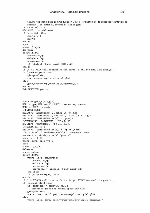
Chapter B6. Special Functions 1091
Returns the incomplete gamma function P (a, x) evaluated by its series representation asgamser. Also optionally returns lnΓ(a) as gln.
INTEGER(I4B) :: nREAL(SP) :: ap,del,summif (x == 0.0) then
gser_s=0.0RETURN
end ifap=asumm=1.0_sp/adel=summdo n=1,ITMAX
ap=ap+1.0_spdel=del*x/apsumm=summ+delif (abs(del) < abs(summ)*EPS) exit
end doif (n > ITMAX) call nrerror(’a too large, ITMAX too small in gser_s’)if (present(gln)) then
gln=gammln(a)gser_s=summ*exp(-x+a*log(x)-gln)
elsegser_s=summ*exp(-x+a*log(x)-gammln(a))
end ifEND FUNCTION gser_s
FUNCTION gser_v(a,x,gln)USE nrtype; USE nrutil, ONLY : assert_eq,nrerrorUSE nr, ONLY : gammlnIMPLICIT NONEREAL(SP), DIMENSION(:), INTENT(IN) :: a,xREAL(SP), DIMENSION(:), OPTIONAL, INTENT(OUT) :: glnREAL(SP), DIMENSION(size(a)) :: gser_vINTEGER(I4B), PARAMETER :: ITMAX=100REAL(SP), PARAMETER :: EPS=epsilon(x)INTEGER(I4B) :: nREAL(SP), DIMENSION(size(a)) :: ap,del,summLOGICAL(LGT), DIMENSION(size(a)) :: converged,zeron=assert_eq(size(a),size(x),’gser_v’)zero=(x == 0.0)where (zero) gser_v=0.0ap=asumm=1.0_sp/adel=summconverged=zerodo n=1,ITMAX
where (.not. converged)ap=ap+1.0_spdel=del*x/apsumm=summ+delconverged = (abs(del) < abs(summ)*EPS)
end whereif (all(converged)) exit
end doif (n > ITMAX) call nrerror(’a too large, ITMAX too small in gser_v’)if (present(gln)) then
if (size(gln) < size(a)) call &nrerror(’gser: Not enough space for gln’)
gln=gammln(a)where (.not. zero) gser_v=summ*exp(-x+a*log(x)-gln)
elsewhere (.not. zero) gser_v=summ*exp(-x+a*log(x)-gammln(a))
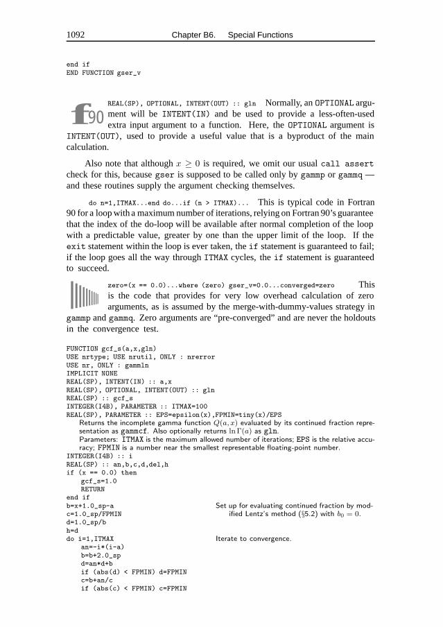
1092 Chapter B6. Special Functions
end ifEND FUNCTION gser_v
f90REAL(SP), OPTIONAL, INTENT(OUT) :: gln Normally, an OPTIONAL argu-ment will be INTENT(IN) and be used to provide a less-often-usedextra input argument to a function. Here, the OPTIONAL argument is
INTENT(OUT), used to provide a useful value that is a byproduct of the maincalculation.
Also note that although x ≥ 0 is required, we omit our usual call assert
check for this, because gser is supposed to be called only by gammp or gammq —and these routines supply the argument checking themselves.
do n=1,ITMAX...end do...if (n > ITMAX)... This is typical code in Fortran90 for a loop with a maximum number of iterations, relying on Fortran 90’s guaranteethat the index of the do-loop will be available after normal completion of the loopwith a predictable value, greater by one than the upper limit of the loop. If theexit statement within the loop is ever taken, the if statement is guaranteed to fail;if the loop goes all the way through ITMAX cycles, the if statement is guaranteedto succeed.
zero=(x == 0.0)...where (zero) gser_v=0.0...converged=zero Thisis the code that provides for very low overhead calculation of zeroarguments, as is assumed by the merge-with-dummy-values strategy in
gammp and gammq. Zero arguments are “pre-converged” and are never the holdoutsin the convergence test.
FUNCTION gcf_s(a,x,gln)USE nrtype; USE nrutil, ONLY : nrerrorUSE nr, ONLY : gammlnIMPLICIT NONEREAL(SP), INTENT(IN) :: a,xREAL(SP), OPTIONAL, INTENT(OUT) :: glnREAL(SP) :: gcf_sINTEGER(I4B), PARAMETER :: ITMAX=100REAL(SP), PARAMETER :: EPS=epsilon(x),FPMIN=tiny(x)/EPS
Returns the incomplete gamma function Q(a, x) evaluated by its continued fraction repre-sentation as gammcf. Also optionally returns lnΓ(a) as gln.Parameters: ITMAX is the maximum allowed number of iterations; EPS is the relative accu-racy; FPMIN is a number near the smallest representable floating-point number.
INTEGER(I4B) :: iREAL(SP) :: an,b,c,d,del,hif (x == 0.0) then
gcf_s=1.0RETURN
end ifb=x+1.0_sp-a Set up for evaluating continued fraction by mod-
ified Lentz’s method (§5.2) with b0 = 0.c=1.0_sp/FPMINd=1.0_sp/bh=ddo i=1,ITMAX Iterate to convergence.
an=-i*(i-a)b=b+2.0_spd=an*d+bif (abs(d) < FPMIN) d=FPMINc=b+an/cif (abs(c) < FPMIN) c=FPMIN
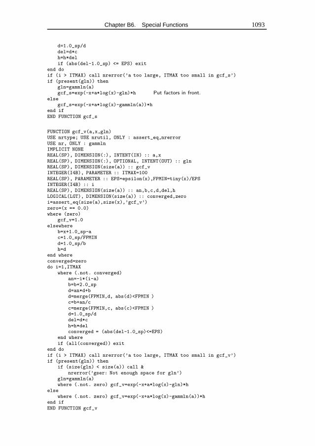
Chapter B6. Special Functions 1093
d=1.0_sp/ddel=d*ch=h*delif (abs(del-1.0_sp) <= EPS) exit
end doif (i > ITMAX) call nrerror(’a too large, ITMAX too small in gcf_s’)if (present(gln)) then
gln=gammln(a)gcf_s=exp(-x+a*log(x)-gln)*h Put factors in front.
elsegcf_s=exp(-x+a*log(x)-gammln(a))*h
end ifEND FUNCTION gcf_s
FUNCTION gcf_v(a,x,gln)USE nrtype; USE nrutil, ONLY : assert_eq,nrerrorUSE nr, ONLY : gammlnIMPLICIT NONEREAL(SP), DIMENSION(:), INTENT(IN) :: a,xREAL(SP), DIMENSION(:), OPTIONAL, INTENT(OUT) :: glnREAL(SP), DIMENSION(size(a)) :: gcf_vINTEGER(I4B), PARAMETER :: ITMAX=100REAL(SP), PARAMETER :: EPS=epsilon(x),FPMIN=tiny(x)/EPSINTEGER(I4B) :: iREAL(SP), DIMENSION(size(a)) :: an,b,c,d,del,hLOGICAL(LGT), DIMENSION(size(a)) :: converged,zeroi=assert_eq(size(a),size(x),’gcf_v’)zero=(x == 0.0)where (zero)
gcf_v=1.0elsewhere
b=x+1.0_sp-ac=1.0_sp/FPMINd=1.0_sp/bh=d
end whereconverged=zerodo i=1,ITMAX
where (.not. converged)an=-i*(i-a)b=b+2.0_spd=an*d+bd=merge(FPMIN,d, abs(d)<FPMIN )c=b+an/cc=merge(FPMIN,c, abs(c)<FPMIN )d=1.0_sp/ddel=d*ch=h*delconverged = (abs(del-1.0_sp)<=EPS)
end whereif (all(converged)) exit
end doif (i > ITMAX) call nrerror(’a too large, ITMAX too small in gcf_v’)if (present(gln)) then
if (size(gln) < size(a)) call &nrerror(’gser: Not enough space for gln’)
gln=gammln(a)where (.not. zero) gcf_v=exp(-x+a*log(x)-gln)*h
elsewhere (.not. zero) gcf_v=exp(-x+a*log(x)-gammln(a))*h
end ifEND FUNCTION gcf_v
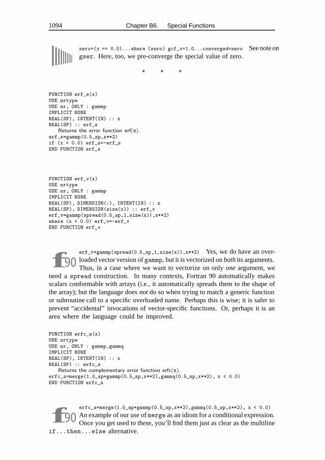
1094 Chapter B6. Special Functions
zero=(x == 0.0)...where (zero) gcf_v=1.0...converged=zero See note ongser. Here, too, we pre-converge the special value of zero.
� � �
FUNCTION erf_s(x)USE nrtypeUSE nr, ONLY : gammpIMPLICIT NONEREAL(SP), INTENT(IN) :: xREAL(SP) :: erf_s
Returns the error function erf(x).erf_s=gammp(0.5_sp,x**2)if (x < 0.0) erf_s=-erf_sEND FUNCTION erf_s
FUNCTION erf_v(x)USE nrtypeUSE nr, ONLY : gammpIMPLICIT NONEREAL(SP), DIMENSION(:), INTENT(IN) :: xREAL(SP), DIMENSION(size(x)) :: erf_verf_v=gammp(spread(0.5_sp,1,size(x)),x**2)where (x < 0.0) erf_v=-erf_vEND FUNCTION erf_v
f90erf_v=gammp(spread(0.5_sp,1,size(x)),x**2) Yes, we do have an over-loaded vector version of gammp, but it is vectorized on both its arguments.Thus, in a case where we want to vectorize on only one argument, we
need a spread construction. In many contexts, Fortran 90 automatically makesscalars conformable with arrays (i.e., it automatically spreads them to the shape ofthe array); but the language does not do so when trying to match a generic functionor subroutine call to a specific overloaded name. Perhaps this is wise; it is safer toprevent “accidental” invocations of vector-specific functions. Or, perhaps it is anarea where the language could be improved.
FUNCTION erfc_s(x)USE nrtypeUSE nr, ONLY : gammp,gammqIMPLICIT NONEREAL(SP), INTENT(IN) :: xREAL(SP) :: erfc_s
Returns the complementary error function erfc(x).erfc_s=merge(1.0_sp+gammp(0.5_sp,x**2),gammq(0.5_sp,x**2), x < 0.0)END FUNCTION erfc_s
f90erfc_s=merge(1.0_sp+gammp(0.5_sp,x**2),gammq(0.5_sp,x**2), x < 0.0)
An example of our use of merge as an idiom for a conditional expression.Once you get used to these, you’ll find them just as clear as the multiline
if...then...else alternative.
Chapter B6. Special Functions 1095
FUNCTION erfc_v(x)USE nrtypeUSE nr, ONLY : gammp,gammqIMPLICIT NONEREAL(SP), DIMENSION(:), INTENT(IN) :: xREAL(SP), DIMENSION(size(x)) :: erfc_vLOGICAL(LGT), DIMENSION(size(x)) :: maskmask = (x < 0.0)erfc_v=merge(1.0_sp+gammp(spread(0.5_sp,1,size(x)), &
merge(x,0.0_sp,mask)**2),gammq(spread(0.5_sp,1,size(x)), &merge(x,0.0_sp,.not. mask)**2),mask)
END FUNCTION erfc_v
f90erfc_v=merge(1.0_sp+...) Another example of the “merge with dummyvalues” idiom described on p. 1090. Here positive values of x in the callto gammp, and negative values in the call to gammq, are first set to the
dummy value zero. The value zero is a special argument that computes very fast.The unwanted dummy function values are then discarded by the final outer merge.
� � �
FUNCTION erfcc_s(x)USE nrtype; USE nrutil, ONLY : polyIMPLICIT NONEREAL(SP), INTENT(IN) :: xREAL(SP) :: erfcc_s
Returns the complementary error function erfc(x) with fractional error everywhere less than1.2 × 10−7.
REAL(SP) :: t,zREAL(SP), DIMENSION(10) :: coef = (/-1.26551223_sp,1.00002368_sp,&
0.37409196_sp,0.09678418_sp,-0.18628806_sp,0.27886807_sp,&-1.13520398_sp,1.48851587_sp,-0.82215223_sp,0.17087277_sp/)
z=abs(x)t=1.0_sp/(1.0_sp+0.5_sp*z)erfcc_s=t*exp(-z*z+poly(t,coef))if (x < 0.0) erfcc_s=2.0_sp-erfcc_sEND FUNCTION erfcc_s
FUNCTION erfcc_v(x)USE nrtype; USE nrutil, ONLY : polyIMPLICIT NONEREAL(SP), DIMENSION(:), INTENT(IN) :: xREAL(SP), DIMENSION(size(x)) :: erfcc_v,t,zREAL(SP), DIMENSION(10) :: coef = (/-1.26551223_sp,1.00002368_sp,&
0.37409196_sp,0.09678418_sp,-0.18628806_sp,0.27886807_sp,&-1.13520398_sp,1.48851587_sp,-0.82215223_sp,0.17087277_sp/)
z=abs(x)t=1.0_sp/(1.0_sp+0.5_sp*z)erfcc_v=t*exp(-z*z+poly(t,coef))where (x < 0.0) erfcc_v=2.0_sp-erfcc_vEND FUNCTION erfcc_v
1096 Chapter B6. Special Functions
f90erfcc_v=t*exp(-z*z+poly(t,coef)) The vector code is identical to thescalar, because the nrutil routine poly has overloaded cases for theevaluation of a polynomial at a single value of the independent variable,
and at multiple values. One could also overload a version with a matrix ofcoefficients whose columns could be used for the simultaneous evaluation ofdifferent polynomials at different values of independent variable. The point is thatas long as there are differences in the shapes of at least one argument, the intendedversion of poly can be discerned by the compiler.
� � �
FUNCTION expint(n,x)USE nrtype; USE nrutil, ONLY : arth,assert,nrerrorIMPLICIT NONEINTEGER(I4B), INTENT(IN) :: nREAL(SP), INTENT(IN) :: xREAL(SP) :: expintINTEGER(I4B), PARAMETER :: MAXIT=100REAL(SP), PARAMETER :: EPS=epsilon(x),BIG=huge(x)*EPS
Evaluates the exponential integral En(x).Parameters: MAXIT is the maximum allowed number of iterations; EPS is the desired relativeerror, not smaller than the machine precision; BIG is a number near the largest representablefloating-point number; EULER (in nrtype) is Euler’s constant γ.
INTEGER(I4B) :: i,nm1REAL(SP) :: a,b,c,d,del,fact,hcall assert(n >= 0, x >= 0.0, (x > 0.0 .or. n > 1), &
’expint args’)if (n == 0) then Special case.
expint=exp(-x)/xRETURN
end ifnm1=n-1if (x == 0.0) then Another special case.
expint=1.0_sp/nm1else if (x > 1.0) then Lentz’s algorithm (§5.2).
b=x+nc=BIGd=1.0_sp/bh=ddo i=1,MAXIT
a=-i*(nm1+i)b=b+2.0_spd=1.0_sp/(a*d+b) Denominators cannot be zero.c=b+a/cdel=c*dh=h*delif (abs(del-1.0_sp) <= EPS) exit
end doif (i > MAXIT) call nrerror(’expint: continued fraction failed’)expint=h*exp(-x)
else Evaluate series.if (nm1 /= 0) then Set first term.
expint=1.0_sp/nm1else
expint=-log(x)-EULERend iffact=1.0do i=1,MAXIT
fact=-fact*x/iif (i /= nm1) then
del=-fact/(i-nm1)
Chapter B6. Special Functions 1097
else ψ(n) appears here.del=fact*(-log(x)-EULER+sum(1.0_sp/arth(1,1,nm1)))
end ifexpint=expint+delif (abs(del) < abs(expint)*EPS) exit
end doif (i > MAXIT) call nrerror(’expint: series failed’)
end ifEND FUNCTION expint
expint does not readily parallelize, and we thus don’t provide a vectorversion. For syntactic convenience you could make a vector version witha do-loop over calls to this scalar version; or, in Fortran 95, you can of
course make the function ELEMENTAL.
� � �
FUNCTION ei(x)USE nrtype; USE nrutil, ONLY : assert,nrerrorIMPLICIT NONEREAL(SP), INTENT(IN) :: xREAL(SP) :: eiINTEGER(I4B), PARAMETER :: MAXIT=100REAL(SP), PARAMETER :: EPS=epsilon(x),FPMIN=tiny(x)/EPS
Computes the exponential integral Ei(x) for x > 0.Parameters: MAXIT is the maximum number of iterations allowed; EPS is the relative error,or absolute error near the zero of Ei at x = 0.3725; FPMIN is a number near the smallestrepresentable floating-point number; EULER (in nrtype) is Euler’s constant γ.
INTEGER(I4B) :: kREAL(SP) :: fact,prev,sm,termcall assert(x > 0.0, ’ei arg’)if (x < FPMIN) then Special case: avoid failure of convergence test
because of underflow.ei=log(x)+EULERelse if (x <= -log(EPS)) then Use power series.
sm=0.0fact=1.0do k=1,MAXIT
fact=fact*x/kterm=fact/ksm=sm+termif (term < EPS*sm) exit
end doif (k > MAXIT) call nrerror(’series failed in ei’)ei=sm+log(x)+EULER
else Use asymptotic series.sm=0.0 Start with second term.term=1.0do k=1,MAXIT
prev=termterm=term*k/xif (term < EPS) exit Since final sum is greater than one, term itself
approximates the relative error.if (term < prev) thensm=sm+term Still converging: add new term.
else Diverging: subtract previous term and exit.sm=sm-prevexit
end ifend doif (k > MAXIT) call nrerror(’asymptotic failed in ei’)ei=exp(x)*(1.0_sp+sm)/x
end ifEND FUNCTION ei
1098 Chapter B6. Special Functions
ei does not readily parallelize, and we thus don’t provide a vectorversion. For syntactic convenience you could make a vector version witha do-loop over calls to this scalar version; or, in Fortran 95, you can of
course make the function ELEMENTAL.
� � �
FUNCTION betai_s(a,b,x)USE nrtype; USE nrutil, ONLY : assertUSE nr, ONLY : betacf,gammlnIMPLICIT NONEREAL(SP), INTENT(IN) :: a,b,xREAL(SP) :: betai_s
Returns the incomplete beta function Ix(a,b).REAL(SP) :: btcall assert(x >= 0.0, x <= 1.0, ’betai_s arg’)if (x == 0.0 .or. x == 1.0) then
bt=0.0else Factors in front of the continued frac-
tion.bt=exp(gammln(a+b)-gammln(a)-gammln(b)&+a*log(x)+b*log(1.0_sp-x))
end ifif (x < (a+1.0_sp)/(a+b+2.0_sp)) then Use continued fraction directly.
betai_s=bt*betacf(a,b,x)/aelse Use continued fraction after making the
symmetry transformation.betai_s=1.0_sp-bt*betacf(b,a,1.0_sp-x)/bend ifEND FUNCTION betai_s
FUNCTION betai_v(a,b,x)USE nrtype; USE nrutil, ONLY : assert,assert_eqUSE nr, ONLY : betacf,gammlnIMPLICIT NONEREAL(SP), DIMENSION(:), INTENT(IN) :: a,b,xREAL(SP), DIMENSION(size(a)) :: betai_vREAL(SP), DIMENSION(size(a)) :: btLOGICAL(LGT), DIMENSION(size(a)) :: maskINTEGER(I4B) :: ndumndum=assert_eq(size(a),size(b),size(x),’betai_v’)call assert(all(x >= 0.0), all(x <= 1.0), ’betai_v arg’)where (x == 0.0 .or. x == 1.0)
bt=0.0elsewhere
bt=exp(gammln(a+b)-gammln(a)-gammln(b)&+a*log(x)+b*log(1.0_sp-x))
end wheremask=(x < (a+1.0_sp)/(a+b+2.0_sp))betai_v=bt*betacf(merge(a,b,mask),merge(b,a,mask),&
merge(x,1.0_sp-x,mask))/merge(a,b,mask)where (.not. mask) betai_v=1.0_sp-betai_vEND FUNCTION betai_v
Chapter B6. Special Functions 1099
f90Compare the scalar
if (x < (a+1.0_sp)/(a+b+2.0_sp)) thenbetai_s=bt*betacf(a,b,x)/a
elsebetai_s=1.0_sp-bt*betacf(b,a,1.0_sp-x)/b
end if
with the vectormask=(x < (a+1.0_sp)/(a+b+2.0_sp))betai_v=bt*betacf(merge(a,b,mask),merge(b,a,mask),&
merge(x,1.0_sp-x,mask))/merge(a,b,mask)where (.not. mask) betai_v=1.0_sp-betai_v
Here merge is used (several times) to evaluate all the required components in asingle call to the vectorized betacf, notwithstanding that some components requireone pattern of arguments, some a different pattern.
FUNCTION betacf_s(a,b,x)USE nrtype; USE nrutil, ONLY : nrerrorIMPLICIT NONEREAL(SP), INTENT(IN) :: a,b,xREAL(SP) :: betacf_sINTEGER(I4B), PARAMETER :: MAXIT=100REAL(SP), PARAMETER :: EPS=epsilon(x), FPMIN=tiny(x)/EPS
Used by betai: Evaluates continued fraction for incomplete beta function by modifiedLentz’s method (§5.2).
REAL(SP) :: aa,c,d,del,h,qab,qam,qapINTEGER(I4B) :: m,m2qab=a+b These q’s will be used in factors that occur
in the coefficients (6.4.6).qap=a+1.0_spqam=a-1.0_spc=1.0 First step of Lentz’s method.d=1.0_sp-qab*x/qapif (abs(d) < FPMIN) d=FPMINd=1.0_sp/dh=ddo m=1,MAXIT
m2=2*maa=m*(b-m)*x/((qam+m2)*(a+m2))d=1.0_sp+aa*d One step (the even one) of the recurrence.if (abs(d) < FPMIN) d=FPMINc=1.0_sp+aa/cif (abs(c) < FPMIN) c=FPMINd=1.0_sp/dh=h*d*caa=-(a+m)*(qab+m)*x/((a+m2)*(qap+m2))d=1.0_sp+aa*d Next step of the recurrence (the odd one).if (abs(d) < FPMIN) d=FPMINc=1.0_sp+aa/cif (abs(c) < FPMIN) c=FPMINd=1.0_sp/ddel=d*ch=h*delif (abs(del-1.0_sp) <= EPS) exit Are we done?
end doif (m > MAXIT)&
call nrerror(’a or b too big, or MAXIT too small in betacf_s’)betacf_s=hEND FUNCTION betacf_s
1100 Chapter B6. Special Functions
FUNCTION betacf_v(a,b,x)USE nrtype; USE nrutil, ONLY : assert_eq,nrerrorIMPLICIT NONEREAL(SP), DIMENSION(:), INTENT(IN) :: a,b,xREAL(SP), DIMENSION(size(x)) :: betacf_vINTEGER(I4B), PARAMETER :: MAXIT=100REAL(SP), PARAMETER :: EPS=epsilon(x), FPMIN=tiny(x)/EPSREAL(SP), DIMENSION(size(x)) :: aa,c,d,del,h,qab,qam,qapLOGICAL(LGT), DIMENSION(size(x)) :: convergedINTEGER(I4B) :: mINTEGER(I4B), DIMENSION(size(x)) :: m2m=assert_eq(size(a),size(b),size(x),’betacf_v’)qab=a+bqap=a+1.0_spqam=a-1.0_spc=1.0d=1.0_sp-qab*x/qapwhere (abs(d) < FPMIN) d=FPMINd=1.0_sp/dh=dconverged=.false.do m=1,MAXIT
where (.not. converged)m2=2*maa=m*(b-m)*x/((qam+m2)*(a+m2))d=1.0_sp+aa*dd=merge(FPMIN,d, abs(d)<FPMIN )c=1.0_sp+aa/cc=merge(FPMIN,c, abs(c)<FPMIN )d=1.0_sp/dh=h*d*caa=-(a+m)*(qab+m)*x/((a+m2)*(qap+m2))d=1.0_sp+aa*dd=merge(FPMIN,d, abs(d)<FPMIN )c=1.0_sp+aa/cc=merge(FPMIN,c, abs(c)<FPMIN )d=1.0_sp/ddel=d*ch=h*delconverged = (abs(del-1.0_sp) <= EPS)
end whereif (all(converged)) exit
end doif (m > MAXIT)&
call nrerror(’a or b too big, or MAXIT too small in betacf_v’)betacf_v=hEND FUNCTION betacf_v
f90d=merge(FPMIN,d, abs(d)<FPMIN ) The scalar version does this with anif. Why does it become a merge here in the vector version, rather than awhere? Because we are already inside a “where (.not.converged)” block,
and Fortran 90 doesn’t allow nested where’s! (Fortran 95 will allow nested where’s.)
� � �
Chapter B6. Special Functions 1101
FUNCTION bessj0_s(x)USE nrtype; USE nrutil, ONLY : polyIMPLICIT NONEREAL(SP), INTENT(IN) :: xREAL(SP) :: bessj0_s
Returns the Bessel function J0(x) for any real x.REAL(SP) :: ax,xx,zREAL(DP) :: y We’ll accumulate polynomials in double precision.REAL(DP), DIMENSION(5) :: p = (/1.0_dp,-0.1098628627e-2_dp,&
0.2734510407e-4_dp,-0.2073370639e-5_dp,0.2093887211e-6_dp/)REAL(DP), DIMENSION(5) :: q = (/-0.1562499995e-1_dp,&
0.1430488765e-3_dp,-0.6911147651e-5_dp,0.7621095161e-6_dp,&-0.934945152e-7_dp/)
REAL(DP), DIMENSION(6) :: r = (/57568490574.0_dp,-13362590354.0_dp,&651619640.7_dp,-11214424.18_dp,77392.33017_dp,&-184.9052456_dp/)
REAL(DP), DIMENSION(6) :: s = (/57568490411.0_dp,1029532985.0_dp,&9494680.718_dp,59272.64853_dp,267.8532712_dp,1.0_dp/)
if (abs(x) < 8.0) then Direct rational function fit.y=x**2bessj0_s=poly(y,r)/poly(y,s)
else Fitting function (6.5.9).ax=abs(x)z=8.0_sp/axy=z**2xx=ax-0.785398164_spbessj0_s=sqrt(0.636619772_sp/ax)*(cos(xx)*&
poly(y,p)-z*sin(xx)*poly(y,q))end ifEND FUNCTION bessj0_s
FUNCTION bessj0_v(x)USE nrtype; USE nrutil, ONLY : polyIMPLICIT NONEREAL(SP), DIMENSION(:), INTENT(IN) :: xREAL(SP), DIMENSION(size(x)) :: bessj0_vREAL(SP), DIMENSION(size(x)) :: ax,xx,zREAL(DP), DIMENSION(size(x)) :: yLOGICAL(LGT), DIMENSION(size(x)) :: maskREAL(DP), DIMENSION(5) :: p = (/1.0_dp,-0.1098628627e-2_dp,&
0.2734510407e-4_dp,-0.2073370639e-5_dp,0.2093887211e-6_dp/)REAL(DP), DIMENSION(5) :: q = (/-0.1562499995e-1_dp,&
0.1430488765e-3_dp,-0.6911147651e-5_dp,0.7621095161e-6_dp,&-0.934945152e-7_dp/)
REAL(DP), DIMENSION(6) :: r = (/57568490574.0_dp,-13362590354.0_dp,&651619640.7_dp,-11214424.18_dp,77392.33017_dp,&-184.9052456_dp/)
REAL(DP), DIMENSION(6) :: s = (/57568490411.0_dp,1029532985.0_dp,&9494680.718_dp,59272.64853_dp,267.8532712_dp,1.0_dp/)
mask = (abs(x) < 8.0)where (mask)
y=x**2bessj0_v=poly(y,r,mask)/poly(y,s,mask)
elsewhereax=abs(x)z=8.0_sp/axy=z**2xx=ax-0.785398164_spbessj0_v=sqrt(0.636619772_sp/ax)*(cos(xx)*&
poly(y,p,.not. mask)-z*sin(xx)*poly(y,q,.not. mask))end whereEND FUNCTION bessj0_v
1102 Chapter B6. Special Functions
where (mask)...bessj0_v=poly(y,r,mask)/poly(y,s,mask) Here we meetthe third solution to the problem of getting masked values from anexternal vector function. (For the other two solutions, see notes to
factrl, p. 1087, and gammp, p. 1090.) Here we simply evade all responsibility andpass the mask into every routine that is supposed to be masked. Let it be somebodyelse’s problem! That works here because your hardworking authors have overloadedthe nrutil routine poly with a masked vector version. More typically, of course,it becomes your problem, and you have to remember to write masked versions of allthe vector routines that you call in this way. (We’ll meet examples of this later.)
� � �
FUNCTION bessy0_s(x)USE nrtype; USE nrutil, ONLY : assert,polyUSE nr, ONLY : bessj0IMPLICIT NONEREAL(SP), INTENT(IN) :: xREAL(SP) :: bessy0_s
Returns the Bessel function Y0(x) for positive x.REAL(SP) :: xx,zREAL(DP) :: y We’ll accumulate polynomials in double precision.REAL(DP), DIMENSION(5) :: p = (/1.0_dp,-0.1098628627e-2_dp,&
0.2734510407e-4_dp,-0.2073370639e-5_dp,0.2093887211e-6_dp/)REAL(DP), DIMENSION(5) :: q = (/-0.1562499995e-1_dp,&
0.1430488765e-3_dp,-0.6911147651e-5_dp,0.7621095161e-6_dp,&-0.934945152e-7_dp/)
REAL(DP), DIMENSION(6) :: r = (/-2957821389.0_dp,7062834065.0_dp,&-512359803.6_dp,10879881.29_dp,-86327.92757_dp,&228.4622733_dp/)
REAL(DP), DIMENSION(6) :: s = (/40076544269.0_dp,745249964.8_dp,&7189466.438_dp,47447.26470_dp,226.1030244_dp,1.0_dp/)
call assert(x > 0.0, ’bessy0_s arg’)if (abs(x) < 8.0) then Rational function approximation of (6.5.8).
y=x**2bessy0_s=(poly(y,r)/poly(y,s))+&
0.636619772_sp*bessj0(x)*log(x)else Fitting function (6.5.10).
z=8.0_sp/xy=z**2xx=x-0.785398164_spbessy0_s=sqrt(0.636619772_sp/x)*(sin(xx)*&
poly(y,p)+z*cos(xx)*poly(y,q))end ifEND FUNCTION bessy0_s
FUNCTION bessy0_v(x)USE nrtype; USE nrutil, ONLY : assert,polyUSE nr, ONLY : bessj0IMPLICIT NONEREAL(SP), DIMENSION(:), INTENT(IN) :: xREAL(SP), DIMENSION(size(x)) :: bessy0_vREAL(SP), DIMENSION(size(x)) :: xx,zREAL(DP), DIMENSION(size(x)) :: yLOGICAL(LGT), DIMENSION(size(x)) :: maskREAL(DP), DIMENSION(5) :: p = (/1.0_dp,-0.1098628627e-2_dp,&
0.2734510407e-4_dp,-0.2073370639e-5_dp,0.2093887211e-6_dp/)REAL(DP), DIMENSION(5) :: q = (/-0.1562499995e-1_dp,&
0.1430488765e-3_dp,-0.6911147651e-5_dp,0.7621095161e-6_dp,&
Chapter B6. Special Functions 1103
-0.934945152e-7_dp/)REAL(DP), DIMENSION(6) :: r = (/-2957821389.0_dp,7062834065.0_dp,&
-512359803.6_dp,10879881.29_dp,-86327.92757_dp,&228.4622733_dp/)
REAL(DP), DIMENSION(6) :: s = (/40076544269.0_dp,745249964.8_dp,&7189466.438_dp,47447.26470_dp,226.1030244_dp,1.0_dp/)
call assert(all(x > 0.0), ’bessy0_v arg’)mask = (abs(x) < 8.0)where (mask)
y=x**2bessy0_v=(poly(y,r,mask)/poly(y,s,mask))+&
0.636619772_sp*bessj0(x)*log(x)elsewhere
z=8.0_sp/xy=z**2xx=x-0.785398164_spbessy0_v=sqrt(0.636619772_sp/x)*(sin(xx)*&
poly(y,p,.not. mask)+z*cos(xx)*poly(y,q,.not. mask))end whereEND FUNCTION bessy0_v
� � �
FUNCTION bessj1_s(x)USE nrtype; USE nrutil, ONLY : polyIMPLICIT NONEREAL(SP), INTENT(IN) :: xREAL(SP) :: bessj1_s
Returns the Bessel function J1(x) for any real x.REAL(SP) :: ax,xx,zREAL(DP) :: y We’ll accumulate polynomials in double precision.REAL(DP), DIMENSION(6) :: r = (/72362614232.0_dp,&
-7895059235.0_dp,242396853.1_dp,-2972611.439_dp,&15704.48260_dp,-30.16036606_dp/)
REAL(DP), DIMENSION(6) :: s = (/144725228442.0_dp,2300535178.0_dp,&18583304.74_dp,99447.43394_dp,376.9991397_dp,1.0_dp/)
REAL(DP), DIMENSION(5) :: p = (/1.0_dp,0.183105e-2_dp,&-0.3516396496e-4_dp,0.2457520174e-5_dp,-0.240337019e-6_dp/)
REAL(DP), DIMENSION(5) :: q = (/0.04687499995_dp,&-0.2002690873e-3_dp,0.8449199096e-5_dp,-0.88228987e-6_dp,&0.105787412e-6_dp/)
if (abs(x) < 8.0) then Direct rational approximation.y=x**2bessj1_s=x*(poly(y,r)/poly(y,s))
else Fitting function (6.5.9).ax=abs(x)z=8.0_sp/axy=z**2xx=ax-2.356194491_spbessj1_s=sqrt(0.636619772_sp/ax)*(cos(xx)*&
poly(y,p)-z*sin(xx)*poly(y,q))*sign(1.0_sp,x)end ifEND FUNCTION bessj1_s
1104 Chapter B6. Special Functions
FUNCTION bessj1_v(x)USE nrtype; USE nrutil, ONLY : polyIMPLICIT NONEREAL(SP), DIMENSION(:), INTENT(IN) :: xREAL(SP), DIMENSION(size(x)) :: bessj1_vREAL(SP), DIMENSION(size(x)) :: ax,xx,zREAL(DP), DIMENSION(size(x)) :: yLOGICAL(LGT), DIMENSION(size(x)) :: maskREAL(DP), DIMENSION(6) :: r = (/72362614232.0_dp,&
-7895059235.0_dp,242396853.1_dp,-2972611.439_dp,&15704.48260_dp,-30.16036606_dp/)
REAL(DP), DIMENSION(6) :: s = (/144725228442.0_dp,2300535178.0_dp,&18583304.74_dp,99447.43394_dp,376.9991397_dp,1.0_dp/)
REAL(DP), DIMENSION(5) :: p = (/1.0_dp,0.183105e-2_dp,&-0.3516396496e-4_dp,0.2457520174e-5_dp,-0.240337019e-6_dp/)
REAL(DP), DIMENSION(5) :: q = (/0.04687499995_dp,&-0.2002690873e-3_dp,0.8449199096e-5_dp,-0.88228987e-6_dp,&0.105787412e-6_dp/)
mask = (abs(x) < 8.0)where (mask)
y=x**2bessj1_v=x*(poly(y,r,mask)/poly(y,s,mask))
elsewhereax=abs(x)z=8.0_sp/axy=z**2xx=ax-2.356194491_spbessj1_v=sqrt(0.636619772_sp/ax)*(cos(xx)*&
poly(y,p,.not. mask)-z*sin(xx)*poly(y,q,.not. mask))*&sign(1.0_sp,x)
end whereEND FUNCTION bessj1_v
� � �
FUNCTION bessy1_s(x)USE nrtype; USE nrutil, ONLY : assert,polyUSE nr, ONLY : bessj1IMPLICIT NONEREAL(SP), INTENT(IN) :: xREAL(SP) :: bessy1_s
Returns the Bessel function Y1(x) for positive x.REAL(SP) :: xx,zREAL(DP) :: y We’ll accumulate polynomials in double precision.REAL(DP), DIMENSION(5) :: p = (/1.0_dp,0.183105e-2_dp,&
-0.3516396496e-4_dp,0.2457520174e-5_dp,-0.240337019e-6_dp/)REAL(DP), DIMENSION(5) :: q = (/0.04687499995_dp,&
-0.2002690873e-3_dp,0.8449199096e-5_dp,-0.88228987e-6_dp,&0.105787412e-6_dp/)
REAL(DP), DIMENSION(6) :: r = (/-0.4900604943e13_dp,&0.1275274390e13_dp,-0.5153438139e11_dp,0.7349264551e9_dp,&-0.4237922726e7_dp,0.8511937935e4_dp/)
REAL(DP), DIMENSION(7) :: s = (/0.2499580570e14_dp,&0.4244419664e12_dp,0.3733650367e10_dp,0.2245904002e8_dp,&0.1020426050e6_dp,0.3549632885e3_dp,1.0_dp/)
call assert(x > 0.0, ’bessy1_s arg’)if (abs(x) < 8.0) then Rational function approximation of (6.5.8).
y=x**2bessy1_s=x*(poly(y,r)/poly(y,s))+&
0.636619772_sp*(bessj1(x)*log(x)-1.0_sp/x)else Fitting function (6.5.10).
Chapter B6. Special Functions 1105
z=8.0_sp/xy=z**2xx=x-2.356194491_spbessy1_s=sqrt(0.636619772_sp/x)*(sin(xx)*&
poly(y,p)+z*cos(xx)*poly(y,q))end ifEND FUNCTION bessy1_s
FUNCTION bessy1_v(x)USE nrtype; USE nrutil, ONLY : assert,polyUSE nr, ONLY : bessj1IMPLICIT NONEREAL(SP), DIMENSION(:), INTENT(IN) :: xREAL(SP), DIMENSION(size(x)) :: bessy1_vREAL(SP), DIMENSION(size(x)) :: xx,zREAL(DP), DIMENSION(size(x)) :: yLOGICAL(LGT), DIMENSION(size(x)) :: maskREAL(DP), DIMENSION(5) :: p = (/1.0_dp,0.183105e-2_dp,&
-0.3516396496e-4_dp,0.2457520174e-5_dp,-0.240337019e-6_dp/)REAL(DP), DIMENSION(5) :: q = (/0.04687499995_dp,&
-0.2002690873e-3_dp,0.8449199096e-5_dp,-0.88228987e-6_dp,&0.105787412e-6_dp/)
REAL(DP), DIMENSION(6) :: r = (/-0.4900604943e13_dp,&0.1275274390e13_dp,-0.5153438139e11_dp,0.7349264551e9_dp,&-0.4237922726e7_dp,0.8511937935e4_dp/)
REAL(DP), DIMENSION(7) :: s = (/0.2499580570e14_dp,&0.4244419664e12_dp,0.3733650367e10_dp,0.2245904002e8_dp,&0.1020426050e6_dp,0.3549632885e3_dp,1.0_dp/)
call assert(all(x > 0.0), ’bessy1_v arg’)mask = (abs(x) < 8.0)where (mask)
y=x**2bessy1_v=x*(poly(y,r,mask)/poly(y,s,mask))+&
0.636619772_sp*(bessj1(x)*log(x)-1.0_sp/x)elsewhere
z=8.0_sp/xy=z**2xx=x-2.356194491_spbessy1_v=sqrt(0.636619772_sp/x)*(sin(xx)*&
poly(y,p,.not. mask)+z*cos(xx)*poly(y,q,.not. mask))end whereEND FUNCTION bessy1_v
� � �
FUNCTION bessy_s(n,x)USE nrtype; USE nrutil, ONLY : assertUSE nr, ONLY : bessy0,bessy1IMPLICIT NONEINTEGER(I4B), INTENT(IN) :: nREAL(SP), INTENT(IN) :: xREAL(SP) :: bessy_s
Returns the Bessel function Yn(x) for positive x and n ≥ 2.INTEGER(I4B) :: jREAL(SP) :: by,bym,byp,toxcall assert(n >= 2, x > 0.0, ’bessy_s args’)tox=2.0_sp/xby=bessy1(x) Starting values for the recurrence.bym=bessy0(x)do j=1,n-1 Recurrence (6.5.7).
1106 Chapter B6. Special Functions
byp=j*tox*by-bymbym=byby=byp
end dobessy_s=byEND FUNCTION bessy_s
FUNCTION bessy_v(n,x)USE nrtype; USE nrutil, ONLY : assertUSE nr, ONLY : bessy0,bessy1IMPLICIT NONEINTEGER(I4B), INTENT(IN) :: nREAL(SP), DIMENSION(:), INTENT(IN) :: xREAL(SP), DIMENSION(size(x)) :: bessy_vINTEGER(I4B) :: jREAL(SP), DIMENSION(size(x)) :: by,bym,byp,toxcall assert(n >= 2, all(x > 0.0), ’bessy_v args’)tox=2.0_sp/xby=bessy1(x)bym=bessy0(x)do j=1,n-1
byp=j*tox*by-bymbym=byby=byp
end dobessy_v=byEND FUNCTION bessy_v
f90Notice that the vector routine is exactly the same as the scalar routine,but operates only on vectors, and that nothing in the routine is specific toany level of precision or kind type of real variable. Cases like this make
us wish that Fortran 90 provided for “template” types that could automatically takethe type and shape of the actual arguments. (Such facilities are available in other,more object-oriented languages such as C++.)
� � �
FUNCTION bessj_s(n,x)USE nrtype; USE nrutil, ONLY : assertUSE nr, ONLY : bessj0,bessj1IMPLICIT NONEINTEGER(I4B), INTENT(IN) :: nREAL(SP), INTENT(IN) :: xREAL(SP) :: bessj_sINTEGER(I4B), PARAMETER :: IACC=40,IEXP=maxexponent(x)/2
Returns the Bessel function Jn(x) for any real x and n ≥ 2. Make the parameter IACClarger to increase accuracy.
INTEGER(I4B) :: j,jsum,mREAL(SP) :: ax,bj,bjm,bjp,summ,toxcall assert(n >= 2, ’bessj_s args’)ax=abs(x)if (ax*ax <= 8.0_sp*tiny(x)) then Underflow limit.
bessj_s=0.0else if (ax > real(n,sp)) then Upwards recurrence from J0 and J1.
tox=2.0_sp/axbjm=bessj0(ax)bj=bessj1(ax)do j=1,n-1
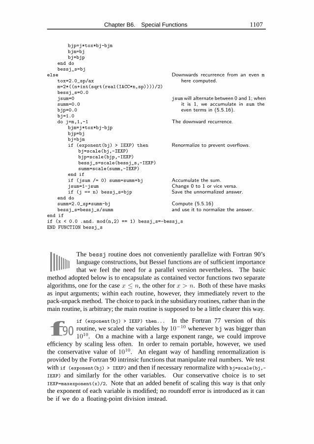
Chapter B6. Special Functions 1107
bjp=j*tox*bj-bjmbjm=bjbj=bjp
end dobessj_s=bj
else Downwards recurrence from an even mhere computed.tox=2.0_sp/ax
m=2*((n+int(sqrt(real(IACC*n,sp))))/2)bessj_s=0.0jsum=0 jsumwill alternate between 0 and 1; when
it is 1, we accumulate in sum theeven terms in (5.5.16).
summ=0.0bjp=0.0bj=1.0do j=m,1,-1 The downward recurrence.
bjm=j*tox*bj-bjpbjp=bjbj=bjmif (exponent(bj) > IEXP) then Renormalize to prevent overflows.
bj=scale(bj,-IEXP)bjp=scale(bjp,-IEXP)bessj_s=scale(bessj_s,-IEXP)summ=scale(summ,-IEXP)
end ifif (jsum /= 0) summ=summ+bj Accumulate the sum.jsum=1-jsum Change 0 to 1 or vice versa.if (j == n) bessj_s=bjp Save the unnormalized answer.
end dosumm=2.0_sp*summ-bj Compute (5.5.16)bessj_s=bessj_s/summ and use it to normalize the answer.
end ifif (x < 0.0 .and. mod(n,2) == 1) bessj_s=-bessj_sEND FUNCTION bessj_s
The bessj routine does not conveniently parallelize with Fortran 90’slanguage constructions, but Bessel functions are of sufficient importancethat we feel the need for a parallel version nevertheless. The basic
method adopted below is to encapsulate as contained vector functions two separatealgorithms, one for the case x ≤ n, the other for x > n. Both of these have masksas input arguments; within each routine, however, they immediately revert to thepack-unpack method. The choice to pack in the subsidiary routines, rather than in themain routine, is arbitrary; the main routine is supposed to be a little clearer this way.
f90if (exponent(bj) > IEXP) then... In the Fortran 77 version of thisroutine, we scaled the variables by 10−10 whenever bj was bigger than1010. On a machine with a large exponent range, we could improve
efficiency by scaling less often. In order to remain portable, however, we usedthe conservative value of 1010. An elegant way of handling renormalization isprovided by the Fortran 90 intrinsic functions that manipulate real numbers. We testwith if (exponent(bj) > IEXP) and then if necessary renormalize with bj=scale(bj,-
IEXP) and similarly for the other variables. Our conservative choice is to setIEXP=maxexponent(x)/2. Note that an added benefit of scaling this way is that onlythe exponent of each variable is modified; no roundoff error is introduced as it canbe if we do a floating-point division instead.
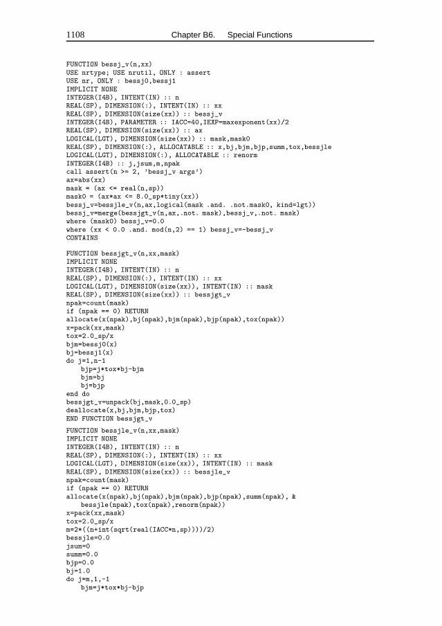
1108 Chapter B6. Special Functions
FUNCTION bessj_v(n,xx)USE nrtype; USE nrutil, ONLY : assertUSE nr, ONLY : bessj0,bessj1IMPLICIT NONEINTEGER(I4B), INTENT(IN) :: nREAL(SP), DIMENSION(:), INTENT(IN) :: xxREAL(SP), DIMENSION(size(xx)) :: bessj_vINTEGER(I4B), PARAMETER :: IACC=40,IEXP=maxexponent(xx)/2REAL(SP), DIMENSION(size(xx)) :: axLOGICAL(LGT), DIMENSION(size(xx)) :: mask,mask0REAL(SP), DIMENSION(:), ALLOCATABLE :: x,bj,bjm,bjp,summ,tox,bessjleLOGICAL(LGT), DIMENSION(:), ALLOCATABLE :: renormINTEGER(I4B) :: j,jsum,m,npakcall assert(n >= 2, ’bessj_v args’)ax=abs(xx)mask = (ax <= real(n,sp))mask0 = (ax*ax <= 8.0_sp*tiny(xx))bessj_v=bessjle_v(n,ax,logical(mask .and. .not.mask0, kind=lgt))bessj_v=merge(bessjgt_v(n,ax,.not. mask),bessj_v,.not. mask)where (mask0) bessj_v=0.0where (xx < 0.0 .and. mod(n,2) == 1) bessj_v=-bessj_vCONTAINS
FUNCTION bessjgt_v(n,xx,mask)IMPLICIT NONEINTEGER(I4B), INTENT(IN) :: nREAL(SP), DIMENSION(:), INTENT(IN) :: xxLOGICAL(LGT), DIMENSION(size(xx)), INTENT(IN) :: maskREAL(SP), DIMENSION(size(xx)) :: bessjgt_vnpak=count(mask)if (npak == 0) RETURNallocate(x(npak),bj(npak),bjm(npak),bjp(npak),tox(npak))x=pack(xx,mask)tox=2.0_sp/xbjm=bessj0(x)bj=bessj1(x)do j=1,n-1
bjp=j*tox*bj-bjmbjm=bjbj=bjp
end dobessjgt_v=unpack(bj,mask,0.0_sp)deallocate(x,bj,bjm,bjp,tox)END FUNCTION bessjgt_v
FUNCTION bessjle_v(n,xx,mask)IMPLICIT NONEINTEGER(I4B), INTENT(IN) :: nREAL(SP), DIMENSION(:), INTENT(IN) :: xxLOGICAL(LGT), DIMENSION(size(xx)), INTENT(IN) :: maskREAL(SP), DIMENSION(size(xx)) :: bessjle_vnpak=count(mask)if (npak == 0) RETURNallocate(x(npak),bj(npak),bjm(npak),bjp(npak),summ(npak), &
bessjle(npak),tox(npak),renorm(npak))x=pack(xx,mask)tox=2.0_sp/xm=2*((n+int(sqrt(real(IACC*n,sp))))/2)bessjle=0.0jsum=0summ=0.0bjp=0.0bj=1.0do j=m,1,-1
bjm=j*tox*bj-bjp
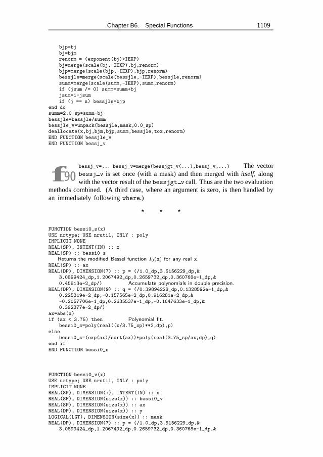
Chapter B6. Special Functions 1109
bjp=bjbj=bjmrenorm = (exponent(bj)>IEXP)bj=merge(scale(bj,-IEXP),bj,renorm)bjp=merge(scale(bjp,-IEXP),bjp,renorm)bessjle=merge(scale(bessjle,-IEXP),bessjle,renorm)summ=merge(scale(summ,-IEXP),summ,renorm)if (jsum /= 0) summ=summ+bjjsum=1-jsumif (j == n) bessjle=bjp
end dosumm=2.0_sp*summ-bjbessjle=bessjle/summbessjle_v=unpack(bessjle,mask,0.0_sp)deallocate(x,bj,bjm,bjp,summ,bessjle,tox,renorm)END FUNCTION bessjle_vEND FUNCTION bessj_v
f90bessj_v=... bessj_v=merge(bessjgt_v(...),bessj_v,...) The vectorbessj v is set once (with a mask) and then merged with itself, alongwith the vector result of the bessjgt v call. Thus are the two evaluation
methods combined. (A third case, where an argument is zero, is then handled byan immediately following where.)
� � �
FUNCTION bessi0_s(x)USE nrtype; USE nrutil, ONLY : polyIMPLICIT NONEREAL(SP), INTENT(IN) :: xREAL(SP) :: bessi0_s
Returns the modified Bessel function I0(x) for any real x.REAL(SP) :: axREAL(DP), DIMENSION(7) :: p = (/1.0_dp,3.5156229_dp,&
3.0899424_dp,1.2067492_dp,0.2659732_dp,0.360768e-1_dp,&0.45813e-2_dp/) Accumulate polynomials in double precision.
REAL(DP), DIMENSION(9) :: q = (/0.39894228_dp,0.1328592e-1_dp,&0.225319e-2_dp,-0.157565e-2_dp,0.916281e-2_dp,&-0.2057706e-1_dp,0.2635537e-1_dp,-0.1647633e-1_dp,&0.392377e-2_dp/)
ax=abs(x)if (ax < 3.75) then Polynomial fit.
bessi0_s=poly(real((x/3.75_sp)**2,dp),p)else
bessi0_s=(exp(ax)/sqrt(ax))*poly(real(3.75_sp/ax,dp),q)end ifEND FUNCTION bessi0_s
FUNCTION bessi0_v(x)USE nrtype; USE nrutil, ONLY : polyIMPLICIT NONEREAL(SP), DIMENSION(:), INTENT(IN) :: xREAL(SP), DIMENSION(size(x)) :: bessi0_vREAL(SP), DIMENSION(size(x)) :: axREAL(DP), DIMENSION(size(x)) :: yLOGICAL(LGT), DIMENSION(size(x)) :: maskREAL(DP), DIMENSION(7) :: p = (/1.0_dp,3.5156229_dp,&
3.0899424_dp,1.2067492_dp,0.2659732_dp,0.360768e-1_dp,&
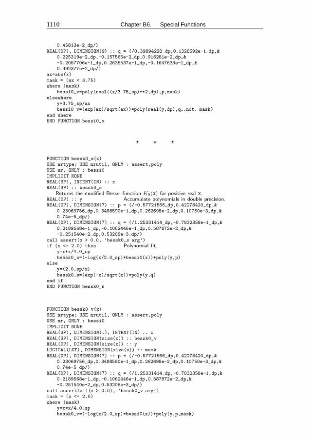
1110 Chapter B6. Special Functions
0.45813e-2_dp/)REAL(DP), DIMENSION(9) :: q = (/0.39894228_dp,0.1328592e-1_dp,&
0.225319e-2_dp,-0.157565e-2_dp,0.916281e-2_dp,&-0.2057706e-1_dp,0.2635537e-1_dp,-0.1647633e-1_dp,&0.392377e-2_dp/)
ax=abs(x)mask = (ax < 3.75)where (mask)
bessi0_v=poly(real((x/3.75_sp)**2,dp),p,mask)elsewhere
y=3.75_sp/axbessi0_v=(exp(ax)/sqrt(ax))*poly(real(y,dp),q,.not. mask)
end whereEND FUNCTION bessi0_v
� � �
FUNCTION bessk0_s(x)USE nrtype; USE nrutil, ONLY : assert,polyUSE nr, ONLY : bessi0IMPLICIT NONEREAL(SP), INTENT(IN) :: xREAL(SP) :: bessk0_s
Returns the modified Bessel function K0(x) for positive real x.REAL(DP) :: y Accumulate polynomials in double precision.REAL(DP), DIMENSION(7) :: p = (/-0.57721566_dp,0.42278420_dp,&
0.23069756_dp,0.3488590e-1_dp,0.262698e-2_dp,0.10750e-3_dp,&0.74e-5_dp/)
REAL(DP), DIMENSION(7) :: q = (/1.25331414_dp,-0.7832358e-1_dp,&0.2189568e-1_dp,-0.1062446e-1_dp,0.587872e-2_dp,&-0.251540e-2_dp,0.53208e-3_dp/)
call assert(x > 0.0, ’bessk0_s arg’)if (x <= 2.0) then Polynomial fit.
y=x*x/4.0_spbessk0_s=(-log(x/2.0_sp)*bessi0(x))+poly(y,p)
elsey=(2.0_sp/x)bessk0_s=(exp(-x)/sqrt(x))*poly(y,q)
end ifEND FUNCTION bessk0_s
FUNCTION bessk0_v(x)USE nrtype; USE nrutil, ONLY : assert,polyUSE nr, ONLY : bessi0IMPLICIT NONEREAL(SP), DIMENSION(:), INTENT(IN) :: xREAL(SP), DIMENSION(size(x)) :: bessk0_vREAL(DP), DIMENSION(size(x)) :: yLOGICAL(LGT), DIMENSION(size(x)) :: maskREAL(DP), DIMENSION(7) :: p = (/-0.57721566_dp,0.42278420_dp,&
0.23069756_dp,0.3488590e-1_dp,0.262698e-2_dp,0.10750e-3_dp,&0.74e-5_dp/)
REAL(DP), DIMENSION(7) :: q = (/1.25331414_dp,-0.7832358e-1_dp,&0.2189568e-1_dp,-0.1062446e-1_dp,0.587872e-2_dp,&-0.251540e-2_dp,0.53208e-3_dp/)
call assert(all(x > 0.0), ’bessk0_v arg’)mask = (x <= 2.0)where (mask)
y=x*x/4.0_spbessk0_v=(-log(x/2.0_sp)*bessi0(x))+poly(y,p,mask)
Chapter B6. Special Functions 1111
elsewherey=(2.0_sp/x)bessk0_v=(exp(-x)/sqrt(x))*poly(y,q,.not. mask)
end whereEND FUNCTION bessk0_v
� � �
FUNCTION bessi1_s(x)USE nrtype; USE nrutil, ONLY : polyIMPLICIT NONEREAL(SP), INTENT(IN) :: xREAL(SP) :: bessi1_s
Returns the modified Bessel function I1(x) for any real x.REAL(SP) :: axREAL(DP), DIMENSION(7) :: p = (/0.5_dp,0.87890594_dp,&
0.51498869_dp,0.15084934_dp,0.2658733e-1_dp,&0.301532e-2_dp,0.32411e-3_dp/)Accumulate polynomials in double precision.
REAL(DP), DIMENSION(9) :: q = (/0.39894228_dp,-0.3988024e-1_dp,&-0.362018e-2_dp,0.163801e-2_dp,-0.1031555e-1_dp,&0.2282967e-1_dp,-0.2895312e-1_dp,0.1787654e-1_dp,&-0.420059e-2_dp/)
ax=abs(x)if (ax < 3.75) then Polynomial fit.
bessi1_s=ax*poly(real((x/3.75_sp)**2,dp),p)else
bessi1_s=(exp(ax)/sqrt(ax))*poly(real(3.75_sp/ax,dp),q)end ifif (x < 0.0) bessi1_s=-bessi1_sEND FUNCTION bessi1_s
FUNCTION bessi1_v(x)USE nrtype; USE nrutil, ONLY : polyIMPLICIT NONEREAL(SP), DIMENSION(:), INTENT(IN) :: xREAL(SP), DIMENSION(size(x)) :: bessi1_vREAL(SP), DIMENSION(size(x)) :: axREAL(DP), DIMENSION(size(x)) :: yLOGICAL(LGT), DIMENSION(size(x)) :: maskREAL(DP), DIMENSION(7) :: p = (/0.5_dp,0.87890594_dp,&
0.51498869_dp,0.15084934_dp,0.2658733e-1_dp,&0.301532e-2_dp,0.32411e-3_dp/)
REAL(DP), DIMENSION(9) :: q = (/0.39894228_dp,-0.3988024e-1_dp,&-0.362018e-2_dp,0.163801e-2_dp,-0.1031555e-1_dp,&0.2282967e-1_dp,-0.2895312e-1_dp,0.1787654e-1_dp,&-0.420059e-2_dp/)
ax=abs(x)mask = (ax < 3.75)where (mask)
bessi1_v=ax*poly(real((x/3.75_sp)**2,dp),p,mask)elsewhere
y=3.75_sp/axbessi1_v=(exp(ax)/sqrt(ax))*poly(real(y,dp),q,.not. mask)
end wherewhere (x < 0.0) bessi1_v=-bessi1_vEND FUNCTION bessi1_v
1112 Chapter B6. Special Functions
� � �
FUNCTION bessk1_s(x)USE nrtype; USE nrutil, ONLY : assert,polyUSE nr, ONLY : bessi1IMPLICIT NONEREAL(SP), INTENT(IN) :: xREAL(SP) :: bessk1_s
Returns the modified Bessel function K1(x) for positive real x.REAL(DP) :: y Accumulate polynomials in double precision.REAL(DP), DIMENSION(7) :: p = (/1.0_dp,0.15443144_dp,&
-0.67278579_dp,-0.18156897_dp,-0.1919402e-1_dp,&-0.110404e-2_dp,-0.4686e-4_dp/)
REAL(DP), DIMENSION(7) :: q = (/1.25331414_dp,0.23498619_dp,&-0.3655620e-1_dp,0.1504268e-1_dp,-0.780353e-2_dp,&0.325614e-2_dp,-0.68245e-3_dp/)
call assert(x > 0.0, ’bessk1_s arg’)if (x <= 2.0) then Polynomial fit.
y=x*x/4.0_spbessk1_s=(log(x/2.0_sp)*bessi1(x))+(1.0_sp/x)*poly(y,p)
elsey=2.0_sp/xbessk1_s=(exp(-x)/sqrt(x))*poly(y,q)
end ifEND FUNCTION bessk1_s
FUNCTION bessk1_v(x)USE nrtype; USE nrutil, ONLY : assert,polyUSE nr, ONLY : bessi1IMPLICIT NONEREAL(SP), DIMENSION(:), INTENT(IN) :: xREAL(SP), DIMENSION(size(x)) :: bessk1_vREAL(DP), DIMENSION(size(x)) :: yLOGICAL(LGT), DIMENSION(size(x)) :: maskREAL(DP), DIMENSION(7) :: p = (/1.0_dp,0.15443144_dp,&
-0.67278579_dp,-0.18156897_dp,-0.1919402e-1_dp,&-0.110404e-2_dp,-0.4686e-4_dp/)
REAL(DP), DIMENSION(7) :: q = (/1.25331414_dp,0.23498619_dp,&-0.3655620e-1_dp,0.1504268e-1_dp,-0.780353e-2_dp,&0.325614e-2_dp,-0.68245e-3_dp/)
call assert(all(x > 0.0), ’bessk1_v arg’)mask = (x <= 2.0)where (mask)
y=x*x/4.0_spbessk1_v=(log(x/2.0_sp)*bessi1(x))+(1.0_sp/x)*poly(y,p,mask)
elsewherey=2.0_sp/xbessk1_v=(exp(-x)/sqrt(x))*poly(y,q,.not. mask)
end whereEND FUNCTION bessk1_v
� � �
Chapter B6. Special Functions 1113
FUNCTION bessk_s(n,x)USE nrtype; USE nrutil, ONLY : assertUSE nr, ONLY : bessk0,bessk1IMPLICIT NONEINTEGER(I4B), INTENT(IN) :: nREAL(SP), INTENT(IN) :: xREAL(SP) :: bessk_s
Returns the modified Bessel function Kn(x) for positive x and n ≥ 2.INTEGER(I4B) :: jREAL(SP) :: bk,bkm,bkp,toxcall assert(n >= 2, x > 0.0, ’bessk_s args’)tox=2.0_sp/xbkm=bessk0(x) Upward recurrence for all x...bk=bessk1(x)do j=1,n-1 ...and here it is.
bkp=bkm+j*tox*bkbkm=bkbk=bkp
end dobessk_s=bkEND FUNCTION bessk_s
FUNCTION bessk_v(n,x)USE nrtype; USE nrutil, ONLY : assertUSE nr, ONLY : bessk0,bessk1IMPLICIT NONEINTEGER(I4B), INTENT(IN) :: nREAL(SP), DIMENSION(:), INTENT(IN) :: xREAL(SP), DIMENSION(size(x)) :: bessk_vINTEGER(I4B) :: jREAL(SP), DIMENSION(size(x)) :: bk,bkm,bkp,toxcall assert(n >= 2, all(x > 0.0), ’bessk_v args’)tox=2.0_sp/xbkm=bessk0(x)bk=bessk1(x)do j=1,n-1
bkp=bkm+j*tox*bkbkm=bkbk=bkp
end dobessk_v=bkEND FUNCTION bessk_v
f90The scalar and vector versions of bessk are identical, and have noprecision-specific constants, another example of where we would like todefine a generic “template” function if the language had this facility.
� � �
1114 Chapter B6. Special Functions
FUNCTION bessi_s(n,x)USE nrtype; USE nrutil, ONLY : assertUSE nr, ONLY : bessi0IMPLICIT NONEINTEGER(I4B), INTENT(IN) :: nREAL(SP), INTENT(IN) :: xREAL(SP) :: bessi_sINTEGER(I4B), PARAMETER :: IACC=40,IEXP=maxexponent(x)/2
Returns the modified Bessel function In(x) for any real x and n ≥ 2. Make the parameterIACC larger to increase accuracy.
INTEGER(I4B) :: j,mREAL(SP) :: bi,bim,bip,toxcall assert(n >= 2, ’bessi_s args’)bessi_s=0.0if (x*x <= 8.0_sp*tiny(x)) RETURN Underflow limit.tox=2.0_sp/abs(x)bip=0.0bi=1.0m=2*((n+int(sqrt(real(IACC*n,sp))))) Downward recurrence from even m.do j=m,1,-1
bim=bip+j*tox*bi The downward recurrence.bip=bibi=bimif (exponent(bi) > IEXP) then Renormalize to prevent overflows.
bessi_s=scale(bessi_s,-IEXP)bi=scale(bi,-IEXP)bip=scale(bip,-IEXP)
end ifif (j == n) bessi_s=bip
end dobessi_s=bessi_s*bessi0(x)/bi Normalize with bessi0.if (x < 0.0 .and. mod(n,2) == 1) bessi_s=-bessi_sEND FUNCTION bessi_s
f90if (exponent(bi) > IEXP) then See discussion of scaling for bessj onp. 1107.
FUNCTION bessi_v(n,x)USE nrtype; USE nrutil, ONLY : assertUSE nr, ONLY : bessi0IMPLICIT NONEINTEGER(I4B), INTENT(IN) :: nREAL(SP), DIMENSION(:), INTENT(IN) :: xREAL(SP), DIMENSION(size(x)) :: bessi_vINTEGER(I4B), PARAMETER :: IACC=40,IEXP=maxexponent(x)/2INTEGER(I4B) :: j,mREAL(SP), DIMENSION(size(x)) :: bi,bim,bip,toxLOGICAL(LGT), DIMENSION(size(x)) :: maskcall assert(n >= 2, ’bessi_v args’)bessi_v=0.0mask = (x <= 8.0_sp*tiny(x))tox=2.0_sp/merge(2.0_sp,abs(x),mask)bip=0.0bi=1.0_spm=2*((n+int(sqrt(real(IACC*n,sp)))))do j=m,1,-1
bim=bip+j*tox*bibip=bibi=bimwhere (exponent(bi) > IEXP)
bessi_v=scale(bessi_v,-IEXP)
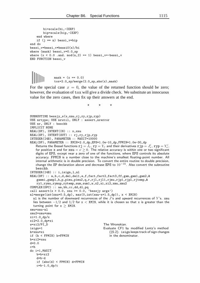
Chapter B6. Special Functions 1115
bi=scale(bi,-IEXP)bip=scale(bip,-IEXP)
end whereif (j == n) bessi_v=bip
end dobessi_v=bessi_v*bessi0(x)/biwhere (mask) bessi_v=0.0_spwhere (x < 0.0 .and. mod(n,2) == 1) bessi_v=-bessi_vEND FUNCTION bessi_v
mask = (x == 0.0)tox=2.0_sp/merge(2.0_sp,abs(x),mask)
For the special case x = 0, the value of the returned function should be zero;however, the evaluation of tox will give a divide check. We substitute an innocuousvalue for the zero cases, then fix up their answers at the end.
� � �
SUBROUTINE bessjy_s(x,xnu,rj,ry,rjp,ryp)USE nrtype; USE nrutil, ONLY : assert,nrerrorUSE nr, ONLY : beschbIMPLICIT NONEREAL(SP), INTENT(IN) :: x,xnuREAL(SP), INTENT(OUT) :: rj,ry,rjp,rypINTEGER(I4B), PARAMETER :: MAXIT=10000REAL(DP), PARAMETER :: XMIN=2.0_dp,EPS=1.0e-10_dp,FPMIN=1.0e-30_dp
Returns the Bessel functions rj = Jν , ry = Yν and their derivatives rjp = J ′ν , ryp = Y ′
ν ,for positive x and for xnu = ν ≥ 0. The relative accuracy is within one or two significantdigits of EPS, except near a zero of one of the functions, where EPS controls its absoluteaccuracy. FPMIN is a number close to the machine’s smallest floating-point number. Allinternal arithmetic is in double precision. To convert the entire routine to double precision,change the SP declaration above and decrease EPS to 10−16. Also convert the subroutinebeschb.
INTEGER(I4B) :: i,isign,l,nlREAL(DP) :: a,b,c,d,del,del1,e,f,fact,fact2,fact3,ff,gam,gam1,gam2,&
gammi,gampl,h,p,pimu,pimu2,q,r,rjl,rjl1,rjmu,rjp1,rjpl,rjtemp,&ry1,rymu,rymup,rytemp,sum,sum1,w,x2,xi,xi2,xmu,xmu2
COMPLEX(DPC) :: aa,bb,cc,dd,dl,pqcall assert(x > 0.0, xnu >= 0.0, ’bessjy args’)nl=merge(int(xnu+0.5_dp), max(0,int(xnu-x+1.5_dp)), x < XMIN)nl is the number of downward recurrences of the J’s and upward recurrences of Y ’s. xmulies between −1/2 and 1/2 for x < XMIN, while it is chosen so that x is greater than theturning point for x ≥ XMIN.
xmu=xnu-nlxmu2=xmu*xmuxi=1.0_dp/xxi2=2.0_dp*xiw=xi2/PI_D The Wronskian.isign=1 Evaluate CF1 by modified Lentz’s method
(§5.2). isign keeps track of sign changesin the denominator.
h=xnu*xiif (h < FPMIN) h=FPMINb=xi2*xnud=0.0c=hdo i=1,MAXIT
b=b+xi2d=b-dif (abs(d) < FPMIN) d=FPMINc=b-1.0_dp/c
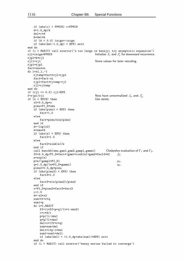
1116 Chapter B6. Special Functions
if (abs(c) < FPMIN) c=FPMINd=1.0_dp/ddel=c*dh=del*hif (d < 0.0) isign=-isignif (abs(del-1.0_dp) < EPS) exit
end doif (i > MAXIT) call nrerror(’x too large in bessjy; try asymptotic expansion’)rjl=isign*FPMIN Initialize Jν and J ′
ν for downward recurrence.rjpl=h*rjlrjl1=rjl Store values for later rescaling.rjp1=rjplfact=xnu*xido l=nl,1,-1
rjtemp=fact*rjl+rjplfact=fact-xirjpl=fact*rjtemp-rjlrjl=rjtemp
end doif (rjl == 0.0) rjl=EPSf=rjpl/rjl Now have unnormalized Jµ and J ′
µ.if (x < XMIN) then Use series.
x2=0.5_dp*xpimu=PI_D*xmuif (abs(pimu) < EPS) then
fact=1.0else
fact=pimu/sin(pimu)end ifd=-log(x2)e=xmu*dif (abs(e) < EPS) then
fact2=1.0else
fact2=sinh(e)/eend ifcall beschb(xmu,gam1,gam2,gampl,gammi) Chebyshev evaluation of Γ1 and Γ2.ff=2.0_dp/PI_D*fact*(gam1*cosh(e)+gam2*fact2*d) f0.e=exp(e)p=e/(gampl*PI_D) p0.q=1.0_dp/(e*PI_D*gammi) q0.pimu2=0.5_dp*pimuif (abs(pimu2) < EPS) then
fact3=1.0else
fact3=sin(pimu2)/pimu2end ifr=PI_D*pimu2*fact3*fact3c=1.0d=-x2*x2sum=ff+r*qsum1=pdo i=1,MAXIT
ff=(i*ff+p+q)/(i*i-xmu2)c=c*d/ip=p/(i-xmu)q=q/(i+xmu)del=c*(ff+r*q)sum=sum+deldel1=c*p-i*delsum1=sum1+del1if (abs(del) < (1.0_dp+abs(sum))*EPS) exit
end doif (i > MAXIT) call nrerror(’bessy series failed to converge’)
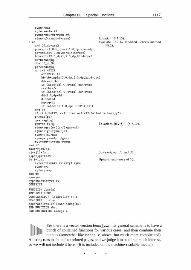
Chapter B6. Special Functions 1117
rymu=-sumry1=-sum1*xi2rymup=xmu*xi*rymu-ry1rjmu=w/(rymup-f*rymu) Equation (6.7.13).
else Evaluate CF2 by modified Lentz’s method(§5.2).a=0.25_dp-xmu2
pq=cmplx(-0.5_dp*xi,1.0_dp,kind=dpc)aa=cmplx(0.0_dp,xi*a,kind=dpc)bb=cmplx(2.0_dp*x,2.0_dp,kind=dpc)cc=bb+aa/pqdd=1.0_dp/bbpq=cc*dd*pqdo i=2,MAXIT
a=a+2*(i-1)bb=bb+cmplx(0.0_dp,2.0_dp,kind=dpc)dd=a*dd+bbif (absc(dd) < FPMIN) dd=FPMINcc=bb+a/ccif (absc(cc) < FPMIN) cc=FPMINdd=1.0_dp/dddl=cc*ddpq=pq*dlif (absc(dl-1.0_dp) < EPS) exit
end doif (i > MAXIT) call nrerror(’cf2 failed in bessjy’)p=real(pq)q=aimag(pq)gam=(p-f)/q Equations (6.7.6) – (6.7.10).rjmu=sqrt(w/((p-f)*gam+q))rjmu=sign(rjmu,rjl)rymu=rjmu*gamrymup=rymu*(p+q/gam)ry1=xmu*xi*rymu-rymup
end iffact=rjmu/rjlrj=rjl1*fact Scale original Jν and J ′
ν .rjp=rjp1*factdo i=1,nl Upward recurrence of Yν .
rytemp=(xmu+i)*xi2*ry1-rymurymu=ry1ry1=rytemp
end dory=rymuryp=xnu*xi*rymu-ry1CONTAINS
FUNCTION absc(z)IMPLICIT NONECOMPLEX(DPC), INTENT(IN) :: zREAL(DP) :: abscabsc=abs(real(z))+abs(aimag(z))END FUNCTION abscEND SUBROUTINE bessjy_s
Yes there is a vector version bessjy v. Its general scheme is to have abunch of contained functions for various cases, and then combine theiroutputs (somewhat like bessj v, above, but much more complicated).
A listing runs to about four printed pages, and we judge it to be of not much interest,so we will not include it here. (It is included on the machine-readable media.)
� � �
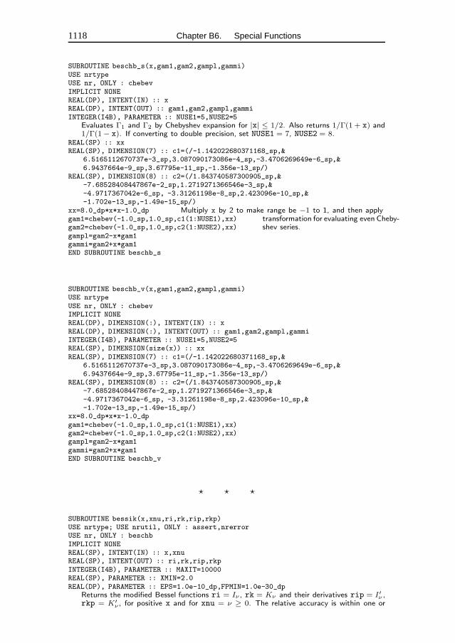
1118 Chapter B6. Special Functions
SUBROUTINE beschb_s(x,gam1,gam2,gampl,gammi)USE nrtypeUSE nr, ONLY : chebevIMPLICIT NONEREAL(DP), INTENT(IN) :: xREAL(DP), INTENT(OUT) :: gam1,gam2,gampl,gammiINTEGER(I4B), PARAMETER :: NUSE1=5,NUSE2=5
Evaluates Γ1 and Γ2 by Chebyshev expansion for |x| ≤ 1/2. Also returns 1/Γ(1 + x) and1/Γ(1 − x). If converting to double precision, set NUSE1 = 7, NUSE2 = 8.
REAL(SP) :: xxREAL(SP), DIMENSION(7) :: c1=(/-1.142022680371168_sp,&
6.5165112670737e-3_sp,3.087090173086e-4_sp,-3.4706269649e-6_sp,&6.9437664e-9_sp,3.67795e-11_sp,-1.356e-13_sp/)
REAL(SP), DIMENSION(8) :: c2=(/1.843740587300905_sp,&-7.68528408447867e-2_sp,1.2719271366546e-3_sp,&-4.9717367042e-6_sp, -3.31261198e-8_sp,2.423096e-10_sp,&-1.702e-13_sp,-1.49e-15_sp/)
xx=8.0_dp*x*x-1.0_dp Multiply x by 2 to make range be −1 to 1, and then applytransformation for evaluating even Cheby-shev series.
gam1=chebev(-1.0_sp,1.0_sp,c1(1:NUSE1),xx)gam2=chebev(-1.0_sp,1.0_sp,c2(1:NUSE2),xx)gampl=gam2-x*gam1gammi=gam2+x*gam1END SUBROUTINE beschb_s
SUBROUTINE beschb_v(x,gam1,gam2,gampl,gammi)USE nrtypeUSE nr, ONLY : chebevIMPLICIT NONEREAL(DP), DIMENSION(:), INTENT(IN) :: xREAL(DP), DIMENSION(:), INTENT(OUT) :: gam1,gam2,gampl,gammiINTEGER(I4B), PARAMETER :: NUSE1=5,NUSE2=5REAL(SP), DIMENSION(size(x)) :: xxREAL(SP), DIMENSION(7) :: c1=(/-1.142022680371168_sp,&
6.5165112670737e-3_sp,3.087090173086e-4_sp,-3.4706269649e-6_sp,&6.9437664e-9_sp,3.67795e-11_sp,-1.356e-13_sp/)
REAL(SP), DIMENSION(8) :: c2=(/1.843740587300905_sp,&-7.68528408447867e-2_sp,1.2719271366546e-3_sp,&-4.9717367042e-6_sp, -3.31261198e-8_sp,2.423096e-10_sp,&-1.702e-13_sp,-1.49e-15_sp/)
xx=8.0_dp*x*x-1.0_dpgam1=chebev(-1.0_sp,1.0_sp,c1(1:NUSE1),xx)gam2=chebev(-1.0_sp,1.0_sp,c2(1:NUSE2),xx)gampl=gam2-x*gam1gammi=gam2+x*gam1END SUBROUTINE beschb_v
� � �
SUBROUTINE bessik(x,xnu,ri,rk,rip,rkp)USE nrtype; USE nrutil, ONLY : assert,nrerrorUSE nr, ONLY : beschbIMPLICIT NONEREAL(SP), INTENT(IN) :: x,xnuREAL(SP), INTENT(OUT) :: ri,rk,rip,rkpINTEGER(I4B), PARAMETER :: MAXIT=10000REAL(SP), PARAMETER :: XMIN=2.0REAL(DP), PARAMETER :: EPS=1.0e-10_dp,FPMIN=1.0e-30_dp
Returns the modified Bessel functions ri = Iν , rk = Kν and their derivatives rip = I ′ν ,rkp = K′
ν , for positive x and for xnu = ν ≥ 0. The relative accuracy is within one or
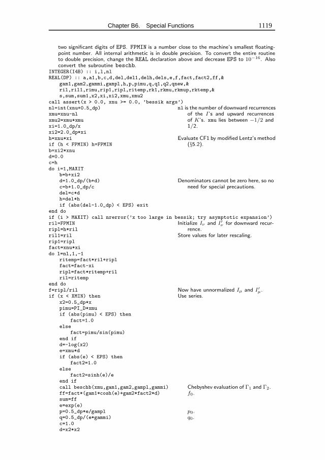
Chapter B6. Special Functions 1119
two significant digits of EPS. FPMIN is a number close to the machine’s smallest floating-point number. All internal arithmetic is in double precision. To convert the entire routineto double precision, change the REAL declaration above and decrease EPS to 10−16. Alsoconvert the subroutine beschb.
INTEGER(I4B) :: i,l,nlREAL(DP) :: a,a1,b,c,d,del,del1,delh,dels,e,f,fact,fact2,ff,&
gam1,gam2,gammi,gampl,h,p,pimu,q,q1,q2,qnew,&ril,ril1,rimu,rip1,ripl,ritemp,rk1,rkmu,rkmup,rktemp,&s,sum,sum1,x2,xi,xi2,xmu,xmu2
call assert(x > 0.0, xnu >= 0.0, ’bessik args’)nl=int(xnu+0.5_dp) nl is the number of downward recurrences
of the I’s and upward recurrencesof K’s. xmu lies between −1/2 and1/2.
xmu=xnu-nlxmu2=xmu*xmuxi=1.0_dp/xxi2=2.0_dp*xih=xnu*xi Evaluate CF1 by modified Lentz’s method
(§5.2).if (h < FPMIN) h=FPMINb=xi2*xnud=0.0c=hdo i=1,MAXIT
b=b+xi2d=1.0_dp/(b+d) Denominators cannot be zero here, so no
need for special precautions.c=b+1.0_dp/cdel=c*dh=del*hif (abs(del-1.0_dp) < EPS) exit
end doif (i > MAXIT) call nrerror(’x too large in bessik; try asymptotic expansion’)ril=FPMIN Initialize Iν and I′ν for downward recur-
rence.ripl=h*rilril1=ril Store values for later rescaling.rip1=riplfact=xnu*xido l=nl,1,-1
ritemp=fact*ril+riplfact=fact-xiripl=fact*ritemp+rilril=ritemp
end dof=ripl/ril Now have unnormalized Iµ and I′µ.if (x < XMIN) then Use series.
x2=0.5_dp*xpimu=PI_D*xmuif (abs(pimu) < EPS) then
fact=1.0else
fact=pimu/sin(pimu)end ifd=-log(x2)e=xmu*dif (abs(e) < EPS) then
fact2=1.0else
fact2=sinh(e)/eend ifcall beschb(xmu,gam1,gam2,gampl,gammi) Chebyshev evaluation of Γ1 and Γ2.ff=fact*(gam1*cosh(e)+gam2*fact2*d) f0.sum=ffe=exp(e)p=0.5_dp*e/gampl p0.q=0.5_dp/(e*gammi) q0.c=1.0d=x2*x2
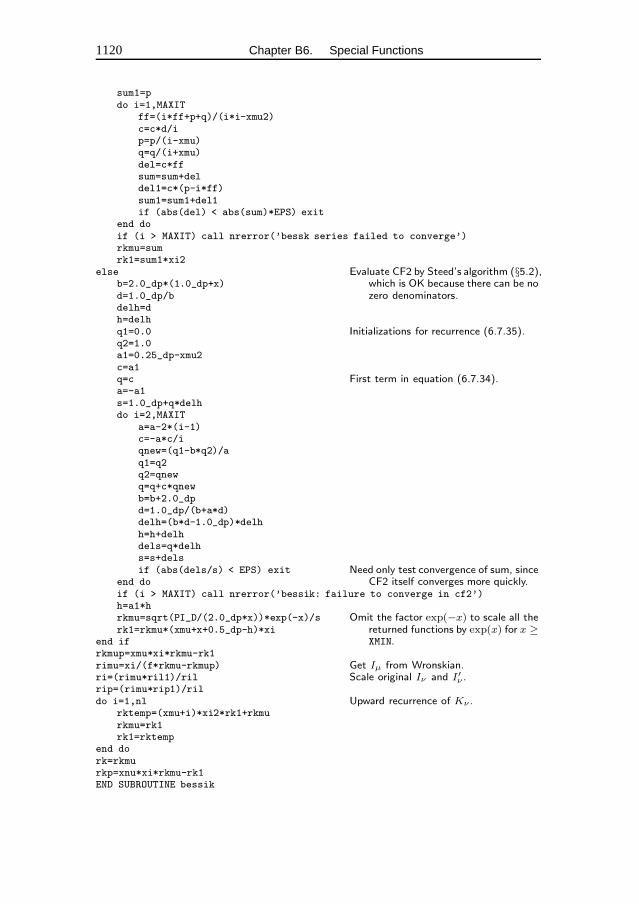
1120 Chapter B6. Special Functions
sum1=pdo i=1,MAXIT
ff=(i*ff+p+q)/(i*i-xmu2)c=c*d/ip=p/(i-xmu)q=q/(i+xmu)del=c*ffsum=sum+deldel1=c*(p-i*ff)sum1=sum1+del1if (abs(del) < abs(sum)*EPS) exit
end doif (i > MAXIT) call nrerror(’bessk series failed to converge’)rkmu=sumrk1=sum1*xi2
else Evaluate CF2 by Steed’s algorithm (§5.2),which is OK because there can be nozero denominators.
b=2.0_dp*(1.0_dp+x)d=1.0_dp/bdelh=dh=delhq1=0.0 Initializations for recurrence (6.7.35).q2=1.0a1=0.25_dp-xmu2c=a1q=c First term in equation (6.7.34).a=-a1s=1.0_dp+q*delhdo i=2,MAXIT
a=a-2*(i-1)c=-a*c/iqnew=(q1-b*q2)/aq1=q2q2=qnewq=q+c*qnewb=b+2.0_dpd=1.0_dp/(b+a*d)delh=(b*d-1.0_dp)*delhh=h+delhdels=q*delhs=s+delsif (abs(dels/s) < EPS) exit Need only test convergence of sum, since
CF2 itself converges more quickly.end doif (i > MAXIT) call nrerror(’bessik: failure to converge in cf2’)h=a1*hrkmu=sqrt(PI_D/(2.0_dp*x))*exp(-x)/s Omit the factor exp(−x) to scale all the
returned functions by exp(x) for x ≥XMIN.
rk1=rkmu*(xmu+x+0.5_dp-h)*xiend ifrkmup=xmu*xi*rkmu-rk1rimu=xi/(f*rkmu-rkmup) Get Iµ from Wronskian.ri=(rimu*ril1)/ril Scale original Iν and I′ν .rip=(rimu*rip1)/rildo i=1,nl Upward recurrence of Kν .
rktemp=(xmu+i)*xi2*rk1+rkmurkmu=rk1rk1=rktemp
end dork=rkmurkp=xnu*xi*rkmu-rk1END SUBROUTINE bessik
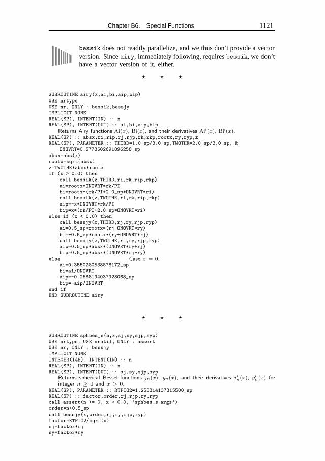
Chapter B6. Special Functions 1121
bessik does not readily parallelize, and we thus don’t provide a vectorversion. Since airy, immediately following, requires bessik, we don’thave a vector version of it, either.
� � �
SUBROUTINE airy(x,ai,bi,aip,bip)USE nrtypeUSE nr, ONLY : bessik,bessjyIMPLICIT NONEREAL(SP), INTENT(IN) :: xREAL(SP), INTENT(OUT) :: ai,bi,aip,bip
Returns Airy functions Ai(x), Bi(x), and their derivatives Ai′(x), Bi′(x).REAL(SP) :: absx,ri,rip,rj,rjp,rk,rkp,rootx,ry,ryp,zREAL(SP), PARAMETER :: THIRD=1.0_sp/3.0_sp,TWOTHR=2.0_sp/3.0_sp, &
ONOVRT=0.5773502691896258_spabsx=abs(x)rootx=sqrt(absx)z=TWOTHR*absx*rootxif (x > 0.0) then
call bessik(z,THIRD,ri,rk,rip,rkp)ai=rootx*ONOVRT*rk/PIbi=rootx*(rk/PI+2.0_sp*ONOVRT*ri)call bessik(z,TWOTHR,ri,rk,rip,rkp)aip=-x*ONOVRT*rk/PIbip=x*(rk/PI+2.0_sp*ONOVRT*ri)
else if (x < 0.0) thencall bessjy(z,THIRD,rj,ry,rjp,ryp)ai=0.5_sp*rootx*(rj-ONOVRT*ry)bi=-0.5_sp*rootx*(ry+ONOVRT*rj)call bessjy(z,TWOTHR,rj,ry,rjp,ryp)aip=0.5_sp*absx*(ONOVRT*ry+rj)bip=0.5_sp*absx*(ONOVRT*rj-ry)
else Case x = 0.ai=0.3550280538878172_spbi=ai/ONOVRTaip=-0.2588194037928068_spbip=-aip/ONOVRT
end ifEND SUBROUTINE airy
� � �
SUBROUTINE sphbes_s(n,x,sj,sy,sjp,syp)USE nrtype; USE nrutil, ONLY : assertUSE nr, ONLY : bessjyIMPLICIT NONEINTEGER(I4B), INTENT(IN) :: nREAL(SP), INTENT(IN) :: xREAL(SP), INTENT(OUT) :: sj,sy,sjp,syp
Returns spherical Bessel functions jn(x), yn(x), and their derivatives j′n(x), y′n(x) forinteger n ≥ 0 and x > 0.
REAL(SP), PARAMETER :: RTPIO2=1.253314137315500_spREAL(SP) :: factor,order,rj,rjp,ry,rypcall assert(n >= 0, x > 0.0, ’sphbes_s args’)order=n+0.5_spcall bessjy(x,order,rj,ry,rjp,ryp)factor=RTPIO2/sqrt(x)sj=factor*rjsy=factor*ry
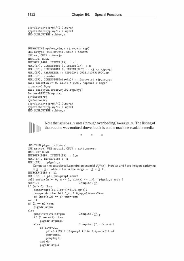
1122 Chapter B6. Special Functions
sjp=factor*rjp-sj/(2.0_sp*x)syp=factor*ryp-sy/(2.0_sp*x)END SUBROUTINE sphbes_s
SUBROUTINE sphbes_v(n,x,sj,sy,sjp,syp)USE nrtype; USE nrutil, ONLY : assertUSE nr, ONLY : bessjyIMPLICIT NONEINTEGER(I4B), INTENT(IN) :: nREAL(SP), DIMENSION(:), INTENT(IN) :: xREAL(SP), DIMENSION(:), INTENT(OUT) :: sj,sy,sjp,sypREAL(SP), PARAMETER :: RTPIO2=1.253314137315500_spREAL(SP) :: orderREAL(SP), DIMENSION(size(x)) :: factor,rj,rjp,ry,rypcall assert(n >= 0, all(x > 0.0), ’sphbes_v args’)order=n+0.5_spcall bessjy(x,order,rj,ry,rjp,ryp)factor=RTPIO2/sqrt(x)sj=factor*rjsy=factor*rysjp=factor*rjp-sj/(2.0_sp*x)syp=factor*ryp-sy/(2.0_sp*x)END SUBROUTINE sphbes_v
Note that sphbes vuses (throughoverloading)bessjy v. The listingofthat routine was omitted above, but it is on the machine-readable media.
� � �
FUNCTION plgndr_s(l,m,x)USE nrtype; USE nrutil, ONLY : arth,assertIMPLICIT NONEINTEGER(I4B), INTENT(IN) :: l,mREAL(SP), INTENT(IN) :: xREAL(SP) :: plgndr_s
Computes the associated Legendre polynomial Pml (x). Here m and l are integers satisfying
0 ≤ m ≤ l, while x lies in the range −1 ≤ x ≤ 1.INTEGER(I4B) :: llREAL(SP) :: pll,pmm,pmmp1,somx2call assert(m >= 0, m <= l, abs(x) <= 1.0, ’plgndr_s args’)pmm=1.0 Compute Pm
m .if (m > 0) then
somx2=sqrt((1.0_sp-x)*(1.0_sp+x))pmm=product(arth(1.0_sp,2.0_sp,m))*somx2**mif (mod(m,2) == 1) pmm=-pmm
end ifif (l == m) then
plgndr_s=pmmelse
pmmp1=x*(2*m+1)*pmm Compute Pmm+1.
if (l == m+1) thenplgndr_s=pmmp1
else Compute Pml , l > m + 1.
do ll=m+2,lpll=(x*(2*ll-1)*pmmp1-(ll+m-1)*pmm)/(ll-m)pmm=pmmp1pmmp1=pll
end doplgndr_s=pll
Chapter B6. Special Functions 1123
end ifend ifEND FUNCTION plgndr_s
f90product(arth(1.0_sp,2.0_sp,m))
That is, (2m − 1)!!
FUNCTION plgndr_v(l,m,x)USE nrtype; USE nrutil, ONLY : arth,assertIMPLICIT NONEINTEGER(I4B), INTENT(IN) :: l,mREAL(SP), DIMENSION(:), INTENT(IN) :: xREAL(SP), DIMENSION(size(x)) :: plgndr_vINTEGER(I4B) :: llREAL(SP), DIMENSION(size(x)) :: pll,pmm,pmmp1,somx2call assert(m >= 0, m <= l, all(abs(x) <= 1.0), ’plgndr_v args’)pmm=1.0if (m > 0) then
somx2=sqrt((1.0_sp-x)*(1.0_sp+x))pmm=product(arth(1.0_sp,2.0_sp,m))*somx2**mif (mod(m,2) == 1) pmm=-pmm
end ifif (l == m) then
plgndr_v=pmmelse
pmmp1=x*(2*m+1)*pmmif (l == m+1) then
plgndr_v=pmmp1else
do ll=m+2,lpll=(x*(2*ll-1)*pmmp1-(ll+m-1)*pmm)/(ll-m)pmm=pmmp1pmmp1=pll
end doplgndr_v=pll
end ifend ifEND FUNCTION plgndr_v
All those if’s (not where’s) may strike you as odd in a vector routine,but it is vectorized only on x, the dependent variable, not on the scalarindices l and m. Much harder to write a routine that is parallel for a
vector of arbitrary triplets (l, m, x). Try it!
� � �
SUBROUTINE frenel(x,s,c)USE nrtype; USE nrutil, ONLY : nrerrorIMPLICIT NONEREAL(SP), INTENT(IN) :: xREAL(SP), INTENT(OUT) :: s,cINTEGER(I4B), PARAMETER :: MAXIT=100REAL(SP), PARAMETER :: EPS=epsilon(x),FPMIN=tiny(x),BIG=huge(x)*EPS,&
XMIN=1.5Computes the Fresnel integrals S(x) and C(x) for all real x.Parameters: MAXIT is the maximum number of iterations allowed; EPS is the relative error;FPMIN is a number near the smallest representable floating-point number; BIG is a number
1124 Chapter B6. Special Functions
near the machine overflow limit; XMIN is the dividing line between using the series andcontinued fraction.
INTEGER(I4B) :: k,nREAL(SP) :: a,ax,fact,pix2,sign,sum,sumc,sums,term,testCOMPLEX(SPC) :: b,cc,d,h,del,csLOGICAL(LGT) :: oddax=abs(x)if (ax < sqrt(FPMIN)) then Special case: avoid failure of convergence test be-
cause of underflow.s=0.0c=ax
else if (ax <= XMIN) then Evaluate both series simultaneously.sum=0.0sums=0.0sumc=axsign=1.0fact=PIO2*ax*axodd=.true.term=axn=3do k=1,MAXIT
term=term*fact/ksum=sum+sign*term/ntest=abs(sum)*EPSif (odd) then
sign=-signsums=sumsum=sumc
elsesumc=sumsum=sums
end ifif (term < test) exitodd=.not. oddn=n+2
end doif (k > MAXIT) call nrerror(’frenel: series failed’)s=sumsc=sumc
else Evaluate continued fraction by modified Lentz’s method(§5.2).pix2=PI*ax*ax
b=cmplx(1.0_sp,-pix2,kind=spc)cc=BIGd=1.0_sp/bh=dn=-1do k=2,MAXIT
n=n+2a=-n*(n+1)b=b+4.0_spd=1.0_sp/(a*d+b) Denominators cannot be zero.cc=b+a/ccdel=cc*dh=h*delif (absc(del-1.0_sp) <= EPS) exit
end doif (k > MAXIT) call nrerror(’cf failed in frenel’)h=h*cmplx(ax,-ax,kind=spc)cs=cmplx(0.5_sp,0.5_sp,kind=spc)*(1.0_sp-&
cmplx(cos(0.5_sp*pix2),sin(0.5_sp*pix2),kind=spc)*h)c=real(cs)s=aimag(cs)
end ifif (x < 0.0) then Use antisymmetry.
c=-c
Chapter B6. Special Functions 1125
s=-send ifCONTAINS
FUNCTION absc(z)IMPLICIT NONECOMPLEX(SPC), INTENT(IN) :: zREAL(SP) :: abscabsc=abs(real(z))+abs(aimag(z))END FUNCTION abscEND SUBROUTINE frenel
f90b=cmplx(1.0_sp,-pix2,kind=spc) It’s a good idea always to include thekind= parameter when you use the cmplx intrinsic. The reason is that,perhaps counterintuitively, the result of cmplx is not determined by the
kind of its arguments, but is rather the “default complex kind.” Since that defaultmay not be what you think it is (or what spc is defined to be), the desired kindshould be specified explicitly.
c=real(cs) And why not specify a kind= parameter here, where it is alsooptionally allowed? Our answer is that the real intrinsic actually merges twodifferent usages. When its argument is complex, it is the counterpart of aimag
and returns a value whose kind is determined by the kind of its argument. Infact aimag doesn’t even allow an optional kind parameter, so we never put one inthe corresponding use of real. The other usage of real is for “casting,” that is,converting one real type to another (e.g., double precision to single precision, or viceversa). Here we always include a kind parameter, since otherwise the result is thedefault real kind, with the same dangers mentioned in the previous paragraph.
� � �
SUBROUTINE cisi(x,ci,si)USE nrtype; USE nrutil, ONLY : nrerrorIMPLICIT NONEREAL(SP), INTENT(IN) :: xREAL(SP), INTENT(OUT) :: ci,siINTEGER(I4B), PARAMETER :: MAXIT=100REAL(SP), PARAMETER :: EPS=epsilon(x),FPMIN=4.0_sp*tiny(x),&
BIG=huge(x)*EPS,TMIN=2.0Computes the cosine and sine integrals Ci(x) and Si(x). Ci(0) is returned as a large negativenumber and no error message is generated. For x < 0 the routine returns Ci(−x) and youmust supply the −iπ yourself.Parameters: MAXIT is the maximum number of iterations allowed; EPS is the relative error,or absolute error near a zero of Ci(x); FPMIN is a number near the smallest representablefloating-point number; BIG is a number near the machine overflow limit; TMIN is the dividingline between using the series and continued fraction; EULER = γ (in nrtype).
INTEGER(I4B) :: i,kREAL(SP) :: a,err,fact,sign,sum,sumc,sums,t,termCOMPLEX(SPC) :: h,b,c,d,delLOGICAL(LGT) :: oddt=abs(x)if (t == 0.0) then Special case.
si=0.0ci=-BIGRETURN
end if Evaluate continued fraction by modified Lentz’smethod (§5.2).if (t > TMIN) then
b=cmplx(1.0_sp,t,kind=spc)
1126 Chapter B6. Special Functions
c=BIGd=1.0_sp/bh=ddo i=2,MAXIT
a=-(i-1)**2b=b+2.0_spd=1.0_sp/(a*d+b) Denominators cannot be zero.c=b+a/cdel=c*dh=h*delif (absc(del-1.0_sp) <= EPS) exit
end doif (i > MAXIT) call nrerror(’continued fraction failed in cisi’)h=cmplx(cos(t),-sin(t),kind=spc)*hci=-real(h)si=PIO2+aimag(h)
else Evaluate both series simultaneously.if (t < sqrt(FPMIN)) then Special case: avoid failure of convergence test
because of underflow.sumc=0.0sums=t
elsesum=0.0sums=0.0sumc=0.0sign=1.0fact=1.0odd=.true.do k=1,MAXIT
fact=fact*t/kterm=fact/ksum=sum+sign*termerr=term/abs(sum)if (odd) then
sign=-signsums=sumsum=sumc
elsesumc=sumsum=sums
end ifif (err < EPS) exitodd=.not. odd
end doif (k > MAXIT) call nrerror(’MAXIT exceeded in cisi’)
end ifsi=sumsci=sumc+log(t)+EULER
end ifif (x < 0.0) si=-siCONTAINS
FUNCTION absc(z)IMPLICIT NONECOMPLEX(SPC), INTENT(IN) :: zREAL(SP) :: abscabsc=abs(real(z))+abs(aimag(z))END FUNCTION abscEND SUBROUTINE cisi
� � �
Chapter B6. Special Functions 1127
FUNCTION dawson_s(x)USE nrtype; USE nrutil, ONLY : arth,geopIMPLICIT NONEREAL(SP), INTENT(IN) :: xREAL(SP) :: dawson_s
Returns Dawson’s integral F (x) = exp(−x2)∫ x0 exp(t2)dt for any real x.
INTEGER(I4B), PARAMETER :: NMAX=6REAL(SP), PARAMETER :: H=0.4_sp,A1=2.0_sp/3.0_sp,A2=0.4_sp,&
A3=2.0_sp/7.0_spINTEGER(I4B) :: i,n0REAL(SP) :: ec,x2,xp,xxREAL(SP), DIMENSION(NMAX) :: d1,d2,e1REAL(SP), DIMENSION(NMAX), SAVE :: c=(/ (0.0_sp,i=1,NMAX) /)if (c(1) == 0.0) c(1:NMAX)=exp(-(arth(1,2,NMAX)*H)**2)Initialize c on first call.
if (abs(x) < 0.2_sp) then Use series expansion.x2=x**2dawson_s=x*(1.0_sp-A1*x2*(1.0_sp-A2*x2*(1.0_sp-A3*x2)))
else Use sampling theorem representation.xx=abs(x)n0=2*nint(0.5_sp*xx/H)xp=xx-real(n0,sp)*Hec=exp(2.0_sp*xp*H)d1=arth(n0+1,2,NMAX)d2=arth(n0-1,-2,NMAX)e1=geop(ec,ec**2,NMAX)dawson_s=0.5641895835477563_sp*sign(exp(-xp**2),x)*& Constant is 1/
√π.
sum(c*(e1/d1+1.0_sp/(d2*e1)))end ifEND FUNCTION dawson_s
f90REAL(SP), DIMENSION(NMAX), SAVE :: c=(/ (0.0_sp,i=1,NMAX) /) Thisis one way to give initial values to an array. Actually, we’re somewhatnervous about using the “implied do-loop” form of the array constructor,
as above, because our parallel compilers might not always be smart enough toexecute the constructor in parallel. In this case, with NMAX=6, the damage potentialis quite minimal. An alternative way to initialize the array would be with a datastatement, “DATA c /NMAX*0.0_sp/”; however, this is not considered good Fortran 90style, and there is no reason to think that it would be faster.
c(1:NMAX)=exp(-(arth(1,2,NMAX)*H)**2) Another example where the arth
function of nrutil comes in handy. Otherwise, this would be
do i=1,NMAXc(i)=exp(-((2.0_sp*i-1.0_sp)*H)**2)
end do
arth(n0+1,2,NMAX)...arth(n0-1,-2,NMAX)...geop(ec,ec**2,NMAX) These are notjust notationallyconvenient for generating the sequences (n 0+1, n0+3, n0+5, . . .),(n0 − 1, n0 − 3, n0 − 5, . . .), and (ec, ec3, ec5, . . .). They also may allow parallel-ization with parallel versions of arth and geop, such as those in nrutil.
FUNCTION dawson_v(x)USE nrtype; USE nrutil, ONLY : arthIMPLICIT NONEREAL(SP), DIMENSION(:), INTENT(IN) :: xREAL(SP), DIMENSION(size(x)) :: dawson_vINTEGER(I4B), PARAMETER :: NMAX=6
1128 Chapter B6. Special Functions
REAL(SP), PARAMETER :: H=0.4_sp,A1=2.0_sp/3.0_sp,A2=0.4_sp,&A3=2.0_sp/7.0_sp
INTEGER(I4B) :: i,nREAL(SP), DIMENSION(size(x)) :: x2REAL(SP), DIMENSION(NMAX), SAVE :: c=(/ (0.0_sp,i=1,NMAX) /)LOGICAL(LGT), DIMENSION(size(x)) :: maskif (c(1) == 0.0) c(1:NMAX)=exp(-(arth(1,2,NMAX)*H)**2)mask = (abs(x) >= 0.2_sp)dawson_v=dawsonseries_v(x,mask)where (.not. mask)
x2=x**2dawson_v=x*(1.0_sp-A1*x2*(1.0_sp-A2*x2*(1.0_sp-A3*x2)))
end whereCONTAINS
FUNCTION dawsonseries_v(xin,mask)IMPLICIT NONEREAL(SP), DIMENSION(:), INTENT(IN) :: xinLOGICAL(LGT), DIMENSION(size(xin)), INTENT(IN) :: maskREAL(SP), DIMENSION(size(xin)) :: dawsonseries_vINTEGER(I4B), DIMENSION(:), ALLOCATABLE :: n0REAL(SP), DIMENSION(:), ALLOCATABLE :: d1,d2,e1,e2,sm,xp,xx,xn=count(mask)if (n == 0) RETURNallocate(n0(n),d1(n),d2(n),e1(n),e2(n),sm(n),xp(n),xx(n),x(n))x=pack(xin,mask)xx=abs(x)n0=2*nint(0.5_sp*xx/H)xp=xx-real(n0,sp)*He1=exp(2.0_sp*xp*H)e2=e1**2d1=n0+1.0_spd2=d1-2.0_spsm=0.0do i=1,NMAX
sm=sm+c(i)*(e1/d1+1.0_sp/(d2*e1))d1=d1+2.0_spd2=d2-2.0_spe1=e2*e1
end dosm=0.5641895835477563_sp*sign(exp(-xp**2),x)*smdawsonseries_v=unpack(sm,mask,0.0_sp)deallocate(n0,d1,d2,e1,e2,sm,xp,xx)END FUNCTION dawsonseries_vEND FUNCTION dawson_v
dawson_v=dawsonseries_v(x,mask) Pass-the-buck method for gettingmasked values, see note to bessj0 v above, p. 1102. Within thecontained dawsonseries, we use the pack-unpack method. Note that,
unlike in dawson s, the sums are done by do-loops, because the parallelization isalready over the components of the vector argument.
� � �
FUNCTION rf_s(x,y,z)USE nrtype; USE nrutil, ONLY : assertIMPLICIT NONEREAL(SP), INTENT(IN) :: x,y,zREAL(SP) :: rf_sREAL(SP), PARAMETER :: ERRTOL=0.08_sp,TINY=1.5e-38_sp,BIG=3.0e37_sp,&
THIRD=1.0_sp/3.0_sp,&
Chapter B6. Special Functions 1129
C1=1.0_sp/24.0_sp,C2=0.1_sp,C3=3.0_sp/44.0_sp,C4=1.0_sp/14.0_spComputes Carlson’s elliptic integral of the first kind, RF (x, y, z). x, y, and z must benonnegative, and at most one can be zero. TINY must be at least 5 times the machineunderflow limit, BIG at most one-fifth the machine overflow limit.
REAL(SP) :: alamb,ave,delx,dely,delz,e2,e3,sqrtx,sqrty,sqrtz,xt,yt,ztcall assert(min(x,y,z) >= 0.0, min(x+y,x+z,y+z) >= TINY, &
max(x,y,z) <= BIG, ’rf_s args’)xt=xyt=yzt=zdo
sqrtx=sqrt(xt)sqrty=sqrt(yt)sqrtz=sqrt(zt)alamb=sqrtx*(sqrty+sqrtz)+sqrty*sqrtzxt=0.25_sp*(xt+alamb)yt=0.25_sp*(yt+alamb)zt=0.25_sp*(zt+alamb)ave=THIRD*(xt+yt+zt)delx=(ave-xt)/avedely=(ave-yt)/avedelz=(ave-zt)/aveif (max(abs(delx),abs(dely),abs(delz)) <= ERRTOL) exit
end doe2=delx*dely-delz**2e3=delx*dely*delzrf_s=(1.0_sp+(C1*e2-C2-C3*e3)*e2+C4*e3)/sqrt(ave)END FUNCTION rf_s
FUNCTION rf_v(x,y,z)USE nrtype; USE nrutil, ONLY : assert,assert_eqIMPLICIT NONEREAL(SP), DIMENSION(:), INTENT(IN) :: x,y,zREAL(SP), DIMENSION(size(x)) :: rf_vREAL(SP), PARAMETER :: ERRTOL=0.08_sp,TINY=1.5e-38_sp,BIG=3.0e37_sp,&
THIRD=1.0_sp/3.0_sp,&C1=1.0_sp/24.0_sp,C2=0.1_sp,C3=3.0_sp/44.0_sp,C4=1.0_sp/14.0_sp
REAL(SP), DIMENSION(size(x)) :: alamb,ave,delx,dely,delz,e2,e3,&sqrtx,sqrty,sqrtz,xt,yt,zt
LOGICAL(LGT), DIMENSION(size(x)) :: convergedINTEGER(I4B) :: ndumndum=assert_eq(size(x),size(y),size(z),’rf_v’)call assert(all(min(x,y,z) >= 0.0), all(min(x+y,x+z,y+z) >= TINY), &
all(max(x,y,z) <= BIG), ’rf_v args’)xt=xyt=yzt=zconverged=.false.do
where (.not. converged)sqrtx=sqrt(xt)sqrty=sqrt(yt)sqrtz=sqrt(zt)alamb=sqrtx*(sqrty+sqrtz)+sqrty*sqrtzxt=0.25_sp*(xt+alamb)yt=0.25_sp*(yt+alamb)zt=0.25_sp*(zt+alamb)ave=THIRD*(xt+yt+zt)delx=(ave-xt)/avedely=(ave-yt)/avedelz=(ave-zt)/aveconverged = (max(abs(delx),abs(dely),abs(delz)) <= ERRTOL)
1130 Chapter B6. Special Functions
end whereif (all(converged)) exit
end doe2=delx*dely-delz**2e3=delx*dely*delzrf_v=(1.0_sp+(C1*e2-C2-C3*e3)*e2+C4*e3)/sqrt(ave)END FUNCTION rf_v
FUNCTION rd_s(x,y,z)USE nrtype; USE nrutil, ONLY : assertIMPLICIT NONEREAL(SP), INTENT(IN) :: x,y,zREAL(SP) :: rd_sREAL(SP), PARAMETER :: ERRTOL=0.05_sp,TINY=1.0e-25_sp,BIG=4.5e21_sp,&
C1=3.0_sp/14.0_sp,C2=1.0_sp/6.0_sp,C3=9.0_sp/22.0_sp,&C4=3.0_sp/26.0_sp,C5=0.25_sp*C3,C6=1.5_sp*C4Computes Carlson’s elliptic integral of the second kind, RD(x, y, z). x and y must benonnegative, and at most one can be zero. z must be positive. TINYmust be at least twicethe negative 2/3 power of the machine overflow limit. BIG must be at most 0.1× ERRTOLtimes the negative 2/3 power of the machine underflow limit.
REAL(SP) :: alamb,ave,delx,dely,delz,ea,eb,ec,ed,&ee,fac,sqrtx,sqrty,sqrtz,sum,xt,yt,zt
call assert(min(x,y) >= 0.0, min(x+y,z) >= TINY, max(x,y,z) <= BIG, &’rd_s args’)
xt=xyt=yzt=zsum=0.0fac=1.0do
sqrtx=sqrt(xt)sqrty=sqrt(yt)sqrtz=sqrt(zt)alamb=sqrtx*(sqrty+sqrtz)+sqrty*sqrtzsum=sum+fac/(sqrtz*(zt+alamb))fac=0.25_sp*facxt=0.25_sp*(xt+alamb)yt=0.25_sp*(yt+alamb)zt=0.25_sp*(zt+alamb)ave=0.2_sp*(xt+yt+3.0_sp*zt)delx=(ave-xt)/avedely=(ave-yt)/avedelz=(ave-zt)/aveif (max(abs(delx),abs(dely),abs(delz)) <= ERRTOL) exit
end doea=delx*delyeb=delz*delzec=ea-ebed=ea-6.0_sp*ebee=ed+ec+ecrd_s=3.0_sp*sum+fac*(1.0_sp+ed*(-C1+C5*ed-C6*delz*ee)&
+delz*(C2*ee+delz*(-C3*ec+delz*C4*ea)))/(ave*sqrt(ave))END FUNCTION rd_s
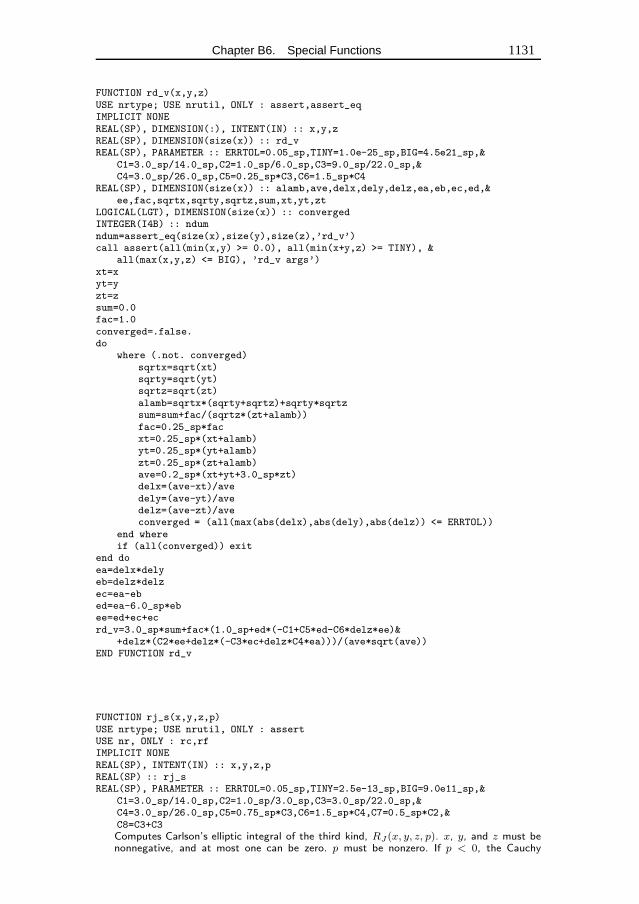
Chapter B6. Special Functions 1131
FUNCTION rd_v(x,y,z)USE nrtype; USE nrutil, ONLY : assert,assert_eqIMPLICIT NONEREAL(SP), DIMENSION(:), INTENT(IN) :: x,y,zREAL(SP), DIMENSION(size(x)) :: rd_vREAL(SP), PARAMETER :: ERRTOL=0.05_sp,TINY=1.0e-25_sp,BIG=4.5e21_sp,&
C1=3.0_sp/14.0_sp,C2=1.0_sp/6.0_sp,C3=9.0_sp/22.0_sp,&C4=3.0_sp/26.0_sp,C5=0.25_sp*C3,C6=1.5_sp*C4
REAL(SP), DIMENSION(size(x)) :: alamb,ave,delx,dely,delz,ea,eb,ec,ed,&ee,fac,sqrtx,sqrty,sqrtz,sum,xt,yt,zt
LOGICAL(LGT), DIMENSION(size(x)) :: convergedINTEGER(I4B) :: ndumndum=assert_eq(size(x),size(y),size(z),’rd_v’)call assert(all(min(x,y) >= 0.0), all(min(x+y,z) >= TINY), &
all(max(x,y,z) <= BIG), ’rd_v args’)xt=xyt=yzt=zsum=0.0fac=1.0converged=.false.do
where (.not. converged)sqrtx=sqrt(xt)sqrty=sqrt(yt)sqrtz=sqrt(zt)alamb=sqrtx*(sqrty+sqrtz)+sqrty*sqrtzsum=sum+fac/(sqrtz*(zt+alamb))fac=0.25_sp*facxt=0.25_sp*(xt+alamb)yt=0.25_sp*(yt+alamb)zt=0.25_sp*(zt+alamb)ave=0.2_sp*(xt+yt+3.0_sp*zt)delx=(ave-xt)/avedely=(ave-yt)/avedelz=(ave-zt)/aveconverged = (all(max(abs(delx),abs(dely),abs(delz)) <= ERRTOL))
end whereif (all(converged)) exit
end doea=delx*delyeb=delz*delzec=ea-ebed=ea-6.0_sp*ebee=ed+ec+ecrd_v=3.0_sp*sum+fac*(1.0_sp+ed*(-C1+C5*ed-C6*delz*ee)&
+delz*(C2*ee+delz*(-C3*ec+delz*C4*ea)))/(ave*sqrt(ave))END FUNCTION rd_v
FUNCTION rj_s(x,y,z,p)USE nrtype; USE nrutil, ONLY : assertUSE nr, ONLY : rc,rfIMPLICIT NONEREAL(SP), INTENT(IN) :: x,y,z,pREAL(SP) :: rj_sREAL(SP), PARAMETER :: ERRTOL=0.05_sp,TINY=2.5e-13_sp,BIG=9.0e11_sp,&
C1=3.0_sp/14.0_sp,C2=1.0_sp/3.0_sp,C3=3.0_sp/22.0_sp,&C4=3.0_sp/26.0_sp,C5=0.75_sp*C3,C6=1.5_sp*C4,C7=0.5_sp*C2,&C8=C3+C3Computes Carlson’s elliptic integral of the third kind, RJ(x, y, z, p). x, y, and z must benonnegative, and at most one can be zero. p must be nonzero. If p < 0, the Cauchy
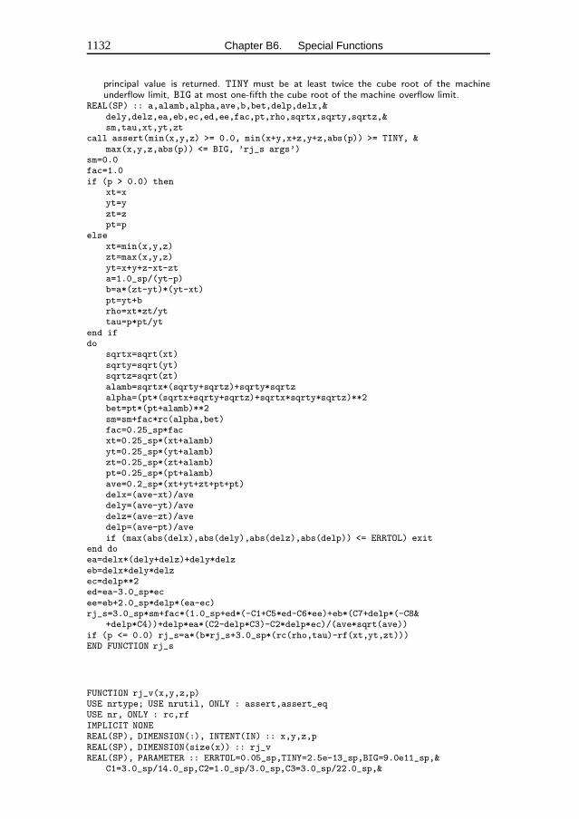
1132 Chapter B6. Special Functions
principal value is returned. TINY must be at least twice the cube root of the machineunderflow limit, BIG at most one-fifth the cube root of the machine overflow limit.
REAL(SP) :: a,alamb,alpha,ave,b,bet,delp,delx,&dely,delz,ea,eb,ec,ed,ee,fac,pt,rho,sqrtx,sqrty,sqrtz,&sm,tau,xt,yt,zt
call assert(min(x,y,z) >= 0.0, min(x+y,x+z,y+z,abs(p)) >= TINY, &max(x,y,z,abs(p)) <= BIG, ’rj_s args’)
sm=0.0fac=1.0if (p > 0.0) then
xt=xyt=yzt=zpt=p
elsext=min(x,y,z)zt=max(x,y,z)yt=x+y+z-xt-zta=1.0_sp/(yt-p)b=a*(zt-yt)*(yt-xt)pt=yt+brho=xt*zt/yttau=p*pt/yt
end ifdo
sqrtx=sqrt(xt)sqrty=sqrt(yt)sqrtz=sqrt(zt)alamb=sqrtx*(sqrty+sqrtz)+sqrty*sqrtzalpha=(pt*(sqrtx+sqrty+sqrtz)+sqrtx*sqrty*sqrtz)**2bet=pt*(pt+alamb)**2sm=sm+fac*rc(alpha,bet)fac=0.25_sp*facxt=0.25_sp*(xt+alamb)yt=0.25_sp*(yt+alamb)zt=0.25_sp*(zt+alamb)pt=0.25_sp*(pt+alamb)ave=0.2_sp*(xt+yt+zt+pt+pt)delx=(ave-xt)/avedely=(ave-yt)/avedelz=(ave-zt)/avedelp=(ave-pt)/aveif (max(abs(delx),abs(dely),abs(delz),abs(delp)) <= ERRTOL) exit
end doea=delx*(dely+delz)+dely*delzeb=delx*dely*delzec=delp**2ed=ea-3.0_sp*ecee=eb+2.0_sp*delp*(ea-ec)rj_s=3.0_sp*sm+fac*(1.0_sp+ed*(-C1+C5*ed-C6*ee)+eb*(C7+delp*(-C8&
+delp*C4))+delp*ea*(C2-delp*C3)-C2*delp*ec)/(ave*sqrt(ave))if (p <= 0.0) rj_s=a*(b*rj_s+3.0_sp*(rc(rho,tau)-rf(xt,yt,zt)))END FUNCTION rj_s
FUNCTION rj_v(x,y,z,p)USE nrtype; USE nrutil, ONLY : assert,assert_eqUSE nr, ONLY : rc,rfIMPLICIT NONEREAL(SP), DIMENSION(:), INTENT(IN) :: x,y,z,pREAL(SP), DIMENSION(size(x)) :: rj_vREAL(SP), PARAMETER :: ERRTOL=0.05_sp,TINY=2.5e-13_sp,BIG=9.0e11_sp,&
C1=3.0_sp/14.0_sp,C2=1.0_sp/3.0_sp,C3=3.0_sp/22.0_sp,&
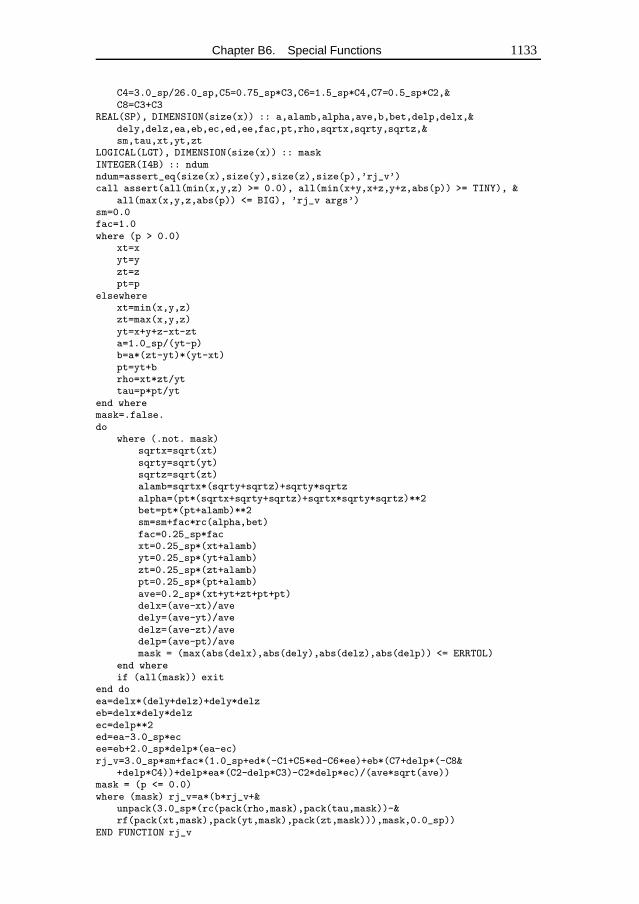
Chapter B6. Special Functions 1133
C4=3.0_sp/26.0_sp,C5=0.75_sp*C3,C6=1.5_sp*C4,C7=0.5_sp*C2,&C8=C3+C3
REAL(SP), DIMENSION(size(x)) :: a,alamb,alpha,ave,b,bet,delp,delx,&dely,delz,ea,eb,ec,ed,ee,fac,pt,rho,sqrtx,sqrty,sqrtz,&sm,tau,xt,yt,zt
LOGICAL(LGT), DIMENSION(size(x)) :: maskINTEGER(I4B) :: ndumndum=assert_eq(size(x),size(y),size(z),size(p),’rj_v’)call assert(all(min(x,y,z) >= 0.0), all(min(x+y,x+z,y+z,abs(p)) >= TINY), &
all(max(x,y,z,abs(p)) <= BIG), ’rj_v args’)sm=0.0fac=1.0where (p > 0.0)
xt=xyt=yzt=zpt=p
elsewherext=min(x,y,z)zt=max(x,y,z)yt=x+y+z-xt-zta=1.0_sp/(yt-p)b=a*(zt-yt)*(yt-xt)pt=yt+brho=xt*zt/yttau=p*pt/yt
end wheremask=.false.do
where (.not. mask)sqrtx=sqrt(xt)sqrty=sqrt(yt)sqrtz=sqrt(zt)alamb=sqrtx*(sqrty+sqrtz)+sqrty*sqrtzalpha=(pt*(sqrtx+sqrty+sqrtz)+sqrtx*sqrty*sqrtz)**2bet=pt*(pt+alamb)**2sm=sm+fac*rc(alpha,bet)fac=0.25_sp*facxt=0.25_sp*(xt+alamb)yt=0.25_sp*(yt+alamb)zt=0.25_sp*(zt+alamb)pt=0.25_sp*(pt+alamb)ave=0.2_sp*(xt+yt+zt+pt+pt)delx=(ave-xt)/avedely=(ave-yt)/avedelz=(ave-zt)/avedelp=(ave-pt)/avemask = (max(abs(delx),abs(dely),abs(delz),abs(delp)) <= ERRTOL)
end whereif (all(mask)) exit
end doea=delx*(dely+delz)+dely*delzeb=delx*dely*delzec=delp**2ed=ea-3.0_sp*ecee=eb+2.0_sp*delp*(ea-ec)rj_v=3.0_sp*sm+fac*(1.0_sp+ed*(-C1+C5*ed-C6*ee)+eb*(C7+delp*(-C8&
+delp*C4))+delp*ea*(C2-delp*C3)-C2*delp*ec)/(ave*sqrt(ave))mask = (p <= 0.0)where (mask) rj_v=a*(b*rj_v+&
unpack(3.0_sp*(rc(pack(rho,mask),pack(tau,mask))-&rf(pack(xt,mask),pack(yt,mask),pack(zt,mask))),mask,0.0_sp))
END FUNCTION rj_v
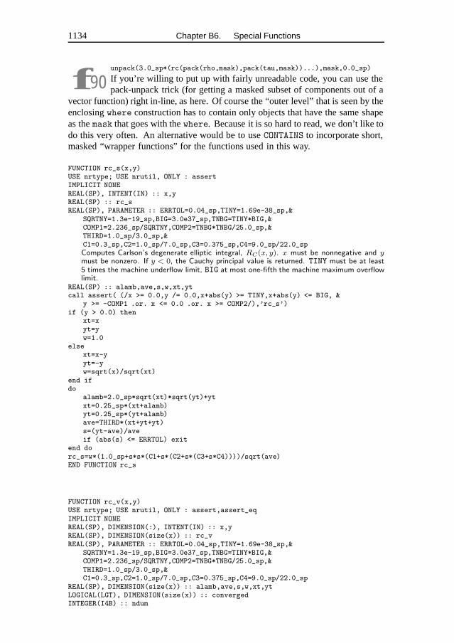
1134 Chapter B6. Special Functions
f90unpack(3.0_sp*(rc(pack(rho,mask),pack(tau,mask))...),mask,0.0_sp)
If you’re willing to put up with fairly unreadable code, you can use thepack-unpack trick (for getting a masked subset of components out of a
vector function) right in-line, as here. Of course the “outer level” that is seen by theenclosing where construction has to contain only objects that have the same shapeas the mask that goes with the where. Because it is so hard to read, we don’t like todo this very often. An alternative would be to use CONTAINS to incorporate short,masked “wrapper functions” for the functions used in this way.
FUNCTION rc_s(x,y)USE nrtype; USE nrutil, ONLY : assertIMPLICIT NONEREAL(SP), INTENT(IN) :: x,yREAL(SP) :: rc_sREAL(SP), PARAMETER :: ERRTOL=0.04_sp,TINY=1.69e-38_sp,&
SQRTNY=1.3e-19_sp,BIG=3.0e37_sp,TNBG=TINY*BIG,&COMP1=2.236_sp/SQRTNY,COMP2=TNBG*TNBG/25.0_sp,&THIRD=1.0_sp/3.0_sp,&C1=0.3_sp,C2=1.0_sp/7.0_sp,C3=0.375_sp,C4=9.0_sp/22.0_spComputes Carlson’s degenerate elliptic integral, RC(x, y). x must be nonnegative and ymust be nonzero. If y < 0, the Cauchy principal value is returned. TINY must be at least5 times the machine underflow limit, BIG at most one-fifth the machine maximum overflowlimit.
REAL(SP) :: alamb,ave,s,w,xt,ytcall assert( (/x >= 0.0,y /= 0.0,x+abs(y) >= TINY,x+abs(y) <= BIG, &
y >= -COMP1 .or. x <= 0.0 .or. x >= COMP2/),’rc_s’)if (y > 0.0) then
xt=xyt=yw=1.0
elsext=x-yyt=-yw=sqrt(x)/sqrt(xt)
end ifdo
alamb=2.0_sp*sqrt(xt)*sqrt(yt)+ytxt=0.25_sp*(xt+alamb)yt=0.25_sp*(yt+alamb)ave=THIRD*(xt+yt+yt)s=(yt-ave)/aveif (abs(s) <= ERRTOL) exit
end dorc_s=w*(1.0_sp+s*s*(C1+s*(C2+s*(C3+s*C4))))/sqrt(ave)END FUNCTION rc_s
FUNCTION rc_v(x,y)USE nrtype; USE nrutil, ONLY : assert,assert_eqIMPLICIT NONEREAL(SP), DIMENSION(:), INTENT(IN) :: x,yREAL(SP), DIMENSION(size(x)) :: rc_vREAL(SP), PARAMETER :: ERRTOL=0.04_sp,TINY=1.69e-38_sp,&
SQRTNY=1.3e-19_sp,BIG=3.0e37_sp,TNBG=TINY*BIG,&COMP1=2.236_sp/SQRTNY,COMP2=TNBG*TNBG/25.0_sp,&THIRD=1.0_sp/3.0_sp,&C1=0.3_sp,C2=1.0_sp/7.0_sp,C3=0.375_sp,C4=9.0_sp/22.0_sp
REAL(SP), DIMENSION(size(x)) :: alamb,ave,s,w,xt,ytLOGICAL(LGT), DIMENSION(size(x)) :: convergedINTEGER(I4B) :: ndum
Chapter B6. Special Functions 1135
ndum=assert_eq(size(x),size(y),’rc_v’)call assert( (/all(x >= 0.0),all(y /= 0.0),all(x+abs(y) >= TINY), &
all(x+abs(y) <= BIG),all(y >= -COMP1 .or. x <= 0.0 &.or. x >= COMP2) /),’rc_v’)
where (y > 0.0)xt=xyt=yw=1.0
elsewherext=x-yyt=-yw=sqrt(x)/sqrt(xt)
end whereconverged=.false.do
where (.not. converged)alamb=2.0_sp*sqrt(xt)*sqrt(yt)+ytxt=0.25_sp*(xt+alamb)yt=0.25_sp*(yt+alamb)ave=THIRD*(xt+yt+yt)s=(yt-ave)/aveconverged = (abs(s) <= ERRTOL)
end whereif (all(converged)) exit
end dorc_v=w*(1.0_sp+s*s*(C1+s*(C2+s*(C3+s*C4))))/sqrt(ave)END FUNCTION rc_v
� � �
FUNCTION ellf_s(phi,ak)USE nrtypeUSE nr, ONLY : rfIMPLICIT NONEREAL(SP), INTENT(IN) :: phi,akREAL(SP) :: ellf_s
Legendre elliptic integral of the 1st kind F (φ, k), evaluated using Carlson’s function RF .The argument ranges are 0 ≤ φ ≤ π/2, 0 ≤ k sinφ ≤ 1.
REAL(SP) :: ss=sin(phi)ellf_s=s*rf(cos(phi)**2,(1.0_sp-s*ak)*(1.0_sp+s*ak),1.0_sp)END FUNCTION ellf_s
FUNCTION ellf_v(phi,ak)USE nrtype; USE nrutil, ONLY : assert_eqUSE nr, ONLY : rfIMPLICIT NONEREAL(SP), DIMENSION(:), INTENT(IN) :: phi,akREAL(SP), DIMENSION(size(phi)) :: ellf_vREAL(SP), DIMENSION(size(phi)) :: sINTEGER(I4B) :: ndumndum=assert_eq(size(phi),size(ak),’ellf_v’)s=sin(phi)ellf_v=s*rf(cos(phi)**2,(1.0_sp-s*ak)*(1.0_sp+s*ak),&
spread(1.0_sp,1,size(phi)))END FUNCTION ellf_v
1136 Chapter B6. Special Functions
FUNCTION elle_s(phi,ak)USE nrtypeUSE nr, ONLY : rd,rfIMPLICIT NONEREAL(SP), INTENT(IN) :: phi,akREAL(SP) :: elle_s
Legendre elliptic integral of the 2nd kind E(φ, k), evaluated using Carlson’s functions RDand RF . The argument ranges are 0 ≤ φ ≤ π/2, 0 ≤ k sinφ ≤ 1.
REAL(SP) :: cc,q,ss=sin(phi)cc=cos(phi)**2q=(1.0_sp-s*ak)*(1.0_sp+s*ak)elle_s=s*(rf(cc,q,1.0_sp)-((s*ak)**2)*rd(cc,q,1.0_sp)/3.0_sp)END FUNCTION elle_s
FUNCTION elle_v(phi,ak)USE nrtype; USE nrutil, ONLY : assert_eqUSE nr, ONLY : rd,rfIMPLICIT NONEREAL(SP), DIMENSION(:), INTENT(IN) :: phi,akREAL(SP), DIMENSION(size(phi)) :: elle_vREAL(SP), DIMENSION(size(phi)) :: cc,q,sINTEGER(I4B) :: ndumndum=assert_eq(size(phi),size(ak),’elle_v’)s=sin(phi)cc=cos(phi)**2q=(1.0_sp-s*ak)*(1.0_sp+s*ak)elle_v=s*(rf(cc,q,spread(1.0_sp,1,size(phi)))-((s*ak)**2)*&
rd(cc,q,spread(1.0_sp,1,size(phi)))/3.0_sp)END FUNCTION elle_v
f90 rd(cc,q,spread(1.0_sp,1,size(phi))) See note toerf v, p. 1094 above.
FUNCTION ellpi_s(phi,en,ak)USE nrtypeUSE nr, ONLY : rf,rjIMPLICIT NONEREAL(SP), INTENT(IN) :: phi,en,akREAL(SP) :: ellpi_s
Legendre elliptic integral of the 3rd kind Π(φ, n, k), evaluated using Carlson’s functions RJ
and RF . (Note that the sign convention on n is opposite that of Abramowitz and Stegun.)The ranges of φ and k are 0 ≤ φ ≤ π/2, 0 ≤ k sinφ ≤ 1.
REAL(SP) :: cc,enss,q,ss=sin(phi)enss=en*s*scc=cos(phi)**2q=(1.0_sp-s*ak)*(1.0_sp+s*ak)ellpi_s=s*(rf(cc,q,1.0_sp)-enss*rj(cc,q,1.0_sp,1.0_sp+enss)/3.0_sp)END FUNCTION ellpi_s
Chapter B6. Special Functions 1137
FUNCTION ellpi_v(phi,en,ak)USE nrtypeUSE nr, ONLY : rf,rjIMPLICIT NONEREAL(SP), DIMENSION(:), INTENT(IN) :: phi,en,akREAL(SP), DIMENSION(size(phi)) :: ellpi_vREAL(SP), DIMENSION(size(phi)) :: cc,enss,q,ss=sin(phi)enss=en*s*scc=cos(phi)**2q=(1.0_sp-s*ak)*(1.0_sp+s*ak)ellpi_v=s*(rf(cc,q,spread(1.0_sp,1,size(phi)))-enss*&
rj(cc,q,spread(1.0_sp,1,size(phi)),1.0_sp+enss)/3.0_sp)END FUNCTION ellpi_v
� � �
SUBROUTINE sncndn(uu,emmc,sn,cn,dn)USE nrtype; USE nrutil, ONLY : nrerrorIMPLICIT NONEREAL(SP), INTENT(IN) :: uu,emmcREAL(SP), INTENT(OUT) :: sn,cn,dn
Returns the Jacobian elliptic functions sn(u, kc), cn(u, kc), and dn(u, kc). Here uu = u,while emmc = k2
c .REAL(SP), PARAMETER :: CA=0.0003_sp The accuracy is the square of CA.INTEGER(I4B), PARAMETER :: MAXIT=13INTEGER(I4B) :: i,ii,lREAL(SP) :: a,b,c,d,emc,uREAL(SP), DIMENSION(MAXIT) :: em,enLOGICAL(LGT) :: boemc=emmcu=uuif (emc /= 0.0) then
bo=(emc < 0.0)if (bo) then
d=1.0_sp-emcemc=-emc/dd=sqrt(d)u=d*u
end ifa=1.0dn=1.0do i=1,MAXIT
l=iem(i)=aemc=sqrt(emc)en(i)=emcc=0.5_sp*(a+emc)if (abs(a-emc) <= CA*a) exitemc=a*emca=c
end doif (i > MAXIT) call nrerror(’sncndn: convergence failed’)u=c*usn=sin(u)cn=cos(u)if (sn /= 0.0) then
a=cn/snc=a*cdo ii=l,1,-1
b=em(ii)
1138 Chapter B6. Special Functions
a=c*ac=dn*cdn=(en(ii)+a)/(b+a)a=c/b
end doa=1.0_sp/sqrt(c**2+1.0_sp)sn=sign(a,sn)cn=c*sn
end ifif (bo) then
a=dndn=cncn=asn=sn/d
end ifelse
cn=1.0_sp/cosh(u)dn=cnsn=tanh(u)
end ifEND SUBROUTINE sncndn
� � �
MODULE hypgeo_infoUSE nrtypeCOMPLEX(SPC) :: hypgeo_aa,hypgeo_bb,hypgeo_cc,hypgeo_dz,hypgeo_z0END MODULE hypgeo_info
FUNCTION hypgeo(a,b,c,z)USE nrtypeUSE hypgeo_infoUSE nr, ONLY : bsstep,hypdrv,hypser,odeintIMPLICIT NONECOMPLEX(SPC), INTENT(IN) :: a,b,c,zCOMPLEX(SPC) :: hypgeoREAL(SP), PARAMETER :: EPS=1.0e-6_sp
Complex hypergeometric function 2F1 for complex a, b, c, and z, by direct integration ofthe hypergeometric equation in the complex plane. The branch cut is taken to lie along thereal axis, Re z > 1.Parameter: EPS is an accuracy parameter.
COMPLEX(SPC), DIMENSION(2) :: yREAL(SP), DIMENSION(4) :: ryif (real(z)**2+aimag(z)**2 <= 0.25) then Use series...
call hypser(a,b,c,z,hypgeo,y(2))RETURN
else if (real(z) < 0.0) then ...or pick a starting point for the pathintegration.hypgeo_z0=cmplx(-0.5_sp,0.0_sp,kind=spc)
else if (real(z) <= 1.0) thenhypgeo_z0=cmplx(0.5_sp,0.0_sp,kind=spc)
elsehypgeo_z0=cmplx(0.0_sp,sign(0.5_sp,aimag(z)),kind=spc)
end ifhypgeo_aa=a Load the module variables, used to pass
parameters “over the head” of odeintto hypdrv.
hypgeo_bb=bhypgeo_cc=chypgeo_dz=z-hypgeo_z0call hypser(hypgeo_aa,hypgeo_bb,hypgeo_cc,hypgeo_z0,y(1),y(2))Get starting function and derivative.
ry(1:4:2)=real(y)
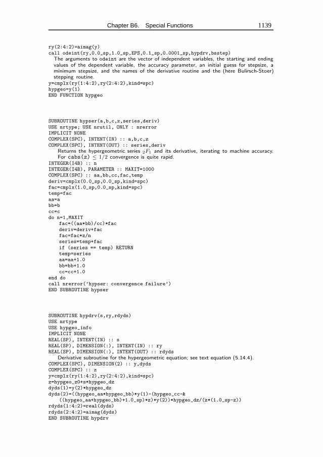
Chapter B6. Special Functions 1139
ry(2:4:2)=aimag(y)call odeint(ry,0.0_sp,1.0_sp,EPS,0.1_sp,0.0001_sp,hypdrv,bsstep)The arguments to odeint are the vector of independent variables, the starting and endingvalues of the dependent variable, the accuracy parameter, an initial guess for stepsize, aminimum stepsize, and the names of the derivative routine and the (here Bulirsch-Stoer)stepping routine.
y=cmplx(ry(1:4:2),ry(2:4:2),kind=spc)hypgeo=y(1)END FUNCTION hypgeo
SUBROUTINE hypser(a,b,c,z,series,deriv)USE nrtype; USE nrutil, ONLY : nrerrorIMPLICIT NONECOMPLEX(SPC), INTENT(IN) :: a,b,c,zCOMPLEX(SPC), INTENT(OUT) :: series,deriv
Returns the hypergeometric series 2F1 and its derivative, iterating to machine accuracy.For cabs(z) ≤ 1/2 convergence is quite rapid.
INTEGER(I4B) :: nINTEGER(I4B), PARAMETER :: MAXIT=1000COMPLEX(SPC) :: aa,bb,cc,fac,tempderiv=cmplx(0.0_sp,0.0_sp,kind=spc)fac=cmplx(1.0_sp,0.0_sp,kind=spc)temp=facaa=abb=bcc=cdo n=1,MAXIT
fac=((aa*bb)/cc)*facderiv=deriv+facfac=fac*z/nseries=temp+facif (series == temp) RETURNtemp=seriesaa=aa+1.0bb=bb+1.0cc=cc+1.0
end docall nrerror(’hypser: convergence failure’)END SUBROUTINE hypser
SUBROUTINE hypdrv(s,ry,rdyds)USE nrtypeUSE hypgeo_infoIMPLICIT NONEREAL(SP), INTENT(IN) :: sREAL(SP), DIMENSION(:), INTENT(IN) :: ryREAL(SP), DIMENSION(:), INTENT(OUT) :: rdyds
Derivative subroutine for the hypergeometric equation; see text equation (5.14.4).COMPLEX(SPC), DIMENSION(2) :: y,dydsCOMPLEX(SPC) :: zy=cmplx(ry(1:4:2),ry(2:4:2),kind=spc)z=hypgeo_z0+s*hypgeo_dzdyds(1)=y(2)*hypgeo_dzdyds(2)=((hypgeo_aa*hypgeo_bb)*y(1)-(hypgeo_cc-&
((hypgeo_aa+hypgeo_bb)+1.0_sp)*z)*y(2))*hypgeo_dz/(z*(1.0_sp-z))rdyds(1:4:2)=real(dyds)rdyds(2:4:2)=aimag(dyds)END SUBROUTINE hypdrv

1140 Chapter B6. Special Functions
f90Notice that the real array (of length 4) ry is immediately mapped into acomplex array of length 2, and that the process is reversed at the end ofthe routine with rdyds. In Fortran 77 no such mapping is necessary: the
calling program sends real arguments, and the Fortran 77 hypdrv simply interpretswhat is sent as complex. Fortran 90’s stronger typing does not encourage (and,practically, does not allow) this convenience; but it is a small price to pay for thevastly increased error-checking capabilities of a strongly typed language.
Chapter B7. Random NumbersOne might think that good random number generators, including those in
Volume 1, should last forever. The world of computing changes very rapidly,however:
• When Volume 1 was published, it was unusual, except on the fastestsupercomputers, to “exhaust” a 32-bit random number generator, that is,to call for all232 sequential random values in its periodic sequence. Now,this is feasible, and not uncommon, on fast desktop workstations. Auseful generator today must have a minimum of 64 bits of state space,and generally somewhat more.
• Before Fortran 90, the Fortran language had no standardized callingsequence for random numbers. Now, although there is still no standardalgorithm defined by the language (rightly, we think), there is at least astandard calling sequence, exemplified in the intrinsicsrandom number
and random seed.• The rise of parallel computing places new algorithmic demands on ran-
dom generators. The classic algorithms, which compute each randomvalue from the previous one, evidently need generalization to a parallelenvironment.
• New algorithms and techniques have been discovered, in some casessignificantly faster than their predecessors.
These are the reasons that we have decided to implement, in Fortran 90,different uniform random number generators from those in Volume 1’s Fortran77 implementations. We hasten to add that there is nothing wrong with any ofthe generators in Volume 1. That volume’sran0 and ran1 routines are, to ourknowledge, completely adequate as 32-bit generators;ran2 has a 64-bit state space,and our previous offer of$1000 forany demonstrated failure in the algorithm hasnever yet been claimed (see[1]).
Before we launch into the discussion of parallelizable generators with Fortran90 calling conventions, we want to attend to the continuing needs of longtime“x=ran(idum)” users with purely serial machines. If you are a satisfied user ofVolume 1’sran0, ran1, or ran2 Fortran 77 versions, you are in this group. Thefollowingroutine,ran, preserves those routines’ calling conventions, is considerablyfaster thanran2, and does not suffer from the oldran0 or ran1’s 32-bit periodexhaustion limitation. It is completely portable to all Fortran 90 environments. Werecommendran as the plug-compatible replacement for the oldran0, ran1, andran2, and we happily offer exactly the same$1000 reward terms as were (and arestill) offered on the oldran2.
1141
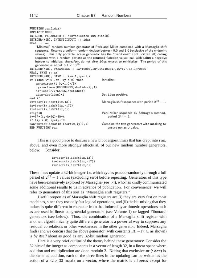
1142 Chapter B7. Random Numbers
FUNCTION ran(idum)IMPLICIT NONEINTEGER, PARAMETER :: K4B=selected_int_kind(9)INTEGER(K4B), INTENT(INOUT) :: idumREAL :: ran
“Minimal” random number generator of Park and Miller combined with a Marsaglia shiftsequence. Returns a uniform random deviate between 0.0 and 1.0 (exclusive of the endpointvalues). This fully portable, scalar generator has the “traditional” (not Fortran 90) callingsequence with a random deviate as the returned function value: call with idum a negativeinteger to initialize; thereafter, do not alter idum except to reinitialize. The period of thisgenerator is about 3.1 × 10¹⁸.
INTEGER(K4B), PARAMETER :: IA=16807,IM=2147483647,IQ=127773,IR=2836REAL, SAVE :: amINTEGER(K4B), SAVE :: ix=-1,iy=-1,kif (idum <= 0 .or. iy < 0) then Initialize.
am=nearest(1.0,-1.0)/IMiy=ior(ieor(888889999,abs(idum)),1)ix=ieor(777755555,abs(idum))idum=abs(idum)+1 Set idum positive.
end ifix=ieor(ix,ishft(ix,13)) Marsaglia shift sequence with period 232 − 1.ix=ieor(ix,ishft(ix,-17))ix=ieor(ix,ishft(ix,5))k=iy/IQ Park-Miller sequence by Schrage’s method,
period 231 − 2.iy=IA*(iy-k*IQ)-IR*kif (iy < 0) iy=iy+IMran=am*ior(iand(IM,ieor(ix,iy)),1) Combine the two generators with masking to
ensure nonzero value.END FUNCTION ran
This is a good place to discuss a new bit of algorithmics that has crept intoran,above, and even more strongly affects all of our new random number generators,below. Consider:
ix=ieor(ix,ishft(ix,13))ix=ieor(ix,ishft(ix,-17))ix=ieor(ix,ishft(ix,5))
These lines update a 32-bit integerix, which cycles pseudo-randomly through a fullperiod of232 − 1 values (excluding zero) before repeating. Generators of this typehave been extensively explored by Marsaglia (see[2]), who has kindlycommunicatedsome additional results to us in advance of publication. For convenience, we willrefer to generators of this sort as “Marsaglia shift registers.”
Useful properties of Marsaglia shift registers are (i) they are very fast on mostmachines, since they use only fast logical operations, and (ii) the bit-mixing that theyinduce is quite different in character from that induced by arithmetic operations suchas are used in linear congruential generators (see Volume 1) or lagged Fibonaccigenerators (see below). Thus, the combination of a Marsaglia shift register withanother, algorithmically quite different generator is a powerful way to suppress anyresidual correlations or other weaknesses in the other generator. Indeed, Marsagliafinds (and we concur) that the above generator (with constants13,−17, 5, as shown)is by itself about as good as any 32-bit random generator.
Here is a very brief outline of the theory behind these generators: Consider the32 bits of the integer as components in a vector of length 32, in a linear space whereaddition and multiplication are done modulo 2. Noting that exclusive-or (ieor) isthe same as addition, each of the three lines in the updating can be written as theaction of a32 × 32 matrix on a vector, where the matrix is all zeros except for
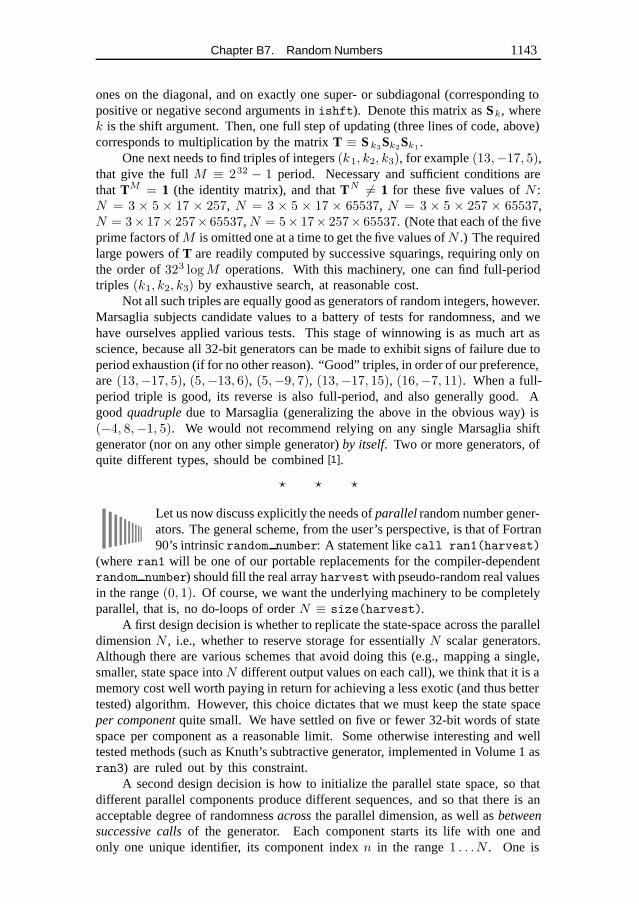
Chapter B7. Random Numbers 1143
ones on the diagonal, and on exactly one super- or subdiagonal (corresponding topositive or negative second arguments inishft). Denote this matrix asSk, wherek is the shift argument. Then, one full step of updating (three lines of code, above)corresponds to multiplication by the matrixT ≡ S k3Sk2Sk1 .
One next needs to find triples of integers(k1, k2, k3), for example(13,−17, 5),that give the fullM ≡ 232 − 1 period. Necessary and sufficient conditions arethat TM = 1 (the identity matrix), and thatTN �= 1 for these five values ofN :N = 3 × 5 × 17 × 257, N = 3 × 5 × 17 × 65537, N = 3 × 5 × 257 × 65537,N = 3× 17× 257× 65537,N = 5× 17× 257× 65537. (Note that each of the fiveprime factors ofM is omitted one at a time to get the five values ofN .) The requiredlarge powers ofT are readily computed by successive squarings, requiring only onthe order of323 logM operations. With this machinery, one can find full-periodtriples (k1, k2, k3) by exhaustive search, at reasonable cost.
Not all such triples are equally good as generators of random integers, however.Marsaglia subjects candidate values to a battery of tests for randomness, and wehave ourselves applied various tests. This stage of winnowing is as much art asscience, because all 32-bit generators can be made to exhibit signs of failure due toperiod exhaustion (if for no other reason). “Good” triples, in order of our preference,are(13,−17, 5), (5,−13, 6), (5,−9, 7), (13,−17, 15), (16,−7, 11). When a full-period triple is good, its reverse is also full-period, and also generally good. Agood quadruple due to Marsaglia (generalizing the above in the obvious way) is(−4, 8,−1, 5). We would not recommend relying on any single Marsaglia shiftgenerator (nor on any other simple generator)by itself. Two or more generators, ofquite different types, should be combined[1].
� � �
Let us now discuss explicitly the needs ofparallel random number gener-ators. The general scheme, from the user’s perspective, is that of Fortran90’s intrinsicrandom number: A statement likecall ran1(harvest)
(whereran1 will be one of our portable replacements for the compiler-dependentrandom number) should fill the real arrayharvestwith pseudo-random real valuesin the range(0, 1). Of course, we want the underlying machinery to be completelyparallel, that is, no do-loops of orderN ≡ size(harvest).
A first design decision is whether to replicate the state-space across the paralleldimensionN , i.e., whether to reserve storage for essentiallyN scalar generators.Although there are various schemes that avoid doing this (e.g., mapping a single,smaller, state space intoN different output values on each call), we think that it is amemory cost well worth paying in return for achieving a less exotic (and thus bettertested) algorithm. However, this choice dictates that we must keep the state spaceper component quite small. We have settled on five or fewer 32-bit words of statespace per component as a reasonable limit. Some otherwise interesting and welltested methods (such as Knuth’s subtractive generator, implemented in Volume 1 asran3) are ruled out by this constraint.
A second design decision is how to initialize the parallel state space, so thatdifferent parallel components produce different sequences, and so that there is anacceptable degree of randomnessacross the parallel dimension, as well asbetweensuccessive calls of the generator. Each component starts its life with one andonly one unique identifier, its component indexn in the range1 . . .N . One is
1144 Chapter B7. Random Numbers
tempted simply to hash the valuesn into the corresponding components of initialstate space. “Random” hashing is a bad idea, however, because differentn’s willproduce identical 32-bit hash results by chance whenN is no larger than∼ 216. Wetherefore prefer to use a kind of reversible pseudo-encryption (similar to the routinepsdes in Volume 1 and below) which guarantees causally that differentn’s producedifferent state space initializations.
f90The machinery for allocating, deallocating, and initializing the statespace, including provision of a user interface for getting or putting thecontents of the state space (as in the intrinsicrandom seed) is fairly
complicated. Rather than duplicate it in each different random generator that weprovide, we have consolidated it in a single module,ran state, whose contentswe will now discuss. Such a discussion is necessarily technical, if not arcane; onfirst reading, you may wish to skip ahead to the actual new routinesran0, ran1,andran2. If you do so, you will need to know only thatran state provides eachvector random routine with five 32-bit vectors of state information, denotediran,jran, kran, mran, nran. (The overloaded scalar generators have five corresponding32-bit scalars, denotediran0, etc.)
MODULE ran_stateThis module supports the random number routines ran0, ran1, ran2, and ran3. It pro-vides each generator with five integers (for vector versions, five vectors of integers), foruse as internal state space. The first three integers (iran, jran, kran) are maintainedas nonnegative values, while the last two (mran, nran) have 32-bit nonzero values. Alsoprovided by this module is support for initializing or reinitializing the state space to a desiredstandard sequence number, hashing the initial values to random values, and allocating anddeallocating the internal workspace.
USE nrtypeIMPLICIT NONEINTEGER, PARAMETER :: K4B=selected_int_kind(9)Independent of the usual integer kind I4B, we need a kind value for (ideally) 32-bit integers.
INTEGER(K4B), PARAMETER :: hg=huge(1_K4B), hgm=-hg, hgng=hgm-1INTEGER(K4B), SAVE :: lenran=0, seq=0INTEGER(K4B), SAVE :: iran0,jran0,kran0,nran0,mran0,ransINTEGER(K4B), DIMENSION(:,:), POINTER, SAVE :: ranseedsINTEGER(K4B), DIMENSION(:), POINTER, SAVE :: iran,jran,kran, &
nran,mran,ranvREAL(SP), SAVE :: ammINTERFACE ran_hash Scalar and vector versions of the hashing procedure.
MODULE PROCEDURE ran_hash_s, ran_hash_vEND INTERFACECONTAINS
(We here intersperse discussion with the listing of the module.) The moduledefinesK4B as an integerKIND that is intended to be 32 bits. If your machine doesn’thave 32-bit integers (hard to believe!) this will be caught later, and an error messagegenerated. The definition of the parametershg, hgm, andhgng makes an assumptionabout 32-bit integers that goes beyond the strict Fortran 90 integer model, that themagnitude of the most negative representable integer is greater by one than that ofthe most positive representable integer. This is a property of thetwo’s complementarithmetic that is used on virtually all modern machines (see, e.g.,[3]).
The global variablesrans (for scalar) andranv (for vector) are used by allof our routines to store theinteger value associated with the most recently returnedcall. You can access these (with a “USE ran state” statement) if you want integer,rather than real, random deviates.
Chapter B7. Random Numbers 1145
The first routine,ran init, is called by routines later in the chapter to initializetheir state space. It isnot intended to be called from a user’s program.
SUBROUTINE ran_init(length)USE nrtype; USE nrutil, ONLY : arth,nrerror,reallocateIMPLICIT NONEINTEGER(K4B), INTENT(IN) :: length
Initialize or reinitialize the random generator state space to vectors of size length. Thesaved variable seq is hashed (via calls to the module routine ran hash) to create uniquestarting seeds, different for each vector component.
INTEGER(K4B) :: new,j,hgtif (length < lenran) RETURN Simply return if enough space is already al-
located.hgt=hgThe following lines check that kind value K4B is in fact a 32-bit integer with the usual propertiesthat we expect it to have (under negation and wrap-around addition). If all of these tests aresatisfied, then the routines that use this module are portable, even though they go beyondFortran 90’s integer model.
if (hg /= 2147483647) call nrerror(’ran_init: arith assump 1 fails’)if (hgng >= 0) call nrerror(’ran_init: arith assump 2 fails’)if (hgt+1 /= hgng) call nrerror(’ran_init: arith assump 3 fails’)if (not(hg) >= 0) call nrerror(’ran_init: arith assump 4 fails’)if (not(hgng) < 0) call nrerror(’ran_init: arith assump 5 fails’)if (hg+hgng >= 0) call nrerror(’ran_init: arith assump 6 fails’)if (not(-1_k4b) < 0) call nrerror(’ran_init: arith assump 7 fails’)if (not(0_k4b) >= 0) call nrerror(’ran_init: arith assump 8 fails’)if (not(1_k4b) >= 0) call nrerror(’ran_init: arith assump 9 fails’)if (lenran > 0) then Reallocate space, or ...
ranseeds=>reallocate(ranseeds,length,5)ranv=>reallocate(ranv,length-1)new=lenran+1
else allocate space.allocate(ranseeds(length,5))allocate(ranv(length-1))new=1 Index of first location not yet initialized.amm=nearest(1.0_sp,-1.0_sp)/hgngUse of nearest is to ensure that returned random deviates are strictly less than 1.0.
if (amm*hgng >= 1.0 .or. amm*hgng <= 0.0) &call nrerror(’ran_init: arth assump 10 fails’)
end ifSet starting values, unique by seq and vector component.
ranseeds(new:,1)=seqranseeds(new:,2:5)=spread(arth(new,1,size(ranseeds(new:,1))),2,4)do j=1,4 Hash them.
call ran_hash(ranseeds(new:,j),ranseeds(new:,j+1))end dowhere (ranseeds(new:,1:3) < 0) & Enforce nonnegativity.
ranseeds(new:,1:3)=not(ranseeds(new:,1:3))where (ranseeds(new:,4:5) == 0) ranseeds(new:,4:5)=1 Enforce nonzero.if (new == 1) then Set scalar seeds.
iran0=ranseeds(1,1)jran0=ranseeds(1,2)kran0=ranseeds(1,3)mran0=ranseeds(1,4)nran0=ranseeds(1,5)rans=nran0
end ifif (length > 1) then Point to vector seeds.
iran => ranseeds(2:,1)jran => ranseeds(2:,2)kran => ranseeds(2:,3)mran => ranseeds(2:,4)nran => ranseeds(2:,5)ranv = nran
1146 Chapter B7. Random Numbers
end iflenran=lengthEND SUBROUTINE ran_init
f90hgt=hg ... if (hgt+1 /= hgng) Bit of dirty laundry here! We are testingwhether the most positive integerhg wraps around to the most negativeintegerhgng when 1 is added to it. We can’t just writehg+1, since some
compilers will evaluate this at compile time and return an overflow error message.If your compiler sees through the charade of the temporary variablehgt, you’llhave to find another way to trick it.
amm=nearest(1.0_sp,-1.0_sp)/hgng... Logically, amm should be a parameter;but the nearest intrinsic is trouble-prone in the initialization expression for aparameter (named constant), so we compute this at run time. We then check thatamm,when multiplied by the largest possible negative integer, does not equal or exceedunity. (Our random deviates are guaranteed never to equal zero or unity exactly.)
You might wonder whyamm is negative, and why we multiply it by negativeintegers to get positive random deviates. The answer, which will become manifestin the random generators given below, is that we want to use the fastnot operationon integers to convert them to nonzero values of all one sign. This is possible if theconversion is to negative values, sincenot(i) is negative for all nonnegativei. Ifthe conversion were to positive values, we would have problems both with zero (itssign bit is already positive) andhgng (sincenot(hgng) is generally zero).
iran0=ranseeds(1,1) ...iran => ranseeds(2:,1)...
The initial state information is stored inranseeds, a two-dimensional array whosecolumn (second) index ranges from 1 to 5 over the state variables.ranseeds(1,:) isreserved for scalar random generators, whileranseeds(2:,:) is for vector-parallelgenerators. Theranseeds array is made available to vector generators throughthe pointersiran, jran, kran, mran, andnran. The corresponding scalar values,iran0,. . ., nran0 are simply global variables, not pointers, because the overhead ofaddressing a scalar through a pointer is often too great. (We will have to copy thesescalar values back intoranseedswhen it, rarely, needs to be addressed as an array.)
call ran_hash(...) Unique, and random, initial state information is obtainedby putting a user-settable “sequence number” intoiran, a component number intojran, and hashing this pair. Thenjran and kran are hashed,kran and mran
are hashed, and so forth.
SUBROUTINE ran_deallocateUser interface to release the workspace used by the random number routines.
if (lenran > 0) thendeallocate(ranseeds,ranv)nullify(ranseeds,ranv,iran,jran,kran,mran,nran)lenran = 0
end ifEND SUBROUTINE ran_deallocate
The above routine is supplied as a user interface for deallocating all the statespace storage.
Chapter B7. Random Numbers 1147
SUBROUTINE ran_seed(sequence,size,put,get)IMPLICIT NONEINTEGER, OPTIONAL, INTENT(IN) :: sequenceINTEGER, OPTIONAL, INTENT(OUT) :: sizeINTEGER, DIMENSION(:), OPTIONAL, INTENT(IN) :: putINTEGER, DIMENSION(:), OPTIONAL, INTENT(OUT) :: get
User interface for seeding the random number routines. Syntax is exactly like Fortran 90’srandom seed routine, with one additional argument keyword: sequence, set to any inte-ger value, causes an immediate new initialization, seeded by that integer.
if (present(size)) thensize=5*lenran
else if (present(put)) thenif (lenran == 0) RETURNranseeds=reshape(put,shape(ranseeds))where (ranseeds(:,1:3) < 0) ranseeds(:,1:3)=not(ranseeds(:,1:3))Enforce nonnegativity and nonzero conditions on any user-supplied seeds.
where (ranseeds(:,4:5) == 0) ranseeds(:,4:5)=1iran0=ranseeds(1,1)jran0=ranseeds(1,2)kran0=ranseeds(1,3)mran0=ranseeds(1,4)nran0=ranseeds(1,5)
else if (present(get)) thenif (lenran == 0) RETURNranseeds(1,1:5)=(/ iran0,jran0,kran0,mran0,nran0 /)get=reshape(ranseeds,shape(get))
else if (present(sequence)) thencall ran_deallocateseq=sequence
end ifEND SUBROUTINE ran_seed
f90 ranseeds=reshape(put,shape(ranseeds)) ...get=reshape(ranseeds,shape(get))
Fortran 90’s convention is that random state space is a one-dimensional array, so wemap to this on both theget andput keywords.
iran0=...jran0=...kran0=...ranseeds(1,1:5)=(/ iran0,jran0,kran0,mran0,nran0 /)
It’s much more convenient to set a vector from a bunch of scalars then the otherway around.
SUBROUTINE ran_hash_s(il,ir)IMPLICIT NONEINTEGER(K4B), INTENT(INOUT) :: il,ir
DES-like hashing of two 32-bit integers, using shifts, xor’s, and adds to make the internalnonlinear function.
INTEGER(K4B) :: is,jdo j=1,4
is=irir=ieor(ir,ishft(ir,5))+1422217823 The various constants are chosen to give
good bit mixing and should not bechanged.
ir=ieor(ir,ishft(ir,-16))+1842055030ir=ieor(ir,ishft(ir,9))+80567781ir=ieor(il,ir)il=is
end doEND SUBROUTINE ran_hash_s
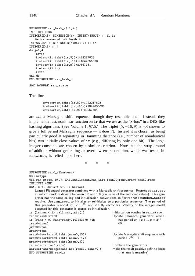
1148 Chapter B7. Random Numbers
SUBROUTINE ran_hash_v(il,ir)IMPLICIT NONEINTEGER(K4B), DIMENSION(:), INTENT(INOUT) :: il,ir
Vector version of ran hash s.INTEGER(K4B), DIMENSION(size(il)) :: isINTEGER(K4B) :: jdo j=1,4
is=irir=ieor(ir,ishft(ir,5))+1422217823ir=ieor(ir,ishft(ir,-16))+1842055030ir=ieor(ir,ishft(ir,9))+80567781ir=ieor(il,ir)il=is
end doEND SUBROUTINE ran_hash_v
END MODULE ran_state
The lines
ir=ieor(ir,ishft(ir,5))+1422217823ir=ieor(ir,ishft(ir,-16))+1842055030ir=ieor(ir,ishft(ir,9))+80567781
are not a Marsaglia shift sequence, though they resemble one. Instead, theyimplement a fast, nonlinear function onir that we use as the “S-box” in a DES-likehashing algorithm. (See Volume 1,§7.5.) The triplet(5,−16, 9) is not chosen togive a full period Marsaglia sequence — it doesn’t. Instead it is chosen as beingparticularly good at separating in Hamming distance (i.e., number of nonidenticalbits) two initially close values ofir (e.g., differing by only one bit). The largeinteger constants are chosen by a similar criterion. Note that the wrap-aroundof addition without generating an overflow error condition, which was tested inran init, is relied upon here.
� � �
SUBROUTINE ran0_s(harvest)USE nrtypeUSE ran_state, ONLY: K4B,amm,lenran,ran_init,iran0,jran0,kran0,nran0,ransIMPLICIT NONEREAL(SP), INTENT(OUT) :: harvest
Lagged Fibonacci generator combined with a Marsaglia shift sequence. Returns as harvesta uniform random deviate between 0.0 and 1.0 (exclusive of the endpoint values). This gen-erator has the same calling and initialization conventions as Fortran 90’s random numberroutine. Use ran seed to initialize or reinitialize to a particular sequence. The period ofthis generator is about 2.0 × 1028, and it fully vectorizes. Validity of the integer modelassumed by this generator is tested at initialization.
if (lenran < 1) call ran_init(1) Initialization routine in ran state.rans=iran0-kran0 Update Fibonacci generator, which
has period p2 +p+1, p = 231−69.
if (rans < 0) rans=rans+2147483579_k4biran0=jran0jran0=kran0kran0=ransnran0=ieor(nran0,ishft(nran0,13)) Update Marsaglia shift sequence with
period 232 − 1.nran0=ieor(nran0,ishft(nran0,-17))nran0=ieor(nran0,ishft(nran0,5))rans=ieor(nran0,rans) Combine the generators.harvest=amm*merge(rans,not(rans), rans<0 ) Make the result positive definite (note
that amm is negative).END SUBROUTINE ran0_s
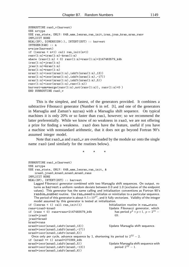
Chapter B7. Random Numbers 1149
SUBROUTINE ran0_v(harvest)USE nrtypeUSE ran_state, ONLY: K4B,amm,lenran,ran_init,iran,jran,kran,nran,ranvIMPLICIT NONEREAL(SP), DIMENSION(:), INTENT(OUT) :: harvestINTEGER(K4B) :: nn=size(harvest)if (lenran < n+1) call ran_init(n+1)ranv(1:n)=iran(1:n)-kran(1:n)where (ranv(1:n) < 0) ranv(1:n)=ranv(1:n)+2147483579_k4biran(1:n)=jran(1:n)jran(1:n)=kran(1:n)kran(1:n)=ranv(1:n)nran(1:n)=ieor(nran(1:n),ishft(nran(1:n),13))nran(1:n)=ieor(nran(1:n),ishft(nran(1:n),-17))nran(1:n)=ieor(nran(1:n),ishft(nran(1:n),5))ranv(1:n)=ieor(nran(1:n),ranv(1:n))harvest=amm*merge(ranv(1:n),not(ranv(1:n)), ranv(1:n)<0 )END SUBROUTINE ran0_v
This is the simplest, and fastest, of the generators provided. It combines asubtractive Fibonacci generator (Number 6 in ref.[1], and one of the generatorsin Marsaglia and Zaman’smzran) with a Marsaglia shift sequence. On typicalmachines it is only 20% or so faster thanran1, however; so we recommend thelatter preferentially. While we know of no weakness inran0, we are not offeringa prize for finding a weakness.ran0 does have the feature, useful if you havea machine with nonstandard arithmetic, that it does not go beyond Fortran 90’sassumed integer model.
Note thatran0 s andran0 v are overloaded by the modulenr onto the singlenameran0 (and similarly for the routines below).
� � �
SUBROUTINE ran1_s(harvest)USE nrtypeUSE ran_state, ONLY: K4B,amm,lenran,ran_init, &
iran0,jran0,kran0,nran0,mran0,ransIMPLICIT NONEREAL(SP), INTENT(OUT) :: harvest
Lagged Fibonacci generator combined with two Marsaglia shift sequences. On output, re-turns as harvest a uniform random deviate between 0.0 and 1.0 (exclusive of the endpointvalues). This generator has the same calling and initialization conventions as Fortran 90’srandom number routine. Use ran seed to initialize or reinitialize to a particular sequence.The period of this generator is about 8.5×1037, and it fully vectorizes. Validity of the integermodel assumed by this generator is tested at initialization.
if (lenran < 1) call ran_init(1) Initialization routine in ran state.rans=iran0-kran0 Update Fibonacci generator, which
has period p2 +p+1, p = 231−69.
if (rans < 0) rans=rans+2147483579_k4biran0=jran0jran0=kran0kran0=ransnran0=ieor(nran0,ishft(nran0,13)) Update Marsaglia shift sequence.nran0=ieor(nran0,ishft(nran0,-17))nran0=ieor(nran0,ishft(nran0,5))Once only per cycle, advance sequence by 1, shortening its period to 232 − 2.
if (nran0 == 1) nran0=270369_k4bmran0=ieor(mran0,ishft(mran0,5)) Update Marsaglia shift sequence with
period 232 − 1.mran0=ieor(mran0,ishft(mran0,-13))mran0=ieor(mran0,ishft(mran0,6))
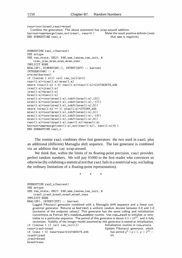
1150 Chapter B7. Random Numbers
rans=ieor(nran0,rans)+mran0Combine the generators. The above statement has wrap-around addition.
harvest=amm*merge(rans,not(rans), rans<0 ) Make the result positive definite (notethat amm is negative).END SUBROUTINE ran1_s
SUBROUTINE ran1_v(harvest)USE nrtypeUSE ran_state, ONLY: K4B,amm,lenran,ran_init, &
iran,jran,kran,nran,mran,ranvIMPLICIT NONEREAL(SP), DIMENSION(:), INTENT(OUT) :: harvestINTEGER(K4B) :: nn=size(harvest)if (lenran < n+1) call ran_init(n+1)ranv(1:n)=iran(1:n)-kran(1:n)where (ranv(1:n) < 0) ranv(1:n)=ranv(1:n)+2147483579_k4biran(1:n)=jran(1:n)jran(1:n)=kran(1:n)kran(1:n)=ranv(1:n)nran(1:n)=ieor(nran(1:n),ishft(nran(1:n),13))nran(1:n)=ieor(nran(1:n),ishft(nran(1:n),-17))nran(1:n)=ieor(nran(1:n),ishft(nran(1:n),5))where (nran(1:n) == 1) nran(1:n)=270369_k4bmran(1:n)=ieor(mran(1:n),ishft(mran(1:n),5))mran(1:n)=ieor(mran(1:n),ishft(mran(1:n),-13))mran(1:n)=ieor(mran(1:n),ishft(mran(1:n),6))ranv(1:n)=ieor(nran(1:n),ranv(1:n))+mran(1:n)harvest=amm*merge(ranv(1:n),not(ranv(1:n)), ranv(1:n)<0 )END SUBROUTINE ran1_v
The routineran1 combinesthree fast generators: the two used inran0, plusan additional (different) Marsaglia shift sequence. The last generator is combinedvia an addition that can wrap-around.
We think that, within the limits of its floating-point precision,ran1 providesperfect random numbers. We will pay$1000 to the first reader who convinces usotherwise (by exhibitinga statistical test thatran1 fails in a nontrivial way, excludingthe ordinary limitations of a floating-point representation).
� � �
SUBROUTINE ran2_s(harvest)USE nrtypeUSE ran_state, ONLY: K4B,amm,lenran,ran_init, &
iran0,jran0,kran0,nran0,mran0,ransIMPLICIT NONEREAL(SP), INTENT(OUT) :: harvest
Lagged Fibonacci generator combined with a Marsaglia shift sequence and a linear con-gruential generator. Returns as harvest a uniform random deviate between 0.0 and 1.0(exclusive of the endpoint values). This generator has the same calling and initializationconventions as Fortran 90’s random number routine. Use ran seed to initialize or reini-tialize to a particular sequence. The period of this generator is about 8.5×1037, and it fullyvectorizes. Validity of the integer model assumed by this generator is tested at initialization.
if (lenran < 1) call ran_init(1) Initialization routine in ran state.rans=iran0-kran0 Update Fibonacci generator, which
has period p2 +p+1, p = 231−69.
if (rans < 0) rans=rans+2147483579_k4biran0=jran0jran0=kran0kran0=rans
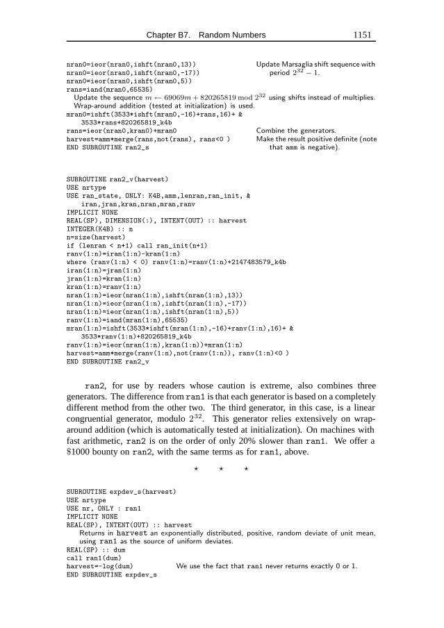
Chapter B7. Random Numbers 1151
nran0=ieor(nran0,ishft(nran0,13)) Update Marsaglia shift sequence withperiod 232 − 1.nran0=ieor(nran0,ishft(nran0,-17))
nran0=ieor(nran0,ishft(nran0,5))rans=iand(mran0,65535)Update the sequence m← 69069m+ 820265819 mod 232 using shifts instead of multiplies.Wrap-around addition (tested at initialization) is used.
mran0=ishft(3533*ishft(mran0,-16)+rans,16)+ &3533*rans+820265819_k4b
rans=ieor(nran0,kran0)+mran0 Combine the generators.harvest=amm*merge(rans,not(rans), rans<0 ) Make the result positive definite (note
that amm is negative).END SUBROUTINE ran2_s
SUBROUTINE ran2_v(harvest)USE nrtypeUSE ran_state, ONLY: K4B,amm,lenran,ran_init, &
iran,jran,kran,nran,mran,ranvIMPLICIT NONEREAL(SP), DIMENSION(:), INTENT(OUT) :: harvestINTEGER(K4B) :: nn=size(harvest)if (lenran < n+1) call ran_init(n+1)ranv(1:n)=iran(1:n)-kran(1:n)where (ranv(1:n) < 0) ranv(1:n)=ranv(1:n)+2147483579_k4biran(1:n)=jran(1:n)jran(1:n)=kran(1:n)kran(1:n)=ranv(1:n)nran(1:n)=ieor(nran(1:n),ishft(nran(1:n),13))nran(1:n)=ieor(nran(1:n),ishft(nran(1:n),-17))nran(1:n)=ieor(nran(1:n),ishft(nran(1:n),5))ranv(1:n)=iand(mran(1:n),65535)mran(1:n)=ishft(3533*ishft(mran(1:n),-16)+ranv(1:n),16)+ &
3533*ranv(1:n)+820265819_k4branv(1:n)=ieor(nran(1:n),kran(1:n))+mran(1:n)harvest=amm*merge(ranv(1:n),not(ranv(1:n)), ranv(1:n)<0 )END SUBROUTINE ran2_v
ran2, for use by readers whose caution is extreme, also combines threegenerators. The difference fromran1 is that each generator is based on a completelydifferent method from the other two. The third generator, in this case, is a linearcongruential generator, modulo232. This generator relies extensively on wrap-around addition (which is automatically tested at initialization). On machines withfast arithmetic,ran2 is on the order of only 20% slower thanran1. We offer a$1000 bounty onran2, with the same terms as forran1, above.
� � �
SUBROUTINE expdev_s(harvest)USE nrtypeUSE nr, ONLY : ran1IMPLICIT NONEREAL(SP), INTENT(OUT) :: harvest
Returns in harvest an exponentially distributed, positive, random deviate of unit mean,using ran1 as the source of uniform deviates.
REAL(SP) :: dumcall ran1(dum)harvest=-log(dum) We use the fact that ran1 never returns exactly 0 or 1.END SUBROUTINE expdev_s
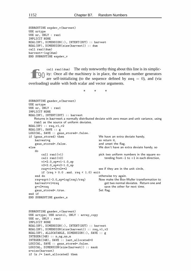
1152 Chapter B7. Random Numbers
SUBROUTINE expdev_v(harvest)USE nrtypeUSE nr, ONLY : ran1IMPLICIT NONEREAL(SP), DIMENSION(:), INTENT(OUT) :: harvestREAL(SP), DIMENSION(size(harvest)) :: dumcall ran1(dum)harvest=-log(dum)END SUBROUTINE expdev_v
f90call ran1(dum) The only noteworthy thing about this line is its simplic-ity: Once all the machinery is in place, the random number generatorsare self-initializing (to the sequence defined byseq = 0), and (via
overloading) usable with both scalar and vector arguments.
� � �
SUBROUTINE gasdev_s(harvest)USE nrtypeUSE nr, ONLY : ran1IMPLICIT NONEREAL(SP), INTENT(OUT) :: harvest
Returns in harvest a normally distributed deviate with zero mean and unit variance, usingran1 as the source of uniform deviates.
REAL(SP) :: rsq,v1,v2REAL(SP), SAVE :: gLOGICAL, SAVE :: gaus_stored=.false.if (gaus_stored) then We have an extra deviate handy,
harvest=g so return it,gaus_stored=.false. and unset the flag.
else We don’t have an extra deviate handy, sodo
call ran1(v1) pick two uniform numbers in the square ex-tending from -1 to +1 in each direction,call ran1(v2)
v1=2.0_sp*v1-1.0_spv2=2.0_sp*v2-1.0_sprsq=v1**2+v2**2 see if they are in the unit circle,if (rsq > 0.0 .and. rsq < 1.0) exit
end do otherwise try again.rsq=sqrt(-2.0_sp*log(rsq)/rsq) Now make the Box-Muller transformation to
get two normal deviates. Return one andsave the other for next time.
harvest=v1*rsqg=v2*rsqgaus_stored=.true. Set flag.
end ifEND SUBROUTINE gasdev_s
SUBROUTINE gasdev_v(harvest)USE nrtype; USE nrutil, ONLY : array_copyUSE nr, ONLY : ran1IMPLICIT NONEREAL(SP), DIMENSION(:), INTENT(OUT) :: harvestREAL(SP), DIMENSION(size(harvest)) :: rsq,v1,v2REAL(SP), ALLOCATABLE, DIMENSION(:), SAVE :: gINTEGER(I4B) :: n,ng,nn,mINTEGER(I4B), SAVE :: last_allocated=0LOGICAL, SAVE :: gaus_stored=.false.LOGICAL, DIMENSION(size(harvest)) :: maskn=size(harvest)if (n /= last_allocated) then
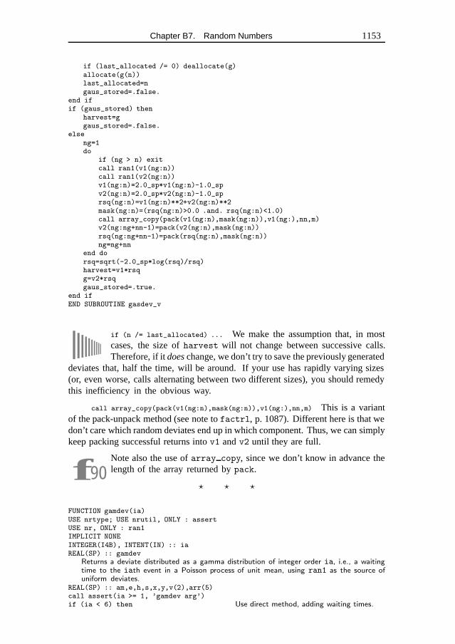
Chapter B7. Random Numbers 1153
if (last_allocated /= 0) deallocate(g)allocate(g(n))last_allocated=ngaus_stored=.false.
end ifif (gaus_stored) then
harvest=ggaus_stored=.false.
elseng=1do
if (ng > n) exitcall ran1(v1(ng:n))call ran1(v2(ng:n))v1(ng:n)=2.0_sp*v1(ng:n)-1.0_spv2(ng:n)=2.0_sp*v2(ng:n)-1.0_sprsq(ng:n)=v1(ng:n)**2+v2(ng:n)**2mask(ng:n)=(rsq(ng:n)>0.0 .and. rsq(ng:n)<1.0)call array_copy(pack(v1(ng:n),mask(ng:n)),v1(ng:),nn,m)v2(ng:ng+nn-1)=pack(v2(ng:n),mask(ng:n))rsq(ng:ng+nn-1)=pack(rsq(ng:n),mask(ng:n))ng=ng+nn
end dorsq=sqrt(-2.0_sp*log(rsq)/rsq)harvest=v1*rsqg=v2*rsqgaus_stored=.true.
end ifEND SUBROUTINE gasdev_v
if (n /= last_allocated) ... We make the assumption that, in mostcases, the size ofharvest will not change between successive calls.Therefore, if itdoes change, we don’t try to save the previously generated
deviates that, half the time, will be around. If your use has rapidly varying sizes(or, even worse, calls alternating between two different sizes), you should remedythis inefficiency in the obvious way.
call array_copy(pack(v1(ng:n),mask(ng:n)),v1(ng:),nn,m) This is a variantof the pack-unpack method (see note tofactrl, p. 1087). Different here is that wedon’t care which random deviates end up in which component. Thus, we can simplykeep packing successful returns intov1 andv2 until they are full.
f90Note also the use ofarray copy, since we don’t know in advance thelength of the array returned bypack.
� � �
FUNCTION gamdev(ia)USE nrtype; USE nrutil, ONLY : assertUSE nr, ONLY : ran1IMPLICIT NONEINTEGER(I4B), INTENT(IN) :: iaREAL(SP) :: gamdev
Returns a deviate distributed as a gamma distribution of integer order ia, i.e., a waitingtime to the iath event in a Poisson process of unit mean, using ran1 as the source ofuniform deviates.
REAL(SP) :: am,e,h,s,x,y,v(2),arr(5)call assert(ia >= 1, ’gamdev arg’)if (ia < 6) then Use direct method, adding waiting times.
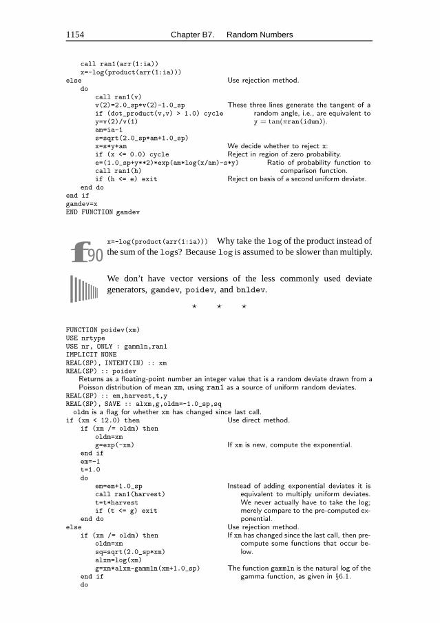
1154 Chapter B7. Random Numbers
call ran1(arr(1:ia))x=-log(product(arr(1:ia)))
else Use rejection method.do
call ran1(v)v(2)=2.0_sp*v(2)-1.0_sp These three lines generate the tangent of a
random angle, i.e., are equivalent toy = tan(πran(idum)).
if (dot_product(v,v) > 1.0) cycley=v(2)/v(1)am=ia-1s=sqrt(2.0_sp*am+1.0_sp)x=s*y+am We decide whether to reject x:if (x <= 0.0) cycle Reject in region of zero probability.e=(1.0_sp+y**2)*exp(am*log(x/am)-s*y) Ratio of probability function to
comparison function.call ran1(h)if (h <= e) exit Reject on basis of a second uniform deviate.
end doend ifgamdev=xEND FUNCTION gamdev
f90x=-log(product(arr(1:ia))) Why take thelog of the product instead ofthe sum of thelogs? Becauselog is assumed to be slower than multiply.
We don’t have vector versions of the less commonly used deviategenerators,gamdev, poidev, andbnldev.
� � �
FUNCTION poidev(xm)USE nrtypeUSE nr, ONLY : gammln,ran1IMPLICIT NONEREAL(SP), INTENT(IN) :: xmREAL(SP) :: poidev
Returns as a floating-point number an integer value that is a random deviate drawn from aPoisson distribution of mean xm, using ran1 as a source of uniform random deviates.
REAL(SP) :: em,harvest,t,yREAL(SP), SAVE :: alxm,g,oldm=-1.0_sp,sqoldm is a flag for whether xm has changed since last call.
if (xm < 12.0) then Use direct method.if (xm /= oldm) then
oldm=xmg=exp(-xm) If xm is new, compute the exponential.
end ifem=-1t=1.0do
em=em+1.0_sp Instead of adding exponential deviates it isequivalent to multiply uniform deviates.We never actually have to take the log;merely compare to the pre-computed ex-ponential.
call ran1(harvest)t=t*harvestif (t <= g) exit
end doelse Use rejection method.
if (xm /= oldm) then If xm has changed since the last call, then pre-compute some functions that occur be-low.
oldm=xmsq=sqrt(2.0_sp*xm)alxm=log(xm)g=xm*alxm-gammln(xm+1.0_sp) The function gammln is the natural log of the
gamma function, as given in §6.1.end ifdo
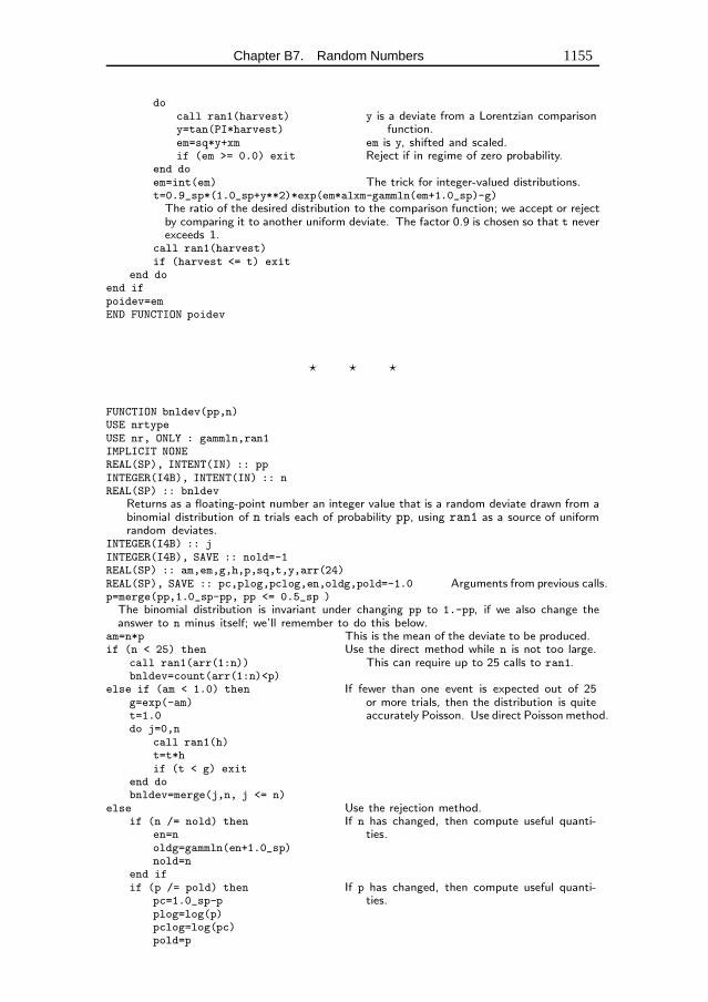
Chapter B7. Random Numbers 1155
docall ran1(harvest) y is a deviate from a Lorentzian comparison
function.y=tan(PI*harvest)em=sq*y+xm em is y, shifted and scaled.if (em >= 0.0) exit Reject if in regime of zero probability.
end doem=int(em) The trick for integer-valued distributions.t=0.9_sp*(1.0_sp+y**2)*exp(em*alxm-gammln(em+1.0_sp)-g)The ratio of the desired distribution to the comparison function; we accept or rejectby comparing it to another uniform deviate. The factor 0.9 is chosen so that t neverexceeds 1.
call ran1(harvest)if (harvest <= t) exit
end doend ifpoidev=emEND FUNCTION poidev
� � �
FUNCTION bnldev(pp,n)USE nrtypeUSE nr, ONLY : gammln,ran1IMPLICIT NONEREAL(SP), INTENT(IN) :: ppINTEGER(I4B), INTENT(IN) :: nREAL(SP) :: bnldev
Returns as a floating-point number an integer value that is a random deviate drawn from abinomial distribution of n trials each of probability pp, using ran1 as a source of uniformrandom deviates.
INTEGER(I4B) :: jINTEGER(I4B), SAVE :: nold=-1REAL(SP) :: am,em,g,h,p,sq,t,y,arr(24)REAL(SP), SAVE :: pc,plog,pclog,en,oldg,pold=-1.0 Arguments from previous calls.p=merge(pp,1.0_sp-pp, pp <= 0.5_sp )The binomial distribution is invariant under changing pp to 1.-pp, if we also change theanswer to n minus itself; we’ll remember to do this below.
am=n*p This is the mean of the deviate to be produced.if (n < 25) then Use the direct method while n is not too large.
This can require up to 25 calls to ran1.call ran1(arr(1:n))bnldev=count(arr(1:n)<p)
else if (am < 1.0) then If fewer than one event is expected out of 25or more trials, then the distribution is quiteaccurately Poisson. Use direct Poisson method.
g=exp(-am)t=1.0do j=0,n
call ran1(h)t=t*hif (t < g) exit
end dobnldev=merge(j,n, j <= n)
else Use the rejection method.if (n /= nold) then If n has changed, then compute useful quanti-
ties.en=noldg=gammln(en+1.0_sp)nold=n
end ifif (p /= pold) then If p has changed, then compute useful quanti-
ties.pc=1.0_sp-pplog=log(p)pclog=log(pc)pold=p
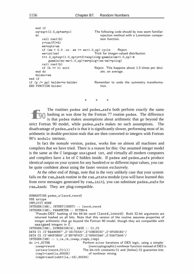
1156 Chapter B7. Random Numbers
end ifsq=sqrt(2.0_sp*am*pc) The following code should by now seem familiar:
rejection method with a Lorentzian compar-ison function.
docall ran1(h)y=tan(PI*h)em=sq*y+amif (em < 0.0 .or. em >= en+1.0_sp) cycle Reject.em=int(em) Trick for integer-valued distribution.t=1.2_sp*sq*(1.0_sp+y**2)*exp(oldg-gammln(em+1.0_sp)-&
gammln(en-em+1.0_sp)+em*plog+(en-em)*pclog)call ran1(h)if (h <= t) exit Reject. This happens about 1.5 times per devi-
ate, on average.end dobnldev=em
end ifif (p /= pp) bnldev=n-bnldev Remember to undo the symmetry transforma-
tion.END FUNCTION bnldev
� � �
f90The routinespsdes and psdes safe both performexactly the samehashing as was done by the Fortran 77 routinepsdes. The differenceis thatpsdes makes assumptions about arithmetic that go beyond the
strict Fortran 90 model, whilepsdes safe makes no such assumptions. Thedisadvantage ofpsdes safe is that it is significantly slower, performing most of itsarithmetic in double-precision reals that are then converted to integers with Fortran90’s modulo intrinsic.
In fact the nonsafe version,psdes, works fine on almost all machines andcompilers that we have tried. There is a reason for this: Our assumed integer modelis the same as theC languageunsigned int, and virtually all modern computersand compilers have a lot ofC hidden inside. Ifpsdes andpsdes safe produceidentical output on your system for any hundred or so different input values, you canbe quite confident about using the faster version exclusively.
At the other end of things, note that in the very unlikely case that your systemfails on theran hash routine in theran statemodule (you will have learned thisfrom error messages generated byran init), you can substitutepsdes safe forran hash: They are plug-compatible.
SUBROUTINE psdes_s(lword,rword)USE nrtypeIMPLICIT NONEINTEGER(I4B), INTENT(INOUT) :: lword,rwordINTEGER(I4B), PARAMETER :: NITER=4
“Pseudo-DES” hashing of the 64-bit word (lword,irword). Both 32-bit arguments arereturned hashed on all bits. Note that this version of the routine assumes properties ofinteger arithmetic that go beyond the Fortran 90 model, though they are compatible withunsigned integers in C.
INTEGER(I4B), DIMENSION(4), SAVE :: C1,C2DATA C1 /Z’BAA96887’,Z’1E17D32C’,Z’03BCDC3C’,Z’0F33D1B2’/DATA C2 /Z’4B0F3B58’,Z’E874F0C3’,Z’6955C5A6’,Z’55A7CA46’/INTEGER(I4B) :: i,ia,ib,iswap,itmph,itmpldo i=1,NITER Perform niter iterations of DES logic, using a simpler
(noncryptographic) nonlinear function instead of DES’s.iswap=rwordia=ieor(rword,C1(i)) The bit-rich constants C1 and (below) C2 guarantee lots
of nonlinear mixing.itmpl=iand(ia,65535)itmph=iand(ishft(ia,-16),65535)
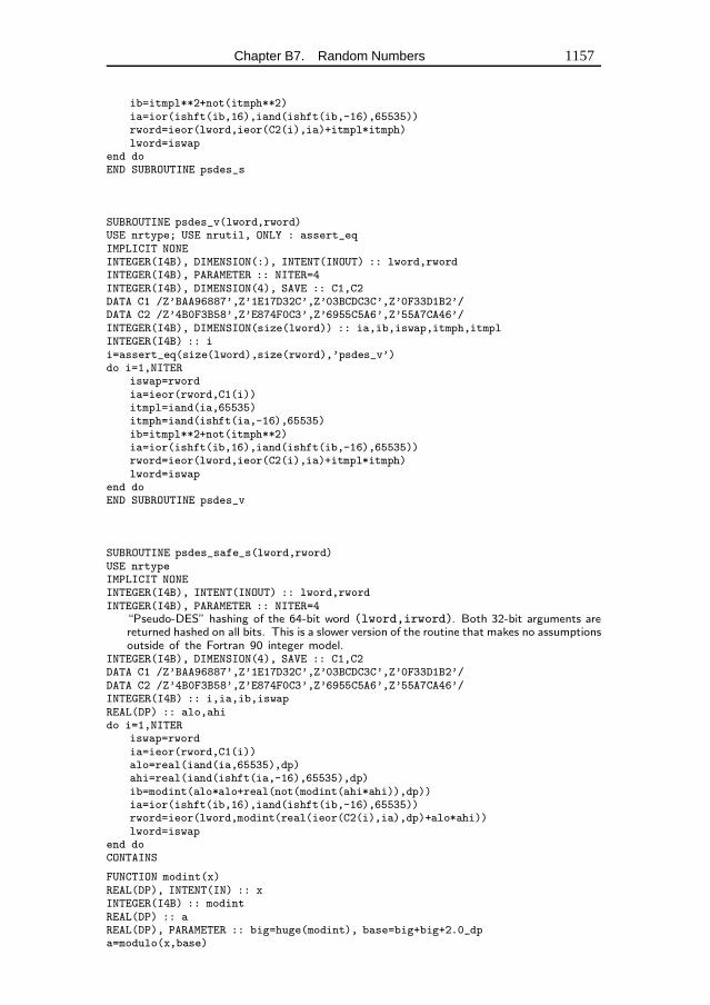
Chapter B7. Random Numbers 1157
ib=itmpl**2+not(itmph**2)ia=ior(ishft(ib,16),iand(ishft(ib,-16),65535))rword=ieor(lword,ieor(C2(i),ia)+itmpl*itmph)lword=iswap
end doEND SUBROUTINE psdes_s
SUBROUTINE psdes_v(lword,rword)USE nrtype; USE nrutil, ONLY : assert_eqIMPLICIT NONEINTEGER(I4B), DIMENSION(:), INTENT(INOUT) :: lword,rwordINTEGER(I4B), PARAMETER :: NITER=4INTEGER(I4B), DIMENSION(4), SAVE :: C1,C2DATA C1 /Z’BAA96887’,Z’1E17D32C’,Z’03BCDC3C’,Z’0F33D1B2’/DATA C2 /Z’4B0F3B58’,Z’E874F0C3’,Z’6955C5A6’,Z’55A7CA46’/INTEGER(I4B), DIMENSION(size(lword)) :: ia,ib,iswap,itmph,itmplINTEGER(I4B) :: ii=assert_eq(size(lword),size(rword),’psdes_v’)do i=1,NITER
iswap=rwordia=ieor(rword,C1(i))itmpl=iand(ia,65535)itmph=iand(ishft(ia,-16),65535)ib=itmpl**2+not(itmph**2)ia=ior(ishft(ib,16),iand(ishft(ib,-16),65535))rword=ieor(lword,ieor(C2(i),ia)+itmpl*itmph)lword=iswap
end doEND SUBROUTINE psdes_v
SUBROUTINE psdes_safe_s(lword,rword)USE nrtypeIMPLICIT NONEINTEGER(I4B), INTENT(INOUT) :: lword,rwordINTEGER(I4B), PARAMETER :: NITER=4
“Pseudo-DES” hashing of the 64-bit word (lword,irword). Both 32-bit arguments arereturned hashed on all bits. This is a slower version of the routine that makes no assumptionsoutside of the Fortran 90 integer model.
INTEGER(I4B), DIMENSION(4), SAVE :: C1,C2DATA C1 /Z’BAA96887’,Z’1E17D32C’,Z’03BCDC3C’,Z’0F33D1B2’/DATA C2 /Z’4B0F3B58’,Z’E874F0C3’,Z’6955C5A6’,Z’55A7CA46’/INTEGER(I4B) :: i,ia,ib,iswapREAL(DP) :: alo,ahido i=1,NITER
iswap=rwordia=ieor(rword,C1(i))alo=real(iand(ia,65535),dp)ahi=real(iand(ishft(ia,-16),65535),dp)ib=modint(alo*alo+real(not(modint(ahi*ahi)),dp))ia=ior(ishft(ib,16),iand(ishft(ib,-16),65535))rword=ieor(lword,modint(real(ieor(C2(i),ia),dp)+alo*ahi))lword=iswap
end doCONTAINS
FUNCTION modint(x)REAL(DP), INTENT(IN) :: xINTEGER(I4B) :: modintREAL(DP) :: aREAL(DP), PARAMETER :: big=huge(modint), base=big+big+2.0_dpa=modulo(x,base)
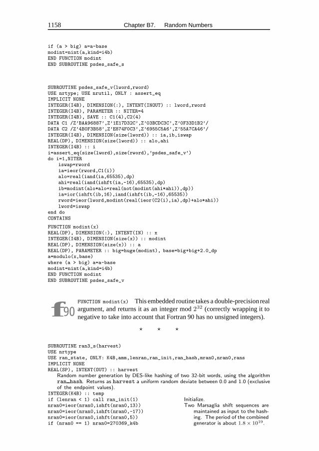
1158 Chapter B7. Random Numbers
if (a > big) a=a-basemodint=nint(a,kind=i4b)END FUNCTION modintEND SUBROUTINE psdes_safe_s
SUBROUTINE psdes_safe_v(lword,rword)USE nrtype; USE nrutil, ONLY : assert_eqIMPLICIT NONEINTEGER(I4B), DIMENSION(:), INTENT(INOUT) :: lword,rwordINTEGER(I4B), PARAMETER :: NITER=4INTEGER(I4B), SAVE :: C1(4),C2(4)DATA C1 /Z’BAA96887’,Z’1E17D32C’,Z’03BCDC3C’,Z’0F33D1B2’/DATA C2 /Z’4B0F3B58’,Z’E874F0C3’,Z’6955C5A6’,Z’55A7CA46’/INTEGER(I4B), DIMENSION(size(lword)) :: ia,ib,iswapREAL(DP), DIMENSION(size(lword)) :: alo,ahiINTEGER(I4B) :: ii=assert_eq(size(lword),size(rword),’psdes_safe_v’)do i=1,NITER
iswap=rwordia=ieor(rword,C1(i))alo=real(iand(ia,65535),dp)ahi=real(iand(ishft(ia,-16),65535),dp)ib=modint(alo*alo+real(not(modint(ahi*ahi)),dp))ia=ior(ishft(ib,16),iand(ishft(ib,-16),65535))rword=ieor(lword,modint(real(ieor(C2(i),ia),dp)+alo*ahi))lword=iswap
end doCONTAINS
FUNCTION modint(x)REAL(DP), DIMENSION(:), INTENT(IN) :: xINTEGER(I4B), DIMENSION(size(x)) :: modintREAL(DP), DIMENSION(size(x)) :: aREAL(DP), PARAMETER :: big=huge(modint), base=big+big+2.0_dpa=modulo(x,base)where (a > big) a=a-basemodint=nint(a,kind=i4b)END FUNCTION modintEND SUBROUTINE psdes_safe_v
f90FUNCTION modint(x) This embedded routine takes a double-precisionrealargument, and returns it as an integer mod232 (correctly wrapping it tonegative to take into account that Fortran 90 has no unsigned integers).
� � �
SUBROUTINE ran3_s(harvest)USE nrtypeUSE ran_state, ONLY: K4B,amm,lenran,ran_init,ran_hash,mran0,nran0,ransIMPLICIT NONEREAL(SP), INTENT(OUT) :: harvest
Random number generation by DES-like hashing of two 32-bit words, using the algorithmran hash. Returns as harvest a uniform random deviate between 0.0 and 1.0 (exclusiveof the endpoint values).
INTEGER(K4B) :: tempif (lenran < 1) call ran_init(1) Initialize.nran0=ieor(nran0,ishft(nran0,13)) Two Marsaglia shift sequences are
maintained as input to the hash-ing. The period of the combinedgenerator is about 1.8× 10¹⁹.
nran0=ieor(nran0,ishft(nran0,-17))nran0=ieor(nran0,ishft(nran0,5))if (nran0 == 1) nran0=270369_k4b
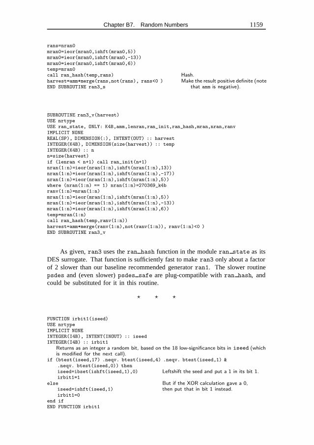
Chapter B7. Random Numbers 1159
rans=nran0mran0=ieor(mran0,ishft(mran0,5))mran0=ieor(mran0,ishft(mran0,-13))mran0=ieor(mran0,ishft(mran0,6))temp=mran0call ran_hash(temp,rans) Hash.harvest=amm*merge(rans,not(rans), rans<0 ) Make the result positive definite (note
that amm is negative).END SUBROUTINE ran3_s
SUBROUTINE ran3_v(harvest)USE nrtypeUSE ran_state, ONLY: K4B,amm,lenran,ran_init,ran_hash,mran,nran,ranvIMPLICIT NONEREAL(SP), DIMENSION(:), INTENT(OUT) :: harvestINTEGER(K4B), DIMENSION(size(harvest)) :: tempINTEGER(K4B) :: nn=size(harvest)if (lenran < n+1) call ran_init(n+1)nran(1:n)=ieor(nran(1:n),ishft(nran(1:n),13))nran(1:n)=ieor(nran(1:n),ishft(nran(1:n),-17))nran(1:n)=ieor(nran(1:n),ishft(nran(1:n),5))where (nran(1:n) == 1) nran(1:n)=270369_k4branv(1:n)=nran(1:n)mran(1:n)=ieor(mran(1:n),ishft(mran(1:n),5))mran(1:n)=ieor(mran(1:n),ishft(mran(1:n),-13))mran(1:n)=ieor(mran(1:n),ishft(mran(1:n),6))temp=mran(1:n)call ran_hash(temp,ranv(1:n))harvest=amm*merge(ranv(1:n),not(ranv(1:n)), ranv(1:n)<0 )END SUBROUTINE ran3_v
As given,ran3 uses theran hash function in the moduleran state as itsDES surrogate. That function is sufficiently fast to makeran3 only about a factorof 2 slower than our baseline recommended generatorran1. The slower routinepsdes and (even slower)psdes safe are plug-compatible withran hash, andcould be substituted for it in this routine.
� � �
FUNCTION irbit1(iseed)USE nrtypeIMPLICIT NONEINTEGER(I4B), INTENT(INOUT) :: iseedINTEGER(I4B) :: irbit1
Returns as an integer a random bit, based on the 18 low-significance bits in iseed (whichis modified for the next call).
if (btest(iseed,17) .neqv. btest(iseed,4) .neqv. btest(iseed,1) &.neqv. btest(iseed,0)) theniseed=ibset(ishft(iseed,1),0) Leftshift the seed and put a 1 in its bit 1.irbit1=1
else But if the XOR calculation gave a 0,iseed=ishft(iseed,1) then put that in bit 1 instead.irbit1=0
end ifEND FUNCTION irbit1
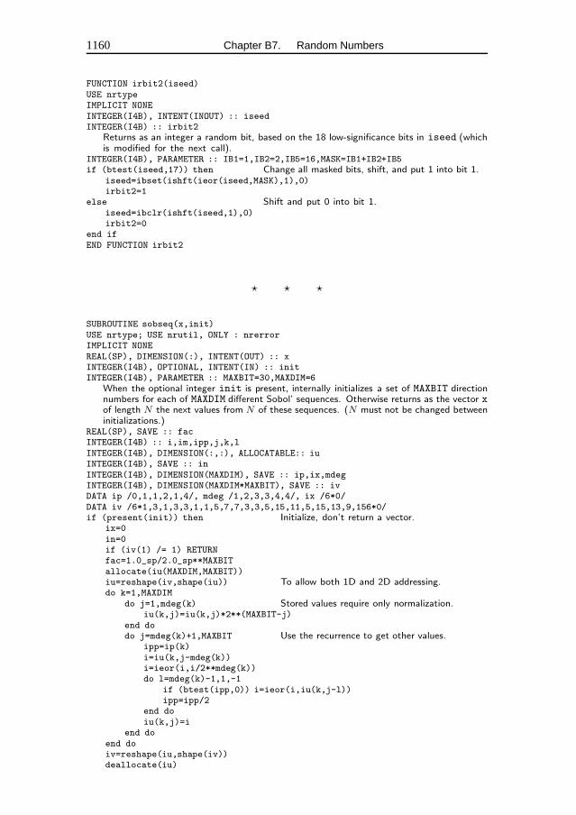
1160 Chapter B7. Random Numbers
FUNCTION irbit2(iseed)USE nrtypeIMPLICIT NONEINTEGER(I4B), INTENT(INOUT) :: iseedINTEGER(I4B) :: irbit2
Returns as an integer a random bit, based on the 18 low-significance bits in iseed (whichis modified for the next call).
INTEGER(I4B), PARAMETER :: IB1=1,IB2=2,IB5=16,MASK=IB1+IB2+IB5if (btest(iseed,17)) then Change all masked bits, shift, and put 1 into bit 1.
iseed=ibset(ishft(ieor(iseed,MASK),1),0)irbit2=1
else Shift and put 0 into bit 1.iseed=ibclr(ishft(iseed,1),0)irbit2=0
end ifEND FUNCTION irbit2
� � �
SUBROUTINE sobseq(x,init)USE nrtype; USE nrutil, ONLY : nrerrorIMPLICIT NONEREAL(SP), DIMENSION(:), INTENT(OUT) :: xINTEGER(I4B), OPTIONAL, INTENT(IN) :: initINTEGER(I4B), PARAMETER :: MAXBIT=30,MAXDIM=6
When the optional integer init is present, internally initializes a set of MAXBIT directionnumbers for each of MAXDIM different Sobol’ sequences. Otherwise returns as the vector xof length N the next values from N of these sequences. (N must not be changed betweeninitializations.)
REAL(SP), SAVE :: facINTEGER(I4B) :: i,im,ipp,j,k,lINTEGER(I4B), DIMENSION(:,:), ALLOCATABLE:: iuINTEGER(I4B), SAVE :: inINTEGER(I4B), DIMENSION(MAXDIM), SAVE :: ip,ix,mdegINTEGER(I4B), DIMENSION(MAXDIM*MAXBIT), SAVE :: ivDATA ip /0,1,1,2,1,4/, mdeg /1,2,3,3,4,4/, ix /6*0/DATA iv /6*1,3,1,3,3,1,1,5,7,7,3,3,5,15,11,5,15,13,9,156*0/if (present(init)) then Initialize, don’t return a vector.
ix=0in=0if (iv(1) /= 1) RETURNfac=1.0_sp/2.0_sp**MAXBITallocate(iu(MAXDIM,MAXBIT))iu=reshape(iv,shape(iu)) To allow both 1D and 2D addressing.do k=1,MAXDIM
do j=1,mdeg(k) Stored values require only normalization.iu(k,j)=iu(k,j)*2**(MAXBIT-j)
end dodo j=mdeg(k)+1,MAXBIT Use the recurrence to get other values.
ipp=ip(k)i=iu(k,j-mdeg(k))i=ieor(i,i/2**mdeg(k))do l=mdeg(k)-1,1,-1
if (btest(ipp,0)) i=ieor(i,iu(k,j-l))ipp=ipp/2
end doiu(k,j)=i
end doend doiv=reshape(iu,shape(iv))deallocate(iu)
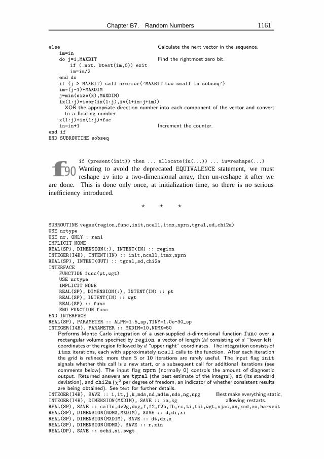
Chapter B7. Random Numbers 1161
else Calculate the next vector in the sequence.im=indo j=1,MAXBIT Find the rightmost zero bit.
if (.not. btest(im,0)) exitim=im/2
end doif (j > MAXBIT) call nrerror(’MAXBIT too small in sobseq’)im=(j-1)*MAXDIMj=min(size(x),MAXDIM)ix(1:j)=ieor(ix(1:j),iv(1+im:j+im))XOR the appropriate direction number into each component of the vector and convertto a floating number.
x(1:j)=ix(1:j)*facin=in+1 Increment the counter.
end ifEND SUBROUTINE sobseq
f90if (present(init)) then ... allocate(iu(...)) ... iu=reshape(...)
Wanting to avoid the deprecatedEQUIVALENCE statement, we mustreshapeiv into a two-dimensional array, then un-reshape it after we
are done. This is done only once, at initialization time, so there is no seriousinefficiency introduced.
� � �
SUBROUTINE vegas(region,func,init,ncall,itmx,nprn,tgral,sd,chi2a)USE nrtypeUSE nr, ONLY : ran1IMPLICIT NONEREAL(SP), DIMENSION(:), INTENT(IN) :: regionINTEGER(I4B), INTENT(IN) :: init,ncall,itmx,nprnREAL(SP), INTENT(OUT) :: tgral,sd,chi2aINTERFACE
FUNCTION func(pt,wgt)USE nrtypeIMPLICIT NONEREAL(SP), DIMENSION(:), INTENT(IN) :: ptREAL(SP), INTENT(IN) :: wgtREAL(SP) :: funcEND FUNCTION func
END INTERFACEREAL(SP), PARAMETER :: ALPH=1.5_sp,TINY=1.0e-30_spINTEGER(I4B), PARAMETER :: MXDIM=10,NDMX=50
Performs Monte Carlo integration of a user-supplied d-dimensional function func over arectangular volume specified by region, a vector of length 2d consisting of d “lower left”coordinates of the region followed by d “upper right” coordinates. The integration consists ofitmx iterations, each with approximately ncall calls to the function. After each iterationthe grid is refined; more than 5 or 10 iterations are rarely useful. The input flag initsignals whether this call is a new start, or a subsequent call for additional iterations (seecomments below). The input flag nprn (normally 0) controls the amount of diagnosticoutput. Returned answers are tgral (the best estimate of the integral), sd (its standarddeviation), and chi2a (χ2 per degree of freedom, an indicator of whether consistent resultsare being obtained). See text for further details.
INTEGER(I4B), SAVE :: i,it,j,k,mds,nd,ndim,ndo,ng,npg Bestmake everything static,allowing restarts.INTEGER(I4B), DIMENSION(MXDIM), SAVE :: ia,kg
REAL(SP), SAVE :: calls,dv2g,dxg,f,f2,f2b,fb,rc,ti,tsi,wgt,xjac,xn,xnd,xo,harvestREAL(SP), DIMENSION(NDMX,MXDIM), SAVE :: d,di,xiREAL(SP), DIMENSION(MXDIM), SAVE :: dt,dx,xREAL(SP), DIMENSION(NDMX), SAVE :: r,xinREAL(DP), SAVE :: schi,si,swgt
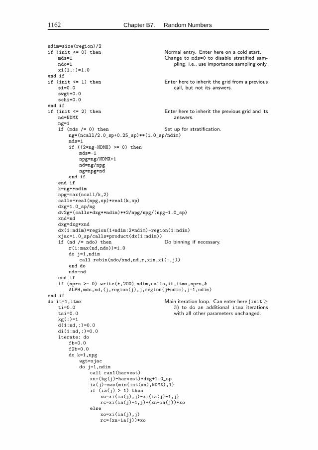
1162 Chapter B7. Random Numbers
ndim=size(region)/2if (init <= 0) then Normal entry. Enter here on a cold start.
mds=1 Change to mds=0 to disable stratified sam-pling, i.e., use importance sampling only.ndo=1
xi(1,:)=1.0end ifif (init <= 1) then Enter here to inherit the grid from a previous
call, but not its answers.si=0.0swgt=0.0schi=0.0
end ifif (init <= 2) then Enter here to inherit the previous grid and its
answers.nd=NDMXng=1if (mds /= 0) then Set up for stratification.
ng=(ncall/2.0_sp+0.25_sp)**(1.0_sp/ndim)mds=1if ((2*ng-NDMX) >= 0) then
mds=-1npg=ng/NDMX+1nd=ng/npgng=npg*nd
end ifend ifk=ng**ndimnpg=max(ncall/k,2)calls=real(npg,sp)*real(k,sp)dxg=1.0_sp/ngdv2g=(calls*dxg**ndim)**2/npg/npg/(npg-1.0_sp)xnd=nddxg=dxg*xnddx(1:ndim)=region(1+ndim:2*ndim)-region(1:ndim)xjac=1.0_sp/calls*product(dx(1:ndim))if (nd /= ndo) then Do binning if necessary.
r(1:max(nd,ndo))=1.0do j=1,ndim
call rebin(ndo/xnd,nd,r,xin,xi(:,j))end dondo=nd
end ifif (nprn >= 0) write(*,200) ndim,calls,it,itmx,nprn,&
ALPH,mds,nd,(j,region(j),j,region(j+ndim),j=1,ndim)end ifdo it=1,itmx Main iteration loop. Can enter here (init ≥
3) to do an additional itmx iterationswith all other parameters unchanged.
ti=0.0tsi=0.0kg(:)=1d(1:nd,:)=0.0di(1:nd,:)=0.0iterate: do
fb=0.0f2b=0.0do k=1,npg
wgt=xjacdo j=1,ndim
call ran1(harvest)xn=(kg(j)-harvest)*dxg+1.0_spia(j)=max(min(int(xn),NDMX),1)if (ia(j) > 1) then
xo=xi(ia(j),j)-xi(ia(j)-1,j)rc=xi(ia(j)-1,j)+(xn-ia(j))*xo
elsexo=xi(ia(j),j)rc=(xn-ia(j))*xo
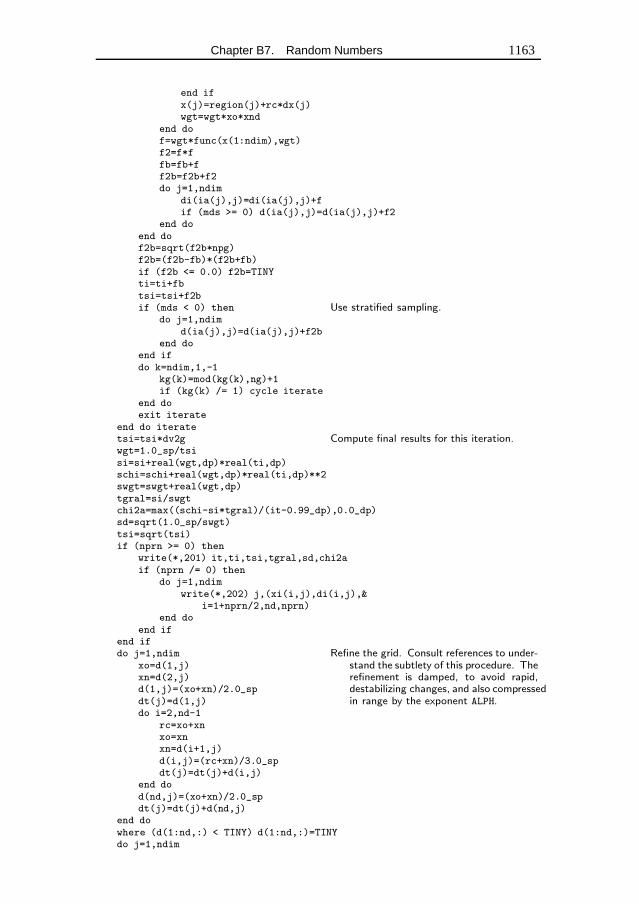
Chapter B7. Random Numbers 1163
end ifx(j)=region(j)+rc*dx(j)wgt=wgt*xo*xnd
end dof=wgt*func(x(1:ndim),wgt)f2=f*ffb=fb+ff2b=f2b+f2do j=1,ndim
di(ia(j),j)=di(ia(j),j)+fif (mds >= 0) d(ia(j),j)=d(ia(j),j)+f2
end doend dof2b=sqrt(f2b*npg)f2b=(f2b-fb)*(f2b+fb)if (f2b <= 0.0) f2b=TINYti=ti+fbtsi=tsi+f2bif (mds < 0) then Use stratified sampling.
do j=1,ndimd(ia(j),j)=d(ia(j),j)+f2b
end doend ifdo k=ndim,1,-1
kg(k)=mod(kg(k),ng)+1if (kg(k) /= 1) cycle iterate
end doexit iterate
end do iteratetsi=tsi*dv2g Compute final results for this iteration.wgt=1.0_sp/tsisi=si+real(wgt,dp)*real(ti,dp)schi=schi+real(wgt,dp)*real(ti,dp)**2swgt=swgt+real(wgt,dp)tgral=si/swgtchi2a=max((schi-si*tgral)/(it-0.99_dp),0.0_dp)sd=sqrt(1.0_sp/swgt)tsi=sqrt(tsi)if (nprn >= 0) then
write(*,201) it,ti,tsi,tgral,sd,chi2aif (nprn /= 0) then
do j=1,ndimwrite(*,202) j,(xi(i,j),di(i,j),&
i=1+nprn/2,nd,nprn)end do
end ifend ifdo j=1,ndim Refine the grid. Consult references to under-
stand the subtlety of this procedure. Therefinement is damped, to avoid rapid,destabilizing changes, and also compressedin range by the exponent ALPH.
xo=d(1,j)xn=d(2,j)d(1,j)=(xo+xn)/2.0_spdt(j)=d(1,j)do i=2,nd-1
rc=xo+xnxo=xnxn=d(i+1,j)d(i,j)=(rc+xn)/3.0_spdt(j)=dt(j)+d(i,j)
end dod(nd,j)=(xo+xn)/2.0_spdt(j)=dt(j)+d(nd,j)
end dowhere (d(1:nd,:) < TINY) d(1:nd,:)=TINYdo j=1,ndim
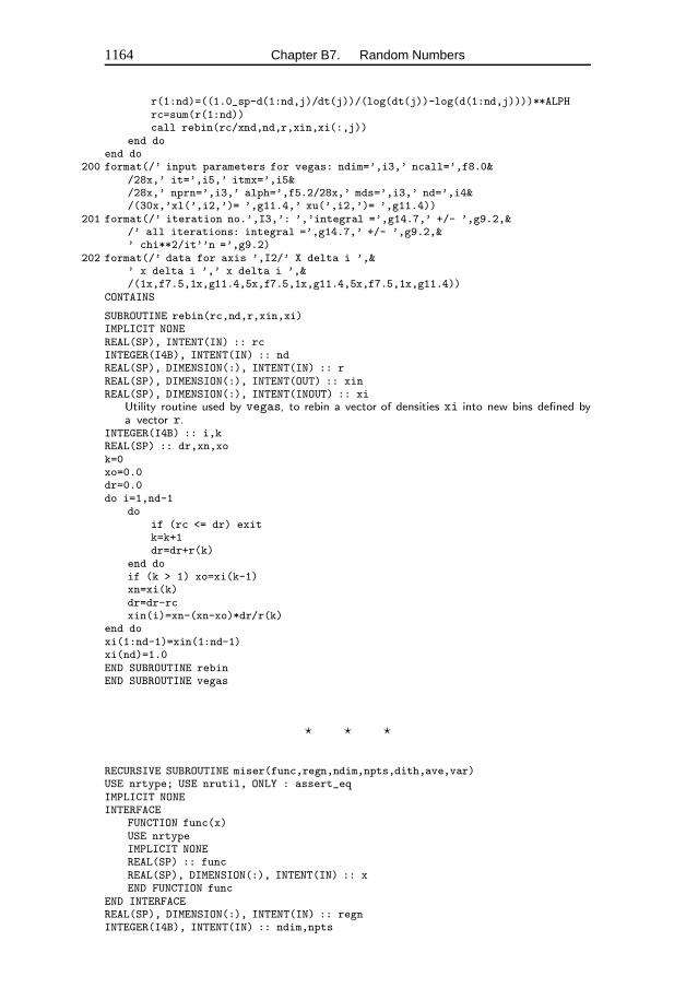
1164 Chapter B7. Random Numbers
r(1:nd)=((1.0_sp-d(1:nd,j)/dt(j))/(log(dt(j))-log(d(1:nd,j))))**ALPHrc=sum(r(1:nd))call rebin(rc/xnd,nd,r,xin,xi(:,j))
end doend do
200 format(/’ input parameters for vegas: ndim=’,i3,’ ncall=’,f8.0&/28x,’ it=’,i5,’ itmx=’,i5&/28x,’ nprn=’,i3,’ alph=’,f5.2/28x,’ mds=’,i3,’ nd=’,i4&/(30x,’xl(’,i2,’)= ’,g11.4,’ xu(’,i2,’)= ’,g11.4))
201 format(/’ iteration no.’,I3,’: ’,’integral =’,g14.7,’ +/- ’,g9.2,&/’ all iterations: integral =’,g14.7,’ +/- ’,g9.2,&’ chi**2/it’’n =’,g9.2)
202 format(/’ data for axis ’,I2/’ X delta i ’,&’ x delta i ’,’ x delta i ’,&/(1x,f7.5,1x,g11.4,5x,f7.5,1x,g11.4,5x,f7.5,1x,g11.4))
CONTAINS
SUBROUTINE rebin(rc,nd,r,xin,xi)IMPLICIT NONEREAL(SP), INTENT(IN) :: rcINTEGER(I4B), INTENT(IN) :: ndREAL(SP), DIMENSION(:), INTENT(IN) :: rREAL(SP), DIMENSION(:), INTENT(OUT) :: xinREAL(SP), DIMENSION(:), INTENT(INOUT) :: xi
Utility routine used by vegas, to rebin a vector of densities xi into new bins defined bya vector r.
INTEGER(I4B) :: i,kREAL(SP) :: dr,xn,xok=0xo=0.0dr=0.0do i=1,nd-1
doif (rc <= dr) exitk=k+1dr=dr+r(k)
end doif (k > 1) xo=xi(k-1)xn=xi(k)dr=dr-rcxin(i)=xn-(xn-xo)*dr/r(k)
end doxi(1:nd-1)=xin(1:nd-1)xi(nd)=1.0END SUBROUTINE rebinEND SUBROUTINE vegas
� � �
RECURSIVE SUBROUTINE miser(func,regn,ndim,npts,dith,ave,var)USE nrtype; USE nrutil, ONLY : assert_eqIMPLICIT NONEINTERFACE
FUNCTION func(x)USE nrtypeIMPLICIT NONEREAL(SP) :: funcREAL(SP), DIMENSION(:), INTENT(IN) :: xEND FUNCTION func
END INTERFACEREAL(SP), DIMENSION(:), INTENT(IN) :: regnINTEGER(I4B), INTENT(IN) :: ndim,npts
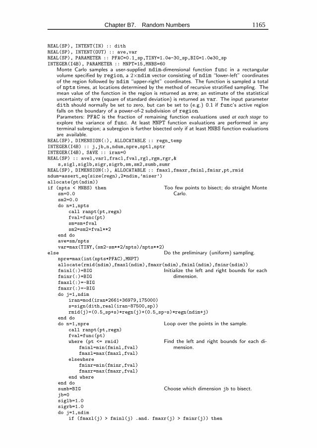
Chapter B7. Random Numbers 1165
REAL(SP), INTENT(IN) :: dithREAL(SP), INTENT(OUT) :: ave,varREAL(SP), PARAMETER :: PFAC=0.1_sp,TINY=1.0e-30_sp,BIG=1.0e30_spINTEGER(I4B), PARAMETER :: MNPT=15,MNBS=60
Monte Carlo samples a user-supplied ndim-dimensional function func in a rectangularvolume specified by region, a 2×ndim vector consisting of ndim “lower-left” coordinatesof the region followed by ndim “upper-right” coordinates. The function is sampled a totalof npts times, at locations determined by the method of recursive stratified sampling. Themean value of the function in the region is returned as ave; an estimate of the statisticaluncertainty of ave (square of standard deviation) is returned as var. The input parameterdith should normally be set to zero, but can be set to (e.g.) 0.1 if func’s active regionfalls on the boundary of a power-of-2 subdivision of region.Parameters: PFAC is the fraction of remaining function evaluations used at each stage toexplore the variance of func. At least MNPT function evaluations are performed in anyterminal subregion; a subregion is further bisected only if at least MNBS function evaluationsare available.
REAL(SP), DIMENSION(:), ALLOCATABLE :: regn_tempINTEGER(I4B) :: j,jb,n,ndum,npre,nptl,nptrINTEGER(I4B), SAVE :: iran=0REAL(SP) :: avel,varl,fracl,fval,rgl,rgm,rgr,&
s,sigl,siglb,sigr,sigrb,sm,sm2,sumb,sumrREAL(SP), DIMENSION(:), ALLOCATABLE :: fmaxl,fmaxr,fminl,fminr,pt,rmidndum=assert_eq(size(regn),2*ndim,’miser’)allocate(pt(ndim))if (npts < MNBS) then Too few points to bisect; do straight Monte
Carlo.sm=0.0sm2=0.0do n=1,npts
call ranpt(pt,regn)fval=func(pt)sm=sm+fvalsm2=sm2+fval**2
end doave=sm/nptsvar=max(TINY,(sm2-sm**2/npts)/npts**2)
else Do the preliminary (uniform) sampling.npre=max(int(npts*PFAC),MNPT)allocate(rmid(ndim),fmaxl(ndim),fmaxr(ndim),fminl(ndim),fminr(ndim))fminl(:)=BIG Initialize the left and right bounds for each
dimension.fminr(:)=BIGfmaxl(:)=-BIGfmaxr(:)=-BIGdo j=1,ndim
iran=mod(iran*2661+36979,175000)s=sign(dith,real(iran-87500,sp))rmid(j)=(0.5_sp+s)*regn(j)+(0.5_sp-s)*regn(ndim+j)
end dodo n=1,npre Loop over the points in the sample.
call ranpt(pt,regn)fval=func(pt)where (pt <= rmid) Find the left and right bounds for each di-
mension.fminl=min(fminl,fval)fmaxl=max(fmaxl,fval)
elsewherefminr=min(fminr,fval)fmaxr=max(fmaxr,fval)
end whereend dosumb=BIG Choose which dimension jb to bisect.jb=0siglb=1.0sigrb=1.0do j=1,ndim
if (fmaxl(j) > fminl(j) .and. fmaxr(j) > fminr(j)) then
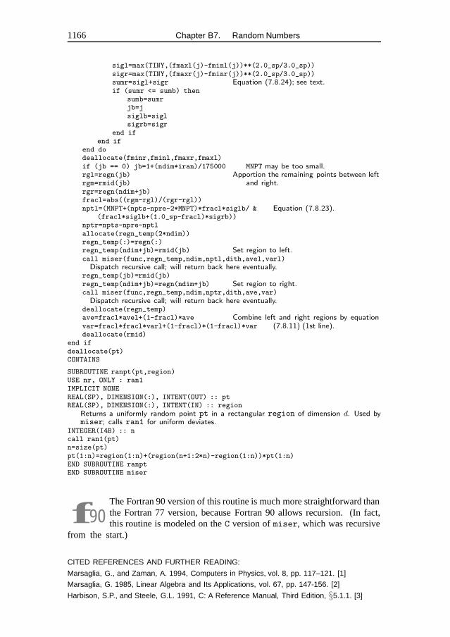
1166 Chapter B7. Random Numbers
sigl=max(TINY,(fmaxl(j)-fminl(j))**(2.0_sp/3.0_sp))sigr=max(TINY,(fmaxr(j)-fminr(j))**(2.0_sp/3.0_sp))sumr=sigl+sigr Equation (7.8.24); see text.if (sumr <= sumb) then
sumb=sumrjb=jsiglb=siglsigrb=sigr
end ifend if
end dodeallocate(fminr,fminl,fmaxr,fmaxl)if (jb == 0) jb=1+(ndim*iran)/175000 MNPT may be too small.rgl=regn(jb) Apportion the remaining points between left
and right.rgm=rmid(jb)rgr=regn(ndim+jb)fracl=abs((rgm-rgl)/(rgr-rgl))nptl=(MNPT+(npts-npre-2*MNPT)*fracl*siglb/ & Equation (7.8.23).
(fracl*siglb+(1.0_sp-fracl)*sigrb))nptr=npts-npre-nptlallocate(regn_temp(2*ndim))regn_temp(:)=regn(:)regn_temp(ndim+jb)=rmid(jb) Set region to left.call miser(func,regn_temp,ndim,nptl,dith,avel,varl)Dispatch recursive call; will return back here eventually.
regn_temp(jb)=rmid(jb)regn_temp(ndim+jb)=regn(ndim+jb) Set region to right.call miser(func,regn_temp,ndim,nptr,dith,ave,var)Dispatch recursive call; will return back here eventually.
deallocate(regn_temp)ave=fracl*avel+(1-fracl)*ave Combine left and right regions by equation
(7.8.11) (1st line).var=fracl*fracl*varl+(1-fracl)*(1-fracl)*vardeallocate(rmid)
end ifdeallocate(pt)CONTAINS
SUBROUTINE ranpt(pt,region)USE nr, ONLY : ran1IMPLICIT NONEREAL(SP), DIMENSION(:), INTENT(OUT) :: ptREAL(SP), DIMENSION(:), INTENT(IN) :: region
Returns a uniformly random point pt in a rectangular region of dimension d. Used bymiser; calls ran1 for uniform deviates.
INTEGER(I4B) :: ncall ran1(pt)n=size(pt)pt(1:n)=region(1:n)+(region(n+1:2*n)-region(1:n))*pt(1:n)END SUBROUTINE ranptEND SUBROUTINE miser
f90The Fortran 90 version of this routine is much more straightforward thanthe Fortran 77 version, because Fortran 90 allows recursion. (In fact,this routine is modeled on theC version ofmiser, which was recursive
from the start.)
CITED REFERENCES AND FURTHER READING:
Marsaglia, G., and Zaman, A. 1994, Computers in Physics, vol. 8, pp. 117–121. [1]
Marsaglia, G. 1985, Linear Algebra and Its Applications, vol. 67, pp. 147-156. [2]
Harbison, S.P., and Steele, G.L. 1991, C: A Reference Manual, Third Edition, §5.1.1. [3]
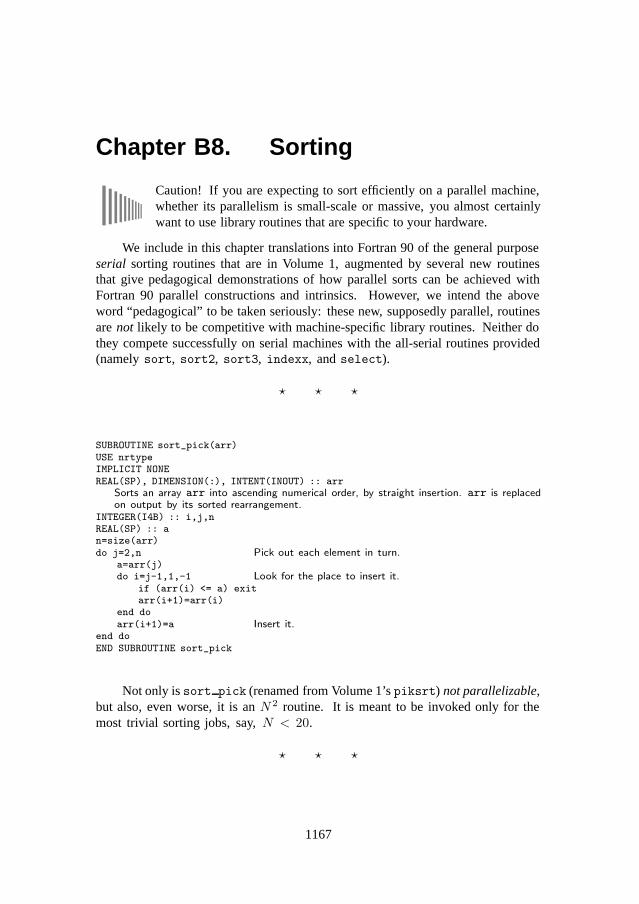
Chapter B8. Sorting
Caution! If you are expecting to sort efficiently on a parallel machine,whether its parallelism is small-scale or massive, you almost certainlywant to use library routines that are specific to your hardware.
We include in this chapter translations into Fortran 90 of the general purposeserial sorting routines that are in Volume 1, augmented by several new routinesthat give pedagogical demonstrations of how parallel sorts can be achieved withFortran 90 parallel constructions and intrinsics. However, we intend the aboveword “pedagogical” to be taken seriously: these new, supposedly parallel, routinesare not likely to be competitive with machine-specific library routines. Neither dothey compete successfully on serial machines with the all-serial routines provided(namely sort, sort2, sort3, indexx, and select).
� � �
SUBROUTINE sort_pick(arr)USE nrtypeIMPLICIT NONEREAL(SP), DIMENSION(:), INTENT(INOUT) :: arr
Sorts an array arr into ascending numerical order, by straight insertion. arr is replacedon output by its sorted rearrangement.
INTEGER(I4B) :: i,j,nREAL(SP) :: an=size(arr)do j=2,n Pick out each element in turn.
a=arr(j)do i=j-1,1,-1 Look for the place to insert it.
if (arr(i) <= a) exitarr(i+1)=arr(i)
end doarr(i+1)=a Insert it.
end doEND SUBROUTINE sort_pick
Not only is sort pick (renamed from Volume 1’s piksrt) not parallelizable,but also, even worse, it is an N 2 routine. It is meant to be invoked only for themost trivial sorting jobs, say, N < 20.
� � �
1167
1168 Chapter B8. Sorting
SUBROUTINE sort_shell(arr)USE nrtypeIMPLICIT NONEREAL(SP), DIMENSION(:), INTENT(INOUT) :: arr
Sorts an array arr into ascending numerical order by Shell’s method (diminishing incrementsort). arr is replaced on output by its sorted rearrangement.
INTEGER(I4B) :: i,j,inc,nREAL(SP) :: vn=size(arr)inc=1do Determine the starting increment.
inc=3*inc+1if (inc > n) exit
end dodo Loop over the partial sorts.
inc=inc/3do i=inc+1,n Outer loop of straight insertion.
v=arr(i)j=ido Inner loop of straight insertion.
if (arr(j-inc) <= v) exitarr(j)=arr(j-inc)j=j-incif (j <= inc) exit
end doarr(j)=v
end doif (inc <= 1) exit
end doEND SUBROUTINE sort_shell
The routine sort shell is renamed from Volume 1’s shell. Shell’s Method,a diminishing increment sort, is not directly parallelizable. However, one can write afully parallel routine (though not an especially fast one — see remarks at beginningof this chapter) in much the same spirit:
SUBROUTINE sort_byreshape(arr)USE nrtype; USE nrutil, ONLY : swapIMPLICIT NONEREAL(SP), DIMENSION(:), INTENT(INOUT) :: arr
Sort an array arr by bubble sorting a succession of reshapings into array slices. The methodis similar to Shell sort, but allows parallelization within the vectorized masked swap calls.
REAL(SP), DIMENSION(:,:), ALLOCATABLE :: tabREAL(SP), PARAMETER :: big=huge(arr)INTEGER(I4B) :: inc,n,mn=size(arr)inc=1do Find the largest increment that fits.
inc=2*inc+1if (inc > n) exit
end dodo Loop over the different shapes for the reshaped
array.inc=inc/2m=(n+inc-1)/incallocate(tab(inc,m)) Allocate space and reshape the array. big en-
sures that fill elements stay at theend.
tab=reshape(arr, (/inc,m/) , (/big/) )do
Bubble sort all the rows in parallel.call swap(tab(:,1:m-1:2),tab(:,2:m:2), &
tab(:,1:m-1:2)>tab(:,2:m:2))call swap(tab(:,2:m-1:2),tab(:,3:m:2), &
tab(:,2:m-1:2)>tab(:,3:m:2))
Chapter B8. Sorting 1169
if (all(tab(:,1:m-1) <= tab(:,2:m))) exitend doarr=reshape(tab,shape(arr)) Put the array back together for the next shape.deallocate(tab)if (inc <= 1) exit
end doEND SUBROUTINE sort_byreshape
The basic idea is to reshape the given one-dimensional array into asuccession of two-dimensional arrays, starting with “tall and narrow”(many rows, few columns), and ending up with “short and wide” (many
columns, few rows). At each stage we sort all the rows in parallel by a bubble sort,giving something close to Shell’s diminishing increments.
� � �
We now arrive at those routines, based on the Quicksort algorithm, that weactually intend for use with general N on serial machines:
SUBROUTINE sort(arr)USE nrtype; USE nrutil, ONLY : swap,nrerrorIMPLICIT NONEREAL(SP), DIMENSION(:), INTENT(INOUT) :: arrINTEGER(I4B), PARAMETER :: NN=15, NSTACK=50
Sorts an array arr into ascending numerical order using the Quicksort algorithm. arr isreplaced on output by its sorted rearrangement.Parameters: NN is the size of subarrays sorted by straight insertion and NSTACK is therequired auxiliary storage.
REAL(SP) :: aINTEGER(I4B) :: n,k,i,j,jstack,l,rINTEGER(I4B), DIMENSION(NSTACK) :: istackn=size(arr)jstack=0l=1r=ndo
if (r-l < NN) then Insertion sort when subarray small enough.do j=l+1,r
a=arr(j)do i=j-1,l,-1
if (arr(i) <= a) exitarr(i+1)=arr(i)
end doarr(i+1)=a
end doif (jstack == 0) RETURNr=istack(jstack) Pop stack and begin a new round of partition-
ing.l=istack(jstack-1)jstack=jstack-2
else Choose median of left, center, and right elementsas partitioning element a. Also rearrange sothat a(l) ≤ a(l+1) ≤ a(r).
k=(l+r)/2call swap(arr(k),arr(l+1))call swap(arr(l),arr(r),arr(l)>arr(r))call swap(arr(l+1),arr(r),arr(l+1)>arr(r))call swap(arr(l),arr(l+1),arr(l)>arr(l+1))i=l+1 Initialize pointers for partitioning.j=ra=arr(l+1) Partitioning element.do Here is the meat.
do Scan up to find element >= a.i=i+1
1170 Chapter B8. Sorting
if (arr(i) >= a) exitend dodo Scan down to find element <= a.
j=j-1if (arr(j) <= a) exit
end doif (j < i) exit Pointers crossed. Exit with partitioning complete.call swap(arr(i),arr(j)) Exchange elements.
end doarr(l+1)=arr(j) Insert partitioning element.arr(j)=ajstack=jstack+2Push pointers to larger subarray on stack; process smaller subarray immediately.
if (jstack > NSTACK) call nrerror(’sort: NSTACK too small’)if (r-i+1 >= j-l) then
istack(jstack)=ristack(jstack-1)=ir=j-1
elseistack(jstack)=j-1istack(jstack-1)=ll=i
end ifend if
end doEND SUBROUTINE sort
f90call swap(...) ... call swap(...) One might think twice about puttingall these external function calls (to nrutil routines) in the inner loopof something as streamlined as a sort routine, but here they are executed
only once for each partitioning.
call swap(arr(i),arr(j)) This call is in a loop, but not the innermost loop.Most modern machines are very fast at the “context changes” implied by subroutinecalls and returns; but in a time-critical context you might code this swap in-line andsee if there is any timing difference.SUBROUTINE sort2(arr,slave)USE nrtype; USE nrutil, ONLY : assert_eqUSE nr, ONLY : indexxIMPLICIT NONEREAL(SP), DIMENSION(:), INTENT(INOUT) :: arr,slave
Sorts an array arr into ascending order using Quicksort, while making the correspondingrearrangement of the same-size array slave. The sorting and rearrangement are performedby means of an index array.
INTEGER(I4B) :: ndumINTEGER(I4B), DIMENSION(size(arr)) :: indexndum=assert_eq(size(arr),size(slave),’sort2’)call indexx(arr,index) Make the index array.arr=arr(index) Sort arr.slave=slave(index) Rearrange slave.END SUBROUTINE sort2
� � �
A close surrogate for the Quicksort partition-exchange algorithm canbe coded, parallelizable, by using Fortran 90’s pack intrinsic. Onreal compilers, unfortunately, the resulting code is not very efficient as
compared with (on serial machines) the tightness of sort’s inner loop, above, or(on parallel machines) supplied library sort routines. We illustrate the principlenevertheless in the following routine.
Chapter B8. Sorting 1171
RECURSIVE SUBROUTINE sort_bypack(arr)USE nrtype; USE nrutil, ONLY : array_copy,swapIMPLICIT NONEREAL(SP), DIMENSION(:), INTENT(INOUT) :: arr
Sort an array arr by recursively applying the Fortran 90 pack intrinsic. The method issimilar to Quicksort, but this variant allows parallelization by the Fortran 90 compiler.
REAL(SP) :: aINTEGER(I4B) :: n,k,nl,nerrINTEGER(I4B), SAVE :: level=0LOGICAL, DIMENSION(:), ALLOCATABLE, SAVE :: maskREAL(SP), DIMENSION(:), ALLOCATABLE, SAVE :: tempn=size(arr)if (n <= 1) RETURNk=(1+n)/2call swap(arr(1),arr(k),arr(1)>arr(k)) Pivot element is median of first, middle,
and last.call swap(arr(k),arr(n),arr(k)>arr(n))call swap(arr(1),arr(k),arr(1)>arr(k))if (n <= 3) RETURNlevel=level+1 Keep track of recursion level to avoid al-
location overhead.if (level == 1) allocate(mask(n),temp(n))a=arr(k)mask(1:n) = (arr <= a) Which elements move to left?mask(k) = .false.call array_copy(pack(arr,mask(1:n)),temp,nl,nerr) Move them.mask(k) = .true.temp(nl+2:n)=pack(arr,.not. mask(1:n)) Move others to right.temp(nl+1)=aarr=temp(1:n)call sort_bypack(arr(1:nl)) And recurse.call sort_bypack(arr(nl+2:n))if (level == 1) deallocate(mask,temp)level=level-1END SUBROUTINE sort_bypack
� � �
The following routine, sort heap, is renamed from Volume 1’s hpsort.
SUBROUTINE sort_heap(arr)USE nrtypeUSE nrutil, ONLY : swapIMPLICIT NONEREAL(SP), DIMENSION(:), INTENT(INOUT) :: arr
Sorts an array arr into ascending numerical order using the Heapsort algorithm. arr isreplaced on output by its sorted rearrangement.
INTEGER(I4B) :: i,nn=size(arr)do i=n/2,1,-1
The index i, which here determines the “left” range of the sift-down, i.e., the element tobe sifted down, is decremented from n/2 down to 1 during the “hiring” (heap creation)phase.
call sift_down(i,n)end dodo i=n,2,-1
Here the “right” range of the sift-down is decremented from n-1 down to 1 during the“retirement-and-promotion” (heap selection) phase.
call swap(arr(1),arr(i)) Clear a space at the end of the array, andretire the top of the heap into it.call sift_down(1,i-1)
end doCONTAINS
SUBROUTINE sift_down(l,r)INTEGER(I4B), INTENT(IN) :: l,r
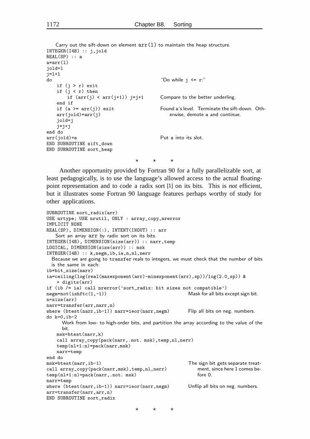
1172 Chapter B8. Sorting
Carry out the sift-down on element arr(l) to maintain the heap structure.INTEGER(I4B) :: j,joldREAL(SP) :: aa=arr(l)jold=lj=l+ldo “Do while j <= r:”
if (j > r) exitif (j < r) then
if (arr(j) < arr(j+1)) j=j+1 Compare to the better underling.end ifif (a >= arr(j)) exit Found a’s level. Terminate the sift-down. Oth-
erwise, demote a and continue.arr(jold)=arr(j)jold=jj=j+j
end doarr(jold)=a Put a into its slot.END SUBROUTINE sift_downEND SUBROUTINE sort_heap
� � �
Another opportunity provided by Fortran 90 for a fully parallelizable sort, atleast pedagogically, is to use the language’s allowed access to the actual floating-point representation and to code a radix sort [1] on its bits. This is not efficient,but it illustrates some Fortran 90 language features perhaps worthy of study forother applications.
SUBROUTINE sort_radix(arr)USE nrtype; USE nrutil, ONLY : array_copy,nrerrorIMPLICIT NONEREAL(SP), DIMENSION(:), INTENT(INOUT) :: arr
Sort an array arr by radix sort on its bits.INTEGER(I4B), DIMENSION(size(arr)) :: narr,tempLOGICAL, DIMENSION(size(arr)) :: mskINTEGER(I4B) :: k,negm,ib,ia,n,nl,nerrBecause we are going to transfer reals to integers, we must check that the number of bitsis the same in each:
ib=bit_size(narr)ia=ceiling(log(real(maxexponent(arr)-minexponent(arr),sp))/log(2.0_sp)) &
+ digits(arr)if (ib /= ia) call nrerror(’sort_radix: bit sizes not compatible’)negm=not(ishftc(1,-1)) Mask for all bits except sign bit.n=size(arr)narr=transfer(arr,narr,n)where (btest(narr,ib-1)) narr=ieor(narr,negm) Flip all bits on neg. numbers.do k=0,ib-2
Work from low- to high-order bits, and partition the array according to the value of thebit.
msk=btest(narr,k)call array_copy(pack(narr,.not. msk),temp,nl,nerr)temp(nl+1:n)=pack(narr,msk)narr=temp
end domsk=btest(narr,ib-1) The sign bit gets separate treat-
ment, since here 1 comes be-fore 0.
call array_copy(pack(narr,msk),temp,nl,nerr)temp(nl+1:n)=pack(narr,.not. msk)narr=tempwhere (btest(narr,ib-1)) narr=ieor(narr,negm) Unflip all bits on neg. numbers.arr=transfer(narr,arr,n)END SUBROUTINE sort_radix
� � �
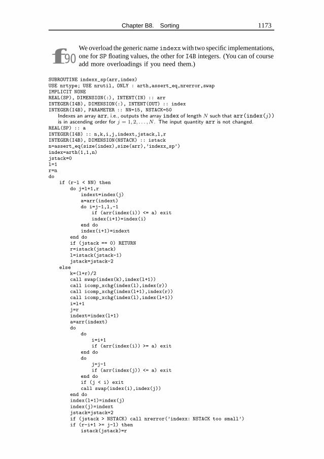
Chapter B8. Sorting 1173
f90We overload the generic name indexxwith two specific implementations,one for SP floating values, the other for I4B integers. (You can of courseadd more overloadings if you need them.)
SUBROUTINE indexx_sp(arr,index)USE nrtype; USE nrutil, ONLY : arth,assert_eq,nrerror,swapIMPLICIT NONEREAL(SP), DIMENSION(:), INTENT(IN) :: arrINTEGER(I4B), DIMENSION(:), INTENT(OUT) :: indexINTEGER(I4B), PARAMETER :: NN=15, NSTACK=50
Indexes an array arr, i.e., outputs the array index of length N such that arr(index(j))is in ascending order for j = 1,2, . . . ,N . The input quantity arr is not changed.
REAL(SP) :: aINTEGER(I4B) :: n,k,i,j,indext,jstack,l,rINTEGER(I4B), DIMENSION(NSTACK) :: istackn=assert_eq(size(index),size(arr),’indexx_sp’)index=arth(1,1,n)jstack=0l=1r=ndo
if (r-l < NN) thendo j=l+1,r
indext=index(j)a=arr(indext)do i=j-1,l,-1
if (arr(index(i)) <= a) exitindex(i+1)=index(i)
end doindex(i+1)=indext
end doif (jstack == 0) RETURNr=istack(jstack)l=istack(jstack-1)jstack=jstack-2
elsek=(l+r)/2call swap(index(k),index(l+1))call icomp_xchg(index(l),index(r))call icomp_xchg(index(l+1),index(r))call icomp_xchg(index(l),index(l+1))i=l+1j=rindext=index(l+1)a=arr(indext)do
doi=i+1if (arr(index(i)) >= a) exit
end dodo
j=j-1if (arr(index(j)) <= a) exit
end doif (j < i) exitcall swap(index(i),index(j))
end doindex(l+1)=index(j)index(j)=indextjstack=jstack+2if (jstack > NSTACK) call nrerror(’indexx: NSTACK too small’)if (r-i+1 >= j-l) then
istack(jstack)=r
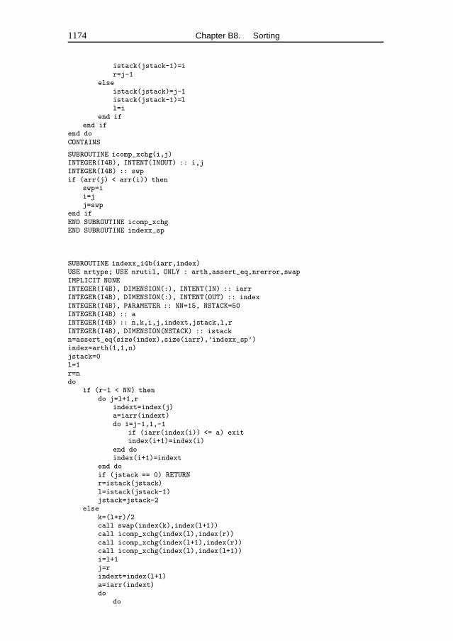
1174 Chapter B8. Sorting
istack(jstack-1)=ir=j-1
elseistack(jstack)=j-1istack(jstack-1)=ll=i
end ifend if
end doCONTAINS
SUBROUTINE icomp_xchg(i,j)INTEGER(I4B), INTENT(INOUT) :: i,jINTEGER(I4B) :: swpif (arr(j) < arr(i)) then
swp=ii=jj=swp
end ifEND SUBROUTINE icomp_xchgEND SUBROUTINE indexx_sp
SUBROUTINE indexx_i4b(iarr,index)USE nrtype; USE nrutil, ONLY : arth,assert_eq,nrerror,swapIMPLICIT NONEINTEGER(I4B), DIMENSION(:), INTENT(IN) :: iarrINTEGER(I4B), DIMENSION(:), INTENT(OUT) :: indexINTEGER(I4B), PARAMETER :: NN=15, NSTACK=50INTEGER(I4B) :: aINTEGER(I4B) :: n,k,i,j,indext,jstack,l,rINTEGER(I4B), DIMENSION(NSTACK) :: istackn=assert_eq(size(index),size(iarr),’indexx_sp’)index=arth(1,1,n)jstack=0l=1r=ndo
if (r-l < NN) thendo j=l+1,r
indext=index(j)a=iarr(indext)do i=j-1,1,-1
if (iarr(index(i)) <= a) exitindex(i+1)=index(i)
end doindex(i+1)=indext
end doif (jstack == 0) RETURNr=istack(jstack)l=istack(jstack-1)jstack=jstack-2
elsek=(l+r)/2call swap(index(k),index(l+1))call icomp_xchg(index(l),index(r))call icomp_xchg(index(l+1),index(r))call icomp_xchg(index(l),index(l+1))i=l+1j=rindext=index(l+1)a=iarr(indext)do
do
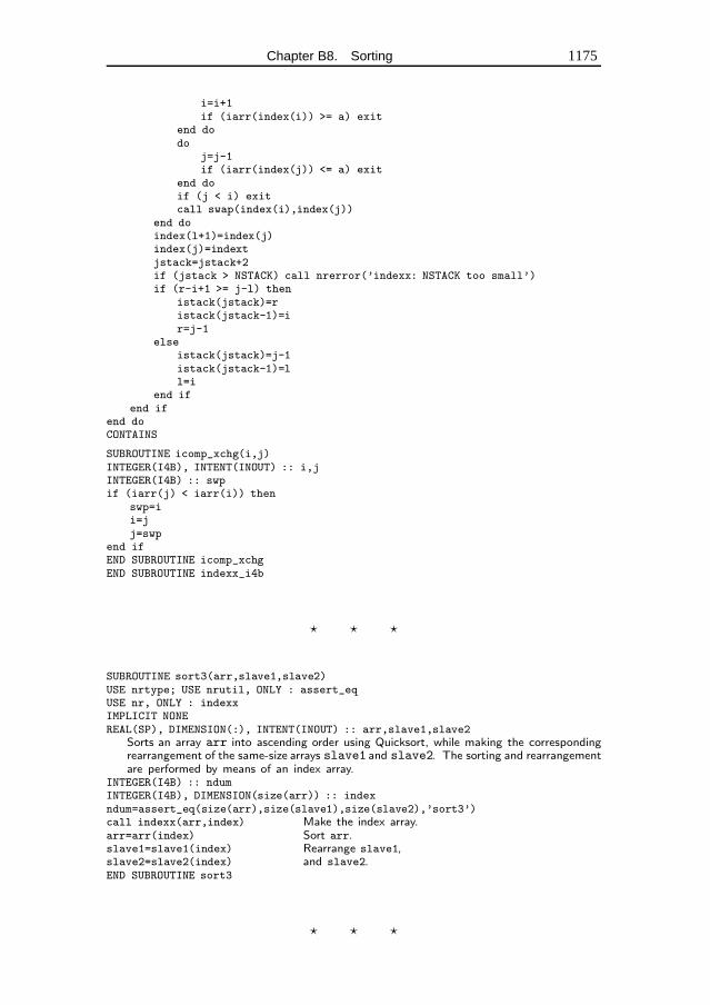
Chapter B8. Sorting 1175
i=i+1if (iarr(index(i)) >= a) exit
end dodo
j=j-1if (iarr(index(j)) <= a) exit
end doif (j < i) exitcall swap(index(i),index(j))
end doindex(l+1)=index(j)index(j)=indextjstack=jstack+2if (jstack > NSTACK) call nrerror(’indexx: NSTACK too small’)if (r-i+1 >= j-l) then
istack(jstack)=ristack(jstack-1)=ir=j-1
elseistack(jstack)=j-1istack(jstack-1)=ll=i
end ifend if
end doCONTAINS
SUBROUTINE icomp_xchg(i,j)INTEGER(I4B), INTENT(INOUT) :: i,jINTEGER(I4B) :: swpif (iarr(j) < iarr(i)) then
swp=ii=jj=swp
end ifEND SUBROUTINE icomp_xchgEND SUBROUTINE indexx_i4b
� � �
SUBROUTINE sort3(arr,slave1,slave2)USE nrtype; USE nrutil, ONLY : assert_eqUSE nr, ONLY : indexxIMPLICIT NONEREAL(SP), DIMENSION(:), INTENT(INOUT) :: arr,slave1,slave2
Sorts an array arr into ascending order using Quicksort, while making the correspondingrearrangement of the same-size arrays slave1 and slave2. The sorting and rearrangementare performed by means of an index array.
INTEGER(I4B) :: ndumINTEGER(I4B), DIMENSION(size(arr)) :: indexndum=assert_eq(size(arr),size(slave1),size(slave2),’sort3’)call indexx(arr,index) Make the index array.arr=arr(index) Sort arr.slave1=slave1(index) Rearrange slave1,slave2=slave2(index) and slave2.END SUBROUTINE sort3
� � �
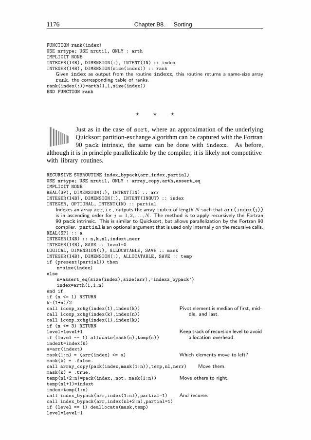
1176 Chapter B8. Sorting
FUNCTION rank(index)USE nrtype; USE nrutil, ONLY : arthIMPLICIT NONEINTEGER(I4B), DIMENSION(:), INTENT(IN) :: indexINTEGER(I4B), DIMENSION(size(index)) :: rank
Given index as output from the routine indexx, this routine returns a same-size arrayrank, the corresponding table of ranks.
rank(index(:))=arth(1,1,size(index))END FUNCTION rank
� � �
Just as in the case of sort, where an approximation of the underlyingQuicksort partition-exchange algorithm can be captured with the Fortran90 pack intrinsic, the same can be done with indexx. As before,
although it is in principle parallelizable by the compiler, it is likely not competitivewith library routines.
RECURSIVE SUBROUTINE index_bypack(arr,index,partial)USE nrtype; USE nrutil, ONLY : array_copy,arth,assert_eqIMPLICIT NONEREAL(SP), DIMENSION(:), INTENT(IN) :: arrINTEGER(I4B), DIMENSION(:), INTENT(INOUT) :: indexINTEGER, OPTIONAL, INTENT(IN) :: partial
Indexes an array arr, i.e., outputs the array index of length N such that arr(index(j))is in ascending order for j = 1,2, . . . ,N . The method is to apply recursively the Fortran90 pack intrinsic. This is similar to Quicksort, but allows parallelization by the Fortran 90compiler. partial is an optional argument that is used only internally on the recursive calls.
REAL(SP) :: aINTEGER(I4B) :: n,k,nl,indext,nerrINTEGER(I4B), SAVE :: level=0LOGICAL, DIMENSION(:), ALLOCATABLE, SAVE :: maskINTEGER(I4B), DIMENSION(:), ALLOCATABLE, SAVE :: tempif (present(partial)) then
n=size(index)else
n=assert_eq(size(index),size(arr),’indexx_bypack’)index=arth(1,1,n)
end ifif (n <= 1) RETURNk=(1+n)/2call icomp_xchg(index(1),index(k)) Pivot element is median of first, mid-
dle, and last.call icomp_xchg(index(k),index(n))call icomp_xchg(index(1),index(k))if (n <= 3) RETURNlevel=level+1 Keep track of recursion level to avoid
allocation overhead.if (level == 1) allocate(mask(n),temp(n))indext=index(k)a=arr(indext)mask(1:n) = (arr(index) <= a) Which elements move to left?mask(k) = .false.call array_copy(pack(index,mask(1:n)),temp,nl,nerr) Move them.mask(k) = .true.temp(nl+2:n)=pack(index,.not. mask(1:n)) Move others to right.temp(nl+1)=indextindex=temp(1:n)call index_bypack(arr,index(1:nl),partial=1) And recurse.call index_bypack(arr,index(nl+2:n),partial=1)if (level == 1) deallocate(mask,temp)level=level-1
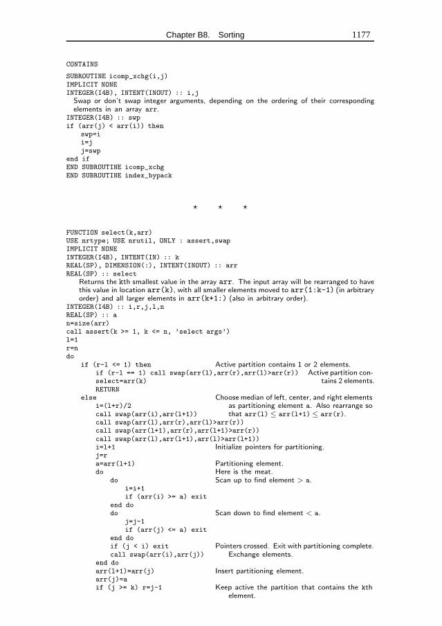
Chapter B8. Sorting 1177
CONTAINS
SUBROUTINE icomp_xchg(i,j)IMPLICIT NONEINTEGER(I4B), INTENT(INOUT) :: i,jSwap or don’t swap integer arguments, depending on the ordering of their correspondingelements in an array arr.
INTEGER(I4B) :: swpif (arr(j) < arr(i)) then
swp=ii=jj=swp
end ifEND SUBROUTINE icomp_xchgEND SUBROUTINE index_bypack
� � �
FUNCTION select(k,arr)USE nrtype; USE nrutil, ONLY : assert,swapIMPLICIT NONEINTEGER(I4B), INTENT(IN) :: kREAL(SP), DIMENSION(:), INTENT(INOUT) :: arrREAL(SP) :: select
Returns the kth smallest value in the array arr. The input array will be rearranged to havethis value in location arr(k), with all smaller elements moved to arr(1:k-1) (in arbitraryorder) and all larger elements in arr(k+1:) (also in arbitrary order).
INTEGER(I4B) :: i,r,j,l,nREAL(SP) :: an=size(arr)call assert(k >= 1, k <= n, ’select args’)l=1r=ndo
if (r-l <= 1) then Active partition contains 1 or 2 elements.if (r-l == 1) call swap(arr(l),arr(r),arr(l)>arr(r)) Active partition con-
tains 2 elements.select=arr(k)RETURN
else Choose median of left, center, and right elementsas partitioning element a. Also rearrange sothat arr(l) ≤ arr(l+1) ≤ arr(r).
i=(l+r)/2call swap(arr(i),arr(l+1))call swap(arr(l),arr(r),arr(l)>arr(r))call swap(arr(l+1),arr(r),arr(l+1)>arr(r))call swap(arr(l),arr(l+1),arr(l)>arr(l+1))i=l+1 Initialize pointers for partitioning.j=ra=arr(l+1) Partitioning element.do Here is the meat.
do Scan up to find element > a.i=i+1if (arr(i) >= a) exit
end dodo Scan down to find element < a.
j=j-1if (arr(j) <= a) exit
end doif (j < i) exit Pointers crossed. Exit with partitioning complete.call swap(arr(i),arr(j)) Exchange elements.
end doarr(l+1)=arr(j) Insert partitioning element.arr(j)=aif (j >= k) r=j-1 Keep active the partition that contains the kth
element.
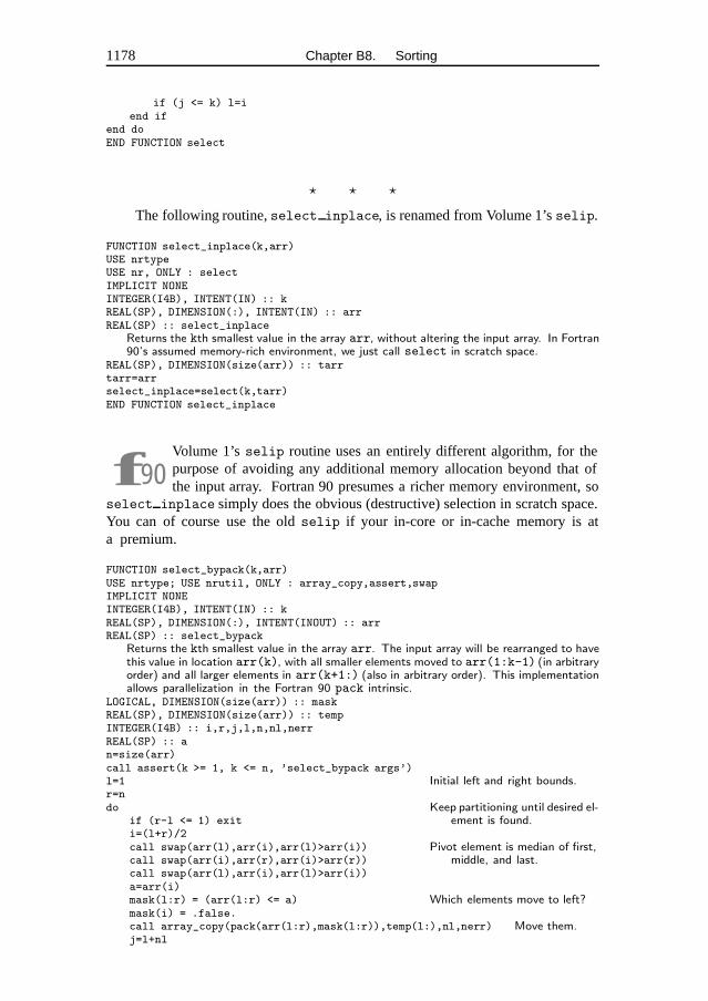
1178 Chapter B8. Sorting
if (j <= k) l=iend if
end doEND FUNCTION select
� � �
The following routine, select inplace, is renamed from Volume 1’s selip.
FUNCTION select_inplace(k,arr)USE nrtypeUSE nr, ONLY : selectIMPLICIT NONEINTEGER(I4B), INTENT(IN) :: kREAL(SP), DIMENSION(:), INTENT(IN) :: arrREAL(SP) :: select_inplace
Returns the kth smallest value in the array arr, without altering the input array. In Fortran90’s assumed memory-rich environment, we just call select in scratch space.
REAL(SP), DIMENSION(size(arr)) :: tarrtarr=arrselect_inplace=select(k,tarr)END FUNCTION select_inplace
f90Volume 1’s selip routine uses an entirely different algorithm, for thepurpose of avoiding any additional memory allocation beyond that ofthe input array. Fortran 90 presumes a richer memory environment, so
select inplace simply does the obvious (destructive) selection in scratch space.You can of course use the old selip if your in-core or in-cache memory is ata premium.
FUNCTION select_bypack(k,arr)USE nrtype; USE nrutil, ONLY : array_copy,assert,swapIMPLICIT NONEINTEGER(I4B), INTENT(IN) :: kREAL(SP), DIMENSION(:), INTENT(INOUT) :: arrREAL(SP) :: select_bypack
Returns the kth smallest value in the array arr. The input array will be rearranged to havethis value in location arr(k), with all smaller elements moved to arr(1:k-1) (in arbitraryorder) and all larger elements in arr(k+1:) (also in arbitrary order). This implementationallows parallelization in the Fortran 90 pack intrinsic.
LOGICAL, DIMENSION(size(arr)) :: maskREAL(SP), DIMENSION(size(arr)) :: tempINTEGER(I4B) :: i,r,j,l,n,nl,nerrREAL(SP) :: an=size(arr)call assert(k >= 1, k <= n, ’select_bypack args’)l=1 Initial left and right bounds.r=ndo Keep partitioning until desired el-
ement is found.if (r-l <= 1) exiti=(l+r)/2call swap(arr(l),arr(i),arr(l)>arr(i)) Pivot element is median of first,
middle, and last.call swap(arr(i),arr(r),arr(i)>arr(r))call swap(arr(l),arr(i),arr(l)>arr(i))a=arr(i)mask(l:r) = (arr(l:r) <= a) Which elements move to left?mask(i) = .false.call array_copy(pack(arr(l:r),mask(l:r)),temp(l:),nl,nerr) Move them.j=l+nl
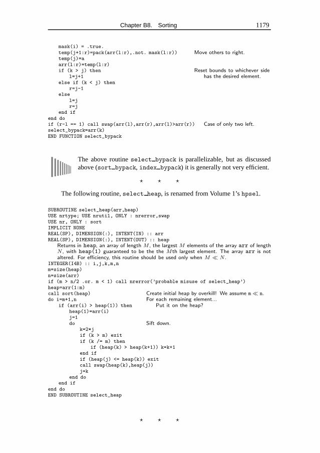
Chapter B8. Sorting 1179
mask(i) = .true.temp(j+1:r)=pack(arr(l:r),.not. mask(l:r)) Move others to right.temp(j)=aarr(l:r)=temp(l:r)if (k > j) then Reset bounds to whichever side
has the desired element.l=j+1else if (k < j) then
r=j-1else
l=jr=j
end ifend doif (r-l == 1) call swap(arr(l),arr(r),arr(l)>arr(r)) Case of only two left.select_bypack=arr(k)END FUNCTION select_bypack
The above routine select bypack is parallelizable, but as discussedabove (sort bypack, index bypack) it is generally not very efficient.
� � �
The following routine, select heap, is renamed from Volume 1’s hpsel.
SUBROUTINE select_heap(arr,heap)USE nrtype; USE nrutil, ONLY : nrerror,swapUSE nr, ONLY : sortIMPLICIT NONEREAL(SP), DIMENSION(:), INTENT(IN) :: arrREAL(SP), DIMENSION(:), INTENT(OUT) :: heap
Returns in heap, an array of length M , the largest M elements of the array arr of lengthN , with heap(1) guaranteed to be the the M th largest element. The array arr is notaltered. For efficiency, this routine should be used only when M � N .
INTEGER(I4B) :: i,j,k,m,nm=size(heap)n=size(arr)if (m > n/2 .or. m < 1) call nrerror(’probable misuse of select_heap’)heap=arr(1:m)call sort(heap) Create initial heap by overkill! We assume m � n.do i=m+1,n For each remaining element...
if (arr(i) > heap(1)) then Put it on the heap?heap(1)=arr(i)j=1do Sift down.
k=2*jif (k > m) exitif (k /= m) then
if (heap(k) > heap(k+1)) k=k+1end ifif (heap(j) <= heap(k)) exitcall swap(heap(k),heap(j))j=k
end doend if
end doEND SUBROUTINE select_heap
� � �
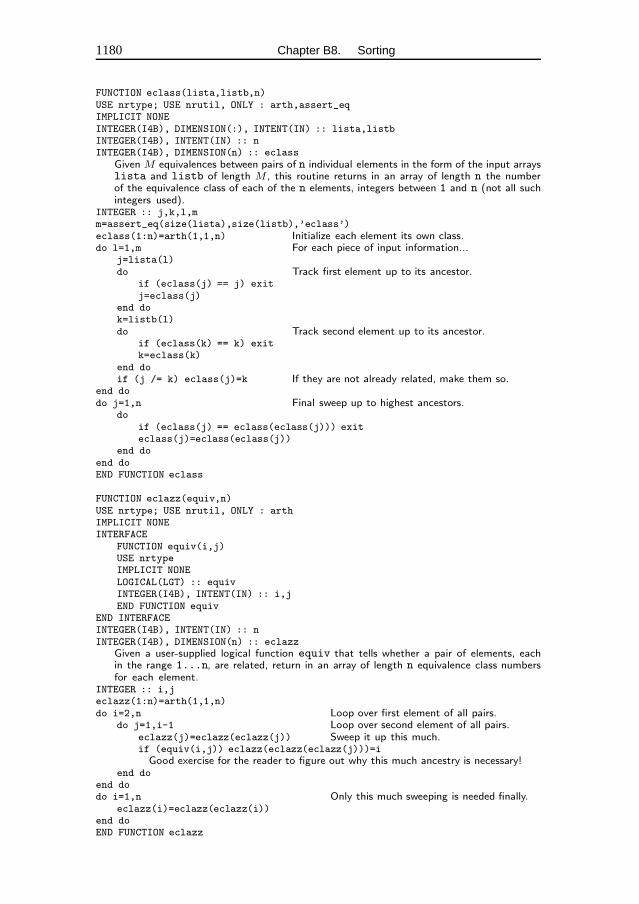
1180 Chapter B8. Sorting
FUNCTION eclass(lista,listb,n)USE nrtype; USE nrutil, ONLY : arth,assert_eqIMPLICIT NONEINTEGER(I4B), DIMENSION(:), INTENT(IN) :: lista,listbINTEGER(I4B), INTENT(IN) :: nINTEGER(I4B), DIMENSION(n) :: eclass
Given M equivalences between pairs of n individual elements in the form of the input arrayslista and listb of length M , this routine returns in an array of length n the numberof the equivalence class of each of the n elements, integers between 1 and n (not all suchintegers used).
INTEGER :: j,k,l,mm=assert_eq(size(lista),size(listb),’eclass’)eclass(1:n)=arth(1,1,n) Initialize each element its own class.do l=1,m For each piece of input information...
j=lista(l)do Track first element up to its ancestor.
if (eclass(j) == j) exitj=eclass(j)
end dok=listb(l)do Track second element up to its ancestor.
if (eclass(k) == k) exitk=eclass(k)
end doif (j /= k) eclass(j)=k If they are not already related, make them so.
end dodo j=1,n Final sweep up to highest ancestors.
doif (eclass(j) == eclass(eclass(j))) exiteclass(j)=eclass(eclass(j))
end doend doEND FUNCTION eclass
FUNCTION eclazz(equiv,n)USE nrtype; USE nrutil, ONLY : arthIMPLICIT NONEINTERFACE
FUNCTION equiv(i,j)USE nrtypeIMPLICIT NONELOGICAL(LGT) :: equivINTEGER(I4B), INTENT(IN) :: i,jEND FUNCTION equiv
END INTERFACEINTEGER(I4B), INTENT(IN) :: nINTEGER(I4B), DIMENSION(n) :: eclazz
Given a user-supplied logical function equiv that tells whether a pair of elements, eachin the range 1...n, are related, return in an array of length n equivalence class numbersfor each element.
INTEGER :: i,jeclazz(1:n)=arth(1,1,n)do i=2,n Loop over first element of all pairs.
do j=1,i-1 Loop over second element of all pairs.eclazz(j)=eclazz(eclazz(j)) Sweep it up this much.if (equiv(i,j)) eclazz(eclazz(eclazz(j)))=iGood exercise for the reader to figure out why this much ancestry is necessary!
end doend dodo i=1,n Only this much sweeping is needed finally.
eclazz(i)=eclazz(eclazz(i))end doEND FUNCTION eclazz

Chapter B8. Sorting 1181
CITED REFERENCES AND FURTHER READING:
Knuth, D.E. 1973, Sorting and Searching, vol. 3 of The Art of Computer Programming (Reading,MA: Addison-Wesley), §5.2.5. [1]
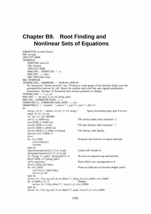
Chapter B9. Root Finding andNonlinear Sets of Equations
SUBROUTINE scrsho(func)USE nrtypeIMPLICIT NONEINTERFACE
FUNCTION func(x)USE nrtypeIMPLICIT NONEREAL(SP), INTENT(IN) :: xREAL(SP) :: funcEND FUNCTION func
END INTERFACEINTEGER(I4B), PARAMETER :: ISCR=60,JSCR=21
For interactive “dumb terminal” use. Produce a crude graph of the function func over theprompted-for interval x1,x2. Query for another plot until the user signals satisfaction.Parameters: Number of horizontal and vertical positions in display.
INTEGER(I4B) :: i,j,jzREAL(SP) :: dx,dyj,x,x1,x2,ybig,ysmlREAL(SP), DIMENSION(ISCR) :: yCHARACTER(1), DIMENSION(ISCR,JSCR) :: scrCHARACTER(1) :: blank=’ ’,zero=’-’,yy=’l’,xx=’-’,ff=’x’do
write (*,*) ’ Enter x1,x2 (= to stop)’ Query for another plot; quit if x1=x2.read (*,*) x1,x2if (x1 == x2) RETURNscr(1,1:JSCR)=yy Fill vertical sides with character ’l’.scr(ISCR,1:JSCR)=yyscr(2:ISCR-1,1)=xx Fill top, bottom with character ’-’.scr(2:ISCR-1,JSCR)=xxscr(2:ISCR-1,2:JSCR-1)=blank Fill interior with blanks.dx=(x2-x1)/(ISCR-1)x=x1do i=1,ISCR Evaluate the function at equal intervals.
y(i)=func(x)x=x+dx
end doysml=min(minval(y(:)),0.0_sp) Limits will include 0.ybig=max(maxval(y(:)),0.0_sp)if (ybig == ysml) ybig=ysml+1.0 Be sure to separate top and bottom.dyj=(JSCR-1)/(ybig-ysml)jz=1-ysml*dyj Note which row corresponds to 0.scr(1:ISCR,jz)=zerodo i=1,ISCR Place an indicator at function height and 0.
j=1+(y(i)-ysml)*dyjscr(i,j)=ff
end dowrite (*,’(1x,1p,e10.3,1x,80a1)’) ybig,(scr(i,JSCR),i=1,ISCR)do j=JSCR-1,2,-1 Display.
write (*,’(12x,80a1)’) (scr(i,j),i=1,ISCR)end dowrite (*,’(1x,1p,e10.3,1x,80a1)’) ysml,(scr(i,1),i=1,ISCR)
1182
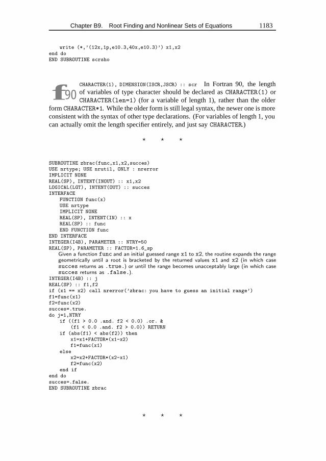
Chapter B9. Root Finding and Nonlinear Sets of Equations 1183
write (*,’(12x,1p,e10.3,40x,e10.3)’) x1,x2end doEND SUBROUTINE scrsho
f90CHARACTER(1), DIMENSION(ISCR,JSCR) :: scr In Fortran 90, the lengthof variables of type character should be declared as CHARACTER(1) orCHARACTER(len=1) (for a variable of length 1), rather than the older
form CHARACTER*1. While the older form is still legal syntax, the newer one is moreconsistent with the syntax of other type declarations. (For variables of length 1, youcan actually omit the length specifier entirely, and just say CHARACTER.)
� � �
SUBROUTINE zbrac(func,x1,x2,succes)USE nrtype; USE nrutil, ONLY : nrerrorIMPLICIT NONEREAL(SP), INTENT(INOUT) :: x1,x2LOGICAL(LGT), INTENT(OUT) :: succesINTERFACE
FUNCTION func(x)USE nrtypeIMPLICIT NONEREAL(SP), INTENT(IN) :: xREAL(SP) :: funcEND FUNCTION func
END INTERFACEINTEGER(I4B), PARAMETER :: NTRY=50REAL(SP), PARAMETER :: FACTOR=1.6_sp
Given a function func and an initial guessed range x1 to x2, the routine expands the rangegeometrically until a root is bracketed by the returned values x1 and x2 (in which casesucces returns as .true.) or until the range becomes unacceptably large (in which casesucces returns as .false.).
INTEGER(I4B) :: jREAL(SP) :: f1,f2if (x1 == x2) call nrerror(’zbrac: you have to guess an initial range’)f1=func(x1)f2=func(x2)succes=.true.do j=1,NTRY
if ((f1 > 0.0 .and. f2 < 0.0) .or. &(f1 < 0.0 .and. f2 > 0.0)) RETURN
if (abs(f1) < abs(f2)) thenx1=x1+FACTOR*(x1-x2)f1=func(x1)
elsex2=x2+FACTOR*(x2-x1)f2=func(x2)
end ifend dosucces=.false.END SUBROUTINE zbrac
� � �
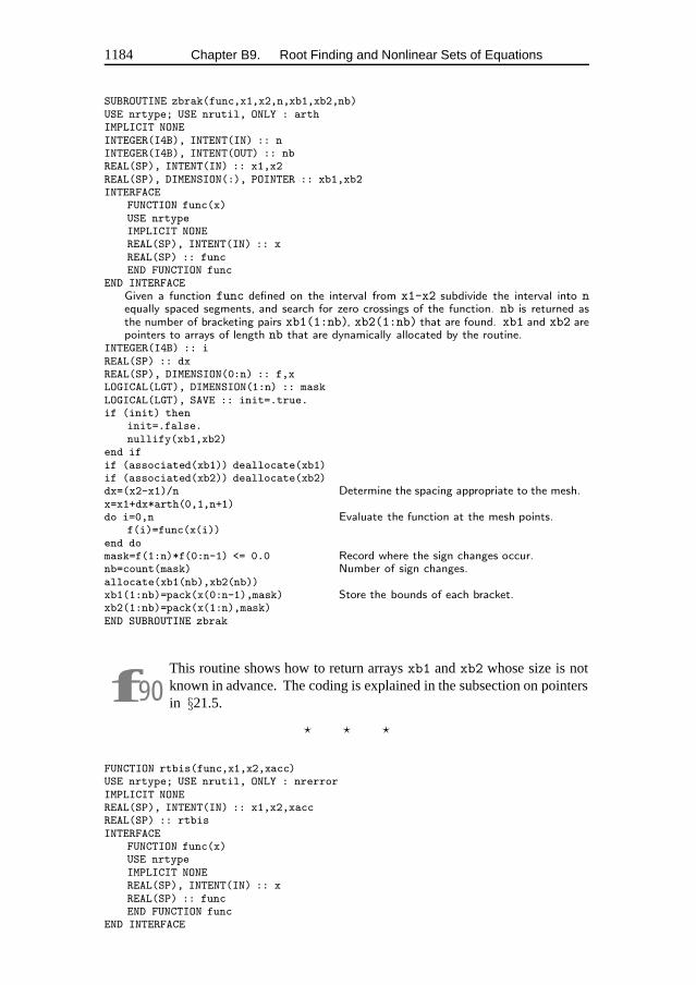
1184 Chapter B9. Root Finding and Nonlinear Sets of Equations
SUBROUTINE zbrak(func,x1,x2,n,xb1,xb2,nb)USE nrtype; USE nrutil, ONLY : arthIMPLICIT NONEINTEGER(I4B), INTENT(IN) :: nINTEGER(I4B), INTENT(OUT) :: nbREAL(SP), INTENT(IN) :: x1,x2REAL(SP), DIMENSION(:), POINTER :: xb1,xb2INTERFACE
FUNCTION func(x)USE nrtypeIMPLICIT NONEREAL(SP), INTENT(IN) :: xREAL(SP) :: funcEND FUNCTION func
END INTERFACEGiven a function func defined on the interval from x1-x2 subdivide the interval into nequally spaced segments, and search for zero crossings of the function. nb is returned asthe number of bracketing pairs xb1(1:nb), xb2(1:nb) that are found. xb1 and xb2 arepointers to arrays of length nb that are dynamically allocated by the routine.
INTEGER(I4B) :: iREAL(SP) :: dxREAL(SP), DIMENSION(0:n) :: f,xLOGICAL(LGT), DIMENSION(1:n) :: maskLOGICAL(LGT), SAVE :: init=.true.if (init) then
init=.false.nullify(xb1,xb2)
end ifif (associated(xb1)) deallocate(xb1)if (associated(xb2)) deallocate(xb2)dx=(x2-x1)/n Determine the spacing appropriate to the mesh.x=x1+dx*arth(0,1,n+1)do i=0,n Evaluate the function at the mesh points.
f(i)=func(x(i))end domask=f(1:n)*f(0:n-1) <= 0.0 Record where the sign changes occur.nb=count(mask) Number of sign changes.allocate(xb1(nb),xb2(nb))xb1(1:nb)=pack(x(0:n-1),mask) Store the bounds of each bracket.xb2(1:nb)=pack(x(1:n),mask)END SUBROUTINE zbrak
f90This routine shows how to return arrays xb1 and xb2 whose size is notknown in advance. The coding is explained in the subsection on pointersin §21.5.
� � �
FUNCTION rtbis(func,x1,x2,xacc)USE nrtype; USE nrutil, ONLY : nrerrorIMPLICIT NONEREAL(SP), INTENT(IN) :: x1,x2,xaccREAL(SP) :: rtbisINTERFACE
FUNCTION func(x)USE nrtypeIMPLICIT NONEREAL(SP), INTENT(IN) :: xREAL(SP) :: funcEND FUNCTION func
END INTERFACE
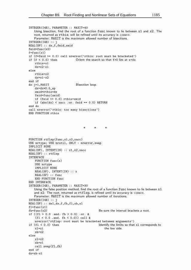
Chapter B9. Root Finding and Nonlinear Sets of Equations 1185
INTEGER(I4B), PARAMETER :: MAXIT=40Using bisection, find the root of a function func known to lie between x1 and x2. Theroot, returned as rtbis, will be refined until its accuracy is ±xacc.Parameter: MAXIT is the maximum allowed number of bisections.
INTEGER(I4B) :: jREAL(SP) :: dx,f,fmid,xmidfmid=func(x2)f=func(x1)if (f*fmid >= 0.0) call nrerror(’rtbis: root must be bracketed’)if (f < 0.0) then Orient the search so that f>0 lies at x+dx.
rtbis=x1dx=x2-x1
elsertbis=x2dx=x1-x2
end ifdo j=1,MAXIT Bisection loop.
dx=dx*0.5_spxmid=rtbis+dxfmid=func(xmid)if (fmid <= 0.0) rtbis=xmidif (abs(dx) < xacc .or. fmid == 0.0) RETURN
end docall nrerror(’rtbis: too many bisections’)END FUNCTION rtbis
� � �
FUNCTION rtflsp(func,x1,x2,xacc)USE nrtype; USE nrutil, ONLY : nrerror,swapIMPLICIT NONEREAL(SP), INTENT(IN) :: x1,x2,xaccREAL(SP) :: rtflspINTERFACE
FUNCTION func(x)USE nrtypeIMPLICIT NONEREAL(SP), INTENT(IN) :: xREAL(SP) :: funcEND FUNCTION func
END INTERFACEINTEGER(I4B), PARAMETER :: MAXIT=30
Using the false position method, find the root of a function func known to lie between x1and x2. The root, returned as rtflsp, is refined until its accuracy is ±xacc.Parameter: MAXIT is the maximum allowed number of iterations.
INTEGER(I4B) :: jREAL(SP) :: del,dx,f,fh,fl,xh,xlfl=func(x1)fh=func(x2) Be sure the interval brackets a root.if ((fl > 0.0 .and. fh > 0.0) .or. &
(fl < 0.0 .and. fh < 0.0)) call &nrerror(’rtflsp: root must be bracketed between arguments’)
if (fl < 0.0) then Identify the limits so that xl corresponds tothe low side.xl=x1
xh=x2else
xl=x2xh=x1call swap(fl,fh)
end ifdx=xh-xl
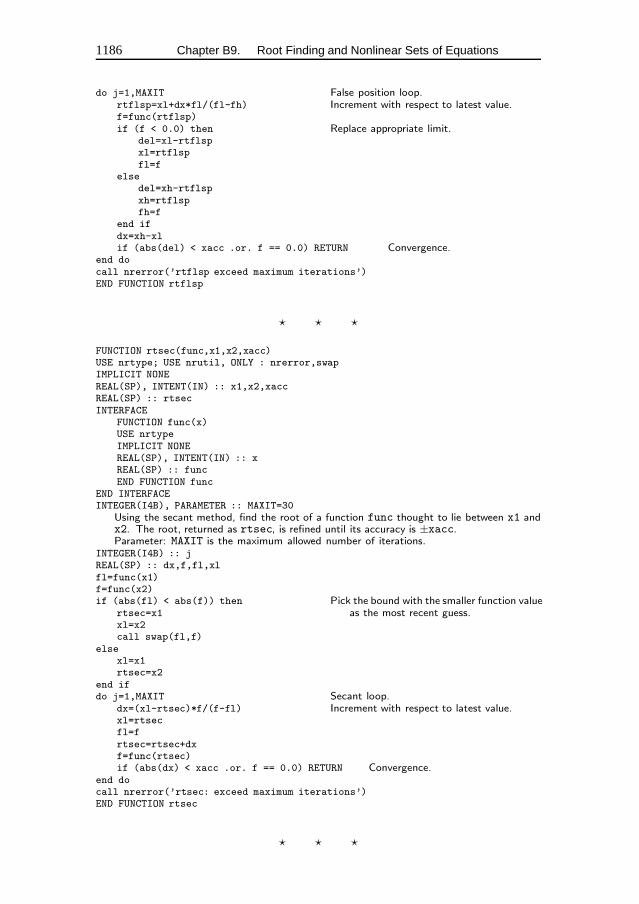
1186 Chapter B9. Root Finding and Nonlinear Sets of Equations
do j=1,MAXIT False position loop.rtflsp=xl+dx*fl/(fl-fh) Increment with respect to latest value.f=func(rtflsp)if (f < 0.0) then Replace appropriate limit.
del=xl-rtflspxl=rtflspfl=f
elsedel=xh-rtflspxh=rtflspfh=f
end ifdx=xh-xlif (abs(del) < xacc .or. f == 0.0) RETURN Convergence.
end docall nrerror(’rtflsp exceed maximum iterations’)END FUNCTION rtflsp
� � �
FUNCTION rtsec(func,x1,x2,xacc)USE nrtype; USE nrutil, ONLY : nrerror,swapIMPLICIT NONEREAL(SP), INTENT(IN) :: x1,x2,xaccREAL(SP) :: rtsecINTERFACE
FUNCTION func(x)USE nrtypeIMPLICIT NONEREAL(SP), INTENT(IN) :: xREAL(SP) :: funcEND FUNCTION func
END INTERFACEINTEGER(I4B), PARAMETER :: MAXIT=30
Using the secant method, find the root of a function func thought to lie between x1 andx2. The root, returned as rtsec, is refined until its accuracy is ±xacc.Parameter: MAXIT is the maximum allowed number of iterations.
INTEGER(I4B) :: jREAL(SP) :: dx,f,fl,xlfl=func(x1)f=func(x2)if (abs(fl) < abs(f)) then Pick the bound with the smaller function value
as the most recent guess.rtsec=x1xl=x2call swap(fl,f)
elsexl=x1rtsec=x2
end ifdo j=1,MAXIT Secant loop.
dx=(xl-rtsec)*f/(f-fl) Increment with respect to latest value.xl=rtsecfl=frtsec=rtsec+dxf=func(rtsec)if (abs(dx) < xacc .or. f == 0.0) RETURN Convergence.
end docall nrerror(’rtsec: exceed maximum iterations’)END FUNCTION rtsec
� � �
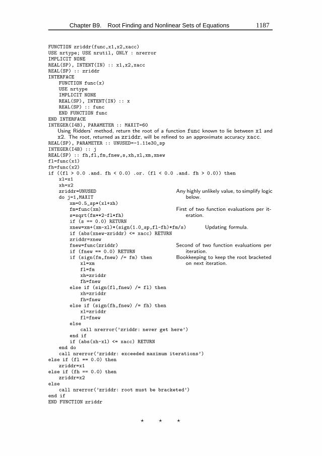
Chapter B9. Root Finding and Nonlinear Sets of Equations 1187
FUNCTION zriddr(func,x1,x2,xacc)USE nrtype; USE nrutil, ONLY : nrerrorIMPLICIT NONEREAL(SP), INTENT(IN) :: x1,x2,xaccREAL(SP) :: zriddrINTERFACE
FUNCTION func(x)USE nrtypeIMPLICIT NONEREAL(SP), INTENT(IN) :: xREAL(SP) :: funcEND FUNCTION func
END INTERFACEINTEGER(I4B), PARAMETER :: MAXIT=60
Using Ridders’ method, return the root of a function func known to lie between x1 andx2. The root, returned as zriddr, will be refined to an approximate accuracy xacc.
REAL(SP), PARAMETER :: UNUSED=-1.11e30_spINTEGER(I4B) :: jREAL(SP) :: fh,fl,fm,fnew,s,xh,xl,xm,xnewfl=func(x1)fh=func(x2)if ((fl > 0.0 .and. fh < 0.0) .or. (fl < 0.0 .and. fh > 0.0)) then
xl=x1xh=x2zriddr=UNUSED Any highly unlikely value, to simplify logic
below.do j=1,MAXITxm=0.5_sp*(xl+xh)fm=func(xm) First of two function evaluations per it-
eration.s=sqrt(fm**2-fl*fh)if (s == 0.0) RETURNxnew=xm+(xm-xl)*(sign(1.0_sp,fl-fh)*fm/s) Updating formula.if (abs(xnew-zriddr) <= xacc) RETURNzriddr=xnewfnew=func(zriddr) Second of two function evaluations per
iteration.if (fnew == 0.0) RETURNif (sign(fm,fnew) /= fm) then Bookkeeping to keep the root bracketed
on next iteration.xl=xmfl=fmxh=zriddrfh=fnew
else if (sign(fl,fnew) /= fl) thenxh=zriddrfh=fnew
else if (sign(fh,fnew) /= fh) thenxl=zriddrfl=fnew
elsecall nrerror(’zriddr: never get here’)
end ifif (abs(xh-xl) <= xacc) RETURN
end docall nrerror(’zriddr: exceeded maximum iterations’)
else if (fl == 0.0) thenzriddr=x1
else if (fh == 0.0) thenzriddr=x2
elsecall nrerror(’zriddr: root must be bracketed’)
end ifEND FUNCTION zriddr
� � �
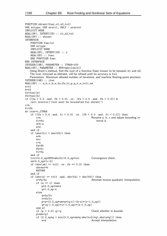
1188 Chapter B9. Root Finding and Nonlinear Sets of Equations
FUNCTION zbrent(func,x1,x2,tol)USE nrtype; USE nrutil, ONLY : nrerrorIMPLICIT NONEREAL(SP), INTENT(IN) :: x1,x2,tolREAL(SP) :: zbrentINTERFACE
FUNCTION func(x)USE nrtypeIMPLICIT NONEREAL(SP), INTENT(IN) :: xREAL(SP) :: funcEND FUNCTION func
END INTERFACEINTEGER(I4B), PARAMETER :: ITMAX=100REAL(SP), PARAMETER :: EPS=epsilon(x1)
Using Brent’s method, find the root of a function func known to lie between x1 and x2.The root, returned as zbrent, will be refined until its accuracy is tol.Parameters: Maximum allowed number of iterations, and machine floating-point precision.
INTEGER(I4B) :: iterREAL(SP) :: a,b,c,d,e,fa,fb,fc,p,q,r,s,tol1,xma=x1b=x2fa=func(a)fb=func(b)if ((fa > 0.0 .and. fb > 0.0) .or. (fa < 0.0 .and. fb < 0.0)) &
call nrerror(’root must be bracketed for zbrent’)c=bfc=fbdo iter=1,ITMAX
if ((fb > 0.0 .and. fc > 0.0) .or. (fb < 0.0 .and. fc < 0.0)) thenc=a Rename a, b, c and adjust bounding in-
terval d.fc=fad=b-ae=d
end ifif (abs(fc) < abs(fb)) then
a=bb=cc=afa=fbfb=fcfc=fa
end iftol1=2.0_sp*EPS*abs(b)+0.5_sp*tol Convergence check.xm=0.5_sp*(c-b)if (abs(xm) <= tol1 .or. fb == 0.0) then
zbrent=bRETURN
end ifif (abs(e) >= tol1 .and. abs(fa) > abs(fb)) then
s=fb/fa Attempt inverse quadratic interpolation.if (a == c) then
p=2.0_sp*xm*sq=1.0_sp-s
elseq=fa/fcr=fb/fcp=s*(2.0_sp*xm*q*(q-r)-(b-a)*(r-1.0_sp))q=(q-1.0_sp)*(r-1.0_sp)*(s-1.0_sp)
end ifif (p > 0.0) q=-q Check whether in bounds.p=abs(p)if (2.0_sp*p < min(3.0_sp*xm*q-abs(tol1*q),abs(e*q))) then
e=d Accept interpolation.
Chapter B9. Root Finding and Nonlinear Sets of Equations 1189
d=p/qelse
d=xm Interpolation failed; use bisection.e=d
end ifelse Bounds decreasing too slowly; use bisec-
tion.d=xme=d
end ifa=b Move last best guess to a.fa=fbb=b+merge(d,sign(tol1,xm), abs(d) > tol1 ) Evaluate new trial root.fb=func(b)
end docall nrerror(’zbrent: exceeded maximum iterations’)zbrent=bEND FUNCTION zbrent
f90REAL(SP), PARAMETER :: EPS=epsilon(x1) The routinezbrentworks bestwhen EPS is exactly the machine precision. The Fortran 90 intrinsic func-tion epsilon allows us to code this in a portable fashion.
FUNCTION rtnewt(funcd,x1,x2,xacc)USE nrtype; USE nrutil, ONLY : nrerrorIMPLICIT NONEREAL(SP), INTENT(IN) :: x1,x2,xaccREAL(SP) :: rtnewtINTERFACE
SUBROUTINE funcd(x,fval,fderiv)USE nrtypeIMPLICIT NONEREAL(SP), INTENT(IN) :: xREAL(SP), INTENT(OUT) :: fval,fderivEND SUBROUTINE funcd
END INTERFACEINTEGER(I4B), PARAMETER :: MAXIT=20
Using the Newton-Raphson method, find the root of a function known to lie in the interval[x1, x2]. The root rtnewtwill be refined until its accuracy is known within ±xacc. funcdis a user-supplied subroutine that returns both the function value and the first derivative ofthe function.Parameter: MAXIT is the maximum number of iterations.
INTEGER(I4B) :: jREAL(SP) :: df,dx,frtnewt=0.5_sp*(x1+x2) Initial guess.do j=1,MAXIT
call funcd(rtnewt,f,df)dx=f/dfrtnewt=rtnewt-dxif ((x1-rtnewt)*(rtnewt-x2) < 0.0)&
call nrerror(’rtnewt: values jumped out of brackets’)if (abs(dx) < xacc) RETURN Convergence.
end docall nrerror(’rtnewt exceeded maximum iterations’)END FUNCTION rtnewt
� � �
1190 Chapter B9. Root Finding and Nonlinear Sets of Equations
FUNCTION rtsafe(funcd,x1,x2,xacc)USE nrtype; USE nrutil, ONLY : nrerrorIMPLICIT NONEREAL(SP), INTENT(IN) :: x1,x2,xaccREAL(SP) :: rtsafeINTERFACE
SUBROUTINE funcd(x,fval,fderiv)USE nrtypeIMPLICIT NONEREAL(SP), INTENT(IN) :: xREAL(SP), INTENT(OUT) :: fval,fderivEND SUBROUTINE funcd
END INTERFACEINTEGER(I4B), PARAMETER :: MAXIT=100
Using a combination of Newton-Raphson and bisection, find the root of a function bracketedbetween x1 and x2. The root, returned as the function value rtsafe, will be refined untilits accuracy is known within ±xacc. funcd is a user-supplied subroutine that returns boththe function value and the first derivative of the function.Parameter: MAXIT is the maximum allowed number of iterations.
INTEGER(I4B) :: jREAL(SP) :: df,dx,dxold,f,fh,fl,temp,xh,xlcall funcd(x1,fl,df)call funcd(x2,fh,df)if ((fl > 0.0 .and. fh > 0.0) .or. &
(fl < 0.0 .and. fh < 0.0)) &call nrerror(’root must be bracketed in rtsafe’)
if (fl == 0.0) thenrtsafe=x1RETURN
else if (fh == 0.0) thenrtsafe=x2RETURN
else if (fl < 0.0) then Orient the search so that f(xl) < 0.xl=x1xh=x2
elsexh=x1xl=x2
end ifrtsafe=0.5_sp*(x1+x2) Initialize the guess for root,dxold=abs(x2-x1) the “stepsize before last,”dx=dxold and the last step.call funcd(rtsafe,f,df)do j=1,MAXIT Loop over allowed iterations.
if (((rtsafe-xh)*df-f)*((rtsafe-xl)*df-f) > 0.0 .or. &abs(2.0_sp*f) > abs(dxold*df) ) thenBisect if Newton out of range, or not decreasing fast enough.
dxold=dxdx=0.5_sp*(xh-xl)rtsafe=xl+dxif (xl == rtsafe) RETURN Change in root is negligible.
else Newton step acceptable. Take it.dxold=dxdx=f/dftemp=rtsafertsafe=rtsafe-dxif (temp == rtsafe) RETURN
end ifif (abs(dx) < xacc) RETURN Convergence criterion.call funcd(rtsafe,f,df) One new function evaluation per iteration.if (f < 0.0) then Maintain the bracket on the root.
xl=rtsafeelse
xh=rtsafe
Chapter B9. Root Finding and Nonlinear Sets of Equations 1191
end ifend docall nrerror(’rtsafe: exceeded maximum iterations’)END FUNCTION rtsafe
� � �
SUBROUTINE laguer(a,x,its)USE nrtype; USE nrutil, ONLY : nrerror,poly,poly_termIMPLICIT NONEINTEGER(I4B), INTENT(OUT) :: itsCOMPLEX(SPC), INTENT(INOUT) :: xCOMPLEX(SPC), DIMENSION(:), INTENT(IN) :: aREAL(SP), PARAMETER :: EPS=epsilon(1.0_sp)INTEGER(I4B), PARAMETER :: MR=8,MT=10,MAXIT=MT*MR
Given an array of M + 1 complex coefficients a of the polynomial∑M+1
i=1 a(i)xi−1, andgiven a complex value x, this routine improves x by Laguerre’s method until it converges,within the achievable roundoff limit, to a root of the given polynomial. The number ofiterations taken is returned as its.Parameters: EPS is the estimated fractional roundoff error. We try to break (rare) limitcycles with MR different fractional values, once every MT steps, for MAXIT total allowediterations.
INTEGER(I4B) :: iter,mREAL(SP) :: abx,abp,abm,errCOMPLEX(SPC) :: dx,x1,f,g,h,sq,gp,gm,g2COMPLEX(SPC), DIMENSION(size(a)) :: b,dREAL(SP), DIMENSION(MR) :: frac = &
(/ 0.5_sp,0.25_sp,0.75_sp,0.13_sp,0.38_sp,0.62_sp,0.88_sp,1.0_sp /)Fractions used to break a limit cycle.
m=size(a)-1do iter=1,MAXIT Loop over iterations up to allowed maximum.
its=iterabx=abs(x)b(m+1:1:-1)=poly_term(a(m+1:1:-1),x) Efficient computation of the polynomial
and its first two derivatives.d(m:1:-1)=poly_term(b(m+1:2:-1),x)f=poly(x,d(2:m))err=EPS*poly(abx,abs(b(1:m+1))) Esimate of roundoff in evaluating polynomial.if (abs(b(1)) <= err) RETURN We are on the root.g=d(1)/b(1) The generic case: Use Laguerre’s formula.g2=g*gh=g2-2.0_sp*f/b(1)sq=sqrt((m-1)*(m*h-g2))gp=g+sqgm=g-sqabp=abs(gp)abm=abs(gm)if (abp < abm) gp=gmif (max(abp,abm) > 0.0) then
dx=m/gpelse
dx=exp(cmplx(log(1.0_sp+abx),iter,kind=spc))end ifx1=x-dxif (x == x1) RETURN Converged.if (mod(iter,MT) /= 0) then
x=x1else Every so often we take a fractional step, to
break any limit cycle (itself a rare occur-rence).
x=x-dx*frac(iter/MT)end if
end docall nrerror(’laguer: too many iterations’)Very unusual — can occur only for complex roots. Try a different starting guess for the root.
END SUBROUTINE laguer
1192 Chapter B9. Root Finding and Nonlinear Sets of Equations
f90b(m+1:1:-1)=poly_term...f=poly(x,d(2:m)) The poly term function innrutil tabulates the partial sums of a polynomial, while poly evaluatesthe polynomialat x. In this example, we use poly termon the coefficient
array in reverse order, so that the value of the polynomial ends up in b(1) and thevalue of its first derivative in d(1).
dx=exp(cmplx(log(1.0_sp+abx),iter,kind=spc)) The intrinsic function cmplxreturns a quantity of type default complex unless the kind argument is present.To facilitate converting our routines from single to double precision, we alwaysinclude the kind argument explicitly so that when you redefine spc in nrtype to bedouble-precision complex the conversions are carried out correctly.
� � �
SUBROUTINE zroots(a,roots,polish)USE nrtype; USE nrutil, ONLY : assert_eq,poly_termUSE nr, ONLY : laguer,indexxIMPLICIT NONECOMPLEX(SPC), DIMENSION(:), INTENT(IN) :: aCOMPLEX(SPC), DIMENSION(:), INTENT(OUT) :: rootsLOGICAL(LGT), INTENT(IN) :: polishREAL(SP), PARAMETER :: EPS=1.0e-6_sp
Given the array of M + 1 complex coefficients a of the polynomial∑M+1
i=1 a(i)xi−1, thisroutine successively calls laguer and finds all M complex roots. The logical variablepolish should be input as .true. if polishing (also by Laguerre’s method) is desired,.false. if the roots will be subsequently polished by other means.Parameter: EPS is a small number.
INTEGER(I4B) :: j,its,mINTEGER(I4B), DIMENSION(size(roots)) :: indxCOMPLEX(SPC) :: xCOMPLEX(SPC), DIMENSION(size(a)) :: adm=assert_eq(size(roots),size(a)-1,’zroots’)ad(:)=a(:) Copy of coefficients for successive deflation.do j=m,1,-1 Loop over each root to be found.
x=cmplx(0.0_sp,kind=spc)Start at zero to favor convergence to smallest remaining root.
call laguer(ad(1:j+1),x,its) Find the root.if (abs(aimag(x)) <= 2.0_sp*EPS**2*abs(real(x))) &
x=cmplx(real(x),kind=spc)roots(j)=xad(j:1:-1)=poly_term(ad(j+1:2:-1),x) Forward deflation.
end doif (polish) then
do j=1,m Polish the roots using the undeflated coeffi-cients.call laguer(a(:),roots(j),its)
end doend ifcall indexx(real(roots),indx) Sort roots by their real parts.roots=roots(indx)END SUBROUTINE zroots
f90x=cmplx(0.0_sp,kind=spc)...x=cmplx(real(x),kind=spc) See the discus-sion of why we include kind=spc just above. Note that while real(x)returns type default real if x is integer or real, it returns single or double
precision correctly if x is complex.
� � �
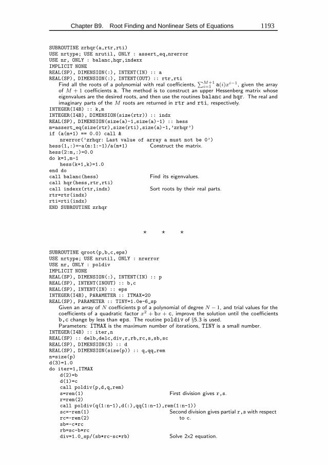
Chapter B9. Root Finding and Nonlinear Sets of Equations 1193
SUBROUTINE zrhqr(a,rtr,rti)USE nrtype; USE nrutil, ONLY : assert_eq,nrerrorUSE nr, ONLY : balanc,hqr,indexxIMPLICIT NONEREAL(SP), DIMENSION(:), INTENT(IN) :: aREAL(SP), DIMENSION(:), INTENT(OUT) :: rtr,rti
Find all the roots of a polynomial with real coefficients,∑M+1
i=1 a(i)xi−1, given the arrayof M + 1 coefficients a. The method is to construct an upper Hessenberg matrix whoseeigenvalues are the desired roots, and then use the routines balanc and hqr. The real andimaginary parts of the M roots are returned in rtr and rti, respectively.
INTEGER(I4B) :: k,mINTEGER(I4B), DIMENSION(size(rtr)) :: indxREAL(SP), DIMENSION(size(a)-1,size(a)-1) :: hessm=assert_eq(size(rtr),size(rti),size(a)-1,’zrhqr’)if (a(m+1) == 0.0) call &
nrerror(’zrhqr: Last value of array a must not be 0’)hess(1,:)=-a(m:1:-1)/a(m+1) Construct the matrix.hess(2:m,:)=0.0do k=1,m-1
hess(k+1,k)=1.0end docall balanc(hess) Find its eigenvalues.call hqr(hess,rtr,rti)call indexx(rtr,indx) Sort roots by their real parts.rtr=rtr(indx)rti=rti(indx)END SUBROUTINE zrhqr
� � �
SUBROUTINE qroot(p,b,c,eps)USE nrtype; USE nrutil, ONLY : nrerrorUSE nr, ONLY : poldivIMPLICIT NONEREAL(SP), DIMENSION(:), INTENT(IN) :: pREAL(SP), INTENT(INOUT) :: b,cREAL(SP), INTENT(IN) :: epsINTEGER(I4B), PARAMETER :: ITMAX=20REAL(SP), PARAMETER :: TINY=1.0e-6_sp
Given an array of N coefficients p of a polynomial of degree N − 1, and trial values for thecoefficients of a quadratic factor x2 + bx + c, improve the solution until the coefficientsb,c change by less than eps. The routine poldiv of §5.3 is used.Parameters: ITMAX is the maximum number of iterations, TINY is a small number.
INTEGER(I4B) :: iter,nREAL(SP) :: delb,delc,div,r,rb,rc,s,sb,scREAL(SP), DIMENSION(3) :: dREAL(SP), DIMENSION(size(p)) :: q,qq,remn=size(p)d(3)=1.0do iter=1,ITMAX
d(2)=bd(1)=ccall poldiv(p,d,q,rem)s=rem(1) First division gives r,s.r=rem(2)call poldiv(q(1:n-1),d(:),qq(1:n-1),rem(1:n-1))sc=-rem(1) Second division gives partial r,s with respect
to c.rc=-rem(2)sb=-c*rcrb=sc-b*rcdiv=1.0_sp/(sb*rc-sc*rb) Solve 2x2 equation.
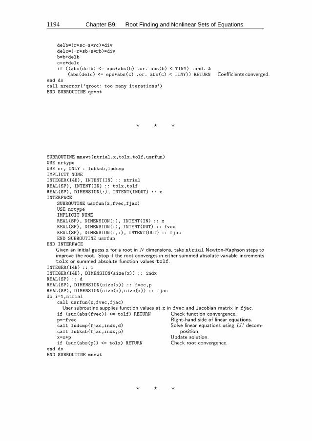
1194 Chapter B9. Root Finding and Nonlinear Sets of Equations
delb=(r*sc-s*rc)*divdelc=(-r*sb+s*rb)*divb=b+delbc=c+delcif ((abs(delb) <= eps*abs(b) .or. abs(b) < TINY) .and. &
(abs(delc) <= eps*abs(c) .or. abs(c) < TINY)) RETURN Coefficients converged.end docall nrerror(’qroot: too many iterations’)END SUBROUTINE qroot
� � �
SUBROUTINE mnewt(ntrial,x,tolx,tolf,usrfun)USE nrtypeUSE nr, ONLY : lubksb,ludcmpIMPLICIT NONEINTEGER(I4B), INTENT(IN) :: ntrialREAL(SP), INTENT(IN) :: tolx,tolfREAL(SP), DIMENSION(:), INTENT(INOUT) :: xINTERFACE
SUBROUTINE usrfun(x,fvec,fjac)USE nrtypeIMPLICIT NONEREAL(SP), DIMENSION(:), INTENT(IN) :: xREAL(SP), DIMENSION(:), INTENT(OUT) :: fvecREAL(SP), DIMENSION(:,:), INTENT(OUT) :: fjacEND SUBROUTINE usrfun
END INTERFACEGiven an initial guess x for a root in N dimensions, take ntrial Newton-Raphson steps toimprove the root. Stop if the root converges in either summed absolute variable incrementstolx or summed absolute function values tolf.
INTEGER(I4B) :: iINTEGER(I4B), DIMENSION(size(x)) :: indxREAL(SP) :: dREAL(SP), DIMENSION(size(x)) :: fvec,pREAL(SP), DIMENSION(size(x),size(x)) :: fjacdo i=1,ntrial
call usrfun(x,fvec,fjac)User subroutine supplies function values at x in fvec and Jacobian matrix in fjac.
if (sum(abs(fvec)) <= tolf) RETURN Check function convergence.p=-fvec Right-hand side of linear equations.call ludcmp(fjac,indx,d) Solve linear equations using LU decom-
position.call lubksb(fjac,indx,p)x=x+p Update solution.if (sum(abs(p)) <= tolx) RETURN Check root convergence.
end doEND SUBROUTINE mnewt
� � �
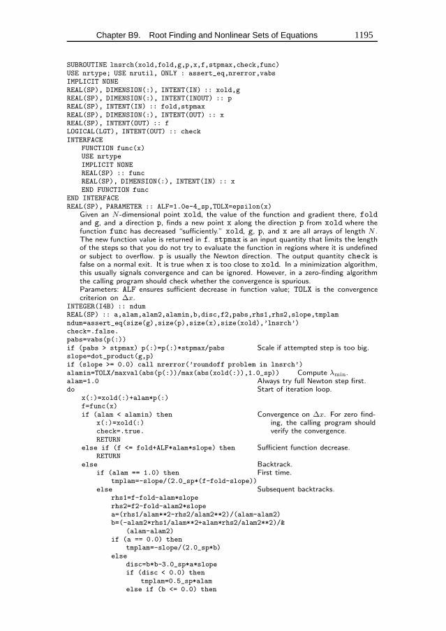
Chapter B9. Root Finding and Nonlinear Sets of Equations 1195
SUBROUTINE lnsrch(xold,fold,g,p,x,f,stpmax,check,func)USE nrtype; USE nrutil, ONLY : assert_eq,nrerror,vabsIMPLICIT NONEREAL(SP), DIMENSION(:), INTENT(IN) :: xold,gREAL(SP), DIMENSION(:), INTENT(INOUT) :: pREAL(SP), INTENT(IN) :: fold,stpmaxREAL(SP), DIMENSION(:), INTENT(OUT) :: xREAL(SP), INTENT(OUT) :: fLOGICAL(LGT), INTENT(OUT) :: checkINTERFACE
FUNCTION func(x)USE nrtypeIMPLICIT NONEREAL(SP) :: funcREAL(SP), DIMENSION(:), INTENT(IN) :: xEND FUNCTION func
END INTERFACEREAL(SP), PARAMETER :: ALF=1.0e-4_sp,TOLX=epsilon(x)
Given an N -dimensional point xold, the value of the function and gradient there, foldand g, and a direction p, finds a new point x along the direction p from xold where thefunction func has decreased “sufficiently.” xold, g, p, and x are all arrays of length N .The new function value is returned in f. stpmax is an input quantity that limits the lengthof the steps so that you do not try to evaluate the function in regions where it is undefinedor subject to overflow. p is usually the Newton direction. The output quantity check isfalse on a normal exit. It is true when x is too close to xold. In a minimization algorithm,this usually signals convergence and can be ignored. However, in a zero-finding algorithmthe calling program should check whether the convergence is spurious.Parameters: ALF ensures sufficient decrease in function value; TOLX is the convergencecriterion on ∆x.
INTEGER(I4B) :: ndumREAL(SP) :: a,alam,alam2,alamin,b,disc,f2,pabs,rhs1,rhs2,slope,tmplamndum=assert_eq(size(g),size(p),size(x),size(xold),’lnsrch’)check=.false.pabs=vabs(p(:))if (pabs > stpmax) p(:)=p(:)*stpmax/pabs Scale if attempted step is too big.slope=dot_product(g,p)if (slope >= 0.0) call nrerror(’roundoff problem in lnsrch’)alamin=TOLX/maxval(abs(p(:))/max(abs(xold(:)),1.0_sp)) Compute λmin.alam=1.0 Always try full Newton step first.do Start of iteration loop.
x(:)=xold(:)+alam*p(:)f=func(x)if (alam < alamin) then Convergence on ∆x. For zero find-
ing, the calling program shouldverify the convergence.
x(:)=xold(:)check=.true.RETURN
else if (f <= fold+ALF*alam*slope) then Sufficient function decrease.RETURN
else Backtrack.if (alam == 1.0) then First time.
tmplam=-slope/(2.0_sp*(f-fold-slope))else Subsequent backtracks.
rhs1=f-fold-alam*sloperhs2=f2-fold-alam2*slopea=(rhs1/alam**2-rhs2/alam2**2)/(alam-alam2)b=(-alam2*rhs1/alam**2+alam*rhs2/alam2**2)/&
(alam-alam2)if (a == 0.0) then
tmplam=-slope/(2.0_sp*b)else
disc=b*b-3.0_sp*a*slopeif (disc < 0.0) then
tmplam=0.5_sp*alamelse if (b <= 0.0) then
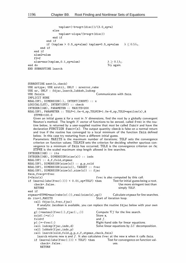
1196 Chapter B9. Root Finding and Nonlinear Sets of Equations
tmplam=(-b+sqrt(disc))/(3.0_sp*a)else
tmplam=-slope/(b+sqrt(disc))end if
end ifif (tmplam > 0.5_sp*alam) tmplam=0.5_sp*alam λ ≤ 0.5λ1.
end ifend ifalam2=alamf2=falam=max(tmplam,0.1_sp*alam) λ ≥ 0.1λ1.
end do Try again.END SUBROUTINE lnsrch
SUBROUTINE newt(x,check)USE nrtype; USE nrutil, ONLY : nrerror,vabsUSE nr, ONLY : fdjac,lnsrch,lubksb,ludcmpUSE fminln Communicates with fmin.IMPLICIT NONEREAL(SP), DIMENSION(:), INTENT(INOUT) :: xLOGICAL(LGT), INTENT(OUT) :: checkINTEGER(I4B), PARAMETER :: MAXITS=200REAL(SP), PARAMETER :: TOLF=1.0e-4_sp,TOLMIN=1.0e-6_sp,TOLX=epsilon(x),&
STPMX=100.0Given an initial guess x for a root in N dimensions, find the root by a globally convergentNewton’s method. The length N vector of functions to be zeroed, called fvec in the rou-tine below, is returned by a user-supplied routine that must be called funcv and have thedeclaration FUNCTION funcv(x). The output quantity check is false on a normal returnand true if the routine has converged to a local minimum of the function fmin definedbelow. In this case try restarting from a different initial guess.Parameters: MAXITS is the maximum number of iterations; TOLF sets the convergencecriterion on function values; TOLMIN sets the criterion for deciding whether spurious con-vergence to a minimum of fmin has occurred; TOLX is the convergence criterion on δx;STPMX is the scaled maximum step length allowed in line searches.
INTEGER(I4B) :: itsINTEGER(I4B), DIMENSION(size(x)) :: indxREAL(SP) :: d,f,fold,stpmaxREAL(SP), DIMENSION(size(x)) :: g,p,xoldREAL(SP), DIMENSION(size(x)), TARGET :: fvecREAL(SP), DIMENSION(size(x),size(x)) :: fjacfmin_fvecp=>fvecf=fmin(x) fvec is also computed by this call.if (maxval(abs(fvec(:))) < 0.01_sp*TOLF) then Test for initial guess being a root.
Use more stringent test thansimply TOLF.
check=.false.RETURN
end ifstpmax=STPMX*max(vabs(x(:)),real(size(x),sp)) Calculate stpmax for line searches.do its=1,MAXITS Start of iteration loop.
call fdjac(x,fvec,fjac)If analytic Jacobian is available, you can replace the routine fdjac below with your ownroutine.
g(:)=matmul(fvec(:),fjac(:,:)) Compute ∇f for the line search.xold(:)=x(:) Store x,fold=f and f .p(:)=-fvec(:) Right-hand side for linear equations.call ludcmp(fjac,indx,d) Solve linear equations by LU decomposition.call lubksb(fjac,indx,p)call lnsrch(xold,fold,g,p,x,f,stpmax,check,fmin)lnsrch returns new x and f . It also calculates fvec at the new x when it calls fmin.
if (maxval(abs(fvec(:))) < TOLF) then Test for convergence on function val-ues.check=.false.
RETURN
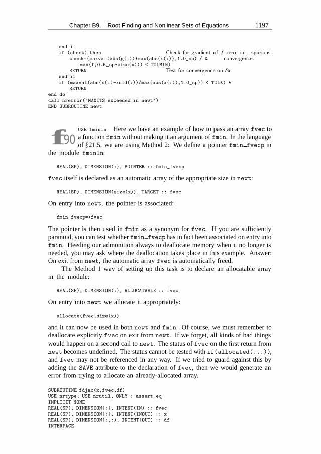
Chapter B9. Root Finding and Nonlinear Sets of Equations 1197
end ifif (check) then Check for gradient of f zero, i.e., spurious
convergence.check=(maxval(abs(g(:))*max(abs(x(:)),1.0_sp) / &max(f,0.5_sp*size(x))) < TOLMIN)
RETURN Test for convergence on δx.end ifif (maxval(abs(x(:)-xold(:))/max(abs(x(:)),1.0_sp)) < TOLX) &
RETURNend docall nrerror(’MAXITS exceeded in newt’)END SUBROUTINE newt
f90USE fminln Here we have an example of how to pass an array fvec toa function fmin without making it an argument of fmin. In the languageof §21.5, we are using Method 2: We define a pointer fmin fvecp in
the module fminln:
REAL(SP), DIMENSION(:), POINTER :: fmin_fvecp
fvec itself is declared as an automatic array of the appropriate size in newt:
REAL(SP), DIMENSION(size(x)), TARGET :: fvec
On entry into newt, the pointer is associated:
fmin_fvecp=>fvec
The pointer is then used in fmin as a synonym for fvec. If you are sufficientlyparanoid, you can test whether fmin fvecp has in fact been associated on entry intofmin. Heeding our admonition always to deallocate memory when it no longer isneeded, you may ask where the deallocation takes place in this example. Answer:On exit from newt, the automatic array fvec is automatically freed.
The Method 1 way of setting up this task is to declare an allocatable arrayin the module:
REAL(SP), DIMENSION(:), ALLOCATABLE :: fvec
On entry into newt we allocate it appropriately:
allocate(fvec,size(x))
and it can now be used in both newt and fmin. Of course, we must remember todeallocate explicitly fvec on exit from newt. If we forget, all kinds of bad thingswould happen on a second call to newt. The status of fvec on the first return fromnewt becomes undefined. The status cannot be tested with if(allocated(...)),and fvec may not be referenced in any way. If we tried to guard against this byadding the SAVE attribute to the declaration of fvec, then we would generate anerror from trying to allocate an already-allocated array.
SUBROUTINE fdjac(x,fvec,df)USE nrtype; USE nrutil, ONLY : assert_eqIMPLICIT NONEREAL(SP), DIMENSION(:), INTENT(IN) :: fvecREAL(SP), DIMENSION(:), INTENT(INOUT) :: xREAL(SP), DIMENSION(:,:), INTENT(OUT) :: dfINTERFACE
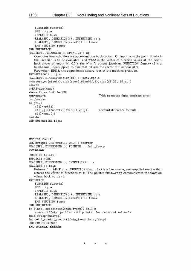
1198 Chapter B9. Root Finding and Nonlinear Sets of Equations
FUNCTION funcv(x)USE nrtypeIMPLICIT NONEREAL(SP), DIMENSION(:), INTENT(IN) :: xREAL(SP), DIMENSION(size(x)) :: funcvEND FUNCTION funcv
END INTERFACEREAL(SP), PARAMETER :: EPS=1.0e-4_sp
Computes forward-difference approximation to Jacobian. On input, x is the point at whichthe Jacobian is to be evaluated, and fvec is the vector of function values at the point,both arrays of length N . df is the N × N output Jacobian. FUNCTION funcv(x) is afixed-name, user-supplied routine that returns the vector of functions at x.Parameter: EPS is the approximate square root of the machine precision.
INTEGER(I4B) :: j,nREAL(SP), DIMENSION(size(x)) :: xsav,xph,hn=assert_eq(size(x),size(fvec),size(df,1),size(df,2),’fdjac’)xsav=xh=EPS*abs(xsav)where (h == 0.0) h=EPSxph=xsav+h Trick to reduce finite precision error.h=xph-xsavdo j=1,n
x(j)=xph(j)df(:,j)=(funcv(x)-fvec(:))/h(j) Forward difference formula.x(j)=xsav(j)
end doEND SUBROUTINE fdjac
MODULE fminlnUSE nrtype; USE nrutil, ONLY : nrerrorREAL(SP), DIMENSION(:), POINTER :: fmin_fvecpCONTAINS
FUNCTION fmin(x)IMPLICIT NONEREAL(SP), DIMENSION(:), INTENT(IN) :: xREAL(SP) :: fmin
Returns f = 12
F ·F at x. FUNCTION funcv(x) is a fixed-name, user-supplied routine thatreturns the vector of functions at x. The pointer fmin vecp communicates the functionvalues back to newt.
INTERFACEFUNCTION funcv(x)USE nrtypeIMPLICIT NONEREAL(SP), DIMENSION(:), INTENT(IN) :: xREAL(SP), DIMENSION(size(x)) :: funcvEND FUNCTION funcv
END INTERFACEif (.not. associated(fmin_fvecp)) call &
nrerror(’fmin: problem with pointer for returned values’)fmin_fvecp=funcv(x)fmin=0.5_sp*dot_product(fmin_fvecp,fmin_fvecp)END FUNCTION fminEND MODULE fminln
� � �
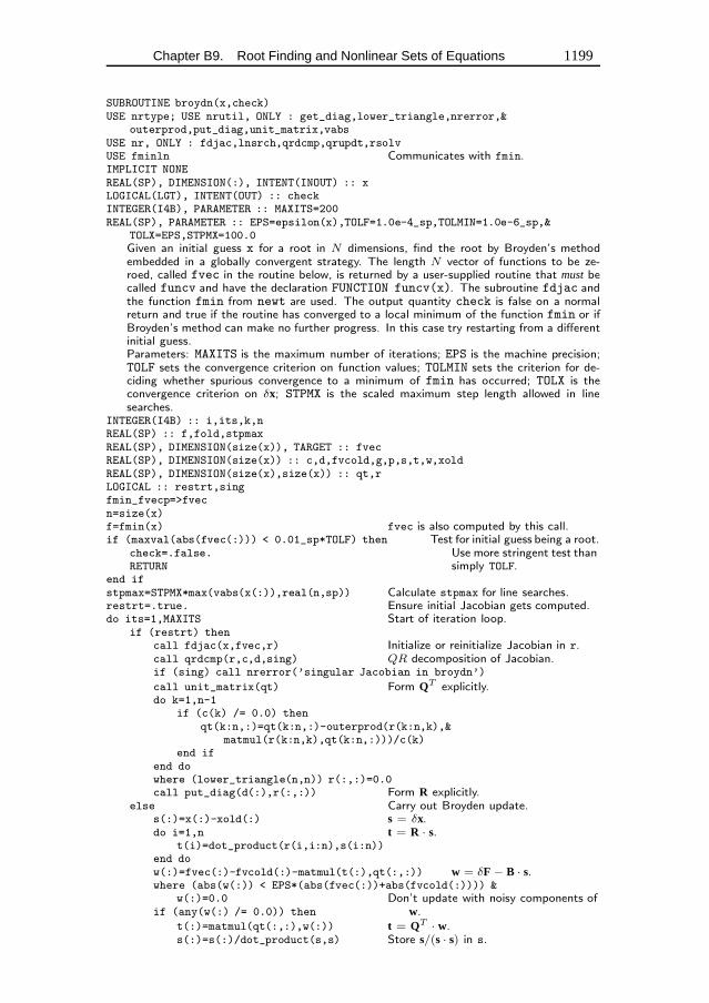
Chapter B9. Root Finding and Nonlinear Sets of Equations 1199
SUBROUTINE broydn(x,check)USE nrtype; USE nrutil, ONLY : get_diag,lower_triangle,nrerror,&
outerprod,put_diag,unit_matrix,vabsUSE nr, ONLY : fdjac,lnsrch,qrdcmp,qrupdt,rsolvUSE fminln Communicates with fmin.IMPLICIT NONEREAL(SP), DIMENSION(:), INTENT(INOUT) :: xLOGICAL(LGT), INTENT(OUT) :: checkINTEGER(I4B), PARAMETER :: MAXITS=200REAL(SP), PARAMETER :: EPS=epsilon(x),TOLF=1.0e-4_sp,TOLMIN=1.0e-6_sp,&
TOLX=EPS,STPMX=100.0Given an initial guess x for a root in N dimensions, find the root by Broyden’s methodembedded in a globally convergent strategy. The length N vector of functions to be ze-roed, called fvec in the routine below, is returned by a user-supplied routine that must becalled funcv and have the declaration FUNCTION funcv(x). The subroutine fdjac andthe function fmin from newt are used. The output quantity check is false on a normalreturn and true if the routine has converged to a local minimum of the function fmin or ifBroyden’s method can make no further progress. In this case try restarting from a differentinitial guess.Parameters: MAXITS is the maximum number of iterations; EPS is the machine precision;TOLF sets the convergence criterion on function values; TOLMIN sets the criterion for de-ciding whether spurious convergence to a minimum of fmin has occurred; TOLX is theconvergence criterion on δx; STPMX is the scaled maximum step length allowed in linesearches.
INTEGER(I4B) :: i,its,k,nREAL(SP) :: f,fold,stpmaxREAL(SP), DIMENSION(size(x)), TARGET :: fvecREAL(SP), DIMENSION(size(x)) :: c,d,fvcold,g,p,s,t,w,xoldREAL(SP), DIMENSION(size(x),size(x)) :: qt,rLOGICAL :: restrt,singfmin_fvecp=>fvecn=size(x)f=fmin(x) fvec is also computed by this call.if (maxval(abs(fvec(:))) < 0.01_sp*TOLF) then Test for initial guess being a root.
Use more stringent test thansimply TOLF.
check=.false.RETURN
end ifstpmax=STPMX*max(vabs(x(:)),real(n,sp)) Calculate stpmax for line searches.restrt=.true. Ensure initial Jacobian gets computed.do its=1,MAXITS Start of iteration loop.
if (restrt) thencall fdjac(x,fvec,r) Initialize or reinitialize Jacobian in r.call qrdcmp(r,c,d,sing) QR decomposition of Jacobian.if (sing) call nrerror(’singular Jacobian in broydn’)
call unit_matrix(qt) Form QT explicitly.do k=1,n-1
if (c(k) /= 0.0) thenqt(k:n,:)=qt(k:n,:)-outerprod(r(k:n,k),&
matmul(r(k:n,k),qt(k:n,:)))/c(k)end if
end dowhere (lower_triangle(n,n)) r(:,:)=0.0call put_diag(d(:),r(:,:)) Form R explicitly.
else Carry out Broyden update.s(:)=x(:)-xold(:) s = δx.do i=1,n t = R · s.
t(i)=dot_product(r(i,i:n),s(i:n))end dow(:)=fvec(:)-fvcold(:)-matmul(t(:),qt(:,:)) w = δF − B · s.where (abs(w(:)) < EPS*(abs(fvec(:))+abs(fvcold(:)))) &
w(:)=0.0 Don’t update with noisy components ofw.if (any(w(:) /= 0.0)) then
t(:)=matmul(qt(:,:),w(:)) t = QT · w.s(:)=s(:)/dot_product(s,s) Store s/(s · s) in s.
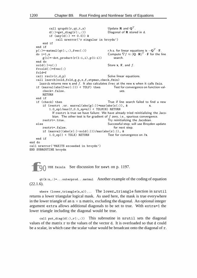
1200 Chapter B9. Root Finding and Nonlinear Sets of Equations
call qrupdt(r,qt,t,s) Update R and QT .d(:)=get_diag(r(:,:)) Diagonal of R stored in d.if (any(d(:) == 0.0)) &
call nrerror(’r singular in broydn’)end if
end ifp(:)=-matmul(qt(:,:),fvec(:)) r.h.s. for linear equations is −QT · F.do i=1,n Compute ∇f ≈ (Q · R)T · F for the line
search.g(i)=-dot_product(r(1:i,i),p(1:i))end doxold(:)=x(:) Store x, F, and f .fvcold(:)=fvec(:)fold=fcall rsolv(r,d,p) Solve linear equations.call lnsrch(xold,fold,g,p,x,f,stpmax,check,fmin)lnsrch returns new x and f . It also calculates fvec at the new x when it calls fmin.
if (maxval(abs(fvec(:))) < TOLF) then Test for convergence on function val-ues.check=.false.
RETURNend ifif (check) then True if line search failed to find a new
x.if (restrt .or. maxval(abs(g(:))*max(abs(x(:)), &1.0_sp)/max(f,0.5_sp*n)) < TOLMIN) RETURNIf restrt is true we have failure: We have already tried reinitializing the Jaco-bian. The other test is for gradient of f zero, i.e., spurious convergence.
restrt=.true. Try reinitializing the Jacobian.else Successful step; will use Broyden update
for next step.restrt=.false.if (maxval((abs(x(:)-xold(:)))/max(abs(x(:)), &
1.0_sp)) < TOLX) RETURN Test for convergence on δx.end if
end docall nrerror(’MAXITS exceeded in broydn’)END SUBROUTINE broydn
f90 USE fminln See discussion for newt on p. 1197.
qt(k:n,:)=...outerprod...matmul Another example of the coding of equation(22.1.6).
where (lower_triangle(n,n))... The lower triangle function in nrutil
returns a lower triangular logical mask. As used here, the mask is true everywherein the lower triangle of an n× n matrix, excluding the diagonal. An optional integerargument extra allows additional diagonals to be set to true. With extra=1 thelower triangle including the diagonal would be true.
call put_diag(d(:),r(:,:)) This subroutine in nrutil sets the diagonalvalues of the matrix r to the values of the vector d. It is overloaded so that d couldbe a scalar, in which case the scalar value would be broadcast onto the diagonal of r.
Chapter B10. Minimization orMaximization of Functions
SUBROUTINE mnbrak(ax,bx,cx,fa,fb,fc,func)USE nrtype; USE nrutil, ONLY : swapIMPLICIT NONEREAL(SP), INTENT(INOUT) :: ax,bxREAL(SP), INTENT(OUT) :: cx,fa,fb,fcINTERFACE
FUNCTION func(x)USE nrtypeIMPLICIT NONEREAL(SP), INTENT(IN) :: xREAL(SP) :: funcEND FUNCTION func
END INTERFACEREAL(SP), PARAMETER :: GOLD=1.618034_sp,GLIMIT=100.0_sp,TINY=1.0e-20_sp
Given a function func, and given distinct initial points ax and bx, this routine searchesin the downhill direction (defined by the function as evaluated at the initial points) andreturns new points ax, bx, cx that bracket a minimum of the function. Also returned arethe function values at the three points, fa, fb, and fc.Parameters: GOLD is the default ratio by which successive intervals are magnified; GLIMITis the maximum magnification allowed for a parabolic-fit step.
REAL(SP) :: fu,q,r,u,ulimfa=func(ax)fb=func(bx)if (fb > fa) then Switch roles of a and b so that we
can go downhill in the directionfrom a to b.
call swap(ax,bx)call swap(fa,fb)
end ifcx=bx+GOLD*(bx-ax) First guess for c.fc=func(cx)do Do-while-loop: Keep returning here
until we bracket.if (fb < fc) RETURNCompute u by parabolic extrapolation from a, b, c. TINY is used to prevent any possibledivision by zero.
r=(bx-ax)*(fb-fc)q=(bx-cx)*(fb-fa)u=bx-((bx-cx)*q-(bx-ax)*r)/(2.0_sp*sign(max(abs(q-r),TINY),q-r))ulim=bx+GLIMIT*(cx-bx)
We won’t go farther than this. Test various possibilities:if ((bx-u)*(u-cx) > 0.0) then Parabolic u is between b and c: try
it.fu=func(u)if (fu < fc) then Got a minimum between b and c.
ax=bxfa=fbbx=ufb=fuRETURN
else if (fu > fb) then Got a minimum between a and u.cx=ufc=fuRETURN
1201

1202 Chapter B10. Minimization or Maximization of Functions
end ifu=cx+GOLD*(cx-bx) Parabolic fit was no use. Use default
magnification.fu=func(u)else if ((cx-u)*(u-ulim) > 0.0) then Parabolic fit is between c and its al-
lowed limit.fu=func(u)if (fu < fc) then
bx=cxcx=uu=cx+GOLD*(cx-bx)call shft(fb,fc,fu,func(u))
end ifelse if ((u-ulim)*(ulim-cx) >= 0.0) then Limit parabolic u to maximum al-
lowed value.u=ulimfu=func(u)
else Reject parabolic u, use default mag-nification.u=cx+GOLD*(cx-bx)
fu=func(u)end ifcall shft(ax,bx,cx,u)call shft(fa,fb,fc,fu) Eliminate oldest point and continue.
end doCONTAINS
SUBROUTINE shft(a,b,c,d)REAL(SP), INTENT(OUT) :: aREAL(SP), INTENT(INOUT) :: b,cREAL(SP), INTENT(IN) :: da=bb=cc=dEND SUBROUTINE shftEND SUBROUTINE mnbrak
f90call shft... There are three places inmnbrak where we need to shiftfour variables around. Rather than repeat code, we makeshft an internalsubroutine, coming after aCONTAINS statement. It is invisible to all
procedures exceptmnbrak.
� � �
FUNCTION golden(ax,bx,cx,func,tol,xmin)USE nrtypeIMPLICIT NONEREAL(SP), INTENT(IN) :: ax,bx,cx,tolREAL(SP), INTENT(OUT) :: xminREAL(SP) :: goldenINTERFACE
FUNCTION func(x)USE nrtypeIMPLICIT NONEREAL(SP), INTENT(IN) :: xREAL(SP) :: funcEND FUNCTION func
END INTERFACEREAL(SP), PARAMETER :: R=0.61803399_sp,C=1.0_sp-R
Given a function func, and given a bracketing triplet of abscissas ax, bx, cx (such thatbx is between ax and cx, and func(bx) is less than both func(ax) and func(cx)),this routine performs a golden section search for the minimum, isolating it to a fractionalprecision of about tol. The abscissa of the minimum is returned as xmin, and the minimum
Chapter B10. Minimization or Maximization of Functions 1203
function value is returned as golden, the returned function value.Parameters: The golden ratios.
REAL(SP) :: f1,f2,x0,x1,x2,x3x0=ax At any given time we will keep track of
four points, x0,x1,x2,x3.x3=cxif (abs(cx-bx) > abs(bx-ax)) then Make x0 to x1 the smaller segment,
x1=bxx2=bx+C*(cx-bx) and fill in the new point to be tried.
elsex2=bxx1=bx-C*(bx-ax)
end iff1=func(x1)f2=func(x2)
The initial function evaluations. Note that we never need to evaluate the function at theoriginal endpoints.
do Do-while-loop: We keep returning here.if (abs(x3-x0) <= tol*(abs(x1)+abs(x2))) exitif (f2 < f1) then One possible outcome,
call shft3(x0,x1,x2,R*x2+C*x3) its housekeeping,call shft2(f1,f2,func(x2)) and a new function evaluation.
else The other outcome,call shft3(x3,x2,x1,R*x1+C*x0)call shft2(f2,f1,func(x1)) and its new function evaluation.
end ifend do Back to see if we are done.if (f1 < f2) then We are done. Output the best of the two
current values.golden=f1xmin=x1
elsegolden=f2xmin=x2
end ifCONTAINS
SUBROUTINE shft2(a,b,c)REAL(SP), INTENT(OUT) :: aREAL(SP), INTENT(INOUT) :: bREAL(SP), INTENT(IN) :: ca=bb=cEND SUBROUTINE shft2
SUBROUTINE shft3(a,b,c,d)REAL(SP), INTENT(OUT) :: aREAL(SP), INTENT(INOUT) :: b,cREAL(SP), INTENT(IN) :: da=bb=cc=dEND SUBROUTINE shft3END FUNCTION golden
f90call shft3...call shft2... See discussion ofshft for mnbrak onp. 1202.
� � �
1204 Chapter B10. Minimization or Maximization of Functions
FUNCTION brent(ax,bx,cx,func,tol,xmin)USE nrtype; USE nrutil, ONLY : nrerrorIMPLICIT NONEREAL(SP), INTENT(IN) :: ax,bx,cx,tolREAL(SP), INTENT(OUT) :: xminREAL(SP) :: brentINTERFACE
FUNCTION func(x)USE nrtypeIMPLICIT NONEREAL(SP), INTENT(IN) :: xREAL(SP) :: funcEND FUNCTION func
END INTERFACEINTEGER(I4B), PARAMETER :: ITMAX=100REAL(SP), PARAMETER :: CGOLD=0.3819660_sp,ZEPS=1.0e-3_sp*epsilon(ax)
Given a function func, and given a bracketing triplet of abscissas ax, bx, cx (such that bxis between ax and cx, and func(bx) is less than both func(ax) and func(cx)), thisroutine isolates the minimum to a fractional precision of about tol using Brent’s method.The abscissa of the minimum is returned as xmin, and the minimum function value isreturned as brent, the returned function value.Parameters: Maximum allowed number of iterations; golden ratio; and a small number thatprotects against trying to achieve fractional accuracy for a minimum that happens to beexactly zero.
INTEGER(I4B) :: iterREAL(SP) :: a,b,d,e,etemp,fu,fv,fw,fx,p,q,r,tol1,tol2,u,v,w,x,xma=min(ax,cx) a and b must be in ascending order, though
the input abscissas need not be.b=max(ax,cx)v=bx Initializations...w=vx=ve=0.0 This will be the distance moved on the step
before last.fx=func(x)fv=fxfw=fxdo iter=1,ITMAX Main program loop.
xm=0.5_sp*(a+b)tol1=tol*abs(x)+ZEPStol2=2.0_sp*tol1if (abs(x-xm) <= (tol2-0.5_sp*(b-a))) then Test for done here.
xmin=x Arrive here ready to exit with best values.brent=fxRETURN
end ifif (abs(e) > tol1) then Construct a trial parabolic fit.
r=(x-w)*(fx-fv)q=(x-v)*(fx-fw)p=(x-v)*q-(x-w)*rq=2.0_sp*(q-r)if (q > 0.0) p=-pq=abs(q)etemp=ee=dif (abs(p) >= abs(0.5_sp*q*etemp) .or. &
p <= q*(a-x) .or. p >= q*(b-x)) thenThe above conditions determine the acceptability of the parabolic fit. Here it isnot o.k., so we take the golden section step into the larger of the two segments.
e=merge(a-x,b-x, x >= xm )d=CGOLD*e
else Take the parabolic step.d=p/qu=x+dif (u-a < tol2 .or. b-u < tol2) d=sign(tol1,xm-x)
end if
Chapter B10. Minimization or Maximization of Functions 1205
else Take the golden section step into the largerof the two segments.e=merge(a-x,b-x, x >= xm )
d=CGOLD*eend ifu=merge(x+d,x+sign(tol1,d), abs(d) >= tol1 )
Arrive here with d computed either from parabolic fit, or else from golden section.fu=func(u)
This is the one function evaluation per iteration.if (fu <= fx) then Now we have to decide what to do with our
function evaluation. Housekeeping follows:if (u >= x) thena=x
elseb=x
end ifcall shft(v,w,x,u)call shft(fv,fw,fx,fu)
elseif (u < x) then
a=uelse
b=uend ifif (fu <= fw .or. w == x) then
v=wfv=fww=ufw=fu
else if (fu <= fv .or. v == x .or. v == w) thenv=ufv=fu
end ifend if
end do Done with housekeeping. Back for anotheriteration.call nrerror(’brent: exceed maximum iterations’)
CONTAINS
SUBROUTINE shft(a,b,c,d)REAL(SP), INTENT(OUT) :: aREAL(SP), INTENT(INOUT) :: b,cREAL(SP), INTENT(IN) :: da=bb=cc=dEND SUBROUTINE shftEND FUNCTION brent
� � �
FUNCTION dbrent(ax,bx,cx,func,dfunc,tol,xmin)USE nrtype; USE nrutil, ONLY : nrerrorIMPLICIT NONEREAL(SP), INTENT(IN) :: ax,bx,cx,tolREAL(SP), INTENT(OUT) :: xminREAL(SP) :: dbrentINTERFACE
FUNCTION func(x)USE nrtypeIMPLICIT NONEREAL(SP), INTENT(IN) :: xREAL(SP) :: funcEND FUNCTION func
FUNCTION dfunc(x)
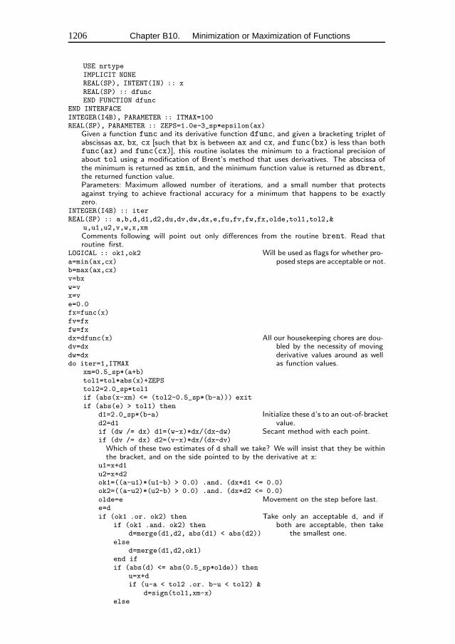
1206 Chapter B10. Minimization or Maximization of Functions
USE nrtypeIMPLICIT NONEREAL(SP), INTENT(IN) :: xREAL(SP) :: dfuncEND FUNCTION dfunc
END INTERFACEINTEGER(I4B), PARAMETER :: ITMAX=100REAL(SP), PARAMETER :: ZEPS=1.0e-3_sp*epsilon(ax)
Given a function func and its derivative function dfunc, and given a bracketing triplet ofabscissas ax, bx, cx [such that bx is between ax and cx, and func(bx) is less than bothfunc(ax) and func(cx)], this routine isolates the minimum to a fractional precision ofabout tol using a modification of Brent’s method that uses derivatives. The abscissa ofthe minimum is returned as xmin, and the minimum function value is returned as dbrent,the returned function value.Parameters: Maximum allowed number of iterations, and a small number that protectsagainst trying to achieve fractional accuracy for a minimum that happens to be exactlyzero.
INTEGER(I4B) :: iterREAL(SP) :: a,b,d,d1,d2,du,dv,dw,dx,e,fu,fv,fw,fx,olde,tol1,tol2,&
u,u1,u2,v,w,x,xmComments following will point out only differences from the routine brent. Read thatroutine first.
LOGICAL :: ok1,ok2 Will be used as flags for whether pro-posed steps are acceptable or not.a=min(ax,cx)
b=max(ax,cx)v=bxw=vx=ve=0.0fx=func(x)fv=fxfw=fxdx=dfunc(x) All our housekeeping chores are dou-
bled by the necessity of movingderivative values around as wellas function values.
dv=dxdw=dxdo iter=1,ITMAX
xm=0.5_sp*(a+b)tol1=tol*abs(x)+ZEPStol2=2.0_sp*tol1if (abs(x-xm) <= (tol2-0.5_sp*(b-a))) exitif (abs(e) > tol1) then
d1=2.0_sp*(b-a) Initialize these d’s to an out-of-bracketvalue.d2=d1
if (dw /= dx) d1=(w-x)*dx/(dx-dw) Secant method with each point.if (dv /= dx) d2=(v-x)*dx/(dx-dv)
Which of these two estimates of d shall we take? We will insist that they be withinthe bracket, and on the side pointed to by the derivative at x:
u1=x+d1u2=x+d2ok1=((a-u1)*(u1-b) > 0.0) .and. (dx*d1 <= 0.0)ok2=((a-u2)*(u2-b) > 0.0) .and. (dx*d2 <= 0.0)olde=e Movement on the step before last.e=dif (ok1 .or. ok2) then Take only an acceptable d, and if
both are acceptable, then takethe smallest one.
if (ok1 .and. ok2) thend=merge(d1,d2, abs(d1) < abs(d2))
elsed=merge(d1,d2,ok1)
end ifif (abs(d) <= abs(0.5_sp*olde)) then
u=x+dif (u-a < tol2 .or. b-u < tol2) &
d=sign(tol1,xm-x)else
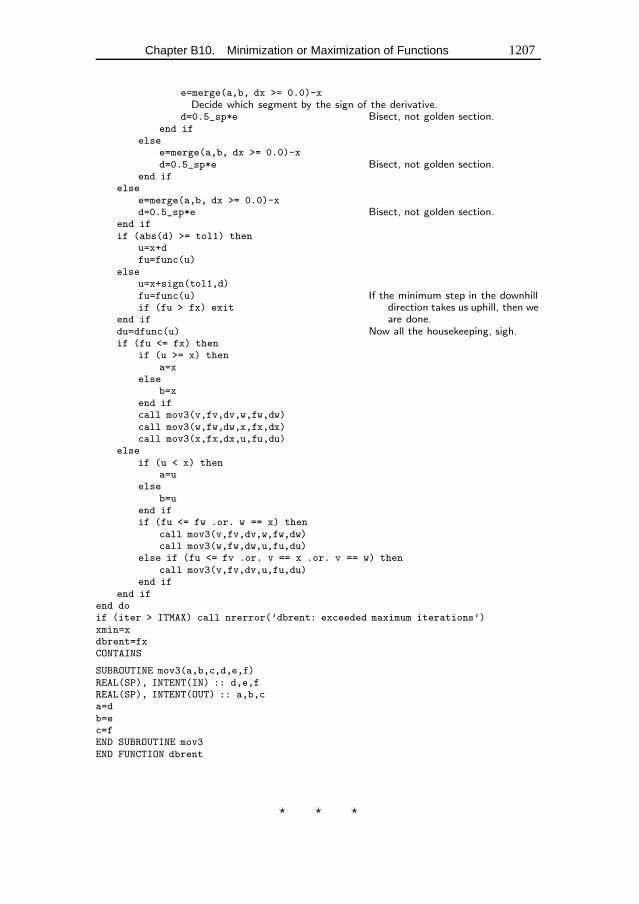
Chapter B10. Minimization or Maximization of Functions 1207
e=merge(a,b, dx >= 0.0)-xDecide which segment by the sign of the derivative.
d=0.5_sp*e Bisect, not golden section.end if
elsee=merge(a,b, dx >= 0.0)-xd=0.5_sp*e Bisect, not golden section.
end ifelse
e=merge(a,b, dx >= 0.0)-xd=0.5_sp*e Bisect, not golden section.
end ifif (abs(d) >= tol1) then
u=x+dfu=func(u)
elseu=x+sign(tol1,d)fu=func(u) If the minimum step in the downhill
direction takes us uphill, then weare done.
if (fu > fx) exitend ifdu=dfunc(u) Now all the housekeeping, sigh.if (fu <= fx) then
if (u >= x) thena=x
elseb=x
end ifcall mov3(v,fv,dv,w,fw,dw)call mov3(w,fw,dw,x,fx,dx)call mov3(x,fx,dx,u,fu,du)
elseif (u < x) then
a=uelse
b=uend ifif (fu <= fw .or. w == x) then
call mov3(v,fv,dv,w,fw,dw)call mov3(w,fw,dw,u,fu,du)
else if (fu <= fv .or. v == x .or. v == w) thencall mov3(v,fv,dv,u,fu,du)
end ifend if
end doif (iter > ITMAX) call nrerror(’dbrent: exceeded maximum iterations’)xmin=xdbrent=fxCONTAINS
SUBROUTINE mov3(a,b,c,d,e,f)REAL(SP), INTENT(IN) :: d,e,fREAL(SP), INTENT(OUT) :: a,b,ca=db=ec=fEND SUBROUTINE mov3END FUNCTION dbrent
� � �
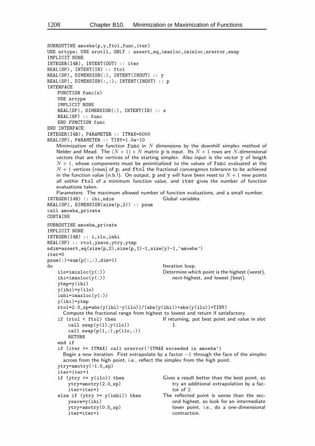
1208 Chapter B10. Minimization or Maximization of Functions
SUBROUTINE amoeba(p,y,ftol,func,iter)USE nrtype; USE nrutil, ONLY : assert_eq,imaxloc,iminloc,nrerror,swapIMPLICIT NONEINTEGER(I4B), INTENT(OUT) :: iterREAL(SP), INTENT(IN) :: ftolREAL(SP), DIMENSION(:), INTENT(INOUT) :: yREAL(SP), DIMENSION(:,:), INTENT(INOUT) :: pINTERFACE
FUNCTION func(x)USE nrtypeIMPLICIT NONEREAL(SP), DIMENSION(:), INTENT(IN) :: xREAL(SP) :: funcEND FUNCTION func
END INTERFACEINTEGER(I4B), PARAMETER :: ITMAX=5000REAL(SP), PARAMETER :: TINY=1.0e-10
Minimization of the function func in N dimensions by the downhill simplex method ofNelder and Mead. The (N + 1) ×N matrix p is input. Its N + 1 rows are N -dimensionalvectors that are the vertices of the starting simplex. Also input is the vector y of lengthN + 1, whose components must be preinitialized to the values of func evaluated at theN + 1 vertices (rows) of p; and ftol the fractional convergence tolerance to be achievedin the function value (n.b.!). On output, p and y will have been reset to N + 1 new pointsall within ftol of a minimum function value, and iter gives the number of functionevaluations taken.Parameters: The maximum allowed number of function evaluations, and a small number.
INTEGER(I4B) :: ihi,ndim Global variables.REAL(SP), DIMENSION(size(p,2)) :: psumcall amoeba_privateCONTAINS
SUBROUTINE amoeba_privateIMPLICIT NONEINTEGER(I4B) :: i,ilo,inhiREAL(SP) :: rtol,ysave,ytry,ytmpndim=assert_eq(size(p,2),size(p,1)-1,size(y)-1,’amoeba’)iter=0psum(:)=sum(p(:,:),dim=1)do Iteration loop.
ilo=iminloc(y(:)) Determine which point is the highest (worst),next-highest, and lowest (best).ihi=imaxloc(y(:))
ytmp=y(ihi)y(ihi)=y(ilo)inhi=imaxloc(y(:))y(ihi)=ytmprtol=2.0_sp*abs(y(ihi)-y(ilo))/(abs(y(ihi))+abs(y(ilo))+TINY)
Compute the fractional range from highest to lowest and return if satisfactory.if (rtol < ftol) then If returning, put best point and value in slot
1.call swap(y(1),y(ilo))call swap(p(1,:),p(ilo,:))RETURN
end ifif (iter >= ITMAX) call nrerror(’ITMAX exceeded in amoeba’)
Begin a new iteration. First extrapolate by a factor −1 through the face of the simplexacross from the high point, i.e., reflect the simplex from the high point.
ytry=amotry(-1.0_sp)iter=iter+1if (ytry <= y(ilo)) then Gives a result better than the best point, so
try an additional extrapolation by a fac-tor of 2.
ytry=amotry(2.0_sp)iter=iter+1
else if (ytry >= y(inhi)) then The reflected point is worse than the sec-ond highest, so look for an intermediatelower point, i.e., do a one-dimensionalcontraction.
ysave=y(ihi)ytry=amotry(0.5_sp)iter=iter+1
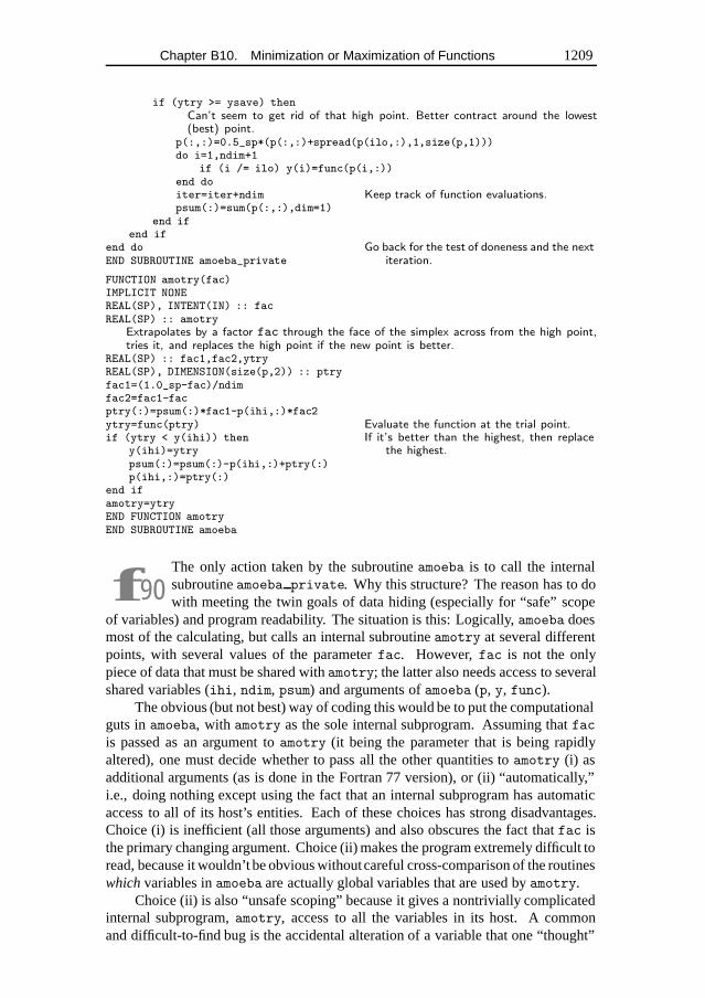
Chapter B10. Minimization or Maximization of Functions 1209
if (ytry >= ysave) thenCan’t seem to get rid of that high point. Better contract around the lowest(best) point.
p(:,:)=0.5_sp*(p(:,:)+spread(p(ilo,:),1,size(p,1)))do i=1,ndim+1
if (i /= ilo) y(i)=func(p(i,:))end doiter=iter+ndim Keep track of function evaluations.psum(:)=sum(p(:,:),dim=1)
end ifend if
end do Go back for the test of doneness and the nextiteration.END SUBROUTINE amoeba_private
FUNCTION amotry(fac)IMPLICIT NONEREAL(SP), INTENT(IN) :: facREAL(SP) :: amotry
Extrapolates by a factor fac through the face of the simplex across from the high point,tries it, and replaces the high point if the new point is better.
REAL(SP) :: fac1,fac2,ytryREAL(SP), DIMENSION(size(p,2)) :: ptryfac1=(1.0_sp-fac)/ndimfac2=fac1-facptry(:)=psum(:)*fac1-p(ihi,:)*fac2ytry=func(ptry) Evaluate the function at the trial point.if (ytry < y(ihi)) then If it’s better than the highest, then replace
the highest.y(ihi)=ytrypsum(:)=psum(:)-p(ihi,:)+ptry(:)p(ihi,:)=ptry(:)
end ifamotry=ytryEND FUNCTION amotryEND SUBROUTINE amoeba
f90The only action taken by the subroutineamoeba is to call the internalsubroutineamoeba private. Why this structure? The reason has to dowith meeting the twin goals of data hiding (especially for “safe” scope
of variables) and program readability. The situation is this: Logically,amoeba doesmost of the calculating, but calls an internal subroutineamotry at several differentpoints, with several values of the parameterfac. However,fac is not the onlypiece of data that must be shared withamotry; the latter also needs access to severalshared variables (ihi, ndim, psum) and arguments ofamoeba (p, y, func).
The obvious (but not best) way of coding this would be to put the computationalguts inamoeba, with amotry as the sole internal subprogram. Assuming thatfac
is passed as an argument toamotry (it being the parameter that is being rapidlyaltered), one must decide whether to pass all the other quantities toamotry (i) asadditional arguments (as is done in the Fortran 77 version), or (ii) “automatically,”i.e., doing nothing except using the fact that an internal subprogram has automaticaccess to all of its host’s entities. Each of these choices has strong disadvantages.Choice (i) is inefficient (all those arguments) and also obscures the fact thatfac isthe primary changing argument. Choice (ii) makes the program extremely difficult toread, because it wouldn’t be obvious withoutcareful cross-comparison of the routineswhich variables inamoeba are actually global variables that are used byamotry.
Choice (ii) is also “unsafe scoping” because it gives a nontrivially complicatedinternal subprogram,amotry, access to all the variables in its host. A commonand difficult-to-find bug is the accidental alteration of a variable that one “thought”
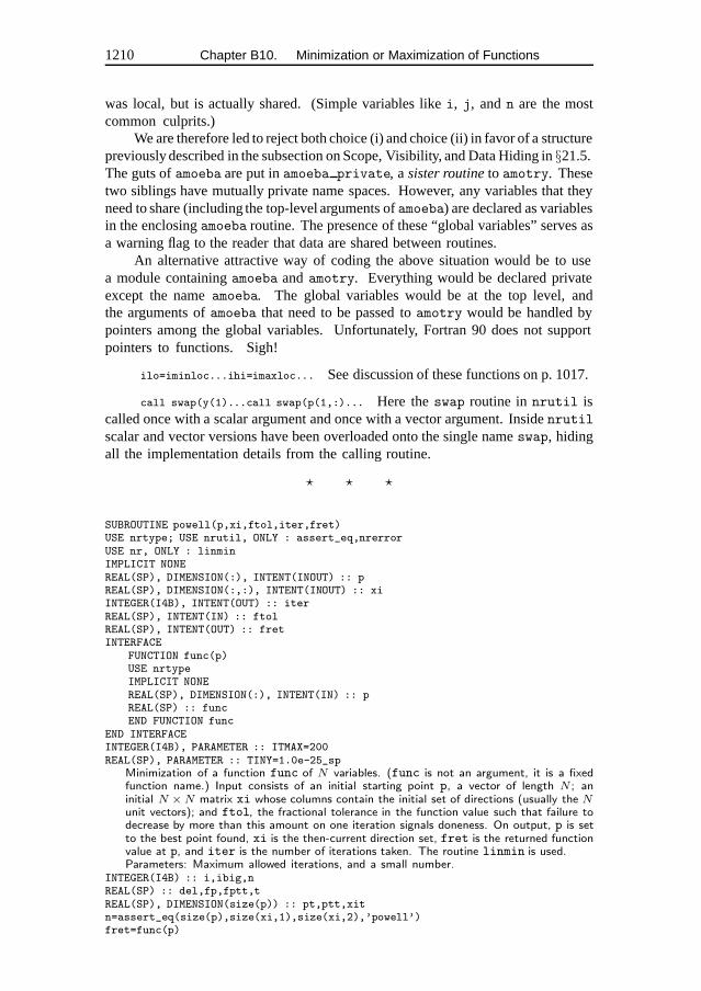
1210 Chapter B10. Minimization or Maximization of Functions
was local, but is actually shared. (Simple variables likei, j, andn are the mostcommon culprits.)
We are therefore led to reject both choice (i) and choice (ii) in favor of a structurepreviously described in the subsection on Scope, Visibility, and Data Hiding in§21.5.The guts ofamoeba are put inamoeba private, a sister routine to amotry. Thesetwo siblings have mutually private name spaces. However, any variables that theyneed to share (including the top-level arguments ofamoeba) are declared as variablesin the enclosingamoeba routine. The presence of these “global variables” serves asa warning flag to the reader that data are shared between routines.
An alternative attractive way of coding the above situation would be to usea module containingamoeba andamotry. Everything would be declared privateexcept the nameamoeba. The global variables would be at the top level, andthe arguments ofamoeba that need to be passed toamotry would be handled bypointers among the global variables. Unfortunately, Fortran 90 does not supportpointers to functions. Sigh!
ilo=iminloc...ihi=imaxloc... See discussion of these functions on p. 1017.
call swap(y(1)...call swap(p(1,:)... Here theswap routine innrutil iscalled once with a scalar argument and once with a vector argument. Insidenrutil
scalar and vector versions have been overloaded onto the single nameswap, hidingall the implementation details from the calling routine.
� � �
SUBROUTINE powell(p,xi,ftol,iter,fret)USE nrtype; USE nrutil, ONLY : assert_eq,nrerrorUSE nr, ONLY : linminIMPLICIT NONEREAL(SP), DIMENSION(:), INTENT(INOUT) :: pREAL(SP), DIMENSION(:,:), INTENT(INOUT) :: xiINTEGER(I4B), INTENT(OUT) :: iterREAL(SP), INTENT(IN) :: ftolREAL(SP), INTENT(OUT) :: fretINTERFACE
FUNCTION func(p)USE nrtypeIMPLICIT NONEREAL(SP), DIMENSION(:), INTENT(IN) :: pREAL(SP) :: funcEND FUNCTION func
END INTERFACEINTEGER(I4B), PARAMETER :: ITMAX=200REAL(SP), PARAMETER :: TINY=1.0e-25_sp
Minimization of a function func of N variables. (func is not an argument, it is a fixedfunction name.) Input consists of an initial starting point p, a vector of length N ; aninitial N × N matrix xi whose columns contain the initial set of directions (usually the Nunit vectors); and ftol, the fractional tolerance in the function value such that failure todecrease by more than this amount on one iteration signals doneness. On output, p is setto the best point found, xi is the then-current direction set, fret is the returned functionvalue at p, and iter is the number of iterations taken. The routine linmin is used.Parameters: Maximum allowed iterations, and a small number.
INTEGER(I4B) :: i,ibig,nREAL(SP) :: del,fp,fptt,tREAL(SP), DIMENSION(size(p)) :: pt,ptt,xitn=assert_eq(size(p),size(xi,1),size(xi,2),’powell’)fret=func(p)
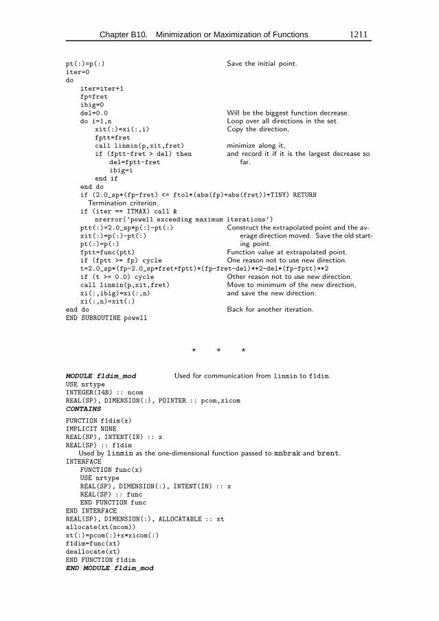
Chapter B10. Minimization or Maximization of Functions 1211
pt(:)=p(:) Save the initial point.iter=0do
iter=iter+1fp=fretibig=0del=0.0 Will be the biggest function decrease.do i=1,n Loop over all directions in the set.
xit(:)=xi(:,i) Copy the direction,fptt=fretcall linmin(p,xit,fret) minimize along it,if (fptt-fret > del) then and record it if it is the largest decrease so
far.del=fptt-fretibig=i
end ifend doif (2.0_sp*(fp-fret) <= ftol*(abs(fp)+abs(fret))+TINY) RETURN
Termination criterion.if (iter == ITMAX) call &
nrerror(’powell exceeding maximum iterations’)ptt(:)=2.0_sp*p(:)-pt(:) Construct the extrapolated point and the av-
erage direction moved. Save the old start-ing point.
xit(:)=p(:)-pt(:)pt(:)=p(:)fptt=func(ptt) Function value at extrapolated point.if (fptt >= fp) cycle One reason not to use new direction.t=2.0_sp*(fp-2.0_sp*fret+fptt)*(fp-fret-del)**2-del*(fp-fptt)**2if (t >= 0.0) cycle Other reason not to use new direction.call linmin(p,xit,fret) Move to minimum of the new direction,xi(:,ibig)=xi(:,n) and save the new direction.xi(:,n)=xit(:)
end do Back for another iteration.END SUBROUTINE powell
� � �
MODULE f1dim_mod Used for communication from linmin to f1dim.USE nrtypeINTEGER(I4B) :: ncomREAL(SP), DIMENSION(:), POINTER :: pcom,xicomCONTAINS
FUNCTION f1dim(x)IMPLICIT NONEREAL(SP), INTENT(IN) :: xREAL(SP) :: f1dim
Used by linmin as the one-dimensional function passed to mnbrak and brent.INTERFACE
FUNCTION func(x)USE nrtypeREAL(SP), DIMENSION(:), INTENT(IN) :: xREAL(SP) :: funcEND FUNCTION func
END INTERFACEREAL(SP), DIMENSION(:), ALLOCATABLE :: xtallocate(xt(ncom))xt(:)=pcom(:)+x*xicom(:)f1dim=func(xt)deallocate(xt)END FUNCTION f1dimEND MODULE f1dim_mod
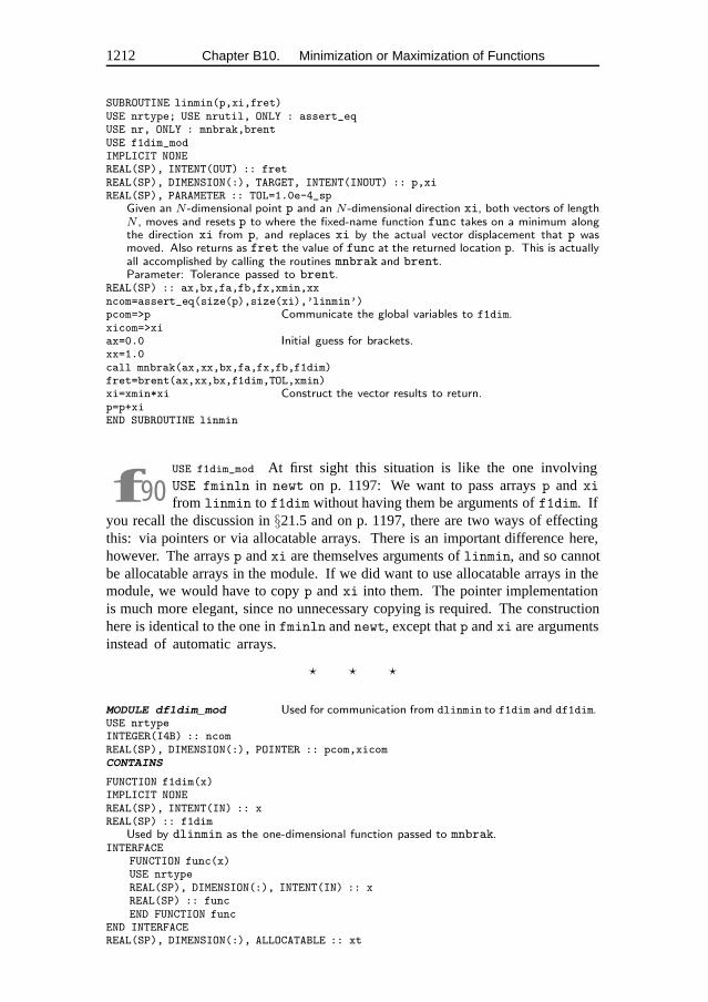
1212 Chapter B10. Minimization or Maximization of Functions
SUBROUTINE linmin(p,xi,fret)USE nrtype; USE nrutil, ONLY : assert_eqUSE nr, ONLY : mnbrak,brentUSE f1dim_modIMPLICIT NONEREAL(SP), INTENT(OUT) :: fretREAL(SP), DIMENSION(:), TARGET, INTENT(INOUT) :: p,xiREAL(SP), PARAMETER :: TOL=1.0e-4_sp
Given an N -dimensional point p and an N -dimensional direction xi, both vectors of lengthN , moves and resets p to where the fixed-name function func takes on a minimum alongthe direction xi from p, and replaces xi by the actual vector displacement that p wasmoved. Also returns as fret the value of func at the returned location p. This is actuallyall accomplished by calling the routines mnbrak and brent.Parameter: Tolerance passed to brent.
REAL(SP) :: ax,bx,fa,fb,fx,xmin,xxncom=assert_eq(size(p),size(xi),’linmin’)pcom=>p Communicate the global variables to f1dim.xicom=>xiax=0.0 Initial guess for brackets.xx=1.0call mnbrak(ax,xx,bx,fa,fx,fb,f1dim)fret=brent(ax,xx,bx,f1dim,TOL,xmin)xi=xmin*xi Construct the vector results to return.p=p+xiEND SUBROUTINE linmin
f90USE f1dim_mod At first sight this situation is like the one involvingUSE fminln in newt on p. 1197: We want to pass arraysp and xi
from linmin to f1dim without having them be arguments off1dim. Ifyou recall the discussion in§21.5 and on p. 1197, there are two ways of effectingthis: via pointers or via allocatable arrays. There is an important difference here,however. The arraysp andxi are themselves arguments oflinmin, and so cannotbe allocatable arrays in the module. If we did want to use allocatable arrays in themodule, we would have to copyp andxi into them. The pointer implementationis much more elegant, since no unnecessary copying is required. The constructionhere is identical to the one infminln andnewt, except thatp andxi are argumentsinstead of automatic arrays.
� � �
MODULE df1dim_mod Used for communication from dlinmin to f1dim and df1dim.USE nrtypeINTEGER(I4B) :: ncomREAL(SP), DIMENSION(:), POINTER :: pcom,xicomCONTAINS
FUNCTION f1dim(x)IMPLICIT NONEREAL(SP), INTENT(IN) :: xREAL(SP) :: f1dim
Used by dlinmin as the one-dimensional function passed to mnbrak.INTERFACE
FUNCTION func(x)USE nrtypeREAL(SP), DIMENSION(:), INTENT(IN) :: xREAL(SP) :: funcEND FUNCTION func
END INTERFACEREAL(SP), DIMENSION(:), ALLOCATABLE :: xt
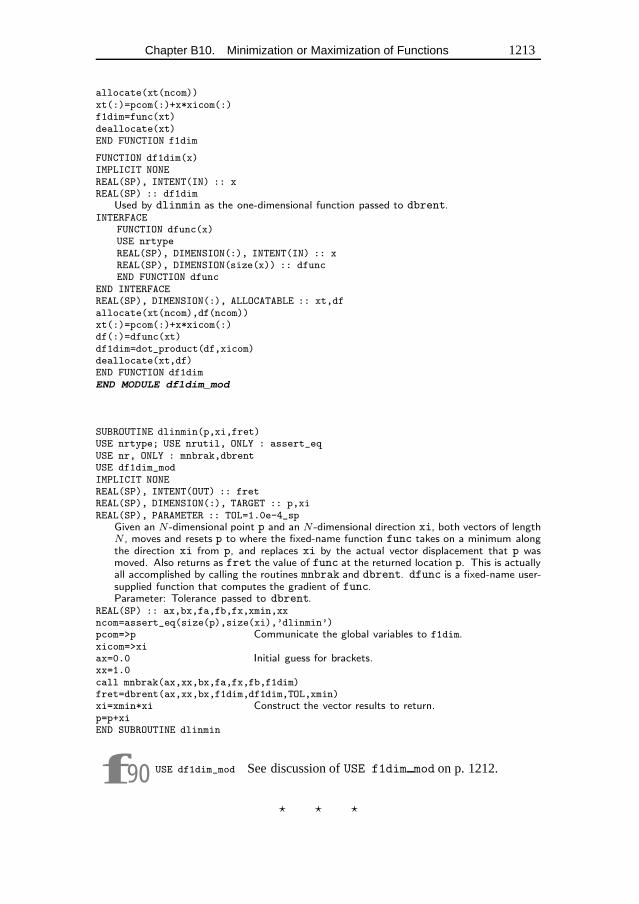
Chapter B10. Minimization or Maximization of Functions 1213
allocate(xt(ncom))xt(:)=pcom(:)+x*xicom(:)f1dim=func(xt)deallocate(xt)END FUNCTION f1dim
FUNCTION df1dim(x)IMPLICIT NONEREAL(SP), INTENT(IN) :: xREAL(SP) :: df1dim
Used by dlinmin as the one-dimensional function passed to dbrent.INTERFACE
FUNCTION dfunc(x)USE nrtypeREAL(SP), DIMENSION(:), INTENT(IN) :: xREAL(SP), DIMENSION(size(x)) :: dfuncEND FUNCTION dfunc
END INTERFACEREAL(SP), DIMENSION(:), ALLOCATABLE :: xt,dfallocate(xt(ncom),df(ncom))xt(:)=pcom(:)+x*xicom(:)df(:)=dfunc(xt)df1dim=dot_product(df,xicom)deallocate(xt,df)END FUNCTION df1dimEND MODULE df1dim_mod
SUBROUTINE dlinmin(p,xi,fret)USE nrtype; USE nrutil, ONLY : assert_eqUSE nr, ONLY : mnbrak,dbrentUSE df1dim_modIMPLICIT NONEREAL(SP), INTENT(OUT) :: fretREAL(SP), DIMENSION(:), TARGET :: p,xiREAL(SP), PARAMETER :: TOL=1.0e-4_sp
Given an N -dimensional point p and an N -dimensional direction xi, both vectors of lengthN , moves and resets p to where the fixed-name function func takes on a minimum alongthe direction xi from p, and replaces xi by the actual vector displacement that p wasmoved. Also returns as fret the value of func at the returned location p. This is actuallyall accomplished by calling the routines mnbrak and dbrent. dfunc is a fixed-name user-supplied function that computes the gradient of func.Parameter: Tolerance passed to dbrent.
REAL(SP) :: ax,bx,fa,fb,fx,xmin,xxncom=assert_eq(size(p),size(xi),’dlinmin’)pcom=>p Communicate the global variables to f1dim.xicom=>xiax=0.0 Initial guess for brackets.xx=1.0call mnbrak(ax,xx,bx,fa,fx,fb,f1dim)fret=dbrent(ax,xx,bx,f1dim,df1dim,TOL,xmin)xi=xmin*xi Construct the vector results to return.p=p+xiEND SUBROUTINE dlinmin
f90 USE df1dim_mod See discussion ofUSE f1dim mod on p. 1212.
� � �
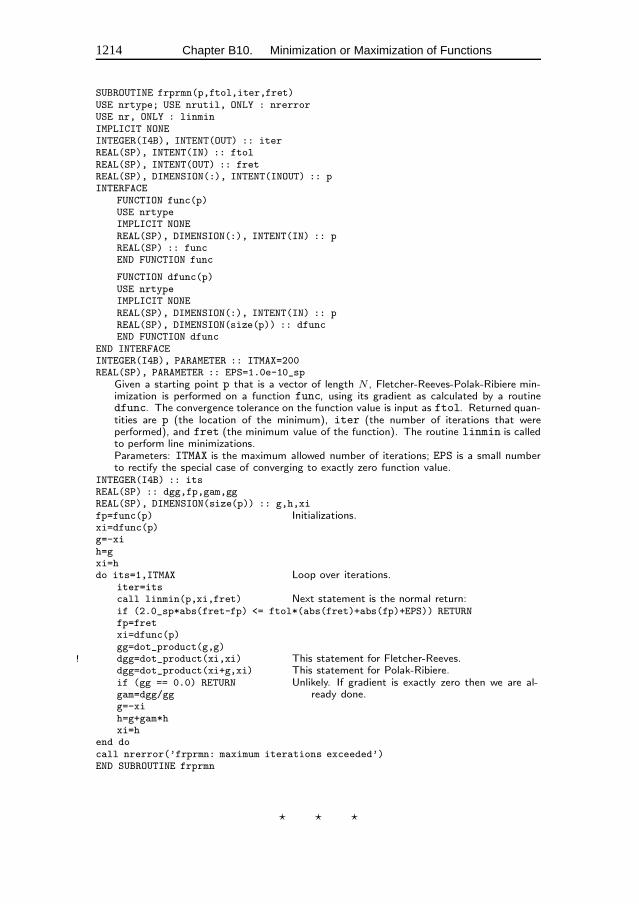
1214 Chapter B10. Minimization or Maximization of Functions
SUBROUTINE frprmn(p,ftol,iter,fret)USE nrtype; USE nrutil, ONLY : nrerrorUSE nr, ONLY : linminIMPLICIT NONEINTEGER(I4B), INTENT(OUT) :: iterREAL(SP), INTENT(IN) :: ftolREAL(SP), INTENT(OUT) :: fretREAL(SP), DIMENSION(:), INTENT(INOUT) :: pINTERFACE
FUNCTION func(p)USE nrtypeIMPLICIT NONEREAL(SP), DIMENSION(:), INTENT(IN) :: pREAL(SP) :: funcEND FUNCTION func
FUNCTION dfunc(p)USE nrtypeIMPLICIT NONEREAL(SP), DIMENSION(:), INTENT(IN) :: pREAL(SP), DIMENSION(size(p)) :: dfuncEND FUNCTION dfunc
END INTERFACEINTEGER(I4B), PARAMETER :: ITMAX=200REAL(SP), PARAMETER :: EPS=1.0e-10_sp
Given a starting point p that is a vector of length N , Fletcher-Reeves-Polak-Ribiere min-imization is performed on a function func, using its gradient as calculated by a routinedfunc. The convergence tolerance on the function value is input as ftol. Returned quan-tities are p (the location of the minimum), iter (the number of iterations that wereperformed), and fret (the minimum value of the function). The routine linmin is calledto perform line minimizations.Parameters: ITMAX is the maximum allowed number of iterations; EPS is a small numberto rectify the special case of converging to exactly zero function value.
INTEGER(I4B) :: itsREAL(SP) :: dgg,fp,gam,ggREAL(SP), DIMENSION(size(p)) :: g,h,xifp=func(p) Initializations.xi=dfunc(p)g=-xih=gxi=hdo its=1,ITMAX Loop over iterations.
iter=itscall linmin(p,xi,fret) Next statement is the normal return:if (2.0_sp*abs(fret-fp) <= ftol*(abs(fret)+abs(fp)+EPS)) RETURNfp=fretxi=dfunc(p)gg=dot_product(g,g)
! dgg=dot_product(xi,xi) This statement for Fletcher-Reeves.dgg=dot_product(xi+g,xi) This statement for Polak-Ribiere.if (gg == 0.0) RETURN Unlikely. If gradient is exactly zero then we are al-
ready done.gam=dgg/ggg=-xih=g+gam*hxi=h
end docall nrerror(’frprmn: maximum iterations exceeded’)END SUBROUTINE frprmn
� � �
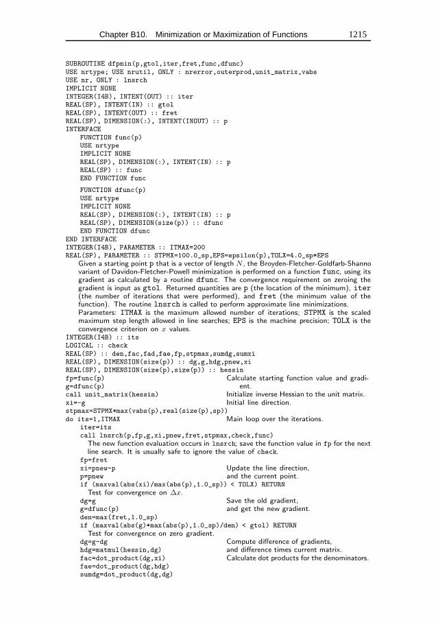
Chapter B10. Minimization or Maximization of Functions 1215
SUBROUTINE dfpmin(p,gtol,iter,fret,func,dfunc)USE nrtype; USE nrutil, ONLY : nrerror,outerprod,unit_matrix,vabsUSE nr, ONLY : lnsrchIMPLICIT NONEINTEGER(I4B), INTENT(OUT) :: iterREAL(SP), INTENT(IN) :: gtolREAL(SP), INTENT(OUT) :: fretREAL(SP), DIMENSION(:), INTENT(INOUT) :: pINTERFACE
FUNCTION func(p)USE nrtypeIMPLICIT NONEREAL(SP), DIMENSION(:), INTENT(IN) :: pREAL(SP) :: funcEND FUNCTION func
FUNCTION dfunc(p)USE nrtypeIMPLICIT NONEREAL(SP), DIMENSION(:), INTENT(IN) :: pREAL(SP), DIMENSION(size(p)) :: dfuncEND FUNCTION dfunc
END INTERFACEINTEGER(I4B), PARAMETER :: ITMAX=200REAL(SP), PARAMETER :: STPMX=100.0_sp,EPS=epsilon(p),TOLX=4.0_sp*EPS
Given a starting point p that is a vector of length N , the Broyden-Fletcher-Goldfarb-Shannovariant of Davidon-Fletcher-Powell minimization is performed on a function func, using itsgradient as calculated by a routine dfunc. The convergence requirement on zeroing thegradient is input as gtol. Returned quantities are p (the location of the minimum), iter(the number of iterations that were performed), and fret (the minimum value of thefunction). The routine lnsrch is called to perform approximate line minimizations.Parameters: ITMAX is the maximum allowed number of iterations; STPMX is the scaledmaximum step length allowed in line searches; EPS is the machine precision; TOLX is theconvergence criterion on x values.
INTEGER(I4B) :: itsLOGICAL :: checkREAL(SP) :: den,fac,fad,fae,fp,stpmax,sumdg,sumxiREAL(SP), DIMENSION(size(p)) :: dg,g,hdg,pnew,xiREAL(SP), DIMENSION(size(p),size(p)) :: hessinfp=func(p) Calculate starting function value and gradi-
ent.g=dfunc(p)call unit_matrix(hessin) Initialize inverse Hessian to the unit matrix.xi=-g Initial line direction.stpmax=STPMX*max(vabs(p),real(size(p),sp))do its=1,ITMAX Main loop over the iterations.
iter=itscall lnsrch(p,fp,g,xi,pnew,fret,stpmax,check,func)
The new function evaluation occurs in lnsrch; save the function value in fp for the nextline search. It is usually safe to ignore the value of check.
fp=fretxi=pnew-p Update the line direction,p=pnew and the current point.if (maxval(abs(xi)/max(abs(p),1.0_sp)) < TOLX) RETURN
Test for convergence on ∆x.dg=g Save the old gradient,g=dfunc(p) and get the new gradient.den=max(fret,1.0_sp)if (maxval(abs(g)*max(abs(p),1.0_sp)/den) < gtol) RETURN
Test for convergence on zero gradient.dg=g-dg Compute difference of gradients,hdg=matmul(hessin,dg) and difference times current matrix.fac=dot_product(dg,xi) Calculate dot products for the denominators.fae=dot_product(dg,hdg)sumdg=dot_product(dg,dg)
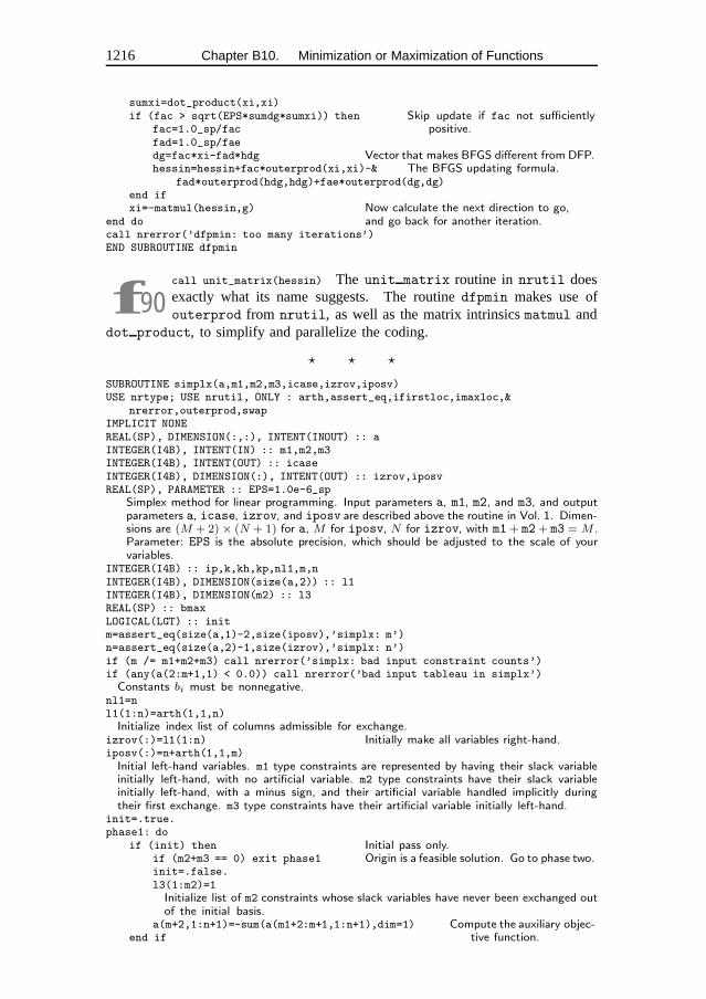
1216 Chapter B10. Minimization or Maximization of Functions
sumxi=dot_product(xi,xi)if (fac > sqrt(EPS*sumdg*sumxi)) then Skip update if fac not sufficiently
positive.fac=1.0_sp/facfad=1.0_sp/faedg=fac*xi-fad*hdg Vector that makes BFGS different from DFP.hessin=hessin+fac*outerprod(xi,xi)-& The BFGS updating formula.
fad*outerprod(hdg,hdg)+fae*outerprod(dg,dg)end ifxi=-matmul(hessin,g) Now calculate the next direction to go,
end do and go back for another iteration.call nrerror(’dfpmin: too many iterations’)END SUBROUTINE dfpmin
f90call unit_matrix(hessin) The unit matrix routine in nrutil doesexactly what its name suggests. The routinedfpmin makes use ofouterprod from nrutil, as well as the matrix intrinsicsmatmul and
dot product, to simplify and parallelize the coding.
� � �
SUBROUTINE simplx(a,m1,m2,m3,icase,izrov,iposv)USE nrtype; USE nrutil, ONLY : arth,assert_eq,ifirstloc,imaxloc,&
nrerror,outerprod,swapIMPLICIT NONEREAL(SP), DIMENSION(:,:), INTENT(INOUT) :: aINTEGER(I4B), INTENT(IN) :: m1,m2,m3INTEGER(I4B), INTENT(OUT) :: icaseINTEGER(I4B), DIMENSION(:), INTENT(OUT) :: izrov,iposvREAL(SP), PARAMETER :: EPS=1.0e-6_sp
Simplex method for linear programming. Input parameters a, m1, m2, and m3, and outputparameters a, icase, izrov, and iposv are described above the routine in Vol. 1. Dimen-sions are (M + 2) × (N + 1) for a, M for iposv, N for izrov, with m1+ m2+ m3 = M .Parameter: EPS is the absolute precision, which should be adjusted to the scale of yourvariables.
INTEGER(I4B) :: ip,k,kh,kp,nl1,m,nINTEGER(I4B), DIMENSION(size(a,2)) :: l1INTEGER(I4B), DIMENSION(m2) :: l3REAL(SP) :: bmaxLOGICAL(LGT) :: initm=assert_eq(size(a,1)-2,size(iposv),’simplx: m’)n=assert_eq(size(a,2)-1,size(izrov),’simplx: n’)if (m /= m1+m2+m3) call nrerror(’simplx: bad input constraint counts’)if (any(a(2:m+1,1) < 0.0)) call nrerror(’bad input tableau in simplx’)
Constants bi must be nonnegative.nl1=nl1(1:n)=arth(1,1,n)
Initialize index list of columns admissible for exchange.izrov(:)=l1(1:n) Initially make all variables right-hand.iposv(:)=n+arth(1,1,m)
Initial left-hand variables. m1 type constraints are represented by having their slack variableinitially left-hand, with no artificial variable. m2 type constraints have their slack variableinitially left-hand, with a minus sign, and their artificial variable handled implicitly duringtheir first exchange. m3 type constraints have their artificial variable initially left-hand.
init=.true.phase1: do
if (init) then Initial pass only.if (m2+m3 == 0) exit phase1 Origin is a feasible solution. Go to phase two.init=.false.l3(1:m2)=1
Initialize list of m2 constraints whose slack variables have never been exchanged outof the initial basis.
a(m+2,1:n+1)=-sum(a(m1+2:m+1,1:n+1),dim=1) Compute the auxiliary objec-tive function.end if
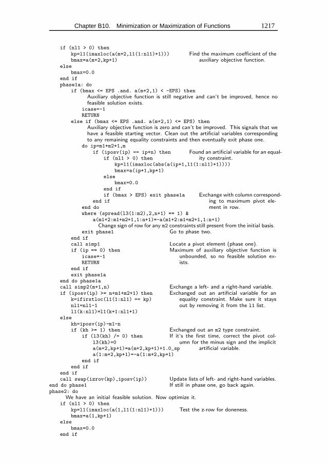
Chapter B10. Minimization or Maximization of Functions 1217
if (nl1 > 0) thenkp=l1(imaxloc(a(m+2,l1(1:nl1)+1))) Find the maximum coefficient of the
auxiliary objective function.bmax=a(m+2,kp+1)else
bmax=0.0end ifphase1a: do
if (bmax <= EPS .and. a(m+2,1) < -EPS) thenAuxiliary objective function is still negative and can’t be improved, hence nofeasible solution exists.
icase=-1RETURN
else if (bmax <= EPS .and. a(m+2,1) <= EPS) thenAuxiliary objective function is zero and can’t be improved. This signals that wehave a feasible starting vector. Clean out the artificial variables correspondingto any remaining equality constraints and then eventually exit phase one.
do ip=m1+m2+1,mif (iposv(ip) == ip+n) then Found an artificial variable for an equal-
ity constraint.if (nl1 > 0) thenkp=l1(imaxloc(abs(a(ip+1,l1(1:nl1)+1))))bmax=a(ip+1,kp+1)
elsebmax=0.0
end ifif (bmax > EPS) exit phase1a Exchange with column correspond-
ing to maximum pivot ele-ment in row.
end ifend dowhere (spread(l3(1:m2),2,n+1) == 1) &
a(m1+2:m1+m2+1,1:n+1)=-a(m1+2:m1+m2+1,1:n+1)Change sign of row for any m2 constraints still present from the initial basis.
exit phase1 Go to phase two.end ifcall simp1 Locate a pivot element (phase one).if (ip == 0) then Maximum of auxiliary objective function is
unbounded, so no feasible solution ex-ists.
icase=-1RETURN
end ifexit phase1a
end do phase1acall simp2(m+1,n) Exchange a left- and a right-hand variable.if (iposv(ip) >= n+m1+m2+1) then Exchanged out an artificial variable for an
equality constraint. Make sure it staysout by removing it from the l1 list.
k=ifirstloc(l1(1:nl1) == kp)nl1=nl1-1l1(k:nl1)=l1(k+1:nl1+1)
elsekh=iposv(ip)-m1-nif (kh >= 1) then Exchanged out an m2 type constraint.
if (l3(kh) /= 0) then If it’s the first time, correct the pivot col-umn for the minus sign and the implicit
artificial variable.l3(kh)=0a(m+2,kp+1)=a(m+2,kp+1)+1.0_spa(1:m+2,kp+1)=-a(1:m+2,kp+1)
end ifend if
end ifcall swap(izrov(kp),iposv(ip)) Update lists of left- and right-hand variables.
end do phase1 If still in phase one, go back again.phase2: do
We have an initial feasible solution. Now optimize it.if (nl1 > 0) then
kp=l1(imaxloc(a(1,l1(1:nl1)+1))) Test the z-row for doneness.bmax=a(1,kp+1)
elsebmax=0.0
end if
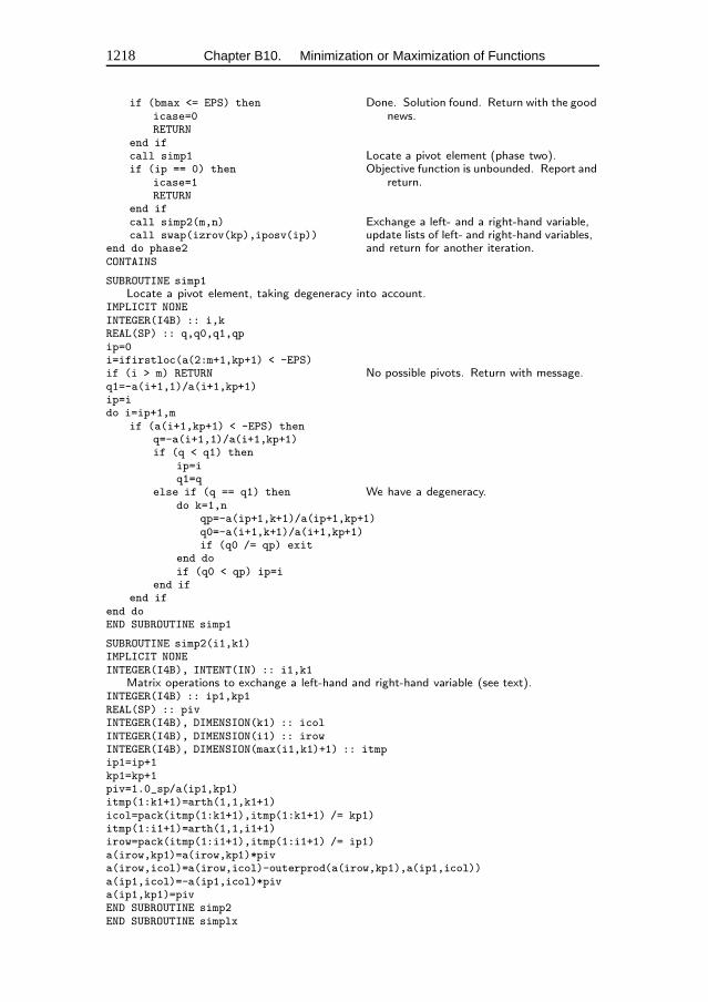
1218 Chapter B10. Minimization or Maximization of Functions
if (bmax <= EPS) then Done. Solution found. Return with the goodnews.icase=0
RETURNend ifcall simp1 Locate a pivot element (phase two).if (ip == 0) then Objective function is unbounded. Report and
return.icase=1RETURN
end ifcall simp2(m,n) Exchange a left- and a right-hand variable,call swap(izrov(kp),iposv(ip)) update lists of left- and right-hand variables,
end do phase2 and return for another iteration.CONTAINS
SUBROUTINE simp1Locate a pivot element, taking degeneracy into account.
IMPLICIT NONEINTEGER(I4B) :: i,kREAL(SP) :: q,q0,q1,qpip=0i=ifirstloc(a(2:m+1,kp+1) < -EPS)if (i > m) RETURN No possible pivots. Return with message.q1=-a(i+1,1)/a(i+1,kp+1)ip=ido i=ip+1,m
if (a(i+1,kp+1) < -EPS) thenq=-a(i+1,1)/a(i+1,kp+1)if (q < q1) then
ip=iq1=q
else if (q == q1) then We have a degeneracy.do k=1,n
qp=-a(ip+1,k+1)/a(ip+1,kp+1)q0=-a(i+1,k+1)/a(i+1,kp+1)if (q0 /= qp) exit
end doif (q0 < qp) ip=i
end ifend if
end doEND SUBROUTINE simp1
SUBROUTINE simp2(i1,k1)IMPLICIT NONEINTEGER(I4B), INTENT(IN) :: i1,k1
Matrix operations to exchange a left-hand and right-hand variable (see text).INTEGER(I4B) :: ip1,kp1REAL(SP) :: pivINTEGER(I4B), DIMENSION(k1) :: icolINTEGER(I4B), DIMENSION(i1) :: irowINTEGER(I4B), DIMENSION(max(i1,k1)+1) :: itmpip1=ip+1kp1=kp+1piv=1.0_sp/a(ip1,kp1)itmp(1:k1+1)=arth(1,1,k1+1)icol=pack(itmp(1:k1+1),itmp(1:k1+1) /= kp1)itmp(1:i1+1)=arth(1,1,i1+1)irow=pack(itmp(1:i1+1),itmp(1:i1+1) /= ip1)a(irow,kp1)=a(irow,kp1)*piva(irow,icol)=a(irow,icol)-outerprod(a(irow,kp1),a(ip1,icol))a(ip1,icol)=-a(ip1,icol)*piva(ip1,kp1)=pivEND SUBROUTINE simp2END SUBROUTINE simplx
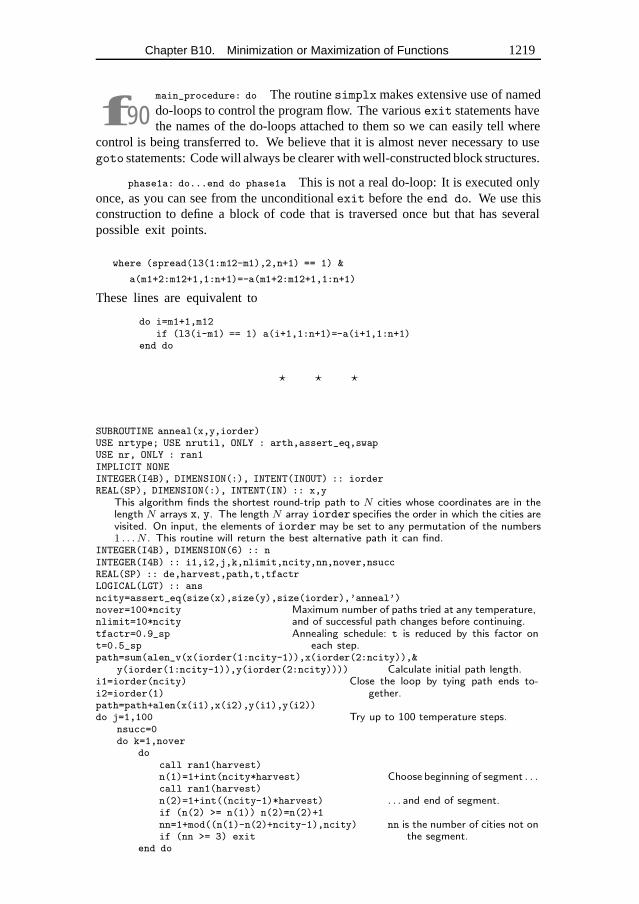
Chapter B10. Minimization or Maximization of Functions 1219
f90main_procedure: do The routinesimplx makes extensive use of nameddo-loops to control the program flow. The variousexit statements havethe names of the do-loops attached to them so we can easily tell where
control is being transferred to. We believe that it is almost never necessary to usegoto statements: Code will always be clearer with well-constructed block structures.
phase1a: do...end do phase1a This is not a real do-loop: It is executed onlyonce, as you can see from the unconditionalexit before theend do. We use thisconstruction to define a block of code that is traversed once but that has severalpossible exit points.
where (spread(l3(1:m12-m1),2,n+1) == 1) &
a(m1+2:m12+1,1:n+1)=-a(m1+2:m12+1,1:n+1)
These lines are equivalent to
do i=m1+1,m12if (l3(i-m1) == 1) a(i+1,1:n+1)=-a(i+1,1:n+1)
end do
� � �
SUBROUTINE anneal(x,y,iorder)USE nrtype; USE nrutil, ONLY : arth,assert_eq,swapUSE nr, ONLY : ran1IMPLICIT NONEINTEGER(I4B), DIMENSION(:), INTENT(INOUT) :: iorderREAL(SP), DIMENSION(:), INTENT(IN) :: x,y
This algorithm finds the shortest round-trip path to N cities whose coordinates are in thelength N arrays x, y. The length N array iorder specifies the order in which the cities arevisited. On input, the elements of iorder may be set to any permutation of the numbers1 . . . N . This routine will return the best alternative path it can find.
INTEGER(I4B), DIMENSION(6) :: nINTEGER(I4B) :: i1,i2,j,k,nlimit,ncity,nn,nover,nsuccREAL(SP) :: de,harvest,path,t,tfactrLOGICAL(LGT) :: ansncity=assert_eq(size(x),size(y),size(iorder),’anneal’)nover=100*ncity Maximum number of paths tried at any temperature,nlimit=10*ncity and of successful path changes before continuing.tfactr=0.9_sp Annealing schedule: t is reduced by this factor on
each step.t=0.5_sppath=sum(alen_v(x(iorder(1:ncity-1)),x(iorder(2:ncity)),&
y(iorder(1:ncity-1)),y(iorder(2:ncity)))) Calculate initial path length.i1=iorder(ncity) Close the loop by tying path ends to-
gether.i2=iorder(1)path=path+alen(x(i1),x(i2),y(i1),y(i2))do j=1,100 Try up to 100 temperature steps.
nsucc=0do k=1,nover
docall ran1(harvest)n(1)=1+int(ncity*harvest) Choose beginning of segment . . .call ran1(harvest)n(2)=1+int((ncity-1)*harvest) . . . and end of segment.if (n(2) >= n(1)) n(2)=n(2)+1nn=1+mod((n(1)-n(2)+ncity-1),ncity) nn is the number of cities not on
the segment.if (nn >= 3) exitend do
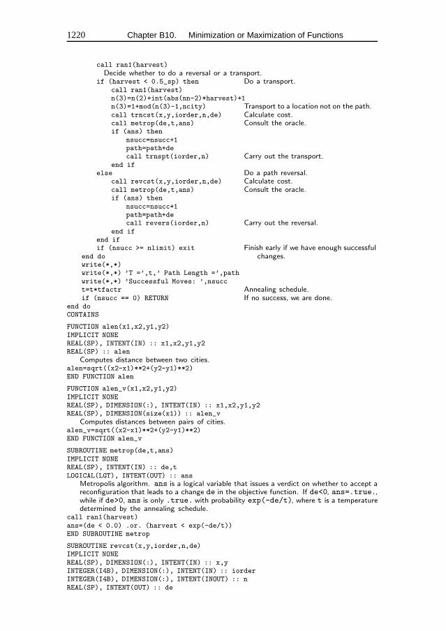
1220 Chapter B10. Minimization or Maximization of Functions
call ran1(harvest)Decide whether to do a reversal or a transport.
if (harvest < 0.5_sp) then Do a transport.call ran1(harvest)n(3)=n(2)+int(abs(nn-2)*harvest)+1n(3)=1+mod(n(3)-1,ncity) Transport to a location not on the path.call trncst(x,y,iorder,n,de) Calculate cost.call metrop(de,t,ans) Consult the oracle.if (ans) then
nsucc=nsucc+1path=path+decall trnspt(iorder,n) Carry out the transport.
end ifelse Do a path reversal.
call revcst(x,y,iorder,n,de) Calculate cost.call metrop(de,t,ans) Consult the oracle.if (ans) then
nsucc=nsucc+1path=path+decall revers(iorder,n) Carry out the reversal.
end ifend ifif (nsucc >= nlimit) exit Finish early if we have enough successful
changes.end dowrite(*,*)write(*,*) ’T =’,t,’ Path Length =’,pathwrite(*,*) ’Successful Moves: ’,nsucct=t*tfactr Annealing schedule.if (nsucc == 0) RETURN If no success, we are done.
end doCONTAINS
FUNCTION alen(x1,x2,y1,y2)IMPLICIT NONEREAL(SP), INTENT(IN) :: x1,x2,y1,y2REAL(SP) :: alen
Computes distance between two cities.alen=sqrt((x2-x1)**2+(y2-y1)**2)END FUNCTION alen
FUNCTION alen_v(x1,x2,y1,y2)IMPLICIT NONEREAL(SP), DIMENSION(:), INTENT(IN) :: x1,x2,y1,y2REAL(SP), DIMENSION(size(x1)) :: alen_v
Computes distances between pairs of cities.alen_v=sqrt((x2-x1)**2+(y2-y1)**2)END FUNCTION alen_v
SUBROUTINE metrop(de,t,ans)IMPLICIT NONEREAL(SP), INTENT(IN) :: de,tLOGICAL(LGT), INTENT(OUT) :: ans
Metropolis algorithm. ans is a logical variable that issues a verdict on whether to accept areconfiguration that leads to a change de in the objective function. If de<0, ans=.true.,while if de>0, ans is only .true. with probability exp(-de/t), where t is a temperaturedetermined by the annealing schedule.
call ran1(harvest)ans=(de < 0.0) .or. (harvest < exp(-de/t))END SUBROUTINE metrop
SUBROUTINE revcst(x,y,iorder,n,de)IMPLICIT NONEREAL(SP), DIMENSION(:), INTENT(IN) :: x,yINTEGER(I4B), DIMENSION(:), INTENT(IN) :: iorderINTEGER(I4B), DIMENSION(:), INTENT(INOUT) :: nREAL(SP), INTENT(OUT) :: de
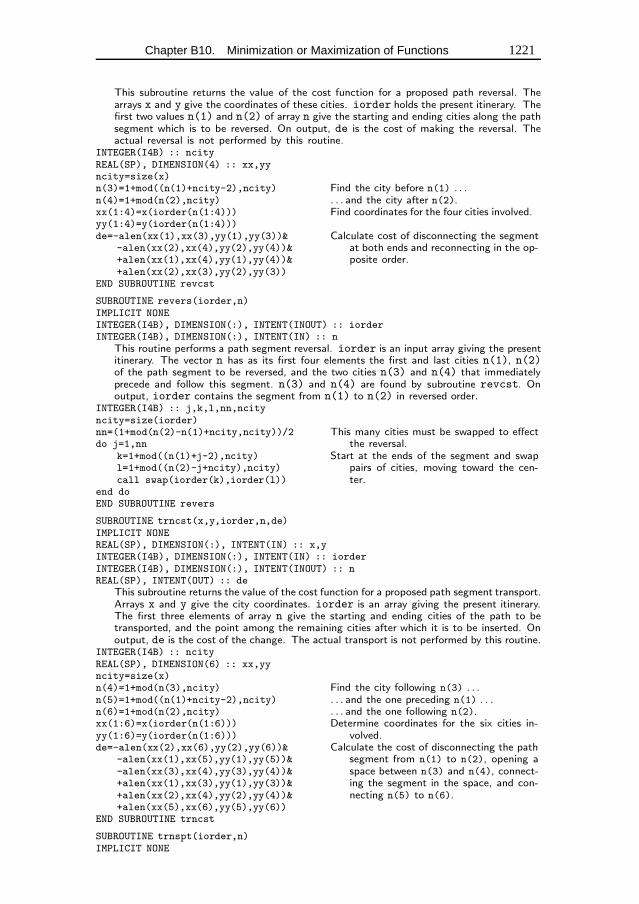
Chapter B10. Minimization or Maximization of Functions 1221
This subroutine returns the value of the cost function for a proposed path reversal. Thearrays x and y give the coordinates of these cities. iorder holds the present itinerary. Thefirst two values n(1) and n(2) of array n give the starting and ending cities along the pathsegment which is to be reversed. On output, de is the cost of making the reversal. Theactual reversal is not performed by this routine.
INTEGER(I4B) :: ncityREAL(SP), DIMENSION(4) :: xx,yyncity=size(x)n(3)=1+mod((n(1)+ncity-2),ncity) Find the city before n(1) . . .n(4)=1+mod(n(2),ncity) . . . and the city after n(2).xx(1:4)=x(iorder(n(1:4))) Find coordinates for the four cities involved.yy(1:4)=y(iorder(n(1:4)))de=-alen(xx(1),xx(3),yy(1),yy(3))& Calculate cost of disconnecting the segment
at both ends and reconnecting in the op-posite order.
-alen(xx(2),xx(4),yy(2),yy(4))&+alen(xx(1),xx(4),yy(1),yy(4))&+alen(xx(2),xx(3),yy(2),yy(3))
END SUBROUTINE revcst
SUBROUTINE revers(iorder,n)IMPLICIT NONEINTEGER(I4B), DIMENSION(:), INTENT(INOUT) :: iorderINTEGER(I4B), DIMENSION(:), INTENT(IN) :: n
This routine performs a path segment reversal. iorder is an input array giving the presentitinerary. The vector n has as its first four elements the first and last cities n(1), n(2)of the path segment to be reversed, and the two cities n(3) and n(4) that immediatelyprecede and follow this segment. n(3) and n(4) are found by subroutine revcst. Onoutput, iorder contains the segment from n(1) to n(2) in reversed order.
INTEGER(I4B) :: j,k,l,nn,ncityncity=size(iorder)nn=(1+mod(n(2)-n(1)+ncity,ncity))/2 This many cities must be swapped to effect
the reversal.do j=1,nnk=1+mod((n(1)+j-2),ncity) Start at the ends of the segment and swap
pairs of cities, moving toward the cen-ter.
l=1+mod((n(2)-j+ncity),ncity)call swap(iorder(k),iorder(l))
end doEND SUBROUTINE revers
SUBROUTINE trncst(x,y,iorder,n,de)IMPLICIT NONEREAL(SP), DIMENSION(:), INTENT(IN) :: x,yINTEGER(I4B), DIMENSION(:), INTENT(IN) :: iorderINTEGER(I4B), DIMENSION(:), INTENT(INOUT) :: nREAL(SP), INTENT(OUT) :: de
This subroutine returns the value of the cost function for a proposed path segment transport.Arrays x and y give the city coordinates. iorder is an array giving the present itinerary.The first three elements of array n give the starting and ending cities of the path to betransported, and the point among the remaining cities after which it is to be inserted. Onoutput, de is the cost of the change. The actual transport is not performed by this routine.
INTEGER(I4B) :: ncityREAL(SP), DIMENSION(6) :: xx,yyncity=size(x)n(4)=1+mod(n(3),ncity) Find the city following n(3) . . .n(5)=1+mod((n(1)+ncity-2),ncity) . . . and the one preceding n(1) . . .n(6)=1+mod(n(2),ncity) . . . and the one following n(2).xx(1:6)=x(iorder(n(1:6))) Determine coordinates for the six cities in-
volved.yy(1:6)=y(iorder(n(1:6)))de=-alen(xx(2),xx(6),yy(2),yy(6))& Calculate the cost of disconnecting the path
segment from n(1) to n(2), opening aspace between n(3) and n(4), connect-ing the segment in the space, and con-necting n(5) to n(6).
-alen(xx(1),xx(5),yy(1),yy(5))&-alen(xx(3),xx(4),yy(3),yy(4))&+alen(xx(1),xx(3),yy(1),yy(3))&+alen(xx(2),xx(4),yy(2),yy(4))&+alen(xx(5),xx(6),yy(5),yy(6))
END SUBROUTINE trncst
SUBROUTINE trnspt(iorder,n)IMPLICIT NONE
1222 Chapter B10. Minimization or Maximization of Functions
INTEGER(I4B), DIMENSION(:), INTENT(INOUT) :: iorderINTEGER(I4B), DIMENSION(:), INTENT(IN) :: n
This routine does the actual path transport, once metrop has approved. iorder is aninput array giving the present itinerary. The array n has as its six elements the beginningn(1) and end n(2) of the path to be transported, the adjacent cities n(3) and n(4)between which the path is to be placed, and the cities n(5) and n(6) that precede andfollow the path. n(4), n(5), and n(6) are calculated by subroutine trncst. On output,iorder is modified to reflect the movement of the path segment.
INTEGER(I4B) :: m1,m2,m3,nn,ncityINTEGER(I4B), DIMENSION(size(iorder)) :: jorderncity=size(iorder)m1=1+mod((n(2)-n(1)+ncity),ncity) Find number of cities from n(1) to n(2) . . .m2=1+mod((n(5)-n(4)+ncity),ncity) . . . and the number from n(4) to n(5)m3=1+mod((n(3)-n(6)+ncity),ncity) . . . and the number from n(6) to n(3).jorder(1:m1)=iorder(1+mod((arth(1,1,m1)+n(1)-2),ncity)) Copy the chosen segment.nn=m1jorder(nn+1:nn+m2)=iorder(1+mod((arth(1,1,m2)+n(4)-2),ncity))
Then copy the segment from n(4) to n(5).nn=nn+m2jorder(nn+1:nn+m3)=iorder(1+mod((arth(1,1,m3)+n(6)-2),ncity))
Finally, the segment from n(6) to n(3).iorder(1:ncity)=jorder(1:ncity) Copy jorder back into iorder.END SUBROUTINE trnsptEND SUBROUTINE anneal
� � �
SUBROUTINE amebsa(p,y,pb,yb,ftol,func,iter,temptr)USE nrtype; USE nrutil, ONLY : assert_eq,imaxloc,iminloc,swapUSE nr, ONLY : ran1IMPLICIT NONEINTEGER(I4B), INTENT(INOUT) :: iterREAL(SP), INTENT(INOUT) :: ybREAL(SP), INTENT(IN) :: ftol,temptrREAL(SP), DIMENSION(:), INTENT(INOUT) :: y,pbREAL(SP), DIMENSION(:,:), INTENT(INOUT) :: pINTERFACE
FUNCTION func(x)USE nrtypeIMPLICIT NONEREAL(SP), DIMENSION(:), INTENT(IN) :: xREAL(SP) :: funcEND FUNCTION func
END INTERFACEINTEGER(I4B), PARAMETER :: NMAX=200
Minimization of the N -dimensional function func by simulated annealing combined with thedownhill simplex method of Nelder and Mead. The (N+1)×N matrix p is input. Its N+1rows are N -dimensional vectors that are the vertices of the starting simplex. Also input isthe vector y of length N+1, whose components must be preinitialized to the values of funcevaluated at the N+1 vertices (rows) of p; ftol, the fractional convergence tolerance to beachieved in the function value for an early return; iter, and temptr. The routine makesiter function evaluations at an annealing temperature temptr, then returns. You shouldthen decrease temptr according to your annealing schedule, reset iter, and call the routineagain (leaving other arguments unaltered between calls). If iter is returned with a positivevalue, then early convergence and return occurred. If you initialize yb to a very large valueon the first call, then yb and pb (an array of length N) will subsequently return the bestfunction value and point ever encountered (even if it is no longer a point in the simplex).
INTEGER(I4B) :: ihi,ndim Global variables.REAL(SP) :: yhiREAL(SP), DIMENSION(size(p,2)) :: psumcall amebsa_private
Chapter B10. Minimization or Maximization of Functions 1223
CONTAINS
SUBROUTINE amebsa_privateINTEGER(I4B) :: i,ilo,inhiREAL(SP) :: rtol,ylo,ynhi,ysave,ytryREAL(SP), DIMENSION(size(y)) :: yt,harvestndim=assert_eq(size(p,2),size(p,1)-1,size(y)-1,size(pb),’amebsa’)psum(:)=sum(p(:,:),dim=1)do Iteration loop.
call ran1(harvest)yt(:)=y(:)-temptr*log(harvest)
Whenever we “look at” a vertex, it gets a random thermal fluctuation.ilo=iminloc(yt(:)) Determine which point is the highest (worst),
next-highest, and lowest (best).ylo=yt(ilo)ihi=imaxloc(yt(:))yhi=yt(ihi)yt(ihi)=yloinhi=imaxloc(yt(:))ynhi=yt(inhi)rtol=2.0_sp*abs(yhi-ylo)/(abs(yhi)+abs(ylo))
Compute the fractional range from highest to lowest and return if satisfactory.if (rtol < ftol .or. iter < 0) then If returning, put best point and value in
slot 1.call swap(y(1),y(ilo))call swap(p(1,:),p(ilo,:))RETURN
end ifBegin a new iteration. First extrapolate by a factor −1 through the face of the simplexacross from the high point, i.e., reflect the simplex from the high point.
ytry=amotsa(-1.0_sp)iter=iter-1if (ytry <= ylo) then Gives a result better than the best point, so
try an additional extrapolation by a fac-tor of 2.
ytry=amotsa(2.0_sp)iter=iter-1
else if (ytry >= ynhi) then The reflected point is worse than the second-highest, so look for an intermediate lowerpoint, i.e., do a one-dimensional contrac-tion.
ysave=yhiytry=amotsa(0.5_sp)iter=iter-1if (ytry >= ysave) then
Can’t seem to get rid of that high point. Better contract around the lowest(best) point.
p(:,:)=0.5_sp*(p(:,:)+spread(p(ilo,:),1,size(p,1)))do i=1,ndim+1
if (i /= ilo) y(i)=func(p(i,:))end doiter=iter-ndim Keep track of function evaluations.psum(:)=sum(p(:,:),dim=1)
end ifend if
end doEND SUBROUTINE amebsa_private
FUNCTION amotsa(fac)IMPLICIT NONEREAL(SP), INTENT(IN) :: facREAL(SP) :: amotsa
Extrapolates by a factor fac through the face of the simplex across from the high point,tries it, and replaces the high point if the new point is better.
REAL(SP) :: fac1,fac2,yflu,ytry,harvREAL(SP), DIMENSION(size(p,2)) :: ptryfac1=(1.0_sp-fac)/ndimfac2=fac1-facptry(:)=psum(:)*fac1-p(ihi,:)*fac2ytry=func(ptry)if (ytry <= yb) then Save the best-ever.
pb(:)=ptry(:)
1224 Chapter B10. Minimization or Maximization of Functions
yb=ytryend ifcall ran1(harv)yflu=ytry+temptr*log(harv) We added a thermal fluctuation to all the cur-
rent vertices, but we subtract it here, soas to give the simplex a thermal Brow-nian motion: It likes to accept any sug-gested change.
if (yflu < yhi) theny(ihi)=ytryyhi=yflupsum(:)=psum(:)-p(ihi,:)+ptry(:)p(ihi,:)=ptry(:)
end ifamotsa=yfluEND FUNCTION amotsaEND SUBROUTINE amebsa
f90See the discussion ofamoeba on p. 1209 for why the routine is codedthis way.
Chapter B11. Eigensystems
SUBROUTINE jacobi(a,d,v,nrot)USE nrtype; USE nrutil, ONLY : assert_eq,get_diag,nrerror,unit_matrix,&
upper_triangleIMPLICIT NONEINTEGER(I4B), INTENT(OUT) :: nrotREAL(SP), DIMENSION(:), INTENT(OUT) :: dREAL(SP), DIMENSION(:,:), INTENT(INOUT) :: aREAL(SP), DIMENSION(:,:), INTENT(OUT) :: v
Computes all eigenvalues and eigenvectors of a real symmetric N×N matrix a. On output,elements of a above the diagonal are destroyed. d is a vector of length N that returns theeigenvalues of a. v is an N ×N matrix whose columns contain, on output, the normalizedeigenvectors of a. nrot returns the number of Jacobi rotations that were required.
INTEGER(I4B) :: i,ip,iq,nREAL(SP) :: c,g,h,s,sm,t,tau,theta,treshREAL(SP), DIMENSION(size(d)) :: b,zn=assert_eq((/size(a,1),size(a,2),size(d),size(v,1),size(v,2)/),’jacobi’)call unit_matrix(v(:,:)) Initialize v to the identity matrix.b(:)=get_diag(a(:,:)) Initialize b and d to the diagonal of
a.d(:)=b(:)z(:)=0.0 This vector will accumulate terms of
the form tapq as in eq. (11.1.14).nrot=0do i=1,50
sm=sum(abs(a),mask=upper_triangle(n,n)) Sum off-diagonal elements.if (sm == 0.0) RETURN
The normal return, which relies on quadratic convergence to machine underflow.tresh=merge(0.2_sp*sm/n**2,0.0_sp, i < 4 )
On the first three sweeps, we will rotate only if tresh exceeded.do ip=1,n-1
do iq=ip+1,ng=100.0_sp*abs(a(ip,iq))
After four sweeps, skip the rotation if the off-diagonal element is small.if ((i > 4) .and. (abs(d(ip))+g == abs(d(ip))) &
.and. (abs(d(iq))+g == abs(d(iq)))) thena(ip,iq)=0.0
else if (abs(a(ip,iq)) > tresh) thenh=d(iq)-d(ip)if (abs(h)+g == abs(h)) then
t=a(ip,iq)/h t = 1/(2θ)else
theta=0.5_sp*h/a(ip,iq) Equation (11.1.10).t=1.0_sp/(abs(theta)+sqrt(1.0_sp+theta**2))if (theta < 0.0) t=-t
end ifc=1.0_sp/sqrt(1+t**2)s=t*ctau=s/(1.0_sp+c)h=t*a(ip,iq)z(ip)=z(ip)-hz(iq)=z(iq)+hd(ip)=d(ip)-hd(iq)=d(iq)+ha(ip,iq)=0.0
1225
1226 Chapter B11. Eigensystems
call jrotate(a(1:ip-1,ip),a(1:ip-1,iq))Case of rotations 1 ≤ j < p.
call jrotate(a(ip,ip+1:iq-1),a(ip+1:iq-1,iq))Case of rotations p < j < q.
call jrotate(a(ip,iq+1:n),a(iq,iq+1:n))Case of rotations q < j ≤ n.
call jrotate(v(:,ip),v(:,iq))nrot=nrot+1
end ifend do
end dob(:)=b(:)+z(:)d(:)=b(:) Update d with the sum of tapq,z(:)=0.0 and reinitialize z.
end docall nrerror(’too many iterations in jacobi’)CONTAINS
SUBROUTINE jrotate(a1,a2)REAL(SP), DIMENSION(:), INTENT(INOUT) :: a1,a2REAL(SP), DIMENSION(size(a1)) :: wk1wk1(:)=a1(:)a1(:)=a1(:)-s*(a2(:)+a1(:)*tau)a2(:)=a2(:)+s*(wk1(:)-a2(:)*tau)END SUBROUTINE jrotateEND SUBROUTINE jacobi
As discussed in Volume 1, jacobi is generally not competitive with tqliin terms of efficiency. However, jacobi can be parallelized whereastqli uses an intrinsically serial algorithm. The version of jacobi
implemented here is likely to be adequate for a small-scale parallel (SSP) machine,but is probably still not competitive with tqli. For a massively multiprocessor(MMP) machine, the order of the rotations needs to be chosen in a more complicatedpattern than here so that the rotations can be executed in parallel. In this case theJacobi algorithm may well turn out to be the method of choice. Parallel replacementsfor tqli based on a divide and conquer algorithm have also been proposed. Seethe discussion after tqli on p. 1229.
f90call unit_matrix...b(:)=get_diag... These routines in nrutil bothrequire access to the diagonal of a matrix, an operation that is notconveniently provided for in Fortran 90. We have split them off into
nrutil in case your compiler provides parallel library routines so you can replaceour standard versions.
sm=sum(abs(a),mask=upper_triangle(n,n)) The upper triangle function innrutil returns an upper triangular logical mask. As used here, the mask is trueeverywhere in the upper triangle of an n × n matrix, excluding the diagonal. Anoptional integer argument extra allows additional diagonals to be set to true. Withextra=1 the upper triangle including the diagonal would be true. By using the mask,we can conveniently sum over the desired matrix elements in parallel.
SUBROUTINE jrotate(a1,a2) This internal subroutine also uses the values of sand tau from the calling subroutine jacobi. Variables in the calling routine arevisible to an internal subprogram, but you should be circumspect in making use ofthis fact. It is easy to overwrite a value in the calling program inadvertently, and it is
Chapter B11. Eigensystems 1227
often difficult to figure out the logic of an internal routine if not all its variables aredeclared explicitly. However, jrotate is so simple that there is no danger here.
� � �
SUBROUTINE eigsrt(d,v)USE nrtype; USE nrutil, ONLY : assert_eq,imaxloc,swapIMPLICIT NONEREAL(SP), DIMENSION(:), INTENT(INOUT) :: dREAL(SP), DIMENSION(:,:), INTENT(INOUT) :: v
Given the eigenvalues d and eigenvectors v as output from jacobi (§11.1) or tqli (§11.3),this routine sorts the eigenvalues into descending order, and rearranges the columns of vcorrespondingly. The method is straight insertion.
INTEGER(I4B) :: i,j,nn=assert_eq(size(d),size(v,1),size(v,2),’eigsrt’)do i=1,n-1
j=imaxloc(d(i:n))+i-1if (j /= i) then
call swap(d(i),d(j))call swap(v(:,i),v(:,j))
end ifend doEND SUBROUTINE eigsrt
f90 j=imaxloc... See discussion of imaxloc on p. 1017.
call swap... See discussion of overloaded versions of swap after amoebaon p. 1210.
� � �
SUBROUTINE tred2(a,d,e,novectors)USE nrtype; USE nrutil, ONLY : assert_eq,outerprodIMPLICIT NONEREAL(SP), DIMENSION(:,:), INTENT(INOUT) :: aREAL(SP), DIMENSION(:), INTENT(OUT) :: d,eLOGICAL(LGT), OPTIONAL, INTENT(IN) :: novectors
Householder reduction of a real, symmetric, N × N matrix a. On output, a is replacedby the orthogonal matrix Q effecting the transformation. d returns the diagonal elementsof the tridiagonal matrix, and e the off-diagonal elements, with e(1)=0. If the optionalargument novectors is present, only eigenvalues are to be found subsequently, in whichcase a contains no useful information on output.
INTEGER(I4B) :: i,j,l,nREAL(SP) :: f,g,h,hh,scaleREAL(SP), DIMENSION(size(a,1)) :: ggLOGICAL(LGT), SAVE :: yesvec=.true.n=assert_eq(size(a,1),size(a,2),size(d),size(e),’tred2’)if (present(novectors)) yesvec=.not. novectorsdo i=n,2,-1
l=i-1h=0.0if (l > 1) then
scale=sum(abs(a(i,1:l)))if (scale == 0.0) then Skip transformation.
e(i)=a(i,l)else
a(i,1:l)=a(i,1:l)/scale Use scaled a’s for transformation.h=sum(a(i,1:l)**2) Form σ in h.
1228 Chapter B11. Eigensystems
f=a(i,l)g=-sign(sqrt(h),f)e(i)=scale*gh=h-f*g Now h is equation (11.2.4).a(i,l)=f-g Store u in the ith row of a.if (yesvec) a(1:l,i)=a(i,1:l)/h Store u/H in ith column of a.do j=1,l Store elements of p in temporarily
unused elements of e.e(j)=(dot_product(a(j,1:j),a(i,1:j)) &+dot_product(a(j+1:l,j),a(i,j+1:l)))/h
end dof=dot_product(e(1:l),a(i,1:l))hh=f/(h+h) Form K, equation (11.2.11).e(1:l)=e(1:l)-hh*a(i,1:l)
Form q and store in e overwriting p.do j=1,l Reduce a, equation (11.2.13).
a(j,1:j)=a(j,1:j)-a(i,j)*e(1:j)-e(j)*a(i,1:j)end do
end ifelse
e(i)=a(i,l)end ifd(i)=h
end doif (yesvec) d(1)=0.0e(1)=0.0do i=1,n Begin accumulation of transforma-
tion matrices.if (yesvec) thenl=i-1if (d(i) /= 0.0) then
This block skipped when i=1. Use u and u/H stored in a to form P · Q.gg(1:l)=matmul(a(i,1:l),a(1:l,1:l))a(1:l,1:l)=a(1:l,1:l)-outerprod(a(1:l,i),gg(1:l))
end ifd(i)=a(i,i)a(i,i)=1.0 Reset row and column of a to iden-
tity matrix for next iteration.a(i,1:l)=0.0a(1:l,i)=0.0
elsed(i)=a(i,i)
end ifend doEND SUBROUTINE tred2
f90This routine gives a nice example of the usefulness of optional arguments.The routine is written under the assumption that usually you will wantto find both eigenvalues and eigenvectors. In this case you just supply
the arguments a, d, and e. If, however, you want only eigenvalues, you supply theadditional logical argument novectors with the value .true.. The routine thenskips the unnecessary computations. Supplying novectorswith the value .false.has the same effect as omitting it.
� � �
SUBROUTINE tqli(d,e,z)USE nrtype; USE nrutil, ONLY : assert_eq,nrerrorUSE nr, ONLY : pythagIMPLICIT NONEREAL(SP), DIMENSION(:), INTENT(INOUT) :: d,eREAL(SP), DIMENSION(:,:), OPTIONAL, INTENT(INOUT) :: z
QL algorithm with implicit shifts, to determine the eigenvalues and eigenvectors of a real,symmetric, tridiagonal matrix, or of a real, symmetric matrix previously reduced by tred2
Chapter B11. Eigensystems 1229
§11.2. d is a vector of length N . On input, its elements are the diagonal elements of thetridiagonal matrix. On output, it returns the eigenvalues. The vector e inputs the subdi-agonal elements of the tridiagonal matrix, with e(1) arbitrary. On output e is destroyed.When finding only the eigenvalues, the optional argument z is omitted. If the eigenvectorsof a tridiagonal matrix are desired, the N × N matrix z is input as the identity matrix. Ifthe eigenvectors of a matrix that has been reduced by tred2 are required, then z is inputas the matrix output by tred2. In either case, the kth column of z returns the normalizedeigenvector corresponding to d(k).
INTEGER(I4B) :: i,iter,l,m,n,ndumREAL(SP) :: b,c,dd,f,g,p,r,sREAL(SP), DIMENSION(size(e)) :: ffn=assert_eq(size(d),size(e),’tqli: n’)if (present(z)) ndum=assert_eq(n,size(z,1),size(z,2),’tqli: ndum’)e(:)=eoshift(e(:),1) Convenient to renumber the elements of
e.do l=1,niter=0iterate: do
do m=l,n-1 Look for a single small subdiagonal ele-ment to split the matrix.dd=abs(d(m))+abs(d(m+1))
if (abs(e(m))+dd == dd) exitend doif (m == l) exit iterateif (iter == 30) call nrerror(’too many iterations in tqli’)iter=iter+1g=(d(l+1)-d(l))/(2.0_sp*e(l)) Form shift.r=pythag(g,1.0_sp)g=d(m)-d(l)+e(l)/(g+sign(r,g)) This is dm − ks.s=1.0c=1.0p=0.0do i=m-1,l,-1 A plane rotation as in the original QL,
followed by Givens rotations to re-store tridiagonal form.
f=s*e(i)b=c*e(i)r=pythag(f,g)e(i+1)=rif (r == 0.0) then Recover from underflow.
d(i+1)=d(i+1)-pe(m)=0.0cycle iterate
end ifs=f/rc=g/rg=d(i+1)-pr=(d(i)-g)*s+2.0_sp*c*bp=s*rd(i+1)=g+pg=c*r-bif (present(z)) then Form eigenvectors.
ff(1:n)=z(1:n,i+1)z(1:n,i+1)=s*z(1:n,i)+c*ff(1:n)z(1:n,i)=c*z(1:n,i)-s*ff(1:n)
end ifend dod(l)=d(l)-pe(l)=ge(m)=0.0
end do iterateend doEND SUBROUTINE tqli
The routine tqli is intrinsically serial. A parallel replacement based ona divide and conquer algorithm has been proposed [1,2]. The idea is tosplit the tridiagonal matrix recursively into two tridiagonal matrices of
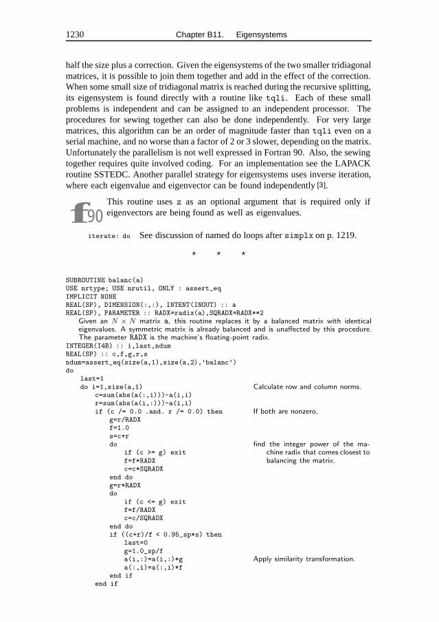
1230 Chapter B11. Eigensystems
half the size plus a correction. Given the eigensystems of the two smaller tridiagonalmatrices, it is possible to join them together and add in the effect of the correction.When some small size of tridiagonal matrix is reached during the recursive splitting,its eigensystem is found directly with a routine like tqli. Each of these smallproblems is independent and can be assigned to an independent processor. Theprocedures for sewing together can also be done independently. For very largematrices, this algorithm can be an order of magnitude faster than tqli even on aserial machine, and no worse than a factor of 2 or 3 slower, depending on the matrix.Unfortunately the parallelism is not well expressed in Fortran 90. Also, the sewingtogether requires quite involved coding. For an implementation see the LAPACKroutine SSTEDC. Another parallel strategy for eigensystems uses inverse iteration,where each eigenvalue and eigenvector can be found independently [3].
f90This routine uses z as an optional argument that is required only ifeigenvectors are being found as well as eigenvalues.
iterate: do See discussion of named do loops after simplx on p. 1219.
� � �
SUBROUTINE balanc(a)USE nrtype; USE nrutil, ONLY : assert_eqIMPLICIT NONEREAL(SP), DIMENSION(:,:), INTENT(INOUT) :: aREAL(SP), PARAMETER :: RADX=radix(a),SQRADX=RADX**2
Given an N × N matrix a, this routine replaces it by a balanced matrix with identicaleigenvalues. A symmetric matrix is already balanced and is unaffected by this procedure.The parameter RADX is the machine’s floating-point radix.
INTEGER(I4B) :: i,last,ndumREAL(SP) :: c,f,g,r,sndum=assert_eq(size(a,1),size(a,2),’balanc’)do
last=1do i=1,size(a,1) Calculate row and column norms.
c=sum(abs(a(:,i)))-a(i,i)r=sum(abs(a(i,:)))-a(i,i)if (c /= 0.0 .and. r /= 0.0) then If both are nonzero,
g=r/RADXf=1.0s=c+rdo find the integer power of the ma-
chine radix that comes closest tobalancing the matrix.
if (c >= g) exitf=f*RADXc=c*SQRADX
end dog=r*RADXdo
if (c <= g) exitf=f/RADXc=c/SQRADX
end doif ((c+r)/f < 0.95_sp*s) then
last=0g=1.0_sp/fa(i,:)=a(i,:)*g Apply similarity transformation.a(:,i)=a(:,i)*f
end ifend if
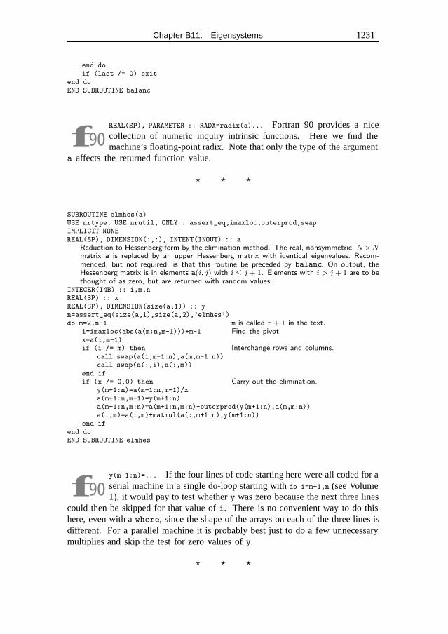
Chapter B11. Eigensystems 1231
end doif (last /= 0) exit
end doEND SUBROUTINE balanc
f90REAL(SP), PARAMETER :: RADX=radix(a)... Fortran 90 provides a nicecollection of numeric inquiry intrinsic functions. Here we find themachine’s floating-point radix. Note that only the type of the argument
a affects the returned function value.
� � �
SUBROUTINE elmhes(a)USE nrtype; USE nrutil, ONLY : assert_eq,imaxloc,outerprod,swapIMPLICIT NONEREAL(SP), DIMENSION(:,:), INTENT(INOUT) :: a
Reduction to Hessenberg form by the elimination method. The real, nonsymmetric, N ×Nmatrix a is replaced by an upper Hessenberg matrix with identical eigenvalues. Recom-mended, but not required, is that this routine be preceded by balanc. On output, theHessenberg matrix is in elements a(i, j) with i ≤ j + 1. Elements with i > j + 1 are to bethought of as zero, but are returned with random values.
INTEGER(I4B) :: i,m,nREAL(SP) :: xREAL(SP), DIMENSION(size(a,1)) :: yn=assert_eq(size(a,1),size(a,2),’elmhes’)do m=2,n-1 m is called r + 1 in the text.
i=imaxloc(abs(a(m:n,m-1)))+m-1 Find the pivot.x=a(i,m-1)if (i /= m) then Interchange rows and columns.
call swap(a(i,m-1:n),a(m,m-1:n))call swap(a(:,i),a(:,m))
end ifif (x /= 0.0) then Carry out the elimination.
y(m+1:n)=a(m+1:n,m-1)/xa(m+1:n,m-1)=y(m+1:n)a(m+1:n,m:n)=a(m+1:n,m:n)-outerprod(y(m+1:n),a(m,m:n))a(:,m)=a(:,m)+matmul(a(:,m+1:n),y(m+1:n))
end ifend doEND SUBROUTINE elmhes
f90y(m+1:n)=... If the four lines of code starting here were all coded for aserial machine in a single do-loop starting with do i=m+1,n (see Volume1), it would pay to test whether y was zero because the next three lines
could then be skipped for that value of i. There is no convenient way to do thishere, even with a where, since the shape of the arrays on each of the three lines isdifferent. For a parallel machine it is probably best just to do a few unnecessarymultiplies and skip the test for zero values of y.
� � �
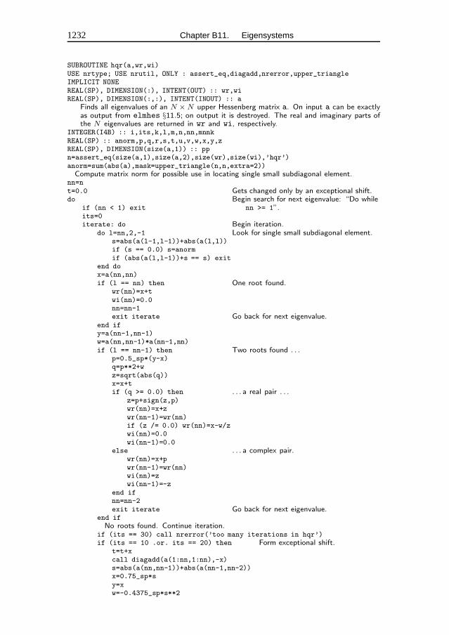
1232 Chapter B11. Eigensystems
SUBROUTINE hqr(a,wr,wi)USE nrtype; USE nrutil, ONLY : assert_eq,diagadd,nrerror,upper_triangleIMPLICIT NONEREAL(SP), DIMENSION(:), INTENT(OUT) :: wr,wiREAL(SP), DIMENSION(:,:), INTENT(INOUT) :: a
Finds all eigenvalues of an N × N upper Hessenberg matrix a. On input a can be exactlyas output from elmhes §11.5; on output it is destroyed. The real and imaginary parts ofthe N eigenvalues are returned in wr and wi, respectively.
INTEGER(I4B) :: i,its,k,l,m,n,nn,mnnkREAL(SP) :: anorm,p,q,r,s,t,u,v,w,x,y,zREAL(SP), DIMENSION(size(a,1)) :: ppn=assert_eq(size(a,1),size(a,2),size(wr),size(wi),’hqr’)anorm=sum(abs(a),mask=upper_triangle(n,n,extra=2))
Compute matrix norm for possible use in locating single small subdiagonal element.nn=nt=0.0 Gets changed only by an exceptional shift.do Begin search for next eigenvalue: “Do while
nn >= 1”.if (nn < 1) exitits=0iterate: do Begin iteration.
do l=nn,2,-1 Look for single small subdiagonal element.s=abs(a(l-1,l-1))+abs(a(l,l))if (s == 0.0) s=anormif (abs(a(l,l-1))+s == s) exit
end dox=a(nn,nn)if (l == nn) then One root found.
wr(nn)=x+twi(nn)=0.0nn=nn-1exit iterate Go back for next eigenvalue.
end ify=a(nn-1,nn-1)w=a(nn,nn-1)*a(nn-1,nn)if (l == nn-1) then Two roots found . . .
p=0.5_sp*(y-x)q=p**2+wz=sqrt(abs(q))x=x+tif (q >= 0.0) then . . . a real pair . . .
z=p+sign(z,p)wr(nn)=x+zwr(nn-1)=wr(nn)if (z /= 0.0) wr(nn)=x-w/zwi(nn)=0.0wi(nn-1)=0.0
else . . . a complex pair.wr(nn)=x+pwr(nn-1)=wr(nn)wi(nn)=zwi(nn-1)=-z
end ifnn=nn-2exit iterate Go back for next eigenvalue.
end ifNo roots found. Continue iteration.
if (its == 30) call nrerror(’too many iterations in hqr’)if (its == 10 .or. its == 20) then Form exceptional shift.
t=t+xcall diagadd(a(1:nn,1:nn),-x)s=abs(a(nn,nn-1))+abs(a(nn-1,nn-2))x=0.75_sp*sy=xw=-0.4375_sp*s**2
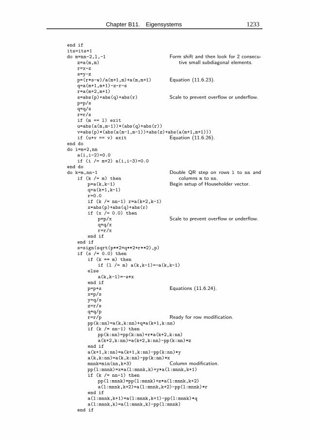
Chapter B11. Eigensystems 1233
end ifits=its+1do m=nn-2,l,-1 Form shift and then look for 2 consecu-
tive small subdiagonal elements.z=a(m,m)r=x-zs=y-zp=(r*s-w)/a(m+1,m)+a(m,m+1) Equation (11.6.23).q=a(m+1,m+1)-z-r-sr=a(m+2,m+1)s=abs(p)+abs(q)+abs(r) Scale to prevent overflow or underflow.p=p/sq=q/sr=r/sif (m == l) exitu=abs(a(m,m-1))*(abs(q)+abs(r))v=abs(p)*(abs(a(m-1,m-1))+abs(z)+abs(a(m+1,m+1)))if (u+v == v) exit Equation (11.6.26).
end dodo i=m+2,nn
a(i,i-2)=0.0if (i /= m+2) a(i,i-3)=0.0
end dodo k=m,nn-1 Double QR step on rows l to nn and
columns m to nn.if (k /= m) thenp=a(k,k-1) Begin setup of Householder vector.q=a(k+1,k-1)r=0.0if (k /= nn-1) r=a(k+2,k-1)x=abs(p)+abs(q)+abs(r)if (x /= 0.0) then
p=p/x Scale to prevent overflow or underflow.q=q/xr=r/x
end ifend ifs=sign(sqrt(p**2+q**2+r**2),p)if (s /= 0.0) then
if (k == m) thenif (l /= m) a(k,k-1)=-a(k,k-1)
elsea(k,k-1)=-s*x
end ifp=p+s Equations (11.6.24).x=p/sy=q/sz=r/sq=q/pr=r/p Ready for row modification.pp(k:nn)=a(k,k:nn)+q*a(k+1,k:nn)if (k /= nn-1) then
pp(k:nn)=pp(k:nn)+r*a(k+2,k:nn)a(k+2,k:nn)=a(k+2,k:nn)-pp(k:nn)*z
end ifa(k+1,k:nn)=a(k+1,k:nn)-pp(k:nn)*ya(k,k:nn)=a(k,k:nn)-pp(k:nn)*xmnnk=min(nn,k+3) Column modification.pp(l:mnnk)=x*a(l:mnnk,k)+y*a(l:mnnk,k+1)if (k /= nn-1) then
pp(l:mnnk)=pp(l:mnnk)+z*a(l:mnnk,k+2)a(l:mnnk,k+2)=a(l:mnnk,k+2)-pp(l:mnnk)*r
end ifa(l:mnnk,k+1)=a(l:mnnk,k+1)-pp(l:mnnk)*qa(l:mnnk,k)=a(l:mnnk,k)-pp(l:mnnk)
end if
1234 Chapter B11. Eigensystems
end doend do iterate Go back for next iteration on current eigen-
value.end doEND SUBROUTINE hqr
f90anorm=sum(abs(a),mask=upper_triangle(n,n,extra=2) See the discussionof upper triangle after jacobi on p. 1226. Setting extra=2 here picksout the upper Hessenberg part of the matrix.
iterate: do We use a named loop to improve the readability and structuringof the routine. The if-blocks that test for one or two roots end with exit iterate,transferring control back to the outermost loop and thus starting a search for thenext root.
call diagadd... The routines that operate on the diagonal of a matrix arecollected in nrutil partly so you can write clear code and partly in the hope thatcompiler writers will provide parallel library routines. Fortran 90 does not provideconvenient parallel access to the diagonal of a matrix.
CITED REFERENCES AND FURTHER READING:
Golub, G.H., and Van Loan, C.F. 1989, Matrix Computations, 2nd ed. (Baltimore: Johns HopkinsUniversity Press), §8.6 and references therein. [1]
Sorensen, D.C., and Tang, P.T.P. 1991, SIAM Journal on Numerical Analysis, vol. 28, pp. 1752–1775. [2]
Lo, S.-S., Philippe, B., and Sameh, A. 1987, SIAM Journal on Scientific and Statistical Computing,vol. 8, pp. s155–s165. [3]
Chapter B12. Fast Fourier TransformThe algorithms underlying the parallel routines in this chapter are described in
§22.4. As described there, the basic building block is a routine for simultaneouslytaking the FFT of each row of a two-dimensional matrix:
SUBROUTINE fourrow_sp(data,isign)USE nrtype; USE nrutil, ONLY : assert,swapIMPLICIT NONECOMPLEX(SPC), DIMENSION(:,:), INTENT(INOUT) :: dataINTEGER(I4B), INTENT(IN) :: isign
Replaces each row (constant first index) of data(1:M,1:N) by its discrete Fourier trans-form (transform on second index), if isign is input as 1; or replaces each row of databy N times its inverse discrete Fourier transform, if isign is input as −1. N must be aninteger power of 2. Parallelism is M -fold on the first index of data.
INTEGER(I4B) :: n,i,istep,j,m,mmax,n2REAL(DP) :: thetaCOMPLEX(SPC), DIMENSION(size(data,1)) :: tempCOMPLEX(DPC) :: w,wp Double precision for the trigonometric recurrences.COMPLEX(SPC) :: wsn=size(data,2)call assert(iand(n,n-1)==0, ’n must be a power of 2 in fourrow_sp’)n2=n/2j=n2This is the bit-reversal section of the routine.
do i=1,n-2if (j > i) call swap(data(:,j+1),data(:,i+1))m=n2do
if (m < 2 .or. j < m) exitj=j-mm=m/2
end doj=j+m
end dommax=1Here begins the Danielson-Lanczos section of the routine.
do Outer loop executed log2 N times.if (n <= mmax) exitistep=2*mmaxtheta=PI_D/(isign*mmax) Initialize for the trigonometric recurrence.wp=cmplx(-2.0_dp*sin(0.5_dp*theta)**2,sin(theta),kind=dpc)w=cmplx(1.0_dp,0.0_dp,kind=dpc)do m=1,mmax Here are the two nested inner loops.
ws=wdo i=m,n,istep
j=i+mmaxtemp=ws*data(:,j) This is the Danielson-Lanczos formula.data(:,j)=data(:,i)-tempdata(:,i)=data(:,i)+temp
end dow=w*wp+w Trigonometric recurrence.
end dommax=istep
1235
1236 Chapter B12. Fast Fourier Transform
end doEND SUBROUTINE fourrow_sp
f90call assert(iand(n,n-1)==0 ... All the Fourier routines in this chapterrequire the dimensionN of the data to be a power of 2. This is easily testedfor by AND’ing N andN − 1: N should have the binary representation
10000 . . . , in which caseN − 1 = 01111 . . . .
SUBROUTINE fourrow_dp(data,isign)USE nrtype; USE nrutil, ONLY : assert,swapIMPLICIT NONECOMPLEX(DPC), DIMENSION(:,:), INTENT(INOUT) :: dataINTEGER(I4B), INTENT(IN) :: isignINTEGER(I4B) :: n,i,istep,j,m,mmax,n2REAL(DP) :: thetaCOMPLEX(DPC), DIMENSION(size(data,1)) :: tempCOMPLEX(DPC) :: w,wpCOMPLEX(DPC) :: wsn=size(data,2)call assert(iand(n,n-1)==0, ’n must be a power of 2 in fourrow_dp’)n2=n/2j=n2do i=1,n-2
if (j > i) call swap(data(:,j+1),data(:,i+1))m=n2do
if (m < 2 .or. j < m) exitj=j-mm=m/2
end doj=j+m
end dommax=1do
if (n <= mmax) exitistep=2*mmaxtheta=PI_D/(isign*mmax)wp=cmplx(-2.0_dp*sin(0.5_dp*theta)**2,sin(theta),kind=dpc)w=cmplx(1.0_dp,0.0_dp,kind=dpc)do m=1,mmax
ws=wdo i=m,n,istep
j=i+mmaxtemp=ws*data(:,j)data(:,j)=data(:,i)-tempdata(:,i)=data(:,i)+temp
end dow=w*wp+w
end dommax=istep
end doEND SUBROUTINE fourrow_dp
SUBROUTINE fourrow_3d(data,isign)USE nrtype; USE nrutil, ONLY : assert,swapIMPLICIT NONECOMPLEX(SPC), DIMENSION(:,:,:), INTENT(INOUT) :: dataINTEGER(I4B), INTENT(IN) :: isign
If isign is input as 1, replaces each third-index section (constant first and second indices)of data(1:L,1:M,1:N) by its discrete Fourier transform (transform on third index); or
Chapter B12. Fast Fourier Transform 1237
replaces each third-index section of data by N times its inverse discrete Fourier transform,if isign is input as −1. N must be an integer power of 2. Parallelism is L× M -fold onthe first and second indices of data.
INTEGER(I4B) :: n,i,istep,j,m,mmax,n2REAL(DP) :: thetaCOMPLEX(SPC), DIMENSION(size(data,1),size(data,2)) :: tempCOMPLEX(DPC) :: w,wp Double precision for the trigonometric recurrences.COMPLEX(SPC) :: wsn=size(data,3)call assert(iand(n,n-1)==0, ’n must be a power of 2 in fourrow_3d’)n2=n/2j=n2This is the bit-reversal section of the routine.
do i=1,n-2if (j > i) call swap(data(:,:,j+1),data(:,:,i+1))m=n2do
if (m < 2 .or. j < m) exitj=j-mm=m/2
end doj=j+m
end dommax=1Here begins the Danielson-Lanczos section of the routine.
do Outer loop executed log2 N times.if (n <= mmax) exitistep=2*mmaxtheta=PI_D/(isign*mmax) Initialize for the trigonometric recurrence.wp=cmplx(-2.0_dp*sin(0.5_dp*theta)**2,sin(theta),kind=dpc)w=cmplx(1.0_dp,0.0_dp,kind=dpc)do m=1,mmax Here are the two nested inner loops.
ws=wdo i=m,n,istep
j=i+mmaxtemp=ws*data(:,:,j) This is the Danielson-Lanczos formula.data(:,:,j)=data(:,:,i)-tempdata(:,:,i)=data(:,:,i)+temp
end dow=w*wp+w Trigonometric recurrence.
end dommax=istep
end doEND SUBROUTINE fourrow_3d
� � �
Exactly as in the preceding routines, we can take the FFT of eachcolumn of a two-dimensional matrix, and for eachfirst-index section ofa three-dimensional array.
SUBROUTINE fourcol(data,isign)USE nrtype; USE nrutil, ONLY : assert,swapIMPLICIT NONECOMPLEX(SPC), DIMENSION(:,:), INTENT(INOUT) :: dataINTEGER(I4B), INTENT(IN) :: isign
Replaces each column (constant second index) of data(1:N,1:M) by its discrete Fouriertransform (transform on first index), if isign is input as 1; or replaces each row of data
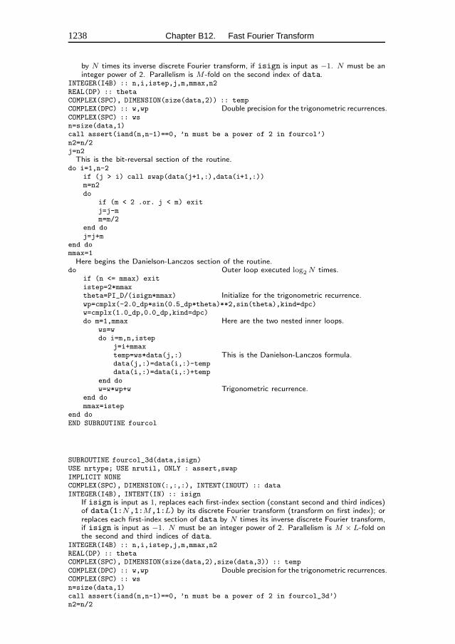
1238 Chapter B12. Fast Fourier Transform
by N times its inverse discrete Fourier transform, if isign is input as −1. N must be aninteger power of 2. Parallelism is M -fold on the second index of data.
INTEGER(I4B) :: n,i,istep,j,m,mmax,n2REAL(DP) :: thetaCOMPLEX(SPC), DIMENSION(size(data,2)) :: tempCOMPLEX(DPC) :: w,wp Double precision for the trigonometric recurrences.COMPLEX(SPC) :: wsn=size(data,1)call assert(iand(n,n-1)==0, ’n must be a power of 2 in fourcol’)n2=n/2j=n2This is the bit-reversal section of the routine.
do i=1,n-2if (j > i) call swap(data(j+1,:),data(i+1,:))m=n2do
if (m < 2 .or. j < m) exitj=j-mm=m/2
end doj=j+m
end dommax=1Here begins the Danielson-Lanczos section of the routine.
do Outer loop executed log2 N times.if (n <= mmax) exitistep=2*mmaxtheta=PI_D/(isign*mmax) Initialize for the trigonometric recurrence.wp=cmplx(-2.0_dp*sin(0.5_dp*theta)**2,sin(theta),kind=dpc)w=cmplx(1.0_dp,0.0_dp,kind=dpc)do m=1,mmax Here are the two nested inner loops.
ws=wdo i=m,n,istep
j=i+mmaxtemp=ws*data(j,:) This is the Danielson-Lanczos formula.data(j,:)=data(i,:)-tempdata(i,:)=data(i,:)+temp
end dow=w*wp+w Trigonometric recurrence.
end dommax=istep
end doEND SUBROUTINE fourcol
SUBROUTINE fourcol_3d(data,isign)USE nrtype; USE nrutil, ONLY : assert,swapIMPLICIT NONECOMPLEX(SPC), DIMENSION(:,:,:), INTENT(INOUT) :: dataINTEGER(I4B), INTENT(IN) :: isign
If isign is input as 1, replaces each first-index section (constant second and third indices)of data(1:N,1:M,1:L) by its discrete Fourier transform (transform on first index); orreplaces each first-index section of data by N times its inverse discrete Fourier transform,if isign is input as −1. N must be an integer power of 2. Parallelism is M × L-fold onthe second and third indices of data.
INTEGER(I4B) :: n,i,istep,j,m,mmax,n2REAL(DP) :: thetaCOMPLEX(SPC), DIMENSION(size(data,2),size(data,3)) :: tempCOMPLEX(DPC) :: w,wp Double precision for the trigonometric recurrences.COMPLEX(SPC) :: wsn=size(data,1)call assert(iand(n,n-1)==0, ’n must be a power of 2 in fourcol_3d’)n2=n/2
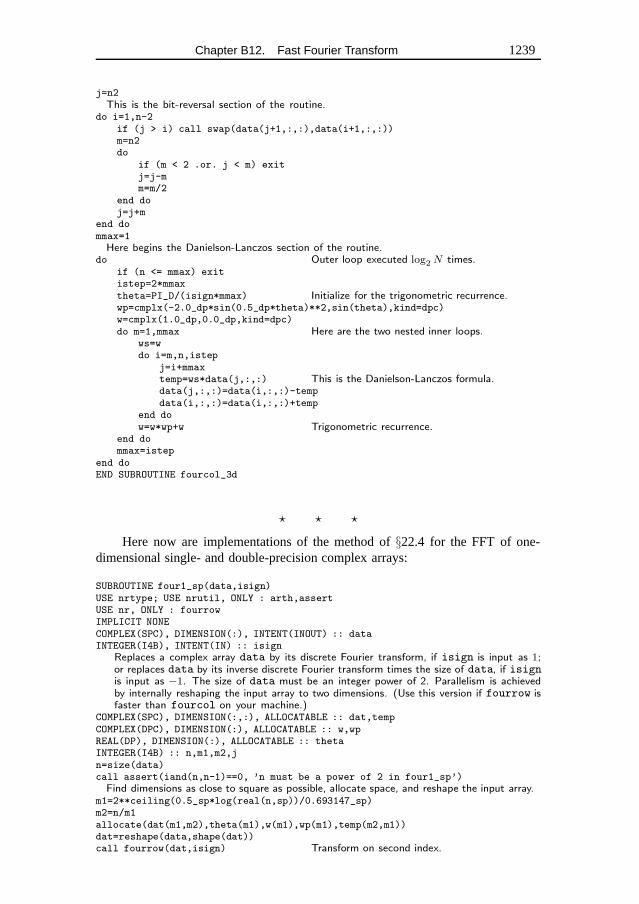
Chapter B12. Fast Fourier Transform 1239
j=n2This is the bit-reversal section of the routine.
do i=1,n-2if (j > i) call swap(data(j+1,:,:),data(i+1,:,:))m=n2do
if (m < 2 .or. j < m) exitj=j-mm=m/2
end doj=j+m
end dommax=1Here begins the Danielson-Lanczos section of the routine.
do Outer loop executed log2 N times.if (n <= mmax) exitistep=2*mmaxtheta=PI_D/(isign*mmax) Initialize for the trigonometric recurrence.wp=cmplx(-2.0_dp*sin(0.5_dp*theta)**2,sin(theta),kind=dpc)w=cmplx(1.0_dp,0.0_dp,kind=dpc)do m=1,mmax Here are the two nested inner loops.
ws=wdo i=m,n,istep
j=i+mmaxtemp=ws*data(j,:,:) This is the Danielson-Lanczos formula.data(j,:,:)=data(i,:,:)-tempdata(i,:,:)=data(i,:,:)+temp
end dow=w*wp+w Trigonometric recurrence.
end dommax=istep
end doEND SUBROUTINE fourcol_3d
� � �
Here now are implementations of the method of§22.4 for the FFT of one-dimensional single- and double-precision complex arrays:
SUBROUTINE four1_sp(data,isign)USE nrtype; USE nrutil, ONLY : arth,assertUSE nr, ONLY : fourrowIMPLICIT NONECOMPLEX(SPC), DIMENSION(:), INTENT(INOUT) :: dataINTEGER(I4B), INTENT(IN) :: isign
Replaces a complex array data by its discrete Fourier transform, if isign is input as 1;or replaces data by its inverse discrete Fourier transform times the size of data, if isignis input as −1. The size of data must be an integer power of 2. Parallelism is achievedby internally reshaping the input array to two dimensions. (Use this version if fourrow isfaster than fourcol on your machine.)
COMPLEX(SPC), DIMENSION(:,:), ALLOCATABLE :: dat,tempCOMPLEX(DPC), DIMENSION(:), ALLOCATABLE :: w,wpREAL(DP), DIMENSION(:), ALLOCATABLE :: thetaINTEGER(I4B) :: n,m1,m2,jn=size(data)call assert(iand(n,n-1)==0, ’n must be a power of 2 in four1_sp’)Find dimensions as close to square as possible, allocate space, and reshape the input array.
m1=2**ceiling(0.5_sp*log(real(n,sp))/0.693147_sp)m2=n/m1allocate(dat(m1,m2),theta(m1),w(m1),wp(m1),temp(m2,m1))dat=reshape(data,shape(dat))call fourrow(dat,isign) Transform on second index.
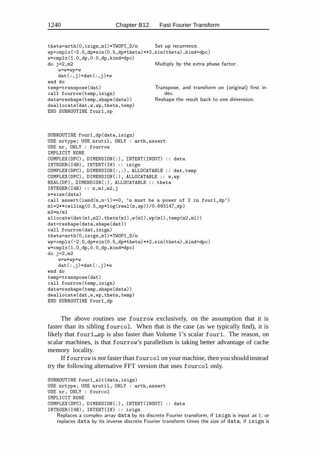
1240 Chapter B12. Fast Fourier Transform
theta=arth(0,isign,m1)*TWOPI_D/n Set up recurrence.wp=cmplx(-2.0_dp*sin(0.5_dp*theta)**2,sin(theta),kind=dpc)w=cmplx(1.0_dp,0.0_dp,kind=dpc)do j=2,m2 Multiply by the extra phase factor.
w=w*wp+wdat(:,j)=dat(:,j)*w
end dotemp=transpose(dat) Transpose, and transform on (original) first in-
dex.call fourrow(temp,isign)data=reshape(temp,shape(data)) Reshape the result back to one dimension.deallocate(dat,w,wp,theta,temp)END SUBROUTINE four1_sp
SUBROUTINE four1_dp(data,isign)USE nrtype; USE nrutil, ONLY : arth,assertUSE nr, ONLY : fourrowIMPLICIT NONECOMPLEX(DPC), DIMENSION(:), INTENT(INOUT) :: dataINTEGER(I4B), INTENT(IN) :: isignCOMPLEX(DPC), DIMENSION(:,:), ALLOCATABLE :: dat,tempCOMPLEX(DPC), DIMENSION(:), ALLOCATABLE :: w,wpREAL(DP), DIMENSION(:), ALLOCATABLE :: thetaINTEGER(I4B) :: n,m1,m2,jn=size(data)call assert(iand(n,n-1)==0, ’n must be a power of 2 in four1_dp’)m1=2**ceiling(0.5_sp*log(real(n,sp))/0.693147_sp)m2=n/m1allocate(dat(m1,m2),theta(m1),w(m1),wp(m1),temp(m2,m1))dat=reshape(data,shape(dat))call fourrow(dat,isign)theta=arth(0,isign,m1)*TWOPI_D/nwp=cmplx(-2.0_dp*sin(0.5_dp*theta)**2,sin(theta),kind=dpc)w=cmplx(1.0_dp,0.0_dp,kind=dpc)do j=2,m2
w=w*wp+wdat(:,j)=dat(:,j)*w
end dotemp=transpose(dat)call fourrow(temp,isign)data=reshape(temp,shape(data))deallocate(dat,w,wp,theta,temp)END SUBROUTINE four1_dp
The above routines usefourrow exclusively, on the assumption that it isfaster than its siblingfourcol. When that is the case (as we typically find), it islikely that four1 sp is also faster than Volume 1’s scalarfour1. The reason, onscalar machines, is thatfourrow’s parallelism is taking better advantage of cachememory locality.
If fourrow is not faster thanfourcol on your machine, then you should insteadtry the following alternative FFT version that usesfourcol only.
SUBROUTINE four1_alt(data,isign)USE nrtype; USE nrutil, ONLY : arth,assertUSE nr, ONLY : fourcolIMPLICIT NONECOMPLEX(SPC), DIMENSION(:), INTENT(INOUT) :: dataINTEGER(I4B), INTENT(IN) :: isign
Replaces a complex array data by its discrete Fourier transform, if isign is input as 1; orreplaces data by its inverse discrete Fourier transform times the size of data, if isign is
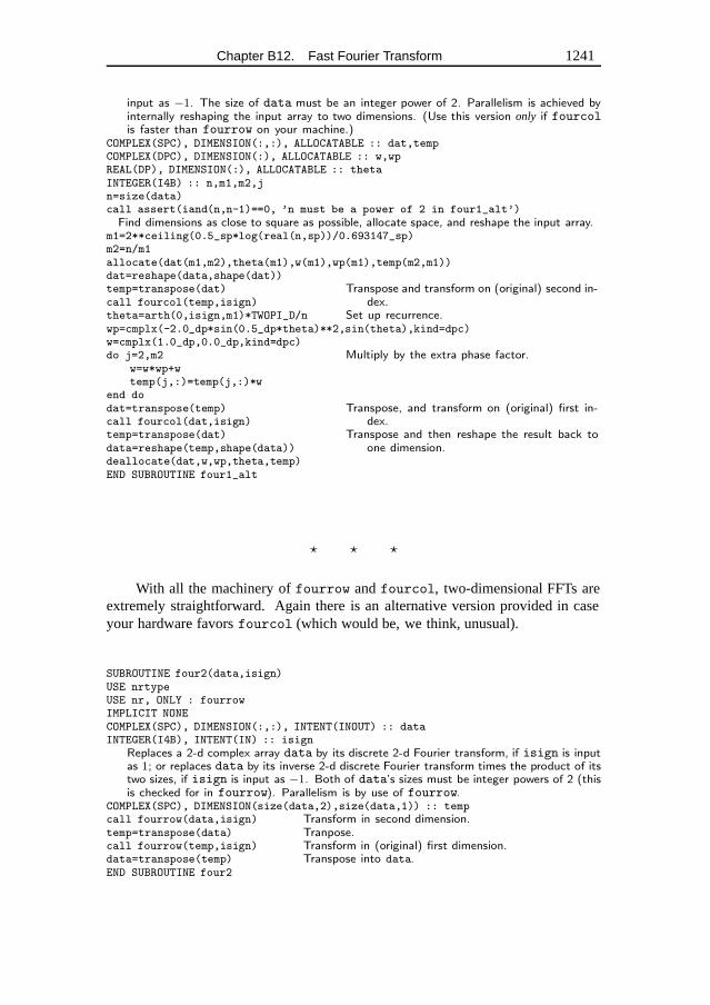
Chapter B12. Fast Fourier Transform 1241
input as −1. The size of data must be an integer power of 2. Parallelism is achieved byinternally reshaping the input array to two dimensions. (Use this version only if fourcolis faster than fourrow on your machine.)
COMPLEX(SPC), DIMENSION(:,:), ALLOCATABLE :: dat,tempCOMPLEX(DPC), DIMENSION(:), ALLOCATABLE :: w,wpREAL(DP), DIMENSION(:), ALLOCATABLE :: thetaINTEGER(I4B) :: n,m1,m2,jn=size(data)call assert(iand(n,n-1)==0, ’n must be a power of 2 in four1_alt’)Find dimensions as close to square as possible, allocate space, and reshape the input array.
m1=2**ceiling(0.5_sp*log(real(n,sp))/0.693147_sp)m2=n/m1allocate(dat(m1,m2),theta(m1),w(m1),wp(m1),temp(m2,m1))dat=reshape(data,shape(dat))temp=transpose(dat) Transpose and transform on (original) second in-
dex.call fourcol(temp,isign)theta=arth(0,isign,m1)*TWOPI_D/n Set up recurrence.wp=cmplx(-2.0_dp*sin(0.5_dp*theta)**2,sin(theta),kind=dpc)w=cmplx(1.0_dp,0.0_dp,kind=dpc)do j=2,m2 Multiply by the extra phase factor.
w=w*wp+wtemp(j,:)=temp(j,:)*w
end dodat=transpose(temp) Transpose, and transform on (original) first in-
dex.call fourcol(dat,isign)temp=transpose(dat) Transpose and then reshape the result back to
one dimension.data=reshape(temp,shape(data))deallocate(dat,w,wp,theta,temp)END SUBROUTINE four1_alt
� � �
With all the machinery offourrow andfourcol, two-dimensional FFTs areextremely straightforward. Again there is an alternative version provided in caseyour hardware favorsfourcol (which would be, we think, unusual).
SUBROUTINE four2(data,isign)USE nrtypeUSE nr, ONLY : fourrowIMPLICIT NONECOMPLEX(SPC), DIMENSION(:,:), INTENT(INOUT) :: dataINTEGER(I4B), INTENT(IN) :: isign
Replaces a 2-d complex array data by its discrete 2-d Fourier transform, if isign is inputas 1; or replaces data by its inverse 2-d discrete Fourier transform times the product of itstwo sizes, if isign is input as −1. Both of data’s sizes must be integer powers of 2 (thisis checked for in fourrow). Parallelism is by use of fourrow.
COMPLEX(SPC), DIMENSION(size(data,2),size(data,1)) :: tempcall fourrow(data,isign) Transform in second dimension.temp=transpose(data) Tranpose.call fourrow(temp,isign) Transform in (original) first dimension.data=transpose(temp) Transpose into data.END SUBROUTINE four2
1242 Chapter B12. Fast Fourier Transform
SUBROUTINE four2_alt(data,isign)USE nrtypeUSE nr, ONLY : fourcolIMPLICIT NONECOMPLEX(SPC), DIMENSION(:,:), INTENT(INOUT) :: dataINTEGER(I4B), INTENT(IN) :: isign
Replaces a 2-d complex array data by its discrete 2-d Fourier transform, if isign is inputas 1; or replaces data by its inverse 2-d discrete Fourier transform times the product ofits two sizes, if isign is input as −1. Both of data’s sizes must be integer powers of 2(this is checked for in fourcol). Parallelism is by use of fourcol. (Use this version onlyif fourcol is faster than fourrow on your machine.)
COMPLEX(SPC), DIMENSION(size(data,2),size(data,1)) :: temptemp=transpose(data) Tranpose.call fourcol(temp,isign) Transform in (original) second dimension.data=transpose(temp) Transpose.call fourcol(data,isign) Transform in (original) first dimension.END SUBROUTINE four2_alt
� � �
Most of the remaining routines in this chapter simply call one or another of theabove FFT routines, with a small amount of auxiliary computation, so they are fairlystraightforward conversions from their Volume 1 counterparts.
SUBROUTINE twofft(data1,data2,fft1,fft2)USE nrtype; USE nrutil, ONLY : assert,assert_eqUSE nr, ONLY : four1IMPLICIT NONEREAL(SP), DIMENSION(:), INTENT(IN) :: data1,data2COMPLEX(SPC), DIMENSION(:), INTENT(OUT) :: fft1,fft2
Given two real input arrays data1 and data2 of length N , this routine calls four1 andreturns two complex output arrays, fft1 and fft2, each of complex length N , that containthe discrete Fourier transforms of the respective data arrays. N must be an integer powerof 2.
INTEGER(I4B) :: n,n2COMPLEX(SPC), PARAMETER :: C1=(0.5_sp,0.0_sp), C2=(0.0_sp,-0.5_sp)COMPLEX, DIMENSION(size(data1)/2+1) :: h1,h2n=assert_eq(size(data1),size(data2),size(fft1),size(fft2),’twofft’)call assert(iand(n,n-1)==0, ’n must be a power of 2 in twofft’)fft1=cmplx(data1,data2,kind=spc) Pack the two real arrays into one complex array.call four1(fft1,1) Transform the complex array.fft2(1)=cmplx(aimag(fft1(1)),0.0_sp,kind=spc)fft1(1)=cmplx(real(fft1(1)),0.0_sp,kind=spc)n2=n/2+1h1(2:n2)=C1*(fft1(2:n2)+conjg(fft1(n:n2:-1))) Use symmetries to separate the
two transforms.h2(2:n2)=C2*(fft1(2:n2)-conjg(fft1(n:n2:-1)))fft1(2:n2)=h1(2:n2) Ship them out in two complex arrays.fft1(n:n2:-1)=conjg(h1(2:n2))fft2(2:n2)=h2(2:n2)fft2(n:n2:-1)=conjg(h2(2:n2))END SUBROUTINE twofft
� � �
Chapter B12. Fast Fourier Transform 1243
SUBROUTINE realft_sp(data,isign,zdata)USE nrtype; USE nrutil, ONLY : assert,assert_eq,zroots_unityUSE nr, ONLY : four1IMPLICIT NONEREAL(SP), DIMENSION(:), INTENT(INOUT) :: dataINTEGER(I4B), INTENT(IN) :: isignCOMPLEX(SPC), DIMENSION(:), OPTIONAL, TARGET :: zdata
When isign = 1, calculates the Fourier transform of a set of N real-valued data points,input in the array data. If the optional argument zdata is not present, the data are replacedby the positive frequency half of its complex Fourier transform. The real-valued first andlast components of the complex transform are returned as elements data(1) and data(2),respectively. If the complex array zdata of length N/2 is present, data is unchanged andthe transform is returned in zdata. N must be a power of 2. If isign = −1, this routinecalculates the inverse transform of a complex data array if it is the transform of real data.(Result in this case must be multiplied by 2/N .) The data can be supplied either in data,with zdata absent, or in zdata.
INTEGER(I4B) :: n,ndum,nh,nqCOMPLEX(SPC), DIMENSION(size(data)/4) :: wCOMPLEX(SPC), DIMENSION(size(data)/4-1) :: h1,h2COMPLEX(SPC), DIMENSION(:), POINTER :: cdata Used for internal complex computa-
tions.COMPLEX(SPC) :: zREAL(SP) :: c1=0.5_sp,c2n=size(data)call assert(iand(n,n-1)==0, ’n must be a power of 2 in realft_sp’)nh=n/2nq=n/4if (present(zdata)) then
ndum=assert_eq(n/2,size(zdata),’realft_sp’)cdata=>zdata Use zdata as cdata.if (isign == 1) cdata=cmplx(data(1:n-1:2),data(2:n:2),kind=spc)
elseallocate(cdata(n/2)) Have to allocate storage ourselves.cdata=cmplx(data(1:n-1:2),data(2:n:2),kind=spc)
end ifif (isign == 1) then
c2=-0.5_spcall four1(cdata,+1) The forward transform is here.
else Otherwise set up for an inverse trans-form.c2=0.5_sp
end ifw=zroots_unity(sign(n,isign),n/4)w=cmplx(-aimag(w),real(w),kind=spc)h1=c1*(cdata(2:nq)+conjg(cdata(nh:nq+2:-1))) The two separate transforms are sep-
arated out of cdata.h2=c2*(cdata(2:nq)-conjg(cdata(nh:nq+2:-1)))Next they are recombined to form the true transform of the original real data:
cdata(2:nq)=h1+w(2:nq)*h2cdata(nh:nq+2:-1)=conjg(h1-w(2:nq)*h2)z=cdata(1) Squeeze the first and last data to-
gether to get them all within theoriginal array.
if (isign == 1) thencdata(1)=cmplx(real(z)+aimag(z),real(z)-aimag(z),kind=spc)
elsecdata(1)=cmplx(c1*(real(z)+aimag(z)),c1*(real(z)-aimag(z)),kind=spc)call four1(cdata,-1) This is the inverse transform for the
case isign=-1.end ifif (present(zdata)) then Ship out answer in data if required.
if (isign /= 1) thendata(1:n-1:2)=real(cdata)data(2:n:2)=aimag(cdata)
end ifelse
data(1:n-1:2)=real(cdata)data(2:n:2)=aimag(cdata)deallocate(cdata)
end if
1244 Chapter B12. Fast Fourier Transform
END SUBROUTINE realft_sp
SUBROUTINE realft_dp(data,isign,zdata)USE nrtype; USE nrutil, ONLY : assert,assert_eq,zroots_unityUSE nr, ONLY : four1IMPLICIT NONEREAL(DP), DIMENSION(:), INTENT(INOUT) :: dataINTEGER(I4B), INTENT(IN) :: isignCOMPLEX(DPC), DIMENSION(:), OPTIONAL, TARGET :: zdataINTEGER(I4B) :: n,ndum,nh,nqCOMPLEX(DPC), DIMENSION(size(data)/4) :: wCOMPLEX(DPC), DIMENSION(size(data)/4-1) :: h1,h2COMPLEX(DPC), DIMENSION(:), POINTER :: cdataCOMPLEX(DPC) :: zREAL(DP) :: c1=0.5_dp,c2n=size(data)call assert(iand(n,n-1)==0, ’n must be a power of 2 in realft_dp’)nh=n/2nq=n/4if (present(zdata)) then
ndum=assert_eq(n/2,size(zdata),’realft_dp’)cdata=>zdataif (isign == 1) cdata=cmplx(data(1:n-1:2),data(2:n:2),kind=spc)
elseallocate(cdata(n/2))cdata=cmplx(data(1:n-1:2),data(2:n:2),kind=spc)
end ifif (isign == 1) then
c2=-0.5_dpcall four1(cdata,+1)
elsec2=0.5_dp
end ifw=zroots_unity(sign(n,isign),n/4)w=cmplx(-aimag(w),real(w),kind=dpc)h1=c1*(cdata(2:nq)+conjg(cdata(nh:nq+2:-1)))h2=c2*(cdata(2:nq)-conjg(cdata(nh:nq+2:-1)))cdata(2:nq)=h1+w(2:nq)*h2cdata(nh:nq+2:-1)=conjg(h1-w(2:nq)*h2)z=cdata(1)if (isign == 1) then
cdata(1)=cmplx(real(z)+aimag(z),real(z)-aimag(z),kind=dpc)else
cdata(1)=cmplx(c1*(real(z)+aimag(z)),c1*(real(z)-aimag(z)),kind=dpc)call four1(cdata,-1)
end ifif (present(zdata)) then
if (isign /= 1) thendata(1:n-1:2)=real(cdata)data(2:n:2)=aimag(cdata)
end ifelse
data(1:n-1:2)=real(cdata)data(2:n:2)=aimag(cdata)deallocate(cdata)
end ifEND SUBROUTINE realft_dp
� � �
Chapter B12. Fast Fourier Transform 1245
SUBROUTINE sinft(y)USE nrtype; USE nrutil, ONLY : assert,cumsum,zroots_unityUSE nr, ONLY : realftIMPLICIT NONEREAL(SP), DIMENSION(:), INTENT(INOUT) :: y
Calculates the sine transform of a set of N real-valued data points stored in array y. Thenumber N must be a power of 2. On exit y is replaced by its transform. This program,without changes, also calculates the inverse sine transform, but in this case the output arrayshould be multiplied by 2/N .
REAL(SP), DIMENSION(size(y)/2+1) :: wiREAL(SP), DIMENSION(size(y)/2) :: y1,y2INTEGER(I4B) :: n,nhn=size(y)call assert(iand(n,n-1)==0, ’n must be a power of 2 in sinft’)nh=n/2wi=aimag(zroots_unity(n+n,nh+1)) Calculate the sine for the auxiliary array.y(1)=0.0y1=wi(2:nh+1)*(y(2:nh+1)+y(n:nh+1:-1))Construct the two pieces of the auxiliary array.
y2=0.5_sp*(y(2:nh+1)-y(n:nh+1:-1)) Put them together to make the auxiliary ar-ray.y(2:nh+1)=y1+y2
y(n:nh+1:-1)=y1-y2call realft(y,+1) Transform the auxiliary array.y(1)=0.5_sp*y(1) Initialize the sum used for odd terms.y(2)=0.0y1=cumsum(y(1:n-1:2)) Odd terms are determined by this running sum.y(1:n-1:2)=y(2:n:2) Even terms in the transform are determined di-
rectly.y(2:n:2)=y1END SUBROUTINE sinft
SUBROUTINE cosft1(y)USE nrtype; USE nrutil, ONLY : assert,cumsum,zroots_unityUSE nr, ONLY : realftIMPLICIT NONEREAL(SP), DIMENSION(:), INTENT(INOUT) :: y
Calculates the cosine transform of a set ofN+1 real-valued data points y. The transformeddata replace the original data in array y. N must be a power of 2. This program, withoutchanges, also calculates the inverse cosine transform, but in this case the output arrayshould be multiplied by 2/N .
COMPLEX(SPC), DIMENSION((size(y)-1)/2) :: wREAL(SP), DIMENSION((size(y)-1)/2-1) :: y1,y2REAL(SP) :: summINTEGER(I4B) :: n,nhn=size(y)-1call assert(iand(n,n-1)==0, ’n must be a power of 2 in cosft1’)nh=n/2w=zroots_unity(n+n,nh)summ=0.5_sp*(y(1)-y(n+1))y(1)=0.5_sp*(y(1)+y(n+1))y1=0.5_sp*(y(2:nh)+y(n:nh+2:-1)) Construct the two pieces of the auxiliary array.y2=y(2:nh)-y(n:nh+2:-1)summ=summ+sum(real(w(2:nh))*y2) Carry along this sum for later use in unfolding
the transform.y2=y2*aimag(w(2:nh))y(2:nh)=y1-y2 Calculate the auxiliary function.y(n:nh+2:-1)=y1+y2call realft(y(1:n),1) Calculate the transform of the auxiliary function.y(n+1)=y(2)y(2)=summ summ is the value of F1 in equation (12.3.21).y(2:n:2)=cumsum(y(2:n:2)) Equation (12.3.20).END SUBROUTINE cosft1
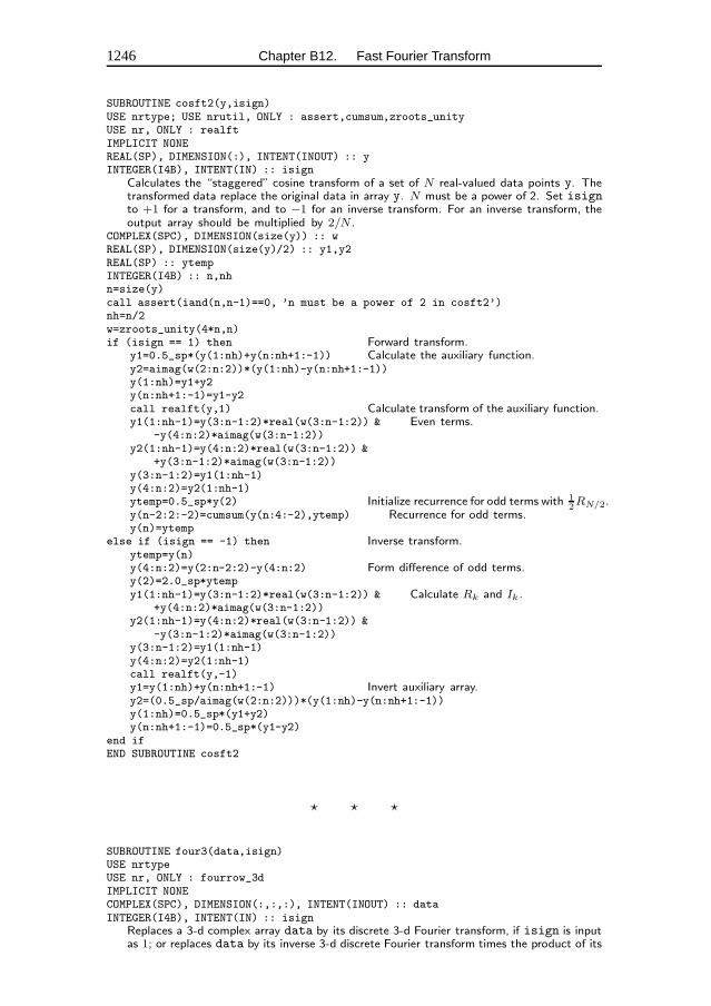
1246 Chapter B12. Fast Fourier Transform
SUBROUTINE cosft2(y,isign)USE nrtype; USE nrutil, ONLY : assert,cumsum,zroots_unityUSE nr, ONLY : realftIMPLICIT NONEREAL(SP), DIMENSION(:), INTENT(INOUT) :: yINTEGER(I4B), INTENT(IN) :: isign
Calculates the “staggered” cosine transform of a set of N real-valued data points y. Thetransformed data replace the original data in array y. N must be a power of 2. Set isignto +1 for a transform, and to −1 for an inverse transform. For an inverse transform, theoutput array should be multiplied by 2/N .
COMPLEX(SPC), DIMENSION(size(y)) :: wREAL(SP), DIMENSION(size(y)/2) :: y1,y2REAL(SP) :: ytempINTEGER(I4B) :: n,nhn=size(y)call assert(iand(n,n-1)==0, ’n must be a power of 2 in cosft2’)nh=n/2w=zroots_unity(4*n,n)if (isign == 1) then Forward transform.
y1=0.5_sp*(y(1:nh)+y(n:nh+1:-1)) Calculate the auxiliary function.y2=aimag(w(2:n:2))*(y(1:nh)-y(n:nh+1:-1))y(1:nh)=y1+y2y(n:nh+1:-1)=y1-y2call realft(y,1) Calculate transform of the auxiliary function.y1(1:nh-1)=y(3:n-1:2)*real(w(3:n-1:2)) & Even terms.
-y(4:n:2)*aimag(w(3:n-1:2))y2(1:nh-1)=y(4:n:2)*real(w(3:n-1:2)) &
+y(3:n-1:2)*aimag(w(3:n-1:2))y(3:n-1:2)=y1(1:nh-1)y(4:n:2)=y2(1:nh-1)ytemp=0.5_sp*y(2) Initialize recurrence for odd terms with 1
2RN/2.
y(n-2:2:-2)=cumsum(y(n:4:-2),ytemp) Recurrence for odd terms.y(n)=ytemp
else if (isign == -1) then Inverse transform.ytemp=y(n)y(4:n:2)=y(2:n-2:2)-y(4:n:2) Form difference of odd terms.y(2)=2.0_sp*ytempy1(1:nh-1)=y(3:n-1:2)*real(w(3:n-1:2)) & Calculate Rk and Ik .
+y(4:n:2)*aimag(w(3:n-1:2))y2(1:nh-1)=y(4:n:2)*real(w(3:n-1:2)) &
-y(3:n-1:2)*aimag(w(3:n-1:2))y(3:n-1:2)=y1(1:nh-1)y(4:n:2)=y2(1:nh-1)call realft(y,-1)y1=y(1:nh)+y(n:nh+1:-1) Invert auxiliary array.y2=(0.5_sp/aimag(w(2:n:2)))*(y(1:nh)-y(n:nh+1:-1))y(1:nh)=0.5_sp*(y1+y2)y(n:nh+1:-1)=0.5_sp*(y1-y2)
end ifEND SUBROUTINE cosft2
� � �
SUBROUTINE four3(data,isign)USE nrtypeUSE nr, ONLY : fourrow_3dIMPLICIT NONECOMPLEX(SPC), DIMENSION(:,:,:), INTENT(INOUT) :: dataINTEGER(I4B), INTENT(IN) :: isign
Replaces a 3-d complex array data by its discrete 3-d Fourier transform, if isign is inputas 1; or replaces data by its inverse 3-d discrete Fourier transform times the product of its
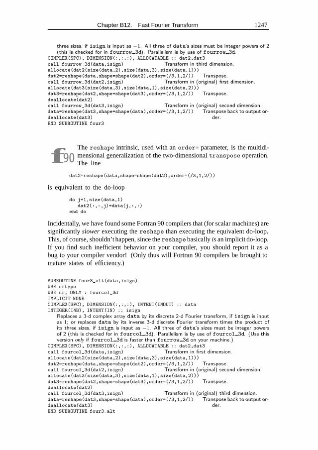
Chapter B12. Fast Fourier Transform 1247
three sizes, if isign is input as −1. All three of data’s sizes must be integer powers of 2(this is checked for in fourrow 3d). Parallelism is by use of fourrow 3d.
COMPLEX(SPC), DIMENSION(:,:,:), ALLOCATABLE :: dat2,dat3call fourrow_3d(data,isign) Transform in third dimension.allocate(dat2(size(data,2),size(data,3),size(data,1)))dat2=reshape(data,shape=shape(dat2),order=(/3,1,2/)) Transpose.call fourrow_3d(dat2,isign) Transform in (original) first dimension.allocate(dat3(size(data,3),size(data,1),size(data,2)))dat3=reshape(dat2,shape=shape(dat3),order=(/3,1,2/)) Transpose.deallocate(dat2)call fourrow_3d(dat3,isign) Transform in (original) second dimension.data=reshape(dat3,shape=shape(data),order=(/3,1,2/)) Transpose back to output or-
der.deallocate(dat3)END SUBROUTINE four3
f90The reshape intrinsic, used with anorder= parameter, is the multidi-mensional generalization of the two-dimensionaltranspose operation.The line
dat2=reshape(data,shape=shape(dat2),order=(/3,1,2/))
is equivalent to the do-loop
do j=1,size(data,1)dat2(:,:,j)=data(j,:,:)
end do
Incidentally, we have found some Fortran 90 compilers that (for scalar machines) aresignificantlyslower executing thereshape than executing the equivalent do-loop.This, of course, shouldn’t happen, since thereshape basicallyis an implicit do-loop.If you find such inefficient behavior on your compiler, you should report it as abug to your compiler vendor! (Only thus will Fortran 90 compilers be brought tomature states of efficiency.)
SUBROUTINE four3_alt(data,isign)USE nrtypeUSE nr, ONLY : fourcol_3dIMPLICIT NONECOMPLEX(SPC), DIMENSION(:,:,:), INTENT(INOUT) :: dataINTEGER(I4B), INTENT(IN) :: isign
Replaces a 3-d complex array data by its discrete 2-d Fourier transform, if isign is inputas 1; or replaces data by its inverse 3-d discrete Fourier transform times the product ofits three sizes, if isign is input as −1. All three of data’s sizes must be integer powersof 2 (this is checked for in fourcol 3d). Parallelism is by use of fourcol 3d. (Use thisversion only if fourcol 3d is faster than fourrow 3d on your machine.)
COMPLEX(SPC), DIMENSION(:,:,:), ALLOCATABLE :: dat2,dat3call fourcol_3d(data,isign) Transform in first dimension.allocate(dat2(size(data,2),size(data,3),size(data,1)))dat2=reshape(data,shape=shape(dat2),order=(/3,1,2/)) Transpose.call fourcol_3d(dat2,isign) Transform in (original) second dimension.allocate(dat3(size(data,3),size(data,1),size(data,2)))dat3=reshape(dat2,shape=shape(dat3),order=(/3,1,2/)) Transpose.deallocate(dat2)call fourcol_3d(dat3,isign) Transform in (original) third dimension.data=reshape(dat3,shape=shape(data),order=(/3,1,2/)) Transpose back to output or-
der.deallocate(dat3)END SUBROUTINE four3_alt
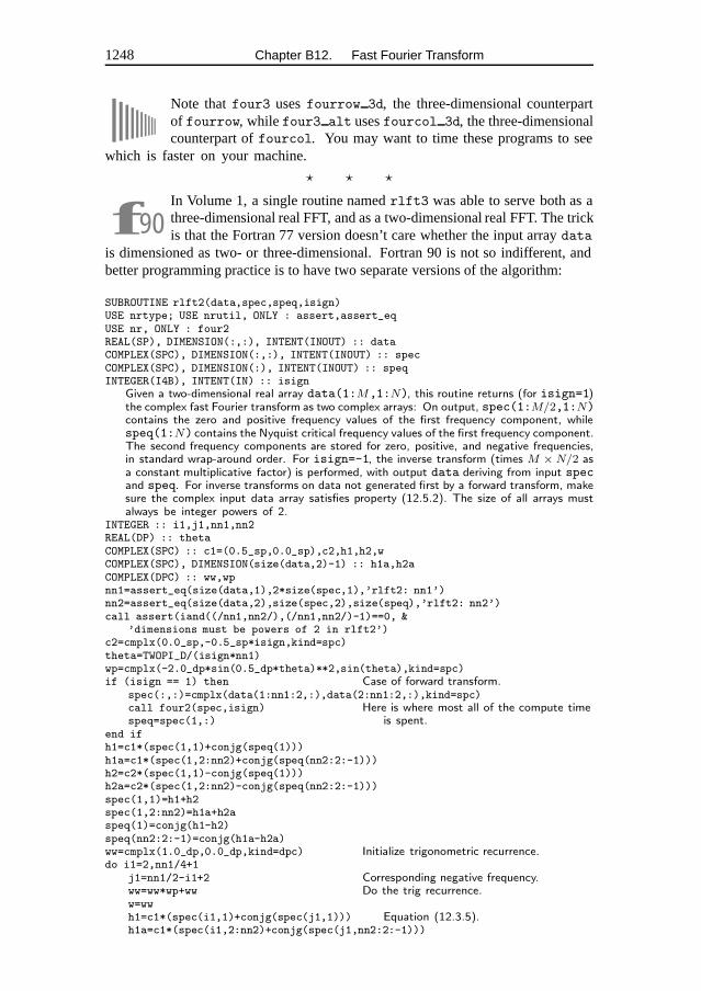
1248 Chapter B12. Fast Fourier Transform
Note thatfour3 usesfourrow 3d, the three-dimensional counterpartof fourrow, whilefour3 alt usesfourcol 3d, the three-dimensionalcounterpart offourcol. You may want to time these programs to see
which is faster on your machine.
� � �
f90In Volume 1, a single routine namedrlft3 was able to serve both as athree-dimensional real FFT, and as a two-dimensional real FFT. The trickis that the Fortran 77 version doesn’t care whether the input arraydata
is dimensioned as two- or three-dimensional. Fortran 90 is not so indifferent, andbetter programming practice is to have two separate versions of the algorithm:
SUBROUTINE rlft2(data,spec,speq,isign)USE nrtype; USE nrutil, ONLY : assert,assert_eqUSE nr, ONLY : four2REAL(SP), DIMENSION(:,:), INTENT(INOUT) :: dataCOMPLEX(SPC), DIMENSION(:,:), INTENT(INOUT) :: specCOMPLEX(SPC), DIMENSION(:), INTENT(INOUT) :: speqINTEGER(I4B), INTENT(IN) :: isign
Given a two-dimensional real array data(1:M,1:N), this routine returns (for isign=1)the complex fast Fourier transform as two complex arrays: On output, spec(1:M/2,1:N)contains the zero and positive frequency values of the first frequency component, whilespeq(1:N) contains the Nyquist critical frequency values of the first frequency component.The second frequency components are stored for zero, positive, and negative frequencies,in standard wrap-around order. For isign=-1, the inverse transform (times M × N/2 asa constant multiplicative factor) is performed, with output data deriving from input specand speq. For inverse transforms on data not generated first by a forward transform, makesure the complex input data array satisfies property (12.5.2). The size of all arrays mustalways be integer powers of 2.
INTEGER :: i1,j1,nn1,nn2REAL(DP) :: thetaCOMPLEX(SPC) :: c1=(0.5_sp,0.0_sp),c2,h1,h2,wCOMPLEX(SPC), DIMENSION(size(data,2)-1) :: h1a,h2aCOMPLEX(DPC) :: ww,wpnn1=assert_eq(size(data,1),2*size(spec,1),’rlft2: nn1’)nn2=assert_eq(size(data,2),size(spec,2),size(speq),’rlft2: nn2’)call assert(iand((/nn1,nn2/),(/nn1,nn2/)-1)==0, &
’dimensions must be powers of 2 in rlft2’)c2=cmplx(0.0_sp,-0.5_sp*isign,kind=spc)theta=TWOPI_D/(isign*nn1)wp=cmplx(-2.0_dp*sin(0.5_dp*theta)**2,sin(theta),kind=spc)if (isign == 1) then Case of forward transform.
spec(:,:)=cmplx(data(1:nn1:2,:),data(2:nn1:2,:),kind=spc)call four2(spec,isign) Here is where most all of the compute time
is spent.speq=spec(1,:)end ifh1=c1*(spec(1,1)+conjg(speq(1)))h1a=c1*(spec(1,2:nn2)+conjg(speq(nn2:2:-1)))h2=c2*(spec(1,1)-conjg(speq(1)))h2a=c2*(spec(1,2:nn2)-conjg(speq(nn2:2:-1)))spec(1,1)=h1+h2spec(1,2:nn2)=h1a+h2aspeq(1)=conjg(h1-h2)speq(nn2:2:-1)=conjg(h1a-h2a)ww=cmplx(1.0_dp,0.0_dp,kind=dpc) Initialize trigonometric recurrence.do i1=2,nn1/4+1
j1=nn1/2-i1+2 Corresponding negative frequency.ww=ww*wp+ww Do the trig recurrence.w=wwh1=c1*(spec(i1,1)+conjg(spec(j1,1))) Equation (12.3.5).h1a=c1*(spec(i1,2:nn2)+conjg(spec(j1,nn2:2:-1)))
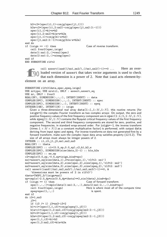
Chapter B12. Fast Fourier Transform 1249
h2=c2*(spec(i1,1)-conjg(spec(j1,1)))h2a=c2*(spec(i1,2:nn2)-conjg(spec(j1,nn2:2:-1)))spec(i1,1)=h1+w*h2spec(i1,2:nn2)=h1a+w*h2aspec(j1,1)=conjg(h1-w*h2)spec(j1,nn2:2:-1)=conjg(h1a-w*h2a)
end doif (isign == -1) then Case of reverse transform.
call four2(spec,isign)data(1:nn1:2,:)=real(spec)data(2:nn1:2,:)=aimag(spec)
end ifEND SUBROUTINE rlft2
f90call assert(iand((/nn1,nn2/),(/nn1,nn2/)-1)==0 ... Here an over-loaded version ofassert that takes vector arguments is used to checkthat each dimension is a power of 2. Note thatiand acts element-by-
element on an array.
SUBROUTINE rlft3(data,spec,speq,isign)USE nrtype; USE nrutil, ONLY : assert,assert_eqUSE nr, ONLY : four3REAL(SP), DIMENSION(:,:,:), INTENT(INOUT) :: dataCOMPLEX(SPC), DIMENSION(:,:,:), INTENT(INOUT) :: specCOMPLEX(SPC), DIMENSION(:,:), INTENT(INOUT) :: speqINTEGER(I4B), INTENT(IN) :: isign
Given a three-dimensional real array data(1:L,1:M,1:N), this routine returns (forisign=1) the complex Fourier transform as two complex arrays: On output, the zero andpositive frequency values of the first frequency component are in spec(1:L/2,1:M,1:N),while speq(1:M,1:N) contains the Nyquist critical frequency values of the first frequencycomponent. The second and third frequency components are stored for zero, positive, andnegative frequencies, in standard wrap-around order. For isign=-1, the inverse transform(times L × M × N/2 as a constant multiplicative factor) is performed, with output dataderiving from input spec and speq. For inverse transforms on data not generated first by aforward transform, make sure the complex input data array satisfies property (12.5.2). Thesize of all arrays must always be integer powers of 2.
INTEGER :: i1,i3,j1,j3,nn1,nn2,nn3REAL(DP) :: thetaCOMPLEX(SPC) :: c1=(0.5_sp,0.0_sp),c2,h1,h2,wCOMPLEX(SPC), DIMENSION(size(data,2)-1) :: h1a,h2aCOMPLEX(DPC) :: ww,wpc2=cmplx(0.0_sp,-0.5_sp*isign,kind=spc)nn1=assert_eq(size(data,1),2*size(spec,1),’rlft2: nn1’)nn2=assert_eq(size(data,2),size(spec,2),size(speq,1),’rlft2: nn2’)nn3=assert_eq(size(data,3),size(spec,3),size(speq,2),’rlft2: nn3’)call assert(iand((/nn1,nn2,nn3/),(/nn1,nn2,nn3/)-1)==0, &
’dimensions must be powers of 2 in rlft3’)theta=TWOPI_D/(isign*nn1)wp=cmplx(-2.0_dp*sin(0.5_dp*theta)**2,sin(theta),kind=dpc)if (isign == 1) then Case of forward transform.
spec(:,:,:)=cmplx(data(1:nn1:2,:,:),data(2:nn1:2,:,:),kind=spc)call four3(spec,isign) Here is where most all of the compute time
is spent.speq=spec(1,:,:)end ifdo i3=1,nn3
j3=1if (i3 /= 1) j3=nn3-i3+2h1=c1*(spec(1,1,i3)+conjg(speq(1,j3)))h1a=c1*(spec(1,2:nn2,i3)+conjg(speq(nn2:2:-1,j3)))h2=c2*(spec(1,1,i3)-conjg(speq(1,j3)))h2a=c2*(spec(1,2:nn2,i3)-conjg(speq(nn2:2:-1,j3)))spec(1,1,i3)=h1+h2spec(1,2:nn2,i3)=h1a+h2a
1250 Chapter B12. Fast Fourier Transform
speq(1,j3)=conjg(h1-h2)speq(nn2:2:-1,j3)=conjg(h1a-h2a)ww=cmplx(1.0_dp,0.0_dp,kind=dpc) Initialize trigonometric recurrence.do i1=2,nn1/4+1
j1=nn1/2-i1+2 Corresponding negative frequency.ww=ww*wp+ww Do the trig recurrence.w=wwh1=c1*(spec(i1,1,i3)+conjg(spec(j1,1,j3))) Equation (12.3.5).h1a=c1*(spec(i1,2:nn2,i3)+conjg(spec(j1,nn2:2:-1,j3)))h2=c2*(spec(i1,1,i3)-conjg(spec(j1,1,j3)))h2a=c2*(spec(i1,2:nn2,i3)-conjg(spec(j1,nn2:2:-1,j3)))spec(i1,1,i3)=h1+w*h2spec(i1,2:nn2,i3)=h1a+w*h2aspec(j1,1,j3)=conjg(h1-w*h2)spec(j1,nn2:2:-1,j3)=conjg(h1a-w*h2a)
end doend doif (isign == -1) then Case of reverse transform.
call four3(spec,isign)data(1:nn1:2,:,:)=real(spec)data(2:nn1:2,:,:)=aimag(spec)
end ifEND SUBROUTINE rlft3
� � �
Referring back to the discussion of parallelism,§22.4, that led tofour1’simplementation with
√N parallelism, you might wonder whether Fortran 90 provides
sufficiently powerful high-level constructs to enable an FFT routine withN -foldparallelism. The answer is, “It does, but you wouldn’t want to use them!” Access toarbitrary interprocessor communication in Fortran 90 is through the mechanism ofthe “vector subscript” (one-dimensional array of indices in arbitrary order). When avector subscript is on the right-hand side of an assignment statement, the operationperformed is effectively a “gather”; when it is on the left-hand side, the operationis effectively a “scatter.”
It is quite possible to write the classic FFT algorithm in terms of gather and scatteroperations. In fact, we do so now. The problem is efficiency: The computationsinvolved in constructing the vector subscripts for the scatter/gather operations,and theactual scatter/gather operations themselves, tend to swamp the underlying very leanFFT algorithm. The result is very slow, though theoretically perfectly parallelizable,code. Since small-scale parallel (SSP) machines can saturate their processors with√N parallelism, while massively multiprocessor (MMP) machines inevitably come
with architecture-optimized FFT library calls, there is really no niche for theseroutines, except as pedagogical demonstrations. We give here a one-dimensionalroutine, and also an arbitrary-dimensional routine modeled on Volume 1’sfourn.Note the complete absence of do-loops of sizeN ; the loops that remain are overlogN stages, or over the number of dimensions.
SUBROUTINE four1_gather(data,isign)USE nrtype; USE nrutil, ONLY : arth,assertIMPLICIT NONECOMPLEX(SPC), DIMENSION(:), INTENT(INOUT) :: dataINTEGER(I4B), INTENT(IN) :: isign
Replaces a complex array data by its discrete Fourier transform, if isign is input as 1;or replaces data by size(data) times its inverse discrete Fourier transform, if isign isinput as −1. The size of data must be an integer power of 2. This routine demonstratescoding the FFT algorithm in high-level Fortran 90 constructs. Generally the result is very
Chapter B12. Fast Fourier Transform 1251
much slower than library routines coded for specific architectures, and also significantly slowerthan the parallelization-by-rows method used in the routine four1.
INTEGER(I4B) :: n,n2,m,mmREAL(DP) :: thetaCOMPLEX(SPC) :: wpINTEGER(I4B), DIMENSION(size(data)) :: jarrINTEGER(I4B), DIMENSION(:), ALLOCATABLE :: jrevCOMPLEX(SPC), DIMENSION(:), ALLOCATABLE :: wtab,dtempn=size(data)call assert(iand(n,n-1)==0, ’n must be a power of 2 in four1_gather’)if (n <= 1) RETURNallocate(jrev(n)) Begin bit-reversal section of the routine.jarr=arth(0,1,n)jrev=0n2=n/2m=n2do Construct an array of pointers from an index
to its bit-reverse.where (iand(jarr,1) /= 0) jrev=jrev+mjarr=jarr/2m=m/2if (m == 0) exit
end dodata=data(jrev+1) Move all data to bit-reversed location by a
single gather/scatter.deallocate(jrev)allocate(dtemp(n),wtab(n2)) Begin Danielson-Lanczos section of the rou-
tine.jarr=arth(0,1,n)m=1mm=n2wtab(1)=(1.0_sp,0.0_sp) Seed the roots-of-unity table.do Outer loop executed log2 N times.
where (iand(jarr,m) /= 0)The basic idea is to address the correct root-of-unity for each Danielson-Lanczosmultiplication by tricky bit manipulations.
dtemp=data*wtab(mm*iand(jarr,m-1)+1)data=eoshift(data,-m)-dtemp This is half of Danielson-Lanczos.
elsewheredata=data+eoshift(dtemp,m) This is the other half. The referenced ele-
ments of dtemp will have been set in thewhere clause.
end wherem=m*2if (m >= n) exitmm=mm/2theta=PI_D/(isign*m) Ready for trigonometry?wp=cmplx(-2.0_dp*sin(0.5_dp*theta)**2, sin(theta),kind=spc)Add entries to the table for the next iteration.
wtab(mm+1:n2:2*mm)=wtab(1:n2-mm:2*mm)*wp+wtab(1:n2-mm:2*mm)end dodeallocate(dtemp,wtab)END SUBROUTINE four1_gather
SUBROUTINE fourn_gather(data,nn,isign)USE nrtype; USE nrutil, ONLY : arth,assertIMPLICIT NONECOMPLEX(SPC), DIMENSION(:), INTENT(INOUT) :: dataINTEGER(I4B), DIMENSION(:) :: nnINTEGER(I4B), INTENT(IN) :: isign
For data a one-dimensional complex array containing the values (in Fortran normal order-ing) of an M -dimensional complex arrray, this routine replaces data by its M -dimensionaldiscrete Fourier transform, if isign is input as 1. nn(1:M) is an integer array containingthe lengths of each dimension (number of complex values), each of which must be a powerof 2. If isign is input as −1, data is replaced by its inverse transform times the product ofthe lengths of all dimensions. This routine demonstrates coding the multidimensional FFTalgorithm in high-level Fortran 90 constructs. Generally the result is very much slower than
1252 Chapter B12. Fast Fourier Transform
library routines coded for specific architectures, and significantly slower than routines four2and four3 for the two- and three-dimensional cases.
INTEGER(I4B), DIMENSION(:), ALLOCATABLE :: jarrINTEGER(I4B) :: ndim,idim,ntot,nprev,n,n2,msk0,msk1,msk2,m,mm,mnREAL(DP) :: thetaCOMPLEX(SPC) :: wpCOMPLEX(SPC), DIMENSION(:), ALLOCATABLE :: wtab,dtempcall assert(iand(nn,nn-1)==0, &
’each dimension must be a power of 2 in fourn_gather’)ndim=size(nn)ntot=product(nn)nprev=1allocate(jarr(ntot))do idim=1,ndim Loop over the dimensions.
jarr=arth(0,1,ntot) We begin the bit-reversal section of theroutine.n=nn(idim)
n2=n/2msk0=nprevmsk1=nprev*n2msk2=msk0+msk1do Construct an array of pointers from an
index to its bit-reverse.if (msk1 <= msk0) exitwhere (iand(jarr,msk0) == 0 .neqv. iand(jarr,msk1) == 0) &
jarr=ieor(jarr,msk2)msk0=msk0*2msk1=msk1/2msk2=msk0+msk1
end dodata=data(jarr+1) Move all data to bit-reversed location by
a single gather/scatter.allocate(dtemp(ntot),wtab(n2))We begin the Danielson-Lanczos section of the routine.
jarr=iand(n-1,arth(0,1,ntot)/nprev)m=1mm=n2mn=m*nprevwtab(1)=(1.0_sp,0.0_sp) Seed the roots-of-unity table.do This loop executed log2 N times.
if (mm == 0) exitwhere (iand(jarr,m) /= 0)
The basic idea is to address the correct root-of-unity for each Danielson-Lanczosmultiplication by tricky bit manipulations.
dtemp=data*wtab(mm*iand(jarr,m-1)+1)data=eoshift(data,-mn)-dtemp This is half of Danielson-Lanczos.
elsewheredata=data+eoshift(dtemp,mn) This is the other half. The referenced el-
ements of dtemp will have been setin the where clause.
end wherem=m*2if (m >= n) exitmn=m*nprevmm=mm/2theta=PI_D/(isign*m) Ready for trigonometry?wp=cmplx(-2.0_dp*sin(0.5_dp*theta)**2,sin(theta),kind=dpc)Add entries to the table for the next iteration.
wtab(mm+1:n2:2*mm)=wtab(1:n2-mm:2*mm)*wp &+wtab(1:n2-mm:2*mm)
end dodeallocate(dtemp,wtab)nprev=n*nprev
end dodeallocate(jarr)END SUBROUTINE fourn_gather
f90call assert(iand(nn,nn-1)==0 ... Once again the vector version ofassert is used to test all the dimensions stored innn simultaneously.
Chapter B13. Fourier and SpectralApplications
FUNCTION convlv(data,respns,isign)USE nrtype; USE nrutil, ONLY : assert,nrerrorUSE nr, ONLY : realftIMPLICIT NONEREAL(SP), DIMENSION(:), INTENT(INOUT) :: dataREAL(SP), DIMENSION(:), INTENT(IN) :: respnsINTEGER(I4B), INTENT(IN) :: isignREAL(SP), DIMENSION(size(data)) :: convlv
Convolves or deconvolves a real data set data (of length N , including any user-suppliedzero padding) with a response function respns, stored in wrap-around order in a real arrayof length M ≤ N . (M should be an odd integer, N a power of 2.) Wrap-around ordermeans that the first half of the array respns contains the impulse response function atpositive times, while the second half of the array contains the impulse response function atnegative times, counting down from the highest element respns(M). On input isign is+1 for convolution, −1 for deconvolution. The answer is returned as the function convlv,an array of length N . data has INTENT(INOUT) for consistency with realft, but isactually unchanged.
INTEGER(I4B) :: no2,n,mCOMPLEX(SPC), DIMENSION(size(data)/2) :: tmpd,tmprn=size(data)m=size(respns)call assert(iand(n,n-1)==0, ’n must be a power of 2 in convlv’)call assert(mod(m,2)==1, ’m must be odd in convlv’)convlv(1:m)=respns(:) Put respns in array of length n.convlv(n-(m-3)/2:n)=convlv((m+3)/2:m)convlv((m+3)/2:n-(m-1)/2)=0.0 Pad with zeros.no2=n/2call realft(data,1,tmpd) FFT both arrays.call realft(convlv,1,tmpr)if (isign == 1) then Multiply FFTs to convolve.
tmpr(1)=cmplx(real(tmpd(1))*real(tmpr(1))/no2, &aimag(tmpd(1))*aimag(tmpr(1))/no2, kind=spc)
tmpr(2:)=tmpd(2:)*tmpr(2:)/no2else if (isign == -1) then Divide FFTs to deconvolve.
if (any(abs(tmpr(2:)) == 0.0) .or. real(tmpr(1)) == 0.0 &.or. aimag(tmpr(1)) == 0.0) call nrerror &(’deconvolving at response zero in convlv’)
tmpr(1)=cmplx(real(tmpd(1))/real(tmpr(1))/no2, &aimag(tmpd(1))/aimag(tmpr(1))/no2, kind=spc)
tmpr(2:)=tmpd(2:)/tmpr(2:)/no2else
call nrerror(’no meaning for isign in convlv’)end ifcall realft(convlv,-1,tmpr) Inverse transform back to time domain.END FUNCTION convlv
1253
1254 Chapter B13. Fourier and Spectral Applications
f90tmpr(1)=cmplx(...kind=spc) The intrinsic functioncmplx returns aquantity of type default complex unless thekind argument is present. Itis therefore a good idea always to include this argument. The intrinsic
functionsreal andaimag, on the other hand, when called with a complex argument,return the same kind as their argument. So it is a good ideanot to put in akind argment for these. (In fact,aimag doesn’t allow one.) Don’t confuse thesesituations, regarding complex variables, with the completely unrelated use ofreal
to convert a real or integer variable to a real value of specified kind. In this lattercase,kind should be specified.
� � �
FUNCTION correl(data1,data2)USE nrtype; USE nrutil, ONLY : assert,assert_eqUSE nr, ONLY : realftIMPLICIT NONEREAL(SP), DIMENSION(:), INTENT(INOUT) :: data1,data2REAL(SP), DIMENSION(size(data1)) :: correl
Computes the correlation of two real data sets data1 and data2 of length N (includ-ing any user-supplied zero padding). N must be an integer power of 2. The answer isreturned as the function correl, an array of length N . The answer is stored in wrap-around order, i.e., correlations at increasingly negative lags are in correl(N) on down tocorrel(N/2+ 1), while correlations at increasingly positive lags are in correl(1) (zerolag) on up to correl(N/2). Sign convention of this routine: if data1 lags data2, i.e.,is shifted to the right of it, then correl will show a peak at positive lags.
COMPLEX(SPC), DIMENSION(size(data1)/2) :: cdat1,cdat2INTEGER(I4B) :: no2,n Normalization for inverse FFT.n=assert_eq(size(data1),size(data2),’correl’)call assert(iand(n,n-1)==0, ’n must be a power of 2 in correl’)no2=n/2call realft(data1,1,cdat1) Transform both data vectors.call realft(data2,1,cdat2)cdat1(1)=cmplx(real(cdat1(1))*real(cdat2(1))/no2, & Multiply to find FFT of their
correlation.aimag(cdat1(1))*aimag(cdat2(1))/no2, kind=spc)cdat1(2:)=cdat1(2:)*conjg(cdat2(2:))/no2call realft(correl,-1,cdat1) Inverse transform gives correlation.END FUNCTION correl
f90cdat1(1)=cmplx(...kind=spc) See just above for why we use the explicitkind type parameterspc for cmplx, but omitsp for real.
� � �
SUBROUTINE spctrm(p,k,ovrlap,unit,n_window)USE nrtype; USE nrutil, ONLY : arth,nrerrorUSE nr, ONLY : four1IMPLICIT NONEREAL(SP), DIMENSION(:), INTENT(OUT) :: pINTEGER(I4B), INTENT(IN) :: kLOGICAL(LGT), INTENT(IN) :: ovrlap True for overlapping segments, false other-
wise.INTEGER(I4B), OPTIONAL, INTENT(IN) :: n_window,unitReads data from input unit 9, or if the optional argument unit is present, from that inputunit. The output is an array p of length M that contains the data’s power (mean squareamplitude) at frequency (j − 1)/2M cycles per grid point, for j = 1, 2, . . . ,M , based on(2*k+1)*M data points (if ovrlap is set .true.) or 4*k*M data points (if ovrlapis set .false.). The number of segments of the data is 2*k in both cases: The routinecalls four1 k times, each call with 2 partitions each of 2M real data points. If the optionalargument n window is present, the routine uses the Bartlett window, the square window,
Chapter B13. Fourier and Spectral Applications 1255
or the Welch window for n window= 1,2, 3 respectively. If n window is not present, theBartlett window is used.
INTEGER(I4B) :: j,joff,joffn,kk,m,m4,m43,m44,mm,iunit,nn_windowREAL(SP) :: den,facm,facp,sumwREAL(SP), DIMENSION(2*size(p)) :: wREAL(SP), DIMENSION(4*size(p)) :: w1REAL(SP), DIMENSION(size(p)) :: w2COMPLEX(SPC), DIMENSION(2*size(p)) :: cw1m=size(p)if (present(n_window)) then
nn_window=n_windowelse
nn_window=1end ifif (present(unit)) then
iunit=unitelse
iunit=9end ifmm=m+m Useful factors.m4=mm+mmm44=m4+4m43=m4+3den=0.0facm=m Factors used by the window function.facp=1.0_sp/mw1(1:mm)=window(arth(1,1,mm),facm,facp,nn_window)sumw=dot_product(w1(1:mm),w1(1:mm)) Accumulate the squared sum of the weights.p(:)=0.0 Initialize the spectrum to zero.if (ovrlap) read (iunit,*) (w2(j),j=1,m) Initialize the “save” half-buffer.do kk=1,k Loop over data segments in groups of two.
do joff=-1,0,1 Get two complete segments into workspace.if (ovrlap) then
w1(joff+2:joff+mm:2)=w2(1:m)read (iunit,*) (w2(j),j=1,m)joffn=joff+mmw1(joffn+2:joffn+mm:2)=w2(1:m)
elseread (iunit,*) (w1(j),j=joff+2,m4,2)
end ifend dow=window(arth(1,1,mm),facm,facp,nn_window) Apply the window to the data.w1(2:m4:2)=w1(2:m4:2)*ww1(1:m4:2)=w1(1:m4:2)*wcw1(1:mm)=cmplx(w1(1:m4:2),w1(2:m4:2),kind=spc)call four1(cw1(1:mm),1) Fourier transform the windowed data.w1(1:m4:2)=real(cw1(1:mm))w1(2:m4:2)=aimag(cw1(1:mm))p(1)=p(1)+w1(1)**2+w1(2)**2 Sum results into previous segments.p(2:m)=p(2:m)+w1(4:2*m:2)**2+w1(3:2*m-1:2)**2+&
w1(m44-4:m44-2*m:-2)**2+w1(m43-4:m43-2*m:-2)**2den=den+sumw
end dop(:)=p(:)/(m4*den) Normalize the output.CONTAINS
FUNCTION window(j,facm,facp,nn_window)IMPLICIT NONEINTEGER(I4B), DIMENSION(:), INTENT(IN) :: jINTEGER(I4B), INTENT(IN) :: nn_windowREAL(SP), INTENT(IN) :: facm,facpREAL(SP), DIMENSION(size(j)) :: windowselect case(nn_window)
case(1)
1256 Chapter B13. Fourier and Spectral Applications
window(j)=(1.0_sp-abs(((j-1)-facm)*facp)) Bartlett window.case(2)
window(j)=1.0 Square window.case(3)
window(j)=(1.0_sp-(((j-1)-facm)*facp)**2) Welch window.case default
call nrerror(’unimplemented window function in spctrm’)end selectEND FUNCTION windowEND SUBROUTINE spctrm
f90The Fortran 90 optional argument feature allows us to make unit 9the default output unit in this routine, but leave the user the option ofspecifying a different output unit by supplying an actual argument for
unit. We also use an optional argument to allow the user the option of overridingthe default selection of the Bartlett window function.
FUNCTION window(j,facm,facp,nn_window) In Fortran 77 we coded this as astatement function. Here the internal function is equivalent, but allows fullspecification of the interface and so is preferred.
� � �
SUBROUTINE memcof(data,xms,d)USE nrtype; USE nrutil, ONLY : nrerrorIMPLICIT NONEREAL(SP), INTENT(OUT) :: xmsREAL(SP), DIMENSION(:), INTENT(IN) :: dataREAL(SP), DIMENSION(:), INTENT(OUT) :: d
Given a real vector data of length N , this routine returns M linear prediction coefficientsin a vector d of length M , and returns the mean square discrepancy as xms.
INTEGER(I4B) :: k,m,nREAL(SP) :: denom,pneumREAL(SP), DIMENSION(size(data)) :: wk1,wk2,wktmpREAL(SP), DIMENSION(size(d)) :: wkmm=size(d)n=size(data)xms=dot_product(data,data)/nwk1(1:n-1)=data(1:n-1)wk2(1:n-1)=data(2:n)do k=1,m
pneum=dot_product(wk1(1:n-k),wk2(1:n-k))denom=dot_product(wk1(1:n-k),wk1(1:n-k))+ &
dot_product(wk2(1:n-k),wk2(1:n-k))d(k)=2.0_sp*pneum/denomxms=xms*(1.0_sp-d(k)**2)d(1:k-1)=wkm(1:k-1)-d(k)*wkm(k-1:1:-1)The algorithm is recursive, although it is implemented as an iteration. It builds up theanswer for larger and larger values of m until the desired value is reached. At this pointin the algorithm, one could return the vector d and scalar xms for a set of LP coefficientswith k (rather than m) terms.
if (k == m) RETURNwkm(1:k)=d(1:k)wktmp(2:n-k)=wk1(2:n-k)wk1(1:n-k-1)=wk1(1:n-k-1)-wkm(k)*wk2(1:n-k-1)wk2(1:n-k-1)=wk2(2:n-k)-wkm(k)*wktmp(2:n-k)
end docall nrerror(’never get here in memcof’)END SUBROUTINE memcof
� � �
Chapter B13. Fourier and Spectral Applications 1257
SUBROUTINE fixrts(d)USE nrtypeUSE nr, ONLY : zrootsIMPLICIT NONEREAL(SP), DIMENSION(:), INTENT(INOUT) :: d
Given the LP coefficients d, this routine finds all roots of the characteristic polynomial(13.6.14), reflects any roots that are outside the unit circle back inside, and then returnsa modified set of coefficients in d.
INTEGER(I4B) :: i,mLOGICAL(LGT) :: polishCOMPLEX(SPC), DIMENSION(size(d)+1) :: aCOMPLEX(SPC), DIMENSION(size(d)) :: rootsm=size(d)a(m+1)=cmplx(1.0_sp,kind=spc) Set up complex coefficients for polynomial
root finder.a(m:1:-1)=cmplx(-d(1:m),kind=spc)polish=.true.call zroots(a(1:m+1),roots,polish) Find all the roots.where (abs(roots) > 1.0) roots=1.0_sp/conjg(roots)Reflect all roots outside the unit circle back inside.
a(1)=-roots(1) Now reconstruct the polynomial coefficients,a(2:m+1)=cmplx(1.0_sp,kind=spc)do i=2,m by looping over the roots
a(2:i)=a(1:i-1)-roots(i)*a(2:i) and synthetically multiplying.a(1)=-roots(i)*a(1)
end dod(m:1:-1)=-real(a(1:m)) The polynomial coefficients are guaranteed
to be real, so we need only return thereal part as new LP coefficients.
END SUBROUTINE fixrts
f90a(m+1)=cmplx(1.0_sp,kind=spc) See afterconvlv on p. 1254 to reviewwhy we use the explicit kind type parameterspc for cmplx.
� � �
FUNCTION predic(data,d,nfut)USE nrtypeIMPLICIT NONEREAL(SP), DIMENSION(:), INTENT(IN) :: data,dINTEGER(I4B), INTENT(IN) :: nfutREAL(SP), DIMENSION(nfut) :: predic
Given an array data, and given the data’s LP coefficients d in an array of length M , thisroutine applies equation (13.6.11) to predict the next nfut data points, which it returns inan array as the function value predic. Note that the routine references only the last Mvalues of data, as initial values for the prediction.
INTEGER(I4B) :: j,ndata,mREAL(SP) :: discrp,smREAL(SP), DIMENSION(size(d)) :: regm=size(d)ndata=size(data)reg(1:m)=data(ndata:ndata+1-m:-1)do j=1,nfut
discrp=0.0This is where you would put in a known discrepancy if you were reconstructing a functionby linear predictive coding rather than extrapolating a function by linear prediction. Seetext.
sm=discrp+dot_product(d,reg)reg=eoshift(reg,-1,sm) [If you want to implement circular arrays, you can
avoid this shifting of coefficients!]predic(j)=smend doEND FUNCTION predic
� � �
1258 Chapter B13. Fourier and Spectral Applications
FUNCTION evlmem(fdt,d,xms)USE nrtype; USE nrutil, ONLY : polyIMPLICIT NONEREAL(SP), INTENT(IN) :: fdt,xmsREAL(SP), DIMENSION(:), INTENT(IN) :: dREAL(SP) :: evlmem
Given d and xms as returned by memcof, this function returns the power spectrum estimateP (f) as a function of fdt = f∆.
COMPLEX(SPC) :: z,zzREAL(DP) :: theta Trigonometric recurrences in double precision.theta=TWOPI_D*fdtz=cmplx(cos(theta),sin(theta),kind=spc)zz=1.0_sp-z*poly(z,d)evlmem=xms/abs(zz)**2 Equation (13.7.4).END FUNCTION evlmem
f90zz=...poly(z,d) Thepoly function innrutil returns the value of thepolynomial with coefficientsd(:) at z. Here a version that takes realcoefficients and a complex argument is actually invoked, but all the
different versions have been overloaded onto the same namepoly.
� � �
SUBROUTINE period(x,y,ofac,hifac,px,py,jmax,prob)USE nrtype; USE nrutil, ONLY : assert_eq,imaxlocUSE nr, ONLY : avevarIMPLICIT NONEINTEGER(I4B), INTENT(OUT) :: jmaxREAL(SP), INTENT(IN) :: ofac,hifacREAL(SP), INTENT(OUT) :: probREAL(SP), DIMENSION(:), INTENT(IN) :: x,yREAL(SP), DIMENSION(:), POINTER :: px,py
Input is a set of N data points with abscissas x (which need not be equally spaced) andordinates y, and a desired oversampling factor ofac (a typical value being 4 or larger).The routine returns pointers to internally allocated arrays px and py. px is filled withan increasing sequence of frequencies (not angular frequencies) up to hifac times the“average” Nyquist frequency, and py is filled with the values of the Lomb normalizedperiodogram at those frequencies. The length of these arrays is 0.5*ofac*hifac*N .The arrays x and y are not altered. The routine also returns jmax such that py(jmax) isthe maximum element in py, and prob, an estimate of the significance of that maximumagainst the hypothesis of random noise. A small value of prob indicates that a significantperiodic signal is present.
INTEGER(I4B) :: i,n,noutREAL(SP) :: ave,cwtau,effm,expy,pnow,sumc,sumcy,&
sums,sumsh,sumsy,swtau,var,wtau,xave,xdif,xmax,xminREAL(DP), DIMENSION(size(x)) :: tmp1,tmp2,wi,wpi,wpr,wrLOGICAL(LGT), SAVE :: init=.true.n=assert_eq(size(x),size(y),’period’)if (init) then
init=.false.nullify(px,py)
elseif (associated(px)) deallocate(px)if (associated(py)) deallocate(py)
end ifnout=0.5_sp*ofac*hifac*nallocate(px(nout),py(nout))call avevar(y(:),ave,var) Get mean and variance of the input data.xmax=maxval(x(:)) Go through data to get the range of abscis-
sas.xmin=minval(x(:))xdif=xmax-xmin
Chapter B13. Fourier and Spectral Applications 1259
xave=0.5_sp*(xmax+xmin)pnow=1.0_sp/(xdif*ofac) Starting frequency.tmp1(:)=TWOPI_D*((x(:)-xave)*pnow) Initialize values for the trigonometric recur-
rences at each data point. The recur-rences are done in double precision.
wpr(:)=-2.0_dp*sin(0.5_dp*tmp1)**2wpi(:)=sin(tmp1(:))wr(:)=cos(tmp1(:))wi(:)=wpi(:)do i=1,nout Main loop over the frequencies to be evalu-
ated.px(i)=pnowsumsh=dot_product(wi,wr) First, loop over the data to get τ and related
quantities.sumc=dot_product(wr(:)-wi(:),wr(:)+wi(:))wtau=0.5_sp*atan2(2.0_sp*sumsh,sumc)swtau=sin(wtau)cwtau=cos(wtau)tmp1(:)=wi(:)*cwtau-wr(:)*swtau Then, loop over the data again to get the
periodogram value.tmp2(:)=wr(:)*cwtau+wi(:)*swtausums=dot_product(tmp1,tmp1)sumc=dot_product(tmp2,tmp2)sumsy=dot_product(y(:)-ave,tmp1)sumcy=dot_product(y(:)-ave,tmp2)tmp1(:)=wr(:) Update the trigonometric recurrences.wr(:)=(wr(:)*wpr(:)-wi(:)*wpi(:))+wr(:)wi(:)=(wi(:)*wpr(:)+tmp1(:)*wpi(:))+wi(:)py(i)=0.5_sp*(sumcy**2/sumc+sumsy**2/sums)/varpnow=pnow+1.0_sp/(ofac*xdif) The next frequency.
end dojmax=imaxloc(py(1:nout))expy=exp(-py(jmax)) Evaluate statistical significance of the maxi-
mum.effm=2.0_sp*nout/ofacprob=effm*expyif (prob > 0.01_sp) prob=1.0_sp-(1.0_sp-expy)**effmEND SUBROUTINE period
f90This routine shows another example of how to return arrays whose size isnot known in advance (cf.zbrac in Chapter B9). The coding is explainedin the subsection on pointers in§21.5. The size of the output arrays,
nout in the code, is available assize(px).
jmax=imaxloc... See discussion ofimaxloc on p. 1017.
SUBROUTINE fasper(x,y,ofac,hifac,px,py,jmax,prob)USE nrtype; USE nrutil, ONLY : arth,assert_eq,imaxloc,nrerrorUSE nr, ONLY : avevar,realftIMPLICIT NONEREAL(SP), DIMENSION(:), INTENT(IN) :: x,yREAL(SP), INTENT(IN) :: ofac,hifacINTEGER(I4B), INTENT(OUT) :: jmaxREAL(SP), INTENT(OUT) :: probREAL(SP), DIMENSION(:), POINTER :: px,pyINTEGER(I4B), PARAMETER :: MACC=4
Input is a set of N data points with abscissas x (which need not be equally spaced) andordinates y, and a desired oversampling factor ofac (a typical value being 4 or larger).The routine returns pointers to internally allocated arrays px and py. px is filled withan increasing sequence of frequencies (not angular frequencies) up to hifac times the“average” Nyquist frequency, and py is filled with the values of the Lomb normalizedperiodogram at those frequencies. The length of these arrays is 0.5*ofac*hifac*N .The arrays x and y are not altered. The routine also returns jmax such that py(jmax) isthe maximum element in py, and prob, an estimate of the significance of that maximumagainst the hypothesis of random noise. A small value of prob indicates that a significant
1260 Chapter B13. Fourier and Spectral Applications
periodic signal is present.Parameter: MACC is the number of interpolation points per 1/4 cycle of highest frequency.
INTEGER(I4B) :: j,k,n,ndim,nfreq,nfreqt,noutREAL(SP) :: ave,ck,ckk,cterm,cwt,den,df,effm,expy,fac,fndim,hc2wt,&
hs2wt,hypo,sterm,swt,var,xdif,xmax,xminREAL(SP), DIMENSION(:), ALLOCATABLE :: wk1,wk2LOGICAL(LGT), SAVE :: init=.true.n=assert_eq(size(x),size(y),’fasper’)if (init) then
init=.false.nullify(px,py)
elseif (associated(px)) deallocate(px)if (associated(py)) deallocate(py)
end ifnfreqt=ofac*hifac*n*MACCnfreq=64do Size the FFT as next power of 2 above nfreqt.
if (nfreq >= nfreqt) exitnfreq=nfreq*2
end dondim=2*nfreqallocate(wk1(ndim),wk2(ndim))call avevar(y(1:n),ave,var) Compute the mean, variance, and range of the data.xmax=maxval(x(:))xmin=minval(x(:))xdif=xmax-xminwk1(1:ndim)=0.0 Zero the workspaces.wk2(1:ndim)=0.0fac=ndim/(xdif*ofac)fndim=ndimdo j=1,n Extirpolate the data into the workspaces.
ck=1.0_sp+mod((x(j)-xmin)*fac,fndim)ckk=1.0_sp+mod(2.0_sp*(ck-1.0_sp),fndim)call spreadval(y(j)-ave,wk1,ck,MACC)call spreadval(1.0_sp,wk2,ckk,MACC)
end docall realft(wk1(1:ndim),1) Take the fast Fourier transforms.call realft(wk2(1:ndim),1)df=1.0_sp/(xdif*ofac)nout=0.5_sp*ofac*hifac*nallocate(px(nout),py(nout))k=3do j=1,nout Compute the Lomb value for each frequency.
hypo=sqrt(wk2(k)**2+wk2(k+1)**2)hc2wt=0.5_sp*wk2(k)/hypohs2wt=0.5_sp*wk2(k+1)/hypocwt=sqrt(0.5_sp+hc2wt)swt=sign(sqrt(0.5_sp-hc2wt),hs2wt)den=0.5_sp*n+hc2wt*wk2(k)+hs2wt*wk2(k+1)cterm=(cwt*wk1(k)+swt*wk1(k+1))**2/densterm=(cwt*wk1(k+1)-swt*wk1(k))**2/(n-den)px(j)=j*dfpy(j)=(cterm+sterm)/(2.0_sp*var)k=k+2
end dodeallocate(wk1,wk2)jmax=imaxloc(py(1:nout))expy=exp(-py(jmax)) Estimate significance of largest peak value.effm=2.0_sp*nout/ofacprob=effm*expyif (prob > 0.01_sp) prob=1.0_sp-(1.0_sp-expy)**effmCONTAINS
Chapter B13. Fourier and Spectral Applications 1261
SUBROUTINE spreadval(y,yy,x,m)IMPLICIT NONEREAL(SP), INTENT(IN) :: y,xREAL(SP), DIMENSION(:), INTENT(INOUT) :: yyINTEGER(I4B), INTENT(IN) :: m
Given an array yy of length N , extirpolate (spread) a value y into m actual array elementsthat best approximate the “fictional” (i.e., possibly noninteger) array element number x.The weights used are coefficients of the Lagrange interpolating polynomial.
INTEGER(I4B) :: ihi,ilo,ix,j,nden,nREAL(SP) :: facINTEGER(I4B), DIMENSION(10) :: nfac = (/ &
1,1,2,6,24,120,720,5040,40320,362880 /)if (m > 10) call nrerror(’factorial table too small in spreadval’)n=size(yy)ix=xif (x == real(ix,sp)) then
yy(ix)=yy(ix)+yelse
ilo=min(max(int(x-0.5_sp*m+1.0_sp),1),n-m+1)ihi=ilo+m-1nden=nfac(m)fac=product(x-arth(ilo,1,m))yy(ihi)=yy(ihi)+y*fac/(nden*(x-ihi))do j=ihi-1,ilo,-1
nden=(nden/(j+1-ilo))*(j-ihi)yy(j)=yy(j)+y*fac/(nden*(x-j))
end doend ifEND SUBROUTINE spreadvalEND SUBROUTINE fasper
f90This routine shows another example of how to return arrays whose size isnot known in advance (cf.zbrac in Chapter B9). The coding is explainedin the subsection on pointers in§21.5. The size of the output arrays,
nout in the code, is available assize(px).
jmax=imaxloc... See discussion ofimaxloc on p. 1017.
if (x == real(ix,sp)) then Without the explicit kind type parametersp,real returns a value of type default real for an integer argument. This preventsautomatic conversion of the routine from single to double precision. Here all youhave to do is redefinesp in nrtype to get double precision.
� � �
SUBROUTINE dftcor(w,delta,a,b,endpts,corre,corim,corfac)USE nrtype; USE nrutil, ONLY : assertIMPLICIT NONEREAL(SP), INTENT(IN) :: w,delta,a,bREAL(SP), INTENT(OUT) :: corre,corim,corfacREAL(SP), DIMENSION(:), INTENT(IN) :: endpts
For an integral approximated by a discrete Fourier transform, this routine computes thecorrection factor that multiplies the DFT and the endpoint correction to be added. Inputis the angular frequency w, stepsize delta, lower and upper limits of the integral a andb, while the array endpts of length 8 contains the first 4 and last 4 function values. The
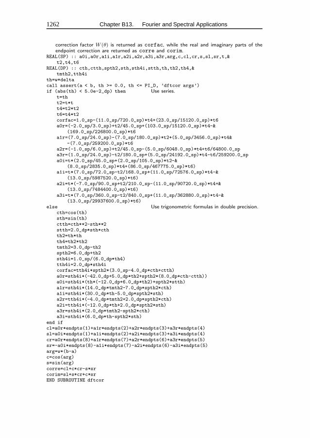
1262 Chapter B13. Fourier and Spectral Applications
correction factor W (θ) is returned as corfac, while the real and imaginary parts of theendpoint correction are returned as corre and corim.
REAL(SP) :: a0i,a0r,a1i,a1r,a2i,a2r,a3i,a3r,arg,c,cl,cr,s,sl,sr,t,&t2,t4,t6
REAL(DP) :: cth,ctth,spth2,sth,sth4i,stth,th,th2,th4,&tmth2,tth4i
th=w*deltacall assert(a < b, th >= 0.0, th <= PI_D, ’dftcor args’)if (abs(th) < 5.0e-2_dp) then Use series.
t=tht2=t*tt4=t2*t2t6=t4*t2corfac=1.0_sp-(11.0_sp/720.0_sp)*t4+(23.0_sp/15120.0_sp)*t6a0r=(-2.0_sp/3.0_sp)+t2/45.0_sp+(103.0_sp/15120.0_sp)*t4-&
(169.0_sp/226800.0_sp)*t6a1r=(7.0_sp/24.0_sp)-(7.0_sp/180.0_sp)*t2+(5.0_sp/3456.0_sp)*t4&
-(7.0_sp/259200.0_sp)*t6a2r=(-1.0_sp/6.0_sp)+t2/45.0_sp-(5.0_sp/6048.0_sp)*t4+t6/64800.0_spa3r=(1.0_sp/24.0_sp)-t2/180.0_sp+(5.0_sp/24192.0_sp)*t4-t6/259200.0_spa0i=t*(2.0_sp/45.0_sp+(2.0_sp/105.0_sp)*t2-&
(8.0_sp/2835.0_sp)*t4+(86.0_sp/467775.0_sp)*t6)a1i=t*(7.0_sp/72.0_sp-t2/168.0_sp+(11.0_sp/72576.0_sp)*t4-&
(13.0_sp/5987520.0_sp)*t6)a2i=t*(-7.0_sp/90.0_sp+t2/210.0_sp-(11.0_sp/90720.0_sp)*t4+&
(13.0_sp/7484400.0_sp)*t6)a3i=t*(7.0_sp/360.0_sp-t2/840.0_sp+(11.0_sp/362880.0_sp)*t4-&
(13.0_sp/29937600.0_sp)*t6)else Use trigonometric formulas in double precision.
cth=cos(th)sth=sin(th)ctth=cth**2-sth**2stth=2.0_dp*sth*cthth2=th*thth4=th2*th2tmth2=3.0_dp-th2spth2=6.0_dp+th2sth4i=1.0_sp/(6.0_dp*th4)tth4i=2.0_dp*sth4icorfac=tth4i*spth2*(3.0_sp-4.0_dp*cth+ctth)a0r=sth4i*(-42.0_dp+5.0_dp*th2+spth2*(8.0_dp*cth-ctth))a0i=sth4i*(th*(-12.0_dp+6.0_dp*th2)+spth2*stth)a1r=sth4i*(14.0_dp*tmth2-7.0_dp*spth2*cth)a1i=sth4i*(30.0_dp*th-5.0_dp*spth2*sth)a2r=tth4i*(-4.0_dp*tmth2+2.0_dp*spth2*cth)a2i=tth4i*(-12.0_dp*th+2.0_dp*spth2*sth)a3r=sth4i*(2.0_dp*tmth2-spth2*cth)a3i=sth4i*(6.0_dp*th-spth2*sth)
end ifcl=a0r*endpts(1)+a1r*endpts(2)+a2r*endpts(3)+a3r*endpts(4)sl=a0i*endpts(1)+a1i*endpts(2)+a2i*endpts(3)+a3i*endpts(4)cr=a0r*endpts(8)+a1r*endpts(7)+a2r*endpts(6)+a3r*endpts(5)sr=-a0i*endpts(8)-a1i*endpts(7)-a2i*endpts(6)-a3i*endpts(5)arg=w*(b-a)c=cos(arg)s=sin(arg)corre=cl+c*cr-s*srcorim=sl+s*cr+c*srEND SUBROUTINE dftcor
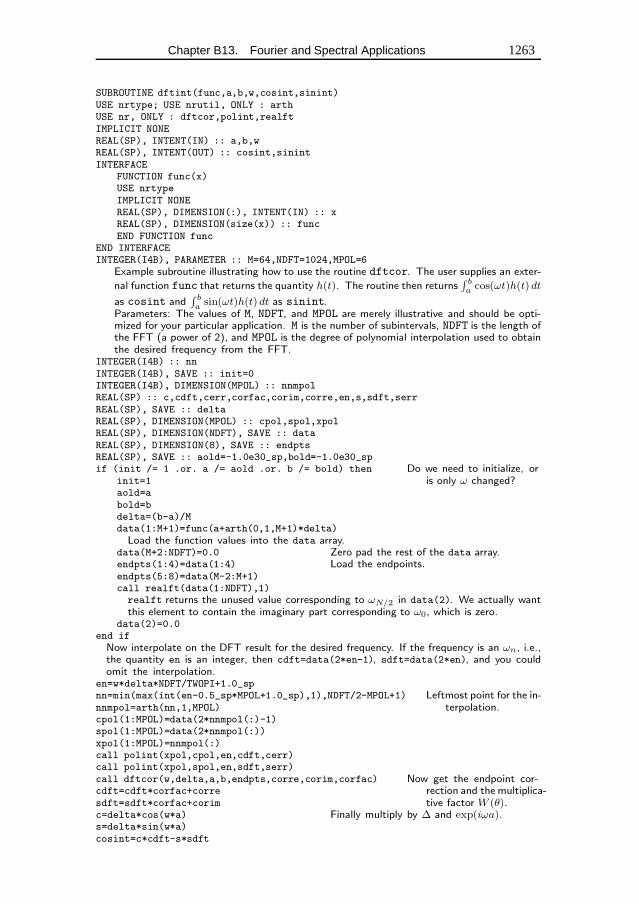
Chapter B13. Fourier and Spectral Applications 1263
SUBROUTINE dftint(func,a,b,w,cosint,sinint)USE nrtype; USE nrutil, ONLY : arthUSE nr, ONLY : dftcor,polint,realftIMPLICIT NONEREAL(SP), INTENT(IN) :: a,b,wREAL(SP), INTENT(OUT) :: cosint,sinintINTERFACE
FUNCTION func(x)USE nrtypeIMPLICIT NONEREAL(SP), DIMENSION(:), INTENT(IN) :: xREAL(SP), DIMENSION(size(x)) :: funcEND FUNCTION func
END INTERFACEINTEGER(I4B), PARAMETER :: M=64,NDFT=1024,MPOL=6
Example subroutine illustrating how to use the routine dftcor. The user supplies an exter-
nal function func that returns the quantity h(t). The routine then returns∫ ba cos(ωt)h(t)dt
as cosint and∫ ba
sin(ωt)h(t)dt as sinint.Parameters: The values of M, NDFT, and MPOL are merely illustrative and should be opti-mized for your particular application. M is the number of subintervals, NDFT is the length ofthe FFT (a power of 2), and MPOL is the degree of polynomial interpolation used to obtainthe desired frequency from the FFT.
INTEGER(I4B) :: nnINTEGER(I4B), SAVE :: init=0INTEGER(I4B), DIMENSION(MPOL) :: nnmpolREAL(SP) :: c,cdft,cerr,corfac,corim,corre,en,s,sdft,serrREAL(SP), SAVE :: deltaREAL(SP), DIMENSION(MPOL) :: cpol,spol,xpolREAL(SP), DIMENSION(NDFT), SAVE :: dataREAL(SP), DIMENSION(8), SAVE :: endptsREAL(SP), SAVE :: aold=-1.0e30_sp,bold=-1.0e30_spif (init /= 1 .or. a /= aold .or. b /= bold) then Do we need to initialize, or
is only ω changed?init=1aold=abold=bdelta=(b-a)/Mdata(1:M+1)=func(a+arth(0,1,M+1)*delta)Load the function values into the data array.
data(M+2:NDFT)=0.0 Zero pad the rest of the data array.endpts(1:4)=data(1:4) Load the endpoints.endpts(5:8)=data(M-2:M+1)call realft(data(1:NDFT),1)realft returns the unused value corresponding to ωN/2 in data(2). We actually wantthis element to contain the imaginary part corresponding to ω0, which is zero.
data(2)=0.0end ifNow interpolate on the DFT result for the desired frequency. If the frequency is an ωn, i.e.,the quantity en is an integer, then cdft=data(2*en-1), sdft=data(2*en), and you couldomit the interpolation.
en=w*delta*NDFT/TWOPI+1.0_spnn=min(max(int(en-0.5_sp*MPOL+1.0_sp),1),NDFT/2-MPOL+1) Leftmost point for the in-
terpolation.nnmpol=arth(nn,1,MPOL)cpol(1:MPOL)=data(2*nnmpol(:)-1)spol(1:MPOL)=data(2*nnmpol(:))xpol(1:MPOL)=nnmpol(:)call polint(xpol,cpol,en,cdft,cerr)call polint(xpol,spol,en,sdft,serr)call dftcor(w,delta,a,b,endpts,corre,corim,corfac) Now get the endpoint cor-
rection and the multiplica-tive factor W (θ).
cdft=cdft*corfac+corresdft=sdft*corfac+corimc=delta*cos(w*a) Finally multiply by ∆ and exp(iωa).s=delta*sin(w*a)cosint=c*cdft-s*sdft
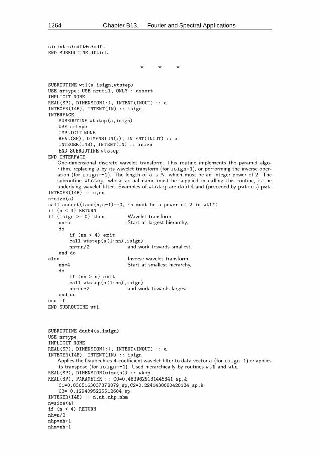
1264 Chapter B13. Fourier and Spectral Applications
sinint=s*cdft+c*sdftEND SUBROUTINE dftint
� � �
SUBROUTINE wt1(a,isign,wtstep)USE nrtype; USE nrutil, ONLY : assertIMPLICIT NONEREAL(SP), DIMENSION(:), INTENT(INOUT) :: aINTEGER(I4B), INTENT(IN) :: isignINTERFACE
SUBROUTINE wtstep(a,isign)USE nrtypeIMPLICIT NONEREAL(SP), DIMENSION(:), INTENT(INOUT) :: aINTEGER(I4B), INTENT(IN) :: isignEND SUBROUTINE wtstep
END INTERFACEOne-dimensional discrete wavelet transform. This routine implements the pyramid algo-rithm, replacing a by its wavelet transform (for isign=1), or performing the inverse oper-ation (for isign=-1). The length of a is N , which must be an integer power of 2. Thesubroutine wtstep, whose actual name must be supplied in calling this routine, is theunderlying wavelet filter. Examples of wtstep are daub4 and (preceded by pwtset) pwt.
INTEGER(I4B) :: n,nnn=size(a)call assert(iand(n,n-1)==0, ’n must be a power of 2 in wt1’)if (n < 4) RETURNif (isign >= 0) then Wavelet transform.
nn=n Start at largest hierarchy,do
if (nn < 4) exitcall wtstep(a(1:nn),isign)nn=nn/2 and work towards smallest.
end doelse Inverse wavelet transform.
nn=4 Start at smallest hierarchy,do
if (nn > n) exitcall wtstep(a(1:nn),isign)nn=nn*2 and work towards largest.
end doend ifEND SUBROUTINE wt1
SUBROUTINE daub4(a,isign)USE nrtypeIMPLICIT NONEREAL(SP), DIMENSION(:), INTENT(INOUT) :: aINTEGER(I4B), INTENT(IN) :: isign
Applies the Daubechies 4-coefficient wavelet filter to data vector a (for isign=1) or appliesits transpose (for isign=-1). Used hierarchically by routines wt1 and wtn.
REAL(SP), DIMENSION(size(a)) :: wkspREAL(SP), PARAMETER :: C0=0.4829629131445341_sp,&
C1=0.8365163037378079_sp,C2=0.2241438680420134_sp,&C3=-0.1294095225512604_sp
INTEGER(I4B) :: n,nh,nhp,nhmn=size(a)if (n < 4) RETURNnh=n/2nhp=nh+1nhm=nh-1
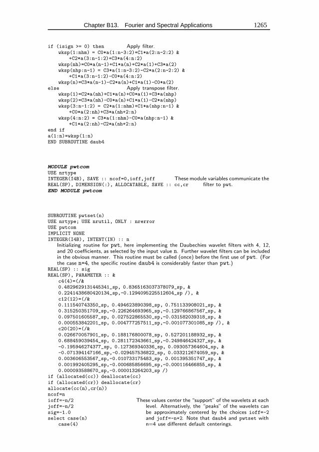
Chapter B13. Fourier and Spectral Applications 1265
if (isign >= 0) then Apply filter.wksp(1:nhm) = C0*a(1:n-3:2)+C1*a(2:n-2:2) &
+C2*a(3:n-1:2)+C3*a(4:n:2)wksp(nh)=C0*a(n-1)+C1*a(n)+C2*a(1)+C3*a(2)wksp(nhp:n-1) = C3*a(1:n-3:2)-C2*a(2:n-2:2) &
+C1*a(3:n-1:2)-C0*a(4:n:2)wksp(n)=C3*a(n-1)-C2*a(n)+C1*a(1)-C0*a(2)
else Apply transpose filter.wksp(1)=C2*a(nh)+C1*a(n)+C0*a(1)+C3*a(nhp)wksp(2)=C3*a(nh)-C0*a(n)+C1*a(1)-C2*a(nhp)wksp(3:n-1:2) = C2*a(1:nhm)+C1*a(nhp:n-1) &
+C0*a(2:nh)+C3*a(nh+2:n)wksp(4:n:2) = C3*a(1:nhm)-C0*a(nhp:n-1) &
+C1*a(2:nh)-C2*a(nh+2:n)end ifa(1:n)=wksp(1:n)END SUBROUTINE daub4
MODULE pwtcomUSE nrtypeINTEGER(I4B), SAVE :: ncof=0,ioff,joff These module variables communicate the
filter to pwt.REAL(SP), DIMENSION(:), ALLOCATABLE, SAVE :: cc,crEND MODULE pwtcom
SUBROUTINE pwtset(n)USE nrtype; USE nrutil, ONLY : nrerrorUSE pwtcomIMPLICIT NONEINTEGER(I4B), INTENT(IN) :: n
Initializing routine for pwt, here implementing the Daubechies wavelet filters with 4, 12,and 20 coefficients, as selected by the input value n. Further wavelet filters can be includedin the obvious manner. This routine must be called (once) before the first use of pwt. (Forthe case n=4, the specific routine daub4 is considerably faster than pwt.)
REAL(SP) :: sigREAL(SP), PARAMETER :: &
c4(4)=(/&0.4829629131445341_sp, 0.8365163037378079_sp, &0.2241438680420134_sp,-0.1294095225512604_sp /), &c12(12)=(/&0.111540743350_sp, 0.494623890398_sp, 0.751133908021_sp, &0.315250351709_sp,-0.226264693965_sp,-0.129766867567_sp, &0.097501605587_sp, 0.027522865530_sp,-0.031582039318_sp, &0.000553842201_sp, 0.004777257511_sp,-0.001077301085_sp /), &c20(20)=(/&0.026670057901_sp, 0.188176800078_sp, 0.527201188932_sp, &0.688459039454_sp, 0.281172343661_sp,-0.249846424327_sp, &-0.195946274377_sp, 0.127369340336_sp, 0.093057364604_sp, &-0.071394147166_sp,-0.029457536822_sp, 0.033212674059_sp, &0.003606553567_sp,-0.010733175483_sp, 0.001395351747_sp, &0.001992405295_sp,-0.000685856695_sp,-0.000116466855_sp, &0.000093588670_sp,-0.000013264203_sp /)
if (allocated(cc)) deallocate(cc)if (allocated(cr)) deallocate(cr)allocate(cc(n),cr(n))ncof=nioff=-n/2 These values center the “support” of the wavelets at each
level. Alternatively, the “peaks” of the wavelets canbe approximately centered by the choices ioff=-2and joff=-n+2. Note that daub4 and pwtset withn=4 use different default centerings.
joff=-n/2sig=-1.0select case(n)
case(4)
1266 Chapter B13. Fourier and Spectral Applications
cc=c4case(12)
cc=c12case(20)
cc=c20case default
call nrerror(’unimplemented value n in pwtset’)end selectcr(n:1:-1) = cccr(n:1:-2) = -cr(n:1:-2)END SUBROUTINE pwtset
f90Here we need to have as global variables arrays whose dimensions areknown only at run time. At first sight the situation is the same as with themodulefminln in newt on p. 1197. If you review the discussion there
and in§21.5, you will recall that there are two good ways to implement this: withallocatable arrays (“Method 1”) or with pointers (“Method 2”). There is a differencehere that makes allocatable arrays simpler. We do not wish to deallocate the arrayson exitingpwtset. On the contrary, the values incc andcr need to be preservedfor use inpwt. Since allocatable arrays are born in the well-defined state of “notcurrently allocated,” we can declare the arrays here as
REAL(SP), DIMENSION(:), ALLOCATABLE, SAVE :: cc,cr
and test whether they were used on a previous call with
if (allocated(cc)) deallocate(cc)if (allocated(cr)) deallocate(cr)
We are then ready to allocate the new storage:
allocate(cc(n),cr(n))
With pointers, we would need the additional machinery of nullifying the pointers onthe initial call, since pointers are born in an undefined state (see§21.5).
There is an additional important point in this example. The module variablesneed to be used by a “sibling” routine,pwt. We need to be sure that they donot become undefined when we exitpwtset. We could ensure this by putting aUSE pwtcom in the main program that calls bothpwtset andpwt, but it’s easy toforget to do this. It is preferable to put explicitSAVEs on all the module variables.
SUBROUTINE pwt(a,isign)USE nrtype; USE nrutil, ONLY : arth,nrerrorUSE pwtcomIMPLICIT NONEREAL(SP), DIMENSION(:), INTENT(INOUT) :: aINTEGER(I4B), INTENT(IN) :: isign
Partial wavelet transform: applies an arbitrary wavelet filter to data vector a (for isign=1)or applies its transpose (for isign=-1). Used hierarchically by routines wt1 and wtn. Theactual filter is determined by a preceding (and required) call to pwtset, which initializesthe module pwtcom.
REAL(SP), DIMENSION(size(a)) :: wkspINTEGER(I4B), DIMENSION(size(a)/2) :: jf,jrINTEGER(I4B) :: k,n,nh,nmodn=size(a)if (n < 4) RETURNif (ncof == 0) call nrerror(’pwt: must call pwtset before pwt’)nmod=ncof*n A positive constant equal to zero mod n.
Chapter B13. Fourier and Spectral Applications 1267
nh=n/2wksp(:)=0.0jf=iand(n-1,arth(2+nmod+ioff,2,nh)) Use bitwise AND to wrap-around the point-
ers. n-1 is a mask of all bits, since n isa power of 2.
jr=iand(n-1,arth(2+nmod+joff,2,nh))do k=1,ncof
if (isign >= 0) then Apply filter.wksp(1:nh)=wksp(1:nh)+cc(k)*a(jf+1)wksp(nh+1:n)=wksp(nh+1:n)+cr(k)*a(jr+1)
else Apply transpose filter.wksp(jf+1)=wksp(jf+1)+cc(k)*a(1:nh)wksp(jr+1)=wksp(jr+1)+cr(k)*a(nh+1:n)
end ifif (k == ncof) exitjf=iand(n-1,jf+1)jr=iand(n-1,jr+1)
end doa(:)=wksp(:) Copy the results back from workspace.END SUBROUTINE pwt
� � �
SUBROUTINE wtn(a,nn,isign,wtstep)USE nrtype; USE nrutil, ONLY : arth,assertIMPLICIT NONEREAL(SP), DIMENSION(:), INTENT(INOUT) :: aINTEGER(I4B), DIMENSION(:), INTENT(IN) :: nnINTEGER(I4B), INTENT(IN) :: isignINTERFACE
SUBROUTINE wtstep(a,isign)USE nrtypeIMPLICIT NONEREAL(SP), DIMENSION(:), INTENT(INOUT) :: aINTEGER(I4B), INTENT(IN) :: isignEND SUBROUTINE wtstep
END INTERFACEReplaces a by its N -dimensional discrete wavelet transform, if isign is input as 1. nn is aninteger array of length N , containing the lengths of each dimension (number of real values),which must all be powers of 2. a is a real array of length equal to the product of theselengths, in which the data are stored as in a multidimensional real FORTRAN array. If isignis input as −1, a is replaced by its inverse wavelet transform. The subroutine wtstep,whose actual name must be supplied in calling this routine, is the underlying wavelet filter.Examples of wtstep are daub4 and (preceded by pwtset) pwt.
INTEGER(I4B) :: i1,i2,i3,idim,n,ndim,nnew,nprev,nt,ntotREAL(SP), DIMENSION(:), ALLOCATABLE :: wkspcall assert(iand(nn,nn-1)==0, ’each dimension must be a power of 2 in wtn’)allocate(wksp(maxval(nn)))ndim=size(nn)ntot=product(nn(:))nprev=1do idim=1,ndim Main loop over the dimensions.
n=nn(idim)nnew=n*nprevif (n > 4) then
do i2=0,ntot-1,nnewdo i1=1,nprev
i3=i1+i2wksp(1:n)=a(arth(i3,nprev,n)) Copy the relevant row or column
or etc. into workspace.i3=i3+n*nprevif (isign >= 0) then Do one-dimensional wavelet trans-
form.nt=ndo
1268 Chapter B13. Fourier and Spectral Applications
if (nt < 4) exitcall wtstep(wksp(1:nt),isign)nt=nt/2
end doelse Or inverse transform.
nt=4do
if (nt > n) exitcall wtstep(wksp(1:nt),isign)nt=nt*2
end doend ifi3=i1+i2a(arth(i3,nprev,n))=wksp(1:n) Copy back from workspace.i3=i3+n*nprev
end doend do
end ifnprev=nnew
end dodeallocate(wksp)END SUBROUTINE wtn
Chapter B14. StatisticalDescription of Data
SUBROUTINE moment(data,ave,adev,sdev,var,skew,curt)USE nrtype; USE nrutil, ONLY : nrerrorIMPLICIT NONEREAL(SP), INTENT(OUT) :: ave,adev,sdev,var,skew,curtREAL(SP), DIMENSION(:), INTENT(IN) :: data
Given an array of data, this routine returns its mean ave, average deviation adev, standarddeviation sdev, variance var, skewness skew, and kurtosis curt.
INTEGER(I4B) :: nREAL(SP) :: epREAL(SP), DIMENSION(size(data)) :: p,sn=size(data)if (n <= 1) call nrerror(’moment: n must be at least 2’)ave=sum(data(:))/n First pass to get the mean.s(:)=data(:)-ave Second pass to get the first (absolute), second, third, and
fourth moments of the deviation from the mean.ep=sum(s(:))adev=sum(abs(s(:)))/np(:)=s(:)*s(:)var=sum(p(:))p(:)=p(:)*s(:)skew=sum(p(:))p(:)=p(:)*s(:)curt=sum(p(:))var=(var-ep**2/n)/(n-1) Corrected two-pass formula.sdev=sqrt(var)if (var /= 0.0) then
skew=skew/(n*sdev**3)curt=curt/(n*var**2)-3.0_sp
elsecall nrerror(’moment: no skew or kurtosis when zero variance’)
end ifEND SUBROUTINE moment
� � �
SUBROUTINE ttest(data1,data2,t,prob)USE nrtypeUSE nr, ONLY : avevar,betaiIMPLICIT NONEREAL(SP), DIMENSION(:), INTENT(IN) :: data1,data2REAL(SP), INTENT(OUT) :: t,prob
Given the arrays data1 and data2, which need not have the same length, this routinereturns Student’s t as t, and its significance as prob, small values of prob indicating that
1269
1270 Chapter B14. Statistical Description of Data
the arrays have significantly different means. The data arrays are assumed to be drawnfrom populations with the same true variance.
INTEGER(I4B) :: n1,n2REAL(SP) :: ave1,ave2,df,var,var1,var2n1=size(data1)n2=size(data2)call avevar(data1,ave1,var1)call avevar(data2,ave2,var2)df=n1+n2-2 Degrees of freedom.var=((n1-1)*var1+(n2-1)*var2)/df Pooled variance.t=(ave1-ave2)/sqrt(var*(1.0_sp/n1+1.0_sp/n2))prob=betai(0.5_sp*df,0.5_sp,df/(df+t**2)) See equation (6.4.9).END SUBROUTINE ttest
� � �
SUBROUTINE avevar(data,ave,var)USE nrtypeIMPLICIT NONEREAL(SP), DIMENSION(:), INTENT(IN) :: dataREAL(SP), INTENT(OUT) :: ave,var
Given array data, returns its mean as ave and its variance as var.INTEGER(I4B) :: nREAL(SP), DIMENSION(size(data)) :: sn=size(data)ave=sum(data(:))/ns(:)=data(:)-avevar=dot_product(s,s)var=(var-sum(s)**2/n)/(n-1) Corrected two-pass formula (14.1.8).END SUBROUTINE avevar
� � �
SUBROUTINE tutest(data1,data2,t,prob)USE nrtypeUSE nr, ONLY : avevar,betaiIMPLICIT NONEREAL(SP), DIMENSION(:), INTENT(IN) :: data1,data2REAL(SP), INTENT(OUT) :: t,prob
Given the arrays data1 and data2, which need not have the same length, this routinereturns Student’s t as t, and its significance as prob, small values of prob indicating thatthe arrays have significantly different means. The data arrays are allowed to be drawn frompopulations with unequal variances.
INTEGER(I4B) :: n1,n2REAL(SP) :: ave1,ave2,df,var1,var2n1=size(data1)n2=size(data2)call avevar(data1,ave1,var1)call avevar(data2,ave2,var2)t=(ave1-ave2)/sqrt(var1/n1+var2/n2)df=(var1/n1+var2/n2)**2/((var1/n1)**2/(n1-1)+(var2/n2)**2/(n2-1))prob=betai(0.5_sp*df,0.5_sp,df/(df+t**2))END SUBROUTINE tutest
� � �
Chapter B14. Statistical Description of Data 1271
SUBROUTINE tptest(data1,data2,t,prob)USE nrtype; USE nrutil, ONLY : assert_eqUSE nr, ONLY : avevar,betaiIMPLICIT NONEREAL(SP), DIMENSION(:), INTENT(IN) :: data1,data2REAL(SP), INTENT(OUT) :: t,prob
Given the paired arrays data1 and data2 of the same length, this routine returns Student’st for paired data as t, and its significance as prob, small values of prob indicating asignificant difference of means.
INTEGER(I4B) :: nREAL(SP) :: ave1,ave2,cov,df,sd,var1,var2n=assert_eq(size(data1),size(data2),’tptest’)call avevar(data1,ave1,var1)call avevar(data2,ave2,var2)cov=dot_product(data1(:)-ave1,data2(:)-ave2)df=n-1cov=cov/dfsd=sqrt((var1+var2-2.0_sp*cov)/n)t=(ave1-ave2)/sdprob=betai(0.5_sp*df,0.5_sp,df/(df+t**2))END SUBROUTINE tptest
� � �
SUBROUTINE ftest(data1,data2,f,prob)USE nrtypeUSE nr, ONLY : avevar,betaiIMPLICIT NONEREAL(SP), INTENT(OUT) :: f,probREAL(SP), DIMENSION(:), INTENT(IN) :: data1,data2
Given the arrays data1 and data2, which need not have the same length, this routinereturns the value of f, and its significance as prob. Small values of prob indicate that thetwo arrays have significantly different variances.
INTEGER(I4B) :: n1,n2REAL(SP) :: ave1,ave2,df1,df2,var1,var2n1=size(data1)n2=size(data2)call avevar(data1,ave1,var1)call avevar(data2,ave2,var2)if (var1 > var2) then Make F the ratio of the larger variance to the smaller one.
f=var1/var2df1=n1-1df2=n2-1
elsef=var2/var1df1=n2-1df2=n1-1
end ifprob=2.0_sp*betai(0.5_sp*df2,0.5_sp*df1,df2/(df2+df1*f))if (prob > 1.0) prob=2.0_sp-probEND SUBROUTINE ftest
� � �
1272 Chapter B14. Statistical Description of Data
SUBROUTINE chsone(bins,ebins,knstrn,df,chsq,prob)USE nrtype; USE nrutil, ONLY : assert_eq,nrerrorUSE nr, ONLY : gammqIMPLICIT NONEINTEGER(I4B), INTENT(IN) :: knstrnREAL(SP), INTENT(OUT) :: df,chsq,probREAL(SP), DIMENSION(:), INTENT(IN) :: bins,ebins
Given the same-size arrays bins containing the observed numbers of events, and ebinscontaining the expected numbers of events, and given the number of constraints knstrn(normally one), this routine returns (trivially) the number of degrees of freedom df, and(nontrivially) the chi-square chsq and the significance prob. A small value of prob indi-cates a significant difference between the distributions bins and ebins. Note that binsand ebins are both real arrays, although bins will normally contain integer values.
INTEGER(I4B) :: ndumndum=assert_eq(size(bins),size(ebins),’chsone’)if (any(ebins(:) <= 0.0)) call nrerror(’bad expected number in chsone’)df=size(bins)-knstrnchsq=sum((bins(:)-ebins(:))**2/ebins(:))prob=gammq(0.5_sp*df,0.5_sp*chsq) Chi-square probability function. See §6.2.END SUBROUTINE chsone
SUBROUTINE chstwo(bins1,bins2,knstrn,df,chsq,prob)USE nrtype; USE nrutil, ONLY : assert_eqUSE nr, ONLY : gammqIMPLICIT NONEINTEGER(I4B), INTENT(IN) :: knstrnREAL(SP), INTENT(OUT) :: df,chsq,probREAL(SP), DIMENSION(:), INTENT(IN) :: bins1,bins2
Given the same-size arrays bins1 and bins2, containing two sets of binned data, and giventhe number of constraints knstrn (normally 1 or 0), this routine returns the number ofdegrees of freedom df, the chi-square chsq, and the significance prob. A small value ofprob indicates a significant difference between the distributions bins1 and bins2. Notethat bins1 and bins2 are both real arrays, although they will normally contain integervalues.
INTEGER(I4B) :: ndumLOGICAL(LGT), DIMENSION(size(bins1)) :: nzeromaskndum=assert_eq(size(bins1),size(bins2),’chstwo’)nzeromask = bins1(:) /= 0.0 .or. bins2(:) /= 0.0chsq=sum((bins1(:)-bins2(:))**2/(bins1(:)+bins2(:)),mask=nzeromask)df=count(nzeromask)-knstrn No data means one less degree of freedom.prob=gammq(0.5_sp*df,0.5_sp*chsq) Chi-square probability function. See §6.2.END SUBROUTINE chstwo
f90nzeromask=...chisq=sum(...mask=nzeromask) We use the optional argu-ment mask in sum to select out the elements to be summed over. Inthis case, at least one of the elements of bins1 or bins2 is not zero
for each term in the sum.
� � �
Chapter B14. Statistical Description of Data 1273
SUBROUTINE ksone(data,func,d,prob)USE nrtype; USE nrutil, ONLY : arthUSE nr, ONLY : probks,sortIMPLICIT NONEREAL(SP), INTENT(OUT) :: d,probREAL(SP), DIMENSION(:), INTENT(INOUT) :: dataINTERFACE
FUNCTION func(x)USE nrtypeREAL(SP), DIMENSION(:), INTENT(IN) :: xREAL(SP), DIMENSION(size(x)) :: funcEND FUNCTION func
END INTERFACEGiven an array data, and given a user-supplied function of a single variable func whichis a cumulative distribution function ranging from 0 (for smallest values of its argument)to 1 (for largest values of its argument), this routine returns the K–S statistic d, and thesignificance level prob. Small values of prob show that the cumulative distribution functionof data is significantly different from func. The array data is modified by being sortedinto ascending order.
INTEGER(I4B) :: nREAL(SP) :: enREAL(SP), DIMENSION(size(data)) :: fvalsREAL(SP), DIMENSION(size(data)+1) :: tempcall sort(data) If the data are already sorted into as-
cending order, then this call can beomitted.
n=size(data)en=nfvals(:)=func(data(:))temp=arth(0,1,n+1)/end=maxval(max(abs(temp(1:n)-fvals(:)), & Compute the maximum distance between
the data’s c.d.f. and the user-suppliedfunction.
abs(temp(2:n+1)-fvals(:))))en=sqrt(en)prob=probks((en+0.12_sp+0.11_sp/en)*d) Compute significance.END SUBROUTINE ksone
f90d=maxval(max... Note the difference between max and maxval: max
takes two or more arguments and returns the maximum. If the argumentsare two arrays, it returns an array each of whose elements is the maximum
of the corresponding elements in the two arrays. maxval takes a single arrayargument and returns its maximum value.
SUBROUTINE kstwo(data1,data2,d,prob)USE nrtype; USE nrutil, ONLY : cumsumUSE nr, ONLY : probks,sort2IMPLICIT NONEREAL(SP), INTENT(OUT) :: d,probREAL(SP), DIMENSION(:), INTENT(IN) :: data1,data2
Given arrays data1 and data2, which can be of different length, this routine returns theK–S statistic d, and the significance level prob for the null hypothesis that the data setsare drawn from the same distribution. Small values of prob show that the cumulativedistribution function of data1 is significantly different from that of data2. The arraysdata1 and data2 are not modified.
INTEGER(I4B) :: n1,n2REAL(SP) :: en1,en2,enREAL(SP), DIMENSION(size(data1)+size(data2)) :: dat,orgn1=size(data1)n2=size(data2)en1=n1en2=n2dat(1:n1)=data1 Copy the two data sets into a single ar-
ray.dat(n1+1:)=data2
1274 Chapter B14. Statistical Description of Data
org(1:n1)=0.0 Define an array that contains 0 when thecorresponding element comes fromdata1, 1 from data2.
org(n1+1:)=1.0call sort2(dat,org)
Sort the array of 1’s and 0’s into the order of the merged data sets.d=maxval(abs(cumsum(org)/en2-cumsum(1.0_sp-org)/en1))
Now use cumsum to get the c.d.f. corresponding to each set of data.en=sqrt(en1*en2/(en1+en2))prob=probks((en+0.12_sp+0.11_sp/en)*d) Compute significance.END SUBROUTINE kstwo
The problem here is how to compute the cumulative distribution function(c.d.f.) corresponding to each set of data, and then find the correspondingKS statistic, without a serial loop over the data. The trick is to define
an array that contains 0 when the corresponding element comes from the first dataset and 1 when it’s from the second data set. Sort the array of 1’s and 0’s into thesame order as the merged data sets. Now tabulate the partial sums of the array.Every time you encounter a 1, the partial sum increases by 1. So if you normalizethe partial sums by dividing by the number of elements in the second data set, youhave the c.d.f. of the second data set.
If you subtract the array of 1’s and 0’s from an array of all 1’s, you get anarray where 1 corresponds to an element in the first data set, 0 the second data set.So tabulating its partial sums and normalizing gives the c.d.f. of the first data set.As we’ve seen before, tabulating partial sums can be done with a parallel algorithm(cumsum in nrutil). The KS statistic is just the maximum absolute difference ofthe c.d.f.’s, computed in parallel with Fortran 90’s maxval function.
FUNCTION probks(alam)USE nrtypeIMPLICIT NONEREAL(SP), INTENT(IN) :: alamREAL(SP) :: probksREAL(SP), PARAMETER :: EPS1=0.001_sp,EPS2=1.0e-8_spINTEGER(I4B), PARAMETER :: NITER=100
Kolmogorov-Smirnov probability function.INTEGER(I4B) :: jREAL(SP) :: a2,fac,term,termbfa2=-2.0_sp*alam**2fac=2.0probks=0.0termbf=0.0 Previous term in sum.do j=1,NITER
term=fac*exp(a2*j**2)probks=probks+termif (abs(term) <= EPS1*termbf .or. abs(term) <= EPS2*probks) RETURNfac=-fac Alternating signs in sum.termbf=abs(term)
end doprobks=1.0 Get here only by failing to converge, which implies the func-
tion is very close to 1.END FUNCTION probks
� � �
Chapter B14. Statistical Description of Data 1275
SUBROUTINE cntab1(nn,chisq,df,prob,cramrv,ccc)USE nrtype; USE nrutil, ONLY : outerprodUSE nr, ONLY : gammqIMPLICIT NONEINTEGER(I4B), DIMENSION(:,:), INTENT(IN) :: nnREAL(SP), INTENT(OUT) :: chisq,df,prob,cramrv,cccREAL(SP), PARAMETER :: TINY=1.0e-30_sp
Given a two-dimensional contingency table in the form of a rectangular integer array nn,this routine returns the chi-square chisq, the number of degrees of freedom df, the signif-icance level prob (small values indicating a significant association), and two measures ofassociation, Cramer’s V (cramrv), and the contingency coefficient C (ccc).
INTEGER(I4B) :: nni,nnjREAL(SP) :: sumnREAL(SP), DIMENSION(size(nn,1)) :: sumiREAL(SP), DIMENSION(size(nn,2)) :: sumjREAL(SP), DIMENSION(size(nn,1),size(nn,2)) :: expctdsumi(:)=sum(nn(:,:),dim=2) Get the row totals.sumj(:)=sum(nn(:,:),dim=1) Get the column totals.sumn=sum(sumi(:)) Get the grand total.nni=size(sumi)-count(sumi(:) == 0.0)
Eliminate any zero rows by reducing the number of rows.nnj=size(sumj)-count(sumj(:) == 0.0) Eliminate any zero columns.df=nni*nnj-nni-nnj+1 Corrected number of degrees of freedom.expctd(:,:)=outerprod(sumi(:),sumj(:))/sumnchisq=sum((nn(:,:)-expctd(:,:))**2/(expctd(:,:)+TINY))
Do the chi-square sum. Here TINY guarantees that any eliminated row or column will notcontribute to the sum.
prob=gammq(0.5_sp*df,0.5_sp*chisq) Chi-square probability function.cramrv=sqrt(chisq/(sumn*min(nni-1,nnj-1)))ccc=sqrt(chisq/(chisq+sumn))END SUBROUTINE cntab1
f90sumi(:)=sum(...dim=2)...sumj(:)=sum(...dim=1) We use the optional ar-gument dim of sum to sum first over the columns (dim=2) to get the rowtotals, and then to sum over the rows (dim=1) to get the column totals.
expctd(:,:)=... This is a direct implementation of equation (14.4.2) usingouterprod from nrutil.
chisq=... And here is a direct implementation of equation (14.4.3).
SUBROUTINE cntab2(nn,h,hx,hy,hygx,hxgy,uygx,uxgy,uxy)USE nrtypeIMPLICIT NONEINTEGER(I4B), DIMENSION(:,:), INTENT(IN) :: nnREAL(SP), INTENT(OUT) :: h,hx,hy,hygx,hxgy,uygx,uxgy,uxyREAL(SP), PARAMETER :: TINY=1.0e-30_sp
Given a two-dimensional contingency table in the form of a rectangular integer array nn,where the first index labels the x-variable and the second index labels the y variable, thisroutine returns the entropy h of the whole table, the entropy hx of the x-distribution, theentropy hy of the y-distribution, the entropy hygx of y given x, the entropy hxgy of xgiven y, the dependency uygx of y on x (eq. 14.4.15), the dependency uxgy of x on y(eq. 14.4.16), and the symmetrical dependency uxy (eq. 14.4.17).
REAL(SP) :: sumnREAL(SP), DIMENSION(size(nn,1)) :: sumiREAL(SP), DIMENSION(size(nn,2)) :: sumjsumi(:)=sum(nn(:,:),dim=2) Get the row totals.sumj(:)=sum(nn(:,:),dim=1) Get the column totals.sumn=sum(sumi(:))hx=-sum(sumi(:)*log(sumi(:)/sumn), mask=(sumi(:) /= 0.0) )/sumn
Entropy of the x distribution,hy=-sum(sumj(:)*log(sumj(:)/sumn), mask=(sumj(:) /= 0.0) )/sumn
1276 Chapter B14. Statistical Description of Data
and of the y distribution.h=-sum(nn(:,:)*log(nn(:,:)/sumn), mask=(nn(:,:) /= 0) )/sumn
Total entropy: loop over both x and y.hygx=h-hx Uses equation (14.4.18),hxgy=h-hy as does this.uygx=(hy-hygx)/(hy+TINY) Equation (14.4.15).uxgy=(hx-hxgy)/(hx+TINY) Equation (14.4.16).uxy=2.0_sp*(hx+hy-h)/(hx+hy+TINY) Equation (14.4.17).END SUBROUTINE cntab2
f90This code exploits both the dim feature of sum (see discussion aftercntab1) and the mask feature to restrict the elements to be summed over.
� � �
SUBROUTINE pearsn(x,y,r,prob,z)USE nrtype; USE nrutil, ONLY : assert_eqUSE nr, ONLY : betaiIMPLICIT NONEREAL(SP), INTENT(OUT) :: r,prob,zREAL(SP), DIMENSION(:), INTENT(IN) :: x,yREAL(SP), PARAMETER :: TINY=1.0e-20_sp
Given two arrays x and y of the same size, this routine computes their correlation coefficientr (returned as r), the significance level at which the null hypothesis of zero correlationis disproved (prob whose small value indicates a significant correlation), and Fisher’s z(returned as z), whose value can be used in further statistical tests as described above theroutine in Volume 1.Parameter: TINY will regularize the unusual case of complete correlation.
REAL(SP), DIMENSION(size(x)) :: xt,ytREAL(SP) :: ax,ay,df,sxx,sxy,syy,tINTEGER(I4B) :: nn=assert_eq(size(x),size(y),’pearsn’)ax=sum(x)/n Find the means.ay=sum(y)/nxt(:)=x(:)-ax Compute the correlation co-
efficient.yt(:)=y(:)-aysxx=dot_product(xt,xt)syy=dot_product(yt,yt)sxy=dot_product(xt,yt)r=sxy/(sqrt(sxx*syy)+TINY)z=0.5_sp*log(((1.0_sp+r)+TINY)/((1.0_sp-r)+TINY)) Fisher’s z transformation.df=n-2t=r*sqrt(df/(((1.0_sp-r)+TINY)*((1.0_sp+r)+TINY))) Equation (14.5.5).prob=betai(0.5_sp*df,0.5_sp,df/(df+t**2)) Student’s t probability.
! prob=erfcc(abs(z*sqrt(n-1.0_sp))/SQRT2)For large n, this easier computation of prob, using the short routine erfcc, would giveapproximately the same value.
END SUBROUTINE pearsn
� � �
Chapter B14. Statistical Description of Data 1277
SUBROUTINE spear(data1,data2,d,zd,probd,rs,probrs)USE nrtype; USE nrutil, ONLY : assert_eqUSE nr, ONLY : betai,erfcc,sort2IMPLICIT NONEREAL(SP), DIMENSION(:), INTENT(IN) :: data1,data2REAL(SP), INTENT(OUT) :: d,zd,probd,rs,probrs
Given two data arrays of the same size, data1 and data2, this routine returns their sum-squared difference of ranks as D, the number of standard deviations by which D deviatesfrom its null-hypothesis expected value as zd, the two-sided significance level of this devia-tion as probd, Spearman’s rank correlation rs as rs, and the two-sided significance level ofits deviation from zero as probrs. data1 and data2 are not modified. A small value ofeither probd or probrs indicates a significant correlation (rs positive) or anticorrelation(rs negative).
INTEGER(I4B) :: nREAL(SP) :: aved,df,en,en3n,fac,sf,sg,t,vardREAL(SP), DIMENSION(size(data1)) :: wksp1,wksp2n=assert_eq(size(data1),size(data2),’spear’)wksp1(:)=data1(:)wksp2(:)=data2(:)call sort2(wksp1,wksp2) Sort each of the data arrays, and convert the
entries to ranks. The values sf and sgreturn the sums
∑(f3
k−fk) and∑
(g3m−
gm), respectively.
call crank(wksp1,sf)call sort2(wksp2,wksp1)call crank(wksp2,sg)wksp1(:)=wksp1(:)-wksp2(:)d=dot_product(wksp1,wksp1) Sum the squared difference of ranks.en=nen3n=en**3-enaved=en3n/6.0_sp-(sf+sg)/12.0_sp Expectation value of D,fac=(1.0_sp-sf/en3n)*(1.0_sp-sg/en3n)vard=((en-1.0_sp)*en**2*(en+1.0_sp)**2/36.0_sp)*fac and variance of D givezd=(d-aved)/sqrt(vard) number of standard deviations,probd=erfcc(abs(zd)/SQRT2) and significance.rs=(1.0_sp-(6.0_sp/en3n)*(d+(sf+sg)/12.0_sp))/sqrt(fac) Rank correlation coeffi-
cient,fac=(1.0_sp+rs)*(1.0_sp-rs)if (fac > 0.0) then
t=rs*sqrt((en-2.0_sp)/fac) and its t value,df=en-2.0_spprobrs=betai(0.5_sp*df,0.5_sp,df/(df+t**2)) give its significance.
elseprobrs=0.0
end ifCONTAINS
SUBROUTINE crank(w,s)USE nrtype; USE nrutil, ONLY : arth,array_copyIMPLICIT NONEREAL(SP), INTENT(OUT) :: sREAL(SP), DIMENSION(:), INTENT(INOUT) :: w
Given a sorted array w, replaces the elements by their rank, including midranking of ties,and returns as s the sum of f3 − f , where f is the number of elements in each tie.
INTEGER(I4B) :: i,n,ndum,ntiesINTEGER(I4B), DIMENSION(size(w)) :: tstart,tend,tie,idxn=size(w)idx(:)=arth(1,1,n) Index vector.tie(:)=merge(1,0,w == eoshift(w,-1))
Look for ties: Compare each element to the one before. If it’s equal, it’s part of a tie, andwe put 1 into tie. Otherwise we put 0.
tie(1)=0 Boundary; the first element must be zero.w(:)=idx(:) Assign ranks ignoring possible ties.if (all(tie == 0)) then No ties—we’re done.
s=0.0RETURN
end ifcall array_copy(pack(idx(:),tie(:)<eoshift(tie(:),1)),tstart,nties,ndum)
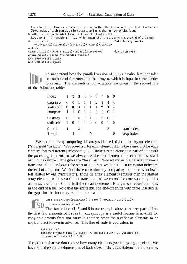
1278 Chapter B14. Statistical Description of Data
Look for 0 → 1 transitions in tie, which mean that the 0 element is the start of a tie run.Store index of each transition in tstart. nties is the number of ties found.
tend(1:nties)=pack(idx(:),tie(:)>eoshift(tie(:),1))Look for 1 → 0 transitions in tie, which mean that the 1 element is the end of a tie run.
do i=1,nties Midrank assignments.w(tstart(i):tend(i))=(tstart(i)+tend(i))/2.0_sp
end dotend(1:nties)=tend(1:nties)-tstart(1:nties)+1 Now calculate s.s=sum(tend(1:nties)**3-tend(1:nties))END SUBROUTINE crankEND SUBROUTINE spear
To understand how the parallel version of crank works, let’s consideran example of 9 elements in the array w, which is input in sorted orderto crank. The elements in our example are given in the second line
of the following table:
index 1 2 3 4 5 6 7 8 9
data in w 0 0 1 1 1 2 3 4 4shift right 0 0 0 1 1 1 2 3 4compare 1 1 0 1 1 0 0 0 1
tie array 0 1 0 1 1 0 0 0 1shift left 1 0 1 1 0 0 0 1 0
0 → 1 1 3 8 start index1 → 0 2 5 9 stop index
We look for ties by comparing this array with itself, right shifted by one element(“shift right” in table). We record a 1 for each element that is the same, a 0 for eachelement that is different (“compare”). A 1 indicates the element is part of a tie withthe preceding element, so we always set the first element to 0, even if it was a 1as in our example. This gives the “tie array.” Now wherever the tie array makes atransition 0 → 1 indicates the start of a tie run, while a 1 → 0 transition indicatesthe end of a tie run. We find these transitions by comparing the tie array to itselfleft shifted by one (“shift left”). If the tie array element is smaller than the shiftedarray element, we have a 0 → 1 transition and we record the corresponding indexas the start of a tie. Similarly if the tie array element is larger we record the indexas the end of a tie. Note that the shifts must be end-off shifts with zeros inserted inthe gaps for the boundary conditions to work.
f90call array_copy(pack(idx(:),tie(:)<eoshift(tie(:),1)),
tstart,nties,ndum)
The start indices (1, 3, and 8 in our example above) are here packed intothe first few elements of tstart. array copy is a useful routine in nrutil forcopying elements from one array to another, when the number of elements to becopied is not known in advance. This line of code is equivalent to
tstart(:)=0tstart(:)=pack(idx(:), tie(:) < eoshift(tie(:),1),tstart(:))nties=count(tstart(:) > 0)
The point is that we don’t know how many elements pack is going to select. Wehave to make sure the dimensions of both sides of the pack statement are the same,
Chapter B14. Statistical Description of Data 1279
so we set the optional third argument of pack to tstart. We then make a separatepass through tstart to count how many elements we copied. Alternatively, wecould have used an additional logical array mask and coded this as
mask(:)=tie(:) < eoshift(tie(:),1)nties=count(mask)tstart(1:nties)=pack(idx(:),mask)
But we still need two passes through the mask array. The beauty of the array copy
routine is that nties is determined from the size of the first argument, without thenecessity for a second pass through the array.
� � �
SUBROUTINE kendl1(data1,data2,tau,z,prob)USE nrtype; USE nrutil, ONLY : assert_eqUSE nr, ONLY : erfccIMPLICIT NONEREAL(SP), INTENT(OUT) :: tau,z,probREAL(SP), DIMENSION(:), INTENT(IN) :: data1,data2
Given same-size data arrays data1 and data2, this program returns Kendall’s τ as tau, itsnumber of standard deviations from zero as z, and its two-sided significance level as prob.Small values of prob indicate a significant correlation (tau positive) or anticorrelation(tau negative).
INTEGER(I4B) :: is,j,n,n1,n2REAL(SP) :: varREAL(SP), DIMENSION(size(data1)) :: a1,a2n=assert_eq(size(data1),size(data2),’kendl1’)n1=0 This will be the argument of one square root in (14.6.8),n2=0 and this the other.is=0 This will be the numerator in (14.6.8).do j=1,n-1 For each first member of pair,
a1(j+1:n)=data1(j)-data1(j+1:n) loop over second member.a2(j+1:n)=data2(j)-data2(j+1:n)n1=n1+count(a1(j+1:n) /= 0.0)n2=n2+count(a2(j+1:n) /= 0.0)
Now accumulate the numerator in (14.6.8):is=is+count((a1(j+1:n) > 0.0 .and. a2(j+1:n) > 0.0) &
.or. (a1(j+1:n) < 0.0 .and. a2(j+1:n) < 0.0)) - &count((a1(j+1:n) > 0.0 .and. a2(j+1:n) < 0.0) &.or. (a1(j+1:n) < 0.0 .and. a2(j+1:n) > 0.0))
end dotau=real(is,sp)/sqrt(real(n1,sp)*real(n2,sp)) Equation (14.6.8).var=(4.0_sp*n+10.0_sp)/(9.0_sp*n*(n-1.0_sp)) Equation (14.6.9).z=tau/sqrt(var)prob=erfcc(abs(z)/SQRT2) Significance.END SUBROUTINE kendl1
SUBROUTINE kendl2(tab,tau,z,prob)USE nrtype; USE nrutil, ONLY : cumsumUSE nr, ONLY : erfccIMPLICIT NONEREAL(SP), DIMENSION(:,:), INTENT(IN) :: tabREAL(SP), INTENT(OUT) :: tau,z,prob
Given a two-dimensional table tab such that tab(k, l) contains the number of events fallingin bin k of one variable and bin l of another, this program returns Kendall’s τ as tau, itsnumber of standard deviations from zero as z, and its two-sided significance level as prob.Small values of prob indicate a significant correlation (tau positive) or anticorrelation (tau
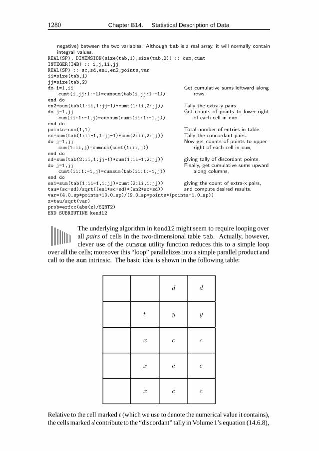
1280 Chapter B14. Statistical Description of Data
negative) between the two variables. Although tab is a real array, it will normally containintegral values.
REAL(SP), DIMENSION(size(tab,1),size(tab,2)) :: cum,cumtINTEGER(I4B) :: i,j,ii,jjREAL(SP) :: sc,sd,en1,en2,points,varii=size(tab,1)jj=size(tab,2)do i=1,ii Get cumulative sums leftward along
rows.cumt(i,jj:1:-1)=cumsum(tab(i,jj:1:-1))end doen2=sum(tab(1:ii,1:jj-1)*cumt(1:ii,2:jj)) Tally the extra-y pairs.do j=1,jj Get counts of points to lower-right
of each cell in cum.cum(ii:1:-1,j)=cumsum(cumt(ii:1:-1,j))end dopoints=cum(1,1) Total number of entries in table.sc=sum(tab(1:ii-1,1:jj-1)*cum(2:ii,2:jj)) Tally the concordant pairs.do j=1,jj Now get counts of points to upper-
right of each cell in cum,cum(1:ii,j)=cumsum(cumt(1:ii,j))end dosd=sum(tab(2:ii,1:jj-1)*cum(1:ii-1,2:jj)) giving tally of discordant points.do j=1,jj Finally, get cumulative sums upward
along columns,cumt(ii:1:-1,j)=cumsum(tab(ii:1:-1,j))end doen1=sum(tab(1:ii-1,1:jj)*cumt(2:ii,1:jj)) giving the count of extra-x pairs,tau=(sc-sd)/sqrt((en1+sc+sd)*(en2+sc+sd)) and compute desired results.var=(4.0_sp*points+10.0_sp)/(9.0_sp*points*(points-1.0_sp))z=tau/sqrt(var)prob=erfcc(abs(z)/SQRT2)END SUBROUTINE kendl2
The underlying algorithm in kendl2 might seem to require looping overall pairs of cells in the two-dimensional table tab. Actually, however,clever use of the cumsum utility function reduces this to a simple loop
over all the cells; moreover this “loop” parallelizes into a simple parallel product andcall to the sum intrinsic. The basic idea is shown in the following table:
d d
t y y
x c c
x c c
x c c
Relative to the cell marked t (which we use to denote the numerical value it contains),the cells marked d contribute to the “discordant” tally in Volume 1’s equation (14.6.8),
Chapter B14. Statistical Description of Data 1281
while the cells marked c contribute to the “concordant” tally. Likewise, the cellsmarked x and y contribute, respectively, to the “extra-x” and “extra-y” tallies. Whatabout the cells left blank? Since we want to count pairs of cells only once, withoutduplication, these cells will be counted, relative to the location shown as t, whent itself moves into the blank-cell area.
Symbolically we have
concordant =∑n
tn
∑
lower right
cm
discordant =∑n
tn
∑
upper right
dm
extra-x =∑n
tn
(∑below
xm
)
extra-y =∑n
tn
∑
to the right
ym
(B14.1)
Here n varies over all the positions in the table, while the limits of the inner sumsare relative to the position of n. (The letters tn, cm, dm, xm, ym all represent thevalue in a cell; we use different letters only to make the relation with the above tableclear.) Now the final trick is to recognize that the inner sums, over cells to the lower-or upper-right, below, and to the right can be done in parallel by cumulative sums(cumsum) sweeping to the right and up. The routine does these in a nonintuitiveorder merely to be able to reuse maximally the scratch spaces cum and cumt.
� � �
SUBROUTINE ks2d1s(x1,y1,quadvl,d1,prob)USE nrtype; USE nrutil, ONLY : assert_eqUSE nr, ONLY : pearsn,probks,quadctIMPLICIT NONEREAL(SP), DIMENSION(:), INTENT(IN) :: x1,y1REAL(SP), INTENT(OUT) :: d1,probINTERFACE
SUBROUTINE quadvl(x,y,fa,fb,fc,fd)USE nrtypeIMPLICIT NONEREAL(SP), INTENT(IN) :: x,yREAL(SP), INTENT(OUT) :: fa,fb,fc,fdEND SUBROUTINE quadvl
END INTERFACETwo-dimensional Kolmogorov-Smirnov test of one sample against a model. Given the x-and y-coordinates of a set of data points in arrays x1 and y1 of the same length, and givena user-supplied function quadvl that exemplifies the model, this routine returns the two-dimensional K-S statistic as d1, and its significance level as prob. Small values of probshow that the sample is significantly different from the model. Note that the test is slightlydistribution-dependent, so prob is only an estimate.
INTEGER(I4B) :: j,n1REAL(SP) :: dum,dumm,fa,fb,fc,fd,ga,gb,gc,gd,r1,rr,sqenn1=assert_eq(size(x1),size(y1),’ks2d1s’)d1=0.0
1282 Chapter B14. Statistical Description of Data
do j=1,n1 Loop over the data points.call quadct(x1(j),y1(j),x1,y1,fa,fb,fc,fd)call quadvl(x1(j),y1(j),ga,gb,gc,gd)d1=max(d1,abs(fa-ga),abs(fb-gb),abs(fc-gc),abs(fd-gd))
For both the sample and the model, the distribution is integrated in each of four quad-rants, and the maximum difference is saved.
end docall pearsn(x1,y1,r1,dum,dumm) Get the linear correlation coefficient r1.sqen=sqrt(real(n1,sp))rr=sqrt(1.0_sp-r1**2)
Estimate the probability using the K-S probability function probks.prob=probks(d1*sqen/(1.0_sp+rr*(0.25_sp-0.75_sp/sqen)))END SUBROUTINE ks2d1s
SUBROUTINE quadct(x,y,xx,yy,fa,fb,fc,fd)USE nrtype; USE nrutil, ONLY : assert_eqIMPLICIT NONEREAL(SP), INTENT(IN) :: x,yREAL(SP), DIMENSION(:), INTENT(IN) :: xx,yyREAL(SP), INTENT(OUT) :: fa,fb,fc,fd
Given an origin (x,y), and an array of points with coordinates xx and yy, count how many ofthem are in each quadrant around the origin, and return the normalized fractions. Quadrantsare labeled alphabetically, counterclockwise from the upper right. Used by ks2d1s andks2d2s.
INTEGER(I4B) :: na,nb,nc,nd,nnREAL(SP) :: ffnn=assert_eq(size(xx),size(yy),’quadct’)na=count(yy(:) > y .and. xx(:) > x)nb=count(yy(:) > y .and. xx(:) <= x)nc=count(yy(:) <= y .and. xx(:) <= x)nd=nn-na-nb-ncff=1.0_sp/nnfa=ff*nafb=ff*nbfc=ff*ncfd=ff*ndEND SUBROUTINE quadct
SUBROUTINE quadvl(x,y,fa,fb,fc,fd)USE nrtypeIMPLICIT NONEREAL(SP), INTENT(IN) :: x,yREAL(SP), INTENT(OUT) :: fa,fb,fc,fd
This is a sample of a user-supplied routine to be used with ks2d1s. In this case, the modeldistribution is uniform inside the square −1 < x < 1, −1 < y < 1. In general this routineshould return, for any point (x, y), the fraction of the total distribution in each of thefour quadrants around that point. The fractions, fa, fb, fc, and fd, must add up to 1.Quadrants are alphabetical, counterclockwise from the upper right.
REAL(SP) :: qa,qb,qc,qdqa=min(2.0_sp,max(0.0_sp,1.0_sp-x))qb=min(2.0_sp,max(0.0_sp,1.0_sp-y))qc=min(2.0_sp,max(0.0_sp,x+1.0_sp))qd=min(2.0_sp,max(0.0_sp,y+1.0_sp))fa=0.25_sp*qa*qbfb=0.25_sp*qb*qcfc=0.25_sp*qc*qdfd=0.25_sp*qd*qaEND SUBROUTINE quadvl
Chapter B14. Statistical Description of Data 1283
SUBROUTINE ks2d2s(x1,y1,x2,y2,d,prob)USE nrtype; USE nrutil, ONLY : assert_eqUSE nr, ONLY : pearsn,probks,quadctIMPLICIT NONEREAL(SP), DIMENSION(:), INTENT(IN) :: x1,y1,x2,y2REAL(SP), INTENT(OUT) :: d,prob
Compute two-dimensional Kolmogorov-Smirnov test on two samples. Input are the x- andy-coordinates of the first sample in arrays x1 and y1 of the same length, and of the secondsample in arrays x2 and y2 of the same length (possibly different from the length of the firstsample). The routine returns the two-dimensional, two-sample K-S statistic as d, and itssignificance level as prob. Small values of prob show that the two samples are significantlydifferent. Note that the test is slightly distribution-dependent, so prob is only an estimate.
INTEGER(I4B) :: j,n1,n2REAL(SP) :: d1,d2,dum,dumm,fa,fb,fc,fd,ga,gb,gc,gd,r1,r2,rr,sqenn1=assert_eq(size(x1),size(y1),’ks2d2s: n1’)n2=assert_eq(size(x2),size(y2),’ks2d2s: n2’)d1=0.0do j=1,n1 First, use points in the first sample as origins.
call quadct(x1(j),y1(j),x1,y1,fa,fb,fc,fd)call quadct(x1(j),y1(j),x2,y2,ga,gb,gc,gd)d1=max(d1,abs(fa-ga),abs(fb-gb),abs(fc-gc),abs(fd-gd))
end dod2=0.0do j=1,n2 Then, use points in the second sample as ori-
gins.call quadct(x2(j),y2(j),x1,y1,fa,fb,fc,fd)call quadct(x2(j),y2(j),x2,y2,ga,gb,gc,gd)d2=max(d2,abs(fa-ga),abs(fb-gb),abs(fc-gc),abs(fd-gd))
end dod=0.5_sp*(d1+d2) Average the K-S statistics.sqen=sqrt(real(n1,sp)*real(n2,sp)/real(n1+n2,sp))call pearsn(x1,y1,r1,dum,dumm) Get the linear correlation coefficient for each sam-
ple.call pearsn(x2,y2,r2,dum,dumm)rr=sqrt(1.0_sp-0.5_sp*(r1**2+r2**2))
Estimate the probability using the K-S probability function probks.prob=probks(d*sqen/(1.0_sp+rr*(0.25_sp-0.75_sp/sqen)))END SUBROUTINE ks2d2s
� � �
FUNCTION savgol(nl,nrr,ld,m)USE nrtype; USE nrutil, ONLY : arth,assert,polyUSE nr, ONLY : lubksb,ludcmpIMPLICIT NONEINTEGER(I4B), INTENT(IN) :: nl,nrr,ld,m
Returns in array c, in wrap-around order (N.B.!) consistent with the argument respns inroutine convlv, a set of Savitzky-Golay filter coefficients. nl is the number of leftward(past) data points used, while nrr is the number of rightward (future) data points, makingthe total number of data points used nl+nrr+1. ld is the order of the derivative desired(e.g., ld = 0 for smoothed function). m is the order of the smoothing polynomial, alsoequal to the highest conserved moment; usual value is m = 2 or m = 4.
REAL(SP), DIMENSION(nl+nrr+1) :: savgolINTEGER(I4B) :: imj,ipj,mm,npINTEGER(I4B), DIMENSION(m+1) :: indxREAL(SP) :: d,smREAL(SP), DIMENSION(m+1) :: bREAL(SP), DIMENSION(m+1,m+1) :: aINTEGER(I4B) :: irng(nl+nrr+1)call assert(nl >= 0, nrr >= 0, ld <= m, nl+nrr >= m, ’savgol args’)do ipj=0,2*m Set up the normal equations of the desired least
squares fit.sm=sum(arth(1.0_sp,1.0_sp,nrr)**ipj)+&sum(arth(-1.0_sp,-1.0_sp,nl)**ipj)
1284 Chapter B14. Statistical Description of Data
if (ipj == 0) sm=sm+1.0_spmm=min(ipj,2*m-ipj)do imj=-mm,mm,2
a(1+(ipj+imj)/2,1+(ipj-imj)/2)=smend do
end docall ludcmp(a(:,:),indx(:),d) Solve them: LU decomposition.b(:)=0.0b(ld+1)=1.0 Right-hand-side vector is unit vector, depending
on which derivative we want.call lubksb(a(:,:),indx(:),b(:))Backsubstitute, giving one row of the inverse matrix.
savgol(:)=0.0 Zero the output array (it may be bigger thannumber of coefficients).irng(:)=arth(-nl,1,nrr+nl+1)
np=nl+nrr+1savgol(mod(np-irng(:),np)+1)=poly(real(irng(:),sp),b(:))
Each Savitzky-Golay coefficient is the value of the polynomial in (14.8.6) at the correspondinginteger. The polynomial coefficients are a row of the inverse matrix. The mod function takescare of the wrap-around order.
END FUNCTION savgol
f90do imj=-mm,mm,2 Here is an example of a loop that cannot be parallelizedin the framework of Fortran 90: We need to access “skew” sections ofthe matrix a.
savgol...=poly(real(irng(:),sp),b(:))) The poly function in nrutil re-turns the value of a polynomial, here the one in equation (14.8.6). We need theexplicit kind type parameter sp in the real function, otherwise it would returntype default real for the integer argument and would not automatically convert todouble precision if desired.
Chapter B15. Modeling of Data
SUBROUTINE fit(x,y,a,b,siga,sigb,chi2,q,sig)USE nrtype; USE nrutil, ONLY : assert_eqUSE nr, ONLY : gammqIMPLICIT NONEREAL(SP), DIMENSION(:), INTENT(IN) :: x,yREAL(SP), INTENT(OUT) :: a,b,siga,sigb,chi2,qREAL(SP), DIMENSION(:), OPTIONAL, INTENT(IN) :: sig
Given a set of data points in same-size arrays x and y, fit them to a straight line y = a+ bxby minimizing χ2. sig is an optional array of the same length containing the individualstandard deviations. If it is present, then a,b are returned with their respective probableuncertainties siga and sigb, the chi-square chi2, and the goodness-of-fit probability q(that the fit would have χ2 this large or larger). If sig is not present, then q is returnedas 1.0 and the normalization of chi2 is to unit standard deviation on all points.
INTEGER(I4B) :: ndataREAL(SP) :: sigdat,ss,sx,sxoss,sy,st2REAL(SP), DIMENSION(size(x)), TARGET :: tREAL(SP), DIMENSION(:), POINTER :: wtif (present(sig)) then
ndata=assert_eq(size(x),size(y),size(sig),’fit’)wt=>t Use temporary variable t to store weights.wt(:)=1.0_sp/(sig(:)**2)ss=sum(wt(:)) Accumulate sums with weights.sx=dot_product(wt,x)sy=dot_product(wt,y)
elsendata=assert_eq(size(x),size(y),’fit’)ss=real(size(x),sp) Accumulate sums without weights.sx=sum(x)sy=sum(y)
end ifsxoss=sx/sst(:)=x(:)-sxossif (present(sig)) then
t(:)=t(:)/sig(:)b=dot_product(t/sig,y)
elseb=dot_product(t,y)
end ifst2=dot_product(t,t)b=b/st2 Solve for a, b, σa, and σb.a=(sy-sx*b)/sssiga=sqrt((1.0_sp+sx*sx/(ss*st2))/ss)sigb=sqrt(1.0_sp/st2)t(:)=y(:)-a-b*x(:)q=1.0if (present(sig)) then
t(:)=t(:)/sig(:)chi2=dot_product(t,t) Calculate χ2.if (ndata > 2) q=gammq(0.5_sp*(size(x)-2),0.5_sp*chi2) Equation (15.2.12).
elsechi2=dot_product(t,t)
1285
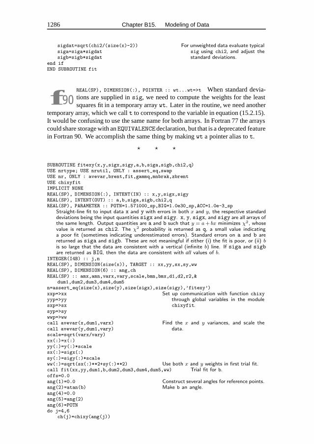
1286 Chapter B15. Modeling of Data
sigdat=sqrt(chi2/(size(x)-2)) For unweighted data evaluate typicalsig using chi2, and adjust thestandard deviations.
siga=siga*sigdatsigb=sigb*sigdat
end ifEND SUBROUTINE fit
f90REAL(SP), DIMENSION(:), POINTER :: wt...wt=>t When standard devia-tions are supplied in sig, we need to compute the weights for the leastsquares fit in a temporary array wt. Later in the routine, we need another
temporary array, which we call t to correspond to the variable in equation (15.2.15).It would be confusing to use the same name for both arrays. In Fortran 77 the arrayscould share storage with an EQUIVALENCEdeclaration, but that is a deprecated featurein Fortran 90. We accomplish the same thing by making wt a pointer alias to t.
� � �
SUBROUTINE fitexy(x,y,sigx,sigy,a,b,siga,sigb,chi2,q)USE nrtype; USE nrutil, ONLY : assert_eq,swapUSE nr, ONLY : avevar,brent,fit,gammq,mnbrak,zbrentUSE chixyfitIMPLICIT NONEREAL(SP), DIMENSION(:), INTENT(IN) :: x,y,sigx,sigyREAL(SP), INTENT(OUT) :: a,b,siga,sigb,chi2,qREAL(SP), PARAMETER :: POTN=1.571000_sp,BIG=1.0e30_sp,ACC=1.0e-3_sp
Straight-line fit to input data x and y with errors in both x and y, the respective standarddeviations being the input quantities sigx and sigy. x, y, sigx, and sigy are all arrays ofthe same length. Output quantities are a and b such that y = a+ bx minimizes χ2, whosevalue is returned as chi2. The χ2 probability is returned as q, a small value indicatinga poor fit (sometimes indicating underestimated errors). Standard errors on a and b arereturned as siga and sigb. These are not meaningful if either (i) the fit is poor, or (ii) bis so large that the data are consistent with a vertical (infinite b) line. If siga and sigbare returned as BIG, then the data are consistent with all values of b.
INTEGER(I4B) :: j,nREAL(SP), DIMENSION(size(x)), TARGET :: xx,yy,sx,sy,wwREAL(SP), DIMENSION(6) :: ang,chREAL(SP) :: amx,amn,varx,vary,scale,bmn,bmx,d1,d2,r2,&
dum1,dum2,dum3,dum4,dum5n=assert_eq(size(x),size(y),size(sigx),size(sigy),’fitexy’)xxp=>xx Set up communication with function chixy
through global variables in the modulechixyfit.
yyp=>yysxp=>sxsyp=>sywwp=>wwcall avevar(x,dum1,varx) Find the x and y variances, and scale the
data.call avevar(y,dum1,vary)scale=sqrt(varx/vary)xx(:)=x(:)yy(:)=y(:)*scalesx(:)=sigx(:)sy(:)=sigy(:)*scaleww(:)=sqrt(sx(:)**2+sy(:)**2) Use both x and y weights in first trial fit.call fit(xx,yy,dum1,b,dum2,dum3,dum4,dum5,ww) Trial fit for b.offs=0.0ang(1)=0.0 Construct several angles for reference points.ang(2)=atan(b) Make b an angle.ang(4)=0.0ang(5)=ang(2)ang(6)=POTNdo j=4,6
ch(j)=chixy(ang(j))
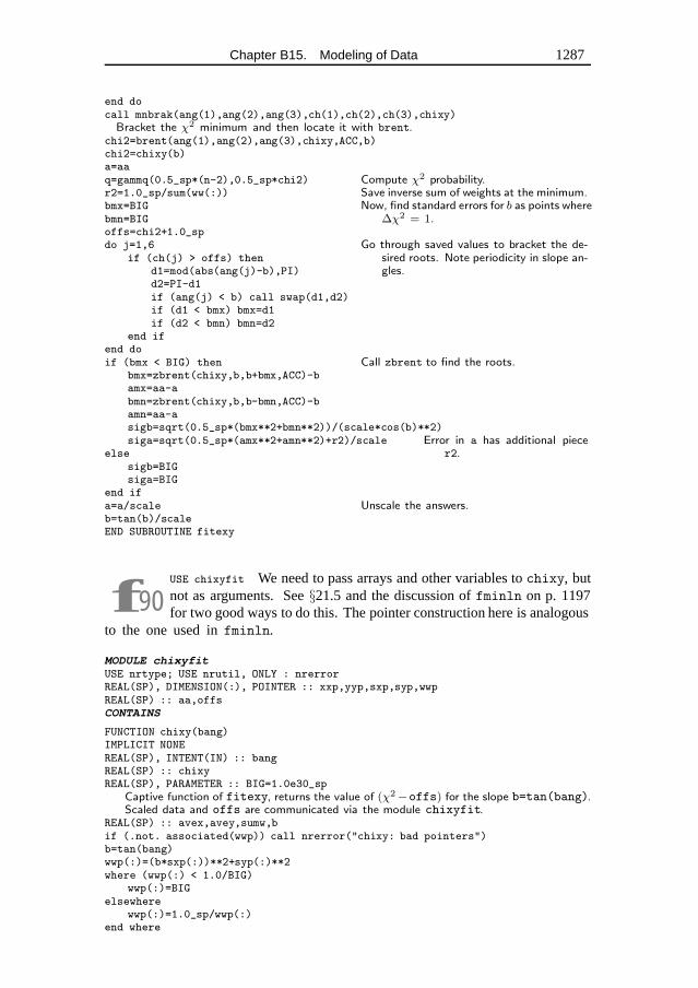
Chapter B15. Modeling of Data 1287
end docall mnbrak(ang(1),ang(2),ang(3),ch(1),ch(2),ch(3),chixy)Bracket the χ2 minimum and then locate it with brent.
chi2=brent(ang(1),ang(2),ang(3),chixy,ACC,b)chi2=chixy(b)a=aaq=gammq(0.5_sp*(n-2),0.5_sp*chi2) Compute χ2 probability.r2=1.0_sp/sum(ww(:)) Save inverse sum of weights at the minimum.bmx=BIG Now, find standard errors for b as points where
∆χ2 = 1.bmn=BIGoffs=chi2+1.0_spdo j=1,6 Go through saved values to bracket the de-
sired roots. Note periodicity in slope an-gles.
if (ch(j) > offs) thend1=mod(abs(ang(j)-b),PI)d2=PI-d1if (ang(j) < b) call swap(d1,d2)if (d1 < bmx) bmx=d1if (d2 < bmn) bmn=d2
end ifend doif (bmx < BIG) then Call zbrent to find the roots.
bmx=zbrent(chixy,b,b+bmx,ACC)-bamx=aa-abmn=zbrent(chixy,b,b-bmn,ACC)-bamn=aa-asigb=sqrt(0.5_sp*(bmx**2+bmn**2))/(scale*cos(b)**2)siga=sqrt(0.5_sp*(amx**2+amn**2)+r2)/scale Error in a has additional piece
r2.elsesigb=BIGsiga=BIG
end ifa=a/scale Unscale the answers.b=tan(b)/scaleEND SUBROUTINE fitexy
f90USE chixyfit We need to pass arrays and other variables to chixy, butnot as arguments. See §21.5 and the discussion of fminln on p. 1197for two good ways to do this. The pointer construction here is analogous
to the one used in fminln.
MODULE chixyfitUSE nrtype; USE nrutil, ONLY : nrerrorREAL(SP), DIMENSION(:), POINTER :: xxp,yyp,sxp,syp,wwpREAL(SP) :: aa,offsCONTAINS
FUNCTION chixy(bang)IMPLICIT NONEREAL(SP), INTENT(IN) :: bangREAL(SP) :: chixyREAL(SP), PARAMETER :: BIG=1.0e30_sp
Captive function of fitexy, returns the value of (χ2 −offs) for the slope b=tan(bang).Scaled data and offs are communicated via the module chixyfit.
REAL(SP) :: avex,avey,sumw,bif (.not. associated(wwp)) call nrerror("chixy: bad pointers")b=tan(bang)wwp(:)=(b*sxp(:))**2+syp(:)**2where (wwp(:) < 1.0/BIG)
wwp(:)=BIGelsewhere
wwp(:)=1.0_sp/wwp(:)end where
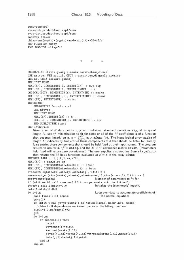
1288 Chapter B15. Modeling of Data
sumw=sum(wwp)avex=dot_product(wwp,xxp)/sumwavey=dot_product(wwp,yyp)/sumwaa=avey-b*avexchixy=sum(wwp(:)*(yyp(:)-aa-b*xxp(:))**2)-offsEND FUNCTION chixyEND MODULE chixyfit
� � �
SUBROUTINE lfit(x,y,sig,a,maska,covar,chisq,funcs)USE nrtype; USE nrutil, ONLY : assert_eq,diagmult,nrerrorUSE nr, ONLY :covsrt,gaussjIMPLICIT NONEREAL(SP), DIMENSION(:), INTENT(IN) :: x,y,sigREAL(SP), DIMENSION(:), INTENT(INOUT) :: aLOGICAL(LGT), DIMENSION(:), INTENT(IN) :: maskaREAL(SP), DIMENSION(:,:), INTENT(INOUT) :: covarREAL(SP), INTENT(OUT) :: chisqINTERFACE
SUBROUTINE funcs(x,arr)USE nrtypeIMPLICIT NONEREAL(SP),INTENT(IN) :: xREAL(SP), DIMENSION(:), INTENT(OUT) :: arrEND SUBROUTINE funcs
END INTERFACEGiven a set of N data points x, y with individual standard deviations sig, all arrays oflength N , use χ2 minimization to fit for some or all of the M coefficients a of a functionthat depends linearly on a, y =
∑Mi=1 ai × afunci(x). The input logical array maska of
length M indicates by true entries those components of a that should be fitted for, and byfalse entries those components that should be held fixed at their input values. The programreturns values for a, χ2 = chisq, and the M ×M covariance matrix covar. (Parametersheld fixed will return zero covariances.) The user supplies a subroutine funcs(x,afunc)that returns the M basis functions evaluated at x = x in the array afunc.
INTEGER(I4B) :: i,j,k,l,ma,mfit,nREAL(SP) :: sig2i,wt,ymREAL(SP), DIMENSION(size(maska)) :: afuncREAL(SP), DIMENSION(size(maska),1) :: betan=assert_eq(size(x),size(y),size(sig),’lfit: n’)ma=assert_eq(size(maska),size(a),size(covar,1),size(covar,2),’lfit: ma’)mfit=count(maska) Number of parameters to fit for.if (mfit == 0) call nrerror(’lfit: no parameters to be fitted’)covar(1:mfit,1:mfit)=0.0 Initialize the (symmetric) matrix.beta(1:mfit,1)=0.0do i=1,n Loop over data to accumulate coefficients of
the normal equations.call funcs(x(i),afunc)ym=y(i)if (mfit < ma) ym=ym-sum(a(1:ma)*afunc(1:ma), mask=.not. maska)Subtract off dependences on known pieces of the fitting function.
sig2i=1.0_sp/sig(i)**2j=0do l=1,ma
if (maska(l)) thenj=j+1wt=afunc(l)*sig2ik=count(maska(1:l))covar(j,1:k)=covar(j,1:k)+wt*pack(afunc(1:l),maska(1:l))beta(j,1)=beta(j,1)+ym*wt
end ifend do
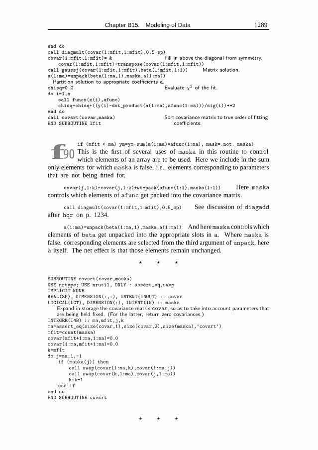
Chapter B15. Modeling of Data 1289
end docall diagmult(covar(1:mfit,1:mfit),0.5_sp)covar(1:mfit,1:mfit)= & Fill in above the diagonal from symmetry.
covar(1:mfit,1:mfit)+transpose(covar(1:mfit,1:mfit))call gaussj(covar(1:mfit,1:mfit),beta(1:mfit,1:1)) Matrix solution.a(1:ma)=unpack(beta(1:ma,1),maska,a(1:ma))Partition solution to appropriate coefficients a.
chisq=0.0 Evaluate χ2 of the fit.do i=1,n
call funcs(x(i),afunc)chisq=chisq+((y(i)-dot_product(a(1:ma),afunc(1:ma)))/sig(i))**2
end docall covsrt(covar,maska) Sort covariance matrix to true order of fitting
coefficients.END SUBROUTINE lfit
f90if (mfit < ma) ym=ym-sum(a(1:ma)*afunc(1:ma), mask=.not. maska)
This is the first of several uses of maska in this routine to controlwhich elements of an array are to be used. Here we include in the sum
only elements for which maska is false, i.e., elements corresponding to parametersthat are not being fitted for.
covar(j,1:k)=covar(j,1:k)+wt*pack(afunc(1:l),maska(1:l)) Here maska
controls which elements of afunc get packed into the covariance matrix.
call diagmult(covar(1:mfit,1:mfit),0.5_sp) See discussion of diagaddafter hqr on p. 1234.
a(1:ma)=unpack(beta(1:ma,1),maska,a(1:ma)) And heremaska controls whichelements of beta get unpacked into the appropriate slots in a. Where maska isfalse, corresponding elements are selected from the third argument of unpack, herea itself. The net effect is that those elements remain unchanged.
� � �
SUBROUTINE covsrt(covar,maska)USE nrtype; USE nrutil, ONLY : assert_eq,swapIMPLICIT NONEREAL(SP), DIMENSION(:,:), INTENT(INOUT) :: covarLOGICAL(LGT), DIMENSION(:), INTENT(IN) :: maska
Expand in storage the covariance matrix covar, so as to take into account parameters thatare being held fixed. (For the latter, return zero covariances.)
INTEGER(I4B) :: ma,mfit,j,kma=assert_eq(size(covar,1),size(covar,2),size(maska),’covsrt’)mfit=count(maska)covar(mfit+1:ma,1:ma)=0.0covar(1:ma,mfit+1:ma)=0.0k=mfitdo j=ma,1,-1
if (maska(j)) thencall swap(covar(1:ma,k),covar(1:ma,j))call swap(covar(k,1:ma),covar(j,1:ma))k=k-1
end ifend doEND SUBROUTINE covsrt
� � �
1290 Chapter B15. Modeling of Data
SUBROUTINE svdfit(x,y,sig,a,v,w,chisq,funcs)USE nrtype; USE nrutil, ONLY : assert_eq,vabsUSE nr, ONLY : svbksb,svdcmpIMPLICIT NONEREAL(SP), DIMENSION(:), INTENT(IN) :: x,y,sigREAL(SP), DIMENSION(:), INTENT(OUT) :: a,wREAL(SP), DIMENSION(:,:), INTENT(OUT) :: vREAL(SP), INTENT(OUT) :: chisqINTERFACE
FUNCTION funcs(x,n)USE nrtypeIMPLICIT NONEREAL(SP), INTENT(IN) :: xINTEGER(I4B), INTENT(IN) :: nREAL(SP), DIMENSION(n) :: funcsEND FUNCTION funcs
END INTERFACEREAL(SP), PARAMETER :: TOL=1.0e-5_sp
Given a set ofN data points x, y with individual standard deviations sig, all arrays of lengthN , use χ2 minimization to determine theM coefficients a of a function that depends linearlyon a, y =
∑Mi=1 ai × afunci(x). Here we solve the fitting equations using singular value
decomposition of the N × M matrix, as in §2.6. On output, the M × M array v and thevector w of length M define part of the singular value decomposition, and can be used toobtain the covariance matrix. The program returns values for the M fit parameters a, andχ2, chisq. The user supplies a subroutine funcs(x,afunc) that returns the M basisfunctions evaluated at x = X in the array afunc.
INTEGER(I4B) :: i,ma,nREAL(SP), DIMENSION(size(x)) :: b,sigiREAL(SP), DIMENSION(size(x),size(a)) :: u,usavn=assert_eq(size(x),size(y),size(sig),’svdfit: n’)ma=assert_eq(size(a),size(v,1),size(v,2),size(w),’svdfit: ma’)sigi=1.0_sp/sig Accumulate coefficients of the fitting matrix in
u.b=y*sigido i=1,n
usav(i,:)=funcs(x(i),ma)end dou=usav*spread(sigi,dim=2,ncopies=ma)usav=ucall svdcmp(u,w,v) Singular value decomposition.where (w < TOL*maxval(w)) w=0.0 Edit the singular values, given TOL from the pa-
rameter statement.call svbksb(u,w,v,b,a)chisq=vabs(matmul(usav,a)-b)**2 Evaluate chi-square.END SUBROUTINE svdfit
f90u=usav*spread(sigi,dim=2,ncopies=ma) Remember how spread works:the vector sigi is copied along the dimension 2, making a matrix whosecolumns are each a copy of sigi. The multiplication here is element by
element, so each row of usav is multiplied by the corresponding element of sigi.
chisq=vabs(matmul(usav,a)-b)**2 Fortran 90’s matmul intrinsic allows us toevaluate χ2 from the mathematical definition in terms of matrices. vabs in nrutil
returns the length of a vector (L2 norm).
SUBROUTINE svdvar(v,w,cvm)USE nrtype; USE nrutil, ONLY : assert_eqIMPLICIT NONEREAL(SP), DIMENSION(:,:), INTENT(IN) :: vREAL(SP), DIMENSION(:), INTENT(IN) :: wREAL(SP), DIMENSION(:,:), INTENT(OUT) :: cvm
Chapter B15. Modeling of Data 1291
To evaluate the covariance matrix cvm of the fit for M parameters obtained by svdfit,call this routine with matrices v,w as returned from svdfit. The dimensions are M forw and M × M for v and cvm.
INTEGER(I4B) :: maREAL(SP), DIMENSION(size(w)) :: wtima=assert_eq((/size(v,1),size(v,2),size(w),size(cvm,1),size(cvm,2)/),&
’svdvar’)where (w /= 0.0)
wti=1.0_sp/(w*w)elsewhere
wti=0.0end wherecvm=v*spread(wti,dim=1,ncopies=ma)cvm=matmul(cvm,transpose(v)) Covariance matrix is given by (15.4.20).END SUBROUTINE svdvar
f90where (w /= 0.0)...elsewhere...end where This is the standard Fortran90 construction for doing different things to a matrix depending on somecondition. Here we want to avoid inverting elements of w that are zero.
cvm=v*spread(wti,dim=1,ncopies=ma) Each column of v gets multiplied bythe corresponding element of wti. Contrast the construction spread(...dim=2...)
in svdfit.
� � �
FUNCTION fpoly(x,n)USE nrtype; USE nrutil, ONLY : geopIMPLICIT NONEREAL(SP), INTENT(IN) :: xINTEGER(I4B), INTENT(IN) :: nREAL(SP), DIMENSION(n) :: fpoly
Fitting routine for a polynomial of degree n − 1, returning n coefficients in fpoly.fpoly=geop(1.0_sp,x,n)END FUNCTION fpoly
� � �
FUNCTION fleg(x,nl)USE nrtypeIMPLICIT NONEREAL(SP), INTENT(IN) :: xINTEGER(I4B), INTENT(IN) :: nlREAL(SP), DIMENSION(nl) :: fleg
Fitting routine for an expansion with nl Legendre polynomials evaluated at x and returnedin the array fleg of length nl. The evaluation uses the recurrence relation as in §5.5.
INTEGER(I4B) :: jREAL(SP) :: d,f1,f2,twoxfleg(1)=1.0fleg(2)=xif (nl > 2) then
twox=2.0_sp*xf2=xd=1.0do j=3,nl
f1=df2=f2+twoxd=d+1.0_sp
1292 Chapter B15. Modeling of Data
fleg(j)=(f2*fleg(j-1)-f1*fleg(j-2))/dend do
end ifEND FUNCTION fleg
� � �
SUBROUTINE mrqmin(x,y,sig,a,maska,covar,alpha,chisq,funcs,alamda)USE nrtype; USE nrutil, ONLY : assert_eq,diagmultUSE nr, ONLY : covsrt,gaussjIMPLICIT NONEREAL(SP), DIMENSION(:), INTENT(IN) :: x,y,sigREAL(SP), DIMENSION(:), INTENT(INOUT) :: aREAL(SP), DIMENSION(:,:), INTENT(OUT) :: covar,alphaREAL(SP), INTENT(OUT) :: chisqREAL(SP), INTENT(INOUT) :: alamdaLOGICAL(LGT), DIMENSION(:), INTENT(IN) :: maskaINTERFACE
SUBROUTINE funcs(x,a,yfit,dyda)USE nrtypeREAL(SP), DIMENSION(:), INTENT(IN) :: x,aREAL(SP), DIMENSION(:), INTENT(OUT) :: yfitREAL(SP), DIMENSION(:,:), INTENT(OUT) :: dydaEND SUBROUTINE funcs
END INTERFACELevenberg-Marquardt method, attempting to reduce the value χ2 of a fit between a set ofNdata points x, y with individual standard deviations sig, and a nonlinear function dependenton M coefficients a. The input logical array maska of length M indicates by true entriesthose components of a that should be fitted for, and by false entries those components thatshould be held fixed at their input values. The program returns current best-fit values for theparameters a, and χ2 = chisq. The M×M arrays covar and alpha are used as workingspace during most iterations. Supply a subroutine funcs(x,a,yfit,dyda) that evaluatesthe fitting function yfit, and its derivatives dyda with respect to the fitting parameters aat x. On the first call provide an initial guess for the parameters a, and set alamda<0 forinitialization (which then sets alamda=.001). If a step succeeds chisq becomes smallerand alamda decreases by a factor of 10. If a step fails alamda grows by a factor of 10.You must call this routine repeatedly until convergence is achieved. Then, make one finalcall with alamda=0, so that covar returns the covariance matrix, and alpha the curvaturematrix. (Parameters held fixed will return zero covariances.)
INTEGER(I4B) :: ma,ndataINTEGER(I4B), SAVE :: mfitcall mrqmin_privateCONTAINS
SUBROUTINE mrqmin_privateREAL(SP), SAVE :: ochisqREAL(SP), DIMENSION(:), ALLOCATABLE, SAVE :: atry,betaREAL(SP), DIMENSION(:,:), ALLOCATABLE, SAVE :: dandata=assert_eq(size(x),size(y),size(sig),’mrqmin: ndata’)ma=assert_eq((/size(a),size(maska),size(covar,1),size(covar,2),&
size(alpha,1),size(alpha,2)/),’mrqmin: ma’)mfit=count(maska)if (alamda < 0.0) then Initialization.
allocate(atry(ma),beta(ma),da(ma,1))alamda=0.001_spcall mrqcof(a,alpha,beta)ochisq=chisqatry=a
end ifcovar(1:mfit,1:mfit)=alpha(1:mfit,1:mfit)call diagmult(covar(1:mfit,1:mfit),1.0_sp+alamda)
Chapter B15. Modeling of Data 1293
Alter linearized fitting matrix, by augmenting diagonal elements.da(1:mfit,1)=beta(1:mfit)call gaussj(covar(1:mfit,1:mfit),da(1:mfit,1:1)) Matrix solution.if (alamda == 0.0) then Once converged, evaluate covariance ma-
trix.call covsrt(covar,maska)call covsrt(alpha,maska) Spread out alpha to its full size too.deallocate(atry,beta,da)RETURN
end ifatry=a+unpack(da(1:mfit,1),maska,0.0_sp) Did the trial succeed?call mrqcof(atry,covar,da(1:mfit,1))if (chisq < ochisq) then Success, accept the new solution.
alamda=0.1_sp*alamdaochisq=chisqalpha(1:mfit,1:mfit)=covar(1:mfit,1:mfit)beta(1:mfit)=da(1:mfit,1)a=atry
else Failure, increase alamda and return.alamda=10.0_sp*alamdachisq=ochisq
end ifEND SUBROUTINE mrqmin_private
SUBROUTINE mrqcof(a,alpha,beta)REAL(SP), DIMENSION(:), INTENT(IN) :: aREAL(SP), DIMENSION(:), INTENT(OUT) :: betaREAL(SP), DIMENSION(:,:), INTENT(OUT) :: alpha
Used by mrqmin to evaluate the linearized fitting matrix alpha, and vector beta as in(15.5.8), and calculate χ2.
INTEGER(I4B) :: j,k,l,mREAL(SP), DIMENSION(size(x),size(a)) :: dydaREAL(SP), DIMENSION(size(x)) :: dy,sig2i,wt,ymodcall funcs(x,a,ymod,dyda) Loop over all the data.sig2i=1.0_sp/(sig**2)dy=y-ymodj=0do l=1,ma
if (maska(l)) thenj=j+1wt=dyda(:,l)*sig2ik=0do m=1,l
if (maska(m)) thenk=k+1alpha(j,k)=dot_product(wt,dyda(:,m))alpha(k,j)=alpha(j,k) Fill in the symmetric side.
end ifend dobeta(j)=dot_product(dy,wt)
end ifend dochisq=dot_product(dy**2,sig2i) Find χ2.END SUBROUTINE mrqcofEND SUBROUTINE mrqmin
f90The organization of this routine is similar to that of amoeba, discussedon p. 1209. We want to keep the argument list of mrqcof to a minimum,but we want to make clear what global variables it accesses, and protect
mrqmin private’s name space.
REAL(SP), DIMENSION(:), ALLOCATABLE, SAVE :: atry,beta These arrays, aswell as da, are allocated with the correct dimensions on the first call to mrqmin.
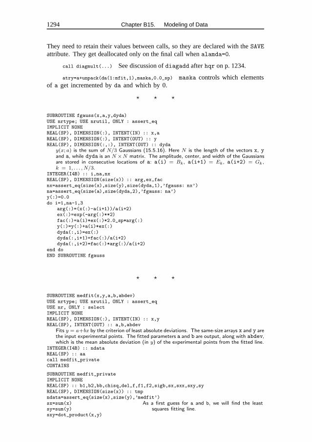
1294 Chapter B15. Modeling of Data
They need to retain their values between calls, so they are declared with the SAVE
attribute. They get deallocated only on the final call when alamda=0.
call diagmult(...) See discussion of diagadd after hqr on p. 1234.
atry=a+unpack(da(1:mfit,1),maska,0.0_sp) maska controls which elementsof a get incremented by da and which by 0.
� � �
SUBROUTINE fgauss(x,a,y,dyda)USE nrtype; USE nrutil, ONLY : assert_eqIMPLICIT NONEREAL(SP), DIMENSION(:), INTENT(IN) :: x,aREAL(SP), DIMENSION(:), INTENT(OUT) :: yREAL(SP), DIMENSION(:,:), INTENT(OUT) :: dyda
y(x; a) is the sum of N/3 Gaussians (15.5.16). Here N is the length of the vectors x, yand a, while dyda is an N ×N matrix. The amplitude, center, and width of the Gaussiansare stored in consecutive locations of a: a(i) = Bk, a(i+1) = Ek, a(i+2) = Gk ,k = 1, . . . , N/3.
INTEGER(I4B) :: i,na,nxREAL(SP), DIMENSION(size(x)) :: arg,ex,facnx=assert_eq(size(x),size(y),size(dyda,1),’fgauss: nx’)na=assert_eq(size(a),size(dyda,2),’fgauss: na’)y(:)=0.0do i=1,na-1,3
arg(:)=(x(:)-a(i+1))/a(i+2)ex(:)=exp(-arg(:)**2)fac(:)=a(i)*ex(:)*2.0_sp*arg(:)y(:)=y(:)+a(i)*ex(:)dyda(:,i)=ex(:)dyda(:,i+1)=fac(:)/a(i+2)dyda(:,i+2)=fac(:)*arg(:)/a(i+2)
end doEND SUBROUTINE fgauss
� � �
SUBROUTINE medfit(x,y,a,b,abdev)USE nrtype; USE nrutil, ONLY : assert_eqUSE nr, ONLY : selectIMPLICIT NONEREAL(SP), DIMENSION(:), INTENT(IN) :: x,yREAL(SP), INTENT(OUT) :: a,b,abdev
Fits y = a+bx by the criterion of least absolute deviations. The same-size arrays x and y arethe input experimental points. The fitted parameters a and b are output, along with abdev,which is the mean absolute deviation (in y) of the experimental points from the fitted line.
INTEGER(I4B) :: ndataREAL(SP) :: aacall medfit_privateCONTAINS
SUBROUTINE medfit_privateIMPLICIT NONEREAL(SP) :: b1,b2,bb,chisq,del,f,f1,f2,sigb,sx,sxx,sxy,syREAL(SP), DIMENSION(size(x)) :: tmpndata=assert_eq(size(x),size(y),’medfit’)sx=sum(x) As a first guess for a and b, we will find the least
squares fitting line.sy=sum(y)sxy=dot_product(x,y)
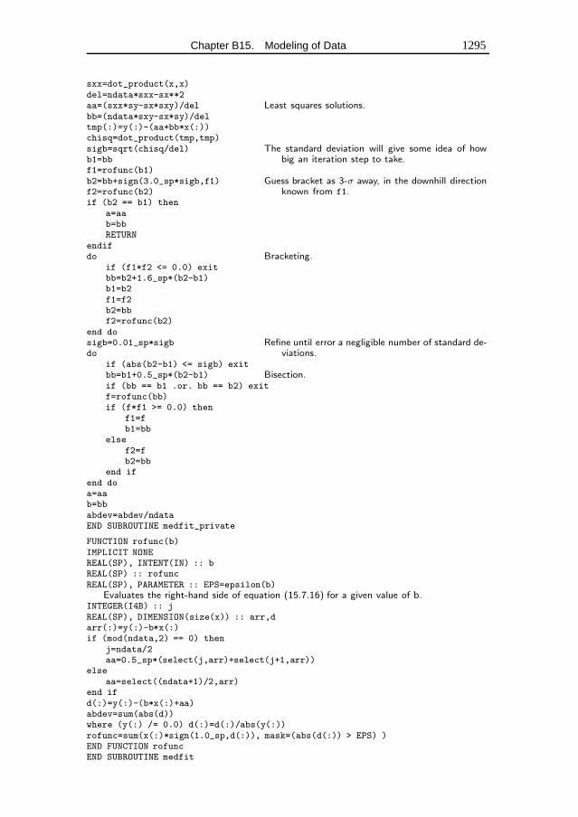
Chapter B15. Modeling of Data 1295
sxx=dot_product(x,x)del=ndata*sxx-sx**2aa=(sxx*sy-sx*sxy)/del Least squares solutions.bb=(ndata*sxy-sx*sy)/deltmp(:)=y(:)-(aa+bb*x(:))chisq=dot_product(tmp,tmp)sigb=sqrt(chisq/del) The standard deviation will give some idea of how
big an iteration step to take.b1=bbf1=rofunc(b1)b2=bb+sign(3.0_sp*sigb,f1) Guess bracket as 3-σ away, in the downhill direction
known from f1.f2=rofunc(b2)if (b2 == b1) then
a=aab=bbRETURN
endifdo Bracketing.
if (f1*f2 <= 0.0) exitbb=b2+1.6_sp*(b2-b1)b1=b2f1=f2b2=bbf2=rofunc(b2)
end dosigb=0.01_sp*sigb Refine until error a negligible number of standard de-
viations.doif (abs(b2-b1) <= sigb) exitbb=b1+0.5_sp*(b2-b1) Bisection.if (bb == b1 .or. bb == b2) exitf=rofunc(bb)if (f*f1 >= 0.0) then
f1=fb1=bb
elsef2=fb2=bb
end ifend doa=aab=bbabdev=abdev/ndataEND SUBROUTINE medfit_private
FUNCTION rofunc(b)IMPLICIT NONEREAL(SP), INTENT(IN) :: bREAL(SP) :: rofuncREAL(SP), PARAMETER :: EPS=epsilon(b)
Evaluates the right-hand side of equation (15.7.16) for a given value of b.INTEGER(I4B) :: jREAL(SP), DIMENSION(size(x)) :: arr,darr(:)=y(:)-b*x(:)if (mod(ndata,2) == 0) then
j=ndata/2aa=0.5_sp*(select(j,arr)+select(j+1,arr))
elseaa=select((ndata+1)/2,arr)
end ifd(:)=y(:)-(b*x(:)+aa)abdev=sum(abs(d))where (y(:) /= 0.0) d(:)=d(:)/abs(y(:))rofunc=sum(x(:)*sign(1.0_sp,d(:)), mask=(abs(d(:)) > EPS) )END FUNCTION rofuncEND SUBROUTINE medfit

1296 Chapter B15. Modeling of Data
f90The organization of this routine is similar to that of amoeba discussed onp. 1209. We want to keep the argument list of rofunc to a minimum,but we want to make clear what global variables it accesses and protect
medfit private’s name space. In the Fortran 77 version, we kept the onlyargument as b by passing the global variables in a common block. This required us tomake copies of the arrays x and y. An alternative Fortran 90 implementation wouldbe to use a module with pointers to the arguments of medfit like x and y that needto be passed to rofunc. We think the medfit private construction is simpler.
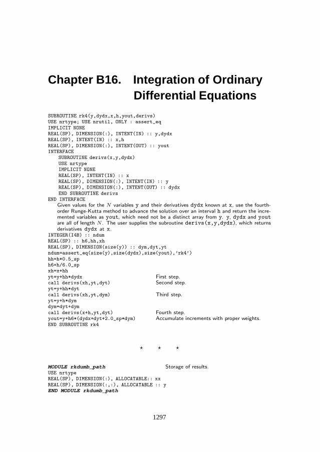
Chapter B16. Integration of OrdinaryDifferential Equations
SUBROUTINE rk4(y,dydx,x,h,yout,derivs)USE nrtype; USE nrutil, ONLY : assert_eqIMPLICIT NONEREAL(SP), DIMENSION(:), INTENT(IN) :: y,dydxREAL(SP), INTENT(IN) :: x,hREAL(SP), DIMENSION(:), INTENT(OUT) :: youtINTERFACE
SUBROUTINE derivs(x,y,dydx)USE nrtypeIMPLICIT NONEREAL(SP), INTENT(IN) :: xREAL(SP), DIMENSION(:), INTENT(IN) :: yREAL(SP), DIMENSION(:), INTENT(OUT) :: dydxEND SUBROUTINE derivs
END INTERFACEGiven values for the N variables y and their derivatives dydx known at x, use the fourth-order Runge-Kutta method to advance the solution over an interval h and return the incre-mented variables as yout, which need not be a distinct array from y. y, dydx and youtare all of length N . The user supplies the subroutine derivs(x,y,dydx), which returnsderivatives dydx at x.
INTEGER(I4B) :: ndumREAL(SP) :: h6,hh,xhREAL(SP), DIMENSION(size(y)) :: dym,dyt,ytndum=assert_eq(size(y),size(dydx),size(yout),’rk4’)hh=h*0.5_sph6=h/6.0_spxh=x+hhyt=y+hh*dydx First step.call derivs(xh,yt,dyt) Second step.yt=y+hh*dytcall derivs(xh,yt,dym) Third step.yt=y+h*dymdym=dyt+dymcall derivs(x+h,yt,dyt) Fourth step.yout=y+h6*(dydx+dyt+2.0_sp*dym) Accumulate increments with proper weights.END SUBROUTINE rk4
� � �
MODULE rkdumb_path Storage of results.USE nrtypeREAL(SP), DIMENSION(:), ALLOCATABLE:: xxREAL(SP), DIMENSION(:,:), ALLOCATABLE :: yEND MODULE rkdumb_path
1297
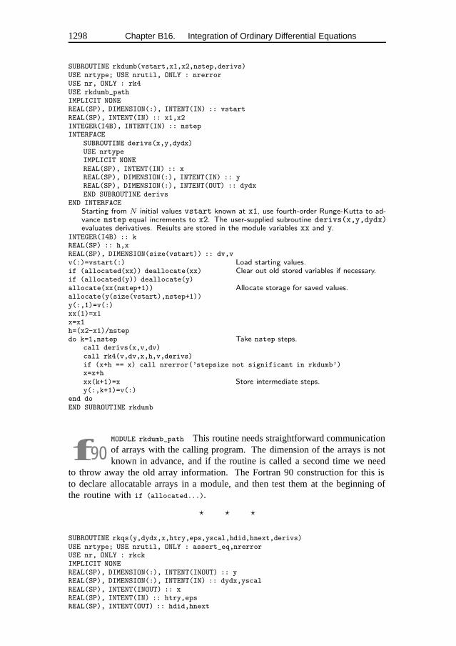
1298 Chapter B16. Integration of Ordinary Differential Equations
SUBROUTINE rkdumb(vstart,x1,x2,nstep,derivs)USE nrtype; USE nrutil, ONLY : nrerrorUSE nr, ONLY : rk4USE rkdumb_pathIMPLICIT NONEREAL(SP), DIMENSION(:), INTENT(IN) :: vstartREAL(SP), INTENT(IN) :: x1,x2INTEGER(I4B), INTENT(IN) :: nstepINTERFACE
SUBROUTINE derivs(x,y,dydx)USE nrtypeIMPLICIT NONEREAL(SP), INTENT(IN) :: xREAL(SP), DIMENSION(:), INTENT(IN) :: yREAL(SP), DIMENSION(:), INTENT(OUT) :: dydxEND SUBROUTINE derivs
END INTERFACEStarting from N initial values vstart known at x1, use fourth-order Runge-Kutta to ad-vance nstep equal increments to x2. The user-supplied subroutine derivs(x,y,dydx)evaluates derivatives. Results are stored in the module variables xx and y.
INTEGER(I4B) :: kREAL(SP) :: h,xREAL(SP), DIMENSION(size(vstart)) :: dv,vv(:)=vstart(:) Load starting values.if (allocated(xx)) deallocate(xx) Clear out old stored variables if necessary.if (allocated(y)) deallocate(y)allocate(xx(nstep+1)) Allocate storage for saved values.allocate(y(size(vstart),nstep+1))y(:,1)=v(:)xx(1)=x1x=x1h=(x2-x1)/nstepdo k=1,nstep Take nstep steps.
call derivs(x,v,dv)call rk4(v,dv,x,h,v,derivs)if (x+h == x) call nrerror(’stepsize not significant in rkdumb’)x=x+hxx(k+1)=x Store intermediate steps.y(:,k+1)=v(:)
end doEND SUBROUTINE rkdumb
f90MODULE rkdumb_path This routine needs straightforward communicationof arrays with the calling program. The dimension of the arrays is notknown in advance, and if the routine is called a second time we need
to throw away the old array information. The Fortran 90 construction for this isto declare allocatable arrays in a module, and then test them at the beginning ofthe routine withif (allocated...).
� � �
SUBROUTINE rkqs(y,dydx,x,htry,eps,yscal,hdid,hnext,derivs)USE nrtype; USE nrutil, ONLY : assert_eq,nrerrorUSE nr, ONLY : rkckIMPLICIT NONEREAL(SP), DIMENSION(:), INTENT(INOUT) :: yREAL(SP), DIMENSION(:), INTENT(IN) :: dydx,yscalREAL(SP), INTENT(INOUT) :: xREAL(SP), INTENT(IN) :: htry,epsREAL(SP), INTENT(OUT) :: hdid,hnext
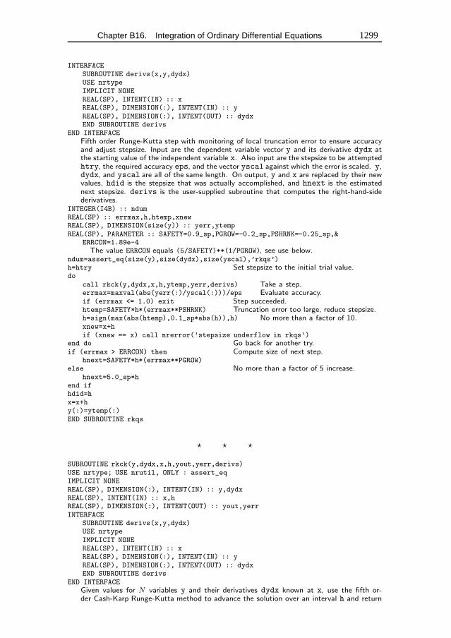
Chapter B16. Integration of Ordinary Differential Equations 1299
INTERFACESUBROUTINE derivs(x,y,dydx)USE nrtypeIMPLICIT NONEREAL(SP), INTENT(IN) :: xREAL(SP), DIMENSION(:), INTENT(IN) :: yREAL(SP), DIMENSION(:), INTENT(OUT) :: dydxEND SUBROUTINE derivs
END INTERFACEFifth order Runge-Kutta step with monitoring of local truncation error to ensure accuracyand adjust stepsize. Input are the dependent variable vector y and its derivative dydx atthe starting value of the independent variable x. Also input are the stepsize to be attemptedhtry, the required accuracy eps, and the vector yscal against which the error is scaled. y,dydx, and yscal are all of the same length. On output, y and x are replaced by their newvalues, hdid is the stepsize that was actually accomplished, and hnext is the estimatednext stepsize. derivs is the user-supplied subroutine that computes the right-hand-sidederivatives.
INTEGER(I4B) :: ndumREAL(SP) :: errmax,h,htemp,xnewREAL(SP), DIMENSION(size(y)) :: yerr,ytempREAL(SP), PARAMETER :: SAFETY=0.9_sp,PGROW=-0.2_sp,PSHRNK=-0.25_sp,&
ERRCON=1.89e-4The value ERRCON equals (5/SAFETY)**(1/PGROW), see use below.
ndum=assert_eq(size(y),size(dydx),size(yscal),’rkqs’)h=htry Set stepsize to the initial trial value.do
call rkck(y,dydx,x,h,ytemp,yerr,derivs) Take a step.errmax=maxval(abs(yerr(:)/yscal(:)))/eps Evaluate accuracy.if (errmax <= 1.0) exit Step succeeded.htemp=SAFETY*h*(errmax**PSHRNK) Truncation error too large, reduce stepsize.h=sign(max(abs(htemp),0.1_sp*abs(h)),h) No more than a factor of 10.xnew=x+hif (xnew == x) call nrerror(’stepsize underflow in rkqs’)
end do Go back for another try.if (errmax > ERRCON) then Compute size of next step.
hnext=SAFETY*h*(errmax**PGROW)else No more than a factor of 5 increase.
hnext=5.0_sp*hend ifhdid=hx=x+hy(:)=ytemp(:)END SUBROUTINE rkqs
� � �
SUBROUTINE rkck(y,dydx,x,h,yout,yerr,derivs)USE nrtype; USE nrutil, ONLY : assert_eqIMPLICIT NONEREAL(SP), DIMENSION(:), INTENT(IN) :: y,dydxREAL(SP), INTENT(IN) :: x,hREAL(SP), DIMENSION(:), INTENT(OUT) :: yout,yerrINTERFACE
SUBROUTINE derivs(x,y,dydx)USE nrtypeIMPLICIT NONEREAL(SP), INTENT(IN) :: xREAL(SP), DIMENSION(:), INTENT(IN) :: yREAL(SP), DIMENSION(:), INTENT(OUT) :: dydxEND SUBROUTINE derivs
END INTERFACEGiven values for N variables y and their derivatives dydx known at x, use the fifth or-der Cash-Karp Runge-Kutta method to advance the solution over an interval h and return
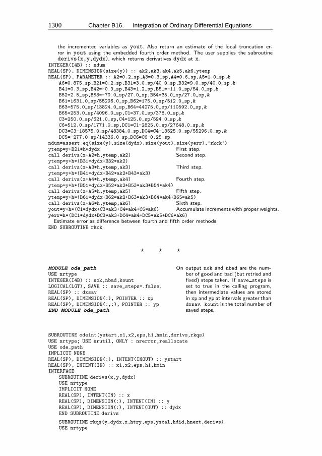
1300 Chapter B16. Integration of Ordinary Differential Equations
the incremented variables as yout. Also return an estimate of the local truncation er-ror in yout using the embedded fourth order method. The user supplies the subroutinederivs(x,y,dydx), which returns derivatives dydx at x.
INTEGER(I4B) :: ndumREAL(SP), DIMENSION(size(y)) :: ak2,ak3,ak4,ak5,ak6,ytempREAL(SP), PARAMETER :: A2=0.2_sp,A3=0.3_sp,A4=0.6_sp,A5=1.0_sp,&
A6=0.875_sp,B21=0.2_sp,B31=3.0_sp/40.0_sp,B32=9.0_sp/40.0_sp,&B41=0.3_sp,B42=-0.9_sp,B43=1.2_sp,B51=-11.0_sp/54.0_sp,&B52=2.5_sp,B53=-70.0_sp/27.0_sp,B54=35.0_sp/27.0_sp,&B61=1631.0_sp/55296.0_sp,B62=175.0_sp/512.0_sp,&B63=575.0_sp/13824.0_sp,B64=44275.0_sp/110592.0_sp,&B65=253.0_sp/4096.0_sp,C1=37.0_sp/378.0_sp,&C3=250.0_sp/621.0_sp,C4=125.0_sp/594.0_sp,&C6=512.0_sp/1771.0_sp,DC1=C1-2825.0_sp/27648.0_sp,&DC3=C3-18575.0_sp/48384.0_sp,DC4=C4-13525.0_sp/55296.0_sp,&DC5=-277.0_sp/14336.0_sp,DC6=C6-0.25_sp
ndum=assert_eq(size(y),size(dydx),size(yout),size(yerr),’rkck’)ytemp=y+B21*h*dydx First step.call derivs(x+A2*h,ytemp,ak2) Second step.ytemp=y+h*(B31*dydx+B32*ak2)call derivs(x+A3*h,ytemp,ak3) Third step.ytemp=y+h*(B41*dydx+B42*ak2+B43*ak3)call derivs(x+A4*h,ytemp,ak4) Fourth step.ytemp=y+h*(B51*dydx+B52*ak2+B53*ak3+B54*ak4)call derivs(x+A5*h,ytemp,ak5) Fifth step.ytemp=y+h*(B61*dydx+B62*ak2+B63*ak3+B64*ak4+B65*ak5)call derivs(x+A6*h,ytemp,ak6) Sixth step.yout=y+h*(C1*dydx+C3*ak3+C4*ak4+C6*ak6) Accumulate increments with proper weights.yerr=h*(DC1*dydx+DC3*ak3+DC4*ak4+DC5*ak5+DC6*ak6)Estimate error as difference between fourth and fifth order methods.
END SUBROUTINE rkck
� � �
MODULE ode_path On output nok and nbad are the num-ber of good and bad (but retried andfixed) steps taken. If save steps isset to true in the calling program,then intermediate values are storedin xp and yp at intervals greater thandxsav. kount is the total number ofsaved steps.
USE nrtypeINTEGER(I4B) :: nok,nbad,kountLOGICAL(LGT), SAVE :: save_steps=.false.REAL(SP) :: dxsavREAL(SP), DIMENSION(:), POINTER :: xpREAL(SP), DIMENSION(:,:), POINTER :: ypEND MODULE ode_path
SUBROUTINE odeint(ystart,x1,x2,eps,h1,hmin,derivs,rkqs)USE nrtype; USE nrutil, ONLY : nrerror,reallocateUSE ode_pathIMPLICIT NONEREAL(SP), DIMENSION(:), INTENT(INOUT) :: ystartREAL(SP), INTENT(IN) :: x1,x2,eps,h1,hminINTERFACE
SUBROUTINE derivs(x,y,dydx)USE nrtypeIMPLICIT NONEREAL(SP), INTENT(IN) :: xREAL(SP), DIMENSION(:), INTENT(IN) :: yREAL(SP), DIMENSION(:), INTENT(OUT) :: dydxEND SUBROUTINE derivs
SUBROUTINE rkqs(y,dydx,x,htry,eps,yscal,hdid,hnext,derivs)USE nrtype
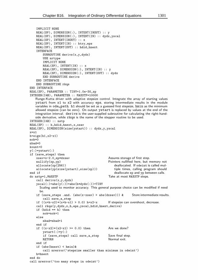
Chapter B16. Integration of Ordinary Differential Equations 1301
IMPLICIT NONEREAL(SP), DIMENSION(:), INTENT(INOUT) :: yREAL(SP), DIMENSION(:), INTENT(IN) :: dydx,yscalREAL(SP), INTENT(INOUT) :: xREAL(SP), INTENT(IN) :: htry,epsREAL(SP), INTENT(OUT) :: hdid,hnextINTERFACE
SUBROUTINE derivs(x,y,dydx)USE nrtypeIMPLICIT NONEREAL(SP), INTENT(IN) :: xREAL(SP), DIMENSION(:), INTENT(IN) :: yREAL(SP), DIMENSION(:), INTENT(OUT) :: dydxEND SUBROUTINE derivs
END INTERFACEEND SUBROUTINE rkqs
END INTERFACEREAL(SP), PARAMETER :: TINY=1.0e-30_spINTEGER(I4B), PARAMETER :: MAXSTP=10000
Runge-Kutta driver with adaptive stepsize control. Integrate the array of starting valuesystart from x1 to x2 with accuracy eps, storing intermediate results in the modulevariables in ode path. h1 should be set as a guessed first stepsize, hmin as the minimumallowed stepsize (can be zero). On output ystart is replaced by values at the end of theintegration interval. derivs is the user-supplied subroutine for calculating the right-hand-side derivative, while rkqs is the name of the stepper routine to be used.
INTEGER(I4B) :: nstpREAL(SP) :: h,hdid,hnext,x,xsavREAL(SP), DIMENSION(size(ystart)) :: dydx,y,yscalx=x1h=sign(h1,x2-x1)nok=0nbad=0kount=0y(:)=ystart(:)if (save_steps) then
xsav=x-2.0_sp*dxsav Assures storage of first step.nullify(xp,yp) Pointers nullified here, but memory not
deallocated. If odeint is called mul-tiple times, calling program shoulddeallocate xp and yp between calls.
allocate(xp(256))allocate(yp(size(ystart),size(xp)))
end ifdo nstp=1,MAXSTP Take at most MAXSTP steps.
call derivs(x,y,dydx)yscal(:)=abs(y(:))+abs(h*dydx(:))+TINYScaling used to monitor accuracy. This general purpose choice can be modified if needbe.
if (save_steps .and. (abs(x-xsav) > abs(dxsav))) & Store intermediate results.call save_a_step
if ((x+h-x2)*(x+h-x1) > 0.0) h=x2-x If stepsize can overshoot, decrease.call rkqs(y,dydx,x,h,eps,yscal,hdid,hnext,derivs)if (hdid == h) then
nok=nok+1else
nbad=nbad+1end ifif ((x-x2)*(x2-x1) >= 0.0) then Are we done?
ystart(:)=y(:)if (save_steps) call save_a_step Save final step.RETURN Normal exit.
end ifif (abs(hnext) < hmin)&
call nrerror(’stepsize smaller than minimum in odeint’)h=hnext
end docall nrerror(’too many steps in odeint’)
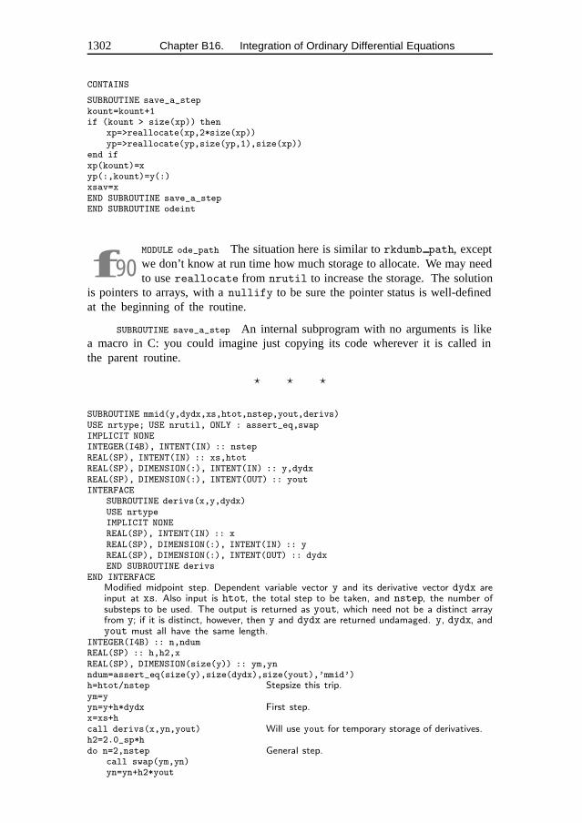
1302 Chapter B16. Integration of Ordinary Differential Equations
CONTAINS
SUBROUTINE save_a_stepkount=kount+1if (kount > size(xp)) then
xp=>reallocate(xp,2*size(xp))yp=>reallocate(yp,size(yp,1),size(xp))
end ifxp(kount)=xyp(:,kount)=y(:)xsav=xEND SUBROUTINE save_a_stepEND SUBROUTINE odeint
f90MODULE ode_path The situation here is similar torkdumb path, exceptwe don’t know at run time how much storage to allocate. We may needto usereallocate from nrutil to increase the storage. The solution
is pointers to arrays, with anullify to be sure the pointer status is well-definedat the beginning of the routine.
SUBROUTINE save_a_step An internal subprogram with no arguments is likea macro in C: you could imagine just copying its code wherever it is called inthe parent routine.
� � �
SUBROUTINE mmid(y,dydx,xs,htot,nstep,yout,derivs)USE nrtype; USE nrutil, ONLY : assert_eq,swapIMPLICIT NONEINTEGER(I4B), INTENT(IN) :: nstepREAL(SP), INTENT(IN) :: xs,htotREAL(SP), DIMENSION(:), INTENT(IN) :: y,dydxREAL(SP), DIMENSION(:), INTENT(OUT) :: youtINTERFACE
SUBROUTINE derivs(x,y,dydx)USE nrtypeIMPLICIT NONEREAL(SP), INTENT(IN) :: xREAL(SP), DIMENSION(:), INTENT(IN) :: yREAL(SP), DIMENSION(:), INTENT(OUT) :: dydxEND SUBROUTINE derivs
END INTERFACEModified midpoint step. Dependent variable vector y and its derivative vector dydx areinput at xs. Also input is htot, the total step to be taken, and nstep, the number ofsubsteps to be used. The output is returned as yout, which need not be a distinct arrayfrom y; if it is distinct, however, then y and dydx are returned undamaged. y, dydx, andyout must all have the same length.
INTEGER(I4B) :: n,ndumREAL(SP) :: h,h2,xREAL(SP), DIMENSION(size(y)) :: ym,ynndum=assert_eq(size(y),size(dydx),size(yout),’mmid’)h=htot/nstep Stepsize this trip.ym=yyn=y+h*dydx First step.x=xs+hcall derivs(x,yn,yout) Will use yout for temporary storage of derivatives.h2=2.0_sp*hdo n=2,nstep General step.
call swap(ym,yn)yn=yn+h2*yout
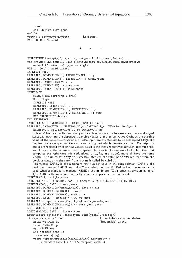
Chapter B16. Integration of Ordinary Differential Equations 1303
x=x+hcall derivs(x,yn,yout)
end doyout=0.5_sp*(ym+yn+h*yout) Last step.END SUBROUTINE mmid
� � �
SUBROUTINE bsstep(y,dydx,x,htry,eps,yscal,hdid,hnext,derivs)USE nrtype; USE nrutil, ONLY : arth,assert_eq,cumsum,iminloc,nrerror,&
outerdiff,outerprod,upper_triangleUSE nr, ONLY : mmid,pzextrIMPLICIT NONEREAL(SP), DIMENSION(:), INTENT(INOUT) :: yREAL(SP), DIMENSION(:), INTENT(IN) :: dydx,yscalREAL(SP), INTENT(INOUT) :: xREAL(SP), INTENT(IN) :: htry,epsREAL(SP), INTENT(OUT) :: hdid,hnextINTERFACE
SUBROUTINE derivs(x,y,dydx)USE nrtypeIMPLICIT NONEREAL(SP), INTENT(IN) :: xREAL(SP), DIMENSION(:), INTENT(IN) :: yREAL(SP), DIMENSION(:), INTENT(OUT) :: dydxEND SUBROUTINE derivs
END INTERFACEINTEGER(I4B), PARAMETER :: IMAX=9, KMAXX=IMAX-1REAL(SP), PARAMETER :: SAFE1=0.25_sp,SAFE2=0.7_sp,REDMAX=1.0e-5_sp,&
REDMIN=0.7_sp,TINY=1.0e-30_sp,SCALMX=0.1_spBulirsch-Stoer step with monitoring of local truncation error to ensure accuracy and adjuststepsize. Input are the dependent variable vector y and its derivative dydx at the startingvalue of the independent variable x. Also input are the stepsize to be attempted htry, therequired accuracy eps, and the vector yscal against which the error is scaled. On output, yand x are replaced by their new values, hdid is the stepsize that was actually accomplished,and hnext is the estimated next stepsize. derivs is the user-supplied subroutine thatcomputes the right-hand-side derivatives. y, dydx, and yscal must all have the samelength. Be sure to set htry on successive steps to the value of hnext returned from theprevious step, as is the case if the routine is called by odeint.Parameters: KMAXX is the maximum row number used in the extrapolation; IMAX is thenext row number; SAFE1 and SAFE2 are safety factors; REDMAX is the maximum factorused when a stepsize is reduced, REDMIN the minimum; TINY prevents division by zero;1/SCALMX is the maximum factor by which a stepsize can be increased.
INTEGER(I4B) :: k,km,ndumINTEGER(I4B), DIMENSION(IMAX) :: nseq = (/ 2,4,6,8,10,12,14,16,18 /)INTEGER(I4B), SAVE :: kopt,kmaxREAL(SP), DIMENSION(KMAXX,KMAXX), SAVE :: alfREAL(SP), DIMENSION(KMAXX) :: errREAL(SP), DIMENSION(IMAX), SAVE :: aREAL(SP), SAVE :: epsold = -1.0_sp,xnewREAL(SP) :: eps1,errmax,fact,h,red,scale,wrkmin,xestREAL(SP), DIMENSION(size(y)) :: yerr,ysav,yseqLOGICAL(LGT) :: reductLOGICAL(LGT), SAVE :: first=.true.ndum=assert_eq(size(y),size(dydx),size(yscal),’bsstep’)if (eps /= epsold) then A new tolerance, so reinitialize.
hnext=-1.0e29_sp “Impossible” values.xnew=-1.0e29_speps1=SAFE1*epsa(:)=cumsum(nseq,1)Compute α(k, q):
where (upper_triangle(KMAXX,KMAXX)) alf=eps1** &(outerdiff(a(2:),a(2:))/outerprod(arth( &
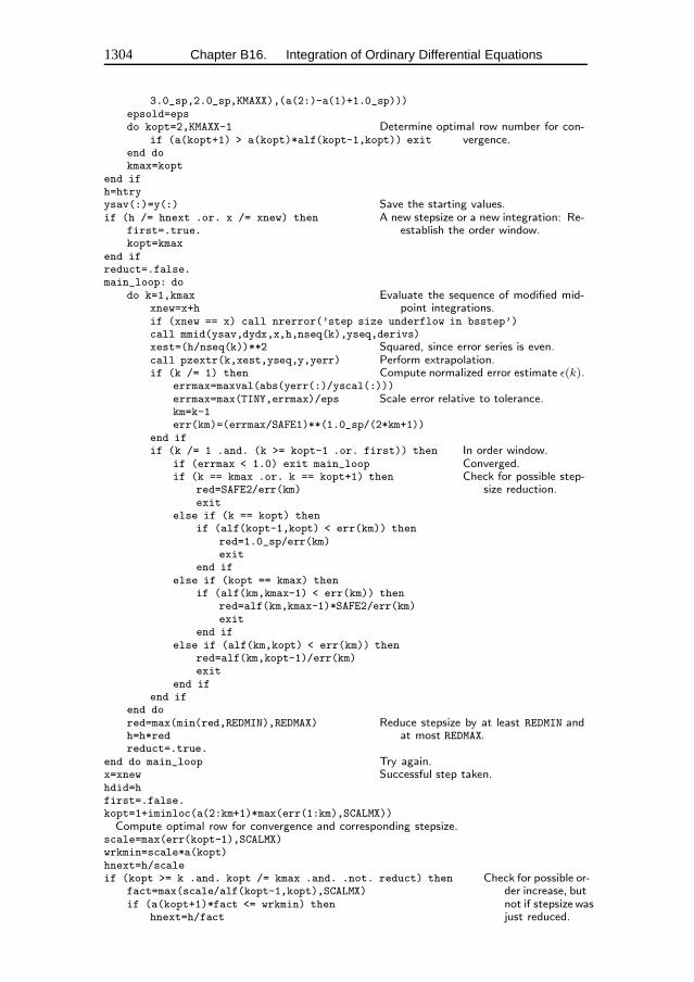
1304 Chapter B16. Integration of Ordinary Differential Equations
3.0_sp,2.0_sp,KMAXX),(a(2:)-a(1)+1.0_sp)))epsold=epsdo kopt=2,KMAXX-1 Determine optimal row number for con-
vergence.if (a(kopt+1) > a(kopt)*alf(kopt-1,kopt)) exitend dokmax=kopt
end ifh=htryysav(:)=y(:) Save the starting values.if (h /= hnext .or. x /= xnew) then A new stepsize or a new integration: Re-
establish the order window.first=.true.kopt=kmax
end ifreduct=.false.main_loop: do
do k=1,kmax Evaluate the sequence of modified mid-point integrations.xnew=x+h
if (xnew == x) call nrerror(’step size underflow in bsstep’)call mmid(ysav,dydx,x,h,nseq(k),yseq,derivs)xest=(h/nseq(k))**2 Squared, since error series is even.call pzextr(k,xest,yseq,y,yerr) Perform extrapolation.if (k /= 1) then Compute normalized error estimate ε(k).
errmax=maxval(abs(yerr(:)/yscal(:)))errmax=max(TINY,errmax)/eps Scale error relative to tolerance.km=k-1err(km)=(errmax/SAFE1)**(1.0_sp/(2*km+1))
end ifif (k /= 1 .and. (k >= kopt-1 .or. first)) then In order window.
if (errmax < 1.0) exit main_loop Converged.if (k == kmax .or. k == kopt+1) then Check for possible step-
size reduction.red=SAFE2/err(km)exit
else if (k == kopt) thenif (alf(kopt-1,kopt) < err(km)) then
red=1.0_sp/err(km)exit
end ifelse if (kopt == kmax) then
if (alf(km,kmax-1) < err(km)) thenred=alf(km,kmax-1)*SAFE2/err(km)exit
end ifelse if (alf(km,kopt) < err(km)) then
red=alf(km,kopt-1)/err(km)exit
end ifend if
end dored=max(min(red,REDMIN),REDMAX) Reduce stepsize by at least REDMIN and
at most REDMAX.h=h*redreduct=.true.
end do main_loop Try again.x=xnew Successful step taken.hdid=hfirst=.false.kopt=1+iminloc(a(2:km+1)*max(err(1:km),SCALMX))Compute optimal row for convergence and corresponding stepsize.
scale=max(err(kopt-1),SCALMX)wrkmin=scale*a(kopt)hnext=h/scaleif (kopt >= k .and. kopt /= kmax .and. .not. reduct) then Check for possible or-
der increase, butnot if stepsize wasjust reduced.
fact=max(scale/alf(kopt-1,kopt),SCALMX)if (a(kopt+1)*fact <= wrkmin) then
hnext=h/fact
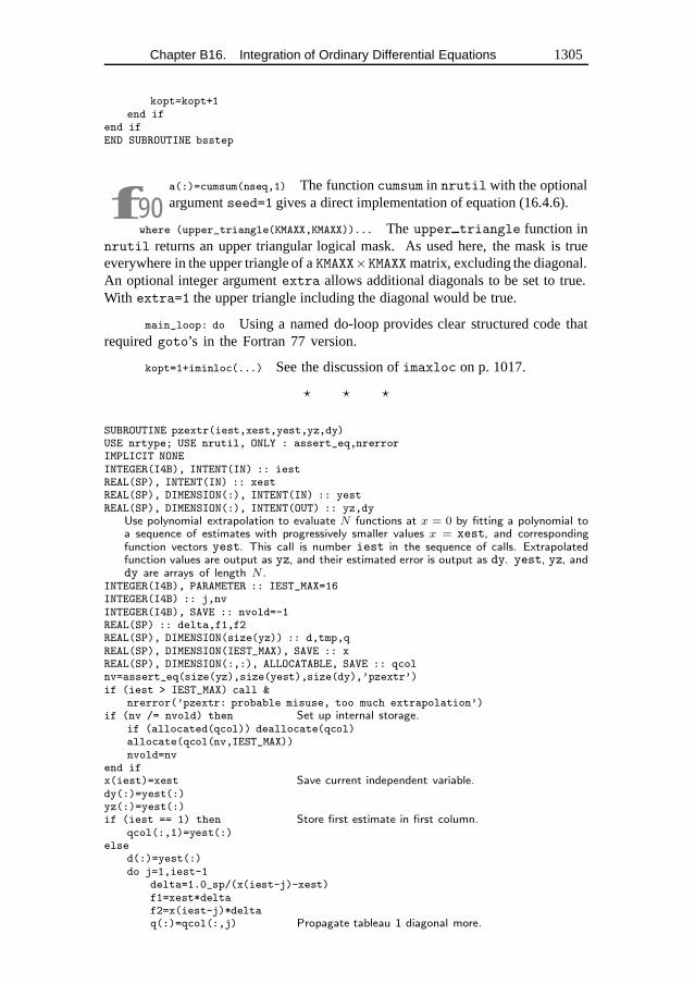
Chapter B16. Integration of Ordinary Differential Equations 1305
kopt=kopt+1end if
end ifEND SUBROUTINE bsstep
f90a(:)=cumsum(nseq,1) The functioncumsum in nrutil with the optionalargumentseed=1 gives a direct implementation of equation (16.4.6).
where (upper_triangle(KMAXX,KMAXX))... The upper triangle function innrutil returns an upper triangular logical mask. As used here, the mask is trueeverywhere in the upper triangle of aKMAXX×KMAXX matrix, excluding the diagonal.An optional integer argumentextra allows additional diagonals to be set to true.With extra=1 the upper triangle including the diagonal would be true.
main_loop: do Using a named do-loop provides clear structured code thatrequiredgoto’s in the Fortran 77 version.
kopt=1+iminloc(...) See the discussion ofimaxloc on p. 1017.
� � �
SUBROUTINE pzextr(iest,xest,yest,yz,dy)USE nrtype; USE nrutil, ONLY : assert_eq,nrerrorIMPLICIT NONEINTEGER(I4B), INTENT(IN) :: iestREAL(SP), INTENT(IN) :: xestREAL(SP), DIMENSION(:), INTENT(IN) :: yestREAL(SP), DIMENSION(:), INTENT(OUT) :: yz,dy
Use polynomial extrapolation to evaluate N functions at x = 0 by fitting a polynomial toa sequence of estimates with progressively smaller values x = xest, and correspondingfunction vectors yest. This call is number iest in the sequence of calls. Extrapolatedfunction values are output as yz, and their estimated error is output as dy. yest, yz, anddy are arrays of length N .
INTEGER(I4B), PARAMETER :: IEST_MAX=16INTEGER(I4B) :: j,nvINTEGER(I4B), SAVE :: nvold=-1REAL(SP) :: delta,f1,f2REAL(SP), DIMENSION(size(yz)) :: d,tmp,qREAL(SP), DIMENSION(IEST_MAX), SAVE :: xREAL(SP), DIMENSION(:,:), ALLOCATABLE, SAVE :: qcolnv=assert_eq(size(yz),size(yest),size(dy),’pzextr’)if (iest > IEST_MAX) call &
nrerror(’pzextr: probable misuse, too much extrapolation’)if (nv /= nvold) then Set up internal storage.
if (allocated(qcol)) deallocate(qcol)allocate(qcol(nv,IEST_MAX))nvold=nv
end ifx(iest)=xest Save current independent variable.dy(:)=yest(:)yz(:)=yest(:)if (iest == 1) then Store first estimate in first column.
qcol(:,1)=yest(:)else
d(:)=yest(:)do j=1,iest-1
delta=1.0_sp/(x(iest-j)-xest)f1=xest*deltaf2=x(iest-j)*deltaq(:)=qcol(:,j) Propagate tableau 1 diagonal more.
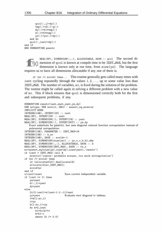
1306 Chapter B16. Integration of Ordinary Differential Equations
qcol(:,j)=dy(:)tmp(:)=d(:)-q(:)dy(:)=f1*tmp(:)d(:)=f2*tmp(:)yz(:)=yz(:)+dy(:)
end doqcol(:,iest)=dy(:)
end ifEND SUBROUTINE pzextr
f90REAL(SP), DIMENSION(:,:), ALLOCATABLE, SAVE :: qcol The second di-mension ofqcol is known at compile time to beIEST MAX, but the firstdimension is known only at run time, fromsize(yz). The language
requires us to have all dimensions allocatable if any one of them is.
if (nv /= nvold) then... This routine generally gets called many times withiest cycling repeatedly through the values1, 2, . . . , up to some value less thanIEST MAX. The number of variables,nv, is fixed during the solution of the problem.The routine might be called again in solving a different problem with a new valueof nv. This if block ensures thatqcol is dimensioned correctly both for the firstand subsequent problems, if any.
SUBROUTINE rzextr(iest,xest,yest,yz,dy)USE nrtype; USE nrutil, ONLY : assert_eq,nrerrorIMPLICIT NONEINTEGER(I4B), INTENT(IN) :: iestREAL(SP), INTENT(IN) :: xestREAL(SP), DIMENSION(:), INTENT(IN) :: yestREAL(SP), DIMENSION(:), INTENT(OUT) :: yz,dy
Exact substitute for pzextr, but uses diagonal rational function extrapolation instead ofpolynomial extrapolation.
INTEGER(I4B), PARAMETER :: IEST_MAX=16INTEGER(I4B) :: k,nvINTEGER(I4B), SAVE :: nvold=-1REAL(SP), DIMENSION(size(yz)) :: yy,v,c,b,b1,ddyREAL(SP), DIMENSION(:,:), ALLOCATABLE, SAVE :: dREAL(SP), DIMENSION(IEST_MAX), SAVE :: fx,xnv=assert_eq(size(yz),size(dy),size(yest),’rzextr’)if (iest > IEST_MAX) call &
nrerror(’rzextr: probable misuse, too much extrapolation’)if (nv /= nvold) then
if (allocated(d)) deallocate(d)allocate(d(nv,IEST_MAX))nvold=nv
end ifx(iest)=xest Save current independent variable.if (iest == 1) then
yz=yestd(:,1)=yestdy=yest
elsefx(2:iest)=x(iest-1:1:-1)/xestyy=yest Evaluate next diagonal in tableau.v=d(1:nv,1)c=yyd(1:nv,1)=yydo k=2,iest
b1=fx(k)*vb=b1-cwhere (b /= 0.0)
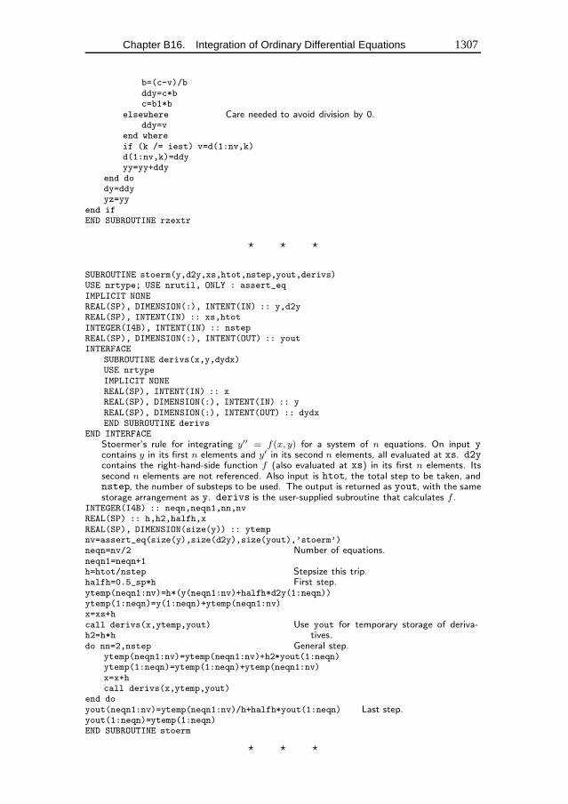
Chapter B16. Integration of Ordinary Differential Equations 1307
b=(c-v)/bddy=c*bc=b1*b
elsewhere Care needed to avoid division by 0.ddy=v
end whereif (k /= iest) v=d(1:nv,k)d(1:nv,k)=ddyyy=yy+ddy
end dody=ddyyz=yy
end ifEND SUBROUTINE rzextr
� � �
SUBROUTINE stoerm(y,d2y,xs,htot,nstep,yout,derivs)USE nrtype; USE nrutil, ONLY : assert_eqIMPLICIT NONEREAL(SP), DIMENSION(:), INTENT(IN) :: y,d2yREAL(SP), INTENT(IN) :: xs,htotINTEGER(I4B), INTENT(IN) :: nstepREAL(SP), DIMENSION(:), INTENT(OUT) :: youtINTERFACE
SUBROUTINE derivs(x,y,dydx)USE nrtypeIMPLICIT NONEREAL(SP), INTENT(IN) :: xREAL(SP), DIMENSION(:), INTENT(IN) :: yREAL(SP), DIMENSION(:), INTENT(OUT) :: dydxEND SUBROUTINE derivs
END INTERFACEStoermer’s rule for integrating y′′ = f(x, y) for a system of n equations. On input ycontains y in its first n elements and y′ in its second n elements, all evaluated at xs. d2ycontains the right-hand-side function f (also evaluated at xs) in its first n elements. Itssecond n elements are not referenced. Also input is htot, the total step to be taken, andnstep, the number of substeps to be used. The output is returned as yout, with the samestorage arrangement as y. derivs is the user-supplied subroutine that calculates f .
INTEGER(I4B) :: neqn,neqn1,nn,nvREAL(SP) :: h,h2,halfh,xREAL(SP), DIMENSION(size(y)) :: ytempnv=assert_eq(size(y),size(d2y),size(yout),’stoerm’)neqn=nv/2 Number of equations.neqn1=neqn+1h=htot/nstep Stepsize this trip.halfh=0.5_sp*h First step.ytemp(neqn1:nv)=h*(y(neqn1:nv)+halfh*d2y(1:neqn))ytemp(1:neqn)=y(1:neqn)+ytemp(neqn1:nv)x=xs+hcall derivs(x,ytemp,yout) Use yout for temporary storage of deriva-
tives.h2=h*hdo nn=2,nstep General step.
ytemp(neqn1:nv)=ytemp(neqn1:nv)+h2*yout(1:neqn)ytemp(1:neqn)=ytemp(1:neqn)+ytemp(neqn1:nv)x=x+hcall derivs(x,ytemp,yout)
end doyout(neqn1:nv)=ytemp(neqn1:nv)/h+halfh*yout(1:neqn) Last step.yout(1:neqn)=ytemp(1:neqn)END SUBROUTINE stoerm
� � �
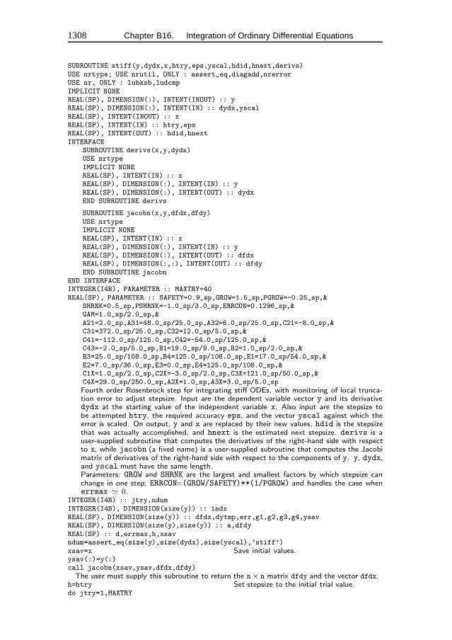
1308 Chapter B16. Integration of Ordinary Differential Equations
SUBROUTINE stiff(y,dydx,x,htry,eps,yscal,hdid,hnext,derivs)USE nrtype; USE nrutil, ONLY : assert_eq,diagadd,nrerrorUSE nr, ONLY : lubksb,ludcmpIMPLICIT NONEREAL(SP), DIMENSION(:), INTENT(INOUT) :: yREAL(SP), DIMENSION(:), INTENT(IN) :: dydx,yscalREAL(SP), INTENT(INOUT) :: xREAL(SP), INTENT(IN) :: htry,epsREAL(SP), INTENT(OUT) :: hdid,hnextINTERFACE
SUBROUTINE derivs(x,y,dydx)USE nrtypeIMPLICIT NONEREAL(SP), INTENT(IN) :: xREAL(SP), DIMENSION(:), INTENT(IN) :: yREAL(SP), DIMENSION(:), INTENT(OUT) :: dydxEND SUBROUTINE derivs
SUBROUTINE jacobn(x,y,dfdx,dfdy)USE nrtypeIMPLICIT NONEREAL(SP), INTENT(IN) :: xREAL(SP), DIMENSION(:), INTENT(IN) :: yREAL(SP), DIMENSION(:), INTENT(OUT) :: dfdxREAL(SP), DIMENSION(:,:), INTENT(OUT) :: dfdyEND SUBROUTINE jacobn
END INTERFACEINTEGER(I4B), PARAMETER :: MAXTRY=40REAL(SP), PARAMETER :: SAFETY=0.9_sp,GROW=1.5_sp,PGROW=-0.25_sp,&
SHRNK=0.5_sp,PSHRNK=-1.0_sp/3.0_sp,ERRCON=0.1296_sp,&GAM=1.0_sp/2.0_sp,&A21=2.0_sp,A31=48.0_sp/25.0_sp,A32=6.0_sp/25.0_sp,C21=-8.0_sp,&C31=372.0_sp/25.0_sp,C32=12.0_sp/5.0_sp,&C41=-112.0_sp/125.0_sp,C42=-54.0_sp/125.0_sp,&C43=-2.0_sp/5.0_sp,B1=19.0_sp/9.0_sp,B2=1.0_sp/2.0_sp,&B3=25.0_sp/108.0_sp,B4=125.0_sp/108.0_sp,E1=17.0_sp/54.0_sp,&E2=7.0_sp/36.0_sp,E3=0.0_sp,E4=125.0_sp/108.0_sp,&C1X=1.0_sp/2.0_sp,C2X=-3.0_sp/2.0_sp,C3X=121.0_sp/50.0_sp,&C4X=29.0_sp/250.0_sp,A2X=1.0_sp,A3X=3.0_sp/5.0_spFourth order Rosenbrock step for integrating stiff ODEs, with monitoring of local trunca-tion error to adjust stepsize. Input are the dependent variable vector y and its derivativedydx at the starting value of the independent variable x. Also input are the stepsize tobe attempted htry, the required accuracy eps, and the vector yscal against which theerror is scaled. On output, y and x are replaced by their new values, hdid is the stepsizethat was actually accomplished, and hnext is the estimated next stepsize. derivs is auser-supplied subroutine that computes the derivatives of the right-hand side with respectto x, while jacobn (a fixed name) is a user-supplied subroutine that computes the Jacobimatrix of derivatives of the right-hand side with respect to the components of y. y, dydx,and yscal must have the same length.Parameters: GROW and SHRNK are the largest and smallest factors by which stepsize canchange in one step; ERRCON=(GROW/SAFETY)**(1/PGROW) and handles the case whenerrmax � 0.
INTEGER(I4B) :: jtry,ndumINTEGER(I4B), DIMENSION(size(y)) :: indxREAL(SP), DIMENSION(size(y)) :: dfdx,dytmp,err,g1,g2,g3,g4,ysavREAL(SP), DIMENSION(size(y),size(y)) :: a,dfdyREAL(SP) :: d,errmax,h,xsavndum=assert_eq(size(y),size(dydx),size(yscal),’stiff’)xsav=x Save initial values.ysav(:)=y(:)call jacobn(xsav,ysav,dfdx,dfdy)The user must supply this subroutine to return the n× n matrix dfdy and the vector dfdx.
h=htry Set stepsize to the initial trial value.do jtry=1,MAXTRY
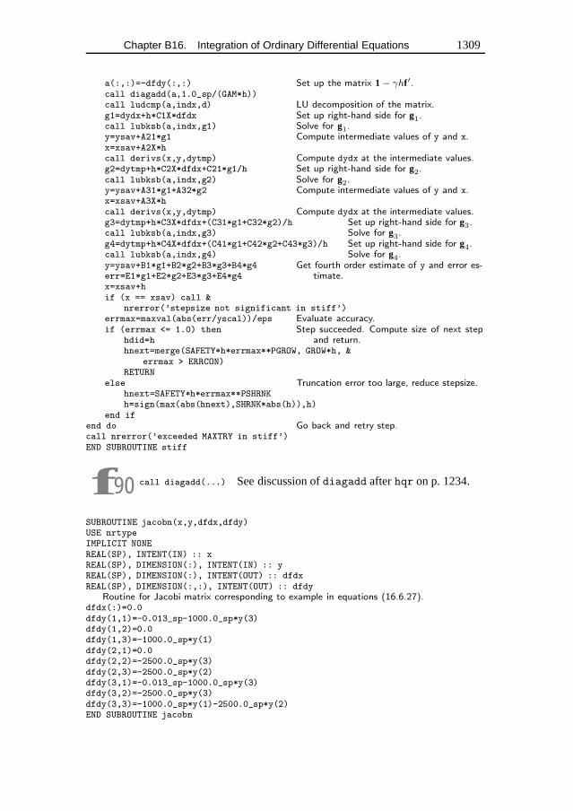
Chapter B16. Integration of Ordinary Differential Equations 1309
a(:,:)=-dfdy(:,:) Set up the matrix 1 − γhf′.call diagadd(a,1.0_sp/(GAM*h))call ludcmp(a,indx,d) LU decomposition of the matrix.g1=dydx+h*C1X*dfdx Set up right-hand side for g1.call lubksb(a,indx,g1) Solve for g1.y=ysav+A21*g1 Compute intermediate values of y and x.x=xsav+A2X*hcall derivs(x,y,dytmp) Compute dydx at the intermediate values.g2=dytmp+h*C2X*dfdx+C21*g1/h Set up right-hand side for g2.call lubksb(a,indx,g2) Solve for g2.y=ysav+A31*g1+A32*g2 Compute intermediate values of y and x.x=xsav+A3X*hcall derivs(x,y,dytmp) Compute dydx at the intermediate values.g3=dytmp+h*C3X*dfdx+(C31*g1+C32*g2)/h Set up right-hand side for g3.call lubksb(a,indx,g3) Solve for g3.g4=dytmp+h*C4X*dfdx+(C41*g1+C42*g2+C43*g3)/h Set up right-hand side for g4.call lubksb(a,indx,g4) Solve for g4.y=ysav+B1*g1+B2*g2+B3*g3+B4*g4 Get fourth order estimate of y and error es-
timate.err=E1*g1+E2*g2+E3*g3+E4*g4x=xsav+hif (x == xsav) call &
nrerror(’stepsize not significant in stiff’)errmax=maxval(abs(err/yscal))/eps Evaluate accuracy.if (errmax <= 1.0) then Step succeeded. Compute size of next step
and return.hdid=hhnext=merge(SAFETY*h*errmax**PGROW, GROW*h, &
errmax > ERRCON)RETURN
else Truncation error too large, reduce stepsize.hnext=SAFETY*h*errmax**PSHRNKh=sign(max(abs(hnext),SHRNK*abs(h)),h)
end ifend do Go back and retry step.call nrerror(’exceeded MAXTRY in stiff’)END SUBROUTINE stiff
f90 call diagadd(...) See discussion ofdiagadd afterhqr on p. 1234.
SUBROUTINE jacobn(x,y,dfdx,dfdy)USE nrtypeIMPLICIT NONEREAL(SP), INTENT(IN) :: xREAL(SP), DIMENSION(:), INTENT(IN) :: yREAL(SP), DIMENSION(:), INTENT(OUT) :: dfdxREAL(SP), DIMENSION(:,:), INTENT(OUT) :: dfdy
Routine for Jacobi matrix corresponding to example in equations (16.6.27).dfdx(:)=0.0dfdy(1,1)=-0.013_sp-1000.0_sp*y(3)dfdy(1,2)=0.0dfdy(1,3)=-1000.0_sp*y(1)dfdy(2,1)=0.0dfdy(2,2)=-2500.0_sp*y(3)dfdy(2,3)=-2500.0_sp*y(2)dfdy(3,1)=-0.013_sp-1000.0_sp*y(3)dfdy(3,2)=-2500.0_sp*y(3)dfdy(3,3)=-1000.0_sp*y(1)-2500.0_sp*y(2)END SUBROUTINE jacobn
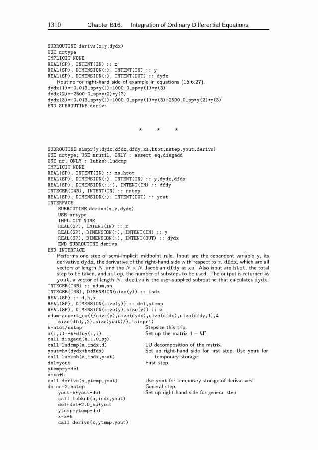
1310 Chapter B16. Integration of Ordinary Differential Equations
SUBROUTINE derivs(x,y,dydx)USE nrtypeIMPLICIT NONEREAL(SP), INTENT(IN) :: xREAL(SP), DIMENSION(:), INTENT(IN) :: yREAL(SP), DIMENSION(:), INTENT(OUT) :: dydx
Routine for right-hand side of example in equations (16.6.27).dydx(1)=-0.013_sp*y(1)-1000.0_sp*y(1)*y(3)dydx(2)=-2500.0_sp*y(2)*y(3)dydx(3)=-0.013_sp*y(1)-1000.0_sp*y(1)*y(3)-2500.0_sp*y(2)*y(3)END SUBROUTINE derivs
� � �
SUBROUTINE simpr(y,dydx,dfdx,dfdy,xs,htot,nstep,yout,derivs)USE nrtype; USE nrutil, ONLY : assert_eq,diagaddUSE nr, ONLY : lubksb,ludcmpIMPLICIT NONEREAL(SP), INTENT(IN) :: xs,htotREAL(SP), DIMENSION(:), INTENT(IN) :: y,dydx,dfdxREAL(SP), DIMENSION(:,:), INTENT(IN) :: dfdyINTEGER(I4B), INTENT(IN) :: nstepREAL(SP), DIMENSION(:), INTENT(OUT) :: youtINTERFACE
SUBROUTINE derivs(x,y,dydx)USE nrtypeIMPLICIT NONEREAL(SP), INTENT(IN) :: xREAL(SP), DIMENSION(:), INTENT(IN) :: yREAL(SP), DIMENSION(:), INTENT(OUT) :: dydxEND SUBROUTINE derivs
END INTERFACEPerforms one step of semi-implicit midpoint rule. Input are the dependent variable y, itsderivative dydx, the derivative of the right-hand side with respect to x, dfdx, which are allvectors of length N , and the N ×N Jacobian dfdy at xs. Also input are htot, the totalstep to be taken, and nstep, the number of substeps to be used. The output is returned asyout, a vector of length N . derivs is the user-supplied subroutine that calculates dydx.
INTEGER(I4B) :: ndum,nnINTEGER(I4B), DIMENSION(size(y)) :: indxREAL(SP) :: d,h,xREAL(SP), DIMENSION(size(y)) :: del,ytempREAL(SP), DIMENSION(size(y),size(y)) :: andum=assert_eq((/size(y),size(dydx),size(dfdx),size(dfdy,1),&
size(dfdy,2),size(yout)/),’simpr’)h=htot/nstep Stepsize this trip.a(:,:)=-h*dfdy(:,:) Set up the matrix 1 − hf′.call diagadd(a,1.0_sp)call ludcmp(a,indx,d) LU decomposition of the matrix.yout=h*(dydx+h*dfdx) Set up right-hand side for first step. Use yout for
temporary storage.call lubksb(a,indx,yout)del=yout First step.ytemp=y+delx=xs+hcall derivs(x,ytemp,yout) Use yout for temporary storage of derivatives.do nn=2,nstep General step.
yout=h*yout-del Set up right-hand side for general step.call lubksb(a,indx,yout)del=del+2.0_sp*youtytemp=ytemp+delx=x+hcall derivs(x,ytemp,yout)
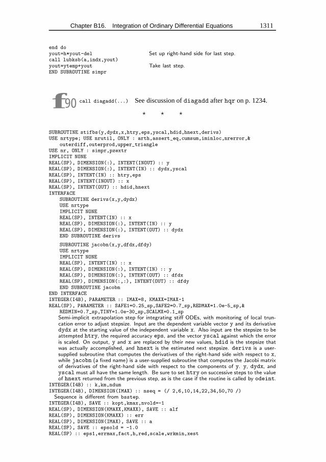
Chapter B16. Integration of Ordinary Differential Equations 1311
end doyout=h*yout-del Set up right-hand side for last step.call lubksb(a,indx,yout)yout=ytemp+yout Take last step.END SUBROUTINE simpr
f90 call diagadd(...) See discussion ofdiagadd afterhqr on p. 1234.
� � �
SUBROUTINE stifbs(y,dydx,x,htry,eps,yscal,hdid,hnext,derivs)USE nrtype; USE nrutil, ONLY : arth,assert_eq,cumsum,iminloc,nrerror,&
outerdiff,outerprod,upper_triangleUSE nr, ONLY : simpr,pzextrIMPLICIT NONEREAL(SP), DIMENSION(:), INTENT(INOUT) :: yREAL(SP), DIMENSION(:), INTENT(IN) :: dydx,yscalREAL(SP), INTENT(IN) :: htry,epsREAL(SP), INTENT(INOUT) :: xREAL(SP), INTENT(OUT) :: hdid,hnextINTERFACE
SUBROUTINE derivs(x,y,dydx)USE nrtypeIMPLICIT NONEREAL(SP), INTENT(IN) :: xREAL(SP), DIMENSION(:), INTENT(IN) :: yREAL(SP), DIMENSION(:), INTENT(OUT) :: dydxEND SUBROUTINE derivs
SUBROUTINE jacobn(x,y,dfdx,dfdy)USE nrtypeIMPLICIT NONEREAL(SP), INTENT(IN) :: xREAL(SP), DIMENSION(:), INTENT(IN) :: yREAL(SP), DIMENSION(:), INTENT(OUT) :: dfdxREAL(SP), DIMENSION(:,:), INTENT(OUT) :: dfdyEND SUBROUTINE jacobn
END INTERFACEINTEGER(I4B), PARAMETER :: IMAX=8, KMAXX=IMAX-1REAL(SP), PARAMETER :: SAFE1=0.25_sp,SAFE2=0.7_sp,REDMAX=1.0e-5_sp,&
REDMIN=0.7_sp,TINY=1.0e-30_sp,SCALMX=0.1_spSemi-implicit extrapolation step for integrating stiff ODEs, with monitoring of local trun-cation error to adjust stepsize. Input are the dependent variable vector y and its derivativedydx at the starting value of the independent variable x. Also input are the stepsize to beattempted htry, the required accuracy eps, and the vector yscal against which the erroris scaled. On output, y and x are replaced by their new values, hdid is the stepsize thatwas actually accomplished, and hnext is the estimated next stepsize. derivs is a user-supplied subroutine that computes the derivatives of the right-hand side with respect to x,while jacobn (a fixed name) is a user-supplied subroutine that computes the Jacobi matrixof derivatives of the right-hand side with respect to the components of y. y, dydx, andyscal must all have the same length. Be sure to set htry on successive steps to the valueof hnext returned from the previous step, as is the case if the routine is called by odeint.
INTEGER(I4B) :: k,km,ndumINTEGER(I4B), DIMENSION(IMAX) :: nseq = (/ 2,6,10,14,22,34,50,70 /)Sequence is different from bsstep.
INTEGER(I4B), SAVE :: kopt,kmax,nvold=-1REAL(SP), DIMENSION(KMAXX,KMAXX), SAVE :: alfREAL(SP), DIMENSION(KMAXX) :: errREAL(SP), DIMENSION(IMAX), SAVE :: aREAL(SP), SAVE :: epsold = -1.0REAL(SP) :: eps1,errmax,fact,h,red,scale,wrkmin,xest
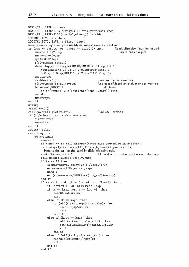
1312 Chapter B16. Integration of Ordinary Differential Equations
REAL(SP), SAVE :: xnewREAL(SP), DIMENSION(size(y)) :: dfdx,yerr,ysav,yseqREAL(SP), DIMENSION(size(y),size(y)) :: dfdyLOGICAL(LGT) :: reductLOGICAL(LGT), SAVE :: first=.true.ndum=assert_eq(size(y),size(dydx),size(yscal),’stifbs’)if (eps /= epsold .or. nvold /= size(y)) then Reinitialize also if number of vari-
ables has changed.hnext=-1.0e29_spxnew=-1.0e29_speps1=SAFE1*epsa(:)=cumsum(nseq,1)where (upper_triangle(KMAXX,KMAXX)) alf=eps1** &
(outerdiff(a(2:),a(2:))/outerprod(arth( &3.0_sp,2.0_sp,KMAXX),(a(2:)-a(1)+1.0_sp)))
epsold=epsnvold=size(y) Save number of variables.a(:)=cumsum(nseq,1+nvold) Add cost of Jacobian evaluations to work co-
efficients.do kopt=2,KMAXX-1if (a(kopt+1) > a(kopt)*alf(kopt-1,kopt)) exit
end dokmax=kopt
end ifh=htryysav(:)=y(:)call jacobn(x,y,dfdx,dfdy) Evaluate Jacobian.if (h /= hnext .or. x /= xnew) then
first=.true.kopt=kmax
end ifreduct=.false.main_loop: do
do k=1,kmaxxnew=x+hif (xnew == x) call nrerror(’step size underflow in stifbs’)call simpr(ysav,dydx,dfdx,dfdy,x,h,nseq(k),yseq,derivs)Here is the call to the semi-implicit midpoint rule.
xest=(h/nseq(k))**2 The rest of the routine is identical to bsstep.call pzextr(k,xest,yseq,y,yerr)if (k /= 1) then
errmax=maxval(abs(yerr(:)/yscal(:)))errmax=max(TINY,errmax)/epskm=k-1err(km)=(errmax/SAFE1)**(1.0_sp/(2*km+1))
end ifif (k /= 1 .and. (k >= kopt-1 .or. first)) then
if (errmax < 1.0) exit main_loopif (k == kmax .or. k == kopt+1) then
red=SAFE2/err(km)exit
else if (k == kopt) thenif (alf(kopt-1,kopt) < err(km)) then
red=1.0_sp/err(km)exit
end ifelse if (kopt == kmax) then
if (alf(km,kmax-1) < err(km)) thenred=alf(km,kmax-1)*SAFE2/err(km)exit
end ifelse if (alf(km,kopt) < err(km)) then
red=alf(km,kopt-1)/err(km)exit
end ifend if
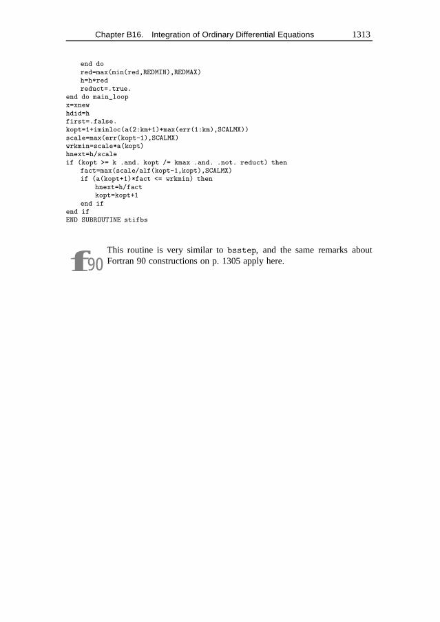
Chapter B16. Integration of Ordinary Differential Equations 1313
end dored=max(min(red,REDMIN),REDMAX)h=h*redreduct=.true.
end do main_loopx=xnewhdid=hfirst=.false.kopt=1+iminloc(a(2:km+1)*max(err(1:km),SCALMX))scale=max(err(kopt-1),SCALMX)wrkmin=scale*a(kopt)hnext=h/scaleif (kopt >= k .and. kopt /= kmax .and. .not. reduct) then
fact=max(scale/alf(kopt-1,kopt),SCALMX)if (a(kopt+1)*fact <= wrkmin) then
hnext=h/factkopt=kopt+1
end ifend ifEND SUBROUTINE stifbs
f90This routine is very similar tobsstep, and the same remarks aboutFortran 90 constructions on p. 1305 apply here.
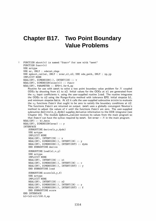
Chapter B17. Two Point BoundaryValue Problems
! FUNCTION shoot(v) is named "funcv" for use with "newt"FUNCTION funcv(v)USE nrtypeUSE nr, ONLY : odeint,rkqsUSE sphoot_caller, ONLY : nvar,x1,x2; USE ode_path, ONLY : xp,ypIMPLICIT NONEREAL(SP), DIMENSION(:), INTENT(IN) :: vREAL(SP), DIMENSION(size(v)) :: funcvREAL(SP), PARAMETER :: EPS=1.0e-6_sp
Routine for use with newt to solve a two point boundary value problem for N coupledODEs by shooting from x1 to x2. Initial values for the ODEs at x1 are generated fromthe n2 input coefficients v, using the user-supplied routine load. The routine integratesthe ODEs to x2 using the Runge-Kutta method with tolerance EPS, initial stepsize h1,and minimum stepsize hmin. At x2 it calls the user-supplied subroutine score to evaluatethe n2 functions funcv that ought to be zero to satisfy the boundary conditions at x2.The functions funcv are returned on output. newt uses a globally convergent Newton’smethod to adjust the values of v until the functions funcv are zero. The user-suppliedsubroutine derivs(x,y,dydx) supplies derivative information to the ODE integrator (seeChapter 16). The module sphoot caller receives its values from the main program sothat funcv can have the syntax required by newt. Set nvar = N in the main program.
REAL(SP) :: h1,hminREAL(SP), DIMENSION(nvar) :: yINTERFACE
SUBROUTINE derivs(x,y,dydx)USE nrtypeIMPLICIT NONEREAL(SP), INTENT(IN) :: xREAL(SP), DIMENSION(:), INTENT(IN) :: yREAL(SP), DIMENSION(:), INTENT(OUT) :: dydxEND SUBROUTINE derivs
SUBROUTINE load(x1,v,y)USE nrtypeIMPLICIT NONEREAL(SP), INTENT(IN) :: x1REAL(SP), DIMENSION(:), INTENT(IN) :: vREAL(SP), DIMENSION(:), INTENT(OUT) :: yEND SUBROUTINE load
SUBROUTINE score(x2,y,f)USE nrtypeIMPLICIT NONEREAL(SP), INTENT(IN) :: x2REAL(SP), DIMENSION(:), INTENT(IN) :: yREAL(SP), DIMENSION(:), INTENT(OUT) :: fEND SUBROUTINE score
END INTERFACEh1=(x2-x1)/100.0_sp
1314
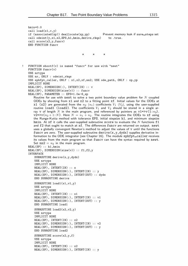
Chapter B17. Two Point Boundary Value Problems 1315
hmin=0.0call load(x1,v,y)if (associated(xp)) deallocate(xp,yp) Prevent memory leak if save steps set
to .true.call odeint(y,x1,x2,EPS,h1,hmin,derivs,rkqs)call score(x2,y,funcv)END FUNCTION funcv
� � �
! FUNCTION shootf(v) is named "funcv" for use with "newt"FUNCTION funcv(v)USE nrtypeUSE nr, ONLY : odeint,rkqsUSE sphfpt_caller, ONLY : x1,x2,xf,nn2; USE ode_path, ONLY : xp,ypIMPLICIT NONEREAL(SP), DIMENSION(:), INTENT(IN) :: vREAL(SP), DIMENSION(size(v)) :: funcvREAL(SP), PARAMETER :: EPS=1.0e-6_sp
Routine for use with newt to solve a two point boundary value problem for N coupledODEs by shooting from x1 and x2 to a fitting point xf. Initial values for the ODEs atx1 (x2) are generated from the n2 (n1) coefficients V1 (V2), using the user-suppliedroutine load1 (load2). The coefficients V1 and V2 should be stored in a single ar-ray v of length N in the main program, and referenced by pointers as v1=>v(1:n2),v2=>v(n2 + 1:N). Here N = n1 + n2. The routine integrates the ODEs to xf usingthe Runge-Kutta method with tolerance EPS, initial stepsize h1, and minimum stepsizehmin. At xf it calls the user-supplied subroutine score to evaluate the N functions f1and f2 that ought to match at xf. The differences funcv are returned on output. newtuses a globally convergent Newton’s method to adjust the values of v until the functionsfuncv are zero. The user-supplied subroutine derivs(x,y,dydx) supplies derivative in-formation to the ODE integrator (see Chapter 16). The module sphfpt caller receivesits values from the main program so that funcv can have the syntax required by newt.Set nn2 = n2 in the main program.
REAL(SP) :: h1,hminREAL(SP), DIMENSION(size(v)) :: f1,f2,yINTERFACE
SUBROUTINE derivs(x,y,dydx)USE nrtypeIMPLICIT NONEREAL(SP), INTENT(IN) :: xREAL(SP), DIMENSION(:), INTENT(IN) :: yREAL(SP), DIMENSION(:), INTENT(OUT) :: dydxEND SUBROUTINE derivs
SUBROUTINE load1(x1,v1,y)USE nrtypeIMPLICIT NONEREAL(SP), INTENT(IN) :: x1REAL(SP), DIMENSION(:), INTENT(IN) :: v1REAL(SP), DIMENSION(:), INTENT(OUT) :: yEND SUBROUTINE load1
SUBROUTINE load2(x2,v2,y)USE nrtypeIMPLICIT NONEREAL(SP), INTENT(IN) :: x2REAL(SP), DIMENSION(:), INTENT(IN) :: v2REAL(SP), DIMENSION(:), INTENT(OUT) :: yEND SUBROUTINE load2
SUBROUTINE score(x2,y,f)USE nrtypeIMPLICIT NONEREAL(SP), INTENT(IN) :: x2REAL(SP), DIMENSION(:), INTENT(IN) :: y
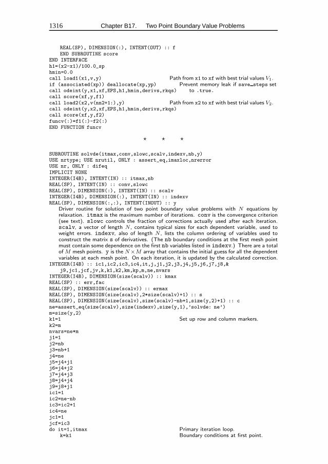
1316 Chapter B17. Two Point Boundary Value Problems
REAL(SP), DIMENSION(:), INTENT(OUT) :: fEND SUBROUTINE score
END INTERFACEh1=(x2-x1)/100.0_sphmin=0.0call load1(x1,v,y) Path from x1 to xf with best trial values V1.if (associated(xp)) deallocate(xp,yp) Prevent memory leak if save steps set
to .true.call odeint(y,x1,xf,EPS,h1,hmin,derivs,rkqs)call score(xf,y,f1)call load2(x2,v(nn2+1:),y) Path from x2 to xf with best trial values V2.call odeint(y,x2,xf,EPS,h1,hmin,derivs,rkqs)call score(xf,y,f2)funcv(:)=f1(:)-f2(:)END FUNCTION funcv
� � �
SUBROUTINE solvde(itmax,conv,slowc,scalv,indexv,nb,y)USE nrtype; USE nrutil, ONLY : assert_eq,imaxloc,nrerrorUSE nr, ONLY : difeqIMPLICIT NONEINTEGER(I4B), INTENT(IN) :: itmax,nbREAL(SP), INTENT(IN) :: conv,slowcREAL(SP), DIMENSION(:), INTENT(IN) :: scalvINTEGER(I4B), DIMENSION(:), INTENT(IN) :: indexvREAL(SP), DIMENSION(:,:), INTENT(INOUT) :: y
Driver routine for solution of two point boundary value problems with N equations byrelaxation. itmax is the maximum number of iterations. conv is the convergence criterion(see text). slowc controls the fraction of corrections actually used after each iteration.scalv, a vector of length N , contains typical sizes for each dependent variable, used toweight errors. indexv, also of length N , lists the column ordering of variables used toconstruct the matrix s of derivatives. (The nb boundary conditions at the first mesh pointmust contain some dependence on the first nb variables listed in indexv.) There are a totalofM mesh points. y is the N×M array that contains the initial guess for all the dependentvariables at each mesh point. On each iteration, it is updated by the calculated correction.
INTEGER(I4B) :: ic1,ic2,ic3,ic4,it,j,j1,j2,j3,j4,j5,j6,j7,j8,&j9,jc1,jcf,jv,k,k1,k2,km,kp,m,ne,nvars
INTEGER(I4B), DIMENSION(size(scalv)) :: kmaxREAL(SP) :: err,facREAL(SP), DIMENSION(size(scalv)) :: ermaxREAL(SP), DIMENSION(size(scalv),2*size(scalv)+1) :: sREAL(SP), DIMENSION(size(scalv),size(scalv)-nb+1,size(y,2)+1) :: cne=assert_eq(size(scalv),size(indexv),size(y,1),’solvde: ne’)m=size(y,2)k1=1 Set up row and column markers.k2=mnvars=ne*mj1=1j2=nbj3=nb+1j4=nej5=j4+j1j6=j4+j2j7=j4+j3j8=j4+j4j9=j8+j1ic1=1ic2=ne-nbic3=ic2+1ic4=nejc1=1jcf=ic3do it=1,itmax Primary iteration loop.
k=k1 Boundary conditions at first point.
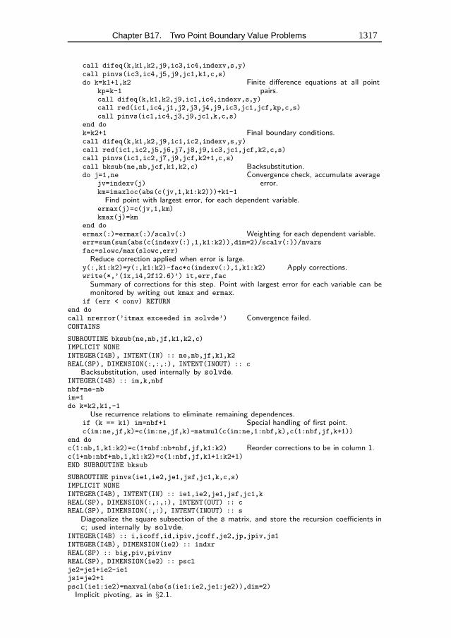
Chapter B17. Two Point Boundary Value Problems 1317
call difeq(k,k1,k2,j9,ic3,ic4,indexv,s,y)call pinvs(ic3,ic4,j5,j9,jc1,k1,c,s)do k=k1+1,k2 Finite difference equations at all point
pairs.kp=k-1call difeq(k,k1,k2,j9,ic1,ic4,indexv,s,y)call red(ic1,ic4,j1,j2,j3,j4,j9,ic3,jc1,jcf,kp,c,s)call pinvs(ic1,ic4,j3,j9,jc1,k,c,s)
end dok=k2+1 Final boundary conditions.call difeq(k,k1,k2,j9,ic1,ic2,indexv,s,y)call red(ic1,ic2,j5,j6,j7,j8,j9,ic3,jc1,jcf,k2,c,s)call pinvs(ic1,ic2,j7,j9,jcf,k2+1,c,s)call bksub(ne,nb,jcf,k1,k2,c) Backsubstitution.do j=1,ne Convergence check, accumulate average
error.jv=indexv(j)km=imaxloc(abs(c(jv,1,k1:k2)))+k1-1Find point with largest error, for each dependent variable.
ermax(j)=c(jv,1,km)kmax(j)=km
end doermax(:)=ermax(:)/scalv(:) Weighting for each dependent variable.err=sum(sum(abs(c(indexv(:),1,k1:k2)),dim=2)/scalv(:))/nvarsfac=slowc/max(slowc,err)Reduce correction applied when error is large.
y(:,k1:k2)=y(:,k1:k2)-fac*c(indexv(:),1,k1:k2) Apply corrections.write(*,’(1x,i4,2f12.6)’) it,err,facSummary of corrections for this step. Point with largest error for each variable can bemonitored by writing out kmax and ermax.
if (err < conv) RETURNend docall nrerror(’itmax exceeded in solvde’) Convergence failed.CONTAINS
SUBROUTINE bksub(ne,nb,jf,k1,k2,c)IMPLICIT NONEINTEGER(I4B), INTENT(IN) :: ne,nb,jf,k1,k2REAL(SP), DIMENSION(:,:,:), INTENT(INOUT) :: c
Backsubstitution, used internally by solvde.INTEGER(I4B) :: im,k,nbfnbf=ne-nbim=1do k=k2,k1,-1
Use recurrence relations to eliminate remaining dependences.if (k == k1) im=nbf+1 Special handling of first point.c(im:ne,jf,k)=c(im:ne,jf,k)-matmul(c(im:ne,1:nbf,k),c(1:nbf,jf,k+1))
end doc(1:nb,1,k1:k2)=c(1+nbf:nb+nbf,jf,k1:k2) Reorder corrections to be in column 1.c(1+nb:nbf+nb,1,k1:k2)=c(1:nbf,jf,k1+1:k2+1)END SUBROUTINE bksub
SUBROUTINE pinvs(ie1,ie2,je1,jsf,jc1,k,c,s)IMPLICIT NONEINTEGER(I4B), INTENT(IN) :: ie1,ie2,je1,jsf,jc1,kREAL(SP), DIMENSION(:,:,:), INTENT(OUT) :: cREAL(SP), DIMENSION(:,:), INTENT(INOUT) :: s
Diagonalize the square subsection of the s matrix, and store the recursion coefficients inc; used internally by solvde.
INTEGER(I4B) :: i,icoff,id,ipiv,jcoff,je2,jp,jpiv,js1INTEGER(I4B), DIMENSION(ie2) :: indxrREAL(SP) :: big,piv,pivinvREAL(SP), DIMENSION(ie2) :: psclje2=je1+ie2-ie1js1=je2+1pscl(ie1:ie2)=maxval(abs(s(ie1:ie2,je1:je2)),dim=2)Implicit pivoting, as in §2.1.
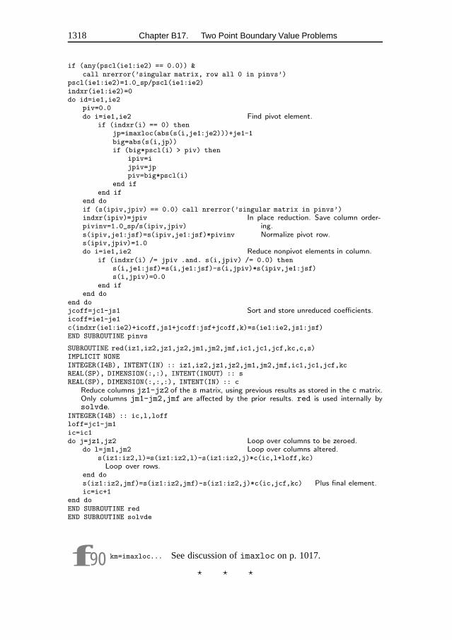
1318 Chapter B17. Two Point Boundary Value Problems
if (any(pscl(ie1:ie2) == 0.0)) &call nrerror(’singular matrix, row all 0 in pinvs’)
pscl(ie1:ie2)=1.0_sp/pscl(ie1:ie2)indxr(ie1:ie2)=0do id=ie1,ie2
piv=0.0do i=ie1,ie2 Find pivot element.
if (indxr(i) == 0) thenjp=imaxloc(abs(s(i,je1:je2)))+je1-1big=abs(s(i,jp))if (big*pscl(i) > piv) then
ipiv=ijpiv=jppiv=big*pscl(i)
end ifend if
end doif (s(ipiv,jpiv) == 0.0) call nrerror(’singular matrix in pinvs’)indxr(ipiv)=jpiv In place reduction. Save column order-
ing.pivinv=1.0_sp/s(ipiv,jpiv)s(ipiv,je1:jsf)=s(ipiv,je1:jsf)*pivinv Normalize pivot row.s(ipiv,jpiv)=1.0do i=ie1,ie2 Reduce nonpivot elements in column.
if (indxr(i) /= jpiv .and. s(i,jpiv) /= 0.0) thens(i,je1:jsf)=s(i,je1:jsf)-s(i,jpiv)*s(ipiv,je1:jsf)s(i,jpiv)=0.0
end ifend do
end dojcoff=jc1-js1 Sort and store unreduced coefficients.icoff=ie1-je1c(indxr(ie1:ie2)+icoff,js1+jcoff:jsf+jcoff,k)=s(ie1:ie2,js1:jsf)END SUBROUTINE pinvs
SUBROUTINE red(iz1,iz2,jz1,jz2,jm1,jm2,jmf,ic1,jc1,jcf,kc,c,s)IMPLICIT NONEINTEGER(I4B), INTENT(IN) :: iz1,iz2,jz1,jz2,jm1,jm2,jmf,ic1,jc1,jcf,kcREAL(SP), DIMENSION(:,:), INTENT(INOUT) :: sREAL(SP), DIMENSION(:,:,:), INTENT(IN) :: c
Reduce columns jz1-jz2 of the s matrix, using previous results as stored in the c matrix.Only columns jm1-jm2,jmf are affected by the prior results. red is used internally bysolvde.
INTEGER(I4B) :: ic,l,loffloff=jc1-jm1ic=ic1do j=jz1,jz2 Loop over columns to be zeroed.
do l=jm1,jm2 Loop over columns altered.s(iz1:iz2,l)=s(iz1:iz2,l)-s(iz1:iz2,j)*c(ic,l+loff,kc)Loop over rows.
end dos(iz1:iz2,jmf)=s(iz1:iz2,jmf)-s(iz1:iz2,j)*c(ic,jcf,kc) Plus final element.ic=ic+1
end doEND SUBROUTINE redEND SUBROUTINE solvde
f90 km=imaxloc... See discussion of imaxloc on p. 1017.
� � �
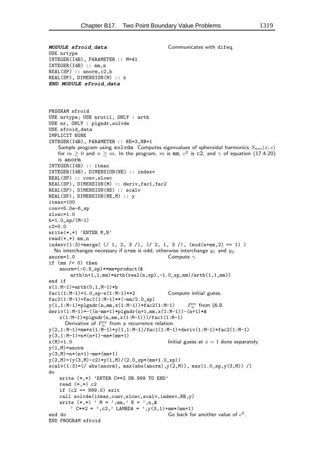
Chapter B17. Two Point Boundary Value Problems 1319
MODULE sfroid_data Communicates with difeq.USE nrtypeINTEGER(I4B), PARAMETER :: M=41INTEGER(I4B) :: mm,nREAL(SP) :: anorm,c2,hREAL(SP), DIMENSION(M) :: xEND MODULE sfroid_data
PROGRAM sfroidUSE nrtype; USE nrutil, ONLY : arthUSE nr, ONLY : plgndr,solvdeUSE sfroid_dataIMPLICIT NONEINTEGER(I4B), PARAMETER :: NE=3,NB=1
Sample program using solvde. Computes eigenvalues of spheroidal harmonics Smn(x; c)for m ≥ 0 and n ≥ m. In the program, m is mm, c2 is c2, and γ of equation (17.4.20)is anorm.
INTEGER(I4B) :: itmaxINTEGER(I4B), DIMENSION(NE) :: indexvREAL(SP) :: conv,slowcREAL(SP), DIMENSION(M) :: deriv,fac1,fac2REAL(SP), DIMENSION(NE) :: scalvREAL(SP), DIMENSION(NE,M) :: yitmax=100conv=5.0e-6_spslowc=1.0h=1.0_sp/(M-1)c2=0.0write(*,*) ’ENTER M,N’read(*,*) mm,nindexv(1:3)=merge( (/ 1, 2, 3 /), (/ 2, 1, 3 /), (mod(n+mm,2) == 1) )No interchanges necessary if n+mm is odd; otherwise interchange y1 and y2.
anorm=1.0 Compute γ.if (mm /= 0) then
anorm=(-0.5_sp)**mm*product(&arth(n+1,1,mm)*arth(real(n,sp),-1.0_sp,mm)/arth(1,1,mm))
end ifx(1:M-1)=arth(0,1,M-1)*hfac1(1:M-1)=1.0_sp-x(1:M-1)**2 Compute initial guess.fac2(1:M-1)=fac1(1:M-1)**(-mm/2.0_sp)y(1,1:M-1)=plgndr(n,mm,x(1:M-1))*fac2(1:M-1) Pm
n from §6.8.deriv(1:M-1)=-((n-mm+1)*plgndr(n+1,mm,x(1:M-1))-(n+1)*&
x(1:M-1)*plgndr(n,mm,x(1:M-1)))/fac1(1:M-1)Derivative of Pm
n from a recurrence relation.y(2,1:M-1)=mm*x(1:M-1)*y(1,1:M-1)/fac1(1:M-1)+deriv(1:M-1)*fac2(1:M-1)y(3,1:M-1)=n*(n+1)-mm*(mm+1)x(M)=1.0 Initial guess at x = 1 done separately.y(1,M)=anormy(3,M)=n*(n+1)-mm*(mm+1)y(2,M)=(y(3,M)-c2)*y(1,M)/(2.0_sp*(mm+1.0_sp))scalv(1:3)=(/ abs(anorm), max(abs(anorm),y(2,M)), max(1.0_sp,y(3,M)) /)do
write (*,*) ’ENTER C**2 OR 999 TO END’read (*,*) c2if (c2 == 999.0) exitcall solvde(itmax,conv,slowc,scalv,indexv,NB,y)write (*,*) ’ M = ’,mm,’ N = ’,n,&
’ C**2 = ’,c2,’ LAMBDA = ’,y(3,1)+mm*(mm+1)end do Go back for another value of c2.END PROGRAM sfroid
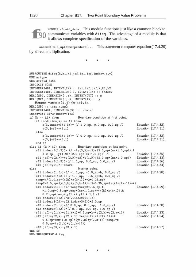
1320 Chapter B17. Two Point Boundary Value Problems
f90MODULE sfroid_data This module functions just like a common block tocommunicate variables with difeq. The advantage of a module is thatit allows complete specification of the variables.
anorm=(-0.5_sp)**mm*product(... This statement computes equation (17.4.20)by direct multiplication.
� � �
SUBROUTINE difeq(k,k1,k2,jsf,is1,isf,indexv,s,y)USE nrtypeUSE sfroid_dataIMPLICIT NONEINTEGER(I4B), INTENT(IN) :: is1,isf,jsf,k,k1,k2INTEGER(I4B), DIMENSION(:), INTENT(IN) :: indexvREAL(SP), DIMENSION(:,:), INTENT(OUT) :: sREAL(SP), DIMENSION(:,:), INTENT(IN) :: y
Returns matrix s(i,j) for solvde.REAL(SP) :: temp,temp2INTEGER(I4B), DIMENSION(3) :: indexv3indexv3(1:3)=3+indexv(1:3)if (k == k1) then Boundary condition at first point.
if (mod(n+mm,2) == 1) thens(3,indexv3(1:3))= (/ 1.0_sp, 0.0_sp, 0.0_sp /) Equation (17.4.32).s(3,jsf)=y(1,1) Equation (17.4.31).
elses(3,indexv3(1:3))= (/ 0.0_sp, 1.0_sp, 0.0_sp /) Equation (17.4.32).s(3,jsf)=y(2,1) Equation (17.4.31).
end ifelse if (k > k2) then Boundary conditions at last point.
s(1,indexv3(1:3))= (/ -(y(3,M)-c2)/(2.0_sp*(mm+1.0_sp)),&1.0_sp, -y(1,M)/(2.0_sp*(mm+1.0_sp)) /) Equation (17.4.35).
s(1,jsf)=y(2,M)-(y(3,M)-c2)*y(1,M)/(2.0_sp*(mm+1.0_sp)) Equation (17.4.33).s(2,indexv3(1:3))=(/ 1.0_sp, 0.0_sp, 0.0_sp /) Equation (17.4.36).s(2,jsf)=y(1,M)-anorm Equation (17.4.34).
else Interior point.s(1,indexv(1:3))=(/ -1.0_sp, -0.5_sp*h, 0.0_sp /) Equation (17.4.28).s(1,indexv3(1:3))=(/ 1.0_sp, -0.5_sp*h, 0.0_sp /)temp=h/(1.0_sp-(x(k)+x(k-1))**2*0.25_sp)temp2=0.5_sp*(y(3,k)+y(3,k-1))-c2*0.25_sp*(x(k)+x(k-1))**2s(2,indexv(1:3))=(/ temp*temp2*0.5_sp,& Equation (17.4.29).
-1.0_sp-0.5_sp*temp*(mm+1.0_sp)*(x(k)+x(k-1)),&0.25_sp*temp*(y(1,k)+y(1,k-1)) /)
s(2,indexv3(1:3))=s(2,indexv(1:3))s(2,indexv3(2))=s(2,indexv3(2))+2.0_sps(3,indexv(1:3))=(/ 0.0_sp, 0.0_sp, -1.0_sp /) Equation (17.4.30).s(3,indexv3(1:3))=(/ 0.0_sp, 0.0_sp, 1.0_sp /)s(1,jsf)=y(1,k)-y(1,k-1)-0.5_sp*h*(y(2,k)+y(2,k-1)) Equation (17.4.23).s(2,jsf)=y(2,k)-y(2,k-1)-temp*((x(k)+x(k-1))*& Equation (17.4.24).
0.5_sp*(mm+1.0_sp)*(y(2,k)+y(2,k-1))-temp2*&0.5_sp*(y(1,k)+y(1,k-1)))
s(3,jsf)=y(3,k)-y(3,k-1) Equation (17.4.27).end ifEND SUBROUTINE difeq
� � �
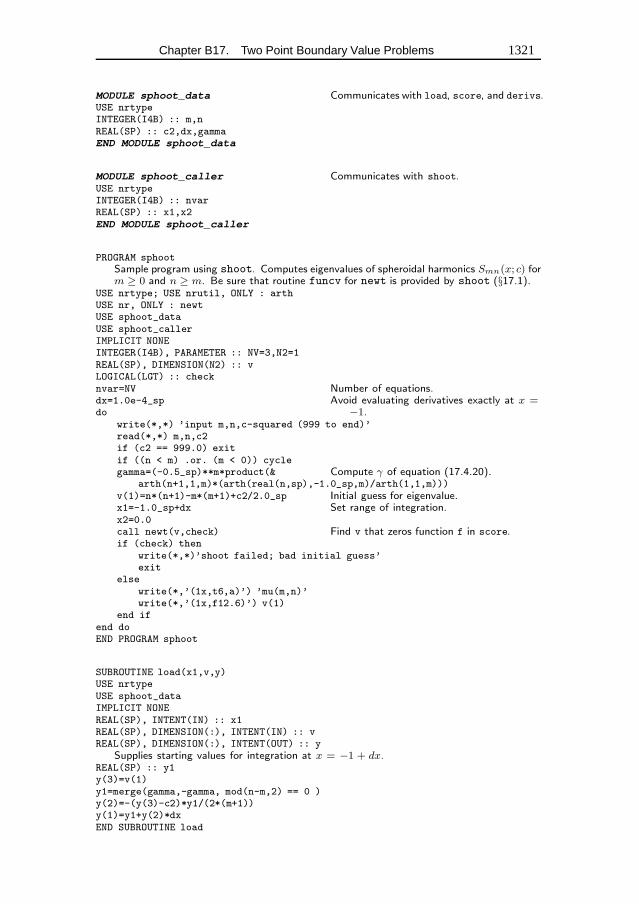
Chapter B17. Two Point Boundary Value Problems 1321
MODULE sphoot_data Communicates with load, score, and derivs.USE nrtypeINTEGER(I4B) :: m,nREAL(SP) :: c2,dx,gammaEND MODULE sphoot_data
MODULE sphoot_caller Communicates with shoot.USE nrtypeINTEGER(I4B) :: nvarREAL(SP) :: x1,x2END MODULE sphoot_caller
PROGRAM sphootSample program using shoot. Computes eigenvalues of spheroidal harmonics Smn(x; c) form ≥ 0 and n ≥ m. Be sure that routine funcv for newt is provided by shoot (§17.1).
USE nrtype; USE nrutil, ONLY : arthUSE nr, ONLY : newtUSE sphoot_dataUSE sphoot_callerIMPLICIT NONEINTEGER(I4B), PARAMETER :: NV=3,N2=1REAL(SP), DIMENSION(N2) :: vLOGICAL(LGT) :: checknvar=NV Number of equations.dx=1.0e-4_sp Avoid evaluating derivatives exactly at x =
−1.dowrite(*,*) ’input m,n,c-squared (999 to end)’read(*,*) m,n,c2if (c2 == 999.0) exitif ((n < m) .or. (m < 0)) cyclegamma=(-0.5_sp)**m*product(& Compute γ of equation (17.4.20).
arth(n+1,1,m)*(arth(real(n,sp),-1.0_sp,m)/arth(1,1,m)))v(1)=n*(n+1)-m*(m+1)+c2/2.0_sp Initial guess for eigenvalue.x1=-1.0_sp+dx Set range of integration.x2=0.0call newt(v,check) Find v that zeros function f in score.if (check) then
write(*,*)’shoot failed; bad initial guess’exit
elsewrite(*,’(1x,t6,a)’) ’mu(m,n)’write(*,’(1x,f12.6)’) v(1)
end ifend doEND PROGRAM sphoot
SUBROUTINE load(x1,v,y)USE nrtypeUSE sphoot_dataIMPLICIT NONEREAL(SP), INTENT(IN) :: x1REAL(SP), DIMENSION(:), INTENT(IN) :: vREAL(SP), DIMENSION(:), INTENT(OUT) :: y
Supplies starting values for integration at x = −1 + dx.REAL(SP) :: y1y(3)=v(1)y1=merge(gamma,-gamma, mod(n-m,2) == 0 )y(2)=-(y(3)-c2)*y1/(2*(m+1))y(1)=y1+y(2)*dxEND SUBROUTINE load
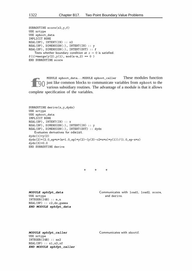
1322 Chapter B17. Two Point Boundary Value Problems
SUBROUTINE score(x2,y,f)USE nrtypeUSE sphoot_dataIMPLICIT NONEREAL(SP), INTENT(IN) :: x2REAL(SP), DIMENSION(:), INTENT(IN) :: yREAL(SP), DIMENSION(:), INTENT(OUT) :: f
Tests whether boundary condition at x = 0 is satisfied.f(1)=merge(y(2),y(1), mod(n-m,2) == 0 )END SUBROUTINE score
f90MODULE sphoot_data...MODULE sphoot_caller These modules functionjust like common blocks to communicate variables from sphoot to thevarious subsidiary routines. The advantage of a module is that it allows
complete specification of the variables.
SUBROUTINE derivs(x,y,dydx)USE nrtypeUSE sphoot_dataIMPLICIT NONEREAL(SP), INTENT(IN) :: xREAL(SP), DIMENSION(:), INTENT(IN) :: yREAL(SP), DIMENSION(:), INTENT(OUT) :: dydx
Evaluates derivatives for odeint.dydx(1)=y(2)dydx(2)=(2.0_sp*x*(m+1.0_sp)*y(2)-(y(3)-c2*x*x)*y(1))/(1.0_sp-x*x)dydx(3)=0.0END SUBROUTINE derivs
� � �
MODULE sphfpt_data Communicates with load1, load2, score,and derivs.USE nrtype
INTEGER(I4B) :: m,nREAL(SP) :: c2,dx,gammaEND MODULE sphfpt_data
MODULE sphfpt_caller Communicates with shootf.USE nrtypeINTEGER(I4B) :: nn2REAL(SP) :: x1,x2,xfEND MODULE sphfpt_caller
Chapter B17. Two Point Boundary Value Problems 1323
PROGRAM sphfptSample program using shootf. Computes eigenvalues of spheroidal harmonics Smn(x; c)form ≥ 0 and n ≥ m. Be sure that routine funcv for newt is provided by shootf (§17.2).The routine derivs is the same as for sphoot.
USE nrtype; USE nrutil, ONLY : arthUSE nr, ONLY : newtUSE sphfpt_dataUSE sphfpt_callerIMPLICIT NONEINTEGER(I4B), PARAMETER :: N1=2,N2=1,NTOT=N1+N2REAL(SP), PARAMETER :: DXX=1.0e-4_spREAL(SP), DIMENSION(:), POINTER :: v1,v2REAL(SP), DIMENSION(NTOT), TARGET :: vLOGICAL(LGT) :: checkv1=>v(1:N2)v2=>v(N2+1:NTOT)nn2=N2dx=DXX Avoid evaluating derivatives exactly at x =
±1.dowrite(*,*) ’input m,n,c-squared (999 to end)’read(*,*) m,n,c2if (c2 == 999.0) exitif ((n < m) .or. (m < 0)) cyclegamma=(-0.5_sp)**m*product(& Compute γ of equation (17.4.20).
arth(n+1,1,m)*(arth(real(n,sp),-1.0_sp,m)/arth(1,1,m)))v1(1)=n*(n+1)-m*(m+1)+c2/2.0_sp Initial guess for eigenvalue and function value.v2(2)=v1(1)v2(1)=gamma*(1.0_sp-(v2(2)-c2)*dx/(2*(m+1)))x1=-1.0_sp+dx Set range of integration.x2=1.0_sp-dxxf=0.0 Fitting point.call newt(v,check) Find v that zeros function f in score.if (check) then
write(*,*) ’shootf failed; bad initial guess’exit
elsewrite(*,’(1x,t6,a)’) ’mu(m,n)’write(*,’(1x,f12.6)’) v1(1)
end ifend doEND PROGRAM sphfpt
SUBROUTINE load1(x1,v1,y)USE nrtypeUSE sphfpt_dataIMPLICIT NONEREAL(SP), INTENT(IN) :: x1REAL(SP), DIMENSION(:), INTENT(IN) :: v1REAL(SP), DIMENSION(:), INTENT(OUT) :: y
Supplies starting values for integration at x = −1 + dx.REAL(SP) :: y1y(3)=v1(1)y1=merge(gamma,-gamma,mod(n-m,2) == 0)y(2)=-(y(3)-c2)*y1/(2*(m+1))y(1)=y1+y(2)*dxEND SUBROUTINE load1
1324 Chapter B17. Two Point Boundary Value Problems
SUBROUTINE load2(x2,v2,y)USE nrtypeUSE sphfpt_dataIMPLICIT NONEREAL(SP), INTENT(IN) :: x2REAL(SP), DIMENSION(:), INTENT(IN) :: v2REAL(SP), DIMENSION(:), INTENT(OUT) :: y
Supplies starting values for integration at x = 1 − dx.y(3)=v2(2)y(1)=v2(1)y(2)=(y(3)-c2)*y(1)/(2*(m+1))END SUBROUTINE load2
SUBROUTINE score(xf,y,f)USE nrtypeUSE sphfpt_dataIMPLICIT NONEREAL(SP), INTENT(IN) :: xfREAL(SP), DIMENSION(:), INTENT(IN) :: yREAL(SP), DIMENSION(:), INTENT(OUT) :: f
Tests whether solutions match at fitting point x = 0.f(1:3)=y(1:3)END SUBROUTINE score
f90MODULE sphfpt_data...MODULE sphfpt_caller These modules functionjust like common blocks to communicate variables from sphfpt to thevarious subsidiary routines. The advantage of a module is that it allows
complete specification of the variables.
Chapter B18. Integral Equationsand InverseTheory
SUBROUTINE fred2(a,b,t,f,w,g,ak)USE nrtype; USE nrutil, ONLY : assert_eq,unit_matrixUSE nr, ONLY : gauleg,lubksb,ludcmpIMPLICIT NONEREAL(SP), INTENT(IN) :: a,bREAL(SP), DIMENSION(:), INTENT(OUT) :: t,f,wINTERFACE
FUNCTION g(t)USE nrtypeIMPLICIT NONEREAL(SP), DIMENSION(:), INTENT(IN) :: tREAL(SP), DIMENSION(size(t)) :: gEND FUNCTION g
FUNCTION ak(t,s)USE nrtypeIMPLICIT NONEREAL(SP), DIMENSION(:), INTENT(IN) :: t,sREAL(SP), DIMENSION(size(t),size(s)) :: akEND FUNCTION ak
END INTERFACESolves a linear Fredholm equation of the second kind by N -point Gaussian quadrature. Oninput, a and b are the limits of integration. g and ak are user-supplied external functions. greturns g(t) as a vector of lengthN for a vector ofN arguments, while ak returns λK(t, s) asan N×N matrix. The routine returns arrays t and f of length N containing the abscissas tiof the Gaussian quadrature and the solution f at these abscissas. Also returned is the arrayw of length N of Gaussian weights for use with the Nystrom interpolation routine fredin.
INTEGER(I4B) :: nINTEGER(I4B), DIMENSION(size(f)) :: indxREAL(SP) :: dREAL(SP), DIMENSION(size(f),size(f)) :: omkn=assert_eq(size(f),size(t),size(w),’fred2’)call gauleg(a,b,t,w) Replace gauleg with another routine if not
using Gauss-Legendre quadrature.call unit_matrix(omk)omk=omk-ak(t,t)*spread(w,dim=1,ncopies=n) Form 1 − λK.f=g(t)call ludcmp(omk,indx,d) Solve linear equations.call lubksb(omk,indx,f)END SUBROUTINE fred2
f90call unit_matrix(omk) The unit matrix routine in nrutil does ex-actly what its name suggests.
1325
1326 Chapter B18. Integral Equations and Inverse Theory
omk=omk-ak(t,t)*spread(w,dim=1,ncopies=n) By now this idiom should besecond nature: the first column of ak gets multiplied by the first element of w,and so on.
� � �
FUNCTION fredin(x,a,b,t,f,w,g,ak)USE nrtype; USE nrutil, ONLY : assert_eqIMPLICIT NONEREAL(SP), INTENT(IN) :: a,bREAL(SP), DIMENSION(:), INTENT(IN) :: x,t,f,wREAL(SP), DIMENSION(size(x)) :: fredinINTERFACE
FUNCTION g(t)USE nrtypeIMPLICIT NONEREAL(SP), DIMENSION(:), INTENT(IN) :: tREAL(SP), DIMENSION(size(t)) :: gEND FUNCTION g
FUNCTION ak(t,s)USE nrtypeIMPLICIT NONEREAL(SP), DIMENSION(:), INTENT(IN) :: t,sREAL(SP), DIMENSION(size(t),size(s)) :: akEND FUNCTION ak
END INTERFACEInput are arrays t and w of length N containing the abscissas and weights of the N -pointGaussian quadrature, and the solution array f of length N from fred2. The functionfredin returns the array of values of f at an array of points x using the Nystrom interpo-lation formula. On input, a and b are the limits of integration. g and ak are user-suppliedexternal functions. g returns g(t) as a vector of length N for a vector of N arguments,while ak returns λK(t, s) as an N × N matrix.
INTEGER(I4B) :: nn=assert_eq(size(f),size(t),size(w),’fredin’)fredin=g(x)+matmul(ak(x,t),w*f)END FUNCTION fredin
f90fredin=g(x)+matmul... Fortran 90 allows very concise coding here,which also happens to be much closer to the mathematical formulationthan the loops required in Fortran 77.
� � �
SUBROUTINE voltra(t0,h,t,f,g,ak)USE nrtype; USE nrutil, ONLY : array_copy,assert_eq,unit_matrixUSE nr, ONLY : lubksb,ludcmpIMPLICIT NONEREAL(SP), INTENT(IN) :: t0,hREAL(SP), DIMENSION(:), INTENT(OUT) :: tREAL(SP), DIMENSION(:,:), INTENT(OUT) :: fINTERFACE
FUNCTION g(t)USE nrtypeIMPLICIT NONEREAL(SP), INTENT(IN) :: tREAL(SP), DIMENSION(:), POINTER :: gEND FUNCTION g
FUNCTION ak(t,s)
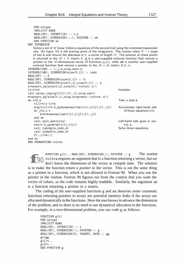
Chapter B18. Integral Equations and Inverse Theory 1327
USE nrtypeIMPLICIT NONEREAL(SP), INTENT(IN) :: t,sREAL(SP), DIMENSION(:,:), POINTER :: akEND FUNCTION ak
END INTERFACESolves a set ofM linear Volterra equations of the second kind using the extended trapezoidalrule. On input, t0 is the starting point of the integration. The routine takes N − 1 stepsof size h and returns the abscissas in t, a vector of length N . The solution at these pointsis returned in the M × N matrix f. g is a user-supplied external function that returns apointer to the M -dimensional vector of functions gk(t), while ak is another user-suppliedexternal function that returns a pointer to the M × M matrix K(t, s).
INTEGER(I4B) :: i,j,n,ncop,nerr,mINTEGER(I4B), DIMENSION(size(f,1)) :: indxREAL(SP) :: dREAL(SP), DIMENSION(size(f,1)) :: bREAL(SP), DIMENSION(size(f,1),size(f,1)) :: an=assert_eq(size(f,2),size(t),’voltra: n’)t(1)=t0 Initialize.call array_copy(g(t(1)),f(:,1),ncop,nerr)m=assert_eq(size(f,1),ncop,ncop+nerr,’voltra: m’)do i=2,n Take a step h.
t(i)=t(i-1)+hb=g(t(i))+0.5_sp*h*matmul(ak(t(i),t(1)),f(:,1)) Accumulate right-hand side
of linear equations in b.do j=2,i-1b=b+h*matmul(ak(t(i),t(j)),f(:,j))
end docall unit_matrix(a) Left-hand side goes in ma-
trix a.a=a-0.5_sp*h*ak(t(i),t(i))call ludcmp(a,indx,d) Solve linear equations.call lubksb(a,indx,b)f(:,i)=b(:)
end doEND SUBROUTINE voltra
f90FUNCTION g(t)...REAL(SP), DIMENSION(:), POINTER :: g The routinevoltra requires an argument that is a function returning a vector, but wedon’t know the dimension of the vector at compile time. The solution
is to make the function return a pointer to the vector. This is not the same thingas a pointer to a function, which is not allowed in Fortran 90. When you use thepointer in the routine, Fortran 90 figures out from the context that you want thevector of values, so the code remains highly readable. Similarly, the argument akis a function returning a pointer to a matrix.
The coding of the user-supplied functions g and ak deserves some comment:functions returning pointers to arrays are potential memory leaks if the arrays areallocated dynamically in the functions. Here the user knows in advance the dimensionof the problem, and so there is no need to use dynamical allocation in the functions.For example, in a two-dimensional problem, you can code g as follows:
FUNCTION g(t)USE nrtypeIMPLICIT NONEREAL(SP), INTENT(IN) :: tREAL(SP), DIMENSION(:), POINTER :: gREAL(SP), DIMENSION(2), TARGET, SAVE :: ggg=>ggg(1)=...g(2)=...END FUNCTION g
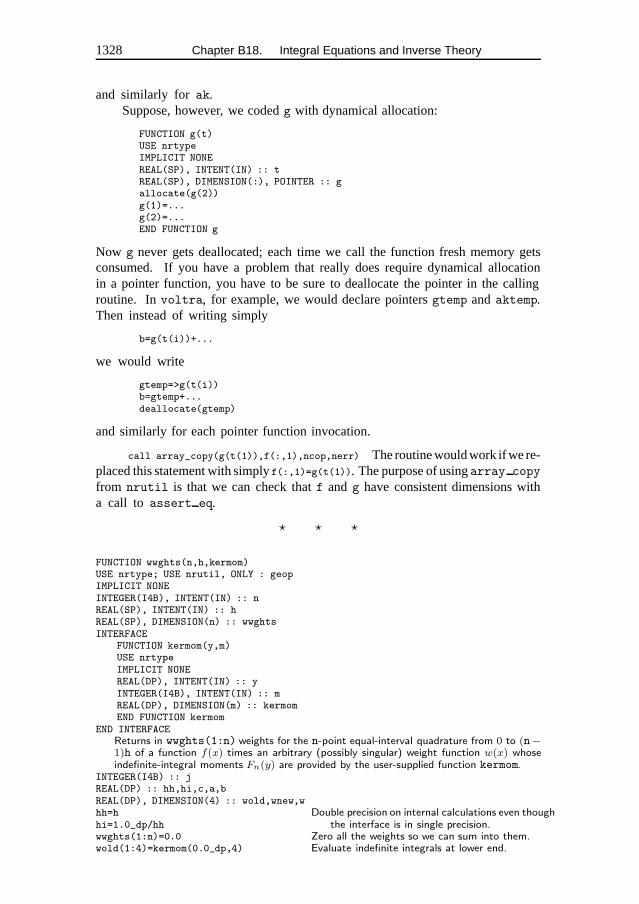
1328 Chapter B18. Integral Equations and Inverse Theory
and similarly for ak.Suppose, however, we coded g with dynamical allocation:
FUNCTION g(t)USE nrtypeIMPLICIT NONEREAL(SP), INTENT(IN) :: tREAL(SP), DIMENSION(:), POINTER :: gallocate(g(2))g(1)=...g(2)=...END FUNCTION g
Now g never gets deallocated; each time we call the function fresh memory getsconsumed. If you have a problem that really does require dynamical allocationin a pointer function, you have to be sure to deallocate the pointer in the callingroutine. In voltra, for example, we would declare pointers gtemp and aktemp.Then instead of writing simply
b=g(t(i))+...
we would write
gtemp=>g(t(i))b=gtemp+...deallocate(gtemp)
and similarly for each pointer function invocation.
call array_copy(g(t(1)),f(:,1),ncop,nerr) The routine would work if we re-placed this statement with simply f(:,1)=g(t(1)). The purpose of using array copy
from nrutil is that we can check that f and g have consistent dimensions witha call to assert eq.
� � �
FUNCTION wwghts(n,h,kermom)USE nrtype; USE nrutil, ONLY : geopIMPLICIT NONEINTEGER(I4B), INTENT(IN) :: nREAL(SP), INTENT(IN) :: hREAL(SP), DIMENSION(n) :: wwghtsINTERFACE
FUNCTION kermom(y,m)USE nrtypeIMPLICIT NONEREAL(DP), INTENT(IN) :: yINTEGER(I4B), INTENT(IN) :: mREAL(DP), DIMENSION(m) :: kermomEND FUNCTION kermom
END INTERFACEReturns in wwghts(1:n) weights for the n-point equal-interval quadrature from 0 to (n−1)h of a function f(x) times an arbitrary (possibly singular) weight function w(x) whoseindefinite-integral moments Fn(y) are provided by the user-supplied function kermom.
INTEGER(I4B) :: jREAL(DP) :: hh,hi,c,a,bREAL(DP), DIMENSION(4) :: wold,wnew,whh=h Double precision on internal calculations even though
the interface is in single precision.hi=1.0_dp/hhwwghts(1:n)=0.0 Zero all the weights so we can sum into them.wold(1:4)=kermom(0.0_dp,4) Evaluate indefinite integrals at lower end.
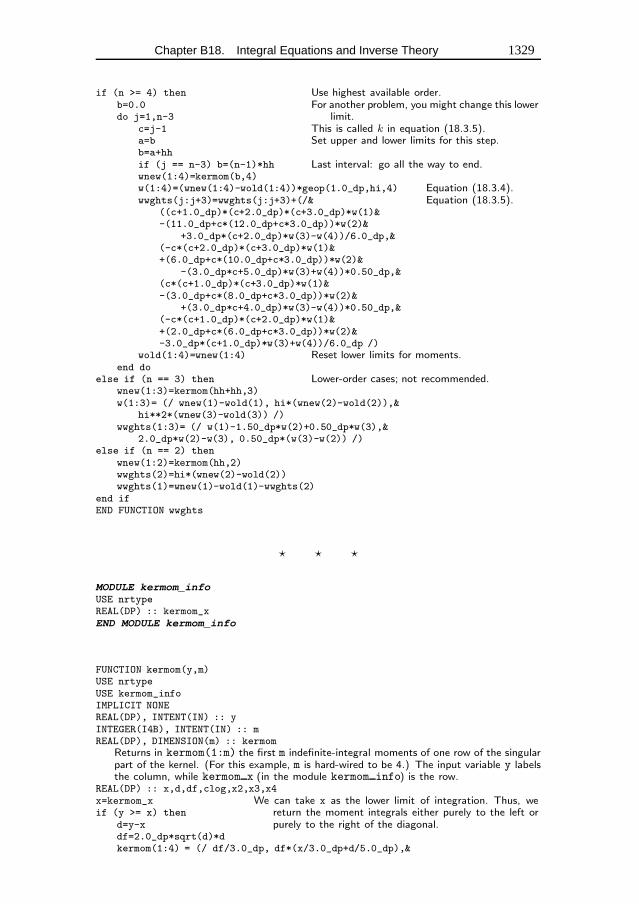
Chapter B18. Integral Equations and Inverse Theory 1329
if (n >= 4) then Use highest available order.b=0.0 For another problem, you might change this lower
limit.do j=1,n-3c=j-1 This is called k in equation (18.3.5).a=b Set upper and lower limits for this step.b=a+hhif (j == n-3) b=(n-1)*hh Last interval: go all the way to end.wnew(1:4)=kermom(b,4)w(1:4)=(wnew(1:4)-wold(1:4))*geop(1.0_dp,hi,4) Equation (18.3.4).wwghts(j:j+3)=wwghts(j:j+3)+(/& Equation (18.3.5).
((c+1.0_dp)*(c+2.0_dp)*(c+3.0_dp)*w(1)&-(11.0_dp+c*(12.0_dp+c*3.0_dp))*w(2)&
+3.0_dp*(c+2.0_dp)*w(3)-w(4))/6.0_dp,&(-c*(c+2.0_dp)*(c+3.0_dp)*w(1)&+(6.0_dp+c*(10.0_dp+c*3.0_dp))*w(2)&
-(3.0_dp*c+5.0_dp)*w(3)+w(4))*0.50_dp,&(c*(c+1.0_dp)*(c+3.0_dp)*w(1)&-(3.0_dp+c*(8.0_dp+c*3.0_dp))*w(2)&
+(3.0_dp*c+4.0_dp)*w(3)-w(4))*0.50_dp,&(-c*(c+1.0_dp)*(c+2.0_dp)*w(1)&+(2.0_dp+c*(6.0_dp+c*3.0_dp))*w(2)&-3.0_dp*(c+1.0_dp)*w(3)+w(4))/6.0_dp /)
wold(1:4)=wnew(1:4) Reset lower limits for moments.end do
else if (n == 3) then Lower-order cases; not recommended.wnew(1:3)=kermom(hh+hh,3)w(1:3)= (/ wnew(1)-wold(1), hi*(wnew(2)-wold(2)),&
hi**2*(wnew(3)-wold(3)) /)wwghts(1:3)= (/ w(1)-1.50_dp*w(2)+0.50_dp*w(3),&
2.0_dp*w(2)-w(3), 0.50_dp*(w(3)-w(2)) /)else if (n == 2) then
wnew(1:2)=kermom(hh,2)wwghts(2)=hi*(wnew(2)-wold(2))wwghts(1)=wnew(1)-wold(1)-wwghts(2)
end ifEND FUNCTION wwghts
� � �
MODULE kermom_infoUSE nrtypeREAL(DP) :: kermom_xEND MODULE kermom_info
FUNCTION kermom(y,m)USE nrtypeUSE kermom_infoIMPLICIT NONEREAL(DP), INTENT(IN) :: yINTEGER(I4B), INTENT(IN) :: mREAL(DP), DIMENSION(m) :: kermom
Returns in kermom(1:m) the first m indefinite-integral moments of one row of the singularpart of the kernel. (For this example, m is hard-wired to be 4.) The input variable y labelsthe column, while kermom x (in the module kermom info) is the row.
REAL(DP) :: x,d,df,clog,x2,x3,x4x=kermom_x We can take x as the lower limit of integration. Thus, we
return the moment integrals either purely to the left orpurely to the right of the diagonal.
if (y >= x) thend=y-xdf=2.0_dp*sqrt(d)*dkermom(1:4) = (/ df/3.0_dp, df*(x/3.0_dp+d/5.0_dp),&
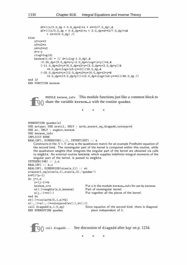
1330 Chapter B18. Integral Equations and Inverse Theory
df*((x/3.0_dp + 0.4_dp*d)*x + d**2/7.0_dp),&df*(((x/3.0_dp + 0.6_dp*d)*x + 3.0_dp*d**2/7.0_dp)*x&
+ d**3/9.0_dp) /)else
x2=x**2x3=x2*xx4=x2*x2d=x-yclog=log(d)kermom(1:4) = (/ d*(clog-1.0_dp),&
-0.25_dp*(3.0_dp*x+y-2.0_dp*clog*(x+y))*d,&(-11.0_dp*x3+y*(6.0_dp*x2+y*(3.0_dp*x+2.0_dp*y))&
+6.0_dp*clog*(x3-y**3))/18.0_dp,&(-25.0_dp*x4+y*(12.0_dp*x3+y*(6.0_dp*x2+y*&
(4.0_dp*x+3.0_dp*y)))+12.0_dp*clog*(x4-y**4))/48.0_dp /)end ifEND FUNCTION kermom
f90MODULE kermom_info This module functions just like a common block toshare the variable kermom x with the routine quadmx.
� � �
SUBROUTINE quadmx(a)USE nrtype; USE nrutil, ONLY : arth,assert_eq,diagadd,outerprodUSE nr, ONLY : wwghts,kermomUSE kermom_infoIMPLICIT NONEREAL(SP), DIMENSION(:,:), INTENT(OUT) :: a
Constructs in the N×N array a the quadrature matrix for an example Fredholm equation ofthe second kind. The nonsingular part of the kernel is computed within this routine, whilethe quadrature weights that integrate the singular part of the kernel are obtained via callsto wwghts. An external routine kermom, which supplies indefinite-integral moments of thesingular part of the kernel, is passed to wwghts.
INTEGER(I4B) :: j,nREAL(SP) :: h,xREAL(SP), DIMENSION(size(a,1)) :: wtn=assert_eq(size(a,1),size(a,2),’quadmx’)h=PI/(n-1)do j=1,n
x=(j-1)*hkermom_x=x Put x in the module kermom info for use by kermom.wt(:)=wwghts(n,h,kermom) Part of nonsingular kernel.a(j,:)=wt(:) Put together all the pieces of the kernel.
end dowt(:)=cos(arth(0,1,n)*h)a(:,:)=a(:,:)*outerprod(wt(:),wt(:))call diagadd(a,1.0_sp) Since equation of the second kind, there is diagonal
piece independent of h.END SUBROUTINE quadmx
f90 call diagadd... See discussion of diagadd after hqr on p. 1234.
� � �
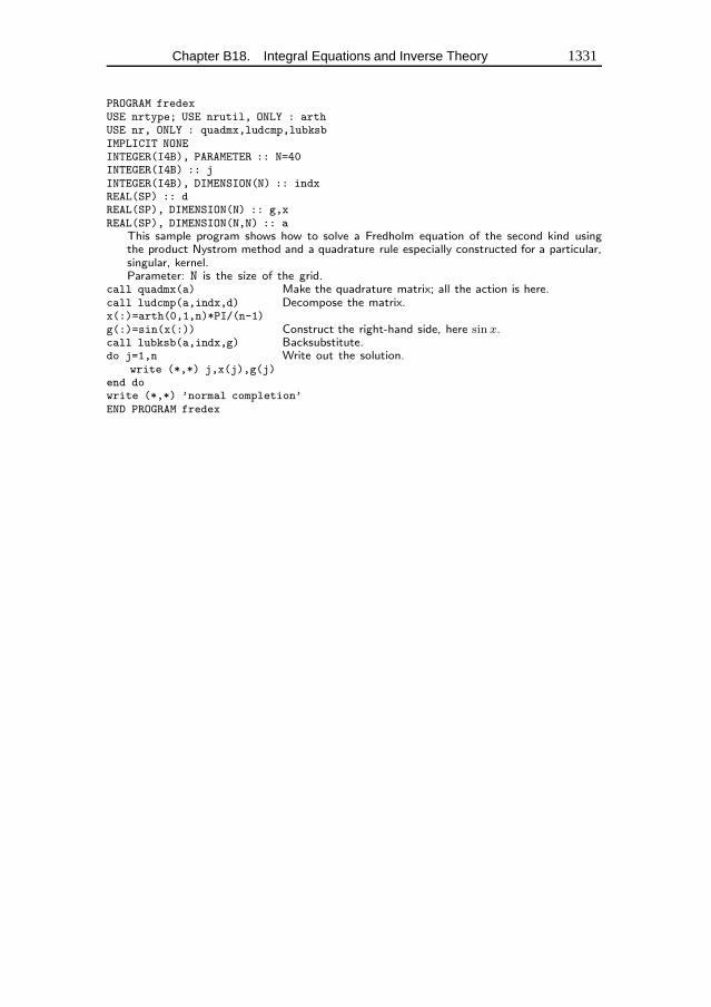
Chapter B18. Integral Equations and Inverse Theory 1331
PROGRAM fredexUSE nrtype; USE nrutil, ONLY : arthUSE nr, ONLY : quadmx,ludcmp,lubksbIMPLICIT NONEINTEGER(I4B), PARAMETER :: N=40INTEGER(I4B) :: jINTEGER(I4B), DIMENSION(N) :: indxREAL(SP) :: dREAL(SP), DIMENSION(N) :: g,xREAL(SP), DIMENSION(N,N) :: a
This sample program shows how to solve a Fredholm equation of the second kind usingthe product Nystrom method and a quadrature rule especially constructed for a particular,singular, kernel.Parameter: N is the size of the grid.
call quadmx(a) Make the quadrature matrix; all the action is here.call ludcmp(a,indx,d) Decompose the matrix.x(:)=arth(0,1,n)*PI/(n-1)g(:)=sin(x(:)) Construct the right-hand side, here sin x.call lubksb(a,indx,g) Backsubstitute.do j=1,n Write out the solution.
write (*,*) j,x(j),g(j)end dowrite (*,*) ’normal completion’END PROGRAM fredex
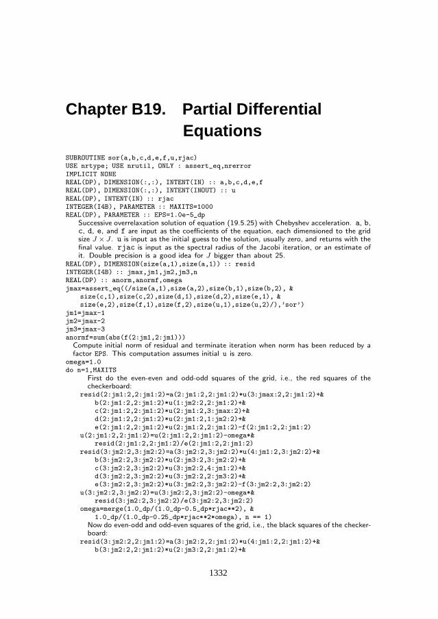
Chapter B19. Partial DifferentialEquations
SUBROUTINE sor(a,b,c,d,e,f,u,rjac)USE nrtype; USE nrutil, ONLY : assert_eq,nrerrorIMPLICIT NONEREAL(DP), DIMENSION(:,:), INTENT(IN) :: a,b,c,d,e,fREAL(DP), DIMENSION(:,:), INTENT(INOUT) :: uREAL(DP), INTENT(IN) :: rjacINTEGER(I4B), PARAMETER :: MAXITS=1000REAL(DP), PARAMETER :: EPS=1.0e-5_dp
Successive overrelaxation solution of equation (19.5.25) with Chebyshev acceleration. a, b,c, d, e, and f are input as the coefficients of the equation, each dimensioned to the gridsize J × J. u is input as the initial guess to the solution, usually zero, and returns with thefinal value. rjac is input as the spectral radius of the Jacobi iteration, or an estimate ofit. Double precision is a good idea for J bigger than about 25.
REAL(DP), DIMENSION(size(a,1),size(a,1)) :: residINTEGER(I4B) :: jmax,jm1,jm2,jm3,nREAL(DP) :: anorm,anormf,omegajmax=assert_eq((/size(a,1),size(a,2),size(b,1),size(b,2), &
size(c,1),size(c,2),size(d,1),size(d,2),size(e,1), &size(e,2),size(f,1),size(f,2),size(u,1),size(u,2)/),’sor’)
jm1=jmax-1jm2=jmax-2jm3=jmax-3anormf=sum(abs(f(2:jm1,2:jm1)))Compute initial norm of residual and terminate iteration when norm has been reduced by afactor EPS. This computation assumes initial u is zero.
omega=1.0do n=1,MAXITS
First do the even-even and odd-odd squares of the grid, i.e., the red squares of thecheckerboard:
resid(2:jm1:2,2:jm1:2)=a(2:jm1:2,2:jm1:2)*u(3:jmax:2,2:jm1:2)+&b(2:jm1:2,2:jm1:2)*u(1:jm2:2,2:jm1:2)+&c(2:jm1:2,2:jm1:2)*u(2:jm1:2,3:jmax:2)+&d(2:jm1:2,2:jm1:2)*u(2:jm1:2,1:jm2:2)+&e(2:jm1:2,2:jm1:2)*u(2:jm1:2,2:jm1:2)-f(2:jm1:2,2:jm1:2)
u(2:jm1:2,2:jm1:2)=u(2:jm1:2,2:jm1:2)-omega*&resid(2:jm1:2,2:jm1:2)/e(2:jm1:2,2:jm1:2)
resid(3:jm2:2,3:jm2:2)=a(3:jm2:2,3:jm2:2)*u(4:jm1:2,3:jm2:2)+&b(3:jm2:2,3:jm2:2)*u(2:jm3:2,3:jm2:2)+&c(3:jm2:2,3:jm2:2)*u(3:jm2:2,4:jm1:2)+&d(3:jm2:2,3:jm2:2)*u(3:jm2:2,2:jm3:2)+&e(3:jm2:2,3:jm2:2)*u(3:jm2:2,3:jm2:2)-f(3:jm2:2,3:jm2:2)
u(3:jm2:2,3:jm2:2)=u(3:jm2:2,3:jm2:2)-omega*&resid(3:jm2:2,3:jm2:2)/e(3:jm2:2,3:jm2:2)
omega=merge(1.0_dp/(1.0_dp-0.5_dp*rjac**2), &1.0_dp/(1.0_dp-0.25_dp*rjac**2*omega), n == 1)
Now do even-odd and odd-even squares of the grid, i.e., the black squares of the checker-board:
resid(3:jm2:2,2:jm1:2)=a(3:jm2:2,2:jm1:2)*u(4:jm1:2,2:jm1:2)+&b(3:jm2:2,2:jm1:2)*u(2:jm3:2,2:jm1:2)+&
1332
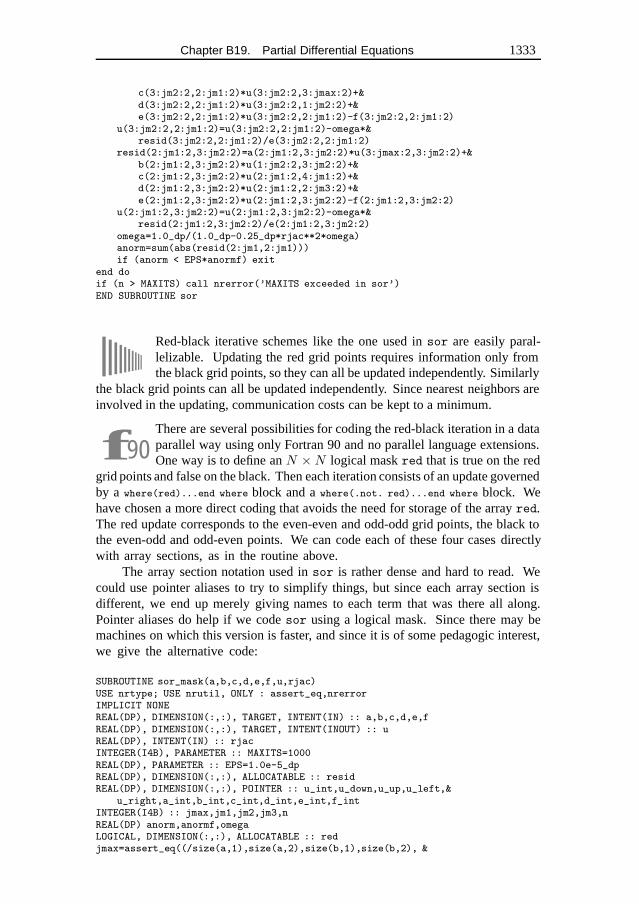
Chapter B19. Partial Differential Equations 1333
c(3:jm2:2,2:jm1:2)*u(3:jm2:2,3:jmax:2)+&d(3:jm2:2,2:jm1:2)*u(3:jm2:2,1:jm2:2)+&e(3:jm2:2,2:jm1:2)*u(3:jm2:2,2:jm1:2)-f(3:jm2:2,2:jm1:2)
u(3:jm2:2,2:jm1:2)=u(3:jm2:2,2:jm1:2)-omega*&resid(3:jm2:2,2:jm1:2)/e(3:jm2:2,2:jm1:2)
resid(2:jm1:2,3:jm2:2)=a(2:jm1:2,3:jm2:2)*u(3:jmax:2,3:jm2:2)+&b(2:jm1:2,3:jm2:2)*u(1:jm2:2,3:jm2:2)+&c(2:jm1:2,3:jm2:2)*u(2:jm1:2,4:jm1:2)+&d(2:jm1:2,3:jm2:2)*u(2:jm1:2,2:jm3:2)+&e(2:jm1:2,3:jm2:2)*u(2:jm1:2,3:jm2:2)-f(2:jm1:2,3:jm2:2)
u(2:jm1:2,3:jm2:2)=u(2:jm1:2,3:jm2:2)-omega*&resid(2:jm1:2,3:jm2:2)/e(2:jm1:2,3:jm2:2)
omega=1.0_dp/(1.0_dp-0.25_dp*rjac**2*omega)anorm=sum(abs(resid(2:jm1,2:jm1)))if (anorm < EPS*anormf) exit
end doif (n > MAXITS) call nrerror(’MAXITS exceeded in sor’)END SUBROUTINE sor
Red-black iterative schemes like the one used in sor are easily paral-lelizable. Updating the red grid points requires information only fromthe black grid points, so they can all be updated independently. Similarly
the black grid points can all be updated independently. Since nearest neighbors areinvolved in the updating, communication costs can be kept to a minimum.
f90There are several possibilities for coding the red-black iteration in a dataparallel way using only Fortran 90 and no parallel language extensions.One way is to define an N ×N logical mask red that is true on the red
grid points and false on the black. Then each iteration consists of an update governedby a where(red)...end where block and a where(.not. red)...end where block. Wehave chosen a more direct coding that avoids the need for storage of the array red.The red update corresponds to the even-even and odd-odd grid points, the black tothe even-odd and odd-even points. We can code each of these four cases directlywith array sections, as in the routine above.
The array section notation used in sor is rather dense and hard to read. Wecould use pointer aliases to try to simplify things, but since each array section isdifferent, we end up merely giving names to each term that was there all along.Pointer aliases do help if we code sor using a logical mask. Since there may bemachines on which this version is faster, and since it is of some pedagogic interest,we give the alternative code:
SUBROUTINE sor_mask(a,b,c,d,e,f,u,rjac)USE nrtype; USE nrutil, ONLY : assert_eq,nrerrorIMPLICIT NONEREAL(DP), DIMENSION(:,:), TARGET, INTENT(IN) :: a,b,c,d,e,fREAL(DP), DIMENSION(:,:), TARGET, INTENT(INOUT) :: uREAL(DP), INTENT(IN) :: rjacINTEGER(I4B), PARAMETER :: MAXITS=1000REAL(DP), PARAMETER :: EPS=1.0e-5_dpREAL(DP), DIMENSION(:,:), ALLOCATABLE :: residREAL(DP), DIMENSION(:,:), POINTER :: u_int,u_down,u_up,u_left,&
u_right,a_int,b_int,c_int,d_int,e_int,f_intINTEGER(I4B) :: jmax,jm1,jm2,jm3,nREAL(DP) anorm,anormf,omegaLOGICAL, DIMENSION(:,:), ALLOCATABLE :: redjmax=assert_eq((/size(a,1),size(a,2),size(b,1),size(b,2), &
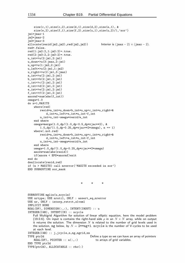
1334 Chapter B19. Partial Differential Equations
size(c,1),size(c,2),size(d,1),size(d,2),size(e,1), &size(e,2),size(f,1),size(f,2),size(u,1),size(u,2)/),’sor’)
jm1=jmax-1jm2=jmax-2jm3=jmax-3allocate(resid(jm2,jm2),red(jm2,jm2)) Interior is (jmax− 2) × (jmax− 2).red=.false.red(1:jm2:2,1:jm2:2)=.true.red(2:jm3:2,2:jm3:2)=.true.u_int=>u(2:jm1,2:jm1)u_down=>u(3:jmax,2:jm1)u_up=>u(1:jm2,2:jm1)u_left=>u(2:jm1,1:jm2)u_right=>u(2:jm1,3:jmax)a_int=>a(2:jm1,2:jm1)b_int=>b(2:jm1,2:jm1)c_int=>c(2:jm1,2:jm1)d_int=>d(2:jm1,2:jm1)e_int=>e(2:jm1,2:jm1)f_int=>f(2:jm1,2:jm1)anormf=sum(abs(f_int))omega=1.0do n=1,MAXITS
where(red)resid=a_int*u_down+b_int*u_up+c_int*u_right+&
d_int*u_left+e_int*u_int-f_intu_int=u_int-omega*resid/e_int
end whereomega=merge(1.0_dp/(1.0_dp-0.5_dp*rjac**2), &
1.0_dp/(1.0_dp-0.25_dp*rjac**2*omega), n == 1)where(.not.red)
resid=a_int*u_down+b_int*u_up+c_int*u_right+&d_int*u_left+e_int*u_int-f_int
u_int=u_int-omega*resid/e_intend whereomega=1.0_dp/(1.0_dp-0.25_dp*rjac**2*omega)anorm=sum(abs(resid))if(anorm < EPS*anormf)exit
end dodeallocate(resid,red)if (n > MAXITS) call nrerror(’MAXITS exceeded in sor’)END SUBROUTINE sor_mask
� � �
SUBROUTINE mglin(u,ncycle)USE nrtype; USE nrutil, ONLY : assert_eq,nrerrorUSE nr, ONLY : interp,rstrct,slvsmlIMPLICIT NONEREAL(DP), DIMENSION(:,:), INTENT(INOUT) :: uINTEGER(I4B), INTENT(IN) :: ncycle
Full Multigrid Algorithm for solution of linear elliptic equation, here the model problem(19.0.6). On input u contains the right-hand side ρ in an N × N array, while on outputit returns the solution. The dimension N is related to the number of grid levels used inthe solution, ng below, by N = 2**ng+1. ncycle is the number of V-cycles to be usedat each level.
INTEGER(I4B) :: j,jcycle,n,ng,ngrid,nnTYPE ptr2d Define a type so we can have an array of pointers
to arrays of grid variables.REAL(DP), POINTER :: a(:,:)END TYPE ptr2dTYPE(ptr2d), ALLOCATABLE :: rho(:)
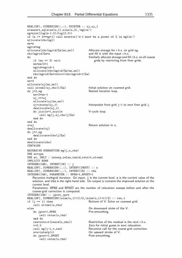
Chapter B19. Partial Differential Equations 1335
REAL(DP), DIMENSION(:,:), POINTER :: uj,uj_1n=assert_eq(size(u,1),size(u,2),’mglin’)ng=nint(log(n-1.0)/log(2.0))if (n /= 2**ng+1) call nrerror(’n-1 must be a power of 2 in mglin’)allocate(rho(ng))nn=nngrid=ngallocate(rho(ngrid)%a(nn,nn)) Allocate storage for r.h.s. on grid ng,rho(ngrid)%a=u and fill it with the input r.h.s.do Similarly allocate storage and fill r.h.s. on all coarse
grids by restricting from finer grids.if (nn <= 3) exitnn=nn/2+1ngrid=ngrid-1allocate(rho(ngrid)%a(nn,nn))rho(ngrid)%a=rstrct(rho(ngrid+1)%a)
end donn=3allocate(uj(nn,nn))call slvsml(uj,rho(1)%a) Initial solution on coarsest grid.do j=2,ng Nested iteration loop.
nn=2*nn-1uj_1=>ujallocate(uj(nn,nn))uj=interp(uj_1) Interpolate from grid j-1 to next finer grid j.deallocate(uj_1)do jcycle=1,ncycle V-cycle loop.
call mg(j,uj,rho(j)%a)end do
end dou=uj Return solution in u.deallocate(uj)do j=1,ng
deallocate(rho(j)%a)end dodeallocate(rho)CONTAINS
RECURSIVE SUBROUTINE mg(j,u,rhs)USE nrtypeUSE nr, ONLY : interp,relax,resid,rstrct,slvsmlIMPLICIT NONEINTEGER(I4B), INTENT(IN) :: jREAL(DP), DIMENSION(:,:), INTENT(INOUT) :: uREAL(DP), DIMENSION(:,:), INTENT(IN) :: rhsINTEGER(I4B), PARAMETER :: NPRE=1,NPOST=1
Recursive multigrid iteration. On input, j is the current level, u is the current value of thesolution, and rhs is the right-hand side. On output u contains the improved solution at thecurrent level.Parameters: NPRE and NPOST are the number of relaxation sweeps before and after thecoarse-grid correction is computed.
INTEGER(I4B) :: jpost,jpreREAL(DP), DIMENSION((size(u,1)+1)/2,(size(u,1)+1)/2) :: res,vif (j == 1) then Bottom of V: Solve on coarsest grid.
call slvsml(u,rhs)else On downward stoke of the V.
do jpre=1,NPRE Pre-smoothing.call relax(u,rhs)
end dores=rstrct(resid(u,rhs)) Restriction of the residual is the next r.h.s.v=0.0 Zero for initial guess in next relaxation.call mg(j-1,v,res) Recursive call for the coarse grid correction.u=u+interp(v) On upward stroke of V.do jpost=1,NPOST Post-smoothing.
call relax(u,rhs)
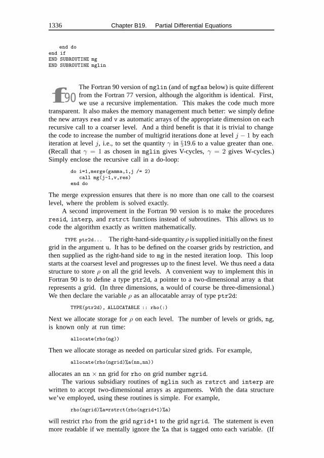
1336 Chapter B19. Partial Differential Equations
end doend ifEND SUBROUTINE mgEND SUBROUTINE mglin
f90The Fortran 90 version of mglin (and of mgfas below) is quite differentfrom the Fortran 77 version, although the algorithm is identical. First,we use a recursive implementation. This makes the code much more
transparent. It also makes the memory management much better: we simply definethe new arrays res and v as automatic arrays of the appropriate dimension on eachrecursive call to a coarser level. And a third benefit is that it is trivial to changethe code to increase the number of multigrid iterations done at level j − 1 by eachiteration at level j, i.e., to set the quantity γ in §19.6 to a value greater than one.(Recall that γ = 1 as chosen in mglin gives V-cycles, γ = 2 gives W-cycles.)Simply enclose the recursive call in a do-loop:
do i=1,merge(gamma,1,j /= 2)call mg(j-1,v,res)
end do
The merge expression ensures that there is no more than one call to the coarsestlevel, where the problem is solved exactly.
A second improvement in the Fortran 90 version is to make the proceduresresid, interp, and rstrct functions instead of subroutines. This allows us tocode the algorithm exactly as written mathematically.
TYPE ptr2d... The right-hand-sidequantityρ is supplied initiallyon the finestgrid in the argument u. It has to be defined on the coarser grids by restriction, andthen supplied as the right-hand side to mg in the nested iteration loop. This loopstarts at the coarsest level and progresses up to the finest level. We thus need a datastructure to store ρ on all the grid levels. A convenient way to implement this inFortran 90 is to define a type ptr2d, a pointer to a two-dimensional array a thatrepresents a grid. (In three dimensions, a would of course be three-dimensional.)We then declare the variable ρ as an allocatable array of type ptr2d:
TYPE(ptr2d), ALLOCATABLE :: rho(:)
Next we allocate storage for ρ on each level. The number of levels or grids, ng,is known only at run time:
allocate(rho(ng))
Then we allocate storage as needed on particular sized grids. For example,
allocate(rho(ngrid)%a(nn,nn))
allocates an nn × nn grid for rho on grid number ngrid.The various subsidiary routines of mglin such as rstrct and interp are
written to accept two-dimensional arrays as arguments. With the data structurewe’ve employed, using these routines is simple. For example,
rho(ngrid)%a=rstrct(rho(ngrid+1)%a)
will restrict rho from the grid ngrid+1 to the grid ngrid. The statement is evenmore readable if we mentally ignore the %a that is tagged onto each variable. (If
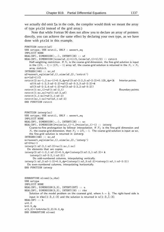
Chapter B19. Partial Differential Equations 1337
we actually did omit %a in the code, the compiler would think we meant the arrayof type ptr2d instead of the grid array.)
Note that while Fortran 90 does not allow you to declare an array of pointersdirectly, you can achieve the same effect by declaring your own type, as we havedone with ptr2d in this example.
FUNCTION rstrct(uf)USE nrtype; USE nrutil, ONLY : assert_eqIMPLICIT NONEREAL(DP), DIMENSION(:,:), INTENT(IN) :: ufREAL(DP), DIMENSION((size(uf,1)+1)/2,(size(uf,1)+1)/2) :: rstrct
Half-weighting restriction. If Nc is the coarse-grid dimension, the fine-grid solution is inputin the (2Nc − 1)× (2Nc − 1) array uf, the coarse-grid solution is returned in the Nc ×Nc
array rstrct.INTEGER(I4B) :: nc,nfnf=assert_eq(size(uf,1),size(uf,2),’rstrct’)nc=(nf+1)/2rstrct(2:nc-1,2:nc-1)=0.5_dp*uf(3:nf-2:2,3:nf-2:2)+0.125_dp*(& Interior points.
uf(4:nf-1:2,3:nf-2:2)+uf(2:nf-3:2,3:nf-2:2)+&uf(3:nf-2:2,4:nf-1:2)+uf(3:nf-2:2,2:nf-3:2))
rstrct(1:nc,1)=uf(1:nf:2,1) Boundary points.rstrct(1:nc,nc)=uf(1:nf:2,nf)rstrct(1,1:nc)=uf(1,1:nf:2)rstrct(nc,1:nc)=uf(nf,1:nf:2)END FUNCTION rstrct
FUNCTION interp(uc)USE nrtype; USE nrutil, ONLY : assert_eqIMPLICIT NONEREAL(DP), DIMENSION(:,:), INTENT(IN) :: ucREAL(DP), DIMENSION(2*size(uc,1)-1,2*size(uc,1)-1) :: interp
Coarse-to-fine prolongation by bilinear interpolation. If Nf is the fine-grid dimension andNc the coarse-grid dimension, then Nf = 2Nc− 1. The coarse-grid solution is input as uc,the fine-grid solution is returned in interp.
INTEGER(I4B) :: nc,nfnc=assert_eq(size(uc,1),size(uc,2),’interp’)nf=2*nc-1interp(1:nf:2,1:nf:2)=uc(1:nc,1:nc)Do elements that are copies.
interp(2:nf-1:2,1:nf:2)=0.5_dp*(interp(3:nf:2,1:nf:2)+ &interp(1:nf-2:2,1:nf:2))Do odd-numbered columns, interpolating vertically.
interp(1:nf,2:nf-1:2)=0.5_dp*(interp(1:nf,3:nf:2)+interp(1:nf,1:nf-2:2))Do even-numbered columns, interpolating horizontally.
END FUNCTION interp
SUBROUTINE slvsml(u,rhs)USE nrtypeIMPLICIT NONEREAL(DP), DIMENSION(3,3), INTENT(OUT) :: uREAL(DP), DIMENSION(3,3), INTENT(IN) :: rhs
Solution of the model problem on the coarsest grid, where h = 12. The right-hand side is
input in rhs(1:3,1:3) and the solution is returned in u(1:3,1:3).REAL(DP) :: hu=0.0h=0.5_dpu(2,2)=-h*h*rhs(2,2)/4.0_dpEND SUBROUTINE slvsml
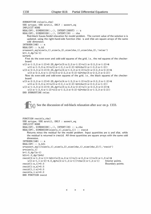
1338 Chapter B19. Partial Differential Equations
SUBROUTINE relax(u,rhs)USE nrtype; USE nrutil, ONLY : assert_eqIMPLICIT NONEREAL(DP), DIMENSION(:,:), INTENT(INOUT) :: uREAL(DP), DIMENSION(:,:), INTENT(IN) :: rhs
Red-black Gauss-Seidel relaxation for model problem. The current value of the solution u isupdated, using the right-hand-side function rhs. u and rhs are square arrays of the sameodd dimension.
INTEGER(I4B) :: nREAL(DP) :: h,h2n=assert_eq(size(u,1),size(u,2),size(rhs,1),size(rhs,2),’relax’)h=1.0_dp/(n-1)h2=h*hFirst do the even-even and odd-odd squares of the grid, i.e., the red squares of the checker-board:
u(2:n-1:2,2:n-1:2)=0.25_dp*(u(3:n:2,2:n-1:2)+u(1:n-2:2,2:n-1:2)+&u(2:n-1:2,3:n:2)+u(2:n-1:2,1:n-2:2)-h2*rhs(2:n-1:2,2:n-1:2))
u(3:n-2:2,3:n-2:2)=0.25_dp*(u(4:n-1:2,3:n-2:2)+u(2:n-3:2,3:n-2:2)+&u(3:n-2:2,4:n-1:2)+u(3:n-2:2,2:n-3:2)-h2*rhs(3:n-2:2,3:n-2:2))
Now do even-odd and odd-even squares of the grid, i.e., the black squares of the checker-board:
u(3:n-2:2,2:n-1:2)=0.25_dp*(u(4:n-1:2,2:n-1:2)+u(2:n-3:2,2:n-1:2)+&u(3:n-2:2,3:n:2)+u(3:n-2:2,1:n-2:2)-h2*rhs(3:n-2:2,2:n-1:2))
u(2:n-1:2,3:n-2:2)=0.25_dp*(u(3:n:2,3:n-2:2)+u(1:n-2:2,3:n-2:2)+&u(2:n-1:2,4:n-1:2)+u(2:n-1:2,2:n-3:2)-h2*rhs(2:n-1:2,3:n-2:2))
END SUBROUTINE relax
f90 See the discussion of red-black relaxation after sor on p. 1333.
FUNCTION resid(u,rhs)USE nrtype; USE nrutil, ONLY : assert_eqIMPLICIT NONEREAL(DP), DIMENSION(:,:), INTENT(IN) :: u,rhsREAL(DP), DIMENSION(size(u,1),size(u,1)) :: resid
Returns minus the residual for the model problem. Input quantities are u and rhs, whilethe residual is returned in resid. All three quantities are square arrays with the same odddimension.
INTEGER(I4B) :: nREAL(DP) :: h,h2in=assert_eq((/size(u,1),size(u,2),size(rhs,1),size(rhs,2)/),’resid’)n=size(u,1)h=1.0_dp/(n-1)h2i=1.0_dp/(h*h)resid(2:n-1,2:n-1)=-h2i*(u(3:n,2:n-1)+u(1:n-2,2:n-1)+u(2:n-1,3:n)+&
u(2:n-1,1:n-2)-4.0_dp*u(2:n-1,2:n-1))+rhs(2:n-1,2:n-1) Interior points.resid(1:n,1)=0.0 Boundary points.resid(1:n,n)=0.0resid(1,1:n)=0.0resid(n,1:n)=0.0END FUNCTION resid
� � �
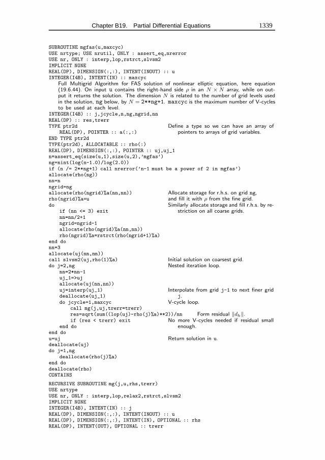
Chapter B19. Partial Differential Equations 1339
SUBROUTINE mgfas(u,maxcyc)USE nrtype; USE nrutil, ONLY : assert_eq,nrerrorUSE nr, ONLY : interp,lop,rstrct,slvsm2IMPLICIT NONEREAL(DP), DIMENSION(:,:), INTENT(INOUT) :: uINTEGER(I4B), INTENT(IN) :: maxcyc
Full Multigrid Algorithm for FAS solution of nonlinear elliptic equation, here equation(19.6.44). On input u contains the right-hand side ρ in an N × N array, while on out-put it returns the solution. The dimension N is related to the number of grid levels usedin the solution, ng below, by N = 2**ng+1. maxcyc is the maximum number of V-cyclesto be used at each level.
INTEGER(I4B) :: j,jcycle,n,ng,ngrid,nnREAL(DP) :: res,trerrTYPE ptr2d Define a type so we can have an array of
pointers to arrays of grid variables.REAL(DP), POINTER :: a(:,:)END TYPE ptr2dTYPE(ptr2d), ALLOCATABLE :: rho(:)REAL(DP), DIMENSION(:,:), POINTER :: uj,uj_1n=assert_eq(size(u,1),size(u,2),’mgfas’)ng=nint(log(n-1.0)/log(2.0))if (n /= 2**ng+1) call nrerror(’n-1 must be a power of 2 in mgfas’)allocate(rho(ng))nn=nngrid=ngallocate(rho(ngrid)%a(nn,nn)) Allocate storage for r.h.s. on grid ng,rho(ngrid)%a=u and fill it with ρ from the fine grid.do Similarly allocate storage and fill r.h.s. by re-
striction on all coarse grids.if (nn <= 3) exitnn=nn/2+1ngrid=ngrid-1allocate(rho(ngrid)%a(nn,nn))rho(ngrid)%a=rstrct(rho(ngrid+1)%a)
end donn=3allocate(uj(nn,nn))call slvsm2(uj,rho(1)%a) Initial solution on coarsest grid.do j=2,ng Nested iteration loop.
nn=2*nn-1uj_1=>ujallocate(uj(nn,nn))uj=interp(uj_1) Interpolate from grid j-1 to next finer grid
j.deallocate(uj_1)do jcycle=1,maxcyc V-cycle loop.
call mg(j,uj,trerr=trerr)res=sqrt(sum((lop(uj)-rho(j)%a)**2))/nn Form residual ‖dh‖.if (res < trerr) exit No more V-cycles needed if residual small
enough.end doend dou=uj Return solution in u.deallocate(uj)do j=1,ng
deallocate(rho(j)%a)end dodeallocate(rho)CONTAINS
RECURSIVE SUBROUTINE mg(j,u,rhs,trerr)USE nrtypeUSE nr, ONLY : interp,lop,relax2,rstrct,slvsm2IMPLICIT NONEINTEGER(I4B), INTENT(IN) :: jREAL(DP), DIMENSION(:,:), INTENT(INOUT) :: uREAL(DP), DIMENSION(:,:), INTENT(IN), OPTIONAL :: rhsREAL(DP), INTENT(OUT), OPTIONAL :: trerr
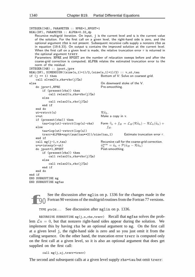
1340 Chapter B19. Partial Differential Equations
INTEGER(I4B), PARAMETER :: NPRE=1,NPOST=1REAL(DP), PARAMETER :: ALPHA=0.33_dp
Recursive multigrid iteration. On input, j is the current level and u is the current valueof the solution. For the first call on a given level, the right-hand side is zero, and theoptional argument rhs is not present. Subsequent recursive calls supply a nonzero rhs asin equation (19.6.33). On output u contains the improved solution at the current level.When the first call on a given level is made, the relative truncation error τ is returned inthe optional argument trerr.Parameters: NPRE and NPOST are the number of relaxation sweeps before and after thecoarse-grid correction is computed; ALPHA relates the estimated truncation error to thenorm of the residual.
INTEGER(I4B) :: jpost,jpreREAL(DP), DIMENSION((size(u,1)+1)/2,(size(u,1)+1)/2) :: v,ut,tauif (j == 1) then Bottom of V: Solve on coarsest grid.
call slvsm2(u,rhs+rho(j)%a)else On downward stoke of the V.
do jpre=1,NPRE Pre-smoothing.if (present(rhs)) then
call relax2(u,rhs+rho(j)%a)else
call relax2(u,rho(j)%a)end if
end dout=rstrct(u) Ruh.v=ut Make a copy in v.if (present(rhs)) then
tau=lop(ut)-rstrct(lop(u)-rhs) Form τh + fH = LH(Ruh) − RLh(uh) +fH .else
tau=lop(ut)-rstrct(lop(u))trerr=ALPHA*sqrt(sum(tau**2))/size(tau,1) Estimate truncation error τ .
end ifcall mg(j-1,v,tau) Recursive call for the coarse-grid correction.u=u+interp(v-ut) unew
h = uh + P(uH − Ruh)do jpost=1,NPOST Post-smoothing.
if (present(rhs)) thencall relax2(u,rhs+rho(j)%a)
elsecall relax2(u,rho(j)%a)
end ifend do
end ifEND SUBROUTINE mgEND SUBROUTINE mgfas
f90See the discussion after mglin on p. 1336 for the changes made in theFortran 90 versions of the multigrid routines from the Fortran 77 versions.
TYPE ptr2d... See discussion after mglin on p. 1336.
RECURSIVE SUBROUTINE mg(j,u,rhs,trerr) Recall that mgfas solves the prob-lem Lu = 0, but that nonzero right-hand sides appear during the solution. Weimplement this by having rhs be an optional argument to mg. On the first callat a given level j, the right-hand side is zero and so you just omit it from thecalling sequence. On the other hand, the truncation error trerr is computed onlyon the first call at a given level, so it is also an optional argument that does getsupplied on the first call:
call mg(j,uj,trerr=trerr)
The second and subsequent calls at a given level supply rhs=tau but omit trerr:
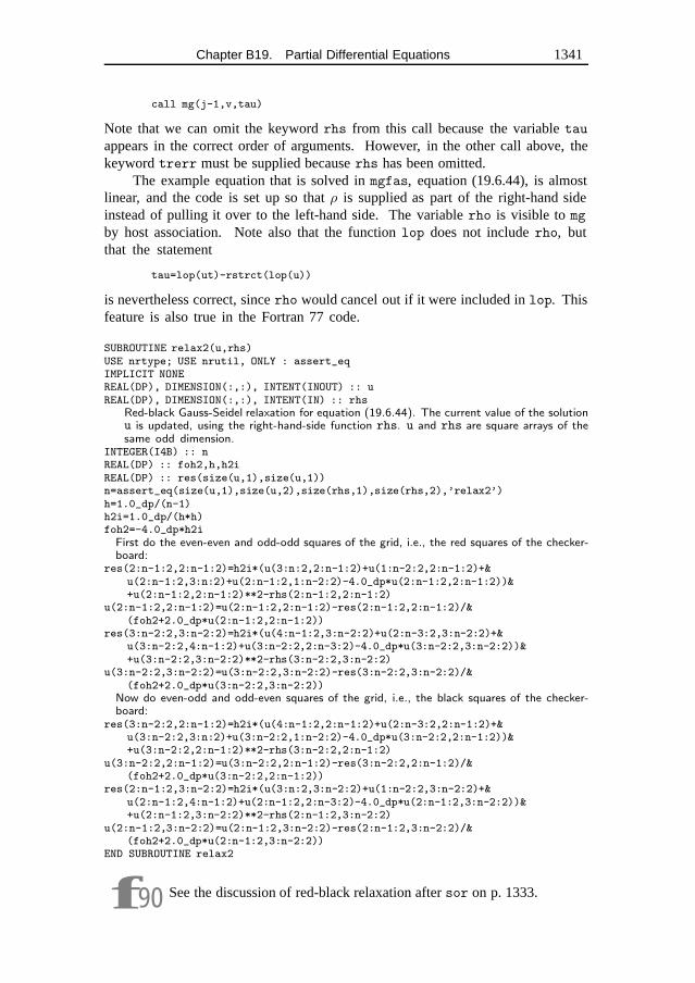
Chapter B19. Partial Differential Equations 1341
call mg(j-1,v,tau)
Note that we can omit the keyword rhs from this call because the variable tau
appears in the correct order of arguments. However, in the other call above, thekeyword trerr must be supplied because rhs has been omitted.
The example equation that is solved in mgfas, equation (19.6.44), is almostlinear, and the code is set up so that ρ is supplied as part of the right-hand sideinstead of pulling it over to the left-hand side. The variable rho is visible to mg
by host association. Note also that the function lop does not include rho, butthat the statement
tau=lop(ut)-rstrct(lop(u))
is nevertheless correct, since rho would cancel out if it were included in lop. Thisfeature is also true in the Fortran 77 code.
SUBROUTINE relax2(u,rhs)USE nrtype; USE nrutil, ONLY : assert_eqIMPLICIT NONEREAL(DP), DIMENSION(:,:), INTENT(INOUT) :: uREAL(DP), DIMENSION(:,:), INTENT(IN) :: rhs
Red-black Gauss-Seidel relaxation for equation (19.6.44). The current value of the solutionu is updated, using the right-hand-side function rhs. u and rhs are square arrays of thesame odd dimension.
INTEGER(I4B) :: nREAL(DP) :: foh2,h,h2iREAL(DP) :: res(size(u,1),size(u,1))n=assert_eq(size(u,1),size(u,2),size(rhs,1),size(rhs,2),’relax2’)h=1.0_dp/(n-1)h2i=1.0_dp/(h*h)foh2=-4.0_dp*h2iFirst do the even-even and odd-odd squares of the grid, i.e., the red squares of the checker-board:
res(2:n-1:2,2:n-1:2)=h2i*(u(3:n:2,2:n-1:2)+u(1:n-2:2,2:n-1:2)+&u(2:n-1:2,3:n:2)+u(2:n-1:2,1:n-2:2)-4.0_dp*u(2:n-1:2,2:n-1:2))&+u(2:n-1:2,2:n-1:2)**2-rhs(2:n-1:2,2:n-1:2)
u(2:n-1:2,2:n-1:2)=u(2:n-1:2,2:n-1:2)-res(2:n-1:2,2:n-1:2)/&(foh2+2.0_dp*u(2:n-1:2,2:n-1:2))
res(3:n-2:2,3:n-2:2)=h2i*(u(4:n-1:2,3:n-2:2)+u(2:n-3:2,3:n-2:2)+&u(3:n-2:2,4:n-1:2)+u(3:n-2:2,2:n-3:2)-4.0_dp*u(3:n-2:2,3:n-2:2))&+u(3:n-2:2,3:n-2:2)**2-rhs(3:n-2:2,3:n-2:2)
u(3:n-2:2,3:n-2:2)=u(3:n-2:2,3:n-2:2)-res(3:n-2:2,3:n-2:2)/&(foh2+2.0_dp*u(3:n-2:2,3:n-2:2))
Now do even-odd and odd-even squares of the grid, i.e., the black squares of the checker-board:
res(3:n-2:2,2:n-1:2)=h2i*(u(4:n-1:2,2:n-1:2)+u(2:n-3:2,2:n-1:2)+&u(3:n-2:2,3:n:2)+u(3:n-2:2,1:n-2:2)-4.0_dp*u(3:n-2:2,2:n-1:2))&+u(3:n-2:2,2:n-1:2)**2-rhs(3:n-2:2,2:n-1:2)
u(3:n-2:2,2:n-1:2)=u(3:n-2:2,2:n-1:2)-res(3:n-2:2,2:n-1:2)/&(foh2+2.0_dp*u(3:n-2:2,2:n-1:2))
res(2:n-1:2,3:n-2:2)=h2i*(u(3:n:2,3:n-2:2)+u(1:n-2:2,3:n-2:2)+&u(2:n-1:2,4:n-1:2)+u(2:n-1:2,2:n-3:2)-4.0_dp*u(2:n-1:2,3:n-2:2))&+u(2:n-1:2,3:n-2:2)**2-rhs(2:n-1:2,3:n-2:2)
u(2:n-1:2,3:n-2:2)=u(2:n-1:2,3:n-2:2)-res(2:n-1:2,3:n-2:2)/&(foh2+2.0_dp*u(2:n-1:2,3:n-2:2))
END SUBROUTINE relax2
f90 See the discussion of red-black relaxation after sor on p. 1333.
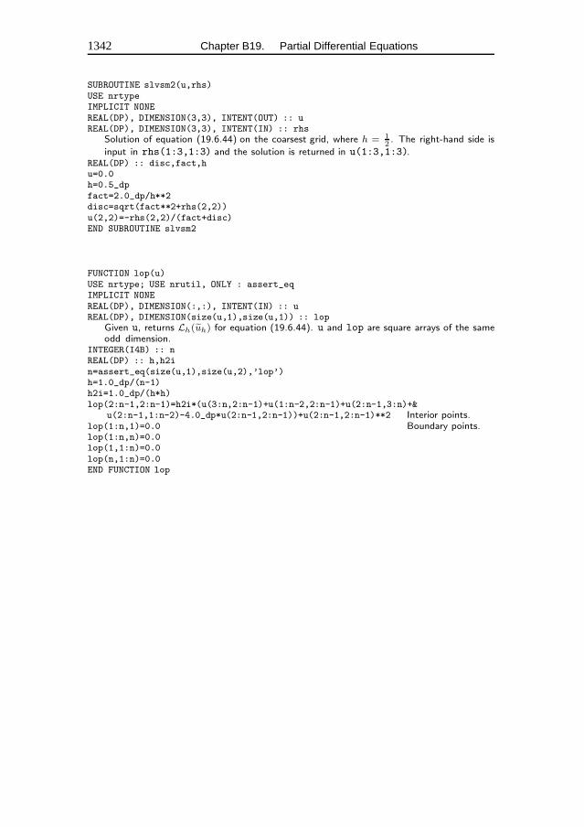
1342 Chapter B19. Partial Differential Equations
SUBROUTINE slvsm2(u,rhs)USE nrtypeIMPLICIT NONEREAL(DP), DIMENSION(3,3), INTENT(OUT) :: uREAL(DP), DIMENSION(3,3), INTENT(IN) :: rhs
Solution of equation (19.6.44) on the coarsest grid, where h = 12. The right-hand side is
input in rhs(1:3,1:3) and the solution is returned in u(1:3,1:3).REAL(DP) :: disc,fact,hu=0.0h=0.5_dpfact=2.0_dp/h**2disc=sqrt(fact**2+rhs(2,2))u(2,2)=-rhs(2,2)/(fact+disc)END SUBROUTINE slvsm2
FUNCTION lop(u)USE nrtype; USE nrutil, ONLY : assert_eqIMPLICIT NONEREAL(DP), DIMENSION(:,:), INTENT(IN) :: uREAL(DP), DIMENSION(size(u,1),size(u,1)) :: lop
Given u, returns Lh(uh) for equation (19.6.44). u and lop are square arrays of the sameodd dimension.
INTEGER(I4B) :: nREAL(DP) :: h,h2in=assert_eq(size(u,1),size(u,2),’lop’)h=1.0_dp/(n-1)h2i=1.0_dp/(h*h)lop(2:n-1,2:n-1)=h2i*(u(3:n,2:n-1)+u(1:n-2,2:n-1)+u(2:n-1,3:n)+&
u(2:n-1,1:n-2)-4.0_dp*u(2:n-1,2:n-1))+u(2:n-1,2:n-1)**2 Interior points.lop(1:n,1)=0.0 Boundary points.lop(1:n,n)=0.0lop(1,1:n)=0.0lop(n,1:n)=0.0END FUNCTION lop
Chapter B20. Less-NumericalAlgorithms
f90Volume 1’s Fortran 77 routinemachar performed various clever con-tortions (due to Cody, Malcolm, and others) to discover the underlyingproperties of a machine’s floating-point representation. Fortran 90, by
contrast, provides a built-in set of “numeric inquiry functions” that accomplish thesame goal. The routinemachar included here makes use of these and is includedlargely for compatibility with the previous version.
SUBROUTINE machar(ibeta,it,irnd,ngrd,machep,negep,iexp,minexp,&maxexp,eps,epsneg,xmin,xmax)
USE nrtypeIMPLICIT NONEINTEGER(I4B), INTENT(OUT) :: ibeta,iexp,irnd,it,machep,maxexp,minexp,negep,ngrdREAL(SP), INTENT(OUT) :: eps,epsneg,xmax,xminREAL(SP), PARAMETER :: RX=1.0
Determines and returns machine-specific parameters affecting floating-point arithmetic. Re-turned values include ibeta, the floating-point radix; it, the number of base-ibeta digitsin the floating-point mantissa; eps, the smallest positive number that, added to 1.0, isnot equal to 1.0; epsneg, the smallest positive number that, subtracted from 1.0, is notequal to 1.0; xmin, the smallest representable positive number; and xmax, the largest rep-resentable positive number. See text for description of other returned parameters. Changeall REAL(SP) declarations to REAL(DP) to find double-precision parameters.
REAL(SP) :: a,beta,betah,one,temp,tempa,two,zeroibeta=radix(RX) Most of the parameters are easily determined
from intrinsic functions.it=digits(RX)machep=exponent(nearest(RX,RX)-RX)-1negep=exponent(nearest(RX,-RX)-RX)-1minexp=minexponent(RX)-1maxexp=maxexponent(RX)iexp=nint(log(real(maxexp-minexp+2,sp))/log(2.0_sp))eps=real(ibeta,sp)**machepepsneg=real(ibeta,sp)**negepxmax=huge(RX)xmin=tiny(RX)one=RX Determine irnd.two=one+onezero=one-onebeta=real(ibeta,sp)a=beta**(-negep)irnd=0betah=beta/twotemp=a+betahif (temp-a /= zero) irnd=1tempa=a+betatemp=tempa+betahif ((irnd == 0) .and. (temp-tempa /= zero)) irnd=2ngrd=0 Determine ngrd.
1343
1344 Chapter B20. Less-Numerical Algorithms
temp=one+epsif ((irnd == 0) .and. (temp*one-one /= zero)) ngrd=1temp=xmin/twoif (temp /= zero) irnd=irnd+3 Adjust irnd to reflect partial underflow.END SUBROUTINE machar
� � �
FUNCTION igray(n,is)USE nrtypeIMPLICIT NONEINTEGER(I4B), INTENT(IN) :: n,isINTEGER(I4B) :: igray
For zero or positive values of is, return the Gray code of n; if is is negative, return theinverse Gray code of n.
INTEGER(I4B) :: idiv,ishif (is >= 0) then This is the easy direction!
igray=ieor(n,n/2)else This is the more complicated direction: In hierarchical stages,
starting with a one-bit right shift, cause each bit to beXORed with all more significant bits.
ish=-1igray=ndo
idiv=ishft(igray,ish)igray=ieor(igray,idiv)if (idiv <= 1 .or. ish == -16) RETURNish=ish+ish Double the amount of shift on the next cycle.
end doend ifEND FUNCTION igray
� � �
FUNCTION icrc(crc,buf,jinit,jrev)USE nrtypeIMPLICIT NONECHARACTER(1), DIMENSION(:), INTENT(IN) :: bufINTEGER(I2B), INTENT(IN) :: crc,jinitINTEGER(I4B), INTENT(IN) :: jrevINTEGER(I2B) :: icrc
Computes a 16-bit Cyclic Redundancy Check for an array buf of bytes, using any of severalconventions as determined by the settings of jinit and jrev (see accompanying table).The result is returned both as an integer icrc and as a 2-byte array crc. If jinit is neg-ative, then crc is used on input to initialize the remainder register, in effect concatenatingbuf to the previous call.
INTEGER(I4B), SAVE :: init=0INTEGER(I2B) :: j,cword,ichINTEGER(I2B), DIMENSION(0:255), SAVE :: icrctb,rchrINTEGER(I2B), DIMENSION(0:15) :: it = & Table of 4-bit bit-reverses.
(/ 0,8,4,12,2,10,6,14,1,9,5,13,3,11,7,15 /)if (init == 0) then Do we need to initialize tables?
init=1do j=0,255 The two tables are: CRCs of all characters,
and bit-reverses of all characters.icrctb(j)=icrc1(ishft(j,8),char(0))rchr(j)=ishft(it(iand(j,15_I2B)),4)+it(ishft(j,-4))
end doend ifcword=crcif (jinit >= 0) then Initialize the remainder register.
cword=ior(jinit,ishft(jinit,8))
Chapter B20. Less-Numerical Algorithms 1345
else if (jrev < 0) then If not initializing, do we reverse the register?cword=ior(rchr(hibyte()),ishft(rchr(lobyte()),8))
end ifdo j=1,size(buf) Main loop over the characters in the array.
ich=ichar(buf(j))if (jrev < 0) ich=rchr(ich)cword=ieor(icrctb(ieor(ich,hibyte())),ishft(lobyte(),8))
end doicrc=merge(cword, & Do we need to reverse the output?
ior(rchr(hibyte()),ishft(rchr(lobyte()),8)), jrev >= 0)CONTAINS
FUNCTION hibyte()INTEGER(I2B) :: hibyteExtracts the high byte of the 2-byte integer cword.
hibyte = ishft(cword,-8)END FUNCTION hibyte
FUNCTION lobyte()INTEGER(I2B) :: lobyteExtracts the low byte of the 2-byte integer cword.
lobyte = iand(cword,255_I2B)END FUNCTION lobyte
FUNCTION icrc1(crc,onech)INTEGER(I2B), INTENT(IN) :: crcCHARACTER(1), INTENT(IN) :: onechINTEGER(I2B) :: icrc1Given a remainder up to now, return the new CRC after one character is added. This routine isfunctionally equivalent to icrc(,,-1,1), but slower. It is used by icrc to initialize its table.
INTEGER(I2B) :: i,ich, bit16, ccittDATA bit16,ccitt /Z’8000’, Z’1021’/ich=ichar(onech) Here is where the character is folded into the
register.icrc1=ieor(crc,ishft(ich,8))do i=1,8 Here is where 8 one-bit shifts, and some XORs
with the generator polynomial,are done.
icrc1=merge(ieor(ccitt,ishft(icrc1,1)), &ishft(icrc1,1), iand(icrc1,bit16) /= 0)
end doEND FUNCTION icrc1END FUNCTION icrc
f90The embedded functionshibyte and lobyte always act on the samevariable,cword. Thus they don’t need any explicit argument.
� � �
FUNCTION decchk(string,ch)USE nrtype; USE nrutil, ONLY : ifirstlocIMPLICIT NONECHARACTER(1), DIMENSION(:), INTENT(IN) :: stringCHARACTER(1), INTENT(OUT) :: chLOGICAL(LGT) :: decchk
Decimal check digit computation or verification. Returns as ch a check digit for appendingto string. In this mode, ignore the returned logical value. If string already ends witha check digit, returns the function value .true. if the check digit is valid, otherwise.false. In this mode, ignore the returned value of ch. Note that string and ch containASCII characters corresponding to the digits 0-9, not byte values in that range. Other ASCIIcharacters are allowed in string, and are ignored in calculating the check digit.
INTEGER(I4B) :: i,j,k,mINTEGER(I4B) :: ip(0:9,0:7) = reshape((/ & Group multiplication and permuta-
tion tables.0,1,2,3,4,5,6,7,8,9,1,5,7,6,2,8,3,0,9,4,&5,8,0,3,7,9,6,1,4,2,8,9,1,6,0,4,3,5,2,7,9,4,5,3,1,2,6,8,7,0,&4,2,8,6,5,7,3,9,0,1,2,7,9,3,8,0,6,4,1,5,7,0,4,6,9,1,3,2,5,8 /),&
1346 Chapter B20. Less-Numerical Algorithms
(/ 10,8 /) )INTEGER(I4B) :: ij(0:9,0:9) = reshape((/ &
0,1,2,3,4,5,6,7,8,9,1,2,3,4,0,9,5,6,7,8,2,3,4,0,1,8,9,5,6,&7,3,4,0,1,2,7,8,9,5,6,4,0,1,2,3,6,7,8,9,5,5,6,7,8,9,0,1,2,3,&4,6,7,8,9,5,4,0,1,2,3,7,8,9,5,6,3,4,0,1,2,8,9,5,6,7,2,3,4,0,&1,9,5,6,7,8,1,2,3,4,0 /),(/ 10,10 /))
k=0m=0do j=1,size(string) Look at successive characters.
i=ichar(string(j))if (i >= 48 .and. i <= 57) then Ignore everything except digits.
k=ij(k,ip(mod(i+2,10),mod(m,8)))m=m+1
end ifend dodecchk=logical(k == 0,kind=lgt)i=mod(m,8) Find which appended digit will check prop-
erly.i=ifirstloc(ij(k,ip(0:9,i)) == 0)-1ch=char(i+48) Convert to ASCII.END FUNCTION decchk
f90Note the use of the utility functionifirstloc to find the first (in thiscase, the only) correct check digit.
� � �
f90The Huffman and arithmetic coding routinesexemplify the use of modulesto encapsulate user-defined data types. In these algorithms, “the code”is a fairly complicated construct containing scalar and array data. We
define typeshuffcode andarithcode, then can pass “the code” from the routinethat constructs it to the routine that uses it as a single variable.
MODULE huf_infoUSE nrtypeIMPLICIT NONETYPE huffcode
INTEGER(I4B) :: nch,nodemaxINTEGER(I4B), DIMENSION(:), POINTER :: icode,left,iright,ncode
END TYPE huffcodeCONTAINSSUBROUTINE huff_allocate(hcode,mc)USE nrtypeIMPLICIT NONETYPE(huffcode) :: hcodeINTEGER(I4B) :: mcINTEGER(I4B) :: mqmq=2*mc-1allocate(hcode%icode(mq),hcode%ncode(mq),hcode%left(mq),hcode%iright(mq))hcode%icode(:)=0hcode%ncode(:)=0END SUBROUTINE huff_allocate
SUBROUTINE huff_deallocate(hcode)USE nrtypeIMPLICIT NONETYPE(huffcode) :: hcodedeallocate(hcode%iright,hcode%left,hcode%ncode,hcode%icode)nullify(hcode%icode)nullify(hcode%ncode)nullify(hcode%left)nullify(hcode%iright)
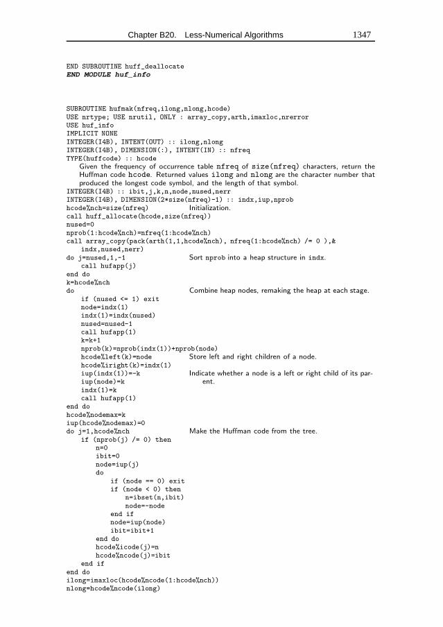
Chapter B20. Less-Numerical Algorithms 1347
END SUBROUTINE huff_deallocateEND MODULE huf_info
SUBROUTINE hufmak(nfreq,ilong,nlong,hcode)USE nrtype; USE nrutil, ONLY : array_copy,arth,imaxloc,nrerrorUSE huf_infoIMPLICIT NONEINTEGER(I4B), INTENT(OUT) :: ilong,nlongINTEGER(I4B), DIMENSION(:), INTENT(IN) :: nfreqTYPE(huffcode) :: hcode
Given the frequency of occurrence table nfreq of size(nfreq) characters, return theHuffman code hcode. Returned values ilong and nlong are the character number thatproduced the longest code symbol, and the length of that symbol.
INTEGER(I4B) :: ibit,j,k,n,node,nused,nerrINTEGER(I4B), DIMENSION(2*size(nfreq)-1) :: indx,iup,nprobhcode%nch=size(nfreq) Initialization.call huff_allocate(hcode,size(nfreq))nused=0nprob(1:hcode%nch)=nfreq(1:hcode%nch)call array_copy(pack(arth(1,1,hcode%nch), nfreq(1:hcode%nch) /= 0 ),&
indx,nused,nerr)do j=nused,1,-1 Sort nprob into a heap structure in indx.
call hufapp(j)end dok=hcode%nchdo Combine heap nodes, remaking the heap at each stage.
if (nused <= 1) exitnode=indx(1)indx(1)=indx(nused)nused=nused-1call hufapp(1)k=k+1nprob(k)=nprob(indx(1))+nprob(node)hcode%left(k)=node Store left and right children of a node.hcode%iright(k)=indx(1)iup(indx(1))=-k Indicate whether a node is a left or right child of its par-
ent.iup(node)=kindx(1)=kcall hufapp(1)
end dohcode%nodemax=kiup(hcode%nodemax)=0do j=1,hcode%nch Make the Huffman code from the tree.
if (nprob(j) /= 0) thenn=0ibit=0node=iup(j)do
if (node == 0) exitif (node < 0) then
n=ibset(n,ibit)node=-node
end ifnode=iup(node)ibit=ibit+1
end dohcode%icode(j)=nhcode%ncode(j)=ibit
end ifend doilong=imaxloc(hcode%ncode(1:hcode%nch))nlong=hcode%ncode(ilong)
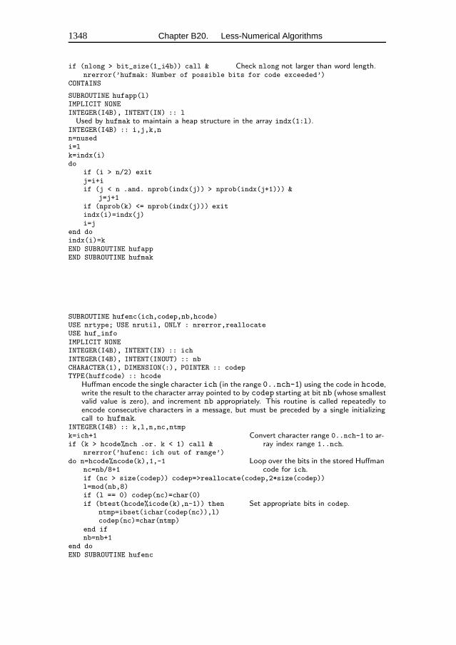
1348 Chapter B20. Less-Numerical Algorithms
if (nlong > bit_size(1_i4b)) call & Check nlong not larger than word length.nrerror(’hufmak: Number of possible bits for code exceeded’)
CONTAINS
SUBROUTINE hufapp(l)IMPLICIT NONEINTEGER(I4B), INTENT(IN) :: lUsed by hufmak to maintain a heap structure in the array indx(1:l).
INTEGER(I4B) :: i,j,k,nn=nusedi=lk=indx(i)do
if (i > n/2) exitj=i+iif (j < n .and. nprob(indx(j)) > nprob(indx(j+1))) &
j=j+1if (nprob(k) <= nprob(indx(j))) exitindx(i)=indx(j)i=j
end doindx(i)=kEND SUBROUTINE hufappEND SUBROUTINE hufmak
SUBROUTINE hufenc(ich,codep,nb,hcode)USE nrtype; USE nrutil, ONLY : nrerror,reallocateUSE huf_infoIMPLICIT NONEINTEGER(I4B), INTENT(IN) :: ichINTEGER(I4B), INTENT(INOUT) :: nbCHARACTER(1), DIMENSION(:), POINTER :: codepTYPE(huffcode) :: hcode
Huffman encode the single character ich (in the range 0..nch-1) using the code in hcode,write the result to the character array pointed to by codep starting at bit nb (whose smallestvalid value is zero), and increment nb appropriately. This routine is called repeatedly toencode consecutive characters in a message, but must be preceded by a single initializingcall to hufmak.
INTEGER(I4B) :: k,l,n,nc,ntmpk=ich+1 Convert character range 0..nch-1 to ar-
ray index range 1..nch.if (k > hcode%nch .or. k < 1) call &nrerror(’hufenc: ich out of range’)
do n=hcode%ncode(k),1,-1 Loop over the bits in the stored Huffmancode for ich.nc=nb/8+1
if (nc > size(codep)) codep=>reallocate(codep,2*size(codep))l=mod(nb,8)if (l == 0) codep(nc)=char(0)if (btest(hcode%icode(k),n-1)) then Set appropriate bits in codep.
ntmp=ibset(ichar(codep(nc)),l)codep(nc)=char(ntmp)
end ifnb=nb+1
end doEND SUBROUTINE hufenc
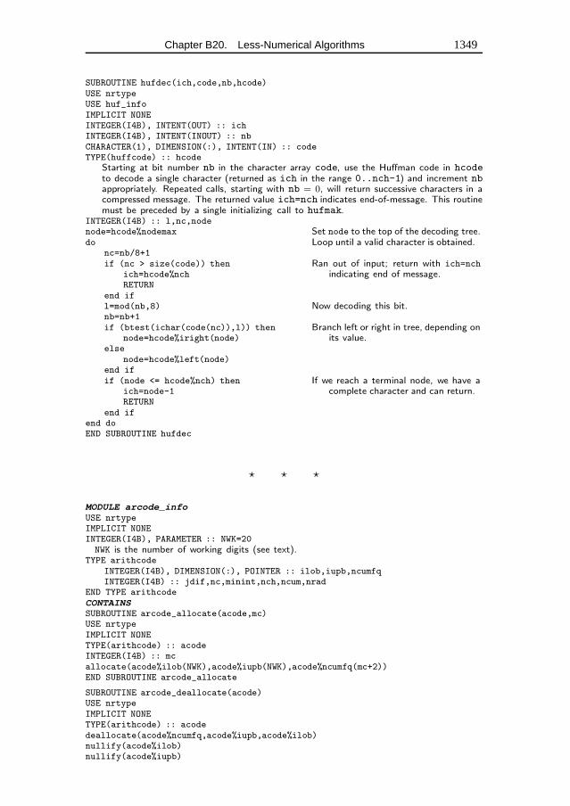
Chapter B20. Less-Numerical Algorithms 1349
SUBROUTINE hufdec(ich,code,nb,hcode)USE nrtypeUSE huf_infoIMPLICIT NONEINTEGER(I4B), INTENT(OUT) :: ichINTEGER(I4B), INTENT(INOUT) :: nbCHARACTER(1), DIMENSION(:), INTENT(IN) :: codeTYPE(huffcode) :: hcode
Starting at bit number nb in the character array code, use the Huffman code in hcodeto decode a single character (returned as ich in the range 0..nch-1) and increment nbappropriately. Repeated calls, starting with nb = 0, will return successive characters in acompressed message. The returned value ich=nch indicates end-of-message. This routinemust be preceded by a single initializing call to hufmak.
INTEGER(I4B) :: l,nc,nodenode=hcode%nodemax Set node to the top of the decoding tree.do Loop until a valid character is obtained.
nc=nb/8+1if (nc > size(code)) then Ran out of input; return with ich=nch
indicating end of message.ich=hcode%nchRETURN
end ifl=mod(nb,8) Now decoding this bit.nb=nb+1if (btest(ichar(code(nc)),l)) then Branch left or right in tree, depending on
its value.node=hcode%iright(node)else
node=hcode%left(node)end ifif (node <= hcode%nch) then If we reach a terminal node, we have a
complete character and can return.ich=node-1RETURN
end ifend doEND SUBROUTINE hufdec
� � �
MODULE arcode_infoUSE nrtypeIMPLICIT NONEINTEGER(I4B), PARAMETER :: NWK=20NWK is the number of working digits (see text).
TYPE arithcodeINTEGER(I4B), DIMENSION(:), POINTER :: ilob,iupb,ncumfqINTEGER(I4B) :: jdif,nc,minint,nch,ncum,nrad
END TYPE arithcodeCONTAINSSUBROUTINE arcode_allocate(acode,mc)USE nrtypeIMPLICIT NONETYPE(arithcode) :: acodeINTEGER(I4B) :: mcallocate(acode%ilob(NWK),acode%iupb(NWK),acode%ncumfq(mc+2))END SUBROUTINE arcode_allocate
SUBROUTINE arcode_deallocate(acode)USE nrtypeIMPLICIT NONETYPE(arithcode) :: acodedeallocate(acode%ncumfq,acode%iupb,acode%ilob)nullify(acode%ilob)nullify(acode%iupb)
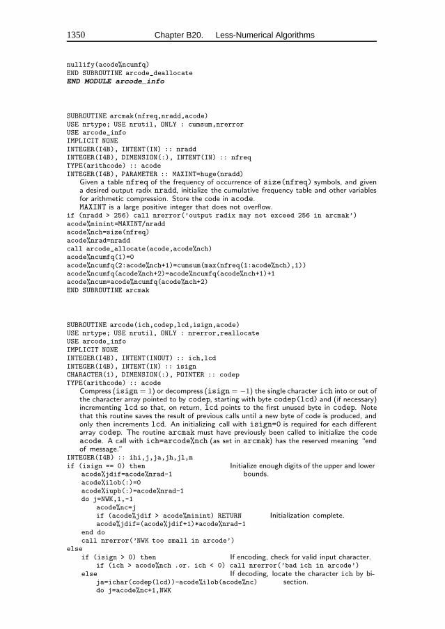
1350 Chapter B20. Less-Numerical Algorithms
nullify(acode%ncumfq)END SUBROUTINE arcode_deallocateEND MODULE arcode_info
SUBROUTINE arcmak(nfreq,nradd,acode)USE nrtype; USE nrutil, ONLY : cumsum,nrerrorUSE arcode_infoIMPLICIT NONEINTEGER(I4B), INTENT(IN) :: nraddINTEGER(I4B), DIMENSION(:), INTENT(IN) :: nfreqTYPE(arithcode) :: acodeINTEGER(I4B), PARAMETER :: MAXINT=huge(nradd)
Given a table nfreq of the frequency of occurrence of size(nfreq) symbols, and givena desired output radix nradd, initialize the cumulative frequency table and other variablesfor arithmetic compression. Store the code in acode.MAXINT is a large positive integer that does not overflow.
if (nradd > 256) call nrerror(’output radix may not exceed 256 in arcmak’)acode%minint=MAXINT/nraddacode%nch=size(nfreq)acode%nrad=nraddcall arcode_allocate(acode,acode%nch)acode%ncumfq(1)=0acode%ncumfq(2:acode%nch+1)=cumsum(max(nfreq(1:acode%nch),1))acode%ncumfq(acode%nch+2)=acode%ncumfq(acode%nch+1)+1acode%ncum=acode%ncumfq(acode%nch+2)END SUBROUTINE arcmak
SUBROUTINE arcode(ich,codep,lcd,isign,acode)USE nrtype; USE nrutil, ONLY : nrerror,reallocateUSE arcode_infoIMPLICIT NONEINTEGER(I4B), INTENT(INOUT) :: ich,lcdINTEGER(I4B), INTENT(IN) :: isignCHARACTER(1), DIMENSION(:), POINTER :: codepTYPE(arithcode) :: acode
Compress (isign = 1) or decompress (isign = −1) the single character ich into or out ofthe character array pointed to by codep, starting with byte codep(lcd) and (if necessary)incrementing lcd so that, on return, lcd points to the first unused byte in codep. Notethat this routine saves the result of previous calls until a new byte of code is produced, andonly then increments lcd. An initializing call with isign=0 is required for each differentarray codep. The routine arcmak must have previously been called to initialize the codeacode. A call with ich=arcode%nch (as set in arcmak) has the reserved meaning “endof message.”
INTEGER(I4B) :: ihi,j,ja,jh,jl,mif (isign == 0) then Initialize enough digits of the upper and lower
bounds.acode%jdif=acode%nrad-1acode%ilob(:)=0acode%iupb(:)=acode%nrad-1do j=NWK,1,-1
acode%nc=jif (acode%jdif > acode%minint) RETURN Initialization complete.acode%jdif=(acode%jdif+1)*acode%nrad-1
end docall nrerror(’NWK too small in arcode’)
elseif (isign > 0) then If encoding, check for valid input character.
if (ich > acode%nch .or. ich < 0) call nrerror(’bad ich in arcode’)else If decoding, locate the character ich by bi-
section.ja=ichar(codep(lcd))-acode%ilob(acode%nc)do j=acode%nc+1,NWK
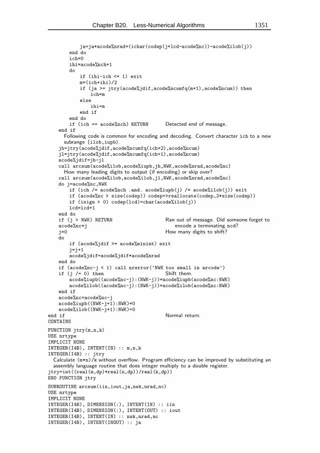
Chapter B20. Less-Numerical Algorithms 1351
ja=ja*acode%nrad+(ichar(codep(j+lcd-acode%nc))-acode%ilob(j))end doich=0ihi=acode%nch+1do
if (ihi-ich <= 1) exitm=(ich+ihi)/2if (ja >= jtry(acode%jdif,acode%ncumfq(m+1),acode%ncum)) then
ich=melse
ihi=mend if
end doif (ich == acode%nch) RETURN Detected end of message.
end ifFollowing code is common for encoding and decoding. Convert character ich to a newsubrange [ilob,iupb).
jh=jtry(acode%jdif,acode%ncumfq(ich+2),acode%ncum)jl=jtry(acode%jdif,acode%ncumfq(ich+1),acode%ncum)acode%jdif=jh-jlcall arcsum(acode%ilob,acode%iupb,jh,NWK,acode%nrad,acode%nc)How many leading digits to output (if encoding) or skip over?
call arcsum(acode%ilob,acode%ilob,jl,NWK,acode%nrad,acode%nc)do j=acode%nc,NWK
if (ich /= acode%nch .and. acode%iupb(j) /= acode%ilob(j)) exitif (acode%nc > size(codep)) codep=>reallocate(codep,2*size(codep))if (isign > 0) codep(lcd)=char(acode%ilob(j))lcd=lcd+1
end doif (j > NWK) RETURN Ran out of message. Did someone forget to
encode a terminating ncd?acode%nc=jj=0 How many digits to shift?do
if (acode%jdif >= acode%minint) exitj=j+1acode%jdif=acode%jdif*acode%nrad
end doif (acode%nc-j < 1) call nrerror(’NWK too small in arcode’)if (j /= 0) then Shift them.
acode%iupb((acode%nc-j):(NWK-j))=acode%iupb(acode%nc:NWK)acode%ilob((acode%nc-j):(NWK-j))=acode%ilob(acode%nc:NWK)
end ifacode%nc=acode%nc-jacode%iupb((NWK-j+1):NWK)=0acode%ilob((NWK-j+1):NWK)=0
end if Normal return.CONTAINS
FUNCTION jtry(m,n,k)USE nrtypeIMPLICIT NONEINTEGER(I4B), INTENT(IN) :: m,n,kINTEGER(I4B) :: jtryCalculate (m*n)/k without overflow. Program efficiency can be improved by substituting anassembly language routine that does integer multiply to a double register.
jtry=int((real(m,dp)*real(n,dp))/real(k,dp))END FUNCTION jtry
SUBROUTINE arcsum(iin,iout,ja,nwk,nrad,nc)USE nrtypeIMPLICIT NONEINTEGER(I4B), DIMENSION(:), INTENT(IN) :: iinINTEGER(I4B), DIMENSION(:), INTENT(OUT) :: ioutINTEGER(I4B), INTENT(IN) :: nwk,nrad,ncINTEGER(I4B), INTENT(INOUT) :: ja
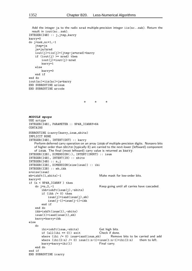
1352 Chapter B20. Less-Numerical Algorithms
Add the integer ja to the radix nrad multiple-precision integer iin(nc..nwk). Return theresult in iout(nc..nwk).
INTEGER(I4B) :: j,jtmp,karrykarry=0do j=nwk,nc+1,-1
jtmp=jaja=ja/nradiout(j)=iin(j)+(jtmp-ja*nrad)+karryif (iout(j) >= nrad) then
iout(j)=iout(j)-nradkarry=1
elsekarry=0
end ifend doiout(nc)=iin(nc)+ja+karryEND SUBROUTINE arcsumEND SUBROUTINE arcode
� � �
MODULE mpopsUSE nrtypeINTEGER(I4B), PARAMETER :: NPAR_ICARRY=64CONTAINS
SUBROUTINE icarry(karry,isum,nbits)IMPLICIT NONEINTEGER(I4B), INTENT(OUT) :: karry
Perform deferred carry operation on an array isum of multiple-precision digits. Nonzero bitsof higher order than nbits (typically 8) are carried to the next-lower (leftward) componentof isum. The final (most leftward) carry value is returned as karry.
INTEGER(I2B), DIMENSION(:), INTENT(INOUT) :: isumINTEGER(I4B), INTENT(IN) :: nbitsINTEGER(I4B) :: n,jINTEGER(I2B), DIMENSION(size(isum)) :: ihiINTEGER(I2B) :: mb,ihhn=size(isum)mb=ishft(1,nbits)-1 Make mask for low-order bits.karry=0if (n < NPAR_ICARRY ) then
do j=n,2,-1 Keep going until all carries have cascaded.ihh=ishft(isum(j),-nbits)if (ihh /= 0) then
isum(j)=iand(isum(j),mb)isum(j-1)=isum(j-1)+ihh
end ifend doihh=ishft(isum(1),-nbits)isum(1)=iand(isum(1),mb)karry=karry+ihh
elsedo
ihi=ishft(isum,-nbits) Get high bits.if (all(ihi == 0)) exit Check if done.where (ihi /= 0) isum=iand(isum,mb) Remove bits to be carried and add
them to left.where (ihi(2:n) /= 0) isum(1:n-1)=isum(1:n-1)+ihi(2:n)karry=karry+ihi(1) Final carry.
end doend ifEND SUBROUTINE icarry
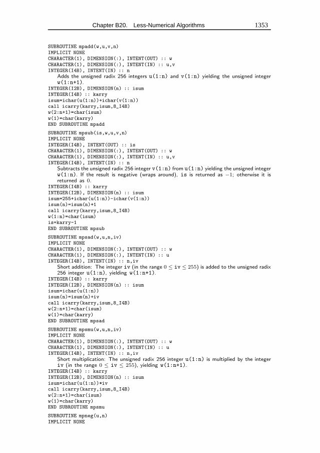
Chapter B20. Less-Numerical Algorithms 1353
SUBROUTINE mpadd(w,u,v,n)IMPLICIT NONECHARACTER(1), DIMENSION(:), INTENT(OUT) :: wCHARACTER(1), DIMENSION(:), INTENT(IN) :: u,vINTEGER(I4B), INTENT(IN) :: n
Adds the unsigned radix 256 integers u(1:n) and v(1:n) yielding the unsigned integerw(1:n+1).
INTEGER(I2B), DIMENSION(n) :: isumINTEGER(I4B) :: karryisum=ichar(u(1:n))+ichar(v(1:n))call icarry(karry,isum,8_I4B)w(2:n+1)=char(isum)w(1)=char(karry)END SUBROUTINE mpadd
SUBROUTINE mpsub(is,w,u,v,n)IMPLICIT NONEINTEGER(I4B), INTENT(OUT) :: isCHARACTER(1), DIMENSION(:), INTENT(OUT) :: wCHARACTER(1), DIMENSION(:), INTENT(IN) :: u,vINTEGER(I4B), INTENT(IN) :: n
Subtracts the unsigned radix 256 integer v(1:n) from u(1:n) yielding the unsigned integerw(1:n). If the result is negative (wraps around), is is returned as −1; otherwise it isreturned as 0.
INTEGER(I4B) :: karryINTEGER(I2B), DIMENSION(n) :: isumisum=255+ichar(u(1:n))-ichar(v(1:n))isum(n)=isum(n)+1call icarry(karry,isum,8_I4B)w(1:n)=char(isum)is=karry-1END SUBROUTINE mpsub
SUBROUTINE mpsad(w,u,n,iv)IMPLICIT NONECHARACTER(1), DIMENSION(:), INTENT(OUT) :: wCHARACTER(1), DIMENSION(:), INTENT(IN) :: uINTEGER(I4B), INTENT(IN) :: n,iv
Short addition: The integer iv (in the range 0 ≤ iv ≤ 255) is added to the unsigned radix256 integer u(1:n), yielding w(1:n+1).
INTEGER(I4B) :: karryINTEGER(I2B), DIMENSION(n) :: isumisum=ichar(u(1:n))isum(n)=isum(n)+ivcall icarry(karry,isum,8_I4B)w(2:n+1)=char(isum)w(1)=char(karry)END SUBROUTINE mpsad
SUBROUTINE mpsmu(w,u,n,iv)IMPLICIT NONECHARACTER(1), DIMENSION(:), INTENT(OUT) :: wCHARACTER(1), DIMENSION(:), INTENT(IN) :: uINTEGER(I4B), INTENT(IN) :: n,iv
Short multiplication: The unsigned radix 256 integer u(1:n) is multiplied by the integeriv (in the range 0 ≤ iv ≤ 255), yielding w(1:n+1).
INTEGER(I4B) :: karryINTEGER(I2B), DIMENSION(n) :: isumisum=ichar(u(1:n))*ivcall icarry(karry,isum,8_I4B)w(2:n+1)=char(isum)w(1)=char(karry)END SUBROUTINE mpsmu
SUBROUTINE mpneg(u,n)IMPLICIT NONE
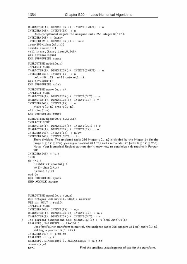
1354 Chapter B20. Less-Numerical Algorithms
CHARACTER(1), DIMENSION(:), INTENT(INOUT) :: uINTEGER(I4B), INTENT(IN) :: n
Ones-complement negate the unsigned radix 256 integer u(1:n).INTEGER(I4B) :: karryINTEGER(I2B), DIMENSION(n) :: isumisum=255-ichar(u(1:n))isum(n)=isum(n)+1call icarry(karry,isum,8_I4B)u(1:n)=char(isum)END SUBROUTINE mpneg
SUBROUTINE mplsh(u,n)IMPLICIT NONECHARACTER(1), DIMENSION(:), INTENT(INOUT) :: uINTEGER(I4B), INTENT(IN) :: n
Left shift u(2..n+1) onto u(1:n).u(1:n)=u(2:n+1)END SUBROUTINE mplsh
SUBROUTINE mpmov(u,v,n)IMPLICIT NONECHARACTER(1), DIMENSION(:), INTENT(OUT) :: uCHARACTER(1), DIMENSION(:), INTENT(IN) :: vINTEGER(I4B), INTENT(IN) :: n
Move v(1:n) onto u(1:n).u(1:n)=v(1:n)END SUBROUTINE mpmov
SUBROUTINE mpsdv(w,u,n,iv,ir)IMPLICIT NONECHARACTER(1), DIMENSION(:), INTENT(OUT) :: wCHARACTER(1), DIMENSION(:), INTENT(IN) :: uINTEGER(I4B), INTENT(IN) :: n,ivINTEGER(I4B), INTENT(OUT) :: ir
Short division: The unsigned radix 256 integer u(1:n) is divided by the integer iv (in therange 0 ≤ iv ≤ 255), yielding a quotient w(1:n) and a remainder ir (with 0 ≤ ir ≤ 255).Note: Your Numerical Recipes authors don’t know how to parallelize this routine in Fortran90!
INTEGER(I4B) :: i,jir=0do j=1,n
i=256*ir+ichar(u(j))w(j)=char(i/iv)ir=mod(i,iv)
end doEND SUBROUTINE mpsdvEND MODULE mpops
SUBROUTINE mpmul(w,u,v,n,m)USE nrtype; USE nrutil, ONLY : nrerrorUSE nr, ONLY : realftIMPLICIT NONEINTEGER(I4B), INTENT(IN) :: n,mCHARACTER(1), DIMENSION(:), INTENT(IN) :: u,vCHARACTER(1), DIMENSION(:), INTENT(OUT) :: w
! The logical dimensions are: CHARACTER(1) :: w(n+m),u(n),v(m)REAL(DP), PARAMETER :: RX=256.0
Uses fast Fourier transform to multiply the unsigned radix 256 integers u(1:n) and v(1:m),yielding a product w(1:n+m).
INTEGER(I4B) :: j,mn,nnREAL(DP) :: cy,tREAL(DP), DIMENSION(:), ALLOCATABLE :: a,b,tbmn=max(m,n)nn=1 Find the smallest useable power of two for the transform.
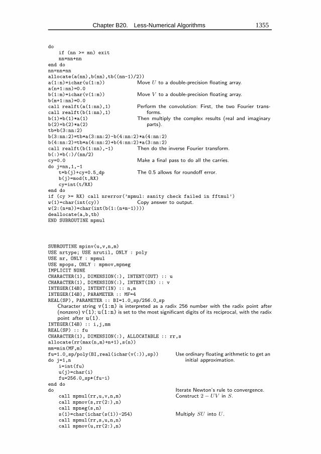
Chapter B20. Less-Numerical Algorithms 1355
doif (nn >= mn) exitnn=nn+nn
end donn=nn+nnallocate(a(nn),b(nn),tb((nn-1)/2))a(1:n)=ichar(u(1:n)) Move U to a double-precision floating array.a(n+1:nn)=0.0b(1:m)=ichar(v(1:m)) Move V to a double-precision floating array.b(m+1:nn)=0.0call realft(a(1:nn),1) Perform the convolution: First, the two Fourier trans-
forms.call realft(b(1:nn),1)b(1)=b(1)*a(1) Then multiply the complex results (real and imaginary
parts).b(2)=b(2)*a(2)tb=b(3:nn:2)b(3:nn:2)=tb*a(3:nn:2)-b(4:nn:2)*a(4:nn:2)b(4:nn:2)=tb*a(4:nn:2)+b(4:nn:2)*a(3:nn:2)call realft(b(1:nn),-1) Then do the inverse Fourier transform.b(:)=b(:)/(nn/2)cy=0.0 Make a final pass to do all the carries.do j=nn,1,-1
t=b(j)+cy+0.5_dp The 0.5 allows for roundoff error.b(j)=mod(t,RX)cy=int(t/RX)
end doif (cy >= RX) call nrerror(’mpmul: sanity check failed in fftmul’)w(1)=char(int(cy)) Copy answer to output.w(2:(n+m))=char(int(b(1:(n+m-1))))deallocate(a,b,tb)END SUBROUTINE mpmul
SUBROUTINE mpinv(u,v,n,m)USE nrtype; USE nrutil, ONLY : polyUSE nr, ONLY : mpmulUSE mpops, ONLY : mpmov,mpnegIMPLICIT NONECHARACTER(1), DIMENSION(:), INTENT(OUT) :: uCHARACTER(1), DIMENSION(:), INTENT(IN) :: vINTEGER(I4B), INTENT(IN) :: n,mINTEGER(I4B), PARAMETER :: MF=4REAL(SP), PARAMETER :: BI=1.0_sp/256.0_sp
Character string v(1:m) is interpreted as a radix 256 number with the radix point after(nonzero) v(1); u(1:n) is set to the most significant digits of its reciprocal, with the radixpoint after u(1).
INTEGER(I4B) :: i,j,mmREAL(SP) :: fuCHARACTER(1), DIMENSION(:), ALLOCATABLE :: rr,sallocate(rr(max(n,m)+n+1),s(n))mm=min(MF,m)fu=1.0_sp/poly(BI,real(ichar(v(:)),sp)) Use ordinary floating arithmetic to get an
initial approximation.do j=1,ni=int(fu)u(j)=char(i)fu=256.0_sp*(fu-i)
end dodo Iterate Newton’s rule to convergence.
call mpmul(rr,u,v,n,m) Construct 2 − UV in S.call mpmov(s,rr(2:),n)call mpneg(s,n)s(1)=char(ichar(s(1))-254) Multiply SU into U .call mpmul(rr,s,u,n,n)call mpmov(u,rr(2:),n)
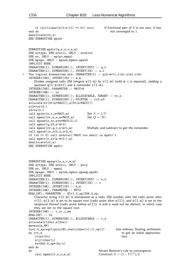
1356 Chapter B20. Less-Numerical Algorithms
if (all(ichar(s(2:n-1)) == 0)) exit If fractional part of S is not zero, it hasnot converged to 1.end do
deallocate(rr,s)END SUBROUTINE mpinv
SUBROUTINE mpdiv(q,r,u,v,n,m)USE nrtype; USE nrutil, ONLY : nrerrorUSE nr, ONLY : mpinv,mpmulUSE mpops, ONLY : mpsad,mpmov,mpsubIMPLICIT NONECHARACTER(1), DIMENSION(:), INTENT(OUT) :: q,rCHARACTER(1), DIMENSION(:), INTENT(IN) :: u,v
! The logical dimensions are: CHARACTER(1) :: q(n-m+1),r(m),u(n),v(m)INTEGER(I4B), INTENT(IN) :: n,m
Divides unsigned radix 256 integers u(1:n) by v(1:m) (with m ≤ n required), yielding aquotient q(1:n-m+1) and a remainder r(1:m).
INTEGER(I4B), PARAMETER :: MACC=6INTEGER(I4B) :: isCHARACTER(1), DIMENSION(:), ALLOCATABLE, TARGET :: rr,sCHARACTER(1), DIMENSION(:), POINTER :: rr2,s3allocate(rr(2*(n+MACC)),s(2*(n+MACC)))rr2=>rr(2:)s3=>s(3:)call mpinv(s,v,n+MACC,m) Set S = 1/V .call mpmul(rr,s,u,n+MACC,n) Set Q = SU .call mpsad(s,rr,n+n+MACC/2,1)call mpmov(q,s3,n-m+1)call mpmul(rr,q,v,n-m+1,m) Multiply and subtract to get the remainder.call mpsub(is,rr2,u,rr2,n)if (is /= 0) call nrerror(’MACC too small in mpdiv’)call mpmov(r,rr(n-m+2:),m)deallocate(rr,s)END SUBROUTINE mpdiv
SUBROUTINE mpsqrt(w,u,v,n,m)USE nrtype; USE nrutil, ONLY : polyUSE nr, ONLY : mpmulUSE mpops, ONLY : mplsh,mpmov,mpneg,mpsdvIMPLICIT NONECHARACTER(1), DIMENSION(:), INTENT(OUT) :: w,uCHARACTER(1), DIMENSION(:), INTENT(IN) :: vINTEGER(I4B), INTENT(IN) :: n,mINTEGER(I4B), PARAMETER :: MF=3REAL(SP), PARAMETER :: BI=1.0_sp/256.0_sp
Character string v(1:m) is interpreted as a radix 256 number with the radix point afterv(1); w(1:n) is set to its square root (radix point after w(1)), and u(1:n) is set to thereciprocal thereof (radix point before u(1)). w and u need not be distinct, in which casethey are set to the square root.
INTEGER(I4B) :: i,ir,j,mmREAL(SP) :: fuCHARACTER(1), DIMENSION(:), ALLOCATABLE :: r,sallocate(r(2*n),s(2*n))mm=min(m,MF)fu=1.0_sp/sqrt(poly(BI,real(ichar(v(:)),sp))) Use ordinary floating arithmetic
to get an initial approxima-tion.
do j=1,ni=int(fu)u(j)=char(i)fu=256.0_sp*(fu-i)
end dodo Iterate Newton’s rule to convergence.
call mpmul(r,u,u,n,n) Construct S = (3 − V U2)/2.
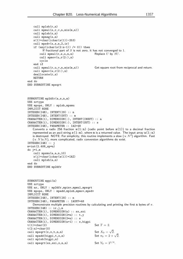
Chapter B20. Less-Numerical Algorithms 1357
call mplsh(r,n)call mpmul(s,r,v,n,min(m,n))call mplsh(s,n)call mpneg(s,n)s(1)=char(ichar(s(1))-253)call mpsdv(s,s,n,2,ir)if (any(ichar(s(2:n-1)) /= 0)) then
If fractional part of S is not zero, it has not converged to 1.call mpmul(r,s,u,n,n) Replace U by SU .call mpmov(u,r(2:),n)cycle
end ifcall mpmul(r,u,v,n,min(m,n)) Get square root from reciprocal and return.call mpmov(w,r(2:),n)deallocate(r,s)RETURN
end doEND SUBROUTINE mpsqrt
SUBROUTINE mp2dfr(a,s,n,m)USE nrtypeUSE mpops, ONLY : mplsh,mpsmuIMPLICIT NONEINTEGER(I4B), INTENT(IN) :: nINTEGER(I4B), INTENT(OUT) :: mCHARACTER(1), DIMENSION(:), INTENT(INOUT) :: aCHARACTER(1), DIMENSION(:), INTENT(OUT) :: sINTEGER(I4B), PARAMETER :: IAZ=48
Converts a radix 256 fraction a(1:n) (radix point before a(1)) to a decimal fractionrepresented as an ascii string s(1:m), where m is a returned value. The input array a(1:n)is destroyed. NOTE: For simplicity, this routine implements a slow (∝ N2) algorithm. Fast(∝ N lnN), more complicated, radix conversion algorithms do exist.
INTEGER(I4B) :: jm=int(2.408_sp*n)do j=1,m
call mpsmu(a,a,n,10)s(j)=char(ichar(a(1))+IAZ)call mplsh(a,n)
end doEND SUBROUTINE mp2dfr
SUBROUTINE mppi(n)USE nrtypeUSE nr, ONLY : mp2dfr,mpinv,mpmul,mpsqrtUSE mpops, ONLY : mpadd,mplsh,mpmov,mpsdvIMPLICIT NONEINTEGER(I4B), INTENT(IN) :: nINTEGER(I4B), PARAMETER :: IAOFF=48
Demonstrate multiple precision routines by calculating and printing the first n bytes of π.INTEGER(I4B) :: ir,j,mCHARACTER(1), DIMENSION(n) :: sx,sxiCHARACTER(1), DIMENSION(2*n) :: t,yCHARACTER(1), DIMENSION(3*n) :: sCHARACTER(1), DIMENSION(n+1) :: x,bigpit(1)=char(2) Set T = 2.t(2:n)=char(0)call mpsqrt(x,x,t,n,n) Set X0 =
√2.
call mpadd(bigpi,t,x,n) Set π0 = 2 +√
2.call mplsh(bigpi,n)
call mpsqrt(sx,sxi,x,n,n) Set Y0 = 21/4.
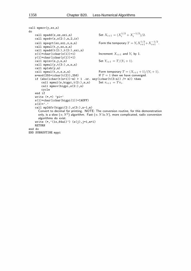
1358 Chapter B20. Less-Numerical Algorithms
call mpmov(y,sx,n)do
call mpadd(x,sx,sxi,n) Set Xi+1 = (X1/2i + X
−1/2i )/2.
call mpsdv(x,x(2:),n,2,ir)
call mpsqrt(sx,sxi,x,n,n) Form the temporary T = YiX1/2i+1+X
−1/2i+1 .
call mpmul(t,y,sx,n,n)call mpadd(t(2:),t(2:),sxi,n)x(1)=char(ichar(x(1))+1) Increment Xi+1 and Yi by 1.y(1)=char(ichar(y(1))+1)call mpinv(s,y,n,n) Set Yi+1 = T/(Yi + 1).call mpmul(y,t(3:),s,n,n)call mplsh(y,n)call mpmul(t,x,s,n,n) Form temporary T = (Xi+1 + 1)/(Yi + 1).m=mod(255+ichar(t(2)),256) If T = 1 then we have converged.if (abs(ichar(t(n+1))-m) > 1 .or. any(ichar(t(3:n)) /= m)) then
call mpmul(s,bigpi,t(2:),n,n) Set πi+1 = Tπi.call mpmov(bigpi,s(2:),n)cycle
end ifwrite (*,*) ’pi=’s(1)=char(ichar(bigpi(1))+IAOFF)s(2)=’.’call mp2dfr(bigpi(2:),s(3:),n-1,m)Convert to decimal for printing. NOTE: The conversion routine, for this demonstrationonly, is a slow (∝ N2) algorithm. Fast (∝ N lnN), more complicated, radix conversionalgorithms do exist.
write (*,’(1x,64a1)’) (s(j),j=1,m+1)RETURN
end doEND SUBROUTINE mppi
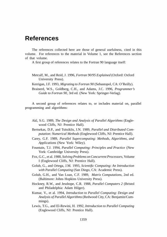
References
The references collected here are those of general usefulness, cited in thisvolume. For references to the material in Volume 1, see the References sectionof that volume.
A first group of references relates to the Fortran 90 language itself:
Metcalf, M., and Reid, J. 1996, Fortran 90/95 Explained(Oxford: OxfordUniversity Press).
Kerrigan, J.F. 1993, Migrating to Fortran 90(Sebastopol, CA: O’Reilly).
Brainerd, W.S., Goldberg, C.H., and Adams, J.C. 1996, Programmer’sGuide to Fortran 90, 3rd ed. (New York: Springer-Verlag).
A second group of references relates to, or includes material on, parallelprogramming and algorithms:
Akl, S.G. 1989, The Design and Analysis of Parallel Algorithms(Engle-wood Cliffs, NJ: Prentice Hall).
Bertsekas, D.P., and Tsitsiklis, J.N. 1989, Parallel and Distributed Com-putation: Numerical Methods(Englewood Cliffs, NJ: Prentice Hall).
Carey, G.F. 1989, Parallel Supercomputing: Methods, Algorithms, andApplications(New York: Wiley).
Fountain, T.J. 1994, Parallel Computing: Principles and Practice(NewYork: Cambridge University Press).
Fox, G.C., et al. 1988, Solving Problems on Concurrent Processors, VolumeI (Englewood Cliffs, NJ: Prentice Hall).
Golub, G., and Ortega, J.M. 1993, Scientific Computing: An Introductionwith Parallel Computing(San Diego, CA: Academic Press).
Golub, G.H., and Van Loan, C.F. 1989, Matrix Computations, 2nd ed.(Baltimore: Johns Hopkins University Press).
Hockney, R.W., and Jesshope, C.R. 1988, Parallel Computers 2(Bristoland Philadelphia: Adam Hilger).
Kumar, V., et al. 1994, Introduction to Parallel Computing: Design andAnalysis of Parallel Algorithms(Redwood City, CA: Benjamin/Cum-mings).
Lewis, T.G., and El-Rewini, H. 1992, Introduction to Parallel Computing(Englewood Cliffs, NJ: Prentice Hall).
1359

1360 References
Modi, J.J. 1988, Parallel Algorithms and Matrix Computation(New York:Oxford University Press).
Smith, J.R. 1993, The Design and Analysis of Parallel Algorithms(NewYork: Oxford University Press).
Van de Velde, E. 1994, Concurrent Scientific Computing(New York:Springer-Verlag).
Van Loan, C.F. 1992, Computational Frameworks for the Fast FourierTransform(Philadelphia: S.I.A.M.).
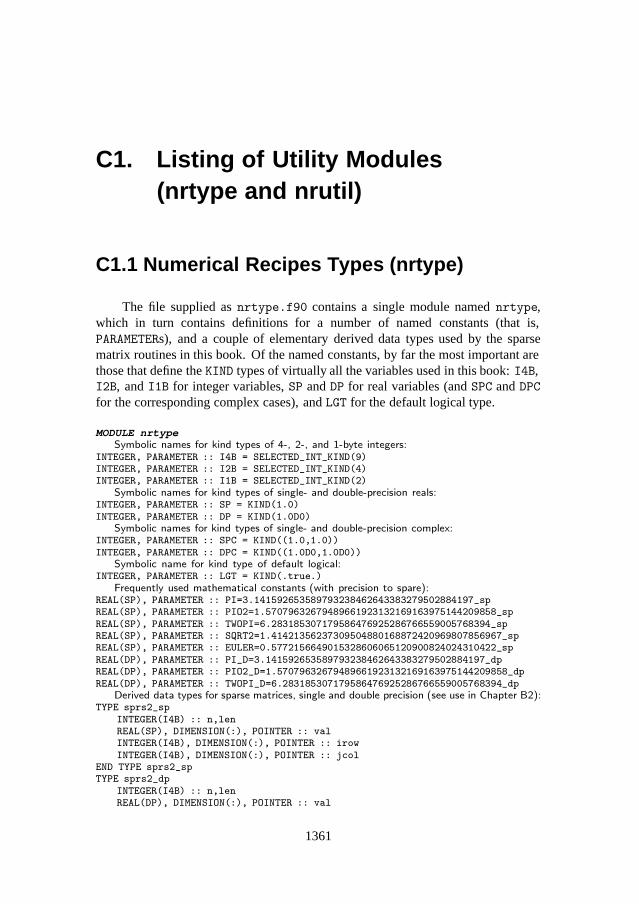
C1. Listing of Utility Modules(nrtype and nrutil)
C1.1 Numerical Recipes Types (nrtype)
The file supplied as nrtype.f90 contains a single module named nrtype,which in turn contains definitions for a number of named constants (that is,PARAMETERs), and a couple of elementary derived data types used by the sparsematrix routines in this book. Of the named constants, by far the most important arethose that define the KIND types of virtually all the variables used in this book: I4B,I2B, and I1B for integer variables, SP and DP for real variables (and SPC and DPC
for the corresponding complex cases), and LGT for the default logical type.
MODULE nrtypeSymbolic names for kind types of 4-, 2-, and 1-byte integers:
INTEGER, PARAMETER :: I4B = SELECTED_INT_KIND(9)INTEGER, PARAMETER :: I2B = SELECTED_INT_KIND(4)INTEGER, PARAMETER :: I1B = SELECTED_INT_KIND(2)
Symbolic names for kind types of single- and double-precision reals:INTEGER, PARAMETER :: SP = KIND(1.0)INTEGER, PARAMETER :: DP = KIND(1.0D0)
Symbolic names for kind types of single- and double-precision complex:INTEGER, PARAMETER :: SPC = KIND((1.0,1.0))INTEGER, PARAMETER :: DPC = KIND((1.0D0,1.0D0))
Symbolic name for kind type of default logical:INTEGER, PARAMETER :: LGT = KIND(.true.)
Frequently used mathematical constants (with precision to spare):REAL(SP), PARAMETER :: PI=3.141592653589793238462643383279502884197_spREAL(SP), PARAMETER :: PIO2=1.57079632679489661923132169163975144209858_spREAL(SP), PARAMETER :: TWOPI=6.283185307179586476925286766559005768394_spREAL(SP), PARAMETER :: SQRT2=1.41421356237309504880168872420969807856967_spREAL(SP), PARAMETER :: EULER=0.5772156649015328606065120900824024310422_spREAL(DP), PARAMETER :: PI_D=3.141592653589793238462643383279502884197_dpREAL(DP), PARAMETER :: PIO2_D=1.57079632679489661923132169163975144209858_dpREAL(DP), PARAMETER :: TWOPI_D=6.283185307179586476925286766559005768394_dp
Derived data types for sparse matrices, single and double precision (see use in Chapter B2):TYPE sprs2_sp
INTEGER(I4B) :: n,lenREAL(SP), DIMENSION(:), POINTER :: valINTEGER(I4B), DIMENSION(:), POINTER :: irowINTEGER(I4B), DIMENSION(:), POINTER :: jcol
END TYPE sprs2_spTYPE sprs2_dp
INTEGER(I4B) :: n,lenREAL(DP), DIMENSION(:), POINTER :: val
1361
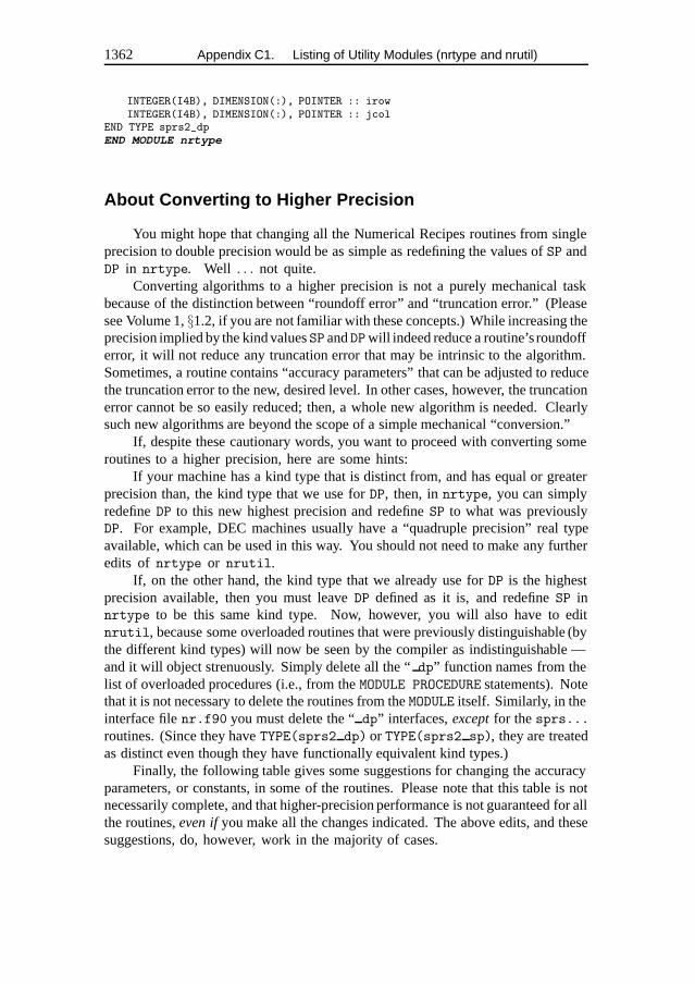
1362 Appendix C1. Listing of Utility Modules (nrtype and nrutil)
INTEGER(I4B), DIMENSION(:), POINTER :: irowINTEGER(I4B), DIMENSION(:), POINTER :: jcol
END TYPE sprs2_dpEND MODULE nrtype
About Converting to Higher Precision
You might hope that changing all the Numerical Recipes routines from singleprecision to double precision would be as simple as redefining the values of SP andDP in nrtype. Well . . . not quite.
Converting algorithms to a higher precision is not a purely mechanical taskbecause of the distinction between “roundoff error” and “truncation error.” (Pleasesee Volume 1, §1.2, if you are not familiar with these concepts.) While increasing theprecision implied by the kind values SP and DPwill indeed reduce a routine’s roundofferror, it will not reduce any truncation error that may be intrinsic to the algorithm.Sometimes, a routine contains “accuracy parameters” that can be adjusted to reducethe truncation error to the new, desired level. In other cases, however, the truncationerror cannot be so easily reduced; then, a whole new algorithm is needed. Clearlysuch new algorithms are beyond the scope of a simple mechanical “conversion.”
If, despite these cautionary words, you want to proceed with converting someroutines to a higher precision, here are some hints:
If your machine has a kind type that is distinct from, and has equal or greaterprecision than, the kind type that we use for DP, then, in nrtype, you can simplyredefine DP to this new highest precision and redefine SP to what was previouslyDP. For example, DEC machines usually have a “quadruple precision” real typeavailable, which can be used in this way. You should not need to make any furtheredits of nrtype or nrutil.
If, on the other hand, the kind type that we already use for DP is the highestprecision available, then you must leave DP defined as it is, and redefine SP innrtype to be this same kind type. Now, however, you will also have to editnrutil, because some overloaded routines that were previously distinguishable (bythe different kind types) will now be seen by the compiler as indistinguishable —and it will object strenuously. Simply delete all the “ dp” function names from thelist of overloaded procedures (i.e., from the MODULE PROCEDURE statements). Notethat it is not necessary to delete the routines from the MODULE itself. Similarly, in theinterface file nr.f90 you must delete the “ dp” interfaces, except for the sprs...routines. (Since they have TYPE(sprs2 dp) or TYPE(sprs2 sp), they are treatedas distinct even though they have functionally equivalent kind types.)
Finally, the following table gives some suggestions for changing the accuracyparameters, or constants, in some of the routines. Please note that this table is notnecessarily complete, and that higher-precision performance is not guaranteed for allthe routines, even if you make all the changes indicated. The above edits, and thesesuggestions, do, however, work in the majority of cases.
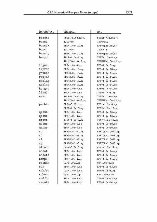
C1.1 Numerical Recipes Types (nrtype) 1363
In routine... change... to...
beschb NUSE1=5,NUSE2=5 NUSE1=7,NUSE2=8
bessi IACC=40 IACC=200
bessik EPS=1.0e-10 dp EPS=epsilon(x)
bessj IACC=40 IACC=160
bessjy EPS=1.0e-10 dp EPS=epsilon(x)
broydn TOLF=1.0e-4 sp TOLF=1.0e-8 sp
TOLMIN=1.0e-6 sp TOLMIN=1.0e-12 sp
fdjac EPS=1.0e-4 sp EPS=1.0e-8 sp
frprmn EPS=1.0e-10 sp EPS=1.0e-18 sp
gauher EPS=3.0e-13 dp EPS=1.0e-14 dp
gaujac EPS=3.0e-14 dp EPS=1.0e-14 dp
gaulag EPS=3.0e-13 dp EPS=1.0e-14 dp
gauleg EPS=3.0e-14 dp EPS=1.0e-14 dp
hypgeo EPS=1.0e-6 sp EPS=1.0e-14 sp
linmin TOL=1.0e-4 sp TOL=1.0e-8 sp
newt TOLF=1.0e-4 sp TOLF=1.0e-8 sp
TOLMIN=1.0e-6 sp TOLMIN=1.0e-12 sp
probks EPS1=0.001 sp EPS1=1.0e-6 sp
EPS2=1.0e-8 sp EPS2=1.0e-16 sp
qromb EPS=1.0e-6 sp EPS=1.0e-10 sp
qromo EPS=1.0e-6 sp EPS=1.0e-10 sp
qroot TINY=1.0e-6 sp TINY=1.0e-14 sp
qsimp EPS=1.0e-6 sp EPS=1.0e-10 sp
qtrap EPS=1.0e-6 sp EPS=1.0e-10 sp
rc ERRTOL=0.04 sp ERRTOL=0.0012 sp
rd ERRTOL=0.05 sp ERRTOL=0.0015 sp
rf ERRTOL=0.08 sp ERRTOL=0.0025 sp
rj ERRTOL=0.05 sp ERRTOL=0.0015 sp
sfroid conv=5.0e-6 sp conv=1.0e-14 sp
shoot EPS=1.0e-6 sp EPS=1.0e-14 sp
shootf EPS=1.0e-6 sp EPS=1.0e-14 sp
simplx EPS=1.0e-6 sp EPS=1.0e-14 sp
sncndn CA=0.0003 sp CA=1.0e-8 sp
sor EPS=1.0e-5 dp EPS=1.0e-13 dp
sphfpt DXX=1.0e-4 sp DXX=1.0e-8 sp
sphoot dx=1.0e-4 sp dx=1.0e-8 sp
svdfit TOL=1.0e-5 sp TOL=1.0e-13 sp
zroots EPS=1.0e-6 sp EPS=1.0e-14 sp
1364 Appendix C1. Listing of Utility Modules (nrtype and nrutil)
C1.2 Numerical Recipes Utilities (nrutil)
The file supplied as nrutil.f90 contains a single module named nrutil,which contains specific implementations for all the Numerical Recipes utilityfunctions described in detail in Chapter 23.
The specific implementations given are something of a compromise betweendemonstrating parallel techniques (when they can be achieved in Fortran 90) andrunning efficiently on conventional, serial machines. The parameters at the beginningof the module (names beginning with NPAR ) are typically related to array lengthsbelow which the implementations revert to serial operations. On a purely serialmachine, these can be set to large values to suppress many parallel constructions.
The length and repetitiveness of the nrutil.f90 file stems in large part fromits extensive use of overloading. Indeed, the file would be even longer if weoverloaded versions for all the applicable data types that each utility could, inprinciple, instantiate. The descriptions in Chapter 23 detail both the full set ofintended data types and shapes for each routine, and also the types and shapesactually here implemented (which can also be gleaned by examining the file). Theintended result of all this overloading is, in essence, to give the utility routines thedesirable properties of many of the Fortran 90 intrinsic functions, namely, to beboth generic (apply to many data types) and elemental (apply element-by-elementto arbitrary shapes). Fortran 95’s provision of user-defined elemental functions willreduce the multiplicity of overloading in some of our routines; unfortunately thenecessity to overload for multiple data types will still be present.
Finally, it is worth reemphasizing the following point, already made in Chapter23: The purpose of the nrutil utilities is to remove from the Numerical Recipesprograms just those programming tasks and “idioms” whose efficient implementationis most hardware and compiler dependent, so as to allow for specific, efficientimplementations on different machines. One should therefore not expect the utmostin efficiency from the general purpose, one-size-fits-all, implementation listed here.
Correspondingly, we would encourage the incorporation of efficient nrutilimplementations, and/or comparable capabilities under different names, with asbroad as possible a set of overloaded data types, in libraries associated with specificcompilers or machines. In supportof this goal, we have specifically put this AppendixC1, and the files nrtype.f90 and nrutil.f90, into the public domain.
MODULE nrutilTABLE OF CONTENTS OF THE NRUTIL MODULE:
routines that move data:array copy, swap, reallocate
routines returning a location as an integer valueifirstloc, imaxloc, iminloc
routines for argument checking and error handling:assert, assert eq, nrerror
routines relating to polynomials and recurrencesarth, geop, cumsum, cumprod, poly, polyterm,zroots unity
routines for ”outer” operations on vectorsouterand, outersum, outerdiff, outerprod, outerdiv
routines for scatter-with-combinescatter add, scatter max
routines for skew operations on matricesdiagadd, diagmult, get diag, put diag,
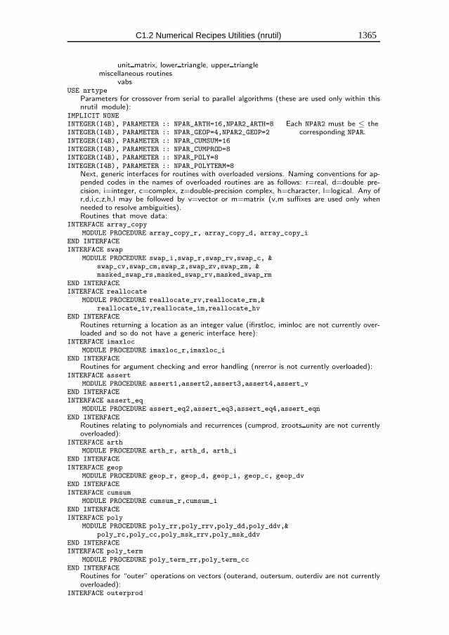
C1.2 Numerical Recipes Utilities (nrutil) 1365
unit matrix, lower triangle, upper trianglemiscellaneous routines
vabsUSE nrtype
Parameters for crossover from serial to parallel algorithms (these are used only within thisnrutil module):
IMPLICIT NONEINTEGER(I4B), PARAMETER :: NPAR_ARTH=16,NPAR2_ARTH=8 Each NPAR2 must be ≤ the
corresponding NPAR.INTEGER(I4B), PARAMETER :: NPAR_GEOP=4,NPAR2_GEOP=2INTEGER(I4B), PARAMETER :: NPAR_CUMSUM=16INTEGER(I4B), PARAMETER :: NPAR_CUMPROD=8INTEGER(I4B), PARAMETER :: NPAR_POLY=8INTEGER(I4B), PARAMETER :: NPAR_POLYTERM=8
Next, generic interfaces for routines with overloaded versions. Naming conventions for ap-pended codes in the names of overloaded routines are as follows: r=real, d=double pre-cision, i=integer, c=complex, z=double-precision complex, h=character, l=logical. Any ofr,d,i,c,z,h,l may be followed by v=vector or m=matrix (v,m suffixes are used only whenneeded to resolve ambiguities).Routines that move data:
INTERFACE array_copyMODULE PROCEDURE array_copy_r, array_copy_d, array_copy_i
END INTERFACEINTERFACE swap
MODULE PROCEDURE swap_i,swap_r,swap_rv,swap_c, &swap_cv,swap_cm,swap_z,swap_zv,swap_zm, &masked_swap_rs,masked_swap_rv,masked_swap_rm
END INTERFACEINTERFACE reallocate
MODULE PROCEDURE reallocate_rv,reallocate_rm,&reallocate_iv,reallocate_im,reallocate_hv
END INTERFACERoutines returning a location as an integer value (ifirstloc, iminloc are not currently over-loaded and so do not have a generic interface here):
INTERFACE imaxlocMODULE PROCEDURE imaxloc_r,imaxloc_i
END INTERFACERoutines for argument checking and error handling (nrerror is not currently overloaded):
INTERFACE assertMODULE PROCEDURE assert1,assert2,assert3,assert4,assert_v
END INTERFACEINTERFACE assert_eq
MODULE PROCEDURE assert_eq2,assert_eq3,assert_eq4,assert_eqnEND INTERFACE
Routines relating to polynomials and recurrences (cumprod, zroots unity are not currentlyoverloaded):
INTERFACE arthMODULE PROCEDURE arth_r, arth_d, arth_i
END INTERFACEINTERFACE geop
MODULE PROCEDURE geop_r, geop_d, geop_i, geop_c, geop_dvEND INTERFACEINTERFACE cumsum
MODULE PROCEDURE cumsum_r,cumsum_iEND INTERFACEINTERFACE poly
MODULE PROCEDURE poly_rr,poly_rrv,poly_dd,poly_ddv,&poly_rc,poly_cc,poly_msk_rrv,poly_msk_ddv
END INTERFACEINTERFACE poly_term
MODULE PROCEDURE poly_term_rr,poly_term_ccEND INTERFACE
Routines for “outer” operations on vectors (outerand, outersum, outerdiv are not currentlyoverloaded):
INTERFACE outerprod
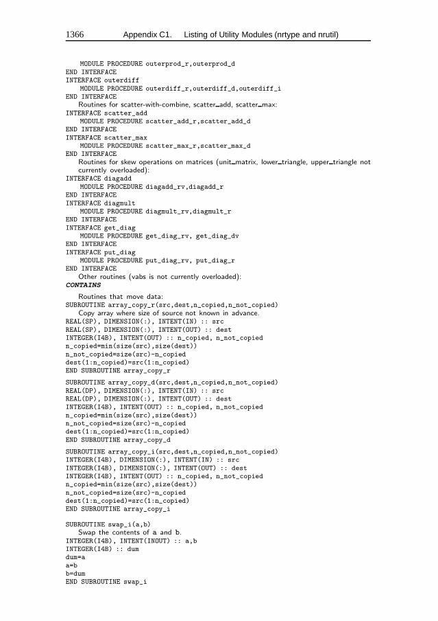
1366 Appendix C1. Listing of Utility Modules (nrtype and nrutil)
MODULE PROCEDURE outerprod_r,outerprod_dEND INTERFACEINTERFACE outerdiff
MODULE PROCEDURE outerdiff_r,outerdiff_d,outerdiff_iEND INTERFACE
Routines for scatter-with-combine, scatter add, scatter max:INTERFACE scatter_add
MODULE PROCEDURE scatter_add_r,scatter_add_dEND INTERFACEINTERFACE scatter_max
MODULE PROCEDURE scatter_max_r,scatter_max_dEND INTERFACE
Routines for skew operations on matrices (unit matrix, lower triangle, upper triangle notcurrently overloaded):
INTERFACE diagaddMODULE PROCEDURE diagadd_rv,diagadd_r
END INTERFACEINTERFACE diagmult
MODULE PROCEDURE diagmult_rv,diagmult_rEND INTERFACEINTERFACE get_diag
MODULE PROCEDURE get_diag_rv, get_diag_dvEND INTERFACEINTERFACE put_diag
MODULE PROCEDURE put_diag_rv, put_diag_rEND INTERFACE
Other routines (vabs is not currently overloaded):CONTAINS
Routines that move data:SUBROUTINE array_copy_r(src,dest,n_copied,n_not_copied)
Copy array where size of source not known in advance.REAL(SP), DIMENSION(:), INTENT(IN) :: srcREAL(SP), DIMENSION(:), INTENT(OUT) :: destINTEGER(I4B), INTENT(OUT) :: n_copied, n_not_copiedn_copied=min(size(src),size(dest))n_not_copied=size(src)-n_copieddest(1:n_copied)=src(1:n_copied)END SUBROUTINE array_copy_r
SUBROUTINE array_copy_d(src,dest,n_copied,n_not_copied)REAL(DP), DIMENSION(:), INTENT(IN) :: srcREAL(DP), DIMENSION(:), INTENT(OUT) :: destINTEGER(I4B), INTENT(OUT) :: n_copied, n_not_copiedn_copied=min(size(src),size(dest))n_not_copied=size(src)-n_copieddest(1:n_copied)=src(1:n_copied)END SUBROUTINE array_copy_d
SUBROUTINE array_copy_i(src,dest,n_copied,n_not_copied)INTEGER(I4B), DIMENSION(:), INTENT(IN) :: srcINTEGER(I4B), DIMENSION(:), INTENT(OUT) :: destINTEGER(I4B), INTENT(OUT) :: n_copied, n_not_copiedn_copied=min(size(src),size(dest))n_not_copied=size(src)-n_copieddest(1:n_copied)=src(1:n_copied)END SUBROUTINE array_copy_i
SUBROUTINE swap_i(a,b)Swap the contents of a and b.
INTEGER(I4B), INTENT(INOUT) :: a,bINTEGER(I4B) :: dumdum=aa=bb=dumEND SUBROUTINE swap_i
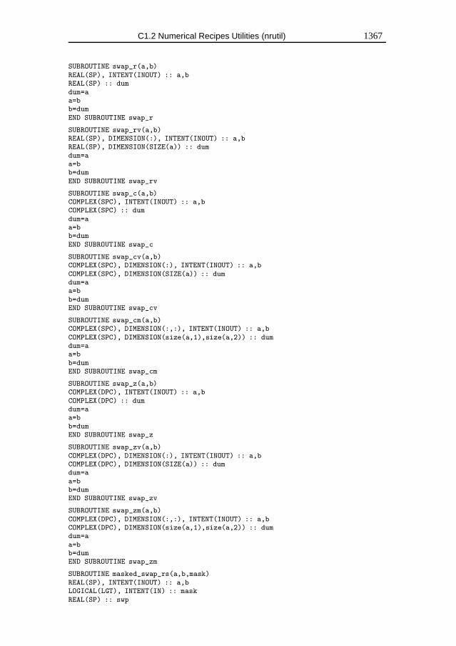
C1.2 Numerical Recipes Utilities (nrutil) 1367
SUBROUTINE swap_r(a,b)REAL(SP), INTENT(INOUT) :: a,bREAL(SP) :: dumdum=aa=bb=dumEND SUBROUTINE swap_r
SUBROUTINE swap_rv(a,b)REAL(SP), DIMENSION(:), INTENT(INOUT) :: a,bREAL(SP), DIMENSION(SIZE(a)) :: dumdum=aa=bb=dumEND SUBROUTINE swap_rv
SUBROUTINE swap_c(a,b)COMPLEX(SPC), INTENT(INOUT) :: a,bCOMPLEX(SPC) :: dumdum=aa=bb=dumEND SUBROUTINE swap_c
SUBROUTINE swap_cv(a,b)COMPLEX(SPC), DIMENSION(:), INTENT(INOUT) :: a,bCOMPLEX(SPC), DIMENSION(SIZE(a)) :: dumdum=aa=bb=dumEND SUBROUTINE swap_cv
SUBROUTINE swap_cm(a,b)COMPLEX(SPC), DIMENSION(:,:), INTENT(INOUT) :: a,bCOMPLEX(SPC), DIMENSION(size(a,1),size(a,2)) :: dumdum=aa=bb=dumEND SUBROUTINE swap_cm
SUBROUTINE swap_z(a,b)COMPLEX(DPC), INTENT(INOUT) :: a,bCOMPLEX(DPC) :: dumdum=aa=bb=dumEND SUBROUTINE swap_z
SUBROUTINE swap_zv(a,b)COMPLEX(DPC), DIMENSION(:), INTENT(INOUT) :: a,bCOMPLEX(DPC), DIMENSION(SIZE(a)) :: dumdum=aa=bb=dumEND SUBROUTINE swap_zv
SUBROUTINE swap_zm(a,b)COMPLEX(DPC), DIMENSION(:,:), INTENT(INOUT) :: a,bCOMPLEX(DPC), DIMENSION(size(a,1),size(a,2)) :: dumdum=aa=bb=dumEND SUBROUTINE swap_zm
SUBROUTINE masked_swap_rs(a,b,mask)REAL(SP), INTENT(INOUT) :: a,bLOGICAL(LGT), INTENT(IN) :: maskREAL(SP) :: swp
1368 Appendix C1. Listing of Utility Modules (nrtype and nrutil)
if (mask) thenswp=aa=bb=swp
end ifEND SUBROUTINE masked_swap_rs
SUBROUTINE masked_swap_rv(a,b,mask)REAL(SP), DIMENSION(:), INTENT(INOUT) :: a,bLOGICAL(LGT), DIMENSION(:), INTENT(IN) :: maskREAL(SP), DIMENSION(size(a)) :: swpwhere (mask)
swp=aa=bb=swp
end whereEND SUBROUTINE masked_swap_rv
SUBROUTINE masked_swap_rm(a,b,mask)REAL(SP), DIMENSION(:,:), INTENT(INOUT) :: a,bLOGICAL(LGT), DIMENSION(:,:), INTENT(IN) :: maskREAL(SP), DIMENSION(size(a,1),size(a,2)) :: swpwhere (mask)
swp=aa=bb=swp
end whereEND SUBROUTINE masked_swap_rm
FUNCTION reallocate_rv(p,n)Reallocate a pointer to a new size, preserving its previous contents.
REAL(SP), DIMENSION(:), POINTER :: p, reallocate_rvINTEGER(I4B), INTENT(IN) :: nINTEGER(I4B) :: nold,ierrallocate(reallocate_rv(n),stat=ierr)if (ierr /= 0) call &
nrerror(’reallocate_rv: problem in attempt to allocate memory’)if (.not. associated(p)) RETURNnold=size(p)reallocate_rv(1:min(nold,n))=p(1:min(nold,n))deallocate(p)END FUNCTION reallocate_rv
FUNCTION reallocate_iv(p,n)INTEGER(I4B), DIMENSION(:), POINTER :: p, reallocate_ivINTEGER(I4B), INTENT(IN) :: nINTEGER(I4B) :: nold,ierrallocate(reallocate_iv(n),stat=ierr)if (ierr /= 0) call &
nrerror(’reallocate_iv: problem in attempt to allocate memory’)if (.not. associated(p)) RETURNnold=size(p)reallocate_iv(1:min(nold,n))=p(1:min(nold,n))deallocate(p)END FUNCTION reallocate_iv
FUNCTION reallocate_hv(p,n)CHARACTER(1), DIMENSION(:), POINTER :: p, reallocate_hvINTEGER(I4B), INTENT(IN) :: nINTEGER(I4B) :: nold,ierrallocate(reallocate_hv(n),stat=ierr)if (ierr /= 0) call &
nrerror(’reallocate_hv: problem in attempt to allocate memory’)if (.not. associated(p)) RETURNnold=size(p)reallocate_hv(1:min(nold,n))=p(1:min(nold,n))
C1.2 Numerical Recipes Utilities (nrutil) 1369
deallocate(p)END FUNCTION reallocate_hv
FUNCTION reallocate_rm(p,n,m)REAL(SP), DIMENSION(:,:), POINTER :: p, reallocate_rmINTEGER(I4B), INTENT(IN) :: n,mINTEGER(I4B) :: nold,mold,ierrallocate(reallocate_rm(n,m),stat=ierr)if (ierr /= 0) call &
nrerror(’reallocate_rm: problem in attempt to allocate memory’)if (.not. associated(p)) RETURNnold=size(p,1)mold=size(p,2)reallocate_rm(1:min(nold,n),1:min(mold,m))=&
p(1:min(nold,n),1:min(mold,m))deallocate(p)END FUNCTION reallocate_rm
FUNCTION reallocate_im(p,n,m)INTEGER(I4B), DIMENSION(:,:), POINTER :: p, reallocate_imINTEGER(I4B), INTENT(IN) :: n,mINTEGER(I4B) :: nold,mold,ierrallocate(reallocate_im(n,m),stat=ierr)if (ierr /= 0) call &
nrerror(’reallocate_im: problem in attempt to allocate memory’)if (.not. associated(p)) RETURNnold=size(p,1)mold=size(p,2)reallocate_im(1:min(nold,n),1:min(mold,m))=&
p(1:min(nold,n),1:min(mold,m))deallocate(p)END FUNCTION reallocate_im
Routines returning a location as an integer value:FUNCTION ifirstloc(mask)
Index of first occurrence of .true. in a logical vector.LOGICAL(LGT), DIMENSION(:), INTENT(IN) :: maskINTEGER(I4B) :: ifirstlocINTEGER(I4B), DIMENSION(1) :: locloc=maxloc(merge(1,0,mask))ifirstloc=loc(1)if (.not. mask(ifirstloc)) ifirstloc=size(mask)+1END FUNCTION ifirstloc
FUNCTION imaxloc_r(arr)Index of maxloc on an array.
REAL(SP), DIMENSION(:), INTENT(IN) :: arrINTEGER(I4B) :: imaxloc_rINTEGER(I4B), DIMENSION(1) :: imaximax=maxloc(arr(:))imaxloc_r=imax(1)END FUNCTION imaxloc_r
FUNCTION imaxloc_i(iarr)INTEGER(I4B), DIMENSION(:), INTENT(IN) :: iarrINTEGER(I4B), DIMENSION(1) :: imaxINTEGER(I4B) :: imaxloc_iimax=maxloc(iarr(:))imaxloc_i=imax(1)END FUNCTION imaxloc_i
FUNCTION iminloc(arr)Index of minloc on an array.
REAL(SP), DIMENSION(:), INTENT(IN) :: arrINTEGER(I4B), DIMENSION(1) :: iminINTEGER(I4B) :: iminlocimin=minloc(arr(:))
1370 Appendix C1. Listing of Utility Modules (nrtype and nrutil)
iminloc=imin(1)END FUNCTION iminloc
Routines for argument checking and error handling:SUBROUTINE assert1(n1,string)
Report and die if any logical is false (used for arg range checking).CHARACTER(LEN=*), INTENT(IN) :: stringLOGICAL, INTENT(IN) :: n1if (.not. n1) then
write (*,*) ’nrerror: an assertion failed with this tag:’, &string
STOP ’program terminated by assert1’end ifEND SUBROUTINE assert1
SUBROUTINE assert2(n1,n2,string)CHARACTER(LEN=*), INTENT(IN) :: stringLOGICAL, INTENT(IN) :: n1,n2if (.not. (n1 .and. n2)) then
write (*,*) ’nrerror: an assertion failed with this tag:’, &string
STOP ’program terminated by assert2’end ifEND SUBROUTINE assert2
SUBROUTINE assert3(n1,n2,n3,string)CHARACTER(LEN=*), INTENT(IN) :: stringLOGICAL, INTENT(IN) :: n1,n2,n3if (.not. (n1 .and. n2 .and. n3)) then
write (*,*) ’nrerror: an assertion failed with this tag:’, &string
STOP ’program terminated by assert3’end ifEND SUBROUTINE assert3
SUBROUTINE assert4(n1,n2,n3,n4,string)CHARACTER(LEN=*), INTENT(IN) :: stringLOGICAL, INTENT(IN) :: n1,n2,n3,n4if (.not. (n1 .and. n2 .and. n3 .and. n4)) then
write (*,*) ’nrerror: an assertion failed with this tag:’, &string
STOP ’program terminated by assert4’end ifEND SUBROUTINE assert4
SUBROUTINE assert_v(n,string)CHARACTER(LEN=*), INTENT(IN) :: stringLOGICAL, DIMENSION(:), INTENT(IN) :: nif (.not. all(n)) then
write (*,*) ’nrerror: an assertion failed with this tag:’, &string
STOP ’program terminated by assert_v’end ifEND SUBROUTINE assert_v
FUNCTION assert_eq2(n1,n2,string)Report and die if integers not all equal (used for size checking).
CHARACTER(LEN=*), INTENT(IN) :: stringINTEGER, INTENT(IN) :: n1,n2INTEGER :: assert_eq2if (n1 == n2) then
assert_eq2=n1else
write (*,*) ’nrerror: an assert_eq failed with this tag:’, &string
STOP ’program terminated by assert_eq2’end if
C1.2 Numerical Recipes Utilities (nrutil) 1371
END FUNCTION assert_eq2
FUNCTION assert_eq3(n1,n2,n3,string)CHARACTER(LEN=*), INTENT(IN) :: stringINTEGER, INTENT(IN) :: n1,n2,n3INTEGER :: assert_eq3if (n1 == n2 .and. n2 == n3) then
assert_eq3=n1else
write (*,*) ’nrerror: an assert_eq failed with this tag:’, &string
STOP ’program terminated by assert_eq3’end ifEND FUNCTION assert_eq3
FUNCTION assert_eq4(n1,n2,n3,n4,string)CHARACTER(LEN=*), INTENT(IN) :: stringINTEGER, INTENT(IN) :: n1,n2,n3,n4INTEGER :: assert_eq4if (n1 == n2 .and. n2 == n3 .and. n3 == n4) then
assert_eq4=n1else
write (*,*) ’nrerror: an assert_eq failed with this tag:’, &string
STOP ’program terminated by assert_eq4’end ifEND FUNCTION assert_eq4
FUNCTION assert_eqn(nn,string)CHARACTER(LEN=*), INTENT(IN) :: stringINTEGER, DIMENSION(:), INTENT(IN) :: nnINTEGER :: assert_eqnif (all(nn(2:) == nn(1))) then
assert_eqn=nn(1)else
write (*,*) ’nrerror: an assert_eq failed with this tag:’, &string
STOP ’program terminated by assert_eqn’end ifEND FUNCTION assert_eqn
SUBROUTINE nrerror(string)Report a message, then die.
CHARACTER(LEN=*), INTENT(IN) :: stringwrite (*,*) ’nrerror: ’,stringSTOP ’program terminated by nrerror’END SUBROUTINE nrerror
Routines relating to polynomials and recurrences:FUNCTION arth_r(first,increment,n)
Array function returning an arithmetic progression.REAL(SP), INTENT(IN) :: first,incrementINTEGER(I4B), INTENT(IN) :: nREAL(SP), DIMENSION(n) :: arth_rINTEGER(I4B) :: k,k2REAL(SP) :: tempif (n > 0) arth_r(1)=firstif (n <= NPAR_ARTH) then
do k=2,narth_r(k)=arth_r(k-1)+increment
end doelse
do k=2,NPAR2_ARTHarth_r(k)=arth_r(k-1)+increment
end dotemp=increment*NPAR2_ARTHk=NPAR2_ARTH
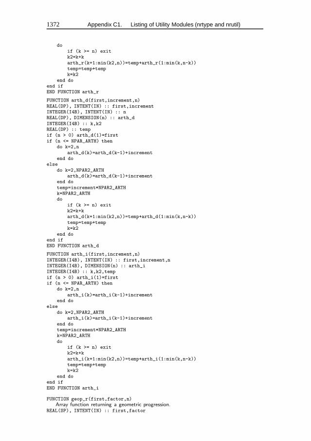
1372 Appendix C1. Listing of Utility Modules (nrtype and nrutil)
doif (k >= n) exitk2=k+karth_r(k+1:min(k2,n))=temp+arth_r(1:min(k,n-k))temp=temp+tempk=k2
end doend ifEND FUNCTION arth_r
FUNCTION arth_d(first,increment,n)REAL(DP), INTENT(IN) :: first,incrementINTEGER(I4B), INTENT(IN) :: nREAL(DP), DIMENSION(n) :: arth_dINTEGER(I4B) :: k,k2REAL(DP) :: tempif (n > 0) arth_d(1)=firstif (n <= NPAR_ARTH) then
do k=2,narth_d(k)=arth_d(k-1)+increment
end doelse
do k=2,NPAR2_ARTHarth_d(k)=arth_d(k-1)+increment
end dotemp=increment*NPAR2_ARTHk=NPAR2_ARTHdo
if (k >= n) exitk2=k+karth_d(k+1:min(k2,n))=temp+arth_d(1:min(k,n-k))temp=temp+tempk=k2
end doend ifEND FUNCTION arth_d
FUNCTION arth_i(first,increment,n)INTEGER(I4B), INTENT(IN) :: first,increment,nINTEGER(I4B), DIMENSION(n) :: arth_iINTEGER(I4B) :: k,k2,tempif (n > 0) arth_i(1)=firstif (n <= NPAR_ARTH) then
do k=2,narth_i(k)=arth_i(k-1)+increment
end doelse
do k=2,NPAR2_ARTHarth_i(k)=arth_i(k-1)+increment
end dotemp=increment*NPAR2_ARTHk=NPAR2_ARTHdo
if (k >= n) exitk2=k+karth_i(k+1:min(k2,n))=temp+arth_i(1:min(k,n-k))temp=temp+tempk=k2
end doend ifEND FUNCTION arth_i
FUNCTION geop_r(first,factor,n)Array function returning a geometric progression.
REAL(SP), INTENT(IN) :: first,factor
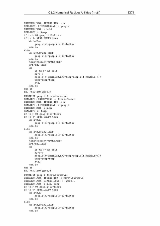
C1.2 Numerical Recipes Utilities (nrutil) 1373
INTEGER(I4B), INTENT(IN) :: nREAL(SP), DIMENSION(n) :: geop_rINTEGER(I4B) :: k,k2REAL(SP) :: tempif (n > 0) geop_r(1)=firstif (n <= NPAR_GEOP) then
do k=2,ngeop_r(k)=geop_r(k-1)*factor
end doelse
do k=2,NPAR2_GEOPgeop_r(k)=geop_r(k-1)*factor
end dotemp=factor**NPAR2_GEOPk=NPAR2_GEOPdo
if (k >= n) exitk2=k+kgeop_r(k+1:min(k2,n))=temp*geop_r(1:min(k,n-k))temp=temp*tempk=k2
end doend ifEND FUNCTION geop_r
FUNCTION geop_d(first,factor,n)REAL(DP), INTENT(IN) :: first,factorINTEGER(I4B), INTENT(IN) :: nREAL(DP), DIMENSION(n) :: geop_dINTEGER(I4B) :: k,k2REAL(DP) :: tempif (n > 0) geop_d(1)=firstif (n <= NPAR_GEOP) then
do k=2,ngeop_d(k)=geop_d(k-1)*factor
end doelse
do k=2,NPAR2_GEOPgeop_d(k)=geop_d(k-1)*factor
end dotemp=factor**NPAR2_GEOPk=NPAR2_GEOPdo
if (k >= n) exitk2=k+kgeop_d(k+1:min(k2,n))=temp*geop_d(1:min(k,n-k))temp=temp*tempk=k2
end doend ifEND FUNCTION geop_d
FUNCTION geop_i(first,factor,n)INTEGER(I4B), INTENT(IN) :: first,factor,nINTEGER(I4B), DIMENSION(n) :: geop_iINTEGER(I4B) :: k,k2,tempif (n > 0) geop_i(1)=firstif (n <= NPAR_GEOP) then
do k=2,ngeop_i(k)=geop_i(k-1)*factor
end doelse
do k=2,NPAR2_GEOPgeop_i(k)=geop_i(k-1)*factor
end do
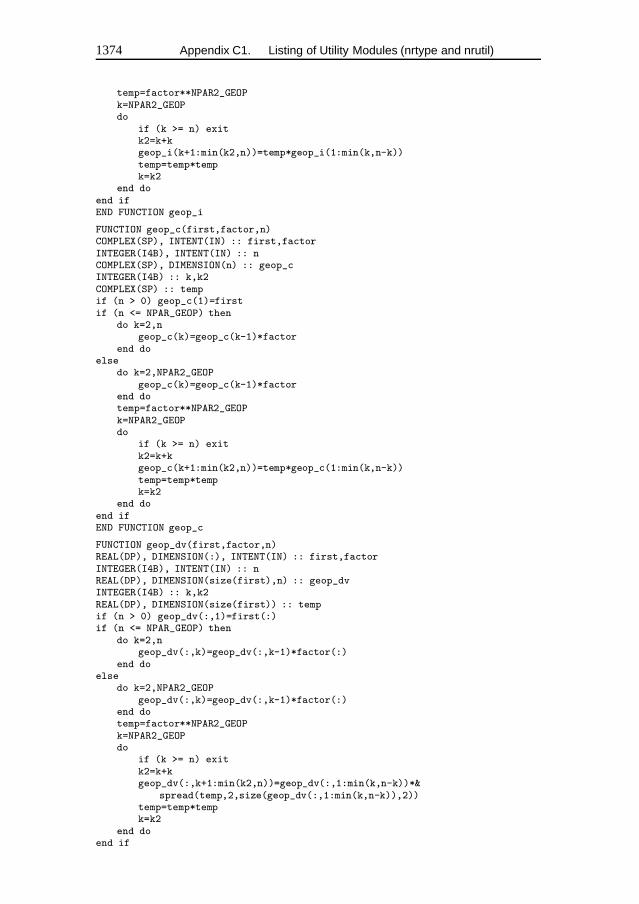
1374 Appendix C1. Listing of Utility Modules (nrtype and nrutil)
temp=factor**NPAR2_GEOPk=NPAR2_GEOPdo
if (k >= n) exitk2=k+kgeop_i(k+1:min(k2,n))=temp*geop_i(1:min(k,n-k))temp=temp*tempk=k2
end doend ifEND FUNCTION geop_i
FUNCTION geop_c(first,factor,n)COMPLEX(SP), INTENT(IN) :: first,factorINTEGER(I4B), INTENT(IN) :: nCOMPLEX(SP), DIMENSION(n) :: geop_cINTEGER(I4B) :: k,k2COMPLEX(SP) :: tempif (n > 0) geop_c(1)=firstif (n <= NPAR_GEOP) then
do k=2,ngeop_c(k)=geop_c(k-1)*factor
end doelse
do k=2,NPAR2_GEOPgeop_c(k)=geop_c(k-1)*factor
end dotemp=factor**NPAR2_GEOPk=NPAR2_GEOPdo
if (k >= n) exitk2=k+kgeop_c(k+1:min(k2,n))=temp*geop_c(1:min(k,n-k))temp=temp*tempk=k2
end doend ifEND FUNCTION geop_c
FUNCTION geop_dv(first,factor,n)REAL(DP), DIMENSION(:), INTENT(IN) :: first,factorINTEGER(I4B), INTENT(IN) :: nREAL(DP), DIMENSION(size(first),n) :: geop_dvINTEGER(I4B) :: k,k2REAL(DP), DIMENSION(size(first)) :: tempif (n > 0) geop_dv(:,1)=first(:)if (n <= NPAR_GEOP) then
do k=2,ngeop_dv(:,k)=geop_dv(:,k-1)*factor(:)
end doelse
do k=2,NPAR2_GEOPgeop_dv(:,k)=geop_dv(:,k-1)*factor(:)
end dotemp=factor**NPAR2_GEOPk=NPAR2_GEOPdo
if (k >= n) exitk2=k+kgeop_dv(:,k+1:min(k2,n))=geop_dv(:,1:min(k,n-k))*&
spread(temp,2,size(geop_dv(:,1:min(k,n-k)),2))temp=temp*tempk=k2
end doend if
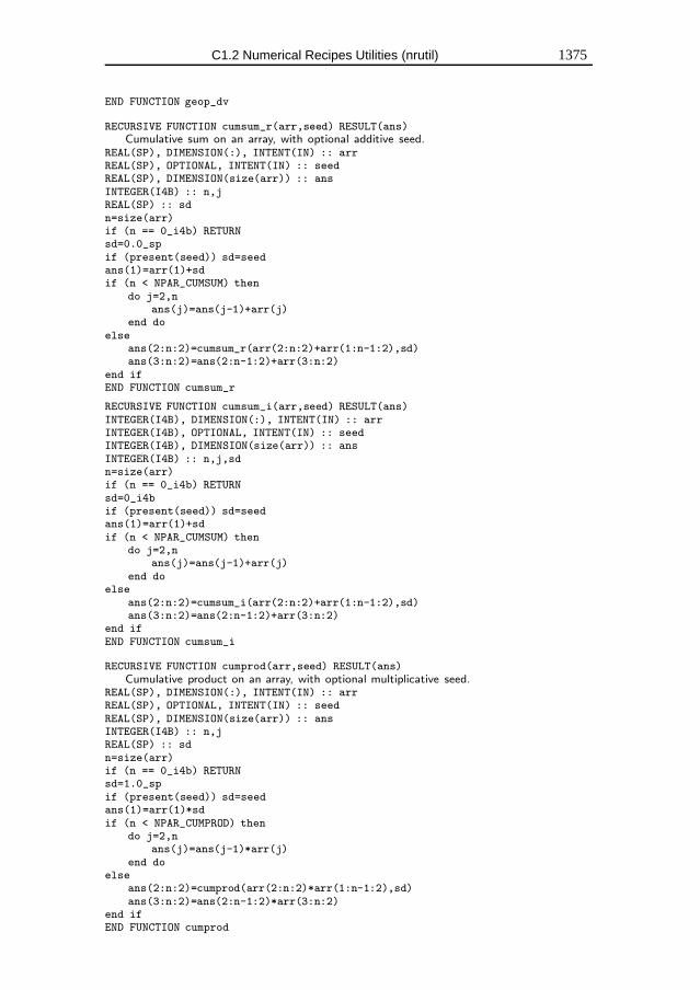
C1.2 Numerical Recipes Utilities (nrutil) 1375
END FUNCTION geop_dv
RECURSIVE FUNCTION cumsum_r(arr,seed) RESULT(ans)Cumulative sum on an array, with optional additive seed.
REAL(SP), DIMENSION(:), INTENT(IN) :: arrREAL(SP), OPTIONAL, INTENT(IN) :: seedREAL(SP), DIMENSION(size(arr)) :: ansINTEGER(I4B) :: n,jREAL(SP) :: sdn=size(arr)if (n == 0_i4b) RETURNsd=0.0_spif (present(seed)) sd=seedans(1)=arr(1)+sdif (n < NPAR_CUMSUM) then
do j=2,nans(j)=ans(j-1)+arr(j)
end doelse
ans(2:n:2)=cumsum_r(arr(2:n:2)+arr(1:n-1:2),sd)ans(3:n:2)=ans(2:n-1:2)+arr(3:n:2)
end ifEND FUNCTION cumsum_r
RECURSIVE FUNCTION cumsum_i(arr,seed) RESULT(ans)INTEGER(I4B), DIMENSION(:), INTENT(IN) :: arrINTEGER(I4B), OPTIONAL, INTENT(IN) :: seedINTEGER(I4B), DIMENSION(size(arr)) :: ansINTEGER(I4B) :: n,j,sdn=size(arr)if (n == 0_i4b) RETURNsd=0_i4bif (present(seed)) sd=seedans(1)=arr(1)+sdif (n < NPAR_CUMSUM) then
do j=2,nans(j)=ans(j-1)+arr(j)
end doelse
ans(2:n:2)=cumsum_i(arr(2:n:2)+arr(1:n-1:2),sd)ans(3:n:2)=ans(2:n-1:2)+arr(3:n:2)
end ifEND FUNCTION cumsum_i
RECURSIVE FUNCTION cumprod(arr,seed) RESULT(ans)Cumulative product on an array, with optional multiplicative seed.
REAL(SP), DIMENSION(:), INTENT(IN) :: arrREAL(SP), OPTIONAL, INTENT(IN) :: seedREAL(SP), DIMENSION(size(arr)) :: ansINTEGER(I4B) :: n,jREAL(SP) :: sdn=size(arr)if (n == 0_i4b) RETURNsd=1.0_spif (present(seed)) sd=seedans(1)=arr(1)*sdif (n < NPAR_CUMPROD) then
do j=2,nans(j)=ans(j-1)*arr(j)
end doelse
ans(2:n:2)=cumprod(arr(2:n:2)*arr(1:n-1:2),sd)ans(3:n:2)=ans(2:n-1:2)*arr(3:n:2)
end ifEND FUNCTION cumprod
1376 Appendix C1. Listing of Utility Modules (nrtype and nrutil)
FUNCTION poly_rr(x,coeffs)Polynomial evaluation.
REAL(SP), INTENT(IN) :: xREAL(SP), DIMENSION(:), INTENT(IN) :: coeffsREAL(SP) :: poly_rrREAL(SP) :: powREAL(SP), DIMENSION(:), ALLOCATABLE :: vecINTEGER(I4B) :: i,n,nnn=size(coeffs)if (n <= 0) then
poly_rr=0.0_spelse if (n < NPAR_POLY) then
poly_rr=coeffs(n)do i=n-1,1,-1
poly_rr=x*poly_rr+coeffs(i)end do
elseallocate(vec(n+1))pow=xvec(1:n)=coeffsdo
vec(n+1)=0.0_spnn=ishft(n+1,-1)vec(1:nn)=vec(1:n:2)+pow*vec(2:n+1:2)if (nn == 1) exitpow=pow*pown=nn
end dopoly_rr=vec(1)deallocate(vec)
end ifEND FUNCTION poly_rr
FUNCTION poly_dd(x,coeffs)REAL(DP), INTENT(IN) :: xREAL(DP), DIMENSION(:), INTENT(IN) :: coeffsREAL(DP) :: poly_ddREAL(DP) :: powREAL(DP), DIMENSION(:), ALLOCATABLE :: vecINTEGER(I4B) :: i,n,nnn=size(coeffs)if (n <= 0) then
poly_dd=0.0_dpelse if (n < NPAR_POLY) then
poly_dd=coeffs(n)do i=n-1,1,-1
poly_dd=x*poly_dd+coeffs(i)end do
elseallocate(vec(n+1))pow=xvec(1:n)=coeffsdo
vec(n+1)=0.0_dpnn=ishft(n+1,-1)vec(1:nn)=vec(1:n:2)+pow*vec(2:n+1:2)if (nn == 1) exitpow=pow*pown=nn
end dopoly_dd=vec(1)deallocate(vec)
end ifEND FUNCTION poly_dd
C1.2 Numerical Recipes Utilities (nrutil) 1377
FUNCTION poly_rc(x,coeffs)COMPLEX(SPC), INTENT(IN) :: xREAL(SP), DIMENSION(:), INTENT(IN) :: coeffsCOMPLEX(SPC) :: poly_rcCOMPLEX(SPC) :: powCOMPLEX(SPC), DIMENSION(:), ALLOCATABLE :: vecINTEGER(I4B) :: i,n,nnn=size(coeffs)if (n <= 0) then
poly_rc=0.0_spelse if (n < NPAR_POLY) then
poly_rc=coeffs(n)do i=n-1,1,-1
poly_rc=x*poly_rc+coeffs(i)end do
elseallocate(vec(n+1))pow=xvec(1:n)=coeffsdo
vec(n+1)=0.0_spnn=ishft(n+1,-1)vec(1:nn)=vec(1:n:2)+pow*vec(2:n+1:2)if (nn == 1) exitpow=pow*pown=nn
end dopoly_rc=vec(1)deallocate(vec)
end ifEND FUNCTION poly_rc
FUNCTION poly_cc(x,coeffs)COMPLEX(SPC), INTENT(IN) :: xCOMPLEX(SPC), DIMENSION(:), INTENT(IN) :: coeffsCOMPLEX(SPC) :: poly_ccCOMPLEX(SPC) :: powCOMPLEX(SPC), DIMENSION(:), ALLOCATABLE :: vecINTEGER(I4B) :: i,n,nnn=size(coeffs)if (n <= 0) then
poly_cc=0.0_spelse if (n < NPAR_POLY) then
poly_cc=coeffs(n)do i=n-1,1,-1
poly_cc=x*poly_cc+coeffs(i)end do
elseallocate(vec(n+1))pow=xvec(1:n)=coeffsdo
vec(n+1)=0.0_spnn=ishft(n+1,-1)vec(1:nn)=vec(1:n:2)+pow*vec(2:n+1:2)if (nn == 1) exitpow=pow*pown=nn
end dopoly_cc=vec(1)deallocate(vec)
end ifEND FUNCTION poly_cc
FUNCTION poly_rrv(x,coeffs)
1378 Appendix C1. Listing of Utility Modules (nrtype and nrutil)
REAL(SP), DIMENSION(:), INTENT(IN) :: coeffs,xREAL(SP), DIMENSION(size(x)) :: poly_rrvINTEGER(I4B) :: i,n,mm=size(coeffs)n=size(x)if (m <= 0) then
poly_rrv=0.0_spelse if (m < n .or. m < NPAR_POLY) then
poly_rrv=coeffs(m)do i=m-1,1,-1
poly_rrv=x*poly_rrv+coeffs(i)end do
elsedo i=1,n
poly_rrv(i)=poly_rr(x(i),coeffs)end do
end ifEND FUNCTION poly_rrv
FUNCTION poly_ddv(x,coeffs)REAL(DP), DIMENSION(:), INTENT(IN) :: coeffs,xREAL(DP), DIMENSION(size(x)) :: poly_ddvINTEGER(I4B) :: i,n,mm=size(coeffs)n=size(x)if (m <= 0) then
poly_ddv=0.0_dpelse if (m < n .or. m < NPAR_POLY) then
poly_ddv=coeffs(m)do i=m-1,1,-1
poly_ddv=x*poly_ddv+coeffs(i)end do
elsedo i=1,n
poly_ddv(i)=poly_dd(x(i),coeffs)end do
end ifEND FUNCTION poly_ddv
FUNCTION poly_msk_rrv(x,coeffs,mask)REAL(SP), DIMENSION(:), INTENT(IN) :: coeffs,xLOGICAL(LGT), DIMENSION(:), INTENT(IN) :: maskREAL(SP), DIMENSION(size(x)) :: poly_msk_rrvpoly_msk_rrv=unpack(poly_rrv(pack(x,mask),coeffs),mask,0.0_sp)END FUNCTION poly_msk_rrv
FUNCTION poly_msk_ddv(x,coeffs,mask)REAL(DP), DIMENSION(:), INTENT(IN) :: coeffs,xLOGICAL(LGT), DIMENSION(:), INTENT(IN) :: maskREAL(DP), DIMENSION(size(x)) :: poly_msk_ddvpoly_msk_ddv=unpack(poly_ddv(pack(x,mask),coeffs),mask,0.0_dp)END FUNCTION poly_msk_ddv
RECURSIVE FUNCTION poly_term_rr(a,b) RESULT(u)Tabulate cumulants of a polynomial.
REAL(SP), DIMENSION(:), INTENT(IN) :: aREAL(SP), INTENT(IN) :: bREAL(SP), DIMENSION(size(a)) :: uINTEGER(I4B) :: n,jn=size(a)if (n <= 0) RETURNu(1)=a(1)if (n < NPAR_POLYTERM) then
do j=2,nu(j)=a(j)+b*u(j-1)
end do
C1.2 Numerical Recipes Utilities (nrutil) 1379
elseu(2:n:2)=poly_term_rr(a(2:n:2)+a(1:n-1:2)*b,b*b)u(3:n:2)=a(3:n:2)+b*u(2:n-1:2)
end ifEND FUNCTION poly_term_rr
RECURSIVE FUNCTION poly_term_cc(a,b) RESULT(u)COMPLEX(SPC), DIMENSION(:), INTENT(IN) :: aCOMPLEX(SPC), INTENT(IN) :: bCOMPLEX(SPC), DIMENSION(size(a)) :: uINTEGER(I4B) :: n,jn=size(a)if (n <= 0) RETURNu(1)=a(1)if (n < NPAR_POLYTERM) then
do j=2,nu(j)=a(j)+b*u(j-1)
end doelse
u(2:n:2)=poly_term_cc(a(2:n:2)+a(1:n-1:2)*b,b*b)u(3:n:2)=a(3:n:2)+b*u(2:n-1:2)
end ifEND FUNCTION poly_term_cc
FUNCTION zroots_unity(n,nn)Complex function returning nn powers of the nth root of unity.
INTEGER(I4B), INTENT(IN) :: n,nnCOMPLEX(SPC), DIMENSION(nn) :: zroots_unityINTEGER(I4B) :: kREAL(SP) :: thetazroots_unity(1)=1.0theta=TWOPI/nk=1do
if (k >= nn) exitzroots_unity(k+1)=cmplx(cos(k*theta),sin(k*theta),SPC)zroots_unity(k+2:min(2*k,nn))=zroots_unity(k+1)*&
zroots_unity(2:min(k,nn-k))k=2*k
end doEND FUNCTION zroots_unity
Routines for “outer” operations on vectors. The order convention is: result(i,j) = first operand(i)(op) second operand(j).
FUNCTION outerprod_r(a,b)REAL(SP), DIMENSION(:), INTENT(IN) :: a,bREAL(SP), DIMENSION(size(a),size(b)) :: outerprod_routerprod_r = spread(a,dim=2,ncopies=size(b)) * &
spread(b,dim=1,ncopies=size(a))END FUNCTION outerprod_r
FUNCTION outerprod_d(a,b)REAL(DP), DIMENSION(:), INTENT(IN) :: a,bREAL(DP), DIMENSION(size(a),size(b)) :: outerprod_douterprod_d = spread(a,dim=2,ncopies=size(b)) * &
spread(b,dim=1,ncopies=size(a))END FUNCTION outerprod_d
FUNCTION outerdiv(a,b)REAL(SP), DIMENSION(:), INTENT(IN) :: a,bREAL(SP), DIMENSION(size(a),size(b)) :: outerdivouterdiv = spread(a,dim=2,ncopies=size(b)) / &
spread(b,dim=1,ncopies=size(a))END FUNCTION outerdiv
FUNCTION outersum(a,b)REAL(SP), DIMENSION(:), INTENT(IN) :: a,b
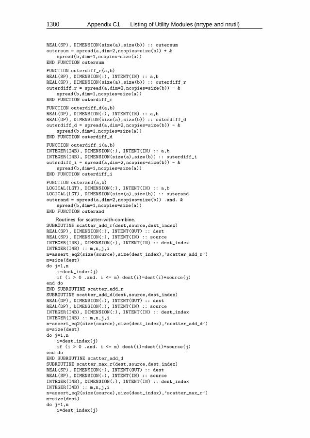
1380 Appendix C1. Listing of Utility Modules (nrtype and nrutil)
REAL(SP), DIMENSION(size(a),size(b)) :: outersumoutersum = spread(a,dim=2,ncopies=size(b)) + &
spread(b,dim=1,ncopies=size(a))END FUNCTION outersum
FUNCTION outerdiff_r(a,b)REAL(SP), DIMENSION(:), INTENT(IN) :: a,bREAL(SP), DIMENSION(size(a),size(b)) :: outerdiff_routerdiff_r = spread(a,dim=2,ncopies=size(b)) - &
spread(b,dim=1,ncopies=size(a))END FUNCTION outerdiff_r
FUNCTION outerdiff_d(a,b)REAL(DP), DIMENSION(:), INTENT(IN) :: a,bREAL(DP), DIMENSION(size(a),size(b)) :: outerdiff_douterdiff_d = spread(a,dim=2,ncopies=size(b)) - &
spread(b,dim=1,ncopies=size(a))END FUNCTION outerdiff_d
FUNCTION outerdiff_i(a,b)INTEGER(I4B), DIMENSION(:), INTENT(IN) :: a,bINTEGER(I4B), DIMENSION(size(a),size(b)) :: outerdiff_iouterdiff_i = spread(a,dim=2,ncopies=size(b)) - &
spread(b,dim=1,ncopies=size(a))END FUNCTION outerdiff_i
FUNCTION outerand(a,b)LOGICAL(LGT), DIMENSION(:), INTENT(IN) :: a,bLOGICAL(LGT), DIMENSION(size(a),size(b)) :: outerandouterand = spread(a,dim=2,ncopies=size(b)) .and. &
spread(b,dim=1,ncopies=size(a))END FUNCTION outerand
Routines for scatter-with-combine.SUBROUTINE scatter_add_r(dest,source,dest_index)REAL(SP), DIMENSION(:), INTENT(OUT) :: destREAL(SP), DIMENSION(:), INTENT(IN) :: sourceINTEGER(I4B), DIMENSION(:), INTENT(IN) :: dest_indexINTEGER(I4B) :: m,n,j,in=assert_eq2(size(source),size(dest_index),’scatter_add_r’)m=size(dest)do j=1,n
i=dest_index(j)if (i > 0 .and. i <= m) dest(i)=dest(i)+source(j)
end doEND SUBROUTINE scatter_add_rSUBROUTINE scatter_add_d(dest,source,dest_index)REAL(DP), DIMENSION(:), INTENT(OUT) :: destREAL(DP), DIMENSION(:), INTENT(IN) :: sourceINTEGER(I4B), DIMENSION(:), INTENT(IN) :: dest_indexINTEGER(I4B) :: m,n,j,in=assert_eq2(size(source),size(dest_index),’scatter_add_d’)m=size(dest)do j=1,n
i=dest_index(j)if (i > 0 .and. i <= m) dest(i)=dest(i)+source(j)
end doEND SUBROUTINE scatter_add_dSUBROUTINE scatter_max_r(dest,source,dest_index)REAL(SP), DIMENSION(:), INTENT(OUT) :: destREAL(SP), DIMENSION(:), INTENT(IN) :: sourceINTEGER(I4B), DIMENSION(:), INTENT(IN) :: dest_indexINTEGER(I4B) :: m,n,j,in=assert_eq2(size(source),size(dest_index),’scatter_max_r’)m=size(dest)do j=1,n
i=dest_index(j)
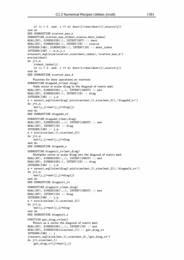
C1.2 Numerical Recipes Utilities (nrutil) 1381
if (i > 0 .and. i <= m) dest(i)=max(dest(i),source(j))end doEND SUBROUTINE scatter_max_rSUBROUTINE scatter_max_d(dest,source,dest_index)REAL(DP), DIMENSION(:), INTENT(OUT) :: destREAL(DP), DIMENSION(:), INTENT(IN) :: sourceINTEGER(I4B), DIMENSION(:), INTENT(IN) :: dest_indexINTEGER(I4B) :: m,n,j,in=assert_eq2(size(source),size(dest_index),’scatter_max_d’)m=size(dest)do j=1,n
i=dest_index(j)if (i > 0 .and. i <= m) dest(i)=max(dest(i),source(j))
end doEND SUBROUTINE scatter_max_d
Routines for skew operations on matrices:SUBROUTINE diagadd_rv(mat,diag)
Adds vector or scalar diag to the diagonal of matrix mat.REAL(SP), DIMENSION(:,:), INTENT(INOUT) :: matREAL(SP), DIMENSION(:), INTENT(IN) :: diagINTEGER(I4B) :: j,nn = assert_eq2(size(diag),min(size(mat,1),size(mat,2)),’diagadd_rv’)do j=1,n
mat(j,j)=mat(j,j)+diag(j)end doEND SUBROUTINE diagadd_rv
SUBROUTINE diagadd_r(mat,diag)REAL(SP), DIMENSION(:,:), INTENT(INOUT) :: matREAL(SP), INTENT(IN) :: diagINTEGER(I4B) :: j,nn = min(size(mat,1),size(mat,2))do j=1,n
mat(j,j)=mat(j,j)+diagend doEND SUBROUTINE diagadd_r
SUBROUTINE diagmult_rv(mat,diag)Multiplies vector or scalar diag into the diagonal of matrix mat.
REAL(SP), DIMENSION(:,:), INTENT(INOUT) :: matREAL(SP), DIMENSION(:), INTENT(IN) :: diagINTEGER(I4B) :: j,nn = assert_eq2(size(diag),min(size(mat,1),size(mat,2)),’diagmult_rv’)do j=1,n
mat(j,j)=mat(j,j)*diag(j)end doEND SUBROUTINE diagmult_rv
SUBROUTINE diagmult_r(mat,diag)REAL(SP), DIMENSION(:,:), INTENT(INOUT) :: matREAL(SP), INTENT(IN) :: diagINTEGER(I4B) :: j,nn = min(size(mat,1),size(mat,2))do j=1,n
mat(j,j)=mat(j,j)*diagend doEND SUBROUTINE diagmult_r
FUNCTION get_diag_rv(mat)Return as a vector the diagonal of matrix mat.
REAL(SP), DIMENSION(:,:), INTENT(IN) :: matREAL(SP), DIMENSION(size(mat,1)) :: get_diag_rvINTEGER(I4B) :: jj=assert_eq2(size(mat,1),size(mat,2),’get_diag_rv’)do j=1,size(mat,1)
get_diag_rv(j)=mat(j,j)
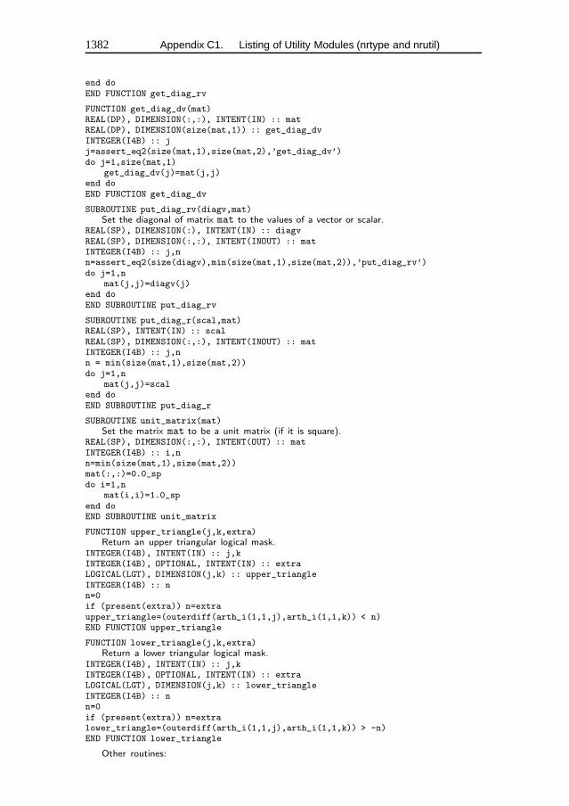
1382 Appendix C1. Listing of Utility Modules (nrtype and nrutil)
end doEND FUNCTION get_diag_rv
FUNCTION get_diag_dv(mat)REAL(DP), DIMENSION(:,:), INTENT(IN) :: matREAL(DP), DIMENSION(size(mat,1)) :: get_diag_dvINTEGER(I4B) :: jj=assert_eq2(size(mat,1),size(mat,2),’get_diag_dv’)do j=1,size(mat,1)
get_diag_dv(j)=mat(j,j)end doEND FUNCTION get_diag_dv
SUBROUTINE put_diag_rv(diagv,mat)Set the diagonal of matrix mat to the values of a vector or scalar.
REAL(SP), DIMENSION(:), INTENT(IN) :: diagvREAL(SP), DIMENSION(:,:), INTENT(INOUT) :: matINTEGER(I4B) :: j,nn=assert_eq2(size(diagv),min(size(mat,1),size(mat,2)),’put_diag_rv’)do j=1,n
mat(j,j)=diagv(j)end doEND SUBROUTINE put_diag_rv
SUBROUTINE put_diag_r(scal,mat)REAL(SP), INTENT(IN) :: scalREAL(SP), DIMENSION(:,:), INTENT(INOUT) :: matINTEGER(I4B) :: j,nn = min(size(mat,1),size(mat,2))do j=1,n
mat(j,j)=scalend doEND SUBROUTINE put_diag_r
SUBROUTINE unit_matrix(mat)Set the matrix mat to be a unit matrix (if it is square).
REAL(SP), DIMENSION(:,:), INTENT(OUT) :: matINTEGER(I4B) :: i,nn=min(size(mat,1),size(mat,2))mat(:,:)=0.0_spdo i=1,n
mat(i,i)=1.0_spend doEND SUBROUTINE unit_matrix
FUNCTION upper_triangle(j,k,extra)Return an upper triangular logical mask.
INTEGER(I4B), INTENT(IN) :: j,kINTEGER(I4B), OPTIONAL, INTENT(IN) :: extraLOGICAL(LGT), DIMENSION(j,k) :: upper_triangleINTEGER(I4B) :: nn=0if (present(extra)) n=extraupper_triangle=(outerdiff(arth_i(1,1,j),arth_i(1,1,k)) < n)END FUNCTION upper_triangle
FUNCTION lower_triangle(j,k,extra)Return a lower triangular logical mask.
INTEGER(I4B), INTENT(IN) :: j,kINTEGER(I4B), OPTIONAL, INTENT(IN) :: extraLOGICAL(LGT), DIMENSION(j,k) :: lower_triangleINTEGER(I4B) :: nn=0if (present(extra)) n=extralower_triangle=(outerdiff(arth_i(1,1,j),arth_i(1,1,k)) > -n)END FUNCTION lower_triangle
Other routines:

C1.2 Numerical Recipes Utilities (nrutil) 1383
FUNCTION vabs(v)Return the length (ordinary L2 norm) of a vector.
REAL(SP), DIMENSION(:), INTENT(IN) :: vREAL(SP) :: vabsvabs=sqrt(dot_product(v,v))END FUNCTION vabs
END MODULE nrutil
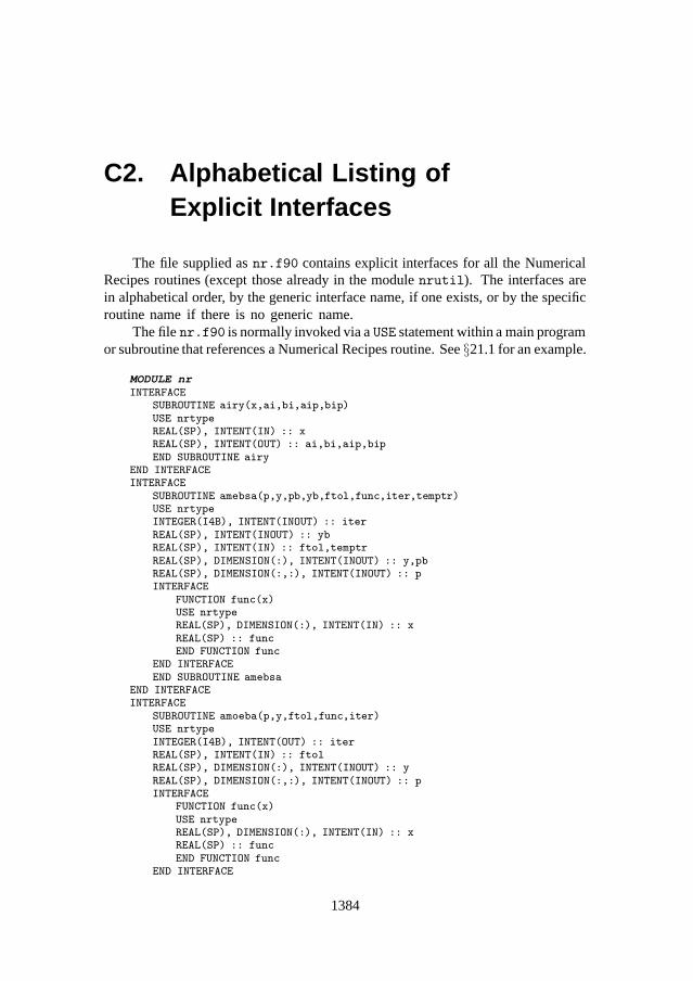
C2. Alphabetical Listing ofExplicit Interfaces
The file supplied as nr.f90 contains explicit interfaces for all the NumericalRecipes routines (except those already in the module nrutil). The interfaces arein alphabetical order, by the generic interface name, if one exists, or by the specificroutine name if there is no generic name.
The file nr.f90 is normally invoked via a USE statement within a main programor subroutine that references a Numerical Recipes routine. See §21.1 for an example.
MODULE nrINTERFACE
SUBROUTINE airy(x,ai,bi,aip,bip)USE nrtypeREAL(SP), INTENT(IN) :: xREAL(SP), INTENT(OUT) :: ai,bi,aip,bipEND SUBROUTINE airy
END INTERFACEINTERFACE
SUBROUTINE amebsa(p,y,pb,yb,ftol,func,iter,temptr)USE nrtypeINTEGER(I4B), INTENT(INOUT) :: iterREAL(SP), INTENT(INOUT) :: ybREAL(SP), INTENT(IN) :: ftol,temptrREAL(SP), DIMENSION(:), INTENT(INOUT) :: y,pbREAL(SP), DIMENSION(:,:), INTENT(INOUT) :: pINTERFACE
FUNCTION func(x)USE nrtypeREAL(SP), DIMENSION(:), INTENT(IN) :: xREAL(SP) :: funcEND FUNCTION func
END INTERFACEEND SUBROUTINE amebsa
END INTERFACEINTERFACE
SUBROUTINE amoeba(p,y,ftol,func,iter)USE nrtypeINTEGER(I4B), INTENT(OUT) :: iterREAL(SP), INTENT(IN) :: ftolREAL(SP), DIMENSION(:), INTENT(INOUT) :: yREAL(SP), DIMENSION(:,:), INTENT(INOUT) :: pINTERFACE
FUNCTION func(x)USE nrtypeREAL(SP), DIMENSION(:), INTENT(IN) :: xREAL(SP) :: funcEND FUNCTION func
END INTERFACE
1384
Appendix C2. Alphabetical Listing of Explicit Interfaces 1385
END SUBROUTINE amoebaEND INTERFACEINTERFACE
SUBROUTINE anneal(x,y,iorder)USE nrtypeINTEGER(I4B), DIMENSION(:), INTENT(INOUT) :: iorderREAL(SP), DIMENSION(:), INTENT(IN) :: x,yEND SUBROUTINE anneal
END INTERFACEINTERFACE
SUBROUTINE asolve(b,x,itrnsp)USE nrtypeREAL(DP), DIMENSION(:), INTENT(IN) :: bREAL(DP), DIMENSION(:), INTENT(OUT) :: xINTEGER(I4B), INTENT(IN) :: itrnspEND SUBROUTINE asolve
END INTERFACEINTERFACE
SUBROUTINE atimes(x,r,itrnsp)USE nrtypeREAL(DP), DIMENSION(:), INTENT(IN) :: xREAL(DP), DIMENSION(:), INTENT(OUT) :: rINTEGER(I4B), INTENT(IN) :: itrnspEND SUBROUTINE atimes
END INTERFACEINTERFACE
SUBROUTINE avevar(data,ave,var)USE nrtypeREAL(SP), DIMENSION(:), INTENT(IN) :: dataREAL(SP), INTENT(OUT) :: ave,varEND SUBROUTINE avevar
END INTERFACEINTERFACE
SUBROUTINE balanc(a)USE nrtypeREAL(SP), DIMENSION(:,:), INTENT(INOUT) :: aEND SUBROUTINE balanc
END INTERFACEINTERFACE
SUBROUTINE banbks(a,m1,m2,al,indx,b)USE nrtypeINTEGER(I4B), INTENT(IN) :: m1,m2INTEGER(I4B), DIMENSION(:), INTENT(IN) :: indxREAL(SP), DIMENSION(:,:), INTENT(IN) :: a,alREAL(SP), DIMENSION(:), INTENT(INOUT) :: bEND SUBROUTINE banbks
END INTERFACEINTERFACE
SUBROUTINE bandec(a,m1,m2,al,indx,d)USE nrtypeINTEGER(I4B), INTENT(IN) :: m1,m2INTEGER(I4B), DIMENSION(:), INTENT(OUT) :: indxREAL(SP), INTENT(OUT) :: dREAL(SP), DIMENSION(:,:), INTENT(INOUT) :: aREAL(SP), DIMENSION(:,:), INTENT(OUT) :: alEND SUBROUTINE bandec
END INTERFACEINTERFACE
SUBROUTINE banmul(a,m1,m2,x,b)USE nrtypeINTEGER(I4B), INTENT(IN) :: m1,m2REAL(SP), DIMENSION(:), INTENT(IN) :: xREAL(SP), DIMENSION(:), INTENT(OUT) :: bREAL(SP), DIMENSION(:,:), INTENT(IN) :: a
1386 Appendix C2. Alphabetical Listing of Explicit Interfaces
END SUBROUTINE banmulEND INTERFACEINTERFACE
SUBROUTINE bcucof(y,y1,y2,y12,d1,d2,c)USE nrtypeREAL(SP), INTENT(IN) :: d1,d2REAL(SP), DIMENSION(4), INTENT(IN) :: y,y1,y2,y12REAL(SP), DIMENSION(4,4), INTENT(OUT) :: cEND SUBROUTINE bcucof
END INTERFACEINTERFACE
SUBROUTINE bcuint(y,y1,y2,y12,x1l,x1u,x2l,x2u,x1,x2,ansy,&ansy1,ansy2)
USE nrtypeREAL(SP), DIMENSION(4), INTENT(IN) :: y,y1,y2,y12REAL(SP), INTENT(IN) :: x1l,x1u,x2l,x2u,x1,x2REAL(SP), INTENT(OUT) :: ansy,ansy1,ansy2END SUBROUTINE bcuint
END INTERFACEINTERFACE beschb
SUBROUTINE beschb_s(x,gam1,gam2,gampl,gammi)USE nrtypeREAL(DP), INTENT(IN) :: xREAL(DP), INTENT(OUT) :: gam1,gam2,gampl,gammiEND SUBROUTINE beschb_s
SUBROUTINE beschb_v(x,gam1,gam2,gampl,gammi)USE nrtypeREAL(DP), DIMENSION(:), INTENT(IN) :: xREAL(DP), DIMENSION(:), INTENT(OUT) :: gam1,gam2,gampl,gammiEND SUBROUTINE beschb_v
END INTERFACEINTERFACE bessi
FUNCTION bessi_s(n,x)USE nrtypeINTEGER(I4B), INTENT(IN) :: nREAL(SP), INTENT(IN) :: xREAL(SP) :: bessi_sEND FUNCTION bessi_s
FUNCTION bessi_v(n,x)USE nrtypeINTEGER(I4B), INTENT(IN) :: nREAL(SP), DIMENSION(:), INTENT(IN) :: xREAL(SP), DIMENSION(size(x)) :: bessi_vEND FUNCTION bessi_v
END INTERFACEINTERFACE bessi0
FUNCTION bessi0_s(x)USE nrtypeREAL(SP), INTENT(IN) :: xREAL(SP) :: bessi0_sEND FUNCTION bessi0_s
FUNCTION bessi0_v(x)USE nrtypeREAL(SP), DIMENSION(:), INTENT(IN) :: xREAL(SP), DIMENSION(size(x)) :: bessi0_vEND FUNCTION bessi0_v
END INTERFACEINTERFACE bessi1
FUNCTION bessi1_s(x)USE nrtypeREAL(SP), INTENT(IN) :: xREAL(SP) :: bessi1_sEND FUNCTION bessi1_s
Appendix C2. Alphabetical Listing of Explicit Interfaces 1387
FUNCTION bessi1_v(x)USE nrtypeREAL(SP), DIMENSION(:), INTENT(IN) :: xREAL(SP), DIMENSION(size(x)) :: bessi1_vEND FUNCTION bessi1_v
END INTERFACEINTERFACE
SUBROUTINE bessik(x,xnu,ri,rk,rip,rkp)USE nrtypeREAL(SP), INTENT(IN) :: x,xnuREAL(SP), INTENT(OUT) :: ri,rk,rip,rkpEND SUBROUTINE bessik
END INTERFACEINTERFACE bessj
FUNCTION bessj_s(n,x)USE nrtypeINTEGER(I4B), INTENT(IN) :: nREAL(SP), INTENT(IN) :: xREAL(SP) :: bessj_sEND FUNCTION bessj_s
FUNCTION bessj_v(n,x)USE nrtypeINTEGER(I4B), INTENT(IN) :: nREAL(SP), DIMENSION(:), INTENT(IN) :: xREAL(SP), DIMENSION(size(x)) :: bessj_vEND FUNCTION bessj_v
END INTERFACEINTERFACE bessj0
FUNCTION bessj0_s(x)USE nrtypeREAL(SP), INTENT(IN) :: xREAL(SP) :: bessj0_sEND FUNCTION bessj0_s
FUNCTION bessj0_v(x)USE nrtypeREAL(SP), DIMENSION(:), INTENT(IN) :: xREAL(SP), DIMENSION(size(x)) :: bessj0_vEND FUNCTION bessj0_v
END INTERFACEINTERFACE bessj1
FUNCTION bessj1_s(x)USE nrtypeREAL(SP), INTENT(IN) :: xREAL(SP) :: bessj1_sEND FUNCTION bessj1_s
FUNCTION bessj1_v(x)USE nrtypeREAL(SP), DIMENSION(:), INTENT(IN) :: xREAL(SP), DIMENSION(size(x)) :: bessj1_vEND FUNCTION bessj1_v
END INTERFACEINTERFACE bessjy
SUBROUTINE bessjy_s(x,xnu,rj,ry,rjp,ryp)USE nrtypeREAL(SP), INTENT(IN) :: x,xnuREAL(SP), INTENT(OUT) :: rj,ry,rjp,rypEND SUBROUTINE bessjy_s
SUBROUTINE bessjy_v(x,xnu,rj,ry,rjp,ryp)USE nrtypeREAL(SP), INTENT(IN) :: xnuREAL(SP), DIMENSION(:), INTENT(IN) :: xREAL(SP), DIMENSION(:), INTENT(OUT) :: rj,rjp,ry,ryp
1388 Appendix C2. Alphabetical Listing of Explicit Interfaces
END SUBROUTINE bessjy_vEND INTERFACEINTERFACE bessk
FUNCTION bessk_s(n,x)USE nrtypeINTEGER(I4B), INTENT(IN) :: nREAL(SP), INTENT(IN) :: xREAL(SP) :: bessk_sEND FUNCTION bessk_s
FUNCTION bessk_v(n,x)USE nrtypeINTEGER(I4B), INTENT(IN) :: nREAL(SP), DIMENSION(:), INTENT(IN) :: xREAL(SP), DIMENSION(size(x)) :: bessk_vEND FUNCTION bessk_v
END INTERFACEINTERFACE bessk0
FUNCTION bessk0_s(x)USE nrtypeREAL(SP), INTENT(IN) :: xREAL(SP) :: bessk0_sEND FUNCTION bessk0_s
FUNCTION bessk0_v(x)USE nrtypeREAL(SP), DIMENSION(:), INTENT(IN) :: xREAL(SP), DIMENSION(size(x)) :: bessk0_vEND FUNCTION bessk0_v
END INTERFACEINTERFACE bessk1
FUNCTION bessk1_s(x)USE nrtypeREAL(SP), INTENT(IN) :: xREAL(SP) :: bessk1_sEND FUNCTION bessk1_s
FUNCTION bessk1_v(x)USE nrtypeREAL(SP), DIMENSION(:), INTENT(IN) :: xREAL(SP), DIMENSION(size(x)) :: bessk1_vEND FUNCTION bessk1_v
END INTERFACEINTERFACE bessy
FUNCTION bessy_s(n,x)USE nrtypeINTEGER(I4B), INTENT(IN) :: nREAL(SP), INTENT(IN) :: xREAL(SP) :: bessy_sEND FUNCTION bessy_s
FUNCTION bessy_v(n,x)USE nrtypeINTEGER(I4B), INTENT(IN) :: nREAL(SP), DIMENSION(:), INTENT(IN) :: xREAL(SP), DIMENSION(size(x)) :: bessy_vEND FUNCTION bessy_v
END INTERFACEINTERFACE bessy0
FUNCTION bessy0_s(x)USE nrtypeREAL(SP), INTENT(IN) :: xREAL(SP) :: bessy0_sEND FUNCTION bessy0_s
FUNCTION bessy0_v(x)USE nrtype
Appendix C2. Alphabetical Listing of Explicit Interfaces 1389
REAL(SP), DIMENSION(:), INTENT(IN) :: xREAL(SP), DIMENSION(size(x)) :: bessy0_vEND FUNCTION bessy0_v
END INTERFACEINTERFACE bessy1
FUNCTION bessy1_s(x)USE nrtypeREAL(SP), INTENT(IN) :: xREAL(SP) :: bessy1_sEND FUNCTION bessy1_s
FUNCTION bessy1_v(x)USE nrtypeREAL(SP), DIMENSION(:), INTENT(IN) :: xREAL(SP), DIMENSION(size(x)) :: bessy1_vEND FUNCTION bessy1_v
END INTERFACEINTERFACE beta
FUNCTION beta_s(z,w)USE nrtypeREAL(SP), INTENT(IN) :: z,wREAL(SP) :: beta_sEND FUNCTION beta_s
FUNCTION beta_v(z,w)USE nrtypeREAL(SP), DIMENSION(:), INTENT(IN) :: z,wREAL(SP), DIMENSION(size(z)) :: beta_vEND FUNCTION beta_v
END INTERFACEINTERFACE betacf
FUNCTION betacf_s(a,b,x)USE nrtypeREAL(SP), INTENT(IN) :: a,b,xREAL(SP) :: betacf_sEND FUNCTION betacf_s
FUNCTION betacf_v(a,b,x)USE nrtypeREAL(SP), DIMENSION(:), INTENT(IN) :: a,b,xREAL(SP), DIMENSION(size(x)) :: betacf_vEND FUNCTION betacf_v
END INTERFACEINTERFACE betai
FUNCTION betai_s(a,b,x)USE nrtypeREAL(SP), INTENT(IN) :: a,b,xREAL(SP) :: betai_sEND FUNCTION betai_s
FUNCTION betai_v(a,b,x)USE nrtypeREAL(SP), DIMENSION(:), INTENT(IN) :: a,b,xREAL(SP), DIMENSION(size(a)) :: betai_vEND FUNCTION betai_v
END INTERFACEINTERFACE bico
FUNCTION bico_s(n,k)USE nrtypeINTEGER(I4B), INTENT(IN) :: n,kREAL(SP) :: bico_sEND FUNCTION bico_s
FUNCTION bico_v(n,k)USE nrtypeINTEGER(I4B), DIMENSION(:), INTENT(IN) :: n,kREAL(SP), DIMENSION(size(n)) :: bico_v
1390 Appendix C2. Alphabetical Listing of Explicit Interfaces
END FUNCTION bico_vEND INTERFACEINTERFACE
FUNCTION bnldev(pp,n)USE nrtypeREAL(SP), INTENT(IN) :: ppINTEGER(I4B), INTENT(IN) :: nREAL(SP) :: bnldevEND FUNCTION bnldev
END INTERFACEINTERFACE
FUNCTION brent(ax,bx,cx,func,tol,xmin)USE nrtypeREAL(SP), INTENT(IN) :: ax,bx,cx,tolREAL(SP), INTENT(OUT) :: xminREAL(SP) :: brentINTERFACE
FUNCTION func(x)USE nrtypeREAL(SP), INTENT(IN) :: xREAL(SP) :: funcEND FUNCTION func
END INTERFACEEND FUNCTION brent
END INTERFACEINTERFACE
SUBROUTINE broydn(x,check)USE nrtypeREAL(SP), DIMENSION(:), INTENT(INOUT) :: xLOGICAL(LGT), INTENT(OUT) :: checkEND SUBROUTINE broydn
END INTERFACEINTERFACE
SUBROUTINE bsstep(y,dydx,x,htry,eps,yscal,hdid,hnext,derivs)USE nrtypeREAL(SP), DIMENSION(:), INTENT(INOUT) :: yREAL(SP), DIMENSION(:), INTENT(IN) :: dydx,yscalREAL(SP), INTENT(INOUT) :: xREAL(SP), INTENT(IN) :: htry,epsREAL(SP), INTENT(OUT) :: hdid,hnextINTERFACE
SUBROUTINE derivs(x,y,dydx)USE nrtypeREAL(SP), INTENT(IN) :: xREAL(SP), DIMENSION(:), INTENT(IN) :: yREAL(SP), DIMENSION(:), INTENT(OUT) :: dydxEND SUBROUTINE derivs
END INTERFACEEND SUBROUTINE bsstep
END INTERFACEINTERFACE
SUBROUTINE caldat(julian,mm,id,iyyy)USE nrtypeINTEGER(I4B), INTENT(IN) :: julianINTEGER(I4B), INTENT(OUT) :: mm,id,iyyyEND SUBROUTINE caldat
END INTERFACEINTERFACE
FUNCTION chder(a,b,c)USE nrtypeREAL(SP), INTENT(IN) :: a,bREAL(SP), DIMENSION(:), INTENT(IN) :: cREAL(SP), DIMENSION(size(c)) :: chderEND FUNCTION chder
Appendix C2. Alphabetical Listing of Explicit Interfaces 1391
END INTERFACEINTERFACE chebev
FUNCTION chebev_s(a,b,c,x)USE nrtypeREAL(SP), INTENT(IN) :: a,b,xREAL(SP), DIMENSION(:), INTENT(IN) :: cREAL(SP) :: chebev_sEND FUNCTION chebev_s
FUNCTION chebev_v(a,b,c,x)USE nrtypeREAL(SP), INTENT(IN) :: a,bREAL(SP), DIMENSION(:), INTENT(IN) :: c,xREAL(SP), DIMENSION(size(x)) :: chebev_vEND FUNCTION chebev_v
END INTERFACEINTERFACE
FUNCTION chebft(a,b,n,func)USE nrtypeREAL(SP), INTENT(IN) :: a,bINTEGER(I4B), INTENT(IN) :: nREAL(SP), DIMENSION(n) :: chebftINTERFACE
FUNCTION func(x)USE nrtypeREAL(SP), DIMENSION(:), INTENT(IN) :: xREAL(SP), DIMENSION(size(x)) :: funcEND FUNCTION func
END INTERFACEEND FUNCTION chebft
END INTERFACEINTERFACE
FUNCTION chebpc(c)USE nrtypeREAL(SP), DIMENSION(:), INTENT(IN) :: cREAL(SP), DIMENSION(size(c)) :: chebpcEND FUNCTION chebpc
END INTERFACEINTERFACE
FUNCTION chint(a,b,c)USE nrtypeREAL(SP), INTENT(IN) :: a,bREAL(SP), DIMENSION(:), INTENT(IN) :: cREAL(SP), DIMENSION(size(c)) :: chintEND FUNCTION chint
END INTERFACEINTERFACE
SUBROUTINE choldc(a,p)USE nrtypeREAL(SP), DIMENSION(:,:), INTENT(INOUT) :: aREAL(SP), DIMENSION(:), INTENT(OUT) :: pEND SUBROUTINE choldc
END INTERFACEINTERFACE
SUBROUTINE cholsl(a,p,b,x)USE nrtypeREAL(SP), DIMENSION(:,:), INTENT(IN) :: aREAL(SP), DIMENSION(:), INTENT(IN) :: p,bREAL(SP), DIMENSION(:), INTENT(INOUT) :: xEND SUBROUTINE cholsl
END INTERFACEINTERFACE
SUBROUTINE chsone(bins,ebins,knstrn,df,chsq,prob)USE nrtype
1392 Appendix C2. Alphabetical Listing of Explicit Interfaces
INTEGER(I4B), INTENT(IN) :: knstrnREAL(SP), INTENT(OUT) :: df,chsq,probREAL(SP), DIMENSION(:), INTENT(IN) :: bins,ebinsEND SUBROUTINE chsone
END INTERFACEINTERFACE
SUBROUTINE chstwo(bins1,bins2,knstrn,df,chsq,prob)USE nrtypeINTEGER(I4B), INTENT(IN) :: knstrnREAL(SP), INTENT(OUT) :: df,chsq,probREAL(SP), DIMENSION(:), INTENT(IN) :: bins1,bins2END SUBROUTINE chstwo
END INTERFACEINTERFACE
SUBROUTINE cisi(x,ci,si)USE nrtypeREAL(SP), INTENT(IN) :: xREAL(SP), INTENT(OUT) :: ci,siEND SUBROUTINE cisi
END INTERFACEINTERFACE
SUBROUTINE cntab1(nn,chisq,df,prob,cramrv,ccc)USE nrtypeINTEGER(I4B), DIMENSION(:,:), INTENT(IN) :: nnREAL(SP), INTENT(OUT) :: chisq,df,prob,cramrv,cccEND SUBROUTINE cntab1
END INTERFACEINTERFACE
SUBROUTINE cntab2(nn,h,hx,hy,hygx,hxgy,uygx,uxgy,uxy)USE nrtypeINTEGER(I4B), DIMENSION(:,:), INTENT(IN) :: nnREAL(SP), INTENT(OUT) :: h,hx,hy,hygx,hxgy,uygx,uxgy,uxyEND SUBROUTINE cntab2
END INTERFACEINTERFACE
FUNCTION convlv(data,respns,isign)USE nrtypeREAL(SP), DIMENSION(:), INTENT(IN) :: dataREAL(SP), DIMENSION(:), INTENT(IN) :: respnsINTEGER(I4B), INTENT(IN) :: isignREAL(SP), DIMENSION(size(data)) :: convlvEND FUNCTION convlv
END INTERFACEINTERFACE
FUNCTION correl(data1,data2)USE nrtypeREAL(SP), DIMENSION(:), INTENT(IN) :: data1,data2REAL(SP), DIMENSION(size(data1)) :: correlEND FUNCTION correl
END INTERFACEINTERFACE
SUBROUTINE cosft1(y)USE nrtypeREAL(SP), DIMENSION(:), INTENT(INOUT) :: yEND SUBROUTINE cosft1
END INTERFACEINTERFACE
SUBROUTINE cosft2(y,isign)USE nrtypeREAL(SP), DIMENSION(:), INTENT(INOUT) :: yINTEGER(I4B), INTENT(IN) :: isignEND SUBROUTINE cosft2
END INTERFACEINTERFACE
Appendix C2. Alphabetical Listing of Explicit Interfaces 1393
SUBROUTINE covsrt(covar,maska)USE nrtypeREAL(SP), DIMENSION(:,:), INTENT(INOUT) :: covarLOGICAL(LGT), DIMENSION(:), INTENT(IN) :: maskaEND SUBROUTINE covsrt
END INTERFACEINTERFACE
SUBROUTINE cyclic(a,b,c,alpha,beta,r,x)USE nrtypeREAL(SP), DIMENSION(:), INTENT(IN):: a,b,c,rREAL(SP), INTENT(IN) :: alpha,betaREAL(SP), DIMENSION(:), INTENT(OUT):: xEND SUBROUTINE cyclic
END INTERFACEINTERFACE
SUBROUTINE daub4(a,isign)USE nrtypeREAL(SP), DIMENSION(:), INTENT(INOUT) :: aINTEGER(I4B), INTENT(IN) :: isignEND SUBROUTINE daub4
END INTERFACEINTERFACE dawson
FUNCTION dawson_s(x)USE nrtypeREAL(SP), INTENT(IN) :: xREAL(SP) :: dawson_sEND FUNCTION dawson_s
FUNCTION dawson_v(x)USE nrtypeREAL(SP), DIMENSION(:), INTENT(IN) :: xREAL(SP), DIMENSION(size(x)) :: dawson_vEND FUNCTION dawson_v
END INTERFACEINTERFACE
FUNCTION dbrent(ax,bx,cx,func,dbrent_dfunc,tol,xmin)USE nrtypeREAL(SP), INTENT(IN) :: ax,bx,cx,tolREAL(SP), INTENT(OUT) :: xminREAL(SP) :: dbrentINTERFACE
FUNCTION func(x)USE nrtypeREAL(SP), INTENT(IN) :: xREAL(SP) :: funcEND FUNCTION func
FUNCTION dbrent_dfunc(x)USE nrtypeREAL(SP), INTENT(IN) :: xREAL(SP) :: dbrent_dfuncEND FUNCTION dbrent_dfunc
END INTERFACEEND FUNCTION dbrent
END INTERFACEINTERFACE
SUBROUTINE ddpoly(c,x,pd)USE nrtypeREAL(SP), INTENT(IN) :: xREAL(SP), DIMENSION(:), INTENT(IN) :: cREAL(SP), DIMENSION(:), INTENT(OUT) :: pdEND SUBROUTINE ddpoly
END INTERFACEINTERFACE
FUNCTION decchk(string,ch)
1394 Appendix C2. Alphabetical Listing of Explicit Interfaces
USE nrtypeCHARACTER(1), DIMENSION(:), INTENT(IN) :: stringCHARACTER(1), INTENT(OUT) :: chLOGICAL(LGT) :: decchkEND FUNCTION decchk
END INTERFACEINTERFACE
SUBROUTINE dfpmin(p,gtol,iter,fret,func,dfunc)USE nrtypeINTEGER(I4B), INTENT(OUT) :: iterREAL(SP), INTENT(IN) :: gtolREAL(SP), INTENT(OUT) :: fretREAL(SP), DIMENSION(:), INTENT(INOUT) :: pINTERFACE
FUNCTION func(p)USE nrtypeREAL(SP), DIMENSION(:), INTENT(IN) :: pREAL(SP) :: funcEND FUNCTION func
FUNCTION dfunc(p)USE nrtypeREAL(SP), DIMENSION(:), INTENT(IN) :: pREAL(SP), DIMENSION(size(p)) :: dfuncEND FUNCTION dfunc
END INTERFACEEND SUBROUTINE dfpmin
END INTERFACEINTERFACE
FUNCTION dfridr(func,x,h,err)USE nrtypeREAL(SP), INTENT(IN) :: x,hREAL(SP), INTENT(OUT) :: errREAL(SP) :: dfridrINTERFACE
FUNCTION func(x)USE nrtypeREAL(SP), INTENT(IN) :: xREAL(SP) :: funcEND FUNCTION func
END INTERFACEEND FUNCTION dfridr
END INTERFACEINTERFACE
SUBROUTINE dftcor(w,delta,a,b,endpts,corre,corim,corfac)USE nrtypeREAL(SP), INTENT(IN) :: w,delta,a,bREAL(SP), INTENT(OUT) :: corre,corim,corfacREAL(SP), DIMENSION(:), INTENT(IN) :: endptsEND SUBROUTINE dftcor
END INTERFACEINTERFACE
SUBROUTINE dftint(func,a,b,w,cosint,sinint)USE nrtypeREAL(SP), INTENT(IN) :: a,b,wREAL(SP), INTENT(OUT) :: cosint,sinintINTERFACE
FUNCTION func(x)USE nrtypeREAL(SP), DIMENSION(:), INTENT(IN) :: xREAL(SP), DIMENSION(size(x)) :: funcEND FUNCTION func
END INTERFACEEND SUBROUTINE dftint
Appendix C2. Alphabetical Listing of Explicit Interfaces 1395
END INTERFACEINTERFACE
SUBROUTINE difeq(k,k1,k2,jsf,is1,isf,indexv,s,y)USE nrtypeINTEGER(I4B), INTENT(IN) :: is1,isf,jsf,k,k1,k2INTEGER(I4B), DIMENSION(:), INTENT(IN) :: indexvREAL(SP), DIMENSION(:,:), INTENT(OUT) :: sREAL(SP), DIMENSION(:,:), INTENT(IN) :: yEND SUBROUTINE difeq
END INTERFACEINTERFACE
FUNCTION eclass(lista,listb,n)USE nrtypeINTEGER(I4B), DIMENSION(:), INTENT(IN) :: lista,listbINTEGER(I4B), INTENT(IN) :: nINTEGER(I4B), DIMENSION(n) :: eclassEND FUNCTION eclass
END INTERFACEINTERFACE
FUNCTION eclazz(equiv,n)USE nrtypeINTERFACE
FUNCTION equiv(i,j)USE nrtypeLOGICAL(LGT) :: equivINTEGER(I4B), INTENT(IN) :: i,jEND FUNCTION equiv
END INTERFACEINTEGER(I4B), INTENT(IN) :: nINTEGER(I4B), DIMENSION(n) :: eclazzEND FUNCTION eclazz
END INTERFACEINTERFACE
FUNCTION ei(x)USE nrtypeREAL(SP), INTENT(IN) :: xREAL(SP) :: eiEND FUNCTION ei
END INTERFACEINTERFACE
SUBROUTINE eigsrt(d,v)USE nrtypeREAL(SP), DIMENSION(:), INTENT(INOUT) :: dREAL(SP), DIMENSION(:,:), INTENT(INOUT) :: vEND SUBROUTINE eigsrt
END INTERFACEINTERFACE elle
FUNCTION elle_s(phi,ak)USE nrtypeREAL(SP), INTENT(IN) :: phi,akREAL(SP) :: elle_sEND FUNCTION elle_s
FUNCTION elle_v(phi,ak)USE nrtypeREAL(SP), DIMENSION(:), INTENT(IN) :: phi,akREAL(SP), DIMENSION(size(phi)) :: elle_vEND FUNCTION elle_v
END INTERFACEINTERFACE ellf
FUNCTION ellf_s(phi,ak)USE nrtypeREAL(SP), INTENT(IN) :: phi,akREAL(SP) :: ellf_s
1396 Appendix C2. Alphabetical Listing of Explicit Interfaces
END FUNCTION ellf_s
FUNCTION ellf_v(phi,ak)USE nrtypeREAL(SP), DIMENSION(:), INTENT(IN) :: phi,akREAL(SP), DIMENSION(size(phi)) :: ellf_vEND FUNCTION ellf_v
END INTERFACEINTERFACE ellpi
FUNCTION ellpi_s(phi,en,ak)USE nrtypeREAL(SP), INTENT(IN) :: phi,en,akREAL(SP) :: ellpi_sEND FUNCTION ellpi_s
FUNCTION ellpi_v(phi,en,ak)USE nrtypeREAL(SP), DIMENSION(:), INTENT(IN) :: phi,en,akREAL(SP), DIMENSION(size(phi)) :: ellpi_vEND FUNCTION ellpi_v
END INTERFACEINTERFACE
SUBROUTINE elmhes(a)USE nrtypeREAL(SP), DIMENSION(:,:), INTENT(INOUT) :: aEND SUBROUTINE elmhes
END INTERFACEINTERFACE erf
FUNCTION erf_s(x)USE nrtypeREAL(SP), INTENT(IN) :: xREAL(SP) :: erf_sEND FUNCTION erf_s
FUNCTION erf_v(x)USE nrtypeREAL(SP), DIMENSION(:), INTENT(IN) :: xREAL(SP), DIMENSION(size(x)) :: erf_vEND FUNCTION erf_v
END INTERFACEINTERFACE erfc
FUNCTION erfc_s(x)USE nrtypeREAL(SP), INTENT(IN) :: xREAL(SP) :: erfc_sEND FUNCTION erfc_s
FUNCTION erfc_v(x)USE nrtypeREAL(SP), DIMENSION(:), INTENT(IN) :: xREAL(SP), DIMENSION(size(x)) :: erfc_vEND FUNCTION erfc_v
END INTERFACEINTERFACE erfcc
FUNCTION erfcc_s(x)USE nrtypeREAL(SP), INTENT(IN) :: xREAL(SP) :: erfcc_sEND FUNCTION erfcc_s
FUNCTION erfcc_v(x)USE nrtypeREAL(SP), DIMENSION(:), INTENT(IN) :: xREAL(SP), DIMENSION(size(x)) :: erfcc_vEND FUNCTION erfcc_v
END INTERFACEINTERFACE
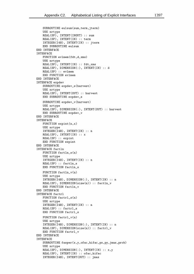
Appendix C2. Alphabetical Listing of Explicit Interfaces 1397
SUBROUTINE eulsum(sum,term,jterm)USE nrtypeREAL(SP), INTENT(INOUT) :: sumREAL(SP), INTENT(IN) :: termINTEGER(I4B), INTENT(IN) :: jtermEND SUBROUTINE eulsum
END INTERFACEINTERFACE
FUNCTION evlmem(fdt,d,xms)USE nrtypeREAL(SP), INTENT(IN) :: fdt,xmsREAL(SP), DIMENSION(:), INTENT(IN) :: dREAL(SP) :: evlmemEND FUNCTION evlmem
END INTERFACEINTERFACE expdev
SUBROUTINE expdev_s(harvest)USE nrtypeREAL(SP), INTENT(OUT) :: harvestEND SUBROUTINE expdev_s
SUBROUTINE expdev_v(harvest)USE nrtypeREAL(SP), DIMENSION(:), INTENT(OUT) :: harvestEND SUBROUTINE expdev_v
END INTERFACEINTERFACE
FUNCTION expint(n,x)USE nrtypeINTEGER(I4B), INTENT(IN) :: nREAL(SP), INTENT(IN) :: xREAL(SP) :: expintEND FUNCTION expint
END INTERFACEINTERFACE factln
FUNCTION factln_s(n)USE nrtypeINTEGER(I4B), INTENT(IN) :: nREAL(SP) :: factln_sEND FUNCTION factln_s
FUNCTION factln_v(n)USE nrtypeINTEGER(I4B), DIMENSION(:), INTENT(IN) :: nREAL(SP), DIMENSION(size(n)) :: factln_vEND FUNCTION factln_v
END INTERFACEINTERFACE factrl
FUNCTION factrl_s(n)USE nrtypeINTEGER(I4B), INTENT(IN) :: nREAL(SP) :: factrl_sEND FUNCTION factrl_s
FUNCTION factrl_v(n)USE nrtypeINTEGER(I4B), DIMENSION(:), INTENT(IN) :: nREAL(SP), DIMENSION(size(n)) :: factrl_vEND FUNCTION factrl_v
END INTERFACEINTERFACE
SUBROUTINE fasper(x,y,ofac,hifac,px,py,jmax,prob)USE nrtypeREAL(SP), DIMENSION(:), INTENT(IN) :: x,yREAL(SP), INTENT(IN) :: ofac,hifacINTEGER(I4B), INTENT(OUT) :: jmax
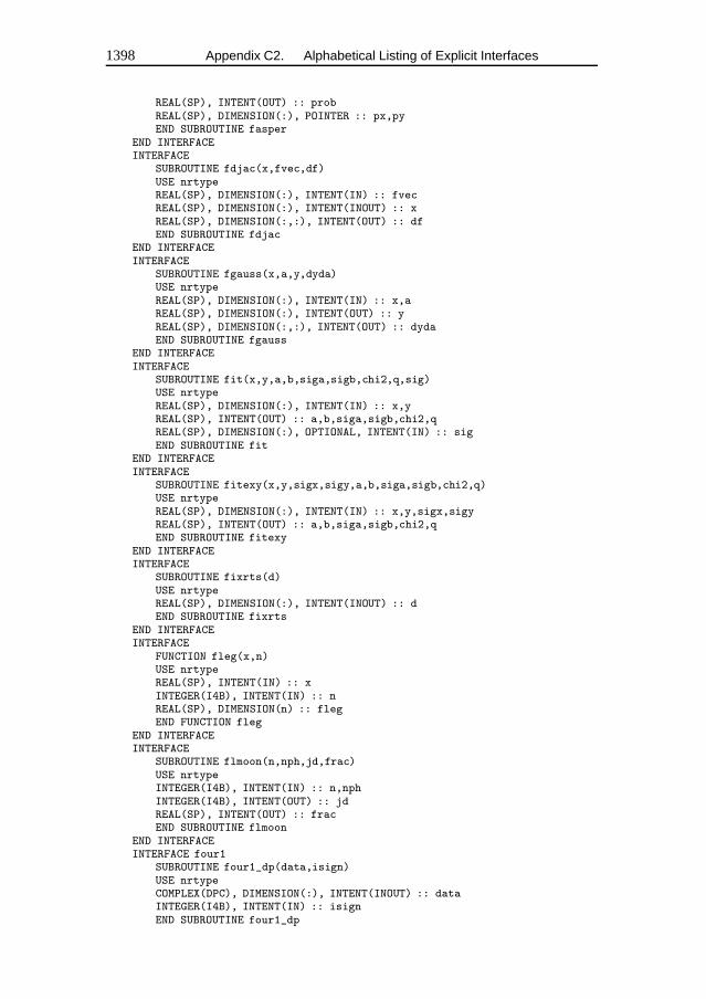
1398 Appendix C2. Alphabetical Listing of Explicit Interfaces
REAL(SP), INTENT(OUT) :: probREAL(SP), DIMENSION(:), POINTER :: px,pyEND SUBROUTINE fasper
END INTERFACEINTERFACE
SUBROUTINE fdjac(x,fvec,df)USE nrtypeREAL(SP), DIMENSION(:), INTENT(IN) :: fvecREAL(SP), DIMENSION(:), INTENT(INOUT) :: xREAL(SP), DIMENSION(:,:), INTENT(OUT) :: dfEND SUBROUTINE fdjac
END INTERFACEINTERFACE
SUBROUTINE fgauss(x,a,y,dyda)USE nrtypeREAL(SP), DIMENSION(:), INTENT(IN) :: x,aREAL(SP), DIMENSION(:), INTENT(OUT) :: yREAL(SP), DIMENSION(:,:), INTENT(OUT) :: dydaEND SUBROUTINE fgauss
END INTERFACEINTERFACE
SUBROUTINE fit(x,y,a,b,siga,sigb,chi2,q,sig)USE nrtypeREAL(SP), DIMENSION(:), INTENT(IN) :: x,yREAL(SP), INTENT(OUT) :: a,b,siga,sigb,chi2,qREAL(SP), DIMENSION(:), OPTIONAL, INTENT(IN) :: sigEND SUBROUTINE fit
END INTERFACEINTERFACE
SUBROUTINE fitexy(x,y,sigx,sigy,a,b,siga,sigb,chi2,q)USE nrtypeREAL(SP), DIMENSION(:), INTENT(IN) :: x,y,sigx,sigyREAL(SP), INTENT(OUT) :: a,b,siga,sigb,chi2,qEND SUBROUTINE fitexy
END INTERFACEINTERFACE
SUBROUTINE fixrts(d)USE nrtypeREAL(SP), DIMENSION(:), INTENT(INOUT) :: dEND SUBROUTINE fixrts
END INTERFACEINTERFACE
FUNCTION fleg(x,n)USE nrtypeREAL(SP), INTENT(IN) :: xINTEGER(I4B), INTENT(IN) :: nREAL(SP), DIMENSION(n) :: flegEND FUNCTION fleg
END INTERFACEINTERFACE
SUBROUTINE flmoon(n,nph,jd,frac)USE nrtypeINTEGER(I4B), INTENT(IN) :: n,nphINTEGER(I4B), INTENT(OUT) :: jdREAL(SP), INTENT(OUT) :: fracEND SUBROUTINE flmoon
END INTERFACEINTERFACE four1
SUBROUTINE four1_dp(data,isign)USE nrtypeCOMPLEX(DPC), DIMENSION(:), INTENT(INOUT) :: dataINTEGER(I4B), INTENT(IN) :: isignEND SUBROUTINE four1_dp
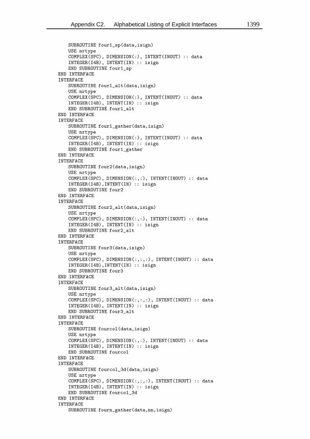
Appendix C2. Alphabetical Listing of Explicit Interfaces 1399
SUBROUTINE four1_sp(data,isign)USE nrtypeCOMPLEX(SPC), DIMENSION(:), INTENT(INOUT) :: dataINTEGER(I4B), INTENT(IN) :: isignEND SUBROUTINE four1_sp
END INTERFACEINTERFACE
SUBROUTINE four1_alt(data,isign)USE nrtypeCOMPLEX(SPC), DIMENSION(:), INTENT(INOUT) :: dataINTEGER(I4B), INTENT(IN) :: isignEND SUBROUTINE four1_alt
END INTERFACEINTERFACE
SUBROUTINE four1_gather(data,isign)USE nrtypeCOMPLEX(SPC), DIMENSION(:), INTENT(INOUT) :: dataINTEGER(I4B), INTENT(IN) :: isignEND SUBROUTINE four1_gather
END INTERFACEINTERFACE
SUBROUTINE four2(data,isign)USE nrtypeCOMPLEX(SPC), DIMENSION(:,:), INTENT(INOUT) :: dataINTEGER(I4B),INTENT(IN) :: isignEND SUBROUTINE four2
END INTERFACEINTERFACE
SUBROUTINE four2_alt(data,isign)USE nrtypeCOMPLEX(SPC), DIMENSION(:,:), INTENT(INOUT) :: dataINTEGER(I4B), INTENT(IN) :: isignEND SUBROUTINE four2_alt
END INTERFACEINTERFACE
SUBROUTINE four3(data,isign)USE nrtypeCOMPLEX(SPC), DIMENSION(:,:,:), INTENT(INOUT) :: dataINTEGER(I4B),INTENT(IN) :: isignEND SUBROUTINE four3
END INTERFACEINTERFACE
SUBROUTINE four3_alt(data,isign)USE nrtypeCOMPLEX(SPC), DIMENSION(:,:,:), INTENT(INOUT) :: dataINTEGER(I4B), INTENT(IN) :: isignEND SUBROUTINE four3_alt
END INTERFACEINTERFACE
SUBROUTINE fourcol(data,isign)USE nrtypeCOMPLEX(SPC), DIMENSION(:,:), INTENT(INOUT) :: dataINTEGER(I4B), INTENT(IN) :: isignEND SUBROUTINE fourcol
END INTERFACEINTERFACE
SUBROUTINE fourcol_3d(data,isign)USE nrtypeCOMPLEX(SPC), DIMENSION(:,:,:), INTENT(INOUT) :: dataINTEGER(I4B), INTENT(IN) :: isignEND SUBROUTINE fourcol_3d
END INTERFACEINTERFACE
SUBROUTINE fourn_gather(data,nn,isign)
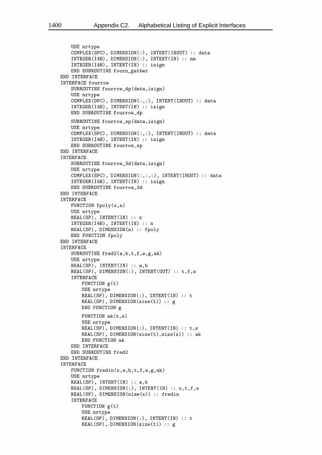
1400 Appendix C2. Alphabetical Listing of Explicit Interfaces
USE nrtypeCOMPLEX(SPC), DIMENSION(:), INTENT(INOUT) :: dataINTEGER(I4B), DIMENSION(:), INTENT(IN) :: nnINTEGER(I4B), INTENT(IN) :: isignEND SUBROUTINE fourn_gather
END INTERFACEINTERFACE fourrow
SUBROUTINE fourrow_dp(data,isign)USE nrtypeCOMPLEX(DPC), DIMENSION(:,:), INTENT(INOUT) :: dataINTEGER(I4B), INTENT(IN) :: isignEND SUBROUTINE fourrow_dp
SUBROUTINE fourrow_sp(data,isign)USE nrtypeCOMPLEX(SPC), DIMENSION(:,:), INTENT(INOUT) :: dataINTEGER(I4B), INTENT(IN) :: isignEND SUBROUTINE fourrow_sp
END INTERFACEINTERFACE
SUBROUTINE fourrow_3d(data,isign)USE nrtypeCOMPLEX(SPC), DIMENSION(:,:,:), INTENT(INOUT) :: dataINTEGER(I4B), INTENT(IN) :: isignEND SUBROUTINE fourrow_3d
END INTERFACEINTERFACE
FUNCTION fpoly(x,n)USE nrtypeREAL(SP), INTENT(IN) :: xINTEGER(I4B), INTENT(IN) :: nREAL(SP), DIMENSION(n) :: fpolyEND FUNCTION fpoly
END INTERFACEINTERFACE
SUBROUTINE fred2(a,b,t,f,w,g,ak)USE nrtypeREAL(SP), INTENT(IN) :: a,bREAL(SP), DIMENSION(:), INTENT(OUT) :: t,f,wINTERFACE
FUNCTION g(t)USE nrtypeREAL(SP), DIMENSION(:), INTENT(IN) :: tREAL(SP), DIMENSION(size(t)) :: gEND FUNCTION g
FUNCTION ak(t,s)USE nrtypeREAL(SP), DIMENSION(:), INTENT(IN) :: t,sREAL(SP), DIMENSION(size(t),size(s)) :: akEND FUNCTION ak
END INTERFACEEND SUBROUTINE fred2
END INTERFACEINTERFACE
FUNCTION fredin(x,a,b,t,f,w,g,ak)USE nrtypeREAL(SP), INTENT(IN) :: a,bREAL(SP), DIMENSION(:), INTENT(IN) :: x,t,f,wREAL(SP), DIMENSION(size(x)) :: fredinINTERFACE
FUNCTION g(t)USE nrtypeREAL(SP), DIMENSION(:), INTENT(IN) :: tREAL(SP), DIMENSION(size(t)) :: g
Appendix C2. Alphabetical Listing of Explicit Interfaces 1401
END FUNCTION g
FUNCTION ak(t,s)USE nrtypeREAL(SP), DIMENSION(:), INTENT(IN) :: t,sREAL(SP), DIMENSION(size(t),size(s)) :: akEND FUNCTION ak
END INTERFACEEND FUNCTION fredin
END INTERFACEINTERFACE
SUBROUTINE frenel(x,s,c)USE nrtypeREAL(SP), INTENT(IN) :: xREAL(SP), INTENT(OUT) :: s,cEND SUBROUTINE frenel
END INTERFACEINTERFACE
SUBROUTINE frprmn(p,ftol,iter,fret)USE nrtypeINTEGER(I4B), INTENT(OUT) :: iterREAL(SP), INTENT(IN) :: ftolREAL(SP), INTENT(OUT) :: fretREAL(SP), DIMENSION(:), INTENT(INOUT) :: pEND SUBROUTINE frprmn
END INTERFACEINTERFACE
SUBROUTINE ftest(data1,data2,f,prob)USE nrtypeREAL(SP), INTENT(OUT) :: f,probREAL(SP), DIMENSION(:), INTENT(IN) :: data1,data2END SUBROUTINE ftest
END INTERFACEINTERFACE
FUNCTION gamdev(ia)USE nrtypeINTEGER(I4B), INTENT(IN) :: iaREAL(SP) :: gamdevEND FUNCTION gamdev
END INTERFACEINTERFACE gammln
FUNCTION gammln_s(xx)USE nrtypeREAL(SP), INTENT(IN) :: xxREAL(SP) :: gammln_sEND FUNCTION gammln_s
FUNCTION gammln_v(xx)USE nrtypeREAL(SP), DIMENSION(:), INTENT(IN) :: xxREAL(SP), DIMENSION(size(xx)) :: gammln_vEND FUNCTION gammln_v
END INTERFACEINTERFACE gammp
FUNCTION gammp_s(a,x)USE nrtypeREAL(SP), INTENT(IN) :: a,xREAL(SP) :: gammp_sEND FUNCTION gammp_s
FUNCTION gammp_v(a,x)USE nrtypeREAL(SP), DIMENSION(:), INTENT(IN) :: a,xREAL(SP), DIMENSION(size(a)) :: gammp_vEND FUNCTION gammp_v
END INTERFACE
1402 Appendix C2. Alphabetical Listing of Explicit Interfaces
INTERFACE gammqFUNCTION gammq_s(a,x)USE nrtypeREAL(SP), INTENT(IN) :: a,xREAL(SP) :: gammq_sEND FUNCTION gammq_s
FUNCTION gammq_v(a,x)USE nrtypeREAL(SP), DIMENSION(:), INTENT(IN) :: a,xREAL(SP), DIMENSION(size(a)) :: gammq_vEND FUNCTION gammq_v
END INTERFACEINTERFACE gasdev
SUBROUTINE gasdev_s(harvest)USE nrtypeREAL(SP), INTENT(OUT) :: harvestEND SUBROUTINE gasdev_s
SUBROUTINE gasdev_v(harvest)USE nrtypeREAL(SP), DIMENSION(:), INTENT(OUT) :: harvestEND SUBROUTINE gasdev_v
END INTERFACEINTERFACE
SUBROUTINE gaucof(a,b,amu0,x,w)USE nrtypeREAL(SP), INTENT(IN) :: amu0REAL(SP), DIMENSION(:), INTENT(INOUT) :: a,bREAL(SP), DIMENSION(:), INTENT(OUT) :: x,wEND SUBROUTINE gaucof
END INTERFACEINTERFACE
SUBROUTINE gauher(x,w)USE nrtypeREAL(SP), DIMENSION(:), INTENT(OUT) :: x,wEND SUBROUTINE gauher
END INTERFACEINTERFACE
SUBROUTINE gaujac(x,w,alf,bet)USE nrtypeREAL(SP), INTENT(IN) :: alf,betREAL(SP), DIMENSION(:), INTENT(OUT) :: x,wEND SUBROUTINE gaujac
END INTERFACEINTERFACE
SUBROUTINE gaulag(x,w,alf)USE nrtypeREAL(SP), INTENT(IN) :: alfREAL(SP), DIMENSION(:), INTENT(OUT) :: x,wEND SUBROUTINE gaulag
END INTERFACEINTERFACE
SUBROUTINE gauleg(x1,x2,x,w)USE nrtypeREAL(SP), INTENT(IN) :: x1,x2REAL(SP), DIMENSION(:), INTENT(OUT) :: x,wEND SUBROUTINE gauleg
END INTERFACEINTERFACE
SUBROUTINE gaussj(a,b)USE nrtypeREAL(SP), DIMENSION(:,:), INTENT(INOUT) :: a,bEND SUBROUTINE gaussj
END INTERFACE
Appendix C2. Alphabetical Listing of Explicit Interfaces 1403
INTERFACE gcfFUNCTION gcf_s(a,x,gln)USE nrtypeREAL(SP), INTENT(IN) :: a,xREAL(SP), OPTIONAL, INTENT(OUT) :: glnREAL(SP) :: gcf_sEND FUNCTION gcf_s
FUNCTION gcf_v(a,x,gln)USE nrtypeREAL(SP), DIMENSION(:), INTENT(IN) :: a,xREAL(SP), DIMENSION(:), OPTIONAL, INTENT(OUT) :: glnREAL(SP), DIMENSION(size(a)) :: gcf_vEND FUNCTION gcf_v
END INTERFACEINTERFACE
FUNCTION golden(ax,bx,cx,func,tol,xmin)USE nrtypeREAL(SP), INTENT(IN) :: ax,bx,cx,tolREAL(SP), INTENT(OUT) :: xminREAL(SP) :: goldenINTERFACE
FUNCTION func(x)USE nrtypeREAL(SP), INTENT(IN) :: xREAL(SP) :: funcEND FUNCTION func
END INTERFACEEND FUNCTION golden
END INTERFACEINTERFACE gser
FUNCTION gser_s(a,x,gln)USE nrtypeREAL(SP), INTENT(IN) :: a,xREAL(SP), OPTIONAL, INTENT(OUT) :: glnREAL(SP) :: gser_sEND FUNCTION gser_s
FUNCTION gser_v(a,x,gln)USE nrtypeREAL(SP), DIMENSION(:), INTENT(IN) :: a,xREAL(SP), DIMENSION(:), OPTIONAL, INTENT(OUT) :: glnREAL(SP), DIMENSION(size(a)) :: gser_vEND FUNCTION gser_v
END INTERFACEINTERFACE
SUBROUTINE hqr(a,wr,wi)USE nrtypeREAL(SP), DIMENSION(:), INTENT(OUT) :: wr,wiREAL(SP), DIMENSION(:,:), INTENT(INOUT) :: aEND SUBROUTINE hqr
END INTERFACEINTERFACE
SUBROUTINE hunt(xx,x,jlo)USE nrtypeINTEGER(I4B), INTENT(INOUT) :: jloREAL(SP), INTENT(IN) :: xREAL(SP), DIMENSION(:), INTENT(IN) :: xxEND SUBROUTINE hunt
END INTERFACEINTERFACE
SUBROUTINE hypdrv(s,ry,rdyds)USE nrtypeREAL(SP), INTENT(IN) :: sREAL(SP), DIMENSION(:), INTENT(IN) :: ry
1404 Appendix C2. Alphabetical Listing of Explicit Interfaces
REAL(SP), DIMENSION(:), INTENT(OUT) :: rdydsEND SUBROUTINE hypdrv
END INTERFACEINTERFACE
FUNCTION hypgeo(a,b,c,z)USE nrtypeCOMPLEX(SPC), INTENT(IN) :: a,b,c,zCOMPLEX(SPC) :: hypgeoEND FUNCTION hypgeo
END INTERFACEINTERFACE
SUBROUTINE hypser(a,b,c,z,series,deriv)USE nrtypeCOMPLEX(SPC), INTENT(IN) :: a,b,c,zCOMPLEX(SPC), INTENT(OUT) :: series,derivEND SUBROUTINE hypser
END INTERFACEINTERFACE
FUNCTION icrc(crc,buf,jinit,jrev)USE nrtypeCHARACTER(1), DIMENSION(:), INTENT(IN) :: bufINTEGER(I2B), INTENT(IN) :: crc,jinitINTEGER(I4B), INTENT(IN) :: jrevINTEGER(I2B) :: icrcEND FUNCTION icrc
END INTERFACEINTERFACE
FUNCTION igray(n,is)USE nrtypeINTEGER(I4B), INTENT(IN) :: n,isINTEGER(I4B) :: igrayEND FUNCTION igray
END INTERFACEINTERFACE
RECURSIVE SUBROUTINE index_bypack(arr,index,partial)USE nrtypeREAL(SP), DIMENSION(:), INTENT(IN) :: arrINTEGER(I4B), DIMENSION(:), INTENT(INOUT) :: indexINTEGER, OPTIONAL, INTENT(IN) :: partialEND SUBROUTINE index_bypack
END INTERFACEINTERFACE indexx
SUBROUTINE indexx_sp(arr,index)USE nrtypeREAL(SP), DIMENSION(:), INTENT(IN) :: arrINTEGER(I4B), DIMENSION(:), INTENT(OUT) :: indexEND SUBROUTINE indexx_spSUBROUTINE indexx_i4b(iarr,index)USE nrtypeINTEGER(I4B), DIMENSION(:), INTENT(IN) :: iarrINTEGER(I4B), DIMENSION(:), INTENT(OUT) :: indexEND SUBROUTINE indexx_i4b
END INTERFACEINTERFACE
FUNCTION interp(uc)USE nrtypeREAL(DP), DIMENSION(:,:), INTENT(IN) :: ucREAL(DP), DIMENSION(2*size(uc,1)-1,2*size(uc,1)-1) :: interpEND FUNCTION interp
END INTERFACEINTERFACE
FUNCTION rank(indx)USE nrtypeINTEGER(I4B), DIMENSION(:), INTENT(IN) :: indx
Appendix C2. Alphabetical Listing of Explicit Interfaces 1405
INTEGER(I4B), DIMENSION(size(indx)) :: rankEND FUNCTION rank
END INTERFACEINTERFACE
FUNCTION irbit1(iseed)USE nrtypeINTEGER(I4B), INTENT(INOUT) :: iseedINTEGER(I4B) :: irbit1END FUNCTION irbit1
END INTERFACEINTERFACE
FUNCTION irbit2(iseed)USE nrtypeINTEGER(I4B), INTENT(INOUT) :: iseedINTEGER(I4B) :: irbit2END FUNCTION irbit2
END INTERFACEINTERFACE
SUBROUTINE jacobi(a,d,v,nrot)USE nrtypeINTEGER(I4B), INTENT(OUT) :: nrotREAL(SP), DIMENSION(:), INTENT(OUT) :: dREAL(SP), DIMENSION(:,:), INTENT(INOUT) :: aREAL(SP), DIMENSION(:,:), INTENT(OUT) :: vEND SUBROUTINE jacobi
END INTERFACEINTERFACE
SUBROUTINE jacobn(x,y,dfdx,dfdy)USE nrtypeREAL(SP), INTENT(IN) :: xREAL(SP), DIMENSION(:), INTENT(IN) :: yREAL(SP), DIMENSION(:), INTENT(OUT) :: dfdxREAL(SP), DIMENSION(:,:), INTENT(OUT) :: dfdyEND SUBROUTINE jacobn
END INTERFACEINTERFACE
FUNCTION julday(mm,id,iyyy)USE nrtypeINTEGER(I4B), INTENT(IN) :: mm,id,iyyyINTEGER(I4B) :: juldayEND FUNCTION julday
END INTERFACEINTERFACE
SUBROUTINE kendl1(data1,data2,tau,z,prob)USE nrtypeREAL(SP), INTENT(OUT) :: tau,z,probREAL(SP), DIMENSION(:), INTENT(IN) :: data1,data2END SUBROUTINE kendl1
END INTERFACEINTERFACE
SUBROUTINE kendl2(tab,tau,z,prob)USE nrtypeREAL(SP), DIMENSION(:,:), INTENT(IN) :: tabREAL(SP), INTENT(OUT) :: tau,z,probEND SUBROUTINE kendl2
END INTERFACEINTERFACE
FUNCTION kermom(y,m)USE nrtypeREAL(DP), INTENT(IN) :: yINTEGER(I4B), INTENT(IN) :: mREAL(DP), DIMENSION(m) :: kermomEND FUNCTION kermom
END INTERFACE
1406 Appendix C2. Alphabetical Listing of Explicit Interfaces
INTERFACESUBROUTINE ks2d1s(x1,y1,quadvl,d1,prob)USE nrtypeREAL(SP), DIMENSION(:), INTENT(IN) :: x1,y1REAL(SP), INTENT(OUT) :: d1,probINTERFACE
SUBROUTINE quadvl(x,y,fa,fb,fc,fd)USE nrtypeREAL(SP), INTENT(IN) :: x,yREAL(SP), INTENT(OUT) :: fa,fb,fc,fdEND SUBROUTINE quadvl
END INTERFACEEND SUBROUTINE ks2d1s
END INTERFACEINTERFACE
SUBROUTINE ks2d2s(x1,y1,x2,y2,d,prob)USE nrtypeREAL(SP), DIMENSION(:), INTENT(IN) :: x1,y1,x2,y2REAL(SP), INTENT(OUT) :: d,probEND SUBROUTINE ks2d2s
END INTERFACEINTERFACE
SUBROUTINE ksone(data,func,d,prob)USE nrtypeREAL(SP), INTENT(OUT) :: d,probREAL(SP), DIMENSION(:), INTENT(INOUT) :: dataINTERFACE
FUNCTION func(x)USE nrtypeREAL(SP), DIMENSION(:), INTENT(IN) :: xREAL(SP), DIMENSION(size(x)) :: funcEND FUNCTION func
END INTERFACEEND SUBROUTINE ksone
END INTERFACEINTERFACE
SUBROUTINE kstwo(data1,data2,d,prob)USE nrtypeREAL(SP), INTENT(OUT) :: d,probREAL(SP), DIMENSION(:), INTENT(IN) :: data1,data2END SUBROUTINE kstwo
END INTERFACEINTERFACE
SUBROUTINE laguer(a,x,its)USE nrtypeINTEGER(I4B), INTENT(OUT) :: itsCOMPLEX(SPC), INTENT(INOUT) :: xCOMPLEX(SPC), DIMENSION(:), INTENT(IN) :: aEND SUBROUTINE laguer
END INTERFACEINTERFACE
SUBROUTINE lfit(x,y,sig,a,maska,covar,chisq,funcs)USE nrtypeREAL(SP), DIMENSION(:), INTENT(IN) :: x,y,sigREAL(SP), DIMENSION(:), INTENT(INOUT) :: aLOGICAL(LGT), DIMENSION(:), INTENT(IN) :: maskaREAL(SP), DIMENSION(:,:), INTENT(INOUT) :: covarREAL(SP), INTENT(OUT) :: chisqINTERFACE
SUBROUTINE funcs(x,arr)USE nrtypeREAL(SP),INTENT(IN) :: xREAL(SP), DIMENSION(:), INTENT(OUT) :: arrEND SUBROUTINE funcs
Appendix C2. Alphabetical Listing of Explicit Interfaces 1407
END INTERFACEEND SUBROUTINE lfit
END INTERFACEINTERFACE
SUBROUTINE linbcg(b,x,itol,tol,itmax,iter,err)USE nrtypeREAL(DP), DIMENSION(:), INTENT(IN) :: bREAL(DP), DIMENSION(:), INTENT(INOUT) :: xINTEGER(I4B), INTENT(IN) :: itol,itmaxREAL(DP), INTENT(IN) :: tolINTEGER(I4B), INTENT(OUT) :: iterREAL(DP), INTENT(OUT) :: errEND SUBROUTINE linbcg
END INTERFACEINTERFACE
SUBROUTINE linmin(p,xi,fret)USE nrtypeREAL(SP), INTENT(OUT) :: fretREAL(SP), DIMENSION(:), TARGET, INTENT(INOUT) :: p,xiEND SUBROUTINE linmin
END INTERFACEINTERFACE
SUBROUTINE lnsrch(xold,fold,g,p,x,f,stpmax,check,func)USE nrtypeREAL(SP), DIMENSION(:), INTENT(IN) :: xold,gREAL(SP), DIMENSION(:), INTENT(INOUT) :: pREAL(SP), INTENT(IN) :: fold,stpmaxREAL(SP), DIMENSION(:), INTENT(OUT) :: xREAL(SP), INTENT(OUT) :: fLOGICAL(LGT), INTENT(OUT) :: checkINTERFACE
FUNCTION func(x)USE nrtypeREAL(SP) :: funcREAL(SP), DIMENSION(:), INTENT(IN) :: xEND FUNCTION func
END INTERFACEEND SUBROUTINE lnsrch
END INTERFACEINTERFACE
FUNCTION locate(xx,x)USE nrtypeREAL(SP), DIMENSION(:), INTENT(IN) :: xxREAL(SP), INTENT(IN) :: xINTEGER(I4B) :: locateEND FUNCTION locate
END INTERFACEINTERFACE
FUNCTION lop(u)USE nrtypeREAL(DP), DIMENSION(:,:), INTENT(IN) :: uREAL(DP), DIMENSION(size(u,1),size(u,1)) :: lopEND FUNCTION lop
END INTERFACEINTERFACE
SUBROUTINE lubksb(a,indx,b)USE nrtypeREAL(SP), DIMENSION(:,:), INTENT(IN) :: aINTEGER(I4B), DIMENSION(:), INTENT(IN) :: indxREAL(SP), DIMENSION(:), INTENT(INOUT) :: bEND SUBROUTINE lubksb
END INTERFACEINTERFACE
SUBROUTINE ludcmp(a,indx,d)
1408 Appendix C2. Alphabetical Listing of Explicit Interfaces
USE nrtypeREAL(SP), DIMENSION(:,:), INTENT(INOUT) :: aINTEGER(I4B), DIMENSION(:), INTENT(OUT) :: indxREAL(SP), INTENT(OUT) :: dEND SUBROUTINE ludcmp
END INTERFACEINTERFACE
SUBROUTINE machar(ibeta,it,irnd,ngrd,machep,negep,iexp,minexp,&maxexp,eps,epsneg,xmin,xmax)
USE nrtypeINTEGER(I4B), INTENT(OUT) :: ibeta,iexp,irnd,it,machep,maxexp,&
minexp,negep,ngrdREAL(SP), INTENT(OUT) :: eps,epsneg,xmax,xminEND SUBROUTINE machar
END INTERFACEINTERFACE
SUBROUTINE medfit(x,y,a,b,abdev)USE nrtypeREAL(SP), DIMENSION(:), INTENT(IN) :: x,yREAL(SP), INTENT(OUT) :: a,b,abdevEND SUBROUTINE medfit
END INTERFACEINTERFACE
SUBROUTINE memcof(data,xms,d)USE nrtypeREAL(SP), INTENT(OUT) :: xmsREAL(SP), DIMENSION(:), INTENT(IN) :: dataREAL(SP), DIMENSION(:), INTENT(OUT) :: dEND SUBROUTINE memcof
END INTERFACEINTERFACE
SUBROUTINE mgfas(u,maxcyc)USE nrtypeREAL(DP), DIMENSION(:,:), INTENT(INOUT) :: uINTEGER(I4B), INTENT(IN) :: maxcycEND SUBROUTINE mgfas
END INTERFACEINTERFACE
SUBROUTINE mglin(u,ncycle)USE nrtypeREAL(DP), DIMENSION(:,:), INTENT(INOUT) :: uINTEGER(I4B), INTENT(IN) :: ncycleEND SUBROUTINE mglin
END INTERFACEINTERFACE
SUBROUTINE midexp(funk,aa,bb,s,n)USE nrtypeREAL(SP), INTENT(IN) :: aa,bbREAL(SP), INTENT(INOUT) :: sINTEGER(I4B), INTENT(IN) :: nINTERFACE
FUNCTION funk(x)USE nrtypeREAL(SP), DIMENSION(:), INTENT(IN) :: xREAL(SP), DIMENSION(size(x)) :: funkEND FUNCTION funk
END INTERFACEEND SUBROUTINE midexp
END INTERFACEINTERFACE
SUBROUTINE midinf(funk,aa,bb,s,n)USE nrtypeREAL(SP), INTENT(IN) :: aa,bbREAL(SP), INTENT(INOUT) :: s
Appendix C2. Alphabetical Listing of Explicit Interfaces 1409
INTEGER(I4B), INTENT(IN) :: nINTERFACE
FUNCTION funk(x)USE nrtypeREAL(SP), DIMENSION(:), INTENT(IN) :: xREAL(SP), DIMENSION(size(x)) :: funkEND FUNCTION funk
END INTERFACEEND SUBROUTINE midinf
END INTERFACEINTERFACE
SUBROUTINE midpnt(func,a,b,s,n)USE nrtypeREAL(SP), INTENT(IN) :: a,bREAL(SP), INTENT(INOUT) :: sINTEGER(I4B), INTENT(IN) :: nINTERFACE
FUNCTION func(x)USE nrtypeREAL(SP), DIMENSION(:), INTENT(IN) :: xREAL(SP), DIMENSION(size(x)) :: funcEND FUNCTION func
END INTERFACEEND SUBROUTINE midpnt
END INTERFACEINTERFACE
SUBROUTINE midsql(funk,aa,bb,s,n)USE nrtypeREAL(SP), INTENT(IN) :: aa,bbREAL(SP), INTENT(INOUT) :: sINTEGER(I4B), INTENT(IN) :: nINTERFACE
FUNCTION funk(x)USE nrtypeREAL(SP), DIMENSION(:), INTENT(IN) :: xREAL(SP), DIMENSION(size(x)) :: funkEND FUNCTION funk
END INTERFACEEND SUBROUTINE midsql
END INTERFACEINTERFACE
SUBROUTINE midsqu(funk,aa,bb,s,n)USE nrtypeREAL(SP), INTENT(IN) :: aa,bbREAL(SP), INTENT(INOUT) :: sINTEGER(I4B), INTENT(IN) :: nINTERFACE
FUNCTION funk(x)USE nrtypeREAL(SP), DIMENSION(:), INTENT(IN) :: xREAL(SP), DIMENSION(size(x)) :: funkEND FUNCTION funk
END INTERFACEEND SUBROUTINE midsqu
END INTERFACEINTERFACE
RECURSIVE SUBROUTINE miser(func,regn,ndim,npts,dith,ave,var)USE nrtypeINTERFACE
FUNCTION func(x)USE nrtypeREAL(SP) :: funcREAL(SP), DIMENSION(:), INTENT(IN) :: xEND FUNCTION func
1410 Appendix C2. Alphabetical Listing of Explicit Interfaces
END INTERFACEREAL(SP), DIMENSION(:), INTENT(IN) :: regnINTEGER(I4B), INTENT(IN) :: ndim,nptsREAL(SP), INTENT(IN) :: dithREAL(SP), INTENT(OUT) :: ave,varEND SUBROUTINE miser
END INTERFACEINTERFACE
SUBROUTINE mmid(y,dydx,xs,htot,nstep,yout,derivs)USE nrtypeINTEGER(I4B), INTENT(IN) :: nstepREAL(SP), INTENT(IN) :: xs,htotREAL(SP), DIMENSION(:), INTENT(IN) :: y,dydxREAL(SP), DIMENSION(:), INTENT(OUT) :: youtINTERFACE
SUBROUTINE derivs(x,y,dydx)USE nrtypeREAL(SP), INTENT(IN) :: xREAL(SP), DIMENSION(:), INTENT(IN) :: yREAL(SP), DIMENSION(:), INTENT(OUT) :: dydxEND SUBROUTINE derivs
END INTERFACEEND SUBROUTINE mmid
END INTERFACEINTERFACE
SUBROUTINE mnbrak(ax,bx,cx,fa,fb,fc,func)USE nrtypeREAL(SP), INTENT(INOUT) :: ax,bxREAL(SP), INTENT(OUT) :: cx,fa,fb,fcINTERFACE
FUNCTION func(x)USE nrtypeREAL(SP), INTENT(IN) :: xREAL(SP) :: funcEND FUNCTION func
END INTERFACEEND SUBROUTINE mnbrak
END INTERFACEINTERFACE
SUBROUTINE mnewt(ntrial,x,tolx,tolf,usrfun)USE nrtypeINTEGER(I4B), INTENT(IN) :: ntrialREAL(SP), INTENT(IN) :: tolx,tolfREAL(SP), DIMENSION(:), INTENT(INOUT) :: xINTERFACE
SUBROUTINE usrfun(x,fvec,fjac)USE nrtypeREAL(SP), DIMENSION(:), INTENT(IN) :: xREAL(SP), DIMENSION(:), INTENT(OUT) :: fvecREAL(SP), DIMENSION(:,:), INTENT(OUT) :: fjacEND SUBROUTINE usrfun
END INTERFACEEND SUBROUTINE mnewt
END INTERFACEINTERFACE
SUBROUTINE moment(data,ave,adev,sdev,var,skew,curt)USE nrtypeREAL(SP), INTENT(OUT) :: ave,adev,sdev,var,skew,curtREAL(SP), DIMENSION(:), INTENT(IN) :: dataEND SUBROUTINE moment
END INTERFACEINTERFACE
SUBROUTINE mp2dfr(a,s,n,m)USE nrtype
Appendix C2. Alphabetical Listing of Explicit Interfaces 1411
INTEGER(I4B), INTENT(IN) :: nINTEGER(I4B), INTENT(OUT) :: mCHARACTER(1), DIMENSION(:), INTENT(INOUT) :: aCHARACTER(1), DIMENSION(:), INTENT(OUT) :: sEND SUBROUTINE mp2dfr
END INTERFACEINTERFACE
SUBROUTINE mpdiv(q,r,u,v,n,m)USE nrtypeCHARACTER(1), DIMENSION(:), INTENT(OUT) :: q,rCHARACTER(1), DIMENSION(:), INTENT(IN) :: u,vINTEGER(I4B), INTENT(IN) :: n,mEND SUBROUTINE mpdiv
END INTERFACEINTERFACE
SUBROUTINE mpinv(u,v,n,m)USE nrtypeCHARACTER(1), DIMENSION(:), INTENT(OUT) :: uCHARACTER(1), DIMENSION(:), INTENT(IN) :: vINTEGER(I4B), INTENT(IN) :: n,mEND SUBROUTINE mpinv
END INTERFACEINTERFACE
SUBROUTINE mpmul(w,u,v,n,m)USE nrtypeCHARACTER(1), DIMENSION(:), INTENT(IN) :: u,vCHARACTER(1), DIMENSION(:), INTENT(OUT) :: wINTEGER(I4B), INTENT(IN) :: n,mEND SUBROUTINE mpmul
END INTERFACEINTERFACE
SUBROUTINE mppi(n)USE nrtypeINTEGER(I4B), INTENT(IN) :: nEND SUBROUTINE mppi
END INTERFACEINTERFACE
SUBROUTINE mprove(a,alud,indx,b,x)USE nrtypeREAL(SP), DIMENSION(:,:), INTENT(IN) :: a,aludINTEGER(I4B), DIMENSION(:), INTENT(IN) :: indxREAL(SP), DIMENSION(:), INTENT(IN) :: bREAL(SP), DIMENSION(:), INTENT(INOUT) :: xEND SUBROUTINE mprove
END INTERFACEINTERFACE
SUBROUTINE mpsqrt(w,u,v,n,m)USE nrtypeCHARACTER(1), DIMENSION(:), INTENT(OUT) :: w,uCHARACTER(1), DIMENSION(:), INTENT(IN) :: vINTEGER(I4B), INTENT(IN) :: n,mEND SUBROUTINE mpsqrt
END INTERFACEINTERFACE
SUBROUTINE mrqcof(x,y,sig,a,maska,alpha,beta,chisq,funcs)USE nrtypeREAL(SP), DIMENSION(:), INTENT(IN) :: x,y,a,sigREAL(SP), DIMENSION(:), INTENT(OUT) :: betaREAL(SP), DIMENSION(:,:), INTENT(OUT) :: alphaREAL(SP), INTENT(OUT) :: chisqLOGICAL(LGT), DIMENSION(:), INTENT(IN) :: maskaINTERFACE
SUBROUTINE funcs(x,a,yfit,dyda)USE nrtype
1412 Appendix C2. Alphabetical Listing of Explicit Interfaces
REAL(SP), DIMENSION(:), INTENT(IN) :: x,aREAL(SP), DIMENSION(:), INTENT(OUT) :: yfitREAL(SP), DIMENSION(:,:), INTENT(OUT) :: dydaEND SUBROUTINE funcs
END INTERFACEEND SUBROUTINE mrqcof
END INTERFACEINTERFACE
SUBROUTINE mrqmin(x,y,sig,a,maska,covar,alpha,chisq,funcs,alamda)USE nrtypeREAL(SP), DIMENSION(:), INTENT(IN) :: x,y,sigREAL(SP), DIMENSION(:), INTENT(INOUT) :: aREAL(SP), DIMENSION(:,:), INTENT(OUT) :: covar,alphaREAL(SP), INTENT(OUT) :: chisqREAL(SP), INTENT(INOUT) :: alamdaLOGICAL(LGT), DIMENSION(:), INTENT(IN) :: maskaINTERFACE
SUBROUTINE funcs(x,a,yfit,dyda)USE nrtypeREAL(SP), DIMENSION(:), INTENT(IN) :: x,aREAL(SP), DIMENSION(:), INTENT(OUT) :: yfitREAL(SP), DIMENSION(:,:), INTENT(OUT) :: dydaEND SUBROUTINE funcs
END INTERFACEEND SUBROUTINE mrqmin
END INTERFACEINTERFACE
SUBROUTINE newt(x,check)USE nrtypeREAL(SP), DIMENSION(:), INTENT(INOUT) :: xLOGICAL(LGT), INTENT(OUT) :: checkEND SUBROUTINE newt
END INTERFACEINTERFACE
SUBROUTINE odeint(ystart,x1,x2,eps,h1,hmin,derivs,rkqs)USE nrtypeREAL(SP), DIMENSION(:), INTENT(INOUT) :: ystartREAL(SP), INTENT(IN) :: x1,x2,eps,h1,hminINTERFACE
SUBROUTINE derivs(x,y,dydx)USE nrtypeREAL(SP), INTENT(IN) :: xREAL(SP), DIMENSION(:), INTENT(IN) :: yREAL(SP), DIMENSION(:), INTENT(OUT) :: dydxEND SUBROUTINE derivs
SUBROUTINE rkqs(y,dydx,x,htry,eps,yscal,hdid,hnext,derivs)USE nrtypeREAL(SP), DIMENSION(:), INTENT(INOUT) :: yREAL(SP), DIMENSION(:), INTENT(IN) :: dydx,yscalREAL(SP), INTENT(INOUT) :: xREAL(SP), INTENT(IN) :: htry,epsREAL(SP), INTENT(OUT) :: hdid,hnext
INTERFACESUBROUTINE derivs(x,y,dydx)
USE nrtypeREAL(SP), INTENT(IN) :: xREAL(SP), DIMENSION(:), INTENT(IN) :: yREAL(SP), DIMENSION(:), INTENT(OUT) :: dydxEND SUBROUTINE derivs
END INTERFACEEND SUBROUTINE rkqs
END INTERFACEEND SUBROUTINE odeint
Appendix C2. Alphabetical Listing of Explicit Interfaces 1413
END INTERFACEINTERFACE
SUBROUTINE orthog(anu,alpha,beta,a,b)USE nrtypeREAL(SP), DIMENSION(:), INTENT(IN) :: anu,alpha,betaREAL(SP), DIMENSION(:), INTENT(OUT) :: a,bEND SUBROUTINE orthog
END INTERFACEINTERFACE
SUBROUTINE pade(cof,resid)USE nrtypeREAL(DP), DIMENSION(:), INTENT(INOUT) :: cofREAL(SP), INTENT(OUT) :: residEND SUBROUTINE pade
END INTERFACEINTERFACE
FUNCTION pccheb(d)USE nrtypeREAL(SP), DIMENSION(:), INTENT(IN) :: dREAL(SP), DIMENSION(size(d)) :: pcchebEND FUNCTION pccheb
END INTERFACEINTERFACE
SUBROUTINE pcshft(a,b,d)USE nrtypeREAL(SP), INTENT(IN) :: a,bREAL(SP), DIMENSION(:), INTENT(INOUT) :: dEND SUBROUTINE pcshft
END INTERFACEINTERFACE
SUBROUTINE pearsn(x,y,r,prob,z)USE nrtypeREAL(SP), INTENT(OUT) :: r,prob,zREAL(SP), DIMENSION(:), INTENT(IN) :: x,yEND SUBROUTINE pearsn
END INTERFACEINTERFACE
SUBROUTINE period(x,y,ofac,hifac,px,py,jmax,prob)USE nrtypeINTEGER(I4B), INTENT(OUT) :: jmaxREAL(SP), INTENT(IN) :: ofac,hifacREAL(SP), INTENT(OUT) :: probREAL(SP), DIMENSION(:), INTENT(IN) :: x,yREAL(SP), DIMENSION(:), POINTER :: px,pyEND SUBROUTINE period
END INTERFACEINTERFACE plgndr
FUNCTION plgndr_s(l,m,x)USE nrtypeINTEGER(I4B), INTENT(IN) :: l,mREAL(SP), INTENT(IN) :: xREAL(SP) :: plgndr_sEND FUNCTION plgndr_s
FUNCTION plgndr_v(l,m,x)USE nrtypeINTEGER(I4B), INTENT(IN) :: l,mREAL(SP), DIMENSION(:), INTENT(IN) :: xREAL(SP), DIMENSION(size(x)) :: plgndr_vEND FUNCTION plgndr_v
END INTERFACEINTERFACE
FUNCTION poidev(xm)USE nrtype
1414 Appendix C2. Alphabetical Listing of Explicit Interfaces
REAL(SP), INTENT(IN) :: xmREAL(SP) :: poidevEND FUNCTION poidev
END INTERFACEINTERFACE
FUNCTION polcoe(x,y)USE nrtypeREAL(SP), DIMENSION(:), INTENT(IN) :: x,yREAL(SP), DIMENSION(size(x)) :: polcoeEND FUNCTION polcoe
END INTERFACEINTERFACE
FUNCTION polcof(xa,ya)USE nrtypeREAL(SP), DIMENSION(:), INTENT(IN) :: xa,yaREAL(SP), DIMENSION(size(xa)) :: polcofEND FUNCTION polcof
END INTERFACEINTERFACE
SUBROUTINE poldiv(u,v,q,r)USE nrtypeREAL(SP), DIMENSION(:), INTENT(IN) :: u,vREAL(SP), DIMENSION(:), INTENT(OUT) :: q,rEND SUBROUTINE poldiv
END INTERFACEINTERFACE
SUBROUTINE polin2(x1a,x2a,ya,x1,x2,y,dy)USE nrtypeREAL(SP), DIMENSION(:), INTENT(IN) :: x1a,x2aREAL(SP), DIMENSION(:,:), INTENT(IN) :: yaREAL(SP), INTENT(IN) :: x1,x2REAL(SP), INTENT(OUT) :: y,dyEND SUBROUTINE polin2
END INTERFACEINTERFACE
SUBROUTINE polint(xa,ya,x,y,dy)USE nrtypeREAL(SP), DIMENSION(:), INTENT(IN) :: xa,yaREAL(SP), INTENT(IN) :: xREAL(SP), INTENT(OUT) :: y,dyEND SUBROUTINE polint
END INTERFACEINTERFACE
SUBROUTINE powell(p,xi,ftol,iter,fret)USE nrtypeREAL(SP), DIMENSION(:), INTENT(INOUT) :: pREAL(SP), DIMENSION(:,:), INTENT(INOUT) :: xiINTEGER(I4B), INTENT(OUT) :: iterREAL(SP), INTENT(IN) :: ftolREAL(SP), INTENT(OUT) :: fretEND SUBROUTINE powell
END INTERFACEINTERFACE
FUNCTION predic(data,d,nfut)USE nrtypeREAL(SP), DIMENSION(:), INTENT(IN) :: data,dINTEGER(I4B), INTENT(IN) :: nfutREAL(SP), DIMENSION(nfut) :: predicEND FUNCTION predic
END INTERFACEINTERFACE
FUNCTION probks(alam)USE nrtypeREAL(SP), INTENT(IN) :: alam
Appendix C2. Alphabetical Listing of Explicit Interfaces 1415
REAL(SP) :: probksEND FUNCTION probks
END INTERFACEINTERFACE psdes
SUBROUTINE psdes_s(lword,rword)USE nrtypeINTEGER(I4B), INTENT(INOUT) :: lword,rwordEND SUBROUTINE psdes_s
SUBROUTINE psdes_v(lword,rword)USE nrtypeINTEGER(I4B), DIMENSION(:), INTENT(INOUT) :: lword,rwordEND SUBROUTINE psdes_v
END INTERFACEINTERFACE
SUBROUTINE pwt(a,isign)USE nrtypeREAL(SP), DIMENSION(:), INTENT(INOUT) :: aINTEGER(I4B), INTENT(IN) :: isignEND SUBROUTINE pwt
END INTERFACEINTERFACE
SUBROUTINE pwtset(n)USE nrtypeINTEGER(I4B), INTENT(IN) :: nEND SUBROUTINE pwtset
END INTERFACEINTERFACE pythag
FUNCTION pythag_dp(a,b)USE nrtypeREAL(DP), INTENT(IN) :: a,bREAL(DP) :: pythag_dpEND FUNCTION pythag_dp
FUNCTION pythag_sp(a,b)USE nrtypeREAL(SP), INTENT(IN) :: a,bREAL(SP) :: pythag_spEND FUNCTION pythag_sp
END INTERFACEINTERFACE
SUBROUTINE pzextr(iest,xest,yest,yz,dy)USE nrtypeINTEGER(I4B), INTENT(IN) :: iestREAL(SP), INTENT(IN) :: xestREAL(SP), DIMENSION(:), INTENT(IN) :: yestREAL(SP), DIMENSION(:), INTENT(OUT) :: yz,dyEND SUBROUTINE pzextr
END INTERFACEINTERFACE
SUBROUTINE qrdcmp(a,c,d,sing)USE nrtypeREAL(SP), DIMENSION(:,:), INTENT(INOUT) :: aREAL(SP), DIMENSION(:), INTENT(OUT) :: c,dLOGICAL(LGT), INTENT(OUT) :: singEND SUBROUTINE qrdcmp
END INTERFACEINTERFACE
FUNCTION qromb(func,a,b)USE nrtypeREAL(SP), INTENT(IN) :: a,bREAL(SP) :: qrombINTERFACE
FUNCTION func(x)USE nrtype
1416 Appendix C2. Alphabetical Listing of Explicit Interfaces
REAL(SP), DIMENSION(:), INTENT(IN) :: xREAL(SP), DIMENSION(size(x)) :: funcEND FUNCTION func
END INTERFACEEND FUNCTION qromb
END INTERFACEINTERFACE
FUNCTION qromo(func,a,b,choose)USE nrtypeREAL(SP), INTENT(IN) :: a,bREAL(SP) :: qromoINTERFACE
FUNCTION func(x)USE nrtypeREAL(SP), DIMENSION(:), INTENT(IN) :: xREAL(SP), DIMENSION(size(x)) :: funcEND FUNCTION func
END INTERFACEINTERFACE
SUBROUTINE choose(funk,aa,bb,s,n)USE nrtypeREAL(SP), INTENT(IN) :: aa,bbREAL(SP), INTENT(INOUT) :: sINTEGER(I4B), INTENT(IN) :: nINTERFACE
FUNCTION funk(x)USE nrtypeREAL(SP), DIMENSION(:), INTENT(IN) :: xREAL(SP), DIMENSION(size(x)) :: funkEND FUNCTION funk
END INTERFACEEND SUBROUTINE choose
END INTERFACEEND FUNCTION qromo
END INTERFACEINTERFACE
SUBROUTINE qroot(p,b,c,eps)USE nrtypeREAL(SP), DIMENSION(:), INTENT(IN) :: pREAL(SP), INTENT(INOUT) :: b,cREAL(SP), INTENT(IN) :: epsEND SUBROUTINE qroot
END INTERFACEINTERFACE
SUBROUTINE qrsolv(a,c,d,b)USE nrtypeREAL(SP), DIMENSION(:,:), INTENT(IN) :: aREAL(SP), DIMENSION(:), INTENT(IN) :: c,dREAL(SP), DIMENSION(:), INTENT(INOUT) :: bEND SUBROUTINE qrsolv
END INTERFACEINTERFACE
SUBROUTINE qrupdt(r,qt,u,v)USE nrtypeREAL(SP), DIMENSION(:,:), INTENT(INOUT) :: r,qtREAL(SP), DIMENSION(:), INTENT(INOUT) :: uREAL(SP), DIMENSION(:), INTENT(IN) :: vEND SUBROUTINE qrupdt
END INTERFACEINTERFACE
FUNCTION qsimp(func,a,b)USE nrtypeREAL(SP), INTENT(IN) :: a,bREAL(SP) :: qsimp
Appendix C2. Alphabetical Listing of Explicit Interfaces 1417
INTERFACEFUNCTION func(x)USE nrtypeREAL(SP), DIMENSION(:), INTENT(IN) :: xREAL(SP), DIMENSION(size(x)) :: funcEND FUNCTION func
END INTERFACEEND FUNCTION qsimp
END INTERFACEINTERFACE
FUNCTION qtrap(func,a,b)USE nrtypeREAL(SP), INTENT(IN) :: a,bREAL(SP) :: qtrapINTERFACE
FUNCTION func(x)USE nrtypeREAL(SP), DIMENSION(:), INTENT(IN) :: xREAL(SP), DIMENSION(size(x)) :: funcEND FUNCTION func
END INTERFACEEND FUNCTION qtrap
END INTERFACEINTERFACE
SUBROUTINE quadct(x,y,xx,yy,fa,fb,fc,fd)USE nrtypeREAL(SP), INTENT(IN) :: x,yREAL(SP), DIMENSION(:), INTENT(IN) :: xx,yyREAL(SP), INTENT(OUT) :: fa,fb,fc,fdEND SUBROUTINE quadct
END INTERFACEINTERFACE
SUBROUTINE quadmx(a)USE nrtypeREAL(SP), DIMENSION(:,:), INTENT(OUT) :: aEND SUBROUTINE quadmx
END INTERFACEINTERFACE
SUBROUTINE quadvl(x,y,fa,fb,fc,fd)USE nrtypeREAL(SP), INTENT(IN) :: x,yREAL(SP), INTENT(OUT) :: fa,fb,fc,fdEND SUBROUTINE quadvl
END INTERFACEINTERFACE
FUNCTION ran(idum)INTEGER(selected_int_kind(9)), INTENT(INOUT) :: idumREAL :: ranEND FUNCTION ran
END INTERFACEINTERFACE ran0
SUBROUTINE ran0_s(harvest)USE nrtypeREAL(SP), INTENT(OUT) :: harvestEND SUBROUTINE ran0_s
SUBROUTINE ran0_v(harvest)USE nrtypeREAL(SP), DIMENSION(:), INTENT(OUT) :: harvestEND SUBROUTINE ran0_v
END INTERFACEINTERFACE ran1
SUBROUTINE ran1_s(harvest)USE nrtype
1418 Appendix C2. Alphabetical Listing of Explicit Interfaces
REAL(SP), INTENT(OUT) :: harvestEND SUBROUTINE ran1_s
SUBROUTINE ran1_v(harvest)USE nrtypeREAL(SP), DIMENSION(:), INTENT(OUT) :: harvestEND SUBROUTINE ran1_v
END INTERFACEINTERFACE ran2
SUBROUTINE ran2_s(harvest)USE nrtypeREAL(SP), INTENT(OUT) :: harvestEND SUBROUTINE ran2_s
SUBROUTINE ran2_v(harvest)USE nrtypeREAL(SP), DIMENSION(:), INTENT(OUT) :: harvestEND SUBROUTINE ran2_v
END INTERFACEINTERFACE ran3
SUBROUTINE ran3_s(harvest)USE nrtypeREAL(SP), INTENT(OUT) :: harvestEND SUBROUTINE ran3_s
SUBROUTINE ran3_v(harvest)USE nrtypeREAL(SP), DIMENSION(:), INTENT(OUT) :: harvestEND SUBROUTINE ran3_v
END INTERFACEINTERFACE
SUBROUTINE ratint(xa,ya,x,y,dy)USE nrtypeREAL(SP), DIMENSION(:), INTENT(IN) :: xa,yaREAL(SP), INTENT(IN) :: xREAL(SP), INTENT(OUT) :: y,dyEND SUBROUTINE ratint
END INTERFACEINTERFACE
SUBROUTINE ratlsq(func,a,b,mm,kk,cof,dev)USE nrtypeREAL(DP), INTENT(IN) :: a,bINTEGER(I4B), INTENT(IN) :: mm,kkREAL(DP), DIMENSION(:), INTENT(OUT) :: cofREAL(DP), INTENT(OUT) :: devINTERFACE
FUNCTION func(x)USE nrtypeREAL(DP), DIMENSION(:), INTENT(IN) :: xREAL(DP), DIMENSION(size(x)) :: funcEND FUNCTION func
END INTERFACEEND SUBROUTINE ratlsq
END INTERFACEINTERFACE ratval
FUNCTION ratval_s(x,cof,mm,kk)USE nrtypeREAL(DP), INTENT(IN) :: xINTEGER(I4B), INTENT(IN) :: mm,kkREAL(DP), DIMENSION(mm+kk+1), INTENT(IN) :: cofREAL(DP) :: ratval_sEND FUNCTION ratval_s
FUNCTION ratval_v(x,cof,mm,kk)USE nrtypeREAL(DP), DIMENSION(:), INTENT(IN) :: x
Appendix C2. Alphabetical Listing of Explicit Interfaces 1419
INTEGER(I4B), INTENT(IN) :: mm,kkREAL(DP), DIMENSION(mm+kk+1), INTENT(IN) :: cofREAL(DP), DIMENSION(size(x)) :: ratval_vEND FUNCTION ratval_v
END INTERFACEINTERFACE rc
FUNCTION rc_s(x,y)USE nrtypeREAL(SP), INTENT(IN) :: x,yREAL(SP) :: rc_sEND FUNCTION rc_s
FUNCTION rc_v(x,y)USE nrtypeREAL(SP), DIMENSION(:), INTENT(IN) :: x,yREAL(SP), DIMENSION(size(x)) :: rc_vEND FUNCTION rc_v
END INTERFACEINTERFACE rd
FUNCTION rd_s(x,y,z)USE nrtypeREAL(SP), INTENT(IN) :: x,y,zREAL(SP) :: rd_sEND FUNCTION rd_s
FUNCTION rd_v(x,y,z)USE nrtypeREAL(SP), DIMENSION(:), INTENT(IN) :: x,y,zREAL(SP), DIMENSION(size(x)) :: rd_vEND FUNCTION rd_v
END INTERFACEINTERFACE realft
SUBROUTINE realft_dp(data,isign,zdata)USE nrtypeREAL(DP), DIMENSION(:), INTENT(INOUT) :: dataINTEGER(I4B), INTENT(IN) :: isignCOMPLEX(DPC), DIMENSION(:), OPTIONAL, TARGET :: zdataEND SUBROUTINE realft_dp
SUBROUTINE realft_sp(data,isign,zdata)USE nrtypeREAL(SP), DIMENSION(:), INTENT(INOUT) :: dataINTEGER(I4B), INTENT(IN) :: isignCOMPLEX(SPC), DIMENSION(:), OPTIONAL, TARGET :: zdataEND SUBROUTINE realft_sp
END INTERFACEINTERFACE
RECURSIVE FUNCTION recur1(a,b) RESULT(u)USE nrtypeREAL(SP), DIMENSION(:), INTENT(IN) :: a,bREAL(SP), DIMENSION(size(a)) :: uEND FUNCTION recur1
END INTERFACEINTERFACE
FUNCTION recur2(a,b,c)USE nrtypeREAL(SP), DIMENSION(:), INTENT(IN) :: a,b,cREAL(SP), DIMENSION(size(a)) :: recur2END FUNCTION recur2
END INTERFACEINTERFACE
SUBROUTINE relax(u,rhs)USE nrtypeREAL(DP), DIMENSION(:,:), INTENT(INOUT) :: uREAL(DP), DIMENSION(:,:), INTENT(IN) :: rhsEND SUBROUTINE relax
1420 Appendix C2. Alphabetical Listing of Explicit Interfaces
END INTERFACEINTERFACE
SUBROUTINE relax2(u,rhs)USE nrtypeREAL(DP), DIMENSION(:,:), INTENT(INOUT) :: uREAL(DP), DIMENSION(:,:), INTENT(IN) :: rhsEND SUBROUTINE relax2
END INTERFACEINTERFACEFUNCTION resid(u,rhs)
USE nrtypeREAL(DP), DIMENSION(:,:), INTENT(IN) :: u,rhsREAL(DP), DIMENSION(size(u,1),size(u,1)) :: residEND FUNCTION resid
END INTERFACEINTERFACE rf
FUNCTION rf_s(x,y,z)USE nrtypeREAL(SP), INTENT(IN) :: x,y,zREAL(SP) :: rf_sEND FUNCTION rf_s
FUNCTION rf_v(x,y,z)USE nrtypeREAL(SP), DIMENSION(:), INTENT(IN) :: x,y,zREAL(SP), DIMENSION(size(x)) :: rf_vEND FUNCTION rf_v
END INTERFACEINTERFACE rj
FUNCTION rj_s(x,y,z,p)USE nrtypeREAL(SP), INTENT(IN) :: x,y,z,pREAL(SP) :: rj_sEND FUNCTION rj_s
FUNCTION rj_v(x,y,z,p)USE nrtypeREAL(SP), DIMENSION(:), INTENT(IN) :: x,y,z,pREAL(SP), DIMENSION(size(x)) :: rj_vEND FUNCTION rj_v
END INTERFACEINTERFACE
SUBROUTINE rk4(y,dydx,x,h,yout,derivs)USE nrtypeREAL(SP), DIMENSION(:), INTENT(IN) :: y,dydxREAL(SP), INTENT(IN) :: x,hREAL(SP), DIMENSION(:), INTENT(OUT) :: youtINTERFACE
SUBROUTINE derivs(x,y,dydx)USE nrtypeREAL(SP), INTENT(IN) :: xREAL(SP), DIMENSION(:), INTENT(IN) :: yREAL(SP), DIMENSION(:), INTENT(OUT) :: dydxEND SUBROUTINE derivs
END INTERFACEEND SUBROUTINE rk4
END INTERFACEINTERFACE
SUBROUTINE rkck(y,dydx,x,h,yout,yerr,derivs)USE nrtypeREAL(SP), DIMENSION(:), INTENT(IN) :: y,dydxREAL(SP), INTENT(IN) :: x,hREAL(SP), DIMENSION(:), INTENT(OUT) :: yout,yerrINTERFACE
SUBROUTINE derivs(x,y,dydx)
Appendix C2. Alphabetical Listing of Explicit Interfaces 1421
USE nrtypeREAL(SP), INTENT(IN) :: xREAL(SP), DIMENSION(:), INTENT(IN) :: yREAL(SP), DIMENSION(:), INTENT(OUT) :: dydxEND SUBROUTINE derivs
END INTERFACEEND SUBROUTINE rkck
END INTERFACEINTERFACE
SUBROUTINE rkdumb(vstart,x1,x2,nstep,derivs)USE nrtypeREAL(SP), DIMENSION(:), INTENT(IN) :: vstartREAL(SP), INTENT(IN) :: x1,x2INTEGER(I4B), INTENT(IN) :: nstepINTERFACE
SUBROUTINE derivs(x,y,dydx)USE nrtypeREAL(SP), INTENT(IN) :: xREAL(SP), DIMENSION(:), INTENT(IN) :: yREAL(SP), DIMENSION(:), INTENT(OUT) :: dydxEND SUBROUTINE derivs
END INTERFACEEND SUBROUTINE rkdumb
END INTERFACEINTERFACE
SUBROUTINE rkqs(y,dydx,x,htry,eps,yscal,hdid,hnext,derivs)USE nrtypeREAL(SP), DIMENSION(:), INTENT(INOUT) :: yREAL(SP), DIMENSION(:), INTENT(IN) :: dydx,yscalREAL(SP), INTENT(INOUT) :: xREAL(SP), INTENT(IN) :: htry,epsREAL(SP), INTENT(OUT) :: hdid,hnextINTERFACE
SUBROUTINE derivs(x,y,dydx)USE nrtypeREAL(SP), INTENT(IN) :: xREAL(SP), DIMENSION(:), INTENT(IN) :: yREAL(SP), DIMENSION(:), INTENT(OUT) :: dydxEND SUBROUTINE derivs
END INTERFACEEND SUBROUTINE rkqs
END INTERFACEINTERFACE
SUBROUTINE rlft2(data,spec,speq,isign)USE nrtypeREAL(SP), DIMENSION(:,:), INTENT(INOUT) :: dataCOMPLEX(SPC), DIMENSION(:,:), INTENT(OUT) :: specCOMPLEX(SPC), DIMENSION(:), INTENT(OUT) :: speqINTEGER(I4B), INTENT(IN) :: isignEND SUBROUTINE rlft2
END INTERFACEINTERFACE
SUBROUTINE rlft3(data,spec,speq,isign)USE nrtypeREAL(SP), DIMENSION(:,:,:), INTENT(INOUT) :: dataCOMPLEX(SPC), DIMENSION(:,:,:), INTENT(OUT) :: specCOMPLEX(SPC), DIMENSION(:,:), INTENT(OUT) :: speqINTEGER(I4B), INTENT(IN) :: isignEND SUBROUTINE rlft3
END INTERFACEINTERFACE
SUBROUTINE rotate(r,qt,i,a,b)USE nrtypeREAL(SP), DIMENSION(:,:), TARGET, INTENT(INOUT) :: r,qt
1422 Appendix C2. Alphabetical Listing of Explicit Interfaces
INTEGER(I4B), INTENT(IN) :: iREAL(SP), INTENT(IN) :: a,bEND SUBROUTINE rotate
END INTERFACEINTERFACE
SUBROUTINE rsolv(a,d,b)USE nrtypeREAL(SP), DIMENSION(:,:), INTENT(IN) :: aREAL(SP), DIMENSION(:), INTENT(IN) :: dREAL(SP), DIMENSION(:), INTENT(INOUT) :: bEND SUBROUTINE rsolv
END INTERFACEINTERFACE
FUNCTION rstrct(uf)USE nrtypeREAL(DP), DIMENSION(:,:), INTENT(IN) :: ufREAL(DP), DIMENSION((size(uf,1)+1)/2,(size(uf,1)+1)/2) :: rstrctEND FUNCTION rstrct
END INTERFACEINTERFACE
FUNCTION rtbis(func,x1,x2,xacc)USE nrtypeREAL(SP), INTENT(IN) :: x1,x2,xaccREAL(SP) :: rtbisINTERFACE
FUNCTION func(x)USE nrtypeREAL(SP), INTENT(IN) :: xREAL(SP) :: funcEND FUNCTION func
END INTERFACEEND FUNCTION rtbis
END INTERFACEINTERFACE
FUNCTION rtflsp(func,x1,x2,xacc)USE nrtypeREAL(SP), INTENT(IN) :: x1,x2,xaccREAL(SP) :: rtflspINTERFACE
FUNCTION func(x)USE nrtypeREAL(SP), INTENT(IN) :: xREAL(SP) :: funcEND FUNCTION func
END INTERFACEEND FUNCTION rtflsp
END INTERFACEINTERFACE
FUNCTION rtnewt(funcd,x1,x2,xacc)USE nrtypeREAL(SP), INTENT(IN) :: x1,x2,xaccREAL(SP) :: rtnewtINTERFACE
SUBROUTINE funcd(x,fval,fderiv)USE nrtypeREAL(SP), INTENT(IN) :: xREAL(SP), INTENT(OUT) :: fval,fderivEND SUBROUTINE funcd
END INTERFACEEND FUNCTION rtnewt
END INTERFACEINTERFACE
FUNCTION rtsafe(funcd,x1,x2,xacc)USE nrtype
Appendix C2. Alphabetical Listing of Explicit Interfaces 1423
REAL(SP), INTENT(IN) :: x1,x2,xaccREAL(SP) :: rtsafeINTERFACE
SUBROUTINE funcd(x,fval,fderiv)USE nrtypeREAL(SP), INTENT(IN) :: xREAL(SP), INTENT(OUT) :: fval,fderivEND SUBROUTINE funcd
END INTERFACEEND FUNCTION rtsafe
END INTERFACEINTERFACE
FUNCTION rtsec(func,x1,x2,xacc)USE nrtypeREAL(SP), INTENT(IN) :: x1,x2,xaccREAL(SP) :: rtsecINTERFACE
FUNCTION func(x)USE nrtypeREAL(SP), INTENT(IN) :: xREAL(SP) :: funcEND FUNCTION func
END INTERFACEEND FUNCTION rtsec
END INTERFACEINTERFACE
SUBROUTINE rzextr(iest,xest,yest,yz,dy)USE nrtypeINTEGER(I4B), INTENT(IN) :: iestREAL(SP), INTENT(IN) :: xestREAL(SP), DIMENSION(:), INTENT(IN) :: yestREAL(SP), DIMENSION(:), INTENT(OUT) :: yz,dyEND SUBROUTINE rzextr
END INTERFACEINTERFACE
FUNCTION savgol(nl,nrr,ld,m)USE nrtypeINTEGER(I4B), INTENT(IN) :: nl,nrr,ld,mREAL(SP), DIMENSION(nl+nrr+1) :: savgolEND FUNCTION savgol
END INTERFACEINTERFACE
SUBROUTINE scrsho(func)USE nrtypeINTERFACE
FUNCTION func(x)USE nrtypeREAL(SP), INTENT(IN) :: xREAL(SP) :: funcEND FUNCTION func
END INTERFACEEND SUBROUTINE scrsho
END INTERFACEINTERFACE
FUNCTION select(k,arr)USE nrtypeINTEGER(I4B), INTENT(IN) :: kREAL(SP), DIMENSION(:), INTENT(INOUT) :: arrREAL(SP) :: selectEND FUNCTION select
END INTERFACEINTERFACE
FUNCTION select_bypack(k,arr)USE nrtype
1424 Appendix C2. Alphabetical Listing of Explicit Interfaces
INTEGER(I4B), INTENT(IN) :: kREAL(SP), DIMENSION(:), INTENT(INOUT) :: arrREAL(SP) :: select_bypackEND FUNCTION select_bypack
END INTERFACEINTERFACE
SUBROUTINE select_heap(arr,heap)USE nrtypeREAL(SP), DIMENSION(:), INTENT(IN) :: arrREAL(SP), DIMENSION(:), INTENT(OUT) :: heapEND SUBROUTINE select_heap
END INTERFACEINTERFACE
FUNCTION select_inplace(k,arr)USE nrtypeINTEGER(I4B), INTENT(IN) :: kREAL(SP), DIMENSION(:), INTENT(IN) :: arrREAL(SP) :: select_inplaceEND FUNCTION select_inplace
END INTERFACEINTERFACE
SUBROUTINE simplx(a,m1,m2,m3,icase,izrov,iposv)USE nrtypeREAL(SP), DIMENSION(:,:), INTENT(INOUT) :: aINTEGER(I4B), INTENT(IN) :: m1,m2,m3INTEGER(I4B), INTENT(OUT) :: icaseINTEGER(I4B), DIMENSION(:), INTENT(OUT) :: izrov,iposvEND SUBROUTINE simplx
END INTERFACEINTERFACE
SUBROUTINE simpr(y,dydx,dfdx,dfdy,xs,htot,nstep,yout,derivs)USE nrtypeREAL(SP), INTENT(IN) :: xs,htotREAL(SP), DIMENSION(:), INTENT(IN) :: y,dydx,dfdxREAL(SP), DIMENSION(:,:), INTENT(IN) :: dfdyINTEGER(I4B), INTENT(IN) :: nstepREAL(SP), DIMENSION(:), INTENT(OUT) :: youtINTERFACE
SUBROUTINE derivs(x,y,dydx)USE nrtypeREAL(SP), INTENT(IN) :: xREAL(SP), DIMENSION(:), INTENT(IN) :: yREAL(SP), DIMENSION(:), INTENT(OUT) :: dydxEND SUBROUTINE derivs
END INTERFACEEND SUBROUTINE simpr
END INTERFACEINTERFACE
SUBROUTINE sinft(y)USE nrtypeREAL(SP), DIMENSION(:), INTENT(INOUT) :: yEND SUBROUTINE sinft
END INTERFACEINTERFACE
SUBROUTINE slvsm2(u,rhs)USE nrtypeREAL(DP), DIMENSION(3,3), INTENT(OUT) :: uREAL(DP), DIMENSION(3,3), INTENT(IN) :: rhsEND SUBROUTINE slvsm2
END INTERFACEINTERFACE
SUBROUTINE slvsml(u,rhs)USE nrtypeREAL(DP), DIMENSION(3,3), INTENT(OUT) :: u
Appendix C2. Alphabetical Listing of Explicit Interfaces 1425
REAL(DP), DIMENSION(3,3), INTENT(IN) :: rhsEND SUBROUTINE slvsml
END INTERFACEINTERFACE
SUBROUTINE sncndn(uu,emmc,sn,cn,dn)USE nrtypeREAL(SP), INTENT(IN) :: uu,emmcREAL(SP), INTENT(OUT) :: sn,cn,dnEND SUBROUTINE sncndn
END INTERFACEINTERFACE
FUNCTION snrm(sx,itol)USE nrtypeREAL(DP), DIMENSION(:), INTENT(IN) :: sxINTEGER(I4B), INTENT(IN) :: itolREAL(DP) :: snrmEND FUNCTION snrm
END INTERFACEINTERFACE
SUBROUTINE sobseq(x,init)USE nrtypeREAL(SP), DIMENSION(:), INTENT(OUT) :: xINTEGER(I4B), OPTIONAL, INTENT(IN) :: initEND SUBROUTINE sobseq
END INTERFACEINTERFACE
SUBROUTINE solvde(itmax,conv,slowc,scalv,indexv,nb,y)USE nrtypeINTEGER(I4B), INTENT(IN) :: itmax,nbREAL(SP), INTENT(IN) :: conv,slowcREAL(SP), DIMENSION(:), INTENT(IN) :: scalvINTEGER(I4B), DIMENSION(:), INTENT(IN) :: indexvREAL(SP), DIMENSION(:,:), INTENT(INOUT) :: yEND SUBROUTINE solvde
END INTERFACEINTERFACE
SUBROUTINE sor(a,b,c,d,e,f,u,rjac)USE nrtypeREAL(DP), DIMENSION(:,:), INTENT(IN) :: a,b,c,d,e,fREAL(DP), DIMENSION(:,:), INTENT(INOUT) :: uREAL(DP), INTENT(IN) :: rjacEND SUBROUTINE sor
END INTERFACEINTERFACE
SUBROUTINE sort(arr)USE nrtypeREAL(SP), DIMENSION(:), INTENT(INOUT) :: arrEND SUBROUTINE sort
END INTERFACEINTERFACE
SUBROUTINE sort2(arr,slave)USE nrtypeREAL(SP), DIMENSION(:), INTENT(INOUT) :: arr,slaveEND SUBROUTINE sort2
END INTERFACEINTERFACE
SUBROUTINE sort3(arr,slave1,slave2)USE nrtypeREAL(SP), DIMENSION(:), INTENT(INOUT) :: arr,slave1,slave2END SUBROUTINE sort3
END INTERFACEINTERFACE
SUBROUTINE sort_bypack(arr)USE nrtype
1426 Appendix C2. Alphabetical Listing of Explicit Interfaces
REAL(SP), DIMENSION(:), INTENT(INOUT) :: arrEND SUBROUTINE sort_bypack
END INTERFACEINTERFACE
SUBROUTINE sort_byreshape(arr)USE nrtypeREAL(SP), DIMENSION(:), INTENT(INOUT) :: arrEND SUBROUTINE sort_byreshape
END INTERFACEINTERFACE
SUBROUTINE sort_heap(arr)USE nrtypeREAL(SP), DIMENSION(:), INTENT(INOUT) :: arrEND SUBROUTINE sort_heap
END INTERFACEINTERFACE
SUBROUTINE sort_pick(arr)USE nrtypeREAL(SP), DIMENSION(:), INTENT(INOUT) :: arrEND SUBROUTINE sort_pick
END INTERFACEINTERFACE
SUBROUTINE sort_radix(arr)USE nrtypeREAL(SP), DIMENSION(:), INTENT(INOUT) :: arrEND SUBROUTINE sort_radix
END INTERFACEINTERFACE
SUBROUTINE sort_shell(arr)USE nrtypeREAL(SP), DIMENSION(:), INTENT(INOUT) :: arrEND SUBROUTINE sort_shell
END INTERFACEINTERFACE
SUBROUTINE spctrm(p,k,ovrlap,unit,n_window)USE nrtypeREAL(SP), DIMENSION(:), INTENT(OUT) :: pINTEGER(I4B), INTENT(IN) :: kLOGICAL(LGT), INTENT(IN) :: ovrlapINTEGER(I4B), OPTIONAL, INTENT(IN) :: n_window,unitEND SUBROUTINE spctrm
END INTERFACEINTERFACE
SUBROUTINE spear(data1,data2,d,zd,probd,rs,probrs)USE nrtypeREAL(SP), DIMENSION(:), INTENT(IN) :: data1,data2REAL(SP), INTENT(OUT) :: d,zd,probd,rs,probrsEND SUBROUTINE spear
END INTERFACEINTERFACE sphbes
SUBROUTINE sphbes_s(n,x,sj,sy,sjp,syp)USE nrtypeINTEGER(I4B), INTENT(IN) :: nREAL(SP), INTENT(IN) :: xREAL(SP), INTENT(OUT) :: sj,sy,sjp,sypEND SUBROUTINE sphbes_s
SUBROUTINE sphbes_v(n,x,sj,sy,sjp,syp)USE nrtypeINTEGER(I4B), INTENT(IN) :: nREAL(SP), DIMENSION(:), INTENT(IN) :: xREAL(SP), DIMENSION(:), INTENT(OUT) :: sj,sy,sjp,sypEND SUBROUTINE sphbes_v
END INTERFACE
Appendix C2. Alphabetical Listing of Explicit Interfaces 1427
INTERFACESUBROUTINE splie2(x1a,x2a,ya,y2a)USE nrtypeREAL(SP), DIMENSION(:), INTENT(IN) :: x1a,x2aREAL(SP), DIMENSION(:,:), INTENT(IN) :: yaREAL(SP), DIMENSION(:,:), INTENT(OUT) :: y2aEND SUBROUTINE splie2
END INTERFACEINTERFACE
FUNCTION splin2(x1a,x2a,ya,y2a,x1,x2)USE nrtypeREAL(SP), DIMENSION(:), INTENT(IN) :: x1a,x2aREAL(SP), DIMENSION(:,:), INTENT(IN) :: ya,y2aREAL(SP), INTENT(IN) :: x1,x2REAL(SP) :: splin2END FUNCTION splin2
END INTERFACEINTERFACE
SUBROUTINE spline(x,y,yp1,ypn,y2)USE nrtypeREAL(SP), DIMENSION(:), INTENT(IN) :: x,yREAL(SP), INTENT(IN) :: yp1,ypnREAL(SP), DIMENSION(:), INTENT(OUT) :: y2END SUBROUTINE spline
END INTERFACEINTERFACE
FUNCTION splint(xa,ya,y2a,x)USE nrtypeREAL(SP), DIMENSION(:), INTENT(IN) :: xa,ya,y2aREAL(SP), INTENT(IN) :: xREAL(SP) :: splintEND FUNCTION splint
END INTERFACEINTERFACE sprsax
SUBROUTINE sprsax_dp(sa,x,b)USE nrtypeTYPE(sprs2_dp), INTENT(IN) :: saREAL(DP), DIMENSION (:), INTENT(IN) :: xREAL(DP), DIMENSION (:), INTENT(OUT) :: bEND SUBROUTINE sprsax_dp
SUBROUTINE sprsax_sp(sa,x,b)USE nrtypeTYPE(sprs2_sp), INTENT(IN) :: saREAL(SP), DIMENSION (:), INTENT(IN) :: xREAL(SP), DIMENSION (:), INTENT(OUT) :: bEND SUBROUTINE sprsax_sp
END INTERFACEINTERFACE sprsdiag
SUBROUTINE sprsdiag_dp(sa,b)USE nrtypeTYPE(sprs2_dp), INTENT(IN) :: saREAL(DP), DIMENSION(:), INTENT(OUT) :: bEND SUBROUTINE sprsdiag_dp
SUBROUTINE sprsdiag_sp(sa,b)USE nrtypeTYPE(sprs2_sp), INTENT(IN) :: saREAL(SP), DIMENSION(:), INTENT(OUT) :: bEND SUBROUTINE sprsdiag_sp
END INTERFACEINTERFACE sprsin
SUBROUTINE sprsin_sp(a,thresh,sa)USE nrtypeREAL(SP), DIMENSION(:,:), INTENT(IN) :: a
1428 Appendix C2. Alphabetical Listing of Explicit Interfaces
REAL(SP), INTENT(IN) :: threshTYPE(sprs2_sp), INTENT(OUT) :: saEND SUBROUTINE sprsin_sp
SUBROUTINE sprsin_dp(a,thresh,sa)USE nrtypeREAL(DP), DIMENSION(:,:), INTENT(IN) :: aREAL(DP), INTENT(IN) :: threshTYPE(sprs2_dp), INTENT(OUT) :: saEND SUBROUTINE sprsin_dp
END INTERFACEINTERFACE
SUBROUTINE sprstp(sa)USE nrtypeTYPE(sprs2_sp), INTENT(INOUT) :: saEND SUBROUTINE sprstp
END INTERFACEINTERFACE sprstx
SUBROUTINE sprstx_dp(sa,x,b)USE nrtypeTYPE(sprs2_dp), INTENT(IN) :: saREAL(DP), DIMENSION (:), INTENT(IN) :: xREAL(DP), DIMENSION (:), INTENT(OUT) :: bEND SUBROUTINE sprstx_dp
SUBROUTINE sprstx_sp(sa,x,b)USE nrtypeTYPE(sprs2_sp), INTENT(IN) :: saREAL(SP), DIMENSION (:), INTENT(IN) :: xREAL(SP), DIMENSION (:), INTENT(OUT) :: bEND SUBROUTINE sprstx_sp
END INTERFACEINTERFACE
SUBROUTINE stifbs(y,dydx,x,htry,eps,yscal,hdid,hnext,derivs)USE nrtypeREAL(SP), DIMENSION(:), INTENT(INOUT) :: yREAL(SP), DIMENSION(:), INTENT(IN) :: dydx,yscalREAL(SP), INTENT(IN) :: htry,epsREAL(SP), INTENT(INOUT) :: xREAL(SP), INTENT(OUT) :: hdid,hnextINTERFACE
SUBROUTINE derivs(x,y,dydx)USE nrtypeREAL(SP), INTENT(IN) :: xREAL(SP), DIMENSION(:), INTENT(IN) :: yREAL(SP), DIMENSION(:), INTENT(OUT) :: dydxEND SUBROUTINE derivs
END INTERFACEEND SUBROUTINE stifbs
END INTERFACEINTERFACE
SUBROUTINE stiff(y,dydx,x,htry,eps,yscal,hdid,hnext,derivs)USE nrtypeREAL(SP), DIMENSION(:), INTENT(INOUT) :: yREAL(SP), DIMENSION(:), INTENT(IN) :: dydx,yscalREAL(SP), INTENT(INOUT) :: xREAL(SP), INTENT(IN) :: htry,epsREAL(SP), INTENT(OUT) :: hdid,hnextINTERFACE
SUBROUTINE derivs(x,y,dydx)USE nrtypeREAL(SP), INTENT(IN) :: xREAL(SP), DIMENSION(:), INTENT(IN) :: yREAL(SP), DIMENSION(:), INTENT(OUT) :: dydxEND SUBROUTINE derivs
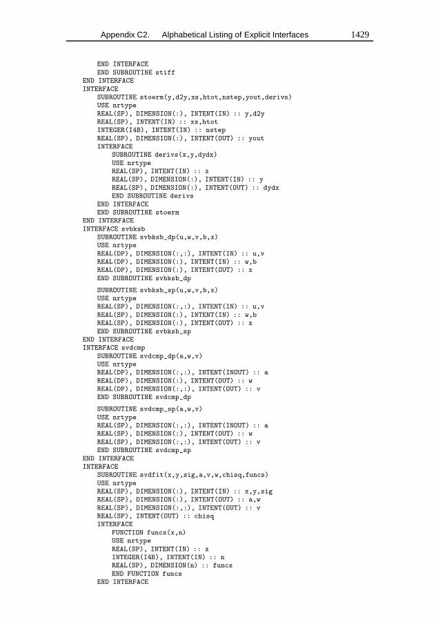
Appendix C2. Alphabetical Listing of Explicit Interfaces 1429
END INTERFACEEND SUBROUTINE stiff
END INTERFACEINTERFACE
SUBROUTINE stoerm(y,d2y,xs,htot,nstep,yout,derivs)USE nrtypeREAL(SP), DIMENSION(:), INTENT(IN) :: y,d2yREAL(SP), INTENT(IN) :: xs,htotINTEGER(I4B), INTENT(IN) :: nstepREAL(SP), DIMENSION(:), INTENT(OUT) :: youtINTERFACE
SUBROUTINE derivs(x,y,dydx)USE nrtypeREAL(SP), INTENT(IN) :: xREAL(SP), DIMENSION(:), INTENT(IN) :: yREAL(SP), DIMENSION(:), INTENT(OUT) :: dydxEND SUBROUTINE derivs
END INTERFACEEND SUBROUTINE stoerm
END INTERFACEINTERFACE svbksb
SUBROUTINE svbksb_dp(u,w,v,b,x)USE nrtypeREAL(DP), DIMENSION(:,:), INTENT(IN) :: u,vREAL(DP), DIMENSION(:), INTENT(IN) :: w,bREAL(DP), DIMENSION(:), INTENT(OUT) :: xEND SUBROUTINE svbksb_dp
SUBROUTINE svbksb_sp(u,w,v,b,x)USE nrtypeREAL(SP), DIMENSION(:,:), INTENT(IN) :: u,vREAL(SP), DIMENSION(:), INTENT(IN) :: w,bREAL(SP), DIMENSION(:), INTENT(OUT) :: xEND SUBROUTINE svbksb_sp
END INTERFACEINTERFACE svdcmp
SUBROUTINE svdcmp_dp(a,w,v)USE nrtypeREAL(DP), DIMENSION(:,:), INTENT(INOUT) :: aREAL(DP), DIMENSION(:), INTENT(OUT) :: wREAL(DP), DIMENSION(:,:), INTENT(OUT) :: vEND SUBROUTINE svdcmp_dp
SUBROUTINE svdcmp_sp(a,w,v)USE nrtypeREAL(SP), DIMENSION(:,:), INTENT(INOUT) :: aREAL(SP), DIMENSION(:), INTENT(OUT) :: wREAL(SP), DIMENSION(:,:), INTENT(OUT) :: vEND SUBROUTINE svdcmp_sp
END INTERFACEINTERFACE
SUBROUTINE svdfit(x,y,sig,a,v,w,chisq,funcs)USE nrtypeREAL(SP), DIMENSION(:), INTENT(IN) :: x,y,sigREAL(SP), DIMENSION(:), INTENT(OUT) :: a,wREAL(SP), DIMENSION(:,:), INTENT(OUT) :: vREAL(SP), INTENT(OUT) :: chisqINTERFACE
FUNCTION funcs(x,n)USE nrtypeREAL(SP), INTENT(IN) :: xINTEGER(I4B), INTENT(IN) :: nREAL(SP), DIMENSION(n) :: funcsEND FUNCTION funcs
END INTERFACE
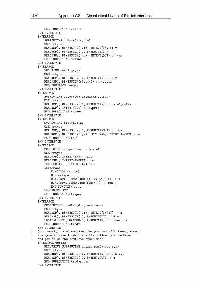
1430 Appendix C2. Alphabetical Listing of Explicit Interfaces
END SUBROUTINE svdfitEND INTERFACEINTERFACE
SUBROUTINE svdvar(v,w,cvm)USE nrtypeREAL(SP), DIMENSION(:,:), INTENT(IN) :: vREAL(SP), DIMENSION(:), INTENT(IN) :: wREAL(SP), DIMENSION(:,:), INTENT(OUT) :: cvmEND SUBROUTINE svdvar
END INTERFACEINTERFACE
FUNCTION toeplz(r,y)USE nrtypeREAL(SP), DIMENSION(:), INTENT(IN) :: r,yREAL(SP), DIMENSION(size(y)) :: toeplzEND FUNCTION toeplz
END INTERFACEINTERFACE
SUBROUTINE tptest(data1,data2,t,prob)USE nrtypeREAL(SP), DIMENSION(:), INTENT(IN) :: data1,data2REAL(SP), INTENT(OUT) :: t,probEND SUBROUTINE tptest
END INTERFACEINTERFACE
SUBROUTINE tqli(d,e,z)USE nrtypeREAL(SP), DIMENSION(:), INTENT(INOUT) :: d,eREAL(SP), DIMENSION(:,:), OPTIONAL, INTENT(INOUT) :: zEND SUBROUTINE tqli
END INTERFACEINTERFACE
SUBROUTINE trapzd(func,a,b,s,n)USE nrtypeREAL(SP), INTENT(IN) :: a,bREAL(SP), INTENT(INOUT) :: sINTEGER(I4B), INTENT(IN) :: nINTERFACE
FUNCTION func(x)USE nrtypeREAL(SP), DIMENSION(:), INTENT(IN) :: xREAL(SP), DIMENSION(size(x)) :: funcEND FUNCTION func
END INTERFACEEND SUBROUTINE trapzd
END INTERFACEINTERFACE
SUBROUTINE tred2(a,d,e,novectors)USE nrtypeREAL(SP), DIMENSION(:,:), INTENT(INOUT) :: aREAL(SP), DIMENSION(:), INTENT(OUT) :: d,eLOGICAL(LGT), OPTIONAL, INTENT(IN) :: novectorsEND SUBROUTINE tred2
END INTERFACE! On a purely serial machine, for greater efficiency, remove! the generic name tridag from the following interface,! and put it on the next one after that.
INTERFACE tridagRECURSIVE SUBROUTINE tridag_par(a,b,c,r,u)USE nrtypeREAL(SP), DIMENSION(:), INTENT(IN) :: a,b,c,rREAL(SP), DIMENSION(:), INTENT(OUT) :: uEND SUBROUTINE tridag_par
END INTERFACE
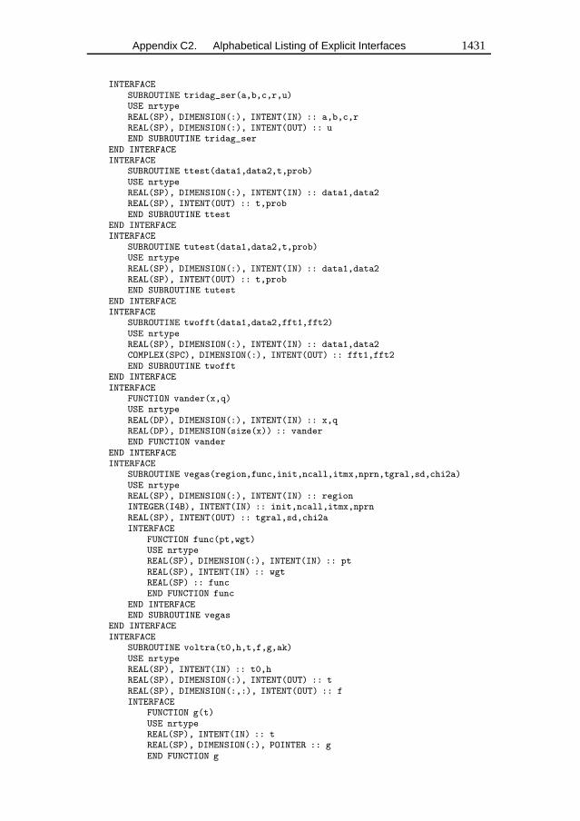
Appendix C2. Alphabetical Listing of Explicit Interfaces 1431
INTERFACESUBROUTINE tridag_ser(a,b,c,r,u)USE nrtypeREAL(SP), DIMENSION(:), INTENT(IN) :: a,b,c,rREAL(SP), DIMENSION(:), INTENT(OUT) :: uEND SUBROUTINE tridag_ser
END INTERFACEINTERFACE
SUBROUTINE ttest(data1,data2,t,prob)USE nrtypeREAL(SP), DIMENSION(:), INTENT(IN) :: data1,data2REAL(SP), INTENT(OUT) :: t,probEND SUBROUTINE ttest
END INTERFACEINTERFACE
SUBROUTINE tutest(data1,data2,t,prob)USE nrtypeREAL(SP), DIMENSION(:), INTENT(IN) :: data1,data2REAL(SP), INTENT(OUT) :: t,probEND SUBROUTINE tutest
END INTERFACEINTERFACE
SUBROUTINE twofft(data1,data2,fft1,fft2)USE nrtypeREAL(SP), DIMENSION(:), INTENT(IN) :: data1,data2COMPLEX(SPC), DIMENSION(:), INTENT(OUT) :: fft1,fft2END SUBROUTINE twofft
END INTERFACEINTERFACE
FUNCTION vander(x,q)USE nrtypeREAL(DP), DIMENSION(:), INTENT(IN) :: x,qREAL(DP), DIMENSION(size(x)) :: vanderEND FUNCTION vander
END INTERFACEINTERFACE
SUBROUTINE vegas(region,func,init,ncall,itmx,nprn,tgral,sd,chi2a)USE nrtypeREAL(SP), DIMENSION(:), INTENT(IN) :: regionINTEGER(I4B), INTENT(IN) :: init,ncall,itmx,nprnREAL(SP), INTENT(OUT) :: tgral,sd,chi2aINTERFACE
FUNCTION func(pt,wgt)USE nrtypeREAL(SP), DIMENSION(:), INTENT(IN) :: ptREAL(SP), INTENT(IN) :: wgtREAL(SP) :: funcEND FUNCTION func
END INTERFACEEND SUBROUTINE vegas
END INTERFACEINTERFACE
SUBROUTINE voltra(t0,h,t,f,g,ak)USE nrtypeREAL(SP), INTENT(IN) :: t0,hREAL(SP), DIMENSION(:), INTENT(OUT) :: tREAL(SP), DIMENSION(:,:), INTENT(OUT) :: fINTERFACE
FUNCTION g(t)USE nrtypeREAL(SP), INTENT(IN) :: tREAL(SP), DIMENSION(:), POINTER :: gEND FUNCTION g
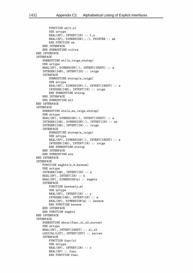
1432 Appendix C2. Alphabetical Listing of Explicit Interfaces
FUNCTION ak(t,s)USE nrtypeREAL(SP), INTENT(IN) :: t,sREAL(SP), DIMENSION(:,:), POINTER :: akEND FUNCTION ak
END INTERFACEEND SUBROUTINE voltra
END INTERFACEINTERFACE
SUBROUTINE wt1(a,isign,wtstep)USE nrtypeREAL(SP), DIMENSION(:), INTENT(INOUT) :: aINTEGER(I4B), INTENT(IN) :: isignINTERFACE
SUBROUTINE wtstep(a,isign)USE nrtypeREAL(SP), DIMENSION(:), INTENT(INOUT) :: aINTEGER(I4B), INTENT(IN) :: isignEND SUBROUTINE wtstep
END INTERFACEEND SUBROUTINE wt1
END INTERFACEINTERFACE
SUBROUTINE wtn(a,nn,isign,wtstep)USE nrtypeREAL(SP), DIMENSION(:), INTENT(INOUT) :: aINTEGER(I4B), DIMENSION(:), INTENT(IN) :: nnINTEGER(I4B), INTENT(IN) :: isignINTERFACE
SUBROUTINE wtstep(a,isign)USE nrtypeREAL(SP), DIMENSION(:), INTENT(INOUT) :: aINTEGER(I4B), INTENT(IN) :: isignEND SUBROUTINE wtstep
END INTERFACEEND SUBROUTINE wtn
END INTERFACEINTERFACE
FUNCTION wwghts(n,h,kermom)USE nrtypeINTEGER(I4B), INTENT(IN) :: nREAL(SP), INTENT(IN) :: hREAL(SP), DIMENSION(n) :: wwghtsINTERFACE
FUNCTION kermom(y,m)USE nrtypeREAL(DP), INTENT(IN) :: yINTEGER(I4B), INTENT(IN) :: mREAL(DP), DIMENSION(m) :: kermomEND FUNCTION kermom
END INTERFACEEND FUNCTION wwghts
END INTERFACEINTERFACE
SUBROUTINE zbrac(func,x1,x2,succes)USE nrtypeREAL(SP), INTENT(INOUT) :: x1,x2LOGICAL(LGT), INTENT(OUT) :: succesINTERFACE
FUNCTION func(x)USE nrtypeREAL(SP), INTENT(IN) :: xREAL(SP) :: funcEND FUNCTION func
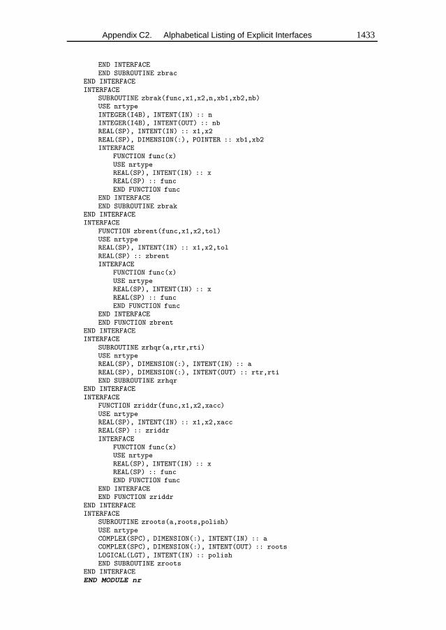
Appendix C2. Alphabetical Listing of Explicit Interfaces 1433
END INTERFACEEND SUBROUTINE zbrac
END INTERFACEINTERFACE
SUBROUTINE zbrak(func,x1,x2,n,xb1,xb2,nb)USE nrtypeINTEGER(I4B), INTENT(IN) :: nINTEGER(I4B), INTENT(OUT) :: nbREAL(SP), INTENT(IN) :: x1,x2REAL(SP), DIMENSION(:), POINTER :: xb1,xb2INTERFACE
FUNCTION func(x)USE nrtypeREAL(SP), INTENT(IN) :: xREAL(SP) :: funcEND FUNCTION func
END INTERFACEEND SUBROUTINE zbrak
END INTERFACEINTERFACE
FUNCTION zbrent(func,x1,x2,tol)USE nrtypeREAL(SP), INTENT(IN) :: x1,x2,tolREAL(SP) :: zbrentINTERFACE
FUNCTION func(x)USE nrtypeREAL(SP), INTENT(IN) :: xREAL(SP) :: funcEND FUNCTION func
END INTERFACEEND FUNCTION zbrent
END INTERFACEINTERFACE
SUBROUTINE zrhqr(a,rtr,rti)USE nrtypeREAL(SP), DIMENSION(:), INTENT(IN) :: aREAL(SP), DIMENSION(:), INTENT(OUT) :: rtr,rtiEND SUBROUTINE zrhqr
END INTERFACEINTERFACE
FUNCTION zriddr(func,x1,x2,xacc)USE nrtypeREAL(SP), INTENT(IN) :: x1,x2,xaccREAL(SP) :: zriddrINTERFACE
FUNCTION func(x)USE nrtypeREAL(SP), INTENT(IN) :: xREAL(SP) :: funcEND FUNCTION func
END INTERFACEEND FUNCTION zriddr
END INTERFACEINTERFACE
SUBROUTINE zroots(a,roots,polish)USE nrtypeCOMPLEX(SPC), DIMENSION(:), INTENT(IN) :: aCOMPLEX(SPC), DIMENSION(:), INTENT(OUT) :: rootsLOGICAL(LGT), INTENT(IN) :: polishEND SUBROUTINE zroots
END INTERFACEEND MODULE nr
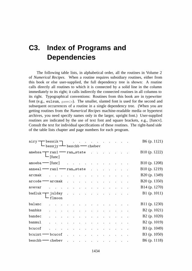
C3. Index of Programs andDependencies
The following table lists, in alphabetical order, all the routines in Volume 2of Numerical Recipes. When a routine requires subsidiary routines, either fromthis book or else user-supplied, the full dependency tree is shown: A routinecalls directly all routines to which it is connected by a solid line in the columnimmediately to its right; it calls indirectly the connected routines in all columns toits right. Typographical conventions: Routines from this book are in typewriterfont (e.g., eulsum, gammln). The smaller, slanted font is used for the second andsubsequent occurrences of a routine in a single dependency tree. (When you aregetting routines from the Numerical Recipes machine-readable media or hypertextarchives, you need specify names only in the larger, upright font.) User-suppliedroutines are indicated by the use of text font and square brackets, e.g., [funcv].Consult the text for individual specifications of these routines. The right-hand sideof the table lists chapter and page numbers for each program.
airy bessik . . . . . . . . . . B6 (p. 1121)bessjy beschb chebev
amebsa ran1 ran state . . . . . . . B10 (p. 1222)[func]
amoeba [func] . . . . . . . . . . . B10 (p. 1208)
anneal ran1 ran state . . . . . . . B10 (p. 1219)
arcmak . . . . . . . . . . . . . . B20 (p. 1349)
arcode arcmak . . . . . . . . . . . B20 (p. 1350)
avevar . . . . . . . . . . . . . . B14 (p. 1270)
badluk julday . . . . . . . . . . . B1 (p. 1011)flmoon
balanc . . . . . . . . . . . . . . B11 (p. 1230)
banbks . . . . . . . . . . . . . . B2 (p. 1021)
bandec . . . . . . . . . . . . . . B2 (p. 1020)
banmul . . . . . . . . . . . . . . B2 (p. 1019)
bcucof . . . . . . . . . . . . . . B3 (p. 1049)
bcuint bcucof . . . . . . . . . . . B3 (p. 1050)
beschb chebev . . . . . . . . . . . B6 (p. 1118)
1434
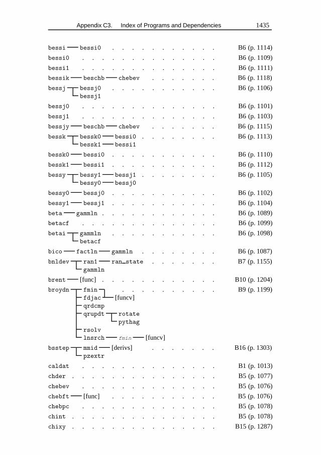
Appendix C3. Index of Programs and Dependencies 1435
bessi bessi0 . . . . . . . . . . . B6 (p. 1114)
bessi0 . . . . . . . . . . . . . . B6 (p. 1109)
bessi1 . . . . . . . . . . . . . . B6 (p. 1111)
bessik beschb chebev . . . . . . . B6 (p. 1118)
bessj bessj0 . . . . . . . . . . . B6 (p. 1106)bessj1
bessj0 . . . . . . . . . . . . . . B6 (p. 1101)
bessj1 . . . . . . . . . . . . . . B6 (p. 1103)
bessjy beschb chebev . . . . . . . B6 (p. 1115)
bessk bessk0 bessi0 . . . . . . . . B6 (p. 1113)bessk1 bessi1
bessk0 bessi0 . . . . . . . . . . . B6 (p. 1110)
bessk1 bessi1 . . . . . . . . . . . B6 (p. 1112)
bessy bessy1 bessj1 . . . . . . . . B6 (p. 1105)bessy0 bessj0
bessy0 bessj0 . . . . . . . . . . . B6 (p. 1102)
bessy1 bessj1 . . . . . . . . . . . B6 (p. 1104)
beta gammln . . . . . . . . . . . . B6 (p. 1089)
betacf . . . . . . . . . . . . . . B6 (p. 1099)
betai gammln . . . . . . . . . . . B6 (p. 1098)betacf
bico factln gammln . . . . . . . . B6 (p. 1087)
bnldev ran1 ran state . . . . . . . B7 (p. 1155)gammln
brent [func] . . . . . . . . . . . . B10 (p. 1204)
broydn fmin . . . . . . . . . . B9 (p. 1199)fdjac [funcv]qrdcmp
qrupdt rotate
pythag
rsolv
lnsrch fmin [funcv]
bsstep mmid [derivs] . . . . . . . B16 (p. 1303)pzextr
caldat . . . . . . . . . . . . . . B1 (p. 1013)
chder . . . . . . . . . . . . . . . B5 (p. 1077)
chebev . . . . . . . . . . . . . . B5 (p. 1076)
chebft [func] . . . . . . . . . . . B5 (p. 1076)
chebpc . . . . . . . . . . . . . . B5 (p. 1078)
chint . . . . . . . . . . . . . . . B5 (p. 1078)
chixy . . . . . . . . . . . . . . . B15 (p. 1287)
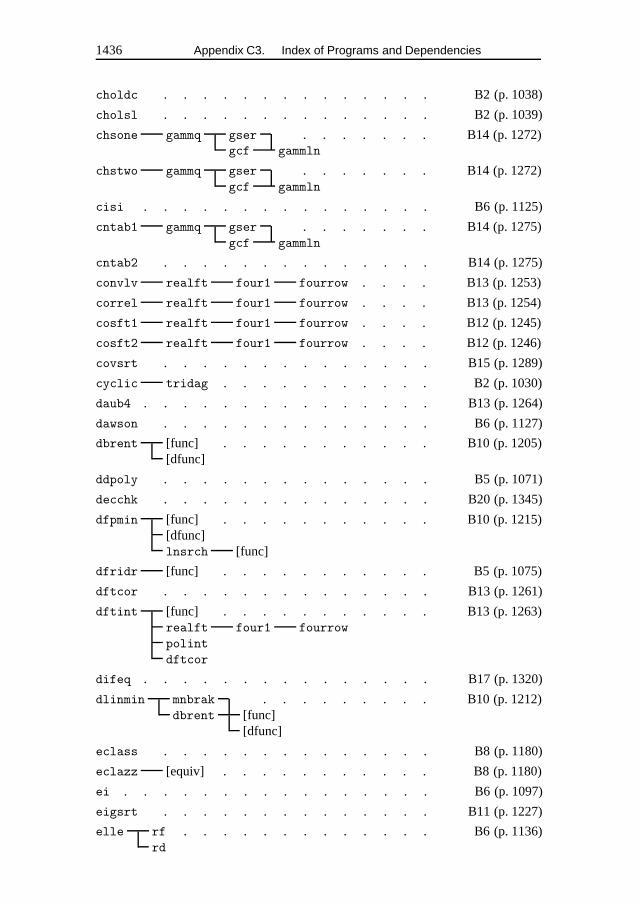
1436 Appendix C3. Index of Programs and Dependencies
choldc . . . . . . . . . . . . . . B2 (p. 1038)
cholsl . . . . . . . . . . . . . . B2 (p. 1039)
chsone gammq gser . . . . . . . B14 (p. 1272)gcf gammln
chstwo gammq gser . . . . . . . B14 (p. 1272)gcf gammln
cisi . . . . . . . . . . . . . . . B6 (p. 1125)
cntab1 gammq gser . . . . . . . B14 (p. 1275)gcf gammln
cntab2 . . . . . . . . . . . . . . B14 (p. 1275)
convlv realft four1 fourrow . . . . B13 (p. 1253)
correl realft four1 fourrow . . . . B13 (p. 1254)
cosft1 realft four1 fourrow . . . . B12 (p. 1245)
cosft2 realft four1 fourrow . . . . B12 (p. 1246)
covsrt . . . . . . . . . . . . . . B15 (p. 1289)
cyclic tridag . . . . . . . . . . . B2 (p. 1030)
daub4 . . . . . . . . . . . . . . . B13 (p. 1264)
dawson . . . . . . . . . . . . . . B6 (p. 1127)
dbrent [func] . . . . . . . . . . . B10 (p. 1205)[dfunc]
ddpoly . . . . . . . . . . . . . . B5 (p. 1071)
decchk . . . . . . . . . . . . . . B20 (p. 1345)
dfpmin [func] . . . . . . . . . . . B10 (p. 1215)[dfunc]lnsrch [func]
dfridr [func] . . . . . . . . . . . B5 (p. 1075)
dftcor . . . . . . . . . . . . . . B13 (p. 1261)
dftint [func] . . . . . . . . . . . B13 (p. 1263)realft four1 fourrow
polint
dftcor
difeq . . . . . . . . . . . . . . . B17 (p. 1320)
dlinmin mnbrak . . . . . . . . . B10 (p. 1212)dbrent [func]
[dfunc]
eclass . . . . . . . . . . . . . . B8 (p. 1180)
eclazz [equiv] . . . . . . . . . . . B8 (p. 1180)
ei . . . . . . . . . . . . . . . . B6 (p. 1097)
eigsrt . . . . . . . . . . . . . . B11 (p. 1227)
elle rf . . . . . . . . . . . . . B6 (p. 1136)rd
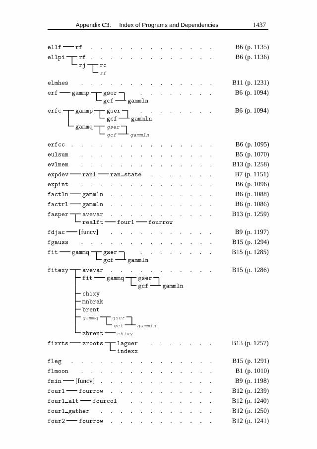
Appendix C3. Index of Programs and Dependencies 1437
ellf rf . . . . . . . . . . . . . B6 (p. 1135)
ellpi rf . . . . . . . . . . . . . B6 (p. 1136)rj rc
rf
elmhes . . . . . . . . . . . . . . B11 (p. 1231)
erf gammp gser . . . . . . . . B6 (p. 1094)gcf gammln
erfc gammp gser . . . . . . . . B6 (p. 1094)gcf gammln
gammq gser
gcf gammln
erfcc . . . . . . . . . . . . . . . B6 (p. 1095)
eulsum . . . . . . . . . . . . . . B5 (p. 1070)
evlmem . . . . . . . . . . . . . . B13 (p. 1258)
expdev ran1 ran state . . . . . . . B7 (p. 1151)
expint . . . . . . . . . . . . . . B6 (p. 1096)
factln gammln . . . . . . . . . . . B6 (p. 1088)
factrl gammln . . . . . . . . . . . B6 (p. 1086)
fasper avevar . . . . . . . . . . . B13 (p. 1259)realft four1 fourrow
fdjac [funcv] . . . . . . . . . . . B9 (p. 1197)
fgauss . . . . . . . . . . . . . . B15 (p. 1294)
fit gammq gser . . . . . . . . B15 (p. 1285)gcf gammln
fitexy avevar . . . . . . . . . . . B15 (p. 1286)fit gammq gser
gcf gammln
chixy
mnbrak
brent
gammq gser
gcf gammln
zbrent chixy
fixrts zroots laguer . . . . . . . B13 (p. 1257)indexx
fleg . . . . . . . . . . . . . . . B15 (p. 1291)
flmoon . . . . . . . . . . . . . . B1 (p. 1010)
fmin [funcv] . . . . . . . . . . . . B9 (p. 1198)
four1 fourrow . . . . . . . . . . . B12 (p. 1239)
four1 alt fourcol . . . . . . . . . B12 (p. 1240)
four1 gather . . . . . . . . . . . . B12 (p. 1250)
four2 fourrow . . . . . . . . . . . B12 (p. 1241)
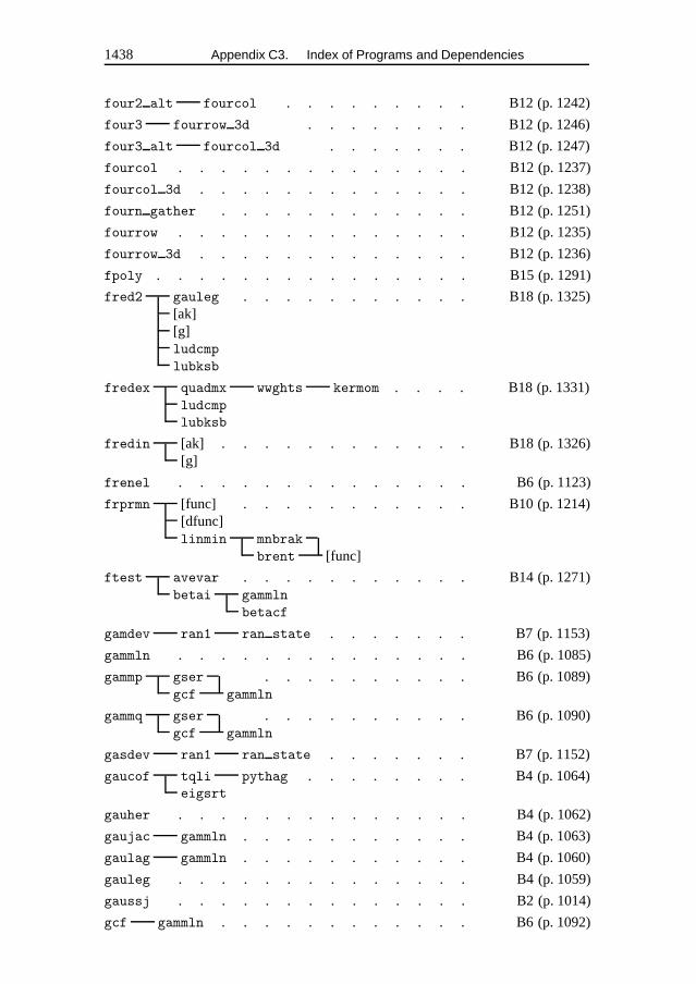
1438 Appendix C3. Index of Programs and Dependencies
four2 alt fourcol . . . . . . . . . B12 (p. 1242)
four3 fourrow 3d . . . . . . . . B12 (p. 1246)
four3 alt fourcol 3d . . . . . . . B12 (p. 1247)
fourcol . . . . . . . . . . . . . . B12 (p. 1237)
fourcol 3d . . . . . . . . . . . . . B12 (p. 1238)
fourn gather . . . . . . . . . . . . B12 (p. 1251)
fourrow . . . . . . . . . . . . . . B12 (p. 1235)
fourrow 3d . . . . . . . . . . . . . B12 (p. 1236)
fpoly . . . . . . . . . . . . . . . B15 (p. 1291)
fred2 gauleg . . . . . . . . . . . B18 (p. 1325)[ak][g]ludcmp
lubksb
fredex quadmx wwghts kermom . . . . B18 (p. 1331)ludcmp
lubksb
fredin [ak] . . . . . . . . . . . . B18 (p. 1326)[g]
frenel . . . . . . . . . . . . . . B6 (p. 1123)
frprmn [func] . . . . . . . . . . . B10 (p. 1214)[dfunc]linmin mnbrak
brent [func]
ftest avevar . . . . . . . . . . . B14 (p. 1271)betai gammln
betacf
gamdev ran1 ran state . . . . . . . B7 (p. 1153)
gammln . . . . . . . . . . . . . . B6 (p. 1085)
gammp gser . . . . . . . . . . B6 (p. 1089)gcf gammln
gammq gser . . . . . . . . . . B6 (p. 1090)gcf gammln
gasdev ran1 ran state . . . . . . . B7 (p. 1152)
gaucof tqli pythag . . . . . . . . B4 (p. 1064)eigsrt
gauher . . . . . . . . . . . . . . B4 (p. 1062)
gaujac gammln . . . . . . . . . . . B4 (p. 1063)
gaulag gammln . . . . . . . . . . . B4 (p. 1060)
gauleg . . . . . . . . . . . . . . B4 (p. 1059)
gaussj . . . . . . . . . . . . . . B2 (p. 1014)
gcf gammln . . . . . . . . . . . . B6 (p. 1092)
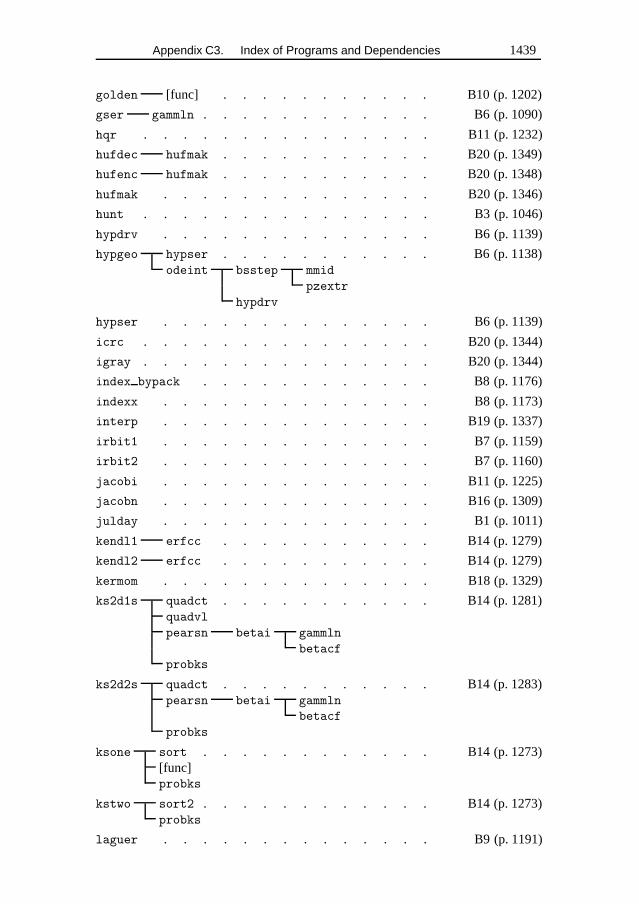
Appendix C3. Index of Programs and Dependencies 1439
golden [func] . . . . . . . . . . . B10 (p. 1202)
gser gammln . . . . . . . . . . . . B6 (p. 1090)
hqr . . . . . . . . . . . . . . . B11 (p. 1232)
hufdec hufmak . . . . . . . . . . . B20 (p. 1349)
hufenc hufmak . . . . . . . . . . . B20 (p. 1348)
hufmak . . . . . . . . . . . . . . B20 (p. 1346)
hunt . . . . . . . . . . . . . . . B3 (p. 1046)
hypdrv . . . . . . . . . . . . . . B6 (p. 1139)
hypgeo hypser . . . . . . . . . . . B6 (p. 1138)odeint bsstep mmid
pzextr
hypdrv
hypser . . . . . . . . . . . . . . B6 (p. 1139)
icrc . . . . . . . . . . . . . . . B20 (p. 1344)
igray . . . . . . . . . . . . . . . B20 (p. 1344)
index bypack . . . . . . . . . . . . B8 (p. 1176)
indexx . . . . . . . . . . . . . . B8 (p. 1173)
interp . . . . . . . . . . . . . . B19 (p. 1337)
irbit1 . . . . . . . . . . . . . . B7 (p. 1159)
irbit2 . . . . . . . . . . . . . . B7 (p. 1160)
jacobi . . . . . . . . . . . . . . B11 (p. 1225)
jacobn . . . . . . . . . . . . . . B16 (p. 1309)
julday . . . . . . . . . . . . . . B1 (p. 1011)
kendl1 erfcc . . . . . . . . . . . B14 (p. 1279)
kendl2 erfcc . . . . . . . . . . . B14 (p. 1279)
kermom . . . . . . . . . . . . . . B18 (p. 1329)
ks2d1s quadct . . . . . . . . . . . B14 (p. 1281)quadvl
pearsn betai gammln
betacf
probks
ks2d2s quadct . . . . . . . . . . . B14 (p. 1283)pearsn betai gammln
betacf
probks
ksone sort . . . . . . . . . . . . B14 (p. 1273)[func]probks
kstwo sort2 . . . . . . . . . . . . B14 (p. 1273)probks
laguer . . . . . . . . . . . . . . B9 (p. 1191)
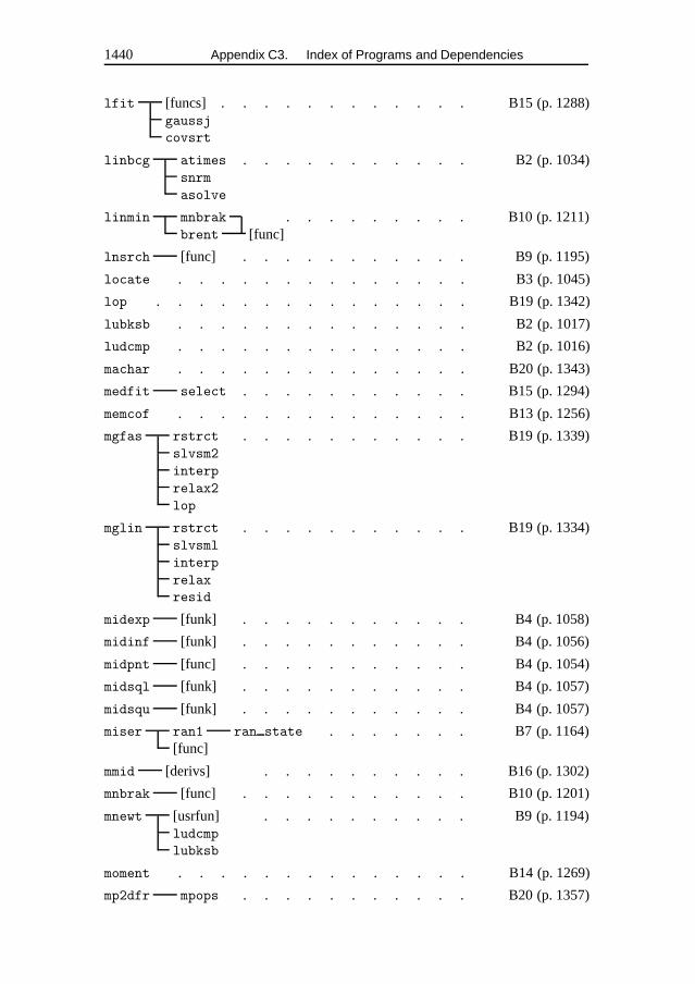
1440 Appendix C3. Index of Programs and Dependencies
lfit [funcs] . . . . . . . . . . . . B15 (p. 1288)gaussj
covsrt
linbcg atimes . . . . . . . . . . . B2 (p. 1034)snrm
asolve
linmin mnbrak . . . . . . . . . B10 (p. 1211)brent [func]
lnsrch [func] . . . . . . . . . . . B9 (p. 1195)
locate . . . . . . . . . . . . . . B3 (p. 1045)
lop . . . . . . . . . . . . . . . B19 (p. 1342)
lubksb . . . . . . . . . . . . . . B2 (p. 1017)
ludcmp . . . . . . . . . . . . . . B2 (p. 1016)
machar . . . . . . . . . . . . . . B20 (p. 1343)
medfit select . . . . . . . . . . . B15 (p. 1294)
memcof . . . . . . . . . . . . . . B13 (p. 1256)
mgfas rstrct . . . . . . . . . . . B19 (p. 1339)slvsm2
interp
relax2
lop
mglin rstrct . . . . . . . . . . . B19 (p. 1334)slvsml
interp
relax
resid
midexp [funk] . . . . . . . . . . . B4 (p. 1058)
midinf [funk] . . . . . . . . . . . B4 (p. 1056)
midpnt [func] . . . . . . . . . . . B4 (p. 1054)
midsql [funk] . . . . . . . . . . . B4 (p. 1057)
midsqu [funk] . . . . . . . . . . . B4 (p. 1057)
miser ran1 ran state . . . . . . . B7 (p. 1164)[func]
mmid [derivs] . . . . . . . . . . B16 (p. 1302)
mnbrak [func] . . . . . . . . . . . B10 (p. 1201)
mnewt [usrfun] . . . . . . . . . . B9 (p. 1194)ludcmp
lubksb
moment . . . . . . . . . . . . . . B14 (p. 1269)
mp2dfr mpops . . . . . . . . . . . B20 (p. 1357)
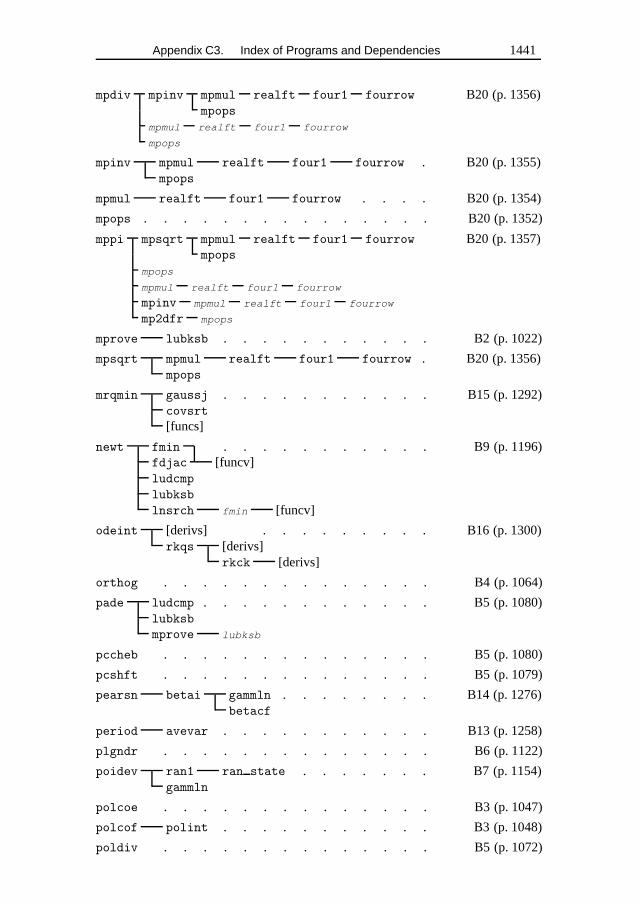
Appendix C3. Index of Programs and Dependencies 1441
mpdiv mpinv mpmul realft four1 fourrow B20 (p. 1356)mpops
mpmul realft four1 fourrow
mpops
mpinv mpmul realft four1 fourrow . B20 (p. 1355)mpops
mpmul realft four1 fourrow . . . . B20 (p. 1354)
mpops . . . . . . . . . . . . . . . B20 (p. 1352)
mppi mpsqrt mpmul realft four1 fourrow B20 (p. 1357)mpops
mpops
mpmul realft four1 fourrow
mpinv mpmul realft four1 fourrow
mp2dfr mpops
mprove lubksb . . . . . . . . . . . B2 (p. 1022)
mpsqrt mpmul realft four1 fourrow . B20 (p. 1356)mpops
mrqmin gaussj . . . . . . . . . . . B15 (p. 1292)covsrt
[funcs]
newt fmin . . . . . . . . . . . B9 (p. 1196)fdjac [funcv]ludcmp
lubksb
lnsrch fmin [funcv]
odeint [derivs] . . . . . . . . . B16 (p. 1300)rkqs [derivs]
rkck [derivs]
orthog . . . . . . . . . . . . . . B4 (p. 1064)
pade ludcmp . . . . . . . . . . . . B5 (p. 1080)lubksb
mprove lubksb
pccheb . . . . . . . . . . . . . . B5 (p. 1080)
pcshft . . . . . . . . . . . . . . B5 (p. 1079)
pearsn betai gammln . . . . . . . . B14 (p. 1276)betacf
period avevar . . . . . . . . . . . B13 (p. 1258)
plgndr . . . . . . . . . . . . . . B6 (p. 1122)
poidev ran1 ran state . . . . . . . B7 (p. 1154)gammln
polcoe . . . . . . . . . . . . . . B3 (p. 1047)
polcof polint . . . . . . . . . . . B3 (p. 1048)
poldiv . . . . . . . . . . . . . . B5 (p. 1072)
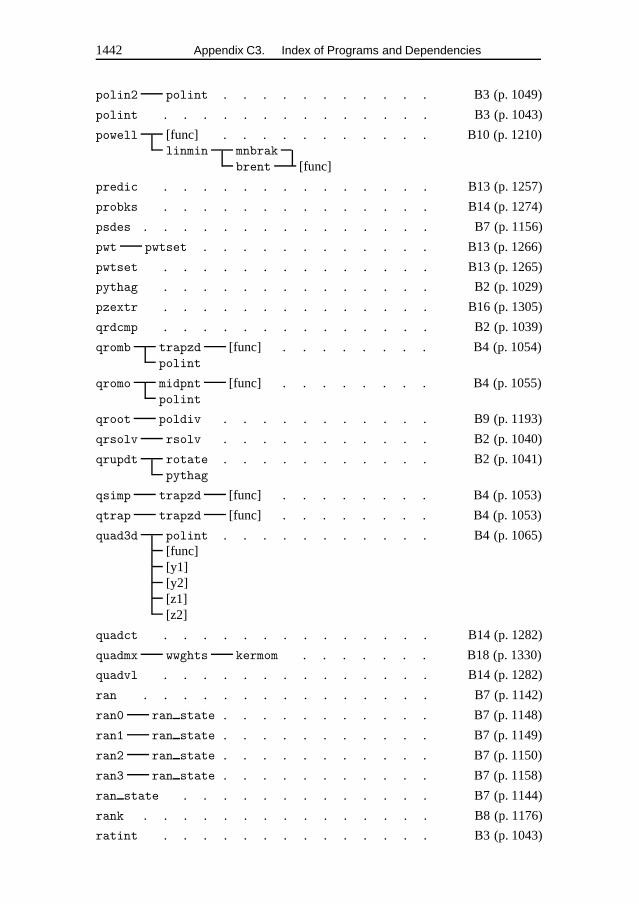
1442 Appendix C3. Index of Programs and Dependencies
polin2 polint . . . . . . . . . . . B3 (p. 1049)
polint . . . . . . . . . . . . . . B3 (p. 1043)
powell [func] . . . . . . . . . . . B10 (p. 1210)linmin mnbrak
brent [func]
predic . . . . . . . . . . . . . . B13 (p. 1257)
probks . . . . . . . . . . . . . . B14 (p. 1274)
psdes . . . . . . . . . . . . . . . B7 (p. 1156)
pwt pwtset . . . . . . . . . . . . B13 (p. 1266)
pwtset . . . . . . . . . . . . . . B13 (p. 1265)
pythag . . . . . . . . . . . . . . B2 (p. 1029)
pzextr . . . . . . . . . . . . . . B16 (p. 1305)
qrdcmp . . . . . . . . . . . . . . B2 (p. 1039)
qromb trapzd [func] . . . . . . . . B4 (p. 1054)polint
qromo midpnt [func] . . . . . . . . B4 (p. 1055)polint
qroot poldiv . . . . . . . . . . . B9 (p. 1193)
qrsolv rsolv . . . . . . . . . . . B2 (p. 1040)
qrupdt rotate . . . . . . . . . . . B2 (p. 1041)pythag
qsimp trapzd [func] . . . . . . . . B4 (p. 1053)
qtrap trapzd [func] . . . . . . . . B4 (p. 1053)
quad3d polint . . . . . . . . . . . B4 (p. 1065)[func][y1][y2][z1][z2]
quadct . . . . . . . . . . . . . . B14 (p. 1282)
quadmx wwghts kermom . . . . . . . B18 (p. 1330)
quadvl . . . . . . . . . . . . . . B14 (p. 1282)
ran . . . . . . . . . . . . . . . B7 (p. 1142)
ran0 ran state . . . . . . . . . . . B7 (p. 1148)
ran1 ran state . . . . . . . . . . . B7 (p. 1149)
ran2 ran state . . . . . . . . . . . B7 (p. 1150)
ran3 ran state . . . . . . . . . . . B7 (p. 1158)
ran state . . . . . . . . . . . . . B7 (p. 1144)
rank . . . . . . . . . . . . . . . B8 (p. 1176)
ratint . . . . . . . . . . . . . . B3 (p. 1043)
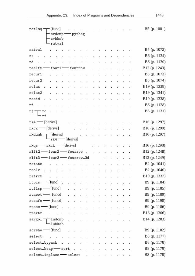
Appendix C3. Index of Programs and Dependencies 1443
ratlsq [func] . . . . . . . . . . . B5 (p. 1081)svdcmp pythag
svbksb
ratval
ratval . . . . . . . . . . . . . . B5 (p. 1072)
rc . . . . . . . . . . . . . . . . B6 (p. 1134)
rd . . . . . . . . . . . . . . . . B6 (p. 1130)
realft four1 fourrow . . . . . . . B12 (p. 1243)
recur1 . . . . . . . . . . . . . . B5 (p. 1073)
recur2 . . . . . . . . . . . . . . B5 (p. 1074)
relax . . . . . . . . . . . . . . . B19 (p. 1338)
relax2 . . . . . . . . . . . . . . B19 (p. 1341)
resid . . . . . . . . . . . . . . . B19 (p. 1338)
rf . . . . . . . . . . . . . . . . B6 (p. 1128)
rj rc . . . . . . . . . . . . . . B6 (p. 1131)rf
rk4 [derivs] . . . . . . . . . . . B16 (p. 1297)
rkck [derivs] . . . . . . . . . . B16 (p. 1299)
rkdumb [derivs] . . . . . . . . . B16 (p. 1297)rk4 [derivs]
rkqs rkck [derivs] . . . . . . . B16 (p. 1298)
rlft2 four2 fourrow . . . . . . . . B12 (p. 1248)
rlft3 four3 fourrow 3d . . . . . B12 (p. 1249)
rotate . . . . . . . . . . . . . . B2 (p. 1041)
rsolv . . . . . . . . . . . . . . . B2 (p. 1040)
rstrct . . . . . . . . . . . . . . B19 (p. 1337)
rtbis [func] . . . . . . . . . . . . B9 (p. 1184)
rtflsp [func] . . . . . . . . . . . B9 (p. 1185)
rtnewt [funcd] . . . . . . . . . . . B9 (p. 1189)
rtsafe [funcd] . . . . . . . . . . . B9 (p. 1190)
rtsec [func] . . . . . . . . . . . . B9 (p. 1186)
rzextr . . . . . . . . . . . . . . B16 (p. 1306)
savgol ludcmp . . . . . . . . . . . B14 (p. 1283)lubksb
scrsho [func] . . . . . . . . . . . B9 (p. 1182)
select . . . . . . . . . . . . . . B8 (p. 1177)
select bypack . . . . . . . . . . . . B8 (p. 1178)
select heap sort . . . . . . . . . . B8 (p. 1179)
select inplace select . . . . . . . . B8 (p. 1178)
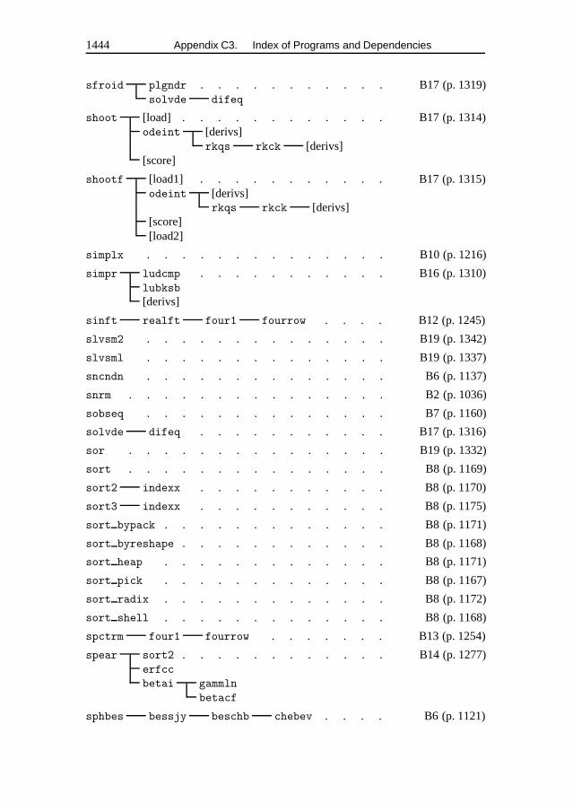
1444 Appendix C3. Index of Programs and Dependencies
sfroid plgndr . . . . . . . . . . . B17 (p. 1319)solvde difeq
shoot [load] . . . . . . . . . . . . B17 (p. 1314)odeint [derivs]
rkqs rkck [derivs][score]
shootf [load1] . . . . . . . . . . . B17 (p. 1315)odeint [derivs]
rkqs rkck [derivs][score][load2]
simplx . . . . . . . . . . . . . . B10 (p. 1216)
simpr ludcmp . . . . . . . . . . . B16 (p. 1310)lubksb
[derivs]
sinft realft four1 fourrow . . . . B12 (p. 1245)
slvsm2 . . . . . . . . . . . . . . B19 (p. 1342)
slvsml . . . . . . . . . . . . . . B19 (p. 1337)
sncndn . . . . . . . . . . . . . . B6 (p. 1137)
snrm . . . . . . . . . . . . . . . B2 (p. 1036)
sobseq . . . . . . . . . . . . . . B7 (p. 1160)
solvde difeq . . . . . . . . . . . B17 (p. 1316)
sor . . . . . . . . . . . . . . . B19 (p. 1332)
sort . . . . . . . . . . . . . . . B8 (p. 1169)
sort2 indexx . . . . . . . . . . . B8 (p. 1170)
sort3 indexx . . . . . . . . . . . B8 (p. 1175)
sort bypack . . . . . . . . . . . . . B8 (p. 1171)
sort byreshape . . . . . . . . . . . . B8 (p. 1168)
sort heap . . . . . . . . . . . . . B8 (p. 1171)
sort pick . . . . . . . . . . . . . B8 (p. 1167)
sort radix . . . . . . . . . . . . . B8 (p. 1172)
sort shell . . . . . . . . . . . . . B8 (p. 1168)
spctrm four1 fourrow . . . . . . . B13 (p. 1254)
spear sort2 . . . . . . . . . . . . B14 (p. 1277)erfcc
betai gammln
betacf
sphbes bessjy beschb chebev . . . . B6 (p. 1121)
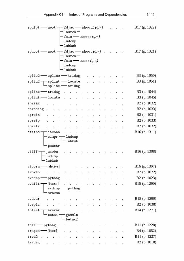
Appendix C3. Index of Programs and Dependencies 1445
sphfpt newt fdjac shootf (q.v.) . . . B17 (p. 1322)lnsrch
fmin shootf (q.v.)ludcmp
lubksb
sphoot newt fdjac shoot (q.v.) . . . . B17 (p. 1321)lnsrch
fmin shoot (q.v.)ludcmp
lubksb
splie2 spline tridag . . . . . . . B3 (p. 1050)
splin2 splint locate . . . . . . . B3 (p. 1051)spline tridag
spline tridag . . . . . . . . . . . B3 (p. 1044)
splint locate . . . . . . . . . . . B3 (p. 1045)
sprsax . . . . . . . . . . . . . . B2 (p. 1032)
sprsdiag . . . . . . . . . . . . . . B2 (p. 1033)
sprsin . . . . . . . . . . . . . . B2 (p. 1031)
sprstp . . . . . . . . . . . . . . B2 (p. 1033)
sprstx . . . . . . . . . . . . . . B2 (p. 1032)
stifbs jacobn . . . . . . . . . . . B16 (p. 1311)simpr ludcmp
lubksb
pzextr
stiff jacobn . . . . . . . . . . . B16 (p. 1308)ludcmp
lubksb
stoerm [derivs] . . . . . . . . . B16 (p. 1307)
svbksb . . . . . . . . . . . . . . B2 (p. 1022)
svdcmp pythag . . . . . . . . . . . B2 (p. 1023)
svdfit [funcs] . . . . . . . . . . . B15 (p. 1290)svdcmp pythag
svbksb
svdvar . . . . . . . . . . . . . . B15 (p. 1290)
toeplz . . . . . . . . . . . . . . B2 (p. 1038)
tptest avevar . . . . . . . . . . . B14 (p. 1271)betai gammln
betacf
tqli pythag . . . . . . . . . . . . B11 (p. 1228)
trapzd [func] . . . . . . . . . . . B4 (p. 1052)
tred2 . . . . . . . . . . . . . . . B11 (p. 1227)
tridag . . . . . . . . . . . . . . B2 (p. 1018)
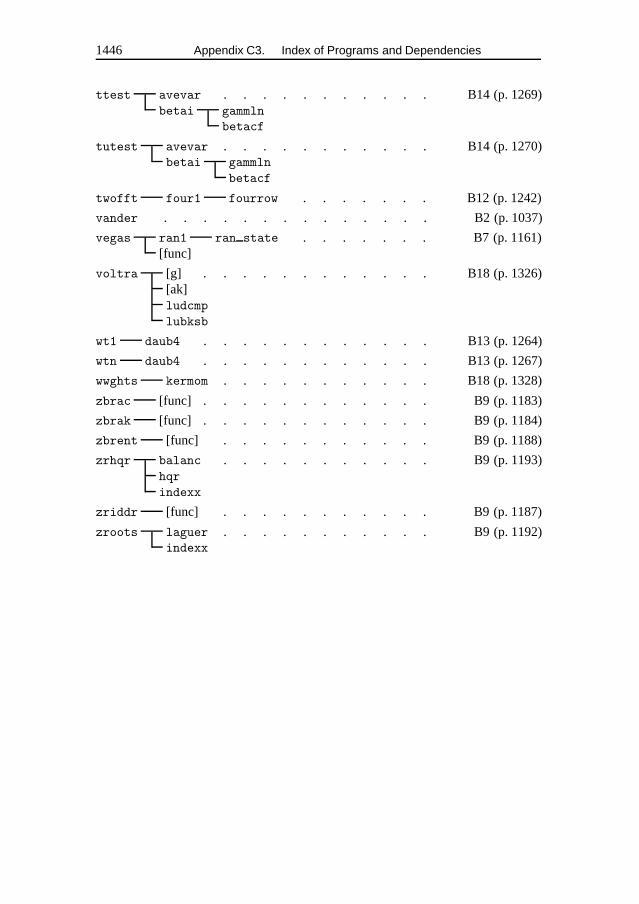
1446 Appendix C3. Index of Programs and Dependencies
ttest avevar . . . . . . . . . . . B14 (p. 1269)betai gammln
betacf
tutest avevar . . . . . . . . . . . B14 (p. 1270)betai gammln
betacf
twofft four1 fourrow . . . . . . . B12 (p. 1242)
vander . . . . . . . . . . . . . . B2 (p. 1037)
vegas ran1 ran state . . . . . . . B7 (p. 1161)[func]
voltra [g] . . . . . . . . . . . . B18 (p. 1326)[ak]ludcmp
lubksb
wt1 daub4 . . . . . . . . . . . . B13 (p. 1264)
wtn daub4 . . . . . . . . . . . . B13 (p. 1267)
wwghts kermom . . . . . . . . . . . B18 (p. 1328)
zbrac [func] . . . . . . . . . . . . B9 (p. 1183)
zbrak [func] . . . . . . . . . . . . B9 (p. 1184)
zbrent [func] . . . . . . . . . . . B9 (p. 1188)
zrhqr balanc . . . . . . . . . . . B9 (p. 1193)hqr
indexx
zriddr [func] . . . . . . . . . . . B9 (p. 1187)
zroots laguer . . . . . . . . . . . B9 (p. 1192)indexx
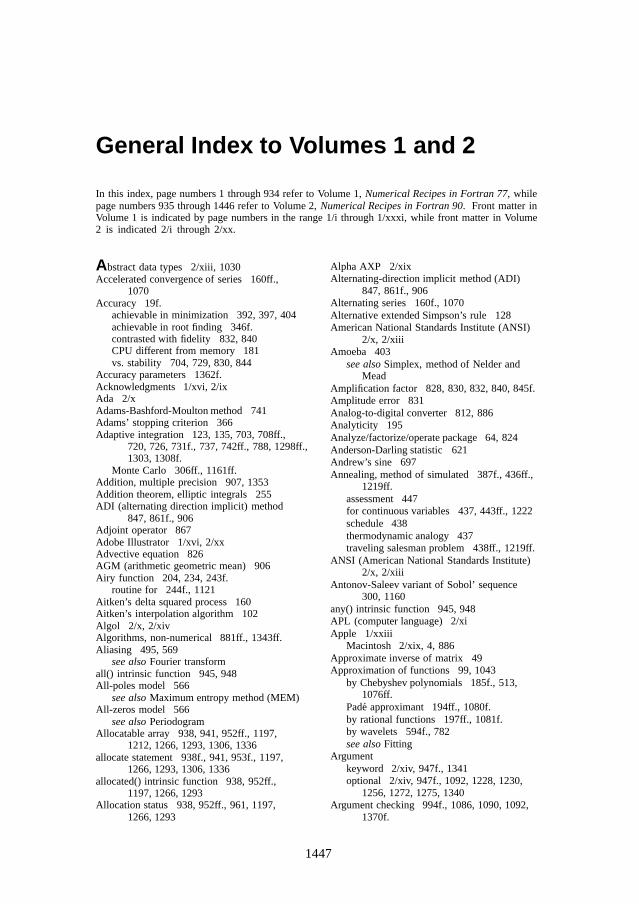
General Index to Volumes 1 and 2
In this index, page numbers 1 through 934 refer to Volume 1, Numerical Recipes in Fortran 77, whilepage numbers 935 through 1446 refer to Volume 2, Numerical Recipes in Fortran 90. Front matter inVolume 1 is indicated by page numbers in the range 1/i through 1/xxxi, while front matter in Volume2 is indicated 2/i through 2/xx.
Abstract data types 2/xiii, 1030Accelerated convergence of series 160ff.,
1070Accuracy 19f.
achievable in minimization 392, 397, 404achievable in root finding 346f.contrasted with fidelity 832, 840CPU different from memory 181vs. stability 704, 729, 830, 844
Accuracy parameters 1362f.Acknowledgments 1/xvi, 2/ixAda 2/xAdams-Bashford-Moulton method 741Adams’ stopping criterion 366Adaptive integration 123, 135, 703, 708ff.,
720, 726, 731f., 737, 742ff., 788, 1298ff.,1303, 1308f.
Monte Carlo 306ff., 1161ff.Addition, multiple precision 907, 1353Addition theorem, elliptic integrals 255ADI (alternating direction implicit) method
847, 861f., 906Adjoint operator 867Adobe Illustrator 1/xvi, 2/xxAdvective equation 826AGM (arithmetic geometric mean) 906Airy function 204, 234, 243f.
routine for 244f., 1121Aitken’s delta squared process 160Aitken’s interpolation algorithm 102Algol 2/x, 2/xivAlgorithms, non-numerical 881ff., 1343ff.Aliasing 495, 569
see also Fourier transformall() intrinsic function 945, 948All-poles model 566
see also Maximum entropy method (MEM)All-zeros model 566
see also PeriodogramAllocatable array 938, 941, 952ff., 1197,
1212, 1266, 1293, 1306, 1336allocate statement 938f., 941, 953f., 1197,
1266, 1293, 1306, 1336allocated() intrinsic function 938, 952ff.,
1197, 1266, 1293Allocation status 938, 952ff., 961, 1197,
1266, 1293
Alpha AXP 2/xixAlternating-direction implicit method (ADI)
847, 861f., 906Alternating series 160f., 1070Alternative extended Simpson’s rule 128American National Standards Institute (ANSI)
2/x, 2/xiiiAmoeba 403
see also Simplex, method of Nelder andMead
Amplification factor 828, 830, 832, 840, 845f.Amplitude error 831Analog-to-digital converter 812, 886Analyticity 195Analyze/factorize/operate package 64, 824Anderson-Darling statistic 621Andrew’s sine 697Annealing, method of simulated 387f., 436ff.,
1219ff.assessment 447for continuous variables 437, 443ff., 1222schedule 438thermodynamic analogy 437traveling salesman problem 438ff., 1219ff.
ANSI (American National Standards Institute)2/x, 2/xiii
Antonov-Saleev variant of Sobol’ sequence300, 1160
any() intrinsic function 945, 948APL (computer language) 2/xiApple 1/xxiii
Macintosh 2/xix, 4, 886Approximate inverse of matrix 49Approximation of functions 99, 1043
by Chebyshev polynomials 185f., 513,1076ff.
Pade approximant 194ff., 1080f.by rational functions 197ff., 1081f.by wavelets 594f., 782see also Fitting
Argumentkeyword 2/xiv, 947f., 1341optional 2/xiv, 947f., 1092, 1228, 1230,
1256, 1272, 1275, 1340Argument checking 994f., 1086, 1090, 1092,
1370f.
1447
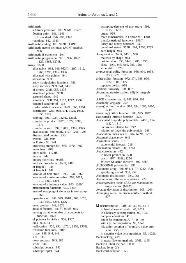
1448 Index to Volumes 1 and 2
Arithmeticarbitrary precision 881, 906ff., 1352ff.floating point 881, 1343IEEE standard 276, 882, 1343rounding 882, 1343
Arithmetic coding 881, 902ff., 1349ff.Arithmetic-geometric mean (AGM) method
906Arithmetic-if statement 2/xiArithmetic progression 971f., 996, 1072,
1127, 1365, 1371f.Array 953ff.
allocatable 938, 941, 952ff., 1197, 1212,1266, 1293, 1306, 1336
allocated with pointer 941allocation 953array manipulation functions 950array sections 939, 941, 943ff.of arrays 2/xii, 956, 1336associated pointer 953f.assumed-shape 942automatic 938, 954, 1197, 1212, 1336centered subarray of 113conformable to a scalar 942f., 965, 1094constructor 2/xii, 968, 971, 1022, 1052,
1055, 1127copying 991, 1034, 1327f., 1365f.cumulative product 997f., 1072, 1086,
1375cumulative sum 997, 1280f., 1365, 1375deallocation 938, 953f., 1197, 1266, 1293disassociated pointer 953extents 938, 949in Fortran 90 941increasing storage for 955, 1070, 1302index loss 967f.index table 1173ff.indices 942inquiry functions 948ff.intrinsic procedures 2/xiii, 948ff.of length 0 944of length 1 949location of first “true” 993, 1041, 1369location of maximum value 993, 1015,
1017, 1365, 1369location of minimum value 993, 1369f.manipulation functions 950, 1247masked swapping of elements in two arrays
1368operations on 942, 949, 964ff., 969, 1026,
1040, 1050, 1200, 1326outer product 949, 1076parallel features 941ff., 964ff., 985passing variable number of arguments to
function 1022of pointers forbidden 956, 1337rank 938, 949reallocation 955, 992, 1070f., 1365, 1368f.reduction functions 948ff.shape 938, 944, 949size 938skew sections 945, 985stride 944subscript bounds 942subscript triplet 944
swapping elements of two arrays 991,1015, 1365ff.
target 938three-dimensional, in Fortran 90 1248transformational functions 948ff.unary and binary functions 949undefined status 952ff., 961, 1266, 1293zero-length 944
Array section 2/xiii, 943ff., 960matches by shape 944pointer alias 939, 944f., 1286, 1333skew 2/xii, 945, 960, 985, 1284vs. eoshift 1078
array copy() utility function 988, 991, 1034,1153, 1278, 1328
arth() utility function 972, 974, 988, 996,1072, 1086, 1127
replaces do-list 968Artificial viscosity 831, 837Ascending transformation, elliptic integrals
256ASCII character set 6, 888, 896, 902Assembly language 269assert() utility function 988, 994, 1086, 1090,
1249assert eq() utility function 988, 995, 1022associated() intrinsic function 952f.Associated Legendre polynomials 246ff., 764,
1122f., 1319recurrence relation for 247relation to Legendre polynomials 246
Association, measures of 604, 622ff., 1275Assumed-shape array 942Asymptotic series 161
exponential integral 218Attenuation factors 583, 1261Autocorrelation 492
in linear prediction 558use of FFT 538f., 1254Wiener-Khinchin theorem 492, 566f.
AUTODIN-II polynomial 890Automatic array 938, 954, 1197, 1212, 1336
specifying size of 938, 954Automatic deallocation 2/xv, 961Autonomous differential equations 729f.Autoregressive model (AR) see Maximum en-
tropy method (MEM)Average deviation of distribution 605, 1269Averaging kernel, in Backus-Gilbert method
807
Backsubstitution 33ff., 39, 42, 92, 1017in band diagonal matrix 46, 1021in Cholesky decomposition 90, 1039complex equations 41direct for computing A−1 · B 40with QR decomposition 93, 1040relaxation solution of boundary value prob-
lems 755, 1316in singular value decomposition 56, 1022f.
Backtracking 419in quasi-Newton methods 376f., 1195
Backus-Gilbert method 806ff.Backus, John 2/xBackward deflation 363
Index to Volumes 1 and 2 1449
Bader-Deuflhard method 730, 735, 1310f.Bairstow’s method 364, 370, 1193Balancing 476f., 1230f.Band diagonal matrix 42ff., 1019
backsubstitution 46, 1021LU decomposition 45, 1020multiply by vector 44, 1019storage 44, 1019
Band-pass filter 551, 554f.wavelets 584, 592f.
Bandwidth limited function 495Bank accounts, checksum for 894Bar codes, checksum for 894Bartlett window 547, 1254ff.Base case, of recursive procedure 958Base of representation 19, 882, 1343BASIC, Numerical Recipes in 1, 2/x, 2/xviiiBasis functions in general linear least squares
665Bayes’ Theorem 810Bayesian
approach to inverse problems 799, 810f.,816f.
contrasted with frequentist 810vs. historic maximum entropy method
816f.views on straight line fitting 664
Bays’ shuffle 270Bernoulli number 132Bessel functions 223ff., 234ff., 936, 1101ff.
asymptotic form 223f., 229f.complex 204continued fraction 234, 239double precision 223fractional order 223, 234ff., 1115ff.Miller’s algorithm 175, 228, 1106modified 229ff.modified, fractional order 239ff.modified, normalization formula 232, 240modified, routines for 230ff., 1109ff.normalization formula 175parallel computation of 1107ff.recurrence relation 172, 224, 232, 234reflection formulas 236reflection formulas, modified functions
241routines for 225ff., 236ff., 1101ff.routines for modified functions 241ff.,
1118series for 160, 223series for Kν 241series for Yν 235spherical 234, 245, 1121f.turning point 234Wronskian 234, 239
Best-fit parameters 650, 656, 660, 698, 1285ff.see also Fitting
Beta function 206ff., 1089incomplete see Incomplete beta function
BFGS algorithm see Broyden-Fletcher-Goldfarb-Shanno algorithm
Bias, of exponent 19Bias, removal in linear prediction 563Biconjugacy 77
Biconjugate gradient methodelliptic partial differential equations 824preconditioning 78f., 824, 1037for sparse system 77, 599, 1034ff.
Bicubic interpolation 118f., 1049f.Bicubic spline 120f., 1050f.Big-endian 293Bilinear interpolation 117Binary constant, initialization 959Binomial coefficients 206ff., 1087f.
recurrences for 209Binomial probability function 208
cumulative 222f.deviates from 281, 285f., 1155
Binormal distribution 631, 690Biorthogonality 77Bisection 111, 359, 1045f.
compared to minimum bracketing 390ff.minimum finding with derivatives 399root finding 343, 346f., 352f., 390, 469,
1184f.BISYNCH 890Bit 18
manipulation functions see Bitwise logicalfunctions
reversal in fast Fourier transform (FFT)499f., 525
bit size() intrinsic function 951Bitwise logical functions 2/xiii, 17, 287,
890f., 951Block-by-block method 788Block of statements 7Bode’s rule 126Boltzmann probability distribution 437Boltzmann’s constant 437Bootstrap method 686f.Bordering method for Toeplitz matrix 85f.Borwein and Borwein method for π 906,
1357Boundary 155f., 425f., 745Boundary conditions
for differential equations 701f.initial value problems 702in multigrid method 868f.partial differential equations 508, 819ff.,
848ff.for spheroidal harmonics 764two-point boundary value problems 702,
745ff., 1314ff.Boundary value problems see Differential
equations; Elliptic partial differentialequations; Two-point boundary valueproblems
Box-Muller algorithm for normal deviate 279f.,1152
Bracketingof function minimum 343, 390ff., 402,
1201f.of roots 341, 343ff., 353f., 362, 364, 369,
390, 1183f.Branch cut, for hypergeometric function 203Branching 9Break iteration 14Brenner, N.M. 500, 517
1450 Index to Volumes 1 and 2
Brent’s methodminimization 389, 395ff., 660f., 1204ff.,
1286minimization, using derivative 389, 399,
1205root finding 341, 349, 660f., 1188f., 1286
Broadcast (parallel capability) 965ff.Broyden-Fletcher-Goldfarb-Shanno algorithm
390, 418ff., 1215Broyden’s method 373, 382f., 386, 1199f.
singular Jacobian 386btest() intrinsic function 951Bubble sort 321, 1168Bugs 4
in compilers 1/xviihow to report 1/iv, 2/iv
Bulirsch-Stoeralgorithm for rational function interpolation
105f., 1043method (differential equations) 202, 263,
702f., 706, 716, 718ff., 726, 740, 1138,1303ff.
method (differential equations), stepsizecontrol 719, 726
for second order equations 726, 1307Burg’s LP algorithm 561, 1256Byte 18
C (programming language) 13, 2/viiiand case construct 1010Numerical Recipes in 1, 2/x, 2/xvii
C++ 1/xiv, 2/viii, 2/xvi, 7f.class templates 1083, 1106
Calendar algorithms 1f., 13ff., 1010ff.Calibration 653Capital letters in programs 3, 937Cards, sorting a hand of 321Carlson’s elliptic integrals 255f., 1128ff.case construct 2/xiv, 1010
trapping errors 1036Cash-Karp parameters 710, 1299f.Cauchy probability distribution see Lorentzian
probability distributionCauchy problem for partial differential equa-
tions 818f.Cayley’s representation of exp(−iHt) 844CCITT (Comite Consultatif International Tele-
graphique et Telephonique) 889f., 901CCITT polynomial 889f.ceiling() intrinsic function 947Center of mass 295ff.Central limit theorem 652f.Central tendency, measures of 604ff., 1269Change of variable
in integration 137ff., 788, 1056ff.in Monte Carlo integration 298in probability distribution 279
Character functions 952Character variables, in Fortran 90 1183Characteristic polynomial
digital filter 554eigensystems 449, 469linear prediction 559matrix with a specified 368, 1193of recurrence relation 175
Characteristics of partial differential equations818
Chebyshev acceleration in successive over-relaxation (SOR) 859f., 1332
Chebyshev approximation 84, 124, 183, 184ff.,1076ff.
Clenshaw-Curtis quadrature 190Clenshaw’s recurrence formula 187, 1076coefficients for 185f., 1076contrasted with Pade approximation 195derivative of approximated function 183,
189, 1077f.economization of series 192f., 195, 1080for error function 214, 1095even function 188and fast cosine transform 513gamma functions 236, 1118integral of approximated function 189,
1078odd function 188polynomial fits derived from 191, 1078rational function 197ff., 1081f.Remes exchange algorithm for filter 553
Chebyshev polynomials 184ff., 1076ff.continuous orthonormality 184discrete orthonormality 185explicit formulas for 184formula for xk in terms of 193, 1080
Check digit 894, 1345f.Checksum 881, 888
cyclic redundancy (CRC) 888ff., 1344f.Cherry, sundae without a 809Chi-by-eye 651Chi-square fitting see Fitting; Least squares
fittingChi-square probability function 209ff., 215,
615, 654, 798, 1272as boundary of confidence region 688f.related to incomplete gamma function 215
Chi-square test 614f.for binned data 614f., 1272chi-by-eye 651and confidence limit estimation 688f.for contingency table 623ff., 1275degrees of freedom 615f.for inverse problems 797least squares fitting 653ff., 1285nonlinear models 675ff., 1292rule of thumb 655for straight line fitting 655ff., 1285for straight line fitting, errors in both coor-
dinates 660, 1286ff.for two binned data sets 616, 1272unequal size samples 617
Chip rate 290Chirp signal 556Cholesky decomposition 89f., 423, 455, 1038
backsubstitution 90, 1039operation count 90pivoting 90solution of normal equations 668
Circulant 585Class, data type 7Clenshaw-Curtis quadrature 124, 190, 512f.
Index to Volumes 1 and 2 1451
Clenshaw’s recurrence formula 176f., 191,1078
for Chebyshev polynomials 187, 1076stability 176f.
Clocking errors 891CM computers (Thinking Machines Inc.) 964CM Fortran 2/xvcn function 261, 1137f.Coarse-grid correction 864f.Coarse-to-fine operator 864, 1337Coding
arithmetic 902ff., 1349ff.checksums 888, 1344decoding a Huffman-encoded message
900, 1349Huffman 896f., 1346ff.run-length 901variable length code 896, 1346ff.Ziv-Lempel 896see also Arithmetic coding; Huffman cod-
ingCoefficients
binomial 208, 1087f.for Gaussian quadrature 140ff., 1059ff.for Gaussian quadrature, nonclassical weight
function 151ff., 788f., 1064for quadrature formulas 125ff., 789, 1328
Cohen, Malcolm 2/xivColumn degeneracy 22Column operations on matrix 29, 31f.Column totals 624Combinatorial minimization see AnnealingComite Consultatif International Telegraphique
et Telephonique (CCITT) 889f., 901Common block
obsolescent 2/xif.superseded by internal subprogram 957,
1067superseded by module 940, 953, 1298,
1320, 1322, 1324, 1330Communication costs, in parallel processing
969, 981, 1250Communication theory, use in adaptive integra-
tion 721Communications protocol 888Comparison function for rejection method
281Compilers 964, 1364
CM Fortran 968DEC (Digital Equipment Corp.) 2/viiiIBM (International Business Machines)
2/viiiMicrosoft Fortran PowerStation 2/viiiNAG (Numerical Algorithms Group) 2/viii,
2/xivfor parallel supercomputers 2/viii
Complementary error function 1094f.see Error function
Complete elliptic integral see Elliptic integralsComplex arithmetic 171f.
avoidance of in path integration 203cubic equations 179f.for linear equations 41quadratic equations 178
Complex error function 252
Complex planefractal structure for Newton’s rule 360f.path integration for function evaluation
201ff., 263, 1138poles in 105, 160, 202f., 206, 554, 566,
718f.Complex systems of linear equations 41f.Compression of data 596f.Concordant pair for Kendall’s tau 637, 1281Condition number 53, 78Confidence level 687, 691ff.Confidence limits
bootstrap method 687f.and chi-square 688f.confidence region, confidence interval 687on estimated model parameters 684ff.by Monte Carlo simulation 684ff.from singular value decomposition (SVD)
693f.Confluent hypergeometric function 204, 239Conformable arrays 942f., 1094Conjugate directions 408f., 414ff., 1210Conjugate gradient method
biconjugate 77, 1034compared to variable metric method 418elliptic partial differential equations 824for minimization 390, 413ff., 804, 815,
1210, 1214minimum residual method 78preconditioner 78f., 1037for sparse system 77ff., 599, 1034and wavelets 599
Conservative differential equations 726, 1307Constrained linear inversion method 799ff.Constrained linear optimization see Linear pro-
grammingConstrained optimization 387Constraints, deterministic 804ff.Constraints, linear 423CONTAINS statement 954, 957, 1067, 1134,
1202Contingency coefficient C 625, 1275Contingency table 622ff., 638, 1275f.
statistics based on chi-square 623ff., 1275statistics based on entropy 626ff., 1275f.
Continued fraction 163ff.Bessel functions 234convergence criterion 165equivalence transformation 166evaluation 163ff.evaluation along with normalization condi-
tion 240even and odd parts 166, 211, 216even part 249, 251exponential integral 216Fresnel integral 248f.incomplete beta function 219f., 1099f.incomplete gamma function 211, 1092f.Lentz’s method 165, 212modified Lentz’s method 165Pincherle’s theorem 175ratio of Bessel functions 239rational function approximation 164, 211,
219f.recurrence for evaluating 164f.
1452 Index to Volumes 1 and 2
and recurrence relation 175sine and cosine integrals 250f.Steed’s method 164f.tangent function 164typography for 163
Continuous variable (statistics) 623Control structures 7ff., 2/xiv
bad 15named 959, 1219, 1305
Convergenceaccelerated, for series 160ff., 1070of algorithm for pi 906criteria for 347, 392, 404, 483, 488, 679,
759eigenvalues accelerated by shifting 470f.golden ratio 349, 399of golden section search 392f.of Levenberg-Marquardt method 679linear 346, 393of QL method 470f.quadratic 49, 351, 356, 409f., 419, 906rate 346f., 353, 356recurrence relation 175of Ridders’ method 351series vs. continued fraction 163f.and spectral radius 856ff., 862
Conversion intrinsic functions 946f.Convex sets, use in inverse problems 804Convolution
denoted by asterisk 492finite impulse response (FIR) 531of functions 492, 503f.of large data sets 536f.for multiple precision arithmetic 909,
1354multiplication as 909, 1354necessity for optimal filtering 535overlap-add method 537overlap-save method 536f.and polynomial interpolation 113relation to wavelet transform 585theorem 492, 531ff., 546theorem, discrete 531ff.treatment of end effects 533use of FFT 523, 531ff., 1253wraparound problem 533
Cooley-Tukey FFT algorithm 503, 1250parallel version 1239f.
Co-processor, floating point 886Copyright rules 1/xx, 2/xixCornwell-Evans algorithm 816Corporate promotion ladder 328Corrected two-pass algorithm 607, 1269Correction, in multigrid method 863Correlation coefficient (linear) 630ff., 1276Correlation function 492
autocorrelation 492, 539, 558and Fourier transforms 492theorem 492, 538treatment of end effects 538f.using FFT 538f., 1254Wiener-Khinchin theorem 492, 566f.
Correlation, statistical 603f., 622Kendall’s tau 634, 637ff., 1279
linear correlation coefficient 630ff., 658,1276
linear related to least square fitting 630,658
nonparametric or rank statistical 633ff.,1277
among parameters in a fit 657, 667, 670in random number generators 268Spearman rank-order coefficient 634f.,
1277sum squared difference of ranks 634,
1277Cosine function, recurrence 172Cosine integral 248, 250ff., 1125f.
continued fraction 250routine for 251f., 1125series 250
Cosine transform see Fast Fourier transform(FFT); Fourier transform
Coulomb wave function 204, 234count() intrinsic function 948Courant condition 829, 832ff., 836
multidimensional 846Courant-Friedrichs-Lewy stability criterion see
Courant conditionCovariance
a priori 700in general linear least squares 667, 671,
1288ff.matrix, by Cholesky decomposition 91,
667matrix, of errors 796, 808matrix, is inverse of Hessian matrix 679matrix, when it is meaningful 690ff.in nonlinear models 679, 681, 1292relation to chi-square 690ff.from singular value decomposition (SVD)
693f.in straight line fitting 657
cpu time() intrinsic function (Fortran 95) 961CR method see Cyclic reduction (CR)Cramer’s V 625, 1275Crank-Nicholson method 840, 844, 846Cray computers 964CRC (cyclic redundancy check) 888ff., 1344f.CRC-12 890CRC-16 polynomial 890CRC-CCITT 890Creativity, essay on 9Critical (Nyquist) sampling 494, 543Cross (denotes matrix outer product) 66Crosstabulation analysis 623
see also Contingency tableCrout’s algorithm 36ff., 45, 1017cshift() intrinsic function 950
communication bottleneck 969Cubic equations 178ff., 360Cubic spline interpolation 107ff., 1044f.
see also Splinecumprod() utility function 974, 988, 997,
1072, 1086cumsum() utility function 974, 989, 997,
1280, 1305Cumulant, of a polynomial 977, 999, 1071f.,
1192
Index to Volumes 1 and 2 1453
Cumulative binomial distribution 222f.Cumulative Poisson function 214
related to incomplete gamma function 214Curvature matrix see Hessian matrixcycle statement 959, 1219Cycle, in multigrid method 865Cyclic Jacobi method 459, 1225Cyclic reduction (CR) 848f., 852ff.
linear recurrences 974tridiagonal systems 976, 1018
Cyclic redundancy check (CRC) 888ff., 1344f.Cyclic tridiagonal systems 67, 1030
D .C. (direct current) 492Danielson-Lanczos lemma 498f., 525, 1235ff.DAP Fortran 2/xiData
assigning keys to 889continuous vs. binned 614entropy 626ff., 896, 1275essay on 603fitting 650ff., 1285ff.fraudulent 655glitches in 653iid (independent and identically distributed)
686modeling 650ff., 1285ff.serial port 892smoothing 604, 644ff., 1283f.statistical tests 603ff., 1269ff.unevenly or irregularly sampled 569, 574,
648f., 1258ff.use of CRCs in manipulating 889windowing 545ff., 1254see also Statistical tests
Data compression 596f., 881arithmetic coding 902ff., 1349ff.cosine transform 513Huffman coding 896f., 902, 1346ff.linear predictive coding (LPC) 563ff.lossless 896
Data Encryption Standard (DES) 290ff., 1144,1147f., 1156ff.
Data hiding 956ff., 1209, 1293, 1296Data parallelism 941, 964ff., 985DATA statement 959
for binary, octal, hexadecimal constants959
repeat count feature 959superseded by initialization expression
943, 959, 1127Data type 18, 936
accuracy parameters 1362f.character 1183derived 2/xiii, 937, 1030, 1336, 1346derived, for array of arrays 956, 1336derived, initialization 2/xvderived, for Numerical Recipes 1361derived, storage allocation 955DP (double precision) 1361f.DPC (double precision complex) 1361I1B (1 byte integer) 1361I2B (2 byte integer) 1361I4B (4 byte integer) 1361
intrinsic 937LGT (default logical type) 1361nrtype.f90 1361f.passing complex as real 1140SP (single precision) 1361f.SPC (single precision complex) 1361user-defined 1346
DAUB4 584ff., 588, 590f., 594, 1264f.DAUB6 586DAUB12 598DAUB20 590f., 1265Daubechies wavelet coefficients 584ff., 588,
590f., 594, 598, 1264ff.Davidon-Fletcher-Powell algorithm 390, 418ff.,
1215Dawson’s integral 252ff., 600, 1127f.
approximation for 252f.routine for 253f., 1127
dble() intrinsic function (deprecated) 947deallocate statement 938f., 953f., 1197, 1266,
1293Deallocation, of allocatable array 938, 953f.,
1197, 1266, 1293Debugging 8DEC (Digital Equipment Corp.) 1/xxiii, 2/xix,
886Alpha AXP 2/viiiFortran 90 compiler 2/viiiquadruple precision option 1362VAX 4
Decomposition see Cholesky decomposition;LU decomposition; QR decomposition;Singular value decomposition (SVD)
Deconvolution 535, 540, 1253see also Convolution; Fast Fourier trans-
form (FFT); Fourier transformDefect, in multigrid method 863Deferred approach to the limit see Richard-
son’s deferred approach to the limitDeflation
of matrix 471of polynomials 362ff., 370f., 977
Degeneracy of linear algebraic equations 22,53, 57, 670
Degenerate kernel 785Degenerate minimization principle 795Degrees of freedom 615f., 654, 691Dekker, T.J. 353Demonstration programs 3, 936Deprecated features
common block 2/xif., 940, 953, 957,1067, 1298, 1320, 1322, 1324, 1330
dble() intrinsic function 947EQUIVALENCE statement 2/xif., 1161,
1286statement function 1057, 1256
Derivativescomputation via Chebyshev approximation
183, 189, 1077f.computation via Savitzky-Golay filters
183, 645matrix of first partial see Jacobian determi-
nantmatrix of second partial see Hessian ma-
trix
1454 Index to Volumes 1 and 2
numerical computation 180ff., 379, 645,732, 750, 771, 1075, 1197, 1309
of polynomial 167, 978, 1071f.use in optimization 388f., 399, 1205ff.
Derived data type see Data type, derivedDES see Data Encryption StandardDescending transformation, elliptic integrals
256Descent direction 376, 382, 419Descriptive statistics 603ff., 1269ff.
see also Statistical testsDesign matrix 645, 665, 795, 801, 1082Determinant 25, 41Deviates, random see Random deviatesDFP algorithm see Davidon-Fletcher-Powell
algorithmdiagadd() utility function 985, 989, 1004diagmult() utility function 985, 989, 1004,
1294Diagonal dominance 43, 679, 780, 856Difference equations, finite see Finite differ-
ence equations (FDEs)Difference operator 161Differential equations 701ff., 1297ff.
accuracy vs. stability 704, 729Adams-Bashforth-Moulton schemes 741adaptive stepsize control 703, 708ff., 719,
726, 731, 737, 742f., 1298ff., 1303ff.,1308f., 1311ff.
algebraically difficult sets 763backward Euler’s method 729Bader-Deuflhard method for stiff 730,
735, 1310f.boundary conditions 701f., 745ff., 749,
751f., 771, 1314ff.Bulirsch-Stoer method 202, 263, 702, 706,
716, 718ff., 740, 1138, 1303Bulirsch-Stoer method for conservative
equations 726, 1307comparison of methods 702f., 739f., 743conservative 726, 1307danger of too small stepsize 714eigenvalue problem 748, 764ff., 770ff.,
1319ff.embedded Runge-Kutta method 709f.,
731, 1298, 1308equivalence of multistep and multivalue
methods 743Euler’s method 702, 704, 728f.forward Euler’s method 728free boundary problem 748, 776high-order implicit methods 730ff., 1308ff.implicit differencing 729, 740, 1308initial value problems 702internal boundary conditions 775ff.internal singular points 775ff.interpolation on right-hand sides 111Kaps-Rentrop method for stiff 730, 1308local extrapolation 709modified midpoint method 716f., 719,
1302f.multistep methods 740ff.multivalue methods 740order of method 704f., 719
path integration for function evaluation201ff., 263, 1138
predictor-corrector methods 702, 730,740ff.
reduction to first-order sets 701, 745relaxation method 746f., 753ff., 1316ff.relaxation method, example of 764ff.,
1319ff.r.h.s. independent of x 729f.Rosenbrock methods for stiff 730, 1308f.Runge-Kutta method 702, 704ff., 708ff.,
731, 740, 1297f., 1308Runge-Kutta method, high-order 705,
1297Runge-Kutta-Fehlberg method 709ff.,
1298scaling stepsize to required accuracy 709second order 726, 1307semi-implicit differencing 730semi-implicit Euler method 730, 735f.semi-implicit extrapolation method 730,
735f., 1311ff.semi-implicit midpoint rule 735f., 1310f.shooting method 746, 749ff., 1314ff.shooting method, example 770ff., 1321ff.similarity to Volterra integral equations
786singular points 718f., 751, 775ff., 1315f.,
1323ff.step doubling 708f.stepsize control 703, 708ff., 719, 726,
731, 737, 742f., 1298, 1303ff., 1308f.stiff 703, 727ff., 1308ff.stiff methods compared 739Stoermer’s rule 726, 1307see also Partial differential equations; Two-
point boundary value problemsDiffusion equation 818, 838ff., 855
Crank-Nicholson method 840, 844, 846Forward Time Centered Space (FTCS)
839ff., 855implicit differencing 840multidimensional 846
Digamma function 216Digital filtering see FilterDihedral group D5 894dim optional argument 948Dimensional expansion 965ff.Dimensions (units) 678Diminishing increment sort 322, 1168Dirac delta function 284, 780Direct method see PeriodogramDirect methods for linear algebraic equations
26, 1014Direct product see Outer product of matricesDirection of largest decrease 410f.Direction numbers, Sobol’s sequence 300Direction-set methods for minimization 389,
406f., 1210ff.Dirichlet boundary conditions 820, 840, 850,
856, 858Disclaimer of warranty 1/xx, 2/xviiDiscordant pair for Kendall’s tau 637, 1281Discrete convolution theorem 531ff.
Index to Volumes 1 and 2 1455
Discrete Fourier transform (DFT) 495ff.,1235ff.
as approximate continuous transform 497see also Fast Fourier transform (FFT)
Discrete optimization 436ff., 1219ff.Discriminant 178, 457Diskettes
are ANSI standard 3how to order 1/xxi, 2/xvii
Dispersion 831DISPO see Savitzky-Golay filtersDissipation, numerical 830Divergent series 161Divide and conquer algorithm 1226, 1229Division
complex 171multiple precision 910f., 1356of polynomials 169, 362, 370, 1072
dn function 261, 1137f.Do-list, implied 968, 971, 1127Do-loop 2/xivDo-until iteration 14Do-while iteration 13Dogleg step methods 386Domain of integration 155f.Dominant solution of recurrence relation 174Dot (denotes matrix multiplication) 23dot product() intrinsic function 945, 949,
969, 1216Double exponential error distribution 696Double precision
converting to 1362as refuge of scoundrels 882use in iterative improvement 47, 1022
Double root 341Downhill simplex method see Simplex, method
of Nelder and MeadDP, defined 937Driver programs 3Dual viewpoint, in multigrid method 875Duplication theorem, elliptic integrals 256DWT (discrete wavelet transform) see Wavelet
transformDynamical allocation of storage 2/xiii, 869,
938, 941f., 953ff., 1327, 1336garbage collection 956increasing 955, 1070, 1302
E ardley, D.M. 338EBCDIC 890Economization of power series 192f., 195,
1080Eigensystems 449ff., 1225ff.
balancing matrix 476f., 1230f.bounds on eigenvalues 50calculation of few eigenvalues 454, 488canned routines 454f.characteristic polynomial 449, 469completeness 450defective 450, 476, 489deflation 471degenerate eigenvalues 449ff.elimination method 453, 478, 1231factorization method 453
fast Givens reduction 463generalized eigenproblem 455Givens reduction 462f.Hermitian matrix 475Hessenberg matrix 453, 470, 476ff., 488,
1232Householder transformation 453, 462ff.,
469, 473, 475, 478, 1227f., 1231ill-conditioned eigenvalues 477implicit shifts 472ff., 1228f.and integral equations 779, 785invariance under similarity transform 452inverse iteration 455, 469, 476, 487ff.,
1230Jacobi transformation 453, 456ff., 462,
475, 489, 1225f.left eigenvalues 451list of tasks 454f.multiple eigenvalues 489nonlinear 455nonsymmetric matrix 476ff., 1230ff.operation count of balancing 476operation count of Givens reduction 463operation count of Householder reduction
467operation count of inverse iteration 488operation count of Jacobi method 460operation count of QL method 470, 473operation count of QR method for Hessen-
berg matrices 484operation count of reduction to Hessenberg
form 479orthogonality 450parallel algorithms 1226, 1229polynomial roots and 368, 1193QL method 469ff., 475, 488f.QL method with implicit shifts 472ff.,
1228f.QR method 52, 453, 456, 469ff., 1228QR method for Hessenberg matrices 480ff.,
1232ff.real, symmetric matrix 150, 467, 785,
1225, 1228reduction to Hessenberg form 478f., 1231right eigenvalues 451shifting eigenvalues 449, 470f., 480special matrices 454termination criterion 484, 488tridiagonal matrix 453, 469ff., 488, 1228
Eigenvalue and eigenvector, defined 449Eigenvalue problem for differential equations
748, 764ff., 770ff., 1319ff.Eigenvalues and polynomial root finding 368,
1193EISPACK 454, 475Electromagnetic potential 519ELEMENTAL attribute (Fortran 95) 961,
1084Elemental functions 2/xiii, 2/xv, 940, 942,
946f., 961, 986, 1015, 1083, 1097f.Elimination see Gaussian eliminationEllipse in confidence limit estimation 688Elliptic integrals 254ff., 906
addition theorem 255
1456 Index to Volumes 1 and 2
Carlson’s forms and algorithms 255f.,1128ff.
Cauchy principal value 256f.duplication theorem 256Legendre 254ff., 260f., 1135ff.routines for 257ff., 1128ff.symmetric form 255Weierstrass 255
Elliptic partial differential equations 818,1332ff.
alternating-direction implicit method (ADI)861f., 906
analyze/factorize/operate package 824biconjugate gradient method 824boundary conditions 820comparison of rapid methods 854conjugate gradient method 824cyclic reduction 848f., 852ff.Fourier analysis and cyclic reduction (FACR)
848ff., 854Gauss-Seidel method 855, 864ff., 876,
1338, 1341incomplete Cholesky conjugate gradient
method (ICCG) 824Jacobi’s method 855f., 864matrix methods 824multigrid method 824, 862ff., 1009, 1334ff.rapid (Fourier) method 824, 848ff.relaxation method 823, 854ff., 1332strongly implicit procedure 824successive over-relaxation (SOR) 857ff.,
862, 866, 1332elsewhere construct 943Emacs, GNU 1/xviEmbedded Runge-Kutta method 709f., 731,
1298, 1308Encapsulation, in programs 7Encryption 290, 1156enddo statement 12, 17Entropy 896
of data 626ff., 811, 1275EOM (end of message) 902eoshift() intrinsic function 950
communication bottleneck 969vector shift argument 1019f.vs. array section 1078
epsilon() intrinsic function 951, 1189Equality constraints 423Equations
cubic 178ff., 360normal (fitting) 645, 666ff., 800, 1288quadratic 20, 178see also Differential equations; Partial dif-
ferential equations; Root findingEquivalence classes 337f., 1180EQUIVALENCE statement 2/xif., 1161, 1286Equivalence transformation 166Error
checksums for preventing 891clocking 891double exponential distribution 696local truncation 875Lorentzian distribution 696f.in multigrid method 863nonnormal 653, 690, 694ff.
relative truncation 875roundoff 180f., 881, 1362series, advantage of an even 132f., 717,
1362systematic vs. statistical 653, 1362truncation 20f., 180, 399, 709, 881, 1362varieties found by check digits 895varieties of, in PDEs 831ff.see also Roundoff error
Error function 213f., 601, 1094f.approximation via sampling theorem 601Chebyshev approximation 214, 1095complex 252for Fisher’s z-transformation 632, 1276relation to Dawson’s integral 252, 1127relation to Fresnel integrals 248relation to incomplete gamma function
213routine for 214, 1094for significance of correlation 631, 1276for sum squared difference of ranks 635,
1277Error handling in programs 2/xii, 2/xvi, 3,
994f., 1036, 1370f.Estimation of parameters see Fitting; Maxi-
mum likelihood estimateEstimation of power spectrum 542ff., 565ff.,
1254ff., 1258Euler equation (fluid flow) 831Euler-Maclaurin summation formula 132, 135Euler’s constant 216ff., 250Euler’s method for differential equations 702,
704, 728f.Euler’s transformation 160f., 1070
generalized form 162f.Evaluation of functions see FunctionEven and odd parts, of continued fraction
166, 211, 216Even parity 888Exception handling in programs see Error han-
dling in programsexit statement 959, 1219Explicit differencing 827Exponent in floating point format 19, 882,
1343exponent intrinsic function 1107Exponential deviate 278, 1151f.Exponential integral 215ff., 1096f.
asymptotic expansion 218continued fraction 216recurrence relation 172related to incomplete gamma function 215relation to cosine integral 250routine for Ei(x) 218, 1097routine for En(x) 217, 1096series 216
Exponential probability distribution 570Extended midpoint rule 124f., 129f., 135,
1054f.Extended Simpson’s rule 128, 788, 790Extended Simpson’s three-eighths rule 789Extended trapezoidal rule 125, 127, 130ff.,
135, 786, 1052ff., 1326roundoff error 132
Extirpolation (so-called) 574, 1261
Index to Volumes 1 and 2 1457
Extrapolation 99ff.in Bulirsch-Stoer method 718ff., 726,
1305ff.differential equations 702by linear prediction 557ff., 1256f.local 709maximum entropy method as type of 567polynomial 724, 726, 740, 1305f.rational function 718ff., 726, 1306f.relation to interpolation 101for Romberg integration 134see also Interpolation
Extremization see Minimization
F -distribution probability function 222F-test for differences of variances 611, 613,
1271FACR see Fourier analysis and cyclic reduc-
tion (FACR)Facsimile standard 901Factorial
double (denoted “!!”) 247evaluation of 159, 1072, 1086relation to gamma function 206routine for 207f., 1086ff.
False position 347ff., 1185f.Family tree 338FAS (full approximation storage algorithm)
874, 1339ff.Fast Fourier transform (FFT) 498ff., 881,
981, 1235f.alternative algorithms 503f.as approximation to continuous transform
497Bartlett window 547, 1254bit reversal 499f., 525and Clenshaw-Curtis quadrature 190column-parallel algorithm 981, 1237ff.communication bottleneck 969, 981, 1250convolution 503f., 523, 531ff., 909, 1253,
1354convolution of large data sets 536f.Cooley-Tukey algorithm 503, 1250Cooley-Tukey algorithm, parallel 1239f.correlation 538f., 1254cosine transform 190, 511ff., 851, 1245f.cosine transform, second form 513, 852,
1246Danielson-Lanczos lemma 498f., 525data sets not a power of 2 503data smoothing 645data windowing 545ff., 1254decimation-in-frequency algorithm 503decimation-in-time algorithm 503discrete autocorrelation 539, 1254discrete convolution theorem 531ff.discrete correlation theorem 538at double frequency 575effect of caching 982endpoint corrections 578f., 1261ff.external storage 525figures of merit for data windows 548filtering 551ff.FIR filter 553four-step framework 983, 1239
Fourier integrals 577ff., 1261Fourier integrals, infinite range 583Hamming window 547Hann window 547history 498IIR filter 553ff.image processing 803, 805integrals using 124inverse of cosine transform 512ff.inverse of sine transform 511large data sets 525leakage 544memory-local algorithm 528multidimensional 515ff., 1236f., 1241,
1246, 1251for multiple precision arithmetic 906for multiple precision multiplication 909,
1354number-theoretic transforms 503f.operation count 498optimal (Wiener) filtering 539ff., 558order of storage in 501parallel algorithms 981ff., 1235ff.partial differential equations 824, 848ff.Parzen window 547periodicity of 497periodogram 543ff., 566power spectrum estimation 542ff., 1254ff.for quadrature 124of real data in 2D and 3D 519ff., 1248f.of real functions 504ff., 519ff., 1242f.,
1248f.related algorithms 503f.row-parallel algorithm 981, 1235f.Sande-Tukey algorithm 503sine transform 508ff., 850, 1245Singleton’s algorithm 525six-step framework 983, 1240square window 546, 1254timing 982treatment of end effects in convolution
533treatment of end effects in correlation
538f.Tukey’s trick for frequency doubling 575use in smoothing data 645used for Lomb periodogram 574, 1259variance of power spectrum estimate 544f.,
549virtual memory machine 528Welch window 547, 1254Winograd algorithms 503see also Discrete Fourier transform (DFT);
Fourier transform; Spectral densityFaure sequence 300Fax (facsimile) Group 3 standard 901Feasible vector 424FFT see Fast Fourier transform (FFT)Field, in data record 329Figure-of-merit function 650Filon’s method 583Filter 551ff.
acausal 552bilinear transformation method 554causal 552, 644
1458 Index to Volumes 1 and 2
characteristic polynomial 554data smoothing 644f., 1283f.digital 551ff.DISPO 644by fast Fourier transform (FFT) 523,
551ff.finite impulse response (FIR) 531, 552homogeneous modes of 554infinite impulse response (IIR) 552ff., 566Kalman 700linear 552ff.low-pass for smoothing 644ff., 1283f.nonrecursive 552optimal (Wiener) 535, 539ff., 558, 644quadrature mirror 585, 593realizable 552, 554f.recursive 552ff., 566Remes exchange algorithm 553Savitzky-Golay 183, 644ff., 1283f.stability of 554f.in the time domain 551ff.
Fine-to-coarse operator 864, 1337Finite difference equations (FDEs) 753, 763,
774alternating-direction implicit method (ADI)
847, 861f.art not science 829Cayley’s form for unitary operator 844Courant condition 829, 832ff., 836Courant condition (multidimensional) 846Crank-Nicholson method 840, 844, 846eigenmodes of 827f.explicit vs. implicit schemes 827forward Euler 826f.Forward Time Centered Space (FTCS)
827ff., 839ff., 843, 855implicit scheme 840Lax method 828ff., 836Lax method (multidimensional) 845f.mesh drifting instability 834f.numerical derivatives 181partial differential equations 821ff.in relaxation methods 753ff.staggered leapfrog method 833f.two-step Lax-Wendroff method 835ff.upwind differencing 832f., 837see also Partial differential equations
Finite element methods, partial differentialequations 824
Finite impulse response (FIR) 531Finkelstein, S. 1/xvi, 2/ixFIR (finite impulse response) filter 552Fisher’s z-transformation 631f., 1276Fitting 650ff., 1285ff.
basis functions 665by Chebyshev approximation 185f., 1076chi-square 653ff., 1285ff.confidence levels related to chi-square val-
ues 691ff.confidence levels from singular value de-
composition (SVD) 693f.confidence limits on fitted parameters 684ff.covariance matrix not always meaningful
651, 690degeneracy of parameters 674
an exponential 674freezing parameters in 668, 700Gaussians, a sum of 682, 1294general linear least squares 665ff., 1288,
1290f.Kalman filter 700K–S test, caution regarding 621f.least squares 651ff., 1285Legendre polynomials 674, 1291f.Levenberg-Marquardt method 678ff., 816,
1292f.linear regression 655ff., 1285ff.maximum likelihood estimation 652f.,
694ff.Monte Carlo simulation 622, 654, 684ff.multidimensional 675nonlinear models 675ff., 1292f.nonlinear models, advanced methods 683nonlinear problems that are linear 674nonnormal errors 656, 690, 694ff.polynomial 83, 114, 191, 645, 665, 674,
1078, 1291by rational Chebyshev approximation 197ff.,
1081f.robust methods 694ff., 1294of sharp spectral features 566standard (probable) errors on fitted pa-
rameters 657f., 661, 667, 671, 684ff.,1285f., 1288, 1290
straight line 655ff., 667f., 698, 1285ff.,1294ff.
straight line, errors in both coordinates660ff., 1286ff.
see also Error; Least squares fitting; Max-imum likelihood estimate; Robust esti-mation
Five-point difference star 867Fixed point format 18Fletcher-Powell algorithm see Davidon-Fletcher-
Powell algorithmFletcher-Reeves algorithm 390, 414ff., 1214Floating point co-processor 886Floating point format 18ff., 882, 1343
care in numerical derivatives 181IEEE 276, 882, 1343
floor() intrinsic function 948Flux-conservative initial value problems 825ff.FMG (full multigrid method) 863, 868, 1334ff.FOR iteration 9f., 12forall statement 2/xii, 2/xv, 960, 964, 986
access to associated index 968skew array sections 985, 1007
Formats of numbers 18ff., 882, 1343Fortran 9
arithmetic-if statement 2/xiCOMMON block 2/xif., 953, 957deprecated features 2/xif., 947, 1057,
1161, 1256, 1286dynamical allocation of storage 869, 1336EQUIVALENCE statement 2/xif., 1161,
1286evolution of 2/xivff.exception handling 2/xii, 2/xvifilenames 935Fortran 2000 (planned) 2/xvi
Index to Volumes 1 and 2 1459
Fortran 95 2/xv, 945, 947, 1084, 1100,1364
HPF (High-Performance Fortran) 2/xvf.Numerical Recipes in 2/x, 2/xvii, 1obsolescent features 2/xif.side effects 960see also Fortran 90
Fortran D 2/xvFortran 77 1/xix
bit manipulation functions 17hexadecimal constants 17
Fortran 8x 2/xi, 2/xiiiFortran 90 3
abstract data types 2/xiii, 1030all() intrinsic function 945, 948allocatable array 938, 941, 953ff., 1197,
1212, 1266, 1293, 1306, 1336allocate statement 938f., 941, 953f., 1197,
1266, 1293, 1306, 1336allocated() intrinsic function 938, 952ff.,
1197, 1266, 1293any() intrinsic function 945, 948array allocation and deallocation 953array of arrays 2/xii, 956, 1336array constructor 2/xii, 968, 971, 1022,
1052, 1055, 1127array constructor with implied do-list 968,
971array extents 938, 949array features 941ff., 953ff.array intrinsic procedures 2/xiii, 948ff.array of length 0 944array of length 1 949array manipulation functions 950array parallel operations 964f.array rank 938, 949array reallocation 955array section 2/xiif., 2/xiii, 939, 941ff.,
960, 1078, 1284, 1286, 1333array shape 938, 949array size 938, 942array transpose 981f.array unary and binary functions 949associated() intrinsic function 952f.associated pointer 953f.assumed-shape array 942automatic array 938, 954, 1197, 1212,
1336backwards-compatibility 935, 946bit manipulation functions 2/xiii, 951bit size() intrinsic function 951broadcasts 965f.btest() intrinsic function 951case construct 1010, 1036case insensitive 937ceiling() intrinsic function 947character functions 952character variables 1183cmplx function 1125communication bottlenecks 969, 981,
1250compatibility with Fortran 77 935, 946compilers 2/viii, 2/xiv, 1364compiling 936conformable arrays 942f., 1094
CONTAINS statement 954, 957, 985,1067, 1134, 1202
control structure 2/xiv, 959, 1219, 1305conversion elemental functions 946count() intrinsic function 948cshift() intrinsic function 950, 969cycle statement 959, 1219data hiding 956ff., 1209data parallelism 964DATA statement 959data types 937, 1336, 1346, 1361deallocate statement 938f., 953f., 1197,
1266, 1293deallocating array 938, 953f., 1197, 1266,
1293defined types 956deprecated features 947, 1057, 1161,
1256, 1286derived types 937, 955dimensional expansion 965ff.do-loop 2/xivdot product() intrinsic function 945, 949,
969, 1216dynamical allocation of storage 2/xiii,
938, 941f., 953ff., 1327, 1336elemental functions 940, 942, 946f., 951,
1015, 1083, 1364elsewhere construct 943eoshift() intrinsic function 950, 969, 1019f.,
1078epsilon() intrinsic function 951, 1189evolution 2/xivff., 959, 987f.example 936exit statement 959, 1219exponent() intrinsic function 1107floor() intrinsic function 948Fortran tip icon 1009garbage collection 956gather-scatter operations 2/xiif., 969, 981,
984, 1002, 1032, 1034, 1250generic interface 2/xiii, 1083generic procedures 939, 1015, 1083, 1094,
1096, 1364global variables 955, 957, 1210history 2/xff.huge() intrinsic function 951iand() intrinsic function 951ibclr() intrinsic function 951ibits() intrinsic function 951ibset() intrinsic function 951ieor() intrinsic function 951IMPLICIT NONE statement 2/xiv, 936implied do-list 968, 971, 1127index loss 967f.initialization expression 943, 959, 1012,
1127inquiry functions 948integer model 1144, 1149, 1156INTENT attribute 1072, 1092interface 939, 942, 1067, 1084, 1384internal subprogram 2/xii, 2/xiv, 957,
1057, 1067, 1202f., 1256, 1302interprocessor communication 969, 981,
1250intrinsic data types 937
1460 Index to Volumes 1 and 2
intrinsic procedures 939, 945ff., 987, 1016ior() intrinsic function 951ishft() intrinsic function 951ishftc() intrinsic function 951ISO (International Standards Organization)
2/xf., 2/xiiif.keyword argument 2/xiv, 947f., 1341kind() intrinsic function 951KIND parameter 937, 946, 1125, 1144,
1192, 1254, 1261, 1284, 1361language features 935ff.lbound() intrinsic function 949lexical comparison 952linear algebra 969f., 1000ff., 1018f., 1026,
1040, 1200, 1326linear recurrence 971, 988linking 936literal constant 937, 1361logo for tips 2/viii, 1009mask 948, 967f., 1006f., 1038, 1102,
1200, 1226, 1305, 1333f., 1368, 1378,1382
matmul() intrinsic function 945, 949, 969,1026, 1040, 1050, 1076, 1200, 1216,1290, 1326
maxexponent() intrinsic function 1107maxloc() intrinsic function 949, 961,
992f., 1015maxval() intrinsic function 945, 948, 961,
1016, 1273memory leaks 953, 956, 1327memory management 938, 953ff.merge() intrinsic function 945, 950, 1010,
1094f., 1099f.Metcalf and Reid (M&R) 935minloc() intrinsic function 949, 961, 992f.minval() intrinsic function 948, 961missing language features 983ff., 987ff.modularization 956f.MODULE facility 2/xiii, 936f., 939f.,
953f., 957, 1067, 1298, 1320, 1322,1324, 1330, 1346
MODULE subprograms 940modulo() intrinsic function 946, 1156named constant 940, 1012, 1361named control structure 959, 1219, 1305nearest() intrinsic function 952, 1146nested where construct forbidden 943not() intrinsic function 951nullify statement 953f., 1070, 1302numerical representation functions 951ONLY option 941, 957, 1067operator overloading 2/xiif.operator, user-defined 2/xiioptional argument 2/xiv, 947f., 1092,
1228, 1230, 1256, 1272, 1275, 1340outer product 969f.overloading 940, 1083, 1102pack() intrinsic function 945, 950, 964,
969, 991, 1170, 1176, 1178pack, for selective evaluation 1087parallel extensions 2/xv, 959ff., 964, 981,
984, 987, 1002, 1032parallel programming 963ff.PARAMETER attribute 1012
pointer 2/xiiif., 938f., 941, 944f., 952ff.,1067, 1070, 1197, 1210, 1212, 1266,1302, 1327, 1336
pointer to function (missing) 1067portability 963present() intrinsic function 952PRIVATE attribute 957, 1067product() intrinsic function 948programming conventions 937PUBLIC attribute 957, 1067quick start 936radix() intrinsic function 1231random number() intrinsic function 1141,
1143random seed() intrinsic function 1141real() intrinsic function 947, 1125RECURSIVE keyword 958, 1065, 1067recursive procedure 2/xiv, 958, 1065,
1067, 1166reduction functions 948reshape() intrinsic function 950, 969, 1247RESULT keyword 958, 1073SAVE attribute 953f., 958f., 1052, 1070,
1266, 1293scale() intrinsic function 1107scatter-with-combine (missing function)
984scope 956ff.scoping units 939select case statement 2/xiv, 1010, 1036shape() intrinsic function 938, 949size() intrinsic function 938, 942, 945,
948skew sections 985sparse matrix representation 1030specification statement 2/xivspread() intrinsic function 945, 950, 966ff.,
969, 1000, 1094, 1290f.statement functions deprecated 1057stride (of an array) 944structure constructor 2/xiisubscript triplet 944sum() intrinsic function 945, 948, 966tiny() intrinsic function 952transformational functions 948transpose() intrinsic function 950, 960,
969, 981, 1247tricks 1009, 1072, 1146, 1274, 1278, 1280truncation elemental functions 946type checking 1140ubound() intrinsic function 949undefined pointer 953unpack() intrinsic function 950, 964, 969USE statement 936, 939f., 954, 957, 1067,
1384utility functions 987ff.vector subscripts 2/xiif., 969, 981, 984,
1002, 1032, 1034, 1250visibility 956ff., 1209, 1293, 1296WG5 technical committee 2/xi, 2/xiii,
2/xvf.where construct 943, 985, 1060, 1291X3J3 Committee 2/viii, 2/xff., 2/xv, 947,
959, 964, 968, 990zero-length array 944
Index to Volumes 1 and 2 1461
see also Intrinsic proceduressee also Fortran
Fortran 95 947, 959ff.allocatable variables 961blocks 960cpu time() intrinsic function 961elemental functions 2/xiii, 2/xv, 940, 961,
986, 1015, 1083f., 1097f.forall statement 2/xii, 2/xv, 960, 964, 968,
986, 1007initialization of derived data type 2/xvinitialization of pointer 2/xv, 961minor changes from Fortran 90 961modified intrinsic functions 961nested where construct 2/xv, 960, 1100pointer association status 961pointers 961PURE attribute 2/xv, 960f., 964, 986SAVE attribute 961side effects 960and skew array section 945, 985see also Fortran
Fortran 2000 2/xviForward deflation 363Forward difference operator 161Forward Euler differencing 826f.Forward Time Centered Space see FTCSFour-step framework, for FFT 983, 1239Fourier analysis and cyclic reduction (FACR)
848f., 854Fourier integrals
attenuation factors 583, 1261endpoint corrections 578f., 1261tail integration by parts 583use of fast Fourier transform (FFT) 577ff.,
1261ff.Fourier transform 99, 490ff., 1235ff.
aliasing 495, 569approximation of Dawson’s integral 253autocorrelation 492basis functions compared 508f.contrasted with wavelet transform 584,
594convolution 492, 503f., 531ff., 909, 1253,
1354correlation 492, 538f., 1254cosine transform 190, 511ff., 851, 1245f.cosine transform, second form 513, 852,
1246critical sampling 494, 543, 545definition 490discrete Fourier transform (DFT) 184,
495ff.Gaussian function 600image processing 803, 805infinite range 583inverse of discrete Fourier transform 497method for partial differential equations
848ff.missing data 569missing data, fast algorithm 574f., 1259Nyquist frequency 494ff., 520, 543, 545,
569, 571optimal (Wiener) filtering 539ff., 558Parseval’s theorem 492, 498, 544
power spectral density (PSD) 492f.power spectrum estimation by FFT 542ff.,
1254ff.power spectrum estimation by maximum
entropy method 565ff., 1258properties of 491f.sampling theorem 495, 543, 545, 600scalings of 491significance of a peak in 570sine transform 508ff., 850, 1245symmetries of 491uneven sampling, fast algorithm 574f.,
1259unevenly sampled data 569ff., 574, 1258and wavelets 592f.Wiener-Khinchin theorem 492, 558, 566f.see also Fast Fourier transform (FFT);
Spectral densityFractal region 360f.Fractional step methods 847f.Fredholm alternative 780Fredholm equations 779f.
eigenvalue problems 780, 785error estimate in solution 784first kind 779Fredholm alternative 780homogeneous, second kind 785, 1325homogeneous vs. inhomogeneous 779f.ill-conditioned 780infinite range 789inverse problems 780, 795ff.kernel 779f.nonlinear 781Nystrom method 782ff., 789, 1325product Nystrom method 789, 1328ff.second kind 779f., 782ff., 1325, 1331with singularities 788, 1328ff.with singularities, worked example 792,
1328ff.subtraction of singularity 789symmetric kernel 785see also Inverse problems
Frequency domain 490Frequency spectrum see Fast Fourier transform
(FFT)Frequentist, contrasted with Bayesian 810Fresnel integrals 248ff.
asymptotic form 249continued fraction 248f.routine for 249f., 1123series 248
Friday the Thirteenth 14f., 1011f.FTCS (forward time centered space) 827ff.,
839ff., 843stability of 827ff., 839ff., 855
Full approximation storage (FAS) algorithm874, 1339ff.
Full moon 14f., 936, 1011f.Full multigrid method (FMG) 863, 868, 1334ff.Full Newton methods, nonlinear least squares
683Full pivoting 29, 1014Full weighting 867Function
Airy 204, 243f., 1121
1462 Index to Volumes 1 and 2
approximation 99ff., 184ff., 1043, 1076ff.associated Legendre polynomial 246ff.,
764, 1122f., 1319autocorrelation of 492bandwidth limited 495Bessel 172, 204, 223ff., 234, 1101ff.,
1115ff.beta 209, 1089binomial coefficients 208f., 1087f.branch cuts of 202f.chi-square probability 215, 798complex 202confluent hypergeometric 204, 239convolution of 492correlation of 492cosine integral 250f., 1123f.Coulomb wave 204, 234cumulative binomial probability 222f.cumulative Poisson 209ff.Dawson’s integral 252ff., 600, 1127f.digamma 216elliptic integrals 254ff., 906, 1128ff.error 213f., 248, 252, 601, 631, 635,
1094f., 1127, 1276f.evaluation 159ff., 1070ff.evaluation by path integration 201ff., 263,
1138exponential integral 172, 215ff., 250,
1096f.F-distribution probability 222Fresnel integral 248ff., 1123gamma 206, 1085hypergeometric 202f., 263ff., 1138ff.incomplete beta 219ff., 610, 1098ff., 1269incomplete gamma 209ff., 615, 654, 657f.,
1089ff., 1272, 1285inverse hyperbolic 178, 255inverse trigonometric 255Jacobian elliptic 261, 1137f.Kolmogorov-Smirnov probability 618f.,
640, 1274, 1281Legendre polynomial 172, 246, 674, 1122,
1291logarithm 255modified Bessel 229ff., 1109ff.modified Bessel, fractional order 239ff.,
1118ff.overloading 1083parallel evaluation 986, 1009, 1084, 1087,
1090, 1102, 1128, 1134path integration to evaluate 201ff.pathological 99f., 343Poisson cumulant 214representations of 490routine for plotting a 342, 1182sine and cosine integrals 248, 250ff.,
1125f.sn, dn, cn 261, 1137f.spherical harmonics 246ff., 1122spheroidal harmonic 764ff., 770ff., 1319ff.,
1323ff.Student’s probability 221f.variable number of arguments 1022Weber 204
Functional iteration, for implicit equations740f.
FWHM (full width at half maximum) 548f.
Gamma deviate 282f., 1153f.Gamma function 206ff., 1085
incomplete see Incomplete gamma func-tion
Garbage collection 956Gather-scatter operations 2/xiif., 984, 1002,
1032, 1034communication bottleneck 969, 981, 1250many-to-one 984, 1002, 1032, 1034
Gauss-Chebyshev integration 141, 144, 512f.Gauss-Hermite integration 144, 789
abscissas and weights 147, 1062normalization 147
Gauss-Jacobi integration 144abscissas and weights 148, 1063
Gauss-Jordan elimination 27ff., 33, 64, 1014f.operation count 34, 39solution of normal equations 667, 1288storage requirements 30
Gauss-Kronrod quadrature 154Gauss-Laguerre integration 144, 789, 1060Gauss-Legendre integration 145f., 1059
see also Gaussian integrationGauss-Lobatto quadrature 154, 190, 512Gauss-Radau quadrature 154Gauss-Seidel method (relaxation) 855, 857,
864ff., 1338nonlinear 876, 1341
Gauss transformation 256Gaussian (normal) distribution 267, 652, 798
central limit theorem 652f.deviates from 279f., 571, 1152kurtosis of 606multivariate 690semi-invariants of 608tails compared to Poisson 653two-dimensional (binormal) 631variance of skewness of 606
Gaussian elimination 33f., 51, 55, 1014f.fill-in 45, 64integral equations 786, 1326operation count 34outer product variant 1017in reduction to Hessenberg form 478,
1231relaxation solution of boundary value prob-
lems 753ff., 777, 1316Gaussian function
Hardy’s theorem on Fourier transforms600
see also Gaussian (normal) distributionGaussian integration 127, 140ff., 789, 1059ff.
calculation of abscissas and weights 142ff.,1009, 1059ff.
error estimate in solution 784extensions of 153f.Golub-Welsch algorithm for weights and
abscissas 150, 1064for integral equations 781, 783, 1325from known recurrence relation 150, 1064
Index to Volumes 1 and 2 1463
nonclassical weight function 151ff., 788f.,1064f., 1328f.
and orthogonal polynomials 142, 1009,1061
parallel calculation of formulas 1009,1061
preassigned nodes 153f.weight function logx 153weight functions 140ff., 788f., 1059ff.,
1328f.Gear’s method (stiff ODEs) 730Geiger counter 266Generalized eigenvalue problems 455Generalized minimum residual method (GM-
RES) 78Generic interface see Interface, genericGeneric procedures 939, 1083, 1094, 1096,
1364elemental 940, 942, 946f., 1015, 1083
Geometric progression 972, 996f., 1365,1372ff.
geop() utility function 972, 974, 989, 996,1127
Geophysics, use of Backus-Gilbert method809
Gerchberg-Saxton algorithm 805get diag() utility function 985, 989, 1005,
1226Gilbert and Sullivan 714Givens reduction 462f., 473
fast 463operation count 463
Glassman, A.J. 180Global optimization 387f., 436ff., 650, 1219ff.
continuous variables 443f., 1222Global variables 940, 953f., 1210
allocatable array method 954, 1197, 1212,1266, 1287, 1298
communicated via internal subprogram954, 957f., 1067, 1226
danger of 957, 1209, 1293, 1296pointer method 954, 1197, 1212, 1266,
1287, 1302Globally convergent
minimization 418ff., 1215root finding 373, 376ff., 382, 749f., 752,
1196, 1314f.GMRES (generalized minimum residual method)
78GNU Emacs 1/xviGodunov’s method 837Golden mean (golden ratio) 21, 349, 392f.,
399Golden section search 341, 389ff., 395, 1202ff.Golub-Welsch algorithm, for Gaussian quadra-
ture 150, 1064Goodness-of-fit 650, 654, 657f., 662, 690,
1285GOTO statements, danger of 9, 959Gram-Schmidt
biorthogonalization 415f.orthogonalization 94, 450f., 1039SVD as alternative to 58
Graphics, function plotting 342, 1182f.Gravitational potential 519
Gray code 300, 881, 886ff., 1344Greenbaum, A. 79Gregorian calendar 13, 16, 1011, 1013Grid square 116f.Group, dihedral 894, 1345Guard digits 882, 1343
Half weighting 867, 1337Halton’s quasi-random sequence 300Hamming window 547Hamming’s motto 341Hann window 547Harmonic analysis see Fourier transformHashing 293, 1144, 1148, 1156
for random number seeds 1147f.HDLC checksum 890Heap (data structure) 327f., 336, 897, 1179Heapsort 320, 327f., 336, 1171f., 1179Helmholtz equation 852Hermite polynomials 144, 147
approximation of roots 1062Hermitian matrix 450ff., 475Hertz (unit of frequency) 490Hessenberg matrix 94, 453, 470, 476ff., 488,
1231see also Matrix
Hessian matrix 382, 408, 415f., 419f., 676ff.,803, 815
is inverse of covariance matrix 667, 679second derivatives in 676
Hexadecimal constants 17f., 276, 293initialization 959
Hierarchically band diagonal matrix 598Hierarchy of program structure 6ff.High-order not same as high-accuracy 100f.,
124, 389, 399, 705, 709, 741High-pass filter 551High-Performance Fortran (HPF) 2/xvf., 964,
981, 984scatter-with-add 1032
Hilbert matrix 83Home page, Numerical Recipes 1/xx, 2/xviiHomogeneous linear equations 53Hook step methods 386Hotelling’s method for matrix inverse 49, 598Householder transformation 52, 453, 462ff.,
469, 473, 475, 478, 481ff., 1227f.operation count 467in QR decomposition 92, 1039
HPF see High-Performance FortranHuffman coding 564, 881, 896f., 902, 1346ff.huge() intrinsic function 951Hyperbolic functions, explicit formulas for
inverse 178Hyperbolic partial differential equations 818
advective equation 826flux-conservative initial value problems
825ff.Hypergeometric function 202f., 263ff.
routine for 264f., 1138Hypothesis, null 603
I2B, defined 937
1464 Index to Volumes 1 and 2
I4B, defined 937iand() intrinsic function 951ibclr() intrinsic function 951ibits() intrinsic function 951IBM 1/xxiii, 2/xix
bad random number generator 268Fortran 90 compiler 2/viiiPC 4, 276, 293, 886PC-RT 4radix base for floating point arithmetic
476RS6000 2/viii, 4
IBM checksum 894ibset() intrinsic function 951ICCG (incomplete Cholesky conjugate gradient
method) 824ICF (intrinsic correlation function) model 817Identity (unit) matrix 25IEEE floating point format 276, 882f., 1343ieor() intrinsic function 951if statement, arithmetic 2/xiif structure 12f.ifirstloc() utility function 989, 993, 1041,
1346IIR (infinite impulse response) filter 552ff.,
566Ill-conditioned integral equations 780Image processing 519, 803
cosine transform 513fast Fourier transform (FFT) 519, 523,
803as an inverse problem 803maximum entropy method (MEM) 809ff.from modulus of Fourier transform 805wavelet transform 596f., 1267f.
imaxloc() utility function 989, 993, 1017iminloc() utility function 989, 993, 1046,
1076Implicit
function theorem 340pivoting 30, 1014shifts in QL method 472ff.
Implicit differencing 827for diffusion equation 840for stiff equations 729, 740, 1308
IMPLICIT NONE statement 2/xiv, 936Implied do-list 968, 971, 1127Importance sampling, in Monte Carlo 306f.Improper integrals 135ff., 1055Impulse response function 531, 540, 552IMSL 1/xxiii, 2/xx, 26, 64, 205, 364, 369,
454In-place selection 335, 1178f.Included file, superseded by module 940Incomplete beta function 219ff., 1098ff.
for F-test 613, 1271routine for 220f., 1097for Student’s t 610, 613, 1269
Incomplete Cholesky conjugate gradient method(ICCG) 824
Incomplete gamma function 209ff., 1089ff.for chi-square 615, 654, 657f., 1272, 1285deviates from 282f., 1153in mode estimation 610routine for 211f., 1089
Increment of linear congruential generator268
Indentation of blocks 9Index 934ff., 1446ff.
this entry 1464Index loss 967f., 1038Index table 320, 329f., 1173ff., 1176Inequality constraints 423Inheritance 8Initial value problems 702, 818f.
see also Differential equations;Partial differential equations
Initialization of derived data type 2/xvInitialization expression 943, 959, 1012, 1127Injection operator 864, 1337Instability see StabilityInteger model, in Fortran 90 1144, 1149,
1156Integer programming 436Integral equations 779ff.
adaptive stepsize control 788block-by-block method 788correspondence with linear algebraic equa-
tions 779ff.degenerate kernel 785eigenvalue problems 780, 785error estimate in solution 784Fredholm 779f., 782ff., 1325, 1331Fredholm alternative 780homogeneous, second kind 785, 1325ill-conditioned 780infinite range 789inverse problems 780, 795ff.kernel 779nonlinear 781, 787Nystrom method 782ff., 789, 1325product Nystrom method 789, 1328ff.with singularities 788ff., 1328ff.with singularities, worked example 792,
1328ff.subtraction of singularity 789symmetric kernel 785unstable quadrature 787f.Volterra 780f., 786ff., 1326f.wavelets 782see also Inverse problems
Integral operator, wavelet approximation of597, 782
Integration of functions 123ff., 1052ff.cosine integrals 250, 1125Fourier integrals 577ff., 1261Fourier integrals, infinite range 583Fresnel integrals 248, 1123Gauss-Hermite 147f., 1062Gauss-Jacobi 148, 1063Gauss-Laguerre 146, 1060Gauss-Legendre 145, 1059integrals that are elliptic integrals 254path integration 201ff.sine integrals 250, 1125see also Quadrature
Integro-differential equations 782INTENT attribute 1072, 1092Interface (Fortran 90) 939, 942, 1067
Index to Volumes 1 and 2 1465
for communication between program parts957, 1209, 1293, 1296
explicit 939, 942, 1067, 1384generic 2/xiii, 940, 1015, 1083, 1094,
1096implicit 939for Numerical Recipes 1384ff.
Interface block 939, 1084, 1384Interface, in programs 2, 8Intermediate value theorem 343Internal subprogram (Fortran 90) 2/xiv, 954,
957, 1067, 1202f., 1226nesting of 2/xiiresembles C macro 1302supersedes statement function 1057, 1256
International Standards Organization (ISO)2/xf., 2/xiii
Internet, availability of code over 1/xx, 2/xviiInterpolation 99ff.
Aitken’s algorithm 102avoid 2-stage method 100avoid in Fourier analysis 569bicubic 118f., 1049f.bilinear 117caution on high-order 100coefficients of polynomial 100, 113ff.,
191, 575, 1047f., 1078for computing Fourier integrals 578error estimates for 100of functions with poles 104ff., 1043f.inverse quadratic 353, 395ff., 1204multidimensional 101f., 116ff., 1049ff.in multigrid method 866, 1337Neville’s algorithm 102f., 182, 1043Nystrom 783, 1326offset arrays 104, 113operation count for 100operator 864, 1337order of 100and ordinary differential equations 101oscillations of polynomial 100, 116, 389,
399parabolic, for minimum finding 395, 1204polynomial 99, 102ff., 182, 1043rational Chebyshev approximation 197ff.,
1081rational function 99, 104ff., 194ff., 225,
718ff., 726, 1043f., 1080, 1306reverse (extirpolation) 574, 1261spline 100, 107ff., 120f., 1044f., 1050f.trigonometric 99see also Fitting
Interprocessor communication 969, 981Interval variable (statistics) 623Intrinsic correlation function (ICF) model 817Intrinsic data types 937Intrinsic procedures
array inquiry 938, 942, 948ff.array manipulation 950array reduction 948array unary and binary functions 949backwards-compatibility 946bit manipulation 2/xiii, 951character 952cmplx 1254
conversion elemental 946elemental 940, 942, 946f., 951, 1083,
1364generic 939, 1083f., 1364lexical comparison 952numeric inquiry 2/xiv, 1107, 1231, 1343numerical 946, 951f.numerical representation 951pack used for sorting 1171random number 1143real 1254top 10 945truncation 946f.see also Fortran 90
Inverse hyperbolic function 178, 255Inverse iteration see EigensystemsInverse problems 779, 795ff.
Backus-Gilbert method 806ff.Bayesian approach 799, 810f., 816f.central idea 799constrained linear inversion method 799ff.data inversion 807deterministic constraints 804ff.in geophysics 809Gerchberg-Saxton algorithm 805incomplete Fourier coefficients 813and integral equations 780linear regularization 799ff.maximum entropy method (MEM) 810,
815f.MEM demystified 814Phillips-Twomey method 799ff.principal solution 797regularization 796ff.regularizing operator 798stabilizing functional 798Tikhonov-Miller regularization 799ff.trade-off curve 795trade-off curve, Backus-Gilbert method
809two-dimensional regularization 803use of conjugate gradient minimization
804, 815use of convex sets 804use of Fourier transform 803, 805Van Cittert’s method 804
Inverse quadratic interpolation 353, 395ff.,1204
Inverse response kernel, in Backus-Gilbertmethod 807
Inverse trigonometric function 255ior() intrinsic function 951ISBN (International Standard Book Number)
checksum 894ishft() intrinsic function 951ishftc() intrinsic function 951ISO (International Standards Organization)
2/xf., 2/xiiiIterated integrals 155Iteration 9f.
functional 740f.to improve solution of linear algebraic
equations 47ff., 195, 1022for linear algebraic equations 26
1466 Index to Volumes 1 and 2
required for two-point boundary valueproblems 745
in root finding 340f.Iteration matrix 856ITPACK 71Iverson, John 2/xi
Jacobi matrix, for Gaussian quadrature 150,1064
Jacobi polynomials, approximation of roots1064
Jacobi transformation (or rotation) 94, 453,456ff., 462, 475, 489, 1041, 1225
Jacobian determinant 279, 774Jacobian elliptic functions 261, 1137f.Jacobian matrix 374, 376, 379, 382, 731,
1197f., 1309singular in Newton’s rule 386
Jacobi’s method (relaxation) 855ff., 864Jenkins-Traub method 369Julian Day 1, 13, 16, 936, 1010ff.Jump transposition errors 895
K -S test see Kolmogorov-Smirnov testKalman filter 700Kanji 2/xiiKaps-Rentrop method 730, 1308Kendall’s tau 634, 637ff., 1279Kennedy, Ken 2/xvKepler’s equation 1061Kermit checksum 889Kernel 779
averaging, in Backus-Gilbert method 807degenerate 785finite rank 785inverse response 807separable 785singular 788f., 1328symmetric 785
Keys used in sorting 329, 889Keyword argument 2/xiv, 947f., 1341kind() intrinsic function 951KIND parameter 946, 1261, 1284
and cmplx() intrinsic function 1125, 1192,1254
default 937for Numerical Recipes 1361for random numbers 1144and real() intrinsic function 1125
Kolmogorov-Smirnov test 614, 617ff., 694,1273f.
two-dimensional 640, 1281ff.variants 620ff., 640, 1281
Kuiper’s statistic 621Kurtosis 606, 608, 1269
L-estimate 694Labels, statement 9Lag 492, 538, 553Lagged Fibonacci generator 1142, 1148ff.Lagrange multiplier 795Lagrange’s formula for polynomial interpola-
tion 84, 102f., 575, 578
Laguerre polynomials, approximation of roots1061
Laguerre’s method 341, 365f., 1191f.Lanczos lemma 498f.Lanczos method for gamma function 206,
1085Landen transformation 256LAPACK 26, 1230Laplace’s equation 246, 818
see also Poisson equationLas Vegas 625Latin square or hypercube 305f.Laurent series 566Lax method 828ff., 836, 845f.
multidimensional 845f.Lax-Wendroff method 835ff.lbound() intrinsic function 949Leakage in power spectrum estimation 544,
548Leakage width 548f.Leapfrog method 833f.Least squares filters see Savitzky-Golay filtersLeast squares fitting 645, 651ff., 655ff., 660ff.,
665ff., 1285f., 1288f.contrasted to general minimization prob-
lems 684ff.degeneracies in 671f., 674Fourier components 570as M-estimate for normal errors 696as maximum likelihood estimator 652as method for smoothing data 645, 1283Fourier components 1258freezing parameters in 668, 700general linear case 665ff., 1288, 1290f.Levenberg-Marquardt method 678ff., 816,
1292f.Lomb periodogram 570, 1258multidimensional 675nonlinear 386, 675ff., 816, 1292nonlinear, advanced methods 683normal equations 645, 666f., 800, 1288normal equations often singular 670, 674optimal (Wiener) filtering 540f.QR method in 94, 668for rational Chebyshev approximation
199f., 1081f.relation to linear correlation 630, 658Savitzky-Golay filter as 645, 1283singular value decomposition (SVD) 25f.,
51ff., 199f., 670ff., 1081, 1290skewed by outliers 653for spectral analysis 570, 1258standard (probable) errors on fitted parame-
ters 667, 671weighted 652see also Fitting
L’Ecuyer’s long period random generator 271,273
Least squares fittingstandard (probable) errors on fitted parame-
ters 1288, 1290weighted 1285
Left eigenvalues or eigenvectors 451Legal matters 1/xx, 2/xviiLegendre elliptic integral see Elliptic integrals
Index to Volumes 1 and 2 1467
Legendre polynomials 246, 1122fitting data to 674, 1291f.recurrence relation 172shifted monic 151see also Associated Legendre polynomials;
Spherical harmonicsLehmer-Schur algorithm 369Lemarie’s wavelet 593Lentz’s method for continued fraction 165,
212Lepage, P. 309Leptokurtic distribution 606Levenberg-Marquardt algorithm 386, 678ff.,
816, 1292advanced implementation 683
Levinson’s method 86, 1038Lewis, H.W. 275Lexical comparison functions 952LGT, defined 937License information 1/xx, 2/xviiff.Limbo 356Limit cycle, in Laguerre’s method 365Line minimization see Minimization, along a
rayLine search see Minimization, along a rayLinear algebra, intrinsic functions for paral-
lelization 969f., 1026, 1040, 1200,1326
Linear algebraic equations 22ff., 1014band diagonal 43ff., 1019biconjugate gradient method 77, 1034ff.Cholesky decomposition 89f., 423, 455,
668, 1038f.complex 41computing A−1 · B 40conjugate gradient method 77ff., 599,
1034cyclic tridiagonal 67, 1030direct methods 26, 64, 1014, 1030Fortran 90 vs. library routines 1016Gauss-Jordan elimination 27ff., 1014Gaussian elimination 33f., 1014f.Hilbert matrix 83Hotelling’s method 49, 598and integral equations 779ff., 783, 1325iterative improvement 47ff., 195, 1022iterative methods 26, 77ff., 1034large sets of 23least squares solution 53ff., 57f., 199f.,
671, 1081, 1290LU decomposition 34ff., 195, 386, 732,
783, 786, 801, 1016, 1022, 1325f.nonsingular 23overdetermined 25f., 199, 670, 797partitioned 70QR decomposition 91f., 382, 386, 668,
1039f., 1199row vs. column elimination 31f.Schultz’s method 49, 598Sherman-Morrison formula 65ff., 83singular 22, 53, 58, 199, 670singular value decomposition (SVD) 51ff.,
199f., 670ff., 797, 1022, 1081, 1290sparse 23, 43, 63ff., 732, 804, 1020f.,
1030
summary of tasks 25f.Toeplitz 82, 85ff., 195, 1038tridiagonal 26, 42f., 64, 109, 150, 453f.,
462ff., 469ff., 488, 839f., 853, 861f.,1018f., 1227ff.
Vandermonde 82ff., 114, 1037, 1047wavelet solution 597ff., 782Woodbury formula 68ff., 83see also Eigensystems
Linear congruential random number generator267ff., 1142
choice of constants for 274ff.Linear constraints 423Linear convergence 346, 393Linear correlation (statistics) 630ff., 1276Linear dependency
constructing orthonormal basis 58, 94of directions in N -dimensional space 409in linear algebraic equations 22f.
Linear equations see Differential equations;Integral equations; Linear algebraicequations
Linear inversion method, constrained 799ff.Linear prediction 557ff.
characteristic polynomial 559coefficients 557ff., 1256compared to maximum entropy method
558compared with regularization 801contrasted to polynomial extrapolation
560related to optimal filtering 558removal of bias in 563stability 559f., 1257
Linear predictive coding (LPC) 563ff.Linear programming 387, 423ff., 1216ff.
artificial variables 429auxiliary objective function 430basic variables 426composite simplex algorithm 435constraints 423convergence criteria 432degenerate feasible vector 429dual problem 435equality constraints 423feasible basis vector 426feasible vector 424fundamental theorem 426inequality constraints 423left-hand variables 426nonbasic variables 426normal form 426objective function 424optimal feasible vector 424pivot element 428f.primal-dual algorithm 435primal problem 435reduction to normal form 429ff.restricted normal form 426ff.revised simplex method 435right-hand variables 426simplex method 402, 423ff., 431ff., 1216ff.slack variables 429tableau 427vertex of simplex 426
1468 Index to Volumes 1 and 2
Linear recurrence see Recurrence relationLinear regression 655ff., 660ff., 1285ff.
see also FittingLinear regularization 799ff.LINPACK 26Literal constant 937, 1361Little-endian 293Local extrapolation 709Local extremum 387f., 437Localization of roots see BracketingLogarithmic function 255Lomb periodogram method of spectral analysis
569f., 1258f.fast algorithm 574f., 1259
Loops 9f.Lorentzian probability distribution 282, 696f.Low-pass filter 551, 644f., 1283f.Lower subscript 944lower triangle() utility function 989, 1007,
1200LP coefficients see Linear predictionLPC (linear predictive coding) 563ff.LU decomposition 34ff., 47f., 51, 55, 64, 97,
374, 667, 732, 1016, 1022for A−1 · B 40backsubstitution 39, 1017band diagonal matrix 43ff., 1020complex equations 41f.Crout’s algorithm 36ff., 45, 1017for integral equations 783, 786, 1325f.for inverse iteration of eigenvectors 488for inverse problems 801for matrix determinant 41for matrix inverse 40, 1016for nonlinear sets of equations 374, 386,
1196operation count 36, 39outer product Gaussian elimination 1017for Pade approximant 195, 1080pivoting 37f., 1017repeated backsubstitution 40, 46solution of linear algebraic equations 40,
1017solution of normal equations 667for Toeplitz matrix 87
Lucifer 290
M&R (Metcalf and Reid) 935M-estimates 694ff.
how to compute 697f.local 695ff.see also Maximum likelihood estimate
Machine accuracy 19f., 881f., 1189, 1343Macintosh, see Apple MacintoshMaehly’s procedure 364, 371Magic
in MEM image restoration 814in Pade approximation 195
Mantissa in floating point format 19, 882,909, 1343
Marginals 624Marquardt method (least squares fitting) 678ff.,
816, 1292f.Marsaglia shift register 1142, 1148ff.Marsaglia, G. 1142, 1149
mask 1006f., 1102, 1200, 1226, 1305, 1333f.,1368, 1378, 1382
optional argument 948optional argument, facilitates parallelism
967f., 1038Mass, center of 295ff.MasterCard checksum 894Mathematical Center (Amsterdam) 353Mathematical intrinsic functions 946, 951f.matmul() intrinsic function 945, 949, 969,
1026, 1040, 1050, 1076, 1200, 1216,1290, 1326
Matrix 23ff.add vector to diagonal 1004, 1234, 1366,
1381approximation of 58f., 598f.band diagonal 42ff., 64, 1019band triangular 64banded 26, 454bidiagonal 52block diagonal 64, 754block triangular 64block tridiagonal 64bordered 64characteristic polynomial 449, 469Cholesky decomposition 89f., 423, 455,
668, 1038f.column augmented 28, 1014complex 41condition number 53, 78create unit matrix 1006, 1382curvature 677cyclic banded 64cyclic tridiagonal 67, 1030defective 450, 476, 489of derivatives see Hessian matrix; Jacobian
determinantdesign (fitting) 645, 665, 801, 1082determinant of 25, 41diagonal of sparse matrix 1033ff.diagonalization 452ff., 1225ff.elementary row and column operations
28f.finite differencing of partial differential
equations 821ff.get diagonal 985, 1005, 1226f., 1366,
1381f.Hermitian 450, 454, 475Hermitian conjugate 450Hessenberg 94, 453, 470, 476ff., 488,
1231ff.Hessian see Hessian matrixhierarchically band diagonal 598Hilbert 83identity 25ill-conditioned 53, 56, 114indexed storage of 71f., 1030and integral equations 779, 783, 1325inverse 25, 27, 34, 40, 65ff., 70, 95ff.,
1014, 1016f.inverse, approximate 49inverse by Hotelling’s method 49, 598inverse by Schultz’s method 49, 598inverse multiplied by a matrix 40iteration for inverse 49, 598
Index to Volumes 1 and 2 1469
Jacobi transformation 453, 456ff., 462,1225f.
Jacobian 731, 1309logical dimension 24lower triangular 34f., 89, 781, 1016lower triangular mask 1007, 1200, 1382multiplication denoted by dot 23multiplication, intrinsic function 949, 969,
1026, 1040, 1050, 1200, 1326norm 50normal 450ff.nullity 53nullspace 25, 53f., 449, 795orthogonal 91, 450, 463ff., 587orthogonal transformation 452, 463ff.,
469, 1227orthonormal basis 58, 94outer product denoted by cross 66, 420partitioning for determinant 70partitioning for inverse 70pattern multiply of sparse 74physical dimension 24positive definite 26, 89f., 668, 1038QR decomposition 91f., 382, 386, 668,
1039, 1199range 53rank 53residual 49row and column indices 23row vs. column operations 31f.self-adjoint 450set diagonal elements 1005, 1200, 1366,
1382similarity transform 452ff., 456, 476, 478,
482singular 53f., 58, 449singular value decomposition 26, 51ff.,
797sparse 23, 63ff., 71, 598, 732, 754, 804,
1030ff.special forms 26splitting in relaxation method 856f.spread 808square root of 423, 455symmetric 26, 89, 450, 454, 462ff., 668,
785, 1038, 1225, 1227threshold multiply of sparse 74, 1031Toeplitz 82, 85ff., 195, 1038transpose() intrinsic function 950transpose of sparse 73f., 1033triangular 453tridiagonal 26, 42f., 64, 109, 150, 453f.,
462ff., 469ff., 488, 839f., 853, 861f.,1018f., 1227ff.
tridiagonal with fringes 822unitary 450updating 94, 382, 386, 1041, 1199upper triangular 34f., 91, 1016upper triangular mask 1006, 1226, 1305,
1382Vandermonde 82ff., 114, 1037, 1047see also Eigensystems
Matrix equations see Linear algebraic equa-tions
Matterhorn 606
maxexponent() intrinsic function 1107Maximization see MinimizationMaximum entropy method (MEM) 565ff.,
1258algorithms for image restoration 815f.Bayesian 816f.Cornwell-Evans algorithm 816demystified 814historic vs. Bayesian 816f.image restoration 809ff.intrinsic correlation function (ICF) model
817for inverse problems 809ff.operation count 567see also Linear prediction
Maximum likelihood estimate (M-estimates)690, 694ff.
and Bayes’ Theorem 811chi-square test 690defined 652how to compute 697f.mean absolute deviation 696, 698, 1294relation to least squares 652
maxloc() intrinsic function 949, 992f., 1015modified in Fortran 95 961
maxval() intrinsic function 945, 948, 961,1016, 1273
Maxwell’s equations 825f.Mean(s)
of distribution 604f., 608f., 1269statistical differences between two 609ff.,
1269f.Mean absolute deviation of distribution 605,
696, 1294related to median 698
Measurement errors 650Median 320
calculating 333of distribution 605, 608f.as L-estimate 694role in robust straight line fitting 698by selection 698, 1294
Median-of-three, in Quicksort 324MEM see Maximum entropy method (MEM)Memory leak 953, 956, 1071, 1327Memory management 938, 941f., 953ff.,
1327, 1336merge construct 945, 950, 1099f.
for conditional scalar expression 1010,1094f.
contrasted with where 1023parallelization 1011
Merge-with-dummy-values idiom 1090Merit function 650
in general linear least squares 665for inverse problems 797nonlinear models 675for straight line fitting 656, 698for straight line fitting, errors in both coor-
dinates 660, 1286Mesh-drift instability 834f.Mesokurtic distribution 606Metcalf, Michael 2/viii
see also M&RMethod of regularization 799ff.
1470 Index to Volumes 1 and 2
Metropolis algorithm 437f., 1219Microsoft 1/xxii, 2/xixMicrosoft Fortran PowerStation 2/viiiMidpoint method see Modified midpoint method;
Semi-implicit midpoint ruleMikado, or Town of Titipu 714Miller’s algorithm 175, 228, 1106MIMD machines (Multiple Instruction Multiple
Data) 964, 985, 1071, 1084Minimal solution of recurrence relation 174Minimax polynomial 186, 198, 1076Minimax rational function 198Minimization 387ff.
along a ray 77, 376f., 389, 406ff., 412f.,415f., 418, 1195f., 1211, 1213
annealing, method of simulated 387f.,436ff., 1219ff.
bracketing of minimum 390ff., 402, 1201f.Brent’s method 389, 395ff., 399, 660f.,
1204ff., 1286Broyden-Fletcher-Goldfarb-Shanno algo-
rithm 390, 418ff., 1215chi-square 653ff., 675ff., 1285, 1292choice of methods 388f.combinatorial 436f., 1219conjugate gradient method 390, 413ff.,
804, 815, 1210, 1214convergence rate 393, 409Davidon-Fletcher-Powell algorithm 390,
418ff., 1215degenerate 795direction-set methods 389, 406ff., 1210ff.downhill simplex method 389, 402ff.,
444, 697f., 1208, 1222ff.finding best-fit parameters 650Fletcher-Reeves algorithm 390, 414ff.,
1214functional 795global 387f., 443f., 650, 1219, 1222globally convergent multidimensional 418,
1215golden section search 390ff., 395, 1202ff.multidimensional 388f., 402ff., 1208ff.,
1214in nonlinear model fitting 675f., 1292Polak-Ribiere algorithm 389, 414ff., 1214Powell’s method 389, 402, 406ff., 1210ff.quasi-Newton methods 376, 390, 418ff.,
1215and root finding 375scaling of variables 420by searching smaller subspaces 815steepest descent method 414, 804termination criterion 392, 404use in finding double roots 341use for sparse linear systems 77ff.using derivatives 389f., 399ff., 1205ff.variable metric methods 390, 418ff., 1215see also Linear programming
Minimum residual method, for sparse system78
minloc() intrinsic function 949, 992f.modified in Fortran 95 961
MINPACK 683minval() intrinsic function 948, 961
MIPS 886Missing data problem 569Mississippi River 438f., 447MMP (massively multiprocessor) machines
965ff., 974, 981, 984, 1016ff., 1021,1045, 1226ff., 1250
Mode of distribution 605, 609Modeling of data see FittingModel-trust region 386, 683Modes, homogeneous, of recursive filters 554Modified Bessel functions see Bessel func-
tionsModified Lentz’s method, for continued frac-
tions 165Modified midpoint method 716ff., 720, 1302f.Modified moments 152Modula-2 7Modular arithmetic, without overflow 269,
271, 275Modular programming 2/xiii, 7f., 956ff.,
1209, 1293, 1296, 1346MODULE facility 2/xiii, 936f., 939f., 957,
1067, 1298, 1320, 1322, 1324, 1330,1346
initializing random number generator 1144ff.in nr.f90 936, 941f., 1362, 1384ff.in nrtype.f90 936f., 1361f.in nrutil.f90 936, 1070, 1362, 1364ff.sparse matrix 1031undefined variables on exit 953, 1266
Module subprogram 940modulo() intrinsic function 946, 1156Modulus of linear congruential generator 268Moments
of distribution 604ff., 1269filter that preserves 645modified problem of 151f.problem of 83and quadrature formulas 791, 1328semi-invariants 608
Monic polynomial 142f.Monotonicity constraint, in upwind differenc-
ing 837Monte Carlo 155ff., 267
adaptive 306ff., 1161ff.bootstrap method 686f.comparison of sampling methods 309exploration of binary tree 290importance sampling 306f.integration 124, 155ff., 295ff., 306ff.,
1161integration, recursive 314ff., 1164ff.integration, using Sobol’ sequence 304integration, VEGAS algorithm 309ff.,
1161and Kolmogorov-Smirnov statistic 622,
640partial differential equations 824quasi-random sequences in 299ff.quick and dirty 686f.recursive 306ff., 314ff., 1161, 1164ff.significance of Lomb periodogram 570simulation of data 654, 684ff., 690stratified sampling 308f., 314, 1164
Index to Volumes 1 and 2 1471
Moon, calculate phases of 1f., 14f., 936,1010f.
Mother functions 584Mother Nature 684, 686Moving average (MA) model 566Moving window averaging 644Mozart 9MS 1/xxii, 2/xixMuller’s method 364, 372Multidimensional
confidence levels of fitting 688f.data, use of binning 623Fourier transform 515ff., 1241, 1246,
1251Fourier transform, real data 519ff., 1248f.initial value problems 844ff.integrals 124, 155ff., 295ff., 306ff., 1065ff.,
1161ff.interpolation 116ff., 1049ff.Kolmogorov-Smirnov test 640, 1281least squares fitting 675minimization 402ff., 406ff., 413ff., 1208ff.,
1214f., 1222ff.Monte Carlo integration 295ff., 306ff.,
1161ff.normal (Gaussian) distribution 690optimization 388f.partial differential equations 844ff.root finding 340ff., 358, 370, 372ff., 746,
749f., 752, 754, 1194ff., 1314ff.search using quasi-random sequence 300secant method 373, 382f., 1199f.wavelet transform 595, 1267f.
Multigrid method 824, 862ff., 1334ff.avoid SOR 866boundary conditions 868f.choice of operators 868coarse-to-fine operator 864, 1337coarse-grid correction 864f.cycle 865dual viewpoint 875fine-to-coarse operator 864, 1337full approximation storage (FAS) algorithm
874, 1339ff.full multigrid method (FMG) 863, 868,
1334ff.full weighting 867Gauss-Seidel relaxation 865f., 1338half weighting 867, 1337importance of adjoint operator 867injection operator 864, 1337interpolation operator 864, 1337line relaxation 866local truncation error 875Newton’s rule 874, 876, 1339, 1341nonlinear equations 874ff., 1339ff.nonlinear Gauss-Seidel relaxation 876,
1341odd-even ordering 866, 869, 1338operation count 862prolongation operator 864, 1337recursive nature 865, 1009, 1336relative truncation error 875relaxation as smoothing operator 865restriction operator 864, 1337
speeding up FMG algorithm 873stopping criterion 875f.straight injection 867symbol of operator 866f.use of Richardson extrapolation 869V-cycle 865, 1336W-cycle 865, 1336zebra relaxation 866
Multiple precision arithmetic 906ff., 1352ff.Multiple roots 341, 362Multiplication, complex 171Multiplication, multiple precision 907, 909,
1353f.Multiplier of linear congruential generator
268Multistep and multivalue methods (ODEs)
740ff.see also Differential Equations; Predictor-
corrector methodsMultivariate normal distribution 690Murphy’s Law 407Musical scores 5f.
NAG 1/xxiii, 2/xx, 26, 64, 205, 454Fortran 90 compiler 2/viii, 2/xiv
Named constant 940initialization 1012for Numerical Recipes 1361
Named control structure 959, 1219, 1305National Science Foundation (U.S.) 1/xvii,
1/xix, 2/ixNatural cubic spline 109, 1044f.Navier-Stokes equation 830f.nearest() intrinsic function 952, 1146Needle, eye of (minimization) 403Negation, multiple precision 907, 1353f.Negentropy 811, 896Nelder-Mead minimization method 389, 402,
1208Nested iteration 868Neumann boundary conditions 820, 840, 851,
858Neutrino 640Neville’s algorithm 102f., 105, 134, 182,
1043Newton-Cotes formulas 125ff., 140Newton-Raphson method see Newton’s ruleNewton’s rule 143f., 180, 341, 355ff., 362,
364, 469, 1059, 1189with backtracking 376, 1196caution on use of numerical derivatives
356ff.fractal domain of convergence 360f.globally convergent multidimensional 373,
376ff., 382, 749f., 752, 1196, 1199,1314f.
for matrix inverse 49, 598in multidimensions 370, 372ff., 749f.,
752, 754, 1194ff., 1314ff.in nonlinear multigrid 874, 876, 1339,
1341nonlinear Volterra equations 787for reciprocal of number 911, 1355safe 359, 1190scaling of variables 381
1472 Index to Volumes 1 and 2
singular Jacobian 386solving stiff ODEs 740for square root of number 912, 1356
Niederreiter sequence 300NL2SOL 683Noise
bursty 889effect on maximum entropy method 567equivalent bandwidth 548fitting data which contains 647f., 650model, for optimal filtering 541
Nominal variable (statistics) 623Nonexpansive projection operator 805Non-interfering directions see Conjugate direc-
tionsNonlinear eigenvalue problems 455Nonlinear elliptic equations, multigrid method
874ff., 1339ff.Nonlinear equations, in MEM inverse prob-
lems 813Nonlinear equations, roots of 340ff.Nonlinear instability 831Nonlinear integral equations 781, 787Nonlinear programming 436Nonnegativity constraints 423Nonparametric statistics 633ff., 1277ff.Nonpolynomial complete (NP-complete) 438Norm, of matrix 50Normal (Gaussian) distribution 267, 652, 682,
798, 1294central limit theorem 652f.deviates from 279f., 571, 1152kurtosis of 607multivariate 690semi-invariants of 608tails compared to Poisson 653two-dimensional (binormal) 631variance of skewness of 606
Normal equations (fitting) 26, 645, 666ff.,795, 800, 1288
often are singular 670Normalization
of Bessel functions 175of floating-point representation 19, 882,
1343of functions 142, 765of modified Bessel functions 232
not() intrinsic function 951Notch filter 551, 555f.NP-complete problem 438nr.f90 (module file) 936, 1362, 1384ff.nrerror() utility function 989, 995nrtype.f90 (module file) 936f.
named constants 1361nrutil.f90 (module file) 936, 1070, 1362,
1364ff.table of contents 1364
Null hypothesis 603nullify statement 953f., 1070, 1302Nullity 53Nullspace 25, 53f., 449, 795Number-theoretic transforms 503f.Numeric inquiry functions 2/xiv, 1107, 1231,
1343Numerical derivatives 180ff., 645, 1075
Numerical integration see QuadratureNumerical intrinsic functions 946, 951f.Numerical Recipes
compatibility with First Edition 4Example Book 3Fortran 90 types 936f., 1361how to get programs 1/xx, 2/xviihow to report bugs 1/iv, 2/ivinterface blocks (Fortran 90) 937, 941f.,
1084, 1384ff.no warranty on 1/xx, 2/xviiplan of two-volume edition 1/xiiitable of dependencies 921ff., 1434ff.as trademark 1/xxiii, 2/xxutility functions (Fortran 90) 936f., 945,
968, 970, 972ff., 977, 984, 987ff., 1015,1071f., 1361ff.
Numerical Recipes Software 1/xv, 1/xxiiff.,2/xviiff.
address and fax number 1/iv, 1/xxii, 2/iv,2/xix
Web home page 1/xx, 2/xviiNyquist frequency 494ff., 520, 543, 545,
569ff.Nystrom method 782f., 789, 1325
product version 789, 1331
Object extensibility 8Objective function 424Object-oriented programming 2/xvi, 2, 8Oblateness parameter 764Obsolete features see Fortran, Obsolescent fea-
turesOctal constant, initialization 959Odd-even ordering
allows parallelization 1333in Gauss-Seidel relaxation 866, 869, 1338in successive over-relaxation (SOR) 859,
1332Odd parity 888OEM information 1/xxiiOne-sided power spectral density 492ONLY option, for USE statement 941, 957,
1067Operation count
balancing 476Bessel function evaluation 228bisection method 346Cholesky decomposition 90coefficients of interpolating polynomial
114f.complex multiplication 97cubic spline interpolation 109evaluating polynomial 168fast Fourier transform (FFT) 498Gauss-Jordan elimination 34, 39Gaussian elimination 34Givens reduction 463Householder reduction 467interpolation 100inverse iteration 488iterative improvement 48Jacobi transformation 460Kendall’s tau 637
Index to Volumes 1 and 2 1473
linear congruential generator 268LU decomposition 36, 39matrix inversion 97matrix multiplication 96maximum entropy method 567multidimensional minimization 413f.multigrid method 862multiplication 909polynomial evaluation 97f., 168QL method 470, 473QR decomposition 92QR method for Hessenberg matrices 484reduction to Hessenberg form 479selection by partitioning 333sorting 320ff.Spearman rank-order coefficient 638Toeplitz matrix 83Vandermonde matrix 83
Operator overloading 2/xiif., 7Operator splitting 823, 847f., 861Operator, user-defined 2/xiiOptimal feasible vector 424Optimal (Wiener) filtering 535, 539ff., 558,
644compared with regularization 801
Optimization see MinimizationOptimization of code 2/xiiiOptional argument 2/xiv, 947f., 1092, 1228,
1230, 1256, 1272, 1275, 1340dim 948mask 948, 968, 1038testing for 952
Ordering Numerical Recipes 1/xxf., 2/xviif.Ordinal variable (statistics) 623Ordinary differential equations see Differential
equationsOrthogonal see Orthonormal functions; Or-
thonormal polynomialsOrthogonal transformation 452, 463ff., 469,
584, 1227Orthonormal basis, constructing 58, 94, 1039Orthonormal functions 142, 246Orthonormal polynomials
Chebyshev 144, 184ff., 1076ff.construct for arbitrary weight 151ff., 1064in Gauss-Hermite integration 147, 1062and Gaussian quadrature 142, 1009, 1061Gaussian weights from recurrence 150,
1064Hermite 144, 1062Jacobi 144, 1063Laguerre 144, 1060Legendre 144, 1059weight function logx 153
Orthonormality 51, 142, 463Outer product Gaussian elimination 1017Outer product of matrices (denoted by cross)
66, 420, 949, 969f., 989, 1000ff., 1017,1026, 1040, 1076, 1200, 1216, 1275
outerand() utility function 989, 1002, 1015outerdiff() utility function 989, 1001outerdiv() utility function 989, 1001outerprod() utility function 970, 989, 1000,
1017, 1026, 1040, 1076, 1200, 1216,1275
outersum() utility function 989, 1001Outgoing wave boundary conditions 820Outlier 605, 653, 656, 694, 697
see also Robust estimationOvercorrection 857Overflow 882, 1343
how to avoid in modulo multiplication269
in complex arithmetic 171Overlap-add and overlap-save methods 536f.Overloading
operator 2/xiif.procedures 940, 1015, 1083, 1094, 1096
Overrelaxation parameter 857, 1332choice of 858
Pack() intrinsic function 945, 950, 964, 991,1031
communication bottleneck 969for index table 1176for partition-exchange 1170for selection 1178for selective evaluation 1087
Pack-unpack idiom 1087, 1134, 1153Pade approximant 194ff., 1080f.Pade approximation 105Parabolic interpolation 395, 1204Parabolic partial differential equations 818,
838ff.Parallel axis theorem 308Parallel programming 2/xv, 941, 958ff., 962ff.,
965f., 968f., 987array operations 964f.array ranking 1278f.band diagonal linear equations 1021Bessel functions 1107ff.broadcasts 965ff.C and C++ 2/viiicommunication costs 969, 981, 1250counting do-loops 1015cyclic reduction 974deflation 977ff.design matrix 1082dimensional expansion 965ff.eigensystems 1226, 1229f.fast Fourier transform (FFT) 981, 1235ff.,
1250in Fortran 90 963ff.Fortran 90 tricks 1009, 1274, 1278, 1280function evaluation 986, 1009, 1084f.,
1087, 1090, 1102, 1128, 1134Gaussian quadrature 1009, 1061geometric progressions 972index loss 967f., 1038index table 1176f.interprocessor communication 981Kendall’s tau 1280linear algebra 969f., 1000ff., 1018f., 1026,
1040, 1200, 1326linear recurrence 973f., 1073ff.logo 2/viii, 1009masks 967f., 1006f., 1038, 1102, 1200,
1226, 1305, 1333f., 1368, 1378, 1382merge statement 1010

1474 Index to Volumes 1 and 2
MIMD (multiple instruction, multiple data)964, 985f., 1084
MMP (massively multiprocessor) machines965ff., 974, 984, 1016ff., 1226ff., 1250
nrutil.f90 (module file) 1364ff.odd-even ordering 1333one-dimensional FFT 982f.parallel note icon 1009partial differential equations 1333in-place selection 1178f.polynomial coefficients from roots 980polynomial evaluation 972f., 977, 998random numbers 1009, 1141ff.recursive doubling 973f., 976f., 979, 988,
999, 1071ff.scatter-with-combine 984, 1002f., 1032f.second order recurrence 974f., 1074SIMD (Single Instruction Multiple Data)
964, 985f., 1009, 1084f.singular value decomposition (SVD) 1026sorting 1167ff., 1171, 1176f.special functions 1009SSP (small-scale parallel) machines 965ff.,
984, 1010ff., 1016ff., 1059f., 1226ff.,1250
subvector scaling 972, 974, 996, 1000successive over-relaxation (SOR) 1333supercomputers 2/viii, 962SVD algorithm 1026synthetic division 977ff., 999, 1048, 1071f.,
1079, 1192tridiagonal systems 975f., 1018, 1229f.utilities 1364ff.vector reduction 972f., 977, 998vs. serial programming 965, 987
PARAMETER attribute 1012Parameters in fitting function 651, 684ff.Parity bit 888Park and Miller minimal standard random gen-
erator 269, 1142Parkinson’s Law 328Parseval’s Theorem 492, 544
discrete form 498Partial differential equations 818ff., 1332ff.
advective equation 826alternating-direction implicit method (ADI)
847, 861f.amplification factor 828, 834analyze/factorize/operate package 824artificial viscosity 831, 837biconjugate gradient method 824boundary conditions 819ff.boundary value problems 819, 848Cauchy problem 818f.caution on high-order methods 844f.Cayley’s form 844characteristics 818Chebyshev acceleration 859f., 1332classification of 818f.comparison of rapid methods 854conjugate gradient method 824Courant condition 829, 832ff., 836Courant condition (multidimensional) 846Crank-Nicholson method 840, 842, 844,
846
cyclic reduction (CR) method 848f., 852ff.diffusion equation 818, 838ff., 846, 855Dirichlet boundary conditions 508, 820,
840, 850, 856, 858elliptic, defined 818error, varieties of 831ff.explicit vs. implicit differencing 827FACR method 854finite difference method 821ff.finite element methods 824flux-conservative initial value problems
825ff.forward Euler differencing 826f.Forward Time Centered Space (FTCS)
827ff., 839ff., 843, 855Fourier analysis and cyclic reduction (FACR)
848ff., 854Gauss-Seidel method (relaxation) 855,
864ff., 876, 1338, 1341Godunov’s method 837Helmholtz equation 852hyperbolic 818, 825f.implicit differencing 840incomplete Cholesky conjugate gradient
method (ICCG) 824inhomogeneous boundary conditions 850f.initial value problems 818f.initial value problems, recommendations on
838ff.Jacobi’s method (relaxation) 855ff., 864Laplace’s equation 818Lax method 828ff., 836, 845f.Lax method (multidimensional) 845f.matrix methods 824mesh-drift instability 834f.Monte Carlo methods 824multidimensional initial value problems
844ff.multigrid method 824, 862ff., 1009, 1334ff.Neumann boundary conditions 508, 820,
840, 851, 858nonlinear diffusion equation 842nonlinear instability 831numerical dissipation or viscosity 830operator splitting 823, 847f., 861outgoing wave boundary conditions 820parabolic 818, 838ff.parallel computing 1333periodic boundary conditions 850, 858piecewise parabolic method (PPM) 837Poisson equation 818, 852rapid (Fourier) methods 508ff., 824, 848ff.relaxation methods 823, 854ff., 1332f.Schrodinger equation 842ff.second-order accuracy 833ff., 840shock 831, 837sparse matrices from 64spectral methods 825spectral radius 856ff., 862stability vs. accuracy 830stability vs. efficiency 821staggered grids 513, 852staggered leapfrog method 833f.strongly implicit procedure 824
Index to Volumes 1 and 2 1475
successive over-relaxation (SOR) 857ff.,862, 866, 1332f.
time splitting 847f., 861two-step Lax-Wendroff method 835ff.upwind differencing 832f., 837variational methods 824varieties of error 831ff.von Neumann stability analysis 827f.,
830, 833f., 840wave equation 818, 825f.see also Elliptic partial differential equa-
tions; Finite difference equations (FDEs)Partial pivoting 29Partition-exchange 323, 333
and pack() intrinsic function 1170Partitioned matrix, inverse of 70Party tricks 95ff., 168Parzen window 547Pascal, Numerical Recipes in 2/x, 2/xvii, 1Pass-the-buck idiom 1102, 1128Path integration, for function evaluation 201ff.,
263, 1138Pattern multiply of sparse matrices 74PBCG (preconditioned biconjugate gradient
method) 78f., 824PC methods see Predictor-corrector methodsPCGPACK 71PDEs see Partial differential equationsPearson’s r 630ff., 1276PECE method 741Pentagon, symmetries of 895Percentile 320Period of linear congruential generator 268Periodic boundary conditions 850, 858Periodogram 543ff., 566, 1258ff.
Lomb’s normalized 569f., 574f., 1258ff.variance of 544f.
Perl (programming language) 1/xviPerron’s theorems, for convergence of recur-
rence relations 174f.Perturbation methods for matrix inversion
65ff.Phase error 831Phase-locked loop 700Phi statistic 625Phillips-Twomey method 799ff.Pi, computation of 906ff., 1352ff., 1357f.Piecewise parabolic method (PPM) 837Pincherle’s theorem 175Pivot element 29, 33, 757
in linear programming 428f.Pivoting 27, 29ff., 46, 66, 90, 1014
full 29, 1014implicit 30, 38, 1014, 1017in LU decomposition 37f., 1017partial 29, 33, 37f., 1017and QR decomposition 92in reduction to Hessenberg form 478in relaxation method 757as row and column operations 32for tridiagonal systems 43
Pixel 519, 596, 803, 811PL/1 2/xPlanck’s constant 842
Plane rotation see Givens reduction; Jacobitransformation (or rotation)
Platykurtic distribution 606Plotting of functions 342, 1182f.POCS (projection onto convex sets) 805Poetry 5f.Pointer (Fortran 90) 2/xiiif., 938f., 944f.,
953ff., 1197, 1212, 1266as alias 939, 944f., 1286, 1333allocating an array 941allocating storage for derived type 955for array of arrays 956, 1336array of, forbidden 956, 1337associated with target 938f., 944f., 952f.,
1197in Fortran 95 961to function, forbidden 1067, 1210initialization to null 2/xv, 961returning array of unknown size 955f.,
1184, 1259, 1261, 1327undefined status 952f., 961, 1070, 1266,
1302Poisson equation 519, 818, 852Poisson probability function
cumulative 214deviates from 281, 283ff., 571, 1154semi-invariants of 608tails compared to Gaussian 653
Poisson process 278, 282ff., 1153Polak-Ribiere algorithm 390, 414ff., 1214Poles see Complex plane, poles inPolishing of roots 356, 363ff., 370f., 1193poly() utility function 973, 977, 989, 998,
1072, 1096, 1192, 1258, 1284Polymorphism 8Polynomial interpolation 99, 102ff., 1043
Aitken’s algorithm 102in Bulirsch-Stoer method 724, 726, 1305coefficients for 113ff., 1047f.Lagrange’s formula 84, 102f.multidimensional 116ff., 1049ff.Neville’s algorithm 102f., 105, 134, 182,
1043pathology in determining coefficients for
116in predictor-corrector method 740smoothing filters 645see also Interpolation
Polynomials 167ff.algebraic manipulations 169, 1072approximate roots of Hermite polynomials
1062approximate roots of Jacobi polynomials
1064approximate roots of Laguerre polynomials
1061approximating modified Bessel functions
230approximation from Chebyshev coefficients
191, 1078f.AUTODIN-II 890CCITT 889f.characteristic 368, 1193characteristic, for digital filters 554, 559,
1257
1476 Index to Volumes 1 and 2
characteristic, for eigenvalues of matrix449, 469
Chebyshev 184ff., 1076ff.coefficients from roots 980CRC-16 890cumulants of 977, 999, 1071f., 1192,
1365, 1378f.deflation 362ff., 370f., 977derivatives of 167, 978, 1071division 84, 169, 362, 370, 977, 1072evaluation of 167, 972, 977, 998f., 1071,
1258, 1365, 1376ff.evaluation of derivatives 167, 978, 1071extrapolation in Bulirsch-Stoer method
724, 726, 1305f.extrapolation in Romberg integration 134fitting 83, 114, 191, 645, 665, 674, 1078f.,
1291generator for CRC 889ill-conditioned 362masked evaluation of 1378matrix method for roots 368, 1193minimax 186, 198, 1076monic 142f.multiplication 169operation count for 168orthonormal 142, 184, 1009, 1061parallel operations on 977ff., 998f., 1071f.,
1192primitive modulo 2 287ff., 301f., 889roots of 178ff., 362ff., 368, 1191ff.shifting of 192f., 978, 1079stopping criterion in root finding 366
poly term() utility function 974, 977, 989,999, 1071f., 1192
Port, serial data 892Portability 3, 963Portable random number generator see Ran-
dom number generatorPositive definite matrix, testing for 90Positivity constraints 423Postal Service (U.S.), barcode 894PostScript 1/xvi, 1/xxiii, 2/xxPowell’s method 389, 402, 406ff., 1210ff.Power (in a signal) 492f.Power series 159ff., 167, 195
economization of 192f., 1061, 1080Pade approximant of 194ff., 1080f.
Power spectral density see Fourier transform;Spectral density
Power spectrum estimation see Fourier trans-form; Spectral density
PowerStation, Microsoft Fortran 2/xixPPM (piecewise parabolic method) 837Precision
converting to double 1362floating point 882, 937, 1343, 1361ff.multiple 906ff., 1352ff., 1362
Preconditioned biconjugate gradient method(PBCG) 78f.
Preconditioning, in conjugate gradient methods824
Predictor-corrector methods 702, 730, 740ff.Adams-Bashforth-Moulton schemes 741adaptive order methods 744
compared to other methods 740fallacy of multiple correction 741with fixed number of iterations 741functional iteration vs. Newton’s rule 742multivalue compared with multistep 742ff.starting and stopping 742, 744stepsize control 742f.
present() intrinsic function 952Prime numbers 915Primitive polynomials modulo 2 287ff., 301f.,
889Principal directions 408f., 1210Principal solution, of inverse problem 797PRIVATE attribute 957, 1067Prize, $1000 offered 272, 1141, 1150f.Probability see Random number generator;
Statistical testsProbability density, change of variables in
278f.Procedure see Program(s); SubprogramProcess loss 548product() intrinsic function 948Product Nystrom method 789, 1331Program(s)
as black boxes 1/xviii, 6, 26, 52, 205,341, 406
dependencies 921ff., 1434ff.encapsulation 7interfaces 2, 8modularization 7f.organization 5ff.type declarations 2typography of 2f., 12, 937validation 3f.
Programming, serial vs. parallel 965, 987Projection onto convex sets (POCS) 805Projection operator, nonexpansive 805Prolongation operator 864, 1337Protocol, for communications 888PSD (power spectral density) see Fourier
transform; Spectral densityPseudo-random numbers 266ff., 1141ff.PUBLIC attribute 957, 1067Puns, particularly bad 167, 744, 747PURE attribute 2/xv, 960f., 964, 986put diag() utility function 985, 990, 1005,
1200Pyramidal algorithm 586, 1264Pythagoreans 392
QL see EigensystemsQR see EigensystemsQR decomposition 91f., 382, 386, 1039f.,
1199backsubstitution 92, 1040and least squares 668operation count 92pivoting 92updating 94, 382, 386, 1041, 1199use for orthonormal basis 58, 94
Quadraticconvergence 49, 256, 351, 356, 409f.,
419, 906equations 20, 178, 391, 457
Index to Volumes 1 and 2 1477
interpolation 353, 364programming 436
Quadrature 123ff., 1052ff.adaptive 123, 190, 788alternative extended Simpson’s rule 128arbitrary weight function 151ff., 789,
1064, 1328automatic 154Bode’s rule 126change of variable in 137ff., 788, 1056ff.by Chebyshev fitting 124, 189, 1078classical formulas for 124ff.Clenshaw-Curtis 124, 190, 512f.closed formulas 125, 127f.and computer science 881by cubic splines 124error estimate in solution 784extended midpoint rule 129f., 135, 1054f.extended rules 127ff., 134f., 786, 788ff.,
1326, 1328extended Simpson’s rule 128Fourier integrals 577ff., 1261ff.Fourier integrals, infinite range 583Gauss-Chebyshev 144, 512f.Gauss-Hermite 144, 789, 1062Gauss-Jacobi 144, 1063Gauss-Kronrod 154Gauss-Laguerre 144, 789, 1060Gauss-Legendre 144, 783, 789, 1059,
1325Gauss-Lobatto 154, 190, 512Gauss-Radau 154Gaussian integration 127, 140ff., 781,
783, 788f., 1009, 1059ff., 1325, 1328f.Gaussian integration, nonclassical weight
function 151ff., 788f., 1064f., 1328f.for improper integrals 135ff., 789, 1055,
1328for integral equations 781f., 786, 1325ff.Monte Carlo 124, 155ff., 295ff., 306ff.,
1161ff.multidimensional 124, 155ff., 1052, 1065ff.multidimensional, by recursion 1052,
1065Newton-Cotes formulas 125ff., 140open formulas 125ff., 129f., 135related to differential equations 123related to predictor-corrector methods 740Romberg integration 124, 134f., 137, 182,
717, 788, 1054f., 1065, 1067semi-open formulas 130Simpson’s rule 126, 133, 136f., 583, 782,
788ff., 1053Simpson’s three-eighths rule 126, 789f.singularity removal 137ff., 788, 1057ff.,
1328ff.singularity removal, worked example 792,
1328ff.trapezoidal rule 125, 127, 130ff., 134f.,
579, 583, 782, 786, 1052ff., 1326f.using FFTs 124weight function logx 153see also Integration of functions
Quadrature mirror filter 585, 593
Quantum mechanics, Uncertainty Principle600
Quartile value 320Quasi-Newton methods for minimization 390,
418ff., 1215Quasi-random sequence 299ff., 318, 881, 888
Halton’s 300for Monte Carlo integration 304, 309, 318Sobol’s 300ff., 1160see also Random number generator
Quicksort 320, 323ff., 330, 333, 1169f.Quotient-difference algorithm 164
R-estimates 694Radioactive decay 278Radix base for floating point arithmetic 476,
882, 907, 913, 1231, 1343, 1357Radix conversion 902, 906, 913, 1357radix() intrinsic function 1231Radix sort 1172Ramanujan’s identity for π 915Random bits, generation of 287ff., 1159f.Random deviates 266ff., 1141ff.
binomial 285f., 1155exponential 278, 1151f.gamma distribution 282f., 1153Gaussian 267, 279f., 571, 798, 1152f.normal 267, 279f., 571, 1152f.Poisson 283ff., 571, 1154f.quasi-random sequences 299ff., 881, 888,
1160f.uniform 267ff., 1158f., 1166uniform integer 270, 274ff.
Random number generator 266ff., 1141ff.bitwise operations 287Box-Muller algorithm 279, 1152Data Encryption Standard 290ff., 1144,
1156ff.good choices for modulus, multiplier and
increment 274ff.initializing 1144ff.for integer-valued probability distribution
283f., 1154integer vs. real implementation 273L’Ecuyer’s long period 271f.lagged Fibonacci generator 1142, 1148ff.linear congruential generator 267ff., 1142machine language 269Marsaglia shift register 1142, 1148ff.Minimal Standard, Park and Miller’s 269,
1142nonrandomness of low-order bits 268f.parallel 1009perfect 272, 1141, 1150f.planes, numbers lie on 268portable 269ff., 1142primitive polynomials modulo 2 287ff.pseudo-DES 291, 1144, 1156ff.quasi-random sequences 299ff., 881, 888,
1160f.quick and dirty 274quicker and dirtier 275in Quicksort 324random access to nth number 293
1478 Index to Volumes 1 and 2
random bits 287ff., 1159f.recommendations 276f.rejection method 281ff.serial 1141f.shuffling procedure 270, 272in simulated annealing method 438spectral test 274state space 1143f.state space exhaustion 1141subtractive method 273, 1143system-supplied 267f.timings 276f., 1151transformation method 277ff.trick for trigonometric functions 280
Random numbers see Monte Carlo; Randomdeviates
Random walk 20random number() intrinsic function 1141,
1143random seed() intrinsic function 1141RANDU, infamous routine 268Range 53f.Rank (matrix) 53
kernel of finite 785Rank (sorting) 320, 332, 1176Rank (statistics) 633ff., 694f., 1277
Kendall’s tau 637ff., 1279Spearman correlation coefficient 634f.,
1277ff.sum squared differences of 634, 1277
Ratio variable (statistics) 623Rational Chebyshev approximation 197ff.,
1081f.Rational function 99, 167ff., 194ff., 1080f.
approximation for Bessel functions 225approximation for continued fraction 164,
211, 219f.Chebyshev approximation 197ff., 1081f.evaluation of 170, 1072f.extrapolation in Bulirsch-Stoer method
718ff., 726, 1306f.interpolation and extrapolation using 99,
104ff., 194ff., 718ff., 726as power spectrum estimate 566interpolation and extrapolation using 1043f.,
1080ff., 1306minimax 198
Re-entrant procedure 1052real() intrinsic function, ambiguity of 947Realizable (causal) 552, 554f.reallocate() utility function 955, 990, 992,
1070, 1302Rearranging see SortingReciprocal, multiple precision 910f., 1355f.Record, in data file 329Recurrence relation 172ff., 971ff.
arithmetic progression 971f., 996associated Legendre polynomials 247Bessel function 172, 224, 227f., 234binomial coefficients 209Bulirsch-Stoer 105f.characteristic polynomial of tridiagonal
matrix 469Clenshaw’s recurrence formula 176f.and continued fraction 175
continued fraction evaluation 164f.convergence 175cosine function 172, 500cyclic reduction 974dominant solution 174exponential integrals 172gamma function 206generation of random bits 287f.geometric progression 972, 996Golden Mean 21Legendre polynomials 172minimal vs. dominant solution 174modified Bessel function 232Neville’s 103, 182orthonormal polynomials 142Perron’s theorems 174f.Pincherle’s theorem 175for polynomial cumulants 977, 999, 1071f.polynomial interpolation 103, 183primitive polynomials modulo 2 287f.random number generator 268rational function interpolation 105f., 1043recursive doubling 973, 977, 988, 999,
1071f., 1073second order 974f., 1074sequence of trig functions 173sine function 172, 500spherical harmonics 247stability of 21, 173ff., 177, 224f., 227f.,
232, 247, 975trig functions 572weight of Gaussian quadrature 144f.
Recursionin Fortran 90 958in multigrid method 865, 1009, 1336
Recursive doubling 973f., 979cumulants of polynomial 977, 999, 1071f.linear recurrences 973, 988, 1073tridiagonal systems 976
RECURSIVE keyword 958, 1065, 1067Recursive Monte Carlo integration 306ff.,
1161Recursive procedure 2/xiv, 958, 1065, 1067,
1166as parallelization tool 958base case 958for multigrid method 1009, 1336re-entrant 1052
Recursive stratified sampling 314ff., 1164ff.Red-black see Odd-even orderingReduction functions 948ff.Reduction of variance in Monte Carlo integra-
tion 299, 306ff.References (explanation) 4f.References (general bibliography) 916ff.,
1359f.Reflection formula for gamma function 206Regula falsi (false position) 347ff., 1185f.Regularity condition 775Regularization
compared with optimal filtering 801constrained linear inversion method 799ff.of inverse problems 796ff.linear 799ff.nonlinear 813
Index to Volumes 1 and 2 1479
objective criterion 802Phillips-Twomey method 799ff.Tikhonov-Miller 799ff.trade-off curve 799two-dimensional 803zeroth order 797see also Inverse problems
Regularizing operator 798Reid, John 2/xiv, 2/xviRejection method for random number genera-
tor 281ff.Relaxation method
for algebraically difficult sets 763automated allocation of mesh points 774f.,
777computation of spheroidal harmonics 764ff.,
1319ff.for differential equations 746f., 753ff.,
1316ff.elliptic partial differential equations 823,
854ff., 1332f.example 764ff., 1319ff.Gauss-Seidel method 855, 864ff., 876,
1338, 1341internal boundary conditions 775ff.internal singular points 775ff.Jacobi’s method 855f., 864successive over-relaxation (SOR) 857ff.,
862, 866, 1332f.see also Multigrid method
Remes algorithmsexchange algorithm 553for minimax rational function 199
reshape() intrinsic function 950communication bottleneck 969order keyword 1050, 1246
Residual 49, 54, 78in multigrid method 863, 1338
Resolution function, in Backus-Gilbert method807
Response function 531Restriction operator 864, 1337RESULT keyword 958, 1073Reward, $1000 offered 272, 1141, 1150f.Richardson’s deferred approach to the limit
134, 137, 182, 702, 718ff., 726, 788,869
see also Bulirsch-Stoer methodRichtmyer artificial viscosity 837Ridders’ method, for numerical derivatives
182, 1075Ridders’ method, root finding 341, 349, 351,
1187Riemann shock problem 837Right eigenvalues and eigenvectors 451Rise/fall time 548f.Robust estimation 653, 694ff., 700, 1294
Andrew’s sine 697average deviation 605double exponential errors 696Kalman filtering 700Lorentzian errors 696f.mean absolute deviation 605nonparametric correlation 633ff., 1277Tukey’s biweight 697
use of a priori covariances 700see also Statistical tests
Romberg integration 124, 134f., 137, 182,717, 788, 1054f., 1065
Root finding 143, 340ff., 1009, 1059advanced implementations of Newton’s rule
386Bairstow’s method 364, 370, 1193bisection 343, 346f., 352f., 359, 390, 469,
698, 1184f.bracketing of roots 341, 343ff., 353f.,
362, 364, 369, 1183f.Brent’s method 341, 349, 660f., 1188f.,
1286Broyden’s method 373, 382f., 386, 1199compared with multidimensional minimiza-
tion 375complex analytic functions 364in complex plane 204convergence criteria 347, 374deflation of polynomials 362ff., 370f.,
1192without derivatives 354double root 341eigenvalue methods 368, 1193false position 347ff., 1185f.Jenkins-Traub method 369Laguerre’s method 341, 366f., 1191f.Lehmer-Schur algorithm 369Maehly’s procedure 364, 371matrix method 368, 1193Muller’s method 364, 372multiple roots 341Newton’s rule 143f., 180, 341, 355ff.,
362, 364, 370, 372ff., 376, 469, 740,749f., 754, 787, 874, 876, 911f., 1059,1189, 1194, 1196, 1314ff., 1339, 1341,1355f.
pathological cases 343, 356, 362, 372polynomials 341, 362ff., 449, 1191f.in relaxation method 754, 1316Ridders’ method 341, 349, 351, 1187root-polishing 356, 363ff., 369ff., 1193safe Newton’s rule 359, 1190secant method 347ff., 358, 364, 399,
1186f.in shooting method 746, 749f., 1314f.singular Jacobian in Newton’s rule 386stopping criterion for polynomials 366use of minimum finding 341using derivatives 355ff., 1189zero suppression 372see also Roots
Root polishing 356, 363ff., 369ff., 1193Roots
Chebyshev polynomials 184complex nth root of unity 999f., 1379cubic equations 179f.Hermite polynomials, approximate 1062Jacobi polynomials, approximate 1064Laguerre polynomials, approximate 1061multiple 341, 364ff., 1192nonlinear equations 340ff.polynomials 341, 362ff., 449, 1191f.quadratic equations 178
1480 Index to Volumes 1 and 2
reflection in unit circle 560, 1257square, multiple precision 912, 1356see also Root finding
Rosenbrock method 730, 1308compared with semi-implicit extrapolation
739stepsize control 731, 1308f.
Roundoff error 20, 881, 1362bracketing a minimum 399compile time vs. run time 1012conjugate gradient method 824eigensystems 458, 467, 470, 473, 476,
479, 483extended trapezoidal rule 132general linear least squares 668, 672graceful 883, 1343hardware aspects 882, 1343Householder reduction 466IEEE standard 882f., 1343interpolation 100least squares fitting 658, 668Levenberg-Marquardt method 679linear algebraic equations 23, 27, 29, 47,
56, 84, 1022linear predictive coding (LPC) 564magnification of 20, 47, 1022maximum entropy method (MEM) 567measuring 881f., 1343multidimensional minimization 418, 422multiple roots 362numerical derivatives 180f.recurrence relations 173reduction to Hessenberg form 479series 164f.straight line fitting 658variance 607
Row degeneracy 22Row-indexed sparse storage 71f., 1030
transpose 73f.Row operations on matrix 28, 31f.Row totals 624RSS algorithm 314ff., 1164RST properties (reflexive, symmetric, transi-
tive) 338Runge-Kutta method 702, 704ff., 731, 740,
1297ff., 1308Cash-Karp parameters 710, 1299f.embedded 709f., 731, 1298, 1308high-order 705quality control 722stepsize control 708ff.
Run-length encoding 901Runge-Kutta method
high-order 1297stepsize control 1298f.
Rybicki, G.B. 84ff., 114, 145, 252, 522, 574,600
S-box for Data Encryption Standard 1148Sampling
importance 306f.Latin square or hypercube 305f.recursive stratified 314ff., 1164stratified 308f.uneven or irregular 569, 648f., 1258
Sampling theorem 495, 543for numerical approximation 600ff.
Sande-Tukey FFT algorithm 503SAVE attribute 953f., 958f., 961, 1052, 1070,
1266, 1293redundant use of 958f.
SAVE statements 3Savitzky-Golay filters
for data smoothing 644ff., 1283f.for numerical derivatives 183, 645
scale() intrinsic function 1107Scallop loss 548Scatter-with-combine functions 984, 1002f.,
1032, 1366, 1380f.scatter add() utility function 984, 990, 1002,
1032scatter max() utility function 984, 990, 1003Schonfelder, Lawrie 2/xiSchrage’s algorithm 269Schrodinger equation 842ff.Schultz’s method for matrix inverse 49, 598Scope 956ff., 1209, 1293, 1296Scoping unit 939SDLC checksum 890Searching
with correlated values 111, 1046f.an ordered table 110f., 1045f.selection 333, 1177f.
Secant method 341, 347ff., 358, 364, 399,1186f.
Broyden’s method 382f., 1199f.multidimensional (Broyden’s) 373, 382f.,
1199Second Euler-Maclaurin summation formula
135f.Second order differential equations 726, 1307Seed of random number generator 267, 1146f.select case statement 2/xiv, 1010, 1036Selection 320, 333, 1177f.
find m largest elements 336, 1179f.heap algorithm 336, 1179for median 698, 1294operation count 333by packing 1178parallel algorithms 1178by partition-exchange 333, 1177f.without rearrangement 335, 1178f.timings 336use to find median 609
Semi-implicit Euler method 730, 735f.Semi-implicit extrapolation method 730,
735f., 1310f.compared with Rosenbrock method 739stepsize control 737, 1311f.
Semi-implicit midpoint rule 735f., 1310f.Semi-invariants of a distribution 608Sentinel, in Quicksort 324, 333Separable kernel 785Separation of variables 246Serial computing
convergence of quadrature 1060random numbers 1141sorting 1167
Serial data port 892
Index to Volumes 1 and 2 1481
Series 159ff.accelerating convergence of 159ff.alternating 160f., 1070asymptotic 161Bessel function Kν 241Bessel function Yν 235Bessel functions 160, 223cosine integral 250divergent 161economization 192f., 195, 1080Euler’s transformation 160f., 1070exponential integral 216, 218Fresnel integral 248hypergeometric 202, 263, 1138incomplete beta function 219incomplete gamma function 210, 1090f.Laurent 566relation to continued fractions 163f.roundoff error in 164f.sine and cosine integrals 250sine function 160Taylor 355f., 408, 702, 709, 754, 759transformation of 160ff., 1070van Wijngaarden’s algorithm 161, 1070
Shaft encoder 886Shakespeare 9Shampine’s Rosenbrock parameters 732, 1308shape() intrinsic function 938, 949Shell algorithm (Shell’s sort) 321ff., 1168Sherman-Morrison formula 65ff., 83, 382Shifting of eigenvalues 449, 470f., 480Shock wave 831, 837Shooting method
computation of spheroidal harmonics 772,1321ff.
for differential equations 746, 749ff.,770ff., 1314ff., 1321ff.
for difficult cases 753, 1315f.example 770ff., 1321ff.interior fitting point 752, 1315f., 1323ff.
Shuffling to improve random number generator270, 272
Side effectsprevented by data hiding 957, 1209, 1293,
1296and PURE subprograms 960
Sidelobe fall-off 548Sidelobe level 548sign() intrinsic function, modified in Fortran 95
961Signal, bandwidth limited 495Significance (numerical) 19Significance (statistical) 609f.
one- vs. two-sided 632peak in Lomb periodogram 570of 2-d K-S test 640, 1281two-tailed 613
SIMD machines (Single Instruction MultipleData) 964, 985f., 1009, 1084f.
Similarity transform 452ff., 456, 476, 478,482
Simplexdefined 402method in linear programming 389, 402,
423ff., 431ff., 1216ff.
method of Nelder and Mead 389, 402ff.,444, 697f., 1208f., 1222ff.
use in simulated annealing 444, 1222ff.Simpson’s rule 124ff., 128, 133, 136f., 583,
782, 788f., 1053f.Simpson’s three-eighths rule 126, 789f.Simulated annealing see Annealing, method of
simulatedSimulation see Monte CarloSine function
evaluated from tan(θ/2) 173recurrence 172series 160
Sine integral 248, 250ff., 1123, 1125f.continued fraction 250series 250see also Cosine integral
Sine transform see Fast Fourier transform(FFT); Fourier transform
Singleton’s algorithm for FFT 525Singular value decomposition (SVD) 23, 25,
51ff., 1022approximation of matrices 58f.backsubstitution 56, 1022f.and bases for nullspace and range 53confidence levels from 693f.covariance matrix 693f.fewer equations than unknowns 57for inverse problems 797and least squares 54ff., 199f., 668, 670ff.,
1081, 1290f.in minimization 410more equations than unknowns 57f.parallel algorithms 1026and rational Chebyshev approximation
199f., 1081f.of square matrix 53ff., 1023use for ill-conditioned matrices 56, 58,
449use for orthonormal basis 58, 94
Singularitiesof hypergeometric function 203, 263in integral equations 788ff., 1328in integral equations, worked example
792, 1328ff.in integrands 135ff., 788, 1055, 1328ff.removal in numerical integration 137ff.,
788, 1057ff., 1328ff.Singularity, subtraction of the 789SIPSOL 824Six-step framework, for FFT 983, 1240size() intrinsic function 938, 942, 945, 948Skew array section 2/xii, 945, 960, 985, 1284Skewness of distribution 606, 608, 1269Smoothing
of data 114, 644ff., 1283f.of data in integral equations 781importance in multigrid method 865
sn function 261, 1137f.Snyder, N.L. 1/xviSobol’s quasi-random sequence 300ff., 1160f.Sonata 9Sonnet 9Sorting 320ff., 1167ff.
bubble sort 1168
1482 Index to Volumes 1 and 2
bubble sort cautioned against 321compared to selection 333covariance matrix 669, 681, 1289eigenvectors 461f., 1227Heapsort 320, 327f., 336, 1171f., 1179index table 320, 329f., 1170, 1173ff.,
1176operation count 320ff.by packing 1171parallel algorithms 1168, 1171f., 1176Quicksort 320, 323ff., 330, 333, 1169f.radix sort 1172rank table 320, 332, 1176ranking 329, 1176by reshaping array slices 1168Shell’s method 321ff., 1168straight insertion 321f., 461f., 1167, 1227
SP, defined 937SPARC or SPARCstation 1/xxii, 2/xix, 4Sparse linear equations 23, 63ff., 732, 1030
band diagonal 43, 1019ff.biconjugate gradient method 77, 599,
1034data type for 1030indexed storage 71f., 1030in inverse problems 804minimum residual method 78named patterns 64, 822partial differential equations 822ff.relaxation method for boundary value prob-
lems 754, 1316row-indexed storage 71f., 1030wavelet transform 584, 598see also Matrix
Spearman rank-order coefficient 634f., 694f.,1277
Special functions see FunctionSpectral analysis see Fourier transform; Peri-
odogramSpectral density 541
and data windowing 545ff.figures of merit for data windows 548f.normalization conventions 542f.one-sided PSD 492periodogram 543ff., 566, 1258ff.power spectral density (PSD) 492f.power spectral density per unit time 493power spectrum estimation by FFT 542ff.,
1254ff.power spectrum estimation by MEM 565ff.,
1258two-sided PSD 493variance reduction in spectral estimation
545Spectral lines, how to smooth 644Spectral methods for partial differential equa-
tions 825Spectral radius 856ff., 862Spectral test for random number generator
274Spectrum see Fourier transformSpherical Bessel functions 234
routine for 245, 1121Spherical harmonics 246ff.
orthogonality 246
routine for 247f., 1122stable recurrence for 247table of 246see also Associated Legendre polynomials
Spheroidal harmonics 764ff., 770ff., 1319ff.boundary conditions 765normalization 765routine for 768ff., 1319ff., 1323ff.
Spline 100cubic 107ff., 1044f.gives tridiagonal system 109natural 109, 1044f.operation count 109two-dimensional (bicubic) 120f., 1050f.
spread() intrinsic function 945, 950, 969,1000, 1094, 1290f.
and dimensional expansion 966ff.Spread matrix 808Spread spectrum 290Square root, complex 172Square root, multiple precision 912, 1356f.Square window 546, 1254ff.SSP (small-scale parallel) machines 965ff.,
972, 974, 984, 1011, 1016ff., 1021,1059f., 1226ff., 1250
Stability 20f.of Clenshaw’s recurrence 177Courant condition 829, 832ff., 836, 846diffusion equation 840of Gauss-Jordan elimination 27, 29of implicit differencing 729, 840mesh-drift in PDEs 834f.nonlinear 831, 837partial differential equations 820, 827f.of polynomial deflation 363in quadrature solution of Volterra equation
787f.of recurrence relations 173ff., 177, 224f.,
227f., 232, 247and stiff differential equations 728f.von Neumann analysis for PDEs 827f.,
830, 833f., 840see also Accuracy
Stabilized Kolmogorov-Smirnov test 621Stabilizing functional 798Staggered leapfrog method 833f.Standard (probable) errors 1288, 1290Standard deviation
of a distribution 605, 1269of Fisher’s z 632of linear correlation coefficient 630of sum squared difference of ranks 635,
1277Standard (probable) errors 610, 656, 661,
667, 671, 684Stars, as text separator 1009Statement function, superseded by internal sub-
program 1057, 1256Statement labels 9Statistical error 653Statistical tests 603ff., 1269ff.
Anderson-Darling 621average deviation 605, 1269bootstrap method 686f.chi-square 614f., 623ff., 1272, 1275f.
Index to Volumes 1 and 2 1483
contingency coefficient C 625, 1275contingency tables 622ff., 638, 1275f.correlation 603f.Cramer’s V 625, 1275difference of distributions 614ff., 1272difference of means 609ff., 1269f.difference of variances 611, 613, 1271entropy measures of association 626ff.,
1275f.F-test 611, 613, 1271Fisher’s z-transformation 631f., 1276general paradigm 603Kendall’s tau 634, 637ff., 1279Kolmogorov-Smirnov 614, 617ff., 640,
694, 1273f., 1281Kuiper’s statistic 621kurtosis 606, 608, 1269L-estimates 694linear correlation coefficient 630ff., 1276M-estimates 694ff.mean 603ff., 608ff., 1269f.measures of association 604, 622ff., 1275measures of central tendency 604ff., 1269median 605, 694mode 605moments 604ff., 608, 1269nonparametric correlation 633ff., 1277Pearson’s r 630ff., 1276for periodic signal 570phi statistic 625R-estimates 694rank correlation 633ff., 1277robust 605, 634, 694ff.semi-invariants 608for shift vs. for spread 620f.significance 609f., 1269ff.significance, one- vs. two-sided 613, 632skewness 606, 608, 1269Spearman rank-order coefficient 634f.,
694f., 1277standard deviation 605, 1269strength vs. significance 609f., 622Student’s t 610, 631, 1269Student’s t, for correlation 631Student’s t, paired samples 612, 1271Student’s t, Spearman rank-order coeffi-
cient 634, 1277Student’s t, unequal variances 611, 1270sum squared difference of ranks 635,
1277Tukey’s trimean 694two-dimensional 640, 1281ff.variance 603ff., 607f., 612f., 1269ff.Wilcoxon 694see also Error; Robust estimation
Steak, without sizzle 809Steed’s method
Bessel functions 234, 239continued fractions 164f.
Steepest descent method 414in inverse problems 804
Stepdoubling 130, 708f., 1052tripling 136, 1055
Stieltjes, procedure of 151
Stiff equations 703, 727ff., 1308ff.Kaps-Rentrop method 730, 1308methods compared 739predictor-corrector method 730r.h.s. independent of x 729f.Rosenbrock method 730, 1308scaling of variables 730semi-implicit extrapolation method 730,
1310f.semi-implicit midpoint rule 735f., 1310f.
Stiff functions 100, 399Stirling’s approximation 206, 812Stoermer’s rule 726, 1307Stopping criterion, in multigrid method 875f.Stopping criterion, in polynomial root finding
366Storage
band diagonal matrix 44, 1019sparse matrices 71f., 1030
Storage association 2/xivStraight injection 867Straight insertion 321f., 461f., 1167, 1227Straight line fitting 655ff., 667f., 1285ff.
errors in both coordinates 660ff., 1286ff.robust estimation 698, 1294ff.
Strassen’s fast matrix algorithms 96f.Stratified sampling, Monte Carlo 308f., 314Stride (of an array) 944
communication bottleneck 969Strongly implicit procedure (SIPSOL) 824Structure constructor 2/xiiStructured programming 5ff.Student’s probability distribution 221f.Student’s t-test
for correlation 631for difference of means 610, 1269for difference of means (paired samples)
612, 1271for difference of means (unequal variances)
611, 1270for difference of ranks 635, 1277Spearman rank-order coefficient 634,
1277Sturmian sequence 469Sub-random sequences see Quasi-random se-
quenceSubprogram 938
for data hiding 957, 1209, 1293, 1296internal 954, 957, 1057, 1067, 1226, 1256in module 940undefined variables on exit 952f., 961,
1070, 1266, 1293, 1302Subscript triplet (for array) 944Subtraction, multiple precision 907, 1353Subtractive method for random number genera-
tor 273, 1143Subvector scaling 972, 974, 996, 1000Successive over-relaxation (SOR) 857ff., 862,
1332f.bad in multigrid method 866Chebyshev acceleration 859f., 1332f.choice of overrelaxation parameter 858with logical mask 1333f.parallelization 1333
sum() intrinsic function 945, 948, 966
1484 Index to Volumes 1 and 2
Sum squared difference of ranks 634, 1277Sums see SeriesSun 1/xxii, 2/xix, 886
SPARCstation 1/xxii, 2/xix, 4Supernova 1987A 640SVD see Singular value decomposition (SVD)swap() utility function 987, 990f., 1015, 1210Symbol, of operator 866f.Synthetic division 84, 167, 362, 370
parallel algorithms 977ff., 999, 1048,1071f., 1079, 1192
repeated 978f.Systematic errors 653
T ableau (interpolation) 103, 183Tangent function, continued fraction 163Target, for pointer 938f., 945, 952f.Taylor series 180, 355f., 408, 702, 709, 742,
754, 759Test programs 3Thermodynamics, analogy for simulated an-
nealing 437Thinking Machines, Inc. 964Threshold multiply of sparse matrices 74,
1031Tides 560f.Tikhonov-Miller regularization 799ff.Time domain 490Time splitting 847f., 861tiny() intrinsic function 952Toeplitz matrix 82, 85ff., 195, 1038
LU decomposition 87new, fast algorithms 88f.nonsymmetric 86ff., 1038
Tongue twisters 333Torus 297f., 304Trade-off curve 795, 809Trademarks 1/xxii, 2/xixf.Transformation
Gauss 256Landen 256method for random number generator 277ff.
Transformational functions 948ff.Transforms, number theoretic 503f.Transport error 831ff.transpose() intrinsic function 950, 960, 969,
981, 1050, 1246Transpose of sparse matrix 73f.Trapezoidal rule 125, 127, 130ff., 134f., 579,
583, 782, 786, 1052, 1326f.Traveling salesman problem 438ff., 1219ff.Tridiagonal matrix 42, 63, 150, 453f., 488,
839f., 1018f.in alternating-direction implicit method
(ADI) 861f.from cubic spline 109cyclic 67, 1030in cyclic reduction 853eigenvalues 469ff., 1228with fringes 822from operator splitting 861f.parallel algorithm 975, 1018, 1229f.recursive splitting 1229f.reduction of symmetric matrix to 462ff.,
470, 1227f.
serial algorithm 1018f.see also Matrix
Trigonometricfunctions, linear sequences 173functions, recurrence relation 172, 572functions, tan(θ/2) as minimal 173interpolation 99solution of cubic equation 179f.
Truncation error 20f., 399, 709, 881, 1362in multigrid method 875in numerical derivatives 180
Tukey’s biweight 697Tukey’s trimean 694Turbo Pascal (Borland) 8Twin errors 895Two-dimensional see MultidimensionalTwo-dimensional K–S test 640, 1281ff.Two-pass algorithm for variance 607, 1269Two-point boundary value problems 702,
745ff., 1314ff.automated allocation of mesh points 774f.,
777boundary conditions 745ff., 749, 751f.,
771, 1314ff.difficult cases 753, 1315f.eigenvalue problem for differential equa-
tions 748, 764ff., 770ff., 1319ff.free boundary problem 748, 776grid (mesh) points 746f., 754, 774f., 777internal boundary conditions 775ff.internal singular points 775ff.linear requires no iteration 751multiple shooting 753problems reducible to standard form 748regularity condition 775relaxation method 746f., 753ff., 1316ff.relaxation method, example of 764ff.,
1319shooting to a fitting point 751ff., 1315f.,
1323ff.shooting method 746, 749ff., 770ff., 1314ff.,
1321ff.shooting method, example of 770ff., 1321ff.singular endpoints 751, 764, 771, 1315f.,
1319ff.see also Elliptic partial differential equa-
tionsTwo-sided exponential error distribution 696Two-sided power spectral density 493Two-step Lax-Wendroff method 835ff.Two-volume edition, plan of 1/xiiiTwo’s complement arithmetic 1144Type declarations, explicit vs. implicit 2
Ubound() intrinsic function 949ULTRIX 1/xxiii, 2/xixUncertainty coefficient 628Uncertainty principle 600Undefined status, of arrays and pointers 952f.,
961, 1070, 1266, 1293, 1302Underflow, in IEEE arithmetic 883, 1343Underrelaxation 857Uniform deviates see Random deviates, uni-
form
Index to Volumes 1 and 2 1485
Unitary (function) 843f.Unitary (matrix) see Matrixunit matrix() utility function 985, 990, 1006,
1216, 1226, 1325UNIX 1/xxiii, 2/viii, 2/xix, 4, 17, 276, 293,
886Upper Hessenberg matrix see Hessenberg ma-
trixU.S. Postal Service barcode 894unpack() intrinsic function 950, 964
communication bottleneck 969Upper subscript 944upper triangle() utility function 990, 1006,
1226, 1305Upwind differencing 832f., 837USE statement 936, 939f., 954, 957, 1067,
1384USES keyword in program listings 2Utility functions 987ff., 1364ff.
add vector to matrix diagonal 1004, 1234,1366, 1381
alphabetical listing 988ff.argument checking 994f., 1370f.arithmetic progression 996, 1072, 1127,
1365, 1371f.array reallocation 992, 1070f., 1365, 1368f.assertion of numerical equality 995, 1022,
1365, 1370f.compared to intrinsics 990ff.complex nth root of unity 999f., 1379copying arrays 991, 1034, 1327f., 1365f.create unit matrix 1006, 1382cumulative product of an array 997f.,
1072, 1086, 1375cumulative sum of an array 997, 1280f.,
1365, 1375data types 1361elemental functions 1364error handling 994f., 1036, 1370f.generic functions 1364geometric progression 996f., 1365, 1372ff.get diagonal of matrix 1005, 1226f., 1366,
1381f.length of a vector 1008, 1383linear recurrence 996location in an array 992ff., 1015, 1017ff.location of first logical “true” 993, 1041,
1369location of maximum array value 993,
1015, 1017, 1365, 1369location of minimum array value 993,
1369f.logical assertion 994, 1086, 1090, 1092,
1365, 1370lower triangular mask 1007, 1200, 1382masked polynomial evaluation 1378masked swap of elements in two arrays
1368moving data 990ff., 1015multiply vector into matrix diagonal 1004f.,
1366, 1381nrutil.f90 (module file) 1364ff.outer difference of vectors 1001, 1366,
1380outer logical and of vectors 1002
outer operations on vectors 1000ff., 1379f.outer product of vectors 1000f., 1076,
1365f., 1379outer quotient of vectors 1001, 1379outer sum of vectors 1001, 1379f.overloading 1364partial cumulants of a polynomial 999,
1071, 1192f., 1365, 1378f.polynomial evaluation 996, 998f., 1258,
1365, 1376ff.scatter-with-add 1002f., 1032f., 1366,
1380f.scatter-with-combine 1002f., 1032f., 1380f.scatter-with-max 1003f., 1366, 1381set diagonal elements of matrix 1005,
1200, 1366, 1382skew operation on matrices 1004ff., 1381ff.swap elements of two arrays 991, 1015,
1365ff.upper triangular mask 1006, 1226, 1305,
1382
V -cycle 865, 1336vabs() utility function 990, 1008, 1290Validation of Numerical Recipes procedures
3f.Valley, long or narrow 403, 407, 410Van Cittert’s method 804Van Wijngaarden-Dekker-Brent method see
Brent’s methodVandermonde matrix 82ff., 114, 1037, 1047Variable length code 896, 1346ff.Variable metric method 390, 418ff., 1215
compared to conjugate gradient method418
Variable step-size integration 123, 135, 703,707ff., 720, 726, 731, 737, 742ff., 1298ff.,1303, 1308f., 1311ff.
Variance(s)correlation 605of distribution 603ff., 608, 611, 613, 1269pooled 610reduction of (in Monte Carlo) 299, 306ff.statistical differences between two 609,
1271two-pass algorithm for computing 607,
1269see also Covariance
Variational methods, partial differential equa-tions 824
VAX 275, 293Vector(s)
length 1008, 1383norms 1036outer difference 1001, 1366, 1380outer operations 1000ff., 1379f.outer product 1000f., 1076, 1365f., 1379
Vector reduction 972, 977, 998Vector subscripts 2/xiif., 984, 1002, 1032,
1034communication bottleneck 969, 981, 1250
VEGAS algorithm for Monte Carlo 309ff.,1161
Verhoeff’s algorithm for checksums 894f.,1345
1486 Index to Volumes 1 and 2
Viete’s formulas for cubic roots 179Vienna Fortran 2/xvVirus, computer 889Viscosity
artificial 831, 837numerical 830f., 837
Visibility 956ff., 1209, 1293, 1296VMS 1/xxii, 2/xixVolterra equations 780f., 1326
adaptive stepsize control 788analogy with ODEs 786block-by-block method 788first kind 781, 786nonlinear 781, 787second kind 781, 786ff., 1326f.unstable quadrature 787f.
von Neuman, John 963, 965von Neumann-Richtmyer artificial viscosity
837von Neumann stability analysis for PDEs 827f.,
830, 833f., 840Vowellish (coding example) 896f., 902
W -cycle 865, 1336Warranty, disclaimer of 1/xx, 2/xviiWave equation 246, 818, 825f.Wavelet transform 584ff., 1264ff.
appearance of wavelets 590ff.approximation condition of order p 585coefficient values 586, 589, 1265contrasted with Fourier transform 584,
594Daubechies wavelet filter coefficients 584ff.,
588, 590f., 594, 598, 1264ff.detail information 585discrete wavelet transform (DWT) 586f.,
1264DWT (discrete wavelet transform) 586f.,
1264ff.eliminating wrap-around 587fast solution of linear equations 597ff.filters 592f.and Fourier domain 592f.image processing 596f.for integral equations 782inverse 587Lemarie’s wavelet 593of linear operator 597ff.mother-function coefficient 587mother functions 584multidimensional 595, 1267f.nonsmoothness of wavelets 591pyramidal algorithm 586, 1264quadrature mirror filter 585smooth information 585truncation 594f.wavelet filter coefficient 584, 587wavelets 584, 590ff.
Wavelets see Wavelet transformWeber function 204Weighted Kolmogorov-Smirnov test 621Weighted least-squares fitting see Least squares
fitting
Weighting, full vs. half in multigrid 867Weights for Gaussian quadrature 140ff., 788f.,
1059ff., 1328f.nonclassical weight function 151ff., 788f.,
1064f., 1328f.Welch window 547, 1254ff.WG5 (ISO/IEC JTC1/SC22/WG5 Committee)
2/xiff.where construct 943, 1291
contrasted with merge 1023for iteration of a vector 1060nested 2/xv, 943, 960, 1100not MIMD 985
While iteration 13Wiener filtering 535, 539ff., 558, 644
compared to regularization 801Wiener-Khinchin theorem 492, 558, 566f.Wilcoxon test 694Window function
Bartlett 547, 1254ff.flat-topped 549Hamming 547Hann 547Parzen 547square 544, 546, 1254ff.Welch 547, 1254ff.
Windowing for spectral estimation 1255f.Windows 95 2/xixWindows NT 2/xixWinograd Fourier transform algorithms 503Woodbury formula 68ff., 83Wordlength 18Workspace, reallocation in Fortran 90 1070f.World Wide Web, Numerical Recipes site
1/xx, 2/xviiWraparound
in integer arithmetic 1146, 1148order for storing spectrum 501problem in convolution 533
Wronskian, of Bessel functions 234, 239
X .25 protocol 890X3J3 Committee 2/viii, 2/xff., 2/xv, 947, 959,
964, 968, 990XMODEM checksum 889X-ray diffraction pattern, processing of 805
Y ale Sparse Matrix Package 64, 71
Z -transform 554, 559, 565Z-transformation, Fisher’s 631f., 1276Zaman, A. 1149Zealots 814Zebra relaxation 866Zero contours 372Zero-length array 944Zeroth-order regularization 796ff.Zip code, barcode for 894Ziv-Lempel compression 896zroots unity() utility function 974, 990, 999