in Documents

Using Graphics to Think

Preparing the graphics first helps you get started and sets out the

framework of your written product

Graphical Display and Scientific Inquiry

• “ . . .the way in which we present the data determines what can be seen in the data.”

• Valiela, Doing Science, p. 183

• Choice of graphical display can reveal new relationships among data.

– representing the data differently can lead to new findings

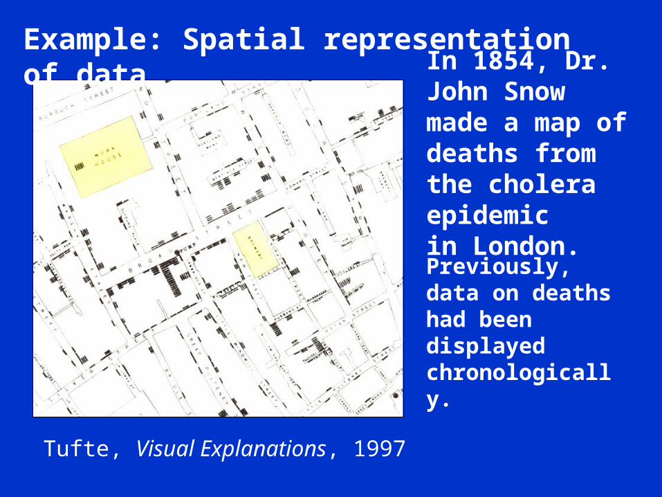
In 1854, Dr. John Snow made a map of deaths from the cholera epidemicin London.

Tufte, Visual Explanations, 1997

Previously, data on deaths had been displayed chronologically.

Example: Spatial representation of data

Brew

ery

Work

House

Graphical Display• Snow took data normally displayed

chronologically (x # of deaths each day throughout the epidemic) and graphed it spatially,

• Spatial display convinced the authorities to shut down the Broad St. pump. From that moment, cholera seriously understood to be linked to bad water.

Lessons

Map makes quantitative comparisons visible and locates them spatially.

Map is appropriate context for showing cause and effect.

Time series chart not as effective. Thinking about how best to display the

data will help you establish useful relationships among the data.

Graphics in Written Documents: Two Important Questions

• When are graphics appropriate?

– What can information display do that words alone cannot?

• What makes a good graphic?

– Are there relevant principles of design?

– See works of William S. Cleveland and Edward R. Tufte

When are graphics appropriate?

• To show complex data in a simplified form– show a lot of data in one place

• To emphasize relationship better than can words alone

• To help the reader remember

• To allow parallel processing of information (visual and verbal)

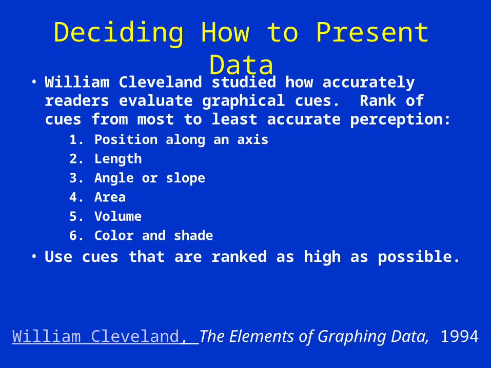
Deciding How to Present Data• William Cleveland studied how accurately readers

evaluate graphical cues. Rank of cues from most to least accurate perception:

1. Position along an axis

2. Length

3. Angle or slope

4. Area

5. Volume

6. Color and shade

• Use cues that are ranked as high as possible.

William Cleveland, The Elements of Graphing Data, 1994

Principles of Information Display• Read the works of Edward Tufte.

– The Visual Display of Quantitative Information, 1983

– Envisioning Information, 1990– Visual Explanations, 1997

• Tufte analyzes visuals displays of data to see which ones help the reader/viewer think through the problem or understand the results. – See article on PowerPoint in Reference list Link

Charles J. Minard’s 1861 graphic depicts Napoleon’s Russian Campaign of 1812 (Tufte, Visual Display)

Tufte calls Minard’s graphic “possibly the best ever constructed.”

• Six variables are plotted:– size of army

– location (latitude)

– location (longitude)

– direction

– temperature

– time (dates)

Create a simple design to help reader get the big picture.

100 cm (Air Outlet)

0 cm

50 cm

75 cm

Bioreactor Packing

Air Sampling Points

25 cm

Column Position (X)

Contaminated Air Inlet

Figure 5.2. Schematic of the experimental bioreactor

Principles of Design

• Keep every graphic as simple and uncluttered as the complexity of your data allows.

• Beware the default parameters in Excel!

             

CE 331 Beam Tests

0.0

5.0

10.0

15.0

20.0

25.0

30.0

-0.50 0.50 1.50 2.50 3.50

Deflection at Mid-Span, in.

Ap

plie

d L

oad

, kip

Series1

Series2

Series3

Series4

CE 331 Beam Tests

0.0

5.0

10.0

15.0

20.0

25.0

30.0

0.0 0.5 1.0 1.5 2.0 2.5 3.0 3.5

Deflection at Mid-Span, in.

Ap

pli

ed

Lo

ad

, k

ip

Beam 1 Beam 2 Beam 3 Beam 4

Figure 1. Deflection of Concrete Beams under Various Loads

Sieve Size Weight Retained (g)

Percent Retained

Cumulative Percent Retained

Percent Passing

#4 54 10.2 10.2 89.9 #8 78 14.7 24.9 75.1 #16 125 23.5 48.4 51.6 #30 116 21.8 70.2 29.8 #50 88 16.6 86.8 13.2 #100 60 11.3 98.1 1.9 #200 5 0.9 99.0 1.0 Pan 5 0.9 100.0 0.0 Total 531 100.0

Table 1: Example of Table Using the Default Parameters in WORD

Table 2: Example of Table with Modified Parameters

Guidelines for Labeling• Labels are a frame . . . of

reference, of orientation.• Label each graphic clearly

with a figure or table number and a title.– Place the figure number and

title beneath a figure (graph, chart, etc.).

– Place the table number and title above a table.

Correct Placement of Figure Title

0

0.2

0.4

0.6

0.8

1

1.2

1.4

1.6

-40 -20 0 20 40 60 80 100 120 140

Temperature (0C)

Den

sity

(kg

/m3)

Figure 3. Relationship between density and temperature of air at standard atmospheric pressure. Source of data: Engineering Fluid Mechanics, 2001

Sieve Size

Weight Retained

(g)

Percent Retained

Cumulative Percent

Retained

Percent Passing

#4 54 10.2 10.2 89.9 #8 78 14.7 24.9 75.1

#16 125 23.5 48.4 51.6 #30 116 21.8 70.2 29.8 #50 88 16.6 86.8 13.2 #100 60 11.3 98.1 1.9 #200 5 0.9 99.0 1.0 Pan 5 0.9 100.0 0.0

Total 531 100.0

Table 2: Example of Table with Modified Parameters

Correct Placement of Table Title

More Labeling Guidelines

• Label both axes. These labels are NOT optional.

• Create a title (or a title and a caption) that draws attention to significant aspects of the graphic.– Give significant details either on the figure

itself or in parentheses (or smaller type) after the title/caption.

• Significant details could be experimental details (such as time of day readings taken) or source information.

Integrate graphics with your text.• In the body of the document, make sure you

do the following:– Describe everything graphed. For tables,

explain column headings, at least.– Draw attention to important features of data.

Try to include them in title too.– Describe conclusions drawn from the data.

What’s significant about those data or findings?

• Place graphic close to its discussion.

Coefficient of Thermal Expansion/ShrinkageA low coefficient of thermal expansion indicates that the material will have minimal change in length given temperature fluctuations. Thermal coefficients for the patching materials are summarized in Table 4; as can be seen, FRP overlay has the lowest.

Table 4. Coefficients of Thermal Expansion/Shrinkage for Patching Materials

Patching MaterialThermal Coefficient

(x106/°C)

(Target Property Values) (14)

High Density Low Slump Concrete

7-20

Fiberglass jackets Not Available

Latex Modified Concrete 13-23

Epoxy Resin-Concrete Composite

27-54

FRP Overlay 5.5

Captions integrate graphics with text.

• Cleveland advocates using captions and says they should make three contributions to understanding:– Describe everything graphed or illustrated– Draw attention to important features of data– Describe conclusions drawn from the data.

• Captions are not conventional in many fields.• At least make title more than “X vs Y.”

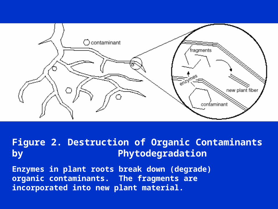
Figure 2. Destruction of Organic Contaminants by Phytodegradation

Enzymes in plant roots break down (degrade) organic contaminants. The fragments are incorporated into new plant material.

Cite the source of every “borrowed” graphic, under the title.

Figure 2. United States Facilities with No. 2 EmissionsSource: Environmental Protection Agency, 2000, www.epa.gov/airs/mapview.htm

Correct Labeling: Cite source of data

0

0.2

0.4

0.6

0.8

1

1.2

1.4

1.6

-40 -20 0 20 40 60 80 100 120 140

Temperature (0C)

Den

sity

(kg

/m3)

Figure 3. Relationship between density and temperature of air at standard atmospheric pressure. Source of data: Crowe, et al. Engineering Fluid Mechanics, 2001