in data , and

1

in data, and

…uncertainty and complexity

in models

2

What do I mean by structure?The key idea is conditional independence:

x and z are conditionally independent given y if p(x,z|y) = p(x|y)p(z|y)

… implying, for example, that p(x|y,z) = p(x|y)

CI turns out to be a remarkably powerful and pervasive idea in probability and statistics

3

How to represent this structure?• The idea of graphical modelling: we

draw graphs in which nodes represent variables, connected by lines and arrows representing relationships

• We separate logical (the graph) and quantitative (the assumed distributions) aspects of the model

4

Markov chains

Graphical models

Contingencytables

Spatial statistics

Sufficiency

Regression

Covariance selection

Statisticalphysics

Genetics

AI

5

Graphical modelling [1]

• Assuming structure to do probability calculations

• Inferring structure to make substantive conclusions

• Structure in model building

• Inference about latent variables

6

Basic DAG

)|()( )(pa vVv

v xxpxp

in general:

for example:

a b

c

d

p(a,b,c,d)=p(a)p(b)p(c|a,b)p(d|c)

7

Basic DAGa b

c

d

p(a,b,c,d)=p(a)p(b)p(c|a,b)p(d|c)

8

A natural DAG from genetics

AB AO

AO OO

OO

9

A natural DAG from genetics

AB AO

AO OO

OO

A

O

AB

A

O

10

DAG for a trivial Bayesian model

y

),|()()(),,( ypppyp

11

DNA forensics example(thanks to Julia Mortera)

• A blood stain is found at a crime scene

• A body is found somewhere else!

• There is a suspect

• DNA profiles on all three - crime scene sample is a ‘mixed trace’: is it a mix of the victim and the suspect?

12

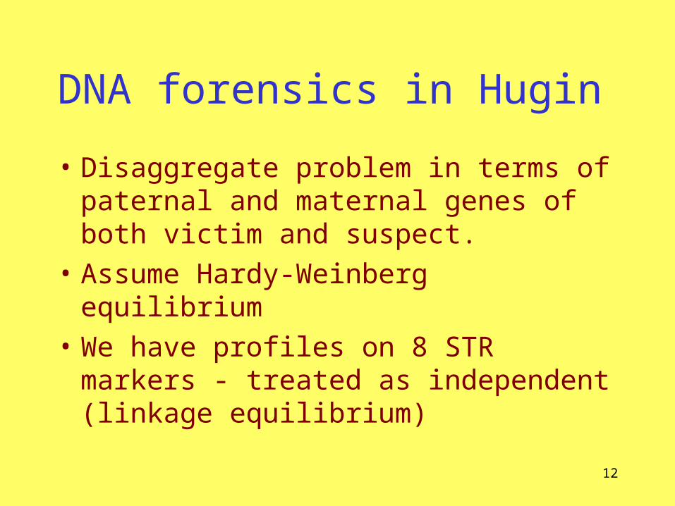
DNA forensics in Hugin

• Disaggregate problem in terms of paternal and maternal genes of both victim and suspect.

• Assume Hardy-Weinberg equilibrium

• We have profiles on 8 STR markers - treated as independent (linkage equilibrium)

13

DNA forensics in Hugin

14

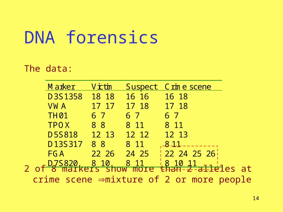
DNA forensics

The data:

2 of 8 markers show more than 2 alleles at crime scene mixture of 2 or more people

Marker Victim Suspect Crime sceneD3S1358 18 18 16 16 16 18VWA 17 17 17 18 17 18TH01 6 7 6 7 6 7TPOX 8 8 8 11 8 11D5S818 12 13 12 12 12 13D13S317 8 8 8 11 8 11FGA 22 26 24 25 22 24 25 26D7S820 8 10 8 11 8 10 11

15

Allele probability8 .18510 .13511 .234x .233y .214

DNA forensics

Population gene frequencies for D7S820 (used as ‘prior’ on ‘founder’ nodes):

C:\Program Files\Hugin\Hugin56_Lite\bin\hugin.exe d:\wp\slides\Oxford\mortera.hkb

C:\Program Files\Hugin\Hugin56_Lite\bin\hugin.exe d:\wp\slides\Oxford\mortera.hkb

16

17

DNA forensics

Results (suspect+victim vs. unknown+victim):

Marker Victim Suspect Crime scene Likelihoodratio (sv/uv)

D3S1358 18 18 16 16 16 18 11.35VWA 17 17 17 18 17 18 15.43TH01 6 7 6 7 6 7 5.48TPOX 8 8 8 11 8 11 3.00D5S818 12 13 12 12 12 13 14.79D13S317 8 8 8 11 8 11 24.45FGA 22 26 24 25 22 24 25 26 76.92D7S820 8 10 8 11 8 10 11 4.90overall 3.93108

18

How does it work?

(1) Manipulate DAG to corresponding (undirected) conditional independence graph(draw an (undirected) edge between

variables and if they are not conditionally independent given all other variables)

19

How does it work?

(2) If necessary, add edges so it is triangulated (=decomposable)

20

7 6 5

2 3 41

12

267 236 345626 36

2

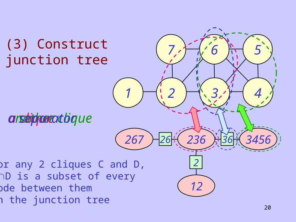
a cliqueanother cliquea separator

For any 2 cliques C and D, CD is a subset of every node between them in the junction tree

(3) Construct junction tree

21

How does it work?

(4) any joint distribution with a triangulated graph can be factorised:

until

sss

ccc

x

xxp

)(

)()(

cliques

separators

22

How does it work?

(5) ‘pass messages’ along junction tree: manipulate the terms of the expression

until

from which marginal probabilities can be read off

sss

ccc

x

xxp

)(

)()(

)()( ccc xpx )()( sss xpx

23

Probabilisticexpertsystems:

Huginfor ‘Asia’example

24

Limitations

• of message passing:– all variables discrete, or– CG distributions (both continuous and

discrete variables, but discrete precede continuous, determining a multivariate normal distribution for them)

• of Hugin:– complexity seems forbidding for truly realistic

medical expert systems

25






26

Conditional independence graphdraw an (undirected) edge between

variables and if they are not conditionally independent given all other variables

27

Infant mortality example

Data on infant mortality from 2 clinics, by level of ante-natal care (Bishop, Biometrics,

1969):

Ante Survived Died % diedless 373 20 5.1more 316 6 1.9

28


Same data broken down also by clinic:

Clinic Ante Survived Died % diedA less 176 3 1.7

more 293 4 1.3B less 197 17 7.9

more 23 2 8.0

29

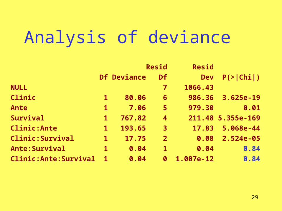
Analysis of deviance

• Resid Resid• Df Deviance Df Dev P(>|Chi|)• NULL 7 1066.43 • Clinic 1 80.06 6 986.36 3.625e-19• Ante 1 7.06 5 979.30 0.01• Survival 1 767.82 4 211.48 5.355e-169• Clinic:Ante 1 193.65 3 17.83 5.068e-44• Clinic:Survival 1 17.75 2 0.08 2.524e-05• Ante:Survival 1 0.04 1 0.04 0.84• Clinic:Ante:Survival 1 0.04 0 1.007e-12 0.84

30


ante

clinic

survival

survival and clinic are dependent

and ante and clinic are dependent

but survival and ante are CI given clinic

31

Prognostic factors for coronary heart disease

strenuous physical work?

family history of CHD?

strenuous mental work?

blood pressure > 140?

smoking?

ratio of and lipoproteins >3?

Analysis of a 26 contingency table(Edwards & Havranek, Biometrika, 1985)

32

How does it work?

Hypothesis testing approaches:

Tests on deviances, possibly penalised (AIC/BIC, etc.), MDL, cross-validation...

Problem is how to search model space when dimension is large

33

How does it work?

Bayesian approaches:

Typically place prior on all graphs, and conjugate prior on parameters (hyper-Markov laws, Dawid & Lauritzen), then use MCMC (see later) to update both graphs and parameters to simulate posterior distribution

34

For example, Giudici & Green (Biometrika, 2000) use junction tree representation for fast local updates to graph

7 6 5

2 3 41

12

267 236 345626 36

2

35

7 6 5

2 3 41

127

267 236 345626 36

27

12

2

36






37

Mixture modellingDAG for a

mixture model

k

jjj yfwy

1

)|(~

k

w

y

38

Mixture modellingDAG for a

mixture model

k

jjj yfwy

1

)|(~

k

w

z

y

)|(~)|( jyfjzy

jwjzp )(

39

Modelling with undirected graphsDirected acyclic graphs are a natural

representation of the way we usually specify a statistical model - directionally:

• disease symptom• past future• parameters data …..

However, sometimes (e.g. spatial models) there is no natural direction

40

Scottish lip cancer data

The rates of lip cancer in 56 counties in Scotland have been analysed by Clayton and Kaldor (1987) and Breslow and Clayton (1993)

(the analysis here is based on the example in the WinBugs manual)

41

Scottish lip cancer data (2)The data include

• a covariate measuring the percentage of the population engaged in agriculture, fishing, or forestry, and• the "position'' of each county expressed as a list of adjacent counties.

• the observed and expected cases (expected numbers based on the population and its age and sex distribution in the county),

42

Scottish lip cancer data (3)

County Obs Exp x SMR Adjacent

cases cases (% in counties

agric.)

1 9 1.4 16 652.2 5,9,11,19

2 39 8.7 16 450.3 7,10

... ... ... ... ... ...

56 0 1.8 10 0.0 18,24,30,33,45,55

43

Model for lip cancer data(1) Graph

observed counts

random spatial effects

covariate

regressioncoefficient

relative risks

44

Model for lip cancer data

• Data:• Link function:

• Random spatial effects:

• Priors:

)(Poisson~ iiO

iiii bxE 10/loglog 10

ji

jin

n bbbbp~

22/1 )4/)(exp()|,...,(

),(~ dr Uniform~, 10

(2) Distributions

45

WinBugs for lip cancer data• Bugs and WinBugs are systems for

estimating the posterior distribution in a Bayesian model by simulation, using MCMC

• Data analytic techniques can be used to summarise (marginal) posteriors for parameters of interest

46

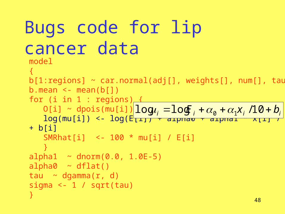
Bugs code for lip cancer data

model{b[1:regions] ~ car.normal(adj[], weights[], num[], tau)b.mean <- mean(b[])for (i in 1 : regions) { O[i] ~ dpois(mu[i]) log(mu[i]) <- log(E[i]) + alpha0 + alpha1 * x[i] / 10 + b[i] SMRhat[i] <- 100 * mu[i] / E[i] }alpha1 ~ dnorm(0.0, 1.0E-5)alpha0 ~ dflat()tau ~ dgamma(r, d) sigma <- 1 / sqrt(tau)} skip

47


model{b[1:regions] ~ car.normal(adj[], weights[], num[], tau)b.mean <- mean(b[])for (i in 1 : regions) { O[i] ~ dpois(mu[i]) log(mu[i]) <- log(E[i]) + alpha0 + alpha1 * x[i] / 10 + b[i] SMRhat[i] <- 100 * mu[i] / E[i] }alpha1 ~ dnorm(0.0, 1.0E-5)alpha0 ~ dflat()tau ~ dgamma(r, d) sigma <- 1 / sqrt(tau)}

)(Poisson~ iiO

48



iiii bxE 10/loglog 10

49



ji

jin

n bbbbp~

22/1 )4/)(exp()|,...,(

50



),(~ dr

51

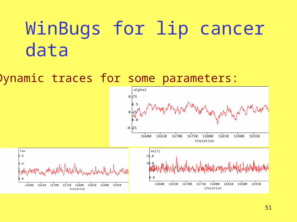
WinBugs for lip cancer data

Dynamic traces for some parameters:alpha1

iteration1695016900168501680016750167001665016600

-0.25

0.0

0.25

0.5

0.75

tau

iteration1695016900168501680016750167001665016600

0.0

2.0

4.0

6.0

mu[1]

iteration1695016900168501680016750167001665016600

0.0

5.0

10.0

15.0

52

WinBugs for lip cancer data

Posterior densities for some parameters:

alpha1 sample: 7000

-0.5 0.0 0.5 1.0

0.0

1.0

2.0

3.0

4.0

mu[1] sample: 7000

0.0 5.0 10.0 15.0

0.0

0.1

0.2

0.3

tau sample: 7000

0.0 2.0 4.0

0.0

0.2

0.4

0.6

0.8

53

How does it work?

• The simplest MCMC method is the Gibbs sampler:

• in each sweep, ‘visit’ each variable in turn, and replace its current value by a random draw from its full conditional distribution - i.e. its conditional distribution given all other variables including the data

skip

54

Full conditionals in a DAG

Basic DAG factorisation

Bayes’ theorem gives full conditionals

involving only parents, children and spouses.

Often this is a standard distribution, by conjugacy.

)|()( )(pa vVv

v xxpxp

)|()|()|( )(pa)(pa:

)(pa wwvw

wvvvv xxpxxpxxp

55

Full conditionals for lip cancer

for example:

)4/)(,2/(~,,,,|~

210

jiji bbdnrbxO

56

Beyond the Gibbs sampler

Where the full conditional is not a standard distribution, other MCMC updates can be used: the Metropolis-Hastings methods use the full conditionals algebraically

57

Limitations of MCMC

• You can’t beat errors

• Autocorrelation limits efficiency

• Possibly-undiagnosed failure to converge

N/1

58






59

Latent variable problems

variable unknown variable known

edges known

value set knownvalue set unknown

edges unknown

60

Hidden Markov models

z0 z1 z2 z3 z4

y1 y2 y3 y4

e.g. Hidden Markov chain

observed

hidden

61

relativerisk

parameters

Hidden Markov models

• Richardson & Green (2000) used a hidden Markov random field model for disease mapping

)(Poisson~ izi Eyi

observedincidence

expectedincidencehidden

MRF

62

Larynx cancer in females in France

SMRs

)|1( ypiz

ii Ey /

63



edges known


edges unknown

64

Ion channel model choiceHodgson and Green, Proc Roy Soc Lond A, 1999

65

Example: hidden continuous time models

O2 O1 C1 C2

O1 O2

C1 C2 C3

66

Ion channelmodel DAG

levels &variances

modelindicator

transitionrates

hiddenstate

data

binarysignal

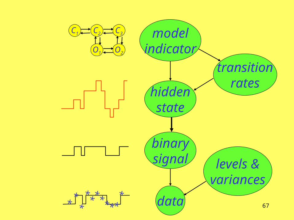
67

levels &variances

modelindicator

transitionrates

hiddenstate

data

binarysignal

O1 O2

C1 C2 C3

** *

******

**

68

Posterior model probabilities

O1 C1

O2 O1 C1

O2 O1 C1 C2

O1 C1 C2

.41

.12

.36

.10

69

‘Alarm’ network

Learning a Bayesian network,for an ICUventilatormanagement system,from 10000 cases on 37 variables(Spirtes & Meek, 1995)

70



edges known


edges unknown

71

Wisconsin students college plans

10,318 high school seniors (Sewell & Shah, 1968, and many authors since)

5 categorical variables:

sex (2)socioeconomic status (4)IQ (4)parental encouragement (2)college plans (2)

sessex

peiq

cp

72

sessex

peiq

cp

5 categorical variables:

sex (2)socioeconomic status (4)IQ (4)parental encouragement (2)college plans (2)

(Vastly) most probable graphaccording to an exact Bayesian analysis by Heckerman (1999)

73

h

Heckerman’s most probable graph with one hidden variable

sessex

peiq

cp

74

CSS book (Complex Stochastic Systems)

• Graphical models and Causality: S Lauritzen• Hidden Markov models: H Künsch• Monte Carlo and Genetics: E Thompson• MCMC: P Green• F den Hollander and G Reinert

ed: O Barndorff-Nielsen, D Cox and

C Klüppelberg, Chapman and Hall (2001)

75

HSSS book (Highly Structured Stochastic Systems)

• Graphical models and causality– T Richardson/P Spirtes, S Lauritzen,

P Dawid, R Dahlhaus/M Eichler

• Spatial statistics– S Richardson, A Penttinen,

H Rue/M Hurn/O Husby

• MCMC– G Roberts, P Green, C Berzuini/W Gilks

76

HSSS book (ctd)

• Biological applications– N Becker, S Heath, R Griffiths

• Beyond parametrics– N Hjort, A O’Hagan

... with 30 discussants

editors: N Hjort, S Richardson & P Green

OUP (2002?), to appear

77

Further reading

• J Whittaker, Graphical models in applied multivariate statistics, Wiley, 1990

• D Edwards, Introduction to graphical modelling, Springer, 1995

• D Cox and N Wermuth, Multivariate dependencies, Chapman and Hall, 1996

• S Lauritzen, Graphical models, Oxford, 1996• M Jordan (ed), Learning in graphical models,

MIT press, 1999

Documents

in data , and