Embed Size (px)
Citation preview

Research Collection
Doctoral Thesis
Statistical decisions based directly on the likelihood function
Author(s): Cattaneo, Marco E.G.V.
Publication Date: 2007
Permanent Link: https://doi.org/10.3929/ethz-a-005463829
Rights / License: In Copyright - Non-Commercial Use Permitted
This page was generated automatically upon download from the ETH Zurich Research Collection. For moreinformation please consult the Terms of use.
ETH Library

Diss. ETH No. 17122
Statistical Decisions Based Directly
on the Likelihood Function
A dissertation submitted to
ETH Zurich
for the degree of
Doctor of Mathematics
presented by
Marco E. G. V. Cattaneo
Dipl. Math. ETH
born September 19, 1976
citizen of Capriasca, Ticino
accepted on the recommendation of
Prof. em. Dr. Frank Hampel, examiner
Prof. Dr. Sara van de Geer, co-examiner
Prof. Dr. Thomas Augustin, co-examiner
2007


Contents
Abstract iii
Sunto v
Notation vii
1 Introduction 1
1.1 Statistical Decisions 1
1.1.1 Classical Decision Theory 3
1.1.2 Bayesian Decision Theory 5
1.2 Likelihood Function 8
1.2.1 Likelihood-Based Inference 10
1.3 Likelihood-Based Statistical Decisions 13
1.3.1 MPL Criterion 13
1.3.2 Other Likelihood-Based Decision Criteria 20
2 Nonadditive Measures and Integrals 25
2.1 Nonadditive Measures 25
2.1.1 Types of Measures 26
2.1.2 Derived Measures 28
2.2 Nonadditive Integrals 30
2.2.1 Shilkret Integral 31
2.2.2 Invariance Properties 35
2.2.3 Regular Integrals 38
2.2.4 Subadditivity 51
2.2.5 Continuity 55
2.2.6 Choquet Integral 58

ii Contents
3 Relative Plausibility 63
3.1 Description of Uncertain Knowledge 63
3.1.1 Representation Theorem 66
3.1.2 Updating 78
3.2 Hierarchical Model 81
3.2.1 Classical and Bayesian Models 83
3.2.2 Imprecise Probability Models 86
4 Likelihood-Based Decision Criteria 95
4.1 Decision Theoretic Properties 95
4.1.1 Attitudes Toward Ignorance 102
4.1.2 Sure-Thing Principle 116
4.2 Statistical Properties 127
4.2.1 Invariance Properties 128
4.2.2 Asymptotic Optimality 138
5 Point Estimation 149
5.1 Likelihood-Based Estimates 149
5.1.1 Asymptotic Efficiency 152
5.2 Shilkret Integral and Quasiconvexity 157
5.2.1 Impossible Estimates 160
References 171
Index 179
Curriculum Vitae 183

Abstract
This thesis studies the possibility of basing statistical decisions directly
on the likelihood function. By describing the problems of statistical infer¬
ence as particular decision problems, the usual likelihood-based inference
methods can be obtained as special cases. These are among the most ap¬
preciated methods of statistical inference, although in general they are not
optimal from the repeated sampling point of view. In fact, their principal
advantages are that, being based on the likelihood function, they are intu¬
itive, generally applicable, and asymptotically optimal. These properties
are shared by all the methods that base decisions on the likelihood function
in some reasonable way.
The decision criteria based on the likelihood function are analyzed, and
some of their decision theoretic properties are related to their representa¬
tions by means of nonadditive integrals; in this connection, the theoryof integration with respect to nonadditive measures is reviewed and ex¬
tended. Some statistical properties of the likelihood-based decision criteria
are studied as well, and a paradigmatic example of statistical decision
problem is examined in more detail: the problem of point estimation in
Euclidean spaces. A simple, intuitive decision criterion emerges as partic¬
ularly interesting: the MPL criterion, which consists in using the likelihood
of the statistical models to weight the respective losses, before applying the
minimax criterion.
The likelihood function can be interpreted as a measure of the relative
plausibility of the statistical models considered, and thus as the second
level of a hierarchical description of uncertain knowledge, of which the sta¬
tistical models form the first level. There is a similarity with the Bayesian
model, in which the second level consists of a probability measure, but the
measure of relative plausibility considered in this thesis can also describe

iv Abstract
ignorance; in particular, in the case of complete ignorance we obtain the
classical model, which in fact consists only of the first level. The mea¬
sure of relative plausibility and the MPL criterion are linked by a simple
representation theorem for preferences between randomized decisions.

Sunto
Questa tesi studia la possibilità di basare le decisioni statistiche diret-
tamente sulla funzione di verosimiglianza. Descrivendo i problemi di in-
ferenza statistica come particolari problemi di decisione, i consueti metodi
di inferenza basati sulla verosimiglianza possono essere ottenuti come casi
particolari. Essi sono tra i più apprezzati metodi di inferenza statistica,benché in generale non siano ottimali secondo il principio del campiona-mento ripetuto. Infatti, i loro principali vantaggi, implicati dall'essere
basati sulla funzione di verosimiglianza, sono l'intuitività, l'applicabilità
generale, e l'ottimalità asintotica. Queste propriété sono condivise da
ogni metodo che basi in modo ragionevole le decisioni sulla funzione di
verosimiglianza.
I criteri di decisione basati sulla funzione di verosimiglianza sono ana-
lizzati, e alcune délie loro propriété inerenti alla teoria délia decisione sono
poste in relazione con le loro rappresentazioni per mezzo di integrali non
additivi; a questo proposito, la teoria dell'integrazione rispetto a misure
non additive è passata in rassegna e ampliata. Alcune propriété statistiche
dei criteri di decisione basati sulla funzione di verosimiglianza sono pure
studiate, e un esempio paradigmatico di problema di decisione è esaminato
più dettagliatamente: il problema délia stima puntuale negli spazi euclidei.
Un criterio di decisione semplice e intuitivo risulta essere particolarmenteinteressante: il criterio MPL, che consiste nell'utilizzare la verosimiglianzadei modelli statistici per pesare le relative perdite prima di applicare il
criterio minimax.
La funzione di verosimiglianza puô essere interpretata come una misura
délia relativa plausibilità dei modelli statistici considerati, e quindi come
il secondo livello di una rappresentazione gerarchica délia conoscenza in-
certa, di cui i modelli statistici costituiscono il primo livello. C'è una chiara

vi Sunto
analogia con il modello bayesiano, nel quale il secondo livello consiste in
una misura di probabilité, ma la misura di plausibilità relativa considerata
in questa tesi puô anche descrivere l'ignoranza; in particolare, in caso di
ignoranza totale otteniamo il modello classico, che di fatto consiste uni-
camente nel primo livello. La misura di plausibilità relativa è associata al
criterio MPL da un semplice teorema di rappresentazione per le preferenzetra decisioni randomizzate.

Notation
Let A and B be two sets. The inclusion of A in B is denoted by A Ç B,while A C B denotes the strict inclusion; the set B \ A is the difference
of B and A. The power set of A is denoted by 2,and \A\ denotes the
cardinality of A. If A is a set of sets, then M A is the union of the elements
of A, with the convention that M 0 = 0.
The set of all functions / : A —> _B is denoted by _BA. If / G -BA, then
/_1 : 2B —> 2 is the mapping assigning to each subset of _B its inverse
image under /; but when / is bijective, /_1 can also denote its inverse
function (the meaning of /_1 should be clear from the context). The imageof a G A under / G B is denoted by f(a) or f[a], but the brackets can
be omitted when there is no ambiguity; for instance, the inverse image of
{b} Ç B can be expressed as /_1{&}. If / G B,and CCA, then f\c
is the restriction of / to C; and if D is a set, and g G DB, then g o f is
the composition of / and (?. The identity function on A is denoted by îd^,while Ia denotes the indicator function of A (the domain of Ia should be
clear from the context).
The set of real numbers is denoted by R, while M denotes the set of
(affmely) extended real numbers: M = M U {oo, —oo}. In the interval nota¬
tion, a round bracket indicates the exclusion of the corresponding endpoint,while a square bracket indicates its inclusion; for instance, if x, y G ffi, then
(x,y] = {z £ ~R : x < z < y}. The set of positive real numbers is denoted
by P, while P denotes the set of nonnegative extended real numbers:
P = (0,oo) and P = [0,oo].
The supremum and infimum of S Ç P are denoted respectively by sup S
and inf S, with the convention that sup0 = 0 and inf 0 = oo. If / G P,

viii Notation
and CCA, then sup / is the supremum of /, and supc / is the supremum
of/|c:supc/ = sup/(a) = sup{/(a) : a G C} = sup/|c;
a£C
and analogously for the infimum. When the supremum is attained, max
can be substituted for sup; and when the infimum is attained, min can be
substituted for inf.
Expressions involving functions are to be interpreted pointwise, when
they do not make sense otherwise; for instance, if /, g G P,then / < g
means that f(a) < g(a) for all a G A. Accordingly, if b G B, then b can also
denote the function in B with constant value b (the domain A should be
clear from the context); for instance, if C Ç A, and Ic has domain A, then
1 — Ic is the indicator function of A \ C. A pair of curly brackets enclosingan expression involving functions denote the subset of the domain of the
functions consisting of all arguments for which the expression is satisfied;for instance, if / G P
,and iéP, then
{f>x} = {aGA: f(a) > x}.
As usual in measure theory, we define 0 oo = oo 0 = 0; but otherwise we
adopt the standard definitions about extended real numbers. In particular,
oo — oo is undefined, and thus in general the difference of two functions
/, g G P is undefined: with a slight abuse in notation we define
\\f - g\\ = sup \f(a) - g(a)\.
The notation is reasonable, because when / and g are bounded, \\f — g\\ is
the supremum norm of their difference; hence, the function (/, g) i—> \\f—g\\on P x P extends the metric induced by the supremum norm. The
notion of uniform convergence can be extended accordingly: the sequence
/lj /2j • • • G P converges uniformly to / G P when linin^oo ||/„ — f\\ =0.
If / G ffi*, and y G ffi, then lim^ f(x) and lim^ f(x) denote the
limits of / at y from the left and from the right, respectively (when the
limits exist). If a; G P, then logo; is the (extended) natural logarithm of
x. If k is a positive integer, and ö G V, then Bg = {x G ffife : \x\ < 0} is
the closed ball in Mfe with center 0 and radius ö, and B^j = Mfe \ B,5 is its
complement (the value of k should be clear from the context). If k is a
positive integer, and y G ffife, then the function ty : x i—> x — y on Mfe is the

Notation ix
translation by —y (the value of k should be clear from the context); for
instance, if ö G P, then t^ÇBg) is the closed ball with center y and radius
S.
Let (Q,C,P) be a probability space. A random object is a measurable
function X : Q —> X, where X is a set equipped with a cr-algebra containingall singletons of X; the random object X is continuous if P{X = x} = 0
for all x G X, and it is discrete if there is a finite or countable y Ç X such
that P{X G y} = 1. A random variable is a random object X : Q —> R,where M is equipped with the Borel cr-algebra.
The symbol D marks the end of a proof, while the symbol 0 marks the
end of an example.


1
Introduction
In the present chapter the basic concepts of statistical decision problem and
of likelihood function are introduced. The usual approaches to statistical
decision problems and the principal likelihood-based inference methods
are briefly described (avoiding foundational issues). Finally, the likelihood-
based decision criteria appearing in the literature are presented.
1.1 Statistical Decisions
A statistical decision problem is described by a loss function
L:V xV ^¥,
where V is a set of probability measures on a measurable space (Q,A),and T> is a set.
V is the set of statistical models considered: these are mathematical
representations of some aspects of the reality under consideration (in par¬
ticular, the observed data can be represented by elements of A). It is
important to note that we use the term "model" to indicate a single prob¬
ability measure (without unknown parameters), while in the statistical
literature it is also used to indicate a whole family of probability measures
(such a family can be a subset of V). It is not assumed that one of the
models in V is in some sense "true", but our conclusions will be based
on V and can thus not be expected to be satisfactory when all models in
V poorly represent the reality. No structure is imposed on P; in particu¬
lar, it is possible to enlarge V in order to improve the robustness of the
conclusions.

2 1 Introduction
T> is the set of possible decisions: a solution of the statistical decision
problem is a subset of T> consisting of the decisions that are optimal ac¬
cording to some criterion. No structure is imposed on T>; in particular, it
is possible to restrict T> by excluding the dominated decisions.
The loss function L summarizes all important aspects of the possibledecisions: L{P, d) is the loss we would incur, according to the model P G V,
by making the decision d G T>. The loss function is usually finite, but
infinite values pose no problems. The decision d is correct for the model
P if L{P, d) = 0 (it is not necessary that for each model there is a correct
decision, or that each decision is correct for some model), and the unit in
which the loss is expressed is of no importance. The loss is thus a relative
quantity: that is, for all c G P, the loss functions L and cL are equivalent,while the loss functions L and L+c are not (because of the peculiar meaningof the value 0). For each d G T>, let Id be the function on V defined by
ld(P) = L(P, d) for all P G V.
If Id < Id', then d! cannot be preferred to d; and if Id = Id', then d and
d! are equivalent (in the sense that no one can be preferred to the other).A decision d is said to dominate a decision d! if Id < Id' and Id ¥" ld'\in this case, if we have to choose between d and d', then we must choose
d (there is no reason for choosing d'). A decision criterion usually corre¬
sponds to a monotonie functional V : P —> P (where monotonie means
that / < /' implies V(l) < V(l')), in the sense that it can be expressed
as follows: minimize V(ld). In this case, an optimal decision (that is, a
decision d minimizing V(ld)) can in general be dominated, but only byanother optimal decision; if necessary, the criterion can thus be refined by
discarding from the set of optimal decisions those that are dominated (byother optimal decisions).
Wald (1939) introduced the statistical decision problem as a general¬ization of the problems of statistical estimation and testing hypotheses.For example, if Q is a set, and g : V —> G is a mapping, then the problemof estimating g(P) can be described by a loss function L on V x G express¬
ing the estimation error: in particular, g(P) is a correct decision for P.
Inference problems (such as estimation problems) can also be stated with¬
out reference to a particular loss function, but some expression of the loss
incurred is actually needed in order to compare different solutions. Often
some standard loss function is used, as in the following simple example,which will be considered throughout the present chapter.

1.1 Statistical Decisions 3
Example 1.1. Let X be the number of successes in n independent binary
experiments (Bernoulli trials) with common success probability p. Assume
that we know n, and we want to estimate p with squared error loss. Let
V = {Pp : p G [0, 1]} be a family of probability measures (the choice
of the measurable space (Q, A) is irrelevant) such that under each model
Pp the random variable X has the binomial distribution with parameters
n and p. The estimation problem is then described by the loss function
L : (Pp, d)^{p- d)2 onPx [0,1]. 0
1.1.1 Classical Decision Theory
Assume first that we have no information at all about which models are
more or less plausible. In this case we only know that, according to the
models in V, the loss we would incur by making the decision d lies in the
range of Id, and thus in particular between inf Id and sup Id- The functional
V = sup gives us a useful upper bound for the loss incurred, and it cor¬
responds to the most important general decision criterion in the case of
complete ignorance about the models in V: the minimax criterion:
minimize sup/^.
By contrast, the functional V = inf gives us a less interesting lower bound
for the loss incurred, and in particular all d G T> that are correct for
some Pd G V are optimal according to the corresponding decision cri¬
terion (called minimin criterion), which is therefore often useless. A
compromise between the minimax and the minimin criteria is given by the
Hurwicz criterion with optimism parameter A G (0, 1):
minimize A inf Id + (1 — A) sup/^.
This criterion was introduced by Hurwicz (1951); it reduces to the minimax
criterion when each d G T> is correct for some Pd G V.
Example 1.2. The minimax criterion applied to the estimation problemof Example 1.1 (without considering the realization of X) leads to the
estimate d = h. Since each possible estimate d G [0, 1] is correct for the
model Pd G V, the minimin criterion is useless, and the Hurwicz criterion
reduces to the minimax criterion. 0

4 1 Introduction
Consider now that an event A G A has been observed: this observation
gives us some information about the relative plausibility of the models in
V; and to be reasonable a decision criterion must be able to use this in¬
formation. The classical approach consists in considering the observation
as a particular realization A = {X = xa} of a random object X : Q —> X,in selecting a whole decision function ö : X —> T> instead of a single deci¬
sion d = S(xa), and in evaluating the different decision functions without
considering that X = xa has already been observed. In this sense, the
selection of the decision function is based on a pre-data evaluation. Let
A be a set of decision functions ö such that for each P G V the func¬
tion x i—> L[P, S(x)] on X is measurable: under each model P the loss we
would incur by using the decision function ö G A is the random variable
L[P,8{X)\. In order to compare different decision functions, the random
loss is reduced to a single, representative value: usually the expected value,but other quantities (such as quantiles) can be used instead. That is, for
each model P G V and each decision function 5 G A we have a represen¬
tative value L'(P, 6) of the random loss: the loss function L' on V x A
describes the problem of selecting a decision function 5 G A. If L'{P, 5) is
defined as the expected value of L[P, ö(X)] with respect to P, then L' is
called risk function, and the minimax criterion applied to the decision
problem described by L' is the minimax risk criterion introduced byWald (1939).
Example 1.3. The minimax risk criterion applied to the estimation problemof Example 1.1 (with X = {0, ...,n}, and A defined as the set of all
decision functions on X) leads to the estimate
XI -/^
K l"(l-^n)ö> witn ^71n I i/n + 1
(see Hodges and Lehmann, 1950). Note that the case with n = 0 corre¬
sponds to the case without observations (^ is the estimate obtained in
Example 1.2), while for large n the estimate is approximately —. 0
The classical approach requires the definition of the random object X;that is, it requires the consideration of what could have been observed
instead of A. In general this is not a problem, since the alternatives to
A have already been considered when defining V. More problematic can
be the assumption that the same decision problem would have been faced
for all possible realizations of X. Even if this assumption is reasonable,

1.1 Statistical Decisions 5
the classical approach has two main drawbacks with respect to conditional
methods (that is, methods selecting a single decision in the light of the
observation X = xa, without considering the other possible realizations of
X). The first one is that selecting a decision function is in general much
more complicated than selecting a single decision. The second one is that
the selection of the decision function is based on a pre-data evaluation,whose meaning can be questionable once the data have been observed (seefor instance Goutis and Casella, 1995).
1.1.2 Bayesian Decision Theory
When no data are observed, the Bayesian approach consists in averaging
over the models in V by means of a probability measure 7r on (V, C), where
C is a cr-algebra of subsets of V such that Id is measurable for all d G T>:
we obtain the Bayesian criterion:
minimize E^Q^d)-
If for each A G A the function P i—> P(A) on V is measurable, then 7r can
be combined with the models in V (interpreted as a stochastic kernel) to
obtain a probability measure Pv on (V x fi, £), where 6 is the cr-algebra of
subsets of V x Q generated by the sets C x A with C G C and A G A. If we
observe an event A G A, then we can condition the probability measure
Pj; on the event V x A G £, obtaining in particular an updated marginal
probability measure on (V,C), which can then be used in the Bayesiancriterion. The Bayesian approach consists thus in combining the models
in V to obtain a single model Pv, in updating it by conditioning it on the
observed data, and in reducing the decision problem described by the loss
function L on V x T> to the one described by the loss function L" on II x 2?,where II = {-Pjr}, and L"(P^, d) is defined as the expected value of L(P, d)with respect to the updated version of Pv. Since II is a singleton, there
is no concern about the decision criterion to be applied to the decision
problem described by L".
Example 1.4- For the estimation problem of Example 1.1, let 7r be a prob¬
ability measure on V corresponding to a beta distribution for the para¬
meter p G [0, 1]. When observing X = x, the updating of 7r correspondsto increasing the two parameters of the beta distribution by x and n — x,
respectively. The estimate of p obtained by applying the Bayesian crite¬
rion is the mean of the resulting beta distribution: if a, b G P are the two

6 1 Introduction
parameters of the initial beta distribution corresponding to 7r, then the
estimate is
X + a ,^/1,n°•
, ^n
—: Ti;=A h(l-A„)——, withA„ = — —.
n + a + b n a + b n + a + b
This estimate depends strongly on the choice of a, b G P; if a + b is largewith respect to n, then the estimate is approximately —j-t ,
while if a + b
is small with respect to n, then the estimate is approximately —.
When the only available information about the relative plausibility of
the models in V is provided by the observation X = x, the two most
popular choices of 7r are the probability measures on V corresponding to
the beta distributions with parameters a = b = 1 (that is, the uniform
distribution on [0,1], proposed by Bayes, 1763) and a = b = ^ (proposedby Jeffreys, 1946), respectively. 0
The Bayesian approach is conditional (the selection of a decision is
based on a post-data evaluation), and it possesses the following important
property of "temporal coherence" between pre-data and post-data evalua¬
tions. Let X : Q —> X be a random object, and define the decision function
8' : X —> T> as follows: let 8'(x) be the decision that we would select after
having observed X = x. If in the pre-data decision problem considered
in Subsection 1.1.1 we define L' as the risk function, some regularity con¬
ditions are satisfied (see for example Brown and Purves, 1973), and A is
sufficiently wide to contain 8', then 8' is an optimal decision, accordingto the Bayesian criterion, for the decision problem described by L'. The
temporal coherence is useful because it allows us to construct an optimaldecision function without having to compare decision functions, but only
single decisions. Thanks to the additivity of En, the Bayesian approach
possesses also the following important property of "coherence with respect
to additive loss". Let L\ and L2 be two loss functions on V x T>\ and
V x 2?2, respectively, let T> = T>\ x 2?2, and let L be the loss function on
V xV defined by L[P,{d1,d2)] = £i(P,di) + L2(P,d2) (for all P G V
and all (di, d2) G T>). If the Bayesian criterion can be applied to the three
decision problems (in the sense that the measurability condition stated at
the beginning of the present subsection is satisfied), and di and d2 are op¬
timal for the decision problems described by L\ and L2, respectively, then
(di, d2) is optimal for the decision problem described by L. The coherence
with respect to additive loss is useful because for some decision problemsit allows us to construct an optimal decision by considering only simpler
problems.

1.1 Statistical Decisions 7
These coherence properties are possible because in the (strict) Bayesian
approach there is no uncertainty about the model: II is a singleton. In fact,the central problem of the Bayesian approach is the choice of the averaging
probability measure 7r, which is usually interpreted either as a statistical
model, or as a description of subjective uncertain knowledge. Indepen¬
dently of the interpretation of 7r, it is reasonable to allow some uncertaintyabout the model P^ by assuming only that 7r is an element of some set
r of probability measures on (V,C); the set T can also be interpreted as
an imprecise probability measure on (V,C): see for example Walley (1991)and Weichselberger (2001). Each element of the set II = {P^ : jt £ T}can be conditioned on the observed data, and the decision problem de¬
scribed by the loss function L on V x T> can be reduced to the one de¬
scribed by the loss function L" on II x 2?, where L" is defined as above.
The minimax criterion applied to the (post-data) decision problem de¬
scribed by L" is the T-minimax criterion, which was introduced byHurwicz (1951) for the pre-data decision problem under the name of "gen¬eralized Bayes-minimax principle" ; but the pre-data and the post-data
applications of the T-minimax criterion do not coincide, since the tem¬
poral coherence of the strict Bayesian approach is lost (see for example
Augustin, 2003). A decision criterion similar in spirit to the T-minimax is
the restricted Bayesian criterion, which was introduced by Hodges and
Lehmann (1952) for the pre-data decision problem. It consists in applyingthe Bayesian criterion (with respect to an averaging probability measure
7r) to the decision problem described by the risk function L', but only af¬
ter having restricted the set A to those decision functions for which the
expected loss is bounded above by a particular constant. The intent of the
restriction of A is to limit the importance of the particular choice of 7r.
Example 1.5. The application of the restricted Bayesian criterion is diffi¬
cult even for the simple estimation problem of Example 1.1: some limited
results are reported by Hodges and Lehmann (1952). The application of
the T-minimax criterion is much simpler, but T must be chosen carefully.For instance, if for the estimation problem of Example 1.1 we choose as
r the family of probability measures on V corresponding to the family of
beta distributions for the parameter p G [0,1], then the resulting estimate
is i, independently of n and of the observation X = x. The family of beta
distributions is a natural choice for T (it is the so-called conjugate familyfor this estimation problem, and for instance the two popular choices of 7r

8 1 Introduction
considered at the end of Example 1.4 belong to it): this example simplyshows that the T-minimax criterion is useless when T is too wide. 0
1.2 Likelihood Function
Let Pbea set of statistical models, and let A represent the observed data
(V is a set of probability measures on a measurable space (Q,A), and
A G A). The likelihood function hk on V induced by the observation of
A is defined by
hk{P) = P{A) for all P G V.
The likelihood function measures the relative plausibility of the models
in the light of the observed data alone. Only ratios of the values of hk
for different models have meaning: proportional likelihood functions are
equivalent. In particular, if the statistic s : X —> S is sufficient for the
random object X : Q —> X, then the likelihood function induced by the
observation X = xa is equivalent to the one induced by the observation
s(X) = s(xa)- That is, (the equivalence class of) the likelihood function
depends only on sufficient statistics.
If X : Q —> X is a random object that is continuous under each model
in V, then the observation X = xa would induce a likelihood function
with constant value 0. But in reality, because of the finite precision of all
measurements, it is only possible to observe X G Na, for a neighborhood
Na of xa If fp is a density of X under the model P, then it can be useful to
consider the approximation P{X G Na} ~ 6 /p(x^), where ö G P. If this
holds for all P G V, then the function P i—> /p(x^) on V is approximately
equivalent to the likelihood function induced by the observation X G Na-
When all fp are densities of X with respect to the same measure on X, the
function P i—> /p(x^) on V is often considered as the likelihood function
induced by the observation X = xa, independently of the quality of the
above approximation. This alternative definition of likelihood function has
some little problems (such as nonuniqueness), but it leads to an elegantmathematical theory, and all the results that we shall obtain for discrete
random objects would be valid also for continuous ones if this alternative
definition were used.
Under each model P G V, the likelihood ratio /fc/PÂ of P against
a different model P' G V almost surely increases without bound when

1.2 Likelihood Function 9
more and more data are observed, if some weak conditions are satisfied.
Consequently, when V is finite, the likelihood function tends to concentrate
around P; and the same holds also when V is infinite, if some regularityconditions are satisfied.
A parametrization of V is a bijection t : V —> O, where the parameter
space O can be any set, but usually O Ç W71. The set V can be identified
with O, and therefore a likelihood function hk on V can be identified
with hk oT1, which is called likelihood function on O (with respect to
t). A pseudo likelihood function on a set Q with respect to a mapping
g : V —> G is a function that, to some extent at least, can be used as if it
were a likelihood function on Q. For instance, the function P i—> fp(xA)on V considered above as an approximation of the likelihood function
induced by the observation X G Na is a pseudo likelihood function on V
with respect to id-p. Other pseudo likelihood functions on V with respect
to id-p can be obtained for example by modifying the likelihood function
in order to take into account the complexity of the models in V. If hk is
a likelihood function on V, and g : V —> G is a mapping, then the profilelikelihood function hkg on G with respect to g is defined by
hkg^) =
sup|fl=7| hk for all 7 G G-
In particular, if t : V —> O is a parametrization of V, then hkt is the likeli¬
hood function on O. The profile likelihood function is a pseudo likelihood
function that is defined for all functions jon?, and that usually leads to
reasonable results; but better results can sometimes be achieved by usingother pseudo likelihood functions. In the literature on likelihood-based sta¬
tistical inference, many alternative pseudo likelihood functions have been
proposed for different situations: see for instance Barndorff-Nielsen (1991)and Severini (2000, Chapters 8 and 9), and the references therein.
Example 1.6. Consider the estimation problem of Example 1.1: the map¬
ping Pp 1—> p is a parametrization of V with parameter space [0,1]. The
likelihood function hk on [0,1] induced by the observation X = x satisfies
hk(p) = (n j px (1 - p)n-'x for all p G [0, 1].
By observing the realization of each one of the n binary experiments, we
would have obtained the likelihood function hk1 on [0,1] defined by
hk'(p) =px(l- p)n~x for all p G [0,1],

10 1 Introduction
00.2 0.4 0.6 0.8 1
Figure 1.1. Profile likelihood functions from Example 1.6.
where x is the number of successes. The likelihood functions lik and lik1
are equivalent (that is, lik oc lik'), and in fact the number of successes is
a sufficient statistic.
Let g be the function on V assigning to each model Pp the probability of
observing at least 3 successes in 5 future independent binary experimentswith the same success probability p:
g(Pp) =J2 (5)/(l-p)5~fe = 6/-15p4+10p3 for all p G [0,1].fe=3W
Figure 1.1 shows the graphs of the profile likelihood functions likg on [0, 1](actually, g is a parametrization of V) induced by the three observations
X = 8 with n = 10 (dotted line), X = 33 with n = 50 (dashed line), and
X = 178 with n = 250 (solid line), respectively (the three functions have
been scaled to have the same maximum). The data have been generated
using the model P0.7, and in fact the profile likelihood function tends to
concentrate around g(Po.7) ~ 0.837. 0
1.2.1 Likelihood-Based Inference
Let lik be a likelihood function (induced by some observation A) on a set
V of statistical models, let Q be a set, and let g : V —> G be a mapping. The
maximum likelihood estimate 7ml of g(P) is the 7 G G maximizing

1.2 Likelihood Function 11
X n 7ml LR(H) {hkg > ß sup hk}
8 10 0.942 0.146 (0.321,1.000)
33 50 0.780 0.074 (0.461,0.952)
178 250 0.852 UT10 (0.741,0.927)
Table 1.1. Likelihood-based inferences from Example 1.7.
hkg, when such a 7 exists and is unique. The method of maximum likeli¬
hood is by far the most popular general method of statistical estimation;it was introduced (in a general form, but limited to the case of parame-
trizations g) by Fisher (1922). The likelihood ratio of a set TL Ç V is the
value
, s sup.,, hk
sup hk
The likelihood ratio test of the null hypothesis Hq : P G TL versus the
alternative Hi : P G V \TL rejects the null hypothesis when LR(TL) < ß,where the critical value ß G (0,1) is chosen in order to obtain a test of
a particular level (that is, ß is chosen on the basis of a pre-data evalua¬
tion). The likelihood ratio tests were introduced by Neyman and Pearson
(1928), and have a central place in both the hypothesis testing literature
and practice; they are closely related to the following confidence regions.The likelihood-based confidence region for g(P) with cutoff point
ß G (0,1) is the set
{7 G G : LR{g = 7} > ß} = {hkg > ß sup hk}.
The (pre-data) coverage probability of a likelihood-based confidence re¬
gion with cutoff point ß depends on the set V of statistical models consid¬
ered (and on the mapping g): this is the so-called calibration problem of
likelihood-based inference.
Example 1.1. The method of maximum likelihood applied to the estima¬
tion problem of Example 1.1 leads to the estimate Pml = (when n > 1;while for n = 0 the maximum likelihood estimate is undefined). Table 1.1
gives some likelihood-based inferences for the mapping g and the data con¬
sidered in Example 1.6 (the corresponding profile likelihood functions hkgare plotted in Figure 1.1). The maximum likelihood estimate 7ml tends to

12 1 Introduction
0950 02 04 06 08 1
Figure 1.2. Coverage probability of the likelihood-based confidence region from
Example 1.7, when n = 10.
the value g(Po 7) « 0.837 of the function g for the model Pq 7 used to gen¬
erate the data. The likelihood ratio LR(Ti) of the hypothesis TL = {g < ^}(which states that the probability g(Pp) is at most ^) tends to 0. The
likelihood-based confidence region for g(P) with cutoff point ß « 0.036 (sothat —2 log/3 is the 99%-quantile of the x2 distribution with one degree of
freedom) is an interval tending to concentrate around g(Po 7) ~ 0.837. For
large n the coverage probability of this likelihood-based confidence regionis approximately 99%; the exact coverage probability for n = 10 is plottedin Figure 1.2 as a function of p G [0, 1]. 0
The method of maximum likelihood is conditional, while the tests and
confidence regions based on the likelihood ratio are fully conditional onlyif the choice of the critical value or cutoff point ß is not based directly
on pre-data evaluations (for example, it can be based on experience and
on analogies with simple situations). Although they are (at least partially)conditional, in general the likelihood-based inference methods perform well
also from the pre-data point of view. Under suitable regularity conditions,
they are consistent and even asymptotically efficient. But they also have
good pre-data performances in a surprisingly large number of importantsmall sample problems, even though examples with bad performances can
be easily constructed.
If we consider a set T of averaging probability measures 7r on V, as
done at the end of Subsection 1.1.2, then we obtain a set II of probabilitymeasures P^ on V x Q. The observation of an event A G A induces a

1.3 Likelihood-Based Statistical Decisions 13
likelihood function hk on T, in the sense that the observation VxA induces
a likelihood function on LT, and the mapping P^ i—> 7r is a paranietrization of
II. The likelihood hk(ji) of 7r is the expected value of P(A) with respect to
7r: that is, it is the average with respect to 7r of the likelihood function on V
induced by the observation of A. The likelihood-based inference methods
can be applied to hk in order to obtain inferences about the averaging
probability measures 7r in L, as proposed for example by Good (1965).
1.3 Likelihood-Based Statistical Decisions
Since the statistical decision problems were introduced as a generalizationof the problems of statistical estimation and testing hypotheses, and the
most appreciated general methods for these inference problems are based
directly on the likelihood function, it is natural to consider general deci¬
sion criteria based directly on the likelihood function. Of particular interest
are decision criteria leading to maximum likelihood estimates and likeli¬
hood ratio tests when applied to (some standard form of) estimation and
hypothesis testing problems, respectively.
1.3.1 MPL Criterion
Consider a statistical decision problem described by a loss function L on
V x T>: let A represent the observed data (V is a set of probability measures
on a measurable space (Q,A), and A G A), and let hk be the likelihood
function on V induced by the observation of A. If we use the likelihood of
the statistical models to weight the respective losses, before applying the
minimax criterion, then we obtain the MPL criterion:
minimize sup/î/e/^.
The MPL criterion was introduced by Cattaneo (2005): "MPL" means
"Minimax Plausibility-weighted Loss", and for the present situation "plau¬
sibility" can simply be read as "likelihood". A likelihood function with
constant value c G P is equivalent to the one induced by the observation of
Q, which corresponds to having observed no data; with such a likelihood
function, the MPL criterion reduces to the minimax criterion. In general,the likelihood function measures the relative plausibility of the models (in

14 1 Introduction
the light of the observed data alone), and the MPL criterion is a simple,intuitive modification of the minimax criterion, making use of the infor¬
mation provided by the likelihood function: the more plausible a model,the larger its influence on the evaluation of the different decisions. In the
extreme case of a likelihood function proportional to I{p\ for a model
P G V (that is, P is infinitely more plausible than every other model in
V), a decision d G T> is optimal according to the MPL criterion when it
minimizes L{P, d): in particular, if d is correct for P, then d is optimal.
Example 1.8. The MPL criterion applied to the estimation problem of Ex¬
ample 1.1 leads to the (unique) estimate
arg min max« (1 — p)~ (p — d) .
de [0,1] Pe [0,1]
Except for the simplest cases (with very small n, or with X = Ç), it is not
possible to express this estimate in a simple form, but its numerical evalua¬
tion poses no problems. When n = 0 or n = 1, this estimate coincides with
the one obtained by applying the minimax risk criterion (considered in
Example 1.3); but as n increases, the present estimate tends to the max¬
imum likelihood estimate pml = (considered in Example 1.7) faster
than the one obtained by applying the minimax risk criterion. Both esti¬
mates obtained by applying the Bayesian criterion with as initial averaging
probability measures TronP the two popular choices considered at the end
of Example 1.4 have a behavior (for increasing n) similar to the one of the
present estimate (which coincides with both of them when n = 0, and
with the one based on the proposal of Jeffreys when n = 1). Figure 1.3
shows, for various n, the graphs of the expected losses (as functions of
p G [0,1]) for the estimates obtained by applying the MPL criterion (solidline), the minimax risk criterion (dotted horizontal line), the method of
maximum likelihood (dotted curved line), and the Bayesian criterion for
the two choices of 7r considered above (dashed lines: when n > 1 and p = ^,the resulting expected loss is larger for the proposal of Jeffreys than for
the one of Bayes). 0
Let Q be a set, and let g : V —> G be a mapping. If the loss function L
depends on the models P only through g{P), in the sense that there is a
function i'ongxD such that L(P, d) = L'[g(P), d] for all P G V and all
d G T>, then the MPL criterion can be expressed as follows:
minimize sup hkg l'd,

1.3 Likelihood-Based Statistical Decisions 15
02-
0 1-
0 02
0 01-
02 04 06 08 1
n = 1
002 04 06 08 1
n = 10
0 002
0 001
0 0002
0 0001
02 04 06 08 1
n = 100
02 04 06 o:
n = 1000
Figure 1.3. Expected losses from Example 1.
where for each d G T> the function l'd on Q is defined by l'd(j) = L'(y, d) (forall 7 G Q). That is, the MPL criterion automatically employs the profilelikelihood function hkg on Q; but other pseudo likelihood functions on Q
(with respect to g) can be used instead of hkg in the above version of the
MPL criterion, if they are expected to give better results.
When Q is finite and we want to estimate g(P), a simple way to define
an estimation error is to assign a constant error to estimates 7 7^ g(P),while assigning no error to the correct estimates 7 = g(P). That is, the
estimation problem can be described by the loss function Iw on V x Q,

16 1 Introduction
where W = {(P, 7) G V x Q : g(P) 7^ 7}. If hkg has a unique maximum
at 7 = 7ml jthen the maximum likelihood estimate 7ml of g(P) is the
unique optimal decision, according to the MPL criterion, for the decision
problem described by Iw This is in general not true when Q is infinite,and in fact in this case the loss function Iw is usually unreasonable. When
the (finite or infinite) set Q possesses a metric p, we can generalize the
finite case by considering the loss function IyyE on V x Q, where e G P,and W£ = {(P, 7) G V x Q : p[g(P), 7] > e}. When a maximum likelihood
estimate 7ml of g(P) exists, it can be considered really unique only if
LR{p(g, 7ml) > 5} < 1 for all ö G P. In this case, if 7 is an optimal de¬
cision, according to the MPL criterion, for the decision problem described
by Iwei then p(7, 7ml) < e- Thus by selecting a sufficiently small e G P,
we obtain a situation which in practice is analogous to the finite case: if
a unique maximum likelihood estimate exists, then it corresponds practi¬
cally to the unique optimal decision (according to the MPL criterion) for
the estimation problem.
Consider now the problem of testing the null hypothesis Hq : P G TL
versus the alternative H\ : P G V \ TL, for a subset Ti of V: a simple
way to define a loss function is to assign constant losses c\, c<i G P to
errors of the first and of the second kind, respectively, where c\ > c<i. That
is, the hypothesis testing problem can be described by the loss function
L on V x {r,n} such that lr = Cil^ and /„ = C21-pVHi where r and
n are respectively the decisions of rejecting and of not rejecting the null
hypothesis. The MPL criterion applied to the decision problem described
by L leads to the rejection of the null hypothesis when LR(7i) < — (whenLR(7i) =
—, both decisions r and n are optimal); that is, practicallyit leads to the likelihood ratio test with critical value ^. The level of
.Cl.
this test depends on the sets TL and V (this is the calibration problem of
likelihood-based inference): it can be argued that those sets should have
been considered when selecting the constants c\ and C2; another way to
address the calibration problem is by using some pseudo likelihood function
depending on the sets 7i and V. The choice of a loss function to describe
the problem of selecting a confidence region for g(P) is complicated bythe fact that also the extent of the region plays a role; but a simple loss
function can be chosen if we consider only a limited set T> C 2s of possibleconfidence regions (for example all the intervals whose length does not
exceed a particular constant). In this case we can assign a constant error
to regions d jj g(P), while assigning no error to regions d 9 g(P)', that is,
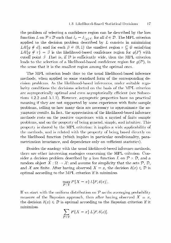
1.3 Likelihood-Based Statistical Decisions 17
the problem of selecting a confidence region can be described by the loss
function L on V x T> such that l& = I{g4d\ f°r aU d G T>. The MPL criterion
applied to the decision problem described by L consists in minimizing
LR{g (fi d}; and for each ß G (0,1) the smallest region r Ç Q satisfying
LR{g ^ r} = ß is the likelihood-based confidence region for g(P) with
cutoff point ß. That is, if 2? is sufficiently wide, then the MPL criterion
leads to the selection of a likelihood-based confidence region for g{P), in
the sense that it is the smallest region among the optimal ones.
The MPL criterion leads thus to the usual likelihood-based inference
methods, when applied to some standard form of the corresponding de¬
cision problems. As the likelihood-based inferences, under suitable regu¬
larity conditions the decisions selected on the basis of the MPL criterion
are asymptotically optimal and even asymptotically efficient (see Subsec¬
tions 4.2.2 and 5.1.1). However, asymptotic properties have no practical
meaning if they are not supported by some experience with finite sample
problems, telling us how many data are necessary to approximate the as¬
ymptotic results. In fact, the appreciation of the likelihood-based inference
methods rests on the positive experience with a myriad of finite sample
problems, and on the property of being general, simple, and intuitive. This
property is shared by the MPL criterion: it implies a wide applicability of
the methods, and is related with the property of being based directly on
the likelihood function (which implies in particular conditionality, para-
metrization invariance, and dependence only on sufficient statistics).
Besides the analogy with the usual likelihood-based inference methods,there are other interesting analogies concerning the MPL criterion. Con¬
sider a decision problem described by a loss function L on V x T>, and a
random object X : Q —> X; and assume for simplicity that the sets V, T>,and X are finite. After having observed X = x, the decision ô(x) G T> is
optimal according to the MPL criterion if it minimizes
maxP{X = x} L[P,ô(x)}.
If we start with the uniform distribution on V as the averaging probability
measure of the Bayesian approach, then after having observed X = x,
the decision ö(x) G T> is optimal according to the Bayesian criterion if it
minimizes
Y/P{X = x}L[P,ö(x)}.Per

18 1 Introduction
The decision function ö G T>x is optimal according to the minimax risk
criterion if it minimizes
m^Y/P{X = x}L[P,ö(x)}.
There is a high similarity between these three expressions, although the
term P{X = x} appears with different meanings. It can be noted that the
MPL criterion corresponds to the minimax risk criterion by assuming that
for all the alternative, unobserved realizations of X we would have selected
a correct decision. If we apply the Bayesian approach (with the uniform
distribution on V as the averaging probability measure) to the pre-datadecision problem described by the risk function, then the decision function
ö G T>x is optimal according to the Bayesian criterion if it minimizes
££ P{X = a:} L[P, <*(*)].P£Vx£X
Since the summation operators commute, we obtain the temporal coher¬
ence of the Bayesian approach. The maximization and summation opera¬
tors do not commute, and in fact the MPL approach does not in general
satisfy this temporal coherence: the MPL criterion for the pre-data deci¬
sion problem described by the risk function corresponds to the minimax
risk criterion (since the likelihood function induced by observing no data
is constant). Since the maximization operators commute, a property anal¬
ogous to the temporal coherence of the Bayesian approach is obtained for
the MPL approach if
maxP{X = x} L[P,ô(x)}x<^X
is used (instead of the expected value) as the representative value of the
random loss of ö G T>x, when defining the loss function L' on V x T>x for
the pre-data decision problem considered in Subsection 1.1.1. This repre¬
sentative value has the drawback of depending on spurious modifications
of the random object X (for example when a possible observation x G X is
"subdivided" into two equiprobable new observations by considering also
the result of flipping a fair coin), but the decision functions obtained byconditional application of the MPL criterion are the only decision func¬
tions that are optimal for all such modifications (according to the MPL
criterion applied to the decision problem described by L').

1.3 Likelihood-Based Statistical Decisions 19
Besides temporal coherence, the Bayesian approach possesses also the
property of coherence with respect to additive loss: the MPL approach
possesses the analogous, important property of "coherence with respect
to maxitive loss". Let L\ and L2 be two loss functions on P x T>\ and
P x 2?2, respectively, let T> = T>\ x T)2l and let L be the loss function
on?xD defined by L[P,(d1,d2)] = maxji^P, dx), L2(P, d2)} (for all
P G V and all (^1,^2) G T>). If di and d2 are optimal for the decision
problems described by L\ and L2, respectively, then (^1,^2) is optimalfor the decision problem described by L. The coherence with respect to
maxitive loss is useful because for some decision problems it allows us to
construct an optimal decision by considering only simpler problems.
Consider a statistical decision problem described by a loss function L
on V x T>: let A represent the observed data, and let lik be the likelihood
function on V induced by the observation of A. If we consider a set F of
averaging probability measures 7r on P, then the MPL criterion for the
decision problem described by the loss function L" considered at the end
of Subsection 1.1.2 can be expressed as follows:
minimize sup E^^hk Id).wer
In fact, it can be easily proved that for all 7r G F and all d G T>
P*(P x A)Ep„[L(P,d)\P xA}= E^hkU).
Since E^{likld) < suphkld, if T can be interpreted as an extension of P,in the sense that T contains, at least as limits, the Dirac measures öp on
P, for all P G P, then the application of the MPL criterion to the decision
problem described by L" leads to the same results as its application to the
decision problem described by L. More precisely, if for each P G P and
each d G T> there is a sequence tt± , tt2 ,... G T such that
lim E^ihkld) = hk(P)ld(P),
then according to the MPL criterion, a decision d G T> is optimal for the
decision problem described by L" if and only if it is optimal for the decision
problem described by L. This property too can be considered as a sort of
coherence; its premise is satisfied in particular when T is the set of all
probability measures on (P,C), and C contains all singletons of P.
20 1 Introduction
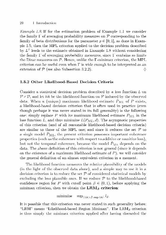
Example 1.9. If for the estimation problem of Example 1.1 we consider
the family T of averaging probability measures on V corresponding to the
family of beta distributions for the parameter p G [0,1], as done in Exam¬
ple 1.5, then the MPL criterion applied to the decision problem described
by L" leads to the estimate obtained in Example 1.8 without consideringthe family T of averaging probability measures, since T contains as limits
the Dirac measures on V. Hence, unlike the T-minimax criterion, the MPL
criterion can be useful even when T is wide enough to be interpreted as an
extension of V (see also Subsection 3.2.2). 0
1.3.2 Other Likelihood-Based Decision Criteria
Consider a statistical decision problem described by a loss function L on
VxD, and let lik be the likelihood function on V induced by the observed
data. When a (unique) maximum likelihood estimate Pml of P exists,a likelihood-based decision criterion that is often used in practice (eventhough perhaps it was never stated in its full generality) is the followingone: simply replace P with its maximum likelihood estimate Pml in the
loss function L, and thus minimize L{Pml, d)- The asymptotic propertiesof this criterion (and of all reasonable likelihood-based decision criteria)are similar to those of the MPL one; and since it reduces the set V to
a single model PmLi the present criterion possesses important coherence
properties (such as the coherence with respect to additive or maxitive loss),but not the temporal coherence, because the model Pml depends on the
data. The above definition of this criterion is not general (since it depends
on the existence of a maximum likelihood estimate of P) : we will consider
the general definition of an almost equivalent criterion in a moment.
The likelihood function measures the relative plausibility of the models
(in the light of the observed data alone), and a simple way to use it in a
decision criterion is to reduce the set V of considered statistical models by
excluding the less plausible ones. If we reduce V to the likelihood-based
confidence region for P with cutoff point ß G (0,1), before applying the
minimax criterion, then we obtain the LRM^ criterion:
minimize sup{hk>ß euphk} ld.
It is possible that this criterion was never stated in such generality before:
"LRM" means "Likelihood-based Region Minimax". The LRM^ criterion
is thus simply the minimax criterion applied after having discarded the

1.3 Likelihood-Based Statistical Decisions 21
models in V that are too implausible (when compared to other models in
V) in the light of the observed data: the larger is ß, the more plausible
are the discarded models. By letting ß tend to 1, we obtain the MLD
criterion:
minimize limsup{hfe>/3 euphk} ld.
This criterion is almost equivalent to the one considered above, based on
the maximum likelihood estimate Pml of P- "MLD" means "Maximum
Likelihood Decision". In fact, if there is a topology on V such that Id is
continuous, and LR(V \ J\f) < 1 for all neighborhoods J\f of Pml, then
1suP{hfe>/3 Bupi.li;} ld = L(PMl, d).
If such a topology does not exist, then the use of L(pML,d) to evaluate
the decision d does not seem very reasonable: we can say that the MLD
criterion corresponds to the one considered at the beginning of the present
subsection, in all the cases in which this is well-defined and reasonable.
When applied to an estimation problem, the MLD criterion leads to
the maximum likelihood estimate if some weak conditions (such as the
above existence of a topology) are satisfied, while the LRM^ criterion does
not in general lead to the maximum likelihood estimate even in the simple
problem described by the loss function Iyy considered in Subsection 1.3.1.
When applied to the hypothesis testing problem considered in Subsec¬
tion 1.3.1 (with c\ > C2), the MLD criterion leads to the rejection of the
null hypothesis H0 : P G H if and only if LR(H) < 1, while the LRM^criterion leads to the rejection of Ho if and only if LR(7i) < ß. That is,the MLD criterion leads to an unreasonable test, while the LRM^ criterion
leads to the likelihood ratio test with critical value ß (independently of — ).Analogously, for the problem of selecting a confidence region considered in
Subsection 1.3.1, a region d G T> is optimal according to the MLD criterion
if LR{g ^ d} < 1, while it is optimal according to the LRM^ criterion if
LR{g ^ d} < ß. In conclusion, both these criteria use the likelihood in a
very limited way: the MLD criterion divides the values of the likelihood
ratio into two categories: equal 1 or not, while the LRM^ criterion divides
them into the two categories: larger than ß or not. The LRM^ criterion
has the advantage of allowing some control through the choice of ß, but
on the other hand this choice is complicated by the calibration problem of
likelihood-based inference.

22 1 Introduction
Example 1.10. Consider the estimation problem of Example 1.1: the esti¬
mate obtained by applying the LRM^ criterion is the midpoint pß of the
interval corresponding to the likelihood-based confidence region for p with
cutoff point ß. The case with n = 0 corresponds to the case without ob¬
servations (the midpoint ^of the interval [0,1] is the estimate obtained
in Example 1.2), while as n increases, the estimate pß tends to the max¬
imum likelihood estimate Pml = (considered in Example 1.7), if ß is
held constant. But note that lim^o pß = \, independently of n and of the
observation X = x. The MLD criterion applied to this estimation prob¬lem leads to the estimate lirngfip^. When n > 1, this is the maximum
likelihood estimate Pml = ~, while for n = 0 the maximum likelihood es-n
i
timate is undefined, and the MLD criterion leads to the estimate pß = k.
It is important to note that the estimates obtained by applying the LRM^and MLD criteria would be the same for all symmetric, strictly increasingestimation errors; that is, for all loss functions L : (Pp,d) i—> f(\p — d\)on V x [0, 1], where / : [0,1] —> P is strictly increasing. This is not true
(when n > 1) for the estimates obtained by applying the minimax risk,
Bayesian, and MPL criteria considered in Examples 1.3, 1.4, and 1.8, re¬
spectively. 0
If we consider a set T of averaging probability measures 7r on V, then
applying the MLD criterion to the decision problem described by the loss
function L" considered at the end of Subsection 1.1.2 usually means apply¬
ing the Bayesian criterion (to the decision problem described by L) with
as averaging probability measure on V the maximum likelihood estimate
t^ml (obtained from the likelihood function on T). As stated at the end of
Subsection 1.2.1, this way of selecting 7r was proposed for example by Good
(1965); but also most instances of the empirical Bayes approach introduced
by Robbins (1951) can be considered as applications of the MLD criterion
(to the decision problem described by L", after having selected a suitable
set r of averaging probability measures). DasGupta and Studden (1989)applied a criterion similar to the LRM^ one to the decision problem (de¬scribed by L") obtained from a particular estimation problem (describedby L) by using a particular set T of averaging probability measures.
The choice of the way of using the likelihood function lik to weightthe function Id in the MPL criterion is intuitive, but arbitrary. In particu¬
lar, reasonable alternative criteria can be easily obtained by transforminghk before multiplying it with Id, or by changing the way in which (thetransformed version of) hk and Id are combined. For example, the LRM^

1.3 Likelihood-Based Statistical Decisions 23
criterion can be obtained by transforming hk into Itß supiifc)00iohk before
multiplying it with l& (the MLD criterion can also be obtained, but in a
slightly more complicated way), while an alternative way of combining hk
and Id was proposed by Cattaneo (2005) under the name of "MPL* cri¬
terion".Such modifications of the MPL criterion are special cases of the
general definition of likelihood-based decision criterion that will be used
in Chapters 4 and 5. The main advantage of the way in which the MPL
criterion combines hk and Id is its simplicity (and thus its applicabilityin difficult problems; see also Subsection 4.1.2 and Section 5.2), and the
best reasons for not transforming hk before multiplying it with Id are the
analogies and the coherence properties considered at the end of Subsec¬
tion 1.3.1 (some transformed versions of hk can simply be interpreted as
pseudo likelihood functions).
Lehmann (1959, Section 1.7, which remained substantially unchangedin the following two editions of the book) proposed a likelihood-based
decision criterion for decision problems that involve at most countably
many possible decisions, and that are formulated as follows: for each model
P G V there is exactly one correct decision ip(P) G T>, which would result
in a positive gain G(P), while every other decision in T> would yield no
gain (ip and G are functions on V). The proposed criterion consists in
selecting the decision tp(P'), where P' is the P G V maximizing hkG,when such a P exists and is unique. That is, this criterion modifies the
one based on the maximum likelihood estimate Pml of P (considered at
the beginning of the present subsection) by using the possible gain G to
weight the likelihood function hk before maximizing it (these two criteria
correspond if G is constant). The above decision problem can be described
by the loss function lon^xP such that Id = Ir^d} G for all d G T>: then
L{P, d) is the additional gain that would have resulted from the selection
of the correct decision ip(P) instead of d (in particular, L[P,ip(P)] = 0
for all P G P). When a P' maximizing hk G exists, it can be considered
really unique, and the decision d! = ip(P') clearly determined, only if
supf^ ,d,\hkG < hk(P') G(P') (this condition could also be formulated
as the existence of a particular topology or metric, in analogy with other
conditions considered above). In this case, d! is the unique optimal decision,
according to the MPL criterion, for the decision problem described by L.
That is, the criterion based on P' can be considered as a special case of the
MPL criterion, applicable to the decision problems that involve at most
countably many possible decisions, and that can be formulated as above
in terms of the functions ip and G on P.

24 1 Introduction
Giang and Shenoy (2002) proposed a likelihood-based decision crite¬
rion for decision problems that are described by a binary utility function
U : V xV -> U, where U = {(a, ft) G [0, l]2 : max{a, b} = 1} is the
set of possible values for the binary utility: if c > c', then (c, 1) is better
than (c', 1), while (l,c) is worse than (l,c'). That is, (0,1) is the worst
value for the binary utility, (1, 0) is the best one, while (1,1) is an in¬
termediate value. Each decision d G T> is evaluated by the binary utility
{s\xphku\, suphku2), where u\ and u<i are the functions on V such that
U(P,d) = (ui(P) sup/î/e, U2(P) suphk) for all P G V: the criterion con¬
sists in selecting the decision with the best evaluation in terms of binary
utility. If a maximum likelihood estimate Pml of P exists, then the eval¬
uation of a decision d lies somewhere (on the binary utility scale) between
U(Pml, d) and (1, 1); that is, the intermediate value (1, 1) plays a peculiarrole in the evaluation of decisions (see also the remarks at the end of Sub¬
section 4.1.2). This criterion is based on a modification of the axiomatic
approach to qualitative decision making with possibility theory studied in
Giang and Shenoy (2001); a direct application of the criterion to a sta¬
tistical decision problem described by a loss function L on V x T> is not
possible, because the values of L must first be translated into (subjective)binary utility values. If the loss function L is bounded above by c G P, then
by defining U = (1, — ), we obtain that the present criterion corresponds to
the MPL one (independently of the choice of the upper bound c). However,this definition of U does not really conform with the above definition of
U, since sup L should in fact be translated into (0, 1), but then we would
be faced with the problematic choice of a loss value to be translated into
(1,1)-

2
Nonadditive Measures and Integrals
This chapter is an introduction to nonadditive measures and integrals,which will be used in the following chapters. The literature on this topic is
extensive and heterogeneous, ranging from pure mathematics to decision
theory and artificial intelligence (a partial survey is given by Grabisch,
Murofushi, and Sugeno, 2000). In particular, many concepts appear in the
literature under different names: the names used in this chapter have been
selected in order to avoid possible confusion. The present introduction
focuses on maxitive measures and regular integrals, because these topics
are particularly important for the following chapters. Many definitions are
new (for example the one of regular integral), and as a consequence many
results are new too, but in general they are rather simple.
2.1 Nonadditive Measures
Usually, a measure is a nonnegative, extended real-valued set function sat¬
isfying countable additivity; while for nonadditive measures the require¬ment of additivity is dropped. Thus, in general a nonadditive measure is
not a measure, and an additive measure is a nonadditive measure. To avoid
such contradictions, we will use the term "measure" to denote the general
concept of nonnegative, extended real-valued set function, which can then
be specialized by attributes such as "countably additive".

26 2 Nonadditive Measures and Integrals
2.1.1 Types of Measures
A measure on a set Q is a function
/i : 2Q - P such that /i(0) = 0.
This definition could be generalized by allowing /i to be defined only on
some subset of 2s, but this generality will not be really needed in the
following. The requirement /i(0) = 0 is not very restrictive, since we will
consider monotonie measures only. A measure /i on Q is said to be mono-
tonic if
AÇB => fi(A) < (j,(B) for all A, B Ç Q.
In this case, if /i(0) = 0 were not required, we would have /i(0) = min/i,and thus /i' = fi—fi(0) would be a monotonie measure satisfying /i'(0) = 0
(except for the uninteresting case with /i = oo). That is, the requirement
/i(0) = 0 simply spares us the subtraction of/i(0). If/i is monotonie, then
/i(<2) = max/i, and therefore /i is bounded when it is finite. A monotonie
measure /i on Q is said to be nonzero if /i(<2) > 0; otherwise it is the zero
measure, which has constant value 0. A monotonie measure /i on Q is said
to be normalized if /i(<2) = 1.
A measure /i on Q is said to be subadditive if
fi(A U B) < fi(A) + fi(B) for all disjoint A,B ÇQ.
A monotonie measure is not necessarily subadditive, and a subadditive
measure is not necessarily monotonie. When combined, monotonicity and
subadditivity have important consequences: in particular, it can be easily
proved that if /i is a monotonie, subadditive measure on <2, and A Ç Q is
a set such that fJ,(A) = 0, then
li{B) = n{B \ A) for all B Ç Q.
Thanks to this property, it make sense to consider a statement whose truth
depends on the elements of Q as true almost everywhere with respect to /i
(written a.e. [/i]) when it is false only on a set ACQ such that fJ,(A) = 0.
A measure /i on Q is said to be 2-alternating if it is monotonie and
[i(A UB)+ fi(A C\B) < fi(A) + n(B) for all A,BCQ.
2.1 Nonadditive Measures 27
A 2-alternating measure is thus monotonie and subadditive, and has other
important properties: see for instance Choquet (1954) and Huber and
Strassen (1973).
If a measure /i on Q is monotonie and subadditive, then
max{/i(A), (J,(B)} < fi(A U B) < fi(A) + fi(B) for all disjoint A, B Ç Q.
In this sense, at one extreme of the class of monotonie, subadditive mea¬
sures we have the finitely additive ones, satisfying
^{A U B) = ^i(A) + ^i(B) for all disjoint A, B Ç Q;
while at the other extreme we have the finitely maxitive ones. A measure
/i on Q is said to be finitely maxitive if
fi(A U B) = max{/i(A), /i(B)} for all disjoint A, B Ç Q.
It can be easily proved that a finitely maxitive measure /i on Q is
2-alternating and satisfies
M I JA) = max^/i for all finite, nonempty A Q 2~
Unlike additivity, this property can be extended without problems to all
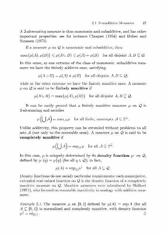
sets A (not only to the countable ones). A measure /i on Q is said to be
completely maxitive if
MM A j = sup^ /i for all A Ç 2~
In this case, /i is uniquely determined by its density function /i^ on Q,defined by fi^(q) = n{q} (for all q G <2); in fact,
fi(A) = sup^ /i^ for all ACQ.
Density functions do not satisfy particular requirements: each nonnegative,extended real-valued function on Q is the density function of a completelymaxitive measure on Q. Maxitive measures were introduced by Shilkret
(1971), who focused on countable maxitivity in analogy with additive mea¬
sures.
Example 2.1. The measure /i on [0,1] defined by fJ,(A) = sup A (for all
^4 Ç [0,1]) is normalized and completely maxitive, with density function
l_i-i =îd[0)1]. 0

28 2 Nonadditive Measures and Integrals
A possibility measure on a set Q is a completely maxitive measure
/i on Q such that /i(<2) < 1. The density function of a possibility mea¬
sure is often called "possibility distribution function", but we will use the
expression "distribution function" with another meaning. Possibility mea¬
sures were introduced by Zadeh (1978) in the context of the theory of
fuzzy sets. Other authors use different definitions: for example, for Dubois
and Prade (1988) a possibility measure is a normalized, finitely maxitive
measure.
A monotonie measure /i on Q is said to be continuous from below if
f°° \/ill An = lim fJ,(An) for all sequences A\ Ç A2 Ç ...
C Q.
V=i /
A completely maxitive measure is continuous from below, while this is in
general not true if the maxitivity is only finite. It can be easily proved that,
as in the case of additivity, a finitely maxitive measure is continuous from
below if and only if it is countably maxitive. But even complete maxitivityis not enough to assure continuity from above.
2.1.2 Derived Measures
The dual of a finite, monotonie measure /i on Q is the finite, monotonie
measure /Ion Q defined by
JI(A) = fj,(Q) - fj,(Q \ A) for all ACQ.
The equality ~ß = fi justifies the use of the term "dual".If /i is subadditive,
then /J < /i, and therefore /J is also subadditive only if /J = /i; in this case
/i is 2-alternating only if it is finitely additive.
It can be easily proved that if Q and T are sets, /i is a measure on <2,and t : Q —> T is a function, then ^oT1 is a measure on T; and if /i
satisfies one of the properties considered in Subsection 2.1.1, then so does
/iot-1. A class A4 of measures (that is, each /i G A4 is a measure on some
set <2M) is said to be closed under transformations if /i o t-1 G A4
for all /i G A4, all sets T, and all functions t : Qß —> T. For instance,the class of all normalized, completely maxitive measures is closed under
transformations.

2.1 Nonadditive Measures 29
If /i is a measure on <2, and £ : P —> P is a nondecreasing function such
that £(0) = 0, then ö o /i is a measure on Q. Among the possible proper¬
ties of /i considered in Subsection 2.1.1, the only ones that are certainlymaintained by ö o /i are monotonicity and finite maxitivity; but if £ is left-
continuous, then also complete maxitivity and continuity from below are
maintained. If c G P, and ö is the function x i—> m on P, then ö o fi = cfi
maintains all the properties of /i, except for the properties of being normal¬
ized and of being a possibility measure. A class Ai of measures is said to
be regular if c /i G Ai for all /i G Ai and all c G P, and .M is closed under
transformations. For instance, the class of all finite, nonzero, completelymaxitive measures is regular.
Example 2.2. Let /i be the completely maxitive measure on [0,1] considered
in Example 2.1, and let 5 be the function on P defined by
r, s f f if 0 < x < 1,
yx if 1 < a; < oo.
The function ö is not left-continuous at 1, and in fact the measure v = So/xon [0, 1] is finitely maxitive, but not continuous from below (and thus not
completely maxitive), since for example
limz40,x) =limJ(x) = \ < 1 = 6(1) = u[0,1).
The restriction /i\a to A Ç Q of the measure /i on Q is the measure
on A defined by h\a(B) = fJ,(B) (for all B Ç A). Since the function /i
on 2s is restricted to 2,we should write (i\2a instead of (j,\a, but the
abuse of notation in writing /i\a is coherent with the abuse of terminologycommitted by saying that /i is a measure on Q when in fact it is a function
on 2s. If /i satisfies one of the properties considered in Subsection 2.1.1,then so does /i\a, except for the properties of being normalized and of
being nonzero. A class .M of measures (each /i G .M is a measure on some
set <2M) is said to be closed under restrictions if /i\a G .M for all /i G .M
and all A Ç Qß. For instance, the class of all finite, completely maxitive
measures is closed under restrictions.

30 2 Nonadditive Measures and Integrals
2.2 Nonadditive Integrals
As with nonadditive measures, to avoid contradictions, we will use the term
"integral" to denote a very general concept, which can then be specialized
by attributes such as "additive".
Let Ai be a class of measures (each /i G Ai is a measure on some set
Qß). An integral on Ai is a function that associates a value J/d/i G P
(the integral of / with respect to /i) to each pair consisting of a measure
/i G .M and of a function / : Qß —> P, and that satisfies the followingindicator property:
/ Ia d/i = /i(A) for all /i e .M and all A Ç QM.
That is, integrals can be seen as extensions of measures: from the indicator
functions to all nonnegative, extended real-valued functions. The definition
of integrals for functions taking also negative values would pose some an¬
noying problems (since oo — oo is undefined) and will not be really needed
in the following.
Usually, a basic property of integrals is linearity, which consists of (fi¬nite) additivity:
/ (/ + (?) d/i = / / d/i + g d/i for all /i G Ai and all /, g G vQp..
and (positive) homogeneity. An integral on Ai is said to be (positively)homogeneous if
c/d/i = c / /d/i for all /i G M, all c G P, and all / G PQ,\
Note that the case with c = 0 is already implied by the indicator prop¬
erty: JO d/i = 0, since /i(0) = 0 by definition. When combined with the
indicator property, homogeneity places no restrictions on the measures
/i G Ai. By contrast, additivity implies that they are finitely additive,since Iaub = IA + Iß f°r aU disjoint A, B Ç Q^. Thus, additivity cannot
be required for an integral on nonadditive measures. But if the measures
are at least monotonie, then the following fundamental consequence of ad-

2.2 Nonadditive Integrals 31
ditivity can still be required. An integral on A4 is said to be monotonie if
f<9 => ffä»<f9ä» forah>G.Mandall/,ffGP^.
When combined with the indicator property, monotonicity implies that
the measures fi G A4 are monotonie, since Ia < Ib f°r all A Ç _B C Qß.
2.2.1 Shilkret Integral
The Shilkret integral associates the value
f-S
/d/i = sup xfi{f > x}
to each pair consisting of a monotonie measure fi on a set Q and of a
function / : Q —> P. It was introduced by Shilkret (1971) as the unique ho¬
mogeneous, countably maxitive integral on countably maxitive measures.
Before examining this aspect, we consider two other characterizations of
the Shilkret integral.
Theorem 2.3. The Shilkret integral is a homogeneous, monotonie integral
on the class of all monotonie measures.
If fi is a monotonie measure on a set Q, and f : Q —> P is a function,then
f d/i < jfa.flfor all homogeneous, monotonie integrals on classes A4 E5 fi. That is, the
Shilkret integral is the minimum of all homogeneous, monotonie integrals.
Proof. The indicator property for the Shilkret integral follows from
l*{lA>x}=l£A> i£f°<X^1' (2.1)
^LJ
[0 if 1 < x < oo.y J
Since for c G P we have x fi{c f > x} = ex' fi{f > x'} with x' =-,
the
Shilkret integral is homogeneous. It is also monotonie, since / < g implies
{/ > x} Q {9 > x}j and /i is monotonie.

32 2 Nonadditive Measures and Integrals
For all x G P we have / > xlrj>x\. Hence, a homogeneous, monotonie
integral satisfies
/ / d/i > J x I{f>xy d/i = x I{f>x} d/i = x fi{f > x}.
The desired result is obtained by taking the supremum (over all x G P) of
the right-hand side of the inequality. D
A well-known nonadditive integral was introduced by Sugeno (1974):the following generalization was considered for instance by Weber (1984),Mesiar (1995), and de Cooman (2000). A generalized Sugeno integralassociates the value
// d/i = sup m(x, fi{f > x})xef
to each pair consisting of a monotonie measure /i on a set Q and of a
function / : Q —> P, where to is a nonnegative, extended real-valued
function on P x P that is nondecreasing in both arguments. In the Sugeno
integral, the function to returns the minimum of its two arguments; if it
returns the product, we obtain the Shilkret integral.
Theorem 2.4. A generalized Sugeno integral satisfies the indicator prop¬
erty if and only if the function to fulfills the following two conditions:
m{x, 0) = 0 for all i£P, (2.2)
m(l,y)=y for ally G P. (2.3)
In this case it is a monotonie integral on the class of all monotonie mea¬
sures.
It is also homogeneous if and only if the function to returns the product
of its two arguments. That is, the Shilkret integral is the homogeneous
version of the generalized Sugeno integral.
Proof. The indicator property implies J 0 d/i = 0, and thus also condi¬
tion (2.2). If condition (2.2) holds, then from the equality (2.1) we obtain
JIa d/i = to[1,/i(A)] (since to is nondecreasing in the first argument),and therefore the indicator property is equivalent to condition (2.3). The
monotonicity of the integral can be proved in the same way as for the
Shilkret integral, since to is nondecreasing in the second argument.

2.2 Nonadditive Integrals 33
Reasoning as above, we obtain Jcl^dfi = m[c, fJ-(A)] for all c G W.
Hence, the homogeneity of the integral implies that m returns the productof its two arguments. The converse was proved in Theorem 2.3. D
Let Ai be a class of measures (each /i G Ai is a measure on some set
<2M). An integral on Ai is said to be (finitely) maxitive if
/ max{/, (?} d/i = max< / /d/i, / gdfi > for all /i G AiJ VJ J ) and all f,g eP^.
When combined with the indicator property, maxitivity implies that the
measures /i G Ai are finitely maxitive, since Iaub = niax{//i,-fB} for all
A, B Ç Qp. It can be easily proved that for an integral on a class of finitelymaxitive measures, maxitivity implies monotonicity, while the converse is
not true.
Theorem 2.5. The Shilkret integral is maxitwe on the class of all finitelymaxitwe measures.
Proof. The maxitivity of the Shilkret integral follows from
^{maxj/, g}>x} = fi({f > x} U {g > x}) = max{/i{/ > x}, fi{g > x}},
since sup and max commute. D
Shilkret (1971) noted that homogeneity and maxitivity do not char¬
acterize his integral: maxitivity must be at least countable. We are not
interested in countable maxitivity, so we proceed directly to the strongest
version of maxitivity. An integral on .M is said to be completely maxi¬
tive if
sup /d/i = sup / /d/i for all /i G .M and all T Ç P^.
fer ferJ
When combined with the indicator property, complete maxitivity impliesthat the measures /i G .M are completely maxitive, since I\ja= snl?AeA IA
for all AC 2s".
Theorem 2.6. The Shilkret integral is completely maxitwe on the class ofall completely maxitwe measures.
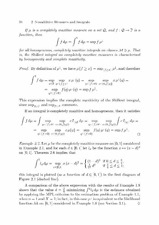
34 2 Nonadditive Measures and Integrals
If fi is a completely maxitive measure on a set Q, and f : Q
function, then* /*S
/ d/i = / / d/i = sup / nl
for all homogeneous, completely maxitive integrals on classes Ai 9 /i. That
is, the Shilkret integral on completely maxitive measures is characterized
by homogeneity and complete maxitivity.
Proof. By definition of/i^, we have /i{/ > x} = supr f>x\ /i^, and therefore
s
/ d/i = sup sup xfi^(q)= sup sup xfi^(q) =xer q{f>x} ge{/>0} xe(o,/(9)]
= sup f(q)nl(q) = sup ffi1.?e{/>0}
This expression implies the complete maxitivity of the Shilkret integral,since sup GS
and supj-Gjr commute.
If an integral is completely maxitive and homogeneous, then it satisfies
//d/i = / sup sup clrq\ dfi = sup sup / cLid/i =J q{f>0} c(0,f(q)) q {/>0} c (0,f(q)) J
= sup sup cfi{q}= sup f(q) /i ((/) = sup//i^.ge{/>0} ce(o,/(g)) ge{/>0}
Example 2.7. Let /i be the completely maxitive measure on [0, f ] consideredin Example 2.f, and for each d G [0, f] let l^ be the function n->(i- d)2on [0,1]. Theorem 2.6 implies that
ld d/i = sup x (x - d)2 = \\3
!3 ^
xe[o,i] I 27a H
4 S« S i,
this integral is plotted (as a function of d G [0,1]) in the first diagram of
Figure 2.1 (dashed line).
A comparison of the above expression with the results of Example 1.8
shows that the value d =-g minimizing Js/dd/i is the estimate obtained
by applying the MPL criterion to the estimation problem of Example 1.1,when n = 1 and X = 1; in fact, in this case /i^ is equivalent to the likelihood
function hk on [0, 1] considered in Example 1.6 (see Section 3.1). 0

2.2 Nonadditive Integrals 35
0.6^
0.4^
0.2-
0"0.2 0.4 0.6 o.: 0.2 0.4 0.6 0.:
Figure 2.1. Integrals and distribution function from Examples 2.7, 2.10, 2.11,and 2.16.
2.2.2 Invariance Properties
The properties considered so far for integrals on classes of measures applyto each measure separately, while the following fundamental invariance
involves integrals with respect to different measures. Let A4 be a class
of measures (each /i £ A4 is a measure on some set <2M) that is closed
under transformations. An integral on A4 is said to be transformation
invariant if
(/ o t) d/i = / / d(/i o t_1) for all /i G A4, all sets T,J
all / GPT, and all t G Ts".
When combined with the indicator property, transformation invariance
places no restrictions on the measures in A4. But it is a powerful property,since the integral of / with respect to /i can be written as
(idpOf)dfi= idpd(p,of x)/d/i
That is, a transformation invariant integral on A4 can be seen as a function
on the subset of A4 consisting of the measures on P.
Theorem 2.8. All transformation invariant integrals on classes A4 ofmeasures (A4 closed under transformations) have the following property:
if fJ, G A4 is a monotonie, subadditive measure on a set Q; the nonempty

36 2 Nonadditive Measures and Integrals
set ACQ satisfies fi(Q \ A) = 0, and /, g : Q —> P are functions, then
/"U cm,
/ /d/i = / /Ud/^U,
and in particular
/ = g o.e. [/i] => / /d/i = / ffd/i.
Proof. As noted in Subsection 2.1.1, we have /i(ß) = A*(-B H A) for all
B Ç Q (since /i is monotonie and subadditive, and fi(Q \ A) =0). Hence,if T is a set, and t : Q —> T is a function, then /i o t_1 = /i|^ o (t|^)_1,since for all C Ç T we have
m[*_1(C0] = m[*_1(C) n A] = m^U)-1^)] = MUKtU)-1^)].
This result implies the first two statements of the theorem. To conclude
that /i\a C Ai, it suffices to choose a function t : Q —> A such that
t|^4 = idj±. we obtain /iot-1 = /i|^, and .M is closed under transformations.
To conclude that J f d/i = J f\A d/i| Aj it suffices to choose t = f: we obtain
/i o /_1 = /i|^ o (/|a)_1, and the integral is transformation invariant.
The last statement of the theorem follows from the first two, except for
the case with {/ = g} = 0. In this case /i is the zero measure on <2, and
therefore J /d/i = 0 for all /, since /io/_1 = /i o (70)_1. D
Let /i be a monotonie measure on a set <2, and let / : <2 —> P be a
function. The essential supremum of / with respect to /i is the value
essM sup / = inf{x G P : /i{/ > x} = 0}.
When /i is also subadditive, we can say that essM sup / is the infimum of
all x G P such that f < x a.e. [/i]. In particular, it can be easily provedthat if /i is completely maxitive, then essM sup/ = supr i>0i /.
The rectangular integral associates the value
/ / d/i = (essM sup /) /i{/ > 0}
to each pair consisting of a monotonie measure /i on a set <2 and of a func¬
tion / : Q —> P. When /i is completely maxitive, the rectangular integral of
/ with respect to /i can be written as Jr/d/i = (supr i>0i /) (supr<>0i /i^).

2.2 Nonadditive Integrals 37
Theorem 2.9. The rectangular integral is a transformation invariant, ho¬
mogeneous, monotonie integral on the class of all monotonie measures.
If fi is a monotonie, subadditive measure on a set Q, and f : Q —> P is
a function, then
r r
f d/i < / / d/i
for all transformation invariant, homogeneous, monotonie integrals on
classes Ai E5 /i. That is, the rectangular integral on monotonie, subadditive
measures is the maximum of all transformation invariant, homogeneous,monotonie integrals.
Proof. The rectangular integral on monotonie measures satisfies the indica¬
tor property, monotonicity, and homogeneity, since the essential supremum
satisfies'
0 if fi(A) = 0,eSSMSup/A-n ifM(A)>0)
f < g => essM sup / < essM sup 9,
essM sup c f = cessM sup / for all c G P.
The rectangular integral is transformation invariant, since for all A Ç P
M{/ot GA} = [MoCfot)-1]^) = [(MorVr1]^) = (Mot"1)!/ G A}.
Let /i be a monotonie, subadditive measure. If essM sup / is infinite, then
/ / d/i = oo. If essM sup / is finite, then for all x G (essM sup /, oo) we have
/ = min{/, x} a.e. [/i]. Hence, a transformation invariant, homogeneous,monotonie integral satisfies
//d/i= / min{/, x} d/i < / a;/{/>o} d/i = x/i{/ > 0}.
The desired result is obtained by letting x tend to ess^sup/. D
Example 2.10. Let /i and /^ be the measure and the functions on [0, f] de¬
fined in Examples 2.f and 2.7, respectively. Since /i is completely maxitive,
'
f (1 - d)2 if0<d<i,/dd/i= (sup(01]/d)(sup[01]Ud}îd[0)1]) = j^2 ifl<d<l-
this integral is plotted (as a function of d G [0,1]) in the first diagramof Figure 2.f (dotted line). Since Js/rfd/i = Jr/^d/i for all d G [0, ^] (see

38 2 Nonadditive Measures and Integrals
Example 2.7), Theorems 2.3 and 2.9 imply that J/^d/i = (1 — d)2 for
all d G [0, i] and all transformation invariant, homogeneous, monotonie
integrals on classes Ai 3 /i. 0
Theorem 2.8 states that for a transformation invariant integral on
Ai, if /i G Al is a monotonie, subadditive measure on a set <2, and
/ : Q —> P is a function, then J/d/i = J/l^d/il^ when AC Q is a
nonempty set such that /a\q\a = 0. The reciprocal invariance property
is that J"/d/i = J/l^d/il^ when AC Q is a nonempty set such that
Î\q\A = 0- But there is a difference: if A = {A Ç Q : /i|g\ ^4= 0}, then
in general /«|g\n.4. 7^ 0 (we are sure that /«|g\n.4. = 0 if /i is also contin¬
uous from below); while if A = {A Ç Q : /|g\4 = 0}, then /|g\n^i = 0,since f]A = {/ > 0}, the support of /. That is, the reciprocal invariance
property can simply be stated as follows.
Let Af be a class of measures (each /i £ Af is a measure on some
set <2M) that is closed under restrictions. An integral on Af is said to be
support-based if
/ /d/i = / /|{/>o}d/i|{/>o} for all /i G AÎ and all / G PQm.
This property places no restrictions on the measures in Af, since for indica¬
tor functions / = Ia it is implied by the indicator property. For instance,the rectangular integral is support-based on the class of all monotonie
measures, since it depends only on /i{/ > 0} and on /i{/ > x} for a; G P.
2.2.3 Regular Integrals
Let X and Y be nonnegative random variables on a probability space with
probability measure P. Usually, Y is said to (first-order) stochasticallydominate X (with respect to P) if
P{X <x}> P{Y < x} for all a; G P.
Since a probability measure is finitely additive, finite, and continuous (fromboth above and below), this condition is equivalent to the following one:
P{X >x}< P{Y > x} for all a; G P.
Let /i be a monotonie measure on a set Q, and let / : Q —> P be a
function. The (decreasing) distribution function of / with respect to /i

2.2 Nonadditive Integrals 39
is the function x i—> /i{/ > x} on P; it shall be denoted by /i{/ > •}. Let Al
be a class of monotonie measures (each /i G AI is a measure on some set
Qß). An integral on AI is said to respect distributional dominance if
/•*{/ > •} < v{g > } =^ / /d/i < / ffdi/ for all /i, ^ G Al,•^ J
all / G Ps", and all j6Ps».
If /i and v are probability measures, then this property corresponds to
respecting (first-order) stochastic dominance with respect to the product
probability measure fi x is.
Example 2.11. Let /i and Id be the measure and the functions on [0, 1]defined in Examples 2.1 and 2.7, respectively. For each d G [0,1], the
distribution function of Id with respect to /i satisfies
(1 if 0<x< (1-d)2,fJ>{ld > x} = < d — ^Jx if (1 — d)2 < x < d2,
[ 0 if max{d2, (1 - d)2} < x < oo;
the function x i—> /i{/4 > x} is plotted in the second diagram of Figure 2.1
for x G [0,1] (solid line).
Let v = ö o n be the finitely maxitive measure on [0,1] considered in
Example 2.2. Since
Hh >-} = So fi{h >}< I{0} + \ I(o,i] = mU{1} > •},
all integrals respecting distributional dominance on classes AI E5 /i, v sat¬
isfy Jlidv < flri-idfj, =
g-This is not the case for the rectangular
integral: in fact, for all d G [0,1]
Id dis = (ess^ sup ld) ö(ji{ld > 0}) = / ld d/i = max{d , (1 - d) },
since f^-jO} = {0} and 0(1) = 1 (see Example 2.10). 0
The property of respecting distributional dominance strengthens mono-
tonicity, implying in particular also monotonicity with respect to measures;
but the next theorem states that at least for integrals on the class of all
completely maxitive measures, it is equivalent to monotonicity, providedthat the invariance properties considered in Subsection 2.2.2 are satisfied.
The term "bimonotonicity" shall designate monotonicity with respect to

40 2 Nonadditive Measures and Integrals
both functions and measures, and analogously, the term "bihomogeneity"shall designate the double homogeneity. An integral on A4 is said to be
bimonotonic if it is monotonie and
/i <v => / /d/i < / / dv for all /i, v G A4 such that Qß = Qv,J J
and all / G Ps".
Theorem 2.12. Let A4 be a class of monotonie measures. All integrals on
A4 respecting distributional dominance are bimonotonic, and they are also
transformation invariant if A4 is closed under transformations.
All transformation invariant, bimonotonic integrals on the class of all
completely maxitive measures respect distributional dominance.
All support-based, transformation invariant, monotonie integrals on the
class of all completely maxitive measures respect distributional dominance.
Proof. An integral respecting distributional dominance is bimonotonic and
transformation invariant, since for all x G P we have
/ < 9 => /"{/ >x}< n{g > x},
H<V =*> fj,{f >x}< v{f > x},
fi{fot>x} = (fiot-1){f>x}.
If /i is a completely maxitive measure and the integral is transformation
invariant, then J f d/i depends only on the function (/io/-1)^ on P. Let /'and /i' be respectively the function and the completely maxitive measure
on Q = P2 x {0,1} defined by
/>(..».,)-., a„d (,T(.,»,«)-{!|* ^t»^'^Then J f d/i = J f d/i', because for all x G P
\tx' o (/r ¥(*) = suptf,)-^^')* = (m° r1)1^).
If v is a completely maxitive measure, then for all x G P
fi{f > x} < v{g > x} O sup[Xi0o](fio f-1)1 < sup[xoo](v o g'1)1.
In this case, for all (x,y) G P2, if y < (/io/_1)^(i), then there is an x' > x
such that y < {y o g^1)-1^'): define g'(x,y, 1) = x' and g'(x,y, 0) = x. We

2.2 Nonadditive Integrals 41
obtain a function g' on Q such that /' < g1, and therefore, if the integral is
monotonie, then J f d/i' < J g' d/i'. Now, let is' be the completely maxitive
measure on Q defined by
y if y < (/i o f~1)^(x) and z = 1,
(z/)^(a;, y, z) = ^ y if y < (z^ o g-1)^^) and z = 0,0 otherwise.
Since /i' < z/, if the integral is bimonotonic, then J g' d/i' < J g' dis'.
To obtain the second statement of the theorem, it suffices to show that
f g' dis' = J g dis; that is, it suffices to show that for all i'éP
[ls'o(g')-l}ï(X')=SuP{g,)-1{x,}(ls'y = (isog-l)ï(X').
The second equality holds, since if g'(x,y, 1) = x' and y < (/i o /_1)^(a;),then y < (is o g~ *) J- (x').
To obtain the third statement of the theorem, it suffices to show that
if the integral is support-based, then the second equality of
/dM= //'dM'= ff'dis'< Ig'dv'= fgdis
holds, since the other two equalities have already been proved, and the
inequality is implied by monotonicity. But if the integral is support-based,then the second equality is implied by (m')I{/'>0} = (^OI-T/'X)}; which
holds since it is equivalent to [(/u')^]l{/'>0} = [(^')^]l{/'>0}-
Let Ai be a regular class of monotonie measures (each /i G Ai is a
measure on some set <2M). An integral on .M is said to be bihomogeneousif it is homogeneous and
/ fd(c/i) = c / /d/i for all /i G M, all c G P, and all / G PQ".
An integral on .M is said to be regular if it is bihomogeneous and it
respects distributional dominance.
The next theorem states that a regular integral on .M corresponds to
a functional on the set
VT(M) = {n{f >}: fiGM, / G PQ"}

42 2 Nonadditive Measures and Integrals
of all distribution functions generated by the measures in A4. Since these
measures are monotonie, DJ7(A4) is a subset of
Aflf = \(p G P : (p is nonincreasingj.
In general DJ7(A4) is a proper subset of AfT^: the class A4 is said to
be exhaustive if the two sets are equal; for example, the class of all
completely maxitive measures is exhaustive. In order to state the theorem,
we need some additional definitions.
Let Q be a set, and let J7 be a subset of Ps. A functional V : J7 —> P
is said to be monotonie if
f<9 => V(f)<V(g) for all/, g G T.
A functional V : J7 —> P is said to be homogeneous if
V(cf) = cV(f) for all / G T and all c G P such that cfGJ7.
For example, if an integral on A4 is monotonie and homogeneous, then for
each measure /i G A4 the functional / i—> J / d/i on Ps>* is monotonie and
homogeneous. If cp : P —> P is a function, and c G_P, then y(-) denotes the
function ï k ip(^) on P. Let * be a subset of Pp. A functional F : * —> P
is said to be bihomogeneous if it is homogeneous and
F[cp(-)] = cF(cp) for all ip G * and all c G P such that y>(-) G *.
Note that if if G ©^(.M) and c G P, then cep, cp(-) G VT(M). A func¬
tional _F : ^ —> P is said to be »-independent, for an x G P, if
^lp\{x} = ^lp\{x} =^ F(ip)=F(iP) for all <^,V> G *.
A functional F : Aflf —> P is said to be calibrated if
F(I[0,i]+yI{0}) = 1 for all y G P.
Note that a O-independent functional F on Aflf is calibrated if and onlyif F(I\nt\]) = 1. The left-continuous version of a function 93 G Aflf is the
function ip~ G .A/ïp defined by
ip~ (x) = infjo x) if for all a; G P.
It can be easily proved that ip~ is left-continuous, and that (tp~)~ = tp~
Note that ip~ (0) =00.

2.2 Nonadditive Integrals 43
Theorem 2.13. Let A4 be a regular class of monotonie measures. An in¬
tegral on A4 is regular if and only if the functional
F:p{f>-}» J /dM
on T>T(A4) is well-defined, monotonie, and bihomogeneous. In this case,
the functional F is x-independent for all x G (0, oo]; if it is also 0-
mdependent and A4 is closed under restrictions, then the integral is
support-based.
Conversely, if F : Aflf —> P is a calibrated, bihomogeneous, monotonie
functional, then the equality
|/dM = F(M{/>-})
defines a regular integral on the class of all monotonie measures. The
integral is support-based if and only if F is 0-mdependent. In this case,
F{}p) = F((p~) for all ip G J\fZp, and in particular, denoting by fi{f > •}the function x i—> /i{/ > x} on W, the integral can be written also as
|/dM = F(M{/>-}).
Proof. An integral on A4 respects distributional dominance if and only if
the functional F is well-defined and monotonie. In this case, the integralis bihomogeneous if and only if F is bihomogeneous. If ip\f\ rx\
= V'lwfxifor an x G P, then for all x' GW\ {x} and all c G (1, oo) we have
4>(x) < ^(f ) = ¥>(f ) and rp(x')=<p(x')<<p(^).
Hence F(tp) < F[ip(-)] = cF(ip) holds when F is monotonie and bihomo¬
geneous: by letting c tend to 1 we obtain the inequality F(tp) < F(ip), and
thus, by symmetry, the x-independence. To prove the oo-independence,consider the following consequence of Theorem 2.3:
lim /i{/ >x}>0 => / /d/i > / /d/i = oo.
xToo J J
If y|[o,oo) = V>l[o,°°)' then limxToo^ = limxTooV>- If this limit is 0, then
ip = tp; otherwise F(ip) = F(ip) = oo. If F is 0-independent, then the

44 2 Nonadditive Measures and Integrals
integral is support-based, since
(mI{/>0}{/|{/>0} > -})l(0,oo] = (Mi/ > -})l(0,oo]-
The integral defined by a calibrated, bihomogeneous, monotonie func¬
tional F : J\flp —> P satisfies the indicator property, since if fJ,(A) G P,then using bihomogeneity and calibration we obtain
J IA dM = F(p{IA > •})=F[p(i)I(o,1]+M(eM)/{o}]=#)>
and using limits and nionotonicity we obtain the same result also for
fJ-(A) G {0,oo}. We have already proved that the integral is regular, that
F is oo-independent, and that the integral is support-based when F is 0-
independent. Now assume that the integral is support-based, and consider
a function cp G J\fX^. To prove the O-independence of F, it suffices to show
that defining ip' = (p I(0,oo] + (suP(o,oo] ^K{0},jwe obtain F(ip) = F(ip').Let /i be the completely maxitive measure on P defined by /i^ = ip. Since
cp is nonincreasing, we have fi{idf > •} = cp, and therefore, since the inte¬
gral is support-based and {id^ > 0} = (0, 00], to obtain the desired result
it suffices to show that /u|(o)0o]{*^pl(o,oo] > x} = (y9'(a;) f°r aU x GV. This
equality clearly holds for positive x, and for i = 0we have
mI(o,oo]{^fI(o,oo] > 0} = /i(0, 00] = sup(0)Oo] (p = ip'(0).
Defining cp" = <pl(n 06) + <y9~ -^{0,00}) we obtain ip~ (x) < <p"{-) for all x G P
and all c G (f,oo), and therefore
F(<p")=F(<p)<F(<p-)<cF(<p").
The equality F(ip) = F{tp~) is obtained by letting c tend to f. The last
statement of the theorem follows from this result, because the equality
(/•*{/ > •})" = (/•*{/ > •})" is obtained from the inequalities
/"{/ > x} < /i{/ >x}< inf[0jX) /i{/ > •}
by considering the left-continuous versions of the corresponding functions
of x G P:
(M{/ > •})" < (M{/ > •})" < [(M{/ > •})"]- = (M{/ > •})". n

2.2 Nonadditive Integrals 45
Many authors (for example Denneberg, 1994) define the distribution
function as /i{/ > •}. Theorem 2.13 assures us that if a support-based,
regular integral on an exhaustive class of monotonie measures is defined
by a functional F on Wîp, then it is not affected by the choice between
/"{/ > •} and /"{/ > •}•
Theorem 2.13 implies that the Shilkret integral is regular and support-
based on the class of all monotonie measures, since it corresponds to the 0-
independent, bihomogeneous, monotonie functional _Fs : MXf —> IP defined
by
Fs(ip) = supxip(x) for all cp G J\fl^.
By contrast, the rectangular integral is not regular on the class of all
monotonie measures, because the functional F is not well-defined, since in
general /i{/ > 0} is not determined by /i{/ > •}. But if /i is continuous
from below, then /i{/ > 0} = supp /i{/ > •}, and therefore the rectangular
integral is regular and support-based on the class of all monotonie measures
that are continuous from below, since it correspond to the 0-independent,
bihomogeneous, monotonie functional Fr : J\fX^ —> P defined by
Fr(ip) = mf{ip = 0} supp cp for all cp G J\fX^.
The regularized rectangular integral is the integral defined by FT
on the class of all monotonie measures: it associates the value
r
/ d/i = (essM sup /) supP fi{f > }
to each pair consisting of a monotonie measure /i on a set Q and of a func¬
tion / : Q —> P. The regularized rectangular integral is thus regular and
support-based on the class of all monotonie measures, and it correspondsto the rectangular integral on the class of all monotonie measures that are
continuous from below.
Example 2.14- Let /i, u, 8, and l& be the measures and the functions defined
in Examples 2.1, 2.2, and 2.7. For all d G [0, 1)
/r/>r irr
Id d/i = max{d , (1 — d) }= / 14 <lv = / ldà.i>;
the first equality holds because /i is completely maxitive (and thus contin¬
uous from below), the second and third ones were proved in Examples 2.10

46 2 Nonadditive Measures and Integrals
and 2.11, and the last one is implied by supp v{ld > •} = 1 = v\ld > 0}.When d = 1, the first three equalities still hold, but the last one does not:
Jrr/i <lv =g,
since supP v{l\ > •} = ^. In fact, Theorem 2.13 implies that
all support-based, regular integrals on exhaustive classes Ai 3 /j,,u satisfy
fhdv =t; J/id/i, because u{h > -}|(o,oo] = \ n{h > -}|(o,oo]- 0
Theorem 2.15. If fi is a monotonie measure on a set Q, and f : Q —> P
is a function, then
S /> irr
/ d/i < / / d/i < / / d/i
/or o// regular integrals on classes Ai 9 /i. That is, the Shilkret integraland the regularized rectangular integral are respectively the minimum and
the maximum of all regular integrals.
In particular, if A Ç Q is a nonempty set, and /i is the completelymaxitwe measure on Q defined by ^ = Ia, then
/ d/i = supA / and / / d/i = infA f
for all regular integrals on classes Ai 9 /i, ~ß.
Proof. Since a regular integral is monotonie and homogeneous, the first
inequality was proved in Theorem 2.3. If y = supp/i{/ > •} G {0,oo},then the second inequality clearly holds. If y G P, then there is an x G P
such that y' = /i{/ > x} G (0,y]. Let g = (essM sup/) 7(/>x} and v = -^ /i.
Since /i{/ > •} < /i(ß) J{0} + 2//(o.ess^sup/] < ^{ff > •}, we have
//•rrgdz^ = (essM sup /) za[/ >x}= /d/i.
Consider now the case with /i^ = i^. If x < sup^ /, then /i{/ > x} = 1;while if x > sup^ /, then /i{/ > x} = 0. Hence we have
/S/>TT
/ d/i = / / d/i = supA /.
The last equality of the theorem can be obtained in the same way: if
x < infa f, then /!{/ > x} = 1 — /i{/ < x} = 1; while if x > infa /, then
ß{f > x} = 1 - /i{/ < x} = 0. D

2.2 Nonadditive Integrals 47
The second part of Theorem 2.15 justifies the use of the expression
"density function" for /i^ (where /i is a completely maxitive measure on
a set <2) when regular integrals are considered, since /i^ is the "Radon-
Nikodym derivative" of /i with respect to the completely maxitive measure
i/onQ defined by v^ = 1. In fact, for all regular integrals on classes A4 9 v
we have
/ p} dv = p^ Ia d-is = sup/i^ Ia = n(A) for all ACQ,
where the left-hand side of the first equality is the usual abbreviation for
the right-hand side.
Geometrically, if we consider the rectangles lying in the first quadrantof the (extended) Cartesian plane and having two sides on the coordi¬
nate axes, then _Fs (<y?) is the area of the largest rectangle lying under the
graph of cp (if such a rectangle exists), while Fr(p) is the area of the small¬
est rectangle containing the portion of the graph of p not lying on the
coordinate axes. From this geometrical standpoint, the most natural cali¬
brated, bihomogeneous, monotonie functional on J\fX^ is probably the one
assigning to each function the area under its graph. That is, the functional
Fc : Afl¥ -> P defined by
/>oo
Fc((f) = / (f(x) dx for all ip G Aflf,Jo
where the right-hand side of the equality is the Lebesgue integral of ip\f(with respect to the Lebesgue measure on P: since cp is nonincreasing, it is
Borel measurable), which corresponds to the improper Riemann integralwhen p\f is finite (in this case, cp is Riemann integrable on every bounded,closed interval i" C IP, since cp\j is bounded and nonincreasing), while the
integral is infinite when p\f is not finite.
The Choquet integral is the integral defined by Fq on the class of
all monotonie measures: it associates the value
C />oo
/d/i= / /i{/ > x} dx
to each pair consisting of a monotonie measure /i on a set Q and of a
function / : Q —> P. The Choquet integral is a well-known nonadditive
integral, which was introduced by Choquet (1954) and then developed by
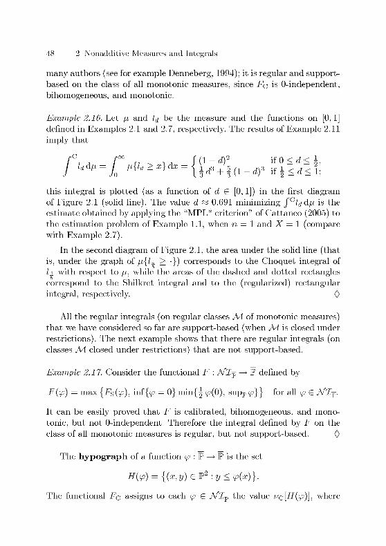
48 2 Nonadditive Measures and Integrals
many authors (see for example Denneberg, 1994); it is regular and support-
based on the class of all monotonie measures, since Fq is O-independent,
bihomogeneous, and monotonie.
Example 2.16. Let /i and l& be the measure and the functions on [0, 1]defined in Examples 2.1 and 2.7, respectively. The results of Example 2.11
imply that
J lddv = jo V{ld>x}dx=l[1_d3 + 5_{1_d)3 ifi<d<21;
this integral is plotted (as a function of d G [0,1]) in the first diagramof Figure 2.1 (solid line). The value d fa 0.691 minimizing Jclddfi is the
estimate obtained by applying the "MPL* criterion" of Cattaneo (2005) to
the estimation problem of Example 1.1, when n = 1 and X = 1 (comparewith Example 2.7).
In the second diagram of Figure 2.1, the area under the solid line (thatis, under the graph of fi{U > •}) corresponds to the Choquet integral of
14. with respect to /i, while the areas of the dashed and dotted rectangles
correspond to the Shilkret integral and to the (regularized) rectangular
integral, respectively. 0
All the regular integrals (on regular classes Ai of monotonie measures)that we have considered so far are support-based (when Ai is closed under
restrictions). The next example shows that there are regular integrals (onclasses .M closed under restrictions) that are not support-based.
Example 2.17. Consider the functional F : J\fX^ —> P defined by
F(ip) = max {Fs(tp), inî{tp = 0} minj^ y(0), supP ip}j for all ip G J\flp.
It can be easily proved that F is calibrated, bihomogeneous, and mono-
tonic, but not 0-independent. Therefore the integral defined by F on the
class of all monotonie measures is regular, but not support-based. 0
The hypograph of a function cp : W —> P is the set
H(p) = {(x,y)eW:y<p(x)}.
The functional Fq assigns to each cp G J\fX^ the value uc[H{ip)\, where

2.2 Nonadditive Integrals 49
vq is the countably additive measure on (the Borel sets of) P2 such that
z^c(P2 \ IP2) = 0, and vc\v2 is the Lebesgue measure on P2. It can be
easily proved that, in analogy with the Choquet integral, each integral
respecting distributional dominance on some class of monotonie measures
can be represented by some (not unique) monotonie measure v on P2, in
the sense that it can be written as
Jfdp = v[H(p{f >•})]. (2.4)
For example, the Shilkret integral and the regularized rectangular integral
are respectively represented by the measures z^s and vT on P2 defined by
vs (^4) = sup x y and vT (A) = I sup x 11 sup y I,(x,y)A \(x,y)£AnP2 J\(x,y)An¥2 )
for all ACW2.
Conversely, if a monotonie measure v on (the Borel sets of) P2 satisfies
is[H(yI[0il]+y'I{0})]=y for all y,y' G P, (2.5)
then the equality (2.4) defines an integral respecting distributional domi¬
nance on the class of all monotonie measures, since the indicator propertyis implied by the condition (2.5). For instance, with the measure v on P2
defined by
u(A) =
supAn(-Pxp) m for all A Ç P2,
where to is a nonnegative, extended real-valued function on P x P that
is nondecreasing in both arguments and that fulfills the conditions (2.2)and (2.3), we obtain the generalized Sugeno integral corresponding to
to. Imaoka (1997) introduced a class of integrals obtained in this way
using a particular kind of countably additive measures. Thanks to the
Carathéodory extension theorem, it can be proved that the Choquet inte¬
gral is the only homogeneous integral that can be represented by a count¬
ably additive measure on (the Borel sets of) P2, although this measure
is not unique. That is, if we call "generalized Imaoka integrals" the in¬
tegrals representable by countably additive measures on (the Borel sets
of) P2, then what distinguishes the Choquet integral among the general¬ized Imaoka integrals is the homogeneity, which is also the distinguishingfeature of the Shilkret integral among the generalized Sugeno integrals.

50 2 Nonadditive Measures and Integrals
The left-continuous pseudo-inverse of a function cp G AfT¥ is the func¬
tion Lpr"J G AfTp defined by
tp" (x) = sup{<y9 > x} = mf{ip < x} for all i£P.
It can be easily proved that (<ßr")~ = tpr"'', and that H(ip"J) is the mirror
image of H((p~) with respect to the diagonal y = x of P2. Hence, if a
support-based, regular integral on the class of all monotonie measures is
represented by a measure on (the Borel sets of) P2 that is invariant with
respect to the reflection about the diagonal y = x, then the correspondingfunctional F on Aflf satisfies
F(<p) = F(<p~) = v\H(<p-)] = v[H(<p~)] = F(<p~) for all <p G AfX¥.
A regular integral on an exhaustive, regular class of monotonie measures
is said to be symmetric if the corresponding functional F : AfT^ —> P
satisfies
F(tp) = F(ipr~J) for all ip G Afl¥.
The Choquet integral, the Shilkret integral, and the regularized rectangular
integral are symmetric, since the measures isc, vs, and vr on (the Borel sets
of) P2 are invariant with respect to the reflection about the diagonal y = x.
The next theorem illustrates an interesting consequence of the symmetry
of an integral.
Theorem 2.18. All symmetric, regular integrals on exhaustive, regularclasses A4 of monotonie measures are support-based (if A4 is closed under
restrictions) and have the following property: if fi G A4 is a completelymaxitive measure on a set Q, and f : Q —> P is a function, then, de¬
noting by F the functional on AfT¥ corresponding to the integral, and by
supr i y 1 / the function x i—> suprßi>x\ f on W, we have
/ fdfi = F(sup{ßly }f);
moreover, if fi is finite, then denoting by inf{ui>^(g)- }/ the functionx i—> inf(„i>„(Q)_xi / on W, we have also
fdß = F(/[0jM(Q)] inf{Mi>M(Q)_ } /)

2.2 Nonadditive Integrals 51
Proof. The integral is support-based, because <y2|(o)0o] = V'lfUoo] implies
Lpr"J = i\)r"J, and therefore F is 0-independent. If we define cp = fi{f > •}and ip = supr i> i /, and we prove that cp~ = ip~, then we can use
Theorem 2.13 to obtain the desired result
/dM = F(<p) = F(y>~) = F(i,-) = F(i>).
The equality cp~ = ip~ can be proved as follows: for all x,y G P we have
<P~(x)<y O Vy'G(y,oo] fi{f > y'} < x
^ Vy'G(y,oo] 3x'g[0,x) {/ > y'} (~l {^ > x'} = 0
^ Vy'G(y,oo] 3x'g[0,x) sup(Ati>x,} / < y'
•<=> ip~ (x) < y.
The last statement of the theorem can be proved in a similar way:
defining ip = Jl{f > •} and ip = I[o,ß(Q)] mi{ßiy^Q)_ y /, it suffices to
show that Lpr"J = ip~. This can be done as follows: for all x, y G P we have
<p~(x)>y o 3y'e(y,oo] ~ß{f >y'}>x
^ 3y'G(y,co] /i{/ < y'} < /i(Q) - x
<^> 3y'£(y, oo] Vx'g[0,x){/ < 2/'} n {m4 > A*(ö) - x'} = 0 and x < /i(Q)
<^> 3y'£(y, oo] Vx'g[0,x)
^o.mCS)]^') inf{Mi>M(Q)-x'} / > V'
& ip~{x)>y. D
2.2.4 Subadditivity
Let Ai be a class of measures (each /i G Af is a measure on some set
Qß). We have seen that if some measures in Ai are not finitely additive,then an integral on Ai cannot be additive; but if the measures in Ai are
subadditive, then we have at least
/ (Ia + Ib) d/i < / Ia d/i + Ib d/i for all fi G Ai'
J Jand all disjoint A, B Ç QM.

52 2 Nonadditive Measures and Integrals
A quasi-subadditive integral extends this property to all pairs of functions
/, g G P^ with disjoint supports (that is, {/ > 0} n {g > 0} = 0). An
integral on A4 is said to be quasi-subadditive if
/ (f+g) d/i < / / d/i+ / g d/i for all /i e .M
and all /, (? G PS,J with disjoint supports.
When combined with the indicator property, quasi-subadditivity impliesthat the measures /i G .M are subadditive, since Iaub = Ia + Ib for all
disjoint A, B Ç Qß. A functional F : AfFp —> P is said to be subadditive if
i% + ip) < F((f) + F{ip) for all ip, V G A/"%.
Theorem 2.19. j4// regular integrals on exhaustive, regular classes A4 of
subadditive, monotonie measures have the following property: if the cor¬
responding functional on AfFp is subadditive, then the integral is support-
based (if A4 is closed under restrictions) and quasi-subadditive.
Proof. The integral is support-based, since the corresponding functional
F on AfFp is 0-independent. In fact, if <y2|(o)0o] = V'lfUoo] and y(0) < ^(0),then (tp — ip) G AfFp, and so there are a measure /i G A4 and a function / on
<2M such that (ïp—ip) = fi{f > •}; but this implies that (ip—cp) = fi{I0 > •},and therefore
F{ip) < F(il>) < F{ip) + F(il> -ip)= F{ip) + j 70 dM = F {ip).
The integral is quasi-subadditive, because if/ and g have disjoint supports,
then {/ + g > x} = {/ > x} U {g > x}, and therefore
(/ + g) dM < F{p{f > •} + n{g > •}) < J f dM + J g dM,
since /i is subadditive. D
Theorem 2.19 implies that the Shilkret integral and the Choquet inte¬
gral are quasi-subadditive on the class of all monotonie, subadditive mea¬
sures, since the functionals Fg and Fc are subadditive. By contrast, the
next example shows that the regularized rectangular integral can be quasi-subadditive only on very limited classes of monotonie, subadditive mea¬
sures.

2.2 Nonadditive Integrals 53
Example 2.20. Let /i be a monotonie, subadditive measure on a set Q. If
there are two disjoint sets A, B C Q such that 0 < fi(A) < \ fi(B) < oo,
then the two functions / = fi(A) Iß and g = fi(B) Ia on Q have disjoint
supports, but
/TT/>TT />TT
(f + g)dfi = fi(AUB)fi(B)>2fi(A)fi(B) = fdfi + gdfi.
0
In fact, as stated by the next two theorems, the Shilkret integral and
the Choquet integral satisfy the following stronger property on suitable
classes of monotonie, subadditive measures. An integral on M. is said to
be subadditive if
(f + g) dfi < f dfi + g dfi for all fi G M and all /, g G Va^.
Theorem 2.21. The Shilkret integral is subadditive on a class of mono-
tonic measures if and only if these are finitely maxitive.
Proof. For the "if part, we can adapt the proof of Shilkret (1971) to the
finitely maxitive measures. It suffices to show
/s/*S
f dfi + / gdfi for all x G P,
since then the desired result is obtained by taking the supremum (over all
x G P) of the left-hand side of the inequality. If one of the two integralsof the right-hand side is infinite, the inequality clearly holds. If both are
finite, observe that
{f + 9>x} Ç {/> Xx}U{g> (1- X)x} for all AG (0,1).
If one of the two integrals is 0, say J gdfi = 0, then fi{g > x'} = 0 for all
x' G P, and therefore
x fi{f + g > x} = sup Xxfi{f + g>x}< sup Xxfi{f>Xx}<Ae(o,i) Ae(o,i)
/'S /'S /'S
< f dfi = fdfi+ gdfi.

54 2 Nonadditive Measures and Integrals
If both the integrals are positive and finite, then setting
JS/dMPfdfi + pgdfi
we obtain
x fi {/ + g > x} < max{i/i{/ > Ai}, x fi{g > (1 — A) x}} <
< maxj - / / d;U, —— / g d^, \ = / f dji + J gdji.
For the "only if part, assume that the Shilkret integral is subadditive
on a class Ai of monotonie measures, let /i G .M be a measure on <2, and
let A, B Ç Q be two disjoint sets. We have
(fi(AUB) ifO<x</i(A),n{n{A UB)IA+ fi(A) IB>x} = < h\ä) if fi(A) <x< fi(A U B),
[0 if fi(AUB) <x <oo;
and therefore
/ [M(A UB)/U M(A) JB] d/i = fj,(A U B) fj,(A).
From this result and the equality
H{A U B) Iaub = HA UB)IA + fjL(A) IB] + HA U B) IB - ii(A) IB],
using the subadditivity of the Shilkret integral and the property
/ clc d/i = c/i(C) for all c G P and all C Ç Q,
we obtain the inequality
H(A U B)2 < fi(A U B) n(A) + HA US)- n(A)] n(B),
which is equivalent to
HA US)- /i(A)] HA US)- /i(B)] < o.
Since both factors of the left-hand side of this inequality are nonnegative,one of them must vanish; that is, fi(A U B) = max{/i(A), fi(B)}. D

2.2 Nonadditive Integrals 55
The next theorem is proved for example in Denneberg (1994, Chap¬ter 6).
Theorem 2.22. The Choquet integral is subadditive on a class of mono¬
tonie measures if and only if these are 2-alternating.
2.2.5 Continuity
There is a correspondence between convergence theorems for regular inte¬
grals on regular classes A4 of monotonie measures, and continuity prop¬
erties of the corresponding functionals on DJ7(A4). The next one is the
convergence theorem corresponding to the continuity property implied by
monotonicity and bihomogeneity.
Theorem 2.23. All regular integrals on regular classes A4 of monotonie
measures have the following property: if the sequence /ii,/i2,... G A4 ofmeasures on a set Q converges uniformly to the measure fi G A4 on Q;the sequence /1; /2,... : Q —> P of functions converges uniformly to the
function f : Q —> W, and one of the following two conditions is fulfilled
lim supp/i„{/„ > •} = supp/u{/ > •} < oo
^°°
(2 6)and lim ess„ sup fn = ess„ sup / < oo,
n^oon
fJ-(Q) and sup/ are finite, and the integral is quasi-subadditive, (2.7)
then
n^oo
lim / /„d/i„ = / /d/i.
Proof. Define
f = /•*{/ > •}> fn = Vn{fn >}, « = SUpp (f, an = SUpp (fn,
b = essM sup / = supp cp~, and bn = essMn sup fn = supp(<y2„)^.
First assume that condition (2.6) is fulfilled: then
e„ = max{||/„ - /||, \\fin - fi\\, \an - a\, \bn - b\, ±}
is positive, and limn^^s-n = 0. If a = 0 or b = 0, then J /d/i = 0, and
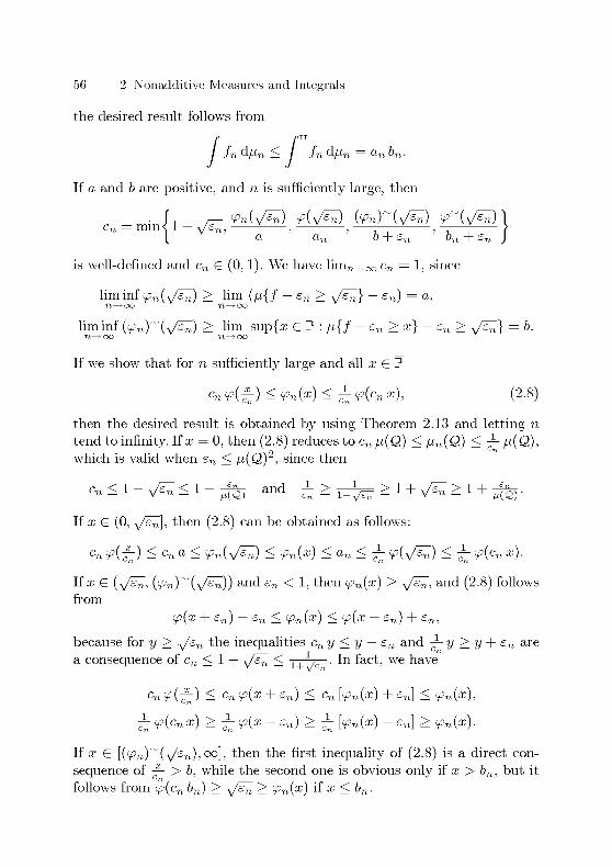
56 2 Nonadditive Measures and Integrals
the desired result follows from
/TT/„d/i„ = anbn.
If a and b are positive, and n is sufficiently large, then
min< 1a
'
a„'
b + en bn + en
is well-defined and cn G (0, 1). We have linin^oo c„ = 1, since
liminf <pn(Je^) > lim (/i{/ - e„ > y^} - e„) = a,n^oo n^oo
liminf (y>n)~(v^?0 > lim sup{x G P : /i{/ - £„ > x} - e„ > V^} = b-n^ oo n^ oo
If we show that for n sufficiently large and all x G P
C„ f(^) < Vn(a;) < ^ V(Cn x), (2-8)
then the desired result is obtained by using Theorem 2.13 and letting n
tend to infinity. If x = 0, then (2.8) reduces to c„ /i(<2) < /i„(<2) < — /i(<2),which is valid when e„ < /i(<2)2, since then
cn<l-V^<l-^S) and ^>ïr^>l + V^>l + ^y-
If a; G (0, y7^«]) then (2.8) can be obtained as follows:
c„<^(^) <cna< ifn{y/ë^) < ipn(x) <an< j-ip(y^) < j-ip(cnx).
If a; G (y'e^, (tPn)"" (\/£n)) and e„ < 1, then (fn(x) > y7^, and (2.8) follows
from
9?(x + e„) - e„ < 9?n(x) < ip(x - e„) + e„,
because for y > a/ë^ the inequalities cny < y— en and — y > y + e„ are
a consequence of c„ < 1 — ^Je^ < 1+ ^—.In fact, we have
c^(^) ^ c„^(x + en) < c„ [<^„(x) + en] < <pn(x),
-^ <p(cnx) > ± (f(x - £„) > -^ [<fn(x) ~ Sn] > (fn(x).
If x G [((pnyj(y/£^), oo], then the first inequality of (2.8) is a direct con¬
sequence of — > ft, while the second one is obvious only if x > bn, but it
follows from (f(cn bn) > y'e^ > fni?) if x < bn.

2.2 Nonadditive Integrals 57
Now assume that condition (2.7) is fulfilled: then
e„ = max{||/„ - /||, \\fin - fi\\, i}
is positive, and linin^oo e„ = 0. Define
/' = min{/, b} and f'n = min{/„, b + 2en}I{f>Fn}.
Since /i{/' > •} = (f, the part of the theorem already proved implies
lim / fn dM« = / / d/i,
because ||/^ - /'|| < 2e„,
SUpp /U„{/^ > •} < Mn{/n > 0} < Hn{f > £«} < y{en) + Sn,
SUpp/i„{/^ > •} > Mn{/n > en} > /"«{/ > 2e„} > <^(2£n) - £„,
essMnsup/4 < b + 2en,
essMn sup/4 > sup{x G P : /i„{/4 > x} > £„} >
> sup{x G P : <p(x +£„) > 2e„} > ipr"(2en) — en.
So, defining A = {/ > £„} and _B = {/„ < b + 2e„}, the desired result
follows from
<
/4 d/Un < fn d/Un <
< / /n^Anßd/in+ / /n/Q\j4d/in+ / fnlA\BdfJ.n<
< fn ÏAnB d/i„ + /i„(Q) supQyA /„ + /in(ß \ -B) sup /„
< fn dfln + Ia*(Ö) + £n] 2 £„ + £„ (sup / + £„)
by letting n tend to infinity. D
Example 2.24- Let /i, z/; and Id be the measures and the functions on [0, 1]defined in Examples 2.1, 2.2, and 2.7, respectively. Since the mappingd i—> Id on [0, 1] is continuous (with respect to the supremum norm), and
supp fi{ld > •} = 1 and ess^sup/^ = max{d, (1 — d)2} for all d G [0,1],Theorem 2.23 implies that the function d i—> J/^d/i on [0,1] is continuous

58 2 Nonadditive Measures and Integrals
for all regular integrals on classes Ai 9 /i. It also implies that the function
d l~^ J Id du on [0,1] is continuous for all quasi-subadditive, regular inte¬
grals on classes Ai 9 v. But since lim^Ti supP is{ld > •} 7^ supP u{l\ > •},Theorem 2.23 does not imply that d 1—> fl^dv is continuous at 1 for all
regular integrals on classes Ai 9 v\ in fact, the results of Example 2.14
show that d 1—> J" /^ dz^ is not continuous at 1. 0
2.2.6 Choquet Integral
An important property of the Choquet integral is the additivity of the
corresponding functional Fc on J\fFp, implying in particular the additivityof the integral with respect to measures:
fd(fJL + u)= / fdfJL+ fdu,
for all pairs of monotonie measures /i, v on a set <2, and all functions
/ : Q —> P. The next theorem states another important property of the
Choquet integral, but first we need some definitions.
Two functions /, g : Q —> P on a set <2 are said to be comonotonic if
f(q)<f(q) => g(q)<g(q) for all 9,9'e e.
Let .M be a class of measures (each /i G .M is a measure on some set <2M).An integral on .M is said to be comonotonic additive if
/ (/ + (?) d/i = f d/i + g dfi for all /i G A^
and all comonotonic /,jëPs^.
Theorem 2.25. The Choquet integral is comonotonic additive on the class
of all monotonie measures.
Proof. The additivity of the Choquet integral for comonotonic, finite func¬
tions is proved for instance in Denneberg (1994, Proposition 5.1); we can
extend this result as follows. If / and g are comonotonic, then there are no
q, q' such that q G {/ < 00} fl {g = 00} and q' G {/ = 00} fl {g < 00}, and
therefore the inclusion A = {/ < 00} Ç {g < 00} can be assumed without
loss of generality. If fJ-iQ^ \A) > 0, then the desired result is obvious, since
both the integrals of / and of (/ + g) are infinite. If /i(QM \ A) = 0, then

2.2 Nonadditive Integrals 59
dehne b = sup^(/ + g), and note that supAg < infg \4 (?, since / and g
are comonotonic. Proposition 4.5 of Denneberg (1994) implies that there
are two continuous, nondecreasing functions u, v : [0, b] —> P such that
u + v = idpib], f\A = uo(f\A + g\A), and g\A = v o (f\A + g\A).
Define h = min{/ + g,b}: Proposition 4.1 of the same book implies that
C pC pC
(u o h) d/i + / (v o h) d/i = h d/i.
The desired result follows from this equality, since uoh = min{/, sup^ /}and v o h = min{(?, sup^ (?}, and for all functions /' : Qß —> P
min{/',supA/'}d/i = / /'d/i,
because fJ-iQ^ \ A) =0, and therefore the distribution functions of /' and
min{/', sup^/'} are equal. D
Schmeidler (1986) proved that for finite, monotonie measures and
bounded functions, the Choquet integral is characterized by monotonic-
ity and comonotonic additivity. But the next example shows that this
characterization fails when the measures or the functions are unbounded
(see also Wakker, 1993).
Example 2.26. Consider the integral that associates the value
fH//_ J/C/dM if Jr7d/i<oo,
to each pair consisting of a monotonie measure /i on a set Q and of a
function / : Q —> P. It can be easily proved that this integral is regularand symmetric on the class of all monotonie measures, and subadditive on
the class of all 2-alternating measures. If the functions /, g : Q —> P are
comonotonic, then for all x G P one of the two sets {/ > x}, {g > x} is a
subset of the other, and therefore
M{/ + 9 > *} < /"{{/ > f} U {g > f}} = max{M{/ > f}, ,i{g > f}}.
Hence, if J f d/i and J g d/i are finite, then so is J (/ + <?) d/i; and thus
the integral defined by (2.9) is comonotonic additive on the class of all
monotonie measures.

60 2 Nonadditive Measures and Integrals
It is interesting to note that this integral can be represented (in the
sense considered at the end of Subsection 2.2.3) by a finitely additive mea¬
sure on (the Borel sets of) P2. That is, homogeneity does not suffice to
characterize the Choquet integral among the ones representable by finitelyadditive measures on (the Borel sets of) P2; and the countable additivityof the measure is not necessary to obtain the comonotonic additivity of
the integral (see also Klement, Mesiar, and Pap, 2004). 0
An integral on Ai is said to be translation equivariant if
/ (/ + c) d/i = / /d/i + cfj,(Q,j,) for all /i G Ai, all c G P,J J
and all / G PQ".
Since two functions are certainly comonotonic when one is constant, all
comonotonic additive, homogeneous integrals are translation equivariant.
By contrast, the next example shows that a maxitive, homogeneous integral
can be translation equivariant only on limited classes of finitely maxitive
measures.
Example 2.21. Let /i be a finitely maxitive, finite measure on a set Q. If
there is a set A C Q such that 0 < fJ,(A) < /i(<2), then all maxitive,
homogeneous integrals on classes Ai E5 /i satisfy
/(/a + I)d/u = max{2fj,(A),fj,(Q\A)} < fj,(A) + fj,(Q) = f IAdfj, + fj,(Q).
0
The equality satisfied by a translation equivariant integral on Ai can
also be considered as a way to define the integral of functions / : Qß —> M
with respect to measures /i G Ai, when inf / and /i(QM) are finite. We
obtain
y"/dM = y"(/-inf/)dM + M(eAt)inf/; (2.10)
and if the translation equivariant integral on .M is regular, subadditive, or
comonotonic additive, then so is the extended integral (when the definition
of distribution function is extended from P to 1). It is important to note
that in general the resulting extended integral does not satisfy the equality
/(—/) d/i = — J /d/i: for example, if A Ç Q^ is a set, then we have
(-IA)dfj,= /(l-/A)d/i-/i(eM) = / /QM\j4d/i-/i(QAt) = - / IAdß.

2.2 Nonadditive Integrals 61
The next theorem (proved for instance in Denneberg, 1994, Proposi¬tion 5.1) states that in the case of the Choquet integral this relation holds
for all bounded functions (not only for the indicator functions).
Theorem 2.28. If fi is a finite, monotonie measure on a set Q; and the
function f : Q —> M is bounded, then the extension of the Choquet integral
by means of equality (2.10) satisfies
j (-/)dM=-y faß.
There is another way to extend a monotonie, translation equivariant
(or homogeneous) integral on M. to functions / : Qß —> M, when inf / and
m(Öm) are finite: it is to define
//d/i= / max{/, 0} d/i - / max{-/, 0} d/i. (2.11)
The right-hand side is certainly well-defined, and the resulting extended
integral satisfies the equality /(—/) d/i = —J /d/i, but in general it does
not maintain the translation equivariance and other possible properties of
the original integral, such as subadditivity or maxitivity.
The extension of the Choquet integral by means of equality (2.10) usu¬
ally keeps the name "Choquet integral", while the extension by means of
equality (2.11) is often called "Sipos integral" (it was introduced by Sipos,
1979). Thanks to Fubini's theorem, it can be proved that if /i is count-
ably additive, then both extended versions of the Choquet integral reduce
to the Lebesgue integral (when either / > 0, or both inf/ and /i(QM) are
finite). So the Choquet integral generalizes the Lebesgue integral to nonad¬
ditive measures, and has strong properties (subadditivity and comonotonic
additivity) on a broad class of measures (the class of all 2-alternating mea¬
sures), containing all finitely additive and all finitely maxitive measures.
By contrast, the Shilkret integral does not generalize the Lebesgue inte¬
gral, and has strong properties (subadditivity and maxitivity) only on the
class of all finitely maxitive measures. The Choquet integral is thus a very
general and powerful integral, while the Shilkret integral is specialized on
maxitive measures: in particular, on completely maxitive measures it re¬
duces to the very simple form stated in Theorem 2.6. The main drawback
of the Shilkret integral is the lack of translation equivariance; this impliesin particular that it cannot be extended in a satisfactory way to functions
taking also negative values.


3
Relative Plausibility
The likelihood function can be considered as a description of uncertain
knowledge about the statistical models: in the present chapter this kind
of description is studied, under the name of "relative plausibility", from
both the static and the dynamic points of view. In particular, it is com¬
pared with the Bayesian, probabilistic description of uncertain knowledgeabout the models, and it is connected to the MPL criterion by a representa¬
tion theorem for preferences between randomized decisions. The statistical
models and their relative plausibility build a hierarchical model with two
levels describing two different kinds of uncertain knowledge: this hierarchi¬
cal model is briefly compared with the classical, Bayesian, and imprecise
probability models.
3.1 Description of Uncertain Knowledge
A relative plausibility measure rp on a set Q is an equivalence class
of completely maxitive measures on Q with respect to the equivalencerelation oc. Thus, to be precise, rp is not a measure (in the sense introduced
in the preceding chapter) but a class of proportional measures; however,this slight abuse of terminology is coherent with the abuse of notation
we commit by using rp to indicate one of its representatives /i, when the
choice of /i G rp is irrelevant. For example, we can say that for each
function / : Q —> P there is a unique relative plausibility measure /^ on
Q such that (/^ oc /. On the other hand, when there is no possibility of
confusion, we use rpot~x and rp\j\ as abbreviations for [(rp ot^1)^ and
[(rPU) ] , respectively (where t is a function on Q, and A is a subset of
Q). A relative plausibility measure rp on Q is said to be nondegenerate

64 3 Relative Plausibility
if rp(Q) G P (that is, if rp is finite and nonzero); in this case, rp denotes
the (unique) normalized representative of rp:
m(A) = T-^\ for all ACQ.rp(Q)
Consider a statistical decision problem described by a loss function L on
VxD, and let hk be the likelihood function on V induced by the observed
data; Theorem 2.6 implies that the MPL criterion can be expressed as
follows:
fSt
minimize / l& dhk '.
The likelihood function hk measures the relative plausibility of the models
in V in the light of the observed data alone, and hk" extends this relative
measure to the subsets of V: it is the relative plausibility measure on V
induced by the observed data. This extension of hk to the subsets of V by
means of the supremum agrees with the profile likelihood: if Q is a set, and
g : V —> Q is a mapping, then lik^ o g~x = (likgY; the extension is thus
in accordance with the likelihood-based inference methods: in particular,if lik^ is nondegenerate, then hk^ (Ti) = LR(Ti) for all TL Ç V.
Hence a relative plausibility measure rp on V can be interpreted as
a description of uncertain knowledge about the models in V, based on
the description rp-1 of the relative plausibility of the elements of V. It is
strictly related to other descriptions of uncertain knowledge appearing in
the literature: "degrees of potential surprise" (Shackle, 1949), "support byeliminative induction" (Cohen, 1966), "consonant plausibility functions"
(Shafer, 1976), and possibility measures (if rp is nondegenerate, then rp
is a normalized possibility measure on V). The models in V are mathe¬
matical representations of some aspects of the reality under consideration;no model is true, but some models represent the observed reality better
than others. The relative plausibility of a model is its relative ability to
represent the observed reality; the ability of a set of models is interpreted
as the ability of its best element. In the Bayesian approach ,the uncertain
knowledge about the models in V is described by an averaging probabilitymeasure 7r on (V,C) (or by a set T of such probability measures), where C
is a cr-algebra of subsets of V. The interpretation of a probability measure
on (V, C) is based on the assumption that exactly one of the models in
V is "true" : V is an exhaustive set of mutually exclusive possible "states
of the world" (at least when C contains all singletons of V). The exhaus-
tivity of V is not implied by the interpretation of a relative plausibility

3.1 Description of Uncertain Knowledge 65
measure rp on V (because rp contains no evaluation of the "absolute plau¬
sibility" of V), although some sort of "actual exhaustivity" is implied bythe fact that we do not consider models that are not in V. The same situa¬
tion can be obtained for the Bayesian approach by considering a "relative
probability measure" on V, in analogy with rp: the Bayesian criterion for
statistical decision problems is unaffected by the "absolute probability" of
V (Hartigan, 1983, developed a Bayesian approach with non-normalized
probability measures). The basic difference between the interpretations of
relative plausibility and probability is that besides the exhaustivity, neither
the mutual exclusivity of the models in V is implied by the interpretationof a relative plausibility measure on V, in the following sense. The proba¬
bility of a model is the probability that it is the "true" one, and truth is
exclusive; but the ability to represent the observed reality is not exclusive:
different models can coexist as satisfactory representations of the reality.Models are mental constructions, not "states of the world", even thoughin particular situations (such as drawing from an urn containing colored
balls) a model can be so strongly associated with a state of the world that
they can almost be identified. The fundamental qualitative difference be¬
tween relative plausibility and probability (see for example Dubois, 1988)is that if Tii, Ti-2, and Ti are subsets of V (in the case of probability theymust be elements of C) such that rp(Tii) > rp(Ti2), and Ti is disjoint from
both Tii and H.2, then the inequality rp(Tii UTi) > rp(Ti2UTi) holds if and
only if rp(Ti) < rp(Tii) (while in the case of probability it always holds). In
fact, the ability of a set Ti of models to represent the observed reality does
not increase when it is enlarged by models that are not more satisfactorythan the ones in Ti: if rp(Tii) < rp(Ti), then rp(Tii U Ti) = rp(Ti).
It is important to note that the identification of the set theoretic oper¬
ations on subsets of V with the connectives of propositional logic is based
on the assumption that exactly one of the models in V is "true". Without
this assumption the identification fails; for example, rp{P, P'} is not the
(relative) plausibility of "P or P'" (in fact, "P or P'" means "P is the
true one or P' is the true one"): it is simply the (relative) plausibility of
the set {P, P'}. The relative plausibility measure lik^ on V is a convenient
extension of the (relative) likelihood lik from the elements of V to the
subsets of V (in accordance with the likelihood-based inference methods),and since we do not assume that one of the models in V is "true", the use
of hk~ does not contradict the assertion of Fisher (1930) that in general"the likelihood of P or P'" has no meaning ( "you do not know what it is
until you know which is meant").

66 3 Relative Plausibility
3.1.1 Representation Theorem
Let ^ be a binary relation on a set S. The binary relations ~ and -<onS
are defined as follows on the basis of ^ :
a ~ b •<=> a ^ b and b ^ a for all a,b G S,
a -< b •<=> a ^ b and not b ^ a for all a,b G S.
The relation ^ is said to be a total preorder on S if it fulfills the followingtwo conditions:
a ^ b or b ^ a for all a,b G S,
a ^ b and ö ^ c => o ^ c for all a,b,c G S.
If ^ is a total preorder on S, then ~ is an equivalence relation on S, and
for all a,b G S exactly one of the following three cases applies: a -< b, b -< a,
or a ~ &. A function / : S —> M is said to represent the relation ^ on S" if
a<b <^> /(a) < f(b) for all a,b G S.
If ^ is represented by some function, then it is a total preorder.
In the Bayesian approach, the use of probability measures as a descrip¬tion of uncertain knowledge is usually justified in terms of representationtheorems for qualitative preference relations. The most famous representa¬
tion theorem is the one of Savage (1954): it gives necessary and sufficient
conditions for a preference relation ^ on Cs (where Q is a set of "states
of the world" and C is a set of consequences) to be represented by the
mapping / i—> E^{v o /) for a normalized, finitely additive measure tt on Q
(the countable additivity is given up, and so measurability problems are
avoided) and a bounded function v : C —> M (a quantitative evaluation of
the consequences). The elements of Cs are functions / : Q —> C associating
a consequence to each state of the world; that is, each / can be considered
as the uncertain consequence of a particular decision. By assuming that
the uncertain consequence summarizes all important aspects of a decision,we identify the decisions with their uncertain consequences, interpretingthe elements of Cs as decisions, and the relation ^ as a description of
preferences between them.
Consider a preference relation ^ on T> Ç Cs: a representation theo¬
rem gives necessary and sufficient conditions for the preferences between

3.1 Description of Uncertain Knowledge 67
decisions to be represented by a particular kind of functional on T>. We
shall obtain a representation theorem where the functional is of the form
/ i—> Js(v o I) drp for a nondegenerate relative plausibility measure rp on
Q and a function v : C —> [0, oo). We interpret f o / as a quantitativeevaluation of the uncertain loss incurred by making the decision l G D,and accordingly we interpret the expression / ^ /' (where /, /' G T>) as "/'
is not preferred to I". For the sake of generality, we formulate the repre¬
sentation theorem with Q as a generic set of alternatives determining the
consequences of the decisions; but when interpreting the conditions, Q can
be regarded as a set of statistical models. The theorem describes the kind
of preference relation on T> induced by the MPL criterion, when applied
(with respect to some nondegenerate relative plausibility measure rp on
Q) to a decision problem described (for some function v : C —> [0, oo)) bythe loss function Lv : (q, I) i—> f[/(g)] on Q x T>.
Representation theorems are often considered as justifications for par¬
ticular approaches (such as the Bayesian one), but even if the postulatedconditions for the preferences between decisions are reasonable, the con¬
clusion that the only reasonable preference relations are represented by a
particular kind of functional is based on the wrong assumption that rea¬
sonable conditions are noncontradictory (compare with Chernoff, 1954).Moreover, the postulated conditions are usually motivated only by ab¬
stract consideration of simple examples; hence their application beyondthose simple examples is in fact unmotivated, and can have unexpected
consequences (see for example Ellsberg, 1961). For these reasons, the rep¬
resentation theorem that we shall obtain should be interpreted as a math¬
ematical theorem showing the distinguishing properties of the preferencesbased on the MPL approach, not as a justification for this approach. The
same considerations apply to the axiomatic justifications for the use of the
likelihood function as a description of the information content of statistical
data: see Birnbaum (1962, 1969) and Evans, Fraser, and Monette (1986).
The first condition postulated by Savage for the preferences between
decisions is that the preference relation is a total preorder on Cs. This is
a necessary condition for the preferences to be represented by a functional,but it is certainly too strong for the real-world preferences of an individ¬
ual, also because it is assumed that T> = Cs (that is, T> is sufficiently wide
to encompass all possible uncertain consequences). Since we do not con¬
sider the representation theorem as a justification for the MPL approach,
we can for simplicity assume that T> = Cs, but we will later consider on

68 3 Relative Plausibility
which subsets of Cs the preference relation suffices to determine its rep¬
resentation by the mapping / i—> Js(v o I) drp for a nondegenerate relative
plausibility measure rp on Q and a function v : C —> [0, oo).
If we assume that the preferences between the consequences in C are
not affected by the particular case q G Q considered, and correspond to the
preferences between the constant (uncertain) consequences in Cs, then the
following condition of monotonicity is hardly debatable. A binary relation
^ on Cs is said to be monotonie if
Kl) ^ l'(<l) for all ? G Q => l£ I' for all /, /' G CQ.
If the preference relation ^ on Cs is induced by the MPL criterion (appliedto the decision problem described by the loss function Lv on Q x Cs),then the preference relation on C is represented by v, and ^ is monotonie,since the Shilkret integral with respect to completely maxitive measures
is homogeneous and monotonie (Theorem 2.3). If / and /' satisfy the left-
hand side of the above condition of monotonicity, and {/ -< I'} is not empty,
then we can say that / dominates /'; the monotonicity of the preferencerelation assures that if /' is dominated by /, then /' is not preferred to /. The
monotonicity is part of Savage's "sure-thing principle" (at least when / and
/' have finite range; see Subsection 4.1.2); but this principle states also that
if / dominates /', then / must be preferred to /', at least when {/ -< I'} is
not impossible (that is, when it has positive "probability"). This condition
is satisfied by the preferences induced by the MPL criterion if we discard
the dominated decisions: the resulting preference relation ^ on Cs is such
that / -< I' if and only if either vol < vol' and v o/ ^ v o/', or / is preferredto /' on the basis of the MPL criterion applied to the decision problemdescribed by Lv. It can be easily proved that in general this preferencerelation is not a total preorder on Cs, since it is not transitive (but it is
important to note that the strict preference relation -< is transitive); this
shows that to be reasonable and useful, a preference relation does not need
to be a total preorder.
The problem of the "sure-thing principle" of Savage is that the premise"when {/ -< I'} is not impossible" cannot be expressed directly in terms
of preferences: therefore the principle was replaced with other conditions.
In particular, the second condition postulated by Savage for the prefer¬ences between decisions states that the preference between two functions
1,1' G Cs does not depend on the values taken by the functions on the set
{/ = /'}, in the sense that the preference is left unchanged when the two

3.1 Description of Uncertain Knowledge 69
functions are modified in the same way on {/ = /'}. This condition is in
general not satisfied by the preferences induced by the MPL criterion, also
if we discard the dominated decisions: it is possible that by modifying the
functions on {/ = /'} a strict preference becomes an equivalence, or vice
versa (but it is impossible that a strict preference is reversed). This dis¬
cord between the preferences induced by the MPL criterion and the second
condition postulated by Savage is strictly related to the fundamental qual¬itative difference between relative plausibility and probability, considered
at the beginning of the present section: for a relative plausibility measure
rp, the additional consideration of TL can neutralize the preference between
TL\ and TL2-
The preferences induced by the MPL criterion present the same kind
of discord with the fourth condition postulated by Savage as with the
second one, while they fulfill the third and fifth ones (the first five pos¬
tulated conditions imply the existence of a qualitative probability on Q).To obtain preferences satisfying the second and fourth conditions postu¬
lated by Savage, it suffices to restrict attention to the subset {/ ^ /'} of
Q when applying the MPL criterion for discriminating between the deci¬
sions /,/' G Cs, but it can be easily proved that in general the resulting
preference relation is not a total preorder on Cs, since it is not transitive
(however, in this case too the strict preference relation is transitive). It
is interesting to note that on the end pages of Savage (1954) the author
restated in a slightly different form the seven postulated conditions that
are scattered through the book: even though he asserted that "the logicalcontent of each postulate is left unaltered", the preferences induced by the
MPL criterion satisfy all the conditions appearing on the end pages, apartfrom the (highly debatable) sixth one. This shows that minimal changes in
the postulated conditions can have important consequences on the implied
representations, and thus points out how unsuitable the representation the¬
orems are as justifications for particular approaches (in the second edition
of the book, published in 1972, the second condition appearing on the end
pages has been corrected, but the fourth one is still flawed).
Ellsberg (1961) showed that the second condition postulated by Savageis at variance with the propensity toward hedging bets, which reveals strict
uncertainty aversion. Schmeidler (1989) proved a representation theorem
where the functional is of the form / i—> J (v o I) d/i for a normalized,monotonie measure /i on Q (a "nonadditive probability" measure) and
a bounded function v : C —> M (a quantitative evaluation of the conse-

70 3 Relative Plausibility
quences): the preferences reveal uncertainty aversion if and only if /i is
2-alternating (they reveal uncertainty neutrality when /i is finitely addi¬
tive) .A strictly related representation theorem for the preferences induced
by the T-minimax criterion was proved by Gilboa and Schmeidler (1989).Both these theorems use the framework of the representation theorem for
the preferences induced by the Bayesian criterion proved by Anscombe and
Aumann (1963) and generalized by Fishburn (1970), in which the set C
is enlarged by including randomized consequences (that is, the existence
of objective probabilities is assumed). We will use this framework too, but
with an important difference: these representation theorems are based on
the one of von Neumann and Morgenstern (1944), which considers the
consequences of economic decisions, while we are interested in statistical
decisions. The main difference is that statistical decision problems possess
an additional element: the concept of correct decision; we assume thus the
existence of the consequence cq G C of a correct decision.
For a set C E5 cq of consequences, we define
R(C, co) = {rG [0, if : |{r > 0}| < 1, r(c0) = 0} ,
and we interpret each element r = p I{c} of R(C, cq) as the following ran¬
domized consequence: c with probability p, and cq with probability 1 — p.
The set C of non-randomized consequences can thus be identified with a
subset of R(C, cq): each c G C\ {cq} can be identified with c = Irc\, and cq
can be identified with cq = 0. In our representation theorem, a total pre-
order ^ on the set R(C\ co)s is considered; that is, the set C is enlarged by
including the randomized consequences of the above form (for all p G (0,1)and all c G C). The first condition of our representation theorem states
the peculiar role of the consequence cq of a correct decision (that is, no
consequence can be preferred to Co):
c0< c for all c G C. (3.1)
In the framework of Anscombe and Aumann, preferences between de¬
cisions in R(C)Q are considered, where
R(C) = {rG [0, If : |{r > 0}| < oo, £cecKc) = 1}
is the set of all the randomized consequences that are mixtures of a finite
number of consequences. The use of R(C) instead of R(C, cq) in our theo¬
rem would pose no problem (a condition should be slightly modified), but

3.1 Description of Uncertain Knowledge 71
thanks to the peculiar role of cq, it suffices to consider the preferences be¬
tween decisions in the set R(C\ co)s, which can be identified with a subset
of R(C)Q. Moreover, Cs can be identified with a subset of R(C\ co)s, and
if l" G CQ is identified with /' G R(C,c0)a, and p G [0,1], then pi' can
be interpreted as the following randomized decision: I" with probability p,
and Co with probability 1 — p. We shall see that the preference relation on
the set of randomized decisions of the form pi' (where /' can be identi¬
fied with an element of Cs) suffices to determine its representation by the
mapping / i—> Js(vol) drp for a nondegenerate relative plausibility measure
rp on Q and a function v' : C —> [0, oo), where v : R{C,cq) —> [0, oo) is
the homogeneous extension off', in the sense that v(pc) = pv'(c) for all
p G (0, 1] and all c G C.
Roughly speaking, each one of the three representation theorems of
Anscombe and Aumann, Schmeidler, and Gilboa and Schmeidler im¬
poses three fundamental conditions on the total preorder ^: independence,
continuity, and monotonicity. The independence condition postulated byAnscombe and Aumann can be formulated as follows: / ^ /' if and only if
pi + (1 — p) I" ^ pi' + (1 — p) /", where p G (0, 1); it can be interpreted as
stating that the preference between two decisions / and /' does not change if
these are randomized by mixing them in the same way with a third decision
I": the influence of I" on the evaluation of the mixed decisions is indepen¬dent of / or /'. This is contradicted by the propensity toward hedging bets
(when / ~ /', the preference pi + (1 — p) /' -< I can be explained by strict
uncertainty aversion: there is a preference for risk differentiation); there¬
fore Schmeidler relaxed the independence condition by assuming that /, /',and I" are pairwise comonotonic (/ and /' are comonotonic if there are no
q,q' G Q such that l(q) -< l(q') and l'(q') -< l'(q))- Gilboa and Schmeidler
relaxed the independence condition even more by assuming instead that
I" is constant; they called this condition "certainty-independence", and
needed to complement it with the one of "uncertainty aversion", which
states that / ~ /' implies p/ + (l— p)/'^/. The second condition of our
representation theorem corresponds to the certainty-independence for the
only case in which it is defined in our framework (that is, for I" = cq):
1<J' ^ pl^pl' for allpG (0, 1) and all /,/' G R(C,co)Q. (3.2)
This condition can be interpreted as stating that if we shall have to decide
with probability p (while with probability 1 — p we shall know the correct
decision), then our preferences must be the same as if we certainly had to
decide; the condition can also be considered as expressing the "scale invari-

72 3 Relative Plausibility
ance" of the preferences (that is, the equivalence of the loss functions L and
a L, for all a G P). It is important to note that in general the preferencesinduced by the MPL criterion would not satisfy the certainty-independencewhen R(C) were used instead of R(C, cq) (because the Shilkret integral is
not translation equivariant); on the other hand, they would satisfy the un¬
certainty aversion (since the Shilkret integral with respect to completelymaxitive measures is subadditive and homogeneous).
The continuity condition is the same for the three representation the¬
orems cited above, and can be formulated as follows: if / -< I' -< /", then
there are p,p' G (0,1) such that pi + (1 -p) I" -< /' -< p' I + (1 -p') I". This
condition can be interpreted as stating that there are randomized decisions
obtained by mixing / and I" that are as close as we want (on the prefer¬ence scale) to / or /"; it is reasonable only if the uncertain consequences
are in some sense "bounded" (see also Wakker, 1993). In our framework,when the monotonicity and the conditions (3.1) and (3.2) are satisfied, the
uncertain consequences can not be preferred to Co, and the only case in
which the above continuity condition is defined and not vacuous is thus
for Z = co. In this case, the second implied preference of this condition
has no problems related to unbounded uncertain consequences, and the
implication is equivalent to the following one:
pl<l' for all p G (0,1) => 1<Ï for all/, /' G R(C, c0)Q. (3.3)
In our representation theorem, we do not need to assume that the uncertain
consequences are bounded above, but for simplicity we can assume that
there are no "infinitely unfavorable" consequences (otherwise we should
impose an additional condition stating their equivalence, to avoid "trans-
finite evaluations" ) : the uncertain consequences can be unbounded only if
C is infinite. The following condition is strictly related to the first implied
preference of the above continuity condition when I" = c (and / = Co); it
assures that the consequences c G C are bounded and that there are no
"infinitesimal evaluations" :
I ~^pc for all p G S, and inf S = 0 => / ~ cq
(3.4)for all c G C, all S Ç (0,1), and all / G R(C, c0)Q.
In the three representation theorems cited above, the monotonicity of
the preference relation is assumed; in our theorem it is replaced by the
following stronger condition (the monotonicity corresponds to the special

3.1 Description of Uncertain Knowledge 73
case with lq = I' for all q G Q):
l(q) -< Uq) and L -< /' for all q£ Q => I < V
(3.5)for all {/, /'} U{lq:qGQ}C R(C, c0)Q.
This condition can be interpreted as stating that the preferences are based
on a "worst-case evaluation" : if for each case q G Q there is a decision
lq whose consequence according to q is not more favorable than the one
of /, and such that /' is not preferred to lq, then /' is not preferred to /
either. The part of this condition that is additional to the monotonicity
can be stated as follows: if /' is preferred to /, then there is a q G Q such
that /' is preferred to H{q\ (the decision that has the same consequence
as / according to q, and is correct according to all q' ^ q). The worst-case
evaluation explains why the preferences considered in our representationtheorem would not satisfy the certainty-independence when R(C) were
used instead of i?(C, Co): the importance of a particular consequence c
depends on the plausibility of the case q implying it, and if p I + (1 — p) c is
evaluated on the basis of the worst case q, then the influence of c on this
evaluation depends on /, since it depends on which q is the worst case.
With this five conditions, we can finally state our representation the¬
orem. A function v : R{C,cq) —> [0, oo) is homogeneous ifv(pr) = pv(r)for all p G (0, 1) and all r G i?(C, Co); in this case v(cq) = 0, and v is
uniquely determined by the function c i—> v(c) on C \ {co}. Hence the
quantitative evaluation v (of the randomized consequences in R(C, cq))considered in our representation theorem is the expected value of a quan¬
titative evaluation (of the non-randomized consequences) v' : C —> [0, oo)with v'(co) = 0.
Theorem 3.1. Let C and Q be two nonempty sets, and let cq G C. A
total preorder ^ on R(C,c0)a fulfills the conditions (3.1), (3.2), (3.3),(3.4), and (3.5) if and only if there are a nondegenerate relative plausibility
measure rp on Q and a homogeneous function v : R(C, cq) —> [0, 00) such
that ^ is represented by the mapping I 1—> Js(v o I) drp; the function v is
unique up to a (positive) multiplicative constant, and rp is unique when v
is not constant.
Proof. The "if part is simple: since v is finite and homogeneous, and the
Shilkret integral is homogeneous (Theorem 2.3), we have
/S/*S /*S
[v o (p /)] drp = p (vol) drp and / (v o c) drp = v(c) rp(Q).

74 3 Relative Plausibility
The first four conditions follow easily from these equalities, and for the
fifth one we obtain v o I < sup G gv o lq : now it suffices to exploit the
monotonicity and the complete maxitivity of the Shilkret integral with
respect to completely maxitive measures (Theorems 2.3 and 2.6).
For the "only if part, consider first the trivial case with c ~ cq for
all c G C: condition (3.2) and monotonicity imply that / ~ cq for all
/ G R(C, co)s, and therefore the desired representation is valid if and onlyif v = 0. When c\ G C does not satisfy à\ ~ cq, condition (3.1) impliesthat Co -< c\: in this case, let V be the functional on R(C, co)s defined by
, s
_JsupjpG [0, 1] :pc! ^ /} if/^Ci,
\ inf{a; G (1, oo) : \ I < Cl} if cx < I.
This definition implies that if / ^ /', then V(l) < V(l'); to prove the
converse we need first the following simple result: if p' < p, then p' I ^ pi,and p' I ~ pi only if pi ~ / for all p G (0,1]. Thanks to monotonicity, it
suffices to show p' I ^ pi for / = c; if pc ~< p1 c = jpc were true (where
7 =— ), then by induction and condition (3.2) we would obtain p c -< jn pc
for all positive integers n, and therefore pc ~ cq by condition (3.4), but
this would contradict pc -< p' c, since p' c = jpc ~ jcq = cq. If p' I ~ pi,then by the same technique we obtain pi ~ Jnpl, and thus p' I ^ pi for
all p' G (0,p]; but p2 I ~ pi and condition (3.2) imply pi ~ /, and thus
p' I ^ I for all p' G (0, 1]. In particular, p' < p implies p' c\ -< pc\, because
otherwise c\ ~ cq would follow from condition (3.4). Using these results
and conditions (3.2) and (3.3), the following equivalences can be easily
proved:
V(l)=pG[0,1] & l~pc!,
V(l) = ±G[l,oo) ^ pl-C!,
V(l)=oo <=> ci ~< pi for all p G (0, 1].
These expressions imply that V is homogeneous (that is, V(pl) = pV(l))and it represents ^: the only difficulty is to show that if V(l) = V(l') = oo,
then / ^ /'. To prove it, consider first that V(c) < oo (for all c G C) follows
from condition (3.4); hence l(q) ^ /' for all q G Q, but then condition (3.5)implies / ^ /' (with lq = l(q))- Let /i be the completely maxitive measure
on Q defined by ^(q) = V(c\ I{q\)', we prove now that /i is normalized,and V(l) = Js(v o I) d/i, where v is the homogeneous function on R(C, Co)defined by v(r) = V(r). Let si = sup GS V[l I{q}]', the monotonicity of
^ implies that V(l) > s;. If V(l) > s; were true, then there would be
3.1 Description of Uncertain Knowledge 75
a c G C such that V(c) > s; (otherwise ^(Z) < s; would follow from
monotonicity), and thus also an r G R(C, cq) such that V(l) > V(r) > s;,
but this is contradicted by the relation / ^ r implied by condition (3.5)with lq = II{q}. Hence V(l) = si, and in particular V(c\) = sup G q ^ (q) ;
thus /i is normalized, since l^(ci) = 1. The above results about V imply
V(r I{q}) = V(r) V{c\ I{q}), and therefore (using Theorem 2.6) we obtain
,s
V(l) = sup V[l(q) I(q\] = s\xpv[l(q)] fJ, (q) = sup(f o /) fj,* = / (vol) drp,
where rp is the nondegenerate relative plausibility measure on Q defined
by rp = /i. The results obtained about V imply that if V : R(C\ co)s —> P
is a homogeneous functional representing ^, then V = V'(c\)V with
V'(ci) G P; this proves the uniqueness results. D
Let T> be a subset of i?(C, co)s that contains c and ci|q| for all c G C
and all q G Q, and that is closed with respect to randomization, in the sense
that if / G T>, then pi G T> for all p G (0,1). It can be easily proved that
Theorem 3.1 is still valid if we substitute T> for R(C\ co)s in its statement
(and in the five conditions); that is, the preference relation on T> suffices
to determine its representation by the mapping / i—> Js(v o I) drp (up to
the slight nonuniqueness of v and rp). In particular, as noted above, T> can
be a set of randomized decisions of the form pi, where / can be identified
with an element of Cs, and p G [0, 1]. The smallest set T> satisfying the
above requirements consists of the decisions r and r I[qy for all r G R(C, cq)and all q G Q; by slightly modifying the postulated conditions, the prefer¬ences between decisions of the form r I[qy would suffice to determine the
representation.
Apart from the fact that the evaluations are not necessarily bounded
above, the main differences of our representation theorem with respect to
the one of Anscombe and Aumann are the peculiar role of Co, the weakeningof the independence condition, and the strengthening of the monotonicitycondition. The monotonicity is strengthened through worst-case evalua¬
tion: this is strictly related to the description of uncertain knowledge by
means of relative plausibility; in fact, this description is based on a "best-
case evaluation", in the sense that the ability of a set of models to representthe observed reality is interpreted as the ability of its best element. The
apparent conflict between "worst-case" and "best-case" in the previous
period is due to the fact that we consider an evaluation of the decisions in

76 3 Relative Plausibility
terms of loss; that is, the negativity of the uncertain consequences is eval¬
uated. This is the reason for interpreting the expression / ^ /' as "/' is not
preferred to /", but in the cited literature about representation theorems
the above expression is interpreted as "/ is not preferred to /'", because
the decisions are evaluated in terms of utility: to avoid confusion, all the
cited conditions and results have been modified (if necessary) in order to
comply with our interpretation of the preference relation (in fact, the only
ones needing changes are those concerning uncertainty aversion). The pe¬
culiar role of Co and the weakening of the independence condition in our
representation theorem with respect to the one of Anscombe and Aumann
are strictly related to the differences between the evaluations of decisions
in terms of loss and in terms of utility.
Usually, a statistical decision problem is described by a loss function L
on V x T>, and there is a clear idea of what constitutes a correct decision
for a model P G V, also when this decision is not an element of T>. The loss
functions L and a L are considered equivalent (for all a G P), and there¬
fore, in order to be representable by an evaluation in terms of loss, the
preferences between decisions must fulfill the scale invariance expressed bythe weak independence condition (3.2), which can be stated in the frame¬
work of Anscombe and Aumann only if the existence of the consequence cq
of a correct decision has been assumed. A general decision problem is often
described by a bounded utility function U : Q x T> —> R, and in generalthe concept of correct decision does not make sense; in this regard it is
important to distinguish between the concept of optimal decision (d G T>
is optimal for q if it maximizes U(q, d) among the elements of T>: the op¬
timally depends thus strongly on T>) and the one of correct decision (acorrect decision for q is not necessarily an element of T>, and its correct¬
ness does not depend on the other elements of T>). The utility functions U
and a U + ß are considered equivalent (for all a G P and all /?£ R), and
therefore, in order to be representable by an evaluation in terms of utility,the preferences between decisions must fulfill the certainty-independencecondition postulated by Gilboa and Schmeidler. If the loss function L and
the utility function U on Q x T> describe the same decision problem and
are expressed in the same scale, then uo(q) = U(q, d) + L(q, d) is the util¬
ity of a correct decision for q G Q (and thus in particular it does not
depend on d). Hence, when a decision problem is described by a utilityfunction U on Q x T>, to obtain a description of the problem by a loss
function we must determine the function uq on Q; but this determination
is problematic for general decision problems, since there is usually no clear

3.1 Description of Uncertain Knowledge 77
idea of what constitutes a correct decision. In order to be representable
by an evaluation in terms of utility or loss avoiding the problems related
to the determination of vq, the preferences between decisions must fulfill
the strong independence condition postulated by Anscombe and Aumann:
in fact, in this case the utility functions U and a U + u are equivalentfor all a G P and all bounded functions u : Q —> M (interpreted as func¬
tions on Q x T> such that u(q, d) does not depend on d). This points out a
fundamental difference between the MPL approach to statistical decision
problems and the Bayesian one: the former is specialized on problems de¬
scribed by loss functions, while the latter is able to cope indifferently with
loss and utility functions; but this ability comes with a price: it implies
uncertainty neutrality, while uncertainty aversion can be considered as the
basic attitude in statistics.
Hence, if the evaluation method allows strict uncertainty aversion, then
the choice of uq matters when translating U into a loss function: two al¬
ternative assumptions about uq are often made when its determination is
problematic. One of them is that for each q G Q a correct decision is con¬
tained in T> (at least as a limit): we obtain the loss function L on Q x T>
defined by L(q, d) = supd/Gl3 U{q, d') — U(q, d) for all (q, d) G Q xT>. That
is, the optiniality is substituted for the correctness of a decision; this kind
of loss function was introduced explicitly by Savage (1951) and is often
called "regret function" : it gives the amount of utility lost for not hav¬
ing selected the best available decision (that is, the optimal decision). If
a method consists in evaluating the decisions on the basis of the regret
function obtained from a utility function, then the induced preferences
satisfy the strong independence condition postulated by Anscombe and
Aumann (and thus reveal uncertainty neutrality), but the preference be¬
tween two decisions can depend on the whole set T> (since the optiniality
depends strongly on T>). The other frequent assumption about uq is that
the utility of a correct decision does not depend on q (that is, uq is con¬
stant): we obtain the loss function c — U on Q x T>, where c > sup U. To
be reasonable, an evaluation of decisions on the basis of c — U must be
independent of c; that is, it must be based on an evaluation method such
that the induced preferences fulfill the certainty-independence condition
postulated by Gilboa and Schmeidler. Hence, the application of the MPL
criterion to the decision problem described by the loss function c — U is
not reasonable: to obtain preferences independent of c we can replace the
Shilkret integral with a translation equivariant integral, and the natural
choice is the Choquet integral.

78 3 Relative Plausibility
A representation theorem analogous to Theorem 3.1, but with the Cho-
quet integral instead of the Shilkret integral (that is, a representation the¬
orem for the preferences induced by the "MPL* criterion" of Cattaneo,
2005), can be easily obtained by imposing an additional condition to the
preferences considered in the representation theorem of Schmeidler. The
additional condition must force the complete maxitivity of the "nonaddi¬
tive probability" measure, as does for example the following one: if 1\a is
constant, and /' -< /, then there is a q G A such that /' -< I I(Q\Ayj{q} (f°rall nonempty ACQ and all /,/' G R(C)Q). This condition can be inter¬
preted as stating that the preferences are based on a worst-case evaluation
limited to cases implying the same consequence; it could also be expressedin a form analogous to the one of condition (3.5), and in this case it would
imply the monotonicity of the preference relation on the set of functions
/ G R(C)Q having finite range (the preference relation on this set suffices
to determine the representation), but anyway this enforcement of complete
maxitivity is rather artificial.
3.1.2 Updating
Let ? be a set of statistical models (V is a set of probability measures
on a measurable space (Q,A)): a relative plausibility measure on ? is a
description of uncertain knowledge about those models. In the previoussubsection we considered the static aspect of this description, in relation
to the preferences induced by the MPL criterion; in the present subsection
we consider the dynamic aspect: the evolution of the description when new
information about the models is acquired.
When we observe an event A G A, we obtain a likelihood function hk
on V, and we must condition on A each model in V; if subsequently we
observe a second event B G A, then we obtain the likelihood function hk'
on V defined by hk'(P) = P(B\A) (for all P G V). To be precise, when we
observe B, we obtain a likelihood function hk" on the set V of the models
in V conditioned on A, but it is convenient to avoid explicit reference to
V1 by considering hk1 = hk" o c instead of hk", where c : V —> V is the
surjection representing the conditioning on A of the models in V. Since
for each P G V we have P(A (~l B) = P(A) P(B\A) (independently of the
definition of P(B\A) when P(A) = 0), the likelihood function on V induced
by the observation of both events A and B is hk hk1] that is, the likelihood
function hk is updated through multiplication with the likelihood function
3.1 Description of Uncertain Knowledge 79
hk' induced by the new observation. We will use the symbol 0 to denote
the binary operation on relative plausibility measures corresponding to
the multiplication of their density functions: rp 0 rp' = [rp-1 (rp')^ for
all pairs of relative plausibility measures rp, rp' on the same set Q. Hence
the relative plausibility measure lik^ is updated through combination with
(lik'y by means of the operation 0.
The dynamic aspect of the description of uncertain knowledge about
statistical models by means of relative plausibility can be incorporated in
our representation theorem (Theorem 3.1, with Q = V) by imposing an
additional condition to the preferences between decisions. This condition
can be stated as follows (in a slightly informal way): if the relation ^on R(C\ cq)v expresses our preferences before observing the event A (themodels in V are assumed to be conditional on past observations), then
our preferences after observing A shall be expressed by the relation ~^a on
R(C\ cq)v defined by: / ~^a /' if and only if I a ^ I'a, where Ia is the decision
whose uncertain consequence will be / when A will occur, and cq otherwise
(l'A is defined analogously, for all /, /' G R(C\ cq)v). This condition can be
interpreted similarly to condition (3.2), as stating that if we shall have to
decide only when A occurs (while otherwise we shall know the correct de¬
cision) ,then our preferences must be the same as if A has already occurred
and we certainly have to decide. Under each model P G V, the decision
IA has the following randomized consequence: l(P) with probability P(A),and Co with probability 1—P(A); that is, I a = hk I. Therefore, if the prefer¬ences before observing A are represented by the mapping / i—> Js(vol) drp,
as stated in Theorem 3.1, then the preferences after observing A will be
represented by the same mapping after the updating of the relative plau¬
sibility measure on V:
/s/*S
[v o (hk I)] drp oc / (v o I) d(rp Ç) hk~).
The relative plausibility measure Ü on P describes the complete ab¬
sence of information for discrimination between the models in V (in the
sense of Kullback and Leibler, 1951): it is the neutral element of the op¬
eration 0, and it is induced for example by the observation of Q, which
corresponds to having observed no data. Basing decisions directly on the
likelihood function hk implies in particular using no information about V
that was available prior to the observation of A: this means using 1^ as
a description of the uncertain knowledge about the models in V prior to

80 3 Relative Plausibility
the observation of A, and in fact lik^ = 1.Î © hk^ is then the updated
description. On the basis of these considerations, it is natural to allow the
possibility of using information about V that was available prior to the
observation of events in A, when this is described by a (prior) relative
plausibility measure rp on V (or equivalently, by a prior likelihood func¬
tion rp*- on V), and the models in V are assumed to be conditional on the
observations that have induced rp: in this case, after observing A we obtain
the updated relative plausibility measure rpÇ) hk\ which can be used for
decision making. The choice of the prior rp can be based on analogies with
the relative plausibility measures encountered in past experience, or with
those induced by hypothetical data in the situation at hand. It is also pos¬
sible to interpret the prior rp operationally: if we observed no data, then
we would base our decisions on rp, and thus the preferences between deci¬
sions can shed light on the form of rp. In particular, if we decide accordingto the MPL criterion, then we can choose the prior rp by considering the
"ideal" form of the uncertain (relative) loss / G V^ : the prior likelihood
function can simply be defined as proportional toj.
Hence in general the description of uncertain knowledge about the mod¬
els in V by means of a relative plausibility measure on V evolves from a
prior rp (which can also describe the complete absence of information for
discrimination between the models) through combination (by means of the
operation ©) with the relative plausibility measures on V induced by the
observations of new data, and the description can be used in any moment
for decision making. There is a strong similarity with the Bayesian ap¬
proach, in which the prior probability measure i on ? evolves through
conditioning of the resulting probability measure Pv on P x Ü, and can be
used in any moment for decision making: in particular, after observing A,the MPL and Bayesian criteria applied to a decision problem described by
a loss function L on V x T> consist in minimizing
/ l^hkdrp and / l^hkäir,
respectively (the second expression is a Lebesgue integral). If 7r possesses a
density (with respect to some measure on V), then this is updated through
multiplication with the likelihood functions induced by the observations of
new data (the normalization of the resulting density is not necessary for
decision making), exactly in the same way as the density function of rp
is updated. But there is a difference: the updating of the density function
of rp is symmetric, in the sense that two likelihood functions are multi-

3.2 Hierarchical Model 81
plied, while the updating of the density of 7r is asymmetric, in the sense
that a likelihood function is multiplied with the density of a probability
measure. A consequence of the symmetry is that when several prior rela¬
tive plausibility measures on V are assumed to be induced by independent
observations, they can be combined without problems by means of the op¬
eration 0 (which is commutative and associative), while the combination
of several prior probability measures is problematic.
However, the fundamental problem with prior probability measures is
the impossibility of describing ignorance (in the sense of absence of in¬
formation for discrimination between the models): the intuition that a
(nearly) constant density function describes a situation of (near) igno¬
rance is wrong for probability measures (see for example Shafer, 1982,and in particular the comment by DeGroot), while it is correct for rela¬
tive plausibility measures. The choice of a prior likelihood function on V
seems thus to be better supported by intuition than the choice of a prior
probability measure on V, also because of the possibility of analogies with
likelihood functions encountered in past experience (we can only observe
relative likelihoods of models, not probabilities of models), or with those
induced by hypothetical data in the situation at hand (see also Dahl, 2005).The relative plausibility measure 1^ on V describes complete ignorance (inthe above sense), but partial ignorance can also be represented: for exam¬
ple, if Q is a set, g : V —> G is a mapping, and f : Q —> W describes the
relative plausibility of the elements of G, then (/ o j)î contains the same
information as /, in the sense that the relative plausibility of the elements
of V is the one (described by /) of their images under g (in this way we
can in particular obtain a relative plausibility measure on V from a pseudolikelihood function / on G)-
3.2 Hierarchical Model
Altogether, our mathematical representation of reality can be considered
as a hierarchical model with two levels: the first one consists of a set V
of statistical models, and the second one consists of a relative plausibility
measure on V. The two levels describe different kinds of uncertain knowl¬
edge: in the first level the uncertainty is stochastic, while in the second one
it is about which of the statistical models in V is the best representationof the reality. When new data are observed, the hierarchical model can be
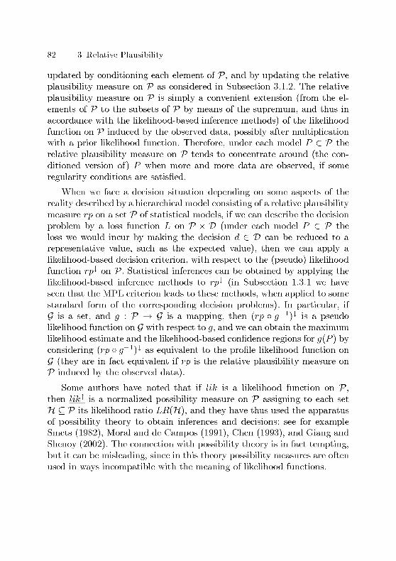
82 3 Relative Plausibility
updated by conditioning each element of V, and by updating the relative
plausibility measure on V as considered in Subsection 3.1.2. The relative
plausibility measure on V is simply a convenient extension (from the el¬
ements of V to the subsets of V by means of the supremum, and thus in
accordance with the likelihood-based inference methods) of the likelihood
function on V induced by the observed data, possibly after multiplicationwith a prior likelihood function. Therefore, under each model P G V the
relative plausibility measure on V tends to concentrate around (the con¬
ditioned version of) P when more and more data are observed, if some
regularity conditions are satisfied.
When we face a decision situation depending on some aspects of the
reality described by a hierarchical model consisting of a relative plausibility
measure rp on a set V of statistical models, if we can describe the decision
problem by a loss function L on V x T> (under each model P G V the
loss we would incur by making the decision d G T> can be reduced to a
representative value, such as the expected value), then we can apply a
likelihood-based decision criterion, with respect to the (pseudo) likelihood
function rp-1 on V. Statistical inferences can be obtained by applying the
likelihood-based inference methods to rp-1 (in Subsection 1.3.1 we have
seen that the MPL criterion leads to these methods, when applied to some
standard form of the corresponding decision problems). In particular, if
Q is a set, and g : V —> Q is a mapping, then (rp o g^1)-1 is a pseudolikelihood function on Q with respect to g, and we can obtain the maximum
likelihood estimate and the likelihood-based confidence regions for g(P) by
considering (rp o g^1)-1 as equivalent to the profile likelihood function on
G (they are in fact equivalent if rp is the relative plausibility measure on
V induced by the observed data).
Some authors have noted that if lik is a likelihood function on V,then hk^ is a normalized possibility measure on V assigning to each set
7i C V its likelihood ratio LR(7i), and they have thus used the apparatus
of possibility theory to obtain inferences and decisions: see for exampleSmets (1982), Moral and de Campos (1991), Chen (1993), and Giang and
Shenoy (2002). The connection with possibility theory is in fact tempting,but it can be misleading, since in this theory possibility measures are often
used in ways incompatible with the meaning of likelihood functions.

3.2 Hierarchical Model 83
3.2.1 Classical and Bayesian Models
From an abstract point of view, the classical and Bayesian models can be
considered as special cases of our hierarchical model, but the approachesto statistical decision problems are different. The classical model consists
of a set V of statistical models, with complete ignorance about which of
the elements of V is the best representation of the reality; in the classi¬
cal approach to statistical decision problems the model is never updated,since only pre-data decision problems are considered. Hence the classical
model corresponds to the hierarchical model with prior relative plausibil¬
ity measure 1^ on the set V, as long as only pre-data decision problems
are considered. In particular, with this prior the MPL criterion applied to
the pre-data decision problem described by the risk function correspondsto the minimax risk criterion. With a general prior relative plausibility
measure on V, the MPL criterion applied to this decision problem consists
in using the prior likelihood of the models to weight the respective losses,before applying the minimax risk criterion. The use of a nondegenerate
prior relative plausibility measure rp on V when applying the MPL crite¬
rion to the pre-data decision problem described by the risk function is thus
a simple way to address the idea behind the restricted Bayesian criterion:
we can use some prior information, but at the same time maintain the
maximum expected loss under control. In fact, if A = inî rp} > 0, then the
maximum expected loss of an optimal decision function according to the
MPL criterion is at most j- times the one of the optimal decision functions
according to the minimax risk criterion.
In Subsection 1.1.2 we have seen that the (strict) Bayesian model con¬
sists of a single probability measure Pv on ? x SÎ, and it is updated by
conditioning P^ on the observed data. Hence the Bayesian model corre¬
sponds to the hierarchical model with as first level the single statistical
model Pjr, since there is a unique nondegenerate relative plausibility mea¬
sure on the singleton {P-k}- Thus only stochastic uncertainty is considered
in the Bayesian model, and this allows the coherence properties stated in
Subsection 1.1.2. In fact, in the Bayesian approach to statistical decision
problems the uncertainty about which of the statistical models in V is the
best representation of the reality is eliminated by assuming that exactly
one of them is "true" and mixing them by means of a prior probability
measure 7r on V. In our approach a prior relative plausibility measure rp
on V is used instead of 7r: the main differences between relative plausibility

84 3 Relative Plausibility
and probability measures have been considered in the previous section. It
is interesting to note that the Bayesian method of maximum a posteri¬ori for the estimation of P G V corresponds to the method of maximum
likelihood, when rp-1 is proportional to the density of 7r with respect to
the considered dominating measure on V, but the method of maximum
likelihood with prior rp can be applied also when the choice of a dominat¬
ing measure on V is problematic (see for example Leonard, 1978). In fact,thanks to their simplicity, relative plausibility measures can be handled
without problems also on sets V that are so wide that using probability
measures on them would be difficult, as in the following example.
Example 3.2. Consider the problem of nonparametric estimation of the
mean of a probability distribution on [0,1], with squared error loss. Let
V be a family of probability measures such that under each of them the
random variables X\,..., Xn are independent and identically distributed
on [0, 1], and such that each probability distribution on [0, 1] for these
random variables corresponds to an element of V. Let g : P i—> Ep(Xi) be
the function on V assigning to each model the mean of the corresponding
probability distribution on [0, 1], and let L : (P, d) i—> [g(P) — d]2 be the
loss function onPx [0, 1] describing the estimation problem. As noted at
the beginning of Section 1.2, for a continuous distribution the observation
X% = x% is impossible: we can only observe X% G Nt, for a neighborhood Nz
of x%. However, for the decision problem at hand, if the neighborhoods Nz
are sufficiently small, then the results are practically equivalent to those
obtained by considering only the discrete distributions on [0,1] and the
exact observations X% = x%.
For instance, in the case with n = 1 we obtain the following (approxi¬mate) profile likelihood function for the mean g(P) of the distribution of
X\\ the function hkg on [0, 1] defined by
rSL ifo<7<a:1,
hkgd) = < 1 if 7 = xi,
[ti if*i<7<l.
If the function / : [0,1] —> P describes the prior relative plausibility of
the possible values of the mean g(P), we can use this prior information
simply by multiplying hkg with /: this amounts to using the prior relative
plausibility measure (f og)î on V. If we do not use prior information, then
the maximum likelihood estimate of g(P) is X\, and the estimate obtained

3.2 Hierarchical Model 85
In i
08: / \
06: ^^^ / \04: /-^^T / \
0 2: / / \
002 04 06 08 1
°02 04 06 08 1
Figure 3.1. Estimators and profile likelihood functions from Example 3.2.
by applying the MPL criterion is m(Xi), where m : [0, 1] —> [^, -g] is an
increasing bijection, plotted in the first diagram of Figure 3.1 (solid line)together with the bijection îdr01i corresponding to the maximum likelihood
estimate (dashed line). It can be proved that the estimate m(Xi) obtained
by applying the MPL criterion is optimal also with respect to the minimax
risk criterion, since the least favorable distribution on [0, 1] with mean 7
is the binomial distribution with parameters n = 1 and p = 7 (consideredin Example 1.8); therefore the maximum expected losses (as functions of
p = 7 G [0,1]) for the estimates obtained by applying the MPL criterion
and the method of maximum likelihood (MLD criterion) are plotted in the
first diagram of Figure 1.3 (solid and dotted curved lines, respectively).
In the cases with n > 1 (without prior information), the maximum
likelihood estimate is simply the arithmetic mean X of the observations
X\,...,Xn, while the estimate obtained by applying the MPL criterion
is not a function of X, because sets of observations with the same mean
can induce rather different profile likelihood functions hkg on [0, 1] (butas n increases, the estimate obtained by applying the MPL criterion tends
rapidly to X). For example, in the case with n = 2 the pairs of observa¬
tions {Xi = 0.4, X2 = 0.4} and {Xx = 0, X2 = 0.8} induce the profilelikelihood functions plotted in the second diagram of Figure 3.1 (solid anddashed lines, respectively; the two functions have been scaled to have the
same maximum): the estimates obtained by applying the MPL criterion
are 0.449 and 0.401, respectively. The first estimate is larger than the
second one because the corresponding profile likelihood function is more

86 3 Relative Plausibility
skew; in fact, the estimates obtained by applying the LRM^ criterion with
ß fa 0.259 (so that —2 log/3 is the 90%-quantile of the x2 distribution with
one degree of freedom) are 0.449 and 0.414, respectively. These estimates
are the midpoints of the intervals corresponding to the likelihood-based
confidence regions for g(P) with cutoff point ß: Owen (1988) proved that
these regions have 90% asymptotic coverage probability. 0
3.2.2 Imprecise Probability Models
As noted at the end of Subsection 1.1.2, the Bayesian model can be gen¬
eralized by considering a whole set T of prior probability measures 7r on
V (with complete ignorance about which of the elements of T is the best
prior). The resulting model consists of a set II of probability measures P^
on V x Q, and it is updated by conditioning each of them on the observed
data, but usually the induced likelihood function on II is not considered
(some methods using the likelihood function have been cited in Subsec¬
tions 1.2.1 and 1.3.2). Hence in general this model cannot be interpretedas a special case of the hierarchical one, because the prior relative plau¬
sibility measure 1^ on II is not updated (that is, we remain in a state of
complete ignorance about which of the elements of II is the best Bayesian
model).
A set V of probability measures on a measurable space (fi, A) can
also be interpreted as an imprecise probability measure on (Q,A): see
for example Walley (1991) and Weichselberger (2001). From V we obtain
in particular the upper probability measure supP (which is normalized,
monotonie, and subadditive) and its dual measure inf V (the lower proba¬
bility measure). Gärdenfors and Sahlin (1982) advocated the necessity of
considering the reliability of the probability measures in V: they stated
that this reliability should be described by a real-valued function p on V,without explaining precisely how p should be updated, but their model
seems to be in agreement with the hierarchical one (through identification
of p and rp-1). The axiomatic approaches of Nau (1992), de Cooman and
Walley (2002), and Giraud (2005) lead to models similar to the hierarchical
one, at least as regards the static aspect. If we start with no information
for discrimination between the probability measures in V, and we observe
an event A G A, then we obtain a likelihood function lik on V, and we
can base inferences and decisions on lik. In particular, if we are interested
in the probability of an event B G A, then we can consider the mapping

3.2 Hierarchical Model 87
g : P i—> P(B\A) on V, and base our inferences on the profile likelihood
function likg on [0,1], as we did in Example 1.7 for the profile likelihood
functions plotted in Figure 1.1. In this regard it is important to note that
hkg does not depend on the definition of P(B\A) when P(A) = 0, since
in this case hk(P) = 0. Of particular interest are the supremum and infi-
mum of the likelihood-based confidence region for g(P) with cutoff point
ß G (0, 1): these can be considered as improved upper and lower proba¬bilities of B, conditional on the observation of A; they correspond to the
upper and lower conditional probabilities of B after the restriction of V
to the likelihood-based confidence region Vß for P with cutoff point ß. It
is important to note that Vß does not depend on the choice of the event
B G A, and that the restriction of V to Vß is only temporary: no element
of V should be really discarded, since the relative plausibility of the ele¬
ments of V can change in the light of new data. The larger is ß, the more
precise are the upper and lower conditional probabilities based on Vß (inthe sense that their distance is smaller), but the lower is the confidence
in them: there is a sort of confidence-precision trade-off. The limits of the
upper and lower conditional probabilities based on Vß as ß tends to 0 corre¬
spond to the "regular extension" considered by Walley (1991, Appendix J)and resulting from the "intuitive concept of conditional probability" stud¬
ied by Weichselberger and Augustin (2003), while their limits as ß tends to
1 correspond to the result of a generalization of the rule for conditioningintroduced by Dempster (1967) and having a central role in the theoryof Shafer (1976): see also Moral and de Campos (1991) and Gilboa and
Schmeidler (1993). Hence, for ß varying in (0,1), the restrictions of V to Vßbuild a continuum between the two extreme cases corresponding to "regu¬lar extension" and "generalized Dempster's conditioning" (inferences other
than upper and lower probabilities can also be based on Vß: for instance
upper and lower expected values of a random variable). As regards upper
and lower conditional probabilities, other compromises between the two
extreme cases have been proposed in the literature: for example, the use of
Jsgdhk]_ as the upper probability of B conditional on the observation of
A (the lower probability can be obtained as dual measure) was considered
by Chen (1993) for some particular cases of independent events A and B,while Moral (1992) proposed to use the Choquet integral or the Sugeno
integral instead of the Shilkret integral in the above expression.
Consider a statistical decision problem described by a loss function L
on V x T>: if we modify the Bayesian approach by using an imprecise prior
probability measure T on (V,C), instead of a (precise) prior probability

88 3 Relative Plausibility
measure on (V, C), then we obtain the imprecise Bayesian model consistingof the set II = {P^ : tï G T} of probability measures on (?xfi,£), consid¬
ered at the end of Subsection 1.1.2. When we observe an event A G A, we
can condition each element of the set II on the event V x A, and we obtain
the likelihood function lik : P^ i—> P-e{V x A) on II. The decision criteria
appearing in the literature on imprecise Bayesian models can usually be
interpreted as criteria applied to the decision problem described by the loss
function L" : (P^d) <-> EPn[L(P,d)\V x A] on II x V without using the
information contained in the likelihood function lik (that is, a part of the
information provided by the data is disregarded). A simple way of using lik
for decision making is to (temporarily) restrict II to the likelihood-based
confidence region Ilg for P^ with cutoff point ß G (0,1), when applyingthe decision criterion (that is, the criterion is applied to the decision prob¬lem described by L"\ußxT>)- In particular, the T-minimax criterion appliedafter having restricted II to 11^ (or equivalently, T to the likelihood-based
confidence region Tß for 7r with cutoff point ß) corresponds to the LRM^criterion applied to the decision problem described by L". The information
contained in the likelihood function lik can be used in a less limited way by
applying other likelihood-based decision criteria (such as the MPL crite¬
rion) to the decision problem described by L". It is interesting to note that
the application of the MPL criterion to the decision problem described byL" can be interpreted as a sort of T-minimax criterion with respect to the
set of non-normalized conditional probability measures (Moral, 1992, ar¬
gued that this set describes the conditional information): in fact, it consists
in minimizing the supremum (over all 7r G T) of
PAV x A)EP„[L(P,d)\V xA]= EP„[L(P,d)IVxA].
The state of complete ignorance about the models in V can be de¬
scribed by the set Tq of all probability measures on (P,C). As noted at
the end of Subsection 1.3.1, if C contains all singletons of V, then usingthe imprecise prior probability measure To on V and applying the MPL
criterion to the decision problem described by L" is equivalent to using the
prior relative plausibility measure 1^ on V and applying the MPL criterion
directly to the decision problem described by L. This property is not pos¬
sessed by other likelihood-based decision criteria, such as the LRM^ one,
the MLD one, or the one obtained by substituting the Choquet integral for
the Shilkret integral in the MPL criterion (that is, the "MPL* criterion" of
Cattaneo, 2005), but in general the likelihood-based methods can be used
without problems with the imprecise prior probability measure Tq on?,

3.2 Hierarchical Model 89
while this is not the case for the methods that do not use the information
contained in the likelihood function lik on II. In fact, when the imprecise
Bayesian model is updated by means of "regular extension" (and thus lik
is used only to discard the Pv G II that are impossible in the light of the
observed data, in the sense that Pv (V x A) = 0), it is in general not pos¬
sible to get out of the state of complete ignorance, because an important
part of the information provided by the data is disregarded (see also the
beginning of Subsection 4.2.2). More generally, a consequence of the disre¬
gard of the information contained in the likelihood function lik is that the
conclusions obtained on the basis of the "regular extension" can be useless
if the imprecise prior probability measure on V has not been selected with
extreme care (see for instance Kriegler, 2005, Chapter 4): this undermines
the intuitive basis of the imprecise Bayesian model.
Example 3.3. In Examples 1.5 and 1.9 we considered (for the estimation
problem of Example 1.1) the imprecise Bayesian model II with as impre¬cise prior probability measure on V the family T of probability measures
on V corresponding to the family of beta distributions for the parameter
p G [0,1]. The observation of X = x induces a likelihood function lik on II:
a method using the information contained in lik (such as the MPL crite¬
rion) can lead to reasonable conclusions, while a method disregarding this
part of the information provided by the data (such as the T-minimax crite¬
rion) will lead to vacuous conclusions. However, non-vacuous conclusions
can be obtained without using the information contained in the likelihood
function lik, when instead of T some narrower set of probability measures
on V is used. Walley (1991, Section 5.3) proposed to use a "near-ignorance
prior" on V: that is, an imprecise prior probability measure on V such that
for all possible observations the upper and lower probabilities are 1 and 0,
respectively; in this way, an apparent initial state of complete ignoranceis obtained (an example of near-ignorance prior is T itself). In particu¬
lar, Walley considered the near-ignorance priors Ts C T corresponding to
the sets of all the beta distributions with sum of the two parameters equal
s G P: the resulting imprecise Bayesian models are special cases of the "im¬
precise Dirichlet models" studied in Walley (1996), where the particularchoices s = 2 and s = 1 are advocated.
Let g' be the function on II corresponding to the function g on V
considered in Example 1.6: that is, g' assigns to each model Pv the prob¬
ability Ep^ [g(P) \X = x] of observing at least 3 successes in 5 future in¬
dependent binary experiments with the same success probability as the n

90 3 Relative Plausibility
0.2 0.4 0.6 o.: 0.2 0.4 0.6 0.:
Figure 3.2. Profile likelihood functions from Example 3.3.
observed ones. Figure 3.2 shows the graphs of the profile likelihood func¬
tions likgt on [0, f] induced by the observations X = 8 with n = fO (firstdiagram), and X = 33 with n = 50 (second diagram), for the three impre¬cise Bayesian models with imprecise prior probability measures T (dottedlines), T2 (dashed lines), and T± (solid lines), respectively (the functions
have been scaled to have the same maximum). The profile likelihood func¬
tions likgt for the imprecise Bayesian model with prior T correspond to
the profile likelihood functions likg for the model V (plotted in Figure 1.1:
dotted and dashed lines, respectively), and also to the limits, as s tends to
infinity, of the profile likelihood functions likgt for the imprecise Bayesianmodels with prior Ts; while as s tends to 0 these functions tend to con¬
centrate on 7' = E^t{g), where 7r' is the probability measure on V corre¬
sponding to the (possibly degenerate) beta distribution with parameters x
and n — x (for the two observations considered, 7' « 0.905 and 7' « 0.771,
respectively; as n increases, 7' tends to the maximum likelihood estimate
7ml, considered in Example 1.7).
The profile likelihood function likgt for the imprecise Bayesian model
with prior T always takes positive values on the whole interval (0, 1), and
therefore only vacuous conclusions can be obtained if the model is updated
by means of "regular extension" (and the information contained in likgtis thus disregarded). But with the priors Ts non-vacuous conclusions can
be obtained even if the model is updated by means of "regular extension",because in this case the range of the function g' (corresponding to the
support of likgt) is usually only a small subset of the interval [0,1]: for the

3.2 Hierarchical Model 91
two observations considered, with s = 2 we obtain the probability intervals
(0.758,0.937) and (0.733,0.790), respectively, while with s = 1 we obtain
the probability intervals (0.833,0.923) and (0.752,0.781), respectively (theendpoints of the probability intervals are the upper and lower probabilitiesof observing at least 3 successes in 5 future independent binary experimentswith the same success probability as the n observed ones). The last column
of Table 1.1 gives the probability intervals obtained by restricting the im¬
precise Bayesian model II with prior T to the likelihood-based confidence
region Ilg for Pv with cutoff point ß « 0.036: this cutoff point is rather
small, but for any reasonable choice of ß the probability intervals based
on Ilg would be much longer than the above ones (based on the "regularextension" of the imprecise Bayesian models with priors 1^ and Ti, re¬
spectively), as can be easily seen from the graphs of Figure 3.2. Anyway,the usefulness of the near-ignorance priors Ts is very limited: it suffices to
slightly modify the model to obtain vacuous conclusions, when the mod¬
ified model is updated by means of "regular extension" (see for example
Piatti, Zaffalon, and Trojani, 2005). 0
It is interesting to consider the possibility of replacing the statistical
models in V with imprecise statistical models: let XV be a set of imprecise
probability measures on a measurable space (Q, A); that is, each IP G XV
is a set of (precise) probability measures on (Q,A). The simplest way
to handle imprecise statistical models within our hierarchical model is to
consider the set V = [JXV of (precise) statistical models, and the mapping
g : V -> XV defined by g~1{IP} = IP (for all IP G XV). To be precise, g
is well-defined only if the elements of XV are disjoint, but this can alwaysbe obtained for example by expanding the measurable space (Q, A) to its
product with the measurable space (XV, 2L'P), and replacing each P G IP
with the product of P and the Dirac measure öjp on XV (for all IP G XV).If we observe an event A G A (or the corresponding event A x XV, when
Q has been expanded to Q x XV), then we obtain a likelihood function lik
on V, and we can base inferences and decisions on the profile likelihood
function hkg on XV. Since
hkg(IP) = sup/P hk = (supIP)(A) for all IP G XV,
hkg is simply the pseudo likelihood function on XV based on the upper
probability measures sup IP. For example, if we have a set V' of statistical
models on (Q,A), and for some e G (0, 1) we replace each P' G V with
its e-contamination class (that is, the imprecise model consisting of the

92 3 Relative Plausibility
contaminated statistical models (1 — e) P' + eP, for all the probability
measures P on (Q,A)), then instead of the likelihood function lik' on V'
we obtain the pseudo likelihood function (1 — e) lik' + e, which can be
interpreted as an attenuate version of lik' (the information contained in
lik' has been discounted, in the sense of Shafer, 1976).
In general, the profile likelihood function likg on XV favors the more
imprecise models in XV (because it is based only on the upper probability
measures sup IP) : this behavior seems to be in agreement with the various
interpretations of the imprecise probability measures, but if in a particular
case it is disapproved, then another pseudo likelihood function on XV, pe¬
nalizing the more imprecise models (for example by explicitly taking into
account also the lower probability measures inf IP), should be used instead
of hkg. When we combine the imprecise statistical models in XV with a
(precise or imprecise) prior probability measure on XV, we obtain the im¬
precise Bayesian model consisting of the probability measures on XV x Q
that result from all the possible combinations of the averaging probability
measures considered and the (precise) statistical models considered; but
if we update the resulting model by means of "regular extension" (disre¬garding thus a part of the information provided by the data), then we can
easily get unreasonable results (see for example Wilson, 2001).
Example 3.4- If in the estimation problem of Example 1.1 we replacethe models for the results of each single binary experiment with their
e-contamination classes, but we still consider the n results as indepen¬dent and identically distributed, then we obtain the problem of estimating
p G [0, 1] (with squared error loss) after having observed the number of
successes in n independent binary experiments with common success prob¬
ability q G [(1 — e)p, (1 — e)p + e\. The first diagram of Figure 3.3 shows
the graphs of the profile likelihood functions likg on [0, 1] for the mapping
g and the three observations considered in Example 1.6, under the conta¬
minated models with e = 0.1 (the three functions have been scaled to have
the same maximum); that is, it shows how the graphs of Figure 1.1 are
modified by the e-contaminations of the binary experiments. From these
graphs we can see that there is an unavoidable uncertainty about p: in fact,even if we knew the actual success probability q, we could only conclude
that p G [max{f5f ,0},min{14i, 1}].
The second diagram of Figure 3.3 shows (for the case with n = 100) the
graphs of the maximum expected losses under the contaminated models
with e = 0.1 (as functions of p G [0,1]) for the estimates obtained by

3 2 Hierarchical Model 93
Figure 3.3. Profile likelihood functions and (maximum) expected losses from
Example 3 4
applying the MPL criterion to these models (upper solid line) and to the
uncontaminated models (upper dashed line), and also the graphs of their
expected losses under the uncontaminated models (lower solid and dashed
lines, respectively) The estimate obtained by applying the MPL criterion
to the uncontaminated models was considered in Example 1 8 (the lower
dashed line of the second diagram of Figure 3 3 corresponds to the solid line
of the third diagram of Figure 1 3) ; its maximum expected loss under the
contaminated models is particularly high for values of p near the endpointsof the interval [0, 1] this is a consequence of the fact that the maximum
(\ + \p — g |) £ of the possible difference between p and the actual success
probability q is larger for values of p near the endpoints than for values of
p near the center of the interval [0,1] The estimate obtained by applyingthe MPL criterion to the contaminated models corrects this behavior by
favoring the values of p near the endpoints of the interval [0,1] 0


4
Likelihood-Based Decision Criteria
This chapter begins with a general definition of likelihood-based decision
criterion. Several additional decision theoretic properties are then consid¬
ered and related to integral representations of the decision criteria. Fi¬
nally, some statistical properties of the likelihood-based decision criteria
are studied; in particular their asymptotic optimality.
4.1 Decision Theoretic Properties
Consider a statistical decision problem described by a loss function L on
?xD, and let rp be a relative plausibility measure on V describing the
uncertain knowledge about the models in V. By definition of L, all im¬
portant aspects of the decisions d G T> are summarized by the respectivefunctions 14 G V^; we will consider only decision criteria that compare the
possible decisions on the basis of some functional Vrp : V^ —> P (dependingon rp), in the sense that the criteria can be expressed as follows:
minimize Vrp(ld).
Each functional Vrp represents a total preorder ^rp on V^, and 14 ^rp 141
can be interpreted as "d! is not preferred to d on the basis of the decision
criterion considered and of the relative plausibility measure rp".
For the sake of generality, we replace V with a generic set of alter¬
natives determining for each possible decision the loss incurred, and we
consider thus decision criteria associating to each (nondegenerate) relative
plausibility measure rp (on some set Qrp) a preference relation ^rp on
pSrp. wnen interpreting the definitions and the results, however, we re¬
gard Qrp as a set of statistical models, and each / G VQrp as the uncertain

96 4 Likelihood-Based Decision Criteria
loss Id incurred by making a particular decision d. The following necessary
condition of monotonicity for the preference relations ^rp was stated at
the beginning of Section 1.1 as a direct consequence of the interpretationof a loss function:
/ </' => l-<rpl' for all/,/' G PQ^. (4.1)
Since the loss functions L and a L are considered equivalent (for all a G P),the following condition of scale invariance for the preference relations ^rpis also necessary:
l<rpï => al<rpaï for all a G P and all /, /' G ^Qrp. (4.2)
To avoid vacuous decision criteria, we can assume the following con¬
dition describing the ability of discrimination between the decisions with
constant losses:
c <rp c' => c<c' for all c, c' G P. (4.3)
The next theorem implies that, given the preceding three conditions, the
following two are sufficient for a total preorder ^rp to be represented by a
functional Vrp : Ps>-p —> P; it can be easily proved that they are also nec¬
essary (except for the cases with inf C = 0 and supC = oo, respectively).
/ Sp c for all c G C => I <rp inf C for all C Ç P
and all / G ¥Qrp.
c ;Sp I f°r all c G C => sup C <rp I for all C Ç P
and all / G PQrp
(4.4)
(4.5)
Theorem 4.1. Let Qrp be a nonempty set. A total preorder ^rp on Ps>-p
fulfills the conditions (4-1), (4-®)> (4-3)> (4-4); and (4-5) if and only if it is
represented by a homogeneous, monotonie functional Vrp : Ps>-p —> P such
that Vrp(c) = c for all c G P; the functional Vrp is unique.
Proof. The "if part is simple: the first two conditions follow from the
monotonicity and the homogeneity of Vrp, respectively, and the last three
conditions are implied by the property that Vrp(c) = c for all c G P.
For the "only if part, define Vrp(l) = sup{c G P : c ^rp /} for all
/ G VQrp. Condition (4.5) implies that Vrp(l) ^rp /, and condition (4.4)
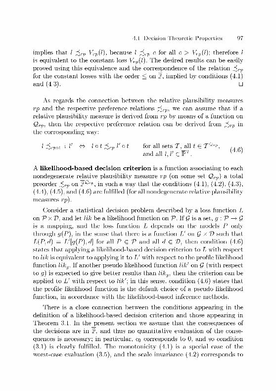
4.1 Decision Theoretic Properties 97
implies that / ^rp Vrp(l), because / ^rp c for all c > Vrp(l); therefore /
is equivalent to the constant loss Vrp(l). The desired results can be easily
proved using this equivalence and the correspondence of the relation ^rpfor the constant losses with the order < on P, implied by conditions (4.1)and (4.3). D
As regards the connection between the relative plausibility measures
rp and the respective preference relations ^rp, we can assume that if a
relative plausibility measure is derived from rp by means of a function on
Qrp, then the respective preference relation can be derived from ^rp in
the corresponding way:
I ;Spot-i I' ^ I ° * ;Sp l' ° * f°r all sets T, all t G TQr*>, . .
and all /, /' G PT* '
A likelihood-based decision criterion is a function associating to each
nondegenerate relative plausibility measure rp (on some set Qrp) a total
preorder ^rp on P2rp, in such a way that the conditions (4.1), (4.2), (4.3),(4.4), (4.5), and (4.6) are fulfilled (for all nondegenerate relative plausibility
measures rp).
Consider a statistical decision problem described by a loss function L
on V x T>, and let hk be a likelihood function on V. If G is a set, g :V —> G
is a mapping, and the loss function L depends on the models P only
through g(P), in the sense that there is a function L' on G x 2? such that
L(P,d) = L'[3(P),d] for all P 6 P and all d G V, then condition (4.6)states that applying a likelihood-based decision criterion to L with respect
to hk is equivalent to applying it to L' with respect to the profile likelihood
function hkg. If another pseudo likelihood function hk' on G (with respect
to g) is expected to give better results than hkg, then the criterion can be
applied to L' with respect to hk'; in this sense, condition (4.6) states that
the profile likelihood function is the default choice of a pseudo likelihood
function, in accordance with the likelihood-based inference methods.
There is a close connection between the conditions appearing in the
definition of a likelihood-based decision criterion and those appearing in
Theorem 3.1. In the present section we assume that the consequences of
the decisions are in P, and thus no quantitative evaluation of the conse¬
quences is necessary; in particular, cq corresponds to 0, and so condition
(3.1) is clearly fulfilled. The monotonicity (4.1) is a special case of the
worst-case evaluation (3.5), and the scale invariance (4.2) corresponds to

98 4 Likelihood-Based Decision Criteria
(3.2). The only effect of assuming condition (4.3) is the exclusion of the
trivial relations ^rp for which all the elements of Ps>-p are equivalent: this
nontriviality is not assumed in Theorem 3.1, but it is necessary and suffi¬
cient for the uniqueness of rp. Conditions (4.4) and (4.5) can be rewritten
as a continuity condition corresponding to (3.3) and two conditions ex¬
pressing the exclusion of "infinitesimal evaluations" and of "transfinite
evaluations" (the cases with inf C = 0 and supC = oo, respectively): the
first of these last two conditions corresponds to (3.4), and the second one
is a special case of (3.5), with the difference that in Subsection 3.1.1 the
boundedness of the consequences is assumed, and thus no consequence cor¬
responds to oo. Condition (4.6) cannot be expressed in the framework of
Subsection 3.1.1 (because in that framework the existence of the relative
plausibility measure rp is not assumed), but it is related to the limited
version of the worst-case evaluation stated at the end of Subsection 3.1.1.
Thus, apart from the assumptions that the consequences are in P, that rp
describes the uncertain knowledge about the elements of Qrp, and that the
preference relation on Ps>-p is nontrivial, the difference between the con¬
ditions appearing in the definition of a likelihood-based decision criterion
and those appearing in Theorem 3.1 is that the worst-case evaluation (3.5)is weakened by replacing it with two special cases (the monotonicity and
the exclusion of "transfinite evaluations") and condition (4.6). The next
theorem states that a likelihood-based decision criterion corresponds to a
functional on the set
S¥={<p£[0,lf:sap<p = l};
the MPL criterion of Theorem 3.1 corresponds to the particular functional
cp i—> sup idp ip on <Sjp.
Theorem 4.2. A function associating to each nondegenerate relative plau¬
sibility measure rp (on some set Qrp) a binary relation ^rp on Ps>-p is
a hkehhood-based decision criterion if and only if there is a functionalS : Sf —> P such that each relation ^rp is represented by the functional
Vrp : I i—> S\{rp_o Z-1)^] and the following three conditions are fulfilled:
S(I{1}) = 1, (4.7)
S[(p(-)]=cS((f) for all ip G <% and aile G W, (4.8)
suP[x,oo] V<
suP[x,oo] V> 1and supj0)X] ip > supj0)X] ip > => S(ip) < S(ip) for all ip, ifi G «%. (4.9)
for all x G P J

4.1 Decision Theoretic Properties 99
Proof. Theorem 4.1 implies that we have a likelihood-based decision cri¬
terion if and only if condition (4.6) is fulfilled and each relation ^rp is
represented by a homogeneous, monotonie functional Vrp : Ps>-p —> P
such that Vrp(l) = 1 (since then Vrp(c) = c for all c G P follows from
homogeneity and nionotonicity). Condition (4.6) corresponds to the ex¬
istence of a functional S : <Sjp —> P such that Vrp(l) = S[(rj) o Z-1)^]. In
fact, the existence of such a functional implies condition (4.6), because
rg o (/ o t)_1 = (rp oT1) o Z_1; conversely, when condition (4.6) holds we
can define S(ip) = Vvr (tdf), since
Vrp{l) = Vrp(td¥ o /) = Vrp[Vrp{l) o /] = Vrpol-i [Vrp{l)\ = Vrpol-i (tdf),
where the last equality is a consequence of the second one. Hence, to
prove the theorem it suffices to show that the property Vrp(l) = 1,the homogeneity, and the nionotonicity of the functionals Vrp correspondto the conditions (4.7), (4.8), and (4.9), respectively. The first two cor¬
respondences follow easily from the equalities (rp o T1)^ = ir-n and
[rp o (c/)_1]^(a;) = (rgoT1)^-), respectively. The nionotonicity of the
functionals Vrp follows from condition (4.9), since by defining
1,9= (rgoT1)^ and ip = [qjo (/')_1]^ (4-10)
the inequality / < /' implies the premise of condition (4.9): in fact,
suprx 001^ = ry\l > x} and supr0 xi cp = rp{l < x}, and analogously for
ip and /'.To prove the converse it suffices to show that for all cp,ip G Spsatisfying the premise of condition (4.9) there are a nondegenerate relative
plausibility measure rp (on some set Qrp) and two functions 1,1' G PSrp
satisfying / < /' and (4.10). Define the set Qrp Ç P x [0,1) x {0,1} as
follows:
QrP = ({(x,y) G P2 : y < <f(x)} x {0}) U ({(x,y) G P2 : y < ip(x)} x {1}),
and let rp be the nondegenerate relative plausibility measure on Qrp de¬
fined by rj>} (x, y, z) = y. Since suprx w| ip < suprx w| ip, for each (x, y) G P2
such that y < (f(x) there is an x' G [x,oo] such that y < ip(x'): define
l(x,y,0) = x and l'(x,y,0) = x'. Analogously, since supr0 xi(p > supr0 x-\ip,for each (x,y) G P2 such that y < ip(x) there is an x' G [0,x] such that
y < ip(x'): define l(x,y, 1) = x' and l'(x,y, 1) = x. We obtain two func¬
tions /, /' G PSrp such that / < /'; the equalities of (4.10) are also satisfied,since l(x,y,z) = x' implies y < y(x'), and conversely y < (f(x') implies
l(x',y,0) = x': therefore (rgo/_1)^(x') = y(x'), and analogously for ^ and
/'. D
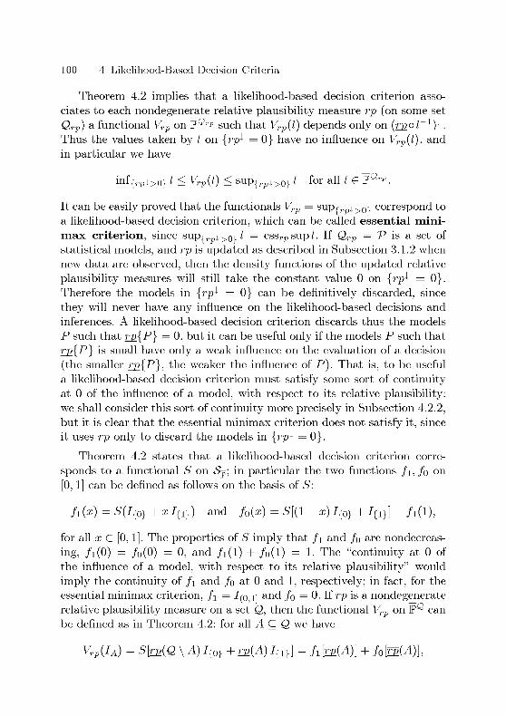
100 4 Likelihood-Based Decision Criteria
Theorem 4.2 implies that a likelihood-based decision criterion asso¬
ciates to each nondegenerate relative plausibility measure rp (on some set
Qrp) a functional Vrp on WQrp such that Vrp(l) depends only on (rpol^1)^.Thus the values taken by / on {rp-1 = 0} have no influence on Vrp(l), and
in particular we have
inf(rpi>0} / < Vrp(l) < sup|rpi>0| / for all / G ps>-p.
It can be easily proved that the functionals Vrp = supr i>0i correspond to
a likelihood-based decision criterion, which can be called essential mini-
max criterion, since supr i>0iI = essrpsup/. If Qrp = V is a set of
statistical models, and rp is updated as described in Subsection 3.1.2 when
new data are observed, then the density functions of the updated relative
plausibility measures will still take the constant value 0 on {rp-1 = 0}.Therefore the models in {rp-1 = 0} can be definitively discarded, since
they will never have any influence on the likelihood-based decisions and
inferences. A likelihood-based decision criterion discards thus the models
P such that rp{P} = 0, but it can be useful only if the models P such that
rp{P} is small have only a weak influence on the evaluation of a decision
(the smaller rj){P}, the weaker the influence of P). That is, to be useful
a likelihood-based decision criterion must satisfy some sort of continuityat 0 of the influence of a model, with respect to its relative plausibility:
we shall consider this sort of continuity more precisely in Subsection 4.2.2,but it is clear that the essential minimax criterion does not satisfy it, since
it uses rp only to discard the models in {rp-1 = 0}.
Theorem 4.2 states that a likelihood-based decision criterion corre¬
sponds to a functional S on Sp; in particular the two functions /i, /o on
[0,1] can be defined as follows on the basis of S:
fx{x) = S(I{o} +xl{i}) and f0(x) = S[(l - x) I{0} + /{i}] - /i(l),
for all x G [0, 1]. The properties of S imply that /i and /o are nondecreas-
ing, /i(0) = /o(0) = 0, and /i(l) + /0(1) = 1. The "continuity at 0 of
the influence of a model, with respect to its relative plausibility" would
imply the continuity of /i and /o at 0 and 1, respectively; in fact, for the
essential minimax criterion, fi = /mi] and /o = 0. If rp is a nondegeneraterelative plausibility measure on a set Q, then the functional Vrp on Ps can
be defined as in Theorem 4.2: for all A Ç Q we have
Vrp(IA)=S[m(Q\A)I{0}+m(A)I{1}]=f1[m(A)] + fç)[m(A%

4.1 Decision Theoretic Properties 101
where rp is the dual of the normalized representative of rp. In particular,if rp = 1Î, then V^ {Ia) = /i(l) f°r aU nonempty A C <2; this implies that
two decisions can be considered equivalent by all likelihood-based decision
criteria, even when one decision dominates the other, their uncertain losses
are bounded, and rp-1 > 0. Moreover, since 1/it(1) = 1, no likelihood-based
decision criterion can correspond to an additive functional V^ on Ps when
Q has at least three elements.
Consider a statistical decision problem described by a loss function
L on V x T>, let rp be a nondegenerate relative plausibility measure on
V describing the uncertain knowledge about the models in V, and let
d, d! G T> be two decisions such that d dominates d!. The monotonicity
(4.1) of the preference relation ^rp assures that d! is not preferred to d,but as shown above, it is possible that d and d! are equivalent accordingto all likelihood-based decision criteria (this is in particular the case when
rgoid = rp o Ij, ). However, as noted at the beginning of Section 1.1,if we have to choose between d and d', then we must choose d; hence, if
necessary, a likelihood-based decision criterion can be refined by discard¬
ing from the set of optimal decisions those that are dominated (by other
optimal decisions). Anyway, if d! is strictly dominated by d, in the sense
that inf (Id' — Id) > 0, then a necessary and sufficient condition for d to be
preferred to d! according to all likelihood-based decision criteria is that Id is
essentially bounded with respect to rp, in the sense that essrp sup Id < oo.
This condition is necessary, because the functionals Vrp = essrp sup cor¬
respond to the essential minimax criterion, and it is sufficient, because if
e = inf(/(2< — Id) and s = essrp sup Id, then ^^ Id < Id' on {rp-1 > 0}, and
thus Vrp(ld) < Vrp(ld') for all likelihood-based decision criteria, since Vrpis monotonie and homogeneous, Vrp(ld) < s, and Vrp(ld') > e.
In Subsection 1.3.1 we have seen that the MPL criterion leads to the
usual likelihood-based inference methods, when applied to some standard
form of the corresponding decision problems; this is true also for a generallikelihood-based decision criterion, if the corresponding functions /i and
/o fulfill some conditions. For the estimation problems described by the
loss functions Iw and IwE considered in Subsection 1.3.1, it can be easily
proved that when a maximum likelihood estimate exists and is (really)unique, a likelihood-based decision criterion leads (practically) to it if and
only if /i(x) < /i(l) + /o(l — x) for all x G [0, 1). When applied to the
hypothesis testing problem considered in Subsection 1.3.1 (with Ci > c^),a likelihood-based decision criterion leads practically to a likelihood ratio

102 4 Likelihood-Based Decision Criteria
test with some critical value ß depending on^ (where "practically" means
that we do not bother about the case with LR(7i) = ß) if and only if
the function / : x i—>, ^uf t_^
on [0,1] is well-defined, it is strictly
increasing on /_1(0,1), and it satisfies sup/0 j\ / = 1 and inf(o,i) / = 0.
The critical value ß is a strictly increasing function of — if and only if
/ is continuous: in this case, ß = /_1(—) (the inverse function /_1 is
well-defined on (0,1)). For the problem of selecting a confidence regionconsidered in Subsection 1.3.1, a likelihood-based decision criterion is able
to discriminate between regions d G T> with different values of LR{g ^ d}if and only if /i is strictly increasing. In conclusion, a likelihood-based
decision criterion leads to the usual likelihood-based inference methods if
and only if fi is continuous and strictly increasing, and /o is continuous
on [0,1); in fact, for the MPL criterion, /i = idr0jli and /o = 0.
4.1.1 Attitudes Toward Ignorance
Let Pbea set of statistical models, and let lik : V —> [0, 1] be the likelihood
function induced by the observed data. If lik = I{p\ for some model P G V,then all likelihood-based decisions and inferences would be the same as if
we were certain of P (that is, as if P were the only representation of
reality that we consider). If lik > I{p\, then we would be more ignorantabout which of the models in V is the best representation of the reality: in
fact, the data would contain less information for discrimination between
P and the other models in V (in the sense of Kullback and Leibler, 1951);the larger lik, the more ignorant we would be. In the extreme case with
lik = I{p\, the data contain infinite information for discrimination between
P and the other models in V; while at the other extreme we have the case of
complete ignorance, in which lik = 1 and the data contain no information
for discrimination between the models. In this sense, if rp and rp' are
two nondegenerate relative plausibility measures on V such that rjo < rp',then we are more ignorant about which of the models in V is the best
representation of the reality when rp1 describes our uncertain knowledgeabout the models than when rp describes it.
A likelihood-based decision criterion reveals ignorance aversion if
the corresponding functionals Vrp satisfy
rp < rp!_ => Vrp < Vrpi
for all pairs of nondegenerate relative plausibility measures rp, rp' on the
same set Q. This property can be expressed as follows in terms of preference

4.1 Decision Theoretic Properties 103
relations:
c TZrp I and TJL < "HßL => c TZrp1 I f°r all c G P and all / G P.
Since the evaluation of the decisions with constant losses c G P does not
depend on our uncertain knowledge about the models, we can use these
decisions to compare our preferences in different states of knowledge: ig¬
norance aversion means that if we do not prefer a particular decision to
the constant loss c, then neither would we when we were more ignorant.
Theorem 4.3. Consider a likelihood-based decision criterion and the cor¬
responding functional S : Sp —> P; the following four assertions are equiv¬
alent:
the decision criterion reveals ignorance aversion,
S is monotonie,
S is ^-independent,
each relation ^rp is represented by the functional Vrp : I i—> S(rj){l > •}).
Proof. Let cp, ip G Sp such that p < ip. If the decision criterion reveals
ignorance aversion, then S(p) = Vptfidp) < V^t (idp) = S(ip), and thus S
is monotonie. If <^L0 c»]= V'lfUoo]) then S(ip) < S(p) follows from condition
(4.9), and therefore S is 0-independent when it is monotonie. If S is 0-
independent, and x = (tM° ^_1)^ then
MO = S(X) = S(I{0} +x/(0,oo]) = S(te{1 > •}),
where the last equality is implied by condition (4.9) with p = I{o}+xl(o,oo]and ip : x i—> suprx w| x
= U>{1 > x}. Finally, if the fourth assertion
holds, then the ignorance aversion is a consequence of condition (4.9),since suprx w| ry\l > •} = rj){l > x} and supr0 xi ry\l > •} = 1. D
Let TL be a nonempty subset of V, and consider the (nondegenerate)relative plausibility measure {IuY on T* Theorem 4.3 implies that the
functional on V^ corresponding to a likelihood-based decision criterion
revealing ignorance aversion is simply V/j y= supw. In particular, in
the case of complete ignorance about which of the models in V is the
best representation of the reality we have V^ = sup, and therefore the
likelihood-based decision criteria revealing ignorance aversion can be con¬
sidered as generalizations of the minimax criterion. Moreover, for these cri-

104 4 Likelihood-Based Decision Criteria
teria /i(l) = S(Ir01\) = S'(/r1i) = 1, and thus /o = 0; hence a likelihood-
based decision criterion revealing ignorance aversion leads to the usual
likelihood-based inference methods if and only if f\ : [0,1] —> [0, 1] is an
increasing bijection. The fourth assertion of Theorem 4.3 suggests the idea
that the functionals Vrp corresponding to a decision criterion revealing
ignorance aversion can be expressed by means of an integral respectingdistributional dominance; the next theorem states that the injectivity of
/i is a sufficient condition for this integral representation.
Theorem 4.4. Consider a likelihood-based decision criterion such that the
corresponding function f\ : [0,1] —> [0, 1] is strictly increasing, and let
Ai be the class of all monotonie measures taking values in the range of
f\. The decision criterion reveals ignorance aversion if and only if there
is a support-based, homogeneous integral respecting distributional domi¬
nance on Ai such that each relation ^rp is represented by the functional
Vrp : I i—> J/d(/i org); the integral is unique.
Proof. The "if part is simple: the decision criterion reveals ignorance aver¬
sion because f\ is nondecreasing and an integral respecting distributional
dominance is monotonie with respect to measures (Theorem 2.12).
For the "only if part, we have Vrp(I^) = fi[rp(A)] for all nondegener-ate relative plausibility measures rp and all A Ç Qrp, and so the equality
J/d(/i org) = Vrp(l) defines an integral on the class Ai' of all measures
of the form f\ o /i, for all normalized, completely maxitive measures /i,
since for each v G Ai' there is a unique nondegenerate relative plausibilitymeasure rp such that v = f\ o rp. Theorem 4.3 implies that the integral
respects distributional dominance, and thus it corresponds to a functional
on VJ-'(Ai') that can be extended to DJ7(Ai) by means of 0-independence.The integral on Ai corresponding to the extended functional satisfies the
desired properties, and its uniqueness can be easily proved by exploitingthe fact that VT{M) = VT{M") for the class .M" of all measures of the
form fi o /i, for all possibility measures /i. D
The integral obtained in Theorem 4.4 can be easily (but not uniquely)extended to a support-based, homogeneous integral respecting distribu¬
tional dominance on the class of all monotonie measures, when f\ is left-
continuous; the next example shows that such an extension is in generalnot possible when f\ is not left-continuous.

4.1 Decision Theoretic Properties 105
Example 4-5- Let ö be the function on P defined in Example 2.2, and con¬
sider the likelihood-based decision criterion associating to each nondegen-erate relative plausibility measure rp (on some set Qrp) the relation ^rpon Ps>-p represented by the functional Vrp : I i—> JTld(öorp). This decision
criterion reveals ignorance aversion and /i = <5|ro,i] is strictly increasing,but the results of Example 2.11 imply that no integral respecting distribu¬
tional dominance on the class of all monotonie measures can correspondto the rectangular integral on the class of all monotonie measures takingvalues in the range of /i. 0
In Theorem 4.4 the injectivity of /i is needed to define the integral
on the basis of the functionals Vrp, but in general for all nondecreasingfunctions /i : [0, 1] —> [0, 1] such that /i(0) = 0 and /i(l) = 1, and for all
homogeneous integrals respecting distributional dominance on the class of
all normalized, monotonie measures taking values in the range of /i, the
functionals Vrp : I i—> J I d(fiorp) correspond to a likelihood-based decision
criterion revealing ignorance aversion. In particular, if the range of /i is
{0, 1}, then the choice of the integral has no influence: Vrp = ess/l0rEsup.
If fi = Itß i] for some ß G (0,1), then the functionals Vrp = ess/, 1]0r£suP
correspond to the LRM^ criterion; while if fi = im, then the func¬
tionals Vrp = ess/r^or^sup correspond to the MLD criterion. These two
likelihood-based decision criteria reveal thus ignorance aversion, and the
corresponding functionals Vrp can be expressed as integrals with respect
to a distortion of rp.
Theorem 4.3 implies that a likelihood-based decision criterion reveal¬
ing ignorance aversion corresponds to a 0-independent functional S on
Sp, but since the functionals Vrp : I i—> S(rj){l > •}) on WQrp depend
on rp through its normalized representative only, in general they are not
"support-based", in the sense that in general rp{l > 0} > 0 does not imply
Vrp(l) = Vrpi (J\{i>o\)- In fact, the essential minimax criterion is the
only likelihood-based decision criterion such that the corresponding func¬
tionals Vrp are "support-based" in this sense. However, for decision criteria
revealing ignorance aversion (and thus generalizing the minimax criterion)it is reasonable to assume that the preference between two decisions does
not depend on the models for which both decisions are correct; that is, the
preference between / and /' is left unchanged when we restrict attention
to the subset {/ > 0} U {/' > 0} = {/ + /'> 0} of Qrp. A likelihood-based
decision criterion is said to be O-independent if for each nondegenerate

106 4 Likelihood-Based Decision Criteria
relative plausibility measure rp (on some set Qrp)
I Sp I' O l\{i+i>>0} Sp\{l+l,>0} l'\{i+i>>0} for all /, /' G P2^ such
that rp{l + /' > 0} > 0.
The next theorem implies in particular that all 0-independent likelihood-
based decision criteria reveal ignorance aversion.
Theorem 4.6. A likelihood-based decision criterion is O-mdependent ifand only if either it is the essential minimax criterion, or there are a
support-based, regular integral on the class of all finite, monotonie mea¬
sures, and a positive real number a such that each relation Sp ls repre¬
sented by the functional I i—> J I d(rp°); in this case, the integral is unique.
Proof. For the "if part, let A Ç Qrp be a set such that rp(A) > 0 and
^Qr \A= 0- The functionals Vrp corresponding to the likelihood-based
decision criterion satisfy Vrp(l) = Vrp\A(l\A) in the case of the essential
minimax criterion, while in the other case they satisfy
vrp(t) = J id(m°)= J i\Ad(m°)\A = ln>(A)]avrpU(i\A),
because the integral is support-based and bihomogeneous. To obtain the
O-independence it suffices to choose A = {/ + /'> 0}.
For the "only if part, first note that the function f\ on [0, 1] cor¬
responding to the 0-independent likelihood-based decision criterion con¬
sidered is positive on (0, 1]. To prove this, let rp be the (nondegenerate)relative plausibility measure on {0, 1} defined by rpHl) = c G (0,1] and
Œi(0) = 1. Then /i(c) = Vrp(I{1}) > Vrp(0) = 0, because rp{l} > 0
and Vrp\ (i"{i}|{i}) = f > 0 = ^rp|m(0|{i].). We can now prove that
the functional S on S^ corresponding to the decision criterion satisfies the
following equality for all c G (0, 1] and all cp G Sp\
S(I{0} + c^7(0,00]) = h(c) S(<p). (4.11)
Define Q = P x {0, 1} x {0,1} and A = {(x,y,z) G Q : z = 1}, let
rp' be the (nondegenerate) relative plausibility measure on Q defined by(rp')Hx. y. z) = czip(x) + (1 — z), and let /,/' be the two functions on
Q defined by l(x,y,z) = xz and l'(x,y,z) =. yA y z, respectively. If
S(ip) = 0, then cp = I{oi, because f\ is positive on (0, 1], and S fulfills
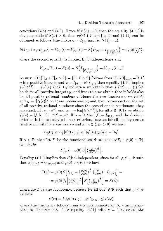
4.1 Decision Theoretic Properties 107
conditions (4.8) and (4.9). Hence if S(p) = 0, then the equality (4.11) is
obvious; while if S(p) > 0, then rp'{l + /' > 0} > 0, and (4.11) can be
obtained as follows (the choice p = irji implies /i(l) = 1):
S(I{0y+cipI(0>oo]) = KP'(0 = Vrp>(l') = S(l{0}+clJ S(V)
fid)
h(c) /i(i)'
where the second equality is implied by 0-independence and
VtP'\a{1\a) = S((p) = S{IS0iJHXl\) = Vrp'\A(l'\A),
because An {l\a +1'\a >0} = {/ + /' > 0} follows from (1 + 1')\q\a =0. If
n is a positive integer, and p = i|o} + c 7[i}, then equality (4.11) implies
f1(cn+1) = /i(c)/!(cn). By induction we obtain that f^cV) = [/i(c)pholds for all positive integers y, and from this we obtain that it holds also
for all positive rational numbers y. Hence the two functions y i—> fi(cy)and y i—> [fi(c)]y on P are nonincreasing and they correspond on the set
of all positive rational numbers: since the second one is continuous, theyare equal. Let c =
h(x) = [h(e-^)\
- e
— log X
and a = — log[/i(e 1)]; for all x G (0, 1) we obtain
If, 0, then /i '(0,1] and the decision
criterion is the essential minimax criterion, because for all nondegeneraterelative plausibility measures rp and all q G {rp^ > 0} we have
Vrp(l) > Vrp[l(q)I{q}] > l(q)h(m{q}) = %)•
If a G P, then let F be the functional on VP
defined by
{<p G Afl¥ : <p(0) G P}
F(p) = p(0)S (-£.)
Equality (4.11) implies that F is 0-independent, since for all cp, ip G ^ such
that p\(o,oo] = V>l(o,oo] and p(0) > ip(0) we have
F{p) = p(0) S
= ¥>(0)/i|($8
7{o} + 1^(0) ) l^(ö),
)a s Uro))
'(0,o
Therefore F is also monotonie, because for all cp,ip G ^ such that p < ip
we have
F (if) = F[rP(0)I{0} + v>/(I,.«,]] < Fty),
where the inequality follows from the monotonicity of S, which is im¬
plied by Theorem 4.3, since equality (4.11) with c = 1 expresses the

108 4 Likelihood-Based Decision Criteria
O-independence of S. Moreover, F is clearly bihomogeneous, and for all
y G [0, oo) we have
F(I[0>1]+yI{0}) = (2/ + l)/i[(^)-] = 1.
Hence F is the restriction to VP of the calibrated, 0-independent, bihomoge¬
neous, monotonie functional cp i—> supr^,G,j, ,/,<„}F on A/"2p, corresponding
to a support-based, regular integral on the class of all monotonie measures
(Theorem 2.13). The desired integral representation follows from Theo¬
rem 4.3:
Vrp(l) = S(m{l > •}) = F[(rjf){l >}]= J ld(ma),
and the uniqueness of the integral on the class of all finite, monotonie
measures follows from the uniqueness of the functionals Vrp (implied byTheorem 4.1). D
Theorem 4.6 implies in particular that a 0-independent likelihood-based
decision criterion leads to the usual likelihood-based inference methods if
and only if it is not the essential minimax criterion, since for this criterion
/l = -^(0,11; while otherwise there is an a G P such that /i : x i—> xa.
In this case, if L is a loss function on ? x D, and lik is the likelihood
function on V induced by the observed data (while before observing the
data we had no information for discrimination between the models in V),then the 0-independent decision criterion applied to the decision problemdescribed by L consists in minimizing J ldd(hka)\ where the integral is
regular and support-based on the class of all monotonie measures. In fact,each support-based, regular integral on the class of all finite, monotonie
measures can be extended to a support-based, regular integral on the class
of all monotonie measures; but the extension is not unique. However, the
extension used in the proof of Theorem 4.6 is the most natural one, since
it is the one characterized by the following continuity property:
/ /d/i= lim / /dmin{/i, c} (4-12)J CT°° J
for all sets <2, all monotonie measures /i on <2, and all functions / : Q —> P.
Thanks to the extension of the integral, the criterion can be applied also
when hk is an unbounded pseudo likelihood function (obtained for exam¬
ple when using the densities of a continuous random object to approximate

4.1 Decision Theoretic Properties 109
the likelihood function). The decision criterion can be interpreted as eval¬
uating the loss we would incur by making each decision d G T> by means
of the integral of Id with respect to a completely maxitive measure whose
density function is proportional to the distorted likelihood function hka.
If a G (0,1), then the distortion represents an attenuation of the like¬
lihood function hk, while it a G (l,oo), then the distortion represents
an intensification of hk; in fact, hka contains a times the information
in hk for discrimination between the models in V (in the sense of Kull-
back and Leibler, 1951). Hence, a G P can be interpreted as a parameter
expressing the confidence in the information provided by the likelihood
function hk, or more generally, by the (nondegenerate) relative plausi¬
bility measure rp. In fact, the limits as a tends to 0 of the functionals
Vrp : I i—> J I &(rya) corresponding to the decision criterion considered are
the functionals Vrp : I i—> J/d(/(0,i] ° £2) corresponding to the essential
minimax criterion (which usually amounts to disregarding the information
provided by rp); while the limit of rpa as a tends to infinity is I^iy o rp,
and the functionals Vrp : I i—> J/d(/r1i o rp) correspond to the MLD cri¬
terion (which usually amounts to considering the model maximizing rp-1
as certain). The limit of Jld(rp°) as a tends to infinity is not necessarily
/ / d(/(i} org), but if essrp sup / < oo, and the integral is quasi-subadditive,then riniajoo J I d(rpa) = J I d(/|1| org) follows easily from Theorem 2.23.
The attitude toward ignorance opposed to aversion can be called attrac¬
tion. A likelihood-based decision criterion reveals ignorance attraction
if the corresponding functionals Vrp satisfy
ry < rp[_ => Vrp > Vrpt
for all pairs of nondegenerate relative plausibility measures rp, rp1 on the
same set Q. This property can be expressed as follows in terms of preferencerelations:
/ ^rp c and rp < rp[_ => / ;^rp< c for all c G P and all / G P ;
ignorance attraction means that if we do not prefer the constant loss c to
a particular decision, then neither would we when we were more ignorant.The next theorem parallels Theorem 4.3, and implies in particular that the
function /i on [0, 1] corresponding to a likelihood-based decision criterion
revealing ignorance attraction satisfies /i(l) = S'(/|o,i}) = ^(^{0}) = 0.
Therefore, a decision criterion cannot reveal both ignorance aversion and
attraction, and a decision criterion such that /i(l) G (0,1) reveals nei-
110 4 Likelihood-Based Decision Criteria
ther ignorance aversion nor attraction (we shall consider examples of such
decision criteria in a moment).
Theorem 4.7. Consider a likelihood-based decision criterion and the cor¬
responding functional S : Sp —> P; the following four assertions are equiv¬
alent:
the decision criterion reveals ignorance attraction,
ip < qp => S(ip) > S(ip) for all ip, ip G Sp,
S is co-independent,
each relation ^rp is represented by the functional Vrp : I i—> S(rj){l < ]),where rj){l < •} denotes the function x i—> ry\l < x} on P.
Proof. Let cp, ip G Sp such that cp < ip. If the decision criterion reveals
ignorance attraction, then S(ip) = Vv^(idp) > V^t (idp) = S(ip), and thus
the second assertion holds. If <y2|[o)0o) = V'lfOjOo)) then S(ip) < S(ip) follows
from condition (4.9), and therefore S is oo-independent when the second
assertion holds. If S is oo-independent, and x = {tR° ^_1)^ then
Vrp(l) = S(x) = S(xl[ol00) +^{00}) = S(rp{l < •}),
where the last equality follows from condition (4.9) with cp = X-^[o,oo)+-^{oo}and ip : x i—> supr0 xi X
= U>{1 < %} Finally, if the fourth assertion holds,then the ignorance attraction is a consequence of condition (4.9), since
sup[X)0o] m{l < •} = 1 and sup[0x] rp{l < } = rä{l < x}. D
Let TL be a nonempty subset of V, and consider the (nondegenerate)relative plausibility measure (lu) on T* Theorem 4.7 implies that the
functional on V^ corresponding to a likelihood-based decision criterion re¬
vealing ignorance attraction is simply V/j y= inf^. In particular, in the
case of complete ignorance about which of the models in V is the best rep¬
resentation of the reality we have V^ = inf, and therefore the likelihood-
based decision criteria revealing ignorance attraction can be considered as
generalizations of the minimin criterion. The counterpart of Theorem 4.4
for a decision criterion revealing ignorance attraction can be easily ob¬
tained: it states in particular that if the corresponding function /o on
[0,1] is strictly increasing, then each relation ^rp is represented by the
functional Vrp : I i—> J/d(/o org), for a (unique) support-based, homo¬
geneous integral on the class of allmonotoniemeasurestakingvalues
in

4.1 Decision Theoretic Properties 111
the range of /o, but the integral would "respect distributional dominance"
only if this property were defined in terms of the "distribution function"
/i{/ > •} instead of /i{/ > •}. However, in general for all nondecreas-
ing functions /o : [0,1] —> [0, 1] such that /o(0) = 0 and /o(l) = 1, and
for all homogeneous integrals respecting distributional dominance on the
class of all normalized, monotonie measures taking values in the range
of /o, the functionals Vrp : I i—> J/d(/o org) correspond to a likelihood-
based decision criterion revealing ignorance attraction. In particular, if
the range of /o is {0,1}, then the choice of the integral has no influence:
Vrp = ess/o0gjsup. If /o = I\\-ß,\] for some ß G (0, 1), then the function¬
als Vrp = ess/. ^orgsup = infrÎI£i>/gi correspond to what can be called
likelihood-based region minimin criterion (in analogy with the LRM^ crite¬
rion) : it consists in reducing V to the likelihood-based confidence region for
P with cutoff point ß, before applying the minimin criterion. If /o = I(o,i\ ,
then the functionals Vrp = ess/(0 or^sup = lirngfi inf{r^->ß\ correspond
to the ignorance attracted analogue of the MLD criterion.
Consider a statistical decision problem described by a loss function L
on V x T>, and let lik be the likelihood function on V induced by the
observed data (while before observing the data we had no information
for discrimination between the models in V). If a maximum likelihood
estimate Pml of P exists, then each decision d G T> that is correct for
Pml is optimal according to all likelihood-based decision criteria revealing
ignorance attraction, since (lik^ol~^ )^(0) = 1 implies Vhk^(ld) = S(l) = 0.
Moreover, if d! G T> is not correct for Pml, and there is a topology on V
such that Id' is continuous, and LR(V\J\f) < 1 for all neighborhoods J\f of
Pml, then Vilkr (Id1) > 0 for all likelihood-based decision criteria such that
/o is positive on (0, 1]. That is, the decision criteria revealing ignoranceattraction and such that /o is positive on (0,1] are almost equivalent to
the MLD criterion, at least when a maximum likelihood estimate Pml
of P exists and there is a correct decision for Pml- So the likelihood-
based decision criteria revealing ignorance attraction are not so useless for
statistical decision problems as the minimin criterion (of which they are
generalizations), but since /i = 0, they do not lead to the usual likelihood-
based inference methods (except for the maximum likelihood method, if
/o is positive on (0, 1]).
Let rp be a nondegenerate relative plausibility measure on V, and let
/ : V —> P be a function. It can be easily proved that if V' is the functional
on V^ corresponding to a likelihood-based decision criterion revealing ig-

112 4 Likelihood-Based Decision Criteria
norance aversion, and V" is the functional on V^ corresponding to a deci¬
sion criterion revealing ignorance attraction, then the following inequalitieshold:
inf{rpi>o} I < Vr'p(0 < linhml>ß}l ^
- ^flSUP{ml>ß} l ^ Vrp(l) ^ SUP{rpi>0} I-(4.13)
That is, a likelihood-based decision criterion revealing ignorance aversion
can be interpreted as comparing the decisions d G T> by means of an
upper evaluation V'(ld) of Id, while a decision criterion revealing ignoranceattraction compares them by means of a lower evaluation V"{ld) of Id- The
sixth value in the inequalities (4.13) is the upper evaluation of / considered
by the essential minimax criterion, and analogously the ignorance attracted
decision criterion using the first value in (4.13) as the lower evaluation of /
can be called essential minimin criterion. The likelihood-based decision
criteria using the fourth and third values in (4.13) as evaluations of / are
the MLD criterion and its ignorance attracted analogue, respectively.
If 5 : [0,1] —> [0, 1] is a nondecreasing function such that 5(0) = 0, then
the dual of 5 is the function 5 on [0,1] defined by
ô(x) = 5(1) - 5(1 - x) for all x G [0,1].
Note that 5 is nondecreasing, with 5(0) = 0 and 5(1) = 5(1); the use of the
term "dual" is justified by the equality 5 = 5 and by the property that if
/i is a normalized, monotonie measure, then 5 o /i = 5 o ~ß. If there are two
nondecreasing functions /i, /o : [0, 1] —> [0,1] such that /i(0) = /o(0) = 0
and /i(l) = /o(l) = 1, and a homogeneous integral respecting distribu¬
tional dominance on the class of all normalized, monotonie measures, such
that V' and V" can be written as integrals with respect to fi o rg and
/o o rg, respectively, then the functionals V' and V" can be considered
as giving conjugate upper and lower evaluations if and only if /i o rg and
/o o rf> are dual to each other (and this holds for all nondegenerate relative
plausibility measures rp if and only if /i and /o are dual to each other).In this case, the inequalities (4.13) can be rewritten as follows:
1 d(7(o,i] ° m) < i d(/i ° re) < i d(/{i> ° re) <J
,
J
f(4.14)
< //d(/(1}oŒ)< //d(/1oŒ)< //d(/(0)i] org),

4.1 Decision Theoretic Properties 113
because the functions I(p,i] an<i I{i} on [0, 1] are dual to each other. Thus
in particular the essential minimax criterion and its ignorance attracted
analogue (the essential minimin criterion) correspond to functionals giving
conjugate upper and lower evaluations, and the same holds for the MLD
criterion and its ignorance attracted analogue. The interpretation of the
fifth and second values in (4.14) as conjugate upper and lower evaluations
of / is particularly clear when fi is left-continuous and the integral is
regular and symmetric on the class of all monotonie measures: in this case,
Theorem 2.18 can be applied, and in particular, if /i|(o,i) has range in
(0,1), then the inequalities (4.14) can be rewritten as follows, using the
notation of Theorem 2.18:
liminf(jl0rEi>1_x} / < -F(/[o,i] inf{/l0azi>i- } 0 < liminf{jl0rEi>1_x| / <x 1 J_ X .J.U
< limsup{/l0azi>x} / < F(/[0ji] sup{/l0rEi> } /) < limsup{/l0azi>x} /.x 1 J_ X .J.U
The functionals V' and V" corresponding to two likelihood-based de¬
cision criteria revealing respectively ignorance aversion and attraction can
thus be interpreted as giving respectively upper and lower evaluations:
these can be combined to obtain intermediate evaluations, by means of an
averaging function a : H{id^) —> P, where H(id^) = {(x, y) G P2 : x > yjis the hypograph of zdp. Using Theorem 4.2, it can be easily proved that
the resulting functionals Vrp = a{V' V") correspond to a likelihood-based
decision criterion if and only if a(l, 1) = 1, the function a is positively ho¬
mogeneous (that is, a(cx,cy) = ca(x,y) for all (x,y) G H(zdp) and all
c G P), and it is nondecreasing in both arguments. In the case of complete
ignorance about which of the models in V is the best representation of
the reality, the resulting decision criterion corresponds to the functional
Vtf = a(sup, inf) on V^; therefore the resulting decision criterion reveals
ignorance aversion or attraction if and only if a(x, y) = x or a(x, y) = y
for all (x,y) G H(zdp), while in all other cases it reveals neither ignoranceaversion nor attraction. In particular, if A G (0, 1), and a\ is the function
on H(zdp) defined by a\(x,y) = Xy + (1 — X) x (for all (x,y) G H(idpj),then the likelihood-based decision criteria obtained by means of the av¬
eraging function a\ can be considered as generalizations of the Hurwicz
criterion with optimism parameter A.
Consider a regular integral on the class of all monotonie measures,
and let /i,/o : [0,1] —> [0,1] be two nondecreasing functions such that
^(0) = /0(0) = 0 and /^l) + /0(1) = 1. A likelihood-based decision

114 4 Likelihood-Based Decision Criteria
criterion with corresponding functions /i,/o can be defined for example
through the functionals
vrp .i I d(/i orjo)+ I d(/0 o rg),
or through the functionals
Vrp:l^-> I d(/i or2 + /0oŒ).
If /i(l) = 1 or /i(l) = 0, then the two definitions correspond, and the
decision criterion reveals respectively ignorance aversion or attraction; but
if /i(l) G (0,1), then in general the two definitions are different, althoughboth decision criteria generalize the Hurwicz criterion with optimism pa¬
rameter A = /o(l). In this case, the first definition corresponds to the
application of the averaging function a\ to the integrals with respect to
jz~\ /l ° TJL and \ /o ° TË, respectively; while in general the second defi¬
nition cannot be obtained as a(V' V") for an averaging function a on
H(idf). However, for the Choquet integral the two definitions correspond
(thanks to the additivity with respect to measures), and in particular, if
j^j /i andj /o are dual to each other, and the function 6 =
y~\ fi = \fois left-continuous, then using Theorem 2.18 we can clarify the connection
with the Hurwicz criterion by expressing the functionals Vrp as follows by
means of the Lebesgue integral (with respect to the Lebesgue measure on
[0,1]):
Vrp:l^ [A inf((5orEi>x} / + (1 - A) sup((5orEi>x} /] dx.
Jo
Since the Choquet integral is translation equivariant, it can be used to
evaluate the decisions also when the decision problem is described by a
bounded utility function U : V x T> —> R. In particular, Theorem 2.28 im¬
plies that if we apply the likelihood-based decision criterion correspondingto the functionals Vrp : I i—> Jcl d(f\ org+ /0 org) to the decision problemdescribed by the loss function c — U, where c is an upper bound of U (wehave considered this kind of loss function at the end of Subsection 3.1.1),then we obtain the following decision criterion:
f°- -
—
maximize / u^ d(/o OQ)+/i o rp).
4.1 Decision Theoretic Properties 115
where the integral is the extension of the Choquet integral by means of
equality (2.10), and for each d G T> the function u& on V is defined by
Ud(P) = U{P, d) (for all P G V). In particular, the ignorance averse deci¬
sion criterion corresponding to the functionals Vrp : I i—> Jcl d(/iorg) com¬
pares the decisions d G T> by means of the lower evaluation JcUd d(/i org)of Ud] while the ignorance attracted decision criterion corresponding to the
functionals Vrp : / i—> Jcl d(/o o rg) compares them by means of the upper
evaluation JCUd d(/o org) of w^.
By contrast, as noted at the end of Subsection 3.1.1, the Shilkret in¬
tegral cannot be used directly to evaluate the decisions when the decision
problem is described by a utility function U : V x T> —> R, because the
utility functions U and a U+ß are considered equivalent (for all a G P and
all ß G ffi). But if the positive values of C7 are interpreted as gains, and the
negative ones as losses, then the functions U and a U + ß are equivalent
only if ß = 0 (because of the peculiar meaning of the value 0), and the
Shilkret integral can be used to evaluate separately gains and losses. If we
evaluate gains and losses by means of the Shilkret integral with respect
to /i o rg, then the uncertain gain resulting from a decision d G T> can
be indifferently defined as max{«(2,0}, as Ud\{Ud>o}j or as ud\{ud>0} (andanalogously for the uncertain loss), since the Shilkret integral is support-
based:
/s/*S
max{«d,0}d(/1or2)= / ud\{Ud>0} d(/i o rjo\{ud>0}).
By contrast, the use of rg_ in the integrals would pose some problems, be¬
cause in general if TL is a subset of V, then rg|^ is different from rp\n-i,since the latter depends also on rjiiV \ TL). The decisions d G T> can thus
be compared on the basis of the two evaluations Js m&x{ud, 0} d(/i o rp)
and Js max{—Ud, 0}d(/i org); for instance, maximizing their difference
corresponds to maximizing j Udd(f\ org), where the integral is the ex¬
tension of the Shilkret integral by means of equality (2.11). It is importantto note that both evaluations of gains and losses are "upper evaluations",and therefore the resulting decision criteria are ignorance attracted as re¬
gards gains, and ignorance averse as regards losses. When /i is continuous,the comparison of decisions on the basis of separate evaluations of gainsand losses by means of the Shilkret integral seems to be in agreement with
the theory of Shackle (1949).

116 4 Likelihood-Based Decision Criteria
4.1.2 Sure-Thing Principle
A likelihood-based decision criterion satisfies the sure-thing principle if
for all disjoint sets A, B, and all nondegenerate relative plausibility mea¬
sures rp on Q = A U B such that rp(A) > 0 and rp(B) > 0, the followingcondition holds:
1\a ^,u 1'\a and I, ,
—
n
, Z „=> ISpl' for all/,/'G PS.
L\B ^rp\B « Iß J
Note that the conditions on rp(A) and rp(B) are necessary only because
~^rp' is undefined if rp' is a relative plausibility measure with constant value
0, but when for instance rp(B) = 0, for all likelihood-based decision criteria
we have 1\a ^,rp\A 1'\a if and only if/ ^rp /'. The above sure-thing principle
corresponds to the first part of the "sure-thing principle" of Savage (1954),while the second part states that if one of the two preferences on the left-
hand side of the implication is strict, then so is the preference on the
right-hand side. This would imply that if / < /', and rp{l < /'} > 0, then
/ must be preferred to /'; therefore, no likelihood-based decision criterion
can satisfy the second part of the "sure-thing principle" of Savage: the
next example shows that this is true also if the dominated decisions are
discarded.
Example 4-8- Let Q = {a,b,c} be a set with three elements, and con¬
sider the relative plausibility measure 1^ on Q. The two functions Ira\and I{b,c\ on Q are considered equivalent by all likelihood-based decision
criteria, since VlT(I[a}) = /i(l) = ^iî(I[b,c}). But I{a}\{c} = 0 is cer¬
tainly preferred to I{b,c\\{c\ = lj while the equivalence of /{0}|{o,6} and
!{b,c}\{a,b} = ^{6}l{a,6} is implied by symmetry. 0
However, the second part of the "sure-thing principle" of Savage does
not really deserve its name, since we are not "sure" of the strict prefer¬ence: we do not assume that the strict preference holds in both alternative
cases A and B. If we were assuming this, then we would obtain the "strict
version" of the above sure-thing principle, in which each one of the three
preferences is strict: it can be easily proved that if a likelihood-based de¬
cision criterion satisfies the sure-thing principle, then it satisfies also its
strict version. Moreover, since relative plausibility measures are (equiva¬lence classes of) finitely maxitive measures, the content of the sure-thing

4.1 Decision Theoretic Properties 117
principle is left unchanged when the assumption that A and B are disjointis dropped (and this is valid also for the strict version).
Consider a statistical decision problem described by a loss function L
on V x T>, and let rp be a nondegenerate relative plausibility measure on
V describing the uncertain knowledge about the models in V. The sure-
thing principle states that for all coverings Ti, Ti' of V (that is, Ti,Ti' Ç Vand V = Ti U Ti1) such that rp(Ti) > 0 and rp(Ti') > 0, if the preferencebetween two decisions in T> is the same when we restrict attention to the
models in Ti or to the models in Ti', then this preference holds also when we
consider all the models in V. In particular, if d G T> is optimal, accordingto a likelihood-based decision criterion satisfying the sure-thing principle,for both the decision problems described by L^xT) and by L\?{ixt>, then
d is optimal also for the decision problem described by L. Moreover, if
for both the restricted decision problems d is the unique optimal decision
in T>, then this holds also for the unrestricted decision problem; but this
conclusion is in general not valid when d is the unique optimal decision
only for one of the two restricted decision problems (since the second part
of the "sure-thing principle" of Savage does not hold).
The "if part of the condition of O-independence is a special case of
the sure-thing principle, while the "only if part is a special case of the
second part of Savage's "sure-thing principle". Theorem 4.6 implies that a
likelihood-based decision criterion can be 0-independent only if the corre¬
sponding function f\ is positive on (0, 1] : the next theorem states that in
this case the O-independence is implied by the sure-thing principle.
Theorem 4.9. A hkehhood-based decision criterion satisfying the sure-
thing principle is 0-mdependent if and only if the corresponding function
/i : [0, 1] —> [0,1] is positive on (0,1].
Proof. The "only if part follows from Theorem 4.6, and to prove the "if
part it suffices to show that if the function f\ is positive on (0, 1], and A is
a subset of Q such that /|q\a = 0, and both rp(A) and rp(Q\ A) are pos¬
itive, then Vrp(l) = Vrp(IA)Vrp\A(l\A), because Vrp(IA) > fi[m{A)] > 0.
The above equality follows from the equivalence of / and Vrp\A(l\A) Ia,which is implied by the sure-thing principle and the equivalence of 1\a and
*W*U).
The sure-thing principle does not follow from the O-independence: for
instance, the likelihood-based decision criterion such that each relation

118 4 Likelihood-Based Decision Criteria
^rp is represented by the functional / i—> Jcldrp (that is, the "MPL*
criterion" of Cattaneo, 2005) is 0-independent (Theorem 4.6), but the next
example shows that it does not satisfy the sure-thing principle. In fact, the
subsequent theorem implies that a likelihood-based decision criterion such
that each relation ~^rp is represented by the functional / i—> J I drp can
satisfy the sure-thing principle only if the integral is maxitive.
Example J^.10. Consider the likelihood-based decision criterion correspond¬
ing to the functionals Vrp : I i—> Jcl drp, and let rp be the (nondegenerate)relative plausibility measure on Q = {0,1, 2} defined by rp(0) = rp(l) = 1
and rp{2) = \. We have Vrp\{0 2} (îdQ|{0,2}) = Kp|{1}Mq|{i}) = 1, but
Vrp(idQ) = §; that is, idQ\^0>2} ^,rP\{02} 1|{0,2} and idQ\^y ;SP|{1} l|{i}>but not idQ ^rp 1. 0
Theorem 4.11. Consider a hkehhood-based decision criterion satisfyingthe sure-thing principle. The corresponding functions /i, /o : [0,1] —> [0, 1]fall into one of the following five alternative cases:
/o = 0 and fx = J(0,1],
/i = 0 and /o = 7(i}'
/o = 0 and fx = ^{1},
/i = 0 ond /o = /(0,l],
/o = 0 ond /i : x i—> xa /or on a G P.
i/ /o = 0, t/ien i/ie decision criterion reveals ignorance aversion, and
for each nondegenerate relative plausibility measure rp (on some set Qrp)the corresponding functional Vrp on WQrp fulfills the following condition:
Vrp(max{l,l'}) =max{Vrp(l),Vrp(l')} for all I, l' ePQr».
Proof. Consider first the case with f\ = 0; let rp be the (nondegenerate)relative plausibility measure on Q = {0, 1, 2} defined by rg{0} = 1 and
rp{l} = rp{2} = 1—x for aniS [0,1], and let / = Ir0\ and /' = fo(x) i{o,i}be two functions on Q. We have
h(x) =Vrphoii(l\m}) =Vrphoii(l'\m}) =Vrp(l) =Vrp(l') = lf0(x)}2,
where the fourth equality is implied by the sure-thing principle, since
'1(2} = 0 = ^'|{2}- Hence the range of /o is {0,1}; to obtain that /o = im

4.1 Decision Theoretic Properties 119
or /o = I(o,i\ jit suffices to show that sup{/o = 0} G (0, 1) leads to a contra¬
diction: assume thus that it is true and define y = (1 — sup{/o = 0}) 5. Let
rp' be the (nondegenerate) relative plausibility measure on Q = {0,1, 2}defined by (rp')^ : k i—> yk, and consider the two functions i|o} and ^{0,1}on Q. We have
Vrp>(I{0}) = /o(l - y) = 0 < 1 = /o(l - y2) = Kp-^o.i});
this contradicts the sure-thing principle, since
Vrp'\{i 2}(7{0,1} I{1,2}) = /o(l ~y) = 0 = Kp'|{1 2}(J{0>I{1,2>)
and ^{o,i}l{o} = 1 = /{o}|{o}-Consider now the case with /i(l) > 0; we first prove that the decision
criterion reveals ignorance aversion (and thus in particular /o = 0). ByTheorem 4.3 it suffices to show that the corresponding functional S on Spis 0-independent; that is, it suffices to show that for all p G Sp we have
equality (4.11) with c = 1 and /i(l) = 1. Define <2, A, rp', /, and /' as in
the proof of Theorem 4.6, but with c = 1; since /|g\4 = 0 = 1'\q\a and
Vrp'\A(l\A) = Si^p) = Vrp'\A(l'\A), the sure-thing principle implies
S(I{o} +93/(0,00]) = KP'(0 = Vrp>(l') = Vrp,\A{l'\A) = S{if).
We now prove that sup{/i = 0} G {0, 1}: analogously to the case with
/1 = 0, assume that sup{/i = 0} G (0,1) and define y = (sup{/i = 0})s.Let rp be the (nondegenerate) relative plausibility measure on Q = {0,1, 2}defined by rg^ : k 1—> yk, and consider the two functions / = i|2} and
I' = fi(y)I{i,2} on Q. We have Frp(/) = h(y2) = 0 < [/^y)]2 = Vrp(l'):this contradicts the sure-thing principle, since l\{oi = 0 = l'\{oi and
yrp|{12}('l{i,2}) = fi(y) = Vrp\{12}(l'\{i,2})- Therefore, either we have
sup{/i = 0} = 1 and thus /1 = I{i}, or we have sup{/i = 0} = 0 and thus
/1 = 7(o,i] or fi : x t-^ xa for an a G P (Theorems 4.9 and 4.6). Since the
decision criterion reveals ignorance aversion, Theorem 4.3 implies
yrp(max{/,/'}) = S(rp{max{l,l'} > •}) =
= S(max{rp{l > -},ffi{/' > •}}) > max{Vrp(l), Vrp(l')},
where the inequality follows from the monotonicity of S. To prove the last
statement of the theorem, it suffices thus to show that this inequality is
an equality; that is, it suffices to show that for all nonincreasing cp, ip G Spwe have S(max{ip, tp}) < max{S(cp), S (ip)}. Define A = H(p) x {0} and

120 4 Likelihood-Based Decision Criteria
B = H(ip) x {1}, where H(p) and H(ip) are the hypographs of p and ip,
respectively, and thus AUB Ç P x [0,1] x {0, 1}; let / and rp be respectivelythe function and the (nondegenerate) relative plausibility measure on AUB
defined by l(x, y,z) = x and rj^-(x,y, z) = y. Since rg{Z|^ > x} = (p(x) and
rj)(A) = 1, we have V^.p|A(Z|ji) = S(p); and analogously K-p|B('|ß) = S(ip).The sure-thing principle implies thus that Vrp(l) < max.{S(cp), S (ip)}, but
Vrp(l) = S(max{(p, ip}), because rp_{l > x} = max{y(x), tp(x)}. D
Theorem 4.11 implies in particular that neither the LRM^ criterion
(for any ß G (0,1)), nor any likelihood-based decision criterion with
/i(l) G (0,1) (such as one generalizing the Hurwicz criterion) can satisfythe sure-thing principle. If a likelihood-based decision criterion satisfies it,and /o = 0, then the decision criterion reveals ignorance aversion, and thus
in particular it generalizes the minimax criterion; but the next exampleshows that a likelihood-based decision criterion satisfying the sure-thing
principle does not necessarily reveal ignorance attraction when /i = 0.
Example J^.12. Let S be the functional on Sp defined by
S^ = { suP{p > 0} if p(0) = 0,fOT a11 f G ^
It can be easily proved that S corresponds to a likelihood-based decision
criterion satisfying the sure-thing principle with /i = 0 and /o = 7;n (thesecond case of Theorem 4.11), but revealing neither ignorance aversion nor
attraction. 0
Five other examples of likelihood-based decision criteria satisfying the
sure-thing principle and falling in the five alternative cases listed in The¬
orem 4.11 are the essential minimax criterion and its ignorance attracted
analogue (the essential minimin criterion), the MLD criterion and its ig¬
norance attracted analogue, and the MPL criterion, respectively. Let S be
the functional on Sf corresponding to a likelihood-based decision criterion,and consider the functional S' on Sp defined by
S'(p) = \ S^ * SUP^ > °| < °°'for all p g Sf.
yrj
[oo if sup{<^ > 0} = oo,r r
It can be easily proved that S' corresponds to a likelihood-based deci¬
sion criterion with the same functions /i,/o as the original one (that is,

4.1 Decision Theoretic Properties 121
the one corresponding to S). If the original decision criterion satisfies the
sure-thing principle or reveals ignorance aversion, then so does the one
corresponding to S"; but this one cannot reveal ignorance attraction, even
when the original one does. The functional on Sp corresponding to the es¬
sential minimax criterion is S : ip i—> sup{<^ > 0}, and in this case S' = S;in fact, using Theorems 4.9 and 4.6 we obtain that the essential minimax
criterion is the only likelihood-based decision criterion satisfying the sure-
thing principle with /o = 0 and /i = I(o,i]- But if S is the functional on
Sp corresponding to one of the other four likelihood-based decision criteria
listed above, then S' is different from S, and thus only the first one of
the five alternative cases of Theorem 4.11 uniquely determines a decision
criterion satisfying the sure-thing principle.
In particular, Theorems 4.9, 4.6, and 4.11 imply that if a likelihood-
based decision criterion satisfies the sure-thing principle with /o = 0 and
/i : x i—> xa for an a G P, then there is a unique support-based, regu¬
lar integral on the class of all finite, monotonie measures, such that each
relation ^rp is represented by the functional / i—> Jld(rp°), and the in¬
tegral is maxitive (on the class of all finitely maxitive measures). Since
the integral is maxitive, homogeneous, and transformation invariant, we
have J/d/i = Js/d/i when / is essentially bounded with respect to /i
(that is, ess^sup/ < oo). But to obtain the Shilkret integral also when
essM sup / = oo, we need something more: for instance countable maxitiv-
ity, or the following continuity property, which parallels condition (4.12):
// d/i = lim / min{/, c} d/i,cTooJ
for all sets <2, all finite, monotonie measures /i on <2, and all functions
/ : Q —> P. This continuity property corresponds to the following condition
for preference relations:
min{/, c} <rp I' for all c G P => I <rp I' for all /, /' G PQ^. (4.15)
The next theorem implies that this condition suffices to determine a uniquelikelihood-based decision criterion satisfying the sure-thing principle in
each one of the three cases with /o = 0 listed in Theorem 4.11; but this
is not true in the two cases with /i = 0: for instance, the condition is
fulfilled by both the essential minimin criterion and the decision criterion
of Example 4.12.

122 4 Likelihood-Based Decision Criteria
Theorem 4.13. Consider a hkehhood-based decision criterion such that
the corresponding function f\ : [0, 1] —> [0, 1] satisfies /i(l) > 0, and
for each nondegenerate relative plausibility measure rp (on some set Qrp)condition (4-15) is fulfilled. The decision criterion satisfies the sure-thing
principle if and only if either it is the essential minimax criterion or the
MLD criterion, or there is a positive real number a such that each relation
^rp is represented by the functional I i—> Jsld(rpa).
Proof. The "if part is simple: the essential minimax criterion satisfies the
sure-thing principle, because
Vrp{l) =essrpsup/ = ma-x{Vrp\A(l\A),Vrp\B(l\B)};
the MLD criterion satisfies it because if rp(A) = rp(B) = 1, then
Vrp{l) =ess/{1}0r£sup/ = ma-x{Vrp\A(l\A),Vrp\B(l\B)},
while if rp(B) < 1, then Vrp(l) = VrpiA(l\A). Finally, in the third case,
using Theorem 2.6 we obtain
Vrp(t) = sup/ (r^r = max{[02(A)]Q VrpU(l\A), [m(B)]aVrp\B(l\B)}.
For the "only if part, Theorem 4.11 implies that /o = 0 and we
have three alternative cases for f\. If f\ = /(o,il, then Theorems 4.9
and 4.6 imply that the decision criterion is the essential minimax crite¬
rion. For /1 = /{1}, we have to prove that if b G (ess/|1|0r2suP^ °°);then Vrp(l) < b; in fact, in this case the decision criterion is the MLD
criterion, because Vrp(l) > ess/|1|0r2sup/ follows from ignorance aver¬
sion (implied by Theorem 4.11). Thanks to condition (4.15), it suffices
to show that Vrp(min{l, c}) < b for all c G (ö, 00): this follows from the
last statement of Theorem 4.11, since min{/, c} < max{&, cln>b\} and
vrp(I{i>b}) = fiimi1 > H) = 0- Finally, if /1 : x i-> xa for an a G P,then Theorems 4.9, 4.6, and 4.11 imply that there is a maxitive, regular
integral on the class of all finite, completely maxitive measures, such that
each relation ^rp is represented by the functional Vrp : I 1—> J ld(rp°). Wehave to prove that Vrp(l) = Jsl d(rpa). and thanks to Theorem 2.15 and
condition (4.15), it suffices to show that J min{/, c} d(rpa) < Jsl d(rpa)
for all c G W. Now, for a bounded function / with finite range, the
value of J f d(rpa) is determined by maxitivity and homogeneity, since
/ can be written as the maximum of a finite number of functions of

4.1 Decision Theoretic Properties 123
the form a/4 with a G P. Therefore J f d(rpa) = Js f d(rpa), but then
J min{/, c} d(rpa) = Js min{/, c} d(rpa) follows for instance from Theo¬
rem 2.23. D
Theorem 4.13 implies that the MPL criterion (possibly applied after
having distorted the likelihood function by raising its values to the power
a G P) is the only likelihood-based decision criterion that satisfies the sure-
thing principle and the continuity condition (4.15), and that leads to the
usual likelihood-based inference methods, when applied to some standard
form of the corresponding decision problems. Moreover, the MPL criterion
possesses also the following property. A likelihood-based decision criterion
is said to be decomposable if the corresponding functionals Vrp satisfy
Vrp(l) = Vrpot-i\yrpht=}(l\{t= })] (4.16)
for all sets Q and T, all nondegenerate relative plausibility measures rp
on <2, all functions / : Q —> P, and all functions t : Q —> T such that
rp{t = t} > 0 for all t G T; where Vrpi _
(l\:t= }) denotes the function
r 1—> Vrp\,t_,(l\[t=Ty) on T. Note that the condition on rp{t = t} is
necessary only because Vrpt is undefined if rp1 is a relative plausibilitymeasure with constant value 0; alternatively, we could drop this condition
and assume simply that Vrpi _
(l\rt= i) denotes a function /' : T —> P
such that l'(r) = Vrpi_t
(l\rt=T\) for all t G {(rp oT1)^ > 0}, since the
values taken by /' outside this set have no influence on Vrpot-i(l').
The equality Vrpot-i [Vrp\ } (/|{t= })] = Vrp[Vrp\{t= } (/|{t= }) o t] holds
for all likelihood-based decision criteria; if a decision criterion is decom¬
posable, then the function Vrpi _
(l\rt= 1) ot can be interpreted as the
"conditional evaluation" of / given t, in analogy with the conditional ex¬
pectation E(X\Y) of a random variable X given a random object Y.
The "conditional evaluation" corresponds to the conditional expectationin many respects; in particular, equality (4.16) corresponds to the prop¬
erty E(X) = E[E(X\Y)]. That is, a likelihood-based decision criterion
is decomposable if it allows the introduction of a concept of "conditional
evaluation" presenting many analogies with the concept of conditional ex¬
pectation.
It can be easily proved that a decomposable decision criterion satisfies
the sure-thing principle: it suffices to choose T = {0,1} and t = Ia- In fact,the property of decomposability can also be expressed as follows: for all
sets A of disjoint sets, and all nondegenerate relative plausibility measures
124 4 Likelihood-Based Decision Criteria
rp on Q = y A such that rp(A) > 0 for all A G A,
1\a ^rp\A 1'\a for all A G A => I <rp I' for all /, /' G PQ.
The sure-thing principle corresponds to the case with finite A, and it is thus
equivalent to the finite decomposability (that is, decomposability with the
additional condition that T is finite). By exploiting the fact that there is a
finite or countable subset Q' of Q such that ?*p|q'o(/|q/)_1 = rpo/-1, it can
be proved that decomposability is equivalent to countable decomposability
(for which T and A are at most countable). As in the case with finite A, also
in the general case the assumption that the elements of A are disjoint can
be dropped without consequences. But contrary to the case with finite A,the above formulation of decomposability does not imply its strict version
(in which both preferences are strict); in fact, no likelihood-based decision
criterion can satisfy the strict version even for countable sets A, since this
would imply that if / and /' have countable range, and / < /', then / is
preferred to /', while it is possible that rp o /_1 = rp o (Z')_1.
Theorem 4.14. Consider a hkehhood-based decision criterion such that
the corresponding function f\ : [0,1] —> [0, 1] is continuous at 0, and the
corresponding function /o : [0, 1] —> [0, 1] is continuous at 1. The decision
criterion is decomposable if and only if there is a positive real number a
such that each relation ^rp is represented by the functional I i—> Jsl d(rpa).
Proof. The "if part is simple: using Theorem 2.6 we obtain
Vrpot-i[Vrp\{t=}(l\{t=})] = SUpVrp\{t=T}(l\{t=T}) (r^{t = T})a =
=
supsup|t=r} / {rpl)a = Vrp(l).
For the "only if part, let l,t and rp be respectively the functions and
the (nondegenerate) relative plausibility measure on Q = (0, 1) x {0, 1}defined by l(x,y) = y and t(x,y) = x, and rp^(x,y) = xy + (1 —y). We
have rp{t = t} = 1 and Vrp\{t=r} (/|{t=r}) = /i(r) for all t G T = (0, 1);and therefore
hi1) = Vrp(l) = Vrp{fx ot) < sup(/i ot) = sup(01) /i.
That is, /i is continuous at 1; the continuity of /o at 0 can be proved
analogously. Theorem 4.11 implies thus that the decision criterion reveals

4.1 Decision Theoretic Properties 125
ignorance aversion, and fi : x i—> xa for an a G P; we have to show that
Vrp(l) = sup/ (rp^)a for all nondegenerate relative plausibility measures
rp (on some set Qrp), and all functions / : Qrp —> P. Let /',£' and rp'be respectively the functions and the (nondegenerate) relative plausibility
measure on Q' = Qrp x {0, 1} defined by l'(q,y) = l(q)y and t'(q,y) = q,
and (rp'y(q,y) = rp*-(g) y + (1 — y). We have Vrp>(l') = Vrp(l), because
ry'\l' > x} = rj/_({l > x} x {1}) = rp_{l > x} for all x G P (Theorem 4.3);and since rp'{t' = t} = 1 and Vrpn ,_ (l'\rti=Ty) = /(t) [rj>}{T)]a for all
t G T = Qrp, we obtain
vrp(i) = vrp,(i') = vrplo(tl)-i[i (n>l)a} = sup/ (n>l)a,
because rp' o (t')_1 = 1^ on Qrp. Ü
At the beginning of the present section we noted that a likelihood-based
decision criterion can be useful only if it satisfies some sort of continuityat 0 of the influence of a model, with respect to its relative plausibility;and thus in particular only if the corresponding functions /i and /o on
[0,1] are continuous at 0 and 1, respectively. In this sense, Theorem 4.14
implies that the MPL criterion (possibly applied after having distorted
the likelihood function by raising its values to the power a G P) is the
only decomposable likelihood-based decision criterion that can be useful;and it is also the only decomposable decision criterion that leads to the
usual likelihood-based inference methods, when applied to some standard
form of the corresponding decision problems. The only consequence of the
assumption about /i in Theorem 4.14 is the exclusion of the essential
minimax criterion, while the assumption about /o does not exclude onlythe essential minimin criterion, but for instance also the decision criterion
of Example 4.12.
Theorem 4.2 states that a likelihood-based decision criterion compares
the decisions on the basis of a functional S : Sp —> P applied to the func¬
tions (rgo/-1)^ describing the relative plausibility of the possible values of
the loss incurred. That is, a decision criterion corresponds to a preferencerelation (represented by S) on the set Sp, which can be identified with the
set of all nondegenerate relative plausibility measures on the set P of the
possible values of the loss. Moreover, the property of decomposability can
be interpreted also as a rule for "combining" the nondegenerate relative
plausibility measures rp o (/|(t=r})_1 on P (for each t G T) on the basis
of the "marginal" nondegenerate relative plausibility measure rp ot^1 on

126 4 Likelihood-Based Decision Criteria
T. Hence, if we assume the sure-thing principle (that is, the finite decom-
posability), then we can consider a framework similar to the one of the
representation theorem of von Neumann and Morgenstern (1944): a de¬
cision criterion corresponds to a preference relation on an abstract set of
consequences (the nondegenerate relative plausibility measures on P), on
which for each r G P we have a binary operation (the combination of two
consequences with plausibility ratio r).
The axiomatic approach to qualitative decision making with possibility
theory of Dubois and Prade (1995) uses a similar framework, and results
in particular in two decision criteria differing from one another only in
their attitudes toward ignorance: one is based on an assumption of igno¬
rance aversion, while the other is based on an assumption of ignoranceattraction. By replacing these assumptions with an axiom of "qualitative
monotonicity", and adapting other axioms to the new attitude toward
ignorance and to the use of profile likelihood functions, we obtain the de¬
cision criterion of Giang and Shenoy (2002), briefly introduced at the end
of Subsection 1.3.2. If we identify the best value (1,0) of the binary util¬
ity with the loss 0, and the worst value (0,1) with the loss 1, then the
assumption of "qualitative monotonicity" corresponds to the assumptionthat both functions /i and /o on [0,1] are strictly increasing. Theorem 4.11
implies that this assumption is incompatible with the sure-thing principle,on which the framework of Giang and Shenoy is based; but there is no
contradiction, because their criterion is not a "likelihood-based decision
criterion" in the sense introduced at the beginning of the present section.
In our framework, the justification of the axiom of "qualitative monoto¬
nicity" by Giang and Shenoy can be expressed as follows: if one of the
functions fi, /o is not strictly increasing, then there is a decision problemin which a decision is considered equivalent to another decision dominat¬
ing it. But this is unavoidable when the decisions are evaluated solely on
the basis of the profile likelihood function on the set of the possible con¬
sequences; moreover, two decisions can be considered equivalent by the
criterion of Giang and Shenoy even when one strictly dominates the other
and they have only a finite number of possible consequences (that is, this
decision criterion does not satisfy the strict version of the sure-thing prin¬
ciple) .In particular, when we are in the state of complete ignorance about
the models considered, and a decision has only a finite number of possible
consequences, if all these consequences are better than the intermediate
value (1,1), then the criterion of Giang and Shenoy evaluates the decision
by its worse consequence, while if all the possible consequences are worse

4.2 Statistical Properties 127
than (1, 1), then the decision is evaluated by its best consequence; other¬
wise the decision is simply evaluated by the intermediate value (1, 1), and
thus two decisions can be considered equivalent even if one is clearly bet¬
ter than the other. It is interesting to note that if we consider a decision
problem described by a utility function, we interpret the positive values
of the utility as gains, and the negative ones as losses, and we identifythe value 0 of the utility with the intermediate value (1,1) of the binary
utility, then the decision criterion of Giang and Shenoy is ignorance averse
as regards gains, and ignorance attracted as regards losses; in oppositionto the decision criterion considered at the end of Subsection 4.1.1, and to
the theory of Shackle (1949).
4.2 Statistical Properties
Consider a statistical decision problem described by a loss function L on
VxD, where V is a set of probability measures on a measurable space
(fi, A). If we regard the observed data as a particular realization of a ran¬
dom object X : Q —> X, then we can consider a loss function L' on V x A
(where A is a set of decision functions 5 : X —> T>), as done in Subsec¬
tion 1.1.1. A likelihood-based decision criterion can be applied either to
the pre-data decision problem described by L', or to the post-data deci¬
sion problem described by L (conditional on the observed realization of
X). When applied to the pre-data decision problem described by the risk
function, all likelihood-based decision criteria revealing ignorance aversion
reduce to the minimax risk criterion (if no prior likelihood function is
used). In general the application of a decision criterion to a pre-data deci¬
sion problem is rather difficult; therefore it can be interesting to consider
the decision function ö obtained by conditional application of a likelihood-
based decision criterion (to the post-data decision problem): that is, S(x)is the decision that we would select after having observed X = x. It X
is continuous (under each model in V), then it is usually possible to base
the decisions 5{x) on the pseudo likelihood functions on V obtained from
the densities of X and considered at the beginning of Section 1.2 as ap¬
proximate likelihood functions. If a statistic s : X —> S is sufficient for
X, then ö depends on x only through s(x); that is, the decision function
obtained by conditional application of a likelihood-based decision criterion
depends only on sufficient statistics. In general the decision function ö is
not optimal from the pre-data point of view (it is not even necessarily in

128 4 Likelihood-Based Decision Criteria
A), but it can nevertheless be useful. The pre-data evaluation of ö in terms
of L' can be of interest even when we are primarily concerned with the
post-data decision problem described by L; in particular, it can be inter¬
esting to consider the expected loss of the decision function ö under each
model in V.
The pre-data performances of the decision functions obtained by con¬
ditional application of a likelihood-based decision criterion can be arbi¬
trarily bad in particular decision problems. But the same is true for the
pre-data performances of the likelihood-based inference methods, and yet
these are the most appreciated general methods for the respective inference
problems, because they are intuitive and their pre-data performances are
usually good in actual applications. A reasonable likelihood-based decision
criterion can be intuitive too, and if it leads to the likelihood-based infer¬
ence methods when applied to some standard form of the correspondingdecision problems, then we can expect that in many actual problems the
decision functions obtained by conditional application of this criterion will
perform well from the pre-data point of view. When this is not the case, the
pre-data performance of these decision functions can often be improved by
replacing the profile likelihood function (which is automatically employed
by the decision criterion) with another pseudo likelihood function (thistechnique is used also for the likelihood-based inference methods).
4.2.1 Invariance Properties
The likelihood-based decision criteria are obviously "paranietrization in¬
variant",since they do not depend on a paranietrization of the set V of
statistical models considered; they possess many other invariance proper¬
ties: in particular the following one.
Theorem 4.15. Consider a statistical decision problem described by a loss
function L on V x T> such that there are two functions f : V —> V and
g :T> —> T>, and a positive real number c satisfying L(P, d) = cL[f{P), g(d)]for all P G V and all d G T>. All hkehhood-based decision criteria have
the following property: the decision d G T> is optimal with respect to the
nondegenerate relative plausibility measure rp on V, if g(d) is optimal with
respect to rpo/-1.
In particular, if rp o f^1 = rp, then for all hkehhood-based decision
criteria the set of all optimal decisions (with respect to rp) is invariant

4.2 Statistical Properties 129
under g 1, and thus if there is a unique optimal decision, then it is a fixed
point of g.
Proof. Since for all x G P we have
{ld = x} = {P G V : L(P, d)=x} = r'llgid) = f},
Theorem 4.2 implies
vrp(id) = sirzoi-1) = SKrzof-'or^i-)} = cvrpof-,{ig{d)),
and therefore d minimizes Vrp(ld) if d! = g(d) minimizes Vrpof-i(ld').
The invariance property stated by Theorem 4.15 can be very useful
when the decision problem presents some symmetries. In particular, the
next theorem states that the decision function ö obtained by conditional
application of a likelihood-based decision criterion is equivariant, if it is
well-defined and the decision problem is invariant. In fact, the premiseof the theorem is the definition of an invariant decision problem: onlythe assumption about the prior relative plausibility measure rp and the
restriction to discrete random objects X are not usual. But the assumptionabout rp is clearly satisfied when we use no prior information (that is, when
rp = 1Î); and the theorem is valid also for continuous X, if we base ö on the
densities of X (and we consider the usual definition of invariant decision
problem). Moreover, the theorem is valid also if condition (4.6) is restricted
to the functions t that are bijective, and this restricted condition can be
satisfied also when the profile likelihood function is replaced by another
pseudo likelihood function.
Theorem 4.16. Let V be a set of probability measures on a measurable
space (fi, A), and let X : Q —> X be a random object that is discrete under-
each model in V. Consider a statistical decision problem described by a
loss function L on V x T>, with prior (nondegenerate) relative plausibility
measure rp on V. Let G,G',G" be three permutation groups on X,V,T),
respectively, and let g i—> g' and g i—> g" be two homomorphisms of G to G'
and G", respectively, such that for all g G G; all x G X', all P G P, and
ail d G T> we have rp o (g')^1 = rp,
P{X = g(x)} = [g'(P)]{X = x}, and L[g'(P),d] = L[P,g"(d)}.
All likelihood-based decision criteria have the following property (for all
g G G, all d G T>, and ail x G X such that there is a P G {rp-1 > 0} with

130 4 Likelihood-Based Decision Criteria
P{X = x} > 0): the decision d is optimal given the observation X = x ifand only if g"(d) is optimal given X = g(x).
In particular, if the decision function ö : X —> T> obtained by conditional
application of a likelihood-based decision criterion is well-defined, then it
is equivariant: that is, ö o g = g" o ö for all g G G.
Proof Since rp^(P)P{X = g(x)} = rp^[g'{P)\ [g'(P)]{X = x}, the de¬
sired result can be easily obtained by applying Theorem 4.15 twice. D
In the classical approach, when the loss function L on V x T> describes
an invariant decision problem (that is, when the premise of Theorem 4.16
is satisfied), the equivariance can be imposed on the decision functions
5 G A, assuring that they present symmetries corresponding to those of
the decision problem; this is particularly useful when G" acts transitively
on V, because then L'{P,S) (the representative value of the random loss
of 5) does not depend on P. For a decision function 5 obtained by condi¬
tional application of a likelihood-based decision criterion, the equivarianceis assured by Theorem 4.16, without need of considering the symmetries of
the decision problem (and only if these are not invalidated by asymmetric
prior information). However, the recognition of these symmetries simpli¬fies the construction of 5 (as in the next example); in particular, if G acts
transitively on X, then ö is uniquely determined by any of its values S(x).
Example 1^.11. The estimation problem of Example 1.1 is invariant with re¬
spect to the permutation group G = {idx, n — idx} on X = {0,..., n}, the
permutation group G" = {idx>, 1 — id-p} on T> = [0,1], and the permutation
group G" on V that corresponds to G" by means of the parametrization
Pp i—> p of V with parameter space T> (considered in Example 1.6); the
two homomorphisms are obvious. Let 5 : X —> T> be the decision function
obtained by conditional application of a likelihood-based decision criterion
(without using prior information). Theorem 4.16 implies that if 5 is well-
defined (this is for instance the case when we use the MPL, LRM^, or MLD
criteria considered in Examples 1.8 and 1.10), then 5(n — x) = 1 — 5{x)for all x G X, and thus ö is uniquely determined by its values ö(x) for
x< f. 0
A very important aspect of a statistical procedure is its robustness
under deviations from the assumed models (see for example Hampel,

4.2 Statistical Properties 131
Ronchetti, Rousseeuw, and Stahel, 1986, Chapter 1). In general the de¬
cisions obtained by conditional application of a likelihood-based decision
criterion are not robust, but they can often be robustified by enlargingthe set V of statistical models considered. In this regard it is important to
consider the possibility of using a prior relative plausibility measure on the
enlarged set V'] for instance the one with density function proportional to
I-p + ß I-p'VP f°r a ß *= [0,1] : the prior relative plausibility of the models
in V' \ V is ß times the one of the models in V (the extreme cases with
ß = 0 and ß = 1 correspond to using the sets V and V1, respectively,without prior information). When V is enlarged to V1, the loss function L
onPxI) must be extended to a loss function L' on V' x T>; this extension
is simple if each model P G V is replaced by a set Tip Ç V' of models in¬
volving the same losses as P (with P G Tip and V1 = {JP-p Tip): we have
L'(P', d) = L[g(P'), d] for all P' G V and all d G V, where g : V -+ V is
the mapping defined by g~1{P} = Tip (for all Pg P). Of course, g and V
are well-defined only if all the sets Tip are disjoint, but when this is not the
case we can "disjoin" them as suggested at the end of Subsection 3.2.2 for
the imprecise statistical models; in fact, if the density function of the priorrelative plausibility measure is constant on each set Tip, then enlarging
V to V1 corresponds to replacing each model P G V with the imprecisestatistical model Tip.
As regards the enlargement of V to V1 by replacing each model P G V
with a set Tip of models involving the same losses as P, it is interesting to
consider the stability of the decisions obtained by conditional applicationof a likelihood-based decision criterion. Let rp be the nondegenerate rela¬
tive plausibility measure on V' describing our uncertain knowledge about
the models after having observed the data, and assume that rp\-p is nonde¬
generate too. For each decision d G T> the uncertain loss with respect to V1
is given by Id o g : T" —> P; hence for all likelihood-based decision criteria
the preferences between the possible decisions remain unchanged (when Vis enlarged to V) if rp o g^1 = rp\-p. This can happen in particular when
each P G V is the most plausible model in Tip in the light of the observed
data, or when the models in Tip that are more plausible than P in the
light of the data have been sufficiently penalized by the prior relative plau¬
sibility measure on V. More generally, for each likelihood-based decision
criterion we can consider the change Vrpog-i (I) — Vrp\v (I) in the evaluation
of the uncertain loss / G P when V is enlarged to V', and in particular the
continuity at rp" = {rp-1 ogY of the mapping rp' i—> Vrp,og-i (I) (defined onthe set of all nondegenerate relative plausibility measures rp' on V1), with

132 4 Likelihood-Based Decision Criteria
respect to \\rj/_ — rp"\\ (note that rp" o g^1 = rp\p). If a likelihood-based
decision criterion always satisfies this continuity when / is bounded, then
the corresponding functions /i, /o on [0,1] are continuous; but if /i is pos¬
itive on (0,1], then the above continuity cannot always be satisfied when
/ is unbounded. Theorem 2.23 implies that the likelihood-based decision
criterion corresponding to the functionals Vrp : I i—> J I d(/i o rp) satisfies
the above continuity for all bounded functions /, if fi : [0,1] —> [0,1] is a
nondecreasing surjection, and the integral is regular and quasi-subadditive
on the class of all completely maxitive measures. The Shilkret integral sat¬
isfies these properties, and its values are particularly stable with respect
to changes in the measure, since the Shilkret integral depends on the dis¬
tribution function only through a supremum. Moreover, ii fi : x i—> xa for
an a G P, then the likelihood-based decision criterion corresponding to the
functionals Vrp : I i—> Js/ d(/i org) (that is, the MPL criterion applied after
having distorted rp by raising its values to the power a G W) satisfies the
sure-thing principle (and its infinite version: the decomposability), which
can also be interpreted as expressing some sort of stability of the prefer¬ences between the possible decisions: in particular, if a preference between
two decisions holds with respect to both V and V1 \ V, then this preferenceremains unchanged when V is enlarged to V1.
It is also interesting to consider the stability of the decisions obtained
by conditional application of a likelihood-based decision criterion, when the
values of the loss function L:?xI)^P are changed. If some important
symmetry of the decision problem is maintained, then the optimal decisions
can remain unchanged; but in general when the change in the values of
L is substantial, the resulting decision problem is very different from the
original one, and so are the optimal decisions. As with the enlargement of
V, we can consider the continuity at / G V^ of the evaluation /' i—> Vrp(l')(that is, of the functional Vrp on V^), with respect to \\l' — l\\; we obtain
in particular that the likelihood-based decision criterion corresponding to
the functionals Vrp : I i—> JI d(/i o rp) satisfies this continuity for all
functions /, if the integral is regular and quasi-subadditive on the class
of all finitely maxitive measures, and /i : [0,1] —> [0,1] is nondecreasing,
/i(0) = 0, and /i(l) = 1. The decisions obtained by conditional applicationof a likelihood-based decision criterion revealing ignorance aversion can
sometimes be "robustified" with respect to the choice of the loss function
L, by replacing it with a whole set jC of loss functions on V x T>, and
using as evaluation of each decision d G T> the supremum of Vrp(l(i) as
L ranges over L (it is important to note that all the loss functions in L

4.2 Statistical Properties 133
must be expressed in the same scale). Theorem 2.6 implies that if fi is
continuous, and Vrp : / i—> Jsld(f\ org), then the same decisions can be
obtained by applying the likelihood-based decision criterion correspondingto the functionals Vrp (that is, by applying the MPL criterion after havingdistorted rj> by means of /i ) to the decision problem described by the loss
function sup£.
Example 1^.18. Consider the problem of estimating the mean of a normal
distribution with known variance, without prior information about the rel¬
ative plausibility of the possible values of the mean (in order to simplifythe results, in the present example the variance is assumed to be known,but analogous results would be obtained without this assumption). Let
V = {Pß : fi G M} be a family of probability measures such that under
each model P^ the random variables X\,..., Xn are independent and nor¬
mally distributed with mean /i and variance 1. These random variables are
continuous: assume that each realization X% = x% is observed with preci¬sion ö G P, in the sense that in fact we observe Xt G [xt — |, xt + |]; for
instance, if the observations are rounded off to m digits after the decimal
point, then ö = 10~m. Suppose that ö is sufficiently small to allow the use
of the function P^ i—> 5 (f(xt — /i) on V (where cp is the continuous densityof the standard normal distribution, with respect to the Lebesgue measure
on R) as approximation of the likelihood function on V induced by the
(imprecise) observation X% = x%. The arithmetic mean X is sufficient for
Xi,..., Xn, and it is normally distributed with mean /i and variance -.
Hence, for a likelihood-based method the problem reduces to the estima¬
tion of /i on the basis of a single observation from a normal distribution
with mean /i and variance—,
and in this reduced problem the only reason¬
able point estimate is the observation itself (that is, the arithmetic mean
X), at least if we consider overestimation and underestimation as equallyharmful.
In fact, using Theorem 4.2 it can be easily proved that X is an optimal
decision, according to all likelihood-based decision criteria, for all symmet¬
ric, nondecreasing estimation errors; that is, for all the decision problemsdescribed by loss functions L : (PM, d) i—> /(|/i — d\) on V x R, where
/ : [0, oo) —> P is nondecreasing. In general this optimal decision is not
unique: for instance, according to the essential minimax criterion all the
decisions in M are equivalent (independently of the choice of /); but if / is
strictly increasing, and lim^oo f(x) [ip(x)]n = 0, then the arithmetic mean
is the unique optimal decision according to the MPL, LRM^, and MLD

134 4 Likelihood-Based Decision Criteria
Figure 4..1. Profile likelihood functions and maximum likelihood estimates of the
number of degrees of freedom from Example 4.18.
criteria. Anyway, for the decision problem described by L, if the decision
obtained by conditional application of a likelihood-based decision criterion
is well-defined, then it is the arithmetic mean, which is not robust with
respect to deviations from the normal models (in particular it is vulner¬
able to outliers). Consider for instance the six observations X\ « 1.176,
X2 « -0.563, X3 « 0.235, AT4 « -L443, X5 « -1.079, and X6 = 5; the
first five have been generated using the model Vo (their arithmetic mean is
X « —0.335), while the sixth one is an artificial outlier, strongly influenc¬
ing the arithmetic mean (which is X « 0.554 when all six observations are
considered). The likelihood functions on M (with respect to the parame-
trization Pß 1—> /i of V) induced by the first five observations and by all six
observations are plotted in the first diagram of Figure 4.1 for /i G [—2, 2](solid and dashed lines, respectively; the two functions have been scaled
to have the same maximum). These functions give no information about
how well the normal models fit the data, and thus no method based only
on the likelihood function can recognize Xq as an outlier, if V does not
contain some other model to which the normal ones can be compared.
In order to robustify the decisions obtained by conditional applica¬tion of a likelihood-based decision criterion, we can for example enlarge
V to the set V1 consisting of all the probability measures such that the
random variables X\,..., Xn are independent and identically distributed
with variance 1 and either normal or t distribution (with any number
v G (2, 00) of degrees of freedom; the normal distribution corresponds to

4.2 Statistical Properties 135
the limit v —> oo). Let m : P i—> /i = .Ep[.Xi] be the function on V1 as¬
signing to each model the expected value of the random variables Xt, and
let L' : (P, d) i—> /[|m(P) — d|] be the obvious extension of L to V1 x 2?.
As above, assume that the likelihood function on V1 induced by the (im¬precise) observation X% = x% can be approximated using the continuous
densities of the random variable X% (with respect to the Lebesgue measure
on R). The profile likelihood functions hkm on M induced by the first five
observations and by all six observations are plotted in the first diagram of
Figure 4.1 for /i G [—2, 2] (solid and dotted lines, respectively; the two func¬
tions have been scaled to have the same maximum). When considering onlythe first five observations, the enlargement of V to V1 has no real conse¬
quence (the t models do not fit these observations considerably better than
the normal models): the profile likelihood functions hkm and hkmiv are al¬
most equal on [—2, 2] (in fact, their graphs are indistinguishable), and tend
very rapidly to 0 outside this interval; hence, each reasonable likelihood-
based decision criterion will give (almost) the same results when appliedto the decision problem described by L' as when applied to the one de¬
scribed by P, if the function / is not too extreme. But when we consider all
six observations, the enlargement of V to V1 has important consequences:
the profile likelihood functions hkm and hkm\v are completely different;that is, the t models fit these observations much better than the normal
models. In fact, the second diagram of Figure 4.1 shows the graph of the
maximum likelihood estimates of the number v of degrees of freedom for
the t models in m^1^} (as a function of fi G [—2, 2]): the estimated val¬
ues of v are quite small (far away from the limit v —> oo correspondingto the normal models). The profile likelihood functions hkm induced bythe first five observations and by all six observations are rather similar,and thus each reasonable likelihood-based decision criterion applied to the
decision problem described by L' will give similar results when the outlier
Xq is considered and when it is discarded, if the function / is not too
extreme. For instance, when applied to the decision problem described byL' with / : x i—> x2 (that is, with squared error loss), the MPL and MLD
criteria lead respectively to the estimates —0.286 and —0.323 when Xq is
considered, and to the estimate —0.335 when Xq is discarded.
The t models with unknown number of degrees of freedom have been
successfully used instead of the normal models to obtain maximum like¬
lihood estimates: see for instance Lange, Little, and Taylor (1989) and
Pinheiro, Liu, and Wu (2001); since the resulting likelihood functions typ¬
ically have several local maxima, even better estimates can perhaps be

136 4 Likelihood-Based Decision Criteria
obtained by using other likelihood-based decision criteria. However, the t
models do not cover all the possible deviations from the normal models; in
particular, they have problems with asymmetric distributions and extreme
outliers. In order to cope with asymmetric distributions, several general¬izations of the t models have been proposed in recent years: see for instance
Azzalini and Capitanio (2003). To allow the possibility of extreme outliers,we could enlarge V by replacing the normal distributions of the random
variables X\,..., Xn with their e-contamination classes for some e G (0, 1),while still considering these random variables as independent and identi¬
cally distributed, as done by Huber (1964). By using the MLD criterion we
could then obtain reasonable results, but since the pseudo likelihood func¬
tion hk' on V would satisfy inf hk1 > 0 (independently of the number n of
observations), each likelihood-based decision criterion revealing ignoranceaversion and such that the corresponding function /i : [0, 1] —> [0, 1] is
positive on (0, 1] would consider all the decisions in M as equivalent, when
applied (with respect to hk1) to the decision problem described by the
loss function L corresponding to an unbounded function /. The problemis that under each contaminated model the random variables X\,..., Xn
are independent and identically distributed, and so for each normal model
the event that all n observations will be arbitrarily extreme outliers has a
probability larger than (-)" under a suitable contaminated model; this is
one of the reasons why Huber evaluated the estimators by means of the
maximum asymptotic variance (and not the maximum variance) under the
contaminated models.
To avoid this problem, we can for example enlarge V to the set V"
consisting of all the probability measures such that n — k of the random
variables X\,..., Xn are independent and normally distributed with the
same mean and variance 1 (while the other k random variables can have
any distribution), where k is any nonnegative integer not larger than the
fixed, positive integer K < ^. Let g be the function on V" assigning to each
model P the mean /i of the majority of the random variables X\,..., Xn,and let L" : (P, d) i—> f[\g(P) — d\] be the obvious extension of L to V" x T>.
By using V", we allow at most K observations to be considered as outliers:
the profile likelihood function hkg on M induced by the n observations is the
maximum of the likelihood functions hkg\v induced by all possible subsets
of n—K observations; in particular, we certainly have inf hkg = 0, and thus
the above problems with unbounded functions / are resolved. Each value
hkg(p,) of the profile likelihood function induced by the n observations
corresponds to the value hk(P^) of the likelihood function induced by the

4.2 Statistical Properties 137
n—K observations nearest to /i; that is, if we use no prior information, then
the number of observations discarded as outliers is always the maximum
possible, because there is no penalty for discarding observations.
This can be changed by using a prior relative plausibility measure on
V" with density function proportional to r o k, where k is the function on
V" assigning to each model P the smallest number k such that n — k of
the random variables X\,..., Xn are independent and normally distrib¬
uted with mean g(P) and variance 1, while the function r on {0,..., K}gives the prior relative plausibility of the number of outliers. Each plausi¬
bility ratio 3^4 can also be interpreted as the penalty factor for discardingk observations: if we apply the same penalty factor c G (0, 1) for each
discarded observation, then we obtain the function r : k i—> ck. In particu¬
lar, if c = 5 (f(x) for an x G P, and rp is the relative plausibility measure
after having observed the data, then for each /i£l the value rp{g = /i}corresponds (up to a positive multiplicative constant independent of /i)to the value hk^P^) of the likelihood function induced by the n "huber-
ized" observations: that is, the n observations after having replaced each
value x% such that \x% — /i\ > x with the value /i + xsign(xt — /i) (whenthere are more than K such values x„ only the K values farthest from
/i are replaced). For example, when using x = 4 and observing the first
five of the six realizations Xz = x% considered above, the density function
of the resulting relative plausibility measure rp o g^1 and the likelihood
function hkgiv induced by these observations are proportional on the in¬
terval [—2.824,2.557]; on the interval [—2.824,1] these two functions are
also proportional to the density function of the relative plausibility mea¬
sure rp o g~x obtained after having observed all six realizations X% = x%.
Outside these intervals the three functions tend very rapidly to 0, and thus
each reasonable likelihood-based decision criterion will give (almost) the
same results when applied to the decision problem described by L" (withor without considering Xq) as when applied to the one described by L
without considering Xq, if the function / is not too extreme. For instance,if / : x i—> x2, then the arithmetic mean of the first five observations is
the estimate obtained by applying the MPL and MLD criteria to the deci¬
sion problem described by L" with or without considering Xq; that is, the
outlier Xq has no influence on the estimate (this holds also for the LRM^criterion, if ß > 0.012). 0

138 4 Likelihood-Based Decision Criteria
4.2.2 Asymptotic Optimality
Consider a statistical decision problem described by a loss function L on
VxD. If the data contain only little information for discrimination be¬
tween the models in V, then different (conditional) decision criteria can
lead to completely different conclusions, when applied to the decision prob¬lem described by L; but if the data contain a lot of information, then
we can expect that the decision criteria lead to similar conclusions. Con¬
sider in particular the simplest nontrivial case, in which L is bounded,
V = {Pi, P2}, and T> = {di, cfo}, and let d\ be the best decision accordingto Pi ; a conditional decision criterion can be reasonable only if it tends to
select d\, when in the light of the observed data Pi tends to be infinitelymore plausible than P2 (and Pi was not discarded by the prior informa¬
tion). For example, the Bayesian criterion is reasonable in this sense, while
in general a decision criterion based on an imprecise Bayesian model up¬
dated by means of "regular extension" will tend to select d\ only if the
lower prior probability of Pi is positive (that is, some prior information is
needed). It can be easily proved that the following property is necessary for
a likelihood-based decision criterion to be reasonable in the above sense;
we shall see that it is also sufficient. A likelihood-based decision criterion is
said to be consistent if the corresponding functional S : Sp —> P satisfies
lim5(/{1} +yl{x}) = 1 for all x G P\{l,oo}.
When compared with condition (4.7), the property of consistency ap¬
pears as a minimal requirement of "continuity at 0 of the influence of a
model, with respect to its relative plausibility". At the beginning of the
previous section we noted that this sort of continuity is necessary for a
likelihood-based decision criterion to be useful, and in fact a decision cri¬
terion that does not tend to select d\ in the above simple situation cannot
be really useful. The consistency of a likelihood-based decision criterion
implies that the corresponding functions /1 and /q on [0,1] are continuous
at 0 and 1, respectively (the continuity of /o at 1 corresponds to the case
with x = 0, and the continuity of /1 at 0 follows easily from the next the¬
orem), and thus in particular the essential minimax and essential minimin
criteria are not consistent. It can be easily proved that the likelihood-based
decision criterion corresponding to the functionals Vrp : I 1—> J I d(/i o rg)is consistent, if /1 : [0, 1] —> [0, 1] is nondecreasing and continuous at 0

4.2 Statistical Properties 139
with /i(0) = 0 and /i(l) = 1, and the integral is homogeneous, quasi-
subadditive, and respects distributional dominance on the class of all nor¬
malized, finitely maxitive measures taking values in the range of f\. Hence
in particular the MPL, LRM^, and MLD criteria are consistent; and The¬
orem 4.14 implies that the MPL criterion (possibly applied after havingdistorted the likelihood function by raising its values to the power a G P)is the only likelihood-based decision criterion that is decomposable and
consistent.
Theorem 4.19. A likelihood-based decision criterion is consistent if and
only if the corresponding functionals Vrp have the following property: ifA and B are two disjoint sets, the sequence rp\, rp2, of nondegeneraterelative plausibility measures on Q = AU B satisfies lirru,.-»,^ rpn(A) = 0,and I : Q —> P is a function such that I \ a is bounded and I \ b has constant
value cgP, then linin^oo VrPn(l) = c.
Proof. To prove the "if part it suffices to consider the functions / such
that 1\a has constant value x G P\{l,oo}, and 1\b has constant value
1. For the "only if part, if d G (c, oo), then /' = sup,A Ia + Ib satis¬
fies d V > / and linin^oo VrPn (/') = 1, and thus limsup,^^ VrPn(l) < d.
Analogously, if c" G (0, c), then I" = 1J^1 IA + Iß satisfies c" I" < I
and linin^oo Vrpn (/") = 1, and thus \imin{n^00Vrpn(l) > c". Hence
linin^oo VrPn(l) = c. a
The continuity property appearing in Theorem 4.19 corresponds to a
special case of the continuity of the evaluations Vrp(l) of the uncertain
losses / G V'P when V is enlarged to P', considered in the previous sub¬
section. In particular, no likelihood-based decision criterion such that the
corresponding function f\ : [0, 1] —> [0, 1] is positive on (0, 1] could satisfy
it, when the assumption that 1\a is bounded were dropped. If Q = V, and
the sequence rp\, rp2, describes the evolution of the uncertain knowl¬
edge about the models in V obtained by observing more and more data,then Theorem 4.19 implies that a consistent likelihood-based decision cri¬
terion tends to evaluate a bounded uncertain loss / correctly, when / is
constant on B and the models in A tend to be discarded by the informa¬
tion obtained. In particular, a consistent likelihood-based decision criterion
would tend to select d\ in the situation considered at the beginning of the
present subsection. Consider a likelihood-based decision criterion and the
corresponding functionals Vrp; a sequence d\,d2,... G T> of decisions is said

140 4 Likelihood-Based Decision Criteria
to be obtained by applying the decision criterion to L with respect to the
sequence rp\, rp2,... of nondegenerate relative plausibility measures on V,if linin^oo ||K.Prt(Zd„) — in-£deT>VrPn(ld)\\ = 0. That is, the single decisions
dn do not need to be strictly optimal according to the decision criterion:
only the limiting behavior of the evaluations VrPn (ldn ) is well-defined, but
this suffices in the next theorems.
Theorem 4.20. Consider a statistical decision problem described by a loss
function L on V x T>; and a consistent hkehhood-based decision criterion
with corresponding junctionals Vrp. Let d\,d,2,... G T> be a sequence ofdecisions obtained by applying the decision criterion to L with respect
to a sequence rp\,rp2, of nondegenerate relative plausibility measures
on V. If
lim lim sup [Vrp (ld) — Vrp (minj/rf, c})] = 0 for all d G T>; (4.17)cjoo ra^oo
l l
and there are a model P G V and a topology on V such that \ld : d G T>}is equicontmuous at P, and linin^oo rpn(V \ TL) = 0 for all neighborhoods
TL of P, then
lim L(P,dn) = inf L(P,d).ra^oo dV
Proof Let e G (0,1), and let d' G V such that P(P, d') < mideV P(P, d)+e.Since {Id : d G T>} is equicontinuous at P, there is a neighborhood TL of P
such that \\ld\H — L{P, d)\\ < e for all d G T>. Condition (4.17) implies that
there is a c' G P such that limsupn_>00[V^.Prl(Zd') — VrPn{rair\.{ld>, c'})] < e.
Let/ = [L{P, d') +e] i^ + min{/d', c'}I-p\^. For sufficiently large n we have
VrPn (I<h) > 1 — e (since /o is continuous at 1), VrPn (I) < L{P, d') + 2 e (byTheorem 4.19), VrPn(ld') — VrPn(mm{ld', c'}) < 2e (thanks to the above
choice of c'), and VrPn(ldn) < inLjgp VrPn(ld) + s (by definition of the
sequence d\, d^-, .). Therefore we obtain
inf L(P,d) > L{P,d')-e> VrPn(l)-3e> VrPn(mm{ld,, c'}) - 3e >d^T)
> VrPn(ld>) -5e > inf Vrpn(ld) - 5e > Vrpn(ldJ -6e >
d^T)
> VrPn (max{P(P, dn) — e, 0} i^) — 6 e >
> max{P(P, dn) — e, 0} V^Pn (In) — 6 e >
> [P(P,d„)-e](l-e)-6e.
This implies the desired result, since e G (0, 1) was chosen arbitrarily. D

4.2 Statistical Properties 141
Note that the boundedness of the uncertain losses l& is sufficient for
condition (4.17) to be satisfied, and their continuity at P is necessary
for {Id : d G T>} to be equicontinuous at P. Theorem 4.20 states that
the decisions obtained by applying a consistent likelihood-based decision
criterion to L with respect to rp\, rp2, tend to be optimal according to
the model P, if condition (4.17) is satisfied (that is, unbounded functions
Id pose no problems), and there is a topology on V that is sufficiently
strong to allow the equicontinuity of {Id ' d G T>} at P and sufficientlyweak to allow limm-»^ rp^iV \ TL) = 0 for all neighborhoods TL of P. A
sequence d\,d2,... of decisions depending on the realizations of a sequence
of random objects is said to be (strongly) asymptotically optimal under
the model P G V (for the decision problem described by L) if the decisions
dn G T> are well-defined for sufficiently large n a.e. [P], and
lim L(P,dn) = inf L(P,d) a.e. [P].ra^oo d£V
When a sequence rp\, rp2,... of nondegenerate relative plausibility mea¬
sures on V is obtained by observing the realizations of a sequence of random
objects, the asymptotic optimality (under the model P) of the decisions
obtained by applying a consistent likelihood-based decision criterion to L
with respect to rp\, rp2, follows easily from the proof of Theorem 4.20,if condition (4.17) holds a.e. [P], and there is a topology on V such that
{Id : d G T>} is equicontinuous at P, and lim^-too EEni'P \ TL) = 0 a.e.
[P] for all neighborhoods TL of P. In particular, if under each model in V
the random objects are independent and identically distributed, then the
last condition can often be proved by means of the next theorem, which
is essentially based on the version of Schervish (1995, Subsection 7.3.2)of the theorem of Wald (1949) on the (strong) consistency of the maxi¬
mum likelihood estimates; in order to state the theorem, we need some
definitions.
Let V be a set of probability measures on a measurable space (Q,A),let X : Q —> X be a random object that is discrete under each model in
V, and for each x G X let rpx be the relative plausibility measure on V
induced by the observation X = x. For each P G V and each TL Ç V define
IX{P,H)=EP(lOS¥±),V rpx (H) J
whereq
is defined as 1 (or any other value in P: this choice has no influence
on Xx (P, 7~L)). If TL = {P'}, then Xx (P, TL) is the expected value (under P)

142 4 Likelihood-Based Decision Criteria
of the information in X for discrimination in favor of P against P1, intro¬
duced by Kullback and Leibler (1951); they proved that Xx(P, {P'}) G IP,and that Xx {P, {P'}) = 0 if and only if X has the same distribution under
P as under P'. In general, Xx(P,TL) can be interpreted as the expectedvalue (under P) of the information in X for discrimination in favor of P
against TL; note that Xx{P, TL) is not necessarily in P (it is not even neces¬
sarily well-defined). For each x G X let hkx be the likelihood function on
V induced by the observation X = x; the value
Hx(P) = EP(-\og[hkx(P)])
is the entropy of the distribution of X under the model P G V, studied
by Shannon (1948). Since hkx < 1 for all x G X, we have HX(P) G P,and if HX{P) is finite, then XX(P,TL) > -HX(P) for all TL Ç V (inparticular, Xx (-P, TL) is well-defined for all TL Ç V). In the next theorems
only discrete random objects are considered, but the results are valid also
for continuous ones, if the approximate likelihood functions based on the
densities are used, and are bounded a.e. [P] (when this is not the case,
the approximation is unreasonable); the approximation must be explicitlyconsidered when determining the entropy of the distributions.
Theorem 4.21. Let V U {P} be a set of probability measures on a mea¬
surable space (fi, A), and let X\, X2, ' £1 —> X be a sequence of random
objects such that under each model in V U {P} the random objects are
discrete, independent, and identically distributed. Let rp be the prior (non-degenerate) relative plausibility measure on V, and let rp±,rp2,... be the
sequence of relative plausibility measures on V obtained by observing the
realizations of the random objects Xx,X<i, If P' G {rp-1 > 0} is the
unique P" G V minimizing Xx1(P, {P"}), and V is equipped with a topol¬
ogy such that there are a compact subset V1 of V and a set A of relatively
open subsets ofT" such that (J A = V'\{P'} andXXl(P,A) > ?x1(P, {P'})for all A G A and also for A = V \ V1, then the relative plausibility mea¬
sures rpi, rp2, are nondegenerate a.e. [P], and linin^oo rjhJyV \ TL) = 0
o.e. [P] for all neighborhoods TL of P'.
In particular, the set A certainly exists if the relative topology on V is
metrizable, the likelihood function on V1 induced by observing the realiza¬
tion of Xi is upper semicontmuous a.e. [P], and Hx1(P) is finite.
Proof. Let hkk be the likelihood function on V induced by observing the
realization of Xf., and let Yj. = infa log'
,k^—-, where ^ is defined as 1,

4.2 Statistical Properties 143
and A is a subset of V such that Xx1 (P, A) > Xx1 (P, {P'})- Since such a
set A certainly exists (for example A = V\P'), we obtain in particular that
Xxt (P, {P'}) is finite, and thus hkk(P') > 0 a.e. [P]. Therefore rp\, rp2,
are nondegenerate a.e. [P], and
. rpn{P'} ( rpt(P'),
^, hkk(PJ\ rp{P'} ,^log TJV =infA log —
+ >log —-— > log—TJ\+L^Yk
rpn{A) y rpi- ^ hkk J rp(A) ^
holds a.e. [P]. The strong law of large numbers implies that the right-handside of the inequality tends to infinity a.e. [P] asm oo, since the Y& are
independent and identically distributed (under P), and
, N/ hkUP) \ ( hk1(P)\
EM) = EP (log_iU_
j- EP (log^j
> o.
That is, lirrim^or, rpn(Ä) = 0 a.e. [P] for all the subsets A of V such that
XXl(P,A) > XXl(P, {P'})- Let W be a neighborhood of P'. There is an
open neighborhood Ti' of P' such that Ti' Ç Ti; and since V' \ Ti' is a
compact subset of y .4, there are A\,..., Am G „4 such that V' \ Ti' is a
subset of y 1 A,. Hence
rpn(V \Ti) < max{rpn(V \ V'), ffi^Ai), • •
•, EEa(An)},
and the right-hand side tends to 0 a.e. [P] as n —> oo.
To prove the last statement of the theorem, we restrict attention to
the set V' equipped with the relative topology. Since this is metrizable,for each P" G V\{P'} there is a sequence Ti\ D Tii D
...of closed
neighborhoods of P" such that Plm=i "^-m = {P"}- Since V' is compact, if
hk\\-pt is upper semicontinuous, then each Tim contains a model Pm such
that hki(Pm) = supw hk\, and limsup^^^ lik\{Pm) < hk\{P"). That
is, linim^oo supw hk\ = hk\{P") a.e. [P]. Since Hx1 (P) is finite, we have
XXl (P, A) > -oofor all A Ç V'. If XXl (P, Ti!) = oo, then
IXl (P, Hi) > XXl (P, P \ V) > XXl (P, {P'}).
If Xx1(P,Tii) < oo, then supWl hk\ > 0 a.e. [P], and
lim inf IXl (P, Wm) = lim inf EP logyUl *
+ JXl (P, Wx) >m^oo m^oo y SUp^ llk\ J
( supWl /î/Cl\
=^1(p,{p"})>^1(p,{p'i),

144 4 Likelihood-Based Decision Criteria
where the first inequality follows from Fatou's lemma. Thus in any case we
have Xx1 {P, "Hm) > 3-Xi (-Pj {P'}) f°r a sufficiently large m; let A Ç 7im be
an open neighborhood of P": since Xxx (P, A) > Xxt (P, "Hm), the collection
A of these sets A (for all P" G P'\{P'}) has the desired properties. D
In Theorem 4.21, the model P generating the data is not assumed to
be in V. If the premise of Theorem 4.21 is satisfied, the loss function L on
V x T> is bounded, and {Id : d G T>} is equicontinuous, then the decisions
obtained by applying a consistent likelihood-based decision criterion to
L with respect to rp\, rp2, tend to be optimal (a.e. [P]) according to
the unique model P' G V that is expected to be the most compatiblewith the data, in the sense that P' minimizes the expected information for
discrimination in favor of P contained in each observation. The situation is
more complicated when this expected information is minimized by several
models in V1, because then the resulting relative plausibility measures can
be asymptotically unstable on the set of these models (see for example
Berk, 1966). If P G V, and the distribution of X\ under P is different from
the distribution of X\ under any other model in V, then P is the uniqueP" G V minimizing Xx1 (P, {-P"}), and thus Theorems 4.20 and 4.21 can
be joined to prove the asymptotic optimality of the decisions obtained by
applying a consistent likelihood-based decision criterion.
Theorem 4.22. Let V be a finite set of probability measures on a mea¬
surable space (fl, A), and let X\, X2, ' £1 —> X be a sequence of random
objects such that under each model in V the random objects are discrete,
independent, and identically distributed, and their distributions are differ¬ent under different models in V. Consider a statistical decision problemdescribed by a finite loss function LonVxV, with prior (nondegenerate)relative plausibility measure rp on V. All sequences of decisions obtained by
applying a consistent likelihood-based decision criterion to L (with respect
to the sequence of relative plausibility measures on V obtained by observ¬
ing the realizations of the random objects X\, X2, ) are asymptotically
optimal under all models m {rp-1 > 0}.
Proof. Let P G {rp-1 > 0}, and consider the discrete topology on V. If
VI = V, and A is the set of all singletons of V \ {P}, then the premise of
Theorem 4.21 is satisfied, with P' = P. Since Id is bounded for all d G T>,and {Id : d G T>} is trivially equicontinuous with respect to the discrete
topology on V, the premise of Theorem 4.20 holds a.e. [P], and the desired
result follows. D

4.2 Statistical Properties 145
When the set V of statistical models considered is infinite, the uncer¬
tain losses Id can be finite but unbounded, and usually the premise of
Theorem 4.21 cannot be satisfied when using the discrete topology on V]hence in general the condition (4.17) and the equicontinuity of {Id : d G T>}are not trivially satisfied. In some cases they pose no problem, as in the
following example, while sometimes the subsequent generalization of The¬
orem 4.20 can be useful.
Example J^.23. Consider the estimation problem of Example 1.1, and let
the random variables X\, X2, ' £1 —> {0, 1} describe the results of each
single binary experiment (that is, X = 5^fe=i^fe)- With respect to the
topology on V induced by the metric p : (Pp,Ppi) 1—> \p — p'\, both likeli¬
hood functions Pp 1—> 1 — p and Pp 1—> p on V induced by observing the
two possible realizations 0 and 1 of X\ are continuous, V is compact, and
\ld(P) ~ k{P')\ < 2p{P,P') for all d G [0,1] and all P,P' G V. Since L is
bounded and HXl{P) < Hxl{Pi-) = log2 for all P G V, Theorems 4.20
and 4.21 imply that as n tends to infinity, all sequences of decisions ob¬
tained by applying a consistent likelihood-based decision criterion to the
decision problem described by L are asymptotically optimal under all mod¬
els in V. To be precise, in order to obtain this result we must consider that
in the proof of Theorem 4.20, for each e G (0, 1) we use the assumption
lirrim^or, rVniV \ TL) = 0 only for a particular neighborhood TL of P. 0
Theorem 4.24. Consider a statistical decision problem described by a loss
function L on V x T>; and a consistent hkehhood-based decision criterion
with corresponding junctionals Vrp. Let rp\, rp2,... be a sequence of rela¬
tive plausibility measures on V, depending on the realizations of a sequence
of random objects. If there are a model P £P and a set Ai of nondegener-ate relative plausibility measures on V such that rpn G M. for sufficiently
large n o.e. [P], and there is a subset V of T> such that
lim sup [Vrp(ld) — Vrp(xmn{ld, c})] = 0 for all d G V',
mfdGV L{P, d) = inf^gp L{P, d), there is a positive real number e such that
all d! G T> satisfying Vrp(ld') < inf^p Vrp(Jd) + e for some rp G M. are in
V', and there is a topology on V such that {Id ' d G T>'} is equicontmuous
at P, and \iran^x rjhJ(P \ TL) =0 o.e. [P] for all neighborhoods TL of P,then all sequences of decisions obtained by applying the decision criterion
to L with respect to rp\, rp2, are asymptoticallyoptimalunderP.Proof.ItsufficestoadapttheproofofTheorem4.20.D

146 4 Likelihood-Based Decision Criteria
If the premise of Theorem 4.21 is satisfied, with P' = P, then its
conclusion can be useful for selecting a set Ai of nondegenerate relative
plausibility measures on V such that rpn G Ai for sufficiently large n a.e.
[P]. Even when we consider a loss function L and a consistent likelihood-
based decision criterion that do not fulfill the condition (4.17) and the
equicontinuity of {Id : d G T>} at P, it is sometimes possible to select a
subset V of T> such that the premise of Theorem 4.24 is satisfied (for somee G P), as in the next example.
Example J^.25. Consider the estimation problem of Example 4.18, with
PM i—> ö Lp{x% — /i) as approximation of the likelihood function on V
induced by the (imprecise) observation X% = x%. With respect to the
topology on V induced by the metric p : (P^^P^) i—> \/i — /i'|, the set
V' = {Pfj,1 : A*' G [/i — 2, /i + 2]} is compact for all /i G ffi, and all the
likelihood functions on V induced by observing the possible realizations
of Xi are continuous. Since Xx1{P^,V \ V') ~ 0.398 for all /i G ffi, and
Hx1 (P) = \ + log ^^, Theorem 4.21 (more precisely, its version for con¬
tinuous random objects) implies that lim^.^n^, ry^jV \ 7i) = 0 a.e. [PM]for all /i G ffi and all neighborhoods 7i of PM, where rp±,rp2, is the
sequence of (nondegenerate) relative plausibility measures on V obtained
by observing the realizations of the random variables X\, X<i,....
Consider for instance the MPL criterion and the decision problem de¬
scribed by the loss function L : (PM, d) i—> (/i — d)2 (that is, the estimation
of /i with squared error loss); since {Id : d G T>} is nowhere equicontinuous
on V, Theorem 4.20 cannot be directly applied. But for each fiel the
above result implies that rpn G -MM for sufficiently large n a.e. [PM], when
.M^ is defined for instance as the set of all (nondegenerate) relative plau¬
sibility measures on V with density function proportional to a function of
the form PM< i—> [(f(x — /i')]m, for all x £ [/i — 1, /i + 1] and all positive
integers m. For each /i G ffi let V = [/i — 2, /i + 2]; Theorems 2.21 and 2.6
imply that for all /i G ffi and all d G V
lim sup I / Id dry — / min{/rf. c} dry I <
/"S< lim sup / max{/d — c, 0} dry <
< lim sup (y — c) expf —2
)—
^rn c exP(2
) = 0.
cTooî/e(^,oo) V / cToo V /
4.2 Statistical Properties 147
Moreover, for each /i£Rwe have mîdev L(P^, d) = 0 = inf^p L(P^, d),and since the Shilkret integral respects distributional dominance (on the
class of all monotonie measures), for e = 1 —2e_1 « 0.264, all d' G T>\T>' ,
and all rp G Ai^ we also have
/S/*S /*S
/rf' dry > / ^'d(I{u org) > 1 = 2e" + e > inf / Id dry + e.
Since supdGl3/ \ld — ld{P^)\ = niax{((l_2J ^+2} — 4 is continuous at P^ (withrespect to the topology on P induced by the metric p) for all /i G M,Theorem 4.24 implies that all sequences of decisions obtained by applyingthe MPL criterion to L with respect to rp±,rp2, are asymptotically
optimal under all models in P. This simply means that as n tends to
infinity, the arithmetic mean of X\,..., Xn is strongly consistent for /i, as
implied also by the strong law of large numbers. 0
Of course, sometimes the premise of Theorem 4.24 cannot be satisfied,
simply because the decisions obtained by applying the likelihood-based
decision criterion considered are not asymptotically optimal, as in the next
example.
Example J^.26. In the situation of Example 4.25, consider the loss function
L on P x {d\, c^} defined by /^ = c\ I^ and ld2 = c<i I*p\Hi where c\, c<i G W
and TL = {Pß : fi G ffi \ P}. That is, consider the problem of testing if the
mean of a normal distribution with known variance is positive or not,
without prior information about the relative plausibility of the possiblevalues of the mean. Since L is bounded, and {ldnld2} is equicontinuousat Pß for all /i G ffi \ {0}, with respect to the topology on P considered
in Example 4.25, Theorem 4.24 implies that all sequences of decisions
obtained by applying a consistent likelihood-based decision criterion to L
with respect to rpi,rp2, are asymptotically optimal under all models
in P\{Po} (it suffices to choose V = {^1,^2}, and define Ai as the set
of all nondegenerate relative plausibility measures on P). But /^ and ld2are continuous at Pq only with respect to a topology on P such that TL
is a neighborhood of Pq, while lim-n^o^ ry^jP \ TL) = 0 a.e. [Pq] does
not hold, since Po{rpn(P \ TL) = 1} = \ for all n. That is, the premise of
Theorem 4.24 cannot be satisfied when P = Pq, and in fact it can be easily
proved that no sequence of decisions obtained by applying a consistent
likelihood-based decision criterion to L with respect to rp\, rp2, can be
asymptotically optimal under Pq. 0


5
Point Estimation
The present chapter focuses on the estimation of points in the Euclidean
space Mfe: many statistical decision problems can be formulated as prob¬lems of point estimation in Mfe by expressing the estimation error in some
specific way (see also Wald, 1939). We shall consider the application of
likelihood-based decision criteria to the problems of point estimation in
Mfe, with particular attention to the asymptotic efficiency of the result¬
ing sequences of estimators, and to some important properties of those
likelihood-based decision criteria that can be represented by means of the
Shilkret integral.
5.1 Likelihood-Based Estimates
Let ? be a set of statistical models, and let g : V —> Mfe be a mapping,where k is a positive integer. Consider the problem of estimating g(P) on
the basis of a nondegenerate relative plausibility measure rp on Mfe describ¬
ing the uncertain knowledge about the elements of Mfe; that is, consider the
problem of estimating g(P) on the basis of the pseudo likelihood function
rpK When some data are observed, rp-1 can be defined as equivalent to
the induced profile likelihood function on Mfe; but other pseudo likelihood
functions with respect to g can also be used, and prior information can be
included. In particular, the complexity of the models in V can be taken
into account: for example by penalizing it in accordance with the criteria
introduced by Akaike (1973) or Rissanen (1978). Moreover, as seen in Ex¬
ample 4.18, in general an estimate of g(P) based on the pseudo likelihood
function rp*- can be robust only if robustness aspects were considered when
defining rp-1.
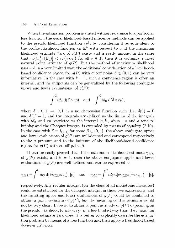
150 5 Point Estimation
When the estimation problem is stated without reference to a particularloss function, the usual likelihood-based inference methods can be appliedto the pseudo likelihood function rp-1, by considering it as equivalent to
the profile likelihood function on Mfe with respect to g. If the maximum
likelihood estimate 7ml of g(P) exists and is really unique, in the sense
that rp\t^ (Bc£)] < rp{jML} for all e G P, then it is certainly a most
natural point estimate of g(P). But the method of maximum likelihood
uses rp-1 in a very limited way: the additional consideration of a likelihood-
based confidence region for g(P) with cutoff point ß G (0, 1) can be very
informative. In the case with k = 1, such a confidence region is often an
interval, and its endpoints can be generalized by the following conjugate
upper and lower evaluations of g(P):
/c/*C
td^ d(ö o rp) and / idy d(ö o rp),
where 5 : [0,1] —> [0,1] is a nondecreasing function such that 0(0) = 0
and £(1) = 1, and the integrals are defined as the limits of the integralswith icfa and rp restricted to the interval [a, b], when —a and b tend to
infinity and the Choquet integral is extended by means of equality (2.10).In the case with ö = I(ß!i] for some ß G (0,1), the above conjugate upper
and lower evaluations of g(P) are well-defined and correspond respectivelyto the supremum and to the infimum of the likelihood-based confidence
region for g(P) with cutoff point ß.
It can be easily proved that if the maximum likelihood estimate 7ml
of g(P) exists, and k = 1, then the above conjugate upper and lower
evaluations of g(P) are well-defined and can be expressed as
/c/*C
idPd(6or£ot^L\P) and Jml~ îdP d[^oŒo(-t^MI/)_1|P],
respectively. Any regular integral (on the class of all monotonie measures)could be substituted for the Choquet integral in these two expressions, and
the resulting upper and lower evaluations of g(P) could be combined to
obtain a point estimate of g(P), but the meaning of this estimate would
not be very clear. In order to obtain a point estimate of g(P) depending on
the pseudo likelihood function rp-1 in a less limited way than the maximum
likelihood estimate 7ml does, it is better to explicitly describe the estima¬
tion problem by means of a loss function and then apply a likelihood-based
decision criterion.

5.1 Likelihood-Based Estimates 151
A function / : Mfe —> P is said to be quasiconvex if
f[\x + {l-\)y] <max{f(x)J(y)} for all x, y G Rk and all AG (0,1);
/ is said to be strictly quasiconvex if the inequality is strict when x ^ y.
An (estimation) error function for the problem of estimating 7 G ffife is
a function Lil'xR^P such that
L(j, d) = w{j) /(7 - d) for all 7, d G Rk,
where w : Mfe —> P is a function, and / : Mfe —> P is a quasiconvex function
with /(0) = 0. The statistical decision problem of estimating (?(P) with
error function L is described by a loss function L' on P x 2?, where 2? is
a subset of Mfe, and L'(P,d) = L[g(P),d] for all P 6 P and all d G V;
obviously, the definition of L outside the set {(g(P), d) : P G T>, d G T>}is irrelevant for the decision problem described by L'. Condition (4.6) im¬
plies that applying a likelihood-based decision criterion to L' with respect
to a likelihood function hk on V is equivalent to applying it to L\Kkx-vwith respect to the profile likelihood function hkg on Mfe. Therefore, more
generally, we can consider a nondegenerate relative plausibility measure
rp on M. and compare the estimates d G T> Ç R by means of the evalu¬
ation Vrp(l,i) of /d, where V^.p is the functional on P* corresponding to a
likelihood-based decision criterion, and for each d G ffife the function 14 on
Rk is defined by ld(j) = L(j, d) (for all 7 G Mfe).
Theorem 5.1. Consider the problem of estimating 7 G M. on the basis
of a nondegenerate relative plausibility measure rp on Mfe, with an error
function L such that f : x 1—> f'(\Mx\), where f is a function on W,and M G Mfexfe is an mvertible matrix. Let Q be the closed convex hull of
{rp-1 > 0}. For each d G ffife there is a d' G G such that according to no
likelihood-based decision criterion d is preferred to d!.
Moreover, if Q is bounded, and L is such that f is strictly increasing,
infrrpi>0} w > 0, and supr i>0i w < oo, then for each d G ffife \ G there
is a d! G Q that is preferred to d according to all likelihood-based decision
criteria.
Proof. Let d ^ G (otherwise we can choose d! = d), and let d! be the
element of G such that Md! is the projection of Md on the closed, convex
set {Mj : 7 G G}- Since \M(j - d')\ < \M(j - d)\ for all 7 G G, we have
Id' |{rpi>0} ^ 'd|{rpi>o}j an<i the first statement of the theorem follows from
Theorem 4.2.

152 5 Point Estimation
At the beginning of Section 4.1 we noted that d! is preferred to d
according to all likelihood-based decision criteria, if essrp sup Id' < oo and
inf(/d — Id') > 0. Theorem 4.2 implies that the second condition can be
weakened to infrrpi>o}()d — Id') > 0, while the first one can be expressed
as supr i>0i Id' < oo; these two conditions follow easily from the premiseof the second statement of the theorem. D
Theorem 5.1 implies that for an important class of error functions, when
applying a likelihood-based decision criterion to the problem of estimating
7 G ffife on the basis of a nondegenerate relative plausibility measure rp
on Mfe, we can restrict attention to the estimates in the closed convex hull
of {rp-1 > 0}. Theorem 5.1 can be easily generalized; in particular, in the
case with k = 1, the assumption about / is not necessary for the first
statement, while for the second one it can be replaced by the assumptionthat / is strictly quasiconvex. It is important to note that for the problemof simultaneous estimation of the components of 7 G Mfe (when k > 1), it
is generally difficult to obtain a reasonable error function by combining in
some way the estimation errors of the single components. In fact, the scale
in which the estimation error is expressed is irrelevant (in the sense that
the error functions L and aL are considered equivalent, for all a G P),but the relative scale of the estimation errors of the single components
can be very important. That is, either 7 G ffife is a genuine vector (in the
sense that we are really interested in 7, and not only in its components
with respect to the standard basis of M. ), in which case reasonable error
functions are usually of the form considered in Theorem 5.1, or else it is
probably better to estimate the k components of 7 separately; therefore,the case with k = 1 is by far the most important one.
5.1.1 Asymptotic Efficiency
Let the loss function L' on V x T> describe the statistical decision problem of
estimating g(P) with an error function L on Mfe x Mfe, where k is a positive
integer, g : V —> Mfe is a mapping, and T> is a subset of Mfe containing the
image of V under g. In Subsection 4.2.2 we have seen that under suitable
regularity conditions, all sequences of decisions obtained by applying a
consistent likelihood-based decision criterion to L' (with respect to the
sequence of relative plausibility measures on V obtained by observing the
realizations of a sequence of random objects) are asymptotically optimal

5.1 Likelihood-Based Estimates 153
under all models in V. This implies that the corresponding sequences of
estimators of g(P) are (strongly) consistent, if the error function L has the
following property: infßc / > 0 for all e G P. The condition /_1{0} = {0}is necessary for this property to hold; in the case with k = 1 it is also
sufficient, while in the case with A; > 1 it is sufficient when / is continuous.
Under suitable regularity conditions, the method of maximum likeli¬
hood leads to an asymptotically efficient sequence of estimators; and un¬
der very similar regularity conditions, the likelihood function tends to be
equivalent to the density of a normal distribution with as mean the maxi¬
mum likelihood estimate (see for example Fraser and McDunnough, 1984).In this case, the next theorem can be used to show that the estimates ob¬
tained by applying a certain kind of likelihood-based decision criterion
(such as the MPL criterion) tend to the maximum likelihood estimates
sufficiently fast to ensure that the corresponding sequences of estimators
are asymptotically efficient as well.
Theorem 5.2. Consider the problem of estimating 7 G ffife with an error
function L such that w is continuous at x' G ffife, and f satisfies
lim sup \C-a f(cx) - \Mx\a\ = 0 for all ÔGW,ci° xeBs
where M G Mfexfe is an mvertible matrix, and a GV. Let rpl7rp2,... be a
sequence of nondegenerate relative plausibility measures on Mfe such that
lim supn^°°xeBs
where the limit of the sequence x\, X2, G ffife is x', and Si, S2,... G Mfexfe
is a sequence of matrices such that linin^oo ^fnYjn exists and is m-
vertible. Consider a likelihood-based decision criterion corresponding to
the functionals Vrp : I 1—> JI d(/i o rp_) for a nondecreasmg surjection
/1 : [0, 1] —> [0, 1] and a regular integral (on the class of all monotonie
measures) such that the corresponding functional F on J\fX^ satisfies
Tp>tpon]? => liminf [F(^pIi0 c}) -F(ipIi0 ci)] > 0 for all ip G Aflp,c^oo
where ip G J\flf is defined by tp(x) = f\ [exp( — x^ )] (for all x G V). If
lim limsup n* \\Vrpn(lxJ - Vrpn(lXn I{Xn+xnX xeBä})\\ = 0, (5.1)
rynHxn + Snx) - expf-^-j 0 for allô G

154 5 Point Estimation
then all sequences di,d,2, G ffife satisfy
0hm n 2
n^oo
Vrpn(ld„) - inf VrPn(ld) hm \/n (dn — xn) = 0.
Proof. Let S = linin^oo ^/n'En, since S is mvertible, for sufficiently large
n the matrices S„ are mvertible too Conditions (5 1) and (4 6) imply that
for all e G P there is a 8£ G P such that for all ö G [ô£, oo) and sufficiently
large n we have
For each 7 G Mfe and each ö G V, let /' and /i^ be respectively the functions
and the completely maxitive measures on Mfe defined by
f!f(x) = \Mi:(x-y)\a and n\(x)h exp '4) if x G Bg
if a; G BS
As n tends to infinity, the completely maxitive measures on Mfe with den¬
sity functions (f\ o rj^} o t~x o S„) Irs + 7bc converge uniformly to fig,
and the functions (w o Ç1 o En)nï (/ o £n) Ig^ converge uniformly to
w(x') /q /ßä Hence, using Theorem 2 23 we obtain that for all ö G [ô£, 00)and sufficiently large n
n^ VrPn(lxJ < w(x') / /o/Bäd/"<5 +2e,
since the integral is regular and condition (2 6) is fulfilled Let a, b G P be
respectively the mfimum and the supremum of {|MEx| x G ffife, \x\ = 1},and let c = w(x') (böi)a + 2 we have n^ V^Pn (/x„) < c for sufficiently large
n Since for all d G ffife and all n we have
n^ VrPn(ld) =n^ ldd(/i or^) > f1[r2ra}(xn)]w(xn)n^ f(xn- d),
for a sufficiently large f £P and sufficiently large n we obtain
inf nt F (/d) > w(x') (a 8')a - 1 > c + 1,
and thus d„ G \xn + Enx x G B,y} for sufficiently large n Assume that
the conclusion of the theorem does not hold, then there is an e' G P such

5.1 Likelihood-Based Estimates 155
that dn (fi {xn + Yjnx : x G B£<} for infinitely many n, and thus there is
a subsequence dni, d„2,... such that linv^oo E^1 (dnm — xUm) = 7' G ffife
with e' < \j'\ < 8'. Conditions (4.1) and (4.6) imply that for all 8 G P and
sufficiently large n we have
VrPn(ldJ >Kp„o(S-1ota;„)-i[(U;0*x„loSn)(/oSnots-i(^_:i.ra))/Bä],
and as above, using Theorem 2.23 we obtain that for all 8 G P and suffi¬
ciently large m
n Vrpnm (ldnm ) > w(x ) / /7< !bs d/"<5 - £•
Now, for all 8 G P we have
J & IBs dM, = (y/2 b)a F (if 1^^ y^ ,
since _F is bihomogeneous (Theorem 2.13) and
M/,/Bä>a;}=//i[exp(-rt)] ifO<*<W,
[O if (bö)a <x<oo.
Analogously, we obtain that there is a ^ G Wîp such that ip > (/? on P,and for all 8 G P
JfylBsdfJis > (y/2b)aF(yi[0i(±.yy).Hence, there are e, 8" G P such that for all 8 G [8", 00) we have
w(x') I /y IBs d/is - w(x') I /o /ßä d/"<5 > 4e,
and thus with J = max{4, ^"} we obtain that for infinitely many n
nf [VrPAldJ ~ VrPn{lxJ] > e > 0,
in contradiction with the assumption about the sequence d\, c^,
Theorem 5.2 can be generalized to a wider class of likelihood-based
decision criteria: in particular, it holds also for the LRM^ and MLD cri¬
teria. In Theorem 5.2, the assumptions about L and about the sequence

156 5 Point Estimation
rpi, rp2,... ensure that locally near xn the estimation problem tends to a
simple form; and the optimality of xn in this simple problem is ensured bythe assumptions about /i and F. The condition on F is rather weak, when
/i is not too extreme; in particular, it is satisfied for both the Shilkret inte¬
gral and the Choquet integral, if there are a, b G P such that f\ (x) < a xb
for all x G [0,1]. Condition (5.1) implies that it suffices to consider the
estimation problem locally near xn; the validity of this condition depends
on the particular problem at hand. For example, if /i satisfies the above
requirement, w is bounded, / : x i—> |Afa;|a, and rp^ is logarithmically
concave for sufficiently large n, then condition (5.1) is fulfilled for both the
Shilkret integral and the Choquet integral.
In Theorem 5.2 it is assumed that locally near 0 the function / tends
to be centrally symmetric about 0; the next example shows that when
this condition is not fulfilled, the conclusion of the theorem does not nec¬
essarily hold, even when all other assumptions are satisfied. In fact, all
asymptotically efficient sequences of estimators of g(P) are asymptoticallynormal with mean g(P) (under each model P G V), while a biased asymp¬
totic distribution can be advantageous when the assumption about / of
Theorem 5.2 does not hold.
Example 5.3. In the situation of Examples 4.18 and 4.25, consider the prob¬lem of estimating /i £ R with an error function L such that w is constant
and / is defined by
f(\_j —2 x if — oo < x < 0,J \x) — |x if 0 < a; < oo.
This estimation error penalizes the overestimation of /i more than its un¬
derestimation; and in fact, if the estimate obtained by applying a particularlikelihood-based decision criterion is well-defined, then there is a nonneg¬
ative real number c such that for each n this estimate is Xj= (where
as usual X denotes the arithmetic mean of the observations X±,..., Xn).The corresponding sequence of estimators of /i is asymptotically efficient if
and only if c = 0; that is, if and only if the resulting estimates are the max¬
imum likelihood estimates X. For the MPL criterion c « 0.345, and thus
the corresponding sequence of estimators is not asymptotically efficient;but the expected loss is 0.915 times the expected loss for the maximum
likelihood estimates (independently of n and /i). 0

5.2 Sliilkret Integral and Quasiconvexity 157
5.2 Shilkret Integral and Quasiconvexity
Consider the problem of estimating 7 G ffife with an error function L, on the
basis of a nondegenerate relative plausibility measure rp on M.k. Let S be
the functional on <Sjp corresponding to a likelihood-based decision criterion
revealing ignorance aversion. Consider first the case with k = 1, and for
each del define ipd = m{hI(d,oc) > } and ipd = m{ldI(-oo,d) > •}•Theorem 4.3 implies that S is monotonie, and Vrp(ld) = S(max.{(fd, ipd})for all d G ffi, where Vrp is the functional on F8 corresponding to the
likelihood-based decision criterion considered. If d,d' G M with d < d',then Lpdt < ipd and ipd' > tpd: that is, if we raise the estimate d, then
the values of ipd decrease and those of tpd increase, while if we reduce the
estimate d, then the values of ipd increase and those of tpd decrease; an
optimal estimate corresponds thus to some sort of equilibrium point. In
the case with k > 1, the situation is more complicated, because there are
infinitely many directions in which the estimate d can be moved; but when
L is of the form considered in Theorem 5.1, for each of these directions we
can obtain two functions with the properties of ipd and ipd by dividing M.k
into two half-spaces. Theorems 5.1 and 5.2 exploit two special cases: in the
first one, for a particular direction we have tpdt < ipd and ipdi = tpd = 0,and thus d cannot be preferred to d'; in the second one, for each direction
we have ipd = ipd, and thus d is optimal. The general case can be simplifiedwhen the likelihood-based decision criterion corresponds to the functional
Vrp : I 1—> Js/ d(/i org) for a nondecreasing function f\ : [0, 1] —> [0,1] such
that /i(0) = 0 and /i(l) = 1: in fact, the maxitivity of the Shilkret integral
implies that Vrp(ld) = max.{S((pd), S(ipd)}- In the case with k = 1, the
function d 1—> Vrp(ld) on M is then quasiconvex (since it is the maximum of
a nonincreasing function and a nondecreasing function); the next theorem
generalizes this result.
Theorem 5.4. Consider the problem of estimating 7 G ffife with an error
function L; on the basis of a nondegenerate relative plausibility measure
rp on M..Let f\ : [0, 1] —> [0,1] be a nondecreasing function such that
fi(0) = 0 and /i(l) = 1, and let Vrp be the functional I 1—>Jsld(f\orp)onP*.Thefunctiond1—>Vrp(ld)onMfeisquasiconvex.Moreover,if{rp-1>0}isbounded,andLissuchthatfiscontinuousandstrictlyquasiconvex,infrrpi>0\w>0,andsupri>0iw<oo,thenthefunctiond1—>Vrp(ld)onMriscontinuousandstrictly
quasiconvex.

158 5 Point Estimation
Proof. For each 7 G ffife the function d 1—> ^(7) is quasiconvex, and
Vrp(ld) = / 'dd(/i or£) = supx/i(r2{Zd > x}) =J xeF
= sup sup x f\ lim inf rpH^fr, )^eP
7lj72j GRfc such thatL n^oo
^(t)^^ for infinitely many n
sup
71,72, el
limsup/d(7„) /1 lim inf ^(7«)
Hence the function d 1—> V^.p(Zd) on Mfe is quasiconvex, since the limit
superior of a sequence of quasiconvex functions is quasiconvex, and so is
the supremum of a set of quasiconvex functions.
To prove the second statement of the theorem, let d! and d" be two
distinct elements of Mfe, and let d = Xd' + (1 — A) d" for some A G (0, 1).The assumptions about rp and L imply that there are a, b G P such that on
|rp4 •> q| we nave max{/(2<, ^//} > ld + a and /^ < &; hence Vrp(ld) < &, and
max{/(2<, /d"} > max{(l + |) Z^, a} on {rp^ > 0}. Since the Shilkret integralis monotonie, homogeneous, niaxitive, and transformation invariant on the
class of all finitely niaxitive measures, and /1 org is finitely niaxitive, usingTheorem 2.8 we obtain
m&x{Vrp(ld,),Vrp(ld„)} = / max{/d/,/d//}d(/! orj)>
> f max{(l + f ) ld, a} d(/i o m) =
= max{(l + f ) Vrp{ld), a} > Vrp(ld);
and this proves the strict quasiconvexity of the function d 1—> Vrp(ld) on
M..Since the Shilkret integral is also subadditive on the class of all finitely
niaxitive measures, using Theorem 2.8 again we obtain
\Vrp(ld) ~ Vrp(ld:)\ < sup{rpi>0} \ld - ld,\ for all d, d' G Rk.
Hence, the continuity at d' G ffife of the function d 1—> Vrp(ld) on Mfe follows
from the equicontinuity at d' of the set of all functions d 1—> ^(7) on ^fe
with 7 G {rp-1 > 0}; and the equicontinuity at each d' G ffife of this set of
functions is implied by the assumptions about rp and L. D

5.2 Sliilkret Integral and Quasiconvexity 159
Consider a likelihood-based decision criterion corresponding to the
functional Vrp : / i—> JSld.(f\orp), where f\ : [0, 1] —> [0,1] is a nondecreas-
ing function such that /i(0) = 0 and /i(l) = 1 (for example the MPL,
LRM^, or MLD criteria). The decision criterion applied to the estimation
problem described by L consists in minimizing Vrp(ld), and Theorem 5.4
states that the function d i—> Vrp(ld) on M. is quasiconvex. Therefore, in
particular, the set of all optimal estimates in Mfe is convex, and if the
function d i—> Vrp(ld) has a strict local minimum at d' G ffife, then d' is
the unique optimal estimate in Mfe. If the premise of the second statement
of the theorem is satisfied, then the function d i—> Vrp(ld) on Mfe is also
continuous and strictly quasiconvex, and so there is at most one optimalestimate in Mfe. It can be easily proved that if the premise of the second
statement of Theorem 5.4 is satisfied, and either k = 1, or L is of the form
considered in Theorem 5.1, then there is a unique optimal estimate in Mfe,and it lies in the closed convex hull of {rp-1 > 0}.
Consider now the case when fi is left-continuous; then fi o rp is com¬
pletely maxitive, and using Theorem 2.6 we obtain
,s
Vrp(ld)= supf(1-d)w(1)f1[m^1)}= / (fotd)dfJi foralldGMfe,7Rfc J
where /i is the completely maxitive measure on Mfe with density function
fj,^- = w (fiorjr1). When /i is finite, applying the considered likelihood-based
decision criterion to L with respect to rp corresponds thus to applying the
MPL criterion to the error function L' : (7, d) 1—> f(j — d) with respect to
the (nondegenerate) relative plausibility measure on Mfe proportional to /i.
In particular, the assumptions about w of Theorem 5.4 can be replaced bythe assumptions that f\ is left-continuous and w (f\ orj>}) is bounded. An
algorithm for approximating the optimal estimates of 7 G Mfe (that is, for
minimizing the function d 1—> Vrp{ld) on Mfe) is suggested by the followingtwo expressions:
Vrp(ld) =sup(Ati>0}(/otd)/ui for all d£ Rk,
{d£Rk:Vrp(ld)<c}= f| {/o(-t7)<^} for all cG P.
7£{/iJ->0}
Let d G Mfe be an initial estimate, and let 71,..., jn G {/i^ > 0} be suitable
approximations of the local maxima of (/ o td) fJ,^. Then the valuec=max{/(7!-d)/i^Ti),•••,f(jn-d)
mHt«)}

160 5 Point Estimation
approximates Vrp(ld), and if actually infd/GRk Vrp(ld') < c, then the optimalestimates lie in the set
A={d'<=Mk:f(rfl-d')<1Irfa, -.., f{lu-d')<1^)}.
The set A is convex (since / is quasiconvex), and the estimate d usuallylies on the border of A; other estimates d' G A lying in the interior of A can
be expected to be better than d, in the sense that Vrp(ld') < Vrp(ld). The
rule for selecting a new estimate d' G A can exploit the properties of the
particular problem at hand, such as the differentiability of f or fiK Once
the estimate d' G A has been selected, a new step of the algorithm can be
carried out by using d! as the initial estimate; and 71,..., 7n can be used
as starting points for approximating the local maxima of (f otd>) fiK That
is, the algorithm can be interpreted as searching for the local maxima of a
function that depends on the obtained approximations of the local maxima:
some steps of the maximization algorithms are alternated with some stepsof an algorithm that redefines the function to be maximized (by selecting
a new estimate d'). The algorithm is particularly simple and effective in
the case with k = 1, but it has proved successful also in multidimensional
problems with k up to 10; however, the speed of convergence depends
strongly on which properties of the estimation problem can be assumed
and exploited when implementing the algorithm, and in particular when
defining the rule for selecting the new estimate d! G A.
5.2.1 Impossible Estimates
Consider the problem of estimating 7 G ffife with an error function L,on the basis of a nondegenerate relative plausibility measure rp on Mfe.
The elements of {rp-1 = 0} can be considered as impossible, since they
are infinitely less plausible than any element of {rp-1 > 0}. If V is a set
of statistical models, g : V —> Mfe is a mapping, and rp-1 is proportionalto the profile likelihood function hkg induced by the observation of some
data, then rp*- vanishes at 7 G M. if and only if either 7 is physically
impossible (in the sense that it does not lie in the image of V under g),or it is impossible in the light of the observed data (in the sense that
the likelihood function on V induced by the observed data vanishes on
{g = 7}). Impossible optimal estimates can be problematic, and even a
unique optimal estimate lying on the border of {rp-1 > 0} can be disturbing.

5.2 Sliilkret Integral and Quasiconvexity 161
Consider a likelihood-based decision criterion corresponding to the
functional Vrp : / i—> Jsld(f\ org), where f\ : [0,1] —> [0,1] is a non-
decreasing function such that /i(0) = 0 and /i(l) = 1. We have seen that
under some conditions, if either k = 1, or L is of the form considered in
Theorem 5.1, then there is a unique optimal estimate 7 G ffife, and 7 lies
in the closed convex hull of {ryr > 0}. Of course, 7 can be impossible (inthe sense that rp^(j) = 0) when {rp-1 > 0} is not convex; for instance, if
k = 2, the error function is L : (7, eZ) 1—> l'y — d\, and rj>} is the indicator
function of the unit circle C = {x G ffi2 : |x| = 1}, then 7 = 0 is the unique
optimal estimate according to all likelihood-based decision criteria reveal¬
ing ignorance aversion. If we try to minimize the function d 1—> Vrp(ld) on
T> = {rp-1 > 0}, then in general the minimum does not exist when T> is
not closed. In fact, 7 can be impossible also when {rp-1 > 0} is convex; for
example, with k and L as above, if rj>} is the indicator function of an open
unit half-disc H = {x G M.2 : \x\ < 1, x y > 0}, where y G M2\{0}, then
7 = 0 is the unique optimal estimate according to all likelihood-based de¬
cision criteria revealing ignorance aversion. The next theorem implies that
under some conditions 7 cannot be an extreme point of the closed convex
hull of {rp-1 > 0}; the above example does not contradict this theorem,since 0 is not an extreme point of the closure of H (the extreme points of
the closure of H are the x G C such that x y > 0). The next theorem
is particularly interesting in the case with k = 1, because then the closed
convex hull of {rp-1 > 0} is an interval ICI, and if 7 is not an extreme
point of /, then it lies in the interior of /, and thus also in the interior of
{rp-1 > 0}, when this is convex.
Theorem 5.5. Consider the problem of estimating 7 G ffife on the basis
of a nondegenerate relative plausibility measure rp on Mfe, with an error-
function L such that supr i>0i w < 00 and f : x 1—> f'(\Mx\), where
/' : P -> P is a function continuous at 0, and M G Mfexfe is an mvert-
ible matrix. Let f\ : [0, 1] —> [0,1] be a nondecreasmg function such that
/i(0) = 0 and /i(l) = 1, and consider a likelihood-based decision criterion
corresponding to the functional Vrp : I 1—> Js/d(/i org). If 7 G ffife is the
unique optimal estimate, and Vrp(lj) > 0, then 7 is not an extreme point
of the closed convex hull of {rp-1 > 0}.
Proof. Let Q be the closed convex hull of {rp-1 > 0}, and assume that 7 is
an extreme point of Q. Then Mj is an extreme point of the closed, convex
set Q' = {Mj : 7 G G}, and thus for each e G P there is an open half-space

162 5 Point Estimation
H£ C Rk such that Mj G H£ and g'nHeC tMx- (B£). For each e G P let j£
be the element of Mfe such that Mj£ is the projection of Mj on the border
of H£: we have \M(j - j£)\ < \M(j - 7)| for all 7 G M"1^ \ i7£). Since
Ö' is not a singleton (because otherwise Vrp(lj) = 0), for sufficiently small
e G P we have \M(j£ — 7)! < e; and the assumptions about L thus implythat there is an e' G P such that lj ,
< Vrpil^) on ÇC\M~1(H£>). Since the
Shilkret integral is monotonie, homogeneous, maxitive, and transformation
invariant on the class of all finitely maxitive measures, and /1 org is finitely
maxitive, using Theorem 2.8 we obtain
Vrp(llc,) = / max{/7e, 7gnM-i(ffe,),/7e, Im-\m"\he,)} d(/i °!ï) <
< / max{Frp(/7),/7}d(/1 org) = Vrp(h),
in contradiction with the assumption that 7 is uniquely optimal. D
Theorem 5.5 can be easily generalized; in particular, in the case with
k = 1, the assumption about / can be replaced by the assumption that / is
continuous at 0. Moreover, as in Theorem 5.4, the assumption about w of
Theorem 5.5 can be replaced by the assumptions that /1 is left-continuous
and w (/1 org}) is bounded. When /_1{0} = {0}, a sufficient condition
for Vrp(Ly) to be positive is that {f\ o rg} > 0} is not a singleton; in
particular, if (as in the following example) rp^ is continuous on {rp^ > 0},and {rp-1 > 0} is convex and is not a singleton, then Vrp(Ly) = 0 is possible
only if /1 = /{1} (that is, only for the MLD criterion).
Example 5.6. The problem of estimating (with squared error loss) the
mean of a normal distribution with known variance is made much more
complex by the additional assumption that the mean lies in a partic¬ular bounded interval. Casella and Strawdernian (1981) proved that if
V1 = {Pß : /i G (—to, to)} is a family of probability measures such
that under each model Pß the random variable X is normally distributed
with mean /i and variance 1, and to G (0, 1.056), then the minimax risk
criterion applied to the decision problem described by the loss function
L' : (PM, d) 1—> (/i — d)2 on V' x M. leads to the estimate TO-tanh(TO-X). For
larger values of to, the estimate obtained by applying the minimax risk
criterion is in general unknown, but Donoho, Liu, and MacGibbon (1990)showed that the maximum expected loss for this estimate is at least 0.8

5.2 Sliilkret Integral and Quasiconvexity 163
times the one for the estimate ?.X. When \X\ > to + —, this esti-
mate is impossible; an estimate that is never impossible and has smaller
expected loss (under all models in V) can be obtained by using the results
of Moors (1981):
sign(X) min{^|X|,mtanh(m|X|)}. (5.2)
The maximum expected loss for this estimate is thus at most 1.25 times
the one for the estimate obtained by applying the minimax risk criterion.
For the hierarchical model described in Section 3.2, the assumption that
the mean /i lies in the interval (—to, to) simply corresponds to a particular
prior relative plausibility measure on the set V = {P^ : /i G ffi} 2 V
considered in Example 4.18 (with n = 1 and X = X\): the prior relative
plausibility measure with density function proportional to the function
Pß i—> I(-m>m) (/i) on V. No probability measure on V can describe this kind
of prior information, but a reasonable estimate can be obtained by applyingto the decision problem described by the loss function L : (Pß, d) i—> (fi—d)2onPxM the Bayesian criterion with as initial averaging probability mea¬
sure on V the one corresponding to the uniform distribution on (—to, to)for the parameter /i (see Gatsonis, MacGibbon, and Strawderman, 1987).When the realization X = x is observed, the above prior relative plausi¬
bility measure can be updated by combining it (as described in Subsec¬
tion 3.1.2) with the relative plausibility measure on V whose density func¬
tion is proportional to the approximate likelihood function Pß i—> ö ip(x—fï)on V considered in Example 4.18. A likelihood-based decision criterion can
then be applied to the decision problem described by L: consider the de¬
cision criteria corresponding to the functionals Vrp : I i—> Jsld(f\ org) for
some nondecreasing function /i : [0, 1] —> [0,1] such that /i(0) = 0 and
/i(l) = 1. Theorems 5.1 and 5.4 imply that there is a unique optimal esti¬
mate in R, and it lies in the closed interval [—m, m]; and Theorem 5.5 im¬
plies that if /i ^ I{\\i then the estimate lies in the open interval (—m, m).That is, the MLD criterion is the only one of the considered likelihood-
based decision criteria that can lead to an impossible estimate, and in fact
it leads to the estimate sign(X) min{|X|, to}, which is impossible when
\X\ > to. When \X\ < to, this estimate corresponds to the maximum
likelihood estimate X; more generally, if /i is not too extreme (it suffices
that there are a, b G P such that f\(x) < axb for all x G [0,1]), then there
is a c G P such that the resulting estimate is X when \X\ < to — c (forall to > c): for instance, c = y2 when f\ = îdr01i (that is, for the MPL

164 5 Point Estimation
Figure 5.1. Estimators and corresponding expected losses from Example 5.6.
criterion). This can be considered as a stability property: when the obser¬
vation x lies in the interval (—to, to) and is sufficiently far away from its
endpoints, the additional assumption that /i G (—to, to) has no influence
on the estimate of /i G R.
The first diagram of Figure 5.1 shows the graphs of some estimates of
/i, as functions of the observation x G [0, 6] (all the estimators considered
are odd functions), in the case with to = 3: the estimate (5.2) (dotted,almost polygonal line), and the estimates obtained by applying the MPL
criterion (dashed line), the MLD criterion (upper solid line), the LRM^criterion with ß fa 0.259 (so that —2 log/3 is the 90%-quantile of the x2distribution with one degree of freedom; lower solid line), and the Bayesiancriterion with initial averaging probability distribution uniform on (—3, 3)(dotted curved line). The second diagram of Figure 5.1 shows the graphsof the corresponding expected losses (as functions of /i G (—3, 3)): for the
estimate (5.2) (dotted line with maximum 0.809 occurring near /i = 0),and for the estimates obtained by applying the MPL criterion (dashed line
with maximum 0.947), the MLD criterion (solid line with maximum 0.995
at /i = 0), the LRM^ criterion with ß « 0.259 (solid line with supremum
1.001 occurring at the endpoints of the interval), and the Bayesian criterion
with initial averaging probability distribution uniform on (—3, 3) (dottedline with supremum 1.000 occurring at the endpoints of the interval). A
consequence of the stability property considered above is that the three
estimates obtained by applying a likelihood-based decision criterion have
a relatively high expected loss under the model Pq. 0

5.2 Sliilkret Integral and Quasiconvexity 165
Using the previous results, it can be easily proved that when the MPL
criterion is applied to the problem of estimating 7 G M with an error
function L, on the basis of a nondegenerate relative plausibility measure
rp on R, if L is such that / is continuous and strictly quasiconvex, w rp-1
is bounded, and
lim f(x — d) w(x) rp^{x) = lim f(x — d) w(x) rp^(x) = 0 for all dgR,
then there is a unique optimal estimate in R, and it lies in the interior of the
convex hull of {rp-1 > 0}, when this is not a singleton. Theorem 2.6 impliesthat applying the MPL criterion to L with respect to rp corresponds to
applying it to the error function L' : (7, d) 1—> f{j — d) with respect to
w^ 0 rp; that is, the weight function w plays the role of a prior likelihood
function on R, to be combined with the pseudo likelihood function rpKMore generally, when V is a set of statistical models, g : V —> R is a
mapping, and we estimate 7 = g(P), a weight function w' can be defined
directly on V: if rp1 is a relative plausibility measure on V, then applyingthe MPL criterion to L' with respect to [(w/)^ 0 rp'] o g~x corresponds to
applying it (with respect to rp') to the decision problem described by the
loss function L" : (P, d) 1—> w'(P) f[g(P)—d] onPxI. When w' depends on
P only through g(P), we recover the above situation, with rp = rp' o g^1and w' = wog. The weight function w' must be chosen carefully: in
general, the resulting estimates have better pre-data performances when
w' is chosen so that estimates with bounded expected losses are possible.
Example 5.7. Famous examples of impossible estimates are the negativeestimates of variance components in random effects models (see for in¬
stance Searle, Casella, and MacCulloch, 1992). Consider in particular the
balanced one-way layout under normality assumptions; that is, consider a
family V' = {P^yVa,vs ' (/•*, va, ve) G R x P x P} of probability measures such
that under each model PlijVajVe the random variables Xly3 are normally dis¬
tributed with mean /i and variance va + ve (for all 1 G {1,..., na} and all
j G {l,...,ne}), and the correlation coefficient of two different random
variables X, ~ and X,> ,< is p = —^f— when 1 = «', and 0 otherwise. Then,
under each model P..,, ,,the random variables -,— and —- are y
distributed with na — 1 and na (ne — 1) degrees of freedom, respectively,where
Sa=neJ2(Xh -J,)2 and Se = g J^(XttJ - Xt> )2,1=1 1=1J=l

166 5 Point Estimation
with X, = — y^e, X, „and X = — Y^"", X, .
The estimates of the
variance components va and ve obtained by applying the method of analy¬sis of variance are
va = — and ve = -,
ne \na-l na (ne - 1J ) na (ne - 1)
respectively; these estimates are unbiased and have minimum variance
among all unbiased estimates, but va can be negative. The problems of
estimating va and ve can be described as statistical decision problems bymeans of two loss functions La and Le on V x R; consider in particularthe loss functions
L (P d)^{Va ~ da)2
and L • (P d)^(^e ~ ^
(neva+vey vi
The squared error loss is not particularly well suited for scale parameters,
but it accords with the estimates va and ve (which have minimum variance
among all unbiased estimates). The weights are chosen so that the decision
problems are location and scale invariant, and estimates with bounded
expected losses are possible (the naive choice -\ for La would in fact
impose the estimate da = 0).
Figure 5.2 shows the graphs of some equivariant estimators of va and
fe, and of the corresponding expected losses, in the case with na = ne = 3;the other cases are qualitatively similar, although the differences are less
marked when na and ne are larger. All the estimates considered depend
on the observations Xly3 only through Sa and Se: the estimates of va and
ve divided by Sa + Se are plotted (as functions of r =s °g G (0,1)) in
the first and second upper diagrams, respectively, while the correspond¬
ing expected losses are plotted (as functions of p G (0,1)) in the first and
second lower diagrams, respectively. The estimates va and ve obtained by
applying the method of analysis of variance (solid straight lines) have rela¬
tively large expected losses (upper solid lines); in particular, the expectedloss for va is large when p is small, because va is negative when r is small:
in fact, the truncated estimate max{wo,0} has smaller expected loss (up¬per dashed line). This truncated estimate is biased; when the requirementof unbiasedness is dropped, many generalizations of the estimate va are
possible. For instance, Härtung (1981) proposed an estimate of va (dottedstraight line) that minimizes the bias among the nonnegative, invariant,
quadratic estimates, but the corresponding expected loss (upper dotted
line) is even larger than the one for va when p is small.

5.2 Sliilkret Integral and Quasiconvexity 167
0.15
0.05
00.2 0.4 0.6 0.8 1
0.15-
0.1-
0.05
0.3-
0.25 -'
0.2 0.4 0.6 0.: 0 0.2 0.4 0.6 o.:
Figure 5.2. Estimators and corresponding expected losses from Example 5.7.
Besides va and ve, the most appreciated estimates of va and ve seem
to be those based on the method of maximum likelihood; consider the
density-based approximation of the likelihood function on V induced bythe observations XtJ. The maximum likelihood estimate of va (dashedline) has a relatively small expected loss (lower dashed line), while for
the maximum likelihood estimate of ve (lower dashed line) the expectedloss (lower dashed line) is small only when p is small; these are the esti¬
mates obtained by applying the MLD criterion to the decision problemsdescribed by La and Le, respectively, without using prior information. The
restricted maximum likelihood estimates considered by Thompson (1962)are obtained by applying the method of maximum likelihood to a partic¬ular pseudo likelihood function on V: they are appreciated because they
are nonnegative and correspond to the estimates obtained by applying the
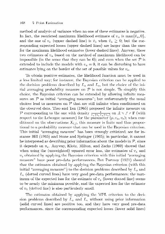
168 5 Point Estimation
method of analysis of variance when no one of these estimates is negative.In fact, the restricted maximum likelihood estimate of va is max{vo,0},and the one of ve (upper dashed line) is ve when va > 0; but the cor¬
responding expected losses (upper dashed lines) are larger than the ones
for the maximum likelihood estimates (lower dashed lines). Anyway, these
two estimates of va based on the method of maximum likelihood can be
impossible (in the sense that they can be 0); and even when the set V is
extended to include the models with va =0, it can be disturbing to have
estimates lying on the border of the set of possible values for va.
To obtain positive estimates, the likelihood function must be used in
a less limited way; for instance, the Bayesian criterion can be applied to
the decision problems described by La and Le, but the choice of the ini¬
tial averaging probability measure on V is not simple. To simplify this
choice, the Bayesian criterion can be extended by allowing infinite mea¬
sures on V as initial "averaging measures" ; but unfortunately the usual
choices lead to measures on V that are still infinite when conditioned on
the observed data. Tiao and Tan (1965) proposed the infinite measure on
V corresponding to the one with density /n \ +v \on M. x P x P (with
respect to the Lebesgue measure) for the parameter (/i, va, ve); when con¬
ditioned on the observations X%>3, this measure is finite and thus propor¬
tional to a probability measure that can be used in the Bayesian criterion.
This initial "averaging measure" has been strongly criticized: see for in¬
stance Hill (1965) and Stone and Springer (1965); in particular, it cannot
be interpreted as describing prior information about the models in V, since
it depends on ne. Anyway, Klotz, Milton, and Zacks (1969) showed that
when using the (unweighted) squared error loss, the estimates of va and
ve obtained by applying the Bayesian criterion with this initial "averagingmeasure" have poor pre-data performances. But Portnoy (1971) showed
that the estimates obtained by applying the Bayesian criterion (with this
initial "averaging measure" ) to the decision problems described by La and
Le (dotted curved lines) have very good pre-data performances: the max¬
imum of the expected loss for the estimate of va (lower dotted line) seems
to be nearly the minimum possible, and the expected loss for the estimate
of ve (dotted line) is also particularly small.
The estimates obtained by applying the MPL criterion to the deci¬
sion problems described by La and Le without using prior information
(solid curved lines) are positive too, and they have very good pre-data
performances, since the corresponding expected losses (lower solid lines)

5.2 Sliilkret Integral and Quasiconvexity 169
are similar to the ones for the estimates studied by Portnoy. Compared to
the Bayesian criterion, the MPL criterion has the important advantage of
avoiding the difficult choice of the initial "averaging measure", when no
prior information is available, or when we do not want to use the available
prior information. 0


References
Akaike, H. (1973). Information theory and an extension of the maximum likeli¬
hood principle. In Petrov and Csâki, 267-281.
Anscombe, F. J., and Aumann, R. J. (1963). A definition of subjective proba¬
bility. Ann. Math. Stat. 34, 199-205.
Augustin, T. (2003). On the suboptiniality of the generalized Bayes rule and
robust Bayesian procedures from the decision theoretic point of view: A cau¬
tionary note on updating imprecise priors. In Bernard et al., 31-45.
Azzalini, A., and Capitanio, A. (2003). Distributions generated by perturbation
of symmetry with emphasis on a multivariate skew ^-distribution. J. R. Stat.
Soc, Ser. B, Stat. Methodol. 65, 367-389.
Ballester, A., Cardûs, D., and Trillas, E., eds. (1982). Proceedings of the Sec¬
ond World Conference on Mathematics at the Service of Man. Universidad
Politécnica de Las Palmas.
Barndorff-Nielsen, O. E. (1991). Likelihood theory. In Hinkley et al., 232-264.
Bayes, T. (1763). An essay towards solving a problem in the doctrine of chances.
Philos. Trans. R. Soc. Lond. 53, 370-418.
Berk, R. H. (1966). Limiting behavior of posterior distributions when the model
is incorrect. Ann. Math. Stat. 37, 51-58.
Bernard, J.-M., Seidenfeld, T., and Zaffalon, M., eds. (2003). ISIPTA '03. Car-
leton Scientific.
Birnbaum, A. (1962). On the foundations of statistical inference. J. Am. Stat.
Assoc. 57, 269-326.
Birnbaum, A. (1969). Concepts of statistical evidence. In Morgenbesser et al.,
112-143.
Bouchon-Meunier, B., Yager, R. R., and Zadeh, L. A., eds. (1991). Uncertainty
m Knowledge Bases. Springer.

172 References
Breese, J. S., and Koller, D., eds. (2001). UAI '01. Morgan Kaufmann.
Brown, L. D., and Purves, R. (1973). Measurable selections of extrema. Ann.
Stat. 1, 902-912.
Casella, G., and Strawderman, W. E. (1981). Estimating a bounded normal
mean. Ann. Stat. 9, 870-878.
Cattaneo, M. (2005). Likelihood-based statistical decisions. In Cozman et al.,
107-116.
Chen, Y. Y. (1993). Bernoulli trials: From a fuzzy measure point of view. J.
Math. Anal. Appl. 175, 392-404.
Chernoff, H. (1954). Rational selection of decision functions. Econometrica 22,422-443.
Choquet, G. (1954). Theory of capacities. Ann. Inst. Fourier 5, 131-295.
Cohen, L. J. (1966). A logic for evidential support. Br. J. Philos. Set. 17, 21-43
and 105-126.
Cozman, F. G., Nau, R., and Seidenfeld, T., eds. (2005). ISIPTA '05. SIPTA.
Dahl, F. A. (2005). Representing human uncertainty by subjective likelihood
estimates. Int. J. Approx. Reasoning 39, 85-95.
Darwiche, A., and Friedman, N., eds. (2002). UAI '02. Morgan Kaufmann.
DasGupta, A., and Studden, W. J. (1989). Frequentist behavior of robust Bayes
estimates of normal means. Stat. Decis. 7, 333-361.
de Cooman, G. (2000). Integration in possibility theory. In Grabisch et al., 124-
160.
de Cooman, G., Fine, T. L., and Seidenfeld, T., eds. (2001). ISIPTA 'Ol. Shaker.
de Cooman, G., Ruan, D., and Kerre, E. E., eds. (1995). Foundations and Ap¬
plications of Possibility Theory. World Scientific.
de Cooman, G., and Walley, P. (2002). A possibilistic hierarchical model for
behaviour under uncertainty. Theory Decis. 52, 327-374.
Dempster, A. P. (1967). Upper and lower probabilities induced by a multivalued
mapping. Ann. Math. Stat. 38, 325-339.
Denneberg, D. (1994). Non-Additive Measure and Integral. Kluwer.
Donoho, D. L., Liu, R. C, and MacGibbon, B. (1990). Minimax risk over hy-
perrectangles, and implications. Ann. Stat. 18, 1416-1437.
Dubois, D. (1988). Possibility theory: Searching for normative foundations. In
Munier, 601-614.
Dubois, D., and Prade, H. (1988). Possibility Theory. Plenum Press.

References 173
Dubois, D., and Prade, H. (1995). Possibilistic mixtures and their applications to
qualitative utility theory — Part II: Decision under incomplete knowledge.
In de Cooman et al., 256-266.
Dubois, D., Wellman, M. P., D'Ambrosio, B., and Smets, P., eds. (1992). UAI
'92. Morgan Kaufmann.
Ellsberg, D. (1961). Risk, ambiguity, and the Savage axioms. Q. J. Econ. 75,643-669.
Evans, M. J., Fraser, D. A. S., and Monette, G. (1986). On principles and argu¬
ments to likelihood. Can. J. Stat. 14, 181-199.
Fishburn, P. C. (1970). Utility Theory for Decision Making. Wiley.
Fisher, R. A. (1922). On the mathematical foundations of theoretical statistics.
Philos. Trans. R. Soc. Lond., Ser. A 222, 309-368.
Fisher, R. A. (1930). Inverse probability. Proc. Carab. Philos. Soc. 26, 528-535.
Fraser, D. A. S., and McDunnough, P. (1984). Further remarks on asymptotic
normality of likelihood and conditional analyses. Can. J. Stat. 12, 183-190.
Gärdenfors, P., and Sahlin, N.-E. (1982). Unreliable probabilities, risk taking,
and decision making. Synthese 53, 361-386.
Gatsonis, C., MacGibbon, B., and Strawderman, W. (1987). On the estimation
of a restricted normal mean. Stat. Probab. Lett. 6, 21-30.
Giang, P. H., and Shenoy, P. P. (2001). A comparison of axiomatic approachesto qualitative decision making using possibility theory. In Breese and Koller,
162-170.
Giang, P. H., and Shenoy, P. P. (2002). Statistical decisions using likelihood
information without prior probabilities. In Darwiche and Friedman, 170-178.
Gilboa, I., and Schmeidler, D. (1989). Maxmin expected utility with non-unique
prior. J. Math. Econ. 18, 141-153.
Gilboa, I., and Schmeidler, D. (1993). Updating ambiguous beliefs. J. Econ.
Theory 59, 33-49.
Giraud, R. (2005). Objective imprecise probabilistic information, second order
beliefs and ambiguity aversion: an axiomatization. In Cozman et al., 183-192.
Good, I. J. (1965). The Estimation of Probabilities. MIT Press.
Goutis, C., and Casella, G. (1995). Frequentist post-data inference. Int. Stat.
Rev. 63, 325-344.
Grabisch, M., Murofushi, T., and Sugeno, M., eds. (2000). Fuzzy Measures and
Integrals. Physica-Verlag.
174 References
Hampel, F. R., Ronchetti, E. M., Rousseeuw, P. J., and Staliel, W. A. (1986).Robust Statistics. Wiley.
Hartigan, J. A. (1983). Bayes Theory. Springer.
Härtung, J. (1981). Nonnegative minimum biased invariant estimation in vari¬
ance component models. Ann. Stat. 9, 278-292.
Hill, B. (1965). Inference about variance components in the one-way model. J.
Am. Stat. Assoc. 60, 806-825.
Hinkley, D. V., Reid, N., and Snell, E. J., eds. (1991). Statistical Theory and
Modelling. Chapman and Hall.
Hodges, J. L., Jr., and Lehmann, E. L. (1950). Some problems in minimax pointestimation. Ann. Math. Stat. 21, 182-197.
Hodges, J. L., Jr., and Lehmann, E. L. (1952). The use of previous experience
in reaching statistical decisions. Ann. Math. Stat. 23, 396-407.
Huber, P. J. (1964). Robust estimation of a location parameter. Ann. Math.
Stat. 35, 73-101.
Huber, P. J., and Strassen, V. (1973). Minimax tests and the Neyman-Pearson
lemma for capacities. Ann. Stat. 1, 251-263.
Hurwicz, L. (1951). Some specification problems and applications to econometric
models. Econometrica 19, 343-344.
Imaoka, H. (1997). On a subjective evaluation model by a generalized fuzzy
integral. Int. J. Uncertain. Fuzzmess Knowl.-Based Syst. 5, 517-529.
Jeffreys, H. (1946). An invariant form for the prior probability in estimation
problems. Proc. R. Soc. Lond., Ser. A 186, 453-461.
Klement, E. P., Mesiar, R., and Pap, E. (2004). Measure-based aggregation op¬
erators. Fuzzy Sets Syst. 142, 3-14.
Klotz, J. H., Milton, R. C, and Zacks, S. (1969). Mean square efficiency of
estimators of variance components. J. Am. Stat. Assoc. 64, 1383-1402.
Kriegler, E. (2005). Imprecise Probability Analysis for Integrated Assessment of
Climate Change. PhD thesis, Universität Potsdam.
Kullback, S., and Leibler, R. A. (1951). On information and sufficiency. Ann.
Math. Stat. 22, 79-86.
Lange, K. L., Little, R. J. A., and Taylor, J. M. G. (1989). Robust statistical
modeling using the t distribution. J. Am. Stat. Assoc. 84, 881-896.
Lehmann, E. L. (1959). Testing Statistical Hypotheses. Wiley.

References 175
Leonard, T. (1978). Density estimation, stochastic processes and prior informa¬
tion. J. R. Stat. Soc, Ser. B 40, 113-146.
Mesiar, R. (1995). Possibility measures based integrals — Theory and applica¬tions. In de Cooman et al., 99-107.
Moors, J. J. A. (1981). Inadmissibility of linearly invariant estimators in trun¬
cated parameter spaces. J. Am. Stat. Assoc. 76, 910-915.
Moral, S. (1992). Calculating uncertainty intervals from conditional convex sets
of probabilities. In Dubois et al., 199-206.
Moral, S., and de Campos, L. M. (1991). Updating uncertain information. In
Bouchon-Meunier et al., 58-67.
Morgenbesser, S., Suppes, P., and White, M., eds. (1969). Philosophy, Science,
and Method. Macmillan.
Munier, B. R., ed. (1988). Risk, Decision and Rationality. Reidel.
Nau, R. F. (1992). Indeterminate probabilities on finite sets. Ann. Stat. 20,
1737-1767.
Neyman, J., ed. (1951). Proceedings of the Second Berkeley Symposium on Math¬
ematical Statistics and Probability. University of California Press.
Neyman, J., and Pearson, E. S. (1928). On the use and interpretation of certain
test criteria for purposes of statistical inference. Biometrika 20A, 175-240
and 263-294.
Owen, A. B. (1988). Empirical likelihood ratio confidence intervals for a single
functional. Biometrika 75, 237-249.
Petrov, B. N., and Csâki, F., eds. (1973). ISIT '71. Akadémiai Kiadö.
Piatti, A., Zaffalon, M., and Trojani, F. (2005). Limits of learning from imperfect
observations under prior ignorance: the case of the imprecise Dirichlet model.
In Cozman et al., 276-286.
Pinheiro, J. C, Liu, C, and Wu, Y. N. (2001). Efficient algorithms for robust es¬
timation in linear mixed-effects models using the multivariate t distribution.
J. Comput. Graph. Stat. 10, 249-276.
Portnoy, S. (1971). Formal Bayes estimation with application to a random effects
model. Ann. Math. Stat. 42, 1379-1402.
Rissanen, J. (1978). Modeling by shortest data description. Automatica 14, 465-
471.
Robbins, H. (1951). Asymptotically subminimax solutions of compound statis¬
tical decision problems. In Neyman, 131-148.

176 References
Savage, L. J. (1951). The theory of statistical decision. J. Am. Stat. Assoc. 46,
55-67.
Savage, L. J. (1954). The Foundations of Statistics. Wiley.
Schervish, M. J. (1995). Theory of Statistics. Springer.
Schmeidler, D. (1986). Integral representation without additivity. Proc. Am.
Math. Soc. 97, 255-261.
Schmeidler, D. (1989). Subjective probability and expected utility without ad¬
ditivity. Econometrica 57, 571-587.
Searle, S. R., Casella, G., and MacCulloch, C. E. (1992). Variance Components.
Wiley.
Severini, T. A. (2000). Likelihood Methods in Statistics. Oxford University Press.
Shackle, G. L. S. (1949). Expectation in Economics. Cambridge University Press.
Shafer, G. (1976). A Mathematical Theory of Evidence. Princeton University
Press.
Shafer, G. (1982). Lindley's paradox. J. Am. Stat. Assoc. 77, 325-351.
Shannon, C. E. (1948). A mathematical theory of communication. Bell System
Tech. J. 27, 379-423 and 623-656.
Shilkret, N. (1971). Maxitive measure and integration. Indag. Math. 33, 109-116.
Sipos, J. (1979). Integral with respect to a pre-measure. Math. Slovaca 29, 141—
155.
Smets, P. (1982). Possibilistic inference from statistical data. In Ballester et al.,
611-613.
Stone, M., and Springer, B. G. F. (1965). A paradox involving quasi prior dis¬
tributions. Biometrika 52, 623-627.
Sugeno, M. (1974). Theory of Fuzzy Integrals and Its Applications. PhD thesis,
Tokyo Institute of Technology.
Thompson, W. A., Jr. (1962). The problem of negative estimates of variance
components. Ann. Math. Stat. 33, 273-289.
Tiao, G. C., and Tan, W. Y. (1965). Bayesian analysis of random-effect models in
the analysis of variance — I: Posterior distribution of variance-components.
Biometrika 52, 37-53.
von Neumann, J., and Morgenstern, O. (1944). Theory of Games and Economic
Behavior. Princeton University Press.
Wakker, P. (1993). Unbounded utility for Savage's "foundations of statistics"
and other models. Math. Oper. Res. 18, 446-485.

References 177
Wald, A. (1939). Contributions to the theory of statistical estimation and testing
hypotheses. Ann. Math. Stat. 10, 299-326.
Wald, A. (1949). Note on the consistency of the maximum likelihood estimate.
Ann. Math. Stat. 20, 595-601.
Walley, P. (1991). Statistical Reasoning with Imprecise Probabilities. Chapman
and Hall.
Walley, P. (1996). Inferences from multinomial data: Learning about a bag of
marbles. J. R. Stat. Soc, Ser. B 58, 3-57.
Weber, S. (1984). _L-decomposable measures and integrals for Archimedean t-
conorms _L. J. Math. Anal. Appl. 101, 114-138.
Weichselberger, K. (2001). Elementare Grundbegriffe einer allgemeineren Wahr¬
scheinlichkeitsrechnung I. Physica-Verlag.
Weichselberger, K., and Augustin, T. (2003). On the symbiosis of two concepts
of conditional interval probability. In Bernard et al., 608-629.
Wilson, N. (2001). Modified upper and lower probabilities based on impreciselikelihoods. In de Cooman et al., 370-378.
Zadeh, L. A. (1978). Fuzzy sets as a basis for a theory of possibility. Fuzzy Sets
Syst. 1, 3-28.


Index
rp 64
lil 27
f 63
P 31
r 47
f 36
r 45
MU 29
7i 28,112
^rp 95
© 79
M{/>-} 39
<P(-C) 42
V?~ 50
V?" 42
c 70
a.e. 26
approach to statistical decision
problems
Bayesian 5-7,17-19,64-78,80-81,
83-84,138
classical 4-5,18, 83, 127-131,
141-147,152-156
imprecise Bayesian 7-8, 12-13,
19-20, 22, 64-65, 70-78, 86-92,
138
MPL 13-20, 63-93,116-169
asymptotic efficiency 152-156
asymptotic optimality 138-147
B,5 viii
Bayesian criterion 5
class of measures
closed under restrictions 29
closed under transformations 28
exhaustive 42
regular 29
coherence
temporal 6, 18
with respect to additive loss 6
with respect to maxitive loss 19
comonotonic functions 58
complete ignorance 3, 79-81, 88-91,
102-103,110
conditional method 5
consequence 66
randomized 70-71
uncertain 66
V 1-2
decision 2,66
correct 2, 70, 76
domination 2
strict 101
randomized 71
decision criterion 2
Bayesian 5
r-minimax 7
Hurwicz 3
likelihood-based 97

180 Index
0-independent 105
consistent 138
decomposable 123
revealing ignorance attraction
109
revealing ignorance aversion 102
satisfying the sure-thing principle
116
LRM^ 20,105
minimax 3
essential 100
minimax risk 4
minimin 3
essential 112
MLD 21, 105
ignorance attracted analogue of
111
MPL 13,64
approximation algorithm
159-160
restricted Bayesian 7
decision function 4
density function 27, 47
VT 41
distribution function 38, 45
distributional dominance 39
dual function 112
e-contamination class 91
equivariance 129-130
error function 151-152, 165
asymmetric 156
ess 36
essential minimax criterion 100
essential minimin criterion 112
essential supremum 36
estimation problem 2-3, 149-152
evaluation
conditional 123
conjugate 112-113, 150
in terms of loss 67, 76-77
in terms of utility 76-77
lower 112-113, 150
post-data 6
pre-data 4-6
upper 112-113,150
worst-case 73, 75-76, 78
fo 100-102
/i 100-102
functional
bihomogeneous 42
calibrated 42
homogeneous 42
monotonie 42
subadditive 52
^-independent 42
T-minimax criterion 7
hierarchical model 81-93
Hurwicz criterion 3
hypograph 48
impossible estimate 160-169
indicator property 30
integral 30
bihomogeneous 41
bimonotonic 40
Choquet 47,61
comonotonic additive 58
generalized Imaoka 49
generalized Sugeno 32
homogeneous 30
maxitive 33
completely 33
monotonie 31
quasi-subadditive 52
rectangular 36
regularized 45
regular 41
respecting distributional dominance
39
Shilkret 31
Sipos 61
subadditive 53

Index 181
support-based 38
symmetric 50
transformation invariant 35
translation equivariant 60
L 1-3
Id 2,151
hk 8-10
hkg 9
likelihood function 8-10, 67
prior 80-81
profile 9
pseudo 9
updating 78-79
likelihood ratio 11
likelihood ratio test 11
likelihood-based confidence region
11
likelihood-based inference 10-13,
15-17,101-102
calibration problem of 11
likelihood ratio test 11
likelihood-based confidence region11
maximum likelihood estimate 10
likelihood-based region minimax 20
likelihood-based region minimin 111
loss function 1-3
LR 11
LRM^ criterion 20, 105
maximum likelihood decision 21
maximum likelihood estimate 10
measure 26
2-alternating 26
continuous from below 28
dual 28
maxitive
completely 27
finitely 27
monotonie 26
nonzero 26
normalized 26
possibility 28
probability 64-65,80-81
imprecise 7,86-93
lower 86-93
prior 80-81,87-91
upper 86-93
relative plausibility 63-65, 78-81
nondegenerate 63
prior 80-81
updating of 79
subadditive 26
minimax criterion 3
minimax plausibility-weighted loss
13
minimax risk criterion 4
minimin criterion 3
MLD criterion 21,105
ignorance attracted analogue of
111
MPL criterion 13, 64
approximation algorithm 159-160
Ml¥ 42
P vii
V 1
parametrization 9
parametrization invariance 128
preference relation 66-79
monotonie 68
representation 66
quasiconvex function 151, 159
strictly 151,159
regular extension 87-92, 138
representation theorem 66-79
restricted Bayesian criterion 7
risk function 4
robustness 92-93,130-137
rp 63-65,78-81
Sp 98

182 Index
sequence of decisions
asymptotically optimal 141
obtained by applying a likelihood-
based decision criterion 140
statistical decision problem 1-3
statistical model 1,64-65
imprecise 91-93, 131
sure-thing principle 116-127, 132
Savage's 68-69, 116-117
strict version 116-117
ty viii
total preorder 66
uncertainty aversion 69-72, 76-77
Vrv 95-102

Curriculum Vitae
Personal Data:
Name
Born
Nationality
Marco E. G. V. Cattaneo
September 19, 1976 in Kaiserslautern, West Germany
Swiss, citizen of Capriasca, Ticino
Education:
1991-1995
1995-2000
2002-2007
Liceo Cantonale di Locarno
ETH Zurich, study of mathematics
ETH Zurich, doctoral studies in mathematics
Teaching Experience:
1997-1998
2000-2002
2002-2006
ETH Zurich, undergraduate teaching assistant
ETH Zurich, teaching assistant in mathematics
ETH Zurich, teaching assistant in statistics