Embed Size (px)
Citation preview
Research Collection
Doctoral Thesis
Sliding friction of polyethylene on snow and ice
Author(s): Bäurle, Lukas
Publication Date: 2006
Permanent Link: https://doi.org/10.3929/ethz-a-005210667
Rights / License: In Copyright - Non-Commercial Use Permitted
This page was generated automatically upon download from the ETH Zurich Research Collection. For moreinformation please consult the Terms of use.
ETH Library
Diss. ETH Nr. 16517
Sliding Friction of
Polyethylene on Snow and Ice
A dissertation submitted to the
Swiss Federal Institute of Technology Zurich
for the degree of Doctor of Technical Sciences
presented by
Lukas BaurleDipl. Ing. ETH
born on 16th June 1976
citizen of Ebikon (LU)
acccepted on the recommendation of
Prof. Dr. Nicolas D. Spencer, examiner
Prof. Dr. Dimos Poulikakos, co-examiner
Dr. Martin Schneebeli, co-examiner
2006

Abstract
The low friction in skiing on snow is due to water films generated through frictional
heating. There is, however, uncertainty about the thickness and the distribution of
these water films. Since direct observation of the water films is difficult, tribometer
measurements including temperature measurements are carried out, and the contact
area between ski and snow is investigated. The work is divided into four parts: the
design of a tribometer, tribometer measurements, investigations on the contact area,
and numerical modeling of snow and ice friction. Due to difficulties in conducting
experiments with snow, the work focuses on friction between polyethylene - the
principal component at the snow-contacting face of skis - and ice.
A large-scale tribometer (diameter 1.80 m, pin-on-disc geometry) for friction mea-
surements on ice has been designed and built. The apparatus is placed in a cold
chamber with an accessible temperature range of Tenv=-20� to +1�. IR thermo-
couples measure the temperature of the track before and after the slider. In addition,
integrated thermocouples are used to measure temperature inside the polyethylene
slider. The friction coefficient (µ) can be determined with an accuracy of ±5%. The
kinetic friction between polyethylene and ice is measured as a function of temper-
ature, velocity, load, apparent contact area, and surface topography. The friction
coefficient, as well as the temperature increase in the slider depends on all of these
parameters. Interpretations are given on the basis of hydrodynamic friction, taking
into account the generation and shearing of thin water films at the contact spots.
For the experimental investigation of the contact area between polyethylene and
snow, scanning electron microscopy and X-ray computer tomography have been
used. Contact spot size can be estimated, and a dependence of the real contact
area on load and snow type can be seen. The investigation of the contact area
between polyethylene and ice (tribometer experiment) is carried out on imprints of
the polyethylene slider and the ice surface, by means of optical profilometry. The
effect of polishing of the ice by the slider during friction experiments is observed. All
methods described give a precise surface characterization, and the results are used
in the prediction of the contact area and contact spot size evolution in the friction
process.
A numerical model for sliding on ice including dry friction and generation of and
i
ii
lubrication by water films is described. Alternative energy dissipation mechanisms
are discussed. The model is verified by comparing it with experimentally determined
temperature evolution and friction coefficients.
The main conclusions are: sliding on snow and ice can be explained by hydrodynamic
principles. Unevenly distributed thin water films are responsible for the low friction
observed. Water film thickness ranges from below 100 nm at low temperatures to
about 1µm close to 0�. Average static contact area with snow is around 5%, with
contact spot diameters of approximately 100 µm. Behavior of the water films and
size of the real contact area can explain the friction process, no capillary attachments
are needed. The most critical parameter determining friction between skis and snow
or ice is the real contact area. Ski friction can be optimized by adjusting the size
and the topography of the ski base.
Zusammenfassung
Durch Reibungswarme generierte Wasserfilme sind verantwortlich fur die tiefe Rei-
bung von Skis auf Schnee. Unsicherheit besteht uber die Dicke und die Verteilung
dieser Wasserfilme. Da direkte Beobachtung der Wasserfilme schwierig ist, wer-
den Tribometer Messungen durchgefuhrt, und die Kontaktflache zwischen Ski und
Schnee wird untersucht. Die Arbeit ist in vier Teile gegliedert: Entwicklung und
Bau des Tribometers, Tribometer Messungen, Untersuchung der Kontaktflache und
numerische Modellierung der Schnee- und Eisreibung. Es wird schwergewichtig die
Reibung zwischen Polyethylen - dem hauptsachlich verwendeten Skibelagsmaterial
- und Eis betrachtet, dies aufgrund von Schwierigkeiten bei der Durchfuhrung von
Experimenten auf Schnee.
Ein grosser Tribometer (Durchmesser 1.80m, pin-on-disc Geometrie) fur Reibungs-
messungen auf Eis wurde entwickelt und gebaut. Die Anordnung steht in einer
Kaltekammer mit einem Temperaturbereich von -20� bis +1�. IR Thermoelemente
messen die Temperatur der Eisspur vor und hinter der Probe. Integrierte Thermo-
elemente messen die Temperatur in der Polyethylen Probe. Der Reibungskoeffizient
(µ) kann mit einer Genauigkeit von ±5% bestimmt werden. Die dynamische Rei-
bung zwischen Polyethylen und Eis wird in Funktion von Temperatur, Geschwindig-
keit, Last, scheinbarer Kontaktflache und Oberflachentopographie bestimmt. Der
Reibungskoeffizient, sowie die Temperaturerhohung in der Probe hangt von allen
diesen Parametern ab. Interpretationen werden gemacht unter der Annahme hydro-
dynamischer Reibung, welche die Generierung und Scherung dunner Wasserfilme
mit einbezieht.
Fur die experimentelle Untersuchung der Kontaktflache zwischen Polyethylen und
Schnee wurden Rasterelektronenmikroskopie und Rontgen-Computertomographie
benutzt. Die Kontaktstellengrosse kann abgeschatzt werden, und die wahre Kontakt-
flache und ihre Abhangigkeit von der Last und der Schneeart kann bestimmt wer-
den. Fur die Untersuchung der Kontaktflache zwischen Polyethylen und Eis (Tri-
bometer Experiment) wurde optische Profilometrie von Abdrucken der Probe und
des Eises durchgefuhrt. Der Poliereffekt des Eises durch die Probe wahrend Rei-
bungsmessungen kann beobachtet werden. Fur alle diese Methoden resultieren
prazise Oberflachencharakterisierungen, welche fur die Vorhersage der Entwicklung
iii
iv
der wahren Kontaktfache und der Kontaktstellengrosse verwendet werden.
Ein numerisches Modell des Gleitens auf Eis wird beschrieben. Es beinhaltet Trocken-
reibung und die Generierung der und Schmierung durch Wasserfilme. Weitere Mech-
anismen der Energieabgabe werden diskutiert. Das Modell wird anhand experimen-
tell bestimmter Temperaturentwicklung und Reibungskoeffizienten verifiziert.
Fazit: Gleiten auf Schnee und Eis kann mit hydrodynamischen Prinzipien beschrie-
ben werden. Unregelmassig verteilte, dunne Wasserfilme sind fur die tiefe Reibung
verantwortlich. Die Wasserfilmdicke reicht von unter 100 nm bei tiefen Tempera-
turen bis ca. 1µm nahe 0�. Mittlere statische Kontaktflache auf Eis ist ca. 5%,
Durchmesser einer Kontaktstelle ist ca. 100 µm. Das Verhalten der Wasserfilme
und die Grosse der wahren Kontaktflache kann den Reibungsprozess erklaren; keine
Kapillarkrafte sind dazu notig. Der fur die Reibung zwischen Ski und Schnee oder
Eis kritischste Parameter ist die wahre Kontaktflache. Die Reibung von Skis kann
optimiert werden durch Verandern der Grosse und der Topographie der Laufflache.
Acknowledgments
This work was performed within the CTI Project, contract 6020.4, with financial
support from Toko AG, Stockli AG, and the Swiss Commission for Technology and
Innovation. This support is gratefully acknowledged.
I wish to express my sincerest gratitude to the following: Nic Spencer for always
encouraging me. Current and former members of the Team Snowsports at SLF:
Hansueli Rhyner, Toni Luthi, Mathieu Fauve, Thomas Richter, and especially Denes
Szabo for all the fruitful discussions. Martin Schneebeli for his important contribu-
tions, Thomas Kampfer and Jakob Rhyner for helping with the numerical modeling.
Jan-Moritz Gwinner for supporting me with the design of the temperature measure-
ments. Bernhard Zingg, Andreas Troger, Urs Suter for their work on the tribometer.
Reto Wetter and Martin Hiller for helping with the electronics. Christoph Sprecher
for carrying out profilmeter measurements. Ph.D. students at SLF for a great time.
And last but not least my parents for making all of this possible in the first place,
and Susanne.
v

vi
Contents
1 Introduction 1
1.1 Sliding Friction on Snow and Ice . . . . . . . . . . . . . . . . . . . . . 1
1.2 Outline . . . . . . . . . . . . . . . . . . . . . . . . . . . . . . . . . . . 3
2 Tribometer Design 5
2.1 Introduction . . . . . . . . . . . . . . . . . . . . . . . . . . . . . . . . 5
2.2 Experimental Setup . . . . . . . . . . . . . . . . . . . . . . . . . . . . 6
2.2.1 Tribometer . . . . . . . . . . . . . . . . . . . . . . . . . . . . 7
2.2.2 Friction Force Measurement . . . . . . . . . . . . . . . . . . . 7
2.2.3 Velocity Measurement . . . . . . . . . . . . . . . . . . . . . . 8
2.2.4 Ice Surface Preparation . . . . . . . . . . . . . . . . . . . . . . 8
2.2.5 Temperature Measurements . . . . . . . . . . . . . . . . . . . 9
2.2.6 Humidity Measurements . . . . . . . . . . . . . . . . . . . . . 11
2.3 Measurements . . . . . . . . . . . . . . . . . . . . . . . . . . . . . . . 12
2.3.1 Parameters . . . . . . . . . . . . . . . . . . . . . . . . . . . . 12
2.3.2 Measurement Procedure . . . . . . . . . . . . . . . . . . . . . 14
2.3.3 Interpretation of the Measurement . . . . . . . . . . . . . . . 14
2.4 Error Analysis . . . . . . . . . . . . . . . . . . . . . . . . . . . . . . . 21
2.4.1 Input Parameters . . . . . . . . . . . . . . . . . . . . . . . . . 21
2.4.2 Measured Parameters . . . . . . . . . . . . . . . . . . . . . . . 22
2.5 Conclusion . . . . . . . . . . . . . . . . . . . . . . . . . . . . . . . . . 23
3 Tribometer Measurements 25
3.1 Introduction . . . . . . . . . . . . . . . . . . . . . . . . . . . . . . . . 25
3.2 Results and Discussion . . . . . . . . . . . . . . . . . . . . . . . . . . 29
3.2.1 Low Temperatures . . . . . . . . . . . . . . . . . . . . . . . . 30
3.2.2 Intermediate Temperatures . . . . . . . . . . . . . . . . . . . . 33
3.2.3 Temperatures Close to the Melting Point . . . . . . . . . . . . 38
3.2.4 Influence of Surface Topography . . . . . . . . . . . . . . . . . 41
3.3 Conclusion . . . . . . . . . . . . . . . . . . . . . . . . . . . . . . . . . 44
vii
viii CONTENTS
4 Contact Area 47
4.1 Introduction . . . . . . . . . . . . . . . . . . . . . . . . . . . . . . . . 47
4.2 Experiments . . . . . . . . . . . . . . . . . . . . . . . . . . . . . . . . 50
4.2.1 Scanning Electron Microscopy . . . . . . . . . . . . . . . . . . 50
4.2.2 X-Ray Computer Tomography . . . . . . . . . . . . . . . . . . 51
4.2.3 Optical Profilometry . . . . . . . . . . . . . . . . . . . . . . . 53
4.3 Results and Discussion . . . . . . . . . . . . . . . . . . . . . . . . . . 53
4.3.1 Scanning Electron Microscopy . . . . . . . . . . . . . . . . . . 53
4.3.2 X-Ray Computer Tomography . . . . . . . . . . . . . . . . . . 54
4.3.3 Optical profilometry . . . . . . . . . . . . . . . . . . . . . . . 59
4.4 Conclusion . . . . . . . . . . . . . . . . . . . . . . . . . . . . . . . . . 64
5 Modeling 67
5.1 Introduction . . . . . . . . . . . . . . . . . . . . . . . . . . . . . . . . 67
5.2 Energy Dissipation Mechanisms . . . . . . . . . . . . . . . . . . . . . 67
5.3 Estimation for Snow Using FEM . . . . . . . . . . . . . . . . . . . . 71
5.4 The Physical Problem . . . . . . . . . . . . . . . . . . . . . . . . . . 72
5.5 Numerical Approximation . . . . . . . . . . . . . . . . . . . . . . . . 74
5.6 Refinement of the Model . . . . . . . . . . . . . . . . . . . . . . . . . 79
5.7 Application of the Model . . . . . . . . . . . . . . . . . . . . . . . . . 96
5.8 Conclusion . . . . . . . . . . . . . . . . . . . . . . . . . . . . . . . . . 97
6 Conclusions and Outlook 99
A Notation 101
Chapter 1
Introduction
There has been much interest in snow and ice friction but considerable uncertainty
about the underlying mechanisms. Nevertheless, a lot of evidence supports the idea
of melt-water lubrication (water generated through frictional heating). The out-
standing questions require increased knowledge of the contact phenomena between
a slider and snow or ice, the role of melt-water lubrication, including thickness and
distribution of the water films, possible occurrence of capillary bonding, and the
presence of dry frictional processes. Knowledge of the effects of load, speed, tem-
perature, snow type, and ski properties on all of these processes and parameters is
critical to understanding the behavior.
1.1 Sliding Friction on Snow and Ice
Although the ultimate goal is to understand snow friction as in a ski sliding on snow,
most of the problems regarding kinetic friction on snow can be addressed by looking
at the kinetic friction on ice. The most important stages in the investigation of ice
friction shall therefore be summarized briefly.
Bowden and Hughes [BH39] found that the low kinetic friction of ice is due to a
partial water layer formed by frictional heating. The kinetic friction coefficient (µ)
is independent of speed, load, and apparent contact area, but decreases with de-
creasing temperature. Experiments on snow showed similar trends at higher friction
coefficients, attributed to the extra work done in displacing and compressing the
snow grains.
Bowden [Bow53] showed that a highly conductive slider has more friction than a
well-insulated one and that the difference between them decreases as temperature
decreases. Indication that the conduction of heat plays a major role in ice friction.
1
2 CHAPTER 1. INTRODUCTION
Evans et al. [ENC76] developed a quantitative model of the frictional heating the-
ory of Bowden and Hughes for the friction of ice. Frictional heat is conducted into
both slider and ice, thereby raising the surface to its melting point. The heat used
in melting is small, most of is conducted into slider and ice. They calculated the
friction coefficient to be proportional to the temperature below the melting point
and to the sliding velocity according to v−1/2, which was in reasonable agreement
with their experiments.
Kuroiwa [Kur77] measured the real contact area between a slider and snow by ob-
serving the snow surface after a sliding experiment through a microscope. He found
the average contact size to be around 0.04 mm2, which results in a contact diameter
of around 200 µm (circular contacts assumed). An estimate showed that only 1%
of the frictional energy is consumed to melt snow, therefore most of it is transferred
to the snow and the slider.
Ambach and Mayr [AM81] measured the thickness of the water films in sliding on
snow using a capacitive probe built into the ski. Their values of several µm are
generally assumed to be too high.
Oksanen and Keinonen [OK82] further developed Evans’ theory by assuming that
the frictional force is caused by viscous shear of the water layers between slider and
ice. Assuming a true contact area calculated from normal load divided by indenta-
tion hardness of ice, they calculated the friction coefficient and its dependence on
temperature, velocity, and normal load. In tribometer experiments, they found the
same dependence, validating their theory.
Glenne [Gle87] presented a general macroscopic view of the friction between ski and
snow. The resistance to sliding is the sum of dry and wet friction, and resistance
caused by displacing and compressing the snow.
Colbeck [Col88, Col92] refined the mathematical description of the process of sliding
on snow. The following mechanisms are assumed to be present: dry friction, bound-
ary lubrication through melt water, and capillary attachments due to excess water
production (water bridges exerting a drag). In the dry friction regime, not enough
frictional heat is generated to allow for melt water to be present. Yet heat accu-
mulates in the snow grains, eventually generating water to lubricate the contacts
between ski and snow. The frictional process is thus one of boundary and mixed
lubrication. Based on this, analytical solutions describing the dependence of friction
1.2. OUTLINE 3
on e.g. temperature, velocity, or snow grain size are developed. Colbeck focuses on
snow friction, and points out the difference between snow and ice friction, but also
states that a snow surface that has seen repeated passes of a slider will exhibit a
contact area of nearly 50% and resemble an ice surface.
Dosch et al. [DLB95] addressed the issue of pre-melting of ice surfaces (also de-
noted quasi-liquid layer) by X-ray scattering. They concluded that a pre-melted
layer starts to be built up at around -12�, reaching several nm at -5�. Other stud-
ies using different measurement principles [DB00, BOF+02] reported similar effects.
Still the question remains as to whether this layer also exists in contact with a solid;
e.g. static friction should then be low, which is not the case.
Strausky et al. [SKLA98] used fluorescence spectroscopy combined with a pin-on-
rotating-ice-disc experiment to detect possible water films. Water films, if present,
must be below about 100 nm (detection limit of their experiment), thus much smaller
than predicted earlier. Their experiment was limited to velocities below 0.1ms−1,
however.
Buhl et al. [BFR01] conducted both field measurements with real skis and labo-
ratory experiments on ice using a pin-on-disc tribometer. They found the friction
coefficient to be lowest at around -3� and to increase for low snow and ice temper-
atures as well as for snow and ice temperatures close to 0�. The influence of load
can only be seen at low temperatures, higher load resulting in lower friction.
Persson [Per00] describes general concepts of heat flow during sliding, and gives a
short summary on sliding on ice and snow. His ideas will be the theoretical basis
for the explanations of snow and ice friction and the development of a numerical
simulation (see Chapter 3 and 5).
1.2 Outline
The work is divided into four parts: the design of a tribometer, tribometer measure-
ments, investigations on the contact area, and numerical modeling of snow and ice
friction. Due to difficulties in conducting experiments with snow, the work focuses
on friction between polyethylene - the principal component at the snow-contacting
face of skis - and ice (if not stated otherwise).
Tribometer Design A large-scale tribometer (pin-on-disc geometry) is built. De-
velopment of friction force and temperature measurements is described. Mea-
4 CHAPTER 1. INTRODUCTION
surement and evaluation procedures are developed.
Tribometer Measurements Friction coefficients as a function of temperature,
normal load, velocity, apparent contact area, and slider surface topography are
measured in the ranges of interest for real skiing. Temperature measurements
using thermocouples built into the slider, and IR measurements of the ice
surface are conducted.
Contact Area The real contact area between polyethylene and snow is determined
using an x-ray computer tomograph. The contact area between polyethylene
and ice is estimated from profilometer data of both surfaces. Theoretical
considerations on the contact mechanisms conclude the studies.
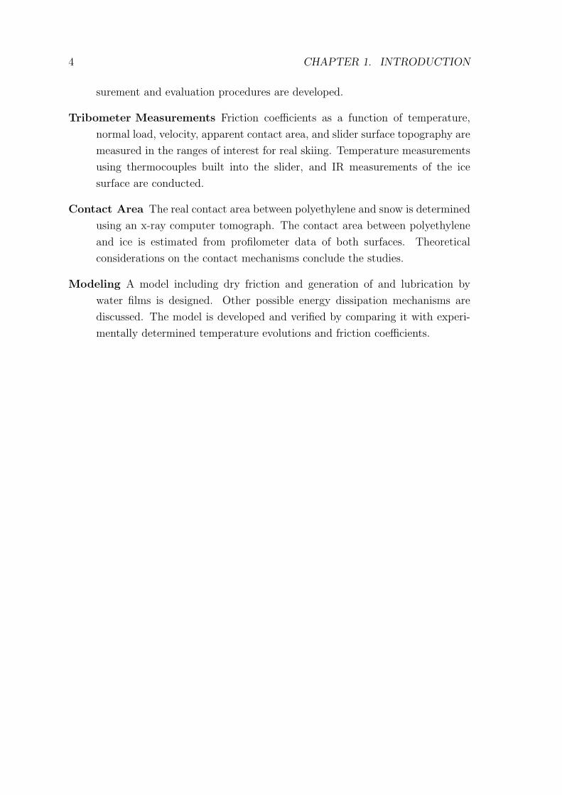
Modeling A model including dry friction and generation of and lubrication by
water films is designed. Other possible energy dissipation mechanisms are
discussed. The model is developed and verified by comparing it with experi-
mentally determined temperature evolutions and friction coefficients.
Chapter 2
Tribometer Design
Abstract
A large-scale tribometer (diameter 1.80 m, pin-on-disc geometry) for friction mea-
surements on ice has been designed and built. The apparatus is placed in a cold
chamber with an accessible temperature range of Tenv=-20� to +1�. Velocity can
be varied between v=0.5ms−1 and 20ms−1, load can be varied between Fn=25N
and 84 N, frictional force being measured using a load cell. Problems associated
with the construction of tribometers are discussed. IR thermocouples measure the
temperature of the track before and after the slider. In addition, integrated thermo-
couples are used to measure temperature inside the polyethylene slider. The friction
coefficient (µ) can be determined with an accuracy of ±5%. An error analysis is
carried out.
2.1 Introduction
A number of investigators have set up experiments in order to measure friction of
different materials on snow and ice (see e.g. [BH39, GG72, Kei78, Leh89, BFR01]).
It was recognized that the warming of the ice track presents a problem, thus either
small tribometers (different designs: pin-on-disc, rotating drum, linear devices) with
low sliding velocities (v < 1ms−1) were used, or larger-scale devices were built. Most
of the latter encountered problems with vibrations, reducing the accuracy of the
measurement. Although it was recognized that the low kinetic friction is due to the
melting of the snow or ice surface, and thus strongly influenced by temperature, none
of the earlier experiments had adequate temperature control. See [God95, Flo83] for
a general discussion of the design of tribometers.
In this project, the requirements for the tribometer were as follows:
� Measurements under conditions encountered in real skiing: temperature, pres-
5
6 CHAPTER 2. TRIBOMETER DESIGN
sure, and especially sliding velocity (v=10ms−1 and above).
� Sufficient accuracy to measure differences between current ski-base-preparation
techniques, and to evaluate new ideas of surface preparations or ski-base ma-
terials.
� Model experiments with monitored temperature evolution at or near the inter-
face should answer questions as to how much heat is generated in the friction
process.
The original idea was to measure friction of ski-base materials on snow. Due to
practical problems with the preparation of a smooth, reproducible snow surface, ice
as a substitute surface for hard-packed snow is used. The limitations of this will be
discussed.
2.2 Experimental Setup
12
34
5
6
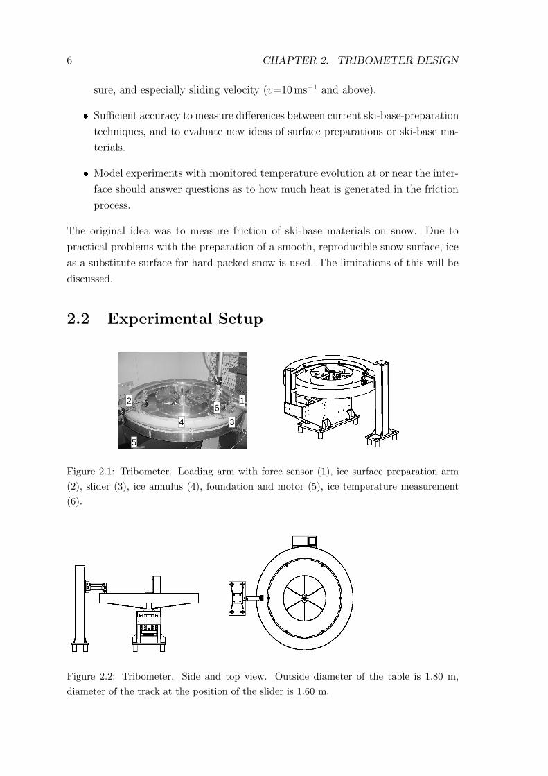
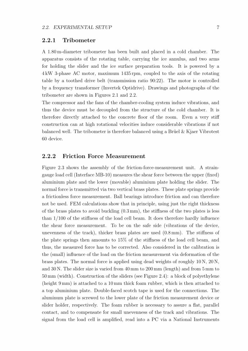
Figure 2.1: Tribometer. Loading arm with force sensor (1), ice surface preparation arm(2), slider (3), ice annulus (4), foundation and motor (5), ice temperature measurement(6).
Figure 2.2: Tribometer. Side and top view. Outside diameter of the table is 1.80 m,diameter of the track at the position of the slider is 1.60 m.
2.2. EXPERIMENTAL SETUP 7
2.2.1 Tribometer
A 1.80 m-diameter tribometer has been built and placed in a cold chamber. The
apparatus consists of the rotating table, carrying the ice annulus, and two arms
for holding the slider and the ice surface preparation tools. It is powered by a
4 kW 3-phase AC motor, maximum 1435 rpm, coupled to the axis of the rotating
table by a toothed drive belt (transmission ratio 90:22). The motor is controlled
by a frequency transformer (Invertek Optidrive). Drawings and photographs of the
tribometer are shown in Figures 2.1 and 2.2.
The compressor and the fans of the chamber-cooling system induce vibrations, and
thus the device must be decoupled from the structure of the cold chamber. It is
therefore directly attached to the concrete floor of the room. Even a very stiff
construction can at high rotational velocities induce considerable vibrations if not
balanced well. The tribometer is therefore balanced using a Bruel & Kjaer Vibrotest
60 device.
2.2.2 Friction Force Measurement
Figure 2.3 shows the assembly of the friction-force-measurement unit. A strain-
gauge load cell (Interface MB-10) measures the shear force between the upper (fixed)
aluminium plate and the lower (movable) aluminium plate holding the slider. The
normal force is transmitted via two vertical brass plates. These plate springs provide
a frictionless force measurement. Ball bearings introduce friction and can therefore
not be used. FEM calculations show that in principle, using just the right thickness
of the brass plates to avoid buckling (0.3 mm), the stiffness of the two plates is less
than 1/100 of the stiffness of the load cell beam. It does therefore hardly influence
the shear force measurement. To be on the safe side (vibrations of the device,
unevenness of the track), thicker brass plates are used (0.8mm). The stiffness of
the plate springs then amounts to 15% of the stiffness of the load cell beam, and
thus, the measured force has to be corrected. Also considered in the calibration is
the (small) influence of the load on the friction measurement via deformation of the
brass plates. The normal force is applied using dead weights of roughly 10N, 20N,
and 30 N. The slider size is varied from 40 mm to 200mm (length) and from 5mm to
50mm (width). Construction of the sliders (see Figure 2.4): a block of polyethylene
(height 9 mm) is attached to a 10 mm thick foam rubber, which is then attached to
a top aluminium plate. Double-faced scotch tape is used for the connections. The
aluminum plate is screwed to the lower plate of the friction measurement device or
slider holder, respectively. The foam rubber is necessary to assure a flat, parallel
contact, and to compensate for small unevenness of the track and vibrations. The
signal from the load cell is amplified, read into a PC via a National Instruments
8 CHAPTER 2. TRIBOMETER DESIGN
PCI-6034E card, and processed in Labview.
1
2
3
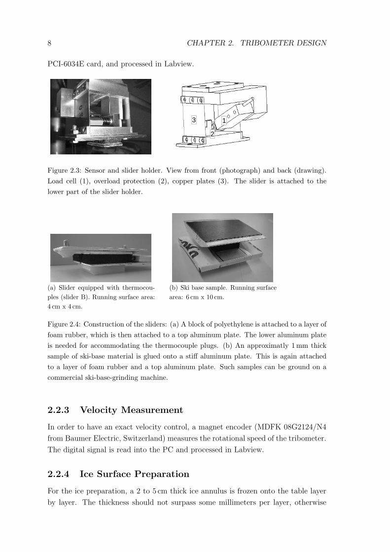
Figure 2.3: Sensor and slider holder. View from front (photograph) and back (drawing).Load cell (1), overload protection (2), copper plates (3). The slider is attached to thelower part of the slider holder.
(a) Slider equipped with thermocou-ples (slider B). Running surface area:4 cm x 4 cm.
(b) Ski base sample. Running surfacearea: 6 cm x 10 cm.
Figure 2.4: Construction of the sliders: (a) A block of polyethylene is attached to a layer offoam rubber, which is then attached to a top aluminum plate. The lower aluminum plateis needed for accommodating the thermocouple plugs. (b) An approximatly 1 mm thicksample of ski-base material is glued onto a stiff aluminum plate. This is again attachedto a layer of foam rubber and a top aluminum plate. Such samples can be ground on acommercial ski-base-grinding machine.
2.2.3 Velocity Measurement
In order to have an exact velocity control, a magnet encoder (MDFK 08G2124/N4
from Baumer Electric, Switzerland) measures the rotational speed of the tribometer.
The digital signal is read into the PC and processed in Labview.
2.2.4 Ice Surface Preparation
For the ice preparation, a 2 to 5 cm thick ice annulus is frozen onto the table layer
by layer. The thickness should not surpass some millimeters per layer, otherwise
2.2. EXPERIMENTAL SETUP 9
crack formation and air inclusions become severe. To account for the expansion
of the ice, foam rubber is used as side wall on the outer side of the track. For
the last couple of layers, or to refresh an existing ice surface, only thin layers of
water are frozen on using a wet towel. Freezing of ice in this way still leads to a
relatively uneven surface. The surface is therefore shaved down to a constant height
using the principle of a lathe. A vertical steel bar of width 2mm at the tip can
be moved manually in vertical and radial direction using linear stages. For most of
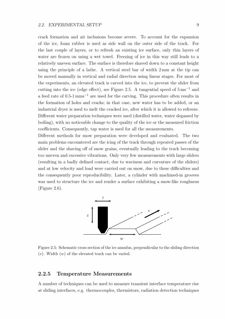
the experiments, an elevated track is carved into the ice, to prevent the slider from
cutting into the ice (edge effect), see Figure 2.5. A tangential speed of 5ms−1 and
a feed rate of 0.5-1mms−1 are used for the carving. This procedure often results in
the formation of holes and cracks; in that case, new water has to be added, or an
industrial dryer is used to melt the cracked ice, after which it is allowed to refreeze.
Different water preparation techniques were used (distilled water, water degassed by
boiling), with no noticeable change to the quality of the ice or the measured friction
coefficients. Consequently, tap water is used for all the measurements.
Different methods for snow preparation were developed and evaluated. The two
main problems encountered are the icing of the track through repeated passes of the
slider and the shaving off of snow grains, eventually leading to the track becoming
too uneven and excessive vibrations. Only very few measurements with large sliders
(resulting in a badly defined contact, due to waviness and curvature of the sliders)
and at low velocity and load were carried out on snow, due to these difficulties and
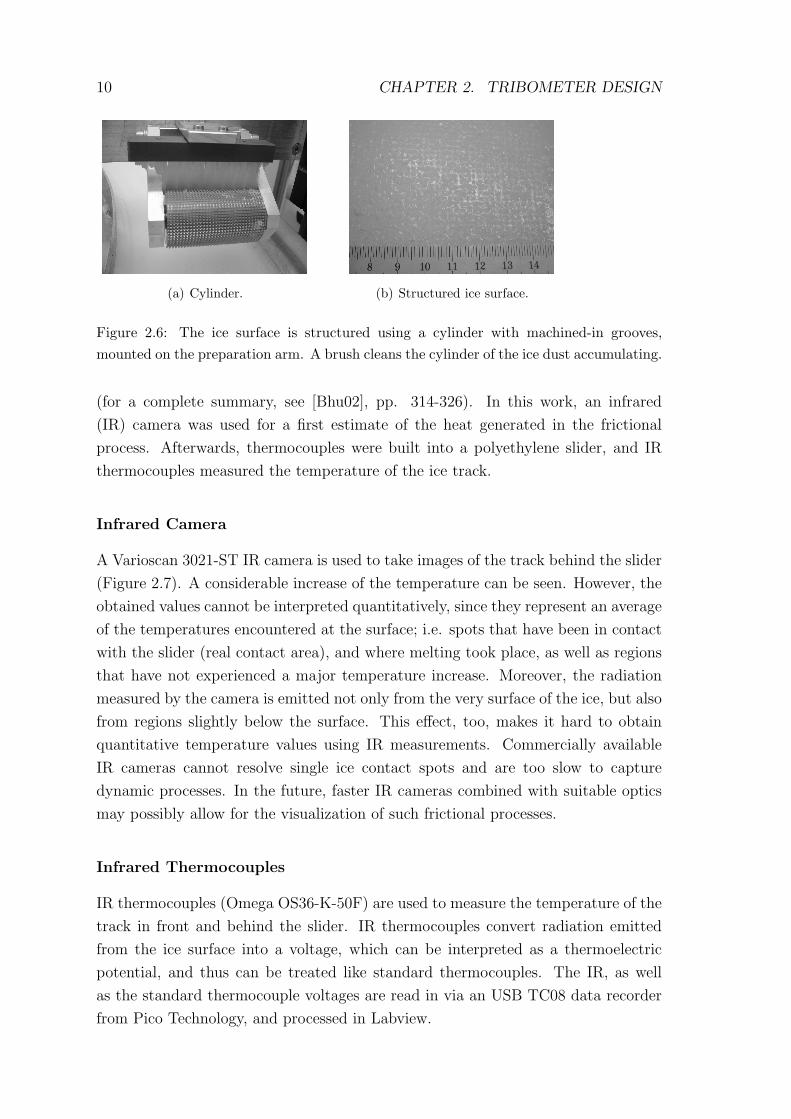
the consequently poor reproducibility. Later, a cylinder with machined-in grooves
was used to structure the ice and render a surface exhibiting a snow-like roughness
(Figure 2.6).
w
z
r
v
Figure 2.5: Schematic cross section of the ice annulus, perpendicular to the sliding direction(v). Width (w) of the elevated track can be varied.
2.2.5 Temperature Measurements
A number of techniques can be used to measure transient interface temperature rise
at sliding interfaces, e.g. thermocouples, thermistors, radiation detection techniques
10 CHAPTER 2. TRIBOMETER DESIGN
(a) Cylinder. (b) Structured ice surface.
Figure 2.6: The ice surface is structured using a cylinder with machined-in grooves,mounted on the preparation arm. A brush cleans the cylinder of the ice dust accumulating.
(for a complete summary, see [Bhu02], pp. 314-326). In this work, an infrared
(IR) camera was used for a first estimate of the heat generated in the frictional
process. Afterwards, thermocouples were built into a polyethylene slider, and IR
thermocouples measured the temperature of the ice track.
Infrared Camera
A Varioscan 3021-ST IR camera is used to take images of the track behind the slider
(Figure 2.7). A considerable increase of the temperature can be seen. However, the
obtained values cannot be interpreted quantitatively, since they represent an average
of the temperatures encountered at the surface; i.e. spots that have been in contact
with the slider (real contact area), and where melting took place, as well as regions
that have not experienced a major temperature increase. Moreover, the radiation
measured by the camera is emitted not only from the very surface of the ice, but also
from regions slightly below the surface. This effect, too, makes it hard to obtain
quantitative temperature values using IR measurements. Commercially available
IR cameras cannot resolve single ice contact spots and are too slow to capture
dynamic processes. In the future, faster IR cameras combined with suitable optics
may possibly allow for the visualization of such frictional processes.
Infrared Thermocouples
IR thermocouples (Omega OS36-K-50F) are used to measure the temperature of the
track in front and behind the slider. IR thermocouples convert radiation emitted
from the ice surface into a voltage, which can be interpreted as a thermoelectric
potential, and thus can be treated like standard thermocouples. The IR, as well
as the standard thermocouple voltages are read in via an USB TC08 data recorder
from Pico Technology, and processed in Labview.
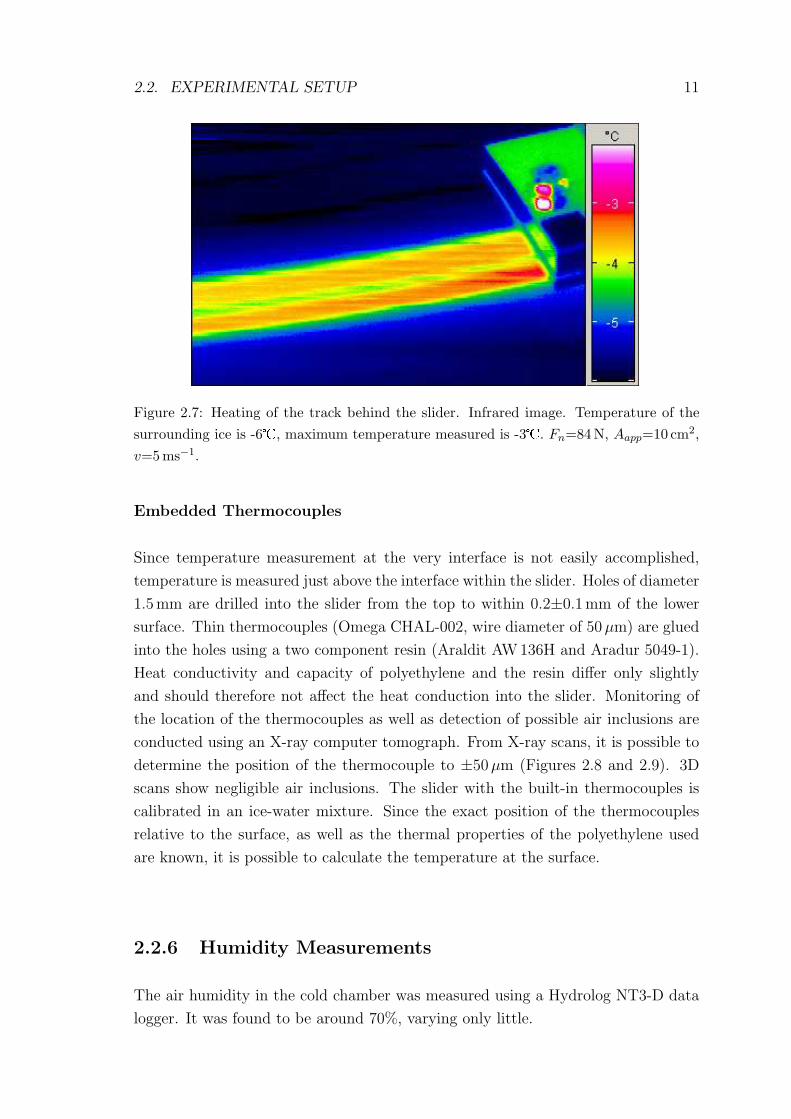
2.2. EXPERIMENTAL SETUP 11
Figure 2.7: Heating of the track behind the slider. Infrared image. Temperature of thesurrounding ice is -6�, maximum temperature measured is -3�. Fn=84N, Aapp=10 cm2,v=5ms−1.
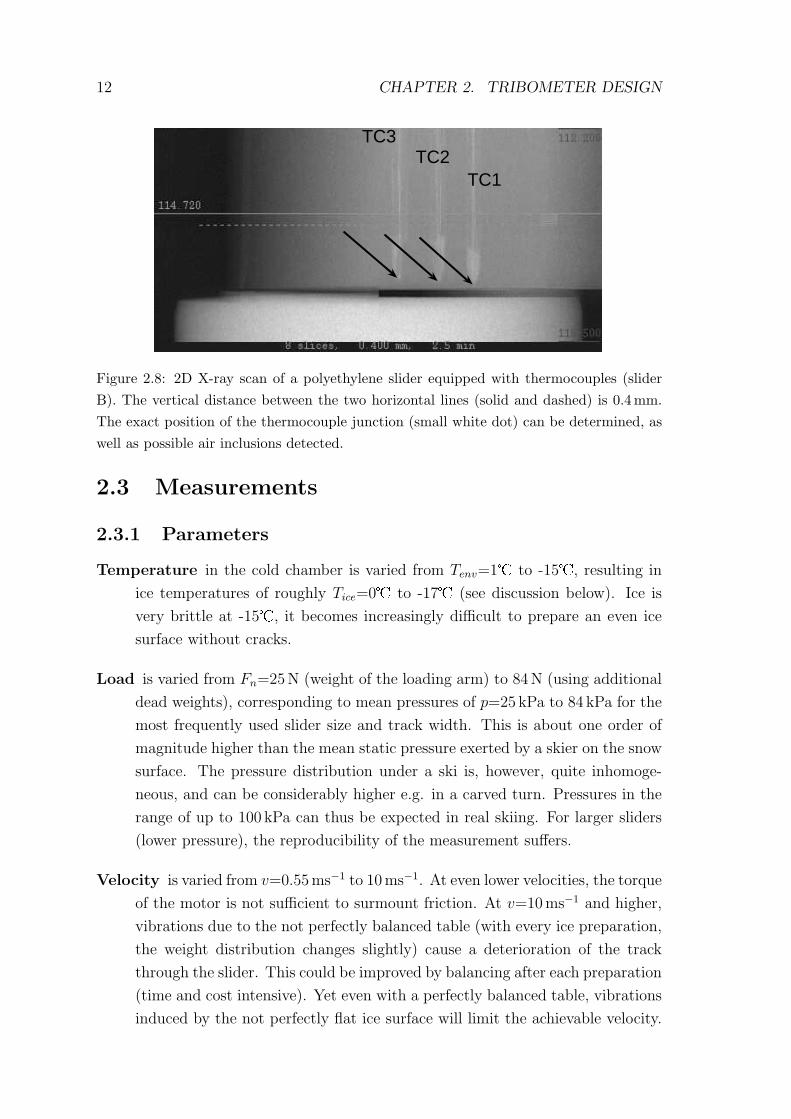
Embedded Thermocouples
Since temperature measurement at the very interface is not easily accomplished,
temperature is measured just above the interface within the slider. Holes of diameter
1.5mm are drilled into the slider from the top to within 0.2±0.1mm of the lower
surface. Thin thermocouples (Omega CHAL-002, wire diameter of 50 µm) are glued
into the holes using a two component resin (Araldit AW136H and Aradur 5049-1).
Heat conductivity and capacity of polyethylene and the resin differ only slightly
and should therefore not affect the heat conduction into the slider. Monitoring of
the location of the thermocouples as well as detection of possible air inclusions are
conducted using an X-ray computer tomograph. From X-ray scans, it is possible to
determine the position of the thermocouple to ±50µm (Figures 2.8 and 2.9). 3D
scans show negligible air inclusions. The slider with the built-in thermocouples is
calibrated in an ice-water mixture. Since the exact position of the thermocouples
relative to the surface, as well as the thermal properties of the polyethylene used
are known, it is possible to calculate the temperature at the surface.
2.2.6 Humidity Measurements
The air humidity in the cold chamber was measured using a Hydrolog NT3-D data
logger. It was found to be around 70%, varying only little.
12 CHAPTER 2. TRIBOMETER DESIGN
TC3TC2
TC1
Figure 2.8: 2D X-ray scan of a polyethylene slider equipped with thermocouples (sliderB). The vertical distance between the two horizontal lines (solid and dashed) is 0.4mm.The exact position of the thermocouple junction (small white dot) can be determined, aswell as possible air inclusions detected.
2.3 Measurements
2.3.1 Parameters
Temperature in the cold chamber is varied from Tenv=1� to -15�, resulting in
ice temperatures of roughly Tice=0� to -17� (see discussion below). Ice is
very brittle at -15�, it becomes increasingly difficult to prepare an even ice
surface without cracks.
Load is varied from Fn=25N (weight of the loading arm) to 84N (using additional
dead weights), corresponding to mean pressures of p=25 kPa to 84 kPa for the
most frequently used slider size and track width. This is about one order of
magnitude higher than the mean static pressure exerted by a skier on the snow
surface. The pressure distribution under a ski is, however, quite inhomoge-
neous, and can be considerably higher e.g. in a carved turn. Pressures in the
range of up to 100 kPa can thus be expected in real skiing. For larger sliders
(lower pressure), the reproducibility of the measurement suffers.
Velocity is varied from v=0.55ms−1 to 10ms−1. At even lower velocities, the torque
of the motor is not sufficient to surmount friction. At v=10ms−1 and higher,
vibrations due to the not perfectly balanced table (with every ice preparation,
the weight distribution changes slightly) cause a deterioration of the track
through the slider. This could be improved by balancing after each preparation
(time and cost intensive). Yet even with a perfectly balanced table, vibrations
induced by the not perfectly flat ice surface will limit the achievable velocity.
2.3. MEASUREMENTS 13
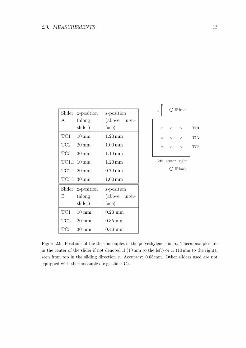
Slider
A
x-position
(along
slider)
z-position
(above inter-
face)
TC1 10mm 1.20mm
TC2 20mm 1.00mm
TC3 30mm 1.10mm
TC1 l 10mm 1.20mm
TC2 r 20mm 0.70mm
TC3 l 30mm 1.00mm
Slider
B
x-position
(along
slider)
z-position
(above inter-
face)
TC1 10 mm 0.20 mm
TC2 20 mm 0.35 mm
TC3 30 mm 0.40 mm
d
d
d
d
d
d
d
d
d
IRfront
IRback
TC1
TC2
TC3
left center right
v
Figure 2.9: Positions of the thermocouples in the polyethylene sliders. Thermocouples arein the center of the slider if not denoted l (10 mm to the left) or r (10mm to the right),seen from top in the sliding direction v. Accuracy: 0.05 mm. Other sliders used are notequipped with thermocouples (e.g. slider C).
14 CHAPTER 2. TRIBOMETER DESIGN
Measurements at high velocities can momentarily only be carried out for a
short time (1-2 minutes).
Apparent contact area size is changed by varying the width of the track (see
Figure 2.5) from w=25mm to 5 mm, resulting in apparent contact areas of
Aapp=10 cm2 to 2 cm2 (the length of the slider is usually kept constant at
l=40mm).
Considerable scatter (about a factor of 2) is observed for some sets of parameters,
especially at very low and very high velocities, and at low normal forces. This is
due to a not well defined contact, and to stronger vibrations at high velocities. In
the course of the experiments, it could be seen that a clearly defined contact which
allows for well reproducible measurements can be achieved for apparent contact ar-
eas of up to Aapp=4 cm2.
2.3.2 Measurement Procedure
Measurements are conducted according to the following procedure:
1. Preparation of the ice surface. Set track width.
2. Run-in period: the slider to be measured is slid for about 5 minutes at high
load (Fn=84N) and velocity (v=5-10ms−1).
3. Sample and ice is left to cool for 5 minutes. With the tribometer still running,
this can be sped up (forced convection).
4. Tribometer is set to desired velocity. Recording of the data is started. Sample
is lowered on the running tribometer.
5. Stop recording. Lift up slider. Proceed with step 3.
Along with the measurements, repeated optical checking of the ice surface and de-
tection of possible vibration is carried out. A new ice surface is prepared if necessary.
2.3.3 Interpretation of the Measurement
Tribology experiments are generally not straightforward. Many parameters (e.g.
surface contaminants, humidity), sometimes hard to control, can influence the result.
A relatively large scatter of the data is common. For tribometer experiments on ice,
this is no different. This section explains how a measurement is analyzed, and
illustrates some peculiarities of ice friction measurements. All measurements shown
relate to polyethylene sliding on ice.
2.3. MEASUREMENTS 15
Temperature-Controlled Friction and Polishing
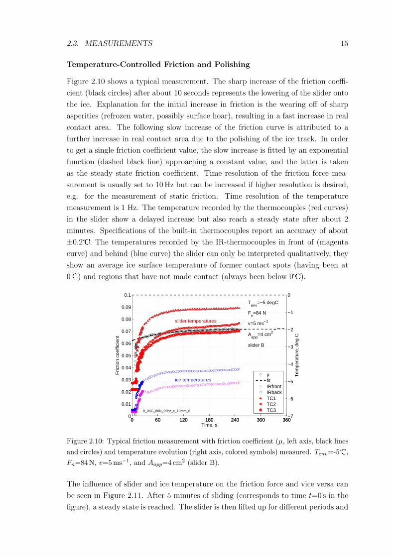
Figure 2.10 shows a typical measurement. The sharp increase of the friction coeffi-
cient (black circles) after about 10 seconds represents the lowering of the slider onto
the ice. Explanation for the initial increase in friction is the wearing off of sharp
asperities (refrozen water, possibly surface hoar), resulting in a fast increase in real
contact area. The following slow increase of the friction curve is attributed to a
further increase in real contact area due to the polishing of the ice track. In order
to get a single friction coefficient value, the slow increase is fitted by an exponential
function (dashed black line) approaching a constant value, and the latter is taken
as the steady state friction coefficient. Time resolution of the friction force mea-
surement is usually set to 10Hz but can be increased if higher resolution is desired,
e.g. for the measurement of static friction. Time resolution of the temperature
measurement is 1 Hz. The temperature recorded by the thermocouples (red curves)
in the slider show a delayed increase but also reach a steady state after about 2
minutes. Specifications of the built-in thermocouples report an accuracy of about
±0.2�. The temperatures recorded by the IR-thermocouples in front of (magenta
curve) and behind (blue curve) the slider can only be interpreted qualitatively, they
show an average ice surface temperature of former contact spots (having been at
0�) and regions that have not made contact (always been below 0�).
0 60 120 180 240 300 3600
0.01
0.02
0.03
0.04
0.05
0.06
0.07
0.08
0.09
0.1
Time, s
Fric
tion
coef
ficie
nt
0 60 120 180 240 300 360−7
−6
−5
−4
−3
−2
−1
0T
empe
ratu
re, d
eg C
B_05C_80N_09hz_c_10mm_6
Tenv
=−5 degC
Fn=84 N
v=5 ms−1
Aapp
=4 cm2
slider B
slider temperatures
ice temperaturesµfitIRfrontIRbackTC1TC2TC3
Figure 2.10: Typical friction measurement with friction coefficient (µ, left axis, black linesand circles) and temperature evolution (right axis, colored symbols) measured. Tenv=-5�,Fn=84N, v=5ms−1, and Aapp=4 cm2 (slider B).
The influence of slider and ice temperature on the friction force and vice versa can
be seen in Figure 2.11. After 5 minutes of sliding (corresponds to time t=0 s in the
figure), a steady state is reached. The slider is then lifted up for different periods and
16 CHAPTER 2. TRIBOMETER DESIGN
0 60 120 180 240 3000
0.01
0.02
0.03
0.04
0.05
0.06
0.07
0.08
0.09
0.1
Time, s
Fric
tion
coef
ficie
nt
0 60 120 180 240 300−6
−5
−4
−3
−2
−1
0
Tem
pera
ture
, deg
C
B_05C_80N_09hz_c_10mm_3_interrupt
Tenv
=−5 degC
Fn=84 N
v=5 ms−1
Aapp
=4 cm2
slider B
contact lifted up
µIRfrontIRbackTC1TC2TC3
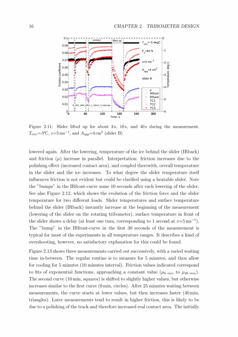
Figure 2.11: Slider lifted up for about 3 s, 10 s, and 40 s during the measurement.Tenv=-5�, v=5ms−1, and Aapp=4 cm2 (slider B)
lowered again. After the lowering, temperature of the ice behind the slider (IRback)
and friction (µ) increase in parallel. Interpretation: friction increases due to the
polishing effect (increased contact area), and coupled therewith, overall temperature
in the slider and the ice increases. To what degree the slider temperature itself
influences friction is not evident but could be clarified using a heatable slider. Note
the ”bumps” in the IRfront-curve some 10 seconds after each lowering of the slider.
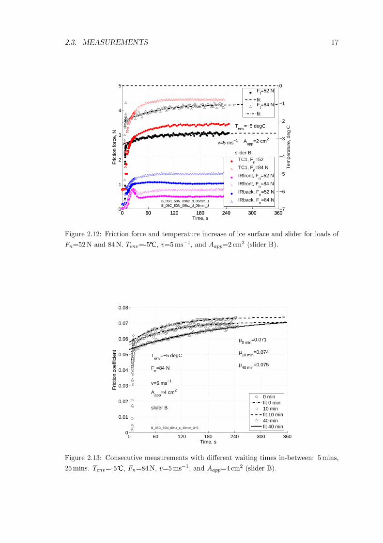
See also Figure 2.12, which shows the evolution of the friction force and the slider
temperature for two different loads. Slider temperatures and surface temperature
behind the slider (IRback) instantly increase at the beginning of the measurement
(lowering of the slider on the rotating tribometer), surface temperature in front of
the slider shows a delay (at least one turn, corresponding to 1 second at v=5ms−1).
The ”bump” in the IRfront-curve in the first 30 seconds of the measurement is
typical for most of the experiments in all temperature ranges. It describes a kind of
overshooting, however, no satisfactory explanation for this could be found.
Figure 2.13 shows three measurements carried out successively, with a varied waiting
time in-between. The regular routine is to measure for 5 minutes, and then allow
for cooling for 5 minutes (10 minutes interval). Friction values indicated correspond
to fits of exponential functions, approaching a constant value (µ0 min to µ40 min).
The second curve (10min, squares) is shifted to slightly higher values, but otherwise
increases similar to the first curve (0min, circles). After 25 minutes waiting between
measurements, the curve starts at lower values, but then increases faster (40min,
triangles). Later measurements tend to result in higher friction, this is likely to be
due to a polishing of the track and therefore increased real contact area. The initially
2.3. MEASUREMENTS 17
0 60 120 180 240 300 3600
1
2
3
4
5
Time, s
Fric
tion
forc
e, N
Ff=52 N
fitF
f=84 N
fit
0 60 120 180 240 300 360−7
−6
−5
−4
−3
−2
−1
0
Tem
pera
ture
, deg
C
B_05C_50N_09hz_d_05mm_1B_05C_80N_09hz_d_05mm_3
Tenv
=−5 degC
v=5 ms−1 Aapp
=2 cm2
slider BTC1, F
n=52
TC1, Fn=84 N
IRfront, Fn=52 N
IRfront, Fn=84 N
IRback, Fn=52 N
IRback, Fn=84 N
Figure 2.12: Friction force and temperature increase of ice surface and slider for loads ofFn=52N and 84 N. Tenv=-5�, v=5 ms−1, and Aapp=2 cm2 (slider B).
0 60 120 180 240 300 3600
0.01
0.02
0.03
0.04
0.05
0.06
0.07
0.08
Time, s
Fric
tion
coef
ficie
nt
µ0 min
=0.071
µ10 min
=0.074
µ40 min
=0.075
B_05C_80N_09hz_c_10mm_3−5
Tenv
=−5 degC
Fn=84 N
v=5 ms−1
Aapp
=4 cm2
slider B
0 minfit 0 min10 minfit 10 min40 minfit 40 min
Figure 2.13: Consecutive measurements with different waiting times in-between: 5mins,25mins. Tenv=-5�, Fn=84N, v=5ms−1, and Aapp=4 cm2 (slider B).
18 CHAPTER 2. TRIBOMETER DESIGN
lower friction after longer waiting times between measurements can be a result of
a change in the track due to evaporation. Other researchers [GG72] who measured
friction of polymers on ice using a tribometer claim that surface hoar builds up on
the ice during the time it is exposed to air. These sharp ice crystals would then
provide low real contact area, or even act as a ”ball bearing”. It is questionable
whether this effect is relevant, compared to the relatively fast evaporation. Both of
these effects would lead to initially less conforming sliding partners and therefore
lower real contact area.
Temperatures
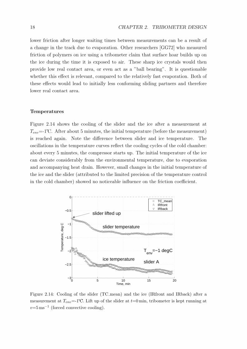
Figure 2.14 shows the cooling of the slider and the ice after a measurement at
Tenv=-1�. After about 5 minutes, the initial temperature (before the measurement)
is reached again. Note the difference between slider and ice temperature. The
oscillations in the temperature curves reflect the cooling cycles of the cold chamber:
about every 5 minutes, the compressor starts up. The initial temperature of the ice
can deviate considerably from the environmental temperature, due to evaporation
and accompanying heat drain. However, small changes in the initial temperature of
the ice and the slider (attributed to the limited precision of the temperature control
in the cold chamber) showed no noticeable influence on the friction coefficient.
0 5 10 15 20−3
−2.5
−2
−1.5
−1
−0.5
0
Time, min
Tem
pera
ture
, deg
C
Tenv
=−1 degC
slider A
slider lifted up
slider temperature
ice temperature
TC_meanIRfrontIRback
Figure 2.14: Cooling of the slider (TC mean) and the ice (IRfront and IRback) after ameasurement at Tenv=-1�. Lift up of the slider at t=0 min, tribometer is kept running atv=5ms−1 (forced convective cooling).
2.3. MEASUREMENTS 19
Contact Problems
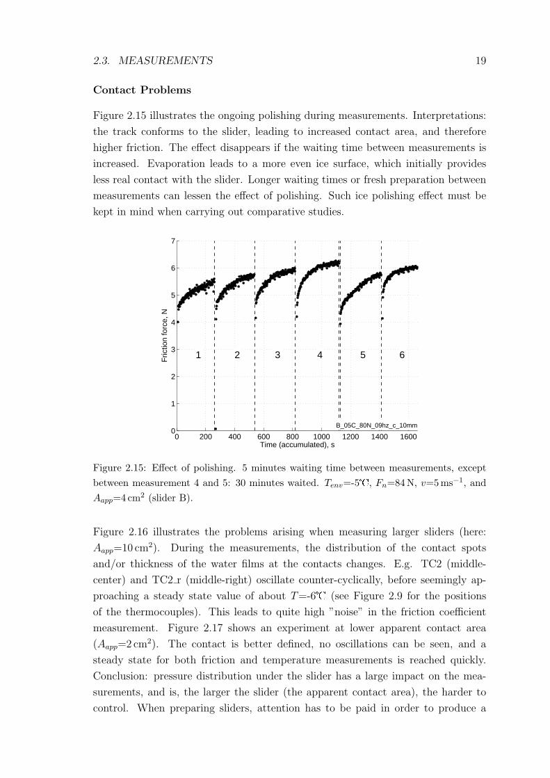
Figure 2.15 illustrates the ongoing polishing during measurements. Interpretations:
the track conforms to the slider, leading to increased contact area, and therefore
higher friction. The effect disappears if the waiting time between measurements is
increased. Evaporation leads to a more even ice surface, which initially provides
less real contact with the slider. Longer waiting times or fresh preparation between
measurements can lessen the effect of polishing. Such ice polishing effect must be
kept in mind when carrying out comparative studies.
0 200 400 600 800 1000 1200 1400 16000
1
2
3
4
5
6
7
Time (accumulated), s
Fric
tion
forc
e, N
1 2 3 4 5 6
B_05C_80N_09hz_c_10mm
Figure 2.15: Effect of polishing. 5 minutes waiting time between measurements, exceptbetween measurement 4 and 5: 30 minutes waited. Tenv=-5�, Fn=84N, v=5ms−1, andAapp=4 cm2 (slider B).
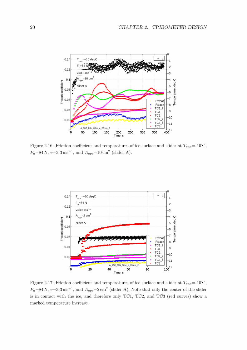
Figure 2.16 illustrates the problems arising when measuring larger sliders (here:
Aapp=10 cm2). During the measurements, the distribution of the contact spots
and/or thickness of the water films at the contacts changes. E.g. TC2 (middle-
center) and TC2 r (middle-right) oscillate counter-cyclically, before seemingly ap-
proaching a steady state value of about T=-6� (see Figure 2.9 for the positions
of the thermocouples). This leads to quite high ”noise” in the friction coefficient
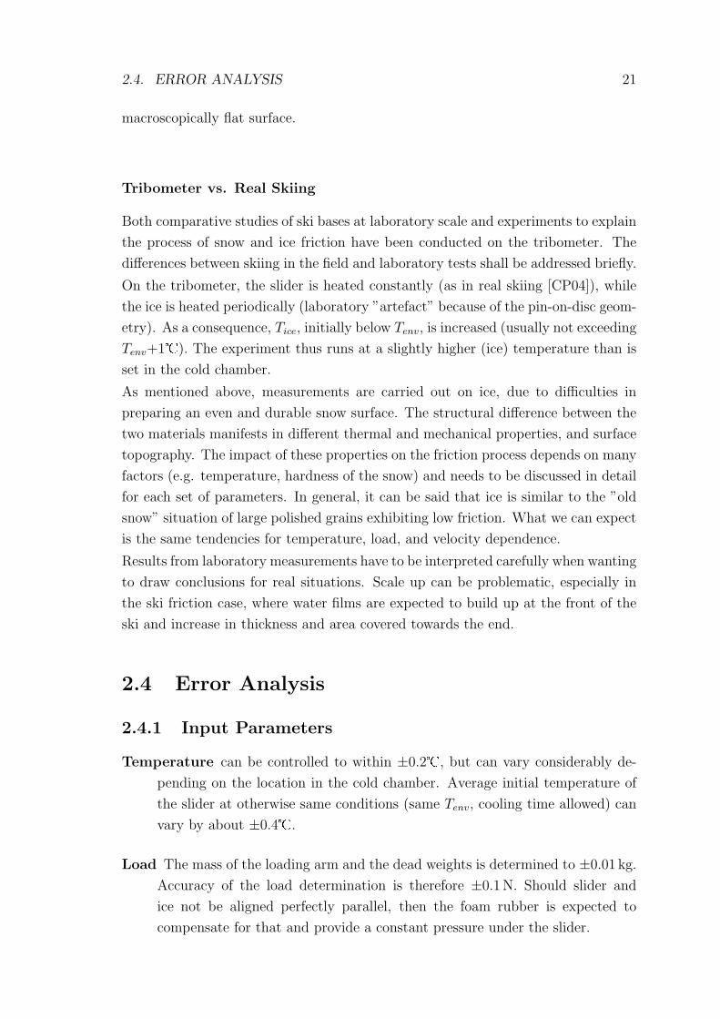
measurement. Figure 2.17 shows an experiment at lower apparent contact area
(Aapp=2 cm2). The contact is better defined, no oscillations can be seen, and a
steady state for both friction and temperature measurements is reached quickly.
Conclusion: pressure distribution under the slider has a large impact on the mea-
surements, and is, the larger the slider (the apparent contact area), the harder to
control. When preparing sliders, attention has to be paid in order to produce a
20 CHAPTER 2. TRIBOMETER DESIGN
0 50 100 150 200 250 300 350 4000
0.02
0.04
0.06
0.08
0.1
0.12
0.14F
rictio
n co
effic
ient
µ
0 50 100 150 200 250 300 350 400−12
−11
−10
−9
−8
−7
−6
−5
−4
−3
−2
−1
0
Tem
pera
ture
, deg
C
Time, s
A_10C_80N_06hz_a_25mm_3
Tenv
=−10 degC
Fn=84 N
v=3.3 ms−1
Aapp
=10 cm2
slider A
IRfrontIRbackTC1_lTC1TC2TC2_rTC3_lTC3
Figure 2.16: Friction coefficient and temperatures of ice surface and slider at Tenv=-10�,Fn=84N, v=3.3ms−1, and Aapp=10 cm2 (slider A).
0 20 40 60 80 1000
0.02
0.04
0.06
0.08
0.1
0.12
0.14
Fric
tion
coef
ficie
nt
µ
0 20 40 60 80 100−12
−11
−10
−9
−8
−7
−6
−5
−4
−3
−2
−1
0
Tem
pera
ture
, deg
C
Time, s
A_10C_80N_06hz_a_05mm_2
Tenv
=−10 degC
Fn=84 N
v=3.3 ms−1
Aapp
=2 cm2
slider A
IRfrontIRbackTC1_lTC1TC2TC2_rTC3_lTC3
Figure 2.17: Friction coefficient and temperatures of ice surface and slider at Tenv=-10�,Fn=84N, v=3.3ms−1, and Aapp=2 cm2 (slider A). Note that only the center of the slideris in contact with the ice, and therefore only TC1, TC2, and TC3 (red curves) show amarked temperature increase.
2.4. ERROR ANALYSIS 21
macroscopically flat surface.
Tribometer vs. Real Skiing
Both comparative studies of ski bases at laboratory scale and experiments to explain
the process of snow and ice friction have been conducted on the tribometer. The
differences between skiing in the field and laboratory tests shall be addressed briefly.
On the tribometer, the slider is heated constantly (as in real skiing [CP04]), while
the ice is heated periodically (laboratory ”artefact” because of the pin-on-disc geom-
etry). As a consequence, Tice, initially below Tenv, is increased (usually not exceeding
Tenv+1�). The experiment thus runs at a slightly higher (ice) temperature than is
set in the cold chamber.
As mentioned above, measurements are carried out on ice, due to difficulties in
preparing an even and durable snow surface. The structural difference between the
two materials manifests in different thermal and mechanical properties, and surface
topography. The impact of these properties on the friction process depends on many
factors (e.g. temperature, hardness of the snow) and needs to be discussed in detail
for each set of parameters. In general, it can be said that ice is similar to the ”old
snow” situation of large polished grains exhibiting low friction. What we can expect
is the same tendencies for temperature, load, and velocity dependence.
Results from laboratory measurements have to be interpreted carefully when wanting
to draw conclusions for real situations. Scale up can be problematic, especially in
the ski friction case, where water films are expected to build up at the front of the
ski and increase in thickness and area covered towards the end.
2.4 Error Analysis
2.4.1 Input Parameters
Temperature can be controlled to within ±0.2�, but can vary considerably de-
pending on the location in the cold chamber. Average initial temperature of
the slider at otherwise same conditions (same Tenv, cooling time allowed) can
vary by about ±0.4�.
Load The mass of the loading arm and the dead weights is determined to ±0.01 kg.
Accuracy of the load determination is therefore ±0.1N. Should slider and
ice not be aligned perfectly parallel, then the foam rubber is expected to
compensate for that and provide a constant pressure under the slider.
22 CHAPTER 2. TRIBOMETER DESIGN
Velocity is set by controlling the torque of the AC-motor. However, sliding friction
of the slider can slow the tribometer down. Independently measured velocity
shows that a velocity set to (e.g.) vset=5ms−1 varies about vmeas=4.8±0.02ms−1.
Apparent contact area is measured to±0.5 mm using a ruler. For small apparent
contact areas (up to Aapp≈4 cm2), the slider is expected to be perfectly flat.
2.4.2 Measured Parameters
T -10� -10� -10� -5�Aapparent 0.8 cm2 4 cm2 10 cm2 4 cm2
n 4 4 5 13
Mean 0.048 0.082 0.108 0.073 -1.6�Scatter ± 0.001 ± 0.003 ± 0.013 ± 0.005 ±0.6�
(± 2%) (± 4%) (± 12%) (± 7%)
SD 0.001 0.003 0.011 0.003 0.4�(± 2%) (± 4%) (± 10%) (± 4%)
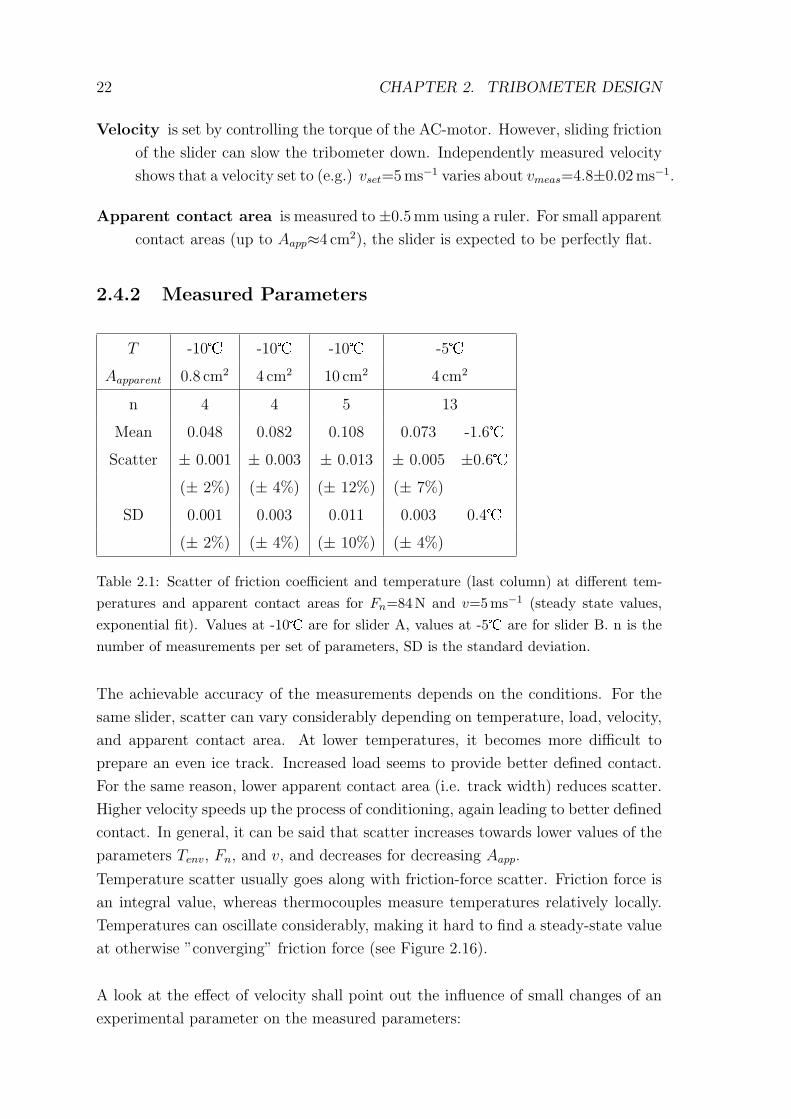
Table 2.1: Scatter of friction coefficient and temperature (last column) at different tem-peratures and apparent contact areas for Fn=84N and v=5ms−1 (steady state values,exponential fit). Values at -10� are for slider A, values at -5� are for slider B. n is thenumber of measurements per set of parameters, SD is the standard deviation.
The achievable accuracy of the measurements depends on the conditions. For the
same slider, scatter can vary considerably depending on temperature, load, velocity,
and apparent contact area. At lower temperatures, it becomes more difficult to
prepare an even ice track. Increased load seems to provide better defined contact.
For the same reason, lower apparent contact area (i.e. track width) reduces scatter.
Higher velocity speeds up the process of conditioning, again leading to better defined
contact. In general, it can be said that scatter increases towards lower values of the
parameters Tenv, Fn, and v, and decreases for decreasing Aapp.
Temperature scatter usually goes along with friction-force scatter. Friction force is
an integral value, whereas thermocouples measure temperatures relatively locally.
Temperatures can oscillate considerably, making it hard to find a steady-state value
at otherwise ”converging” friction force (see Figure 2.16).
A look at the effect of velocity shall point out the influence of small changes of an
experimental parameter on the measured parameters:
2.5. CONCLUSION 23
� A sharp drop in friction is expected for a velocity (and thus heat generation)
that is high enough to raise the temperature at a contact to the melting point,
and provide water lubrication. This can explain large scatter at a certain
velocity, where slightly different velocities decide whether friction is ”dry” or
”wet”.
� For low velocities, the ice on the tribometer is allowed for longer cooling be-
tween two contacts with the slider. The temperature of the ice does not rise
as high. The conformation process of slider and ice is slower, and in addition,
the ice can be leveled out by evaporation between two contacts. This can
lead to both increased (lower temperatures) and decreased (worse conforming
surfaces) friction, an estimation a priori is difficult.
The effects described can be responsible for the scatter observed e.g. at low veloci-
ties in Figure 3.5, Chapter 3. Similar considerations can be made for the influence
of load, however, velocity seems to be a more critical parameter.
2.5 Conclusion
On the tribometer, it is possible to reproducibly measure friction of ski-base ma-
terials on ice, as well as the temperature evolution in the slider and in the ice.
Temperature (Tenv) and sliding velocity (v) can be chosen according to conditions
encountered in real skiing, while load (Fn) and sample size (Aapp) have to be ad-
justed to the laboratory scale. Depending on the conditions (above all: Tenv and
Aapp), the friction coefficient can be determined ±2%. This should be sufficient to
measure differences between current ski-base-preparation techniques. Some pecu-
liarities of the tribometer measurement, e.g. the heating of the ice, have to be kept
in mind, especially when comparing laboratory and field measurements.

24 CHAPTER 2. TRIBOMETER DESIGN
Chapter 3
Tribometer Measurements
Abstract
The kinetic friction between polyethylene and ice is measured as a function of tem-
perature, velocity, load, apparent contact area, and surface topography. The friction
coefficient, as well as the temperature increase in the slider depends on all of these
parameters. Interpretations are given on the basis of hydrodynamic friction, taking
into account the generation and shearing of thin water films at the contact spots.
3.1 Introduction
Ice shows very special tribological behavior. This is not surprising, since at most
temperatures relevant to e.g. skiing, ice is at a very high homologous temperature
(T/Tm, where Tm is the melting point temperature). Classical friction laws for plas-
tically deforming materials (which most materials are, at a not-too-low roughness)
predict a friction coefficient independent of load (Fn), velocity (v), and apparent
contact area (Aapp). For materials sliding on ice, this does not hold. Rather, friction
can be very much dependent on the above parameters. Discussion of the results pre-
sented is based on the assumption that the shearing of water films generated through
frictional melting processes is responsible for friction. The amount of frictional heat
generated is
P = µ · Fn · v = Ff · v, (3.1)
where Ff is the friction force. Note that µ represents the kinetic friction coefficient
(also denoted µk), as opposed to the static friction coefficient (µs). Alternatively,
the total heat flux q′′ = P/A through the area A into the upper and the lower solid
can be written as
25
26 CHAPTER 3. TRIBOMETER MEASUREMENTS
q′′ = v · σk, (3.2)
where σk is the shear stress necessary to slide two surface with the relative velocity
v. For an estimate, the shear stress is written as σk = µσ0, where the perpendicular
stress σ0 in a contact spot is assumed to be equal to the penetration hardness of the
softer material.
q′′
s
q′′
i
v
Ff
Fn
slider
ice
0
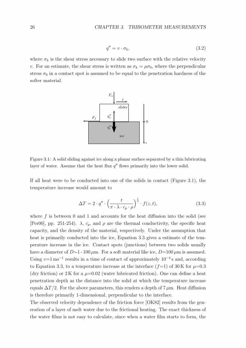
z
Figure 3.1: A solid sliding against ice along a planar surface separated by a thin lubricatinglayer of water. Assume that the heat flux q′′ flows primarily into the lower solid.
If all heat were to be conducted into one of the solids in contact (Figure 3.1), the
temperature increase would amount to
∆T = 2 · q′′ ·( t
π · λ · cp · ρ) 1
2 · f(z, t), (3.3)
where f is between 0 and 1 and accounts for the heat diffusion into the solid (see
[Per00], pp. 251-254). λ, cp, and ρ are the thermal conductivity, the specific heat
capacity, and the density of the material, respectively. Under the assumption that
heat is primarily conducted into the ice, Equation 3.3 gives a estimate of the tem-
perature increase in the ice. Contact spots (junctions) between two solids usually
have a diameter of D∼1 - 100µm. For a soft material like ice, D=100µm is assumed.
Using v=1ms−1 results in a time of contact of approximately 10−4 s and, according
to Equation 3.3, to a temperature increase at the interface (f=1) of 30K for µ=0.3
(dry friction) or 2K for a µ=0.02 (water lubricated friction). One can define a heat
penetration depth as the distance into the solid at which the temperature increase
equals ∆T/2. For the above parameters, this renders a depth of 7 µm. Heat diffusion
is therefore primarily 1-dimensional, perpendicular to the interface.
The observed velocity dependence of the friction force [OK82] results from the gen-
eration of a layer of melt water due to the frictional heating. The exact thickness of
the water films is not easy to calculate, since when a water film starts to form, the
3.1. INTRODUCTION 27
sliding friction drops rapidly, resulting in a drop in the frictional heat production.
Latent heat must be taken into account for melting to occur. Using
µ =η · v
hwf · σ0
(3.4)
where η is the kinematic viscosity of water at 0�, even a hwf=10nm thick water
layer between two (smooth) surfaces would result in a friction coefficient of about
0.01 (penetration hardness of ice: σ0≈2×10⁷ Nm−2, v=1ms−1). It is assumed that
the pressure at the contacts does not reach such high values (due to creep), and
therefore thicker water layers are required for low friction.
Alternatively, using σ0 = Fn/Areal and relRCA = Areal/Aapp, Equation 3.4 can be
rewritten to yield the friction force given by
Ff =η · v · Areal
hwf
= η · v · Aapp · relRCA
hwf
, (3.5)
A higher heat flux, due to e.g. higher velocity, can lead to both increased film
thickness (in turn leading to lower friction, see Equation 3.5) or increased real contact
area (leading to higher friction). How these two processes are linked depends on the
roughness (see Chapter 4) of the sliding partners. For simplicity, it is assumed that a
perfectly flat slider slides on ”rough” ice (roughness in the order of Ra=0.1 to 1µm,
gaussian-like height distribution), and ”slices off” ice asperities according to the
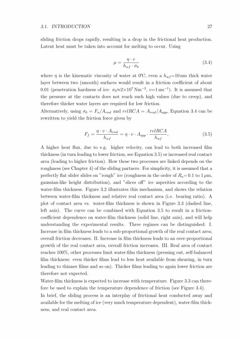
water-film thickness. Figure 3.2 illustrates this mechanism, and shows the relation
between water-film thickness and relative real contact area (i.e. bearing ratio). A
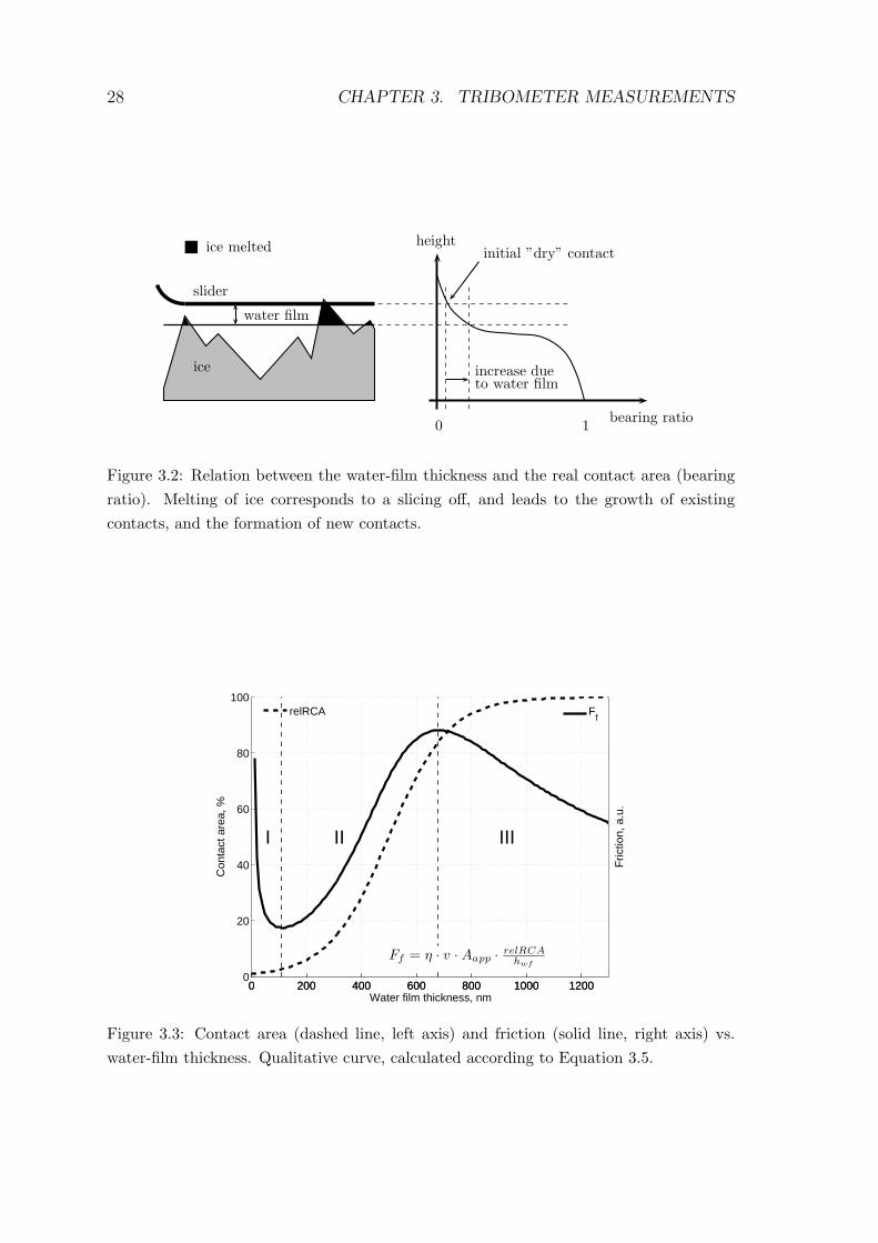
plot of contact area vs. water-film thickness is shown in Figure 3.3 (dashed line,
left axis). The curve can be combined with Equation 3.5 to result in a friction-
coefficient dependence on water-film thickness (solid line, right axis), and will help
understanding the experimental results. Three regimes can be distinguished: I.
Increase in film thickness leads to a sub-proportional growth of the real contact area;
overall friction decreases. II. Increase in film thickness leads to an over-proportional
growth of the real contact area, overall friction increases. III. Real area of contact
reaches 100%, other processes limit water-film thickness (pressing out, self-balanced
film thickness: even thicker films lead to less heat available from shearing, in turn
leading to thinner films and so on). Thicker films leading to again lower friction are
therefore not expected.
Water-film thickness is expected to increase with temperature. Figure 3.3 can there-
fore be used to explain the temperature dependence of friction (see Figure 3.4).
In brief, the sliding process is an interplay of frictional heat conducted away and
available for the melting of ice (very much temperature dependent), water-film thick-
ness, and real contact area.
28 CHAPTER 3. TRIBOMETER MEASUREMENTS
slider
ice
water film
ice melted
bearing ratio10
height
increase dueto water film
initial ”dry” contact
Figure 3.2: Relation between the water-film thickness and the real contact area (bearingratio). Melting of ice corresponds to a slicing off, and leads to the growth of existingcontacts, and the formation of new contacts.
0 200 400 600 800 1000 12000
20
40
60
80
100
Water film thickness, nm
Con
tact
are
a, %
0 200 400 600 800 1000 1200
Fric
tion,
a.u
.
I II III
Ff = η · v · Aapp ·
relRCAhwf
relRCA Ff
Figure 3.3: Contact area (dashed line, left axis) and friction (solid line, right axis) vs.water-film thickness. Qualitative curve, calculated according to Equation 3.5.
3.2. RESULTS AND DISCUSSION 29
−18 −16 −14 −12 −10 −8 −6 −4 −2 00
0.02
0.04
0.06
0.08
0.1
0.12
0.14
0.16
Ice temperature, deg C
Fric
tion
coef
ficie
nt
10 cm2
4 cm2
2 cm2
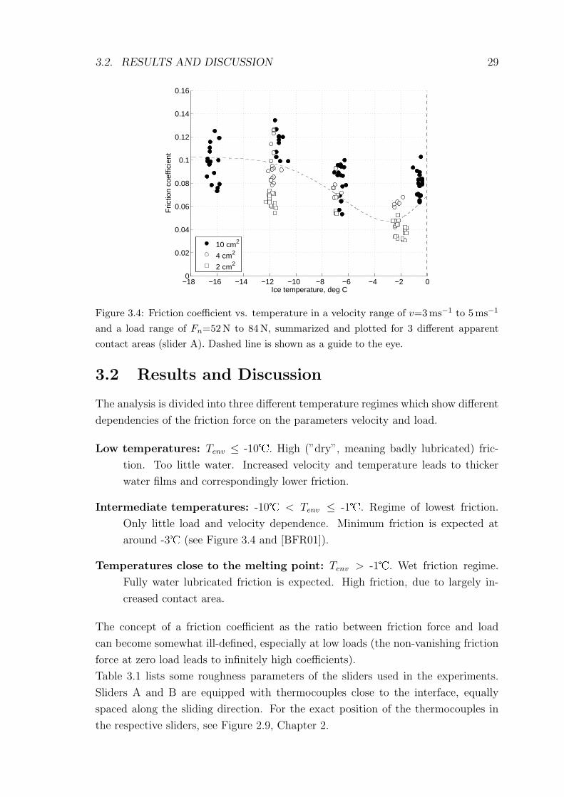
Figure 3.4: Friction coefficient vs. temperature in a velocity range of v=3ms−1 to 5 ms−1
and a load range of Fn=52N to 84N, summarized and plotted for 3 different apparentcontact areas (slider A). Dashed line is shown as a guide to the eye.
3.2 Results and Discussion
The analysis is divided into three different temperature regimes which show different
dependencies of the friction force on the parameters velocity and load.
Low temperatures: Tenv ≤ -10�. High (”dry”, meaning badly lubricated) fric-
tion. Too little water. Increased velocity and temperature leads to thicker
water films and correspondingly lower friction.
Intermediate temperatures: -10� < Tenv ≤ -1�. Regime of lowest friction.
Only little load and velocity dependence. Minimum friction is expected at
around -3� (see Figure 3.4 and [BFR01]).
Temperatures close to the melting point: Tenv > -1�. Wet friction regime.
Fully water lubricated friction is expected. High friction, due to largely in-
creased contact area.
The concept of a friction coefficient as the ratio between friction force and load
can become somewhat ill-defined, especially at low loads (the non-vanishing friction
force at zero load leads to infinitely high coefficients).
Table 3.1 lists some roughness parameters of the sliders used in the experiments.
Sliders A and B are equipped with thermocouples close to the interface, equally
spaced along the sliding direction. For the exact position of the thermocouples in
the respective sliders, see Figure 2.9, Chapter 2.
30 CHAPTER 3. TRIBOMETER MEASUREMENTS
Parameter Slider A Sliders B & C Description
Pa 2µm 3.6µm Average roughness
Pz 22µm 40µm Average maximum height of profile
Table 3.1: Roughness of the sliders used in the experiments. The surfaces of the slidersare ground with fine emery paper. Slider A was polished in addition. Sliders B and Cexhibit similar roughnesses, and still a ”hairy” surface originating from the grinding.
3.2.1 Low Temperatures
At temperatures of Tenv=-10� and below, a major part of the frictional heat gen-
erated is expected to be conducted into slider and (mainly) ice, due to high tem-
perature gradients. Only little heat is therefore available for melting water, and
only thin water films form. This is very pronounced at low velocities, where the
heat generation P = µFnv is small (see Figure 3.5 at Tenv=-15�). The decreas-
ing friction with increasing velocity can be explained by more heat being available
to melt water, and more water increasing the average water-film thickness (while
real contact area negligibly increases), which leads to lower friction (corresponds to
regime I, see Figure 3.3). Earlier measurements [ENC76, OK82] showed the friction
coefficient to follow v−0.5. At even higher velocities, the competing processes will
be the growth of the water films (decreasing friction) and the shearing of the latter
(increasing friction with velocity), leading to a finite friction coefficient, or possibly
to an overall increase.
Otherwise the behavior is somewhat classical: friction force increases linearly with
load (Figure 3.6), yielding a friction coefficient µ≈0.1 at v=5ms−1. The extrapo-
lated slider temperature at the interface can be interpreted as an average of contact
spots at T=0� and regions of the slider that have not made contact and are still
at T=-15� (assumption for not too large relative real contact areas, where con-
tact spots are few and fairly well separated). A temperature of T=-12� therefore
corresponds to a relative real contact area of approximately 20%. This however
represents an upper limit, since non-contacting regions at the interface have also
been warmed by adjacent contacting areas.
If all frictional heat is assumed to be conducted into the slider, a calculation for
the slope of the temperature rise vs. load curve (Equations 3.1 and 3.3, after about
t=120 s, a steady state is reached) results in a value that is 100 times higher than
the experimentally obtained 0.06KN−1. This implies that only a small fraction of
the frictional heat enters the slider; most if it is conducted into the ice, or used in
the phase transfer from ice to water. Apart form the seven times higher thermal
conductivity of ice, as compared to polyethylene, the temperature gradients in the
ice are higher. The ice is at a lower temperature, since it is constantly ”refreshed”,
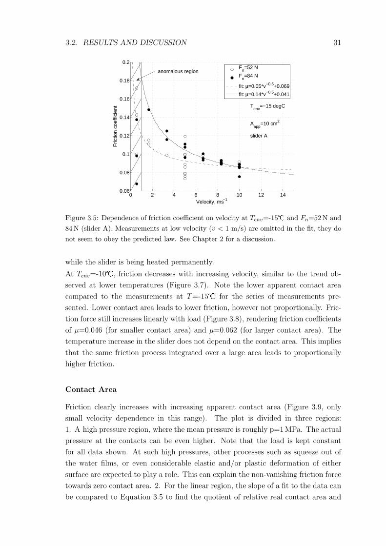
3.2. RESULTS AND DISCUSSION 31
0 2 4 6 8 10 12 140.06
0.08
0.1
0.12
0.14
0.16
0.18
0.2
Velocity, ms−1
Fric
tion
coef
ficie
nt
anomalous region
Tenv
=−15 degC
Aapp
=10 cm2
slider A
Fn=52 N
Fn=84 N
fit: µ=0.05*v−0.5+0.069
fit: µ=0.14*v−0.5+0.041
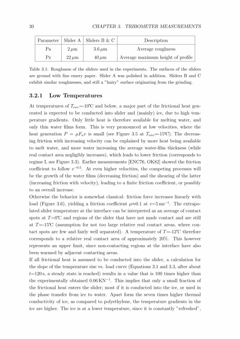
Figure 3.5: Dependence of friction coefficient on velocity at Tenv=-15� and Fn=52N and84N (slider A). Measurements at low velocity (v < 1 m/s) are omitted in the fit, they donot seem to obey the predicted law. See Chapter 2 for a discussion.
while the slider is being heated permanently.
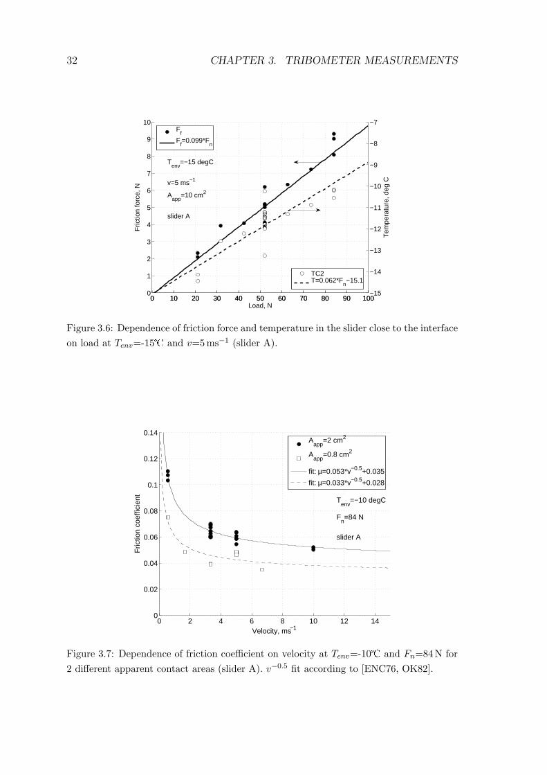
At Tenv=-10�, friction decreases with increasing velocity, similar to the trend ob-
served at lower temperatures (Figure 3.7). Note the lower apparent contact area
compared to the measurements at T=-15� for the series of measurements pre-
sented. Lower contact area leads to lower friction, however not proportionally. Fric-
tion force still increases linearly with load (Figure 3.8), rendering friction coefficients
of µ=0.046 (for smaller contact area) and µ=0.062 (for larger contact area). The
temperature increase in the slider does not depend on the contact area. This implies
that the same friction process integrated over a large area leads to proportionally
higher friction.
Contact Area
Friction clearly increases with increasing apparent contact area (Figure 3.9, only
small velocity dependence in this range). The plot is divided in three regions:
1. A high pressure region, where the mean pressure is roughly p=1MPa. The actual
pressure at the contacts can be even higher. Note that the load is kept constant
for all data shown. At such high pressures, other processes such as squeeze out of
the water films, or even considerable elastic and/or plastic deformation of either
surface are expected to play a role. This can explain the non-vanishing friction force
towards zero contact area. 2. For the linear region, the slope of a fit to the data can
be compared to Equation 3.5 to find the quotient of relative real contact area and
32 CHAPTER 3. TRIBOMETER MEASUREMENTS
0 10 20 30 40 50 60 70 80 90 1000
1
2
3
4
5
6
7
8
9
10
Load, N
Fric
tion
forc
e, N
Ff
Ff=0.099*F
n
0 10 20 30 40 50 60 70 80 90 100−15
−14
−13
−12
−11
−10
−9
−8
−7
Tem
pera
ture
, deg
C
Tenv
=−15 degC
v=5 ms−1
Aapp
=10 cm2
slider A
TC2T=0.062*F
n−15.1
Figure 3.6: Dependence of friction force and temperature in the slider close to the interfaceon load at Tenv=-15� and v=5ms−1 (slider A).
0 2 4 6 8 10 12 140
0.02
0.04
0.06
0.08
0.1
0.12
0.14
Velocity, ms−1
Fric
tion
coef
ficie
nt Tenv
=−10 degC
Fn=84 N
slider A
Aapp
=2 cm2
Aapp
=0.8 cm2
fit: µ=0.053*v−0.5+0.035
fit: µ=0.033*v−0.5+0.028
Figure 3.7: Dependence of friction coefficient on velocity at Tenv=-10� and Fn=84N for2 different apparent contact areas (slider A). v−0.5 fit according to [ENC76, OK82].
3.2. RESULTS AND DISCUSSION 33
0 10 20 30 40 50 60 70 80 90 1000
1
2
3
4
5
6
Load, N
Fric
tion
forc
e, N
Ff, A
app=0.8 cm2
Ff, A
app=2 cm2
fit: Ff=0.046*F
nfit: F
f=0.062*F
n
0 10 20 30 40 50 60 70 80 90 100
−10
−8
−6
−4
−2
0
Tem
pera
ture
, deg
CTenv
=−10 degC
v=5 ms−1
slider A
TC2, Aapp
=0.8 cm2
TC2, Aapp
=2 cm2
fit: T=0.052*Fn
fit: T=0.054*Fn
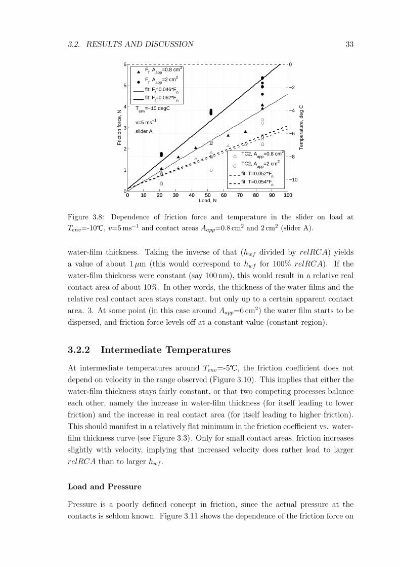
Figure 3.8: Dependence of friction force and temperature in the slider on load atTenv=-10�, v=5 ms−1 and contact areas Aapp=0.8 cm2 and 2 cm2 (slider A).
water-film thickness. Taking the inverse of that (hwf divided by relRCA) yields
a value of about 1µm (this would correspond to hwf for 100% relRCA). If the
water-film thickness were constant (say 100 nm), this would result in a relative real
contact area of about 10%. In other words, the thickness of the water films and the
relative real contact area stays constant, but only up to a certain apparent contact
area. 3. At some point (in this case around Aapp=6 cm2) the water film starts to be
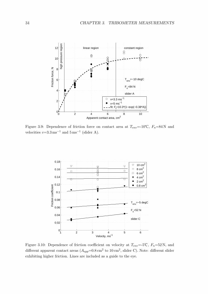
dispersed, and friction force levels off at a constant value (constant region).
3.2.2 Intermediate Temperatures
At intermediate temperatures around Tenv=-5�, the friction coefficient does not
depend on velocity in the range observed (Figure 3.10). This implies that either the
water-film thickness stays fairly constant, or that two competing processes balance
each other, namely the increase in water-film thickness (for itself leading to lower
friction) and the increase in real contact area (for itself leading to higher friction).
This should manifest in a relatively flat minimum in the friction coefficient vs. water-
film thickness curve (see Figure 3.3). Only for small contact areas, friction increases
slightly with velocity, implying that increased velocity does rather lead to larger
relRCA than to larger hwf .
Load and Pressure
Pressure is a poorly defined concept in friction, since the actual pressure at the
contacts is seldom known. Figure 3.11 shows the dependence of the friction force on
34 CHAPTER 3. TRIBOMETER MEASUREMENTS
0 2 4 6 8 100
2
4
6
8
10
12
high
pre
ssur
e re
gion
linear region constant region
Apparent contact area, cm2
Fric
tion
forc
e, N
Tenv
=−10 degC
Fn=84 N
slider A
high
pre
ssur
e re
gion
linear region constant region
Tenv
=−10 degC
Fn=84 N
slider A
v=3.3 ms−1
v=5 ms−1
fit: Ff=10.3*(1−exp(−0.38*A))
Figure 3.9: Dependence of friction force on contact area at Tenv=-10�, Fn=84N andvelocities v=3.3ms−1 and 5 ms−1 (slider A).
1 2 3 4 5 60
0.02
0.04
0.06
0.08
0.1
0.12
0.14
0.16
0.18
Velocity, ms−1
Fric
tion
coef
ficie
nt
Tenv
=−5 degC
Fn=52 N
slider C
10 cm2
8 cm2
6 cm2
4 cm2
2 cm2
0.8 cm2
Figure 3.10: Dependence of friction coefficient on velocity at Tenv=-5�, Fn=52 N, anddifferent apparent contact areas (Aapp=0.8 cm2 to 10 cm2, slider C). Note: different sliderexhibiting higher friction. Lines are included as a guide to the eye.
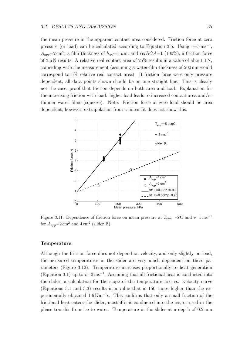
3.2. RESULTS AND DISCUSSION 35
the mean pressure in the apparent contact area considered. Friction force at zero
pressure (or load) can be calculated according to Equation 3.5. Using v=5ms−1,
Aapp=2 cm2, a film thickness of hwf=1µm, and relRCA=1 (100%), a friction force
of 3.6 N results. A relative real contact area of 25% results in a value of about 1 N,
coinciding with the measurement (assuming a water-film thickness of 200 nm would
correspond to 5% relative real contact area). If friction force were only pressure
dependent, all data points shown should be on one straight line. This is clearly
not the case, proof that friction depends on both area and load. Explanation for
the increasing friction with load: higher load leads to increased contact area and/or
thinner water films (squeeze). Note: Friction force at zero load should be area
dependent, however, extrapolation from a linear fit does not show this.
0 100 200 300 400 5000
1
2
3
4
5
6
7
8
Mean pressure, kPa
Fric
tion
forc
e, N
Tenv
=−5 degC
v=5 ms−1
slider B
Aapp
=4 cm2
Aapp
=2 cm2
fit: Ff=0.02*p+0.93
fit: Ff=0.008*p+0.90
Figure 3.11: Dependence of friction force on mean pressure at Tenv=-5� and v=5ms−1
for Aapp=2 cm2 and 4 cm2 (slider B).
Temperature
Although the friction force does not depend on velocity, and only slightly on load,
the measured temperatures in the slider are very much dependent on these pa-
rameters (Figure 3.12). Temperature increases proportionally to heat generation
(Equation 3.1) up to v=3ms−1. Assuming that all frictional heat is conducted into
the slider, a calculation for the slope of the temperature rise vs. velocity curve
(Equations 3.1 and 3.3) results in a value that is 150 times higher than the ex-
perimentally obtained 1.6Km−1s. This confirms that only a small fraction of the
frictional heat enters the slider; most if it is conducted into the ice, or used in the
phase transfer from ice to water. Temperature in the slider at a depth of 0.2 mm
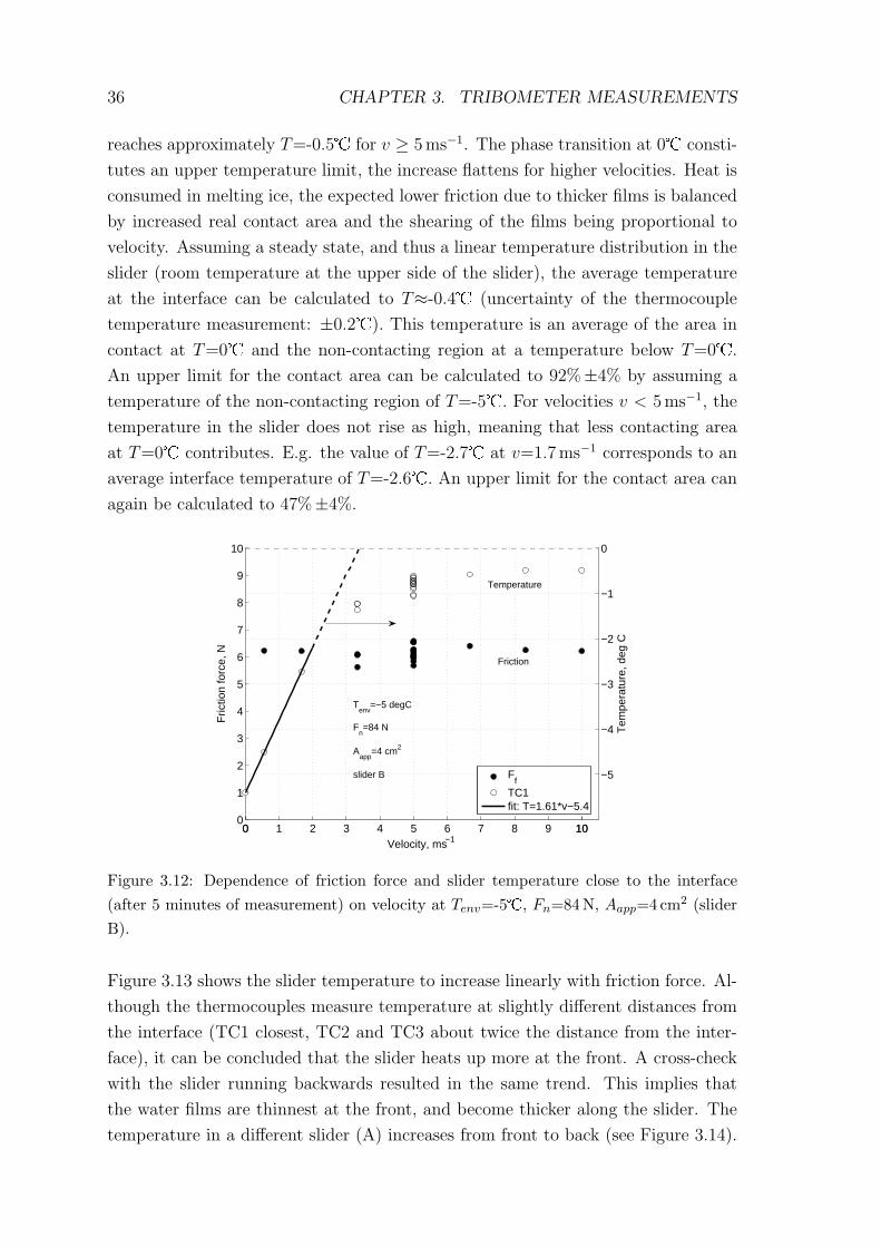
36 CHAPTER 3. TRIBOMETER MEASUREMENTS
reaches approximately T=-0.5� for v ≥ 5ms−1. The phase transition at 0� consti-
tutes an upper temperature limit, the increase flattens for higher velocities. Heat is
consumed in melting ice, the expected lower friction due to thicker films is balanced
by increased real contact area and the shearing of the films being proportional to
velocity. Assuming a steady state, and thus a linear temperature distribution in the
slider (room temperature at the upper side of the slider), the average temperature
at the interface can be calculated to T≈-0.4� (uncertainty of the thermocouple
temperature measurement: ±0.2�). This temperature is an average of the area in
contact at T=0� and the non-contacting region at a temperature below T=0�.
An upper limit for the contact area can be calculated to 92%±4% by assuming a
temperature of the non-contacting region of T=-5�. For velocities v < 5ms−1, the
temperature in the slider does not rise as high, meaning that less contacting area
at T=0� contributes. E.g. the value of T=-2.7� at v=1.7ms−1 corresponds to an
average interface temperature of T=-2.6�. An upper limit for the contact area can
again be calculated to 47%±4%.
0 100
1
2
3
4
5
6
7
8
9
10
Velocity, ms−1
Fric
tion
forc
e, N
0 1 2 3 4 5 6 7 8 9 10
−5
−4
−3
−2
−1
0
Tem
pera
ture
, deg
C
Tenv
=−5 degC
Fn=84 N
Aapp
=4 cm2
slider B
Temperature
Friction
Ff
TC1fit: T=1.61*v−5.4
Figure 3.12: Dependence of friction force and slider temperature close to the interface(after 5 minutes of measurement) on velocity at Tenv=-5�, Fn=84N, Aapp=4 cm2 (sliderB).
Figure 3.13 shows the slider temperature to increase linearly with friction force. Al-
though the thermocouples measure temperature at slightly different distances from
the interface (TC1 closest, TC2 and TC3 about twice the distance from the inter-
face), it can be concluded that the slider heats up more at the front. A cross-check
with the slider running backwards resulted in the same trend. This implies that
the water films are thinnest at the front, and become thicker along the slider. The
temperature in a different slider (A) increases from front to back (see Figure 3.14).
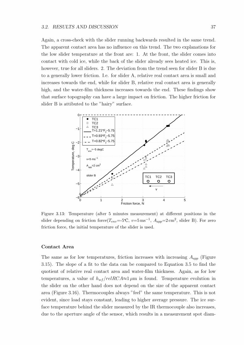
3.2. RESULTS AND DISCUSSION 37
Again, a cross-check with the slider running backwards resulted in the same trend.
The apparent contact area has no influence on this trend. The two explanations for
the low slider temperature at the front are: 1. At the front, the slider comes into
contact with cold ice, while the back of the slider already sees heated ice. This is,
however, true for all sliders. 2. The deviation from the trend seen for slider B is due
to a generally lower friction. I.e. for slider A, relative real contact area is small and
increases towards the end, while for slider B, relative real contact area is generally
high, and the water-film thickness increases towards the end. These findings show
that surface topography can have a large impact on friction. The higher friction for
slider B is attibuted to the ”hairy” surface.
0 1 2 3 4 5−6
−5
−4
−3
−2
−1
0
Friction force, N
Tem
pera
ture
, deg
C
Tenv
=−5 degC
v=5 ms−1
Aapp
=2 cm2
slider B TC1 TC2 TC3
v
TC1TC2TC3T=1.21*F
f−5.75
T=0.93*Ff−5.75
T=0.82*Ff−5.75
Figure 3.13: Temperature (after 5 minutes measurement) at different positions in theslider depending on friction force(Tenv=-5�, v=5 ms−1, Aapp=2 cm2, slider B). For zerofriction force, the initial temperature of the slider is used.
Contact Area
The same as for low temperatures, friction increases with increasing Aapp (Figure
3.15). The slope of a fit to the data can be compared to Equation 3.5 to find the
quotient of relative real contact area and water-film thickness. Again, as for low
temperatures, a value of hwf/relRCA≈1µm is found. Temperature evolution in
the slider on the other hand does not depend on the size of the apparent contact
area (Figure 3.16). Thermocouples always ”feel” the same temperature. This is not
evident, since load stays constant, leading to higher average pressure. The ice sur-
face temperature behind the slider measured by the IR thermocouple also increases,
due to the aperture angle of the sensor, which results in a measurement spot diam-
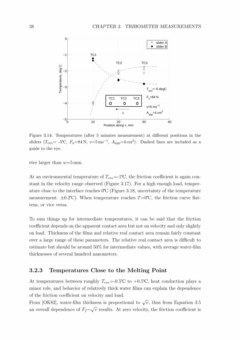
38 CHAPTER 3. TRIBOMETER MEASUREMENTS
0 10 20 30 40−5
−4
−3
−2
−1
0
Position along x, mm
Tem
pera
ture
, deg
C
Tenv
=−5 degC
Fn=84 N
v=5 ms−1
Aapp
=4 cm2
TC1 TC2 TC3
v
TC1
TC2 TC3
slider Aslider B
Figure 3.14: Temperatures (after 5 minutes measurement) at different positions in thesliders (Tenv= -5�, Fn=84N, v=5ms−1, Aapp=4 cm2). Dashed lines are included as aguide to the eye.
eter larger than w=5mm.
At an environmental temperature of Tenv=-1�, the friction coefficient is again con-
stant in the velocity range observed (Figure 3.17). For a high enough load, temper-
ature close to the interface reaches 0� (Figure 3.18, uncertainty of the temperature
measurement: ±0.2�). When temperature reaches T=0�, the friction curve flat-
tens, or vice versa.
To sum things up for intermediate temperatures, it can be said that the friction
coefficient depends on the apparent contact area but not on velocity and only slightly
on load. Thickness of the films and relative real contact area remain fairly constant
over a large range of these parameters. The relative real contact area is difficult to
estimate but should be around 50% for intermediate values, with average water-film
thicknesses of several hundred nanometers.
3.2.3 Temperatures Close to the Melting Point
At temperatures between roughly Tenv=-0.5� to +0.5�, heat conduction plays a
minor role, and behavior of relatively thick water films can explain the dependence
of the friction coefficient on velocity and load.
From [OK82], water-film thickness is proportional to√
v, thus from Equation 3.5
an overall dependence of Ff∼√
v results. At zero velocity, the friction coefficient is
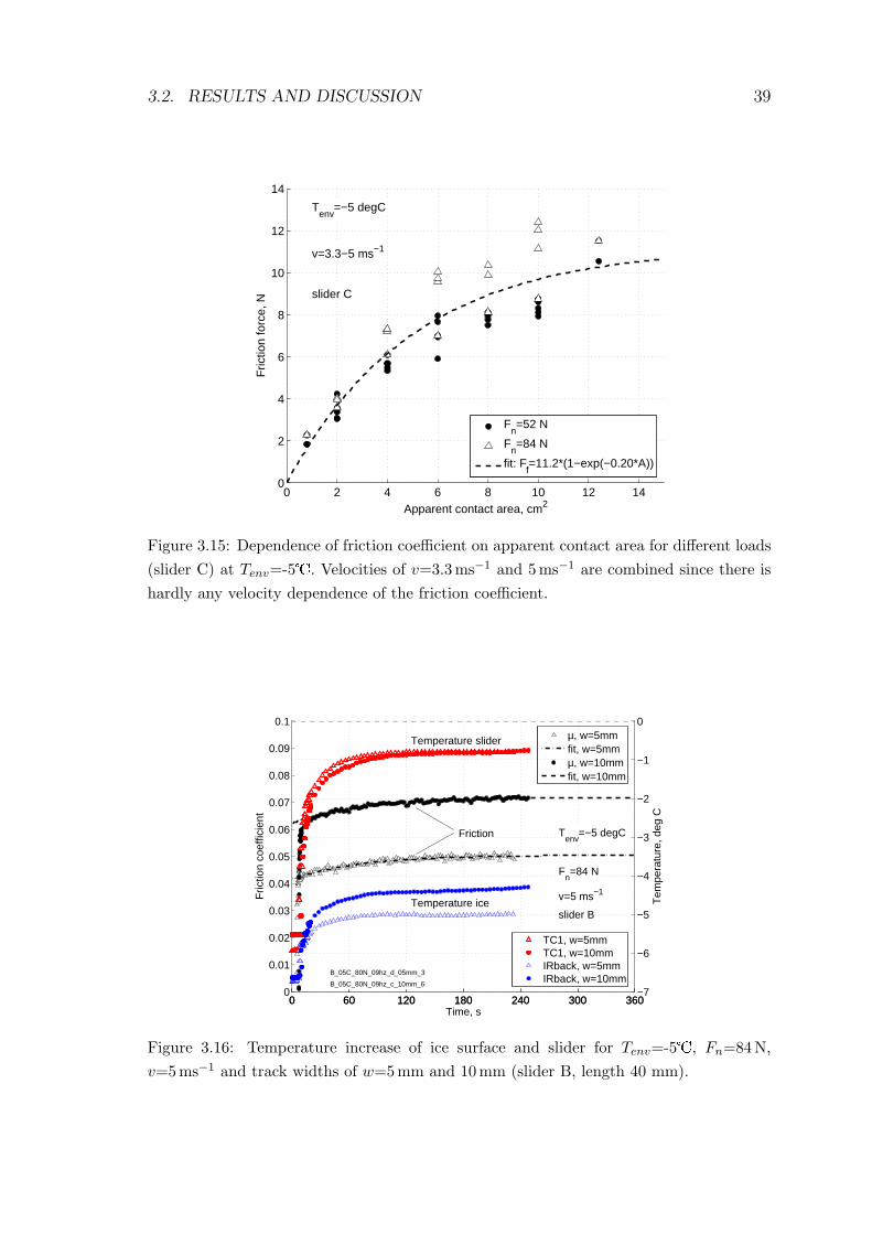
3.2. RESULTS AND DISCUSSION 39
0 2 4 6 8 10 12 140
2
4
6
8
10
12
14
Apparent contact area, cm2
Fric
tion
forc
e, N
Tenv
=−5 degC
v=3.3−5 ms−1
slider C
Fn=52 N
Fn=84 N
fit: Ff=11.2*(1−exp(−0.20*A))
Figure 3.15: Dependence of friction coefficient on apparent contact area for different loads(slider C) at Tenv=-5�. Velocities of v=3.3ms−1 and 5 ms−1 are combined since there ishardly any velocity dependence of the friction coefficient.
0 60 120 180 240 300 3600
0.01
0.02
0.03
0.04
0.05
0.06
0.07
0.08
0.09
0.1
Time, s
Fric
tion
coef
ficie
nt
µ, w=5mmfit, w=5mmµ, w=10mmfit, w=10mm
0 60 120 180 240 300 360−7
−6
−5
−4
−3
−2
−1
0
Tem
pera
ture
, deg
C
B_05C_80N_09hz_d_05mm_3
B_05C_80N_09hz_c_10mm_6
Tenv
=−5 degC
Fn=84 N
v=5 ms−1
slider B
Temperature slider
Temperature ice
Friction
TC1, w=5mmTC1, w=10mmIRback, w=5mmIRback, w=10mm
Figure 3.16: Temperature increase of ice surface and slider for Tenv=-5�, Fn=84N,v=5ms−1 and track widths of w=5mm and 10 mm (slider B, length 40 mm).
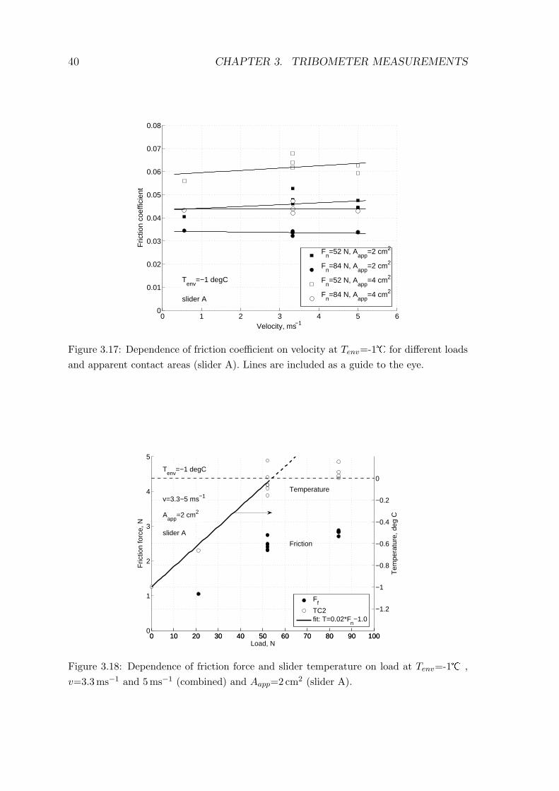
40 CHAPTER 3. TRIBOMETER MEASUREMENTS
0 1 2 3 4 5 60
0.01
0.02
0.03
0.04
0.05
0.06
0.07
0.08
Velocity, ms−1
Fric
tion
coef
ficie
nt
Tenv
=−1 degC
slider A
Fn=52 N, A
app=2 cm2
Fn=84 N, A
app=2 cm2
Fn=52 N, A
app=4 cm2
Fn=84 N, A
app=4 cm2
Figure 3.17: Dependence of friction coefficient on velocity at Tenv=-1� for different loadsand apparent contact areas (slider A). Lines are included as a guide to the eye.
0 10 20 30 40 50 60 70 80 90 1000
1
2
3
4
5
Load, N
Fric
tion
forc
e, N
0 10 20 30 40 50 60 70 80 90 100
−1.2
−1
−0.8
−0.6
−0.4
−0.2
0
Tem
pera
ture
, deg
C
Tenv
=−1 degC
v=3.3−5 ms−1
Aapp
=2 cm2
slider A
Temperature
Friction
Ff
TC2fit: T=0.02*F
n−1.0
Figure 3.18: Dependence of friction force and slider temperature on load at Tenv=-1� ,v=3.3ms−1 and 5ms−1 (combined) and Aapp=2 cm2 (slider A).
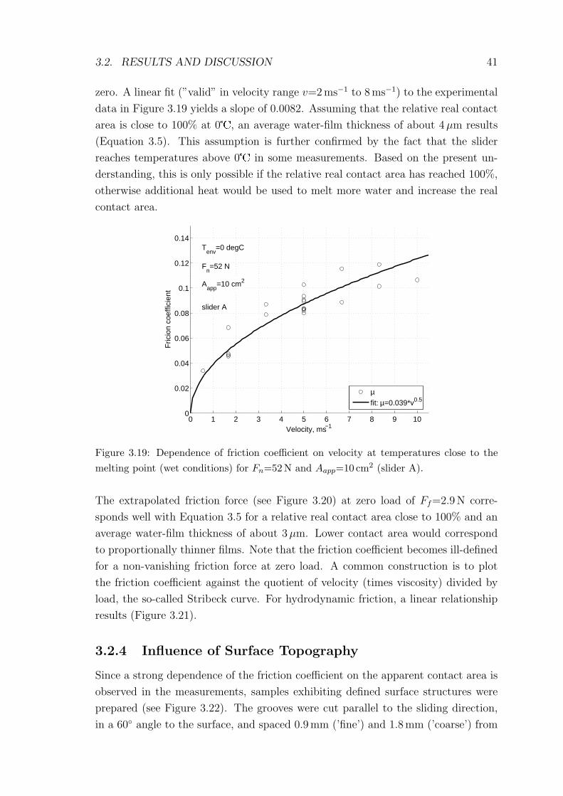
3.2. RESULTS AND DISCUSSION 41
zero. A linear fit (”valid” in velocity range v=2ms−1 to 8ms−1) to the experimental
data in Figure 3.19 yields a slope of 0.0082. Assuming that the relative real contact
area is close to 100% at 0�, an average water-film thickness of about 4 µm results
(Equation 3.5). This assumption is further confirmed by the fact that the slider
reaches temperatures above 0� in some measurements. Based on the present un-
derstanding, this is only possible if the relative real contact area has reached 100%,
otherwise additional heat would be used to melt more water and increase the real
contact area.
0 1 2 3 4 5 6 7 8 9 100
0.02
0.04
0.06
0.08
0.1
0.12
0.14
Velocity, ms−1
Fric
ion
coef
ficie
nt
Tenv
=0 degC
Fn=52 N
Aapp
=10 cm2
slider A
µfit: µ=0.039*v0.5
Figure 3.19: Dependence of friction coefficient on velocity at temperatures close to themelting point (wet conditions) for Fn=52N and Aapp=10 cm2 (slider A).
The extrapolated friction force (see Figure 3.20) at zero load of Ff=2.9N corre-
sponds well with Equation 3.5 for a relative real contact area close to 100% and an
average water-film thickness of about 3 µm. Lower contact area would correspond
to proportionally thinner films. Note that the friction coefficient becomes ill-defined
for a non-vanishing friction force at zero load. A common construction is to plot
the friction coefficient against the quotient of velocity (times viscosity) divided by
load, the so-called Stribeck curve. For hydrodynamic friction, a linear relationship
results (Figure 3.21).
3.2.4 Influence of Surface Topography
Since a strong dependence of the friction coefficient on the apparent contact area is
observed in the measurements, samples exhibiting defined surface structures were
prepared (see Figure 3.22). The grooves were cut parallel to the sliding direction,
in a 60◦ angle to the surface, and spaced 0.9mm (’fine’) and 1.8mm (’coarse’) from
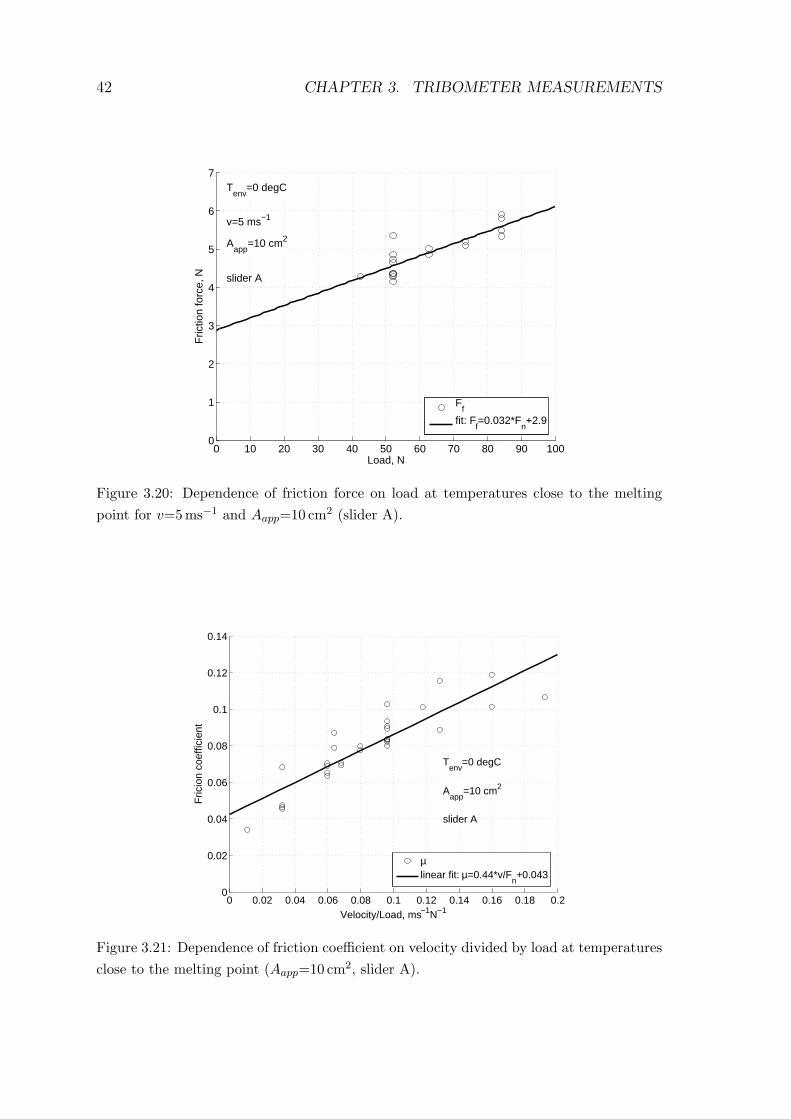
42 CHAPTER 3. TRIBOMETER MEASUREMENTS
0 10 20 30 40 50 60 70 80 90 1000
1
2
3
4
5
6
7
Load, N
Fric
tion
forc
e, N
Tenv
=0 degC
v=5 ms−1
Aapp
=10 cm2
slider A
Ff
fit: Ff=0.032*F
n+2.9
Figure 3.20: Dependence of friction force on load at temperatures close to the meltingpoint for v=5ms−1 and Aapp=10 cm2 (slider A).
0 0.02 0.04 0.06 0.08 0.1 0.12 0.14 0.16 0.18 0.20
0.02
0.04
0.06
0.08
0.1
0.12
0.14
Velocity/Load, ms−1N−1
Fric
ion
coef
ficie
nt
Tenv
=0 degC
Aapp
=10 cm2
slider A
µlinear fit: µ=0.44*v/F
n+0.043
Figure 3.21: Dependence of friction coefficient on velocity divided by load at temperaturesclose to the melting point (Aapp=10 cm2, slider A).
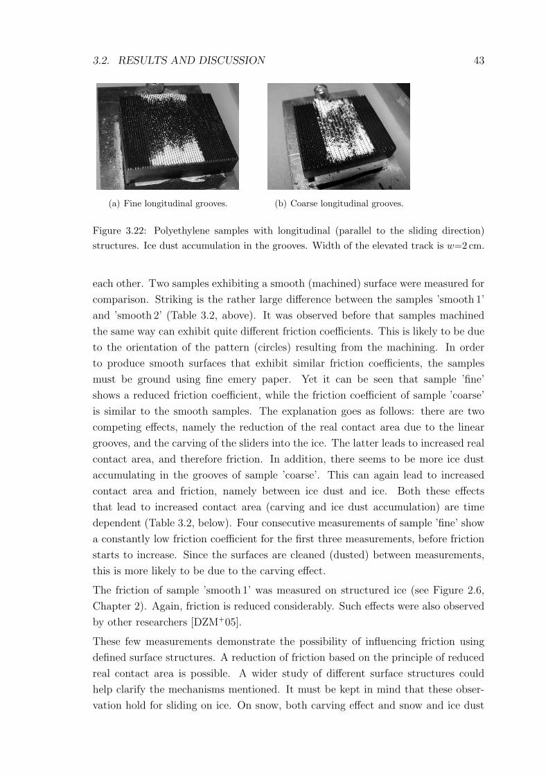
3.2. RESULTS AND DISCUSSION 43
(a) Fine longitudinal grooves. (b) Coarse longitudinal grooves.
Figure 3.22: Polyethylene samples with longitudinal (parallel to the sliding direction)structures. Ice dust accumulation in the grooves. Width of the elevated track is w=2 cm.
each other. Two samples exhibiting a smooth (machined) surface were measured for
comparison. Striking is the rather large difference between the samples ’smooth 1’
and ’smooth 2’ (Table 3.2, above). It was observed before that samples machined
the same way can exhibit quite different friction coefficients. This is likely to be due
to the orientation of the pattern (circles) resulting from the machining. In order
to produce smooth surfaces that exhibit similar friction coefficients, the samples
must be ground using fine emery paper. Yet it can be seen that sample ’fine’
shows a reduced friction coefficient, while the friction coefficient of sample ’coarse’
is similar to the smooth samples. The explanation goes as follows: there are two
competing effects, namely the reduction of the real contact area due to the linear
grooves, and the carving of the sliders into the ice. The latter leads to increased real
contact area, and therefore friction. In addition, there seems to be more ice dust
accumulating in the grooves of sample ’coarse’. This can again lead to increased
contact area and friction, namely between ice dust and ice. Both these effects
that lead to increased contact area (carving and ice dust accumulation) are time
dependent (Table 3.2, below). Four consecutive measurements of sample ’fine’ show
a constantly low friction coefficient for the first three measurements, before friction
starts to increase. Since the surfaces are cleaned (dusted) between measurements,
this is more likely to be due to the carving effect.
The friction of sample ’smooth 1’ was measured on structured ice (see Figure 2.6,
Chapter 2). Again, friction is reduced considerably. Such effects were also observed
by other researchers [DZM+05].
These few measurements demonstrate the possibility of influencing friction using
defined surface structures. A reduction of friction based on the principle of reduced
real contact area is possible. A wider study of different surface structures could
help clarify the mechanisms mentioned. It must be kept in mind that these obser-
vation hold for sliding on ice. On snow, both carving effect and snow and ice dust
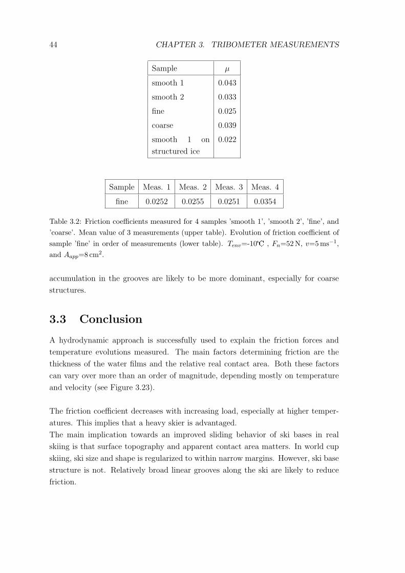
44 CHAPTER 3. TRIBOMETER MEASUREMENTS
Sample µ
smooth 1 0.043
smooth 2 0.033
fine 0.025
coarse 0.039
smooth 1 on
structured ice
0.022
Sample Meas. 1 Meas. 2 Meas. 3 Meas. 4
fine 0.0252 0.0255 0.0251 0.0354
Table 3.2: Friction coefficients measured for 4 samples ’smooth 1’, ’smooth 2’, ’fine’, and’coarse’. Mean value of 3 measurements (upper table). Evolution of friction coefficient ofsample ’fine’ in order of measurements (lower table). Tenv=-10� , Fn=52N, v=5 ms−1,and Aapp=8 cm2.
accumulation in the grooves are likely to be more dominant, especially for coarse
structures.
3.3 Conclusion
A hydrodynamic approach is successfully used to explain the friction forces and
temperature evolutions measured. The main factors determining friction are the
thickness of the water films and the relative real contact area. Both these factors
can vary over more than an order of magnitude, depending mostly on temperature
and velocity (see Figure 3.23).
The friction coefficient decreases with increasing load, especially at higher temper-
atures. This implies that a heavy skier is advantaged.
The main implication towards an improved sliding behavior of ski bases in real
skiing is that surface topography and apparent contact area matters. In world cup
skiing, ski size and shape is regularized to within narrow margins. However, ski base
structure is not. Relatively broad linear grooves along the ski are likely to reduce
friction.
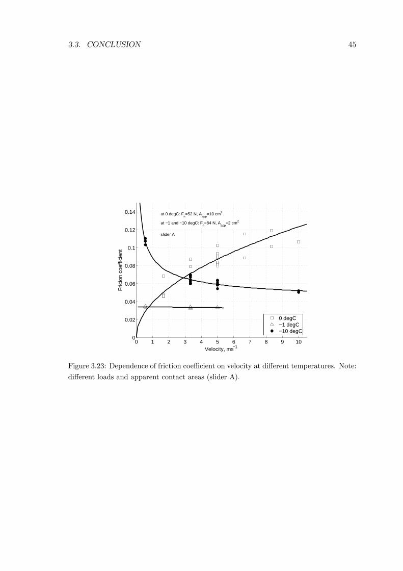
3.3. CONCLUSION 45
0 1 2 3 4 5 6 7 8 9 100
0.02
0.04
0.06
0.08
0.1
0.12
0.14
Velocity, ms−1
Fric
ion
coef
ficie
nt
at 0 degC: Fn=52 N, A
app=10 cm2
at −1 and −10 degC: Fn=84 N, A
app=2 cm2
slider A
0 degC−1 degC−10 degC
Figure 3.23: Dependence of friction coefficient on velocity at different temperatures. Note:different loads and apparent contact areas (slider A).

46 CHAPTER 3. TRIBOMETER MEASUREMENTS
Chapter 4
Investigations of the Contact Area
between Polyethylene and a Snow
or Ice Surface
Abstract
A good estimate of the relative real contact area and the contact spot size is es-
sential to deduce a model for the sliding friction of polyethylene on snow and ice.
Real contact area is in general hard to determine experimentally, especially for dy-
namic processes (see [Bhu02], pp. 154-161). For the experimental investigation of
the contact area between polyethylene and snow (”real” skiing situation), scanning
electron microscopy and X-ray computer tomography have been used. Contact spot
size can be estimated, and a dependence of the real contact area on load and snow
type can be seen. The investigation of the contact area between polyethylene and
ice (tribometer experiment) is carried out on imprints of the polyethylene slider and
the ice surface, by means of optical profilometry. The effect of polishing of the ice
by the slider during friction experiments is observed. All methods described give a
very precise surface characterization, and the results will be used in the prediction of
the contact area and contact spot size evolution in the friction process. Note, how-
ever, that the measurements are merely static, and can therefore only yield rough
estimates.
4.1 Introduction
The real contact area between polymers (here: polyethylene) and snow or ice is of
great interest with regard to snow and ice friction. In most tribological systems, the
real contact area (Areal) between two surfaces is generally less than the apparent
47
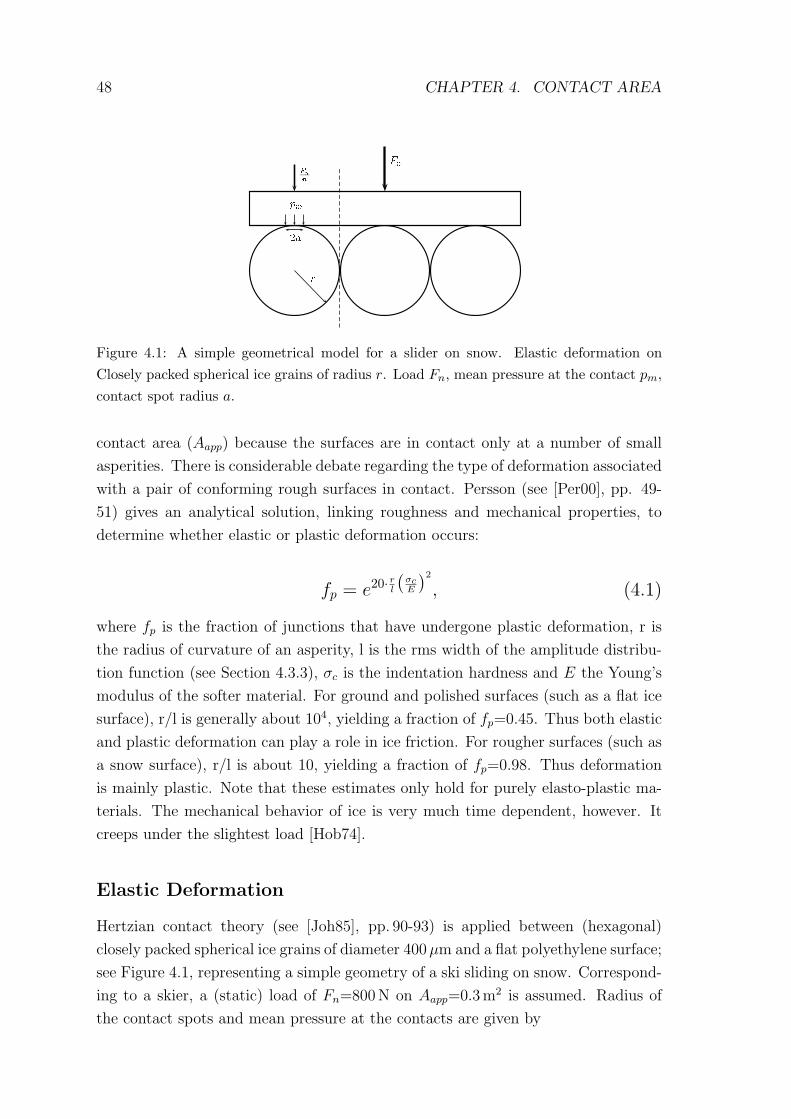
48 CHAPTER 4. CONTACT AREA
Fnr
pm2aFnn
Figure 4.1: A simple geometrical model for a slider on snow. Elastic deformation onClosely packed spherical ice grains of radius r. Load Fn, mean pressure at the contact pm,contact spot radius a.
contact area (Aapp) because the surfaces are in contact only at a number of small
asperities. There is considerable debate regarding the type of deformation associated
with a pair of conforming rough surfaces in contact. Persson (see [Per00], pp. 49-
51) gives an analytical solution, linking roughness and mechanical properties, to
determine whether elastic or plastic deformation occurs:
fp = e20· rl(
σcE
)2
, (4.1)
where fp is the fraction of junctions that have undergone plastic deformation, r is
the radius of curvature of an asperity, l is the rms width of the amplitude distribu-
tion function (see Section 4.3.3), σc is the indentation hardness and E the Young’s
modulus of the softer material. For ground and polished surfaces (such as a flat ice
surface), r/l is generally about 104, yielding a fraction of fp=0.45. Thus both elastic
and plastic deformation can play a role in ice friction. For rougher surfaces (such as
a snow surface), r/l is about 10, yielding a fraction of fp=0.98. Thus deformation
is mainly plastic. Note that these estimates only hold for purely elasto-plastic ma-
terials. The mechanical behavior of ice is very much time dependent, however. It
creeps under the slightest load [Hob74].
Elastic Deformation
Hertzian contact theory (see [Joh85], pp. 90-93) is applied between (hexagonal)
closely packed spherical ice grains of diameter 400 µm and a flat polyethylene surface;
see Figure 4.1, representing a simple geometry of a ski sliding on snow. Correspond-
ing to a skier, a (static) load of Fn=800N on Aapp=0.3m2 is assumed. Radius of
the contact spots and mean pressure at the contacts are given by
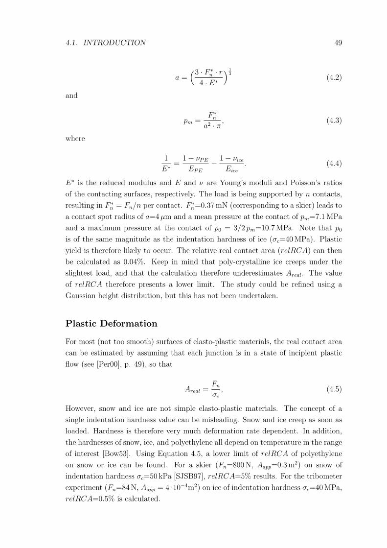
4.1. INTRODUCTION 49
a =(3 · F ∗
n · r4 · E∗
) 13
(4.2)
and
pm =F ∗
n
a2 · π , (4.3)
where
1
E∗ =1− νPE
EPE
− 1− νice
Eice
. (4.4)
E∗ is the reduced modulus and E and ν are Young’s moduli and Poisson’s ratios
of the contacting surfaces, respectively. The load is being supported by n contacts,
resulting in F ∗n = Fn/n per contact. F ∗
n=0.37mN (corresponding to a skier) leads to
a contact spot radius of a=4µm and a mean pressure at the contact of pm=7.1MPa
and a maximum pressure at the contact of p0 = 3/2 pm=10.7MPa. Note that p0
is of the same magnitude as the indentation hardness of ice (σc=40MPa). Plastic
yield is therefore likely to occur. The relative real contact area (relRCA) can then
be calculated as 0.04%. Keep in mind that poly-crystalline ice creeps under the
slightest load, and that the calculation therefore underestimates Areal. The value
of relRCA therefore presents a lower limit. The study could be refined using a
Gaussian height distribution, but this has not been undertaken.
Plastic Deformation
For most (not too smooth) surfaces of elasto-plastic materials, the real contact area
can be estimated by assuming that each junction is in a state of incipient plastic
flow (see [Per00], p. 49), so that
Areal =Fn
σc
, (4.5)
However, snow and ice are not simple elasto-plastic materials. The concept of a
single indentation hardness value can be misleading. Snow and ice creep as soon as
loaded. Hardness is therefore very much deformation rate dependent. In addition,
the hardnesses of snow, ice, and polyethylene all depend on temperature in the range
of interest [Bow53]. Using Equation 4.5, a lower limit of relRCA of polyethylene
on snow or ice can be found. For a skier (Fn=800N, Aapp=0.3m2) on snow of
indentation hardness σc=50 kPa [SJSB97], relRCA=5% results. For the tribometer
experiment (Fn=84N, Aapp = 4 ·10−4m2) on ice of indentation hardness σc=40MPa,
relRCA=0.5% is calculated.
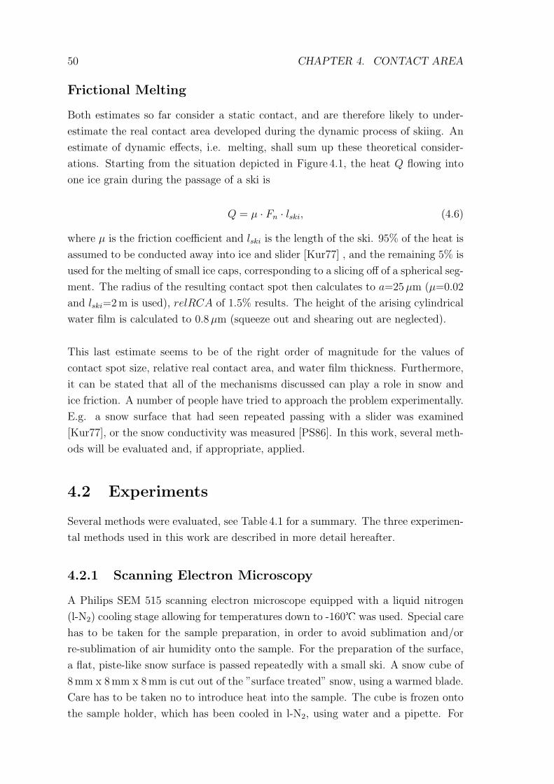
50 CHAPTER 4. CONTACT AREA
Frictional Melting
Both estimates so far consider a static contact, and are therefore likely to under-
estimate the real contact area developed during the dynamic process of skiing. An
estimate of dynamic effects, i.e. melting, shall sum up these theoretical consider-
ations. Starting from the situation depicted in Figure 4.1, the heat Q flowing into
one ice grain during the passage of a ski is
Q = µ · Fn · lski, (4.6)
where µ is the friction coefficient and lski is the length of the ski. 95% of the heat is
assumed to be conducted away into ice and slider [Kur77] , and the remaining 5% is
used for the melting of small ice caps, corresponding to a slicing off of a spherical seg-
ment. The radius of the resulting contact spot then calculates to a=25µm (µ=0.02
and lski=2m is used), relRCA of 1.5% results. The height of the arising cylindrical
water film is calculated to 0.8 µm (squeeze out and shearing out are neglected).
This last estimate seems to be of the right order of magnitude for the values of
contact spot size, relative real contact area, and water film thickness. Furthermore,
it can be stated that all of the mechanisms discussed can play a role in snow and
ice friction. A number of people have tried to approach the problem experimentally.
E.g. a snow surface that had seen repeated passing with a slider was examined
[Kur77], or the snow conductivity was measured [PS86]. In this work, several meth-
ods will be evaluated and, if appropriate, applied.
4.2 Experiments
Several methods were evaluated, see Table 4.1 for a summary. The three experimen-
tal methods used in this work are described in more detail hereafter.
4.2.1 Scanning Electron Microscopy
A Philips SEM 515 scanning electron microscope equipped with a liquid nitrogen
(l-N2) cooling stage allowing for temperatures down to -160� was used. Special care
has to be taken for the sample preparation, in order to avoid sublimation and/or
re-sublimation of air humidity onto the sample. For the preparation of the surface,
a flat, piste-like snow surface is passed repeatedly with a small ski. A snow cube of
8mm x 8mm x 8mm is cut out of the ”surface treated” snow, using a warmed blade.
Care has to be taken no to introduce heat into the sample. The cube is frozen onto
the sample holder, which has been cooled in l-N2, using water and a pipette. For
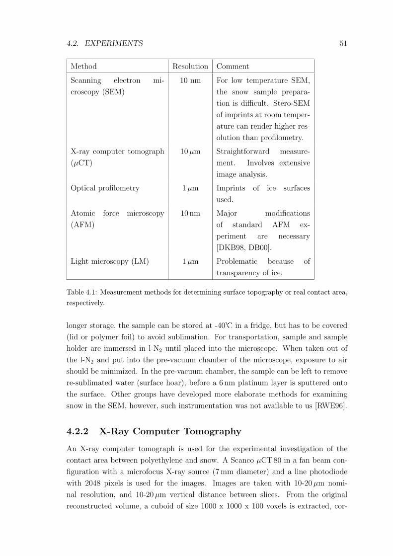
4.2. EXPERIMENTS 51
Method Resolution Comment
Scanning electron mi-
croscopy (SEM)
10 nm For low temperature SEM,
the snow sample prepara-
tion is difficult. Stero-SEM
of imprints at room temper-
ature can render higher res-
olution than profilometry.
X-ray computer tomograph
(µCT)
10µm Straightforward measure-
ment. Involves extensive
image analysis.
Optical profilometry 1µm Imprints of ice surfaces
used.
Atomic force microscopy
(AFM)
10 nm Major modifications
of standard AFM ex-
periment are necessary
[DKB98, DB00].
Light microscopy (LM) 1µm Problematic because of
transparency of ice.
Table 4.1: Measurement methods for determining surface topography or real contact area,respectively.
longer storage, the sample can be stored at -40� in a fridge, but has to be covered
(lid or polymer foil) to avoid sublimation. For transportation, sample and sample
holder are immersed in l-N2 until placed into the microscope. When taken out of
the l-N2 and put into the pre-vacuum chamber of the microscope, exposure to air
should be minimized. In the pre-vacuum chamber, the sample can be left to remove
re-sublimated water (surface hoar), before a 6 nm platinum layer is sputtered onto
the surface. Other groups have developed more elaborate methods for examining
snow in the SEM, however, such instrumentation was not available to us [RWE96].
4.2.2 X-Ray Computer Tomography
An X-ray computer tomograph is used for the experimental investigation of the
contact area between polyethylene and snow. A Scanco µCT80 in a fan beam con-
figuration with a microfocus X-ray source (7 mm diameter) and a line photodiode
with 2048 pixels is used for the images. Images are taken with 10-20 µm nomi-
nal resolution, and 10-20 µm vertical distance between slices. From the original
reconstructed volume, a cuboid of size 1000 x 1000 x 100 voxels is extracted, cor-
52 CHAPTER 4. CONTACT AREA
responding to physical side lengths of 10 mm x 10 mm x 1mm. Image processing
and stereological characterization: the raw sinograms of the computed tomography
scanner are transformed to 16-bit images. The stacked images are median filtered,
Gaussian filtered (2 x 2 x 2) and segmented by threshold, resulting in a binary set
of data. The threshold is determined from the histogram.
The snow is prepared by sieving, using sieves of 500 µm, 700µm, 1000µm, and
1400µm mesh size. For the most often used snow of grain size 500-1000 µm, an
average density of about 300 kgm−3 results. Only the density at the very surface
is relevant for the measurement, however. There, the snow can be very much com-
pressed, depending on the sample preparation. The snow is sieved directly into the
sample holder, a cylindrical beaker of diameter 20.5mm or 32mm. Special care has
to be taken to achieve a horizontal snow surface before pressing on it. Two different
ways of applying pressure onto the snow surface are used. One is to press a perfectly
fitting polyethylene piston into the cylinder and onto the surface, and applying the
desired load using dead weights. Vertical grooves cut into the piston avoid air en-
trapment. The piston is then kept in place by freezing it to the side wall of the
beaker using water. The macroscopic strain is therefore kept constant. Another
method is to use a spring with a known spring constant with which a defined initial
pressure can be applied. Then, the stress is kept constant (if creep is neglected).
For experimental determiniation of the influence of frictional heat on the snow sur-
face, a 15mm x 15 mm peltier element (Quick-Cool 4.6W) is used to melt the surface
of a cylindrical snow sample. For these surface melting experiments, samples are
first prepared in a cylinder, pressed, and left to sinter overnight. The snow sample
is then taken out of the cylinder, and loaded with the peltier element plus addi-
tional load. A thin sheet of polyethylene (non-sticking) is placed between the snow
and the heated plate. Heat conductive paste is used to connect polyethylene and
peltier element. A fan and cooling fins provide efficient cooling at the upper side
of the peltier element. The cooling-heating-cooling cycle is monitored using a relay.
A voltage of U=2V, resulting in a current of I=2A is applied and reversed for 4
seconds (procedure: cool - heat for 4 s - cool). The heat flow into the snow surface
is q′′=18 kWm2, or somewhat less, due to the thermal resistance of the polyethylene
sheet. The fan is left running during the whole experiment. The snow cylinder is
placed in the sample holder. Great care has to be taken not to deposit snow debris
on the melted snow surface.
4.3. RESULTS AND DISCUSSION 53
4.2.3 Optical Profilometry
It is not easily possible to carry out topographic measurements on snow and ice sur-
faces with a high resolution (higher than the 10 µm provided by the X-ray computer
tomograph). The transparency of ice makes it impossible to use optical profilome-
try, and standard contact profilometry cannot be used due to the creep behavior of
ice. Imprints of ice surfaces are thus used. Preliminary tests with different imprint
materials were carried out. Criteria were the curing behavior at temperatures be-
low 0� (time of curing, heat of curing) and the resolution. The dimethyl siloxane
polymer PROVIL novo Light C.D.2 ’fast set’ gave very good results: curing time at
sub-zero temperatures is about one hour, resolution is in the sub-micrometer range
[SKd+06]. For an exact quantitative analysis, the thermal expansion of the imprint
material would have to be considered, since the profilometer measurement is carried
out at room temperature. This, however, was neglected.
For the topographic measurements, a Fries Research and Technology (FRT) Micro
Prof is used. The sample is illuminated by a focused white light. An internal
passive optics, using chromatic aberration, splits the white light into different colors
(corresponding to different wavelengths). A miniaturized spectrometer detects the
color of the light reflected by the sample and determines the position of the focus
point. By means of an internal calibration table, the vertical position on the sample
surface is determined. Sub-micron resolution is achieved.
4.3 Results and Discussion
4.3.1 Scanning Electron Microscopy
Figure 4.2 shows a snow surface that has seen repeated passes of a miniature ski
(smooth polyethylene base) at magnitudes of roughly 10:1 (left) and 100:1 (right).
Clearly visible are the flattened regions that have seen contact and are evidence of
melting processes. They are very unevenly distributed. The detail image on the
right shows one single flat contact of a diameter of about 400 µm. The flakes are an
artefact resulting from the delamination of the platinum layer.
It remains to be investigated whether these images are representative of a real ski
slope that has been skied on. Yet it can be concluded that electron microscopy is a
suitable instrument for determining contact spot size an relative real contact area,
if a careful sample collection and preparation is conducted.
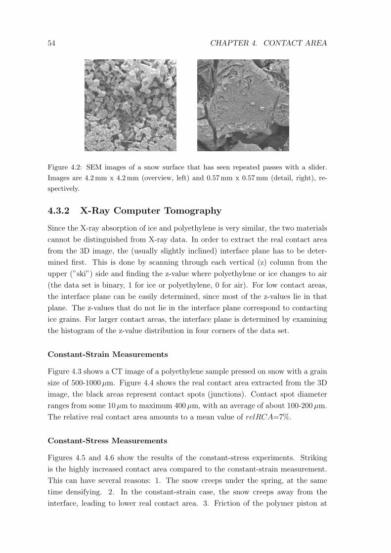
54 CHAPTER 4. CONTACT AREA
Figure 4.2: SEM images of a snow surface that has seen repeated passes with a slider.Images are 4.2 mm x 4.2mm (overview, left) and 0.57 mm x 0.57 mm (detail, right), re-spectively.
4.3.2 X-Ray Computer Tomography
Since the X-ray absorption of ice and polyethylene is very similar, the two materials
cannot be distinguished from X-ray data. In order to extract the real contact area
from the 3D image, the (usually slightly inclined) interface plane has to be deter-
mined first. This is done by scanning through each vertical (z) column from the
upper (”ski”) side and finding the z-value where polyethylene or ice changes to air
(the data set is binary, 1 for ice or polyethylene, 0 for air). For low contact areas,
the interface plane can be easily determined, since most of the z-values lie in that
plane. The z-values that do not lie in the interface plane correspond to contacting
ice grains. For larger contact areas, the interface plane is determined by examining
the histogram of the z-value distribution in four corners of the data set.
Constant-Strain Measurements
Figure 4.3 shows a CT image of a polyethylene sample pressed on snow with a grain
size of 500-1000µm. Figure 4.4 shows the real contact area extracted from the 3D
image, the black areas represent contact spots (junctions). Contact spot diameter
ranges from some 10µm to maximum 400 µm, with an average of about 100-200 µm.
The relative real contact area amounts to a mean value of relRCA=7%.
Constant-Stress Measurements
Figures 4.5 and 4.6 show the results of the constant-stress experiments. Striking
is the highly increased contact area compared to the constant-strain measurement.
This can have several reasons: 1. The snow creeps under the spring, at the same
time densifying. 2. In the constant-strain case, the snow creeps away from the
interface, leading to lower real contact area. 3. Friction of the polymer piston at
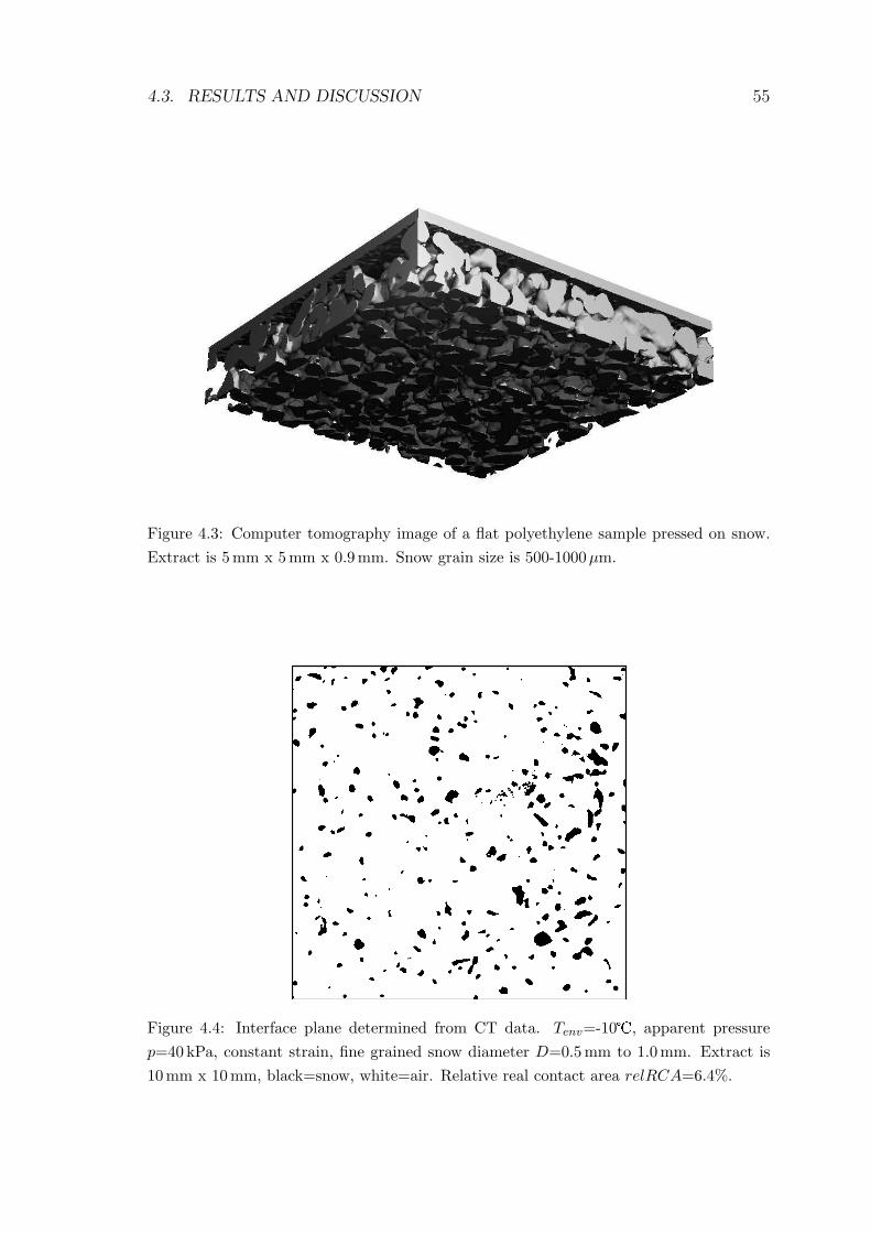
4.3. RESULTS AND DISCUSSION 55
Figure 4.3: Computer tomography image of a flat polyethylene sample pressed on snow.Extract is 5mm x 5 mm x 0.9 mm. Snow grain size is 500-1000µm.
Figure 4.4: Interface plane determined from CT data. Tenv=-10�, apparent pressurep=40 kPa, constant strain, fine grained snow diameter D=0.5mm to 1.0 mm. Extract is10mm x 10 mm, black=snow, white=air. Relative real contact area relRCA=6.4%.
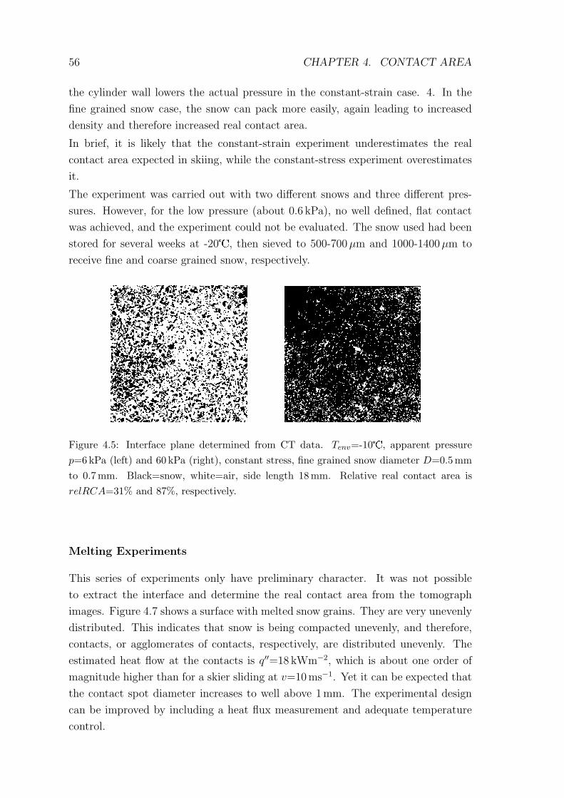
56 CHAPTER 4. CONTACT AREA
the cylinder wall lowers the actual pressure in the constant-strain case. 4. In the
fine grained snow case, the snow can pack more easily, again leading to increased
density and therefore increased real contact area.
In brief, it is likely that the constant-strain experiment underestimates the real
contact area expected in skiing, while the constant-stress experiment overestimates
it.
The experiment was carried out with two different snows and three different pres-
sures. However, for the low pressure (about 0.6 kPa), no well defined, flat contact
was achieved, and the experiment could not be evaluated. The snow used had been
stored for several weeks at -20�, then sieved to 500-700 µm and 1000-1400 µm to
receive fine and coarse grained snow, respectively.
Figure 4.5: Interface plane determined from CT data. Tenv=-10�, apparent pressurep=6kPa (left) and 60 kPa (right), constant stress, fine grained snow diameter D=0.5mmto 0.7 mm. Black=snow, white=air, side length 18 mm. Relative real contact area isrelRCA=31% and 87%, respectively.
Melting Experiments
This series of experiments only have preliminary character. It was not possible
to extract the interface and determine the real contact area from the tomograph
images. Figure 4.7 shows a surface with melted snow grains. They are very unevenly
distributed. This indicates that snow is being compacted unevenly, and therefore,
contacts, or agglomerates of contacts, respectively, are distributed unevenly. The
estimated heat flow at the contacts is q′′=18 kWm−2, which is about one order of
magnitude higher than for a skier sliding at v=10ms−1. Yet it can be expected that
the contact spot diameter increases to well above 1mm. The experimental design
can be improved by including a heat flux measurement and adequate temperature
control.
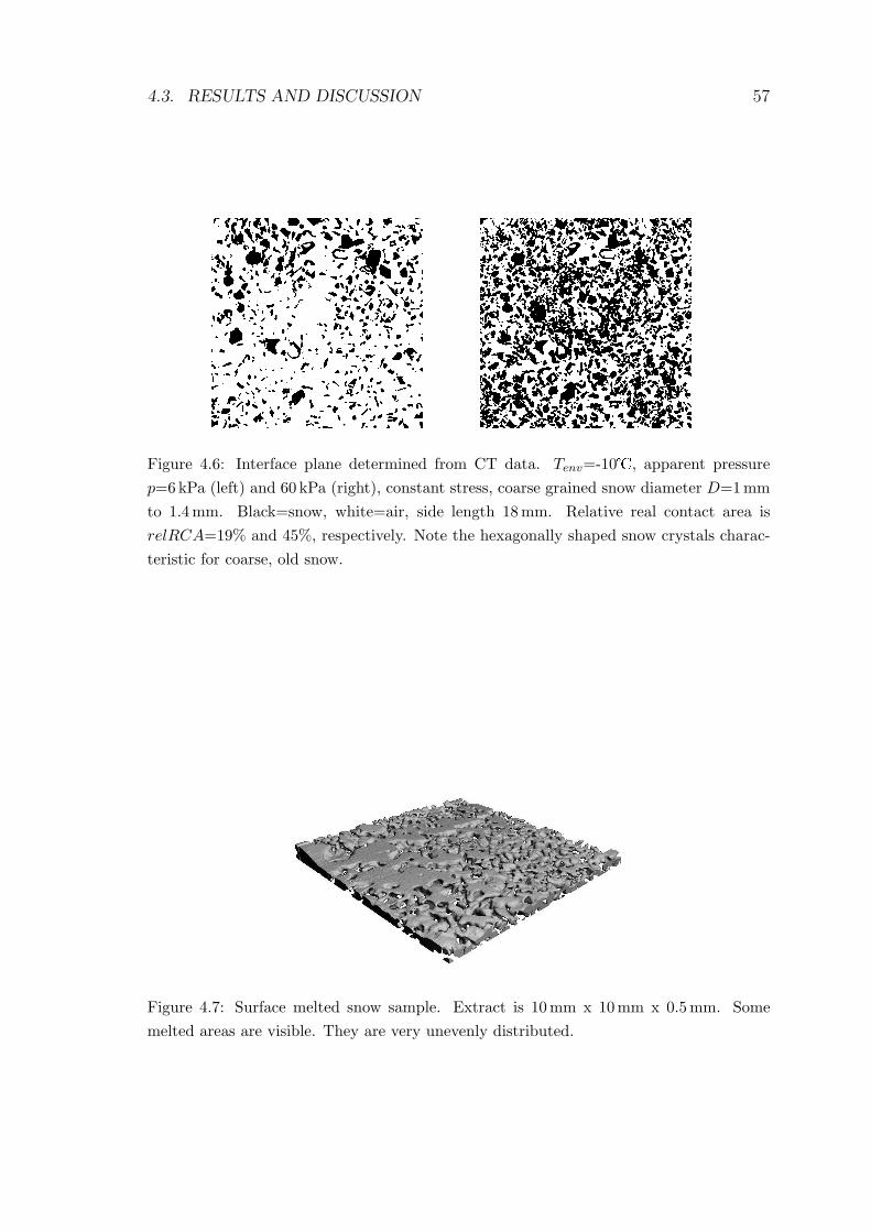
4.3. RESULTS AND DISCUSSION 57
Figure 4.6: Interface plane determined from CT data. Tenv=-10�, apparent pressurep=6kPa (left) and 60 kPa (right), constant stress, coarse grained snow diameter D=1 mmto 1.4mm. Black=snow, white=air, side length 18 mm. Relative real contact area isrelRCA=19% and 45%, respectively. Note the hexagonally shaped snow crystals charac-teristic for coarse, old snow.
Figure 4.7: Surface melted snow sample. Extract is 10mm x 10mm x 0.5mm. Somemelted areas are visible. They are very unevenly distributed.
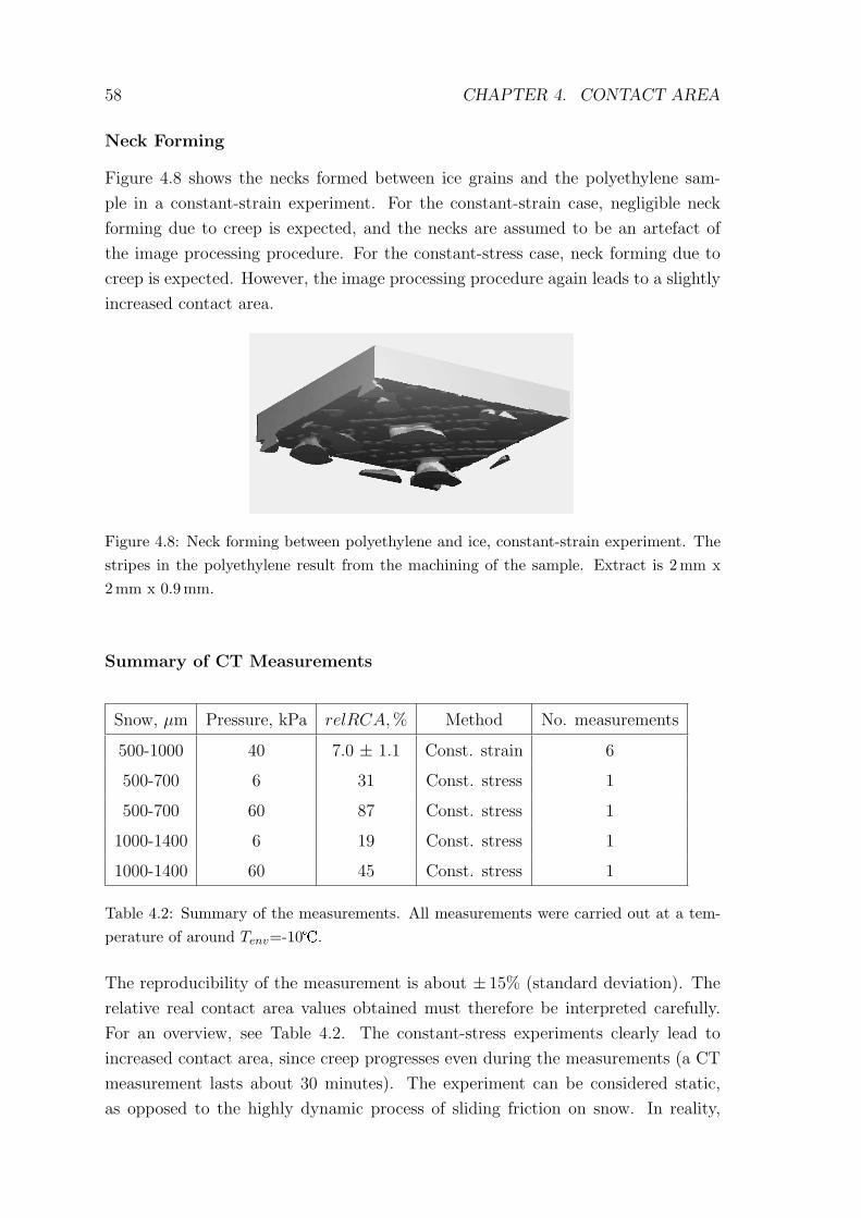
58 CHAPTER 4. CONTACT AREA
Neck Forming
Figure 4.8 shows the necks formed between ice grains and the polyethylene sam-
ple in a constant-strain experiment. For the constant-strain case, negligible neck
forming due to creep is expected, and the necks are assumed to be an artefact of
the image processing procedure. For the constant-stress case, neck forming due to
creep is expected. However, the image processing procedure again leads to a slightly
increased contact area.
Figure 4.8: Neck forming between polyethylene and ice, constant-strain experiment. Thestripes in the polyethylene result from the machining of the sample. Extract is 2 mm x2mm x 0.9 mm.
Summary of CT Measurements
Snow, µm Pressure, kPa relRCA, % Method No. measurements
500-1000 40 7.0 ± 1.1 Const. strain 6
500-700 6 31 Const. stress 1
500-700 60 87 Const. stress 1
1000-1400 6 19 Const. stress 1
1000-1400 60 45 Const. stress 1
Table 4.2: Summary of the measurements. All measurements were carried out at a tem-perature of around Tenv=-10�.
The reproducibility of the measurement is about ± 15% (standard deviation). The
relative real contact area values obtained must therefore be interpreted carefully.
For an overview, see Table 4.2. The constant-stress experiments clearly lead to
increased contact area, since creep progresses even during the measurements (a CT
measurement lasts about 30 minutes). The experiment can be considered static,
as opposed to the highly dynamic process of sliding friction on snow. In reality,
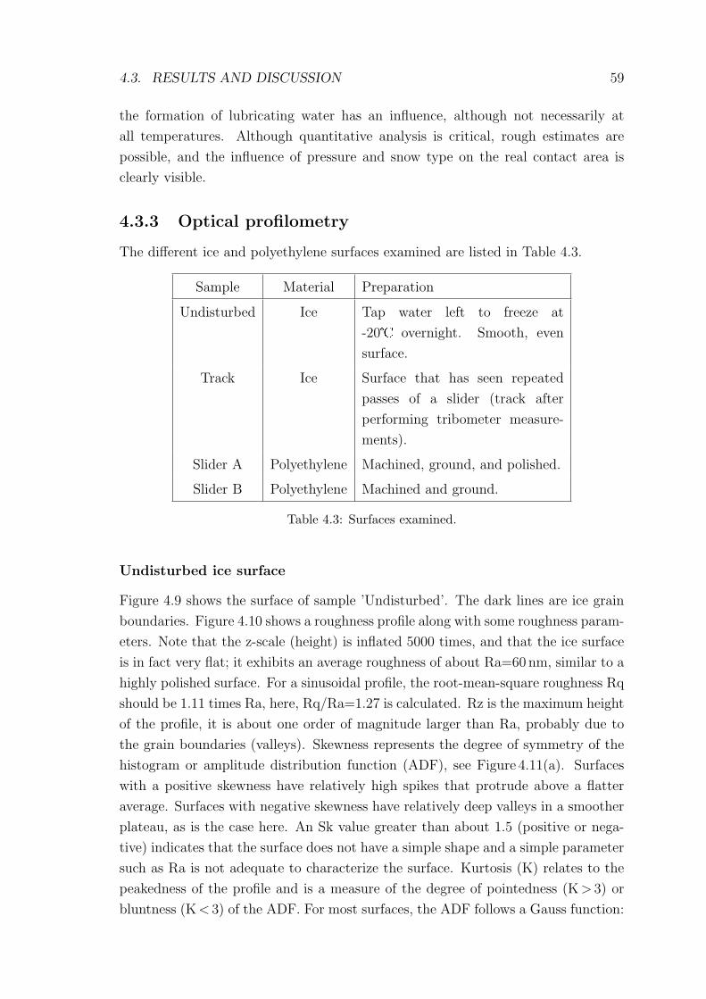
4.3. RESULTS AND DISCUSSION 59
the formation of lubricating water has an influence, although not necessarily at
all temperatures. Although quantitative analysis is critical, rough estimates are
possible, and the influence of pressure and snow type on the real contact area is
clearly visible.
4.3.3 Optical profilometry
The different ice and polyethylene surfaces examined are listed in Table 4.3.
Sample Material Preparation
Undisturbed Ice Tap water left to freeze at
-20� overnight. Smooth, even
surface.
Track Ice Surface that has seen repeated
passes of a slider (track after
performing tribometer measure-
ments).
Slider A Polyethylene Machined, ground, and polished.
Slider B Polyethylene Machined and ground.
Table 4.3: Surfaces examined.
Undisturbed ice surface
Figure 4.9 shows the surface of sample ’Undisturbed’. The dark lines are ice grain
boundaries. Figure 4.10 shows a roughness profile along with some roughness param-
eters. Note that the z-scale (height) is inflated 5000 times, and that the ice surface
is in fact very flat; it exhibits an average roughness of about Ra=60 nm, similar to a
highly polished surface. For a sinusoidal profile, the root-mean-square roughness Rq
should be 1.11 times Ra, here, Rq/Ra=1.27 is calculated. Rz is the maximum height
of the profile, it is about one order of magnitude larger than Ra, probably due to
the grain boundaries (valleys). Skewness represents the degree of symmetry of the
histogram or amplitude distribution function (ADF), see Figure 4.11(a). Surfaces
with a positive skewness have relatively high spikes that protrude above a flatter
average. Surfaces with negative skewness have relatively deep valleys in a smoother
plateau, as is the case here. An Sk value greater than about 1.5 (positive or nega-
tive) indicates that the surface does not have a simple shape and a simple parameter
such as Ra is not adequate to characterize the surface. Kurtosis (K) relates to the
peakedness of the profile and is a measure of the degree of pointedness (K > 3) or
bluntness (K< 3) of the ADF. For most surfaces, the ADF follows a Gauss function:
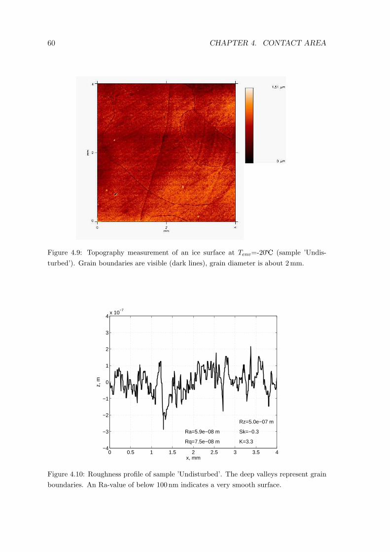
60 CHAPTER 4. CONTACT AREA
Figure 4.9: Topography measurement of an ice surface at Tenv=-20� (sample ’Undis-turbed’). Grain boundaries are visible (dark lines), grain diameter is about 2 mm.
0 0.5 1 1.5 2 2.5 3 3.5 4−4
−3
−2
−1
0
1
2
3
4x 10
−7
x, mm
z, m
Ra=5.9e−08 m
Rq=7.5e−08 m
Rz=5.0e−07 m
Sk=−0.3
K=3.3
Figure 4.10: Roughness profile of sample ’Undisturbed’. The deep valleys represent grainboundaries. An Ra-value of below 100 nm indicates a very smooth surface.
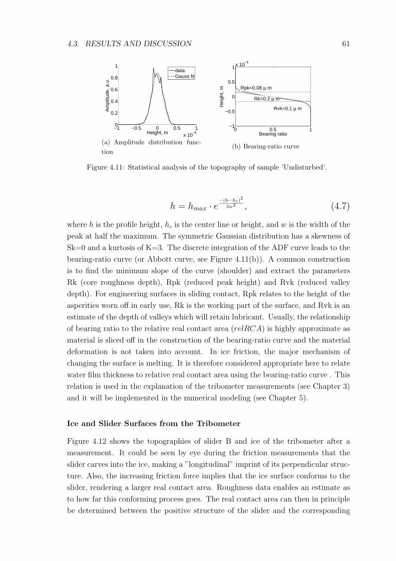
4.3. RESULTS AND DISCUSSION 61
−1 −0.5 0 0.5 1x 10
−6
0
0.2
0.4
0.6
0.8
1
Height, m
Am
plitu
de, a
.u.
dataGauss fit
(a) Amplitude distribution func-tion
0 0.5 1−1
−0.5
0
0.5
1x 10⁻⁶
Bearing ratio
Hei
ght,
m Rpk=0.08 µ m
Rk=0.2 µ m
Rvk=0.1 µ m
(b) Bearing-ratio curve
Figure 4.11: Statistical analysis of the topography of sample ’Undisturbed’.
h = hmax · e−(h−hc)2
2w2 , (4.7)
where h is the profile height, hc is the center line or height, and w is the width of the
peak at half the maximum. The symmetric Gaussian distribution has a skewness of
Sk=0 and a kurtosis of K=3. The discrete integration of the ADF curve leads to the
bearing-ratio curve (or Abbott curve, see Figure 4.11(b)). A common construction
is to find the minimum slope of the curve (shoulder) and extract the parameters
Rk (core roughness depth), Rpk (reduced peak height) and Rvk (reduced valley
depth). For engineering surfaces in sliding contact, Rpk relates to the height of the
asperities worn off in early use, Rk is the working part of the surface, and Rvk is an
estimate of the depth of valleys which will retain lubricant. Usually, the relationship
of bearing ratio to the relative real contact area (relRCA) is highly approximate as
material is sliced off in the construction of the bearing-ratio curve and the material
deformation is not taken into account. In ice friction, the major mechanism of
changing the surface is melting. It is therefore considered appropriate here to relate
water film thickness to relative real contact area using the bearing-ratio curve . This
relation is used in the explanation of the tribometer measurements (see Chapter 3)
and it will be implemented in the numerical modeling (see Chapter 5).
Ice and Slider Surfaces from the Tribometer
Figure 4.12 shows the topographies of slider B and ice of the tribometer after a
measurement. It could be seen by eye during the friction measurements that the
slider carves into the ice, making a ”longitudinal” imprint of its perpendicular struc-
ture. Also, the increasing friction force implies that the ice surface conforms to the
slider, rendering a larger real contact area. Roughness data enables an estimate as
to how far this conforming process goes. The real contact area can then in principle
be determined between the positive structure of the slider and the corresponding
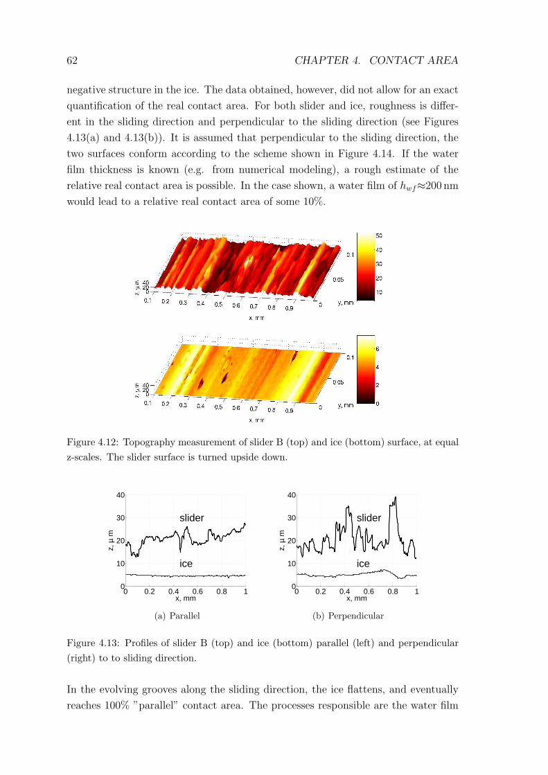
62 CHAPTER 4. CONTACT AREA
negative structure in the ice. The data obtained, however, did not allow for an exact
quantification of the real contact area. For both slider and ice, roughness is differ-
ent in the sliding direction and perpendicular to the sliding direction (see Figures
4.13(a) and 4.13(b)). It is assumed that perpendicular to the sliding direction, the
two surfaces conform according to the scheme shown in Figure 4.14. If the water
film thickness is known (e.g. from numerical modeling), a rough estimate of the
relative real contact area is possible. In the case shown, a water film of hwf≈200 nm
would lead to a relative real contact area of some 10%.
Figure 4.12: Topography measurement of slider B (top) and ice (bottom) surface, at equalz-scales. The slider surface is turned upside down.
0 0.2 0.4 0.6 0.8 10
10
20
30
40
ice
slider
x, mm
z, µ
m
(a) Parallel
0 0.2 0.4 0.6 0.8 10
10
20
30
40
ice
slider
x, mm
z, µ
m
(b) Perpendicular
Figure 4.13: Profiles of slider B (top) and ice (bottom) parallel (left) and perpendicular(right) to to sliding direction.
In the evolving grooves along the sliding direction, the ice flattens, and eventually
reaches 100% ”parallel” contact area. The processes responsible are the water film
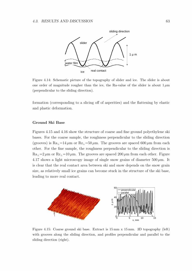
4.3. RESULTS AND DISCUSSION 63
1 µ m
slider
ice
water film
real contact
sliding direction
Figure 4.14: Schematic picture of the topography of slider and ice. The slider is aboutone order of magnitude rougher than the ice, the Ra-value of the slider is about 1µm(perpendicular to the sliding direction).
formation (corresponding to a slicing off of asperities) and the flattening by elastic
and plastic deformation.
Ground Ski Base
Figures 4.15 and 4.16 show the structure of coarse and fine ground polyethylene ski
bases. For the coarse sample, the roughness perpendicular to the sliding direction
(grooves) is Ra⊥=14µm or Rz⊥=50µm. The grooves are spaced 600 µm from each
other. For the fine sample, the roughness perpendicular to the sliding direction is
Ra⊥=2µm or Rz⊥=10µm. The grooves are spaced 200 µm from each other. Figure
4.17 shows a light microscopy image of single snow grains of diameter 500 µm. It
is clear that the real contact area between ski and snow depends on the snow grain
size, as relatively small ice grains can become stuck in the structure of the ski base,
leading to more real contact.
0 5 10 150
20
40
60
x, mm
z, µ
m
perpendicularparallel
Figure 4.15: Coarse ground ski base. Extract is 15 mm x 15 mm. 3D topography (left)with grooves along the sliding direction, and profiles perpendicular and parallel to thesliding direction (right).
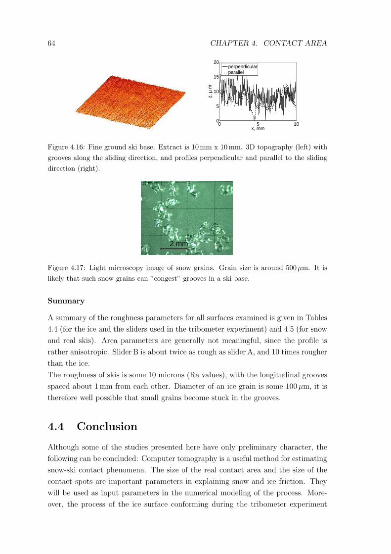
64 CHAPTER 4. CONTACT AREA
0 5 100
5
10
15
20
x, mm
z, µ
m
perpendicularparallel
Figure 4.16: Fine ground ski base. Extract is 10mm x 10 mm. 3D topography (left) withgrooves along the sliding direction, and profiles perpendicular and parallel to the slidingdirection (right).
2 mm
Figure 4.17: Light microscopy image of snow grains. Grain size is around 500µm. It islikely that such snow grains can ”congest” grooves in a ski base.
Summary
A summary of the roughness parameters for all surfaces examined is given in Tables
4.4 (for the ice and the sliders used in the tribometer experiment) and 4.5 (for snow
and real skis). Area parameters are generally not meaningful, since the profile is
rather anisotropic. SliderB is about twice as rough as sliderA, and 10 times rougher
than the ice.
The roughness of skis is some 10 microns (Ra values), with the longitudinal grooves
spaced about 1 mm from each other. Diameter of an ice grain is some 100 µm, it is
therefore well possible that small grains become stuck in the grooves.
4.4 Conclusion
Although some of the studies presented here have only preliminary character, the
following can be concluded: Computer tomography is a useful method for estimating
snow-ski contact phenomena. The size of the real contact area and the size of the
contact spots are important parameters in explaining snow and ice friction. They
will be used as input parameters in the numerical modeling of the process. More-
over, the process of the ice surface conforming during the tribometer experiment
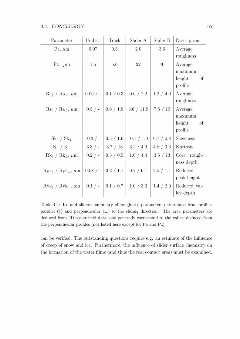
4.4. CONCLUSION 65
Parameter Undist. Track Slider A Slider B Description
Pa, µm 0.07 0.3 2.0 3.6 Average
roughness
Pz , µm 1.5 5.6 22 40 Average
maximum
height of
profile
Ra‖ / Ra⊥, µm 0.06 / - 0.1 / 0.3 0.6 / 2.2 1.2 / 4.0 Average
roughness
Rz‖ / Ra⊥, µm 0.5 / - 0.6 / 1.8 3.6 / 11.9 7.5 / 19 Average
maximum
height of
profile
Sk‖ / Sk⊥ -0.3 / - 0.5 / 1.6 -0.1 / 1.0 0.7 / 0.8 Skewness
K‖ / K⊥ 3.3 / - 3.7 / 13 3.2 / 4.9 4.8 / 3.6 Kurtosis
Rk‖ / Rk⊥, µm 0.2 / - 0.3 / 0.5 1.6 / 4.4 3.5 / 13 Core rough-
ness depth
Rpk‖ / Rpk⊥, µm 0.08 / - 0.2 / 1.1 0.7 / 6.1 2.5 / 7.4 Reduced
peak height
Rvk‖ / Rvk⊥, µm 0.1 / - 0.1 / 0.7 1.0 / 3.3 1.4 / 2.9 Reduced val-
ley depth
Table 4.4: Ice and sliders: summary of roughness parameters determined from profilesparallel (‖) and perpendicular (⊥) to the sliding direction. The area parameters arededuced from 2D scalar field data, and generally correspond to the values deduced fromthe perpendicular profiles (not listed here except for Pa and Pz).
can be verified. The outstanding questions require e.g. an estimate of the influence
of creep of snow and ice. Furthermore, the influence of slider surface chemistry on
the formation of the water films (and thus the real contact area) must be examined.
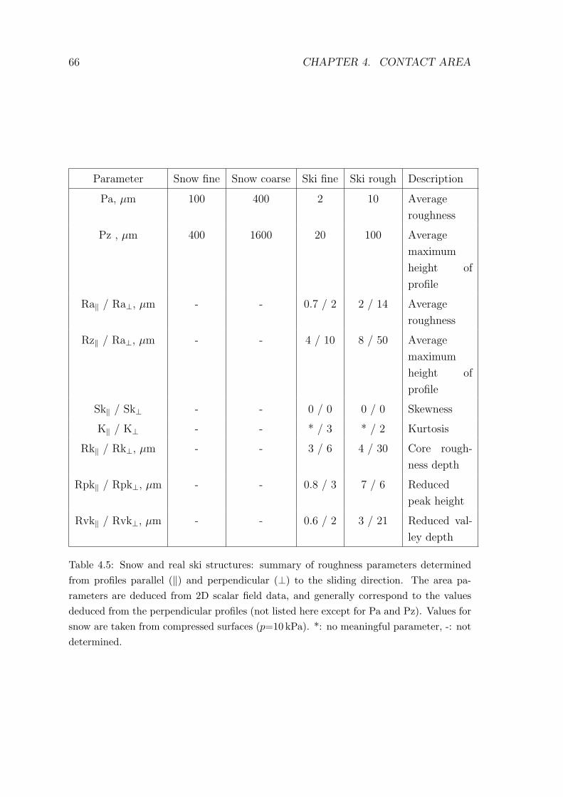
66 CHAPTER 4. CONTACT AREA
Parameter Snow fine Snow coarse Ski fine Ski rough Description
Pa, µm 100 400 2 10 Average
roughness
Pz , µm 400 1600 20 100 Average
maximum
height of
profile
Ra‖ / Ra⊥, µm - - 0.7 / 2 2 / 14 Average
roughness
Rz‖ / Ra⊥, µm - - 4 / 10 8 / 50 Average
maximum
height of
profile
Sk‖ / Sk⊥ - - 0 / 0 0 / 0 Skewness
K‖ / K⊥ - - * / 3 * / 2 Kurtosis
Rk‖ / Rk⊥, µm - - 3 / 6 4 / 30 Core rough-
ness depth
Rpk‖ / Rpk⊥, µm - - 0.8 / 3 7 / 6 Reduced
peak height
Rvk‖ / Rvk⊥, µm - - 0.6 / 2 3 / 21 Reduced val-
ley depth
Table 4.5: Snow and real ski structures: summary of roughness parameters determinedfrom profiles parallel (‖) and perpendicular (⊥) to the sliding direction. The area pa-rameters are deduced from 2D scalar field data, and generally correspond to the valuesdeduced from the perpendicular profiles (not listed here except for Pa and Pz). Values forsnow are taken from compressed surfaces (p=10 kPa). *: no meaningful parameter, -: notdetermined.
Chapter 5
Modeling
Abstract
A numerical model for sliding on ice including dry friction and generation of and
lubrication by water films is described. Alternative energy dissipation mechanisms
are discussed. The model is verified by comparing it with experimentally determined
temperature evolution and friction coefficients.
5.1 Introduction
From estimations for real skiing and from laboratory friction measurements, the
friction coefficient of polyethylene sliding on snow and ice is fairly well known. The
heat generation involved in the process for a skier sliding at v=20ms−1 (µ=0.03,
Fn=800N) is roughly 500W. What is not known a priori are the energy dissipation
mechanisms involved. Possible mechanisms are: dry friction, water generation, hy-
drodynamic friction, squeeze out of water films, capillary attachments, electrostatic
charges, plowing and compaction of the snow. The mechanisms considered relevant
will be discussed and, based thereon, the numerical model is introduced. Validation
of the model is done by comparison with the tribometer experiment (see Chapter
3).
5.2 Energy Dissipation Mechanisms
Possible energy dissipation mechanisms are described and estimations of their rele-
vance for the process are made.
67
68 CHAPTER 5. MODELING
Dry Friction
Dry friction is friction between two bodies in absence of lubricating films. This is
hard to achieve for ice; one has to go to low temperatures and low velocities not
to have lubricating water films at the interface of a material sliding on ice (see
e.g. [DLB95]). Nevertheless, there are regions of the interface between a material
sliding on snow or ice at velocities relevant for skiing where there is badly lubricated
sliding [Col92]. Friction arises from elastic and plastic deformation of either surface
and from very thin (not exceeding some nm) lubricating water films exhibiting high
friction. A detailed discussion of these (”dry”) friction processes would go beyond
the scope of this chapter, but they can be approximated by a dry friction law and
adoption of a generally agreed on value of µdry=0.3 [Bow53].
Water Generation
Neglecting wear processes, friction arises from the transfer of translational kinetic
energy into heat (lattice vibrations). This frictional heat is generated only at the
contacts, is therefore very unevenly distributed, and can cause very high temperature
increases (so-called flash temperatures). In ice friction, this provokes the contacting
regions of the ice to reach the melting point quite fast, and a phase change is to be
expected. A large fraction of the frictional heat is conducted into (primarily) the ice
and into the slider, depending on their individual thermal conductivities [Kur77].
The remaining heat is consumed in the phase change process and this is expected
to result in water lubrication. Assuming that all heat is conducted into the ice, the
temperature increase at the interface can be calculated analytically using
∆T = 2 · q′′ ·( t
π · λ · cp · ρ) 1
2, (5.1)
where λ, cp, and ρ are the thermal conductivity, the specific heat capacity, and the
density of ice, respectively. q′′ is the heat flux given by
q′′ = σk · v = µ · σ0 · v, (5.2)
where σk is the shear stress, µ the kinetic friction coefficient (here: dry friction),
and σ0 the perpendicular stress (here: indentation hardness). Assuming that the
total heat flux passes into the ice, it then takes 3 µs for the temperature to rise from
T=-10� to T=0� (v=1 ms−1). Note that this only holds for a perfectly flat slider in
contact with the ice, a slider exhibiting roughness or waviness at any scale will cause
intermittent heating of an ice contact, temperature increase will be correspondingly
slower. For a rough slider sliding on rough ice, an average contact-spot diameter
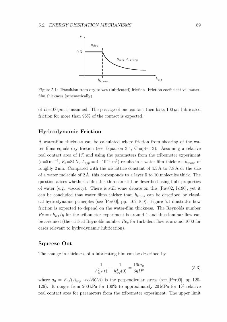
5.2. ENERGY DISSIPATION MECHANISMS 69
-
6µ
hwf
0.3
htrans
µdry
µwet < µdry
Figure 5.1: Transition from dry to wet (lubricated) friction. Friction coefficient vs. water-film thickness (schematically).
of D=100µm is assumed. The passage of one contact then lasts 100 µs, lubricated
friction for more than 95% of the contact is expected.
Hydrodynamic Friction
A water-film thickness can be calculated where friction from shearing of the wa-
ter films equals dry friction (see Equation 3.4, Chapter 3). Assuming a relative
real contact area of 1% and using the parameters from the tribometer experiment
(v=5ms−1, Fn=84N, Aapp = 4 · 10−4 m2) results in a water-film thickness htrans of
roughly 2 nm. Compared with the ice lattice constant of 4.5 A to 7.8 A or the size
of a water molecule of 2 A, this corresponds to a layer 5 to 10 molecules thick. The
question arises whether a film this thin can still be described using bulk properties
of water (e.g. viscosity). There is still some debate on this [Rav02, Isr90], yet it
can be concluded that water films thicker than htrans can be described by classi-
cal hydrodynamic principles (see [Per00], pp. 102-109). Figure 5.1 illustrates how
friction is expected to depend on the water-film thickness. The Reynolds number
Re = vhwf/η for the tribometer experiment is around 1 and thus laminar flow can
be assumed (the critical Reynolds number Rec for turbulent flow is around 1000 for
cases relevant to hydrodynamic lubrication).
Squeeze Out
The change in thickness of a lubricating film can be described by
1
h2wf (t)
− 1
h2wf (0)
=16tσ0
3ηD2(5.3)
where σ0 = Fn/(Aapp · relRCA) is the perpendicular stress (see [Per00], pp. 120-
126). It ranges from 200 kPa for 100% to approximately 20MPa for 1% relative
real contact area for parameters from the tribometer experiment. The upper limit
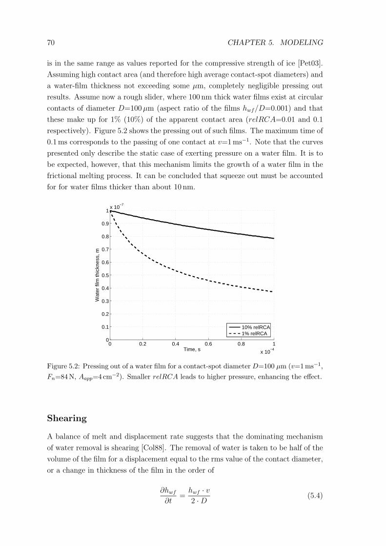
70 CHAPTER 5. MODELING
is in the same range as values reported for the compressive strength of ice [Pet03].
Assuming high contact area (and therefore high average contact-spot diameters) and
a water-film thickness not exceeding some µm, completely negligible pressing out
results. Assume now a rough slider, where 100 nm thick water films exist at circular
contacts of diameter D=100µm (aspect ratio of the films hwf/D=0.001) and that
these make up for 1% (10%) of the apparent contact area (relRCA=0.01 and 0.1
respectively). Figure 5.2 shows the pressing out of such films. The maximum time of
0.1ms corresponds to the passing of one contact at v=1ms−1. Note that the curves
presented only describe the static case of exerting pressure on a water film. It is to
be expected, however, that this mechanism limits the growth of a water film in the
frictional melting process. It can be concluded that squeeze out must be accounted
for for water films thicker than about 10 nm.
0 0.2 0.4 0.6 0.8 1
x 10−4
0
0.1
0.2
0.3
0.4
0.5
0.6
0.7
0.8
0.9
1x 10
−7
Time, s
Wat
er fi
lm th
ickn
ess,
m
10% relRCA1% relRCA
Figure 5.2: Pressing out of a water film for a contact-spot diameter D=100 µm (v=1 ms−1,Fn=84N, Aapp=4 cm−2). Smaller relRCA leads to higher pressure, enhancing the effect.
Shearing
A balance of melt and displacement rate suggests that the dominating mechanism
of water removal is shearing [Col88]. The removal of water is taken to be half of the
volume of the film for a displacement equal to the rms value of the contact diameter,
or a change in thickness of the film in the order of
∂hwf
∂t=
hwf · v2 ·D (5.4)
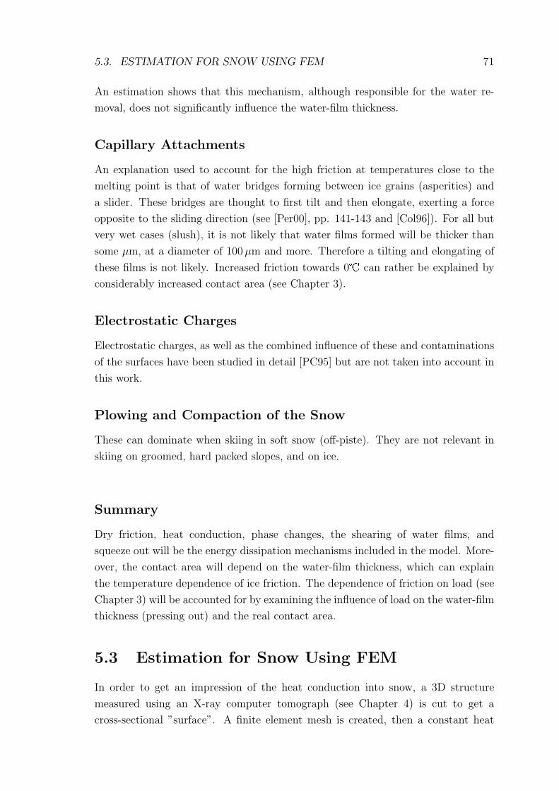
5.3. ESTIMATION FOR SNOW USING FEM 71
An estimation shows that this mechanism, although responsible for the water re-
moval, does not significantly influence the water-film thickness.
Capillary Attachments
An explanation used to account for the high friction at temperatures close to the
melting point is that of water bridges forming between ice grains (asperities) and
a slider. These bridges are thought to first tilt and then elongate, exerting a force
opposite to the sliding direction (see [Per00], pp. 141-143 and [Col96]). For all but
very wet cases (slush), it is not likely that water films formed will be thicker than
some µm, at a diameter of 100 µm and more. Therefore a tilting and elongating of
these films is not likely. Increased friction towards 0� can rather be explained by
considerably increased contact area (see Chapter 3).
Electrostatic Charges
Electrostatic charges, as well as the combined influence of these and contaminations
of the surfaces have been studied in detail [PC95] but are not taken into account in
this work.
Plowing and Compaction of the Snow
These can dominate when skiing in soft snow (off-piste). They are not relevant in
skiing on groomed, hard packed slopes, and on ice.
Summary
Dry friction, heat conduction, phase changes, the shearing of water films, and
squeeze out will be the energy dissipation mechanisms included in the model. More-
over, the contact area will depend on the water-film thickness, which can explain
the temperature dependence of ice friction. The dependence of friction on load (see
Chapter 3) will be accounted for by examining the influence of load on the water-film
thickness (pressing out) and the real contact area.
5.3 Estimation for Snow Using FEM
In order to get an impression of the heat conduction into snow, a 3D structure
measured using an X-ray computer tomograph (see Chapter 4) is cut to get a
cross-sectional ”surface”. A finite element mesh is created, then a constant heat
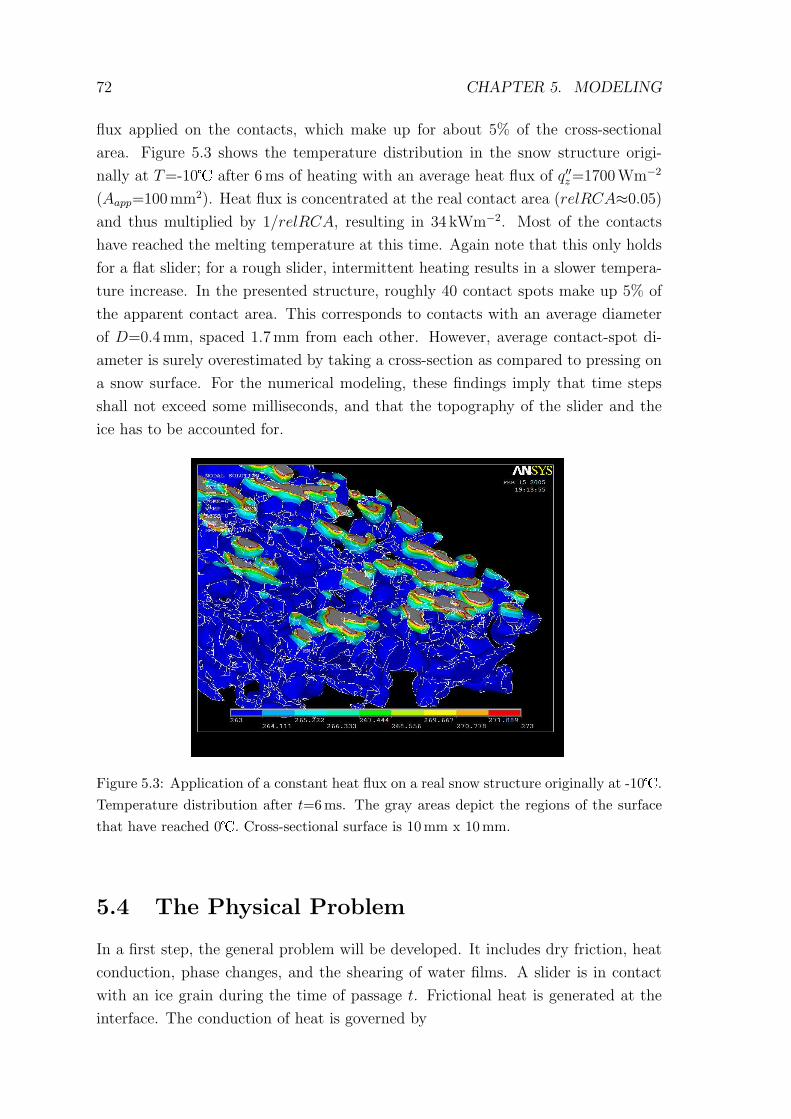
72 CHAPTER 5. MODELING
flux applied on the contacts, which make up for about 5% of the cross-sectional
area. Figure 5.3 shows the temperature distribution in the snow structure origi-
nally at T=-10� after 6 ms of heating with an average heat flux of q′′z=1700Wm−2
(Aapp=100mm2). Heat flux is concentrated at the real contact area (relRCA≈0.05)
and thus multiplied by 1/relRCA, resulting in 34 kWm−2. Most of the contacts
have reached the melting temperature at this time. Again note that this only holds
for a flat slider; for a rough slider, intermittent heating results in a slower tempera-
ture increase. In the presented structure, roughly 40 contact spots make up 5% of
the apparent contact area. This corresponds to contacts with an average diameter
of D=0.4mm, spaced 1.7mm from each other. However, average contact-spot di-
ameter is surely overestimated by taking a cross-section as compared to pressing on
a snow surface. For the numerical modeling, these findings imply that time steps
shall not exceed some milliseconds, and that the topography of the slider and the
ice has to be accounted for.
Figure 5.3: Application of a constant heat flux on a real snow structure originally at -10�.Temperature distribution after t=6ms. The gray areas depict the regions of the surfacethat have reached 0�. Cross-sectional surface is 10 mm x 10mm.
5.4 The Physical Problem
In a first step, the general problem will be developed. It includes dry friction, heat
conduction, phase changes, and the shearing of water films. A slider is in contact
with an ice grain during the time of passage t. Frictional heat is generated at the
interface. The conduction of heat is governed by
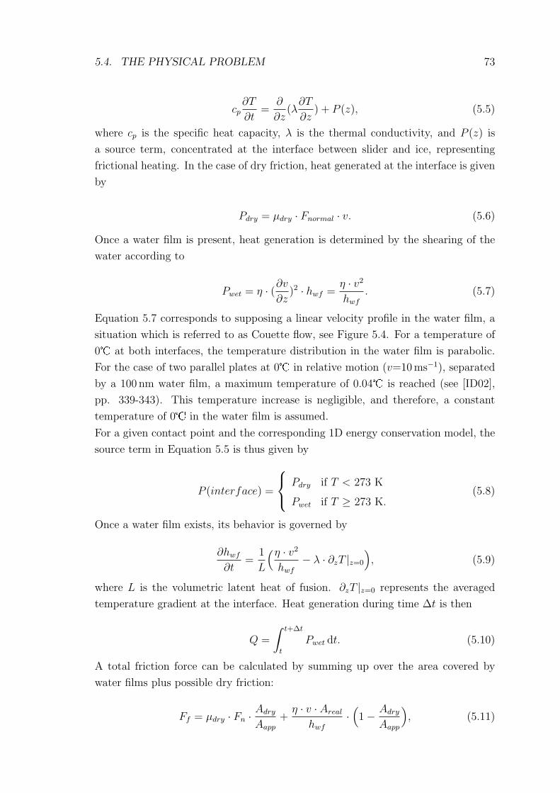
5.4. THE PHYSICAL PROBLEM 73
cp∂T
∂t=
∂
∂z(λ
∂T
∂z) + P (z), (5.5)
where cp is the specific heat capacity, λ is the thermal conductivity, and P (z) is
a source term, concentrated at the interface between slider and ice, representing
frictional heating. In the case of dry friction, heat generated at the interface is given
by
Pdry = µdry · Fnormal · v. (5.6)
Once a water film is present, heat generation is determined by the shearing of the
water according to
Pwet = η · (∂v
∂z)2 · hwf =
η · v2
hwf
. (5.7)
Equation 5.7 corresponds to supposing a linear velocity profile in the water film, a
situation which is referred to as Couette flow, see Figure 5.4. For a temperature of
0� at both interfaces, the temperature distribution in the water film is parabolic.
For the case of two parallel plates at 0� in relative motion (v=10ms−1), separated
by a 100 nm water film, a maximum temperature of 0.04� is reached (see [ID02],
pp. 339-343). This temperature increase is negligible, and therefore, a constant
temperature of 0� in the water film is assumed.
For a given contact point and the corresponding 1D energy conservation model, the
source term in Equation 5.5 is thus given by
P (interface) =
Pdry if T < 273 K
Pwet if T ≥ 273 K.(5.8)
Once a water film exists, its behavior is governed by
∂hwf
∂t=
1
L
(η · v2
hwf
− λ · ∂zT |z=0
), (5.9)
where L is the volumetric latent heat of fusion. ∂zT |z=0 represents the averaged
temperature gradient at the interface. Heat generation during time ∆t is then
Q =
∫ t+∆t
t
Pwet dt. (5.10)
A total friction force can be calculated by summing up over the area covered by
water films plus possible dry friction:
Ff = µdry · Fn · Adry
Aapp
+η · v · Areal
hwf
·(1− Adry
Aapp
), (5.11)
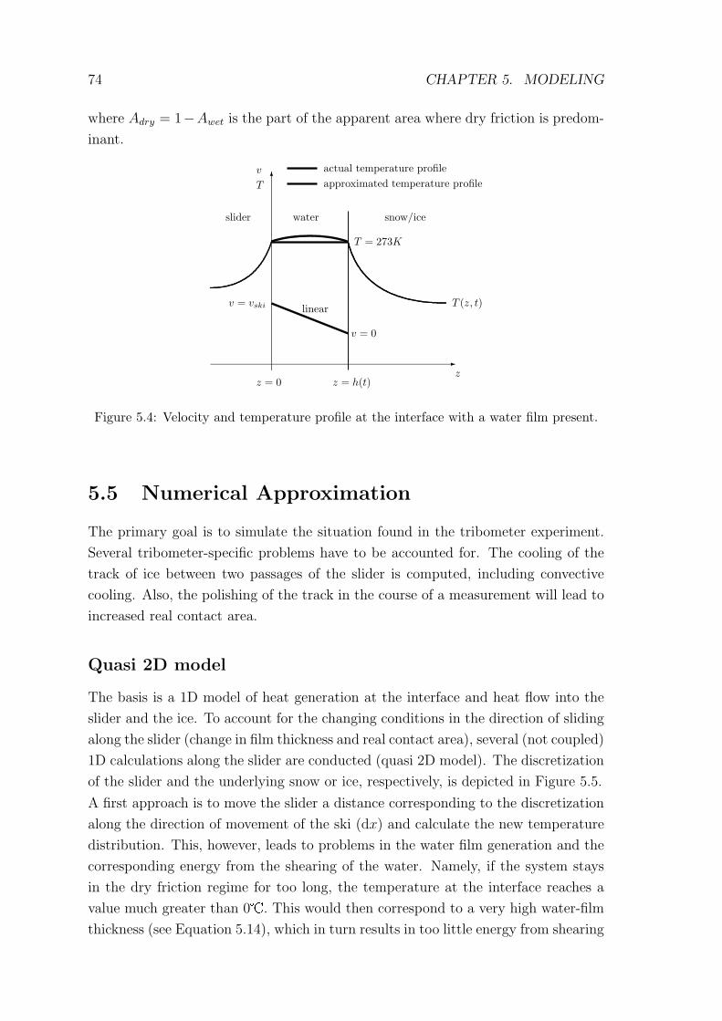
74 CHAPTER 5. MODELING
where Adry = 1−Awet is the part of the apparent area where dry friction is predom-
inant.
-
6v
T
z
v = 0
v = vski
T = 273K
z = 0 z = h(t)
slider water snow/ice
linear
actual temperature profile
approximated temperature profile
T (z, t)
Figure 5.4: Velocity and temperature profile at the interface with a water film present.
5.5 Numerical Approximation
The primary goal is to simulate the situation found in the tribometer experiment.
Several tribometer-specific problems have to be accounted for. The cooling of the
track of ice between two passages of the slider is computed, including convective
cooling. Also, the polishing of the track in the course of a measurement will lead to
increased real contact area.
Quasi 2D model
The basis is a 1D model of heat generation at the interface and heat flow into the
slider and the ice. To account for the changing conditions in the direction of sliding
along the slider (change in film thickness and real contact area), several (not coupled)
1D calculations along the slider are conducted (quasi 2D model). The discretization
of the slider and the underlying snow or ice, respectively, is depicted in Figure 5.5.
A first approach is to move the slider a distance corresponding to the discretization
along the direction of movement of the ski (dx) and calculate the new temperature
distribution. This, however, leads to problems in the water film generation and the
corresponding energy from the shearing of the water. Namely, if the system stays
in the dry friction regime for too long, the temperature at the interface reaches a
value much greater than 0�. This would then correspond to a very high water-film
thickness (see Equation 5.14), which in turn results in too little energy from shearing
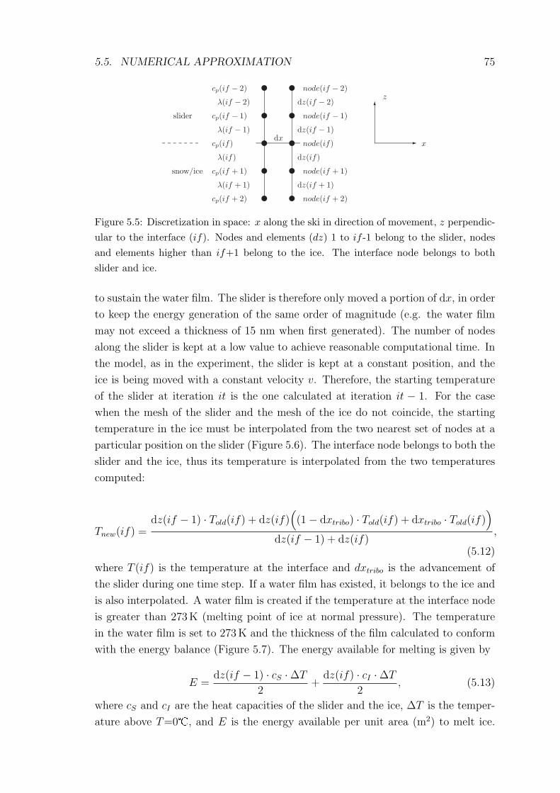
5.5. NUMERICAL APPROXIMATION 75
slider
snow/ice
v
v
v
v
v
v
v
v
v
v node(if − 2)
node(if − 1)
node(if)
node(if + 1)
node(if + 2)
dx
dz(if − 2)
dz(if − 1)
dz(if)
dz(if + 1)
cp(if − 2)
cp(if − 1)
cp(if)
cp(if + 1)
cp(if + 2)
λ(if − 2)
λ(if − 1)
λ(if)
λ(if + 1)
-
6
x
z
Figure 5.5: Discretization in space: x along the ski in direction of movement, z perpendic-ular to the interface (if). Nodes and elements (dz) 1 to if -1 belong to the slider, nodesand elements higher than if+1 belong to the ice. The interface node belongs to bothslider and ice.
to sustain the water film. The slider is therefore only moved a portion of dx, in order
to keep the energy generation of the same order of magnitude (e.g. the water film
may not exceed a thickness of 15 nm when first generated). The number of nodes
along the slider is kept at a low value to achieve reasonable computational time. In
the model, as in the experiment, the slider is kept at a constant position, and the
ice is being moved with a constant velocity v. Therefore, the starting temperature
of the slider at iteration it is the one calculated at iteration it − 1. For the case
when the mesh of the slider and the mesh of the ice do not coincide, the starting
temperature in the ice must be interpolated from the two nearest set of nodes at a
particular position on the slider (Figure 5.6). The interface node belongs to both the
slider and the ice, thus its temperature is interpolated from the two temperatures
computed:
Tnew(if) =dz(if − 1) · Told(if) + dz(if)
((1− dxtribo) · Told(if) + dxtribo · Told(if)
)
dz(if − 1) + dz(if),
(5.12)
where T (if) is the temperature at the interface and dxtribo is the advancement of
the slider during one time step. If a water film has existed, it belongs to the ice and
is also interpolated. A water film is created if the temperature at the interface node
is greater than 273K (melting point of ice at normal pressure). The temperature
in the water film is set to 273 K and the thickness of the film calculated to conform
with the energy balance (Figure 5.7). The energy available for melting is given by
E =dz(if − 1) · cS ·∆T
2+
dz(if) · cI ·∆T
2, (5.13)
where cS and cI are the heat capacities of the slider and the ice, ∆T is the temper-
ature above T=0�, and E is the energy available per unit area (m2) to melt ice.
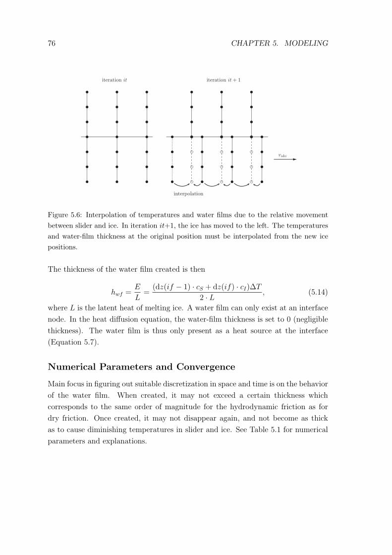
76 CHAPTER 5. MODELING
t
t
t
t
t
t
t
t
t
t
t
t
t
t
t
t
t
t
t
t
t
t
t
t
t
t
t
t
t
t
t
t
t
t
t
t
t
t
t
t
t
t
t
t
t
t
t
t
t
d
d
d
d
d
d
d
d
d
d
d
d
-
vski
iteration it iteration it + 1
interpolation
Figure 5.6: Interpolation of temperatures and water films due to the relative movementbetween slider and ice. In iteration it+1, the ice has moved to the left. The temperaturesand water-film thickness at the original position must be interpolated from the new icepositions.
The thickness of the water film created is then
hwf =E
L=
(dz(if − 1) · cS + dz(if) · cI)∆T
2 · L , (5.14)
where L is the latent heat of melting ice. A water film can only exist at an interface
node. In the heat diffusion equation, the water-film thickness is set to 0 (negligible
thickness). The water film is thus only present as a heat source at the interface
(Equation 5.7).
Numerical Parameters and Convergence
Main focus in figuring out suitable discretization in space and time is on the behavior
of the water film. When created, it may not exceed a certain thickness which
corresponds to the same order of magnitude for the hydrodynamic friction as for
dry friction. Once created, it may not disappear again, and not become as thick
as to cause diminishing temperatures in slider and ice. See Table 5.1 for numerical
parameters and explanations.
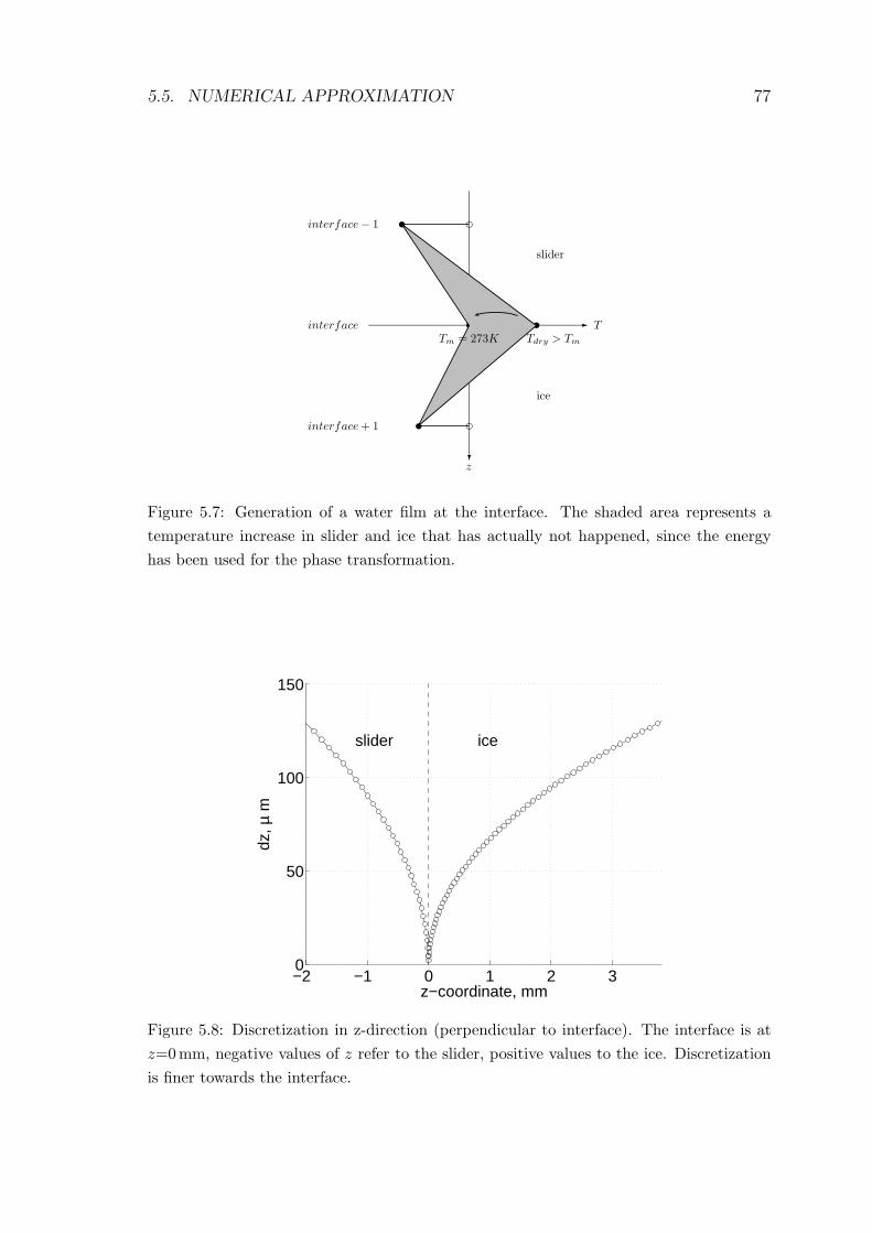
5.5. NUMERICAL APPROXIMATION 77
-
?
T
z
t
t
t t
d
d
interface − 1
interface
interface + 1
slider
ice
Tm = 273K Tdry > Tm
Figure 5.7: Generation of a water film at the interface. The shaded area represents atemperature increase in slider and ice that has actually not happened, since the energyhas been used for the phase transformation.
−2 −1 0 1 2 30
50
100
150
z−coordinate, mm
dz, µ
m
slider ice
Figure 5.8: Discretization in z-direction (perpendicular to interface). The interface is atz=0mm, negative values of z refer to the slider, positive values to the ice. Discretizationis finer towards the interface.
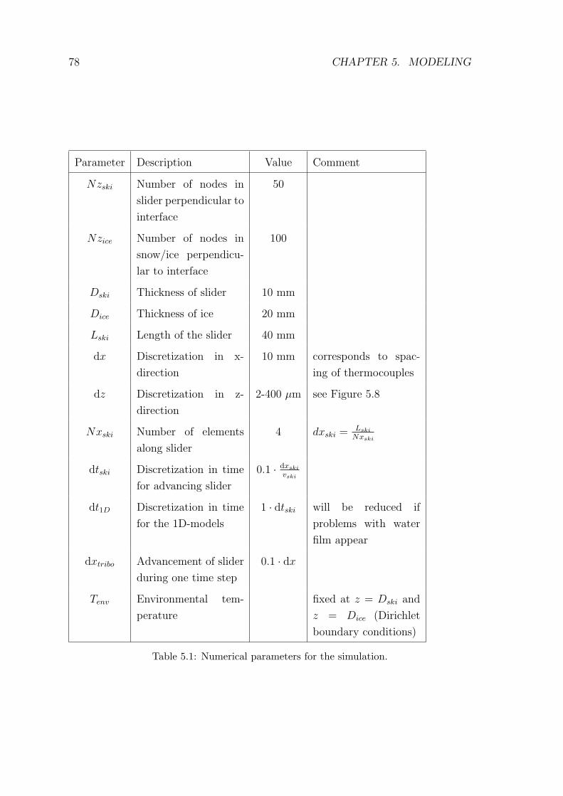
78 CHAPTER 5. MODELING
Parameter Description Value Comment
Nzski Number of nodes in
slider perpendicular to
interface
50
Nzice Number of nodes in
snow/ice perpendicu-
lar to interface
100
Dski Thickness of slider 10 mm
Dice Thickness of ice 20 mm
Lski Length of the slider 40 mm
dx Discretization in x-
direction
10 mm corresponds to spac-
ing of thermocouples
dz Discretization in z-
direction
2-400 µm see Figure 5.8
Nxski Number of elements
along slider
4 dxski = Lski
Nxski
dtski Discretization in time
for advancing slider
0.1 · dxski
vski
dt1D Discretization in time
for the 1D-models
1 · dtski will be reduced if
problems with water
film appear
dxtribo Advancement of slider
during one time step
0.1 · dx
Tenv Environmental tem-
perature
fixed at z = Dski and
z = Dice (Dirichlet
boundary conditions)
Table 5.1: Numerical parameters for the simulation.
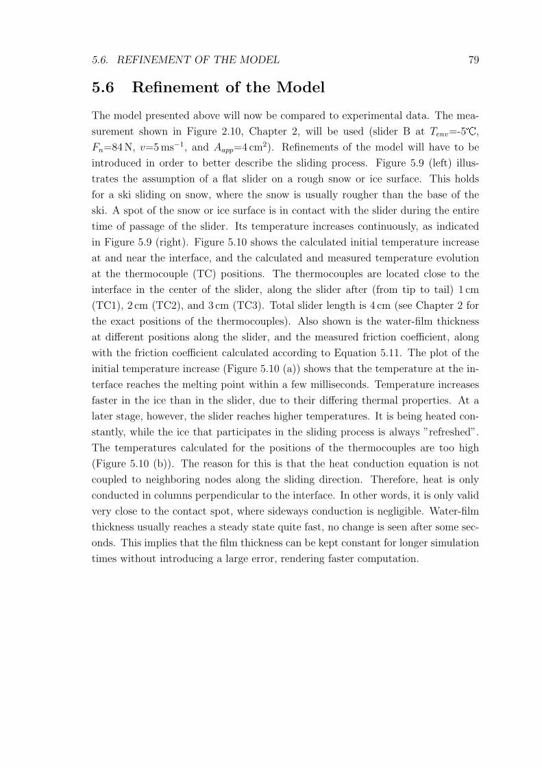
5.6. REFINEMENT OF THE MODEL 79
5.6 Refinement of the Model
The model presented above will now be compared to experimental data. The mea-
surement shown in Figure 2.10, Chapter 2, will be used (slider B at Tenv=-5�,
Fn=84N, v=5ms−1, and Aapp=4 cm2). Refinements of the model will have to be
introduced in order to better describe the sliding process. Figure 5.9 (left) illus-
trates the assumption of a flat slider on a rough snow or ice surface. This holds
for a ski sliding on snow, where the snow is usually rougher than the base of the
ski. A spot of the snow or ice surface is in contact with the slider during the entire
time of passage of the slider. Its temperature increases continuously, as indicated
in Figure 5.9 (right). Figure 5.10 shows the calculated initial temperature increase
at and near the interface, and the calculated and measured temperature evolution
at the thermocouple (TC) positions. The thermocouples are located close to the
interface in the center of the slider, along the slider after (from tip to tail) 1 cm
(TC1), 2 cm (TC2), and 3 cm (TC3). Total slider length is 4 cm (see Chapter 2 for
the exact positions of the thermocouples). Also shown is the water-film thickness
at different positions along the slider, and the measured friction coefficient, along
with the friction coefficient calculated according to Equation 5.11. The plot of the
initial temperature increase (Figure 5.10 (a)) shows that the temperature at the in-
terface reaches the melting point within a few milliseconds. Temperature increases
faster in the ice than in the slider, due to their differing thermal properties. At a
later stage, however, the slider reaches higher temperatures. It is being heated con-
stantly, while the ice that participates in the sliding process is always ”refreshed”.
The temperatures calculated for the positions of the thermocouples are too high
(Figure 5.10 (b)). The reason for this is that the heat conduction equation is not
coupled to neighboring nodes along the sliding direction. Therefore, heat is only
conducted in columns perpendicular to the interface. In other words, it is only valid
very close to the contact spot, where sideways conduction is negligible. Water-film
thickness usually reaches a steady state quite fast, no change is seen after some sec-
onds. This implies that the film thickness can be kept constant for longer simulation
times without introducing a large error, rendering faster computation.
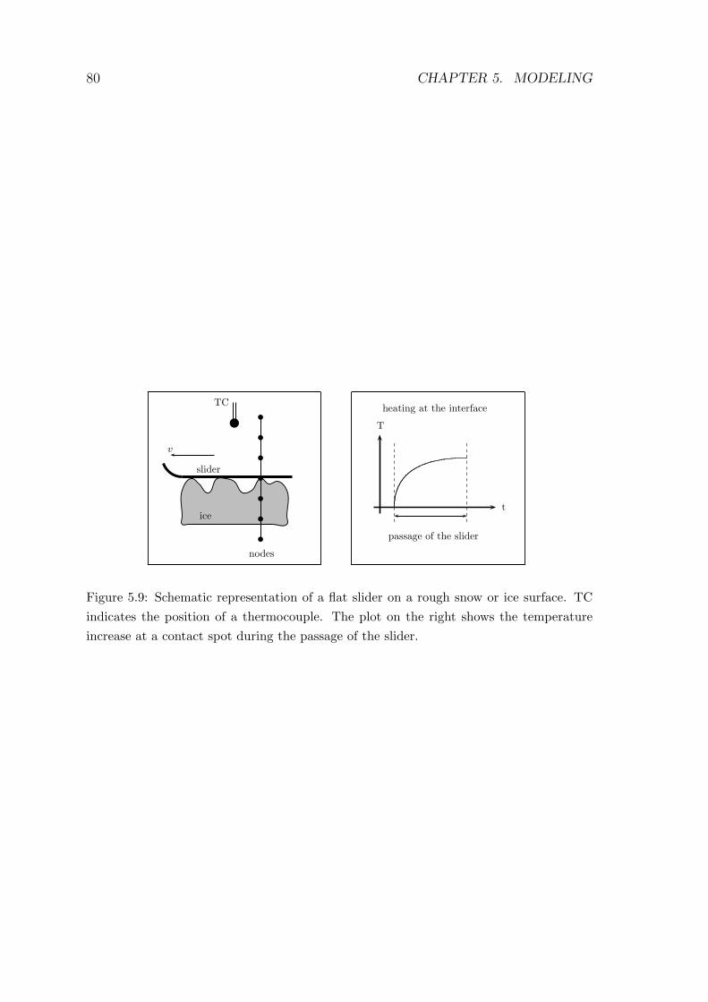
80 CHAPTER 5. MODELING
ice
slider
x
TC
t
t
t
t
t
t
t
v
nodes
T
t
passage of the slider
heating at the interface
Figure 5.9: Schematic representation of a flat slider on a rough snow or ice surface. TCindicates the position of a thermocouple. The plot on the right shows the temperatureincrease at a contact spot during the passage of the slider.
5.6. REFINEMENT OF THE MODEL 81
0 0.02 0.04 0.06 0.08 0.1−5
−4
−3
−2
−1
0
Time, s
Tem
pera
ture
, deg
C
x=20 mm
interface2.2 µ m (ice)−4.3 µ m (ski)
(a) Initial temperature increase.
0 1 2 3 4 5 6 7 8 9 10−5
−4
−3
−2
−1
0
Time, s
Tem
pera
ture
, deg
C
TC1 expTC1 simTC2 expTC2 simTC3 expTC3 sim
(b) Temperature at the TC positions.
0 1 2 3 4 5 6 7 8 9 100
1
2
3
4
5
6x 10
−7
Time, s
Wat
er fi
lm th
ickn
ess,
m
0 1 2 3 4 5 6 7 8 9 100
0.02
0.04
0.06
0.08
0.1
Fric
tion
coef
ficie
nt
hwf
at x=0 mm
hwf
at x=10 mm
hwf
at x=20 mm
hwf
at x=30 mm
hwf
at x=40 mm
µ expµ sim
(c) Water-film thickness and friction coefficient.
Figure 5.10: Results of a calculation using the ’unrefined’ model (lines), and comparisonto experimental data (open and closed symbols). relRCA=1%.
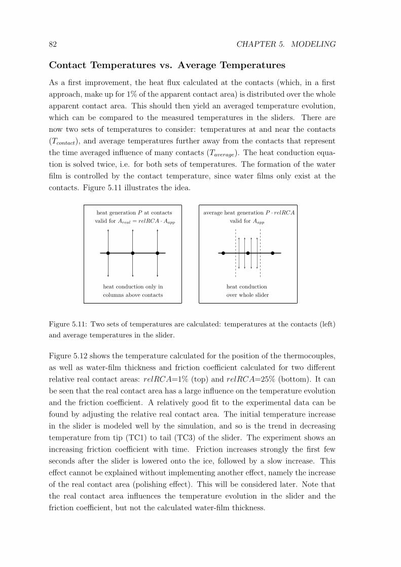
82 CHAPTER 5. MODELING
Contact Temperatures vs. Average Temperatures
As a first improvement, the heat flux calculated at the contacts (which, in a first
approach, make up for 1% of the apparent contact area) is distributed over the whole
apparent contact area. This should then yield an averaged temperature evolution,
which can be compared to the measured temperatures in the sliders. There are
now two sets of temperatures to consider: temperatures at and near the contacts
(Tcontact), and average temperatures further away from the contacts that represent
the time averaged influence of many contacts (Taverage). The heat conduction equa-
tion is solved twice, i.e. for both sets of temperatures. The formation of the water
film is controlled by the contact temperature, since water films only exist at the
contacts. Figure 5.11 illustrates the idea.
u u u
heat conduction only in
columns above contacts
heat generation P at contacts
valid for Areal = relRCA · Aapp
u u u
heat conduction
over whole slider
average heat generation P · relRCA
valid for Aapp
Figure 5.11: Two sets of temperatures are calculated: temperatures at the contacts (left)and average temperatures in the slider.
Figure 5.12 shows the temperature calculated for the position of the thermocouples,
as well as water-film thickness and friction coefficient calculated for two different
relative real contact areas: relRCA=1% (top) and relRCA=25% (bottom). It can
be seen that the real contact area has a large influence on the temperature evolution
and the friction coefficient. A relatively good fit to the experimental data can be
found by adjusting the relative real contact area. The initial temperature increase
in the slider is modeled well by the simulation, and so is the trend in decreasing
temperature from tip (TC1) to tail (TC3) of the slider. The experiment shows an
increasing friction coefficient with time. Friction increases strongly the first few
seconds after the slider is lowered onto the ice, followed by a slow increase. This
effect cannot be explained without implementing another effect, namely the increase
of the real contact area (polishing effect). This will be considered later. Note that
the real contact area influences the temperature evolution in the slider and the
friction coefficient, but not the calculated water-film thickness.
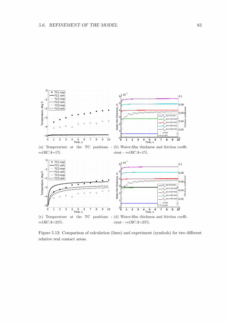
5.6. REFINEMENT OF THE MODEL 83
0 1 2 3 4 5 6 7 8 9 10−5
−4
−3
−2
−1
0
Time, s
Tem
pera
ture
, deg
C
TC1 expTC1 simTC2 expTC2 simTC3 expTC3 sim
(a) Temperature at the TC positions -relRCA=1%.
0 1 2 3 4 5 6 7 8 9 100
1
2
3
4
5
6x 10
−7
Time, s
Wat
er fi
lm th
ickn
ess,
m
0 1 2 3 4 5 6 7 8 9 100
0.02
0.04
0.06
0.08
0.1
Fric
tion
coef
ficie
nt
hwf
at x=0 mm
hwf
at x=10 mm
hwf
at x=20 mm
hwf
at x=30 mm
hwf
at x=40 mm
µ expµ sim
(b) Water-film thickness and friction coeffi-cient - relRCA=1%.
0 1 2 3 4 5 6 7 8 9 10−5
−4
−3
−2
−1
0
Time, s
Tem
pera
ture
, deg
C
TC1 expTC1 simTC2 expTC2 simTC3 expTC3 sim
(c) Temperature at the TC positions -relRCA=25%.
0 1 2 3 4 5 6 7 8 9 100
1
2
3
4
5
6x 10
−7
Time, s
Wat
er fi
lm th
ickn
ess,
m
0 1 2 3 4 5 6 7 8 9 100
0.02
0.04
0.06
0.08
0.1
Fric
tion
coef
ficie
nth
wf at x=0 mm
hwf
at x=10 mm
hwf
at x=20 mm
hwf
at x=30 mm
hwf
at x=40 mm
µ expµ sim
(d) Water-film thickness and friction coeffi-cient - relRCA=25%.
Figure 5.12: Comparison of calculation (lines) and experiment (symbols) for two differentrelative real contact areas.
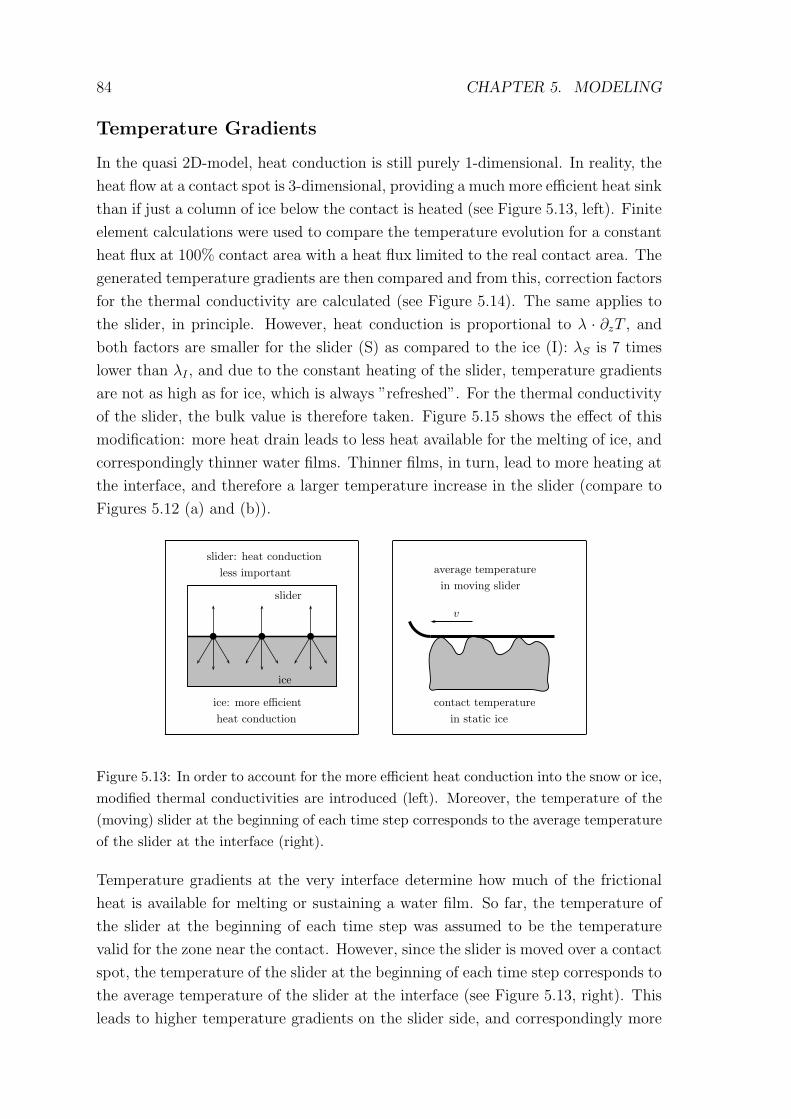
84 CHAPTER 5. MODELING
Temperature Gradients
In the quasi 2D-model, heat conduction is still purely 1-dimensional. In reality, the
heat flow at a contact spot is 3-dimensional, providing a much more efficient heat sink
than if just a column of ice below the contact is heated (see Figure 5.13, left). Finite
element calculations were used to compare the temperature evolution for a constant
heat flux at 100% contact area with a heat flux limited to the real contact area. The
generated temperature gradients are then compared and from this, correction factors
for the thermal conductivity are calculated (see Figure 5.14). The same applies to
the slider, in principle. However, heat conduction is proportional to λ · ∂zT , and
both factors are smaller for the slider (S) as compared to the ice (I): λS is 7 times
lower than λI , and due to the constant heating of the slider, temperature gradients
are not as high as for ice, which is always ”refreshed”. For the thermal conductivity
of the slider, the bulk value is therefore taken. Figure 5.15 shows the effect of this
modification: more heat drain leads to less heat available for the melting of ice, and
correspondingly thinner water films. Thinner films, in turn, lead to more heating at
the interface, and therefore a larger temperature increase in the slider (compare to
Figures 5.12 (a) and (b)).
u u u
slider
slider: heat conduction
less important
ice
ice: more efficient
heat conduction
v
average temperature
in moving slider
contact temperature
in static ice
Figure 5.13: In order to account for the more efficient heat conduction into the snow or ice,modified thermal conductivities are introduced (left). Moreover, the temperature of the(moving) slider at the beginning of each time step corresponds to the average temperatureof the slider at the interface (right).
Temperature gradients at the very interface determine how much of the frictional
heat is available for melting or sustaining a water film. So far, the temperature of
the slider at the beginning of each time step was assumed to be the temperature
valid for the zone near the contact. However, since the slider is moved over a contact
spot, the temperature of the slider at the beginning of each time step corresponds to
the average temperature of the slider at the interface (see Figure 5.13, right). This
leads to higher temperature gradients on the slider side, and correspondingly more
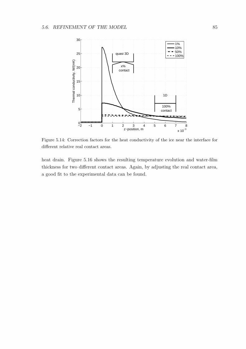
5.6. REFINEMENT OF THE MODEL 85
−2 −1 0 1 2 3 4 5 6 7 8
x 10−3
0
5
10
15
20
25
30
z−position, m
The
rmal
con
duct
ivity
, W/(
mK
)
quasi 3D
x%contact
1D
100%contact
1%10%50%100%
Figure 5.14: Correction factors for the heat conductivity of the ice near the interface fordifferent relative real contact areas.
heat drain. Figure 5.16 shows the resulting temperature evolution and water-film
thickness for two different contact areas. Again, by adjusting the real contact area,
a good fit to the experimental data can be found.
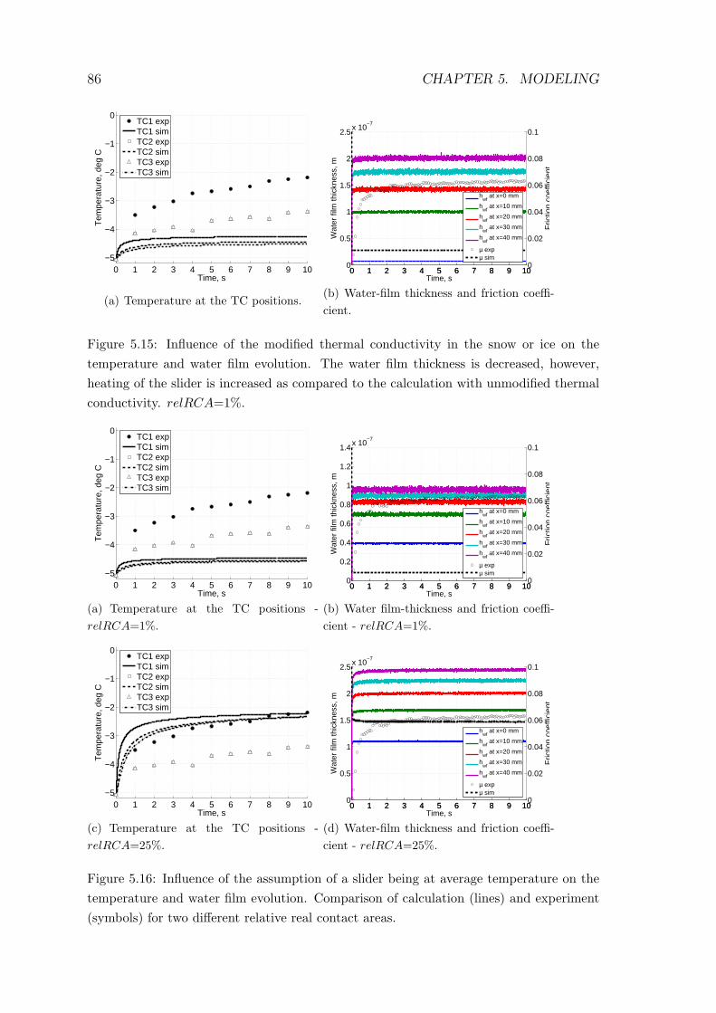
86 CHAPTER 5. MODELING
0 1 2 3 4 5 6 7 8 9 10−5
−4
−3
−2
−1
0
Time, s
Tem
pera
ture
, deg
C
TC1 expTC1 simTC2 expTC2 simTC3 expTC3 sim
(a) Temperature at the TC positions.
0 1 2 3 4 5 6 7 8 9 100
0.5
1
1.5
2
2.5x 10
−7
Time, s
Wat
er fi
lm th
ickn
ess,
m
0 1 2 3 4 5 6 7 8 9 100
0.02
0.04
0.06
0.08
0.1
Fric
tion
coef
ficie
nt
hwf
at x=0 mm
hwf
at x=10 mm
hwf
at x=20 mm
hwf
at x=30 mm
hwf
at x=40 mm
µ expµ sim
(b) Water-film thickness and friction coeffi-cient.
Figure 5.15: Influence of the modified thermal conductivity in the snow or ice on thetemperature and water film evolution. The water film thickness is decreased, however,heating of the slider is increased as compared to the calculation with unmodified thermalconductivity. relRCA=1%.
0 1 2 3 4 5 6 7 8 9 10−5
−4
−3
−2
−1
0
Time, s
Tem
pera
ture
, deg
C
TC1 expTC1 simTC2 expTC2 simTC3 expTC3 sim
(a) Temperature at the TC positions -relRCA=1%.
0 1 2 3 4 5 6 7 8 9 100
0.2
0.4
0.6
0.8
1
1.2
1.4x 10
−7
Time, s
Wat
er fi
lm th
ickn
ess,
m
0 1 2 3 4 5 6 7 8 9 100
0.02
0.04
0.06
0.08
0.1
Fric
tion
coef
ficie
nt
hwf
at x=0 mm
hwf
at x=10 mm
hwf
at x=20 mm
hwf
at x=30 mm
hwf
at x=40 mm
µ expµ sim
(b) Water film-thickness and friction coeffi-cient - relRCA=1%.
0 1 2 3 4 5 6 7 8 9 10−5
−4
−3
−2
−1
0
Time, s
Tem
pera
ture
, deg
C
TC1 expTC1 simTC2 expTC2 simTC3 expTC3 sim
(c) Temperature at the TC positions -relRCA=25%.
0 1 2 3 4 5 6 7 8 9 100
0.5
1
1.5
2
2.5x 10
−7
Time, s
Wat
er fi
lm th
ickn
ess,
m
0 1 2 3 4 5 6 7 8 9 100
0.02
0.04
0.06
0.08
0.1
Fric
tion
coef
ficie
nt
hwf
at x=0 mm
hwf
at x=10 mm
hwf
at x=20 mm
hwf
at x=30 mm
hwf
at x=40 mm
µ expµ sim
(d) Water-film thickness and friction coeffi-cient - relRCA=25%.
Figure 5.16: Influence of the assumption of a slider being at average temperature on thetemperature and water film evolution. Comparison of calculation (lines) and experiment(symbols) for two different relative real contact areas.
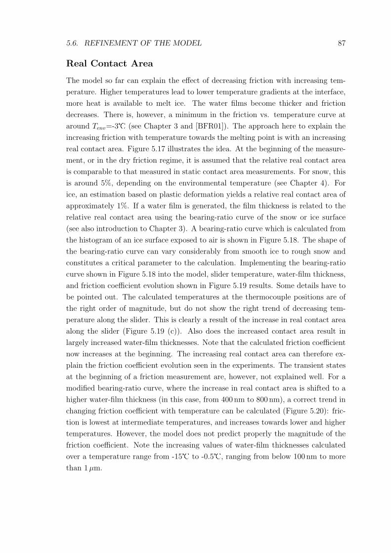
5.6. REFINEMENT OF THE MODEL 87
Real Contact Area
The model so far can explain the effect of decreasing friction with increasing tem-
perature. Higher temperatures lead to lower temperature gradients at the interface,
more heat is available to melt ice. The water films become thicker and friction
decreases. There is, however, a minimum in the friction vs. temperature curve at
around Tenv=-3� (see Chapter 3 and [BFR01]). The approach here to explain the
increasing friction with temperature towards the melting point is with an increasing
real contact area. Figure 5.17 illustrates the idea. At the beginning of the measure-
ment, or in the dry friction regime, it is assumed that the relative real contact area
is comparable to that measured in static contact area measurements. For snow, this
is around 5%, depending on the environmental temperature (see Chapter 4). For
ice, an estimation based on plastic deformation yields a relative real contact area of
approximately 1%. If a water film is generated, the film thickness is related to the
relative real contact area using the bearing-ratio curve of the snow or ice surface
(see also introduction to Chapter 3). A bearing-ratio curve which is calculated from
the histogram of an ice surface exposed to air is shown in Figure 5.18. The shape of
the bearing-ratio curve can vary considerably from smooth ice to rough snow and
constitutes a critical parameter to the calculation. Implementing the bearing-ratio
curve shown in Figure 5.18 into the model, slider temperature, water-film thickness,
and friction coefficient evolution shown in Figure 5.19 results. Some details have to
be pointed out. The calculated temperatures at the thermocouple positions are of
the right order of magnitude, but do not show the right trend of decreasing tem-
perature along the slider. This is clearly a result of the increase in real contact area
along the slider (Figure 5.19 (c)). Also does the increased contact area result in
largely increased water-film thicknesses. Note that the calculated friction coefficient
now increases at the beginning. The increasing real contact area can therefore ex-
plain the friction coefficient evolution seen in the experiments. The transient states
at the beginning of a friction measurement are, however, not explained well. For a
modified bearing-ratio curve, where the increase in real contact area is shifted to a
higher water-film thickness (in this case, from 400 nm to 800 nm), a correct trend in
changing friction coefficient with temperature can be calculated (Figure 5.20): fric-
tion is lowest at intermediate temperatures, and increases towards lower and higher
temperatures. However, the model does not predict properly the magnitude of the
friction coefficient. Note the increasing values of water-film thicknesses calculated
over a temperature range from -15� to -0.5�, ranging from below 100 nm to more
than 1µm.
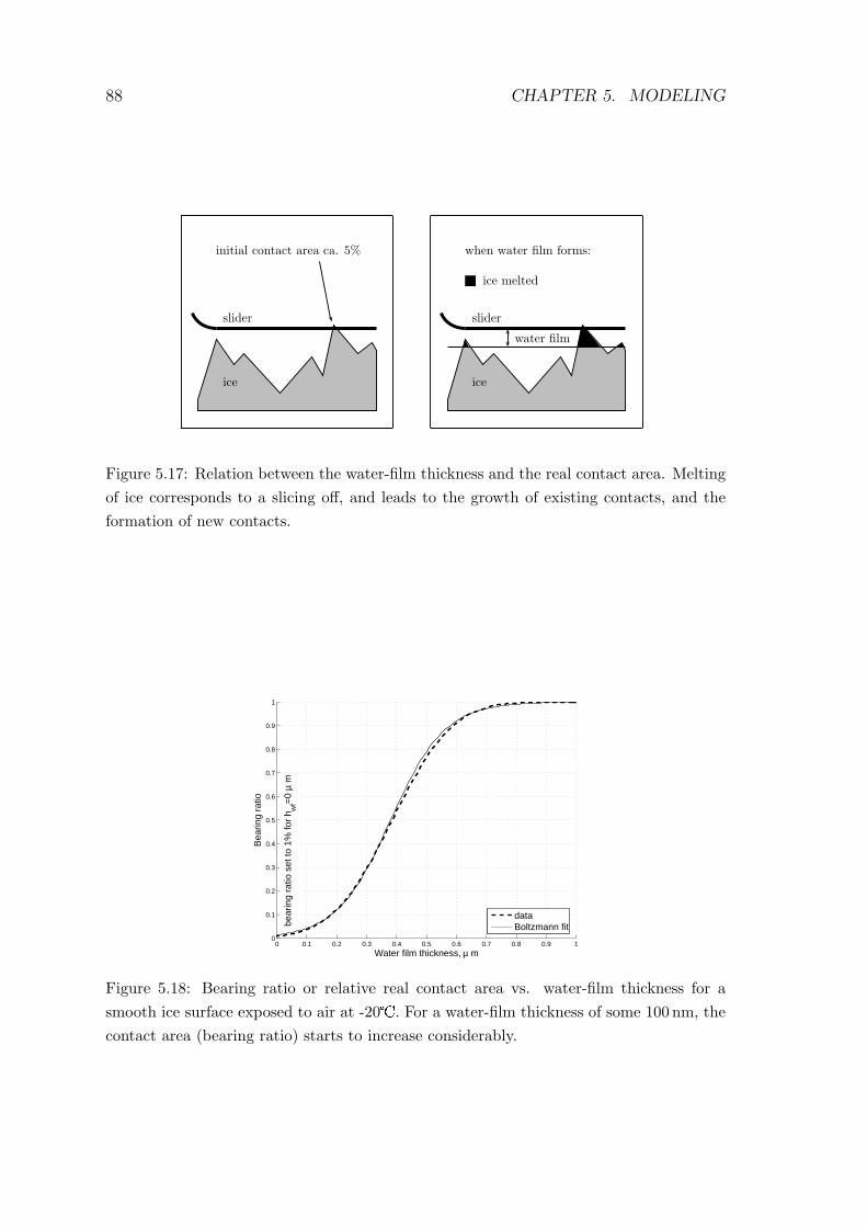
88 CHAPTER 5. MODELING
slider
ice
initial contact area ca. 5%
water film
slider
ice
when water film forms:
ice melted
Figure 5.17: Relation between the water-film thickness and the real contact area. Meltingof ice corresponds to a slicing off, and leads to the growth of existing contacts, and theformation of new contacts.
0 0.1 0.2 0.3 0.4 0.5 0.6 0.7 0.8 0.9 10
0.1
0.2
0.3
0.4
0.5
0.6
0.7
0.8
0.9
1
Water film thickness, µ m
Bea
ring
ratio
bear
ing
ratio
set
to 1
% fo
r h w
f=0
µ m
bear
ing
ratio
set
to 1
% fo
r h w
f=0
µ m
dataBoltzmann fit
Figure 5.18: Bearing ratio or relative real contact area vs. water-film thickness for asmooth ice surface exposed to air at -20�. For a water-film thickness of some 100 nm, thecontact area (bearing ratio) starts to increase considerably.
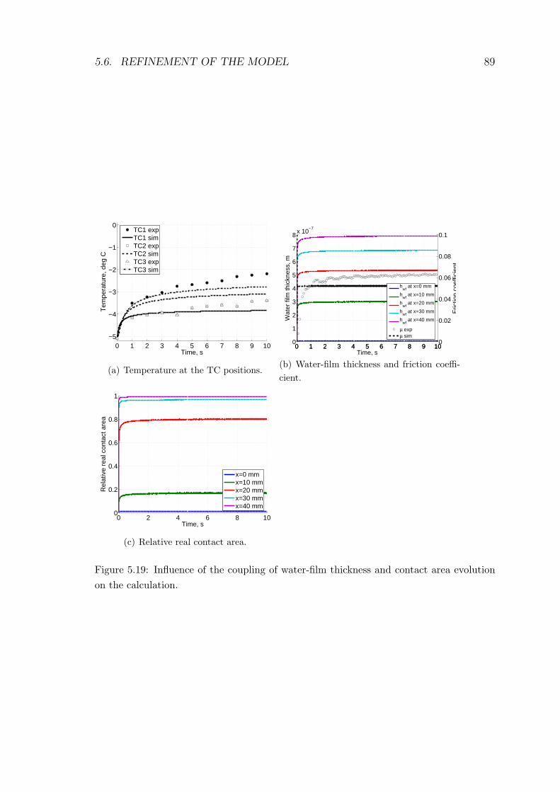
5.6. REFINEMENT OF THE MODEL 89
0 1 2 3 4 5 6 7 8 9 10−5
−4
−3
−2
−1
0
Time, s
Tem
pera
ture
, deg
C
TC1 expTC1 simTC2 expTC2 simTC3 expTC3 sim
(a) Temperature at the TC positions.
0 1 2 3 4 5 6 7 8 9 100
1
2
3
4
5
6
7
8x 10
−7
Time, s
Wat
er fi
lm th
ickn
ess,
m
0 1 2 3 4 5 6 7 8 9 100
0.02
0.04
0.06
0.08
0.1
Fric
tion
coef
ficie
nt
hwf
at x=0 mm
hwf
at x=10 mm
hwf
at x=20 mm
hwf
at x=30 mm
hwf
at x=40 mm
µ expµ sim
(b) Water-film thickness and friction coeffi-cient.
0 2 4 6 8 100
0.2
0.4
0.6
0.8
1
Time, s
Rel
ativ
e re
al c
onta
ct a
rea
x=0 mmx=10 mmx=20 mmx=30 mmx=40 mm
(c) Relative real contact area.
Figure 5.19: Influence of the coupling of water-film thickness and contact area evolutionon the calculation.
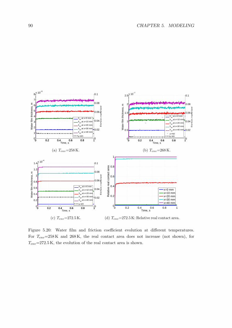
90 CHAPTER 5. MODELING
0 0.2 0.4 0.6 0.8 10
1
2
3
4
5
6
7
8x 10
−8
Time, s
Wat
er fi
lm th
ickn
ess,
m
0 0.2 0.4 0.6 0.8 10
0.02
0.04
0.06
0.08
0.1
Fric
tion
coef
ficie
nt
hwf
at x=0 mm
hwf
at x=10 mm
hwf
at x=20 mm
hwf
at x=30 mm
hwf
at x=40 mm
µ sim
(a) Tenv=258K.
0 0.2 0.4 0.6 0.8 10
0.5
1
1.5
2
2.5x 10
−7
Time, s
Wat
er fi
lm th
ickn
ess,
m
0 0.2 0.4 0.6 0.8 10
0.02
0.04
0.06
0.08
0.1
Fric
tion
coef
ficie
nt
hwf
at x=0 mm
hwf
at x=10 mm
hwf
at x=20 mm
hwf
at x=30 mm
hwf
at x=40 mm
µ expµ sim
(b) Tenv=268K.
0 0.2 0.4 0.6 0.8 10
0.2
0.4
0.6
0.8
1
1.2
1.4x 10
−6
Time, s
Wat
er fi
lm th
ickn
ess,
m
0 0.2 0.4 0.6 0.8 10
0.02
0.04
0.06
0.08
0.1
Fric
tion
coef
ficie
nt
hwf
at x=0 mm
hwf
at x=10 mm
hwf
at x=20 mm
hwf
at x=30 mm
hwf
at x=40 mm
µ sim
(c) Tenv=272.5K.
0 0.2 0.4 0.6 0.8 10
0.2
0.4
0.6
0.8
1
Time, s
Rel
ativ
e re
al c
onta
ct a
rea
x=0 mmx=10 mmx=20 mmx=30 mmx=40 mm
(d) Tenv=272.5K: Relative real contact area.
Figure 5.20: Water film and friction coefficient evolution at different temperatures.For Tenv=258 K and 268 K, the real contact area does not increase (not shown), forTenv=272.5K, the evolution of the real contact area is shown.
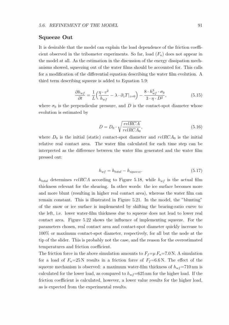
5.6. REFINEMENT OF THE MODEL 91
Squeeze Out
It is desirable that the model can explain the load dependence of the friction coeffi-
cient observed in the tribometer experiments. So far, load (Fn) does not appear in
the model at all. As the estimation in the discussion of the energy dissipation mech-
anisms showed, squeezing out of the water films should be accounted for. This calls
for a modification of the differential equation describing the water film evolution. A
third term describing squeeze is added to Equation 5.9:
∂hwf
∂t=
1
L
(η · v2
hwf
− λ · ∂zT |z=0
)− 8 · h3
wf · σ0
3 · η ·D2, (5.15)
where σ0 is the perpendicular pressure, and D is the contact-spot diameter whose
evolution is estimated by
D = D0 ·√
relRCA
relRCA0
, (5.16)
where D0 is the initial (static) contact-spot diameter and relRCA0 is the initial
relative real contact area. The water film calculated for each time step can be
interpreted as the difference between the water film generated and the water film
pressed out:
hwf = htotal − hsqueeze. (5.17)
htotal determines relRCA according to Figure 5.18, while hwf is the actual film
thickness relevant for the shearing. In other words: the ice surface becomes more
and more blunt (resulting in higher real contact area), whereas the water film can
remain constant. This is illustrated in Figure 5.21. In the model, the ”blunting”
of the snow or ice surface is implemented by shifting the bearing-ratio curve to
the left, i.e. lower water-film thickness due to squeeze does not lead to lower real
contact area. Figure 5.22 shows the influence of implementing squeeze. For the
parameters chosen, real contact area and contact-spot diameter quickly increase to
100% or maximum contact-spot diameter, respectively, for all but the node at the
tip of the slider. This is probably not the case, and the reason for the overestimated
temperatures and friction coefficient.
The friction force in the above simulation amounts to Ff=µFn=7.0N. A simulation
for a load of Fn=25N results in a friction force of Ff=6.6N. The effect of the
squeeze mechanism is observed: a maximum water-film thickness of hwf=710 nm is
calculated for the lower load, as compared to hwf=625 nm for the higher load. If the
friction coefficient is calculated, however, a lower value results for the higher load,
as is expected from the experimental results.
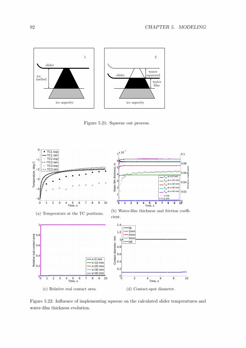
92 CHAPTER 5. MODELING
1
icemelted
slider
ice asperity
2
water
film
water
squeezedslider
ice asperity
Figure 5.21: Squeeze out process.
0 1 2 3 4 5 6 7 8 9 10−5
−4
−3
−2
−1
0
Time, s
Tem
pera
ture
, deg
C
TC1 expTC1 simTC2 expTC2 simTC3 expTC3 sim
(a) Temperature at the TC positions.
0 1 2 3 4 5 6 7 8 9 100
1
2
3
4
5
6
7x 10
−7
Time, s
Wat
er fi
lm th
ickn
ess,
m
0 1 2 3 4 5 6 7 8 9 100
0.02
0.04
0.06
0.08
0.1
Fric
tion
coef
ficie
nt
hwf
at x=0 mm
hwf
at x=10 mm
hwf
at x=20 mm
hwf
at x=30 mm
hwf
at x=40 mm
µ expµ sim
(b) Water-film thickness and friction coeffi-cient.
0 1 2 3 4 5 6 7 8 9 100
0.2
0.4
0.6
0.8
1
Time, s
Rel
ativ
e re
al c
onta
ct a
rea
x=0 mmx=10 mmx=20 mmx=30 mmx=40 mm
(c) Relative real contact area.
0 2 4 6 8 100
0.2
0.4
0.6
0.8
1
1.2
1.4
Time, s
Con
tact
dia
met
er, m
m
tip1mm2mm3mmtail
(d) Contact-spot diameter.
Figure 5.22: Influence of implementing squeeze on the calculated slider temperatures andwater-film thickness evolution.
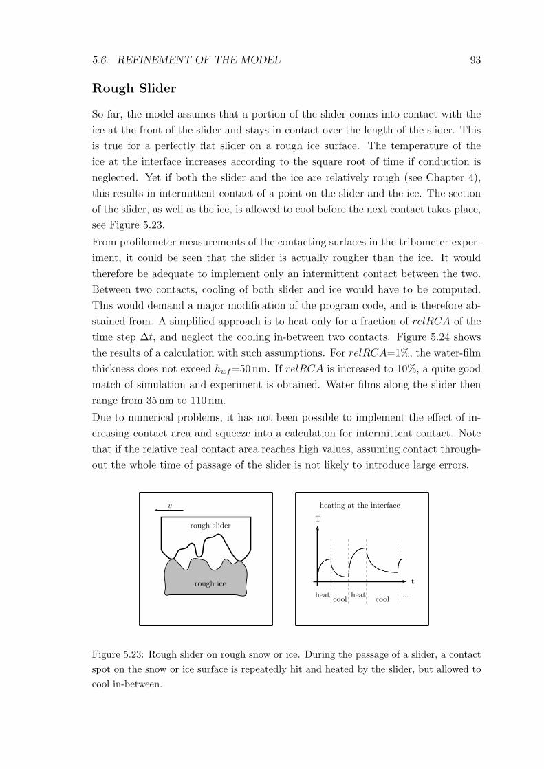
5.6. REFINEMENT OF THE MODEL 93
Rough Slider
So far, the model assumes that a portion of the slider comes into contact with the
ice at the front of the slider and stays in contact over the length of the slider. This
is true for a perfectly flat slider on a rough ice surface. The temperature of the
ice at the interface increases according to the square root of time if conduction is
neglected. Yet if both the slider and the ice are relatively rough (see Chapter 4),
this results in intermittent contact of a point on the slider and the ice. The section
of the slider, as well as the ice, is allowed to cool before the next contact takes place,
see Figure 5.23.
From profilometer measurements of the contacting surfaces in the tribometer exper-
iment, it could be seen that the slider is actually rougher than the ice. It would
therefore be adequate to implement only an intermittent contact between the two.
Between two contacts, cooling of both slider and ice would have to be computed.
This would demand a major modification of the program code, and is therefore ab-
stained from. A simplified approach is to heat only for a fraction of relRCA of the
time step ∆t, and neglect the cooling in-between two contacts. Figure 5.24 shows
the results of a calculation with such assumptions. For relRCA=1%, the water-film
thickness does not exceed hwf=50nm. If relRCA is increased to 10%, a quite good
match of simulation and experiment is obtained. Water films along the slider then
range from 35 nm to 110 nm.
Due to numerical problems, it has not been possible to implement the effect of in-
creasing contact area and squeeze into a calculation for intermittent contact. Note
that if the relative real contact area reaches high values, assuming contact through-
out the whole time of passage of the slider is not likely to introduce large errors.
rough ice
rough slider
v
T
t
heatcool
heatcool
...
heating at the interface
Figure 5.23: Rough slider on rough snow or ice. During the passage of a slider, a contactspot on the snow or ice surface is repeatedly hit and heated by the slider, but allowed tocool in-between.
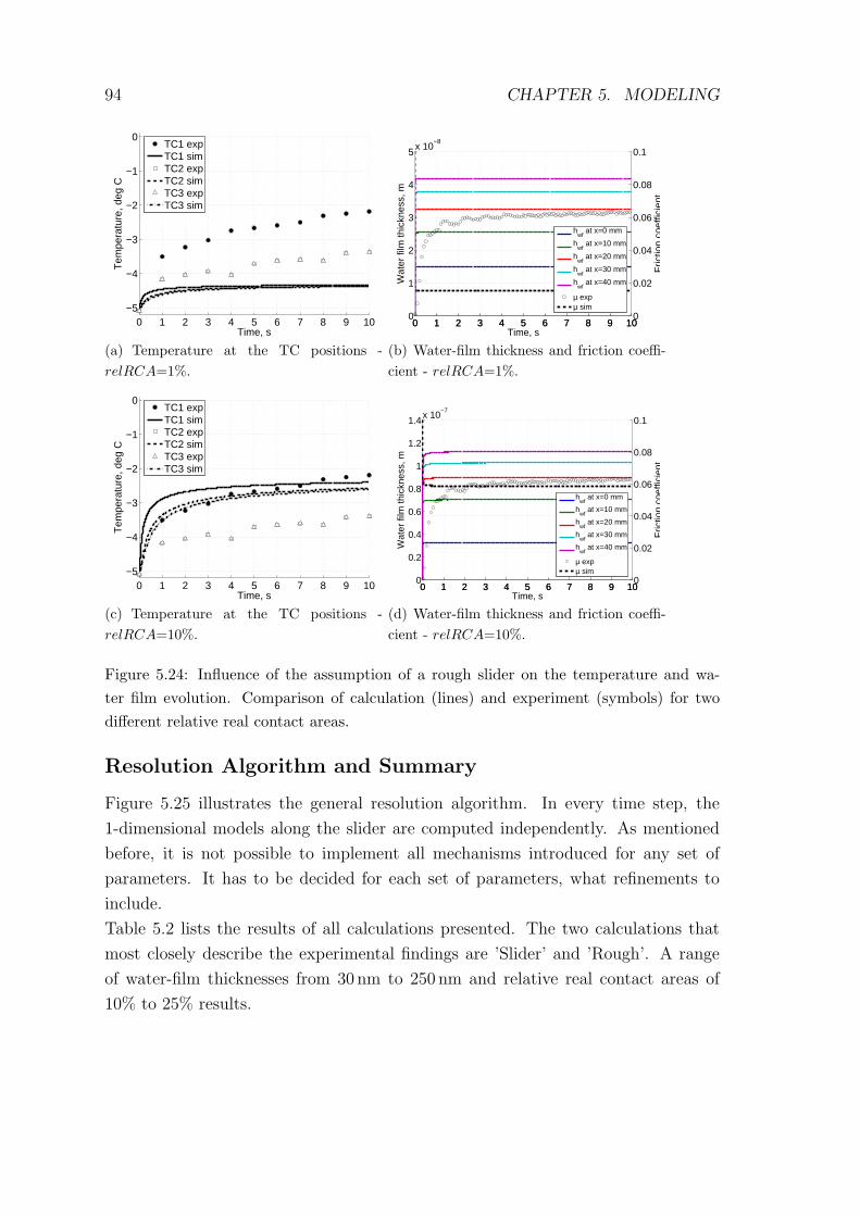
94 CHAPTER 5. MODELING
0 1 2 3 4 5 6 7 8 9 10−5
−4
−3
−2
−1
0
Time, s
Tem
pera
ture
, deg
C
TC1 expTC1 simTC2 expTC2 simTC3 expTC3 sim
(a) Temperature at the TC positions -relRCA=1%.
0 1 2 3 4 5 6 7 8 9 100
1
2
3
4
5x 10
−8
Time, s
Wat
er fi
lm th
ickn
ess,
m
0 1 2 3 4 5 6 7 8 9 100
0.02
0.04
0.06
0.08
0.1
Fric
tion
coef
ficie
nt
hwf
at x=0 mm
hwf
at x=10 mm
hwf
at x=20 mm
hwf
at x=30 mm
hwf
at x=40 mm
µ expµ sim
(b) Water-film thickness and friction coeffi-cient - relRCA=1%.
0 1 2 3 4 5 6 7 8 9 10−5
−4
−3
−2
−1
0
Time, s
Tem
pera
ture
, deg
C
TC1 expTC1 simTC2 expTC2 simTC3 expTC3 sim
(c) Temperature at the TC positions -relRCA=10%.
0 1 2 3 4 5 6 7 8 9 100
0.2
0.4
0.6
0.8
1
1.2
1.4x 10
−7
Time, s
Wat
er fi
lm th
ickn
ess,
m
0 1 2 3 4 5 6 7 8 9 100
0.02
0.04
0.06
0.08
0.1
Fric
tion
coef
ficie
nt
hwf
at x=0 mm
hwf
at x=10 mm
hwf
at x=20 mm
hwf
at x=30 mm
hwf
at x=40 mm
µ expµ sim
(d) Water-film thickness and friction coeffi-cient - relRCA=10%.
Figure 5.24: Influence of the assumption of a rough slider on the temperature and wa-ter film evolution. Comparison of calculation (lines) and experiment (symbols) for twodifferent relative real contact areas.
Resolution Algorithm and Summary
Figure 5.25 illustrates the general resolution algorithm. In every time step, the
1-dimensional models along the slider are computed independently. As mentioned
before, it is not possible to implement all mechanisms introduced for any set of
parameters. It has to be decided for each set of parameters, what refinements to
include.
Table 5.2 lists the results of all calculations presented. The two calculations that
most closely describe the experimental findings are ’Slider’ and ’Rough’. A range
of water-film thicknesses from 30 nm to 250 nm and relative real contact areas of
10% to 25% results.
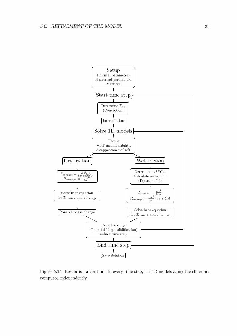
5.6. REFINEMENT OF THE MODEL 95
Setup
Physical parameters
Numerical parameters
Matrices
Start time step
Determine Told
(Convection)
Interpolation
Solve 1D models
Checks
(wf-T-incompatibility,
disappearance of wf)
Dry friction Wet friction
Pcontact =µ·Fn·v
l·w·relRCA
Paverage =µ·Fn·v
l·w
Determine relRCA
Calculate water film
(Equation 5.9)
Solve heat equation
for Tcontact and Taverage
Pcontact =η·v2
hwf
Paverage =η·v2
hwf· relRCA
Possible phase changeSolve heat equation
for Tcontact and Taverage
Error handling
(T diminishing, solidification)
reduce time step
End time step
Save Solution
Figure 5.25: Resolution algorithm. In every time step, the 1D models along the slider arecomputed independently.
96 CHAPTER 5. MODELING
5.7 Application of the Model
Of interest for the design of sliders (e.g. skis) is the dependence of friction on slider
properties such as thermal conductivity or surface roughness.
Thermal Conductivity
It is to be expected that increased thermal conductivity of the slider leads to
higher friction at low temperatures. The simulation (assumption of a rough ski,
relRCA=10%, increase of contact area and squeeze neglected) shows that a thermal
conductivity increased by a factor of 3 (1Wm−1K−1 as compared to 0.34 Wm−1K−1)
in fact leads to a generally decreased water-film thickness (maximum hwf=85nm
as compared to hwf=115 nm ) and an increased friction coefficient (from µ=0.058
to µ=0.075) for the parameters used above: Tenv=-5�, Fn=84N, v=5ms−1, and
Aapp=4 cm2. At temperatures close to Tenv=0�, however, the simulation showed no
change in water-film thicknesses and friction coefficient for a thermal conductivity
increased by a factor of 3. The conclusion is that thermal conductivity has quite
a large influence on friction at lower temperatures, but none close to the melting
point.
Colbeck et al. [CP04] observed that skis with black bases run at a higher temper-
ature than equally constructed skis with transparent ski bases. This is explained
by enhanced absorption of solar radiation by the black base. The absorbed heat
contributes to the production of melt water, facilitating sliding. It is difficult to
estimate the magnitude of the heat from solar radiation reaching the ski base. Yet
it is again to be expected that this effect leads to thicker water films and therefore
lower friction at low temperatures, whereas it does not influence friction at higher
temperatures (above about Tenv=-2�).
Concluding from the above discussion, the current practice of adding carbon black
(soot) to the ski base is beneficial for friction at lower temperatures, due to the
absorbtion of solar heat, but disadvantageous because of increased thermal conduc-
tivity. There are, however, other reasons for the addition of carbon black, namely
increased abrasion resistance and increased electrical conductivity. An increased
electrical conductivity is thought to reduce static charging of the ski base, therefore
reducing dirt adsorption, and consequently reducing friction.
Slider Topography
Figure 5.24 showed the results of the simulations for two different real contact areas.
Remember that the approach was to heat only for a fraction of relRCA of the time
step ∆t, and neglect the cooling in-between two contacts. For a contact that lasts
5.8. CONCLUSION 97
only 0.01 ·∆t, the frictional heating at the interface is only able to generate a water
film in the order of 15 nm to 40 nm (front to back of slider). For a contact that lasts
for 0.1 ·∆t, thicker films are generated (30 nm to 110 nm). However, the real contact
area also increases, leading to higher friction. From this point of view, it would be
beneficial to have few contact spots, but oriented along the sliding direction. The
time of contact must be long enough for the building-up of a thick enough water
film to offer low friction.
5.8 Conclusion
The model explains the evolution of slider temperature and friction coefficient ob-
served in the measurements. Approaches for explaining the temperature and load
dependence of temperature and friction evolution are presented. The main factors
determining friction are the thickness of the water films and the relative real con-
tact area. Thickness of these films is calculated to 30 nm to 250 nm along a slider
at intermediate temperatures (Tenv=-5�). Relative real contact areas are calculated
to 10% to 25%. For lower temperatures (Tenv=-15�), water-film thicknesses below
100 nm, and for higher temperatures (close to the melting temperature) water-film
thicknesses of around 1 µm result. The relative real contact area can increase to
almost 100% in warm conditions (close to 0�). The model can be used to discover
general trends in the dependence of friction on slider properties. However, caution
has to be exercised in providing exact values of water-film thickness and real contact
area.
The range of physical parameters (Tenv, Fn, v, Aapp) that do not result in numerical
problems is currently very limited. Also is the calculation very sensitive to input
parameters as bearing-ratio curve, or contact-spot diameter. More work has to be
done in order to come up with a comprehensive model that can describe the friction
process for a larger range of parameters.
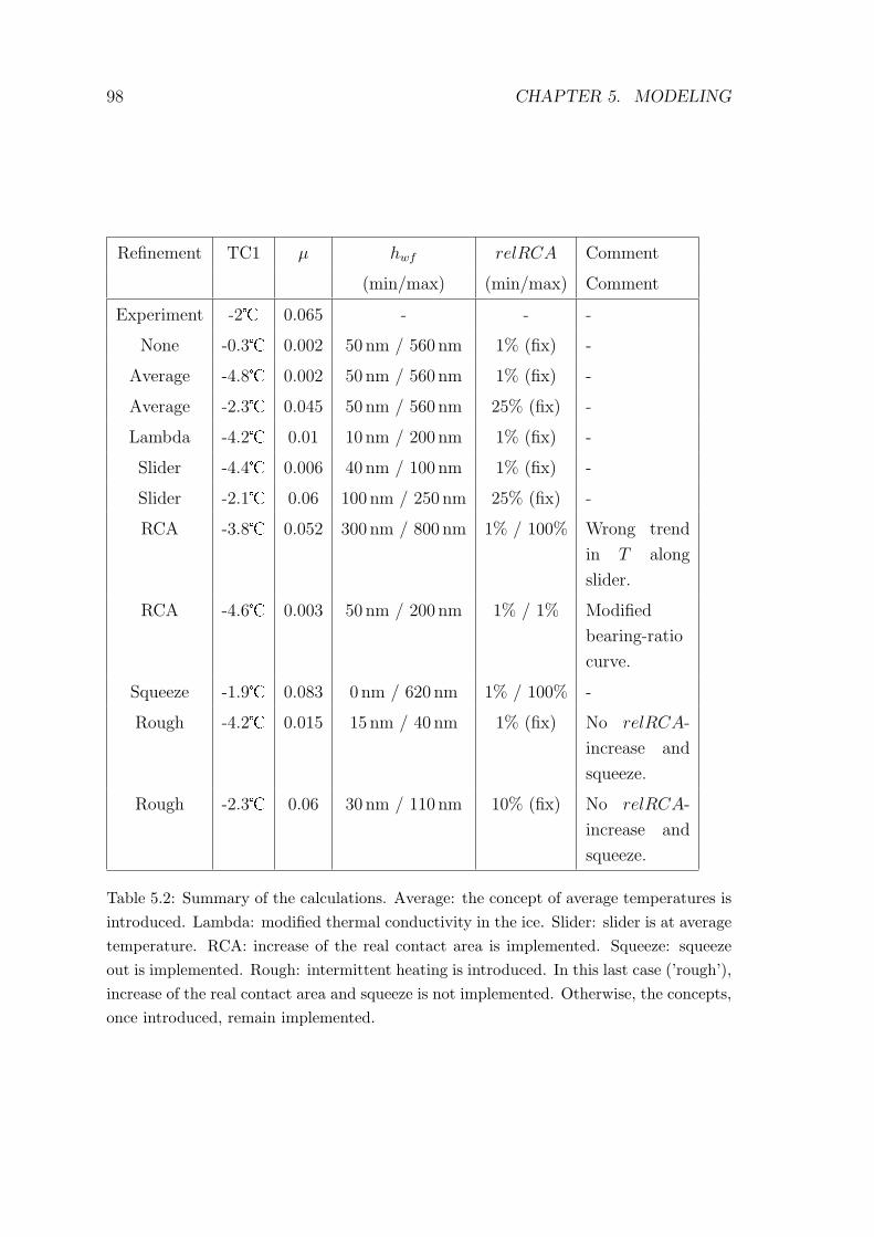
98 CHAPTER 5. MODELING
Refinement TC1 µ hwf relRCA Comment
(min/max) (min/max) Comment
Experiment -2� 0.065 - - -
None -0.3� 0.002 50 nm / 560 nm 1% (fix) -
Average -4.8� 0.002 50 nm / 560 nm 1% (fix) -
Average -2.3� 0.045 50 nm / 560 nm 25% (fix) -
Lambda -4.2� 0.01 10 nm / 200 nm 1% (fix) -
Slider -4.4� 0.006 40 nm / 100 nm 1% (fix) -
Slider -2.1� 0.06 100 nm / 250 nm 25% (fix) -
RCA -3.8� 0.052 300 nm / 800 nm 1% / 100% Wrong trend
in T along
slider.
RCA -4.6� 0.003 50 nm / 200 nm 1% / 1% Modified
bearing-ratio
curve.
Squeeze -1.9� 0.083 0 nm / 620 nm 1% / 100% -
Rough -4.2� 0.015 15 nm / 40 nm 1% (fix) No relRCA-
increase and
squeeze.
Rough -2.3� 0.06 30 nm / 110 nm 10% (fix) No relRCA-
increase and
squeeze.
Table 5.2: Summary of the calculations. Average: the concept of average temperatures isintroduced. Lambda: modified thermal conductivity in the ice. Slider: slider is at averagetemperature. RCA: increase of the real contact area is implemented. Squeeze: squeezeout is implemented. Rough: intermittent heating is introduced. In this last case (’rough’),increase of the real contact area and squeeze is not implemented. Otherwise, the concepts,once introduced, remain implemented.
Chapter 6
Conclusions and Outlook
A hydrodynamic approach is successfully used to explain the friction forces and
temperature evolution measured. The main factors determining friction are the
thickness of the water films and the relative real contact area. Unevenly distributed
thin water films are responsible for the low friction observed. Thickness of these films
is calculated to 30-250 nm along the slider at intermediate temperatures (Tenv=-5�).
Average static contact area with snow is around 5%, with contact spot diameters of
approximately 100µm (flat PE sample on fine grained snow at Tenv=-10�). Both
these values depend considerably on temperature and snow type. Behavior of the
water films and size of the real contact area can explain the friction process, no
capillary attachments are needed. The most critical parameter determining friction
between skis and snow or ice is the real contact area.
The tribometer at its present state allows for the reproducible measurement of fric-
tion on ice. It has been seen that trends seen in the laboratory measurements are
not always obeyed in real skiing. This is thought to be due to the difference between
sliding on snow as compared to ice. Laboratory measurements on snow are therefore
desired. An approach to producing a snow or snow-like surface on the tribometer
is to sieve snow onto the track during a friction measurement, with the instrument
running. First attempts using an industrial dryer to have the snow grains stick to
the underlying ice yielded promising results, but more work is needed. The studies
could then be extended to friction on snow.
As far as friction on ice is concerned, the studies with sliders exhibiting defined
surface topographies can be extended first to more relatively simple patterns, and
later even to complex structures. Apart from that, a systematic examination of the
influence of the chemical properties of a surface can be carried out. Attention has to
be paid, however, to differentiate between chemical and topographical effects, e.g.
the materials compared must exhibit identical surface topographies.
For an improved determination of the contact area between a slider and snow or ice,
the influence of creep of snow and ice must be considered. More extensively and
99
100 CHAPTER 6. CONCLUSIONS AND OUTLOOK
carefully conducted SEM measurements of snow surfaces that have seen passes with
a slider seem to be a promising approach.
With the present model, the influence of the chemical properties of the slider surface
on friction cannot be investigated. There is considerable debate about the use of
waxes with regard to rendering the ski base more hydrophobic. In the model, it is
assumed that the relative velocity at the ice-water interface is 0, while the relative
velocity at the water-slider interface equals the velocity of the slider. For the rather
hydrophobic polyethylene, it can be expected that the surface is not wetted by
the lubricating water, which may result in a weaker shear mechanism. There are,
however, limits to the possibilities of a quasi-2D simulation. A real 2D-simulation
is likely to overcome some of the numerical problems.

Appendix A
Notation
Table A.1: List of symbols - physical properties.
a radius of a circular contact [m]
Aapp apparent contact area [m2]
Areal real contact area [m2]
cp specific heat capacity [J kg−1 K−1]
D diameter of a circular contact [m]
E Young’s modulus [Pa]
E∗ Reduced modulus [Pa]
fp fraction of plastic deformation [-]
Ff friction force [N]
Fn load, normal force [N]
F ∗n load at a contact [N]
hwf water-film thickness [m]
l rms width of the ADF [m]
L volumetric latent heat of fusion [J m−3]
n number of contact spots [-]
p pressure [Pa]
p0 maximum pressure at a contact [Pa]
pm mean pressure at a contact [Pa]
P heat generation [W]
q′′z heat flux, heat current [W m−2]
Q heat [J]
r radius of curvature of an asperity [m]
relRCA relative real contact area [-]
continued on next page
101
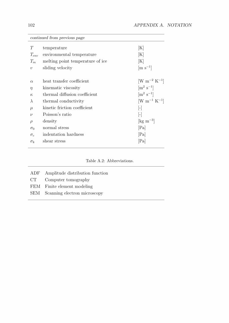
102 APPENDIX A. NOTATION
continued from previous page
T temperature [K]
Tenv environmental temperature [K]
Tm melting point temperature of ice [K]
v sliding velocity [m s−1]
α heat transfer coefficient [W m−2 K−1]
η kinematic viscosity [m2 s−1]
κ thermal diffusion coefficient [m2 s−1]
λ thermal conductivity [W m−1 K−1]
µ kinetic friction coefficient [-]
ν Poisson’s ratio [-]
ρ density [kg m−3]
σ0 normal stress [Pa]
σc indentation hardness [Pa]
σk shear stress [Pa]
Table A.2: Abbreviations.
ADF Amplitude distribution function
CT Computer tomography
FEM Finite element modeling
SEM Scanning electron microscopy
Bibliography
[AM81] W. Ambach and B. Mayr. Ski gliding and water film. Cold Regions
Science and Technology, 5:59–65, 1981.
[BFR01] D. Buhl, M. Fauve, and H. Rhyner. The kinetic friction of polyethylene
on snow: the influence of the snow temperature and the load. Cold
Regions Science and Technology, 33:133–140, 2001.
[BH39] F.P. Bowden and T.P. Hughes. The mechanism of sliding on ice and snow.
Proceedings of the Royal Society of London. Series A, Mathematical and
Physical Sciences, 172:280–298, 1939.
[Bhu02] B. Bhushan. Introduction to Tribology. John Wiley & Sons, New York,
2002.
[BOF+02] H. Bluhm, D.F. Ogletree, C. Fadley, Z. Hussain, and M. Salmeron. The
premelting of ice studied with photoelectron spectroscopy. Journal of
Physics: Condensed Matter, 14:L227–L233, 2002.
[Bow53] F.P. Bowden. Friction on snow and ice. Proceedings of the Royal Society
of London. Series A, Mathematical and Physical Sciences, 217:462–478,
1953.
[Col88] S.C. Colbeck. The kinetic friction of snow. Journal of Glaciology,
34(116):78–86, 1988.
[Col92] S.C. Colbeck. A review of the processes that control snow friction. CR-
REL Report, 92-2, 1992.
[Col96] S.C. Colbeck. Capillary bonding to wet surfaces. Surface & Coatings
Technology, 81:209–214, 1996.
[CP04] S.C. Colbeck and D.K. Perovich. Temperature effects of black versus
white polyethylene bases for snow skis. Cold Regions Science and Tech-
nology, 39:33–38, 2004.
103
104 BIBLIOGRAPHY
[DB00] A. Doeppenschmidt and H.J. Butt. Measuring the thickness of the liquid-
like layer on ice surfaces with afm. Langmuir, 16:6709–6714, 2000.
[DKB98] A. Doeppenschmidt, M. Kappel, and H.J. Butt. Surface properties of
ice studied by atomic force microscopy. Journal of Physical Chemistry
B, 102:7813–7819, 1998.
[DLB95] J.H. Dosch, A. Lied, and J.H. Bilgram. Glancing x-ray scattering studies
of the premelting of ice surfaces. Surface Science, 327:145–164, 1995.
[DZM+05] S. Ducret, H. Zahouania, A. Midola, P. Lanterib, and T.G. Mathia.
Friction and abrasive wear of uhmwpe sliding on ice. Wear, 258:26–31,
2005.
[ENC76] D.C.B. Evans, J.F. Nye, and K.J. Cheesman. The kinetic friction of ice.
Proceedings of the Royal Society of London. Series A, Mathematical and
Physical Sciences, 347(1651):493–512, 1976.
[Flo83] A. Floquet. Thermal considerations in the design of tribometers. Wear,
88:45–56, 1983.
[GG72] W. Gnoerich and K.A. Grosch. The friction of polymers on ice. Journal
of the Institution of the Rubber Industry, 6:192–196, 1972.
[Gle87] B. Glenne. Sliding friction and boundary lubrication of snow. Transac-
tions of the ASME, 109:614, 1987.
[God95] D. Godfrey. Friction oscillations with a pin-on-disc tribometer. Tribology
International, 28(2):119–126, 1995.
[Hob74] P.V. Hobbes. Ice Physics. Clarendon Press, Oxford, 1974.
[ID02] F.P. Incropera and D.P. DeWitt. Fundamentals of Heat and Mass Trans-
fer. John Wiley & Sons, New York, 2002.
[Isr90] J. Israelachvili. Liquid dynamics in molecularly thin films. Journal of
Physics: Condensed Matter, 2:SA89–SA98, 1990.
[Joh85] K.L. Johnson. Contact Mechanics. Cambridge University Press, 1985.
[Kei78] J. Keinonen. An experimental device for measuring friction between ski
and snow. Acta Polytechnica Scandinavica. Applied Physics Series, 123,
1978.
[Kur77] D. Kuroiwa. The kinetic friction on snow and ice. Journal of Glaciology,
19(81):141–152, 1977.
BIBLIOGRAPHY 105
[Leh89] A. Lehtovaara. Kinetic Friction between Ski and Snow. PhD thesis,
Tampere University of Technology, 1989.
[OK82] P. Oksanen and J. Keinonen. The mechanism of friction of ice. Wear,
78:315–324, 1982.
[PC95] V. F. Petrenko and S.C. Colbeck. Generation of electric fields by ice and
snow friction. Journal of Applied Physics, 77(9):4518–4521, 1995.
[Per00] B. Persson. Sliding Friction: Physical Principles and Applications.
Springer, Berlin, 2000.
[Pet03] J.J. Petrovic. Review mechanical properties of ice and snow. Journal of
Materials Science, 38:1–6, 2003.
[PS86] P. Pihkala and E. Spring. Determination of the contact area between ski
and snow using a simple thermal conductivity meter. Report Series in
Geophysics, 22, Helsinki, 1986.
[Rav02] U. Raviv. Viscosity of ultra-thin water films confined between hydropho-
bic or hydrophilic surfaces. Journal of Physics: Condensed Matter,
14:9275–9283, 2002.
[RWE96] A. Rango, W.P. Wergin, and E.F. Erbe. Snow crystal imaging using
scanning electron microscopy. Hydrological Sciences Journal, 41(2):219–
234, 1996.
[SJSB97] L.H. Shapiro, J.B. Johnson, M. Sturm, and G.L. Blaisdell. Snow me-
chanics. CRREL Report, 97-3, 1997.
[SKd+06] M. Schuler, T.P Kuenzler, M. deWild, C.M. Sprecher, M. Textor, D.M.
Brunette, and S. Tosatti. Production and use of tio2-coated epoxy repli-
cas with dual-type topographies for cell proliferation and morphology
investigations. in preparation, 2006.
[SKLA98] H. Strausky, J.R. Krenn, F.R. Leitner, and F.R. Aussenegg. Sliding
plastic on ice: fluorescence spectroscopic studies on interfacial water
layers in the micrometer thickness regime. Applied Physics B, 66:599–
602, 1998.

Lukas Baurle
Sagenstrasse 50
6030 Ebikon
Date of birth June 16, 1976
Nationality Swiss
Phone +41 41 440 62 33
E-mail [email protected]
Education
2002 - 2006 Swiss Federal Institute for Snow and Avalanche Research (SLF),
Davos, and Swiss Federal Institute of Technology (ETH), Zurich,
Switzerland. Ph.D. in materials science and engineering. Thesis
subject: friction of polyethylene on snow and ice.
1997 - 2002 ETH Zurich, Switzerland. Studies of materials science and en-
gineering, concluded with earning a degree in materials science
and engineering (Dipl. Werkstoff-Ingenieur ETH, equivalent to
M.S. degree). Diploma thesis in the field of polymer wear.
1994 - 1995 High school year in Kansas City, USA.
1989 - 1997 Kantonsschule, Lucerne, Switzerland. Focus on mathematics
and natural sciences (Matura, Typus C).
Work Experience
2003 - 2005 SLF Davos. Cooperation in a CTI project ”Sliding friction on
snow”.
2001 - 2002 Teachers training college, Lucerne, Switzerland. Mathematics
teacher (part-time).
2000 (3 months) Instituto Nacional de Tecnologia Industrial, Buenos Aires, Ar-
gentina. Internship in the field of materials testing.
1998 - 2000 ETH Zurich, Insitute of Forming Technologies. Research assis-
tent.


![library.dip.go.thlibrary.dip.go.th/multim6/edoc/2556/21487.pdf · (F) anuaa ball-on-disk [1] Coefficient of friction (g) Tribometer ball-on-disk SPECIAL th EA URE anuaa Tribometer](https://img.pdfslide.us/doc/110x75/5e08e38a3bb35b4943166407/f-anuaa-ball-on-disk-1-coefficient-of-friction-g-tribometer-ball-on-disk-special.jpg)