Inflation, Demand for Liquidity and Welfare∗

Shutao Cao† Cesaire A. Meh‡ Jose-Vıctor Rıos-Rull§ Yaz Terajima¶

December 6, 2012

Preliminary. Please do not circulate or quote.

Abstract

Cross-sectional data show that money holding differs significantly over household con-

sumption and age. Liquidity demand for money (i.e., money holding per dollar of con-

sumption) decreases as household consumption increases. It also increases with household

age conditional on the level of consumption. Observed age differences in money holdings

contain not only age-specific information but also cohort-specific one. Using a life-cycle

model, this paper disentangles these two effects on money demand and quantifies wel-

fare gains of reducing the long-run inflation rate. We dynamically calibrate the model

to micro data and macroeconomic conditions over time. We find that, although a large

part of the observed cross-sectional age differences in money demand can be accounted

for by some age effects, cohort effects play a non-negligible part, supporting a presence

of financial innovation. In addition, changing inflation has significantly different impacts

across household groups due to their heterogeneity in money holding. When inflation

increases from the 2009 level to 10%, we find the aggregate welfare loss in consumption

to be 1.34%. These losses are accrued mostly by generations that are currently alive and

less by future cohorts. Finally, poorer households lose more than their rich peers.

Keywords: Welfare cost, inflation, demand for money, age and cohort effects.

∗We thank participants in the 2010 Society for Economic Dynamics Annual Meeting, the 16th InternationalConference on Computing in Economics and Finance, the 2010 Econometric Society World Congress, theconference for Sixty Years Since Baumol-Tobin at New York University, and the seminar at Tohoku Universityand the Bank of Japan. Jill Ainsworth, Neil Simpson, Wesley Tse and Xuezhi Liu provided excellent researchassistance, and we also thank Katya Kartashova for sharing data codes. All remaining errors are those of theauthors. The views expressed in this paper are those of the authors and not necessarily those of the Bank ofCanada, the Federal Reserve Bank of Minneapolis or the Federal Reserve System.†Bank of Canada, caos@bankofcanada.ca.‡Bank of Canada, cmeh@bankofcanada.ca.§The University of Minnesota, Federal Reserve Bank of Minneapolis, CAERP, and NBER, vr0j@umn.edu.¶Bank of Canada, yterajima@bankofcanada.ca.

1 Introduction

A literature on money demand has mostly focused on aggregate money demand. In this

paper, using cross-sectional data, we document money demand patterns across household’s

age and social class. Measuring money demand across age based on cross-sectional data

raises a potential issue of whether observed differences are the age effects or the cohort

effects. The potential existence of these two effects implies that an identification of age-

specific money demand requires separating out the cohort effects from those that purely

come from age. Although there is a growing literature documenting heterogeneity over money

holdings of households, there has not been any study disentangling age and cohort effects

of money demand. In addressing this issue, we develop an overlapping generations model

with a choice of cash and credit purchases of consumption goods, where transaction costs of

credit incorporate age and cohort dependence. In addition, an analysis of cohort effects (i.e.,

multiple generations born at different points in time) necessarily requires an incorporation of

time effects on money demand from macroeconomic conditions such as inflation and interest

rates. Hence, we calibrate the model dynamically over a long horizon where macroeconomic

conditions change over time and use cross-sectional money demand patterns over two periods

to disentangle the contributions of age and cohort effects to observed money demand patterns.

We use the calibrated model to conduct analysis on welfare costs of inflation and interest

rate elasticity of money.

We use money-consumption ratio as a measure of money demand for transaction purpose.

Cross-sectional data show that money-consumption ratios increase with household age and

decrease with consumption. Regarding age-specific money demand, on one hand, age would

make credit transaction more costly as potentially complex information processing is required

for credit transactions (e.g., reading fine prints of a credit contract) than it would for money

(i.e., the age effects). On other hand, currently old households would have faced more costly

credit transaction technologies when they were young relative to those that currently young

households face today due to financial innovation (i.e., the cohort effects). We introduce age-

and cohort-dependent credit transaction costs in our model to allow flexibility in capturing

these possibilities. Credit transactions face a fixed cost with respect to total consumption,

increasing credit use relative to the use of money with the level of consumption. This fixed

cost is age specific, giving the model flexibility to capture age variations of money demand.

We also introduce a cohort (or generation) specific parameter in credit transaction costs. Our

1

identification strategy in separating the age and cohort effects is the following. We target two

sets of moments: (i) money-consumption ratios by age given a time period and (ii) money-

consumption ratios across two periods given age. These moments allow us to separately

identify the age and cohort effects as the moment (i) contains information on both age and

cohort effects and the moment (ii) only the cohort effects. We simultaneously calibrate the

age and cohort parameters to match these moments from the model and the data.

The calibrated model replicates money demand variations across households in the data

well. We find that age-dependent cost parameters are increasing with age as well as generating

more elastic money demand with age. Calibrated cohort-dependent cost parameter implies

that credit transaction has become less costly for generations who were born later, an evidence

supporting financial innovation. In addition, the calibrated model allows us to disentangle

how much each of the age and cohort effects contributes to the observed money demand.

By conducting a hypothetical simulation without cohort effects, we find that about 12.5% to

21.5% of the observed money demand variations across age groups in 2009 are coming from

the cohort effects (and the rest from the age effects).

We also conduct welfare analysis of inflation. When inflation is increased from the 2009

level of 1.92% to 10%, we find that aggregate welfare decreases by 1.34%, measure in con-

sumption equivalence. Some part of these losses becomes additional seignorage revenues to

the government. Since this amounts to 0.79%, the net loss to the economy is 0.55%. Our

model of different household types can tell us who bear these losses. This loss is mostly ac-

crued by generations that are alive in 2009, e.g., a loss of almost 2% of average consumption

by 60 year-old households in 2009. On the social class dimension, poor households lose the

most, 2.35% of their average consumption while their rich peers only lose 0.94%.

There is a long list of previous studies measuring the welfare cost of inflation. Lucas

(2000) finds that when the annual inflation rate is reduced from 10 per cent to 0 per cent, the

gain is slightly less than 1 per cent of real income. However, Lucas points out that “...Using

aggregate evidence only, it may not be possible to estimate reliably the gains from reducing

inflation further, ...”. That is, in order to accurately and reliably assess the cost of inflation,

one needs to look into the cross-section evidence on the demand for money. Mulligan and

Sala-i Martin (2000) document that 59 per cent of the U.S. households hold cash and checking

accounts, and do not hold interest-bearing financial assets. This fact is interpreted as the

existence of fixed cost for financial transactions. The fixed cost is one form of dead weight loss

in models of money demand. As the inflation rate decreases, households will hold more cash,

2

and avoid paying the fixed cost of financial transactions. The aggregate dead weight loss is

not necessarily equal to the area under the inverse aggregate money demand curve, except

in extreme cases. Ignoring the fixed (adoption) costs will underestimate the welfare cost of

higher inflation. Attanasio, Guiso, and Jappelli (2002) use a household level data set with

much richer information on cash holding, cash transactions, and usage of ATM cards. They

estimate the demand for cash and for interest-bearing assets, and find that the welfare cost of

inflation varies considerably within the population but is small (0.1 per cent of consumption or

less). Alvarez and Lippi (2009) make important contributes to the analysis of money demand

using micro data. They extend cash-inventory management models of Baumol (1952) and

Tobin (1956) to incorporate precautionary cash holdings due to uncertainty with respect to a

chance to withdraw cash without cost. They use Italian household survey data with detailed

information on cash management to estimate the model. They use the estimated model

for quantitatively analyzing the elasticity of money demand as well as the welfare cost of

inflation. Also related to our study is Ragot (2010) that finds the money across households

is similar to the distribution of financial assets than to that of consumption. It shows that

transaction frictions in the financial market explains 85% of total money demand.

Another important contribution to measuring the welfare cost of inflation is given by Erosa

and Ventura (2002). They extend the Aiyagari model to include the cash-in-advance con-

straint and study the welfare distribution of changing inflation rates. On the other hand, Chiu

and Molico (2010) calibrate a search-theoretical model of demand for money, and find that

the welfare cost of inflation is 40 per cent smaller than that in complete market representative-

agent models, such as Lucas (2000). However, the existing studies often ignore the age profile

of money holding. One of existing studies that analyze age profiles of money is Heer and

Maussner (2007). They document that the money-age profile is hump-shaped in the U.S.,

and money is only weakly correlated with income and wealth.

In the next section, we use the Canadian data and document how money holding varies

with age and consumption. A life-cycle model of demand for money is developed in Section

3, and Section 4 discuss the model calibration. In Section 5, we discuss disentangling age

and cohort effects. Section 6 evaluate welfare from changing inflation. Finally, Section 7

concludes the paper.

3

2 Money demand in Canadian households

Our measure of money demand for transaction purpose is the ratio of money holdings

to consumption. Data availability on both household money holdings and consumption ex-

penditures is limited. In Canada, the Canadian Financial Monitor (CFM) by Ipsos Reid

contains information on household income, expenditure and balance sheets for the 2008-2010

period. CFM also covers the period 1999-2007 but without the information on consumption.1

We focus on the CFM data for most of our analysis, however, in addition, we use another

household survey data set, the Survey of Household Spending (SHS) by Statistics Canada,

for consumption information prior to 2008. The SHS provides detailed annual consumption

information of households since 1999.2

We analyze money holdings and consumption, where our definition of money includes

balances on checking and low-interest rate savings accounts. Since a focus of this paper is to

analyze effects of inflation on households, a broad measure of liquid assets, that are used for

transactions and whose values are sensitive to inflation, is used.3

We define consumption as the household’s sum of gross monthly spending on non-durable

goods, services, and durable goods. Excluded from this consumption definition are the prop-

erty tax and housing services from owned and rented residential properties. Some durable

spending is at the annual frequency, including the purchase of a vehicle, home appliances and

electronics, home furnishings, vacation trips, home renovation. We divide them by twelve to

obtain the monthly average spending on these goods and services.

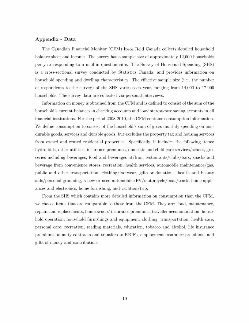
Figure 1 displays average money-consumption ratios over the 1999-2009 period, where

we calculate the average money holdings from the CFM and the average consumption from

the SHS. Household money demand for transaction purpose appears to vary over time. Fur-

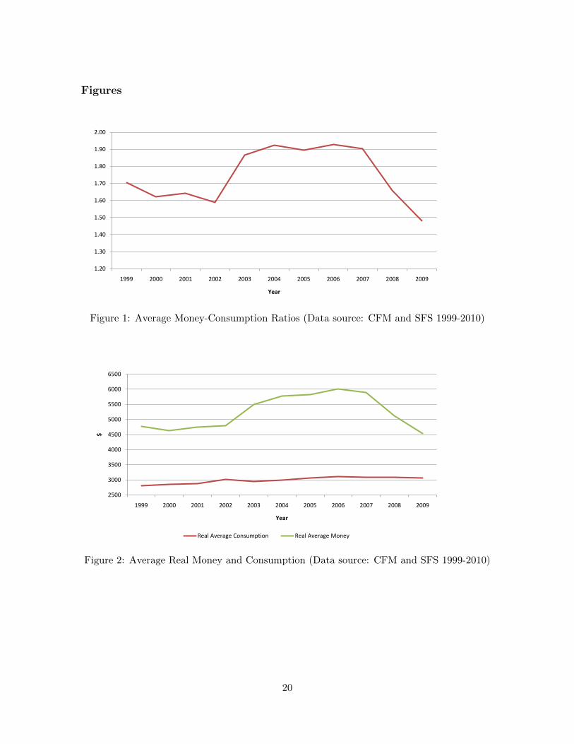
thermore, Figure 2 shows that this variation of money demand is mostly driven by money

holdings rather than by consumption. If financial innovation that lowers the cost of credit

transactions were the main factor driving money demand, we would observe a secular de-

crease in money demand. Hence, other effects are likely at work, including time effects such

as the movements in inflation, a cost of holding money.

1See Appendix for more detailed description of CFM.2The SHS does not contain information on household assets. See Appendix for more detailed description

of SHS.3Data on “cash in wallet” are also available in the CFM but only from 2009. Hence, we do not include it

in our analysis. It does not qualitatively impact our study as cash holdings are relatively small compared tobank account balances.

4

2.1 Money demand by age

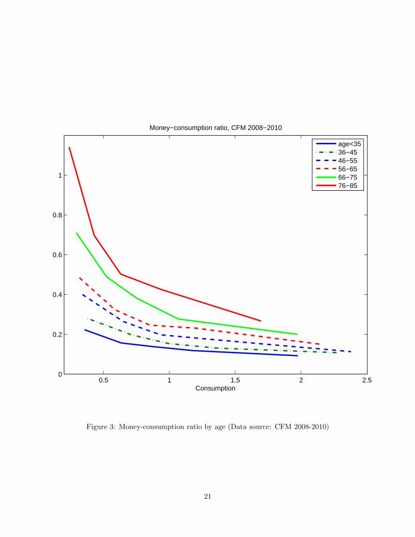
In order to observe money-consumption ratios over age, we group households by the age

of the household head into six categories: less than or equal to 35 years old, 36-45 years old,

46-55 years old, 56-65 years old, 66-75 years old, and 76-85 years old. Given an age group, we

further make five sub-groups based on consumption quintile. Money-consumption ratios are

calculated by taking the ratio of the average money holding and the average consumption of

a given group. Using the 2008-2010 CFM data, Figure 3 displays the three stylized facts re-

garding money-consumption ratios, where the values on the horizontal axis are relative to the

overall average consumption. We observe that (i) money holding per dollar of consumption

(i.e., money-consumption ratio) decreases with consumption; (ii) money-consumption ratio

increases with age conditional on consumption; and (iii) age differences in money-consumption

ratio shrink as consumption increases.

The first fact has been documented in previous studies (see Erosa and Ventura (2002)).

It suggests that, as household consumption increases, a fraction of consumption purchased

with money becomes smaller, implying non-cash payment methods become more important

as consumption increases.4 What has not been studied previously is the age aspect of money

holding, i.e., the second and the third stylized facts.

The use of cross-sectional data raises an issue in interpreting what may be the causes

of these observations. For example, the observed age differences in money demand may

be a result of both age effects and cohort effects. All else equal (i.e., a same person in a

non-changing environment over time), age effects imply a change in money demand due to

aging, e.g., higher cost of credit transactions that require processing complex information

such as a credit contract with fine prints. Alternatively, cohort effects imply a change in

money demand due to the experience of different generations of households, e.g., financial

innovation. Currently old households have lived their lives under a path of historical financial

technologies. The experience that currently young households will have growing up to be the

same age as the currently old households will be quiet different and under a path of future

financial technologies. A dynamic nature of these cohort effects requires money demand

information beyond what cross-sectional data can provide.

Finally and in addition to age and cohort effects, macroeconomic environments are chang-

ing over time such as inflation, interest rates and taxes. These conditions capture time-specific

4Erosa and Ventura (2002) replicate this fact by assuming that the transaction cost of using credit displayseconomies of scale as in Dotsey and Ireland (1996).

5

macroeconomic effects (i.e., time effects) on money demand and interact with age and cohort

effects. In analyzing welfare cost of inflation in aggregate as well as by type of households, it

is important to disentangle these effects as underlying fundamentals affecting the magnitude

of these effects are changing over time. For example, age distributions change over time,

affecting the magnitude of age effects in aggregate. In addition, there will always be new

cohorts being born who will face new financial technology. A structural model that allows

these three effects is necessary to separately identify the effects for the analysis of welfare

cost of inflation. In the next section, we describe such a model.

3 Model

In this section, we present an over-lapping generation model of money holding. There is

no uncertainty. There is a continuum of households in the economy. Each household lives

for I periods and belong to one of the J social classes, where i indexes the age and j their

class. In addition, let h index a cohort of households. They supply labour exogenously given

a fixed labour endowment. In each period, households use money and credit to purchase

consumption good.5 A fraction of consumption purchased with money is subject to a cash-

in-advance constraint. Purchasing by credit requires a fixed transaction cost.

A trade-off between the use of money and credit is the following. On one hand, holding

money is subject to inflation tax as inflation reduces the real value of money. Using credit,

on the other hand, involves a direct cost. The credit transaction technology is a function of

the fraction of consumption purchased with credit, s, and specified as:6

γih(s) =

∫ s

0γi · ηh ·

(x

1− x

)θidx, (1)

where γi > 0, θi ≥ 1 and η > 0.7 This function is convex and strictly increasing in s for

all s ∈ [0, 1). It is independent of the level of consumption. Thus, the credit technology

exhibits increasing returns to scale: the credit transaction cost per unit of consumption

decreases with consumption. This assumption helps generate the first stylized fact: money-

consumption ratio decreases with consumption. We allow both γi and θi to vary with age.

5There is only one type of good which can be purchased by money or credit.6This specification is similar to those used in Dotsey and Ireland (1996) and Erosa and Ventura (2002)

except that we introduce age specific parameters and a parameter capturing cohort effects.7The assumption, θj ≥ 1, guarantees that money holdings increase with consumption at a decreasing rate,

i.e., stylized fact (i) discussed in Section 2.1. See a discussion below with Equation 4 below.

6

The empirical evidence shown in the previous section suggests that the demand for money

is higher for the older households than for the younger counterparts. One possible reason is

that old households face more difficulty processing complex financial information associated

with a use the credit technology.8 Age-specific parameters, γi and θi, allow the model to

capture these age effects. Another possible explanation is that currently old households have

not experienced the same level of financial technologies growing up that later generations

would, leading the currently old to use less financial-technology intensive money as a means

of payment. In this explanation, currently young households with their experience in later

financial technology will use less money and more credit as a means of payment in their old

age than do the currently old households. Hence, this cohort effect may explain the cross-

sectional age differences in money demand. This possibility will be captured by η in the cost

function (1), where h is an integer indexing the cohort. Thus, we assume that cohort effects

take a form of secular changes in financial innovation.

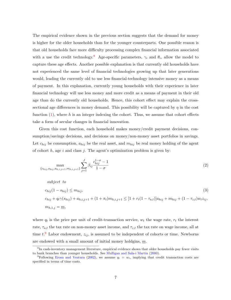
Given this cost function, each household makes money/credit payment decisions, con-

sumption/savings decisions, and decisions on money/non-money asset portfolios in savings.

Let chij be consumption, ahij be the real asset, and mhij be real money holding of the agent

of cohort h, age i and class j. The agent’s optimization problem is given by:

max{chij ,shij ,ah,i,j+1,mh,i,j+1}

J∑j=1

βijc1−σhij − 1

1− σ(2)

subject to

chij(1− shij) ≤ mhij , (3)

chij + qtγ(shij) + ah,i,j+1 + (1 + πt)mh,i,j+1 ≤ [1 + rt(1− τa,t)]ahij +mhij + (1− τz,t)wtzij ,

mh,1,j = m,

where qt is the price per unit of credit-transaction service, wt the wage rate, rt the interest

rate, τa,t the tax rate on non-money asset income, and τz,t the tax rate on wage income, all at

time t.9 Labor endowment, zij , is assumed to be independent of cohorts or time. Newborns

are endowed with a small amount of initial money holdgins, m.

8In cash-inventory management literature, empirical evidence shows that older households pay fewer visitsto bank branches than younger households. See Mulligan and Sala-i Martin (2000).

9Following Erosa and Ventura (2002), we assume qt = wt, implying that credit transaction costs arespecified in terms of time costs.

7

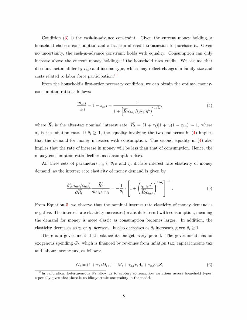
Condition (3) is the cash-in-advance constraint. Given the current money holding, a

household chooses consumption and a fraction of credit transaction to purchase it. Given

no uncertainty, the cash-in-advance constraint holds with equality. Consumption can only

increase above the current money holdings if the household uses credit. We assume that

discount factors differ by age and income type, which may reflect changes in family size and

costs related to labor force participation.10

From the household’s first-order necessary condition, we can obtain the optimal money-

consumption ratio as follows:

mhij

chij= 1− shij =

1

1 +[Rtchij/(qtγiηh)

]1/θi , (4)

where Rt is the after-tax nominal interest rate, Rt = (1 + πt)[1 + rt(1 − τa,t)] − 1, where

πt is the inflation rate. If θi ≥ 1, the equality involving the two end terms in (4) implies

that the demand for money increases with consumption. The second equality in (4) also

implies that the rate of increase in money will be less than that of consumption. Hence, the

money-consumption ratio declines as consumption rises.

All three sets of parameters, γi’s, θi’s and η, dictate interest rate elasticity of money

demand, as the interest rate elasticity of money demand is given by

∂(mhij/chij)

∂Rt

Rtmhij/chij

= − 1

θi·

1 +

(qtγiη

h

Rtchij

)1/θi−1 . (5)

From Equation 5, we observe that the nominal interest rate elasticity of money demand is

negative. The interest rate elasticity increases (in absolute term) with consumption, meaning

the demand for money is more elastic as consumption becomes larger. In addition, the

elasticity decreases as γi or η increases. It also decreases as θi increases, given θi ≥ 1.

There is a government that balance its budget every period. The government has an

exogenous spending Gt, which is financed by revenues from inflation tax, capital income tax

and labour income tax, as follows:

Gt = (1 + πt)Mt+1 −Mt + τa,trtAt + τz,twtZ, (6)

10In calibration, heterogeneous β’s allow us to capture consumption variations across household types,especially given that there is no idiosyncratic uncertainty in the model.

8

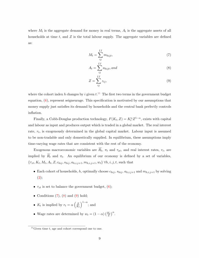
where Mt is the aggregate demand for money in real terms, At is the aggregate assets of all

households at time t, and Z is the total labour supply. The aggregate variables are defined

as:

Mt =IJ∑ij

mhijt, (7)

At =

IJ∑ij

ahijt, and (8)

Z =IJ∑ij

zij , (9)

where the cohort index h changes by i given t.11 The first two terms in the government budget

equation, (6), represent seigneurage. This specification is motivated by our assumptions that

money supply just satisfies its demand by households and the central bank perfectly controls

inflation.

Finally, a Cobb-Douglas production technology, F (Kt, Z) = Kαt Z

1−α, exists with capital

and labour as input and produces output which is traded in a global market. The real interest

rate, rt, is exogenously determined in the global capital market. Labour input is assumed

to be non-tradable and only domestically supplied. In equilibrium, these assumptions imply

time-varying wage rates that are consistent with the rest of the economy.

Exogenous macroeconomic variables are Rt, πt and τat, and real interest rates, rt, are

implied by Rt and πt. An equilibrium of our economy is defined by a set of variables,

{τzt,Kt,Mt, At, Z, chij , shij , ah,i,j+1,mh,i,j+1, wt} ∀h, i, j, t, such that

• Each cohort of households, h, optimally choose chij , shij , ah,i,j+1 and mh,i,j+1 by solving

(2);

• τzt is set to balance the government budget, (6);

• Conditions (7), (8) and (9) hold;

• Kt is implied by rt = α(ZKt

)1−α; and

• Wage rates are determined by wt = (1− α)(KtZ

)α.

11Given time t, age and cohort correspond one to one.

9

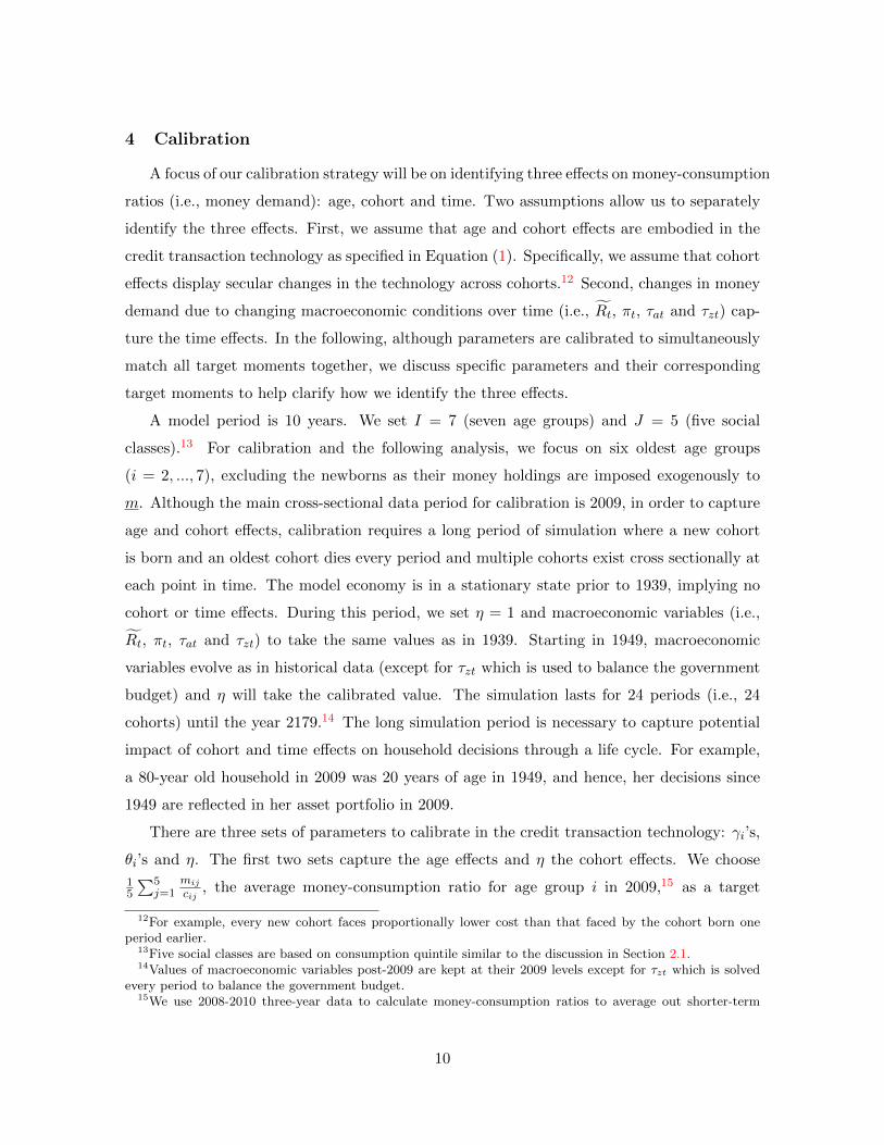
4 Calibration

A focus of our calibration strategy will be on identifying three effects on money-consumption

ratios (i.e., money demand): age, cohort and time. Two assumptions allow us to separately

identify the three effects. First, we assume that age and cohort effects are embodied in the

credit transaction technology as specified in Equation (1). Specifically, we assume that cohort

effects display secular changes in the technology across cohorts.12 Second, changes in money

demand due to changing macroeconomic conditions over time (i.e., Rt, πt, τat and τzt) cap-

ture the time effects. In the following, although parameters are calibrated to simultaneously

match all target moments together, we discuss specific parameters and their corresponding

target moments to help clarify how we identify the three effects.

A model period is 10 years. We set I = 7 (seven age groups) and J = 5 (five social

classes).13 For calibration and the following analysis, we focus on six oldest age groups

(i = 2, ..., 7), excluding the newborns as their money holdings are imposed exogenously to

m. Although the main cross-sectional data period for calibration is 2009, in order to capture

age and cohort effects, calibration requires a long period of simulation where a new cohort

is born and an oldest cohort dies every period and multiple cohorts exist cross sectionally at

each point in time. The model economy is in a stationary state prior to 1939, implying no

cohort or time effects. During this period, we set η = 1 and macroeconomic variables (i.e.,

Rt, πt, τat and τzt) to take the same values as in 1939. Starting in 1949, macroeconomic

variables evolve as in historical data (except for τzt which is used to balance the government

budget) and η will take the calibrated value. The simulation lasts for 24 periods (i.e., 24

cohorts) until the year 2179.14 The long simulation period is necessary to capture potential

impact of cohort and time effects on household decisions through a life cycle. For example,

a 80-year old household in 2009 was 20 years of age in 1949, and hence, her decisions since

1949 are reflected in her asset portfolio in 2009.

There are three sets of parameters to calibrate in the credit transaction technology: γi’s,

θi’s and η. The first two sets capture the age effects and η the cohort effects. We choose

15

∑5j=1

mij

cij, the average money-consumption ratio for age group i in 2009,15 as a target

12For example, every new cohort faces proportionally lower cost than that faced by the cohort born oneperiod earlier.

13Five social classes are based on consumption quintile similar to the discussion in Section 2.1.14Values of macroeconomic variables post-2009 are kept at their 2009 levels except for τzt which is solved

every period to balance the government budget.15We use 2008-2010 three-year data to calculate money-consumption ratios to average out shorter-term

10

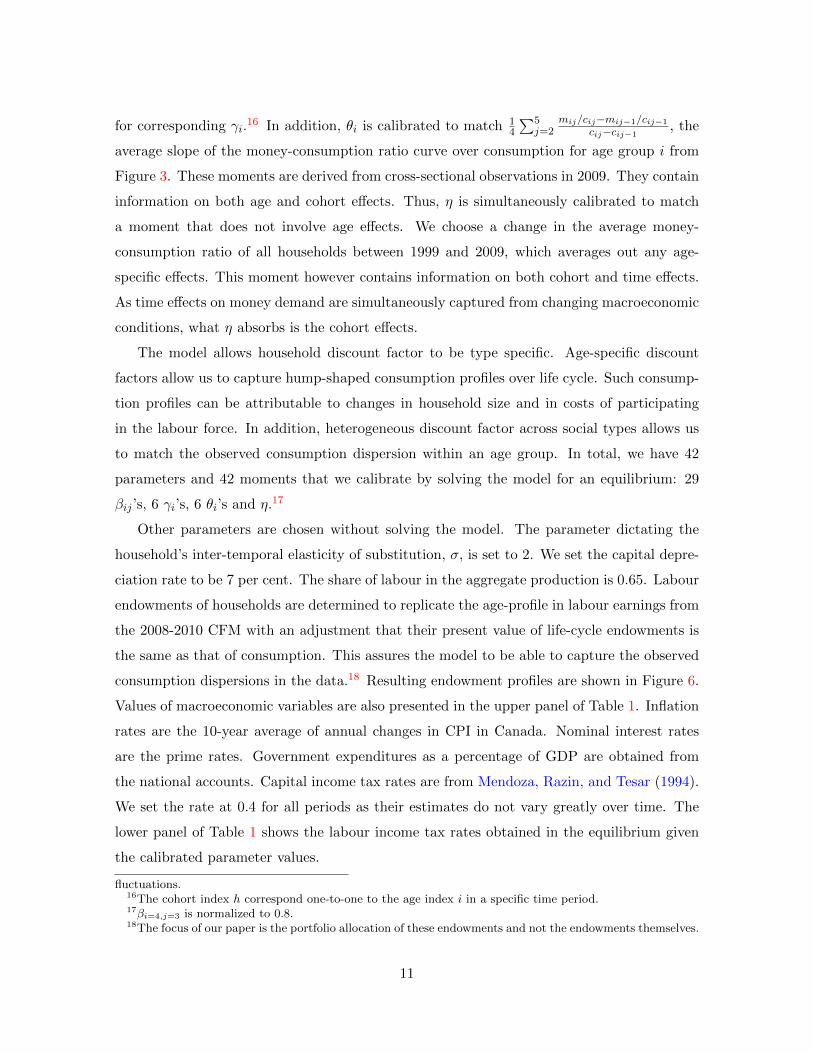
for corresponding γi.16 In addition, θi is calibrated to match 1

4

∑5j=2

mij/cij−mij−1/cij−1

cij−cij−1, the

average slope of the money-consumption ratio curve over consumption for age group i from

Figure 3. These moments are derived from cross-sectional observations in 2009. They contain

information on both age and cohort effects. Thus, η is simultaneously calibrated to match

a moment that does not involve age effects. We choose a change in the average money-

consumption ratio of all households between 1999 and 2009, which averages out any age-

specific effects. This moment however contains information on both cohort and time effects.

As time effects on money demand are simultaneously captured from changing macroeconomic

conditions, what η absorbs is the cohort effects.

The model allows household discount factor to be type specific. Age-specific discount

factors allow us to capture hump-shaped consumption profiles over life cycle. Such consump-

tion profiles can be attributable to changes in household size and in costs of participating

in the labour force. In addition, heterogeneous discount factor across social types allows us

to match the observed consumption dispersion within an age group. In total, we have 42

parameters and 42 moments that we calibrate by solving the model for an equilibrium: 29

βij ’s, 6 γi’s, 6 θi’s and η.17

Other parameters are chosen without solving the model. The parameter dictating the

household’s inter-temporal elasticity of substitution, σ, is set to 2. We set the capital depre-

ciation rate to be 7 per cent. The share of labour in the aggregate production is 0.65. Labour

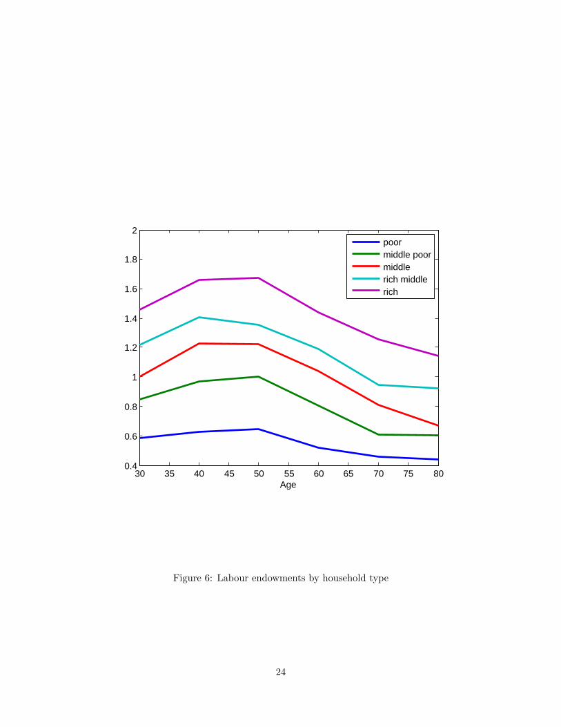
endowments of households are determined to replicate the age-profile in labour earnings from

the 2008-2010 CFM with an adjustment that their present value of life-cycle endowments is

the same as that of consumption. This assures the model to be able to capture the observed

consumption dispersions in the data.18 Resulting endowment profiles are shown in Figure 6.

Values of macroeconomic variables are also presented in the upper panel of Table 1. Inflation

rates are the 10-year average of annual changes in CPI in Canada. Nominal interest rates

are the prime rates. Government expenditures as a percentage of GDP are obtained from

the national accounts. Capital income tax rates are from Mendoza, Razin, and Tesar (1994).

We set the rate at 0.4 for all periods as their estimates do not vary greatly over time. The

lower panel of Table 1 shows the labour income tax rates obtained in the equilibrium given

the calibrated parameter values.

fluctuations.16The cohort index h correspond one-to-one to the age index i in a specific time period.17βi=4,j=3 is normalized to 0.8.18The focus of our paper is the portfolio allocation of these endowments and not the endowments themselves.

11

Table 1: Macroeconomic variables

1939 1949 1959 1969 1979 1989 1999 2009

Exogenous variables:Annual inflation (%) 2.37 4.00 1.75 5.60 8.11 3.36 2.02 1.92Annual nominal interest rate (%) 4.96 4.50 5.60 7.53 12.50 9.70 5.50 4.11Government expenditure (% of GDP) 26 26 26 27 26 25 22 24Capital income tax rate 0.4 0.4 0.4 0.4 0.4 0.4 0.4 0.4

Labour income tax rate 0.25 0.42 0.25 0.38 0.29 0.23 0.24 0.30

4.1 Calibration results

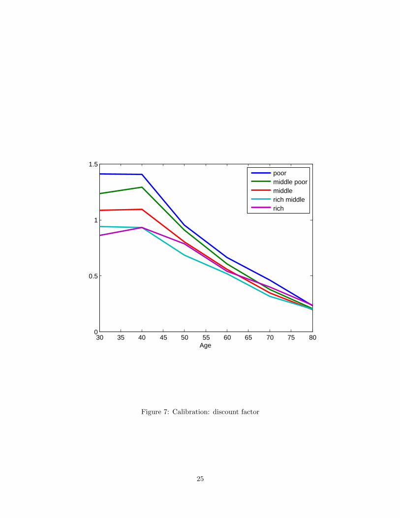
Figure 7 shows the parameter values for βij ’s. Given a social class, the discount factors

are monotonically declining in age except for the first two age groups. Table 2 shows the rest

of the parameters calibrated by solving the model equilibrium. γi is monotonically increasing

in age and θi monotonically declining. This implies that, given a level of consumption and a

fraction of purchase of the consumption by credit, the increase in γi with age (while holding

θi fixed) increases the cost, and the decrease in θi with age increases the nominal-interest-rate

elasticity of money demand (while holding γi fixed).19 The target moment for η is the ratio

of average money-consumption ratios in 1999 and 2009, m1999c1999

/m2009c2009

. The value of calibrated

η suggests that the cost of credit transactions declines by about 18% for each new cohort

every 10 years.

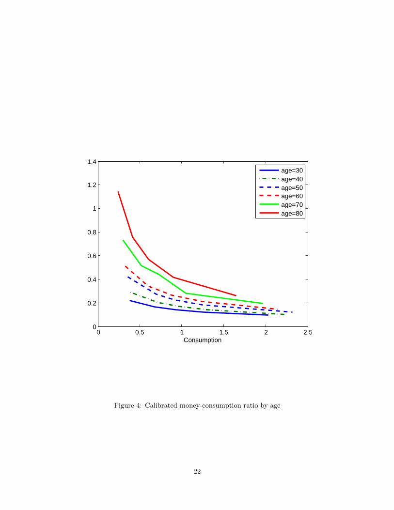
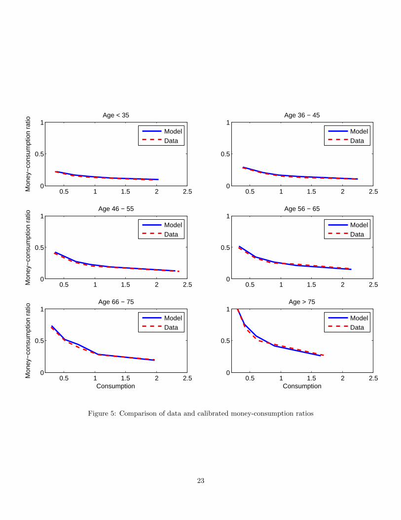
Figure 4 displays the model outcome of money-consumption ratios by age in 2009. Fig-

ure 5 separately shows each age group and compares the model generated results to the data.

The calibrated model results fairly match the data in the cross-sectional variation of money

demand by household type.

5 Disentangling age and cohort effects

Our model and calibration allow us disentangle the age and cohort effects into the pa-

rameters of the model: γi, θi and η. We can quantitatively simulate the model to disentangle

19The second statement involving θi can be shown using Equation (5).

12

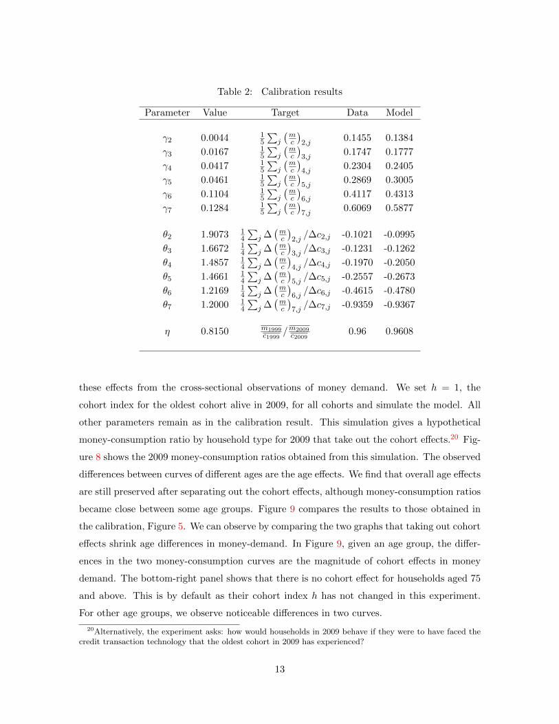
Table 2: Calibration results

Parameter Value Target Data Model

γ2 0.0044 15

∑j

(mc

)2,j

0.1455 0.1384

γ3 0.0167 15

∑j

(mc

)3,j

0.1747 0.1777

γ4 0.0417 15

∑j

(mc

)4,j

0.2304 0.2405

γ5 0.0461 15

∑j

(mc

)5,j

0.2869 0.3005

γ6 0.1104 15

∑j

(mc

)6,j

0.4117 0.4313

γ7 0.1284 15

∑j

(mc

)7,j

0.6069 0.5877

θ2 1.9073 14

∑j ∆(mc

)2,j/∆c2,j -0.1021 -0.0995

θ3 1.6672 14

∑j ∆(mc

)3,j/∆c3,j -0.1231 -0.1262

θ4 1.4857 14

∑j ∆(mc

)4,j/∆c4,j -0.1970 -0.2050

θ5 1.4661 14

∑j ∆(mc

)5,j/∆c5,j -0.2557 -0.2673

θ6 1.2169 14

∑j ∆(mc

)6,j/∆c6,j -0.4615 -0.4780

θ7 1.2000 14

∑j ∆(mc

)7,j/∆c7,j -0.9359 -0.9367

η 0.8150 m1999c1999

/m2009c2009

0.96 0.9608

these effects from the cross-sectional observations of money demand. We set h = 1, the

cohort index for the oldest cohort alive in 2009, for all cohorts and simulate the model. All

other parameters remain as in the calibration result. This simulation gives a hypothetical

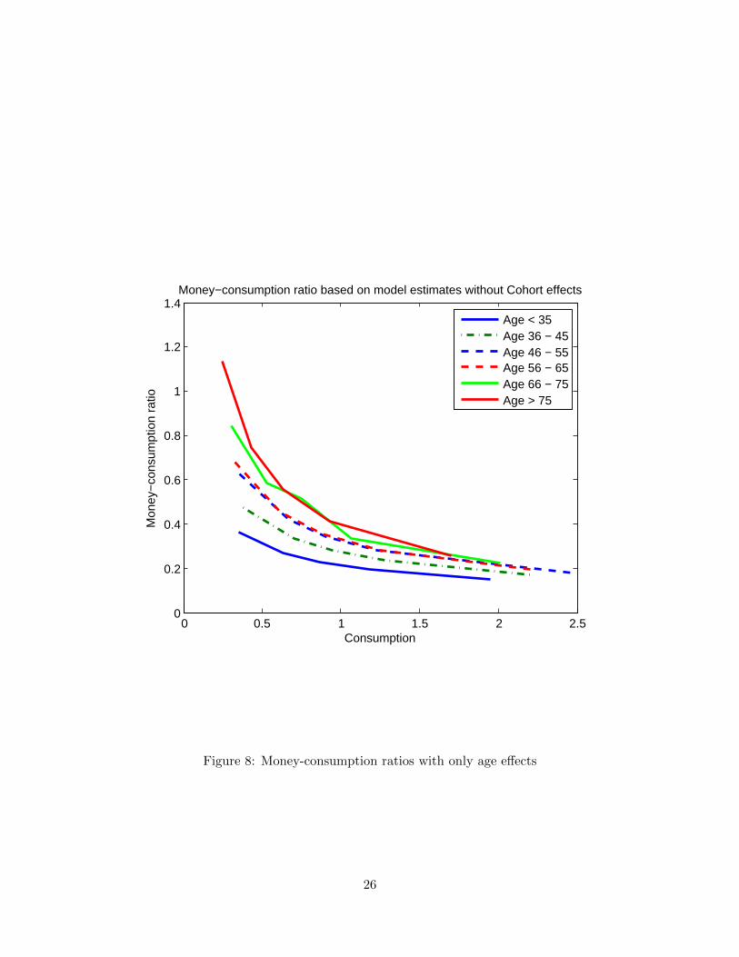
money-consumption ratio by household type for 2009 that take out the cohort effects.20 Fig-

ure 8 shows the 2009 money-consumption ratios obtained from this simulation. The observed

differences between curves of different ages are the age effects. We find that overall age effects

are still preserved after separating out the cohort effects, although money-consumption ratios

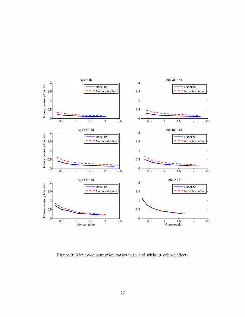
became close between some age groups. Figure 9 compares the results to those obtained in

the calibration, Figure 5. We can observe by comparing the two graphs that taking out cohort

effects shrink age differences in money-demand. In Figure 9, given an age group, the differ-

ences in the two money-consumption curves are the magnitude of cohort effects in money

demand. The bottom-right panel shows that there is no cohort effect for households aged 75

and above. This is by default as their cohort index h has not changed in this experiment.

For other age groups, we observe noticeable differences in two curves.

20Alternatively, the experiment asks: how would households in 2009 behave if they were to have faced thecredit transaction technology that the oldest cohort in 2009 has experienced?

13

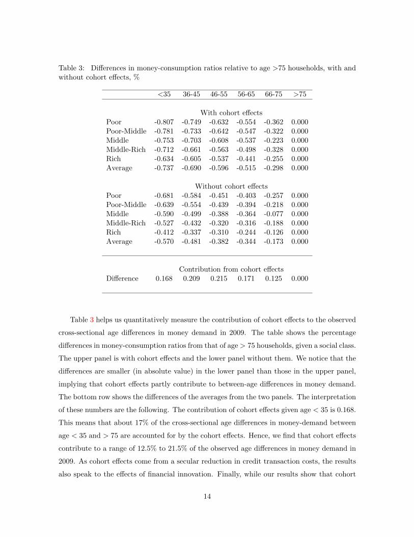
Table 3: Differences in money-consumption ratios relative to age >75 households, with andwithout cohort effects, %

<35 36-45 46-55 56-65 66-75 >75

With cohort effectsPoor -0.807 -0.749 -0.632 -0.554 -0.362 0.000Poor-Middle -0.781 -0.733 -0.642 -0.547 -0.322 0.000Middle -0.753 -0.703 -0.608 -0.537 -0.223 0.000Middle-Rich -0.712 -0.661 -0.563 -0.498 -0.328 0.000Rich -0.634 -0.605 -0.537 -0.441 -0.255 0.000Average -0.737 -0.690 -0.596 -0.515 -0.298 0.000

Without cohort effectsPoor -0.681 -0.584 -0.451 -0.403 -0.257 0.000Poor-Middle -0.639 -0.554 -0.439 -0.394 -0.218 0.000Middle -0.590 -0.499 -0.388 -0.364 -0.077 0.000Middle-Rich -0.527 -0.432 -0.320 -0.316 -0.188 0.000Rich -0.412 -0.337 -0.310 -0.244 -0.126 0.000Average -0.570 -0.481 -0.382 -0.344 -0.173 0.000

Contribution from cohort effectsDifference 0.168 0.209 0.215 0.171 0.125 0.000

Table 3 helps us quantitatively measure the contribution of cohort effects to the observed

cross-sectional age differences in money demand in 2009. The table shows the percentage

differences in money-consumption ratios from that of age> 75 households, given a social class.

The upper panel is with cohort effects and the lower panel without them. We notice that the

differences are smaller (in absolute value) in the lower panel than those in the upper panel,

implying that cohort effects partly contribute to between-age differences in money demand.

The bottom row shows the differences of the averages from the two panels. The interpretation

of these numbers are the following. The contribution of cohort effects given age < 35 is 0.168.

This means that about 17% of the cross-sectional age differences in money-demand between

age < 35 and > 75 are accounted for by the cohort effects. Hence, we find that cohort effects

contribute to a range of 12.5% to 21.5% of the observed age differences in money demand in

2009. As cohort effects come from a secular reduction in credit transaction costs, the results

also speak to the effects of financial innovation. Finally, while our results show that cohort

14

effects are present in the observed cross-sectional differences in money demand of households

across age, age effects account for large parts of the observed differences in 2009.

6 Welfare cost of inflation

In the calibrated economy, inflation rates in 2009 and onwards are 1.92%. We calculate

changes in aggregate welfare and its distribution when inflation increases from 1.92% in 2009

to 10% in 2019 and onwards. Changes in welfare are measured as the consumption equivalent

variation. Let λhj be the consumption equivalent variation for cohort h and social class j.

Let V 0hj be the life time utility of the households of type hj,

V 0hj =

7∑i=2

βiju(c0hij),

where c0hij is the consumption obtained in the calibrated model. The welfare measure for

household hj is obtained from the following equation,

7∑i=2

βiju(chij + λhj) = V 0hj ,

where chij is the consumption under the new inflation rates. The welfare measure for house-

hold hj is then calculated as

Whj =6λhj∑7i=2 c

0hij

× 100.

From Whj , the cohort-specific and the class-specific welfare measures are, respectively:

Wh =6 ·∑5

j=1 λhj∑7i=2

∑5j=1 c

0hij

× 100, and (10)

Wj =6 ·∑h2069

h=h1949λhj∑h2069

h=h1949

∑7i=2 c

0hij

× 100, (11)

where the last cohort for welfare calculations is set to h2069, the cohort born in 2069. Finally,

the aggregate welfare measure is obtained from aggregating Whj as follows:

W =6 ·∑h2069

h=h1949

∑5j=1 λhj∑h2069

h=h1949

∑7i=2

∑5j=1 c

0hij

× 100.

15

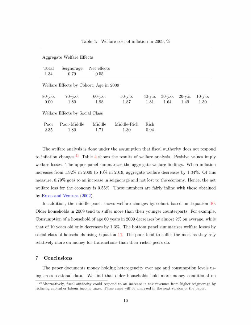
Table 4: Welfare cost of inflation in 2009, %

Aggregate Welfare Effects

Total Seignorage Net effects1.34 0.79 0.55

Welfare Effects by Cohort, Age in 2009

80-y.o. 70–y.o. 60-y.o. 50-y.o. 40-y.o. 30-y.o. 20-y.o. 10-y.o.0.00 1.80 1.98 1.87 1.81 1.64 1.49 1.30

Welfare Effects by Social Class

Poor Poor-Middle Middle Middle-Rich Rich2.35 1.80 1.71 1.30 0.94

The welfare analysis is done under the assumption that fiscal authority does not respond

to inflation changes.21 Table 4 shows the results of welfare analysis. Positive values imply

welfare losses. The upper panel summarizes the aggregate welfare findings. When inflation

increases from 1.92% in 2009 to 10% in 2019, aggregate welfare decreases by 1.34%. Of this

measure, 0.79% goes to an increase in seignorage and not lost to the economy. Hence, the net

welfare loss for the economy is 0.55%. These numbers are fairly inline with those obtained

by Erosa and Ventura (2002).

In addition, the middle panel shows welfare changes by cohort based on Equation 10.

Older households in 2009 tend to suffer more than their younger counterparts. For example,

Consumption of a household of age 60 years in 2009 decreases by almost 2% on average, while

that of 10 years old only decreases by 1.3%. The bottom panel summarizes welfare losses by

social class of households using Equation 11. The poor tend to suffer the most as they rely

relatively more on money for transactions than their richer peers do.

7 Conclusions

The paper documents money holding heterogeneity over age and consumption levels us-

ing cross-sectional data. We find that older households hold more money conditional on

21Alternatively, fiscal authority could respond to an increase in tax revenues from higher seigniorage byreducing capital or labour income taxes. These cases will be analyzed in the next version of the paper.

16

consumption. The observed cross-sectional age differences in money demand contains both

age-specific and cohort-specific effects. In order to separately identify these effects, an over-

lapping generation model is developed and dynamically calibrated to match the observed

heterogeneity in money holding over two data periods. The calibrated model shows that,

while the age effects are a major factor in accounting for the cross-sectional age differences,

the cohort effects are also present and account for up to 20% of the observed differences. We

also use the calibrated model to conduct welfare analysis for the aggregate economy as well

as for the welfare distribution across households. When inflation increase from 1.92% in 2009

to 10%, we find a welfare change that is consistent with the literature, and in addition find

that large differences in welfare cost across households. Currently alive generations as well

as the poor households absorb a large portion of the welfare losses.

17

References

Alvarez, F., and F. Lippi (2009): “Financial Innovation and the Transactions Demand for

Cash,” Econometrica, 77, 363–402.

Attanasio, O. P., L. Guiso, and T. Jappelli (2002): “The Demand for Money, Financial

Innovation, and the Welfare Cost of Inflation: An Analysis with Household Data,” Journal

of Political Economy, 110(2), 317–351.

Baumol, W. J. (1952): “The Transactions Demand for Cash: An Inventory Theoretic

Approach,” Quarterly Journal of Economics, 66, 545–556.

Chiu, J., and M. Molico (2010): “Liquidity, redistribution, and the welfare cost of infla-

tion,” Journal of Monetary Economics, 57(4), 428–438.

Dotsey, M., and P. Ireland (1996): “The welfare cost of inflation in general equilibrium,”

Journal of Monetary Economics, 37(1), 29–47.

Erosa, A., and G. Ventura (2002): “On inflation as a regressive consumption tax,”

Journal of Monetary Economics, 49(4), 761–795.

Heer, B., and A. Maussner (2007): “The Money-Age Distribution: Empirical Facts and

Limited Monetary Models,” CESifo Working Paper Series 1917, CESifo Group.

Lucas, R. E. J. (2000): “Inflation and Welfare,” Econometrica, 68(2), 247–274.

Mendoza, E. G., A. Razin, and L. Tesar (1994): “Effective Tax Rates in Macroeco-

nomics: Cross Country Estimates of Tax Rates on Factor Incomes and Consumption,”

Journal of Monetary Economics, 34, 297–323.

Mulligan, C. B., and X. Sala-i Martin (2000): “Extensive Margins and the Demand

for Money at Low Interest Rates,” Journal of Political Economy, 108(5), 961–991.

Ragot, X. (2010): “The Case for a Financial Approach to Money Demand,” Working Papers

300, Banque de France.

Tobin, J. (1956): “The Interest Elasticity of the Transactions Demand for Cash,” Review

of Economics and Statistics, 38(3), 241–247.

18

Appendix - Data

The Canadian Financial Monitor (CFM) Ipsos Reid Canada collects detailed household

balance sheet and income. The survey has a sample size of approximately 12,000 households

per year responding to a mail-in questionnaire. The Survey of Household Spending (SHS)

is a cross-sectional survey conducted by Statistics Canada, and provides information on

household spending and dwelling characteristics. The effective sample size (i.e., the number

of respondents to the survey) of the SHS varies each year, ranging from 14,000 to 17,000

households. The survey data are collected via personal interviews.

Information on money is obtained from the CFM and is defined to consist of the sum of the

household’s current balances in checking accounts and low-interest-rate saving accounts in all

financial institutions. For the period 2008-2010, the CFM contains consumption information.

We define consumption to consist of the household’s sum of gross monthly spending on non-

durable goods, services and durable goods, but excludes the property tax and housing services

from owned and rented residential properties. Specifically, it includes the following items:

hydro bills, other utilities, insurance premiums, domestic and child care services/school, gro-

ceries including beverages, food and beverages at/from restaurants/clubs/bars, snacks and

beverage from convenience stores, recreation, health services, automobile maintenance/gas,

public and other transportation, clothing/footwear, gifts or donations, health and beauty

aids/personal grooming, a new or used automobile/RV/motorcycle/boat/truck, home appli-

ances and electronics, home furnishing, and vacation/trip.

From the SHS which contains more detailed information on consumption than the CFM,

we choose items that are comparable to those from the CFM. They are: food, maintenance,

repairs and replacements, homeowners’ insurance premiums, traveller accommodation, house-

hold operation, household furnishings and equipment, clothing, transportation, health care,

personal care, recreation, reading materials, education, tobacco and alcohol, life insurance

premiums, annuity contracts and transfers to RRIFs, employment insurance premiums, and

gifts of money and contributions.

19

Figures

1.20

1.30

1.40

1.50

1.60

1.70

1.80

1.90

2.00

1999 2000 2001 2002 2003 2004 2005 2006 2007 2008 2009

Year

Figure 1: Average Money-Consumption Ratios (Data source: CFM and SFS 1999-2010)

2004

2500

3000

3500

4000

4500

5000

5500

6000

6500

1999 2000 2001 2002 2003 2004 2005 2006 2007 2008 2009

$

Year

Real Average Consumption Real Average Money

Figure 2: Average Real Money and Consumption (Data source: CFM and SFS 1999-2010)

20

0.5 1 1.5 2 2.50

0.2

0.4

0.6

0.8

1

Consumption

Money−consumption ratio, CFM 2008−2010

age<3536−4546−5556−6566−7576−85

Figure 3: Money-consumption ratio by age (Data source: CFM 2008-2010)

21

0 0.5 1 1.5 2 2.50

0.2

0.4

0.6

0.8

1

1.2

1.4

Consumption

age=30age=40age=50age=60age=70age=80

Figure 4: Calibrated money-consumption ratio by age

22

0.5 1 1.5 2 2.50

0.5

1

Mon

ey−

cons

umpt

ion

ratio

Age < 35

ModelData

0.5 1 1.5 2 2.50

0.5

1Age 36 − 45

ModelData

0.5 1 1.5 2 2.50

0.5

1

Mon

ey−

cons

umpt

ion

ratio

Age 46 − 55

ModelData

0.5 1 1.5 2 2.50

0.5

1Age 56 − 65

ModelData

0.5 1 1.5 2 2.50

0.5

1

Consumption

Mon

ey−

cons

umpt

ion

ratio

Age 66 − 75

ModelData

0.5 1 1.5 2 2.50

0.5

1

Consumption

Age > 75

ModelData

Figure 5: Comparison of data and calibrated money-consumption ratios

23

30 35 40 45 50 55 60 65 70 75 800.4

0.6

0.8

1

1.2

1.4

1.6

1.8

2

Age

poormiddle poormiddlerich middlerich

Figure 6: Labour endowments by household type

24

30 35 40 45 50 55 60 65 70 75 800

0.5

1

1.5

Age

poormiddle poormiddlerich middlerich

Figure 7: Calibration: discount factor

25

0 0.5 1 1.5 2 2.50

0.2

0.4

0.6

0.8

1

1.2

1.4

Consumption

Mon

ey−

cons

umpt

ion

ratio

Money−consumption ratio based on model estimates without Cohort effects

Age < 35Age 36 − 45Age 46 − 55Age 56 − 65Age 66 − 75Age > 75

Figure 8: Money-consumption ratios with only age effects

26

0.5 1 1.5 2 2.50

0.5

1

1.5

2

Mon

ey−

cons

umpt

ion

ratio

Age < 35

BaselineNo cohort effect

0.5 1 1.5 2 2.50

0.5

1

1.5

2Age 36 − 45

BaselineNo cohort effect

0.5 1 1.5 2 2.50

0.5

1

1.5

2

Mon

ey−

cons

umpt

ion

ratio

Age 46 − 55

BaselineNo cohort effect

0.5 1 1.5 2 2.50

0.5

1

1.5

2Age 56 − 65

BaselineNo cohort effect

0.5 1 1.5 2 2.50

0.5

1

1.5

2

Consumption

Mon

ey−

cons

umpt

ion

ratio

Age 66 − 75

BaselineNo cohort effect

0.5 1 1.5 2 2.50

0.5

1

1.5

2

Consumption

Age > 75

BaselineNo cohort effect

Figure 9: Money-consumption ratios with and without cohort effects

27