IMT Institute for Advanced Studies, Lucca

Lucca, Italy

Essays on Empirical Banking

PhD Program in Economics, Markets, Institutions

XX Cycle

By

Caterina Giannetti

2008

The dissertation of Caterina Giannetti is approved.

Program Coordinator: Prof. Fabio Pammolli, Università di Firenze

Supervisor: Prof. Giampiero M. Gallo, Università di Firenze

Tutor: Prof. Fabio Pammolli, Università di Firenze

The dissertation of Caterina Giannetti has been reviewed by:

Prof. Elena Carletti, University of Frankfurt

Prof. Hans Degryse, University of Tilburg

IMT Institute for Advanced Studies, Lucca

2008

To my familyTo Eugenio Paladini, Santo Perrotta and Franca Pompilio

Contents

Acknowledgements ix

Vita and Publications x

Abstract xii

1 Intensity of competition and Market structure in the Ital-ian Banking Industry 11.1 Introduction . . . . . . . . . . . . . . . . . . . . . . . . . . . 11.2 The theoretical approach . . . . . . . . . . . . . . . . . . . 21.3 Exogenous sunk cost industries: the model . . . . . . . . . . 51.4 The game: equilibrium analysis . . . . . . . . . . . . . . . . 61.5 The Italian retail banking industry . . . . . . . . . . . . . . 101.6 Exogenous or endogenous sunk costs? . . . . . . . . . . . . 111.7 Market equilibrium . . . . . . . . . . . . . . . . . . . . . . . 121.8 Characteristics and construction of the

dataset . . . . . . . . . . . . . . . . . . . . . . . . . . . . . . 131.9 Intensity of competition and concentration: Empirical model

and results . . . . . . . . . . . . . . . . . . . . . . . . . . . 151.10 Model description: identifying the size of the submarket . . 161.11 Model description: testing market size-market concentra-

tion relationship . . . . . . . . . . . . . . . . . . . . . . . . 181.12 Results . . . . . . . . . . . . . . . . . . . . . . . . . . . . . . 191.13 Robustness checks . . . . . . . . . . . . . . . . . . . . . . . 211.14 Conclusions . . . . . . . . . . . . . . . . . . . . . . . . . . . 23

vii

References 24

2 Unit Roots and the Dynamics of Market Shares: an anal-ysis using Italian Banking micro-panel 382.1 Introduction . . . . . . . . . . . . . . . . . . . . . . . . . . . 12.2 Characteristics and construction of the

dataset . . . . . . . . . . . . . . . . . . . . . . . . . . . . . . 32.3 Tests for unit roots: the model . . . . . . . . . . . . . . . . 5

2.3.1 OLS . . . . . . . . . . . . . . . . . . . . . . . . . . . 72.3.2 A test for Cross Section Dependence . . . . . . . . . 9

2.4 The Italian case . . . . . . . . . . . . . . . . . . . . . . . . . 102.4.1 Cross Section Dependence in Dynamics Panels . . . 12

2.5 Panel Unit Root Tests for Cross Sectionally Dependent Panels 132.6 Conclusions . . . . . . . . . . . . . . . . . . . . . . . . . . . 15

References 17

3 Relationship Lending and Firm Innovativeness: New Em-pirical Evidence 13.1 Introduction . . . . . . . . . . . . . . . . . . . . . . . . . . . 13.2 Literature Review . . . . . . . . . . . . . . . . . . . . . . . 33.3 Relationship lending and Firm innovativeness . . . . . . . . 5

3.3.1 Empirical determinants of relationship lending . . . 53.3.2 Relationship lending and innovation . . . . . . . . . 6

3.4 Data description . . . . . . . . . . . . . . . . . . . . . . . . 73.5 The empirical model and results . . . . . . . . . . . . . . . 9

3.5.1 Relationship Lending and Measure of Dependenceon External Finance . . . . . . . . . . . . . . . . . . 12

3.5.2 Bank competition and Innovation . . . . . . . . . . . 163.6 Relationship lending in the discovery

phase . . . . . . . . . . . . . . . . . . . . . . . . . . . . . . 173.7 Conclusions . . . . . . . . . . . . . . . . . . . . . . . . . . . 19

References 21.1 APPENDIX I . . . . . . . . . . . . . . . . . . . . . . . . . . 26

viii

Acknowledgements

1. I am deeply indebted with Giancarlo Spagnolo, GiampieroGallo, Elena Carletti, Hans Degryse, and Luigi Buzzacchi.I also wish to thank Marcello Messori, Giorgio Rodano,Giuseppe de Arcangelis, Mark Dincecco, Stefano Caiazza,people at CENTER and TILEC (University of Tilburg),as well as people at CORE (Université Catholique deLouvain). I also aknowledge financial support from theFLAFR (Fondazione Lucchese per lAlta Formazione e laRicerca).

2. Special thanks to Barbara Aretino, Maria Bigoni, SerenaBrandini, Elena d’Alfonso, Marilena Filippelli, ManuelaForte, Giulia Gobbo, Marianna Madìa, Luigi Moretti, Va-lerio Novembre, Carlo Stagnaro, Alessia Savoldi.

ix

Vita

31/07/1978 Born, Roma, Italy

2008 Visiting PhD studentUniversiteit Van Tilburg - The Netherlands

2006 Visiting PhD studentUniversité Catholique de Louvain - Belgium

2004 Master Degree in Development and International Coop-eration. University of Bologna

2002 Degree in Economics. University of Tor Vergata. Finalmark: summa cum laude

2005 CIDE Summer School in Microeconometrics2006 SEEC Summer School in Applied Economics

CIDE Summer School in Time SeriesESSID Summer School in Industrial Dynamics

2006 CORE - Center For Operations Research and Economet-rics - Marie Curie Visiting Fellow - EDNET Program -"Network of the European doctoral program in quanti-tative economics"

2007 EUROSTAT (Luxembourg) - Paid Trainee2005 Italian Competition Authority - Unpaid Trainee2005 ’Ca Foscari University (Venice - Italy) - Teaching Assis-

tant Political Economy

x

Publications

1. Bagella, M., and Caiazza, S., and Carletti, E. and Giannetti, C. and Spag-nolo, G. (2008) “Analasi della Concorrenza nei Servizi Bancari Europei:Il punto di vista delle Autorità sulla Concorrenza”, Rapporto sul sistemafinanziario forthcoming

2. C. Giannetti (2007) ‘Intensity of Competition and Market Structure in theItalian banking Industry’ CORE Discussion Paper, N. 41.

Presentations

1. TILEC - Tilburg University - 2008 - Tilburg - The Netherlands2. DTE - Università La Sapienza -2007 - Rome - Italy3. ISAE Monitoring Italy 2007 - Rome - Italy4. EARIE CONFERENCE 2007 - Valencia - Spain5. CES - Université de Paris I 2007- France6. ESSID Workshop 2006 - Cargèse - France7. Doctoral Workshop in Economics 2006 - Louvain-la-Neuve - Belgium8. ZEW - 2005 - Mannheim - Germany

xi

Abstract

The thesis is structured in three articles which develop micro-econometric analysis on the Italian banking industry. The firsttwo articles investigate, relying on different theoretical frame-works and techniques, the degree of competition in the retailsegment whereas the third article examines the effects of rela-tionship banking on firm innovativeness.The first article is entitled "Intensity of Competition and Mar-ket Structure in the Italian Banking Industry". The aim ofthis work is to empirically test Sutton’s predictions for indus-try with exogenous sunk costs in the Italian banking industry.In particular, I focus my attention only on the retail segmentsince products are rather standardized and there is a limitedscope for cost-decreasing or quality increasing investments.The second article is entitled "Unit Roots and the Dynamic ofMarket Shares". In this article I rely on panel unit roots testsin order to infer the degree of competition in the industry. Themain idea is to verify if market shares of the first five bankscontain unit roots. If so, it is possible to infer that there isthe chance for competitors to displace permanently the leader.On the contrary, if share are mean reverting, it is reasonableto infer that the industry is rather stable, and actors reachedpositions difficult to overcome.The third article is entitled "Relationship lending and Firminnovativeness: New Empirical Evidence". The aim of thisstudy is to test the effect of firm-bank ties on the degree of firminnovativeness using data on a sample of Italian manufacturingfirms. In particular, this article departs from previous micro-econometric works since it distinguishes the discovery phasefrom the introduction phase of new technologies.

xii

Chapter 1

Intensity of competitionand Market structure inthe Italian BankingIndustry

Abstract

This work tests the predictions of Sutton’s model of independent submar-kets for the Italian retail banking industry. In the first part of this paper,I develop a model of endogenous mergers to evidence the relationship be-tween firms’ conduct, market entry and market structure. In the secondpart, I identify the submarket dimension and estimate the relationshipbetween market size and market structure using data on bank branches.The size of the submarkets turned out to be at most provincial whereasthe limiting concentration index - as argued by Sutton for industries withexogenous sunk costs - goes to zero as the market becomes larger.

Keywords: Concentration, Truncated Poisson and Negative Binomialmodels, quantile regressionsJEL Classification: C24, D43, L11, L89

1.1 Introduction

Sutton’s model of independent submarkets emphasizes the strategic choiceof sunk costs and, unlike the traditional structure-conduct-performanceapproach, considers how changes in firms’ conduct affects the conditionof entry, altering by consequence market structure. Under this scheme,both homogeneous-horizontally differentiated products and advertising-R&D intensive (vertically differentiated products) industries can be anal-ysed. For the former type of industries, with fixed sunk costs, it is possibleto show an inverse relationship between market size and market struc-ture. For the latter type of industries, where sunk costs are endogenous,such a negative relationship does not necessarily emerge as market sizeincreases. This is because sunk costs, such as advertising or R&D expen-diture, raise with market size. Such expenditures are choice variables of(perceived) quality: by increasing the level of advertising-R&D, firms areable to gain (or to maintain) market share. Therefore, as market size be-comes larger, an ‘escalation mechanism’ could raise fixed costs per firmto such an extent that the negative relationship between market size andmarket structure will break down. Sutton’s model offers therefore veryclear and testable predictions about the relationship between market-sizeand market-concentration. The aim to this paper is to analyse the Ital-ian retail banking industry as a special case of the first type of industries,since products are rather standardized and there is a limited scope forcost-decreasing or quality increasing investments. This industry can beviewed as made of a large number of local markets that arise becausethere are many different geographical locations throughout the country:in every submarket products are fairly good substitutes and banks com-pete against each other by means of their branch locations. The degree ofsubstitutability is substantially lower for products and services offered inneighbour submarkets. In the first part of this paper, relying on the modeldeveloped by Vasconcelos (2006), I examine the firm strategic behaviourreferring to a three-stage non cooperative game. In line with Sutton’s the-ory, the aim is to highlight the relationship between firm conduct, entryand market structure while explicitly allowing for a merger process in the

1

industry. In so doing, it is possible to show that the incentives to mergeto a monopoly are lead by the intensity of competition and by the degreeof product substitution. This ultimately shows how the number of banksas well as the share of the main bank are determined in each submarket,and offers indications on the variables to be used in the empirical section.In the second part, I will estimate the market structure-market size rela-tionship in the Italian retail banking industry. Testing this relationshipempirically requires identifying a set of independent submarkets. In orderto do that, I estimate the number of firms in each province using data onthe national bank branch location. To take into account that the numberof firms is discrete and greater than zero, a truncated Poisson and Nega-tive Binomial models are used. This analysis confirms that the province(at most) is the size of each submarket. In fact, firm variables relatedto neighbour provinces turned out to be insignificant in determining thenumber of bank in each province. Once the size of the submarket hasbeen identified, I will investigate the market structure-market size rela-tionship by regressing the one firm concentration ratio on the market sizevariables. As the limiting concentration ratio approaches zero as marketsize goes to infinity, the hypothesis of exogenous sunk costs for the retailbanking industry can be accepted. The paper is organized as follows. Thenext section presents the theoretical framework to analyse the relationshipbetween firm conduct and concentration based on the Sutton approach.Sections 3 and 4 describe respectively the banking industry referring tothis framework and the characteristic and the construction of the dataset.In section 5 the econometric model and results are presented. Conclusionsare in the final section.

1.2 The theoretical approach

Sutton (1991, 1997, 1998) describes the impact of firm conduct on marketstructure identifying two key aspects: the intensity of competition andthe level of endogenous sunk costs. Considering these elements, he distin-guishes between two general types of industry. One class is characterizedby industries that produce homogeneous and horizontally differentiated

2

products. The other category is composed of industries engaged in theproduction of vertically differentiated products. In the first type of indus-tries, the only important sunk costs are the exogenously determined setupcosts, given by the technology. In such industries Sutton (1998) predictsa lower bound to concentration, which goes to zero as the market sizeincreases and rises with the intensity of price competition. The idea isthat as market size increases, profits also increase, and given free entry,other firms will enter the market until the last entrant just covers the ex-ogenous cost for entry. Also, the higher the competition, the higher theconcentration index. In fact, as the competition gets stronger, the entrybecomes less profitable and the higher the level of concentration is to be inorder to allow firms to cover their entry cost1. It is important to underlinethat the intensity of competition will not simply represent firm strategiesbut, rather, the functional relationship between market structure, pricesand profits. It is derived by institutional factors, and therefore is notonly captured by the price-cost margin. More generally, an increase inthe intensity of competition could be represented by any exogenous influ-ence that makes entry less profitable, e.g the introduction of a competitionlaw (Symeodonis (2000), Symeodonis (2002)). In the second type of in-dustries sunk costs are endogenous. Firms pay some sunk cost to enterbut can make further investments to enhance their demand. As marketsize increases, the incentive to gain market share through advertising andR&D expenditure also increases, leading to higher fixed cost per firm.Even though room for other firms is potentially created, the ‘escalationmechanism’ will raise the endogenous fixed costs, possibly breaking downthe negative structure-size relationship that exists in the other type of in-dustries. For such industries Sutton’s model predicts that the minimumequilibrium value of seller concentration remains positive as the marketgrows2. Sutton’s model offers very clear predictions for the first group of

1A way to model an increase in the ‘toughness of price competition’ is to consider amovement from monopoly model to Cournot and Bertrand model. For any given marketsize, the higher the competition at final stage, the lower the number of firms enteringat stage 1, and the higher the concentration index (ex-post). See Sutton (2004).

2To be more precise, Sutton goes further in distinguishing within the endogenouscost categories between low-α and high-α industries. In the low-α type industries, dueto R&D trajectories, we will still observe low level of concentration

3

industries whereas it is not possible for industries where sunk costs areendogenous. Despite Sutton’s insights on the relationship between mar-ket concentration and market size, there are few empirical works testingthese predictions. Previous works that test the Sutton approach are Sut-ton (1998) for the US Cement Industry, Buzzacchi and Valletti (2005) forthe Italian Motor Insurance Industry, Asplund and Sandin (1999) for theSwedish Driving Schools Sector, (Walsh and Whelan (2002)) in Carbon-ated Soft Drinks in the Irish retail market, Hutchinson et al. (2006) acrossmanufacturing industries in UK and Belgium, and Ellickson (2007) forthe supermarket industry in the United States. These papers mainly testSutton’s predictions by typically looking if a measure of firm inequality- such as the Gini coefficient - increases with the number of submarkets.Specific to the banking sector are the works of Dick (2007) for the BankingIndustry in the United States and de Juan (2003) for the Spanish RetailBanking Sector. Although Dick (2007) investigated the relationship be-tween market size and market concentration, she considered the bankingindustry without distinguishing the retail segment from the wholesale. Inparticular, she focused on banking quality through a set of variables, suchas geographic diversification, employees compensation and branch density,finding a non-decreasing concentration ratio as market size gets larger.She concluded that endogenous quality model characterized the industry.de Juan (2003) analysed instead another important insight of Sutton’sanalysis: the degree of concentration and the level of aggregation of sub-markets. Focusing on retail market only, and after having identified theindividual submarkets, she tested the bound on the inequality of firm sizedistribution at different levels, local, regional and national. The purposeof this paper is to verify if empirical evidence for the Italian retail bankingindustry is consistent with Sutton’s predictions. To apply this frameworkto the Italian banking industry is of interest since during the nineties itexperienced a deregulation and consolidation process. Therefore, in orderto identify the relationship proposed by Sutton, the choice of the year iscrucial. I will assume that the industry reached in 2005, the year of theanalysis, an equilibrium. Similar to de Juan (2003), I will make an effortto empirically test the size of the submarket but I will depart from her

4

work by investigating the market size- market concentration relationship.As the focus is on the retail banking, this paper also differentiates fromDick (2007) as she considered both the industry segments, wholesale andretail. The present paper is also strictly related to the theoretical analysisdeveloped by Cerasi (1996). Cerasi developed a model of retail bankingcompetition in which banks compete first in branching and then in prices.In line with Sutton’s analysis her model predicts that deregulation shouldlead to an increase in the degree of concentration whereas, with respectto branching, an increase in market size is followed by a decrease in thedegree of concentration in branching.

1.3 Exogenous sunk cost industries: the modelUsing the model developed by Vasconcelos (2006), as modified in order toexplicitly account for the intensity of competition, this section analyses themarket size-concentration relationship in exogenous sunk cost industries.In such industries, firms will face some sunk cost to enter but cannot makefurther investment in order to enhance their demand. Assuming that allconsumers have the same utility function over n substitute goods (or n

varieties of the same product) as follows:

U(x1, ....., xn;M) =∑

k

(xk − x2k)− 2σ

∑k

∑l<k

xkxl + M, (1.1)

where xk is the quantity of good k and M denotes expenditure onoutside goods whose price is fixed exogenously at unity. The parameter σ,0 ≤ σ ≤ 1, measures the degree of substitution between goods3. When σ =0 the cross product term in the utility function vanishes so that productvarieties are independent in demand, whereas if σ = 1, the goods areperfect substitutes. For the utility function (1.1), the individual demandfor good k is:

3This is a quadratic utility function and it has previously used by Spence(1976),Shaked and Sutton (1990), Sutton (1997, 1998) and Symeodonis (2000). The bankingsector is usually analysed under hotelling-type model. However, it is possible to showthat any hotelling-type model is a special case of vertical production differentiation.See Cremer and Thisse (1991).

5

pk = 1− 2xk − 2σ∑l 6=k

xl (1.2)

If there are S identical consumers in the market and we denote withxk the per-capita quantity demanded of good k, market demand for thisgood is Sxk.

Considering now a three stage game. In the first stage, a sufficientlylarge number of ex-ante identical firms, N0, simultaneously decide whetheror not to enter the market incurring an entry cost of ε. In the second stage,firms that have decided to enter decide to join a coalition. All the firmsthat have decided to join the same coalition then merge. In the thirdstage, firms set their output. All coalitions are assumed to face the samemarginal cost of production c, which we can normalize to zero.

1.4 The game: equilibrium analysis

In stage 2, each firm i ∈ {1, ...., N} simultaneously announces a list ofplayers that it wishes to form a coalition with. Firms that make exactlythe same announcencement form a coalition together. For example, iffirms 1 an 2 both announced coalition {1, 2, 3}, while firm 3 announcedsomething different, then only players 1 and 2 form a coalition. Since allfirms are initially symmetric, members of each coalition are assumed toequally share the final stage profit.

Let λ = dxj

dxirepresent firm i’s conjectural variation, that is its ex-

pectation about the change in its competitors production resulting froma change in its own production level, and assume that this conjecture isidentical for all firms (λi = dxj

dxi= λ).

Assuming that quantity is a strategic variable, profit maximizationrequires that ∂Πi/∂xi = 0. In equilibrium:

xi =1

2(2 + (N − 1)σ(1 + λ))(1.3)

and the profit of each of the N firms is

6

SΠi = S1 + λ(N − 1)σ

2(2 + (N − 1)σ(1 + λ))2− F (1.4)

Let Λ be equal to σ(N −1)λ. It is possible to refer to Λ as the competitiveintensity of the industry, with lower values of Λ corresponding to moreintense competition.

For F ≥ 0, N ≥ 2 and −1 ≤ Λ ≤ 1 , and 0 ≤ σ ≤ 1 each firm’s profit isa decreasing function of the number of firms in the industry, its competitiveintensity and the amount of fixed costs. Two reasons could lead firms tomerge: market power and efficiency. To maintain things simpler, I avoidto account for efficiency gains. In this analysis, firms could not make anyfurther investments to enhance their quality (and hence the demand) ofthe product offered. So, it possible to set F = 0. In any case, a clearpicture in similar framework is offered by Rodrigues (2001).

Following the traditional backward induction procedure, I analyze thecondition under which I get a monopoly in exogenous sunk cost industriesmodel.

Quantity setting stage Let N2, N2 ≤ N ≤ N0, denote the numberof coalitions of firms at the end of stage 2. From equation (1.4) firm profitsare

SΠ(N2) =1 + Λ

2(2 + σ(N2 − 1) + Λ))2(1.5)

Coalition formation stage At this stage those firms who enteredmay merge to form a coalition. A coalition structure is said to be anoutcome of a Nash equilibrium if no player has incentive to either (indi-vidually) migrate to another coalition or to stay alone (Vasconcelos (2006);Yi (1997))4. Consider a coalition structure composed of coalitions of thesame size. It is said to be stand-alone stable if

N2

N[SΠ(N2|Λ, σ)] > S[Π(N2 + 1)|Λ, σ] (1.6)

4To be more precise, this latter case in which no firm can unilaterally improve itspayoff by forming a singleton coalition is called stand-alone stability. However, stand-alone stability is a necessary condition for Nash stability.

7

In case of monopoly, N2 = 1. Hence, in order for a single ‘grand coali-tion’ to be the outcome of a Nash equilibrium of the coalition formationgame in exogenous sunk cost industries, the following is a necessary andsufficient condition5

Π(1)/N > Π(2) (1.7)

Hence,(1 + Λ)

2(2 + σ + Λ))2<

18N

N <(2 + σ + Λ))2

4(1 + Λ)≡ N(σ,Λ) (1.8)

I restrict the industry conjectural variation coefficient to the range −1 ≤Λ ≤ 1. In so doing, the possibility of Λ being larger than the value thatwould imply perfectly collusive post-merger behaviour is restricted.

A merger towards monopoly leads to the formation of a single grandcoalition with N firms. A firm belonging to the initial wave of N entrantswill get a share 1/N of the coalition overall profits, whereas by free-ridingon its N-1 merging rivals it can obtain duopoly profits. Each time in whichthe ‘grand coalition’ is unstable, as market size increases, more firms wantto enter and to free ride and form a duopoly instead of joining the grandcoalition. That means, as the market size rises, the concentration ratiogoes down 6. This result shows how this process in turn can affect the onefirm concentration ratio, C1 = q

N2q = 1/N2.When Λ lies in the range previously defined, and fixed costs are zero,

N(σ,Λ) is strictly decreasing in Λ. Therefore, the weaker the competitiveintensity, the larger the pre-merger market concentration should be for amonopoly to emerge through merger.

In particular, if σ = 1, we can rewrite equation (1.8) as

N <1(Λ + 3)2

4(Λ + 1)(1.9)

5The only possible deviation it is in fact towards the singleton coalition.6It is valuable to remark that in this model it is implicitly assumed that the pre-

merger behaviour is not affected by the coalition formation stage.

8

The RHS is strictly decreasing in Λ. As Λ approaches -1, the valueof perfect competition, condition (1.9) is alway satisfied, and so, mergerto monopoly would occur whatever the number of firms in the industry.Hence, the higher the intensity of competition at stage 3, the lower the pre-merger market concentration could be in order for a monopoly to emergethrough merger. When Λ = 0, that is firms behave as in Cournot, monop-olization will occur only if σ ≥ 0.83. If this condition is not met and morethan two firms enter in stage 1, and merge in a single grand coalition, thatequilibrium might not be stable. As σ approaches 1, competition becomestougher as products are closer substitutes, and the lower bound to the onefirm concentration ratio decreases as market size increases. On the otherhand, in perfectly cooperative industries, where Λ = 1, or when demandsare perfectly independent, where σ = 0, merger to monopolization willnever occur. However, it is important to remark that we are not consid-ering cost efficiency gains that would probably give an incentive to mergeeven in the case that market demands are completely independent.

Entry stage At stage 1 firms decide to enter.If σ = 1 products are perfect substitutes, a merger to monopoly will

occur at the second stage of the game if firms compete very toughly. Then,if firms anticipate that a monopoly coalition structure is going to be formedat stage 2, firms will enter up to a point at which N is the largest integervalue satisfying

1N

(SΠ(1)) ≥ ε (1.10)

where ε > 0 is the entry fee. By the same reasoning, therefore, if thecompetitive intensity is extremely strong, the firms will merge to monopoly.For any given level of market size, the equilibrium level of concentrationis higher. However, entry will occur at the first stage and the lower boundto concentration goes down7. If products are imperfect substitutes - andΛ = 0 - a merger to monopoly might not take place. In particular, when

7Also, from the previous analysis, since ∂Π/∂N < 0 and ∂Π/∂Λ > 0, by applying theimplicit function theorem, one concludes that ∂N/∂Λ =

−∂Π/∂Λ∂Π/∂N

> 0. The equilibriumnumber of firms is decreasing in the intensity of competition at stage 3.

9

σ < 0.83, a merger to monopoly might not take place since a firm couldprefer to get all the profits of a duopolist. This means that as the marketsize rises, more firms enter and this makes the monopoly unsustainableas individual firms want to free ride and form a duopoly. Thus, there isan upper bound to concentration that goes down as market size increases(Vasconcelos (2006)).

1.5 The Italian retail banking industryThe presence of different territorial dynamics is a characteristic of theItalian banking industry (Guiso et al. (2004, 2006); Colombo and Turati(2004)). I consider the retail Italian banking industry as belonging to anindustry of the first type, where sunk costs are exogenous and the size of thesubmarkets is provincial. Since lending and borrowing take place mostly ina narrow geographical place and operation are similar and repeated duringtime, this industry can in fact be viewed as made of a large number of localmarkets, corresponding to different provinces (geographical units close toUS counts). These submarkets are independent both from the supplyand demand side. On the supply side, in each one of these independentsubmarkets, banks’ goods are fairly substitute whereas banks’ productsof neighbouring provinces are not. In particular, in each province bankscan mitigate price (interest rate) competition by means of their branchlocation8. However, opening new branches, independently of the size oftheir operations, has fixed costs, for example the cost of hiring personnel,the cost of renting or buying facilities in particular province and otherprovince specific elements. As documented in (Cerasi et al. (2000)), in Italyin the recent years, as a result of reforms on entry and branching regulation,the cost of branching has decreased. On the demand side, despite theadvances in home and phone banking, preferences of customers seem tobe still biased toward entities with strong regional and local contents. Acustomer is likely to shop only at those banks that operate in the local areawhere he lives and works. In other words, zero/small cross-elasticities arelikely to characterize the demand of geographically separated submarkets

8See also Cerasi et al. (2002) and Cohen and Mazzeo (2004)

10

whereas positive elasticities are likely to characterize the demand in eachprovince.

1.6 Exogenous or endogenous sunk costs?As we would expect both exogenous and endogenous sunk costs to be rel-evant in the banking industry, with both horizontal and vertical differen-tiation, some point of remarks are deserved. In this work I am consideringthe retail sector by looking at branches as the main distributional channelof certain standardized banking products. Therefore, I am not looking asin Dick (2007) at branches, as one of the costs in advertising and quality(employee compensation, branch staffing) that banks will incur in order toenhance consumer willingness to pay. Indeed, as banks become more andmore visible through branches, one could consider branches as a form ofadvertising itself. In other words, I am assuming that branches of differentbanks offer similar (bundle of) services despite bank size and, hence, thenumber of branches in a given submarket could be considered as the num-ber of varieties of services offered by banks. Even in the case, however,there are circumstances in which endogenous costs could arise. As pointedout by Petersen and Rajan (1995) relationship lending may generate severebarriers to entry. However, the advent of information and communicationtechnologies increased the ability of banks to open branches in distantlocations, considerably reducing the cost of distance-related trade and en-hancing competition in local banking markets (Berger and Udell (2006),Affinito and Piazza (2005))9. In addition, developments in the financialindustries with new contracts and new intermediaries are likely to reducethe role of close bank-firm relationships (Rajan and Zingales (2003)). Theopinions are not unique. Whatever the conclusion might be, we can foreseethat it will at least influence the structure of the banking system in terms

9 Besides, Berger himself has recently taken an opposite view with respect to hisprevious study (Berger et al. (2003)) where it is claimed that services to small firmsare likely to be provided by small banking institutions since they meet the demandsof informationally opaque SMEs that may be constrained in the financing by largeinstitutions. He now claims that this vision could be an oversimplification: new trans-action technologies are now available enabling large banks to overcome informationalconstraints.

11

of the local nature of the banks but not the number of branches that couldbe opened given market demand10. It is obvious that in the industry asa whole (retail and wholesale) both endogenous and exogenous interactcosts with one another to determine market structure. The approach andconclusion could be very different (Dick (2007)).

1.7 Market equilibrium

The predictions of Sutton’s model apply to markets in equilibrium. How-ever, discontinuities in the normative (or economic) conditions can lead toprocess of consolidation. Unless when are observing the market at the endof this process, it will be difficult to disentangle the relationship betweencompetition and concentration as predicted by Sutton from that causedby mergers and acquisitions. This means that I am making the implicitassumption that the retail baking sector reached an equilibrium in 2005,the year for which I collected the observations. This assumption - thoughstrong - seems reasonable. Beginning in the 1980s, the Italian Bankingsystem underwent a series of reforms aimed at increasing the competitionin the market through liberalizing branching and easing the geographicalrestrictions on lending. In fact, the opening of new branches had beenregulated by the ‘branch distribution plan’, issued every four years. Thelast distribution plan was issued in 1986 and, since March 1990, the estab-lishment of new branches has been completely liberalized. The number ofbranches increased steadily, up to 31.081 in 2005, as well as the numberof people served by each branch, 47 per 100.000 inhabitants in 2004 (com-pared to 59 EU mean). In particular, the number of banks mergers andacquisitions of control per year was 45 in 1990 and decreased substantiallyto 5 in 200511. At the same time, in more than 50% of the provinces, newbanks entered the market. This process of new entry, parallel to the pro-

10To have a picture of the role of local banks and how the probability of branchingin a new market depends on the features of both the local market and the potentialentrant, see Di Salvo et al. (2004), Bofondi and Gobbi (2004) and Felici and Pagnini(2005).

11Referring to December 2005. It is important to remark that the process of consoli-dation with foreign banks is now gaining relevance. See ICB (2004).

12

cess of consolidation, made the average number of banks in each provincerise from 29 in 1990 to 34 in 2005.

1.8 Characteristics and construction of thedataset

The dataset is composed of 103 Italian provinces and 784 banks. In total,there are 85 groups of banks to which 230 banks belong. The greater part ofbanks, 554, does not belong to any group. The Italian territory is dividedinto 20 regions and 103 provinces, which are geographical units close toUS counties. For each provinces, I have data on the number of banksand their number of branches for the year 2005 as collected by the ItalianCentral Bank (Banca d’Italia)12. I also have data about GDP, numberof inhabitants, density of population as collected by National Institute ofStatistics (Istat). According to the criteria developed below, four provinceswill be excluded when estimating the submarket size since these are - bydefinition - considered ‘isolated’ provinces13. A description of the variablesinvolved in the analysis follows, as well as indications for the theoreticalsvariables they should account for. The name of the variable that will beused in the empirical assessment is reported in square brackets. Summarystatistics are reported in tables (1).

• Concentration = C1

To measure concentration the ‘one-bank concentration ratio’, [C1],is used. The bank concentration ratio is defined as the fraction of thenumber of branches owned by the largest bank within the market.

• Market size = S

12http://siotec.bancaditalia.it/sportelli/main.do?function=language\&language=ita.

13These provinces are: Potenza, Palermo, Trapani and Sassari. Therefore,in that case I considered 573 banks or group of banks over 99 provinces fora total of 2673 observations. I do not consider in this count the num-ber of branches belonging to foreign banks. For further information, seeICB (2005) and http://www.bancaditalia.it/pubblicazioni/ricec/relann/rel05/rel05it/vigilanza/rel05_attivita_vigilanza.pdf

13

It is likely to vary with the level of demand measured by GDP ,[V A_pct], and by population, [logPOP ], in the province consid-ered14.

• Intensity of competition and product differentiation = Λ and σ

So as to control for different market features, I control for popu-lation density, [DENS], measuring thousands of people per Km2.The higher the density, the lower the number of banks: comparingtwo submarkets with the same number of inhabitants, I expect thatthe number of branches will be less in the submarket with a highpopulation density.

To measure the intensity of competition and product differentiation,I computed three indices:

- [K] = Totalbranches/Km2. It represents the monopolistic powerof each branch and could be considered as a proxy of the (inverse of)transportation costs. More branches in the same provinces means,for each consumer, a lower distance to cover to reach a branch, aweaker power exerted by bank branch and an overall higher degreeof competition.

- [P ] = Totalbranches/Population. It is the number of branches fora thousand inhabitants. The higher P, the higher the competition.It can be considered as a proxy for the (inverse of) queueing costs.The less the population served by each branch (or the higher thenumber of branches for each individual), the lower the cost met bythe customers15.

- [CV ] =standarddeviation/Branchesmean. It is the coefficientof variation. It is a dimensionless number and it is calculated bydividing the standard deviation by the mean of branches in each

14Since data on GDP for the year 2005 was not available,in the analysis I used thepercentage of value added pertaining to each province for year 2004. The relativeposition of each province is unlikely to markedly change from one year to another.Regarding data on population for the year 2005 I relied on Istat forecasting at http://demo.istat.it/stimarapida/

15It is interesting to note that these two indices, K and P , split the informationcontained in the density of population, DENS = population/Km2

14

province. The higher the CV, the higher the degree of differentiationby branches opening, since some bank has smaller branch networksize whereas others have greater branch network size.

• Market Borders

Since the unit of observation is the bank (or group of banks), I alsocompute for each bank in every submarket (province)

- the total number of its own branches [NB_OWNim ]

- the total number of branches of its competitors [NB_COMPim]

The same quantities are also computed for all the ‘closest’ provinces(less than 100 Km) [NB_OWN_OUTim ] and [NB_COMP_OUTim ]16.

1.9 Intensity of competition and concentra-tion: Empirical model and results

According to Sutton’s model, the number of branches per submarket is afunction of the relative size of the submarket, of the intensity of compe-tition and of the cost incurred to entry. As market size increases, profitsalso increase, and given free entry, other firms will enter the market untilthe last entrant just covers the exogenous cost of entry. As the previousanalysis also showed, the relationship between the number of firms (orconcentration) and the market size will in general depend on the intensityof competition and the degree of product differentiation.

The Italian Antitrust Authority defines the province as the relevantmarket. Prior to analyse the relationship between the one-bank firm con-centration ratio and market size, this hypothesis is tested.

16I performed an alternative analysis computing the number of branches of each bank,and those of its competitors, outside the province but in the same region. The reason fortrying this specification is to test the alternative regional dimension for market size thatis, in general, used by the authorities or in similar studies. The results are substantiallyanalogous.

15

1.10 Model description: identifying the sizeof the submarket

In order to test the submarket dimension, I construct a model for the num-ber of competitors in each province. Given the data, no observations arepossible for provinces with zero banks, since a criterion for sample inclusionis that there is at least one banks in the province. This is to be distin-guished from datasets without 0 values, but which may have 0s. Thus, thedependent variable of the model, the number of banks in each province, istruncated at zero, taking only positive values. A zero-truncated Poissonand Negative Binomial models are therefore appropriate, since these mod-els allows us to take into account that the dependent variable, NFIRMS,is also a non negative-integer. The truncated densities of these models areeasily obtainable by slightly modifying the untruncated models and havebeen presented in Cameron and Trivedi (1998), Gurmu and Trivedi (1992)and Gurmu (1991).

The latent variable, NFIRMS∗, is assumed to be

NFIRMS∗im= X ′

imδ + eim

(1.11)

where m = 1...99 is the submarket, im is bank i in submarket m,

Xim≡ (NB_OWNim

, NB_COMPim, NB_OWN_OUTim

,

NB_COMP_OUTim, CVm, Pm,Km, V Am_pct)

and

NFIRMSim= NFIRMS∗im

if NFIRMS∗im> 0 (1.12)

Since not all of the 573 banks (or group of banks) are active in ev-ery province, the subscript im goes, for each m, from Nm−1 + 1 to Nm,where the total numbers of banks, Nm = Nm−1 + nm, gets incrementedby nm, the total number of banks in each province and N0 = 0. Theoverall sample size, n1 + .... + n99, is equal to 2673. Observations maybe considered independent across provinces (clusters), but not necessarilywithin groups. Cluster devices must be adopted. The number of bank

16

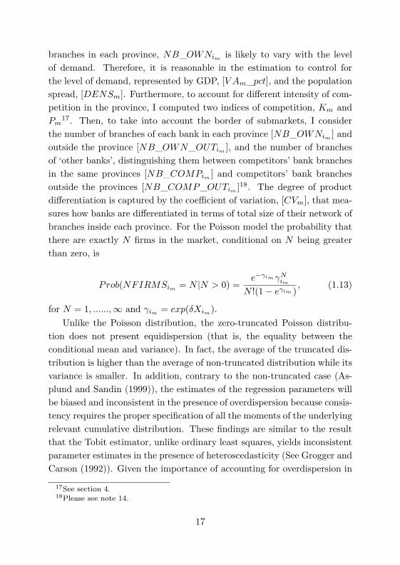
branches in each province, NB_OWNim is likely to vary with the levelof demand. Therefore, it is reasonable in the estimation to control forthe level of demand, represented by GDP, [V Am_pct], and the populationspread, [DENSm]. Furthermore, to account for different intensity of com-petition in the province, I computed two indices of competition, Km andPm

17. Then, to take into account the border of submarkets, I considerthe number of branches of each bank in each province [NB_OWNim

] andoutside the province [NB_OWN_OUTim ], and the number of branchesof ‘other banks’, distinguishing them between competitors’ bank branchesin the same provinces [NB_COMPim

] and competitors’ bank branchesoutside the provinces [NB_COMP_OUTim ]18. The degree of productdifferentiation is captured by the coefficient of variation, [CVm], that mea-sures how banks are differentiated in terms of total size of their network ofbranches inside each province. For the Poisson model the probability thatthere are exactly N firms in the market, conditional on N being greaterthan zero, is

Prob(NFIRMSim = N |N > 0) =e−γim γN

im

N !(1− eγim ), (1.13)

for N = 1, ......,∞ and γim= exp(δXim

).Unlike the Poisson distribution, the zero-truncated Poisson distribu-

tion does not present equidispersion (that is, the equality between theconditional mean and variance). In fact, the average of the truncated dis-tribution is higher than the average of non-truncated distribution while itsvariance is smaller. In addition, contrary to the non-truncated case (As-plund and Sandin (1999)), the estimates of the regression parameters willbe biased and inconsistent in the presence of overdispersion because consis-tency requires the proper specification of all the moments of the underlyingrelevant cumulative distribution. These findings are similar to the resultthat the Tobit estimator, unlike ordinary least squares, yields inconsistentparameter estimates in the presence of heteroscedasticity (See Grogger andCarson (1992)). Given the importance of accounting for overdispersion in

17See section 4.18Please see note 14.

17

the truncated context, I also present a model for truncated counts basedon the Negative Binomial distribution. The conditional distribution of atruncated Negative Binomial is

Prob(NFIRMSim= N |N > 0) =

Γ(N + 1α )

Γ(N + 1)Γ 1α

∗ 1

(1 + αγ)1α − 1

∗( αγ

1 + αγ)N ,

(1.14)As for the Poisson distribution, the average of the truncated negative bino-mial distribution is higher than that of the non-truncated one. Though thetruncated Poisson distribution no longer shows the equidispersion charac-teristic, the truncated Negative Poisson model introduce overdispersion,in the sense that its variance is higher than that of the Poisson19.

1.11 Model description: testing market size-market concentration relationship

In practice the relationship between market size and market concentrationhas been investigated by estimating a lower bound where a concentrationmeasure is regressed on market size variables. In that case,

log(C1

1− C1) = a + b

1log(S/ε)

+ v (1.15)

The constant represents the value of the limiting concentration as themarket size approaches infinite, that is C∞ = exp(a)/1 + exp(a). Themost used approach is the Smith’s two step procedure, where the errordistribution is a two or three parameters assumed to be drawn from aWeibull distribution. See for example Marìn and Siotis (2007). Lyons and

19For the truncated Poisson distribution the first and the second moment are:• E(N |N > 0; X) = u = λ + σ

• V (N |N > 0; X) = σ2 = λ − σ(u − 1)

with σ = λ/(eλ − 1). The mean and the variance of the truncated negative binomialregression are the following:

• E(N |N > 0; X) = u∗ = λ + σ∗

• V (N |N > 0; X) = σ∗2 = λ + αλ − σ∗(u∗ − 1)

with σ∗ = λ/((1 + α)α−1λ − 1).

18

Matraves (1996) proposed to use a stochastic (cost) frontier approach,allowing for disequilibrium deviations from the bound. As estimating astochastic lower bound by maximum likelihood methods is possible onlywhen the least squares residuals are positively skewed, Symeodonis (2000)suggest to simply use OLS regressions. I will follow Giorgetti (2003) relyingon quantile regression, as estimations obtained with this procedure arerobust to outliers. In particular, I will estimate the following lower bound

log(C1

1− C1) = a + a1TY PE1 + a2TY PE2 + a3REGION1 (1.16)

+a4REGION2 + b 1log(S/ε) + v

where TYPE and REGION are dummies variables, which account for dif-ferent macro regions in which the Italian territory can be divided and forthe different type of banks. For example, the limiting concentration ratioin a province in the NORTH, where the major bank is a cooperative, willbe equal to C∞ = exp(a + a1 + a3)/1 + exp(a + a1 + a3).

1.12 ResultsThe results of the zero truncated Poisson are reported in table (2). Theseresults suggest that province could be considered - in general - as an in-dependent submarket. As expected, the value of the coefficient is higherfor branches in the same provinces [NB_OWNim

] and [NB_COMPim],

and lower and close to zero for banks outside [NB_COMP_OUTim]. Re-

gression in column 2 and 3 in table (2) replicate the analysis in column 1 ac-counting for i) different macro-regions (REGION1=Nord,REGION2=Centre,REGION3=South) in which it is possible to group provinces, and ii) dif-ferent types of banks (TY PE1=BCC, TY PE2=BP, TY PE3= S.p.A).The inclusions of these variables improve the explanatory power of themodel (likelihood ratio tests are significant). In particular, supporting thepoint of independence among provincial submarkets, we can accept thenull hypothesis that both the coefficients of branches belonging to banksoutside the province are zero. The sign for the K coefficient is negative andsignificant whereas the value of the P coefficient is smaller, positive and

19

significant. These results suggest, as one could expect, that transportationcosts are more relevant in the retail market, and, therefore, a higher branchdensity increases competition lowering the expected (ex-post) number ofbanks. The value of the coefficient on CV is positive and significant. In ac-cordance with the model developed in the previous section, the higher thedegree of differentiation, the higher the number of banks. Since consumershave preferences about total number of branches, some banks have greaternetwork size with respect to other competitors and are able to capturemore consumers by differentiating themselves by opening more branches.In equilibrium, therefore, higher asymmetry in branch size (a higher valueof CV) is compatible with a large number of banks. On the contrary, thesign of the coefficient for the density of population is significant with unex-pected signs, where GPD is positive and insignificant. This is probably dueto the non-linear relationship between these variables and the dependentvariable, and to the fact that higher density will capture the same effectof GDP (since higher density is associated with higher GDP ). Resultsfor the zero Truncated Negative Binomial are reported in table (3). Theseregressions are in line with those of the zero Truncated Poisson. How-ever, our interest lies in measuring the change in the conditional mean ofNBANKS when regressors X change by one unit, the so called marginaleffects20. For reporting purposes, in tables (4) a single response value - themean of the independent variables - is used to evaluate the marginal effectsfor regression 3 in table (2) and (3). At this point it is important to con-trol for overdispersion, since in context with truncation and censoring itleads to problems of inconsistency (Hilbe (2007)). Several test procedurescan be followed to test the (truncated and untruncated) Poisson modelagainst the Negative Binomial model. As the Negative Binomial modeldegenerate into a Poisson model when α = 0, all tests (score test, Waldtest, likelihood test) are based on testing the overdispersion parameter α

equal to zero (Yen and Adamowicz (1993)). Since both the Poisson andthe Negative Binomial model have been estimated a likelihood-ratio test

20For linear regression marginal effects coincide with the estimated coefficients. Fornon linear regression this is no longer true. In that case, E[NBANKS|X] = exp(X′β),then ∂E[NBANKS|X]/∂X = exp(X′β)β is a function of both estimated parametersand regressors.

20

is straightforward. From the previous tables, it is possible to compute thelikelihood-ratio test of α = 0. This is the likelihood-ratio chi-square testthat is equal to χ2

(1) = −2(ll(Poisson)−ll(NegativeBinomial)). The largetest statistic would suggest that the response variable is over-dispersed andit is not sufficiently described by the Poisson distribution. In all cases, thistest is significant (for example, for regressions (3) is equal to χ2

(1) = 357.26,p < 0.001). In the end, these preliminary analysis allows me to analyse themain relationship of interest, that is the one between the size of the marketand the one-firm concentration ratio at the provincial level, relying only ona subsample made of one observation for each submarket. I will measuremarket size by means of two variables: the population in each provinceand the number of banks as estimated in previous section. Concerning thechoice of this latter variables, it important to notice that in homogeneousindustries, the number of firms represents the ratio between market sizeand sunk costs, that is S/ε . In addition, I can rely on 99 submarketsinstead of 103 since four provinces has been excluded from the previousregressions as were considered isolated by definition. Tables (5) and (6)report quantile regressions for the fifth, tenth and fiftieth percentile. Theresults are very similar and support the hypothesis that the retail bankingindustry is characterized by exogenous sunk costs: the estimated limitingconcentration C∞, approaches zero as the market size approaches infinite.It would be better to have an industry with endogenous costs so as tocompare the value of the limiting concentration. However, the quantile re-gressions, using both measures of market size, indicate that when marketsize increases, the concentration index goes down. This result is weaker inprovinces located in the South and in the Centre whereas it is stronger inprovince where the main banks is a TYPE2 (that is, Banche Popolari).

1.13 Robustness checks

The aim of this section is to control for issues that could weaken previousresults, mainly endogeneity and model specifications. Endogeneity may bean important concern when testing the size of each submarket, since thereare variables that could be considered jointly determined with the number

21

of banks if the industry has not reached an equilibrium. In particular, atfirm level, a troubling variable could be the number of branches a bankhas in the province (NB_OWN). The easiest way to test for endogene-ity is to use a method suggested by Wooldridge (1997) for count modelswith endogenous explanatory variables along similar lines to those sug-gested in other limited dependent variable contexts by Smith and Blundell(1986) and Rivers and Voung (1988). For any given explanatory variable x

which is potentially endogenous, it is possible to estimate a reduced formregression of the form

x = z′π + v (1.17)

where z represents a vector of exogenous explanatory variables includingat least one not included in x for identification, π the vector of reducedform coefficients and v is the reduced form error term. If it is possibleto obtain consistent estimates of π, Wooldrige shows that the residualsv = x − z′π can be included as an additional covariate in a maximumlikelihood estimator for count data model. A significant coefficient on v inthe augmented regression is a robust test of endogeneity of x. I test forpossible endogeneity of NB_OWN using as an identifying instrument thesame variable in year t− 2. The reason to choose NB_OWNt−2 insteadof in year NB_OWNt−1 is to avoid the risk of unit root. The reducedform is presented in table (7), whereas the residuals from this regressionare then used as an additional covariate in the zero truncated NegativeBinomial regression in table (8). The coefficient of the residuals is not sig-nificant, suggesting that in year 2005 the Italian Banking industry reachedan equilibrium. To analogous (not reported) conclusions leads a test forendogeneity of NB_OWN and NB_COMP . Another concern is relatedto the specification on the model for the relationship between market sizeand the one firm concentration ratio. A better alternative to estimate amodel where the dependent variable is a proportion is to use generalizedlinear models (Papke and Wooldridge (1996)). Results reported in table(9) confirm those obtained by means of standard regression model .

22

1.14 ConclusionsThe aim of this work was to test Sutton model of independent submar-kets checking his predictions for the Italian retail banking industry andusing the framework for the exogenous sunk costs industries. Even thoughthe banking industry as a whole should be considered as characterized byendogenous sunk costs, there are several features that indicate the retailindustry to be one of the former type. In particular, as banks branches sellslightly differentiated products in the retail sector, it is possible to lookat the number of banks branches as different varieties of the same prod-uct offered by banks to their client. In addition, despite the advances ofthe phone banking, consumers’ preferences are still biased toward regionalentity, suggesting province as submarket dimension.

The model developed in the first part of the paper indicates whichfactors should influence the number of banks in each submarket, and as aconsequence the one firm concentration ratio: the initial number of banks,the intensity of competition and the degree of product differentiation.

In the second part, a truncated Poisson and Negative Binomial modelhave been used in order to estimate the number of banks in each submarket.This way of proceeding allowed me to check the hypothesis about thesize and the independence among submarkets. In fact, the value of thecoefficient on the number of branches for banks outside the provinces, butwithin a radius of a hundred of kilometers, turned out to be insignificant.These results permitted to examine the one bank concentration ratio atprovincial level. Interestingly, the limiting concentration ratio approacheszero as market size goes to infinity. That means that exogenous sunk costsare involved in the Italian retail banking industry. As argued by Sutton,as the dimension of the submarket becomes larger, and given free entry,the value of concentration ratio has to go down.

23

References

Affinito, M. and Piazza, M. (2005), “What determines banking structurein European regions?” Paper prepared for the XIV International TorVergata Conference on Banking and Finance.

Asplund, M. and Sandin, R. (1999), “The Number of Firms and Produc-tion Capacity in Relation to Market Size,” The Journal of IndustrialEconomics, 69–85.

Berger, A.N. and Udell, G. (2006), “A More Complete Conceptual Frame-work for SME Finance,” Journal of Banking and Finance, vol. 30, 2945–2966.

Berger, A., Dai, Q., Ongena, S. and Smith (2003), “To What Extent Willthe Banking Industry be Globalized? A study of bank nationality andreach in 20 European nations,” Journal of Banking and Finance, vol. 27,383–415.

Bofondi, M. and Gobbi, G. (2004), “Bad Loans and Entry into Local CreditMarkets,” Banca d’Italia Temi di discussione, No 509.

Buzzacchi, L. and Valletti, T. (2005), “Firm Size Distribution: Testing theIndependent Submarkets Model in the Italian Motor Insurance Indus-try,” International Journal of Industrial Organization, vol. 24, 1–50.

Cameron, A.C. and Trivedi, P.K. (1998), Regression Analysis of CountData, Cambridge University Press.

Cerasi, V. (1996), “A model of Retail Banking Competition,” mimeo.

24

Cerasi, V., Chizzolini, B. and Ivaldi, M. (2000), “Branching and Compet-itiveness across Regions in the Italian Banking Industry,” in “IndustriaBancaria e Concorrenza,” Il Mulino, a cura di Polo, M.

Cerasi, V., Chizzolini, B. and Ivaldi, M. (2002), “Branching and Compe-tition in the European Banking Industry,” Applied Economics, vol. 34,2213–2225.

Cohen, M. and Mazzeo, M. (2004), “Market Structure and CompetitionAmong Retail Depository Institutions,” FEDS Working Paper, No 4.

Cremer, H. and Thisse, J. (1991), “Location Models of Horizontal Dif-ferentation: a Special Case of Vertical Differentiation, Models,” TheJournal of Industrial Economics, vol. 39, 383–390.

de Juan, R. (2003), “The Independent Submarkets Model: an Applica-tion to the Spanish Retail Banking Market,” International Journal ofIndustrial Organization, vol. 21, 1461–1487.

Di Salvo, R., Lopez, J.S. and Mazzilis, C. (2004), “I Processi Concorrenzialie l’Evoluzione del Relationship Banking nei Mercati Creditizi locali,” in“La Competitività dell’Industria Bancaria Italiana,” Nono Rapporto sulSistema Finanziario Italiano. Fondazione Rosselli, a cura di Bracchi G.e Masciandaro D., pages 87–118.

Dick, A.A. (2007), “Market Size, Service Quality and Competition inBanking,” Journal of Money, Credit and Banking, vol. 39, 49–81.

Ellickson, P. (2007), “Does Sutton apply to supermarkets?” The RANDJournal of Economics, vol. 38, 43–59.

Felici, R. and Pagnini, M. (2005), “Distance, bank heterogeneity, and entryin local banking market,” Banca d’Italia Temi di discussione, No 557.

Giorgetti, M. (2003), “Lower Bound Estimation - Quantile Regression andSimplex Method: An Application to Italian Manufacturing Sectors,”Journal of Industrial Economics, vol. 51, 113–120.

25

Grogger, J.T. and Carson, R.T. (1992), “Models for Truncated Counts,”Journal of Applied Econometrics, vol. 6, 225–238.

Gurmu, S. (1991), “Tests for Detecting Overdispersion in the Positive Pois-son Regression Model,” Journal of Business and Economic Statistics,vol. 54, 347–370.

Gurmu, S. and Trivedi, P. (1992), “Overdispersion Test for TruncatedPoisson Regression,” Journal of Econometrics, vol. 54, 347–370.

Hilbe, J. (2007), Negative Binomial Regression, Cambridge UniversityPress.

Hutchinson, J., Konings, J. and Walsh, P. (2006), “Company Size, Indus-try and Product Diversification. Evidence from the UK and Belgium,”mimeo.

ICB (2004), “Relazione Annuale,” Banca d’Italia.

ICB (2005), “Relazione Annuale,” Banca d’Italia.

Lyons, B. and Matraves, C. (1996), “Industrial Concentration,” in “Indus-trial Organization in the European Union: Structure, Strategy, and theCompetitive Mechanism,” Oxford University Press, Lyons et al. (eds).

Marìn, P. and Siotis, G. (2007), “Innovation and Market Structure: anEmpirical Evaluation of the ’Bound Approach’ in the Chemical Indus-try’,” Journal of Industrial Economics, vol. 55.

Papke, L. and Wooldridge, J. (1996), “Econometric methods for frac-tional response variables with an application to 401(k) plan participationrates,” Journal of Applied Econometrics, vol. 11, 619–632.

Petersen, M. and Rajan, R. (1995), “The Effect of Credit Market Compe-tition on Lending Relationship,” Quarterly Journal of Economics, vol.110, 407–43.

Rajan, R. and Zingales, L. (2003), “Banks and Markets: The ChangingCharacter of European Finance,” NBER Working paper series.

26

Rivers, D. and Voung, Q. (1988), “Limited Information Estimators andExogeneity Tests for Simultaneous Probit Models,” Journal of Econo-metrics, vol. 39, 347–366.

Rodrigues, V. (2001), “Endogenous mergers and market structure,” Inter-national Journal of Industrial Organization, vol. 47, 1245–1261.

Smith, R. and Blundell, R.W. (1986), “An Exogeneity Test for a Simul-taneous Equation Tobit-Model with an Application to Labor Supply,”Econometrica, vol. 54, 679–685.

Sutton, J. (1991), Sunk Costs and Market Structure, MIT Press.

Sutton, J. (1997), “Game Theoretic Models of Market Structure,” in “Ad-vances in Economics and Econometrics: Theory and Applications,”Cambridge Univ. Press, Kreps, D. M. and Wallis, K. F (eds).

Sutton, J. (1998), Sunk Costs & Market Structure: Theory and History,MIT Press.

Sutton, J. (2002), “Market Structure. The Bound Approach,” LSE, Paperprepared for the Volume 3 of the Handbook of I.O.

Symeodonis, G. (2000), “Price Competition and Market Structure: Theimpact of Cartel Policy on Concentration in the UK,” The Journal ofIndustrial Economics, vol. 48, 1–26.

Symeodonis, G. (2002), The Effect of Competition Cartel Policy and theEvolution of Strategy and Structure in British Industry, MIT Press.

Vasconcelos, H. (2006), “Endogenous mergers in endogenous sunk costindustries,” International Journal of Industrial Organization, vol. 24,227–250.

Walsh, P. and Whelan, P. (2002), “Portfolio Effects and Firms Size Dis-tribution: Carbonate Soft Drinks,” The Economic and Social Review,vol. 33, 43–54.

27

Wooldridge, J. (1997), “Quasi-maximum Likelihood Methods for CountData,” in “Handbook of Applied Econometrics Vol II,” Oxford; Black-wells, Pesaran, H. and Schimdt, P. (eds), pages –.

Yen, S. and Adamowicz, W. (1993), “Statistical Properties of Welfare Mea-sures from Count-Data Models of Recreation Demand,” Review of Agri-cultural Economics, vol. 15, 203–215.

Yi, S. (1997), “Stable Coalition Structure with Externalities,” Game andEconomic Behavior, vol. 20, 201–237.

28

Table 1: Summary statistics

Variable Mean Std. Dev. Min. Max. NNbanks 34.598 19.096 8 86 2673C1 24.869 8.153 12.963 80.672 2673CV 1.626 0.419 0.691 2.648 2673DENS 0.033 0.044 0.004 0.264 2673K 0.002 0.002 0 0.012 2673P 0.06 0.019 0.022 0.104 2673NB_OWN 0.001 0.002 0 0.043 2673NB_COMP 0.045 0.048 0.002 0.231 2673NB_OWN_OUT 0.005 0.01 0 0.093 2673NB_COMP_OUT 0.177 0.156 0.002 0.631 2673

Table 2: Estimation results: Zero Truncated PoissonDependent variable: Numbers of Banks - equation (3.3)

Variable (1) (2) (3)NB_OWN 9.242*** 9.080*** 9.043***

(2.062) (1.967) (1.744)NB_COMP 8.190*** 8.482*** 8.404***

(1.344) (1.242) (1.204)NB_OWN_OUT -2.699*** -2.122*** -0.874

(0.623) (0.566) (0.594)NB_COMP_OUT -0.049 0.004 -0.011

(0.182) (0.216) (0.205)CV 0.167 0.228 0.231*

(0.151) (0.140) (0.134)K -141.197*** -126.401*** -124.354***

(48.777) (41.179) (39.865)P 9.768*** 12.335*** 11.658***

(2.876) (2.900) (2.737)DENS 3.859*** 3.163*** 3.135***

(1.322) (1.105) (1.065)VA_pct 1.627 0.572 0.677

(2.158) (1.741) (1.675)REGIONE1 -0.204* -0.198

(0.123) (0.121)REGIONE2 -0.248** -0.229*

(0.123) (0.118)TYPE1 0.106***

(0.031)TYPE2 0.032***

(0.012)Constant 2.338*** 2.237*** 2.231***

(0.219) (0.200) (0.191)ll -9490.302 -9347.755 -9266.454N 2673 2673 2673chi2 1051.747 1067.701 1097.830p 0.000 0.000 0.000* p<0.10, ** p<0.05, *** p<0.01

30

Table 3: Estimation results: Zero Truncated Negative BinomialDependent variable: Numbers of Banks

Variable (1) (2) (3)NB_OWN 9.227*** 8.933*** 9.042***

(2.278) (2.194) (1.890)NB_COMP 8.564*** 8.615*** 8.527***

(1.428) (1.279) (1.236)NB_OWN_OUT -2.559*** -2.121*** -0.843

(0.601) (0.562) (0.600)NB_COMP_OUT -0.032 0.026 0.010

(0.170) (0.206) (0.195)CV 0.163 0.219 0.222*

(0.142) (0.137) (0.132)K -141.481*** -124.063*** -121.415***

(48.087) (42.405) (40.864)P 8.761*** 11.128*** 10.515***

(2.610) (2.885) (2.751)DENS 3.729*** 3.081*** 3.045***

(1.294) (1.161) (1.115)VA_pct 1.479 0.557 0.647

(2.352) (1.846) (1.762)REGIONE1 -0.177 -0.173

(0.124) (0.121)REGIONE2 -0.209* -0.193

(0.123) (0.118)TYPE1 0.114***

(0.032)TYPE2 0.036***

(0.013)Constant 2.392*** 2.289*** 2.278***

(0.193) (0.189) (0.181)lnalpha -3.676*** -3.831*** -3.930***

(0.371) (0.425) (0.422)ll -9196.711 -9138.896 -9087.824N 2673 2673 2673chi2 600.999 641.091 657.921p 0.000 0.000 0.000* p<0.10, ** p<0.05, *** p<0.01

31

Table 4: Estimation results: Marginal effects

Variable (ztp) (ztnb) (Variable Mean)NB_OWN 283.1834 283.0865 .0011403

(52.357) (56.701)NB_COMP 263.1779 266.9689 .0447364

(36.787) (38.366)NB_OWN_OUT -27.37672 -26.40309 .005079

(18.463) (18.601)NB_COMP_OUT -.3452477 .2979915 .1772281

(6.431) (6.110)CV 7.227972 6.952858 1.625817

(4.238) (4.167)K -3894.202 -3801.284 .0018006

(1238.163) (1277.182)P 365.0903 329.2003 .0600712

(87.430) (87.960)DENS 98.17784 95.34141 .0327039

(32.976) (34.739)VA_pct 21.21327 20.25852 .0143725

(52.418) (55.120)REGIONE1 (d) -6.113763 -5.35278

(3.697) (3.708)REGIONE2 (d) -6.920037 -5.862967

(3.473) (3.508)TYPE1 (d) 3.423496 3.673721

(1.037) (1.093)TYPE2 (d) 1.002621 1.144445

(0.392) (0.417)(d)marginals for discrete change of dummy variable from 0 to 1

32

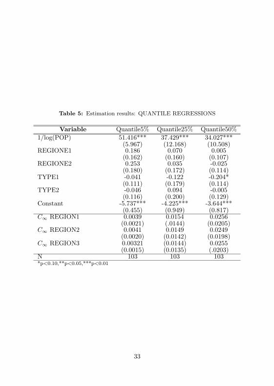
Table 5: Estimation results: QUANTILE REGRESSIONS

Variable Quantile5% Quantile25% Quantile50%1/log(POP) 51.416*** 37.429*** 34.027***

(5.967) (12.168) (10.508)REGIONE1 0.186 0.070 0.005

(0.162) (0.160) (0.107)REGIONE2 0.253 0.035 -0.025

(0.180) (0.172) (0.114)TYPE1 -0.041 -0.122 -0.204*

(0.111) (0.179) (0.114)TYPE2 -0.046 0.094 -0.005

(0.116) (0.200) (0.129)Constant -5.737*** -4.225*** -3.644***

(0.455) (0.949) (0.817)C∞ REGION1 0.0039 0.0154 0.0256

(0.0021) (.0144) (0.0205)C∞ REGION2 0.0041 0.0149 0.0249

(0.0020) (0.0142) (0.0198)C∞ REGION3 0.00321 (0.0144) 0.0255

(0.0015) (0.0135) (.0203)N 103 103 103*p<0.10,**p<0.05,***p<0.01

33

Table 6: Estimation results: QUANTILE REGRESSIONS

Variable Quantile5% Quantile25% Quantile50%1/log(banks) 7.556* 7.078 2.947

(4.440) (5.069) (3.001)REGIONE1 0.428*** 0.232 0.029

(0.099) (0.199) (0.100)REGIONE2 0.437*** 0.196 -0.022

(0.132) (0.202) (0.102)TYPE1 0.011 -0.108 -0.198**

(0.186) (0.203) (0.097)TYPE2 0.057 -0.019 -0.054

(0.089) (0.237) (0.116)Constant -3.123*** -2.498*** -1.500***

(0.719) (0.818) (0.489)C∞ REGION1 0.0633 0.0940 0.1824**

(0.0455) (0.0646) (0.0730)C∞ REGION2 0.0638 0.0909 0.1791***

(0.0441) (0.0655) (0.0679)C∞ REGION3 0.0422 0.0760 0.1868***

(0.0290) (0.0574) (0.0683)N 99 99 99*p<0.10,**p<0.05,***p<0.01

34

Table 7: Estimation results: OLS - Reduced formDependent variable: NB_OWN

Variable CoefficientNB_OWN_03 0.9798***

(0.008)NB_COMP 0.0003*

(0.000)NB_OWN_OUT 0.0002

(0.001)NB_COMP_OUT 0.0001

(0.000)CV -0.0000

(0.000)K -0.0025

(0.009)P 0.0002

(0.000)DENS 0.0002

(0.000)VA_pct 0.0003

(0.000)TYPE1 0.0000

(0.000)TYPE2 0.0001***

(0.000)REGION1 -0.0000

(0.000)REGION2 0.0000

(0.000)Constant 0.0000

(0.000)R2 .9883225N 2414.000p 0.000* p<0.10, ** p<0.05, *** p<0.01

35

Table 8: Estimation results: Augmented Zero Truncated Negative Bino-mialDependent variable: Numbers of Banks

Variable (1)NB_OWN 9.170***

(1.923)NB_COMP 8.556***

(1.255)NB_OWN_OUT -0.591

(0.587)NB_COMP_OUT 0.006

(0.203)CV 0.225*

(0.135)K -121.924***

(41.176)P 10.713***

(2.718)DENS 3.087***

(1.128)VA_pct 0.613

(1.770)TYPE1 0.121***

(0.032)TYPE2 0.034**

(0.014)REGION1 -0.181

(0.124)REGION2 -0.201*

(0.120)vhat -2.433

(8.790)Constant 2.260***

(0.186)-3.852***

(0.404)ll -8245.051N 2414.000chi2 666.529p 0.000* p<0.10, ** p<0.05, *** p<0.01

36

Table 9: Estimation results: GLMAs the dependent variable C1 is a proportion, it is to use generalized linear modelwith family binomial family, logistic link function. Standard errors scaled usingsquare root of Pearson X2-based dispersion

Variable1/log(POP) 43.956***

(12.273)REGIONE1 -0.173 -0.145

(0.117) (0.136)REGIONE2 -0.227* -0.188

(0.124) (0.139)TYPE1 -0.234* -0.263*

(0.132) (0.138)TYPE2 0.040 -0.088

(0.145) (0.160)1/log(banks) -0.848

(4.023)Constant -4.221*** -0.686

(0.957) (0.656)C∞ REGION1 0.0122 0.3034**

(.0115 ) ( 0.1256)C∞ REGION2 0.0116 0.2943**

(0.1098) (0.1283)C∞ REGION3 0.01450 0.3349**

(0.0144) (0.1462)N 103 99*p<0.10,**p<0.05,***p<0.01

37

Chapter 2

Unit Roots and theDynamics of MarketShares: an analysis usingItalian Bankingmicro-panel

Abstract

The paper proposes the use of panel data unit root tests to assess marketshare instability in order to have (preliminary) indications of the industrydynamic. The idea is to consider the movements in market shares notonly as element of the market structure but rather reflecting competitors’conduct. If shares are mean-reverting, the firm actions have a temporaryeffect on shares only. On the other hand, if they are evolving, as signaled bythe presence of unit roots, the gain in shares respect with the competitorscould be long-term. To illustrate the potential of unit roots tests, I consideran application to the Italian retail banking industry.

Keywords: turbulence, cross-section dependence.JEL Classification: C23; D40.

2.1 Introduction

In order to get an understanding of the dynamic of an industry, a first stepcould be to examine whether the market shares are stationary or evolving.If shares are mean-reverting, the firm actions only have a temporary effecton shares. On the contrary, if they are evolving, as signaled by the presenceof unit roots, the gain (or loss) in shares respect with the competitors couldbe long-term. In the first case, it is reasonable to infer that the industryis rather stable - or mature - where actors reached positions difficult toovercome. In the second case, instead, the possibility for a competitor tobecome permanently a leader (or to loose the leadership) could be a signalthat the industry experienced the displacement of existing technology byalternative ones and/or the displacement of existing products by new andsuperior substitutes. In other words, by considering the movements inmarket shares not only as elements of the market structure but ratherreflecting competitors’ conduct that arise from the market (Asplund andNocke (2006); Caves (1998); Matraves and Rondi (2007); Sutton (2004);Uchida and Cook (2005)), unit root tests could be a way to empiricallytest the influence of industry characteristics on the degree of turbulence(Davies and Geroski (1997); Sutton (1997)).

An important characteristic of market share data sets is the logicalconsistency requirement in market share models. In fact, market sharesare bounded between 0 and 1 and they sum to unity. This relationshipmust be taken into account if one want to study all the actors in themarket1. Another possibility is to consider only few actors in the market.

According to this latter procedure, this paper proposes the use of micro-panel data unit root models to assess market share instability in the ItalianBanking Industry for a sample of firms made of the first 5 banks in eachprovince. On the one hand, the assessment of the competitive conditionsof the Italian banking industry is of interest since the industry has knowna marked consolidation process along with a remarkable deregulation pro-

1An interesting approach is presented in the work of Franses et al. (2001). Theyexploit the consistency requirement to apply the Johansen test, relying on a system-based test rather than a single equation test. In addition, the fact that the data arebounded from below and above renders a deterministic model implausible.

1

cess since the beginning of the nineties. To the best of my knowledge, thispaper is the first to apply this methodology to test banking competition.On the other hand, given the well-known low power of conventional unitroot tests when applied to single short time series, panel unit root testscan be fruitfully employed in analysis of firms or industries that rely onmicro-panels, where the time dimension may be of limited length but ob-served across several units. One of the main advantages of panel unit roottests is that their asymptotic distribution is standard normal. This is incontrast to individual time series unit roots which are non-standard nor-mal asymptotic distributions. However, these tests are not exempt fromcritics. In particular, few tests consider the possibility of cross-sectioncorrelation and spillovers amongst countries, regions or provinces (Baltagiet al. (2007)). In this regard, Pesaran (2004) suggests a test for cross-sectional dependence and way of getting rid of it by augmenting the usualADF regression with lagged cross-sectional mean and its first-difference tocapture the cross-sectional dependence that arises through a single factormodel. Other important aspects concerning panel unit roots are relatedto their asymptotic behavior under the two dimension of the panel, N andT and their requirement for a balanced panel (no missing data for any i

not t).Clearly, the use of panel unit root tests can only offer (preliminary)

indications of the dynamic in the industry. As any other statistical test,there is a risk of incorrect inference but it could be minimized by prop-erly selecting the test in relation to the main features of the dataset used.In any case, results must be supported by other qualitative - and if it isfeasible - quantitative evidence. However, the existence of dynamic in thepositions of the first 5 banks - as signalled by the presence of unit rootsin the market shares - suggests that the Italian retail banking industryexperienced overtime a movement towards higher level of competition. Inparticular, in the same spirit of Kim et al. (2003), a dynamic in marketshares could be interpreted as an indirect signal for a reduction of switch-ing costs that make easier to consumers to move to different banks and,consequently, for banks to acquire new customers.

The structure of the paper is as follows. The next section briefly intro-

2

duces the data and the main features of the industry under investigation.Section 3 presents the model for micro-panels, whereas in section 4 panelunit roots tests are computed for the first 5 banks in every Italian province.Section 5 provides the Pesaran’s test of cross-section dependence. The fol-lowing section, taking into account these results, computes the unit roottest proposed by Pesaran which deals with the cross-section dependence.The conclusions are presented in the final section.

2.2 Characteristics and construction of thedataset

A peculiarity of the Italian banking industry is the presence of different ter-ritorial dynamics (Colombo and Turati (2004); Guiso et al. (2004, 2006)).In particular, the retail Italian Banking Industry can be viewed as madeof a large number of local markets corresponding to different geographicallocations. In each one of these submarkets, there are several branches ofdifferent banks competing against each other. The Italian territory is di-vided into 20 regions and 103 provinces, which are geographical units closeto US counties. In accordance with the Italian Antitrust Authority, thepresumption is that the province is the relevant market.

Given the widespread differences in local economic conditions and theirinfluence on the competition process, I will focus on local markets by mea-suring market shares at the provincial level using data on branches asproxies for the market share of individual (or group of) banks. The rea-sons behind the choice to compute market shares relying on this variableare various. First of all, the number of branches (or branch density) iscommonly used in the empirical literature on local banking competition(see, for instance, Degryse and Ongena (2005)). Secondly, it captures thedimension of banking competition that has been more heavily affected bythe deregulation process. Since March 1990, the establishment of newbranches has been completely liberalized. The number of branches in-creased steadily, up to 32.337 in 2007, as well as the number of peopleserved by each branch, 47 per 100.000 inhabitants in 2004 (compared to

3

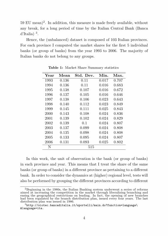
59 EU mean)2. In addition, this measure is made freely available, withoutany break, for a long period of time by the Italian Central Bank (Bancad’Italia) 3.

Hence, the (unbalanced) dataset is composed of 103 Italian provinces.For each province I computed the market shares for the first 5 individualbanks (or group of banks) from the year 1993 to 2006. The majority ofItalian banks do not belong to any groups.

Table 1: Market Share Summary statistics

Year Mean Std. Dev. Min. Max.1993 0.136 0.11 0.017 0.7071994 0.136 0.11 0.016 0.6831995 0.138 0.107 0.016 0.6721996 0.137 0.105 0.016 0.6461997 0.138 0.106 0.023 0.6431998 0.140 0.112 0.023 0.8491999 0.145 0.111 0.025 0.8432000 0.143 0.108 0.024 0.8362001 0.139 0.102 0.024 0.8292002 0.139 0.1 0.024 0.8072003 0.137 0.099 0.024 0.8082004 0.135 0.098 0.024 0.8082005 0.133 0.095 0.024 0.8072006 0.131 0.093 0.025 0.802

N 515

In this work, the unit of observation is the bank (or group of banks)in each province and year. This means that I treat the share of the samebanks (or group of banks) in a different province as pertaining to a differentbank. In order to consider the dynamics at (higher) regional level, tests willalso be performed by grouping the different provinces according to different

2Beginning in the 1980s, the Italian Banking system underwent a series of reformsaimed at increasing the competition in the market through liberalizing branching andeasing the geographical restrictions on lending. In fact, the opening of new brancheshad been regulated by the branch distribution plan, issued every four years. The lastdistribution plan was issued in 1986.

3http://siotec.bancaditalia.it/sportelli/main.do?function=language\&language=ita.

4

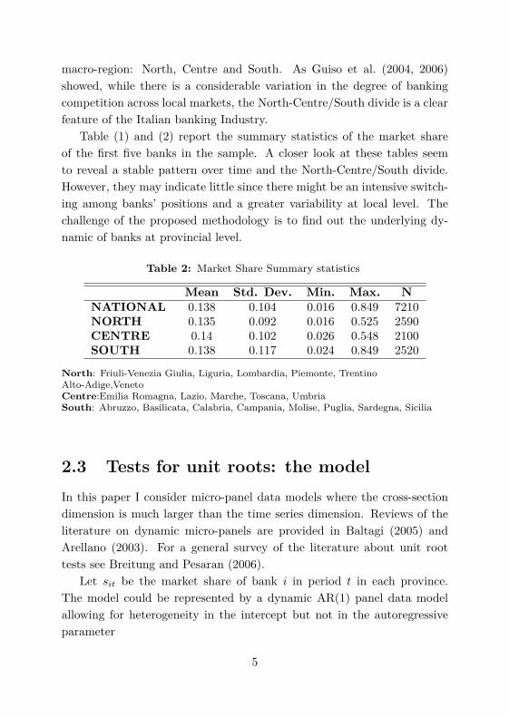
macro-region: North, Centre and South. As Guiso et al. (2004, 2006)showed, while there is a considerable variation in the degree of bankingcompetition across local markets, the North-Centre/South divide is a clearfeature of the Italian banking Industry.

Table (1) and (2) report the summary statistics of the market shareof the first five banks in the sample. A closer look at these tables seemto reveal a stable pattern over time and the North-Centre/South divide.However, they may indicate little since there might be an intensive switch-ing among banks’ positions and a greater variability at local level. Thechallenge of the proposed methodology is to find out the underlying dy-namic of banks at provincial level.

Table 2: Market Share Summary statistics

Mean Std. Dev. Min. Max. NNATIONAL 0.138 0.104 0.016 0.849 7210NORTH 0.135 0.092 0.016 0.525 2590CENTRE 0.14 0.102 0.026 0.548 2100SOUTH 0.138 0.117 0.024 0.849 2520

North: Friuli-Venezia Giulia, Liguria, Lombardia, Piemonte, TrentinoAlto-Adige,VenetoCentre:Emilia Romagna, Lazio, Marche, Toscana, UmbriaSouth: Abruzzo, Basilicata, Calabria, Campania, Molise, Puglia, Sardegna, Sicilia

2.3 Tests for unit roots: the modelIn this paper I consider micro-panel data models where the cross-sectiondimension is much larger than the time series dimension. Reviews of theliterature on dynamic micro-panels are provided in Baltagi (2005) andArellano (2003). For a general survey of the literature about unit roottests see Breitung and Pesaran (2006).

Let sit be the market share of bank i in period t in each province.The model could be represented by a dynamic AR(1) panel data modelallowing for heterogeneity in the intercept but not in the autoregressiveparameter

5

si0 = δ0 + δ1ηi + vi0

sit = αisi,t−1 + uit

uit = (1− αi)ηi + vit (2.1)

where α1 = · · · = αN = α for each i = 1 . . . N , t = 2 . . . T , and whereN is large and T is fixed. The series have a unit root (or are integrated oforder one) if αi = 1 and are stationary if αi < 1. A test for the presenceof a unit root in the panel is presented by the null hypothesis H0 : α = 1in equation (2.1).

In case of independence across firms, the error term satisfies

E(ηi) = 0, E(vit) = 0 (2.2)

for i = 1, . . . , N and t = 2, . . . , T and

E(vitvis) = 0 (2.3)

for i = 1, . . . , N and t 6= s.In the literature two types of panel unit root tests can be distinguished,

dependent on the alternative under consideration. The first type of testconsiders a homogeneous alternative, i.e H0 = α1 = · · · = αN = α < 1.An example is Levin et al. (2002). The idea of this approach is to performa pooled Dickey-Fuller (DF ) test with the residuals. The second type oftest allow for heterogeneity of all parameters. Im et al. (2003) criticizethe assumption of common root under the alternative and they require|αi| < 1 for a sufficiently large number of units. Consequently in this case,it is natural to perform N tests individually and to average over individualDF statistics.

In that model there are two sources of persistency. One is the autore-gressive mechanism, which is the same for all cross-section units, and theother is the unobserved individual-specific term. The unit root hypothesiscan be considered as an extreme case where all the presistency is caused bythe autoregressive mechanism. In this context, the time dimension of the

6

panel dataset is an important issue to look at, as well as the specificationof the initial value.

In this paper, two distinct regression-based test procedures will be pro-posed: one based on a simple OLS regression of market shares on theirlagged values; the second test, proposed by Breitung and Meyer (1994),specifies the regression in terms of deviations from initial conditions andit is therefore more powerful if the variance of individual effects is high.These simple t-tests based on least-squared estimators, which are consis-tent only under the unit root null, are shown to have good size propertiesand at least as high power as test based on GMM and ML estimators(Bond et al. (2005)). It is known that instrumental variable and GMMprocedures provide consistent estimate of dynamic coefficients in caseswhere pooled least squares are inconsistent (Arellano (2003), Phillips andSul (2007)). However, these procedures are also known to suffer bias andweak instrumentation problem when the dynamic coefficient αi is close tounity.

However, these tests are not exempt from critics. In particular, theyassume cross-section independence. Hence, the Pesaran’s test for cross-section independence will be computed. The test can in fact be applied to awide range of panel data model, including panel with short time dimension.As that test evidenced the presence of cross-section dependence, the panelunit root test allowing for cross-section dependence proposed by Pesaranwill be also computed.

2.3.1 OLSAs Bond et al. (2005); Madsen (2003); Hall (2002) have shown, the t-test based on the OLS levels estimator performs much better than otherestimators (GMM, FD, WG,..) in micro panels, that is when T is verysmall in comparison with N . Both simulation and asymptotic analysishave demonstrated that the OLS estimator has the highest power to rejectalternative that are close to the null hypothesis that α = 1.

Because the number of periods is small, properties of the initial con-dition are also relevant. Madsen (2003) shows that the asymptotic powerof the OLS test under the alternative differs depending on the assumption

7

made about the initial value. In particular, the advantage of using OLSis expected to be high when the initial value are such that the time-seriesprocess become covariance stationary, even for value of α close to unity4.In the other cases, when the initial values are such that the time-seriesbecome mean stationary and when the variation in the individual-specificterms is high, the highest power can be obtained using a t-test for theleast squares estimator in the transformed model proposed by Breitungand Meyer (1994). As emerged from the previous works, these two testsmust be considered jointly.

Under the null H0 : α = 1, the OLS estimator of α in model 2.1 isconsistent. The t-test based on OLS estimator is

tOLS =αOLS − 1√

ˆV ar(αOLS)(2.4)

where

ˆV ar(αOLS) = (s′−1s−1)−1

(N∑i

s′i,−1eie′isi,−1

)(s′−1s−1)−1 (2.5)

with ei = si−si,1αOLS , si = (si,2, . . . , si,T )′, si,−1 = (si,1, . . . , si,T−1)′,and s−1 = (s′1,−1, . . . , s

′N,−1)

′. Under the null, α = 1, tOLS has an asymp-totic standard normal distribution as N →∞.

Under the alternative, the OLS estimator is biased upwards, more sowhen the variance of ηit is large relative to the variance of vit. The powerof this test will therefore depend on the magnitude of V ar(ηi)/V ar(vit)(Bond et al. (2005)).

Breitung and Meyer (1994) suggest an alternative estimation approachwhich involves deducting the first observation si0 for each firm from theright hand side of equation (2.1). The estimable model becomes

sit − si0 = α(si,t−1 − si,0) + εit (2.6)st = st−1 + εit t = 3, . . . , T (2.7)

4Mean stationarity (constant first moment) requires αi < 1 and δ0 = 0 and δ1 = 1.The covariance stationarity (constant first and second moments) in addition requireshomeschedatisticity over time of the vit shocks (i.e. var(vit) = σ2

vi for i = 1, . . . , N)and that var(vi0) = σvi/(1 − αi)

2.

8

where ε = vit−(1−α)(si0−ηi). Again, the OLS estimator is consistentwhen α = 1 and upward biased under the alternative. Breitung and Meyerhowever showed that the bias is α + 1−α

2 . That means that the power ofthe test, contrary to the previous case, is not affected by the individual-specific term, that is by the term V ar(ηi)

V ar(vit). For long T panels, none of these

could be applied, since the asymptotic distribution tends to a DF: so it isnecessary to combine N DF/ADF tests as in Im et al. (2003).

2.3.2 A test for Cross Section Dependence

Pesaran (2004), Baltagi et al. (2007) show that there can be considerablesize distortions in panel when the hypothesis of cross section independenceis violated and the specification exhibits, for example, spatial error corre-lation.

When N is small and the time dimension T is sufficiently large, thecross section correlation can be modeled using seemingly unrelated regres-sion (SURE), and traditional times series techniques - such the LagrangeMultiplier (LM) of Breusch and Pagan - can be applied5. However incases where N is large, standard techniques are not applicable. Anotherapproach, used in the literature of spatial statistics, measures the extentof cross dependence by means of a spatial matrix.

Pesaran (2004) proposes instead a simple diagnostic test that neitherrequires any a priori specification of a connection matrix nor suffers ofpanel data model limitations. It is therefore applicable in a variety of con-texts, including stationarity dynamic and unit-root heterogeneous panelswith short T and large N . The test, in all its various formulation, is basedon simple averages of pair-wise correlation coefficients of OLS residualsfrom individual regressions.

5For example, Chu et al. (2007) used the panel SURADF tests to investigate Gibrat’slaw of proportionate effects for 48 electronic firms in Taiwan. Panel SURADF tests han-dle cross-sectional dependence across firms and, at the same time, investigate a separateunit-root null hypothesis for each and every individual panel member, identifying howmany and which series in the panel are stationary process

9

CD =

√2T

N(N − 1)

N−1∑i=1

N∑j=i+1

ρij

(2.8)

where

ρij =∑T

t=1 vitvjt(∑Tt=1 vit

2)1/2 (∑T

t=1 vjt2)1/2

(2.9)

Unlike the LM statistic, the CD statistic has exactly mean at zero forfixed value of T and N , under a wider range of panel data model, and itis shown to have a standard normal distribution, assuming that the errorsare symmetrically distributed, vit are i.i.d.(0, 1). In addition, it can beapplied to unbalanced panels. In this last case, equation (2.10) can bemodified by

CD =

√2

N(N − 1)

N−1∑i=1

N∑j=i+1

√Tij ρij

(2.10)

where Tij =∑

1Ti∩Tj (the number of common time series observationsbetween units i and j) and

ρij =

∑t∈Tij

(vit − ¯vit)(vjt − ¯vjt)(∑Tt=1(vit − ¯vit)2

)1/2 (∑Tt=1(vjt − ¯vjt))2

)1/2(2.11)

with ¯vit =∑

t∈Tijuij/Tij . Finally, in cases where the cross section

units can be ordered a priori, as with spatial observations, the CD testcan be generalized capturing the spatial pattern too (Pesaran (2004)).

2.4 The Italian caseAs previously stated, the Italian banking industry is of interest since it ex-perienced a deregulation process during the nineties that lead, among otherthings, to liberalized entry and easier procedures to open new branches.

10

Therefore, it is reasonable to expect a movement towards higher level ofcompetition, both at National and macro-regional level.

Let’s start with the two simple t-tests based on OLS regressions.

Table 3: OLS:Dependent variable: Firm shares

Variable NATIONAL NORTH CENTRE SOUTHt* 2.91 3.17 0.65 1.06p-value 0.004 0.002 0.517 0.290with time dummiest* 4.8 6.93 6.2 4.8p-value 0.000 0.000 0.000 0.000N 5758 2086 1695 1977

*Note: the t-statistic for H0: β = 1 against H1 : β < 1

Results relying on constrained estimations - imposing restrictions on the constantbeing equal or greater than zero - are substantially identical.

Table 4: Breitung and Meyer 1994:Dependent variable: Firm shares

Variable NATIONAL NORTH CENTRE SOUTHt* 3.19 2.5 0.31 2.9p-value 0.001 0.012 0.750 0.004N 5758 2086 1695 1977

*Note: the t-statistic for H0: β = 1 against H1: β < 1.

As table (3) and (4) show, the null hypothesis H0 : α = 1 cannot alwaysbe rejected and the series seem to present unit roots, especially in themarket-share related to the provinces in the Centre/South of Italy. Theseresults disappear when it is controlled for common shocks (captured byyear dummies). If the hypothesis of unit root cannot be rejected, it meansthat the positions of the main banks in the market could be displacedpermanently by other actors, and there is evidence for a shift towardshigher degree of competition.

11

2.4.1 Cross Section Dependence in Dynamics Panels

In the previous section, as it is typically assumed in panel data models,disturbances are treated as cross sectionally independent. To check if thepanel at hand is characterized by cross-section dependence, the CD test isapplied6. Two specification are used: one with residuals of homogeneousregression and one with residuals from N individual regressions from model(2.1). In both cases, the tests draw also on the residuals of the specifica-tion with/without the intercept and the observations are grouped again ac-cording to macro-regional classification (North, Center and South)7. Thecorrelation are computed over the common set of observations for i andj. As it is already noted, the OLS estimates of the constant, (1 − αi)ηi,and slope αi for the individual series are biased when T is small. Andthat bias could be substantial for value of α near unity. However, the CDTEST advanced by Pesaran (2004) is valid for all values of α in model 2.1,including unity. The main reason lies in the fact that despite the samplebias of the parameters estimates, the OLS have exactly mean zero even fora fixed T, so long as the errors are symmetrically distributed. The mainlimitation of Pesaran’s test relies in its pair wise construction since it couldbe possible that pair wise correlation compensate each others, summingto zero. While allowing for different value of αi and cross-section correla-tion, we still assume that in model (2.1) vit are serially uncorrelated withzero mean. Due to computational reasons, I restrict the analysis to thebalanced panel made of 20% of the observations. Table (5) reports re-sults for the cross section dependence test developed by Pesaran. In bothcases, allowing or not for heterogeneity, there is evidence for cross sectiondependence in all the macro-region considered.

6For this test I built a STATA command csdar.ado relying on xtcsd.ado as developedby De Hoyos and Sarafidis (2006).

7Results in table (5) refer to estimation without intercept. Those with intercept areanalogous and are not reported.

12

Table 5: Pesaran’s Test of Cross Section Independence

NATIONAL NORTH CENTRE SOUTHResidualsfrom a regression*CD Statistic 6.875 50.370 44.920 52.694P-value 0.000 0.000 0.000 0.000Residualsfrom N regression*CD Statistic 5.106 50.228 44.334 52.864P-value 0.000 0.000 0.000 0.000* without intercept

2.5 Panel Unit Root Tests for Cross Section-ally Dependent Panels

Overall, the outcome of the preceding tests clearly indicates the presenceof cross section dependence amongst units.

Pesaran builds on the assumption that the error terms vit of equation(2.1) follow a single common factor structure

vit = λift + εit (2.12)

The common factor is assumed to be stationary and to impact thecross-section with a fraction determined by the individual specific factorloading λi. Because of the common factor, cross section dependence arisesand can be approximated by the cross-section mean st = 1

N

∑Ni=1 sit. As

usual, the εit are assumed to be i.i.d across i and t with zero mean andvariance σ2

i , and E(εit)4 < ∞. Furthermore, εit, ft and λi are mutuallyindependently distributed for all i.

Pesaran proposes the following augmented Dickey-Fuller regression:

∆sit = ci + ρisi,t−1 +βist−1 +p∑

j=1

γij∆si,t−j +p∑

j=0

γij∆si,t−j + εit (2.13)

where, as usual in the univariate case, lagged first-differences on both si

and si are added in order to take into account also for possible correlation

13

in the error term. Either individually or in a combined fashion, the t-valueof ρi can be used to test the presence of unit roots. In the first case,the statistic is called cross-sectionally augmented Dickey-Fuller (CADFi)while in the second case the statistic is constructed as

CIPS =1N

N∑i

CADFi (2.14)

It is called CIPS since it resembles the IPS statistic (Im et al. (2003)).In the case were T is fixed, to ensure the CADF statistics do not dependon the nuisance parameters, Pesaran (2003) suggests to apply the test tothe deviations of the variable from initial cross-section mean.

Table 6: Pesaran’s Test for Unit Root

NATIONAL NORTH CENTRE SOUTHCADF (0 lag)t -1.563 -2.020 -2.067 -2.086z[t-bar] 1.178 -1.309 -2.067 -2.086P-value 0.881 0.095 0.023 0.084CADF (1 lag)t -1.333 -2.708 -1.590 -1.262z[t-bar] 3.024 -1.560 0.744 1.644P-value 0.999 0.059 0.772 0.950

Table (6) shows the Pesaran’s test for unit root computed using Ital-ian Banking dataset. Due to the presence of the lagged level of the crosssectional average, the limiting distribution of the CADF statistics and theCIPS statistic does not follow a standard Dickey-Fuller distribution. How-ever, Peseran provides critical values based on simulations for the CADFand CIPS-distributions for three cases (no intercept and no trend, interceptonly, intercept and trend). As results from this test suggests, cross-sectiondependence does matter. When controlling for it, the series exhibit thepresence of unit roots. That means that there is a dynamic in the positionsof the main competitors in the market, and there exist the possibility forthe main actors to be displaced by competitors. The question to be ad-dressed now is what are the factors which drive the results. It seems likely

14

that more than one factor play a role. Merger and acquisition activity,the presence of scale economies, and the role of regulation each appear tohave had a role. As suggested by Kim et al. (2003), movements in marketshares can also be used to infer (and measure) switching costs. By makingit costly for consumers to change bank - and consequently more difficultfor a new bank to acquire new clients, switching costs tend to limit entryas well as shuffle in market shares. To this end, other investigations arerequired. However, from this simple analysis is possible to infer that theItalian Banking industry experienced movement towards higher levels ofcompetition. In particular, these results match those on the local levelcompetition of Guiso et al. (2004). By looking at the long-term effectof the regulatory restriction, they found that, after the deregulation pro-cess, there was a catching up of the areas (especially the provinces in theSouth) where the banking market was less competitive during the regula-tion period. So, the presence of unit root in the market share data of thismacro-region is consistent with their analysis.

2.6 Conclusions

The paper proposed the use of unit root tests in the setting of micro paneldata sets to assess market share instability in order to get an understandingof the competitive condition in an industry. Using Italian Banking micro-panel, this study empirically tests the presence of unit roots in the series ofmarket shares of the first five banks in each province. The presence of unitroots in the market share data could be interpreted, in fact, as signal ofan industry that experienced the displacement of the leading bank by itscompetitors. On the other hand, if share turn out to be mean reverting, itis reasonable to conclude that the industry is rather stable and competitorsreached positions difficult to overcome.

Two simple t-tests based on least squares estimators, which are consis-tent only under the unit root null, have been proposed. Those tests areshown to have good size properties and at least as high power as tests basedon GMM and ML estimators. According to those tests, the hypothesis ofunit root tests cannot always be rejected for all the subgroups considered

15

in the analysis.However, these tests do not consider the possibility of cross-section

correlation amongst units. To check if the panel at hand is characterized bycross-section dependence, the Pesaran’s cross-section dependence test wasapplied. The Pesaran’s statistics clearly indicated the presence of cross-section dependence. As a consequence, the ADF regression proposed byPesaran was applied. In that case, results strongly confirmed the presenceof unit root tests.

The kind of exercises performed in this article could only offer (pre-liminary) indications of the dynamic of market shares in an industry. Toindividuate which factors drive the results, of course, other analyses arerequired. Nevertheless, as this simple application to the Italian bankingcase shows, panel unit root tests are useful and versatile tools that, com-bined with an institutional knowledge of the industry under investigation,could offer interesting insights on the industry competitive process.

16

References

Arellano, M. (2003), Panel Data Econometrics, Oxford: Oxford UniversityPress.

Asplund, M. and Nocke, V. (2006), “Firm Turnover in Imperfectly Com-petitive Markets,” Review of Economic Studies, vol. 73, 295–237.

Baltagi, B., Bresson, G. and Pirrotte, A. (2007), “Panel Unit Root Testsand Spatial Dependence,” .

Baltagi, B. (2005), Econometric Analysis of Panel Data - Third Edition,Wiley.

Bond, S., Nauges, C. and Windmeijer, F. (2005), “Unit Roots: Identifica-tion and Testing in Micro Panels,” Cemmap Working Paper No. 07/05.

Breitung, J. and Meyer, W. (1994), “Testing for unit roots in panel data:are wages on different bargaining levels cointegrated?” Applied Eco-nomics, vol. 26, 353–361.

Breitung, J. and Pesaran, H. (2006), “Unit Roots and Cointegration inPanels,” in “The Econometrics of Panel Data: Fundamentals and RecentDevelopments in Theory and Practice,” Kluwer Academic Publishers,ch.8, forthcoming, in L. Mátyás and P. Sevestre (eds.), pages –.

Caves, R. (1998), “Industrial Organization and New Findings on theTurnover and Mobility of Firms,” Journal of Economic and Literature,vol. 36, 1947–1982.

17

Chu, H., Sher, P. and Yeh, M. (2007), “Revisiting Gibrat’s law using panelSURADF tests,” Applied Economics Letters, vol. 1, 1–7.

Colombo, L. and Turati, G. (2004), “The role of local real and financialvariables in banking industry consolidation: the case of Italy,” WorkingPaper 80, Department of Economics and Finance.

Davies, S. and Geroski, P. (1997), “Change in Concentration, Turbulence,and the Dynamics of Market Shares,” The Review of Economics andStatistics, vol. 79, 383–391.

De Hoyos, R. and Sarafidis, V. (2006), “Testing for Cross-sectional Depen-dence in Panel Data Models,” The Stata Journal, vol. 6, 482–498.

Degryse, H. and Ongena, S. (2005), “Distance, Lending Relationship andCompetition,” Journal of Finance, 231–266.

Franses, P.H., Srinivasan, S. and Boswijk, P. (2001), “Testing Unit Rootsin Market Shares,” Marketing Letters, vol. 12, 351–364.

Guiso, L., Sapienza, P. and Zingales, L. (2004), “Does Local FinancialDevelopment Matter,” The Quarterly Journal of Economics, 929–969.

Guiso, L., Sapienza, P. and Zingales, L. (2006), “The Cost of BankingRegulation,” CEPR Discussion Paper, No 5864.

Hall, B. and Mairesse, J. (2002), “Testing for unit roots in panel data: Anexploration using real and simulated data,” .

Im, K., S.C., A. and Shin, Y. (2003), “Testing for Unit Roots in Hetero-geneous Panels,” Journal of Econometrics, vol. 115, 53–74.

Kim, M., Kliger, D. and Vale, B. (2003), “Estimating switching costs: thecase of banking,” Journal of Financial Intermediation, vol. 12, 25–56.

Levin, A., Lin, F. and Chu, C. (2002), “Unit root tests in panel data:Asymptotic and finite-sample properties,” Journal of Econometrics, vol.108, 1–24.

18

Madsen, E. (2003), “Unit Root Inference in Panel Data Models whereTime-Series Dimension is Fixed: a Comparison of Different Tests,” CAMWorking Paper No. 13.

Matraves, C. and Rondi, L. (2007), “Product Differentiation, IndustryConcentration and Market Share Turbolence,” International Journal ofEconomic and Business, vol. 14, 37–57.

Pesaran, M.H. (2004), “General Diagnostic Tests for Cross Section Depen-dence in Panels,” CESifo Working Paper No. 1229.

Phillips, P. and Sul, D. (2007), “Bias in Dynamic Panel Estimation withFixed Effects, incidental trends and cross section dependence,” Journalof Econometrics, vol. 137, 162–188.

Sutton, J. (1997), “Gibrat’s Legacy,” Journal of Economic Literature,vol. 35, 40–59.

Sutton, J. (2004), “Market Share Dynamics and the Persistence of Lead-ership’ Debate,” London School of Economics Working Paper.

Uchida, Y. and Cook, P. (2005), “Innovation and Market Structure inthe Manifacturing Sector: an Application of Linear Feedback Models,”Oxford Bullettin of Economics and Statistics, 557–580.

19

Chapter 3

Relationship Lending andFirm Innovativeness: NewEmpirical Evidence

Abstract

The aim of this study is to investigate the effects of relationship lending onfirm innovativeness, disentangling the impact of bank ties on the discoveryphase from that in the introduction phase of new technologies. Resultssuggest that for small and low-tech firms, banks do not carry out a sophis-ticated intervention at the stage of development of new technologies and,rather, they play their traditional role in financing investments of other-wise financially constrained firms. On the contrary, relationship banks doplay an important role even in the discovery phase for high-tech firms.

Keywords: Credit relationship, external financing, bank competition.JEL Classification: C34, G21, O31.

3.1 Introduction

As the fourth Community Innovation Survey highlighted, for the majorityof Italian firms the main obstacle inhibiting innovation is still representedby financial factors. Firm’s financial need, however, is not constant andvaries in relation to firm characteristics as well as project phases. Forexample, during the so-called seed phase, the financial need to carry out afeasibility study is rather low, whereas it is high in the start-up phase, whenthe project has to be implemented. During the early growth stage, instead,a firm requires considerable fundings in order to market its innovativeproducts. Lacking the visibility of more established firms, young and smallfirms are likely to suffer even more for the financing of their investmentsbecause of asymmetric information problems (Berger and Udell (1998)).Moreover, the different phases of a project are characterized by differentdegree of risk.

Relying on a panel of Italian manufacturing firms, the main objec-tive of the following empirical investigation is to examine the effects ofrelationship lending on firm innovativeness identifying two phases of theinnovation process: the ‘discovery phase’, which roughly corresponds tothe seed and start-up phases, and the ‘introduction phase’, which in thespirit of this paper is similar to the early growth phase.

As Italy has strongly relied on relationship banking to finance invest-ments, focusing on Italian firms allows to isolate the role of bank-firmrelationship in fostering innovation. In particular, Italian banks seem bet-ter suited to financing innovation embodied in physical capital rather thanR&D investment. As it is documented in Ughetto (2007), there is a strik-ing difference in the share of bank loans as a source of funds for fixedcapital compared with that one for R&D projects. In the same line, Her-rera and Minetti (2007) suggest that relationship banks do not carry out asophisticated intervention at the stage of assessment and development ofnew technologies and they, rather, play their traditional role in financinginvestments of otherwise financially constrained firms.

In order to disentangle the effects of bank ties on the discovery phasefrom those in the phase of introduction and adoption of new technolo-

1

gies, the following analysis proceed in two steps, first by measuring firmpropensity to innovate, and, then, by estimating firm intensity to innovatein the introduction phase, as measured by the percentage of new productsin total sales. From the econometric perspective, it means to adopt a gen-eralised tobit model which tries to account for the fact that firms are eitherinnovative or not, and, for those that are innovative, the extent to whichthey are so (Mohnen et al. (2006)). This strategy has several advantages.Firstly, it allows to distinguish between different levers that bank can useto influence innovation, among which the provision of funds is of coursethe most important. Distinguishing between invention and introduction ofnew technologies is also important in the light of firm innovation patterns,as Italian firms tend to absorb innovations from outside than in carryingout research. Finally, it allows to control for selectivity problems.

As the empirical determinants of relationship lending have been alreadyinvestigated in the literature (i.e., Elsas (2005)), I will only give a recall ofits key elements so as to focus on the reasons why bank ties should affectfirm innovative capacity.

To get a complete picture, since the dataset also offers indications onthe other type of financing, I will take into account other sources of financeavailable to the firms, as well as the role of public incentives. Since banksare by far the most important source of external finance in Italy, it isreasonable to expect the internal sources to play a crucial role in financinginnovation.

Another important peculiarity of the Italian banking system is its de-limitation in local areas, corresponding to 103 provinces which are geo-graphical units close to US counties (Colombo and Turati (2004); Guisoet al. (2004, 2006)). The geographical segmentation is relevant in orderto identify the level at which competition indicators, which are importantcontrol variables in the present analysis, have to be computed.

Closely related to this analysis are the works of Benfratello et al. (2007)and Herrera and Minetti (2007). However, it differentiates from them forvarious reasons. First of all, the more recent dataset used. This work willin fact rely also on the last Capitalia survey (the ninth). It also departsfrom Benfratello et al. (2007) for having a deeper look at the effects on

2

innovation of specific bank-firm ties (such as the duration), distinguish-ing the discovery from the introduction phase, instead of focusing on thelevel of financial development. With respect to the work of Herrera andMinetti (2007), the methodology adopted is substantially different. Theseauthors in fact investigated the possibility of endogeneity of the relation-ship variables while estimating the probability of introducing innovation.In this work, the method of estimation should account for this problem,considering in addition other important variables that in their work havebeen neglected. In particular, the effects of intensity of fixed capital andR&D Investment, as well as the role of internal source of financing in theprobability of being innovative.

The paper is structured in the following way. Next section gives anoverview of the literature while section 3, after a brief recall of the empiricaldeterminants of relationship lending, explores its possible links with firminnovativeness. Section 4 presents the dataset and the main descriptivestatistics on the degree of firm innovativeness. Section 5 presents the modeland the results by distinguishing the introduction and discovery phases ofinnovation. On the contrary, section 6 presents a deeper analysis for thediscovery phase only. The final section summarizes the paper.

3.2 Literature Review

A lively macro-economic debate on the role of financial architecture infostering innovation and technology is the one on the bank-based versusmarket-based system (i.e.,Carlin and Mayer (2003), Levine (2002)). Arebank-based systems at the advantage in processing information particu-larly relevant for firms’ incentive to innovate? The available evidence israther mixed but findings suggest that market-based system do not domi-nate bank-based system and vice-versa in all times. However, knowledge-intensive industries, with soft, hard-to-monitor complex activities seem toget on better in bank based financial systems (Tadesse (2007)).

Even though researchers have argued theoretically, and tested empir-ically, that there is a link between finance and innovation, there is stilllittle in the extant micro-economic literature about the functions of the

3

various sources of funding in the different phases of innovation (O’ Sullivan(2004)). The main contribution of this paper is to make another step inthis direction, enhancing our understanding of the role played by banksties in the phases of invention and introduction of new technologies.

In fact, this paper relates to two, somehow separated, strands of em-pirical literature. The first comprehends articles on the economics of in-novation. During the past decade, a number of countries in Europe haveimplemented enterprise-based surveys of innovative activity (i.e., Commu-nity Innovation Survey (CIS). At the same time, important progress hasbeen made in modelling appropriate econometric methods for innovationsurvey data. Hall and Mairasse (2006) provide an interesting review of theempirical studies on innovation.

The second strand mainly relates to works investigating bank-firm re-lationship. Since there is a vast literature, I only refer to works related tothe Italian banking system. For a review of the literature see Elyasiani andGoldberg (2004) and Degryse and Ongena (2008). Some of these worksinvestigate the credit access for firms belonging to industrial districts. Re-lying on the ninth Capitalia survey Ughetto (2006) and Rotondi(2005)show that firms in industrial districts are less likely to be credit rationed.In particular, Alessandrini et al. (2008) evidence that the incidence of rela-tionship lending for firms in industrial districts is not significantly differentfrom the average. Ferri and Messori (2000) show that arm’s length pat-terns prevail in the Northwest, the area of oldest industrialization withlarger banks and firms, whereas relationship banking patterns prevail inthe rest of the country, populated to a larger extent by smaller banks andfirms.

Someways in-between, there are the works of Benfratello et al. (2007)and Herrera and Minetti (2007) which, instead, stress - at micro level - therole of Italian banks in fostering innovation. Benfratello et al. (2007) findstrong evidence that banking development has a significant and importantimpact effect on process innovation and a weaker effect on product inno-vation. In addition, they find that banking development has lessened theseverity of financing constraints faced by small firms. Herrera and Minetti(2007) test the impact on innovation of the information of the main bank

4

- proxied by the duration of credit relationship. They observe that firmswith longer credit relationship have higher probability to innovate. Fur-thermore, the length of the relationship seem to foster the acquisition ofnew technologies rather than internal research. Using a large panel of UScompanies, Atanassov et al. (2007) explore the relationship between arm’slength financing and innovation taking patents as a measure of innovativeoutput. They found that firms that relied more on arm’s length financingare associated with a larger number of patents. They also conclude thatthis correlation is mainly driven by innovative firms choosing their capitalstructure. Relying on firm-level data from a survey conducted in Finland,but looking instead at the role of public policy, the work of Hyytinen andToivanen (2005) provides evidence that capital-market imperfections de-lay innovation, and government funding disproportionately helps firms inindustries that are more dependent on external finance. They used as ameasure of firm innovativeness the level of R&D expenditure.

3.3 Relationship lending and Firm innova-tiveness

In this section, in order to identify the main variables to be used in theempirical analysis, first, I will recall the key elements of relationship lend-ing. Then, I will investigate the reasons why relationship lending shouldaffect the phases of innovation. For a detailed description of the empiricaldeterminants of relationship lending see Elsas (2005), whereas for an ana-lytical survey on the effects of relationship lending on the pricing of loans,as well as its effect on the degree of competition, see Freixas (2005).

3.3.1 Empirical determinants of relationship lending

Relationship lending represents the informational privilege that a bank ac-cumulates over time by establishing close ties with its borrower (Ongenaand Smith (2001)). Reflecting the idea that long tenure depicts the rela-tionship intensity, the most commonly proxy for relationship lending is theduration of a bank-borrower relationship. The exclusivity of bank relation-

5

ship is also regarded as an indicator of close ties between the bank and theborrower. In this regards, the number of bank relationships should capturethe possibility for bank to realize the economic benefit associated with therelationship. A negative correlation between the number of banks and thedevelopment of relationship lending is reasonable. Finally, a higher debtfinancing share should increase the likelihood of relationship lending.

3.3.2 Relationship lending and innovationIn Italy relationship lending has always been a way to channel funds toproductive investments. In fact, despite its development, the stock marketdoes not play a crucial role, while specialized financiers play a marginalrole. In 2004, in the comparison between the Italian and the Europeanventure capital industry - in term of venture capital and private equityinstruments over GDP - Italy ranked 12th, with all other large Europeaneconomies ranking well above. In addition, the Italian venture capital in-dustry is focused on later-stage investments: on average, in 2004, earlystage financing represented only 2% of total investments in Italy com-pared with 6.4% in Europe (Gregoriou et al. (2006)). Banks, in particular,turned out to be better suited to finance innovation embodied in physi-cal capital rather than technological progress (Ughetto (2007)). As Ital-ian firms typically do not receive external equity, internal equity finance(auto-financing/cashflow) represented an important source of innovationfinancing as well. Capitalia survey shows that, in 2001-2003, for 83% offirms auto-financing still represents the main source to finance innovation,followed by 10% of firms relying more on public incentives, and 5% onbanks loans.

Different theoretical arguments point out that investment in R&D ac-tivities is different from investment in capital goods. First, R&D projectmay not be easily understood by outsiders and create large intangibleassets which cannot be used as a collateral (Hall (2002)). In addition,expected returns of R&D are uncertain and difficult to estimate. Finally,as suggested by Bhattacharya and Chiesa (1995), firms may be reluctantto finance externally their R&D project for strategic reasons.

In which way then, relationship lending affects firm innovative capac-

6

ity? Can it mitigate firm resort to internal finance? What makes a rela-tionship lender special?

In addition to have a direct effect on the quantity of R&D and invest-ment spending, banks may also affect the nature of the selected project,the quality of internal inputs as well as their effectiveness in generating in-novation. In particular, their ability to offer multi-period contracts, whichare much more effective than one-shot contracts (i.e. transactions) in ex-tracting information, may be helpful in the allocation process and themechanisms that allow firms to make commitments of resources to innova-tive activities, notwithstanding the challenges of doing so. As Boot (2000)argued, relationship banking goes beyond lending and includes other ser-vices as well. In this regard, relationship lending leaves room for flexibilityand discretion allowing the utilization of non-contractable information andaddressing contractual features that are possibly unique. Furthermore, thefirm can disclose information to the bank without worrying about it spillingover competitors.

On the other hand, close and durable relationship may involve ineffi-ciencies related to the hold-up and soft-budget-constraint problems. Thehold-up problem refers to the possibility that relationship bank may ex-tract rents thus causing inefficient choice investment (see von Thadden(1995), and for a review Allen and Carletti (2008)), whereas the soft-budget-constraint problem concerns the bank’s incentive to refinance someof the ex-post inefficient projects (Dewatripont and Roland (2000)).

3.4 Data description

The data used in this work are obtained by the two most recent waves - the8th and the 9th - of the comprehensive survey on Italian manufacturingfirms carried out by Capitalia (and previously by Mediocredito Centrale)every three years1. These surveys are conducted through questionnaires,administered to a representative sample of manufacturing firms within thenational borders. Questionnaires collected information over the previous

1See “Indagine sulle imprese manifatturiere” http://www.capitalia.it/pages/studi02b.htm.

7

three years (1998-2000 and 2001-2003) and, for the majority of the firms,are supplemented with standard balance sheet data. The 8th and the 9thsurvey include respectively 4289 and 4497 firms. To broaden the sampleperiod of the analysis, I merged these two waves and obtained a reducedsample of 2097 firms. This sample includes only those firms exiting in bothsurveys and therefore with potentially complete observations over the 1998-2003 period. I further excluded firms with incomplete information or withextreme values. I will progressively use the panel structure of the data inorder to check and address the endogeneity problems.

Based on this sample, tables (1) and (2) report the population per-centages (and standard errors) of firms with either product or processinnovation. The most important information is the increasing percentageof innovative firms, across size and sectors, over the period considered (theonly exception is the % of firms with more than 500 employes doing pro-cess innovation). These higher percentages reflect the higher number offirms doing R&D. As table (3) shows, particularly in high-tech industries,the majority of firms are envolved in R&D activities. This is even morevisible for larger firms where this percentage reached 92% in high-tech sec-tors2. Table (4) reports the (population) mean of the variables measuringrelationship lending for the period 2001-2003. There are not significantdifferences in the duration of the relationship with the main bank, in thebank main share, and in the number of lending banks between small low-tech and high-tech firms, as well as for large low-tech and high-tech firms.There are significant differences when comparing these values according tothe size variable. Interesting to note, however, is that there are no signif-icant differences for small and large high-tech firms in the mean value ofthe variables related to the main bank (duration and share).

2Firms where classified as in:

- low-tech sectors: textile, wood, food, plastic, paper, coke, non metallic and nec(not elsewhere classified).

- high-tech sectors: vehicles, machinery and chemicals

8

3.5 The empirical model and resultsI adopt a generalized (Type 2) Tobit model consisting of two equations,where the first one is a probit equation determining whether a firm in-novates or not (“propensity to innovate”), and the second one is a linearregression (the Tobit equation or “intensity to innovate”) explaining howmuch the firm innovates (Mohnen et al. (2006)). I will measure firm inno-vative propensity by means of new processes and new products introducedinto the market, whereas the firm innovation intensity can be measuredby the share of innovative sales in total sales. Contrary to other type ofsurveys (i.e, Community Innovation Survey - CIS), it is not possible todistinguish between innovative sales corresponding to products new to thefirm but possibly known to the market, which can be considered imitationsof products already produced by other competitors, and those correspond-ing to products only new to the market, which can be regarded as trueinnovations.

Denoting by y1i the binary variable indicating if firm i is an innovatingfirm - that is, a dummy variable indicating whether the firm either hasintroduced at least one product or process innovation - I can write

y1i ={

= 1 if y∗1i > 0= 0 if y∗1i ≤ 0 (3.1)

where y∗1i = x1ib1+u1i is a latent variable that represents the incentivesto innovate. x1i is a vector of explanatory variables, b1 is a vector of pa-rameters to be estimated, and u1i is a random error term, which includesthe effect of left-out omitted variables. As explanatory variables x1i, inaddition to the amount of resources spent on R&D per employee ([IE])and fixed capital per employee([INV EST ]), I use an industry dummy([HIGH_TECH]), a size variable ([LOGSIZE]), and a dummy for listedcompany ([LISTED]). The industry dummy (HIGH_TECH]) capturestechnological opportunity conditions, industry-targeted innovation poli-cies, and high-tech specific differential demand growth effect. Size - mea-sured by the log of the number of employees - reflects access to finance,scale economies and difference in the organization of work (Mohnen et al.(2006)). In order to account for the fact that young firms grow faster

9

(Klomp 1996), I add a dummy for firms that are less than three years old([Y OUNG]). It could be valuable to include a dummy also for firms thatunderwent structural change ([M&As]) during the period of the analysisand for firms operating in international markets ([INTERN. COMP ]).

As the main objective of my investigation is to control how relationshiplending affect firm innovativeness, I estimate the probability to be innova-tive controlling for relationship lending including in the explanatory set,x1i, variables representing

• the share of the main bank: [BANK_SHARE]

• the duration of the relationship: [LENGTH]

• the number of bank lenders: [NUM_BANKS]

Finally, to account for the possibility to have access to other sources offunding, I include in the regressors a dummy variable, [FIN_INSTR], forfirms that relied on innovative financial instruments, such as financial bills,project finance, or private bond. The second equation of the Tobit (type 2)model is specified in terms of a second latent variable y∗2i which is equal tothe actual share of innovative sales y2i, if the firm is innovative (i.e, y∗1i >

0). Since the share of innovative sales is bounded by 0 and 1, it is preferableto perform a logit transformation of the data and express this secondequation in terms of the latent logit-share variable z∗2i = ln(y∗2i/(1− y∗2i))which vary from −∞ to +∞. Thus I can write our second equation as

z2i ={

= z∗2i if y∗1i > 0= undefined if y∗1i ≤ 0 (3.2)

or equivalently

y2i ={

= ez∗2i/(1 + ez∗2i) if y∗1i > 0= 0 if y∗1i ≤ 0

(3.3)

where z∗2i = x2ib2 + u2i.x2 is a vector of explanatory variables, b2 is a vector of parameters to

be estimated and u2i > 0 is an error term reflecting omitted variables.Since I have data on sale growth for the majority of the firms in the panel,

10

I decide to exploit the panel structure of the data in order to exclude thevariable past sales growth ([g_sales[t−1]]) from the explanatory variablesI have in x2i, and to include it in x1i. This variable in fact can be a de-termining factor of innovation, as reflecting stronger demand and easierinternal and external access to finance. There are a lot of missing valuesin the variables of interest. For example, many firms do not indicate theamount of resources spent on R&D. The final sample is made of 1258 ob-servations for the period 2001-2003. I also present some results using asexclusionary variable [rationed[t−1]], a dummy variable which is equal to1 if the firm answered to be credit rationed in the previous survey. Resultsare substantially equal, even though this variable resulted more signifi-cant in some specifications. However, g_sales[t−1] seems more reliablesince it based on balance sheet data - instead of being determined by firmassessment - and it offers indications on the role of internal sources 3.

Assuming that u1 and u2 are bivariate normal with zero mean, andσu1 = 1, I can estimate the model as a generalized Tobit (type 2) model us-ing STATA Heckman procedure for survey analysis. Preliminary results forthe model without considering any financial variables are reported in table(5). Table (6) reports results for the basic model relying on rationed[t−1]

instead of g_sales[t−1] as exclusionary variable. Those preliminary resultssuggest the plausibility of the model, and the significance of the ρ coef-ficient indicates selection problems in the intensity innovation equation.Results for traditional regressors are in line with the literature. Firmswith higher spending on R&D and fixed investments are those most likelyto introduce an innovation. Larger and listed firms, especially in high-techindustries, are also more likely to be innovative and to have a higher per-centage of sales stemming from innovative products. International agree-ments on production as well as public incentives also positively affect firmcapacity to innovate.

In table (7) results for the model controlling for financial variables are

3More precisely, firms are defined to be credit rationed if answer yes to all thefollowing question: 1. whether at the current market interest rate they wish a largeramount of credit; 2. whether they would be willing to accept a small increase in theinterest rate charged in order to obtain more credit 3. whether they have applied forcredit but have been turned down by the financial intermediary.

11

reported. These results evidence that relationship variables do matter inexplaining firm innovative capacity: the variables accounting for the shareof the main bank and the number of lending banks are jointly highly signif-icant, both in the intensity and propensity to innovate equation. However,theoretical and empirical works suggest that the market for SME financeis imperfect (see, for example, Alessandrini et al. (2007); Carpenter andPetersen (2002); Hyytinen and Toivanen (2005)): the opportunity costof investments (the marginal cost of capital schedule) is higher for smallfirms (upward-sloping curve). That means, SMEs that are in need of (ex-ternal) capital are more likely to pursue some innovations and positivelyaffected by long-term relationship with some banks. To account for thispossibility, and to control how it will affect the role of bank relationshipin fostering innovation, table (7) also reports results for relationship vari-ables interacted with a dummy variable for SMALL firms. A higher shareof the major lending bank will have a positive effect on the capacity ofsmall firms to translate innovation into a greater percentage of firm salesstemming from innovative products. This result is in line with those ofHerrera and Minetti (2007) which found that relationship banks do notcarry out a sophisticated intervention at the stage of assessment and de-velopment of new technologies. On the other hand, contrary to what havebeen found by Herrera and Minetti (2007), longer relationship may havecounter positive effect on firm capacity to innovate. However, this result isnot highly significant. The overall effect on both the capacity and intensityto innovate is significant at 10% level. Moreover, these results are robustand reinforced if [SMALL] is replaced by [LOGSIZE] as in the baselineregression, and if the exclusionary variable [g_sales[t− 1]] is replaced bya dummy variable for firms being credit rationed in the previous survey(see table (8)).

3.5.1 Relationship Lending and Measure of Depen-dence on External Finance

Relying on the same set of variables used in the previous section, and byfurther exploiting the panel structure of the data, in this section I will es-timate the previous model by identifying industries’ technological demand

12

for external finance. The reason for bringing into the picture this variableis related to the necessity to control for some specific industry featureswhich may affect both the firm capacity to innovate and the role of bankties. In order to do that, following Hyytinen and Toivanen (2005) anddifferently from Benfratello et al. (2007), I will compute my own measurefor external dependence for Italian manufacturing firms, amending the Ra-jan and Zingales (1998)’s methodology (RZ). The main assumption of RZis that there are technological reasons why some industries rely more onexternal finance than others (i.e, gestation periods of products, the initialproject scale, the cash harvest period). It seems important therefore tolook how these ’intrinsic’ industry features may affect bank ties, and ulti-mately firm capacity to innovate. It is reasonable to think that the effectsof relationship lending variables should vary with the needs of externalcapital: the more firms are dependent on external finance, the strongerthe ties with banks, and the higher the effects on firm innovativeness.However, it would be risky to assume that industry demands for externalfinancing in Italy will be the same of large listed US firms. Shifting thefocus to between industry differences, therefore, I will build a measure ofexternal finance dependence using firm-level variables as collected duringthe eight Capitalia survey. As in Hyytinen and Toivanen (2005), I estimatethe measure of external finance, using a financial planning model (calledalso the percentage of sales approach, see Demirgüç-Kunt and Maksimovic(2002)). This index, denoted by EFN , measures the proportion of firmswhose annual growth rate of sales exceeds the maximum growth rate thatcan be financed if a firm relies only on its internal resources and maintainits dividend (see box 1).

13

Box 1: External FinancialNeed The percentage of sales modelrelates a firm growth rate to its needfor external funds. The external fi-nancing need, EFNt, at time t grow-ing at gt percent a year is given by

EFNt = gtAssetst −(1 + gt)Earningst ∗ bt

On the right hand side, the first termis the required investment for growingat gt percent while the second term isthe internally available capital for in-vestment, taking bt - the proportionof the firm earnings that are retainedfor reinvestment at time t - as given.Earnings are calculated after interestand taxes. I compute two estimatesof each firm’s attainable growth rate.The maximum growth rate that canbe financed if a firm relies only on itsinternal resources and maintains itsdividend, IG, is obtained by assum-ing that the firm retains all its earn-ings (that is bt = 1), equating EFNt

to zero and solving for gt

IGt = ROAt/(1−ROAt)

where ROA is the firm’s return on as-sets. Thus, more profitable firms canfind more resources internally. Then,I compare for each firm in the sampleits actual growth rate with the rate,IG, defined above.

Finally, I compute for each indus-try (according to NACE classifica-tion) the proportion of firms in finan-cial needs, that is those firms whosemean actual growth rate is above themean maximum attainable. To checkthe robustness of the measure, I alsocompute the same percentage, assum-ing that firms does not pay dividendsand obtain just enough debt financ-ing to maintain a constant ratio oftotal debt to assets (implicitly also asumming that the firm does not issueequity or increase leverage). Again,setting EFNt to zero, and using thevalue of equity in place of total as-sets, the growth rate is now equal toSG = ROE/(1− ROE). These mea-sure are conservative in three ways.First, each maximum growth assumesthat a firm utilizes the unconstrainedsources of finance no more intensivelythat it is currently doing. Second,firms with spare capacity do not needto invest and may grow at a fasterrate than predicted by the model.Third, the financial planning modelabstract from technical advancementthat reduce the requirements for in-vestment capital. Thus it may over-state the cost of growth and underes-timate the maximum growth rate at-tainable using unconstrained sourcesof finance (Demirgüç-Kunt and Mak-simovic (1998, 2002)).

Those firms whose actual mean growth rates are above the maximumone are assumed to be in need of external finance. The main advantage ofcomputing this index is to (partially) control also for reverse causality. Aspointed out by Herrera and Minetti (2007), measures such as the length

14

of the relationship might be endogenous to the innovation process. Theeconometric specification chosen, already accounts for selectivity problem,as the significance level of ρ coefficient in the various specification indeedpoints out. Since the measure of external financial dependence is computedat industry level (NACE classifications), and using data on the eight sur-vey, it is not affected by the current firm behaviour. The introduction ofsuch a measure in interaction with relationship lending variables shouldtherefore account for the possibility that firm with greater financial needwill tend to have longer/strength ties with lending banks. Results are re-ported in table (9) using the ROE version of the EFN index (see Box 1).In the first two column, the variable EFN is simply added to the basicmodel. In the last two column of table (9), EFN is introduced also ininteraction with relationship lending variables. From that analysis threepoints deserve a remark. First of all, and contrary to the previous analysisfor small banks, the variables accounting for relationship lending turnedout to be jointly significant at 1% level in the ’discovery phase’, suggest-ing that banks play an important role in the process of discovering newproducts and processes in those sector that grow faster, that is, which aremore in need of external finance. Secondly, these regressions play down theimportance of the share of the main banks (although still positive for firmwith higher EFN), being significant only at 10% level in both equations.Finally, the length of the relationship and the number of lending banksare now significant - respectively at 10% and 5% level - in the propensityto innovate equation. In particular, they have a negative effect on theprobability of introducing an innovation in those sectors that are more infinancial need. Results using the ROA version of the EFN (not reported)instead only confirms the (weak) explanatory power of the bank share vari-able. Even in this case, results are not affected if the exclusionary variable[g_sales[t − 1]] is replaced by a dummy variable for firms being creditrationed in the previous survey.

To sum up, the analysis performed controlling also for financial needconfirms the importance of the role of the main bank in fostering innovationand suggest some possible counter positive effects when this relationshipbecomes longer.

15

3.5.2 Bank competition and Innovation

The level of competition among banks represents a factor which may ei-ther strengthen or weaken firm ties with the bank. On the one hand,there are theories that argue that competition and relationships are in-compatible since banks may not enjoy the possibilities to extract profitlater on in the relationship (Petersen and Rajan (1995)). On the otherhand, other theories argue that more competition may instead increaserelationship lending, allowing banks to mitigate the effects of fiercer com-petition extracting higher rents (Boot (2000); Boot and Thakor (2000)).Empirical works indeed suggest that competition and relationship lendingare not necessary inimical (Degryse and Ongena (2007), Elsas (2005)). Inorder to bring this element into the analysis, I will compute an index ofbanking competition at provincial level. The Italian territory is dividedinto 20 regions and 103 provinces, which are geographical units close toUS counties. In accordance with the Italian Antitrust Authority, the pre-sumption is that the province is the relevant market. More specifically,I will include in the regressors the number of bank branches per squaredkilimoter [BANK_COMP ] in each province. The branch density repre-sents the monopolistic power of each branch and could be considered as aproxy of the (inverse of) transportation costs. More branches in the sameprovinces means, for each consumer, a lower distance to cover to reacha branch, a weaker power exerted by bank branch and an overall higherdegree of competition (Degryse and Ongena (2005)). BANK_COMP isa measure similar to the one propose by Benfratello et al. (2007), the num-ber of branches per habitants4. In addition to that index, I also considera traditional measure of market concentration, represented by sum of themarket share of the first three banks [CH3]. Even in this case, I will focuson local markets by measuring market shares at the provincial level usingdata on branches as proxies for the market share of individual (or groupof) banks. However, one must be cautious in interpreting this measure asa proxy of banking competition. As Claessens and Laeven (2004)’ analy-

4This measure can be considered as a proxy for the (inverse of) queuing costs. Theless the population served by each branch (or the higher the number of branches foreach individual), the lower the cost met by the customers.

16

sis shows, variables describing the banking system structure may not begood summary statistics for bank competitive environment. Conversely,these authors found that more concentrated banking system face a greaterdegree of competition. In this case, BANK_COMP and CH3 are nega-tively correlated (-0.41599). Table (10) presents results adding the bankingcompetition controls. Interestingly, for both those measures, there is a neg-ative correlation with the firm innovativeness, in the introduction as wellas in the discovery phase. However, BANK_COMP is not significant.The concentration index CH3 is instead significant at 10% level. This re-sult suggests that less concentrated credit markets might foster innovation(Spagnolo (2004)). It is interesting to see how that variable interact withthe external financial need. Results are reported in the last two column oftable (10). The relationship is negative and significant in the introductionphase, whereas it is not possible to reject the hypothesis that the overall ef-fect in the discovery phase is zero. Instead, no significant interactions havebeen found between relationship and competition variables (not reported).

3.6 Relationship lending in the discoveryphase

Relying on the same set of (time-varying) variables used in the previoussection, and by completely exploiting the panel structure of the data, inthis final section I will focus on the effects of bank ties in the discoveryphase only, in order to better control for endogeneity issues. Given thatI only have two observations about the introduction of innovation (in theeight and ninth survey), it is not possible to fully address the endogeneityproblems and to identify casual links. However, since one fundamentalproblem is to control for unobserved firm characteristics that are constantover time, the conditional logit model will work properly. Conditionallogit models eliminate the firm specific effects, but only switchers (thatis, firms that introduced an innovation in just one of the two sub-periods)contribute to the likelihood function. Therefore, I can rely on a restrictednumber of observations, as only around 40% of the sample is made up ofswicthers and not all the explanatory variables are observed for all firms

17

in both periods. I cannot indeed control for another potential source ofendogeneity caused by technological shock that leads, for example, to anincrease both in the probability of observing an innovation and in theresearch intensity (Parisi et al. (2006)). As in the previous analysis, re-lationship lending variables turned out to be significant in explaining theprobability of introducing process or product innovations. In the modelpresented in table (11), they are jointly significant at 10% level. The mostimportant result is again the role played by the share of the main bank.However, and coherently with the previous analysis, it is not possible toreject the hypthosis that the overall effect of small firms is equal to zero.Again, banks seems not play a crucial role in the discovery phase for smallfirms. In the second column of table (11), I reestimate the model usinga dummy variable for R&D, in [IE]’s stead, the variable measuring theamount of resource spent in R&D per employee, since there are firms thathave reported to do R&D but were not able to indicate how much theyspent for this purpose. In the same way, [INV E] - replacing [INV EST ] -is a dummy variable equals to 1 if a firm declared that has invested in fixedcapital but was not able to indicate the amount. Results are substantiallyidentical.

In addition, in table (12), I repeat the same analysis but distinguishingthe effects for high-tech and low-tech firms. At 10% level, it is possible toreject the hypothesis that the variables representing bank ties are jointlyequal to zero for high-tech firms, whereas the same it is not true for low-tech firms. Looking at high-tech firms, then, it seems that bank mightplay a crucial role also in the introduction phase. In particular, for high-tech firms, the length of the relationship turned out to be individuallysignificant at 10% level. Those results are confirmed and reinforced incolumn (2).

These regressions confirm the importance of bank ties in affecting firminnovative capacity, even though this is particularly true for firms in hightech sectors. The variables representing bank relationship behave in bothregressions alike. Then, in line with the results of Herrera and Minetti(2007), it is possible to conclude that for small and low-tech firms, banksdo not carry out a sophisticated intervention at the stage of assessment and

18

development of new technologies and they, rather, play their traditionalrole in financing investments of otherwise financially constrained firms.For high-tech firms, instead, banks do play an important role even in thediscovery phase.

3.7 Conclusions

Using data on sample of Italian manufacturing firms, this study investi-gated the effects of relationship lending on firm innovativeness, disentan-gling the impact of bank ties on the discovery phase from that in the intro-duction phase and adoption of new technologies. As Schumpeter argued inhis earliest writing on the microeconomics of innovation, banks are pivotalplayers in the innovation process and play a central role in real-sector in-novation, not merely as a conduits for the movement of capital funds fromsaver to entrepreneur. In Italy, in particular, relationship lending has al-ways been a way to channel funds to productive investments, since boththe stock market and specialized financiers have played a marginal role.However, despite the current richness of enterprise-based survey on inno-vative activity, there is still little in the extant micro-economic literatureabout the different role of the various sources of funding in the introduc-tion and invention of new technologies. On the contrary, at a macro-level,there is a lively debate on the role of financial architecture (bank-basedversus market-based) in fostering innovation and technology.

Results from the present micro-econometric analysis suggest that forsmall firms and low-tech firms, banks do not carry out a sophisticated in-tervention at the development stage of the innovation. Similarly to otheranalysis, Italian banks appear to play their traditional role in financinginvestments of otherwise financially constrained firms. In particular, ahigher share of the main lending bank has a positive impact on the capac-ity of small firms to translate the innovation into a greater percentage offirms sales stemming from innovative products. On the contrary, relation-ship banks turned out to play an important role even in discovery phasefor firms in high-tech sectors. These results are robust after controlling fora measure of external financial dependence across sectors and the level of

19

banking competition. In particular, even if some regressions downplayedits role, the share of the main bank proved to be a key variable. The lengthof the relationship and the number of lending banks exhibit instead nega-tive and significant effects on the probability of introducing an innovation,especially in those sectors that are more in financial need.

20

References

Alessandrini, P., Presbitero, A.F. and Zazzaro, A. (2008), “Banks andFirms in Industrial Districts (Banche e imprese nei distretti industriali),”SSRN eLibrary.

Alessandrini, P., Zazzaro, A. and Presbitero, A. (2007), “Bank Size orDistance: What Hampers Innovation Adoption by SMEs ?” WorkingPapers 304, Universita’ Politecnica delle Marche (I), Dipartimento diEconomia.

Allen, F. and Carletti, E. (2008), “The Roles of Banks in Financial Sys-tems,” in “Oxford Handbook of Banking,” forthcoming, Berger, A. andMolyneux, P. and Wilson, J.

Atanassov, J., Nanda, V.N. and Seru, A. (2007), “Finance and Innovation:The Case of Publicly Traded Firms,” SSRN eLibrary.

Benfratello, L., Schiantarelli, F. and Sembenelli, A. (2007), “Banks andInnovation: Microeconometric Evidence on Italian Firms,” Boston Col-lege Working Papers in Economics 631, Boston College Department ofEconomics.

Berger, A. and Udell, G. (1998), “The economics of small business finance:The roles of private equity and debt markets in the financial growthcycle,” Journal of Banking & Finance, vol. 22, 613–673.

Bhattacharya, S. and Chiesa, G. (1995), “Proprietary Information, Fi-nancial Intermediation, and Research Incentives,” Journal of FinancialIntermediation, vol. 4, 328–357.

21

Boot, A. (2000), “Relationship Banking: What do we know?” Journal ofFinancial Intermediation, vol. 9.

Boot, A. and Thakor, A. (2000), “Can Relationship Banking Survive Com-petition?” Journal of Finance, vol. 55, 679–713.

Carlin, W. and Mayer, C. (2003), “Finance, investment, and growth,”Journal of Financial Economics, vol. 69, 191–226.

Carpenter, R. and Petersen, B. (2002), “Is The Growth Of Small FirmsConstrained By Internal Finance?” The Review of Economics andStatistics, vol. 84, 298–309.

Claessens, S. and Laeven, L. (2004), “What Drives Bank Competition?Some International Evidence,” Journal of Money, Credit and Banking,vol. 36, 563–583.

Colombo, L. and Turati, G. (2004), “The role of local real and financialvariables in banking industry consolidation: the case of Italy,” WorkingPaper 80, Department of Economics and Finance. 10

Degryse, H. and Ongena, S. (2005), “Distance, Lending Relationship andCompetition,” Journal of Finance, 231–266.

Degryse, H. and Ongena, S. (2007), “The Impact of Competition on BankOrientation,” Journal of Financial Intermediation, vol. 16, 399–424.

Degryse, H. and Ongena, S. (2008), “Competition and regulation in thebanking sector: A review of the empirical evidence on the sources ofbank rents„” in “Handbook of Financial Intermediation and Banking,”Elsevier, Thakor A. and A. Boot (eds.), pages –.

Demirgüç-Kunt, A. and Maksimovic, V. (1998), “Law, Finance, and FirmGrowth,” Journal of Finance, vol. 53, 2107–2137.

Demirgüç-Kunt, A. and Maksimovic, V. (2002), “Funding growth in bank-based and market-based financial systems: evidence from firm-leveldata,” Journal of Financial Economics, vol. 65, no. 3, 337–363.

22

Dewatripont, M. and Roland, G. (2000), “Soft Budget Constraints, Tran-sition, and Industrial Change,” Journal of Institutional and TheoreticalEconomics (JITE), vol. 127, 245–.

Elsas, R. (2005), “Empirical determinants of relationship lending,” Journalof Financial Intermediation, vol. 14, 32–57.

Elyasiani, E. and Goldberg, L. (2004), “Relationship lending: a survey ofthe literature,” Journal of Economics and Business, vol. 56, 315–330.

Ferri, G. and Messori, M. (2000), “Bank-firm relationships and allocativeefficiency in Northeastern and Central Italy and in the South,” Journalof Banking and Finance, vol. 24, 1067–1095.

Freixas, X. (2005), “Deconstructing relationship banking,” InvestigacionesEconomicas, vol. 29, 3–31.

Gregoriou, G.N., Kooli, M. and Kraeussl, R. (2006), Venture Capital inEurope: Quantitative Finance.

Guiso, L., Sapienza, P. and Zingales, L. (2004), “Does Local FinancialDevelopment Matter?” The Quarterly Journal of Economics, vol. 119,929–969. 10

Guiso, L., Sapienza, P. and Zingales, L. (2006), “The Cost of BankingRegulation,” CEPR Discussion Papers 5864, C.E.P.R. Discussion Pa-pers. 10

Hall, B. (2002), “The Financing of Research and Development,” Depart-ment of Economics, Working Paper Series 1004, Department of Eco-nomics, Institute for Business and Economic Research, UC Berkeley.

Hall, B. and Mairasse, J. (2006), “Empirical Studies of Innovation in theKnowledge-driven Economy,” Economics of Innovation and New Tech-nology,, vol. 15, 289–299.

Herrera, A.M. and Minetti, R. (2007), “Informed finance and technolog-ical change: Evidence from credit relationships,” Journal of FinancialEconomics, vol. 83, 223–269.

23

Hyytinen, A. and Toivanen, O. (2005), “Do financial constraints hold backinnovation and growth?: Evidence on the role of public policy,” ResearchPolicy, vol. 34, 1385–1403.

Levine, R. (2002), “Bank-Based or Market-Based Financial Systems:Which Is Better?” Journal of Financial Intermediation, vol. 11, 398–428.

Mohnen, P., Mairesse, J. and Dagenais, M. (2006), “Innovativity: A Com-parison Across Seven European Countries,” CIRANO Série Scientifique.

O’ Sullivan, M. (2004), “Finance and Innovation,” in “Handbook of Inno-vation,” Oxford University Press, J. Fagerberg, and D. Mowery and R.Nelson (eds), pages 240–265.

Ongena, S. and Smith, D.C. (2001), “The duration of bank relationships,”Journal of Financial Economics, vol. 61, 449–475.

Parisi, M., Schiantarelli, F. and Sembenelli, A. (2006), “Productivity, Inno-vation and R&D: Micro Evidence for Italy,” European Economic Review,vol. 50, 2037–2061.

Petersen, M. and Rajan, R. (1995), “The Effect of Credit Market Compe-tition on Lending Relationship,” Quarterly Journal of Economics, vol.110, 406–443.

Rajan, R. and Zingales, L. (1998), “Financial Dependence and Growth,”American Economic Review, vol. 88, 559–86.

Spagnolo, G. (2004), “Debt as a (Credible) Collusive Device: ‘EverybodyHappy But the Consumer’,” Working Paper in Economics and Finance243, Stockholm School of Economics.

Tadesse, S. (2007), “Innovation, Information and Financial Architecture,”William Davidson Institute Working Papers Series 877, William David-son Institute at the University of Michigan Stephen M. Ross BusinessSchool.

24

Ughetto, E. (2007), “Does Finance Matter for R&D Investment? NewEvidence from a Panel of Italian Firms,” Innovation Studies WorkingPaper 10, Politecnico di Torino.

von Thadden, E. (1995), “Long-Term Contracts, Short-Term Investmentand Monitoring,” Review of Economic Studies, vol. 62, 557–75.

25

.1 APPENDIX I

In this section the variables used in the regressions are described. Theyare obtained from the 8th and 9th survey on Italian manufacturing firmscarried out by Capitalia every three years.

INNOVATION: dummy variable which takes the value 1 if the enterprisereports having introduced new production processes or products during2001Pct_SALES: Share of turnover in 2003 due to new products or processintroduced during 2001-2003.IE:Average total expenditure for internal and external R&D divided peremployees over the period 2001-2003.R&D: dummy variable which takes the value 1 if the firm reports to havedone R&D during the period 2001-2003.INVEST: Average gross investments in innovative tangible goods per em-ployees over the period 2001-2003.INVE: dummy variable which takes the value 1 if the firm reports to haveinvested in innovative tangible during the period 2001-2003.YOUNG: dummy equal to 1 if the firms is less then three years oldSMALL: dummy equal to 1 if the firms has less than 50 employees.M&As: dummy variable which takes the value 1 if the firm’s was involvedin merger and acquisition dealings.INTERN._COMP: dummy variable which takes the value 1 if the en-terprise’s most significant market is international (outside EU).INTERN._AGR.: dummy variable which takes the value 1 if the en-terprise has developed technical agreement with firms operating in inter-national markets (outside EU).PATENTS_BOUGHT: dummy which takes the value 1 if the firmsbought patents during the period 2001-2003.PATENTS_SOLD: dummy which takes the value 1 if the firms soldpatents during the period 2001-2003.PUBLIC_INCEN.: dummy which takes the value 1 if the firms reliedon public incentives during the period 2001-2003.

26

LISTED: dummy which takes the value 1 if the firm is listed in the stockmarketLOGSIZE: the log of the average number of employees during the period.2001-2003BANK_SHARE: the share of the main bankLENGTH:the duration of the relationship with the main bankNUM_BANKS: the number of bank lendersFIN._INSTR.: Dummy which takes the value 1 if the firm relied oninnovative financial instruments during the period 2001-2003BANK_COMP: number of branches per squared kilometerCH3: market share of the first three banksEFN: index of external financial dependence computed using firm-levelvariables as collected during the period 1998-2000g_sales[t-1]: the turnover growth rate computed using variables as col-lected during the period 1998-2000rationed[t-1]: dummy variable which takes the value 1 if the firm turnedout be credit rationed during the period 1998-2000

27

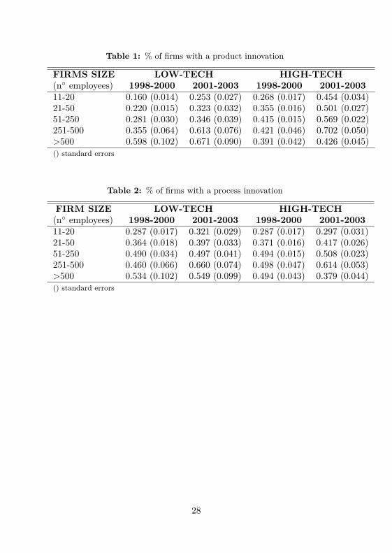
Table 1: % of firms with a product innovation

FIRMS SIZE LOW-TECH HIGH-TECH(n◦ employees) 1998-2000 2001-2003 1998-2000 2001-200311-20 0.160 (0.014) 0.253 (0.027) 0.268 (0.017) 0.454 (0.034)21-50 0.220 (0.015) 0.323 (0.032) 0.355 (0.016) 0.501 (0.027)51-250 0.281 (0.030) 0.346 (0.039) 0.415 (0.015) 0.569 (0.022)251-500 0.355 (0.064) 0.613 (0.076) 0.421 (0.046) 0.702 (0.050)>500 0.598 (0.102) 0.671 (0.090) 0.391 (0.042) 0.426 (0.045)() standard errors

Table 2: % of firms with a process innovation

FIRM SIZE LOW-TECH HIGH-TECH(n◦ employees) 1998-2000 2001-2003 1998-2000 2001-200311-20 0.287 (0.017) 0.321 (0.029) 0.287 (0.017) 0.297 (0.031)21-50 0.364 (0.018) 0.397 (0.033) 0.371 (0.016) 0.417 (0.026)51-250 0.490 (0.034) 0.497 (0.041) 0.494 (0.015) 0.508 (0.023)251-500 0.460 (0.066) 0.660 (0.074) 0.498 (0.047) 0.614 (0.053)>500 0.534 (0.102) 0.549 (0.099) 0.494 (0.043) 0.379 (0.044)() standard errors

28

Table 3: % of firms doing R&D

FIRMS SIZE LOW-TECH HIGH-TECH(n◦ employees) 1998-2000 2001-2003 1998-2000 2001-200311-20 0.216 (0.016) 0.372 (0.030) 0.220 (0.016) 0.462 (0.034)21-50 0.317 (0.017) 0.529 (0.034) 0.347 (0.016) 0.590 (0.026)51-250 0.452 (0.034) 0.720 (0.037) 0.480(0.015) 0.704 (0.020)251-500 0.632 (0.066) 0.879 (0.051) 0.561 (0.047) 0.783 (0.049)>500 0.835 (0.079) 0.873 (0.069) 0.791 (0.044) 0.923 (0.031)() standard errors

Table 4: Summary Statistics: Population Mean - Period 2001-2003

BANK_SHARE LENGHT NUM_BANKSLARGE & LT 30.3299 20.0506 7.0150

(1.451) (0.819) (0.235)LARGE & HT 32.1561 18.0048 6.8789

(2.009) (1.013) (0.260)SMALL & LT 35.3025 16.8680 4.1788

(0.913) (0.330) (0.068)SMALL & HT 34.0666 17.0709 4.1107

(1.558) (0.582) (0.102)

Small firms: less than 50 employees

29

Table 5: Estimation results: HECKMAN BASE RESULTSIn the propensity equation the dependent variable is a dummy variable whichtakes value 1 if the firm has introduced at least one product or process innovationwhereas in the intensity equation the dependent variable is a logit transformationof the actual share of innovative sales. The exclusionary variable is g_sales[t−1]

Intensity PropensityEq(2) Eq(1)

IE 0.2278*** (0.028) 0.1438*** (0.032)INVEST -0.0046 (0.010) 0.0125** (0.006)YOUNG 0.1046 (0.624) 0.0569 (0.235)M&As 0.6525* (0.336) 0.2164 (0.149)INTERN._COMP 0.3084 (0.228) 0.1603 (0.104)PATENTS_BOUGHT 0.0900 (0.610) 0.1722 (0.324)PATENTS_SOLD -1.8541** (0.887) -0.5622 (0.364)INTERN._AGR. 0.3725 (0.328) 0.3026* (0.171)PUBLIC_INCEN. 0.5420** (0.234) 0.2723*** (0.091)LISTED 2.5741*** (0.870) 1.2456*** (0.372)LOGSIZE 0.1748 (0.119) 0.2274*** (0.059)HIGH_TECH 0.2377 (0.245) 0.1996** (0.096)Constant -10.0413*** (1.982) -3.9594*** (0.806)g_sales[t−1] 0.0285 (0.084)ρ 0.9237*** 0.0234σ 2.4707*** 0.19138ll -35393.72N 584 1258

*p<0.10,**p<0.05,***p<0.01Note: Regressions include dummies for area

30

Table 6: Estimation results: HECKMAN BASE RESULTSIn the propensity equation the dependent variable is a dummy variable whichtakes value 1 if the firm has introduced at least one product or process innovationwhereas in the intensity equation the dependent variable is a logit transformationof the actual share of innovative sales. The exclusionary variable is rationed[t−1]

Intesity PropensityEq(2) Eq(1)

IE 0.2260*** (0.028) 0.1453*** (0.032)INVEST -0.0051 (0.010) 0.0130** (0.006)YOUNG 0.1013 (0.620) 0.0646 (0.236)M&As 0.6440* (0.334) 0.2224 (0.150)INTERN._COMP. 0.3010 (0.226) 0.1545 (0.105)PATENTS_BOUGHT 0.0851 (0.603) 0.1778 (0.326)PATENTS_SOLD -1.8268** (0.873) -0.5608 (0.364)INTERN._AGR. 0.3658 (0.325) 0.3098* (0.172)PUBLIC_INCEN. 0.5229** (0.234) 0.2797*** (0.092)LISTED 2.5191*** (0.865) 1.2605*** (0.371)LOGSIZE 0.1659 (0.119) 0.2351*** (0.059)HIGH_TECH 0.2336 (0.245) 0.1974** (0.097)Constant -9.8536*** (1.976) -4.0201*** (0.803)rationedt−1 0.3398* (0.194)ρ 0.9196*** (0.0254)σ 2.4521*** 0.1926ll -35360.57N 584 1258

*p<0.10,**p<0.05,***p<0.01Note: Regressions include dummies for area

Table 7: Estimation results: HECKMAN ADDING FINANCIAL VARI-ABLES

Intensity Propensity Intensity PropensityEq(2) Eq(1) Eq(2) Eq(1)

IE 0.2349*** 0.1396*** 0.2356*** 0.1408***(0.030) (0.030) (0.031) (0.031)

INVEST -0.0064 0.0122* -0.0064 0.0124**(0.011) (0.006) (0.010) (0.006)

YOUNG 0.0339 0.0268 0.0831 0.0295(0.623) (0.234) (0.615) (0.233)

M&As 0.6397* 0.2060 0.6583* 0.2181(0.350) (0.151) (0.348) (0.152)

INTERN._COMP 0.3074 0.1652 0.3092 0.1706*(0.234) (0.103) (0.233) (0.103)

PATENTS_BOUGHT 0.0478 0.1818 0.1366 0.2098(0.576) (0.299) (0.547) (0.292)

PATENTS_SOLD -1.7819** -0.5457 -1.9887** -0.5056(0.823) (0.359) (0.877) (0.366)

INTERN._AGR. 0.3818 0.2922* 0.3833 0.2778*(0.341) (0.164) (0.334) (0.164)

PUBLIC_INCEN. 0.5859** 0.2676*** 0.5951** 0.2666***(0.235) (0.090) (0.235) (0.091)

LISTED 2.4746*** 1.2991*** 2.7991*** 1.2784***(0.875) (0.375) (0.815) (0.356)

BANK_SHARE 0.0114*** 0.0032** -0.0021 -0.0013(0.004) (0.002) (0.006) (0.003)

NUM_BANKS 0.0566 0.0306* 0.0822** 0.0347**(0.037) (0.016) (0.040) (0.017)

LENGTH -0.0133 0.0003 0.0216* 0.0027(0.011) (0.004) (0.013) (0.006)

FIN._INSTR -0.4861 0.2980 1.3071* 0.6892**(0.543) (0.241) (0.730) (0.325)

SMALL -0.3079 -0.2663*** 0.3389 -0.2871(0.223) (0.096) (0.585) (0.244)

HIGH_TECH 0.2260 0.2191** 0.2417 0.2239**(0.250) (0.096) (0.251) (0.096)

Constant -9.6042*** -3.3918*** -10.7604*** -3.3197***(1.882) (0.788) (1.787) (0.746)

NUM_BANKSxSMALL -0.0389 -0.0055(0.062) (0.026)

BANK_SHARExSMALL 0.0143* 0.0048(0.007) (0.003)

LENGTHxSMALL -0.0414** -0.0033(0.018) (0.007)

FIN._INSTRxSMALL -2.1136** -0.4595(0.979) (0.418)

past_sales[t−1] 0.0604 0.0631(0.083) (0.084)

ρ 0.9462*** (0.0162) 0.9463*** (0.0160)σ 2.5408*** (0.1895) 2.5408*** (0.1895)ll -35236.53 -35159.27N 584 1258 584 1258

Table 8: Estimation results: HECKMAN ADDING FINANCIAL VARI-ABLES

Intensity Propensity Intensity PropensityEq(2) Eq(1) Eq(2) Eq(1)

IE 0.2330*** 0.1401*** 0.2338*** 0.1409***(0.030) (0.031) (0.031) (0.031)

INVEST -0.0067 0.0131** -0.0070 0.0134**(0.010) (0.006) (0.010) (0.006)

YOUNG 0.0237 0.0386 0.0374 0.0451(0.615) (0.234) (0.612) (0.232)

M&As 0.6182* 0.1974 0.6241* 0.2127(0.346) (0.154) (0.346) (0.154)

INTERN._COMP 0.2954 0.1536 0.2988 0.1601(0.232) (0.104) (0.231) (0.104)

PATENTS_BOUGHT -0.0083 0.1425 0.1006 0.1695(0.575) (0.308) (0.544) (0.305)

PATENTS_SOLD -1.7264** -0.6184* -1.9318** -0.5793*(0.784) (0.347) (0.867) (0.351)

INTERN._AGR. 0.3411 0.2850* 0.3510 0.2722(0.336) (0.167) (0.332) (0.168)

PUBLIC_INCEN. 0.5513** 0.2565*** 0.5535** 0.2561***(0.235) (0.091) (0.235) (0.091)

LISTED 2.4816*** 1.5039*** 2.7548*** 1.4223***(0.908) (0.367) (0.832) (0.351)

BANK_SHARE 0.0113*** 0.0031** -0.0051 -0.0008(0.004) (0.002) (0.006) (0.003)

NUM_BANKS 0.0482 0.0249 0.0520 0.0268(0.036) (0.016) (0.040) (0.019)

LENGTH -0.0136 -0.0004 0.0165 0.0014(0.011) (0.004) (0.012) (0.006)

STRUMENTI_FIN -0.5045 0.3072 1.2439* 0.5693*(0.551) (0.252) (0.731) (0.336)

LOGSIZE 0.1747 0.2080*** 0.0875 0.2174**(0.131) (0.062) (0.181) (0.085)

HIGH_TECH 0.2062 0.2117** 0.2208 0.2192**(0.250) (0.097) (0.250) (0.098)

NUM_BANKSxSMALL -0.0079 -0.0016(0.049) (0.021)

BANK_SHARExSMALL 0.0178*** 0.0042(0.007) (0.003)

LENGTHxSMALL -0.0356** -0.0026(0.016) (0.007)

FIN._INSTRxSMALL -2.0708** -0.3200(0.992) (0.434)

rationedt−1 0.3238* 0.3423*(0.180) (0.184)

Constant -10.3087*** -4.6389*** -10.5396*** -4.5023***(2.050) (0.796) (2.021) (0.808)

ρ 0.9414*** (0.0193) 0.9419*** (0.0192)σ 2.5096*** (0.1929) 2.4956*** (0.1918)ll -35136.9 -35059.69N 584 1258 584 1258

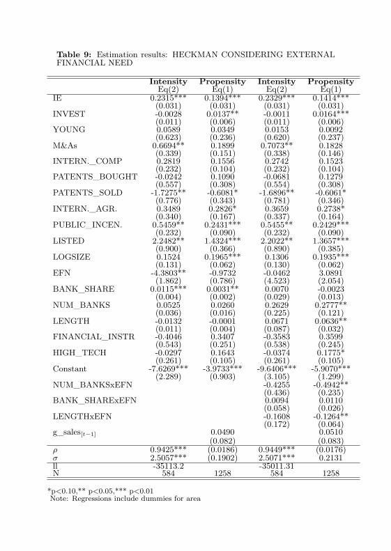
Table 9: Estimation results: HECKMAN CONSIDERING EXTERNALFINANCIAL NEED

Intensity Propensity Intensity PropensityEq(2) Eq(1) Eq(2) Eq(1)

IE 0.2315*** 0.1394*** 0.2329*** 0.1414***(0.031) (0.031) (0.031) (0.031)

INVEST -0.0028 0.0137** -0.0011 0.0164***(0.011) (0.006) (0.011) (0.006)

YOUNG 0.0589 0.0349 0.0153 0.0092(0.623) (0.236) (0.620) (0.237)

M&As 0.6694** 0.1899 0.7073** 0.1828(0.339) (0.151) (0.338) (0.146)

INTERN._COMP 0.2819 0.1556 0.2742 0.1523(0.232) (0.104) (0.232) (0.104)

PATENTS_BOUGHT -0.0242 0.1090 -0.0681 0.1279(0.557) (0.308) (0.554) (0.308)

PATENTS_SOLD -1.7275** -0.6081* -1.6896** -0.6061*(0.776) (0.343) (0.781) (0.346)

INTERN._AGR. 0.3489 0.2826* 0.3659 0.2738*(0.340) (0.167) (0.337) (0.164)

PUBLIC_INCEN. 0.5459** 0.2431*** 0.5455** 0.2429***(0.232) (0.090) (0.232) (0.090)

LISTED 2.2482** 1.4324*** 2.2022** 1.3657***(0.900) (0.366) (0.890) (0.385)

LOGSIZE 0.1524 0.1965*** 0.1306 0.1935***(0.131) (0.062) (0.130) (0.062)

EFN -4.3803** -0.9732 -0.0462 3.0891(1.862) (0.786) (4.523) (2.054)

BANK_SHARE 0.0115*** 0.0031** 0.0070 -0.0023(0.004) (0.002) (0.029) (0.013)

NUM_BANKS 0.0525 0.0260 0.2629 0.2777**(0.036) (0.016) (0.225) (0.121)

LENGTH -0.0132 -0.0001 0.0671 0.0636**(0.011) (0.004) (0.087) (0.032)

FINANCIAL_INSTR -0.4046 0.3407 -0.3583 0.3599(0.543) (0.251) (0.538) (0.245)

HIGH_TECH -0.0297 0.1643 -0.0374 0.1775*(0.261) (0.105) (0.261) (0.105)

Constant -7.6269*** -3.9733*** -9.6406*** -5.9070***(2.289) (0.903) (3.105) (1.299)

NUM_BANKSxEFN -0.4255 -0.4942**(0.436) (0.235)

BANK_SHARExEFN 0.0094 0.0110(0.058) (0.026)

LENGTHxEFN -0.1608 -0.1264**(0.172) (0.064)

g_sales[t−1] 0.0490 0.0510(0.082) (0.083)

ρ 0.9425*** (0.0186) 0.9449*** (0.0176)σ 2.5057*** (0.1902) 2.5071*** 0.2131ll -35113.2 -35011.31N 584 1258 584 1258

*p<0.10,** p<0.05,*** p<0.01Note: Regressions include dummies for area

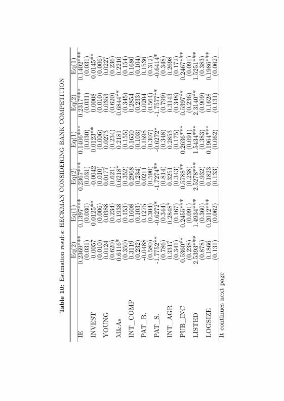
Tab

le10

:E

stim

atio

nre

sults

:H

EC

KM

AN

CO

NSI

DE

RIN

GB

AN

KC

OM

PE

TIT

ION

Eq(2

)Eq

(1)

Eq(2

)Eq

(1)

Eq(2

)Eq

(1)

IE0.

2369

***

0.13

97**

*0.

2367

***

0.14

06**

*0.

2317

***

0.14

02**

*(0

.031

)(0

.030

)(0

.031

)(0

.030

)(0

.031

)(0

.031

)IN

VES

T-0

.005

70.

0125

**-0

.004

20.

0123

**0.

0008

0.01

45**

(0.0

10)

(0.0

06)

(0.0

10)

(0.0

06)

(0.0

10)

(0.0

06)

YO

UN

G0.

0124

0.03

880.

0177

0.02

730.

0353

0.02

27(0

.620

)(0

.234

)(0

.621

)(0

.234

)(0

.620

)(0

.236

)M

&A

s0.

6116

*0.

1938

0.62

18*

0.21

810.

6844

**0.

2210

(0.3

50)

(0.1

53)

(0.3

52)

(0.1

55)

(0.3

45)

(0.1

54)

INT

_C

OM

P0.

3119

0.16

080.

2968

0.16

500.

2854

0.16

80(0

.232

)(0

.103

)(0

.234

)(0

.103

)(0

.233

)(0

.104

)PA

T_

B.

-0.0

488

0.12

750.

0211

0.15

980.

0204

0.15

36(0

.580

)(0

.304

)(0

.590

)(0

.307

)(0

.564

)(0

.312

)PA

T_

S.-1

.775

2**

-0.6

272*

-1.7

274*

*-0

.627

2*-1

.757

7**

-0.6

414*

(0.7

86)

(0.3

44)

(0.8

14)

(0.3

48)

(0.7

99)

(0.3

48)

INT

_A

GR

0.33

170.

2848

*0.

3251

0.28

530.

3143

0.26

98(0

.341

)(0

.167

)(0

.343

)(0

.175

)(0

.348

)(0

.172

)PU

B_

INC

0.53

60**

0.24

55**

*0.

5788

**0.

2636

***

0.53

97**

0.24

67**

*(0

.238

)(0

.091

)(0

.238

)(0

.091

)(0

.236

)(0

.091

)LI

STED

2.53

93**

*1.

4934

***

2.52

78**

*1.

5434

***

2.31

40**

1.52

51**

*(0

.878

)(0

.360

)(0

.932

)(0

.383

)(0

.909

)(0

.383

)LO

GSI

ZE0.

1866

0.20

12**

*0.

1823

0.19

64**

*0.

1628

0.19

86**

*(0

.131

)(0

.062

)(0

.133

)(0

.062

)(0

.131

)(0

.062

)It

cont

inue

sne

xtpa

ge

Tabl

e10

cont

inue

sEq

(2)

Eq(1

)Eq

(2)

Eq(1

)Eq

(2)

Eq(1

)B

AN

K_

SH0.

0111

***

0.00

30*

0.01

14**

*0.

0031

**0.

0114

***

0.00

31**

(0.0

04)

(0.0

02)

(0.0

04)

(0.0

02)

(0.0

04)

(0.0

02)

NU

M_

BA

N0.

0462

0.02

340.

0509

0.02

470.

0510

0.02

58(0

.037

)(0

.016

)(0

.037

)(0

.016

)(0

.036

)(0

.016

)LE

NG

TH

-0.0

134

-0.0

002

-0.0

141

0.00

02-0

.013

00.

0005

(0.0

11)

(0.0

04)

(0.0

11)

(0.0

04)

(0.0

11)

(0.0

04)

FIN

_IN

S.-0

.509

50.

3116

-0.5

148

0.32

81-0

.497

90.

3350

(0.5

44)

(0.2

47)

(0.5

48)

(0.2

47)

(0.5

34)

(0.2

49)

HT

0.21

050.

2175

**0.

2009

0.21

47**

-0.0

138

0.17

40*

(0.2

51)

(0.0

97)

(0.2

52)

(0.0

97)

(0.2

62)

(0.1

05)

Con

s.-1

0.35

06**

*-4

.566

5***

-10.

2864

***

-4.2

505*

**-1

5.82

54**

*-8

.097

7***

(2.0

03)

(0.7

91)

(2.1

77)

(0.8

50)

(5.5

66)

(2.1

41)

BA

NK

_C

O-3

9.47

54-6

.076

2(4

1.10

2)(1

7.49

6)C

H3

-0.4

454

-0.8

572*

14.6

859

7.17

74**

(1.2

23)

(0.5

01)

(9.1

26)

(3.5

33)

EFN

11.8

780

7.55

62**

(9.7

05)

(3.7

26)

CH

3xEF

N-2

9.76

25*

-15.

6612

**(1

7.68

8)(6

.781

)g_

sale

s [t−

1]

0.04

470.

0345

0.03

68(0

.083

)(0

.078

)(0

.078

)ρ

0.94

47**

*(0

.176

)0.

9487

***

(0.0

173)

0.94

63**

*(0

.018

0)σ

2.52

6***

(0.1

911)

2.53

91**

*(0

.193

0)2.

5121

***

(0.1

903)

ll-3

5156

.65

-351

09.3

1-3

5002

.96

N58

412

5858

412

5858

412

58

Table 11: Estimation results: CONDITIONAL LOGITIn this model only switchers - that is, firms that introduced an innovation injust one of the two periods - contribute to the likelihood function. It controlsfor unobserved firm characteristics that are constant over time. The dependentvariable is a dummy variable equal to 1 if the firm introduced an innovation injust one of the two periods

(1) (2)IE 0.0942

(0.091)INVEST 0.0592***

(0.020)R&D 1.1852***

(0.295)INVE 0.0705***

(0.022)PATENTS_SOLD -1.4270 -0.9091

(1.185) (1.031)PATENTS_BOUGHT 1.0923 0.4738

(1.671) (1.057)INTERN._AGR. 1.6552*** 1.5007**

(0.534) (0.612)M&As 1.1833*** 0.7833*

(0.385) (0.436)INTERN._COMP 0.3529 0.3976

(0.393) (0.399)LOGSIZE 0.5377 0.6246

(0.541) (0.543)PUBLIC_INCEN. 0.4973** 0.5279**

(0.238) (0.248)LISTED 2.6798** 2.5719**

(1.351) (1.301)BANK_SHARE 0.0448** 0.0430**

(0.021) (0.018)NUM_BANKS 0.1362 0.0741

(0.107) (0.110)LENGTH -0.0074 0.0003

(0.019) (0.002)FIN._INSTR 0.6966 0.9219*

(0.487) (0.501)BANK_SHARE*SMALL -0.0478** -0.0481***

(0.021) (0.018)NUM_BANKS*SMALL -0.0129 0.0748

(0.115) (0.118)LENGTH*SMALL 0.0116 0.0028

(0.020) (0.002)SALES 0.0000 -0.0000

(0.000) (0.000)ll -4161.4137 -4211.8384N 320 344*p<0.10,** p<0.05, ***p<0.01

Table 12: Estimation results: CONDITIONAL LOGITIn this model only switchers - that is, firms that introduced an innovation injust one of the two periods - contribute to the likelihood function. It controlsfor unobserved firm characteristics that are constant over time. The dependentvariable is a dummy variable equal to 1 if the firm introduced an innovation injust one of the two periods

(1) (2)IE 0.0900

(0.101)INVEST 0.0589***

(0.021)R&D 1.1740***

(0.292)INVE 0.0676***

(0.022)PATENTS_SOLD -1.3398 -0.8299

(1.310) (1.152)PATENTS_BOUGHT 1.7168 0.6122

(1.677) (0.958)INTERN._AGR. 1.7995*** 1.6157***

(0.553) (0.590)M&As 1.1113*** 0.6764

(0.402) (0.448)INTERN._COMP 0.4203 0.4472

(0.376) (0.373)LOGSIZE 0.8827** 0.9098**

(0.442) (0.459)PUBLIC_INCEN. 0.5625** 0.6107**

(0.239) (0.249)LISTED 0.9050 1.0268

(1.179) (1.114)BANK_SHARE -0.0064 -0.0103*

(0.006) (0.006)NUM_BANKS 0.1015 0.1081

(0.091) (0.105)LENGTH 0.0034** 0.0029***

(0.002) (0.001)FIN._INSTR 0.6187 0.8385

(0.507) (0.536)BANK_SHARE*HIGH_TECH 0.0142 0.0223**

(0.013) (0.011)NUM_BANKS*HIGH_TECH 0.2271 0.1813

(0.209) (0.230)LENGTH*HIGH_TECH -0.0031 -0.0025**

(0.002) (0.001)SALES -0.0000 -0.0000

(0.000) (0.000)ll -4191.3611 -4124.6814N 320 344*p<0.10,** p<0.05,*** p<0.01

Unless otherwise expressly stated, all original material of whatevernature created by Caterina Giannetti and included in this thesis,is licensed under a Creative Commons Attribution NoncommercialShare Alike 2.5 Italy License.Check creativecommons.org/licenses/by-nc-sa/2.5/it/ for the legalcode of the full license.Ask the author about other uses.