energies

Article

Improving the Traffic Model to Be Used in theOptimisation of Mass Transit SystemElectrical Infrastructure

Álvaro J. López-López * ID , Ramón R. Pecharromán, Antonio Fernández-Cardadorand Asunción P. Cucala

Institute for Research in Technology, ICAI School of Engineering, Comillas Pontifical University,28015 Madrid, Spain; ramon.rodriguez@iit.comillas.edu (R.R.P.); antonio.fernandez@iit.comillas.edu (A.F.-C.);paloma.cucala@iit.comillas.edu (A.P.C.)* Correspondence: alvaro.lopez@iit.comillas.edu; Tel.: +34-91-542-28-00

Academic Editor: Rui XiongReceived: 20 June 2017; Accepted: 28 July 2017; Published: 2 August 2017

Abstract: Among the different approaches for minimising the energy consumption of mass transitsystems (MTSs), a common concern for MTS operators is the improvement of the electricalinfrastructure. The traffic on the lines under analysis is one of the most important inputs to the studiesdevoted to improving MTS infrastructure, since it represents where and how frequently it is possibleto save energy. However, on the one hand, MTS electrical studies usually simplify the traffic model,which may lead to a misrepresentation of the energy interactions between trains. On the other hand, ifthe stochastic traffic is rigorously modelled, the size of the simulation problem could grow excessively,which in turn could make the time to obtain results unmanageable. To cope with this issue, this paperpresents a method to obtain a reduced-size set of representative scenarios. Firstly, a traffic modelincluding the most representative stochastic traffic variables is developed. Secondly, a function highlycorrelated with energy savings is proposed to make it possible to properly characterise the trafficscenarios. Finally, this function is used to select the most representative scenarios. The representativescenario set obtained by the application of this method is shown to be sufficiently accurate witha limited number of scenarios. The traffic approach in this paper improves the accuracy with respectto the usual traffic approach used in the literature.

Keywords: stochastic traffic model; mass transit systems; electrical infrastructure; reversiblesubstations; energy saving; energy efficiency

1. Introduction

Despite their high energy efficiency, there is still room for improvement in mass transit systems(MTSs) from an energy standpoint. Some studies state that the energy savings achievable by takingfull advantage of regenerative braking are greater than 30% [1,2]. It may hence be stated thatregenerative-braking energy boosts the energy efficiency of MTSs, making these transport systemseven cleaner. The only condition is to have the system receptive to this source of energy.

Currently, several research efforts to improve MTS energy efficiency concentrate on reducingthe frequency of rheostat braking events, which lead to rheostat losses. In a general MTS with diodesubstations (SSs), these events take place when regenerative braking power cannot be consumedinstantaneously by motoring trains. If rheostat-loss events exhibiting large losses during significanttimes are frequent, the energy efficiency of the system decreases. A receptivity factor [3,4] may be usedto measure this loss of receptivity to regenerative braking.

Energies 2017, 10, 1134; doi:10.3390/en10081134 www.mdpi.com/journal/energies

Energies 2017, 10, 1134 2 of 18

In general, receptivity will be higher in average terms when the traffic density in the line is high(small headways), whereas it will be likely to decrease for large headways. Nevertheless, trains usuallydeviate from their scheduled operation. Thus, for a given headway, the relative positions of brakingand motoring trains may be affected by the traffic conditions. These stochastic traffic conditions arelikely to change receptivity with respect to the scheduled traffic situation.

There are two main qualitatively different ways of increasing receptivity in an MTS, makingit insensitive to the headway: (1) designing the operation timetables to minimise the number ofsimultaneous braking events, which is likely to lead to rheostat loss events [5–8]; and (2) designing theelectrical infrastructure in such a way that it is able to absorb braking power even when there are notenough trains consuming power in the line. This paper focuses on the latter research interest.

In this field, the current trend to improve the electrical infrastructure of an MTS consists ofinstalling reversible SSs (RSs) and energy storage systems (ESSs). Currently, for their better robustness,energy efficiency, and cost per MW, RSs tend to be the selected technology when reverse power flowsare remunerated [9,10]. For this reason, this research focuses on RSs. The developments and resultsare easily applicable to ESSs, but no emphasis will be put on this technology in this paper.

In any case, the inclusion of devices to increase receptivity leads to large investments, so theirnecessity must be properly motivated. Several issues, such as the total number of devices installed, andtheir size, location, or control parameters must be properly determined. Consequently, the literatureprovides many studies dealing with the optimal location of RSs or ESSs in a given system. Owing tothe high complexity of railway systems from an electrical standpoint, these studies employ multi-trainsimulators. These simulators allow for the calculation of power flows, and hence to obtain globalenergy figures under different infrastructure topologies. The traffic (train timetable) in the line understudy is one of the main inputs of the simulators.

The method used to obtain the optimal enhancements of electrical infrastructure differs fromone study to another. However, to the best of our knowledge, there are only a few examples ofpapers which include a rigorous modelling of the traffic’s stochastic conditions. In general, the MTSinfrastructure optimisation studies share a common feature: the traffic scenarios used to extract generalconclusions are simplified, i.e., although they are rigorous studies, they do not include stochastictraffic variables.

The work by [11] proposed a genetic algorithm (GA) for optimising RS positioning. It only usesa time instant with 14 fixed trains. The studies in [12,13] used two different algorithms to obtainoptimum RS locations, taking several headways into account. This means a qualitative improvementin the way traffic is tackled. However, the dwell time at passenger stations is fixed, and a singledeterministic traffic scenario for each headway studied is used to obtain the results. In a more recentwork, reference [14] presented a comprehensive study of the way the inclusion of RSs in a line affectsenergy consumption. Although this study takes many factors into account, the traffic input consistsof several different headways with deterministic traffic parameters. The work by [15] studied theeffects of installing ESSs in a Korean line. Specifically, it assesses the reduction of operation costsinduced by peak shaving and a receptivity increase. The study only includes peak-time headway witha fixed dwell time (deterministic). References [16,17] are two rigorous studies by the same workgroupdevoted to the optimal location and sizing of ESSs. They use three headways with a single trafficscenario per headway.

There is another type of work, which focuses on the study of the optimal control curve of ESSs.The study in [18] analysed the control parameters of an ESS. Several headways are used, but a singledeterministic traffic scenario per headway is considered. Reference [19] conducted another studyaimed at determining the optimal control parameters of the direct current (DC)-DC converter in anESS; traffic was also simplified. The model presented in the cited article includes no uncertainties indwell times. Table 1 summarises this review of the traffic models used in the MTS optimisation studiesfound in the literature.

Energies 2017, 10, 1134 3 of 18

Table 1. Traffic models in mass transit system (MTS) electrical infrastructure optimisation studies.Abbreviations: GA: genetic algorithm; RS: reversible substation; ESS: energy storage system.

Optimisation Study Scope Headways Remarks

Chang et al. [11] GA for optimising RS firing angle. One No stochastic variables.Only 14 trains.

Chuang [12] Immune Algorithm for optimising RS placement. Several

No stochastic variables.Single traffic scenario

Hui-Jen et al. [13] GA for optimising RS placement. Several

Bae [14] Study of the effect of the inclusion of RSs in an MTS Several

Lee et al. [15] Peak power reduction using a wayside ESS One

Xia et al. [16] GA for optimising wayside ESS placement, sizing andenergy management. Several

Wang et al. [17] GA for optimising wayside ESS placement and sizing. Several

D’Avanzo et al. [18] Optimum design of a wayside ESS Several

Battistelli et al. [19] Optimum design of a wayside ESS Several

In a different research field, there are several studies devoted to modelling and optimisingon-board ESSs. In this case, the interactions with the rest of the trains in the system are not the centraltopic to be tackled. For this reason, the traffic conditions are even more simplified, and sometimesonly a single train is included in the studies. Accordingly, the study by [20] uses a simple trainload-regeneration profile because its focus is set on the control parameters of the ultracapacitor ESS.However, although it falls outside the scope of the study, the authors explain the importance of takingtraffic (timetable) stochastic variables into account. Other examples of on-board ESSs studies withsimplified traffic conditions may be found in the literatures [21,22].

As Table 1 illustrates, the literature on MTS infrastructure optimisation provides no worksthat thoroughly deal with traffic stochastic variables. On the one hand, this could lead to erroneousconclusions in studies oriented to saving energy in MTSs, as explained in [23]. On the other hand, whenstochastic traffic is included in the MTS model, the number of traffic scenarios that must be analysedsoars steadily. Therefore, the simulation time in the optimisation study could dramatically increase.

Although not specifically devoted to MTS optimisation, there are two references on alternatingcurrent (AC)-system infrastructure that have focused on the importance of the traffic stochasticvariables in the power system results obtained by simulation. Reference [24] presented a stochastictraffic model which is based on the probability of trains being in different locations in the line. Then,these probability distributions are used to obtain the electrical magnitude probability distributions byapplying the Monte-Carlo method. This represents a rigorous study, which however may be improved,especially regarding its application to DC MTSs, by a better representation of dwell times and thepositions where trains in different tracks pass by each other.

Then, reference [25] proposed to use the Monte-Carlo method to represent different trafficsituations. This work focuses on the main traffic concerns, and it proposes the inclusion of severalscenarios to obtain general results. However, it lacks an assessment on the number of scenarios to beused to increase the results’ accuracy without an excessive computational burden.

The aim of this paper is to advance in the representation of the traffic stochastic conditions in MTSinfrastructure optimisation. This approach may be applied both to simulation or classical closed-formoptimisation models. The application of a stochastic traffic approach is devoted to lead to an enhancedenergy-saving accuracy with respect to the classical single-scenario traffic approach. The computationalburden increase associated with the inclusion of several scenarios in the new approach must be takeninto account in order not to have excessively heavy optimisation processes from a computationalstandpoint. To tackle this concern, this paper presents a method to obtain a condensed set of trafficscenarios for MTS energy optimisation studies.

Energies 2017, 10, 1134 4 of 18

1.1. Background, Proposal, and the Paper’s Structure

It has been observed in the literature review in this section that the most important optimisationstudies do not take traffic-variable uncertainties into account. However, two relevant studies [24,25]have proved that these variables may affect the operation of MTSs, leading to inaccurate energy-savingresults that might in turn lead to taking erroneous investment decisions.

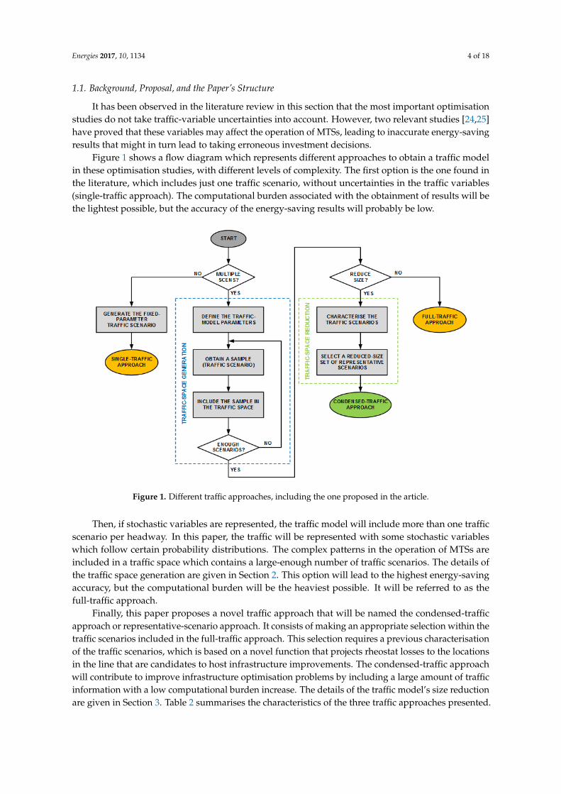
Figure 1 shows a flow diagram which represents different approaches to obtain a traffic modelin these optimisation studies, with different levels of complexity. The first option is the one found inthe literature, which includes just one traffic scenario, without uncertainties in the traffic variables(single-traffic approach). The computational burden associated with the obtainment of results will bethe lightest possible, but the accuracy of the energy-saving results will probably be low.

Energies 2017, 10, 1134 4 of 18

1.1. Background, Proposal, and the Paper’s Structure

It has been observed in the literature review in this section that the most important optimisation

studies do not take traffic-variable uncertainties into account. However, two relevant studies [24,25]

have proved that these variables may affect the operation of MTSs, leading to inaccurate energy-

saving results that might in turn lead to taking erroneous investment decisions.

Figure 1 shows a flow diagram which represents different approaches to obtain a traffic model

in these optimisation studies, with different levels of complexity. The first option is the one found in

the literature, which includes just one traffic scenario, without uncertainties in the traffic variables

(single-traffic approach). The computational burden associated with the obtainment of results will be

the lightest possible, but the accuracy of the energy-saving results will probably be low.

Figure 1. Different traffic approaches, including the one proposed in the article.

Then, if stochastic variables are represented, the traffic model will include more than one traffic

scenario per headway. In this paper, the traffic will be represented with some stochastic variables

which follow certain probability distributions. The complex patterns in the operation of MTSs are

included in a traffic space which contains a large-enough number of traffic scenarios. The details of

the traffic space generation are given in Section 2. This option will lead to the highest energy-saving

accuracy, but the computational burden will be the heaviest possible. It will be referred to as the full-

traffic approach.

Finally, this paper proposes a novel traffic approach that will be named the condensed-traffic

approach or representative-scenario approach. It consists of making an appropriate selection within

the traffic scenarios included in the full-traffic approach. This selection requires a previous

characterisation of the traffic scenarios, which is based on a novel function that projects rheostat

losses to the locations in the line that are candidates to host infrastructure improvements. The

condensed-traffic approach will contribute to improve infrastructure optimisation problems by

including a large amount of traffic information with a low computational burden increase. The details

of the traffic model’s size reduction are given in Section 3. Table 2 summarises the characteristics of

the three traffic approaches presented.

Figure 1. Different traffic approaches, including the one proposed in the article.

Then, if stochastic variables are represented, the traffic model will include more than one trafficscenario per headway. In this paper, the traffic will be represented with some stochastic variableswhich follow certain probability distributions. The complex patterns in the operation of MTSs areincluded in a traffic space which contains a large-enough number of traffic scenarios. The details ofthe traffic space generation are given in Section 2. This option will lead to the highest energy-savingaccuracy, but the computational burden will be the heaviest possible. It will be referred to as thefull-traffic approach.

Finally, this paper proposes a novel traffic approach that will be named the condensed-trafficapproach or representative-scenario approach. It consists of making an appropriate selection within thetraffic scenarios included in the full-traffic approach. This selection requires a previous characterisationof the traffic scenarios, which is based on a novel function that projects rheostat losses to the locationsin the line that are candidates to host infrastructure improvements. The condensed-traffic approachwill contribute to improve infrastructure optimisation problems by including a large amount of trafficinformation with a low computational burden increase. The details of the traffic model’s size reductionare given in Section 3. Table 2 summarises the characteristics of the three traffic approaches presented.

Energies 2017, 10, 1134 5 of 18

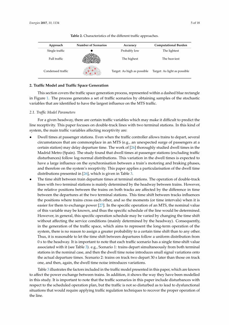
Table 2. Characteristics of the different traffic approaches.

Approach Number of Scenarios Accuracy Computational Burden

Single traffic Probably low The lightest

Full traffic

Energies 2017, 10, 1134 5 of 18

Table 2. Characteristics of the different traffic approaches.

Approach Number of Scenarios Accuracy Computational Burden

Single traffic Probably low The lightest

Full traffic

The highest The heaviest

Condensed traffic

Target: As high as possible Target: As light as possible

2. Traffic Model and Traffic Space Generation

This section covers the traffic space generation process, represented within a dashed blue

rectangle in Figure 1. The process generates a set of traffic scenarios by obtaining samples of the

stochastic variables that are identified to have the largest influence on the MTS traffic.

2.1. Traffic Model Parameters

For a given headway, there are certain traffic variables which may make it difficult to predict

the line receptivity. This paper focuses on double-track lines with two terminal stations. In this kind

of system, the main traffic variables affecting receptivity are:

Dwell times at passenger stations. Even when the traffic controller allows trains to depart,

several circumstances that are commonplace in an MTS (e.g., an unexpected surge of passengers

at a certain station) may delay departure time. The work of [26] thoroughly studied dwell times

in the Madrid Metro (Spain). The study found that dwell times at passenger stations (excluding

traffic disturbances) follow log-normal distributions. This variation in the dwell times is

expected to have a large influence on the synchronisation between a train’s motoring and

braking phases, and therefore on the system’s receptivity. This paper applies a particularisation

of the dwell time distributions presented in [26], which is given in Table 3.

The time shift between train departure times at terminal stations. The operation of double-track

lines with two terminal stations is mainly determined by the headway between trains. However,

the relative positions between the trains on both tracks are affected by the difference in time

between the departures at the two terminal stations. This time shift between tracks influences

the positions where trains cross each other, and so the moments (or time intervals) when it is

easier for them to exchange power [27]. In the specific operation of an MTS, the nominal value

of this variable may be known, and thus the specific schedule of the line would be determined.

However, in general, this specific operation schedule may be varied by changing the time shift

without affecting the service conditions (mainly determined by the headway). Consequently, in

the generation of the traffic space, which aims to represent the long-term operation of the system,

there is no reason to assign a greater probability to a certain time shift than to any other. Thus,

it is reasonable to let the time shift between departures follow a uniform distribution from 0 s to

the headway. It is important to note that each traffic scenario has a single time-shift value

associated with it (see Table 3). e.g., Scenario 1: trains depart simultaneously from both terminal

stations in the nominal case, and then the dwell time noise introduces small signal variations

onto the actual departure times. Scenario 2: trains on track two depart 30 s later than those on

track one, and then, again, the dwell time noise introduces variations.

Table 3 illustrates the factors included in the traffic model presented in this paper, which are

known to affect the power exchange between trains. In addition, it shows the way they have been

modelled in this study. It is important to note that the traffic scenarios in this paper include

disturbances with respect to the scheduled operation plan, but the traffic is not so disturbed as to lead

to dysfunctional situations that would require applying traffic regulation techniques to recover the

proper operation of the line.

The highest The heaviest

Condensed traffic

Energies 2017, 10, 1134 5 of 18

Table 2. Characteristics of the different traffic approaches.

Approach Number of Scenarios Accuracy Computational Burden

Single traffic Probably low The lightest

Full traffic

The highest The heaviest

Condensed traffic

Target: As high as possible Target: As light as possible

2. Traffic Model and Traffic Space Generation

This section covers the traffic space generation process, represented within a dashed blue

rectangle in Figure 1. The process generates a set of traffic scenarios by obtaining samples of the

stochastic variables that are identified to have the largest influence on the MTS traffic.

2.1. Traffic Model Parameters

For a given headway, there are certain traffic variables which may make it difficult to predict

the line receptivity. This paper focuses on double-track lines with two terminal stations. In this kind

of system, the main traffic variables affecting receptivity are:

Dwell times at passenger stations. Even when the traffic controller allows trains to depart,

several circumstances that are commonplace in an MTS (e.g., an unexpected surge of passengers

at a certain station) may delay departure time. The work of [26] thoroughly studied dwell times

in the Madrid Metro (Spain). The study found that dwell times at passenger stations (excluding

traffic disturbances) follow log-normal distributions. This variation in the dwell times is

expected to have a large influence on the synchronisation between a train’s motoring and

braking phases, and therefore on the system’s receptivity. This paper applies a particularisation

of the dwell time distributions presented in [26], which is given in Table 3.

The time shift between train departure times at terminal stations. The operation of double-track

lines with two terminal stations is mainly determined by the headway between trains. However,

the relative positions between the trains on both tracks are affected by the difference in time

between the departures at the two terminal stations. This time shift between tracks influences

the positions where trains cross each other, and so the moments (or time intervals) when it is

easier for them to exchange power [27]. In the specific operation of an MTS, the nominal value

of this variable may be known, and thus the specific schedule of the line would be determined.

However, in general, this specific operation schedule may be varied by changing the time shift

without affecting the service conditions (mainly determined by the headway). Consequently, in

the generation of the traffic space, which aims to represent the long-term operation of the system,

there is no reason to assign a greater probability to a certain time shift than to any other. Thus,

it is reasonable to let the time shift between departures follow a uniform distribution from 0 s to

the headway. It is important to note that each traffic scenario has a single time-shift value

associated with it (see Table 3). e.g., Scenario 1: trains depart simultaneously from both terminal

stations in the nominal case, and then the dwell time noise introduces small signal variations

onto the actual departure times. Scenario 2: trains on track two depart 30 s later than those on

track one, and then, again, the dwell time noise introduces variations.

Table 3 illustrates the factors included in the traffic model presented in this paper, which are

known to affect the power exchange between trains. In addition, it shows the way they have been

modelled in this study. It is important to note that the traffic scenarios in this paper include

disturbances with respect to the scheduled operation plan, but the traffic is not so disturbed as to lead

to dysfunctional situations that would require applying traffic regulation techniques to recover the

proper operation of the line.

Target: As high as possible Target: As light as possible

2. Traffic Model and Traffic Space Generation

This section covers the traffic space generation process, represented within a dashed blue rectanglein Figure 1. The process generates a set of traffic scenarios by obtaining samples of the stochasticvariables that are identified to have the largest influence on the MTS traffic.

2.1. Traffic Model Parameters

For a given headway, there are certain traffic variables which may make it difficult to predict theline receptivity. This paper focuses on double-track lines with two terminal stations. In this kind ofsystem, the main traffic variables affecting receptivity are:

• Dwell times at passenger stations. Even when the traffic controller allows trains to depart, severalcircumstances that are commonplace in an MTS (e.g., an unexpected surge of passengers at acertain station) may delay departure time. The work of [26] thoroughly studied dwell times in theMadrid Metro (Spain). The study found that dwell times at passenger stations (excluding trafficdisturbances) follow log-normal distributions. This variation in the dwell times is expected tohave a large influence on the synchronisation between a train’s motoring and braking phases,and therefore on the system’s receptivity. This paper applies a particularisation of the dwell timedistributions presented in [26], which is given in Table 3.

• The time shift between train departure times at terminal stations. The operation of double-tracklines with two terminal stations is mainly determined by the headway between trains. However,the relative positions between the trains on both tracks are affected by the difference in timebetween the departures at the two terminal stations. This time shift between tracks influencesthe positions where trains cross each other, and so the moments (or time intervals) when it iseasier for them to exchange power [27]. In the specific operation of an MTS, the nominal valueof this variable may be known, and thus the specific schedule of the line would be determined.However, in general, this specific operation schedule may be varied by changing the time shiftwithout affecting the service conditions (mainly determined by the headway). Consequently,in the generation of the traffic space, which aims to represent the long-term operation of thesystem, there is no reason to assign a greater probability to a certain time shift than to any other.Thus, it is reasonable to let the time shift between departures follow a uniform distribution from0 s to the headway. It is important to note that each traffic scenario has a single time-shift valueassociated with it (see Table 3). e.g., Scenario 1: trains depart simultaneously from both terminalstations in the nominal case, and then the dwell time noise introduces small signal variations ontothe actual departure times. Scenario 2: trains on track two depart 30 s later than those on trackone, and then, again, the dwell time noise introduces variations.

Table 3 illustrates the factors included in the traffic model presented in this paper, which are knownto affect the power exchange between trains. In addition, it shows the way they have been modelledin this study. It is important to note that the traffic scenarios in this paper include disturbances withrespect to the scheduled operation plan, but the traffic is not so disturbed as to lead to dysfunctionalsituations that would require applying traffic regulation techniques to recover the proper operation ofthe line.

Energies 2017, 10, 1134 6 of 18

Table 3. Factors included in the traffic model and values used in this study.

Traffic Parameter Model Used in the Study Remarks

Headway 4-, 7-, and 15-min headwaysThree headways to cover thedifferent traffic densities in theoperation of the line.

Dwell times at passenger stations Log-normal distribution.

Parameters:

Mean: 30 s. Parameters tuned to represent thetraffic in the line withoutdysfunctional situations.

Standard deviation: 3 s.Minimum dwell time: 20 sMaximum dwell time: 60 s

Time shift between departuretimes at terminal stations

Uniform distribution from 0 s tothe headway

Different time shift values to coverall the possible operation schedules.

2.2. Traffic Space Generation

A traffic scenario is a sample of the total traffic space associated with a given headway.The expression of the total traffic space for the headway hw is given in Equation (1).

TShw = scen1(·), . . . , scenE(·) (1)

where scenω(·) is the traffic scenario ω, defined in Equation (2), and E is the total number of scenariosin the traffic space.

scenω(shi f tω, tr1,ω(·), . . . , trT,ω(·)) = snp1, . . . , snpS (2)

where:

• shi f tω is the realisation of the time shift for the traffic scenario ω, obtained with the probabilitydistribution presented in Table 3.

• trt,ω

(dw1

t,ω, . . . , dwN_ESTt,ω

)is the evolution of the position and power for train t in the traffic

scenario ω, which depends on the realisations of the stochastic dwell times (dwut,ω) at all the

passenger stations (from 1 to N_EST). It must be noted that the dwell times are independent ofthe time shift and between them.

• snpv is the snapshot v, which represents the sampling of the positions and powers of all the trainsin the line for the time instant v. The sample time selected in this study equals 1 s.

• S is the total number of snapshots included in the scenario (for one-second sampling time, thenumber of snapshots in a traffic scenario equals 60 times the headway in minutes).

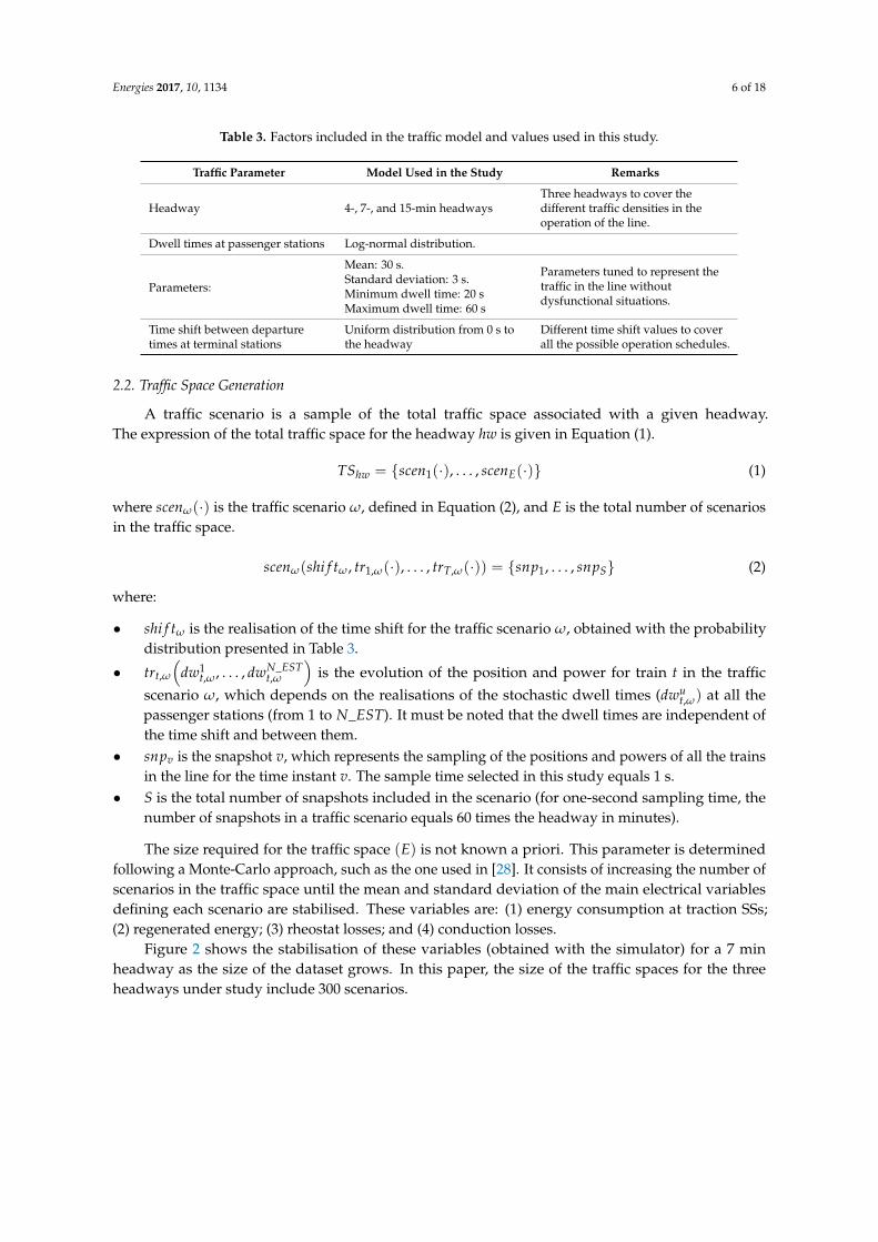
The size required for the traffic space (E) is not known a priori. This parameter is determinedfollowing a Monte-Carlo approach, such as the one used in [28]. It consists of increasing the number ofscenarios in the traffic space until the mean and standard deviation of the main electrical variablesdefining each scenario are stabilised. These variables are: (1) energy consumption at traction SSs;(2) regenerated energy; (3) rheostat losses; and (4) conduction losses.

Figure 2 shows the stabilisation of these variables (obtained with the simulator) for a 7 minheadway as the size of the dataset grows. In this paper, the size of the traffic spaces for the threeheadways under study include 300 scenarios.

Energies 2017, 10, 1134 7 of 18

Energies 2017, 10, 1134 7 of 18

Figure 2. Stabilisation of the main energy-related variables as the size of the dataset grows. 7 min headway.

3. Condensation of the Traffic Model

This section presents the method proposed in this paper to condense the traffic model included in the optimisation studies. The process is represented within a dashed green rectangle in Figure 1. The application of this method will make it possible to approximate the results that would be obtained with the whole traffic space ( ) by means of a small number of representative scenarios. The fundamentals of this traffic space condensation are based on the analysis of the system’s electrical variables. Specifically, since energy savings are the key variable in the kind of studies covered by this paper, the method is based on the rheostat-loss reduction mechanisms presented in [29].

3.1. Characterisation of the Traffic Scenarios

The key to making the traffic-space condensation possible is to properly characterise the traffic scenarios. In particular, it is important that the characterisation captures the rheostat-loss events, representing not only the global rheostat loss figures, but also their distribution along the line and their frequency of occurrence. In addition, it was presented in [29] that there are obstacles to the absorption rheostat losses from certain locations, so it is essential to represent these interferences in the traffic scenario’s characterisation.

Each traffic scenario may contain a large number of rheostat loss events, which are the result of the complex interactions between trains. Then, there are several candidate locations to install devices to improve receptivity (RSs in this paper), which will be able to fully absorb some rheostat-loss

0 100 200 300 400 500480

500

520

540Substation consumption

Number of scenarios

Mea

n (k

Wh)

0 100 200 300 400 5000

20

40

60

Number of scenarios

St. d

ev. (

kWh)

0 100 200 300 400 500450

455

460

465Regenerated energy

Number of scenarios

Mea

n (k

Wh)

0 100 200 300 400 5000

5

10

15

20

Number of scenarios

St. d

ev. (

kWh)

0 100 200 300 400 500140

150

160

170Rheostat losses

Number of scenarios

Mea

n (k

Wh)

0 100 200 300 400 5000

10

20

30

40

Number of scenarios

St. d

ev. (

kWh)

0 100 200 300 400 50042

44

46

48Conduction losses

Number of scenarios

Mea

n (k

Wh)

0 100 200 300 400 5000

1

2

3

Number of scenarios

St. d

ev. (

kWh)

Figure 2. Stabilisation of the main energy-related variables as the size of the dataset grows.7 min headway.

3. Condensation of the Traffic Model

This section presents the method proposed in this paper to condense the traffic model included inthe optimisation studies. The process is represented within a dashed green rectangle in Figure 1.The application of this method will make it possible to approximate the results that would beobtained with the whole traffic space (TShw) by means of a small number of representative scenarios.The fundamentals of this traffic space condensation are based on the analysis of the system’s electricalvariables. Specifically, since energy savings are the key variable in the kind of studies covered by thispaper, the method is based on the rheostat-loss reduction mechanisms presented in [29].

3.1. Characterisation of the Traffic Scenarios

The key to making the traffic-space condensation possible is to properly characterise the trafficscenarios. In particular, it is important that the characterisation captures the rheostat-loss events,representing not only the global rheostat loss figures, but also their distribution along the line and theirfrequency of occurrence. In addition, it was presented in [29] that there are obstacles to the absorptionrheostat losses from certain locations, so it is essential to represent these interferences in the trafficscenario’s characterisation.

Each traffic scenario may contain a large number of rheostat loss events, which are the result ofthe complex interactions between trains. Then, there are several candidate locations to install devicesto improve receptivity (RSs in this paper), which will be able to fully absorb some rheostat-loss events,

Energies 2017, 10, 1134 8 of 18

but unable to reduce other ones. For these reasons, we propose a method that computes the projectionof all the rheostat losses to all the candidate locations, which is based on the rheostat loss reductionmechanisms. Therefore, we assign to each traffic scenario a vector which contains as many valuesas there are RS candidate locations in the system (Equation (3)). Each of the elements in the vectorcontains the projection of all of the rheostat-loss events to the set of candidate locations (Equation (4)).

sceni ⇒(

ai,1, . . . , ai,NLOC

)(3)

ai,loc =R

∑r=1

RPr(·) (4)

where i and loc are respectively the traffic scenario and location under study (from 1 to NLOC); R isthe total number of rheostat-loss events that take place in the scenario scen; and RPr(·) is the Rheostatloss Projection (RP) function, which is proposed to represent the energy-saving potential associatedwith each pair of rheostat loss event and location. It is defined hereafter.

For each rheostat loss event and candidate location, it is required: (1) to identify whether it ispossible to reduce the rheostat losses in this specific event from the candidate location under analysis;and (2) to detect the type of rheostat loss reduction mechanism to be applied.

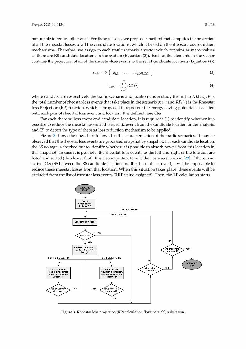
Figure 3 shows the flow chart followed in the characterisation of the traffic scenarios. It may beobserved that the rheostat loss events are processed snapshot by snapshot. For each candidate location,the SS voltage is checked out to identify whether it is possible to absorb power from this location inthis snapshot. In case it is possible, the rheostat-loss events to the left and right of the location arelisted and sorted (the closest first). It is also important to note that, as was shown in [29], if there is anactive (ON) SS between the RS candidate location and the rheostat loss event, it will be impossible toreduce these rheostat losses from that location. When this situation takes place, these events will beexcluded from the list of rheostat loss events (0 RP value assigned). Then, the RP calculation starts.

Energies 2017, 10, 1134 8 of 18

events, but unable to reduce other ones. For these reasons, we propose a method that computes the

projection of all the rheostat losses to all the candidate locations, which is based on the rheostat loss

reduction mechanisms. Therefore, we assign to each traffic scenario a vector which contains as many

values as there are RS candidate locations in the system (Equation (3)). Each of the elements in the

vector contains the projection of all of the rheostat-loss events to the set of candidate locations

(Equation (4)).

𝑠𝑐𝑒𝑛𝑖 ⇒ (𝑎𝑖,1, … , 𝑎𝑖,𝑁𝐿𝑂𝐶) (3)

𝑎𝑖,𝑙𝑜𝑐 =∑𝑅𝑃𝑟(∙)

𝑅

𝑟=1

(4)

where 𝑖 and 𝑙𝑜𝑐 are respectively the traffic scenario and location under study (from 1 to 𝑁𝐿𝑂𝐶); 𝑅

is the total number of rheostat-loss events that take place in the scenario 𝑠𝑐𝑒𝑛; and 𝑅𝑃𝑟(∙) is the

Rheostat loss Projection (RP) function, which is proposed to represent the energy-saving potential

associated with each pair of rheostat loss event and location. It is defined hereafter.

For each rheostat loss event and candidate location, it is required: (1) to identify whether it is

possible to reduce the rheostat losses in this specific event from the candidate location under analysis;

and (2) to detect the type of rheostat loss reduction mechanism to be applied.

Figure 3 shows the flow chart followed in the characterisation of the traffic scenarios. It may be

observed that the rheostat loss events are processed snapshot by snapshot. For each candidate

location, the SS voltage is checked out to identify whether it is possible to absorb power from this

location in this snapshot. In case it is possible, the rheostat-loss events to the left and right of the

location are listed and sorted (the closest first). It is also important to note that, as was shown in [29],

if there is an active (ON) SS between the RS candidate location and the rheostat loss event, it will be

impossible to reduce these rheostat losses from that location. When this situation takes place, these

events will be excluded from the list of rheostat loss events (0 RP value assigned). Then, the RP

calculation starts.

Figure 3. Rheostat loss projection (RP) calculation flowchart. SS, substation. Figure 3. Rheostat loss projection (RP) calculation flowchart. SS, substation.

Energies 2017, 10, 1134 9 of 18

The rheostat loss events are processed one by one. The type of rheostat loss reduction mechanismis detected, and the RP for this location is updated. If the RP calculation shows that the rheostat powerin this event would not be completely absorbed, it can be concluded that the load flow beyond thattrain will remain invariant and no more rheostat loss reduction will take place. This process is carriedout for both sides of the candidate location.

With respect to the RP formulae, it is important to note that, although it is not formally proven to be,the RP will usually be at a higher bound of the rheostat loss reduction attainable from a given location.

The expression applied to a rheostat loss event when the case (a) is detected is given in Equation (5).

RP(Erhi, drhi, Vloc) = min(

VRh(VRh −VRS)

Rldrhi∆t, Erhi

)(5)

where:

• Vloc represents the voltage of the RS location in the load flow for the base system. The base systemrefers to the base configuration of the infrastructure, without any improvement.

• V0 is the SS no-load voltage.• Erhi is the energy lost in each rheostat loss event.• drhi is the relative position of the rheostat train with respect to the RS location loc.• VRh is the rheostat braking voltage threshold.• VRS represents an hypothetical voltage in the RS location after the installation of the RS.• Rl is the resistance of the supply system, in Ω/km.• ∆t is the sampling time used in the traffic scenario generation.

The expression in Equation (5) represents a simplification of the power transmission from aVRh-volt voltage source to another point in the line in which voltage is clamped to a certain level.This expression does not aim to be an accurate representation of the actual load flow, but a simplifiedmeans to rapidly obtain the potential rheostat loss reduction from the RS location. As can be observed,the RP value is limited to the magnitude of the rheostat loss event and then normalised.

When the case (b) is detected, the RP is calculated following Equation (6).

RP(Erhi, drhi, Vloc) = min(

VRh(VRh −VRS)

Rldrhi·Vloc −VRSVRh −VRS

∆t, Erhi

)(6)

From the analysis of Equation (6), it may be extracted that the RP function represents the rheostatloss reduction when the RS is in a power exchange path by modulating the expression in Equation (5)with a coefficient between 0 and 1: (Vloc −VRS)/VRh −VRS). This coefficient will naturally tend to 1when the RS location is close to the rheostat train (the voltage in the base system is close to the rheostatthreshold) and to 0 when it is close to the motoring train (or an active SS). With this modulation, it ispossible to obtain an approximate figure of the actual rheostat loss reduction.

Finally, Equation (7) presents the RP expression applied when case (c) is detected.

RP(Erhi, drhi, Vloc) = min(

VBTr(VBTr −VRS)

RldBTr· Vloc −VRSVBTr −VRS

∆t, Erhi

)· fON_SS (7)

where:

• VBTr is the voltage of the braking train that is causing the high base system RS location voltage.It must be noted that in this case, this train is not in rheostat mode.

• dBTr is the distance between the braking train that is causing the high base system RS locationvoltage and the RS location.

• fON_SS is a binary factor which is set to zero if there is an active (ON) SS between the rheostattrain under study and the RS location. This is used to represent the decoupling effect of active SSsthat was presented in [29].

Energies 2017, 10, 1134 10 of 18

The expression in Equation (7) is applied when there are no active SSs between the rheostat losstrain and the RS location. When there is an active SS between the rheostat event under study and theRS location, the rheostat loss reduction is marginal, and the RP function is consequently set to zero.

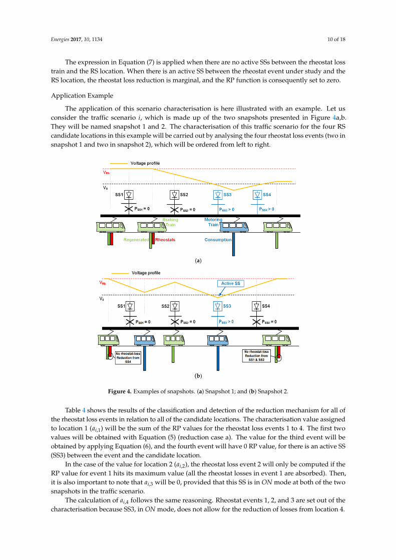
Application Example

The application of this scenario characterisation is here illustrated with an example. Let usconsider the traffic scenario i, which is made up of the two snapshots presented in Figure 4a,b.They will be named snapshot 1 and 2. The characterisation of this traffic scenario for the four RScandidate locations in this example will be carried out by analysing the four rheostat loss events (two insnapshot 1 and two in snapshot 2), which will be ordered from left to right.

Energies 2017, 10, 1134 10 of 18

The expression in Equation (7) is applied when there are no active SSs between the rheostat loss

train and the RS location. When there is an active SS between the rheostat event under study and the

RS location, the rheostat loss reduction is marginal, and the RP function is consequently set to zero.

Application Example

The application of this scenario characterisation is here illustrated with an example. Let us

consider the traffic scenario 𝑖, which is made up of the two snapshots presented in Figure 4a,b. They

will be named snapshot 1 and 2. The characterisation of this traffic scenario for the four RS candidate

locations in this example will be carried out by analysing the four rheostat loss events (two in

snapshot 1 and two in snapshot 2), which will be ordered from left to right.

(a)

(b)

Figure 4. Examples of snapshots. (a) Snapshot 1; and (b) Snapshot 2.

Table 4 shows the results of the classification and detection of the reduction mechanism for all

of the rheostat loss events in relation to all of the candidate locations. The characterisation value

assigned to location 1 (𝑎𝑖,1) will be the sum of the RP values for the rheostat loss events 1 to 4. The

first two values will be obtained with Equation (5) (reduction case a). The value for the third event

will be obtained by applying Equation (6), and the fourth event will have 0 RP value, for there is an

active SS (SS3) between the event and the candidate location.

In the case of the value for location 2 (𝑎𝑖,2), the rheostat loss event 2 will only be computed if the

RP value for event 1 hits its maximum value (all the rheostat losses in event 1 are absorbed). Then, it

is also important to note that 𝑎𝑖,3 will be 0, provided that this SS is in ON mode at both of the two

snapshots in the traffic scenario.

The calculation of 𝑎𝑖,4 follows the same reasoning. Rheostat events 1, 2, and 3 are set out of the

characterisation because SS3, in ON mode, does not allow for the reduction of losses from location 4.

Figure 4. Examples of snapshots. (a) Snapshot 1; and (b) Snapshot 2.

Table 4 shows the results of the classification and detection of the reduction mechanism for all ofthe rheostat loss events in relation to all of the candidate locations. The characterisation value assignedto location 1 (ai,1) will be the sum of the RP values for the rheostat loss events 1 to 4. The first twovalues will be obtained with Equation (5) (reduction case a). The value for the third event will beobtained by applying Equation (6), and the fourth event will have 0 RP value, for there is an active SS(SS3) between the event and the candidate location.

In the case of the value for location 2 (ai,2), the rheostat loss event 2 will only be computed if theRP value for event 1 hits its maximum value (all the rheostat losses in event 1 are absorbed). Then,it is also important to note that ai,3 will be 0, provided that this SS is in ON mode at both of the twosnapshots in the traffic scenario.

The calculation of ai,4 follows the same reasoning. Rheostat events 1, 2, and 3 are set out of thecharacterisation because SS3, in ON mode, does not allow for the reduction of losses from location 4.

Energies 2017, 10, 1134 11 of 18

Table 4. Classification of the rheostat loss events for each candidate location in the application example.

Application ExampleCandidate Location

SS 1 SS 2 SS 3 SS 4

Rh. Event

1 (Snp 1) Left 1. Type a Left 1. Type b N/A N/A2 (Snp 1) Right 1. Type a Left 2. Type b N/A N/A3 (Snp 2) Left 1. Type b Left 1. Type c N/A N/A4 (Snp 2) N/A N/A N/A Right 1. Type b

3.2. Representative Scenario Selection

The selection process is based on the RP characterisation presented, and on its correlation withenergy savings, which will be checked out in Section 4.2. It aims to reduce the size of the traffic inputto an MTS optimisation study, preventing it from using 300 scenarios for each traffic space.

The strategy proposed to perform this size reduction is: a set of traffic scenarios are selected to berepresentative of the traffic space if, for all of the RS locations, the average RP values of the reduced setare close to the average RP values of the total traffic space.

In this paper, the threshold to classify whether the average RP values of both sets are closeenough has been set to ±5%. This value has a strong relation with the desired energy-saving accuracy.If a more restrictive threshold is selected (e.g., 3%), the representative scenario set will contain moretraffic scenarios, and vice-versa.

4. Results

In this section, we apply the traffic model presented in the paper to a case study line. After thepresentation of the case study in Section 4.1, we analyse the accuracy of the condensed traffic approachfor different sizes and subgroups of traffic scenarios within the total traffic spaces with respect to arandom scenario selection approach (Section 4.2). Then, in Section 4.3, we carry out a comprehensiveenergy-saving accuracy analysis, where we first use a test to verify that the method is accurate for allof the candidate locations, and then we test its generalisation capability by measuring the accuracy fordifferent infrastructure configurations.

4.1. Case Study Line and Definitions

All of the results in this paper have been obtained by means of an electrical multi-train simulatordeveloped in the Institute for Research in Technology (Comillas Pontifical University, Madrid, Spain).Its details may be found in [2].

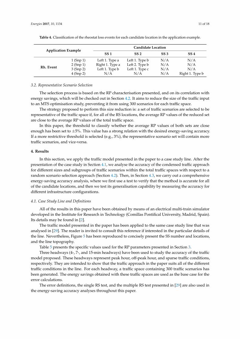
The traffic model presented in the paper has been applied to the same case study line that wasanalysed in [29]. The reader is invited to consult this reference if interested in the particular details ofthe line. Nevertheless, Figure 5 has been reproduced to concisely present the SS number and locations,and the line topography.

Table 5 presents the specific values used for the RP parameters presented in Section 3.Three headways (4-, 7-, and 15-min headways) have been used to study the accuracy of the traffic

model proposed. These headways represent peak hour, off-peak hour, and sparse traffic conditions,respectively. They are intended to show that the traffic approach in the paper suits all of the differenttraffic conditions in the line. For each headway, a traffic space containing 300 traffic scenarios hasbeen generated. The energy savings obtained with these traffic spaces are used as the base case for theerror calculations.

The error definitions, the single RS test, and the multiple RS test presented in [29] are also used inthe energy-saving accuracy analyses throughout this paper.

Energies 2017, 10, 1134 12 of 18

Energies 2017, 10, 1134 12 of 18

Figure 5. Case study line passenger stations, SSs, and topography [29].

Table 5. Specific values for the RP function parameters.

RP parameter Selected value Remarks

VRh 710 V 10 V lower than the maximum

pantograph voltage allowed.

VRS 646.4 V 640 V + 1%

Rl 22.4 mΩ Active and return line impedance

4.2. Condensed Traffic Model: Correlation and Size Results

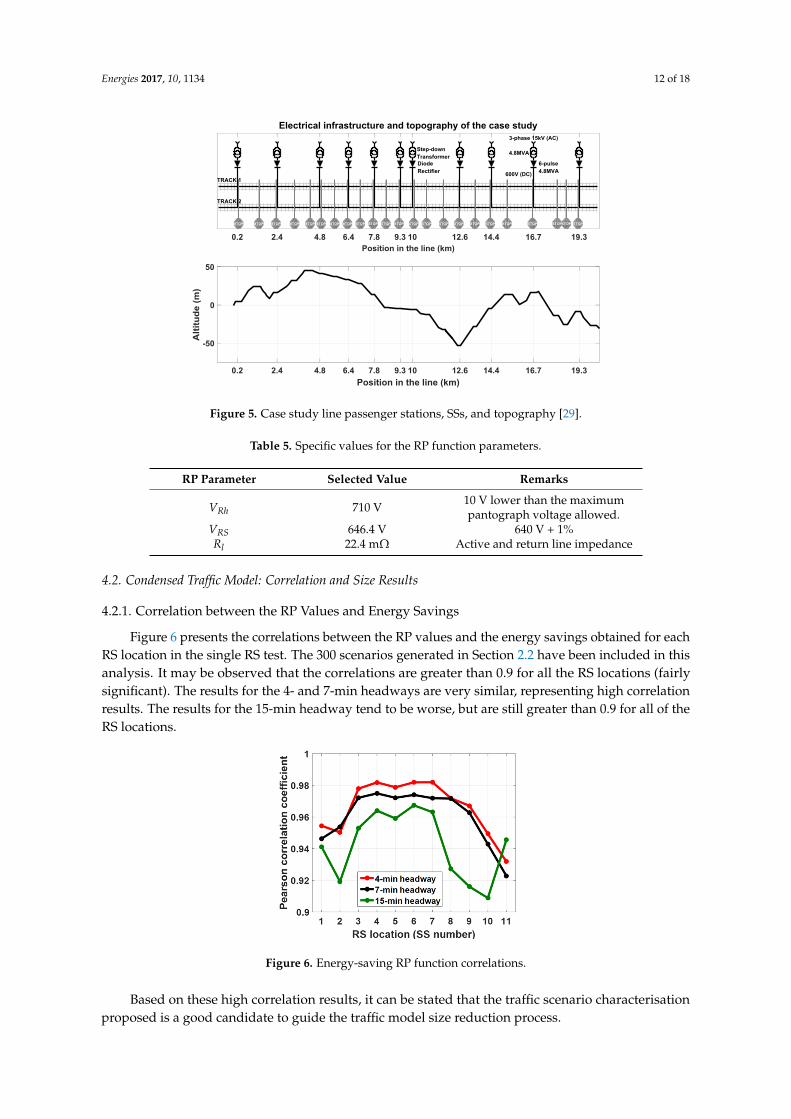
4.2.1. Correlation between the RP Values and Energy Savings

Figure 6 presents the correlations between the RP values and the energy savings obtained for

each RS location in the single RS test. The 300 scenarios generated in Section 2.2 have been included

in this analysis. It may be observed that the correlations are greater than 0.9 for all the RS locations

(fairly significant). The results for the 4- and 7-min headways are very similar, representing high

correlation results. The results for the 15-min headway tend to be worse, but are still greater than 0.9

for all of the RS locations.

Figure 6. Energy-saving RP function correlations.

Based on these high correlation results, it can be stated that the traffic scenario characterisation

proposed is a good candidate to guide the traffic model size reduction process.

Figure 5. Case study line passenger stations, SSs, and topography [29].

Table 5. Specific values for the RP function parameters.

RP Parameter Selected Value Remarks

VRh 710 V 10 V lower than the maximumpantograph voltage allowed.

VRS 646.4 V 640 V + 1%Rl 22.4 mΩ Active and return line impedance

4.2. Condensed Traffic Model: Correlation and Size Results

4.2.1. Correlation between the RP Values and Energy Savings

Figure 6 presents the correlations between the RP values and the energy savings obtained for eachRS location in the single RS test. The 300 scenarios generated in Section 2.2 have been included in thisanalysis. It may be observed that the correlations are greater than 0.9 for all the RS locations (fairlysignificant). The results for the 4- and 7-min headways are very similar, representing high correlationresults. The results for the 15-min headway tend to be worse, but are still greater than 0.9 for all of theRS locations.

Energies 2017, 10, 1134 12 of 18

Figure 5. Case study line passenger stations, SSs, and topography [29].

Table 5. Specific values for the RP function parameters.

RP parameter Selected value Remarks

VRh 710 V 10 V lower than the maximum

pantograph voltage allowed.

VRS 646.4 V 640 V + 1%

Rl 22.4 mΩ Active and return line impedance

4.2. Condensed Traffic Model: Correlation and Size Results

4.2.1. Correlation between the RP Values and Energy Savings

Figure 6 presents the correlations between the RP values and the energy savings obtained for

each RS location in the single RS test. The 300 scenarios generated in Section 2.2 have been included

in this analysis. It may be observed that the correlations are greater than 0.9 for all the RS locations

(fairly significant). The results for the 4- and 7-min headways are very similar, representing high

correlation results. The results for the 15-min headway tend to be worse, but are still greater than 0.9

for all of the RS locations.

Figure 6. Energy-saving RP function correlations.

Based on these high correlation results, it can be stated that the traffic scenario characterisation

proposed is a good candidate to guide the traffic model size reduction process.

Figure 6. Energy-saving RP function correlations.

Based on these high correlation results, it can be stated that the traffic scenario characterisationproposed is a good candidate to guide the traffic model size reduction process.

Energies 2017, 10, 1134 13 of 18

4.2.2. Traffic Model Size Reduction Results

This section assesses the required number of traffic scenarios that the condensed traffic modelshould include. Two approaches are compared:

• The representative scenario selection proposed in the paper, where the traffic scenarios arecharacterised by means of the RP function.

• A random selection process where scenarios are grouped without information.

The method to analyse the number of scenarios required consists of making random combinationsof scenarios of increasing size. In the case of the representative scenario selection, a combination ofscenarios is only accepted if it accomplishes the criterion explained in Section 3. In the case of therandom selection process, since there is no information on the adequacy of the selection, all of thecombinations are accepted. For each condensed traffic size and approach, 1000 samples are obtainedto have statistically significant results.

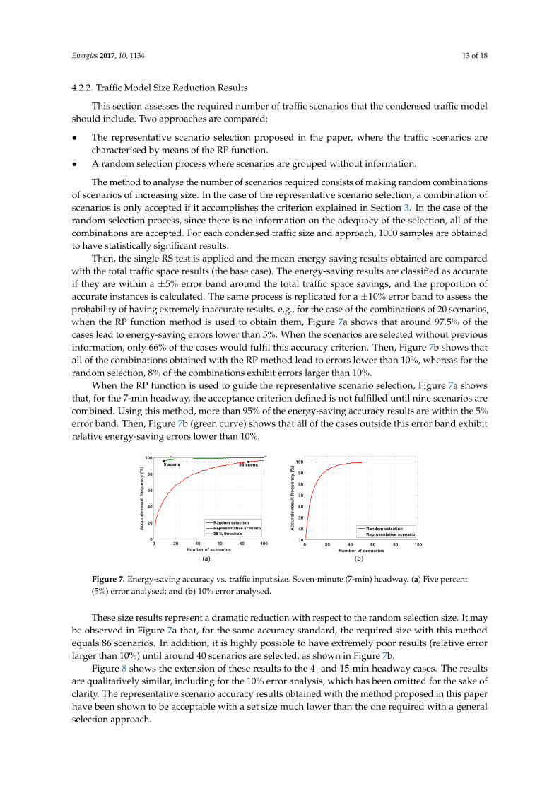
Then, the single RS test is applied and the mean energy-saving results obtained are comparedwith the total traffic space results (the base case). The energy-saving results are classified as accurateif they are within a ±5% error band around the total traffic space savings, and the proportion ofaccurate instances is calculated. The same process is replicated for a ±10% error band to assess theprobability of having extremely inaccurate results. e.g., for the case of the combinations of 20 scenarios,when the RP function method is used to obtain them, Figure 7a shows that around 97.5% of thecases lead to energy-saving errors lower than 5%. When the scenarios are selected without previousinformation, only 66% of the cases would fulfil this accuracy criterion. Then, Figure 7b shows thatall of the combinations obtained with the RP method lead to errors lower than 10%, whereas for therandom selection, 8% of the combinations exhibit errors larger than 10%.

When the RP function is used to guide the representative scenario selection, Figure 7a showsthat, for the 7-min headway, the acceptance criterion defined is not fulfilled until nine scenarios arecombined. Using this method, more than 95% of the energy-saving accuracy results are within the 5%error band. Then, Figure 7b (green curve) shows that all of the cases outside this error band exhibitrelative energy-saving errors lower than 10%.

Energies 2017, 10, 1134 13 of 18

4.2.2. Traffic Model Size Reduction Results

This section assesses the required number of traffic scenarios that the condensed traffic model

should include. Two approaches are compared:

The representative scenario selection proposed in the paper, where the traffic scenarios are

characterised by means of the RP function.

A random selection process where scenarios are grouped without information.

The method to analyse the number of scenarios required consists of making random

combinations of scenarios of increasing size. In the case of the representative scenario selection, a

combination of scenarios is only accepted if it accomplishes the criterion explained in Section 3. In

the case of the random selection process, since there is no information on the adequacy of the

selection, all of the combinations are accepted. For each condensed traffic size and approach, 1000

samples are obtained to have statistically significant results.

Then, the single RS test is applied and the mean energy-saving results obtained are compared

with the total traffic space results (the base case). The energy-saving results are classified as accurate

if they are within a ±5% error band around the total traffic space savings, and the proportion of

accurate instances is calculated. The same process is replicated for a ±10% error band to assess the

probability of having extremely inaccurate results. e.g., for the case of the combinations of 20

scenarios, when the RP function method is used to obtain them, Figure 7a shows that around 97.5%

of the cases lead to energy-saving errors lower than 5%. When the scenarios are selected without

previous information, only 66% of the cases would fulfil this accuracy criterion. Then, Figure 7b

shows that all of the combinations obtained with the RP method lead to errors lower than 10%,

whereas for the random selection, 8% of the combinations exhibit errors larger than 10%.

When the RP function is used to guide the representative scenario selection, Figure 7a shows

that, for the 7-min headway, the acceptance criterion defined is not fulfilled until nine scenarios are

combined. Using this method, more than 95% of the energy-saving accuracy results are within the

5% error band. Then, Figure 7b (green curve) shows that all of the cases outside this error band exhibit

relative energy-saving errors lower than 10%.

(a) (b)

Figure 7. Energy-saving accuracy vs. traffic input size. Seven-minute (7-min) headway. (a) Five

percent (5%) error analysed; and (b) 10% error analysed.

These size results represent a dramatic reduction with respect to the random selection size. It

may be observed in Figure 7a that, for the same accuracy standard, the required size with this method

equals 86 scenarios. In addition, it is highly possible to have extremely poor results (relative error

larger than 10%) until around 40 scenarios are selected, as shown in Figure 7b.

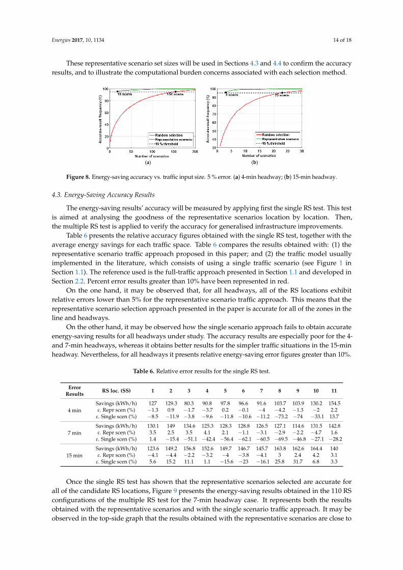
Figure 8 shows the extension of these results to the 4- and 15-min headway cases. The results are

qualitatively similar, including for the 10% error analysis, which has been omitted for the sake of

clarity. The representative scenario accuracy results obtained with the method proposed in this paper

have been shown to be acceptable with a set size much lower than the one required with a general

selection approach.

Figure 7. Energy-saving accuracy vs. traffic input size. Seven-minute (7-min) headway. (a) Five percent(5%) error analysed; and (b) 10% error analysed.

These size results represent a dramatic reduction with respect to the random selection size. It maybe observed in Figure 7a that, for the same accuracy standard, the required size with this methodequals 86 scenarios. In addition, it is highly possible to have extremely poor results (relative errorlarger than 10%) until around 40 scenarios are selected, as shown in Figure 7b.

Figure 8 shows the extension of these results to the 4- and 15-min headway cases. The resultsare qualitatively similar, including for the 10% error analysis, which has been omitted for the sake ofclarity. The representative scenario accuracy results obtained with the method proposed in this paperhave been shown to be acceptable with a set size much lower than the one required with a generalselection approach.

Energies 2017, 10, 1134 14 of 18

These representative scenario set sizes will be used in Sections 4.3 and 4.4 to confirm the accuracyresults, and to illustrate the computational burden concerns associated with each selection method.

Energies 2017, 10, 1134 14 of 18

These representative scenario set sizes will be used in Sections 4.3 and 4.4 to confirm the accuracy

results, and to illustrate the computational burden concerns associated with each selection method.

(a) (b)

Figure 8. Energy-saving accuracy vs. traffic input size. 5 % error. (a) 4-min headway; (b) 15-min

headway.

4.3. Energy-Saving Accuracy Results

The energy-saving results’ accuracy will be measured by applying first the single RS test. This

test is aimed at analysing the goodness of the representative scenarios location by location. Then, the

multiple RS test is applied to verify the accuracy for generalised infrastructure improvements.

Table 6 presents the relative accuracy figures obtained with the single RS test, together with the

average energy savings for each traffic space. Table 6 compares the results obtained with: (1) the

representative scenario traffic approach proposed in this paper; and (2) the traffic model usually

implemented in the literature, which consists of using a single traffic scenario (see Figure 1 in Section

1.1). The reference used is the full-traffic approach presented in Section 1.1 and developed in Section

2.2. Percent error results greater than 10% have been represented in red.

On the one hand, it may be observed that, for all headways, all of the RS locations exhibit relative

errors lower than 5% for the representative scenario traffic approach. This means that the

representative scenario selection approach presented in the paper is accurate for all of the zones in

the line and headways.

On the other hand, it may be observed how the single scenario approach fails to obtain accurate

energy-saving results for all headways under study. The accuracy results are especially poor for the

4- and 7-min headways, whereas it obtains better results for the simpler traffic situations in the 15-

min headway. Nevertheless, for all headways it presents relative energy-saving error figures greater

than 10%.

Table 6. Relative error results for the single RS test.

Error

results RS loc. (SS) 1 2 3 4 5 6 7 8 9 10 11

4 min

Savings (kWh/h) 127 129.3 80.3 90.8 97.8 96.6 91.6 103.7 103.9 130.2 154.5

ε. Repr scen (%) −1.3 0.9 −1.7 −3.7 0.2 −0.1 −4 −4.2 −1.3 −2 2.2

ε. Single scen (%) −8.5 −11.9 −3.8 −9.6 −11.8 −10.6 −11.2 −73.2 −74 −33.1 13.7

7 min

Savings (kWh/h) 130.1 149 134.6 125.3 128.3 128.8 126.5 127.1 114.6 131.5 142.8

ε. Repr scen (%) 3.5 2.5 3.5 4.1 2.1 −1.1 −3.1 −2.9 −2.2 −4.7 1.6

ε. Single scen (%) 1.4 −15.4 −51.1 −42.4 −56.4 −62.1 −60.5 −69.5 −46.8 −27.1 −28.2

15 min

Savings (kWh/h) 123.6 149.2 156.8 152.6 149.7 146.7 145.7 163.8 162.6 164.4 140

ε. Repr scen (%) −4.1 −4.4 −2.2 −3.2 −4 −3.8 −4.1 3 2.4 4.2 3.1

ε. Single scen (%) 5.6 15.2 11.1 1.1 −15.6 −23 −16.1 25.8 31.7 6.8 3.3

Once the single RS test has shown that the representative scenarios selected are accurate for all

of the candidate RS locations, Figure 9 presents the energy-saving results obtained in the 110 RS

configurations of the multiple RS test for the 7-min headway case. It represents both the results

obtained with the representative scenarios and with the single scenario traffic approach. It may be

Figure 8. Energy-saving accuracy vs. traffic input size. 5 % error. (a) 4-min headway; (b) 15-min headway.

4.3. Energy-Saving Accuracy Results

The energy-saving results’ accuracy will be measured by applying first the single RS test. This testis aimed at analysing the goodness of the representative scenarios location by location. Then,the multiple RS test is applied to verify the accuracy for generalised infrastructure improvements.

Table 6 presents the relative accuracy figures obtained with the single RS test, together with theaverage energy savings for each traffic space. Table 6 compares the results obtained with: (1) therepresentative scenario traffic approach proposed in this paper; and (2) the traffic model usuallyimplemented in the literature, which consists of using a single traffic scenario (see Figure 1 inSection 1.1). The reference used is the full-traffic approach presented in Section 1.1 and developed inSection 2.2. Percent error results greater than 10% have been represented in red.

On the one hand, it may be observed that, for all headways, all of the RS locations exhibitrelative errors lower than 5% for the representative scenario traffic approach. This means that therepresentative scenario selection approach presented in the paper is accurate for all of the zones in theline and headways.

On the other hand, it may be observed how the single scenario approach fails to obtain accurateenergy-saving results for all headways under study. The accuracy results are especially poor for the 4-and 7-min headways, whereas it obtains better results for the simpler traffic situations in the 15-minheadway. Nevertheless, for all headways it presents relative energy-saving error figures greater than 10%.

Table 6. Relative error results for the single RS test.

ErrorResults RS loc. (SS) 1 2 3 4 5 6 7 8 9 10 11

4 minSavings (kWh/h) 127 129.3 80.3 90.8 97.8 96.6 91.6 103.7 103.9 130.2 154.5ε. Repr scen (%) −1.3 0.9 −1.7 −3.7 0.2 −0.1 −4 −4.2 −1.3 −2 2.2

ε. Single scen (%) −8.5 −11.9 −3.8 −9.6 −11.8 −10.6 −11.2 −73.2 −74 −33.1 13.7

7 minSavings (kWh/h) 130.1 149 134.6 125.3 128.3 128.8 126.5 127.1 114.6 131.5 142.8ε. Repr scen (%) 3.5 2.5 3.5 4.1 2.1 −1.1 −3.1 −2.9 −2.2 −4.7 1.6

ε. Single scen (%) 1.4 −15.4 −51.1 −42.4 −56.4 −62.1 −60.5 −69.5 −46.8 −27.1 −28.2

15 minSavings (kWh/h) 123.6 149.2 156.8 152.6 149.7 146.7 145.7 163.8 162.6 164.4 140ε. Repr scen (%) −4.1 −4.4 −2.2 −3.2 −4 −3.8 −4.1 3 2.4 4.2 3.1

ε. Single scen (%) 5.6 15.2 11.1 1.1 −15.6 −23 −16.1 25.8 31.7 6.8 3.3

Once the single RS test has shown that the representative scenarios selected are accurate forall of the candidate RS locations, Figure 9 presents the energy-saving results obtained in the 110 RSconfigurations of the multiple RS test for the 7-min headway case. It represents both the resultsobtained with the representative scenarios and with the single scenario traffic approach. It may beobserved in the top-side graph that the results obtained with the representative scenarios are close to

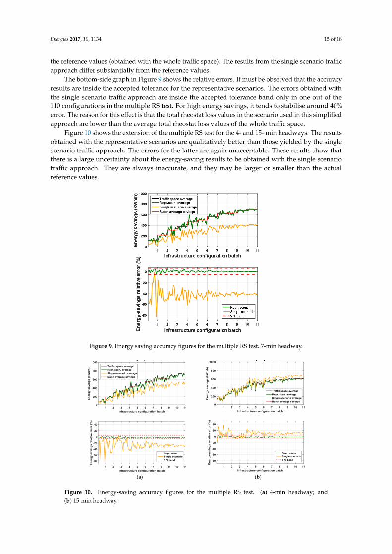
Energies 2017, 10, 1134 15 of 18

the reference values (obtained with the whole traffic space). The results from the single scenario trafficapproach differ substantially from the reference values.

The bottom-side graph in Figure 9 shows the relative errors. It must be observed that the accuracyresults are inside the accepted tolerance for the representative scenarios. The errors obtained withthe single scenario traffic approach are inside the accepted tolerance band only in one out of the110 configurations in the multiple RS test. For high energy savings, it tends to stabilise around 40%error. The reason for this effect is that the total rheostat loss values in the scenario used in this simplifiedapproach are lower than the average total rheostat loss values of the whole traffic space.

Figure 10 shows the extension of the multiple RS test for the 4- and 15- min headways. The resultsobtained with the representative scenarios are qualitatively better than those yielded by the singlescenario traffic approach. The errors for the latter are again unacceptable. These results show thatthere is a large uncertainty about the energy-saving results to be obtained with the single scenariotraffic approach. They are always inaccurate, and they may be larger or smaller than the actualreference values.

Energies 2017, 10, 1134 15 of 18

observed in the top-side graph that the results obtained with the representative scenarios are close to

the reference values (obtained with the whole traffic space). The results from the single scenario traffic

approach differ substantially from the reference values.

The bottom-side graph in Figure 9 shows the relative errors. It must be observed that the

accuracy results are inside the accepted tolerance for the representative scenarios. The errors obtained

with the single scenario traffic approach are inside the accepted tolerance band only in one out of the

110 configurations in the multiple RS test. For high energy savings, it tends to stabilise around 40%

error. The reason for this effect is that the total rheostat loss values in the scenario used in this

simplified approach are lower than the average total rheostat loss values of the whole traffic space.

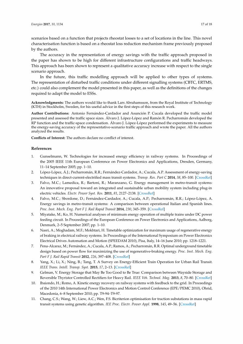
Figure 10 shows the extension of the multiple RS test for the 4- and 15- min headways. The

results obtained with the representative scenarios are qualitatively better than those yielded by the

single scenario traffic approach. The errors for the latter are again unacceptable. These results show

that there is a large uncertainty about the energy-saving results to be obtained with the single scenario

traffic approach. They are always inaccurate, and they may be larger or smaller than the actual

reference values.

Figure 9. Energy saving accuracy figures for the multiple RS test. 7-min headway.

(a) (b)

Figure 9. Energy saving accuracy figures for the multiple RS test. 7-min headway.

Energies 2017, 10, 1134 15 of 18

observed in the top-side graph that the results obtained with the representative scenarios are close to

the reference values (obtained with the whole traffic space). The results from the single scenario traffic

approach differ substantially from the reference values.

The bottom-side graph in Figure 9 shows the relative errors. It must be observed that the

accuracy results are inside the accepted tolerance for the representative scenarios. The errors obtained

with the single scenario traffic approach are inside the accepted tolerance band only in one out of the

110 configurations in the multiple RS test. For high energy savings, it tends to stabilise around 40%

error. The reason for this effect is that the total rheostat loss values in the scenario used in this

simplified approach are lower than the average total rheostat loss values of the whole traffic space.

Figure 10 shows the extension of the multiple RS test for the 4- and 15- min headways. The

results obtained with the representative scenarios are qualitatively better than those yielded by the

single scenario traffic approach. The errors for the latter are again unacceptable. These results show

that there is a large uncertainty about the energy-saving results to be obtained with the single scenario

traffic approach. They are always inaccurate, and they may be larger or smaller than the actual

reference values.

Figure 9. Energy saving accuracy figures for the multiple RS test. 7-min headway.

(a) (b)

Figure 10. Energy-saving accuracy figures for the multiple RS test. (a) 4-min headway; and(b) 15-min headway.

Energies 2017, 10, 1134 16 of 18

4.4. Computational Burden Analysis

The details of the optimisation model are outside the scope of this paper. For this reason, theoptimiser presented in [16] has been used as a reference for obtaining computation time results.That work implements a genetic algorithm to search for optimum infrastructure configurations.This population-based algorithm has been parameterised with 40 elements and 100 generations. Thus,to obtain the optimum infrastructure configuration, the optimisation process requires 4000 simulationsof the system at the different headways included in the traffic model. It is important to note that therelative computation time savings associated with the representative scenario approach would beconserved for other optimisation algorithms, which may take less or more simulations to obtain theoptimum infrastructure solution.

The traffic model and the computation times in [16] have been replaced by the model in this paperand the simulation times obtained with our simulator. The average simulation times measured fora single traffic scenario are 0.77 s, 1.31 s, and 2.73 s for the 4-, 7-, and 15-min headways, respectively.The computation times required to generate the elements in the population and to apply the geneticalgorithm’s rules are in the range of milliseconds, and have been consequently neglected. The machineused to perform the simulation campaign features an Intel(R) Core(TM) i7-2600 CPU@3.4 GHzprocessor and 8 GB RAM memory.

With this information, it is possible to compare the optimisation times and accuracies for the threetraffic approaches defined in this paper. For the full-traffic approach, this analysis uses the numberof scenarios obtained in Section 4.2 instead of all 300 scenarios per headway obtained in Section 2.2.This aims to make a fairer analysis of the computation time advantages associated with the applicationof the selection process presented in this paper.

These results are presented in Table 7. The main conclusions to be drawn are:

• The single traffic approach is, of course, the less demanding traffic model in computational terms.However, its energy-saving accuracy is too low to trust the results obtained.

• For the required 5% energy-saving accuracy, the random selection of traffic scenarios within thetotal traffic spaces makes the optimisation time soar dramatically. It would take around twoweeks to perform the optimisation process with this traffic approach.

• The RP function-characterised selection of representative scenarios proposed in this paper leadsto an 88% reduction in the expected optimisation time with respect to the random selectioncase. The optimisation time is around 7 times larger than the one with the usual approach in theliterature, but this time increase is necessary to obtain reliable energy-saving results.

Table 7. Optimisation process characteristics for the three traffic approaches analysed.

Characteristics of Traffic Approaches Single Traffic Condensed Traffic Full Traffic

Energy-saving error Unacceptable <5% 0

Number ofscenarios

4-min 1 18 1547-min 1 9 86

15-min 1 3 23

Computation time 5.4 h 37.2 h 323.5 h

5. Conclusions

This paper has presented a method to obtain a condensed traffic model for MTS electricalinfrastructure optimisation studies. The method represents an evolution of the classical traffic approachin the railway optimisation literature, which consists of using a fixed deterministic dwell time at stationsfor the generation of a single traffic scenario per headway.

This condensed set of representative scenarios are selected from a general stochastic traffic spacein a novel approach. The traffic condensation is attained by performing a characterisation of the traffic

Energies 2017, 10, 1134 17 of 18

scenarios based on a function that projects rheostat losses to a set of locations in the line. This novelcharacterisation function is based on a rheostat loss reduction mechanism frame previously proposedby the authors.

The accuracy in the representation of energy savings with the traffic approach proposed inthe paper has shown to be high for different infrastructure configurations and traffic headways.This approach has been shown to represent a qualitative accuracy increase with respect to the singlescenario approach.

In the future, this traffic modelling approach will be applied to other types of systems.The representation of disturbed traffic conditions under different signalling systems (CBTC, ERTMS,etc.) could also complement the model presented in this paper, as well as the definitions of the changesrequired to adapt the model to ESSs.

Acknowledgments: The authors would like to thank Lars Abrahamsson, from the Royal Institute of Technology(KTH) in Stockholm, Sweden, for his useful advice in the first steps of this research work.

Author Contributions: Antonio Fernández-Cardador and Asunción P. Cucala developed the traffic modelpresented and assessed the traffic space sizes. Álvaro J. López-López and Ramón R. Pecharromán developed theRP function and the traffic-space condensation. Álvaro J. López-López performed the experiments to measurethe energy-saving accuracy of the representative-scenario traffic approach and wrote the paper. All the authorsanalyzed the results.

Conflicts of Interest: The authors declare no conflict of interest.

References

1. Gunselmann, W. Technologies for increased energy efficiency in railway systems. In Proceedings ofthe 2005 IEEE 11th European Conference on Power Electronics and Applications, Dresden, Germany,11–14 September 2005; pp. 1–10.

2. López-López, Á.J.; Pecharromán, R.R.; Fernández-Cardador, A.; Cucala, A.P. Assessment of energy-savingtechniques in direct-current-electrified mass transit systems. Transp. Res. Part C 2014, 38, 85–100. [CrossRef]

3. Falvo, M.C.; Lamedica, R.; Bartoni, R.; Maranzano, G. Energy management in metro-transit systems:An innovative proposal toward an integrated and sustainable urban mobility system including plug-inelectric vehicles. Electr. Power Syst. Res. 2011, 81, 2127–2138. [CrossRef]

4. Falvo, M.C.; Sbordone, D.; Fernández-Cardador, A.; Cucala, A.P.; Pecharromán, R.R.; López-López, A.Energy savings in metro-transit systems: A comparison between operational Italian and Spanish lines.Proc. Inst. Mech. Eng. Part F J. Rail Rapid Transit 2014, 230, 345–359. [CrossRef]

5. Miyatake, M.; Ko, H. Numerical analyses of minimum energy operation of multiple trains under DC powerfeeding circuit. In Proceedings of the European Conference on Power Electronics and Applications, Aalborg,Denmark, 2–5 September 2007; pp. 1–10.

6. Nasri, A.; Moghadam, M.F.; Mokhtari, H. Timetable optimization for maximum usage of regenerative energyof braking in electrical railway systems. In Proceedings of the International Symposium on Power ElectronicsElectrical Drives Automation and Motion (SPEEDAM 2010), Pisa, Italy, 14–16 June 2010; pp. 1218–1221.

7. Pena-Alcaraz, M.; Fernández, A.; Cucala, A.P.; Ramos, A.; Pecharromán, R.R. Optimal underground timetabledesign based on power flow for maximizing the use of regenerative-braking energy. Proc. Inst. Mech. Eng.Part F J. Rail Rapid Transit 2012, 226, 397–408. [CrossRef]

8. Yang, X.; Li, X.; Ning, B.; Tang, T. A Survey on Energy-Efficient Train Operation for Urban Rail Transit.IEEE Trans. Intell. Transp. Syst. 2015, 17, 2–13. [CrossRef]

9. Gelman, V. Energy Storage that May Be Too Good to Be True: Comparison between Wayside Storage andReversible Thyristor Controlled Rectifiers for Heavy Rail. IEEE Veh. Technol. Mag. 2013, 8, 70–80. [CrossRef]

10. Ibaiondo, H.; Romo, A. Kinetic energy recovery on railway systems with feedback to the grid. In Proceedingsof the 2010 14th International Power Electronics and Motion Control Conference (EPE/PEMC 2010), Ohrid,Macedonia, 6–8 September 2010; pp. T9-94–T9-97.

11. Chang, C.S.; Wang, W.; Liew, A.C.; Wen, F.S. Bicriterion optimisation for traction substations in mass rapidtransit systems using genetic algorithm. IEE Proc. Electr. Power Appl. 1998, 145, 49–56. [CrossRef]

Energies 2017, 10, 1134 18 of 18

12. Chuang, H.J. Optimisation of inverter placement for mass rapid transit systems by immune algorithm.IEE Proc. Electr. Power Appl. 2005, 152, 61–71. [CrossRef]

13. Hui-Jen, C.; Chao-Shun, C.; Chia-Hung, L.; Shi-Hong, C. Optimization of inverter placement for mass rapidtransit systems using genetic algorithm. In Proceedings of the 2005 IEEE/PES Transmission and DistributionConference and Exhibition: Asia and Pacific, Dalian, China, 18 August 2005; pp. 1–6.

14. Bae, C.H. A simulation study of installation locations and capacity of regenerative absorption inverters inDC 1500 V electric railways system. Simul. Model. Pract. Theory 2009, 17, 829–838. [CrossRef]

15. Lee, H.; Jung, S.; Cho, Y.; Yoon, D.; Jang, G. Peak power reduction and energy efficiency improvementwith the superconducting flywheel energy storage in electric railway system. Phys. C Supercond. 2013, 494,246–249. [CrossRef]

16. Xia, H.; Chen, H.; Yang, Z.; Lin, F.; Wang, B. Optimal Energy Management, Location and Size for StationaryEnergy Storage System in a Metro Line Based on Genetic Algorithm. Energies 2015, 8, 11618–11640. [CrossRef]

17. Wang, B.; Yang, Z.; Lin, F.; Zhao, W. An Improved Genetic Algorithm for Optimal Stationary Energy StorageSystem Locating and Sizing. Energies 2014, 7, 6434–6458. [CrossRef]

18. D’Avanzo, S.; Iannuzzi, D.; Murolo, F.; Rizzo, R.; Tricoli, P. A sample application of supercapacitor storagesystems for suburban transit. In Proceedings of the Electrical Systems for Aircraft, Railway and ShipPropulsion (ESARS), Bologna, Italy, 19–21 October 2010; pp. 1–7.

19. Battistelli, L.; Ciccarelli, F.; Lauria, D.; Proto, D. Optimal design of DC electrified railway stationary storagesystem. In Proceedings of the International Conference on Clean Electrical Power (ICCEP), Capri, Italy,9–11 June 2009; pp. 739–745.

20. Ianuzzi, D.; Ciccarelli, F.; Lauria, D. Stationary ultracapacitors storage device for improving energy savingand voltage profile of light transportation networks. Transp. Res. Part C Emerg. Technol. 2012, 21, 321–337.[CrossRef]

21. Arboleya, P.; Coto, M.; González-Morán, C.; Arregui, R. On board accumulator model for power flow studiesin DC traction networks. Electr. Power Syst. Res. 2014, 116, 266–275. [CrossRef]

22. Ciccarelli, F.; Iannuzzi, D.; Tricoli, P. Control of metro-trains equipped with onboard supercapacitors forenergy saving and reduction of power peak demand. Transp. Res. Part C Emerg. Technol. 2012, 24, 36–49.[CrossRef]

23. Bierlaire, M. Simulation and optimization: A short review. Transp. Res. Part C 2015, 55, 4–13. [CrossRef]24. Ho, T.K.; Chi, Y.L.; Wang, J.; Leung, K.K.; Siu, L.K.; Tse, C.T. Probabilistic load flow in AC electrified railways.

IEE Proc. Electr. Power Appl. 2005, 152, 1003–1013. [CrossRef]25. Pilo de la Fuente, E.; Jiménez-Octavio, J.; Rodriguez-Pecharroman, R.; Lopez Lopez, A. Stochastic traffic

generator for Montecarlo load flow simulation. WIT Trans. Model. Simul. 2011, 51, 659–669.26. Martínez, I.; Vitoriano, B.; Fernandez, A.; Cucala, A.P. Statistical dwell time model for metro lines. WIT Trans.

Built Environ. 2007, 96, 1–10.27. Mellitt, B.; Mouneimne, Z.S.; Goodman, C.J. Simulation study of DC transit systems with inverting

substations. IEE Proc. B Electr. Power Appl. 1984, 131, 38–50. [CrossRef]28. Söder, L.; Amelin, M. Simulation of electricity markets. In Efficient Operation and Planning of Power Systems,

11th ed.; Söder, L., Amelin, M., Eds.; Royal Institute of Technology, Electric Power Systems: Stockholm,Sweden, 2011; pp. 83–154.

29. López-López, A.J.; Pecharromán, R.R.; Fernández-Cardador, A.; Cucala, A.P. Smart traffic-scenariocompressor for the efficient electrical simulation of mass transit systems. Int. J. Electr. Power Energy Syst.2017, 88, 150–163. [CrossRef]

© 2017 by the authors. Licensee MDPI, Basel, Switzerland. This article is an open accessarticle distributed under the terms and conditions of the Creative Commons Attribution(CC BY) license (http://creativecommons.org/licenses/by/4.0/).