Embed Size (px)
Citation preview

Improving the Manufacturing Process of
brick based products using FIT Principles
and Discrete Event Simulation
Sajith Soman
School of Engineering
Cardiff University
This thesis is submitted to Cardiff University in fulfilment of the requirements
for the Degree of Master of Philosophy
March 2017

ii
Declaration
This work has not been submitted in substance for any other degree or
award at this or any other university or place of learning, nor is being
submitted concurrently in candidature for any degree or other award.
Signed …………………………………… (candidate) Date …………………………
STATEMENT 1
This thesis is being submitted in partial fulfillment of the requirements for the degree
of …………………………(insert MCh, MD, MPhil, PhD etc, as appropriate)
Signed ……………………………….…... (candidate) Date …………………………
STATEMENT 2
This thesis is the result of my own independent work/investigation, except where
otherwise stated.
Other sources are acknowledged by explicit references. The views expressed are
my own.
Signed …………………………………... (candidate) Date …………………………
STATEMENT 3
I hereby give consent for my thesis, if accepted, to be available for photocopying and
for inter-library loan, and for the title and summary to be made available to outside
organisations.
Signed …………………………………... (candidate) Date …………………………
STATEMENT 4: PREVIOUSLY APPROVED BAR ON ACCESS
I hereby give consent for my thesis, if accepted, to be available for photocopying and
for inter-library loans after expiry of a bar on access previously approved by the
Academic Standards & Quality Committee.
Signed …………………………………... (candidate) Date …………………………

iii
Abstract
The aim of the study was to improve the current manufacturing process
through the application of FIT manufacturing principles with the aid of Discrete
Event Simulation (DES) technique.
FIT principles focus on making the manufacturing process lean, agile and
sustainable while maintaining the productivity rates, profitability and waste at
their optimum levels. Discrete Event Simulation (DES) is a powerful tool which
can be used to build a model of the current manufacturing process and later
utilised to study the effects on the process flow by simulating the model under
different scenarios corresponding to different key process parameters. In this
study, WITNESS software was used as a platform to build the DES model and
run simulations. The simulations were carried out manually i.e. by an intuitive
approach and later run automatically i.e. using the embedded optimising
module within WITNESS to collect the necessary data for improving the
current manufacturing process.
This study has been conducted as part of a Knowledge Transfer Partnership
(KTP) program within a traditional manufacturing industry. Data has been
collected from the company, process flow was mapped for 3 different product
categories, plant layout of existing manufacturing facility was created in CAD
package and a DES model was created to test different methodologies
suggested by FIT manufacturing. For the simulation model, specific rules and
functions were created to mimic the process flow based on the extracted
knowledge of current practice.
Three different FIT scenarios were tested against measured outputs to see the
potential benefits to the company. The results were validated by setting the
process parameters to the values suggested by the optimised DES model. The
fourth scenario was tested by modelling breakdown pattern of the machines in
the simulation.
In the first scenario, manual improvements were made intuitively using FIT
principles to allow the process to be more lean, agile and sustainable by critical
evaluation and analysis such as line balancing of existing processes.

iv
However, due to thresholds met by this approach in terms of improvements to
the manufacturing process, the DES model was simulated for the second and
third scenarios using the Experimenter module in WITNESS to capture the
complex relationships that exist between the 3 FIT components considering
the level of investment required as a constraint for decision making. The fourth
scenario was used to study the effect of breakdowns of the machines on the
production line and the effect of predictive maintenance on the overall
manufacturing process.
The study showed that, in general, resources such as machines and labour
that are shared between production lines caused undue pressure on the
production line. Also, maximum allocation of resources does not always lead
to maximum increase in productivity. On the contrary, lesser but smarter
investment on resources improved productivity by a higher margin. Employing
people with multiple skills who can carry out multiple operations was found to
improve productivity significantly. It was also found that increasing the
efficiency of one production line did not always increase the overall efficiency
due to cross-functional relationships within the manufacturing processes and
increasing the efficiency of one production line is likely to cause a bottleneck
on the other inter-dependent operations.
Breakdown of machinery were found to impact the production process flow
negatively. In contrary to the belief that preventive maintenance is the effective
solution, it was found that a reactive maintenance strategy of having a spare
machine is more cost effective, in this case. This option is viable in the current
manufacturing model, but not always on all scenarios.
Overall, the study showed that the application of FIT manufacturing principles
applied with the help of a DES model could add significant value to the
organisation and increase the operational efficiencies. This work can be easily
adapted to other manufacturing industries to identify the inefficiencies in the
manufacturing process and remedy the bottlenecks as well as remove non-
value adding activities.

v
Acknowledgements
I would like to express my sincere gratitude to Dr Michael Packianather for
being my guide throughout the project and gently pushing me to achieve the
results both during the MPhil and the Knowledge Transfer Partnership (KTP)
project. I would also like to thank Mr Alan Davies for his support and ‘out of
the box’ thinking, which had a major impact on my thoughts and shaping this
project.
I also wish to express my heart-felt appreciation, especially to Mr John White
at Brick Fabrication Ltd for passing on his wisdom and giving me the
opportunities during the KTP project and beyond which forms a major part of
this thesis. Credit also goes to my colleagues at Brick Fabrication Ltd for their
assistance in critical data collection and tolerating my inquisitiveness.
My gratitude extends to Dr Anthony Soroka, Mr Paul Prickett and technicians
at Cardiff University who manufactured critical components for the project and
provided feedback on my ideas.
I also wish to acknowledge the magnificent work which is being done by the
Innovate UK and Welsh Government for managing and funding KTP projects
which helps young graduates like me to shape a career.
Finally, I would like to thank my family for their continued support and
especially to my wife Simi, who endured the evenings and weekends being
spent on the project.

vi
Table of Contents
Declaration ................................................................................................... ii
Abstract .................................................................................................... iii
Acknowledgements ..................................................................................... v
List of Figures .............................................................................................. x
List of Tables ............................................................................................. xiii
Abbreviations and Acronyms .................................................................. xiv
1 Introduction ..................................................................................... 1
1.1 KTP Project overview........................................................................ 3
1.2 Company overview ........................................................................... 4
1.3 Project Aims and Objectives ............................................................. 4
1.4 Research methodology ..................................................................... 5
1.5 Project timeline ................................................................................. 6
1.6 Software used ................................................................................... 6
1.7 Organisation of the thesis ................................................................. 6
2 Literature Review ............................................................................ 7
2.1 Global economic situation ................................................................. 7
2.2 Advanced manufacturing strategies .................................................. 7
2.2.1 Manufacturing Systems 8
2.2.2 Lean manufacturing 10
2.2.3 Agile manufacturing 12
2.2.4 Sustainable manufacturing 13
2.3 FIT manufacturing perspective ....................................................... 14
2.4 Need for FIT manufacturing ............................................................ 15
2.5 Strategies for a manufacturing company to be FIT ......................... 15
2.5.1 What manufacturing companies can learn from the Martial
Arts 15

vii
2.5.2 Fit manufacturing: a framework for sustainability 16
2.5.3 FIT Sigma – An Integrated Strategy for Manufacturing
Sustainability 22
2.5.4 Advanced manufacturing technology implementation 25
2.6 Simulation ....................................................................................... 26
2.6.1 Continuous simulation 27
2.6.2 Discrete Event Simulation (DES) 28
2.7 Chapter Summary ........................................................................... 29
3 Existing manufacturing capability at Brick Fabrication Ltd. ..... 30
3.1 Process map of existing manufacturing layout ................................ 32
3.2 Production process for Brick Specials ............................................ 33
3.2.1 Value-Stream Map for Brick Specials 35
3.3 Production process for Prefabricated Arches .................................. 37
3.4 Production process for Brick-clad chimneys ................................... 39
3.5 Chapter Summary ........................................................................... 45
4 Simulation Model .......................................................................... 46
4.1 Simulation Methodology .................................................................. 46
4.2 Factory layout: Main Factory ........................................................... 47
4.3 Assumptions ................................................................................... 48
4.4 Building the Witness model ............................................................. 50
4.4.1 Parts 54
4.4.2 Buffers 56
4.4.3 Machines 59
4.4.4 Labour resources 62
4.4.5 Shift pattern 63
4.4.6 Input parameters 65
4.4.7 Output parameters 65

viii
4.4.8 Rules in the Simulation model 66
4.5 Chapter Summary ........................................................................... 68
5 Manual optimisation of resources ............................................... 69
5.1 DES model validation...................................................................... 69
5.1.1 Results 72
5.2 Scenario 01 – Initial results analysis and manual optimisation ....... 77
5.2.1 Pre-fabricated arch production line 77
5.2.2 Brick Specials production line 79
5.2.3 Brick-clad chimney production line 80
5.2.4 Suggested changes to the model for scenario 01 84
5.2.5 Results 85
5.2.6 Validation of results 89
5.3 Chapter Summary ........................................................................... 90
6 Automatic optimisation and experimentation ............................ 91
6.1 Experimentation and Optimisation procedure in Witness................ 91
6.2 Scenario 02: Pre-fabricated arches - maximum throughput with
minimum investment ................................................................... 92
6.3 Scenario 03: Maximising cycle time efficiency for Brick-clad
chimneys ..................................................................................... 95
6.4 Validation of results ...................................................................... 101
6.5 Chapter Summary ......................................................................... 102
7 Evaluation of the effect of breakdown of machines on
productivity ................................................................................. 103
7.1 Machine breakdown data collection .............................................. 103
7.2 Scenario 04: DES modelling of breakdown patterns ..................... 107
7.3 Results .......................................................................................... 110
7.4 Proactive and reactive strategies to tackle machine breakdowns . 110
7.5 Validation of results ...................................................................... 112

ix
7.6 Chapter summary ......................................................................... 113
8 Results & Discussion ................................................................. 114
8.1 Increase in turnover ...................................................................... 115
8.2 Impact on gross profit ................................................................... 117
8.3 Chapter summary ......................................................................... 119
9 Conclusions ................................................................................ 120
9.1 Contributions to knowledge ........................................................... 121
9.2 Future work ................................................................................... 122
References................................................................................................ 124
Appendix A: Gross Value Added (GVA) Estimation ............................. 129
Appendix B: FIT-Sigma Process, Tools and Techniques ..................... 130
Appendix C: Order analysis for Brick-clad chimneys .......................... 131
Appendix D: Value-stream map for pre-fabricated arches ................... 132
Appendix E: List of rules and variables used in DES model................ 134
Appendix F: Published papers ............................................................... 135

x
List of Figures
Figure 1.1 Whole-economy labour productivity per hour (Alina Barnett,
2014) ............................................................................................. 1
Figure 2.1: Relationship among flexibility types (Jim Browne, 1984) ............. 9
Figure 2.2: A history of industrial revolutions (Brenna Sniderman, 2016) .... 10
Figure 2.3: Waste in Lean philosophy (The Basics of Lean Six Sigma) ....... 11
Figure 2.4: Agile manufacturing model (Dewson, 2006) .............................. 12
Figure 2.5: Cost, volume and profit analysis (Pham & Thomas, 2012) ........ 13
Figure 2.6: Region of sustainability (Pham & Thomas, 2012) ...................... 14
Figure 2.7: Fit manufacturing framework (Pham & Thomas, 2012) .............. 17
Figure 2.8: Core structure of FMF ................................................................ 19
Figure 2.9: Operational framework for FMF ................................................. 20
Figure 2.10: OEE (Pham & Thomas, 2012) ................................................. 21
Figure 2.11: Lead time reduction (Pham & Thomas, 2012) ......................... 21
Figure 2.12: On-time delivery (Pham & Thomas, 2012) ............................... 22
Figure 2.13: Gross value added (Pham & Thomas, 2012) ........................... 22
Figure 2.14: The FIT Sigma triad (Thomas and Barton, 2008)..................... 23
Figure 2.15: Integrated FIT-Sigma strategy (Thomas and Barton, 2008) ..... 24
Figure 2.16: FIT Sigma control system (Thomas and Barton, 2008) ............ 24
Figure 2.17: FIT model (Thomas, et al., 2007) ............................................. 26
Figure 2.18: Continuous simulation output (Banks, 2007) ........................... 27
Figure 2.19: DES output (Banks, 2007) ....................................................... 28
Figure 3.1: Product hierarchy diagram ......................................................... 31
Figure 3.2: Production process map for arches, brick specials & brick-
clad chimneys ............................................................................. 32
Figure 3.3: PL.2 Plinth Header (Brick Specials, 2017) ................................. 33
Figure 3.4: PS.1 Pistol Soldier (Brick Specials, 2017) ................................. 33
Figure 3.5: Semi-raised flat gauge arch (Prefabricated Arches, 2017) ........ 37
Figure 3.6: Brick-clad chimney ..................................................................... 40
Figure 3.7: Chimney roof position ................................................................ 41
Figure 4.1: Plant layout: Main factory ........................................................... 47
Figure 4.2: Plant layout: GRP factory ........................................................... 48
Figure 4.3: Simulation model - entire factory ............................................... 52

xi
Figure 4.4: Simulation model - with part movements ................................... 53
Figure 4.5: Ply_boards arrival profile ........................................................... 54
Figure 4.6: Cap_material - arrival profile ...................................................... 55
Figure 4.7: Panel_boards - arrival profile ..................................................... 56
Figure 4.8: Buffer - 'Cut_Ply' ........................................................................ 57
Figure 4.9: Modelling delay time .................................................................. 58
Figure 4.10: Modelling a machine - CNC_Machine ...................................... 59
Figure 4.11: Cycle time function................................................................... 60
Figure 4.12: Labour rule for Bonding ........................................................... 60
Figure 4.13: Assembly machine example .................................................... 61
Figure 4.14: Weekly (40 hour) shift pattern .................................................. 64
Figure 5.1: Report on shift time without warmup time .................................. 71
Figure 5.2: Report on shift time with warmup time ....................................... 72
Figure 5.3: Quantity of finished products ..................................................... 73
Figure 5.4: Turnover per product ................................................................. 73
Figure 5.5: Turnover (Blue: chimneys, Green: Brick Specials, Red-
Arches) ........................................................................................ 74
Figure 5.6: Machine statistics....................................................................... 75
Figure 5.7: Labour resource utilisation for Brick-clad chimneys ................... 76
Figure 5.8: Pre-fabricated arches machine statistics ................................... 77
Figure 5.9: Bonding_Arches operation model .............................................. 78
Figure 5.10: 50 hour working shift details .................................................... 78
Figure 5.11: Brick Specials machine statistics ............................................. 79
Figure 5.12: Brick specials labour statistics ................................................. 80
Figure 5.13: Brick-clad chimney machine statistics ...................................... 81
Figure 5.14: Brick-clad chimney line balancing ............................................ 82
Figure 5.15: Brick-clad chimney - labour statistics ....................................... 83
Figure 5.16: Results after Scenario 1 ........................................................... 85
Figure 5.17: Scenario 1: Brick-clad chimney results .................................... 88
Figure 5.18: Scenario 1: Line balancing ....................................................... 88
Figure 6.1: Scenario 02: Input parameters ................................................... 93
Figure 6.2: Scenario 02: model configuration .............................................. 93
Figure 6.3: Scenario 02: Variance data ........................................................ 94
Figure 6.4: Scenario 02: Simulation results 01 ............................................ 94

xii
Figure 6.5: Scenario 02: Best scenario results (options vs. total turnover) .. 94
Figure 6.6: Scenario 02: Box plot results ..................................................... 95
Figure 6.7: Scenario 02: Confidence chart ................................................... 95
Figure 6.8: Lean 7 wastes (Sarhan, 2017) ................................................... 97
Figure 6.9: Scenario 03: Input parameters ................................................... 98
Figure 6.10: Scenario 03: Model configuration ............................................ 98
Figure 6.11: Scenario 03: Variance data ...................................................... 98
Figure 6.12: Scenario 04: Confidence chart ................................................. 99
Figure 6.13: Scenario 03: Results ................................................................ 99
Figure 6.14: Scenario 03: Actual scenario vs. total turnover ...................... 100
Figure 6.15: Scenario 03: Parameter analysis ........................................... 100
Figure 6.16: Scenario 03: Variance chart ................................................... 101
Figure 7.1: Machine downtime report ......................................................... 104
Figure 7.2: Arch_saw_02 breakdown pattern ............................................ 108
Figure 7.3: Slip_machine breakdown pattern ............................................. 109
Figure 7.4: Bndng_saw_01 breakdown pattern.......................................... 109
Figure 8.1 Results: Number of products shipped trend: ............................. 115
Figure 8.2: Initial model turnover ratio ........................................................ 116
Figure 8.3: Optimised model turnover ratio ................................................ 117

xiii
List of Tables
Table 2.1: Simulation benefits (Faget, et al., 2005) ...................................... 29
Table 3.1: Resource requirement summary for Brick Specials .................... 35
Table 3.2: Value-stream map - Brick Specials ............................................. 36
Table 3.3: Resource requirement summary for pre-fabricated arches ......... 39
Table 3.4: Resource requirement summary for Brick-clad chimneys ........... 45
Table 4.1: Operations vs. Machine elements ............................................... 51
Table 4.2: Machines parameters in the simulation model ............................ 62
Table 4.3: Labour resources ........................................................................ 63
Table 5.1: Brick-clad chimneys - total number of orders processed ............. 82
Table 5.2: Changes in results after Scenario 1 ............................................ 86
Table 5.3: Scenario 01: Results validation ................................................... 89
Table 7.1: Machine downtime statistics ..................................................... 105
Table 7.2: Machine numbers ..................................................................... 106
Table 7.3: Breakdown codes ..................................................................... 106
Table 7.4: Breakdown pattern per machine ............................................... 107
Table 7.5: Results of breakdown modelling ............................................... 110
Table 7.6: Analysis of proactive and reactive maintenance strategies ....... 111
Table 8.1: Results: Number of products shipped ....................................... 114
Table 8.2: Results: Increase in turnover, % change accounts for scenario
03 only ...................................................................................... 116
Table 8.3: Cost of implementing changes .................................................. 118

xiv
Abbreviations and Acronyms
AMT - Advanced Manufacturing Technologies
BS - British Standard
CAD - Computer Aided Design
CO - Cooling time
CU - Curing time
DES - Discrete Event Simulation
EU - European Union
FIT - Flexible Integrated Technology
FMF - FIT Manufacturing Framework
FMS - Flexible Manufacturing Systems
GDP - Gross Domestic Product
GRP - Glass Reinforced Plastic
GVA - Gross value added
KPI - Key Performance Indicators
KTP - Knowledge Transfer Partnership
OEE - Overall equipment efficiency
OTD - On-time delivery
PMASEE - Plan, Measure, Analyse, Solve, Execute and Embed
RMS - Reconfigurable Manufacturing Systems
SME - Small & medium sized enterprises
TPS - Toyota Production System
UK - United Kingdom
USA - United States of America
VRTM - Vacuum resin transfer moulding
WIP - Work-in progress

1. Introduction
1
1 Introduction
United Kingdom (UK) has one of the strongest economies in the modern world.
Based on the gross domestic product (GDP), UK is the fifth largest economy
in the world which comprises of 4% of the world GDP (Exchequer, 2015).
Considering the European Union (EU), UK is the second largest economy after
Germany. In the world, UK has a strong position for job creation and attracting
industries.
While the figures above infer a good state of affairs, the UK Government and
the Bank of England has raised concerns about the labour productivity per
hour. The Government suggests measures for narrowing the productivity gap
and predicts a rise in GDP by 31% if productivity would match that of the United
States (US) (Exchequer, 2015). The Figure 1.1 is an extract from a report by
the Bank of England showing the actual and predicted shortfall in labour
productivity per hour.
Figure 1.1 Whole-economy labour productivity per hour (Alina Barnett, 2014)

1. Introduction
2
The sudden drop is due to the recession period and the recovery following
recession is at a slow pace than predicted.
A series of long-term measures were announced by the UK Government to fix
the economy in 2015, a few of which are given below (Treasury, 2015).
• Competitive tax system
• Highly skilled workforce
• World leading universities
• Modern transport system
• Low carbon energy
The most important of these is a detailed plan to increase the UK productivity
outlined ‘Fixing the foundations: Creating a more prosperous nation’
(Treasury, 2015). In this document, 16 various strategies or focus points are
specified to increase the whole-economy labour productivity per hour.
This is even more critical in manufacturing industries as the most value-adding
processes in the internal supply chain are within the Production department.
Thus, increasing the labour productivity per hour would be most useful for
sustainability for all industries as well as the economy.
Traditional manufacturing industries have created various methodologies to
achieve this increase over the last couple of decades. Of which the most
common accepted standard is the implementation of Lean manufacturing
principles which was originally developed by the Toyota Production System
(TPS). Other manufacturing philosophies include Agile manufacturing,
Sustainable manufacturing and so on.
In this thesis, an investigation is carried out into the implementation of FIT
(Flexible Integrated Technology) manufacturing within the context of
promoting its use in a traditional manufacturing firm. The work is part of a
Knowledge Transfer Partnership (KTP) funded by the Welsh Government
between Cardiff University Engineering School and Brick Fabrication Ltd in
Pontypool, details of which are given below.

1. Introduction
3
1.1 KTP Project overview
The KTP project was for the duration of 21 months starting in June 2013. The
aims and objectives of the project are given below.
KTP Project Aim: To increase production output and sustainability of the
current process via the integration of CAD-CAM, and design and
commissioning of an automated brick cutting machinery together with the
introduction of a ‘FIT’ manufacturing system.
The project was broken down into stages with clear objectives, which are given
below:
KTP Project Objectives: To design and implement a ‘FIT’ manufacturing
system for the company which features automated brick cutting machinery
with 3D CAD-CAM design capabilities.
• Stage 1 – Undertake a review of the current company order processing
and manufacturing system to identify potential cost saving
improvements via a ‘FIT’ system redesign.
o Output 1: (a) Agreed manufacturing system improvement plan
and (b) automation solution for the brick cutting process.
• Stage 2 – Design and develop a suitable automation enhancement to
the existing brick cutting machinery to achieve a product and production
rate improvement.
o Output 2: Implemented and validated 3D CAD-CAM design,
automatic production capability and process improvement.
• Stage 3 – Implementation and integration of initial automatic production
process capability within a revised ’FIT’ manufacturing system.
o Output 3: Enhanced production capability and performance via
an integrated ‘FIT’ manufacturing system featuring 3D CAD-
CAM design and fully automated brick cutting system in-service.
• Stage 4 – Investigate current assembly systems for employing cut
bricks in pre-fabricated building products, and evaluate ideas for
improvement.

1. Introduction
4
o Output 4: Introduction of advanced assembly processes
resulting in improved assembly processes integrated with ‘FIT’
brick cutting manufacturing system.
The research into exploring the application of FIT manufacturing was carried
out as part of the KTP Project. Data was collected from the company and the
main aims and objectives of this thesis were formulated based on the KTP
Project.
1.2 Company overview
The project was undertaken in collaboration with Brick Fabrication Ltd in
Pontypool. The company manufactures pre-fabricated building products for
the UK house building industry. The customer base is niche and blue-chip.
Major products include decorative chimneys, pre-fabricated arches, brick
specials, GRP (Glass Reinforce Plastic) canopies and dormers.
The company turns over £3 million per annum, and has experienced
sustainable growth even during recession periods. It has 2 factories in UK,
with a workforce of around 80 and a strong 20 years of trading history.
As the current stimulus policy of the UK government is to support and expand
the house building sector, the company has an expectation that the demand
for its pre-fabricated building products will continue to increase.
1.3 Project Aims and Objectives
The aims and objectives of this thesis are given below.
Aim: The project aims to improve the manufacturing process of brick based
products using FIT principles and Discrete Event Simulation of the process
flow model.
Objectives: To design and implement a FIT manufacturing system for the
company using DES. This work can be broken down into the following
objectives:

1. Introduction
5
i. Undertake a review of the current company order processing and
manufacturing system. Process flow maps, value-stream maps, layout
models in CAD, resource allocation were all carried out. This is
discussed in Chapter 3.
ii. Build a DES model using WITNESS software to replicate the
manufacturing process in the factory. This is discussed in Chapter 4.
iii. Design and develop a suitable enhancement to the existing
manufacturing process to build a product and achieve production rate
improvement using FIT principles. This is discussed in Chapters 5 and
6.
iv. Investigate the effect of machine breakdowns on the manufacturing
process flow and suggest potential options to reduce the impact. This
is discussed in Chapter 7.
v. Review the effect of changes on real time vs. simulation to validate
theories. This is discussed in the sub-section ‘Validation of results’ in
Chapters 5 to 7 and in detail in Chapter 8.
1.4 Research methodology
Data was collected on the current manufacturing processes of 3 different
production lines from the company shop floor. Previous order history,
manufacturing performance and data on resources such as machines and
labour were collected from the factory.
Process flow maps, value-stream maps, factory layout and data on breakdown
of machines were collected and formulated into presentable form of
information as part of this project. Personal interviews/online
questionnaire/meetings were used to identify requirements of brick cutting
systems.
The above information was utilised to develop a DES model using WITNESS
software. The model and the results were validated using both data and
feedback from the management and people on the shop floor.
The viability of suggested changes was verified using the same methodology
and changes were implemented in the factory.

1. Introduction
6
1.5 Project timeline
The research timeline is to follow the KTP Project timeline and writing up of
the thesis to follow completion of the KTP Project.
1.6 Software used
The DES software chosen to build the model and simulate the manufacturing
processes is called Witness supplied by Lanner Ltd., based in Henley-in-Arden
in UK. Witness is a process modelling and simulation software widely used in
the industry worldwide especially for business planning, decision making and
risk management.
The manufacturing process within the company was modelled in Witness by
using the data collected from the shop floor and the knowledge extracted from
the operators and management team. The accuracy of the model was
validated with real-time outputs obtained by implementing the changes to the
production process. This validated model was then used to test the results of
introducing FIT manufacturing principles and for optimisation purpose.
Other software used in the research are AutoCAD and Autodesk Inventor for
modelling the factory and Microsoft Office packages.
1.7 Organisation of the thesis
A literature review of FIT manufacturing principles is given in Chapter 2. The
manufacturing process in the factory for 3 production lines are explained in
detail in Chapter 3. This information is then used to build the DES model, which
is given in Chapter 4. In Chapter 5, the first FIT scenario (where changes are
identified intuitively) to improve the manufacturing model is discussed. Second
and third FIT scenarios using automatic optimisation feature in WITNESS is
discussed in Chapter 6. The effect of machine breakdowns on the production
flow is discussed in Chapter 7. The results of the research are discussed in
Chapter 8 and conclusions in Chapter 9.

2. Literature Review
7
2 Literature Review
The aim of this chapter is to critically review current state of the art literature
on FIT manufacturing to see how best they could be adopted by different
manufacturing processes.
2.1 Global economic situation
Numerous developments have been made in manufacturing strategies.
Enhancing productivity and reducing waste has been the focus of all these.
Notable examples of advanced manufacturing strategies include Total Quality
Management, Just-In-Time, Business Process Re-engineering, Agile
manufacturing, Lean manufacturing and Six Sigma. Many of these are proven
to be successful under various circumstances. Companies take pride in
tagging themselves with the manufacturing strategy they use.
Arguably these advanced methods are seen to fail as a long-term strategy
although they bring short term economic benefits as the work force resort to
previous working (Pham & Thomas, 2012). The validity of this claim is subject
to debate as increasing number of manufacturing companies adopt these
modern manufacturing strategies.
2.2 Advanced manufacturing strategies
Numerous developments have been made in manufacturing strategies in
recent years. Enhancing productivity and reducing waste has been the focus
of all these. Notable examples of advanced manufacturing strategies include
Total Quality Management, Just-In-Time, Business Process Re-engineering,
Agile manufacturing, Lean manufacturing and Six Sigma. Many of these are
proven to be successful under various circumstances. Companies take pride
in tagging themselves with the manufacturing strategy they use.
Arguably these advanced methods are seen to fail as a long-term strategy
although they bring short term economic benefits as the work force resort to
previous working pattern (Pham & Thomas, 2012). The validity of this claim is

2. Literature Review
8
subject to debate as increasing number of manufacturing companies adopt
these modern manufacturing strategies.
2.2.1 Manufacturing Systems
Modern manufacturing systems have become sophisticated and automated
compared to traditional model which were based on people as primary
resource. Manufacturing was considered to be a transformative process.
(Parnaby, 1979). This was classified as a system which transforms raw
materials into products. In this process, the value of the product is increasing.
This was refined into inputs which are transformed into outputs. The
integration of all sub-systems into one integrated system was also one of the
outputs of earlier research (Parnaby, 1979). In the same literature, it was
stated that “manufacturing systems involve many people and exist to serve
people, and clear recognition of this fundamental point is critical to good
control”. This compared to the latest evolution in the field of manufacturing
systems through the introduction of Industry 4.0 as a standard to follow
focusses more on technologies than people, thus introducing a paradigm shift.
Defining Manufacturing systems has also been subject to debate.
Manufacturing systems which are subject to change were classified as
‘flexible’ (Jim Browne, 1984). ‘A flexible manufacturing system (FMS) was
defines as an integrated, computer-controlled complex of automated material
handling devices and numerically controlled machine tools that can
simultaneously process medium sized volumes of variety of part types’ (Jim
Browne, 1984). This definition when comparing with advanced automated
factories is still relevant and shows the growth of the sector and change. It is
worth noting that the overall change is due to the advancement in technologies
rather than the philosophy behind it.
According to Jim Browne, the following 8 flexibilities are vital for healthy
operation of the manufacturing sector:
i. Machine flexibility
ii. Process flexibility
iii. Product flexibility

2. Literature Review
9
iv. Routing flexibility
v. Volume flexibility
vi. Expansion flexibility
vii. Operation flexibility and
viii. Production flexibility
Figure 2.1: Relationship among flexibility types (Jim Browne, 1984)
But the literature also concludes that the FMS’s consists of similar components
even though the machine types and numbers may vary.
Another manufacturing system concept was Reconfigurable Manufacturing
System (RMS). According to ElMaraghy (ElMaraghy, 2005), this has seven
core characteristics which are given below:
i. Automatability: the ability to change degree of automation and
upgrade or downgrade automation in assembly level.
ii. Diagnosibility: the ability of system to automatically detect the
current situation and understand defects in production and the
reason for deflections. Thus, this system can control the
operations.
iii. Modularity: the way that different elements in manufacturing unit
change in order to response to requirements of production plan
and obtain the best optimum arrangement to meet the
production need.
iv. Convertibility: the ability of system to shift from one function to
another function inside the system. For instance machines, tools
and control interfaces to meet new production requirements.

2. Literature Review
10
v. Scalability: the ability of system to easily change current
production volume through changes in arrangement of
production system (change in components).
vi. Integrability: the ability of system for putting together all existing
modules. It should be quick and accurate and system will use
different interfaces (mechanical, electrical, etc) for this purpose.
vii. Mobility: The ability to move the whole system or change the
location of elements or sub parts.
These systems have evolved into the latest Industry 4.0 standard which
connects the embedded system production technologies and smart production
processes. The history of industrial revolution has been projected as shown in
Figure 2.2.
Figure 2.2: A history of industrial revolutions (Brenna Sniderman, 2016)
In the current KTP project, particular focus is given to the implementation of
FIT manufacturing, components of which are explained below.
2.2.2 Lean manufacturing
This is a set of production philosophy or management principles that focusses
on value addition by elimination of waste. The philosophy is developed from

2. Literature Review
11
the perspective of the customer. The term “value” is defined as any process
or action that the customer is ready to pay for. Thus, everything else is
classified as waste and is reduced to a minimum (Womack & Jones, 1996).
Lean manufacturing has evolved from the Toyota Production System (TPS)
during the 1990’s.
Waste is classified into seven categories, the reduction of which improves
customer value. The seven waste classifications per TPS are given in Figure
2.1. The success story is evident as almost 50% of UK manufacturing firms
adopt lean techniques in manufacturing (Pham & Thomas, 2012).
Figure 2.3: Waste in Lean philosophy (The Basics of Lean Six Sigma)
On the contrary, the sustainability of Lean principles is often questioned. It is
stated that “the success of “Lean” in companies often mirrors the classic
change curve – improvements in productivity after an intervention are soon

2. Literature Review
12
followed by a steady decline to baseline, and sometimes even below baseline
levels” (Pham & Thomas, 2012).
Lean is seen to lack the ability to implement a holistic approach as it is mainly
process driven. Involvement of Information Technology into manufacturing,
leadership styles, long term strategy are other areas that Lean manufacturing
does not address.
2.2.3 Agile manufacturing
The ability of an organisation to quickly adapt to changing customer demands
and market fluctuations is defined as agility. It gives the company competitive
advantage as it could deliver its products at greater speed than its competitors.
If lean focusses on value addition through waste reduction, agility focusses on
rapid response to customer demands. Agile manufacturing is seen to build on
lean manufacturing (Dewson, 2006).
Figure 2.4: Agile manufacturing model (Dewson, 2006)
The key elements of agility shown in Figure 2.2 are:
• Modular product design: Designing products in modular fashion which
enables rapid response to changes.
• Information technology.

2. Literature Review
13
• Corporate Partners.
• Knowledge Culture: Indicates investing in employees to promote rapid
change.
Agile manufacturers define their manufacturing process in such a way that it
can respond to customer demands quickly without significant capital
investment.
2.2.4 Sustainable manufacturing
The ability of the organisation to penetrate new markets, expand and prosper
through improved product and customer diversification is referred to as
sustainable. It is not just considered to be a strategy to penetrate new markets
while maintaining current production capacity. Sustainability is the ability to
meet the current needs as well as the ability of future generations to meet
future demands (Pham & Thomas, 2012).
As Lean and Agile manufacturing does not address the aspect of new market
penetration, sustainability is critical to business development and for the future
of the company as shown in Figures 2.3 and 2.4.
Figure 2.5: Cost, volume and profit analysis (Pham & Thomas, 2012)
Considering an organisation only to be Lean and Agile and not sustainable, it
is only a matter of time that escalation of operating costs meets the sales
pushing the company to loss.

2. Literature Review
14
Figure 2.6: Region of sustainability (Pham & Thomas, 2012)
Thus, a combination of Lean, Agile and Sustainable framework is required in
the long term for any manufacturing organisation to be profitable sustainably.
This is the basic idea of FIT manufacturing framework.
2.3 FIT manufacturing perspective
A FIT company is defined to be lean, agile and sustainable at the same time
all be it at varying levels. Leanness focusses on value addition and waste
reduction to improve efficiency resulting in increased production. Agility is the
ability to adapt to changing demands and circumstances in minimal time.
Sustainability refers to the idea of constant renewal by process and product
innovation along with identifying new market opportunities (Baines et al, 2005)
Leagility considers Lean and Agile aspects at the same time combining the
benefits of both paradigms. Leagility is a philosophy best suited the entire
supply chain. Leagile supply chain separates the lean and agile principles
through a decoupling point. The aim of the leagile supply chain remains to
postpone the products as far as to the customer end, in order to efficiently
handle the demand uncertainties. The FIT concept further advances the theory
of combining different manufacturing paradigms for maximum benefit to the
organisation (Chan 2014).
Adoption of a FIT Manufacturing Framework (FMF) is thought to help
manufacturing firms increase their operational efficiency and economic

2. Literature Review
15
sustainability. The concept is based on integrating innovative concepts to
existing manufacturing ideas, the success of which is proven by Thomas and
Pham (Pham & Thomas, 2012) on three SME’s.
Hence, from the above definition, a company has to be lean, agile and
sustainable in order to be classified as a FIT enterprise.
2.4 Need for FIT manufacturing
Lean and Agile manufacturing are proven to deliver desirable results. But the
effectiveness of lean and agile manufacturing depends on the demand and
volume of production. These are less effective for companies whose products
require a greater level of customisation leaving the company at a
disadvantaged position. However, lean approach is seen not to include
strategy, process, leadership and technology (Pham & Thomas, 2012).
FMF proposes a holistic approach that can be implemented in any
manufacturing firm to improve operational efficiency and economic
sustainability. The new paradigm focusses on linking the four major themes
discussed in the previous paragraph: strategy, process, leadership and
technology.
2.5 Strategies for a manufacturing company to be FIT
Various strategies/methodologies are defined to measure the fitness of a
company or to convert a manufacturing company to be fit. Some of the fitness
enhancing ideas proposed on various sources is given below.
2.5.1 What manufacturing companies can learn from the Martial Arts
This column by Duc Pham (Pham, 2008) tries to bring to the forefront the link
between the skills required in martial arts and in manufacturing to maximise
efficiency. Some of the fitness enhancing factors is given below.
• Focus: One major idea defined which enhances the fitness of a
company is the focus on the target. The focus on target makes the
company concentrate efforts on deliverables which results in value
addition and waste reduction.
2. Literature Review
16
• Leverage: Companies that uses force to enhance different sections
such as finance, resources and human elements to maximise
production are seen to increase the fitness of the company.
• Momentum: A fit company is considered to use the momentum within
the commercial environment to its advantage.
Every manufacturing firm engages in all these different aspects in various
degrees. Hence all manufacturing firms can arguably be defined as fit
manufacturing firms. This creates confusion while trying to define the fitness
of a company.
Thus, for a company to be effectively called a fit manufacturing firm, there
should be a defined level of leanness, agility and sustainability. Hence, it
becomes necessary to quantify or determine the fitness of a company.
An effort in this direction is discussed in the following section.
2.5.2 Fit manufacturing: a framework for sustainability
This paper by Duc T. Pham and Andrew J. Thomas (Pham & Thomas, 2012)
proposes a framework to identify the parameters that can be used to define
the fitness of a company.
Different approaches are taken to determine the fitness of a company one of
which is shown in Figure 2.7. The challenges in this method are to identify the
parameters for quantifying and defining the fitness of the company. Secondly,
it should be broken down to action lists for implementation.
The second step of determining the actions for implementation is not
discussed in this paper. The question that is being answered is the elements
contributing towards fitness of a company.

2. Literature Review
17
Figure 2.7: Fit manufacturing framework (Pham & Thomas, 2012)
A fit manufacturing company is not defined only to maximise its potential but it
also penetrates new markets, encourages development of new products
depending upon the viability of the product idea.
The FMF is broken down into 3 stages: core, operational and business. The
movement is sequential starting with core, operational and then business. The
next stage is to be started only after successful completion of the previous
stage.
A brief outline of the strategy in each stage proposed in the paper is given
below.
Core
The first step is to create one combined strategy which integrates marketing,
manufacturing, operational and all relevant key strategies into one document.
This is the initial step to be taken in implementing a FMF. The aim of creating
one core strategy is to ensure that there is only one vision for the entire

2. Literature Review
18
organisation which guides all different aspects such as marketing,
manufacturing, operations and so on.
The next step suggested is to carry out a fiscal analysis of the company. The
aim of which is to identify the profitability of each product, financial profile of
the company and potential to support further changes.
Simultaneously, the company should identify competitors, customers and
potential markets. It is also important to identify the product life cycle if it is
relevant and this information enables the company to design strategies to
maximise performance. The company is advised to also get information on
areas of under-performance.
The last stage suggested in the core of the FMF is to audit and identify the
current knowledge base and skill set of the workforce. This includes analysis
of managerial and leadership as well as shop floor skills of the entire
workforce. This is to identify the gap in skills and resources within the company
that will enable them in developing the strategy to meet future demands and
comply with the company vision.
The overall activity can be summarised below as shown in Figure 2.8 and
Figure 2.9.

2. Literature Review
19
Figure 2.8: Core structure of FMF
As the organisation successfully completes the ‘Core’ stage, it moves on to
the operational stage.
Operational
The starting point in developing an operational strategy is to have a clear
sustainability agenda. The operational strategy is defined according to the
sustainability agenda aiming at wealth creation and cost reduction. New
product ideas and customer needs are discussed within this section.
The lean and agility requirements are defined and discussed within the
operational frame work of the FMF. An integrated approach is required at this
Create combined
strategy for company
• Define
• Manufacturing strategy
• Marketing strategy
• Operations strategy
• Other relevant strategies
Carry out fiscal analysis
• Identify
• Profitability of products
• Potential investments
• Current financial position
Carry out market research
• Identify
• Competitors
• Customers
• Potential markets
• Product life cycle
Audit current staff potential
• Identify for existing staff
• Leadership skills
• Managerial skills
• Shop floor skills

2. Literature Review
20
stage as to identify the correct lean/agility requirement. Companies that mass
produce same product sets focus more on lean elements whereas companies
that survive on bespoke products focus on agility factor.
The output of this stage is the well-defined operational strategy for the
company that links with the core strategy.
Figure 2.9: Operational framework for FMF
Business
The basic difference of a fit manufacturing business system to lean or agile is
the multi strategic approach. The fit manufacturing system is not just the ability
to change but also adapt and meet changes in the customer demands and
market fluctuations. The company’s response is more rapid to changes in
circumstances.
The aim of developing three core strategies: core, operational and business is
to support each other and to support the single company vision as the design
of each stage building on to the next one makes the implementation effective.
The FMF suggested emphasises on review meetings and stage gate
implementation of the project to make sure the satisfactory completion of each
stage. They serve as quality check points.
Case Study
The effectiveness of the FMF is outlined in the case study presented in the
paper. Six similar companies (SME’s) were chosen to study the effectiveness
of FMF. Three companies developed FMF for 2 years and the other two
companies implemented lean principles only to identify the difference.
The effectiveness of FMF was measured using four Key Performance
Indicators (KPI’s) namely:
Operational Strategy
• Define
• Sustainability Agenda
• Lean requirements
• Agility requirements

2. Literature Review
21
• Overall equipment effectiveness (OEE)
• Manufacturing lead time from point of enquiry
• On-time delivery (OTD)
• Gross value added (GVA) contribution
Detailed procedure to measure the above factors are given in Appendix A:
Gross Value Added (GVA) Estimation. The results based on KPI’s following
the 2-year application of the FMF are given in Figures 2.8, 2.9, 2.10 and 2.11.
Figure 2.10: OEE (Pham & Thomas, 2012)
Figure 2.11: Lead time reduction (Pham & Thomas, 2012)

2. Literature Review
22
Figure 2.12: On-time delivery (Pham & Thomas, 2012)
Figure 2.13: Gross value added (Pham & Thomas, 2012)
For all selected companies over the entire range of KPI’s, significant
improvements of 10-20% are noted clearly indicating the effectiveness of
implementing FMF framework.
Though the effectiveness of the FMF has been undoubtedly proven, the author
has not failed to mention that the workforce tends to adhere to traditional ways
of working. This makes it difficult to quantify the extent of FMF application and
the individual contributions of lean, agile and sustainable manufacturing are
still not clear. Also, efforts need to be made to minimize the influence of noise
factors.
2.5.3 FIT Sigma – An Integrated Strategy for Manufacturing
Sustainability
The premise of this article argues that the integration of lean and six sigma
concepts have failed to introduce a coherent business improvement system.

2. Literature Review
23
The author goes further questioning the ambiguity of Lean Six Sigma
concepts. The solution to the stated problem is the proposed FIT Sigma
framework (Thomas and Barton, 2008).
The proposed FIT-Sigma strategy is argued to increase sustainability via cost
reduction. The initial step in this direction is suggested to lay down applicable
lean principles and Six Sigma methodology. This might vary depending upon
the type of company.
Three major areas are identified which will improve because of FIT-Sigma
strategy as shown in Figure 2.12.
• Achieve Performance target,
• Reduce variation in performance and
• Increase efficiency of performance.
Figure 2.14: The FIT Sigma triad (Thomas and Barton, 2008)
The implementation strategy proposed is: Plan, Measure, Analyse, Solve,
Execute and Embed (PMASEE). This is different from the traditional Six Sigma
implementation as the proposal is to integrate lean principles to come up with
a FIT-Sigma strategy. The integrated concept is shown in Figure 2.13.

2. Literature Review
24
Figure 2.15: Integrated FIT-Sigma strategy (Thomas and Barton, 2008)
The paper also proposes development of a control system which helps monitor
the developments as there is the tendency to resort back to previous ways of
working.
The proposed control system design is given in Figure 2.14.
Figure 2.16: FIT Sigma control system (Thomas and Barton, 2008)
Overall the article calls for an integrated FIT-Sigma strategy which
incorporates:

2. Literature Review
25
• Highly effective supply chain system
• Combined lean and agile manufacturing system and
• Development of a sustainability system.
Thus, the holistic FIT-Sigma structure integrates lean, agile and six sigma
principles to improve the economic sustainability. The framework for
implementation is given in Appendix B: FIT-Sigma Process, Tools and
Techniques.
But again, the theoretical model of FIT-Sigma suggested here has no proven
track record. There are no quantified benefits anticipated. All companies will
already be using most of these principles in the form of trying to reduce waste,
improve economic sustainability and so on. Thus, it is important to specify
where the company stands in the scale of things and to define potential
improvements. Different FIT strategies need to be defined based on industry
and size such as SME’s or large firms, service sectors or manufacturing firms
and so on.
2.5.4 Advanced manufacturing technology implementation
This paper (Thomas, et al., 2007) discusses the attitude of SME’s towards
Advanced Manufacturing Technologies (AMT), reasons for the approach and
a proposal of a strategic model for effective implementation.
Pre-decided qualitative and quantitative data were captured during the survey
which is given below for companies who have implemented and yet to
implement AMT’s.
• Financial data
• Company profile
• Business type
• Attitude to technology
• Attitude to developing business
• Operational process
• Working process
• IT, information and communication process

2. Literature Review
26
The most important inference from the survey states the inability to bring
culture change within the company. There is also reluctance in recognising the
full benefits of AMT’s. The implementation phase has been identified as the
most difficult phase where maximum numbers of failures occur. The size of
the company also played a vital role in implementation of AMT.
SME’s also failed to measure the impact of AMT implementation as they
lacked the benchmark against which to measure (Mohsen, et. al., 2010). The
FIT model given in Figure 2.17 shows the structure that could be applied to
different scenarios (Thomas, et al., 2007).
Figure 2.17: FIT model (Thomas, et al., 2007)
In this study, approaches mentioned in sections 2.5.1 & 2.5.4 will be
investigated. This is identified due to the requirements of the KTP objectives
and company preferences.
2.6 Simulation
Simulation is the imitation of an act or process (Hollocks, 2006). In this study,
the production operations that are to be investigated are simulated using the
software called Witness provided by Lanner Ltd.
2. Literature Review
27
There are different types of simulations being used in the industry. The most
common types of simulation used in manufacturing industry are (Bangsow
2012):
• Continuous simulation and
• Discrete event simulation (DES)
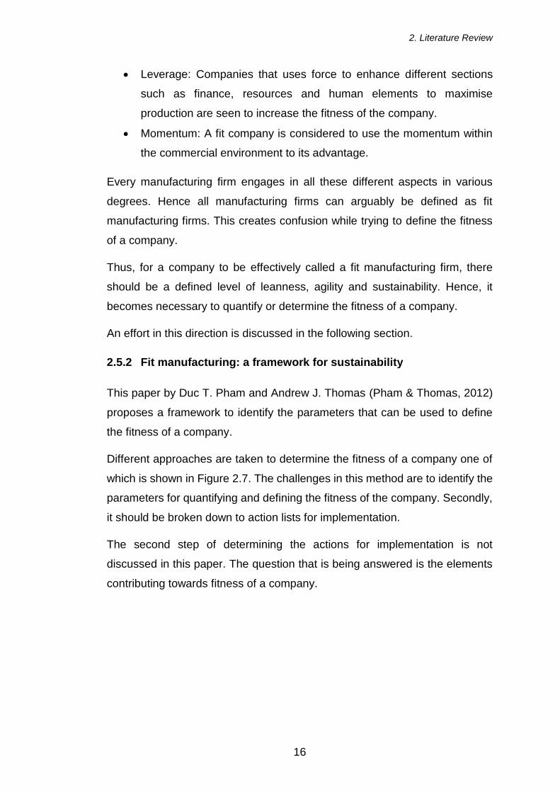
2.6.1 Continuous simulation
Continuous simulation tracks the response of the system over a period of time
continuously. Fluid model simulation in a factory can be a typical example of
a continuous simulation. The output obtained from continuous simulation is a
continuous graph (Banks, 2007) The result obtained from a continuous
simulation for the sales output against time for a simulation model is given in
Figure 2.18.
Figure 2.18: Continuous simulation output (Banks, 2007)
Mathematical models when simulated will give an output which is continuous.
Simulation of physical phenomenon such as flight dynamics, electric motors,
hydraulics and so on are examples of continuous simulation phenomenon.
2. Literature Review
28
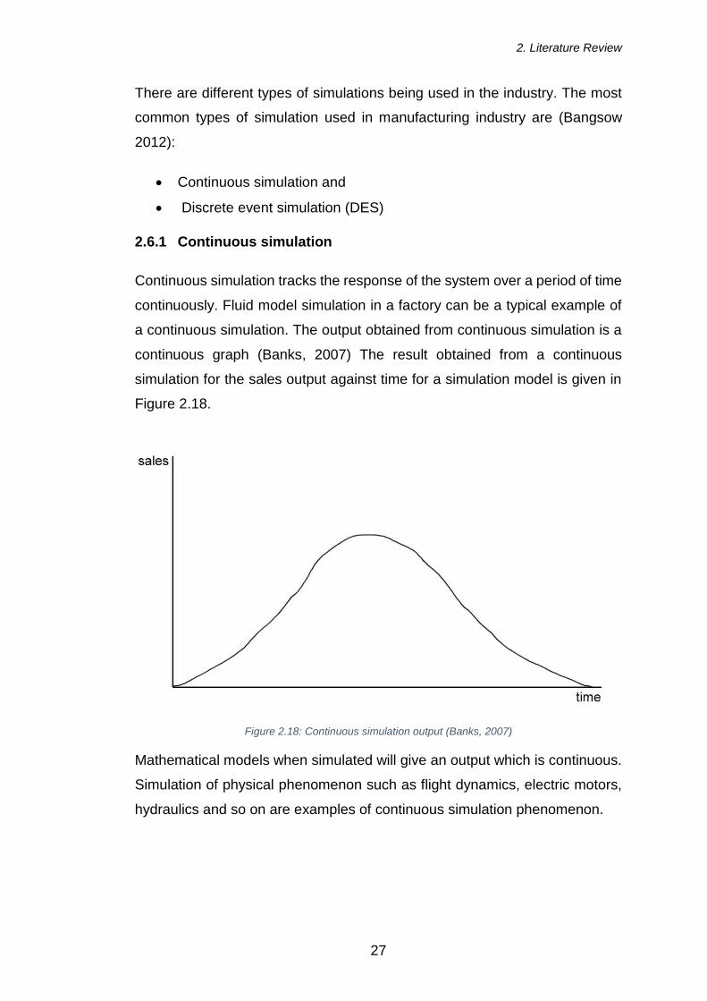
2.6.2 Discrete Event Simulation (DES)
Mimicking the operations or events occurring as discrete events in time are
called Discrete Event Simulation (DES). The change in the simulation are
captured at different intervals and reported. Over the progressing time scale
the changes over the system are captured from event to event whereas in
continuous simulation, it varies continually over time (Diamond, 2010).
An example of a DES would be the modelling of a widget factory where each
process has a cycle time to complete the operation. The events and
parameters are captured after the completion of an operation. The outputs of
a DES, if plotted in a graph for the outputs from a Sales office against time is
shown in Figure 2.19.
Figure 2.19: DES output (Banks, 2007)
Simulation is widely used in the manufacturing industry for mainly prediction
and decision making for getting ahead of the competition. In this thesis,
simulation is used to create a working model of the production facility that is
being studied to investigate different scenarios before implementing the
proposed ideas for improving the production process.
Both continuous and discrete event simulations are used in the industry
depending on the application. The simulation model of a hydraulics
2. Literature Review
29
manufacturing industry would be continuous whereas of a widget
manufacturing industry would be discrete.
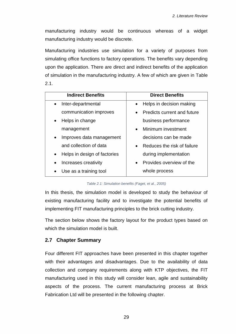
Manufacturing industries use simulation for a variety of purposes from
simulating office functions to factory operations. The benefits vary depending
upon the application. There are direct and indirect benefits of the application
of simulation in the manufacturing industry. A few of which are given in Table
2.1.
Indirect Benefits Direct Benefits
• Inter-departmental
communication improves
• Helps in change
management
• Improves data management
and collection of data
• Helps in design of factories
• Increases creativity
• Use as a training tool
• Helps in decision making
• Predicts current and future
business performance
• Minimum investment
decisions can be made
• Reduces the risk of failure
during implementation
• Provides overview of the
whole process
Table 2.1: Simulation benefits (Faget, et al., 2005)
In this thesis, the simulation model is developed to study the behaviour of
existing manufacturing facility and to investigate the potential benefits of
implementing FIT manufacturing principles to the brick cutting industry.
The section below shows the factory layout for the product types based on
which the simulation model is built.
2.7 Chapter Summary
Four different FIT approaches have been presented in this chapter together
with their advantages and disadvantages. Due to the availability of data
collection and company requirements along with KTP objectives, the FIT
manufacturing used in this study will consider lean, agile and sustainability
aspects of the process. The current manufacturing process at Brick
Fabrication Ltd will be presented in the following chapter.

3. Existing manufacturing capability
30
3 Existing manufacturing capability at Brick
Fabrication Ltd.
The product range for the company is categorised into 2 major streams,
specifically:
• Brick-clad chimneys &
• Cut & bond products which include
o Prefabricated arches and
o Brick Specials
The production process is modelled using the Discrete Event Simulation (DES)
package called Witness (Lanner, 2013).
It contributes to a turnover of circa £3 million pounds per year supplied
premium products that are difficult to make on the house building site. This
makes installation of the products easier and reduces the dependence on
trained operatives on the building sites.
With the predicted increase and higher demand for housing in UK, with
regulations and house designs including the supplied products, future of this
industry looks promising. Thus, it is significant to investigate the potential
benefits of introducing FIT manufacturing using discrete event simulation to
identify process improvements
The sections below explain the existing manufacturing processes using the
process map tool. In the following sections, the production process for each
product is explained in detail. For simulation purposes, the categorisation is
limited to materials, labour and machines.
The product hierarchy diagram is given in Figure 3.1.

3. Existing manufacturing capability
31
Figure 3.1: Product hierarchy diagram

3. Existing manufacturing capability
32
3.1 Process map of existing manufacturing layout
The process map for 3 different products within the company is given in Figure
3.2.
Figure 3.2: Production process map for arches, brick specials & brick-clad chimneys

3. Existing manufacturing capability
33
The above process map is for the production only. Tasks pertaining to the
offices are not included in this Figure 3.2. No decision elements are included
in this process map as it represents only the operations carried out in the
factory. Most of the decisions pertaining to the operations are taken by
Production Management from the Office. The production process for each
product is explained below:
3.2 Production process for Brick Specials
Another product range offered by the company is Brick Specials that conform
to BS 4729:2005 standard. There are over hundred varieties of brick specials
offered by the company. Figure 3.3 and Figure 3.4 show 2 different types of
Brick Specials offered from the product range.
Figure 3.3: PL.2 Plinth Header (Brick Specials, 2017)
Figure 3.4: PS.1 Pistol Soldier (Brick Specials, 2017)
The materials used for manufacturing Brick Specials are:

3. Existing manufacturing capability
34
• Bricks: Same as for pre-fabricated arches, bricks are supplied by
customers to match the colour and texture of the bricks used in building
houses. These are collected by the company and delivered to the
factory for processing.
• Bonding materials: For brick specials that require cut bricks to be
bonded together, bonding materials are used. The type of bonding
material used depends upon whether the bricks are dry or wet. As
explained in 3.3, 2 different types of glue are used for bonding cut bricks
together.
• Colouring materials: This is not applicable for all brick specials.
Certain type of brick specials requires re-facing of the surface to regain
the texture lost during the cutting process. This is achieved by mixing
sand with colouring pigments which is then mixed to proportion in the
glue to achieve the colour.
The process for manufacturing Brick Specials are given below:
• Brick Cutting: This is the first stage process where bricks delivered to
the company are cut to required shapes conforming to the BS
4729:2005 standard. The Slip machine and 2 manual brick cutting
machines are used for this purpose. 1 operator per machine amounts
to 3 operators overall used for this purpose. Not all 3 machines are
utilised for cutting for one product. Per product, depending upon the
type, only one machine and one operator will be used in manufacturing.
The cycle time also depends upon the type of products. For a batch
quantity of 100, the cycle time is 30 minutes.
• Kiln: All brick cutting machines are water cooled which leaves the cut
bricks wet following the process. This leads to the requirement of drying
the bricks for better adhesion while using the bonding materials. The
drying process is in the kiln where cut bricks are dried in a large oven
to remove moisture. As explained, this does not require labour
resource, has a cycle time of 2 hours followed by a cooling time of 2
hours, thus amounting to a total cycle time of 4 hours. The kiln is a
shared resource between all the products.

3. Existing manufacturing capability
35
• Bonding: The cut bricks are bonded together in this process. It is a 4
men operation done in batches of 100. The colouring of the surface of
the brick also happens during this process. The cycle time for this
process depends upon the type of the brick special required by the
customer. For analysis purposes, the cycle time is taken as the average
of 35 minutes for a batch of 100. Following bonding process, there is a
curing time of 8 hours for the glue to ensure bonded bricks are adhered
together for full strength as the brick specials are structural components
in the building.
• Quality Control & Packaging: The finished brick specials are checked
for quality of the surface, order quantity and product type before being
labelled, packed and passed to the logistics department for delivery.
The packaging is a one labour one machine operation with a cycle time
of 10 minutes and is a shared resource between all departments.
Overall, manufacturing of brick specials requires 3 different types of materials,
3 operations, 5 machines, 8 labour resources and 75 minutes of values added
time and 12 hours of cooling and curing times without any overhead operation
times as given in Table 3.1Error! Reference source not found..
Materials Operations Labour resources Total cycle time
3 3 5 13 hours 15
minutes
Table 3.1: Resource requirement summary for Brick Specials
This information is used in the simulation modelling to understand the
integration of shared resources and predict the behaviour of systems. Brick
specials amount to circa 30% of company’s turnover. Brick specials and
prefabricated arches combined are termed as Cut and Bond department within
the company.
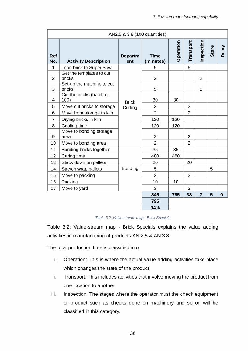
3.2.1 Value-Stream Map for Brick Specials
The value-stream map for manufacturing of the brick special product called
AN.2.5 and AN.3.8 for 100 order quantity is given below.
3. Existing manufacturing capability
36
AN2.5 & 3.8 (100 quantities)
Ref No. Activity Description
Department
Time (minutes) O
pera
tio
n
Tra
ns
po
rt
Insp
ec
tio
n
Sto
re
De
lay
1 Load brick to Super Saw
Brick Cutting
5 5
2 Get the templates to cut bricks 2 2
3 Set-up the machine to cut bricks 5 5
4 Cut the bricks (batch of 100) 30 30
5 Move cut bricks to storage 2 2
6 Move from storage to kiln 2 2
7 Drying bricks in kiln 120 120
8 Cooling time 120 120
9 Move to bonding storage area 2 2
10 Move to bonding area 2 2
11 Bonding bricks together
Bonding
35 35
12 Curing time 480 480
13 Stack down on pallets 20 20
14 Stretch wrap pallets 5 5
15 Move to packing 2 2
16 Packing 10 10
17 Move to yard 3 3
845 795 38 7 5 0
795
94%
Table 3.2: Value-stream map - Brick Specials
Table 3.2: Value-stream map - Brick Specials explains the value adding
activities in manufacturing of products AN.2.5 & AN.3.8.
The total production time is classified into:
i. Operation: This is where the actual value adding activities take place
which changes the state of the product.
ii. Transport: This includes activities that involve moving the product from
one location to another.
iii. Inspection: The stages where the operator must the check equipment
or product such as checks done on machinery and so on will be
classified in this category.

3. Existing manufacturing capability
37
iv. Store: If a product must be stored in a location before the next process
is taken place, the time is recorded in this category.
v. Delay: The delay in any process such as waiting for raw-materials and
so on are captured in this category.
All stages except the Operation are considered non-value adding. In this case,
the total time required to manufacture is 845 minutes, of which 795 minutes
are value-adding. This amounts to 94% of the total time. The value adding
activities in the process are the ones that change the nature of the product.
3.3 Production process for Prefabricated Arches
An arch is generally a structure which covers a space within a building. Arches
are generally installed above doorways and windows. A picture of one type of
arch is shown in Figure 3.5.
Figure 3.5: Semi-raised flat gauge arch (Prefabricated Arches, 2017)
The materials used for manufacturing arches are:
• Bricks: They are usually supplied by the customers as the colour of the
brick has to match the bricks used to build houses. Thus, to avoid any
discrepancy, the bricks required are supplied by the customers.
• Backing board: This holds the bricks together which is made of cement
particles and foam. This is purchased from a regular supplier and
contributes a large percentage towards the cost of materials.
• Bonding material: Bricks are stuck on to the backing board using
bonding materials such as glue. There are 2 different types of bonding
materials used – type 1 glue which is used to bond dry bricks to the

3. Existing manufacturing capability
38
backing boards and type 2 glue which is used to bond wet bricks to the
backing board. The curing time after bonding process varies depending
upon the type of glue used.
The process for manufacturing is explained below:
• Panel & Board Cutting: This process cuts the backing board to the
required size and shape based on the order requirements. This is
carried out using a CNC machine. This resource is shared with the
brick-clad chimney production line. It is a one operator process. The
time required to cut the backing board per arch varies according to the
size and type of arch, but for modelling purposes, an average of 2
minutes is taken.
• Brick cutting: The bricks supplied by the customers are cut into
specified size and shapes in this process. This operation happens in
the cutting room. For arches, one semi-automated (slip machine) and
2 manual brick cutting machines are available for this purpose. For a
single arch, the process starts with the slip machine followed by a
manual brick cutting machine. The cycle time for cutting arches on the
slip machine is 15 minutes and for manual brick cutting machine is 90
minutes per flat-gauge arch and 20 minutes per segmental arch. 2
machines and 2 operators are required in the Brick Cutting process.
• Kiln: In this process, the cut bricks are dried inside the kiln to remove
moisture. This enables bricks to be glued to the backing board using
type 1 glue. This is a machine operation and does not require labour. A
minimum cycle time of 2 hours is required for this operation. Following
this operation, a cooling time is also required (represented by CO in
Figure 3.2). The minimum required cooling time is 2 hours. The
temperature of the bricks after being taken out of kiln is higher for
manual handling. Thus, the total cycle time for the process is 4 hours,
require 1 machine and no labour.
• Bonding: The bricks following the previous process are glued on to the
backing board in this process. This is a manual operation (1 operator)
and does not include any machinery. The cycle time for this operation
per arch is 5 minutes. Following bonding, the arches are stored in

3. Existing manufacturing capability
39
racking for curing for the glue. This is represented by CU in Figure 3.2.
The minimum curing time is 8 hours.
• Quality Control: Before products are packed, labelled and sent to the
customers, they go through final quality inspection. This is a one-man
operation. Products at random are selected and checked for quality, not
all products. Thus, this process is not modelled in the simulation.
• Packing: This is the final process before the product is passed on to
be delivered to the customer. This operation is a shared resource
between all the products in the company. The cycle time for this process
is 10 minutes. It is a one operator one machine operation. In simulation
modelling, Packing is considered as the last operation and counters are
set at this stage.
Overall, to manufacture one single arch, it would take 3 different types of
materials, 6 operations, 5 labour resources and 14 hours and 2 minutes
(including cooling and curing times) as shown in Table 3.3.
Materials Operations Labour resources Total cycle time
3 6 5 14 hours 2
minutes
Table 3.3: Resource requirement summary for pre-fabricated arches
This only includes the production time and not overheads such as delivery,
planning etc. The calculation of value-added time and non-value-added time
for pre-fabricated arch production line is given in Appendix D: Value-stream
map for pre-fabricated arches.
3.4 Production process for Brick-clad chimneys
Chimneys have been an essential part of UK houses for centuries which act
as a ventilation for hot gases arising from fireplace, boilers, stove and so on.
The gases are released to the atmosphere using the ventilation inside the
chimneys. The majority of UK houses are equipped with chimneys.
Although, recent developments and innovations in the UK housing sector
especially in the boiler and heating systems has made the requirement of a

3. Existing manufacturing capability
40
live working chimney redundant. But due to building regulations and aesthetic
requirements, UK house builders use chimneys on the house design. A typical
chimney supplied by the company is shown in Figure 3.6.
Figure 3.6: Brick-clad chimney
As there is no requirement for a live working chimney with ventilation in most
of the houses, the chimneys supplied by the company are decorative and not
functional. The company also supplies live functional chimneys upon request
by customers but is not a standard option offered. A typical chimney is fitted
to the roof along the ridge of the roof.
The defining characteristics of the chimney are:
• Width: This is the dimension of the chimney along the roof ridge.
• Depth: This is the dimension of the chimney across the roof ridge.
• Height: This is the dimension from the bottom of the core to the top of
the chimney core excluding the height of the pot.
• Roof pitch: This is the angle of the roof.
• Roof position: This specifies the location of the chimney on the roof.
There are 4 standard positions which are given below:

3. Existing manufacturing capability
41
Figure 3.7: Chimney roof position
Other features that can be specified on a chimney are corbel details, cap
options, pot options and brick-bond pattern.
The company offers 2 types of chimneys to customers:
• Brick-clad chimney: In this option, the chimney core is made of
laminated ply wood and brick slips are attached to the core to make a
look alike decorative brick-clad chimney.
• GRP chimney: Glass Reinforced Plastic (GRP) is another type of
chimney which looks alike like a brick-clad chimney but is made of
plastic materials. GRP is a matrix of glass fibre sheets which is set in
resin.
As over 80% of chimney orders are brick-clad with standard options, for
analysis purposes, it is being considered and the processes explained below.
As the company offers many options on different features such as width,
depth, roof pitch etc., the total number of combinations of a chimney that can
be specified are over 10,000.
The manufacturing process explained below is for a brick-clad chimney without
a live flue in it.
The materials used for manufacturing are:
• Bricks: Same as for previous products, to match the brick type and
brick colour on the construction site, bricks are supplied by the
customer. This is collected from the site by the company and delivered
to the factory for processing.

3. Existing manufacturing capability
42
• Laminated ply wood: The core of the chimney is made from laminated
ply. There are 2 different types of laminated by used in manufacturing
– 5.5 mm thick ply and 12mm thick ply sheets. They are purchased and
cut to the required size as per order in the manufacturing facility.
• Timber: The cut sheets of ply are assembled together using 3”x2”
timber. Timber is bought in lengths and supplied to the factory which is
cut to size as required.
• GRP laminate & resin: Even though the chimney is not GRP, the core
of the chimney is made waterproof by spraying the core with GRP
laminate and impregnating with resin. Essential components that are
specified with the chimney are caps and/or pots. This is made using a
moulding process using GRP and resin materials.
• Bonding materials: The brick slips are glued on to the core of the
chimney using bonding materials like arches and brick specials.
• Nuts, bolts, nails, lifting eyes: Various kinds of fixing materials such
as nuts, bolts and nails are used along the processes. Examples
include fixing the core of the chimney to pallets to using lifting eyes to
lift the chimney from the floor to the roof.
• Plastic sheets: This is used to pack the chimney to prevent any
damage during transport to the customer. After the manufacturing is
complete, the chimney is packed using plastic sheets and secured on
to a pallet, ready for delivery.
Not all materials used for manufacturing are specified below. Only the
significant items that contribute to the cost and environmental sustainability
are specified above.
The processes for manufacturing brick-clad chimneys are given below:
• Cut Boards: This is the start of the process. In this the laminated ply
sheets are cut to the required size and shape using an automated 3-
axis CNC router. The operator programs the pieces to be cut using a
CAD-CAM software and then cuts the 12mm and 5.5 mm to shapes
and sizes. One operator is required for this operation with a cycle time

3. Existing manufacturing capability
43
of 45 minutes per average chimney. This varies depending upon the
size and features on the chimney.
• Assemble Core: The cut sheets of ply are assembled to make the core
of the chimney in this process. The sheets of ply are assembled
together using 3”x2” timber frame. Two operators are required for this
operation with a cycle time of 65 minutes.
• Laminate Core: In this operation, the assembled chimneys are spray
laminated using the GRP fibreglass and resin. This is to make sure the
chimney is waterproof and provides structural integrity to the core of the
chimney. One machine and 2 operators are working simultaneously in
the process with a cycle time of 45 minutes. Following the laminating
process, there is a curing time of 8 hours for the resin to cure. This is
temperature dependant and varies. Generally, it takes longer (greater
than 8 hours) to cure in colder climate especially in winter season and
shorter (less than 5 hours) during summer season.
• Trim Core & Add Flow-coat: Following the laminating process, after
the resin has cured, the edges of the core of the chimney are left with
sharp GRP materials. In this process, the edges are trimmed and
sanded down to ensure no sharp laminate is present. Following this a
special material is coated to the edges and corners of the chimney core
to ensure water tightness. This is a thick layer (around 3mm) of flow
coat. This is a one operator function with a cycle time of around 20
minutes. Following this process, there is a curing time of 8 hours for the
flow coat. This is not dependent on the ambient temperature. The
operation is a one man one machine operation
• Cut Brick Slips: The brick slips supplied by the customer are cut to
25mm thick slips. A standard brick is 215 x 102 x 65 mm. This is cut to
215 x 65 x 25 mm. The face of the brick is maintained. The other portion
of the brick is waste unless the brick is double faced where two 25mm
thick brick slips are obtained from a standard brick. This is a one-
operator one machine operation with a cycle time of 60 minutes. This
is a sub-assembly line which is carried out separate to the main
assembly line as shown in Figure 3.2.

3. Existing manufacturing capability
44
• Dry brick slips: The cut brick slips are dried in a Kiln like arches and
brick specials as the brick cutting machines are all water cooled. The
Kiln removes moisture and makes the bricks dry which are easier to
bond it to the core of the chimney. This operation does not require a
labour resource, has a cycle time of 2 hours followed by the cooling
time for bricks which is another 2 hours. Thus, the total cycle time for
this operation is 4 hours irrespective of the type of product.
• Brick Cladding: In this process, the cut brick slips are glued to the core
of the chimney. The chimney core after flow coating is cured and
supplied to this process. The core of the chimney is sanded down to
make it rough for the brick slips to be glued correctly. The cut slips are
glued to the core using adhesive. This operation requires 2 operators
and a cycle time of 45 minutes. Following this process, there is a curing
time of 8 hours for the adhesive.
• Manufacturing Caps & Pots: This is not represented in the process
map as it is a sub-assembly process. In this process, the caps and pots
are manufactured using injection moulding process and using open
laminating process. This is then fed to a Kanban storage system which
stores minimum specified of each category of cap and pot. According
to the order quantity and type, this is then picked and delivered to the
operation. This is a 2-operative process with a cycle time of 60 minutes.
• Adding Caps & Pots/Finishing: Caps and pots are specific to the
order. Some chimneys may not have them and some might have 2 pots.
Caps and pots manufactured are delivered to this operation. This is a
single operative no machine operation with a cycle time of 20 minutes.
Adhesive is used to fix the cap and pot to the core of the chimney. There
is a curing time for this operation of 8 hours.
• Quality inspection: This is the final process where the chimney is
inspected by a trained quality co-ordinator before passing on to the
packaging department. It is a one-person operation and required 10
minutes’ cycle time.
• Packaging: In this final stage, the chimney that is being signed-off by
the quality inspector is packed using polythene sheets to prevent any

3. Existing manufacturing capability
45
damage during transport. The chimney is secured on to the pallet,
wrapped with plastic sheets; labels are attached and are moved to the
yard to deliver on-time in full to the customer.
Overall, manufacturing of brick-clad chimneys requires 7 major different types
of materials, 10 operations, 9 machines, 11 labour resources and 305 minutes
of value added time and 28 hours of cooling and curing times without any
overhead operation times as given in Table 3.4.
Materials Operations Labour
resources Total cycle time
7 10 11 33 hours 05
minutes
Table 3.4: Resource requirement summary for Brick-clad chimneys
3.5 Chapter Summary
The existing process flow of the nature and complexities of manufacturing
three different products have been described in detail. Overall, the
manufacturing facility discussed has 24 operatives not including fork lift drivers
and 16 operations to produce 3 different types of products. This information
will be used in the next chapter to build the simulation model of the production
process.

4. Simulation Model
46
4 Simulation Model
Before proceeding with the decision that simulation is the solution, the
techniques used in simulation needs to be analysed. The queuing nature of
the model and the randomness in the system, simulation modelling is found
appropriate to solve the situations. (Beck, 2011) They model of Brick
Fabrication Ltd is of similar nature which makes simulation appropriate to the
situation.
4.1 Simulation Methodology
The simulation is carried out following the methodology given below as
described by Ulgen (Onur M. Ulgen, 2016). This is to ensure the robustness
of the process and to make sure all the steps are followed to achieve the result.
i. Define the problem
ii. Design the study
iii. Build the conceptual model
iv. Formulate inputs, assumptions and processes
v. Build, verify and validate the simulation model
vi. Experiment with the model
vii. Document and present the results
viii. Define the model life cycle
The stages are not to be followed in sequence as some stages may have to
be done prior to others. For example, the data might need to be collected
before defining the problem as data might throw anomalies which require
attention that could be the problem.
Similar approach is taken in the article (Joanne Berry, 2011). In this simulation,
the problem is defined in Section 1.3. All the other phases of building the model
is explained in later sections of the thesis. This is the model that is followed in
the thesis to obtain the result.

4. Simulation Model
47
4.2 Factory layout: Main Factory
The company has 2 major sites for manufacturing in UK, one in Pontypool and
the other in Stoke-on-Trent. This study is being conducted in the factory at
Pontypool. In Pontypool, the company has 2 factories; one has the main
production line and the other which manufactures sub-assembly parts which
is called the GRP (Glass Reinforced Plastic) unit. The production of pre-
fabricated arches and Brick Specials takes place in the main factory, and the
manufacturing of the Brick-clad chimneys takes place both in the main factory
and in the GRP factory where a sub-assembly part is made.
The layout of the main factory is shown in Figure 4.1.
Figure 4.1: Plant layout: Main factory
For pre-fabricated arches, the process flows from Brick cutting to Bonding.
Same applies for Brick Specials. The Kiln which is used to dry cut bricks is
located in the Brick Cutting part of the process. Following the Bonding process,
the products move to the holding bay to be checked for Quality and then to the
Packing bay. Following packaging, the products are moved to the yard to be
delivered to the customers.

4. Simulation Model
48
For manufacturing of the Brick-clad chimneys, the process starts with the CNC
Machine followed by the Assembly process. After the Assembly process, the
assembled core of the chimney is transported to the GRP factory.
The layout of the GRP factory is shown in Figure 4.2.
Figure 4.2: Plant layout: GRP factory
The laminating process and the trim & flow coat process takes place in the
GRP factory. Also, this is the manufacturing unit for the Caps & Pots. They are
manufactured and finished completely in this unit. Following this process, the
chimney core and caps & pots are delivered to the main factory.
The rest of the process takes place in the main factory where brick slips are
clad to the chimney, and when it is finished, quality checked and packed.
Following packing, the chimneys are transported to the customers.
In the following section, assumptions used in the simulation model are
discussed.
4.3 Assumptions
Following are the assumptions used in building the simulation model.
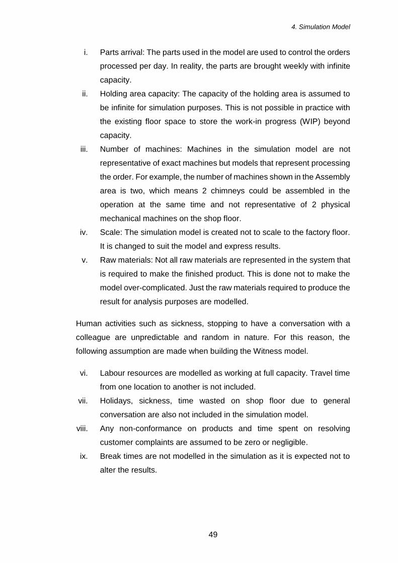
4. Simulation Model
49
i. Parts arrival: The parts used in the model are used to control the orders
processed per day. In reality, the parts are brought weekly with infinite
capacity.
ii. Holding area capacity: The capacity of the holding area is assumed to
be infinite for simulation purposes. This is not possible in practice with
the existing floor space to store the work-in progress (WIP) beyond
capacity.
iii. Number of machines: Machines in the simulation model are not
representative of exact machines but models that represent processing
the order. For example, the number of machines shown in the Assembly
area is two, which means 2 chimneys could be assembled in the
operation at the same time and not representative of 2 physical
mechanical machines on the shop floor.
iv. Scale: The simulation model is created not to scale to the factory floor.
It is changed to suit the model and express results.
v. Raw materials: Not all raw materials are represented in the system that
is required to make the finished product. This is done not to make the
model over-complicated. Just the raw materials required to produce the
result for analysis purposes are modelled.
Human activities such as sickness, stopping to have a conversation with a
colleague are unpredictable and random in nature. For this reason, the
following assumption are made when building the Witness model.
vi. Labour resources are modelled as working at full capacity. Travel time
from one location to another is not included.
vii. Holidays, sickness, time wasted on shop floor due to general
conversation are also not included in the simulation model.
viii. Any non-conformance on products and time spent on resolving
customer complaints are assumed to be zero or negligible.
ix. Break times are not modelled in the simulation as it is expected not to
alter the results.

4. Simulation Model
50
4.4 Building the Witness model
The simulation model for the manufacturing is shown in Figure 4.3. It shows
the layout of the plant in the simulation model representing parts, machines,
labour resources and layout.
In Figure 4.4, the model is shown with the process flow map which shows the
movement of parts in the factory. The parts are processed using the machines.
Once a process is completed, the parts are stored in a holding area before the
next operation is started. These holding areas are represented by Buffers in
the model which is represented as numbers. Before 2 different processes, the
parts are held in a buffer which is shown by numbers. In Figure 4.3,
Arch_storage is an example of a buffer.
The process map for the model is given in Figure 3.2: Production process map
for arches, brick specials & brick-clad chimneys. The operations on the first
column on Figure 3.2 represents actual operations in the factory. The second,
third and fourth columns represent the process flow for each product. This is
modelled below in Figure 4.3 and Figure 4.4. The factory is split into main
factory, Brick Cutting and GRP. With reference to Figure 3.2, each operation
is represented by a machine in the simulation model which is stationed in one
part of the factory. This is explained in Table 4.1.
Operation
(Figure
3.2)
Name of the
Machine used
in Witness
Location
Panel &
Board
cutting
CNC_Machine Main
Factory
Assembly Assembly
Bonding Bonding_Arches
Bonding
Cladding Cladding
Finishing Finishing
Packing Packing

4. Simulation Model
51
Brick
Cutting
Slip_machine
Bndng_saw_01
Bndng_saw_02
Arch_saw_01
Arch_saw_02
Chmny_saw
Brick
Cutting
Laminating Laminating GRP
Factory Trim/Flow
coat
Trim_coat
GRPVRTM Cap_n_Pots
Table 4.1: Operations vs. Machine elements

4. Simulation Model
52
Figure 4.3: Simulation model - entire factory

4. Simulation Model
53
Figure 4.4: Simulation model - with part movements

4. Simulation Model
54
4.4.1 Parts
Parts are the components that get processed in the model to create the
finished products. They are representative of raw materials but as discussed
in the Assumptions, not all raw materials are modelled. The parts modelled in
the system are given below:
• Ply_boards: This is the part used to manufacture chimneys. It is
represented as ‘Ply_boards’ in the model. The part is pushed into the
buffer ‘Bay2’ from which the ‘CNC_Machine’ pulls the part for
manufacturing. It is represented by blue in colour. The arrival profile for
the part is controlled by the parameter ‘Chimney_orders_per_day’
which is given in Figure 4.5:
Figure 4.5: Ply_boards arrival profile
It can be seen that a lot size arrives at time zero, followed by the next
lot size at intervals of 1440 minutes which is every 24 hours. The lot
size is controlled by the variable ‘Chimney_orders_per_day’, value of
which is given when the model is initialised.

4. Simulation Model
55
• Cap_materials: This is used to manufacture Caps & Pots. It is pushed
into the buffer ‘Cap_holding’ from where it is pulled into the machine
‘Cap_n_Pots’. The material is represented by blue in colour. The arrival
profile of the part is given in Figure 4.6:
Figure 4.6: Cap_material - arrival profile
It can be seen that the first lot size arrives at time zero, followed by the
next lot size at time intervals of 24 hours (1440 minutes). This is
controlled by the variable ‘Chimney_orders_per_day’ which is given in
the model initialisation.
• Panel_boards: This part is used to manufacture pre-fabricated arches.
It is pushed into the buffer Bay1 which is used by the CNC_Machine to
manufacture arches. The material is represented by red in colour. The
arrival profile of the part is given in Figure 4.7.

4. Simulation Model
56
Figure 4.7: Panel_boards - arrival profile
The arrival time and inter arrival time are similar to other parts and is
also controlled by the variable ‘Chimeny_orders_per_day’. But the
number of orders arrived per day is 35 compared to that of chimneys of
10.
• Ch_bricks: This is the bricks used to make chimney slips. The arrival
profile is similar to other raw materials used for manufacturing
chimneys.
• Ar_bricks & CnB_bricks: This is the bricks used to manufacture
arches and brick specials. The first arrival is at time zero followed by
inter arrivals at 24 hours with the lot size of 1000 for arches and 10 for
brick specials respectively.
4.4.2 Buffers
Buffers are used in the model to represent work holding areas. For example,
if a delay is present in starting a process after the previous process and the
work needs to be held for a while, it is represented by a buffer in the system.

4. Simulation Model
57
Buffers can be represented by parts of numbers. In this simulation model,
buffers are represented by numbers which represent the number of parts held
in the buffer at a particular point in time. For example, the work processed by
the CNC Machine is completed and moved into a holding bay in the factory.
This is then processed by the Assembly area depending upon the numbers of
jobs in the queue. This is represented by the buffer ‘Cut_Ply’ in the model. The
example of this buffer is given in Figure 4.8
Figure 4.8: Buffer - 'Cut_Ply'
It can be seen from the detail above that the buffer has a maximum capacity
of 1000 which means it can hold 1000 jobs in the buffer at one point of time.
Buffers are also used to model delay time. Some processes require a delay
time (such as cooling time or curing time) after the process is completed and
before the next process is started. An example would be chimneys that are
laminated requires a delay of 8 hours before the next process is started. This
is modelled in the simulation in buffers as the delay time shown in Figure 4.9.

4. Simulation Model
58
Figure 4.9: Modelling delay time
The buffers used in the simulation model are given below:
• Arch_bricks
• Arch_storage
• Assembled
• Bay1
• Bay2
• Bond_bricks
• Brick_slips
• Bricks_ar
• Bricks_ch
• Cap_holding
• Cap_Pot
• Caps_n_Pots
• Clad_chimenys
• Cut_Panel
• Cut_Ply

4. Simulation Model
59
• Cut_slips
• Dry_bricks
• Fin_chimneys
• Laminated
• Trimmed_chim
20 different buffers are used in the model to simulate the manufacturing
processes in the factory.
4.4.3 Machines
Machines are representative of processes in the factory and not exact models
of mechanical machines. For example, in the model, the machine ‘Assembly’
represents the Assembly operation in the factory and not a physical machine
on the factory floor. The parameters required to model a machine are given in
Figure 4.10.
Figure 4.10: Modelling a machine - CNC_Machine
The most important parameters of modelling a machine are:
• Input: It represents the path from which a part is pulled to the machine.
Normally it is from a buffer.

4. Simulation Model
60
• Cycle Time: The cycle time is one of the most important parameters in
a model. It represents the amount of time required to process the part
in the machine. It can be given as a number or controlled by a function.
In the above example for ‘CNC_Machine’, the cycle time is controlled
by a function as the cycle time changes depending upon the type of
product that is processed. The function used to control the machine is
given in Figure 4.11.
Figure 4.11: Cycle time function
This function sets the cycle time to be 2 minutes if ‘Part_type’ 1 is being
processed, else to 45 minutes.
• Labour Rule: In this parameter, the labour resources can be specified
on the machine. The machine can be modelled for one labour resource
or 2 labour resources. This can be modelled in WITNESS using ‘AND’
or ‘OR’ function to tell the machine which combination of labour
resources are to be used The example of Bonding machine is given in
Figure 4.12:
Figure 4.12: Labour rule for Bonding

4. Simulation Model
61
This shows that any of the 4 bonders are only required to operate the
machine ‘Bonding’.
• Type: There are 7 different types of machines that can be modelled
using Witness which are given below:
i. Single
ii. Batch
iii. Assembly
iv. Production
v. General
vi. Multiple Cycle
vii. Multiple Station
In this simulation model, only Single and Assembly machines are used.
In a Single machine, there is one input and one output. In an Assembly
machine, there are 2 or more part inputs and one output. This is used
to represent an operation which assembles different parts to one. This
is controlled by the input quantity. Following is an example of an
Assembly machine as shown in Figure 4.13.
Figure 4.13: Assembly machine example
In the above machine, it can be seen that the input quantity required is
given as 2 and the Type of the machine is selected as Assembly which
indicates 2 parts are required by the machine to produce an output. This
can be compared to Figure 4.10 which is a Single machine.

4. Simulation Model
62
• Output: In this tab, the output parameters of the machine as specified.
The output of a machine is generally to a buffer using the PUSH rule.
The different types of machines modelled in the simulation with its parameters
are given in Table 4.2.
Machine Type Input
quantity
Cycle
time
(min)
Labour
resources
Output
quantity
Arch_saw_01 Single 1 90 1 1
Arch_saw_02 Single 1 20 1 1
Assembly Single 1 65 2 1
Bndng_saw_01 Single 1 30 1 1
Bndng_saw_02 Single 1 30 1 1
Bonding Single 1 30 1 1
Bonding_Arches Assembly 2 5 1 1
Cap_n_Pots Single 1 60 2 1
Chmny_saw Single 1 60 1 1
Cladding Assembly 2 45 2 1
CNC_Machine Single 1 2 or 45 1 1
Finishing Assembly 2 20 1 1
Laminating Single 1 45 2 1
Packing Single 1 10 1 1
Slip_machine Single 1 15 2 1
Trim_coat Single 1 20 1 1
Table 4.2: Machines parameters in the simulation model
16 different operations are modelled using the machines in the simulation.
Some machines are considered a shared resource between different products.
4.4.4 Labour resources
Labour resources are modelled in the simulation using the ‘labor’ parameter.
Labour resources are allocated to each machine. The Table 4.3 shows the
labour resources allocated to each product where a few resources are shared.

4. Simulation Model
63
Brick-clad chimneys Pre-fabricated arches Brick specials
CNC_Operator Bonding_cutter1
Slip_cutter1 Bonding_cutter2
Slip_cutter2 Bonder1
Chimney_cutter Arch_cutter1 Bonder2
Assembler1 Arch_cutter2 Bonder3
Assembler2 Bonding_arches1 Bonder4
Laminator1
Laminator2
Trim_operator
Cladding1
Cladding2
Cap_operator
Pot_operator
Packer
Table 4.3: Labour resources
23 labour resources are modelled in the simulation, 3 of which are shared for
2 product lines, the Packer is a shared resource between all 3 products. The
rest of the resources are dedicated resources to each particular product.
4.4.5 Shift pattern
The factory operates on a 40 hour/week shift pattern. In order to get accurate
results from the simulation model, the model needs to represent the real-life
situation. If shift patterns are not modelled into the simulation, it will not
represent the actual results from the factory. The shift pattern used in the
simulation is given in Figure 4.14 which is for a standard 40-hour work week
Monday to Friday.

4. Simulation Model
64
Figure 4.14: Weekly (40 hour) shift pattern
The Working Time represents the time the model is run and the Rest Time
represents the non-working times. Period 1 to 5 represents Monday to Friday
respectively with working time of 8 hours (represented as 480 minutes) and
non-working time of 16 hours (960 minutes). Saturday and Sunday are non-
working times represented by 2880 minutes (48 hours) in the model.
The total working time for the week is 2400 minutes and non-working time of
7680 minutes. To simulate a full working week, the running time should be
10080 minutes. A warm up time is also required while running the simulation
to make sure enough parts are in the system before calculating the results so
the model is not empty when running.

4. Simulation Model
65
4.4.6 Input parameters
These are used to control the simulation model. The input parameters used in
the model are given below.
i. Chimney_orders_per_day: It is the number of orders per day received
for brick-clad chimneys. This parameter tells the model how many
chimneys needs to be produced per day. It is given as 10 on the initial
model. An example of calculation of input parameters to find out the
chimney orders per day is given in Appendix C: Order analysis for Brick-
clad chimneys.
ii. Arch_orders_per_day: This parameter represents the number of arch
orders that arrive in the factory per day. In the initial model, it is given
as 35.
iii. CnB_orders_per_day: This parameter is modelled to input the number
of batch order (100/batch) of Brick Specials that arrive in the factory for
processing. The number of batch orders per day is given as 1000.
4.4.7 Output parameters
The outputs from the simulation model is captured using the output
parameters. Below are the output parameters modelled in the simulation.
i. No_chimneys_shipped: Represents the number of chimneys
produced in the simulation time.
ii. No_arches_shipped: Captures the number of arches produced in the
simulation time.
iii. No_CnB_shipped: Captures the number (batches of 100) of Brick
Specials produced in the simulation time.
iv. Value_chimneys_shipped: This represents the ‘£’ value (cumulative
sum) of the total number of chimneys shipped during the simulation time
at an average price of £535/chimney.
v. Value_arches_shipped: This represents the cumulative sum of the
value of the arches shipped (£55/arch) during the simulation time.
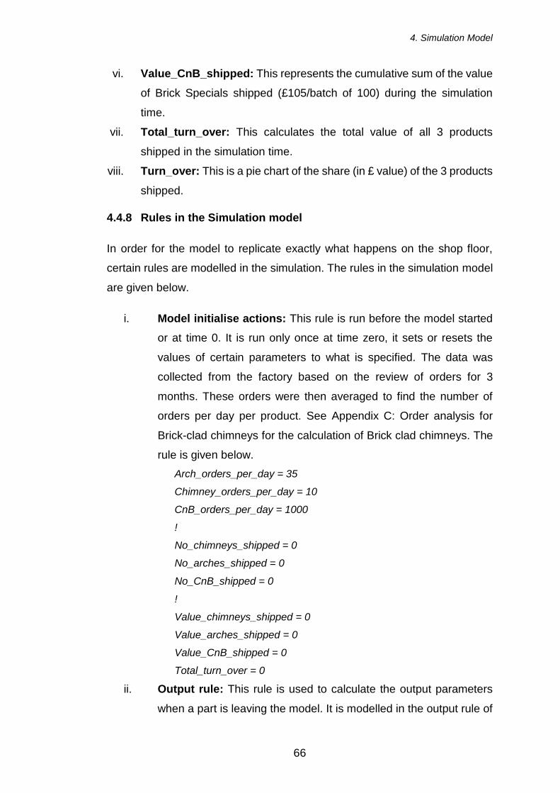
4. Simulation Model
66
vi. Value_CnB_shipped: This represents the cumulative sum of the value
of Brick Specials shipped (£105/batch of 100) during the simulation
time.
vii. Total_turn_over: This calculates the total value of all 3 products
shipped in the simulation time.
viii. Turn_over: This is a pie chart of the share (in £ value) of the 3 products
shipped.
4.4.8 Rules in the Simulation model
In order for the model to replicate exactly what happens on the shop floor,
certain rules are modelled in the simulation. The rules in the simulation model
are given below.
i. Model initialise actions: This rule is run before the model started
or at time 0. It is run only once at time zero, it sets or resets the
values of certain parameters to what is specified. The data was
collected from the factory based on the review of orders for 3
months. These orders were then averaged to find the number of
orders per day per product. See Appendix C: Order analysis for
Brick-clad chimneys for the calculation of Brick clad chimneys. The
rule is given below.
Arch_orders_per_day = 35
Chimney_orders_per_day = 10
CnB_orders_per_day = 1000
!
No_chimneys_shipped = 0
No_arches_shipped = 0
No_CnB_shipped = 0
!
Value_chimneys_shipped = 0
Value_arches_shipped = 0
Value_CnB_shipped = 0
Total_turn_over = 0
ii. Output rule: This rule is used to calculate the output parameters
when a part is leaving the model. It is modelled in the output rule of
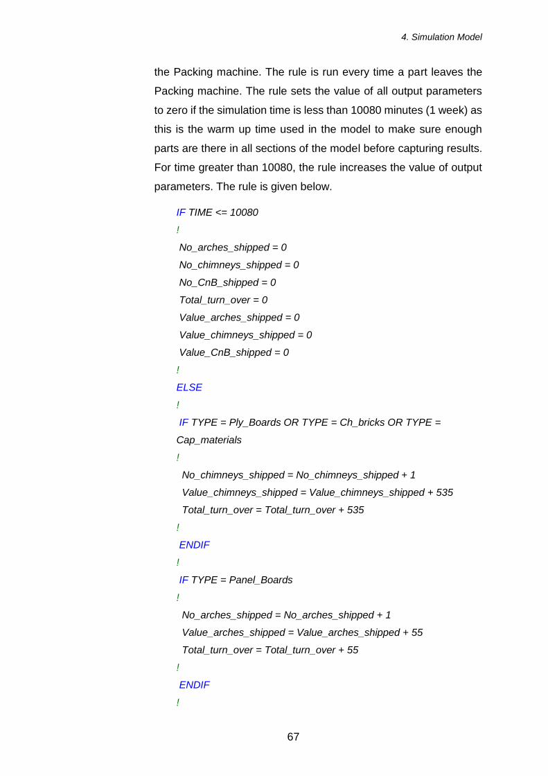
4. Simulation Model
67
the Packing machine. The rule is run every time a part leaves the
Packing machine. The rule sets the value of all output parameters
to zero if the simulation time is less than 10080 minutes (1 week) as
this is the warm up time used in the model to make sure enough
parts are there in all sections of the model before capturing results.
For time greater than 10080, the rule increases the value of output
parameters. The rule is given below.
IF TIME <= 10080
!
No_arches_shipped = 0
No_chimneys_shipped = 0
No_CnB_shipped = 0
Total_turn_over = 0
Value_arches_shipped = 0
Value_chimneys_shipped = 0
Value_CnB_shipped = 0
!
ELSE
!
IF TYPE = Ply_Boards OR TYPE = Ch_bricks OR TYPE =
Cap_materials
!
No_chimneys_shipped = No_chimneys_shipped + 1
Value_chimneys_shipped = Value_chimneys_shipped + 535
Total_turn_over = Total_turn_over + 535
!
ENDIF
!
IF TYPE = Panel_Boards
!
No_arches_shipped = No_arches_shipped + 1
Value_arches_shipped = Value_arches_shipped + 55
Total_turn_over = Total_turn_over + 55
!
ENDIF
!

4. Simulation Model
68
IF TYPE = CnB_bricks
!
No_CnB_shipped = No_CnB_shipped + 1
Value_CnB_shipped = Value_CnB_shipped + 105
Total_turn_over = Total_turn_over + 105
!
ENDIF
!ENDIF
The full list of rules such as input, labour and output rules inside each machine
in the simulation model is given in Appendix E: List of rules and variables used
in DES model.
4.5 Chapter Summary
In this chapter, the simulation of models including Continuous and Discrete
simulations have been introduced. The parameters required for the building of
the simulation model has been discussed in detail with the factory layouts.
Assumptions used in the model has been explained clearly. All the important
components of the model have been explained along with the rules and
parameters used to capture the outputs. The model which has been
developed will be used in the following chapter to conduct simulations of the
process flow under different conditions.

5. Manual optimisation of resources
69
5 Manual optimisation of resources
In this chapter, the Discrete Event Simulation (DES) model is optimised
manually in an intuitive manner by changing the model parameters. Changes
that could improve the productivity of the model were identified by using FIT
manufacturing principles to allow the process to be more lean and agile.
Critical analysis and evaluation of the simulation model were carried out
intuitively using line balancing techniques to identify scenarios to maximise
productivity. These scenarios were manually tested in the model to study the
changes in the manufacturing process flow.
The DES model offers the opportunity to study the behaviour of the existing
production process. Hence, the model was utilised conveniently by
considering different parameters that would improve the process in such a way
to get more out from the existing system without having to make more
investment.
In other words, various model parameters are optimised using different line
balancing solutions to find the optimal way of operating the plant with reduced
costs and maximum output. The simulation model explained in the previous
chapter is the basis of the experiments. Thus, it is even more critical to ensure
that the simulation model developed is an exact replica of the real-life
production lines that are operating at the factory and the results obtained using
the model is validated before any experiments are carried out. In the next sub-
section, the authenticity of the created DES model is validated.
5.1 DES model validation
The simulation model being validated is the initial model developed in Chapter
4.
Validation strategy: This model is run for a specified amount of time, the
results are collected and compared against the actual values from the shop
floor. If the values are found to be matching, the DES model can be considered
valid and ready for conducting simulation experiments. The three important
strategies that are used for validation are given below.

5. Manual optimisation of resources
70
• Conceptual validity: This strategy looks at validating the model ‘within
the scope of the initial plan’ against the real world. For this to happen,
the purpose of the model needs to be specified initially (Semanco,
Marton, 2013). For example, if a model is built to predict the breakdown
pattern of a conveyor, and the simulation provides results which is in
line with the outputs obtained from the conveyor but not exact
breakdown patters, the model cannot be validated.
• Operational validity: This validity considers the operational side of the
model. Operational validity is a data oriented strategy of comparing the
output data against real life scenarios. This is set by the simulation
engineer when building the model (Robinson, 1994). For example, if the
objective of the simulation model is to increase the outputs within the
existing manufacturing constraints, the output data is compared with
the real-life plant to validate the model.
• Believability: As the term explains, believability is subjective rather
than objective. It entails if the end user of simulation, in this case, the
Production Management at the company has faith in the model and the
suggested solutions (Opper, 1999). The end user may differ in their
choice of solutions generated within the context of the KTP project.
Different solutions for the selection of process parameters
recommended by the simulation model is a prediction of production
lines operating under the same conditions in a real-life scenario. This
prediction must be believed by the end user depending on how close
this result is to the real world. This is the concept of believability.
Tolerances: A tolerance of 5% is allowed in the results for validation. If the
output results are found to be within ± 5%, the model can be considered valid.
For example, if the expected output for a product per week is 100 and the
model produces a result within the range of 95 -105, the model is acceptable.
Warmup time: While trying to obtain results from any model, a warm up time
is essential. The parts enter the simulation at time 0. It gets processed at the
first operation, goes to a buffer and then to the next operation. This process
goes on till the last operation until the part is shipped (Mahajan, Ingalls, 2004).

5. Manual optimisation of resources
71
In this way, the last operation is idle till the parts travel through the whole
simulation model. For example, in the existing simulation model, for a part for
chimney to reach the end stage of Packing, it takes 33 hours and 5 minutes.
Until then, the Packing operation and the operator will be idle. This will be
reflected on the simulation output as well.
But this is not the scenario in real practice. At the start of a week, every
operation in the factory will have a part to process and will be busy. Thus, the
results obtained from the simulation will be wrong if the model is run without a
warmup time. As the maximum process time in this model is for Brick-clad
chimneys (33 hours and 5 minutes), the warmup time is given as 1 week.
Figure 5.1 gives the results of the operator usage without a warmup time for a
run time of 10080 minutes.
Figure 5.1: Report on shift time without warmup time
The results of the same simulation without changing any parameters with a
warmup time of 10080 minutes (1 week) and run time of 10080 minutes is
given in Figure 5.2.

5. Manual optimisation of resources
72
Figure 5.2: Report on shift time with warmup time
It can be seen from Figure 5.1 that the first 3 operators are not 100% busy
over the simulation period. This is without the warmup time. But when including
the warmup time, as it can be seen from Figure 5.2, all the operators are 100%
busy which would be similar to the actual scenario. Thus, it is essential in this
simulation to include a warmup time of 1 week (10080 minutes).
5.1.1 Results
The DES model is run for 20160 minutes (2 weeks) with a warmup time of
10080 minutes (1 week). The following are the input parameters:
• Arch_orders_per_day: This parameter represents the number of arch
orders that arrive in the factory. This information is taken from the
company data. It is set to 35 in the model.
• Chimney_orderes_per_day: On average, it is taken as 10 based on the
company data.
• CnB_orders_per_day: Each order is represented in a batch of 100 of
Brick Specials. The number of orders received per day is given as 100.
The results from the simulation model are given below.

5. Manual optimisation of resources
73
Figure 5.3: Quantity of finished products
• Number of chimneys produced: This is obtained from the parameter
No_chimnyes_shipped. For a 40-hour 5 day working week, with an
input orders of 10/day, the total number of chimneys produced in a
week is 50. This is the maximum capacity of the plant for the chimney
production line and is within the range of outputs produced per week.
• Number of arches produced: With an order input of 35 per day, the
output produced is 60 per week. The result obtained from the simulation
model is 59 per week which is within the tolerance limit. Thus, this can
be considered acceptable.
• Quantity of Brick Specials produced: A total of 131 jobs were
completed for the week against an order quantity of 100 per day.
Another parameter used to measure and validate the outputs from the model
is the turnover values of the products. This is given in Figure 5.4 for the
simulation model.
Figure 5.4: Turnover per product
The company turns over £25,000 - £30,000 for Brick-clad chimneys per week.
The value obtained from the model is £26,750 which is within the expected
range. The large range is due to the fact that, in the company, each order is
customer specified which has a different price. Since this is not required to
meet the objective of the simulation, an average value for the chimney is
modelled which produces a definitive range. The value generated by this

5. Manual optimisation of resources
74
product in a week is shown in Figure 5.3 in comparison with the other two
products.
Figure 5.5: Turnover (Blue: chimneys, Green: Brick Specials, Red- Arches)
The value of arches produced per week is £3,245 and Brick Specials is
£13,755. The total turnover for the week is approximately £43,750 from the
model which is within the expected limit for the company. Thus overall, the
turnover for the company from the above 3 products is circa £2,275,000. The
overall turnover for the company is circa £3 million. The above 3 products
contribute towards 75% of the total company turnover which is fairly accurate.
The utilisation of resources is also checked to validate the model. The different
types of resources available are machine resources, labour resources and
buffer quantities.

5. Manual optimisation of resources
75
Figure 5.6: Machine statistics
The charts in Figure 5.6 show the utilisation of machines within the shift time.
It can be seen that almost all the machines are 100% busy within the specified
shift. The machines that are less busy are Bonding_Arches which is utilised
only 11.38% which represents the real-life scenario at the company. Other
underutilised machine resources are Finishing and Assembly. These are also
representative of the real-world situation.

5. Manual optimisation of resources
76
The charts in Figure 5.7show the labour resource utilisation.
Figure 5.7: Labour resource utilisation for Brick-clad chimneys
The underutilised labour resources are Assembler1 and Assembler2. This is
representative of the actual scenario in the factory. This is due to the fact that
the factory operates in a 110% manning level to cover for holidays and
absences. The assembly operators are modelled to cover for these. From the
above, it can be inferred that the model is a true representative of the real-
world situation.
In order to have a relative target of what could be achieved within the restricted
time frame, the following 3 scenarios were selected.

5. Manual optimisation of resources
77
5.2 Scenario 01 – Initial results analysis and manual optimisation
In this section, the results from the model are analysed manually in an intuitive
manner and changes are recommended in the model to improve the
production output without changing the existing number of resources. This is
done on the production line for each product.
5.2.1 Pre-fabricated arch production line
To carry out an initial analysis, the machines in the arch production line are
analysed. The data used for analysis is given in Figure 5.8.
Figure 5.8: Pre-fabricated arches machine statistics
From the above table, it can be clearly inferred that all the operations are busy
at 100% level except Bonding_Arches which is idle for 88% of time. This
provides an improvement opportunity to get more out of the existing system.
But to change the output, the reason for the machine being idle should be
found out.

5. Manual optimisation of resources
78
Figure 5.9: Bonding_Arches operation model
The Figure 5.9 shows the operation of Bonding_Arches. For the operation, 2
parts are required, one which is taken from Cut_Panel and other taken from
Arch_bricks. The Figure 5.9 shows that the Cut_Panel is empty which explains
the idle time of the operation. Further investigation suggests that the
Cut_Panel is empty as the CNC_Machine is operating at full capacity. Thus,
the CNC_Machine is the bottleneck in this process. It is envisaged that by
increasing the resource allocation of the CNC_Machine in the process flow will
improve the throughput of the pre-fabricated arch production line.
Suggested improvement: In this scenario, the suggested solution is to
increase the number of working hours on the CNC_Machine and the operator
to a 50-hour working week with 10 hours a day corresponding to a normal shift
duration. The shift pattern is given in Figure 5.10.
Figure 5.10: 50 hour working shift details
This is not to be achieved by a single operator working 50 hours per week.
The suggested improvement is to make the operation available for 50 hours a

5. Manual optimisation of resources
79
week. This is achieved in the company by an operator starting 2 hours earlier
than the normal 8 hour working shift, operating the machine for 2 hours and
handing it over to the normal operative when the normal shift starts. The
operator starting early would finish early as well with a total of 8 hours per day.
This would give the capability of 10 hours per day for the utilisation of the
machine which amounts to 50 hours per week.
5.2.2 Brick Specials production line
Analysis similar to the above section is carried out on the Brick Specials
production line with the aim of optimising the production flow. The machine
statistics of the production line and the labour resource usage is given in
Figure 5.11.
Figure 5.11: Brick Specials machine statistics
All the machines are utilised to the maximum capacity as it can be seen from
the above statistics. The labour statistics are given in the Figure 5.11. From
both the figures, it can be seen that the Packing operation is fully utilised with

5. Manual optimisation of resources
80
240 operation. As this is a shared resource between 3 different production
lines, it can be improved by increasing the shift pattern.
Figure 5.12: Brick specials labour statistics
Suggested improvement: Increasing the shift pattern for the packaging
operation and operative to a 50 hours shift as this resource is shared between
the 3 production lines. It is anticipated this would increase the production
throughput.
5.2.3 Brick-clad chimney production line
The initial analysis of Brick-clad chimney production line is more critical as
around 50% of the company turnover is from this product. Also, comparing the
value-adding work force which excludes the management, fork truck drivers
and so on is also circa 50%.

5. Manual optimisation of resources
81
The simulation model is run for a week with a warmup time of 1 week. Results
are collated and shown in Figure 5.13. Machines, buffers and labour resources
are analysed.
Figure 5.13: Brick-clad chimney machine statistics
From the Figure 5.13, it can be clearly seen that not all the operations are
100% busy. Assembly operations average about 70% busy time. Every other
operation is utilised over 80% except for Finishing which is heavily
underutilised at around 42%.
As the operation Finishing has spare capacity but it cannot be utilised to
produce more chimneys. But the operator can be considered of having spare
capacity and can be utilised elsewhere to increase the throughput.
The number of operations processed is a critical feature in analysing the line
balancing. This provides information to determine over or under allocation of

5. Manual optimisation of resources
82
resources in the production line. The total number of orders processed by each
operation is given in Table 5.1. For example, Assembly is one operation
represented by 2 machines for which the sum is given.
Operation Number of
operations
CNC
Machine
51
Assembly 51
Laminating 51
Caps_n_Pots 70
Cladding 48
Finishing 50
Packing 50
Table 5.1: Brick-clad chimneys - total number of orders processed
Figure 5.14: Brick-clad chimney line balancing
From the graph in Figure 5.14, it can be clearly seen that the operation
Caps_n_Pots has over allocation of resources. As the average production per
week is circa 50 chimneys, there is no need to produce 70 Caps_n_Pots as
there will be a surplus production of 20 per week. Thus, this over allocation of
resource could be re-distributed to optimise the production line. Also from
Figure 5.13, Caps_n_Pots are running at only 87% utilisation with 13% idle
0
10
20
30
40
50
60
70
80
Number of operations
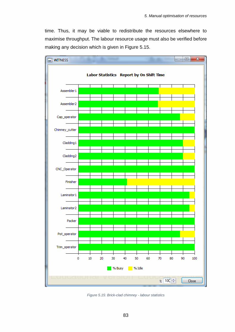
5. Manual optimisation of resources
83
time. Thus, it may be viable to redistribute the resources elsewhere to
maximise throughput. The labour resource usage must also be verified before
making any decision which is given in Figure 5.15.
Figure 5.15: Brick-clad chimney - labour statistics

5. Manual optimisation of resources
84
From the Figure 5.15, similar to the machine statistics, the operator in the
Finishing operation is underutilised. Also, there is no requirement to over
produce on Caps_n_Pots. Both of these could suggest redistribution of
resources to produce more within the existing parameters.
Suggested improvement: Cross training the Finishing operative on
Caps_n_Pots will enable the operator to do both jobs. Set the priority of the
Finishing operation to be highest as it is in the critical path for the chimney
production line. This will enable the company to reduce the workforce by 1 in
the Cap_n_Pot production (currently 2 operatives) by utilising the underutilised
resource in Finishing operation.
5.2.4 Suggested changes to the model for scenario 01
From the analysis of initial results in the previous sections, the following
changes to the model are made to see changes in the model. The changes
are identified using the FIT manufacturing principles of line balancing,
bottleneck analysis and Takt time. They enable the company to be FIT by
producing more with less resources.
i. CNC Machine: As this resource is shared between the Brick-clad
chimneys and pre-fabricated arch production lines, it is essential to
increase the number of working hours on this machine. From the
analysis, this is identified as one of the bottlenecks in the model.
ii. Packing: This resource is shared between all the 3 product streams
that are being modelled and is utilised at 100%. Comparing the number
of operations that are pending to be processed on this machine, it is
essential to increase the working time on this operation to reduce the
bottleneck at this stage.
iii. Line balancing by cross training: As the finishing operation is
underutilised and Caps_n_Pots produce more than what is required
with 2 men, the line is not balanced. One operative in Caps_n_Pots can
be replaced by cross-training the Finishing operative. This is expected
to balance the line and create savings to the company by reducing the
workforce by 1.

5. Manual optimisation of resources
85
iv. Increasing the order input/day: The simulation model is run at
specific order inputs per day: 70 for arches, 10 for chimneys and 100
for Brick Specials which is limiting the model. This doesn’t utilise the
maximum manufacturing capability of the model which is against the
FIT manufacturing principles. To utilise the maximum capacity, the
model input values are increased imagining a scenario where the ‘Order
Book’ is full with no limited orders per day. This also means in real
world, a change in the planning way which is limited to the number or
orders per day (for example, 10/day in chimneys). Thus, the input
parameters are changed to 1000 to state the availability of unlimited
orders in the pipeline.
5.2.5 Results
After the suggested changes to the DES model are made, the simulation
model is run to the same amount of time as the initial model to ensure the
comparison is between similar models. The results are given in Figure 5.16
and Table 5.2.
Figure 5.16: Results after Scenario 1

5. Manual optimisation of resources
86
Before
scenario 1
After
scenario 2
% Change
No_chimneys_shipped 50 51 2.0%
No_arches_shipped 59 64 8.5%
No_CnB_shipped 131 137 4.6%
Value_chimneys_shipped £26,750 £27,285 2.0%
Value_arches_shipped £3,245 £3,520 8.5%
Value_CnB_shipped £13,755 £14,385 4.6%
Total_turn_over £43,750 £45,190 3.3%
Table 5.2: Changes in results after Scenario 1
From the Table 5.2, it can be seen that the changes made to the model
according the FIT manufacturing principles based on an intuitive approach has
produced effective results and improved the simulation results. Each of the
changes are discussed below.
i. Number of chimneys shipped: This has increased the results by 2%
by a quantity of 1 per week. Although changes were made to reduce
the labour resources by 1, there is an increase in throughput by 2%
which is due to the increase in input parameters. Over the year, with an
average price of £535/chimney, the turnover is expected to rise by
£27,820. This is achieved by reducing the labour resources which also
has a positive impact on the profit margin. With the current resources,
this is considered the maximum capacity of the manufacturing model.
ii. Number of arches shipped: This has increased by a significant
amount of 8.5%. In a real-life scenario, it is considered difficult to
improve the performance of a manufacturing model by 8.5% by
changing the shift pattern of 1 operation by 10 hours/week. The
turnover for arches also increased by 8.5%, and over the year, this is
projected to increase the sales by £14,300.

5. Manual optimisation of resources
87
iii. Number of Brick Specials shipped: The total number of batches
shipped increased by 4.6%. This has a significant impact on the lead
times as more parts are processed in the same time. Thus, customers
do not have to wait for the products as before. Over the year, this will
produce an extra revenue of £32,760.
From the Figure 5.17 it can be seen that the packaging operation that was
100% busy and processed 240 jobs is now 84% busy while processing 252
operations.
The Caps_n_Pots compared to previous model has now time waiting for
labour, with busy time around 80% compared to previous values of 87%. But
in the optimised model, the total number of Caps_n_Pots produced is 64
compared to 70 from the previous model with one less operator. The demand
per week is only 51. This clearly shows the potential savings that could be
made.

5. Manual optimisation of resources
88
Figure 5.17: Scenario 1: Brick-clad chimney results
The changes to the number of products produced per week and line balancing
graph is shown in Figure 5.18 against the number of operations on y-axis.
Figure 5.18: Scenario 1: Line balancing
0
10
20
30
40
50
60
70
Number of operations

5. Manual optimisation of resources
89
The throughput of both CNC_Machine and Assembly has increased from 51
to 64 with the suggested changes. Laminating seems to be the new bottleneck
in the model which limits the throughput further along the production line by
producing only 51. From Figure 5.17, Cladding has 12.5% spare capacity,
along the production line, Finishing and Packing also has spare capacity.
Thus, the new bottleneck of Laminating can be addressed in scenario 2.
5.2.6 Validation of results
The suggestions for increasing the shift pattern of shared resources such as
CNC Machine and Packaging were implemented in the factory. The cross
training of the operators was also completed and implemented. This increased
the throughput from the production lines as predicted.
But increasing the order quantity was not practically achieved as orders
received per day depends upon the market conditions and buying decisions
made by customers.
The results were obtained from the company following implementation of
changes which is given in Table 5.3. The data from company has slight
variation from the predicted result. This is due to the variations found in the
order quantity as explained above. The results are within the 5% tolerance
limit and hence through the process of Operational validity, the simulation
results produced by the model has been verified.
Before
scenario 1
After
scenario 1
Simulation
Data from
company
No_chimneys_shipped 50 51 51
No_arches_shipped 59 64 63
No_CnB_shipped 131 137 136
Table 5.3: Scenario 01: Results validation

5. Manual optimisation of resources
90
5.3 Chapter Summary
In this chapter, the DES model has been verified by comparing the behaviour
and outputs from the model with the results from the shop floor. An initial
analysis of the model has been carried out and improvements were suggested
using the FIT manufacturing principles in an intuitive manner. The suggested
changes increased the throughput of all 3 production lines, and the overall
turnover for the company for the year could potentially be increased by circa
£74,880 which is an increase by 3.3%.
It has been found that resources such as machines and labour that are shared
between production lines may cause undue pressure on the production lines.
Also, people with multiple skills who can carry out multiple operations have
been found to improve productivity significantly.
The intuitively optimised model also showed new bottlenecks in the re-
designed manufacturing system which will be addressed in scenario 2 as
explained in the following chapter.

6. Automatic optimisation and experimentation
91
6 Automatic optimisation and experimentation
In the previous chapter, focus was on implementing the changes based on FIT
manufacturing principles in terms of allocation of resources, especially labour
resources and line balancing. Those changes did not require significant
investment from the side of the company apart from introducing changes to
the shift patterns and cross training.
In this chapter, the DES model is further refined using FIT manufacturing
principles particularly those changes that require investment. As the
production lines interact with each other and has shared resources, testing
different scenarios and comparing the output values might become difficult
(Law, 2010). Thus, to enable this, the Experimenter module in Witness
software is used which uses an in-built optimisation algorithm to maximise the
output parameter by testing the model at different user specified scenarios.
The procedure for experimentation and optimisation is given below.
6.1 Experimentation and Optimisation procedure in Witness
Following are the steps taken in carrying out experiments and optimising
parameters using Witness (Ford, 2010).
i. Open the Experimenter module in Witness from the Model menu.
ii. Specify in the model, the number of different scenarios to be run.
iii. Input the parameters that correspond to the scenarios. For example, if
the model is to optimise the production output by changing the labour
force level, input parameter will be the labour force levels and output
parameter will be the production output.
iv. In the Model settings, specify the warmup and run length times.
v. Include the number of iterations required and run the model.
The model throws out results of different scenarios with the output parameter
which helps the team to make an informed decision. The scenarios may or
may not involve investments. In the following sections, potential improvement
ideas are tested to improve the throughput of the production line.

6. Automatic optimisation and experimentation
92
6.2 Scenario 02: Pre-fabricated arches - maximum throughput
with minimum investment
To further advance the manufacturing facility, the company requires to expand
the current operational practices. It has been identified that the lead times for
pre-fabricated arches are low compared to competitors. Thus, a decision
needs to be made to maximise the throughput for the production lines. Three
different options for optimising the production line will be discussed according
to the level of investment required.
The reason for choosing the given 3 options were investment options
suggested by the Production Management in the company to obtain maximum
gain. This will be modelled in Witness on the existing manufacturing model
and experimented to find the best solution.
In this scenario, 3 different options are considered which is expected to
significantly improve the performance of the manufacturing model. The options
are ranked according to the level of investment required. Following evaluation
of the 3 options using the experimenter module in WITNESS, a decision can
be made.
i. Option 01 – Extra arch saw: Invest in purchase of an extra Arch brick
cutting saw which will produce more bricks for the arches and hence
more turnover. This is considered a low investment option. With the
extra saw, an extra operator will also be required.
ii. Option 02 - Extra CNC machine: This is a medium investment option
with purchase of an extra CNC machine. A trained CNC operator will
also be required. This option will also have an impact on the chimney
production line as the CNC machine also serves the chimney
production line.
iii. Option 03 – Extra CNC machine + Slip machine: This is a high
investment option with the purchase of 2 extra machines which requires
3 extra operatives. But this option is also considered depending upon
the return on investment.

6. Automatic optimisation and experimentation
93
The options are modelled in the Experimenter. A new function called
Turn_over_function is created which return the value of total turnover as
shown in Figure 6.1. The simulation attempts to maximise this value.
Figure 6.1: Scenario 02: Input parameters
Three different scenarios are modelled with 7 input parameters which are used
to model the scenarios. The output parameter is the Turn_over_function which
is maximised.
Figure 6.2: Scenario 02: model configuration
The model is configured using the values in Figure 6.2 to run for 20160 minutes
(2 weeks) with a warmup time of 10080 minutes (1 week) for 100 replications.
From initial analysis, this was found to be sufficient to produce stable results.
Simulation was run for a total duration of 1 minutes and 29 second with and
average duration of 23 seconds. The results in Figure 6.3 were considered
consistent as the mean and best values were matching for all 100 iterations
with a standard deviation of zero.

6. Automatic optimisation and experimentation
94
Figure 6.3: Scenario 02: Variance data
The result of the scenario is given in Figure 6.4.
Figure 6.4: Scenario 02: Simulation results 01
Option 01 will increase turnover to £42,300, Option 02 to £44,715 and Option
03 to £44,690. The actual values may vary and can be found from the model.
Figure 6.5: Scenario 02: Best scenario results (options vs. total turnover)

6. Automatic optimisation and experimentation
95
Figure 6.6: Scenario 02: Box plot results
From the data above, it can be concluded that the Option 02 of purchase of an
extra CNC machine, which is a medium investment decision would increase
the turnover by a larger margin than of the lower and higher investment
options. The Box plot results suggest a percentile of 75 for Options 02 and 03
and a 25 percentile for Option 01. The confidence chart in Figure 6.7 also
indicates a minimum value of 90% has been achieved whereby making the
results reliable.
Figure 6.7: Scenario 02: Confidence chart
6.3 Scenario 03: Maximising cycle time efficiency for Brick-clad
chimneys
From Figure 5.18, it was discussed in the previous chapter that the number of
operations processed by the Laminating, Cladding and brick cutting were at
the lowest level of 52 compared to the entire production line of 62 per

6. Automatic optimisation and experimentation
96
operation. Thus, it is necessary to investigate and optimise the production line
to increase the number of chimneys shipped to a maximum.
The reason for choosing the 3 options are to investigate the benefits of
implementing Lean manufacturing principles in the business. Implementation
of the Lean principles were part of the KTP project objectives. The ideas were
generated by reducing different wastes as discussed in Section 2.2.2 and this
is shown in Figure 6.8.
Like the previous scenario experimented, 3 different options are modelled. As
Laminating, Cladding and brick cutting are manual operations, investment in
new machinery is not required. Changes needs to be made are related to
reducing the cycle time or Takt time of the operations so they produce more
per operation. The options are explained below based on the level of
investment required.
i. Option 01 – Reduce laminating cycle time: As this is the initial
bottleneck in the modified production line, reducing the cycle time
for laminating might improve the results significantly. This is
possible in real life scenario by implementing Lean manufacturing
principles. The current cycle time is reduced from 45 minutes to 30
minutes. This is a low investment option for the company which
requires no extra machine.
ii. Option 02 – Reduce laminating & cladding cycle time: Along with
reducing laminating cycle time, reduce the cycle time of cladding
from 45 minutes to 30 minutes. But in real life, this requires an
additional labour resource which needs to be modelled. This is a
medium investment option for the company which requires no extra
machine.
iii. Option 03: Reduce laminating and add resource in brick
cutting: The number of operations processed by the brick cutting
for chimneys are at 40, thus this option also needs to be investigated
to maximise the output of the processes. This requires apart from
changes suggested in Option 01, an extra chimney brick cutting
machine and labour resource. This is a high investment option for

6. Automatic optimisation and experimentation
97
the company which requires a new machine as well as an additional
operator.
Lean manufacturing principles are used to reduce the cycle time for the above
3 options. Typical Lean tools used in Manufacturing are given below:
Figure 6.8: Lean 7 wastes (Sarhan, 2017)
From the value stream maps explained in Table 3.2, each one of the process
is broken down into one of the above category. If it is categorised as waste,
measures are taken either to reduce or eliminate that process. This way, the
savings explained in the 3 proposed options could be achieved.
The options are modelled in the Experimenter module of Witness. All the
options are practically achievable in the shop floor with changes in the
structure of production. The input parameters and the configuration used in
the model are given in Figure 6.9 and Figure 6.10.
7 wastes
Transport
Inventory
Motion
WaitingOver-
processing
Over-production
Defects

6. Automatic optimisation and experimentation
98
Figure 6.9: Scenario 03: Input parameters
The experiment was run for 20160 minutes (2 weeks) with a warmup time of
10080 minutes (1 week) for 100 replications.
Figure 6.10: Scenario 03: Model configuration
The variance data in Figure 6.11 has a standard deviation of zero. The
confidence chart in Figure 6.12 also indicates a minimum confidence level of
90% has been achieved which means the results obtained from the model are
reliable.
Figure 6.11: Scenario 03: Variance data

6. Automatic optimisation and experimentation
99
Figure 6.12: Scenario 04: Confidence chart
The model was run for a total time of 1 minute and 09 seconds with an average
scenario duration of 23 seconds. The results of the experiments are given in
Figure 6.13.
Figure 6.13: Scenario 03: Results
It can be clearly seen from the above data that the option 03 of reducing the
cycle time of laminating process along with adding an extra resource at brick
cutting by introducing a new machine produced significant changes in the
production output.
The total turnover is expected to increase to £96,710 for 2 weeks. But this is
for the total of 2 weeks. Thus, the actual increase in turnover would be half of
that – which is up to £48,355. In actual scenario, this may change by 10%
because the minimum confidence level of the model is 90%.
The Figure 6.14 shows the response of the model against the objective.

6. Automatic optimisation and experimentation
100
Figure 6.14: Scenario 03: Actual scenario vs. total turnover
The best results obtained from the simulation is found to be better than the set
objective in the function. The Options 01 & 02 results were similar to each
other, whereas the results of Option 03 were significantly higher than the
others. In order to quantify the benefits of the suggested improvements the
parameter analysis given in Figure 6.15 is conducted.
Figure 6.15: Scenario 03: Parameter analysis

6. Automatic optimisation and experimentation
101
From the parameter analysis, the maximum benefit can be seen with Option
03 with a percentage benefit of 9.848% which is significant in terms of
turnover. Options 01 & 02 consistently seems to produce only a benefit of
0.545% which rules out these options.
Figure 6.16: Scenario 03: Variance chart
The variance chart in Figure 6.16 also validates the improvement Option 03
over the other two options. Thus, it can be concluded that the Option 03 would
produce a significant increase in turnover by 9.8%.
6.4 Validation of results
As the options explained in the scenarios require significant investment which
requires time if it is to be implemented on the shop floor. Therefore, the
suggested options could not be validated by data after implementing the
changes from the shop floor.
Instead, the results were validated by discussion with the management and
shop floor personnel using the Believability principle as explained in Section
5.1. The model results were seen to be sensible and considered feasible in

6. Automatic optimisation and experimentation
102
terms of improving the current production process without having to make any
large investments.
Interestingly, comparing the results of the simulation model with the shop floor
data threw out some anomalies. Following further investigation, it was found
that the breakdown on machines on the shop floor had a significant impact on
the productivity. This is investigated and discussed in Chapter 7.
6.5 Chapter Summary
The chapter discussed the use of Experimenter module within Witness which
is used to model difficult and complex scenarios in the simulation. Two
different scenarios were run on 2 different production lines using FIT
manufacturing principles. The first scenario suggested an increase in turnover
by 5.7% and the second suggested a further increase by 9.8%.
It has been shown that the maximum allocation of resources does not always
mean maximum increase in productivity. On the contrary, lesser but smarter
investment improved productivity by a higher margin.
Further, it has been found that increasing the efficiency of one production line
does not always increase the overall efficiency if cross-functional relationships
exist because increasing the efficiency of one production line is likely to cause
a bottleneck on the inter-dependent operations.
In the following chapter, the DES model will be enhanced by including the
inefficiencies in the production lines due to machine breakdown to further
improve the production process.

7. Evaluation of the effect of breakdown of machines on productivity
103
7 Evaluation of the effect of breakdown of machines
on productivity
This chapter investigates the effect of breakdown of machines on the shop
floor on the productivity of the manufacturing process. From the previous
chapter, while validating the results, some anomalies were noted which was
found to be due to the breakdown of the machines on the shop floor.
The machines considered for the analysis are the machines from the Brick
Cutting area. This was chosen because brick cutting is the most critical part of
the manufacturing process. This is validated from previous analyses in
Chapter 6 as majority of the processes are operating at maximum possible
levels.
Another reason as suggested by Lu (L Lu, 2011) for investigating breakdowns
was that there is evidence of correlation between machine downtime and
production throughput.
7.1 Machine breakdown data collection
A system to capture breakdown was created on the shop floor using forms.
When a machine was broken down, a downtime form was created which
investigated the root cause analysis of the breakdown. This was carried out as
part of this thesis. The template of the form is given in Figure 7.1 and the
sample data in Table 7.1.

7. Evaluation of the effect of breakdown of machines on productivity
104
Figure 7.1: Machine downtime report

7. Evaluation of the effect of breakdown of machines on productivity
105
Table 7.1: Machine downtime statistics
Site Pontypool
Type Breakdown Monitoring System
Date Time Date Time Date Time Date Time
1 3 4 04/03/2014 15:30 04/03/2014 16:00 04/03/2014 15:50 04/03/2014 16:00 0.5 0.17 £1.0 £1.3 £27.0 £29.3
2 6 3a 05/03/2014 08:30 05/03/2014 09:00 05/03/2014 08:30 05/03/2014 09:00 0.5 0.5 £45.5 £3.8 £27.0 £76.3
3 2 5 05/03/2014 09:00 24/03/2014 24/03/2014 24/03/2014 1.5 1.5 £44.5 £11.5 £81.0 £137.1
4 3 7 21/03/2014 24/03/2014 24/03/2014 09:00 24/03/2014 09:10 3 0.17 £0.0 £1.3 £162.0 £163.3
2 3b 31/03/2014 09:20 31/03/2014 13:30
5 6 9 24/03/2014 25/03/2014 25/03/2014 08:30 25/03/2014 08:40 8 0.17 £0.0 £1.3 £432.0 £433.3
Total 13.5 2.51 £91.0 £19.3 £729.0 £839.3
1 6 10 10/04/2014 14:20 10/04/2014 15:00 0.66 £35.6 £35.6
2 2 9 23/04/2014 14:00 24/04/2014 09:00 24/04/2014 08:00 24/04/2014 08:30 4 0.5 £3.8 £216.0 £219.8
3 3 10 23/04/2014 14:30 24/04/2014 09:00 24/04/2014 08:30 24/04/2014 08:45 3.5 0.25 £1.9 £189.0 £190.9
4 3 6 24/04/2014 15:00 24/04/2014 15:30 24/04/2014 15:00 24/04/2014 15:30 0.5 0.5 £3.8 £27.0 £30.8
Total 8.66 1.25 £9.6 £467.6 £477.3
1 2 7 02/05/2014 06:00 06/05/2014 09:00 06/05/2014 14:00 06/05/2014 15:50 19 1.83 £0.0 £14.1 £1,026.0 £1,040.1
2 2 3b 07/05/2014 07:30 13/05/2014 14:20 13/05/2014 08:30 13/05/2014 09:45 38 1.25 £65.0 £9.6 £2,052.0 £2,126.6
3 6 10 07/05/2014 08:00 07/05/2014 10:00 07/05/2014 08:15 07/05/2014 09:35 2 1.33 £0.0 £10.2 £108.0 £118.2
4 4 10 13/05/2014 14:20 14/05/2014 14:30 14/05/2014 09:05 14/05/2014 12:00 8.16 3 £0.0 £23.1 £440.6 £463.7
5 6 10 19/05/2014 07:00 20/05/2014 09:15 20/05/2014 08:45 20/05/2014 09:15 10 0.5 £0.0 £3.8 £540.0 £543.8
Total 77.16 7.91 £65.0 £60.8 £4,166.6 £4,292.5
1 4 3b 06/062014 14:30 09/06/2014 14:30 06/06/2014 14:30 09/06/2014 12:00 8 0.5 £1.4 £3.8 £432.0 £437.2
2 3 3a 13/06/2014 10:55 13/06/2014 11:20 13/06/2014 10:55 13/06/2014 11:20 0.41 0.41 £4.2 £8.1 £22.1 £34.4
3 5 3b 16/06/2014 14:00 18/06/2014 14:00 16/06/2014 14:00 18/06/2014 14:00 16 5 £24.0 £38.5 £864.0 £926.5
4 5 10 25/06/2014 14:00 25/06/2014 14:40 25/06/2014 14:00 25/06/2014 14:40 0.67 0.67 £0.0 £5.2 £36.2 £41.3
5 2 4, 6 26/06/2014 06:00 26/06/2014 09:00 26/06/2014 08:00 26/06/2014 08:40 3 0.67 £75.0 £5.2 £162.0 £242.2
Total 28.08 7.25 £104.6 £60.7 £1,516.3 £1,681.6
Jul-14 0 0 £0.0 £0.0 £0.0 £0.0
1 6 4, 10 26/08/2014 08:15 26/08/2014 09:15 26/08/2014 08:15 26/08/2014 09:15 1 1 £29.0 £7.7 £54.0 £90.7
2 3 3b, 5, 10 27/08/2014 14:30 27/08/2014 16:05 27/08/2014 14:30 27/08/2014 16:05 1.58 1.58 £12.1 £12.2 £85.3 £109.6
3 4 3a 27/08/2014 14:15 27/08/2014 14:30 27/08/2014 14:15 27/08/2014 14:30 0.25 0.25 £4.0 £1.9 £13.5 £19.4
Total 2.83 2.83 £45.1 £21.8 £152.8 £219.7
1 1 3b 05/09/2014 12:30 08/09/2014 10:00 05/09/2014 12:30 08/09/2014 09:14 4 3.45 £40.0 £26.5 £216.0 £282.5
2 6 3a 09/09/2014 14:40 09/09/2014 15:05 09/09/2014 14:40 09/09/2014 15:05 0.42 0.42 £4.2 £3.2 £22.7 £30.1
Total 4.42 3.87 £44.2 £29.8 £238.7 £312.6
1 1 3a 10/10/2014 11:30 10/10/2014 12:00 10/10/2014 11:30 10/10/2014 12:00 0.5 0.5 £4.2 £3.8 £27.0 £35.0
2 2 9 13/10/2014 08:15 13/10/2014 08:30 13/10/2014 08:15 13/10/2014 08:30 0.25 0.25 £1.2 £1.9 £13.5 £16.6
3 4 10 16/10/2014 14:30
4 2 10 30/10/2014 12:00 31/10/2014 11:00 30/10/2014 12:00 31/10/2014 11:00 8 8 £0.0 £61.5 £432.0 £493.5
Total 8.75 8.75 £5.4 £67.3 £472.5 £545.2
Mar-14
Month
No
Production
InProduction
Maintenance
In Out
Time (Hours)
Maintenance
Associated Costs (£)
Total
Sep-14
Oct-14
ProductionMaterial Labour
Jun-14
Aug-14
May-14
Apr-14
Machine
No
Breakdown
Code
Out

7. Evaluation of the effect of breakdown of machines on productivity
106
The data in Table 7.1 shows the breakdown statistics of machines within the
cutting room. Machines were numbered 1 to 6. The correlation of the machine
numbers to the machines on the DES model is given in Table 7.2.
Machine number DES model machine
1 Arch_saw_01
2 Arch_saw_02
3 Bndng_saw_01
4 Bndng_saw_02
5 Chmny_saw
6 Slip_Machine
Table 7.2: Machine numbers
A code was created for each type of breakdown as this would help classify
each breakdown and analyse the breakdown data. The codes created are
given in Table 7.3.
No Breakdown type Breakdown Code
Main Sub
1 Blade
Change
350 mm Hard Blade 1a
350 mm Soft Blade 1b
450 mm Block Saw 1c
650 mm Deco Machine 1d
2 Blade stuck to shaft 2
3 Bearing
Failure
Trolley Wheels 3a
Cutting Spindle 3b
4 Cutting head spring breakage 4
5 Start/Stop buttons failure 5
6 Loss of tension on belts 6
7 Rust handle 7
8 Motor failure 8
9 Changing Water pipes 9
10 Other 10
Table 7.3: Breakdown codes

7. Evaluation of the effect of breakdown of machines on productivity
107
This data was used to identify and predict the breakdown patterns in the
simulation model. The breakdown data added to the simulation model is
described in the following section.
7.2 Scenario 04: DES modelling of breakdown patterns
Following analysis of the data, breakdown pattern for the machines were found
and modelled in the simulation. The frequency of breakdown of machines
against the breakdown code was found and is given in Table 7.4 together with
the repair time.
The probability of breakdowns is assumed to be linear and not following a
distribution. This is considered as the objective is to find the overall impact of
the breakdown over a prolonged period of time and not the particular spike or
fall on the model’s performance as a result of a particular breakdown. Thus,
the time at which the breakdown occurs is irrelevant as long as the total time
the machine was not working remains the same over the period of entire
simulation. This is why the modelling is carried out as explained below.
DES model
machine
Breakdown
code
Frequency of
breakdown
Repair time
(minutes)
Arch_saw_01 - - -
Arch_saw_02 05 3000 minutes 60
Bndng_saw_01 - - -
Bndng_saw_02 02 2880 minutes 30
Chmny_saw - - -
Slip_Machine 01 50 operations 90
Table 7.4: Breakdown pattern per machine
From this table, only one saw per production line is modelled for breakdowns.
This is since the breakdown frequency is double for each saw. But the
simulation model is only run for a week. Thus, the breakdown frequency is
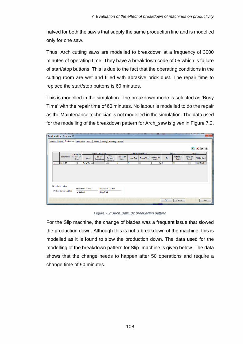
7. Evaluation of the effect of breakdown of machines on productivity
108
halved for both the saw’s that supply the same production line and is modelled
only for one saw.
Thus, Arch cutting saws are modelled to breakdown at a frequency of 3000
minutes of operating time. They have a breakdown code of 05 which is failure
of start/stop buttons. This is due to the fact that the operating conditions in the
cutting room are wet and filled with abrasive brick dust. The repair time to
replace the start/stop buttons is 60 minutes.
This is modelled in the simulation. The breakdown mode is selected as ‘Busy
Time’ with the repair time of 60 minutes. No labour is modelled to do the repair
as the Maintenance technician is not modelled in the simulation. The data used
for the modelling of the breakdown pattern for Arch_saw is given in Figure 7.2.
Figure 7.2: Arch_saw_02 breakdown pattern
For the Slip machine, the change of blades was a frequent issue that slowed
the production down. Although this is not a breakdown of the machine, this is
modelled as it is found to slow the production down. The data used for the
modelling of the breakdown pattern for Slip_machine is given below. The data
shows that the change needs to happen after 50 operations and require a
change time of 90 minutes.

7. Evaluation of the effect of breakdown of machines on productivity
109
Figure 7.3: Slip_machine breakdown pattern
The breakdown of Bonding saw which supplies the Brick special production
line was found to happen due to blade getting stuck on shaft for a cycle time
of 2880 minutes of operational time. The repair time is 30 minutes. This is
taken in proportion to 2 machines and modelled in a single machine like the
Arch_saw 02. The modelling data used in the software for Bonding_saw is
givenin Figure 7.4.
Figure 7.4: Bndng_saw_01 breakdown pattern
Following modelling of the breakdown patterns, the simulation model is run for
a simulation time on 20160 minutes (2 weeks) with a warmup time of 10080
minutes (1 week) similar to all previous simulations in order to make
comparison. The results of the simulation are given in the following section.

7. Evaluation of the effect of breakdown of machines on productivity
110
7.3 Results
Following the implementation of scenario 04 in the simulation model, there has
been slight decrease in the output in terms of the number of finished products
shipped. The results are given in Table 7.5.
Initial
model
After
Scenario
3
%
change
After
Scenario
4
%
change
No_chimneys_shippe
d
50 74 48% 70 40%
No_arches_shipped 59 113 92% 110 86%
No_CnB_shipped 131 113 -14% 105 -20%
Table 7.5: Results of breakdown modelling
This also will have an impact on the total turnover and profit margin. This
implies the significance of introducing preventive maintenance strategies into
the production process. But any decision on preventive maintenance should
be offset against costs.
7.4 Proactive and reactive strategies to tackle machine
breakdowns
The research into breakdown patterns highlighted the need to improve the
process by introducing 2 different strategies. The first was to have a proactive
strategy to implement a preventive maintenance schedule. The second was to
have a reactive strategy of having a spare machine on the shop floor, so that
in case there was a breakdown, the company could react quickly by utilising
the spare machine.
For the proactive strategy, the preventive maintenance schedule could fall
during the production time. As the factory operates on a 40-hour work week
which consists 8 hour working day, maintenance could be carried out during
off-shifts such as evenings or weekends. This would minimise the impact of
breakdown of machinery on the productivity. Although, machines go through
preventive maintenance this cannot be a guarantee that the machines will not

7. Evaluation of the effect of breakdown of machines on productivity
111
breakdown. If the machine breaks down, the effect on production will be
significant.
The second reactive strategy is purchase and installation of a spare machine
in case of breakdown of a machine. This is only possible if all the machines
used in production are of same type as only one spare is required. This
solution is not universal and might not be easily adopted for all manufacturing
processes. However, this has been made possible in this scenario considered.
In case of a machine breakdown, the operators could quickly use the spare
machine while the broken-down machine is repaired without any loss of
production.
Of the two strategies described above, the best option needs to be found for
the manufacturing process considered in this study. For this, a cost study was
carried out between the two strategies. Labour costs, cost of a new machine
(modelled in depreciation per year) and the cost of breakdown repairs per year
ere compared between the 2 options.
The cost comparison is given in Table 7.6. The estimates were made by the
company based on previous data for over a period of 8 months which costs
them losses of £8,368.20. Based on this figure, the yearly breakdown costs
will amount to a sum of £12,552.30.
Proactive strategy -
Preventive
maintenance schedule
Reactive strategy -
Spare machine
Labour costs £15,000 0
Machine cost 0 £1,000
Breakdown repair
cost
£628 £12,552
Total costs/year £15,628 £13,552
Table 7.6: Analysis of proactive and reactive maintenance strategies

7. Evaluation of the effect of breakdown of machines on productivity
112
To have a proactive maintenance schedule, a maintenance operator is
required who should at least be employed for 30 hours a week. This is
calculated roughly as £15,000 per year which includes the cost of National
Insurance and tax contribution by the company. This figure is an estimate
made by the company based on previous data. By having a proactive schedule
does not guarantee 100% elimination of breakdowns. There will be a minimal
amount (around 20%) which is expected to cost the company circa £628 per
year. Thus, the total cost of having a proactive maintenance schedule is
expected to be around £15,628 per year.
But the reactive maintenance strategy of having a spare machine is expected
to cost only £13,552 per year. The cost of a new machine is circa £5,000 with
a life expectancy of 5 years. Thus, the depreciation is modelled per year as
£1,000 on a linear rate. The total cost of breakdown repairs is around £12,552
a year from company data. This totals to £13,552/year. This option is viable in
this scenario as all the machines in the cutting room are of the same type
which makes it possible to replace with a spare machine.
It can be found that a preventive maintenance schedule is not always the best
option in any scenario. Reactive maintenance is found to be the cost-effective
solution at this stage. There is expected to be a savings of around £2,000 per
year when compared to the proactive strategy.
7.5 Validation of results
The results were validated by comparing against potential and actual targets
achieved on the shop floor for periods of time when there was a breakdown. It
was found that the breakdown of machinery did impact negatively on
production.
A cost analysis of the 2 options, one to have a proactive preventive
maintenance schedule or to have a reactive alternate machine breakdown
strategy were discussed. Due to cost effectiveness, the reactive strategy was
preferred by the company.

7. Evaluation of the effect of breakdown of machines on productivity
113
7.6 Chapter summary
This chapter evaluated the effect of machine breakdowns on the production
efficiency. It was found that machine breakdowns did impact the production
efficiency negatively. This has been validated using the DES model and the
results were compared with actual data from the shop floor.
Reactive and proactive strategies were compared against each other to find
the best option in the current scenario. It has been found that the proactive
strategy of having a maintenance schedule is not always the best option.
Instead, the reactive strategy of having a spare machine was found to be a
more cost-effective solution in this particular case.

8. Results & Discussion
114
8 Results & Discussion
The study started with the initial simulation model. This produced a turnover
of £43,750 per week which was validated from the company KPI’s. Overall one
manual, meaning intuitive, and 2 automatic scenarios were carried out to
increase the throughput from the production line of 3 different products. The
parameters being monitored for outputs were the number of products shipped
and the turnover per product which increased the leanness and agility of the
manufacturing model.
The results of the number of products shipped per product is given in Table
8.1 for the 3 simulations.
Initial
model
After
Scenario
1
After
Scenario
2
After
Scenario
3
%
change
No_chimneys_shipp
ed
50 51 51 74 48.0%
No_arches_shipped 59 64 124 113 91.5%
No_CnB_shipped 131 137 125 113 -13.7%
Table 8.1: Results: Number of products shipped
After the first stage of scenario following a manual intuitive approach, the
number of products produced for all the products increased. However, the
improvements were restricted by a threshold which the intuitive method was
unable to break. There is no change in the number of chimneys shipped on
scenario 2 compared to scenario 1 as the latter is about maximising the
throughput for arches and cut and bond bricks. But following Scenarios 02 &
03, which uses an automatic approach based on the in-built Witness optimiser,
the number of chimneys increased by 48% and of arches by 91.5%. But the
number of Brick Specials decreased by 13.7% as shown in Figure 8.1. This is
due to the inter-dependence of production lines. Another reason for this

8. Results & Discussion
115
decrease is the shared resources such as Packing being over used by the
other two products.
This change is considered acceptable as the changes to the other production
lines are significantly higher. There is a cost associated with the increase in
throughput as scenarios 02 and 03 relied on some investment. This needs to
be considered while implementing the changes.
Figure 8.1 Results: Number of products shipped trend:
The trends in the graph also shows significant improvements in the model
which achieves the objective of simulation. This needs to be compared with
financial objectives and costs of implementing these changes.
Scenario 1 is implemented and verified albeit operational validity. Results of
scenarios 2 and 3 were presented to the company to act upon. As scenarios
2 and 3 involves significant investment and time, the implementation was not
completed within the time frame of this project.
8.1 Increase in turnover
The increase in turnover against the initial objectives after the 3 scenarios are
given in Table 8.2.
50 51 51
74
5964
124113
131137
125
113
0
20
40
60
80
100
120
140
160
Initial model After Opt.1 After Opt.2 After Opt.3
Number of products shipped
No_chimneys_shipped
No_arches_shipped
No_CnB_shipped

8. Results & Discussion
116
Initial
model
After
Scenaro
1
After
Scenario
2
After
Scenario
3
%
change
Value_chimneys_ship
ped
£26,750 £27,285 £27,285 £39,590 48.0%
Value_arches_shippe
d
£3,245 £3,520 £6,820 £6,215 91.5%
Value_CnB_shipped £13,755 £14,385 £13,125 £11,865 -13.7%
Total_turn_over £43,750 £45,190 £47,230 £57,670 31.8%
Table 8.2: Results: Increase in turnover, % change accounts for scenario 03 only
%change = (𝑉𝑎𝑙𝑢𝑒 𝑎𝑓𝑡𝑒𝑟 𝑠𝑐𝑒𝑛𝑎𝑟𝑖𝑜 3−𝑉𝑎𝑙𝑢𝑒 𝑎𝑡 𝑖𝑛𝑖𝑡𝑖𝑎𝑙 𝑚𝑜𝑑𝑒𝑙)
𝑉𝑎𝑙𝑢𝑒 𝑎𝑡 𝑖𝑛𝑖𝑡𝑖𝑎𝑙 𝑚𝑜𝑑𝑒𝑙 x 100
After the 3 scenarios, the turnover of the entire company has increased by
31.8% by a value of £57,670 per week from the initial model which is initial
model against scenario 3. The majority of this is contributed by the increase in
the chimney production line. The highest percentage change is noted in the
arch production line. Pie charts in Figure 8.2 and Figure 8.3 show the turnover
produced by each product before and after the improvements.
Figure 8.2: Initial model turnover ratio
Value_chimneys_shipped
61%Value_arches_shipped7%
Value_CnB_shipped
32%
Initial model

8. Results & Discussion
117
As shown in Figure 8.2, in the initial model, 61% of the turnover was from the
chimney production line, followed by Brick Specials as 32%. Arches only
contributed towards 7% of the turnover.
Figure 8.3: Optimised model turnover ratio
As shown in Figure 8.3, after the final scenario, turnover from chimneys
increased to 69%. Brick specials contribution towards turnover reduced to 20%
and also in value. Arches turnover increased significantly both in value and
percentage to 11%.
8.2 Impact on gross profit
As a result of the improvements made to the production process through DES
modelling the company turnover per week increased from £43,750 to £57,670
after final stage of optimisation. This amounts to an increase in £13,920 in
turnover per week, which is approximately £696,000 a year considering 50 full
working weeks.
However, the suggested changes in the model has costs associated with it.
This needs to be accounted for to investigate the profitability of the changes.
The suggested changes and costs are given in Table 8.3.
Value_chimneys_shipped
69%
Value_arches_shipped11%
Value_CnB_shipped
20%
After scenario 3

8. Results & Discussion
118
Suggested changes Costs
Scenario 01
Increase CNC shift by 10
hours/week
£5,000
Increase Packing shift by 10
hours/week
£5,000
Cross-train finishing
operative
£0
Reduce cap & pot operative
by 1
-£15,000
Increase order quantity £0
Scenario 02
Purchase additional CNC
Machine
£100,000
Additional CNC Operative £30,000
Scenario 03
Reduce laminating cycle time £25,000
Additional brick cutting
machine
£10,000
Additional brick cutting
operative
£20,000
Increase buffer capacity &
consumables
£250,000
Total Costs £430,000
Table 8.3: Cost of implementing changes
From the above, scenario 01 does not cost anything but saves the company
£5,000 per year in addition to the increased turnover. But scenarios 02 & 03
are costly and implementing the recommended changes amounting to a

8. Results & Discussion
119
combined £185,000 pounds. This is due to the significant investment required
to make those changes.
In addition, as the number of products produced is nearly doubled, the cost of
raw materials also increases. Overheads such as electricity, maintenance
costs will also increase. More space on the shop floor is required to store these
additional product quantities. This amounts to a significant £250,000 increase
in costs.
The total cost of implementing and maintaining the suggested improvements
amount to £430,000. This can be offset against a projected savings of
£696,000. Thus, an increase in gross profit of £266,000 is predicted by the
recommended changes of implementing the FIT manufacturing principles in
the manufacturing industry.
8.3 Chapter summary
The results have shown potential savings and gains in the production process
modelling following various scenarios by implementing FIT manufacturing
principles and Discrete Event Simulation. It has been shown that the number
of products shipped per week has nearly doubled giving an increase in the
turnover. But the suggested improvements have costs associated with it. This
needs to be offset to find the profitability of the changes. Overall, it has been
found that the gross profit is expected to improve by £266,000 per year if the
recommended changes are to be implemented.

9. Conclusions & future work
120
9 Conclusions
The aim of the study was to improve the performance of the current
manufacturing process through the application of FIT manufacturing
principles. This has been achieved successfully using Discrete Event
Simulation (DES) modelling and simulation with the help of the software
Witness. The simulation models suggested a significant improvement in the
throughput of the manufacturing plant and an overall £266,000 in gross profits
per year.
It has been found that the resources such as machines and labour that are
shared between production lines may cause undue pressure on the production
line. Also, maximum allocation of resources does not always mean maximum
increase in productivity. On the contrary, lesser but smarter investment
improved productivity by a higher margin. People with multiple skills who can
carry out multiple operations have been found to improve productivity
significantly. It has also been found that increasing the efficiency of one
production line might not always increase the overall efficiency if cross-
functional relationships exists, as increasing the efficiency of one production
line is likely to cause a bottleneck on the inter-dependent operations.
Breakdown of machinery has been found to impact the production negatively.
In contrary to the belief that preventive maintenance is the effective solution,
it has been found that a reactive maintenance strategy of having a spare
machine is more cost effective in this case. This option is viable in the current
manufacturing model, but not always on all scenarios.
The study has demonstrated the significance of implementing FIT
manufacturing principles in the manufacturing industry. DES has been a very
useful tool to validate proposed changes which are complex mathematical
models. DES has been used to test different FIT scenarios without any
investment in plant and machinery.
The company could expect the following benefits by implementing FIT
manufacturing principles in their production facility:

9. Conclusions & future work
121
• Improve the gross profit margin by £266,000 per year.
• Reduce the lead time of existing products, thus improving customer
satisfaction.
• Increase the turnover per year.
• Balance the production time using Takt time.
• Optimise labour and machine resources and reduce operating costs.
• Increase sustainability and agility of the manufacturing processes.
Overall, FIT manufacturing principles have been very effective in improving
the operational efficiency of a manufacturing plant. Although the
recommended changes have been validated through simulation and
Believability in general, in practice they should be tested and validated using
any DES tool and on the shop floor before significant investments are made.
9.1 Contributions to knowledge
The contributions made to the existing knowledge of FIT manufacturing and
DES are as follows.
• Maximum allocation of resources does not always mean maximum
increase in productivity. On the contrary, lesser but smarter investment
improved productivity by a higher margin.
• Multi skilled operatives that are trained to operate between different
production lines can significantly increase productivity with minimal
investment.
• Shared resources such as machines and labour are critical points on
the production line which are subject to undue pressure during the
process flow and may cause bottlenecks.
• Increasing the productivity of one production line might not always
increase the overall productivity if cross-functional relationships exist.
• Reactive maintenance practices such as having a spare machinery was
found more cost effective, in this case, than a proactive option of having
a preventive maintenance schedule in this scenario.

9. Conclusions & future work
122
• Promoting the application of DES & FIT manufacturing in brick cutting
and fabricating industry by use of Witness Experimenter and
Optimisation tools.
• Valuable information and simulation model for Cardiff University
knowledge base to support existing teaching material and research.
• As a legacy of this research, the company has embedded the capability
and work done on process mapping, value-stream mapping and FIT
manufacturing principles.
• As a contribution to knowledge, five different conference papers were
published which are listed in Appendix F: Published papers.
The process of data collection, simulation modelling, experimentation and the
analysis of results could be used as a procedure and guide to similar types of
manufacturing processes.
The list of papers publishes as part of this study are given in Appendix F.
9.2 Future work
This research has opened another set of questions which require further
investigation, a few of which are given below.
• Three optimisations were carried out to find the optimal use of
resources within a manufacturing plant. But each optimisation stage
opens another set of possibilities. Hence, one should know how to
define the convergence of results and when to stop the process.
• The existing model is an example of a complex manufacturing
environment. This could be used to test and develop other
manufacturing principles.
• A further study is required to investigate the effectiveness of proactive
maintenance schedules against reactive maintenance due to machine
breakdown with options such as spare machinery or sub-contract
options is required to find the optimal solution or framework which will
work in all scenarios.

9. Conclusions & future work
123
• Research could also be carried out on modelling the effect of human
behaviour on production throughput based on different distribution
patterns.
The recommendations above are not limited to and could be expanded
depending upon the application. Further advancement and existential
evidence is required to prove and accept the principle of FIT manufacturing,
for which widespread research is essential.

Appendices
124
References
A, G. (2004). Simulation Modelling for Business. Ashgate Publishing Ltd.
A.J. Thomas, R. B. (July 2008). FIT Sigma - An Integrated Strategy for
Manufacturing Sustainability. 4'th International Conference on
Intelligent Production Machines and Systems, Cardiff University.
A.J. Thomas, R. B. (September 2007). Advanced manufacturing technology
implementation. Emerald Insight, 156-176.
Agile Manufacturing. (n.d.). Retrieved 07 2014, from LeanProduction.com:
http://www.leanproduction.com/agile-manufacturing.html
Alina Barnett, S. B.-B. (2014). The UK productivity puzzle. London: Bank of
England.
B. W. Hollocks. 2006. Forty Years of Discrete-Event Simulation: A Personal
Reflection. The Journal of the Operational Research Society, Vol. 57, No. 12.
Dec, 2006, pp. 1383-1399
Baines, T. Mason, S. Siebers, P. Ladbrook, J. 2004. Humans: the missing link
in manufacturing simulation? Journal of Simulation Modelling Practice and
Theory 12 pp. 515–526
Bangsow, S. 2012. Use Cases of Discrete Event Simulation, appliance and
Research (Ed.) 2012 Springer Books.
Banks, J. 2007. Handbook of Simulation: Principles, Methodology, Advances,
Applications and Practice. Published online Dec 2007. John Wiley & Sons, Inc.
Banks, J. Carson, J. Nelson, B. Nicol, D. 2001. Discrete-Event System
Simulation. (3rd Edition) Prentice Hall. 2001.
Beck, A. (2011). Case study: modelling passenger flows in Heathrow Terminal
5. Journal of Simulation.
Brenna Sniderman, M. M. (2016). Industry 4.0 and manufacturing eco
systems. Deloitte University Press.

Appendices
125
Brick Specials. (2017, 02 11). Retrieved from Brickfab:
http://www.brickfab.com/product/brick-specials/
Chan, F.T.S, Kumar Vikas (2014). Performance Optimisation of a Leagility
Inspired Supply Chain Model: A CFGTSA Algorithm based Approach.
ElMaraghy, H. (2005). Flexible and reconfigurable manufacturing systems
paradigms. International Journal of Flexible Manufacturing Systems,
261-276.
Exchequer, C. o. (2015). Fixing the foundations: Creating a more prosperous
nation. London: HM Treasury.
Dewson, 2006. Simulation Philosophies within Ford Motor Company. MRes
Dissertation, Cranfield University.
Diamond (2010) as cited in “The Application of Discrete-Event Simulation in
Production: A case study in Volvo CE.” 2012. Norouzilame, F
(Mälardalen University, School of Innovation, Design and Engineering)
Faget, P. Eriksson, U, Herrman, F. 2005. Applying Discrete Event Simulation
and an Automated Bottleneck Analysis as An Aid To Detect Running
Production Constraints. Proceedings of the 2005 Winter Simulation
Conference. Dec 2005. Orlando, USA.
Ford UK, 2010. News from Ford Available at:
http://www.ford.co.uk/experience-ford/AboutFord/
News/CompanyNews/2010/ PrinceofWales [Accessed: 20 August
2013]
Ford UK, 2013. Ford Bridgend earns multi-million pound investment to
produce new 1.5-litre EcoBoost Engin. Available at:
http://www.ford.co.uk/FordFleet/NewsAndReviews/FordForBusiness/2
013/May/Multi-Million-Pound-Investment [Accessed: 3 November
2013]
Jim Browne, D. D. (1984). Types of flexibilities and classification of Flexible
Manufacturing Systems. Division of Research, University of Michigan.

Appendices
126
Joanne Berry, K. V. (2011). The Hanford Waste Feed Delivery Operational
Research Model. Winter Simulation Conference.
Lanner Forms Partnership, 2013. Design Products & Applications. Available
at: http://www.dpaonthenet.net/article/56408/Lanner-forms-partnership-with-
Virtalis.aspx [Accessed November 2013]
Lanner, Ford Engine Assembly Line Simulation Tool Case Study. Available at:
http://www.lanner.com [Accessed: June 2013]
Lanner, About Lanner Available at: http://www.lanner.com/en/about-us.cfm
[Accessed: October 2013]
Law, A. 2010. Statistical Analysis Of Simulation Output Data: The Practical
State Of The Art. Proceedings of the 2010 Winter Simulation Conference.
December 2010. Baltimore, USA.
Law, A.M. 2007. Simulation Modelling and Analysis. 4rd Edition. McGraw-Hill,
New York.
L Lu, C. C. (2011). Classification analysis for simulation of the duration of
machine breakdowns. Journal of the Operational Research Society,
760-767.
Onur M. Ulgen, J. J. (2016). Simulation Methodology - A practitioner
perspective. Michigan Simulation User Group.
Parnaby, J. (1979). Concept of Manufacturing System. International Journal
of Production Research.
Pham, D. (n.d.). What manufacturing companies can learn from the Martial
Arts. CMM International, p. 49.
Prefabricated Arches. (2017, February 11). Retrieved from Brickfab:
http://www.brickfab.com/product/prefabricated-arches/
The Basics of Lean Six Sigma. (n.d.). Retrieved 07 29, 2014, from Go Lean
Six Sigma: http://www.goleansixsigma.com/

Appendices
127
Thomas, A. J., & Pham, D. T. (2012). Fit manufacturing: a framework for
sustainability. Journal of Manufacturing Technology Management,
103-123.
Mason, S. Baines, T. Kay, J. Ladbrook, J. 2005. Improving the design
process for factories: Modeling Human performance variation. Journal
of Manufacturing Systems. Volume 24, Issue 1, 2005, Pages 47–54.
Mason, S. Baines, T. Kay, J. Ladbrook, J. 2005. Improving the Design
Process for Factories: Modelling Human Performance Variation.
Journal of Manufacturing Systems Vol. 25/ No.1 2005.
Mohsen, J. Eldabib, T. Naseera, N. Lampros, K. Stergioulasa. 2010.
Simulation in manufacturing and business: A review. European journal
of operational research, Volume 203, Issue 1, 16 May 2010, Pages 1–
13.
Pavol Semanco, David Marton. 2013. Simulation Tools Evaluation using
Theoretical Manufacturing Model. Acta Polytechnica Hungarica Vol.
10, No. 2, 2013.
Robinson, S. 1994. Successful Simulation: A Practical Approach to
Simulation Projects. UK: McGraw-Hill Book Company Europe.
Robinson, S. 2007. Simulation the Practice of Model Development and Use.
UK: John Wiley and Sons.
Robinson, S. A. 2002. Statistical Process Control Approach for Estimating
the Warm-Up Period. Proceedings of the 2002 Winter Simulation
Conference. December 2002. San Diego, USA.
Roser, C. Nakano, M. Tanaka, M. 2003. A Practical Bottleneck Detection
Method. Proceedings of the 2003 Winter Simulation Conference.
December 2003. New Orleans, USA.
Sarhan, S. (2017). The Concept of Waste as Understood in Lean Construction.
Retrieved from Lean Construction Blog:
http://leanconstructionblog.com/The-Concept-of-Waste-as-
Understood-in-Lean-Construction.html

Appendices
128
Sargent, R. 2010. Verification and Validation of Simulation Models.
Proceedings of the 2010 Winter Simulation Conference. December
2010. Baltimore, USA.
Treasury, H. (2015, July 10). Productivity plan launced. Retrieved from
GOV.UK: https://www.gov.uk/government/news/productivity-plan-
launched
The Basics of Lean Six Sigma. (n.d.). Retrieved 07 29, 2014, from Go Lean
Six Sigma: http://www.goleansixsigma.com/
Womack, J., & Jones, D. (1996). "Lean" Thinking. New York: Simon &
Schuster.

Appendices
129
Appendix A: Gross Value Added (GVA) Estimation
The following Table A.1 can be used to measure the GVA for the
manufacturing system.
Factor Basic measure: units per direct
operator hour
Defect/scrap reduction % = defective units/total units
On-time delivery improvement % of products delivered on time
Improved space utilisation £ per 𝑚2= sales turnover/area
Increase in stock turns
Number of turns = Sales turnover of
the product/value of (raw materials
+ WIP + finished goods)
Gross value added per person £/person = (output value – input
value)/ number of employees
Overall equipment effectiveness % = Availability % × Performance %
× Quality %
Increased turnover £ = New turnover – old turnover
Table A.1: GVA estimation (A.J. Thomas R. B., July 2008)

Appendices
130
Appendix B: FIT-Sigma Process, Tools and
Techniques
The following Table B.1 explains the FIT-Sigma processes, tools and
techniques that can be used in the industry while implementing FIT
manufacturing.
Table B.1: FIT Sigma process, tools and techniques

Appendices
131
Appendix C: Order analysis for Brick-clad chimneys
The analysis of the orderbook for Brick-clad chimneys were carried out for a
period of 3 months with the objective of finding the average price and orders
received per day as shown in Table C.1. As the size of the chimneys vary per
order, a ‘units worth’ value for each chimney is calculated, 1 being the average
size. Any size less than the average is given a unit worth of less than 1 and
vice versa.
Chimneys
Units
Worth
Chimneys
made to
order
Chimneys
made for
other
purposes
Total
chimneys
produced
Total
units
value of
chimneys
Sales Price
Avg.
Unit
Price
0.5 12 3 15 6 £5,720 £953
1 217 4 221 217 £122,346 £564
1.25 2 0 2 2.5 £1,510 £604
1.5 82 0 82 123 £61,167 £497
2 13 0 13 26 £10,684 £411
2.5 1 0 1 2.5 £1,619 £648
3 8 0 8 24 £14,884 £620
Total 335 7 342 401 £217,930 £543
Table C.1: Chimney order analysis
It was calculated that the average number of chimneys made per day is 7 with
an average price of £543/chimney. But in the simulation, the value considered
is £535 due to the decision from the company to reduce a percentage of the
profit margin in the simulation.

Appendices
132
Appendix D: Value-stream map for pre-fabricated
arches
The value-stream map (VSM) exercise helps map the value-added activities
for a production line. It also provides an excellent format for identifying and
making changes to the existing production line to improve the performance.
The VSM of the pre-fabricated arch production line is given in Table D.1.
Pre-fabricated arches
Ref No.
Activity Description
Dept Time
(mins)
Op
era
tio
n
Tra
ns
po
rt
Insp
ec
tio
n
Sto
re
De
lay
1 Transport bricks to Slip machine
Brick cutting
5 5
2 Cut slips 10 10
3 Label the job 1 1
4 Stretch wrap cut slips 2 2
5 Move to storage area 2 2
6 Move to super saw 2 2
7 Locate the template to cut bricks 3 3
8 Cut the slips to shape in super saw 60 60
9 Move to kiln 2 2
10 Drying in kiln 30 30
11 Move from kiln to storage 2 2
12 Cooling off time 20 20
13 Transport to bonding area 5 5
14 Check - job number, size etc.
Panel cutting
2 2
15 Set the machine to cut required size 5 5
16 Cut the ply board on panel saw 10 10
17 Mark on cut ply using template 3 3
18 Cut to shape on band saw 5 5

Appendices
133
19 Palletise cut panel boards 2 2
20 Move bricks to bonding area
Bonding
2 2
21
Move cut panel boards to bonding area 2 2
22 Glue arches 7 7
23 Move to storage area 2 2
24 Curing time 60 60
25 Stack on pallet 2 2
26 Packing Packing 5 5
27 Ship to yard 5 5
256 213 29 10 4 0
213
83%
Table D.1: VSM of pre-fabricated arches
It can be seen clearly that 83% of activities in the pre-fabricated arch
production line are value adding.

Appendices
134
Appendix E: List of rules and variables used in DES
model
The list of rules used for each machine on the simulation model is given in
Table E.1.
Machine Input Rule Labour Rule Output Rule
Arch_saw_01 PULL from Cut_slips Arch_cutter1#1 PUSH to Arch_bricks
Arch_saw_02 PULL from Cut_slips Arch_cutter2#1 PUSH to Arch_bricks
Assembly PULL from Cut_Ply(1) Assembler1#1 OR Assembler2#1
PUSH to Assembled(1)
Bndng_saw_01 PULL from
Bricks_CnB Bonding_cutter1#1 PUSH to Dry_bricks
Bndng_saw_02 PULL from
Bricks_CnB Bonding_cutter2#1 PUSH to Dry_bricks
Bonding PULL from Dry_bricks
Bonder1#1 AND Bonder2#1 OR Bonder3#1 AND Bonder4#1
PUSH to Bond_bricks
Bonding_Arches SEQUENCE /Wait Cut_Panel(1)#(1), Arch_bricks(1)#(1)
Bonding_arches1#1 PUSH to Arch_storage
Cap_n_Pots PULL from Cap_holding
Cap_operator#1 OR Finisher#1
PUSH to Cap_Pot(1)
Chmny_saw PULL from Bricks_ch Chimney_cutter#1 PUSH to Brick_slips(1)
Cladding SEQUENCE /Wait Brick_slips#(1), Trimmed_chim#(1)
Cladding1#1 AND Cladding2#1
PUSH to Clad_chimneys(1)
CNC_Machine SEQUENCE /Next Bay1#(1), Bay2(1)#(1)
CNC_Operator#1 PUSH Panel_Boards to Cut_Panel,Ply_Boards to Cut_Ply
Finishing SEQUENCE /Wait Clad_chimneys#(1), Caps_n_Pots#(1)
Finisher#1 PUSH to Fin_chimneys(1)
Laminating PULL from Assembled(1)
Laminator1#1 AND Laminator2#1
PUSH to Laminated(1)
Packing SEQUENCE /Next Fin_chimneys(1)#(1), Arch_storage(1)#(1), Bond_bricks(1)#(1)
Packer#1 PUSH to SHIP
Slip_machine PULL from Bricks_ar Slip_cutter1#1 AND Slip_cutter2#1
PUSH to Cut_slips
Trim_coat SEQUENCE /Next Laminated(1)#(2), Cap_Pot(1)#(1)
Trim_operator#1 PUSH Ply_Boards to Trimmed_chim,Cap_materials to Caps_n_Pots
Table E.1: Rules used in machine models

Appendices
135
Appendix F: Published papers
The following papers were published as part of the project.
1. Achieving sustainability in small to medium sized manufacturing
enterprises through Educational awareness; SDM’15 Second
International Conference on Sustainable Design and Manufacturing,
Seville, Spain; April 2015; Alan Davis, Michael Packianather, John
White, Sajith Soman.
2. Identifying inefficiencies in a process flow and rectifying it through
discrete event simulation and FIT manufacturing techniques; ICIDM16
International Conference on Innovative Design and Manufacturing,
Auckland, New Zealand; Jan 2016; Alan Davis, Michael Packianather,
John White, Sajith Soman, Williams H.J.
3. Achieving sustainability in SME Manufacturing Operations via the use
of Flexible Integrated Technology and Product Symbiosis; SDM'16
Third International Conference on Sustainable Design and
Manufacturing, Crete, Greece; April 2016; Alan Davis, Michael
Packianather, John White, Sajith Soman.
4. Data mining techniques applied to a manufacturing SME; 10th CIRP
Conference on Intelligent Computation in Manufacturing Engineering -
CIRP ICME '16; Michael S Packianather, Alan Davies, Sam Harraden,
Sajith Soman, John White.
5. Manufacturing process flow improvements using simulation and
sustainable manufacturing; World Automation Congress (WAC), 2016;
Michael S Packianather, Alan Davies, Mohamed AlNemr AlZarooni,
Sajith Soman, John White.