Improving the Energy Flexibility of Single-Family Homes

Improving the Energy Flexibility of

Single-Family Homes through Adjustments to

Envelope and Heat Pump Parameters

Mario Feldhofer

William M. Healy

Engineering Laboratory, National Institute of Standards and Technology

100 Bureau Drive Gaithersburg, MD 20899

Content submitted to and published by:

Journal of Building Engineering

Vol. 39

July 2021

https://doi.org/10.1016/j.jobe.2021.102245

U.S. Department of Commerce

Gina Raimondo, Secretary of Commerce

National Institute of Standards and Technology

James K. Olthoff, Performing the Non-Exclusive Functions and Duties of the

Under Secretary of Commerce for Standards and Technology & Director

Improving the Energy Flexibility of Single-Family Homes through

Adjustments to Envelope and Heat Pump Parameters

Abstract

With the increase of fluctuating renewable resources both on the grid and locally on

buildings, a need arises for buildings to be flexible such that its energy demand can be

modified to match energy generation. This study aims to characterize key approaches

to increase the flexibility of a single-family home subject to a number of climate

conditions. The home is modeled in TRNSYS in 5 climates, and building thermal mass,

heat pump characteristics, and water heating setpoints are adjusted to assess the

impact of each on the building flexibility. The key metric used to assess flexibility is the

cumulative absolute residual load over a year, where the residual load is defined as the

difference between the average hourly demand of electricity and the average hourly

available electricity. A control scheme is employed to implement demand response, but

overall energy demand and thermal comfort are also considered throughout the year to

assess effectiveness of the demand response approach. Results presented on 21

variations to the base house show the benefit of thermal mass in maintaining thermal

comfort while changing thermostat setpoints and demonstrate the benefit of variable

speed heat pumps for meeting available electricity supply. In the best case, a 36 %

decrease in residual load over the year is found for a simulation in Gaithersburg, MD

compared to the base case. Results from this work suggest best approaches to take

when developing new housing stock if consideration is needed to how well the buildings

can respond to fluctuations in energy generation from intermittent sources such as wind

and solar.

Keywords: Energy flexibility; single family residential; demand management; phase change

materials; heat pumps

1. Introduction

The introduction of fluctuating renewable energy sources to both the electric grid and to buildings

presents new challenges to the utility and building industry [1]. Historically, the matching of supply and

demand occurred by regulating energy production, an arrangement that is logical given the predictable

generation of fossil-fuel, hydropower, and nuclear-powered generation. The introduction of variable

renewable energy sources such as solar and wind, however, will strain the current electricity generation

and distribution systems such that they may not be able to withstand sudden disturbances caused by

these variable generators [2]. While flexibility in the power system is currently provided by generators

that can easily be turned on or off, the projections for renewables on the grid will necessitate even

greater flexibility to match supply and demand. One sector that can be tapped for increasing demand

flexibility is the residential building sector. With advancements in communication technologies and the

increasing electrification of heating in residential buildings, novel use of this sector could have a

dramatic impact on the flexibility of the electricity system given that the building and building

construction sector account for 40 % of global energy consumption [3]. As evidence of this possibility,

the International Energy Agency’s (IEA’s) Energy in Buildings and Communities Program Annex 67:

Energy Flexible Buildings was set up to explore how energy flexibility provided by buildings can be

achieved and measured [4]. Energy flexibility of a building is defined by this annex as the ability to

manage demand and generation according to local climate conditions, user needs, and grid

requirements. Studies of buildings’ energy flexibility have been conducted using ventilation systems [5],

structural thermal mass [6–8], and heat pumps including thermal energy storage (TES) [9], [10]. The use

of microencapsulated phase change material (PCM) (e.g., in gypsum wall board) as TES is also a known

approach to regulating energy efficient buildings [11,12].

The modification of electricity consumption in a building, or Demand Response (DR), is possible

with a variety of different resources and can be implemented in response to different signals, such as

the price of electricity or the availability of renewable energy [13]. Stand-alone batteries, battery-

powered electric vehicles, and Thermostatically Controlled Loads (TCLs) can all be used for DR if properly

managed [14]. Even though electrochemical energy storage is a common system for smart grids and DR,

using the capacity of a building’s thermal mass has the potential to provide a more cost-effective

alternative or complement to conventional batteries [15].

Annex 67 focuses on the flexibility of both single buildings and clusters of buildings. Clusters of

buildings provide significant DR potential to the grid when loads are aggregated across all buildings.

While a single home has much less potential for impacting the grid as a whole, studying the flexibility of

a single building has value in increasing the understanding of the flexibility of clusters of buildings and

situations where DR at a local level is required. An example of the latter is when net-metering is not

available, such that energy drawn from the utility grid costs more than the price that a building owner

receives when locally generated electricity is sent back to the grid. In such a situation, there is incentive

for a building to be flexible to match local supply, such as that from a rooftop solar array. Hence, the

scope of the present work is on the flexibility of a single residence.

This paper focuses on DR with TCLs (space conditioning and water heating), largely because HVAC

operations account for nearly 52 % of U.S. building energy consumption, and domestic hot water (DHW)

accounts for 19 % [16]. Additionally, TCL’s can take advantage of thermal storage capacity within

buildings to shift energy consumption to better match fluctuating electricity generation while still

meeting the needs of occupants [17]. Thermal energy can be stored by cooling, heating, melting,

solidifying, or vaporizing a material [18]. In this paper the cooling and heating of building materials and

DHW, as well as the melting and solidifying of a PCM (paraffin wax with an average heat of fusion of 230

kJ/kg) is used for TES.

The intent of the analysis is to examine an energy-efficient home that would be typical in style to

one built in the United States at a time when renewable generation approaches 50 % of the utility mix.

For this work, that time is estimated to be around the year 2050. A home with a well-insulated and

airtight envelope that approaches Passive House standards, the Net-Zero Energy Residential Test Facility

(NZERTF) on the campus of the National Institute of Standard and Technology (NIST) in Gaithersburg,

MD, USA [19], is used as the basis for this analysis.

The goal of this work is to assess the energy flexibility provided by a variety of design and

operational features of the home. These features include building construction, thermostat setpoints,

heat pump characteristics, and climate. Another key aspect of this paper is a consideration of side

effects of DR. First, overall energy consumption is considered. Second, estimates of thermal comfort

are provided to evaluate the impact of DR approaches on the occupant satisfaction. ASHRAE Standard

55 defines strict constraints for thermal comfort, thus the control strategy cannot focus on matching

energy supply to energy demand exclusively [20]. The work presented here is a synopsis of a more

detailed thesis; for more insight, readers are referred to Feldhofer [21].

2. Methodology

2.1 Building Simulation

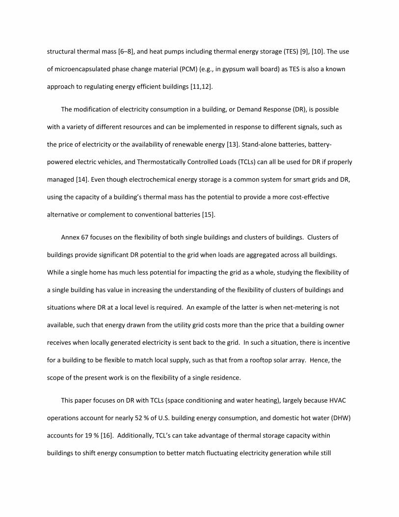
To accomplish the goals of this work, a numerical model of the NZERTF is utilized. The NZERTF

(Figure 1) is a highly insulated, detached single-family house with a floor area of 251 m2 on its two main

floors and a conditioned basement with an area of 135 m2 [19]. Given that approximately 50 % of newly

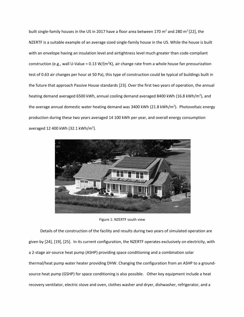
built single-family houses in the US in 2017 have a floor area between 170 m2 and 280 m2 [22], the

NZERTF is a suitable example of an average sized single-family house in the US. While the house is built

with an envelope having an insulation level and airtightness level much greater than code-compliant

construction (e.g., wall U-Value = 0.13 W/(m2K), air change rate from a whole house fan pressurization

test of 0.63 air changes per hour at 50 Pa), this type of construction could be typical of buildings built in

the future that approach Passive House standards [23]. Over the first two years of operation, the annual

heating demand averaged 6500 kWh, annual cooling demand averaged 8400 kWh (16.8 kWh/m2), and

the average annual domestic water heating demand was 3400 kWh (21.8 kWh/m2). Photovoltaic energy

production during these two years averaged 14 100 kWh per year, and overall energy consumption

averaged 12 400 kWh (32.1 kWh/m2).

Figure 1: NZERTF south view

Details of the construction of the facility and results during two years of simulated operation are

given by [24], [19], [25]. In its current configuration, the NZERTF operates exclusively on electricity, with

a 2-stage air-source heat pump (ASHP) providing space conditioning and a combination solar

thermal/heat pump water heater providing DHW. Changing the configuration from an ASHP to a ground-

source heat pump (GSHP) for space conditioning is also possible. Other key equipment include a heat

recovery ventilator, electric stove and oven, clothes washer and dryer, dishwasher, refrigerator, and a

microwave oven. While no people live in the house, occupancy is emulated through activation of

appliances and water fixtures as well as the use of heat and moisture generators to simulate occupancy

of a four-person family.

Balke et al. [26,27] developed a simulation model of the facility in the transient systems simulation

program TRNSYS that was validated against the experimental data and which forms the basis of the

current study. That model is modified for this study in a number of ways. The solar thermal collectors are

removed, and controlled outside shading is added to study the building in different climates. The local PV

production is removed so that all power is drawn from the utility grid. This new building is used as the

Base Variant for all following models. All simulations are carried out with a one-minute time step for a

complete year using Typical Meteorological Year weather files for the location being studied [28]. The

key results reported from these simulations include the average hourly power draw, the annual energy

consumption, and the average hourly thermal comfort. In this paper adequate thermal comfort is

characterized as times when the Predicted Percentage of Dissatisfied (PPD) is lower than 10 %. A PPD

between 10 % and 15 % is seen as a transition area between comfortable and uncomfortable. Therefore,

the annual hours in this range should be minimized. All modifications to the base building are compared

to the Base Variant to assess the ability to accommodate DR while maintaining thermal comfort.

2.2 Electric Generation Profile

The assessment of the energy flexibility of a building requires an assumption of an electric

generation profile. DR is most effective when the share of variable renewable energy is high such that

there are multiple peaks in the electricity generation profile. The 18 % share of renewable generation in

the U.S. today is assumed to be insufficient to properly display the potential of DR [29]. Hence, a

generation profile is created for the year 2050 with an expected share of fluctuating renewable

generation of approximately 50 %. The electric supply in Maryland, U.S. is provided via the PJM

Interconnection, which supplies 65 million people in the eastern portion of the United States, so data

from that system is used to estimate the 2050 profile. It should be stressed that this profile is meant to

test the flexibility of the house and that any number of profiles could be used to do so. However, this

approach will capture many of the characteristics that would likely be present in a grid of the future.

First, the PJM generation profile from 2018 is extrapolated to 2050 based on projected

population growth as documented in [30] and increased electricity demand. Based on projections from

the U.S. Department of Energy’s Energy Information Administration, the total electricity demand is

expected to increase from 829 TWh to 1152 TWh and that attributed to the residential sector from

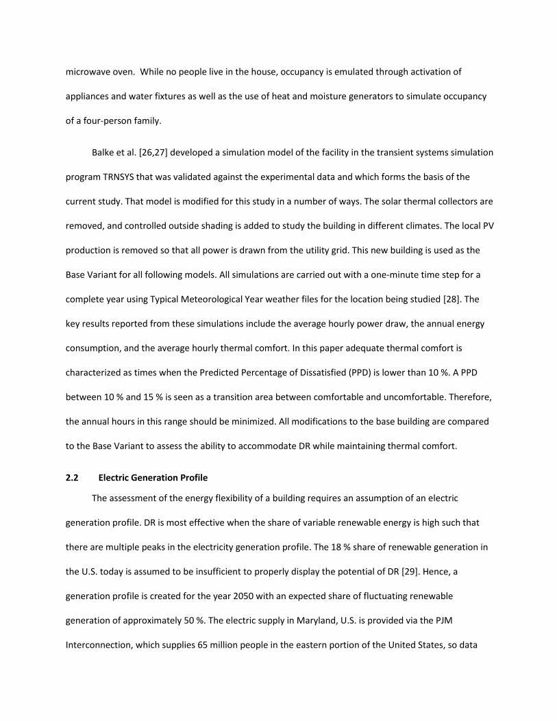
319 TWh to 383 TWh [31]. Based on the forecasts for renewable energy potential [32] [33], the

electricity demand supplied by the PJM Interconnection with a 50 % share of renewable energy is

provided by the generation sources shown in Figure 2. To obtain the profile, the current generation

profile from each source (e.g., solar, wind, coal, etc.) is scaled up to achieve the output noted in Figure

2. Secondly, the fraction of the total electricity demand used by detached single-family homes in 2018 is

63 % of the residential sector. That fraction is applied to the 2050 profile, and the overall demand is

divided by the number of predicted detached single-family homes in 2050. The result is a generation

profile that provides the energy to operate a single-family home using a 50 % mix of variable renewable

energy, with an average annual demand of approximately 12 000 kWh per household. This profile will

be used to assess the flexibility of the different variants of the house.

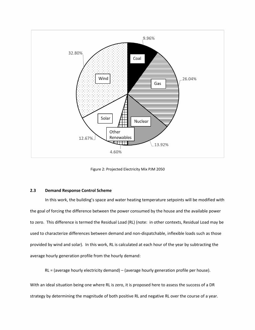
Figure 2: Projected Electricity Mix PJM 2050

2.3 Demand Response Control Scheme

In this work, the building’s space and water heating temperature setpoints will be modified with

the goal of forcing the difference between the power consumed by the house and the available power

to zero. This difference is termed the Residual Load (RL) (note: in other contexts, Residual Load may be

used to characterize differences between demand and non-dispatchable, inflexible loads such as those

provided by wind and solar). In this work, RL is calculated at each hour of the year by subtracting the

average hourly generation profile from the hourly demand:

RL = (average hourly electricity demand) – (average hourly generation profile per house).

With an ideal situation being one where RL is zero, it is proposed here to assess the success of a DR

strategy by determining the magnitude of both positive RL and negative RL over the course of a year.

When RL is positive, the power consumption of the house must be decreased, so the

temperature setpoints of the space heating system are adjusted to reduce the operation of the heat

pump, and the setpoint of the water heater is decreased to reduce its operation. When RL is negative,

those setpoints are adjusted to increase the power consumption of both the heat pump and water

heater by storing energy in the air and the water.

Figure 3a displays the control scheme implemented in this work for a two speed heat pump. As

discussed, the RL (in units of W) is used to set the thermostat for both the space conditioning system

and the water heater; each system has its own heat pump and operates independently of the other. A

few stipulations need to be noted, however. First, deadbands on the RL are incorporated in the

threshold to activate DR to ensure that the equipment does not cycle excessively. Additionally, a 5-

minute delay on changes for the heat pump is also implemented to prevent short-cycling as was done in

the unit used in the NZERTF. If RL is greater than the deadband, heating setpoints are decreased and

cooling setpoints are increased to reduce power consumption. If RL is less than the negative deadband,

setpoints are adjusted to increase space conditioning and water heating power consumption. The lower

and upper limits of the setpoints are set as shown to reduce the possibility of violating thermal comfort

requirements. The TRNSYS model selects high speed or low speed operation based on the difference

between the setpoint temperature and the room temperature.

(a) (b)

Figure 3: Setpoint and heat pump power control scheme (a) two speed heat pump (b) variable speed heat pump.

Figure 3b displays the control scheme implemented when the heat pump is variable speed and, hence,

consumes a variable amount of power. HPPmax is the maximum power draw by the heat pump. A one-

minute delay is implemented in changing the power consumption to coordinate with the time step in

the simulations. Heat pump power is adjusted to offset residual load. When RL is positive, the heat

pump is limited to 50 % of its maximum power as is implemented in the unit installed in the test house

noted previously. Absolute values of the RL are used as part of the control scheme in recognition of the

fact that this unit will aim to handle both positive and negative RL’s. It is acknowledged that current

control approaches for heat pumps do not directly modify the power consumption but rather change

temperature setpoints. This control approach is envisioned as one with direct control of heat pump

power. The TRNSYS model uses experimental data that provides the COP of the unit as a function of

outdoor temperature and indoor temperature for all speeds of operation.

The key metric that will be presented to assess a building’s energy flexibility is the cumulative RL

over the year. This RL will be split into both positive and negative RL to help understand whether the

building tends to draw too much power or too little power to match the generation profile. In addition

to reporting RL, the results section will also present overall energy consumption. While energy

minimization is not the goal of the control scheme, it is obviously an important quantity, particularly

financially given the current typical means of charging for electricity. Therefore, energy consumption by

the space heating, space cooling, and water heating systems will also be presented.

2.4 Building Variants

In this study, 21 variants of the NZERTF are investigated. All variants, excluding variant 0, include

a DR strategy. The variants are developed progressively to investigate the flexibility introduced by

adding different features to the residence. Table 1 lists the variants that are studied in this work. There

are 9 variants to the structure that are investigated in the climate of Gaithersburg, MD with DR. Three

of these variants are then selected to be simulated in different climates. The first variant from the base

case, which is the NZERTF as built with fixed temperature setpoints, is one where the DR approach

discussed in Section 2.3 is implemented. Subsequent variants involve differences in construction, heat

pump characteristics, and climate. The three variants studied in different climates include the base

case, the base case with DR, and the combination of features that showed the greatest reduction in

cumulative RL in the Gaithersburg simulation.

Table 1: Results for all variants; all variants except for ID = 0 implement DR.

Energy Demand (kWh) Res. Load (kWh) PPD (% of annual hours)

ID Variant Heating Cooling DHW positive negative 10 < PPD < 15 PPD ≥ 15

Gaithersburg, MD

0 NZERTF, no DR 3276 2503 1927 3252 3905 9.9 % 7.4 %

1 NZERTF, DR 2327 2481 2715 2751 3007 9.4 % 6.0 %

2 Massive Construction 2201 2369 2745 2566 3029 6.6 % 6.2 %

3 IECC min. Insulation 4650 2482 2687 4526 2493 16.5 % 10.2 %

PCM

4 ASHP, passive PCM 2314 2461 2714 2725 3015 9.7 % 5.2 %

5 GSHP, active PCM 2121 2728 2684 2415 2660 3.6 % 2.0 %

greater ΔT

6 ASHP, passive PCM 2443 2554 2694 2752 2842 10.8 % 1.8 %

7 GSHP, active PCM 2307 2851 2660 2482 2442 11.7 % 2.3 %

8 2-stage GSHP 2440 2749 2654 2366 2301 7.6 % 1.8 %

9 var. speed GSHP 2423 2832 2607 2349 2264 10.3 % 2.5 %

Vienna, Austria

10 Base Variant, no DR 4141 533 1936 3304 4476 5.2 % 2.2 %

11 Base Variant, DR 2633 497 2847 2027 3827 4.6 % 0.6 %

12 PCM, var. speed GSHP, > ΔT 2637 1287 2788 1860 2973 0.1 % 0.0 %

Phoenix, Arizona


14 Base Variant, DR 507 3039 2818 2439 3851 4.9 % 1.4 %


Miami, Florida


17 Base Variant, DR 365 8742 2065 4568 1171 6.1 % 0.6 %


Fairbanks, Alaska


20 Base Variant, DR 15576 161 2736 12762 2195 2.8 % 0.3 %


2.4.1 Construction Differences

The intent of these variations to the base case is to investigate how changes in the thermal mass

and insulation levels impact building flexibility. The base NZERTF is a lightweight wooden frame

construction having a roof U-value = 0.093 W/(m2K) and a wall U-value = 0.145 W/(m2K). The windows

have a U-value = 1.16 W/(m2K). Variant 2 investigates the impact of thermal mass by modeling the home

with reinforced concrete ceilings, interior and exterior brick walls, and a concrete roof while keeping the

U-value of the wall the same. Variant 3 explores the impact of a decrease in the efficiency of the walls

on RL by setting the U-values of the structure to match those mandated by the current version of the

International Energy Conservation Code (IECC) as shown in Table 2.

Table 2: NZERTF U-Values compared with minimum requirement for U-Values by the IECC in W/(m2K) [29]

Fenestration Roof Frame Wall Mass Wall Basement Floor Basement Wall

NZERTF 1.16 0.093 0.145 n/a 0.56 0.24

IECC Minimum

2.00 0.15 0.34 0.56 0.57 0.34

To further examine the impact of thermal mass as applied in lightweight construction, variants 4

through 9 consider the use of phase change materials embedded in 2.5 cm thick gypsum boards applied

to the inside of the exterior walls. The application solely in the exterior walls is meant to temper the

temperature difference between the outdoors and indoors and to have the best impact on improving

thermal comfort by keeping the surface temperatures of exterior walls more stable. The PCM can be

used in a passive sense, meaning that they respond to changes induced by the forced air heating and

cooling system, or they can be used in an active manner. In the active mode, it is assumed that water

tube coils are embedded in the PCM boards to activate the PCM directly via heated or cooled fluid from

the heat pump. The primary means of heating and cooling the space in this configuration is still forced

air. While this approach may be more costly, there is value in investigating this approach as an upper

bound on the possibilities of PCM in homes.

2.4.2 Heat Pump Characteristics

Variants 4 through 9 incorporate different types of heat pumps and operational strategies.

Variant 4 includes an ASHP with a forced air distribution system, and Variant 5 incorporates a GSHP that

heats or cools water circulated through tubes to activate the PCM in the gypsum walls. Variants 6

through 9 modify the operational controls by increasing the deadbands used in the heat pump controls.

Heating setpoints are varied from (20 °C to 22 °C) to (19 °C to 23 °C), and the range of cooling setpoints

is varied from (24 °C to 26 °C) to (23 °C to 26 °C). Variants 6 and 7 use the same configuration as in

Variants 4 and 5, respectively, with these larger deadbands.

The final two variants for Gaithersburg introduce a variable speed GSHP coupled with the active

PCM. Variant 8 involves a two-stage GSHP, and Variant 9 includes a GSHP with continuous variability

from 50 % of its maximum power to full power.

2.4.3 Climate Differences

The building’s performance at reducing RL’s is evaluated in the following climate zones by simulating

Variants 0, 1, and 9 in the noted city:

▪ Cold winter, humid and hot summer (Gaithersburg, Maryland) – ASHRAE Climate Zone 4A

▪ Cold winter, dry and warm summer (Vienna, Austria) – ASHRAE Climate Zone 4A

▪ Warm winter, very hot and humid summer (Miami, Florida) – ASHRAE Climate Zone 1A

▪ Cool winter, dry and very hot summer (Phoenix, Arizona) – ASHRAE Climate Zone 2B

▪ Very cold winter, dry and warm summer (Fairbanks, Alaska) – ASHRAE Climate Zone 8

Vienna is chosen for the simulations despite being in the same climate zone as Gaithersburg to explore

the impact of relative humidity on the ability of the building to be flexible. It should be noted that a full

factorial study of impacts is not undertaken in this work. Rather, the approach provided is intended as a

screening study to identify those factors that could impact energy flexibility while maintaining or

improving thermal comfort.

2.5 Thermal Comfort

To assess thermal comfort, hours are compiled throughout the year when PPD rises above 10 %.

To accentuate larger deviations from comfort levels, hours when PPD is between 10 % and 15 % are

grouped as are hours when PPD equals or exceeds 15 %. Results are presented as a percentage of total

annual hours.

3. Results

Table 1 provides results for all variants investigated as described in the Methodology section.

Prior to discussing the annual results, it is valuable to investigate how DR can impact the energy demand

and better match demand to supply.

3.1 Weekly Profile

To display how demand response modifies energy consumption to meet energy supply,

temporal profiles of the demand and grid generation over the course of a week are presented. A typical

summer week without DR is shown in Figure 4. The total cumulative absolute RL during this week is

162 kWh. The building’s load fluctuates heavily and rarely matches the grid generation. This behavior is

especially clear during the sixth and seventh day where the house load is at a minimum during the times

of peak renewable generation. The load peaks, with a power greater than 5 kW, are typically caused by

the clothes dryer. This appliance is turned on during the first, second, and fifth day. The other peaks are

mainly caused by household appliances, such as toasters, microwaves, and hair dryers.

Figure 5 shows that same week with the consumption profile of the variant that maximized

reduction of RL (Variant 9, with DR, a variable speed GSHP, and active PCM). The total cumulative

absolute RL during this week is 99 kWh. For the first five days of this week, the demand can be matched

very well to the generation profile. The major peak load that causes positive RL is the clothes dryer. On

the sixth and seventh day the increased load, caused by the DR strategy, accurately tracks the grid’s

peak generation until the thermal storage capacity is fully charged. The grid generation during these

days greatly exceeds the building’s potential for demand response. Therefore, only about a third of the

peak is compensated.

Figure 4: Energy demand and supply and Cumulative Residual Load during a typical summer week for

the Base Variant.

Figure 5: Energy demand and supply and Cumulative Residual Load for Variant variable speed GSHP

and PCM in Gaithersburg.

3.2 Annual Results in Gaithersburg

Figure 6 presents the annual results graphically for three of the variants described in Table 1: the

base variant, the base variant with DR, and the best-case variant in terms of RL reduction, the GSHP with

active PCM. The use of DR while leaving other system parameters unchanged results in a decrease of

cumulative absolute RL of 19.5 % compared to the Base Case. The increase in DHW energy consumption

in the DR case occurs because the control algorithm increases the setpoint temperature of the water

heater to counteract negative RL. This higher temperature means that there will be greater standby

losses from the water heater and, hence, higher energy consumption. Lower heating setpoint

temperatures lead to a decreased heating demand, which reduces the positive RL during Winter. The

increase in DHW demand is offset by the reduced heating demand so the overall energy demand is

approximately equal to that of the Base Variant. Lower cooling setpoints in summer slightly decrease the

overall PPD > 10 % from 17.2 % to 15.3 %. There is no technical reason not to use DR since the building

performs better than the Base Variant in all performance metrics.

Using a variable-speed GSHP leads to a 35.5 % reduction in cumulative absolute RL compared to

the Base Variant. Instantaneous changes to the compressor power allow accurate tracking of the RL

signal by the controller. In this variant the PCM can actively be used to store energy during times of

negative RL. The increased thermal capacitance allows for a greater ability to shift peak loads compared

to lightweight construction, thus resulting in lower positive and negative RLs compared to the variant

with DR. This variant achieves the lowest RL of all variants investigated.

Figure 6. Results for Variants 0, 1, and 9.

There is a seasonal dependency to the residual loads. During a typical week in the winter, the

total residual load dropped 46 % from 105 kWh to 57 kWh when moving from Variant 0 to Variant 9.

During a typical week in the summer, the residual load dropped 39 % from 162 kWh to 99 kWh. The

slightly smaller drop in summer is due to a dehumidification load that is independent of outside

temperature that must be maintained to achieve desired thermal comfort. In Spring and Fall, the lower

energy demand in the home can cause large residual loads when renewable generation is high.

The distribution of average hourly RLs in Figure 7 shows that the majority of RLs can be lowered

to less than 1 kW with a DR strategy. Nevertheless, DR is insufficient for reducing the highest positive

(5 kW dryer) and negative (3 kW peak PV generation) RLs. Instead of focusing on increasing the DR

potential, peak positive RLs for a single home should be reduced through energy efficiency measures.

More efficient appliances, better insulation, and intelligent control schemes contribute to lower energy

consumption and, therefore, lower positive RLs. Such efficiency steps, however, sometimes limit

options for reducing negative RL since the maximum amount of power drawn by the house is reduced.

Energy storage options, such as the thermal storage studied here, can reduce part of the negative RL.

For groups of homes, aggregation of loads and scheduling can help achieve reduction in positive RLs, but

single residences require changes to the power consumption of appliances.

DR is only one part of the equation for reducing negative RL. In an electrical grid without

significant storage capacity, limiting the active power of renewable power plants will be necessary.

Feeding reactive power into the grid will not be sufficient to keep voltage levels in the required range. A

variety of different storage technologies (electrochemical, mechanical, chemical, etc.) will likely be

necessary along with DR to transition to 100 % renewable energy generation.

Figure 7. Distribution of average hourly RL throughout the year for Variants 0,1, and 9 in Gaithersburg.

3.3 Climate Effects

To examine any major trends that arise due to climate, three of the variants studied in

Gaithersburg were simulated in alternative climates. The three variants selected represent the base

case, the base case with DR, and the variant that had the greatest reduction in RL in Gaithersburg. All

results are presented in Table 1: Results for all variants. Figure 8 provides a visual representation of the

results for Vienna, Austria. Implementing a DR control strategy for the building in Vienna’s climate

results in a 24.8 % decrease in total RL compared to the base case simulated in Vienna. Changing to a

variable speed GSHP in combination with an active PCM layer results in a 37.9 % decrease in total RL.

The same conclusions from results of simulations in Gaithersburg hold true in the climate of Vienna.

Higher energy efficiency (GSHP) reduces positive RL, but it also limits options for reducing negative RL

whereas more compressor stages and a higher thermal capacitance help reduce negative RL. In a climate

with lower relative humidity, such as Vienna, it is easier to sustain thermal comfort even when altering

-4.00

-3.00

-2.00

-1.00

0.00

1.00

2.00

3.00

4.00

5.00

0

10

00

20

00

30

00

40

00

50

00

60

00

70

00

80

00

Re

sid

ual

Lo

ad in

kW

Hours

no DR DR var. speed GSHP + PCM

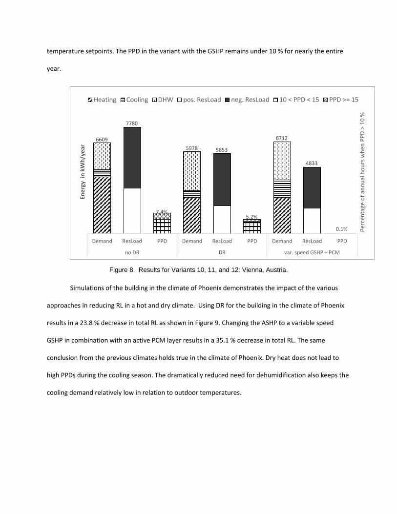
temperature setpoints. The PPD in the variant with the GSHP remains under 10 % for nearly the entire

year.

Figure 8. Results for Variants 10, 11, and 12: Vienna, Austria.

Simulations of the building in the climate of Phoenix demonstrates the impact of the various

approaches in reducing RL in a hot and dry climate. Using DR for the building in the climate of Phoenix

results in a 23.8 % decrease in total RL as shown in Figure 9. Changing the ASHP to a variable speed

GSHP in combination with an active PCM layer results in a 35.1 % decrease in total RL. The same

conclusion from the previous climates holds true in the climate of Phoenix. Dry heat does not lead to

high PPDs during the cooling season. The dramatically reduced need for dehumidification also keeps the

cooling demand relatively low in relation to outdoor temperatures.

6609

7780

7.4%

5978 5853

5.2%

6712

4833

0.1%

Demand ResLoad PPD Demand ResLoad PPD Demand ResLoad PPD

no DR DR var. speed GSHP + PCM

Per

cen

tage

of

ann

ual

ho

urs

wh

en P

PD

> 1

0 %

Ene

rgy

in k

Wh

/ye

ar

Heating Cooling DHW pos. ResLoad neg. ResLoad 10 < PPD < 15 PPD >= 15

Figure 9. Results for Variants 13, 14, and 15: Phoenix, AZ.

The hot and humid climate of Miami leads to a 150 % higher cooling demand compared to the

dry desert climate in Phoenix. Additionally, the constant dehumidification demand decreases energy

flexibility. Even the best performing variant with a GSHP and active PCM can only reduce RLs by 26.2 %

as shown in Table 1.

In the cold climate of Fairbanks, DR can reduce RLs by 12.5 %. In comparison a system with a

GSHP can reduce RLs by 83.8 %. This large difference, compared to the previous climates, arises

primarily because of the low efficiency of the ASHP in very cold climates. The importance of energy

efficiency for decreasing positive RL is further emphasized by this result. While decreased heat pump

power consumption reduces the flexibility to counteract available surplus energy, the long runtimes of

the heat pump in this climate mean that negative RL is not very large.

4. Discussion

The results presented here illustrate a number of points related to the flexibility of single family

homes. First, these results show how increased thermal mass from PCM can increase the potential for

DR. Although not presented here, similar increases in DR potential were observed when simulating

massive construction versus lightweight construction [21]. While increased thermal mass can shift the

times of day when heating or cooling is needed and can decrease the maximum power required by the

heat pump, one of the significant benefits of increased thermal mass is its ability to maintain a higher

level of thermal comfort when thermostat deadbands are expanded. The use of PCM as part of

lightweight construction shows some benefit, but the heat transfer to and from the PCM appears to

limit its benefits. If the PCM were charged in a more active manner, for example by circulating fluid

through it, its benefits are greater. More research is needed to investigate the heat transfer limitations

of passive PCMs.

Increased energy efficiency, either through more highly insulated walls or improved heat pumps

and water heaters, has the benefit of decreasing the required power to condition the home or provide

hot water. That lower power reduces positive residual loads when intermittent energy supply is low and

also limits overshoot when trying to match the supply of intermittent electricity. As defined in this

work, efficiency helps to decrease positive RL but lower power consumption by the heat pump and

water heater may mean that negative RL increases since the home may not be able to consume enough

power to meet the amount of supply available.

Variable speed heat pumps increase the flexibility of homes in two main ways. First, the nearly

continuous range of available power consumption up to the maximum power consumption of the units

allows better matching of the available power than can be achieved in single- or two-stage systems.

Second, systems with one or two stages typically require minimum run-times at each stage for

equipment longevity, whereas variable speed systems typically allow for more frequent adjustment of

the power level. This flexibility allows one to better match the fluctuating supply resources.

This study focused on the flexibility of a single home. When considering the needs of a utility,

an aggregation of multiple buildings is more important, and solutions for controlling loads to meet

intermittent supply may be different than those implemented in a single building. Nevertheless, the

flexibility of a single home may still be important for several reasons. First, aggregation would benefit

from some understanding of the basic flexibilities afforded by single buildings. Second, for those homes

with on-site renewables, there is potential benefit to consuming that locally generated power on-site as

opposed to sending surplus to the grid in light of changing policies that would charge customers more to

purchase electricity from the grid than they would get credited for sending an equal amount of energy

to the grid. A flexible building could help balance supply and demand on a local scale in that situation.

5. Conclusions

As intermittent renewable generating resources take up a larger part of the electricity

generation mix, buildings can serve as a key resource in balancing the supply and demand of electricity.

The flexibility of a building, meaning its ability to change power demand to balance supply, is an

important quality and has been investigated in this work. An efficient single-family detached house that

might be typical of construction in the year 2050 was used to assess the impacts of thermal mass, heat

pump characteristics, and climate on the flexibility using thermally controlled loads (i.e., heat pump and

water heater). The cumulative Residual Load, here defined as the difference between electricity

demand and electricity supply, over the course of a year is used to assess the building’s flexibility. Simple

demand response to match power consumption to the supply resulted in a 20 % reduction in cumulative

residual load in a mixed-humid climate. The best case investigated here, which involved a variable

speed ground-source heat pump charging phase change material, resulted in a 36 % decrease in

cumulative residual load in that same climate. Although the cases utilizing paraffin wax as PCM provide

the greatest reduction in residual load, they are not economically viable. The most cost-effective

approach is to not change the system components and use a simple DR strategy. Increased thermal

mass, either through masonry or phase change materials in outer walls, had the major benefit of

maintaining or improving thermal comfort despite larger variations in setpoint temperatures under a DR

strategy. Energy consumption was generally not improved over the year, largely due to the increased

temperature in the water heater or the more extreme setpoint temperatures for the space conditioning

system. More efficient systems, such as the ground-source heat pump, decreased times when power

consumption exceeded power supply, but certain appliances such as clothes dryers, electric stoves, and

ovens drew significant power that could not be fully supplied by the assumed power profile. Likewise,

efficient heating and cooling equipment occasionally struggled to draw enough power to match a large

supply of electricity. Nevertheless, the strategies implemented in this paper (use of thermal mass along

with temperature setpoint adjustments) suggest that single family homes can provide a degree of

energy flexibility to meet variable supply of electricity from renewables.

6. References

[1] IEEE, A Framework for and Assessment of Demand Response and Energy Storage in Power Systems, (2013).

[2] P.F. Lyons, P. Trichakis, R. Hair, P.C. Taylor, Predicting the technical impacts of high levels of small-scale embedded generators on low-voltage networks, IET Renewable Power Generation. 2 (2008) 249–262. https://doi.org/10.1049/iet-rpg:20080012.

[3] D. Kolokotsa, D. Rovas, E. Kosmatopoulos, K. Kalaitzakis, A roadmap towards intelligent net zero- and positive-energy buildings, Solar Energy. 85 (2011) 3067–3084. https://doi.org/10.1016/j.solener.2010.09.001.

[4] S.Ø. Jensen, A. Marszal-Pomianowska, R. Lollini, W. Pasut, A. Knotzer, P. Engelmann, A. Stafford, G. Reynders, IEA EBC Annex 67 Energy Flexible Buildings, Energy and Buildings. 155 (2017) 25–34. https://doi.org/10.1016/j.enbuild.2017.08.044.

[5] S. Rotger-Griful, R.H. Jacobsen, D. Nguyen, G. Sørensen, Demand response potential of ventilation systems in residential buildings, Energy and Buildings. 121 (2016) 1–10. https://doi.org/10.1016/j.enbuild.2016.03.061.

[6] K. Foteinaki, R. Li, T. Pean, C. Rode, J. Salom, Evaluation of energy flexibility of low-energy residential buildings connected to district heating, Energy Build. 213 (2020) 109804. https://doi.org/10.1016/j.enbuild.2020.109804.

[7] J. Sanchez Ramos, M. Pavon Moreno, M. Guerrerot Delgado, S. Alvarez Dominguez, L.F. Cabeza, Potential of energy flexible buildings: Evaluation of DSM strategies using building thermal mass, Energy Build. 203 (2019) 109442. https://doi.org/10.1016/j.enbuild.2019.109442.

[8] J. Vivian, U. Chiodarelli, G. Emmi, A. Zarrella, A sensitivity analysis on the heating and cooling energy flexibility of residential buildings, Sust. Cities Soc. 52 (2020) 101815. https://doi.org/10.1016/j.scs.2019.101815.

[9] B. Alimohammadisagvand, J. Jokisalo, S. Kilpeläinen, M. Ali, K. Sirén, Cost-optimal thermal energy storage system for a residential building with heat pump heating and demand response control, Applied Energy. 174 (2016) 275–287. https://doi.org/10.1016/j.apenergy.2016.04.013.

[10] B. Baeten, F. Rogiers, L. Helsen, Reduction of heat pump induced peak electricity use and required generation capacity through thermal energy storage and demand response, Applied Energy. 195 (2017) 184–195. https://doi.org/10.1016/j.apenergy.2017.03.055.

[11] S. Ben Romdhane, A. Amamou, R. Ben Khalifa, N.M. Said, Z. Younsi, A. Jemni, A review on thermal energy storage using phase change materials in passive building applications, J. Build. Eng. 32 (2020) 101563. https://doi.org/10.1016/j.jobe.2020.101563.

[12] P. Fitzpatrick, F. D’Ettorre, M. De Rosa, M. Yadack, U. Eicker, D.P. Finn, Influence of electricity prices on energy flexibility of integrated hybrid heat pump and thermal storage systems in a residential building, Energy Build. 223 (2020) 110142. https://doi.org/10.1016/j.enbuild.2020.110142.

[13] C.D. Korkas, S. Baldi, I. Michailidis, E.B. Kosmatopoulos, Occupancy-based demand response and thermal comfort optimization in microgrids with renewable energy sources and energy storage, Applied Energy. 163 (2016) 93–104. https://doi.org/10.1016/j.apenergy.2015.10.140.

[14] F. Oldewurtel, T. Borsche, M. Bucher, P. Fortenbacher, M. Gonzalez Vaya, T. Haring, J.L. Mathieu, O. Megel, E. Vrettos, G. Andersson, A framework for and assessment of demand response and energy storage in power systems, in: 2013 IREP Symposium Bulk Power System Dynamics and Control - IX Optimization, Security and Control of the Emerging Power Grid, IEEE, Rethymno, 2013: pp. 1–24. https://doi.org/10.1109/IREP.2013.6629419.

[15] M.J.N. Oliveira Panão, N.M. Mateus, G. Carrilho da Graça, Measured and modeled performance of internal mass as a thermal energy battery for energy flexible residential buildings, Applied Energy. 239 (2019) 252–267. https://doi.org/10.1016/j.apenergy.2019.01.200.

[16] U.S. Energy Information Administration, Annual household site end-use consumption in the U.S. - totals and averages, 2015, Residential Energy Consumption Survey - 2015. (2018). https://www.eia.gov/consumption/residential/data/2015/c&e/pdf/ce3.1.pdf (accessed September 25, 2020).

[17] A. Arteconi, N.J. Hewitt, F. Polonara, State of the art of thermal storage for demand-side management, Applied Energy. 93 (2012) 371–389. https://doi.org/10.1016/j.apenergy.2011.12.045.

[18] A. Arteconi, N.J. Hewitt, F. Polonara, Domestic demand-side management (DSM): Role of heat pumps and thermal energy storage (TES) systems, Applied Thermal Engineering. 51 (2013) 155–165. https://doi.org/10.1016/j.applthermaleng.2012.09.023.

[19] A.H. Fanney, V. Payne, T. Ullah, L. Ng, M. Boyd, F. Omar, M. Davis, H. Skye, B. Dougherty, B. Polidoro, W. Healy, J. Kneifel, B. Pettit, Net-zero and beyond! Design and performance of NIST’s net-zero energy residential test facility, Energy and Buildings. 101 (2015) 95–109. https://doi.org/10.1016/j.enbuild.2015.05.002.

[20] ASHRAE, ASHRAE Standard 55 - Thermal Environmental Conditions for Human Occupancy, (2013). [21] M. Feldhofer, Utilization of thermostatically controlled loads for demand response and increased

energy flexibility in U.S. residential buildings, University of Applied Sciences Technikum Wien, 2019. [22] US Census, Square Feet of Floor Area in New Single-Family Houses Completed, (2017).

https://www.census.gov/construction/chars/pdf/squarefeet.pdf (accessed February 21, 2019). [23] Passive House Institute, Criteria for the passive house, EnerPHit and PHI low energy building

standard.pdf, (2016). https://passiv.de/downloads/03_building_criteria_en.pdf. [24] B. Pettit, C. Gates, A.H. Fanney, W.M. Healy, Design Challenges of the NIST Net Zero Energy

Residential Test Facility, National Institute of Standards and Technology, 2015. https://doi.org/10.6028/NIST.TN.1847.

[25] A. Hunter Fanney, W. Healy, V. Payne, J. Kneifel, L. Ng, B. Dougherty, T. Ullah, F. Omar, Small Changes Yield Large Results at NIST’s Net-Zero Energy Residential Test Facility, Journal of Solar Energy Engineering. 139 (2017) 061009. https://doi.org/10.1115/1.4037815.

[26] E. Balke, Modeling, Validation and Evaluation of the NIST Net Zero Energy Residential Test Facility, 2016.

[27] E. Balke, G. Nellis, S. Klein, H. Skye, V. Payne, T. Ullah, Detailed energy model of the National Institute of Standards and Technology Net-Zero Energy Residential Test Facility: Development, modification, and validation, Science and Technology for the Built Environment. 24 (2018) 700–713. https://doi.org/10.1080/23744731.2017.1381828.

[28] S. Wilcox, W. Marion, Users Manual for TMY3 Data Sets, National Renewable Energy Laboratory, Golden, CO, 2008.

[29] EIA, Annual Energy Outlook 2019 with projections to 2050, (2019). [30] U.S. Census Bureau, Projections of the Size and Composition of the U.S. Population: 2014 to 2060,

United States Census Bureau, 2014. [31] U.S. Energy Information Administration, Annual Energy Outlook 2020 with projections to 2050, U.S.

Department of Energy, 2020. https://www.eia.gov/outlooks/aeo/pdf/AEO2020%20Full%20Report.pdf (accessed September 25, 2020).

[32] AWS Truepower, PJM Renewable Integration Study, (2012). https://www.pjm.com/~/media/committees-groups/subcommittees/irs/postings/pris-task-1-wind-and-solar-power-profiles-final-report.ashx.

[33] General Electric, PJM Renewable Integration Study, (2014).

Funding: This work was supported by the National Institute of Standards and Technology and the

Austrian Marshall Plan Foundation.

Documents

Improving the Energy Flexibility of Single-Family Homes