IMPROVING STRATEGIC DECISION-MAKING IN A CLOSED …

IMPROVING STRATEGIC DECISION-MAKING IN A CLOSED-LOOP RAIL

NETWORK WITH HYBRID SIMULATION-OPTIMIZATION MODELING

Jorge Ubirajara Pedreira Junior1, Ademar Nogueira do Nascimento2, Cristiano Hora de

Oliveira Fontes2

1 Federal University of Bahia, Department of Transportation Engineering and Geodesy, R. Aristides Novis, 02,

Salvador (BA), Brazil. 2 Federal University of Bahia, Industrial Engineering Graduate Program, R. Aristides Novis, 02, Salvador (BA),

Brazil.

Corresponding Author: 1 email: [email protected]; tel: +55 71 99404 3873

ABSTRACT

The availability of rail infrastructure resources is a major driver of rail operations performance.

To evaluate the impact of infrastructure provision, network simulation models can be used to

accurately represent train traffic behavior in a wide range of scenarios. However, performing

this task can result in a problem of high combinatorial nature as the number of factors and their

associated levels increase. This requires more sophisticated techniques such as experimental

design formulations or optimization modeling in order to yield satisfactory results. Yet the

research in network simulation models for rail systems has hitherto been limited to simple what-

if analysis, made up from few factors that cannot represent the whole spectrum of interventions.

This is especially critical in closed-loop rail systems where trains are subject to various

interferences. Local improvements can be misleading as the queues are merely transferred

within the network. Considering this, we propose a hybrid simulation-optimization model to

aid the strategic decision of minimizing supplementary capital costs in a heavy-haul Brazilian

railroad under construction. As soon as the railroad is completed, investments in both loading

and unloading rail terminals will be necessary. First, we developed a representative and flexible

model capable of dealing with complex relations between variable infrastructure provision and

the resulting operational performance. Then, we simulated this system to prove that the current

set of proposed infrastructure resources cannot meet the transportation demands. Afterwards,

we demonstrate that local improvements can be delusive as the queues are shifted from loading

to unloading operations, reciprocally. Then, we solve an optimization model to define the

minimal supplementary investment in order to meet the commercial goals of mining companies.

This is done by choosing the best trackage configuration, equipment quantity and capacity and

fleet sizing in 3 different production scenarios. The best values of the objective function were

found by improving both loading and unloading equipment and increasing the number of trains.

Keywords: Network simulation modeling; Rail Infrastructure; Hybrid-Simulation

Optimization

Preprints (www.preprints.org) | NOT PEER-REVIEWED | Posted: 27 May 2019 doi:10.20944/preprints201905.0312.v1

© 2019 by the author(s). Distributed under a Creative Commons CC BY license.

https://doi.org/10.20944/preprints201905.0312.v1

http://creativecommons.org/licenses/by/4.0/

1. INTRODUCTION

Increasing demand in rail transport puts hard pressure in existing rail infrastructure. Insufficient

infrastructure resources can lead to rapid congestion in rail networks (Gorman, 2009) as train

delays increase exponentially with growing traffic (Sogin, Barkan and Saat, 2011). The

resulting poor operational performance entail low level of service for rail costumers

(Pouryousef and Lautala, 2015), worsening rail transport competitiveness.

Previous models investigated the impacts of infrastructural changes in railway operations

(Dessouky and Leachman, 1995; Dessouky, Lu and Leachman, 2002; Atanassov and Dick,

2015). Although important correlations were found, these models did not cover a wide range of

infrastructure parameters. This fact is particularly critical in railways running on a closed-loop

framework composed by unit trains (carrying the same commodity). In such systems trains are

formed once in the network with a fixed number of railcars and run through the following closed

circuit without being split or stored in the route: (i) loading; (ii) moving loaded to a rail port

terminal; (iii) unloading; and (iv) moving empty to a loading terminal (Franzese, Fioroni and

Botter, 2003; De Faria and Cruz, 2015). Closed-loop systems are modeled as opposed to the

ordinary dispatching model, where trains are formed and disposed in the edges of the network

with the purpose of analyzing line utilization and total delay. Cyclic trains are subject to several

interferences from both interaction with other trains and disruptions in loading and unloading

processes. Therefore, local and isolated solutions are ineffective since queues are only

transferred within this closed circuit.

Moreover, the railway industry is very capital intensive and the provision of infrastructure is

very costly (Abril et al., 2008; Gorman, 2009). Although managing the existing capacity is a

more cost-effective approach, growing traffic will eventually require capital expansion. Thus,

from a wide range of possible improvements one must choose a subset that meets the expected

performance at minimal cost. So far, it appears that not only rail modeling is limited to a narrow

and unintegrated range of infrastructural solutions but they did also not account for the cost

dimension of the decision-making process.

Against this backdrop, we propose a hybrid simulation-optimization model to fill this gap in

the railway modeling research. The Brazilian heavy haul West-East Integration Railroad

(Ferrovia de Integração Oeste Leste – FIOL) and its branching lines in loading and unloading

operations is chosen to perform this task. We prove that the current set of infrastructure

parameters will not be able to meet the transportation demands from iron ore mining companies.



By pointing out the bottlenecks of the system, we also demonstrate that local solutions do not

achieve the desired goal, demanding a broader experimental approach. This work consists of 3

steps: (a) modeling freight train traffic and associated activities within this supply chain; (b)

simulating this model in a discrete-event basis to obtain the annual volume of iron ore delivered

in port; (c) based upon the simulation results, minimizing total investment in tracks, vehicles

and equipment in the system, subject to the mining companies’ commercial goals and

operational constraints.

2. LITERATURE REVIEW

2.1. Railway Traffic Modeling

The rail planning literature considers three classical levels of management decision-making:

strategic, tactical and operational (Assad, 1980; Crainic and Laporte, 1997; Marinov, Zunder

and Islam, 2010). Strategic decision involves the highest level of management and determines

capital investments over long time horizons. Tactical planning, in turn, focuses on resource

allocation to meet demand origin-destination requirements in the medium term. Finally,

operational planning is concerned with day-to-day activities of the railroad, such as empty car

distribution, locomotive scheduling and dispatching decisions to solve train conflicts.

An important measure to be determined in this context is rail capacity. Rail capacity is referred

to as the maximum number of trains that can operate on a pre-defined infrastructure, during a

specific time interval and given some operational conditions (Abril et al., 2008). A rail network

consists of lines of track (links) associated with stations, junctions and yards (nodes) where

freight trains undergo several activities such as classification, fueling and loading/unloading

operations (Assad, 1980). A malfunctioning railway node may compromise the entire service,

causing upstream delays and downstream idle periods (Marinov and Viegas, 2011). Therefore,

capacity analysis must be performed in a global and integrated manner, i.e. in a network-wide

perspective (Crainic and Laporte, 1997).

There are three main methods to evaluate rail capacity: analytic, optimization and simulation

(Petersen and Taylor, 1982). Analytical methods aim at defining a preliminary solution, often

used as a reference or comparison (Abril et al., 2008). They consist of mathematical formulae

or algebraic expressions that relies on several assumptions about system modeled (e.g. queuing

theory). However, modeling real-world train traffic analytically is a very complex task.

Dessouky and Leachman (1995) state that compound delays and ripple effects from train

conflicts pose a hard challenge on developing analytical models.



On the other hand, optimization strategies are employed to provide the feasible best (or near

best) solution to routing traffic through the rail network. These models are often concerned with

minimizing total delay (or costs) or maximizing the number of trains in a timetable by means

of mixed integer linear programming formulations or meta-heuristic algorithms. An extensive

review of these models and methods and their applicability can be found in Caimi, Kroon and

Liebchen (2017). A recent trend in optimization models is the real-time rescheduling problem,

applied to when the traffic is disrupted and a new schedule must be developed quickly. Corman

and Quaglietta (2015) address the main challenges in their applicability and highlight the best

available control scheme to implement such solutions.

Simulation methods, in turn, attempt to imitate the movement of trains through the railway

network, taking a given set of parameters such as trains, lines, yards and operation policies as

inputs (Assad, 1980; Abril et al., 2008; Motraghi and Marinov, 2012). Because simulation

models prescind from typical unrealistic assumptions of analytical models, they can represent

very accurately real-world systems. Train traffic is rather complex and dispatching rules can be

more realistic represented by simulation models (Medanic and Dorfman, 2002). Moreover, train

movement in rail yards are very contingent on yard layout and operational policies that vary

greatly from case to case.

Crainic, Perboli and Rosano (2018) list 4 objectives of a simulation model, namely: (a) what-if

analysis, when multiple scenarios are generated by changing input values to compare system

alternatives; (b) forecasting, to predict the system future performance under various conditions;

(c) validation, to confirm that either a proposed scenario or a modeling approach represent the

real-world system; and (d) enhancement, when the simulation is combined with techniques such

as optimization modeling to improve the solution.

In the rail context, simulation methods seem to be a preferred approach between practitioners.

Ferreira (1997) explains that optimization models have not been widely embraced by rail

organizations because of the complexity of the overall task and practical issues (Corman and

Quaglietta, 2015) that prevent optimal results from being implemented. Michal et al. (2017)

reinforce that view stating that optimization models require the decision makers to have a good

grasp in mathematical modeling, limiting their use in real situations.

To work with comprehensive data input a simulation tool is required. Well-known specific rail

network simulation software are RailSys and OpenTrack, used in Europe, and Rail Traffic

Controller (RTC), the foremost software used in North America (Motraghi and Marinov, 2012).



It is also possible to work with general purpose simulation software such as Arena and Simul8

to represent train traffic (Marinov and Viegas, 2011). They provide an intuitive platform that

eases the simulation modeling task and allows for complex reality implementation. There are

also cases where new simulations platforms are developed in Michal et al. (2017) and

Hernando, Roanes-Lozano and García-Álvarez (2010).

Due to the abovementioned arguments, simulation network models are the focus of this paper.

Crainic, Perboli and Rosano (2018) classify the technical implementation of simulation by two

perspectives. Regarding the evolution over time, these models can be either static (i.e. time is

not explicitly considered, but rather the system is evaluated in a steady state) or dynamic (when

the system changes over time). With respect to the inclusion of uncertainty, models can be

either stochastic (when random inputs are used) or deterministic (in case the inputs are not

uncertain).

2.2. Simulation Network Models

Dessouky and Leachman (1995) investigated the implementation of an alternative high capacity

corridor near a port area served by three major railroad companies. They concluded that further

improvements should be considered in order to obtain a better level of service. Later, Dessouky,

Lu and Leachman (2002) proposed doubling and tripling existing tracks and the addition of a

passenger train flyover to the same system. Atanassov and Dick (2015) addressed the problem

of passing sidings with limited size in face of increasing train lengths. They carried out a

factorial experimental design considering the number of trains, the percentage of long trains,

the percent of long sidings and the directional distribution of long trains in the network. From

the 196 scenarios tested (out of 224 combinations), it was demonstrated that routes with roughly

50% of long sidings eliminate any delay-based consequences of running long trains on the

route. A similar challenge has also been investigated in a developed simulation tool by

Hernando, Roanes-Lozano and García-Álvarez, (2010) for a Spanish railroad. Michal et al.

(2017) tested 2 improvements in the unloading facility of coal cyclic trains in Australia,

consisting of extending the existing coal arrivals roads to 850 m and doubling the existing

unloading capacity. In a similar vein, Fioroni et al. (2013) evaluated the total coal transported

in a Colombian railroad by upgrading a stacker-reclaimer system at port and augmenting the

number of railcars in a typical coal freight train.

Although abovementioned studies contemplated improvements in infrastructure resources,

most of simulation network models is focused on analyzing the network performance by



changing the number of vehicles and/or operational policies. De Faria and Cruz (2015) modeled

a major Brazilian railroad running with iron ore cyclic trains. The authors tested 3 scenarios

with different number of railcars and suggest the expansion of existing tracks. Woroniuk and

Marinov (2013) simulated a Spanish railway network with low line utilization in order to

investigate the impact of the inclusion of a freight service.

Heterogeneity of train traffic pose a great challenge in railway networks, since passenger trains

usually have higher speeds and higher priority over freight trains. Sogin, Barkan and Saat

(2011) simulated 113 scenarios considering the inclusion of freight and passenger trains with

different speeds, demonstrating that priority and speed differential increases the mean and

variance of freight trains delays. Dingler, Lai and Barkan (2014) added other heterogeneity

factors in their analysis such as acceleration/breaking rates proving its significance in average

delay increase.

With respect to operational policy, Marinov and Viegas (2011) compared the performance of

two productions patterns, namely improvised operations and structured-fixed schedules in a rail

freight network in Portugal. In the first case, freight trains leave loading facilities only when

they have enough tonnage to fill them to the capacity limits of the rail lines. This is a very

common operation pattern in worldwide freight rail networks outside Center and Western

Europe (Marinov and Viegas, 2011; Marinov et al., 2013). Structured-fixed schedules, in turn,

are based on the philosophy that freight trains have to be as reliable as passenger, even if they

run as reduced formations. In their work, Marinov and Viegas (2011) proved that rail lines and

yards presented lower percent of time awaiting work, higher utilization and less saturation.

Similar results were found when Motraghi and Marinov (2012) evaluated the inclusion of

freight train services within a urban metro system.

2.2.1. Hybrid Simulation-Optimization Models

Simulation can be combined with optimization techniques to enhance the decision-making

process and the approaches are often named “hybrid” simulation-optimization (Abril et al.,

2008; Crainic, Perboli and Rosano, 2018). In the rail context, Abril et al. (2008) point out that

optimization methods usually obtain a desired train schedule which is validated by means of

simulation. There are 3 ways simulation and optimization can interact (Crainic, Perboli and

Rosano, 2018): (a) simulation with optimization-based iterations (SOI), when one or more

complete optimization procedures are performed in a simulation run; (b) alternate simulation-

optimization (ASO): meaning that simulation and optimization run alternately more than once,



with feedback loops in each iteration; and (c) sequential simulation-optimization (SSO): when

these methods run after each other, only once, with either optimization following simulation or

the opposite.

Fioroni (2008), based on improvements of previous works (Franzese, Fioroni and Botter, 2003;

Fioroni et al., 2005), provided a model to validate empty car loading distribution of cyclic trains

in a major Brazilian rail network. In the validation process, the coefficients of a distribution

equation were taken as decision variables in order to approximate the simulated tonnage

transported to real-world target values. Both an optimization procedure within the simulation

(SOI approach) and an ASO procedure were tested against the option of random choice of

distribution. The first two approaches presented satisfactory results, with mean error below 5%,

meanwhile random choice was 12% far from real values. Camargo and Barbieri (2012)

analyzed operational policies involving queueing disciplines in loading/unloading facilities and

empty railcar distribution. A heuristic approach was used in an ASO framework in order to

choose a subset of combinations to provide a near-optimal operational policy. The authors

found that proposed prioritization rules performed better than conventional rules (such as FIFO

or random choice) and also that the unloading facility in the port represent the bottleneck of the

system.

Behiri, Belmokhtar-berraf and Chu (2018) used a simulation model to verify the results of a

schedule provided by a Freight-Rail Scheduling problem. The main objective was to evaluate

the addition of freight trains in a passenger rail network in terms of train waiting times and

space required by goods to be loaded/unloaded in stations by a SSO approach. The authors

found only 2% increase in average travel time when comparing no demands to many (100)

demands.

Layeb et al. (2018) formulated a Service Network Design optimization model in a multimodal

perspective, including roadway, railway and waterway modes, using more realistic travel time

inputs with skewed and multimodal distributions. In an ASO procedure, a multi-objective

function considering transport costs, delay and CO2 emissions was minimized. The authors

managed to obtain on-time delivered services in more than 90% of times within reasonable

computational time (less than or equal to 60 min).

2.3. Summary and Timeliness of the Research

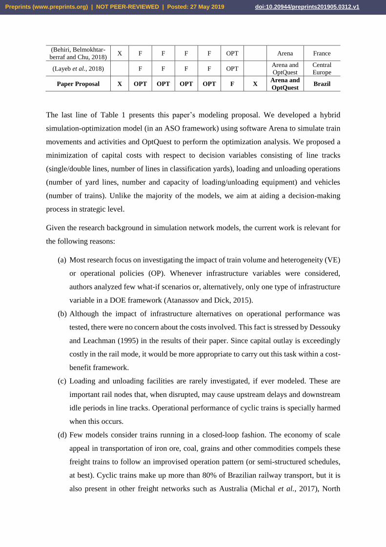
A summary of the simulation network models discussed is chronologically shown in Table 1.

The second column indicates whether or not dispatching rules (DR) were considered in the



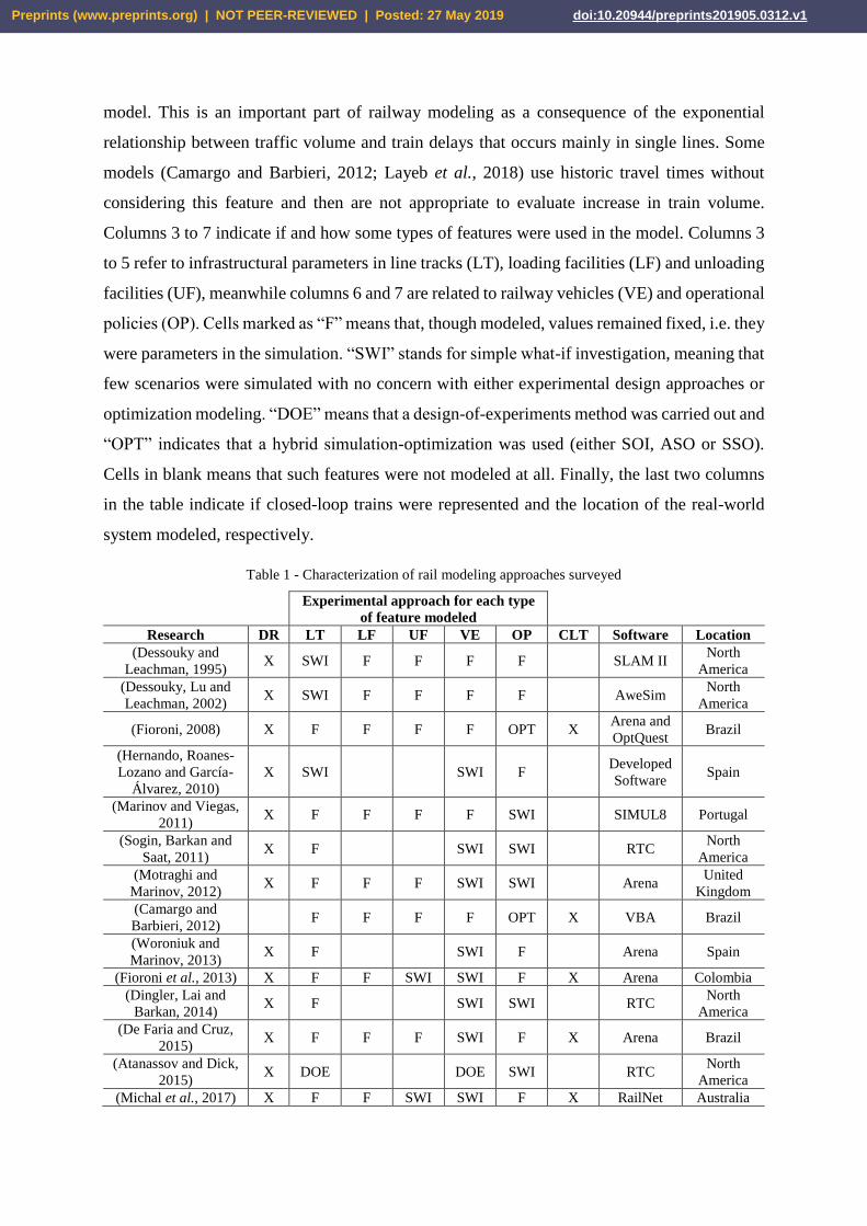
model. This is an important part of railway modeling as a consequence of the exponential

relationship between traffic volume and train delays that occurs mainly in single lines. Some

models (Camargo and Barbieri, 2012; Layeb et al., 2018) use historic travel times without

considering this feature and then are not appropriate to evaluate increase in train volume.

Columns 3 to 7 indicate if and how some types of features were used in the model. Columns 3

to 5 refer to infrastructural parameters in line tracks (LT), loading facilities (LF) and unloading

facilities (UF), meanwhile columns 6 and 7 are related to railway vehicles (VE) and operational

policies (OP). Cells marked as “F” means that, though modeled, values remained fixed, i.e. they

were parameters in the simulation. “SWI” stands for simple what-if investigation, meaning that

few scenarios were simulated with no concern with either experimental design approaches or

optimization modeling. “DOE” means that a design-of-experiments method was carried out and

“OPT” indicates that a hybrid simulation-optimization was used (either SOI, ASO or SSO).

Cells in blank means that such features were not modeled at all. Finally, the last two columns

in the table indicate if closed-loop trains were represented and the location of the real-world

system modeled, respectively.

Table 1 - Characterization of rail modeling approaches surveyed

Experimental approach for each type

of feature modeled

Research DR LT LF UF VE OP CLT Software Location

(Dessouky and

Leachman, 1995) X SWI F F F F SLAM II

North

America

(Dessouky, Lu and

Leachman, 2002) X SWI F F F F AweSim

North

America

(Fioroni, 2008) X F F F F OPT X Arena and

OptQuest Brazil

(Hernando, Roanes-

Lozano and García-

Álvarez, 2010)

X SWI SWI F Developed

Software Spain

(Marinov and Viegas,

2011) X F F F F SWI SIMUL8 Portugal

(Sogin, Barkan and

Saat, 2011) X F SWI SWI RTC

North

America

(Motraghi and

Marinov, 2012) X F F F SWI SWI Arena

United

Kingdom

(Camargo and

Barbieri, 2012) F F F F OPT X VBA Brazil

(Woroniuk and

Marinov, 2013) X F SWI F Arena Spain

(Fioroni et al., 2013) X F F SWI SWI F X Arena Colombia

(Dingler, Lai and

Barkan, 2014) X F SWI SWI RTC

North

America

(De Faria and Cruz,

2015) X F F F SWI F X Arena Brazil

(Atanassov and Dick,

2015) X DOE DOE SWI RTC

North

America

(Michal et al., 2017) X F F SWI SWI F X RailNet Australia



(Behiri, Belmokhtar-

berraf and Chu, 2018) X F F F F OPT Arena France

(Layeb et al., 2018) F F F F OPT Arena and

OptQuest

Central

Europe

Paper Proposal X OPT OPT OPT OPT F X Arena and

OptQuest Brazil

The last line of Table 1 presents this paper’s modeling proposal. We developed a hybrid

simulation-optimization model (in an ASO framework) using software Arena to simulate train

movements and activities and OptQuest to perform the optimization analysis. We proposed a

minimization of capital costs with respect to decision variables consisting of line tracks

(single/double lines, number of lines in classification yards), loading and unloading operations

(number of yard lines, number and capacity of loading/unloading equipment) and vehicles

(number of trains). Unlike the majority of the models, we aim at aiding a decision-making

process in strategic level.

Given the research background in simulation network models, the current work is relevant for

the following reasons:

(a) Most research focus on investigating the impact of train volume and heterogeneity (VE)

or operational policies (OP). Whenever infrastructure variables were considered,

authors analyzed few what-if scenarios or, alternatively, only one type of infrastructure

variable in a DOE framework (Atanassov and Dick, 2015).

(b) Although the impact of infrastructure alternatives on operational performance was

tested, there were no concern about the costs involved. This fact is stressed by Dessouky

and Leachman (1995) in the results of their paper. Since capital outlay is exceedingly

costly in the rail mode, it would be more appropriate to carry out this task within a cost-

benefit framework.

(c) Loading and unloading facilities are rarely investigated, if ever modeled. These are

important rail nodes that, when disrupted, may cause upstream delays and downstream

idle periods in line tracks. Operational performance of cyclic trains is specially harmed

when this occurs.

(d) Few models consider trains running in a closed-loop fashion. The economy of scale

appeal in transportation of iron ore, coal, grains and other commodities compels these

freight trains to follow an improvised operation pattern (or semi-structured schedules,

at best). Cyclic trains make up more than 80% of Brazilian railway transport, but it is

also present in other freight networks such as Australia (Michal et al., 2017), North



America and Western Europe (Marinov and Viegas, 2011). Despite the benefits of

structured-fixed schedules, this operational production pattern requires high level of

management standardization that has not yet been fully implemented.

3. METHOD

3.1. System Description

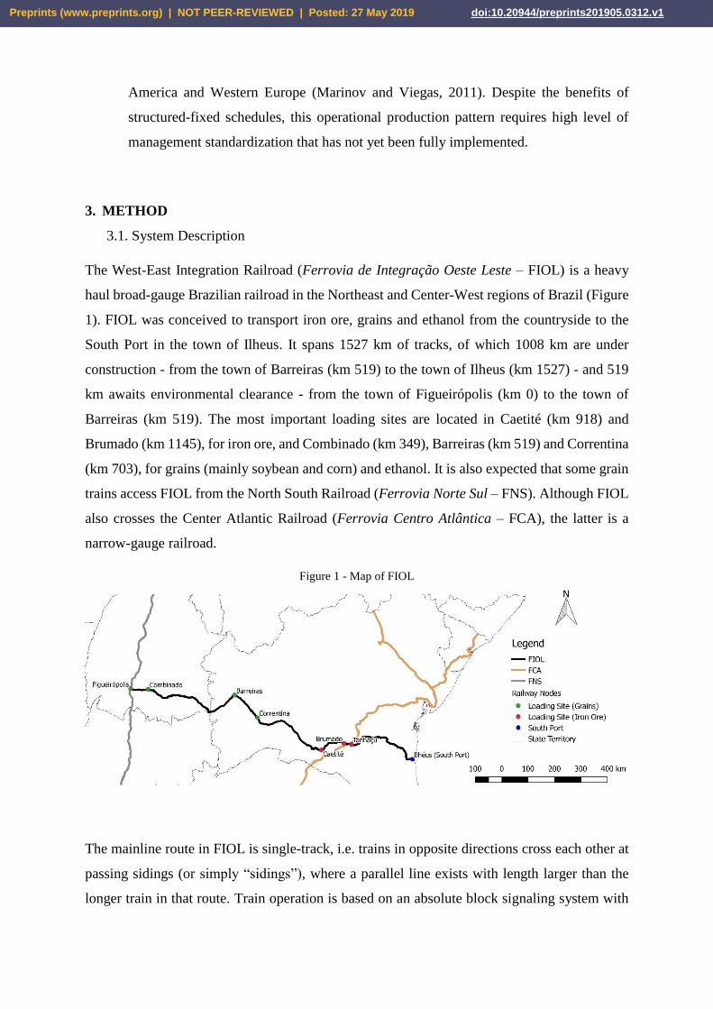
The West-East Integration Railroad (Ferrovia de Integração Oeste Leste – FIOL) is a heavy

haul broad-gauge Brazilian railroad in the Northeast and Center-West regions of Brazil (Figure

1). FIOL was conceived to transport iron ore, grains and ethanol from the countryside to the

South Port in the town of Ilheus. It spans 1527 km of tracks, of which 1008 km are under

construction - from the town of Barreiras (km 519) to the town of Ilheus (km 1527) - and 519

km awaits environmental clearance - from the town of Figueirópolis (km 0) to the town of

Barreiras (km 519). The most important loading sites are located in Caetité (km 918) and

Brumado (km 1145), for iron ore, and Combinado (km 349), Barreiras (km 519) and Correntina

(km 703), for grains (mainly soybean and corn) and ethanol. It is also expected that some grain

trains access FIOL from the North South Railroad (Ferrovia Norte Sul – FNS). Although FIOL

also crosses the Center Atlantic Railroad (Ferrovia Centro Atlântica – FCA), the latter is a

narrow-gauge railroad.

Figure 1 - Map of FIOL

The mainline route in FIOL is single-track, i.e. trains in opposite directions cross each other at

passing sidings (or simply “sidings”), where a parallel line exists with length larger than the

longer train in that route. Train operation is based on an absolute block signaling system with



2 section blocks between sidings. It is important to mention that only one train at a time is

allowed to travel along each block. Maximum train speed is 60 km/h for loaded trains and 70

km/h for empty trains and no passenger service is envisaged to run in FIOL. Then, there is no

concern about priority heterogeneity in this railroad.

3.2. System Modeling and Simulation

The transport of iron ore plays an important role in the feasibility of FIOL. It is expected that

70% of total freight revenues comes from the transport of such commodity in early operational

phase (Brasil, 2010). For this reason, the scope of the model is limited to train traffic in 539 km

of tracks between Caetité and Ilhéus, including train activities in loading and unloading

terminals. The construction of this stretch of railroad achieved 80% of physical progress (Brasil,

2019) and, when completed, further investments in nonexistent loading/unloading terminals

and vehicles are going to be necessary. Although upstream train movements and activities from

Figueirópolis to Caetité were not modeled, the expected flow from these trains within the region

modeled were considered.

The iron ore rail freight is conceived based upon a closed-loop system. As mentioned before,

cyclic trains are unitarian trains with a fixed number of railcars that run continuously through a

closed-circuit comprising loading, moving loaded to a port rail terminal, unloading and moving

empty to a loading terminal next to the mines. These trains are subject to several interferences

from both interaction with other trains and disruptions in loading and unloading processes.

To model this system, we used a decomposition approach, breaking down the rail network into

3 components: rail lines, rail loading terminal and rail unloading terminal. Marinov and Viegas

(2011) point out that this is a practical approach that has already proven its credibility. By

bringing these pieces together the railway network can be precisely modeled. The conceptual

models from these three parts are described in sections 3.2.1 to 3.2.3.

3.2.1. Rail Line

The 539 km of tracks between Caetité and Ilhéus consists of single lines interleaved by 19

sidings. A typical iron ore train consists of 2 locomotives and 140 gondola railcars. In order to

fit these trains, sidings between Caetité and Ilhéus have 2023 m length. The conceptual model

for train movement in rail lines has the main objective to the decide whether to halt or allow for

each train to move to the next section of track. The decision of halting a train is made in order

to avoid a frontal collision, a rear collision or a deadlock. According to Pachl (2007), “a



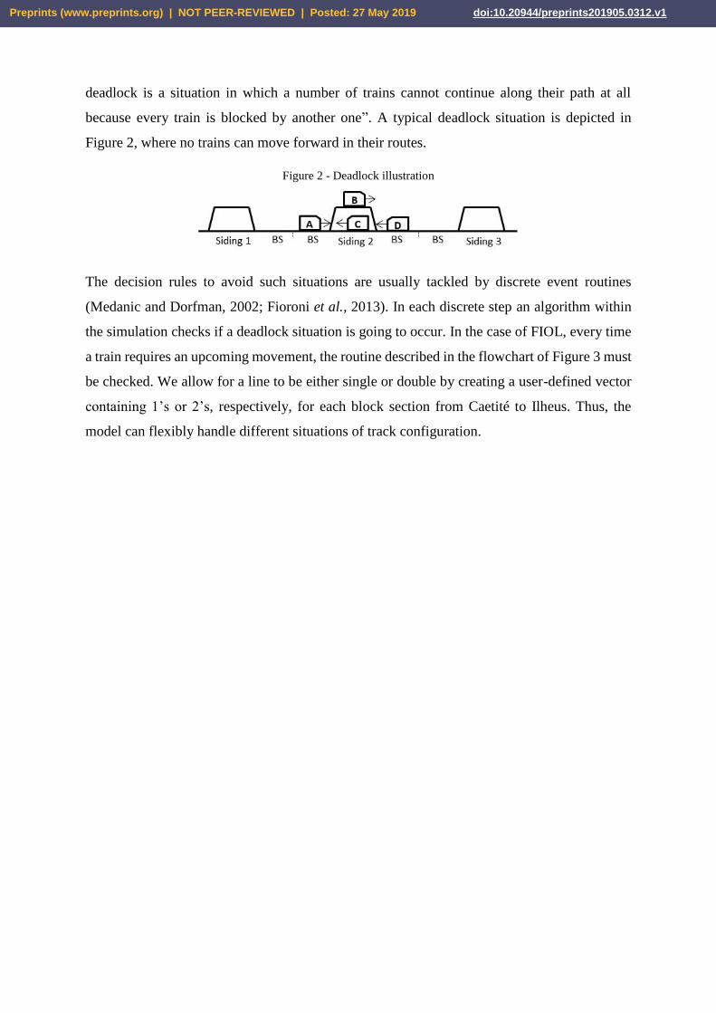
deadlock is a situation in which a number of trains cannot continue along their path at all

because every train is blocked by another one”. A typical deadlock situation is depicted in

Figure 2, where no trains can move forward in their routes.

Figure 2 - Deadlock illustration

The decision rules to avoid such situations are usually tackled by discrete event routines

(Medanic and Dorfman, 2002; Fioroni et al., 2013). In each discrete step an algorithm within

the simulation checks if a deadlock situation is going to occur. In the case of FIOL, every time

a train requires an upcoming movement, the routine described in the flowchart of Figure 3 must

be checked. We allow for a line to be either single or double by creating a user-defined vector

containing 1’s or 2’s, respectively, for each block section from Caetité to Ilheus. Thus, the

model can flexibly handle different situations of track configuration.



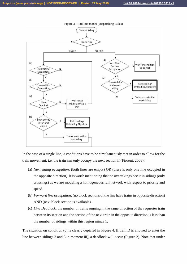
Figure 3 - Rail line model (Dispatching Rules)

In the case of a single line, 3 conditions have to be simultaneously met in order to allow for the

train movement, i.e. the train can only occupy the next section if (Fioroni, 2008):

(a) Next siding occupation: (both lines are empty) OR (there is only one line occupied in

the opposite direction). It is worth mentioning that no overtakings occur in sidings (only

crossings) as we are modeling a homogeneous rail network with respect to priority and

speed.

(b) Forward line occupation: (no block sections of the line have trains in opposite direction)

AND (next block section is available).

(c) Line Deadlock: the number of trains running in the same direction of the requester train

between its section and the section of the next train in the opposite direction is less than

the number of sidings within this region minus 1.

The situation on condition (c) is clearly depicted in Figure 4. If train D is allowed to enter the

line between sidings 2 and 3 in moment iii), a deadlock will occur (Figure 2). Note that under



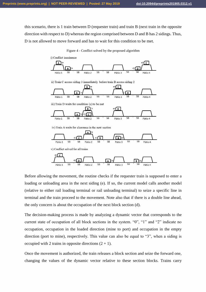
this scenario, there is 1 train between D (requester train) and train B (next train in the opposite

direction with respect to D) whereas the region comprised between D and B has 2 sidings. Thus,

D is not allowed to move forward and has to wait for this condition to be met.

Figure 4 - Conflict solved by the proposed algorithm

Before allowing the movement, the routine checks if the requester train is supposed to enter a

loading or unloading area in the next siding (e). If so, the current model calls another model

(relative to either rail loading terminal or rail unloading terminal) to seize a specific line in

terminal and the train proceed to the movement. Note also that if there is a double line ahead,

the only concern is about the occupation of the next block section (d).

The decision-making process is made by analyzing a dynamic vector that corresponds to the

current state of occupation of all block sections in the system. “0”, “1” and “2” indicate no

occupation, occupation in the loaded direction (mine to port) and occupation in the empty

direction (port to mine), respectively. This value can also be equal to “3”, when a siding is

occupied with 2 trains in opposite directions (2 + 1).

Once the movement is authorized, the train releases a block section and seize the forward one,

changing the values of the dynamic vector relative to these section blocks. Trains carry



attributes related to the direction of travel (“1” for loaded direction and “2” for empty direction).

This attribute is changed as soon as trains leave terminals. As they seize (release) a section, the

vector slot relative to this section is added (subtracted) by this attribute value. Therefore, it is

possible for all trains in a discrete step in time move onwards or wait for an opportunity to do

so.

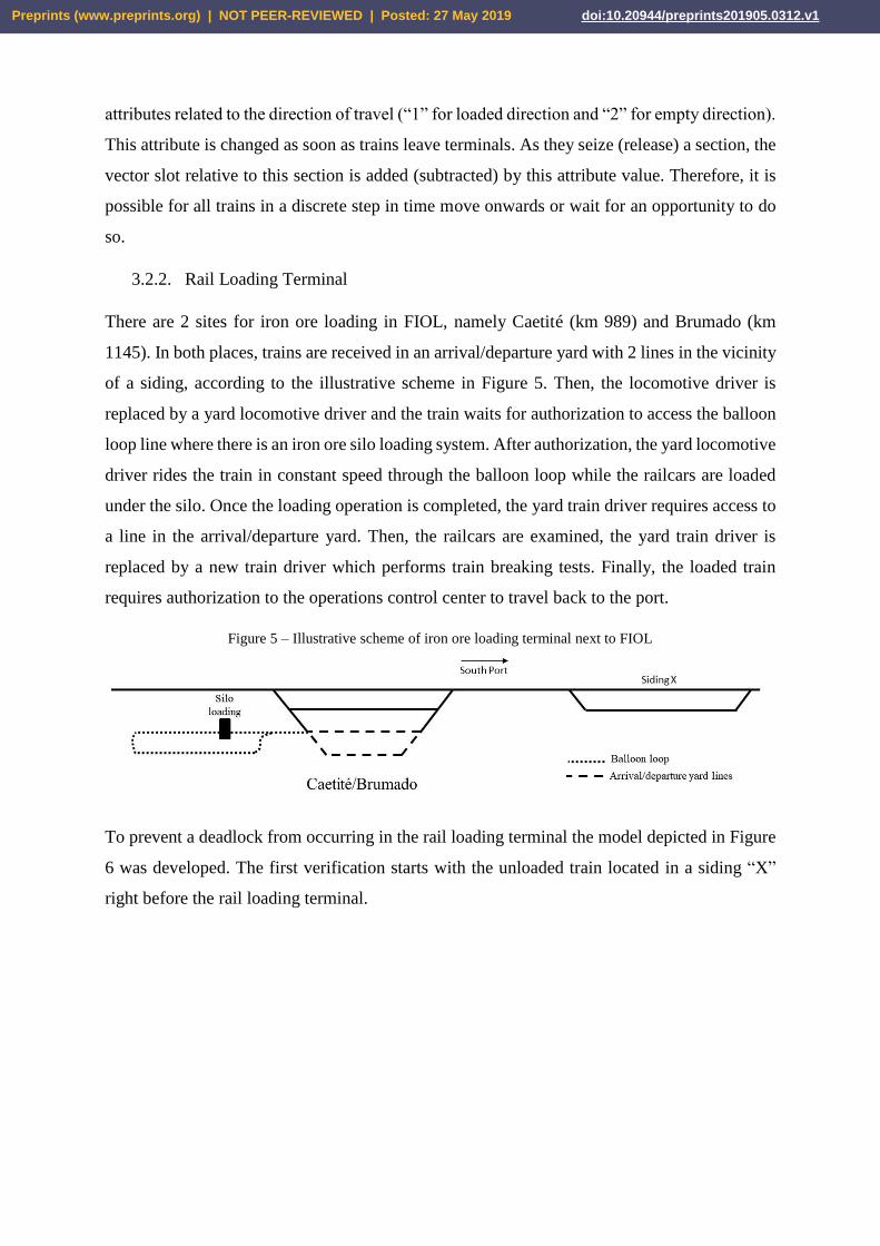
3.2.2. Rail Loading Terminal

There are 2 sites for iron ore loading in FIOL, namely Caetité (km 989) and Brumado (km

1145). In both places, trains are received in an arrival/departure yard with 2 lines in the vicinity

of a siding, according to the illustrative scheme in Figure 5. Then, the locomotive driver is

replaced by a yard locomotive driver and the train waits for authorization to access the balloon

loop line where there is an iron ore silo loading system. After authorization, the yard locomotive

driver rides the train in constant speed through the balloon loop while the railcars are loaded

under the silo. Once the loading operation is completed, the yard train driver requires access to

a line in the arrival/departure yard. Then, the railcars are examined, the yard train driver is

replaced by a new train driver which performs train breaking tests. Finally, the loaded train

requires authorization to the operations control center to travel back to the port.

Figure 5 – Illustrative scheme of iron ore loading terminal next to FIOL

To prevent a deadlock from occurring in the rail loading terminal the model depicted in Figure

6 was developed. The first verification starts with the unloaded train located in a siding “X”

right before the rail loading terminal.



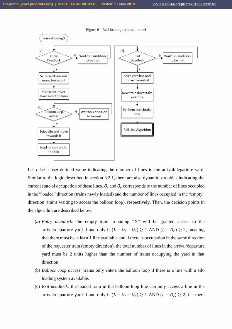
Figure 6 - Rail loading terminal model

Let 𝐿 be a user-defined value indicating the number of lines in the arrival/departure yard.

Similar to the logic described in section 3.2.1, there are also dynamic variables indicating the

current state of occupation of these lines. 𝑂𝑙 and 𝑂𝑒 corresponds to the number of lines occupied

in the “loaded” direction (trains newly loaded) and the number of lines occupied in the “empty”

direction (trains waiting to access the balloon loop), respectively. Then, the decision points in

the algorithm are described below:

(a) Entry deadlock: the empty train in siding “X” will be granted access to the

arrival/departure yard if and only if (𝐿 − 𝑂𝑙 − 𝑂𝑒) ≥ 1 AND (𝐿 − 𝑂𝑒) ≥ 2, meaning

that there must be at least 1 line available and if there is occupation in the same direction

of the requester train (empty direction), the total number of lines in the arrival/departure

yard must be 2 units higher than the number of trains occupying the yard in that

direction.

(b) Balloon loop access: trains only enters the balloon loop if there is a line with a silo

loading system available.

(c) Exit deadlock: the loaded train in the balloon loop line can only access a line in the

arrival/departure yard if and only if (𝐿 − 𝑂𝑙 − 𝑂𝑒) ≥ 1 AND (𝐿 − 𝑂𝑙) ≥ 2, i.e. there



must be at least 1 line available and if there is occupation in the same direction of the

requester train (loaded direction), the total number of lines in the arrival/departure yard

must be 2 units higher than the number of trains occupying the yard in that direction.

Note again that the model rules allow for different number of lines in the arrival/departure yard

and more than one silo loading system without loss of generality.

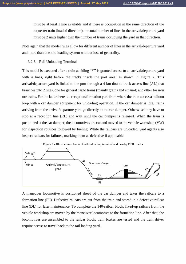
3.2.3. Rail Unloading Terminal

This model is executed after a train at siding “Y” is granted access to an arrival/departure yard

with 4 lines, right before the tracks inside the port area, as shown in Figure 7. This

arrival/departure yard is linked to the port through a 4 km double-track access line (AL) that

branches into 2 lines, one for general cargo trains (mainly grains and ethanol) and other for iron

ore trains. For the latter there is a reception/formation yard from where the train access a balloon

loop with a car dumper equipment for unloading operation. If the car dumper is idle, trains

arriving from the arrival/departure yard go directly to the car dumper. Otherwise, they have to

stop at a reception line (RL) and wait until the car dumper is released. When the train is

positioned at the car dumper, the locomotives are cut and moved to the vehicle workshop (VW)

for inspection routines followed by fueling. While the railcars are unloaded, yard agents also

inspect railcars for failures, marking them as defective if applicable.

Figure 7 - Illustrative scheme of rail unloading terminal and nearby FIOL tracks

A maneuver locomotive is positioned ahead of the car dumper and takes the railcars to a

formation line (FL). Defective railcars are cut from the train and stored in a defective railcar

line (DL) for later maintenance. To complete the 140-railcar block, fixed-up railcars from the

vehicle workshop are moved by the maneuver locomotive to the formation line. After that, the

locomotives are assembled to the railcar block, train brakes are tested and the train driver

require access to travel back to the rail loading yard.



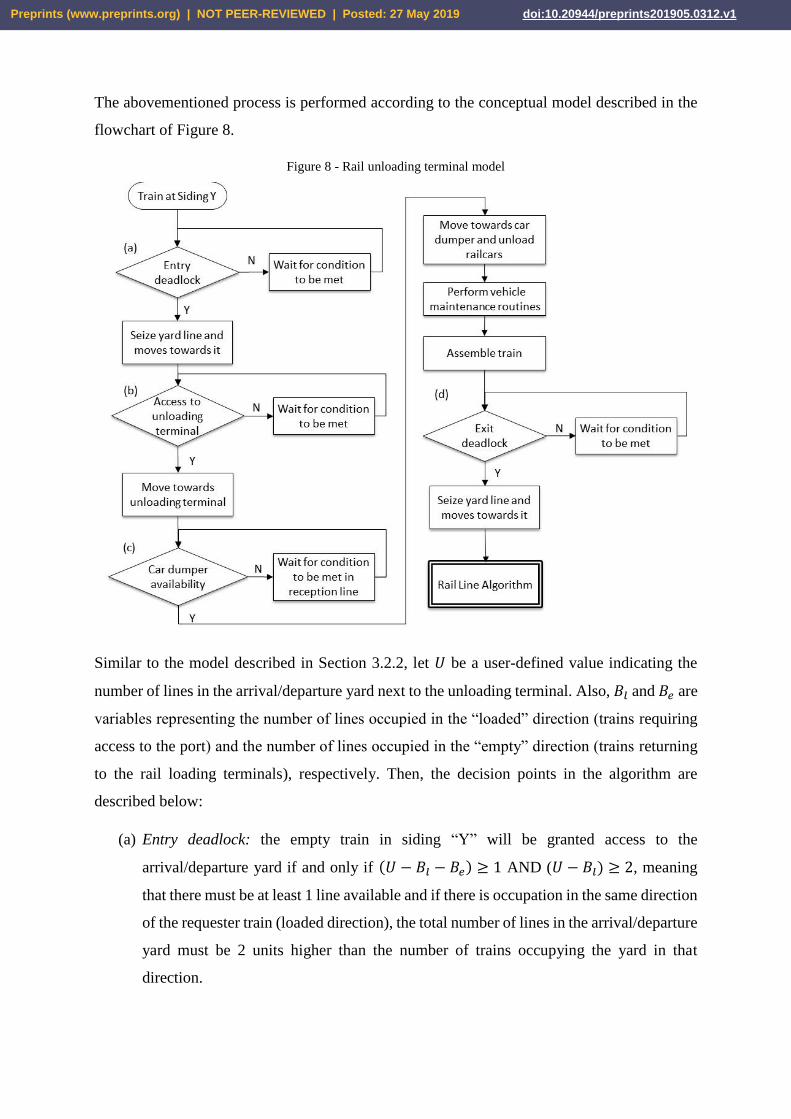
The abovementioned process is performed according to the conceptual model described in the

flowchart of Figure 8.

Figure 8 - Rail unloading terminal model

Similar to the model described in Section 3.2.2, let 𝑈 be a user-defined value indicating the

number of lines in the arrival/departure yard next to the unloading terminal. Also, 𝐵𝑙 and 𝐵𝑒 are

variables representing the number of lines occupied in the “loaded” direction (trains requiring

access to the port) and the number of lines occupied in the “empty” direction (trains returning

to the rail loading terminals), respectively. Then, the decision points in the algorithm are

described below:

(a) Entry deadlock: the empty train in siding “Y” will be granted access to the

arrival/departure yard if and only if (𝑈 − 𝐵𝑙 − 𝐵𝑒) ≥ 1 AND (𝑈 − 𝐵𝑙) ≥ 2, meaning

that there must be at least 1 line available and if there is occupation in the same direction

of the requester train (loaded direction), the total number of lines in the arrival/departure

yard must be 2 units higher than the number of trains occupying the yard in that

direction.



(b) Access to unloading terminal: (access line is available) AND (formation line is

available).

(c) Car dumper availability: verifies if there is a car dumper line available. If so, train

access car dumper directly. Otherwise, train must wait in the reception line.

(d) Exit Deadlock: the unloaded train in the formation line can only access a line in the

arrival/departure yard if and only if (𝑈 − 𝐵𝑙 − 𝐵𝑒) ≥ 1 AND (𝐿 − 𝐵𝑒) ≥ 2, i.e. there

must be at least 1 line available and if there is occupation in the same direction of the

requester train (empty direction), the total number of lines in the arrival/departure yard

must be 2 units higher than the number of trains occupying the yard in that direction

The rules can be applied to any value of 𝑈 without loss of generality. For the sake of simplicity,

we do not consider maintenance aspects of the system, i.e. the time elapsed from the end of

unloading operation to the formation of the train is considered as if all railcars are not defective.

3.2.4. Simulation

The conceptual models from previous sections were implemented in Arena, developed by

Rockwell Software, the most used simulation tool in supply chain and logistics (Oliveira, Lima

and Montevechi, 2016). The computational model is developed by attaching command blocks

to the work area representing pre-defined actions in the SIMAN language. The software allows

for an intuitive development environment that facilitates the construction of models and their

evaluation by standardized reports and experimental routines.

All input values of the model were collected from operational reports from both FIOL (Brasil,

2010) and South Port (Bahia, 2011). Time values include but are not limited to: loading and

unloading times, travel times between sidings, inspection and breaking tests and licensing

authorization. As these values are deterministic, we carried out a simulation in a dynamic-

deterministic fashion.

The entities of the model are the trains, inserted by CREATE blocks. Two CREATE blocks

generate a pre-defined number of cyclic iron ore trains at Caetité and Brumado that move

through the system until the end of simulation. Eight CREATE blocks are placed at the borders

of the system (4 in Caetité and 4 in Ilhéus) to generate the volume associated with grain and

ethanol trains in both directions. The times between arrivals for these eight CREATE blocks

were defined based on the generation of trains from Figueirópolis, Combinado, Barreiras and

Correntina. As soon as these trains hit the opposite frontier relative to where they were created,

a DISPOSE block remove them from the system.



The trains move through the system between geographically separated locations (represented

by STATION blocks) using ROUTE blocks. They obey the model logic and demand resources

(such as rail lines and equipment like silos and car dumpers) as soon as they are available. After

being used, the resource is released and becomes available for another train to use it. All this

process is performed by using SEIZE, DELAY and RELEASE blocks. When these resources

are busy or the trains are not allowed to use them in order to avoid an accident or a deadlock,

they must wait for a favorable condition. In these cases, they wait in the queue of either a SEIZE

block or a HOLD block, the latter being able to deal with more complex logical decisions.

Important times are recorded such as waiting times, time elapsed within terminals as well as

the whole iron ore cycle (load → move → unload → move). It is also recorded the total tonnage

delivered in port for a specific period by RECORD blocks that store this quantity in a tally

variable.

The system works in a non-terminal fashion, i.e. it starts in a specific period of time and runs

indefinitely. Since the system starts empty, the first trains move throughout their routes without

facing conflicts with other trains, biasing down the average iron ore cycle time. Accordingly, it

was defined a warm-up period of 200 hours in which the results are removed from the

simulation. Thus, the system is analyzed from the stationary state onwards. As the simulation

is deterministic it was carried out a unique replication of 1 month to produce and analyze the

outcomes.

3.3. Optimization Model

The proposed optimization model was motivated by the hypothesis that the current set of

projected infrastructure parameters does not provide an operational efficiency that meets the

overall mining production from Caetité and Brumado. As soon as the construction of FIOL

finishes, it will be necessary to incur in supplementary capital costs related to rail terminals and

vehicles. Then, some interventions considering trackage configuration, quantity and capacity

of equipment and fleet sizing are tested in order to achieve this goal at minimal cost. The model

is defined as follows:

𝑀𝑖𝑛 𝑍 = 𝑅𝑉 + 𝐿𝐷 + 𝑆𝐿 + 𝑌𝐿 + 𝑈𝑇 + 𝐶𝐷 + 𝑌𝑈, 𝑠. 𝑡.: (1)

𝑃𝐶𝐴𝐸 ≥ 𝐺𝐶𝐴𝐸 (2)

𝑃𝐵𝑅𝑈 ≥ 𝐺𝐵𝑅𝑈 (3)

𝑆𝐶𝐴𝐸𝐼 + 𝑆𝐶𝐴𝐸

𝐼𝐼 + 𝑆𝐶𝐴𝐸𝐼𝐼𝐼 ≥ 1 (4)



𝑆𝐵𝑅𝑈𝐼 + 𝑆𝐵𝑅𝑈

𝐼𝐼 + 𝑆𝐵𝑅𝑈𝐼𝐼𝐼 ≥ 1 (5)

𝐷𝑃1𝐼 + 𝐷𝑃1

𝐼𝐼 ≥ 1 (6)

𝐷𝑃2𝐼 + 𝐷𝑃2

𝐼𝐼 ≥ 𝑃 (7)

0 ≤ 𝑆𝐶𝐴𝐸𝑗

≤ 2, ∀ 𝑗 (8)

0 ≤ 𝑆𝐵𝑅𝑈𝑗

≤ 2, ∀ 𝑗 (9)

0 ≤ 𝐷𝑃1𝑘 ≤ 2, ∀ 𝑘 (10)

0 ≤ 𝐷𝑃2𝑘 ≤ 2, ∀ 𝑘 (11)

6 ≤ 𝑇𝐶𝐴𝐸 ≤ 9 (12)

8 ≤ 𝑇𝐵𝑅𝑈 ≤ 12 (13)

2 ≤ 𝐿𝐶𝐴𝐸 ≤ 5 (14)

2 ≤ 𝐿𝐵𝑅𝑈 ≤ 5 (15)

4 ≤ 𝑈 ≤ 7 (16)

𝑆𝐶𝐴𝐸𝑗

, 𝑆𝐵𝑅𝑈𝑗

, ∀𝑗; 𝐷𝑃1𝑘 , 𝐷𝑃2

𝑘 , ∀𝑘; 𝑇𝐶𝐴𝐸, 𝑇𝐵𝑅𝑈, 𝐿𝐶𝐴𝐸, 𝐿𝐵𝑅𝑈, 𝑈 ∈ 𝒁+ (17)

𝐵𝑖 ∈ (0,1), ∀ 𝑖 e 𝑃 ∈ (0,1) (18)

In the objective function (1), 𝑍 is the sum of all supplementary investments to be made in this

rail network. It consists of the following items:

a) Rail Vehicles (𝑅𝑉):

(𝑇𝐶𝐴𝐸 + 𝑇𝐵𝑅𝑈)(140𝐶𝑟𝑐 + 2𝐶𝑙𝑐)

Where 𝑇𝐶𝐴𝐸 e 𝑇𝐵𝑅𝑈 are decision variables representing the number of trains

formed in both Caetité and Brumado. 𝐶𝑟𝑐 and 𝐶𝑙𝑐 are the purchasing costs of a

gondola railcar and a GE Dash 9 locomotive, respectively, both in Brazilian

Reais/unit (R$/unit);

b) Line Duplication (𝐿𝐷):

∑ 𝐵𝑖𝑙𝑖𝐶𝑚𝑙

19

𝑖=1

Where 𝐵𝑖 is a binary decision variable indicating whether the line 𝑖 between

adjacent sidings has to be duplicated (1) or not (0). 𝑙𝑖 is the length of this line (in

km) and 𝐶𝑚𝑙 is the average cost of mainline duplication (in R$/km).

c) Silo Loading System (𝑆𝐿):



∑(𝑆𝐶𝐴𝐸𝑗

+ 𝑆𝐵𝑅𝑈𝑗

)(𝐶𝑠𝑗

+ 𝑙𝑠𝐶𝑦)

𝐼𝐼𝐼

𝑗=𝐼

Where 𝑆𝐶𝐴𝐸𝑗

e 𝑆𝐵𝑅𝑈𝑗

are decision variables corresponding to the number of silo

loading systems of type 𝑗 in the rail loading terminals of Caetité and Brumado,

respectively. There are 3 types of system depending on the capacity of the

equipment used: type I loads 4000 t/h (4.32 h/train), type II loads 6000 t/h (2.88

h/train) and type 3 loads 16000 t/h (1.08 h/train). Also, 𝐶𝑠𝑗 is the cost of silo

equipment of type 𝑗, 𝑙𝑠 is the length of the balloon loop of the silo (in km) and

𝐶𝑦 is the average cost of yard lines (in R$/km).

d) Arrival/departure yard in the loading rail terminal (𝑌𝐿):

(𝐿𝐶𝐴𝐸 + 𝐿𝐵𝑅𝑈)(𝑙𝑦𝑙𝐶𝑦 + 2𝐶𝑠𝑤)

Where 𝐿𝐶𝐴𝐸 and 𝐿𝐵𝑅𝑈 are decision variables representing the number of lines in

the arrival/departure yard in the loading terminal of Caetité and Brumado,

respectively. 𝑙𝑦𝑙 is the length of each line (in km), 𝐶𝑦 is the average cost of yard

lines (in R$/km) and 𝐶𝑠𝑤 is the cost of a railroad switch (in R$/unit).

e) Unloading Port Terminal (𝑈𝑇):

(𝑃 + 1)𝐶𝑝

Where 𝑃 is a binary decision variable relative to the existence of an additional

unloading port terminal, consisting of a stacker-reclaimer system, conveyor

belts, civil works and ancillary equipment. 𝑃 is equal to 1 if an additional

terminal has to be implemented and 0 otherwise. 𝐶𝑝 is the capital cost of this

unloading port terminal (R$/terminal).

f) Car Dumper System (𝐶𝐷):

∑(𝐷𝑃1𝑘 + 𝐷𝑃2

𝑘 )(𝐶𝑑𝑘 + 𝑙𝑑𝐶𝑦)

𝐼𝐼

𝑘=𝐼

Where 𝐷𝑃1𝑘 and 𝐷𝑃2

𝑘 are decision variables defining the number of car dumper

systems (i.e. a car dumper equipment and a balloon loop) of type 𝑘 in the original

unloading port terminals (P1) and the additional terminal (P2), respectively. 𝑘 =

𝐼 represents a simple car dumper, with capacity of 4000 t/h (4.32 h/train) and

𝑘 = 𝐼𝐼 refers to a double car dumper, with capacity of 9400 t/h (2.16 h/train).

𝐶𝑑𝑘 is the cost of a car-dumper equipment of type 𝑘 (in R$/unit) and 𝑙𝑑 is the

length of the balloon loop (in km).



g) Arrival/departure yard next to the unloading rail terminal (𝑌𝑈):

𝑈(𝑙𝑦𝑢𝐶𝑦 + 2𝐶𝑠𝑤)

Where 𝑈 is the decision variable relative to the number of lines in the

arrival/departure yard next to the port and 𝑙𝑦𝑢 is the length of a line in this

terminal.

The cost values above (𝐶.) were gathered from the operational reports mentioned before (Brasil,

2010; Bahia, 2011) and surveys conducted with the Brazilian National Agency of Land

Transport and the commercial department of the equipment manufacturing company

Thyssenkrupp. As these nominal values did not correspond to the same moment at time, they

were adjusted for inflation to the base year of 2019.

The inequalities in (2) and (3) guarantee that the monthly iron ore delivered in port, 𝑃𝐶𝐴𝐸 and

𝑃𝐵𝑅𝑈, are greater than or equal to pre-defined goals 𝐺𝐶𝐴𝐸 and 𝐺𝐵𝑅𝑈, respectively. Next, the

constraints (4) to (7) assure that all trains are met by at list 1 silo system in their loading

operations and by at least 1 car dumper system in their unloading port terminals. The ranges

from (8) to (16) define a hyperspace of feasible solutions for the integer decision variables of

the model. Finally, (17) and (18) define variables as either integer or binary, respectively.

As mentioned before, the approach to solve this problem is given by an alternate simulation-

optimization (ASO) approach in which a search algorithm uses the results of a simulation trial

in order to continually improve the solution. This model is solved using OptQuest, a commercial

software provided by OptTek System Inc. OptQuest uses a combination of meta-heuristics like

tabu search and scatter search along with neural networks for its search algorithm (Layeb et al.,

2018). From an initial solution given by the user, it was defined a maximum number of

iterations equal to 2000 to observe the evolution of the objective function.

4. COMPUTATIONAL RESULTS AND ANALYSIS

The model was validated by comparing the average cycle time of iron ore trains loading in

Caetité given by the simulation to the results observed in previous operational studies (Brasil,

2010),for two production levels. The first production level accounts for only 6 iron ore trains

loading in Caetité whereas the second includes other trains from Barreiras, Correntina and

Combinado. The model produced satisfactory results with cyclic time differential of 3,54% in

the first scenario and 1,33% for the second one. The model was also verified with respect to the

rules developed in sections 3.2.1 to 3.2.3, producing neither deadlocks nor insecure conditions.



4.1. Simulation of Baseline Scenario

The baseline scenario consists of single tracks (𝐵𝑖 = 0, ∀ 𝑖), 6 trains loading in Caetité (𝑇𝐶𝐴𝐸 =

6), one silo loading system of type I for Caetité and Brumado (𝑆𝐶𝐴𝐸𝐼 = 𝑆𝐵𝑅𝑈

𝐼 = 1), 2 lines for

the arrival/departure yard in the loading terminal for Caetité and Brumado (𝐿𝐶𝐴𝐸 = 𝐿𝐵𝑅𝑈 = 2),

no additional unloading terminal (𝑃 = 0), a double car dumper system (𝐷𝑃1𝐼𝐼 = 1) and 4 lines in

the arrival/departure yard next to the unloading terminal (𝑈 = 4).

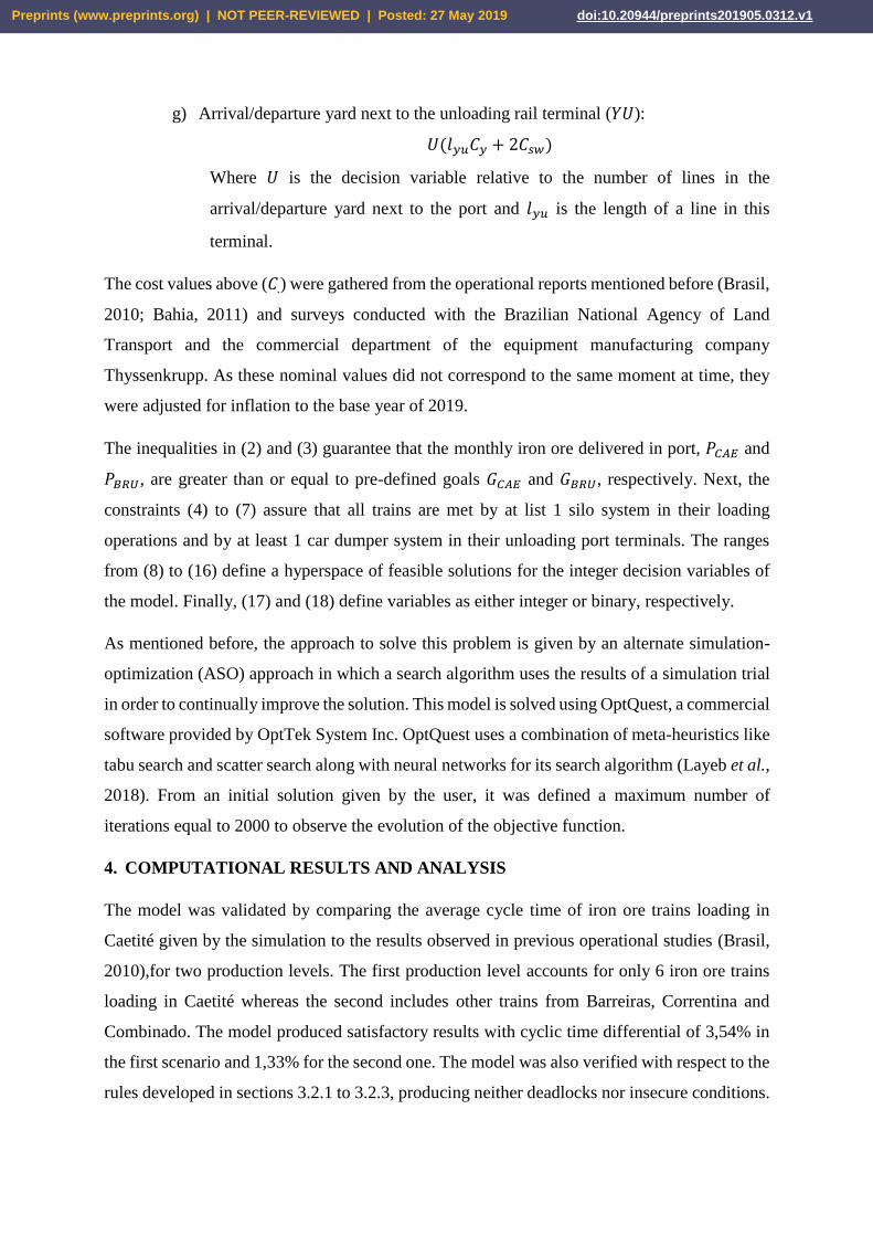
The production goals for the mining companies is roughly 𝐺𝐶𝐴𝐸 = 1.67 million t/month for

Caetité and 𝐺𝐵𝑅𝑈 = 2.92 million t/month for Brumado. However, the number of trains for the

latter was not investigated in early operational studies (Brasil, 2010) as new mining companies

intended to join the supply chain afterwards. The impacts of the inclusion of trains loading in

Brumado in the total tonnage delivered in port is shown in Figure 9.

Figure 9 – Plot of average cyclic time (primary axis) and iron ore delivered in port (secondary axis).

According to the simulation outcomes no combinations among 𝑇𝐶𝐴𝐸 = 6 and 𝑇𝐵𝑅𝑈 =

{0, . . . ,12} result in the desired production goals for both sites. To diagnose the causes,

resources utilization was observed. In fact, for 𝑇𝐵𝑅𝑈 ≥ 7, the average occupation rate of the

yard/departure lines and silo loading system of the rail loading terminal in Brumado is nearly

100%. Consequently, trains loading in that site have to wait in the mainline of FIOL, provoking

queues that harms overall cyclic times for all trains, including those loading in Caetité. The

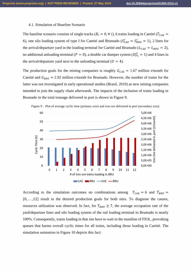
simulation animation in Figure 10 depicts this fact:



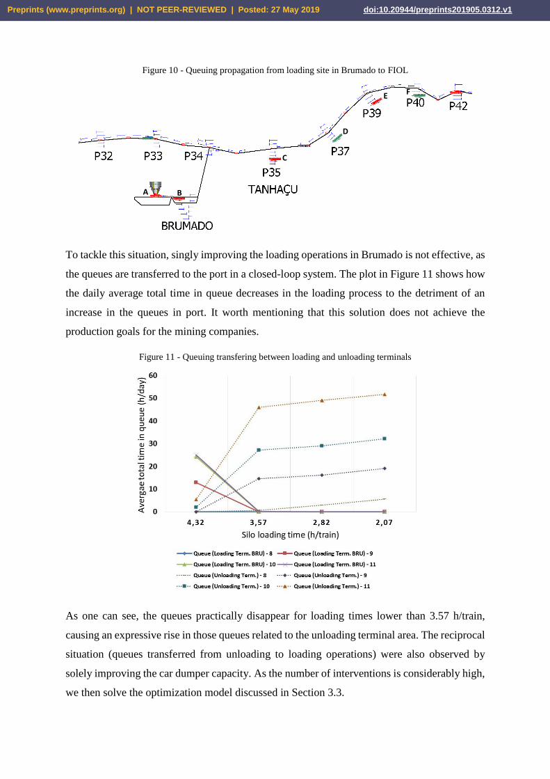
Figure 10 - Queuing propagation from loading site in Brumado to FIOL

To tackle this situation, singly improving the loading operations in Brumado is not effective, as

the queues are transferred to the port in a closed-loop system. The plot in Figure 11 shows how

the daily average total time in queue decreases in the loading process to the detriment of an

increase in the queues in port. It worth mentioning that this solution does not achieve the

production goals for the mining companies.

Figure 11 - Queuing transfering between loading and unloading terminals

As one can see, the queues practically disappear for loading times lower than 3.57 h/train,

causing an expressive rise in those queues related to the unloading terminal area. The reciprocal

situation (queues transferred from unloading to loading operations) were also observed by

solely improving the car dumper capacity. As the number of interventions is considerably high,

we then solve the optimization model discussed in Section 3.3.

A B

C

D

E F



4.2. Simulation-Optimization Results

The simulation-optimization model was run in an Intel Core i5 3.2 GHz processor, with 4.0 GB

RAM. The initial solution provided was 𝑇𝐶𝐴𝐸 = 6, 𝑇𝐵𝑅𝑈 = 9, 𝑃 = 1, 𝑆𝐶𝐴𝐸𝐼 = 𝑆𝐵𝑅𝑈

𝐼 = 𝐷𝑃1𝐼 =

𝐷𝑃2𝐼 = 1, 𝐿𝐶𝐴𝐸 = 𝐿𝐵𝑅𝑈 = 3, 𝑈 = 4 and 𝐵𝑖 = 0, ∀ 𝑖. All remaining decision variables were

assigned the value 0. The model was executed 3 times considering the current production goals

for Caetité and Brumado (baseline scenario) along with 10% and 20% increase in such levels.

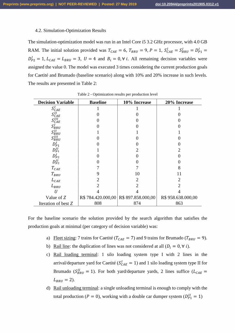
The results are presented in Table 2:

Table 2 - Optimization results per production level

Decision Variable Baseline 10% Increase 20% Increase

𝑆𝐶𝐴𝐸𝐼 1 1 1

𝑆𝐶𝐴𝐸𝐼𝐼 0 0 0

𝑆𝐶𝐴𝐸𝐼𝐼𝐼 0 0 0

𝑆𝐵𝑅𝑈𝐼 0 0 0

𝑆𝐵𝑅𝑈𝐼𝐼 1 1 1

𝑆𝐵𝑅𝑈𝐼𝐼𝐼 0 0 0

𝐷𝑃1𝐼 0 0 0

𝐷𝑃1𝐼𝐼 1 2 2

𝐷𝑃2𝐼 0 0 0

𝐷𝑃2𝐼𝐼 0 0 0

𝑇𝐶𝐴𝐸 7 7 8

𝑇𝐵𝑅𝑈 9 10 11

𝐿𝐶𝐴𝐸 2 2 2

𝐿𝐵𝑅𝑈 2 2 2

𝑈 4 4 4

Value of 𝑍 R$ 784.420.000,00 R$ 897.858.000,00 R$ 958.638.000,00

Iteration of best 𝑍 808 874 863

For the baseline scenario the solution provided by the search algorithm that satisfies the

production goals at minimal (per category of decision variable) was:

a) Fleet sizing: 7 trains for Caetité (𝑇𝐶𝐴𝐸 = 7) and 9 trains for Brumado (𝑇𝐵𝑅𝑈 = 9).

b) Rail line: the duplication of lines was not considered at all (𝐷𝑖 = 0, ∀ 𝑖).

c) Rail loading terminal: 1 silo loading system type I with 2 lines in the

arrival/departure yard for Caetité (𝑆𝐶𝐴𝐸𝐼 = 1) and 1 silo loading system type II for

Brumado (𝑆𝐵𝑅𝑈𝐼𝐼 = 1). For both yard/departure yards, 2 lines suffice (𝐿𝐶𝐴𝐸 =

𝐿𝐵𝑅𝑈 = 2).

d) Rail unloading terminal: a single unloading terminal is enough to comply with the

total production (𝑃 = 0), working with a double car dumper system (𝐷𝑃1𝐼𝐼 = 1)



The fact that the model responds to increasing production by allocating more trains and adding

another double car dumper system to the unloading rail terminal is noteworthy. It appears that

after solving the loading problem with a higher capacity silo in Brumado, the unloading facility

remains the bottleneck of the system. Another important finding is that for all scenarios tested,

the duplication in FIOL mainline route and the addition of lines in arrival/departure yards were

not chosen as alternatives. First, it seems that besides being a costly intervention, the current

trackage configuration in single lines are sufficient to the current volume of traffic. Secondly,

adding lines in departure yards is a costly alternative and do not bring any improvement in times

as the single benefit is releasing the traffic in the mainline route.

5. CONCLUSION

This work presented a hybrid simulation-optimization model to define the best set of

supplementary investments in the iron ore corridor of the West-East Integration Railroad

(FIOL), in Brazil. A state-of-the-art review was carried out to demonstrate the existing gap in

simulation network literature addressing strategic decision-making integrating mainline tracks,

loading and unloading operations. A dynamic model of the system was developed in software

Arena, including train traffic in single lines and operations in loading and unloading facilities.

Dispatching rules were developed to avoid real-world prohibited train movements that result in

collisions and deadlocks. After validation, preliminary simulation results demonstrated that the

proposed system configuration cannot meet the current iron ore production goals. It was proven

that isolated solutions in the bottlenecks of a closed-loop railway network was not effective as

the queues are merely transferred within the system. In order to present a cost-effective solution,

we minimized a capital cost function comprising investments in the mainline of the railroad,

enhancements in terminal areas and fleet sizing. For 3 production levels, the search algorithm

of the OptQuest software was able to find the best solutions by improving both silo loading and

car dumper systems and increasing the number of trains.

REFERENCES

Abril, M. et al. (2008) ‘An assessment of railway capacity’, Transportation Research Part E: Logistics and

Transportation Review, 44(5), pp. 774–806. doi: 10.1016/j.tre.2007.04.001.

Assad, A. A. (1980) ‘Models for Rail Transportation’, Transportation Research Part A: General, 14(3), pp.

205–220.

Atanassov, I. and Dick, C. T. (2015) ‘Capacity of Single-Track Railway Lines with Short Sidings to Support



Operation of Long Freight Trains’, Transportation Research Record: Journal of the Transportation Research

Board, 2475(1), pp. 95–101. doi: 10.3141/2475-12.

Bahia (2011) Estudo de Impacto Ambiental (EIA) do Porto Sul - Tomo 1 Caracterização do Empreendimento.

Behiri, W., Belmokhtar-berraf, S. and Chu, C. (2018) ‘Urban freight transport using passenger rail network :

Scienti fi c issues and quantitative analysis’, Transportation Research Part E. Elsevier, 115(May 2018), pp.

227–245. doi: 10.1016/j.tre.2018.05.002.

Brasil (2010) EF-334 - Ferrovia de Integração Oeste Leste (Estudos Operacionais). Available at:

http://www.valec.gov.br/acoes_programas/FerroviaIntegracaoOesteLeste.php (Accessed: 20 March 2019).

Brasil (2019) Ferrovia de Integração Oeste Leste (FIOL), VALEC website. Available at:

http://valec.gov.br/ferrovias/ferrovia-de-integracao-oeste-leste (Accessed: 20 March 2019).

Caimi, G., Kroon, L. and Liebchen, C. (2017) ‘Models for railway timetable optimization: Applicability and

applications in practice’, Journal of Rail Transport Planning and Management. Elsevier Ltd, 6(4), pp. 285–312.

doi: 10.1016/j.jrtpm.2016.11.002.

Camargo, P. V. De and Barbieri, C. (2012) ‘An hybrid simulation-optimization model for assessing the capacity

of a closed-loop rail transport system for bulk agricultural grains (written in Portuguese)’, Journal of Transport

Literature, 6, pp. 33–65.

Corman, F. and Quaglietta, E. (2015) ‘Closing the loop in real-time railway control : Framework design and

impacts on operations’, Transportation Research Part C. Elsevier Ltd, 54, pp. 15–39. doi:

10.1016/j.trc.2015.01.014.

Crainic, T. G. and Laporte, G. (1997) ‘Planning models for freight transportation’, European Journal of

Operational Research, 97(3), pp. 409–438. doi: 10.1016/S0377-2217(96)00298-6.

Crainic, T. G., Perboli, G. and Rosano, M. (2018) ‘Simulation of intermodal freight transportation systems : a

taxonomy’, European Journal of Operational Research. Elsevier B.V., 270(2), pp. 401–418. doi:

10.1016/j.ejor.2017.11.061.

Dessouky, M. M. and Leachman, R. C. (1995) ‘A Simulation Modeling Methodology for Analyzing Large

Complex Rail Networks’, Simulation, 65(August 1995), pp. 131–142. doi: 10.1177/003754979506500205.

Dessouky, M. M., Lu, Q. and Leachman, R. C. (2002) ‘Using simulation modeling to asses rail track

infrastructure in densely trafficked metropolitan areas’, in. doi: 10.1109/WSC.2002.1172953.

Dingler, M. H., Lai, Y.-C. and Barkan, C. . P. L. (2014) ‘Effect of Train Type Heterogeneity on Single-Track

Heavy Haul Railway Line Capacity’, in Proceedings of the Institution of Mechanical Engineers, Part F: Journal

of Rail and Rapid Transit, pp. 845–856.

De Faria, C. H. F. and Cruz, M. M. D. C. (2015) ‘Simulation modelling of Vitória-Minas closed-loop rail

network’, Transport Problems, 10, pp. 126–139.

Ferreira, L. (1997) ‘Planning Australian Freight Rail Operations: An Overview’, Transportation Research part



A: Policy and practice, 8564(4), pp. 335–348.

Fioroni, M. M. et al. (2005) ‘Railroad infrastructure simulator’, Proceedings - Winter Simulation Conference,

2005, pp. 2581–2584. doi: 10.1109/WSC.2005.1574554.

Fioroni, M. M. (2008) Closed-loop simulation of rail networks and its applications in Brazil: evaluation of

empty car distribution alternatives (written in portuguese). Universidade de São Paulo. Available at:

http://www.teses.usp.br/teses/disponiveis/3/3135/tde-03062008-180002/.

Fioroni, M. M. et al. (2013) ‘Signal-oriented railroad simulation’, Proceedings of the 2013 Winter Simulation

Conference - Simulation: Making Decisions in a Complex World, WSC 2013, (1998), pp. 3533–3543. doi:

10.1109/WSC.2013.6721715.

Franzese, L. A. G., Fioroni, M. M. and Botter, R. C. (2003) ‘Railroad Simulator on Closed Loop’, in

Proceedings of the 2003 Winter Simulation Conference, pp. 1602–1606.

Gorman, M. F. (2009) ‘Statistical estimation of railroad congestion delay’, Transportation Research Part E.

Elsevier Ltd, 45(3), pp. 446–456. doi: 10.1016/j.tre.2008.08.004.

Hernando, A., Roanes-Lozano, E. and García-Álvarez, A. (2010) ‘An accelerated-time microscopic simulation

of a dedicated freight double-track railway line’, Mathematical and Computer Modelling. Elsevier Ltd, 51(9–

10), pp. 1160–1169. doi: 10.1016/j.mcm.2009.12.032.

Layeb, S. B. et al. (2018) ‘Computers & Industrial Engineering A simulation-optimization approach for

scheduling in stochastic freight transportation’, Computers & Industrial Engineering. Elsevier, 126(October

2017), pp. 99–110. doi: 10.1016/j.cie.2018.09.021.

Marinov, M. et al. (2013) ‘Railway operations, time-tabling and control’, Research in Transportation

Economics, 41(1), pp. 59–75. doi: 10.1016/j.retrec.2012.10.003.

Marinov, M. and Viegas, J. (2011) ‘A mesoscopic simulation modelling methodology for analyzing and

evaluating freight train operations in a rail network’, Simulation Modelling Practice and Theory. Elsevier B.V.,

19(1), pp. 516–539. doi: 10.1016/j.simpat.2010.08.009.

Marinov, M., Zunder, T. and Islam, D. M. Z. (2010) ‘Concepts , Models and Methods for Rail Freight and

Logistics Performances : an Inception Paper’, in Proceedings Media of the 12th World Conference on Transport

Research, pp. 1–26.

Medanic, J. and Dorfman, M. J. (2002) ‘Efficient scheduling of traffic on a railway line’, Journal of

Optimization Theory and Applications, 115(3), pp. 587–602. doi: 10.1023/A:1021255214371.

Michal, G. et al. (2017) ‘RailNet: A simulation model for operational planning of rail freight’, in Transportation

Research Procedia. Elsevier B.V., pp. 461–473. doi: 10.1016/j.trpro.2017.05.426.

Motraghi, A. and Marinov, M. V. (2012) ‘Analysis of urban freight by rail using event based simulation’,

Simulation Modelling Practice and Theory. Elsevier B.V., 25, pp. 73–89. doi: 10.1016/j.simpat.2012.02.009.

Oliveira, J. B., Lima, R. S. and Montevechi, J. A. B. (2016) ‘Perspectives and relationships in Supply Chain



Simulation : A systematic literature review’, Simulation Modelling Practice and Theory, 62, pp. 166–191. doi:

10.1016/j.simpat.2016.02.001.

Pachl, J. (2007) ‘Avoiding Deadlocks in Synchronous Railway Simulations’, in 2nd International Seminar on

Railway Operations Modelling and Analysis, pp. 1–10.

Petersen, E. R. and Taylor, A. J. (1982) ‘A Structured Model for Rail Line Simulation and Optimization’,

Transportation Science, 16(2), pp. 192–206. doi: 10.1287/trsc.16.2.192.

Pouryousef, H. and Lautala, P. (2015) ‘Hybrid simulation approach for improving railway capacity and train

schedules’, Journal of Rail Transport Planning & Management. Elsevier Ltd, 5(4), pp. 211–224. doi:

10.1016/j.jrtpm.2015.10.001.

Sogin, S., Barkan, C. P. L. and Saat, M. R. (2011) ‘Simulating the Effects of Higher Speed Passenger Trains in

Single Track Freight Networks’, in Proceedings of the 2011 Winter Simulation Conference (WSC), pp. 3684–

3692.

Woroniuk, C. and Marinov, M. (2013) ‘Simulation modelling to analyse the current level of utilisation of

sections along a rail route’, Journal of Transport Literature, 7(2), pp. 235–252. doi: 10.1590/s2238-

10312013000200012.



Documents

IMPROVING STRATEGIC DECISION-MAKING IN A CLOSED …