Embed Size (px)
Citation preview

Improving Software Defect Assignment Accuracy
With the LSTM and Rule Engine Model
by
Robert Zhu, B.E., M.S., M.A.S.
Submitted in partial fulfillment
of the requirements for the degree of
Doctor of Professional Studies
in Computing
at
Seidenberg School of Computer Science and Information Systems
Pace University
2019


ii
Abstract
After a software defect is reported with a title and a text description, a competent developer needs to
be assigned to fix it. The accuracy of this assignment has big impact on the quality of the resulting
software, and the speed of the debugging process. Traditionally this software defect assignment process
is conducted by product managers based on his/her knowledge of the software and the developers,
which is not very scalable. In the recent years, this defect assignment problem has been formulated as
a problem of (1) feature extraction from the defect title and description, and (2) classification of the
resulting feature sets to the developers. Machine learning has been used to automate this software defect
assignment problem.
The research improves the existing approaches in automatic defect assignment by (1) improving the
feature extraction by NLP and Vector for Words technology, (2) introducing rule-based engine aka
expert system to better character the strength of each developer, instead of the traditional characterizing
a developer only by the descriptions of the bugs he/she has resolved; (3) combining the two layers
model of our model (Layer 1, NLP and Vector for Words and Layer 2, Long Short-Term Memory and
Rule-based Engine).
The optimal results are achieved on the CHROME dataset based on our new model of Long Short-
Term Memory(LSTM) with Rule-based Engine in comparison with the traditional ML model - Naïve
Bayes model.
The proposed neural network model extracts text features on its own, considering not only the word
order messages that the word bag model ignores, but also the grammatical and semantic characteristics
of the text. Rule-based Engine has absorbed developers’ history data, and activity information.
The structure of these two layers network model with Rule-based Engine is relatively simple, i.e. the
model is parallel structure, ideal for parallel computing, plus a dedicated hardware processing
accelerator GPU makes the model not only high accuracy, but also faster.
The new approach that we introduced in the research shows that it has better accuracy than traditional
Naïve Bayes model and pure LSTM model.
The new model can expand and migrate the system to generic bug assignment problems. The model is
expandable and migratable.
iii
Acknowledgements
First and foremost, I want to thank my wife, my daughters and parents for putting up with my time spent
on this dissertation. I can still hear the complaints from them pointing out another weekend thrown away.
More importantly I want to thank Dr. Lixin Tao. His patience and guidance were the light that shone my
path. Also, all my friends and family who kept asking me when the day would come, well, it finally comes.

iv
Trademarks
All terms mentioned in this dissertation that are known to be trademarks have been appropriately capitalized.
However, the author cannot guarantee the accuracy of this information. A list of these trademarks is given
below (It is not exhaustive):
TENSORFLOW is Registered Trademark of Google Inc.
CUDA and NVIDIA® GPU are Registered Trademarks of Nvidia Inc.
CHROME is Registered Trademark of Google Inc.
FIREFOX is Registered Trademark of Mozilla Foundation.

v
Table of Contents
Abstract....................................................................................................................................................... ii
Acknowledgements .................................................................................................................................... iii
Trademarks ................................................................................................................................................ iv
List of Tables ............................................................................................................................................ vii
Table of Figures ....................................................................................................................................... viii
Chapter 1 Introduction ................................................................................................................................ 1
1.1 Research Background........................................................................................................................ 1
1.2 Research Challenges ......................................................................................................................... 5
1.3 Research Problem Statement ............................................................................................................. 8
1.4 Research Methodology ..................................................................................................................... 8
1.5 Dissertation Roadmap ..................................................................................................................... 13
Chapter 2 Software defect assignment traditional theory and approaches................................................. 15
2.1 Model Based on Fuzzy Logic.......................................................................................................... 15
2.2 Model based on Traditional Machine-learning................................................................................ 18
2.3 Expert System Model ...................................................................................................................... 20
2 .4 Tossing-graph Model ..................................................................................................................... 22
2 .5 Social-network model .................................................................................................................... 22
2.6 Topic-model .................................................................................................................................... 23
2.7 Chapter summary ............................................................................................................................ 24

vi
Chapter 3 New Software Defect Assignment Model – Layer 1: NLP and Vector for Words.................... 26
3.1 Model Overview ............................................................................................................................. 26
3.2 Word Vector Representation ........................................................................................................... 32
3.3 Chapter summary ............................................................................................................................ 53
Chapter 4 New Software Defect Assignment Model – Layer 2: LSTM and Rule-based Engine .............. 54
4.1 Model Overview – Layer 2: LSTM and Rule-based Engine ........................................................... 55
4.2 Artificial Intelligence Neural Networks/Recurrent Neural Network ............................................... 60
4.3 LSTM.............................................................................................................................................. 62
4.4 Rule Engines ................................................................................................................................... 65
4.5 Chapter summary ............................................................................................................................ 77
Chapter 5 Data Collection and Experiments Result .................................................................................. 79
5.1 Data preparation and preprocessing ................................................................................................ 80
5.2 Experimental design ........................................................................................................................ 88
5.3 Experiment Results ......................................................................................................................... 91
5.4 Chapter summary .......................................................................................................................... 102
Chapter 6 Conclusion.............................................................................................................................. 104
6.1 Major Achievements and Research Contributions ........................................................................ 104
6.2 Future Work .................................................................................................................................. 105
References .............................................................................................................................................. 107

vii
List of Tables
Table 1 Function to preprocess the text in bug report ............................................................................... 38
Table 2 Code to predict next word probability .......................................................................................... 44
Table 3 The code of constructing LSTM for software bug assignment model .......................................... 64
Table 4 Algorithm of Rule Engine Core ................................................................................................... 68
Table 5 Rule Definition Format ................................................................................................................ 70
Table 6 Algorithm of Rule Engine Initialization Design ........................................................................... 72
Table 7 Algorithm of Rule Engine Execution Design ............................................................................... 74
Table 8 Python Code of Rule Engine Web Request and Keyword Overlaps Design ................................ 76
Table 9 Function to preprocess the text in bug report ............................................................................... 86
Table 10 Hardware specification for experiments ..................................................................................... 88

viii
Table of Figures
Figure 1 Bug Report Fields - Bug 1380991’s fields in Firefox Browser project ......................................... 2
Figure 2 Bug Report Description - Bug 1380991 description text in Firefox Browser project ................... 3
Figure 3 Software defect life cycle ............................................................................................................. 4
Figure 4 New Software Defect Assignment Hybrid Model....................................................................... 10
Figure 5 Fuzzy Software Defect Assignment System Inputs and Output .................................................. 18
Figure 6 The model of new software defect assignment system ............................................................... 25
Figure 7 Defect Assignment Model Layer 1 ............................................................................................. 28
Figure 8 Bug Assigner Matrix Factorization ............................................................................................. 36
Figure 9 Neural network for Developer Assignment ................................................................................ 41
Figure 10 CBOW model in word2vec model ............................................................................................ 42
Figure 11 Skip-Gram model in word2vec model ...................................................................................... 43
Figure 12 Bug words distribution distance map ........................................................................................ 48
Figure 13 Software Defect Assignment Model Layer 2 ............................................................................ 57
Figure 14 Time-expanded RNN Network ................................................................................................. 61
Figure 15 LSTM connected with other part of network including rule engine .......................................... 63
Figure 16 LSTM feeds into developer experience rule engine .................................................................. 65
Figure 17 Forward Chaining ..................................................................................................................... 68
Figure 18 Backward Chaining .................................................................................................................. 69
Figure 19 End to End Bug Assignment with developer experience rule engine ........................................ 74
Figure 20 The process of software defects prediction ............................................................................... 80
Figure 21 High-level Text Data Process ................................................................................................... 85
Figure 22 Text Extracting, Transforming, and Loading Process ............................................................... 88

1
Chapter 1 Introduction
As the complexity of software continues to increase, the probability of software defects will increase
exponentially. In order to ensure the quality of computer software and enhance the reliability and
usability of software, software defects must be assigned accurately.
1.1 Research Background
The goal of software maintenance is to fix defects in the software or to develop new features for the
software. Software defects in production software each year can cause billions of dollars in losses. At
the same time many software companies have spent huge amount of money on software maintenance
and software evolution. Therefore, it is necessary to pay more attention to the research and practice of
software defect fix. Later part of the dissertation will use defect and bug interchangeably as in the
software industry, they are the same.
Moreover, in large software development projects, developers use bug repositories to manage and
perform normal software development. At the heart of the defect tracking system are software artifacts,
such as defect reports, source code, and change history.
Those artifacts are important parts of the defect repairing task, because software developers in the
project often use these software artifacts to manage and repair software defects.
In the maintenance of large software projects, bug reporting in software products is an important tool
to help software developers to fix defects. Users, developers, software test engineers, program
managers and others can create and fill out a software defect report with what they have found, and
log them into bug database once they have discovered some defects in the software during the process
of using or developing the software in order to facilitate software engineers to quickly verify and repair
defects. In general, a complete defect report should consist of three parts: predefined fields like bug

2
title, owner fields, status, type of bug, priority, severity, release milestone, area path, resolution, fixes,
and history, etc. The second part is the bug description field including repro steps, which is natural
language text, and the third party is the related attachments including repro picture, videos, crash dump
or trace files, and etc. The bug report’s fields can be configurable and system administrators of the bug
database can define what fields are needed to satisfy all the software engineering process, as shown in
Figure 1 and Figure 2.
Figure 1 Bug Report Fields - Bug 1380991’s fields in Firefox Browser project

3
Figure 2 Bug Report Description - Bug 1380991 description text in Firefox Browser project
The predefined fields of the defect report are primarily metadata describing the defect report. For
example, status as "resolved by fix" means that the bug has been resolved. Importance as “P0” means
is very high and developers need to drop everything and start to work on the bug now. Assignee is
whom the defect shall be assigned to, Triage Owner is the person who is charge of triaging the bug,
and Reporter is the person who initially reported the bug.
All bug reports constitute the basic characteristics of the defect. The natural language text part can be
divided into three parts: Summary, Description, and Comments. Summary is mainly to make a proper
title for the defect content, so that others can browse and view it. Description will detail how to
reproduce defects, as well as some basic analysis about defects. Comments are generally free
discussions by relevant software developers on current bug, which are either long or short.
In general, these discussions are very helpful in fixing defects. In addition, software developers provide
attachments, such as repro videos, crash dumps, pictures, test cases, and others.
As mentioned earlier, the bug fix process has a life cycle. It starts with bug creation, then to bug
distribution, to bug fix and final resolution phase and bug close phase. The process is also reflected in
the predefined field status of the defect report, as shown in Figure 3. After the reporter submits a new
bug report, the bug reviewer, who usually is the program manager or product manager, in Microsoft
for instance, will verify the bug. After the bug reviewer has verified the bug is not a duplicate bug, the
bug reviewer will change the status of the bug “unconfirmed” to “new defect”. Next, the bug reviewer
will assign it to the appropriate software developer for a fix based on the content of the defect report
and the relevant developer information. After that, the bug status will be changed to “in progress” state.
If the bug is successfully fixed, the corresponding status in the bug report becomes “Resolved”. Finally,
after the software test engineer verifies that the defect was successfully repaired, the corresponding

4
status in the bug report will become "closed". However, this does not mean the end of the life cycle of
the bug.
After that, if it is found that the defect has not been completely repaired, for example a regression has
been found, then the corresponding state will be changed to "active" state again. If the bug reviewer
verifies the bug is a real bug, the bug will go to "new defect" state and repeat the above steps.
Figure 3 Software defect life cycle
From the perspective of the life cycle of bug management, the bug repair process is roughly divided
into three stages: the bug understanding phase, the bug triage and assignment phase, and the bug fixing
phase. When the bug report changes from the "unconfirmed" status to the "new defect" status, the bug

5
reviewer needs to fully understand the content of the bug report. By capturing important information
of the bug, the bug reviewer can duplicate the bug to another bug, or simply add a bug hit count number
to increase the bug’s frequency or file a new bug report.
Some important feature fields (such as Priority, Severity, etc.) are ultimate relevant for future bug fix
work, and the corresponding phase is called the bug understanding phase. After the bug is fully be
understood, the bug will enter the triage and assignment stage.
In the triage and assignment phase, usually the software development manager, senior software
engineers will look into the bug report. They will manually assign the bug to software engineers based
on the bug reviewers’ understanding of the report and the reviewers’ empirical experience and
knowledge on relevant developers’ expertise. Many times, those tribal knowledges are not accurate
and results in assigning the bug to the wrong software engineer and leads to delaying of bug fix.
The software developer who is assigned to the bug will perform the repair work based on the
understanding of the bug report and his or her related experience. Then the bug goes into the bug fixing
phase.
Finally, the bug fixing phase is further divided into two steps: the first step is to complete the root cause
analysis of the bug aka, RCA work. The second step is to come up a solution and create a service pack
or patch for the bug and complete the bug fixing life cycle.
1.2 Research Challenges
The dissertation is designed to improve the automatic bug assignment accuracy for large software
projects. The improvement of the bug assignment accuracy and efficiency is of great significance to
alleviate the burden of the bug assignment engineering staff and improving the quality of the software.
Traditionally managers will assign the defects to their developers and assign the defects to the
components according to managers’ experience. However, this method of manual assignment not only

6
consumes a lot of valuable time for managers, moreover, the accuracy of the assignment is bad. Later
on, researchers started automatic defect assignment models which mostly gives a general empirical
estimation formula through empirical analysis. Such prediction methods often have certain limitations,
and their accuracy is not ideal. With the emergence of machine learning and data mining techniques,
these theories or methods are gradually used in software defect assignment prediction. The way of
defect assignment prediction has also evolved from the early empirical formula estimation to the
prediction of defect assignment classic data mining science.
In order to improve the efficiency of defect assignment, it is necessary to fully understand the details
of the bug report, understand the competency, capacity, and resources like tools and equipment of the
relevant software developers have, and other necessary information like the environment and location
he or she is at, for example, if the software engineer is trying to do a root cause analysis on a mobile
phone bug with cellular issue in AT&T cellular network, but the engineer has no AT&T cellular signal
in his or her location, so the bug reviewer needs to find a proper engineer with the access of the cellular
network available to re-produce the bug. Those requirements are the criteria for the bug to be root
cause analysis (RCA), and be properly fixed and verified.
From the above requirements, we can imagine we need to have a very experienced engineering manager
and rich experienced engineers triage the bugs, while they have huge burden to triage the high volume
of incoming bug reports.
Even so, the accuracy of assigning bug reports to the right developers is difficult to guarantee. The bugs
are often like hot potatoes being passed around and are never earned a chance to be fixed. The study
by Jeong et al. [1] shows that the more re-routing of the bugs, the less chance of the bug will be fixed.
Sometimes, the bug has never found a right host to address its problem.
In order to solve the above problems, the researcher began to propose various methods and models for
automatically assigning bugs, and they hoped to use automated methods to recommend bugs to the

7
appropriate software engineers, thereby reducing the work pressure of the bug reviewers and software
engineering managers and solving the low efficiency and inaccuracy of bug assignment problems.
Undoubtedly, the existing models have achieved some reasonable and limited results on the automatic
assignment of defects. It can also reduce the probability of multiple re-routing of bug
assignments. However, some of the existing methods do not make full use of text information (such as
word classification based on the word bag model), and some require a large amount of manual feature
selection work (such as C4.5 based text classification method). Therefore, there is still a long way to
go to achieve efficient, accurate and smart automatic bug assignments.
Firstly, the existing models are usually impossible to effectively deal with many mixed and irregular
natural language texts in bug reports.
Secondly, the existing methods are often based on the word bag model and its transformation of words
usually cannot effectively deal with word order and the models are too sparse in terms of word hashing.
Thirdly, the current traditional approach usually requires a large number of human interfered feature
extraction or labor-intensive work on feature selections to achieve their bug assignment efficiency,
which adds the burden of bug assignment engineering process.
Recently thanks to the rapid development of artificial intelligence especially in the area of deep learning
neural network, the field of natural language processing has undergone tremendous
breakthroughs. Deep learning has achieved remarkable results in many aspects of natural language
processing (such as text modeling, text categorization, machine translation, etc.) and has gone beyond
traditional methods.
Therefore, with the idea of deep neural network (DNN) in combination of rule-based engine research,
the dissertation introduces the successful experience of deep learning in the field of text classification
into the field of automatic software bug assignment to improve many shortcomings of the previous
automatic bug assignment models. The rule-based engine on top of DNN further tunes the models.
8
With the hybrid of advanced deep learning neural networks with rule-based engine technology, the
research actively explores how to make full use of the hybrid model to address the above shortcomings
in order to achieve the high accuracy and high efficiency of smart automatic software bug assignments.
The key is to incorporate and rate the right candidate developers for bugs through rule-based
engine. After applying DNN model at the first layer, the research uses the rule-based engine in the
second layer of the hybrid model to evaluate the developer's experience and rate the developers. Then
the hybrid model gives out its recommended developer to be chosen based on rule-engine ranker to
further modify the DNN’s preliminary suggested developer data.
1.3 Research Problem Statement
The research is aimed at improving the existing approaches in automatic defect assignment by (1)
improving the feature extraction by NLP and Vector for Words technology, (2) introducing rule-based
engine aka expert system to better character the strength of each developer, instead of the traditional
characterizing a developer only by the descriptions of the bugs he/she has resolved; (3) combining two
layers model (Layer 1, NLP and Vector for Words and Layer 2, LSTM and Rule-based Engine).
1.4 Research Methodology
How to improve the accuracy of automatic bug assignment process? Firstly, good training data must be
collected. The researcher believes that the bug report can be used as the effective bug assignment basis
for the bug assignment. It can be used as the training set. The text information in the bug report can
provide insightful knowledge for bug assignment. The bug assignment prediction model learns these
inside knowledge through training, the accuracy of bug assignment can be effectively improved.

9
How can we learn this insightful information that is crucial to the assignment of defects? The question
raises a challenge for us to find deep learning model with rule-based engine of the defect text for the
bug assignment model. The current work is still far from meeting this challenge. The research has
already clarified this point in Section 1.2.
Therefore, this dissertation aims at the hybrid model of Layer 1: natural language processing (NLP)
and Layer 2: deep learning neural network model, and rule engine method. The deep learning neural
network is currently widely used in the field of natural language processing. It is expected to learn
from the well-developed text processing ideas and model methods. The combination of deep learning
neural network with rule-based engine is the new methodology to try it on bug assignment area. The
hybrid approach is introduced into the field of automatic bug assignment problem space and is
developed as a more accurate model to fit the real engineering bug practice. The hybrid model includes
the layer 1 – vector for words, and layer 2 – LSTM and rule-based engine. The new model is shown in
Fig 4.

10
Figure 4 New Software Defect Assignment Hybrid Model
Researchers found that deep neural networks such as FFN, CNN, RNN, especially long-short-time
memory (LSTM) proposed by Dyer et al. [6][7] LSTM has strong advantages in the field of natural
language processing, especially in text classification.
Firstly, it has the natural advantage of dealing with local features selection. Moreover, this advantage
is more prominent in the field of natural language processing, a lot of work [2][3][4][5] indicates that
texts are based on deep learning models based on RNN, and it variant LSTM.
When classifying, the optimal effect can be achieved at that time. It can be also seen that DNN has a
good ability to capture local text features. Moreover, LSTM operation can take full advantage of the
text information, for example, the regional word order can be learned. LSTM can also have the ability
to mine grammatical and semantic information, which cannot be achieved by the traditional word bag
model. LSTM can automatically capture text features without any manual involvement, which can
automatically assign the bugs to right owners.
Secondly, the hybrid model of NLP, LSTM with rule engine runs reasonable fast by using modern GPU,
and the neuron weight and bias computation can not only reduce a large number of network model
parameters, but also make the model have parameter sharing characteristics, which helps to quickly
train the model.
Finally, there is also a special operation accelerator GPU to provide parallelized acceleration for neuron
computation, SoftMax operations and cross entropy calculations in DNN in order to have the entire
model built quickly and easily.
After reading a large number of references and researches, the dissertation is aimed at designing a deep
learning model based on natural language processing (NLP), LSTM neural network and rule-based
engine.
11
In the research, a dependency syntax analysis model to create word representations using shallow neural
network [61] is created to get the word vectors. It reconstructs linguistic contexts of words. It is named
as Word2vec and used to produce word embeddings. Word2vec uses the text corpus as input values to
produce a vector space in serval hundred dimensions. Each individual word in the corpus is assigned
a specific vector in the space. Word vectors are positioned in the vector space, so the words share
common contexts in the corpus are located in close to each other in the vector space.
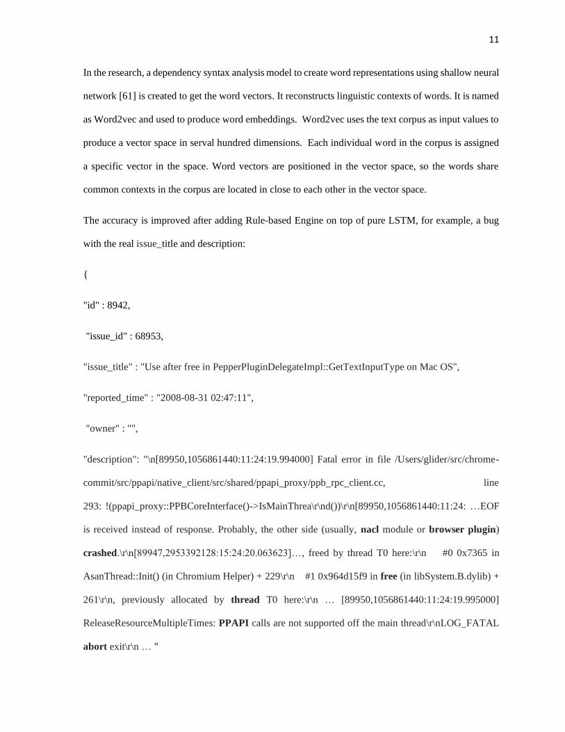
The accuracy is improved after adding Rule-based Engine on top of pure LSTM, for example, a bug
with the real issue_title and description:
{
"id" : 8942,
"issue_id" : 68953,
"issue_title" : "Use after free in PepperPluginDelegateImpl::GetTextInputType on Mac OS",
"reported_time" : "2008-08-31 02:47:11",
"owner" : "",
"description": "\n[89950,1056861440:11:24:19.994000] Fatal error in file /Users/glider/src/chrome-
commit/src/ppapi/native_client/src/shared/ppapi_proxy/ppb_rpc_client.cc, line
293: !(ppapi_proxy::PPBCoreInterface()->IsMainThrea\r\nd())\r\n[89950,1056861440:11:24: …EOF
is received instead of response. Probably, the other side (usually, nacl module or browser plugin)
crashed.\r\n[89947,2953392128:15:24:20.063623]…, freed by thread T0 here:\r\n #0 0x7365 in
AsanThread::Init() (in Chromium Helper) + 229\r\n #1 0x964d15f9 in free (in libSystem.B.dylib) +
261\r\n, previously allocated by thread T0 here:\r\n … [89950,1056861440:11:24:19.995000]
ReleaseResourceMultipleTimes: PPAPI calls are not supported off the main thread\r\nLOG_FATAL
abort exit\r\n … "

12
}
Pure LSTM model assigns the bug’s owner field with email alias: [email protected], a wrong
developer. The reason of why we know it is wrong is because the pre-collected data has the right
answers(email aliases) in the owner field in the training set. LSTM is a supervised learning, and the
training model gives a confusion matrix, and it shows that record has the wrong owner prediction
[email protected]. But after the Rule-based engine, since there are many words including nacl,
browser, plugin, crashed, free, thread, PPAPI and abort in the bug’s description are matching the
attributes aka keywords list of developer [email protected]. According to a preconfigured
threshold value on overlapping of the bug’s title, description keywords with the developer’s attributed
keywords, the Rule-based engine on top of LSTM correctly assigns it to [email protected], a
correct developer. With more records running through Rule-based engine, the accuracy of confusion
matrix becomes higher and higher for the hybrid model.
The dissertation adds LSTM and rule-based engine with expert system and fuzzy logic basic idea to
design a new bug assignment model. LSTM uses deep neural networks to perform all encoding on such
transition states as stack, cache, history transfer sequence state, and current dependent subtree collection
state. By this way, it makes full use of historical transfer information. More fine-grained modeling of
words, stacks, caches, transfer sequences, etc. It has more flexible control of parameters tuning in a
multitasking learning framework.
With a little more complexity by adding additional memory gates storages and introducing Rule-based
engine, the hybrid of Layer 1 and Layer 2 model proves that it has better accuracy and generalization
in the experiment to compare with traditional ones.

13
1.5 Dissertation Roadmap
The research is divided into six chapters, the content of each chapter is arranged as follows:
Chapter 1 Introduction The research introduces the background of the field of software bug fix
engineering system and process. It states the main problem space of this dissertation is addressing, the
automatic defects assignment related work, and briefly introduces the main researches on how deep
learning neural networks and Rule-based engine aka expert system can solve the automatic defect
assignment challenges.
Chapter 2 Software defect assignment traditional theory and approaches The traditional defect
assignment models divides the current research work into four categories:
1) Model Based on Fuzzy Logic
2) Model based on Traditional Machine-learning
3) Expert System Model
4) Tossing-graph model
5) Social-network model
6) Topic-model.
Chapter 3 New Software Defect Assignment Model – Layer 1: NLP and Vector for Words The chapter
introduces the methods of automatic software defect assignment based on text classification aka natural
language processing. The method of defect is assignment fundamentally based on the text classification
and how to create word vector dictionary. Generally, the defect report is the main feature to be used for
the text classification and the developer acts as a label, and then the defect assignment problem is
converted into the text classification problem.

14
Chapter 4 New Software Defect Assignment Model – Layer 2: LSTM and Rule-based Engine Inspired
by LSTM, decision trees, and expert systems theories on software defect assignment, the chapter
decided to apply LSTM, rule engine approach to the automatic of defect assignment research areas.
The combination of text classification training on LSTM with developer productivity rule architecture
is discussed for bug assignment project.
Chapter 5 Data Collection and Experiments Result Many comparative studies are presented. Through
experiments, it is found that the hybrid model not only has a significant effect on text classification, but
also has a higher accuracy rate than the traditional learning method for the problem of automatic defect
assignment.
Chapter 6 Summary and Future Work This paper summarizes the work of the dissertation, explains the
main contribution of the research in the field of defect assignment field, and future looks to the next
step (like BERT, GPT 2 system) based on the current research topics.

15
Chapter 2 Software defect assignment traditional theory and approaches
It is the major and complex task for bug reviewers to assign defects to appropriate assignees in order
to achieve the purpose of rapid repair defects. Automating the distribution of bugs can reduce the
probability of re-routing of bugs and save valuable time for bug fixing.
However, how to identify candidates of bug assignee and the order of appropriate bug assignees will
be a huge challenge. At present, there are a large number of methods based on segmentation and
classification (such as traditional Machine-learning algorithm, social network matrix, etc.) to evaluate
the experience of software developers, so that you can select the right candidate and pick the most
suitable bugs for them.
The traditional defect assignment models divide the current research work into six categories: 1) Model
Based on Fuzzy Logic 2) Model based on Traditional Machine-learning 3) Expert System Model 4)
Tossing-graph model 5) Social-network model 6) Topic-model. The details are as follows.
2.1 Model Based on Fuzzy Logic
The Bugzie method proposed by Tamrawi et al. [8][9] is a method for automatic bug assignment based
on fuzzy set and Cache-based model. Bugzie extracts a number of technical aspects of the software
system, each technical aspect has a number of technical terms (Technical terms).
Technical capabilities are characterized by a fuzzy set of terminology. Specifically, for developers,
fuzzy collections represent the expertise of a developer or the ability to resolve defects; for defect
reporting, a fuzzy collection represents a defect report that requires the expertise of a software developer
or the ability to resolve defects, and the matching relationship between them, is measured using the

16
membership score. Finally, sorting the candidate developers according to the value of the Membership
score and selecting the most suitable developer. Experiments show that Bugzie is superior to other
models in research.[10][11][12][13] For example, in the open source Eclipse dataset, when the
recommended number is tops, Bugzie only reached it in 22 minutes. 72% accuracy, 49 times faster than
SVM [12], and accuracy rate has increased by 19%.
Fuzzy logic absorbs the ambiguity of human thinking, and uses the functions of membership function,
fuzzy relationship and decision-making in fuzzy mathematics to obtain control actions, which are
generally classified into functions, fuzzy reasoning and fuzzy decision making. Fuzzy logic technology
has been widely used in the software and hardware industries. It has the following characteristics:
1. Simple
Human thinking has the characteristics of ambiguity, and fuzzy logic is similar to human thinking.
It does not need to first analyze the mathematical model of the system like software bug assignment
system and can directly use the opinions of experts. It allows designers to describe inputs, rules,
and outputs with IF...THEN... statements. Its fuzzy subset and membership functions (such as cold,
hot, etc.) are generally very intuitive. Each input requires only 3 to 8 fuzzy subsets. The membership
function can also use a simple triangle or trapezoidal form, and often only it takes ten to dozens of
rules. But using these simple modules can form a control system that performs very complex
tasks.[14]
2. The software for implementing fuzzy control is short and requires less storage space.
The fuzzy control system generally requires only a short program and less storage space, which
requires much less storage space than the control system using the look-up table method and
requires less storage space than the control system using mathematical calculation methods. There
are also fewer.[15]

17
3. High speed
Fuzzy logic software systems can perform complex tasks in a short period of time, rather than
requiring a large amount of mathematical calculations using mathematical methods. In this way, a
simple 8-bit microcontroller can be used to perform functions that may require a 32-bit or RISC
processor. It also performs tasks that were previously too complicated to complete due to
mathematical calculations. Moreover, since the fuzzy calculation itself is a parallel structure,
each input can be fuzzified at the same time, or each rule can be reasoned. This allows fuzzy
reasoning to be done at high speed using parallel processing hardware. For example, the existing
fuzzy \ logic chip can complete a fuzzy control within tens of microseconds.
4. Easy and fast development
With fuzzy logic, you can start designing the approximate fuzzy subset and rules, and then adjust
the parameters step by step to optimize the system. The various components of the fuzzy inference
process are functionally independent, so that the system such defect assignment can be easily
modified. For example, you can add rules or input variables without having to change the overall
design. For a conventional software defect assignment, adding an input variable will change the
overall algorithm. When developing a fuzzy bug assignment system, you can concentrate on
functional goals rather than analyzing mathematical models, so you have more time to enhance and
analyze the system. [16]
5. Different from Neural Networks
The basic unit of neural network is a neuron. The two layers of networks are connected by weights.
Therefore, the knowledge information after learning is distributed in the middle of the weight, while
the fuzzy logic system stores the knowledge in a regular way, as shown in Fig. 5. The input in the
figure is the fuzzy variable A, which is an n-dimensional vector, which is mapped to the

18
dimensional fuzzy vector B by m set of rules, and each rule gets a value like B1, …Bm. The total
decision vector B as shown below. The system has more human factors in the form of rule sets, the
size of regional division and the formulation of rules. If the experience and expert knowledge are
used, the structure and result of fuzzy logic software system are better than neural network. The
neural network is obtained by learning by itself. The result is related to the sample set. If the sample
set is atypical (i.e., the selection is unreasonable), the knowledge storage is not optimal. [17]
Figure 5 Fuzzy Software Defect Assignment System Inputs and Output
2.2 Model based on Traditional Machine-learning
Traditional Machine-learning model, which is different from deep learning neural networks model, can
learn from the data and create a model. Early work such as Naive Bayes, SVM, and etc. uses traditional
machine learning methods to determine the appropriate defect assignment.
The earliest work was a solution proposed by Murphy and Cubranic [18] to automate the distribution
of software defects. Specifically, they regard the defect assignment task as a text classification problem,
each defect assignee is a category, and each defect report corresponds to only one category. They used
one of the most commonly used models in machine learning -the Naive Bayes model. It is more
appropriate to predict which software developers should be assigned to a bug. However, the accuracy
19
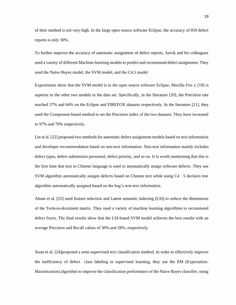
of their method is not very high. In the large open source software Eclipse, the accuracy of 859 defect
reports is only 30%.
To further improve the accuracy of automatic assignment of defect reports, Anvik and his colleagues
used a variety of different Machine-learning models to predict and recommend defect assignment. They
used the Naive Bayes model, the SVM model, and the C4.5 model.
Experiments show that the SVM model is in the open source software Eclipse, Mozilla Fire x [19] is
superior to the other two models in the data set. Specifically, in the literature [20], the Precision rate
reached 57% and 64% on the Eclipse and FIREFOX datasets respectively. In the literature [21], they
used the Component-based method to set the Precision index of the two datasets. They have increased
to 97% and 70% respectively.
Lin et al. [22] proposed two methods for automatic defect assignment models based on text information
and developer recommendation based on non-text information. Non-text information mainly includes
defect types, defect submission personnel, defect priority, and so on. It is worth mentioning that this is
the first time that text in Chinese language is used to automatically assign software defects. They use
SVM algorithm automatically assigns defects based on Chinese text while using C4 · 5 decision tree
algorithm automatically assigned based on the bug’s non-text information.
Ahsan et al. [23] used feature selection and Latent semantic indexing (LSI) to reduce the dimensions
of the Term-to-document matrix. They used a variety of machine learning algorithms to recommend
defect fixers. The final results show that the LSI-based SVM model achieves the best results with an
average Precision and Recall values of 30% and 28%, respectively.
Xuan et al. [24]proposed a semi-supervised text classification method. In order to effectively improve
the inefficiency of defect class labeling in supervised learning, they use the EM (Expectation-
Maximization) algorithm to improve the classification performance of the Naive Bayes classifier, using
20
a small number of marked bug reports and a large number of unmarked defect reports to complete the
auto bug assignment task. Experiments have shown that this semi-supervised model can improve the
accuracy of 6% compared to the normal Naïve Bayes method.
In order to filter the noise data reported by the defect filing process, Zou et al [25]. used the feature
selection model and the instance selection model to reduce the scale of the training set and improve the
quality of the training data. They use the Naive Bayes method to verify the effect of automatic defect
assignment. The results show that the Naive Bayes method using the feature selection model is 5%
better than the normal Naive Bayes, while the Naive Bayes method using the instance selection model
is not as effective as the normal Ne Bayes.
Xia et al. [26] proposed a precise assignment model called DevRec to implement the recommendations
of defect repairers. DevRec comprises two analysis methods, one is based on the analysis method of
Bug reporting, abbreviated as BR assay (BR- based analysis), the other is based on analysis of the
Developer, referred to as D assay (D-based analysis). Using feature values in defect reports, such as
Terms, Product, Component, Topics, etc., BR analysis can use Multi-Label KNN to find K historical
defects related to newly found defects. D analysis uses the characteristics of Terms, Product,
Component, and Topic to calculate the similarity between developers. Finally, the BR analysis method
and the D analysis method are combined to complete the automatic assignment task of the defect report.
Experiments show that the average Recall rate of the DevRec method is increased by 39.39% and 89.36%
compared with the Bugzie [27] model and the DREX [28] model, respectively, under the
recommendation of top 10 developers.
2.3 Expert System Model
Matter et al [29]. modeled the software developer's source code vocabulary and the vocabulary in the
defect report and used the Cosine measure to calculate the similarity of two-word vectors. Experiments

21
show that, in the case of the recommended number is top 1, Precision rate may reach 33.6%; in the case
of the recommended number is top10, recall rate may reach 71%.
Servant et al. [30] developed a tool for implementing the automatic bug assignment, which consists of
bug line location, history mining, and expertise assignment. Specifically, the historical information of
the source code change is combined with the diagnosis information about the defect location, and the
candidate developers are sorted to achieve the recommendation purpose. Experiments show that under
the condition that the recommended number is top3, the accuracy rate of 81.44% can be achieved.
Expert system model and neural network system have different precision. Both systems can map a
nonlinear system, but their mapping surfaces are different. The neural network uses point-point
mapping, so the functional relationship between its output and input is different, and the expert system
is different. It is a reflection between the rule regions. If the regions are relatively coarse, the surface
of the mirror output has low precision. For example, if each rule is a trapezoidal step, the output will
be coarse. Therefore, for the mapping with higher precision, the artificial neural network is better, and
for the lower precision requirement, the expert system can be used for mapping. For software defect
assignment, we need high precision, therefore neural network will work better.
Neural networks need to calculate multiplication, accumulation, and exponential operations, while
expert system calculations are relatively small, and the rules involved in each iteration are generally
small. However, when the accuracy of the expert system needs to be improved, the number of rule
subsets increases correspondingly, and the amount of calculation increases.
Furthermore, the neural network is connected to the feed-forward network. For example, once the input
and output and the hidden layer are determined, the connection structure is determined. After learning,
almost every neuron is associated with the previous layer of neurons, so it is controlled. In each iteration
of iteration, each weight and bias must be learned. In expert system model, each input may be related
to only a few rules, so the connection is not fixed, and the rules for each input and output are changeable.

22
2 .4 Tossing-graph Model
In general, the process of assigning a defect begins with the first assignee and then passes to the next
developer until the last fixer. Each pass is called a Tossing step, and a set of pass steps is called a
Tossing path. Assuming that the transmission path of a defect is A-B-C-D, the goal of Jeong et al [31].
is to predict a shorter transit path from A to D will speed up the process of defect repair. Experiments
show that on the open source software Eclipse and Mozilla datasets, compared to pure machine
learning-based models (such as Naive Bayes and Bayesian Network [32]), the Tossing model can
greatly improve the accuracy of automatic defect assignment.
Bhattacharya and Neamtiu [33] use a variety of techniques to shorten the length of the delivery path ,
including the use of additional features for Refined classification and update model during real time
training, using more accurate ranking methods, and Multi-features of Tossing graph, etc. Experiments
show that the accuracy rates of the open source software Eclipse and Mozilla datasets are 84% and
82.59%, respectively.
In the literature [34], Bhattacharya uses the Naive Bayes model based on the product-component feature
and combines the Tossing graph and the incremental learning (Incremental learning) method to
complete the task of automatic defect allocation. The accuracy rate on the Mozilla dataset has increased
to 85 % and the accuracy rate on the Eclipse dataset has increased to 86%. Compared to the previous
work, the automatic allocation effect is greatly improved.
2 .5 Social-network model
In recent years, social network (Social network) technology began to be used defect assignment
research area. Usually people use the comment and social chat and rating activity in the defect web site
or reports to build a social network, and then through the social network between the developers to

23
analyze, you can know which developers have a wealth of repair experience in solving certain defects.
With that information, the model can give right defects to proper developer to fix.
Wu et al. [35] use the KNN model to search for historical defect reports similar to newfound bugs.
Then the reviewers involved in the historical defect report are used as candidates, and the last use
frequency and other six social network indicators (In-degree centrality, Out-degree centrality, Degree
centrality, PageRank, Betweenness centrality, Closeness centrality) to recommend a suitable defect
repairer. After comparing the frequency and the distribution of the other six social network indicators,
the authors believe that the frequency and Out-degree indicators can achieve the best results.
Xu et al. [36] analyzed the social network to explore the developer prioritization information and then
integrated it into the SVM model or Naive Bayes model to automatically assign defects. The results
show that the analysis of the developer priority information obtained by the social network can
effectively improve the accuracy of the SVM model and Naive Bayes model defect assignment.
2.6 Topic-model
The more similar topic the bugs have, the closer the bugs are related. Therefore, the topical modeling
of the defect report (Topic model) can be used to evaluate the similarity between the new defect and
the historically fixed defect. Researchers hope to further improve the accuracy of the defect assignment
model by introducing relevant methods of topic modeling.
Xie et al. [37] proposed a defect repairer recommendation method called DRETOM, which uses
Stanford Topic Modeling Toolbox (TMT). [38]
Given a new defect report, it is easy to confirm which set of topics the defect report should belong to,
and then by analyzing the interests and experience of the developers in each set of topics, you can assign
appropriate repairers to the new defects. Experimental results show that the DRETOM method works

24
better than general machine-based learning (such as SVM model, KNN model) and social network-
based methods.
The LDA [39] model is a probability generation model that generates different topics for discrete data.
Naguib et al. [40] used the LDA model to classify defect reports into different topics, then created an
activity profile for each developer by mining historical log records and topic models, and finally they
used activity profiles and new defects information. The topic models and their own sorting algorithms
are used to find the most appropriate defect fixers. Experiments show that the average hit rate (Hitrate)
of this model can be reached 88%.
Yang et al. [41] used TMT to model the defect assignment, and then extracted historical defect reports
with the same subject as the new bug. Based on multiple features of the new bug such as Product,
Component, Priority, the model re-screens those bugs. Then it rebuilds the social network model based
on the developers in the remaining historical defect reports. Finally, it uses the bugs’ comment activity
related to the source code and the activity of change lists for defect assignment. Experimental results
show that this method is better than DRETOM and social network-based methods.
Zhang et al. [42] also used the LDA method to extract historical information from defects reports. It
obtains information on whether developers are interested in a topic by understanding the code check-
in of activities of relevant developers under the same area. In addition, Zhang et al. analyzed the
relationship between relevant developers (such as defect reporters and defect fixers) and then combined
the topic model with the relationship model. Experiments show that on the open source software Eclipse
dataset, this method is 3 % and 16.5% higher than the DRETOM and the previous mentioned activity
summary-based models.
2.7 Chapter summary
The chapter mainly introduces the mainstream methods in the field of automatic assignment of software
defects. They are the following six principal methods: 1) Model Based on Fuzzy Logic 2) Model based

25
on Traditional Machine-learning 3) Expert System Model 4) Tossing-graph model 5) Social-network
model 6) Topic-model.
Firstly, fuzzy logic methods are applied to bug assignments in the early stage of research topic.
Secondly, the traditional machine learning method was the mainstream of defect assignment, many
improved methods are based on it.
Thirdly, feature selection or composite models can improve the accuracy of machine learning-based
methods like Expert System Model and Tossing-graph model.
Finally, the introduction of new technologies (such as social networks and topic models) can further
enhance the effects of machine learning-based models.
Next two chapters the paper will introduce a new software defect assignment model. It includes the
layer 1 – vector for words, and layer 2 – LSTM and rule-based engine. The new model flow diagram
is shown in Fig. 6.
Figure 6 The model of new software defect assignment system

26
Chapter 3 New Software Defect Assignment Model – Layer 1: NLP and
Vector for Words
The method of defect assignment is fundamentally based on the text classification. Generally, the
defect report is the main feature to be used for the text classification and the developer acts as a label,
and then the defect assignment problem is converted into the text classification problem. Therefore, in
the following descriptions of text classification and defect assignment, the two problems of text
classification and defect assignment are deemed as the same problem space we are addressing, we use
the two wordings interchangeably.
The traditional practice of text categorization is to use a bag model to represent text features and then
use standard machine learning’s classification models (such as SVM models) for classification. As we
all know, the word bag model does not contain the word order information of the text, and then lacks
the representation of the grammatical and semantic aspects of the text, resulting in limited accuracy of
the final classification model.
The literature [43][44][45] use two-word phrases (Bi-grams) instead of single words (Unigrams) to
make up for the lack of text on the lack of word order information.
However, the work of the document [46] proves to use a multi-word phrase (N-Grams, the method of
N>1) is not a very effective method. Although this method alleviates the problem of missing word order,
it greatly increases the sparseness of text representation.
Therefore, it is a challenge to make full use of the word order information of the text, and learn the
grammatical and semantic knowledge of the text sequence, while at the same time cannot increase the
sparseness of the text representation.
3.1 Model Overview

27
In the text classification algorithm introduced in the previous chapter, most algorithms need to construct
text features manually. Such feature construction is very labor-intensive, and the scalability is not good,
and it is not easy to obtain during the process of feature extraction. Therefore, the models presented in
this chapter do not use these classic text features. The paper is proposing two layers model to solve the
problem.
The word vector representation is the first layer in my software defect assignment problem space,
followed by the second layer which is modeled with LSTM and rule-engine which will be discussed by
Chapter 4 in details.
The first layer for word vector model maps discrete words in each text into a fixed-dimensional feature
vector to get the word direction. They are accessed by the second layer hierarchical LSTM to get a
vectorized representation of the entire document.
Chapter 3 will focus on my model research on the layer 1: Defect Reports and Vector for Whole Words
areas.
For our bug text reports, we need to build a word vector to feed into the LSTM described above so in
the text, each word has its own probability and statistics. Therefore, word vector representation, also
named as Word Embedding needs to be introduced. Before elucidating the vector model, the first thing
to determine is the size of the text and how to represent text sequences. The model that solves such
problems is called a vector representation, because the process of text sequence representation is the
process of vectorizing the text sequence. This paper is designed to explain it as much as possible, which
is beneficial for later understanding of the LSTM neural network model.
New model summary with focus on layer 1 is described in the following diagram Fig 7.

28
Figure 7 Defect Assignment Model Layer 1
Algorithm 1: Dataset Preprocessing by word2vector
Input:
Untriaged bug set and triaged bug set
Output:
A set of unique words that occurred for at least k-times in the corpus
1: BEGIN
2: Set up the min_count, size, window of word2vec function
3: Set up the batch_size, epoch, iteration of classifier hyper parameters
4: Preprocess the untriaged bug set and extract the vocabulary and learn the word2vec representation
5: FOR each sample in untriaged bug set
6: Remove the return character “\r”
7: Remove the URLs of online resource
8: Remove the stack trace
9: Remove the hex code
10: Change all letters to lower case
11: Handle the tokenize
12: Remove the punctuation marks
13: END FOR
14: PRINT a set of unique words
15: Learn the word2vec model and extract vocabulary
16: Preprocess the triaged bug set and use the extracted the vocabulary
17: FOR each sample in triaged bug set
18: Remove the return character “\r”
19: Remove the URLs of online resource

29
20: Remove the stack trace
21: Remove the hex code
22: Change all letters to lower case
23: Handle the tokenize
24: Remove the punctuation marks
25: END FOR
26: Add all values of label “owner” to array all_owner
27: END
Let’s go through the implementation of our approach. The necessary packages for the implementation
are: Numpy, NLTK, Gensim, Keras and Scikit-learn. They can be imported into python as following:
import numpy as np
import warnings
warnings.filterwarnings(action='ignore', category=UserWarning, module='gensim')
np.random.seed(1337)
import json, re, nltk, string
from nltk.corpus import wordnet
from gensim.models import Word2Vec
from keras.preprocessing import sequence
from keras.models import Model
from keras.layers import Dense, Dropout, Embedding, LSTM, Input, merge, Concatenate,
concatenate
from keras.optimizers import RMSprop
from keras.utils import np_utils
from sklearn.feature_extraction.text import CountVectorizer
from sklearn.feature_extraction.text import TfidfTransformer
from sklearn.naive_bayes import MultinomialNB
from sklearn import svm
from sklearn.linear_model import LogisticRegression
from sklearn.multiclass import OneVsRestClassifier
from sklearn.metrics.pairwise import cosine_similarity
from keras.utils import to_categorical
First, we hard-coded the dataset absolute path first to ensure our system could get the source of data
needed to process. In this project, we use two datasets: 1. Untriaged bug dataset is used to learn the
target deep learning model in an unsupervised manner. 2. Triaged bug dataset is used for classifier
training and testing by cross validation. Another web data is used for bug triage improvement by custom
rule engine.

30
open_bugs_json = 'C:\dataset\TestData.json'
closed_bugs_json = 'C:\dataset\TrainData.json'
web_data_address = 'C:\dataset\webData.json'
Second, we set up the initialization of global variable, which divides into two parts. The parameters of
first part is for word2vector function as following:
min_word_frequency_word2vec = 5
embed_size_word2vec = 200
context_window_word2vec = 5
min_word_frequency_word2vec means a set of unique words that occurred for at least specific times is
extracted as the vocabulary. embed_size_word2vec means dimension of the embedding vector.
context_window_word2vec means how many words to consider left and right. The parameter of second
part is to define the number of cross validations, the number of iteration times and the batch size of
parallel computing.
numCV = 5
max_sentence_length = 50
min_sentence_length = 15
rankK = 10
batch_size = 32
myEpochs = 5
numCV means the number of cross validations, myEpochs means the number of iteration times for all
the training examples, batch_size means the number of samples that will be propagated through the
network. The higher the batch size, the more memory space you'll need. For instance, let's say you have
1000 training samples and you want to set up a batch_size equal to 100. The algorithm takes the first
100 samples (from 1st to 100th) from the training dataset and trains the network. Next, it takes the
second 100 samples (from 101st to 200th) and trains the network again. We can keep doing this
procedure until we have propagated all samples through of the network. rankK means the user can
configure your own specific times for accuracy. min_sentence_length means the minimum processing

31
range of time steps in LSTM model. max_sentence_length means the maximum processing range of
time steps in LSTM model.
Third, there are id, issue id, issue title, reported time, owner and description options in each bug sample
of the untriaged dataset, one case is shown in the following table. It is necessary to preprocess them so
that we can process the valid data easier. For untriaged dataset, we only focus on the issue title and
description. We removed the return character “\r”, the URLs of online resource, the stack trace, the hex
code and so on, and store these scattered words into an array: all_data as following:
[testing, if, chromium, id, works, what, steps, will, reproduce, the, problem, is, expected, output, do you
see instead, please, use, labels, and, text, to, provide, additional, information ]
{
"id" : 1,
"issue_id" : 2,
"issue_title" : "Testing if chromium id works",
"reported_time" : "2008-08-30 16:00:21",
"owner" : "",
"description" : "\nwhat steps will reproduce the problem\n1\n2\n3\n\r\nwhat is the expected
output what do you see instead\n\r\n\r\nplease use labels and text to provide additional information\n
\n"
}
We use the Word2Vec method to learn a bug representation (Continuous Bag of Words) model, then
extract vocabulary. The vocabulary is in the vocab field of the Word2Vec model's wv property, as a
dictionary, with the keys being each token (word).
wordvec_model = Word2Vec( all_data, min_count=min_word_frequency_word2vec,
size=embed_size_word2vec, window=context_window_word2vec)
vocabulary = wordvec_model.wv.vocab
Fourth, to preprocess the triaged dataset is very similar to the operation of processing the untriaged
dataset. We store the title and description of every bug into an array, and the owner into another array
as well for the following computing. The use-case of triaged dataset is shown below.

32
{
"owner" : "[email protected]",
"issue_title" : "Scrolling with some scroll mice (touchpad, etc.) scrolls down but not up",
"description" : "\nProduct Version : <see about:version>\r\nURLs (if
applicable) :0.2.149.27\r\nOther browsers tested: Firefox / IE\r\nAdd OK or FAIL after other
browsers where you have tested this issue:\nSafari 3:\n Firefox 3: OK\r\n IE 7:OK\r\n\r\nWhat
steps will reproduce the problem?\n1. Open any webpage on compaq 6715s running vista.\r\n2. Try
scrolling with the touchpad\r\n3. Scrolling down will work , but up will not.\r\n\r\nWhat is the
expected result?\nThe page to scroll up.\r\n\r\nWhat happens instead?\nThe page doesn't
move.\r\n\r\nPlease provide any additional information below. Attach a screenshot if
\r\npossible.\r\nOnly a minor bug.\n "
}
After preprocessing, the all_data and all_owner will be:
All_data = [ scrolling, with, some, scroll, mice, touchpad, etc, scrolls, down, but, not, up, product,
version, see about, if, applicable, other, browsers, tested, firefox, ie, add, ok, or, fail, after, other,
browsers, where, you, have, tested, this, issue, safari, 3, 7, what, steps, will, reproduce, the, problem,
open, any, webpage, on, cmpaq, 6715s, running, vista, 2, try, touchpad, down, but, is, expected, result,
page, to, happens, instead, doesn't, provide, any, additional, information, below, attach, a, screenshot,
possible, only, a, minor, bug ]
All_owner = [[email protected] ]
3.2 Word Vector Representation
Text granularity is generally divided into characters, words, phrases, even paragraphs and even an
article, which are theoretically acceptable. They correspond to character vectors, word vectors, and
phrase vectors respectively (some papers are also called region vectors), paragraph vector and article
vector. My paper uses a word vector model based on word granularity, which is also a commonly used
vector model in the field of natural language processing.
The first method for word embedding is one-hot method. The model treats words as an indivisible
individual, and then use a dimension equal to the number of words, only the position corresponding to

33
the word is 1 and the rest of the sparse vector is 0. This representation is called a "one-hot
representation". However, this method also has a serious flaw, that is, the words exist in isolation, and
the similarity between two words cannot be quantified.
For example, there are three words software, networking, kernel. Then generate a three-dimensional
vector, each word occupies a position in the vector, software: [1,0,0] networking: [0,1,0] kernel: [0,0,1].
So if an article now has 1000 words, then each vocabulary will be represented by a 1000-dimensional
vector, where only the position of the word is 1, and the rest of the positions are all 0, and each word
vector is irrelevant.. The benefits of doing this are simple, but not very realistic. It ignores the
correlation between words, ignoring the tense of English words, such as get and got have the same
meaning, but the tense is different.
The second method is n-gram method. N-gram refers to consecutive n items in the text (item can be
phoneme, syllable, letter, word or base pairs). In n-gram, if n=1, it is unigram, n=2 is bigram, and n=3
is trigram. After n>4, it is directly referred to by numbers, such as 4-gram, 5-gram. These are the linear
relationships of the semantic space. We can do addition and subtraction. Moreover the language model
for n-gram is to estimate the probability of word sequence, for a word sequence: W1, W2, W3, …., Wn,
it can get the Probability of (W1, W2, W3, …., Wn ).
For example, we have a sentence, “We are going to assign the UI crash bug to Peter”, if bigram is used,
it will be: We are, are going, going to, to assign, assign the, the UI, UI crash, crash bug, bug to, to Peter.
In Python code to implement bigram model:
sent= “We are going to assign the UI crash bug to Peter”
bigram = []
for i in range(len(sent)-1):
bigram.append(sent[i] + sent[i+1])
print(bigram)
Output will be:

34
We are, are going, going to, to assign, assign the, the UI, UI crash, crash
bug, bug to, to Peter
and the language model for bi gram:
P (“We are going to assign the UI crash bug to Peter”) =P(We|START)
P(are|We) P(going|are) P(to|going) P(assign|to) P(the|assign) P(UI|the)
P(crash|UI) P(bug|crash) P(to|bug) P(Peter|to)
P(Peter|to) = Count (to Peter) / Count(to)
It is easy to generalize to trigram and n-gram. If trigram is used, it will be: We are going, are going to,
going to assign, to assign the, assign the UI, the UI crash, UI crash bug, crash bug to, bug to Peter. In
Python code to implement trigram model:
sent= “We are going to assign the UI crash bug to Peter”
trigram = []
for i in range(len(sent)-2):
trigram.append(sent[i] + sent[i+1] + sent[i+2])
print(trigram)
Output will be:
We are going, are going to, going to assign, to assign the, assign the UI,
the UI crash, UI crash bug, crash bug to, bug to Peter
Finally, n-gram implementation will be as follows:
def nGram(lst,n):
ngram = []
for i in range(len(lst)-n+1):
ngram.append(lst[i:i+n])
print(ngram)
35
Call nGram(), sent==" We are going to assign the UI crash bug to Peter ", n can be a number less than
len(lst).
The challenge of n-gram is the estimated probability is not accurate, especially when we consider n-
gram with large n because of data sparsity, shortage of training data, and uncontrollable size of
dictionary. Though there is some solution like language model smoothing by giving some small
probability to address the challenge, the results are not ideal.
There is a very successful view in the field of modern statistical natural language processing: the word
can be well studied using only the words around the word. This provides a new idea: one of the easiest
and quickest ways is to use a window-based co-occurrence matrix to represent text, using different
window lengths to capture different syntax and semantics about text. The final co-occurrence matrix
can get some generalized topics (such as software words, engineering words, etc.), which is equivalent
to a shallow semantic analysis (Latin Semantic Analysis, LSA).
However, as the size of vocabulary in the corpus continues to increase, the co-occurrence matrix will
become larger and larger, which will not only cause large-scale storage problems, but also encounter
large-scale sparse matrix problems during training, which is more important. The model is not robust
enough and does not have good generalization capabilities.
This is because the dimensions of the model are too high. Is it possible to use a fixed, low-dimensional
vector to store text information? In fact, this model is real, and this vector is generally called a dense
vector. There are two main ways to get a dense vector: the first one, using dimensionality reduction to
reduce the sparse high-dimensional data into dense low-dimensional data, the typical method is singular
value decomposition (SVD); the second, direct learning can be used to represent dense vectors of words.
In related models (including deep learning models), there are many models that can learn the dense
vector of words by model training. This dense vector is not only very effective, but also plays an
important role in the field of natural language processing.

36
To solve the above problems, many neural networks model uses the matrix factorization language
model including the following Word2Vec method. The following Figure 8 shows how matrix
factorization works. From the table in the following diagram, the history of developer “Peter” and
“Rob” can have similar hPeter and hRob. If vfix Kernel ∙ hRob is large, vfix Kernel ∙ hPeter would be large
accordingly, even though we have never seen “Peter fixes Kernel bug”. The neural network has the
smoothing automatically done.
Figure 8 Bug Assigner Matrix Factorization
Mainstream of NLP prediction method is based on neural network models. On the contrary to traditional
Statistics Method such as N-gram model, the neural network models are based on many parameters,
and a judgment model. It employs the word vectors of text context as inputs and compute the current
word probability distribution through the neural network. The current popular method is the third one,
Word2Vec, which my research has chosen for defect assignment model. This is a method that Tomas
Mikolov invented when working at Google and is also the name of a toolkit that is open sourced by

37
Google. Specifically, Word2Vec involves two algorithms, one is CBOW and the other is Skip-Gram.
This is also the Word Embedding method based on neural networks after deep learning is popular. The
reason why Word2Vec is so popular now is different from some previous Word Embedding methods,
which can automatically implement: 1) the measurement of semantic similarity of words; 2) the analogy
of semantics of vocabulary. Here, the semantic analogy reflects a relationship. Word2vec is a two-layer
neural net that processes text. Its input is a text corpus and its output is a set of vectors: feature vectors
for words in that corpus.
While Word2vec is not a deep neural network, it turns text into a numerical form that deep nets can
understand. Word2vec’s applications extend beyond parsing sentences in the wild. It can be applied
just as well to genes, code, likes, playlists, social media graphs and other verbal or symbolic series.
Because words are simply discrete states like the other data mentioned above, and we are simply
looking for the transitional probabilities between those states: the likelihood that they will co-occur.
The purpose and usefulness of Word2vec is to group the vectors of similar words together in vector
space. That is, it detects similarities mathematically. Word2vec creates vectors that are distributed
numerical representations of word features, features such as the context of individual words. It does so
without human intervention. Given enough data, usage and contexts, Word2vec can make highly
accurate guesses about a word’s meaning based on past appearances. Those guesses can be used to
establish a word’s association with other words (e.g. “developer” is to “tester” what “coder” is to
“verifier”), or cluster documents and classify them by topic. Those clusters can form the basis of search,
sentiment analysis and recommendations in such diverse fields as scientific research, legal discovery,
e-commerce and customer relationship management.
The output of the Word2vec neural net is a vocabulary in which each item has a vector attached to it,
which can be fed into a deep-learning net or simply queried to detect relationships between words.
Measuring cosine similarity, no similarity is expressed as a 90-degree angle, while total similarity of 1

38
is a 0-degree angle, complete overlap. The detailed code for bug defect on word2vec in my project is
implemented in the Table 1. Those noise words are removed from the model.
from gensim.models import Word2Vec
# Word2vec parameters
min_word_frequency_word2vec = 5
embed_size_word2vec = 200
context_window_word2vec = 5
wordvec_model = Word2Vec (all_data,
min_count=min_word_frequency_word2vec, size=embed_size_word2vec,
window=context_window_word2vec)
# vocabulary
vocabulary = wordvec_model.wv.vocab
vocab_size = len(vocabulary)
Table 1 Function to preprocess the text in bug report
A vector representation refers to a multi-dimensional vector table for an objective natural language (eg,
a word). It is usually characterized by low dimensionality, continuous, and dense properties. In fact,
there are two definitions in the field of natural language processing for word distribution. First one is
called " distributional representation " and can be traced back to Semantic distributional Hypothesis
(Distributional Hypothesis) proposed last century Firth: "You shall know a word by the company it
keeps” [48][50]. The hypothesis states that the meaning of a word is determined by its context. That is
to say, words with similar contexts usually have similar meanings. The definition is called “distributed
representation” was first proposed by Hinton [51].
Hinton considers the activation vector of the middle-hidden layer neurons in neural network as
“distributed representation” of the input data. Bengio firstly uses the "word embedding" method, which
maps words to their distributed representation vectors, and then passes the neural network language

39
model as Neural Network Language Model, referred NNLM., its iterative update [52]. Therefore, this
lexical distribution representation is also known as word embedding.
we first build a word-context (word-context) occurrence matrix, then using the matrix decomposition
technique to reduce the dimension, to get the score of each word’s distributional representation vector.
There are three important technical details:
1. The choice of context. Different contexts determine the nature of the resulting word distributional
representation. The more commonly used context is the documents model [53], or the model on words
in the context of a certain window [54].
In general, if the context is a document or a disordered context, then the word representation is more
inclined to show the subjective or semantic level characteristic. If the context is a word that is closer to
the target word, or the word order information is preserved, then the word distributional representation
will contain more syntactic properties.
Feature on the context syntax tree constructs semantic spaces that take syntactic relations into
account. [55] From the model, the word representation will contain more properties of the dependent
syntactic relations.
2. Determination of the median value of the co-occurrence matrix. It is generally necessary to weight
the co-occurrence matrix to make the matrix’s every element able to express the better interaction
between words and context. Commonly used weighting methods are, Pointwise Mutual Information
(PMI), logarithm, and so on.
3. Dimension reduction. In the co-occurrence matrix, each word corresponds to a high-dimensional and
sparse vector representation. Therefore, it is necessary to reduce the dimension. The most commonly
used dimension reduction methods are SVD described before, Non-negative Matrix Factorization
(Non-negative Matrix Factorization, NMF), Canonical Correlation Analysis (CCA), and Hellinger

40
PCA [56], etc. In addition, some nonlinear dimension reduction methods can also be used, such as self-
encoders Autoencoder.
Dimension reduction can eliminate some of the noise contained in the original vector, and it will also
lose some of the information that may be valuable. Therefore, in real practices, it needs to be properly
adjusted for the vector dimension after dimension reduction. It is worth mentioning that
the Glove model proposed by Pennington et al. [57] Glove model can be considered a matrix
decomposition on word to word basis, which uses regression to fit the model on the weighted co-
occurrence matrix. Unlike other matrix decomposition methods, Glove only considers non-zero values
in the matrix.
For the following example, there is an article with 1000 words, but we don't need 1000-dimensional
representation now, but map these 1000 words to 100-dimensional or other smaller dimensions, and
then each word is a 100-dimensional vector. Each vector is not as sparse as the one-hot method but has
specific values. We can see that the n words after mapping are similar in semantics, such as fix xml and
fix kernel, which are verbs, and both developers Peter and Rob are software engineers. Then the word
vector of the two words (the vector where the line where the word is located is connected to the origin)
is relatively close. The advantage of doing this is that synonyms or words with different tenses will
have their word vectors very close, preserving the semantics of the article.
The following Figure 9 shows how neural network works for language modelling.

41
Figure 9 Neural network for Developer Assignment
The model uses Maximum likelihood estimation, MLE or other proper loss function to train the network
parameters. After training, every line in the matrix E has corresponding word vector distribution
representation.
If the model is used to train the text or description in bug report, the inputs are the words. If the model
is aimed at obtaining distribution representation, the inputs can be anything, can be any words including
predicting words, phrases before or after the training sentence, or other information. Word embedding
concepts are applied to RNN language model (RNNLM). [58]RNNLM is a time sequence model that
allows the language to be built by feedback from the hidden layer to the input layer. The model can
take advantage of longer historical information. In addition, Mnih and Hinton propose log-
bilinear Introduction model (referred to LBL) [59][60], to remove the non-linear transformation

42
operation in hidden layer, at the same time, the output layer directly uses the word vector matrix as the
weight matrix.
LBL model’s training efficiency is significantly better than the feedforward neural network language
model and the RNNLM. Based on similarity theory, Mikolov proposed word2vec [61], which greatly
simplified the structure of the feedforward neural network language model and optimized the learning
efficiency of the model, made the model easily train big data to obtain the distribution function of
training words.
Two important models are used in word2vec, one is Continuous Bag-of-Words Model, referred as
CBOW and the other is Skip-gram Model. For the CBOW model, conditions on context, and generate
center word as shown below, Figure 10.
Figure 10 CBOW model in word2vec model
Compared with the previous model, the CBOW model has simplified the networks in two
ways: 1. Removed the nonlinear hidden Layer; 2. Compared with LBL , CBOW does not consider the
word order information of the context, but sums the input context words’ vectors and averages, and
gets the product of the vector and the target word vector.
word2vec uses two distribution matrices, one for word vectors’ input and the other for output. In
addition, word2vec actually is a directed graph, all of "context" to "word" connections are all directed
edges. Therefore, it has different matrices for input and output, as in the LSA.
In fact, similar to "counting" model, word2vec prediction model can also use richer contexts, such as
the context of dependencies [62].

43
For the Skip-Gram model, it is to generate each word in context given center word as shown below,
Figure 11. The Skip-gram model can be considered as a special case of the CBOW model. In the Skip-
gram model, we only select one-word c from the context set C each time and use its word vector as a
model to predict the target word.
Similarly, maximum likelihood estimation can be used for training. So, in the Skip-gram model,
actually it is directly modeling the context co-occurrence relationship between "word" and "word” and
is similar to LSA. Since it is time inefficient to traverse the entire vocabulary in output
layer, word2vec provides two methods in order to improve training efficiency. Firstly,
hierarchical SoftMax [63], and secondly negative sampling technology. It has been proven that
the Skip-gram model using negative sampling technique is equivalent to an implicit matrix
decomposition [64].
Figure 11 Skip-Gram model in word2vec model
In recent years, the academic community has been discussing the advantages of the "counting" model
and the "prediction" model. For example, Baroni et al. demonstrated with experimental results on
lexical semantic related tasks the fact that the "prediction" model is significantly better than the
"counting" "Model" [65].
While Levy et al. prove that if similar technical methods in word2vec are applied to the “counting”
model, there is no significant difference in the performance of the “predicting” and “counting” models

44
[66]. But overall, because "counting" model involves matrix decomposition operations with high
memory overhead, it limits its extensibility to bigger data size.
At the same time, the “counting” model generally requires detailed adjustments to the details in order
to reach high efficiency, as comparable to “predicting” model. Therefore, researchers are using more
"predicting" models, especially such as word2vec.
To get a closer look at Skip-Gram and CBOW, we will actually use Word2Vec in Python. Note that
the corpus we use to train the model is the Brown corpus in NLTK. In practice, obtaining a higher
quality model often means a larger corpus, which of course means more training time shows in Table
2. Those noise words are removed from the model.
Import gensim, logging, os
logging.basicConfig(format='%(asctime)s : %(levelname)s : %(message)s'
, level=logging.INFO)
Import nltk
Corpus = nltk.corpus.brown.sents()
Fname = 'brown_skipgram.model'
If os.path.exists(fname):
Model = gensim.models.Word2Vec.load(fname)
Else:
Model = gensim.models.Word2Vec(corpus, size=10, min_count=5,
workers=4, iter=30)
Model.save(fname)
Now that we have the model, let's evaluate the quality of the model.
We want to evaluate the similarity between the following words.
Words = "kernel drivers sensor hardware gps location productivity
bug".split()
For w1 in words:
For w2 in words:
Print(w1, w2, model.similarity(w1, w2))
Table 2 Code to predict next word probability
The output sample is as follows:
Kernel kernel 1.0
Kernel drivers 0.3451595268
Kernel sensor 0.607956254336
Kernel hardware 0.761190251497
Kernel gps 0.55852293015
Kernel location 0.24118403927

45
Kernel productivity 0.178044251325
Kernel bug 0.0751838683173
The output content is long, not all listed here, the reader can perform the experiment and observe the
output. The Word2vec model can easily and quickly fuse new sentences and documents or add new
words to the vocabulary. It not only encodes the similarity of words well, but also captures more
complex text features. Such as grammatical features. More importantly, the trained word vector can
enhance the effect of other text tasks and has a strong ability to generalize and migrate.
In general, to get a good set of dense word vectors, we not only need good representation models and
parameter debugging, but the model also uses a large amount of corpus data. This paper uses the pre-
trained word vector as the reference vector, that is, the word vector model trained on the Google News
dataset (about 100 billion words) based on the CBOW model of Word2Vec (download URL:
https://code.googIe.com/ Arch1ve/p/word2vec).
Moreover, Distribution representation has a wide range of applications in natural language processing
tasks. Firstly, the distribution representation is intended to comprehensively describe the semantics of
natural language processing objects, so they can be easily used for semantic similarity evaluation.
Secondly, the distribution representations learned from unlabeled text can be traditional statistical
natural language processing model provides additional features. Those features can alleviate the
discrete symbolic representations’ data sparse problem.
Finally, the distribution representation can be combined with nonlinear models such as deep neural
networks. With the powerful feature combination and learning ability of deep neural networks, the
distribution of basic features can obtain a higher level, more abstract, and more related representation
of target words. There are three perspectives are explained as follows.
1. Semantic similarities characteristic
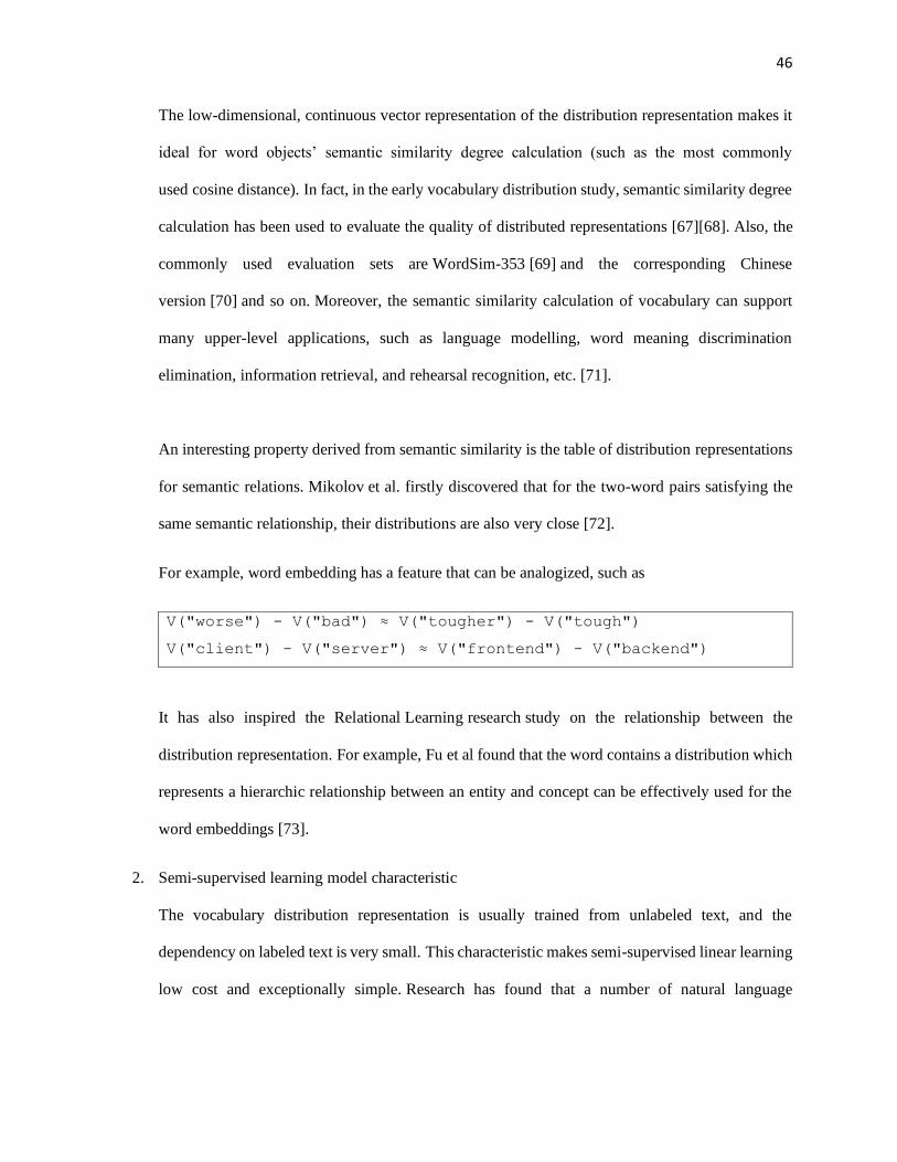
46
The low-dimensional, continuous vector representation of the distribution representation makes it
ideal for word objects’ semantic similarity degree calculation (such as the most commonly
used cosine distance). In fact, in the early vocabulary distribution study, semantic similarity degree
calculation has been used to evaluate the quality of distributed representations [67][68]. Also, the
commonly used evaluation sets are WordSim-353 [69] and the corresponding Chinese
version [70] and so on. Moreover, the semantic similarity calculation of vocabulary can support
many upper-level applications, such as language modelling, word meaning discrimination
elimination, information retrieval, and rehearsal recognition, etc. [71].
An interesting property derived from semantic similarity is the table of distribution representations
for semantic relations. Mikolov et al. firstly discovered that for the two-word pairs satisfying the
same semantic relationship, their distributions are also very close [72].
For example, word embedding has a feature that can be analogized, such as
V("worse") - V("bad") ≈ V("tougher") - V("tough")
V("client") - V("server") ≈ V("frontend") - V("backend")
It has also inspired the Relational Learning research study on the relationship between the
distribution representation. For example, Fu et al found that the word contains a distribution which
represents a hierarchic relationship between an entity and concept can be effectively used for the
word embeddings [73].
2. Semi-supervised learning model characteristic
The vocabulary distribution representation is usually trained from unlabeled text, and the
dependency on labeled text is very small. This characteristic makes semi-supervised linear learning
low cost and exceptionally simple. Research has found that a number of natural language

47
processing tough problems are solved by semi-supervised linear learning from big unlabeled data
to get word clustering such as Brown clustering [74] and related information.
Specifically, great success has been achieved in the areas such as sequence labeling (word
segmentation, Part-of-Speech tagging for online conversational text with word clusters, real
name word recognition [75][76][77] and dependency syntax parsing and analysis [78] and so on.
The basic idea of word clustering is to label a context similar word as a discrete label, equivalent
to a fine-grained part of speech, but it limits the semantics information. However, the study of the
distributional representation provides a semi-supervised linear learning model a new approach to
look at the problem.
For the first time, Turian et al. incorporated a word based on neural network language model in the
sequence labeling model for distributional representation and achieved significant higher accuracy
in the word entity recognition and chunking problem [79].
Their approach is to directly combine the original feature word vector (discrete, sparse, high-
dimensional) and distribution representation feature vectors (continuous, dense, low-dimensional)
together to form a new set of feature vectors.
Wang et al. have done much research on the comparative study of the linear representation and the
nonlinear model [80]. Their experiments show that for the distributional representation of feature
spaces, the nonlinear model is far superior to the linear model.
If it is represented by a graph, it is as shown below Figure 12.

48
Figure 12 Bug words distribution distance map
3. Non-linear model feature learning (FFN, CNN, RNN, LSTM, ELMo, BERT and GPT-2)
Feature learning using nonlinear models is based on the collection of combined features. Natural
language processing research, especially structural prediction problems on sequence labeling and
syntax analysis use huge hypothesis space.
Therefore, a good feature representation is crucial to learning for statistical models. In the traditional
method, because the linear model cannot effectively express the combination of features, therefore,
engineers has used their empirical knowledge and engineering practices to design complex combination
feature models.
Taking Semantic Role Labeling (SRL) as an example, the best system in CoNLL 2009 uses more
than 50 features. [81]. This labor-intensive feature analysis engineering, which relies heavily on expert
knowledge, is not only costly but also suffers from incomplete selection of high dimension features
space, and inefficient feature extraction.
49
Therefore, for natural language processing, deep neural networks with the strength of nonlinear
modelling provides huge advantages. The case, especially the neural network language model
introduced before such as NNLM model which uses context distributional representation vector as an
input, the vector goes through a nonlinear hidden layer tanh activation function and becomes
intermediate vector. The probability distribution of the target word is calculated by the output layer
with SoftMax - a generalized linear model.
In the feedforward neural network (FFN), the intermediate distributional representation vector is
obtained by the hidden layer to process context segment input vector and combine and abstract them.
The same idea can be applied to other NLP areas such as syntactic analysis. In a dependency semantic
parser system research, Chen and Manning has non-linear hidden layer cube activation function
calculate the distributional representation of the transition state, and SoftMax is used to predict the
transition action.
Their model only needs to use a small number of basic features of the distributional representation as
input, but in the hidden layer it implementation the aggregation of feature vectors, which greatly
improves the efficiency of dependency parsing. It can process 1,000 sentences per second.
In addition to the relatively simple structure of the feedforward neural network, the network structure
commonly used in natural language processing are recurrent neural networks, convolutional neural
networks (CNN) and recursive neural networks (RNN).
CNN [86] is based on the simulation of biological neural networks’ local reception field effects. In
CNN model, hidden neurons are connected to only a portion of input layer neurons are connected, while

50
the local connection weights of the different hidden layer neurons are shared. CNN is mainly composed
of convolutional layer and pooling layer.
The local connection property of CNN makes it change for the translation, scaling, and tilting of the
data highly invariant and is now widely used in the field of image processing [87] .
At the same time, this advantage of CNN can be applied in many natural language processing tasks,
such as classifying the review text, the blog comments like Amazon book reviews which are often
determined by some local phrases, without regard to the context or the position of these phrases in the
text. Therefore, CNN has also been widely used in text classification related tasks in recent years and
has achieved reasonable results [88][89][90].
In fact, the earliest application of CNN in natural language processing was proposed by Collobert et
al. to handle NLP by deep neural networks with multitasking learning. The framework is also known
as the C&W model. [91][92]
C&W model is mainly designed for word labeling tasks to use the distributional representation features
such as words, word affixes, POS, etc. as multi-tasking deep neural network input, automatically learn
the aggregation and interaction between features through CNN, then through the non-linear hidden
layer fully connected layers, make the final prediction label at the output layer in the end.
However, because word sequence labeling tasks are very sensitive to information such as word order,
so CNN is not necessarily the most ideal feature learning model. The later research shows that a more
ideal solution is to use the recursive neural network.
RNN has achieved great success in natural language processing. As early as the last century, RNN
was just proposed. At the time, researchers have successfully applied it to natural language processing
such as word tagging and oral language analysis. However, limited by the computing power at that
time, RNN did not attract widespread attention. In recent years, with the excellent

51
performance of RNN on language model [82][83], researchers notice that RNN is highly applicable to
text processing, which is sensitive to long-distance dependence.
Currently, RNN is used in almost all-natural language processing problems, including traditional
structural predictions (lexical, syntactic, semantic analysis, etc.) and hot topics like NLP - machine
translation.
Simultaneously, RNN also shed lights on many tough research areas that are difficult to achieve with
traditional techniques, such as text summaries, poems generation, dialogue system, picture caption
generation, and more.
However, we found if RNN has too extreme deep layers, it has severe gradient vanish or gradient
explosion problem during training process. It is not ideal for the RNN to capture long-distance
dependence in practice.
To solve the above issues, Hochreiter and Schmidhuber proposed Long Short-Term Memory
(LSTM) which is a gated RNN, re-emphasize or forget a certain input vectors to a gate in a network. [84]
These controlled inputs enable the flow of information in the RNN to be efficiently transmitted over
long distances. Furthermore, coder-decoder framework is proposed [85] to solve a series of sequence-
to-sequence problems with a simple and effective end-to-end solution. The above two proposals have
made great breakthroughs on solving gradient vanishing and explosion problems.
In recent NLP development, a new model ELMo is created in 2018 by AllenNLP. [93] It employees a
deep, bi-directional LSTM model to gain word representations. Instead of a dictionary of words and
their corresponding vectors, ELMo studys words within the context that they are used and use the
model to form representations of out-of-vocabulary words.

52
ELMo is used is quite different to word2vec or fast Text. Instead of having a dictionary ‘look-up’ of
words and their corresponding vectors, ELMo builds vectors on-the-fly by passing text through the
deep learning model.
Google researchers create a deep bidirectional transformer model for 11 natural language processing
tasks that surpasses human performance in the area of question answering. The system is called BERT
which is a bidirectional encoder to capture long-distance dependencies compared to a RNN
architecture.[94] It is an outstanding feature that differentiates BERT from OpenAI GPT (a left-to-right
Transformer) and ELMo (a concatenation of independently trained left-to-right and right- to-left
LSTM).
BERT pre-trains a binarized next sentence prediction task that can be trivially generated from any
monolingual corpus. It is a huge model, with 24 Transformer blocks, 1024 hidden layers, and 340M
parameters. Moreover, BERT pre-trains on 40 epochs over a 3.3-billion-word corpus, including
BooksCorpus (800 million words) and English Wikipedia (2.5 billion words).
In early 2019, OpenAI GPT-2 (Generative Pretrained Transformer-2) model recently achieved leading
results across several language modeling benchmarks in a zero-shot setting. [95] The model has the
ability to generate coherent text in areas of question answering, summarization, and etc.
Word2vec is an algorithm used to obtain distributed representations of words. Unfortunately, it does
not address polysemy, or the co-existence of many possible meanings for a given word or phrase. For
example, go is a verb and it is also a board game. The meaning of a given word type such as go varies
according to its context such as the words that surround it.
ELMo, BERT and GPT-2 can obtain much better results in natural language processing tasks by
encoding the context of a given word, by including information about preceding and succeeding words
in the vector that represents a given instance of a word.

53
3.3 Chapter summary
The chapter mainly introduces the mainstream methods in the field of natural language processing
especially in the areas of word vector representation. They are the following principals in word vector
model: 1) CBOW and NGram 2) Skip Gram 3) LSA
Firstly, word vectors form the basis in natural-language processing. Word2vec is an algorithm used to
produce distributed representations of words. By that, the word types, for instance, any given word in
a vocabulary, such as get or grab or go has its own word vector, and those vectors are stored in a lookup
table or dictionary.
Secondly, word2vec library is applied to bug assignments in the codes for my dissertation’s
experiments. The model can be tuned with the following consideration: the choice of context,
determination of the median value of the co-occurrence matrix, and dimension reduction.
Thirdly, word distribution representation can be categorized as many characteristics, empirical, linear,
and nonlinear models. Therefore, the chapter discusses semantic similarities characteristic, semi-
supervised learning model characteristic and non-linear model feature learning (FFN, CNN, RNN,
LSTM, ELMo, BERT and GPT-2).
Next chapter the paper will introduce a new software defect assignment model’s layer 2 – LSTM and
rule-based engine.
54
Chapter 4 New Software Defect Assignment Model – Layer 2: LSTM and
Rule-based Engine
From Figure 4, the paper starts with defects reports analysis by building a vector for the defect report.
We will analyze the defect report and choose the method to build the vector for word. There are many
methods below this paper presents. Then it finds the Word2Vec model built upon neural networks can
have the best results.
Our defect assignment LSTM Framework has two neural networks connected, the first one is the
Word2Vec neural network, on top of Word2Vec neural network, is the LSTM for the final label
prediction on assignment to developer.
At present, the text classification field introduces a brand-new model-Recurrent neural network model.
Recurrent neural networks (RNN) [47] have achieved great success in the field of natural language
processing. RNN has the recurrent feature in its network model and can store the relationship between
the previous neuron and current neuron. It is a feedback structured neural network, which output not
only depends on the value of current inputs and their weights, but the output also counts the weights
and values of the previous neurons. By this way, RNN learns more and trains recurrently.
In traditional neural networks, the model starts from input layer to hidden layer, then to output layer.
The layers are connected but the nodes in each layer is not connected. Because of the missing
connections between nodes in each layer, the traditional neural networks are unable to handle many
problems. For example, if you want to predict what next word the sentence is going to be, you need to
know the previous words because the words before and after in a sentence are not independent.
However, RNN can preserve the relationship between the previous node and current node in a sequence
of words. Moreover, RNN calculates the output value with the consideration of previous hidden layer’s
nodes’ interrelation. RNN’s current hidden layer’s inputs capture not only the output of its input layer

55
information, but also the output of the previous hidden layer’s output information. It can also handle
unlimited length sentence’s weight and bias computation.
Though feedforward neural network has good ability to fit the curve with nonlinear function, it has no
state information. RNN has FFN advantage but also can keep the signal from one neuron to another
one, and will not lose it, and has the signal preserved for a period of time, like having memory capability.
RNN has three categories, 1) Fully recurrent neural networks. 2) Locally recurrent neural network. 3)
Long short-term memory neural networks. Among the above three categories, LSTM has the great
benefits, because it has solved other RNN’s shortcoming, which is not able to store the neuron to neuron
relationship for a long term Error! Reference source not found..
LSTM structure has unparalleled natural advantages in extracting features such as natural language
sentences. It is good at capturing local parts of words (can be easily understood). For a small part of
phrases, such as short phrases, LSTM extract and combine these layers, from basic features to complex
features, to finally identify its meaning, in other words, the local features of the extracted text sequence.
The specific introduction is as follows.
The biggest feature of LSTM model is to allow memory operations to quickly learn useful context
features and filter out other useless words. Our auto bug assignment takes advantage of the context
memorization operation.
4.1 Model Overview – Layer 2: LSTM and Rule-based Engine
The layer 1 - word vector representation is connected to layer 2 – LSTM and rule-based engine. The
word vector model maps discrete words in each text into a fixed-dimensional feature vector to get the
word direction. They are accessed by the layer 2 - LSTM to get a vectorized representation of the entire
document.

56
In order to solve the problem that existing LSTM does not perform well in modeling long sequences
and cannot describe the natural existence of documents. This paper improves the ordinary LSTM model
with one additional rule engine layer. LSTM models text in the sentence level, meanwhile the weights
of the LSTM model are shared with the additional rule engine layer in the evaluation of developers’
experience.
The LSTM that models each sentence is to read the word direction of each sentence. The quantity then
produces the sentence vector corresponding to each sentence, so that the entire text becomes a sequence
of sentence vectors. Then, in this level of developers’ experience modeling, another rule engine will
read the output of LSTM model, resulting in vectorized representation of the entire final output.
In this process, the structural information between the words in each sentence is very good. The location
is preserved, and the structural information between each sentence vectorization is expressed.
After getting the vectorized representation of the bug report, the model begins text label classification
of the document. One multi-label classification strategy is proposed, the first is a multi-label
classification strategy based on label confidence ranking, which performs multiple logistic regression
on bug report features after vectorization expression, and obtains a confidence level for each label. ,
representing the probability that the document belongs to the tag, on the basis of which a dynamic
threshold is used to select those tags whose confidence is higher than the threshold as the prediction
result. The dynamic threshold is obtained by the lease square multiplication regression, which can be
dynamically adjusted according to the various confidence values obtained by multiple logistic
regression.
Then a classifier is trained on each non-leaf node on the hierarchical tag tree, and the classifier defines
the overhead of moving from that node to each of its child nodes by the developer experience rule
engine. In the prediction, similar to the classification method of the decision tree, the algorithm

57
gradually selects the child node from the root through the classifier on the non-leaf node, and finally
obtains a path with the best cost, and all the nodes on the path serve as the output prediction.
Chapter 4 will focus on my model research on the Layer 2: LSTM and Rule-based Engine areas.
Layer 2 Model summary is described in the following diagram Fig 13:
Figure 13 Software Defect Assignment Model Layer 2
Algorithm 2: Construct deep learning model
Input:
The data set of the removed noise
Output:
The validation result of the untriaged data
1: BEGIN
2: Get the sample length of cross validation of each time
3: FOR each cross validation
4: Divide triaged dataset into training set and testing set according to the concept of cross validation
5: FOR each sample of training data set
6: IF the length of current train filter is larger than minimum sentence length
7: Remove words outside the vocabulary from training data set
8: Remove words outside the vocabulary from the owner array of training data set

58
9: END IF
10: END FOR
11: FOR each sample of testing data set
12: IF the length of current test filter is larger than minimum sentence length
13: Remove words outside the vocabulary from testing data set
14: Remove words outside the vocabulary from the owner array of testing data set
15: END IF
16: END FOR
17: FOR each sample of processed test_owner array
18: IF the owner of testing sample doesn’t exist in (test_owner – train_owner)
19: Remove data from test set that is not there in train set
20: Remove owner of test set that is not there in train set
21: END IF
22: END FOR
23: Create train and test data for deep learning model
24: Construct the deep learning model by LSTM
25: Test the testing data set and print out the test accuracy
26: END FOR
27: END
According to the result of triaged dataset preprocessing, we can get the arrays all_data and all_owner.
and the triaged dataset is split into training data and testing data with a specific number of cross
validations you provide to remove training bias. Let’s say the number of cross validations is 3, the
whole triaged bug dataset is divided into three parts, we can call them, sub1, sub2 and sub3. In the first
iteration, we use sub1 as training data, in the meantime, use sub1 as testing data as well. In the second
iteration, we use sub1 + sub2 as training data and use sub2 as testing data. In the third iteration, we use
sub1 + sub2 + sub3 as training data and use sub3 as testing data. The process above is a classic concept
of cross validation.
train_data = all_data[:i * splitLength - 1]
test_data = all_data[(i-1) * splitLength:i * splitLength - 1]
train_owner = all_owner[:i * splitLength - 1]
test_owner = all_owner[(i-1) * splitLength:i * splitLength - 1]
For each bug of training data, we would remove words outside the vocabulary (generated by untriaged
bug dataset) from training data, and also remove words outside the vocabulary from the owner array if
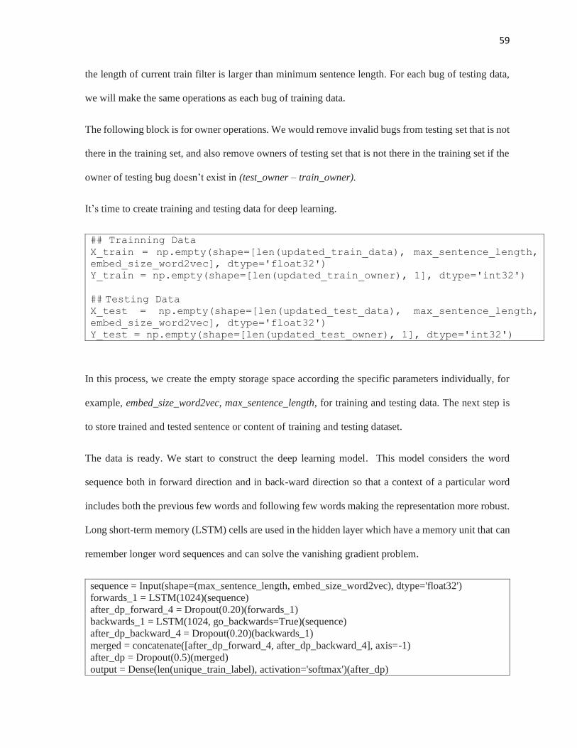
59
the length of current train filter is larger than minimum sentence length. For each bug of testing data,
we will make the same operations as each bug of training data.
The following block is for owner operations. We would remove invalid bugs from testing set that is not
there in the training set, and also remove owners of testing set that is not there in the training set if the
owner of testing bug doesn’t exist in (test_owner – train_owner).
It’s time to create training and testing data for deep learning.
## Trainning Data
X_train = np.empty(shape=[len(updated_train_data), max_sentence_length,
embed_size_word2vec], dtype='float32')
Y_train = np.empty(shape=[len(updated_train_owner), 1], dtype='int32')
## Testing Data X_test = np.empty(shape=[len(updated_test_data), max_sentence_length,
embed_size_word2vec], dtype='float32')
Y_test = np.empty(shape=[len(updated_test_owner), 1], dtype='int32')
In this process, we create the empty storage space according the specific parameters individually, for
example, embed_size_word2vec, max_sentence_length, for training and testing data. The next step is
to store trained and tested sentence or content of training and testing dataset.
The data is ready. We start to construct the deep learning model. This model considers the word
sequence both in forward direction and in back-ward direction so that a context of a particular word
includes both the previous few words and following few words making the representation more robust.
Long short-term memory (LSTM) cells are used in the hidden layer which have a memory unit that can
remember longer word sequences and can solve the vanishing gradient problem.
sequence = Input(shape=(max_sentence_length, embed_size_word2vec), dtype='float32')
forwards_1 = LSTM(1024)(sequence)
after_dp_forward_4 = Dropout(0.20)(forwards_1)
backwards_1 = LSTM(1024, go_backwards=True)(sequence)
after_dp_backward_4 = Dropout(0.20)(backwards_1)
merged = concatenate([after_dp_forward_4, after_dp_backward_4], axis=-1)
after_dp = Dropout(0.5)(merged)
output = Dense(len(unique_train_label), activation='softmax')(after_dp)

60
model = Model(inputs=sequence, outputs=output)
rms = RMSprop(lr=0.001, rho=0.9, epsilon=1e-08)
model.compile(loss='categorical_crossentropy', optimizer=rms, metrics=['accuracy'])
4.2 Artificial Intelligence Neural Networks/Recurrent Neural Network
Artificial intelligence neural networks are computational models that mimic the structure of biological
nervous systems. The most basic structural unit in the biological nervous system is neurons, which
mimic the structure of neurons in the biological nervous system.
In 1943, McCulloch and Pitts [96] abstracted biological neurons as “M-P neuron model” that has been
used today. A single neuron accepts multiple inputs from other neurons and gives different weights to
each input. The input is subtracted from the threshold of the neuron by summing the weights, and an
activation function is used to generate the output of the neuron. Though a single neuron is calculated
in such a simple way, artificial neural network with multiple neurons connected to each other can be
used to fit complex function maps.
Although the prototype of the neural network was proposed as early as 1943, it has never been popular
until the Back Propagation [97] (referred to as the BP calculation) was proposed and BP’s successful
application in neural network systems. In 1988, Hinton et al. successfully used BP algorithm to
effectively trains some shallow networks [98], and then artificial neural network research has begun
widely.
Recurrent Neural Network is a special kind of neural network. In FFN network, the edges between
nodes in the neural network could not form a loop, because if there is a loop, the nodes of the entire
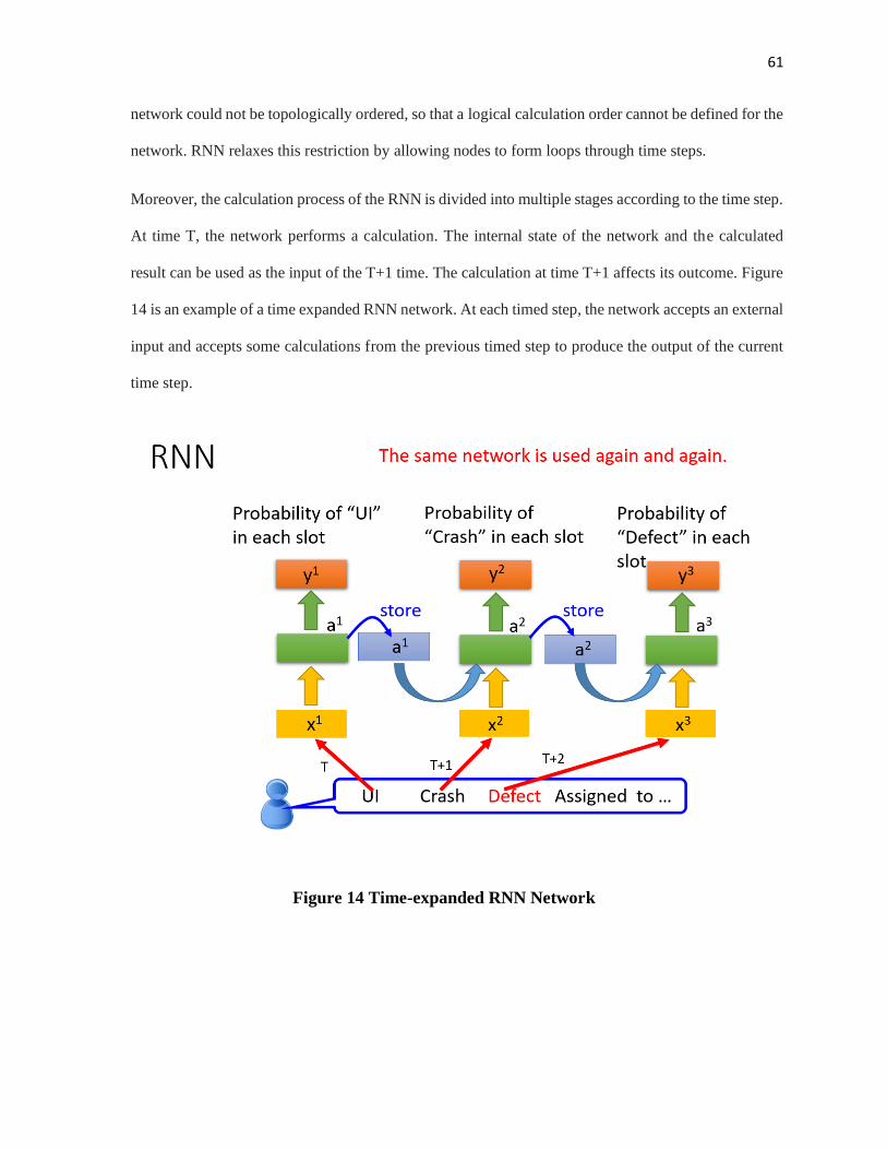
61
network could not be topologically ordered, so that a logical calculation order cannot be defined for the
network. RNN relaxes this restriction by allowing nodes to form loops through time steps.
Moreover, the calculation process of the RNN is divided into multiple stages according to the time step.
At time T, the network performs a calculation. The internal state of the network and the calculated
result can be used as the input of the T+1 time. The calculation at time T+1 affects its outcome. Figure
14 is an example of a time expanded RNN network. At each timed step, the network accepts an external
input and accepts some calculations from the previous timed step to produce the output of the current
time step.
Figure 14 Time-expanded RNN Network

62
During the time expansion of the RNN, an output sequence is generated step by step by an input
sequence. At any T+1 time, the output of the network is the interaction of all the inputs and outputs of
the former T and the internal states of the nodes in the network.
The results of such a feature allows the network can "see" the sequence of historical information that
can be modeled RNN time series.
There is no essential difference between training RNN and the training of ordinary neural networks.
After the RNN is expanded based on time steps, the entire network becomes a common neural network.
It has inputs sequences and output sequences.
It can be trained by using the BP algorithm for this expanded network. From this perspective, RNN is
just a common neural network that shares weights over multiple time steps while delivering network
state between adjacent time steps. RNN is more like a recursive call to a traditional neural network.
4.3 LSTM
Although RNN can “see” all the historical information before time T+1, it can get blurred when the
recursive deep first traverse call to its network. To be specific, when the network is trained by BP
algorithm, the influence of these historical information on the network will gradually disappear with
the network’s expansion. RNN’s such drawback is described as "vanishing gradient problem".[99]
In practice, this flaw can cause the RNN network to be unable to learn events at a certain moment with
an event that happens after more than 10 hours.[99]
In order to solve this defect of RNN, many methods have been proposed like Time Delays [101],
principle of history compression [102], etc. But so far, the most effective solution is the Long Short-
Term Memory Artificial Neural Network Architecture as LSTM. Figure 15 shows the layer 2’s
modified LSTM architecture.
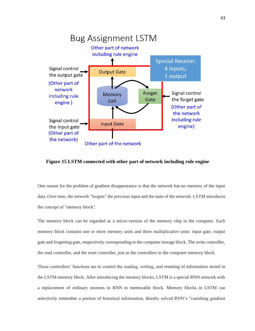
63
Figure 15 LSTM connected with other part of network including rule engine
One reason for the problem of gradient disappearance is that the network has no memory of the input
data. Over time, the network "forgets" the previous input and the state of the network. LSTM introduces
the concept of "memory block".
The memory block can be regarded as a micro-version of the memory chip in the computer. Each
memory block contains one or more memory units and three multiplicative units: input gate, output
gate and forgetting gate, respectively corresponding to the computer storage block. The write controller,
the read controller, and the reset controller, just as the controllers in the computer memory block.
Those controllers’ functions are to control the reading, writing, and resetting of information stored in
the LSTM memory block. After introducing the memory blocks, LSTM is a special RNN network with
a replacement of ordinary neurons in RNN to memorable block. Memory blocks in LSTM can
selectively remember a portion of historical information, thereby solved RNN’s "vanishing gradient

64
problem". The detailed code for bug defect on constructing LSTM layer in the project is implemented
in the Table 3.
sequence = Input(shape=(max_sentence_len, embed_size_word2vec),
dtype='float32')
forwards_1 = LSTM(1024)(sequence)
after_dp_forward_4 = Dropout(0.20)(forwards_1)
backwards_1 = LSTM(1024, go_backwards=True)(sequence)
after_dp_backward_4 = Dropout(0.20)(backwards_1)
merged = merge([after_dp_forward_4, after_dp_backward_4],
mode='concat', concat_axis=-1)
after_dp = Dropout(0.5)(merged)
output = Dense(len(unique_train_label), activation='softmax')(after_dp)
model = Model(input=sequence, output=output)
rms = RMSprop(lr=0.001, rho=0.9, epsilon=1e-08)
model.compile(loss='categorical_crossentropy', optimizer=rms,
metrics=['accuracy'])
hist = model.fit(X_train, y_train, batch_size=batch_size,
epochs=myEpochs)
predict = model.predict(X_test)
Table 3 The code of constructing LSTM for software bug assignment model
With the increase of length of LSTM and limitation of inputs, its functionality decreases and is limited.
To improve its accuracy, recall rate, and precision rate, the paper proposes a new component rule based
engine with the consideration of developer’s experience and productivity. Figure 16 shows the LSTM
to connect with developer experience rule engine.

65
Figure 16 LSTM feeds into developer experience rule engine
4.4 Rule Engines
Knowledge representation is the area of A.I. concerned with how knowledge is represented and
manipulated. Rule Engines use knowledge representation to facilitate the codification of knowledge
into a knowledge base which can be used for reasoning, i.e., we can process data with this knowledge
base to infer conclusions. Rule Engines are based on Expert Systems, which are also known as
Knowledge-based Systems and Knowledge-based Expert Systems and are considered to be "applied
artificial intelligence".
Algorithm 3: Rule Engine Algorithm
Input:
The absolute path of target file
Output:
Generate 'Rule Prediction' result
1: BEGIN
2: Create the translation table
3: IF exists target file
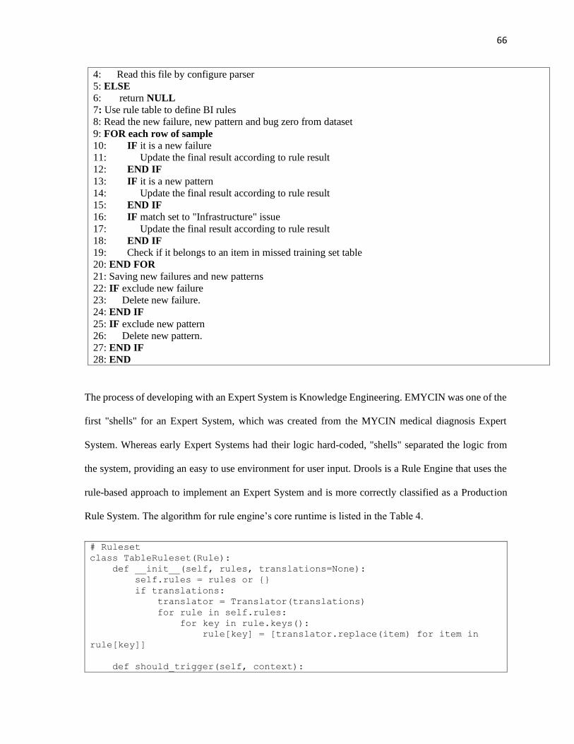
66
4: Read this file by configure parser
5: ELSE
6: return NULL
7: Use rule table to define BI rules
8: Read the new failure, new pattern and bug zero from dataset
9: FOR each row of sample
10: IF it is a new failure
11: Update the final result according to rule result
12: END IF
13: IF it is a new pattern
14: Update the final result according to rule result
15: END IF
16: IF match set to "Infrastructure" issue
17: Update the final result according to rule result
18: END IF
19: Check if it belongs to an item in missed training set table
20: END FOR
21: Saving new failures and new patterns
22: IF exclude new failure
23: Delete new failure.
24: END IF
25: IF exclude new pattern
26: Delete new pattern.
27: END IF
28: END
The process of developing with an Expert System is Knowledge Engineering. EMYCIN was one of the
first "shells" for an Expert System, which was created from the MYCIN medical diagnosis Expert
System. Whereas early Expert Systems had their logic hard-coded, "shells" separated the logic from
the system, providing an easy to use environment for user input. Drools is a Rule Engine that uses the
rule-based approach to implement an Expert System and is more correctly classified as a Production
Rule System. The algorithm for rule engine’s core runtime is listed in the Table 4.
# Ruleset
class TableRuleset(Rule):
def __init__(self, rules, translations=None):
self.rules = rules or {}
if translations:
translator = Translator(translations)
for rule in self.rules:
for key in rule.keys():
rule[key] = [translator.replace(item) for item in
rule[key]]
def should_trigger(self, context):
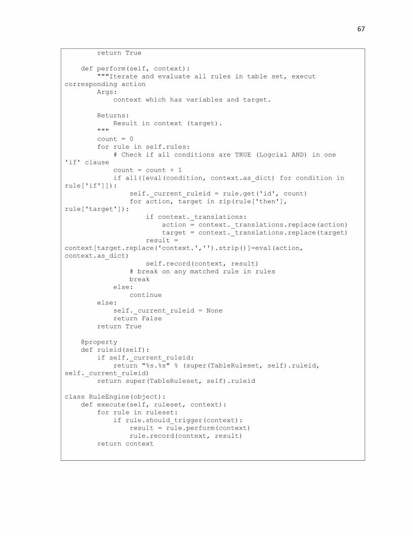
67
return True
def perform(self, context):
"""Iterate and evaluate all rules in table set, execut
corresponding action
Args:
context which has variables and target.
Returns:
Result in context (target).
"""
count = 0
for rule in self.rules:
# Check if all conditions are TRUE (Logcial AND) in one
'if' clause
count = count + 1
if all([eval(condition, context.as_dict) for condition in
rule['if']]):
self._current_ruleid = rule.get('id', count)
for action, target in zip(rule['then'],
rule['target']):
if context._translations:
action = context._translations.replace(action)
target = context._translations.replace(target)
result =
context[target.replace('context.','').strip()]=eval(action,
context.as_dict)
self.record(context, result)
# break on any matched rule in rules
break
else:
continue
else:
self._current_ruleid = None
return False
return True
@property
def ruleid(self):
if self._current_ruleid:
return "%s.%s" % (super(TableRuleset, self).ruleid,
self._current_ruleid)
return super(TableRuleset, self).ruleid
class RuleEngine(object):
def execute(self, ruleset, context):
for rule in ruleset:
if rule.should_trigger(context):
result = rule.perform(context)
rule.record(context, result)
return context

68
Table 4 Algorithm of Rule Engine Core
There are two methods of execution for a rule system: Forward Chaining and Backward Chaining;
systems that implement both are called Hybrid Chaining Systems. Understanding these two modes of
operation is the key to understanding why a Production Rule System is different and how to get the best
from it. Forward chaining is "data-driven" and thus reactionary, with facts being asserted into working
memory, which results in one or more rules being concurrently true and scheduled for execution by the
Agenda.
Figure 17 Forward Chaining
Backward chaining is "goal-driven", meaning that we start with a conclusion which the engine tries to
satisfy. If it can't it then searches for conclusions that it can satisfy; these are known as sub-goals, that
will help satisfy some unknown part of the current goal. It continues this process until either the initial
conclusion is proven or there are no more sub-goals. Prolog is an example of a Backward Chaining
engine. Drools can also do backward chaining, which we refer to as derivation queries.

69
Figure 18 Backward Chaining
The proposed software defect assignment rule engine has used both forward chaining rule and backward
chaining model, and captured the experience of developer, and developer’s productivity, developer’s
context switching time, and dwelling time on the previous bugs. It uses the developers’ social
networking, membership in technical areas, his/her relationship and decision-making in domain areas

70
to obtain rule engine actions. Their expertise is generally classified into their core competency, core
capability, their reasoning and decision making. Rule engine has been effectively used in the
experimental work for bug assignment.
It has the following characteristics. Firstly, just obtains the characteristics of developers’ activity. It
does not need to first analyze the mathematical model of the system like software bug assignment
system and can directly use the opinions of experts. It allows system to describe rules with IF...THEN...
statements. The rules are generally very intuitive. Inference rules are derived from the experience of
experts. Its form is as follows:
If X1 AND X2 AND ......Xn then Y1 AND Y2 AND ...... Ym
Here n is equal to the number of system input variables, and m is equal to the number of system
output variables. The sample code for rule engine’s rules is implemented in the Table 5.
[rule]
# To determine if it's new failure, check failure table
db_newfailure_table = ChromeJob
db_newpattern_table = FireFoxPattern
# use RulesTable to correct result or not
RulesTable = { 'if': ['DeveloperInBlog >= 1', 'rerun >= 1', 'staticset == 1'], \
'then' : ['Increase Defect Assignment by 50'],\
'target':['rulepredict']\
},\
{ 'if': ['EngineerinStackoverflow >= 1', 'rerun >= 1', 'staticset == 1'], \
'then' : ['Add Code Defect to dev more weight by 20'], \
'target': ['rulepredict']\
}
Table 5 Rule Definition Format
Secondly, the software for implementing rule engine is easy and requires less storage space and
computation. Production rule system generally requires only a small number of code lines and less
storage space such as using the look-up table method.

71
Using the detected information such as developers’ comments on stackoverflow.com sites, developers’
code snippets in git, developers’ tag in software engineering forum, developers’ interest groups, and so
on, then the rule reasoning is performed according to the inference rule, and finally the rule engine
makes decision according to the activated rules to assign bug to the appropriate developer.
Each input variable is divided into three levels:
Developer degree of expertise in certain technical area: low, medium and high
Developer quantity of comments in stackoverflow.com site: less, medium and more
Developer quality of reviews in staockoverflow.com site: low, medium and high
Developer involvement in certain interest group: light, medium and heavy
For the output variables, Confidence in assigning the right developer to the bug into 5 levels: very low,
low, medium, high, very high; Name of developer to be assigned to the bug; List of candidate
developers to be assigned to the bug.
The algorithm of Rule Engine Initialization design is shown in the Table 6.
import os
import sys
import pandas as pd
class DictObject(object):
"""class to convert dictionary access as object's members
"""
def __init__(self, initial=None):
self._data = {}
if initial:
self.update(initial)
def __getattr__(self, name):
return self._data.get(name)
def __setattr__(self, name, value):
if name.startswith('_'):
object.__setattr__(self, name, value)
else:
self.__dict__['_data'][name] = value

72
def update(self, other):
for k in other:
self.__setattr__(k, other[k])
def to_dict(self):
return self._data
class Translator(object):
def __init__(self, translations):
self.translations = translations
def replace(self, input):
input = " %s " % input
for source, target in self.translations:
input = input.replace(" %s" % source, " %s " % target)
return input
def rreplace(self, input):
input = "%s" % input
for target, source in self.translations:
input = input.replace("%s" % source, "%s" % target)
return input
Table 6 Algorithm of Rule Engine Initialization Design
For bug assignment developer rules, firstly the rules, which have more data and fact supported by
experts and more reasonable to be understood, will have higher precedence over those rules which are
not vigorously verified. When the rules are used to calibrate the bug assignment system, their
contribution to the accuracy, precision and recall rates can be more effective.
Developers’ rules and other rules like bug-to-tech areas, bug-to-component lookup rules, etc. can be
obtained based on the hierarchical set of input variables and output variables. For example, developer’s
assignment can be expressed by the following 27 rules:
Rule 1: If the bug report says UI, the bug has low priority, and the bug is not very severe, then a junior
developer in UI area will be assigned.
Rule 2: If the bug is critical, the bug is in kernel area, and it requires developers with a lot of experience,
as the developers need to contribute 20K lines codes in git code repository, then a senior developer in
Kernel area, and he has met the line of codes in git criteria will be assigned.
......

73
In the same way, the combination of the bug’s component area, which code path the bug is in, the
developer’s activity requirement can obtain the rule representation of the bug assignment as well as the
Layer1 and LSTM output evaluation. The combination of the degree of developers’ social networking
and stack overflow comments, and other blog history property can obtain the rule representation of
which area of the bug belongs to.
Rule engine can perform complex tasks in a short period of time, rather than requiring a large amount
of mathematical calculations using mathematical methods. Moreover, since the rule engine
calculation itself is a parallel structure, each input can be computed at the same time, or each rule can
be reasoned. The algorithm of Rule Engine Execution design is shown in the Table 7.
class RuleContext(DictObject):
"""
Rule context to store values and attributes (or any object).
Used when applying rule engine
"""
def __init__(self):
super(RuleContext, self).__init__()
self._executed=[]
def __setitem__(self, item, value):
self.__setattr__(item, value)
def __getattr__(self, item):
if not item in self.__dict__ and not item in self._data:
return None
return super(RuleContext, self).__getattr__(item)
@property
def as_dict(self):
return {'context' : self}
# Single rule
class Rule(object):
"""
Rule class - virtual class for table rule set
"""
def should_trigger(self, context):
pass
def perform(self, context):
pass
def record(self, context, result):
context._executed.append((self.ruleid, result))
@property
def ruleid(self):
return self.__class__.__name__.split('.')[-1]
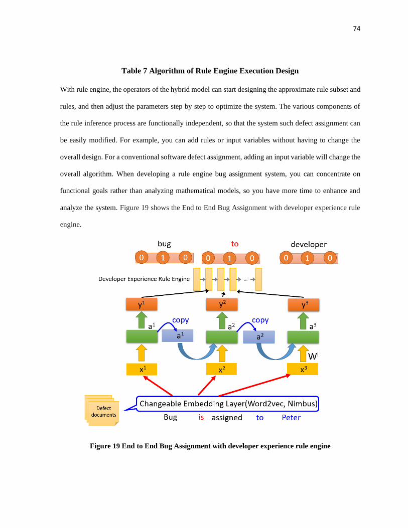
74
Table 7 Algorithm of Rule Engine Execution Design
With rule engine, the operators of the hybrid model can start designing the approximate rule subset and
rules, and then adjust the parameters step by step to optimize the system. The various components of
the rule inference process are functionally independent, so that the system such defect assignment can
be easily modified. For example, you can add rules or input variables without having to change the
overall design. For a conventional software defect assignment, adding an input variable will change the
overall algorithm. When developing a rule engine bug assignment system, you can concentrate on
functional goals rather than analyzing mathematical models, so you have more time to enhance and
analyze the system. Figure 19 shows the End to End Bug Assignment with developer experience rule
engine.
Figure 19 End to End Bug Assignment with developer experience rule engine

75
print('=====Deep learning + rule engine method=====')
for k in range(1, rankK + 1):
id = 0
user_index = 0
runs = 100
trueNum = 0
lableOwner = []
lableOwnerId = []
for sortedInd in sortedIndices:
pred_classes.append(classes[sortedInd[:k]])
if Y_test[id] in sortedInd[:k]:
trueNum += 1
# store error data
elif user_index < runs and k == rankK:
lableOwner.append(classes[Y_test[id]])
lableOwnerId.append(id)
# Base url setup
#print('rule engine start')
# u_email = '[email protected]'
u_email = ' '.join(map(str,
lableOwner[user_index]))
base_url = 'https://monorail-
prod.appspot.com/p/chromium/issues/list?can=1&q='
url = base_url + u_email
try:
# Get the webpage
f = requests.get(url, timeout=5)
soup = BeautifulSoup(f.content, "lxml")
# Get the key words
res = []
for keywords in soup.find_all('td',
class_='col_8'):
a = (keywords.find_all('span'))
b = str(a[0].string).split()
for val in b:
res.append(val)
unique_result = list(set(res))
# Get test set
test =
testedContent[lableOwnerId[user_index]]
# Get overlap percentage
overlap = set(unique_result) &
set(list(filter(None, test)))
percentage_overlap = float(len(overlap)
/ len(test))
# The customize rule

76
bar_percentage = 0.3
rule_flag = True if percentage_overlap >
bar_percentage else False
if rule_flag:
trueNum += 1
#print('user_index: ', user_index)
#print('overlap percentage::: ',
percentage_overlap)
#print('rule result::: ', rule_flag)
#print('rule engine end')
except requests.exceptions.RequestException
as e: # This is the correct syntax
print (e)
user_index += 1
else:
lableOwner.append(classes[Y_test[id]])
lableOwnerId.append(id)
id += 1
accuracy.append((float(trueNum) / len(predict)) *
100)
print('Test accuracy:', accuracy[-1])
Table 8 Python Code of Rule Engine Web Request and Keyword Overlaps Design
After the running of the LSTM model on the training set, and the model is applied to real data, and
with the real data, a HTTP web request is called to retrieve the developer’s experience such as the
bugs he has fixed and the bugs’ description. From the HTTP content, the Python code is used to
extract the keywords of the developers’ experience. Meanwhile a configured value is used, such as
bar percentage = 0.3, that means if the developers’ keywords has 30 percent overlap with the on-field
bugs’ description, that the model overwrites the LSTM results with the developers’ experience values
and reassign the bug to that developer. Overall with the rule engine, the confusion matrix accuracy
has drastically increased.
overlap = set(unique_result) & set(list(filter(None, test)))
percentage_overlap = float(len(overlap) / len(test))
bar_percentage = 0.3
rule_flag = True if percentage_overlap > bar_percentage else False

77
We call the above process that is “online” mode. Sometimes, the user cannot connect the internet, we
also provide a “offline” mode to ensure the efficiency of our system. First, we collect the valuable
information of each bug owner by web crawler. Second, store them to a JSON file: webData.json, the
reason that selecting JSON as storage format is the transition and searching speed is very fast between
JSON and Python. Third, the system may get the information from the file webData.json directly, the
processing speed is faster than getting data by HTTP requests.
4.5 Chapter summary
The chapter mainly introduces the hybrid model’s layer 2: LSTM and Rule-based Engine,
Firstly, it gives an overview on Artificial Intelligence Neural Networks/Recurrent Neural Network. It
describes the history of Artificial Intelligence Neural Networks and its evolution. FFN and RNN are
illustrated briefly. RNN’s shortcoming such as "vanishing gradient problem" is pointed out, and LSTM
is introduced to solve the problem.
Secondly, one reason for the problem of gradient disappearance is that the network has no memory of
the input data. Over time, the network "forgets" the previous input and the state of the network. LSTM
introduces the concept of "memory block".
Thirdly, rule engine is the core of the Layer 2 of the paper’s hybrid model, and is based on Expert
Systems, which are also known as Knowledge-based Systems. Knowledge-based Expert Systems and
are considered to be "applied artificial intelligence". The proposed software defect assignment rule
engine has used both forward chaining rule and backward chaining model, and captured the experience
of developer, and developer’s productivity, developer’s context switching time, and dwelling time on
the previous bugs. It uses the developers’ social networking, membership in technical areas, his/her
relationship and decision-making in domain areas to obtain rule engine actions.

78
Fourthly, for bug assignment developer rules, the rules, which have more data and fact supported by
experts and more reasonable to be understood, will have higher precedence over those rules which are
not vigorously verified. When the rules are used to calibrate the bug assignment system, their
contribution to the accuracy, precision and recall rates can be more effective.
Finally, with rule engine, the operators of the hybrid model can start designing the approximate rule
subset and rules, and then adjust the parameters step by step to optimize the system. The various
components of the rule inference process are functionally independent, so that the system such defect
assignment can be easily modified.
79
Chapter 5 Data Collection and Experiments Result
Software defect assignment is a process of reporting that potentially contain defects, analyzing them,
and assigning developers to fix potentially buggy code. Figure 20 presents a typical software defect
assignment process which is commonly adopted. As the process shows, the first step is to collect source
code files (instances) from software archives and label them as buggy or clean. The labeling process is
based on the number of post-release defects of each file. A file is labeled as buggy if it contains at least
one post-release bug. Otherwise, the file is labeled as clean. The second step is to extract features from
each file. There are many traditional features defined in past studies, which can be categorized into two
kinds: code metrics and process metrics. The instances with the corresponding features and labels are
subsequently employed to train predictive classifiers using various machine learning algorithms such
as SVM, Naive Bayes, and Dictionary Learning. Finally, new instances are fed into the trained classifier,
which can predict whom the bug should be assigned to. In our case, it employs the hybrid model of
NLP, LSTM and rule-based engine.
The set of instances used for building the classifier is training set, while test set includes the instances
used for evaluating the learned classifier. In this work, we focus on within-project defect assignment,
i.e., the training and test sets belong to the same project. Following the previous work in this field, we
use the instances from an older version of this project for training, and instances from a newer version
for test.

80
Figure 20 The process of software defects prediction
5.1 Data preparation and preprocessing
In the software development process, once the software is found to be defective and needs to be repaired,
the relevant personnel will submit it to the defect library in the form of a report to form a defect report.
A defect report mainly consists of three parts: 1) the summary and predefined fields (mainly including
status, product, component, etc.); 2) is a description, describes how to achieve the recurrence of defects,
to help developers understand the occurrence of defects. The process is to find out the cause of the
defect; 3) the comment, which mainly records some suggestions and suggestions from the developer
for the defect.
This paper selects the defect data of large open source software projects of Chrome as the experimental
data set. TrainData.json file contains training sets for using training and validation. That file has 114750
records which is downloaded from https://www.kaggle.com/crawford/deeptriage#classifier_data_0.csv.
That file might be updated since last time downloaded.
TrainData.json file has the following field descriptions for each row
Email address Bug owner (person who will fix it)
issue_title Title of bug description
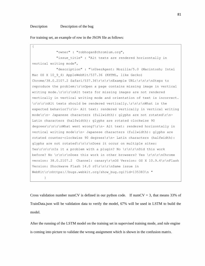
81
Description Description of the bug
For training set, an example of row in the JSON file as follows:
{
"owner" : "[email protected]",
"issue_title" : "Alt texts are rendered horizontally in
vertical writing mode",
"description" : "\nUserAgent: Mozilla/5.0 (Macintosh; Intel
Mac OS X 10_9_4) AppleWebKit/537.36 (KHTML, like Gecko)
Chrome/38.0.2107.2 Safari/537.36\r\n\r\nExample URL:\r\n\r\nSteps to
reproduce the problem:\r\nOpen a page contains missing image in vertical
writing mode.\r\n\r\nAlt texts for missing images are not rendered
vertically in vertical writing mode and orientation of text is incorrect.
\r\n\r\nAlt texts should be rendered vertically.\r\n\r\nWhat is the
expected behavior?\r\n- Alt text: rendered vertically in vertical writing
mode\r\n- Japanese characters (fullwidth): glyphs are not rotated\r\n-
Latin characters (halfwidth): glyphs are rotated clockwise 90
degrees\r\n\r\nWhat went wrong?\r\n- Alt text: rendered horizontally in
vertical writing mode\r\n- Japanese characters (fullwidth): glyphs are
rotated counter-clockwise 90 degrees\r\n- Latin characters (halfwidth):
glyphs are not rotated\r\n\r\nDoes it occur on multiple sites:
Yes\r\n\r\nIs it a problem with a plugin? No \r\n\r\nDid this work
before? No \r\n\r\nDoes this work in other browsers? Yes \r\n\r\nChrome
version: 38.0.2107.2 Channel: canary\r\nOS Version: OS X 10.9.4\r\nFlash
Version: Shockwave Flash 14.0 r0\r\n\r\nSame issue in
WebKit\r\nhttps://bugs.webkit.org/show_bug.cgi?id=135383\n "
}
Cross validation number numCV is defined in our python code. If numCV = 3, that means 33% of
TrainData.json will be validation data to verify the model, 67% will be used in LSTM to build the
model.
After the running of the LSTM model on the training set in supervised training mode, and rule engine
is coming into picture to validate the wrong assignment which is shown in the confusion matrix.

82
Since it is the supervised learning, the confusion matrix knows the wrong assignment. Rule engine is
applied to real data, and with the real data. Rule Engine is set for using to correct the wrong owner
assignment during the validation. The more developers to be run and the more developers’ keywords
info, the better of accuracy
There are two modes of Rule Engines validation, one is the online mode, and the other is the offline
mode. If it is online mode, a HTTP web request is called to retrieve the developer’s experience such
as the bugs he has fixed and the bugs’ description. The code call the https://monorail-
prod.appspot.com/p/chromium/issues to get the owners’ keywords. From the HTTP content, the
Python code is used to extract the keywords of the developers’ experience from the training set.
Meanwhile a configured value is used, such as bar percentage = 0.3, that means if the developers’
keywords has 30 percent overlap with the on-field bugs’ description, that the model overwrites the
LSTM wrong prediction results with the developers’ experience values and reassign the bug to that
developer. Overall with the rule engine, the confusion matrix accuracy has drastically increased.
Sometimes, the user cannot connect the internet, or we want to have consistent model benchmark, we
also provide a “offline” mode to ensure the efficiency of our system. First, we collect the valuable
information of each bug owner by web crawler. Second, store them to a JSON file permanently:
webData.json, the reason that selecting JSON as storage format is the transition and searching speed
is very fast between JSON and Python. Third, the system may get the information from the file
webData.json directly, the processing speed is faster than getting data by HTTP requests.
WebData.json is obtained by our data populator and get them from the https://monorail-
prod.appspot.com/p/chromium/issues for only one time and then we can train the data offline.
getownerjson.py is the code to create the above WebData.json.

83
WebData.json has the following field descriptions for each row
Email address Developer (person who will fix it)
Keywords list Developer’s activity, technical ability and key attributes
TestData.json contains all the bug reports, and Owner field is the developer’s email alias which is empty
before running our model. Once our model is deployed in production to predict the Owner field, the
model will predict which email alias and fill the email address in the Owner field.
TestData.json has the following field descriptions for each row
Id Bug id
issue_id issue id
issue_title Title of bug description
reported_time Time bug was reported
Owner email address of owner of the bug (person who will fix it)
Description Description of the bug
Bug reports from the Google Chromium project were downloaded for the duration of 2008-09-02
(Bug ID: 3) - 2013-09-05 (Bug ID: 633012).
For test set to be predicted after using our bug assignment model, an example of row in the JSON file
as follows:
{
"id" : 3,
"issue_id" : 5,
"issue_title" : "Java not working yet",
"reported_time" : "2008-09-02 19:04:27",
"owner" : "",
fariie\r\nadd ok or fail after other browsers where you have tested this
issue\n safari 3 ok\r\n firefox 3 ok\r\n ie 7 ok\r\n\r\nwhat
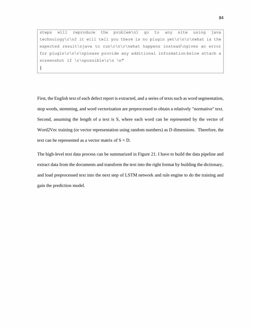
84
steps will reproduce the problem\n1 go to any site using java
technology\r\n2 it will tell you there is no plugin yet\r\n\r\nwhat is the
expected result\njava to run\r\n\r\nwhat happens instead\ngives an error
for plugin\r\n\r\nplease provide any additional information below attach a
screenshot if \r\npossible\r\n \n"
}
First, the English text of each defect report is extracted, and a series of texts such as word segmentation,
stop words, stemming, and word vectorization are preprocessed to obtain a relatively "normative" text.
Second, assuming the length of a text is S, where each word can be represented by the vector of
Word2Vec training (or vector representation using random numbers) as D dimensions. Therefore, the
text can be represented as a vector matrix of S × D.
The high-level text data process can be summarized in Figure 21. I have to build the data pipeline and
extract data from the documents and transform the text into the right format by building the dictionary,
and load preprocessed text into the next step of LSTM network and rule engine to do the training and
gain the prediction model.

85
Figure 21 High-level Text Data Process
Since the original text contains irregular words, extra punctuation marks, and meaningless pause words,
the algorithm first needs to filter the noise in the text. When filtering the noise, it also needs to perform
sentence segmentation and word segmentation on the text. The model in my research treats the
document as a sequence of sentences. For each sentence, the model is processed separately, so the
process of clauses is necessary. After the clauses and participles are completed, each word needs to be
processed and becomes case-insensitive, and the number of times they appear is counted, and a
dictionary is constructed. The words with very low number of occurrences in the dictionary are
considered to be low-frequency noise words. Those noise words are removed from the model. The
detailed code is implemented in the Table 9.
with open(closed_bugs_json) as data_file:
data = json.load(data_file, strict=False)
all_data = []
all_owner = []

86
for item in data:
# Step 1. Remove \r
current_title = item['issue_title'].replace('\r', ' ')
current_desc = item['description'].replace('\r', ' ')
# Step 2. Remove URLs
current_desc = re.sub(r'http[s]?://(?:[a-zA-Z]|[0-9]|[$-
_@.&+]|[!*\(\),]|(?:%[0-9a-fA-F][0-9a-fA-F]))+', '', current_desc)
# Step 3. Remove Stack Trace
start_loc = current_desc.find("Stack trace:")
current_desc = current_desc[:start_loc]
# Step 4. Remove hex code
current_desc = re.sub(r'(\w+)0x\w+', '', current_desc)
current_title= re.sub(r'(\w+)0x\w+', '', current_title)
# Step 5. Change to lower case
current_desc = current_desc.lower()
current_title = current_title.lower()
# Step 6. Tokenize
# A sentence or data can be split into words using the method
word_tokenize()
current_desc_tokens = nltk.word_tokenize(current_desc)
current_title_tokens = nltk.word_tokenize(current_title)
# Step 7. Strip punctuation marks
current_desc_filter = [word.strip(string.punctuation) for word in
current_desc_tokens]
current_title_filter = [word.strip(string.punctuation) for word in
current_title_tokens]
# Step 8. Join the lists
current_data = current_title_filter + current_desc_filter
###########################
# current_data = filter(None, current_data)
current_data = list(filter(None, current_data))
###########################
all_data.append(current_data)
all_owner.append(item['owner'])
Table 9 Function to preprocess the text in bug report

87
In this paper, only the words in the dictionary after removing the low frequency words mentioned above
are vectorized, and other words are represented by vectors of all 0s. In the subsequent processing, the
model is implemented to automatically ignore all 0s. Text entered into the subsequent model is the
word after all low frequency words are removed. The specific process can be summarized in Figure 22.

88
Figure 22 Text Extracting, Transforming, and Loading Process
5.2 Experimental design
The experiment in this paper is carried out on the Surface Book 2, and its configuration is listed in
Table 10.
Table 10 Hardware specification for experiments
The operating system is Window 10, the software requirements: Python 3.6.5, “Visual Studio
Community 2015 with Update 3”, and NVIDIA® GPU drivers —CUDA 9.0 requires 384.x or higher,
CUDA® Toolkit, TENSORFLOW, and Keras.
The increment (ten-fold incremental) method is used for training. The data sets are ordered by time and
they are equally divided into 11 copies. First, in the first round, the first fold is used as the training set,
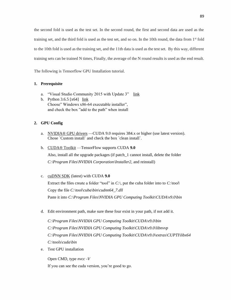
89
the second fold is used as the test set. In the second round, the first and second data are used as the
training set, and the third fold is used as the test set, and so on. In the 10th round, the data from 1st fold
to the 10th fold is used as the training set, and the 11th data is used as the test set. By this way, different
training sets can be trained N times, Finally, the average of the N round results is used as the end result.
The following is Tensorflow GPU Installation tutorial.
1. Prerequisite
a. “Visual Studio Community 2015 with Update 3” link
b. Python 3.6.5 [x64] link
Choose” Windows x86-64 executable installer”,
and check the box ”add to the path” when install
2. GPU Config
a. NVIDIA® GPU drivers —CUDA 9.0 requires 384.x or higher (use latest version).
Chose `Custom install` and check the box `clean install`.
b. CUDA® Toolkit —TensorFlow supports CUDA 9.0
Also, install all the upgrade packages (if patch_1 cannot install, delete the folder
C:\Program Files\NVIDIA Corporation\Installer2, and reinstall)
c. cuDNN SDK (latest) with CUDA 9.0
Extract the files create a folder “tool” in C:\, put the cuba folder into to C:\tool\
Copy the file C:\tool\cuba\bin\cudnn64_7.dll
Paste it into C:\Program Files\NVIDIA GPU Computing Toolkit\CUDA\v9.0\bin
d. Edit environment path, make sure these four exist in your path, if not add it.
C:\Program Files\NVIDIA GPU Computing Toolkit\CUDA\v9.0\bin
C:\Program Files\NVIDIA GPU Computing Toolkit\CUDA\v9.0\libnvvp
C:\Program Files\NVIDIA GPU Computing Toolkit\CUDA\v9.0\extras\CUPTI\libx64
C:\tools\cuda\bin
e. Test GPU installation
Open CMD, type nvcc -V
If you can see the cuda version, you’re good to go.

90
3. virtual environment
a. install virtualenv, Open CMD as administrator
pip install virtualenv
b. Create a new virtual environment by choosing a Python interpreter and making a
C:\tensorflow directory to hold it:
In CMD type
virtualenv --system-site-packages -p python C:\tensorflow
4. Install tensorflow and keras
a. Activate the virtual environment: (Every time you start use tensorflow)
In CMD type
C:\tensorflow\Scripts\activate
b. Install packages, In CMD type
pip install --upgrade pip
pip list
# Installing tensorflow
pip install --upgrade tensorflow-gpu==1.11.0
# Verify the install:
python -c "import tensorflow as tf;
tf.enable_eager_execution();print(tf.reduce_sum(tf.random_normal([1000, 1000])))"
# Installing keras, genism, punkt, scikit-learn, beautifulsoup4, lxml
pip install keras==2.2.4
pip install gensim==3.6.0
pip install nltk==3.3
pip install scikit-learn==0.20.0
pip install beautifulsoup4
pip install lxml
python >>> import nltk
python >>> nltk.download(‘punkt’)
c. When you finish using tensorflow to exit environment
In CMD type

91
deactivate
5.3 Experiment Results
This section conducts experiments and compares bug assignment models using Naïve Bayes, LSTM
and “LSTM + Rule Engine”.
1) Bag of words (BOW) + Naïve Bayes (NB)
The bag of words (BOW) feature representation of the bug report creates a Boolean array marking
true or false for each vocabulary word in the bug report. During training, the Naïve Bayes classifier
will learn this representation to the corresponding owner label. The Naïve Bayes classifier uses
only the classifier training and testing data and do not use the un-triaged bug reports and is
implemented using the Python scikit-learn package.
Naïve Bayes algorithm is implemented using the scikit package of python. It is implemented as
following:
classifierModel = MultinomialNB(alpha=0.01)
classifierModel = OneVsRestClassifier(classifierModel).fit(train_feats, updated_train_owner)
predict = classifierModel.predict_proba(test_feats)
classes = classifierModel.classes_
accuracy = []
sortedIndices = []
pred_classes = []
for ll in predict:
sortedIndices.append(sorted(range(len(ll)), key=lambda ii: ll[ii], reverse=True))
for k in range(1, rankK + 1):
id = 0
trueNum = 0
for sortedInd in sortedIndices:
pred_classes.append(classes[sortedInd[:k]])
if(id < len(Y_test)):
if Y_test[id] in sortedInd[:k]:
trueNum += 1
id += 1
accuracy.append((float(trueNum) / len(predict)) * 100)

92
print ('Naive Bayes accuracy:', accuracy)
The multinomial Naive Bayes classifier is suitable for classification with discrete features (e.g.,
word counts for text classification). The multinomial distribution normally requires integer
feature counts. Firstly, we create a classifier model for multinomial Naïve Bayes. Secondly, we
use OneVsRestClassifier strategy to fit underlying estimators. This strategy consists in fitting one
classifier per class. For each classifier, the class is fitted against all the other classes. In addition
to its computational efficiency, one advantage of this approach is its interpretability. Since each
class is represented by one and one classifier only, it is possible to gain knowledge about the class
by inspecting its corresponding classifier. Third, according to term frequency-based bag-of-words
model features, we will make the probability estimates. Finally, we use the real data to get test
accuracy. The experiment result is shown in the following table.
2) LSTM
Our deep learning model can learn sentence representation to keep the sequence and syntax of
words (title + description), also retain the semantic relationship using LSTM, which are used in the
hidden layer of the whole model. At the same time, LSTM also can solve the vanishing gradient
problem. The model is implemented using the Python keras package. The experiment result is
shown in the following table.
3) LSTM + Rule Engine
Comparing with traditional method, we have obtained the remarkable experiment results. But
there is still a lot of room to improve the accuracy of recognition. We provide a rule engine over
our deep learning model to add the customize rules and improve the test accuracy. In our first use
cases (only process first 1000 incorrect owners), we use web crawler to collect the additional
information of owners and calculate the overlapping between collected information of owners and
the content of predicted sentences. The customize rule uses the parameter bar_percentage. The

93
rule is “if the overlapping rate is greater than 0.35”( bar_percentage = 0.35), we would assign the
correct owner to the bug report.
The experiment results are shown in two categories, offline and online. As the research mentions
before, the offline is using all data locally, and can be rerun and achieve the similar number except some
minor randomness, but it is reproducible. The online result is more dynamic depending on the latest http
web request to get the developers’ keywords data.
The first one is the benchmark for how to do just run one number of cross validation, and one
epoch, and is run as offline. The second result table is also run as offline but number of cross validation is
5 and number of epochs is also 5, other parameters are listed as well. The third one is run as online mode,
and other parameters are listed in the configuration table as well.
The following experiment configuration arguments are following and run offline:
numCV = 1
max_sentence_length = 50
min_sentence_length = 15
rankK = 10
batch_size = 32
myEpochs = 1
bar_percentage = 0.3
In the following use case, we processed 16000 incorrect owners and it takes about 30 minutes to
finish. The experiment result is shown in the following table.
Classifier BOW + NB LSTM LSTM + Rule Engine
1st Cross Validation 13.64 27.41 29.74

94
The above graph shows that in offline mode, pure LSTM has a better result than BOW+NB
model, the hybrid LSTM+Rule Engine has the best accuracy overall.
The following experiment configuration arguments are following and run offline:
numCV = 5
max_sentence_length = 50
min_sentence_length = 15
rankK = 10
batch_size = 32
myEpochs = 5
bar_percentage = 0.3
In the following use case, we processed 16000 incorrect owners and it takes about 10 hours to
finish. The experiment result is shown in the following table.
Classifier BOW + NB LSTM LSTM + Rule Engine
1st Cross Validation 22.12 65.71 70.88
2nd Cross Validation 20.76 49.20 57.50
3rd Cross Validation 17.39 30.58 41.32
13.64
27.4129.74
0
5
10
15
20
25
30
35
BOW+NB LSTM LSTM+Rule Engine
AC
CU
RA
CY
APPROACHES
processed 16000 incorrect owners with Rule Engine

95
4th Cross Validation 23.99 27.07 38.98
5th Cross Validation 8.99 27.29 38.86
The above graph shows that in offline mode for 5 cross validations, pure LSTM has a better result
than BOW+NB model, the hybrid LSTM+Rule Engine has improved the accuracy over pure LSTM
further.
The following experiment configuration arguments are following and run online:
numCV = 10
22.12 20.7617.39
23.99
8.99
65.71
49.2
30.5827.07 27.29
70.88
57.5
41.3238.98 38.86
1 2 3 4 5
Acc
ura
cy
Nth Cross Validation
Rule Engine with 16000 incorrect owners offline
BOW+NB LSTM LSTM+Rule Engine
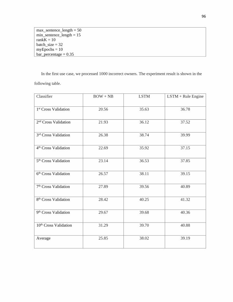
96
max_sentence_length = 50
min_sentence_length = 15
rankK = 10
batch_size = 32
myEpochs = 10
bar_percentage = 0.35
In the first use case, we processed 1000 incorrect owners. The experiment result is shown in the
following table.
Classifier BOW + NB LSTM LSTM + Rule Engine
1st Cross Validation 20.56 35.63 36.78
2nd Cross Validation 21.93 36.12 37.52
3rd Cross Validation 26.38 38.74 39.99
4th Cross Validation 22.69 35.92 37.15
5th Cross Validation 23.14 36.53 37.85
6th Cross Validation 26.57 38.11 39.15
7th Cross Validation 27.89 39.56 40.89
8th Cross Validation 28.42 40.25 41.32
9th Cross Validation 29.67 39.68 40.36
10th Cross Validation 31.29 39.70 40.88
Average 25.85 38.02 39.19

97
The above graph shows that in online mode for 10 cross validations, pure LSTM has a better
result than BOW+NB model, the hybrid LSTM+Rule Engine has applied its rules to 1000 incorrect
owners and has improved the accuracy over pure LSTM further.
In the second use case, we processed 2000 incorrect owners. The experiment result is shown in
the following table.
Classifier BOW + NB LSTM LSTM + Rule Engine
1st Cross Validation 20.12 33.25 35.12
2nd Cross Validation 22.34 34.63 36.21
3rd Cross Validation 25.94 37.98 39.34
4th Cross Validation 22.78 36.13 37.43
5th Cross Validation 22.97 36.72 37.98
6th Cross Validation 25.37 38.45 39.76
7th Cross Validation 27.18 39.26 40.57
0
5
10
15
20
25
30
35
40
45
1 2 3 4 5 6 7 8 9 10
Acc
ura
cy
Nth Cross Validation
Rule Engine with 1000 first incorrect owners
BOW+NB LSTM LSTM+Rule Engine

98
8th Cross Validation 27.45 41.26 42.67
9th Cross Validation 28.59 39.32 40.47
10th Cross Validation 30.13 40.12 41.65
Average 25.29 37.71 39.12
The above graph shows that in online mode for 10 cross validations, pure LSTM has a better
result than BOW+NB model, the hybrid LSTM+Rule Engine has applied its rules to 2000 incorrect
owners and has improved the accuracy over pure LSTM further.
In the next use case, we processed 3000 incorrect owners. The experiment result is shown in the
following table.
Classifier BOW + NB LSTM LSTM + Rule Engine
1st Cross Validation 20.63 31.95 33.58
2nd Cross Validation 22.08 36.34 37.92
0
5
10
15
20
25
30
35
40
45
1 2 3 4 5 6 7 8 9 10
Acc
ura
cy
Nth Cross Validation
Rule Engine with 2000 first incorrect owners
BOW+NB LSTM LSTM+Rule Engine

99
3rd Cross Validation 26.45 38.92 40.59
4th Cross Validation 23.74 36.13 37.76
5th Cross Validation 23.98 37.32 38.99
6th Cross Validation 26.56 38.45 40.07
7th Cross Validation 28.04 39.88 41.43
8th Cross Validation 28.43 40.12 41.48
9th Cross Validation 29.21 39.54 41.23
10th Cross Validation 30.88 39.92 41.84
Average 26.01 37.86 39.49
The above graph shows that in online mode for 10 cross validations, pure LSTM has a better
result than BOW+NB model, the hybrid LSTM+Rule Engine has applied its rules to 3000 incorrect
owners and has improved the accuracy over pure LSTM further.
0
5
10
15
20
25
30
35
40
45
1 2 3 4 5 6 7 8 9 10
Acc
ura
cy
Nth Cross Validation
Rule Engine with 3000 first incorrect owners
BOW+NB LSTM LSTM+Rule Engine

100
In the fourth use case, we processed 4000 incorrect owners. The experiment result is shown in the
following table.
Classifier BOW + NB LSTM LSTM + Rule Engine
1st Cross Validation 20.34 33.38 35.45
2nd Cross Validation 22.12 35.24 37.19
3rd Cross Validation 26.45 38.35 40.38
4th Cross Validation 22.57 36.03 38.03
5th Cross Validation 23.56 37.02 39.11
6th Cross Validation 26.13 38.43 40.46
7th Cross Validation 27.76 39.42 41.43
8th Cross Validation 28.58 40.66 42.67
9th Cross Validation 29.45 39.45 41.56
10th Cross Validation 31.12 39.54 41.68
Average 25.81 37.75 39.80

101
The above graph shows that in online mode for 10 cross validations, pure LSTM has a better
result than BOW+NB model, the hybrid LSTM+Rule Engine has applied its rules to 4000 incorrect
owners and has improved the accuracy over pure LSTM further.
In the fifth use case, we processed 5000 incorrect owners. The experiment result is shown in the
following table.
Classifier BOW + NB LSTM LSTM + Rule Engine
1st Cross Validation 20.31 34.78 37.12
2nd Cross Validation 22.08 35.98 38.27
3rd Cross Validation 26.32 38.46 40.79
4th Cross Validation 22.48 35.17 37.50
5th Cross Validation 23.57 36.32 38.65
6th Cross Validation 26.12 38.45 40.73
0
5
10
15
20
25
30
35
40
45
1 2 3 4 5 6 7 8 9 10
Acc
ura
ry
Nth cross validation
Rule Engine with 4000 first incorrect owners
BOW+NB LSTM LSTM+Rule Engine

102
7th Cross Validation 27.97 39.76 42.03
8th Cross Validation 28.23 40.33 42.67
9th Cross Validation 29.85 39.54 41.84
10th Cross Validation 31.12 39.88 42,15
Average 25.80 37.88 40.18
The above graph shows that in online mode for 10 cross validations, pure LSTM has a better
result than BOW+NB model, the hybrid LSTM+Rule Engine has applied its rules to 5000 incorrect
owners and has improved the accuracy over pure LSTM further.
5.4 Chapter summary
This chapter conducts experiments and comparative analysis of the performance of three models, Naïve
Bayes, LSTM and Hybrid model proposed in the paper. It introduces the hybrid NLP, LSTM and Rule-
0
5
10
15
20
25
30
35
40
45
1 2 3 4 5 6 7 8 9 10
Acc
ura
cy
Nth Cross Validation
Rule Engine with 5000 first incorrect owners
BOW+NB LSTM LSTM+Rule Engine
103
based Engine model into the experimental verification flied of defect automatic assignment software
engineering. Use the textual information such as summary, description, and commentary of the defect
report to train the developer to predict the model for Chromium.
Experiments data show that the proposed hybrid model has obvious advantages in accuracy compared
with the machine learning NB algorithm and the pure deep learning LSTM model. It proves the validity
of the hybrid model and provides a new solution for automatic defect assignment problem.

104
Chapter 6 Conclusion
6.1 Major Achievements and Research Contributions
In this research we have designed and implemented a reusable software two-layer new model to assign
bugs to right developers. The combination of both layers Layer 1: NLP and Vector for Words and Layer
2: LSTM and Rule-based Engine cover a wide spectrum of validation requirements making our model
a versatile research or business value. For the problem of software defects and AI assignment based on
text classification, below is a bulleted list of these contributions:
• Leveraged the combination of both layers Layer 1: NLP and Vector for Words and Layer 2: LSTM and
Rule-based Engine is successfully introduced into the field of defect self-assignment. The traditional
method of defect self-assignment is based on the traditional text word bag model and the machine
learning model, which is not only inefficient, but also labor-intensive. If you use deep learning models
such as LSTM-based networks, you don't need to spend a lot of time and effort on the feature extraction
engineering required for a machine study model, you just need to put text into a simple line, and then
enter the model.
• The proposed neural network model extracts text features on its own, taking into account not only the
word order messages that the word bag model ignores, but also the grammatical and semantic
characteristics of the text, improving the effect of the defect allocation model. Moreover, more
importantly, the structure of these two layers network models with rule-based engine is relatively
simple, i.e. the model, with only NLP network architecture, word2Vec, LSTM, Rule-based engine
parallel structure, ideal for parallel computing, plus a dedicated hardware processing accelerator GPU
the use of this paper makes the model not only high accuracy, but also faster.

105
• My work contributes three different model comparison Naïve Bayes, LSTM and LSTM with Rule-
based Engine neural network model structures. LSTM model is more effective than the Naïve Bayes
algorithm commonly used in machine learning for bug assignment. Rule Engine is a new attempt, and
the model works well, and has been designed on the basis of LSTM model. The optimal results were
achieved on both the CHROME dataset. In general, the three models, from simple to complex, from
traditional to more advanced hybrid approach gradually increase the accuracy of the bug assignment.
• The model based on the combination of both layers Layer 1: NLP and Vector for Words and Layer 2:
LSTM and Rule-based Engine proposed in this paper is simple, but highly effective in defect self-
assignment and has the ability to expand and migrate the system to other datasets. The model simply
relies on defect text, does not use other complex techniques and tribal knowledge of defect analysis,
and the traditional method is based on feature extraction engineering approach, which is only valid for
special datasets, making it difficult to be applied to other datasets. The model is expandable and
migratable.
6.2 Future Work
The research can still be improved to allow it to stay relevant with the changing technology trends.
Below is a list of potential future work examples.
• Although the text classification method based on convolutional neural network proposed in this paper
has achieved great results in the automatic assignment of defects, this method still has certain
limitations, such as only considering the text keywords features of defect reports overlapping with
developers’ keywords, but ignoring other possible data source such as developers’ blogging activities,
their Facebook, and other data.
• Although the two layers models training has achieved some achievements, it does not involve the latest
methods in the field of natural language processing, such as BERT (Bidirectional Encoder
Representations from Transformers) is a recent paper published by researchers at Google AI Language.

106
Moreover, it can include GPT-2[103], a powerful NLP model in the layer 1 in the future study as well.
For training models, there are new models such as GAN and Transfer Learning are recently proposed
as well. It indicates that there is room for further improvement in the methods proposed in this paper.
107
References
[1] Jeong, Kim S, Zimmermann T. Improving bug triage with bug tossing graphs[C].
Proceedings of the 7th joint meeting of the European software engineering conference and
the ACM SIGSOFT symposium on the foundations of software engineering
(FSE/ESEC’09) ACM,2009:111-120.
[2] Beauvais F., Sak H Senior’A W Long short-term memory recurrent neural network
architectures for large scale acoustic modeling[C] INTERSPEECH 2014: 338-342.
[3] H. Sak, A. Senior, and F. Beauvais, “Long Short-Term Memory Based Recurrent Neural
Network Architectures for Large Vocabulary Speech Recognition,” ArXiv e-prints, Feb.
2014.
[4] S. Hochreiter and J. Schmidhuber, “Long short-term memory,” Neural Computation, vol. 9,
no. 8, pp. 1735–1780, Nov. 1997.
[5] Y. Bengio, P. Simard, and P. Frasconi, “Learning long-term dependencies with gradient
descent is difficult,” Neural Networks, IEEE Transactions on, vol. 5, no. 2, pp. 157–166,
1994
[6] Dyer C, Ballesteros M, Ling W, et al. Transition-Based Dependency Parsing with Stack
Long Short-Term Memory[C] Proceedings of the 53rd Annual Meeting of the Association
for Computational Linguistics and the 7thInternational Joint Conference on Natural
Language Processing (Volume1: Long Papers). Beijing, China: Association for
Computational Linguistics, 2015:334–343.
[7] Ballesteros M, Dyer C, Smith N A. Improved Transition-based Parsing by Modeling
Characters instead of Words with LSTM[C] Proceedings of the 2015 Conference on
Empirical Methods in Natural Language Processing. Lisbon, Portugal: Association for
Computational Linguistics, 2015:349–359.

108
[8] Tamrawi A, Nguyen T, Al-Kofahi J M, et al. Fuzzy set and cache-based approach for bug
triaging [C]. Proceedings of the 19th ACM SIGSOFT Symposium on the Foundations of
Software Engineering (FSE-19) and the 13th European Software Engineering
Conference(ESEC-13). ACM, 2011: 365-375.
[9] Tamrawi A, Nguyen T, Al-Kofahi J M, et al. Fuzzy set-based automatic bug triaging:
NIER track. http://home.engineering.iastate.edu/~atamrawi/publications/bugzie-neir-
icse.pdf
[10] Murphy G, Cubranic D. Automatic bug triage using text categorization[C] . Proceedings
of the Sixteenth International Conference on Software Engineering & Knowledge
Engineering (SEKE 504). SEKE, 2004: 92- 97
[11] Anvik J, Hiew L, Murphy G C. Who should fix this bug? [C]. Proceedings of the 28th
international conference on Software engineering (ICSE, 06). ACM, 2006: 3 6 1 - 3 70.
[12] Matter D, Kuhn A, Nierstrasz O. Assigning bug reports using a vocabulary - based
expertise model of developers [C]. Proceedings of the 6th IEEE International Working
Conference on Mining Software Repositories (M SR ' 09). IEEE, 2009: 131 - 140.
[13] Bhattacharya P, Neamtiu I. Fine -grained incremental learning and multi -feature tossing
graphs to improve bug triaging [C]. Proceedings of the 2010 IEEE International Conference
on Software Maintenance (ICS M1 1 0). IEEE, 2010: 1 - 1 0.
[14] Thierry Denoeux and Regis Lengelle, Initializing Back Propagatioox E. Adaptive fuzzy
systems.IEEE Spectrum,1993, 58-61
[15] Xu C W.Decoupling fuzzy relation systems:An output feedback approach.IEEE Trans
Syst Man Cybern,1989.19(1)
[16] Xu C W.Lu Y Z.Decoupling in fuzzy system:A cascade companion approach.Fuzzy
Set Syst.1989.29:177-185
[17] Bart Kosko, Neural Networks and Fuzzy SystemPrentice-Hall International Inc., 1992

109
[18] Murphy G, Cubranic D. Automatic bug triage using text categorization[C] Proceedings of
the Sixteenth International Conference on Software Engineering &Knowledge Engineering
(S EKE 5 04). SEKE ,2 004 :92- 97
https://pdfs.semanticscholar.org/169b/b50e92c1a5feb756295e4a9e5492e79cf382.pdf
[19] Firefox provides a web browser and can be found at www.mozilla.org/products/firefox/
[20] Anvik J, Hiew L, Murphy G C. Who should fix this bug? [C]. Proceedings of the 28th
international conference on Software engineering (ICSE, 0 6). ACM, 2006: 3 6 1 - 3 70.
[21] Anvik J, MurphyGC. Reducing the effort of bug report triage: Recommenders for
development - oriented decisions [J]. ACM Transactions on Software Engineering and
Methodology (TO SEM’ l l), 20 1 1, 20(3): 1 0.
[22] Lin Z, Shu F, Yang Y, et al. An empirical study on bug assignment automation using
Chinese bug data[C]. Proceedings of the 3rd international symposium on empirical
Software Engineering and Measurement (ES EM 5 09). IEEE,2009 :4 5 1 - 455.
[23] Ahsan SN, Ferzund J, Wotawa F. Automatic software bug triage system (bts) based on
latent semantic indexing and support vector machine [C]. Proceedings of the Fourth
International Conference on Software Engineering Advances (IC SEA ' 09). IEEE, 2009: 2
1 6 - 22 1.
[24] Xuan J, Jiang H, Re n Z, et al. Automatic bug triage using semi - supervised text
classification [J]. Proceedings of the 22nd International Conference on Software
Engineering & Knowledge Engineering (SEKE '2010), 2 010:209 -214.
[25] Zou W, Hu Y, Xuan J et al. Towards training set reduction for bug triage [C]. Proceeding s
of the 35th Annual Conference on Computer Software and Applications Conference
(COMPS ACM 1). IEEE, 2011: 576-581.
[26] Xia X, Lo D, Wang X, et al. Accurate developer recommendation for bug resolution [C].
Proceedings of the 20th working conference on reverse engineering (WCRE513). IEEE,
2013: 72- 81.

110
[27] Tamrawi A, Nguyen T, Al- Kofahi J M, et al. Fuzzy set and cache-based approach for bug
triaging [C]. Proceedings of the 19th ACM SIGSOFT Symposium on the Foundations of
Software Engineering (FSE- 19) and the 13th European Software Engineering Conference
(ES EC - 1 3). ACM, 2011: 365 - 375.
[28] Wu W, Zhang W, Yang Y, et al. Drex: Developer recommendation with k-nearest-
neighbor search and expertise ranking [C]. Proceedings of the 18th Asia Pacific Software
Engineering Conference (AP SEC 511). IEEE, 2011:389 -396.
[29] Matter D, Kuhn A, Nierstrasz O. Assigning bug reports using a vocabulary - based
expertise model of developers [C]. Proceedings of the 6th IEEE International Working
Conference on Mining Software Repositories (MSR ' 09). IEEE, 2009: 131 - 140.
[30] Servant F, Jones J A. Whose Fault: automatic developer-to-fault assignment through fault
localization [C]. Proceedings of the 34th International Conference on Software
Engineering (IC SE, 1 2). IEEE, 2012: 36- 46
[31] Jeong G, Kim S, Zimmermann T. Improving bug triage with bug tossing graphs [C].
Proceedings of the 7th joint meeting of the European software engineering conference and
the ACM SIGSOFT symposium on the foundations of software engineering (FSE/ESEC’
09) ACM, 2009: 111 - 120.
[32] Friedman N, Nachman I, Peer D. Learning bayesian network structure from massive
datasets: the sparse candidate algorithm [C]. Proceedings of the 15thconference on
Uncertainty in artificial intelligence (UAF 99). Morgan Kaufmann Publishers Inc., 1999:
206 -215
[33] Bhattacharya P, NeamtiuI. Fine -grained incremental learning and multi -feature tossing
graphs to improve bug triaging [C]. Proceedings of the 2010 IEEE International
Conference on Software Maintenance (ICS M110). IEEE, 2010: 1 -10.

111
[34] Bhattacharya P, Neamtiu I, Shelton C R. Automated, highly- accurate, bug assignment
using machine learning and tossing graph s [J]. Journal of Systems and Software, 2012,
85(10): 2275 - 2292.
[35] Wu W, Zhang W, Yang Y, et al. Drex: Developer recommendation with k- nearest-
neighbor search and expertise ranking [C]. Proceeding s of the 18th Asia Pacific Software
Engineering Conference (AP SEC 511). IEEE, 2011: 389 -396.
[36] Xuan J, Jiang H, Ren Z, et al. Developer prioritization i n bug repositories [C]. Proceedings
of the 34th International Conference on Software Engineering (IC SE 512). IEEE, 2012:
25 -35.
[37] http://nlp.Stanford.edu/software/tmt/tmt-0.4/
[38] Xie X, Zhang W, Yang Y, et al. Dretom: Developer recommendation based on topic
models for bug resolution [C]. Proceedings of the 8th international conference on
predictive models in software engineering (PROMI SE 512). ACM, 2012: 19 -28.
[39] Wei X, Croft W B. LDA -based document models for ad-hoc retrieval. Proceedings of the
29th annual international ACM SIG IR conference on Research and development in
information retrieval (SIGIR 5 06). ACM, 200 6: 178 - 185.
[40] Naguib H, Narayan N, Brugge B, et al. Bug report assignee recommendation using activity
profiles. Proceedings of the 10th IEEE Working Conference on Mining Software
Repositories (MSRM 3). IEEE, 2013: 22 - 30.
[41] Yang G, Zhang T, Lee B. Towards semi-automatic bug triage and severity prediction
based on topic model and multi- feature of bug reports. Proceedings of the 3 8th annual
conference on computer software and applications conference (COMPSAC, 14). IEEE,
2014: 97- 106.
[42] Zhang T, Yang G, Lee B, etal. A novel developer ranking algorithm for automatic bug
triage using topic model and developer relations [C]. 21st As i a- Pacific Software
Engineering Conference (APSEC ^ K). IEEE, 2014, 1: 223 - 230.

112
[43] Miyato T, Dai AM, Goodfellow I J, et al. Adversarial Training for Semi-Supervised Text
Classification[J]. arXiv, arXiv:ab s/1 605.07725, 2016.
[44] Rie Johnson, Tong Zhang, etal. Supervised and semi-supervised text categorization using
LSTM for region embeddings, ICML'16 Proceedings of the 33rd International Conference
on International Conference on Machine Learning - Volume 48. Pages 526-534, 2016.
[45] Wang S, Manning C D. Baselines and bigrams : Simple , good sentiment and topic
classification [C] . Proceedings of the 50th Annual Meeting of the Association for
Computational Linguistics (ACL512 ). ACL, 2012:90-94 .
[46] Tan C M, Wang Y F, Lee C D . The use of bigrams to enhance text categorization [J] .
Information processing & management, 2002 , 38 (4) : 529-546.
[47] Mikolov T’Karafit M,Burget L,et a1.Recurrent neural network based language model
INTERSPEECH.2010,2:3.
[48] http://bugtriage.mybluemix.net/paper/DeepTriage.pdf
[49] Firth J R. THE TECHNIQUE OF SEMANTICS.[J]. Transactions of the philological
society, 1935, 34(1):36–73.
[50] Firth J R. A synopsis of linguistic theory 1930–1955[J]. Studies in linguistic analysis,
1957:1–32.
[51] Hinton G, McClelland J, Rumelhart D. Distributed representations[J]. Parallel distributed
processing: explorations in the microstructure of cognition, vol. 1, 1986:77–109.
[52] Bengio Y, Ducharme R, Vincent P, et al. A Neural Probabilistic Language Model[J].
Journal of Machine Learning Research, 2003, 3:1137–1155.
[53] Landauer TK, Foltz PW, LahamD. An introduction to latent semantic analysis[J].
Discourse processes, 1998, 25(2-3):259–284.
[54] Schutze H. Dimensions of meaning[C]//Supercomputing’92., Proceedings. Minneapolis,
MN, USA: IEEE, 1992:787–796.

113
[55] Pad´o S, Lapata M. Dependency-based construction of semantic space models[J].
Computational Linguistics, 2007, 33(2):161–199.
[56] LebretR,CollobertR. WordEmbeddingsthroughHellingerPCA[J]. EACL2014, 2014:482.
[57] Pennington J, Socher R, Manning C. Glove: Global Vectors for Word
Representation[C]//Proceedings of the 2014 Conference on Empirical Methods in Natural
Language Processing (EMNLP). Doha, Qatar: Association for Computational Linguistics,
2014:1532–1543.
[58] Mikolov T, Karafi´at M, Burget L, et al. Recurrent neural network based language
model[C]//Proceedings of 11th Annual Conference of the International Speech
Communication Association (Interspeech). Makuhari, Chiba, Japan: ISCA, 2010:1045–
1048.
[59] Mnih A, Hinton G E. A Scalable Hierarchical Distributed Language Model[M]//Advances
in Neural Information Processing Systems 21. Vancouver, B.C., Canada: Curran
Associates, Inc., 2009:1081–1088.
[60] Mnih A, Hinton G. Three New Graphical Models for Statistical Language
Modelling[C]//Proceedings of the 24th International Conference on Machine Learning.
2007. Corvalis, Oregon, USA: ACM, ICML ’07.
[61] Mikolov T, Chen K, Corrado G, etal. Efficient Estimation of Word Representations in
Vector Space[J]. International Conference on Learning Representations (ICLR) Workshop,
2013.
[62] Levy O, Goldberg Y. Dependency-Based Word Embeddings[C]//Proceedings of the 52nd
Annual Meeting of the Association for Computational Linguistics (Volume 2: Short
Papers). Baltimore, Maryland: Association for Computational Linguistics, 2014:302–308.
[63] Mnih A, Hinton G E. A Scalable Hierarchical Distributed Language Model[M]//Advances
in Neural Information Processing Systems 21. Vancouver, B.C., Canada: Curran
Associates, Inc., 2009:1081–1088.

114
[64] Levy O, Goldberg Y. Neural word embedding as implicit matrix
factorization[C]//Advances in neural information processing systems. Montreal, Canada:
Curran Associates, Inc., 2014:2177–2185.
[65] Baroni M, Dinu G,Kruszewski G. Don’t count, predict! A systematic comparison
ofcontext-countingvs.context-predictingsemanticvectors[C]//Proceedingsofthe
52ndAnnualMeetingoftheAssociationforComputationalLinguistics(Volume1: Long Papers).
Baltimore, Maryland: Association for Computational Linguistics, 2014:238–247.
[66] Levy O, Goldberg Y, Dagan I. Improving distributional similarity with lessons learned
from word embeddings[J]. Transactions of the Association for Computational Linguistics,
2015, 3:211–225.
[67] Schutze H. Dimensions of meaning[C]//Supercomputing’92., Proceedings. Minneapolis,
MN, USA: IEEE, 1992:787–796.
[68] Dagan I, Lee L, Pereira F C. Similarity-based models of word cooccurrence
probabilities[J]. Machine Learning, 1999, 34(1-3):43–69.
[69] Finkelstein L, Gabrilovich E, Matias Y, et al. Placing search in context: The concept
revisited[C]//Proceedings of the 10th international conference on World Wide Web. Hong
Kong, China: ACM, 2001:406–414.
[70] JinP, Wu Y. SemEval-2012Task4: Evaluating Chinese Word Similarity[C]//*SEM 2012:
The First Joint Conference on Lexical and Computational Semantics – Volume 1:
Proceedings of the main conference and the shared task, and Volume 2: Proceedings of the
Sixth International Workshop on Semantic Evaluation(Sem Eval 2012). Montreal, Canada:
Association for Computational Linguistics, 2012:374– 377.
[71] Socher R, Huang E H, Pennin J, et al. Dynamic Pooling and Unfolding Recursive
Autoencoders for Paraphrase Detection[M]//Advances in Neural Information Processing
Systems 24. Granada, Spain: Curran Associates, Inc., 2011:801–809.

115
[72] Mikolov T, Yih W t, Zweig G. Linguistic Regularities in Continuous Space Word
Representations[C]//Proceedings of the 2013 Conference of the North American
ChapteroftheAssociationforComputationalLinguistics: HumanLanguageTechnologies.
Atlanta,Georgia: AssociationforComputationalLinguistics,2013:746– 751.
[73] Fu R, Guo J, Qin B, et al. Learning Semantic Hierarchies via Word
Embeddings[C]//Proceedings of the 52nd Annual Meeting of the Association for
Computational Linguistics (Volume 1: Long Papers). Baltimore, Maryland: Association for
Computational Linguistics, 2014:1199–1209.
[74] Brown P F, Desouza P V, Mercer R L, et al. Class-based n-gram models of natural
language[J]. Computational linguistics, 1992, 18(4):467–479.
[75] Miller S, Guinness J, Zamanian A. Name Tagging with Word Clusters and Discriminative
Training[C]//HLT-NAACL 2004: Main Proceedings. Boston, Massachusetts, USA:
Association for Computational Linguistics, 2004:337–342.
[76] Huang F, Yates A. Distributional Representations for Handling Sparsity in Supervised
Sequence-Labeling[C]//Proceedings of the Joint Conference of the 47th Annual Meeting of
the ACL and the 4th International Joint Conference on Natural Language Processing of the
AFNLP. Suntec, Singapore: Association for Computational Linguistics, 2009:495–503.
[77] Owoputi O, O’Connor B, Dyer C, et al. Improved Part-of-Speech Tagging for Online
Conversational Text with Word Clusters[C]//Proceedings of the 2013 Conference of the
North American Chapter of the Association for Computational Linguistics: Human
Language Technologies. Atlanta, Georgia: Association for Computational Linguistics,
2013:380–390.
[78] Koo T, Carreras X, Collins M. Simple Semi-supervised Dependency
Parsing[C]//Proceedings of ACL-08: HLT. Columbus, Ohio: Association for
Computational Linguistics, 2008:595–603.

116
[79] Turian J, Ratinov L A, Bengio Y. Word Representations: A Simple and General Method for
Semi-Supervised Learning[C]//Proceedings of the 48th Annual Meeting of the Association
for Computational Linguistics. Uppsala, Sweden: Association for Computational
Linguistics, 2010:384–394.
[80] Wang M, Manning C D. Effect of Non-linear Deep Architecture in Sequence
Labeling[C]//Proceedings of the Sixth International Joint Conference on Natural Language
Processing. Nagoya, Japan: Asian Federation of Natural Language Processing, 2013:1285–
1291.
[81] Che W, Li Z, Li Y, et al. Multilingual Dependency-based Syntactic and Semantic
Parsing[C]//Proceedings of the Thirteenth Conference on Computational Natural Language
Learning (CoNLL 2009): Shared Task. Boulder, Colorado: Association for Computational
Linguistics, 2009:49–54.
[82] Mikolov T, Karafi´at M, Burget L, et al. Recurrent neural network based language
model[C]//Proceedings of 11th Annual Conference of the International Speech
Communication Association (Interspeech). Makuhari, Chiba, Japan: ISCA, 2010:1045–
1048.
[83] Mikolov T. Statistical Language Models Based on Neural Networks[D]. Czech Republic:
Brno University of Technology, 2012.
[84] Hochreiter S, Schmidhuber J. Long short-term memory[J]. Neural computation, 1997,
9(8):1735–1780.
[85] Cho K, van Merrienboer B, Gulcehre C, et al. Learning Phrase Representations using RNN
Encoder–Decoder for Statistical Machine Translation[C]//Proceedings of the 2014
Conference on Empirical Methods in Natural Language Processing (EMNLP). Doha,
Qatar: Association for Computational Linguistics, 2014:1724– 1734.
[86] Hubel D H, Wiesel T N. Receptive fields and functional architecture of monkey striate
cortex[J]. The Journal of physiology, 1968, 195(1):215–243.

117
[87] Krizhevsky A, Sutskever I, Hinton G E. Imagenet classification with deep convolutional
neural networks[C]//Advances in neural information processing systems. Stateline, NV,
USA: Curran Associates, Inc., 2012:1097–1105.
[88] Kim Y. Convolutional Neural Networks for Sentence Classification[C]//Proceedings of the
2014 Conference on Empirical Methods in Natural Language Processing (EMNLP). Doha,
Qatar: Association for Computational Linguistics, 2014:1746–1751.
[89] Johnson R, Zhang T. Effective Use of Word Order for Text Categorization with
Convolutional Neural Networks[C]//Proceedings of the 2015 Conference of the North
American Chapter of the Association for Computational Linguistics: Human Language
Technologies. Denver, Colorado: Association for Computational Linguistics, 2015:103–
112.
[90] Zhang X, Zhao J, LeCun Y. Character-level convolutional networks for text classification
//Advances in Neural Information Processing Systems. Montreal, Canada: Curran
Associates, Inc., 2015:649–657.
[91] Collobert R, Weston J. A Unified Architecture for Natural Language Processing: Deep
Neural Networks with Multitask Learning[C]//Proceedings of the 25th International
Conference on Machine Learning. 2008. Helsinki, Finland: ACM, ICML ’08.
[92] Collobert R, Weston J, Bottou L, et al. Natural language processing (almost) from
scratch[J]. Journal of Machine Learning Research, 2011, 12:2493–2537.
[93] Matt Gardner, Joel Grus, Mark Neumann, Oyvind Tafjord, Pradeep Dasigi, Nelson F. Liu,
Matthew E. Peters, Michael Schmitz, and Luke Zettlemoyer. 2018. AllenNLP: A deep
semantic natural language processing platform. In Proc. of NLP-OSS
[94] Devlin, J., Chang, M., Lee, K., & Toutanova, K. (2018). BERT: pretraining of deep
bidirectional transformers for language understanding. CoRR, abs/1810.04805 . URL
http://arxiv.org/abs/1810.04805

118
[95] Alec Radford, Jeffrey Wu, Rewon Child, David Luan, Dario Amodei, and Ilya Sutskever.
2019. Language models are unsupervised multitask learners. Technical report.
[96] McCulloch W S, Pitts W A logical calculus of the ideas immanent in nervous
activity[J].The bulletin of mathematical biophysics,1943, 5(4): 115—133.
[97] Bryson A E. A gradient method for optimizing multi-stage allocation processes [C]//Proc.
Harvard Univ. Symposium on digital computers and their applications. 1961
[98] Rumelhart D E,Hinton G E,Williams R J.Learning representations by
backpropagating errors[J]. Cognitive modeling, 1988, 5(3):1
[99] Bengio Y,Simard P,Frasconi R Learning long-term dependencies with gradient descent
is difficult[J]. IEEE transactions on neural networks, 1994, 5(2):157-166.
[100] Hochreiter S,Bengio Y Frasconi P,et al. Gradient flow in recurrent net: the difficulty
of learning long-term dependencies[J]. 2001.
[101] Lang K J,Waibel AH,Hinton GE. A time-delay neural network architecture for
isolated word recognition[J].Neural networks, 1990, 3(1):22-43.
[102] Schmidhuber J.Learning complex,extended sequences using the principle of history
compression[J].Neural Computation, 1992,4(2):234-242.
[103] https://towardsdatascience.com/too-powerful-nlp-model-generative-pre-training-2-
4cc6afb6655


![Improve Accuracy of Defect Severity Categorization Using ... · In a literature survey [8], ... machine learning techniques in the area of software defect severity prediction. In](https://img.pdfslide.us/doc/110x75/5aefd2627f8b9ad0618d5206/improve-accuracy-of-defect-severity-categorization-using-a-literature-survey.jpg)