Embed Size (px)
Citation preview
University of WindsorScholarship at UWindsor
Electronic Theses and Dissertations
4-13-2017
Improving Robustness in Social Fabric-basedCultural AlgorithmsBahram ZaeriUniversity of Windsor
Follow this and additional works at: https://scholar.uwindsor.ca/etd
This online database contains the full-text of PhD dissertations and Masters’ theses of University of Windsor students from 1954 forward. Thesedocuments are made available for personal study and research purposes only, in accordance with the Canadian Copyright Act and the CreativeCommons license—CC BY-NC-ND (Attribution, Non-Commercial, No Derivative Works). Under this license, works must always be attributed to thecopyright holder (original author), cannot be used for any commercial purposes, and may not be altered. Any other use would require the permission ofthe copyright holder. Students may inquire about withdrawing their dissertation and/or thesis from this database. For additional inquiries, pleasecontact the repository administrator via email ([email protected]) or by telephone at 519-253-3000ext. 3208.
Recommended CitationZaeri, Bahram, "Improving Robustness in Social Fabric-based Cultural Algorithms" (2017). Electronic Theses and Dissertations. 5958.https://scholar.uwindsor.ca/etd/5958
Improving Robustness in Social Fabric-based Cultural Algorithms
By
Bahram Zaeri
A Thesis
Submitted to the Faculty of Graduate Studies
Through the School of Computer Science
In Partial Fulfillment of the Requirements for
the Degree of Master of Science
at the University of Windsor
Windsor, Ontario, Canada
2017
c© 2017, Bahram Zaeri
Improving Robustness in Social Fabric-based Cultural Algorithms
by
Bahram Zaeri
APPROVED BY:
Dr. Kemal Tepe
Department of Electrical and Computer Engineering
Dr. Mehdi Kargar
School of Computer Science
Dr. Ziad Kobti, Advisor
School of Computer Science
January 24, 2017

DECLARATION OF ORIGINALITYI at this moment certify that I am the sole author of this thesis and that no part
of this thesis has been published or submitted for publication.
I certify that, to the best of my knowledge, my thesis does not infringe upon
anyone’s copyright nor violate any proprietary rights and that any ideas, techniques,
quotations, or any other material from the work of other people included in my
thesis, published or otherwise, are fully acknowledged in accordance with the standard
referencing practices. Furthermore, to the extent that I have included copyrighted
material that surpasses the bounds of fair dealing within the meaning of the Canada
Copyright
Act, I certify that I have obtained a written permission from the copyright owner(s)
to include such material(s) in my thesis and have included copies of such copyright
clearances to my appendix.
I declare that this is a true copy of my thesis, including any final revisions, as approved
by my thesis committee and the Graduate Studies office, and that this thesis has not
been submitted for a higher degree to any other University or Institution.
iii
ABSTRACTIn this thesis, we propose two new approaches which aim at improving robustness
in social fabric-based cultural algorithms. Robustness is one of the most significant
issues when designing evolutionary algorithms. These algorithms should be capable
of adapting themselves to various search landscapes.
In the first proposed approach, we utilize the dynamics of social interactions in solving
complex and multi-modal problems. In the literature of Cultural Algorithms, Social
fabric has been suggested as a new method to use social phenomena to improve
the search process of CAs. In this research, we introduce the Irregular Neighbor-
hood Restructuring as a new adaptive method to allow individuals to rearrange their
neighborhoods to avoid local optima or stagnation during the search process.
In the second approach, we apply the concept of Confidence Interval from Inferential
Statistics to improve the performance of knowledge sources in the Belief Space. This
approach aims at improving the robustness and accuracy of the normative knowledge
source. It is supposed to be more stable against sudden changes in the values of
incoming solutions.
The IEEE-CEC2015 benchmark optimization functions are used to evaluate our pro-
posed methods against standard versions of CA and Social Fabric. IEEE-CEC2015
is a set of 15 multi-modal and hybrid functions which are used as a standard bench-
mark to evaluate optimization algorithms. We observed that both of the proposed
approaches produce promising results on the majority of benchmark functions. Fi-
nally, we state that our proposed strategies enhance the robustness of the social
fabric-based CAs against challenges such as multi-modality, copious local optima,
and diverse landscapes.
iv
DEDICATION
To my loving family:
Mother: Marzieh Taghavi
Brother: Behnam Zaeri
Sister: Sheida Zaeri
Sister: Narges Zaeri
v

ACKNOWLEDGEMENTSI would like to express the deepest appreciation to my supervisor Dr. Ziad Kobti,
who has the attitude and the substance of a genius: he continually and convincingly
conveyed a spirit of adventure regarding research and scholarship and excitement with
teaching. Without his guidance and persistent help, this thesis would not have been
possible.
I would like to thank my committee members, Dr. Mehdi Kargar and Dr. Kemal
Tepe as the internal and external readers respectively for their support and positive
attitude towards my research work.
I appreciate Mrs. Gloria Mensah, the secretary of the director and Mrs. Karen
Bourdeau, the graduate secretary for their help and support whenever I needed any
assistance in academic issues.
Finally, I would like to thank my family and friends for their unconditional support
in every step of my life.
vi
TABLE OF CONTENTS
DECLARATION OF ORIGINALITY iii
ABSTRACT iv
DEDICATION v
ACKNOWLEDGEMENTS vi
LIST OF TABLES xi
LIST OF FIGURES xiii
LIST OF ABBREVIATIONS/SYMBOLS xv
1 Introduction 1
1.1 Evolutionary Algorithms . . . . . . . . . . . . . . . . . . . . . . . . . 1
1.2 Robustness in Evolutionary Algorithms . . . . . . . . . . . . . . . . . 2
1.3 Research Motivation . . . . . . . . . . . . . . . . . . . . . . . . . . . 3
1.4 Thesis Contribution . . . . . . . . . . . . . . . . . . . . . . . . . . . . 3
1.5 Thesis Outline . . . . . . . . . . . . . . . . . . . . . . . . . . . . . . . 4
2 Related Works 6
2.1 Cultural Algoithms . . . . . . . . . . . . . . . . . . . . . . . . . . . . 6
2.1.1 Heterogeneous Multi-Population Cultural Algorithm . . . . . 6
vii
2.1.2 The Social Fabric Approach as an Approach to Knowledge In-
tegration in Cultural Algorithms . . . . . . . . . . . . . . . . 8
2.1.3 Robust Evolution Optimization at the Edge of Chaos: Com-
mercialization of Culture Algorithms . . . . . . . . . . . . . . 10
2.1.4 Socio-Cultural Evolution via Neighborhood-Restructuring in In-
tricate Multi-Layered Networks . . . . . . . . . . . . . . . . . 11
2.1.5 Leveraged Neighborhood Restructuring in Cultural Algorithms
for Solving Real-World Numerical Optimization Problems . . 14
2.2 Particle Swar Optimization . . . . . . . . . . . . . . . . . . . . . . . . 16
2.2.1 Tribe-PSO: A novel global optimization algorithm and its ap-
plication in molecular docking . . . . . . . . . . . . . . . . . . 16
2.2.2 Heterogeneous Particle Swarm Optimizers . . . . . . . . . . . 17
2.3 Chapter Conclusion . . . . . . . . . . . . . . . . . . . . . . . . . . . . 19
3 Evolutionary Algorithms 20
3.1 Evolutionary Algorithms . . . . . . . . . . . . . . . . . . . . . . . . . 20
3.2 Cultural Algorithms . . . . . . . . . . . . . . . . . . . . . . . . . . . 22
3.2.1 Belief Space . . . . . . . . . . . . . . . . . . . . . . . . . . . . 22
3.2.2 Population Space . . . . . . . . . . . . . . . . . . . . . . . . . 23
3.2.3 Communication Protocol . . . . . . . . . . . . . . . . . . . . . 23
3.3 Social Fabric-based Cultural Algorithms . . . . . . . . . . . . . . . . 24
3.3.1 Evolution Phases . . . . . . . . . . . . . . . . . . . . . . . . . 25
3.3.2 Strategic Neighborhood Restructuring . . . . . . . . . . . . . 25
3.3.3 Social fabric based influence function . . . . . . . . . . . . . . 26
3.4 Particle Swarm Optimization . . . . . . . . . . . . . . . . . . . . . . 26
3.4.1 Tribe-PSO . . . . . . . . . . . . . . . . . . . . . . . . . . . . . 28
3.5 Chapter Conclusion . . . . . . . . . . . . . . . . . . . . . . . . . . . . 29
viii
4 Proposed Approaches: Improving Robustness in Social Fabric 30
4.1 Self-organization . . . . . . . . . . . . . . . . . . . . . . . . . . . . . 31
4.2 Irregular Neighborhood Restructuring . . . . . . . . . . . . . . . . . . 32
4.3 Confidence based Normative Knowledge Source . . . . . . . . . . . . 34
5 Experimental Setup 35
5.1 Description . . . . . . . . . . . . . . . . . . . . . . . . . . . . . . . . 35
5.2 Benchmark Functions . . . . . . . . . . . . . . . . . . . . . . . . . . . 36
5.2.1 Unimodal Functions . . . . . . . . . . . . . . . . . . . . . . . 36
5.2.2 Simple Multimodal Functions . . . . . . . . . . . . . . . . . . 37
5.2.3 Hybrid Functions . . . . . . . . . . . . . . . . . . . . . . . . . 39
5.2.4 Composite Functions . . . . . . . . . . . . . . . . . . . . . . . 40
5.3 Parameters Settings . . . . . . . . . . . . . . . . . . . . . . . . . . . . 43
6 Evaluation, Analysis and Comparisons 44
6.1 Function 1: Bent Cigar Function . . . . . . . . . . . . . . . . . . . . 44
6.2 Function 2: Discus Function . . . . . . . . . . . . . . . . . . . . . . . 46
6.3 Function 3: Weierstrass Function . . . . . . . . . . . . . . . . . . . . 47
6.4 Function 4: Modified Schwefel’s Function . . . . . . . . . . . . . . . . 49
6.5 Function 5: Katsura Function . . . . . . . . . . . . . . . . . . . . . . 50
6.6 Function 6: HappyCat Function . . . . . . . . . . . . . . . . . . . . . 52
6.7 Function 7: HGBat Function . . . . . . . . . . . . . . . . . . . . . . . 54
6.8 Function 8: Griewank’s plus Rosenbrock’s Function . . . . . . . . . . 55
6.9 Function 9: Expanded Scaffer’s F6 Function . . . . . . . . . . . . . . 57
6.10 Function 10: Hybrid Function 1 . . . . . . . . . . . . . . . . . . . . . 58
6.11 Function 11: Hybrid Function 2 . . . . . . . . . . . . . . . . . . . . . 59
6.12 Function 12: Hybrid Function 3 . . . . . . . . . . . . . . . . . . . . . 61
6.13 Function 13: Composition Function 1 . . . . . . . . . . . . . . . . . . 62
ix
6.14 Function 14: Composition Function 2 . . . . . . . . . . . . . . . . . . 64
6.15 Function 15: Composition Function 3 . . . . . . . . . . . . . . . . . . 65
6.16 Summary of Results . . . . . . . . . . . . . . . . . . . . . . . . . . . 67
7 Conclusion and Future Work 69
7.1 Conclusion . . . . . . . . . . . . . . . . . . . . . . . . . . . . . . . . . 69
7.2 Future Work and Applications . . . . . . . . . . . . . . . . . . . . . . 70
BIBLIOGRAPHY 72
VITA AUCTORIS 79
x
LIST OF TABLES
Table 6.1 function-1, dimension-10 . . . . . . . . . . . . . . . . . . . . . 45
Table 6.2 function-1, dimension-30 . . . . . . . . . . . . . . . . . . . . . 45
Table 6.3 function-2, dimension-10 . . . . . . . . . . . . . . . . . . . . . 46
Table 6.4 function-2, dimension-30 . . . . . . . . . . . . . . . . . . . . . 46
Table 6.5 function-3, dimension-10 . . . . . . . . . . . . . . . . . . . . . 48
Table 6.6 function-3, dimension-30 . . . . . . . . . . . . . . . . . . . . . 49
Table 6.7 function-4, dimension-10 . . . . . . . . . . . . . . . . . . . . . 49
Table 6.8 function-4, dimension-30 . . . . . . . . . . . . . . . . . . . . . 50
Table 6.9 function-5, dimension-10 . . . . . . . . . . . . . . . . . . . . . 50
Table 6.10 function-5, dimension-30 . . . . . . . . . . . . . . . . . . . . . 51
Table 6.11 function-6, dimension-10 . . . . . . . . . . . . . . . . . . . . . 52
Table 6.12 function-6, dimension-30 . . . . . . . . . . . . . . . . . . . . . 52
Table 6.13 function-7, dimension-10 . . . . . . . . . . . . . . . . . . . . . 54
Table 6.14 function-7, dimension-30 . . . . . . . . . . . . . . . . . . . . . 54
Table 6.15 function-8, dimension-10 . . . . . . . . . . . . . . . . . . . . . 55
Table 6.16 function-8, dimension-30 . . . . . . . . . . . . . . . . . . . . . 56
Table 6.17 function-9, dimension-10 . . . . . . . . . . . . . . . . . . . . . 57
Table 6.18 function-9, dimension-30 . . . . . . . . . . . . . . . . . . . . . 57
Table 6.19 function-10, dimension-10 . . . . . . . . . . . . . . . . . . . . 58
Table 6.20 function-10, dimension-30 . . . . . . . . . . . . . . . . . . . . 58
Table 6.21 function-11, dimension-10 . . . . . . . . . . . . . . . . . . . . 60
xi

Table 6.22 function-11, dimension-30 . . . . . . . . . . . . . . . . . . . . 61
Table 6.23 function-12, dimension-10 . . . . . . . . . . . . . . . . . . . . 61
Table 6.24 function-12, dimension-30 . . . . . . . . . . . . . . . . . . . . 61
Table 6.25 function-13, dimension-10 . . . . . . . . . . . . . . . . . . . . 63
Table 6.26 function-13, dimension-30 . . . . . . . . . . . . . . . . . . . . 63
Table 6.27 function-14, dimension-10 . . . . . . . . . . . . . . . . . . . . 64
Table 6.28 function-14, dimension-30 . . . . . . . . . . . . . . . . . . . . 64
Table 6.29 function-15, dimension-10 . . . . . . . . . . . . . . . . . . . . 66
Table 6.30 function-15, dimension-30 . . . . . . . . . . . . . . . . . . . . 66
xii

LIST OF FIGURES
Figure 2.1 H-MPCA Architecture [Raeesi and Kobti, 2013] . . . . . . . . 7
Figure 2.2 Scale of social interactions [Reynolds and Ali, 2008] . . . . . . 8
Figure 2.3 Multi-Layered Social Network with CA [Ali et al., 2012] . . . 12
Figure 2.4 Two-class taxonomy of the tribal CA [Ali et al., 2016] . . . . . 15
Figure 3.1 Cultural Algorithms [Raeesi and Kobti, 2013] . . . . . . . . . 24
Figure 3.2 Standard Neighborhood Restructuring Process . . . . . . . . . 25
Figure 3.3 Social Fabric Influence Function[Ali and Reynolds, 2009] . . . 27
Figure 3.4 Social interaction model of PSO . . . . . . . . . . . . . . . . . 28
Figure 3.5 Tribal-PSO . . . . . . . . . . . . . . . . . . . . . . . . . . . . 29
Figure 6.1 Average fitness values for Function 1 with 10 dimensions . . . 45
Figure 6.2 Average fitness values for Function 1 with 30 dimensions . . . 46
Figure 6.3 Average fitness values for Function 2 with 10 dimensions . . . 47
Figure 6.4 Average fitness values for Function 2 with 30 dimensions . . . 47
Figure 6.5 Average fitness values for Function 3 with 10 dimensions . . . 48
Figure 6.6 Average fitness values for Function 3 with 30 dimensions . . . 48
Figure 6.7 Average fitness values for Function 4 with 10 dimensions . . . 49
Figure 6.8 Average fitness values for Function 4 with 30 dimensions . . . 50
Figure 6.9 Average fitness values for Function 5 with 10 dimensions . . . 51
Figure 6.10 Average fitness values for Function 5 with 30 dimensions . . . 51
Figure 6.11 Average fitness values for Function 6 with 10 dimensions . . . 52
Figure 6.12 Average fitness values for Function 6 with 30 dimensions . . . 53
xiii

Figure 6.13 Average fitness values for Function 7 with 10 dimensions . . . 54
Figure 6.14 Average fitness values for Function 7 with 30 dimensions . . . 55
Figure 6.15 Average fitness values for Function 8 with 10 dimensions . . . 56
Figure 6.16 Average fitness values for Function 8 with 30 dimensions . . . 56
Figure 6.17 Average fitness values for Function 9 with 10 dimensions . . . 57
Figure 6.18 Average fitness values for Function 9 with 30 dimensions . . . 58
Figure 6.19 Average fitness values for Function 10 with 10 dimensions . . . 59
Figure 6.20 Average fitness values for Function 10 with 30 dimensions . . . 59
Figure 6.21 Average fitness values for Function 11 with 10 dimensions . . . 60
Figure 6.22 Average fitness values for Function 11 with 30 dimensions . . . 60
Figure 6.23 Average fitness values for Function 12 with 10 dimensions . . . 62
Figure 6.24 Average fitness values for Function 12 with 30 dimensions . . . 62
Figure 6.25 Average fitness values for Function 13 with 10 dimensions . . . 63
Figure 6.26 Average fitness values for Function 13 with 30 dimensions . . . 64
Figure 6.27 Average fitness values for Function 14 with 10 dimensions . . . 65
Figure 6.28 Average fitness values for Function 14 with 30 dimensions . . . 65
Figure 6.29 Average fitness values for Function 15 with 10 dimensions . . . 66
Figure 6.30 Average fitness values for Function 15 with 30 dimensions . . . 67
xiv
LIST OF ABBREVIATIONS/SYMBOLS
EA-Evolutionary Algorithms
CA-Cultural Algorithms
PSO-Particle Swarm Intelligence
EP-Evolutionary Programming
ACO-Ant Colony Optimization
H-MPCA: Heterogeneous Multi-Population Cultural Algorithm
MPCA-Multi-Population Cultural Algorithms
SF-Social Fabric
CI-Confidence Interval
RN-Neighborhood Restructuring
SFCA-Social Fabric-based Cultural Algorithms
ISFCA-Social Fabric-based Cultural Algorithms with Irregular Restructuring
ISFCA-Social Fabric-based Cultural Algorithms with Confidence Interval
xv
Chapter 1
Introduction
Evolutionary Algorithms
Evolutionary algorithms take their roots from the evolution theory of Darwin. These
algorithms try to mimic the collective behavior of natural systems. Natural processes
such as natural selection, survival of the fittest, and reproduction have been subject to
inspiration as the fundamental components of evolutionary problem-solving methods
[Burke et al., 2005]. The basic part of all these algorithms is that they start with a
randomly generated set of solutions. Then, they try to evolve the solutions through
applying a set evolutionary operators such as mutation and crossover.
Evolutionary algorithms are not limited to biological processes. There is another cat-
egory of evolutionary algorithms known as Swarm Intelligence (SI). These algorithms
take inspiration from social behaviors of living colonies such as ants, flocks, schools,
and hives [Kennedy et al., 2001]. Within these swarms, individuals have relatively
simple structures, but their collective behavior usually looks very complicated. The
complex behavior of a swarm emerges as a result of the interactions between the in-
dividuals over time. This complex behavior can not be easily predicted by observing
the simple behaviors of the agents separately.
1
There are some well-known examples categorized as evolutionary algorithms:
1. Genetic Algorithms
2. Cultural Algorithms
3. Particle Swarm Optimization
4. Ant Colony Optimization
5. Honey Bee Colony
Both categories of evolutionary algorithms share the same idea of evolving some ini-
tially generated solutions. However, the difference is in the way that they manipulate
and evolve individuals through applying evolutionary operators.
Robustness in Evolutionary Algorithms
In the evolutionary algorithms literature, robustness means that an algorithm can
be used to solve many kinds of problems, with a minimum number of adjustments
to address particular problems with particular qualities [Che et al., 2010]. Also, it
can mean the capability of algorithms to deal acceptably with noisy or missing data
[Kennedy et al., 2001]. Most of the optimization problems suffer from issues such as
multi-modality and copious local optima. The most important defect that evolution-
ary algorithms face with is getting stuck in local optima. Evolutionary algorithms are
expected to have enough flexibility (robustness) to detect the stagnation situations
and deploy the strategies to get rid of them.
Swarm intelligence, as a state of the art evolutionary method, suggests the concept
of self-organization improves robustness in population-based algorithms [Blum and
Groß, 2015]. Self-organized algorithms are capable of coping with various search
landscapes. They can learn and adapt themselves to different environments. So,
2
self-organized strategies allow the evolutionary algorithms to address a wide range of
optimization problems in comparison with traditional methods since they need less
initial parameters settings.
To evaluate how our approaches improve the robustness of evolutionary algorithms,
we tested the appraoches on a set of complex functions. The reported values for
mean, best, and standard deviation of each function can give us a measure to see how
our proposed methods improve the robustness of search algorithms against different
problems.
Research Motivation
Our main motivation for this research work originates from scrutinizing different op-
timization algorithms and their capabilities of tackling various functions and search
problems. As stated by No Free Lunch (NFL) theorem, there is no algorithm better
than others over all cost functions [Wolpert and Macready, 1997]. It means, there
is no guarantee for an algorithm to work well for all functions if it shows promising
results for a particular category of them. Therefore, robustness has been one of the
most desired features which motivates researchers to invent new methods which are
less dependent on the kind of a problem than others. The aim of this research work
is to improve robustness in evolutionary algorithms. In our thesis, we mostly empha-
size on exploring different approaches to improving robustness in cultural algorithms
regarding both belief and population spaces.
Thesis Contribution
In the thesis, we are going to improve the robustness of Cultural Algorithms in both
components of population and belief spaces. In the population space, a new neigh-
3
borhood restructuring strategy is proposed which works based on a dynamic and
irregular topology. In our approach, neighborhood restructuring occurs at a micro-
scopic level, and every individual decides to change its neighborhood size. In the
belief space, a new normative knowledge source is proposed which works based on
the Confidence Interval concept inspired from Inferential Statistics. Also, we recog-
nized that both Social fabric and PSO algorithm utilize the same social structure to
facilitate social interactions between the individuals. So, we decided to use PSO in
the population component of our proposed approach. We hypothesize that both of
our approaches help the algorithm to resist against perturbations and not get affected
by the fluctuations in the search space. The first approach lets the individuals adjust
their relationships autonomously (self-organization). The second method makes the
normative ranges in the belief space robust against fluctuations in the input data.
Various benchmark functions have been used to evaluate the efficiency of evolutionary
algorithms. As a reliable benchmark, we chose IEEE-CEC2015 function set which cov-
ers most of the desired properties for an optimization testbed such as multi-modality,
copious local optima, and non-separability [Chen et al., 2014]. In our thesis, they are
categorized in four categories: Unimodal, Simple multimodal, Hybrid, and Composite
functions.
Thesis Outline
In the first chapter of this thesis, we give a general explanation of our motivation and
contribution. The remaining chapters explain our research work in detail. Chapter
2 contains the related works done on the social fabric and the particle swarm opti-
mization. This chapter is composed of 7 selected papers which 5 of them are about
multi-population cultural algorithms and social fabric and how to apply them to-
gether. And, two of them are about PSO variants. In Chapter 3, we explain cultural
4
algorithms, social fabric, and PSO as our research background on evolutionary algo-
rithms. Chapter 4 is composed of a detailed description of our proposed approaches
to improve robustness in cultural algorithms. Chapter 5 explains IEEE-CEC2015
function set as the benchmark to evaluate the performance of our proposed methods
against the standard social fabric algorithm. In Chapter 6, we present the result and
comparison of the output of different methods on the benchmark functions in detail.
Finally, in chapter 7, we conclude our work and suggest some new ideas for future
works.
5
Chapter 2
Related Works
Many variants of CAs have been proposed in a vast range of different applications such
as single and multi-objective optimization, dynamic problems, social interactions sim-
ulation. Here, we are interested in studying socially motivated and multi-population
variants as some modern approaches in solving optimization problems.
Cultural Algoithms
Heterogeneous Multi-Population Cultural Algorithm
[Raeesi and Kobti, 2013] proposed a new architecture for cultural algorithms. In this
pproach, the whole population is divided into a set of independent sub-populations
which work in parallel without direct communication. They referred to the works of
[Xu et al., 2010], [Guo et al., 2011], [Vasile et al., 2011], and [Sharma et al., 2011].
As their motivation they stated that most of proposed variants of evolutionary algo-
rithms suffers from immature convergence. This occurs because these algorithms can
not hold the diversity at a reasonable level. Based on existing research works, they
hypothesized that multi-population streategies would be a better choice as they have
the potential to perfrom an efficient search on complex landscapes. In their approach,
6
the optimization parameters are divided among some heterogenous sub-populations.
the sub-populations are called heterogenous because each sub-population is respon-
sible for optimizing a different subset of parameters. Each sub-population represents
a partial solution instead of a complete solution. To evaluate a partial solution, it
gets completed by its complement parameter values from the belief space. The com-
plete solution is evaluated based on a numerical optimization function. Also, to make
the convergence process faster a simple local search strategy is incorporated into the
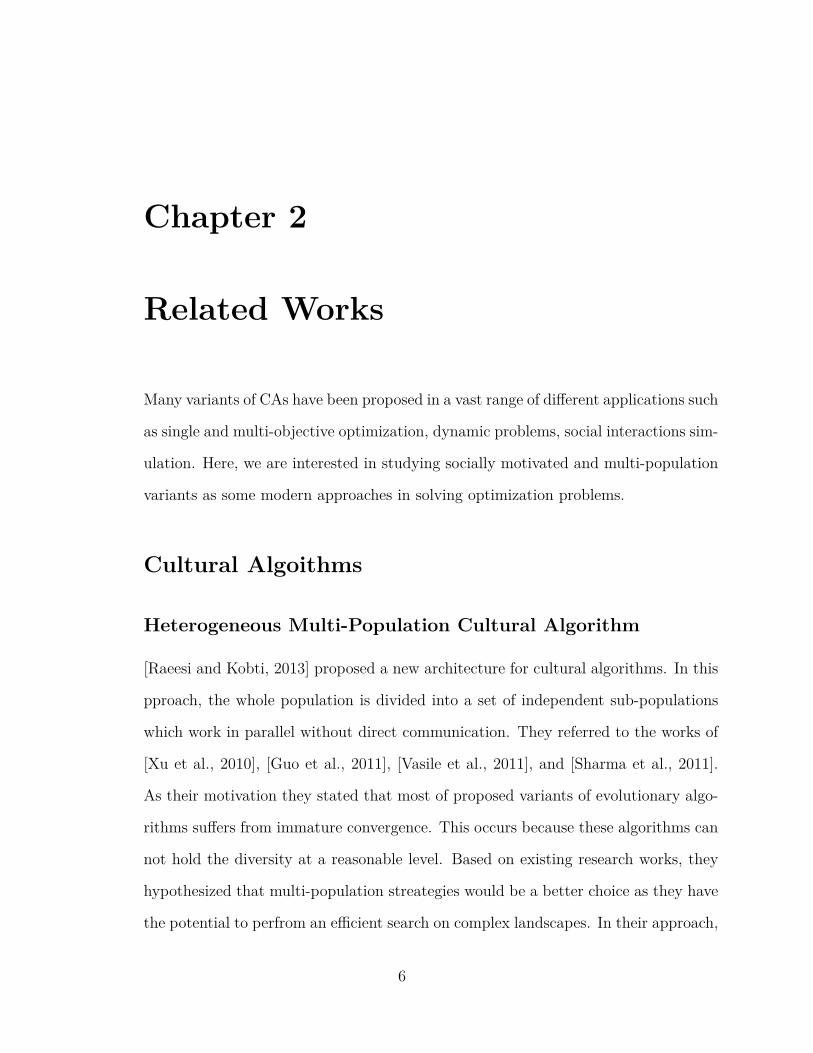
proppsed algorithm. The general architecture of their algorithm is presented in Fig-
ure 2.1
In the experiments, they considered the whole population size to be 1000 individ-
Figure 2.1: H-MPCA Architecture [Raeesi and Kobti, 2013]
uals. It is divided into 30 sub-populations. So, the size of each sub-popualtion is
33. The algorithm runs for the maximum of 10000 generations and the local search
strategy runs only for 10 iterations. They evaluated HMP-CA on a set of 8 complex
optimization functions. It is able to find the minimum value for 7 functions out of 8.
However, when the local search strategy is applied to the expriments, the proposed
method outperforms all of the functions and it finds the optimum value very quickly.
Ultimately, they claimed that their porpsed approach is efficient in both time and
space complexity.
7
The Social Fabric Approach as an Approach to Knowledge
Integration in Cultural Algorithms
[Reynolds and Ali, 2008] begins with a brief introduction to socially motivated meth-
ods to problem solving. They referred to the works of [Hu et al., 2003], [Reynolds and
Ali, 2007], and [Cheng et al., 2005]. It compares qualities of Ant Colony Optimization
(ACO), Particle Swarm Optimization (PSO), and Cultural Algorithms (CA) regard-
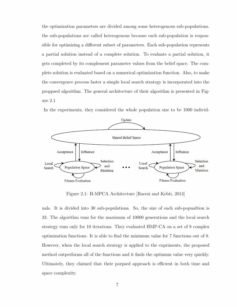
ing the scale in which the interactions between agents occur. Figure 2.2 compares
PSO, ACO, and CA in terms of the time and space continuum over which the so-
cial interactions occur. Individuals in ACO and PSO tend to interact in a reatively
limited temporal and spatial scales. It is obvious because the agents in both ant and
paricle swarm algorithms exchange information with only other agents in their local
neighborhood. On the other hand, cultural algorithms let the individuals interact
together using various types of symbolic information emerged from complex cultural
systems. In cultural algorithms the interactions among individuals occur indirectly
through a shared belief space. So, cultural algorithms allow individuals interact in a
global scale. Then, they asked the essential question of what social structures might
Figure 2.2: Scale of social interactions [Reynolds and Ali, 2008]
emerege alongisde the search process?. To answer such questions, they introduced
8
a new influence function which utilizes the social fabric phenomena. The old influ-
ence function assumes no interactions between agents and works based on the simple
roulete wheel method. On the other hand, in the new influence function, the individ-
uals are connected through a social network (fabric). Multiple layers of such networks
could be employed in a population. The interplay of these network connection forms
a social fabric. At each iteration, an individual could specify its controller knowledge
source. In this approach, the contoller knowledge source is chosen based on the ma-
jority of knowledge sources in the neighborhood of an individual. The neighborhood
size of an individual is specified by the topology of the fabric. Inspired by Particle
Swarm Optimization literature, different topologies could be taken into consideration
to model the relationships among individuals. In their work, they only considered
Ring and Square topologies. They stated that, the topology of the social fabric deter-
mines the extent to which the influence of knowledge sources could be spread thorugh
the network.
To evaluate the social fabric approach, they implemented it in Repast frameork.
Repast is a simuation tool for multi-agent systems. They created a cultual algo-
rithms toolkit (CAT) to view the capabilities of cultural algorithms in solving various
problems. They chose Cone World problem to evaluate and compare their approach
with the standard cultural algorithm. The reason that they chose this problem is that
by changing its parameters during the evolution process, it can show a dynamic be-
havior. So, Cone World problem provides an efficient way to test flexibility of search
algorithms. They set the parameters of CAT as: 100 individuals, 100 cones and 1000
generations. They used ring and square topologies to from he social fabric. They
stated that square topology works better than ring as it finds the solution after 250
iterations. While, the ring topology finds the best solution 450 iterations.
9
Robust Evolution Optimization at the Edge of Chaos: Com-
mercialization of Culture Algorithms
[Che et al., 2010] aimed at commercializing Cultural Algorithm Toolkit (CAT) thourgh
developing a robust variant of it. By robustness, they mean to develop a cultural al-
gorithm which is capable of being applied across a vast range of complex problems.
At first, they referred to [Peng, 2005] as an standard model cultural algorithms which
assumes no connection between individuals. Then, they referred to [Ali, 2008], which
introduced the concept of social fabric to allow individuals interact together. The
authors extended the work of Ali by allowing the social networks having a memory.
In addition, they utilized a variety of different networks in order to deteremine the
relationship between network and problem complexity.
They brought up the hypothesis that there might be multiple independent networks
for different purposes such as kinship and economics. In such networks, there are al-
ways some individuals which are member of multiple networks and so, they can play
the role of mediator between differet networks. To preserve the diversity, the authors
utilized a variety of different topologies such as Lbest, Square, Hexagon, Octagon,
Hexadecagon, and Gbest.
They stated that in the previous work of [Ali, 2008], he employed an un-weighted
majority win strategy to determine the contoller knowledge source of an individual.
It just relied on the count of each knowledge source in the neighborhood of each indi-
vidual. The authors replaced it with a new strategy which use the average fitness of
each KSs instead of each KSs count. So, the performance of individuals in a neigh-
borhood influences which knowledge source to be chosen for the next iteration.
To evaluate the robustness of the algorithm, the authors used Cone World Generator
[Morrison and De Jong, 1999] as a dynamic problem. Reffered to the work by [Lewin,
1999] ,they defined three classes of entropy in the connes world problem:
10
1. Fixed: There is a low entropy and the parameters of the environment do not
tend to change at all.
2. Periodic: The environment parameters change in a regular period of time. So,
the algorithm should be capable adapting itself regularly.
3. Chaotic: In this case, the parameters change without any order and no pre-
diction could be made about them. In fact, it is more similar to real-world
cases.
For the fixed category, the square topology successfully solved 84% of the problems
and as the best topology. For the periodic case, the octagon topology showed a better
performance than other toplogies. And, for the chaotic category, Gbest showed a
better result mostly in terms of average time to find a solution and the standard
deviation. In summary, as the complexity of problems grows, there is the need for
more connections between individuals in a social fabric to keep the robustness of the
algorithm.
Socio-Cultural Evolution via Neighborhood-Restructuring in
Intricate Multi-Layered Networks
[Ali et al., 2012] aimed at exploring the utilization of neighborhoods in the population
level of cultural algorithms and see how it influences the knowledge swarming in the
belief space. Their approach uses a dynamic neighborhood restructuring to preserve
diversity efficiently. They referred to the reasearch works of [Elsayed et al., 2011],
[Asafuddoula et al., 2011], and [Asafuddoula et al., 2011]. Those papers proposed
some adaptive methods which tried to make a trade-off between exploration and
eploitation properties of evolutionary algoithms. Among the referred papers, the
work by [Ali et al., 2010] used the social fabric phenomena to from multi-layered
hierarchical network structures in both homogenous and heterogeneous networks.
11
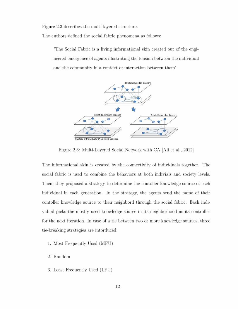
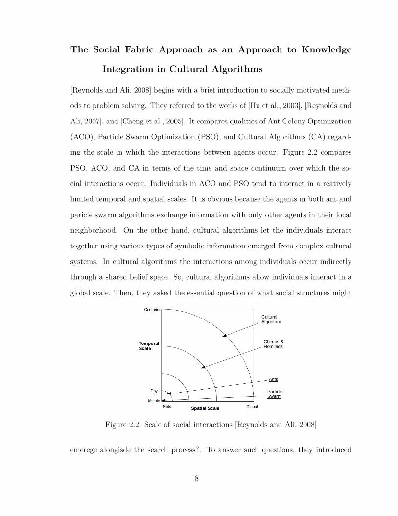
Figure 2.3 describes the multi-layered structure.
The authors defined the social fabric phenomena as follows:
"The Social Fabric is a living informational skin created out of the engi-
neered emergence of agents illustrating the tension between the individual
and the community in a context of interaction between them"
Figure 2.3: Multi-Layered Social Network with CA [Ali et al., 2012]
The informational skin is created by the connectivity of individuals together. The
social fabric is used to combine the behaviors at both indivials and society levels.
Then, they proposed a strategy to determine the contoller knowledge source of each
individual in each generation. In the strategy, the agents send the name of their
contoller knowledge source to their neighbord through the social fabric. Each indi-
vidual picks the mostly used knowledge source in its neighborhood as its controller
for the next iteration. In case of a tie between two or more knowledge sources, three
tie-breaking strategies are intorduced:
1. Most Frequently Used (MFU)
2. Random
3. Least Frequently Used (LFU)
12
They stated that their proposed approach is inspired from a previous work of [Reynolds
et al., 2008]. The new idea was called Cultual Algorithm with Restructuring Layered
Social Fabric (CARLSOF). In this approach, the whole population is divided into two
layers of rudimentary and advanced members. There are some independent tribes in
the population space which their best performing individuals form the advanced layer
and the others form the rudimantary level. In the previous works, the topology of
social fabrics were supposed to be fixed and homogenous. They utilized a variety of
regular topologies to form the social fabric. The authors proposed a new strategy to
enable the fabric to be restructured in the case of stagnation. Each tribe may decide
to change its topology to a denser (with more conections) or sparser (with less connec-
tions). They referred to two different restructuring strategies as similar approaches.
The first one was Layered Delaunay Triangulation which is based on voronoi diagram.
The second approach was Random Rewiring Procedure which starts with a regular
topology and then rewire each edge randomly with the probability p.
To evaluate the performance of CARLSOF, they used function set of IEEE-CEC2011
evolutiosry competition. The algorithm was implemented in JAVA. The authors re-
ported that CARLSOF was successful to enhance all of the functions in the testbed
interms of average, best, and worst obtained values. Also, they claimed that CARL-
SOF outperforms the best previously obtained results for European Space Agency
(P12) and Casini (P13) problems results. They reported 2.983 km/sec compared to
previous best 7.095. For p13, they reported 8.383091 km/sec compared to previous
best 8.3832.
13
Leveraged Neighborhood Restructuring in Cultural Algorithms
for Solving Real-World Numerical Optimization Prob-
lems
[Ali et al., 2016] made an overall review of related works on Cultural Algorithms
and Social Fabric [Peng, 2005], [Reynolds and Ali, 2008], [Chen et al., 2006], and
[Kennedy, 1999]. They introduced the concept of social fabric as an infrastructure
which facilitates the propagation of the influence of the knowledge sources thorugh the
population space. The whole population is divided into multiple small sized tribes.
Unlike other PSO-based multi-swarm variants, the tribal sub-swarms change their
topology during the evolution process to keep diversity against stagnations.
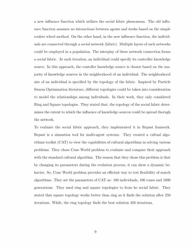
The tribes are organized in a two-layer structure of advanced and rudimentary classes.
The advanced calss is composed of best perfoming individuals of each tribe. From
each tribe, two examplars are chosen. The first one is the best of explorer knowledge
sources (Normative and Topopgraphic) and the second one is the best of exploiter
knowlegde sources (Situational). Figure 2.4 describes the two-layer structure. The
authors utilized only three kinds of knowledge sources: Normative, Topographic, and
Situational. They claimed that, other types of knowledge sources are suitable for
dynamic problems. However, they used a set of static problems to evaluate their
approach. The authors divided the evolution process of CAs into three stages: the
secluion stage , the rapport stage , and the cohesive stage. In the seclusion stage, the
tribes evolve independetly and without any exchange of information. Then, in the
rapport stage, the tribes start to exchange knowledge via the advenced class. Also,
the neighborhood restructuring strategy is lunched in each tribe. So, the tribes have
the capability to restructure their topology to keep diversity and avoid local optima.
The first two stages ensure that diversity has been kept in the initial iterations of
the search process. Finally, in the third stage, all the tribes are merged together
14

and continue the search process as a single CA model. Based on the categorization
Figure 2.4: Two-class taxonomy of the tribal CA [Ali et al., 2016]
proposed in [De Oca et al., 2009], the authors claimed that their apparoach is heterp-
geneous regarding update-rule heterogeneity and neighborhood heteogeneity. Since
the topology of each tribe is changing during the evolution process, the tribes might
use different toplogies at the same time. So, it could be considered as heterogenous
neuighborhood restructuring. Also, their approach utilizes update-rule heteogeneity
because, there are individuals with different roles (explorer and exploiter).
In the exprimental results section, the authors used IEEE-CEC2011 competition on
testing evolutionary algorithms on real-world numerical optimization problems. They
presented an extended comparison of their approach with other propsed methods. At
first, the authors tested the approach (T-SCANeR) with different values for these pa-
rameters: tie-breaking rule, Mthresh, and number of elites. There is no best value for
tie-breaking rule as it is problem-dependent. For the Mthresh parameter, the results
show that the best value is 50. The best value for ntElite is 2. The second expriment
was on varying the window size within which the social fabricis applied and aggre-
gated (Wsize). The best reported value for Wsize is 20.
In the two first exprients the best values for the parameters were determined. Based
on the obtained values, the authors compared T-SCANeR with five other evolution-
15

ary algorithms on the IEEE-CEC2011 which is a set of 18 functions. T-SCANeR
managed to outperform for most of the functions except for T3, T4, T6, and T11.5.
Problems T12 (full messenger problem) and T13 (cassini problem) are associated with
the European Space Agency (ESA). The authors claimed that T-SCANeR outper-
formed other methods by 2.193724 km/s for the messenger problem and 8.383090 for
the cassini problem.
Particle Swar Optimization
Tribe-PSO: A novel global optimization algorithm and its ap-
plication in molecular docking
[Chen et al., 2006] proposed a new variant of Particle Swarm Optimization (PSO)
called Tribe-PSO for the primary purpose of molecular docking in chemometrics.
As some previous research work, they referred to [Jones et al., 1997] and [Clerc
and Kennedy, 2002]. Their approach is inspired from Hierarchical Fair Competition
concept [Jianjun et al., 2002]. They divided the whole population into some tribes
and the evolution process into three phases. The tribes are organized into two layers
of basic and upper individuals.
The individuals in each tribe are completely isolated from other tribes. So, they
form the basic layer. On the other hand, the best members of each tribe can see the
other tribes and exchange information with their best members as well. The problem-
solving process is divided into three phases: isolated, communing, and united. In the
first phase, the tribes are completely isolated and there is no exchange of information.
In the second phase, the two-layered model is formed and the tribes begin to exchange
information through their best performing individuals. In the third phase, all the
tribes are merged into a single popualtion. Then, it operates as basic PSO model
16

until meeting some stopping criteria. The autohrs claimed that their approach helps
the individuals preserving diversity and avoiding local optima against multi-modal
solution spaces.
The authors used two testbeds to evaluate and compare the performance of Tribe-
PSO with standard PSO. The first was De Jong’s function set and the second was a
test set of 100 receptor-ligand X-ray structures selected for docking benchmark. In
the De Jong’s testbed, the basic PSO showed a better performance in the isolated
phase. However, in the communing phase Tribe-PSO converged to a better value
than basic PSO. In the unity phase, the basic PSO seemed to get stuck in a local
optimum. However, Tribe-PSO continued to accelerate convergence and got better
results than basic PSO. In the docking benchmark, Tribe-PSO was compared to the
AutoDock library. Four parameters are calculated after 10 independent runs: Best,
Run1, Average, and Standard Deviation of the results. The relative difference of
the four benchmark factors between Tribe-PSO and AutoDock were calculated. The
results for the four factors showed that Tribe-PSO leads to a better performance than
AutoDock.
Heterogeneous Particle Swarm Optimizers
[De Oca et al., 2009] peresented a survey on heterogeneous variants of Paritcle Swarm
Optimization (PSO). They claim that the homogenous models have been attractive
because of their simplicity in conceptual and application levels. However, heteroge-
neous models are ubiquitous in nature. Here, heterogeneity means the individuals
may differ from each other regarding their parameters and search behavior.
At first, the authors presented a breif description of three well-known variants of PSO:
Accelerated PSO [Zhang et al., 2003], Fully-informed PSO [Mendes et al., 2004], and
Bare Bones PSO [Kennedy, 2003]. Then, they authors categirzed the heterogeneous
variants of PSO into four categories:
17
1. Neighborhood
2. Model of Influence
3. Update Rule
4. Parameters
Neighborhood heterogeneity refers to the cases that the topology of the swarm is not
regular. This type of heterogeneity occurs when the neighborhood size of each indi-
vidual is different. They claimed that the neighborhood heterogeneity allows some
population to be more influential than otehrs. Individuals with higher number of
connections have the potential to attract more individuals through the search process
[Kennedy et al., 2001].
Model of Influence heterogeneity refers to the situations that the individuals employ
different strategies to specify their informers. The word Informer refers to an indi-
vidual which is going to influence another individual.
Update-rule heterogeneity means the individuals utilize different strategies to update
their position in the search space. This kind of heteogeneity makes it possible for the
individuals to explore the search space in several ways. Also, the particles can play
different but complementary roles. For example, some of them may tend to explore
unseen parts of the solution space and some others only follow those scout individuals.
The second type are the exploiters.
Parameter heterogeneity occurs when some individuals in a group which follow the
same update rule use different update rule’s parameter settings. Having different
search parameters, even in a group of similar particles, leads to various search be-
haviors which improves the level of diversity. The authors referred to [Mendes, 2004]
and [Montes de Oca and Stützle, 2008] which utilize different initial values for the
parameters such as acceleration coefficient, maximum velocities and inertia weight.
To compare the mentioned categories, the authors careted two test cases. The first
18
one compared two PSO variants with different update rules: Velocity-based and Bare
bones swarm. The evaluation results confirmed that velocity-based outperformed the
other one. The second test case compared two PSO variants with different models
of influence: best-of-neighborhood and fully-informed swarm. The evaluation results
showed that the fully-informed algorithm outperfromed the best-of-neighborhood.
Chapter Conclusion
From the chosen research works, we will be utilizing the concept of heterogeneous
neighborhood structures by [De Oca et al., 2009] to improve the robustness of social
fabric-based cultural algorithm [Ali et al., 2016]. We replace the population compo-
nent of [Ali et al., 2016] with PSO algorithm.
19

Chapter 3
Evolutionary Algorithms
This chapter presents a detailed description of related evolutionary algorithms such
as cultural algorithms, particle swarm optimization, and their social variations. In
this section, we try to give a brief description of those evolutionary algorithms as a
background to our proposed approaches.
Evolutionary Algorithms
Evolutionary computing is a research area within computer science. As the name
suggests, it is a particular flavor of computing, which draws inspiration from the pro-
cess of natural evolution. In fact, they are computer programs which try to solve
and optimize complex problems by simulating the behavior of natural systems. They
utilize evolutionary operators such as crossover and mutation to improve the quality
of a population of solutions [Burke et al., 2005].
Evolutionary algorithms start with a population of randomly generated solutions for
a particular problem. Then, the algorithm modifies the solutions in an iteration-
based process of some finite number of generations. The modification occurs through
applying the so-called evolutionary operators such as crossover and mutation. The
evolutionary operators might be binary or unary. For example, the crossover is a bi-
20
nary operator because it combines two solutions (individuals) to generate a new one.
On the other hand, mutation is a unary operator because it makes random modifica-
tions on a single solution to improving its performance [Eiben and Smith, 2003]. The
performance of each is evaluated using a fitness function. The fitness function repre-
sents the problem that needs to be solved or optimized. Usually, the fitness function
is chosen from NP problems which are hard to solve by traditional problem-solving
methods. In each iteration of an evolutionary algorithm, the evolutionary operators
are applied to the individuals and the best performing offsprings will be transferred
to the next generation. This process continues until meeting some stopping criteria
which are already defined by a human user. Some examples of evolutionary lgorithms
are:
1. Genetic Algorithms
2. Evolutionary Porgramming
3. Differential Evolution
However, the evolutionary algorithms are not restricted to biological processes. Some
researchers have drawn inspiration from social systems to find solutions to complex
problems. The complex and coordinated behavior of swarms not only fascinates bi-
ologists but also is an inspiration to computer scientists [Bonabeau et al., 1999]. Ant
colonies and birds flocking are remarkable examples of coordinated collective behavior
that emerges without centralized control. Swarm intelligence is a field of computer
science that invents computational methods for solving problems in a way that is in-
spired by the behavior of real swarms and colonies. Principles of self-organization and
communication (local and indirect) are essential to understanding the complex col-
lective behavior [Stützle, 2009]. There are different types of swarm-based algorithms
such as:
1. Particle Swarm Optimization (PSO)
21

2. Ant Colony Optimization (ACO)
3. Cultural Algorithms (CA)
Cultural Algorithms
Cultural Algorithms (CA) were introduced by Reynolds as a type of population-
based problem-solving approaches. CA combines biological evolution with socio-
cognitive concepts to yield an optimization approach based on a dual inheritance
theory [Reynolds, 1994]. As defined by [Durham, 1991], culture is a “system of
symbolically encoded conceptual phenomena that are socially and historically trans-
mitted within and between populations”.From the definition, it can be stated that
in cultural systems, evolution occurs at two levels: Macro-evolutionary level and
micro-evolutionary level. Cultural algorithms define the evolution process through
the cooperation of three distinct components:
1. Belief Space (Macro-evolutionary Level)
2. Population Space (Micro-evolutionary Level)
3. Communication Protocol
Belief Space
Belief space keeps different kinds of knowledge obtained from the individuals’ experi-
ence during the evolution process. It extracts the knowledge from the population and
stores the knowledge in various formats called knowledge sources (KS). Each knowl-
edge source extracts and keeps knowledge about a particular aspect of the search
space.
After each iteration, the best performing individuals are chosen and sent to the belief
space to be utilized by the knowledge sources. The stored knowledge is used to bias
22
the search process in the population space. Five types of knowledge sources have
been identified in the belief space:
1. Situational Knowledge: Successful exemplars of individuals
2. Normative Knowledge: The best range of value for each parameter
3. Topographic Knowledge: The best areas of the search space
4. Domain knowledge: The domain ranges for all the parameters and the best
exemplars
5. Temporal Knowledge: Knowledge about the past changes in a dynamic envi-
ronment
Population Space
In the population space, any population-based algorithm could be used. In the earlier
variants of cultural algorithms, only GA was used. However, researchers utilized
other population-based algorithms such as PSO and EP in the population component.
In each generation, the best individuals are sent to the belief space to update the
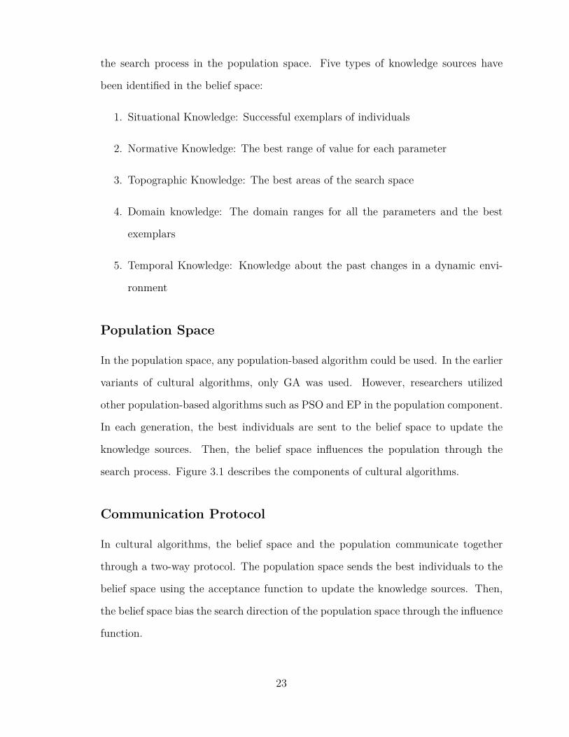
knowledge sources. Then, the belief space influences the population through the
search process. Figure 3.1 describes the components of cultural algorithms.
Communication Protocol
In cultural algorithms, the belief space and the population communicate together
through a two-way protocol. The population space sends the best individuals to the
belief space using the acceptance function to update the knowledge sources. Then,
the belief space bias the search direction of the population space through the influence
function.
23
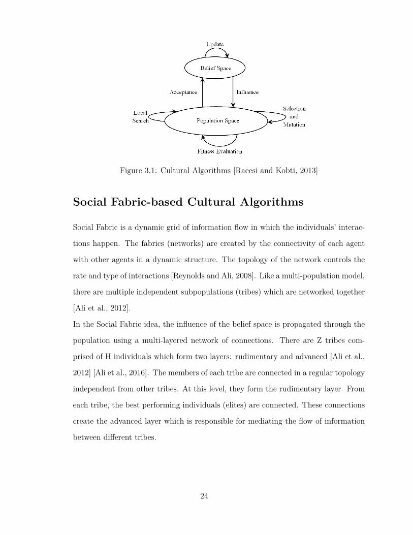
Figure 3.1: Cultural Algorithms [Raeesi and Kobti, 2013]
Social Fabric-based Cultural Algorithms
Social Fabric is a dynamic grid of information flow in which the individuals’ interac-
tions happen. The fabrics (networks) are created by the connectivity of each agent
with other agents in a dynamic structure. The topology of the network controls the
rate and type of interactions [Reynolds and Ali, 2008]. Like a multi-population model,
there are multiple independent subpopulations (tribes) which are networked together
[Ali et al., 2012].
In the Social Fabric idea, the influence of the belief space is propagated through the
population using a multi-layered network of connections. There are Z tribes com-
prised of H individuals which form two layers: rudimentary and advanced [Ali et al.,
2012] [Ali et al., 2016]. The members of each tribe are connected in a regular topology
independent from other tribes. At this level, they form the rudimentary layer. From
each tribe, the best performing individuals (elites) are connected. These connections
create the advanced layer which is responsible for mediating the flow of information
between different tribes.
24
Evolution Phases
The whole evolution process is split into three phases: seclusion, rapport, and cohe-
sive. In the first stage, each tribe evolves as an independent basic CA model with
no communication between tribes. In the second step, the advanced layer is formed
by connecting elites of each tribe. Then, tribes start to exchange information dur-
ing their evolution process. Ultimately, in the third step, all the tribes are merged
into one CA model. Then the search process continues until meeting some stopping
criteria.
Strategic Neighborhood Restructuring
In Social Fabric literature, Strategic Restructuring is a technique to help individuals
to get rid of stagnation where there are copious local optima in the search landscape.
Each tribe maintains a particular topology until it gets stagnated in a local optimum
for a certain number of iterations. Then, the topology is reinitialized to motivate the
individuals for a new search. Here, four types of topologies are utilized: Ring, Mesh,
Hybrid-Tree, and Global [Ali et al., 2016]. Figure 3.2 describes how the process of
neighborhood restructuring occurs.
Figure 3.2: Standard Neighborhood Restructuring Process
25
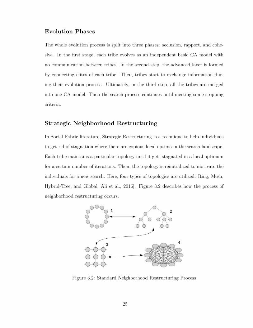
Social fabric based influence function
In this model, the individuals might decide to change their controller KS using the
majority of KSs which they receive from their neighborhood. Here, Majority Voting is
used to find the controller KS of an individual [Che et al., 2010]. Figures 3.3 describes
the social fabric influence function. In the case of a tie, some tie-breaking rules are
deployed such as MFU (most frequently used), LFU (least frequently used), Direct
(the direct influencing KS), Random (a random choice), Last-used (the KS which
controlled the KS in the last iteration) [Ali et al., 2012]. In the equation 3.1 the sum
denotes the counts of KSs in ith node neighborhood and ψi is its contoller KS. τi is
the net affecting KS for the next iteration [Ali et al., 2016] [Sterling, 2004].
τi =∑
j∈Nbr(i)mij + ψi (3.1)
The Social Fabric approach can be generalized on different topologies as follows:
KS(t+ 1) =
KSi, ∀KSj ∈ {KS −KSi} ⇒ weight(KSi) > weight(KSj)
KScr, otherwise
(3.2)
Where KS is the set of all knowledge sources, KSi, KSj ∈ KS. weight(ÜţKSi) is
the number of neighbors that belong to the knowledge source KSi. KScr denotes the
knowledge source chosen by a tie-breaking rule.
Particle Swarm Optimization
The initial idea for particle swarm optimization of Kennedy and Eberhart were es-
sentially aimed at producing computational intelligence by utilizing simple models of
social interaction, rather than purely single-agent cognitive capabilities.
26

Figure 3.3: Social Fabric Influence Function[Ali and Reynolds, 2009]
In PSO, some simple-structured individuals (the particles) moving around in the
search space of a function, and each particle evaluates the objective function based
on its current location. Then, each particle determines its movement direction and
velocity through the search space by combining its historical best experience and
the best (best-fitness) particle in its visible neighborhood in the swarm, with some
random fluctuations for keeping diversity. This process repeats at each iteration.
Eventually, the swarm as a whole, like a flock of birds collectively searching for food
sources, is similar to move around for finding an extremum of the fitness function.
Each particle is comprised of a position vector and velocity vector [Bratton and
Kennedy, 2007]. Particles adjust their velocities and positions as follows:
vid(t+1) = w · vid
(t) + c1r1(pid − xid(t)) + c2r2(pgd − xid
(t)) (3.3)
xid(t+1) = xid
(t) + vid(t+1) (3.4)
27
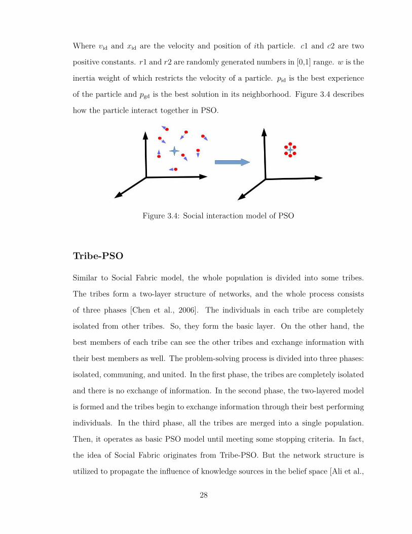
Where vid and xid are the velocity and position of ith particle. c1 and c2 are two
positive constants. r1 and r2 are randomly generated numbers in [0,1] range. w is the
inertia weight of which restricts the velocity of a particle. pid is the best experience
of the particle and pgd is the best solution in its neighborhood. Figure 3.4 describes
how the particle interact together in PSO.
Figure 3.4: Social interaction model of PSO
Tribe-PSO
Similar to Social Fabric model, the whole population is divided into some tribes.
The tribes form a two-layer structure of networks, and the whole process consists
of three phases [Chen et al., 2006]. The individuals in each tribe are completely
isolated from other tribes. So, they form the basic layer. On the other hand, the
best members of each tribe can see the other tribes and exchange information with
their best members as well. The problem-solving process is divided into three phases:
isolated, communing, and united. In the first phase, the tribes are completely isolated
and there is no exchange of information. In the second phase, the two-layered model
is formed and the tribes begin to exchange information through their best performing
individuals. In the third phase, all the tribes are merged into a single population.
Then, it operates as basic PSO model until meeting some stopping criteria. In fact,
the idea of Social Fabric originates from Tribe-PSO. But the network structure is
utilized to propagate the influence of knowledge sources in the belief space [Ali et al.,
28
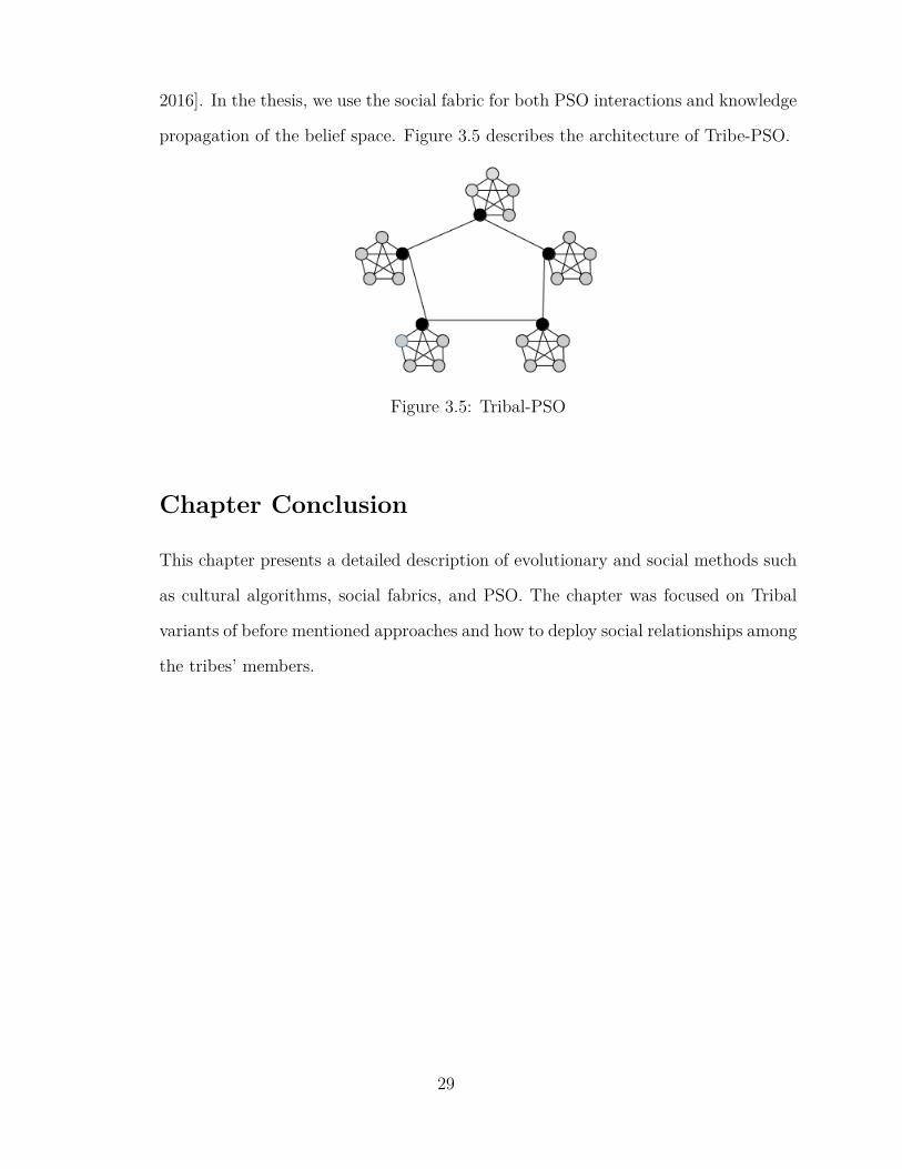
2016]. In the thesis, we use the social fabric for both PSO interactions and knowledge
propagation of the belief space. Figure 3.5 describes the architecture of Tribe-PSO.
Figure 3.5: Tribal-PSO
Chapter Conclusion
This chapter presents a detailed description of evolutionary and social methods such
as cultural algorithms, social fabrics, and PSO. The chapter was focused on Tribal
variants of before mentioned approaches and how to deploy social relationships among
the tribes’ members.
29
Chapter 4
Proposed Approaches: Improving
Robustness in Social Fabric
Inspired by natural systems, many evolutionary algorithms have been proposed to
solve various optimization problems. These algorithms are expected to exhibit a
consistent problem-solving behavior against different optimization landscapes. Un-
fortunately, as stated by No Free Lunch (NFL) theorem by [Wolpert and Macready,
1997], there is no algorithm better than others over all cost functions. It means, there
is no guarantee for an algorithm to work well for all functions if it shows promising
results for a particular category of them. Therefore, robustness has been one of the
most desired features which motivates researchers to invent new methods which are
less dependent on the kind of a problem than others. Here, robustness means we
need to develop search strategies which are capable of adapting themselves across
different landscapes which might vary regarding aspects such as multimodality and
the number of local optima.
In this section, we are going to improve the robustness of CAs in both population
space and belief space components. In the population space, a new neighborhood
restructuring strategy will be proposed which aims at microscopic inspections for
30
stagnation regarding individuals’ local experience. Then, in the belief space, a new
model of Normative KS will be proposed, which defines the normative ranges based
on Confidence Interval inspired from Inferential Statistics. It stops the normative KS
to be affected by sudden fluctuations in the input data.
Self-organization
A self-organized system is a group of agents with specific behavioral patterns which
could not be predicted from the simple behaviors of the individuals who make up the
system. [Kennedy et al., 2001] described self-organization as follows:
"Self-organization The ability of some systems to generate their form with-
out external pressures, either wholly or in part. It can be viewed as
a system’s constant attempts to organize itself into ever more complex
structures, even in the face of the constant forces of dissolution described
by the second law of thermodynamics."
Some of the primary attributes of self-organizing systems are listed below:
1. Self-organizing systems usually exhibit the behaviors that appear to be sponta-
neous order.
2. Self-organization can be considered as a system’s constant attempts to organize
itself into a variety of complex structures, even in the face of the forces of
deviation (Robustness).
3. The overall status of a self-organizing system is an emergent property of all the
ingredients of the system.
4. Interconnected components of the system become organized in a meaningful
way based on local interactions of the components.
31

5. Complex systems have the potential to self-organize themselves.
6. The self-organization process works close to the "edge of chaos".
In the section, we will propose a new approach to improve the robustness of cultural
algorithms regarding self-organization.
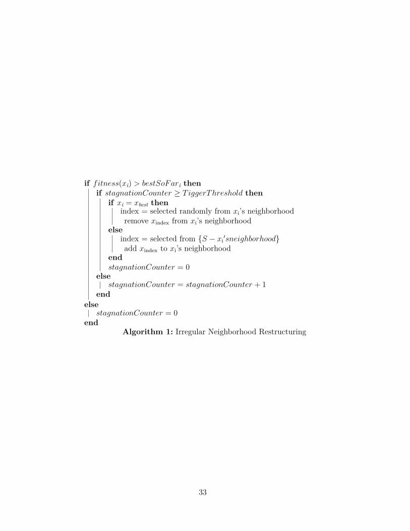
Irregular Neighborhood Restructuring
As proposed by [Ali et al., 2016], when the agents of a tribe get stuck in a local
optimum, then they choose a topology with fewer connections such as ring topol-
ogy to motivate exploration. When the agents lack information, the topology is
changed to a denser topology like Mesh, and ultimately Global. Whenever a tribe
does not make progress for Mthresh iterations, then the algorithm decides on upgrad-
ing/downgrading the current topology to other topologies. Downgrading happens by
moving in the direction of gbest→tree→mesh→lbest and Upgrading occurs in the
direction of lbest→mesh→tree →gbest. In our proposed approach, the restructuring
process occurs at a microscopic level. There is no daemon process for inspecting stag-
nation. Every agent checks its performance for stagnation. If it gets stuck in a local
optimum, it decides to upgrade/downgrade its neighborhood. The proposed strategy
is described in the algorithm 1. If the particle is the best in its neighborhood, it starts
to decrease the number of connections to motivate exploration. However, if it is not
the best, it needs to increase the neighborhood size to facilitate exploitation. Here,
the topology is dynamic and irregular and the neighborhood size is different for each
agent. So, it could be considered as a heterogeneous variant of CAs [De Oca et al.,
2009]. The ultimate topology of the fabric is formed through local interactions of the
agents. In this way, it improves the robustness of CAs regarding self-organization
concept [Kennedy et al., 2001]. Psudo-code 1 describes the irregular neighborhood
restructuring algorithm in detail.
32
if fitness(xi) > bestSoFari thenif stagnationCounter ≥ TiggerThreshold then
if xi = xbest thenindex = selected randomly from xi’s neighborhoodremove xindex from xi’s neighborhood
elseindex = selected from {S − xi
′sneighborhood}add xindex to xi’s neighborhood
endstagnationCounter = 0
elsestagnationCounter = stagnationCounter + 1
endelse
stagnationCounter = 0end
Algorithm 1: Irregular Neighborhood Restructuring
33
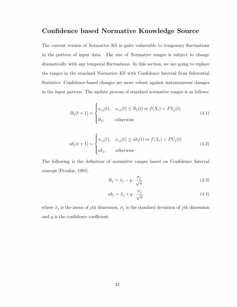
Confidence based Normative Knowledge Source
The current version of Normative KS is quite vulnerable to temporary fluctuations
in the pattern of input data. The size of Normative ranges is subject to change
dramatically with any temporal fluctuations. In this section, we are going to replace
the ranges in the standard Normative KS with Confidence Interval from Inferential
Statistics. Confidence-based changes are more robust against instantaneous changes
in the input pattern. The update process of standard normative ranges is as follows:
lbj(t+ 1) =
xi,j(t), xi,j(t) ≤ lbj(t) or f(Xi) < PLj(t)
lbj, otherwise(4.1)
ubj(t+ 1) =
xi,j(t), xi,j(t) ≥ ubj(t) or f(Xi) < PUj(t)
ubj, otherwise(4.2)
The following is the definition of normative ranges based on Confidence Interval
concept [Proakis, 1985].
lbj = x̄j − q ·σj√n
(4.3)
ubj = x̄j + q · σj√n
(4.4)
where x̄j is the mean of jth dimension, σj is the standard deviation of jth dimension
and q is the confidence coefficient.
34
Chapter 5
Experimental Setup
In this chapter, we explain the experimental setup, how to set the parameters and the
optimization functions as the benchmark to evaluate the efficiency of our proposed
approaches.
Description
In this section, we describe IEEE-CEC2015 as the function set which we have chosen
for our benchmark optimization purpose [Chen et al., 2014]. IEEE-CEC2015 is a set
of 15 functions with different properties such as multi-modality, copious local optima,
and non-separability. All test functions are minimization problems defined as follows:
Y = f(x1, x2, x3, · · · , xD) (5.1)
where D is the number of dimensions.
Before evaluation, all the vectors are shifted and rotated as described in [Chen et al.,
2014].oi = [oi1, oi2, · · · , oiD] is the shifted global optimum, which is randomly dis-
tributed in [-80,80] D For convenience, the same search ranges are defined for all test
functions as [−100, 100]D
35

Benchmark Functions
In this section, we describe the IEEE-CEC2015 functions and their properties as a
well-known benchmark adopted by many researchers to evaluate innovative ideas in
solving complex optimization problems.
Unimodal Functions
Rotated Bent Cigar Function
f1(x) = x21 + 106
D∑i=2
x2i (5.2)
F1(x) = f1(M(x− o1)) + F ∗1 (5.3)
Properties:
1. Unimodal
2. Non-separable
3. Smooth but narrow ridge
Rotated Discus Function
f2(x) = 106x21 +
D∑i=2
x2i (5.4)
F2(x) = f2(M(x− o2)) + F ∗2 (5.5)
Properties:
1. Unimodal
2. Non-separable
3. With one sensitive direction
36

Simple Multimodal Functions
Shifted and Rotated Weierstrass Function
f3(x) =D∑
i=1(
kmax∑k=0
[ak cos(2πbk(xi + 0.5))])−Dkmax∑k=0
[ak cos(2πbk · 0.5)] (5.6)
where a=0.5, b=3, and kmax=20.
F3(x) = f3(M(0.5(x− o3)100 )) + F ∗3 (5.7)
Properties:
1. Multi-modal
2. Non-separable
3. Continuous but differentiable only on a set of points
Shifted and Rotated Schwefel’s Function
f4(x) = 418.9829×D −D∑
i=1g(zi), zi = xi + 4.209687462275036e+ 002 (5.8)
F4(x) = f4(M(1000(x− o4)100 )) + F ∗4 (5.9)
Properties:
1. Multi-modal
2. Non-separable
3. Local optima’s number is huge and second better local optimum is far from the
global optimum.
37

Shifted and Rotated Katsuura Function
f5(x) = 10D2
D∏i=1
(1 + i32∑
j=1
|2jxi − rand(2jxi)|2j
)10
D1.2 − 10D2 (5.10)
F5(x) = f5(M(5(x− o5)100 )) + F ∗5 (5.11)
Properties:
1. Multi-modal
2. Non-separable
3. Continuous everywhere yet differentiable nowhere
Shifted and Rotated HappyCat Function
f6 = |D∑
i=1x2
i −D|0.25 + 0.5 ∑Di=1 x
2i + ∑D
i=1 xi
D + 0.5 (5.12)
F6(x) = f6(M(5(x− o6)100 )) + F ∗6 (5.13)
Properties:
1. Multi-modal
2. Non-separable
Shifted and Rotated HGBat Function
f7 = |(D∑
i=1x2
i )2 − (D∑
i=1xi)2|0.25 + 0.5 ∑D
i=1 x2i + ∑D
i=1 xi
D + 0.5 (5.14)
F7(x) = f7(M(5(x− o7)100 )) + F ∗7 (5.15)
Properties:
1. Multi-modal
2. Non-separable
38

Shifted and Rotated Expanded Griewank’s plus Rosenbrock’s Function
f8(x) = f11(f10(xx1,x2)) + f11(f10(xx2,x3)) + · · ·+ f11(f10(xxD−1,xD)) + f11(f10(xxD,x1))
(5.16)
F8(x) = f8(M(5(x− o8)100 ) + 1) + F ∗8 (5.17)
Properties:
1. Multi-modal
2. Non-separable
Shifted and Rotated Expanded Scaffer’s F6 Function
g(x, y) = 0.5 + (sin2(√x2 + y2)− 0.5
(1 + 0.001(x2 + y2))2 (5.18)
f9(x) = g(x1, x2) + g(x2, x3) + · · ·+ g(xD−1, xD) + g(xD, x1) (5.19)
F9(x) = f9(M(x− o9) + 1) + F ∗9 (5.20)
Properties:
1. Multi-modal
2. Non-separable
Hybrid Functions
Hybrid Function 1
This function is a hybrid of three functions: Modified Schwefel’s function, Rastrigin’s
function, and High Conditioned Elliptic function.
F10(x) = 0.3× F4(x) + 0.3× F12(x) + 0.4× F13(x) (5.21)
39
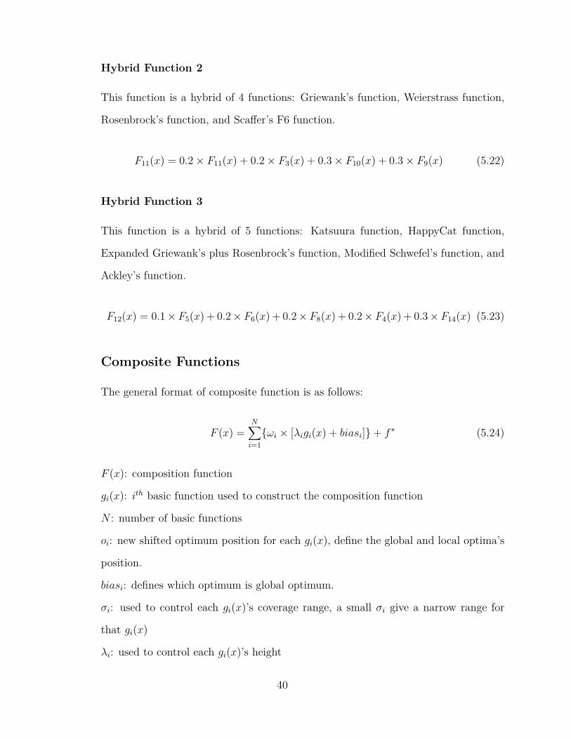
Hybrid Function 2
This function is a hybrid of 4 functions: Griewank’s function, Weierstrass function,
Rosenbrock’s function, and Scaffer’s F6 function.
F11(x) = 0.2× F11(x) + 0.2× F3(x) + 0.3× F10(x) + 0.3× F9(x) (5.22)
Hybrid Function 3
This function is a hybrid of 5 functions: Katsuura function, HappyCat function,
Expanded Griewank’s plus Rosenbrock’s function, Modified Schwefel’s function, and
Ackley’s function.
F12(x) = 0.1×F5(x) + 0.2×F6(x) + 0.2×F8(x) + 0.2×F4(x) + 0.3×F14(x) (5.23)
Composite Functions
The general format of composite function is as follows:
F (x) =N∑
i=1{ωi × [λigi(x) + biasi]}+ f ∗ (5.24)
F (x): composition function
gi(x): ith basic function used to construct the composition function
N : number of basic functions
oi: new shifted optimum position for each gi(x), define the global and local optima’s
position.
biasi: defines which optimum is global optimum.
σi: used to control each gi(x)’s coverage range, a small σi give a narrow range for
that gi(x)
λi: used to control each gi(x)’s height
40

wi: weight value for each gi(x), calculated as follows:
wi = 1√∑Dj=1(xj − oij)2
exp(−∑D
j=1(xj − oij)2
2Dσ2i
) (5.25)
Now, the value of ωi weight is calculated as:
ωi = wi∑ni=1 wi
(5.26)
Composition Function 1
Five types of basic functions are combined to construct this function:
N= 5, σ = [10, 20, 30, 40, 50], λ = [1, 1e-6, 1e-26, 1e-6, 1e-6], bias = [0, 100, 200,
300, 400]
g1 : Rotated Rosenbrock’s Function f10
g2 : High Conditioned Elliptic Function f13
g3 : Rotated Bent Cigar Function f1
g4 : Rotated Discus Function f2
g5 : High Conditioned Elliptic Function f13
Properties:
1. Multi-modal
2. Non-separable
3. Asymmetrical
4. Different properties around different local optima
Composition Function 2
Three types of basic functions are combined to construct this function:
N = 3, σ = [10, 30, 50], λ = [0.25, 1, 1e-7], bias = [0, 100, 200]
41

g1 : Rotated Schwefel’s function f4
g2 : Rotated Rastrigin’s function f12
g3 : Rotated High Conditioned Elliptic function f13
Properties:
1. Multi-modal
2. Non-separable
3. Asymmetrical
4. Different properties around different local optima
Composition Function 3
Five types of basic functions are combined to construct this function:
N = 5, σ = [10, 10, 10, 20, 20], λ = [10, 10, 2.5, 25, 1e-6], bias = [0, 100, 200, 300,
400]
g1 : Rotated HGBat Function f7
g2 : Rotated Rastrigin’s Function f12
g3 : Rotated Schwefel’s Function f4
g4 : Rotated Weierstrass Function f3
g5 : Rotated High Conditioned Elliptic Function f13
Properties:
1. Multi-modal
2. Non-separable
3. Asymmetrical
4. Different properties around different local optima
42
Parameters Settings
We used the same initial values for the parameters as presented by [Ali et al., 2016]:
• Population Size: 90
• Number of tribes: 10
• The window-size for applying the social influence with restructuring (Wsize):
20
• The proportion of the best agents to be sent to the belief space (Pa): 0.25
• The number of elites in each tribe (nelite): 2
• The threshold trigger for restructuring (Mthresh): 50
• Tie-breaking rule (TieR): MFU
• The maximum number of function evaluations (MaxFES): 150000
• The social factor (Sf) is an integer value variable that takes a value between 0
and 3. Note that these figures correspond to topologies, lbest, von-Neumann,n-
star-bus, and gbest.
Here, we use MaxFES as a stopping criterion. There are 20 independent runs for
each function. And each function is tested for 10 and 30 number of dimensions.
43
Chapter 6
Evaluation, Analysis and
Comparisons
In this chapter, we present a detailed comparison of our two approaches: Irregu-
lar neighborhood restructuring (ISFCA) and Confidence-based normative knowledge
source (CSFCA) with other methods. We chose the standard social fabric algorithm
by [Ali et al., 2016] and Tribe-PSO by [Chen et al., 2006] for the purpose of compar-
ison, as both of them utilize social structures and a tribal approach.
We compare the approaches on each function with 10 and 30 dimensions. For each
function, an overall comparison is presented regarding mean, median, best, and stan-
dard deviation (StdDev). Then, average fitness values of 10 experiments with different
random generator settings are presented.
Function 1: Bent Cigar Function
In table 6.1 and figure 6.1, we can see that both of our approaches (ISFCA and
CSFCA) and TPSO outperform the standard SFCA impressively with 98% and 55%
for optimization of 10 dimensions. In the case of 30-dimension optimization, ISFCA
and CSFCA perform with 60% and 42% improvement respectively.
44
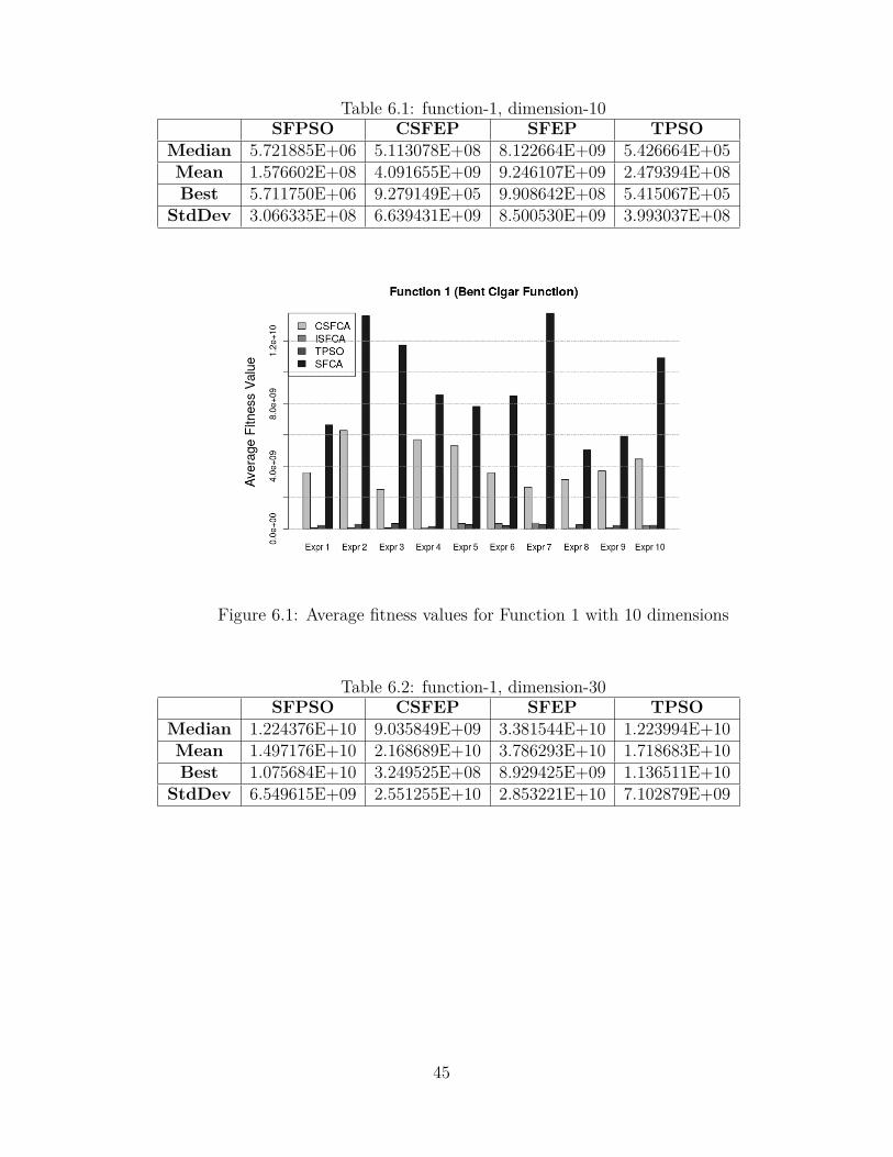
Table 6.1: function-1, dimension-10SFPSO CSFEP SFEP TPSO
Median 5.721885E+06 5.113078E+08 8.122664E+09 5.426664E+05Mean 1.576602E+08 4.091655E+09 9.246107E+09 2.479394E+08Best 5.711750E+06 9.279149E+05 9.908642E+08 5.415067E+05
StdDev 3.066335E+08 6.639431E+09 8.500530E+09 3.993037E+08
Figure 6.1: Average fitness values for Function 1 with 10 dimensions
Table 6.2: function-1, dimension-30SFPSO CSFEP SFEP TPSO
Median 1.224376E+10 9.035849E+09 3.381544E+10 1.223994E+10Mean 1.497176E+10 2.168689E+10 3.786293E+10 1.718683E+10Best 1.075684E+10 3.249525E+08 8.929425E+09 1.136511E+10
StdDev 6.549615E+09 2.551255E+10 2.853221E+10 7.102879E+09
45
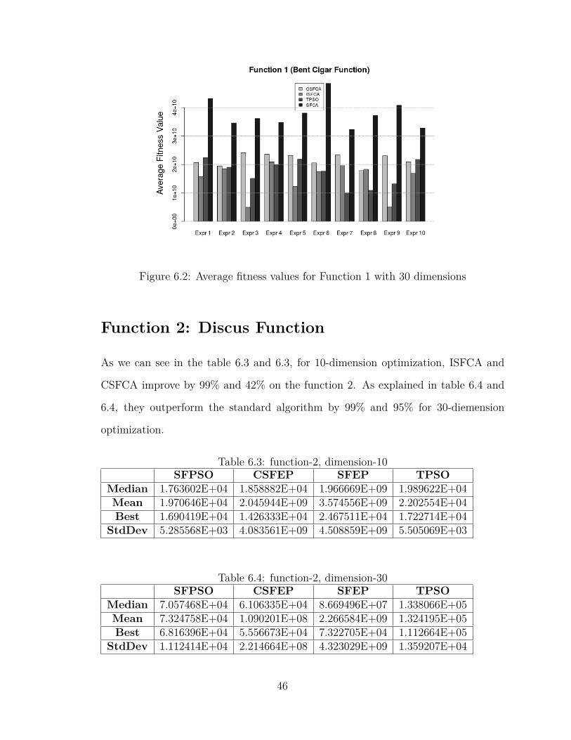
Figure 6.2: Average fitness values for Function 1 with 30 dimensions
Function 2: Discus Function
As we can see in the table 6.3 and 6.3, for 10-dimension optimization, ISFCA and
CSFCA improve by 99% and 42% on the function 2. As explained in table 6.4 and
6.4, they outperform the standard algorithm by 99% and 95% for 30-diemension
optimization.
Table 6.3: function-2, dimension-10SFPSO CSFEP SFEP TPSO
Median 1.763602E+04 1.858882E+04 1.966669E+09 1.989622E+04Mean 1.970646E+04 2.045944E+09 3.574556E+09 2.202554E+04Best 1.690419E+04 1.426333E+04 2.467511E+04 1.722714E+04
StdDev 5.285568E+03 4.083561E+09 4.508859E+09 5.505069E+03
Table 6.4: function-2, dimension-30SFPSO CSFEP SFEP TPSO
Median 7.057468E+04 6.106335E+04 8.669496E+07 1.338066E+05Mean 7.324758E+04 1.090201E+08 2.266584E+09 1.324195E+05Best 6.816396E+04 5.556673E+04 7.322705E+04 1.112664E+05
StdDev 1.112414E+04 2.214664E+08 4.323029E+09 1.359207E+04
46
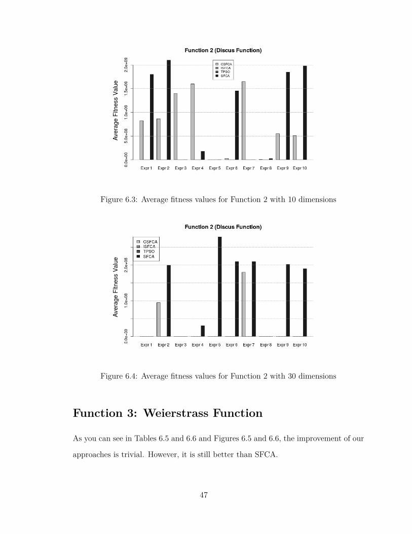
Figure 6.3: Average fitness values for Function 2 with 10 dimensions
Figure 6.4: Average fitness values for Function 2 with 30 dimensions
Function 3: Weierstrass Function
As you can see in Tables 6.5 and 6.6 and Figures 6.5 and 6.6, the improvement of our
approaches is trivial. However, it is still better than SFCA.
47
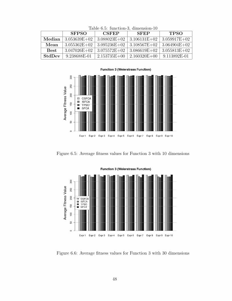
Table 6.5: function-3, dimension-10SFPSO CSFEP SFEP TPSO
Median 3.053639E+02 3.088023E+02 3.106131E+02 3.059917E+02Mean 3.055362E+02 3.095236E+02 3.108567E+02 3.064904E+02Best 3.047026E+02 3.075572E+02 3.086619E+02 3.055813E+02
StdDev 9.238688E-01 2.153735E+00 2.160320E+00 9.113892E-01
Figure 6.5: Average fitness values for Function 3 with 10 dimensions
Figure 6.6: Average fitness values for Function 3 with 30 dimensions
48
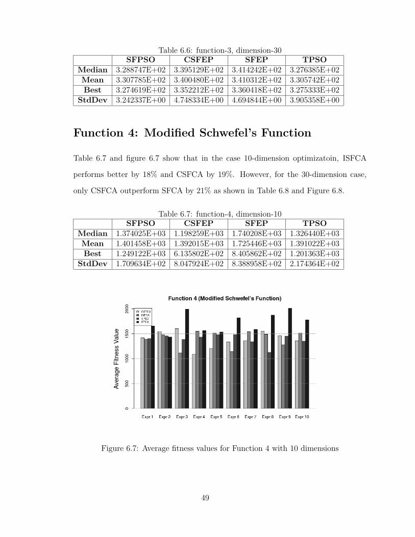
Table 6.6: function-3, dimension-30SFPSO CSFEP SFEP TPSO
Median 3.288747E+02 3.395129E+02 3.414242E+02 3.276385E+02Mean 3.307785E+02 3.400480E+02 3.410312E+02 3.305742E+02Best 3.274619E+02 3.352212E+02 3.360418E+02 3.275333E+02
StdDev 3.242337E+00 4.748334E+00 4.694844E+00 3.905358E+00
Function 4: Modified Schwefel’s Function
Table 6.7 and figure 6.7 show that in the case 10-dimension optimizatoin, ISFCA
performs better by 18% and CSFCA by 19%. However, for the 30-dimension case,
only CSFCA outperform SFCA by 21% as shown in Table 6.8 and Figure 6.8.
Table 6.7: function-4, dimension-10SFPSO CSFEP SFEP TPSO
Median 1.374025E+03 1.198259E+03 1.740208E+03 1.326440E+03Mean 1.401458E+03 1.392015E+03 1.725446E+03 1.391022E+03Best 1.249122E+03 6.135802E+02 8.405862E+02 1.201363E+03
StdDev 1.709634E+02 8.047924E+02 8.388958E+02 2.174364E+02
Figure 6.7: Average fitness values for Function 4 with 10 dimensions
49
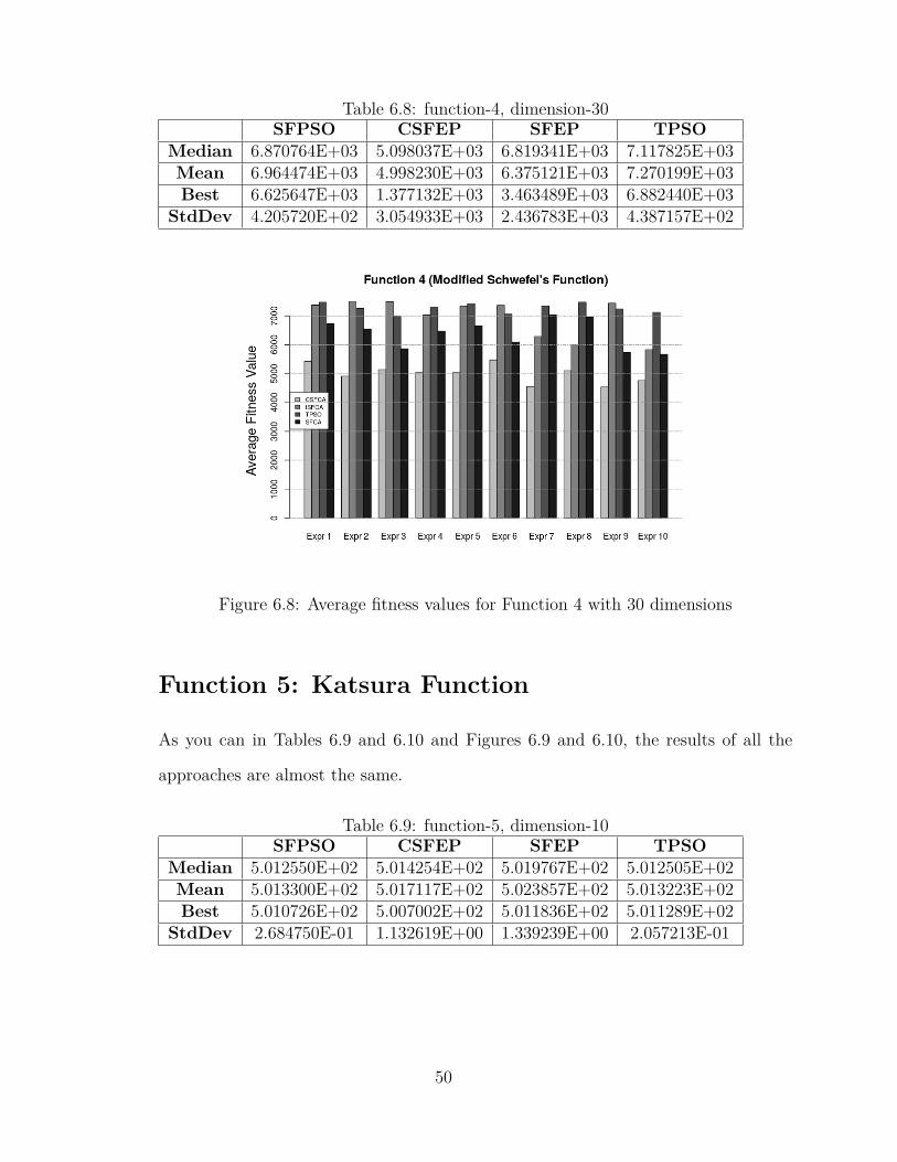
Table 6.8: function-4, dimension-30SFPSO CSFEP SFEP TPSO
Median 6.870764E+03 5.098037E+03 6.819341E+03 7.117825E+03Mean 6.964474E+03 4.998230E+03 6.375121E+03 7.270199E+03Best 6.625647E+03 1.377132E+03 3.463489E+03 6.882440E+03
StdDev 4.205720E+02 3.054933E+03 2.436783E+03 4.387157E+02
Figure 6.8: Average fitness values for Function 4 with 30 dimensions
Function 5: Katsura Function
As you can in Tables 6.9 and 6.10 and Figures 6.9 and 6.10, the results of all the
approaches are almost the same.
Table 6.9: function-5, dimension-10SFPSO CSFEP SFEP TPSO
Median 5.012550E+02 5.014254E+02 5.019767E+02 5.012505E+02Mean 5.013300E+02 5.017117E+02 5.023857E+02 5.013223E+02Best 5.010726E+02 5.007002E+02 5.011836E+02 5.011289E+02
StdDev 2.684750E-01 1.132619E+00 1.339239E+00 2.057213E-01
50
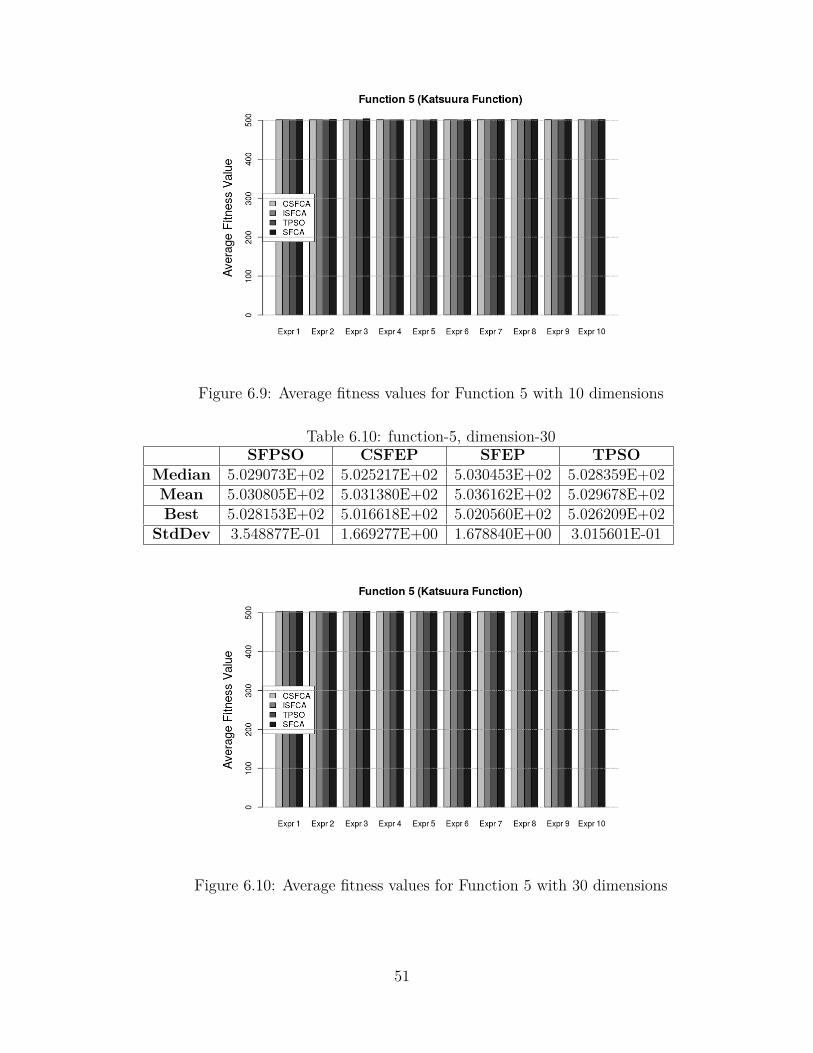
Figure 6.9: Average fitness values for Function 5 with 10 dimensions
Table 6.10: function-5, dimension-30SFPSO CSFEP SFEP TPSO
Median 5.029073E+02 5.025217E+02 5.030453E+02 5.028359E+02Mean 5.030805E+02 5.031380E+02 5.036162E+02 5.029678E+02Best 5.028153E+02 5.016618E+02 5.020560E+02 5.026209E+02
StdDev 3.548877E-01 1.669277E+00 1.678840E+00 3.015601E-01
Figure 6.10: Average fitness values for Function 5 with 30 dimensions
51
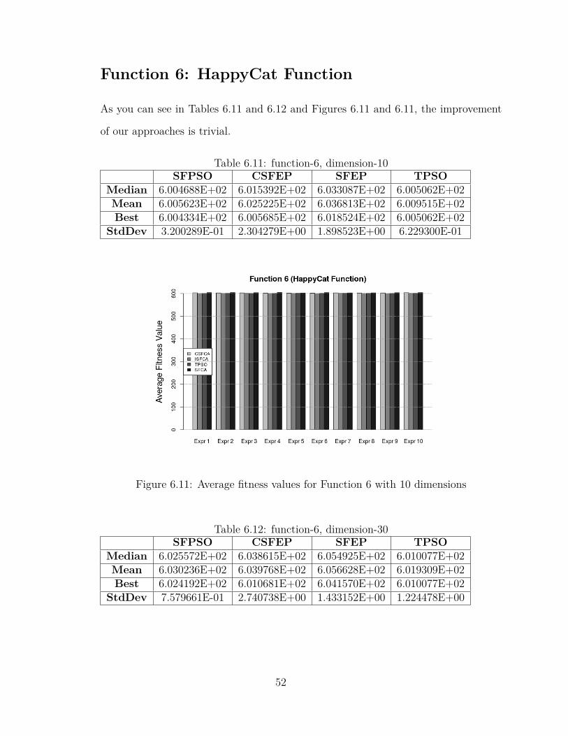
Function 6: HappyCat Function
As you can see in Tables 6.11 and 6.12 and Figures 6.11 and 6.11, the improvement
of our approaches is trivial.
Table 6.11: function-6, dimension-10SFPSO CSFEP SFEP TPSO
Median 6.004688E+02 6.015392E+02 6.033087E+02 6.005062E+02Mean 6.005623E+02 6.025225E+02 6.036813E+02 6.009515E+02Best 6.004334E+02 6.005685E+02 6.018524E+02 6.005062E+02
StdDev 3.200289E-01 2.304279E+00 1.898523E+00 6.229300E-01
Figure 6.11: Average fitness values for Function 6 with 10 dimensions
Table 6.12: function-6, dimension-30SFPSO CSFEP SFEP TPSO
Median 6.025572E+02 6.038615E+02 6.054925E+02 6.010077E+02Mean 6.030236E+02 6.039768E+02 6.056628E+02 6.019309E+02Best 6.024192E+02 6.010681E+02 6.041570E+02 6.010077E+02
StdDev 7.579661E-01 2.740738E+00 1.433152E+00 1.224478E+00
52
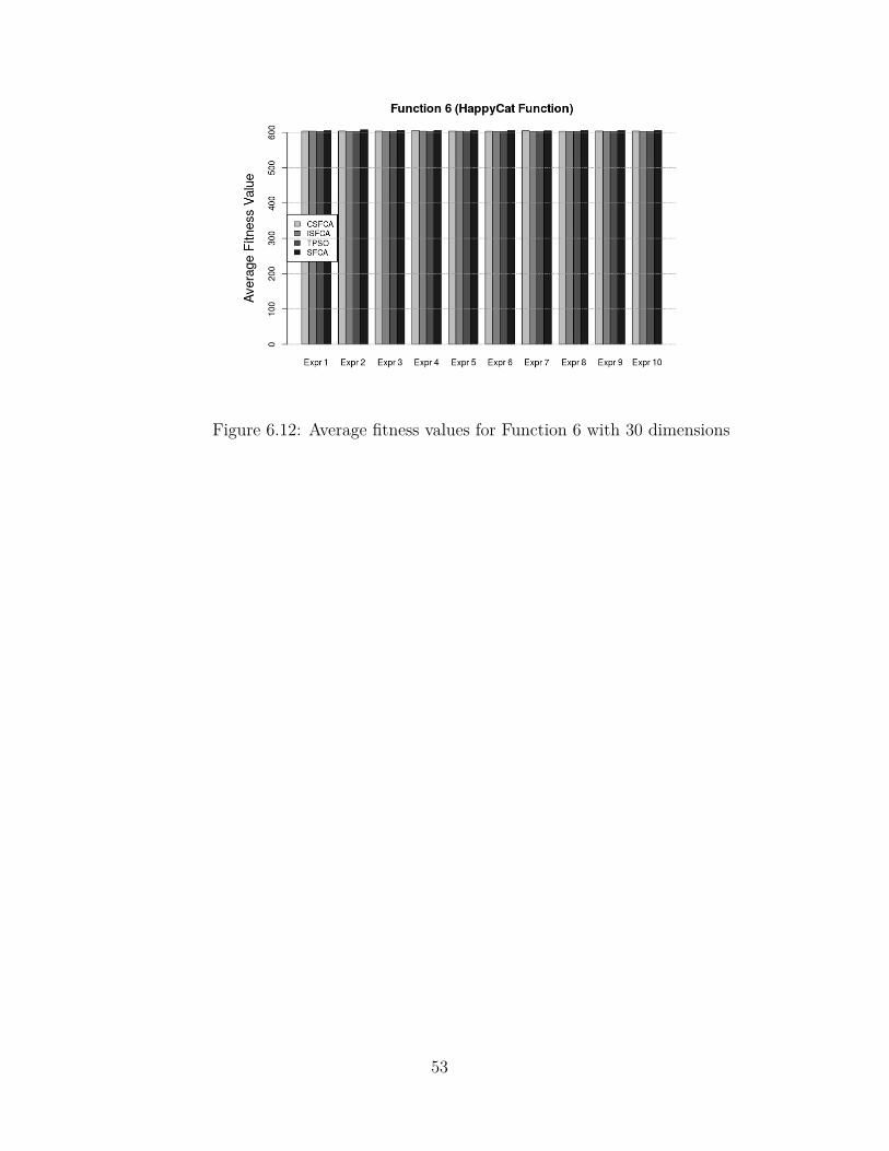
Figure 6.12: Average fitness values for Function 6 with 30 dimensions
53
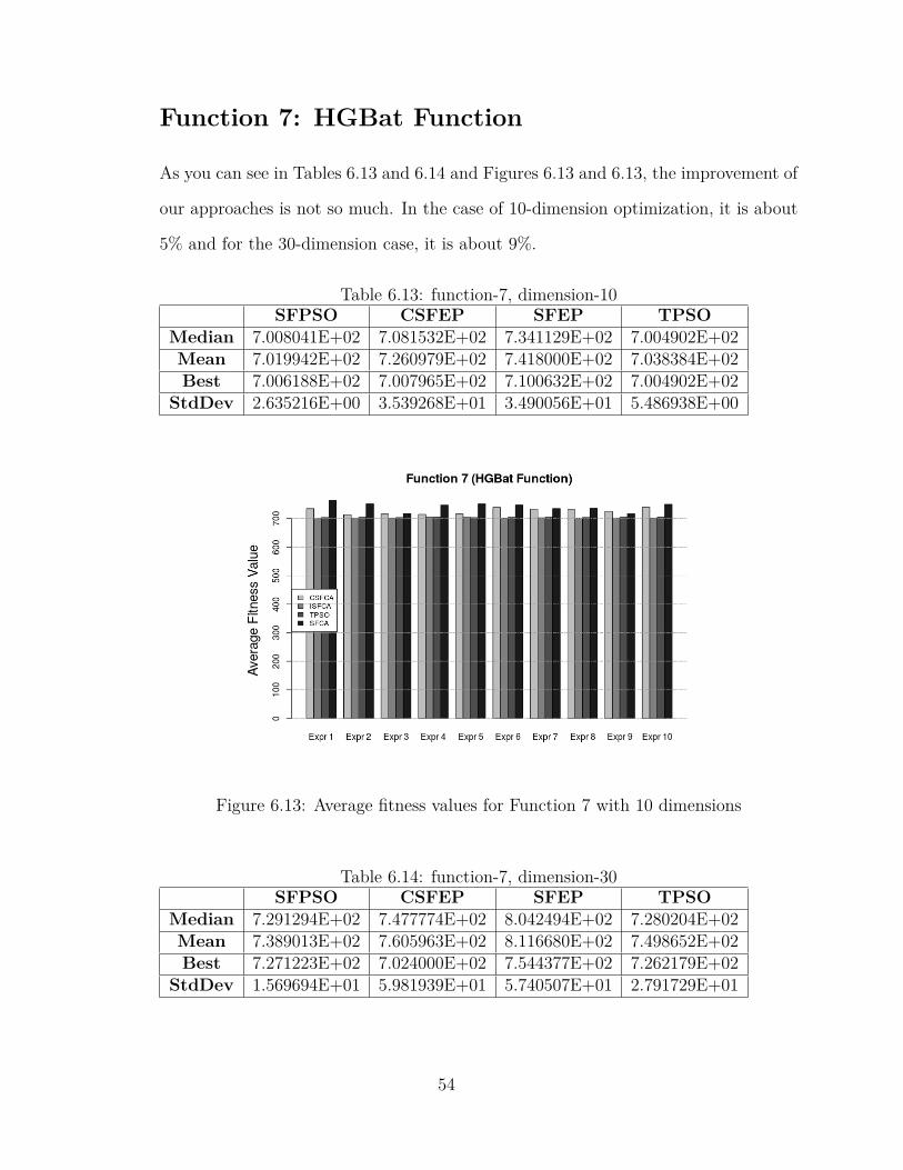
Function 7: HGBat Function
As you can see in Tables 6.13 and 6.14 and Figures 6.13 and 6.13, the improvement of
our approaches is not so much. In the case of 10-dimension optimization, it is about
5% and for the 30-dimension case, it is about 9%.
Table 6.13: function-7, dimension-10SFPSO CSFEP SFEP TPSO
Median 7.008041E+02 7.081532E+02 7.341129E+02 7.004902E+02Mean 7.019942E+02 7.260979E+02 7.418000E+02 7.038384E+02Best 7.006188E+02 7.007965E+02 7.100632E+02 7.004902E+02
StdDev 2.635216E+00 3.539268E+01 3.490056E+01 5.486938E+00
Figure 6.13: Average fitness values for Function 7 with 10 dimensions
Table 6.14: function-7, dimension-30SFPSO CSFEP SFEP TPSO
Median 7.291294E+02 7.477774E+02 8.042494E+02 7.280204E+02Mean 7.389013E+02 7.605963E+02 8.116680E+02 7.498652E+02Best 7.271223E+02 7.024000E+02 7.544377E+02 7.262179E+02
StdDev 1.569694E+01 5.981939E+01 5.740507E+01 2.791729E+01
54

Figure 6.14: Average fitness values for Function 7 with 30 dimensions
Function 8: Griewank’s plus Rosenbrock’s Function
In table 6.15 and figure 6.15, we can see that both of our approaches (ISFCA and
CSFCA) and TPSO outperform the standard SFCA impressively with 99% and 77%
for optimization of 10 dimensions. In the case of 30-dimension optimization, ISFCA
and CSFCA perform with 97% and 52% improvement respectively as shown in Table
6.16 and Figure 6.16.
Table 6.15: function-8, dimension-10SFPSO CSFEP SFEP TPSO
Median 8.060488E+02 4.762535E+03 5.638811E+05 8.057399E+02Mean 8.327824E+02 3.080861E+05 1.374142E+06 8.319941E+02Best 8.060488E+02 8.475602E+02 4.118304E+03 8.057399E+02
StdDev 1.428379E+02 5.970746E+05 1.940514E+06 7.254239E+01
55
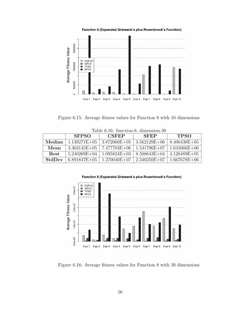
Figure 6.15: Average fitness values for Function 8 with 10 dimensions
Table 6.16: function-8, dimension-30SFPSO CSFEP SFEP TPSO
Median 1.139271E+05 3.872060E+05 3.562129E+06 8.406430E+05Mean 3.363145E+05 7.477703E+06 1.541796E+07 1.645666E+06Best 5.240269E+04 1.095824E+03 8.508643E+04 4.126489E+05
StdDev 6.891847E+05 1.270040E+07 2.340250E+07 1.667678E+06
Figure 6.16: Average fitness values for Function 8 with 30 dimensions
56
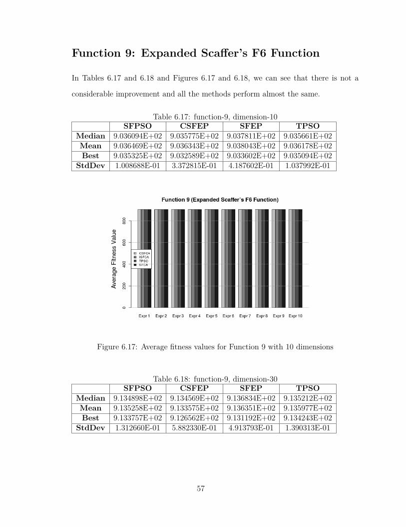
Function 9: Expanded Scaffer’s F6 Function
In Tables 6.17 and 6.18 and Figures 6.17 and 6.18, we can see that there is not a
considerable improvement and all the methods perform almost the same.
Table 6.17: function-9, dimension-10SFPSO CSFEP SFEP TPSO
Median 9.036094E+02 9.035775E+02 9.037811E+02 9.035661E+02Mean 9.036469E+02 9.036343E+02 9.038043E+02 9.036178E+02Best 9.035325E+02 9.032589E+02 9.033602E+02 9.035094E+02
StdDev 1.008688E-01 3.372815E-01 4.187602E-01 1.037992E-01
Figure 6.17: Average fitness values for Function 9 with 10 dimensions
Table 6.18: function-9, dimension-30SFPSO CSFEP SFEP TPSO
Median 9.134898E+02 9.134569E+02 9.136834E+02 9.135212E+02Mean 9.135258E+02 9.133575E+02 9.136351E+02 9.135977E+02Best 9.133757E+02 9.126562E+02 9.131192E+02 9.134243E+02
StdDev 1.312660E-01 5.882330E-01 4.913793E-01 1.390313E-01
57
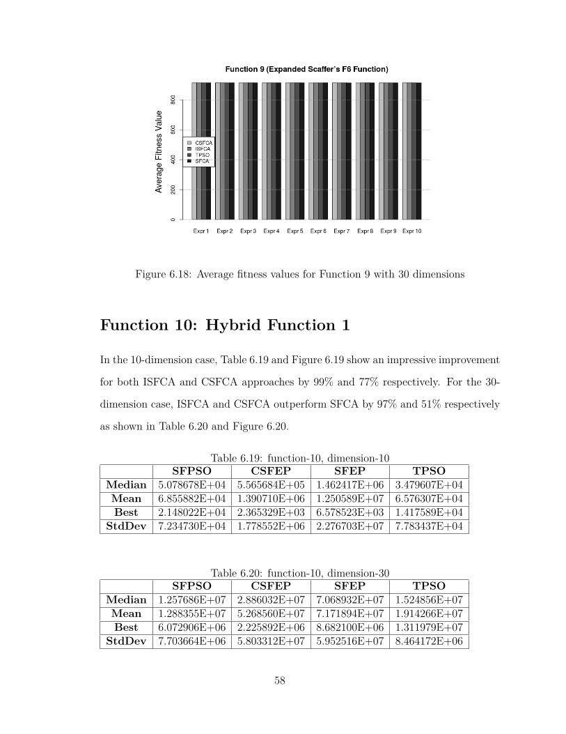
Figure 6.18: Average fitness values for Function 9 with 30 dimensions
Function 10: Hybrid Function 1
In the 10-dimension case, Table 6.19 and Figure 6.19 show an impressive improvement
for both ISFCA and CSFCA approaches by 99% and 77% respectively. For the 30-
dimension case, ISFCA and CSFCA outperform SFCA by 97% and 51% respectively
as shown in Table 6.20 and Figure 6.20.
Table 6.19: function-10, dimension-10SFPSO CSFEP SFEP TPSO
Median 5.078678E+04 5.565684E+05 1.462417E+06 3.479607E+04Mean 6.855882E+04 1.390710E+06 1.250589E+07 6.576307E+04Best 2.148022E+04 2.365329E+03 6.578523E+03 1.417589E+04
StdDev 7.234730E+04 1.778552E+06 2.276703E+07 7.783437E+04
Table 6.20: function-10, dimension-30SFPSO CSFEP SFEP TPSO
Median 1.257686E+07 2.886032E+07 7.068932E+07 1.524856E+07Mean 1.288355E+07 5.268560E+07 7.171894E+07 1.914266E+07Best 6.072906E+06 2.225892E+06 8.682100E+06 1.311979E+07
StdDev 7.703664E+06 5.803312E+07 5.952516E+07 8.464172E+06
58

Figure 6.19: Average fitness values for Function 10 with 10 dimensions
Figure 6.20: Average fitness values for Function 10 with 30 dimensions
Function 11: Hybrid Function 2
Table 6.21 and Figure 6.21 show a trivial improvement for the 10-dimension case.
On the other hand, Table 6.22 and Figure 6.22 explain that ISFCA and CSFCA
outperform the standard algorithm by 30% and 15% respectively.
59

Table 6.21: function-11, dimension-10SFPSO CSFEP SFEP TPSO
Median 1.104725E+03 1.109982E+03 1.111399E+03 1.104917E+03Mean 1.105085E+03 1.137076E+03 1.140188E+03 1.105442E+03Best 1.104062E+03 1.106581E+03 1.105492E+03 1.104723E+03
StdDev 1.339530E+00 5.229237E+01 4.994351E+01 9.340507E-01
Figure 6.21: Average fitness values for Function 11 with 10 dimensions
Figure 6.22: Average fitness values for Function 11 with 30 dimensions
60
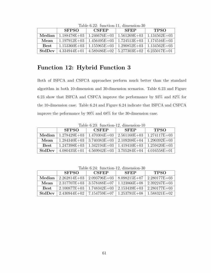
Table 6.22: function-11, dimension-30SFPSO CSFEP SFEP TPSO
Median 1.188478E+03 1.246676E+03 1.561269E+03 1.134562E+03Mean 1.197912E+03 1.456495E+03 1.724513E+03 1.174516E+03Best 1.153360E+03 1.155965E+03 1.290852E+03 1.134562E+03
StdDev 4.334944E+01 4.589486E+02 5.277303E+02 6.235017E+01
Function 12: Hybrid Function 3
Both of ISFCA and CSFCA approaches perform much better than the standard
algorithm in both 10-dimension and 30-dimension scenarios. Table 6.23 and Figure
6.23 show that ISFCA and CSFCA improve the performance by 93% and 82% for
the 10-dimension case. Table 6.24 and Figure 6.24 indicate that ISFCA and CSFCA
improve the peformance by 99% and 68% for the 30-dimension case.
Table 6.23: function-12, dimension-10SFPSO CSFEP SFEP TPSO
Median 1.278429E+03 1.470304E+03 2.561160E+03 1.274117E+03Mean 1.284340E+03 3.740383E+03 2.109208E+04 1.290392E+03Best 1.247398E+03 1.342194E+03 1.419410E+03 1.259420E+03
StdDev 4.080435E+01 4.569942E+03 3.705284E+04 4.016558E+01
Table 6.24: function-12, dimension-30SFPSO CSFEP SFEP TPSO
Median 2.262814E+03 2.093796E+03 8.098215E+07 2.280177E+03Mean 2.317707E+03 3.578488E+07 1.123866E+08 2.392247E+03Best 2.100877E+03 1.748342E+03 2.153439E+03 2.280177E+03
StdDev 2.430944E+02 7.154759E+07 1.253791E+08 1.588321E+02
61
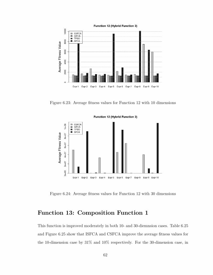
Figure 6.23: Average fitness values for Function 12 with 10 dimensions
Figure 6.24: Average fitness values for Function 12 with 30 dimensions
Function 13: Composition Function 1
This function is improved moderately in both 10- and 30-diemnsion cases. Table 6.25
and Figure 6.25 show that ISFCA and CSFCA improve the average fitness values for
the 10-dimension case by 31% and 10% respectively. For the 30-dimension case, in
62
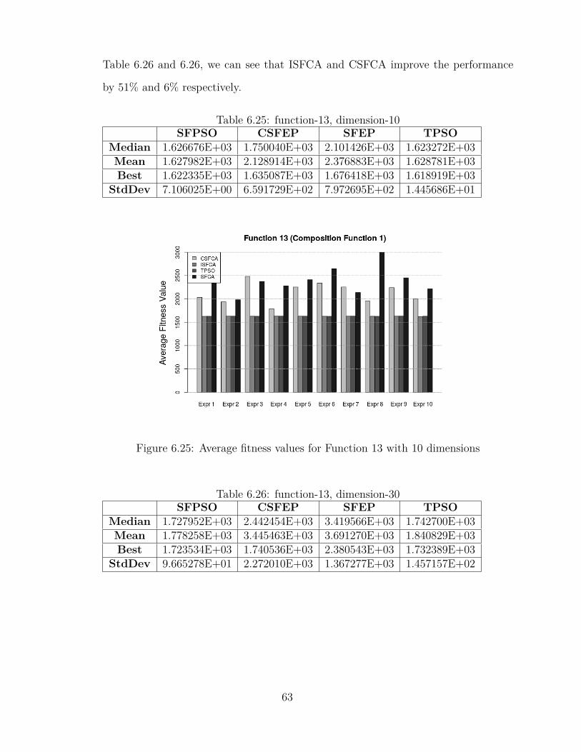
Table 6.26 and 6.26, we can see that ISFCA and CSFCA improve the performance
by 51% and 6% respectively.
Table 6.25: function-13, dimension-10SFPSO CSFEP SFEP TPSO
Median 1.626676E+03 1.750040E+03 2.101426E+03 1.623272E+03Mean 1.627982E+03 2.128914E+03 2.376883E+03 1.628781E+03Best 1.622335E+03 1.635087E+03 1.676418E+03 1.618919E+03
StdDev 7.106025E+00 6.591729E+02 7.972695E+02 1.445686E+01
Figure 6.25: Average fitness values for Function 13 with 10 dimensions
Table 6.26: function-13, dimension-30SFPSO CSFEP SFEP TPSO
Median 1.727952E+03 2.442454E+03 3.419566E+03 1.742700E+03Mean 1.778258E+03 3.445463E+03 3.691270E+03 1.840829E+03Best 1.723534E+03 1.740536E+03 2.380543E+03 1.732389E+03
StdDev 9.665278E+01 2.272010E+03 1.367277E+03 1.457157E+02
63
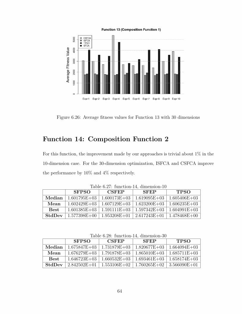
Figure 6.26: Average fitness values for Function 13 with 30 dimensions
Function 14: Composition Function 2
For this function, the improvement made by our approaches is trivial about 1% in the
10-dimension case. For the 30-dimension optimization, ISFCA and CSFCA improve
the performance by 10% and 4% respectively.
Table 6.27: function-14, dimension-10SFPSO CSFEP SFEP TPSO
Median 1.601795E+03 1.600173E+03 1.619095E+03 1.605406E+03Mean 1.602429E+03 1.607129E+03 1.623200E+03 1.606235E+03Best 1.601385E+03 1.591111E+03 1.597342E+03 1.604991E+03
StdDev 1.577398E+00 1.953208E+01 2.617243E+01 1.478468E+00
Table 6.28: function-14, dimension-30SFPSO CSFEP SFEP TPSO
Median 1.675847E+03 1.731879E+03 1.820677E+03 1.664094E+03Mean 1.676279E+03 1.791878E+03 1.865010E+03 1.685711E+03Best 1.646723E+03 1.660532E+03 1.693461E+03 1.658174E+03
StdDev 2.842502E+01 1.553106E+02 1.760265E+02 3.566090E+01
64
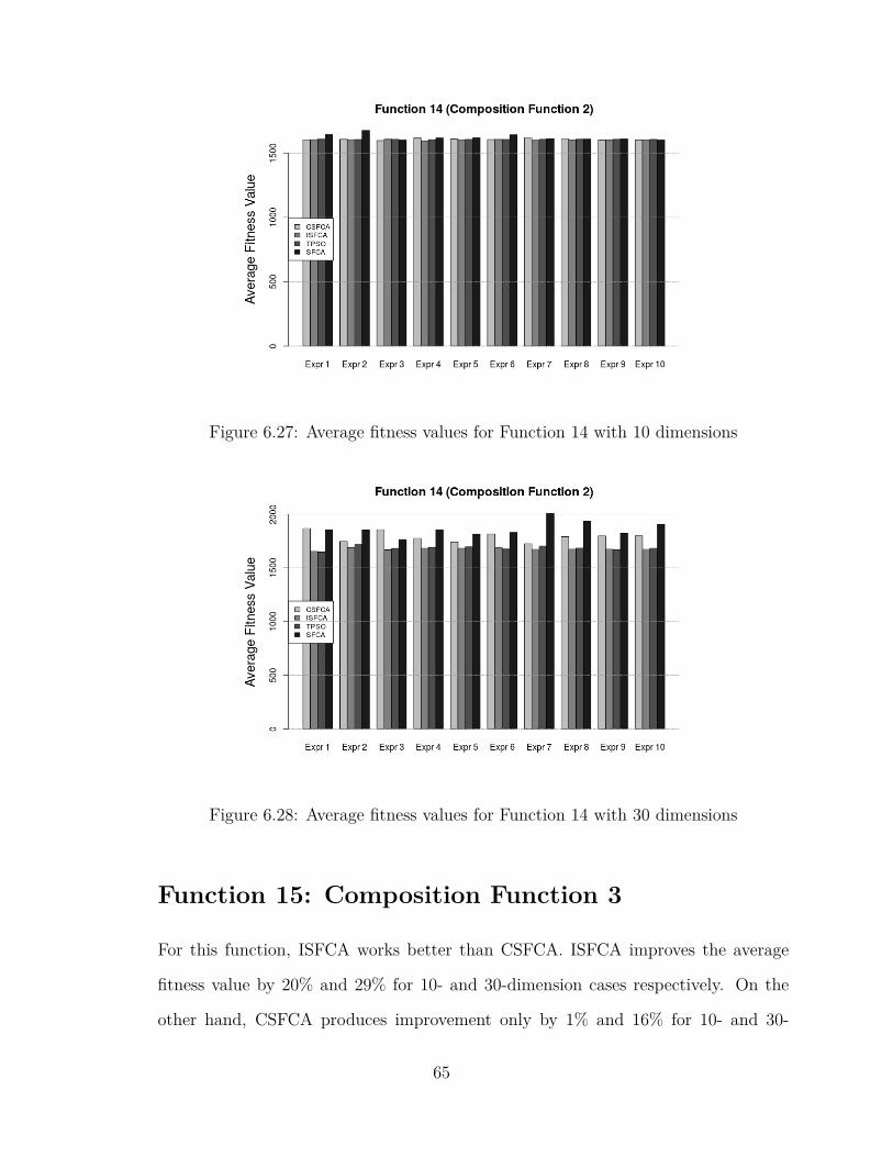
Figure 6.27: Average fitness values for Function 14 with 10 dimensions
Figure 6.28: Average fitness values for Function 14 with 30 dimensions
Function 15: Composition Function 3
For this function, ISFCA works better than CSFCA. ISFCA improves the average
fitness value by 20% and 29% for 10- and 30-dimension cases respectively. On the
other hand, CSFCA produces improvement only by 1% and 16% for 10- and 30-
65
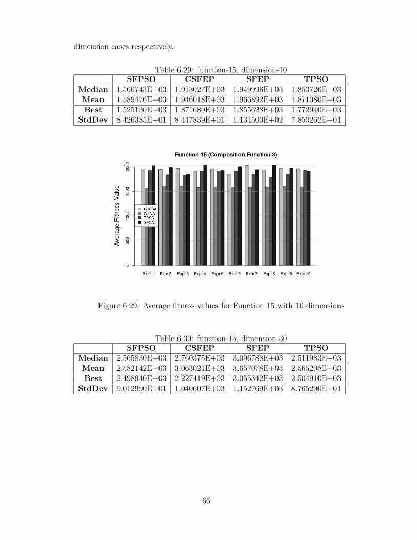
dimension cases respectively.
Table 6.29: function-15, dimension-10SFPSO CSFEP SFEP TPSO
Median 1.560743E+03 1.913027E+03 1.949996E+03 1.853726E+03Mean 1.589476E+03 1.946018E+03 1.966892E+03 1.871080E+03Best 1.525130E+03 1.871689E+03 1.855628E+03 1.772940E+03
StdDev 8.426385E+01 8.447839E+01 1.134500E+02 7.850262E+01
Figure 6.29: Average fitness values for Function 15 with 10 dimensions
Table 6.30: function-15, dimension-30SFPSO CSFEP SFEP TPSO
Median 2.565830E+03 2.760375E+03 3.096788E+03 2.511983E+03Mean 2.582142E+03 3.063021E+03 3.657078E+03 2.565208E+03Best 2.498940E+03 2.227419E+03 3.055342E+03 2.504910E+03
StdDev 9.012990E+01 1.040607E+03 1.152769E+03 8.765290E+01
66
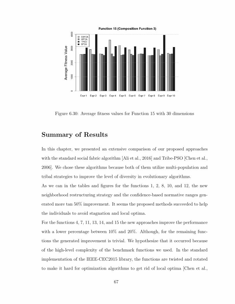
Figure 6.30: Average fitness values for Function 15 with 30 dimensions
Summary of Results
In this chapter, we presented an extensive comparison of our proposed approaches
with the standard social fabric algorithm [Ali et al., 2016] and Tribe-PSO [Chen et al.,
2006]. We chose these algorithms because both of them utilize multi-population and
tribal strategies to improve the level of diversity in evolutionary algorithms.
As we can in the tables and figures for the functions 1, 2, 8, 10, and 12, the new
neighborhood restructuring strategy and the confidence-based normative ranges gen-
erated more tan 50% improvement. It seems the proposed methods succeeded to help
the individuals to avoid stagnation and local optima.
For the functions 4, 7, 11, 13, 14, and 15 the new approaches improve the performance
with a lower percentage between 10% and 20%. Although, for the remaining func-
tions the generated improvement is trivial. We hypothesize that it occurred because
of the high-level complexity of the benchmark functions we used. In the standard
implementation of the IEEE-CEC2015 library, the functions are twisted and rotated
to make it hard for optimization algorithms to get rid of local optima [Chen et al.,
67
2014]. Also, as it is stated by above mentioned the No-Free Lunch Theorem, it is not
expected for an optimization algorithm to work well on all of the possible functions
[Wolpert and Macready, 1997].
68

Chapter 7
Conclusion and Future Work
Conclusion
In this thesis, two novel strategies were introduced to improve the robustness of
CAs in both population and belief spaces. In the first strategy, a new neighborhood
restructuring strategy is employed which aims at individuals with irregular and het-
erogeneous neighborhood structures. There is no centralized coordinator to control
the topology of a population because the individuals are responsible for inspecting
and modifying their neighborhood in a self-organized manner. Increasing the level
of self-organization and autonomy is a key approach to improving robustness in a
complex system. In the second strategy, the standard implementation of normative
ranges in the belief space was replaced by the confidence intervals inspired from In-
ferential Statistics. The new knowledge source shows a more robust search behavior
to fluctuations in the input data. Now, the size of normative ranges does not change
dramatically with any temporal fluctuations.
For the new neighborhood restructuring, a fundamental assumption is that the in-
dividuals have to handle their interactions within a social network (fabric) infras-
tructure. Here, the social fabric is modeled using a dynamic graph which the neigh-
69
borhood size of the nodes (individuals) changes with time. This assumption implies
another assumption that the interactions between agents occur locally. It means that
the amount of influence which the individuals can receive from the other members
is limited by their neighborhood size. In fact, this assumption is a key to avoiding
immature convergence. As the agents are responsible for inspecting and modifying
their neighborhood, the only limitation which we surmise when the size of a popu-
lation increase, is the performance issues. Since the population is divided into some
independent subpopulations (tribes), each tribe could be run in a separate thread.
Running all the population in a single thread may pose a heavy burden on perfor-
mance.
The second approach, confidence-based normative knowledge source, does not assume
anything more than its standard version. It is entirely independent of the strategies
deployed in the population space. In fact, the confidence-based approach could be
utilized in the same framework as well as the standard method. So, it does not pose
any additional limitations to the algorithm.
Future Work and Applications
The performance of both proposed approaches is assessed through a test-suite of 15
multi-modal and hybrid functions from IEEE-CEC2015. Both methods are compared
to the original version of the social fabric based CA [Ali et al., 2016]. The results
show improvement in most of the functions. In some of them, the results are quite
promising.
We only tested our approaches against static functions, which means there is no
change in the feedback from the environment. The improved robustness of the new
methods makes them suitable to be utilized in dynamic problems like real-time appli-
cations where the algorithm needs to inspect and adapt itself to a changing environ-
70
ment continuously and as fast as possible [Che et al., 2010]. The new neighborhood
restructuring method allows the individuals to develop relationships in promising
parts of the search space autonomously. The deployed inspect and adapt strategy
makes it easy for the agents to change their point of focus and restructure them-
selves to find new optimum points in a non-stable search space. Also, the new update
scheme for the normative ranges in the belief space can be considered suitable for
such applications since it avoids deviation with any temporal change in the input
data pattern.
With the growing industrial demands for data analytics, evolutionary algorithms
could be the source of inspiration for the solutions to address such problems. The
self-organization aspect of EAs makes them scalable to be used for analyzing datasets
with a high level of complexity. [Xiaodong et al., 2008], [Pizzuti, 2008], and [Sherkat
et al., 2015] are the examples which show promising results in social network analysis.
They used EA methods such as GA, CA, and PSO for community detection and link
prediction applications. [Sousa et al., 2004] and [Otero et al., 2012] are the examples
which proposed new approaches for data classification based on PSO and ACO. So,
these research works have created a good background to use our proposed strategies
for analytic applications.
71
BIBLIOGRAPHY
[1] M. Z. Ali and R. G. Reynolds. An intelligent social fabric influence compo-
nent in cultural algorithms for knowledge learning in dynamic environments.
In 2009 IEEE/WIC/ACM International Joint Conference on Web Intelligence
and Intelligent Agent Technology, volume 2, pages 161–168, Sept 2009. doi:
10.1109/WI-IAT.2009.146.
[2] Mostafa Z Ali. Using cultural algorithms to solve optimization problems with a
social fabric approach. ProQuest, 2008.
[3] Mostafa Z Ali, Robert G Reynolds, and Rose Ali. Enhancing cultural learning
under environmental variability using layered heterogeneous sociometry-based
networks. In Web Intelligence and Intelligent Agent Technology (WI-IAT), 2010
IEEE/WIC/ACM International Conference on, volume 2, pages 69–74. IEEE,
2010.
[4] Mostafa Z Ali, Ayad M Salhieh, and Robert G Reynolds. Socio-cultural evolution
via neighborhood-restructuring in intricate multi-layered networks. In 2012 IEEE
Congress on Evolutionary Computation, pages 1–8. IEEE, 2012.
[5] Mostafa Z Ali, Ponnuthurai N Suganthan, Robert G Reynolds, and Amer F
Al-Badarneh. Leveraged neighborhood restructuring in cultural algorithms for
solving real-world numerical optimization problems. IEEE transactions on evo-
lutionary computation, 20(2):218–231, 2016.
[6] Md Asafuddoula, Tapabrata Ray, and Ruhul Sarker. An adaptive differential
evolution algorithm and its performance on real world optimization problems.
In 2011 IEEE Congress of Evolutionary Computation (CEC), pages 1057–1062.
IEEE, 2011.
72
[7] Christian Blum and Roderich Groß. Swarm intelligence in optimization and
robotics. In Springer Handbook of Computational Intelligence, pages 1291–1309.
Springer, 2015.
[8] Eric Bonabeau, Marco Dorigo, and Guy Theraulaz. Swarm intelligence: from
natural to artificial systems. Number 1. Oxford university press, 1999.
[9] Daniel Bratton and James Kennedy. Defining a standard for particle swarm op-
timization. In 2007 IEEE swarm intelligence symposium, pages 120–127. IEEE,
2007.
[10] Edmund K Burke, Graham Kendall, et al. Search methodologies. Springer, 2005.
[11] Xiangdong Che, Mostafa Ali, and Robert G Reynolds. Robust evolution opti-
mization at the edge of chaos: Commercialization of culture algorithms. In IEEE
Congress on Evolutionary Computation, pages 1–8. IEEE, 2010.
[12] Kai Chen, Tonghua Li, and Tongcheng Cao. Tribe-pso: A novel global opti-
mization algorithm and its application in molecular docking. Chemometrics and
intelligent laboratory systems, 82(1):248–259, 2006.
[13] Q Chen, B Liu, Q Zhang, JJ Liang, PN Suganthan, and BY Qu. Problem defi-
nitions and evaluation criteria for cec 2015 special session on bound constrained
single-objective computationally expensive numerical optimization. Technical re-
port, Technical Report, Computational Intelligence Laboratory, Zhengzhou Uni-
versity, Zhengzhou, 2014.
[14] Li-Te Cheng, John Patterson, Steven L Rohall, Susanne Hupfer, and Steven
Ross. Weaving a social fabric into existing software. In Proceedings of the 4th
international conference on Aspect-oriented software development, pages 147–
158. ACM, 2005.
73

[15] Maurice Clerc and James Kennedy. The particle swarm-explosion, stability,
and convergence in a multidimensional complex space. IEEE transactions on
Evolutionary Computation, 6(1):58–73, 2002.
[16] Marco A Montes De Oca, Jorge Peña, Thomas Stutzle, Carlo Pinciroli, and
Marco Dorigo. Heterogeneous particle swarm optimizers. In 2009 IEEE Congress
on Evolutionary Computation, pages 698–705. IEEE, 2009.
[17] William H Durham. Coevolution: Genes, culture, and human diversity. Stanford
University Press, 1991.
[18] Agoston E Eiben and James E Smith. Introduction to evolutionary computing,
volume 53. Springer, 2003.
[19] Saber M Elsayed, Ruhul A Sarker, and Daryl L Essam. Differential evolution
with multiple strategies for solving cec2011 real-world numerical optimization
problems. In 2011 IEEE Congress of Evolutionary Computation (CEC), pages
1041–1048. IEEE, 2011.
[20] Yi-nan Guo, Jian Cheng, Yuan-yuan Cao, and Yong Lin. A novel multi-
population cultural algorithm adopting knowledge migration. Soft computing,
15(5):897–905, 2011.
[21] Xiaohui Hu, Russell C Eberhart, and Yuhui Shi. Engineering optimization with
particle swarm. In Swarm Intelligence Symposium, 2003. SIS’03. Proceedings of
the 2003 IEEE, pages 53–57. IEEE, 2003.
[22] Hu Jianjun, Erik D Goodman, Kisung Seo, and Min Pei. Adaptive hierarchical
fair competition (ahfc) model for parallel evolutionary algorithms. In Proceedings
of the Genetic and Evolutionary Computation Conference, New York, pages 772–
779, 2002.
74
[23] Gareth Jones, Peter Willett, Robert C Glen, Andrew R Leach, and Robin Taylor.
Development and validation of a genetic algorithm for flexible docking. Journal
of molecular biology, 267(3):727–748, 1997.
[24] J. Kennedy. Small worlds and mega-minds: effects of neighborhood topology on
particle swarm performance. In Proceedings of the 1999 Congress on Evolutionary
Computation-CEC99 (Cat. No. 99TH8406), volume 3, page 1938 Vol. 3, 1999.
doi: 10.1109/CEC.1999.785509.
[25] James Kennedy. Bare bones particle swarms. In Swarm Intelligence Symposium,
2003. SIS’03. Proceedings of the 2003 IEEE, pages 80–87. IEEE, 2003.
[26] James Kennedy, James F Kennedy, Russell C Eberhart, and Yuhui Shi. Swarm
intelligence. Morgan Kaufmann, 2001.
[27] Roger Lewin. Complexity: Life at the edge of chaos. University of Chicago Press,
1999.
[28] Rui Mendes. Population topologies and their influence in particle swarm perfor-
mance. PhD thesis, Citeseer, 2004.
[29] Rui Mendes, James Kennedy, and José Neves. The fully informed particle swarm:
simpler, maybe better. IEEE transactions on evolutionary computation, 8(3):
204–210, 2004.
[30] Marco A Montes de Oca and Thomas Stützle. Convergence behavior of the
fully informed particle swarm optimization algorithm. In Proceedings of the 10th
annual conference on Genetic and evolutionary computation, pages 71–78. ACM,
2008.
[31] Ronald W Morrison and Kenneth Alan De Jong. A test problem generator
75
for non-stationary environments. In Evolutionary Computation, 1999. CEC 99.
Proceedings of the 1999 Congress on, volume 3. IEEE, 1999.
[32] Fernando EB Otero, Alex A Freitas, and Colin G Johnson. Inducing decision
trees with an ant colony optimization algorithm. Applied Soft Computing, 12
(11):3615–3626, 2012.
[33] Bin Peng. Knowledge and population swarms in cultural algorithms for dynamic
environments. 2005.
[34] Clara Pizzuti. Ga-net: A genetic algorithm for community detection in social
networks. In International Conference on Parallel Problem Solving from Nature,
pages 1081–1090. Springer, 2008.
[35] J Proakis. Probability, random variables and stochastic processes. IEEE Trans-
actions on Acoustics, Speech, and Signal Processing, 33(6):1637–1637, 1985.
[36] M. R. Raeesi and Z. Kobti. Heterogeneous multi-population cultural algorithm.
In 2013 IEEE Congress on Evolutionary Computation, pages 292–299, June 2013.
doi: 10.1109/CEC.2013.6557583.
[37] Robert G Reynolds. An introduction to cultural algorithms. In Proceedings of the
third annual conference on evolutionary programming, volume 131139. Singapore,
1994.
[38] Robert G Reynolds and Mostafa Z Ali. Exploring knowledge and population
swarms via an agent-based cultural algorithms simulation toolkit (cat). In 2007
IEEE Congress on Evolutionary Computation, pages 2711–2718. IEEE, 2007.
[39] Robert G Reynolds and Mostafa Z Ali. The social fabric approach as an approach
to knowledge integration in cultural algorithms. In 2008 IEEE Congress on Evo-
76

lutionary Computation (IEEE World Congress on Computational Intelligence),
pages 4200–4207. IEEE, 2008.
[40] Robert G Reynolds, Mostafa Ali, and Thaer Jayyousi. Mining the social fabric
of archaic urban centers with cultural algorithms. Computer, 41(1):64–72, 2008.
[41] Manisha Sharma, Manjaree Pandit, and Laxmi Srivastava. Reserve constrained
multi-area economic dispatch employing differential evolution with time-varying
mutation. International journal of electrical power & energy systems, 33(3):753–
766, 2011.
[42] Ehsan Sherkat, Maseud Rahgozar, and Masoud Asadpour. Structural link pre-
diction based on ant colony approach in social networks. Physica A: Statistical
Mechanics and its Applications, 419:80–94, 2015.
[43] Tiago Sousa, Arlindo Silva, and Ana Neves. Particle swarm based data mining
algorithms for classification tasks. Parallel Computing, 30(5):767–783, 2004.
[44] Sara E Sterling. Aggregation techniques to characterize social networks. Tech-
nical report, DTIC Document, 2004.
[45] Thomas Stützle. Ant colony optimization. In International Conference on Evo-
lutionary Multi-Criterion Optimization, pages 2–2. Springer, 2009.
[46] Massimiliano Vasile, Edmondo Minisci, and Marco Locatelli. An inflationary
differential evolution algorithm for space trajectory optimization. IEEE Trans-
actions on Evolutionary Computation, 15(2):267–281, 2011.
[47] David H Wolpert and William G Macready. No free lunch theorems for opti-
mization. IEEE transactions on evolutionary computation, 1(1):67–82, 1997.
[48] Duan Xiaodong, Wang Cunrui, Liu Xiangdong, and Lin Yanping. Web commu-
nity detection model using particle swarm optimization. In 2008 IEEE Congress
77
on Evolutionary Computation (IEEE World Congress on Computational Intelli-
gence), pages 1074–1079. IEEE, 2008.
[49] Wei Xu, Lingbo Zhang, and Xingsheng Gu. A novel cultural algorithm and its
application to the constrained optimization in ammonia synthesis. In Life System
Modeling and Intelligent Computing, pages 52–58. Springer, 2010.
[50] Wen Zhang, Yutian Liu, and Maurice Clerc. An adaptive pso algorithm for
reactive power optimization. 2003.
78
VITA AUCTORISBahram Zaeri completed his Bachelor’s degree in Computer Science from the
Islamic Azad University in Iran in the year 2008. Then, he started working as a
software developer in Tehran, Iran for about 5 years. He has worked in numerous big
and medium scale projects as both back-end and front-end developer with different
languages such as Java, Javascript, C#, and etc. Also, he is interested in AI and
specially Swarm Intelligence. He has published some papers and articles about Ant
Colony Optimization (ACO) and its applications. He will complete his Master of
Science in Computer Science in 2017 through the University of Windsor.
Publications:
• 1
Conference: FLAIRS-2017
Title: Improving Robustness in Social Fabric-based Cultural Algorithms with
Two New Approaches in Population and Belief Spaces
Status: Accepted for publication
• 2
Confenece: Canadian AI 2017
Title: Self-Organized Neighborhood Restructuring in Social Fabric
Status: Submitted.
79