Embed Size (px)
Citation preview
University of Central Florida University of Central Florida
STARS STARS
Electronic Theses and Dissertations, 2004-2019
2004
Improving Project Management With Simulation And Completion Improving Project Management With Simulation And Completion
Distributi Distributi
Grant Cates University of Central Florida
Part of the Engineering Commons
Find similar works at: https://stars.library.ucf.edu/etd
University of Central Florida Libraries http://library.ucf.edu
This Doctoral Dissertation (Open Access) is brought to you for free and open access by STARS. It has been accepted
for inclusion in Electronic Theses and Dissertations, 2004-2019 by an authorized administrator of STARS. For more
information, please contact [email protected].
STARS Citation STARS Citation Cates, Grant, "Improving Project Management With Simulation And Completion Distributi" (2004). Electronic Theses and Dissertations, 2004-2019. 167. https://stars.library.ucf.edu/etd/167
IMPROVING PROJECT MANAGEMENT WITH SIMULATION AND COMPLETION DISTRIBUTION FUNCTIONS
by
GRANT R. CATES B.S. Colorado State University, 1981
M.S. University of Central Florida, 1996
A dissertation submitted in partial fulfillment of the requirements for the degree of Doctor of Philosophy
in the Department of Industrial Engineering and Management Sciences in the College of Engineering and Computer Sciences
at the University of Central Florida Orlando, Florida
Fall Term 2004

© 2004 Grant R. Cates
ii
ABSTRACT
Despite the critical importance of project completion timeliness, management
practices in place today remain inadequate for addressing the persistent problem of
project completion tardiness. Uncertainty has been identified as a contributing factor in
late projects. This uncertainty resides in activity duration estimates, unplanned upsetting
events, and the potential unavailability of critical resources.
This research developed a comprehensive simulation based methodology for
conducting quantitative project completion-time risk assessments. The methodology
enables project stakeholders to visualize uncertainty or risk, i.e. the likelihood of their
project completing late and the magnitude of the lateness, by providing them with a
completion time distribution function of their projects. Discrete event simulation is used
to determine a project’s completion distribution function.
The project simulation is populated with both deterministic and stochastic
elements. Deterministic inputs include planned activities and resource requirements.
Stochastic inputs include activity duration growth distributions, probabilities for
unplanned upsetting events, and other dynamic constraints upon project activities.
Stochastic inputs are based upon past data from similar projects. The time for an entity to
complete the simulation network, subject to both the deterministic and stochastic factors,
represents the time to complete the project. Multiple replications of the simulation are run
iii

to create the completion distribution function.
The methodology was demonstrated to be effective for the on-going project to
assemble the International Space Station. Approximately $500 million per month is being
spent on this project, which is scheduled to complete by 2010. Project stakeholders
participated in determining and managing completion distribution functions. The first
result was improved project completion risk awareness. Secondly, mitigation options
were analyzed to improve project completion performance and reduce total project cost.
iv

ACKNOWLEDGMENTS
First and foremost, I thank Dr. Mansooreh Mollaghasemi for introducing me to
discrete event simulation modeling and for mentoring me through the subsequent
projects, classes, and this resulting dissertation. Likewise, the members of my
dissertation committee, Dr. Linda Malone, Dr. Michael Georgiopoulos, Dr. Tim Kotnour,
and Dr. Luis Rabelo provided extremely valuable leadership as well. Dr. Martin Steele of
NASA, Dr. José Sepulveda of UCF, and Dr. Ghaith Rabadi of Old Dominion University
also provided greatly appreciated guidance.
My participation in a graduate program would not have been possible without the
tremendous encouragement and support I received from numerous NASA and UCF
officials. These include Conrad Nagel, Mike Wetmore, and Dave King all of whom
recommended me for the Kennedy Graduate Fellowship Program. My participation in
that program was expertly administered by Kari Heminger, June Perez, Chris Weaver,
and Ed Markowski all from NASA, along with Don Hutsko of the United States
Department of Agriculture. General Roy Bridges and Jim Kennedy as directors of the
Kennedy Space Center provided the vision and leadership for the partnership between
NASA and the University of Central Florida. Special thanks to Joy Tatlonghari, for
providing the administrative guidance and support throughout the entire program of
classes, research, and dissertation. Thanks to UCF thesis Editor Katie Grigg as well as
v

NASA’s Bill Raines, Sam Lewellen, and Wayne Ranow for their assistance during the
publication process.
The support and encouragement I received from a host of current and former
NASA officials all steadfastly determined to create the greatest Space Station ever built
was nothing short of fantastic. These skilled and dedicated individuals include Mike
Leinbach, Steve Cash, Pepper Phillips, Frank Izquierdo, Doug Lyons, Jeff Angermeier,
Tom Overton, Andy Warren, Jessica Mock, John Coggeshall, John Shannon, Ron
Dittemore, Bill Gerstenmaier, Bill Parsons, Tassos Abadiotakis, Scott Thurston,
Stephanie Stilson, Shari Bianco, Bill Hill, Elric McHenry, and Larry Ross.
In particular I wish to thank Janet Letchworth and Bill Cirillo both of NASA
along with Joe Fragola, Blake Putney, and Chel Stromgren all of SAIC, and Dan
Heimerdinger of Valador Inc., for their many contributions to the evolution of this
research.
I also received greatly appreciated support and encouragement from Dawn
Cannister and Tom Hayson of Rockwell Software with respect to the use of the Arena
simulation software. Dr. Averill Law of Averill M. Law and Associates provided
guidance on simulation modeling as well as the use of their excellent ExpertFit software.
My family provided great support throughout. Thanks to my parents, Chuck and
Iola Cates, my brother Rick, my sister Leslie and her husband Kevin Blackham, and my
sister Wendy and her husband Jeff Jones. My greatest appreciation is to my wife Alicia
for her love, encouragement, and patience.
vi

TABLE OF CONTENTS
LIST OF FIGURES .......................................................................................................... xii
LIST OF TABLES............................................................................................................ xv
LIST OF ABBREVIATIONS.......................................................................................... xvi
CHAPTER ONE: INTRODUCTION................................................................................. 1
Large Projects Advanced Science of Project Management ............................................ 5
PAST and the International Space Station...................................................................... 8
Applicability to Other Projects ....................................................................................... 9
Overview of Subsequent Chapters................................................................................ 10
CHAPTER TWO: LITERATURE REVIEW................................................................... 11
Project Schedule Risk Analysis/Assessment ................................................................ 11
Project Management Tools ........................................................................................... 16
Gantt Charts .............................................................................................................. 17
CPM .......................................................................................................................... 17
PERT......................................................................................................................... 18
Activity Duration Specification ............................................................................ 19
Estimating Project Completion Times .................................................................. 21
Precedence Diagramming ......................................................................................... 25
Merging of PERT, CPM, and Precedence Diagramming ......................................... 25
vii
Performance Measurement and Earned Value.......................................................... 27
GERT and Q-GERT.................................................................................................. 27
VERT ........................................................................................................................ 29
The Project Management Institute ................................................................................ 30
Critical Chain Project Management.............................................................................. 32
Activity Embedded Safety Time............................................................................... 35
Project and Feeding Buffers...................................................................................... 38
CCPM on Project Completion Time Distribution Function ..................................... 40
Empirical Data for Input Analysis ................................................................................ 41
CHAPTER THREE: METHODOLOGY ......................................................................... 44
Part I: The Project Assessment by Simulation Technique (PAST) .............................. 44
Managerial Controls Component of PAST............................................................... 47
Introductory Briefings........................................................................................... 48
Assessment Requirements .................................................................................... 49
Communications ................................................................................................... 49
Simulation Modeling Component of PAST.............................................................. 50
Activity Construct................................................................................................. 53
Probabilistic Event Construct ............................................................................... 61
Cyclical Element Construct .................................................................................. 62
Input Analysis Component of PAST ........................................................................ 63
Output Analysis Component of PAST...................................................................... 67
Creating the PCDF................................................................................................ 68
viii

Determining the PCDF Confidence Band............................................................. 69
Verification and Validation for PAST ...................................................................... 73
Verification ........................................................................................................... 73
Validation.............................................................................................................. 74
Measuring Progress................................................................................................... 76
Part II: Research Methodology (Case Study) ............................................................... 77
Case Study Definitions ............................................................................................. 78
Components of Research Design .............................................................................. 79
Study Question...................................................................................................... 79
Proposition ............................................................................................................ 80
Units of Measurement........................................................................................... 81
Logic for Linking Data to Proposition.................................................................. 82
Criteria for Interpreting the Findings.................................................................... 83
Ensuring Case Study Design Quality........................................................................ 83
Construct Validity................................................................................................. 84
Internal Validity .................................................................................................... 87
External Validity................................................................................................... 87
Reliability.............................................................................................................. 88
The Specific Case Study Design............................................................................... 88
CHAPTER FOUR: FINDINGS........................................................................................ 90
Section I: The Pilot Case Study .................................................................................... 90
Background............................................................................................................... 91
ix

Space Shuttle Processing Flow ................................................................................. 94
Margin Assessment Results ...................................................................................... 98
Initial Analysis of the Project Margin Problem ...................................................... 100
Project Assessment by Simulation Technique Prototype ....................................... 105
Managerial Controls Component........................................................................ 105
Simulation Model Component............................................................................ 106
Input Analysis Component ................................................................................. 108
Verification ......................................................................................................... 110
Output Analysis .................................................................................................. 111
Section II: Three Additional Case Studies.................................................................. 116
Background Information......................................................................................... 116
Case Study 1: Launch Window Analysis................................................................ 118
Case Study 2: Manifest Option 04A-29.................................................................. 122
Work Force Augmentation ................................................................................. 125
Reducing Project Content ................................................................................... 128
Case Study 3: Project Buffer Benefit...................................................................... 129
Section III: Evolution of PAST................................................................................... 133
Modeling Automation............................................................................................. 134
Output Analysis Automation .................................................................................. 135
Management Issues................................................................................................. 136
PAST: Step-by-Step............................................................................................ 137
Scale of Effort ..................................................................................................... 139
x

Organizational Residence ................................................................................... 140
Analysis Distribution Controls ........................................................................... 140
The Completion Quantity Distribution Function Graphic ...................................... 142
CHAPTER FIVE: CONCLUSION................................................................................. 146
Summary of Case Study Results................................................................................. 146
Observations and Recommendations.......................................................................... 148
Completion Quantity Distribution Function ........................................................... 148
Timeliness of Analysis............................................................................................ 149
Politics of Risk Assessment .................................................................................... 150
Future Research .......................................................................................................... 152
Continued Use of PAST to Support ISS Assembly ................................................ 152
PAST and Critical Chain Project Management ...................................................... 156
The PAST Input Analysis Methodology................................................................. 157
Closing Thoughts ........................................................................................................ 157
END NOTES .................................................................................................................. 159 LIST OF REFERENCES................................................................................................ 161
xi

LIST OF FIGURES
Figure 1: The Four Components of PAST.......................................................................... 2
Figure 2: Example Project Completion Distribution Function........................................... 4
Figure 3: Improved Project Completion Timeliness........................................................... 5
Figure 4: Activity Duration Distribution Function ........................................................... 35
Figure 5: Multitasking Increases Task Durations ............................................................. 37
Figure 6: Visual Display of Project Completion Risk (Example) .................................... 44
Figure 7: Overview of the PAST Methodology................................................................ 45
Figure 8: PAST Flow Diagram......................................................................................... 46
Figure 9: Simulation Modeling Component ..................................................................... 51
Figure 10: Activity Modeling Construct with Deterministic Duration and Reserve ........ 55
Figure 11: Activity Modeling Construct with Stochastic Duration Added ...................... 56
Figure 12: Reserve Reduction Feature Added to Activity Construct ............................... 58
Figure 13: Resource Element Added to Activity Construct ............................................. 59
Figure 14: Completed Activity Construct......................................................................... 60
Figure 15: Predictable Need to Use an Alternate Route ................................................... 61
Figure 16: Cyclical Process .............................................................................................. 62
Figure 17: Input Analysis for Activity Construct ............................................................. 63
xii

Figure 18: Input Analysis Component of PAST............................................................... 64
Figure 19: Output Analysis Component of PAST ............................................................ 67
Figure 20: Presentation of a Project Completion Time Density Function........................ 69
Figure 21: Graphical Presentation of Confidence Band ................................................... 72
Figure 22: Notional Project Planned Completion Date versus PCDF .............................. 81
Figure 23: Research Methodology Chronological Overview ........................................... 89
Figure 24: Space Shuttle Orbiter Space Station Assembly Sequence .............................. 92
Figure 25: Orbiter Resource Utilization Chart.................................................................. 93
Figure 26: Space Shuttle Mission Cycle........................................................................... 94
Figure 27: Shuttle Gantt Chart.......................................................................................... 95
Figure 28: Work Days Added to the OPF Flow Post Delta LSFR ................................. 101
Figure 29: Histogram and CFD for OPF Added Work Days.......................................... 102
Figure 30: Available Margin Diagram for the Node-2 Milestone .................................. 104
Figure 31: OPF Empirical Distribution for Added Work Days...................................... 109
Figure 32: Completion Time Distribution Function for STS-120 Launch Date............. 111
Figure 33: Working Holidays Improves STS-120 Launch Date .................................... 114
Figure 34: STS-120 Launch Date Improvement from Working Holidays ..................... 115
Figure 35: Launch Window Analysis ............................................................................. 120
Figure 36: Launch Probability with Winter Weather Modifier ...................................... 121
Figure 37: Launch Probability Comparisons .................................................................. 122
Figure 38: Initial Analysis of 04A-29 Manifest Option.................................................. 124
Figure 39: Potential Benefit from Workforce Augmentation. ........................................ 127
xiii

Figure 40: CTDF for STS-141 Launch Month ............................................................... 129
Figure 41: Analysis of 04A-49 Option with S1.O Assumptions .................................... 131
Figure 42: Confidence Bands for STS-136 Launch Date ............................................... 132
Figure 43: Modeling Component of PAST..................................................................... 134
Figure 44: Organizational Hierarchy .............................................................................. 141
Figure 45: CQDF for Analysis Team.............................................................................. 143
Figure 46: CQDF with PLOV at .01............................................................................... 144
Figure 47: Improvement from Elimination of Launch on Need Requirement ............... 145
Figure 48: Accelerating ISS Assembly Completion....................................................... 153
xiv

LIST OF TABLES
Table 1: Buffer Sizes as Proposed by Yongyi Shou and Yeo........................................... 40
Table 2: Confidence Band Calculation ............................................................................. 71
Table 3: Margin Assessment............................................................................................. 99
Table 4: Margin Days Required To Ensure Next Project Starts on Time ...................... 103
Table 5: 04A-29 Manifest Option................................................................................... 123
Table 6: 04A-49 Manifest Option................................................................................... 130
xv
LIST OF ABBREVIATIONS
AOA Activity on Arrow
AON Activity on Node
AXAF Advanced X-Ray Astrophysics Facility
CAIB Columbia Accident Investigation Board
CCPM Critical Chain Project Management
CPM Critical Path Method
CQDF Completion Quantity Distribution Function
CTD Completion Time Distribution
CTDF Completion Time Distribution Function
DES Discrete Event Simulation
DFRC Dryden Flight Research Center
DOD Department of Defense
GERT Graphical Evaluation and Review Technique
ISS International Space Station
KSC Kennedy Space Center
LON Launch on Need
MAST Manifest Analysis by Simulation Tool
MPS Main Propulsion System
xvi

NASA National Aeronautics and Space Administration
OPF Orbiter Processing Facility
PAST Project Assessment by Simulation Technique
PCDF Project Completion Distribution Function
PDM Precedence Diagramming Network
PERT Project Evaluation and Review Technique
PLOV Probability of Loss of Vehicle
PMI Project Management Institute
PRACA Problem Reporting and Corrective Action
STS Space Transportation System
TOC Theory of Constraints
VAB Vehicle Assembly Building
VERT Venture Evaluation and Review Technique
xvii

CHAPTER ONE: INTRODUCTION
Despite the critical importance of project completion timeliness, project
management practices in place today remain inadequate for addressing the persistent
problem of project completion tardiness. A major culprit causing project completion
tardiness is uncertainty, which most, if not all, projects are inherently subjected to
(Goldratt 1997). This uncertainty is present in many places including the estimates for
activity durations, the occurrence of unplanned and unforeseen events, and the
availability of critical resources. In planning, scheduling, and controlling their projects,
managers may use tools such as Gantt charts and or network diagrams such as those
provided by Project Evaluation and Review Technique (PERT) or Critical Path Method
(CPM). These tools, however, are limited in their ability to help managers quantify
project completion risk. Consequently, large and highly important projects can end up
finishing later than planned and project stakeholders including politicians, project
managers, and project customers may be unpleasantly surprised when this happens.
The typically cited method for quantitative schedule risk analysis has been called
“stochastic CPM” (Galway 2004). This process uses Monte Carlo simulation to analyze a
project network in order to produce a project completion distribution function. However,
as noted by Galway (2004) there is lack of literature on the use of this technique in
practice and a lack of case studies that illustrate when this method works or fails.
1

Consequently, developing a more complete practical methodology for quantitative project
completion timeliness analysis and demonstrating its effectiveness in a real world
application would seem to be advised.
This research develops a comprehensive methodology for project schedule risk
analysis. It is called the Project Assessment by Simulation Technique (PAST) and
consists of four major components. These are the managerial controls, modeling, input
analysis, and output analysis components. Figure 1 shows the components of PAST and
how they are interconnected in a logical fashion.
SimulationModeling
ManagerialControls
Input Analysis:Deterministic& Stochastic
OutputAnalysis
FeedbackLoops
File: Project Analysis Process R1.vsd
Figure 1: The Four Components of PAST
PAST and its four major components are described briefly below. They are fully
described in Chapter 3. The managerial controls component provides a facilitating
interface between those performing the assessment and the project stakeholders. The
input analysis component contains both deterministic and stochastic elements. The
2

deterministic element includes the schedule information such as project activities, their
durations, along with their precedence and critical resource requirements. This
information is use to create a simulation model of the project. The simulation model
includes stochastic inputs in the form of potential growth in activity durations and the
probability of upsetting events occurring during the project. These upsetting events may
cause project stoppages or may require the addition of new work. The basis of estimate
for the stochastic inputs stems from empirical information. The simulation model of the
project is run for many hundreds or thousands of replications so as to produce a large
quantity of possible project completion end dates. This data set is then used by the output
analysis component to create a visual display of project completion uncertainty in the
form of a completion distribution function.
Project stakeholders can visualize project performance uncertainty, e.g. the
likelihood of the project completing late and the magnitude of the lateness, by being
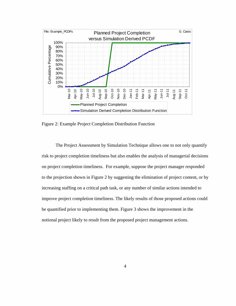
shown the completion distribution function for the project. Figure 2 is an example of a
project completion distribution function. For this notional project, the planned completion
time is October of 2010. The simulation derived completion distribution function for the
project indicates that there is only an approximately 30 percent chance of completing the
project by that time. Moreover, the project may finish as much as a year late.
3
Planned Project Completion versus Simulation Derived PCDF
0%10%20%30%40%50%60%70%80%90%
100%
Mar
-10
Apr-
10
May
-10
Jun-
10
Jul-1
0
Aug-
10
Sep-
10
Oct
-10
Nov
-10
Dec
-10
Jan-
11
Feb-
11
Mar
-11
Apr-
11
May
-11
Jun-
11
Jul-1
1
Aug-
11
Sep-
11
Oct
-11
Project Completion Month
Cum
ulat
ive
Per
cent
age
Planned Project CompletionSimulation Derived Completion Distribution Function
File: Example_PCDFs G. Cates
Figure 2: Example Project Completion Distribution Function
The Project Assessment by Simulation Technique allows one to not only quantify
risk to project completion timeliness but also enables the analysis of managerial decisions
on project completion timeliness. For example, suppose the project manager responded
to the projection shown in Figure 2 by suggesting the elimination of project content, or by
increasing staffing on a critical path task, or any number of similar actions intended to
improve project completion timeliness. The likely results of those proposed actions could
be quantified prior to implementing them. Figure 3 shows the improvement in the
notional project likely to result from the proposed project management actions.
4

Planned Project Completion versus Simulation Derived CDF
0%10%20%30%40%50%60%70%80%90%
100%
Dec
-09
Jan-
10
Feb-
10
Mar
-10
Apr-
10
May
-10
Jun-
10
Jul-1
0
Aug-
10
Sep-
10
Oct
-10
Nov
-10
Dec
-10
Jan-
11
Feb-
11
Mar
-11
Apr-
11
Project Completion Month
Cum
ulat
ive
Per
cent
age
Planned Project CompletionSimulation Derived Completion Distribution Function
File: Example PCDF.xls G. Cates
Figure 3: Improved Project Completion Timeliness
In the above example the proposed action of the project manager increased the
likelihood of on-time project completion to approximately 80 percent.
Large Projects Advanced Science of Project Management
The importance of this research comes from the importance that is placed upon
project completion performance particularly with respect to large projects. Examples of
large projects include cargo ship building during World War I, the Manhattan Project to
build the first Atomic Bomb, the Polaris missile program, the Minuteman missile
program, and the Apollo program. The science of project management has been advanced
as a result of such critically important large projects.
5
During World War I there was a pressing need for cargo ships in order to transfer
war supplies from America to Europe. Henry Gantt reduced the time to build cargo ships
through the use of bar charts he invented. The charts, later to be named Gantt charts,
visually displayed the activities, and their durations, required to build each ship. In World
War II robust and accurate project planning, scheduling, and tracking methods were
required and developed to carry out the Manhattan Project (Morris 1994, 1997).
During the 1950s, the United States began to grow concerned about the Soviet
Union’s advancement in space and especially with respect to their deploying nuclear
capable intercontinental ballistic missiles. This fear had profound effects upon the
United States and served to spark a space race to develop ICBMs. The United States Air
Force managed the development of ground based ICBMs. The liquid fueled rocket was
called Atlas and the solid fueled rocket was called Minuteman. The Navy managed a
similar project—the Polaris Missile Project—to develop an ICBM to be launched from
submarines. It was critically important to national survival to develop these systems as
soon as possible. The science of project management was advanced out of this necessity.
The Project Evaluation and Review Technique (PERT) was developed to support
the Polaris project (Malcolm 1959; Levin and Kirkpatrick 1966; Moder et al 1983).
According to the Navy, through using PERT, the Polaris project was completed two years
ahead of the original estimated schedule completion date. 1 2
In 1957, the Soviet Union became the first nation to place a satellite—Sputnik—
in orbit around the earth. The event increased the pressure upon the American military to
deploy the Atlas and Polaris missile systems as soon as possible. Sputnik also prompted
6

the creation, in 1958, of the National Aeronautics and Space Administration (NASA).
The Mercury program, initiated in 1958, was NASA’s project for placing an American in
space before the Soviet Union. In April of 1961, the Soviets were the first to achieve this
milestone when they orbited Yuri Gagarin around the earth. In May the United States
responded with the suborbital launch of Alan Sheppard. As the Soviet Union was clearly
leading the space race President Kennedy established a project that was far enough away
and difficult enough to achieve such that the United States would have an opportunity to
catch and surpass the Soviets. This project was the landing of an American on the moon.
Kennedy set the completion milestone of ‘by the end of the 1960s.’
It is interesting to note that President Kennedy, in announcing the decision to go
to the moon gave the nation a large project completion buffer. The original estimate was
that the United States could land on the moon by as early as 1966 or 1967 (Johnson
1971). In his public announcement, Kennedy charged that the moon landing should occur
by the end of the decade. Thus, there was anywhere from a 3 to 4 year project buffer.3
The Apollo program—the project to achieve the manned lunar landing—has been
called a “paradigm of modern project management” (Morris, 1997). During the program
the project management techniques described above were used and in some cases
improved upon. Additionally, new project management techniques were developed that
have since become commonplace in project management. Examples include phased
project planning and configuration control.
In 1962, NASA and the Department of Defense published the “DoD and NASA
Guide PERT/Cost Systems Design.” This newer PERT/Cost system included a cost
7

element, which was not included in the original PERT. Additionally, the 1962 guide
introduced government management to the Work Breakdown Structure. The Work
Breakdown Structure has since become a central component of management for large
government projects (Morris, 1997).
In 1963, Brigadier General Phillips on the Minuteman ICBM program developed
the Earned Value system (Morris 1994, 1997). Earned Value has also gone on to being a
widely used tool for project management (Fleming & Koppelman 2000).
In 1966 A. Alan B. Pritsker of the RAND Corporation developed the Graphical
Evaluation and Review Technique (GERT) for NASA’s Apollo program (Pritsker 1966).
In GERT branches of the project network can have a probabilistic chance of not having to
be accomplished whereas in PERT/CPM all branches must be accomplished. GERT
allows for looking back in the project and repeating earlier steps whereas PERT/CPM are
‘one time through’ networks.
PAST and the International Space Station
The Project Assessment by Simulation Technique (PAST) like Gantt charts,
PERT, and GERT was developed to meet the specific needs of a large and important
project. The particular project that sparked the need for PAST is the on-going effort to
assemble the International Space Station. Additionally, this research not only developed
a new methodology for project risk analysis, but also used case study research techniques
to demonstrate the use and effectiveness of this new management tool on that project.
8

Project stakeholders participated in developing and managing completion
distribution functions for that project. The results were improved project completion risk
awareness and projected improvements in project completion performance. Timely
completion of the International Space Station project will free up billions of dollars in
annual funding required to begin important follow-on space projects e.g. returning to the
moon and landing on Mars.
Furthermore, just like these earlier project management tools such as Gantt charts
and PERT, the PAST methods may be applicable to other projects.
Applicability to Other Projects
Financial benefit/penalty based on project completion is a widely used strategy on
highway construction projects (Jaraiedi et al 2002). The contractor is rewarded for
finishing early and penalized for finishing late. Consequently, it is desirable to accurately
quantify the completion time distribution function of the project. This ability may be
important during the project bid and/or planning phases as well during the project. For
example a contracting agency should have some idea of the risk associated with a project
before establishing the financial incentives and disincentives for the contract for that
project. The companies bidding on the contract require similar knowledge in order to
submit a competitive bid that if chosen will allow them to earn a profit.
9
Overview of Subsequent Chapters
The literature review in Chapter 2 focuses first on the most recent work
concerning project risk analysis and the use of simulation. The chapter then shifts to a
chronological review of management tools, including Gantt charts, PERT, etc., the
Project Management Institute, and the Critical Chain Project Management philosophy.
The chapter concludes with a brief review regarding using empirical data to develop (1)
probability distributions for activity durations and (2) event probabilities. Chapter 3
presents the details of the Project Completion Distribution Function methodology and
also develops the ground rules for conducting subsequent case studies in a real world
environment to determine if the methodology provides practical benefits. Chapter 4
describes the case studies in detail and presents the results. Chapter 5 summarizes and
concludes the research.
10

CHAPTER TWO: LITERATURE REVIEW
There is an extensive body of literature on the subject of project management.
This review focuses upon that subset pertaining to project analysis, risk, and uncertainty
with respect to completion performance. The more recent literature specific to project
schedule risk analysis and assessment is presented first as it is most germane to the
research presented in subsequent chapters. The chapter also includes a historical review
regarding the development of classic project management tools pertaining to schedule
risk during the twentieth century. These include Gantt Charts, PERT/CPM, Precedence
Diagramming, GERT/Q-GERT and VERT. The formation of the Project Management
Institute is presented along with the relevant recommendations from that organization
with respect to handling project risk and uncertainty. The Critical Chain Project
Management philosophy is also discussed. The chapter concludes with a review of
literature pertaining to the use of empirical data for estimating project activity durations.
Project Schedule Risk Analysis/Assessment
Galway (2004) states that the literature on project risk analysis, which typically
includes both cost and schedule risk, is found primarily in textbooks along with some
professional society sponsored tutorials and training seminars. There are a few textbooks
11

dedicated to project risk analysis such as Schuyler (2001). However, their content can be
found in more general texts on risk analysis including Cooper and Chapman 1987), Vose
(1996, 2000), and Bedford and Cooke (2001).
The typically cited procedure for project schedule risk analysis may be referred to
as ‘stochastic CPM,’ (Galway 2004). This process starts with a project network that is
then analyzed using Monte Carlo simulation. Soliciting expert opinion is the typically
recommended method for obtaining probability distributions for task durations and
probabilities for events. Bedford and Cooke (2001) state that, “it is the exception rather
than the rule to have access to reliable and applicable historical data.” The estimates of
the experts are most likely to be converted into triangular distributions in the case of
activity durations. For events, Bedford and Cooke suggest that experts be asked for the
probability of the event and if it occurs how long the resulting delay would be. Output
analysis focuses on (1) understanding the project completion distribution function and (2)
determining the probability that any given task is on the critical path.
The use of cumulative frequency distributions is the graphic of choice with
respect to presenting the completion time of the project. Vose (1996), Bedford and Cooke
(2001), and Roberts et al (2003) all utilize cumulative distribution functions for
representing the project completion time results from the Monte Carlo simulation.
However, none of these sources discuss the confidence interval or band for the CDF.
There is also typically little or no information presented with respect to how one
goes about managing such an analysis in a real world environment. Galway emphasized
the lack of literature on the actual use of this technique.
12

The striking lack in the textbook literature is that there is little literature cited
on the use of the techniques. That is, there are no pointers to critical literature
about the techniques such as when they are useful, or if there are any projects
or project characteristics that would make it difficult to apply these methods.
There are also few or no sets of case studies that would illustrate when the
methods worked or failed.4
Galway (2004) expresses concern that the literature examples of simulation
assessments for project completion times were typically anecdotal. For example, Roberts
et al (2003) cited success in using project completion distribution functions provided via
Monte Carlo simulation but did not go into detail.
Monte Carlo Simulation, as opposed to Discrete Event Simulation (DES), seems
to dominate the project management literature. This may stem from the manner in which
DES is taught. Foundational books on DES such as Law and Kelton’s, Simulation,
Modeling, and Analysis, Kelton, Sadowski, and Sadowski’s, Simulation with Arena, and
Banks et al’s Discrete-Event System Simulation do not discuss using DES for project
management. Nonetheless, DES seems ideally suited for modeling projects and analyzing
when project completion may occur. First, there is the ability of DES to handle
stochastic input and output. Secondly, the basic constructs of commercially available
DES software e.g. Arena by Rockwell Software are similar to PERT-CPM constructs i.e.
activity on node network diagrams. DES software also allows one to include multiple
resource constraints, which all projects are subject to at least to some degree.
13

There are more recent examples of DES being suggested for use in project
management. Ottjes and Veeke (2000) and Simmons (2002) used discrete event
simulation to model PERT/CPM project networks so as to determine the completion time
distribution of example projects.
Williams (1995), in his classified bibliography of recent research on project risk
management, stated that no research had been done on analytical techniques for project
networks having resource constraints. He noted that simulation and modeling of projects
with either resource constraints or complex uncertainties was the advised technique. He
cited research by Kidd (1991) as an example.
Kidd (1991) demonstrated how a manager can get a different message regarding
the risk of completing a project on time based upon which tool is used i.e. CPM, PERT,
or VERT. In Kidd’s example, the project manager would have to pay a penalty if the
project duration was greater than 52 days. With the deterministic based CPM, the project
completed on time by definition. The same project modeled using the PERT method
showed a high probability of completing in 52 days. With the simulation based method
titled VERT (Venture and Evaluation and Review Technique), the project had a low
probability of completing in 52 days. Also of note here is that the VERT results were
presented as a project completion time distribution.
14
Kidd proposed that, as a rule, the simulation based VERT should be used for
projects having uncertainty and stochastic branching. Kidd acknowledged that VERT
was more expensive than PERT, which was in turn more expensive that CPM.
Nonetheless, VERT was warranted for complex projects where the costs of failure were
high.
While VERT has not grown into a widely used project management tool, the
capacity to conduct simulation modeling of projects has increased. Voss (1996) lists
several products that enable Monte Carlo modeling of projects. These include @RISK
(an add-on to Microsoft Excel and Microsoft Project) by Palisade; Monte Carlo by Euro
Log Limited; OPERA by Welcom Software Technology UK; PREDICT! by Risk
Decisions UK; RISK 7000 by Chaucer Group Ltd UK; and RISK+ by Program
Management Solutions, Inc.
The Project Management Institute, in the 2000 edition of the Project Management
Body of Knowledge (PMBOK®) identifies Monte Carlo simulation, along with decision
analysis, as a viable tool for conducting quantitative risk analysis. “A project simulation
uses a model that translates the uncertainties specified at a detailed level into their
potential impact on objectives that are expressed at the level of the total project. Project
simulations are typically performed using the Monte Carlo technique.” Examples of
outputs from quantitative risk analysis include forecasts for possible completion dates
and their associated confidence levels, and the probability of completing the project on
schedule. As the project progresses and assuming quantitative analysis is repeated, trends
can also be identified. 5
15

Project Management Tools
Morris (1994, 1997) provides an excellent in depth history and evolution of the
management of projects in general. He includes discussion and references for project
management tools including those directly related to schedule risk. Galway (2004), with
acknowledgement to Morris, presents a more narrowly focused discussion on the history,
evolution, and current state of quantitative risk analysis tools and methods for project
management.
The development of twentieth century project management tools began in the
early 1900s with the establishment of Gantt charts. In the late 1950s two analytical
methodologies for project management were developed independently. These were
Critical Path Method (CPM) and Project Evaluation and Review Technique (PERT).
CPM consists of precedence network diagrams that map or connect the activities required
to complete the project. PERT also consists of similar diagrams. Subsequent to the
independent development of CPM and PERT in the late 1950s and early 1960s, these
tools have become synonymous. They are sometimes referred to as PERT-CPM. While
both PERT and CPM are similar in form, there are differences in their functionality.
Development of the GERT and VERT tools followed shortly after the PERT/CPM tools
became well known.
16

Gantt Charts
In 1908 Henry Lawrence Gantt of the Philadelphia Naval Shipyard developed
milestone charts that displayed transatlantic shipping schedules (Gantt, 1919; Rathe,
1961; Devaux, 1999). These charts were later adapted so as to be used on any project. A
Gantt chart displays tasks to be done in a project in a waterfall fashion along with the
duration of the tasks. The typically cited weakness of Gantt charts is their inability to
shows the interrelationships between the tasks (Morris, 1997). This is especially true for
complex projects (Galway, 2004). Nonetheless, Gantt charts, which are sometimes
referred to as “bar charts,” are an excellent visual tool and are still widely used (Devaux,
1999).6
CPM
Critical Path Method (CPM) was developed in the 1956-1959 timeframe for plant
maintenance and construction projects by the du Pont Company and Remington Rand
Univac (Walker and Sayer 1959). Kelly (1961) described the mathematical basis for
CPM. Moder et al (1983) stated that a prime focus of the CPM developers was to create
a method for quantifying the tradeoffs between project completion time and project cost.7
CPM is adept at handling activity cost variability with respect to normal activity
versus “crash” activity duration. An activity is considered to be crashed when its
duration has been minimized as a result of applying additional resources e.g. people,
17

machines, or overtime. Using CPM, one can calculate a deterministic range of dates
based upon the level of money that will be spent on “crashing” or reducing the activity
durations. CPM allows an analyst to determine optimal use of resources with respect to
various completion dates. However, CPM techniques and methodologies do not allow
for consideration of the stochastic nature of activity durations and project completion
dates.
PERT
Malcolm et al (1959) described the basics of PERT as well as its development
history. PERT (Program Evaluation and Review Technique) was developed by a joint
government/industry team consisting of the U.S. Navy, Lockheed Aircraft Corporation,
and the consulting firm of Booz, Allen & Hamilton. Malcolm et al (1959) described the
basics of PERT as well as its development history. PERT was developed in support of the
Navy’s Polaris project—an effort to build the first submarine launched nuclear armed
ballistic missile. The Polaris project consisted of 250 prime contractors and
approximately 9,000 subcontractors. According to the Navy, through using PERT, the
Polaris project was completed two years ahead of the original estimated schedule
completion date. 8 9
Sapolsky (1972), however, writes that there was internal resistance to using
PERT, that it was used by only a small portion of the Polaris team, and that its main
18

benefit was in the manipulation of external stakeholders. The senior leadership of the
Polaris program made a point to advertise the development and use of PERT. The
publicly held appearance that the Polaris program was being managed with a modern
management methodology i.e. PERT was beneficial in deflecting micromanagement
attempts coming from higher Naval headquarters and Congress.
Levin and Kirkpatrick (1966) have indicated that a forerunner of PERT may have
been Gantt’s milestone charts. The networks that formed the basis of PERT represented a
considerable improvement upon Gantt charts. PERT networks could show more of the
interrelationships, were more adept at supporting large and complicated projects, and
employed probability theory when specifying task durations and overall project
completion. 10
Activity Duration Specification
A fundamental premise of PERT is that when specifying activity i.e. task
durations, only estimates can be provided, typically because the specific activity has not
been done before. Note that PERT was developed for a research and development
project in which much of the work was new. Consequently, Malcolm et al (1959)
established a process by which competent engineers responsible for the specific activity
would provide estimates for activity durations in the form of the most likely, most
optimistic, and most pessimistic duration. PERT typically utilizes the notation of a
19

(optimistic), b (pessimistic), and m (most likely). This practice was intended to
“disassociate the engineer from his built-in knowledge of the existing schedule and to
provide more information concerning the inherent difficulties and variability in the
activity being estimated” (Malcolm et al, 1959).11 The expected activity duration (Te) is
derived by using the weighted average method calculation shown in Equation 1.
Te = (a +4m + b)/6 (Equation 1)
This method was based upon a decision by the developers of PERT that the beta
distribution was most appropriated for specifying the range of uncertainty with task
durations. It was also assumed that the distance between the most optimistic and
pessimistic duration estimates would equate to 6 standard deviations. Standard
deviations, based upon this assumption, can be calculated for each estimated task
duration in accordance with Equation 2.
Standard Deviation = (a +b)/6 (Equation 2)
The expected project completion date is given by the Te calculation and then the
standard deviation can be applied to it to create a normal curve.
Levin and Kirkpatrick (1966) noted that the need to use the single value of the
weighted average came about because PERT could not deal with continuous distributions
or even only three different times simultaneously. They also stated that in PERT, ‘a
20

probability of .6 or better of finishing on time is considered good.” 12
It is also noteworthy that the three estimate basis for activity durations has proved
difficult in practice. For example, in the early 1960s NASA used PERT but abandoned
the utilization of three estimates (Morris 1997).
Estimating Project Completion Times
PERT provides for the capability to estimate a project’s completion time
distribution function. However, that estimate is based upon simplifying assumptions that
may not be warranted for the particular project. Additionally, the PERT estimate is
known to be biased optimistically.
After a PERT network of a project has been created, an expected completion date
can be calculated by summing the weighted averages for each of the project activities
along the critical path. With this method, the stochastic nature of project completion time
is essentially reduced to a deterministic estimate. However, it is possible to create a
standard normal curve about the calculated project completion date by summing the
activity standard deviations. This implies that projects will have an equal probability for
completing before or after the calculated completion date. For most projects, however, it
is far easier for projects to be delayed than it is for them to be completed early.
The PERT method is also subject to a “merge-event bias problem,” whereby
project completion times are underestimated. Following the introduction of PERT in the
21
late 1950s, it was soon recognized that the PERT methodology for determining the
completion time distribution function of a project was biased optimistically because of a
number of issues. MacCrimmon and Ryanec (1962 and 1965) discussed these bias
causing factors, which included the use of the Beta distribution for activity durations, the
methodology for calculating activity duration mean and variance, the assumed
independence of activities, and assumption that the completion time for the project is
normally distributed. For projects having multiple paths, with one being identified as the
critical path and several other paths being identified as non-critical, there was some
probability that one of the non-critical paths would grow to become the critical path.
This probability increased when non-critical paths were close to being critical.
Ultimately, the issue of PERT providing optimistic completion time estimates became
known as the ‘merge-event bias problem’ or the ‘PERT problem’.
Beginning in the early 1960s several methods for mitigating the merge-event bias
problem have been studied. One of these has been Monte Carlo simulation. Van Slyke
(1963) showed that Monte Carlo techniques could be used to analyze PERT networks.
He noted that with Monte Carlo there was great flexibility in that any distribution could
be used for the activity durations. More importantly, he showed that these techniques
provided an accurate and unbiased estimate of the mean duration of a project. Van Slyke
also considered the issue of the project-duration cumulative distribution function (c.d.f.).
In the 1963 time frame, excessive time was required to generate random numbers
for Monte Carlo analysis. To reduce this problem, Van Slyke suggested that one discard
activities that are rarely or never on the critical path. In that way the size of the model
22

can be reduced. To go along with this technique, he suggested two heuristic methods to
identify such non-critical activities.
In the first method—min-max path deletion—one sets all the activity durations at
their minimum and then identifies the critical path. All activities not on the critical path
then have their durations set to the maximum. All the paths, and their corresponding
activities, that do not take longer than the critical path can be discarded from the analysis
because they can never be on the critical path. In the second method—statistical path
deletion—one models the entire network, and then runs a “relatively view” initial set of
replications. All activities that were not on the critical path in any of these initial
replications are eliminated. The simulation is then run for a full set of replications.
Cook and Jennings (1979) added a third heuristic method, called dynamic shut-off
in order to further increase simulation efficiency by reducing the total number of
replications required. “After each one hundred iterations the cumulative density function
of project completion time is compared to the c.d.f from one hundred iterations earlier.
If, using a standard Kolmogorov-Smirnov test, there is no significant difference between
two successive c.d.f’s at the 0.05 level, the simulation terminates.” Note that Cook and
Jennings concluded after comparing the three heuristics that path deletion methods
provided the most benefit.
Because modern Discrete Event Simulation running on modern desktop
computers has such increased computational speed, the necessity to identify non-critical
tasks through the methods proposed by Van Slyke and Cook/Jennings has been reduced.
Researchers have also proposed non-Monte Carlo techniques for analyzing PERT
23

networks. Some of these researchers validated their proposed techniques by comparing
them to the results of Monte Carlo simulation. All of these techniques are limited to
acyclic networks in which there are no resource-constraints.
Martin (1965) proposed a generic method for transforming a directed acyclic
network to series-parallel form so as to accommodate series-parallel reduction to a single
polynomial that represents the time through the network. The advantageous to this
approach is that it provides accuracy that is only limited by the approximation of activity
durations with polynomials. However, Robillard and Trahan (1977) noted that a
drawback is the large amount of calculation required to implement the method.
Hartley and Wortham (1966) presented integral operators for non-crossed
networks and those containing a Wheatstone bridge. Ringer (1969) developed integral
operators for more complex crossed networks—networks that could be described as
containing double Wheatstone bridges or crisscross network.
Lower and or Upper Bound Analysis has been used to estimate the completion
time distribution of PERT networks. Kleindorfer (1971) used distributions to bound the
activity completion distribution function. Robillard and Trahan (1977) developed a
method by which one uses a lower bound approximation. Dodin (1985) further
developed techniques to reduce PERT networks to a single equivalent activity and to then
estimate the bounds of the completion distribution.
Sculli (1983) proposed an approximation algorithm based on the assumptions that
the activity durations are normally distributed and the paths in the network are
independent. Kamburoski built upon Sculli’s work by adding upper and lower bounds.
24

Adlakha and Kulkarni (1989) published a classified bibliography of research on
stochastic PERT networks. Of particular interest to stochastic PERT networks were the
distribution of the project completion time along with the mean and variance of the
completion time. Also of interest were the criticality indexes for any particular path or
activity. The bibliography was organized into sections including exact analysis,
approximation and bounds, and Monte Carlo sampling.
Precedence Diagramming
John W. Fondahl of Stanford University, in doing research for the Navy Bureau
of Yards and Docks developed precedence matrices, along with lag values, for projects
(Fondahl 1961). He also developed and advocated the use of activity on circle a.k.a. node
notation rather than activity on arrow notation for network development. Creation of
activity on node networks was found to be faster, less prone to error, and easier to revise
than activity on arrow diagrams (Fondahl 1962). Fondahl is largely credited with the
development of Precedence Diagramming (Morris, 1997).
Merging of PERT, CPM, and Precedence Diagramming
In 1964 Moder and Phillips published Project Management with CPM and PERT.
This book, and its subsequent editions, is the standard textbook for project network
25

scheduling (Morris 1994, 1997). Moder and Phillips recognized the similarities between
CPM and PERT with respect to the creation of a project network. Both CPM and PERT
methodologies started with a high level Gantt chart, then developed more detailed bar
charts for lower level activities, and finally created project network diagrams to indicate
activity relationships. Moder and Phillips described the generic network component of
CPM and PERT as being represented by ‘activity on arrow’ since both represented
activities by arrows. The difference between CPM and PERT, with respect to activity
durations i.e. deterministic versus stochastic, was a function of the information their
developers had. In the projects of interest to Du Pont, there was a relatively good
understanding of how long activities could be expected to take because similar activities
had been done in the past. Whereas, the content and duration of activities was not well
understood for Navy’s research, development, and activation program to develop the first
ever submarine based ICBM. The merging of PERT and CPM into PERT/CPM was
enabled with the assumption that either stochastic of deterministic inputs can be used for
activity durations.
The subsequent merging of PERT/CPM with Precedence Diagramming is related
to the change from activity on arrow to the ‘activity on node’ convention of Precedence
Diagramming. Showing complex project activity relationships is easier with the activity
on node convention. In 1965, Engineering News Record reported that private industry
was shifting to Precedence Diagramming. By the later half of the 1970s, Morris (1994,
1997) indicates that Activity on Node became more popular than the original PERT/CPM
convention of Activity on Arrow. Signifying the merging of PERT/CPM with
26

Precedence Diagramming, in 1983 Moder and Phillips incorporated Precedence
Diagramming into the title of their third edition—Project Management with CPM, PERT,
and Precedence Diagramming.
Performance Measurement and Earned Value
In 1963 Brigadier General Phillips developed a simple project tracking metric for
PERT/COST that was part of his Minuteman Contractor Performance Measurement
System (Morris, 1997). This metric, which was a comparison of the actual versus planned
progress, was known as the Earned Value system. This system developed the measures of
Budgeted Cost of Work Scheduled (BCWS), Budgeted Cost of Work Performed
(BCWP), and Actual Cost of Work Performed (ACWP). These measures can be used to
estimate in a deterministic fashion when a project is likely to finish and how much it will
ultimately cost. Performance Measurement is often used synonymously with Earned
Value (Morris, 1997).
GERT and Q-GERT
Pritsker (1966) developed the Graphical Evaluation and Review Technique
(GERT) technique for analyzing stochastic networks (Pritsker 1966, 1968). Supporting
Pritsker in the development of GERT were Happ and Whitehouse (Pritsker and Happ
27

1966; Pritsker and Whitehouse 1966). In PERT and CPM all branches of the network are
performed during the project. However, in GERT probabilities could be assigned to the
various branches in order to indicate that branches might or might not actually be
performed during the project. GERT also allowed for looping back in a project network
so as to repeat earlier activities. Activity durations were not limited to deterministic
estimates (CPM) or the beta distribution (PERT), but could instead be represented by
continuous or discrete variables.
Analysis of the network proceeded by first determining the Moment Generating
Function (M.G.F) of the activity duration variables. The MGFs for each activity duration
were then multiplied by the probability of occurrence of that activity. This multiplication
provided a “w” function that formed a system of linear independent equations that could
then be reduced to one equation. As originally presented, the GERT procedure could be
used to determine the mean and variance of the time to complete a network. The
completion time distribution function could be determined by Monte Carlo simulation. It
was noted that further work was required in order to be able to determine confidence
intervals.
GERT was subsequently enhanced with a cost processing module (Arisawa and
Elmahgraby 1972) and the ability to model resource constraints (Hebert 1975). In 1977
Pritsker’s book Modeling and Analysis using Q-GERT Networks presented the updated
version of GERT that contained these and other improvements.
After its development and through the 1980s, GERT was not widely used (Morris,
1997). This was due to the computational complexities, high costs, and the limited
28

performance of computers. In the 1990s, advances in statistics and improved desktop
computing powers resulted in increased interest in risk analysis that is enabled by
probabilistic network schedules as provided by GERT.
VERT
Venture Evaluation and Review Technique (VERT) was developed to assess risks
involved with new ventures. Moeller (1972) introduced VERT and it was later updated
by Moeller and Digman (1981) along with Lee, Moeller, and Digman (1982). VERT is
similar to PERT/CPM in that it is structured as a network. However, each activity is
characterized by costs incurred and performance generated in addition to time consumed.
VERT was based upon the thinking that there is a relationship between time, cost, and
performance. With VERT, a manager could obtain a more integrated analysis of a
venture or project. Thirteen statistical distributions, including uniform, triangular, normal,
and lognormal, are available for direct use in VERT. There is also a histogram input
capability for other distributions. Analysis of a VERT network is done via simulation.
Information on completion time, cost, and performance can thus be obtained. For
example, distributions for completion time and completion cost are produced.
The VERT method was found to provide accurate estimates of time required to
complete projects (Kidd, 1987). Kidd advocated the use of VERT by project managers.
He noted that the creating the VERT based model of the project would be time
29

consuming, but that the resultant ability through the simulation process to pose ‘what-if’
questions would be beneficial. However, VERT has not become a widely used tool like
PERT/CPM. It is used even less often than GERT (Morris 1994, 1997).
The Project Management Institute
In 1969 the Project Management Institute (PMI) was founded by a group of
project managers in the United States. PMI is dedicated to providing global leadership in
developing standards for the practice of project management. This institute has over
100,000 members worldwide. PMI publishes three periodicals—PM Network (a monthly
magazine), Project Management Journal (a quarterly journal), and PMI Today (a
monthly newsletter). The Project Management Institute also publishes the PMBOK®
Guide (A Guide to the Project Management Body of Knowledge). As the title implies,
this book covers a wide variety of topics pertaining to project management.
Chapter 6—project time management—addresses activities including their
definition, sequencing and duration estimating, along with the topics of schedule
development and control. Precedence Diagramming Method (PDM), which is also called
Activity-On-Node (AON), is presented as the method for activity sequencing. The
diagrams created by PDM are commonly called PERT charts. “Finish-to-Start” is the
recommended precedence relationship for project activities. According to that
relationship, a successor activity starts immediately following the completion of the
predecessor activity. The PMBOK® Guide notes that PDM does not allow loops or
30
conditional branching. GERT and System Dynamics models are listed as examples of
project network diagramming tools that allow loops.
Forrester (1961) described System Dynamics and its development in the late
1950s. System Dynamics is a simulation approach to modeling complex problems.
Forrester defined it as “the study of the information-feedback characteristics of industrial
activity to show how organization structure, amplification and time delays interact to
influence the success of the enterprise.” Sterman (1992) states that System Dynamics is
widely used in project management. Howick (2002) describes its frequent use to support
litigation ensuing from large projects that have time and cost overruns. However, the fact
that System Dynamics receives no mention in Morris’s book on the Management of
Project suggests that System Dynamics is not a main stream project management tool on
par with PERT/CPM.
Activity duration estimates according to the PMBOK® Guide are based upon
project scope and resources, and are typically provided by those most familiar with the
specific activity. Relevant historical information is often available from previous project
files, commercial databases, and the memories of project team members. The latter
source is said to be “far less reliable” than documented results. Along with historical
information, expert judgment, analogous estimating, and quantitative (rate based)
calculations methods are recommended.
The PMBOK® Guide also states that reserve time (a.k.a. contingency or buffer)
may be added into the activity duration or elsewhere in the project network. No
quantitative guidance is provided for how big the reserve should be.
31
CPM, GERT, and PERT are listed as the most widely used mathematical analysis
tools for supporting the schedule development process. The PMBOK® Guide
acknowledges that these tools do not consider resources.
Under the heading of resource leveling heuristics, critical chain is mentioned as “a
technique that modifies the project schedule to account for limited resources.”
Simulation is described as a tool for analyzing project schedules and alternatives.
According to PMBOK, the most common simulation technique is Monte Carlo Analysis.
Critical Chain Project Management
Goldratt (1997) proposed new project management methods in his “business
novel” Critical Chain. He noted that the current project management methods and tools
were ineffective in keeping projects on time and within budget. A common problem was
found to be uncertainty—‘uncertainties embedded in projects are the major causes of
mismanagement.’13 The new methods proposed by Goldratt were in part an extension of
his earlier work on the Theory of Constraints (TOC), which had been described in his
1984 book titled The Goal. Under the tenets of TOC, a production system is limited by a
constraint i.e. a bottleneck. In order to maximize system output a feeding buffer is placed
in front of the bottleneck so that the bottleneck is continuously operating to full capacity.
The rate at which the bottleneck can operate represents the drumbeat to which the rest of
the system operates. As applied to project management, the constraint or bottleneck is
analogous to the critical path. Additionally, however, the critical path must take into
32

account the added constraint of critical resources. When resources are taken into
account, the critical path may change. This is called the critical chain.
Interestingly, Goldratt noted that the lateness of a project could be far more
financially devastating to a company than the project’s financial overrun. The reason for
this was revenues, or payback, from the project are delayed and potentially reduced or
even eliminated by the project being late. Consequently, the Critical Chain methods tend
to be focused on improving project completion timeliness.
The Critical Chain methods for project management included identifying the true
critical path i.e. the critical chain, which includes resource considerations, and
strategically placing safety time in the project network. These strategic locations are at
the end of the project, called a “project buffer,” and at nodes, called “feeding buffers,”
where non-critical activities feed into the critical chain. Goldratt also stresses limiting
safety time in all other areas. Because of the relationship between theory of constraints
and the critical chain methods the new project management methods have become known
synonymously as either Theory of Constraints Project Management or Critical Chain
Project Management (CCPM).
Since 1997, the topic of Critical Chain Project Management a.k.a. Theory of
Constraints Project Management, has been the subject of papers presented at conferences,
papers published in journals, and books. Elton and Roe (1998) reviewed Critical Chain
for Harvard Business Review. They gave the concepts good marks for individual
projects, especially those involved with developing new products. However, they felt
Goldratt had not fully extended the Theory of Constraints to companies managing
33

multiple projects. Newbold (1998) and Leach (2000) each authored books on Critical
Chain. Leach suggests that CCPM is essentially a result of synthesizing Total Quality
Management (TQM), Theory of Constraints, and the Project Management Body of
Knowledge (PMBOK®). Jacob and McClelland (2001) provide an introduction into the
basics of Theory of Constraints Project Management. At the Project Management
Institute Annual Seminars and Symposium in 2000, the Critical Chain Project
Management methodology was called “one of today’s hottest and most controversial
methodologies to come out in a long time” (Leigh, Givens, Filiatrault, and Peterson
2000). Ning, Jianhua, and Yeo (2000) proposed that Supply Chain and Critical Chain
concepts be combined to manage procurement uncertainties in Design (Engineering),
Procurement, and Construction (EPC) projects. Hagemann (2001) discussed the results
of using the Critical Chain Project Management technique at the NASA Langley
Research Center. CCPM was used at Langley beginning in 1999 in the hopes that wind
tunnel testing productivity could be improved. The results were successful enough such
that other organizations within Langley have asked to be trained in how to implement
CCPM.
A summary of the details of the Critical Chain methods proposed by Goldratt and
extended by other researchers is presented below.
34
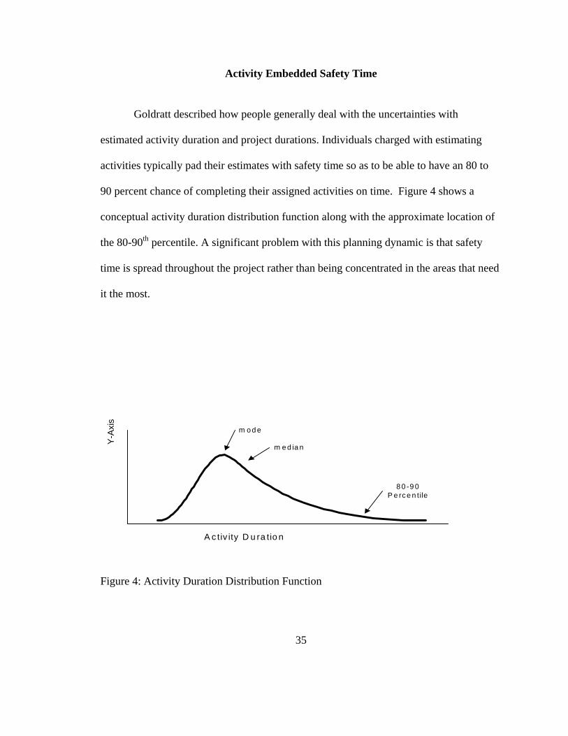
Activity Embedded Safety Time
Goldratt described how people generally deal with the uncertainties with
estimated activity duration and project durations. Individuals charged with estimating
activities typically pad their estimates with safety time so as to be able to have an 80 to
90 percent chance of completing their assigned activities on time. Figure 4 shows a
conceptual activity duration distribution function along with the approximate location of
the 80-90th percentile. A significant problem with this planning dynamic is that safety
time is spread throughout the project rather than being concentrated in the areas that need
it the most.
Y-A
xis
A c tiv ity D u ra tio n
8 0 -9 0P e rc e n tile
m e d ia n
m o d e
Figure 4: Activity Duration Distribution Function
35

Despite the presence of large amounts of safety time embedded within individual
tasks, these tasks can still finish late. Consider the following situation with a project
activity. This particular activity duration is actually 3 days assuming all goes well. The
schedule allows 15 days for the work to be done, based upon the padded estimates.
Knowing the existence of the pad, the manager waits until the last 3 days to start.
Goldratt calls this the “student syndrome” because students have a tendency to wait to the
last minute to study for an examination. If the activity experiences problems, then the
project schedule is impacted.
In making their estimates, Goldratt also noted that the practice of multitasking
causes activities to take longer. Additionally, the knowledge that multitasking exists in
the workplace is taken into consideration when making estimates. An illustration of the
impacts of multitasking is seen in Figure 5.
36
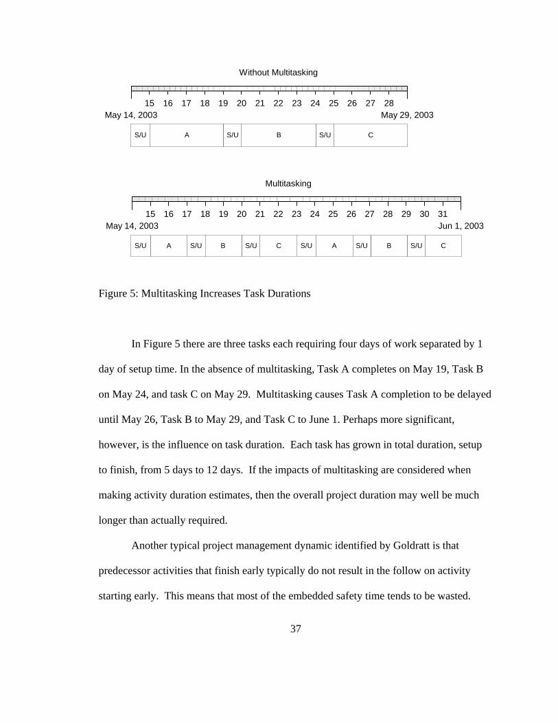
A B C
May 14, 2003 May 29, 200315 16 17 18 19 20 21 22 23 24 25 26 27 28
A B C
S/U S/U
S/U S/U S/U A B CS/U S/U
May 14, 2003 Jun 1, 200315 16 17 18 19 20 21 22 23 24 25 26 27 28 29 30 31
S/U
S/U
Without Multitasking
Multitasking
Figure 5: Multitasking Increases Task Durations
In Figure 5 there are three tasks each requiring four days of work separated by 1
day of setup time. In the absence of multitasking, Task A completes on May 19, Task B
on May 24, and task C on May 29. Multitasking causes Task A completion to be delayed
until May 26, Task B to May 29, and Task C to June 1. Perhaps more significant,
however, is the influence on task duration. Each task has grown in total duration, setup
to finish, from 5 days to 12 days. If the impacts of multitasking are considered when
making activity duration estimates, then the overall project duration may well be much
longer than actually required.
Another typical project management dynamic identified by Goldratt is that
predecessor activities that finish early typically do not result in the follow on activity
starting early. This means that most of the embedded safety time tends to be wasted.
37

Newbold (1998) provides guidance on estimating activity durations. Estimates
should be based upon dedicated workers, having required resources, and with no
multitasking. The average duration for an activity should be the baseline estimate. Thus
50 percent of the time the activity will take longer than planned. Subsequent buffers,
either feeding or project, are in place to absorb activities that take longer than average.
Project and Feeding Buffers
Goldratt’s proposed solution for improving project completion timeliness includes
removing most of the safety time from the individual activities. This can result in a
dramatic reduction to the overall project duration. To account for uncertainty so as to
ensure a reasonably chance of completing the project on time, safety time is then
strategically placed in the project in so called feeding and project buffers.
Feeding buffers consisting of safety time or management reserve are placed where
non critical activities feed into the critical chain. Perhaps the more important place for
safety time is at the end of the critical chain, which also represents the end of the project.
This safety time is called the project buffer.
Newbold (1998) discusses the issue of sizing the project buffer and identifies two
“very approximate” methods. The first method is called a rule of thumb, which is to set it
at 50 percent of the unpadded critical chain duration. This rule is said to be adequate for
most projects. The second approach, which is more scientific according to Newbold, is
38

provided by Tony Rizzo of Lucent Technologies. In this method one aggregates the risk
along the chain feeding the buffer. This is done by first estimating the 90 percentile
worst case (wi) and the average duration (ai) for each activity. The difference between wi
and ai is thus about two standard deviations, assuming a standard normal distribution.
Assuming that one desires approximately 90 percent assurance, or two standard
deviations of protection, then the buffer should be sized in accordance with Equation 3.
(Eq. 3)
Yongyi Shou and Yeo (2000) considered the question of how to estimate the
proper size for the project buffers. They interpreted Goldratt’s method as making the
buffers equal to one-half the duration of the path they are intended to protect. They
suggest instead a two step process to calculate a more appropriate buffer size. The first
step is to categorize the activities into four categories (A-D) according to the activity’s
level of uncertainty. Category A represents very low uncertainty, B low uncertainty, C for
high uncertainty, and D for very high uncertainty. The next step is to ascertain the risk
attitude or desired safety level of the decision maker. The risk attitude level is divided
into three levels—low, median, and high. These levels appear to be analogous to one,
two, and three sigma respectively. The buffers sizes proposed by Yongyi Shou and Yeo
are shown in Table 1.
39

Table 1: Buffer Sizes as Proposed by Yongyi Shou and Yeo
Uncertainty Category Low Safety (68%)
Median Safety (95%)
High Safety (99.7%)
A: Very Low 4% 8% 12%
B: Low 12% 24% 36%
C: High 20% 40% 60%
D: Very High 28% 57% 85%
Leigh, Givens, Filiatrault, and Peterson (2000) performed a broad review of
CCPM, which included a recommendation for how to size the buffers. Their
recommendation was to employ the four components of the risk management process as
described by the PMBOK guide. These components were to identify the risk driving the
contingency, incorporate that risk into the project’s risk management system, quantify
that risk, and develop a risk response plan. The stated benefits of following those
components were that unknown-unknowns would be reduced, the size of the project
buffer could thus be reduced, the risk to the project is being dealt with in an open manner,
and the stakeholders are better assured that the project buffer is appropriately sized.
CCPM on Project Completion Time Distribution Function
Despite the emphasis of critical chain on recognizing and mitigating project
uncertainty, the Critical Chain literature does not appear to recommend the use of Project
Completion Time Distribution functions.
40

Newbold (1998) identifies three data elements that should be monitored in each
section of project’s network schedule that contains a buffer. These are the current task,
the amount of buffer that is still available, and the remaining duration of the chain of
tasks feeding that buffer. Newbold suggests that projects managers have sufficient
experience and intuition to judge if the remaining buffer is large enough to cover the risk
associated with the remaining tasks. Newbold does not present any material on
quantitative risk analysis measures such as completion time distribution functions.
Leach (2000) categorized risk assessments as being either quantitative or
qualitative. Examples of quantitative risk assessment tools were failure modes and
effects analysis (FMEA), Monte Carlo analysis, project simulation, PERT, probabilistic
safety assessments (PSA), and management oversight or risk tree (MORT). Leach
discounts these quantitative tools stating, “I focus on qualitative risk assessment because
the data usually are not available to justify quantitative risk assessment; and supplying
numbers tends to yield a false sense of believability.”14 Leach does not cover the topic of
Completion Time Distribution Functions. Instead, monitoring and managing the
buffers—the project buffer and the feeding buffers—is the recommended method for
ensuring that the project completes on time.
Empirical Data for Input Analysis
In any simulation model the input that goes into it is critically important. For the
particular application described in the following chapters a primary interest is in the
41
inputs for project activity durations and project event probabilities. The literature
indicates that whenever possible such inputs should be based upon empirical evidence.
Law and Kelton (2000) state that, “it is imperative to collect data on a random variable of
interest if at all possible.” They identify three methods for using existing data to describe
process durations in simulation models. In the first method—direct use of historical
data—the data values themselves are used in the simulation. In this technique, when an
entity begins a process, the duration of that process is determined by selecting a duration
from the historical data. In the second method, the historical data is used to define an
empirical distribution. In the third and generally preferred method, a theoretical
distribution is fitted to the historical data. It is their experience that using triangular or
beta distributions to approximate an unknown distribution can cause large errors.
It is true that projects do contain new elements (activities and events that have not
been done before). In those cases, it is still important to rely on related empirical data.
Law and Kelton indicate that if the only available data is from a legacy system [one could
easily substitute the word project in place of system], then it is imperative that one make
maximum utilization of that data. Pegdon, Shannon, and Sadowski (1995) on the other
hand recommend caution on the subject of using data from a similar existing system
when modeling a non-existent system. Similarity may stem from a new system being a
variant of an older system. They note that inferences from such systems are risky and that
the ability to test validity may be limited.
In the situation where empirical data is not available, textbooks recommend that
you seek the opinions of subject matter experts for the process being modeled. Pegdon,
42

Shannon, and Sadowski note that there are dangers in relying upon subject matter experts
for estimates. They reference the research of Tversky and Kahneman (1974). These
researchers found that even people highly familiar with activities can be very poor at
estimating. Extreme cases are typically forgotten, and recent events are overemphasized.
Pegdon, Shannon, and Sadowski suggest four sources for parameter estimates in
the absence of empirical data. These are operator estimates, designer estimates, vendor
claims, and theoretical considerations. Problems with operator estimates have been
discussed above. Designer estimates are typically optimistic in that the designer typically
expects that his/her system will operate as designed and per specification. Likewise,
vendor claims are likely to be optimistic. Two examples of theoretical considerations are
how inter-arrival times tend to follow the exponential distribution and how the mean time
between electronic equipment failures typically follows a Weibull distribution.
Another factor to consider when modeling and managing a project is workforce
behavior. Gutierrez and Kouvelis (1991) state that classical PERT/CPM methods do not
take into consideration work force behavior, which may cause or contribute to project
delays. They cite Parkinson’s Law—“work expands so as to fill the time available for its
completion”—as being a factor in how long projects take.
Chapter 11 of the PMBOK covers project risk management. Six major processes
are associated with a project risk management system. These are Risk Management
Planning, Risk Identification, Qualitative Risk Analysis, Quantitative Risk Analysis, Risk
Response Planning, and Risk Monitoring and Control. Historical information is listed as
one of four inputs to identifying project risks.
43

CHAPTER THREE: METHODOLOGY
This chapter consists of two parts. In part 1, the Project Assessment by Simulation
Technique is described in detail. In part 2, the case study methodology as it pertains to
using PAST in a real world project management environment is described.
Part I: The Project Assessment by Simulation Technique (PAST)
The overarching goal of the Project Assessment by Simulation Technique
(PAST) is to provide project stakeholders with a visual display of project completion risk
and thereby enable them to respond as appropriate so as to improve project completion
performance. The visual display is in the form of a Project Completion Distribution
Function (PCDF) overlaid with the planned project completion date (Figure 6).
0%20%40%60%80%
100%
5/30
5/31 6/1
6/2
6/3
6/4
6/5
6/6
6/7
6/8
Project Completion Day
Cum
ulat
ive
Perc
enta
ge
Planned Project CompletionProject Completion Distribution Function
File: Example_PCDFs
Figure 6: Visual Display of Project Completion Risk (Example)
44
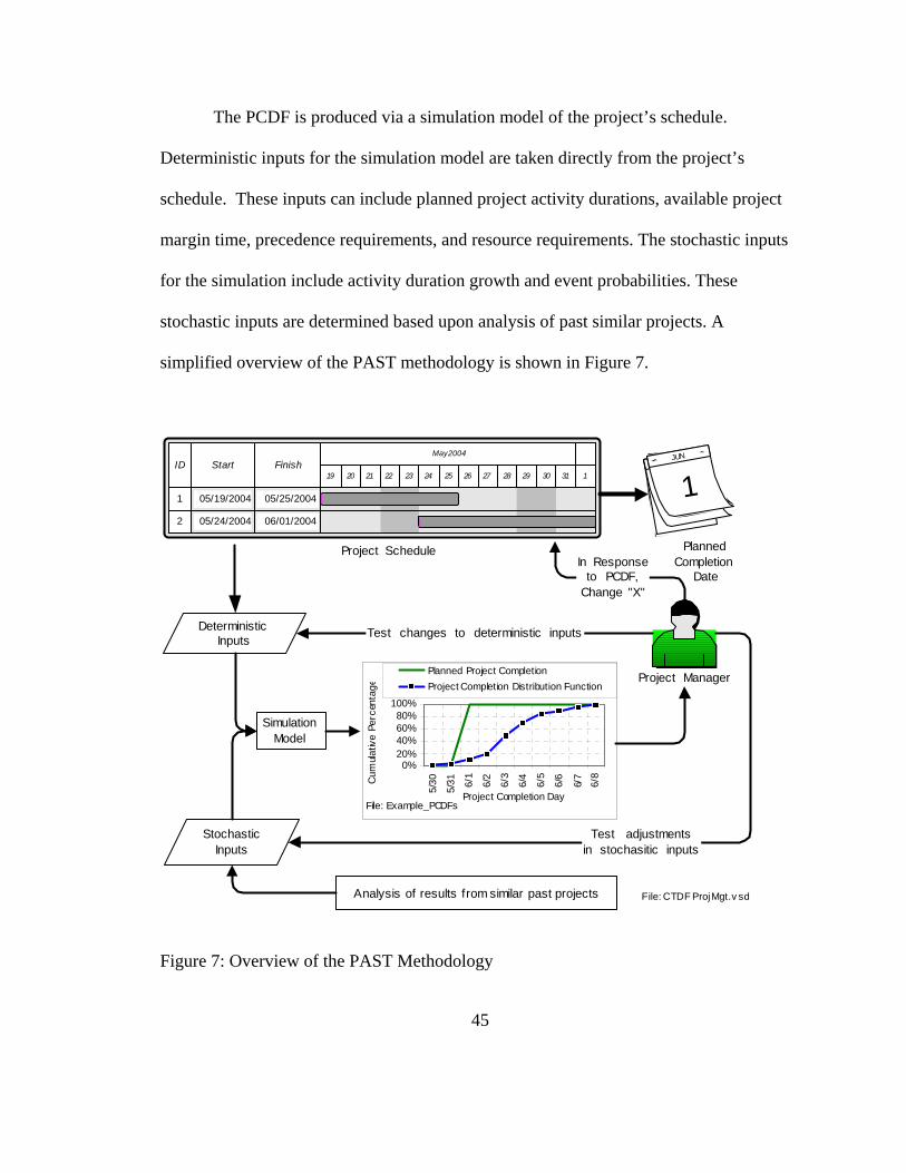
The PCDF is produced via a simulation model of the project’s schedule.
Deterministic inputs for the simulation model are taken directly from the project’s
schedule. These inputs can include planned project activity durations, available project
margin time, precedence requirements, and resource requirements. The stochastic inputs
for the simulation include activity duration growth and event probabilities. These
stochastic inputs are determined based upon analysis of past similar projects. A
simplified overview of the PAST methodology is shown in Figure 7.
SimulationModel
DeterministicInputs
Project Manager
ID Start FinishJUN
1
In Responseto PCDF,
Change "X"
PlannedCompletion
Date
Project Schedule
StochasticInputs
Test changes to deterministic inputs
Test adjustmentsin stochasitic inputs
File: CTDF Proj Mgt.v sd
0%20%40%60%80%
100%
5/30
5/31 6/
1
6/2
6/3
6/4
6/5
6/6
6/7
6/8
Project Completion Day
Cum
ulat
ive
Perc
enta
ge
Planned Project CompletionProject Completion Distribution Function
File: Example_PCDFs
May 2004
19 20 21 22 23 24 25 26 27 28 29 30 31 1
1
2
05/25/200405/19/2004
06/01/200405/24/2004
Analysis of results from similar past projects
Figure 7: Overview of the PAST Methodology
45
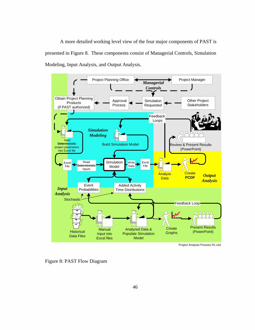
A more detailed working level view of the four major components of PAST is
presented in Figure 8. These components consist of Managerial Controls, Simulation
Modeling, Input Analysis, and Output Analysis.
st
Project ManagerProject Planning Office
ExcelFile
SimulationModel
ReadDeterministic
inputs
ExcelFile
WriteData
EventProbabilities
Added ActivityTime Distributions
Review & Present Results(PowerPoint)
CreatePCDF
InputDeterministic
project parametersinto Excel file
Build Simulation Model
ManualInput intoExcel files
AnalyzeData
Analyzed Data &Populate Simulation
Model
Present Results(PowerPoint)
CreateGraphs
Feedback Loop
HistoricalData Files
InputAnalysis
SimulationModeling
OutputAnalysis
Project Analysis Process R1.vsd
Obtain Project PlanningProducts
(if PAST authorized)
SimulationRequested
Other ProjectStakeholders
ApprovalProcess
ManagerialControls
Stochastic
Feedback Loops
Figure 8: PAST Flow Diagram
46

Each component of PAST is described in greater detail in the following sections.
Managerial Controls Component of PAST
The primary purpose of the managerial controls component is to provide a
facilitating interface between those performing the Project Assessment by Simulation
Technique and the multitude of diverse project stakeholders including, project planners,
managers, budgeters, and customers. A PAST activity can be thought of as having three
phases, (1) introduction of PAST and obtaining concurrence to perform the assessment,
(2) performing the assessment, and (3) providing the results. Managerial controls will
vary depending upon which phase you are in.
During the first phase emphasis is placed upon explaining the Project Assessment
by Simulation Technique to project stakeholders. This is necessary for gaining approval
to perform the assessment and to obtain project stakeholder assistance for the work to be
done. Success in this phase also lays the foundation for later project stakeholder
acceptance of the assessment results. The managerial controls to be abided by while
performing the simulation and when providing the results should also be discussed and
agreed to up front.
Project stakeholders will generally have a keen interest in project completion
timeliness. The stakeholders have diverse frames of reference. These include those that
are charged with ensuring that the project completes on time along with those that are
47

depending upon the project to complete on time. Consequently, an analysis of a project’s
completion risk has the potential of becoming contentious or even controversial.
In light of this potential, it is not a good strategy to show up uninvited to a project,
build a simulation model, and proceed to inform project stakeholders that their project
has little to no chance of completing on time. Doing so is likely to result in a rather harsh
rebuke of an otherwise well intended product. Hands-on learning of this lesson can be
avoided by having a strategy for working with and for project stakeholders and putting in
place agreed to managerial controls.
Introductory Briefings
The first step in the managerial controls component of PAST is to introduce the
project manager, the project planning office, or other project stakeholders to the PAST
methodology and secure sponsorship for a PAST based analysis of the targeted project.
Figure 7 and Figure 8 can be used in these introductory meetings to provide an overview
of the PAST methodology. Examples of analyses from previous similar projects should
be shown. If this is a first time analysis for the analyst, then a notional sample analysis
could be created. The introduction can be given either in a briefing to a group or in less
formal meetings with key individuals.
The hoped for outcome of these briefings or meetings is that at least some project
stakeholders will be willing to sponsor an assessment of the project using PAST.
48

Assessment Requirements
After permission has been granted to perform a PAST based project assessment,
the various requirements for the analysis should be discussed and agreed upon. First there
will be a need to have access to the existing project schedule. An understanding of major
assumptions within that schedule or likely alternative schedules of interest should be
acquired as well. If the effort will also include an analysis of past historical data, then
access to that data will need to be established. Expectations for when the first PCDF is to
be provided should be established. There should also be preliminary discussions
concerning follow-on analysis effort for the inevitable what-if questions that will occur in
response to the initial PCDF.
The specificity of the assessment requirements may vary depending upon the
situation. For example, an in-house effort would likely requires less concrete specifics
then an analysis that would be the result of a contractual arrangement. Additionally,
specificity will probably increase with experience on the part of both the analyst and the
sponsor.
Communications
It is critically important to establish clear communication norms early in the
analysis. An area of great concern will likely be the issue of who will be privy to the
resulting assessment and any potential recommendations. One strategy would be to brief
49

the sponsor in a private setting and then let the sponsor decide if further communications
with a wider audience are warranted. This strategy seems appropriate when there is a
strong sponsor or a contractual arrangement.
The situation may be more complex in the case of an in-house analysis done by a
lower tier organization or in the absence of a sponsor in a position of power. In that case
careful thought should be given to which stakeholders to share the assessment results
with so as to build support for the analysis.
Simulation Modeling Component of PAST
The simulation modeling component of PAST contains multiple subcomponents.
These include a simulation engine with modeling constructs uniquely tailored for the
PAST methodology, an input file that contains the deterministic information from the
project being modeled, and an output file for writing the simulation produced project
completion dates to. The modeling component processes and entities are shown in the
shaded area of Figure 9.
50
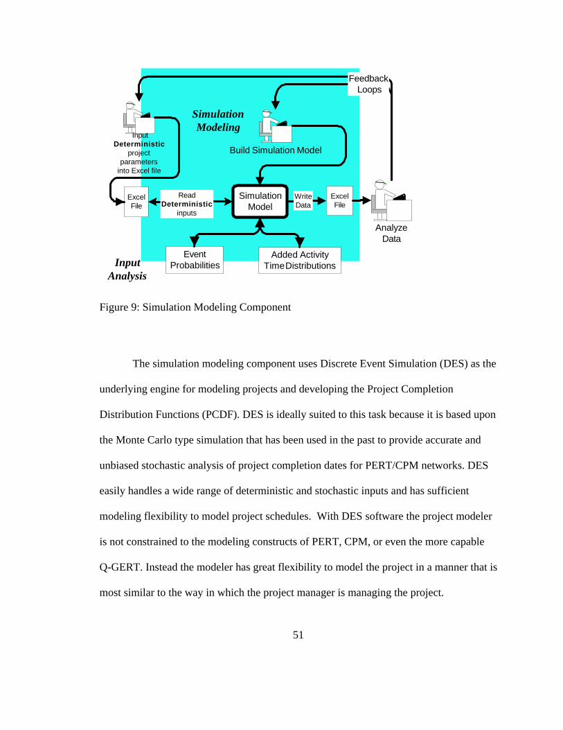
ExcelFile
SimulationModel
ReadDeterministic
inputs
ExcelFile
WriteData
EventProbabilities
Added ActivityTime Distributions
InputDeterministic
projectparameters
into Excel file
Build Simulation Model
AnalyzeData
InputAnalysis
SimulationModeling
Feedback Loops
Figure 9: Simulation Modeling Component
The simulation modeling component uses Discrete Event Simulation (DES) as the
underlying engine for modeling projects and developing the Project Completion
Distribution Functions (PCDF). DES is ideally suited to this task because it is based upon
the Monte Carlo type simulation that has been used in the past to provide accurate and
unbiased stochastic analysis of project completion dates for PERT/CPM networks. DES
easily handles a wide range of deterministic and stochastic inputs and has sufficient
modeling flexibility to model project schedules. With DES software the project modeler
is not constrained to the modeling constructs of PERT, CPM, or even the more capable
Q-GERT. Instead the modeler has great flexibility to model the project in a manner that is
most similar to the way in which the project manager is managing the project.
51

There are other practical reasons for why DES was considered as being an
attractive alternative to PERT/CPM. Commercially available DES software operates
efficiently in a desktop computer environment, and at prices ranging in the thousands of
dollars, such software is available for most companies. A wide range of projects, from
small to very large and complex, can be modeled. DES is also adept at modeling
resources such as people, material, machinery, or facilities that constrain many, if not
most or all, projects.
The simulation model is built by the analyst and is specific to the project being
analyzed. That model reads the project’s deterministic inputs from an Excel file.
Stochastic parameters, which come from the input analysis process, are entered directly
into the model. The model may also include the capability, as required, to accommodate
various assumptions of interest to the project stakeholder. The output of the simulation
model is written into an Excel file that is used for later analysis.
Note that the PAST methodology is intended to be consistent with the norms for
conducting Discrete Event Simulation modeling. While these norms include guidelines
for conducting input analysis and output analysis, these two subjects are discussed later in
their own separate sections.
PAST models are similar to the precedence diagram networks developed by
PERT/CPM, GERT, and VERT, along with the capabilities inherent to discrete event
simulation software. In support of the PAST methodology three project network
modeling constructs are presented. These are an activity construct, a probabilistic event
construct, and a cyclical construct. These constructs contain logical operators that
52
provide modeling complexity and fidelity beyond PERT/CPM. Event probability nodes
allow one to model unplanned but not unpredictable event occurrences that necessitate
additional activities in the project. Cyclical constructs allow the modeling of projects that
have at least some cyclical activities. Note that the PERT/CPM methods were developed
primarily for acyclic or once through projects. Event nodes and cyclical constructs have
been used in GERT and VERT. The most unique modeling construct of the PAST
methodology is the activity construct. The rationale for creating the constructs is to
enable the modeling of real world projects and project management environments.
Activity Construct
The level of detail in which the project is being managed is an important
considered with respect to the activity construct. For example, consider the case of a
very large project in which there are thousands of activities. No single project manager
can be effective in managing all of the activities. One method to handle such an
overwhelming situation is to group the activities so as to create lower-level projects that
when combined make up the entire project. Lower-level project managers, who report to
the overarching project manager, are assigned to manage each of the lower-level projects.
The activity construct assumes such a situation. Consequently, each “activity” construct
actually represents a lower-level project that feeds into the overall project.
The activity construct is structured such that it allows the overarching project
53

manager to specify the planned or target duration for an activity—the lower level project.
The unit of time is days. The construct accommodates the reality that such activities don’t
necessarily go according to plan. It specifically considers the possibility that predecessor
activities may be late, resources may be unavailable, and once the activity does get
started, it may take longer than planned. The construct also provides the overarching
project manager with the ability to give schedule reserve to the lower-level manager for
that manager’s use in completing the activity on schedule.
In PERT, an activity’s duration is established by an analyst estimating the most
optimistic, most likely, and most pessimistic times. For example, in a PERT network an
activity might have a duration of 8, 10, and 15 days, which represent the optimistic,
likely, and pessimistic estimates by the analyst. These three estimates are then used to
calculate an expected time for the activity.
In the PAST methodology the activity duration is initially specified
deterministically. The stochastic elements along with the precedence and resource
requirements are added later. For the deterministic component, the activity duration is
based upon a realistic assessment of what the activity should reasonably take, plus a
deterministic amount of margin time (this is a key component of the management control
mechanism). Figure 10 shows how this would look.
54

Planned ActivityDuration Reserve Activity
EndActivity
Start
Figure 10: Activity Modeling Construct with Deterministic Duration and Reserve
A potential process for specifying the activity duration is illustrated by the
following example. Suppose a task is planned to be accomplished in 10 days (analogous
to optimistic time a) and that the project manager has allotted an additional 2 days of
margin time to account for potential problems. Thus total available time is 12 days to
complete the task. The actual duration of the task will ultimately be 10 days plus
whatever additional days are required as a result of problems encountered. So long as
these additional days are 2 or fewer days, then the task will complete on schedule.
However, if greater than 2 added days are required, then the task will complete late.
In other words, in the proposed construct, activity durations are established in a
way that is fundamentally different than PERT in that they are established through a
different management dynamic. This dynamic is that an overarching manager provides
or dictates the duration for an activity. The dictated duration should, however, be based
upon an intelligent assessment of what the duration should be i.e. the duration is
reasonable and achievable assuming things go well.
An important assumption of PAST is that actual activity durations are positively
correlated to planned activity durations. This assumption should be tested during the
review of past similar project activities.
55
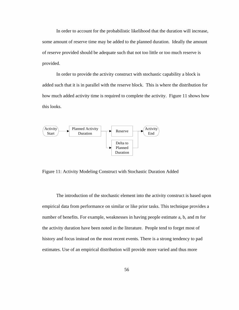
In order to account for the probabilistic likelihood that the duration will increase,
some amount of reserve time may be added to the planned duration. Ideally the amount
of reserve provided should be adequate such that not too little or too much reserve is
provided.
In order to provide the activity construct with stochastic capability a block is
added such that it is in parallel with the reserve block. This is where the distribution for
how much added activity time is required to complete the activity. Figure 11 shows how
this looks.
Planned ActivityDuration Reserve Activity
EndActivity
Start
Delta toPlannedDuration
Figure 11: Activity Modeling Construct with Stochastic Duration Added
The introduction of the stochastic element into the activity construct is based upon
empirical data from performance on similar or like prior tasks. This technique provides a
number of benefits. For example, weaknesses in having people estimate a, b, and m for
the activity duration have been noted in the literature. People tend to forget most of
history and focus instead on the most recent events. There is a strong tendency to pad
estimates. Use of an empirical distribution will provide more varied and thus more
56

accurate distribution shapes than beta distributions. Additionally, empirical distributions
may be easier for managers to understand, especially if the distributions are from
historical events that the managers are familiar with.
The manner in which the deterministic/stochastic construct shown in Figure 11
would behave is illustrated with the following example. Recall the three duration values
of the PERT example previously described i.e. 8, 10, and 15. The corresponding values in
the proposed activity construct could for example be 8 in the planned activity duration
block, 2 in the reserve block, and an empirical distribution with an average of 2 and
ranging from 0 as the minimum to 7 as the maximum. Given an added constraint such
that the activity cannot finish ahead of its planned completion date, then the activity
would end after a duration of 8 plus the longest path of either the management reserve or
the delta to planned duration.
The assumption that an activity cannot finish ahead of its planned completion date
is essentially the same as saying that the follow-on activity is constrained such that it
cannot start early. There are two reasons for invoking such a constraint. The first is that
it simplifies the modeling constructs. The second and more important reason is that in
real projects it is often the case that activities, particularly in large complex projects,
cannot be started early. For example there may be some unique resource that will not be
made available until that date. Similarly, the start date for the activity may be contingent
upon a contract start date. Likewise, consider a commercial aircraft and its planned
departure time. An early departure is typically not allowed, either because the need to
ensure that all passengers have an opportunity to make the flight, or because the flight
57

plan specifies a takeoff time so as to smooth integration into air traffic control. In the case
of a space launch, the opening of the launch window may be constrained such that it
cannot be moved up. This is typically true when the vehicle being launched is going to
rendezvous with either another spacecraft or a planetary body.
We continue now with development of the activity construct. If a subsequent
activity starts late relative to its planned start date, then the reserve within that activity
would in essence be automatically used by the project manager so as to maintain that
activity’s completion date. Figure 12 shows the Activity Modeling Construct with the
addition of the reserve reduction feature.
Planned ActivityDuration Reserve Activity
End
ActivityStart
Delta toPlannedDuration
Check Actualversus Planned
Start Date
Reduce ReserveAccordingly
Figure 12: Reserve Reduction Feature Added to Activity Construct
The next thing to add to the activity construct is the resource required for the
activity. Before the activity can begin, any required resource must be acquired and made
58

ready. In DES terminology this is called seizing a resource. Figure 13 shows the activity
construct now that the resource requirement has been added.
Planned ActivityDuration Reserve Activity
End
ActivityStart
Delta toPlannedDuration
Check Actualversus Planned
Start Date
Reduce ReserveAccordingly
SiezeRequiredResources
ReleaseRequiredResource
Figure 13: Resource Element Added to Activity Construct
The final item required to complete the activity construct is a block to indicate
completion of the predecessor activities. Figure 14 shows the complete notional activity
construct.
59

Planned ActivityDuration Reserve Activity
End
ActivityStart
Delta toPlannedDuration
Check Actualversus Planned
Start Date
Reduce ReserveAccordingly
SiezeRequiredResources Release
Resources
Completion ofPredecessorActivities
Figure 14: Completed Activity Construct
The above technique has the following benefits. The use of one value for the
deterministic duration is simpler than making three estimates. The technique allows the
overarching project manager to avoid padding of activity durations by analysts or lower-
level managers. The addition of a deterministic amount of margin time provides the
project manager with a control mechanism. Another benefit is that after a simulation
model of the project has been built, validation is simplified by the use of deterministic
values. For example, by setting the stochastic added duration to zero, and assuming
availability of resources, then the simulation should end exactly on the planned project
completion date. This builds confidence and acceptance of the model.
60
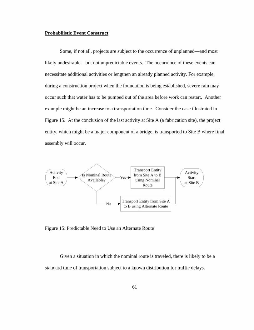
Probabilistic Event Construct
Some, if not all, projects are subject to the occurrence of unplanned—and most
likely undesirable—but not unpredictable events. The occurrence of these events can
necessitate additional activities or lengthen an already planned activity. For example,
during a construction project when the foundation is being established, severe rain may
occur such that water has to be pumped out of the area before work can restart. Another
example might be an increase to a transportation time. Consider the case illustrated in
Figure 15. At the conclusion of the last activity at Site A (a fabrication site), the project
entity, which might be a major component of a bridge, is transported to Site B where final
assembly will occur.
Is Nominal RouteAvailable?
ActivityEnd
at Site A
ActivityStart
at Site B
Transport Entityfrom Site A to Busing Nominal
Route
Yes
Transport Entity from Site Ato B using Alternate Route
No
Figure 15: Predictable Need to Use an Alternate Route
Given a situation in which the nominal route is traveled, there is likely to be a
standard time of transportation subject to a known distribution for traffic delays.
61
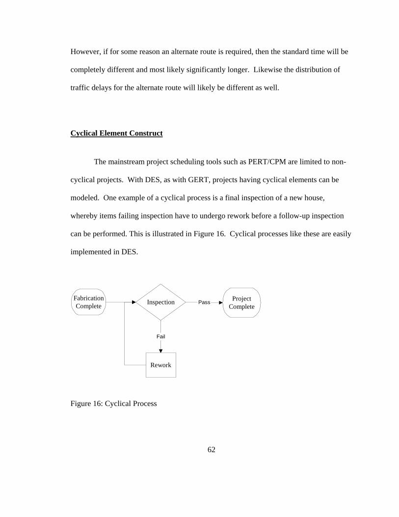
However, if for some reason an alternate route is required, then the standard time will be
completely different and most likely significantly longer. Likewise the distribution of
traffic delays for the alternate route will likely be different as well.
Cyclical Element Construct
The mainstream project scheduling tools such as PERT/CPM are limited to non-
cyclical projects. With DES, as with GERT, projects having cyclical elements can be
modeled. One example of a cyclical process is a final inspection of a new house,
whereby items failing inspection have to undergo rework before a follow-up inspection
can be performed. This is illustrated in Figure 16. Cyclical processes like these are easily
implemented in DES.
InspectionFabricationComplete
ProjectComplete
Pass
Rework
Fail
Figure 16: Cyclical Process
62
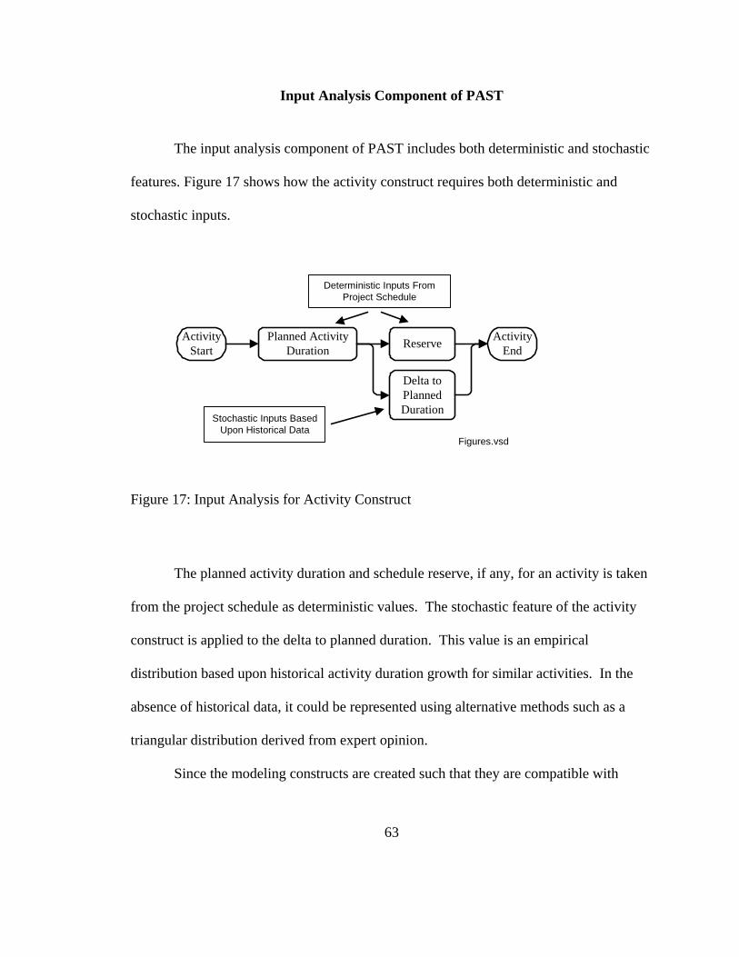
Input Analysis Component of PAST
The input analysis component of PAST includes both deterministic and stochastic
features. Figure 17 shows how the activity construct requires both deterministic and
stochastic inputs.
Planned ActivityDuration Reserve Activity
EndActivity
Start
Delta toPlannedDuration
Figures.vsd
Deterministic Inputs FromProject Schedule
Stochastic Inputs BasedUpon Historical Data
Figure 17: Input Analysis for Activity Construct
The planned activity duration and schedule reserve, if any, for an activity is taken
from the project schedule as deterministic values. The stochastic feature of the activity
construct is applied to the delta to planned duration. This value is an empirical
distribution based upon historical activity duration growth for similar activities. In the
absence of historical data, it could be represented using alternative methods such as a
triangular distribution derived from expert opinion.
Since the modeling constructs are created such that they are compatible with
63
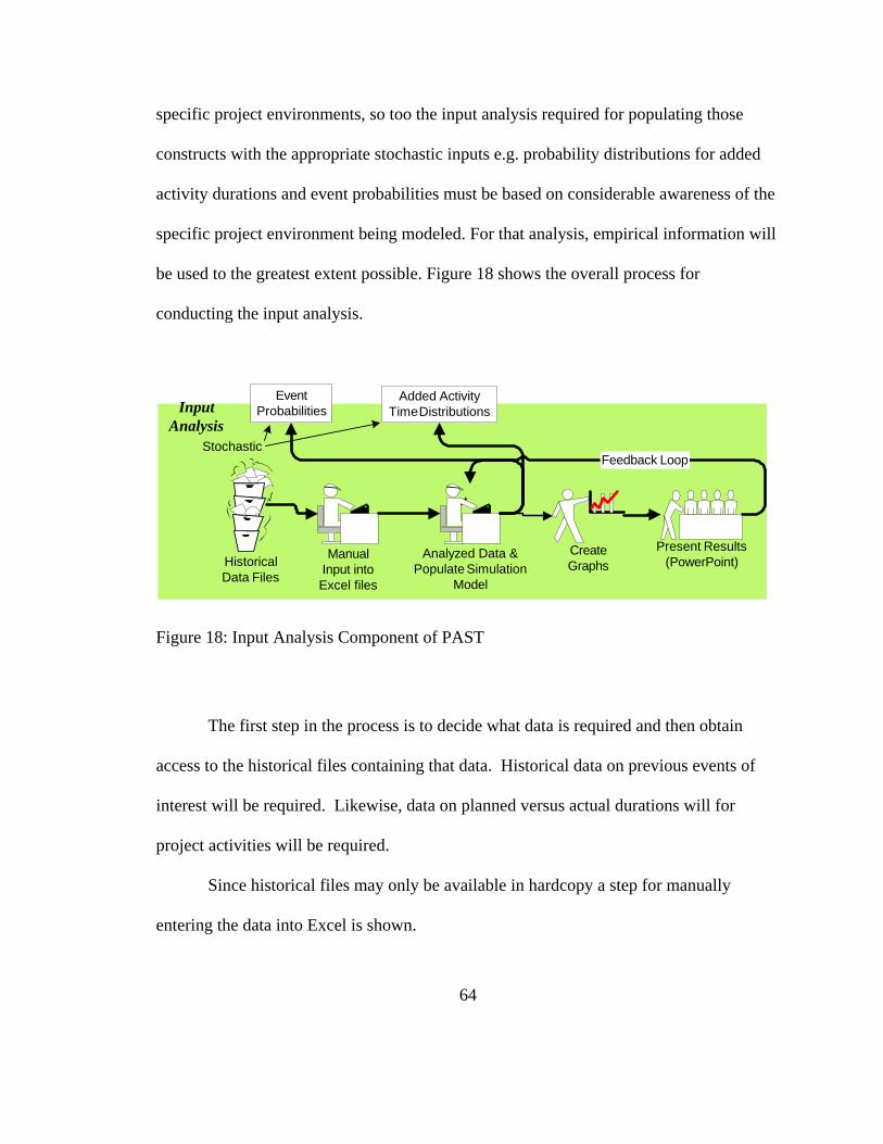
specific project environments, so too the input analysis required for populating those
constructs with the appropriate stochastic inputs e.g. probability distributions for added
activity durations and event probabilities must be based on considerable awareness of the
specific project environment being modeled. For that analysis, empirical information will
be used to the greatest extent possible. Figure 18 shows the overall process for
conducting the input analysis.
st
EventProbabilities
Added ActivityTime Distributions
ManualInput intoExcel files
Analyzed Data &Populate Simulation
Model
Present Results(PowerPoint)
CreateGraphs
Feedback Loop
HistoricalData Files
InputAnalysis
Stochastic
Figure 18: Input Analysis Component of PAST
The first step in the process is to decide what data is required and then obtain
access to the historical files containing that data. Historical data on previous events of
interest will be required. Likewise, data on planned versus actual durations will for
project activities will be required.
Since historical files may only be available in hardcopy a step for manually
entering the data into Excel is shown.
64

Once the data is entered into Excel it can be analyzed either within Excel or
copied into other software tools such as ExpertFit. The analysis process typically includes
the creation of run charts, outlier analysis, and the creation of histograms and cumulative
frequency distributions. This process results in the production of the stochastic inputs—
event probabilities and added activity duration distributions —for the project simulation
model. Event probabilities, such as the probability of a primary transportation route
being available or the likelihood of an inspection failure, can be based upon the
percentage of time that the event has occurred in the past. Modifications of this
probability can be made during the modeling phase in order to understand the sensitivity
of this factor. A relative simple comparison of the delta between planned versus actual
duration allows one to generate an empirical distribution for the Added Activity Time
Distributions. If there is enough information, a theoretical distribution may be used,
providing the appropriate goodness-of-fit tests are satisfied. For this research, empirical
distributions were used.
All inputs should be shared with the appropriate project stakeholders so as to
obtain their feedback and concurrence. This step will help to build validity into the
model.
The input analysis phase can also be used to assist the project planners and project
manager determine planned duration for project activities. Recall that in the previous
section it was stated that the duration should be reasonable and achievable assuming most
things go well. How does one go about making that determination? Perhaps the best way
is to make the determination based upon empirical information. For example in the past,
65

this same activity or similar activity has taken so much time. The selected duration might
be the minimum duration or alternatively the average duration from the historical data
base. Ultimately, however, the planned duration will be the decision of the overarching
project manager. Nonetheless, it will still be important to show how the planned duration
compares to the historical data base.
Similarly, the historical information can provide insight into the how much
activity reserve should be provided for any given project activity. Just like the selected
activity duration, the overarching project manager will make the final determination as to
what quantity of reserve will be allotted to the lower-level managers. Ideally, the reserve
should be adequate such that not too little or too much reserve is provided. Three issues
will be addressed when considering the amount of reserve to be imbedded. The first is
the distribution for how much added time will be required to complete the task over and
above what was planned for the task. The second is the potential lateness of the
predecessor tasks, and the third is the potential unavailability of resources.
An area of interest for this research is the influence of schedule reserve on the
project completion distribution function. For example, the strategy of Critical Chain
Project Management is to not imbed schedule reserve in individual activities, but instead
place it at the end of the project in a “project buffer” and also at places called “feeding
buffers” where non-critical chains feed into the critical path. The project modeling
constructs proposed by this research enable some exploration of the project buffer
strategy.
66

Output Analysis Component of PAST
The output analysis component consists of the functions necessary to analyze the
simulation supplied results, create project completion distribution functions, and present
the relevant information to project stakeholders. If the validity is questioned, feedback
loops allows the project simulation model to be modifed. Once validated, at least in the
eyes of the analyst, the results are then shared with the selected project stakeholders
consistent with the agreed to managerial controls. Feedback from this group is
anticipated and accommodated as required. Figure 19 illustrates the process.
Review & Present Results(PowerPoint)
CreatePCDF
InputDeterministic
projectparameters
into Excel file
Build Simulation Model
AnalyzeData
OutputAnalysis
Feedback Loops
Figure 19: Output Analysis Component of PAST
Determining the PCDF using a simulation model is a straight forward process.
Note first that the modeling of a project using DES is a terminating simulation in which
67
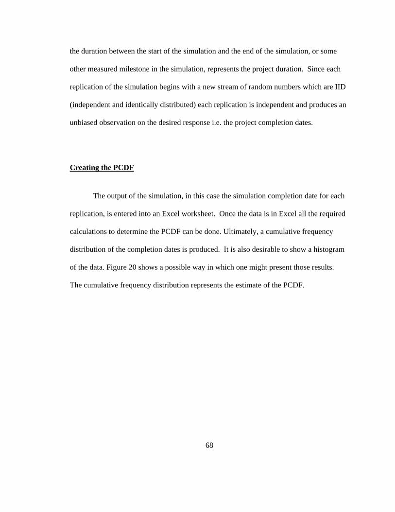
the duration between the start of the simulation and the end of the simulation, or some
other measured milestone in the simulation, represents the project duration. Since each
replication of the simulation begins with a new stream of random numbers which are IID
(independent and identically distributed) each replication is independent and produces an
unbiased observation on the desired response i.e. the project completion dates.
Creating the PCDF
The output of the simulation, in this case the simulation completion date for each
replication, is entered into an Excel worksheet. Once the data is in Excel all the required
calculations to determine the PCDF can be done. Ultimately, a cumulative frequency
distribution of the completion dates is produced. It is also desirable to show a histogram
of the data. Figure 20 shows a possible way in which one might present those results.
The cumulative frequency distribution represents the estimate of the PCDF.
68

Histogram 1000 Reps
020406080
100120140160180200
1 2 3 4 5 6 7 8 9 10 11 12 13 14 15 16 17 18 19 20 21 22 23Days
Freq
uenc
y
0%10%20%30%40%50%60%70%80%90%100%
FrequencyCumulat ive %
Figure 20: Presentation of a Project Completion Time Density Function
Determining the PCDF Confidence Band
The next step is to calculate a confidence band about this estimate. Unfortunately,
this is somewhat problematic. The problem stems from the PCDF being a distribution or
density function as opposed to a single number. The typical response of a discrete event
simulation is a single number e.g. an average activity duration. Consider the data in
Figure 20. The mean completion day is 9.825. Or in other words, 50 percent of the time
the project completes within 9.825 days and 50 percent of the time it takes longer.
However, because this mean is calculated from 1000 simulation replications, which
essentially represent samples from a population, what we should really provide is a
confidence interval for when the project will complete 50 percent of the time.
69

Equation 4 shows the Law and Kelton (2000) recommended equation for
calculating the confidence interval for a mean from the data supplied by a simulation.
Applying this equation to the data that went into Figure 20 yields a 95 percent confidence
interval that spans from 9.634 to 10.016.
nnStX an
n)(2
21,1
)(−−
±= (Equation 4)
where:
)(nX = the mean of the sample of size n
21,1 an
t−−
= the Student t value for n-1, 1-α/2
α = the desired level of confidence
S2 = the sample variance
Determining the confidence band along the entire PCDF, as opposed to a mean
completion date, requires additional work. For that we must perform Equation 4 for each
day that the project might complete. This method is explained using the data from Figure
20. The data from the 1000 replications is divided into 10 sets of 100 replications.
Consequently the value of n is now 10 instead of 1,000. Note that what the number of
replications and sets should be will depend upon the specific project and desired level of
accuracy. Once the data has been divided into the desired number of sets, a cumulative
frequency distribution is calculated for each of the sets. For each day that the project
70

might complete by, i.e. from 1 to 23 days, a mean and 95 percent confidence band is
created. Table 2 shows how this is set up using Excel. Figure 21 shows a graphical
representation of the confidence band.
Table 2: Confidence Band Calculation
n-1 = 10n-1 = 9
alpha = 0.05Confidence Interval Completion Day Probabilities of each Sample
Day Upper Average LowerHalf
Width t valueSQRT of
Var/NSample Var /
NSample Variance
1st 100
2nd 100
3rd 100
4th 100
5th 100
6th 100
7th 100
8th 100
9th 100
10th 100
1 0.003 0.001 0.000 0.002 2.262 0.001 0.0000 0.0000 0.00 0.00 0.00 0.00 0.01 0.00 0.00 0.00 0.00 0.002 0.006 0.003 0.000 0.003 2.262 0.002 0.0000 0.0000 0.01 0.00 0.00 0.01 0.01 0.00 0.00 0.00 0.00 0.003 0.019 0.014 0.009 0.005 2.262 0.002 0.0000 0.0000 0.02 0.01 0.01 0.01 0.02 0.02 0.00 0.01 0.02 0.024 0.040 0.031 0.022 0.009 2.262 0.004 0.0000 0.0002 0.03 0.04 0.03 0.04 0.03 0.04 0.00 0.04 0.04 0.025 0.088 0.074 0.060 0.014 2.262 0.006 0.0000 0.0004 0.07 0.10 0.07 0.10 0.10 0.05 0.06 0.08 0.06 0.056 0.142 0.130 0.118 0.012 2.262 0.005 0.0000 0.0003 0.14 0.14 0.12 0.15 0.14 0.13 0.09 0.13 0.12 0.147 0.259 0.236 0.213 0.023 2.262 0.010 0.0001 0.0010 0.29 0.26 0.22 0.27 0.25 0.22 0.18 0.22 0.22 0.238 0.368 0.350 0.332 0.018 2.262 0.008 0.0001 0.0006 0.38 0.35 0.34 0.39 0.35 0.35 0.33 0.36 0.30 0.359 0.519 0.485 0.451 0.034 2.262 0.015 0.0002 0.0023 0.58 0.46 0.48 0.54 0.48 0.44 0.47 0.50 0.49 0.41
10 0.635 0.595 0.555 0.040 2.262 0.018 0.0003 0.0032 0.66 0.59 0.56 0.67 0.60 0.57 0.60 0.63 0.60 0.4711 0.733 0.712 0.691 0.021 2.262 0.009 0.0001 0.0009 0.78 0.70 0.70 0.73 0.70 0.71 0.67 0.71 0.73 0.6912 0.814 0.795 0.776 0.019 2.262 0.008 0.0001 0.0007 0.83 0.78 0.75 0.77 0.81 0.77 0.79 0.82 0.81 0.8213 0.909 0.888 0.867 0.021 2.262 0.009 0.0001 0.0009 0.93 0.87 0.83 0.93 0.89 0.88 0.88 0.87 0.90 0.9014 0.954 0.938 0.922 0.016 2.262 0.007 0.0001 0.0005 0.97 0.93 0.90 0.94 0.95 0.94 0.91 0.94 0.97 0.9315 0.977 0.962 0.947 0.015 2.262 0.007 0.0000 0.0005 0.98 0.93 0.94 0.99 0.98 0.96 0.93 0.97 0.97 0.9716 0.994 0.984 0.974 0.010 2.262 0.005 0.0000 0.0002 0.98 0.97 0.96 1.00 1.00 0.98 0.97 0.99 0.99 1.0017 0.999 0.991 0.983 0.008 2.262 0.003 0.0000 0.0001 0.99 0.98 0.97 1.00 1.00 0.99 0.98 1.00 1.00 1.0018 0.999 0.993 0.987 0.006 2.262 0.003 0.0000 0.0001 0.99 0.98 0.98 1.00 1.00 0.99 0.99 1.00 1.00 1.0019 1.000 0.996 0.992 0.004 2.262 0.002 0.0000 0.0000 0.99 0.99 0.99 1.00 1.00 0.99 1.00 1.00 1.00 1.0020 1.000 0.999 0.997 0.002 2.262 0.001 0.0000 0.0000 1.00 1.00 0.99 1.00 1.00 1.00 1.00 1.00 1.00 1.0021 1.000 0.999 0.997 0.002 2.262 0.001 0.0000 0.0000 1.00 1.00 0.99 1.00 1.00 1.00 1.00 1.00 1.00 1.0022 1.000 0.999 0.997 0.002 2.262 0.001 0.0000 0.0000 1.00 1.00 0.99 1.00 1.00 1.00 1.00 1.00 1.00 1.0023 1.000 1.000 1.000 0.000 2.262 0.000 0.0000 0.0000 1.00 1.00 1.00 1.00 1.00 1.00 1.00 1.00 1.00 1.00
71
Confidence Interval for CTDF
0.00.10.20.30.40.50.60.70.80.91.0
1 2 3 4 5 6 7 8 9 10 11 12 13 14 15 16 17 18 19 20 21 22 23
Days
Probability
UpperAverageLower
Figure 21: Graphical Presentation of Confidence Band
A fundamental assumption in the above discussion of the confidence band for the
PCDF is that the various activity duration estimates and event probabilities within the
project are valid. For projects in which there is a sufficient amount of empirical data this
will generally be the case. However, when modeling a project for which there is not
sufficient empirical data, this assumption will not be valid. For those cases it would be
important to perform sensitivity analysis on the various estimates of activity durations
and event probabilities.
Automation of these steps is desirable because project stakeholders have a
tendency to request repeated simulations using alternative assumptions or inputs.
Automation helps to reduce the analysis time such that analysis products are provided in
a timely basis.
72

Verification and Validation for PAST
Following the creation and population of a typical DES model, the next step is to
verify and validate the model. Verification deals with building the model right, whereas
validation deals with building the right model.15 Verification is the process of
determining whether a simulation computer program works as intended i.e. according to
the modeling assumptions that were made. This may also be referred to as debugging the
computer program. Validation is the process of determining whether the conceptual
model is an accurate representation of the actual system being analyzed. This means
“ensuring that the model behaves the same as the real world system.”16
Verification
The Project Assessment by Simulation Technique contains two features that
facilitate verification. First of all, the activity constructs are repetitive modules and this
improves the ability to write and debug the simulation model of the project incrementally.
Secondly, the simulation model is structured such that it allows one to run it in a
deterministic mode to ensure that it will produce the planned project completion date.
While the ultimate goal is to obtain an output of the project completion date, intermediate
project milestones can be compared to expected values to identify where problems in the
program occur.
Experts in simulation recommend that simulation builders start with a minimally
73
detailed model of the project and build upon that as needed. This practice is followed in
PAST. Additionally, the stochastic features can be incrementally added-in, and later
switched on or off, to see if the influence upon project completion is as expected. Some
animation is also recommended so that the analyst can use that animation to verify that
entities traverse the network as expected and identify where entities get “hung-up.”
Validation
The primary focus of the validation process is to ascertain if the output of the
model—the project completion distribution function—is reasonable in the view of both
the analyst and the client. Three primary techniques are used for validation. They are: (1)
developing a model with high face validity; (2) testing the assumptions of the model
empirically; and (3) testing model output for reasonableness to the actual project being
modeled. Each of these three techniques is described in greater detail below.
Face validity for simulation models of projects should inherently be high because
we are modeling an existing project plan or PERT/CPM network. Consequently, so long
as the model is a reasonable representation of the existing plan, then project stakeholders
should be inclined to accept the model. The project manager, the project planning office,
or some similar stakeholder provides the project plan that will be modeled. The client
(project manage or representative) and other stakeholders are briefed on the methodology
to be used to develop the model of the project plan. This briefing includes a description
74

of the modeling constructs—activity, event, and cyclical—as well as the manner in which
historical data is used to determine probability distributions and event probabilities. Past
uses of the methodology in similar situations are presented. All modeling assumptions
are discussed with the project stakeholders and agreed upon. The desired output
performance measures are also determined jointly with the project stakeholders. This
early involvement of the project stakeholders helps to ensure that the final model and its
output have high face validity. Another tactic for ensuring high face validity will be to
see if past projects completed within the PCDFs that would have been predicted had the
PAST methodology been used for those projects.
Testing the assumptions of the model empirically is enabled by the fundamental
structure of the PAST methodology. For example, in PAST a heavy reliance is placed on
using empirical project data to develop empirical distributions for added days in the
activity constructs. In classic system simulation modeling, one might fit a theoretical
distribution to historical data and then perform goodness of fit tests. In this methodology
we are primarily using empirical distributions due to the following important benefits.
Face validity is enhanced because project stakeholders are likely to recognize and
therefore relate to data from past projects. It is also easier to explain to clients how the
simulation model makes use of an empirical distribution versus a theoretical distribution.
Reliance upon empirical distributions can create problems. For example, there
may be a lack of data. This problem can be address by soliciting opinions from project
stakeholders or individuals deemed by the project stakeholders to be experts. Another
problem is that future performance may lie outside the bounds of the historical data. This
75
problem can be mitigated by running sensitivity analysis e.g. use of theoretical
distributions.
The third validation technique is to determine how representative the simulation
output is to the actual project being modeled. This technique will start with running the
model with all the added activity duration distributions and event probabilities set to zero,
and with activities being unconstrained by resources. In that way, if the model accurately
reflects the project, then the model will show a completion date exactly on the planned
completion date. This step may also be performed as part of the model verification steps.
After a successful verification/validation run in the deterministic mode, the model is
populated with the added activity duration distributions, event probabilities, and resource
constraints. This model is used to produce the PCDF, which is then analyzed for
reasonableness. That determination is dependent upon both the analyst and the client
accepting the PCDF as reasonable.
Measuring Progress
The project completion distribution function can be updated as the project
progresses over time. For example, once a task has been completed, the simulation
model of the project can be run from that point forward to the end of the project. An
alternative method would be to run the simulation from the project start date, with all
completed tasks modeled as constants. Either way, the new distribution function is
76

created and compared to the previous distribution function. In that way, it is possible to
see if the project is improving, staying the same, or getting worse with respect to the
likely completion date.
Likewise, as project managers make changes to the project, the model can be
updated and a new distribution function created. A comparison can then be made to the
old distribution function to see if the changes helped or hurt the distribution function.
Part II: Research Methodology (Case Study)
The next step was to apply the Project Assessment by Simulation Technique
described above and see if it is in fact beneficial. To test PAST, one could envision an
experimental method in which the dependent variable is project completion timeliness.
The independent variable that would be varied would be the management methodology
used e.g. with or without PAST. The hypothesis in this hypothetical experiment being
that project completion timeliness will be better for projects managed with PAST than
without. Unfortunately, setting up such an experiment is difficult and likely to be rather
expensive. Therefore, an alternative case study methodology for conducting a
preliminary validation of the benefits of PAST was employed. Assuming PAST gains at
least preliminary acceptance as a result of those case studies, then the resources and
necessary support for the more desired experiment might be obtainable.
For the alternative method, multiple case studies were performed in which the
measure of interest was the response of the project stakeholders to the Project
77
Assessment by Simulation Technique. The case study methodology and how it was
employed for this research are described below.
Case Study Definitions
The Project Assessment by Simulation Technique was tested in a real world
project management environment using Yin’s (2003) case study research design and
methods as a general guide. Yin provides a two-part technical definition of a case study.
The first is that, “a case study is an empirical inquiry that investigates a contemporary
phenomenon within its real-life context, especially when the boundaries between
phenomenon and context are not clearly evident.” For the case studies described in
Chapter 4, the phenomenon was project completion timeliness and the real-life context
was the organization implementing and managing the project.
The second part of Yin’s definition is that, “the case study inquiry copes with the
technically distinctive situation in which there will be many more variables of interest
than data points, and as one result relies on multiple sources of evidence, with data
needing to converge in a triangulating fashion, and as another result benefits from the
prior development of theoretical propositions to guide data collection and analysis.” As
such, the case study is a comprehensive research strategy that includes study design logic,
techniques for data collection, and specifies approaches to data analysis.
78

Components of Research Design
There are five components to case study research designs. These are: (1) a
study’s questions; (2) its propositions, if any; (3) its unit(s) of analysis; (4) the logic
linking the data to the propositions; and (5) the criteria for interpreting the findings.
These components and how they were addressed by the case studies presented in Chapter
4 are discussed below.
Study Question
The case study question of interest was, “How will project stakeholders respond
to the Project Assessment by Simulation Technique?” According to Yin, the case study
strategy is most likely to be appropriate for addressing “how” questions. Such questions
are also explored through experiments. Perhaps more importantly, the case study is
advantageous when such a question “is being asked about a contemporary set of events,
over which the investigator has little or no control.” The only influence that the author
had in the studies reported in the next chapter was to provide to project stakeholders
either descriptive information on the Project Assessment by Simulation Technique and/or
Project Completion Distributions derived from PAST.
79
Proposition
In a case study the study proposition is analogous to an experiment’s hypothesis.
The case studies were centered upon using the Project Assessment by Simulation
Technique to develop models of various aspects of a large and complex project. The
PAST methodology, the models it produces, and the analysis from the models, i.e. the
project completion distribution function (PCDF), were presented to various project
stakeholders. The proposition was, “Project stakeholders will react positively to the
Project Assessment by Simulation Technique and may, in certain situations, take action
to improve project completion performance.” Of course, it was hoped that project
stakeholders would be receptive of the PAST methodology and make use of the
information it provides, i.e. the PCDF, to improve project completion performance. For
example, consider the scenario depicted by Figure 22.
80

Project Completion Day 18 19 20 21 22 23 24 25 26 27 28 29 30Percentage 2% 5% 28% 19% 14% 9% 7% 5% 4% 3% 2% 1% 1%
CTDF (Cumulative Percentage) 2% 7% 35% 54% 68% 77% 84% 89% 93% 96% 98% 99% 100%CTDF Plan (Theoretical Best) 0% 0% 100% 100% 100% 100% 100% 100% 100% 100% 100% 100% 100%
Completion Time Distribution FunctionExample project that is planned to be completed in 20 days.
0%10%20%30%40%50%60%70%80%90%
100%
Cumulative Percentage
CTDF (Cumulative Percentage)CTDF Plan (Theoretical Best)
Figure 22: Notional Project Planned Completion Date versus PCDF
Given a PCDF that shows a considerable likelihood of the project being late,
would the project stakeholders be motivated to take actions that would likely pull the
PCDF in the direction of the arrow—closer to the planned completion date? If
stakeholders suggest or take action then the proposition can be answered in the
affirmative.
Units of Measurement
The units of measurement for the studies were the project stakeholders. These
were typically individuals representing either themselves or the respective project
interests of their organization. On occasion, small groups were the unit of measurement.
81

Note that the actions of specific individuals are not published per se. Instead the
collective actions of individuals, organizations, and/or small ad hoc teams observed
during each case study are reported in a manner which, while providing accurate
information relevant to the case study, avoids identifying specific individuals or work
groups. Actions of government officials that have already become public knowledge are
presented, but only to place the case studies in their historical context.
Logic for Linking Data to Proposition
The logic for linking the data to the proposition was founded on the data gathered
during the case studies. That data was the reactions of the project stakeholders to the
Project Assessment by Simulation Technique. The data was captured via direct
observation. For some cases a PCDF of a project was simply presented directly to
stakeholders. In these cases the PCDF typically indicated that the project was likely to
finish much later than planned. The response of the stakeholders to this information was
recorded. Additionally, two small ad hoc work groups specifically chartered to analyze a
project were introduced to the Project Assessment by Simulation Technique. At the
conclusion of the briefing on PAST, they chose to utilize PAST to support their effort.
Their subsequent utilization of PAST was observed by direct observation as well.
82
Criteria for Interpreting the Findings
The criteria for interpreting the findings varied based upon the particulars of the
case studies. In some cases the PCDF indicated that the project was likely to complete
much later than planned. Examples of positive responses for those types of studies would
include project stakeholders requesting alternative assessments under varying
assumptions or making actual changes to the project plan, scope, or budget. A negative
response would be recorded if the stakeholder did nothing despite the fact that action
seemed warranted. For the situation in which PAST was described to the two ad hoc
groups and offered as a potential tool, a positive response could be recorded based upon
those groups choosing to use PAST.
The potential value of PAST for improving project management will be
established if the majority of the case studies have positive responses. The management
of the particular projects in the cases under study may in fact benefit from the PAST
methodology. However, a generalization that PAST provides universal improvement of
project management is beyond the scope of this research. Given the success of the case
studies presented in the next chapter, it is nonetheless hoped that stakeholders in other
projects will benefit from PAST.
Ensuring Case Study Design Quality
There are four established tests—construct validity, internal validity, external
83
validity, and reliability—for determining the quality of empirical social research and they
are directly applicable to the conduct of case studies. Kidder& Judd (1986) define these
tests as follows:
1. Construct validity: Establishing correct operational measures for the
concepts being studied.
2. Internal validity: establishing a causal relationship, whereby certain
conditions are shown to lead to other conditions, as distinguished from
spurious relationships.
3. External validity: establishing the domain to which a study’s findings can
be generalized.
4. Reliability: demonstrating that the operations of a study—such as the data
collection procedures—can be repeated, with the same results.
How these tests were dealt with during the course of the case studies is described
below.
Construct Validity
Yin recommends that case study investigators cover two steps to assist in ensuring
that the case study meets construct validity test. The first of these is to “select the specific
types of changes that are to be studied (and relate them to the original objectives of the
study).” In the case studies shown in Chapter 4 the specific change under study was the
84
response of the project stakeholders after exposure to the Project Assessment by
Simulation Technique.
The second step is to “demonstrate that the selected measures of these changes do
indeed reflect the specific types of changes that have been selected.” The selected
measures of these changes are the direct observation of the project stakeholders.
Three tactics are described by Yin to increase construct validity.17 The first of
these is to “use multiple sources of evidence.” Six sources of evidence are typically
associated with case studies. These are documentation, archival records, interviews,
direct observations, participant-observation, and physical artifacts. The case studies
shown in Chapter 4 utilized participant-observation as the main source. As a participant-
observer, I participated in the projects under study due to my position as a NASA
employee. This position afforded considerable access to project stakeholders. As such I
was able to introduce the PAST methodology to various project stakeholders and observe
their responses. Additionally, I could respond to questions and comments. The potential
downside to reliance on this methodology is that of bias. I assumed an advocate role on
behalf of the PAST methodology and therefore my observations may contain bias. To
mitigate that potential I endeavored to maintain a factual based report of the observations.
In addition to participant-observer evidence, the case studies in Chapter 4 also contain
documentation sources. These include project plans/schedules and records of
communications. These sources help to ensure that the case studies are accurately
described and also helped to minimize participant-observer bias.
The second tactic is to “establish a chain of evidence.” The last link in the chain is
85

the report of the case study itself. While the case studies are directly reported in Chapter
4, the entirety of this document represents that final link. It is the intent of this research
that a reader of this document can follow the chain of evidence from the initial research
question, through the multiple case studies presented in Chapter 4, and finally to the
conclusions presented in Chapter 5.
The chain of evidence was also bolstered by the modern information technology
of the Internet, powerful desktop computers, and applications software. For example,
much of the communications during the course of the case studies occurred via email.
Consequently, that set of case study evidence was well documented and easily sorted
either by subject or chronologically. The creation of the Project Completion Distribution
Functions for each of the case studies was done via simulation models and Excel files
that are maintained in an orderly fashion and can be reviewed by subject or
chronologically. The PCDFs were typically presented to project stakeholders in a
PowerPoint presentation and these files were also well archived.
The third tactic is to “have key informants review the draft case study report.”
The key informants are the project stakeholders that participated in the case study. The
intent of the review is to ensure that there is agreement with the facts presented in the
report of the studies.
86

Internal Validity
Yin discusses two threats to internal validity. An example of one of these is that
an investigator may incorrectly conclude that event A led to event B, when in fact some
other unidentified event caused event B. In that example, the research design failed to
account for a threat to internal validity. The second threat to internal validity discussed by
Yin focuses on the inferences that an investigator may make when direct observations are
not possible. In those cases the investigator may be relying upon historical documentation
and interviews collected during the case study. Since the case studies in Chapter 4 relied
primarily upon direct observation, both of these threats are mitigated.
External Validity
The question of external validity is whether or not the findings of the case study
can be generalized to a larger spectrum. Single case studies are deemed to provide
insufficient evidence for making generalized findings. This concern has been addressed
in part by conducting multiple case studies over an extended period of time. It is
acknowledged, however, that these multiple case studies were related in that the same
large organization and large scale project was the subject of all the case studies.
Consequently, any generalizations that are made are not for all projects in all
environments but are instead appropriately limited to the type of project and project
environment observed in the case studies.
87

Reliability
The test for reliability focused upon the issue of repeatability e.g. ensuring that
subsequent researchers would be able to obtain the same results given the same scenario.
Consequently, documenting procedures used during the cases study along with
minimizing errors and biases during the study were all important for achieving reliability.
The Specific Case Study Design
The research presented in Chapter 4 followed a two-phase approach. First there
was a single pilot case study in which a prototype version of PAST was developed and
used in response to specific project stakeholders. The lessons learned from this pilot
study were then incorporated into a more formalized version of PAST. In the second
phase, multiple case studies were conducted in a variety of contextual settings. A
chronological overview of the research is depicted in Figure 23.
88

InitialProblem
IdentificationNov. 02
Develop PASTconcept &prototype Dec. 02
Conduct PilotCase Study
(Node-2)Dec. 02-Jan. 03
FormalizePAST
May-Oct. 03
Launch WindowAnalysis
October 2003
Develop Completion QuantityDistribution Function (CQDF)
Apr. - May 2004
Modeling AutomationNovember 2003
Work ForceAugmentationMarch 2004
Project BufferBenefit
May 2004
ThreeCase
Studies
File: Project Analysis Process R1.vsd
ManifestOption04A-29
EvolvePAST
Output Analysis AutomationApril-May 2004
Managerial ComponentMar-Apr 2004
ReduceProjectContent
April 2004
Figure 23: Research Methodology Chronological Overview
These studies were opportunity based in that they were in response to project
stakeholder requests. While the research occurred over a period of time of greater than
one year, the individual case studies were short lived in nature. Consequently, there was
opportunity for PAST to evolve in response to findings from the earlier studies.
89
CHAPTER FOUR: FINDINGS
The Project Assessment by Simulation Technique was used in support of the on-
going project to assemble the International Space Station. This is a large complex
project. The critical path to assembling the International Space Station is dominated by
the ability of the Space Shuttle to deliver the components of the International Space
Station to orbit. Consequently, this aspect of the International Space Station project was
modeled and became the central focus of the case studies.
This chapter is divided into three major sections. The pilot case study is
presented in the first section. In the second section three additional case studies are
presented. The third section describes refinements to PAST that were made along the
way.
Section I: The Pilot Case Study
The pilot case study focused on building the International Space Station through
an interim milestone known as United States Core Complete. This study originated in
December of 2002 during a time period when there was great interest in completing the
United States Core portion of the Space Station by February 19, 2004.
90

Background
Since 1984, NASA had been engaged in a massive project to create the largest
and most complex orbiting Space Station ever built. This project included international
partners from Russia, Europe, and Japan. The project fell significantly behind schedule
and went significantly over budget. In 2001 the project was “on probation” and NASA
was pressured to prove that future schedules and budgets could be met. Consequently, a
goal was established to complete the United States core portion of the Space Station by
February 19, 2004. “If this goal was not met, NASA would risk losing support from the
White House and Congress for subsequent Space Station Growth.”18
By late 2002, the plan to achieve the February 19, 2004 goal was in jeopardy. In
December, NASA initiated an assessment to determine how much margin, a.k.a. safety
time or slack, was in the processing schedules for each of the seven Space Shuttle
missions required to complete the interim milestone of U.S. Core Complete.
To get from December of 2002 to “U.S. Core Complete” by February 19, 2004
would require seven successful Space Shuttle missions. The missions were designated
STS-114, 115, 116, 117, 118, 119, and 120. Each mission was unique and the seven
missions needed to occur in that precise order. U.S. Core Complete was synonymous
with delivery of the Node-2 component to the International Space Station. STS-120 was
slated to fly the Node-2 mission. In regard to the order of the missions, the project was
similar to the construction of a multiple story building, with the second story needing the
first story to be structurally complete and so on.
91

Three critical resources were required to accomplish the seven missions. These
were the three Space Shuttle orbiters—Columbia, Atlantis, and Endeavour—that would
perform the assembly missions. The order of the Space Station assembly missions, with
respect to the Space Shuttle orbiter that would fly the respective missions, was Atlantis,
Endeavor, Atlantis, Endeavour, Columbia, Atlantis, and finally Endeavour. Figure 24
shows this sequencing of the missions on each orbiter graphically.
STS-115 STS-117 STS-120
STS-114 STS-116 STS-119
STS-118Columbia
Atlantis
Endeavour
Figure 24: Space Shuttle Orbiter Space Station Assembly Sequence
Figure 25 shows excerpts from an actual planning document used by NASA
during this time period.
92
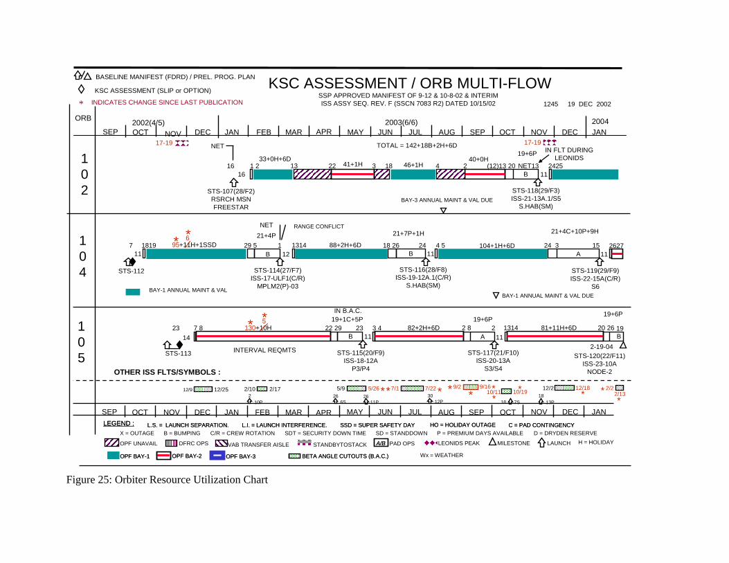
*
BASELINE MANIFEST (FDRD) / PREL. PROG. PLAN
KSC ASSESSMENT (SLIP or OPTION)
INDICATES CHANGE SINCE LAST PUBLICATION
KSC ASSESSMENT / ORB MULTI-FLOW
DEC
1245 19 DEC 2002
X = OUTAGE
OPF BAY-1 OPF BAY-2 OPF BAY-3OPF BAY-1 OPF BAY-2 OPF BAY-3
DFRC OPSOPF UNAVAIL A/BA/B PAD OPS
B = BUMPING
Wx = WEATHER
MILESTONE LAUNCH
OCT NOV DEC JANSEP
SSP APPROVED MANIFEST OF 9-12 & 10-8-02 & INTERIMISS ASSY SEQ. REV. F (SSCN 7083 R2) DATED 10/15/02
FEB APR MAYMAR
SEP OCT NOV
SD = STANDDOWN
VAB TRANSFER AISLE
JUN
JAN
JUL
FEB MAR APR
AUG SEP OCT
MAY
NOV DEC JAN
JUN JUL
BETA ANGLE CUTOUTS (B.A.C.)BETA ANGLE CUTOUTS (B.A.C.)
AUG SEP OCT NOV DEC JAN
LEGEND : L.I. = LAUNCH INTERFERENCE.L.S. = LAUNCH SEPARATION. C = PAD CONTINGENCYHO = HOLIDAY OUTAGESSD = SUPER SAFETY DAYLEGEND : L.I. = LAUNCH INTERFERENCE.L.S. = LAUNCH SEPARATION. C = PAD CONTINGENCYHO = HOLIDAY OUTAGESSD = SUPER SAFETY DAY
2002(4/5)
OTHER ISS FLTS/SYMBOLS :
P = PREMIUM DAYS AVAILABLE D = DRYDEN RESERVEH = HOLIDAYLEONIDS PEAK
C/R = CREW ROTATION
2003(6/6)
SDT = SECURITY DOWN TIME
10P 12P
5/2612/9 12/25 2/10 2/17 5/9
17-19
6S30
BAY-1 ANNUAL MAINT & VAL DUE
7/1 7/22
STANDBYTOSTACK
TOTAL = 142+18B+2H+6D 17-19
10/11 10/19 12/2
13P
12/18
7S18
18
NET IN FLT DURINGLEONIDS
STS-120(22/F11)ISS-23-10A
NODE-2
11P262 26
STS-107(28/F2)RSRCH MSNFREESTAR
16131 216
STS-118(29/F3)ISS-21-13A.1/S5
S.HAB(SM)
4 (12)13 2046+1HB
19+6P
NET13 242511
33+0H+6D3
40+0H22 241+1H 18
102
104
105
ORB
BAY-1 ANNUAL MAINT & VAL
STS-116(28/F8)ISS-19-12A.1(C/R)
S.HAB(SM)
B
STS-112
711
1819 29 5
STS-114(27/F7)ISS-17-ULF1(C/R)
MPLM2(P)-03
112
1314 18 26
21+7P+1H
24B 11
4 5 24 3 15104+1H+6D
STS-119(29/F9)ISS-22-15A(C/R)
S6
21+4P88+2H+6D+1 +1SSD95 1H
A
21+4C+10P+9H
130 10H+
STS-115(20/F9)ISS-18-12A
P3/P4
23
STS-113
147 8 22 29
B 113 4
11
STS-117(21/F10)ISS-20-13A
S3/S4
A223
19+6P82+2H+6D
19+1C+5P13142 8
112627
20 2681+11H+6D
19+6P
19
2-19-04
2004
B
NET
BAY-3 ANNUAL MAINT & VAL DUE
IN B.A.C.
RANGE CONFLICT
* ** *
INTERVAL REQMTS
9/169/2**
* *2/2
2/13***
*5*
*6*
Figure 25: Orbiter Resource Utilization Chart
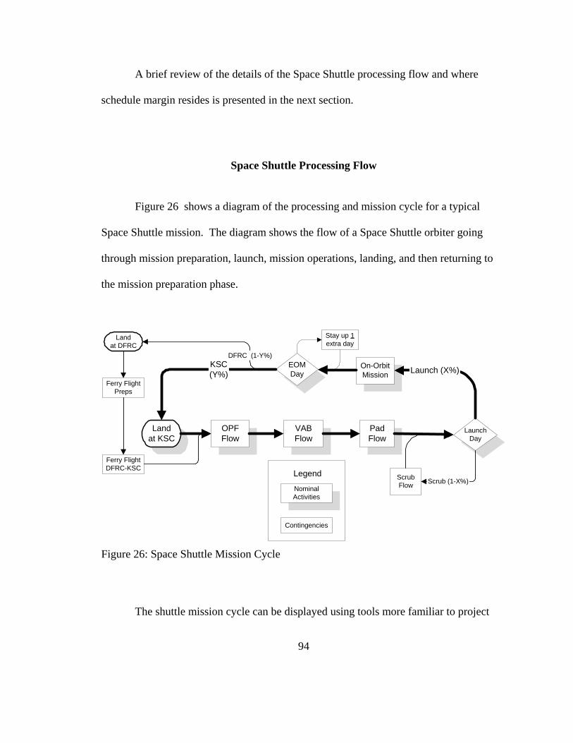
A brief review of the details of the Space Shuttle processing flow and where
schedule margin resides is presented in the next section.
Space Shuttle Processing Flow
Figure 26 shows a diagram of the processing and mission cycle for a typical
Space Shuttle mission. The diagram shows the flow of a Space Shuttle orbiter going
through mission preparation, launch, mission operations, landing, and then returning to
the mission preparation phase.
OPFFlow
VABFlow
PadFlow
LaunchDay
On-OrbitMission
EOMDay
Stay up 1extra day
Landat KSC
Landat DFRC
Ferry FlightDFRC-KSC
Ferry FlightPreps
ScrubFlow Scrub (1-X%)
Launch (X%)
DFRC (1-Y%)KSC(Y%)
Legend
NominalActivities
Contingencies
Figure 26: Space Shuttle Mission Cycle
The shuttle mission cycle can be displayed using tools more familiar to project
94

management such as Gantt charts or PERT/CPM precedence diagram. Figure 27 shows a
Gantt chart of the Space Shuttle mission cycle.
ID Task Name DurationJul 2004 Aug 2004 Sep 2004 Oct 2004 Nov 2004
7/18 7/25 8/1 8/8 8/15 8/22 8/29 9/5 9/12 9/19 9/26 10/3 10/10 10/17 10/24 10/31 11/7 11/14
1 13wOPF Flow
2 1wVAB Flow
3 3wPad Flow
4 3dLaunchCountdown
5 0wLaunch
6 1w 4dOn-orbit
7 0wLanding
11/21
Shuttle Gantt Chart.vsd Figure 27: Shuttle Gantt Chart
The first step of mission preparation is accomplished in the Orbiter Processing
Facility (OPF) and is called the OPF Flow. In the OPF the orbiter is deconfigured from
the previous mission, undergoes detailed inspections and testing, and finally is configured
for the upcoming mission. The process takes approximately 90 calendar days. There is,
however, great variability in that number. Planned work is scheduled Monday through
Friday, typically on a 2 shift per day basis. It is rare that any of these days are available as
margin days. About three quarters of the Saturdays have planned work with the
remainder available as margin. About one quarter of the Sundays have scheduled work
and the remainders are available as margin. Given a 13 week processing flow, then 2
Saturdays and 5 Sundays might typically be available as margin. These numbers will vary
95

based upon the specifics of the processing flow for each mission. The Saturday and
Sunday margin days are used as required to accommodate work content growth that
occurs during the processing flow. Holiday margin may also be available if the OPF flow
extends over a time period containing a holiday such as Thanksgiving, Fourth of July,
Christmas to New Years, etc. Holidays are typically protected as much as possible and
used only as a last resort.
A category of margin unique to the OPF flow is called Dryden Reserve and it
stems from the potential that the orbiter may land in California. There is approximately a
20 percent chance that an orbiter will be diverted to the Dryden Flight Research Center in
California. When this happens it takes several days to prepare and ferry the orbiter back
to Florida. The start of the OPF processing flow is delayed by that amount.
Consequently, NASA holds 6 days of Dryden Reserve in each OPF processing flow as
schedule insurance should the orbiter be so diverted.
Once the orbiter has been processed through the OPF, the orbiter then goes to the
Vehicle Assembly Building (VAB) where it is integrated with the Solid Rocket Boosters
and External Tank. This activity typically occurs over 7 calendar days. Five of these
days have planned work and two are available as margin. As with the OPF flow, if the
VAB activity occurs over a holiday, then that day will not be worked. It may be used as
margin.
Finally the orbiter, which is now a part of what is called an Integrated Space
Shuttle Vehicle, goes to the launch pad where it is prepared for launch. Launch
preparations at the launch pad typically take about three weeks with six weekend days
96

usually available as margin. There may also be a couple in-week contingency days
depending upon the specific mission. Like the OPF and VAB activities, if the Pad flow
extends over a holiday period, then those days will be protected and potentially available
as margin.
In summary, the OPF, VAB, and Pad pre-launch activities are the only places
where schedule margin resides. However, there are other important activities in the
operations cycle of the orbiter and they are described below. These activities are
important to understand because, while they have little schedule margin—on the order of
a few hours—they are significant contributors to schedule risk.
After the launch countdown preparations have been completed, the three-day
launch countdown is conducted. There is approximately a 55 percent chance of
launching. Approximately 45 percent of the time launch does not occur. The duration of
the time required to get back to a subsequent launch attempt is highly dependent upon the
reason for the delay. For weather related delays, it typically takes one day. More difficult
technical problems may take several weeks to correct before launch can be attempted
again. Because delays experienced during launch countdown occur after all the margin
for that mission has been used, the main effect of these delays is to delay the start of the
subsequent OPF processing flow.
Once launch does occur the orbiter enters earth orbit to perform its assigned
mission. Mission duration is typically planned for 10 to 11 days. However, the duration
of the mission can grow. For example, it happens on occasion that the mission is
extended by one day so as to achieve all of the mission objectives. More often it is the
97
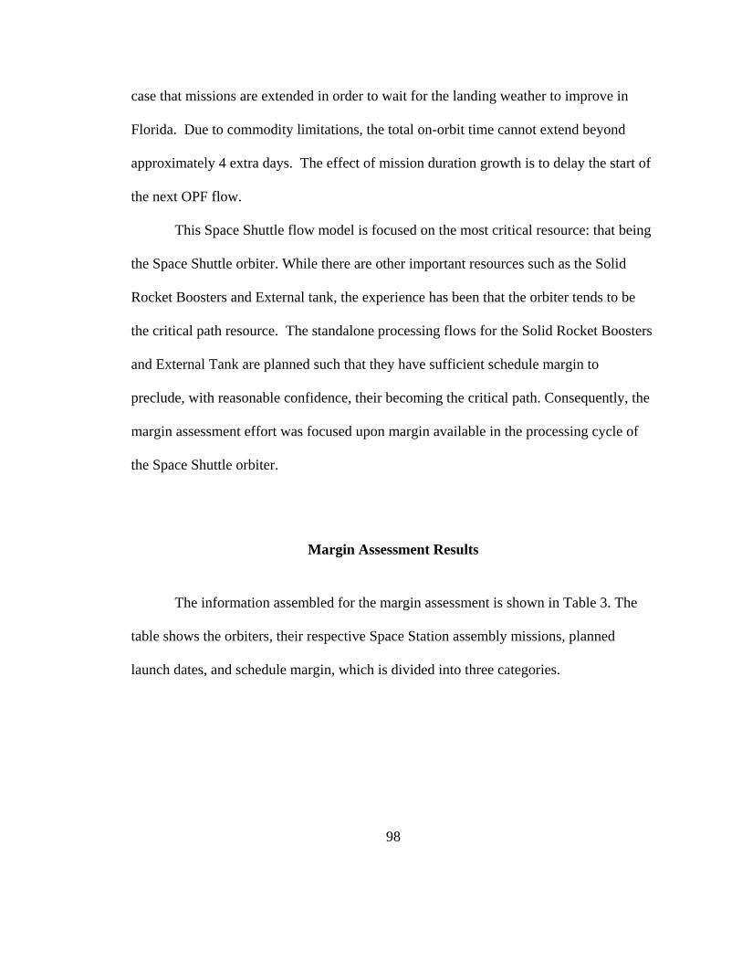
case that missions are extended in order to wait for the landing weather to improve in
Florida. Due to commodity limitations, the total on-orbit time cannot extend beyond
approximately 4 extra days. The effect of mission duration growth is to delay the start of
the next OPF flow.
This Space Shuttle flow model is focused on the most critical resource: that being
the Space Shuttle orbiter. While there are other important resources such as the Solid
Rocket Boosters and External tank, the experience has been that the orbiter tends to be
the critical path resource. The standalone processing flows for the Solid Rocket Boosters
and External Tank are planned such that they have sufficient schedule margin to
preclude, with reasonable confidence, their becoming the critical path. Consequently, the
margin assessment effort was focused upon margin available in the processing cycle of
the Space Shuttle orbiter.
Margin Assessment Results
The information assembled for the margin assessment is shown in Table 3. The
table shows the orbiters, their respective Space Station assembly missions, planned
launch dates, and schedule margin, which is divided into three categories.
98
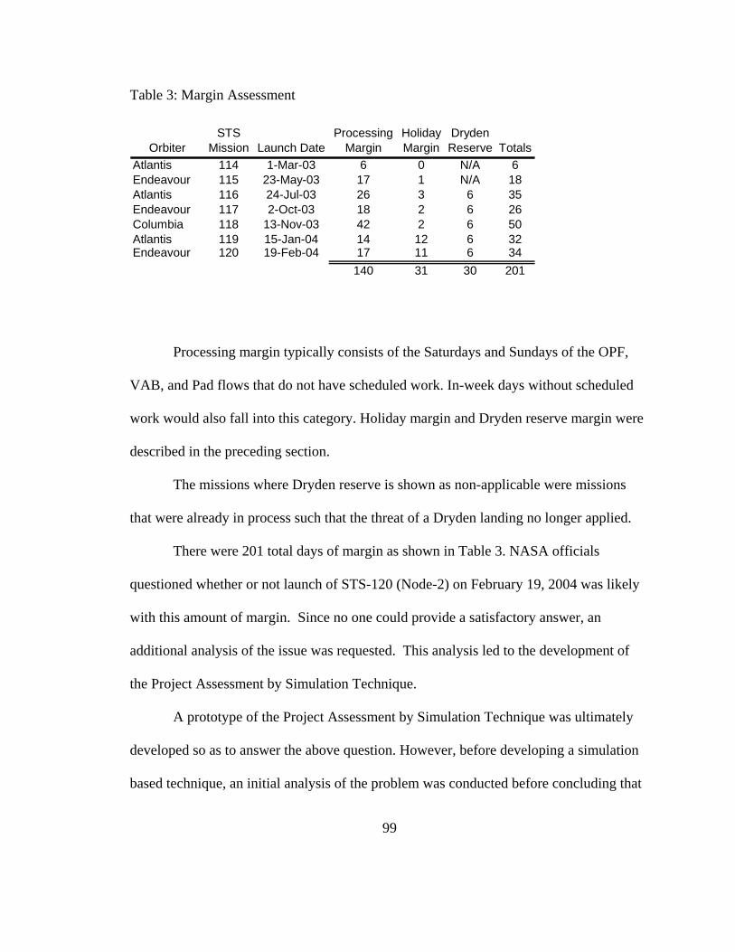
Table 3: Margin Assessment
OrbiterSTS
Mission Launch DateProcessing
MarginHoliday Margin
Dryden Reserve Totals
Atlantis 114 1-Mar-03 6 0 N/A 6Endeavour 115 23-May-03 17 1 N/A 18Atlantis 116 24-Jul-03 26 3 6 35Endeavour 117 2-Oct-03 18 2 6 26Columbia 118 13-Nov-03 42 2 6 50Atlantis 119 15-Jan-04 14 12 6 32Endeavour 120 19-Feb-04 17 11 6 34
140 31 30 201
Processing margin typically consists of the Saturdays and Sundays of the OPF,
VAB, and Pad flows that do not have scheduled work. In-week days without scheduled
work would also fall into this category. Holiday margin and Dryden reserve margin were
described in the preceding section.
The missions where Dryden reserve is shown as non-applicable were missions
that were already in process such that the threat of a Dryden landing no longer applied.
There were 201 total days of margin as shown in Table 3. NASA officials
questioned whether or not launch of STS-120 (Node-2) on February 19, 2004 was likely
with this amount of margin. Since no one could provide a satisfactory answer, an
additional analysis of the issue was requested. This analysis led to the development of
the Project Assessment by Simulation Technique.
A prototype of the Project Assessment by Simulation Technique was ultimately
developed so as to answer the above question. However, before developing a simulation
based technique, an initial analysis of the problem was conducted before concluding that
99

discrete event simulation was well suited for this particular problem.
Initial Analysis of the Project Margin Problem
The analysis of the project margin problem began with a review of historical data
to determine past performance in achieving the orbiter related milestones critical to the
manifest. Because the main question was with respect to how much margin was required,
it was clearly important to understand how often margin days were used in the past. This
historical data was used to build chronological run charts of added work days after
project activity durations are established at the Delta Launch Site Flow Review. This
review is analogous to a formal project review in which project task durations are agreed
to. The run chart were analyzed to identify trends and outliers before determining what
subset of the total historical data should be used as being predictive of future
performance. Histograms and cumulative frequency distributions for added work days
were then built for each of the project activities i.e. OPF, VAB, and Pad flows.
An analysis of the OPF historical data illustrates the process. Figure 28 shows the
run chart that was produced for the OPF and presented to NASA. Causes for added work
days include new work—modifications and special tests called “chits”—along with
Problem Reporting and Corrective Action (PRACA). PRACA is the NASA terminology
for the discovery of minor to major problems on the orbiter and their subsequent repair.
100

Sources of added work days include new program requirements (chits and modifications) and problems encountered during processing i.e. PRACA.
112
97
9299
93
-5
15
35
55
75
95
115
113110104981069395879481787569676462585552454839383634
Work Days Added to the OPF Flow Post Delta LSFR
STS Number
Work Days
STS-93 (AXAF Payload Delays created opportunity to add work)STS-99 (Wiring Inspections)STS-92 (Launch Date Rebaselining created opportunity to add work)STS-97 (Same as 92)STS-112 (MPS Flow Liner)
Figure 28: Work Days Added to the OPF Flow Post Delta LSFR
Note the flows—STS-93, 99, 92, 97, and 112—that experienced large amounts of
added workdays. The reasons for the work growth for these flows were researched. For
example, the STS-93 mission had an unusually large amount of added work because the
Advanced X-Ray Astrophysics Facility (AXAF) was delayed. The large amount of
added work for the STS-112 mission was due to the difficulty in solving a technical
problem involving small cracks in the flow liner of the Main Propulsion System (MPS).
It was subsequently decided to exclude those data points under the assumption that they
would not be predictive of the next seven Space Shuttle missions.
Figure 29 shows the corresponding histogram and cumulative frequency
distribution for the data chosen from Figure 28 as being predictive of the future.
101
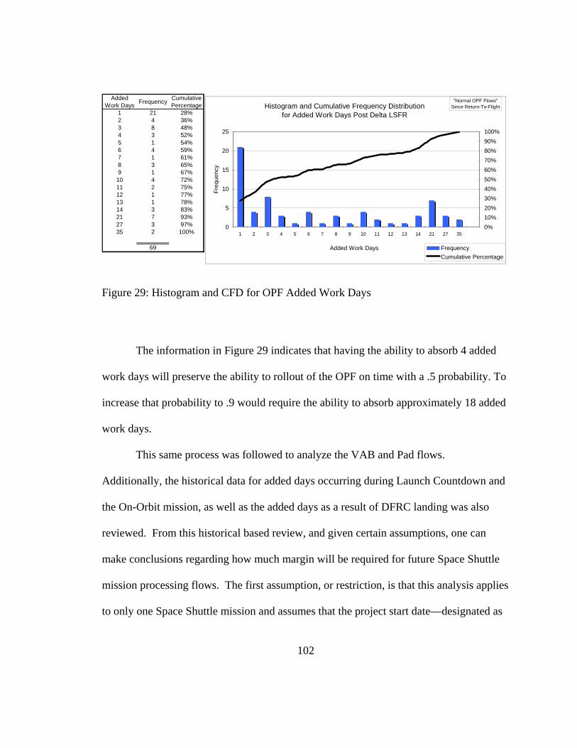
Added Work Days Frequency Cumulative
Percentage1 21 28%2 4 36%3 8 48%4 3 52%5 1 54%6 4 59%7 1 61%8 3 65%9 1 67%
10 4 72%11 2 75%12 1 77%13 1 78%14 3 83%21 7 93%27 3 97%35 2 100%
69
0
5
10
15
20
25
1 2 3 4 5 6 7 8 9 10 11 12 13 14 21 27 35
Freq
uenc
y
0%10%20%30%40%50%60%70%80%90%100%
FrequencyCumulative Percentage
Histogram and Cumulative Frequency Distributionfor Added Work Days Post Delta LSFR
Added Work Days
"Normal OPF Flows" Since Return-To-Flight
Figure 29: Histogram and CFD for OPF Added Work Days
The information in Figure 29 indicates that having the ability to absorb 4 added
work days will preserve the ability to rollout of the OPF on time with a .5 probability. To
increase that probability to .9 would require the ability to absorb approximately 18 added
work days.
This same process was followed to analyze the VAB and Pad flows.
Additionally, the historical data for added days occurring during Launch Countdown and
the On-Orbit mission, as well as the added days as a result of DFRC landing was also
reviewed. From this historical based review, and given certain assumptions, one can
make conclusions regarding how much margin will be required for future Space Shuttle
mission processing flows. The first assumption, or restriction, is that this analysis applies
to only one Space Shuttle mission and assumes that the project start date—designated as
102

OPF roll-in—occurs on time. Additionally, the amount of margin required is a function
of the level of confidence you want to have in achieving an on-time start to the next
project. Table 4 shows the combined results.
Table 4: Margin Days Required To Ensure Next Project Starts on Time
Number of Margin Days Required To Ensure Next Flow Is Not Impacted
Desired Level Of Confidence OPF VAB Launch
PadLaunch
CountdownOn-Orbit Duration
DFRC Landing Total
30% 1 0 1 0 0 0 240% 2 0 2 0 0 0 450% 4 0 3 0 0 0 760% 6 1 4 1 0 0 1270% 10 2 6 2 0 0 2080% 14 3 9 5 1 12 4490% 18 4 14 14 1 13 6499% 32 14 28 70 3 14 161
The information in Table 3 and Table 4 was combined with the sequencing of the
seven Space Shuttle missions in an attempt to see what conclusions could be drawn
regarding likelihood of completing the project on time. Figure 30 shows the seven Space
Shuttle missions with the available margin.
103
STS-115 STS-117 STS-120
STS-114 STS-116 STS-119
STS-118
26 34
35 32
Columbia
Atlantis
Endeavour64
4452 24
45
17
File: Shuttle Flow.vsd
6
18
50
Figure 30: Available Margin Diagram for the Node-2 Milestone
In Figure 30 the thick horizontal bars represent the OPF, VAB, and Pad activities
up to start of launch countdown. The numbers within these bars are the amount of
available margin days. The thin diagonal bars represent the sequencing constraints of the
Space Shuttle mission. The numbers within these diagonal bars are the number of days
that the launch of the preceding mission can slip without impact the next launch. The
rectangular boxes represent the time period of launch countdown, on-orbit mission, and
landing. These periods contain no significant margin.
The above process did not yield a quantitative assessment of the range of likely
launch dates for the STS-120 Node-2 mission. Consequently, it was decided to utilize a
discrete event simulation based assessment.
104
Project Assessment by Simulation Technique Prototype
Once it had been decided to employ discrete event simulation, the effort focused
upon developing a model that would make use of the already available historical data
analysis. It was not at first recognized that this task would lead to a more generic
methodology for project management. Formalization of the Project Assessment by
Simulation Technique would come later. The primary goal for the model of the Node-2
launch date was to provide a quantitative assessment of the likelihood of project
completion by the planned date, i.e. that STS-120 (Node-2) would launch on February
19, 2004 or subsequent dates. A second influential goal was that of providing NASA with
a tool for assessing how proposed actions would support or hinder timely project
completion.
Managerial Controls Component
The managerial controls component for the pilot case study was essentially
established when the analysis was requested. It was assumed that any results would be
shown exclusively to the requestors. Where the results would go from there would be
determined by those requestors.
105

Simulation Model Component
A first step was to build a simulation model of Space Shuttle mission preparation
and performance. This model was built such that it was consistent with the modeling
constructs as described in Chapter 3.
The activity construct was used to model the three major Space Shuttle mission
preparation operations—OPF, VAB, and Pad. The model takes in as inputs planned
processing days along with available margin days for each of the three major mission
preparation operations. During runs of the simulation, arrival of the orbiter entity at each
of the three locations is checked versus the planned arrival date and the amount of margin
is adjusted accordingly. The margin days were modeled as processing margin, which
included Dryden Reserve, and holiday margin. For modeling purposes Dryden Reserve
was added to processing margin since that reserve becomes available as margin should
the orbiter land in Florida as planned. Holiday margin was modeled separately because
it was initially assumed that holidays were not available to be worked unless directed by
management. There is higher cost for working over holidays.
Launch of the shuttle was modeled using a combination of the cyclical and
alternative path event probability constructs. The event probability element includes the
probability of launching or being delayed and the delay type. The delay type determines
the alternative path and thereby length of time required to return to the next launch
attempt.
Likewise, modeling of the landing at KSC versus landing at DFRC included both
106

the cyclical and alternate path event probability constructs. The cyclical component
models the checking to see if weather is favorable for landing at KSC. If it is favorable,
then landing at KSC occurs. If weather is unacceptable, then the shuttle can remain on
orbit in the hope that the weather will improve. In addition to this cyclical component,
there is also a probabilistic component in terms of the final outcome i.e. the orbiter can
land some place other than KSC. This is driven by the fact that there is a limit to how
many days the shuttle can wait on orbit. This time frame is on the order of 2 to 4 days.
Thus, if the weather does not appear to be improving, Space Shuttle managers will decide
to have the orbiter land in California.
The simulation model was tailored to specifically model the processing and
sequencing of the seven missions. A predecessor mission on the orbiter Columbia that
was not part of the seven missions was not included in the model. Additionally, the
possibility of a serious anomaly such as a loss of vehicle event was discounted.
Unfortunately, a loss of vehicle event did occur on the predecessor mission flown by
Columbia. However, that accident occurred after the simulation model was built and
after the analysis was presented to the project stakeholders. Consequently the loss of
Columbia did not influence the prototype case study. It did, however, influence
subsequent case studies, which will be discussed later.
107

Input Analysis Component
Historical Space Shuttle processing data was analyzed in order to populate the
model with representative distributions for added processing days in each of the Space
Shuttle missions. It was initially intended to use theoretical rather than empirical
distributions. In fact the first simulation based analysis of the margin problem used
theoretical distributions. This analysis was presented to NASA officials on December 12,
2002. These project stakeholders, unfamiliar with discrete event simulation, were equally
unfamiliar with the Gamma and Weibull distributions selected to model added work
durations for the OPF and Launch Pad respectively. Difficulty was also encountered
when trying to explain how these distributions are used in the simulation model to
determine added work. Greater success, in terms of gaining stakeholder understanding
and acceptance, was achieved when empirical distributions were used. Consequently,
subsequent to December 12, 2002 empirical distributions were predominantly used.
The analysis already performed with respect to creating histograms and
cumulative frequency distributions for added work days in the various activities—OPF,
VAB, Pad, etc.—was used to create the required empirical distributions. For example, the
information in Figure 29—the histogram and cumulative frequency distribution for 69
past orbiter flows—yielded the empirical distribution shown in Figure 31.
108

Empirical using 69 sample values
0 1 2 3 4 5 6 7 8 9 10 11 12 13 14 15 16 17 18 19 20 21 22 23 24 25 26 27 28 29 30 31 32 33 34 350-10.0
0.1
0.2
0.3
0.4
0.5
0.6
0.7
0.8
0.9
1.0
OPF Empirical Distribution Function Plot
Added Work Days
F(x)
(Pro
port
ion)
Figure 31: OPF Empirical Distribution for Added Work Days
The graphic in Figure 31 is produced by Averill M. Law’s ExpertFit software.
This empirical distribution was transformed, again using ExpertFit, into a discrete
distribution for the Discrete Event Simulation software. The discrete distribution is
shown in Equation 5.
DISC(0.2464,0, 0.3043,1, 0.3623,2, 0.4783,3, 0.5217,4, 0.5362,5, 0.5942,6, 0.6087,7, 0.6522,8, 0.6667,9,
0.7246,10, 0.7536,11, 0.7681,12, 0.7826,13, 0.8261,14, 0.8696,15, 0.8986,17, 0.9130,19, 0.9275,20,
0.9565,22, 0.9710,25, 0.9855,31, 1.0000,34) (Equation 5)
A similar process was used to develop the distributions for added work days for
the preparations that occur in the VAB and at the Launch Pad. Likewise, an empirical
109
distribution was determined for added on-orbit mission time. For example, a planned 11-
day mission may grow to 12 days when the mission operation team determines that an
added day is required to accomplish all the mission objectives.
Historical data was also used to determine the event probabilities for a launch
versus a scrubbed or delayed launch. The probability of launch was determined to be
.55 and the probability of a scrub or delay occurring was .45. After a scrub or delay, a
period of time is required to recover from the delayed launch attempt so as to be in a
position to launch again. The historical data was analyzed to determine the appropriate
empirical distribution for that time duration. The data was also analyzed to see if the
probability of launched changed after the occurrence of a delay. There did not appear to
be a significant change, thus the launch probability was held constant.
Historical data was also used to determine the event probabilities for landing at
KSC versus landing at DFRC at the end of the Space Shuttle mission. It was observed
that the probability of achieving a KSC landing after waiving off the previous day
changed. Consequently, this variation was included in the model.
Verification
The model was first run in a deterministic mode to ensure that it would properly
reproduce launch of STS-120 on the planned date. After this step was successfully
achieved the model was populated with the stochastic elements.
110

Output Analysis
The model was initially run in the stochastic mode for 300 replications. The
choice of 300 replications was based upon the thinking that this would be a sufficiently
large number of replication to achieve reasonable results. Figure 32 shows a histogram of
the 300 replications along with the cumulative percentage. The cumulative percentage
line represents the completion time distribution function for the launch date of STS-120.
0
5
10
15
20
25
30
35
40
45
50
2/19
2/26 3/4
3/11
3/18
3/25 4/1
4/8
4/15
4/22
4/29
Freq
uenc
y
0%
10%
20%
30%
40%
50%
60%
70%
80%
90%
100%
FrequencyCumulative %
Histogram and Cumulative Percentage for STS-120 Launch Date
Launch
Figure 32: Completion Time Distribution Function for STS-120 Launch Date
Launch of STS-120 occurred on the planned date—February 19, 2004—
approximately 16 percent of the runs (47 of 300 runs). Note that this 16 percent figure
was a middle value of a normally distributed range of possible values. Further simulation
111
runs would be required to specify the confidence interval. Launch occurred within one
week of the planed launch date 117 of 300 runs or approximately 39 percent. The 50th
percent probability of launch occurred between March 2nd and March 3rd. The 80th
percentile occurred between March 21st and 22nd and the 90th percentile occurred on April
3rd. The 99 percentile is approximately June 7th.
Figure 32 was embedded in a PowerPoint presentation that was first presented to
NASA on January 6, 2003. A second presentation to a wider audience of higher level
NASA officials occurred the next day. The then present political imperative to achieve
the February 19, 2004 launch date was well known. Consequently, it was also known
that a quantitative analysis indicating that this date was unlikely to be achieved might be
unwelcome. Consequently, during the briefing on January 7th, emphasis was placed on
explaining that the analysis included launch dates beyond February 19th and showed
nearly a 90 percent chance of launch occurring by the first of April. This assessment was
actually consistent with the official Space Shuttle Program position on the issue of the
STS-120 launch date. That position was that February 19th was the planned launch date,
but that there was up to a 45-day (plus or minus 15 days) threat to that date.19 This
consistency lent validity to the results obtained via the Project Assessment by Simulation
Technique. This indicated, therefore, that the first goal of PAST for this case study—
providing a quantitative measure—had been successfully achieved.
During the briefing, NASA officials requested that the analysis be repeated with
the assumption that holidays be treated as margin. This request suggested, at least in this
case, that project stakeholders when made aware of a high likelihood of project tardiness
112

would take action to improve project completion timeliness. The request also provided an
opportunity to fulfill the second goal of the methodology, which was to show the
influence of managerial decisions on project completion timeliness.
The simulation was repeated as requested. This time, however, 3,000 replications
of the two scenarios—one with Holidays as margin and one without Holidays as
margin—were run so as to enable the determination of a confidence band along the entire
Project Completion Distribution Functions. The requested analysis was completed and
distributed for review on January 27, 2003. Figure 33 shows the results. The blue (darker)
lines represent the simulation results for using Holidays as margin. The red (lighter) lines
represent the baseline. The 95% confidence range is represented by the narrower lines.
113

86.9%
53.7%
14.9%
92.0%
67.1%
24.5%
0%
10%
20%
30%
40%
50%
60%
70%
80%
90%
100%
2/19
2/26 3/4
3/11
3/18
3/25 4/
1
4/8
4/15
4/22
4/29
Upper
Mean Baseline
Lower
Upper
Mean Holidaysare MarginLower
Treating Holidays as Margin Significantly Improves the Node-2 Launch Date
Figure 33: Working Holidays Improves STS-120 Launch Date
Working through holidays when required improves the STS-120 launch date. The
lower limit 95-percent confidence for the ‘holidays-are-margin’ case does not overlap the
upper limit for the Baseline case. This indicates that the improvement is significant.
Figure 34 shows more clearly the improvement to the launch date that is achieved
by working holidays.
114
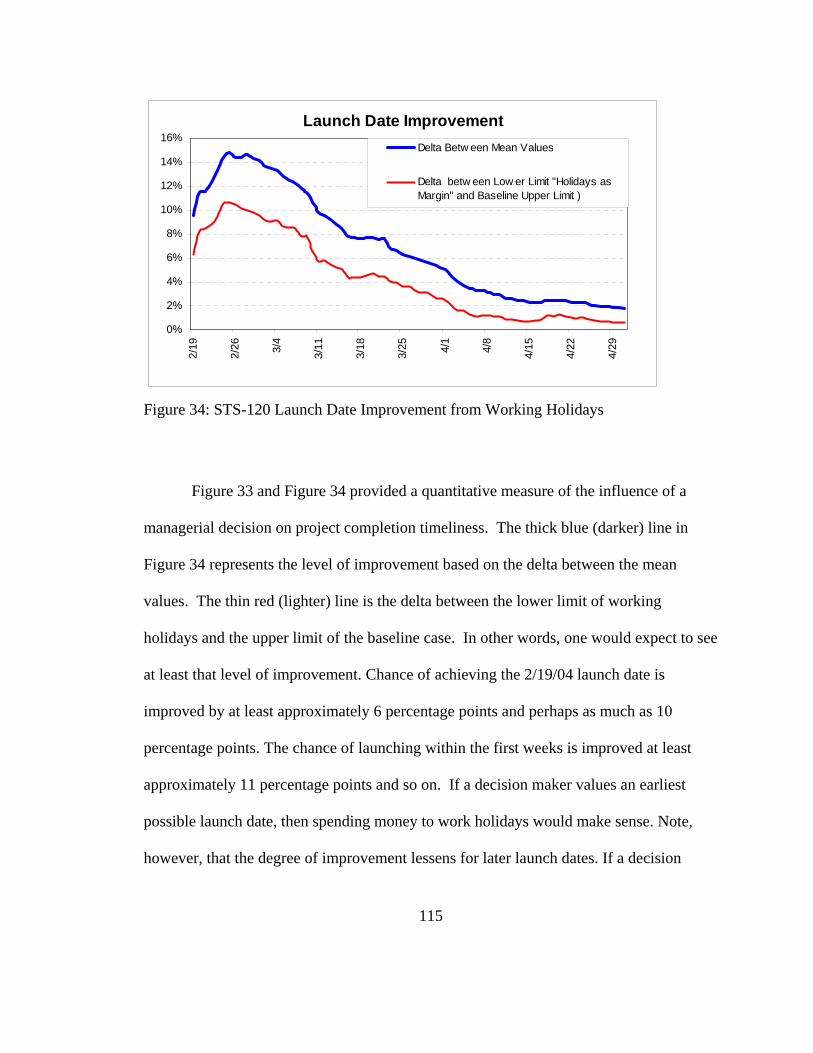
Launch Date Improvement
0%
2%
4%
6%
8%
10%
12%
14%
16%
2/19
2/26 3/4
3/11
3/18
3/25 4/1
4/8
4/15
4/22
4/29
Delta Betw een Mean Values
Delta betw een Low er Limit "Holidays asMargin" and Baseline Upper Limit )
Figure 34: STS-120 Launch Date Improvement from Working Holidays
Figure 33 and Figure 34 provided a quantitative measure of the influence of a
managerial decision on project completion timeliness. The thick blue (darker) line in
Figure 34 represents the level of improvement based on the delta between the mean
values. The thin red (lighter) line is the delta between the lower limit of working
holidays and the upper limit of the baseline case. In other words, one would expect to see
at least that level of improvement. Chance of achieving the 2/19/04 launch date is
improved by at least approximately 6 percentage points and perhaps as much as 10
percentage points. The chance of launching within the first weeks is improved at least
approximately 11 percentage points and so on. If a decision maker values an earliest
possible launch date, then spending money to work holidays would make sense. Note,
however, that the degree of improvement lessens for later launch dates. If a decision
115

maker is willing to accept launch dates beyond April, then working holidays might be
considered less attractive.
Section II: Three Additional Case Studies
The Pilot Case study was completed just prior to the Columbia accident. As a
result of the February 1, 2003 accident the ability to conduct further case studies was put
on hold. The February through July time frame was occupied with various tasks related to
recovering the Columbia debris and understanding the causes of the accident. However,
beginning in August, the imperative to further develop PAST increased and time became
available to do so. From October 2003 through June of 2004 three case studies were
conducted. To set theses case studies in their proper context additional background
information is provided first.
Background Information
In August of 2003, the Columbia Accident Investigation Board released its first
report, Volume 1, on the accident. The CAIB in section 6.2 of its report noted that there
was pressure to achieve the Node-2 launch date of February 19, 2004 and that this
pressure may have contributed to the loss of Columbia. Consequently, the CAIB
advocated improved project risk management. CAIB recommendation 6.2-1 focused
attention on future shuttle flight schedules.
116

Adopt and maintain a Shuttle flight schedule that is consistent with available
resources. Although schedule deadlines are an important management tool,
those deadlines must be regularly evaluated to ensure that any additional risks
incurred to meet the schedule is recognized, understood, and acceptable.20
The NASA administrator stated that NASA accepted the findings of the CAIB
and would comply with all of its recommendation. The NASA Inspector General,
through a series of audits, also assisted the agency in complying with the
recommendations.21
Additionally, the NASA administrator committed the agency to raising the bar by
going above and beyond just complying with the specific recommendations. As a result,
additional launch restrictions would come to be placed upon the shuttle and these would
have to be factored into future PAST models. Case study 1 focused solely on the issue of
one of these new launch restrictions.
In January 2004, President George W. Bush announced a new vision for space
exploration. This vision called for the extension of human presence across the solar
system, starting with a human return to the moon by 2020, in preparation for human
exploration of Mars and other destinations. Funding for the vision, which requires new
vehicles to enable lunar and Mars missions, is thought to come in large part from the
funding wedge currently occupied by the Space Shuttle and International Space Station
programs. This funding wedge is on the order of $6 billion per year, which equates to a
117

spending rate of approximately $500 million per month.22
The Vision for Space Exploration provides specific directives for the Space
Shuttle. The first of these is to return the Space Shuttle to flight as soon as safely
practical. After return-to-flight, NASA is directed to focus use of the Space Shuttle to
complete assembly of the International Space Station. The shuttle is to be retired as soon
as assembly of the International Space Station is completed—planned for the end of this
decade. At that point, major funding will be available for lunar and Mars missions.
Consequently, there is great interest in understanding when the ISS assembly will be
finished and the Space Shuttle retired.
Enabling the vision for space exploration became a central theme of case studies 2
and 3. Case study 2 first explored the influence of augmenting the work force when a
project appears to be likely to finish late. Case study 2 then analyzed the effects of project
content reduction. Case study 3 shows the benefit, to project completion timeliness, in
having a large project buffer.
Case Study 1: Launch Window Analysis
At the end of September 2003, NASA published the implementation plan for
shuttle return to flight and beyond. This plan identified a new requirement to launch the
shuttle in daylight. A PAST based analysis was requested in order to understand the
potential impact of this new requirement.
118

Time periods when Space Shuttles can be launched to rendezvous with the
International Space Station are constrained by a number of factors. There are only a few
minutes out of each day in which the Space Station orbital ground track is sufficiently
close to the Kennedy Space Center to allow a launch. Approximately 70 days out of the
year the solar angle of incidence to the Space Station is such that, for a variety of reasons,
the Space Shuttle orbiter cannot be docked to the Space Station. Consequently the Space
Shuttle cannot be launched during these periods. The daylight only requirement would
mean that approximately 170 days out of each year are unavailable for launches. The
combination of all these restrictions would mean that windows of opportunity to launch
the Space Shuttle in the future could be greatly limited. For example, it was postulated
that in some situations there might only be a three-day launch window, with each of the
three days having less than 10 minutes of opportunity. If the shuttle did not launch on
one of those three days, then the next launch attempt might have to wait several weeks.
Given such a potentially onerous restriction, there was interest in the overall
impact to launch probability and the potential benefit of taking mitigating actions. For
example, changing the altitude of the Space Station could increase the launch window
from 3 days to 5 days. Officials wanted to know if that change would improve overall
launch probability, and if so, by how much.
PAST was used to determine the launch probability for 3-day versus 5-day
windows of opportunity. The analysis was done under a variety of assumptions. Figure
35 shows the analysis under the assumption that the orbiter arrives at the launch pad on
time and the processing flow has six days of margin.
119
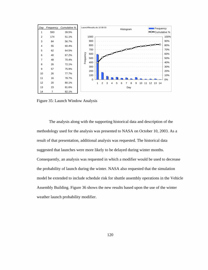
Day Frequency Cumulative %
1 593 39.5%
2 174 51.1%
3 84 56.7%
4 55 60.4%
5 62 64.5%
6 40 67.2%
7 48 70.4%
8 26 72.1%
9 57 75.9%
10 26 77.7%
11 16 78.7%
12 20 80.1%
13 23 81.6%
14 7 82.1%
Histogram
0
100
200
300
400
500
600
700
800
900
1000
1 2 3 4 5 6 7 8 9 10 11 12 13 14
DayFr
eque
ncy
0%
10%
20%
30%
40%
50%
60%
70%
80%
90%
100%
FrequencyCumulative %
LaunchResults.xls 10 08 03
Figure 35: Launch Window Analysis
The analysis along with the supporting historical data and description of the
methodology used for the analysis was presented to NASA on October 10, 2003. As a
result of that presentation, additional analysis was requested. The historical data
suggested that launches were more likely to be delayed during winter months.
Consequently, an analysis was requested in which a modifier would be used to decrease
the probability of launch during the winter. NASA also requested that the simulation
model be extended to include schedule risk for shuttle assembly operations in the Vehicle
Assembly Building. Figure 36 shows the new results based upon the use of the winter
weather launch probability modifier.
120

Bin Frequency Cumulative %
1 687 45.80%
2 206 59.53%
3 107 66.67%
4 64 70.93%
5 54 74.53%
6 39 77.13%
7 18 78.33%
8 26 80.07%
9 36 82.47%
10 20 83.80%
11 14 84.73%
12 20 86.07%
13 17 87.20%
14 7 87.67%
Histogram
0
100
200
300
400
500
600
700
800
900
1000
1 2 3 4 5 6 7 8 9 10 11 12 13 14
DayFr
eque
ncy
0%
10%
20%
30%
40%
50%
60%
70%
80%
90%
100%
FrequencyCumulative %
LaunchResults.xlsLCD 10 15 Winter Wx
Figure 36: Launch Probability with Winter Weather Modifier
Probability of launching during a three-day window of opportunity is
approximately 67% and approximately 75% for a five-day window: a gain of 8 percent.
Recall that without the winter weather modifier the results were 72% and 78% for the
three and five-day windows respectively.
The complete set of requested analysis was graphed together to facilitate
visualization of the results. The simulation results graphed included the VAB activity,
launch pad activity, launch countdown, and winter weather modifier for launch
probabilities, and with various quantities of launch pad margin days. Figure 37 shows
that graphic.
121

Increasing Number of Pad Margin Days Improves Probability of Launching with Respect to Planned Launch Day
0%
10%
20%
30%
40%
50%
60%
70%
80%
1 2 3 4 5 6 7
Actual Launch Day Relative to Planned Launch Day
Freq
uenc
y
Start Count on Time25 Days Margin20 Days Margin15 Days Margin10 Days Margin5 Days Margin0 Days Margin
LaunchResults.xlsSummary Analysis
Figure 37: Launch Probability Comparisons
The increased probability of launch, brought about by having 5 days of
opportunity, was not considered great enough to risk lowering the altitude of the Space
Station. Consequently, that option is no longer being considered.
Case Study 2: Manifest Option 04A-29
In March of 2004, NASA created manifest option 04A-29, which was
subsequently used in support of developing the budget for the Space Shuttle program.
Table 5 shows the relevant details of that option.
122
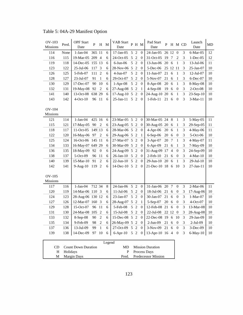
Table 5: 04A-29 Manifest Option
OV-103 Missions Pred. OPF Start
Date P H M VAB Start Date P H M Pad Start
Date P H M CD Launch Date MD
114 None 1-Jan-04 365 11 6 17-Jan-05 5 2 0 24-Jan-05 26 12 0 3 6-Mar-05 12116 115 19-Mar-05 209 4 6 24-Oct-05 5 2 0 31-Oct-05 19 7 2 3 1-Dec-05 12119 118 14-Dec-05 155 13 6 6-Jun-06 5 2 0 13-Jun-06 20 6 1 3 13-Jul-06 11123 122 25-Jul-06 117 3 6 28-Nov-06 5 2 0 5-Dec-06 25 12 11 3 25-Jan-07 10126 125 5-Feb-07 111 2 6 4-Jun-07 5 2 0 11-Jun-07 21 6 1 3 12-Jul-07 10128 127 23-Jul-07 91 1 6 29-Oct-07 5 2 0 5-Nov-07 21 6 1 3 6-Dec-07 10130 129 17-Dec-07 90 10 6 1-Apr-08 5 2 0 8-Apr-08 20 6 1 3 8-May-08 10132 131 19-May-08 92 2 6 27-Aug-08 5 2 1 4-Sep-08 19 6 0 3 2-Oct-08 10141 140 13-Oct-08 638 29 6 17-Aug-10 5 2 0 24-Aug-10 20 6 1 3 23-Sep-10 10143 142 4-Oct-10 96 11 6 25-Jan-11 5 2 0 1-Feb-11 21 6 0 3 3-Mar-11 10
OV-104 Missions
121 114 1-Jan-04 425 16 6 23-Mar-05 5 2 0 30-Mar-05 24 8 1 3 5-May-05 11115 121 17-May-05 90 2 6 23-Aug-05 5 2 0 30-Aug-05 20 6 1 3 29-Sep-05 11118 117 11-Oct-05 149 13 6 28-Mar-06 5 2 0 4-Apr-06 20 6 1 3 4-May-06 11122 120 16-May-06 97 2 6 29-Aug-06 5 2 1 6-Sep-06 20 6 0 3 5-Oct-06 10125 124 16-Oct-06 145 11 6 27-Mar-07 5 2 0 3-Apr-07 20 7 1 3 4-May-07 11134 133 16-May-07 649 29 6 30-Mar-09 5 2 0 6-Apr-09 21 6 1 3 7-May-09 10136 135 18-May-09 92 0 6 24-Aug-09 5 2 0 31-Aug-09 17 4 0 3 24-Sep-09 10138 137 5-Oct-09 96 11 6 26-Jan-10 5 2 0 2-Feb-10 21 6 0 3 4-Mar-10 10140 139 15-Mar-10 91 2 6 22-Jun-10 5 2 0 29-Jun-10 20 6 1 3 29-Jul-10 10142 141 9-Aug-10 119 2 6 14-Dec-10 5 2 0 21-Dec-10 18 6 10 3 27-Jan-11 10
OV-105 Missions
117 116 1-Jan-04 712 34 8 24-Jan-06 5 2 0 31-Jan-06 20 7 0 3 2-Mar-06 11120 119 14-Mar-06 110 3 6 11-Jul-06 5 2 0 18-Jul-06 21 6 0 3 17-Aug-06 10124 123 28-Aug-06 130 12 6 23-Jan-07 5 2 0 30-Jan-07 21 6 0 3 1-Mar-07 10127 126 12-Mar-07 160 3 6 28-Aug-07 5 2 1 5-Sep-07 20 6 0 3 4-Oct-07 10129 128 15-Oct-07 96 11 6 5-Feb-08 5 2 0 12-Feb-08 21 6 0 3 13-Mar-08 10131 130 24-Mar-08 105 2 6 15-Jul-08 5 2 0 22-Jul-08 22 12 0 3 28-Aug-08 10133 132 8-Sep-08 90 2 6 15-Dec-08 5 2 0 22-Dec-08 19 6 10 3 29-Jan-09 10135 134 9-Feb-09 98 2 6 26-May-09 5 2 0 2-Jun-09 21 6 0 3 2-Jul-09 10137 136 13-Jul-09 99 1 6 27-Oct-09 5 2 0 3-Nov-09 21 6 0 3 3-Dec-09 10139 138 14-Dec-09 97 10 6 6-Apr-10 5 2 0 13-Apr-10 16 4 0 3 6-May-10 10
LegendCD Count Down Duration MD Mission Duration
H Holidays P Process DaysM Margin Days Pred. Predecessor Mission
123
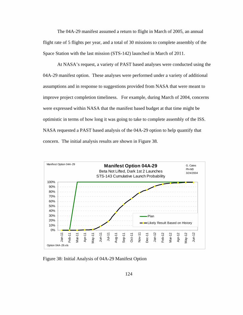
The 04A-29 manifest assumed a return to flight in March of 2005, an annual
flight rate of 5 flights per year, and a total of 30 missions to complete assembly of the
Space Station with the last mission (STS-142) launched in March of 2011.
At NASA’s request, a variety of PAST based analyses were conducted using the
04A-29 manifest option. These analyses were performed under a variety of additional
assumptions and in response to suggestions provided from NASA that were meant to
improve project completion timeliness. For example, during March of 2004, concerns
were expressed within NASA that the manifest based budget at that time might be
optimistic in terms of how long it was going to take to complete assembly of the ISS.
NASA requested a PAST based analysis of the 04A-29 option to help quantify that
concern. The initial analysis results are shown in Figure 38.
0%10%20%30%40%50%60%70%80%90%
100%
Jan-
11
Feb-
11
Mar
-11
Apr
-11
May
-11
Jun-
11
Jul-1
1
Aug
-11
Sep
-11
Oct
-11
Nov
-11
Dec
-11
Jan-
12
Feb-
12
Mar
-12
Apr
-12
May
-12
Jun-
12
Plan
Likely Result Based on History
Manifest Option 04A-29Beta Not Lifted, Dark 1st 2 Launches
STS-143 Cumulative Launch Probability
Manifest Option 04A-29 G. Cates PH-M33/24/2004
Option 04A-29.xls
Figure 38: Initial Analysis of 04A-29 Manifest Option
124

The cumulative launch probability function indicates that the actual launch date
for STS-143 (the 30th mission), planned for March of 2011, could be anywhere from May
of 2011 through June of 2012.
NASA responded positively to the PAST analysis in two ways that should result
in improved project completion performance. The first was to request an increase in the
size of the work force. The second was to suggest reduced project content. Both of these
suggested actions were analyzed by PAST at NASA’s request.
Work Force Augmentation
The analysis shown in Figure 38 was used by NASA officials in support of budget
negotiations to augment the United Space Alliance Ground Operations work force.
United Space Alliance is the prime contractor to NASA for performing Space Shuttle
processing. It was believed that a work force augmentation on the order of approximately
300 people would provide processing flexibility to meet the manifest. There were also
recommendations from the Columbia Accident Investigation Board that indicated work
force augmentation was desirable. A new simulation analysis was requested to analyze
the influence of workforce augmentation.
Note first that the simulation results displayed in Figure 38 were subsequently
determined to be optimistic due to assumptions in the model and also requirements that
were not modeled. The risk of a delay to the first Post-Columbia launch was assumed to
125

be equal to that of any other launch. In reality, there is a greater likelihood that the first
launch will experience a delay. Additionally, the potential magnitude of that delay is
likely to be greater than for other launches. Similarly, the risk of schedule delays for OPF
flows was assumed to be equal for all flows. In reality, longer duration flows in which
extensive maintenance and modifications are performed are more likely to be delayed by
greater durations. Not included in the model was the then emerging requirement to have a
shuttle ready to “launch-on-need” to perform a rescue of a crippled orbiter.
Consequently, the first step in the new analysis was to address the aforementioned
optimistic assumptions and missing launch-on-need requirement in the model. The
assumptions were changed to reflect a more accurate view of schedule risk for longer
duration OPF flows. The launch-on-need requirement was added into the model. These
changes resulted in shift to the right of the completion distribution function for Space
Station assembly completion.
The question then became how to model the augmented work force. Perhaps more
precisely, the question was how would the additional workers be used? These questions,
while not fully resolved, essentially boiled down to two alternatives. The first alternative
assumed that the additional workers would provide a roving team that would focus on
minimizing the effects of added work occurring in the OPF. In this way, the OPF rollout
milestone would be more likely to occur on time. The second alternative assumed that the
added workers could be used to reduce the planned activity duration. The second
alternative was used for the new analysis. Figure 39 shows the potential benefit from
augmenting the shuttle workforce under that assumption.
126

Scenario Comparison for STS-143 Launch Date
0
0.1
0.2
0.3
0.4
0.5
0.6
0.7
0.8
0.9
1
Feb-
11
Mar
-11
Apr-
11
May
-11
Jun-
11
Jul-1
1
Aug-
11
Sep-
11
Oct
-11
Nov
-11
Dec
-11
Jan-
12
Feb-
12
Mar
-12
Apr-
12
May
-12
Jun-
12
Jul-1
2
Aug-
12
Sep-
12
Oct
-12
Nov
-12
Dec
-12
Jan-
13
Cum
ulat
ive
Per
cent
age
PlanWork Force AugmentationSimulation Results
Manifest Study 04A-29 G. CatesPH-M34/21/04
This analysis has not been endorsed by KSC, SSP, or OSF.04A-29 input_output f ile R3.xls
Figure 39: Potential Benefit from Workforce Augmentation.
The PAST based analysis showed a significant improvement to the ISS assembly
complete milestone. At the 50th percentile, completion of the Space Station was improved
by 8 months. This equates to a cost savings of approximately $4 billion assuming that
combined annual expenditures for the Space Shuttle program and Space Station assembly
are approximately $6 billion. Note again that the actual benefit from the workforce
augmentation will be dependent upon how that work force is utilized. That issue requires
further exploration. Nonetheless, the results were persuasive enough to bolster the case
for workforce augmentation.
The NASA Implementation Plan for Space Shuttle Return to Flight and Beyond,
127

Vol.1, Revisions 2.1 dated July 28, 2004 shows that funding at the level of approximately
$32 million in FY04 and $36 million in FY05 was subsequently approved for Kennedy
Space Center Ground Operations work force augmentation. It is assumed that this level of
funding, adjusted for inflation, will be authorized in future years. If that assumption
holds, then the total cost to augment the work force should be on the order of $400
million. This indicates that there is the potential for a tenfold return on investment.
Reducing Project Content
In April NASA requested an analysis based upon 28 shuttle missions being
required to complete the Space Station. Previously it had been 30 missions, but missions
29 and 30 were scheduled beyond 2010. Given that NASA’s goal was to complete the
ISS and retire the shuttle by 2010, completing the Space Station with fewer missions was
desirable.
The results of the analysis were as expected. A 28-mission assembly sequence
would naturally finish before a 30-mission sequence. However, the simulation results still
indicated that 28th mission was likely to launch after the desired completion deadline of
“by 2010.” Consequently, NASA also requested that work force augmentation be
factored into the 28-mission sequence analysis. Figure 40 shows the Completion Time
Distribution Functions for the Space Station given a 28-mission assembly sequence.
128

0%
10%
20%
30%
40%
50%
60%
70%
80%
90%
100%
Aug
-10
Sep
-10
Oct
-10
Nov
-10
Dec
-10
Jan-
11
Feb-
11
Mar
-11
Apr
-11
May
-11
Jun-
11
Jul-1
1
Aug
-11
Sep
-11
Oct
-11
Nov
-11
Dec
-11
Jan-
12
Feb-
12
Mar
-12
Apr
-12
May
-12
Jun-
12
Jul-1
2
Goal: Complete ISS By FY 2010
Simulation Results with Work ForceAugmentation
Simulation Results
Manifest Option 04A-29 28th Mission Cumulative Probability for Launch Month
Manifest Option 04A-29 G. Cates PH-M34/12/2004
Results STS-141 04A-29.xls Work sheet: Case Study 3R1
Figure 40: CTDF for STS-141 Launch Month
The ability to complete the assembly of the International Space Station by
December 2010 is improved by reducing the planned number of missions from 30 to 28.
Even greater improvement can be gained if work force augmentation is included.
Case Study 3: Project Buffer Benefit
The last analysis to be presented in this chapter highlights the benefits of having a
large project buffer as suggested by the Critical Chain Project Management philosophy.
On May 26th, NASA requested an analysis of manifest option 04A-49, which had only 23
129

missions. Table 6 shows the details of the 04A-49 option.
Table 6: 04A-49 Manifest Option
OV-103 Missions Pred. OPF Start
Date P H M VAB Start Date P H M Pad Start
Date P H M CD Launch Date MD
114 None 1-Jan-04 365 11 6 17-Jan-05 5 2 0 24-Jan-05 26 12 0 3 6-Mar-05 12116 115 19-Mar-05 209 4 6 24-Oct-05 5 2 0 31-Oct-05 19 7 2 3 1-Dec-05 12118 117 14-Dec-05 93 11 6 3-Apr-06 5 2 0 10-Apr-06 17 4 0 3 4-May-06 11120 119 16-May-06 90 2 6 22-Aug-06 5 2 0 29-Aug-06 21 6 0 3 28-Sep-06 10123 122 9-Oct-06 90 11 6 24-Jan-07 5 2 0 31-Jan-07 20 6 0 3 1-Mar-07 10125 124 12-Mar-07 90 2 6 18-Jun-07 5 2 0 25-Jun-07 21 6 1 3 26-Jul-07 10128 127 6-Aug-07 117 3 6 10-Dec-07 5 2 0 17-Dec-07 23 9 10 3 31-Jan-08 10131 130 11-Feb-08 99 2 6 28-May-08 5 2 0 4-Jun-08 20 6 0 3 3-Jul-08 10
OV-104 Missions
121 114 1-Jan-04 425 16 6 23-Mar-05 5 2 0 30-Mar-05 24 8 1 3 5-May-05 11115 121 17-May-05 91 2 6 24-Aug-05 5 2 0 31-Aug-05 20 6 0 3 29-Sep-05 11126 125 11-Oct-05 634 31 6 13-Aug-07 5 2 0 20-Aug-07 21 6 1 3 20-Sep-07 11129 128 2-Oct-07 103 11 6 30-Jan-08 5 2 0 6-Feb-08 20 6 0 3 6-Mar-08 10132 131 17-Mar-08 152 3 6 25-Aug-08 5 2 0 1-Sep-08 20 7 1 3 2-Oct-08 10134 133 13-Oct-08 90 11 6 28-Jan-09 5 2 0 4-Feb-09 20 6 0 3 5-Mar-09 10136 135 16-Mar-09 97 2 6 29-Jun-09 5 2 1 7-Jul-09 21 6 0 3 6-Aug-09 10
OV-105 Missions
117 116 1-Jan-04 693 34 6 3-Jan-06 5 3 0 11-Jan-06 20 6 0 3 9-Feb-06 11119 118 21-Feb-06 91 2 6 31-May-06 5 2 0 7-Jun-06 21 6 1 3 8-Jul-06 10122 120 19-Jul-06 89 1 6 23-Oct-06 5 2 0 30-Oct-06 21 6 1 3 30-Nov-06 10124 123 11-Dec-06 92 9 6 28-Mar-07 5 2 0 4-Apr-07 20 6 0 3 3-May-07 10127 126 14-May-07 138 3 6 8-Oct-07 5 2 0 15-Oct-07 21 6 1 3 15-Nov-07 10130 129 26-Nov-07 112 10 6 2-Apr-08 5 2 0 9-Apr-08 20 6 0 3 8-May-08 10133 132 19-May-08 194 5 6 10-Dec-08 5 2 0 17-Dec-08 22 8 10 3 29-Jan-09 10135 134 9-Feb-09 99 2 6 27-May-09 5 2 0 3-Jun-09 20 6 0 3 2-Jul-09 10
LegendCD Count Down Duration MD Mission Duration
H Holidays P Process DaysM Margin Days Pred. Predecessor Mission
The last mission (STS-136, OV-104) was planned for launch on August 6, 2009,
130

which was greater than 1 year prior to the “by the end of the decade” desired completion
date.
The simulation was run under a variety of assumptions. The simulation run that
produced the best results included an assumption that normal OPF flows were limited to
90 days with the remainder of the time available as end of flow margin. Additionally, for
the OMDP flow on OV-104, that 22-month duration was modeled as 16 months plus 6
months of margin. The results for this scenario, identified as S1.O, are shown in Figure
41. The chance of completing ISS by the end of FY2010 was approximately 73 percent.
This was much better than any of the other manifest options previously analyzed.
STS-136 Launch MonthFY 2010 Goal versus Sim Results
Manifest Study 04A-49
00.10.20.30.40.50.60.70.80.9
1
Jul-0
9
Aug-
09
Sep-
09
Oct
-09
Nov
-09
Dec
-09
Jan-
10
Feb-
10
Mar
-10
Apr-
10
May
-10
Jun-
10
Jul-1
0
Aug-
10
Sep-
10
Oct
-10
Nov
-10
Dec
-10
Jan-
11
Feb-
11
Mar
-11
Apr-
11
May
-11
Jun-
11
Jul-1
1
Aug-
11
Sep-
11
Oct
-11
Nov
-11
Dec
-11
Cum
ulat
ive
Per
cent
age
By FY 2010 Goal
Keep all Pads and MLPs active
Mothball 1 pad and 1 MLP after STS-131
G. CatesPH-O5/28/04
This analysis has not been endorsed by KSC, SSP, or OSF.04A-49 input_output file R2.xls
Loss of Vehicle Probability: ZeroLaunch On Need: SupportedDark Restriction: Lif ted after 2nd LaunchOPF End of Flow Margin: OPF Flow duration - 90 days.OMDP End of Flow Margin: OPF duration - 16 months.RTF Schedule Risk: =OMDP/OMM Risk
Launch Pad: 2 to End of Program versus mothball 1 after STS-131MLP: 3 to End of Program versus mothball 1 after STS-131
Figure 41: Analysis of 04A-49 Option with S1.O Assumptions
131

NASA was also interested in the influence of incrementally shutting down
facilities after STS-131—the planned last mission of OV-103, which was scheduled to be
launched July 3, 2008. The simulation results suggested that this action had only a small
affect upon the results. Note how the simulation results overlap for the most part, with the
potentially notable exception of the time period August 2009 through February 2010. An
analysis of the confidence bands was required to see if this was a significant difference.
Figure 42 shows confidence bands during the time period of interest.
Confidence Bands for STS-136 Launch MonthManifest Study 04A-49
0%
5%
10%
15%
20%
25%
30%
Aug-
09
Sep-
09
Oct
-09
Nov
-09
Dec
-09
Jan-
10
Feb-
10
Launch Month
Cum
ulat
ive
Per
cent
age Upper Limit (95%)
Low er Limit (95%)
Upper Limit (95%) w ithPad/MLP ClosedLow er Limit (95%) WithPad/MLP Closed
File: 04A-49 input_output file R2
Loss of Vehicle Probability: ZeroLaunch On Need: SupportedDark Restriction: Lifted after 2nd LaunchOPF End of Flow Margin: Flow duration - 90 daysOMDP End of Flow Margin: Flow duration - 6 monthsRTF Schedule Risk: =OMDP/OMM Risk
Figure 42: Confidence Bands for STS-136 Launch Date
The confidence bands do not overlap during the time period of September 2009
through January 2010. This indicates that there is a statistically significant benefit to
132
maintaining the complete set of shuttle facilities.
After May 28th the 04A-49 option was no longer being actively considered by
NASA because a 23 mission scenario for completing the Space Station was not
considered viable. Consequently, the analysis results produced up until that point were
distributed and further analysis of that option was halted.
Section III: Evolution of PAST
After the pilot case study PAST evolved in response to lessons learned and
queries from project stakeholders. A recognized weakness of the PAST modeling
component in the pilot case study was the length of time required to model alternative
scenarios. This weakness led first to the creation of a generic modeling component that
could be linked to an Excel input file. Later, the output analysis process was automated
in response to requests for faster turnaround time during case studies 2 and 3. As PAST
became more widely used project stakeholders desired increased understanding of the
process used to perform PAST based analyses. This led to further development of the
managerial component. The output analysis component evolved in response to customer
requests for a Completion Quantity Distribution Function. These aspects of PAST’s
evolution are described in greater detail below.
133
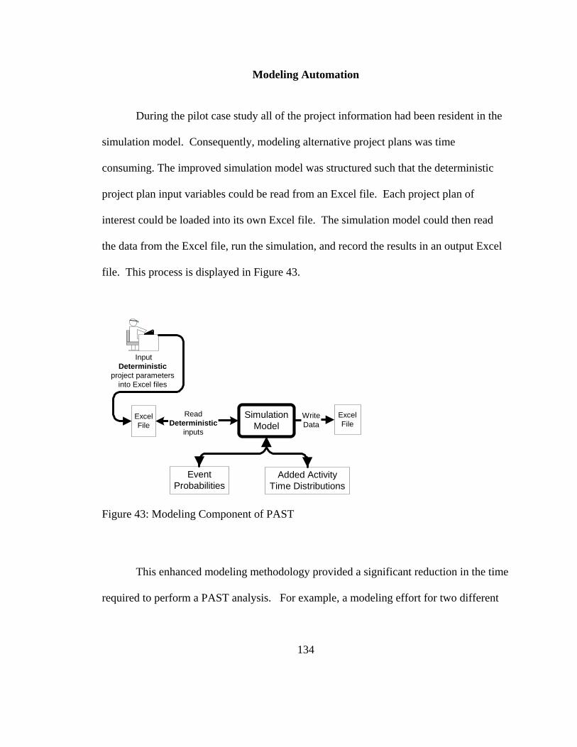
Modeling Automation
During the pilot case study all of the project information had been resident in the
simulation model. Consequently, modeling alternative project plans was time
consuming. The improved simulation model was structured such that the deterministic
project plan input variables could be read from an Excel file. Each project plan of
interest could be loaded into its own Excel file. The simulation model could then read
the data from the Excel file, run the simulation, and record the results in an output Excel
file. This process is displayed in Figure 43.
ExcelFile
SimulationModel
ReadDeterministic
inputs
ExcelFile
WriteData
EventProbabilities
Added ActivityTime Distributions
InputDeterministic
project parametersinto Excel files
Figure 43: Modeling Component of PAST
This enhanced modeling methodology provided a significant reduction in the time
required to perform a PAST analysis. For example, a modeling effort for two different
134
manifest options that began on November 17, 2003 was completed at 1:00 pm the next
day for a total time of approximately 1 day. The time required to model the Node-2
launch date had been on the order of two weeks. The enhanced modeling methodology
was used in case studies 2 and 3.
Output Analysis Automation
During case studies 2 and 3 project stakeholders requested increasingly faster
turnaround times for analysis of alternatives. Initially a turnaround time of a day or two
was acceptable. Later, however, requests for 2 hour turnaround times were made. There
was even a request that an update be made in 10 minutes. The response to these customer
demands was to automate the Excel portion of the output analysis component of PAST.
When first conceived the output analysis process was not automated. Each time a
simulation was run the replication results, usually 1000 data points, were written directly
into Excel from the simulation model. Histograms, cumulative distribution functions, and
confidence bands were then created from those data points using the graphing and
charting functions resident in Excel. This process was particularly tedious and time
consuming because it required several actions on the part of the analyst.
It was found, however, that most of the output analysis process could be
automated in Excel. The automation process required extensive use of the “COUNTIF”
function in Excel. This function counts the number of cells within a specified Range that
135

meet a specified condition. The range was the simulation output from the 1,000
replications. The given condition was the number of instances in those 1,000 replications
in which the project completed within a specified time frame. The results of the
COUNTIF function could then be used to create tables and graphs for histograms,
cumulative frequency distributions, and confidence bands. Because these tables and
graphs were dependent upon the COUNTIF function results they automatically updated
each time a new set of simulation results were written into Excel.
Management Issues
The managerial component of PAST both expanded and required greater
definition during the time that the case studies were active. This evolution occurred in
response to several questions from project stakeholders. First they desired greater
understanding of the process of conducting a PAST analysis. This led to the
development of a step-by-step process explanation, an estimate of how long the steps
take, and an estimate for the level of resources required or scope of the effort. The issue
of where the analyst should reside organizationally was also explored. An area that
received great attention was the need to establish distribution controls and disclaimers for
the analysis results.
136

PAST: Step-by-Step
In April of 2003 NASA asked for a more detailed explanation of the PAST
process and how long a PAST analysis of a manifest option typically takes. This is
information that needs to be included during the introductory briefing. It should also be
specified in the requirements section of the managerial component of PAST.
Additionally, a summary level step-by-step process, similar to the one described below,
should be provided to project stakeholders.
Step 1 in the process is to obtain the manifest option(s) needing to be analyzed.
This is typically provided via email, and the option is printed so as to facilitate the next
step.
Step 2 is to manually enter the data from the manifest option into Excel. That
process takes approximately two hours. The process includes semi-automated error
checking in Excel to ensure that the manifest data is entered correctly. This step could be
further enhanced by fully automating the transfer of manifest option data into Excel.
Step 3 is to run the model in a deterministic mode just to make sure that the
simulation will execute the manifest and achieve the planned launch on the planned
launch date. This helps to ensure that the Excel file and the simulation model are a
correct representation of the manifest option. If that goes well, then it takes only a few
minutes. However, if it doesn’t produce the right output, then time is required to correct
the mistakes. Sometimes this can take several hours, but usually it is relatively easy to
find and fix in an hour or two.
137

After it is all coded correctly, Step 4 is to run the simulation in the variable mode
(stochastic) and the results are written to an Excel file. To run 1,000 replications in the
simulation takes approximately 1-2 minutes. Step 4 is repeated for each of the requested
scenarios for that manifest. For example, one scenario might assume the daylight launch
requirement goes away after the second shuttle launch and an alternative scenario could
be that the requirement remains in place for all missions.
Step 5 is to perform the analysis in the Excel output file. This analysis includes
producing histograms, cumulative probability curves, and confidence bands. Excel is
structured such that these products are produced in a largely automated fashion. The
product titles, dates, and assumptions must still be manually edited on the graphics. The
products are then checked to see if they make sense i.e. do they look like what was
expected. A typical time to perform this analysis, assuming the results look valid, is
approximately 1 hour. If the results appear to be invalid, then it may be necessary to
return to any of the earlier steps in a trouble shooting mode. The solution to the problem
may take only a few minutes, but can take much longer.
Step 6 is to paste the useful charts into a PowerPoint presentation. Components of
the PowerPoint presentation include the title chart, assumptions, requested measures of
performance, the manifest being analyzed, and the results charts. This process takes about
an hour.
Under the best conditions, the time from start to a finished product is 4 to 6 hours.
But it can go longer if problems are encountered. The time estimates assume dedicated
effort.
138
Once a particular manifest option is modeled correctly with Excel input file,
simulation model, Excel output file, and PowerPoint presentation file, additional runs can
be performed very quickly. Less than an hour depending upon quantity of information
desired.
The estimate for the total number of manifest options that could be analyzed on a
weekly basis was said to be “a few.” That number could be increased if the manual
processes could be automated. Those processes were the loading of the manifest option
data into input Excel file and the editing of the various figures in the output Excel file.
Scale of Effort
“What is the scale of the effort?” This question relates to how many resources
would be dedicated to performing PAST based analysis work became a topic of interest
that needed discussion.
A one-person dedicated effort to the manifest analysis effort seemed reasonable
for a number of reasons. There was at that time no one else performing this function in
the Space Shuttle organization. The level at which this analysis could influence the Space
Shuttle and Space Station programs, as well as the interest in PAST by other senior
NASA officials indicated that dedicating at least one person to this task was appropriate.
Additional support, beyond one dedicated individual, could be added later if
desired to increase the robustness of the service being provided. This growth might
139

include furthering partnerships with other organizations in NASA where simulation and
modeling expertise existed. Consideration could also be given to a modest level of
additional staffing to more economically perform the more routine functions. This could
actually reduce the cost of providing the service because some of the more tedious tasks,
e.g. the manual input into excel, manual input of historical data into Excel, and creating a
web site, etc. could be more economically performed by less expensive employees.
Organizational Residence
Another consideration was the location of the service. Should the analysis
function remain in a line organization or should it be a Shuttle Program level function or
even some form of a NASA Independent Assessment Office function. There were
arguments for any of those alternatives. A prime argument for where it currently resides
was that the function is probably best done locally where the manifest options are being
generated. More generically speaking, performing the service in-house or via acquired
temporary consultant service should be considered.
Analysis Distribution Controls
During the case studies concerns were expressed PAST based analyses of Space
Shuttle manifests were being distributed external to the Space Shuttle program prior to
140

their being fully staffed through the Space Shuttle program. Figure 44 helps to illustrate
some relevant organizational boundaries within NASA.
Office of Space Flight
SpaceShuttle
Program
NASA
File:Project Analysis Process R1.vsd
InternationalSpaceStation
Program
Figure 44: Organizational Hierarchy
The Space Shuttle program is under the direction of the Office of Space Flight.23
That Office also manages the International Space Station program. The outermost NASA
circle represents all other areas of NASA outside the Office of Space Flight. The concern
was that an analysis product had gone outside the circle of the Space Shuttle program,
and in fact outside the Office of Space Flight circle, without having been fully
coordinated. This concern served as catalyst to further develop the managerial
component of PAST, primarily to ensure appropriate staffing for PAST analyses.
141
The Completion Quantity Distribution Function Graphic
Interestingly, the Completion Quantity Distribution Function, in addition to the
Completion Time Distribution Function, became a required output product. The use of
this product in analyzing Manifest Option 04A-29, under three different assumptions, is
illustrated below.
First there was the issue of whether or not the shuttle would be restricted to
daylight only launches for the remainder of the program. This possibility was mentioned
in NASA’s return to flight plans. “For the time being we will launch the Space Shuttle
missions in daylight conditions to maximize imagery capability until we fully understand
and can mitigate the risk that ascent debris poses to the Shuttle.”24 All previous models
had been run under the assumption that the daylight only restriction would be lifted after
the second mission.
A second modeling assumption was with respect to the need to have a backup
shuttle ready to launch a rescue mission within a set time period. “For the first two
flights, NASA will ensure that the SSP has the capability to launch a rescue Shuttle
mission with the time period that the ISS Program can reasonably predict that the Shuttle
crew can be sustained on the ISS.”25 The time period was initially estimated to be 90
days, but other time periods could be modeled. The model was also set up to run under
the assumption that the need to have a launch-on-need (LON) shuttle might extend to the
end of the program.
Finally, there was also interest in including a non-zero probability for loss-of-
142

vehicle (PLOV) during mission operations. Consequently, the simulation model was set
up to run alternatives with PLOV set at either 0 or .01. All previous modeling had
discounted the possibility of a non-zero PLOV.
On May 5th the results from these analyses were presented to NASA. Figure 45
shows the CQDF curves representing the number of launches likely to be achieved
through the end of Fiscal Year 2010.
Number of Launches Through September 2010 versus 28 PlannedLOV Probability Set to Zero
0.00.10.20.30.40.50.60.70.80.91.0
0 1 2 3 4 5 6 7 8 9 10 11 12 13 14 15 16 17 18 19 20 21 22 23 24 25 26 27 28 29 30
Cum
ulat
ive
Per
cent
age
Plan-28S1.OS4.OS1.PS4.P
Manifest Study 04A-29 G. Cates PH-M3 5/05/04
04A-29 input_output f ile R5.xls This analysis has not been endorsed by KSC, SSP, or OSF.
Figure 45: CQDF for Analysis Team
The analysis indicated that manifest option 04A-29 was unlikely to produce the
desired result of 28 launches by the end of Fiscal Year 2010. This result held true under
a variety of assumptions. The bounding cases at that time were thought to be S1.O (best
case) and S4.P (worst case), both of which assumed that the launch on need requirement
143

continued to the end of the program. The S1.O scenario was defined as the darkness
restriction being lifted after the second shuttle mission and included improvements in the
way the shuttle program manages schedule margin. These improvements would be
enabled by workforce augmentation. The S4.P scenario assumed that the darkness
restriction was never lifted, that the shuttle program managed schedule margin in the
same manner that they have in the past, and that the workforce would not be augmented.
Figure 46 shows the CQDF simulation results when PLOV is set at .01.
Number of Launches Through September 2010 versus 28 PlannedLOV Probability Set to 1 in 100
0.0
0.1
0.2
0.3
0.4
0.5
0.6
0.7
0.8
0.9
1.00 1 2 3 4 5 6 7 8 9 10 11 12 13 14 15 16 17 18 19 20 21 22 23 24 25 26 27 28 29 30
Cum
ulat
ive
Per
cent
age
Plan-28S1.O LOVS1.P LOVS4.O LOVS4.P LOV
Manifest Study 04A-29 G. Cates PH-M35/05/04
04A-29 input_output f ile R5.xls This analysis has not been endorsed by KSC, SSP, or OSF.
Figure 46: CQDF with PLOV at .01
If the launch-on-need requirement were to go away, then some improvement in
144

the number of achieved launches by Fiscal Year 2010 could be expected. Figure 47
shows the improvement to the bounding cases, with PLOV set to zero, brought about by
elimination of the launch on need requirement. Note that this analysis assumed a launch-
on-need requirement of 90 days.
Number of Launches Through September 2010 versus 28 PlannedLOV Probability Set to Zero
0.00.10.20.30.40.50.60.70.80.91.0
0 1 2 3 4 5 6 7 8 9 10 11 12 13 14 15 16 17 18 19 20 21 22 23 24 25 26 27 28 29 30
Cum
ulat
ive
Per
cent
age
Plan-28S1.O No LONS1.OS4.P No LONS4.P
Manifest Study 04A-29 G. Cates PH-M3 5/05/04
04A-29 input_output f ile R5.xls This analysis has not been endorsed by KSC, SSP, or OSF.
Figure 47: Improvement from Elimination of Launch on Need Requirement
NASA gave “high marks” to this new type of quantitative assessment.
145

CHAPTER FIVE: CONCLUSION
The Project Assessment by Simulation Technique was found to be an effective
tool for supporting various project stakeholders. Use of the PAST methodology, as
applied to analyzing the project to assemble the International Space Station, gained a
modest level of acceptance within NASA over the time period December 2002 through
August 2004. Project stakeholders have a greater understanding of how that project
stands with respect to finishing.
During the case studies the methodology was called MAST which stands for
“Manifest Assessment Simulation Tool.” The more generic term for the methodology
was chosen to be Project Assessment Simulation Technique (PAST) because the
methodology is based upon an underlying assumption that past performance is likely to
be indicative of future results. Use of the word “technique” comes from the PERT,
GERT, and VERT methodologies.
Summary of Case Study Results
Recall that the question of interest for the case study was, “How would project
stakeholders respond to the Project Assessment by Simulation Technique?” The
corresponding proposition was that “Project stakeholders would react positively to the
146

Project Assessment by Simulation Technique and might, in certain situations, take action
to improve project completion performance.” This proposition was found to be true in
the case of the pilot case study and subsequently case studies 1 and 2.
In all of those cases the project stakeholders reacted positively to PAST and took
or proposed action to improve project completion performance. In the pilot case study
weekend work was proposed. In case study 1, lowering of the Space Station was
proposed. This proposal was rejected after it was shown, using the PAST methodology,
that this would not provide sufficient improvement to overcome other considerations.
Work force augmentation was proposed and shown by PAST in case study 2 to provide
significant improvement. This information was then used to implement an actual
change—i.e. augment the workforce. Project content reduction was also proposed during
case study 2 and shown to provide significant improvement to project completion
timeliness. There was no recorded stakeholder response for case study 3 because it’s
underlying need—the manifest option under consideration—was scrapped.
It is important to note first, however, that the PAST based analysis was not the
sole justification for decisions or actions taken by NASA. Assembly of the International
Space Station is of such complexity in terms of its technical, political, and safety issues
that most decisions and actions require a broad spectrum of decision support tools. PAST
became a part of that suite during the case studies.
A majority of the case studies showed a positive response to PAST. As such the
potential for PAST to improve project management, at least for the International Space
Station assembly project, has been established. It may be said that similar projects should
147
have the potential to benefit from PAST as well.
Recall that one of the downsides conducting the research as a participant-observer
was the potential to introduce bias into the findings and conclusions. As such there could
be the potential that the conclusions expressed above are overstated in terms of being too
positive. To that concern I would offer the following. PAST, or MAST as called by
NASA, was cited as being a “technology infusion success story” by the NASA project
stakeholders. This citation was suggested without my involvement.
Observations and Recommendations
During the case study many observations were made and some of these need to be
highlighted. Recommendations are offered in response to these recommendations.
Completion Quantity Distribution Function
At the start of the case study, the primary output of PAST was thought to be the
project Completion Time Distribution Function. However, during the case study, the
generation of a Completion Quantity Distribution Function (CQDF) became important.
The CQDF was subsequently found to be so valuable that it was added as a standard
output of all subsequent analyses during the case study.
It is recommended, therefore, that future PAST based analysis efforts consider the
addition of the CQDF as a standard output product. In the future, other project
148
stakeholders making use of PAST may come up with requests for novel output products.
These customer requests should be given high priority.
Timeliness of Analysis
During the case study it was observed that project stakeholders seemed to desire
near real-time results. “If you can’t produce the simulation results in 2 hours then don’t
bother.” At that time an input model of that particular manifest option had not been
created. That project stakeholder was not supported because the entire process for
creating the input file, performing the simulation runs, analyzing the output, and
producing output products would take a minimum of 6 hours. However, as a result of this
request the output analysis process was automated in Excel. When a subsequent email
stating that “I need these results charts updated by 10:00 a.m.” was received at 8:10 a.m.
the automated analysis process allowed that request to be met.
Successful implementation of PAST in any real world project management
environment may depend upon the speed in which the analysis can be accomplished.
Some latitude for a lengthy period of time to develop the first model of a particular
project will be expected. However, subsequent analyses of changes to that project’s plans
need to be accomplished such that the information is available when project stakeholders
demand it.
In response to these observations, it is recommended that future PAST based
149

analysis efforts place high priority on providing timely products. Automating the
modeling and output analysis components of the PAST methodology will facilitate this
timeliness. For example, as the case studies progressed greater and greater automation
was built into the output Excel files. This enabled the automatic generation of the CTDF,
the CQDF, and their associated confidence bands. Within the simulation model of the
project, various “switches” were created such that assumptions could be changed easily.
The most tedious and time consuming process in PAST during the case study was the
manual input of the manifest option data into the Excel input file. Automation in this
area was not possible because the manifest options being created used a legacy software
system that was not compatible with exporting to Excel.
Politics of Risk Assessment
During the case study it was observed that some project stakeholders became
concerned about an analysis showing a low likelihood of completing the Space Station
assembly by the end of the decade. This concern may be attributable to the politics of
risk assessment.
Large and expensive public projects, such as the project to assembly the
International Space Station must take into account political considerations. A project can
be cancelled at anytime if congressional support falters. A well intended project risk
assessment that portrays a low probability of success with respect to an important project
150

goal may be used as justification to cancel a project. Given that scenario one can
understand the resistance to performing or publishing quantitative project risk
assessments especially if the assessment suggests a low likelihood of success. The
unfortunate aspect of this political dilemma is that by avoiding quantitative risk analysis,
the opportunity to identify critical risk drivers, mitigate those risks, and measure the
resulting improvement quantitatively is lost.
Bell and Esch (1989) describe the case of a probabilistic risk assessment by
General Electric during the Apollo program. GE, under contract to NASA, performed a
quantitative probabilistic risk assessment of the likelihood of success in landing a man on
the moon and returning him safely. Their assessment was quite low, less than a 5 percent
chance of success. The NASA Administrator believed that this assessment, if publicized,
would do irreparable harm. Consequently, NASA stayed away from numerical risk
assessments and adopted qualitative risk assessments.
One has to wonder if continuation of GE’s quantitative assessment and mitigation
of the identified risk drivers from the assessment might have prevented the Apollo 1 fire
or the failure of the Apollo 13 mission to land on the moon. Likewise, would better
attention to empirical data and quantitative risk assessment have prevented the
Challenger accident? In the aftermath of that accident NASA was directed to make use of
quantitative probabilistic risk assessments.
151
Future Research
Future research opportunities could proceed along several different fronts. A case
study encompassing the present time frame through assembly completion of the
International Space Station and retirement of the Space Shuttle is a natural follow-on to
this research. Assuming that PAST is used throughout this period, then there should be
substantial empirical evidence as to whether or not PAST provides benefit to project
management, at least with respect to one large project. PAST is intended for a wide
variety of major projects. Consequently, case studies on the use of PAST on other
projects would be desirable. These projects could be in any area, e.g. defense, aerospace,
construction, etc. There are also a variety of issues related to the PAST methodology that
could be explored. These include the reliance upon historical data and the creation of
empirical distributions.
Continued Use of PAST to Support ISS Assembly
On May 7, 2004, the existence of the PAST based analysis was brought up at a
meeting with the NASA Administrator. At this meeting it was relayed that achieving 28
flights by the end of FY 2010 would likely be problematic. Consequently, NASA has
subsequently been working towards improving the likelihood of completing the assembly
of the International Space Station by the end of the decade. In concert with those efforts,
PAST is being used in an iterative fashion to determine what it might take to achieve ISS
152
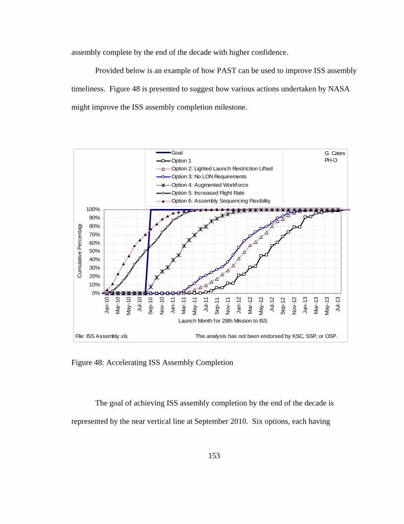
assembly complete by the end of the decade with higher confidence.
Provided below is an example of how PAST can be used to improve ISS assembly
timeliness. Figure 48 is presented to suggest how various actions undertaken by NASA
might improve the ISS assembly completion milestone.
0%10%20%30%40%50%60%70%80%90%
100%
Jan-
10
Mar
-10
May
-10
Jul-1
0
Sep-
10
Nov
-10
Jan-
11
Mar
-11
May
-11
Jul-1
1
Sep-
11
Nov
-11
Jan-
12
Mar
-12
May
-12
Jul-1
2
Sep-
12
Nov
-12
Jan-
13
Mar
-13
May
-13
Jul-1
3
Launch Month for 28th Mission to ISS
Cum
ulat
ive
Perc
enta
ge
GoalOption 1Option 2: Lighted Launch Restriction LiftedOption 3: No LON RequirementsOption 4: Augmented WorkforceOption 5: Increased Flight RateOption 6: Assembly Sequencing Flexibility
This analysis has not been endorsed by KSC, SSP, or OSP.
G. Cates PH-O
File: ISS Assembly.xls
Figure 48: Accelerating ISS Assembly Completion
The goal of achieving ISS assembly completion by the end of the decade is
represented by the near vertical line at September 2010. Six options, each having
153

different input assumptions, were modeled. Option 1 assumes a five flight per year
manifest plan with all launches being restricted to daylight and requires that a backup
shuttle be ready to launch on need (LON) no more than 90 days after any shuttle has been
launched. As shown by the graph, Option 1 has virtually no chance of achieving ISS
assembly complete by the end of the decade. At the 50th percentile, assembly complete
occurs in the July 2012 timeframe—nearly two years late. The current annual cost for
operating the Space Shuttle and building the Space Station is approximately $6 billion.
Consequently, if NASA were to continue with the Option 1 scenario, the expected
additional costs to complete the ISS is approximately $12 billion.
Option 2 lifts the lighted launch restriction after the 2nd shuttle mission. This
action improves the ISS assembly completion milestone, as measured by the 50th
percentile to February 2012. The savings from the 5-month acceleration could equate to
as much as $2.5 billion. Option 3 is the same as Option 2 with the addition that the
requirement to have a LON rescue shuttle goes away after the 2nd shuttle mission. Option
3 is approximately 2 months and $1 billion better than Option 2.
Option 4 is the same as Option 3 plus it includes an augmented workforce. . This
option indicates the augmentation of the workforce, depending upon how it is utilized
could accelerate ISS completion by as much as 10 months and save NASA approximately
$5 billion. Given that the cost to augment the workforce for the 7-year period 2004
through 2010 is on the order of $300 million demonstrates the tremendous benefit
achievable by Option 4. Option 4 is the option closest to NASA’s ISS assembly planning
assumptions as of this writing. However, the strategy for how to utilize the workforce
154

augmentation has not been fully decided. Consequently, it may not achieve all of the
savings shown above. Nonetheless, significant savings are possible.
Option 5 is based upon a 6-flight per year manifest as opposed to the 5-flight per
year manifest for the previous 4 options. Given a 6-flight per manifest, the planned
launch of the 28th shuttle mission occurs in November of 2009. Under this option there is
a 10-month project buffer between the earliest possible project completion date and the
desired project completion date. According to Goldratt having a large project buffer is
highly desirable and should lead to considerable improvement in project completion
timeliness. The simulation results as shown in Figure 48 support this viewpoint. Given
option 5, the ISS assembly completion is achieved in the desired time frame at the 50th
percentile. Additional funding, beyond that provided for the workforce augmentation of
Option 4, would be required in order to carry out Option 5. The quantity of that
additional funding had not been estimated as of this writing.
Like Option 5, Option 6 is based upon a 6-flight per year manifest. However,
under Option 6 it is assumed that the sequence of shuttle missions can be modified. For
example suppose that shuttle mission 20 is delayed such that mission 21 is ready launch
sooner. Under all the earlier options mission 21 has to wait for mission 20. In Option 6,
however mission 21 could go ahead and mission 20 would launch after words. Under
Option 6 the likelihood completing the ISS on time is increased to approximately 75
percent.
Option 6 might appear to be akin to saying that the 21st story of a high rise could
be erected before the 20th story has been built. However, in theory, such a scenario is
155
achievable for ISS assembly. For example, if the component of the ISS in the 20th
mission could be moved at the last minute to the shuttle flying the 21st mission, then the
on-orbit assembly sequence is unaltered. The only thing that changed was which shuttle
delivered the component. In practice, late swapping of mission elements between
shuttles is difficult to achieve. Another scenario would be to go ahead and launch the 21st
component and then park it temporarily near the station until the 20th component has been
installed. In practice, this too would be problematic. Nonetheless, the benefit provided
by having sequencing flexibility does indicate that such possibilities deserve further
exploration.
PAST and Critical Chain Project Management
Proponents of new project management strategies, such as Eliyahu Goldratt’s
Critical Chain Project Management, may also use the Project Assessment by Simulation
Technique to quantify the benefit of new strategies. For example Goldratt places
emphasis on decreasing activity durations within the project so as to create a buffer
between the planned project completion time and the desired project completion date.
PAST could be used to quantify the influence of such actions.
156

The PAST Input Analysis Methodology
PAST relies heavily upon having historical data and using that data to create
empirical distributions. There are problems with that method that could be explored.
First, as noted in the literature, obtaining relevant historical data can be problematic.
Consequently, a case study in which one uses expert opinion to create triangular
probability distributions would complement the present research. Second, even when one
does have sufficient historical data to create reasonable empirical distributions, there can
be problems. One problem is that empirical distributions are limited in terms of the
extreme values. For example, a project activity in which there has historically been at
most only a delay of 20 days may experience a greater delay in the future. Consequently,
there may be value to transforming empirical distributions into less bounded theoretical
distributions that at least have low probabilities of larger values.
Closing Thoughts
The Project Assessment by Simulation Technique can provide practical value to
project stakeholders. First, they can gain greater understanding of when their project is
likely to complete versus when it is planned to complete. Secondly, they can also see the
influence of varying assumptions or managerial decisions. When opportunities to make
improvements to the project are considered they will be able to quantify the benefits of
implementing those opportunities. For example, one project strategy might be to install
management reserve within the individual project activities. The corresponding Project
157

Completion Distribution Function will quantify the effect of this strategy. Likewise,
when things go awry mangers will be able to measure the negative influence on the
project’s completion time. This will provide them with earlier opportunities to take
corrective actions. A corrective action might be to use overtime to reduce or “crash” an
activity’s duration. The resulting PCDF will quantify the corrective influence of that
action.
The Project Assessment by Simulation Technique as developed in Chapter 3 and
described in the case studies of Chapter 4 provides a constructive example for future
PAST practitioners and project stakeholders alike. PAST practitioners can use it as a
guide to providing project stakeholders with understandable, statistically valid, and
accurate assessments of project completion dates, and then to make appropriate
comparisons of alternatives. Project stakeholders can use it so as to better understand the
potential benefit that may be derived from such analysis. Successful implementation of
PAST into the management of large projects can improve project completion
performance.
158

END NOTES
159
1 Joseph J. Moder, Cecil R. Phillips, and Edward W. Davis, Project Management with CPM, PERT and
precedence diagramming, 3rd Edition, Von Nostrand Reinhold Company, NY, 1983, pp. 12-13.
2 Richard I. Levin and Charles A. Kirkpatrick, Planning and Control with PERT/CPM, McGraw-Hill Book
Company, 1966, pgs. 2-8.
3 Johnson, Lyndon Baines, The Vantage Point, Perspectives of the Presidency, 1963-1969, Holt, Rinehart
and Winston, 1971, page 281.
4 Galway, L., “Quantitative Risk Analysis for Project Management: A Critical Review,” RAND working
paper, The RAND Corporation, WR-112-RC, Santa Monica, California, Feb. 2004, pg. 15.
5 Project Management Institute, Project Management Body of Knowledge, PMBOK Guide, 2000 pg. 139.
6 Stephan A. Devaux, Total Project Control: A Manager’s Guide to Integrated Project Planning,
Measuring, and Tracking, John Wiley & Sons, Inc., 1999, pgs 190-191.
7 Joseph J. Moder, Cecil R. Phillips, and Edward W. Davis, Project Management with CPM, PERT and
precedence diagramming, 3rd Edition, Von Nostrand Reinhold Company, NY, 1983, pp. 13.
8 Joseph J. Moder, Cecil R. Phillips, and Edward W. Davis, Project Management with CPM, PERT and
precedence diagramming, 3rd Edition, Von Nostrand Reinhold Company, NY, 1983, pp. 12-13.
9 Richard I. Levin and Charles A. Kirkpatrick, Planning and Control with PERT/CPM, McGraw-Hill Book
Company, 1966, pgs. 2-8.
10 Richard I. Levin and Charles A. Kirkpatrick, Planning and Control with PERT/CPM, McGraw-Hill Book
Company, 1966, pg. 7.
11 D.G. Malcolm, J.H. Roseboom, and C.E. Clark, “Application of a Technique for Research and
Development Program Evaluation,” Operations Research, Vol. 7, Issue 5 (Sep-Oct 1959) pp. 650-651.

160
12 Richard I. Levin and Charles A. Kirkpatrick, Planning and Control with PERT/CPM, McGraw-Hill Book
Company, 1966, pp. 25-45 and chapter 7.
13 Goldratt, Eliyahu, M., Critical Chain, The North River Press, Great Barrinton, MA, pg. 41.
14 Lawrence P. Leach, Critical Chain Project Management, Artech House, 2000, pg. 259.
15 Mollaghasemi, “Introduction to Simulation Modeling Seminar,” 1999
16 Kelton, Sadowski, and Sadowski, Simulation with Arena, McGraw-Hill Series in Industrial Engineering
and Management Sciences, WCB/McGraw-Hill, 1998, pgs. 173 and 444.
17 Yin, Robert K., Case Study Research: Design and Methods, Third Edition, Applied Social Research
Methods Series, Vol. 5, SAGE Publications, Thousand Oaks, California, 2003, pg. 35.
18 Gehman, Harold W. Jr., et al., Report of the Columbia Accident Investigation Board, Vol. 1, August
2003, pg. 131.
19 Gehman, Harold W. Jr., et al., Report of the Columbia Accident Investigation Board, Vol. 1, August
2003, pp. 136-7.
20 Gehman, Harold W. Jr., et al., Report of the Columbia Accident Investigation Board, Vol. 1, August
2003, pg. 139.
21 On December 11, 2003, the NASA Inspector General announced an audit intended to review activities
planned to address the recommendation made by the Columbia Accident Investigation Board (CAIB) for
adopting and maintaining a Shuttle flight schedule consistent with available resources (CAIB
recommendation R6.2-1). This audit was numbered A-04-011-00.
22 The President’s FY 2005 Budget Request for the National Aeronautics and Space Administration
requests $4.319 billion for the Space Shuttle and $1.863 billion for the International Space Station.
23 The Office of Space Flight became the Space Operations Mission Directorate in 2004.
24 NASA’s Implementation Plan for Space Shuttle Return to Flight and Beyond, NASA, April 26, 2004,
page xvi.
25 NASA’s Implementation Plan for Space Shuttle Return to Flight and Beyond, NASA, July, 28, 2004,
page 2-5.

LIST OF REFERENCES
Adlakha, V.G. and Kulkarni, V.G., “A classified bibliography of research on stochastic PERT networks: 1966-1987, INFOR, 27 pp. 272-296 (1989)
Arisaw, S. and Elmaghraby, S.E., “Optimal Time-Cost Tradeoffs in GERT Networks,” Management Science, Vol. 18, No. 11, July 1972
Banks, J., Carson J.S. II, Nelson, B.L., and Nicol, D.M., Discrete-Event System Simulation, 3rd edition, Prentice Hall International Series in Industrial and Systems Engineering, 2001
Barton, R.R. and Schruben, L.W., “Resampling Methods for Input Modeling,” Proceedings of the 2001 Winter Simulation Conference, B.A. Peters, J.S. Smith, D.J. Medeiros, and M.W. Rohrer, eds, (372-378)
Bedford, Tim, and Cooke, Roger, Probabilistic Risk Analysis: Foundations and Methods, Cambridge University Press, Cambridge, UK, 2001
Bell, T.E. and Esch, K., “The Space Shuttle: a case of subjective engineering,” IEEE Spectrum, June 1989 pp. 42-46
Cates, G.R. “Node-2 Manifest Margin Assessment With Initial Simulation Results,” PowerPoint Presentation, NASA, December 12, 2002
Cook, T.M. and Jennings, R.H., “Estimating a project’s completion time distribution using intelligent simulation methods,” Journal of the Operational Research Society, Volume 30 (12), pp. 1103-1108 (1979)
Devaux, Stephan A., Total Project Control: A Manager’s Guide to Integrated Project Planning, Measuring, and Tracking, John Wiley & Sons, Inc., 1999
Dodin, B.M., “Bounding the project completion time distribution in PERT networks,” Operations Research, 33, pp. 862-881 (1985)
Elmaghraby, S., Activity Networks, Wiley, New York, 1977
Elton, J. and Roe, J., “Bringing Discipline to Project Management,” Harvard Business Review, Mar-Apr 1998, pp. 153-159
Fatemi Ghomi, S.M.T. and Rabbani, M., “Approximating completion time distribution function for stochastic PERT networks,” Proceedings of the 5th Annual International Conference on Industrial Engineering—Theory, Applications and Practice, Dec. 13-15, Hsinchu, Taiwan
161

Fleming, Q. W. and Koppelman J. M., Earned Value Project Management, 2nd Edition, Project Management Institute, 2000
Fondahl, J.W., “Non-computer approach to the critical path method for the construction industry,” Prepared under Contract No. NBy-17798 for the Bureau of Yards and Docks, U.S. Navy, Stanford University Department of Civil Engineering, Technical Report 9, November, 1961, Revised 1962
Forrester, J.W., 1961, “Industrial dynamics,” MIT Press, Cambridge
Fulkerson, D.R., “Expected Critical Path Lengths in PERT Networks, prepared for United States Air Force Project RAND, The Rand Corporation, Memorandum RM-3075-PR, Mar. 1962
Galway, L., “Quantitative Risk Analysis for Project Management: A Critical Review,” RAND working paper, The RAND Corporation, WR-112-RC, Santa Monica, California, Feb. 2004
Gantt, H. Organizing for work, Harcourt, Brace & Hove, New York, 1919
Goldratt, Eliyahu M., Critical Chain, North River Press, 1997
Goldratt, Eliyahu M., The Goal, North River Press, 1984
Gutierrez, G.J. and Kouvelis, P., “Parkinson’s Law and Its Implications for Project Management,” Management Science, Vol. 37, No. 8, Aug. 1992, pp. 990-1001
Hagemann, A.G., “Use of the Critical Chain Project Management Technique at NASA, Langley Research Center,” The 20th Conference on Digital Avionics Systems (DASC), Vol. 1, Oct. 14-18, 2001, pages 4B1/1-10
Hebert, J.E., Critical path analysis and a simulation program for resource-constrained activity scheduling in GERT project networks, Purdue University, PhD dissertation, 1975
Hill, L.S., “Some Possible Pitfalls in the Design and Use of PERT Networking,” The Rand Corporation, Memorandum P-3038, Jan. 1965
Hoeting, J. A., Madigan, D., Raftery, A.E., and Volinsky, C.T. (1999) “Bayesian Model Averaging: A Tutorial (with discussion),” Statistical Science, 14:4, 382-417.
Howick, S., “Should System Dynamics be used to Model Disruption and Delay for Litigation? An Exploration of Criteria,” Strathclyde Business School, Scotland, Management Science, Theory, Method, and Practice, Research Paper No. 2002/1
Johnson, Lyndon Baines, The Vantage Point, Perspectives of the Presidency, 1963-1969, Holt, Rinehart and Winston, 1971
Jaraiedi, M., Plummer, R.W. and Aber, M.S., “Incentive/Disincentive Guidelines for Highway Construction Contracts,” Journal of Construction Engineering and Management, Vol. 121, No.1, Mar, 1995, pp. 112-120
Kamburoski, J., Normally distributed activity durations in PERT networks,” Journal of 162
Operational Research Society, 36, pp. 1051-1057 (1985)
Kelly, J., “Critical Path Planning and Scheduling: Mathematical Basis,” Operations Research, Vol. 9, No. 3, May-June-1961, pp. 296-321
Kelton, W.D., Sadowski, R.P., and Sadowski, D.A., Simulation with Arena, McGraw-Hill Series in Industrial Engineering and Management Science, McGraw-Hill, 2001
Kelton, W.D., Sadowski, R.P., and Sadowski, D.A., Simulation with Arena, 2nd edition, McGraw-Hill Series in Industrial Engineering and Management Science, McGraw Hill, 2001
Kidd, J.B., “A Comparison Between the VERT Program and Other Methods of Project Duration Estimation,” OMEGA International Journal of Management Science, Vol. 15, No.2, pp 129-134, 1987
Kidd, J.B., “Do today’s projects need powerful network planning tools?” International Journal of Production Research, Vol. 29, No. 10, pp 1969-1978, (1991)
Kleindorfer, G.B., “Boundary distributions for a stochastic acyclic network,” Operations Research, 20, pp. 800-812, (1971)
Kljajic, Miroljub, Bernik, I., and Skraba A., “Simulation Approach to Decision Assessment in Enterprises,” Simulation, Oct. 2000, pgs. 199-210
Law, A.M. and Kelton, W.D., Simulation Modeling and Analysis, 3rd edition, McGraw Hill, 2000
Leach, L.P., Critical Chain Project Management, Artech House, 2000
Lee, S.M., Moeller, G.L, and Digman, L.A., Network Analysis for Management Decisions, Kluwer-Nijhoff Publishing, 1982
Leigh Givens Filiatrault, C. and Peterson C.D., “Five Behaviors That Can Reduce Schedule Risk,” Proceedings of the Project Management Institute Annual Seminars and Symposium, Sep 7-16, 2000, Houston, Texas, USA
Levin, Richard I. and Charles A. Kirkpatrick, Planning and Control with PERT/CPM, McGraw-Hill Book Company, 1966
Lindsey, J.H. II, “Notes on Combinatorial Mathematics: An Estimate of Expected Critical Path Length in PERT Networks,” prepared for United States Air Force Project RAND, The Rand Corporation, R-544-PR, Oct. 1970
MacCrimmon, K.R. and Ryavec,C.A., “An analytical study of the PERT assumptions,” Operations Research, Vol. 12, 404-421, (1965) See also Rand Research Memorandum RM-3408-PR (December 1962)
MacCrimmon, K.R. and Ryavec,C.A., “An analytical study of the PERT assumptions,” prepared for United States Air Force Project RAND, The Rand Corporation, Memorandum RM-3408-PR, Dec. 1962
Malcolm, D.G., “Application of a technique for research and development program 163
evaluation,” Operations Research, Vol. 7, 646-669 (1959)
Martin, J.J., “Distribution of time through a directed acyclic network,” Operations Research, 13, pp. 46-66 (1965)
Moder, J., and C. Phillips, Project Management with CPM and PERT, Van Nostrand Reinhold, New York, 1964
Moder, J., and C. Phillips, Project Management with CPM and PERT, 2nd edition, Van Nostrand Reinhold, New York, 1970
Moder. J., with C. Phillips and E. Davis, Project Management with CPM, PERT, and Precedence Diagramming, 3rd edition, Van Nostrand Reinhold, New York, 1983
Moeller, G.L. and Digman, L.A., “Operations Planning with VERT,” Operations Research, Vol. 29, Issue 4, July-Aug. 1981, pp. 676-697
Moeller, G.L., 1972. “VERT,” Technical Papers: Twenty-Third Institute Conference and Convention, American Institute of Industrial Engineers
Morris, P.W.G., The Management of Projects, London, Thomas Telford, first published 1994, paperback edition, 1997
NASA, NASA’s Implementation Plan for Space Shuttle Return to Flight and Beyond, Vol.1, Revision 2.1, National Aeronautics and Space Administration, July 28, 2004
Newbold, Robert C., Project Management in the Fast Lane: Applying the Theory of Constraints, St. Lucie Press, 1998
Ng, S.-H., and Chick, S.E., “Reducing Input Parameter Uncertainty for Simulations,” Proceedings of the 2001 Winter Simulation Conference, B.A. Peters, J.S. Smith, D.J. Medeiros, and M.W. Rohrer, eds, (364-370).
Ottjes, J.A. and Veeke, H.P.M., “Project Management With Simulation: A Critical View on the Critical Path,” Proceedings of the ICSC Symposia on Intelligent Systems & Applications (ISA’2000), December 2000, Wollongong Australia [ICSC], ISBN 3-906454-24-X.
Pegden, D.C., Shannon, R.E., and Sadowski, R.P., Introduction to Simulation Using SIMAN, 2nd edition, McGraw-Hill, Inc., 1995
Pinto, J.K., “”Some constraints on the Theory of Constraints: Taking a Critical Look at the Critical Chain,” PM Network, Project Management Institute, August 1999, pp. 49-51.
Pritsker A.A.B. and Happ, W.W., “GERT: Graphical evaluation and review technique, Part I, fundamentals,” Journal of Industrial Engineering, Vol. 17 (5), 267-274 (1966)
Pritsker A.A.B. and Whitehorse, G.E., “GERT: Graphical evaluation and review technique, Part II, probabilistic and industrial engineering applications,” Journal of Industrial Engineering, Vol. 17 (6), 293-301 (1966)
164

Pritsker, A.A.B., “GERT: Graphical Evaluation and Review Technique,” The RAND Corporation, RM-4937-NASA, Santa Monica, California 1966
Pritsker, A.Alan B., Modeling and analysis using Q-GERT networks, Wiley, New York, NY, 1979
Project Management Institute, A Guide to the Project Management Body of Knowledge, (PMBOK® Guide), Project Management Institute, 2000
Rathe, A.W. (ed), Gantt on management, American Management Association, New York, 1961.
Ringer, L. J., “Numerical operators for statistical PERT critical path analysis,” Management Science, 16, pp. 136-143 (1969)
Roberts, B., Smith, C., and Frost, D., “Risk-based decision support techniques for programs and projects,” Acquisition Review Quarterly, Spring 2003 Defense Acquisition University Press
Robillard, Pierre, and Trahan, Michel, “The Completion Time of PERT Networks,” Operations Research, Vol. 25, No. 1, Jan-Feb 1977, pp. 15-29
Sapolsky, H.M., The Polaris System Development: Bureaucratic and Programmatic Success in Government, Harvard University Press, Cambridge, MA, 1972
Schuyler, John, Risk and Decision Analysis in Projects, 2nd Edition, Project Management Institute, 2001
Sculli, D., “The completion time of PERT networks,” Journal of Operational Research Society, 34, pp. 155-158 (1983)
Sheppard, M., and Cartwright, M., “Predicting with Sparse Data,” IEEE Transactions on Software Engineering, Vol. 27, No. 11, November 2001, 987-998
Simmons, L.F., “Project Management-Critical Path Method (CPM) and PERT Simulated with ProcessModel,” Proceedings of the 2002 Winter Simulation Conference, E. Yücesan, C.-H. Chen, J.L. Snowdon, and J.M. Charnes, eds, (1786-9)
Sterman, J.D., “System Dynamics Modeling for Project Management,” Sloan School of Management, MIT, Cambridge MA, 1992
Taha, Hamdy, A., Operations Research, An Introduction, 5th Edition, MacMillan, 1992
Tversky, A. and Kahneman, D., “Judgment under Uncertainty: Heuristics and Biases,” Science, Vol. 185, No. 4157, 27 September 1974, 1124-1131
Van Slyke, R., “Uses of Monte Carlo in PERT,” prepared for United States Air Force Project RAND, The Rand Corporation, Memorandum RM-3367-PR, Feb. 1963
Van Slyke, R.R., Monte Carlo methods and the PERT problem,” Operations Research, 11, pp. 839-860 (1963)
Vose, David, Quantitative Risk Analysis: A Guide to Monte Carlo Simulation Modeling,
165
John Wiley & Sons, England, 1996
Walker, M.R. and Sawyer, J.S., “Project Planning and Scheduling,” Report 6959, E.I. duPont de Nemours and Co., Wilmington, Delaware, March 1959
Williams, D.L., Finke, D.A. Medeiros, D.J., “Discrete Simulation Development for a Proposed Shipyard Steel Processing Facility,” Proceedings of the 2001 Winter Simulation Conference, B.A. Peters, J.S. Smith, D.J. Medeiros, and M.W. Rohrer, eds, (882-887).
Williams, Terry, “A classified bibliography of recent research relating to project risk management,” European Journal of Operational Research, pp. 18-38 (1995)
Yin, Robert K., Case Study Research: Design and Methods, Third Edition, Applied Social Research Methods Series, Vol. 5, SAGE Publications, Thousand Oaks, California, 2003
Yongyi Shou and Yeo, K.T., “Estimation of Project Buffers in Critical Chain Project Management,” International Conference on Management of Innovation and Technology (ICMIT), IEEE, pages 162-167, 2000
Zouaoui, F. and Wilson J.R., “Accounting for Input Model and Parameter Uncertainty in Simulation,” Proceedings of the 2001 Winter Simulation Conference, B.A. Peters, J.S. Smith, D.J. Medeiros, and M.W. Rohrer, eds, (290-299)
Zouaoui, F. and Wilson J.R., “Accounting for Parameter Uncertainty in Simulation Input Modeling,” Proceedings of the 2001 Winter Simulation Conference, B.A. Peters, J.S. Smith, D.J. Medeiros, and M.W. Rohrer, eds, (354-363)
166