Embed Size (px)
Citation preview

BACHELOR THESIS
Improving production planning for a
food processing company
Jörn Harbers Industrial Engineering and Management
University of Twente 06-10-2020
Improving production planning for a food
processing company
Bachelor Thesis Industrial Engineering and Management
Author
J.J.G. Harbers Industrial Engineering and Management University of Twente
Supervisors
University of Twente Company X
Dr. Ir. J.M.J. Schutten Supply Chain Manager Company X Faculty of Behavioural, Management and Social Sciences (BMS)
Dr. Ir. E.A. Lalla Faculty of Behavioural, Management and Social Sciences (BMS)
Publication Date: 6 October 2020 Number of pages excluding appendices: 66 Number of pages including appendices: 79 Number of pages appendices: 13
This report was written as part of the bachelor thesis of the Industrial Engineering
and Management educational program at the University of Twente.

iii
Preface
Dear reader,
I present you my bachelor thesis “Improving production planning for a food processing
company”. This bachelor thesis is written to complete my bachelor programme Industrial
Engineering and Management at the University of Twente. This thesis focus on improving
production planning in a large producer of plant-based meat alternatives.
First of all, I would like to thank my colleagues of Company X for their interest and their support
during my time at the company. Also, I want to thank my colleagues in the supply chain
department. Even in the strange times of the Covid-19 period they made me part of the team
and showed their support. Also, the team always made time available for helping me in finding
the necessary information. Especially, I would thank my supervisor. During the discussions we
had, he helped me to stay open-minded, giving me helpful insights, and looking for
opportunities for improving my thesis.
Moreover, I would like to thank Marco Schutten for his guidance. During the contact moments,
he provided me with new and helpful insights for improving my thesis. I also want to mention
that it was pleasant that he provided feedback in a relatively short time.
Finally, I would like to thank my family for their support and interest. They made working at
home more pleasant.
Enjoy reading my bachelor thesis!
Jörn Harbers
Holten, October 2020

iv
Management summary Problem description
Company X is a large producer of plant-based meat alternatives. The production of the plant-
based meat alternatives is divided into two-stages, also called a two-stage production
system. In the first stage of a two-stage production system, semi-finished products are
produced on one of the four production lines, namely production line 11, 21, 31, and the
production line at Company Z. The second stage consists of packaging the semi-finished
product. This stage creates a finished product. Between the two stages, there is an
intermediate warehouse for storing the semi-finished products. Currently, the supply chain
has difficulties with production planning of semi-finished products.
After an analysis of the current performance of production planning for semi-finished
products we find the following core problem: “Production planning takes too much time”. At
the moment, production planning of semi-finished takes 38 hours. The goal is to reduce the
time for production planning of semi-finished products with 50% to 19 hours per week.
Make-to-order and make-to-stock
We perform a demand and variability analysis to distinguish make-to-order and make-to-
stock semi-finished products. The idea behind this analysis is that we do not include make-
to-order products in our solution for production planning. From a total of 58 semi-finished
products, we exclude 19 semi-finished products. We exclude these products in the solution
design because of the characteristics for make-to-order, for example, low demand and high
variability in demand. The remaining 39 semi-finished products are assigned to a preferred
production line. The preference is based on efficiency or technical reasons. We go not in
further detail for make-to-order products. The make-to-order products are produced with the
remaining processing capacity after producing make-to-stock products.
Fundamental cycle period
We describe a procedure for creating a cyclic production plan with a maximum inventory
duration. This procedure is based on the methods described by Soman et al. (2004) and Doll
and Whybark (1973). A cyclic production plan in a two-stage production system has the
advantage that it will periodically supply semi-finished products to the packaging stage. This
reduces the capacity in the intermediate warehouse. Also, the quantities, production
frequencies, processing times, and cycle length are already given.
This procedure calculates the fundamental cycle period, also called the length of a single
cycle, for every production line. We assign a maximum inventory duration to semi-finished
products and this procedure makes sure that this duration is not violated. We also have the
production frequencies of the semi-finished products. The production frequencies tell us how
many times we need to produce a semi-finished product. With the least common multiple of
the production frequencies and the fundamental cycle period we can calculate the total cycle
length. For the four production lines we have the following results:
Production line 11
Production line 21
Production line 31
Production line Company Z
#Products 16 13 7 3
Fundamental cycle period (length single cycle) in weeks 0.6460 0.4997 0.6786 0.5482

v
Fundamental cycle period (length single cycle) in days (5 production days per week) 3.23 2.5 3.39 2.71
Least common multiple of the production frequencies 8 8 4 4
Total cycle length in weeks 5.17 4.00 2.71 2.19
Holding cost for the total cycle length € 1,266.28 € 1,062.51 € 643.89 € 316.82
Setup cost for the total cycle length € 1,266.28 € 1,062.51 € 643.89 € 316.82
Total cost for the total cycle length € 2,532.55 € 2,125.02 € 1,287.78 € 633.63
Sequence-dependent scheduling We use a heuristic described by Gupta and Magnusson (2008) for scheduling the semi-
finished products on the production lines. We use the fundamental cycle period and the
production frequencies of the procedure of the fundamental cycle period as input for the
scheduling heuristic. The heuristic consists of three steps, namely: Initialize, Sequence, and
Improve (ISI). In the initialize step we assign the semi-finished products to a cycle based on
the production frequencies. During the assignment, we look at the available processing hours
per cycle. After the initialize step we sequence the semi-finished products. For sequencing,
we look at the allergens of the semi-finished products. Each product has a specific allergen
code. We need to produce the semi-finished products in a specific order of allergen. When
we switch to an allergen code that is not in this order then we have a setup time of 5 to 6
hours for cleaning the production line. After executing the ISI heuristic with the fundamental
cycle period and the production frequencies we have the following results:
Production line 11
Production line 21
Production line 31
Production line Company Z
#Products 16 13 7 3
Total cycle length in days 24 16 12 12
Total number of required cleanings over the total cycle length 16 0 0 4
Total available time 384 256 192 192
Total processing time with cleaning time 461.79 197.22 91.61 67.28
Total remaining processing time -23.08 58.78 100.39 124.72
For production line 11 we need overtime because of the negative total remaining processing
time. However, overtime violates the cycle planning. Therefore, we apply the improvement
step of the heuristic. We look for improvements so that we have sufficient processing time
available. We reduce the production frequencies of the semi-finished products. This reduces
the number of setups. When we change the production frequencies we also need to apply
the procedure that calculates the fundamental cycle period and the scheduling heuristic
again. We find a solution with a feasible schedule after changing some production

vi
frequencies of the semi-finished products. Improved results of the scheduling heuristic are
provided below. The number of required cleanings is reduced and therefore also the total
processing time.
Production line 11
Production line 21
Production line 31
Production line Company Z
#Products 16 13 7 3
Fundamental cycle period (length single cycle) in weeks 0.5882 0.4997 0.6786 0.5482
Total cycle length in days 24 16 12 12
Total number of required cleanings over the total cycle length 14 0 0 4
Total available time in hours 384 256 192 192
Total processing time with cleaning time in hours 377.90 197.22 91.61 67.28
Total remaining processing time in hours 6.10 58.78 100.39 124.72
Validation of the results The result of the fundamental cycle period is not practical because it will give cycles that start
and end in the middle of the day. We have changed some production frequencies for
eliminating overtime in the schedule. Changing the production frequencies also influences
the results of the procedure of the fundamental cycle period. Based on a 5 day production
week the fundamental cycle period in days is 2.94, 2.5, 3.39, and 2.74 for production lines
11, 21, 31, and Company Z respectively. To make the results more practical we recalculate
the procedure of the fundamental cycle period with periods of a full day production day. A
summary of the key results:
Production line 11
Production line 21
Production line 31
Production line Company Z
Fundamental cycle period (length single cycle) in weeks 0.6000 0.6000 0.8000 0.6000
Fundamental cycle period (length single cycle) in days 3 3 4 3
Least common multiple of the production frequencies 8 8 4 4
Total cycle length in weeks 4.80 4.80 3.20 2.40
Total cost for the total cycle length € 2,527.66 € 2,135.15 € 1,305.27 € 636.22
From the procedure, we can also calculate the processing times and the longest duration a
semi-finished product is in inventory. The processing times are the number of hours we need
to produce a semi-finished product in a given cycle. When we compare these results with the
current situation than we can conclude that the average processing time reduces drastically
with ± 55% for production lines 11, 21, and 31. For Company Z the average processing time
reduces by 24%. The average longest duration in inventory will slightly increase for
vii
production lines 11 and 21. For production line 31 and Company Z the longest duration in
inventory reduces with 33%, and 36% respectively.
We evaluated the solution design with the stakeholders of Company X. The cyclic planning
has several advantages that reduce the time for production planning. Also, it takes the
maximum inventory duration into account. Next to this, the solution design also provides a
feasible schedule. The production planner only needs to control and improve the cycle
planning and the schedule. This reduces the time that is needed for production planning. The
stakeholder of Company X foresees significantly reduction for the time that is needed for
production planning. Unfortunately, due to the available time for this research we cannot
calculate the real decrease in time.
Conclusion and recommendations A cyclic production plan is a solution for reducing the time that is needed for production
planning. We recommend doing a demand and variability analysis every quarter. This gives
more insight into the demand variability of the semi-finished products and helps in the
classification the semi-finished products in make-to-order or make-to-stock. Furthermore, we
also recommended reviewing the production plan and the outcome of the calculation of the
fundamental cycle period after every total cycle.
The schedule heuristic that we provide is relatively easy to understand and to implement. It
gives a good starting point in the scheduling of the semi-finished products. We recommend
to review and improve the schedule. For the production planner this is a continues process.

viii
Table of Contents Preface .................................................................................................................................. iii
Management summary .......................................................................................................... iv
List of Abbreviations .............................................................................................................. xi
1 Introduction .................................................................................................................... 1
1.1 Company X ............................................................................................................. 1
1.2 Research Motivation ................................................................................................ 1
1.3 Problem Identification .............................................................................................. 3
1.3.1 Problem Cluster ............................................................................................... 3
1.3.2 The core problem ............................................................................................. 5
1.3.3 Measurement of norm and reality ..................................................................... 5
1.3.4 Research scope ............................................................................................... 5
1.4 Research questions ................................................................................................. 5
1.4.1 What is the current situation at Company X regarding production planning? .... 6
1.4.2 What literature is available to improve production planning? ............................ 6
1.4.3 How can we improve production planning based on the literature? .................. 6
1.4.4 How can we implement the solution design for the Company X case? ............. 6
1.4.5 What are the conclusion and recommendations of this research? .................... 6
2 Analysis of the current situation ...................................................................................... 7
2.1 Supply chain design of Company X ......................................................................... 7
2.1.1 Supply chain footprint ....................................................................................... 7
2.2 The production process semi-finished products at Company X ............................... 8
2.2.1 Overview of the production process ................................................................. 8
2.2.2 Process specifications ...................................................................................... 9
2.2.3 Production process layout ...............................................................................10
2.3 Systems for production planning ............................................................................10
2.3.1 Systems used for supply chain and production planning .................................10
2.3.2 Cyclic production plan .....................................................................................12
2.4 Current production planning ...................................................................................12
2.4.1 Production planning overview ..........................................................................12
2.4.2 Production scheduling .....................................................................................17
2.5 Key Performance Indicators ...................................................................................18
2.5.1 Current KPIs for production planning ...............................................................18
2.5.2 Relationship between KPIs and the production plan ........................................19
2.6 Conclusion .............................................................................................................19
3 Literature review ............................................................................................................21
3.1 Two-stage production planning...............................................................................21
ix
3.1.1 Food processing systems ................................................................................21
3.1.2 Two-stage food processing systems ...............................................................21
3.1.3 Hierarchical production planning .....................................................................21
3.2 Make-to-order and make-to-stock in the food processing industry ..........................22
3.3 Sequence-dependent setup scheduling ..................................................................23
3.4 Production planning performance ...........................................................................24
3.5 Conclusion .............................................................................................................24
4 Solution design ..............................................................................................................26
4.1 First stage production planning...............................................................................26
4.2 Make-to-order and make-to-stock ...........................................................................26
4.3 Fundamental cycle period and MTO/MTS considerations.......................................27
4.3.1 Fundamental cycle period ...............................................................................27
4.3.2 MTO and MTS considerations in the fundamental cycle period .......................30
4.4 Production scheduling ............................................................................................30
4.4.1 Scheduling heuristic ........................................................................................30
4.5 Overview of fundamental cycle period and scheduling ...........................................34
4.6 Production planning performance ...........................................................................35
4.7 Conclusion .............................................................................................................35
5 Implementation ..............................................................................................................36
5.1 Data availability ......................................................................................................36
5.2 Execution of the solution design .............................................................................36
5.3 MTO and MTS considerations ................................................................................36
5.4 Fundamental cycle period calculation .....................................................................37
5.5 Scheduling .............................................................................................................40
5.5.1 Feasibility check ..............................................................................................41
5.6 Production planning performance ...........................................................................43
5.7 Sensitivity analysis .................................................................................................43
5.7.1 Scenario 1 .......................................................................................................44
5.7.2 Scenario 2 .......................................................................................................45
5.7.3 Scenario 3 .......................................................................................................45
5.8 Validation ...............................................................................................................46
5.8.1 Results of the fundamental cycle period ..........................................................46
5.8.2 Results of the schedule ...................................................................................48
5.8.3 Comparison with the current situation .............................................................48
5.8.4 Reduction time for production planning ...........................................................49
5.9 Conclusion .............................................................................................................49
6 Conclusion, recommendation and further research .......................................................51
x
6.1 Conclusion .............................................................................................................51
6.2 Recommendations .................................................................................................52
6.3 Contribution to theory .............................................................................................53
6.4 Limitations and further research .............................................................................54
References ...........................................................................................................................55
Appendix A: Allergen flow scheme .......................................................................................57
Appendix B: Fundamental cycle period procedure ................................................................58
Appendix C: Demand analysis ..............................................................................................60
Appendix D: Input data .........................................................................................................62
Appendix E: Results of the fundamental cycle period ...........................................................64
Results initial plan .............................................................................................................64
Results after changing the values .....................................................................................65
Appendix F: Sensitivity analysis graphs ................................................................................66
Scenario 1 ........................................................................................................................66
Scenario 2 ........................................................................................................................67
Scenario 3 ........................................................................................................................68

xi
List of Abbreviations Abbreviation Full description
BPMN Business Process Model and Notation
CLSP Capacitated Lot-Sizing Scheduling Problem
CODP Customer Order Decoupling Point
ERP Enterprise Resource Planning
FTE Full-time Equivalents
HPP Hierarchical Production Planning
IOQ Incremental Order Quantity
ISI Initialize, Sequence, Improve
KPI Key Performance Indicator
LCM Least Common Multiple
MOQ Minimum Order Quantity
MTO Make-To-Order
MTS Make-To-Stock
SKU Stock Keeping Unit
1
1 Introduction This chapter gives an introduction to the research. Section 1.1 describes the background
information of Company X. Next, Section 1.2 explains the research motivation. Furthermore,
Section 1.3 gives the problem identification. From the problem identification, Section 1.4
describes the research questions.
1.1 Company X Company X is a large producer of plant-based meat alternatives. The products of Company X
can be found in retailers across Europe under the label of Company X or private labels.
Company X was founded in 1990 by Z Food Group, which consisted of Company Z. Company
Z was a large meat processing company. In 2019, Company Z was sold and the name changed
to Company X Food Group, which consists nowadays of the companies Company X, Company
Y, and Company DTC. Company X chose a new strategy and therefore they sold Company Z.
They want to focus completely on the fast-growing demand in plant-based meat alternatives.
In the last three years, Company X had an average annual growth of 25%, resulting in €80
million expected revenue in 2020. Company X has an average weekly production of 1.5 million
plant-based products, which is around 300 tons in weight. Within five years they expect to
achieve a revenue of €250 million, which is a growth of more than 200%. This fast-growing
pace brings challenges to the company and especially to the supply chain of Company X.
1.2 Research Motivation The supply chain manager of Company X is facing difficulties with the production planning of
the semi-finished products. To explain the production planning of semi-finished products we
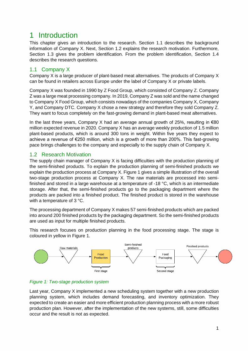
explain the production process at Company X. Figure 1 gives a simple illustration of the overall
two-stage production process at Company X. The raw materials are processed into semi-
finished and stored in a large warehouse at a temperature of -18 °C, which is an intermediate
storage. After that, the semi-finished products go to the packaging department where the
products are packed into a finished product. The finished product is stored in the warehouse
with a temperature of 3 °C.
The processing department of Company X makes 57 semi-finished products which are packed
into around 200 finished products by the packaging department. So the semi-finished products
are used as input for multiple finished products.
This research focuses on production planning in the food processing stage. The stage is
coloured in yellow in Figure 1.
Figure 1: Two-stage production system
Last year, Company X implemented a new scheduling system together with a new production
planning system, which includes demand forecasting, and inventory optimization. They
expected to create an easier and more efficient production planning process with a more robust
production plan. However, after the implementation of the new systems, still, some difficulties
occur and the result is not as expected.
2
The supply chain manager sees the following concrete problems that happen in the supply
chain:
1. Production planning takes too much time.
2. The frozen period1 in production plan is violated.
3. Inventory of the semi-finished products is too high or too low.
4. The inventory of the raw materials is too high or too low.
5. There are extra deliveries from suppliers which result in high cost.
Due to these problems, the supply chain manager is not satisfied with the current performance
of production planning. So we can state that Company X does not achieve the current
performance of the production plan.
We explain the performance of the production planning of Company X in two different
categories namely, performance regarding the product and performance regarding the
process. We explain the two categories below.
Product:
• The cost of the production plan execution: These costs are linked to materials,
machines, and staff. Also, costs due to backorders are part of this.
• Resource utilization: The supply chain department needs to take into account the
utilization. For example machine utilization.
• Stability of the production plan: Stability is the degree to which the production plan
is robust. In other words, the production plan should be changed as little as possible.
Process:
• Cost of production planning: These costs are linked to the number of hours a
production planner needs to make and maintain a production plan.
• Communication quality: This is the way the production planner communicates
changes to its stakeholders.
• The flexibility of production plan adjustment: The production plan should be able
to change to a certain extend.
These performance criteria can be linked back to the events that are currently happening in
the supply chain. For example, for resource utilization, we have machine utilization. Company
X wants to have sufficient utilization of the machines. Not achieving the desired performance
causes disturbances and uncertainties in the whole supply chain, from supplier to finished
product.
Before we go to the problem identification, which we explain in Section 1.3, we give three
definitions namely, production planning, production scheduling, and production planning and
control. This helps to have a better understanding of the definitions that are widely used in this
research. The paragraphs below explain the distinction between the meanings.
Production planning: production planning is an administrative process that takes place within
a manufacturing company. The goal of production planning is to establish an overall level of
output, which is called a production plan. To establish the production plan, production planning
needs to take into account the planned sales levels and also the company’s general objectives.
General objectives are, for example, profit, productivity, lead times, and customer satisfaction.
(Encyclopedia.com, 2020)
1 The frozen period is the period in which changes in the production plan should not occur.

3
Production scheduling: production scheduling is a process to create a production schedule.
The production schedule is derived from the production plan. Production scheduling is an
assignment problem that describes what quantity of an item that the company wants to produce
in a certain time frame. Also, scheduling is the problem of allocating machines to competing
jobs over time, subject to the constraints (Fera, Fruggiero, Lambiase, Giada, & Nenni, 2013).
A constraint is, for example, the total available machine time.
Production planning and control: According to Slack et al. (2013) production planning and
control is about the activities that attempt to merge the demands of the market and the ability
of the operation’s resources to deliver. Production planning and control provide the systems,
procedures, and decisions to merge the different aspects of supply and demand.
1.3 Problem Identification This section identifies the problem the
help of a problem cluster. Section 1.3.1
describes the problem cluster. From the
problem cluster, Section 1.3.2
describes the core problem. Section
1.3.3 measures the core problem and
compares it to the current situation.
Next, Section 1.3.4. describes the
research scope of this research.
1.3.1 Problem Cluster
Together with the Supply Chain
Manager and the production planner,
we investigate the relationships
between the current problems to find a
potential core problem. We make a
problem cluster to create a clear
overview of the problems. Figure 2
shows the problem cluster.
Next, we explain the problem cluster in
more detail.
1.3.1.1 Current planning systems are not efficient
The current production planning and scheduling systems are not efficient. The production
planning system gives a proposal for the quantities that need to be produced based on a
forecast and input parameters from the production planner or the demand planner. Some input
parameters, for example, the Minimum Order Quantity (MOQ), are not optimal. The MOQ is
the minimum quantity that needs to be ordered or in case of production planning the minimum
quantity that needs to be produced. For the processing in the first stage is the MOQ a half-day
or a full-day production. A full day means 16 hours of production on weekdays.
Next to the planning system, the scheduling system is also not efficient. Making changes in
the scheduling system takes a long time due to many calculations that need to be done by
hand.
1.3.1.2 Communication between stakeholders is not efficient
With the term communication, we mean the way production plans are communicated to other
stakeholders. The stakeholders are, for example, the supply chain manager, processing
Figure 2: Problem Cluster

4
manager, team leader processing, operators, and supply planning. The production planner
must communicate with each stakeholder in case of new product plans or changes in the
production plans. At the moment, it is not always clear to what extent new production plans
and changes are communicated with different stakeholders. This leads to information
asymmetry and causes disruptions.
1.3.1.3 Machine failures
For the frozen period, Company X has the following definition: The frozen period is the period
in which changes in the production plan should not occur. The reality is that changes occur in
the frozen period. One of the changes is due to machine failures. Machine failures occur
randomly and when it is not possible to fix the problem in a short time, the production planner
needs to change the production plan.
1.3.1.4 Disturbances due to raw materials shortages
Violation of the frozen period is due to shortages of raw materials. This happens when the raw
materials are not in time for production from an external warehouse or there are not sufficient
raw materials available. Almost all of the raw materials are stored at an external warehouse
which is 45 minutes’ drive from Company X. When there is too much time loss due to the raw
materials there is a chance that the production plan needs to change.
To decrease the downtime Company X has stored internal some “emergency” raw materials
for a few products. However, the production planner first needs to change the production plan
to produce these products. Also, future production plan needs to revise.
1.3.1.5 Forecast accuracy below the desired norm
Company X is using a program that calculates the forecast for all stock keeping units (SKUs).
However, demand has high uncertainty and it appears that the forecast accuracy is below the
norm of 70% accuracy.
1.3.1.6 The high cost of extra deliveries from suppliers
The current production planning leads to additional costs. Company X needs additional
deliveries from suppliers to sustain their plan because of the multiple consequences of the low
performance of the production plan. However, this leads to a higher cost because these orders
are not regular orders but extra orders. For extra orders, the suppliers charge additional costs.
1.3.1.7 The production planning takes too much time
The current time that a production planner needs for the process is too long. Some of the tasks
in this process are: making a production plan and schedule for the coming weeks, control the
production plan and changing the production plan if needed. Due to the overall low
performance of the production planning process, the production planner spends a lot of his
time on the process of planning. This time is at the expense of other tasks. Other tasks are,
for example, improvement projects to be more in control in the production plan and schedule.
1.3.1.8 Production plan constraints
To make a production plan, constraints are taken into account. Production plan constraints
are, for example, the available time for processing.
1.3.1.9 Scheduling constraints
The production planner has scheduling constraints. It is not possible to produce some products
directly after each other because of the allergen of the semi-finished products. Every product
has an allergen classification that is taken into account when scheduling. Also, the number of
available machines is a constraint. Each product is made on a special kind of machine and
there are not always enough machines available.

5
1.3.2 The core problem
From this selection, we choose problem number 14 “The production planning takes too much
time” as the core problem. This problem is for the supply chain department the most important.
The expectation of the supply chain department is when the time of the production planning
process reduces, the production planner is more in control of the production plan and have
time for other tasks such as improvement projects. This can eventually lead to a higher overall
performance of production planning because other problems can be tackled, such as problems
that are mentioned in the problem cluster.
1.3.3 Measurement of norm and reality
To have a clear overview of the core problem, we measure the norm and reality. Most of the
problems are linked to a key performance indicator (KPI). Company X keeps already track of
different KPI to evaluate the efficiency in the supply chain. However, these measurements do
not measure the core problem itself. To measure the core problem we need to define the cost
of time. We do this by measuring the number of full-time equivalents, also known as FTEs.
FTE refers to the number of hours worked by a single employee in a week. At Company X a
workweek of a full-time employee consists of a working week of 38 hours. So 1 FTE is 38
hours. The production planner executes production planning and scheduling. Currently, to
make and schedule a production plan and to maintain the plan takes a certain time. The
following norm and reality are established:
Norm: 0,5 FTE (19 hours)
Reality: 1 FTE (38 hours)
This means that the time to make, schedule, and maintain a production plan needs to decrease
by 50%. With this reduction in time, the production planner has more time for other tasks, such
as improvement projects. Next to this, it is possible for the production planner to be in control
of the production plan and can oversee potential problems earlier. This will also increase other
performances in the supply chain.
1.3.4 Research scope
This research is restricted to the production planning of semi-finished products, which is the
first stage in the overall production system. The first stage consists of 4 production lines namely
production line 11, 21, 31, and production line at Company Z. Company X has a two-stage
production system and therefore production planning in the first stage depends on the second
stage and the other way around. However, we do not cover the second stage, product
packaging, because of the different characteristics, the complexity of the two-stage production
system, and the time limitations for this research. The second stage, product packaging, is
closely related to the first stage. We use the second stage for retrieving data but we will not
explain this extensively. Also, the interaction between the first stage and the second stage is
important for improving production planning. We will look for opportunities to improve the
interaction between the two stages, however, we primarily focus on the first stage.
1.4 Research questions Section 1.3 explains the core problem. To execute the research, we formulate several research
questions. First, we describe an analysis of the current situation at Company X regarding
production planning. Second, we conduct a literature review to find literature for improving
production planning. Third, we formulate a solution design for improving production planning
at Company X. We implement this solution design at the Company X case. Last, we provide a
conclusion, give recommendations and explain possibilities for further research.

6
1.4.1 What is the current situation at Company X regarding production planning?
To find the causes of the core problem we will look at the current situation. First, we look at the
current supply chain of Company X and how production planning is integrated into the supply
chain. After this, we analyse the process of production planning. Lastly, we analyse the
relationship between key performance indicators and the production plan. At the moment,
there is no clear insight into what extent KPIs are related to the production plan and how the
KPIs influence the decision-making for the production plan. We have the following sub-
questions:
1. What is the supply chain design of Company X?
2. How does the first-stage production process of Company X look like?
3. What steps are currently taken by the production planner to make a production plan
and schedule?
4. What is the relationship between the current production plan and the KPIs of the supply
chain department?
1.4.2 What literature is available to improve production planning?
To formulate solutions, we conduct a literature review. Chapter 3 describes the literature
review.
We want to create a robust production plan. With a robust production plan, we mean that the
production plan is capable of performing without failure under a wide range of conditions
(Merriam-Webster, sd). First, we look at production planning in a two-stage production system.
We choose to look at a two-stage system instead of a single-stage system because we want
to know the interaction between these stages. Input in the first-stage depends on the
information of the second-stage.
Next, we look at the consideration of make-to-order and make-to-stock in the food processing
industry. In the food processing industry, we deal with high market standards, such as high
delivery performance, and shelf life constraints. Therefore, we want to find the impact of these
considerations on production and production planning.
Next to the production plan, we want to find a feasible schedule in a sequence-dependent
setup environment. Lastly, we want to measure production planning. Therefore, we look for
performance measurements in production planning.
5. How to develop a robust production plan in a two-stage production system?
6. How can we incorporate make-to-order and make-to-stock decisions in production
planning?
7. How to create a production schedule with sequence-dependent setups?
8. How can the performance of the production planning be measured?
1.4.3 How can we improve production planning based on the literature?
In Chapter 4 we present a solution to improve production planning at Company X based on
the literature that we explain in Chapter 3.
1.4.4 How can we implement the solution design for the Company X case?
In Chapter 5 we implement the solution design of Chapter 4 for the Company X case. We
formulate a work way to implement the solution design for Company X. We also look at the
data availability for the solution design.
1.4.5 What are the conclusion and recommendations of this research?
Based on the solution that we present in Chapter 4 and Chapter 5 we will formulate the
conclusions and the recommendations of this research.

7
2 Analysis of the current situation This chapter describes the analysis of the current situation based on the research questions
that are formulated in Section 1.4. The chapter starts with describing the current supply chain
design of Company X in Section 2.1. After this description, Section 0 describes the production
process in the first stage to give more context to production planning. Section 2.3 explains the
current systems that the supply chain department uses. Next, Section 2.4 describes the current
process of production planning. Section 2.5 explains the current KPIs and performs an analysis
based on the data of the current situation. Last, Section 2.6 provides a conclusion.
2.1 Supply chain design of Company X In this section, we analyse the supply chain design of Company X. We explain the relationships
between the activities and the processes. Next, we explain the use of the current systems in
the supply chain department. When describing the systems we focus on systems for production
planning.
2.1.1 Supply chain footprint
A supply chain footprint refers to the positioning of operation activities in terms of the value
chain. The supply chain footprint identifies different operational activities and relationships.
Company X Foodgroup consists of multiple companies that produce products for Company X.
The importance of this footprint is to find the scope of production planning at Company X.
Before positioning of the operational activities in the supply chain, we explain the corporate
structure of Company X Foodgroup. As mentioned in Section 1.1, Company X Foodgroup
consists of Company X, Company Y, and Company DTC. Company Z was also part of
Company X Foodgroup but was sold in 2019. However, the name of Company Z is still being
used because production facilities of Company Z are used for operations of Company X.
Section 1.2 illustrates a simple two-stage production system. However, this illustration does
not give a complete overview of Company X. To make this overview complete we need to
elaborate on Company Y, Company DTC, and Company Z. Company Y, Company DTC, and
Company Z can be seen as an intercompany. They produce products that are sold through the
parent Company X. Most of the products that they produce are semi-finished products (first-
stage) and are transformed to finished products by Company X (second-stage). Company DTC
and Company Y make semi-finished products that cannot be made by the processing
department of Company X. These companies operate mostly individually and deliver products
to Company X.
8
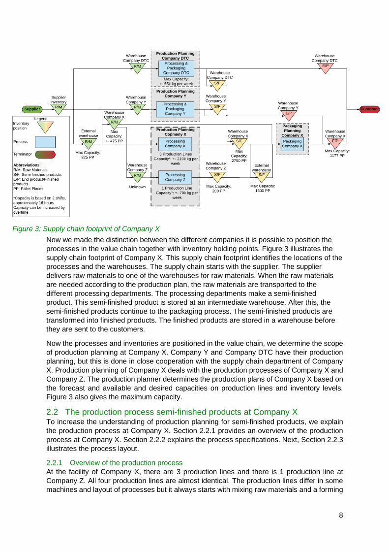
Now we made the distinction between the different companies it is possible to position the
processes in the value chain together with inventory holding points. Figure 3 illustrates the
supply chain footprint of Company X. This supply chain footprint identifies the locations of the
processes and the warehouses. The supply chain starts with the supplier. The supplier
delivers raw materials to one of the warehouses for raw materials. When the raw materials
are needed according to the production plan, the raw materials are transported to the
different processing departments. The processing departments make a semi-finished
product. This semi-finished product is stored at an intermediate warehouse. After this, the
semi-finished products continue to the packaging process. The semi-finished products are
transformed into finished products. The finished products are stored in a warehouse before
they are sent to the customers.
Now the processes and inventories are positioned in the value chain, we determine the scope
of production planning at Company X. Company Y and Company DTC have their production
planning, but this is done in close cooperation with the supply chain department of Company
X. Production planning of Company X deals with the production processes of Company X and
Company Z. The production planner determines the production plans of Company X based on
the forecast and available and desired capacities on production lines and inventory levels.
Figure 3 also gives the maximum capacity.
2.2 The production process semi-finished products at Company X To increase the understanding of production planning for semi-finished products, we explain
the production process at Company X. Section 2.2.1 provides an overview of the production
process at Company X. Section 2.2.2 explains the process specifications. Next, Section 2.2.3
illustrates the process layout.
2.2.1 Overview of the production process
At the facility of Company X, there are 3 production lines and there is 1 production line at
Company Z. All four production lines are almost identical. The production lines differ in some
machines and layout of processes but it always starts with mixing raw materials and a forming
Figure 3: Supply chain footprint of Company X

9
machine. The process ends with freezing and bulk packaging. Some products do not require
coating or frying but do require cooking.
Figure 4: Simple overview of the production process at Company X
Figure 4 illustrates the process steps at Company X. First, the raw materials are mixed. The
main component in semi-finished products is soybeans. The output after mixing is called
dough. When mixing is complete, the dough is transported to a forming machine. This machine
makes a certain form. For example, plant-based hamburgers have a circular form. Next, the
product is coated, fried and/or cooked according to the product recipe. The last step in
production is freezing, which cools down the product to -18°C.
The final step is to pack the products in crates and pack the crates on a pallet. Finally, the
pallets are stored at the intermediate storage before the packaging department uses the
products. The transfer of semi-finished products to the packaging department has a lead time
of at least 3 days. This is because the products undergo a laboratory test. This laboratory test
is for a check on any hazardous bacteria. When a semi-finished product has a positive release
it is available for the packaging department.
2.2.2 Process specifications
The semi-finished products are produced in batches sizes that contain a half-day or a full-day
production. A full-day production gives around 15,000 kg of semi-finished products depending
on the product specifications. These batch sizes are relatively large because of the cleaning
time between production. Semi-finished products are produced according to an allergen
scheme. We illustrate the allergen scheme in Appendix A: Allergen flow scheme. Switching to
a different semi-finished product that is not part of the allergen flow scheme requires cleaning.
Cleaning the production line and the processing department takes around 5 to 6 hours and this
is taking place every night after two production shifts.

10
2.2.3 Production process layout
Most of the semi-finished products have a preferred production line and some have a fixed
production line. Most of the time the products are scheduled on the preferred line. This
preference is because of efficiency reasons. For example, semi-finished products produced
on a particular line have less waste in comparison with other production lines due to newer
machines. Products with a fixed production line are produced on this line because of technical
reasons. Figure 5 illustrates the layout of the processing department. Between the different
machines in the production line, there are curved arrows. These arrows represent the belts
between the machines. For example, on production line 31 there is a curved flow line between
the frying and cooking. Some products cannot make this curve and therefore it is not possible
to produce this product on the production line.
Figure 5: Production process layout
2.3 Systems for production planning In this section, we explain the systems that are used for production planning. Section 2.3.1
explains the different systems that are used in the supply chain department and production
planning. Next, Section 2.3.2 describes cyclic production planning at Company X.
2.3.1 Systems used for supply chain and production planning
The supply chain department of Company X is using three different systems namely, an
enterprise resource planning (ERP) system, an inventory management system, and a

11
production planning and scheduling system. The inventory management system and the
production and scheduling system are implemented last year and they are currently still
implementing additional features and making improvements to the systems. The three systems
respectively are explained along with the different connections between these systems. These
systems play an important role in production planning. First, Section 2.3.1.1 explains the ERP
system. Furthermore, Section 2.3.1.2 explains the inventory management system. Next,
Section 2.3.1.3 describes the production planning and scheduling system.
2.3.1.1 ERP system
The first system is an enterprise resource planning (ERP) system, named Fobis. Fobis is used
to manage and integrate the important parts of the company, so not only the supply chain
department. The ERP program is important for the company because it helps them by
integrating all the processes that are needed to run the company with a single system. Fobis
is mainly used for processing and tracking customer orders, purchasing orders, production
orders and real-time inventory control.
2.3.1.2 Inventory management system
Next to the ERP program, the supply chain department uses an inventory management system
named Slim4. Slim4 is a program that is used for forecasting, demand planning, supply
planning and inventory optimisation. Slim4 is for a large part a stand-alone system, however,
it is also connected with Fobis to get input about the customer orders, inventory levels,
outstanding purchasing orders and production orders. Also, Slim4 gets input from a database
that contains historical data and the master data about every product, such as lead times,
MOQs and lot sizes. Slim4 uses this information to determine forecasts for every SKU based
on the forecast of the finished products. This can be seen as a top-down process. Forecast for
finished products will lead to a forecast for semi-finished products and eventually leads to a
forecast for raw materials.
Based on the forecast Slim4 gives a purchasing and production advice to optimize the
inventory and prevent non-deliveries. Non-deliveries means a failure to deliver a finished
product to the customer. It is a very extensive program in which a lot of parameters can be
used. For example, SKUs can be grouped or can have different production strategies such as
make-to-order (MTO) or make-to-stock (MTS). However, Slim4 does not take into account the
total capacity of production lines and inventory capacity.
2.3.1.3 Production planning and scheduling system
The third program that is used is Rob-Ex, a production planning and scheduling system. Slim4
is connected with Rob-Ex to advise about production plans. For example, based on the
forecast, Slim4 advises on the quantity that needs to be produced of a semi-finished product
and gives the due date. This advice is turned into a production order which is placed in the
ERP system Fobis. This production order is now visible in Rob-Ex where the final production
plan is determined and scheduled. However, it is also possible to plan products not based on
the direct advice of Slim4. The plans can also be created from external input and implemented
into Rob-Ex. Section 2.3.2 explains a cyclic production plan that is used by production
planning.
When the final production plan is established, Slim4 calculates the required quantities of raw
materials that are needed to execute the production plan. Based on this purchasing orders are
generated and supply planning orders the raw materials by suppliers. Also, the production
schedule is translated to production orders in the ERP system. To illustrate, Figure 6 gives a
simple overview of the connections between the different systems and which processes take
place. The process of the systems could be visualised as an ongoing circle.

12
Figure 6: Relationships between the systems
2.3.2 Cyclic production plan
Section 2.3.1 explains the different systems that the supply chain department uses. Production
plans are based on the production advice of Slim4 or from an external input. The supply chain
department also uses production plans that are created in Excel. This production plan is based
on a cyclic production plan. The cyclic plan is a fixed plan that repeats every four weeks. The
cyclic production plan is based on a demand forecast from Slim4, batch sizes, capacity, and
line speeds. The batch sizes are based on a half or full-day production capacity. Table 1
illustrates an example of a 4-week cyclic production plan.
Product Week 1 Week 2 Week 3 Week 4 Total
55750 15,000 kg 0 15,000 kg 0 30,000 kg
55760 0 10,000 kg 0 10,000 kg 20,000 kg
55770 0 0 10,000 kg 0 10,000 kg
Table 1: 4-week cyclic production plan
A cyclic production plan has several advantages according to Company X. It reduces the
complexity of creating a production plan, it reduces planning costs and it could give more
stability in the supply chain. However, cyclic production plans need to be revised after a certain
period and there is not a procedure for this.
2.4 Current production planning Production planning is an administrative process and it is a function of establishing an overall
level of output which is called a production plan. The production planner is in charge of
production planning. In this process, several actions are taken by a production planner for
establishing a production plan. Section 2.4.1 explains the current process of production
planning. Business Process Modelling Notation (BPMN) (OMG, 2010) is used to make a
graphical representation of the process. BPMN is a standardization for describing and
visualizing business processes. Next, Section 2.4.2 explains production scheduling at
Company X.
2.4.1 Production planning overview
Production planning is executed every week. Every week a production plan is created for
week+4. For example, if the current week is week number 20, the production planner makes
a production plan for week 24. In this process, several actions are taken by the production
planner to establish a production plan. Figure 7 illustrates the BPMN model of production
planning. This model has two subprocesses which are illustrated in Figure 9 and Figure 10.
We divide the explanation into 4 subsections. Section 2.4.1.1 explains the check of the

13
production advice. Section 2.4.1.2 explains the planning methods. Section 2.4.1.3 explains the
capacity check. Section 2.4.1.4 provides a conclusion.
2.4.1.1 Check production advice
Figure 7, underneath Section 2.4.1.4, illustrates all the steps of the production planner. The
first task in production planning is to check the production advice that is given by Slim4 in Rob-
Ex. In this advice, the quantity of the semi-finished (S/F) product is given and also a due date
and the plan window. The due date is the date before which the order needs to be produced.
If it is produced after this date there is a likely chance that the semi-finished product will go out
of stock in a short time. The plan window is the date when there are sufficient raw materials to
produce. So the due date and plan window gives the time interval in which production can and
should take place. The check of the production advice is done to find any urgent production
orders, so with a due date that is earlier than week+4. When there is an urgent order the
production planner will choose if the product should be made earlier than week+4. This means
that the frozen period of the production plan is violated, so most of the time this will not be
done.
2.4.1.2 Choose planning method
After the checks, the production planner chooses a method to create a production plan. The
production planner can choose between the cyclic planning and planning based on Slim4.
Each plan method has both its advantages and disadvantages. With the cyclic plan method
the semi-finished products, quantities and schedule are already determined and only have to
be loaded into the planning system which is less time-consuming. However, because the
products and quantities are already determined it is more difficult to change this plan in the
systems. Production advice of Slim4 has the advantage that the production planner can create
a production plan that is more flexible but it is also more time-consuming. The production
planner mentioned that both methods are for now not optimal.
When the cyclic production plan is used as a planning method it will be loaded into the planning
system. The cyclic production plan does not cover the capacity of a full week, so there is some
capacity left for products that are not in the cyclic production plan for that week. Therefore the
production planner waits a day and Slim4 will calculate new production advice. Calculation of
new production advice is done through the night and therefore the production planner needs
to wait until the next day. The next day Slim4 has generated new production advice for certain
semi-finished products and the production planner will loop through these products in Slim4 to
see what impact the advice has on inventory in combination with the forecast. This is modelled
as a subprocess in Figure 9 and loops until all the product advices are checked.
This subprocess is executed because the production advice is not always in line with the real
situation. This can have multiple causes. For example, the actual due date is later or earlier.
This means that production needs to take place earlier than the suggested due date. Also, the
given forecast is not accurate and therefore it needs a check to validate if there are no strange
deviations. The production planner first looks if the advised quantity is sufficient. It is sufficient
when it covers demand with a maximum of 4 weeks of inventory. If not, the production planner
changes the advised quantity of the products and also the underlying components. This task
is done manually. This means that the production planner needs to determine the new quantity
that needs to be produced. Also, the quantity of underlying components needs to calculated
again. If the quantity is sufficient then the production planner checks the forecast and the input
parameters. For example, if the forecast deviates too much, the production planner can adjust
the forecast. After this, the production planner will choose if the product needs to be planned
in week+4 or not. Input parameters are MOQ and IOQ. When the forecast is low it is not
efficient to have a high MOQ because leads to higher inventories.

14
Scheduling is modelled as a subprocess and it is a loop until all the products are scheduled.
Figure 10 illustrates this subprocess. Scheduling is done based on the constraints, preferences
of the processing department and if it is produced at Company Z facility or Company X facility.
A fixed number of products are produced at the Company Z facility or the Company X facility.
Section 2.4.2 provides more information on production scheduling at Company X.
When the production planner chooses to plan based on Slim4 advice the production planner
does not need to wait till the next day and can start to plan. The production planner will check
for every semi-finished product the development in Slim4. This is the same subprocess as
explained in the paragraph above. However, now more products need to be checked so the
number of loops is larger in the subprocess. This step requires a lot of time. After the checks
to products are scheduled.
2.4.1.3 Capacity check
When the production plan is determined and the products are scheduled on the production
lines at Company Z or Company X, a total overview is generated. This overview gives the
amount of kg that is produced in week+4. This amount of kg is checked in the capacity plan of
Company X. The capacity plan gives for every week the forecasted required amount of kg, the
currently planned amount of kg and the impact on the inventory development. The operational
management set the bandwidth of total kg inventory of semi-finished products between the
750,000 and the 800,000 kg. This range is based on following starting points: target of 98%
delivery performance and 3 to 4 weeks of safety stock per semi-finished product. Aggregating
this safety stock minus the forecasted sales gives this range. In this research, we refer to this
range as the capacity plan. The objective is to stay in between this range. So when the total
amount of kg of the production plan of week+4 does violate the capacity plan, the production
plan is changed to a certain extent. Therefore, the production planner needs to check again if
it is possible to change the quantities of some semi-finished products.
When the production plan is according to the capacity plan, then the production plan and
schedule is communicated with the different stakeholders, such as the Manager Processing
and the team leaders of the processing departments. When the schedule is sufficient, then
production planning is finished. If it is not sufficient some changes will be done in the schedule
until the schedule is sufficient. A schedule is not sufficient when, for example, a product is
scheduled after a product with a different allergen when there are better options. This results
in a long setup time.
2.4.1.4 Conclusion of production planning
Both production plan methods have time-consuming tasks in the process. The subprocess of
checking every semi-finished product development is time-consuming. This is because the
production advice of Slim4 is not always reliable. It is not always reliable because Slim4 does
not take into account capacity, due dates can appear to be earlier or later, and the forecast is
not accurate.
The production plan needs to take into account the capacity of Company X. It is difficult to
control this capacity level because there are no real-time insights from systems and the
systems do not take into account the capacity level. Therefore the capacity is manually
controlled by checking the production plan every time. According to Company X, the cyclic
production plan can help in controlling the capacity. However, the cyclic production plan is not
so extensive that takes capacity into account.
Choosing a planning method is also challenging for the production planner because both plan
methods have their advantages and disadvantages. There is no fixed decision rule so the
production planner needs to choose based on his interpretation. For the production planner,

15
the ideal situation is a fixed planning method where the production planner does not need to
validate every decision each time. Also, preferably, the planning method needs to take into
account constraints such as the capacity level or give insight into the capacity level.
The current production planning does not give insight into the impact of the production plan.
Insights in inventory development, capacities and cost are hard to determine and also time-
consuming. Section 2.4.2 explains some KPIs that are used in production planning.

16
Figure 7: Production planning process
Figure 8: Legend
Figure 10: Subprocess 2, scheduling
Figure 9: Subprocess 1, Check S/F
17
2.4.2 Production scheduling
Production scheduling is part of production planning. After a production plan is set for week+4,
the production planner makes a schedule for the production lines. The production planner
takes the following into account when scheduling:
1. Allergens. Semi-finished products are scheduled based on allergen combinations to
prevent allergen contamination. It is only possible to follow a specific order. This
allergens order is illustrated in Appendix A. Switching to an allergen that is not in the
specified order requires a cleaning. Cleaning the production line takes 5 to 6 hours.
2. Within these allergen combinations, semi-finished products are also categorized on
product characteristics. For example, round formed products are categorized as “balls”
and hamburgers as “patty”. Switching between these products categorizations takes
additional setup times because a switch between machines is needed.
3. Preferences of the processing department. The processing department has
preferences about the sequence of production and allocations of the products on a
production line.
The production planner is required to take allergens (point 1) into account. Point 2 is important
for efficiency. The production planner wants to have a schedule with the highest efficiency, so
without long setup times. Point 3 is not specifically necessary but the production planner tries
to fulfil all the desired preferences.
Section 2.4.1 describes the process of production planning. In this process, the schedule is
validated by different stakeholders. Stakeholders have the opportunity to advise on changes
in the schedule. The production planner decides whether to accept these changes or not.
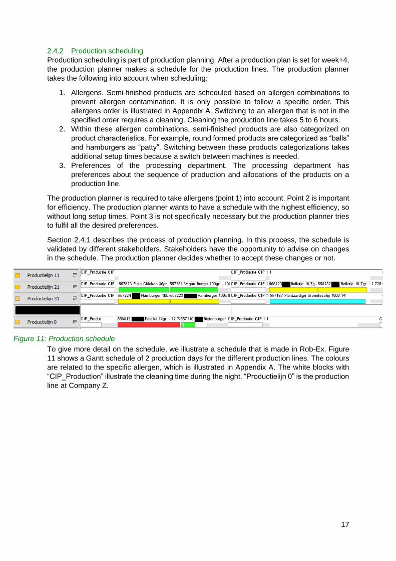
To give more detail on the schedule, we illustrate a schedule that is made in Rob-Ex. Figure
11 shows a Gantt schedule of 2 production days for the different production lines. The colours
are related to the specific allergen, which is illustrated in Appendix A. The white blocks with
“CIP_Production” illustrate the cleaning time during the night. “Productielijn 0” is the production
line at Company Z.
Figure 11: Production schedule

18
2.5 Key Performance Indicators Key performance indicators are performance measurements to evaluate a business activity.
Production planning has also KPIs to evaluate the process. Section 2.5.1 describes the current
KPIs for production planning. Section 2.5.2 explains the relationships between KPIs and the
production plan.
2.5.1 Current KPIs for production planning
The supply chain department has several KPIs to evaluate certain processes within the supply
chain. The most important objective for the supply chain is the delivery performance. The
delivery performance depends on a lot of different processes of which production planning is
one. When a semi-finished product is out of stock the packaging department cannot pack a
finished product which leads to non-delivery. This results in lower delivery performance.
Therefore, it is important that production planning and packaging planning are well aligned.
Another important KPI that influences the supply chain department is the forecast accuracy of
finished products. In production planning forecasts are used by Slim4 to give production advice
to optimize inventory and reduce chances of non-deliveries. Therefore, it is important to have
a good forecast accuracy. However, the forecast accuracy is not very good at the moment. A
forecast influences the production advice of Slim4 and the KPIs. From week 1 to week 20 in
2020 the average forecast accuracy was 50%. This means that the forecasted quantities
deviate from the real ordered quantity with on average 50%. The production planner takes this
forecast accuracy into account but this is difficult because the forecast is measured for finished
products. Forecast accuracy for semi-finished products is not possible at the moment. The
supply chain department is investigating if it would be possible to also measure the forecast
accuracy for semi-finished products. Measuring the forecast accuracy for semi-finished
products will give a better indication in the reliability of the production advices of Slim4.
Within production planning, there are two KPIs used by the production planner. One KPI that
is reported weekly and one that is reported daily. Daily, the production planner reports the
percentage of planned versus the real output. This could influence production planning
because with a low percentage
the production plan may need
to revise or rescheduled.
Rescheduling occurs 2 to 3
times a week depending on the
situation.
Every week the total inventory
of semi-finished products in
days is displayed. This is the
coverage of the inventory in
days relative to the forecasted
orders. Figure 12 illustrates this
KPI. The target is to have a
coverage level between 20 and
29 days. Figure 12: KPI Inventory in days

19
2.5.2 Relationship between KPIs and the production plan
From the current KPIs, it is not possible to
see the direct influence on the production
plan. The delivery performance is an
important KPI but the supply chain
department has no performance measure
to see the influence of the production plan
on the delivery performance. Therefore we
do this performance measure with the
available data of the supply chain
department. From the current information,
it is possible to find the percentage of non-
deliveries that were caused by an out of
stock of semi-finished products relative to
the ordered volume. Figure 13 illustrates
the percentage of non-deliveries that were
caused by an out of stock of semi-finished
products relative to the ordered volume. At the beginning of the year, a lot of non-deliveries
were caused by out of stock of semi-finished products produced at Company X or Company
Z. However, from week 10 it is very stable and below 1%. This is because the production
planner evaluates the production plan and checks the development of the inventory of semi-
finished critically. Also, the target to have a safety stock of 3 to 4 weeks for semi-finished
products helps to prevent non-deliveries.
2.6 Conclusion The production system of Company X consists of a two-stage production system. The first
stage is the processing department which makes semi-finished products. The second stage is
the packaging department which makes finished products. Production planning at Company X
is concerned with the planning of semi-finished products at Company X and the facility of
Company Z. For production planning, three different systems are used which are connected.
The main systems that are used for production planning are Slim4 and Rob-Ex.
Every week the production planner will make a production plan for week+4. To create a
production plan, the production planner can choose between two plan methods. The two plan
methods are a cyclic production plan or a production plan created from the advice of Slim4.
The cyclic production plan is an almost fixed production plan which is easy to control and plan.
However, because it is fixed it is hard to change the plan. Planning based on Slim4 is more
flexible because the production planner can create a plan from scratch and can, therefore, take
into account preferences from stakeholders. However, to create this plan it is also time-
consuming.
In the process of production planning, the production planner always needs to take two things
into account. The inventory development and forecast of individual semi-finished products and
the total inventory development of all semi-finished products, also known as the capacity plan.
The check of individual semi-finished products is done in Slim4. Advises from Slim4 are not
always reliable because of a forecast accuracy of 50%. Therefore the advices need to be
checked. The capacity plan cannot be integrated into Slim4 and therefore Slim4 does not take
into account capacity. This check is done in a separate file and therefore it is difficult and time-
consuming to make a production plan that takes into account the capacity plan.
The goal for the production planner is to prevent non-deliveries that are caused by having an
out-of-stock of semi-finished products that are produced at Company X or Company Z. To
Figure 13: Volume non-deliveries relative to ordered volume
0,00%
0,50%
1,00%
1,50%
2,00%
2,50%
3,00%
3,50%
4,00%
4,50%
5,00%
1 2 3 4 5 6 7 8 9 10 11 12 13 14 15 16 17 18 19 20
Week
Non-deliveries in kg relative to total ordered volume in kg in percentage

20
prevent non-deliveries it requires more time to critically check inventory and forecast for every
semi-finished product. In combination with the capacity plan and controlling the KPI inventory
in days, production planning is very time-consuming.

21
3 Literature review This chapter reviews the literature for the research questions formulated in Chapter 1. Section
3.1 reviews the literature for a two-stage production system. Section 3.2 explains the
considerations in make-to-order and make-to-stock in the food processing industry. Section
3.3 provides literature for scheduling with sequence-dependent setup. Section 3.4 defines
performance measures for production planning that are found in the literature. Last, Section
3.5 provides a conclusion of the chapter.
3.1 Two-stage production planning Production planning at Company X needs to take into account the two-stage production system
with capacitated intermediate storage between the stages. The output from the first stage is
input for the second stage and the other way around. We divide the literature of this section in
3 subsections. Section 3.1.1 explains the literature about food processing systems. Next,
Section 3.1.2 describes literature about two-stage food processing systems. Last, Section
3.1.3 explains literature about hierarchical production planning.
3.1.1 Food processing systems
Food processing systems are widely analysed and described by researchers as Akkerman,
Soman, and Donk. Donk presents a framework for determining the customer order decoupling
point (CODP) in the food processing industry (Donk, 2001). This framework helps managers
to make decisions and find influences of the factors in changing the decoupling point. Van
Wezel, Donk & Gaalman (2006) review the planning flexibility bottleneck in the food processing
industry. Potential profits are lost because organizations do not know how to respond to
unexpected events. They present a framework that analyses unexpected events in planning.
Also, the framework presents a way to reason about reconsiderations of planning decisions
within a planning hierarchy.
3.1.2 Two-stage food processing systems
Akkerman, Donk, and Gaalman (2007) describe the influence of capacity- and time-
constrained intermediate storage in two-stage food production systems. Perishable products
and shared resources, such as storage tanks, are characteristics that suggest the presence of
capacity- and time-constrained intermediate storage. Time constraints occur when the
products have a short shelf-life. In their research, the researchers describe a situation with the
presence of capacity- and time-constrained intermediate storage in a two-stage production
system. The first stage concerns a batch process. Batch processing is used for efficiency
reasons and technical reasons. Efficiency reasons are, for example, minimizing setup-times.
Technical reasons in the processing are often concerning non-discrete products and
processing technologies that implies the need for batching. The researchers present a cyclic
scheduling approach for the first stage. Cyclic scheduling is often used in flow lines with limited
intermediate storage (Akkerman, Donk, & Gaalman, 2007). Also, it is an attractive approach
because it will periodically supply different intermediate products to the second stage of the
production system. Soman, Donk, and Gaalman (2004) described earlier an approach for
economic lot scheduling with shelf life considerations. In this approach, the researchers
provide a procedure to find the common cycle time which takes shelf life into account. The
cycle time is from the procedure of Doll and Whybark (1973). This cycle time is modified to
take into account shelf life considerations.
3.1.3 Hierarchical production planning
Hierarchical production planning in a two-stage production system is also a well-described
topic in production planning. Bitran et al. (1982) describe this two-stage hierarchical production
planning (HPP). HPP model provides a hierarchy of decisions that have to be made. Aggregate
decisions (e.g. strategic and tactical) are made first and lay down constraints for making more

22
detailed (operational) decisions. For a complete description of HPP see Bitran et al. (1982).
Tsubone et al. (1991) elaborate on HPP in a two-stage system by analysing the relationship
between the production planning rules and the role of buffer inventory level in terms of
production system performances.
Aghezzaf et al. (2011) use the HPP model to propose a production planning approach. HPP
approaches typically consider holding costs at the aggregate level and setup cost at a detailed
level. However, in the proposed production planning approach this is not the case. The first
stage is considered as the aggregate level and the second stage as the detailed level which is
disaggregated with a coupling plan that connects the two planning levels. Setup costs in the
first stage are significantly higher than in the setup cost in the second stage, which is taken
into account. Also, the demands of semi-finished products in the first stage is relatively stable
due to aggregation and therefore a cyclic planning model is proposed. The researchers use
the procedure of Doll and Whybark (1973) to find a fundamental cycle period. The fundamental
cycle period is the length of a single cycle. Also, this procedure gives the production
frequencies of each semi-finished product. Together with the fundamental cycle period and the
production frequencies, it is possible to determine the total cycle length.
Earlier, Aghezzaf and Landeghem (2002) present a two-stage production model that is not
based on HPP. The first stage is a processing production system and the second stage a job-
shop production system. The two stages are decoupled with an intermediate warehouse. The
inventory policy at the intermediate warehouse is determined based on the semi-finished
products’ demands behaviour. This research is not to propose a new heuristic but use the
available results reported in the literature to achieve excellent performance in solving the case
described in the research.
The objective of the proposed models is to minimize cost for production while maintaining
target performance. However, in production planning, the input parameters can be uncertain.
Input parameters such as demand and production. Data uncertainty can be taken into account
by applying robust optimization (Rahmani et al., 2013). The researchers present a model for a
multi-period multi-product multi-machine two-stage production system. The researchers use
robust optimization to create a robust production plan that is less sensitive to the change in the
uncertain data.
3.2 Make-to-order and make-to-stock in the food processing industry In the last decades, food processing industries are expected to deliver a greater variety of
products and meet higher logistical demand while keeping costs as low as possible. Therefore,
food processing companies are looking for flexibility to deal with these market demands. As a
consequence, food processing companies operate often under a hybrid MTO-MTS strategy
(Soman et al., 2004a). MTO systems offer a high variety of customer-specific products which
are typically more expensive. Production planning focus on customer orders. On the other
hand, MTS systems provide a low variety of customer-specific products which are typically
less expensive. In this system, production planning focusses on anticipating the forecasted
demand (Soman et al., 2004a). The main problem in the MTS system is inventory capacity, lot
sizing, and demand forecasting. According to Soman et al. (2004a), many previous articles
use simplistic rules to tackle issues in MTO/MTS. Therefore, they provide a hierarchical
planning framework for managing main problems in a combined MTO-MTS system. This
hierarchical framework encourages the use of the customer order decoupling point to make
MTO/MTS decisions. The customer order decoupling point distinguish order-driven activities
and forecast driven activities and it is the main point from which deliveries to customers are
made. The concept of the customer order decoupling point in the food processing industry is
extensively described by Van Donk (2001). The decision level for MTO/MTS is often in the

23
second stage of the production system where semi-finished products are disaggregated into
multiple different finished products variations.
Later, Soman et al. (2006) describe a hybrid MTO-MTS production situation with capacity
restrictions and stochastic demand. In this article, they compare four different dynamic
scheduling methods for a combined MTO-MTS situation. First, a target cycle time is pre-
calculated by using an economic manufacturing quantity or the procedure described by Doll
and Whybark (1973). To deal with demand uncertainty safety stocks and order up-to-levels
are pre-calculated based on the mean and standard deviation of the demand. After the
determination of the target cycle times, a scheduling heuristic is used to find the sequence of
production. The methods perform well for pure MTS situations but not necessarily for hybrid
MTO-MTS situations.
Soman et al. (2007) describe a case study for capacitated planning and scheduling for
combined MTO-MTS production in the food industry. They use the framework for combined
MTO-MTS production situation of Soman et al. (2004a). Additionally, they identify areas of
improvements and suggest analytical decision aids. According to Soman et al. (2007), demand
variability analysis forms the main activity to segregate MTO and MTS products. Companies
often categorise products into either A, B, or C categories. In category A are MTS products
while in the B and C category are MTO items. However, the researchers find this too simplistic.
They describe an analysis by looking at the average weekly demand and variability. Typical
MTO candidates are products with low set-up times, products with high holding costs,
customized products, and highly perishable products. MTO and MTS decisions are
strategically orientated and are complicated because of the complex trade-offs between
demand and product-process characteristics.
3.3 Sequence-dependent setup scheduling Scheduling in the food processing industry is a challenging task. Food processing industry
deals with sequence-dependent setups due to the required cleaning times between different
product families. Also, within product families there exist additional sequence-dependent
setups. Section 3.2 already reviews the hybrid MTO-MTS production systems described by
Soman et al. (2006, 2007). They give insight into scheduling methods for MTO-MTS production
systems. However, these researchers do not provide a detailed method for sequencing.
Gupta and Magnusson (2005) describe a capacitated lot-sizing and scheduling problem
(CLSP) with sequence-dependent setup costs and setup times. When one or more machines
are used to meet forecasted demand for multiple products over multiple periods encounters a
CLSP. CLSP with sequence-dependent setup times is related to the travelling salesman
problem and the vehicle routing problem and these problems are NP-hard (Gupta &
Magnusson, 2005). Problems that are NP-hard are difficult to solve and have long
computational times when the problem increases. Therefore, they provide next to an algorithm
also a heuristic to make the CLSP more practical. The goal of the heuristic is to find a near-
optimal solution that minimizes cost with consideration of capacity.
The well-known travelling salesman problem is a popular heuristic for sequence-dependent
scheduling. Ozgur and Brown (1995) provide a well-described procedure to find a near-optimal
solution for sequence-dependent scheduling. The travelling salesman heuristic consists of two-
stages. In the first stage, a changeover setup time matrix is used to cluster product families
and sequence the products within the product families. The second stage determines the
sequence of the product families. The heuristic can quickly find good solutions to the
scheduling problem.
24
Group scheduling of product families is also described by Gupta and Chantaravapan (2008).
They use the total tardiness as a performance measure for scheduling. First, they apply a
greedy heuristic to generate an initial sequence. After this, the sequence is improved by
applying a swap heuristic or simulated annealing. The swap heuristic is recommended for
problems with a few families, tighter due dates, a large number of products and/or large family
setup times (Gupta & Chantaravarapan, 2008). In other cases, simulated annealing is the
recommended option.
Other heuristics that are described for sequence-dependent scheduling are local search
heuristics. Crauwels et al. (1997) investigate the performance of several local search
heuristics. They start by testing the “standard” version of each method and improve the
methods if the solutions are not of sufficiently high quality. The local search heuristics that they
use are neighbourhood search, simulated annealing, threshold accepting, and tabu search.
Simulated annealing, threshold accepting and tabu search all generate solutions of high
quality.
3.4 Production planning performance Production planning has certain objectives. To measure these objectives it is important to have
performance measurement. Section 2.4.2 explains the current key performance indicators.
The production planner takes into account the delivery performance and the inventory in days
of semi-finished products. At the moment there are no other KPIs that measure production
planning and the production plan. To find potential performance measures for production
planning the performance measures of the models in Section 3.1 are described and analysed.
The different models described in Section 3.1 have a particular objective function to improve
particular performances. HPP models are mostly cost-based (Tsubone, Matsuura, & Tsutsu,
1991) and aim to minimize the total cost. Total cost is an important performance measure but
it does not capture all the effects of production planning on the production performance. For
example, opportunity loss due to capacity.
This is also partly the case in the model of Aghezzaf et al., (2002, 2011) but they take service
level into account. Tsubone et al. (1991) use the following four performance measures: unfilled
rate, the average inventory levels, the ratio of set-up time to total processing time, and the
deviation in production rate. Rahmani et al., (2013) also take total cost as performance
measures. However, the total cost is extended with regular cost and overtime cost,
subcontracting cost, backorder cost, labor cost, hiring cost, and downsizing cost.
3.5 Conclusion Akkerman et al. (2007) described a model that takes the influences of capacity- and time-
constrained intermediate storage into account in a two-stage food production system. The first
stage is a batch process which has multiple advantages. In a batch process, a cyclic schedule
is often used.
Additionally, a widely described model for production planning in a two-stage production
system is an HPP model. An HPP model gives divides the decisions into aggregate decisions
(i.e. strategic and tactical level) and detailed (i.e. operational) decisions.
Aghezzef et al., (2011) use the HPP model to propose an alternative production planning
approach in a two-stage system. The first stage is considered as the aggregate level and the
second stage as the detailed level. The two stages are disaggregated with a coupling plan. In
the first stage, the demand for semi-finished is relatively stable and therefore a cyclic planning
model is proposed. Planning in the second stage is based on a periodic review policy.

25
All the described models use certain performance measures to reach a certain objective. HPP
models are mostly cost-based and aim to minimize total cost. Performance measures that are
often used in production planning are cost, set-up, utilization, average inventory levels and
unfilled rate for market demand. The total cost can be divided into different categories such as
overtime cost, backorder cost and labour cost.
Food processing companies often operate under a hybrid MTO-MTS strategy due to the
changes in market characteristics. A demand variability analysis helps to segregate MTO and
MTS products. However, strategically decisions about MTO and MTS is complicated because
of the complex trade-offs between demand and product-process characteristics.
Scheduling in the food processing industry is a complex task because of the sequence-
dependent setups and the required cleaning times. Most scheduling problems are NP-hard
which means that they are hard to solve and to compute. Instead of these algorithms heuristics
provide a practical procedure to solve the problem and find a near-optimal solution. Gupta and
Magnusson (2005) describe a heuristic for capacitated lot-sizing and scheduling problem
(CLSP) with sequence-dependent setup costs and setup times.
Ozgur and Brown (1995) describe a heuristic based on the travelling salesman problem. This
heuristic consists of two stages. In the first stage, a changeover setup matrix is used to cluster
product families and sequence the products within the product families. The second stage
determines the sequence of the product families.
Group or family scheduling is also described by Gupta and Chantaravapan (2008). The
heuristic minimizes the total tardiness of the schedule. First, a greedy heuristic is used to
generate an initial sequence. They improve the schedule by using the swap heuristic or
simulated annealing. The swap heuristic is recommended for problems with a few families,
tighter due dates, a large number of products and/or large family setup times.

26
4 Solution design This chapter describes a production planning model and a heuristic for finding a feasible
schedule. Section 4.1 looks at the implications of production planning in the first stage of a
two-stage production system. Section 4.2 describes the considerations of make-to-order and
make-to-stock in production planning. Section 4.3 describes a procedure to find the
fundamental cycle period in an economic lot scheduling problem. Next, Section 4.4 provides a
heuristic to find a feasible schedule by taking into account the cycle length from Section 4.3.
Section 4.5 gives an overview of the solution design. Furthermore, Section 4.6 explains the
production planning performance for the solution design. Finally, Section 4.7 provides a
conclusion of the chapter.
4.1 First stage production planning We focus on the first stage of a two-stage production model. We use the demand from the
second stage as input for the first stage. Most of the two-stage production models provide a
feasible plan for both stages. However, the scope of this research is the first stage and we
focus only on production planning and scheduling in the first stage.
Section 3.1 mentions HPP as a widely described model in a two-stage production system. HPP
decomposed the problem into subproblems. Aghezzaf et al., (2010) use this to describe the
first stage of a two-stage production system as the aggregate level and the second level as
the disaggregated level. We can find this structure of data already at Company X. Slim4
calculates the forecast for the finished products (disaggregated level) and aggregate this to a
forecast for semi-finished products (aggregated level).
In the solution design, we use cyclic production planning. Aghezzaf et al. (2010, 2011) and
Akkerman et al. (2007) describe the advantages and implications of a cyclic planning model in
the first stage. Aghezzaf et al., (2011) use a procedure by Doll and Whybark (1973) to find the
fundamental cycle period and lot-size for every product and the total cycle length.
Aghezzaf et al. (2011) use the fundamental cycle period in a linear programming model to
minimize the cost and to take into account capacity. On the other hand, Akkerman et al. (2007)
use cyclic planning that takes into account the capacity and time constraint. The capacity
constraint applies to a limited number of storage tanks as intermediate storage. This means
that production is not possible when a storage tank is filled. However, at Company X the
intermediate storage is a large warehouse where the storage of multiple semi-finished products
is possible. Also, a shelf life constraint does not necessarily apply because of the one-year
shelf life of semi-finished products. However, we can apply a time constraint to limit the storage
time of semi-finished products in the intermediate storage. Semi-finished products are stored
at the warehouse of Company X and in an external warehouse. Especially the external
warehouse gives relatively high holding costs. Therefore, it could be beneficial to shorten the
inventory time. Soman et al. (2004) use a shelf-life constraint when calculation the fundamental
cycle period. We use this shelf-life constraint for limiting the duration a semi-finished product
is in inventory.
4.2 Make-to-order and make-to-stock Section 3.2 describes literature about the importance and decision-making in MTO and MTS
in the food processing industry. However, most of the decision-making in MTO and MTS is
considered for finished products and not necessarily for semi-finished products. Still, we
provide an analysis of the demand variability, which is considered as the main activity to
segregate MTO and MTS products (Soman et al., 2007). We use the analysis described by
Soman et al. (2007). We analyse the semi-finished products on the average weekly demand
and the demand variability. For the demand variability, we use the coefficient of variation
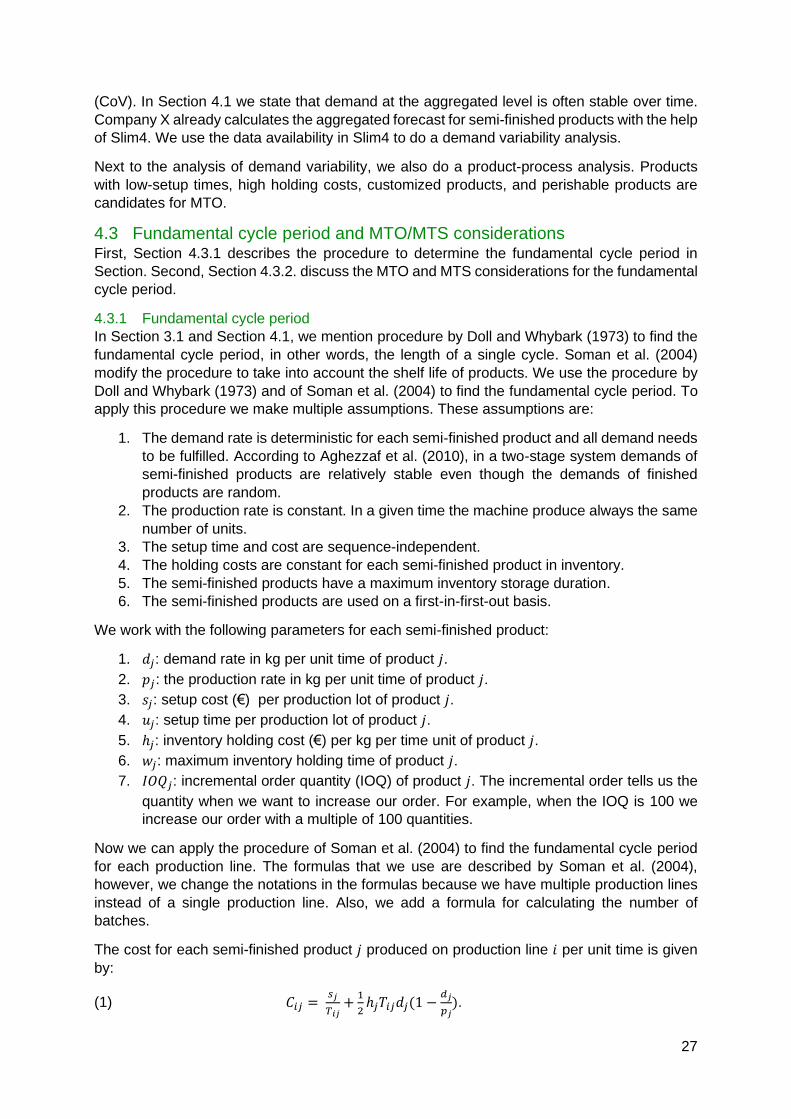
27
(CoV). In Section 4.1 we state that demand at the aggregated level is often stable over time.
Company X already calculates the aggregated forecast for semi-finished products with the help
of Slim4. We use the data availability in Slim4 to do a demand variability analysis.
Next to the analysis of demand variability, we also do a product-process analysis. Products
with low-setup times, high holding costs, customized products, and perishable products are
candidates for MTO.
4.3 Fundamental cycle period and MTO/MTS considerations First, Section 4.3.1 describes the procedure to determine the fundamental cycle period in
Section. Second, Section 4.3.2. discuss the MTO and MTS considerations for the fundamental
cycle period.
4.3.1 Fundamental cycle period
In Section 3.1 and Section 4.1, we mention procedure by Doll and Whybark (1973) to find the
fundamental cycle period, in other words, the length of a single cycle. Soman et al. (2004)
modify the procedure to take into account the shelf life of products. We use the procedure by
Doll and Whybark (1973) and of Soman et al. (2004) to find the fundamental cycle period. To
apply this procedure we make multiple assumptions. These assumptions are:
1. The demand rate is deterministic for each semi-finished product and all demand needs
to be fulfilled. According to Aghezzaf et al. (2010), in a two-stage system demands of
semi-finished products are relatively stable even though the demands of finished
products are random.
2. The production rate is constant. In a given time the machine produce always the same
number of units.
3. The setup time and cost are sequence-independent.
4. The holding costs are constant for each semi-finished product in inventory.
5. The semi-finished products have a maximum inventory storage duration.
6. The semi-finished products are used on a first-in-first-out basis.
We work with the following parameters for each semi-finished product:
1. 𝑑𝑗: demand rate in kg per unit time of product 𝑗.
2. 𝑝𝑗: the production rate in kg per unit time of product 𝑗.
3. 𝑠𝑗: setup cost (€) per production lot of product 𝑗.
4. 𝑢𝑗: setup time per production lot of product 𝑗.
5. ℎ𝑗: inventory holding cost (€) per kg per time unit of product 𝑗.
6. 𝑤𝑗: maximum inventory holding time of product 𝑗.
7. 𝐼𝑂𝑄𝑗: incremental order quantity (IOQ) of product 𝑗. The incremental order tells us the
quantity when we want to increase our order. For example, when the IOQ is 100 we
increase our order with a multiple of 100 quantities.
Now we can apply the procedure of Soman et al. (2004) to find the fundamental cycle period
for each production line. The formulas that we use are described by Soman et al. (2004),
however, we change the notations in the formulas because we have multiple production lines
instead of a single production line. Also, we add a formula for calculating the number of
batches.
The cost for each semi-finished product 𝑗 produced on production line 𝑖 per unit time is given
by:
(1) 𝐶𝑖𝑗 = 𝑠𝑗
𝑇𝑖𝑗+
1
2ℎ𝑗𝑇𝑖𝑗𝑑𝑗(1 −
𝑑𝑗
𝑝𝑗).

28
𝑇𝑖𝑗 is the cycle period of product 𝑗 produced on production line 𝑖. We can obtain 𝑇𝑖𝑗 from the
formula:
(2) 𝑇𝑖𝑗 = 𝑘𝑖𝑗𝑇𝑖∗.
𝑇𝑖∗ is the fundamental cycle period of production line 𝑖 and 𝑘𝑖𝑗 are the production frequencies
of product 𝑗 produced on production line 𝑖. For the production frequencies, we use integers
that are of the power of two, i.e. (1, 2, 4, 8, 16,…). We use integers of the power of two because
it becomes easier to define the total cycle length. According to Soman et al. (2004), it is
common to use the power of two in economic lot-sizing problems. The use of integers of the
power of two results in a 6% costlier solution in the worst case. We explain later how we
determine the total cycle length.
Now we can define the total cost for all the production lines per unit time:
(3) 𝐶 = ∑ ∑ 𝐶𝑖𝑗𝑁𝑗=1
4𝑖=1 = ∑ ∑ {
𝑠𝑗
𝑘𝑖𝑗𝑇𝑖∗ +
1
2ℎ𝑗𝑘𝑖𝑗𝑇𝑖
∗𝑑𝑗 (1 −𝑑𝑗
𝑝𝑗)}𝑁
𝑗=14𝑖=1
In (3), 𝑁 is the set of semi-finished products produced on production line 𝑖.
The maximum duration of a semi-finished product in inventory is: 𝑇𝑖𝑗(1 −𝑑𝑗
𝑝𝑗) (4). When we set
an inventory duration constraint we have the following condition:
(5) 𝑇𝑖∗ ≤ {
𝑤𝑗
𝑘𝑖𝑗(1−𝑑𝑗
𝑝𝑗)}
From (5) we can set an upper bound for a given set of products 𝑗 produced on production line
𝑖 by:
(6) 𝑇𝑖∗ ≤ min
𝑗{
𝑤𝑗
𝑘𝑖𝑗(1−𝑑𝑗
𝑝𝑗)}
Equation (6) gives the maximum duration a product is in inventory. We take the lowest value
from a given set of products produced on production line 𝑖. The fundamental cycle period must
be smaller or equal to this duration.
We can also set a lower bound. There must be sufficient time to handle the average number
of setups required for all semi-finished products. The lower bound is defined by:
(7) 𝑇𝑖∗ ≥
∑ 𝑢𝑗/𝑘𝑖𝑗𝑁𝑗=1
(1−∑𝑑𝑗
𝑝𝑗
𝑁𝑗=1 )
To obtain a feasible plan for every production line we define a plan with a length that is equal
to the least common multiple (LCM) of 𝑘𝑖𝑗 values times the fundamental cycle period 𝑇𝑖∗. The
LCM is the smallest positive integer that is divisible by the values 𝑘𝑖𝑗. With the production
frequencies 𝑘𝑖𝑗 that are equal to integers of the power-of-two, i.e. (1, 2, 4, 8, 16,…), we can
find easily the least common multiple because LCM(𝑘𝑖𝑗) is 𝑚𝑎𝑥(𝑘𝑖𝑗). Now we can define the
total cycle length on production line 𝑖 by 𝐿𝐸𝑁𝐺𝑇𝐻𝑖 = 𝐿𝐶𝑀(𝑘𝑖𝑗) × 𝑇𝑖∗ (8).
Soman et al. (2004) describe a 7 step procedure to find the values for the fundamental cycle
period. We provide a slightly modified procedure of Soman et al. (2004) in Appendix B to find

29
the fundamental cycle period for every production line by taking into account a maximum
inventory duration constraint.
The fundamental cycle period values 𝑇𝑖∗ together with the production frequency integer
multiples 𝑘𝑖𝑗 we have a good indication and the starting point of a production plan. We can
define the total processing time per lot by 𝑃𝑇𝑖𝑗 = 𝑇𝑖𝑗𝑑𝑗/𝑝𝑗 (9) where 𝑇𝑖𝑗 = 𝑘𝑖𝑗𝑇𝑖∗ (2) the cycle
time for product 𝑗 on production line 𝑖. From this formula, we see those semi-finished products
with a low ratio of 𝑑𝑗/𝑝𝑗 result in a relatively short processing time per lot. For the processing
department of Company X, very short processing times per lot are not favourable. We can
increase the processing time by increasing the maximum inventory waiting time or increasing
the production frequency integer multiple 𝑘𝑖𝑗 values to obtain a higher fundamental cycle
period. Increasing the production frequency reduces the fundamental cycle period.
Also, semi-finished products are produced in batches. Therefore, we need to take into account
the batch size of semi-finished products. To find the next batch size we define the formula:
𝐵𝐴𝑇𝐶𝐻𝑗 = 𝑃𝑇𝑖𝑗𝑝𝑗
𝐼𝑂𝑄𝑗 (10) where 𝐵𝐴𝑇𝐶𝐻𝑗 are the number of batches for semi-finished product 𝑗
and where 𝐼𝑂𝑄𝑗 is the incremental order quantity for product 𝑗. In this formula, we multiply the
processing time with the production rate. This will give the total quantity that we produce. When
we divide by the incremental order quantity we have the number of batches.
Figure 14 illustrates a graph to give a better understanding of the fundamental cycle period. In
this graph, we have a production plan for semi-finished products 1, 2, 3, 4 with a fundamental
cycle period of 𝑇𝑖∗ and 𝑘𝑖𝑗 values of 1, 2, 2, 4 respectively. We indicate the processing times
𝑃𝑇𝑖𝑗, the setup times 𝑢𝑗. Semi-finished product 1 is produced every period while semi-finished
products 2 and 3 are both produced in the first and third period. Semi-finished product 4 is
produced only in the second period. We also illustrate the inventory development over time for
Figure 14: Example production plan with the fundamental cycle period. Applied from Soman et al. (2004) but modificated
0
1
2
3
4
5
6
7
8
9
10
0 1 2 3 4 5 6 7 8 9 10 11 12 13 14 15 16 17 18 19 20 21 22 23 24 25 26 27 28 29 30 31 32 33 34 35 36 37 38 39 40
Period 1 Period 2 Period 3 Period 4
Total Cycle Length
Maximum duration product in inventory =
Idle
tim
e
Idle
tim
e
Idle
tim
e
Idle
tim
e
Slope
Slope

30
semi-finished products 1 and 3, the colours blue and orange respectively. Next to this, we also
show the cycle time and the maximum duration in the inventory of semi-finished product 3.
4.3.2 MTO and MTS considerations in the fundamental cycle period
The decision for MTO and MTS for semi-finished products is complex and requires close
relationships with the packaging department and the customers. We decide to not use MTO
products in the calculation of the fundamental cycle period. Soman et al. (2007) suggested to
reserve capacity for MTO products in each cycle or use the idle time.
Another consideration is the relatively low demand for semi-finished products. From formula 9
we see that low demands lead to short processing times. We can handle semi-finished
products as MTO products and leave these products out of the calculation of the fundamental
cycle period. When we reserve capacity for MTO products we can produce these products
when they are needed. With a combination of inventory management software, like Slim4, it is
possible to let the software decide when to produce an MTO product.
4.4 Production scheduling Scheduling is a complex task, especially when we have sequence-dependent setups between
products. Section 4.4.1 describes a heuristic to find a feasible schedule for every production
line in every fundamental cycle period. We do not consider MTO products in the schedule
because they are not produced regularly. We want to first create a relatively fixed schedule for
MTS products. For MTO products, we advise using human interaction and decision-making in
scheduling.
4.4.1 Scheduling heuristic
First, we define a setup matrix for product families. The product families are the corresponding
allergen codes of the semi-finished products. Appendix A provides an allergen flow scheme.
Semi-finished products need to follow a specific order to avoid allergen contamination. When
we switch to an allergen that is not in the determined order, a cleaning time of 6 hours is
required. Table 2 specifies the setups between allergen codes from the overview of the
allergen flow scheme.
To
1 2 3 4 5 6 7 8 9 10 11
From 1 0 0 0 0 0 0 0 0 0 0 0
2 0 0 6 6 0 0 0 0 0 0 0
3 0 6 0 6 6 6 6 0 6 6 0
4 0 6 6 0 6 0 6 6 0 0 0
5 0 6 6 6 0 6 6 0 0 6 0
6 0 6 6 6 6 0 6 6 0 0 0
7 0 6 6 6 6 6 0 0 6 0 0
8 0 6 6 6 6 6 6 6 6 6 0
9 0 6 6 6 6 6 6 6 0 6 0
10 0 6 6 6 6 6 6 6 6 0 0
11 0 6 6 6 6 6 6 6 6 6 0
Table 2: Allergen setup matrix
Gupta and Magnusson (2008) describe a scheduling heuristic named: Initialize, Sequence,
and Improve (ISI). We describe the steps Initialize, Sequence, and Improve in Section 4.4.1.1,
Section 4.4.1.2, and Section 4.4.1.3 respectively. This scheduling heuristic finds a feasible
solution for sequence-dependent products without exceeding capacity and minimizing setup
cost. In the heuristic, it is allowed to have overtime when it is not possible to schedule all

31
products within the available time. However, we do not want overtime because it violates cycle
planning. Section 4.4.1.3 describes the suggestions for eliminating overtime.
Besides the possibility of overtime, the heuristic is easily adaptable and provides a good
structure. Therefore, we apply some general guidelines from this heuristic to find a feasible
schedule.
4.4.1.1 Initialize
Section 4.3 describes a procedure to find a feasible production plan for MTS products. From
this procedure, we find an optimal cycle length for every production line which cover all the
product cycles. Applying the algorithm from Section 4.3 we find the fundamental cycle period
𝑇𝑖∗, the total cycle length 𝐿𝐸𝑁𝐺𝑇𝐻𝑖, and the production frequencies 𝑘𝑖𝑗. We illustrate an
example with simplistic numbers to give an impression of the first step in finding a feasible
schedule.
𝑖, 𝑗 𝑘𝑖𝑗
1,1 1
1,2 1
1,3 2
1,4 2
1,5 4
Table 3: Production frequency example
We have semi-finished products 𝑗 = 1, … ,5 to be produced on production line 𝑖 = 1. The
corresponding production frequencies 𝑘𝑖𝑗 are:
The total cycle length is 𝐿𝐸𝑁𝐺𝑇𝐻1 = 4 weeks and the fundamental cycle period is 𝑇1∗ = 1 week.
Product Week 1 Week 2 Week 3 Week 4
1 100 100 100 100
2 100 100 100 100
3 0 50 0 50
4 50 0 50 0
5 25 0 0 0
Table 4: Production plan example
Table 3 gives the production frequency of the products. So, we produce product 1 and 2 every
week (𝑘𝑖𝑗 = 1), product 3 and 4 once in two weeks (𝑘𝑖𝑗 = 2) and product 5 once in four weeks
(𝑘𝑖𝑗 = 4). Table 4 illustrates an example of the production plan based on the production
frequencies.
Therefore, we already determined which product we produce in a cycle period. Products with
values 𝑘𝑖𝑗 > 1 are more flexible to schedule. However, we need to take into account the cycle
period and the production frequencies of these products.
In the first step of initializing the schedule, we ignore setup times. We start with all products
where 𝑘𝑖𝑗 = 1. We need to produce these products every period. We sequence the products
in order of decreasing processing time during a cycle period. So we start with products with
the highest processing time. The idea is that it is easier to generate a possible schedule by
scheduling products with longer processing times first. We fill the gaps in the sequence by
producing products with shorter processing times. After all products with 𝑘𝑖𝑗 = 1, we take
values of 𝑘𝑖𝑗 = 2. Also here, we start with the product with the highest demand. When the
product exceeds the capacity constraint in the given period we shift that product to the next
period. We continue increasing 𝑘𝑖𝑗 until we have scheduled all the products. We need to take

32
into account the cycle times of 𝑘𝑖𝑗. So when 𝑘𝑖𝑗 = 2 we schedule that product once every two
cycle periods.
In a cycle period we have a capacity constraint. The capacity constraint is defined by the total
processing hours that are available in a cycle period. We do not use the demand as a constraint
because every product has a different production rate. Therefore, some products can have a
shorter processing time with equal demand. The capacity constraint is given by
∑𝑇𝑖𝑗𝑑𝑗
𝑝𝑗≤ 𝐾𝑇𝑖
∗𝑗∈𝑁 (11) for all 𝑖 = 1, … ,4 with 𝐾𝑇𝑖∗ the available processing time per cycle period
and 𝑁 the set of semi-finished products.
Now we have allocated production of all period we compute the potential capacity that is
required to meet the schedule by taking into account possible setup time between products
with different allergen codes.
Next, we work backwards from the end of the planning horizon to the first period. The objective
is to not violate the capacity constraint in each period. When the capacity constraint is violated
we move the remaining products to the next period. Keep in mind that we need to produce
products with 𝑘𝑖𝑗 = 1 in every cycle period. This means we cannot move these products to
different cycle periods. We continue until we reach period 1. We can use the remaining
available processing time at the end of each period for production MTO products. We believe
that the production planner can decide what to do with the remaining production time.
Therefore, we do not fill the gap by the heuristic.
If we do not have sufficient capacity in the first period we do the procedure again. We
concentrate on the products with production frequency larger than 1, i.e. 𝑘𝑖𝑗 > 1. We check if
we can produce some products in different cycle periods that have processing time available.
If we do not find a feasible schedule after the second check then the heuristic stops and
conclude that it is not possible to generate a feasible schedule given the available capacity.
4.4.1.2 Sequence
We have now determined which products we need to produce in each period. For sequencing,
we start with the first product in each period with the longest processing time. We have
categorized families based on the allergen of the products. Appendix A illustrates the allergen
flow scheme. We continue to look for a product with an allergen code that is ranked highest in
the allergen flow scheme. In our situation allergen numbers 2, 3, or 4 are ranked highest. It is
more ideal to start at the top of the flow scheme and work downwards. The advantage of
working from top to bottom is the reduced number of allergen switches that require additional
cleaning.
The next product to be sequenced is the one with the lowest setup time. The lowest setup time
is a product of the same family. Therefore, we look for products from the same family. After all
the products from the same family are scheduled we look for a product with the lowest setup
time. Keep in mind that we work from top to bottom in the allergen flow scheme. So, we can
go from allergen code 6 to allergen code 11 without additional setup time. However, we first
look for products with allergen code 9 or 10. We continue until we have scheduled all products
in a given period. We go to the next period and start the sequencing procedure again. We do
this until we have scheduled all periods.
In the initialize step we do not take into account the setup times. We have only a limit available
processing time per cycle. When the setup time is included we may have overtime in a cycle.
Section 4.4.1.3 provides solutions for improving the schedule and eliminate overtime.

33
4.4.1.3 Improve
Gupta and Magnusson (2008) apply an improvement step to the feasible solution obtained
from the first two steps. They test whether it is possible to lower cost by shifting production in
two different periods to a single period. This results in fewer setups but higher inventory levels
thus higher holding costs. This improvement step is reasonable when the setup cost is
significantly higher than the holding cost per product. Section 4.4.1.2 mentions the possibility
of having over time in a cycle. However, we do not want overtime because this violates the
cycle planning. Therefore, we provide some solutions for eliminating overtime.
First, we can change the production frequency 𝑘𝑖𝑗 from the calculation of the fundamental cycle
period. Increasing these values will result in longer processing times and fewer setups. After
changing the production frequency we need to apply the procedure of the fundamental cycle
period and the scheduling heuristic again. We change the production frequencies until we find
a feasible schedule with the elimination of overtime.
Second, it is possible to shift products to a different production line. Most of the products have
an alternative production line. However, this is mostly not the most efficient production. We
can shift products to a production line with sufficient available processing time. When we shift
products to a different production line we need to calculate the procedure of the fundamental
cycle period and the scheduling heuristic again.

34
4.5 Overview of fundamental cycle period and scheduling Figure 15 illustrates all the steps of the solution design in a flow scheme. This flow scheme will
help to execute the solution design. We divide the flow scheme is in 3 sections. We start with
MTO-MTS considerations. We continue to the calculation of the fundamental cycle period.
Last, we apply the ISI scheduling heuristic. When we do not have sufficient processing time
available we change the production frequencies of the semi-finished products.
Figure 15: Solution design overview

35
4.6 Production planning performance Section 3.4 describes performance measurements for production planning. The models that
we find for two-stage production systems are mostly focused on total costs. For Company X
the delivery performance is one of the most important KPIs. However, because we only focus
on the first stage of a two-stage production system it becomes difficult to measure the delivery
performance from our proposed solution design. From the proposed models in our solution
design we can measure the following performances:
- Total costs. This is the setup and the holding costs.
- Average processing times. Take the average of the results from equation 9 from
Section 4.3.1.
- Average inventory duration. Take the average of the results from equation 4 from
Section 4.3.1.
- Number of required cleanings in the schedule
We use these performance measures for the solution design. Also, Company X is already
using the KPI inventory in days to measure the total inventory time of semi-finished products.
4.7 Conclusion In this chapter describes a solution design based on the literature of Chapter 3. We look at
how we can improve production planning in the first stage of a two-stage production system.
In the first stage often a cyclic production planning is used. The procedure described by Doll
and Whybark (1973) is a well know procedure for cyclic production planning. Soman et al.
(2004) use this procedure in combination with a shelf-life constraint.
We use and modify the procedures described by Doll and Whybark (1973) and Soman et al.
(2004) for creating a cyclic production planning with a fundamental cycle period. We define the
parameters in the formulas of the procedure. Before we execute this procedure we describe
the MTO and MTS considerations in the calculation of the fundamental cycle period. We do
not include MTO products in this procedure. By reserving capacity in the cycle planning we
can produce MTO products.
We use the fundamental cycle period as input for the schedule. We create a schedule by the
means of the ISI heuristic. The ISI heuristic has three steps, namely: Initialize, Sequence, and
Improve. This heuristic takes into account the sequence dependency between the products.
In the initialize step we create a schedule based on the production frequencies and the
available processing time per cycle. In the sequence step, we sequence the products in each
cycle based on the allergens of the semi-finished products. The allergens are defined by the
means of an allergen flow scheme. We require a setup when we switch to an allergen that is
not in the order of this flow scheme. The improve step is for looking for opportunities to improve
the schedule. There may be overtime in the schedule. The overtime is not allowed because
this violates the cycle planning. We provide a solution to eliminate overtime. Next to this, we
provide an overview of all the steps of the solution design.
Last, we look at the production planning performances. We use the total cost, average
processing times, average inventory duration, and the number of required cleanings in the
schedule as performance measurements.
36
5 Implementation In this chapter implements the solution design that is described in Chapter 4. Section 5.1
explains the data availability at Company X. Next, Section 5.2 explains the execution of the
solution design from Chapter 4. Section 5.3 performs a demand variability analysis to check
for MTO and MTS products. Furthermore, Section 5.4 calculates the fundamental cycle period
for every production line. Section 5.5 applies the scheduling heuristic to transform the
production plan into a feasible schedule. Section 5.6 explains the performance measurements.
Section 5.7 performs a sensitivity analysis. Section 5.8 gives the validation of the results. Last,
Section 5.9 provides a conclusion.
5.1 Data availability The first step is to get the required information that is needed for the solution design. Section
2.3 explains the systems that are used in production planning. The main systems are Slim4
and the ERP system Fobis. We use the data of Slim4 to derive the forecast for the semi-
finished products. This forecast is an aggregated forecast from the finished products.
Unfortunately, it is not possible to retrieve accurate historical data for the demand of semi-
finished products. Therefore, we only consider the forecast for the upcoming 52 weeks. We
use the data from the date 14-08-2020.
We use Fobis to retrieve the data for the bill of materials and other specific information. For
example, we retrieve the production rates, IOQ, and MOQ.
We retrieve the information about costs, such as holding cost and setup cost, from the financial
department of Company X.
5.2 Execution of the solution design To execute the solution design, we program the models in Visual Basic. Visual Basic is built
into Excel. We choose Visual Basic because it is a relatively easy programme language and it
works with Excel. Excel is easily accessible for other persons and is also widely used by
employees of Company X. The programme is executed based on the visual illustration of the
solution design that we present in Section 4.5.
5.3 MTO and MTS considerations Section 4.2 discusses the consideration of MTO and MTS products. We perform a demand
variability analysis to check for MTO and MTS products. We use the average weekly
forecasted demand based on the coming 52 weeks. We retrieve this forecast from Slim4. Also,
we calculate the coefficient of variation for the variability in the demand. Several semi-finished
products have an average weekly demand of zero. This means that the product is already
MTO or is in the phased-out. Therefore, we exclude these products in the analysis.

37
Figure 16: Demand variability analysis
Figure 16 illustrates the analysis. On the X-axes, we have the average weekly demand on a
logarithmic scale and on the Y-axes the coefficient of variance. Semi-finished products with
high-volume and low variability are candidates for MTS. Products with low volume and high
variability are candidates for MTO.
Products 17, 25, and 38 are good candidates for MTO. The remaining products have relatively
low variability. However, several products do not have a high volume. We can consider semi-
finished products with very low volume as MTO. As a guideline, we decide to exclude products
with demand lower than the incremental order quantity. This will exclude the products in the
calculation of the fundamental cycle period. Appendix C illustrates an overview of the semi-
finished products together with the required information.
The advantage of excluding MTO products is the reduced number of cycle periods and longer
processing times. Also, Slim4 is a powerful tool to advice when to produce an MTO product
based on actual information, such as new customer orders.
5.4 Fundamental cycle period calculation We apply the algorithm from Section 4.3. We have an Excel file that calculates the fundamental
cycle period for every production line. We use the products that remain after the constraints
that we set in Section 5.3. This gives a list of a total of 39 semi-finished products that we include
and we exclude 19 semi-finished products.
For the holding cost, we use a fixed holding cost per kg per week for every product. We do not
have enough detailed information for the calculation of the holding cost for every semi-finished
product. However, because the semi-finished products are stored on pallets with 320 kg each,
we assume that the holding costs are equal for all semi-finished products. For the setup cost,
we perform an analysis of the average setup time for every semi-finished product from year to
date. With this time, we use a cost price per time unit. For the maximum duration in inventory,
we consider a maximum of 6 weeks. The supply chain has as target an inventory level of 3 to
4 weeks. However, with 6 weeks we have a sufficient maximum inventory duration for all the
production lines. Preferably, the maximum duration can change to a lower level. Appendix D
presents all the input data. We use weeks as time unit were one week is 5 working days.
38
25
517 365149 27 472350 4 43284256 4522355 2026 37 35524813 53 957 1241 14 3239 46 2171 8243431 195430 3315 44102 16 1840 11 296
0
50
100
150
200
250
300
350
400
1 10 100 1.000 10.000 100.000
Co
V
Average weekly demand (logarithmic scale)

38
We apply the algorithm with the given data. After applying the procedure of Soman et al.
(2004), which is explained in Section 4.3 and Appendix B, we have the following results for the
lower bound, upper bound, fundamental cycle period, least common multiple of the production
frequency, the total holding and setup cost, total cost, and the total cycle length. Table 5
illustrates these results. The total cost for the 4 production lines is €6,369.08. Table 6 illustrates
the results of 5 semi-finished products. The results for every semi-finished product are
illustrated in Appendix E.
Production line 11 (𝒊 = 𝟏)
Production line 21 (𝒊 = 𝟐)
Production line 31 (𝒊 = 𝟑)
Production line Company Z (𝒊 =𝟒)
#Products 16 13 7 3
Lower bound T* in weeks 0.1412 0.0531 0.0258 0.0067
Upper bound T* in weeks 3.0192 1.5132 3.0446 3.0744
Fundamental cycle period 𝑻𝒊
∗ in weeks 0.89 0.69 0.79 0.63
Least common multiple of 𝒌𝒊𝒋 2 4 2 2
Total Cycle Length in weeks 1.78 2.76 1.58 1.27
Holding cost for the total cycle length € 1,211.24 € 1,031.14 € 638.24 € 303.91
Setup cost for the total cycle length € 1,211.24 € 1,031.14 € 638.24 € 303.91
Total cost for the total cycle length € 2,422.48 € 2,062.28 € 1,276.49 € 607.83
Table 5: Initial plan
Product nr
Art. Code
Production line
Demand per week in kg
Processing time in hours
Duration in inventory in weeks
LOT size in kg #Batches
Production frequency
38 557356 11 690 1.21 1.77 1,231 2.37 2
36 557311 11 760 1.79 1.76 1,355 2.14 2
16 557822 11 3,630 3.75 0.84 3,237 2.59 1
12 557122 11 5,130 3.81 0.84 4,575 3.63 1
13 557145 11 4,910 3.86 0.84 4,379 2.28 1
Table 6: Results of 5 semi-finished products from the initial plan
We give some explanation for Table 5. The lower bound and upper bound of T* are determined
by equations 6 and 7 from Section 4.3.1 respectively. The fundamental cycle period or the
cycle length needs to be higher than the lower bound and lower than the upper bound. The
LCM is the smallest positive integer that is divisible by the values 𝑘𝑖𝑗. With the LCM and the
fundamental cycle period we can determine the total cycle length, see equation 8 in Section
4.3.1. We determine the total cost with equation 3.
We notice that the total cycle length is not practical to use, i.e. 1.78 weeks is 8.9 working days.
Section 5.8.1 explains the practical use of the results.
After examining the processing time per lot for the semi-finished products, we decide to try to
increase the processing time to a minimum of around 3 to 4 hours processing time. Shorter
processing times are not favourable for the processing department. We do this by increasing

39
the production frequencies. Section 4.3.1 mentions the use integers of the power-of-two for
the production frequencies, i.e. 1, 2, 4, 8, 16. However, we do not increase the production
frequency higher than the 8. Therefore, we only change the production frequency to 1, 2, 4, or
8. We choose to go no higher than 8 because increasing the production frequency higher than
8 will result in too many cycles with short fundamental cycle periods.
Table 7 illustrates the result after changing the production frequencies and Table 8 the results
of 5 semi-finished products. The results of all the semi-finished products are given in Appendix
E.
Production line 11 (𝒊 = 𝟏)
Production line 21 (𝒊 = 𝟐)
Production line 31 (𝒊 = 𝟑)
Production line Company Z (𝒊 =𝟒)
#Products 16 13 7 3
Lower bound T* in weeks 0.0466 0.0162 0.0100 0.0028
Upper bound T* in weeks 0.7548 0.7566 1.5223 1.5372
Fundamental cycle period 𝑻𝒊
∗ in weeks 0.6460 0.4997 0.6786 0.5482
Least common multiple of 𝒌𝒊𝒋 8 8 4 4
Total Cycle Length in weeks 5.17 4.00 2.71 2.19
Holding cost for the total cycle length € 1,266.28 € 1,062.51 € 643.89 € 316.82
Setup cost for the total cycle length € 1,266.28 € 1,062.51 € 643.89 € 316.82
Total cost for the total cycle length € 2,532.55 € 2,125.02 € 1,287.78 € 633.63
Feasibility Feasible Feasible Feasible Feasible
Table 7: Results after changing the production frequencies
Product nr
Art. Code
Production line
Demand in kg
Processing time in hours
Duration in inventory in weeks
LOT size in kg #Batches
Production frequency
4 558203 11 9,680 8.17 0.54 6,253 3.42 1
28 557172 11 1,960 2.22 1.26 2,532 4.62 2
34 557853 11 850 3.63 2.54 2,196 3.72 4
38 557356 11 690 3.50 5.12 3,566 6.86 8
37 557139 11 760 3.27 5.13 3,928 6.99 8
Table 8: Results of 5 semi-finished products after changing the production frequencies
The total cost for the 4 production lines is €6578.98 which is 3.3% higher than before the
change. The fundamental cycle period is reduced but the total cycle length is increased. So,
we have shorter cycles over a longer planning horizon. The fundamental cycle period is still
feasible which means all the semi-finished products have an inventory duration shorter than 6
weeks. Also here, we have total cycle lengths that are not practical for production line 11, 31
and Company Z. Section 5.8 explains the practical use of the results.
40
The average processing times per production line is:
Production line Average processing time in hours
Average inventory duration in weeks
Production line 11 3.78 1.89
Production line 21 3.37 1.57
Production line 31 4.04 1.11
Production line Company Z
4.55 1.04
5.5 Scheduling Section 5.4 describes a feasible production plan. We schedule this production plan over the
planning horizon. For every production line, we find a fundamental cycle period. This cycle
period is the length of a single cycle. We have the following results for the fundamental cycle
period:
11 21 31 Company Z
Fundamental cycle period 𝑻𝒊∗
in weeks 0.6460 0.4997 0.6786 0.5482
This is not a practical number. Therefore we choose to round the fundamental cycle period to
the nearest value that gives whole production days. In Section 5.8 we provide further
explanation of the practical use of the results. We transform the results from weeks to working
days. We have 5 working days in a week, so the results are now:
11 21 31 Company Z
Fundamental cycle period 𝑻𝒊∗
in days
3 days 2 days 3 days 3 days
Multiplying the fundamental cycle period by the least common multiple of the production
frequencies we find the total cycle length. See Figure 14 in Section 4.3 for an example of a
cyclic production plan. We start by arranging the semi-finished products in order of long
processing times to short processing times. Then we work backwards from the last cycle to
the first cycle to make sure we do not violate the capacity.
After we have a schedule that does not violate the capacity in every cycle we continue with
sequencing. First, we look for the products with an allergen that is at the top of the allergen
flow scheme. We continue by working from top to bottom in the allergen flow scheme. When
we reach the bottom and still have semi-finished products to schedule then cleaning is
required. After the cleaning, we can start again at the top of the allergen flow scheme and work
downwards until all semi-finished products are scheduled.
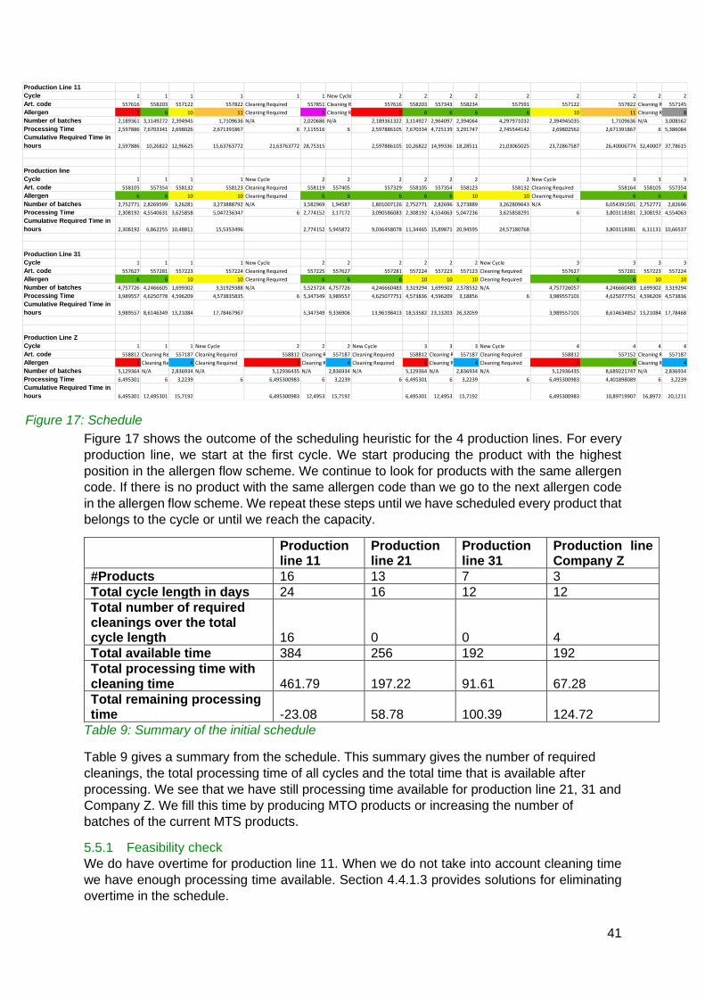
41
Figure 17 shows the outcome of the scheduling heuristic for the 4 production lines. For every
production line, we start at the first cycle. We start producing the product with the highest
position in the allergen flow scheme. We continue to look for products with the same allergen
code. If there is no product with the same allergen code than we go to the next allergen code
in the allergen flow scheme. We repeat these steps until we have scheduled every product that
belongs to the cycle or until we reach the capacity.
Production line 11
Production line 21
Production line 31
Production line Company Z
#Products 16 13 7 3
Total cycle length in days 24 16 12 12
Total number of required cleanings over the total cycle length 16 0 0 4
Total available time 384 256 192 192
Total processing time with cleaning time 461.79 197.22 91.61 67.28
Total remaining processing time -23.08 58.78 100.39 124.72
Table 9: Summary of the initial schedule
Table 9 gives a summary from the schedule. This summary gives the number of required
cleanings, the total processing time of all cycles and the total time that is available after
processing. We see that we have still processing time available for production line 21, 31 and
Company Z. We fill this time by producing MTO products or increasing the number of
batches of the current MTS products.
5.5.1 Feasibility check
We do have overtime for production line 11. When we do not take into account cleaning time
we have enough processing time available. Section 4.4.1.3 provides solutions for eliminating
overtime in the schedule.
Figure 17: Schedule
Production Line 11
Cycle 1 1 1 1 1 1 New Cycle 2 2 2 2 2 2 2 2 2
Art. code 557616 558203 557122 557822 Cleaning Required 557851 Cleaning Required 557616 558203 557343 558234 557591 557122 557822 Cleaning Required557145
Allergen 2 6 10 11 Cleaning Required 5 Cleaning Required 2 6 6 6 6 10 11 Cleaning Required 8
Number of batches 2,189361 3,1149272 2,394945 1,7109636 N/A 2,020686 N/A 2,189361322 3,114927 2,964097 2,394064 4,297971032 2,394945035 1,7109636 N/A 3,008562
Processing Time 2,597886 7,6703341 2,698026 2,671391867 6 7,115516 6 2,597886105 7,670334 4,725139 3,291747 2,745544142 2,69802562 2,671391867 6 5,386084
Cumulative Required Time in
hours 2,597886 10,26822 12,96625 15,63763772 21,63763772 28,75315 2,597886105 10,26822 14,99336 18,28511 21,03065025 23,72867587 26,40006774 32,40007 37,78615
Production line
Cycle 1 1 1 1 New Cycle 2 2 2 2 2 2 2 New Cycle 3 3 3
Art. code 558105 557354 558132 558123 Cleaning Required 558119 557405 557329 558105 557354 558123 558132 Cleaning Required 558164 558105 557354
Allergen 6 6 10 10 Cleaning Required 6 6 6 6 6 10 10 Cleaning Required 6 6 6
Number of batches 2,752771 2,8269599 3,26281 3,273888792 N/A 3,582969 1,94587 1,801007126 2,752771 2,82696 3,273889 3,262809643 N/A 6,054391501 2,752771 2,82696
Processing Time 2,308192 4,5540631 3,625858 5,047236347 6 2,774152 3,17172 3,090586083 2,308192 4,554063 5,047236 3,625858291 6 3,803118381 2,308192 4,554063
Cumulative Required Time in
hours 2,308192 6,862255 10,48811 15,5353496 2,774152 5,945872 9,036458078 11,34465 15,89871 20,94595 24,57180768 3,803118381 6,11131 10,66537
Production Line 31
Cycle 1 1 1 1 New Cycle 2 2 2 2 2 2 New Cycle 3 3 3 3
Art. code 557627 557281 557223 557224 Cleaning Required 557225 557627 557281 557224 557223 557123 Cleaning Required 557627 557281 557223 557224
Allergen 6 6 10 10 Cleaning Required 6 6 6 10 10 10 Cleaning Required 6 6 10 10
Number of batches 4,757726 4,2466605 1,699302 3,31929388 N/A 5,523724 4,757726 4,246660483 3,319294 1,699302 2,578532 N/A 4,757726057 4,246660483 1,699302 3,319294
Processing Time 3,989557 4,6250778 4,596209 4,573835835 6 5,347349 3,989557 4,625077751 4,573836 4,596209 3,18856 6 3,989557101 4,625077751 4,596209 4,573836
Cumulative Required Time in
hours 3,989557 8,6146349 13,21084 17,78467967 5,347349 9,336906 13,96198413 18,53582 23,13203 26,32059 3,989557101 8,614634852 13,21084 17,78468
Production Line Z
Cycle 1 1 1 New Cycle 2 2 2 New Cycle 3 3 3 New Cycle 4 4 4 4
Art. code 558812 Cleaning Required557187 Cleaning Required 558812 Cleaning Required557187 Cleaning Required 558812 Cleaning Required557187 Cleaning Required 558812 557152 Cleaning Required557187
Allergen 2 Cleaning Required 4 Cleaning Required 2 Cleaning Required 4 Cleaning Required 2 Cleaning Required 4 Cleaning Required 2 6 Cleaning Required 4
Number of batches 5,129364 N/A 2,836934 N/A 5,12936435 N/A 2,836934 N/A 5,129364 N/A 2,836934 N/A 5,12936435 8,689221747 N/A 2,836934
Processing Time 6,495301 6 3,2239 6 6,495300983 6 3,2239 6 6,495301 6 3,2239 6 6,495300983 4,401898089 6 3,2239
Cumulative Required Time in
hours 6,495301 12,495301 15,7192 6,495300983 12,4953 15,7192 6,495301 12,4953 15,7192 6,495300983 10,89719907 16,8972 20,1211

42
We want to have a schedule that has sufficient available processing time for all the production
lines. We choose to change some production frequencies for semi-finished products produced
on production line 11. Increasing the production frequency results in fewer setups. We change
the production frequency of the product with the lowest processing time. We do this until we
have a schedule with sufficient available processing time. However, this procedure also
changes the results of the procedure of the fundamental cycle period. Table 10 presents the
new results of the fundamental cycle period.
Production line 11 (𝒊 = 𝟏)
Production line 21 (𝒊 = 𝟐)
Production line 31 (𝒊 = 𝟑)
Production line Company Z (𝒊 =𝟒)
Lower bound T* in weeks 0.0416 0.0162 0.0100 0.0028
Upper bound T* in weeks 0.7548 0.7566 1.5223 1.5372
Fundamental cycle period 𝑻𝒊
∗ in weeks 0.5882 0.4997 0.6786 0.5482
Least common multiple of 𝒌𝒊𝒋 8 8 4 4
Total Cycle Length in weeks 4.71 4.00 2.71 2.19
Holding cost for the total cycle length € 1,263.58 € 1.062,51 € 643.89 € 316.82
Setup cost for the total cycle length € 1,263.58 € 1,062.51 € 643.89 € 316.82
Total cost for the total cycle length € 2,527.17 € 2,125.02 € 1,287.78 € 633.63
Feasibility Feasible Feasible Feasible Feasible
Table 10: Results of the fundamental cycle period with a feasible schedule
Table 11 shows the effect on the average processing time and the average inventory duration.
Production line Average processing time in hours
Average inventory duration in weeks
Production line 11 3.71 1.83
Production line 21 3.37 1.57
Production line 31 4.04 1.11
Production line Company Z
4.55 1.04
Table 11: Results of the new measurements
After changing the results we find a lower cost for production line 11. The total cost is now
€6,573.60. However, the average processing time and the average inventory duration is
slightly reduced. Table 12 presents the new summary of the results after applying the
scheduling heuristic.

43
Production line 11
Production line 21
Production line 31
Production line Company Z
#Products 16 13 7 3
Total cycle length in days 24 16 12 12
Total number of required cleanings over the total cycle length 14 0 0 4
Total available time in hours 384 256 192 192
Total processing time with cleaning time in hours 377.90 197.22 91.61 67.28
Total remaining processing time in hours 6.10 58.78 100.39 124.72
Table 12: Final results of the schedule
We see that we now have sufficient time available for scheduling all the semi-finished products.
With the remaining processing time, we can produce 19 MTO products. The production planner
can divide the products over the production lines. We do not create a schedule with the MTO
products because we do not have sufficient information when to produce an MTO product.
When it is not possible to create sufficient processing time it is possible to shift products to a
different production line. For example, production line 31 has 100 hours of remaining
processing time. So we can shift products from production line 11 to production line 31.
5.6 Production planning performance Section 4.6 presents several performance measurements for the solution design. The total
costs, average processing time, and the number of required cleanings are already given in
Section 5.4 and Section 5.5.
Production line 11 (𝒊 = 𝟏)
Production line 21 (𝒊 = 𝟐)
Production line 31 (𝒊 = 𝟑)
Production line Company Z (𝒊 =𝟒)
Total cost € 2,527.17 €2,125.02 €1,287.78 €633.63
Average processing time in hours
3.71 3.37 4.04 4.55
Average inventory duration in weeks
1.83 1.57 1.11 1.04
Total number of required cleanings
14 0 0 4
Table 13: Summary performance measurements
Table 13 summarises the performance measurements. Company X can use these
performance measurements to validate the solution design after implementing this solution
design in production planning. Section 5.7 performs a sensitivity analysis to see the change in
total costs and average processing time when we change some parameters.
5.7 Sensitivity analysis Section 5.3 calculates the fundamental cycle period for every production line. We perform a
sensitivity analysis to see the impact on the result when we change certain parameters. We
decide to do a sensitivity analysis for the following scenarios:

44
1. Calculate the fundamental cycle period with inventory duration constraints with a
maximum of 2, 3, 4, 5, 6, 7, 8, 9, and 10 weeks.
2. Increasing the demand for semi-finished products with 10%, 20%, 30%, and 40%.
3. Reduce the production rates of the semi-finished products to 90%, 80%, and 70%.
We will look if we can create a feasible production plan and schedule without changing the
production frequencies. Section 5.7.1 explains scenario 1. For scenario 1, we look at the total
cost and the average processing time.
Next, Section 5.7.2 explains scenario 2. In scenario 2, we keep the maximum inventory time
on 6 weeks and increase the demand with the given percentages. We look at the impact on
the total cost and the average processing time.
Last, Section 5.7.3 explains scenario 3. In scenario 3, we reduce the production rates per hour
from 100% to the given percentages. We keep the demand at the same level as in the original
situation. We look at the impact on the total cost and the average inventory time.
5.7.1 Scenario 1
In this scenario, we change the maximum inventory duration. We start with a maximum of 2
weeks and we increase this to a maximum of 10 weeks for every semi-finished product. We
do not start with 1 week because it does not guarantee a feasible outcome and it is also not
realistic to have maximum inventory duration of 1 week given the weekly demands of the semi-
finished products.
Appendix F: Scenario 1, we have
illustrated 4 graphs of the different
production lines. In this section, we
explain the results for production
line 11, which we illustrate in
Figure 18. For explanation and
remarks for production line 21, 31,
and Company Z consult Appendix
F.
Figure 18 presents the total cost
and the average processing times.
We see that that the total cost and
the average processing changes
when we increase the maximum
inventory duration.
Section 4.3.1 sets an upper bound
𝑇𝑖∗ with equation 6. When we have a short maximum inventory duration, we need to reduce
the production frequencies 𝑘𝑖𝑗 of some products to generate a feasible plan. By reducing the
production frequencies of some products we increase the upper bound that we set for 𝑇𝑖∗.
When we do not have a relatively short maximum inventory duration the procedure looks for
opportunities to reduce the total cost. The procedure finds a lower total cost with a lower
fundamental cycle period. In equation 2 and 9 we see that the fundamental cycle period
influences the calculation of the processing times. With a lower fundamental cycle period, we
have shorter processing times.
When the maximum inventory duration is greater or equal than 4 weeks, the total costs and
the average processing time do not change. This is because with 4 weeks the calculated upper
3,76
3,78
3,80
3,82
3,84
3,86
3,88
3,90
3,92
3,94
3,96
€ 2.390,00
€ 2.400,00
€ 2.410,00
€ 2.420,00
€ 2.430,00
€ 2.440,00
€ 2.450,00
€ 2.460,00
€ 2.470,00
€ 2.480,00
€ 2.490,00
2 3 4 5 6 7 8 9 10
Ave
rage
pro
cess
ing
tim
e
Tota
l co
st
Production line 11
Total cost Average Processing Time
Figure 18: Result production line 11 scenario 1
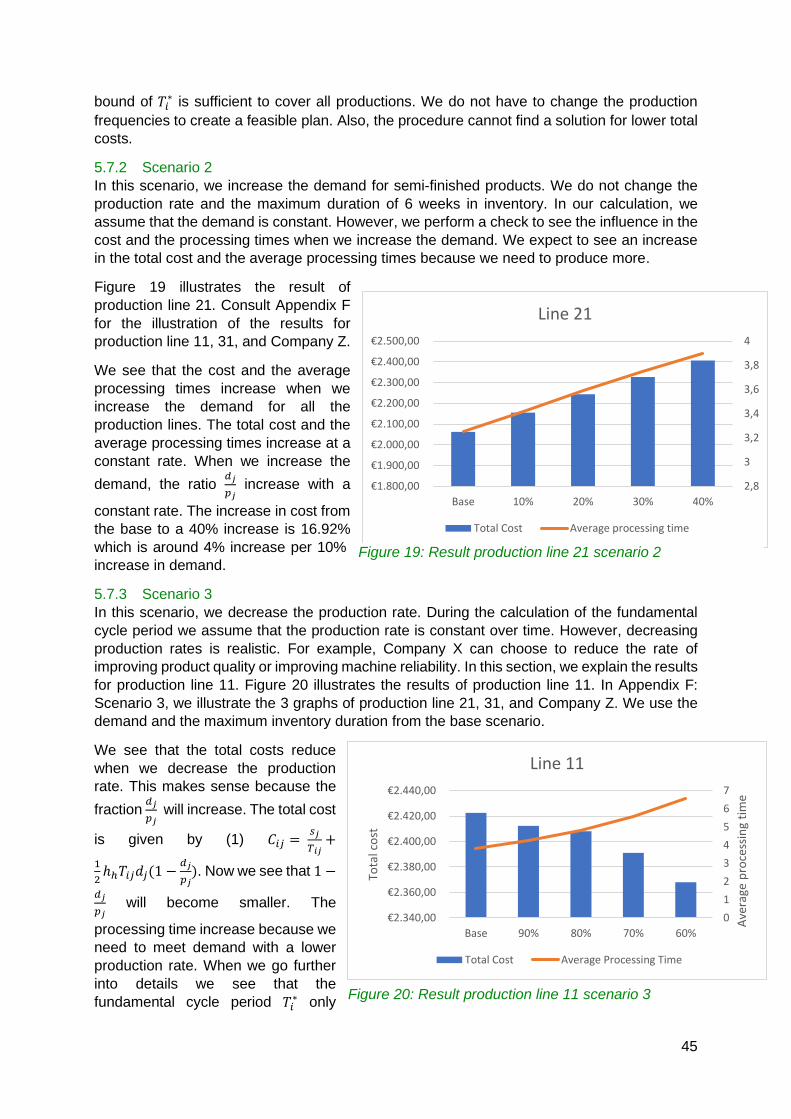
45
bound of 𝑇𝑖∗ is sufficient to cover all productions. We do not have to change the production
frequencies to create a feasible plan. Also, the procedure cannot find a solution for lower total
costs.
5.7.2 Scenario 2
In this scenario, we increase the demand for semi-finished products. We do not change the
production rate and the maximum duration of 6 weeks in inventory. In our calculation, we
assume that the demand is constant. However, we perform a check to see the influence in the
cost and the processing times when we increase the demand. We expect to see an increase
in the total cost and the average processing times because we need to produce more.
Figure 19 illustrates the result of
production line 21. Consult Appendix F
for the illustration of the results for
production line 11, 31, and Company Z.
We see that the cost and the average
processing times increase when we
increase the demand for all the
production lines. The total cost and the
average processing times increase at a
constant rate. When we increase the
demand, the ratio 𝑑𝑗
𝑝𝑗 increase with a
constant rate. The increase in cost from
the base to a 40% increase is 16.92%
which is around 4% increase per 10%
increase in demand.
5.7.3 Scenario 3
In this scenario, we decrease the production rate. During the calculation of the fundamental
cycle period we assume that the production rate is constant over time. However, decreasing
production rates is realistic. For example, Company X can choose to reduce the rate of
improving product quality or improving machine reliability. In this section, we explain the results
for production line 11. Figure 20 illustrates the results of production line 11. In Appendix F:
Scenario 3, we illustrate the 3 graphs of production line 21, 31, and Company Z. We use the
demand and the maximum inventory duration from the base scenario.
We see that the total costs reduce
when we decrease the production
rate. This makes sense because the
fraction 𝑑𝑗
𝑝𝑗 will increase. The total cost
is given by (1) 𝐶𝑖𝑗 = 𝑠𝑗
𝑇𝑖𝑗+
1
2ℎℎ𝑇𝑖𝑗𝑑𝑗(1 −
𝑑𝑗
𝑝𝑗). Now we see that 1 −
𝑑𝑗
𝑝𝑗 will become smaller. The
processing time increase because we
need to meet demand with a lower
production rate. When we go further
into details we see that the
fundamental cycle period 𝑇𝑖∗ only
2,8
3
3,2
3,4
3,6
3,8
4
€1.800,00
€1.900,00
€2.000,00
€2.100,00
€2.200,00
€2.300,00
€2.400,00
€2.500,00
Base 10% 20% 30% 40%
Line 21
Total Cost Average processing time
0
1
2
3
4
5
6
7
€2.340,00
€2.360,00
€2.380,00
€2.400,00
€2.420,00
€2.440,00
Base 90% 80% 70% 60%
Ave
rage
pro
cess
ing
tim
e
Tota
l co
st
Line 11
Total Cost Average Processing Time
Figure 20: Result production line 11 scenario 3
Figure 19: Result production line 21 scenario 2

46
increase slightly. It looks attractive to have a lower production rate because of the lower cost.
However, because the fundamental cycle period only slightly increases we come to a moment
where we do not have sufficient processing time available. This results in a production plan
and schedule that is not feasible.
The slope of the average processing time increases after 70% production rate. From equation
(9) 𝑃𝑇𝑖𝑗 = 𝑇𝑖𝑗𝑑𝑗/𝑝𝑗 together with equation (2) 𝑇𝑖𝑗 = 𝑘𝑖𝑗𝑇𝑖∗ we calculate the processing time per
semi-finished product. When we look at the results we see that some production frequencies
𝑘𝑖𝑗 increase at a production rate of 60%. The fundamental cycle period 𝑇𝑖∗ only slightly
increase. Because of the increase of some production frequencies the slope of the average
processing time increases.
5.8 Validation This section explains the validation of the results. We divide this section into three subsections.
First, Section 5.8.1 explains the results of the calculation for the fundamental cycle period.
Second, Section 5.8.2 looks at the results of the schedule. Third, Section 5.8.3 uses historical
data to compare the results with the current situation.
5.8.1 Results of the fundamental cycle period
We have some remarks on the results of the calculation of the fundamental cycle period and
the schedule. The outcome of the calculation of the cycle periods we get a fundamental cycle
period that is not equal to the whole day and/or week. In practice, a fundamental cycle period
of 0.5882 weeks or 2.941 days (based on a week with 5 production days) is not practical. We
could decide to change this fundamental cycle period to full working days. This will create more
practical results. We have the results from Section 0:
11 21 31 Company Z
Fundamental cycle period 𝑻𝒊∗ 0.5882 0.4997 0.6786 0.5482
In Section 5.5 we already did a modification on the fundamental cycle period to make a more
practical result for the schedule. When we round these to the nearest full working day based
on 5 working days. So we have:
11 21 31 Company Z
Fundamental cycle period 𝑻𝒊∗ 3 days 2 days 3 days 3 days
We need to choose if we round up or down to a full working day. In the results above we round
up or down based on the nearest full production day. These results create a feasible production
plan and schedule. However, we may not have sufficient processing time available per cycle
when we round up or down because the fundamental cycle period influences the processing
times. We execute both scenarios and examine the results. When we round down the
fundamental cycle period we do not have sufficient processing time available for processing
all the products on production line 11. When we round up the fundamental cycle period we do
have enough processing time available for all production lines. Also, for production line 21, 31,
and Company Z the remaining processing time increases. Because we want to have a feasible
schedule for all production lines we decide to round up the fundamental cycle period.
Production line 11 (𝒊 = 𝟏)
Production line 21 (𝒊 = 𝟐)
Production line 31 (𝒊 = 𝟑)
Production line Company Z (𝒊 =𝟒)
Lower bound T* in weeks 0.0416 0.0167 0.0100 0.0028
Upper bound T* in weeks 0.7548 0.7579 1.5223 1.5372

47
Fundamental cycle period 𝑻𝒊
∗ in weeks 0.6000 0.6000 0.8000 0.6000
Least common multiple of 𝒌𝒊𝒋 8 8 4 4
Total Cycle Length in weeks 4.80 4.80 3.20 2.40
Holding cost for the total cycle length € 1,288.86 € 1,228.46 € 759.13 € 346.75
Setup cost for the total cycle length € 1,238.80 € 906.68 € 546.15 € 289.46
Total cost for the total cycle length € 2,527.66 € 2,135.15 € 1,305.27 € 636.22
Feasibility Feasible Feasible Feasible Feasible
Table 14: Results when rounding up fundamental cycle period
Table 14 shows the results after changing rounding the fundamental cycle period. When we
convert the fundamental cycle period from weeks to working days we have:
Production line 11
Production line 21
Production line 31
Production line Company Z
Fundamental cycle period 𝑻𝒊∗
in working days 3 3 4 3
The total cost is €6,604.30 in Table 14. When we compare the results of Table 14 with the
results of Table 7 in Section 0 we see that the total cost increases with 0.38%.
Production line 11
Production line 21
Production line 31
Production line COMPANY Z
#Products 16 13 7 3
Number of required cleanings 14 0 0 4
Total available time in hours 384 384 256 192
Total Processing time with cleaning time in hours 383.49 235.34 107.28 71.23
Total available processing time after processing in hours 0.51 148.66 148.72 120.77
Table 15: Summary schedule after rounding fundamental cycle period
Table 15 presents a summary of the new result of the schedule. When we compare these
results with Table 12 we see that the available processing time after processing reduces for
production line 11 and Company Z. However, for production line 21 and 31 it increases.
When we look at the number of batches of the semi-finished products we see that these are
not of type integer. The production planner can decide to round up or down the number of
batches based on factors like current inventory level or demand. This will influence the
processing time slightly. However, this will not be a problem when the fundamental cycle period
has extra capacity available.

48
5.8.2 Results of the schedule
The fundamental cycle period assumes that the setup is sequence-independent. However, the
procedure set a lower bound that makes sure that there is sufficient time for producing all the
semi-finished products based on the given setup times. We provide these setup times based
on historical information of Company X. Nevertheless, these setup times are not based on the
sequence dependency. Sequence dependency results in longer setup times between
products. However, when we include sufficient time processing time in the fundamental cycle
period it is possible to make a schedule with sequence-dependent setups.
Also, in the schedule, we present a feasible schedule based on the allergen of the semi-
finished products. However, we do not take into account product specifications in the schedule.
For example, switching to different types of machines takes more time than continue producing
on the same machine. Also, we have a long setup time if we switch to an allergen that is not
in order of the allergen flow scheme. However, in the current situation, Company X cleans the
processing department every night. This means that it is possible to switch to a different
allergen without loss of available processing time. There are some opportunities for further
research on the schedule.
5.8.3 Comparison with the current situation
We look if we can compare some results of the fundamental cycle period with the current
situation. First, we find the average processing times on the production lines from the beginning
of the year. Second, we look at the average inventory time from the beginning of March 1 2020.
Production line 11
Production line 21
Production line 31
Production line Company Z
Current situation
Average processing times in hours
8.38 7.85 9.02 6.01
Results fundamental cycle period
Average processing times in hours
3.71 3.37 4.04 4.55
Percentage change current situation versus results fundamental cycle period
-55.7% -57.1% -55.2% -24.3%
Table 16: Average processing times in hours
First, we look at the average processing times. We take the data from March 2nd to August
14th. Table 16 illustrates the results from the historical situation together with the results from
Table 13. We see that the results from the fundamental cycle period drastically decrease the
average processing times for production line 11, 21, and 31. For production line Company Z
we see a more moderate decrease.
Production line 11
Production line 21
Production line 31
Production line Company Z
Current situation
Average inventory duration in weeks
1.75 1.45 1.66 1.63
Results fundamental cycle period
Average inventory duration in weeks
1.83 1.57 1.11 1.04

49
Percentage change current situation versus results fundamental cycle period
4.6% 8.3% -33.1% -36.2%
Table 17: Average inventory duration in weeks
For the average inventory duration, we took historical data from March 1st to August 13th. Table
17 illustrates the results per production line. We also give the results of the fundamental cycle
period which is adapted from Table 13. When we compare these results we see that for
production line 11 and 21 the average inventory duration is longer than in the current situation.
However, these values are relatively close. For production line 31 and Company Z, we have
in the current situation a high average inventory duration compared to the results of the
fundamental cycle period.
When we want to compare the total costs with the current situation it becomes fairly difficult.
We need to gather more data and we need to do a more in-depth analysis in the data of the
current situation. We are not going to do this because of the available time we have for this
research.
5.8.4 Reduction time for production planning
The previous sections of this chapter give the results after implementation of the solution
design. However, we do not have the answer yet for the core problem of this research. With
the solution design, we want to reduce the time that is needed for production planning at
Company X. We already mentioned the advantages of a cyclic production plan in Chapter 2
and 3. A cyclic production plan reduces the complexity of creating a production plan. With the
presented solution design, the cycle length, production frequencies, quantities, and cycle
lengths are already determined.
Together with the stakeholders at Company X, we evaluated the solution design and the
implementation of the solution design. They mention that the solution design helps in reducing
the time for production planning. Also, it gives a fixed planning method. Section 2.4 mentions
two different production planning methods. With this solution design, the production planner
does not have to choose a planning method. Also, the quantities, production frequencies, and
cycle lengths are determined by the solution design. Therefore, the production planner only
has to control and improve the procedure of the fundamental cycle period and the scheduling
heuristic.
When we want to measure the reduction of time needed for production planning we need to
implement the results of this research in the current environment of Company X. Due to the
time limits we have for this research, it becomes very hard to have good measurements.
However, all the stakeholders expect that the time will significantly reduce because the
production planner has only one plan method and only needs to control and improve the
production planning and schedule.
5.9 Conclusion We apply the solution design that we describe in Chapter 4. Before applying the procedure of
the fundamental cycle period we perform a demand and variability analysis. From this analysis,
it is possible to separate the MTO and MTS products. Only the MTS products are included in
the calculation of the fundamental cycle period. This means 39 MTS products are included and
19 MTO products are excluded.
We execute the fundamental cycle period that is described in Section 4.3. The procedure gives
an initial result. We want to have processing times of around 3 hours. The initial result does

50
not satisfy this. Therefore, we decide to increase the production frequencies which increases
the processing times. We find a feasible result after changing the production frequencies.
The results of the fundamental cycle period are applied in the ISI heuristic. After applying the
initialize and the sequence step we do not find a feasible schedule for production line 11
because there is not sufficient processing time available. Therefore, we reduce the production
frequencies of some semi-finished products. This leads to fewer setups and therefore more
available time for processing. Changing the production frequencies also leads to a change in
the results of the fundamental cycle period. After changing some production frequencies we
find a feasible schedule.
We provide a validation of the solution design. We do not find a practical result in the final
result of the fundamental cycle period. Therefore, we change the fundamental cycle period to
make it more practical. This results in slightly different outcomes of the procedure and the
heuristic of the schedule.
Next to this, the final results of the fundamental cycle period are compared with the current
situation at Company X. The average processing times decrease with ± 55% for production
line 11, 21, and 31. For production line Company Z the average processing time decreases
with 24%. The average inventory duration slightly increases for production line 11 and 21.
However, for production line 31 and Company Z it decreases with 33% and 36% respectively.
Finally, we discuss whether the solution design decreases the time that is needed for
production planning. With this solution design, the production planner only has one plan
method. Also, the quantities, production frequencies, and cycle lengths are already determined
by the solution design. The production planner only needs to control and improve the
production plan and the scheduling heuristic. Therefore, the stakeholders of Company X
foresee a significant reduction of time for production planning. Unfortunately, we cannot give
calculate the time reduction because we have limited available time for this research.

51
6 Conclusion, recommendation and further research This chapter provides a conclusion of this research, gives recommendations, limitations, and
possibilities for further research. Section 6.1 gives the conclusion of this research. Section 6.2
provides recommendations. Section 6.3 gives a contribution to the theory. Last, Section 6.4
describes the limitations and possibilities for further research.
6.1 Conclusion The core problem in this research is: “The production planning takes too much time”. In the
current situation, production planning takes around 1.0 FTE (38 hours). The supply chain
department wants to reduce production planning with 50% to 0.5 FTE (19 hours).
For reducing the time for production planning we describe a cyclic production plan based on
the research of Doll and Whybark (1973) and Soman et al. (2004). A cyclic production plan in
a two-stage production system has the advantage that it will periodically supply semi-finished
products to the packaging stage. This reduces the capacity in the intermediate warehouse.
Also, the quantities, production frequencies, processing times, and cycle length are already
given. The solution design describes a procedure to find the fundamental cycle period with
maximum inventory duration for every production line. The fundamental cycle period is the
length of a single cycle. Also, this procedure gives the production frequencies of the semi-
finished products. The production frequencies are the total number of production occurrences
over a given total cycle length. With the least common multiple of the production frequencies
and the fundamental cycle period, we can calculate the total cycle length. Next to this, the
procedure tries to find a feasible cyclic production plan with maximum inventory duration.
Before we execute the procedure of the fundamental cycle period we look at the MTO and
MTS considerations for production planning. We do a demand variability analysis to decide
which product are MTO or MTS orientated. We leave the MTO products in the calculation of
the fundamental cycle period. The procedure of the fundamental cycle period gives the
following result:
Production line 11
Production line 21
Production line 31
Production line Company Z
Fundamental cycle period in weeks
0.6460 0.4997 0.6786 0.5482
Total cycle length in weeks
5.17 4.00 2.71 2.19
The total cost is €6,578.98. From this result, we create a schedule. This schedule takes into
account the processing capacity per fundamental cycle period and the allergens of the
products. On production line 21, 31, and Company Z we have sufficient processing time
available after scheduling the products. With this available time, it is possible to produce MTO
products. For production line 11 we do have overtime. We do not want overtime because this
violates the cycle planning. As a solution, we improve the schedule by changing the production
frequencies until we have sufficient processing time for production line 11. Changing the
production frequencies also influences the results of the fundamental cycle procedure and
therefore we apply the procedure again. The new results are:
Production line 11
Production line 21
Production line 31
Production line Company Z
Fundamental cycle period in weeks 0.5882 0.4997 0.6786 0.5482

52
Total Cycle Length in weeks 4.71 4.00 2.71 2.19
This gives a total cost of €6,573.60. The results of the final schedule are:
Production line 11
Production line 21
Production line 31
Production line Company Z
Total available time in hours 384 256 192 192
Total processing time with cleaning time in hours 377.90 197.22 91.61 67.28
Total remaining processing time in hours 6.10 58.78 100.39 124.72
We use the performance measurements total cost, average processing time in hours, average
inventory duration, and the total number of required cleanings. These performance
measurements can Company X help to keep track of the solution design after implementing.
Especially the average processing time and the average inventory duration are helpful.
We do a sensitivity analysis to find the impact on the total cost and the average processing
time when we change certain parameters. In three different scenarios, we change the
maximum inventory duration, demand, and the production rate respectively. We see that the
maximum inventory duration only has a large influence when we set a short maximum
inventory duration. When we increase the demand we see a linear growth in the average
processing time. Also, the total cost shows almost linear growth. If we decrease the production
rate we see an almost linear growth in the average processing time. The total cost will
decrease. It is tempting to reduce the production rate because of lower cost, however, at a
certain point, we do not have sufficient processing time available.
We comment on the practical results of the fundamental cycle period. It is better to have a
fundamental cycle period in full production days. We look at the scenario of rounding up or
down the fundamental cycle period to the nearest full production day. We have better results
when we round up to the nearest full production day. From this, we calculate the new results
of the procedure of the fundamental cycle period. We see that the cost slightly increase,
however, we have a sufficient solution and a more practical solution.
We also compare the average processing times and the average inventory duration with the
current situation. We see that the average processing times decreases significantly with ± 55%
for production lines 11, 21, and 31. For the average inventory duration, we see that the
procedure of the fundamental cycle period gives slightly higher results for production line 11
and 21. For production line 31 and Company Z, it is the opposite. The average inventory
duration is reduced by ± 35%.
The solution design is evaluated with the stakeholders of Company X. They foresee a serious
reduction in the time that is needed for processing. First of all, the production planner only has
one planning method. Also, the quantities, production frequencies, and cycle lengths are
already determined. The production planner only needs to control and improve production
planning and schedule. Unfortunately, it is not possible to do measure the time reduction
specifically.
6.2 Recommendations Based on our solution design and the conclusions from Section 6.1 we would recommend the
following to Company X:

53
- Do a demand variability analysis for the semi-finished products regularly. This will give
insight into the demand and the variability of the semi-finished products. This can help
in assigning products as MTO or MTS.
- Use a cyclic production plan for semi-finished products. A cyclic production plan is easy
to use and it creates stability in production planning and the supply chain department.
A cyclic production plan reduces the time for production planning because a large part
of the planning is already determined. Use the remaining capacity for producing MTO
products or extra MTS productions. With the Excel file that we developed, it becomes
relatively easy to calculate the fundamental cycle periods and the planning horizon. It
also gives insight into total costs, processing times, and the number of batches. When
the initial results are not feasible or favourable it is possible to change the fundamental
cycle period by changing the production frequencies.
- We advise revising the calculation of the fundamental cycle period after the total cycle
length. Mainly the change in demand is important. The sequence in the schedule can
remain the same as long the total processing time is not larger than the available
capacity. The processing times and the number of batches can change.
- Look constant for opportunities to improve the schedule. When the sequence of some
semi-finished products is not favourable, try to change and improve the sequence. This
is a continues process and does not have to stop after applying it once. When semi-
finished products are shifted to another production line, the fundamental cycle period
needs to be calculated again.
- To keep track of the performance of the cycle, we advise using the average inventory
duration and the average processing times. These two performance measurements are
fairly easy to calculate. Also, Company X is already using the KPI inventory in days for
semi-finished products.
6.3 Contribution to theory The solution design is created for the situation at Company X. However, we have findings that
are useful for the theory. This research connects different practical findings from the literature
into one research. Also, we have changed some findings from the literature that will be useful
for further research. We present an overview of findings that a have a contribution to the theory.
- At first, we provide a summary of practical solutions for a two-stage production system.
Hierarchical production planning is useful in a two-stage production system. Together
with a coupling plan to couple the first-stage and the second-stage, it is possible to
create a robust production plan for both stages.
- We provide a demand variability for the first-stage. This demand variability gives insight
into the MTO and MTS considerations for semi-finished products. MTO and MTS
considerations are mostly focused on finished products and not on semi-finished
products. This analysis can give insight into how these considerations are adopted in
production planning in the first stage of a two-stage production system.
- We use the procedure of Doll and Whybark (1973) and Soman et al. (2004) to calculate
the fundamental cycle period with maximum inventory duration. These calculations are
based on a single production line and therefore change it for the use of multiple
production lines. We apply this procedure to calculate the fundamental cycle period for
4 production lines. Also, we first look at the considerations of MTO and MTS products.
With these results, we determine if we include a product in the calculation of the
fundamental cycle period.
- We use the results of the fundamental cycle period to create a schedule. We use a
scheduling heuristic from Gupta and Magnusson (2008). We change this heuristic to
apply it to the food industry. We take into account the available processing time at a
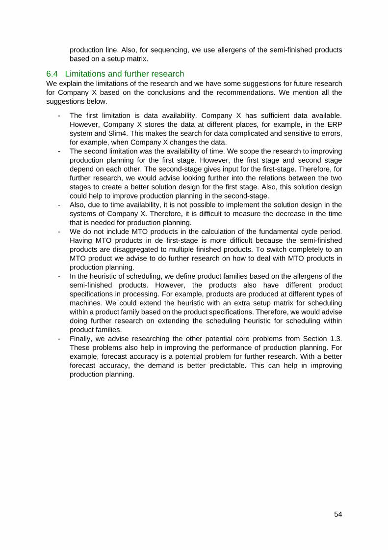
54
production line. Also, for sequencing, we use allergens of the semi-finished products
based on a setup matrix.
6.4 Limitations and further research We explain the limitations of the research and we have some suggestions for future research
for Company X based on the conclusions and the recommendations. We mention all the
suggestions below.
- The first limitation is data availability. Company X has sufficient data available.
However, Company X stores the data at different places, for example, in the ERP
system and Slim4. This makes the search for data complicated and sensitive to errors,
for example, when Company X changes the data.
- The second limitation was the availability of time. We scope the research to improving
production planning for the first stage. However, the first stage and second stage
depend on each other. The second-stage gives input for the first-stage. Therefore, for
further research, we would advise looking further into the relations between the two
stages to create a better solution design for the first stage. Also, this solution design
could help to improve production planning in the second-stage.
- Also, due to time availability, it is not possible to implement the solution design in the
systems of Company X. Therefore, it is difficult to measure the decrease in the time
that is needed for production planning.
- We do not include MTO products in the calculation of the fundamental cycle period.
Having MTO products in de first-stage is more difficult because the semi-finished
products are disaggregated to multiple finished products. To switch completely to an
MTO product we advise to do further research on how to deal with MTO products in
production planning.
- In the heuristic of scheduling, we define product families based on the allergens of the
semi-finished products. However, the products also have different product
specifications in processing. For example, products are produced at different types of
machines. We could extend the heuristic with an extra setup matrix for scheduling
within a product family based on the product specifications. Therefore, we would advise
doing further research on extending the scheduling heuristic for scheduling within
product families.
- Finally, we advise researching the other potential core problems from Section 1.3.
These problems also help in improving the performance of production planning. For
example, forecast accuracy is a potential problem for further research. With a better
forecast accuracy, the demand is better predictable. This can help in improving
production planning.

55
References Aghezzaf, H. E., & Landeghem, H. V. (2002). An integrated model for inventory and
production planning in a two-stage hybrid production system. International Journal of
Production Research, 4323-4339.
Aghezzaf, H. E., Sitompul, C., & Broecke, V. F. (2011). A robust hierarchical production
planning for a capacitated two-stage production system. Computers and Industrial
Engineering, 361-372.
Akkerman, R., Donk, D. V., & Gaalman, G. (2007). Influence of capacity- and time-
constrained intermediate storage in two-stage food production systems. International
Journal of Production Research, 2955-2973.
Bitran, G., Haas, E., & Hax, A. (1982). HIERARCHICAL PRODUCTION PLANNING: A TWO-
STAGE SYSTEM. Operations Research, 232-251.
Crauwels, H., Potts, C., & Wassenhove, L. V. (1997). Local search heuristics for single
machine scheduling with batch set-up times to minimize total weighted completion
time. Annals of Operations Research, 261-279.
Doll, C., & Whybark, D. C. (1973). An Iterative Procedure for the Single-Machine Multi-
Product Lot Scheduling Problem. Management Science, 50-55.
Donk, D. V. (2001). Make to stock or make to order: The decoupling point in the food
processing industries. International Journal of Production Economics, 297-306.
Encyclopedia.com. (2020, 4 17). Production Planning And Scheduling. Retrieved from
encyclopedia.com: https://www.encyclopedia.com/management/encyclopedias-
almanacs-transcripts-and-maps/production-planning-and-scheduling
Fera, M., Fruggiero, F., Lambiase, A., Giada, M., & Nenni, M. E. (2013). Production
Scheduling Approaches for Operations Management. IntechOpen.
Gupta, D., & Magnusson, T. (2005). The capacitated lot-sizing and scheduling problem with
sequence-dependent setup costs and setup times. Computers and Operations
Research, 727-747.
Gupta, J., & Chantaravarapan, S. (2008). Single machine group scheduling with family
setups to minimize total tardiness. International Journal of Production Research,
1707-1722.
Hammer, M. (2015). What is Business Process Management. Berlin: Springer.
Merriam-Webster. (n.d.). Dictionary. Retrieved from Merriam-Webster: https://www.merriam-
webster.com/dictionary/robust
Ozgur, C., & Brown, J. (1995). A Two-Stage Traveling for the Single Machine Scheduling
Salesman Procedure Sequence-Dependent . International Journal Management
Science, 205-219.
Rahmani, D., Ramezanian, R., Fattahi, P., & Heydari, M. (2013). A robust optimization model
for multi-product two-stage capacitated production planning under uncertainty.
Applied Mathematical Modelling, 8957-8971.
Slack, N., Brandon-Jones, A., & Johnston, R. (2013). Operations Management. Edinburgh
Gate: Pearson Education Limited.

56
Soman, C., Donk, D. V., & Gaalman, G. (2004). A basic period approach to the economic lot
scheduling problem with shelf life considerations. International Journal of Production
Research, 1677-1689.
Soman, C., Donk, D. V., & Gaalman, G. (2004a). Combined make-to-order and make-to-
stock in a food production system. International Journal of Production Economics,
223-235.
Soman, C., Donk, D. V., & Gaalman, G. (2006). Comparison of dynamic scheduling policies
for hybrid make-to-order and make-to-stock production systems with stochastic
demand. International Journal of Production Economics, 441-453.
Soman, C., Donk, D. V., & Gaalman, G. (2007). Capacitated planning and scheduling for
combined make-to-order and make-to-stock production in the food industry: An
illustrative case study. International Journal of Production Economics, 191-199.
Tsubone, H., Matsuura, H., & Tsutsu, T. (1991). Hierarchical production planning system for
a two-stage process. International Journal of Production Research, 769-785.
Wezel, W. V., Donk, D. V., & Gaalman, G. (2006). The planning flexibility bottleneck in food
processing industries. Journal of Operations Management, 287-300.
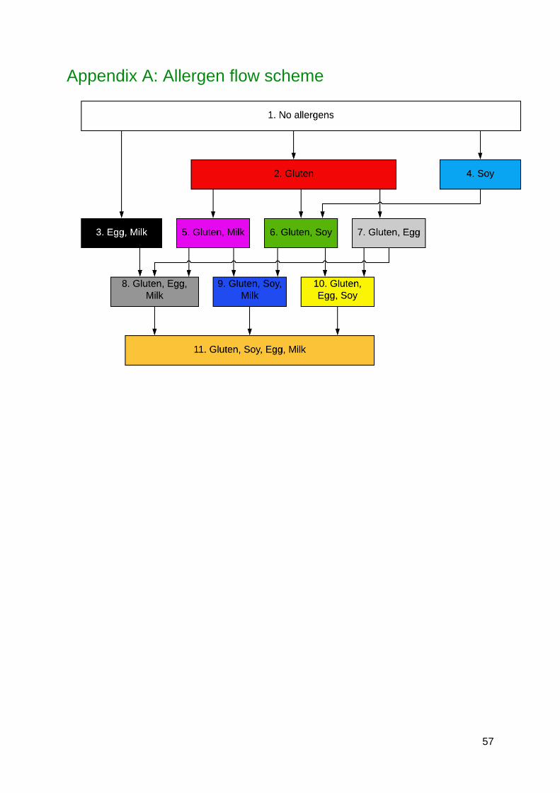
57
Appendix A: Allergen flow scheme

58
Appendix B: Fundamental cycle period procedure Step 1: Execute the procedure of Dolby and Whybark (1973) with the power of two policy.
This gives good starting points of 𝑇𝑖∗ and 𝑘𝑖𝑗. We further information about this procedure we
refer the reader to the research of Doll and Whybark (1973).
Step 2: Check if 𝑇𝑖∗ satisfy the constraint given by (7).
𝑇𝑖∗ = max {𝑇𝑖
∗,∑ 𝑠𝑗/𝑘𝑖𝑗𝑗
1 − ∑ 𝑑𝑗/𝑝𝑗𝑗}
Step 3: Check if 𝑇𝑗∗ satisfy the maximum inventory time.
𝑇𝑖∗ = min {𝑇𝑖
∗, min𝑗
[𝑤𝑖𝑗
𝑘𝑖𝑗(1 − 𝑑𝑗/𝑝𝑗]}
Check if a feasible plan can be made with fundamental cycle period equal to 𝑇𝑖∗ =
min𝑗
{𝑤𝑗/𝑘𝑖𝑗(1 −𝑑𝑗
𝑝𝑗)}. If this is possible go to step 4. If not. go to step 5.
Step 4: The 𝑇𝑖∗ of step 2 is systematically increased until a feasible plan can be made or till it
reaches min𝑗
{𝑤𝑗/𝑘𝑖𝑗(1 −𝑑𝑗
𝑝𝑗)}. The plan has a feasible solution when it generates a lower cost
for so far. We safe this solution as ‘the current best solution’ and go to step 5.
Step 5: (a) if max{𝑘𝑖𝑗} = 1. go to step 7.
(b) for each semi-finished product with 𝑘𝑖𝑗 > 1. halve the value of 𝑘𝑖𝑗 and calculate
the lower cost bound of the cost per unit time using (7).
where 𝑇𝑖∗ = {
2[∑𝑠𝑗
𝑘𝑖𝑗𝑗 ]
[∑ ℎ𝑗𝑑𝑗𝑘𝑖𝑗(1−𝑑𝑗
𝑝𝑗)𝑗 ]
}1/2 .
(c) Sort the products in ascending order of their cost and store this in a list.
(d) if there is a ‘current best solution’ stored in step 4 then ignore semi-finished
products which give a higher minimum cost than the ‘current best solution’ and
update the list. If the list is empty the procedure terminates and the ‘current best
solution’ is the solution.
(e) choose the first semi-finished product in the list.
(f) Use equation (6) to calculate the upper bound of the new 𝑘𝑖𝑗 values for every 𝑖.
The 𝑘𝑖𝑗 value of the first product is halved while other 𝑘𝑖𝑗 from step 2 remain the
same. Store these 𝑘𝑖𝑗 in vector 𝐾𝑖.
(g) Check if is possible to generate a feasible plan for new vector 𝐾𝑖 and 𝑇𝑖∗ equal to
the new upper bound from (f). If a feasible plan can be made, go to step 6. If not, go
to (h)
(h) Choose the next semi-finished product in the list and go to (f). If the end of the list
is reached, choose the first semi-finished product and go to Step 6.
59
Step 6: Halve the value of 𝑘𝑖𝑗 that is obtained in Step 5. If max(𝑘𝑖𝑗) > 1 go to Step 2,
otherwise go to Step 7.
Step 7: Stop the procedure. If there is a ‘current best solution’ this is the final solution.
Otherwise use the common cycle approach that is described by Silver (1989)

60
Appendix C: Demand analysis
Nr code Average weekly demand Standard deviation CoV IOQ Include or Exclude
1 558165 1078.04 235.64 21.86 1804 Exclude
2 557311 735.69 137.39 18.67 633 Include
3 558221 459.02 127.28 27.73 487 Exclude
4 557866 829.22 299.89 36.17 1147 Exclude
5 558812 11158.59 8220.97 73.67 1253 Include
6 557420 1577.65 269.11 17.06 815 Include
7 557343 4045.10 896.76 22.17 1667 Include
8 557354 12241.37 2620.25 21.40 2220 Include
9 557187 5991.76 1508.71 25.18 1200 Include
10 558132 5686.67 1087.52 19.12 902 Include
11 557356 679.22 120.32 17.72 520 Include
12 557281 7340.98 1815.98 24.74 1200 Include
13 557182 395.10 103.06 26.08 475 Exclude
14 558234 2811.57 680.88 24.22 1430 Include
15 557823 2162.55 423.43 19.58 342 Include
16 557523 909.02 167.03 18.37 513 Include
17 558696 102.12 70.31 68.85 339 Exclude
18 557232 2456.08 445.60 18.14 645 Include
19 557224 5658.82 1176.84 20.80 1200 Include
20 558105 3182.75 862.88 27.11 599 Include
21 558123 11362.75 2528.79 22.26 1804 Include
22 557139 700.00 195.28 27.90 562 Include
23 557583 690.78 272.57 39.46 1728 Exclude
24 557223 5672.55 1208.57 21.31 2340 Include
25 557824 167.84 260.67 155.31 947 Exclude
26 558129 231.96 62.75 27.05 344 Exclude
27 558164 1615.49 719.64 44.55 548 Include
28 557119 341.37 105.70 30.96 351 Exclude
29 557591 2497.25 441.06 17.66 698 Include
30 557146 544.90 110.66 20.31 500 Include
31 557822 3471.37 730.14 21.03 1248 Include
32 557627 5885.29 1366.66 23.22 870 Include
33 558203 9453.73 1902.19 20.12 1828 Include
34 557616 4284.90 911.01 21.26 1158 Include
35 557851 7189.80 1918.92 26.69 2160 Include
36 557675 637.06 422.67 66.35 2100 Exclude
37 557145 4833.14 1295.14 26.80 1920 Include
38 557301 30.20 104.89 347.36 2532 Exclude
39 557172 1890.20 436.78 23.11 548 Include
40 557004 322.94 58.59 18.14 378 Exclude
41 557153 1563.53 379.60 24.28 1800 Exclude
42 558152 323.14 93.32 28.88 3786 Exclude

61
43 557151 1302.35 435.96 33.47 420 Include
44 557122 4929.80 961.27 19.50 1260 Include
45 558126 992.16 278.25 28.04 615 Include
46 557225 3365.49 772.97 22.97 855 Include
47 558119 3042.94 1287.65 42.32 873 Include
48 557123 2201.96 582.56 26.46 1200 Include
49 557336 947.25 450.94 47.61 1152 Exclude
50 557865 350.20 126.89 36.23 1548 Exclude
51 557853 811.37 489.40 60.32 590 Include
52 557405 3291.57 875.23 26.59 1741 Include
53 557329 3180.20 806.90 25.37 1820 Include
54 557009 817.65 169.12 20.68 555 Include
55 557323 443.33 120.78 27.24 506 Exclude
56 557601 308.24 87.17 28.28 487 Exclude
57 557152 2018.63 504.97 25.02 535 Include
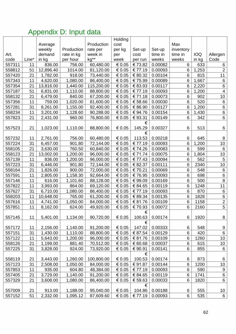
62
Appendix D: Input data
Art. code Line*
Average weekly demand in kg
Production rate in kg per hour
Production rate per week in kg**
Holding cost per kg per week
Set-up cost per run
Set-up time in weeks
Max inventory time in weeks
IOQ in kg
Allergen Code
557311 11 836.00 756.00 60,480.00 € 0.05 € 73.82 0.00082 6 633 6
558812 51 12,896.40 1014.00 81,120.00 € 0.05 € 77.19 0.00093 6 1,253 2
557420 21 1,782.00 918.00 73,440.00 € 0.05 € 80.32 0.00104 6 815 11
557343 11 4,620.00 1,080.00 86,400.00 € 0.05 € 75.99 0.00089 6 1,667 6
557354 21 13,816.00 1,440.00 115,200.00 € 0.05 € 83.93 0.00117 6 2,220 6
557187 51 6,831.00 1,110.00 88,800.00 € 0.05 € 77.19 0.00093 6 1,200 4
558132 21 6,479.00 840.00 67,200.00 € 0.05 € 71.18 0.00073 6 902 10
557356 11 759.00 1,020.00 81,600.00 € 0.05 € 58.66 0.00030 6 520 6
557281 31 8,261.00 1,155.00 92,400.00 € 0.05 € 86.90 0.00127 6 1,200 6
558234 11 3,201.00 1,128.60 90,288.00 € 0.05 € 94.76 0.00154 6 1,430 6
557823 21 2,431.00 960.00 76,800.00 € 0.05 € 93.31 0.00149 6 342 6
557523 21 1,023.00 1,110.00 88,800.00 € 0.05 €
145.29 0.00327 6 513 6
557232 11 2,761.00 756.00 60,480.00 € 0.05 €
113.53 0.00218 6 645 8
557224 31 6,457.00 901.80 72,144.00 € 0.05 € 77.19 0.00093 6 1,200 10
558105 21 3,630.00 760.50 60,840.00 € 0.05 € 74.26 0.00083 6 599 6
558123 21 13,002.00 1,200.00 96,000.00 € 0.05 € 71.74 0.00075 6 1,804 10
557139 11 836.00 1,200.00 96,000.00 € 0.05 € 77.43 0.00094 6 562 5
557223 31 6,446.00 901.80 72,144.00 € 0.05 € 82.37 0.00111 6 2340 10
558164 21 1,826.00 900.00 72,000.00 € 0.05 € 70.21 0.00069 6 548 6
557591 11 2,805.00 1,158.30 92,664.00 € 0.05 € 76.95 0.00093 6 698 6
557146 11 616.00 1,101.60 88,128.00 € 0.05 € 99.09 0.00169 6 500 8
557822 11 3,993.00 864.00 69,120.00 € 0.05 € 84.65 0.00119 6 1248 11
557627 31 6,710.00 1,080.00 86,400.00 € 0.05 € 77.19 0.00093 6 870 6
558203 11 10,648.00 765.00 61,200.00 € 0.05 € 89.34 0.00135 6 1828 6
557616 11 4,741.00 1,050.00 84,000.00 € 0.05 € 81.76 0.00109 6 1158 2
557851 11 8,162.00 624.00 49,920.00 € 0.05 € 70.93 0.00072 6 2160 5
557145 11 5,401.00 1,134.00 90,720.00 € 0.05 €
100.63 0.00174 6 1920 8
557172 11 2,156.00 1,140.00 91,200.00 € 0.05 €
147.02 0.00333 6 548 9
557151 31 1,430.00 1,110.00 88,800.00 € 0.05 € 87.54 0.00129 6 420 6
557122 11 5,643.00 1,200.00 96,000.00 € 0.05 € 81.76 0.00109 6 1260 10
558126 21 1,199.00 881.40 70,512.00 € 0.05 € 60.68 0.00037 6 615 10
557225 31 3,828.00 924.00 73,920.00 € 0.05 € 90.91 0.00141 6 855 6
558119 21 3,443.00 1,260.00 100,800.00 € 0.05 €
100.53 0.00174 6 873 6
557123 31 2,508.00 1,050.00 84,000.00 € 0.05 € 91.87 0.00144 6 1200 10
557853 11 935.00 604.80 48,384.00 € 0.05 € 77.19 0.00093 6 590 9
557405 21 3,729.00 1,140.00 91,200.00 € 0.05 € 84.65 0.00119 6 1741 6
557329 21 3,608.00 1,080.00 86,400.00 € 0.05 € 59.63 0.00033 6 1820 6
557009 21 913.00 1,188.00 95,040.00 € 0.05 €
104.86 0.00188 6 555 10
557152 51 2,332.00 1,095.12 87,609.60 € 0.05 € 77.19 0.00093 6 535 6
63
*Line 51 is the production line at the facility of Company Z.
**Production rate based on 5 days a week with 16 hours of production per day.

64
Appendix E: Results of the fundamental cycle period
Results initial plan
Product nr
Art. Code
Production line
Demand in kg
Processing time in hours
Inventory duration in weeks
LOT size in kg #Batches
Production frequency
38 557356 11 690 1.21 1.77 1,231 2.37 2
36 557311 11 760 1.79 1.76 1,355 2.14 2
37 557139 11 760 1.13 1.77 1,355 2.41 2
34 557853 11 850 2.51 1.75 1,516 2.57 2
39 557146 11 560 0.91 1.77 999 2.00 2
23 557591 11 2,550 1.96 0.87 2,274 3.26 1
22 558234 11 2,910 2.30 0.86 2,595 1.81 1
24 557232 11 2,510 5.92 1.71 4,477 6.94 2
16 557822 11 3,630 3.75 0.84 3,237 2.59 1
15 557343 11 4,200 3.47 0.85 3,745 2.25 1
14 557616 11 4,310 3.66 0.85 3,844 3.32 1
28 557172 11 1,960 3.07 1.75 3,496 6.38 2
12 557122 11 5,130 3.81 0.84 4,575 3.63 1
13 557145 11 4,910 3.86 0.84 4,379 2.28 1
6 557851 11 7,420 10.60 0.76 6,617 3.06 1
4 558203 11 9,680 11.28 0.75 8,632 4.72 1
32 558126 21 1,090 1.70 1.36 1,502 2.44 2
35 557009 21 830 1.93 2.73 2,287 4.12 4
29 558164 21 1,660 2.54 1.35 2,287 4.17 2
33 557523 21 930 2.31 2.73 2,563 5.00 4
30 557420 21 1,620 2.43 1.35 2,232 2.74 2
20 557329 21 3,280 2.09 0.66 2,260 1.24 1
26 557823 21 2,210 3.17 1.34 3,045 8.90 2
19 558105 21 3,300 2.99 0.65 2,274 3.80 1
18 557405 21 3,390 2.05 0.66 2,336 1.34 1
21 558119 21 3,130 3.42 1.34 4,313 4.94 2
9 558132 21 5,890 4.83 0.63 4,058 4.50 1
2 558123 21 11,820 6.79 0.60 8,144 4.51 1
1 557354 21 12,560 6.01 0.61 8,654 3.90 1
31 557151 31 1,300 1.85 1.56 2,054 4.89 2
25 557123 31 2,280 3.43 1.54 3,603 3.00 2
17 557225 31 3,480 2.98 0.75 2,749 3.22 1
10 557224 31 5,870 5.14 0.73 4,638 3.86 1
11 557223 31 5,860 5.13 0.73 4,630 1.98 1
8 557627 31 6,100 4.46 0.73 4,819 5.54 1
5 557281 31 7,510 5.14 0.73 5,933 4.94 1
27 557152 51 2,120 2.46 1.24 2,692 5.03 2
7 557187 51 6,210 3.55 0.59 3,943 3.29 1
3 558812 51 11,724 7.34 0.54 7,444 5.94 1

65
Results after changing the values
Product nr
Art. Code
Production line
Demand in kg
Processing time in hours
Inventory duration in weeks
LOT size in kg #Batches
Production frequency
38 557356 11 690 3.18 4.67 3,247 6.24 8
36 557311 11 760 2.37 2.32 1,788 2.83 4
37 557139 11 760 2.98 4.67 3,576 6.36 8
34 557853 11 850 3.31 2.31 2,000 3.39 4
39 557146 11 560 2.39 4.68 2,635 5.27 8
23 557591 11 2,550 2.59 1.14 3,000 4.30 2
22 558234 11 2,910 3.03 1.14 3,424 2.39 2
24 557232 11 2,510 3.91 1.13 2,953 4.58 2
16 557822 11 3,630 2.47 0.56 2,135 1.71 1
15 557343 11 4,200 4.58 1.12 4,941 2.96 2
14 557616 11 4,310 2.41 0.56 2,535 2.19 1
28 557172 11 1,960 4.05 2.30 4,612 8.42 4
12 557122 11 5,130 2.51 0.56 3,018 2.39 1
13 557145 11 4,910 5.09 1.11 5,776 3.01 2
6 557851 11 7,420 6.99 0.50 4,365 2.02 1
4 558203 11 9,680 7.44 0.50 5,694 3.11 1
32 558126 21 1,090 2.47 1.97 2,179 3.54 4
35 557009 21 830 2.79 3.96 3,318 5.98 8
29 558164 21 1,660 3.69 1.95 3,318 6.05 4
33 557523 21 930 3.35 3.96 3,718 7.25 8
30 557420 21 1,620 3.53 1.95 3,238 3.97 4
20 557329 21 3,280 3.04 0.96 3,278 1.80 2
26 557823 21 2,210 4.60 1.94 4,417 12.92 4
19 558105 21 3,300 2.17 0.47 1,649 2.75 1
18 557405 21 3,390 2.97 0.96 3,388 1.95 2
21 558119 21 3,130 2.48 0.97 3,128 3.58 2
9 558132 21 5,890 3.50 0.46 2,943 3.26 1
2 558123 21 11,820 4.92 0.44 5,906 3.27 1
1 557354 21 12,560 4.36 0.45 6,276 2.83 1
31 557151 31 1,300 3.18 2.67 3,529 8.40 4
25 557123 31 2,280 2.95 1.32 3,094 2.58 2
17 557225 31 3,480 5.11 1.29 4,723 5.52 2
10 557224 31 5,870 4.42 0.62 3,983 3.32 1
11 557223 31 5,860 4.41 0.62 3,976 1.70 1
8 557627 31 6,100 3.83 0.63 4,139 4.76 1
5 557281 31 7,510 4.41 0.62 5,096 4.25 1
27 557152 51 2,120 4.24 2.14 4,649 8.69 4
7 557187 51 6,210 3.07 0.51 3,404 2.84 1
3 558812 51 11.724 6.34 0.47 6,427 5.13 1
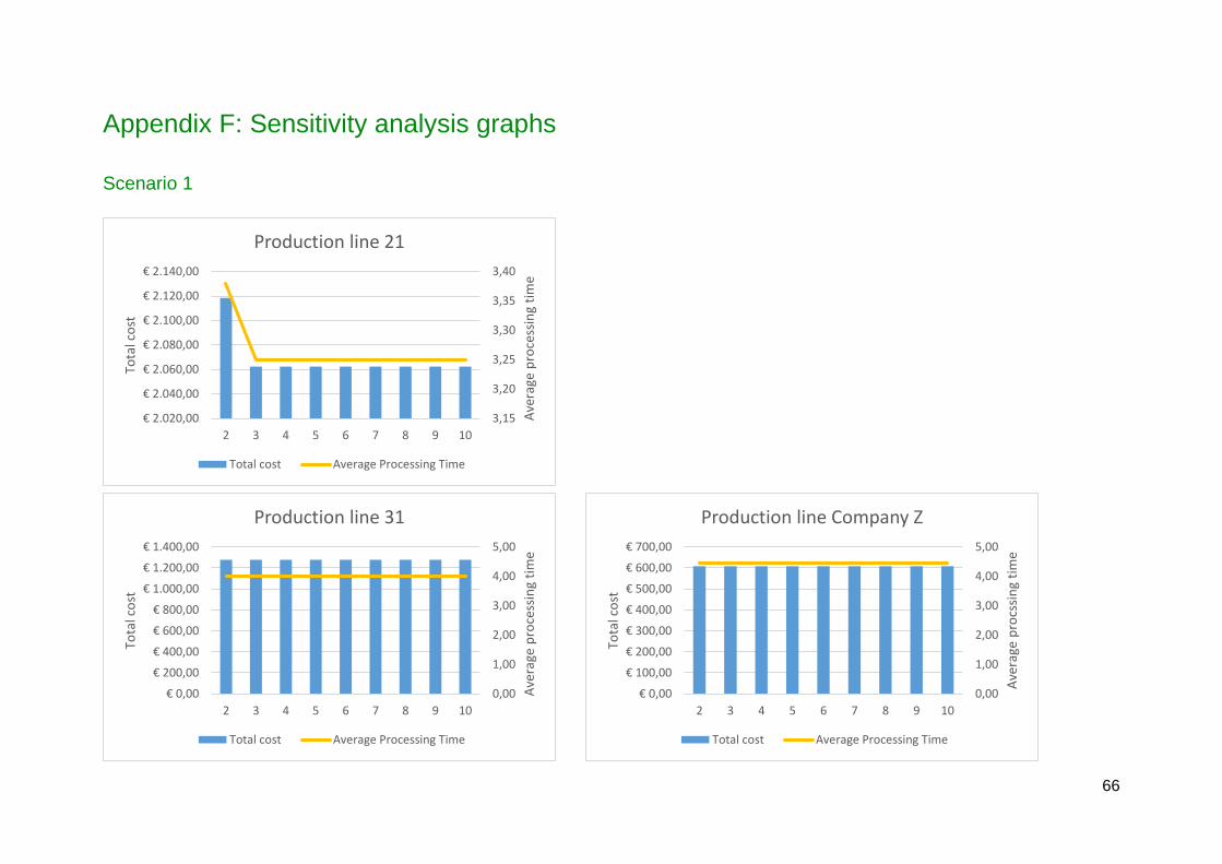
66
Appendix F: Sensitivity analysis graphs
Scenario 1
3,15
3,20
3,25
3,30
3,35
3,40
€ 2.020,00
€ 2.040,00
€ 2.060,00
€ 2.080,00
€ 2.100,00
€ 2.120,00
€ 2.140,00
2 3 4 5 6 7 8 9 10
Ave
rage
pro
cess
ing
tim
e
Tota
l co
st
Production line 21
Total cost Average Processing Time
0,00
1,00
2,00
3,00
4,00
5,00
€ 0,00
€ 200,00
€ 400,00
€ 600,00
€ 800,00
€ 1.000,00
€ 1.200,00
€ 1.400,00
2 3 4 5 6 7 8 9 10
Ave
rage
pro
cess
ing
tim
e
Tota
l co
st
Production line 31
Total cost Average Processing Time
0,00
1,00
2,00
3,00
4,00
5,00
€ 0,00
€ 100,00
€ 200,00
€ 300,00
€ 400,00
€ 500,00
€ 600,00
€ 700,00
2 3 4 5 6 7 8 9 10
Ave
rage
pro
cssi
ng
tim
e
Tota
l co
st
Production line Company Z
Total cost Average Processing Time

67
Scenario 2
In all the three graphs we see a linear increase in the average processing time. Also, the total cost is almost increasing linearly.
3,4
3,6
3,8
4
4,2
4,4
4,6
4,8
€2.200,00
€2.300,00
€2.400,00
€2.500,00
€2.600,00
€2.700,00
€2.800,00
€2.900,00
Base 10% 20% 30% 40%
Line 11
Total Cost Average processing time
3,6
3,8
4
4,2
4,4
4,6
4,8
5
€1.150,00
€1.200,00
€1.250,00
€1.300,00
€1.350,00
€1.400,00
€1.450,00
€1.500,00
€1.550,00
Base 10% 20% 30% 40%
Line 31
Total Cost Average processing time
0
1
2
3
4
5
6
€550,00
€600,00
€650,00
€700,00
€750,00
Base 10% 20% 30%
COMPANY Z
Total Cost Average processing time

68
Scenario 3
0
1
2
3
4
5
6
€1.980,00 €1.990,00 €2.000,00 €2.010,00 €2.020,00 €2.030,00 €2.040,00 €2.050,00 €2.060,00 €2.070,00
Base 90% 80% 70% 60%
Ave
rage
pro
cess
ing
tim
e
Tota
l co
st
Line 21
Total Cost Average Processing Time
0
1
2
3
4
5
6
7
8
€1.230,00
€1.240,00
€1.250,00
€1.260,00
€1.270,00
€1.280,00
Base 90% 80% 70% 60%
Ave
rage
pro
cess
ing
tim
e
Tota
l co
st
Line 31
Total Cost Average Processing Time
0
2
4
6
8
10
570
575
580
585
590
595
600
605
610
Base 90% 80% 70% 60%
Ave
rage
pro
cess
ing
tim
e
Tota
l co
st
Line Company Z
Total Cost Average Processing Time

69
In scenario 3 see an increase in the average processing time after 70% from the base
production rate. Some production frequencies change after 70% which affect on the average
processing times. The total cost will reduce because of the fraction 𝑑𝑖
𝑝𝑖.